Black Sea Mixed Layer Sensitivity to Various Wind and Thermal Forcing Products on Climatological...

Black Sea Mixed Layer Sensitivity to Various Wind and Thermal Forcing Products onClimatological Time Scales*

A. BIROL KARA, HARLEY E. HURLBURT, AND ALAN J. WALLCRAFT

Oceanography Division, Naval Research Laboratory, Stennis Space Center, Mississippi

MARK A. BOURASSA

Center for Ocean–Atmospheric Prediction Studies, Tallahassee, Florida

(Manuscript received 3 December 2004, in final form 8 June 2005)

ABSTRACT

This study describes atmospheric forcing parameters constructed from different global climatologies,applied to the Black Sea, and investigates the sensitivity of Hybrid Coordinate Ocean Model (HYCOM)simulations to these products. Significant discussion is devoted to construction of these parameters beforeusing them in the eddy-resolving (�3.2-km resolution) HYCOM simulations. The main goal is to answerhow the model dynamics can be substantially affected by different atmospheric forcing products in theBlack Sea. Eight wind forcing products are used: four obtained from observation-based climatologies,including one based on measurements from the SeaWinds scatterometer on the Quick Scatterometer(QuikSCAT) satellite, and the rest formed from operational model products. Thermal forcing parameters,including solar radiation, are formed from two operational models: the European Centre for Medium-Range Weather Forecasts (ECMWF) and the Fleet Numerical Meteorology and Oceanography Center(FNMOC) Navy Operational Global Atmospheric Prediction System (NOGAPS). Climatologically forcedBlack Sea HYCOM simulations (without ocean data assimilation) are then performed to assess the accuracyand sensitivity of the model sea surface temperature (SST) and sea surface circulation to these wind andthermal forcing products. Results demonstrate that the model-simulated SST structure is quite sensitive tothe wind and thermal forcing products, especially near coastal regions. Despite this sensitivity, severalrobust features are found in the model SST in comparison to a monthly 9.3-km-resolution satellite-basedPathfinder SST climatology. Annual mean HYCOM SST usually agreed to within ��0.2° of the climatol-ogy in the interior of the Black Sea for any of the wind and thermal forcing products used. The fine-resolution (0.25° � 0.25°) wind forcing from the scatterometer data along with thermal forcing fromNOGAPS gave the best SST simulation with a basin-averaged rms difference value of 1.21°C, especiallyimproving model results near coastal regions. Specifically, atmospherically forced model simulations withno assimilation of any ocean data suggest that the basin-averaged rms SST differences with respect to thePathfinder SST climatology can vary from 1.21° to 2.15°C depending on the wind and thermal forcingproduct. The latter rms SST difference value is obtained when using wind forcing from the National Centersfor Environmental Prediction (NCEP), a product that has a too-coarse grid resolution of 1.875° � 1.875°for a small ocean basin such as the Black Sea. This paper also highlights the importance of using high-frequency (hybrid) wind forcing as opposed to monthly mean wind forcing in the model simulations. Finally,there are large variations in the annual mean surface circulation simulated using the different wind sets, withgeneral agreement between those forced by the model-based products (vector correlation is usually �0.7).Three of the observation-based climatologies generally yield unrealistic circulation features and currentsthat are too weak.

* Naval Research Laboratory Contribution Number NRL/JA/7304/04/0002.

Corresponding author address: Birol Kara, Naval Research Laboratory, Code 7320, Bldg. 1009, Stennis Space Center, MS 39529-5004.E-mail: [email protected]

5266 J O U R N A L O F C L I M A T E VOLUME 18

© 2005 American Meteorological Society

1. Introduction and motivation

Given the dynamical importance of heat and momen-tum exchange at the air–sea interface, ocean generalcirculation model (OGCM) studies necessitate reliableatmospheric forcing fields that can be used for simula-tions. The use of quality atmospheric forcing fields isespecially important for the Black Sea because thereare large uncertainities in the existing heat and windstress climatologies constructed from local observa-tions. Detailed investigations were performed to com-pare atmospheric forcing parameters obtained from lo-cal datasets (Staneva and Stanev 1998; Schrum et al.2001). The conclusion was that the existing local atmos-pheric forcing fields need improvements because thelocal observational datasets are too sparse in time andspace to form realistic climatologies for the Black Sea.

Wind stress and heat fluxes for the Black Sea thathave been used for ocean model simulations weremainly constructed from local observations (e.g.,Sorkina 1974; Altman and Kumish 1986; Simonov andAltman 1991; Trukhchev and Demin 1992), and they allpresent large uncertainties (e.g., Staneva and Stanev1998). For example, climatological wind fields wereusually computed from many years of ship observa-tions. However, wind speed and direction, air and seatemperatures, and other meteorological parametersnear the sea surface are not routinely measured atmany coastal locations and in the interior of the BlackSea where the depth of water is �1300 m (Fig. 1). Thisis even true over the wide northwestern continentalshelf where the depth is �200 m. Thus, traditional insitu observations are sparse and inhomogeneous. Thismakes it difficult to obtain complete information ontemporal and spatial scales.

When the local climatologies mentioned above wereused in forcing OGCMs, they resulted in unrealisticmodel simulations. In particular, the model study byOguz and Malanotte-Rizzoli (1996), who examined sea-sonal variability of the Black Sea, used a monthly meanheat flux climatology (Efimov and Timofeev 1990),which was formed from local datasets. That study indi-cated the need to reanalyze the heat flux climatologybecause their model simulations produced unrealistictemperature simulations in the mixed layer. Their simu-lations also suggested that reducing the original fluxesby one-half might be a reasonable estimate for the win-ter, and a smaller reduction of the heat fluxes should besufficient for summer, demonstrating shortcomings ofthe existing local climatologies in predicting upper-ocean parameters, such as sea surface temperature(SST). Similarly, local climatologies of evaporation andprecipitation may induce unrealistic temperature distri-

butions and water mass properties in the surface layerwhen they are used as atmospheric forcing in modelsimulations (Oguz and Malanotte-Rizzoli 1996).

Discussions presented above clearly indicate thatBlack Sea modeling studies need high-quality atmos-pheric forcing. Wind stress and surface heat flux prod-ucts from operational models have been exploited assurface forcing for OGCMs in the Black Sea becausethey provide complete information at all modeled tem-poral and spatial scales. In addition, a fine-resolution(0.25° � 0.25°) wind stress climatology based on space-borne scatterometer observations of wind speed anddirection is introduced over the Black Sea for the firsttime. Sensitivity studies are then performed by usingthese atmospheric products to force an OGCM.

The availability of these atmospheric forcing prod-ucts raises important questions. 1) How do these prod-ucts compare with each other and with local datasets inthe Black Sea? 2) What is the best wind stress or sur-face heat flux to use in forcing a Black Sea OGCM?3) Do operational atmospheric model products providea more accurate representation of the surface stressexperienced by the ocean, or is it better to use their10-m winds with a parameterized drag coefficient toconstruct wind stresses? Answers to all of these ques-tions are discussed throughout the text. In addition, weinvestigate whether or not newly constructed atmos-pheric forcing products differ from climatologiesformed from local observations as reported in earlierBlack Sea modeling studies.

As expected, both observation-based climatologiesand operational model products have their unique bi-ases, and they can differ significantly in some regions ofthe global ocean (e.g., Rienecker et al. 1996; Trenberthet al. 2001; Metzger 2003). Thus, the use of these prod-ucts in OGCM simulations may result in various re-sponses in different regions of the global ocean asshown in many OGCM studies (e.g., Schopf andLoughe 1995; Fu and Chao 1997; Samuel et al. 1999;Ezer 1999; Townsend et al. 2000; Metzger 2003; Lee etal. 2005; Hogan and Hurlburt 2005). In this paper, thefocus is to investigate the impact of these climatologicalforcing fields on Black Sea OGCM simulations. Spe-cifically, in the first part of this paper, we extend thestudies of (Staneva and Stanev 1998; Schrum et al.2001), so that a more-detailed and comprehensive pic-ture of the atmospheric forcing in the Black Sea can begiven. In the second part of the paper, an eddy-resolving OGCM with �3.2-km resolution set up forthe Black Sea (Kara et al. 2005a) is forced with theseatmospheric forcing fields to answer how they affectmodel performance in predicting SST. Since SST is thebest observed oceanic field of the Black Sea mixed

15 DECEMBER 2005 K A R A E T A L . 5267

layer (e.g., Kara et al. 2005b), this gives us a basis forjudging which of the simulations is better for this aspect(either annually or in seasons) and therefore, for de-ciding on optimal forcing products for SST in the BlackSea.

Although the atmospheric forcing fields and OGCMSST sensitivity to them is the primary focus, the sensi-

tivity of the Black Sea mean surface circulation to dif-ferent atmospheric wind stress products is also exam-ined since the circulation is mainly wind driven (Oguzet al. 1995; Zatsepin et al. 2003). Specificially, the sig-nificant complexity of the Black Sea circulation (e.g.,Staneva et al. 2001; Afanasyev et al. 2002; Zatsepin etal. 2003) is investigated using the eddy-resolving

FIG. 1. The Black Sea bottom topography constructed from the 1-min DBDB-V resolutiondataset of NAVOCEANO. Two different color bars are used to emphasize different depthranges in the Black Sea: (top) deep water and (bottom) shallow water (� 200 m). Major riversdischarged into the Black Sea are in yellow. The land area map was produced using asubregion from the true color image of the National Aeronautics and Space Administration(NASA) earth observatory. Also shown are a few geographical locations mentioned in thetext.


OGCM in an attempt to mitigate the sparseness of ob-servational data for evaluation of surface circulationfeatures and the associated current speed and direction.One of our major purposes in writing this paper is torecommend to the Black Sea modeling communitywhich wind and thermal forcing climatologies are rea-sonable and which ones should be avoided in simulatingSST and circulation features in the Black Sea.

This paper is organized as follows. Section 2 de-scribes atmospheric forcing fields in the Black Sea,along with a brief comparison between atmosphericforcing used in previous OGCM studies and those usedhere, several for the first time in the Black Sea. Section3 gives general characteristics of the primitive equation,eddy-resolving OGCM used in this study. Section 4 dis-cusses differences in model SST simulations, when themodel is forced with various forcing fields formed fromobservation-based climatologies and operational modelproducts, along with the impact of high-frequency ver-sus monthly mean wind forcing on the simulations. Sec-tion 5 investigates the sensitivity of modeled Black Seasurface circulation to eight different wind stress prod-ucts. Finally, section 6 gives the summary and conclu-sions of this paper.

2. Climatological atmospheric forcing in theBlack Sea

Most previous Black Sea OGCM studies (e.g., Oguzet al. 1995; Oguz and Malanotte-Rizzoli 1996; Stanevand Beckers 1999; Staneva et al. 2001) made use ofatmospheric forcing formed from local datasets, andthose most commonly used are summarized in Table 1.Some of these data sources (e.g., Altman and Kumish1986; Altman et al. 1987; Efimov and Timofeev 1990)

are not documented in English or are not readily avail-able. Through a detailed analysis, this section presentsalternative sources for atmospheric forcing fields. Inparticular, the forcing products are constructed fromoperational model outputs and other observation-basedclimatologies, most of which have not been used in ear-lier Black Sea studies.

a. Candidate atmospheric forcing sets

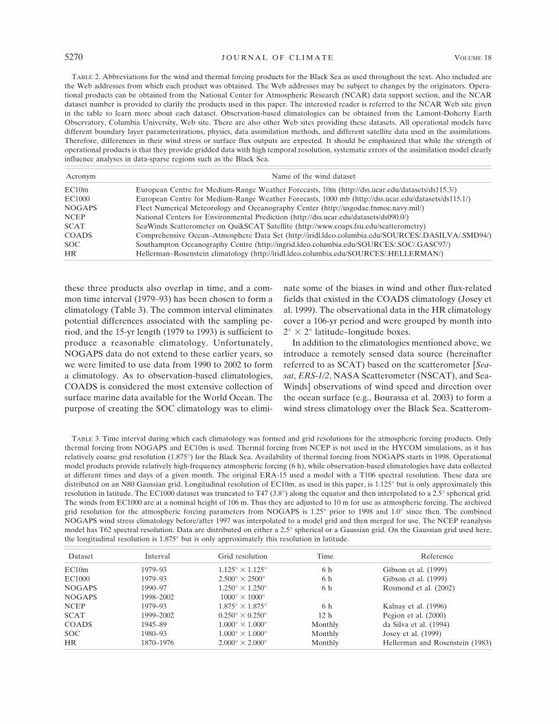
Atmospheric forcing fields covering the Black Seaare formed from eight different products. Table 2shows these products, along with their abbreviationsused throughout the text. All atmospheric forcing fieldswere obtained in the form of global climatologies onthe grid provided, and most are available online. Spe-cifically, European Centre for Medium-Range WeatherForecasts: 10 m (EC10m), European Centre for Me-dium-Range Weather Forecasts: 1000 mb (EC1000),Navy Operational Global Atmospheric Prediction Sys-tem (NOGAPS), and the National Centers for Envi-ronmental Prediction (NCEP) are climatologies formedfrom operational or reanalyzed model products, whilethe SeaWinds Scatterometer on Quick Scatterometer(QuikSCAT) satellite (SCAT), ComprehensiveOcean–Atmosphere Data Set (COADS), SouthamptonOceanography Centre (SOC), and Hellerman–Rosenstein (HR) are climatologies based mainly on ob-servational data. The grid resolution of these globalclimatologies varies from 0.25° to 2.5° (Table 3). A briefdescription of each dataset is given below.

EC10m, EC1000, and NCEP are all reanalyses thatused a consistent data assimilation scheme and atmos-pheric forecast model; therefore, they are unaffected byoperational model upgrades. The reanalyses from

TABLE 1. Atmospheric forcing sources (wind and thermal) that have been commonly used in previous Black Sea studies. Alsoincluded are data sources for initialization of temperature and salinity (T/S). Thermal forcing includes net shortwave radiation, net solarradiation (net shortwave plus net longwave radiation), air temperature, and air mixing ratio at 10 m above the sea surface. Some of theclimatologies based on local datasets have coarse grid resolutions that may not be adequate for a small ocean basin, such as the BlackSea. Only a few Black Sea model studies used a model product (only NCEP) as atmospheric forcing (e.g., Stanev et al. 1997; Stanevaet al. 2001), and Stanev et al. (2003) later used wind and thermal forcing parameters from the atmospheric analyses of the UKMO,demonstrating the accuracy of the latter in comparison to NCEP.

Wind forcing Thermal forcing T/S initialization

Sorkina (1974) Makerov (1961) Altman et al. (1987)Hellerman and Rosenstein (1983) Sorkina (1974) Stanev (1990)Rachev et al. (1991) Golubeva (1984) Trukhchev and Demin (1992)NCEP 1000 mb (1980–86) NCEP 1000 mb (1980–86)UKMO meteorolgoical data (1991–94) Altman and Kumish (1986)Staneva and Stanev (1998) Efimov and Timofeev (1990)

Stanev (1990)Simonov and Altman (1991)Golubev and Kuftarkov (1993)UKMO Meteorological data (1991–94)Staneva and Stanev (1998)


these three products also overlap in time, and a com-mon time interval (1979–93) has been chosen to form aclimatology (Table 3). The common interval eliminatespotential differences associated with the sampling pe-riod, and the 15-yr length (1979 to 1993) is sufficient toproduce a reasonable climatology. Unfortunately,NOGAPS data do not extend to these earlier years, sowe were limited to use data from 1990 to 2002 to forma climatology. As to observation-based climatologies,COADS is considered the most extensive collection ofsurface marine data available for the World Ocean. Thepurpose of creating the SOC climatology was to elimi-

nate some of the biases in wind and other flux-relatedfields that existed in the COADS climatology (Josey etal. 1999). The observational data in the HR climatologycover a 106-yr period and were grouped by month into2° � 2° latitude–longitude boxes.

In addition to the climatologies mentioned above, weintroduce a remotely sensed data source (hereinafterreferred to as SCAT) based on the scatterometer [Sea-sat, ERS-1/2, NASA Scatterometer (NSCAT), and Sea-Winds] observations of wind speed and direction overthe ocean surface (e.g., Bourassa et al. 2003) to form awind stress climatology over the Black Sea. Scatterom-

TABLE 3. Time interval during which each climatology was formed and grid resolutions for the atmospheric forcing products. Onlythermal forcing from NOGAPS and EC10m is used. Thermal forcing from NCEP is not used in the HYCOM simulations, as it hasrelatively coarse grid resolution (1.875°) for the Black Sea. Availability of thermal forcing from NOGAPS starts in 1998. Operationalmodel products provide relatively high-frequency atmospheric forcing (6 h), while observation-based climatologies have data collectedat different times and days of a given month. The original ERA-15 used a model with a T106 spectral resolution. These data aredistributed on an N80 Gaussian grid. Longitudinal resolution of EC10m, as used in this paper, is 1.125° but is only approximately thisresolution in latitude. The EC1000 dataset was truncated to T47 (3.8°) along the equator and then interpolated to a 2.5° spherical grid.The winds from EC1000 are at a nominal height of 106 m. Thus they are adjusted to 10 m for use as atmospheric forcing. The archivedgrid resolution for the atmospheric forcing parameters from NOGAPS is 1.25° prior to 1998 and 1.0° since then. The combinedNOGAPS wind stress climatology before/after 1997 was interpolated to a model grid and then merged for use. The NCEP reanalysismodel has T62 spectral resolution. Data are distributed on either a 2.5° spherical or a Gaussian grid. On the Gaussian grid used here,the longitudinal resolution is 1.875° but is only approximately this resolution in latitude.

Dataset Interval Grid resolution Time Reference

EC10m 1979–93 1.125° � 1.125° 6 h Gibson et al. (1999)EC1000 1979–93 2.500° � 2500° 6 h Gibson et al. (1999)NOGAPS 1990–97 1.250° � 1.250° 6 h Rosmond et al. (2002)NOGAPS 1998–2002 1000° � 1000°NCEP 1979–93 1.875° � 1.875° 6 h Kalnay et al. (1996)SCAT 1999–2002 0.250° � 0.250° 12 h Pegion et al. (2000)COADS 1945–89 1.000° � 1.000° Monthly da Silva et al. (1994)SOC 1980–93 1.000° � 1.000° Monthly Josey et al. (1999)HR 1870–1976 2.000° � 2.000° Monthly Hellerman and Rosenstein (1983)

TABLE 2. Abbreviations for the wind and thermal forcing products for the Black Sea as used throughout the text. Also included arethe Web addresses from which each product was obtained. The Web addresses may be subject to changes by the originators. Opera-tional products can be obtained from the National Center for Atmospheric Research (NCAR) data support section, and the NCARdataset number is provided to clarify the products used in this paper. The interested reader is referred to the NCAR Web site givenin the table to learn more about each dataset. Observation-based climatologies can be obtained from the Lamont-Doherty EarthObservatory, Columbia University, Web site. There are also other Web sites providing these datasets. All operational models havedifferent boundary layer parameterizations, physics, data assimilation methods, and different satellite data used in the assimilations.Therefore, differences in their wind stress or surface flux outputs are expected. It should be emphasized that while the strength ofoperational products is that they provide gridded data with high temporal resolution, systematic errors of the assimilation model clearlyinfluence analyses in data-sparse regions such as the Black Sea.

Acronym Name of the wind dataset

EC10m European Centre for Medium-Range Weather Forecasts, 10m (http://dss.ucar.edu/datasets/ds115.3/)EC1000 European Centre for Medium-Range Weather Forecasts, 1000 mb (http://dss.ucar.edu/datasets/ds115.1/)NOGAPS Fleet Numerical Meteorology and Oceanography Center (http://usgodae.fnmoc.navy.mil/)NCEP National Centers for Environmental Prediction (http://dss.ucar.edu/datasets/ds090.0/)SCAT SeaWinds Scatterometer on QuikSCAT Satellite (http://www.coaps.fsu.edu/scatterometry)COADS Comprehensive Ocean–Atmosphere Data Set (http://iridl.ldeo.columbia.edu/SOURCES/.DASILVA/.SMD94/)SOC Southampton Oceanography Centre (http://ingrid.ldeo.columbia.edu/SOURCES/.SOC/.GASC97/)HR Hellerman–Rosenstein climatology (http://iridl.ldeo.columbia.edu/SOURCES/.HELLERMAN/)


eters are spaceborne radars that infer surface windsfrom the roughness of the sea surface as explained inLiu et al. (1998), and Liu (2002), in detail. Wind speedand direction are inferred from measurement of micro-wave backscattered power from a given location on thesea surface at multiple antenna look angles. Measure-ments of radar backscatter from a given location on thesea surface are obtained from multiple azimuth anglesas the satellite travels along its orbit. Estimates of vec-tor winds are derived from these radar measurementsover a single broad swath of 1600-km width centeredaround the satellite ground track (e.g., Liu 2002). Scat-terometer wind retrievals are calibrated to the neutralstability wind at a height of 10 m above the sea surface(Chelton et al. 2001). The SeaWinds scatterometer is anactive microwave sensor that covers �90% of the ice-free ocean in one day, with an average of two observa-tions per 25 km � 25 km grid cell each day. The gaps inthe coverage are filled by using a variational methodthat minimizes a function with three constraints (Pe-gion et al. 2000). The functional term consists of misfitsto the scatterometer observations, a penalty function tosmooth with respect to a background field based onspatially smoothed scatterometer observations, and amisfit to the vorticity of the background field, which isa problem.

All data sources mentioned above are subject to theirown unique biases. For example, errors and discrepan-cies exist in the observation-based climatologies be-cause of varying quality and density of the input sourcesand changes in observing practices and data processingprocedures throughout the history of data collection(e.g., Kent et al. 1993; Josey et al. 2002). Sampling errorin the monthly SCAT winds is very small (e.g., Schlax etal. 2001). In operational atmospheric products, spurioustrends may exist because of operational changes in theanalysis/forecast system and changes in the input datastream as new data sources become available (e.g.,Trenberth and Guillemot 1998).

b. Constructing wind and thermal forcing fields

For the Black Sea model, wind and thermal forcingparameters are formed from datasets discussed in sec-tion 2a. Wind forcing includes zonal and meridionalwind stress magnitudes, and the total wind speed. Ther-mal forcing includes air temperature and air mixing ra-tio at 10 m above the sea surface, net shortwave radia-tion at the sea surface, and net solar radiation (netshortwave radiation plus net longwave radiation at thesea surface). Precipitation is also a thermal forcing pa-rameter (see section 2d). Additional forcing parametersare a monthly climatological SST field for longwaveradiation correction and a satellite-based ocean color

climatology for attenuation of shortwave radiation (seesection 3). The ocean model used in this paper reads inthe time-varying wind and thermal atmospheric forcingfields.

Wind speed used for the model simulations is calcu-lated from wind stress (Kara et al. 2002). By doing so,air–sea stability through the wind drag coefficient istaken into account, a consistent method for all windstress products. Wind forcing products presented in thispaper are unsmoothed in time, and a cubic spline isapplied in space for interpolation to the model grid.Here, we first explain the methodology used to formwind stress from each product. Monthly mean windstresses from NOGAPS, NCEP, COADS, and SOC aredirectly obtained from their original sources as surfacestresses (N m�2). Wind stress from HR is convertedfrom dyn cm�2 to N m�2 using a scale factor of 0.1.Wind stresses from EC1000 and SCAT are obtained aspseudo stresses (m2 s�2), and they are later convertedto surface stresses (N m�2) by multiplying �air � CD,where �air is air density and CD is variable wind dragcoefficient. Here �a at the air–sea interface is calculatedusing the ideal gas law formulation (�a � 100 Pa/[Rgas

(Ta 273.16)] in kg m�3), where Ta is air temperature(°C) at 10 m above the sea surface, Rgas is the gas con-stant with a value of 287.1 J kg�1 K�1 for dry air, and Pa

is the atmospheric pressure at the sea surface with avalue of 1013 mb. It is not necessary to consider a vari-able Pa in the density formulation because its effect on�a is negligible in comparison to variations in Ta. Notethat Ta values are taken from EC10m in this calculationfor both products.

Wind stress (N m�2) for EC10m is calculated usingzonal and meridional wind velocities, Ta at 10 m abovethe sea surface, and SST, rather than using the surfacestress product directly provided by ECMWF. The rea-son for not using the surface stresses is that they sufferfrom significant orographic effects near the coast.These result from Gibb’s waves in the spectral modelcaused by the spectral truncation of the orography to106 waves, triangular truncation (P. Kållberg, ECMWF,2005, personal communication). They are most promi-nent in regions near steep mountains. After averagingfields originally created in the ECMWF spectral geom-etry, traces of the originally minute Gibb’s waves be-come more visible, and after using the monthly meansfor certain derived parameters, such as the wind stresscurl, they become even more prominent. On the otherhand, the atmospheric variables in the EC10m productare from post-processed Businger profiles where thespectral traces have been removed. Thus, the use ofsurface stresses directly from the ECMWF model is notpreferred. While NOGAPS provides atmospheric vari-


ables from which wind stress can be calculated, we usesurface stresses directly from NOGAPS, which doesnot exhibit the Gibb’s wave problem (e.g., Metzger2003).

The wind stress calculation for EC10m uses bulk for-mulas that include a stability-dependent drag coeffi-cient through air–sea temperature difference and tem-perature-dependent air density (Kara et al. 2002). SomeOGCMs in the Black Sea have used wind stresses thatare constructed from 10-m winds and a constant dragcoefficient. For example, Oguz and Malanotte-Rizzoli(1996) used a drag coefficient value of 1.3 � 10�3. How-ever, such wind stresses exclude the significant changesin magnitude that can occur due to effects of windspeed and air–sea stability in the drag coefficient, whichcan make it quite variable. This becomes especially im-portant for OGCMs that predict SST because air–seastability depends mainly upon the air–sea temperaturedifference and wind speed. As noted above, the use ofa bulk formula for wind stress can be more desirablewhen performing fine-resolution OGCM simulationsthan using the direct product from an operationalmodel. While more advanced methods exist (e.g., Fair-all et al. 2003; Bourassa et al. 2005), the bulk formulaused here (Kara et al. 2002) for wind stress forcing of anOGCM with SST is generally accurate and computa-tionally much more efficient.

We now present the spatial patterns of long-term an-nual mean wind speed (Fig. 2a). The basin-averagedNCEP wind speed has an annual mean of 4.6 m s�1, thehighest from the eight products (Table 4). Not surpris-ingly, the NCEP product (Table 3) is probably not apreferred product in the Black Sea because the windspeeds have relatively large differences in comparisonto those from research vessel measurements (e.g.,Smith et al. 2001; Josey et al. 2002). Wind speed fromthe finest-resolution dataset, SCAT, resolves manysmall-scale futures. In general, HR wind stresses tendto be strong over the global ocean because they werecreated using relatively large drag coefficients (Harri-son 1989). The spatial patterns of annual mean windstress curl from the eight products also differ substan-tially (Fig. 2b). In particular, wind stress curl fromNCEP is rather large and from COADS and SOCrather small in comparison to the other products.

Climatologies of monthly mean thermal forcing pa-rameters are constructed using 6-hourly (hereinafter re-ferred to as 6-h) model output during 1979–93 forECMWF, 1998–2002 for NOGAPS, and 1948–2003 forNCEP. Similar to the wind forcing, thermal forcing pa-rameters are daily averages that are linearly interpo-lated to 6-h intervals. A cubic spline in space is appliedto all thermal forcing parameters for interpolation to

the model grid. Although thermal forcing fields fromNCEP are presented for comparison purposes, they arenot used in the model simulations. The main reason isthat NCEP has rather coarse resolution (1.875° �1.875°) for a small ocean basin, such as the Black Sea.In addition, atmospheric forcing from NCEP needs tobe corrected before use in an OGCM because themeans of thermal forcing parameters from NCEP arequite different in comparison to those from local clima-tological sets and those from the atmospheric analysesof the U.K. Met Office (UKMO) in the Black Sea(Staneva and Stanev 1998; Stanev et al. 2003). Previ-ously, it was also shown that the oceanic response tovery smooth NCEP forcing resulted in unrealistic simu-lations in the Black Sea (Stanev et al. 1997).

Thermal forcing parameters from EC10m, NOGAPS,and NCEP differ in the annual means (Fig. 2c). Thesedifferences can be partially attributed to the time inter-vals over which the climatologies were constructed:1979–93 for EC10m and 1998–2002 for NOGAPS. Be-cause no NOGAPS thermal forcing is available prior to1998, we had to form the climatology based on only a5-yr model output. A comparison between EC10m andNOGAPS over the same time period (1998–2002) gavebetter agreement (not shown). Annual mean air tem-perature from EC10m is colder than that fromNOGAPS by �2°–4°C over the northernmost BlackSea, including the northwestern shelf and either side ofthe Crimean peninsula. This is an indication of the factthat, in addition to improper land–sea masks discussedin Kara et al. (2005b), the local orography can have amajor effect on the accuracy of climatological fieldsconstructed from operational model outputs. In mostregions, the spatial pattern and magnitude of air tem-perature are generally similar for all three datasets. Inaddition, all three have usually similar spatial patternsfor air mixing ratio at 10 m above the sea surface. Themost obvious differences between EC10m, NOGAPS,and NCEP are seen in the shortwave and net solarradiation values (see also Table 4).

In addition to the annual mean, the seasonal cycle ofthe wind and thermal forcing fields is examined to de-termine if the annual mean is dominated by values inany specific season. There are relatively weak winds(�2.5 m s�1) in spring from April to June, and this istrue for almost all products except NCEP andNOGAPS (Fig. 3). The basin-averaged climatologicalmonthly mean speed given by a local dataset (Efimovand Timofeev 1990) reports values of 5 to 8 m s�1 fromsummer to winter, which is usually higher than the windforcing products presented here. The remotely sensedSCAT data can be considered as a good measure ofwind speed over the Black Sea as it was calculated from


FIG. 2. Climatological annual mean of wind and thermal forcing parameters formed from observation-based climatologies andoperational model outputs: (a) wind speed, (b) wind stress curl, and (c) thermal forcing from 15-yr ECMWF Re-Analysis (ERA-15),NOGAPS, and NCEP. In general, wind speed climatologies constructed from observations (COADS and SOC) are very smooth. Thewind fields from NCEP reveal very different spatial patterns in comparison to other operational model products (i.e., EC10m, EC1000,and NOGAPS).


calibrated wind speed and direction measurements ofthe SeaWinds scatterometer on the QuikSCAT satel-lite. The available record of QuickSCAT winds used inthis paper is from August 1999 through March 2002.

Although this time period (2.5 yr) is relatively short torepresent the climatological conditions, the SCAT cli-matology has the advantage of providing fine spatialresolution. The differences existing in wind speed arealso reflected in the wind stress curl (Fig. 4). Windstress curl from NCEP is too large, and previouslySchrum et al. (2001) also noted unrealistic wind stresscurl from NCEP in the Black Sea but used fields con-structed over a different time period from that usedhere. They note that the amplitude of the seasonal cyclebased on the EC10m data is very different than thatestimated from the NCEP data, but the wind stress curlfrom EC10m is comparable to estimates from local cli-matic data and higher-resolution UKMO data over1993–96.

There is a strong seasonal cycle in all thermal forcingparameters (Fig. 5). Using the local datasets, Stanevaand Stanev (1998) reported basin-averaged air tem-peratures of �5°C in January and February, whichagrees with those from EC10m, NOGAPS, and NCEP.Basin-averaged net solar radiation values shown in Fig.3a of Oguz and Malanotte-Rizzoli (1996), as deter-mined from local climatologies, are roughly 15, 40, and85 W m�2 in January, February, and March and 190,210, and 200 W m�2 in May, June, and July, respec-tively. These values are larger than those obtained fromEC10m. Interestingly, Oguz and Malanotte-Rizzoli(1996) indicated that original flux values based on localdatasets, as used in their model simulations, are prob-ably too large in winter, and slightly larger (e.g., 10 to30 W m�2) in summer, resulting in unrealistic tempera-ture simulations. This partly demonstrates the reliabil-ity of net solar radiation values from EC10m in com-parison to the local datasets. The most striking featureof monthly mean thermal forcing parameters in theBlack Sea is that net shortwave radiation from EC10mis consistently lower than that from NOGAPS andNCEP by an offset of �30 W m�2 in all months (Fig. 6).Such a difference can change the amount of net fluxthat penetrates to depth, especially during summerwhen very thin mixed layers are present in the BlackSea (Kara et al. 2005a).

c. Addition of a high-frequency component

There are two main reasons for adding a high-frequency component to monthly mean atmosphericforcing fields: 1) the mixed layer is sensitive to varia-tions in surface forcings on time scales of a day or less(e.g., Kelly et al. 1999; Sui et al. 2003; Wallcraft et al.2003; Kara et al. 2003; Stanev et al. 2004), and 2) ourfuture goal is to perform simulations forced by high-frequency interannual atmospheric fields from opera-tional weather centers.

TABLE 4. Basin-averaged annual mean values of atmosphericforcing parameters in the Black Sea. Also given are min and maxvalues in the annual mean fields. Std dev is calculated over theannual cycle using monthly mean values. The similarity based ondifferent sources suggests that a basin-averaged annual meanvalue of �3 m s�1 is probably a good estimate for the Black Sea.Net shortwave and net solar radiation values from EC10m andNOGAPS are different by �30 W m�2. Basin-averaged thermalforcing values from NCEP are included for only comparison pur-poses. The climatological relative bias values for air temperature,air mixing ratio, net shortwave radiation, and net solar radiationcalculated for NOGAPS–EC10m (NCEP–EC10m) are 0.3°C(�0.8°C), �0.7 g kg�1 (0.2 g kg�1), 32.8 W m�2 (29.9 W m�2), and36.2 W m�2 (29.9 W m�2), respectively. Similarly, bias values forNOGAPS–NCEP are 0.9°C, �0.9 g kg�1, 2.9 W m�2, and 6.3 Wm�2.

Forcing product Mean Min Max Std dev

Wind speed (m s�1)

EC10m 3.5 1.3 4.8 0.78EC1000 3.4 1.9 4.2 0.82NOGAPS 4.0 2.4 5.4 0.84NCEP 4.6 2.6 8.5 0.96SCAT 3.0 1.6 4.2 0.76COADS 2.7 2.5 3.3 0.37SOC 3.7 3.6 3.9 0.82HR 3.4 2.4 4.9 0.63

Wind stress curl (�108) (Pa m�1)

EC10m 2.6 �24.2 24.1 2.6EC1000 1.4 �10.4 9.3 2.7NOGAPS 6.3 �21.9 39.1 5.4NCEP 8.0 �15.1 42.3 11.4SCAT 0.9 �19.1 25.1 2.4COADS 1.1 0.1 4.2 1.1SOC �0.1 �1.7 4.1 1.9HR 2.2 �9.8 8.8 2.1

Air temperature (°C)

EC10m 12.9 7.6 16.0 6.5NOGAPS 13.2 6.9 14.6 6.5NCEP 12.1 5.7 13.8 6.4

Air mixing ratio (g kg�1)

EC10m 8.0 5.3 9.4 3.3NOGAPS 7.3 4.7 8.1 2.9NCEP 8.2 6.6 8.8 3.0

Shortwave radiation (W m�2)

EC10m 141.3 122.2 154.1 77.6NOGAPS 174.1 146.3 198.2 77.4NCEP 171.2 148.4 184.5 79.8

Net solar radiation (W m�2)

EC10m 71.4 58.0 84.1 75.1NOGAPS 107.6 80.1 135.0 81.2NCEP 101.3 80.0 107.4 77.2


Hybrid winds consist of monthly winds from eachproduct plus EC10m intramonthly wind anomalies. Thefirst step for creating hybrid winds is to take themonthly climatologies from each wind product (seeTable 3) and perform a 6-h linear interpolation be-tween the monthly values. The intramonthly EC10manomalies interpolated to the product grid are added toEC10m, EC1000, NOGAPS, NCEP, SCAT, COADS,SOC, and HR, separately, to form hybrid wind prod-ucts to be used in ocean model studies.

Construction of the EC10m hybrid winds is brieflydescribed here. The same procedure is applied to otherproducts. For the OGCM wind stress forcing, 6-h intra-monthly anomalies from EC10m are used in combina-tion with the monthly mean wind stress climatology ofEC10m interpolated to 6-h intervals. The 6-h anomaliesare obtained from a reference year. For this purpose,the winds from September 1994 through September1995 (6 h) are used because they represented a typicalannual cycle of the EC10m winds, and because the Sep-tember winds in 1994 and 1995 most closely matched

each other. The 6-h September 1994 and September1995 wind stresses are blended to make a completeannual cycle, which is denoted by �EC10m. The windstresses are calculated from EC10m winds using thebulk formulas of Kara et al. (2002), as mentionedabove. Monthly averages are first formed from the Sep-tember 1994 through September 1995 EC10m windstresses (�EC10m). These are then linearly interpolatedto the time intervals of the 6-h EC10m winds to pro-duce a wind stress product (�I). The anomalies are thenobtained by applying the difference (�A � �EC10m � �I).Scalar wind speed is obtained from the input windstress and therefore has 6-h variability. Note that otherproducts provide surface stress directly so the high-frequency component (�A) is added to the interpolatedmonthly mean wind stress directly.

d. Evaporation and precipitation

The Black Sea model simulations presented in thispaper are carried out in a closed basin configuration.Thus, the excess of precipitation and river runoff over

FIG. 3. Basin-averaged monthly mean wind speed obtained from (a) operational modelproducts (upper group) and (b) observation-based climatologies (lower group). Note thatscatterometers are spaceborne radars that infer surface winds from the roughness of the seasurface, and the available record of SCAT winds used in this paper is from Aug 1999 throughMar 2002. Wind speeds from operational products commonly demonstrate large differences,while the observation-based wind climatologies usually agree better with each other.


evaporation must be removed, leading to a zero bal-ance in the Black Sea. The net freshwater balance(Pnet) in the Black Sea model is expressed as Pnet � E P PRiver PBosp., where E is evaporation, P isinflow precipitation due to rain or snow, PRiver is inflowinput as an equivalent volume of precipitation, andPBosp. is outflow treated as negative precipitation due tothe net southward transport through the BosporusStrait. The model treats a total of six major riversshown in Fig. 1 as a “runoff” addition to the surfaceprecipitation field, and the Bosporus Strait as a nega-tive river precipitation (i.e., a river evaporation) toclose freshwater flux balance. The monthly mean riverdischarge values are taken from Vörösmarty et al.(1997), whose annual mean values usually agree withthose reported by Perry et al. (1996). As expected, Pnet

would not be zero because there are rivers, havingsmall discharge values, which are not used in modelsimulations. The small net bias is made up with a pre-cipitation offset in the model simulations, leading to azero freshwater flux within the basin.

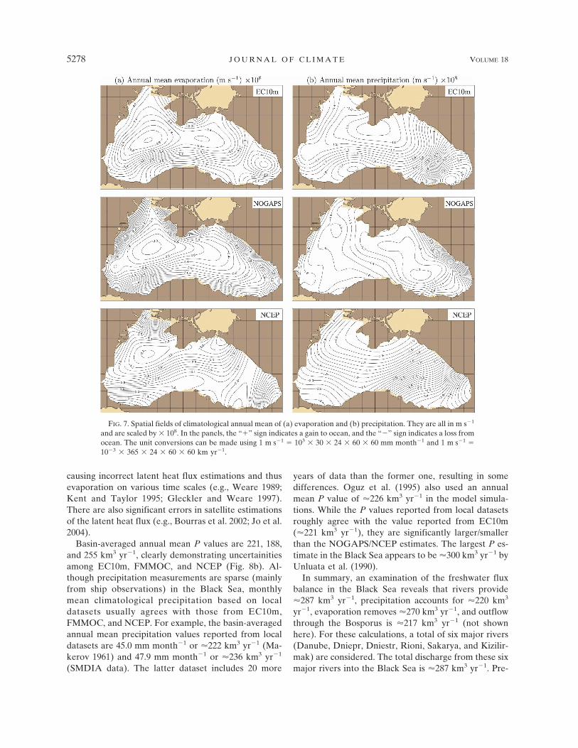
Here, the focus is to examine E and P values ob-tained from EC10m, NOGAPS, and NCEP (Fig. 7) andto compare them with values reported in earlier studies.Evaporation values are directly calculated from latentfluxes from EC10m, NOGAPS, and NCEP to be con-sistent with evaporation estimates from local datasets.The monthly mean E values are estimated using E �QL/(�w L), where QL is latent heat flux (W m�2), �w iswater density (1022 kg m�3), and L is latent heat ofvaporization [L � (2.501 � 0.00237 � �SST)106 J kg�1]with SST obtained from EC10m, NOGAPS, andNCEP. Basin-averaged annual mean E values forEC10m, NOGAPS, and NCEP are ��270, �266, and�335 km3 yr�1, respectively (Fig. 8a). Unluata et al.(1990) provided an estimate of 350 km3 yr�1 for E and300 km3 yr�1 for P, which are very large in comparisonto those obtained from EC10m and NOGAPS. Theagreement in E values from EC10m and NOGAPS isdue to the agreement in latent heat fluxes from thesetwo models (not shown).

Using the Sevastopol Marine Data Information As-

FIG. 4. Basin-averaged monthly mean wind stress curl obtained from (a) operational modelproducts and (b) observation-based climatologies. It should be emphasized that wind stresscurl from NCEP is substantially larger than that from other products. A comparison of windstress curl from the NCEP reanalysis (1948–2003) to one from the NCEP data used in thispaper (1979–93) revealed almost identical patterns and magnitudes (not shown), demonstrat-ing that the time period used for constructing the climatology is not the reason for seeing largewind stress.


sociation (SMDIA) data for the Black Sea, Oguz et al.(1995) gave a climatological annual mean E of 384 km3

yr�1 in their OGCM study, a value which is �110 km3

yr�1 greater than those obtained from EC10m andNOGAPS. In addition, based on observational localdatasets (Efimov and Timofeev 1990; Stanev 1990), ba-sin-averaged E reaches its maximum with a value of��150 mm month�1 (740 km3 yr�1) in August (see Fig.

4a of Oguz and Malanotte-Rizzoli 1996), which is alsotrue for NOGAPS with one-month delay (i.e., Septem-ber) for EC10m and NCEP. However, this maximum Evalue is almost twice as large as EC10m (��80 mmmonth�1 or �392 km3 yr�1), NOGAPS (��84 mmmonth�1 or �413 km3 yr�1), and also larger than that ofNCEP (��108 mm month�1 or �533 km3 yr�1). All ofthese analyses demonstrate that the largest values arefrom SMDIA, giving an overestimation in E in com-parison to EC10, NOGAPS, and NCEP. The uncer-tainty in E is not surprising at all since knowledge of theannual and interannual variability of the moisture fluxis rather limited in many regions of the global oceanbecause of the lack of available in situ measurements,

FIG. 5. Basin-averaged monthly mean thermal forcing param-eters obtained from EC10m, NOGAPS, and NCEP: (a) air tem-perature at 10 m above the sea surface, (b) air mixing ratio at 10m above the sea surface, (c) net shortwave radiation at the seasurface, and (d) net solar radiation, which is the sum of net short-wave radiation and net longwave radiation at the sea surface. Allof these parameters are directly formed from the 6-h outputs ofthree operational models over the Black Sea. The rms differencevalues calculated over the annual cycle (cf. section 4) for air tem-perature, air mixing ratio, net shortwave radiation, and net solarradiation between EC10m and NOGAPS (NCEP) are 0.5°C(0.8°C), 0.8 g kg�1 (0.4 g kg�1), 33.0 W m�2 (30.4 W m�2), and37.4 W m�2 (29.2 W m�2), respectively. Similarly, those betweenNCEP and NOGAPS are 1.1°C, 0.9 g kg�1, 4.8 W m�2, and 11.4W m�2.

FIG. 6. Same as in Fig. 5, but for monthly mean differencesbetween thermal forcing parameters. Some of the differences areattributed to fact that the climatology from NOGAPS output wasformed using 5 yr of model output (1998–2002), which is the onlyavailable time period as of this writing, while a 15-yr period ofmodel output (1979–93) was used to obtain the climatology fromEC10m and NCEP. This was confirmed from climatologies con-structed using the same time period (1998–2002), which did notshow significant differences.


causing incorrect latent heat flux estimations and thusevaporation on various time scales (e.g., Weare 1989;Kent and Taylor 1995; Gleckler and Weare 1997).There are also significant errors in satellite estimationsof the latent heat flux (e.g., Bourras et al. 2002; Jo et al.2004).

Basin-averaged annual mean P values are 221, 188,and 255 km3 yr�1, clearly demonstrating uncertainitiesamong EC10m, FMMOC, and NCEP (Fig. 8b). Al-though precipitation measurements are sparse (mainlyfrom ship observations) in the Black Sea, monthlymean climatological precipitation based on localdatasets usually agrees with those from EC10m,FMMOC, and NCEP. For example, the basin-averagedannual mean precipitation values reported from localdatasets are 45.0 mm month�1 or �222 km3 yr�1 (Ma-kerov 1961) and 47.9 mm month�1 or �236 km3 yr�1

(SMDIA data). The latter dataset includes 20 more

years of data than the former one, resulting in somedifferences. Oguz et al. (1995) also used an annualmean P value of �226 km3 yr�1 in the model simula-tions. While the P values reported from local datasetsroughly agree with the value reported from EC10m(�221 km3 yr�1), they are significantly larger/smallerthan the NOGAPS/NCEP estimates. The largest P es-timate in the Black Sea appears to be �300 km3 yr�1 byUnluata et al. (1990).

In summary, an examination of the freshwater fluxbalance in the Black Sea reveals that rivers provide�287 km3 yr�1, precipitation accounts for �220 km3

yr�1, evaporation removes �270 km3 yr�1, and outflowthrough the Bosporus is �217 km3 yr�1 (not shownhere). For these calculations, a total of six major rivers(Danube, Dniepr, Dniestr, Rioni, Sakarya, and Kizilir-mak) are considered. The total discharge from these sixmajor rivers into the Black Sea is �287 km3 yr�1. Pre-

FIG. 7. Spatial fields of climatological annual mean of (a) evaporation and (b) precipitation. They are all in m s�1

and are scaled by � 108. In the panels, the “” sign indicates a gain to ocean, and the “�” sign indicates a loss fromocean. The unit conversions can be made using 1 m s�1 � 103 � 30 � 24 � 60 � 60 mm month�1 and 1 m s�1 �10�3 � 365 � 24 � 60 � 60 km yr�1.


cipitation and evaporation estimates are based on theEC10m data. Bosporus outflow values are taken fromFig. 7b of Staneva and Stanev (1998).

3. HYCOM description

The Hybrid Coordinate Ocean Model (HYCOM) isbased on primitive equations (Bleck 2002). It containsfive prognostic equations: two for the horizontal veloc-ity components, a mass continuity or layer thicknesstendency equation, and two conservation equations fora pair of thermodynamic variables, such as salt andtemperature or salt and density.

HYCOM behaves like a conventional (terrain fol-lowing) model in very shallow oceanic regions, like az-level coordinate model in the mixed layer or otherunstratified regions, and like an isopycnic-coordinatemodel in stratified regions. However, the model is notlimited to these coordinate types (Chassignet et al.

2003). The model has several mixed layer/vertical mix-ing options, which are discussed and evaluated in Hal-liwell (2004). In this paper, we use the nonslab K-Profile Parameterization (KPP) of Large et al. (1997).

The net surface heat flux that has been absorbed (orlost) by the upper ocean to depth is parameterized asthe sum of the downward surface solar irradiance, up-ward longwave radiation, and the downward latent andsensible heat fluxes. The amount of net shortwave ra-diation that enters the mixed layer depends on the solarattenuation depths, which can significantly influenceupper open variables in the Black Sea simulations(Kara et al. 2005c). Thus, the effect of turbidity on solarradiation penetrating to depth is accounted for by usinga monthly attenuation of photosynthetically availableradiation (kPAR) climatology over 1997–2001. Thesesatellite-based climatological kPAR fields are derivedfrom Sea-Viewing Wide Field-of-View Sensor(SeaWiFS) data on the spectral diffuse attenuation co-efficient at 490 nm (k490) and have been processed tohave smoothly varying and continuous coverage (Karaet al. 2004).

Latent and sensible heat fluxes at the air–sea inter-face are calculated using efficient and computationallyinexpensive bulk formulas that include the effects ofdynamic stability (Kara et al. 2002). Our experiencewith the model simulations confirms that the surfaceheat flux forcing causes the model SST to relax towardan equilibrium state prescribed by the air temperatureand air mixing ratio climatologies. Thus, it is reasonableto expect successful HYCOM simulations of SST byletting the model calculate its own surface heat fluxesincluding effects of atmospheric stability via exchangecoefficients. Net solar radiation at the sea surface is sodependent on cloudiness that it is taken directly fromECMWF (or NOGAPS) for use in the model. Basingfluxes on the model SST automatically provides aphysically realistic tendency toward the correct SST(Wallcraft et al. 2003). A longwave radiation correctionis applied in the form of a relaxation term (Kara et al.2005b).

The Black Sea model setup is explained in Kara et al.(2005b) in detail. The model has a resolution of 1/25° �1/25° cos(lat), (latitude � longitude) (�3.2 km). Thereare a total of 15 hybrid layers (10 predominantly iso-pycnal and 5 always or z levels). The model has iso-pycnal coordinates in the stratified ocean but uses thelayered continuity equation to make a dynamicallysmooth transition to z levels (fixed-depth coordinates)in the unstratified surface mixed layer and levels (ter-rain-following coordinates) in shallow water. The opti-mal coordinate is chosen every time step using a hybridcoordinate generator. Thus, HYCOM automatically

FIG. 8. Basin-averaged monthly mean values for (a) evapora-tion and (b) precipitation. They were both obtained in m s�1 andconverted to km3 yr�1. Although evaporation is calculated in themodel (i.e., it is not a prescribed forcing) using simulated latentheat flux at each time step, it is shown here for comparison.Monthly mean precipitation fields that are linearly interpolated to6-h intervals are directly read into the model in m s�1. The cli-matological annual mean evaporation (precipitation) bias valuesare 4.4 (�33.5), �65.0 (33.6), and 69.4 (�67.1) km3 m�1 forNOGAPS–EC10m, NCEP–EC10m, and NOGAPS–NCEP, re-spectively. The rms difference values calculated over the annualcycle (cf. section 4) for evaporation (precipitation) are 37.3 (83.7),78.2 (59.7), and 88.2 (82.3) km3 m�1 between the pairs ofNOGAPS and EC10m, NCEP and EC10m, and NOGAPS andNCEP. Similarly, linear correlation coefficients are 0.96 (0.01),0.95 (0.40), and 0.92 (0.49) for the same pairs, indicating thatmonthly mean evaporation from all three products have similarseasonal cycles, while this is not true for the precipitation.


generates the lighter isopycnal layers needed for thepycnocline during summer. These become z-levels dur-ing winter. The density values for the isopycnals andthe decreasing change in density with depth betweenisopycnal coordinate surfaces are based on the densityclimatology from the Modular Ocean Data Assimila-tion System (MODAS; Fox et al. 2002). HYCOM isinitialized using temperature and salinity profiles fromthe MODAS climatology. The Black Sea bottom to-pography (Fig. 1) was formed from the 1-min DigitalBathymetric Database-Variable (DBDB-V) resolutiondataset, which also includes river bathymetry, obtainedfrom the Naval Oceanographic Office (NAVOCEANO).Lighting (shading) in the bathymetry is intended toshow detailed features of canyons, shelf break areas,and mountain ranges.

4. The impact of atmospheric forcing on the modelSST simulations

Climatologically forced HYCOM simulations (Table5) are performed to examine the sensitivity of SST tothe choice of atmospheric forcing products for SST.During the model integration, there is no assimilationof any oceanic data except for relaxation to sea surfacesalinity (SSS) from the MODAS climatology. Themodel is initialized using temperature and salinity fromthe MODAS climatology. The nominal e-folding timefor the SSS relaxation is 30 days, assuming a constantmixed-layer depth (MLD) of 30 m. The actual e-foldingtime depends on the mixed layer depth and is 30 �30(MLD)-1 days, that is, it is more rapid when theMLD is shallow and less so when it is deep. The windforcing includes monthly mean wind stresses with theaddition of high-frequency components as explained insection 2c.

For evaluation of the model results, monthly meanSSTs are formed from daily fields using the last 4 modelyears (years 5 through 8). At least a 4-yr mean wasneeded because HYCOM with 3.2-km resolution has astrong nondeterministic component due to flow insta-bilities. These are a major contribution to the simulatedBlack Sea circulation at this resolution. Monthly meanHYCOM SST fields are then compared to climatologi-cal SST fields at each model grid point. Our main goalis not only to investigate which atmospheric forcingproduct gives the best Black Sea simulation, but also todetermine which one yields a better simulation nearland/sea boundaries or in the interior.

a. HYCOM evaluation

The climatological SST (truth) used here is the Path-finder dataset, which is based directly on satellite mea-surements (Casey and Cornillon 1999). The monthlyclimatology covers 1985–97, and it has a resolution of�9.3 km. Both daytime and nighttime daily SST valuesare included in each monthly average. A 7 � 7 mediansmoother box filter was applied to remove small-scalenoise, replacing each pixel with the median of the pixelsin the surrounding 7 � 7 pixel box, effectively yieldingspatial resolution of �30 km. The final monthly meanPathfinder SST climatology was also smoothed 7 timesto get rid of the blocky SST variability found in theoriginal data source. The Pathfinder climatology is pre-ferred for the model–data comparisons as it outper-forms the commonly used climatologies (Casey andCornillon 1999), and it also has much finer resolutionthan the others, which is appropriate for the fine-resolution Black Sea model used in this paper.

Several statistical measures are considered to assessthe strength of the relationship between SST values

TABLE 5. A description of 16 climatologically forced HYCOM simulations used in this paper. The reader is referred to the text forconstruction of each atmospheric forcing product. River forcing is considered under the thermal forcing. The model array size is 360� 206, and performing a 1-month simulation takes �0.7 wall-clock hours using 64 HP/COMPAQ SC45 processors at the U.S. ArmyEngineer Research and Development Center (ERDC). The model is run until it reaches statistical equilibrium using climatologicalmonthly mean thermal atmospheric forcing, but with wind forcing that includes the 6-h variability as explained in the text. It takes about5–8 model years for a simulation to reach statistical equilibrium for all model parameters. The model is deemed to be in statisticalequilibrium when the rate of potential energy change is acceptably small (e.g., � 1% in 5 yr) in all layers.

HYCOMsimulation

Windforcing

Thermalforcing

HYCOMsimulation

Windforcing

Thermalforcing

Expt 1 EC10m EC10m Expt 9 EC10m NOGAPSExpt 2 EC1000 EC10m Expt 10 EC1000 NOGAPSExpt 3 NOGAPS EC10m Expt 11 NOGAPS NOGAPSExpt 4 NCEP EC10m Expt 12 NCEP NOGAPSExpt 5 SCAT EC10m Expt 13 SCAT NOGAPSExpt 6 COADS EC10m Expt 14 COADS NOGAPSExpt 7 SOC EC10m Expt 15 SOC NOGAPSExpt 8 HR EC10m Expt 16 HR NOGAPS


predicted by the model (HYCOM SST) and those fromthe climatology (Pathfinder SST). The latter is interpo-lated to the model grid for model–data comparisons.We evaluate time series of monthly mean SST at eachmodel grid point over the Black Sea. Following Murphy(1988), the statistical relationships between themonthly mean Pathfinder SST (X) and HYCOM SST(Y) can be expressed as follows:

ME � Y � X, �1�

rms � �1n

i�1

n

�Yi � Xi�2�1�2

, �2�

R �1n

i�1

n

�Xi � X��Yi � Y��X�Y�, �3�

SS � R2 � �R � ��Y��X��2

Bcond

� ��Y � X��X�2

Buncond

, �4�

where n � 12, ME is the mean error, rms is the root-mean-square difference, R is the correlation coefficient,SS is the skill score, and X(Y)and X (Y) are the meanand standard deviations of the Pathfinder (HYCOM)SST values, respectively.

The nondimensional SS in (4) includes conditionaland unconditional biases (Murphy 1992). It is used forthe model–data comparisons because one needs to ex-amine more than the shape of the seasonal cycle usingR. The nondimensional SS measures the accuracy ofSST simulations relative to Pathfinder SST. The condi-tional bias (Bcond) is the bias in standard deviation ofthe HYCOM SST, while the unconditional bias(Buncond) is the mismatch between the mean HYCOMand Pathfinder SST. The value of R2 can be considereda measure of “potential” skill, that is, the skill that onecan obtain by eliminating bias from the HYCOM SST.Note that the SS is 1.0 for perfect HYCOM SSTs, andpositive SS is considered as a successful simulation. Thenondimensional SS takes bias into account, somethingnot done by R. Part of the reduction in SS values incomparison to R stems from the squaring of correlationin the SS calculation. Biases are taken into account inthe rms differences, but in some cases the latter can besmall when SS and R are poor. This can occur where theamplitude of seasonal cycle is small.

Annual mean HYCOM SST error and rms SST dif-ference calculated over the seasonal cycle with respectto the Pathfinder climatology are shown in Fig. 9. TheSST bias is small (�0.25°) in most of the Black Sea, andthis is true regardless of the atmospheric forcing prod-uct used in the model simulations except for NCEP.This is clearly evident from the basin-averaged ME val-

ues (Table 6). There are relatively cold and warm SSTbiases in different regions of the Black Sea for NCEPforcing, but they tend to cancel in the areal average,resulting in small ME (Fig. 9a). For a given wind forc-ing, HYCOM usually gives slightly warm SST bias (i.e.,ME � 0°C) in the interior of the Black Sea when usingthermal forcing from EC10m. On the other hand, thereverse is true when using thermal forcing fromNOGAPS. The most obvious feature of the ME maps isthat HYCOM SST errors are relatively large (1°–2°C)near the coastal regions, especially on the northeasterncoast near the Caucasus Peninsula (Fig. 1), in compari-son to the interior of the region for all of the windforcing products.

Some of the errors very close to the coastal regions(e.g., near Caucasus Peninsula) are primarily caused bythe incorrect land–sea masks that exist in the atmos-pheric forcing products (Kara et al. 2005b). This resultsfrom problems representing sea points near land in theatmospheric forcing for the HYCOM simulations. Inparticular, a serious problem arises when using thesecoarse-resolution products (1.125° � 1.125° for EC10mand 1.875° � 1.875° for NCEP) in forcing fine-resolution (1/25° � 1/32°) Black Sea HYCOM. This isbecause atmospheric forcing values over water duringinterpolation to the finer ocean grid are contaminatedby those over the land near the coastal regions mainlybecause of the much coarser atmospheric computa-tional grid. A creeping sea-fill methodology could be asolution to reduce the improper representation of sca-lar atmospheric forcing parameters near coastal re-gions, although such methodology is only designed toapply thermal forcing parameters rather than vectorfields, such as wind stress forcing (Kara et al. 2005,manuscript submitted to J. Phys. Oceanogr.).

A final remark about the ME maps is that the use ofwind forcing from NCEP in the model simulations givesrelatively large mean SST errors in comparison to thosefrom other wind products. This is true when using ther-mal forcing from either EC10m or NOGAPS. In thiscase, HYCOM SST bias can be as large as 2°–3°C oreven �3°C east of Trabzon (labeled on Fig. 1) in theeasternmost part of the Black Sea. However, it shouldbe emphasized that the atmospheric forcing from theoperational model products is not quite correct in theeasternmost part of the Black Sea. For example, exam-ining the EC10m reanalysis product during 1979–93,Schrum et al. (2001) confirmed that the air temperatureat 10 m above the sea surface is unrealistically low, andthe air mixing ratio at 10 m above the sea surface islarge in comparison to the climatic data from the ob-servation-based climatologies in the easternmost re-gion. Thus, some of the model errors in predicting the


FIG. 9. Spatial mean error (ME) and rms difference maps between HYCOM SST and the Pathfinder SST climatology (HYCOM �Pathfinder) over the Black Sea. HYCOM was forced by eight different wind stress products using thermal forcing from (a) EC10m and(b) NOGAPS, separately. Note that all climatologically forced model simulations are performed without assimilation of any SST, andthere is no relaxation to any SST climatology.


SST annual cycle can be attributed to the atmosphericforcing used in the simulations.

Similarly, wind speed from NCEP is much larger onbasin average (�5 m s�1) from Fig. 2a than from theother products mainly because it is so much stronger inthe easternmost area. In fact, wind speeds from NCEPare usually at least twice as strong as from other atmo-spheric forcing products in the southeasternmost regionof the Black Sea. This is an indication that such largewind speeds are unrealistic. The amplitude of the windstress seasonal cycle based on the NCEP was also foundto be unrealistically larger than the one estimated fromthe EC10m by Schrum et al. (2001), who used a differ-ent time period (1980–86) to construct the NCEP cli-matology. It is obvious that the wind forcing fromNCEP is in error in the Black Sea, resulting in unreal-istic model simulations.

Using an OGCM, Oguz and Malanotte-Rizzoli

(1996) indicated that the monthly climatological surfacefluxes impose too much cooling on the northwesternshelf during winter and too much warming in the east-ern basin during summer, resulting in unrealistic SSTsimulations from their model. Such large biases do notexist in HYCOM simulations, partly explaining the im-portance of using 1) high-quality atmospheric forcingalong with a hybrid coordinate model approach with noSST assimilation or relaxation, and 2) model SST incalculating latent and sensible heat fluxes rather thanusing net fluxes in model simulations. However, directcomparison between the two models is not the subjectof this paper.

The rms SST differences between HYCOM and thePathfinder climatology are generally small, typicallyabout 1.2°C in the interior (Fig. 9b). This is true for allwind forcing products except NCEP with thermal forc-ing from EC10m and NOGAPS. The rms SST differ-ence becomes large (�2°C) in the southern Black Seawhen HYCOM is forced with NCEP winds along withthermal forcing from either EC10m or NOGAPS. Inparticular, the HYCOM simulation using NCEP windsresulted in the largest basin-averaged rms SST differ-ence with a value of 2.16°C (2.15°C) when using ther-mal forcing from EC10m (NOGAPS) as seen fromTable 6. The impact of using a fine-resolution windforcing in the model simulations is most easily seen inthe northwestern shelf, including the coastal regionsnear the Crimea Peninsula. In particular, the rms SSTdifference is reduced by 1° to 1.5°C when the model isforced with SCAT winds, which have a resolution of0.25° � 0.25°. It should be emphasized that SCATwinds were produced from measurements that were alltaken over the water, that is, there are no land values inthe interpolated model forcing field. The rms SST dif-ference is generally small (�0.5°C) in the easternmostpart of the Black Sea for a given wind forcing whenusing thermal forcing from EC10m (e.g., off Trabzon)as opposed to using thermal forcing from NOGAPS.On the contrary, the reverse is true in the interior, thatis, the use of thermal forcing from NOGAPS tends toreduce rms SST difference. HYCOM is usually rela-tively insensitive to the thermal forcing in comparisonto the wind forcing as evident from all rms SST differ-ence maps, at least for the two forcing products(EC10m and NOGAPS) used in this paper.

HYCOM success in predicting SST is especially evi-dent from the nondimensional SS values (�0.96) in al-most all simulations over the majority of the Black Sea(Fig. 10a). Based on the SS definition (4), any positiveSS value is considered as representative of a successfulsimulation, and all the HYCOM simulations yielded SSvalues much greater than zero. Even the HYCOM

TABLE 6. Basin-averaged SST verification statistics: the 3.2-kmHYCOM vs the 9.3-km Pathfinder climatology. The latter is in-terpolated onto the model grid for comparisons. Results areshown for the model response when forced with each individualwind product. Thermal forcing is from either EC10m orNOGAPS when using various wind forcing products. Statistics arecalculated using monthly mean values (i.e., monthly mean HY-COM SST vs monthly mean Pathfinder SST) at each model gridpoint. An SS value of 1 indicates perfect HYCOM simulation withrespect to the Pathfinder SST climatology. All R values are �0.97and statistically significant in comparison to a 0.7 correlationvalue at a 95% confidence interval. A correlation coefficient of0.98 is not statistically different from a correlation coefficient of0.99.

Windforcing

HYCOM uses thermal forcing from EC10m

ME(°C)

Rms(°C) Bcond Buncond SS R

EC10m 0.00 1.24 0.02 0.00 0.96 0.99EC1000 �0.04 1.27 0.03 0.00 0.95 0.99NOGAPS �0.01 1.25 0.02 0.00 0.96 0.99NCEP �0.40 2.26 0.09 0.01 0.86 0.98SCAT �0.01 1.29 0.03 0.00 0.95 0.99COADS �0.10 1.39 0.03 0.00 0.95 0.99SOC �0.10 1.38 0.03 0.01 0.95 0.99HR �0.06 1.45 0.02 0.00 0.94 0.98

Windforcing

HYCOM uses thermal forcing from NOGAPS

ME(°C)

Rms(°C) Bcond Buncond SS R

EC10m �0.10 1.24 0.02 0.00 0.96 0.99EC1000 �0.20 1.26 0.02 0.00 0.96 0.99NOGAPS �0.04 1.24 0.02 0.00 0.96 0.99NCEP �0.30 2.25 0.09 0.01 0.86 0.98SCAT �0.20 1.21 0.02 0.00 0.96 0.99COADS �0.30 1.35 0.03 0.00 0.95 0.99SOC �0.20 1.32 0.03 0.00 0.95 0.99HR �0.20 1.39 0.03 0.00 0.95 0.99


FIG. 10. Nondimensional SST skill score (SS) and SST conditional bias (Bcond) maps between HYCOM and the Pathfinder clima-tology over the Black Sea. HYCOM was forced by eight different wind stress products using thermal forcing from (a) EC10m and (b)NOGAPS, separately. In these comparisons the Pathfinder SST climatology is treated as “perfect.” An SS value of 1.0 indicates perfectSST simulations from HYCOM. Note that all climatologically forced model simulations are performed with no assimilation of any SST,and there is no relaxation to any SST climatology.


simulation forced with NCEP winds gives SS values(�0.8) over the most of the Black Sea despite the low-est skill in comparison to other simulations in predict-ing the SST.

Here it is worthwhile to note that SST standard de-viation over the seasonal cycle is generally �5°C overthe Black Sea. The relatively low SS from the NCEP-forced simulations corresponds to relatively inaccurateHYCOM SSTs in the Black Sea region, but the NCEPSS is quite high compared to the SS from a variety ofatmospheric forcings in some other regions of the glob-al ocean. For example, in the equatorial Pacific warmpool, SST standard deviation is very small (e.g.,�0.5°C), and rms SST differences can be quite low.However, it is usually difficult to obtain positive SSTskill in this region when using atmospherically forcedOGCMs (e.g., Kara et al. 2003). When the model wasforced with SCAT winds along with thermal forcingfrom either EC10m or NOGAPS, the agreement be-tween HYCOM and Pathfinder SST is quite remark-able, especially in the coastal regions of the northwest-ern shelf. The use of the fine-resolution wind forcingreduced rms SST differences in these regions (Fig. 9b).

It is noteworthy that the contributions to SS are fromR2, Bcond, and Buncond as given in (4). Both biases arevery small with values close to zero, and correlationsare significantly large over the Black Sea (see Table 6).In particular, Bcond values are relatively larger than Bun-

cond regardless of the wind or thermal forcing used inthe model simulations. This means that SST errors aredue mostly to the bias in the standard deviation ratherthan bias in the mean. Spatial maps of Bcond are shownin Fig. 10b. Because Buncond values are almost zero, andR values are very large (�0.98), their maps are notincluded here.

Major differences in all model simulations are seen inthe coastal regions where, unlike SCAT, the coarse-resolution atmospheric forcing products were usuallycontaminated from land values. The SST simulationswere improved when using SCAT winds, especiallyalong the northwestern shelf where rms difference val-ues were �0.5°C. It should be emphasized that the at-mospheric forcing fields used in model simulationsshow considerable differences not simply due to nativegrid resolution or methodology for obtaining them,but may be partly due to the differences in averagingperiods ranging from several years (i.e., SCAT andNOGAPS) to 100 yr (HR). For this reason, the focus inpresenting model results was the HYCOM SST re-sponse to different atmospheric forcing products, notthe accuracy of the atmospheric forcing products them-selves.

b. Importance of high-frequency wind forcing

As explained in section 2c, the hybrid wind approachis used in all HYCOM simulations. A primary reasonfor using high-frequency (6 h) climatological forcing isto get time-varying wind speeds. A particular questionarises here. What is the importance of using high-frequency winds in the model simulations?

One of the HYCOM simulations using thermal andhigh-frequency wind forcing from NOGAPS is re-peated with the same thermal forcing but with themonthly mean wind forcing to investigate the impor-tance of using hybrid winds. Both simulations werestarted from the same initial state. Model–data com-parisons demonstrate that the annual mean HYCOMSST obtained using the monthly mean wind forcing ismuch less accurate in comparison to the Pathfinder SST(Fig. 11). The mean model SST generally has a warmbias in the case of monthly mean wind forcing. This isexpected because the vertical mixing tends to be low,allowing excessive warming in a shallow mixed layerthat is too shallow (not shown) because the variabilityin wind stress is too low. By including appropriate vari-ability in wind stress, the HYCOM simulation using thehigh-frequency winds generates mixing, distributingheat over a thicker mixed layer and entraining morecold water from below (not shown), resulting in realis-tic SSTs. Thus, it is clear that a mixed layer modeltuned with monthly winds cannot be optimal for inter-annual high-frequency forcing. Note that the 6-h sub-monthly wind stress anomalies in HYCOM have zeromonthly mean wind stress, but they don’t have azero monthly mean wind speed. This implies that someof the SST improvement obtained from the high-frequency wind forcing may be due to improved aver-age wind speed.

5. Sea surface circulation

Wind stress curl from the eight wind products is verydifferent over the Black Sea (see section 2). Therefore,the main features of the climatological mean sea sur-face circulation simulated under different wind forcingis briefly investigated in this section. Thus, if resultsfrom this paper are used in selecting atmospheric forc-ing products, simulation of both the circulation and themixed layer/SST can be considered.

The surface circulation system over the Black Sea hasbeen investigated in various studies using observations,ocean models, and satellite images (e.g., Stanev 1990;Oguz et al. 1995; Stanev et al. 1997; Gawarkiewicz et al.1999; Staneva et al. 2001; Afanasyev et al. 2002; Ginz-burg et al. 2002; Korotaev et al. 2003; Zatsepin et al.2003). These studies generally reveal the main point


that the permanent feature of the upper-layer circula-tion is the Rim Current, which forms a cyclonic gyrearound the entire continental shelf of the Black Sea,including two well-organized gyres in the interior. Thiscyclonic circulation is driven by the quasi-permanentpositive wind stress curl field. Based on limited obser-vations, the current speed, which varies seasonally, canbe up to 40 cm s�1 or even higher along the Rim Cur-rent (Oguz et al. 1993).

The climatologically forced HYCOM simulationsforced with eight wind stress products give very differ-ent spatial patterns for mean sea surface circulation(Fig. 12). The thermal forcing is from EC10m in allsimulations. The velocity vectors from the 3.2-kmHYCOM are subsampled to display the general surfacecirculation clearly. The western and eastern cyclonicgyres in the interior are well-known features of theBlack Sea circulation, and they are reproduced whenHYCOM uses wind forcing from EC10m andNOGAPS.

Korotaev et al. (2003) reports a current speed of 50cm s�1 within the Rim Current near the sea surfacewith the use of data assimilation. Although there is noassimilation of any ocean data in our model simulations(except for relaxation to SSS), HYCOM forced with

climatological wind stress products from EC10m,NOGAPS, and NCEP can give mean current speeds of�30 cm s�1, even reaching maximum values of �45cm s�1 (see arrow lengths in Fig. 12) near the westernpart of the Turkish coast as well. While the simulationsperformed with wind forcings from EC1000 and NCEPalso demonstrate the existence of the Rim Current,they lack the closed cyclonic gyre systems in the inte-rior. Observational-based climatologies, especiallyCOADS and SOC, result in currents that are too weak,and the same is also partially true for SCAT.

Surface circulation features from HYCOM simula-tions using NOGAPS thermal forcing are found to besimilar to those using EC10m thermal forcing (Fig. 12);therefore, they are not shown here. We only present thevector correlation between each simulation withEC10m thermal forcing and the corresponding simula-tion using NOGAPS thermal forcing for a given windproduct. The vector correlation depends on the speedand the cosine of the angle between the two sets ofvectors. Thus, vectors pointing in the same directionhave a positive relationship and those pointing in op-posite directions have a negative relationship (e.g.,Crosby et al. 1993). The vector correlations are 0.99,0.97, 0.98, and 0.99 when the wind forcing is from

FIG. 11. Comparisons of climatologically forced HYCOM simulations using high-frequency vsmonthly mean wind forcing: (a) annual mean model SST error and (b) rms SST difference. Both (a) and(b) are calculated with respect to the Pathfinder climatology. The basin-averaged annual mean SSTbiases are �0.04° and 1.79°C for the high-frequency and monthly wind forcing cases, respectively.Similarly, rms SST difference calculated over the seasonal cycle increases significantly from 1.24°C(high-frequency wind forcing) to 2.29°C (monthly mean wind forcing), demonstrating the impact ofhigh-frequency wind forcing in the eddy-resolving OGCM simulations.


EC10m, EC1000, NOGAPS, and NCEP for the EC10mthermal forcing versus NOGAPS thermal forcing simu-lations. Therefore, almost all of the variance existing insimulations with EC10m thermal forcing is also ex-plained by simulations using NOGAPS thermal forcing.Smaller vector correlations of 0.92, 0.91, 0.89, and 0.94are found for the SCAT, COADS, SOC, and HR simu-lations, but they are still statistically significant. Thus,

we conclude that the use of different thermal forcing(i.e., EC10m versus NOGAPS) does not have signifi-cant impact on spatial variations of the speed and di-rection of sea surface currents. On the other hand, vec-tor correlations between HYCOM simulations usingvarious wind forcings for a given thermal forcing can bequite variable (Table 7). For example, a strong relation-ship exists between sea surface current from any pair of

FIG. 12. Climatological mean sea surface currents overlaid on sea surface current speeds (cm s�1)obtained from HYCOM simulations forced with eight different wind stress products over the Black Sea.The thermal forcing is from EC10m in all simulations. The length of the reference velocity vector is 15cm s�1. The velocity vectors are subsampled for plotting. See section 2d in the text for construction ofthe wind and thermal forcing fields.


EC10m, EC1000, NOGAPS, NCEP, and HR, with thehighest one between EC10m and NOGAPS, a value of0.96 when thermal forcing from NOGAPS is used forboth. With only one exception, all other pairings yield alower vector correlation than the lowest between any ofthe preceding, with the lowest value being 0.04 betweenSCAT and SOC when NOGAPS thermal forcing isused. This quantitative evaluation and the earlier com-parisons for the Rim Current indicate relative accuracyof sea surface currents from HYCOM simulationsforced with EC10m, EC1000, NOGAPS, NCEP,and HR.

Sea surface circulation is also examined on the north-western shelf (Fig. 13). This is the region where currentspeeds are relatively weak in comparison to those inmost of Black Sea, including the main pathways of theRim Current (Fig. 12). There are noticeable differencesin the strength and structure of climatological mean seasurface currents on the shallow northwestern shelf. Themodel response to atmospheric wind forcing is quiteeffective on the locations of small eddies and gyres,while all simulations generally reveal the big gyre cen-tered around 30°E except NCEP. The HR simulationalso gives the basic features of the Rim Current even ifits original spacing (2.0° � 2.0°) is very large for a smallbasin, such as Black Sea. In addition, relatively strongupwelling along the eastern boundary is a common fea-ture of the model simulations.

HYCOM simulation forced with the SCAT winds re-veals two eddies between 45°40�N and 46°N in the east-

ern part of the northwestern shelf (see Fig. 13) that areabsent in all other simulations. The main shortcomingof the SCAT winds is the numerical noise at the scale oftwo grid intervals, which generates these oceanic eddiesat the scales of 0.5° or so. Although the use of satellite-based SCAT wind stress resulted in very reliable SSTsimulations from HYCOM (see section 4), relativelypoor simulation of sea surface circulation could be dueto the short observational time period (August 1999through March 2002) used for constructing the clima-tology over the Black Sea. SCAT also has an accuracyof 20° for wind direction (http://winds.jpl.nasa.gov/missions/quikscat/).

It is obvious that circulation features are quite similarand complex on the northwestern shelf even though thewind forcing is so poorly resolved, except SCAT. Thisindicates that in addition to wind stress, other con-straints, such as bottom topography (1-min resolutionused here), the coastline and riverline outflow stronglyaffects the surface circulation of the northwestern shelf,but such detailed investigation is beyond the focus ofthis paper.

6. Summary and conclusions

The development of a high-resolution ocean generalcirculation model (OGCM) of the Black Sea is a greatchallenge since there are not many eddy-resolvingmodel studies in the region. Observations over theBlack Sea are also too sparse and inhomogeneous to

TABLE 7. Vector correlations of climatological mean sea surface currents between the pairs of HYCOM simulations forced withvarious wind stress products. The thermal forcing is either from EC10m or NOGAPS for a given wind forcing set.

Windforcing

HYCOM uses thermal forcing from EC10m

EC10m EC1000 NOGAPS NCEP SCAT COADS SOC HR

EC10m 1.00 0.82 0.92 0.75 0.35 0.45 0.26 0.79EC1000 0.82 1.00 0.72 0.84 0.49 0.52 0.31 0.92NOGAPS 0.92 0.72 1.00 0.75 0.31 0.45 0.27 0.76NCEP 0.75 0.84 0.75 1.00 0.45 0.45 0.22 0.80SCAT 0.35 0.49 0.31 0.45 1.00 0.24 0.09 0.39COADS 0.45 0.52 0.45 0.45 0.24 1.00 0.68 0.53SOC 0.26 0.31 0.27 0.22 0.09 0.68 1.00 0.34HR 0.79 0.92 0.76 0.80 0.39 0.53 0.34 1.00

Windforcing

HYCOM uses thermal forcing from NOGAPS

EC10m EC1000 NOGAPS NCEP SCAT COADS SOC HR

EC10m 1.00 0.74 0.96 0.76 0.41 0.34 0.25 0.71EC1000 0.74 1.00 0.70 0.83 0.42 0.48 0.28 0.91NOGAPS 0.96 0.70 1.00 0.76 0.35 0.36 0.27 0.69NCEP 0.76 0.83 0.76 1.00 0.37 0.39 0.21 0.80SCAT 0.41 0.42 0.35 0.37 1.00 0.07 0.04 0.38COADS 0.34 0.48 0.36 0.39 0.07 1.00 0.76 0.48SOC 0.25 0.28 0.27 0.21 0.04 0.76 1.00 0.32HR 0.71 0.91 0.69 0.80 0.38 0.48 0.32 1.00


produce the fine-resolution and high-quality climatolo-gies that can be used as atmospheric forcing in OGCMstudies. Therefore, wind stress and thermal forcing pa-rameters presented in this paper are aimed at providingatmospheric forcing for OGCMs and other possiblestudies of the Black Sea. The sensitivity of climatologi-cally forced simulations to these products is then exam-ined using a fine-resolution (�3.2 km) Hybrid Coordi-nate Ocean Model (HYCOM).

Eight wind forcing products were used to form atmo-spheric forcing parameters for the Black Sea. The threeclimatologies formed from the observation-based prod-

ucts are COADS, SOC. and HR; the four formed fromoperational model products are EC10m, EC1000,NOGAPS, and NCEP. Measurements from the SeaWinds scatterometer on the QuikSCAT satellite werealso used to produce the finest-resolution (0.25° �0.25°) climatological product (SCAT) for the BlackSea. Atmospheric forcing parameters were constructedunder two categories: 1) wind forcing (wind stress) and2) thermal forcing (air temperature and air mixing ratioat 10 m above the sea surface, precipitation, net short-wave radiation at the sea surface, and net solar radia-tion, which is the sum of net shortwave radiation and

FIG. 13. Same as in Fig. 12, but for currents in a zoom region on a small part of the northwestern shelfwhere water depths are generally �60 m. Note that the length of the reference velocity vector is 2cm s�1, and mean current speeds are very weak. The velocity vectors are subsampled for plottingcurrents obtained from the eddy-resolving (�3.2 km) HYCOM simulations.


net longwave radiation at the sea surface). Thermalforcing from EC10m or NOGAPS was used in all simu-lations.

It is demonstrated that some of the climatologicalforcing parameters reported in earlier studies, whichare based on sparse local observations, include someerrors. Previous observational and OGCM studies usu-ally used or reported relatively large wind stresses asthe wind speeds are larger than those reported in thisstudy. Here, both observation-based climatologies andclimatologies based on operational model products areshown to give a basin-averaged wind speed of 3–4 m s�1

in the Black Sea with the exception of the extremevalue of 4.6 m s�1 from NCEP. Overall, observation-based climatologies (COADS, SOC, and HR) are toosmooth. Consequently, they should not be used ineddy-resolving OGCM studies of the Black Sea or forsimilar smaller ocean basins. Basin-averaged annualmean values from EC10m and NOGAPS suggest veryclose estimates for evaporation and precipitation (�270km3 yr�1 for evaporation and �220 km3 yr�1 for pre-cipitation) in the Black Sea. These values are signifi-cantly lower than those reported in earlier studies(�350 km3 yr�1 for evaporation and � 300 km3 yr�1 forprecipitation). Air temperatures at 10 m above the seasurface from EC10m and NOGAPS usually agree withthose from local data sources except that operationalmodels are 2°C colder from January through April.

Using eight wind products and two thermal forcingproducts (EC10m and NOGAPS), a total of 16 clima-tologically forced HYCOM simulations with no oceandata assimilation or SST relaxation (except for relax-ation to climatological sea surface salinity) were per-formed to investigate the sensitivity of Black Sea HY-COM to the choice of atmospheric forcing product.Comparisons of monthly mean SST between HYCOMand a satellite-based climatology (Pathfinder) revealedthat the best SST simulation was obtained whenHYCOM used wind forcing from SCAT and thermalforcing from NOGAPS, with a basin-averaged rmsdifference value of 1.21°C and a skill score of 0.96 overthe annual cycle. In particular, when HYCOM usedthermal forcing from EC10m, basin-averaged rms SSTdifferences with respect to the Pathfinder SST clima-tology are 1.24°, 1.27°, 1.25°, and 2.16°C when usingwind forcing from EC10m, EC1000, NOGAPS, andNCEP (operational model products), respectively, and1.39°, 1.38°, and 1.45°C when using wind forcing fromCOADS, SOC, and HR (observation-based products).These results remained nearly the same when HYCOMused thermal forcing from NOGAPS. Although netshortwave radiation from NOGAPS is larger than thatfrom EC10m by �30 W m�2, the use of these two prod-

ucts in the model simulations yielded similar SST re-sults on climatological time scales. The simulated SSTsfrom all simulations are typically accurate to within�0.1° to � 0.3°C in the interior of the Black Sea, whenthere is no assimilation of SST data and when themodel SST is used in calculation of latent and sensibleheat fluxes. The paper also demonstrates that themodel skill in simulating the annual SST cycle improvessignificantly when using high-frequency wind forcing,which is composed of 6-h wind stress anomalies addedto the monthly mean wind stress.

While the model SST response to the various atmos-pheric forcing products usually remained robust in theHYCOM simulations, the wind stress patterns andmagnitudes from the eight atmospheric forcing prod-ucts presented in this paper clearly imply that thechoice of the atmospheric forcing product can havelarge influences on the simulated sea surface circulationfeatures of the Black Sea. The location and strength ofthe Rim Current vary greatly, depending on the atmos-pheric wind product used. Although the use of SCATwind improves the accuracy SST simulations because ofits fine resolution and accuracy near coastal regions, itdoes not provide very realistic circulation features.Thus, the best atmospheric forcing for simulating SST isnot necessarily the best for simulating Black Sea circu-lation because of relative sensitivity to wind speed andwind stress curl.

HYCOM simulations forced with observation-basedwind stress climatologies (e.g., COADS and SOC) yieldweak surface current speeds and disorganized Rim Cur-rent structure over the continental shelf. Additionally,the locations of small gyres and eddies remain almostrobust regardless of the wind forcing product used inHYCOM simulations over the northwestern shelf. Thissuggests that other constraints, such as the topography,coastline, and riverline inflow, have a larger impactthan atmospheric forcing on the sea surface circulationin this region.

Given that HYCOM SST simulations are relativelypoor near coastal regions, there is a clear message forregional and coastal ocean modelers. There are system-atic biases in gridded atmospheric forcing products(such as EC10m, NOGAPS, and NCEP) near coastalboundaries when the spatial resolution is too poor tosample these regions appropriately, that is, at the scaleof a much finer ocean grid (e.g., 3.2-km HYCOM). Formany studies in which an accurate representation of theocean dynamics and atmospheric forcing is neededclose to the coastline, a procedure is needed to reduceland contamination. The availability of satellite-derivedatmospheric forcing products (e.g., SCAT winds) with ahigher spatial resolution than weather center analyses is


very promising for future studies focused mainly onatmospheric forcing near land–sea boundaries. An-other valuable step would be atmospheric forcing prod-ucts from weather centers that are provided on theircomputational model grid for use in fine-resolutionOGCM studies, especially in coastal regions.

Finally, this paper utilizes a single ocean model de-sign (HYCOM) in examining the impact of atmos-pheric forcing on the SST simulations. While worth-while and interesting, including additional Black Seamodel designs is beyond the scope of this paper but is aworthwhile topic for future research. Investigating theseasonal variability of various atmospheric forcingproducts, such as those discussed here, is another sub-ject for future study.

Acknowledgments. The numerical HYCOM simula-tions were performed under the Department of De-fense High Performance Computing ModernizationProgram on an IBM SP POWER3 at the NavalOceanographic Office, Stennis Space Center, Missis-sippi, and on a HP/COMPAQ SC45 at the UnitedStates Army Engineer Research and DevelopmentCenter (ERDC), Vicksburg, Mississippi. We thank G.Halliwell of University of Miami and E. J. Metzger andJ. F. Shriver of the Naval Research Laboratory (NRL)for their discussions. The authors would also like toacknowledge two reviewers, T. Oguz and E. V. Stanev,who provided helpful suggestions. This research isfunded by the Office of Naval Research (ONR) underProgram Element 601153N as part of the NRL 6.1 Dy-namics of Low Latitude Western Boundary Current(DLLWBC) project. This is paper has been approvedfor public release by the Naval Research Laboratory.

REFERENCES

Afanasyev, Y. D., A. G. Kostianoy, A. G. Zatsepin, and P.-M.Poulain, 2002: Analysis of velocity field in the eastern BlackSea from satellite data during the Black Sea ‘99 experiment.J. Geophys. Res., 107, 3098, doi:10.1029/2000JC000578.

Altman, E. N., and N. I. Kumish, 1986: Interannual and seasonalvariability of the Black Sea fresh water balance (in Russian).Tr. Gos. Okeanogr. Inst., 145, 3–15.

——, I. F. Gertman, and Z. A. Golubeva, 1987: Climatologicalfields of salinity and temperature in the Black Sea (in Rus-sian). State Oceanography Institute Tech. Rep., 109 pp.[Available from the State Oceanography Institute, Sevasto-pol Branch, Sevastopol, Ukraine.]

Bleck, R., 2002: An oceanic general circulation model framed inhybrid isopycnic-Cartesian coordinates. Ocean Modell., 4,55–88.

Bourassa, M. A., D. M. Legler, J. J. O’Brien, and S. R. Smith,2003: SeaWinds validation with research vessels. J. Geophys.Res., 108, 3019, doi:10.1029/2001JC001028.

——, R. Rosario, S. R. Smith, and J. J. O’Brien, 2005: A new FSUwinds climatology. J. Climate, 18, 3692–3704.

Bourras, D., L. Eymard, and W. T. Liu, 2002: A neural network toestimate the latent heat flux over oceans from satellite ob-servations. Int. J. Remote Sens., 23, 2405–2423.

Casey, K. S., and P. Cornillon, 1999: A comparison of satellite andin situ–based sea surface temperature climatologies. J. Cli-mate, 12, 1848–1863.

Chassignet, E. P., L. T. Smith, G. R. Halliwell Jr., and R. Bleck,2003: North Atlantic simulations with the Hybrid CoordinateOcean Model (HYCOM): Impact of the vertical coordinatechoice, reference pressure, and thermobaricity. J. Phys.Oceanogr., 33, 2504–2526.

Chelton, D. B., J. C. Ries, B. J. Haines, L. L. Fu, and P. Callahan,2001: Satellite altimetry. Satellite Altimetry and Earth Sci-ences, L. L. Fu and A. Cazanave, Eds., Academic Press, 57–64.

Crosby, D. S., L. C. Breaker, and W. H. Gemmill, 1993: A pro-posed definition for vector correlation in geophysics: Theoryand application. J. Atmos. Oceanic Technol., 10, 355–367.

da Silva, A. M., C. C. Young, and S. Levitus, 1994: Algorithms andProcedures. Vol. 1, Atlas of Surface Marine Data 1994,NOAA Atlas NESDIS 6, 83 pp.

Efimov, E. V., and A. Timofeev, 1990: Investigation of the BlackSea and Azov Sea heat balance. Ukrainian Academy of Sci-ence, Sevastopol, Ukraine, 237 pp.

Ezer, T., 1999: Decadal variabilities of the upper layers of thesubtropical North Atlantic: An ocean model study. J. Phys.Oceanogr., 29, 3111–3124.

Fairall, C. W., E. F. Bradley, J. E. Hare, A. A. Grachev, and J. B.Edson, 2003: Bulk parameterization of air–sea fluxes: Up-dates and verification for the COARE algorithm. J. Climate,16, 571–591.

Fox, D. N., W. J. Teague, C. N. Barron, M. R. Carnes, and C. M.Lee, 2002: The Modular Ocean Data Assimilation System(MODAS). J. Atmos. Oceanic Technol., 19, 240–252.

Fu, L. L., and Y. Chao, 1997: The sensitivity of a global oceanmodel to wind forcing: A test using sea level and wind ob-servations from satellites and operational wind analysis. Geo-phys. Res. Lett., 24, 1783–1786.

Gawarkiewicz, G., G. Korotaev, S. Stanichny, L. Repetin, and D.Soloviev, 1999: Synoptic upwelling and cross-shelf transportprocesses along the Crimean coast of the Black Sea. Cont.Shelf Res., 19, 977–1005.

Gibson, J. K., P. Kållberg, S. Uppala, A. Hernandez, A. Nomura,and E. Serrano, 1999: ECMWF Re-Analysis Project ReportSeries: 1. ERA description (Version 2), 74 pp. [Availablefrom ECMWF, Shinfield Park, Reading RG2 9AX, UnitedKingdom.]

Ginzburg, A. I., A. G. Kostianoy, N. P. Nezlin, D. M. Soloviev,and S. V. Stanichny, 2002: Anticyclonic eddies in the north-western Black Sea. J. Mar. Syst., 32, 91–106.

Gleckler, P. J., and B. C. Weare, 1997: Uncertainties in globalocean surface heat flux climatologies derived from ship ob-servations. J. Climate, 10, 2764–2781.

Golubev, Y. N., and A. Y. Kuftarkov, 1993: On the flux of mo-mentum at the Black Sea surface (in Russian). Meteor.Gidrol., 3, 92–97.

Golubeva, A., 1984: Variability of the Black Sea heat balance (inRussian). Tr. Gos. Okeanogr. Inst., 180, 21–32.

Halliwell, G. R., Jr., 2004: Evaluation of vertical coordinate andvertical mixing algorithms in the HYbrid Coordinate OceanModel (HYCOM). Ocean Modell., 7, 285–322.


Harrison, D. E., 1989: On climatological monthly mean windstress and wind stress curl fields over the World Ocean. J.Climate, 2, 57–70.

Hellerman, S., and M. Rosenstein, 1983: Normal monthly windstress over the world ocean with error estimates. J. Phys.Oceanogr., 13, 1093–1104.

Hogan, P. J., and H. E. Hurlburt, 2005: Sensitivity of simulatedcirculation dynamics to the choice of surface wind forcing inthe Japan/East Sea. Deep-Sea Res., 52, 1464–1489.

Jo, Y.-H., X.-H. Yan, J. Pan, and W. T. Liu, 2004: Sensible andlatent heat flux in the tropical Pacific from satellite multi-sensor data. Remote Sens. Environ., 90, 166–177.

Josey, S. A., E. C. Kent, and P. K. Taylor, 1999: New insights intothe ocean heat budget closure problem from analysis of theSOC air–sea flux climatology. J. Climate, 12, 2856–2880.

——, ——, and ——, 2002: Wind stress forcing of the ocean in theSOC climatology: Comparisons with the NCEP–NCAR,ECMWF, UWM/COADS, and Hellerman and Rosensteindatasets. J. Phys. Oceanogr., 32, 1993–2019.

Kalnay, E., and Coauthors, 1996: The NCEP/NCAR 40-Year Re-analysis Project. Bull. Amer. Meteor. Soc., 77, 437–471.

Kara, A. B., H. E. Hurlburt, and P. A. Rochford, 2000: Efficientand accurate bulk parameterizations of air–sea fluxes for usein general circulation models. J. Atmos. Oceanic Technol., 17,1421–1438.

——, ——, and ——, 2002: Air–sea flux estimates and the 1997–1998 ENSO event. Bound.-Layer Meteor., 103, 439–458.

——, A. J. Wallcraft, and H. E. Hurlburt, 2003: ClimatologicalSST and MLD simulations from NLOM with an embeddedmixed layer. J. Atmos. Oceanic Technol., 20, 1616–1632.

——, H. E. Hurlburt, P. A. Rochford, and J. J. O’Brien, 2004: Theimpact of water turbidity on the interannual sea surface tem-perature simulations in a layered global ocean model. J. Phys.Oceanogr., 34, 345–359.

——, A. J. Wallcraft, and H. E. Hurlburt, 2005a: A new solarradiation penetration scheme for use in ocean mixed layerstudies: An application to the Black Sea using a fine-resolution Hybrid Coordinate Ocean Model (HYCOM). J.Phys. Oceanogr., 35, 13–32.

——, ——, and ——, 2005b: Sea surface temperature sensitivity towater turbidity from simulations of the turbid Black Sea us-ing HYCOM. J. Phys. Oceanogr., 35, 33–54.

——, ——, and ——, 2005c: How does solar attenuation depthaffect the ocean mixed layer? Water turbidity and atmo-spheric forcing impacts on the simulation of seasonal mixedlayer variability in the turbid Black Sea. J. Climate, 18, 389–409.

Kelly, K. A., S. Dickinson, and Z.-J. Yu, 1999: NSCAT tropicalwind stress maps: Implications for improving ocean model-ing. J. Geophys. Res., 104, 291–310.

Kent, E. C., and P. K. Taylor, 1995: A comparison of heat fluxestimates for the North Atlantic Ocean. J. Phys. Oceanogr.,25, 1530–1549.

——, ——, B. S. Truscott, and J. A. Hopkins, 1993: The accuracyof voluntary observing ships’ meteorological observations—Results of the VSOP-NA. J. Atmos. Oceanic Technol., 10,591–608.

Korotaev, G. K., T. Oguz, A. Nikiforov, and C. J. Koblinsky, 2003:Seasonal, interannual and mesoscale variability of the BlackSea upper layer circulation derived from altimeter data. J.Geophys. Res., 108, 3122, doi:10.1029/2002JC001508.

Lee, S.-K., D. B. Enfield, and C. Wang, 2005: Ocean general cir-culation model sensitivity experiments on the annual cycle of

the Western Hemisphere Warm Pool. J. Geophys. Res., 110,C09004, doi:10.1029/2004JC002640.

Liu, W. T., 2002: Progress in scatterometer application. J. Ocean-ogr., 58, 121–136.

——, W. Tang, and P. S. Polito, 1998: NASA Scatterometer pro-vides global ocean-surface wind fields with more structuresthan numerical weather prediction. Geophys. Res. Lett., 25,761–764.

Makerov, Y. V., 1961: Heat balance of the Black Sea (in Russian).Tr. Gos. Okeanogr. Inst., 61, 169–183.

Metzger, E. J., 2003: Upper ocean sensitivity to wind forcing in theSouth China Sea. J. Oceanogr., 59, 783–798.

Murphy, A. H., 1988: Skill scores based on the mean square errorand their relationships to the correlation coefficient. Mon.Wea. Rev., 116, 2417–2424.

——, 1992: Climatology, persistence, and their linear combinationas standards of reference in skill scores. Wea. Forecasting, 7,692–698.

Oguz, T., and P. Malanotte-Rizzoli, 1996: Seasonal variability ofwind and thermohaline driven circulation in the Black Sea:Modeling studies. J. Geophys. Res., 101, 16 551–16 569.

——, ——, and D. Aubrey, 1995: Wind and thermohaline circu-lation of the Black Sea driven by yearly mean climatologicalforcing. J. Geophys. Res., 100, 6845–6863.

Pegion, P. J., M. A. Bourassa, D. M. Legler, and J. J. O’Brien,2000: Objectively derived daily “winds” from satellite scat-terometer data. Mon. Wea. Rev., 128, 3150–3168.

Perry, G. D., P. B. Duffy, and N. L. Miller, 1996: An extendeddata set of river discharges for validation of general circula-tion models. J. Geophys. Res., 101, 21 339–21 349.

Rachev, N. H., V. M. Roussenov, and E. V. Stanev, 1991: TheBlack Sea climatological wind stress (in Bulgarian). Bulg. J.Meteor. Hydrol., 2, 72–79.

Rienecker, M. M., R. Atlas, S. D. Schubert, and C. S. Willett,1996: A comparison of surface wind products over the NorthPacific Ocean. J. Geophys. Res., 101, 1011–1023.

Rosmond, T. E., J. Teixeira, M. Peng, T. F. Hogan, and R. Pauley,2002: Navy Operational Global Atmospheric Prediction Sys-tem (NOGAPS): Forcing for ocean models. Oceanography,15, 99–108.

Samuel, S. L., K. Haines, S. A. Josey, and P. G. Myers, 1999: Re-sponse of the Mediterranean Sea thermohaline circulation toobserved changes in the winter wind stress field in the period1980–93. J. Geophys. Res., 104, 7771–7784.

Schlax, M. G., D. B. Chelton, and M. H. Freilich, 2001: Samplingerrors in wind fields constructed from single and tandem scat-terometer datasets. J. Atmos. Oceanic Technol., 18, 1014–1036.

Schopf, P. S., and A. Loughe, 1995: A reduced-gravity isopycnalocean model: Hindcasts of El Niño. Mon. Wea. Rev., 123,2839–2863.

Schrum, C., J. Staneva, E. Stanev, and E. Ozsoy, 2001: Air–seaexchange in the Black Sea estimated from atmospheric analy-sis for the period 1979–1993. J. Mar. Syst., 31, 3–19.

Simonov, A. I., and E. N. Altman, 1991: Black Sea. Vol. 4, Hy-drometerology and Hydrochemistry of the USSR Seas,Gidrometeoizdat, 430 pp.

Smith, S. R., D. M. Legler, and K. V. Verzone, 2001: Quantifyinguncertainties in NCEP reanalyses using high-quality researchvessel observations. J. Climate, 14, 4062–4072.

Sorkina, A. I., 1974: Reference Book on the Black Sea Climate (inRussian). Gidrometeoizdat, 406 pp.


Stanev, E. V., 1990: On the mechanisms of the Black Sea circu-lation. Earth-Sci. Rev., 28, 285–319.

——, and J.-M. Beckers, 1999: Numerical simulations of seasonaland interannual variability of the Black Sea thermohalinecirculation. J. Mar. Syst., 22, 241–267.

——, J. V. Staneva, and V. M. Roussenov, 1997: On the Black Seawater mass formation. Model sensitivity study to atmosphericforcing and parameterization of some physical processes. J.Mar. Syst., 13, 245–272.

——, M. J. Bowman, E. L. Peneva, and J. V. Staneva, 2003: Con-trol of Black Sea intermediate water mass formation by dy-namics and topography: Comparison of numerical simula-tions, survey and satellite data. J. Mar. Res., 61, 59–99.

——, J. Staneva, J. L. Bullister, and J. W. Murray, 2004: Ventila-tion of the Black Sea pycnocline. Parameterization of con-vection, numerical simulations and validations against ob-served chlorofluorocarbon data. Deep-Sea Res., 51, 2137–2169.

Staneva, J. V., and E. V. Stanev, 1998: Oceanic response to atmos-pheric forcing derived from different climatic data sets.Ocean. Acta, 21, 393–417.

——, D. E. Dietrich, E. V. Stanev, and M. J. Bowman, 2001: RimCurrent and coastal eddy mechanisms in an eddy-resolvingBlack Sea general circulation. J. Mar. Syst., 31, 137–157.

Sui, C.-H., X. Li, M. M. Rienecker, K.-M. Lau, and R. T. Pinker,2003: The role of daily surface forcing in the upper oceanover the tropical Pacific: A numerical study. J. Climate, 16,756–766.

Townsend, T. L., H. E. Hurlburt, and P. J. Hogan, 2000: ModeledSverdrup flow in the North Atlantic from 11 different windstress climatologies. Dyn. Atmos. Oceans, 32, 373–417.

Trenberth, K. E., and C. J. Guillemot, 1998: Evaluation of theatmospheric moisture and hydrological cycle in the NCEP/NCAR reanalyses. Climate Dyn., 14, 213–231.

——, D. P. Stepaniak, J. W. Hurrell, and M. Fiorino, 2001: Qualityof reanalyses in the Tropics. J. Climate, 14, 1499–1510.

Trukhchev, D. I., and Y. L. Demin, 1992: The Black Sea generalcirculation and climatic temperature and salinity fields.Woods Hole Oceanographic Institution Tech. Rep. WHOI-92-34, 136 pp. [Available from MBL/WHOI Library, 7 MBLStreet, Woods Hole, MA 02543.]

Unluata, U., T. Oguz, M. A. Latif, and E. Ozsoy, 1990: On thephysical oceanography of the Turkish Straits. The PhysicalOceanography of Sea Straits, G. Pratt, Ed., NATO ASI SeriesC, Kluwer, 25–60.

Vörösmarty, C. J., K. Sharma, B. M. Fekete, A. H. Copeland, J.Holden, J. Marble, and J. A. Lough, 1997: The storage andaging of continental runoff in large reservoir systems of theworld. Ambio, 26, 210–219.

Wallcraft, A. J., A. B. Kara, H. E. Hurlburt, and P. A. Rochford,2003: The NRL Layered Global Ocean Model (NLOM) withan embedded mixed layer submodel: Formulation and tun-ing. J. Atmos. Oceanic Technol., 20, 1601–1615.

Weare, B. C., 1989: Uncertainties in estimates of surface heatfluxes derived from marine reports over the tropical and sub-tropical oceans. Tellus, 41A, 357–370.

Zatsepin, A. G., A. I. Ginzburg, A. G. Kostianoy, V. V. Kre-menitskiy, V. G. Krivosheya, S. V. Stanichny, and P.-M. Pou-lain, 2003: Observations of Black Sea mesoscale eddies andassociated horizontal mixing. J. Geophys. Res., 108, 3246,doi:10.1029/2002JC001390.


Black Sea Mixed Layer Sensitivity to Various Wind and Thermal Forcing Products on Climatological...

Documents

Transcript of Black Sea Mixed Layer Sensitivity to Various Wind and Thermal Forcing Products on Climatological...