Modeling reference evapotranspiration over complex terrains from

minimum climatological data

Nazzareno Diodato1 and Gianni Bellocchi2

Received 8 August 2006; revised 29 January 2007; accepted 14 February 2007; published 31 May 2007.

[1] This work presents methods where monthly based climate data are used to estimatereference evapotranspiration (ET0). The objective was to evaluate two monthly ET0models (Hargreaves-Samani, HS; Droogers-Allen HS, DAHS) and compare the resultswith an improved model (reference evapotranspiration model for complex terrains,REMCT). HS and DAHS are both based on the monthly temperature range (DT), whileREMCT replaces DT with a monthly adjusted function (reference minimum airtemperature). The test area was peninsular-insular Italy, where 13 stations with sufficientdata to calculate FAO-56 Penman-Monteith ET0 were available. The three models wereevaluated against FAO-56 over a validation data set of six stations, using a multiple-statistics indicator: 0 (best) � IET � 1 (worst). The REMCT estimates generally comparedwell with the FAO-56 estimates (mean IET = 0.029 against 0.187 and 0.255 with HSand DAHS, respectively). The three models performed similarly at low-altitude sites.REMCT was superior at sites higher than 500 m above sea level, where the ET0 � DTrelationship was distorted (e.g., by an asymmetric lapse rate between maximum andminimum air temperatures).

Citation: Diodato, N., and G. Bellocchi (2007), Modeling reference evapotranspiration over complex terrains from minimum

climatological data, Water Resour. Res., 43, W05444, doi:10.1029/2006WR005405.

1. Introduction

[2] Reference evapotranspiration (ET0), defined as thepotential evapotranspiration of a hypothetical surface ofgreen grass of uniform height, actively growing and ade-quately watered, is one of the most important hydrologicalvariables for designing and scheduling irrigation systems,preparing input data to hydrological water balance models,and calculating actual evapotranspiration for a land [Dyck,1983; Hobbins et al., 2001a, 2001b; Xu and Li, 2003; Xuand Singh, 2005].[3] Accurate computation of water balance is necessary

to keep up sustainable development and environmentallysound water management [Weisse and Oestreicher, 2001;Xu and Li, 2003]. ET0 can be computed from meteorolog-ical data by means of different methods (see Gong et al.[2006] for a categorization). However, reliable determina-tion of ET0 may be a difficult issue at different spatial scales[Biftu and Gan, 2000; Thomas, 2000], because ET0 isdriven by a nonlinear combination of radiative and humidityforcing [Hobbins et al., 2001b]. The Penman-Monteith(PM) formulation [Monteith, 1965] is regarded as a goodET0 estimator for a wide variety of climatic conditions. TheU.N. Food and Agriculture Organization (FAO) adopted animplementation of the PM method as a global standard(referred to hereinafter as FAO-56) to estimate ET0 frommeteorological data [Allen et al., 1998]. A major drawback

to application of the FAO-56 model is the relatively highdata demand, requiring air temperature, wind speed, relativehumidity, and global solar radiation data. The number ofmeteorological stations where all required inputs are regis-tered is limited in many areas of the globe [Xu, 2002; Irmaket al., 2003; Gavilan et al., 2006]. Hargreaves and Samani[1985] developed an alternative approach to ET0 computa-tion (referred to hereinafter as the HS model), using dailymaximum and minimum air temperature data as the onlyinput. Evidence is provided from research [Droogers andAllen, 2002; Stockle et al., 2004; Vanderlinden et al., 2004]indicating that this equation is nearly as accurate as FAO-56in estimating ET0 on a weekly or longer time steps, and istherefore recommended in cases where reliable data forFAO-56 computation are lacking. In such respect, Droogersand Allen [2002] resolved the Hargreaves-Samani approachand a modified form of the HS model (referred to herein-after as the DAHS model) to estimate monthly ET0, usingmonthly climate inputs from the World Water and ClimateAtlas of the International Water Management Institute Water(http://www.iwmi.cgiar.org). However, the suitability ofmodels such as HS and DAHS for specific regions largelydepends on local calibration of empirical parameters againstreliable actual measurements. ET0 estimates are particularlysensitive to nonlinear interactions among diverse meteoro-logical variables, thus posing an issue of suitable applica-bility of ET0 models using actual air temperature range (DT)as the only input (as in the HS model), or merely modulatedby precipitation (as in the DAHS model). There are indeedfactors such as latitude, elevation, cloud pattern, advection,and proximity to large bodies of water that can influence therelationship between actualDT, and solar radiation [Dai andTrenberth, 1999; Thornton et al., 2000] and, in turn, ET0.

1Monte Pino Research Observatory, TEMS Network-Terrestrial Ecosys-tem Monitoring Sites, Benevento, Italy.

2Agrichiana Farming, Abbadia di Montepulciano, Siena, Italy.

Copyright 2007 by the American Geophysical Union.0043-1397/07/2006WR005405$09.00

W05444

WATER RESOURCES RESEARCH, VOL. 43, W05444, doi:10.1029/2006WR005405, 2007ClickHere

for

FullArticle

1 of 12

Then, the use of actual DT in HS-based algorithms easilyintroduces biases in the estimates related to latitude andaltitude gradients, when applied for monthly estimates incomplex terrains. Conditions of this type are likely to occur inMediterranean areas, where the climate is characterized bygreat inland-coast, valley-hilly contrasts in air temperatures,regional and local advection, and high shift between nightand day values of diverse agrometeorological variables[Rana and Katerji, 2000]. Mediterranean areas are alsoparticularly sensitive to climate change [Palutikof et al.,1994] and extreme events (droughts and intense rainfall[Brunetti et al., 2002]), turning into impacts on the evapo-transpiration rates [Sousa and Pereira, 1999; Dalezios et al.,2002] and consequently on crop growth [Belda and Melia,2000].[4] This is particularly true for Italy, centrally located in

the Mediterranean basin and characterized by a heteroge-neous mix of geographic systems (peninsular shape, Alpschain in the north, Apennines chain all along the peninsula).Reliable collection of wind speed, air humidity, and espe-cially solar radiation is quite limited in Italy [Giacobello,1980; Petrarca et al., 2000], compared with records of airtemperature and precipitation. In Italy, an historical clima-tological database is available containing about 300 stations[Pitzalis et al., 1989; Esposito and Beltrano, 1996], nearlyall of which having daily rainfall and temperature recordswhile only 70 of them record other variables. There are evenfewer stations where meteorological variables required byFAO-56 evapotranspiration model are accurately and regu-larly measured for quite a long time.[5] For sites where time series of weather measurements

are only available as monthly summaries, it is desirable tobe able to use monthly available data to estimate ET0.Monthly time step is also appropriate for climate trendstudies [Xu et al., 2005] and for use in climate models[Schulze, 2000]. It was also used to compute ET0 at diversescales [Shevenell, 1999; Xu and Singh, 2000; Castellvi etal., 2001; Garcia et al., 2004] and for water balance studies[Weisse and Oestreicher, 2001] and irrigation requirements[Doll and Siebert, 2002]. Since temperature and rainfallattributes are frequently available on a regional scale, anapproach estimating ET0 using minimum data could in-crease spatial resolution in data-sparse areas. According tothe relevant factors affecting evapotranspiration outlined byDiodato and Ceccarelli [2005], a new evapotranspirationmodel with monthly time step (reference evapotranspirationmodel for complex terrains, or REMCT) was developed,linking ET0 to rainfall occurrence and air temperature, andincluding the effect of climate and site elevation with thepurpose to skip over limitations observed with both HS andDAHS in complex terrains. REMCT incorporates a monthlyfunction of minimum air temperature, also conditioned bythe precipitation status, to account for seasonal shifts.REMCT was applied to a range of terrains in Italy. At thesame sites, REMCT estimates were compared with both HSand DAHS estimates.

2. Materials and Methods

2.1. Database and Data Sources

[6] The study region was the peninsular and insular(Sicily) Italy. The main feature of this central part of the

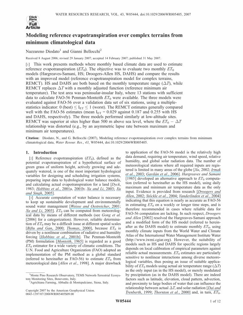
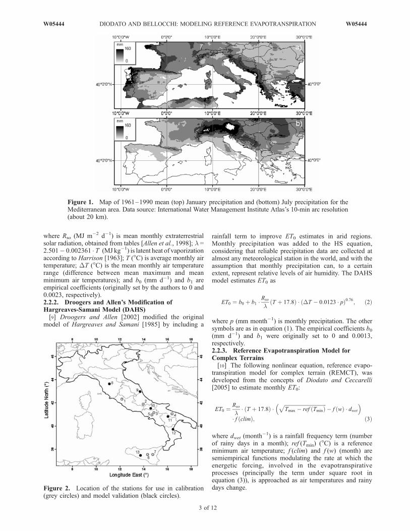
Mediterranean area is the geography and land use diversityincluding a large latitudinal gradient with transition zonesfrom semiarid to humid mountain climate [Lionello et al.,2006]. The Mediterranean basin represents a humiditysource for surrounding land areas as the moisture releasedby evaporation is redistributed by the atmospheric circula-tion [Fernandez et al., 2003] and by the course of precip-itation (Figure 1). However, drought is a frequent problemfor agriculture during summer (Figure 1b), when the lack ofwater resources often compromises the crops in largeregions [Agnew and Palutikof, 2000], including southernItaly [Brunetti et al., 2004]. A database of weather valueswas generated using observations from about 40 Italianstations including measurements of air temperature, solarradiation, relative humidity, and wind speed, required forcomputation of FAO-56 ET0. After data cleaning, a total of13 weather stations with a minimum period of 24 months ofrecords were used for this study (Table 1). With the onlyexception of Montevergine, where data of the 1940s wereavailable, the records were from the years 1994–2005.Daily data were available at these stations includingprecipitation, maximum and minimum air temperatures,global solar radiation, maximum and minimum relativehumidity, and wind speed. Such data were used to computeFAO-56 reference evapotranspiration at all but Montevergineof the 13 stations. Cloud cover data were available at this site,but not radiation data, and thus solar radiation for use inFAO-56 computation was estimated at Montevergine usingthe model of Supit and van Kappel [1998]. Monthly meanvalues of precipitation and air temperature data were used asinputs of the three models evaluated. Monthly averagedFAO-56 estimates were taken as ‘‘true’’ values of referencecrop ET0. The mapping of stations used, roughly rangingfrom 35� to 44� latitude North (Figure 2), representsdifferent climatic zones, and the station distribution isconsistent with the spatial variation in precipitation regis-tered in Italy (Figure 1). As shown in Figure 2, the fulldatabase was split into two data sets (I and II). Data set I(seven stations) was used to determine model parameters(calibration data set). Data set II (six locations) was used forevaluating model estimates (validation data set). The cali-bration data set was selected in such a way to bothrepresenting the all study area and including a wide rangeof elevations (i.e., from 183 to 1270 m above sea level (asl))and distances from the coast (i.e., from 12 to 62 km). Thevalidation data set also included sites representative ofcentral and southern Italy, with elevations between 10 and572 m asl, and distances from the coast between 4 and67 km.

2.2. Reference Evapotranspiration Models

[7] For each site and year of available data, mean monthlyevapotranspiration (mm d�1) values were estimated usingthree models based on a combination of monthly weatherinputs.2.2.1. Hargreaves-Samani Model (HS)[8] The Hargreaves-Samani model [Hargreaves and

Samani, 1985] estimates ET0 as

ET0 ¼ b0 þ b1 �Rso

lT þ 17:8ð Þ �

ffiffiffiffiffiffiffiffiDT

p; ð1Þ

2 of 12

W05444 DIODATO AND BELLOCCHI: MODELING REFERENCE EVAPOTRANSPIRATION W05444

where Rso (MJ m�2 d�1) is mean monthly extraterrestrialsolar radiation, obtained from tables [Allen et al., 1998]; l =2.501� 0.002361 � T (MJ kg�1) is latent heat of vaporizationaccording to Harrison [1963]; T (�C) is average monthly airtemperature; DT (�C) is the mean monthly air temperaturerange (difference between mean maximum and meanminimum air temperatures); and b0 (mm d�1) and b1 areempirical coefficients (originally set by the authors to 0 and0.0023, respectively).2.2.2. Droogers and Allen’s Modification ofHargreaves-Samani Model (DAHS)[9] Droogers and Allen [2002] modified the original

model of Hargreaves and Samani [1985] by including a

rainfall term to improve ET0 estimates in arid regions.Monthly precipitation was added to the HS equation,considering that reliable precipitation data are collected atalmost any meteorological station in the world, and with theassumption that monthly precipitation can, to a certainextent, represent relative levels of air humidity. The DAHSmodel estimates ET0 as

ET0 ¼ b0 þ b1 �Rso

lT þ 17:8ð Þ � DT � 0:0123 � pð Þ0:76; ð2Þ

where p (mm month�1) is monthly precipitation. The othersymbols are as in equation (1). The empirical coefficients b0(mm d�1) and b1 were originally set to 0 and 0.0013,respectively.2.2.3. Reference Evapotranspiration Model forComplex Terrains[10] The following nonlinear equation, reference evapo-

transpiration model for complex terrain (REMCT), wasdeveloped from the concepts of Diodato and Ceccarelli[2005] to estimate monthly ET0:

ET0 ¼Rso

l� T þ 17:8ð Þ �

ffiffiffiffiffiffiffiffiffiffiffiffiffiffiffiffiffiffiffiffiffiffiffiffiffiffiffiffiffiffiffiffiffiTmax � ref Tminð Þ

p� f wð Þ � dwet

� �� f climð Þ; ð3Þ

where dwet (month�1) is a rainfall frequency term (numberof rainy days in a month); ref (Tmin) (�C) is a referenceminimum air temperature; f (clim) and f (w) (month) aresemiempirical functions modulating the rate at which theenergetic forcing, involved in the evapotranspirativeprocesses (principally the term under square root inequation (3)), is approached as air temperatures and rainydays change.

Figure 1. Map of 1961–1990 mean (top) January precipitation and (bottom) July precipitation for theMediterranean area. Data source: International Water Management Institute Atlas’s 10-min arc resolution(about 20 km).

Figure 2. Location of the stations for use in calibration(grey circles) and model validation (black circles).

W05444 DIODATO AND BELLOCCHI: MODELING REFERENCE EVAPOTRANSPIRATION

3 of 12

W05444

[11] The reference minimum air temperature varies withmonth (m) as follows:

ref Tminð Þ ¼ a � 1� a � cos 2 � p � m� b

c

� �� �ð4Þ

where a(�C), a, b, and c are empirical parameters. The twosemiempirical equations are as follows:

f climð Þ ¼ d � e �ffiffiffiffiffiffiffiffiffiffiffiffiffiffiffiffiffiffiffiffiffiffiffiffiffiffiffiffiffig � Eð Þ � P

1000

r� h � E

!; ð5Þ

f wð Þ ¼ k þ q � T að Þmax � 10� 3

; ð6Þ

where T(a)max (�C) is long-term yearly mean daily maximumtemperature; E is the site’s elevation (m); P is the long-termmean annual precipitation (m); d, e (m�1), g (m), h (m�1),k (�C0.5 month), and q (�C�3) are empirical parameters.

2.3. Model Parameterization and Evaluation

[12] The empirical parameters of each radiation modelwere determined using data set I (calibration). The mass ofdata was not enough for a site-specific calibration, so thecalibration was run pooling the data from different sitesinto one set only. Basically, parameter values were esti-mated against mean monthly FAO-56 estimates by using asolver that minimized the square error of estimation. Aniterative calibration process was employed for equation (3).First, the set of parameters was determined for ref (Tmin)(equation (4)), f (clim) (equation (5)), and f (w) (equation (6))fitting the ET0 values keeping constant the parameters ofequation (3). Next, the parameters of equation (3) werecalibrated against the FAO-56 estimates. The process wasreiterated up to reach a converging solution. In this process,

parameter g of equation (5) was set equal to 2000 m, that is,the upper elevation for REMCT to be applied.[13] Computed ET0 values were compared against FAO-

56 values. The agreement between estimates and FAO-56values was evaluated by the regression lines and, limited tothe validation data set, through elementary statistics (mean,standard error) and by a set of performance statistics. Theperformances of the HS, DAHS, and REMCT models overthe validation data set were tested using the fuzzy logicbased multiple-statistics assessment system initially devel-oped by Bellocchi et al. [2002] and applied by Rivington etal. [2005] for radiation model testing. By this method, arange of performance statistics is aggregated into a singlemodular indicator (IET, indicator for evaluation of evapo-transpiration estimates), based on an expert weighting ex-pression of the balance of importance of the individualperformance statistics and their aggregation into modules.The performance statistics used were (Table 2) relative rootmean square error (RRMSE), modeling efficiency (EF),probability of equal means by the paired Student t test(P(t)), Pearson’s correlation coefficient of the estimatesversus measurements (R), and two pattern indices (4-group,range-based [Donatelli et al., 2004]), one computed versusmonth of year (PImonth, mm d�1), and the other versusminimum air temperature (PITmin, mm d�1). Such statisticswere aggregated into the modules of Table 2, and then themodules were further aggregated into the final indicator IET.Both modules and indicators are evaluation metrics in therange 0 (best model performance) to 1 (worst model perfor-mance), calculated via a fuzzy-based procedure. A fulldescription of the fuzzy-based methodology was given byBellocchi et al. [2002] and Rivington et al. [2005] and is notreproduced here. Dedicated libraries provided with the toolIRENE_DLL [Fila et al., 2003] were used for computing theperformance statistics and the fuzzy-based metrics.

Table 1. Calibration and Validation Data Setsa

CodeNumber Site

Elevation,m

Latitude,deg

Longitude,deg

DistanceFrom Coast,

kmP,mm

T(a)max,�C

T(a)min,�C

Dwet,year�1

ET0, mmd�1

Numberof

Months Years Sourceb

Calibration Data Set1 Caprarola 650 42.40 12.10 42 964 18.3 9.9 102 2.71 36 2002–2004 RAN2 Castel di Sangro 810 41.65 14.10 62 935 17.0 2.4 93 2.10 42 2000, 2001,

2003, 2005RAN

3 Benevento-Monte Pino 180 41.11 41.12 46 900 19.6 9.2 66 2.33 51 2001–2005 TEMS4 Palo del Colle 191 41.02 16.70 12 600 19.6 8.7 92 2.70 48 1996, 1998,

1999, 2002RAN

5 Montevergine 1270 40.95 14.75 31 1700 12.8 6.0 116 2.00 48 1946–1949 RIRC6 Enna 930 37.52 13.65 50 624 18.0 9.3 53 3.21 60 1989–1993 AM7 Libertinia 183 37.52 14.65 46 459 23.0 9.3 76 3.25 36 1996–1998 RAN

Validation Data Set8 San Casciano 230 43.70 11.16 67 870 20.0 10.1 83 2.57 30 2003–2005 RAN9 Monsampolo 43 42.90 13.78 9 702 19.8 8.6 78 2.18 48 1994–1997 RAN10 Campochiaro 502 41.50 14.50 65 1050 19.1 4.4 105 2.05 48 1994, 1995,

1998, 1999RAN

11 Genzano di Lucania 572 40.76 16.02 57 600 18.0 10.7 74 3.16 24 2003, 2004 RAN12 Sibari 10 39.72 16.49 4 625 22.3 11.0 63 2.96 43 1994–1997 RAN13 Pietranera 158 35.53 13.50 27 530 23.4 8.5 59 3.04 36 1998–2000 RAN

aIncluded are code number (see Figure 1), sites, climate summaries, data availability and source. T(a)max is mean yearly maximum air temperature, T(a)min

is mean yearly minimum air temperature, Dwet is mean number of rainy days in a year with precipitation 1.0 mm, and ET0 is annual mean referenceevapotranspiration (mm d�1).

bRAN, Rete Agrometeorologica Nazionale; TEMS, Terrestrial Ecosystem Monitoring Sites; RIRC, Rete Idropluviometrica Regione Campania; AM,Aeronautica Militare.

4 of 12

W05444 DIODATO AND BELLOCCHI: MODELING REFERENCE EVAPOTRANSPIRATION W05444

[14] For a selected number of locations included in thevalidation data set, the differences between mean monthlyestimated and FAO-56 data were calculated and plottedagainst the month of year, to illustrate the temporal distri-bution of mean monthly errors over the period of a year andindicate possible systematic model behavior.

3. Results

3.1. Model Parameterization

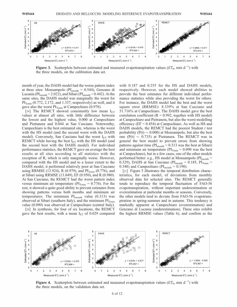
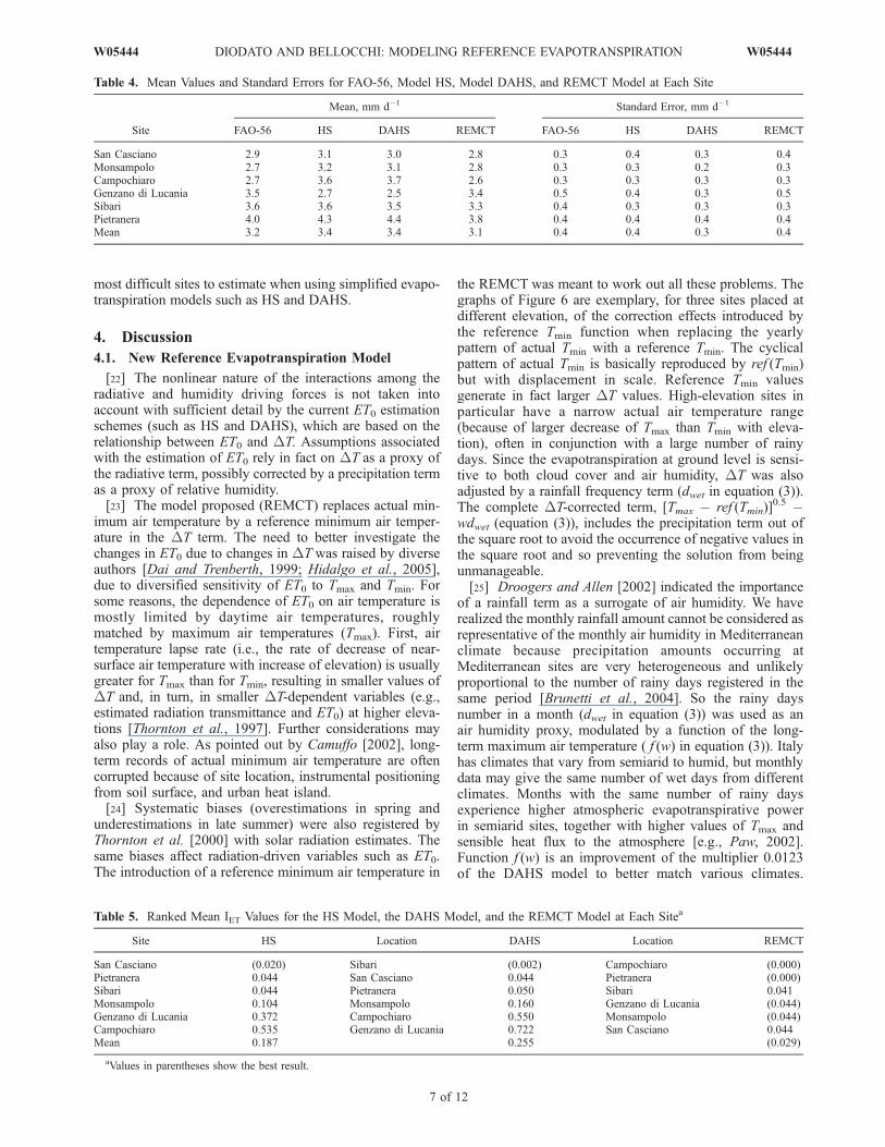
[15] Table 3 shows the parameter values determined viacalibration for the three models. The estimated coefficientb1 = 0.0021 is quite similar (�8.7%) to the original HSvalue (b1 = 0.0023). For the DAHS model, the estimateof b1 (0.000959) is 26% less than the original value(b1 = 0.0013). For both models, a non-null intercept(parameter b0) was estimated. These parameter values,estimated from the data, roughly matched the FAO-56data of both the calibration (Figure 3) and the validation(Figure 4) data sets. Figures 3 and 4 show substantiallygood agreement between estimated and FAO-56 values, aspoints tend to line up around the 1:1 line (regressionparameters are close to 0 and 1 for intercept and slope,respectively). However, a major spread is apparent in bothfigures with the two simplified models.

3.2. Model Evaluation

[16] According to Table 4, both HS and DAHS overesti-mated the FAO-56 estimated data (mean values 3.4 mm d�1

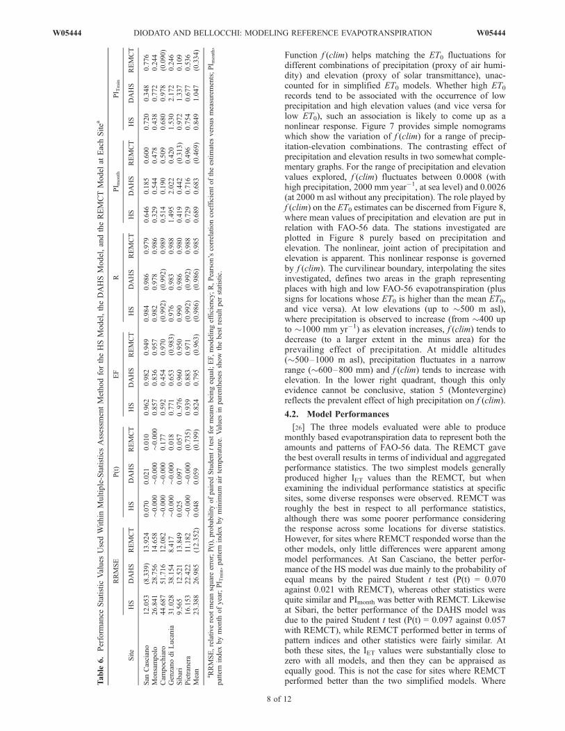
against 3.2 mm d�1), while the REMCT approximatelygave the same average estimate (3.1 mm d�1) as theFAO-56 model. The DAHS model only produced a slightlylower standard error (0.3 against 0.4 mm d�1).[17] The ranked mean values per site and model for IET

are given in Table 5, while the individual performancestatistic results are detailed in Table 6. Mean IET value ofthe HS model was 0.187 across all sites (�27% than theDAHS model). The HS model produced better IET valuesthan the DAHS model at all sites with the exception ofSibari. For the DAHS, the lowest IET value was at Sibari(0.002) and a slightly different ranking of the sites wasgiven in comparison with the HS model. For the HS, thebest IET (0.020) was at San Casciano and the highest IET(0.535) was at Campochiaro. Both HS and DAHS were ableto produce evapotranspiration data that resulted in compar-atively low IET values (<0.200) at a diverse range oflatitudes and longitudes, e.g., for HS, IET = 0.020 at SanCasciano (central Italy), IET = 0.044 at Pietranera (inlandSicily) and Sibari (coastal Southern Italy), and IET = 0.104at Monsanpolo (east side central Italy). Some relationshipwas observed between model performance and elevation ofthe site. For instance, the worst IET values of HS areassociated with the highest sites: Genzano di Lucania(IET = 0.372) is the highest site (572 m asl) and Campochiaro(IET = 0.535) the second highest (502 m asl). Similar resultswere given by the DAHS model, with the worst perfor-mance (IET = 0.722) at the highest site.[18] For individual performance statistics, the HS model

was slightly better than the DAHS model for RRMSE(23.388% against 26.985%) and EF (0.824 against 0.795).According to the correlation coefficient, the two models hadon average the same performance (R = 0.986). The DAHSmodel was the best at San Casciano (central Italy) whenassessed by all but P(t) statistics. The DAHS model was alsothe best at Campochiaro (central Italy, 502 m asl), as itresults from correlation between estimates and measure-ments (R = 0.992, together with HS) and month-dependentpattern index (PITmin = 0.190). The tendency to generatepatterns versus time and minimum air temperature is worsewith this model than with the HS model. With respect to

Table 2. Multiple-Statistics Assessment Method Modules and Basic Statistics

Module Statistic Value, Range, and Purpose

Accuracy(magnitude ofresiduals)

RRMSE, relative root meansquare error

0 to positive infinity; the smaller RRMSE, the better the model performance;a dimensionless index allowing comparisons among a range of differentmodel responses regardless of units

EF, modeling efficiency 1 to negative infinity; best performance given when EF = 1, negative valuesof EF indicating that average value of the measured values is a betterestimator than the model

P(t), probability of pairedStudent t test for meansbeing equal

0 to 1; best value is P(t) = 1, and worst is 0

Correlation(between estimatesand measurements)

R, Pearson’s correlationcoefficient of the estimatesversus measurements

�1 (full negative correlation) to 1 (full positive correlation); the closervalues are to 1, the better the model

Pattern(presence/absence ofpatterns in residuals)

PImonth, pattern index bymonth of year

0 to positive infinity; the closer values are to 0 the better the model;month of year (from 1 to 12) is an independent variable

PITmin, pattern index byminimum air temperature

0 to positive infinity; the closer values are to 0 the better the model;monthly minimum air temperature is an independent variable

Table 3. Parameter Values Estimated for Hargreaves-Samani (HS)

Model, Modified Hargreaves-Samani (DAHS), and Reference

Evapotranspiration Model for Complex Terrains (REMCT)

Parameter HS DAHS REMCT

b0 �0.0363 0.433 . . .b1, mm d�1 0.0021 0.000959 . . .a, �C . . . . . . �2.64a . . . . . . 1.79b . . . . . . 6.50c . . . . . . 12.0d . . . . . . 0.00247e, m�1 . . . . . . 0.000000831g, m . . . . . . 2000h, m�1 . . . . . . 0.1k, �C0.5 month�1 . . . . . . 0.0397q, �C�3 . . . . . . 0.000079228

W05444 DIODATO AND BELLOCCHI: MODELING REFERENCE EVAPOTRANSPIRATION

5 of 12

W05444

month of year, the DAHS model had the worse pattern indexat three sites: Monsampolo (PImonth = 0.544), Genzano diLucania (PImonth = 2.022), and Sibari (PImonth = 0.442). At thesame sites, the DAHS model was marginally the worst forPITmin (0.772, 2.172, and 1.337, respectively) as well, and itgave also the worst PITmin at Campochiaro (0.978).[19] The REMCT showed consistently low mean IET

values at almost all sites, with little difference betweenthe lowest and the highest value, 0.000 at Campochiaroand Pietranera and 0.044 at San Casciano. Noteworthy,Campochiaro is the best estimated site, whereas is the worstwith the HS model (and the second worst with the DAHSmodel). Conversely, San Casciano had the worst IET withREMCT while having the best IET with the HS model (andthe second best with the DAHS model). For individualperformance statistics, the REMCT gave on average the bestresults at all sites according to all statistics with theexception of R, which is only marginally worse. However,compared with the HS model and to a lesser extent to theDAHS model, it performed relatively poor at San Cascianousing RRMSE (13.924), R (0.979), and PITmin (0.776), andat Sibari using RRMSE (13.849), EF (0.950), and R (0.980).At San Casciano, the REMCT had the worst pattern indexversus minimum air temperature (PITmin = 0.776). For therest, it showed a quite good ability to prevent estimates fromshowing patterns versus both months and minimum airtemperatures. The minimum PImonth value (0.313) wasobserved at Sibari (southern Italy), and the minimum PITmin

value (0.090) was observed at Campochiaro (central Italy).[20] In synthesis, for four of six locations, the REMCT

gave the best results, with a mean IET of 0.029 compared

with 0.187 and 0.255 for the HS and DAHS models,respectively. However, each model showed abilities toprovide the best estimates for different individual perfor-mance statistics while also providing the worst for others.For instance, the DAHS model had the best and the worstsquare error (RRMSE): 8.339% at San Casciano and51.716% at Campochiaro. The DAHS model gave the bestcorrelation coefficient (R = 0.992, together with HS model)at Campochiaro and Pietranera, but also the worst modellingefficiency (EF = 0.454) at Campochiaro. As well as HS andDAHS models, the REMCT had the poorest Student t testprobability (P(t) 0.000) at Monsampolo, but also the bestone (P(t) 0.735) at Pietranera. The REMCT was ingeneral the best model to prevent errors from showingpatterns against time (PImonth = 0.313 was the best at Sibari)and minimum air temperature (PITmin = 0.090 was the bestat Campochiaro), but in a few cases, one of the other modelsperformed better: e.g., HS model at Monsampolo (PImonth =0.329), DAHS at San Casciano (PImonth = 0.185, PITmin =0.348) and Campochiaro (PImonth = 0.190).[21] Figure 5 illustrates the temporal distribution charac-

teristics, for each model, of deviations from monthlyobserved data for selected sites. The REMCT generallytends to reproduce the temporal fluctuation of FAO-56evapotranspiration, without important underestimation oroverestimation at particular months or seasons. Conversely,the other models tend to deviate from FAO-56 evapotrans-piration in spring-summer and in autumn. This tendency ismarkedly apparent at Campochiaro (overestimation) andGenzano di Lucania (underestimation). These sites exhibitthe highest RRMSE values (Table 6), and confirm as the

Figure 3. Scatterplots between estimated and measured evapotranspiration values (ET0, mm d�1) withthe three models, on the calibration data set.

Figure 4. Scatterplots between estimated and measured evapotranspiration values (ET0, mm d�1) withthe three models, on the validation data set.

6 of 12

W05444 DIODATO AND BELLOCCHI: MODELING REFERENCE EVAPOTRANSPIRATION W05444

most difficult sites to estimate when using simplified evapo-transpiration models such as HS and DAHS.

4. Discussion

4.1. New Reference Evapotranspiration Model

[22] The nonlinear nature of the interactions among theradiative and humidity driving forces is not taken intoaccount with sufficient detail by the current ET0 estimationschemes (such as HS and DAHS), which are based on therelationship between ET0 and DT. Assumptions associatedwith the estimation of ET0 rely in fact on DT as a proxy ofthe radiative term, possibly corrected by a precipitation termas a proxy of relative humidity.[23] The model proposed (REMCT) replaces actual min-

imum air temperature by a reference minimum air temper-ature in the DT term. The need to better investigate thechanges in ET0 due to changes in DT was raised by diverseauthors [Dai and Trenberth, 1999; Hidalgo et al., 2005],due to diversified sensitivity of ET0 to Tmax and Tmin. Forsome reasons, the dependence of ET0 on air temperature ismostly limited by daytime air temperatures, roughlymatched by maximum air temperatures (Tmax). First, airtemperature lapse rate (i.e., the rate of decrease of near-surface air temperature with increase of elevation) is usuallygreater for Tmax than for Tmin, resulting in smaller values ofDT and, in turn, in smaller DT-dependent variables (e.g.,estimated radiation transmittance and ET0) at higher eleva-tions [Thornton et al., 1997]. Further considerations mayalso play a role. As pointed out by Camuffo [2002], long-term records of actual minimum air temperature are oftencorrupted because of site location, instrumental positioningfrom soil surface, and urban heat island.[24] Systematic biases (overestimations in spring and

underestimations in late summer) were also registered byThornton et al. [2000] with solar radiation estimates. Thesame biases affect radiation-driven variables such as ET0.The introduction of a reference minimum air temperature in

the REMCT was meant to work out all these problems. Thegraphs of Figure 6 are exemplary, for three sites placed atdifferent elevation, of the correction effects introduced bythe reference Tmin function when replacing the yearlypattern of actual Tmin with a reference Tmin. The cyclicalpattern of actual Tmin is basically reproduced by ref (Tmin)but with displacement in scale. Reference Tmin valuesgenerate in fact larger DT values. High-elevation sites inparticular have a narrow actual air temperature range(because of larger decrease of Tmax than Tmin with eleva-tion), often in conjunction with a large number of rainydays. Since the evapotranspiration at ground level is sensi-tive to both cloud cover and air humidity, DT was alsoadjusted by a rainfall frequency term (dwet in equation (3)).The complete DT-corrected term, [Tmax � ref (Tmin)]

0.5 �wdwet (equation (3)), includes the precipitation term out ofthe square root to avoid the occurrence of negative values inthe square root and so preventing the solution from beingunmanageable.[25] Droogers and Allen [2002] indicated the importance

of a rainfall term as a surrogate of air humidity. We haverealized the monthly rainfall amount cannot be considered asrepresentative of the monthly air humidity in Mediterraneanclimate because precipitation amounts occurring atMediterranean sites are very heterogeneous and unlikelyproportional to the number of rainy days registered in thesame period [Brunetti et al., 2004]. So the rainy daysnumber in a month (dwet in equation (3)) was used as anair humidity proxy, modulated by a function of the long-term maximum air temperature ( f (w) in equation (3)). Italyhas climates that vary from semiarid to humid, but monthlydata may give the same number of wet days from differentclimates. Months with the same number of rainy daysexperience higher atmospheric evapotranspirative powerin semiarid sites, together with higher values of Tmax andsensible heat flux to the atmosphere [e.g., Paw, 2002].Function f (w) is an improvement of the multiplier 0.0123of the DAHS model to better match various climates.

Table 5. Ranked Mean IET Values for the HS Model, the DAHS Model, and the REMCT Model at Each Sitea

Site HS Location DAHS Location REMCT

San Casciano (0.020) Sibari (0.002) Campochiaro (0.000)Pietranera 0.044 San Casciano 0.044 Pietranera (0.000)Sibari 0.044 Pietranera 0.050 Sibari 0.041Monsampolo 0.104 Monsampolo 0.160 Genzano di Lucania (0.044)Genzano di Lucania 0.372 Campochiaro 0.550 Monsampolo (0.044)Campochiaro 0.535 Genzano di Lucania 0.722 San Casciano 0.044Mean 0.187 0.255 (0.029)

aValues in parentheses show the best result.

Table 4. Mean Values and Standard Errors for FAO-56, Model HS, Model DAHS, and REMCT Model at Each Site

Site

Mean, mm d�1 Standard Error, mm d�1

FAO-56 HS DAHS REMCT FAO-56 HS DAHS REMCT

San Casciano 2.9 3.1 3.0 2.8 0.3 0.4 0.3 0.4Monsampolo 2.7 3.2 3.1 2.8 0.3 0.3 0.2 0.3Campochiaro 2.7 3.6 3.7 2.6 0.3 0.3 0.3 0.3Genzano di Lucania 3.5 2.7 2.5 3.4 0.5 0.4 0.3 0.5Sibari 3.6 3.6 3.5 3.3 0.4 0.3 0.3 0.3Pietranera 4.0 4.3 4.4 3.8 0.4 0.4 0.4 0.4Mean 3.2 3.4 3.4 3.1 0.4 0.4 0.3 0.4

W05444 DIODATO AND BELLOCCHI: MODELING REFERENCE EVAPOTRANSPIRATION

7 of 12

W05444

Function f (clim) helps matching the ET0 fluctuations fordifferent combinations of precipitation (proxy of air humi-dity) and elevation (proxy of solar transmittance), unac-counted for in simplified ET0 models. Whether high ET0records tend to be associated with the occurrence of lowprecipitation and high elevation values (and vice versa forlow ET0), such an association is likely to come up as anonlinear response. Figure 7 provides simple nomogramswhich show the variation of f (clim) for a range of precip-itation-elevation combinations. The contrasting effect ofprecipitation and elevation results in two somewhat comple-mentary graphs. For the range of precipitation and elevationvalues explored, f (clim) fluctuates between 0.0008 (withhigh precipitation, 2000 mm year�1, at sea level) and 0.0026(at 2000 m asl without any precipitation). The role played byf (clim) on the ET0 estimates can be discerned from Figure 8,where mean values of precipitation and elevation are put inrelation with FAO-56 data. The stations investigated areplotted in Figure 8 purely based on precipitation andelevation. The nonlinear, joint action of precipitation andelevation is apparent. This nonlinear response is governedby f (clim). The curvilinear boundary, interpolating the sitesinvestigated, defines two areas in the graph representingplaces with high and low FAO-56 evapotranspiration (plussigns for locations whose ET0 is higher than the mean ET0,and vice versa). At low elevations (up to 500 m asl),where precipitation is observed to increase (from 400 upto 1000 mm yr�1) as elevation increases, f (clim) tends todecrease (to a larger extent in the minus area) for theprevailing effect of precipitation. At middle altitudes(500–1000 m asl), precipitation fluctuates in a narrowrange (600–800 mm) and f (clim) tends to increase withelevation. In the lower right quadrant, though this onlyevidence cannot be conclusive, station 5 (Montevergine)reflects the prevalent effect of high precipitation on f (clim).

4.2. Model Performances

[26] The three models evaluated were able to producemonthly based evapotranspiration data to represent both theamounts and patterns of FAO-56 data. The REMCT gavethe best overall results in terms of individual and aggregatedperformance statistics. The two simplest models generallyproduced higher IET values than the REMCT, but whenexamining the individual performance statistics at specificsites, some diverse responses were observed. REMCT wasroughly the best in respect to all performance statistics,although there was some poorer performance consideringthe response across some locations for diverse statistics.However, for sites where REMCT responded worse than theother models, only little differences were apparent amongmodel performances. At San Casciano, the better perfor-mance of the HS model was due mainly to the probability ofequal means by the paired Student t test (P(t) = 0.070against 0.021 with REMCT), whereas other statistics werequite similar and PImonth was better with REMCT. Likewiseat Sibari, the better performance of the DAHS model wasdue to the paired Student t test (P(t) = 0.097 against 0.057with REMCT), while REMCT performed better in terms ofpattern indices and other statistics were fairly similar. Atboth these sites, the IET values were substantially close tozero with all models, and then they can be appraised asequally good. This is not the case for sites where REMCTperformed better than the two simplified models. WhereT

able

6.Perform

ance

Statistic

Values

UsedWithin

Multiple-StatisticsAssessm

entMethodfortheHSModel,theDAHSModel,andtheREMCTModel

atEachSitea

Site

RRMSE

P(t)

EF

RPI m

onth

PI T

min

HS

DAHS

REMCT

HS

DAHS

REMCT

HS

DAHS

REMCT

HS

DAHS

REMCT

HS

DAHS

REMCT

HS

DAHS

REMCT

San

Casciano

12.053

(8.339)

13.924

0.070

0.021

0.010

0.962

0.982

0.949

0.984

0.986

0.979

0.646

0.185

0.600

0.720

0.348

0.776

Monsampolo

26.841

28.756

14.658

0.000

0.000

0.000

0.857

0.836

0.957

0.982

0.978

0.986

0.329

0.544

0.478

0.438

0.772

0.244

Cam

pochiaro

44.687

51.716

12.082

0.000

0.000

0.177

0.592

0.454

0.970

(0.992)

(0.992)

0.989

0.514

0.190

0.509

0.680

0.978

(0.090)

GenzanodiLucania

31.028

38.154

8.417

0.000

0.000

0.018

0.771

0.653

(0.983)

0.976

0.983

0.988

1.495

2.022

0.420

1.530

2.172

0.246

Sibari

9.565

12.521

13.849

0.025

0.097

0.057

0..976

0.960

0.950

0.990

0.986

0.980

0.419

0.442

(0.313)

0.972

1.337

0.109

Pietranera

16.153

22.422

11.182

0.000

0.000

(0.735)

0.939

0.883

0.971

(0.992)

(0.992)

0.988

0.729

0.716

0.496

0.754

0.677

0.536

Mean

23.388

26.985

(12.352)

0.048

0.059

(0.199)

0.824

0.795

(0.963)

(0.986)

(0.986)

0.985

0.689

0.683

(0.469)

0.849

1.047

(0.334)

aRRMSE,relativerootmeansquareerror;P(t),probabilityofpairedStudentttestformeansbeingequal;EF,modelingefficiency;R,Pearson’scorrelationcoefficientoftheestimates

versusmeasurements;PI m

onth,

pattern

index

bymonth

ofyear;PI T

min,pattern

index

byminim

um

airtemperature.Values

inparentheses

show

thebestresultper

statistic.

8 of 12

W05444 DIODATO AND BELLOCCHI: MODELING REFERENCE EVAPOTRANSPIRATION W05444

estimates are poor with the HS and DAHS models(Campochiaro, Genzano di Lucania, and, to lesser extent,Monsampolo), this paper has shown that correction factorsof REMCT are able to account for influential factorspotentially distorting the estimates. Statistics were alsocomputed on the calibration data set, but are not shown,which confirm the better performance of the REMCT.[27] Localized climates could be attributed to some results

for eachmodel. The air temperature range-evapotranspirationresponse may be influenced by site-specific characteristics.Campochiaro and Genzano di Lucania (where both HS andDAHS models performed at worst) are middle-altitude(>500 m asl) sites of inland southern Italy. Both sites areApennines high valleys and show unique features in thecontext of the sites studied. They have frequent nocturnalradiative cooling, and occasional sea breezes and fog,potentially distorting the basis of the air temperature-evapotranspiration relationship, well interpreted by the

most complex model, as reflected in the low IET values(0.000 and 0.044) given by the REMCT. In particular,long-term minimum air temperature at Campochiaro(4.4�C as yearly average, Table 1) is much lower thanother stations, whereas maximum air temperature (19.1�Cas yearly average, Table 1) is similar. This confirms theprevalence at Campochiaro of factors capable of affectingthe air temperature range and as a result, distorting theevapotranspiration estimates. At this site, poor accuracymeasures for the two simplified models (RRMSE 40–50%, P(t) 0, and EF 0.5; Table 6) are compatiblewith the best correlation between estimates and FAO-56data (R > 0.99). This essentially means that big discrepantestimates are given by both HS and DAHS models, but theytend to be uniformly distributed over the range of FAO-56data. Provided that Campochiaro is the more extreme forrainfall amount and number of rainy days, REMCT likelycaptures such influential factors into rain-based parameters.

Figure 5. Deviation of estimates from FAO-56 evapotranspiration versus month of year for HS (modelHargreaves-Samani), DAHS (modified Hargreaves-Samani), and REMCT (reference evapotranspirationmodel for complex terrains) at selected sites.

Figure 6. Seasonal pattern of actual and reference Tmin at three stations with different elevation:(a) Benevento (180 m asl), (b) Caprarola (650 m asl), and (c) Montevergine (1270 m asl).

W05444 DIODATO AND BELLOCCHI: MODELING REFERENCE EVAPOTRANSPIRATION

9 of 12

W05444

Genzano di Lucania does not show temperature and precip-itation patterns similar to Campochiaro, but it is character-ized by large evaporative demand (long-term average of3.16 mm d�1). The air temperature range is quite narrow atthis site (6�C), roughly incompatible in itself with sus-tained evapotranspiration rates. So it sounds reasonable toexpect other factors are likely playing a role here forcing theevaporation level, not fully taken into account by simplifiedmodels such as HS and DAHS. The best performance forsuch models was registered at low-altitude sites such asSibari (IET = 0.002 with the DAHS model), where the meanevapotranspiration rate is relatively high (2.96 mm d�1) andharmonizes well with quite large air temperature range(11�C).[28] This investigation has used generic optimized param-

eters, which are crude estimates over multiple years. Theoptimized parameters determined over a pool of data fromall sites help ensure a generic spatial and temporal repre-sentation, i.e., a single parameter value was used at all sitesfor all years. The REMCT may appear more sensitive tovariation in its several parameters than the HS and DAHSmodels are to their few parameters. The application of theREMCT to other Mediterranean sites may therefore belimited by the ability to provide appropriate site-representativeparameters able to capture the temporal variability of evap-otraspiration data. Specific geographical locations may haveparticular characteristics that cause the parameters to deviatefrom reference values, and may require local optimization.A spatial sensitivity analysis goes beyond the goal of thisstudy, but testing the stability of model parameters at

changing conditions might be required in view of general-ized applications of the REMCT. However, some consid-erations may be set forth that indicate that the parameters ofequations (3) and (4) can display a potential stability acrosssites. Function f (w) in equation (3) closely resembles thepluviometric parameter estimated by Droogers and Allen

Figure 7. Variation of function f (clim) with a variety of precipitation (mm) and elevation (m) values.

Figure 8. Relationship between precipitation, elevation,and FAO-56 data. Numbers identify the sites (see Table 1);plus and minus signs indicate sites with larger and smaller,respectively, FAO-56 evapotranspiration than the meanvalue. The line is an approximate double parabolainterpolating across the site data points.

10 of 12

W05444 DIODATO AND BELLOCCHI: MODELING REFERENCE EVAPOTRANSPIRATION W05444

[2002] and included in their modified form of the HSmodel. As in equation (3), a precipitation-based amount tobe subtracted to DT was given by the authors, with a singleestimated value attached to the pluviometric parameter,obtained from a worldwide data set and proposed forgeneral use in monthly estimates of evapotranspiration. Asregards equation (4), the cosine function used hereapproaches the same seasonal fluctuation that is commonto vast areas of Europe (including Mediterranean sites).Trigonometric functions are indeed typically implementedto represent cyclical processes, including climatologicalcourses as, for instance, in hydrological models estimatingrainfall erosivity [Yu et al., 2001]. As regards the multipli-cation factor of site elevation (parameter h in equation (4)),this parameter was estimated from evapotranspiration datataken at elevations in a wide range up to 1270 m asl(Table 1), so it can be considered as being quite stable forelevations up to well above 1000 m (g = 2000 sets the abovelimit to 2000 m asl). Parameters d and e of equation (5) andk and q of equation (6) might actually require localcalibration to rescale the relationships against elevation-precipitation ( f (clim)) and maximum air temperature-based( f (w)) regressors.

5. Conclusions

[29] When the number of rainy days is available on amonthly basis, along with air temperature data, it is prefer-able to use REMCT to estimate monthly mean referenceevapotranspiration, rather than the models based on airtemperature only, or air temperature plus precipitation.However, given the greater availability of air temperaturedata, both spatially and temporally, the two air temperaturebased models evaluated here will make estimates to enablethe creation of complete monthly data sets. The results havedemonstrated that each model is capable of making betterestimates at some locations and poorer ones at others. TheREMCT does not show sizeable systematic, seasonal esti-mation errors, whereas the HS and DAHS models tend tounderestimate or overestimate values in spring and summerat certain sites.[30] This study limited to Italian sites makes the REMCT

suitable to estimate the monthly mean ET0 on heteroge-neous surfaces in Italy. However, the limited number ofmeteorological stations used in this study raises the need forrefinement of the proposed model and wider validationwork. This model may potentially be suitable for applica-tions at other places in the Mediterranean basin, providedthat model parameters will be documented for other sitesthan the ones investigated here. Further research using datasets from the Mediterranean area can be considered thenatural evolution of this study.

[31] Acknowledgments. Pierre Marchand (International Water Man-agement Institute) is gratefully acknowledged for facilitating the collectionof the weather data from IWMI world database.

ReferencesAgnew, M. D., and J. P. Palutikof (2000), GIS-based construction of base-line climatologies for the Mediterranean using terrain variables, Clim.Res., 14, 115–127.

Allen, R., L. S. Pereira, D. Raes, and M. Smith (Eds.) (1998), Crop evapo-transpiration: Guidelines for computing crop water requirements, Irrig.and Drain. Pap. 56, 300 pp., U.N. Food and Agric. Organ., Rome.

Belda, F., and J. Melia (2000), Relationships between climatic parametersand forest vegetation: Application to burned area in Alicante (Spain),For. Ecol. Manag., 135, 195–204.

Bellocchi, G., M. Acutis, G. Fila, and M. Donatelli (2002), An indicator ofsolar radiation model performance based on a fuzzy expert system,Agron. J., 94, 1222–1233.

Biftu, G. F., and T. Y. Gan (2000), Assessment of evapotranspiration mod-els applied to a watershed of Canadian prairies with mixed land-uses,Hydrol. Processes, 14, 1305–1325.

Brunetti, M., M. Maugeri, T. Nanni, and A. Navarra (2002), Droughts andextreme events in regional daily Italian precipitation series, Int. J. Cli-matol., 22, 543–558.

Brunetti, M., M. Maugeri, F. Monti, and T. Nanni (2004), Changes in dailyprecipitation frequency and distribution in Italy over the last 120 years,J. Geophys. Res., 109, D05102, doi:10.1029/2003JD004296.

Camuffo, D. (2002), History of the long series of daily air temperature inPadova (1725–1998), Clim. Change, 53, 7–75.

Castellvi, F., C. O. Stockle, P. J. Perez, and M. Ibanez (2001), Comparisonof methods for applying the Priestley-Taylor equation at a regional scale,Hydrol. Processes, 15, 1609–1620.

Dai, A., and K. E. Trenberth (1999), Effects of clouds, soil moisture, pre-cipitation, and water vapour on diurnal temperature range, J. Clim., 12,2451–2473.

Dalezios, N. R., A. Loukas, and D. Bampzelis (2002), Spatial variabilityof reference evapotranspiration in Greece, Phys. Chem. Earth, 27,1031–1038.

Diodato, N., and M. Ceccarelli (2005), Environinformatics in ecologicalrisk assessment of agroecosystems pollutant leaching, Stochast. Environ.Res. Risk A, 19, 292–300.

Doll, P., and S. Siebert (2002), Global modeling of irrigation water require-ments, Water Resour. Res., 38(4), 1037, doi:10.1029/2001WR000355.

Donatelli, M., M. Acutis, G. Bellocchi, and G. Fila (2004), New indices toquantify patterns of residuals produced by model estimates, Agron. J.,96, 631–645.

Droogers, P., and R. G. Allen (2002), Estimating reference evapotranspira-tion under inaccurate data conditions, Irrig. Drain. Syst., 16, 33–45.

Dyck, S. (1983), Overview on the present status of the concepts of waterbalance models: New approaches in water balance computations, paperpresented at the 18th General Assembly, Int. Union of Geod. and Geo-phys., Hamburg, Germany, 15–27 August.

Esposito, S., and M. C. Beltrano (1996), La Rete Agrometeorologica Na-zionale, Agricoltura, 277, 72–84.

Fernandez, J., J. Saez, and E. Zorita (2003), Analysis of wintertime atmo-spheric moisture transport and its variability over the Mediterraneanbasin in the NCEP-Reanalyses, Clim. Res., 23, 195–215.

Fila, G., G. Bellocchi, M. Donatelli, and M. Acutis (2003), IRENE_DLL:Object-oriented library for evaluating numerical estimates, Agron. J., 95,1330–1333.

Garcia, M., D. Raes, R. Allen, and C. Herbas (2004), Dynamics of refer-ence evapotranspiration in the Bolivian highlands (Altiplano), Agric. For.Meteorol., 125, 67–82.

Gavilan, P., I. J. Lorite, S. Tornero, and J. Berengena (2006), Regionalcalibration of Hargreaves equation for estimating reference ET in a semi-arid environment, Agric. Water Manage., 81, 257–281.

Giacobello, N. (1980), On the relationship between solar radiation andcloud cover, Riv. Meteorol. Aeronaut., 40, 225–230.

Gong, L., C.-Y. Xu, D. Chen, S. Halldin, and Y. D. Chen (2006), Sensitivityof the Penman-Monteith reference evapotranspiration to key climaticvariables in the Changjiang (Yangtze River) basin, J. Hydrol., 329,620–629.

Hargreaves, G. H., and Z. A. Samani (1985), Reference crop evapotran-spiration from temperature, Appl. Eng. Agric., 1, 96–99.

Harrison, L. P. (1963), Fundamentals concepts and definitions relating tohumidity, inHumidity andMoisture, vol. 3, edited byA.Wexler, Reinhold,New York.

Hidalgo, H. G., D. R. Cayan, and M. D. Dettinger (2005), Sources ofvariability of evapotranspiration in California, J. Hydrometeorol., 6,3–19.

Hobbins, M. T., J. A. Ramirez, and T. C. Brown (2001a), The complemen-tary relationship in estimation of regional evapotranspiration: An en-hanced advection-aridity model, Water Resour. Res., 37, 1389–1403.

Hobbins, M. T., J. A. Ramirez, T. C. Brown, and L. H. J. M. Claessens(2001b), The complementary relationship in estimation of regionalevapotranspiration: The complementary relationship areal evapotran-spiration and advection-aridity models, Water Resour. Res., 37,1367–1387.

W05444 DIODATO AND BELLOCCHI: MODELING REFERENCE EVAPOTRANSPIRATION

11 of 12

W05444

Irmak, S., R. G. Allen, and E. B. Whitty (2003), Daily grass and alfalfa-reference evapotranspiration estimates and alfalfa-to-grass evapotran-spiration ratios in Florida, J. Irrig. Drain. Eng., 129, 360–370.

Lionello, P., et al. (2006). The Mediterranean climate: An overview of themain characteristics and issues, in Mediterranean Climate Variability,edited by P. Lionello et al., pp. 1–25, Elsevier, New York.

Monteith, J. (1965), Climate and the efficiency of crop production in Britain,Philos. Trans. R. Soc. London, 281, 277–329.

Palutikof, J. P., C. Goodes, and X. Guo (1994), Climate change, potentialevapotranspiration and moisture availability in the Mediterranean basin,Int. J. Climatol., 14, 853–869.

Paw, U. K. T. (2002), Soil-plant-atmosphere models, in Advanced ShortCourse on Agricultural, Forest and Micrometeorology, edited by F. Rossiet al., pp. 140–152, Italian Res. Natl. Counc., Inst. of Biometeorol.,Sassari, Italy.

Petrarca, S., E. Cogliani, and F. Spinelli (Eds.) (2000), La RadiazioneSolare Globale al Suolo in Italia, 200 pp., Ente per le Nuove Technol.,l’Energie, el’ Ambiente, Rome.

Pitzalis, M., M. C. Lorenzetti, A. M. Pandolfi, and M. Nardi (1989), Dis-tribuzione di parametri agroclimatici in Italia, paper presented at Agro-meteorologia, Agricoltura e Ambiente, Consiglio Nazionale delleRicerche, Florence, Italy, 21–23 Nov.

Rana, G., and N. Katerji (2000), Measurement and estimation of actualevapotranspiration in the field under Mediterranean climate: A review,Eur. J. Agron., 13, 125–153.

Rivington, M., G. Bellocchi, K. B. Matthews, and K. Buchan (2005),Evaluation of three model estimations of solar radiation at 24 UK sta-tions, Agric. For. Meteorol., 135, 228–243.

Schulze, R. (2000), Transcending scales of space and time in impact studiesof climate and climate change on agrohydrological responses, Agric.Ecosyst. Environ., 82, 185–212.

Shevenell, L. (1999), Regional potential evapotranspiration in arid climatesbased on temperature, topography and calculated solar radiation, Hydrol.Processes, 13, 577–596.

Sousa, V., and L. S. Pereira (1999), Regional analysis of irrigation waterrequirements using kriging: Application to potato crop (Solanumtuberosum L.) at Tras-os-Montes, Agric. Water Manage., 40, 221–233.

Stockle, C. O., J. Kjelgaard, and G. Bellocchi (2004), Evaluation of esti-mated weather data for calculating Penman-Monteith reference crop eva-potranspiration, Irrig. Sci., 1, 39–46.

Supit, I., and R. R. van Kappel (1998), A simple method to estimate solarradiation, Sol. Energy, 63, 147–160.

Thomas, A. (2000), Spatial and temporal characteristics of potential evapo-transpiration trends over china, Int. J. Climatol., 20, 381–396.

Thornton, P. E., S. W. Running, and M. A. White (1997), Generating sur-face of daily meteorological variables over large regions of complexterrain, J. Hydrol., 190, 214–251.

Thornton, P. E., H. Hasenauer, and M. A. White (2000), Simultaneousestimation of daily solar radiation and humidity from observed tempera-ture and precipitation: An application over complex terrain in Austria,Agric. For. Meteorol., 104, 255–271.

Vanderlinden, K., J. V. Giraldez, and M. van Meirvenne (2004), Assessingreference evapotranspiration by the Hargreaves method in southernSpain, J. Irrig. Drain. Eng., 130, 184–191.

Weisse, R., and R. Oestreicher (2001), Reconstruction of potential evapora-tion for water balance studies, Clim. Res., 16, 123–131.

Xu, C.-Y. (2002), Hydrologic Models, 365 pp., Dep. of Earth Sci. Hydrol.,Uppsala Univ, Uppsala, Sweden.

Xu, C.-Y., and V. P. Singh (2000), Evaluation and generalization of radia-tion-based methods for calculating evaporation, Hydrol. Processes, 14,339–349.

Xu, C.-Y., and V. P. Singh (2005), Evaluation of three complementaryrelationship evapotranspiration models by water balance approach toestimate actual regional evapotranspiration in different climatic regions,J. Hydrol., 308, 105–121.

Xu, J., S. Haginoya, K. Saito, and K. Motoya (2005), Surface heat balanceand pan evaporation trends in eastern Asia in the period 1971–2000,Hydrol. Processes, 19, 2161–2186.

Xu, Z. X., and J. Y. Li (2003), A distributed approach for estimatingcatchment evapotranspiration: Comparison of the combination equationand the complementary relationship approaches, Hydrol. Processes, 17,1509–1523.

Yu, B., G. M. Hashim, and Z. Eusof (2001), Estimating the r-factor withlimited rainfall data: A case study from peninsular Malaysia, J. SoilWater Conserv., 56, 101–105.

����������������������������G. Bellocchi, Agrichiana Farming, Abbadia di Montepulciano, Via di

Sciarti n. 33/A, I-53040 Siena, Italy.N. Diodato, Monte Pino Research Observatory, via Contrada Monte

Pino, I-82100 Benevento, Italy. (nazdiod@tin.it)

12 of 12

W05444 DIODATO AND BELLOCCHI: MODELING REFERENCE EVAPOTRANSPIRATION W05444