Sound speed in the Mediterranean Sea: an analysis from a climatological data set

Annales Geophysicae (2003) 21: 833–846c© European Geosciences Union 2003Annales

Geophysicae

Sound speed in the Mediterranean Sea: an analysis from aclimatological data set

S. Salon1, A. Crise1, P. Picco2, E. de Marinis3, and O. Gasparini3

1Istituto Nazionale di Oceanografia e di Geofisica Sperimentale–OGS, Borgo Grotta Gigante 42/C, I-34010 Sgonico–Trieste,Italy2Centro Ricerche Ambiente Marino, CRAM-ENEA, S.Teresa, Localita Pozzuolo di Lerici, I-19100, La Spezia, Italy3DUNE s.r.l., Via Tracia 4, I-00183 Roma, Italy

Received: 9 April 2002 – Revised: 26 August 2002 – Accepted: 18 September 2002

Abstract. This paper presents an analysis of sound speeddistribution in the Mediterranean Sea based on climatologi-cal temperature and salinity data. In the upper layers, prop-agation is characterised by upward refraction in winter andan acoustic channel in summer. The seasonal cycle of theMediterranean and the presence of gyres and fronts create awide range of spatial and temporal variabilities, with rele-vant differences between the western and eastern basins. Itis shown that the analysis of a climatological data set canhelp in defining regions suitable for successful monitoring bymeans of acoustic tomography. Empirical Orthogonal Func-tions (EOF) decomposition on the profiles, performed on theseasonal cycle for some selected areas, demonstrates that twomodes account for more than 98% of the variability of the cli-matological distribution. Reduced order EOF analysis is ableto correctly represent sound speed profiles within each zone,thus providing the a priori knowledge for Matched Field To-mography. It is also demonstrated that salinity can affect thetomographic inversion, creating a higher degree of complex-ity than in the open oceans.

Key words. Oceanography: general (marginal and semien-closed seas; ocean acoustics)

1 Introduction

Acoustic methods have been widely applied for underwatercommunication and for the remote observation of ocean in-teriors. The basin-scale ATOC project (Acoustic Thermom-etry of Ocean Climate; Munk, 1996; ATOC Consortium,1998) has been one of the major applications of the acous-tic tomographic approach for observing climate signal in thedeep ocean. In the Western Mediterranean Sea, the nine-months-long experiment THETIS-2 (Send et al., 1997) hasestimated the seasonal heat budget, but this experience re-mains an unicum among tomographic Mediterranean basin-scale studies. Convective events have been successfully ob-

Correspondence to:S. Salon ([email protected])

served in the northwestern Mediterranean (Send et al., 1995)and in the Greenland Sea (Pawlowicz et al., 1995; Morawitzet al., 1996). Ocean acoustic tomography has also proved tobe a methodology for the observation of currents and internaltides (Shang and Wang, 1994; Demoulin et al., 1997). Thesesuccessful applications propose ocean tomography as a toolfor large-scale monitoring of the oceans in the frame of thedevelopment of Global Oceans Observing Systems (GOOS).

In spite of this growing interest in acoustic inversion, ananalysis of the sound speed field in the Mediterranean Sea isstill lacking. The aim of this paper is to provide a descriptionof sound speed characteristics (and a first guess on the soundspeed structure) in the Mediterranean Sea, its seasonal vari-ability and spatial distribution, starting from a climatologicaldata set of temperature and salinity. Furthermore, the analy-sis of the climatological data set will lead to the considerationof the following three issues:

1. The climatological sound speed profiles (SSPs) repre-sent a good quality reference to be used as an initialcondition for the environmental parameters in propaga-tion models and for the solution of inverse problems.

2. The SSP analysis can help in designing tomographicexperiments, while EOF analysis, which estimates thenumber of significant modes to be taken into consider-ation for each area, provides a base for Matched FieldTomography (Munk et al., 1995).

3. The knowledge of the dependence of sound speed onboth salinity and temperature climatological profiles al-lows a more precise inversion than the temperature-based one alone.

2 Methodology

2.1 Mediterranean Oceanic data base – MED6 data set

The analysis performed in this work is based on MED6(Brankart and Pinardi, 2001), a gridded analysis of monthly

834 S. Salon et al.: Sound speed in the Mediterranean Sea

Table 1. Numerical coefficients of the MacKenzie sound speed for-mula (1981)

A 1448.96 m s−1

B 4.591 m s−1◦C−1

C −5.304· 10−2 m s−1 ◦C−2

D 2.374·10−4 m s−1 ◦C−3

E 1.340 m s−1

F 1.630·10−2 s−1

G 1.675·10−7 m−1 s−1

H −1.025·10−2 m s−1◦C−1

J −7.139·10−13 m−2 s−1◦C−1

estimates of the climatological cycle of in situ tempera-ture and salinity for the whole Mediterranean and the nearNorth Atlantic area at14

◦ resolution. MED6 is based onthe MEDATLAS historical database (MEDATLAS Group,1994). The data set is obtained using the statistical analy-sis scheme developed for the Mediterranean Oceanic DataBase (MODB; Brasseur et al., 1996), where a Gaussian timecorrelation function has been introduced to enhance the timecoherence of the solution. The main additional informationcontained in the MEDATLAS data set comes from the in-clusion of about 80 000 XBTs, bringing the total number oftemperature profiles from 120 000 to about 200 000. We haveapplied some small adjustments to the data set: in particular,some temperature values in the Adriatic appeared to be toohigh and an additional check in the gridded data set for thatregion was done. Comparing the mean summer temperatureat 200 m with a recent climatological study of the AdriaticSea (Giorgetti, 1999), it was decided to eliminate from theoriginal gridded data set all the grid boxes in this area withtemperature values higher than 14.3◦C.

2.2 Sound speed computation

Several formulas have been proposed to compute soundspeed (also referred as SS) from temperature, salinity, andpressure or depth in the sea water (Del Grosso, 1974; Clayand Medwin, 1977; MacKenzie, 1981; Chen and Millero,1977). In the range of interest for the Mediterranean Sea,differences among formulas higher than 1.2 m/s are foundat great depths, while in the surface layers the discrepancynever exceeds 0.2 m/s. For this work the one from MacKen-zie (1981) was chosen: it is computationally efficient andhas an accuracy of about 0.1 m/s (Dushaw et al., 1993). It ismore accurate than that from Clay and Medwin (1977), pro-posed as a standard for tomographic applications by Jensenet al. (1994), and in the meantime it is suitable for analyticalinversion:

c(T , S, z) = A + BT + CT 2+ DT 3

+ E(S − 35)

+Fz + Gz2+ HT (S − 35) + JT z3 , (1)

wherec is sound speed (m/s),T is temperature (◦C), S issalinity andz is depth (m). The coefficients are reported in

Table 1. Sound speed has been computed for each grid pointand for each month of the MED6 data set, and from this fieldthe annual average was also obtained.

2.2.1 Error analysis

The error on sound speed computation associated with theuncertainty on temperature, salinity and depth, can be esti-mated by the error propagation formula:

1c =∂c

∂T1T +

∂c

∂S1S +

∂c

∂z1z

= (B + 2CT + 3DT 2+ H(S − 35) + Jz3)1T +

= (E + HT )1S + (F + 2Gz + 3JT z2)1z . (2)

The contribution of depth uncertainty can be safely ne-glected, and we consider1T and1S to be approximatelyone order of magnitude larger than the modern CTD stan-dard (1T = 0.05◦C and1S = 0.05), to include the intrinsicerrors of some historical measurements. In the wide rangesof 5–30◦C and 34–39, the maximum error is slightly morethan 0.26 m/s.

Since the MacKenzie formula is nonlinear, the operationsof the averaging process and SS computation do not com-mute strictu sensu. The computations carried out in this workwere instead obtained by first interpolatingT andS on theregular grid and then deriving SS. This can be justified be-cause in this way the information contained in the measure-ments can be better exploited also when only temperature orsalinity is available. At the same time, this work can take fulladvantage of the data quality control and analysis carried outon theT andS fields. Last, but not least, the commutationerror can be neglected, as is demonstrated hereafter.

Assuming that the depth measures are error-free, we iden-tify the T and S fields of the gridded data set with an overbar,since the gridding adopted is a weighted linear average. Inthe following we consider that the weights are equal, as thespatial distribution of the samples is assumed to be homoge-neous. This assumption is corroborated by the vast amountof data available. Using Eq. (1) the average SS based on thegridded data set (cG) is, therefore

cG(T , S, z) = A + BT + CT2+ DT

3+ E(S − 35)

+Fz + Gz2+ HT (S − 35) + JT z3 . (3)

In the case of the SS calculation from the original mea-surements, the averaged sound speed (cM ) reads:

cM(T , S, z) = A + BT + CT 2 + DT 3 + E(S − 35)

+Fz + Gz2 + HT (S − 35) + JT z3

= A + BT + CT 2 + DT 3 + E(S − 35)

+Fz + Gz2+ HT (S − 35) + JT z3 . (4)

The error introduced is the absolute difference between theaverage calculated on the measures (4) and that one estimateddirectly on the gridded data set (3), and depends only on thenonlinear terms:

|cM −cG| = |C(T 2−T2)+D(T 3−T

3)+H(T S −T S)|(5)

S. Salon et al.: Sound speed in the Mediterranean Sea 835

The first term on the right-hand side is simply the varianceof the temperature (σ 2

T ). The second term can be developedfurther assuming thatT = T + T ′, whereT ′ represents thefluctuation associated with the measure (assumed zero-meannormally distributed stochastic process), we have:

T 3 − T3

= (T + T ′)3 − T3

= T3+ T ′3 + 3T

2T ′

+3T T ′2 − T3

=

T ′3 + 3T2T ′ + 3T T ′2 = 3T σ 2

T . (6)

The first term in Eq. (6) is the skewness that is zero for anormal distribution; the second is also zero because the fluc-tuation is supposed to be zero-mean; the third is proportionalto the variance of temperature. The mixed term of temper-ature and salinity is treated in a similar way, assuming thatS = S + S′ (with the same statistical properties ofT ′):

T S − T S = (T + T ′)(S + S′) − T S =

(T S + T ′S + T S′ + T ′S′) − T S = T ′S′ , (7)

which could be neglected assuming incorrelated fields oftemperature and salinity anomalies. The expression (5) thusreduces to:

|cM − cG| = |Cσ 2T + 3DT σ 2

T | = σ 2T |C + 3DT |. (8)

Assuming, for example, a temperature value of 20◦C andtaking its variance equal to 1◦C2, in order to take into ac-count the approximations adopted (this value is twice that ofthe one found in Brankart and Pinardi, 2001, for the samedata set), we obtain an error of 0.05 m/s, which is one orderof magnitude lower than the uncertainty associated with theformula. As a summary, the total error associated with thecomputation of the SS field is obtained by:√

A2 + 1c2 + |cM − cG|2 ≈ 0.28 m/s, (9)

whereA is the accuracy of 0.1 m/s, and the second and thirdterms come from Eqs. (2) and (8).

2.2.2 Salinity uncertainty

An estimate of the importance of salinity uncertainty in thetomographic inversion process can be appraised using the SSsensitivity expressed in Eq. (2). A development of the valueof SS in terms of the salinity anomaly in a Taylor series canbe truncated at the first order, since Eq. (1) is linear inS.The SS anomaly with respect to salinity,|c(S(x, t))−c(S0)|,where(x, t) represents the data location and time andS0 isthe mean value below defined, is then linearly dependent onthe salinity anomaly weighted by the SS derivative with re-spect toS and is equal to|(E + HT (x, t))(S(x, t) − S0)|.

To estimate the SS anomaly for the upper layer of theMediterranean, we have calculated from the MED6 data setthe absolute values of the deviation of salinity with its verti-cal average. For the sake of simplicity, we use the continuousformulation:

1S(x, t) = |S(x, t) − S0| with S0 =1

B

∫ 0

−B

S(x, t)dz, (10)

1500 1505 1510 1515 1520 1525 1530

sound speed (m/s)

11

12

13

14

15

16

17

18

19

20

21

tem

pera

ture

(°C

)

a)

1500 1505 1510 1515 1520 1525 1530

sound speed (m/s)

35

35,5

36

36,5

37

37,5

38

38,5

39

39,5

salin

ity

b)

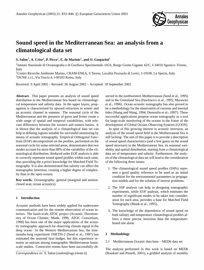
Fig. 1. Scatter plot of areal annual means in the North Atlantic (+),West Mediterranean (�), East Mediterranean (•) and Adriatic Sea(∗), between 5 and 500 m of(a) temperature (◦C) and sound speed(m/s) and(b) salinity and sound speed (m/s).

where the integral was taken over the entire water column(between bottom, “−B”, and surface). Then spatial and tem-poral averages of the salinity anomaly are computed for theupper 700 m, where the variability is larger, and where theacoustic methods can be applied to resolve the seasonal cy-cle, obtaining a value of1S = 0.177. With the salinity de-viation estimate given by Eq. (10), the following basin-wideclimatological anomaly is obtained:

|c(S(x, t)) − c(S0)| = |(E + HT )1S| = 0.21m/s, (11)

whereT = 14.7◦C is the spatial average of the climatologi-cal temperature in the upper 700 m. It is worth noting that theaverage salinity deviation1S introduces an error in the SScalculation of the same order as that one obtained just by sub-stituting each salinity profile with its (spatial- and temporal-dependent) mean,as estimated in Eq. (9). A better resolutionis needed to distinguish between different water masses indeeper layers, where the typical variability of temperatureand salinity affects the sound speed by less than 0.5 m/s.

To characterise the relation of sound speed with temper-ature and salinity, plots of sound speed versus temperature(Fig. 1a) and versus salinity (Fig. 1b) for different areas,have been analysed. Four subsets of the data set, corre-sponding to the two main sub-basins, namely the WesternMediterranean (5.5◦ W–12◦ E and 32◦ N–44.5◦ N), the East-ern Mediterranean (12◦ E–36◦ E and 30.5◦ N–38◦ N), a re-gional sea, the Adriatic Sea (12◦ E–19.5◦ E and 40.5◦ N–45.5◦ N) and, as a comparison, the area of the North Atlantic,west of Gibraltar Strait (9.375◦ W–5.5◦ W and 34◦ N–38◦ N)were considered. To highlight the differences, the spatial av-eraged annual mean SS profiles and the corresponding valueof temperature and salinity were obtained for each level froma 5 to 500 m depth and reported asT / SS andS/ SS dia-grams. The scatter plots, in Fig. 1, evidence significant dif-


ferences between the North Atlantic region and the Mediter-ranean. In the North Atlantic, apart from the near-surfacelayer, the curve is monotonic, with a quite linear dependencefor both temperature and salinity, and the range of variabilityof sound speed is limited between 1505 and 1520 m/s. In theMediterranean Sea, the dependence of sound speed on tem-perature and salinity in the thermocline region is more com-plicated, with a peculiar behaviour for each selected basin,thus making it complex to estimate the temperature from thesound speed without a good TS statistic of the interested area.In both the western and eastern basins no relation of soundspeed with temperature can be found in the upper layer, asa negligible variation of sound speed corresponds to a widetemperature interval (up to 1.5◦C close to 1515 m/s in theeastern basin); the same occurs for salinity in the westernpart, up to 0.5 around 1508 m/s. In the eastern basin, thepresence of the LIW can be evidenced by a minimum soundspeed (1515 m/s) corresponding to temperature and salinityvalues higher than those relative to the minimum of soundspeed in the western basin (between 1507 and 1508 m/s),where the minimum corresponds to the thermocline. Belowthe thermocline, where temperature and salinity are almostconstant with depth, the wide variability of sound speed ismainly due to pressure effects.

2.3 EOF decomposition

Empirical Orthogonal Function (EOF) decomposition repre-sents an efficient approach to SSP parameterisation and iswidely used in many Ocean Acoustic Tomography (OAT) orMatched Field applications (Shang and Wang, 1994), sinceit permits the description of a complex variable field as alinear combination of a few eigenfunctions, a crucial issuewhen a reduced parameter space is needed to solve the in-verse problem. The structure of the SSP is statistically ex-plained by a few orthogonal functions (vertical eigenfunc-tions) which cannot always be easily interpreted as the contri-bution of distinct dynamical mechanisms acting on the watercolumn structure. EOF analysis decouples the spatial com-ponent from the temporal one, thus enabling an immediateinterpretation of the SSP seasonal evolution. The analysis ofthe eigenvalues’ distribution allowed us to select the relativeweight of the dominating EOFs, as the smaller eigenvaluesare generally associated with noise and sampling errors. EOFanalysis not only speeds up tomographic inversion, but alsoavoids the introduction of unwanted components in the inver-sion. In this work, EOF analysis has been applied to spatiallyaveraged vertical profilesc(z) of sound speed in 14 differentregions described in Sect. 3.2. The vertical EOFs were com-puted by using the traditional methodology proposed, amongothers, by Davis (1976) and Weare et al. (1976), and heresummarized:

c(z) = c0(z) + 1c(z), (12)

where the monthly mean sound speed profilec(z) has beendecomposed in an annual mean valuec0(z) plus a perturba-

tion term1c(z), expressed as:

1c(z) =

N∑i=1

αi(t)Fi(z). (13)

In Eq. (13),αi(t) are the time coefficients,Fi(z) representthe vertical eigenfunctions andN is the number of possiblemodes, which in our case coincides with the number of levelsrelative to each area (maximum isN = 34).

In the case of a gridded data set, obtained from an objec-tive analysis based on the Gauss-Markov estimation (as forMODB-MED6), the expected value of the deviation1c(z)

calculated from the data set itself can be better than thoseobtained using only measurements. In other words, we canapply the EOF analysis on the gridded data instead of on themeasured set without incurring, on average, additional er-rors. Proof for a generic vertical profile, of scalar quantity inthe case of a gridded data set, is given in Appendix A. Thisproof constitutes a validation of our approach and guaranteesthe reliability of the EOF computation.

3 Results

3.1 Sound speed distribution: annual mean and seasonalvariability

This analysis focuses on the layer between 50 and 400 m,since – in terms of acoustic propagation – in the upper mixedlayer the acoustic wave undergoes a near-surface upward re-fraction; therefore and it is not exploitable for tomographicapplications, while in the deeper layers sound speed differ-ences are not strong enough to be resolved by this methodol-ogy.

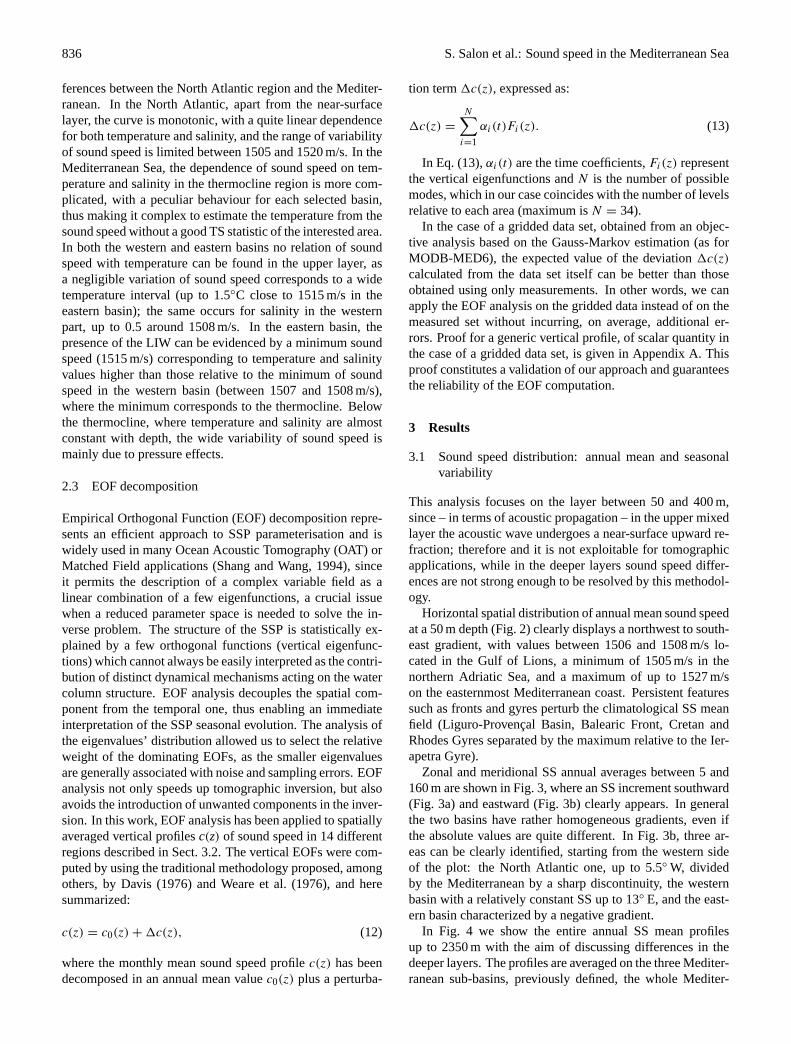
Horizontal spatial distribution of annual mean sound speedat a 50 m depth (Fig. 2) clearly displays a northwest to south-east gradient, with values between 1506 and 1508 m/s lo-cated in the Gulf of Lions, a minimum of 1505 m/s in thenorthern Adriatic Sea, and a maximum of up to 1527 m/son the easternmost Mediterranean coast. Persistent featuressuch as fronts and gyres perturb the climatological SS meanfield (Liguro-Provencal Basin, Balearic Front, Cretan andRhodes Gyres separated by the maximum relative to the Ier-apetra Gyre).

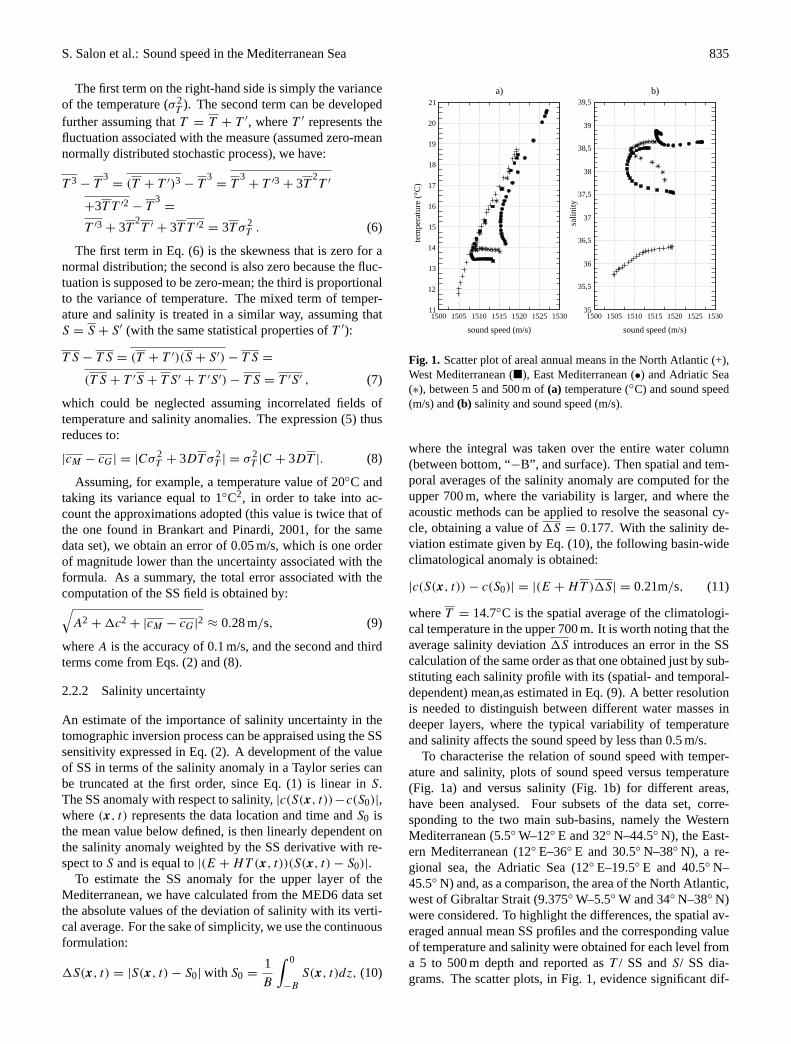
Zonal and meridional SS annual averages between 5 and160 m are shown in Fig. 3, where an SS increment southward(Fig. 3a) and eastward (Fig. 3b) clearly appears. In generalthe two basins have rather homogeneous gradients, even ifthe absolute values are quite different. In Fig. 3b, three ar-eas can be clearly identified, starting from the western sideof the plot: the North Atlantic one, up to 5.5◦ W, dividedby the Mediterranean by a sharp discontinuity, the westernbasin with a relatively constant SS up to 13◦ E, and the east-ern basin characterized by a negative gradient.

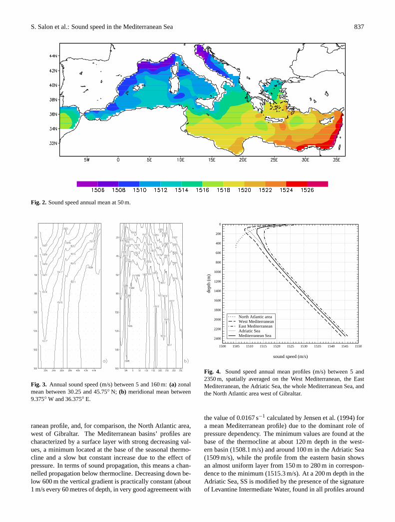
In Fig. 4 we show the entire annual SS mean profilesup to 2350 m with the aim of discussing differences in thedeeper layers. The profiles are averaged on the three Mediter-ranean sub-basins, previously defined, the whole Mediter-


Fig. 2. Sound speed annual mean at 50 m.

Fig. 3. Annual sound speed (m/s) between 5 and 160 m:(a) zonalmean between 30.25 and 45.75◦ N; (b) meridional mean between9.375◦ W and 36.375◦ E.

ranean profile, and, for comparison, the North Atlantic area,west of Gibraltar. The Mediterranean basins’ profiles arecharacterized by a surface layer with strong decreasing val-ues, a minimum located at the base of the seasonal thermo-cline and a slow but constant increase due to the effect ofpressure. In terms of sound propagation, this means a chan-nelled propagation below thermocline. Decreasing down be-low 600 m the vertical gradient is practically constant (about1 m/s every 60 metres of depth, in very good agreemeent with

1500 1505 1510 1515 1520 1525 1530 1535 1540 1545 1550

sound speed (m/s)

0

200

400

600

800

1000

1200

1400

1600

1800

2000

2200

2400

dept

h (m

)

North Atlantic areaWest MediterraneanEast MediterraneanAdriatic SeaMediterranean Sea

Fig. 4. Sound speed annual mean profiles (m/s) between 5 and2350 m, spatially averaged on the West Mediterranean, the EastMediterranean, the Adriatic Sea, the whole Mediterranean Sea, andthe North Atlantic area west of Gibraltar.

the value of 0.0167 s−1 calculated by Jensen et al. (1994) fora mean Mediterranean profile) due to the dominant role ofpressure dependency. The minimum values are found at thebase of the thermocline at about 120 m depth in the west-ern basin (1508.1 m/s) and around 100 m in the Adriatic Sea(1509 m/s), while the profile from the eastern basin showsan almost uniform layer from 150 m to 280 m in correspon-dence to the minimum (1515.3 m/s). At a 200 m depth in theAdriatic Sea, SS is modified by the presence of the signatureof Levantine Intermediate Water, found in all profiles around


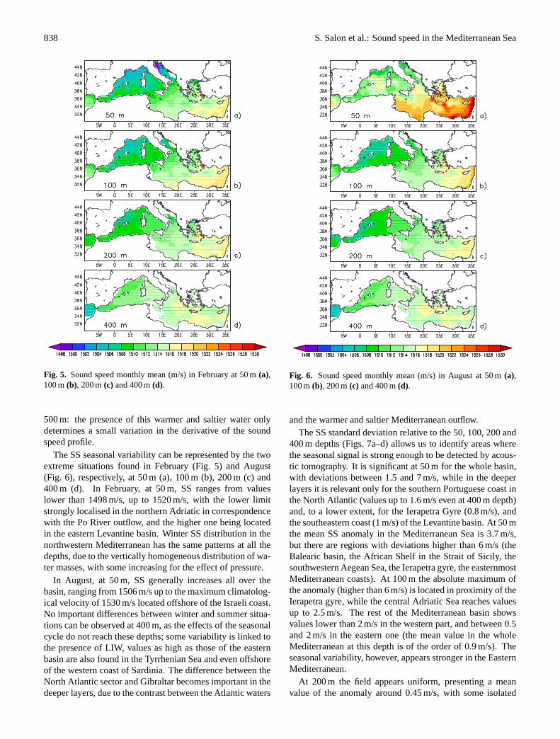
Fig. 5. Sound speed monthly mean (m/s) in February at 50 m(a),100 m(b), 200 m(c) and 400 m(d).

500 m: the presence of this warmer and saltier water onlydetermines a small variation in the derivative of the soundspeed profile.

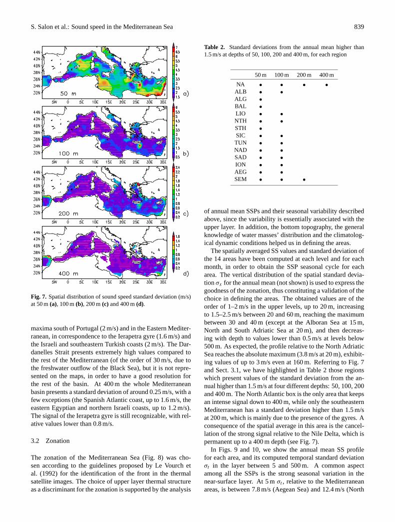
The SS seasonal variability can be represented by the twoextreme situations found in February (Fig. 5) and August(Fig. 6), respectively, at 50 m (a), 100 m (b), 200 m (c) and400 m (d). In February, at 50 m, SS ranges from valueslower than 1498 m/s, up to 1520 m/s, with the lower limitstrongly localised in the northern Adriatic in correspondencewith the Po River outflow, and the higher one being locatedin the eastern Levantine basin. Winter SS distribution in thenorthwestern Mediterranean has the same patterns at all thedepths, due to the vertically homogeneous distribution of wa-ter masses, with some increasing for the effect of pressure.

In August, at 50 m, SS generally increases all over thebasin, ranging from 1506 m/s up to the maximum climatolog-ical velocity of 1530 m/s located offshore of the Israeli coast.No important differences between winter and summer situa-tions can be observed at 400 m, as the effects of the seasonalcycle do not reach these depths; some variability is linked tothe presence of LIW, values as high as those of the easternbasin are also found in the Tyrrhenian Sea and even offshoreof the western coast of Sardinia. The difference between theNorth Atlantic sector and Gibraltar becomes important in thedeeper layers, due to the contrast between the Atlantic waters

Fig. 6. Sound speed monthly mean (m/s) in August at 50 m(a),100 m(b), 200 m(c) and 400 m(d).

and the warmer and saltier Mediterranean outflow.The SS standard deviation relative to the 50, 100, 200 and

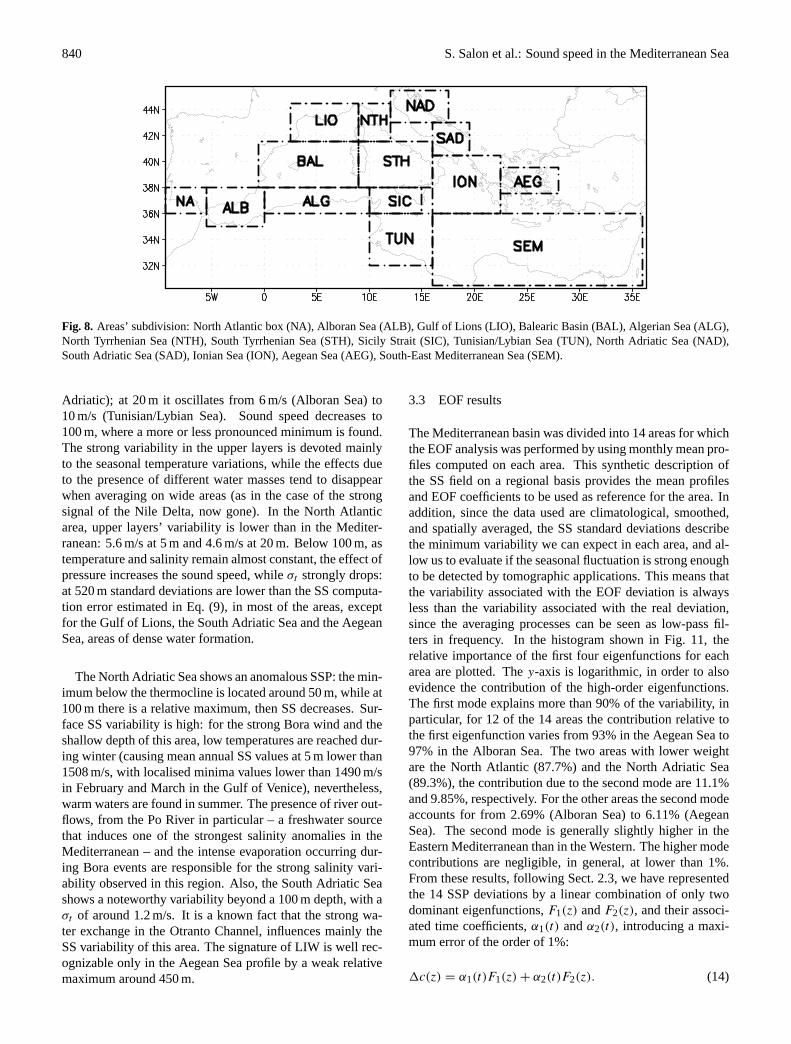
400 m depths (Figs. 7a–d) allows us to identify areas wherethe seasonal signal is strong enough to be detected by acous-tic tomography. It is significant at 50 m for the whole basin,with deviations between 1.5 and 7 m/s, while in the deeperlayers it is relevant only for the southern Portuguese coast inthe North Atlantic (values up to 1.6 m/s even at 400 m depth)and, to a lower extent, for the Ierapetra Gyre (0.8 m/s), andthe southeastern coast (1 m/s) of the Levantine basin. At 50 mthe mean SS anomaly in the Mediterranean Sea is 3.7 m/s,but there are regions with deviations higher than 6 m/s (theBalearic basin, the African Shelf in the Strait of Sicily, thesouthwestern Aegean Sea, the Ierapetra gyre, the easternmostMediterranean coasts). At 100 m the absolute maximum ofthe anomaly (higher than 6 m/s) is located in proximity of theIerapetra gyre, while the central Adriatic Sea reaches valuesup to 2.5 m/s. The rest of the Mediterranean basin showsvalues lower than 2 m/s in the western part, and between 0.5and 2 m/s in the eastern one (the mean value in the wholeMediterranean at this depth is of the order of 0.9 m/s). Theseasonal variability, however, appears stronger in the EasternMediterranean.

At 200 m the field appears uniform, presenting a meanvalue of the anomaly around 0.45 m/s, with some isolated


Fig. 7. Spatial distribution of sound speed standard deviation (m/s)at 50 m(a), 100 m(b), 200 m(c) and 400 m(d).

maxima south of Portugal (2 m/s) and in the Eastern Mediter-ranean, in correspondence to the Ierapetra gyre (1.6 m/s) andthe Israeli and southeastern Turkish coasts (2 m/s). The Dar-danelles Strait presents extremely high values compared tothe rest of the Mediterranean (of the order of 30 m/s, due tothe freshwater outflow of the Black Sea), but it is not repre-sented on the maps, in order to have a good resolution forthe rest of the basin. At 400 m the whole Mediterraneanbasin presents a standard deviation of around 0.25 m/s, with afew exceptions (the Spanish Atlantic coast, up to 1.6 m/s, theeastern Egyptian and northern Israeli coasts, up to 1.2 m/s).The signal of the Ierapetra gyre is still recognizable, with rel-ative values lower than 0.8 m/s.

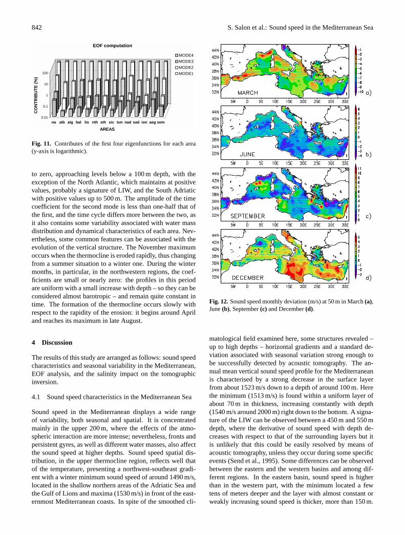
3.2 Zonation

The zonation of the Mediterranean Sea (Fig. 8) was cho-sen according to the guidelines proposed by Le Vourch etal. (1992) for the identification of the front in the thermalsatellite images. The choice of upper layer thermal structureas a discriminant for the zonation is supported by the analysis

Table 2. Standard deviations from the annual mean higher than1.5 m/s at depths of 50, 100, 200 and 400 m, for each region

50 m 100 m 200 m 400 m

NA • • • •

ALB • •

ALG •

BAL •

LIO • •

NTH • •

STH •

SIC • •

TUN • •

NAD • •

SAD • •

ION • •

AEG • •

SEM • • •

of annual mean SSPs and their seasonal variability describedabove, since the variability is essentially associated with theupper layer. In addition, the bottom topography, the generalknowledge of water masses’ distribution and the climatolog-ical dynamic conditions helped us in defining the areas.

The spatially averaged SS values and standard deviation ofthe 14 areas have been computed at each level and for eachmonth, in order to obtain the SSP seasonal cycle for eacharea. The vertical distribution of the spatial standard devia-tionσx for the annual mean (not shown) is used to express thegoodness of the zonation, thus constituting a validation of thechoice in defining the areas. The obtained values are of theorder of 1–2 m/s in the upper levels, up to 20 m, increasingto 1.5–2.5 m/s between 20 and 60 m, reaching the maximumbetween 30 and 40 m (except at the Alboran Sea at 15 m,North and South Adriatic Sea at 20 m), and then decreas-ing with depth to values lower than 0.5 m/s at levels below500 m. As expected, the profile relative to the North AdriaticSea reaches the absolute maximum (3.8 m/s at 20 m), exhibit-ing values of up to 3 m/s even at 160 m. Referring to Fig. 7and Sect. 3.1, we have highlighted in Table 2 those regionswhich present values of the standard deviation from the an-nual higher than 1.5 m/s at four different depths: 50, 100, 200and 400 m. The North Atlantic box is the only area that keepsan intense signal down to 400 m, while only the southeasternMediterranean has a standard deviation higher than 1.5 m/sat 200 m, which is mainly due to the presence of the gyres. Aconsequence of the spatial average in this area is the cancel-lation of the strong signal relative to the Nile Delta, which ispermanent up to a 400 m depth (see Fig. 7).

In Figs. 9 and 10, we show the annual mean SS profilefor each area, and its computed temporal standard deviationσt in the layer between 5 and 500 m. A common aspectamong all the SSPs is the strong seasonal variation in thenear-surface layer. At 5 mσt , relative to the Mediterraneanareas, is between 7.8 m/s (Aegean Sea) and 12.4 m/s (North


Fig. 8. Areas’ subdivision: North Atlantic box (NA), Alboran Sea (ALB), Gulf of Lions (LIO), Balearic Basin (BAL), Algerian Sea (ALG),North Tyrrhenian Sea (NTH), South Tyrrhenian Sea (STH), Sicily Strait (SIC), Tunisian/Lybian Sea (TUN), North Adriatic Sea (NAD),South Adriatic Sea (SAD), Ionian Sea (ION), Aegean Sea (AEG), South-East Mediterranean Sea (SEM).

Adriatic); at 20 m it oscillates from 6 m/s (Alboran Sea) to10 m/s (Tunisian/Lybian Sea). Sound speed decreases to100 m, where a more or less pronounced minimum is found.The strong variability in the upper layers is devoted mainlyto the seasonal temperature variations, while the effects dueto the presence of different water masses tend to disappearwhen averaging on wide areas (as in the case of the strongsignal of the Nile Delta, now gone). In the North Atlanticarea, upper layers’ variability is lower than in the Mediter-ranean: 5.6 m/s at 5 m and 4.6 m/s at 20 m. Below 100 m, astemperature and salinity remain almost constant, the effect ofpressure increases the sound speed, whileσt strongly drops:at 520 m standard deviations are lower than the SS computa-tion error estimated in Eq. (9), in most of the areas, exceptfor the Gulf of Lions, the South Adriatic Sea and the AegeanSea, areas of dense water formation.

The North Adriatic Sea shows an anomalous SSP: the min-imum below the thermocline is located around 50 m, while at100 m there is a relative maximum, then SS decreases. Sur-face SS variability is high: for the strong Bora wind and theshallow depth of this area, low temperatures are reached dur-ing winter (causing mean annual SS values at 5 m lower than1508 m/s, with localised minima values lower than 1490 m/sin February and March in the Gulf of Venice), nevertheless,warm waters are found in summer. The presence of river out-flows, from the Po River in particular – a freshwater sourcethat induces one of the strongest salinity anomalies in theMediterranean – and the intense evaporation occurring dur-ing Bora events are responsible for the strong salinity vari-ability observed in this region. Also, the South Adriatic Seashows a noteworthy variability beyond a 100 m depth, with aσt of around 1.2 m/s. It is a known fact that the strong wa-ter exchange in the Otranto Channel, influences mainly theSS variability of this area. The signature of LIW is well rec-ognizable only in the Aegean Sea profile by a weak relativemaximum around 450 m.

3.3 EOF results

The Mediterranean basin was divided into 14 areas for whichthe EOF analysis was performed by using monthly mean pro-files computed on each area. This synthetic description ofthe SS field on a regional basis provides the mean profilesand EOF coefficients to be used as reference for the area. Inaddition, since the data used are climatological, smoothed,and spatially averaged, the SS standard deviations describethe minimum variability we can expect in each area, and al-low us to evaluate if the seasonal fluctuation is strong enoughto be detected by tomographic applications. This means thatthe variability associated with the EOF deviation is alwaysless than the variability associated with the real deviation,since the averaging processes can be seen as low-pass fil-ters in frequency. In the histogram shown in Fig. 11, therelative importance of the first four eigenfunctions for eacharea are plotted. They-axis is logarithmic, in order to alsoevidence the contribution of the high-order eigenfunctions.The first mode explains more than 90% of the variability, inparticular, for 12 of the 14 areas the contribution relative tothe first eigenfunction varies from 93% in the Aegean Sea to97% in the Alboran Sea. The two areas with lower weightare the North Atlantic (87.7%) and the North Adriatic Sea(89.3%), the contribution due to the second mode are 11.1%and 9.85%, respectively. For the other areas the second modeaccounts for from 2.69% (Alboran Sea) to 6.11% (AegeanSea). The second mode is generally slightly higher in theEastern Mediterranean than in the Western. The higher modecontributions are negligible, in general, at lower than 1%.From these results, following Sect. 2.3, we have representedthe 14 SSP deviations by a linear combination of only twodominant eigenfunctions,F1(z) andF2(z), and their associ-ated time coefficients,α1(t) andα2(t), introducing a maxi-mum error of the order of 1%:

1c(z) = α1(t)F1(z) + α2(t)F2(z). (14)


1500

1510

1520

1530

1540

0

100

200

300

400

500

Algerian Sea

1500

1510

1520

1530

1540

0

100

200

300

400

500

North Atlantic

1500

1510

1520

1530

1540

0

100

200

300

400

500

N. Tyrrhen. Sea

1500

1510

1520

1530

1540

0

100

200

300

400

500

Alboran Sea

1500

1510

1520

1530

1540

0

100

200

300

400

500

S. Tyrrhen. Sea

1500

1510

1520

1530

1540

0

100

200

300

400

500

Gulf of Lion

1500

1510

1520

1530

1540

0

100

200

300

400

500

Sicily Strait

1500

1510

1520

1530

1540

0

100

200

300

400

500

Balearic Islands

Fig. 9. West Mediterranean: annual mean sound speed profile (m/s)and relative computed temporal standard deviationσt between a 5and 500 m depth.

SSP deviations obtained by using only the first two EOFsdiffer from those of the original profiles between a minimumof 0.2% for the Alboran Sea and a maximum of 1.2% forNorth Atlantic box. In terms of sound speed, the differencebetween the original profile and that obtained by using onlytwo modes, is about 0.86 m/s for the worst case (North At-lantic in August at a 5 m depth), and only 0.12 m/s for thebetter one (Alboran Sea, in August, at a 5 m depth). Tovalidate the reliability of the method explained in Sect. 2.3to our data, we have compared the values obtained by theEOF linear combination with four monthly SSP deviations at50 m (Fig. 12). The areal mean, on which we have character-ized the reliability of the EOF analysis, gives us a sufficientcondition to provide the evidence of a strong signal, appro-priate for tomographic applications. In this sense, for whatconcerns us, the EOF estimation is correct within the uncer-tainty associated with areal averaging, and corroborates ourapproach. In Fig. 13 and Fig. 14, the two first eigenfunctionsbetween 5 and 500 m and the associated monthly coefficientsare shown for each area, respectively, for the Western andEastern Mediterranean Sea (as1c(z) is in m/s, and time co-efficients have no unit measure, the eigenfunctions are mea-sured in m/s). The signal in the first eigenfunction profile isconcentrated in the upper layers, where the effects of sea-sonal variability are more intense, and is near zero below100 m, except for the profile relative to the North Atlanticbox that has slightly negative values.

The trend of temporal coefficients associated with the firstmode is common among all the areas, following the seasonal

1500

1510

1520

1530

1540

0

100

200

300

400

500

Aegean Sea

1500

1510

1520

1530

1540

0

100

200

300

400

500

N. Adriatic Sea

1500

1510

1520

1530

1540

0

100

200

300

400

500

Tunisian Sea

1500

1510

1520

1530

1540

0

100

200

300

400

500

S. Adriatic Sea

1500

1510

1520

1530

1540

0

100

200

300

400

500

Southeastern Med. Sea

1500

1510

1520

1530

1540

0

100

200

300

400

500

Ionian Sea

Fig. 10.East Mediterranean: annual mean sound speed profile (m/s)and relative computed temporal standard deviationσt between a 5and 500 m depth.

cycle of sea surface temperature, with the minimum betweenFebruary and March, and the maximum between August andSeptember. A nonlinear best-fit using a sinusoidal functionwas applied to the time coefficient associated with the firstmode,α1(t), to evidence a possible phase shift in the annualcycle among the different areas:

α1(t) = A0 cos(2π

12(t + A1)

). (15)

Computing Eq. (15) among all the areas, the coefficientA0 resulted as 16.0 for the North Atlantic box, around 22for the Alboran Sea and the Aegean Sea, and between 27.1and 33.7 for all the other areas. Concerning coefficientA1,the sinusoidal fit has computed quite a uniform response, incorrespondence to month 8.2–8.7 for all the regions, indicat-ing that the maximum is normally performed in mid-August.Even though the winter minimum is around February in thenorthwestern Mediterranean regions and tends to be in Marchin the eastern ones, the estimated phase shifts in the differentareas turn out to be below the sampling time (1 month). Sim-ilar results were obtained in the Eastern Mediterranean byMarullo et al. (1999) for the sea surface temperature seasonalvariability measured with the advanced, very high resolutionradiometer (AVHRR).

The second mode eigenfunction profiles are negative at thenear surface and increase toward positive values, with a max-imum located at 40–50 m, in correspondence to the changein the second derivative of the first eigenfunction. As in thecase of the first mode, the second one also decreases rapidly


0.01

0.1

1

10

100

CO

NTR

IBU

TE (%

)

na alb alg bal lio nth sth sic tun nad sad ion aeg sem

AREAS

EOF computation

MODE4MODE3MODE2MODE1

Fig. 11. Contributes of the first four eigenfunctions for each area(y-axis is logarithmic).

to zero, approaching levels below a 100 m depth, with theexception of the North Atlantic, which maintains at positivevalues, probably a signature of LIW, and the South Adriaticwith positive values up to 500 m. The amplitude of the timecoefficient for the second mode is less than one-half that ofthe first, and the time cycle differs more between the two, asit also contains some variability associated with water massdistribution and dynamical characteristics of each area. Nev-ertheless, some common features can be associated with theevolution of the vertical structure. The November maximumoccurs when the thermocline is eroded rapidly, thus changingfrom a summer situation to a winter one. During the wintermonths, in particular, in the northwestern regions, the coef-ficients are small or nearly zero: the profiles in this periodare uniform with a small increase with depth – so they can beconsidered almost barotropic – and remain quite constant intime. The formation of the thermocline occurs slowly withrespect to the rapidity of the erosion: it begins around Apriland reaches its maximum in late August.

4 Discussion

The results of this study are arranged as follows: sound speedcharacteristics and seasonal variability in the Mediterranean,EOF analysis, and the salinity impact on the tomographicinversion.

4.1 Sound speed characteristics in the Mediterranean Sea

Sound speed in the Mediterranean displays a wide rangeof variability, both seasonal and spatial. It is concentratedmainly in the upper 200 m, where the effects of the atmo-spheric interaction are more intense; nevertheless, fronts andpersistent gyres, as well as different water masses, also affectthe sound speed at higher depths. Sound speed spatial dis-tribution, in the upper thermocline region, reflects well thatof the temperature, presenting a northwest-southeast gradi-ent with a winter minimum sound speed of around 1490 m/s,located in the shallow northern areas of the Adriatic Sea andthe Gulf of Lions and maxima (1530 m/s) in front of the east-ernmost Mediterranean coasts. In spite of the smoothed cli-

Fig. 12.Sound speed monthly deviation (m/s) at 50 m in March(a),June(b), September(c) and December(d).

matological field examined here, some structures revealed –up to high depths – horizontal gradients and a standard de-viation associated with seasonal variation strong enough tobe successfully detected by acoustic tomography. The an-nual mean vertical sound speed profile for the Mediterraneanis characterised by a strong decrease in the surface layerfrom about 1523 m/s down to a depth of around 100 m. Herethe minimum (1513 m/s) is found within a uniform layer ofabout 70 m in thickness, increasing constantly with depth(1540 m/s around 2000 m) right down to the bottom. A signa-ture of the LIW can be observed between a 450 m and 550 mdepth, where the derivative of sound speed with depth de-creases with respect to that of the surrounding layers but itis unlikely that this could be easily resolved by means ofacoustic tomography, unless they occur during some specificevents (Send et al., 1995). Some differences can be observedbetween the eastern and the western basins and among dif-ferent regions. In the eastern basin, sound speed is higherthan in the western part, with the minimum located a fewtens of meters deeper and the layer with almost constant orweakly increasing sound speed is thicker, more than 150 m.


1 12

-20

0

20

0 0,5

0

200

400

M1: 95%

1 12

-20

0

20

0 0,5

0

200

400

M1: 87.7%

1 12

0

10

-0,3 0,3

0

200

400

M2: 4.61%

1 12

0

10

-0,3 0,3

0

200

400

M2: 11.1%

1 12

-20

0

20

0 0,5

0

200

400

M1: 95.7%

1 12

-20

0

20

0 0,5

0

200

400

M1: 97.1%

1 12

0

10

-0,3 0,3

0

200

400

M2: 3.9%

1 12

0

10

-0,3 0,3

0

200

400

M2: 2.69%

1 12

-20

0

20

0 0,5

0

200

400

M1: 95.8%

1 12

-20

0

20

0 0,5

0

200

400

M1: 95.5%

1 12

0

10

-0,3 0,3

0

200

400

M2: 3.87%

1 12

0

10

-0,3 0,3

0

200

400

M2: 4.18%

1 12

-20

0

20

0 0,5

0

200

400

M1: 96.3%

1 12

-20

0

20

0 0,5

0

200

400

M1: 96.4%

1 12

0

10

-0,3 0,3

0

200

400

M2: 3.42%

1 12

0

10

-0,3 0,3

0

200

400

M2: 3.31%

North Atlantic box Alboran Sea Balearic Islands Gulf of Lion

North Tyrrhen. Sea South Tyrrhen. Sea Sicily Strait Algerian Sea

Fig. 13. West Mediterranean: eigenfunctionsF1(z) andF2(z) (m/s) between 5 and 500 m, and the associated coefficientsα1(t) andα2(t).

In the northern regions, during winter, the mixed layer canreach high depths, thus leading to an almost vertically ho-mogeneous profile with a smooth increase due to increasingdepth. Mediterranean SSPs differ from those in temperatezones of the open oceans (Munk et al., 1995), mainly for awell-pronounced minimum below the seasonal thermoclineand for the absence of the deep SOFAR channel – generallylocated between 800 and 1200 m, with values at the axis min-imum at mid-latitudes up to 1480 m/s (see Flatte et al., 1979,for the Pacific Ocean; Northup and Colborn, 1974, for theAtlantic Ocean) – which characterises sound speed propaga-tion in the oceans. This is due to the thermal vertical struc-ture of the Mediterranean Sea, characterised by a reduced orabsent permanent thermocline and by warmer deep waters.The characteristics of sound speed propagation can change,according to the season and the geographic region, from a

channelled propagation during summer to surface reflectedduring strong winter cooling periods in the northern regions.

4.2 EOF analysis

The EOF analysis, on averaged regional monthly mean pro-files, has shown that two modes are able to explain morethan 98% of variability, about 95% of which is accountedfor by the first one. Even though the time and spatial av-eraged profiles analysed here cannot completely resolve thesmall-scale vertical structure, the use of a two-dimensionalparameter space for the inversion analysis is widely accepted(Shang and Wang, 1994). The base for EOF decompositionfor different regions and the relative monthly mean coeffi-cients provided here can thus be considered as an importanttool when approaching inverse problems, mitigating the need


1 12

-20

0

20

0 0,5

0

200

400

M1: 94.1%

1 12

-20

0

20

0 0,5

0

200

400

M1: 89.3%

1 12

0

10

-0,3 0,3

0

200

400

M2: 5.34%

1 12

0

10

-0,3 0,3

0

200

400

M2: 9.85%

1 12

-20

0

20

0 0,5

0

200

400

M1: 92.8%

1 12

-20

0

20

0 0,5

0

200

400

M1: 95.6%

1 12

0

10

-0,3 0,3

0

200

400

M2: 6.11%

1 12

0

10

-0,3 0,3

0

200

400

M2: 3.91%

1 12

-20

0

20

0 0,5

0

200

400

M1: 94.2%

1 12

-20

0

20

0 0,5

0

200

400

M1: 94.9%

1 12

0

10

-0,3 0,3

0

200

400

M2: 5.37%

1 12

0

10

-0,3 0,3

0

200

400

M2: 4.6%

North Adriatic Sea South Adriatic Sea Ionian Sea

Tunisian Sea Aegean Sea South-East Med. Sea

Fig. 14. East Mediterranean: eigenfunctionsF1(z) andF2(z) (m/s) between 5 and 500 m, and the associated coefficientsα1(t) andα2(t).

of exhaustive monitoring of physical parameters during to-mographic experiments. The EOF analysis based on SSPsobtained by data interpolated on a regular grid does not gen-erate additional error, on average, as demonstrated in Ap-pendix A.

4.3 Salinity profiles and the tomographic inversion

In the inversion, the climatological salinity profile can help ifexplicitly introduced in the backward calculation of temper-ature from the SS field. This gives an average improvementof 0.21 m/s, compared with the typical variability of SS inthe upper 700 m, which accounts for 2.12 m/s (and 1.78 m/sbetween 50 and 700 m, a suitable layer for tomographic ap-plications – as in Sect. 2.2., this averaged SS mean has beenestimated from the MED6 data set). The higher relative im-portance of the salinity contribution can be foreseen if pre-

cise estimates are expected for the layer below the seasonalthermocline, where the seasonal signal of the temperature ismuch weaker.

5 Conclusions

To summarize, the analysis of the sound speed field in theMediterranean, based on a climatological data set, allows usto highlight three points:

1. The definition of regions where the variability is suffi-cient to successfully apply acoustic tomography;

2. The computation of a reduced EOF set and its timeevolution is able to reproduce correctly SS profileswithin each zone, thus providing an operational base forMatched Field Tomography;


3. The importance of the integration of climatologicalsalinity profiles in the inversion process cannot be dis-regarded in the Mediterranean Sea. As a consequence,we demonstrated how a climatological data set can helpto identify regions and exploit existing knowledge forsuccessful tomographic experiments.

Appendix A

We want to demonstrate that the estimation error of the meanvalue of a random variable calculated starting from exper-imental data can be higher than that one obtained from aninterpolated set of the same data. LetG be a random vari-able, supposed ergodic, defined with a normal distribution(µ, σr) on an area A, and let{Gr

k, k = 1, N} be N real-izations ofG associated with a statistical variableε, definedwith a normal distribution(0, σε), which represents the ex-perimental uncertainty. Let us define an arithmetic mean es-timatorAT

= (1/N...1/N), in a vector form, such that themean can be written asµ = AT (Gr

+ ε). The estimationerror associated to the mean is, therefore,

σA√

N=

√σ 2

r + σ 2ε

√N

, (A1)

that is the squared sum of the variance estimate relative tothe random variable and that relative to the experimental un-certainty. The interpolated gridded data setGi is defined interms of a interpolation matrixW : Gi

= WGr . The in-terpolation matrix represents the minimum variance linearunbiased estimator obtained from the Gauss-Markov theo-rem, which provides the theoretical background to a largeclass of objective analysis methods used in meteorology andoceanography – see, for example, the seminal papers ofGandin (1965) and Bretherton (1976). Recalling the resultsobtained in these works and referring to the paper by Criseand Manca (1992),W is derived by the composition of thetwo matrices:R0, that represents the covariance between apoint of the gridded data set and a measured point, and theinverse ofRij , which is proportional to the matrix of the co-variance between all pairs of observations with a contribu-tion due to the experimental error variance. Under the abovehypotheses the estimation error for each elementGi

0 of thegridded data set is:

σ 2W ≡ 〈(G0 − G0)

2〉

= σ 2A

1 −

∑ij

ρ0iρ0j R−1ij +

(1 −

∑ij ρ0iR

−1ij

)2

∑ij R−1

ij

,(A2)

whereρ0i is the autocorrelation function, and the variance isobtained as the sum of three contributions: the first acts asif the process was uncorrelated, the second depends on thecovariance function and the third is related to the estimationerror of the meanµ, supposed unknown. Generally, for ef-ficiency and numerical stability reasons, a range influence is

established, in order to take into account only a limited num-ber of realizations close to the estimation point. In this sense,the mean can be estimated with a local average which miti-gates the effect of the background deterministic signal. If:(

1 −∑

ij ρ0iR−1ij

)2

∑ij R−1

ij

>∑ij

ρ0iρ0j R−1ij , (A3)

then the squared estimation error of each interpolated valueis lower than its estimated squared varianceσ 2

A. The errorassociated with the mean ofGi , defined asµ = AT G, is:

σ ≡σA√

N

√√√√√1 −

∑ij

ρ0iρ0j R−1ij +

(1 −

∑ij ρ0iR

−1ij

)2

∑ij R−1

ij

.(A4)

In the case of the algebric sum of the correlation function,the number of experimental points and their spatial distribu-tion yields1 −

∑ij

ρ0iρ0j R−1ij +

(1 −

∑ij ρ0iR

−1ij

)2

∑ij R−1

ij

< 1

thenσ <σA√

N. (A5)

The above demonstration proves that the estimation of themean starting from the interpolated data can be even betterthan that obtained by a direct averaging procedure on themeasures.

Acknowledgements.This work was carried out in the frame of theTOMPACO project, included in the Italian program “MediterraneanEnvironment: analysis and assessment of observation methodolo-gies” partially supported by MIUR. The MED6 temperature andsalinity data set in its original form was kindly made available byN. Pinardi. The OGS authors wish to thank V. Mosetti for her sup-port in the computations. The authors wish also to thank the usefulcomments made by the referees.

Topical Editor N. Pinardi thanks R. Onken and another refereefor their help in evaluating this paper.

References

ATOC Consortium (Baggeroer, A. B., Birdsall, T. G., Clark, C.,Colosi, J. A., Cornuelle, B. D., Costa, D., Dushaw, B. D., Dzieci-uch, M., Forbes, A. M. G., Hill, C., Howe, B. M., Marshall, J.,Menemenlis, D., Mercer, J. A., Metzger, K., Munk, W., Spindel,R. C., Stammer, D., Worcester, P. F., and Wunsch, C.): Oceanclimate change: comparison of acoustic tomography, satellite al-timetry, and modelling, Science, 281, 1327–1332, 1998.

Brankart, J. M. and Pinardi, N.: Abrupt cooling of the Mediter-ranean Levantine Intermediate Water at the beginning of the1980s: observational evidence and model simulation, J. Phys.Oceanogr., 31, 2307–2320, 2001.

Brasseur, P., Beckers, J. M., Brankart, J. M., and Schoenauen, R.:Seasonal temperature and salinity fields in the MediterraneanSea: Climatological analyses of an historical data set, Deep-SeaRes., 43, 159–192, 1996.


Bretherton, F. P., Davis, R. E., and Fandry, C. B.: A technique forobjective analysis and design of oceanographic experiments ap-plied to MODE-73, Deep-Sea Res., 23, 559–582, 1976.

Chen, C. T. and Millero, F. J.: The Sound Speed in Seawater, J.Acoust. Soc. Am., 62, 1129–1135, 1977.

Clay, C. S. and Medwin, H.: Acustical Oceanography, Wiley-Interscience, New York, 1977.

Crise, A. and Manca, B.: Digital thematic maps from CTD mea-surements. A case study in the Adriatic Sea, Boll. Geof. Teor.Appl., 10, 15–40, 1992.

Davis, R. E.: Predictability of sea surface temperature and sealevel pressure anomalies over the North Pacific Ocean, J. Phys.Oceanogr., 6, 249–266, 1976.

Del Grosso, V. A.: New equations for the speed of sound in natu-ral waters (with comparison to other equations), J. Acoust. Soc.Am., 56, 1084–1091, 1974.

Demoulin, X., Stephan, Y., Jesus, S., Coelho, E., and Porter, M. B.:INTIMATE96: a shallow water tomography experiment devotedto the study of internal tides, Proc. of SWAC’97, Beijing, 1997.

Dushaw, B. D., Worcester, P. F., Cornuelle, B. D., and Howe, B. M.:On equations for the speed of sound in sea water, J. Acoust. Soc.Am., 93, 255–275, 1993.

Flatte S. M., Dashen, R., Munk, W., Watson, K., and Zachariasen,F.: Sound Transmission Through a Fluctuating Ocean, Cam-bridge University Press, 1979.

Gandin, L. S.: Objective analysis of meteorological fields, No.1373, Israel Program for Scientific Translation, Jerusalem, 1965.

Giorgetti, A.: Climatological analysis of the Adriatic Sea thermo-haline characteristics, Boll. Geof. Teor. Appl., 40, 53–73, 1999.

Jensen, F. B., Kuperman, W. A., Porter, M. B., and Schmidt, H.:Computational Ocean Acoustics, AIP Series in Modern Acous-tics and Signal Processing, 1994.

Le Vourch, J., Millot, C., Castagne, N., Le Borgne, P., and Olry,J. P.: Atlas des fronts thermiques en mer Mediterranee d’apresl’imagerie satellitaire, Musee Oceanographique Monaco, 1992.

MacKenzie, K. V.: Nine-term equation for sound speed in theoceans, J. Acoust. Soc. Am., 70, 807–812, 1981.

Marullo S., Santoleri, R., Malanotte-Rizzoli, P., and Bergamasco,A.: The sea surface temperature field in the Eastern Mediter-ranean from advanced very high resolution radiometer (AVHRR)data, Part I: Seasonal variability, J. Mar. System, 20, 63–81,1999.

MEDATLAS Group: Specifications for Mediterranean Data Bank-ing and regional quality controls, SISMER Rep. IS/94–014, 1994(revised version 1995).

MODB: http://modb.oce.ulg.ac.be/Morawitz, W. M. L., Sutton, P. J., Worcester, P. F., Cornuelle, B. D.,

Lynch, J. F., and Pawlowicz, R.: Three-dimensional observationsof a deep convective chimney in the Greenland Sea during winter1988/1989, J. Phys. Oceanogr., 26, 2316–2343, 1996.

Munk W., Worcester, P., and Wunsch, C.: Ocean Acoustic Tomog-raphy, Cambridge University Press, 1995.

Munk, W.: Acoustic thermometry of ocean climate, J. Acoust. Soc.Am., 100, 2580, 1996.

Northrup, J. and Colborn, J. G.: Sofar channel axial sound speedand depth in the Atlantic Ocean, J. Geophys. Res., 79, 5633–5641, 1974.

Pawlowicz, R., Lynch, J. F., Owens, W. B., Worcester, P. F.,Morawitz, W. M. L., and Sutton, P. J.: Thermal evolution of theGreenland Sea Gyre in 1988–1989, J. Geophys. Res., 100, 4727–4750, 1995.

Send, U., Schott, F., Gaillard, F., and Desaubies, Y.: Oberservationof a deep convection regime with acoustic tomography, J. Geo-phys. Res., 100, 6927–6941, 1995.

Send, U., Krahmann, G., Mauuary, D., Desaubies, Y., Gaillard, F.,Terre, T., Papadakis, J., Taroudakis, M., Skarsoulis, E., and Mil-lot, C.: Acoustic observations of heat content across the Mediter-ranean Sea, Nature, 385, 615–617, 1997.

Shang, E. C. and Wang, Y. Y.: Tomographic inversion of the El Ninoprofile by using a matched-mode processing (MMP) method,IEEE J. Ocean. Engin., 19, 208–213, 1994.

Weare, B. C., Navato, A. R., and Newell, R. E.: Empirical or-thogonal analysis of Pacific Sea surface temperatures, J. Phys.Oceanogr., 6, 671–678, 1976.

Sound speed in the Mediterranean Sea: an analysis from a climatological data set

Documents

Transcript of Sound speed in the Mediterranean Sea: an analysis from a climatological data set