carbon, evapotranspiration and energy balance dynamics of

CARBON, EVAPOTRANSPIRATION AND ENERGY BALANCE DYNAMICS OF

POTENTIAL BIOENERGY CROPS COMPARED TO COTTON IN THE

SOUTHERN GREAT PLAINS

A Dissertation

by

SUMIT SHARMA

Submitted to the Office of Graduate and Professional Studies of

Texas A&M University

in partial fulfillment of the requirements for the degree of

DOCTOR OF PHILOSOPHY

Chair of Committee, Nithya Rajan

Committee Members, Kenneth D. Casey

Srinivasulu Ale

Russell W. Jessup

Head of Department, David Baltensperger

May 2017

Major Subject: Agronomy

Copyright 2017 Sumit Sharma

ii

ABSTRACT

The Southern Great Plains has potential to produce bioenergy crops on a large

scale. However, the potential environmental impact of large scale production of

bioenergy crops on carbon, evapotranspiration (ET) and energy dynamics of the region

are not understood. This study focuses on land use change associated with bioenergy

crops production in the Southern Great Plains and its implication on on-site carbon,

energy and ET balances. The carbon and energy balance of two potential bioenergy

crops, irrigated sorghum (Sorghum bicolor L.) and dryland old world bluestem (OWB)

(Bothriochloa bladhii L.), were assessed and compared with conventional irrigated and

dryland cotton (Gossypium hirsutum L.) cropping system of the region. Experiments

were conducted on four large producer fields (irrigated sorghum, dryland OWB,

irrigated and dryland cotton) in the Texas High plains region. An eddy covariance

system was installed in the middle of each field. Continuous measurement of carbon

dioxide, latent heat, and sensible heat exchange between plant canopy and atmosphere

were made using eddy covariance systems. In addition, net radiation, soil heat flux, air

temperature, soil temperature, relative humidity, vapor pressure deficit, soil moisture,

photosynthetically active radiation (PAR), and total solar irradiance were measured at

each site. Our results showed that mean seasonal net carbon uptake of the sorghum was -

615.7 g C m-2

, OWB was -334.9 g C m-2

, irrigated cotton was -136.3 g C m-2

and

dryland cotton was -104.4 g C m-2

. Similarly, mean seasonal ET from sorghum was

480.4 mm, OWB was 384.4 mm, irrigated cotton was 462.9 mm and dryland cotton was

iii

323.2 mm. At an annual scale both sorghum and OWB acted as robust sinks of carbon,

whereas cotton cropping systems remained source of carbon. Mean annual net

ecosystem exchange of carbon in was -248.1 g C m-2

in sorghum, -284.9 g C m-2

in

OWB, 112.6 g C m-2

in irrigated cotton, and 37.2 g C m-2

. At an annual scale irrigated

crops recorded higher ET than total annual rainfall. It was also observed that bioenergy

crops registered greater ecosystem water use efficiency (3.3 g C kg-1

H2O in sorghum

and 2.8 g C kg-1

H2O in OWB) than cotton (2.0 g C kg-1

H2O in irrigated cotton and 1.4 g

C kg-1

H2O in dryland cotton), indicating more sustainability in terms of water usage by

bioenergy crops. Among bioenergy crops, sorghum due to irrigation performed better

than OWB in terms of carbon assimilation. However, smaller annual ET from OWB than

annual rainfall indicated greater groundwater recharge potential. Higher growth rates in

C4 bioenergy crops were responsible for their high net carbon sinking capacities.

Overall, land use shift from cotton to bioenergy crops was found to be more sustainable

in terms of carbon sequestration and water usage.

iv

DEDICATION

I dedicate this dissertation to my family. Their support and encouragement

always motivated me to pursue higher education. They have been a big inspiration to me

throughout my journey from under-graduation to PhD.

v

ACKNOWLEDGEMENTS

I would like to thank my committee chair, Dr. Nithya Rajan, and my committee

members, Dr. Kenneth Casey, Dr. Srinivasulu Ale, and Dr. Russell Jessup, for their

guidance and support throughout the course of this research.

Thanks also go to my friends and colleagues and the department faculty and staff

for making my time at Texas A&M University and Texas Tech University a great

experience. I would like to thank Dr. Stephan Maas for his guidance, and Mr. Glenn

Schur, and Mr. Eric Mayfield for their help in conducting the field study. I would like to

thank my mother, Neelam Sharma and father, Dev Sharma, for their encouragement and

confidence in me. Also, I would like to thank my brother Saurabh and sister Monica for

all their support and help.

My final thanks are to my grandfather, Late Jugal Kishore Sharma, and my

grandmother, Late Rama Sharma; because it was them who planted a dream of pursuing

higher education in me, so that I could serve the society with my knowledge.

vi

CONTRIBUTORS AND FUNDING SOURCES

This work was supported by dissertation advisory committee including Professors

Nithya Rajan [chair] and Russell W. Jessup of the Soil and Crop Sciences Department,

Srinivasulu Ale of Texas A&M Agrilife Center at Vernon, Kenneth D. Casey of the

Texas A&M Agrilife Research Center at Amarillo. The dissertation work was completed

independently by the student.

Funding for this work was supported by the National Institute of Food and

Agriculture, U.S. Department of Agriculture, under award number NIFA-2012-67009

-19595. Any opinions, findings, conclusions, or recommendations expressed in this

publication are those of the author(s) and do not necessarily reflect the view of the U.S.

Department of Agriculture.

vii

TABLE OF CONTENTS

Page

ABSTRACT .............................................................................................................. ii

DEDICATION .......................................................................................................... iv

ACKNOWLEDGEMENTS ...................................................................................... v

TABLE OF CONTENTS .......................................................................................... vii

LIST OF FIGURES ................................................................................................... ix

LIST OF TABLES .................................................................................................... xiv

CHAPTER I INTRODUCTION .......................................................................... 1

CHAPTER II SEASONAL VARIABILITY IN EVAPOTRANSPIRATION

AND NET ECOSYSTEM CARBON EXCHANGE OF HIGH BIOMASS

FORAGE SORGHUM IN THE SOUTHERN GREAT PLAINS ............................ 7

Introduction ........................................................................................................ 7

Materials and Methods ........................................................................................ 10

Results and Discussion ........................................................................................ 15

Conclusion ........................................................................................................ 36

CHAPTER III INTERANNUAL AND SEASONAL CARBON EXCHANGE

DYNAMICS OF A POTENTIAL PERENNIAL AND ANNUAL BIOENERGY

CROP IN THE SOUTHERN GREAT PLAINS ....................................................... 37

Introduction ....................................................................................................... 37


Results ...................................................................................................... 51

Discussion ....................................................................................................... 73

Conclusion ....................................................................................................... 79

CONTRIBUTORS AND FUNDING SOURCES........................................................ vi

viii

Conclusion ........................................................................................................ 117

CHAPTER V IMPLICATIONS OF BIOENERGY CROPS INDUCED LAND

USE CHANGE ON ENERGY BALANCE AND EVAPOTRANSPIRATION IN

THE SOUTHERN GREAT PLAINS ....................................................................... 119

Introduction ........................................................................................................ 119



Conclusion ........................................................................................................ 154

CHAPTER VI SUMMARY AND CONCLUSIONS ............................................. 156

REFERENCES .......................................................................................................... 161

CHAPTER IV CARBON DYNAMICS OF BIOENERGY CROPS AND

CONVETNIONAL CROPPING SYSTEMS IN THE SOUTHERN GREAT

PLAINS: IMPLICATIONS OF LAND USE CHANGE ON CARBON

BALANCE ...................................................................................................... 81

Introduction ........................................................................................................ 81



ix

LIST OF FIGURES

FIGURE Page

1.1 Southern Great Plains region and major cropping systems. Source of map:

USDA-NASS Cropscape ............................................................................... 2

2.1 Energy Balance Closure of Sorghum during growing season

(July-September). High quality 30 minute values of latent heat (LE), Rn (net

radiation), soil heat (G) and sensible heat (H) were used to calculate energy

balance ........................................................................................................... 15

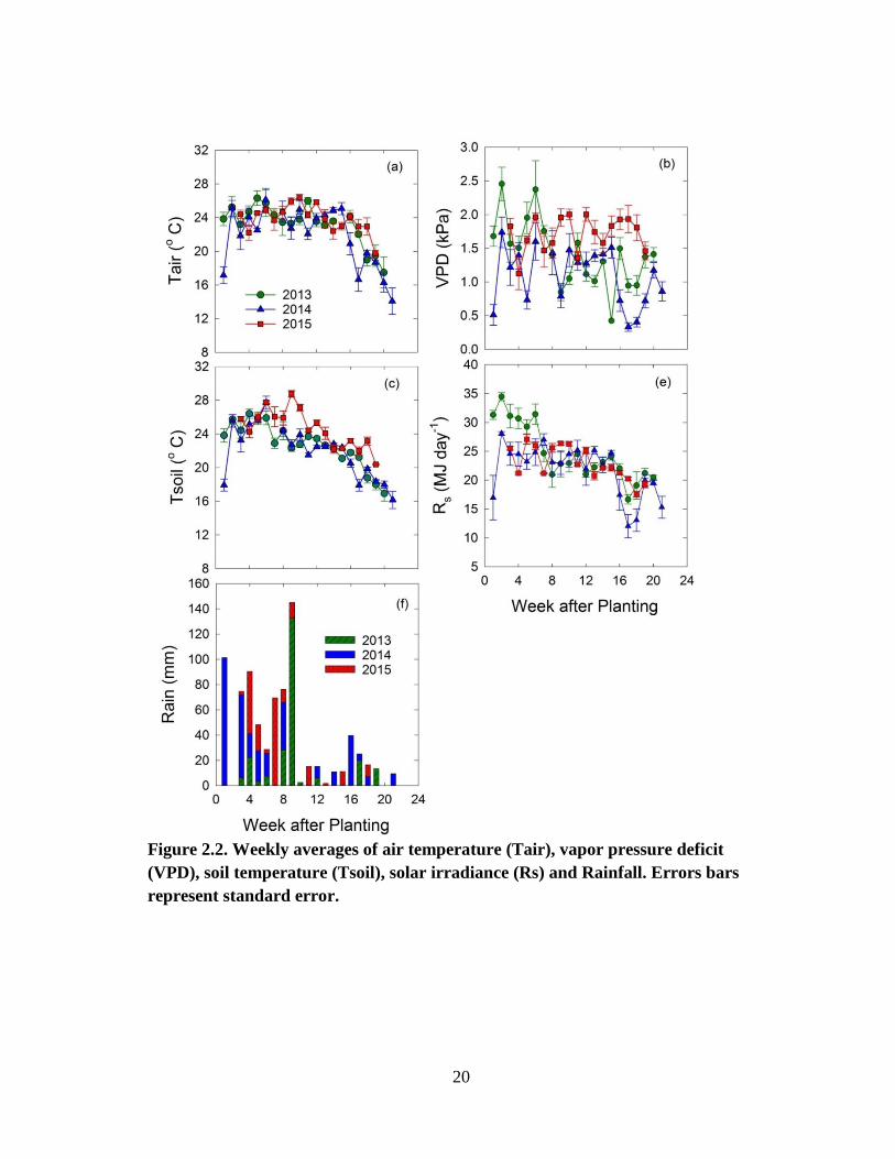
2.2 Weekly averages of air temperature (Tair), vapor pressure deficit (VPD), soil

temperature (Tsoil), solar irradiance (Rs) and Rainfall. Errors bars represent

standard error ................................................................................................. 20

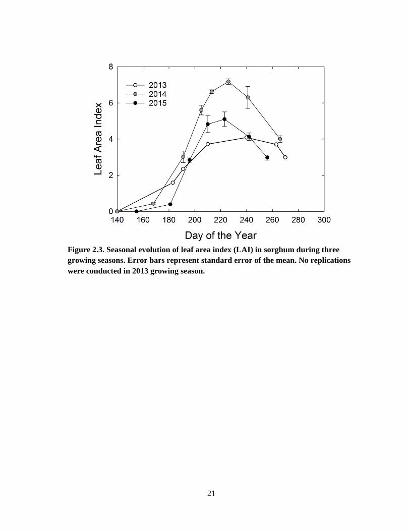
2.3 Seasonal evolution of leaf area index (LAI) in sorghum during three growing

seasons. Error bars represent standard error of the mean. No replications

were conducted in 2013 growing season ....................................................... 21

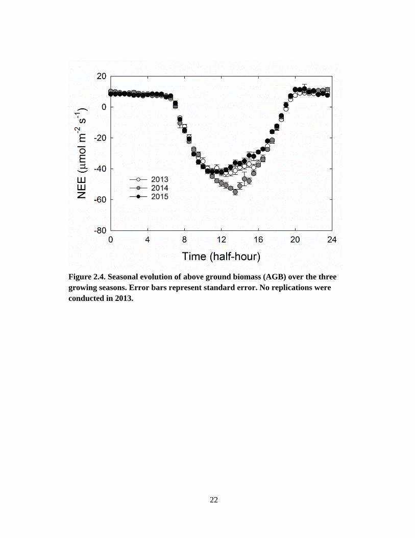
2.4 Seasonal evolution of above ground biomass (AGB) over the three growing

seasons. Error bars represent standard error. No replications were conducted

in 2013 ........................................................................................................... 22

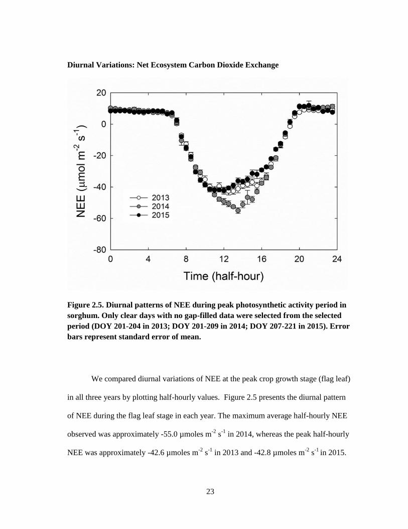
2.5 Diurnal patterns of NEE during peak photosynthetic activity period in

sorghum. Only clear days were selected from the selected period

(DOY 201-204 in 2013; DOY 201-209 in 2014; DOY 207-221 in 2015).

Error bars represent standard error of mean .................................................. 23

2.6 Diurnal trends (a) evapotranspiration (ET), (b) net radiation (Rn), (c) vapor

pressure deficit (VPD), and (d) air temperature from a selected period

during peak photosynthetic period. The crop was at similar phenological

(flag leaf) stage during this period ................................................................ 26

2.7 Hysteretic relationship between (from top to bottom) evapotranspiration

(ET) and air temperature, ET and vapor pressure deficit, and ET and net

radiation (Rn) during selected period of peak photosynthetic activity period.

The crop was at similar phenological stage during this time under optimum

soil moisture conditions. Days of the year selected are same as in

Figure 2.6 ...................................................................................................... 27

2.8 Seasonal courses of daily (sums of) (a) net ecosystem exchange (NEE), (b)

x

gross primary production (GPP) and (c) ecosystem respiration (Reco).

Seasonal integrals of (d) NEE, (e) GPP, and (f) Reco. As per sign

convention, negative values indicate carbon uptake and positive sign

denotes carbon release to the atmosphere ..................................................... 31

2.9 Relationship between carbon content in above ground biomass (g C m-2

)

and cumulative GPP (g C m-2

) ...................................................................... 32

2.10 Regression between monthly integrals of (negative) gross primary

production (GPP) and evapotranspiration (ET) during active growing season

(June-September) across all three year. Coefficient of determination was

(0.89) ............................................................................................................. 33

3.1 Surface soil moisture (volumetric water content in m3 m

-3) presented by line

plot and precipitation presented by red bars in (a) sorghum field at 5 cm and

(b) old world bluestem at 10 cm .................................................................... 53

3.2 Energy balance closure during growing season in old world bluestem

(black circles) and sorghum (grey circles). Only original data (no gap filled)

was used when all the variables were available. All linear relationships were

significant (p<0.0001) ................................................................................... 55

3.3 Average above ground biomass in sorghum and old world bluestem.

Measurements was started in June once the significant biomass was

accumulated in the fields. Error bars represent standard error.

Three replications were conducted in sorghum in 2014 and 2015, and 4

replications in old world bluestem during all growing seasons. No

replications were done in 2013 in sorghum field .......................................... 57

3.4 Evolution of litter over the course of growing season in old world

bluestem. Error bars represent standard error. Four replications were

conducted during each sampling. .................................................................. 58

3.5 Daily sums of NEE (top), Reco (middle) and GPP (bottom) in old world

bluestem site from Jan 1, 2013 to December 25, 2015, and from May 22,

2013 to December 15, 2015 in sorghum. ...................................................... 61

3.6 Monthly average diurnal trends of net ecosystem exchange (NEE) in old

world bluestem field. The error bars represent the standard error. .............. 64

3.7 Monthly average diurnal trends of net ecosystem exchange (NEE) in

sorghum field. Month of May is not included as the crop was just emerging

in that month or was not planted (in 2015). Only days before harvest were

included during month of October i.e. 8 days in 2013 and 14 days in 2014.

xi

The error bars represent the standard error of the mean ............................... 65

3.8 Light response curves of old world bluestem (a, b, c representing 2013,

2014 and 2015, respectively) and sorghum (e, f, g representing 2013, 2014

and 2015, respectively) at peak photosynthetic activity phase of the growing

season. Seven to ten clear days were selected from each growing season,

crops were at the same phenological stage with no soil moisture stress.

However, LAI for sorghum was different at this stage (3.8 in 2013, 5.8 in

2014, and 4.8 in 2015).Only original data was used for this analysis ........... 71

3.9 Relationship between half-hourly diurnal averages of Net Ecosystem

Exchange (NEE) and Gross Primary Production (GPP) with corresponding

VPD during warm and dry conditions (VWC 0.19 m3 m

-3) in old world

bluestem field. Error bars represent the standard error of the mean ............. 72

3.10 Relationship between average weekly nighttime Reco (g C m-2

) against

average soil temperature (Tsoil in oC) at 5cm depth for (a) sorghum in 2013

(𝑅𝑒𝑐𝑜 = 0.0320𝑒0.0672𝑇𝑠𝑜𝑖𝑙)), 2014 (𝑅𝑒𝑐𝑜 = 0.0241𝑒0.0934𝑇𝑠𝑜𝑖𝑙) and 2015

𝑅𝑒𝑐𝑜 = 0.0248𝑒0.0776𝑇𝑠𝑜𝑖𝑙 (b) OWB for 2013 (𝑅𝑒𝑐𝑜 = 0.0107𝑒0.0915𝑇𝑠𝑜𝑖𝑙),2014 (𝑅𝑒𝑐𝑜 = 0.0114𝑒0.1090𝑇𝑠𝑜𝑖𝑙) and 2015 (𝑅𝑒𝑐𝑜 = 0.0103𝑒0.0110𝑇𝑠𝑜𝑖𝑙). R2

ranged from 0.81-0.89 during all years. White circles/triangles/squares

represent the Reco during dry conditions (VWC <0.19 m3 m

-3) for respective

years .............................................................................................................. 76

4.1 Maximum and minimum air temperature and rainfall during 2013 (green),

2014 (black) and 2015 (red) in all the research fields. Line scattered plot

represent minimum and maximum temperature, and bar plot represent

rainfall ........................................................................................................... 96

4.2 Rainfall and soil moisture at 5 cm depth in all the crops from starting of

data collection to end of the study period ..................................................... 97

4.3 Seasonal evolution of leaf area index (LAI) of the dryland cotton, irrigated

cotton, and sorghum. No data was collected in dryland cotton during 2013

as the crop failed due to lack of rainfall. No LAI data was collected in old

world bluestem. ............................................................................................. 100

4.4 Evolution of above ground biomass (AGB) over the growing season in

dryland cotton, sorghum, old world bluestem (OWB). Dryland cotton

failed in 2013, therefore no data was presented for this crops in 2013 ......... 101

4.5 Energy balance closure at different sites during study period. Energy

balance components during peak growing season (July-August) were

selected from each growing season and plotted together to obtain an

xii

aggregated energy balance closure. Each plot consists more than 4000 data

points ............................................................................................................. 104

4.6 Daily integrated net ecosystem exchange (NEE), gross primary production

(GPP) and ecosystem respiration (Reco) during the period of study. All

three years data was available for old world bluestem (OWB). Data

collection from sorghum started from planting in 2013. Data collection in

irrigated cotton started after about a month of planting in 2013. Dryland

cotton failed in 2013; therefore data from only two seasons is presented.

As per sign convention, negative values indicate carbon uptake by the

system and positive signs denote carbon release from the system to

atmosphere. Line plots represent GPP and Reco, bar plot represents NEE .... 106

4.7 Light response curves of sorghum, old world bluestem (OWB), irrigated

cotton and dryland cotton for 2013, 2014 and 2015. Selected clear days

during peak photosynthetic activity were chosen. Phenological stage for

each individual crop was similar. All the relationships were significant

(p<0.0001) with R2 ranging from 0.85-0.94 .................................................. 108

4.8 Relationship between gross primary production (GPP) and vapor pressure

deficit (VPD) in irrigated cotton, dryland cotton, and old world bluestem

during selected days. Clear days were selected when volumetric water

content was below 0.20 m3 m

-3. (DOY 225-228 in 2014 for OWB and

DOY 256-260 in 2015 for irrigated and dryland cotton) ............................ 109

4.9 Relationship between average weekly nighttime ecosystem respiration

(Reco) and nighttime temperature (Tsoil) for sorghum, old world bluestem

(OWB), irrigated cotton and dryland cotton during non-growing season

January-April in OWB and January-May in row crops. Only original data

were used. All relationships were significant at p<0.0001 (R2= ranged

from 0.57-0.93) ............................................................................................. 114

5.1 Energy partitioning in net radiation (Rn), latent heat (LE), sensible heat (H)

and soil heat flux (G) during the study period in different crop fields.

Measurement in sorghum and irrigated cotton started from May and July

2013, respectively. Dryland cotton failed in 2013 and has not been

presented in this data ..................................................................................... 135

5.2 Relationship of daily Bowen ratio with daily average soil moisture (5cm)

content. Daily Bowen ratio from all three active growing seasons

(June-August) was plotted together against respective soil moisture.

Irrigated cotton (R2=0.25) and old world bluestem (R

2=0.41) had

significant relationships. Sorghum and dryland cotton were not

significantly related to soil moisture ............................................................. 138

xiii

5.3 Daily evapotranspiration for the complete study period. Old world

bluestem had all three years of data, whereas data collection from irrigated

crops started following planting in 2013. Dryland cotton crop failed due to

lack of rainfall in 2014, thus the data was lost during that year .................... 140

5.4 Monthly diurnal patterns of evapotranspiration (ET) in different crops.

Dryland cotton in year 2013 failed due to lack of rainfall, therefore we

were unable to collect the data ...................................................................... 145

5.5 Relationship between evapotranspiration (ET) and photosynthetically

active radiation (PAR) for (a) sorghum, (b) old world bluestem (c) irrigated

cotton (d) dryland cotton. Three-five consecutive clear days were

selected during peak photosynthetic activity of growing season in 2013

(grey line), 2014 (dashed line), and 2015 (solid black line). Phenological

stage was similar for each crop and soil moisture was > 0.20 m3 m

-3. Each

crop displayed peak photosynthetic activity during the selected period. All

relationships were significantly linear (p<0.0001). All the R2 values ranged

from 0.88 to 0.94 ........................................................................................... 147

5.6 Monthly water use efficiency for (a) sorghum (b) OWB, (c) irrigated

cotton and (d) dryland cotton across 2013 (grey), 2014 (white), and 2015

(black). Monthly WUE was calculated by dividing monthly GPP (g C m-2

)

with monthly ET (kg H2O m-2

). Only days before harvesting were selected

during October. .............................................................................................. 149

5.7 Relationship of normalized evapotranspiration (ET) and normalized gross

primary production (GPP) with vapor pressure deficit (VPD). Clear days

during dry period were selected for this analysis (DOY 256-260 in 2015

for both irrigated and dryland cotton; DOY 224-227 in 2014 for dryland

cotton). ET was a significant logarithmic function of VPD for all crops

(R2 = 0.67, 0.69 and 0.32 for irrigated, dryland cotton, and OWB

respectively). GPP was not a strong function of VPD, except in dryland

cotton (R2=0.24) ............................................................................................ 151

xiv

LIST OF TABLES

TABLE Page

2.1 Cumulative seasonal gross primary production (GPP), evapotranspiration

(ET), and ecosystem water use efficiency (EWUE)...................................... 34

3.1 Monthly average maximum (Tmax) and minimum (Tmin) air temperature

values in (a) old world bluestem and (b) sorghum field for year 2013, 2014

and 2015 . ................................................................................................... 52

3.2 Seasonal and annual cumulative carbon fluxes in old world bluestem and

sorghum field. Two complete years were available for sorghum and three

complete years were available for old world bluestem (OWB). SD is

standard deviation ......................................................................................... 68

3.3 Seasonal net ecosystem exchange (NEE) as reported in different studies

for different bioenergy crops ......................................................................... 74

4.1 Seasonal integrals of NEE, GPP and Reco in sorghum, old world bluestem

(OWB), irrigated cotton, and dryland cotton. Lower case alphabets

alongside mean values represent the statistical difference at p<0.05 ............ 107

4.2 Mean apparent quantum yield (alpha) and mean GPPmax for all the crops.

Rectangular hyperbolic relationship was plotted between GPP and PAR for

5-10 selected clear days during peak photosynthetic activity. Lower case

alphabets besides values indicate significance level at p<0.05 ..................... 107

4.3 Annual net ecosystem exchange (NEE) of the irrigated cotton,

sorghum, dryland cotton, and old world bluestem. ...................................... 112

5.1 Seasonal and annual evapotranspiration and rainfall in different crops ........ 141

5.2 Seasonal ET for different bioenergy crops as well as cotton reported in

different studies ............................................................................................. 143

5.3 Seasonal ecosystem water use efficiency for different crops during

different study years. Year 2013 does not represent the full cropping season

for irrigated cotton as the data collection started about a month after

planting .......................................................................................................... 152

1

CHAPTER I

INTRODUCTION

According to the current renewable fuel standard (RFS), the United States will

require 136 billion liters of biofuels per year by 2022 (USDA, 2010). The RFS

mandates that out of this 136 billion liter target, 80 billion liters will need to be produced

from second generation biofuels (USDA, 2010). Second generation biofuels are mainly

produced from the by-products of first generation crops or from biomass crops grown

with less-intensive agricultural activities conducted on marginal lands using substantially

reduced resource inputs. In the 2010 Biofuels Strategic Production Report, the USDA

has identified regions in the United States that have a comparative advantage of

producing specific bioenergy crops based on the prevailing cropping systems, their

yields and the current producer interest in growing these crops. Approximately 50% of

the 80 billion liters target of second-generation biofuels is estimated to be produced from

the southeast region of the United States including the Southern Great Plains. However,

environmental impacts and long-term sustainability of large scale production of

bioenergy crops in the Southern Great Plains has not been addressed adequately.

The Texas High Plains region in the Southern Great Plains is a major agricultural

region in the United States (Fig. 1.1). This region is semi-arid with a long-term (1911-

2005) mean annual rainfall of about 465 mm (Allen et al., 2008). The Texas High Plains

2

region was dominated by shortgrass prairie prior to the discovery of the vast

underground Ogallala Aquifer (Gould, 1975; Allen et al., 2008). Availability of water

for irrigation from the Ogallala Aquifer transformed this semi-arid region into one of the

most intensively cultivated agricultural production regions in the U.S. (Allen et al.,

2008; Rajan et al., 2014). In fact, the Southern Great Plains is the largest producer of

cotton (Gossypium hirsutum L.) in the U.S. (Attia et al., 2015). Grain sorghum

(Sorghum

Figure 1.1: Southern Great Plains region and major cropping systems. Reprinted

from: USDA-National Agricultural Statistics Service CropScape- Cropland Data

Layer. Copyright © Center for Spatial Information Science and Systems 2009-2016

bicolor L.), corn (Zea mays L.), and winter wheat (Triticum aestivum L.) are other major

crops in the region. More than 95% of the water pumped from the Ogallala Aquifer is

currently used for irrigation of agricultural crops (Nair et al., 2013). However, excessive

3

extraction of water for agricultural use has depressed the water table of the Ogallala

Aquifer by over 30 m in most parts of the Southern Great Plains (Rajan et al., 2015). The

declining water for irrigation in this region poses big challenges to the production of first

generation biofuels such as corn as it has high water requirement compared to other

cellulosic bioenergy crops.

Continuous cotton under conventional tillage has been a dominant row cropping

system in the Southern Great Plains for several decades (Fig. 1.1) (Acosta-Martinez et

al., 2010). Low returns of organic matter from cotton cropping systems has depleted the

organic matter reserves of the soils in Southern Great Plains and declined the soil quality

(Moore et al., 2000; Wright et al., 2008; Allen et al., 2008; Acosta-Martinez, 2010). Soil

organic matter accumulation is important for soil health as it improves soil structure,

prevents soil erosion, improves infiltration and water holding capacity, and sequesters

atmospheric carbon dioxide (Lal, 2004). Land use change from conventional cropping

systems to bioenergy cropping systems will have major environmental implications.

Several recent studies have reported the net carbon sinking capacity of annual and

perennial bioenergy crops at ecosystem scale in different parts of North America (Zeri et

al., 2011; Wagle et al., 2015; Oikawa et al., 2015; Eichelmann et al., 2016). Several

studies have reported improved soil organic matter status with bioenergy crops

depending upon management practices and amount of residues left on the surface after

harvest (Halvin et al., 1990;Polley, 1992; Tolbert et al., 2002; Cotton, 2013b; Meki et

al., 2013). Similarly, conversion of croplands to perennial grasslands can reclaim the soil

organic carbon and improve soil health over time depending upon climatic conditions

4

(Burke et al., 1988; McLauchlan et al., 2006). However, more investigation is necessary

to understand the carbon dynamics as a result of land use change from cotton to

bioenergy crop production systems in the Southern Great Plains.

Another major implication of land use change in the Southern High Plains to

bioenergy crops will be on surface energy balance. Surface energy fluxes include the

turbulent fluxes of latent heat or evapotranspiration (ET), sensible heat, and solar and

terrestrial radiative fluxes (Rajan et al., 2010). The differences in canopy structure and

background soil characteristics affect how incoming solar energy is partitioned among

various components of the energy balance, which can be written as:

Rn = LE + H + G + M + S

where Rn is the net radiation, LE is the latent heat flux, H is the sensible heat

flux, G is the soil heat flux, M is the metabolic energy associated with plant

photosynthesis and respiration, and S is the heat storage in the above-ground biomass.

Land use changes can alter surface characteristics such as vegetation cover, surface

roughness, albedo, and soil moisture (Kueppers et al, 2008). Changes in one or more of

these variables can significantly alter the fluxes and energy balance, which can

ultimately lead to changes in local and regional climate. If large areas of the Southern

Great Plains are converted to second-generation biofuel feedstocks, it is possible that

such a change will significantly impact the surface energy fluxes in the region.

Similar to energy fluxes, surface and near-surface hydrological processes are also

modified due to changes in crop characteristics and management practices. Cotton,

5

biomass sorghum, and perennial grasses have unique leaf distribution and density

characteristics which, in turn, affect the micro-climatic regimes within the plant canopy.

The denser canopy of perennial grasses limits the amount of radiation reaching the

ground surface, thereby affecting the soil evaporation component of ET (Schulze et al.,

1994; Rajan et al., 2010). Le et al. (2011) reported that, under current climatic

conditions, land use change from corn to bioenergy crops such as switchgrass and

Miscanthus could increase the seasonal ET by 56% and 36%, respectively, in the

Midwest. Similar results were also reported for the Midwest region by Hickman et al.

(2010), using the residual energy balance method, and by VanLoocke et al. (2010) using

modeling. The potential for biofuel crops such as perennial grasses and biomass

sorghum to alter the regional hydrologic cycle by replacing the immense acreage of

cotton in the Southwestern Cotton Belt region is unknown and thus needs to be

investigated.

This study includes results from the on-site research conducted on bioenergy and

conventional cropping systems in the Southern Great Plains. We investigated carbon,

energy and evapotranspiration dynamics of potential bioenergy cropping systems and

conventional cotton cropping systems. This dissertation consists of six chapters.

Chapter I provides introduction and background of the study.

Chapter II is dedicated to the assessment of seasonal dynamics of carbon and ET

of high biomass forage sorghum, its biofuel generation capacities and potential to

establish itself as a bioenergy crop in the Southern Great Plains. Phenological

6

and environmental controls over seasonal carbon dynamics of sorghum are also

discussed in this chapter.

Chapter III compares seasonal and inter-annual on-site carbon dynamics of a

potential annual (sorghum) and perennial (Old World Bluestem) bioenergy crops

in the Southern Great Plains. In addition to growth habits and environmental

controls, potential environmental impacts of large scale production of these crops

are also discussed in this chapter. Biomass production and possible ecosystem

services of both bioenergy crops are also discussed in this chapter.

Chapter IV assesses and compares the carbon dynamics of bioenergy crops with

irrigated and dryland cotton cropping systems. Possible impacts of land use

change from cotton cropping systems to bioenergy cropping systems on

biosphere-atmosphere carbon exchanges are discussed in this chapter.

Chapter V assesses and compares seasonal and inter-annual energy balance, ET

and water use efficiency (WUE) of all the crops studied as part of this

dissertation research in the Southern Great Plains. Potential implications of land

use change on ET, energy balance and water use efficiency in the Southern Great

Plains are also discussed.

Chapter VI provides overall summary of this research and recommendations for

future work.

7

CHAPTER II

SEASONAL VARIABILITY IN EVAPOTRANSPIRATION AND

NET ECOSYSTEM CARBON DIOXIDE EXCHANGE OF HIGH

BIOMASS FORAGE SORGHUM IN THE SOUTHERN GREAT

PLAINS

INTRODUCTION

Despite recent low oil prices, fuel ethanol production in the U.S. has increased

from 10.60 Billion Gallons (BG) in 2009 to 14.70 BG in 2015 (RFS, 2016). Corn (Zea

mays L) has been the primary feedstock for fuel ethanol production in the U.S.

Approximately, 850 million gallons (MG) of U.S. fuel ethanol was exported to more

than 50 countries in 2015 (RFS, 2016). Although U.S. is the largest exporter of fuel

ethanol in the world, it also imported 96 MG of ethanol in 2015. Majority of this

imported ethanol came from Brazil. The main reason for the import was because the

Renewable Fuel Standard (RFS) and the Low Carbon Fuel Standards (LCFS) of

California and other states specify the use of biofuels with low greenhouse gas (GHG)

emissions (Whistance et al., 2017). Based on life cycle analyses, GHG emissions from

sugarcane (Saccharum spp.) cropping systems in Brazil are considered to have less GHG

emissions compared to corn cropping systems in the U.S., thus promoting its import. The

RFS statutory requirement for renewable fuel production is 30 BG in 2020, of which at

8

least 35% of total renewable fuels must be produced from cellulosic biofuels with low

GHG emissions.

Cellulosic biofuels are considered second generation biofuels and are produced

from ligno-cellulosic biomass feedstock using advanced conversion technological

processes (Naik et al., 2010). The main cellulosic biomass feedstocks include

agricultural residues and dedicated herbaceous and woody energy crops such as

switchgrass (Panicum virgatum), Miscanthus, biomass sorghum (Sorghum bicolor L),

and hybrid poplar (Populus deltoids × Populus trichocarpa). Many cellulosic bioenergy

crops are ideal candidates for growing in the Southern Great Plains due to their

adaptation to water-limited and semi-arid environmental conditions. For example,

switchgrass is a cellulosic biofuel feedstock adapted to the environmental conditions in

the Southern Great Plains (Sanderson et al., 2006; Jefferson and McCaughey, 2012;

Chen et al., 2016). Another potential bioenergy crop that is gaining popularity in the

Southern Great Plains is sorghum. Several studies have reported the drought tolerance

and high WUE characteristics of biomass and forage sorghums in the Southern Great

Plains (Hao et al., 2014; Chen et al., 2016; Wagle et al., 2015; Yimam et al., 2015). In

addition to agronomic characteristics such as high WUE and high biomass production,

physical and chemical properties of the feedstocks also play major roles in determining

their suitability for biofuel production (Corredor et al., 2009; Karmakar et al., 2010;

Atabani et al., 2013). The brown midrib (bmr) cultivars of forage sorghum have lower

lignin content, and hence are more suitable for ethanol production as lignin tends to

prevent the enzymes from accessing cellulose (Corredor et al., 2009; Dien et al, 2009;

9

Sattler et al., 2010). In addition, forage sorghum is cheaper to produce than corn. These

attributes promote the use of forage sorghum for biofuel production (Shoemaker and

Bransby, 2010). Several new bmr cultivars of forage sorghum have already been

successfully introduced in the Southern Great Plains region.

Significant changes in land use from conventional cropping systems to second

generation cellulosic cropping systems such as biomass or forage sorghum have several

environment-related implications. Changes in land surface properties and management

practices due to land use change to cellulosic biofuel crops can significantly affect net

ecosystem CO2 exchange (NEE) and evapotranspiration (ET) (Claussen et al., 2001;

Rydsaa et al., 2015). In recent years, eddy covariance systems have been increasingly

used for direct measurements of NEE and ET from various ecosystems (Baldocchi,

2003; Reichstein et al., 2007; Foken et al., 2012). Scientists have established networks of

experimental sites such as Ameriflux with eddy covariance systems for measuring NEE,

ET and energy exchange in key ecosystems in North America (Law, 2007). Data from

these experimental sites are critical for gaining a proper understanding of regional and

global carbon and hydrologic cycles. However, very few studies have been conducted

investigating ET and carbon flux dynamics of biomass sorghum (Wagle, 2016). In this

three-year study (2013 to 2015), we examined half-hourly, daily, and seasonal ET, and

carbon flux dynamics (NEE, Gross Primary Production/GPP and Ecosystem

Respiration/Reco) of annual sorghum in the Southern Great Plains. In addition, we

studied energy partitioning and ecosystem WUE. Our results provide further insights

10

into the dynamics of carbon fluxes and ET for this lesser studied, yet crucial, cellulosic

biofuel cropping system.

MATERIALS AND METHODS

Study Site

The study was conducted in a farmer’s center-pivot irrigated field planted to high

biomass forage sorghum for commercial seed production. The field was located

approximately 4.5 km northeast of Plainview, TX in the Southern Great Plains region

(34°12’34.70’’ N and 101°37’50.85’’ W, 1100 m elevation). The total area of the center

pivot field was 50 ha and sorghum was planted to half of the area (25 ha). Remaining

half of the field was planted to cotton (Gossypium hirsutum L). The sorghum cultivar

planted was Surpass XL bmr. The crop was planted on 20 May in 2013 and 2014. Heavy

rains in 2015 delayed planting, thus the crop was planted on June 4 (DOY 155) that year.

In all three years, the seeding rate was the same, 4.5 lbs ac-1

. However, the row spacing

was narrower in 2014 (50 cm) compared to 2013 and 2015 (100 cm). The field was

supplied with 150 kg N ha-1

via Urea (32-0-0) broadcasting in spring before planting. In

addition, 30 kg P2O5 ha-1

was also applied prior to planting. For the first 40 days, the

field was supplied with approximately 19 mm of water during each irrigation event. For

the rest of the season, the field was irrigated with 38 mm of water during each irrigation

event. Overall, the field was supplied with 400 mm of irrigation water in 2013 (12

irrigations) and 2014 (12 irrigations), and 267 mm of irrigation water in 2015 (7

irrigations). The field was harvested for seed on 8 October in 2013, 14 October in 2014,

and 1 October in 2015. The growing season was 141, 147, and 119 days long in 2013,

11

2014, and 2015, respectively. The field was disked in early spring to incorporate

residues from cotton. The field was disked again before planting and was cultivated

twice in June to control weeds. The major soil mapping unit at the study site is Pullman

Clay Loam (a fine, mixed, superactive, thermic Torrertic Paleustoll) with 0 to 1% slope.

Eddy Covariance and Ancillary Data Collection

Continuous measurements of CO2 and water vapor were made using an eddy

covariance flux tower established in the field at the beginning of planting. The height of

the instrument tower was adjusted periodically to maintain a distance of 1.5 m from the

top of the canopy and eddy covariance instruments. The movement of the irrigation

system did not interfere with data collection as the height of the center-pivot system was

over 3 m. Wind velocity, CO2, and water vapor concentrations were measured using

IRGASON, which is an integrated open-path infrared gas analyzer (IRGA, Model EC-

150, Campbell Scientific) and sonic anemometer (Model CSAT-3A, Campbell

Scientific) system. These instruments were set up facing southwest (into the prevailing

wind direction). Other environmental variables measured included air temperature (Tair)

and relative humidity (RH) (HMP50, Campbell Scientific), net radiation (Kipp & Zonen

NR-Lite net radiometer), photosynthetic photon flux density (PPFD) (LI-200SL

quantum sensor, LI-COR), global irradiance (LI-190SB pyranometer, LI-COR),

precipitation (TE525 rain gauge, Campbell Scientific), soil temperature (Tsoil) at 4 cm

below the surface (TCAV averaging soil thermocouples, Campbell Scientific), and soil

volumetric water content at 4 cm below the surface (CS-616 water content reflectometer,

Campbell Scientific). The IRGA and net radiometer surfaces were cleaned weekly

12

according to the manufacturers’ guidelines to avoid accumulation of dust. Soil heat flux

(G8cm) was measured using self-calibrating soil heat flux plates (HFPSC-01, Hukseflux,

Campbell Scientific, Logan, UT) at 8 cm depth from the soil surface. Soil heat storage

above the heat flux plate was calculated using the following equation and was added to

the measured soil heat flux at 8 cm to obtain soil heat flux at the surface (G) (Eq. 2.1).

𝐺 = 𝐺8𝑐𝑚 + 𝑆 [2.1]

𝑆 =∆𝑇𝑠𝐶𝑠𝑑

𝑡 [2.2]

where S is heat storage, ∆𝑇𝑠 is change in surface soil temperature, d is depth of soil in

meters above soil heat flux plate, Cs is the heat capacity of moist soil, and t is time in

seconds. Heat capacity of soil in Eq. 2 can be calculated using bulk density (𝜌𝑏 =

1.3 gm 𝑐𝑚−3), volumetric water content (𝜃𝑣), density of water (𝜌𝑤 = 1000 𝑘𝑔 𝑚−3),

heat capacity of water (𝐶𝑤 = 4.2 𝑘𝐽 𝑘𝑔−1𝐾−1 ), and heat capacity of dry soil (Cd = 840 J

kg-1

K-1

) as follows:

𝐶𝑠 = 𝜌𝑏𝐶𝑑 + 𝜃𝑣𝜌𝑤𝐶𝑤 [2.3]

Data from the CSAT3A sonic anemometer and EC150 system were measured at

10-Hz sampling rate using a CR3000 datalogger (Campbell Scientific). All other

environmental variables were measured at 5 seconds interval. The datalogger was

programmed to calculate and save 30-min average values of all environmental variables.

The raw 10-Hz wind velocity, CO2, and water vapor data were saved for further post-

processing and analysis of NEE, GPP, Reco, ET and H.

13

Supporting plant measurements collected include height, leaf area index (LAI),

and biomass. Height was measured from the soil surface to the top of the canopy. Plant

samples were taken randomly from the field to measure leaf area index (LAI) and

biomass. Plants were stored in an ice chest in the field and leaf area was measured (after

separating leaves from shoots) using a leaf area meter (Model LI-3100, Licor

Biosciences, Lincoln, NE) immediately after they were brought to the laboratory. Plant

density (number of plants per m2) and leaf area were used to calculate the LAI.

Eddy Covariance Data Processing and Analysis

Using the eddy covariance method, half-hourly fluxes of CO2 and latent heat

(LE) were calculated as the covariance between fluctuations from the mean vertical wind

speed and corresponding fluctuations of CO2 and water vapor. The sensible heat was

calculated similarly using vertical wind speed and air temperature. We used the open

source EddyPro 4.0 software (LI-COR Biosciences, Lincoln, NE) to compute half-hourly

fluxes using the eddy covariance method. Calculation of fluxes requires a series of

operations including raw data filtering and applications of algorithms for calculating and

correcting fluxes. Some of these corrections include spike removal, spectral corrections

for flux losses (Moncrieff et al., 1997), and corrections for air density fluctuations

(Webb et al., 1980). Eddy Pro assigns quality flags based on widely used tests for steady

state and turbulence (Göckede et al., 2008). The flag ‘0’ indicates high quality fluxes and

‘1’ indicates intermediate quality fluxes. All poor quality fluxes are flagged as ‘2’. The

processed half-hourly fluxes were subjected to additional quality control before gap

filling. In addition to 30 min data that were flagged as ‘2’, data were discarded during

14

precipitation, equipment maintenance, and low turbulence conditions (when the friction

velocity was <0.10 m s–1

).

All missing 30 min flux data (NEE, LE and H) were filled using the online

CarboEurope and Fluxnet eddy covariance gap-filling tool (http://www.bgc-

jena.mpg.de/~MDIwork/eddyproc/). This online tool uses methods similar to those

described in Falge et al (2001) and Reichstein et al (2005). All missing 30 min fluxes

were replaced by the average value under similar meteorological conditions within a

time-window of 7 days. This window was expanded to ±14 days in case similarity in

meteorological conditions were not present within 7 days window. This online tool also

provided estimations of half-hourly GPP and Reco. Night-time NEE values represent

Reco. Daytime Reco was estimated using short-term temperature sensitivity equations

developed between night-time NEE measurements and corresponding soil temperature

(Tsoil) measurements made at the 4-cm depth. The GPP was estimated as the difference

between Reco and NEE.

We examined energy balance closure to assess the quality of eddy covariance

estimates of LE and H (Wilson et al., 2002). The difference between Rn and G represents

the available energy at the surface. Assuming negligible heat storage within the canopy

and net horizontal advection of energy, the energy balance can be described in Eq. 2.4:

Rn – G = LE + H [2.4]

The sign convention used for Rn and G are positive when the flux is downwards

and negative when the flux is upward. The sign convention used for LE, H and C fluxes

15

was a positive flux represents flux from the ecosystem to the atmosphere, while a

negative flux represents flux from the atmosphere to the ecosystem.

Evapotranspiration and Water Use Efficiency

The 30 min LE data was used to calculate ET using the following equation:

𝐸𝑇 =𝐿𝐸

𝜌𝑤𝜆 [2.5]

where, 𝜌𝑤 density of water (1000 kg m-3

), and LE is the latent heat of vaporization (2.5

× 106 J kg

-1). Ecosystem WUE (WUEECO) at monthly, and seasonal scales were

calculated by dividing daytime cumulative GPP by daytime cumulative ET at monthly,

and seasonal timescales, respectively.

RESULTS AND DISCUSSION

Energy Balance Closure

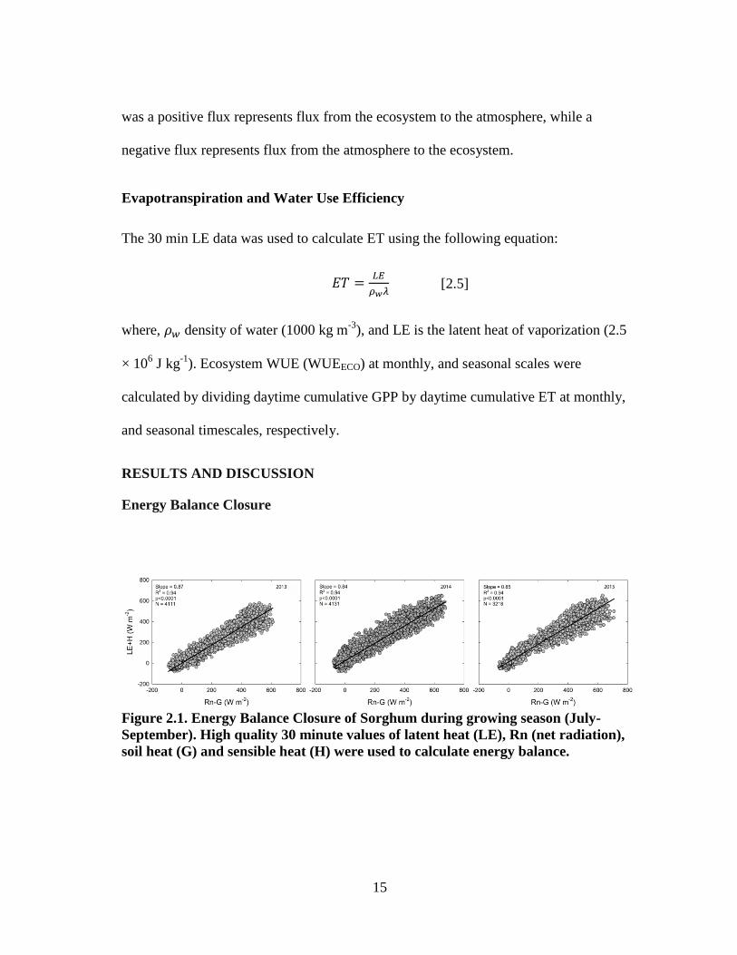
Figure 2.1. Energy Balance Closure of Sorghum during growing season (July-

September). High quality 30 minute values of latent heat (LE), Rn (net radiation),

soil heat (G) and sensible heat (H) were used to calculate energy balance.

16

Seasonal energy balance closure was calculated using half-hourly turbulent

fluxes (LE and H) and available energy (Rn and G) components. Data were included in

the analysis only when all four measurements were available. The sum of half-hourly LE

and H was strongly correlated to the sum of available energy (Rn-G) in all three years

with an R2 value of 0.94 (Fig. 2.1). The degree of surface energy balance closure is

indicated by the slope of the linear regression line through these data. The slope of the

regression lines were 0.87, 0.84 and 0.85 for 2013, 2014, and 2015, respectively,

indicating that 84 to 87% of the variation in daily available energy (Rn-G) was accounted

for by the sum of the turbulent energy fluxes (Fig. 2.1). This degree of energy balance

closure at our site is similar to those reported in other studies. Foken (2008) reported that

energy balance closure was in the range of 70 to 90% for a variety of ecosystems studied

using eddy covariance measurements. Wagle and Kakani (2014) reported closure on the

order of 77% for a biomass sorghum field in the Southern Great Plains. In our study, we

did not use a correction factor to close the energy balance because the causes of

underestimation of eddy covariance fluxes are not fully understood and are continually

debated (Aubinet et al., 2000; Twine et al., 2000).

Meteorological Conditions and Plant Phenology

Weekly average environmental data from the site is presented in Figure 2.2. The

2013 growing season precipitation (241 mm) was less than the precipitation received in

2014 (328 mm) and 2015 (271 mm). The precipitation distribution over the growing

season also varied across the three growing seasons. This resulted in differences in

weekly average VPD and solar irradiance among the three study years. Weekly average

17

VPD over the course of the growing season ranged from 0.42 to 2.4 kPa in 2013, 0.33 to

1.7 kPa in 2014 and 1.1 to 1.9 kPa in 2015. Weekly average VPD was the lowest in

2014, year with the highest growing season precipitation. Dry and clear sky conditions in

Late May and early June in 2013 caused VPD to peak above 1.5 kPa that year. During

the peak growing months in 2013 and 2014, VPD dropped to below 1.5 kPa on most

days. However in 2015, less precipitation received during the peak growing months

(July and August) resulted in high VPD (above 1.5 kPa) on most days.

Weekly averages of air and soil temperature at 4 cm depths were closely

correlated (R = 0.91 in 2013 and 2014 and R = 0.84 in 2015). Early in the season (May

and June), average Tsoil was slightly higher than Tair which decreased to below Tair later

in the season. Weekly average Tair during study period ranged from 17.5 to 26.3 oC in

2013, 14.1 to 26.1 oC in 2014, and 19.8 to 26.4

oC in 2015. Average Tair for the growing

season was 23.2 oC in 2013, 21.9

oC in 2014, and 23.9

oC in 2015. In 2013 and 2015,

seasonal average Tair was close to the 30 year average temperature for the corresponding

period (23.6 oC). In 2014, seasonal average Tair was approximately 2

oC less than the

long-term average temperature. The average daily Tair during the first week after

planting in 2014 was approximately 8 oC less than the Tair during the corresponding

period in 2013 (Figure 3a). Similar to Tair, the average daily Tsoil during the first week

after planting in 2014 was approximately 6 oC lower than the Tsoil during the

corresponding period in 2013. Year 2014 also had low growing season average Tsoil

(21.9 oC) compared to 2013 (22.8

oC) and 2015 (24.6

oC). Spring 2014 was cooler than

18

normal and the low air and soil temperatures were due to late spring cold fronts passing

over the region.

Measurements of phenological development were started once the plant stand

was well established (June). In all three years, LAI changed rapidly during the growing

season. The maximum LAI measured was 4.1 in 2013, 7.2 in 2014 and 5.1 in 2015 (Fig.

2.3). In all three years, LAI remained at its peak for approximately 2 weeks.

Aboveground biomass (AGB) increased significantly from June to September. Peak

AGB measured was 18 Mg ha-1

in 2013, 24 Mg ha-1

in 2014, and 21 Mg ha-1

in 2015

(Fig. 2.4). The inter-annual variation in LAI and AGB was primarily due to the

difference in plant population density. Plant emergence was higher in 2014 (11 plants m-

2) compared to that in 2013 (8.33 plants m-2) and 2015 (9.25 plants m

-2). The higher plant

density in 2014 was due to narrower row spacing. The influence of plant density on LAI

and biomass has been reported in several previous studies (Steiner et al., 1986; Wall and

Kanemasu, 1990; Kross et al., 2015).

The growth period of sorghum from emergence to maturity was approximately

100 days in our study. Even without a second harvest, the biomass production of

sorghum at our study site was comparable to the seasonal biomass production of several

other bioenergy crops in the U.S (Song et al., 2015). Researchers have reported the yield

of biomass sorghum ranging from less than 10 Mg ha-1

to over 30 Mg ha-1

, depending on

the region and growing conditions. Oikawa et al. (2015) reported dry biomass

production of sorghum ranging from 11.7 Mg ha-1

to 16.2 Mg ha-1

for three harvests

between February and November in Arizona. In Florida, Singh et al. (2012) reported

19

19.4 Mg ha-1

of AGB production for biomass sorghum. Cotton et al. (2013) reported dry

biomass yield for forage sorghum ranging from 13.2 to 30.1 Mg ha-1

in the Texas High

Plains. These authors reported that the biomass yield varied depending upon irrigation

level and cultivar characteristics. Results from our study suggest that high biomass

forage sorghum could be a promising biomass crop in the semi-arid Southern Great

Plains under irrigated conditions. The short growing period to reach maturity in this

region also suggests ratooning and double-cropping possibilities with winter wheat or

other short duration crops.

20

Figure 2.2. Weekly averages of air temperature (Tair), vapor pressure deficit

(VPD), soil temperature (Tsoil), solar irradiance (Rs) and Rainfall. Errors bars

represent standard error.

21

Figure 2.3. Seasonal evolution of leaf area index (LAI) in sorghum during three

growing seasons. Error bars represent standard error of the mean. No replications

were conducted in 2013 growing season.

22

Figure 2.4. Seasonal evolution of above ground biomass (AGB) over the three

growing seasons. Error bars represent standard error. No replications were

conducted in 2013.

23

Diurnal Variations: Net Ecosystem Carbon Dioxide Exchange

Figure 2.5. Diurnal patterns of NEE during peak photosynthetic activity period in

sorghum. Only clear days with no gap-filled data were selected from the selected

period (DOY 201-204 in 2013; DOY 201-209 in 2014; DOY 207-221 in 2015). Error

bars represent standard error of mean.

We compared diurnal variations of NEE at the peak crop growth stage (flag leaf)

in all three years by plotting half-hourly values. Figure 2.5 presents the diurnal pattern

of NEE during the flag leaf stage in each year. The maximum average half-hourly NEE

observed was approximately -55.0 µmoles m-2

s-1

in 2014, whereas the peak half-hourly

NEE was approximately -42.6 µmoles m-2

s-1

in 2013 and -42.8 µmoles m-2

s-1

in 2015.

24

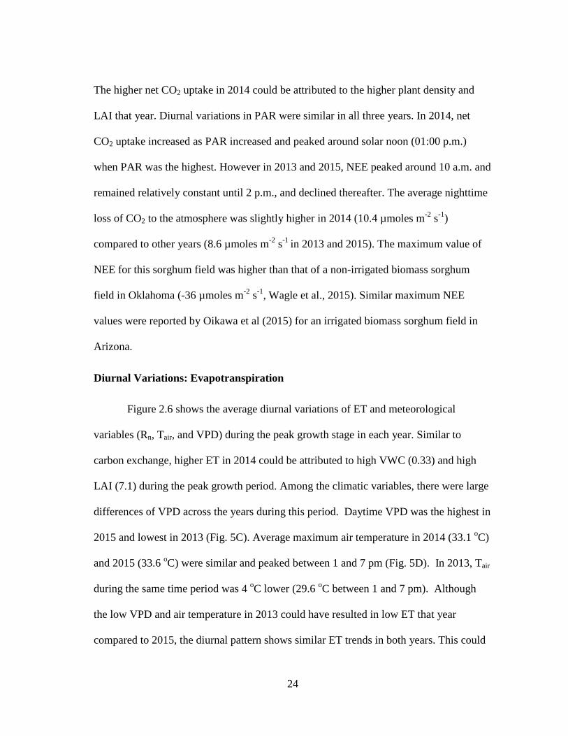
The higher net CO2 uptake in 2014 could be attributed to the higher plant density and

LAI that year. Diurnal variations in PAR were similar in all three years. In 2014, net

CO2 uptake increased as PAR increased and peaked around solar noon (01:00 p.m.)

when PAR was the highest. However in 2013 and 2015, NEE peaked around 10 a.m. and

remained relatively constant until 2 p.m., and declined thereafter. The average nighttime

loss of CO2 to the atmosphere was slightly higher in 2014 (10.4 µmoles m-2

s-1

)

compared to other years (8.6 µmoles m-2

s-1

in 2013 and 2015). The maximum value of

NEE for this sorghum field was higher than that of a non-irrigated biomass sorghum

field in Oklahoma (-36 µmoles m-2

s-1

, Wagle et al., 2015). Similar maximum NEE

values were reported by Oikawa et al (2015) for an irrigated biomass sorghum field in

Arizona.

Diurnal Variations: Evapotranspiration

Figure 2.6 shows the average diurnal variations of ET and meteorological

variables (Rn, Tair, and VPD) during the peak growth stage in each year. Similar to

carbon exchange, higher ET in 2014 could be attributed to high VWC (0.33) and high

LAI (7.1) during the peak growth period. Among the climatic variables, there were large

differences of VPD across the years during this period. Daytime VPD was the highest in

2015 and lowest in 2013 (Fig. 5C). Average maximum air temperature in 2014 (33.1 oC)

and 2015 (33.6 oC) were similar and peaked between 1 and 7 pm (Fig. 5D). In 2013, Tair

during the same time period was 4 oC lower (29.6

oC between 1 and 7 pm). Although

the low VPD and air temperature in 2013 could have resulted in low ET that year

compared to 2015, the diurnal pattern shows similar ET trends in both years. This could

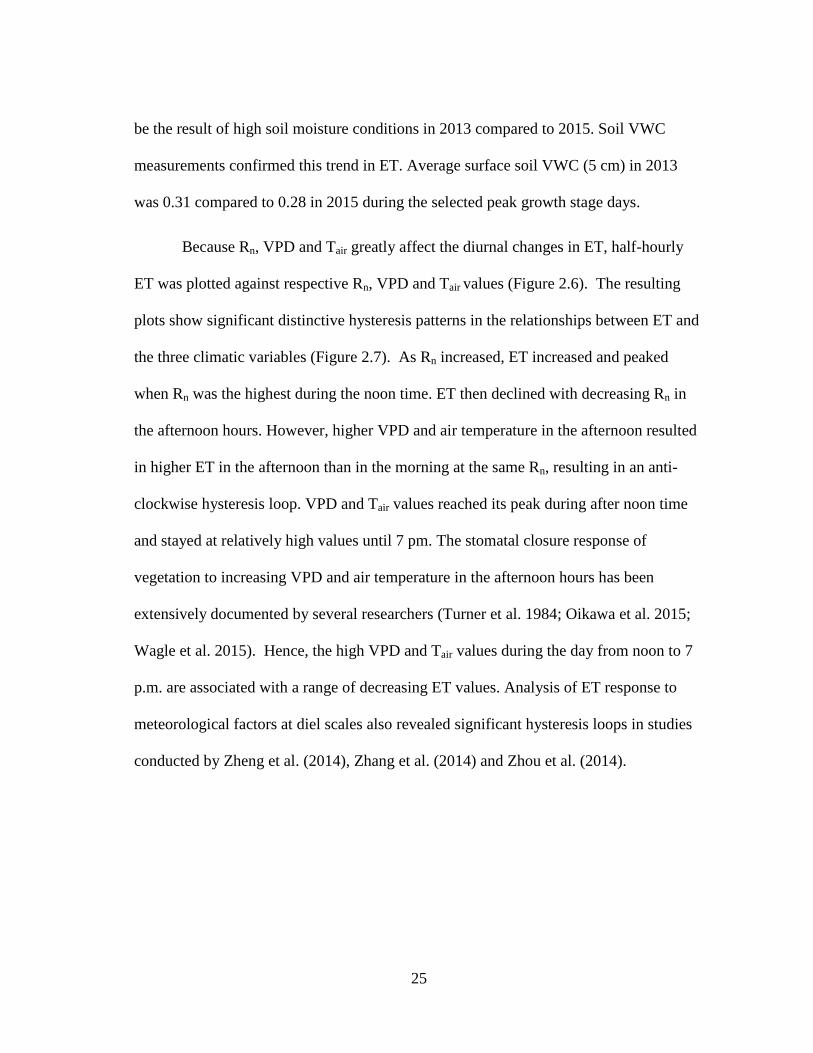
25

be the result of high soil moisture conditions in 2013 compared to 2015. Soil VWC

measurements confirmed this trend in ET. Average surface soil VWC (5 cm) in 2013

was 0.31 compared to 0.28 in 2015 during the selected peak growth stage days.

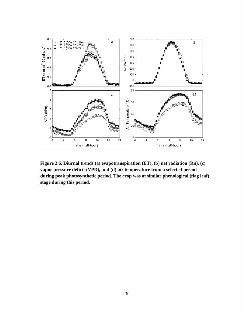
Because Rn, VPD and Tair greatly affect the diurnal changes in ET, half-hourly

ET was plotted against respective Rn, VPD and Tair values (Figure 2.6). The resulting

plots show significant distinctive hysteresis patterns in the relationships between ET and

the three climatic variables (Figure 2.7). As Rn increased, ET increased and peaked

when Rn was the highest during the noon time. ET then declined with decreasing Rn in

the afternoon hours. However, higher VPD and air temperature in the afternoon resulted

in higher ET in the afternoon than in the morning at the same Rn, resulting in an anti-

clockwise hysteresis loop. VPD and Tair values reached its peak during after noon time

and stayed at relatively high values until 7 pm. The stomatal closure response of

vegetation to increasing VPD and air temperature in the afternoon hours has been

extensively documented by several researchers (Turner et al. 1984; Oikawa et al. 2015;

Wagle et al. 2015). Hence, the high VPD and Tair values during the day from noon to 7

p.m. are associated with a range of decreasing ET values. Analysis of ET response to

meteorological factors at diel scales also revealed significant hysteresis loops in studies

conducted by Zheng et al. (2014), Zhang et al. (2014) and Zhou et al. (2014).

26

Figure 2.6. Diurnal trends (a) evapotranspiration (ET), (b) net radiation (Rn), (c)

vapor pressure deficit (VPD), and (d) air temperature from a selected period

during peak photosynthetic period. The crop was at similar phenological (flag leaf)

stage during this period.

27

Figure 2.7. Hysteretic relationship between (from top to bottom)

evapotranspiration (ET) and air temperature, ET and vapor pressure deficit

(VPD), and ET and net radiation (Rn) during selected period of peak

photosynthetic activity period. The crop was at similar phenological stage during

this time under optimum soil moisture conditions. Days of the year selected are

same as in Figure 2.6.

28

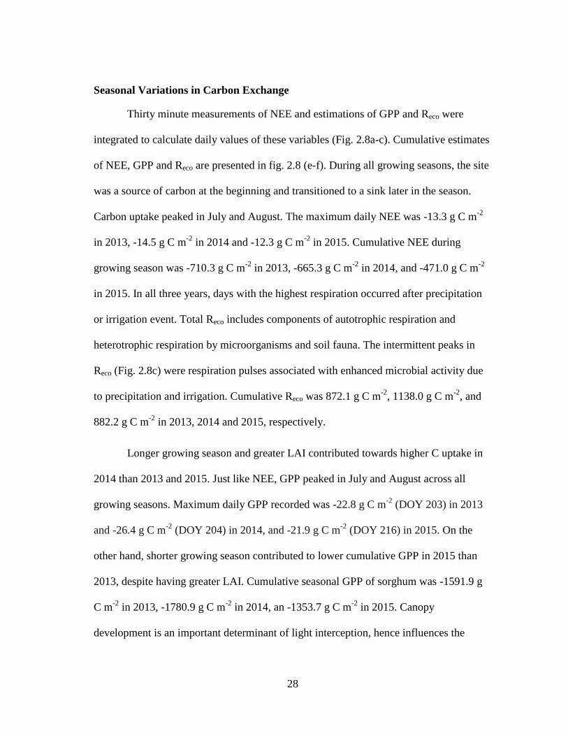
Seasonal Variations in Carbon Exchange

Thirty minute measurements of NEE and estimations of GPP and Reco were

integrated to calculate daily values of these variables (Fig. 2.8a-c). Cumulative estimates

of NEE, GPP and Reco are presented in fig. 2.8 (e-f). During all growing seasons, the site

was a source of carbon at the beginning and transitioned to a sink later in the season.

Carbon uptake peaked in July and August. The maximum daily NEE was -13.3 g C m-2

in 2013, -14.5 g C m-2

in 2014 and -12.3 g C m-2

in 2015. Cumulative NEE during

growing season was -710.3 g C m-2

in 2013, -665.3 g C m-2

in 2014, and -471.0 g C m-2

in 2015. In all three years, days with the highest respiration occurred after precipitation

or irrigation event. Total Reco includes components of autotrophic respiration and

heterotrophic respiration by microorganisms and soil fauna. The intermittent peaks in

Reco (Fig. 2.8c) were respiration pulses associated with enhanced microbial activity due

to precipitation and irrigation. Cumulative Reco was 872.1 g C m-2

, 1138.0 g C m-2

, and

882.2 g C m-2

in 2013, 2014 and 2015, respectively.

Longer growing season and greater LAI contributed towards higher C uptake in

2014 than 2013 and 2015. Just like NEE, GPP peaked in July and August across all

growing seasons. Maximum daily GPP recorded was -22.8 g C m-2

(DOY 203) in 2013

and -26.4 g C m-2

(DOY 204) in 2014, and -21.9 g C m-2

(DOY 216) in 2015. On the

other hand, shorter growing season contributed to lower cumulative GPP in 2015 than

2013, despite having greater LAI. Cumulative seasonal GPP of sorghum was -1591.9 g

C m-2

in 2013, -1780.9 g C m-2

in 2014, an -1353.7 g C m-2

in 2015. Canopy

development is an important determinant of light interception, hence influences the

29

primary production and carbon balance (Chen and Black, 1992; Bange et al., 1997;

Monteith 1997; Nouvellon et al., 2000; Bréda, 2003; Nagler et al. 2004). As reported by

Steiner (1986), increased plant population due to narrow row spacing in sorghum

improved light interception and growth. Similarly, Barbieri et al. (2008) reported

improved initial growth and light interception in maize when row spacing was reduced.

Many studies have indicated greater biomass production following improved light

interception as a consequence of reduced row spacing (Andrade et al., 2002; Sharratt and

McWilliams, 2005; Drouet and Kiniry, 2008).

We calculated carbon content in the AGB (assuming 50% carbon content in

biomass) measured over the growing season. The carbon content of AGB was a strong

linear function of the cumulative GPP. Gross primary production is mainly distributed

among above ground biomass, below ground biomass and autotrophic respiration (Ise et

al., 2010). Combined AGB and below ground biomass constitute net primary production.

The slope of AGB and GPP relationship was about 65%, which indicates that 65% of

total GPP was allocated to above ground biomass (Fig. 2.9). Apparently, rest of the mass

may have been allocated to below ground biomass and autotrophic respiration. Campioli

et al. (2015) obtained a similar relationship for managed and unmanaged ecosystems,

including forests, grasslands, and croplands. The authors concluded that managed

systems favor allocation of more carbon to above ground biomass due to better nutrient

influxes. However, our estimates of carbon allocation to AGB are greater (72%) than

those reported by Campioli et al. (2015) for managed (about 50%) croplands. Allocation

of biomass to different parts could be life strategy for different types of vegetation

30

(Johnson and Thornley, 1987). For example, Blum and Arkin (1984) reported that

sorghum plants growing under water stressed conditions had deep and uniform roots

while well irrigated sorghum plants had a high concentration of roots in shallower soil.

This suggests that good management of cropping system in terms of nutrients and water

in our study may have been responsible for higher biomass allocation to AGB than

below ground biomass.

31

Figure 2.8. Seasonal courses of daily (sums of) (a) net ecosystem exchange (NEE),

(b) gross primary production (GPP) and (c) ecosystem respiration (Reco). Seasonal

integrals of (d) NEE, (e) GPP, and (f) Reco. As per sign convention, negative values

indicate carbon uptake and positive sign denotes carbon release to the atmosphere.

32

Figure 2.9. Relationship between carbon content in above ground biomass (g C m-2

)

and cumulative GPP (g C m-2

).

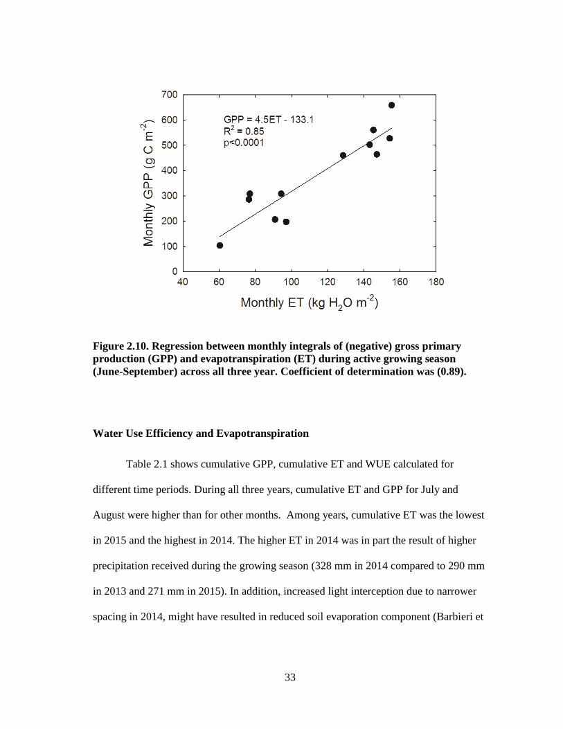
33

Figure 2.10. Regression between monthly integrals of (negative) gross primary

production (GPP) and evapotranspiration (ET) during active growing season

(June-September) across all three year. Coefficient of determination was (0.89).

Water Use Efficiency and Evapotranspiration

Table 2.1 shows cumulative GPP, cumulative ET and WUE calculated for

different time periods. During all three years, cumulative ET and GPP for July and

August were higher than for other months. Among years, cumulative ET was the lowest

in 2015 and the highest in 2014. The higher ET in 2014 was in part the result of higher

precipitation received during the growing season (328 mm in 2014 compared to 290 mm

in 2013 and 271 mm in 2015). In addition, increased light interception due to narrower

spacing in 2014, might have resulted in reduced soil evaporation component (Barbieri et

34

al. 2012). As such, transpiration component of ET might have increased with more shade

and uniform root system due to narrower spacing.

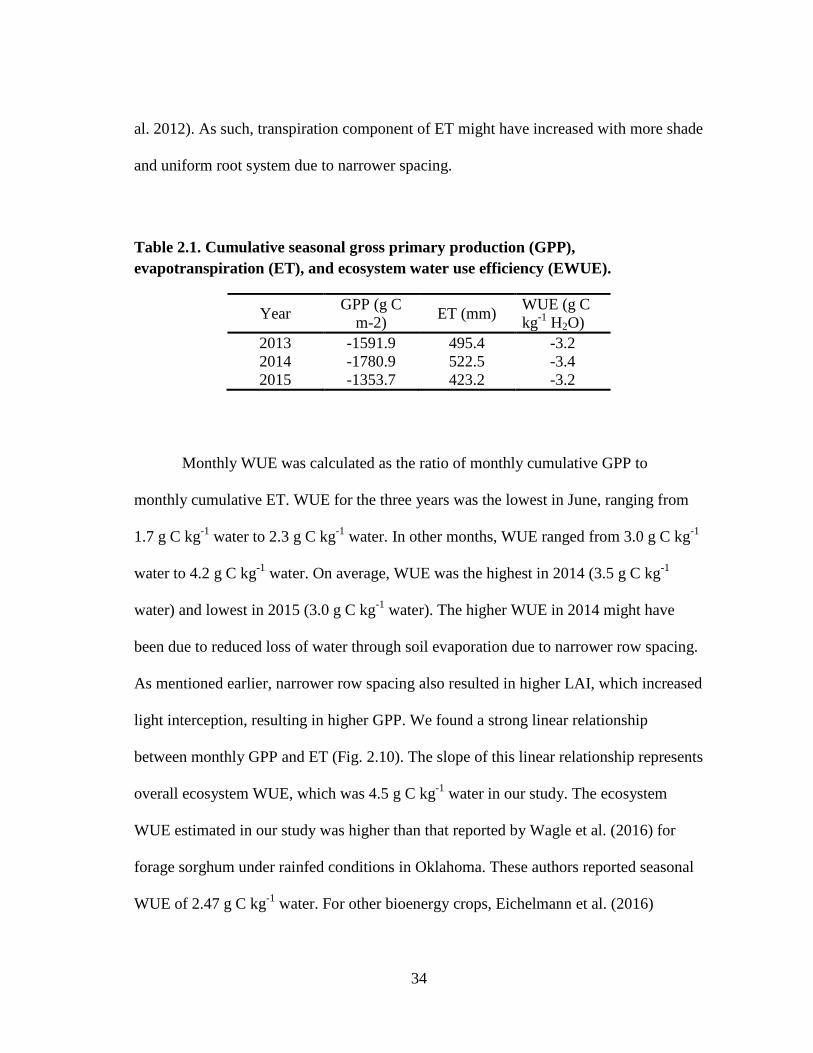
Table 2.1. Cumulative seasonal gross primary production (GPP),

evapotranspiration (ET), and ecosystem water use efficiency (EWUE).

Year GPP (g C

m-2) ET (mm)

WUE (g C

kg-1

H2O)

2013 -1591.9 495.4 -3.2

2014 -1780.9 522.5 -3.4

2015 -1353.7 423.2 -3.2

Monthly WUE was calculated as the ratio of monthly cumulative GPP to

monthly cumulative ET. WUE for the three years was the lowest in June, ranging from

1.7 g C kg-1

water to 2.3 g C kg-1

water. In other months, WUE ranged from 3.0 g C kg-1

water to 4.2 g C kg-1

water. On average, WUE was the highest in 2014 (3.5 g C kg-1

water) and lowest in 2015 (3.0 g C kg-1

water). The higher WUE in 2014 might have

been due to reduced loss of water through soil evaporation due to narrower row spacing.

As mentioned earlier, narrower row spacing also resulted in higher LAI, which increased

light interception, resulting in higher GPP. We found a strong linear relationship

between monthly GPP and ET (Fig. 2.10). The slope of this linear relationship represents

overall ecosystem WUE, which was 4.5 g C kg-1

water in our study. The ecosystem

WUE estimated in our study was higher than that reported by Wagle et al. (2016) for

forage sorghum under rainfed conditions in Oklahoma. These authors reported seasonal

WUE of 2.47 g C kg-1

water. For other bioenergy crops, Eichelmann et al. (2016)

35

reported WUE of 3.7 g C kg-1

water for rainfed switchgrass in Canada and Wagle et al.

(2014) reported 3.2 g C kg-1

water for rainfed switchgrass in Oklahoma (Wagle et al.

2014). The higher ecosystem WUE of sorghum in our study is comparable to that of

corn (4.1 g C kg-1

water) reported by Abraha et al (2016) for the U.S. Midwest. Unlike

less intensively managed switchgrass fields, our sorghum field was intensively managed

with fertilizer application and irrigation to boost production. Thus, the relatively high

ecosystem WUE of forage sorghum at our site is not surprising.

Bioenergy Production Potential

Theoretical ethanol yields were calculated using biomass measurements made

during the growing season by assuming a conversion rate of 0.30 L ethanol per kg of dry

biomass (Oikawa et al., 2015; Chandel et al., 2010). Biomass measured in 2013 before

plants entered soft dough stage was 14.6 Mg ha-1

, which can produce 4,380 L ha-1

of

ethanol. Since the farmer kept the crop growing for rest of the season to produce seed,

the biomass increased to 17.8 Mg ha-1

on DOY 264. Estimated theoretical ethanol yield

at this stage was 5,340 L ha-1

. In 2014, the theoretical ethanol yield was 7,682 L ha-1

at

soft dough stage (Day 241) and 8,906 L ha-1

of ethanol at physiological maturity (DOY

267). In 2015, these numbers reduced to 3,420 L ha-1

at soft dough stage (Day 242) and

6,980 L ha-1

at physiological maturity (DOY 267). In a two year study conducted by

Maw et al in central Missouri, average ethanol yield based on a conversion rate of 0.30 L

ethanol per kg of dry biomass of high biomass sorghum ranged from 2,010 to 6,270 L

ha-1

.

36

CONCLUSION

Seasonal patterns of carbon flux exchanges along with ET and WUE were

analyzed for irrigated sorghum in the Southern Great Plains. Phenological and abiotic

factors accompanied by length of growing season influenced seasonal carbon uptake

properties of sorghum. Narrower row spacing resulted in greater leaf area in 2014.

Greater LAI in 2014 resulted in improved light interception and hence considerably

higher GPP in that year as compared to 2013 and 2015. Smaller growing season in 2015

resulted in lowest GPP as well as NEE in 2015, despite higher maximum LAI value than

2013. Improved light interception also resulted in greater EWUE in 2014. Overall

seasonal NEE and EWUE of irrigated sorghum during all the growing seasons was

greater than those reported for rainfed sorghum in the Southern Great Plains region, and

matched well with those reported for specific biomass crops at different locations in

other studies. These results demonstrate the strong potential of irrigated forage sorghum

for production as annual bioenergy crop in the Southern Great Plains. However, the

declining water table in the Ogallala aquifer will largely determine the fate of irrigation

in the region. Therefore, more investigation is required to quantify the performance of

sorghum under irrigated and dryland conditions for future policy and decision making.

37

CHAPTER III

INTER-ANNUAL AND SEASONAL CARBON EXCHANGE

DYNAMICS OF A PERENNIAL GRASSLAND COMPARED TO

BIOMASS SORGHUM IN THE SOUTHERN GREAT PLAINS

INTRODUCTION

In addition to meeting the traditional goal of food security , current U.S.

agriculture is facing an unprecedented challenge in securing America’s energy future.

The Renewable Fuels Standard Program (RFS2) has projected a requirement of 36

billion gallons (BG) of renewable fuel to be blended into transportation fuel by 2022, an

increase of 27 BG compared to the 9 billion gallon target established in 2008 (USDA,

2010; RFA 2016). Despite lower crude oil prices in recent times, a record ethanol

production of about 23 BG was registered in the U. S. in 2016 (RFA, 2017). Out of the

23 BG, the share of advanced second generation, biomass based biofuels (50% or more

lifecycle greenhouse gas reduction) was only about 5.7 BG. To bridge this gap, an

increase in the production of second generation bioenergy crops is anticipated in future.

Large scale production of bioenergy crops is expected to have significant implications

on local as well regional environment. However, environmental impacts of large scale

production of bioenergy crops have not been addressed adequately (Berndes, 2002;

Robertson et al., 2008; Rowe, 2009; Wagle et al., 2015). Therefore, it is important to

assess the potential environmental impacts of large scale production of bioenergy crops.

38

Second generation biofuels can be produced from annual crops or perennial

crops. Compared to annual crops, perennial crops have relatively lower agronomic

management requirements (such as tillage), lower nutrient requirements, greater energy

production, and reduced greenhouse gas emissions (GHG) (Adler et al., 2007; Parrish

and Fike, 2005; Heaton, et al., 2004). Perennial grasslands with generally high root to

shoot ratio can add significantly to below ground carbon storage (Jackson et al., 1997).

However, perennial grasses such as miscanthus and switchgrass (Panicum virgatum L.)

can take a number of years to establish a significant crop stand for lucrative biofuel

production (Propheter et al., 2010). Several researchers have reported annual crops

performing comparable to or better than perennial crops in productive and marginal

environmental conditions, mainly due to lower yields of perennial grasses during the

initial establishment years (Hallam et al., 2001; Boehmel et al., 2008; Propheter et al.,

2010; Zenone et al., 2013). In addition, annual crops provide flexibility of crop rotation

to farmers (Carpita and McCann, 2008; Cotton et al., 2013). Such factors associated with

perennial and annual bioenergy crops are critical for producers’ acceptance of these

bioenergy crops.

Sorghum (Sorghum bicolor L.) is a drought tolerant annual crop with potential to

establish itself as a major annual bioenergy crop especially in semi-arid areas (Rooney,

2007). Sorghum production is cheaper than corn production due to its drought tolerant

properties, lower requirement of fertilizers and efficient use of nitrogen, phosphorus and

potassium (Rooney, 2007; Shoemaker and Bransby, 2010). In addition, sorghum

production has shown to restore soil organic matter in several studies depending upon

39

tillage practices and amount of biomass left on soil surface (Halvin et al., 1990; Polley,

1992; Cotton et al. 2013b; Meki et al, 2013;). Improved sorghum cultivars with brown

midrib (bmr) mutation have lesser extent of lignin content in cell wall than conventional

forage sorghum. Hence bmr cultivars of sorghum have better conversion efficiency of

lignocellulose to ethanol (Bucholtz et al., 1980; Cherney et al., 1991; Saballos et al,

2008; Corredor, 2009; Dein et al., 2009). Sorghum is an established cropping system

throughout the world including the U. S. for grain as well as forage production.

Therefore, sorghum with its already established cropping systems and physiological

advantage over corn, has the potential to emerge as a major annual bioenergy crop.

Perennial grasses such as switchgrass and miscanthus are becoming popular as

major bioenergy crops in North america and Europe. While the popularity of specific

perennial biomass crops such as switchgrass and miscanthus as bioenergy crops has

peaked recently (McLaughlin et al., 1999; Lewandowski et al., 2003), the perennial

grasslands had been considered as potential bioenergy sources since 1980s, especially in

Europe and North America (McLaughlin et al., 2002; Lewandowski et al., 2003;

Prochow et al., 2009). Bothriochloa bladhii also known as old world bluestem (OWB) is

a C4 perennial bunch grass, native to India that had been introduced successfully in the

Southern Great Plains in 1990s (Rajan et al., 2015). Many cultivars of Bothriochloa spp.

with different physiological and growing properties had been successfully introduced as

pastures in the Southern Great Plains. Old world bluestem has been shown to respond

positively to N fertilization and irrigation (Berg, 1990; Berg and Sims, 1995; Buttrey et

al. 2011). Buttrey et al. (2011) compared six perennial grasses (for multiple clippings)

40

including switchgrass and OWB (WW Spar) under irrigated and dryland conditions. The

authors reported OWB to be the best overall grass in terms of dry matter yield, forage

quality and water use efficiency (WUE). Griffith et al. (2010) demonstrated the

dominance of the OWB in a mixed-prairie where OWB cover increased from 73 to 96%

within three years of planting. Old World Bluestem is one of the dominating grasses

grown on the conservation reserve program (CRP) lands in the Southern Great Plains (Li

et al., 2017). These CRP lands can well serve as sources of biofuel feedstock. As such,

bringing these lands to production will eliminate the cost government incurs to refrain

producers from cultivating these lands. Old World Bluestem has many desirable

characteristics as a biofuel crop, such as wide range of adaptation and high biomass

productivity (Grabowski et al., 2000).

Environmental sustainability is important for large scale production of bioenergy

cropping systems. Carbon exchange and energy balance of a system can indicate the

overall environmental sustainability of a cropping system (Zenone et al., 2013).

Therefore, the objective of this study was to assess and compare seasonal and inter-

annual variation of net ecosystem exchange (NEE) of carbon dioxide (CO2), ecosystem

respiration (Reco) and gross primary production (GPP) of high biomass forage sorghum

and OWB in the Souhtern Great Plains. Both cropping systems were managed by

producers, therefore this provided us an opportunity to collect data under standard

managements practices followed in the region. Environmental variables driving these

flux exchanges were also assessed in this study.

41

Eddy covariance method is the most popular method for studying the C cycle of

different ecosystems (Baldocchi et al., 2001; Baldocchi, 2003). Using this method, the

carbon dioxide (CO2) flux is determined as the covariance between vertical wind

velocity and CO2 concentration which are measured using fast-response instruments

(Goulden et al., 1996; Ham and Heilman, 2003). The net ecosystem exchange (NEE)

measured using the eddy covariance represents the balance between C uptake and

release. The carbon flux exchanges in the two selected fields crops were measured using

the eddy covariance method. Carbon exchange dynamics of sorghum and OWB have

been rarely addressed using eddy covariance systems, especially in the Southern Great

Plains. It is important to study and assess the physiological behavior of these crops as

different biomes have different physiological responses to environmental variables.

Eddy covariance data will be useful in validating land surface and remote sensing

models to extrapolate carbon balance of the agroecosystems to different temporal and

spatial scales (Xu and Baldocchi, 2004). More importantly, environmental sustainability

of annual and perennial bioenergy crops will be critical for decision and policy making

agencies before proceeding with large scale production of these crops (Berndes, 2002;

Robertson et al., 2008; Fargione et al., 2008; Rowe, 2009; Zenone et al., 2013)


Study Site

This study was conducted in two different farmers’ fields fitted with a center

pivot irrigation systems in the Texas High Plains region. The high biomass forage

sorghum field, managed for commercial seed production, was located approximately 4.5

42

km northeast of Plainview, TX (34°12’34.70’’ N and 101°37’50.85’’ W, 1100 m

elevation). The cultivar planted was Surpass XL bmr. Sorghum was planted on one half

of the field and the remaining half was planted with cotton (Gossypium hirsutum L.).

The farmer practiced crop rotation between these crops on both halves of the field.

Management practices prior to planting sorghum included mowing of cotton stalk after

harvesting previous cotton crop followed by tillage in spring and before planting the

crop. Total area planted with sorghum each time was about 25 ha. The crop was planted

on 20 May in 2013 and 2014 at a seeding rate of 4.5 lbs acre-1

. Heavy rains in late May

during 2015 delayed planting, thus the crop was planted on June 4 in 2015 at the same

seeding rate. The row spacing in 2013 and 2015 was 1 m and 0.5 m inches in 2014.

Urea was broadcasted in the field in spring before planting at a rate of 150 kg N ha-1

. In

addition, 30 kg P2O5 ha-1

was also applied prior to planting. The field was irrigated with

low elevation application center-pivot irrigation system during the crop growth period.

For first 40 days the field was supplied with 19 mm and for rest of the season it was

supplied with 38 mm inch water during each irrigation event. The field was supplied

with about 400 mm of water through irrigation in 2013 and 2014 each, and about 270

mm in 2015. Also, the field was cultivated between the plant rows to kill weeds twice in

June every year when the crop was still small. The field was harvested for seed on 8

October in 2013, on 14 October in 2014, and on October 1 in 2015. The growing season

was 140, 147, and 119 days long for 2013, 2014, and 2015, respectively. Equipment

availability and late season rainfall affected the timings of harvest. The field remained

fallow post-harvest in winter and spring. The remaining stalk was grazed by cattle in

43

March 2014 and in January 2015. A fence was put around the tower while the cattle

were present in the field. Since the crop was grown in rotation with cotton, the new crop

was planted on other half of the field where cotton was produced in previous season. The

major soil mapping unit at the study site is Pullman clay loam (a fine, mixed,

superactive, thermic Torrertic Paleustoll) with 0 to 1% slope.

The perennial grassland was located about 5 km (34o 08’47” N, 101

o25’48” W)

west of Lockney, TX and was established in 2007. The pasture was seeded with WW-B

Dahl Old World Bluestem (OWB) (Bothriochloa bladhii L.) at the seeding rate of 2.8

Kg seed ha-1

. “WW-B. Dahl” OWB was released in 1994 jointly by USDA-ARS,

USDA-SCS, Texas Tech University, and the Texas Agricultural Experiment Station

originally from a selection made in India (Rogers et al., 2012). It is a bunchgrass with

an upright growth habit and has better drought tolerance and water use efficiency than

conventional cropping systems in the Southern Great Plains (Allen et al., 2005). Total

area of the site was about 42 ha. Until 2011, the field was used for grazing by the cattle

or for seed production. Although, this field was equipped with a center pivot irrigation

system, no irrigation was supplied during the study period (2013-2015). Moreover, no

nutrients were supplied and the field was never grazed during the period of study. The

growing season for the crop roughly ranged from May to October. Peak growing season

occurred from June to July depending upon precipitation. The grass remained in

vegetative state for the most part of the growing season and bloomed in late

September/early October. The field was harvested for seed on November 14, 2014. No

44

seed harvesting was done in 2013 and 2015. The field was never harvested for hay.

Major soil mapping unit in the field was Pullman clay loam with 0-1% slope.

Eddy Covariance Data Collection

Carbon dioxide, water vapor/latent heat (LE) and sensible heat (H) fluxes were

measured in the fields using eddy covariance systems. While the eddy covariance system

in grassland was established in 2010, the tower in sorghum was established at planting in

2013. Both towers were set up in the middle of the fields, with a fetch of about 150 m

from all directions. An integrated sonic anemometer (Model CSAT-3A, Campbell

Scientific) and infra-red gas analyzer (IRGA, Model EC-150, Campbell Scientific)

called the IRGASON was used to measure wind velocity and CO2, H2O vapor

concentration, and H in the ambient atmosphere. In the grassland, the CO2, H2O vapor

concentration was measured using a LI-7500 IRGA (LI-COR Biosciences) and wind

velocity and sensible heat flux were measured using sonic anemometer (Model CSAT-

3A, Campbell Scientific). These instruments were set up facing south-southwest (in the

prevailing wind direction) at a height of about 2.1 m from ground surface. The height of

the instrument was adjusted in sorghum field during growing season with increasing

crop height to a final height of about 2.6 m from ground. Other environmental variables

measured at both sites included air temperature (Tair) and relative humidity (RH)

(HMP50, Campbell Scientific), net radiation (Kipp & Zonen NR-Lite net radiometer),

photosynthetically active radiation (PAR) (LI-200SL quantum sensor, LI-COR), solar

irradiance (LI-190SB pyranometer, LI-COR), precipitation (TE525 rain gauge,

Campbell Scientific), soil temperature (Tsoil) at 4 cm below the surface (TCAV

45

averaging soil thermocouples, Campbell Scientific), and soil volumetric water content at

4 cm below the surface (CS-616 water content reflectometer, Campbell Scientific). Self-

calibrating soil heat flux plates (HFPSC-01, Hukseflux, Campbell Scientific, Logan, UT)

were used to measure soil heat flux at 8 cm depth from soil surface. Soil heat storage

which is the amount of heat stored in 8 cm soil depth over soil heat flux plates was

calculated using the following equation:


𝑡 [3.1]

Where S is the storage term, ∆𝑇𝑠 is change in surface soil temperature, d is depth of soil

in meters above soil heat flux plate, Cs is the heat capacity of moist soil, and t is time in

seconds. Heat capacity of soil can be calculated from following equation using bulk

density (𝜌𝑏 = 1.3 gm 𝑐𝑚−3), volumetric water content (𝜃𝑣), density of water (𝜌𝑤 =

1000 𝑘𝑔 𝑚−3), heat capacity of water (𝐶𝑤 = 4.2 𝑘𝐽 𝑘𝑔−1𝐾−1), and heat capacity of dry

soil (𝐶𝑑 = 840 𝐽 𝑘𝑔−1𝐾−1):


Soil heat storage term was calculated using temporal variations in soil temperature and

soil moisture in Eq. [3.1] and [3.2]. Soil heat storage term and measured soil heat flux

were added to obtain soil heat flux at surface (G).

Infra-red gas analyzer and net radiometer surfaces were cleaned regularly as per

the manufacturers’ guidelines to avoid accumulation of dust. Data from the CSAT3A

sonic anemometer and IRGA system were measured at 10-Hz sampling rate using a

CR3000 datalogger (Campbell Scientific). All other environmental variables were

46

measured at 5 seconds interval. The datalogger was programmed to calculate and save

30-min average values of all environmental variables. The raw 10-Hz wind velocity and

EC150/LI-7500 data were saved for further post-processing and analysis of CO2 and

energy fluxes.

Data Processing and Gap filling

Data from eddy covariance system was used to calculate half-hourly CO2 and

energy fluxes. The flux measured from the eddy covariance tower is the average of the

product of the covariance between scalar (CO2, water vapor and temperature) and vector

(vertical motions of wind). The high frequency data were analyzed using EddyPro 4.0

software (LI-COR Biosciences, Lincoln, NE). Flux computation requires a series of

operations in order to apply corrections to raw data for flux computation. Some of these

corrections include spike removal, block averaging, coordinate rotation, spectral

corrections for flux losses (Moncrieff et al., 1997), and correction for air density

fluctuations (Webb et al., 1980). EddyPro software has built-in functions to apply these

corrections and process the eddy covariance data.

Occasional gaps in the flux data occurred during power failure or maintenance

and they were gap filled. In addition, the physically implausible values in the data were

also filtered and gap filled. Further, the flux is usually underestimated during low

turbulence conditions and therefore, data during low turbulence conditions (when the

friction velocity (u*) was <0.10 m s–1

(Rajan et al., 2015)) was filtered and gap-filled. In

sorghum, the average u* during growing season was 0.31 ms-1

, 0.33 ms-1

, and 0.31 ms-1

in 2013, 2014, and 2015, respectively. The average u* during growing season in

47

grassland was 0.31 m s-1

, 0.36 m s-1

, 0.31 m s-1

in OWB. After screening the data for out

of the range and above mentioned filtering criteria, the amount of data which was either

missing or did not meet the quality check criteria was about 21%, 8%, and 40% in 2013,

2014, and 2015, respectively. During the growing season, 21%, 13% and 3% data was

gap-filled in 2013, 2014, and 2015 respectively. The amount of data to be gap filled in

grassland was 32, 16 and 25% of the total data in 2013, 2014, and 2015, respectively.

The CarboEurope and Fluxnet eddy covariance gap-filling on-line tool

(http://www.bgc-jena.mpg.de/∼MDIwork/eddyproc/) was used for gap filling, which is

based on the methods similar to those described in Falge et al. (2001) and Reichstein et

al. (2005). The data of direct interest such as fluxes is gap filled by averages of ± 7 days

windows under similar meteorological conditions when all the meteorological variables

are available. The similarity of meteorological conditions is defined when radiation, Tair

and VPD do not fluctuate beyond threshold values of ±50 W m-2

, ±2.5 oC, and ±0.5 kPa,

respectively. This window is expanded to ±14 days, in case similarity in meteorological

conditions is not achieved within 7 days window.

Flux partitioning into GPP and Reco were done using empirical model developed

from night-time NEE and soil temperature (4 cm) data. Night-time NEE values represent

Reco, which includes soil and plant respiration. Night time was selected when the global

radiation was below 20 W m-2

threshold. Daytime Reco was evaluated using an

exponential regression model developed between nighttime NEE measurements and

corresponding soil temperature (Tsoil) measurements made at the 4-cm depth. The

general form of the regression model is:

48

)*( TsoilB

eco AeR [3.3]

where A and B are constants evaluated with least squares regression.

Only original measured data was used to parametrize this model. Further, daily

Reco and NEE was calculated by integrating daytime and nighttime measurements. Daily

gross primary production (GPP) was calculated as:

NEERGPP eco [3.4]

Ecosystem respiration includes both heterotrophic and autotrophic respiration. The sign

convention used was a positive flux represents flux from the ecosystem to the

atmosphere, while a negative flux represents flux from the atmosphere to the ecosystem.


Quality of eddy covariance data is very important and can be determined by the

energy balance closure (Wilson et al., 2002). The energy balance closure at the site was

examined by regressing 30-min Rn data against the corresponding sum of LE, H, and G.

To examine energy balance closure a linear regression was performed between available

energy (Rn-G), and energy fluxes of LE and H. While soil heat storage term was

calculated as mentioned above, the canopy storage and energy used for photosynthesis

was not calculated for this analysis. Good quality original data for LE and H were used

to assess energy balance closure when all the energy balance components were available.

Physical and biochemical energy storage terms in the crop canopy layer were assumed to

be negligible and thus, were not used in the energy balance closure (Wilson et al., 2002).

49

The difference between Rn and G represents the available energy at the surface.

Assuming negligible heat storage within the canopy and net horizontal advection of

energy, the energy balance can be described as:

Rn – G = LE + H [3.5]

The sign convention used for Rn and G are positive when the flux is downwards and

negative when the flux is upward. The sign convention used for LE, H and C fluxes was

a positive flux represents flux from the ecosystem to the atmosphere, while a negative

flux represents flux from the atmosphere to the ecosystem.

Light Response Curves

Light response curves were obtained by obtaining the relationship between

daytime NEE with photosynthetic photon flux density (PPFD). Daytime was

differentiated from night when photosynthetic photon flux density (PPFD) was >1 μmol

photon m–2

s–1

. To understand the photosynthetic response of the sorghum crop at

different growth stages, a rectangular hyperbola model was used (Flanagan et al., 2002;

Hussain et al., 2011).

R

GPPPAR

PARGPPGPP

max

max

1

[3.6]

where NEEmax is the maximum NEE rate (μmol CO2 m–2

s–1

), PAR is the photosynthetic

active radiation (μmol photon m–2

s–1

), α is the initial slope of the light response curve

(μmol CO2 m–2

s–1

/μmol photon m–2

s–1

), GPPmax/α is the PAR associated with half of

the maximum GPP rate, and R is the intercept term, which is the average daytime Reco

50

(μmol CO2 m–2

s–1

). In the present study, we evaluated Eq. [3.6] at PAR of 2000 μmol

photon m–2

s–1

, and the term (NEEmax + R)2000 represents the average maximum uptake

rate.

Plant Data

Plant dry biomass weight was measured during the growing season. Sorghum

plant samples were taken randomly (3 replications) from the field to measure leaf area

index (LAI), dry leaf mass and dry shoot mass. For grasslands, four random plant

samples (for green, yellow leaves and litter) were taken from 0.25 m2 area. No LAI

measurements were conducted on the grass samples. Plants were stored in an ice chest in

the field and leaf area of sorghum was measured (after separating leaves from shoots)

using a leaf area meter (Model LI-3100, Licor Biosciences, Lincoln, NE) immediately

after they were brought to the laboratory. For grass samples, green and yellow leaves

were separated after samples were brought to the lab. After measuring leaf area, leaves

and shoots were stored in paper bags and dried at 65oC for one week. Dry mass of shoot

and leaves was taken immediately after removing the dried samples from the oven. Plant

density (number of plants per m2) and leaf area were used to calculate the LAI.

51

RESULTS

Weather

With the fields separated by roughly 15 km, precipitation events occurred in both

fields, with more-or-less in temporal synchrony with slight difference in magnitude (Fig.

3.1). Long term (2002-2010) average annual precipitation recorded by local mesonet

station in Plainview is 470 mm. Years 2011 and 2012 were exceptionally dry and thus

were excluded from the long term average calculation. During the study period both

fields received about 10, 15 and 80% more precipitation than the long-term average in

2013, 2014 and 2015, respectively. Years 2013 and 2015 received fewer precipitation

events during the non-growing season, while year 2014 remained relatively dry during

this time. May 2013 remained dry, while the corresponding time in 2014 and 2015

received considerable amount of rainfall. In 2013, first significant precipitation event

came in June. Most of the precipitation received in 2015 was received till first week of

July. Month of August was comparatively drier in 2014 and 2015 than in 2013. An

extended dry period was observed in 2015 from mid-July to late September.

52

Table 3.1: Monthly average maximum (Tmax) and minimum (Tmin) air

temperature values in (a) old world bluestem and (b) sorghum field for year 2013,

2014 and 2015.

(a)

Month 2013 2014 2015

Tmax Tmin Tmax Tmin Tmax Tmin

Degree C Degree C Degree C

January 11.7 -2.6 12.7 -7.1 9.1 -3.5

February 12.4 -3.3 12.1 -4.6 13.6 -3.3

March 19.4 0.75 18.4 -1.3 19.2 1.0

April 22.9 3.5 23.4 5.3 23.6 7.2

May 28.4 10.6 28.2 10.8 23.9 11.3

June 32.6 18 30.9 17.4 30.0 17.5

July 31.5 18.4 30.3 17.8 31.9 19.1

August 32.8 18.2 33.5 17.3 32.6 17.4

September 30.2 14.7 25.9 15.4 31.0 16

October 23.7 6.7 24.4 7.5 23.6 9.6

November 15.2 0.5 14.8 -1.3 17.0 1.9

December 10.1 -5.3 10.9 -1.0 15.5 -1.0

(b)

Month 2013 2014 2015

Tmax Tmin Tmax Tmin Tmax Tmin

Degree C Degree C Degree C

January 12 -6.5 9 -3.5

February 11.9 -4.4 13.3 -3.1

March 17.9 -1.4 18.6 1.4

April 22.7 5.0 23 7.2

May 27.1 10.9 23 11.6

June 32.1 18.1 30.9 17.4 30.3 17.9

July 29.8 17.2 29.9 17.9 31.5 19.1

August 31.3 17.2 31.8 16.6 31.3 17.2

September 29.1 14.2 26 15 30 15.6

October 22.7 6.8 24.5 7.2 23.2 9.7

November 14.8 0.7 14.8 -1.6 16.9 1.7

December 10.2 -5.5 11.5 -2.2 15.1 -0.1

53

Figure 3.1. Surface soil moisture (volumetric water content in m3 m

-3) presented by

line plot and precipitation presented by red bars in (a) sorghum field at 5 cm and

(b) old world bluestem at 5 cm.

Soil moisture was sensitive to precipitation timings and magnitude in OWB field

(Fig. 3.1). In OWB, average surface volumetric water content (VWC) at 5 cm depth,

during growing season (May-October) was 0.15 in 2013, 0.18 in 2014, and 0.25 in 2015.

The driest months of the season in OWB were May (VWC 0.10) in 2013, August (VWC

0.10) in 2014, and September in 2015 (VWC 0.17). On the other hand, dry conditions

hardly prevailed in sorghum during the growing season as it was irrigated regularly.

54

Average surface VWC (5 cm) during active growing season (June-September) was 0.27

in 2013, 0.24 in 2014, and 0.21 in 2015. Soil VWC declined once the irrigation was

stopped by second week of September in sorghum field, though late season rainfalls in

2013 and 2014 replenished the soil moisture in late September.

Table 3.1a, and b show the mean monthly maximum and minimum temperature

in OWB and sorghum fields along with 30 year monthly averages. Monthly averages

maximum temperature and minimum temperature were within ±0.5 oC to the 30 year

averages (1981-2010), except in September 2014 and May 2015 (accessed from

http://www.usclimatedata.com/climate/plainview/texas/united-states/ustx1059/2017/1).

Average maximum temperature in September 2014 and May 2015 was about 2.1oC and

1 oC lower than 30 year mean. Both fields showed a dip in maximum temperature during

these months due to cold fronts and rainfall that took place during these months.

Average annual temperature recorded for two complete years in sorghum was 13.8 oC

and 14.8 oC in 2014 and 2015, respectively. Average annual temperature recorded at the

OWB field was 14.4, 14.0, and 15.0 in 2013, 2014, and 2015, respectively. The recorded

annual average temperatures were close to the mean annual 30 year (1981 – 2010)

average temperature (15.0 oC) recorded in Hale and Floydada county (obtained from

http://www.usclimatedata.com/climate) in 2013 and 2015.

http://www.usclimatedata.com/climate

55

Energy Balance

Figure 3.2: Energy balance closure during growing season in old world bluestem

(black circles) and sorghum (grey circles). Only original data (no gap filled) was

used when all the variables were available. All linear relationships were significant

(p<0.0001).

56

Energy balance closure is an important assessment of the quality of eddy

covariance data (Wilson et al., 2002; Foken et al., 2008). Growing season data was used

to obtain energy balance closure. Figure 3.2 shows energy balance of the both crops

during each growing season. Energy balance closure was similar among both crops,

ranging from 84% to 87% (with coefficient of regression (r2) more than 0.90 during all

years of study). These energy balance closure values fall within the range (70-90%)

generally reported for croplands (Stoy et al. 2013). Lack of energy balance closure can

result from distribution of remaining energy to photosynthesis and canopy layer, and

uncertainty in the measurement of the energy fluxes by the instruments (Twine et al.,

2000; Cook et al., 2004). However, an energy balance closure observed in this study

confirms the quality of eddy covariance data for further analysis.

Phenology

Phenological properties were measured from June once the plant stand was

significant. The length of the growing season in sorghum was 140 days in 2013, 147

days in 2014, and 119 days in 2015. Peak plant height and biomass of both crops

differed considerably from each other. Maximum plant height for sorghum was about

140 cm in 2013, and about 130 cm in 2014 and 2015. Leaf area index (LAI) of sorghum

varied among three growing seasons. Maximum leaf area in sorghum was observed in

August (DOY 213-243), once the flag leaf was fully open and crop was flowering. Peak

LAI observed in sorghum was 4.1 in 2013, 7.1 in 2014, and 5.1 in 2015 (refer to chapter

1). Higher plant density in 2014 (11 plants m-2

) as compared to 2013 (8.3 plants m-2

) and

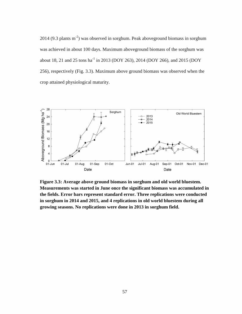
57

2014 (9.3 plants m-2

) was observed in sorghum. Peak aboveground biomass in sorghum

was achieved in about 100 days. Maximum aboveground biomass of the sorghum was

about 18, 21 and 25 tons ha-1

in 2013 (DOY 263), 2014 (DOY 266), and 2015 (DOY

256), respectively (Fig. 3.3). Maximum above ground biomass was observed when the

crop attained physiological maturity.

Figure 3.3: Average above ground biomass in sorghum and old world bluestem.

Measurements was started in June once the significant biomass was accumulated in

the fields. Error bars represent standard error. Three replications were conducted

in sorghum in 2014 and 2015, and 4 replications in old world bluestem during all

growing seasons. No replications were done in 2013 in sorghum field.

58

Figure 3.4: Evolution of litter over the course of growing season in old world

bluestem. Error bars represent standard error. Four replications were conducted

during each sampling.

Old World Bluestem achieved a maximum height of about 75-90 cm in 2013 and

2015 and reached up to 110 cm in 2014. Peak aboveground biomass (Green+Yellow

leaves) for different seasons was achieved at different times. Maximum biomass

observed in OWB was about 7.3, 10.2, and 10.3 Mg ha-1

in 2013 (DOY 303), 2014

(DOY 274), and 2015 (DOY 223), respectively (Fig. 3.3). Maximum green leaf biomass

achieved in OWB was 4.3, 7.0, 7.6 Mg ha-1

on same days of maximum aboveground

biomass. Rigorous growth in early season of 2015 contributed to greater green biomass

in 2015. Old world bluestem bloomed in 2014, whereas no significant bloom was

observed in 2013 or 2015. Old World bluestem goes through stem elongation during

59

bloom in September-October, which explains greater height and added biomass in crop

towards the end of the season. No leaf area measurements were made in OWB.

Additionally, we collected litter samples from the OWB field from same points where

green and yellow leaf samples were collected. During all years of study, the litter

amount followed a declining trend from a higher amount at beginning of the growing

season to low values during peak growing period and then ascending again towards the

end of the season (Fig. 3.4). Maximum amount of litter was noticed early in the season

on DOY 210 (DOY 9.6 Mg ha-1

) in 2013, on DOY 155 (5.4 Mg ha-1

) in 2014, on DOY

162 (6.5 Mg ha-1

) in 2015. Lowest amount of the litter was recorded at the peak growth

period on DOY 240 (4.4 Mg ha-1

), DOY 191 (2.5 Mg ha-1

) in 2014, and DOY 209 (3.9

Mg ha-1

) in 2015. Amount of litter at final sampling of the season in the field was 6.9

Mg ha-1

(DOY 303) in 2013, 6.3 Mg ha-1

in 2014 (DOY 317) and 6.8 Mg ha-1

in 2015

(DOY 272).

Non-Growing Season Carbon Fluxes

The inter-annual and seasonal carbon fluxes differed considerably between the

two agroecosystems (Fig. 3.5). Non-growing season for grassland was from January to

April in spring and November-December in fall, whereas for sorghum it stretched (mid-

October to May) from harvest to planting in next year. Presence of annual weeds

(horseweed: Erigeron canadensis) generated slight photosynthetic activity in both fields,

though Reco was the dominant carbon flux during non-growing season. The average non-

growing season NEE value in sorghum was 0.9 g C m-2

day-1

in 2014 and 1.7 g C m-2

day-1

in 2015. Average Reco in sorghum through non-growing season was 2.3 g C m-2

60

day-1

in 2013 and 2014, 2.9 g C m-2

day-1 in 2015. Net cumulative carbon release was 90

g C m-2

in 2013, 191.4 g C m-2

in 2014 and 368.8 g C m-2

in 2015 from sorghum field

through the non-growing season. It should be noted that the non-growing season for

sorghum in 2013 was only for November and December, whereas 2014 and 2015

include January to April and November-December. On the other hand, average non

growing season NEE in grassland was 0.1 g C m-2

day-1

, 0.3 g C m-2

day-1

and 0.5 g C m-

2 day

-1 in 2013, 2014 and 2015, respectively. Average Reco in OWB through the non-

growing season was 0.9 g C m-2

day-1

in 2013, 0.9 g C m-2

day-1

in 2014 and 1.2 g C m-2

day-1

in 2015. Cumulative NEE in grassland through dormant season was 11.7 g C m-2

,

50.5 g C m-2

, and 84.9 g C m-2


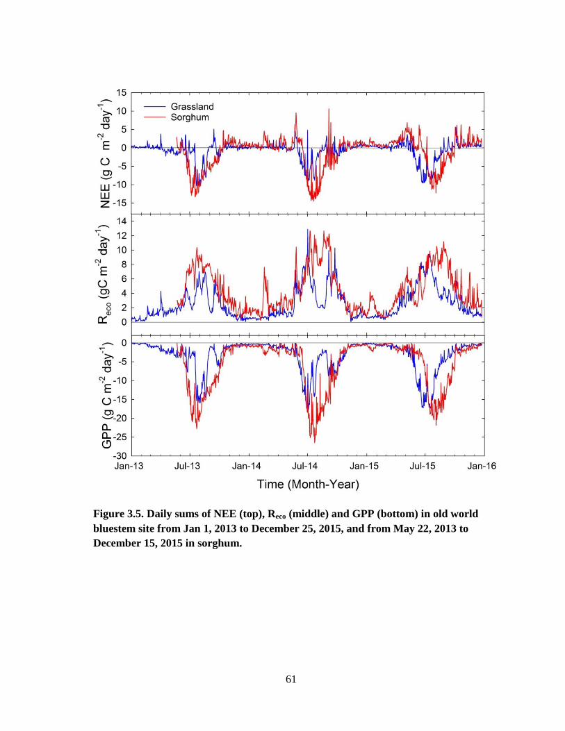
61

Figure 3.5. Daily sums of NEE (top), Reco (middle) and GPP (bottom) in old world

bluestem site from Jan 1, 2013 to December 25, 2015, and from May 22, 2013 to

December 15, 2015 in sorghum.

62

Growing Season Carbon Fluxes

Net Ecosystem Exchange: Figure 3.5 show daily carbon uptakes throughout the study

period in OWB field. Variation in seasonal and diurnal trends of carbon uptake was

more evident in grass than sorghum during three growing seasons of study (Fig. 3.6,

3.7). Net carbon uptake dynamics of grassland were sensitive to magnitude and timing of

precipitation. Average daily net carbon uptake during growing season was -1.7 g C m-2

day-1

in 2013, -1.7 g C m-2

day-1

in 2014 and -2.0 g C m-2

day-1

in 2015. Net carbon

uptake picked up in May 2013 using soil moisture stored during winter. However, net

carbon uptake was suppressed in June 2013 probably due to declining soil VWC during

first half of the month. In May 2014 and 2015, despite initiation of new growth, the grass

field acted as a source of carbon, mainly due to greater magnitude of respiration

following early season rainfall events and rising soil temperatures. The field transitioned

into a strong sink of carbon in June 2014 and 2015. Carbon uptake and Reco declined in

August 2014 and September 2015, due to extended dry period. Net carbon uptake

declined in October until the field became a net source in non-growing months. Overall

the net seasonal uptake of carbon in grassland was -314 g C m-2

in 2013, -301 g C m-2

in

2014, and -374 g C m-2

in 2015 (Table 3.2).

Despite shorter growing season, sorghum had consistently higher seasonal

carbon uptake than grass. As a result of irrigation, the seasonal pattern of carbon uptake

was similar among all growing seasons (Fig. 3.5). Average daily carbon uptake for

sorghum during growing season was -5.0 g C m-2

day-1

, -4.6 g C m-2

day-1

in 2014, and -

3.9 g C m-2

day-1

in 2013, 2014 and 2015, respectively. Sorghum field remained a weak

63

source of carbon during early days of growth, especially in 2014 and 2015 following

early season rainfalls, before transitioning into a strong sink. The NEE increased

gradually until its peak in July and August during active growing season across all the

years. The field remained a strong sink until September. Sorghum accumulated -710.3 g

C m-2

, -665.3 g C m-2

, and -471 g C m-2

in 2013, 2014, and 2015, respectively.

Diurnal patterns of carbon uptake during active growing season are presented in

figure 3.6 for OWB and figure 3.7 for sorghum. In OWB, net carbon uptake rates during

daytime were low in May during all growing seasons. The carbon uptake rates improved

following rainfall in June 2014 and 2015. Net carbon uptake rate further improved in

July for all growing seasons. In fact, maximum mean monthly net carbon uptake rates of

season were observed in July for year 2014 (-21.1 µmol m-2

s-1

) and 2015 (-28.3 µmol

m-2

s-1

) (Fig. 5). For 2013, the maximum mean monthly net carbon uptake rate (-20.0

µmol m-2

s-1

) was observed in August following precipitation events in late July and in

mid-August. On the contrary, the NEE declined in August 2014 and 2015 following dry

and warm conditions. Photosynthetic activity declined in September 2013 and 2015, as a

result the site transitioned into weak source of carbon (Fig. 3.5). The field remained a

weak sink of carbon in September and October 2014.

Figure 3.6 shows diurnal variation of carbon exchange during active growing

period in sorghum. Monthly diurnal patterns of sorghum were consistent during all

growing seasons. Maximum mean monthly carbon uptake rate was always greater in

sorghum in comparison to OWB. Rapid growth period was observed in June 2013, 2014

and 2015. Monthly average peak NEE values observed were -38.7 µmol m-2

s-1

in July

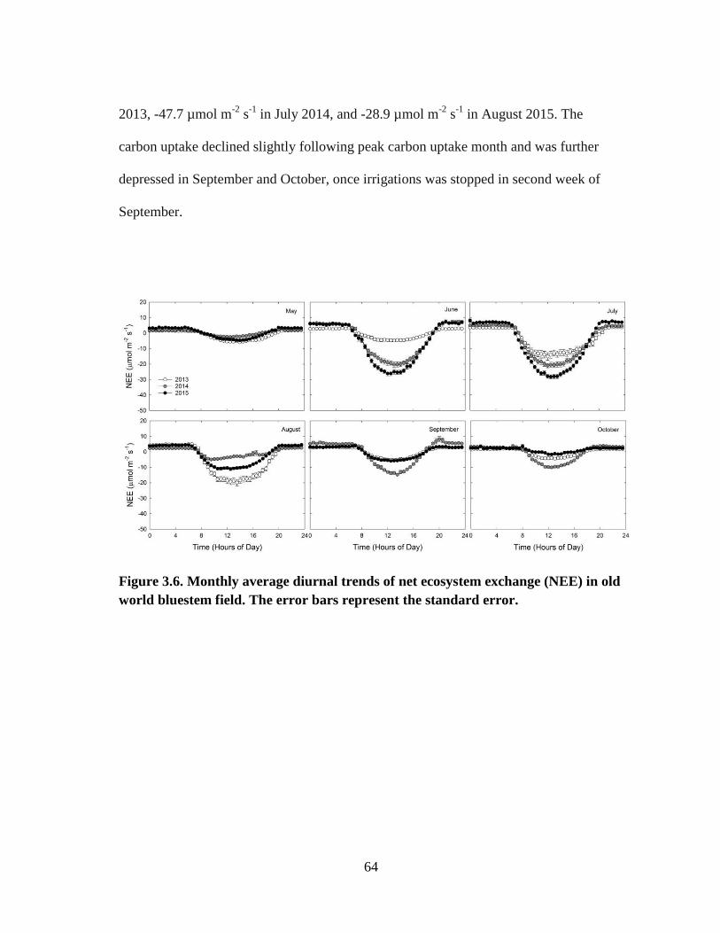
64

2013, -47.7 µmol m-2

s-1

in July 2014, and -28.9 µmol m-2

s-1

in August 2015. The

carbon uptake declined slightly following peak carbon uptake month and was further

depressed in September and October, once irrigations was stopped in second week of

September.

Figure 3.6. Monthly average diurnal trends of net ecosystem exchange (NEE) in old

world bluestem field. The error bars represent the standard error.

65

Figure 3.7: Monthly average diurnal trends of net ecosystem exchange (NEE) in

sorghum field. Month of May is not included as the crop was just emerging in that

month or was not planted (in 2015). Only days before harvest were included during

month of October i.e. 8 days in 2013 and 14 days in 2014. The error bars represent

the standard error.

Gross primary production: Daily sums of GPP are presented in Figure 3.5 for OWB and

sorghum. The photosynthetic activity of OWB started around first week of May and

continued until October through all years of study. Seasonal trends of daily GPP imitated

the trends of the NEE once the field transitioned into a net carbon sink. Trends of daily

GPP did not follow the NEE during early growing season (before fields transitioned to

net sink) as the latter was dominated by Reco in both grassland as well as sorghum. Old

World bluestem registered an average daily GPP of -4.8 g C m-2

day-1

in 2013, -6.2 g C

m-2

day-1

in 2014, and -6.7 g C m-2

day-1

in 2015. Since the photosynthetic activity in

66

grassland started earlier than sorghum, the GPP of grassland dominated that of sorghum

in May and June in 2014 and 2015 as the latter was not planted or plants were still small.

Maximum daily GPP recorded in OWB was -15.9 g C m-2

in 2013 (DOY 214), -17.7 g C

m-2

in 2014 (DOY 185), and -17.3 g C m-2

in 2015 (DOY 199). Gross primary

production declined as the season progressed in September and October. In our study,

OWB recorded -877.2 g C m-2

in 2013, -1140.1 g C m-2

in 2014, and -1233.5 g C m-2

in

2015.

Average daily GPP in sorghum was -11.4 g C m-2

day-1

in 2013, -12.2 g C m-2

day-1

in 2014, and -11.3 g C m-2

day-1

in 2015. Gross primary production of sorghum

dominated OWB during active growing months of July, August and September mainly

due to frequently replenished soil moisture through irrigations. Maximum daily GPP

recorded for sorghum was -22.8 g C m-2

(DOY 203) in 2013 and -26.4 g C m-2

(DOY

204) in 2014, and -21.9 g C m-2

(DOY 216) in 2015. Cumulative GPP of the season was

also greater for sorghum in all years of study than OWB. Gross primary production

varied among the growing season due to length of the growing season in sorghum.

Overall the seasonal GPP of sorghum was -1591.9 g C m-2

in 2013, -1780.9 g C m-2

in

2014, and -1353.7 g C m-2

in 2015.

Ecosystem Respiration: Magnitudes of Reco were greater during growing season than that

of non-growing season due to rising soil temperatures and added plant respiration (Fig.

3.5). Seasonal respiration in sorghum was similar in 2013 and 2015, while 2014 growing

season registered about 30% higher Reco. On the other hand, seasonal respiration in

OWB in 2014 and 2015 was about 30.0% and 33.0% higher than that recorded in 2013.

67

Average daily respiration in OWB was 3.1 g C m-2

day-1

in 2013, 4.5 g C m-2

day-1

in

2014, and 4.7 g C m-2

day-1

in 2015. Average daily respiration in sorghum was 6.3 g C

m-2

day-1

, 7.8 g C m-2

day-1

, and 7.4 g C m-2

day-1


Seasonal Reco followed the seasonal trend of GPP in both crops except in May 2014 and

2015. Highest Reco recorded in sorghum was 10.3 g C m-2

day-1

in 2013 (DOY 204), 12.8

g C m-2

day-1

(DOY 248) and 10.5 g C m-2

day-1

in 2015 (DOY 239). Highest daily Reco

recorded in OWB was 7.0 g C m-2

day-1

in 2013 (DOY 211), 12.8 g C m-2

day-1

in 2014

(DOY 164), and 9.4 g C m-2

day-1

in 2015 (DOY 192). Overall the cumulative seasonal

Reco in sorghum was 877.2 g C m-2

, 1108.7 g C m-2

, and 867.0 g C m-2

in 2013, 2014,

and 2015, respectively. For OWB, cumulative seasonal Reco was 562.8 g C m-2

, 823.2 g

C m-2

, and 860.3 g C m-2

in 2013, 2014, and 2015, respectively.

Annual Fluxes

Table 3.2 shows the summary of the annual fluxes calculated from sorghum and

OWB. Two complete (2014 and 2015) years of sorghum and three (2013, 2014 and

2015) complete years of OWB were available. While the GPP was high during growing

season in both fields, volunteer plants and summer/winter annual weeds in both fields

contributed a small portion of GPP during non-growing season. Non growing season

contributed 9-14% of the total GPP in OWB, and 14-18% in sorghum during complete

years. Non-growing season Reco contributed 30% and 44% of total annual respiration in

sorghum during 2013 and 2014, respectively. Similarly, non-growing season Reco

contributed 22%, 16% and 20% total respiration in OWB field during 2013, 2014, and

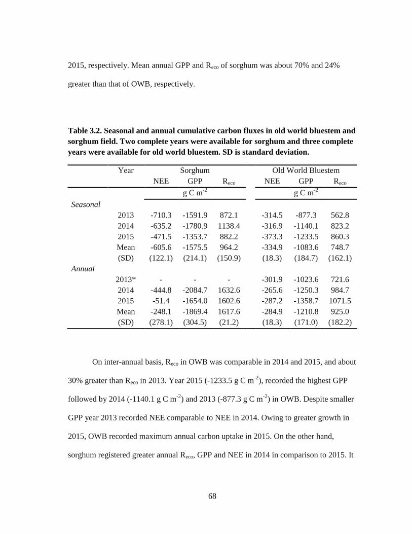
68

2015, respectively. Mean annual GPP and Reco of sorghum was about 70% and 24%

greater than that of OWB, respectively.

Table 3.2. Seasonal and annual cumulative carbon fluxes in old world bluestem and

sorghum field. Two complete years were available for sorghum and three complete

years were available for old world bluestem. SD is standard deviation.

Year Sorghum Old World Bluestem

NEE GPP Reco NEE GPP Reco

g C m-2

g C m-2

Seasonal

2013 -710.3 -1591.9 872.1 -314.5 -877.3 562.8

2014 -635.2 -1780.9 1138.4 -316.9 -1140.1 823.2

2015 -471.5 -1353.7 882.2 -373.3 -1233.5 860.3

Mean -605.6 -1575.5 964.2 -334.9 -1083.6 748.7

(SD) (122.1) (214.1) (150.9) (18.3) (184.7) (162.1)

Annual

2013* - - - -301.9 -1023.6 721.6

2014 -444.8 -2084.7 1632.6 -265.6 -1250.3 984.7

2015 -51.4 -1654.0 1602.6 -287.2 -1358.7 1071.5

Mean

(SD)

-248.1

(278.1)

-1869.4

(304.5)

1617.6

(21.2)

-284.9

(18.3)

-1210.8

(171.0)

925.0

(182.2)

On inter-annual basis, Reco in OWB was comparable in 2014 and 2015, and about

30% greater than Reco in 2013. Year 2015 (-1233.5 g C m-2

), recorded the highest GPP

followed by 2014 (-1140.1 g C m-2

) and 2013 (-877.3 g C m-2

) in OWB. Despite smaller

GPP year 2013 recorded NEE comparable to NEE in 2014. Owing to greater growth in

2015, OWB recorded maximum annual carbon uptake in 2015. On the other hand,

sorghum registered greater annual Reco, GPP and NEE in 2014 in comparison to 2015. It

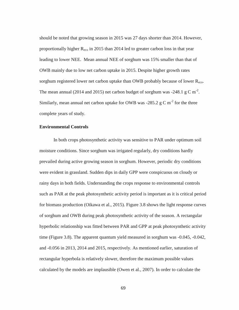
69

should be noted that growing season in 2015 was 27 days shorter than 2014. However,

proportionally higher Reco in 2015 than 2014 led to greater carbon loss in that year

leading to lower NEE. Mean annual NEE of sorghum was 15% smaller than that of

OWB mainly due to low net carbon uptake in 2015. Despite higher growth rates

sorghum registered lower net carbon uptake than OWB probably because of lower Reco.

The mean annual (2014 and 2015) net carbon budget of sorghum was -248.1 g C m-2

.

Similarly, mean annual net carbon uptake for OWB was -285.2 g C m-2

for the three

complete years of study.

Environmental Controls

In both crops photosynthetic activity was sensitive to PAR under optimum soil

moisture conditions. Since sorghum was irrigated regularly, dry conditions hardly

prevailed during active growing season in sorghum. However, periodic dry conditions

were evident in grassland. Sudden dips in daily GPP were conspicuous on cloudy or

rainy days in both fields. Understanding the crops response to environmental controls

such as PAR at the peak photosynthetic activity period is important as it is critical period

for biomass production (Oikawa et al., 2015). Figure 3.8 shows the light response curves

of sorghum and OWB during peak photosynthetic activity of the season. A rectangular

hyperbolic relationship was fitted between PAR and GPP at peak photosynthetic activity

time (Figure 3.8). The apparent quantum yield measured in sorghum was -0.045, -0.042,

and -0.056 in 2013, 2014 and 2015, respectively. As mentioned earlier, saturation of

rectangular hyperbola is relatively slower, therefore the maximum possible values

calculated by the models are implausible (Owen et al., 2007). In order to calculate the

70

GPPmax, we used the method proposed by Owen et al. (2007), where parameters

calculated by the model were used to obtain GPPmax at PAR level of 2000 µmol m-2

s-1

(notated as (GPPmax)2000). Maximum GPP (GPPmax)2000 calculated for sorghum was -53.0

µmol m-2

s-1

in 2013 and 2015, and -65.5 µmol m-2

s-1

in 2014. Slightly greater

(GPPmax)2000 in 2014 could be attributed to greater leaf area in that year. Similarly, light

use efficiency in OWB was -0.032 in 2013, -0.048 in 2014 and -0.040 µmol CO2 per unit

µmol of photons. Similarly, (GPPmax)2000 was similar at peak photosynthetic activity for

OWB. Maximum GPP recorded during this period in OWB was -43.3 µmol m-2

s-1

for

2013 and 2014, and -45.3 µmol m-2

s-1

in 2015.

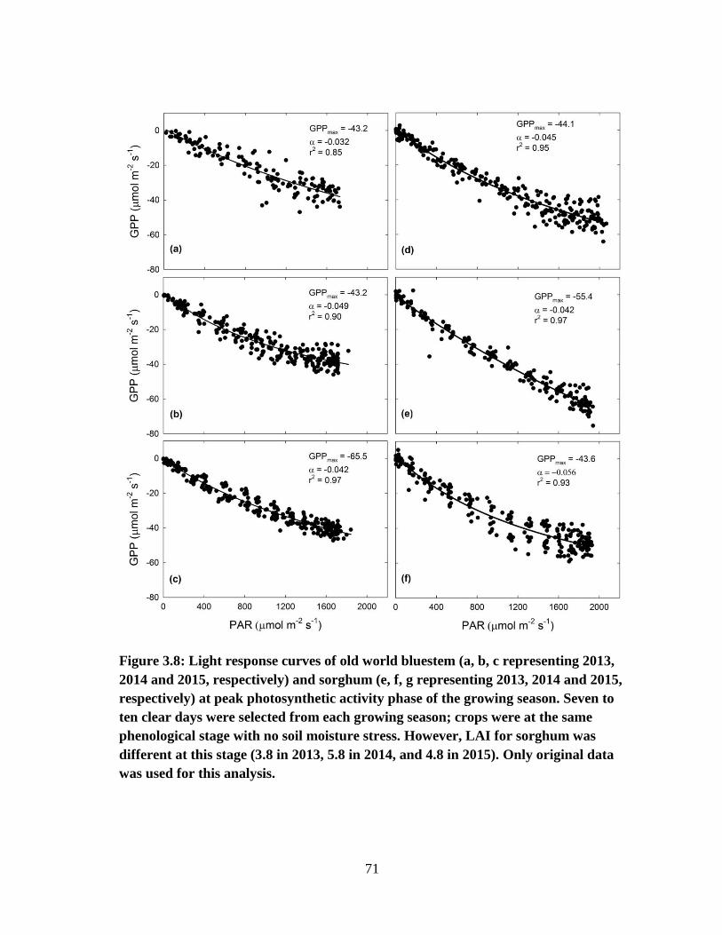
71

Figure 3.8: Light response curves of old world bluestem (a, b, c representing 2013,

2014 and 2015, respectively) and sorghum (e, f, g representing 2013, 2014 and 2015,

respectively) at peak photosynthetic activity phase of the growing season. Seven to

ten clear days were selected from each growing season; crops were at the same

phenological stage with no soil moisture stress. However, LAI for sorghum was

different at this stage (3.8 in 2013, 5.8 in 2014, and 4.8 in 2015). Only original data

was used for this analysis.

72

Figure 3.9: Relationship between half-hourly diurnal averages of Net Ecosystem

Exchange (NEE) and Gross Primary Production (GPP) with corresponding VPD

during warm and dry conditions (VWC 0.19 m3 m

-3) in old world bluestem field.

Error bars represent the standard error of the mean.

Conversely, carbon uptake potential of OWB declined during dry and warm

condition of dry months. Figure 3.9 shows the rise in carbon uptake in OWB with rising

VPD during early morning hours before declining in the afternoon with increasing VPD.

Net ecosystem exchange and GPP under warm and dry conditions (during growing

season) were aggregated over three growing seasons and plotted against aggregated

VPD. Average soil volumetric water content at 10 cm depth was 0.19 m3 m

-3 during

these days. Carbon uptake peaked in between up to 1.7 kPa and declined thereafter. No

considerable inhibition of carbon uptake was observed in sorghum during active growing

season of 2013 and 2014 as the field was irrigated regularly.

73

DISCUSSION

High growth rates and drought tolerance make sorghum and OWB fit for

production as major bioenergy crops in the Southern Great Plains. In this study,

consistently higher carbon uptake rates were found in irrigated sorghum, an annual crop

over rainfed OWB, a perennial bunch grass. Similarly, high carbon uptake rates in

sorghum have been reported by Oikawa et al. (2015) for irrigated sorghum in California.

Mean seasonal NEE values for sorghum in our study are almost double than those

reported by Wagle et al. (2015) for rainfed biomass sorghum. Wagle et al. (2015)

attributed the suppression of carbon uptake in sorghum during warm and dry conditions

due to rising VPD. No significant reduction in photosynthetic activity due to rising VPD

was noticed in sorghum in our study, due to continuous water supply through irrigation.

Mean seasonal carbon uptake for OWB in this study are higher than those reported by

Rajan et al. (2013) (164 g C m-2

) for the same site in normal precipitation year (2010).

During the time Rajan et al. (2013) conducted this study, the field was grazed three times

during growing season, which may explains lower NEE values in their findings.

However, mean seasonal NEE for OWB under dryland conditions are comparable to

seasonal NEE of rainfed sorghum reported by Wagle et al. (2015) (-261 ±48 g C m-2

and

-330 ± 45 g C m-2

) in Oklahoma during two years (dry year and wet year) of study. This

finding in our study is important as it suggests that under rainfed conditions in normal

rainfall years the OWB can match the carbon uptakes of rainfed sorghum. Seasonal NEE

values reported in our study are in good terms with those reported for specific biomass

crops by Wagle et al. (2015) for switchgrass in Oklahoma, Eichelmann et al. (2016) for

74

switchgrass in Canada, Zeri et al. (2011) for switchgrass and miscanthus, and

Chocubhair et al. (2015) for miscanthus in Ireland (Table 3.3). in different regions of

United States and other countries. Annual NEE for sorghum and OWB in our study

matched well with to those of -268 g C m-2

and -344 g C m-2

reported for native prairies

by Suyker and Verma (2004) in Oklahoma and Zeri et al. (2011) in Illinois, respectively

(Table 3.3).

Table 3.3. Seasonal net ecosystem exchange (NEE) as reported in different studies

for different bioenergy crops.

Authors Crop Region NEE (g C m-2)

Wagle et al. (2015) Switchgrass Oklahoma -406

Wagle et al. (2015) Swtichgrass Oklahoma -490

Eichelmann et al.

(2016) Switchgrass Canada -540

Zeri et al. (2011) Switchgrass Illinois -485

Zeri et al. (2011) Maize Illinois -307

Zeri et al. (2011) Miscanthus Illinois -405

Choncubhair et al.

(2016) Miscanthus Ireland -411

Suyker and Verma

(2004) Native prairie Oklahoma -268

Zeri et al. (2011) Native prairie Illinois -344

Carbon exchange properties of OWB were sensitive to the precipitation. Old

world bluestem showed a typical C4 grass response to relatively warm and wet summers

in 2014 and 2015, with increased photosynthetic activity and biomass production during

May-July (Teeri and Stowe, 1976). However, prevailing warm and dry conditions in

June 2013, August 2014 and September 2015 limited the carbon uptake potential of the

crop. This is in good agreement with findings of Rajan et al. (2013). The authors showed

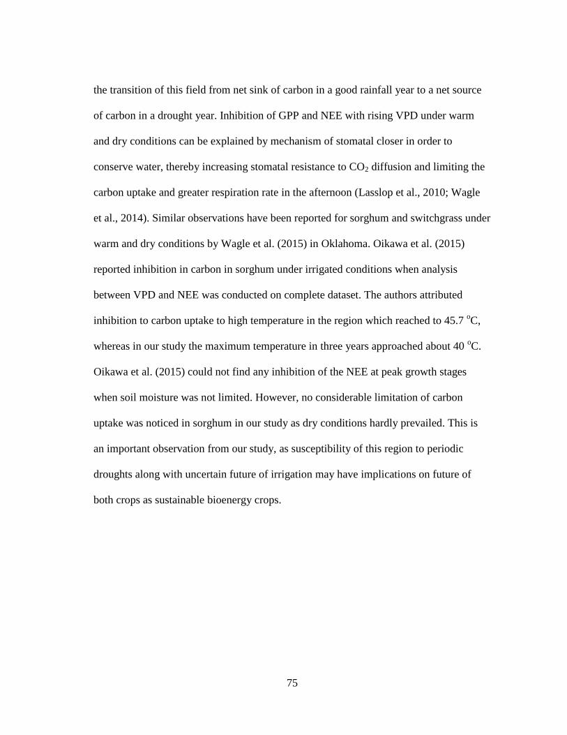
75

the transition of this field from net sink of carbon in a good rainfall year to a net source

of carbon in a drought year. Inhibition of GPP and NEE with rising VPD under warm

and dry conditions can be explained by mechanism of stomatal closer in order to

conserve water, thereby increasing stomatal resistance to CO2 diffusion and limiting the

carbon uptake and greater respiration rate in the afternoon (Lasslop et al., 2010; Wagle

et al., 2014). Similar observations have been reported for sorghum and switchgrass under

warm and dry conditions by Wagle et al. (2015) in Oklahoma. Oikawa et al. (2015)

reported inhibition in carbon in sorghum under irrigated conditions when analysis

between VPD and NEE was conducted on complete dataset. The authors attributed

inhibition to carbon uptake to high temperature in the region which reached to 45.7 oC,

whereas in our study the maximum temperature in three years approached about 40 oC.

Oikawa et al. (2015) could not find any inhibition of the NEE at peak growth stages

when soil moisture was not limited. However, no considerable limitation of carbon

uptake was noticed in sorghum in our study as dry conditions hardly prevailed. This is

an important observation from our study, as susceptibility of this region to periodic

droughts along with uncertain future of irrigation may have implications on future of

both crops as sustainable bioenergy crops.

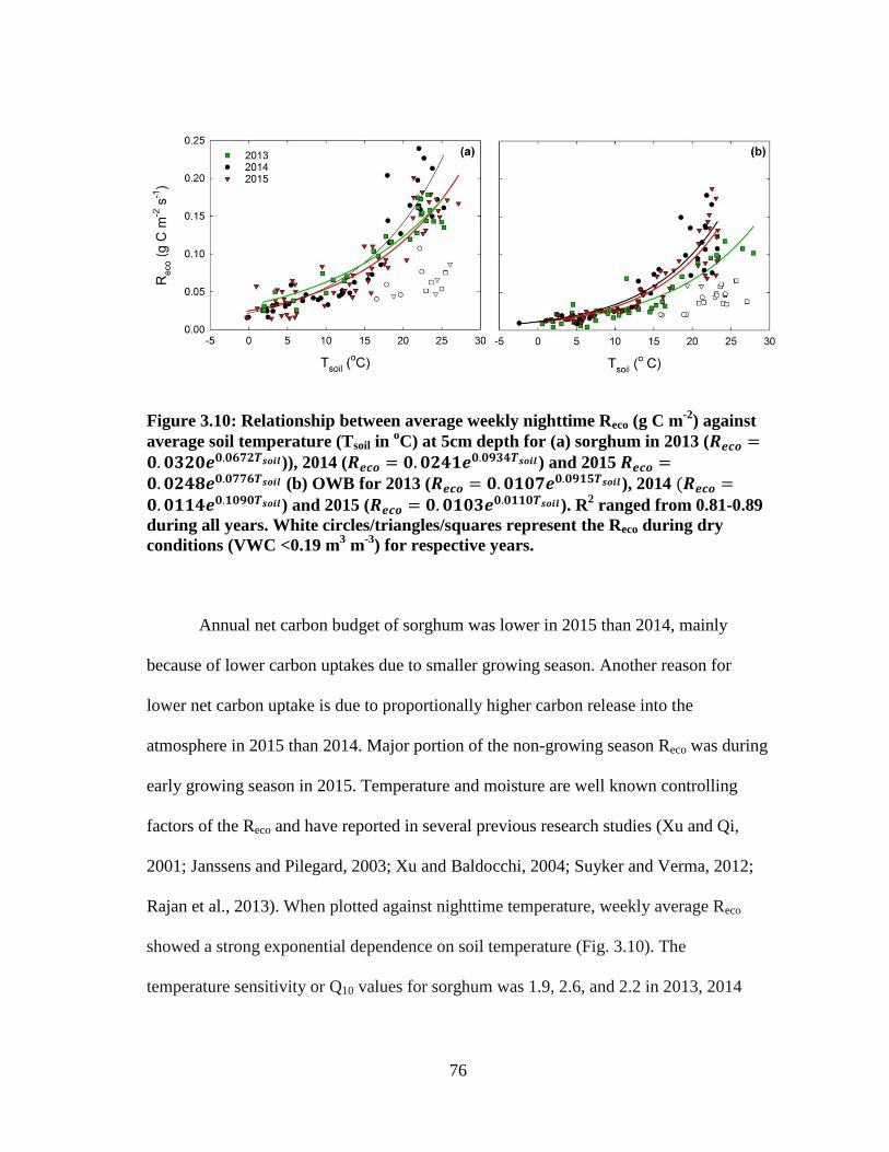
76

Figure 3.10: Relationship between average weekly nighttime Reco (g C m-2

) against

average soil temperature (Tsoil in oC) at 5cm depth for (a) sorghum in 2013 (𝑹𝒆𝒄𝒐 =

𝟎. 𝟎𝟑𝟐𝟎𝒆𝟎.𝟎𝟔𝟕𝟐𝑻𝒔𝒐𝒊𝒍)), 2014 (𝑹𝒆𝒄𝒐 = 𝟎. 𝟎𝟐𝟒𝟏𝒆𝟎.𝟎𝟗𝟑𝟒𝑻𝒔𝒐𝒊𝒍) and 2015 𝑹𝒆𝒄𝒐 =𝟎. 𝟎𝟐𝟒𝟖𝒆𝟎.𝟎𝟕𝟕𝟔𝑻𝒔𝒐𝒊𝒍 (b) OWB for 2013 (𝑹𝒆𝒄𝒐 = 𝟎. 𝟎𝟏𝟎𝟕𝒆𝟎.𝟎𝟗𝟏𝟓𝑻𝒔𝒐𝒊𝒍), 2014 (𝑹𝒆𝒄𝒐 =𝟎. 𝟎𝟏𝟏𝟒𝒆𝟎.𝟏𝟎𝟗𝟎𝑻𝒔𝒐𝒊𝒍) and 2015 (𝑹𝒆𝒄𝒐 = 𝟎. 𝟎𝟏𝟎𝟑𝒆𝟎.𝟎𝟏𝟏𝟎𝑻𝒔𝒐𝒊𝒍). R

2 ranged from 0.81-0.89

during all years. White circles/triangles/squares represent the Reco during dry

conditions (VWC <0.19 m3 m

-3) for respective years.

Annual net carbon budget of sorghum was lower in 2015 than 2014, mainly

because of lower carbon uptakes due to smaller growing season. Another reason for

lower net carbon uptake is due to proportionally higher carbon release into the

atmosphere in 2015 than 2014. Major portion of the non-growing season Reco was during

early growing season in 2015. Temperature and moisture are well known controlling

factors of the Reco and have reported in several previous research studies (Xu and Qi,

2001; Janssens and Pilegard, 2003; Xu and Baldocchi, 2004; Suyker and Verma, 2012;

Rajan et al., 2013). When plotted against nighttime temperature, weekly average Reco

showed a strong exponential dependence on soil temperature (Fig. 3.10). The

temperature sensitivity or Q10 values for sorghum was 1.9, 2.6, and 2.2 in 2013, 2014

77

and 2015, respectively. However, Reco declined when VWC was in the range of wilting

point (0.19 m3 m

-3) point. Majority of the early non-growing season in 2014 remained

relatively dry and thus respiration from the site was lower in 2014 than in 2015. Infact,

Suyker and Verma (2012) and Rajan et al. (2013) reported similar observations of

declining Reco under low soil moisture conditions. In a normal precipitation year, Rajan

et al. (2013) reported about 750 g C m-2

from the same field from DOY 152 to 365,

which was in good terms with Reco in this study (786 g C m-2

) for corresponding period

in 2014 in this study.

In comparison to sorghum, the Q10 value for the OWB field was 2.6, 3.0, 3.0 in

2013, 2014 and 2015, respectively. However, in our results, sorghum registered greater

Reco during non-growing season than OWB. Greater magnitude of carbon released from

sorghum could be attributed to longer non-growing season. In addition to abiotic factors

Reco is also driven by biotic factors and their interaction with abiotic factors (Flanagan,

2005). Several research studies have reported a positive correlation between Reco and

site productivity/photosynthesis (Craine et al., 1999; Janssens et al., 2001; Falgnan,

2005; Wagle et al., 2014). Greater Reco in sorghum despite lower Q10 values can be

mathematical. The mathematical reason for higher Reco from sorghum despite lower Q10

values than OWB is that the initial value of respiration is nearly double in sorghum than

OWB. This explains greater Reco in sorghum field during growing season. Our values of

Reco are greater than those reported by Suyker and Verma, (2001) for a tallgrass prairie

in Oklahoma. In both crops, Reco surged and peaked in the months when GPP peaked

78

and declined with the depressing carbon uptake and declining temperatures towards the

end of the season.

Biomass production is an important parameter for the bioenergy crops. In this

study, biomass production of sorghum was of the same order of magnitude reported by

Cotton et al., (2013) (13 to 30 tons ha-1

) in the Texas High plains, Oikawa et al. (2015)

(43.7 tons ha-1

) from three harvests of single crop within one year in California, Wagle et

al. (2015) (30 tons ha-1

) in Oklahoma for rainfed crop, Singh et al. (2012) (19.4 tons ha-

1) in Florida, Hallam et al. (2001) (16 ton ha

-1), and Propheter et al. (2010b) (26.2 tons

ha-1

). On the other hand, biomass production of OWB was of the same order as reported

by Dalrymple, (1991) (15 tons ha-1

) and Griffith et al. (2011) (for B. ischaemum), and

Buttrey and Bean, (2011). In comparison to specific biomass crops, biomass production

in OWB is lower than what has been reported for switchgrass and miscanthus in several

studies. For example, Wagle et al. (2015) reported 17 tons ha-1

and 13 tons ha-1

in two

years of their study for switchgrass under dryland conditions. Eichelmann et al. (2016)

reported an average of 12 tons ha-1

of biomass production in Canada, Sanderson et al.

(1996) reported up to 26 tons ha-1

biomass production in Alabama. Green vegetative

biomass of sorghum before flowering is used for processing and biofuel production

(Saballos, 2008). Wagle et al. (2014) and Cotton et al. (2013) reported the maximum

biomass of sorghum by mid-august at heading stage. In our study, the heading stage was

achieved in mid-August itself, indicating possibility of an early harvest from sorghum.

Also, our results show that sorghum is capable of considerable amount of carbon uptake

in August and September under optimum soil moisture conditions. Oikawa et al. (2015)

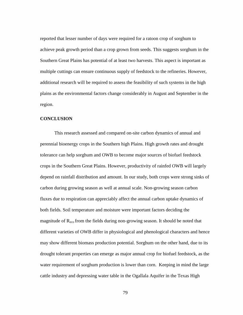
79

reported that lesser number of days were required for a ratoon crop of sorghum to

achieve peak growth period than a crop grown from seeds. This suggests sorghum in the

Southern Great Plains has potential of at least two harvests. This aspect is important as

multiple cuttings can ensure continuous supply of feedstock to the refineries. However,

additional research will be required to assess the feasibility of such systems in the high

plains as the environmental factors change considerably in August and September in the

region.

CONCLUSION

This research assessed and compared on-site carbon dynamics of annual and

perennial bioenergy crops in the Southern high Plains. High growth rates and drought

tolerance can help sorghum and OWB to become major sources of biofuel feedstock

crops in the Southern Great Plains. However, productivity of rainfed OWB will largely

depend on rainfall distribution and amount. In our study, both crops were strong sinks of

carbon during growing season as well at annual scale. Non-growing season carbon

fluxes due to respiration can appreciably affect the annual carbon uptake dynamics of

both fields. Soil temperature and moisture were important factors deciding the

magnitude of Reco from the fields during non-growing season. It should be noted that

different varieties of OWB differ in physiological and phenological characters and hence

may show different biomass production potential. Sorghum on the other hand, due to its

drought tolerant properties can emerge as major annual crop for biofuel feedstock, as the

water requirement of sorghum production is lower than corn. Keeping in mind the large

cattle industry and depressing water table in the Ogallala Aquifer in the Texas High

80

Plains, sorghum and OWB with their drought tolerant and forage properties could

emerge as major pasture/silage and biofuel feedstock crops in the region. Early

achievement of harvestable biomass gives opportunity of multiple harvests from both

crops. In addition to biomass production, conversion efficiency of the feedstock is also

an important factor for bioenergy crops. Since, the biomass produced from these fields

will be removed in actually biofuel production scenarios, these dynamics are subject to

change. Therefore, more research is required to assess the off-site and life-cycle analysis

of the bioenergy production systems. More research will also be required to assess the

complete environmental services of the OWB and sorghum as bioenergy crops.

81

CHAPTER IV

CARBON DYNAMICS OF BIOENERGY CROPS AND

CONVENTIONAL COTTON CROPPING SYSTEMS IN SOUHTERN

GREAT PLAINS: IMPLICATIONS OF LAND USE CHANGE ON

CARBON BALANCE

INTRODUCTION

Large scale land use change to bioenergy crops driven by expanding biofuel

industries is expected to have significant impact on the global C cycle (Fargione et al.,

2010; Searchinger, 2010; Anderson-Teixeira et al., 2013). Most of the land requirement

for bioenergy crops will be met from existing cropland, retired croplands/CRP and

marginal lands (Fargione et al. 2010; Qin et al., 2012). However, with rapid expansion of

croplands in recent times, land itself has become a limited resource (Qin et al., 2012).

Land use conversion to cropland itself is expanding at a rate of 3.4 million ha year-1

to

maintain food security of growing population (FAO, 2010). Expansion of area dedicated

to bioenergy crops will not only lead to competition for land between food crops and

bioenergy crops, but also for water and energy resources. In the United States itself, it is

estimated that 15% of the existing cropland will be converted to bioenergy cropping

systems to meet the target of 136 billion liters of biofuel by 2022 (Qin et al., 2012).

About 80 billion liters will be produced as second generation lignocellulosic biofuels. By

82

2014, about 15 billion gallons of biofuel were produced, of which only 25% was

contributed by second generation biofuels. Therefore, there is a scope for expansion of

second generation bioenergy crops in the United States. Nearly half of this amount will

be produced in the South Eastern United States. It is estimated that this production will

induce a land use change on about 11% existing croplands in the South-Eastern United

States, including the Southern Great Plains (USDA, 2010).

The Southern Great Plains is a semi-arid region with long-term (1911-2005)

mean annual rainfall of about 465 mm (Allen et al., 2008). Prior to farming the region

was dominated by shortgrass prairie. Discovery of the vast underground Ogallala

Aquifer transformed the region to one of the major agricultural regions in the United

States (Gould, 1975; Allen et al., 2008; Rajan et al., 2014). The Southern Great Plains is

the largest producer of cotton (Gossypium hirsutum L.) in the U.S. (Attia et al., 2015).

Grain sorghum (Sorghum bicolor L.), corn (Zea mays L.), and winter wheat (Triticum

aestivum L.) are other major crops in the region. However, excessive extraction of water

for agricultural use has depressed the water table of the Ogallala Aquifer by over 30 m in

most parts of the Southern Great Plains (Rajan et al., 2015). Continuous cotton under

conventional tillage has been a dominant row cropping system in the Southern Great

Plains for several decades (Acosta-Martinez et al., 2010). Low returns of organic matter

from cotton cropping systems has depleted the organic matter reserves of the soils in

Southern Great Plains and declined the soil quality (Moore et al., 2000; Wright et al.,

2008; Allen et al., 2008; Acosta-Martinez, 2010). Soil organic matter accumulation is

important for soil health as it improves soil structure, prevents soil erosion, improves

83

infiltration and water holding capacity, and sequesters atmospheric carbon dioxide (Lal,

2004). Therefore, more sustainable production systems are required which can promise

long-term sustainability in terms of carbon sequestration. Sustainability of a system

could be assessed from its carbon and energy balance properties (Zenone et al., 2013).

Moreover, carbon and energy balance properties of different ecosystems interact

differently to the regional environment. Therefore, a large scale land use change from

cotton to bioenergy crops will have significant effects on carbon balance of the region.

Bioenergy crops are regarded as carbon neutral crops as the carbon fixed in

biomass is lost to atmosphere, however life cycle analysis of carbon budget has been

reported the bioenergy crops to be net source or sink of carbon to the atmosphere

depending on the vegetation and management practices and processing technologies

(Tilman et al., 2006; Cherubini et al., 2009; Johnson, 2009;). Although each step in the

life cycle of the biofuels is vital, but it is very important to study the carbon balance of

the bioenergy crops in their production systems itself. Several recent studies have

reported net carbon sinking capacity of annual and perennial bioenergy crops at

ecosystem scale in different parts of North America (Zeri et al., 2011; Wagle et al.,

2015; Oikawa et al., 2015; Eichelmann et al., 2015). Bioenergy crops have been

reported to improve soil organic matter status depending upon management practices

and amount of residues left on the surface after harvest (Halvin et al., 1990; Polley,

1992; Tolbert et al., 2002; Cotton et al., 2013; Qin et al., 2012; Meki et al., 2013).

Annual bioenergy crops have been shown to have greater yields than perennial crops

during early of years of establishment (Propheter et al., 2010). Perennial bioenergy crops

84

especially native grasses have added benefits associated with lower resource

requirement, lower agronomic management, and ecosystem services linked to wildlife.

While, net carbon exchange fluxes of corn, switchgrass and other bioenergy crops have

been widely reported, the net carbon exchanges of some less popular potential bioenergy

crops such as sorghum and old world bluestem (OWB) have been scarcely reported.

In this study, carbon budget dynamics of a potential annual and perennial

bioenergy crop was investigated and compared with conventional cotton cropping

system in the Southern Great Plains using eddy covariance systems. Potential bioenergy

crops investigated in this study are high biomass forage sorghum and old world

bluestem. While, sorghum has established cropping systems for grain and silage

production in the Southern Great Plains, OWB is popular as pasture and is one of the

most planted crops on CRP lands in this region. Studies regarding direct measurements

of carbon exchange between canopy and atmosphere are rare in the Southern Great

Plains. Also, in our knowledge this is the first such study investigating carbon exchange

dynamics of irrigated and dryland cotton in this region. The main objective of this study

was to describe seasonal and annual net carbon exchange dynamics of an established

OWB field along with annual bioenergy and conventional row crops in the Southern

Great Plains.

85


Study Site

This study was conducted in four different farmers’ fields fitted with central



miles northeast of Plainview, TX (34°12’34.70’’ N and 101°37’50.85’’ W, 1100 m

elevation). The cultivar planted was Surpass XL bmr (brown midrib). Sorghum was

planted on one half of the field and the remaining half was planted with cotton

(Gossypium hirsutum L.). The farmer practiced crop rotation between these crops on

both halves of the field. Management practices prior to planting sorghum included

mowing down of cotton stubbles after harvesting previous cotton crop followed by

tillage in spring and before planting the crop. Total area planted with sorghum each time

was about 25 ha. The crop was planted on 20 May in 2013 and 2014 at a seeding rate of

4.9 kg ha-1

. Heavy rains in late May during 2015 delayed planting, thus the crop was

planted on June 4 in 2015 at the same seeding rate. The row spacing in 2013 and 2015

was 40 inches and 20 inches in 2014. Urea was broadcasted in the field in spring before

planting at a rate of 150 kg N ha-1

. In addition, 30 kg P2O5 ha-1

was also applied prior to

planting. The field was irrigated with low elevation application center-pivot irrigation

system during the crop growth period. For first 40 days the field was supplied with 0.75

inch and for rest of the season it was supplied with 1.5 inch water during each irrigation

86

event. The field was supplied with about 400 mm of water through irrigation in 2013,

about 400 mm in 2014 and about 270 mm in 2015. Also, the field was cultivated in

between the plant rows to kill weeds twice in June every year when the crop was still

small. The field was harvested for seed on 8 October in 2013, on 14 October in 2014,

and on October 1 in 2015. The growing season was 140, 147, and 119 days long for

2013, 2014, and 2015, respectively. Equipment availability and late season rainfall

affected the timings of harvest. The field remained fallow post-harvest in winter and

spring. The farmer let the remaining stalk grazed by cattle in March 2014 and in January

2015. A fence was put around the tower during the presence of cattle in the field. Since

the crop was grown in rotation with cotton, the new crop was planted on other half of the

field where cotton was produced in previous season. The major soil mapping unit at the

study site is Pullman clay loam (a fine, mixed, superactive, thermic Torrertic Paleustoll)

with 0 to 1% slope.


o25’48” W)



Kg seed ha-1



originally from a selection made in India (Rogers et al., 2012). It is a bunchgrass with

an upright growth habit and has better drought tolerance and water use efficiency than

conventional cropping systems in the Southern Great Plains (Allen et al., 2005). Total

area of the site is about 42 ha. Until 2011 the field was used for grazing by the cattle or

87

for seed production. This field was equipped with a center pivot irrigation system;

however, no irrigation, nutrient supply or grazing operation was conducted during the

study period (2013-2015). The growing season for the crop roughly ranged from May to

October. Peak growing season occurred from June to July depending upon precipitation.

The grass remained in vegetative state for most part of the growing season and bloomed

in late September/early October. The field was harvested for seed on November 14,

2014. No seed harvesting was done in 2013 and 2015. The field was never harvested for

hay. Major soil mapping unit in the field was Pullman clay loam with 0-1% slope.

The irrigated cotton field was located adjacent to sorghum field about 4 km

north-east of Plainview in Hale county. In 2013, Cotton was planted in first week of

June. In 2014, first planting of cotton on May 30 was failed and cotton was replanted on

June 9. In 2015, cotton was planted on June 2. Cotton variety planted was Fibermax

2322 at a seeding rate of 40,000 seeds per acre during all years of study. Cotton was

applied with 100 Kg ha-1

of nitrogen (N) and 35 Kg ha-1

of P2O5 before planting. Total

area of cotton planted was about 60 acres. Row spacing was 1 m. The field was irrigated

using a center-pivot irrigation system. Cotton was sprayed with defoliator (Ginstar)

during last week of October. Cotton was harvested on November 7-8 each year of study.

Cotton stubbles were mowed down to about 4 inch height after harvest. Cotton field was

planted in rotation with sorghum.

Dryland Cotton field was located about 3 km north of Lockney, TX. Dryland was

planted on June 1 in 2013, 2014 and 2015. The crop failed in 2013 and farmer ploughed

the field to claim crop insurance. In 2015, the farmer decided to plant grain sorghum in

88

the field. As a result, the tower was moved to a nearby dryland cotton field. The size of

both fields was about 100 acres. The crop was planted with variety Fibermax 2011

during all years of study. Row spacing was 1 m. Crop was planted at seed rate of 26000

seeds per acre. No fertilizer was applied to the field in 2014 and 2015. The field was

sprayed with defoliator (Ginstar) on October 21 in 2014. The field was harvested on

November 6. In 2015, late season rains damaged the cotton bolls and farmer did not

harvest the field.




in grassland was established in 2010, the tower in sorghum, dryland cotton and irrigated

cotton was established at planting in 2013. Data collection from irrigated cotton started

from July 2nd

2013. Both towers were set up in the middle of the all fields, with fetch of

about 150 m from all directions. An integrated sonic anemometer (Model CSAT-3A,

Campbell Scientific) and infra-red gas analyzer (IRGA, Model EC-150, Campbell

Scientific) called the IRGASON was used to measure wind velocity and CO2, H2O vapor

concentration, and H in the ambient atmosphere. In grassland the CO2, H2O vapor

concentration was measured using Li-7500 IRGA (LI-COR Biosciences) and wind

velocity and sensible heat flux were measured using sonic anemometer sonic

anemometer (Model CSAT-3A, Campbell Scientific). The system was installed in

middle of each field with fetch of 150 m or more from all directions. These instruments

were set up facing south-southwest (in the prevailing wind direction) at a height of about

89

2.1 m from ground surface. The height of the instrument was adjusted in sorghum field

during growing season with increasing crop height to a final height of about 2.6 m from

ground. Other environmental variables measured at both sites included air temperature

(Tair) and relative humidity (RH) (HMP50, Campbell Scientific), net radiation (Kipp &

Zonen NR-Lite net radiometer), photosynthetically active radiation (PAR) (LI-200SL

quantum sensor, LI-COR), solar irradiance (LI-190SB pyranometer, LI-COR),




Campbell Scientific). Self-calibrating soil heat flux plates (HFPSC-01, Hukseflux,

Campbell Scientific, Logan, UT) were used to measure soil heat flux at 8 cm depth from

soil surface. Soil heat storage which is the amount of heat stored in 8 cm soil depth over

soil heat flux plates was calculated using the following equation:


𝑡 [4.1]






soil (𝐶𝑑 = 840 𝐽 𝑘𝑔−1𝐾−1):


90





manufacturers’ guidelines to avoid accumulation of dust. Data from the CSAT3A sonic

anemometer and IRGA system were measured at 10-Hz sampling rate using a CR3000

datalogger (Campbell Scientific). All other environmental variables were measured at 5

seconds interval. The datalogger was programmed to calculate and save 30-min average

values of all environmental variables. The raw 10-Hz wind velocity and EC150/LI-7500

data were saved for further post-processing and analysis of CO2 and energy fluxes.












91


were gap filled. In addition, the physically implausible values in the data were also

filtered and gap filled. Further, the flux is usually underestimated during low turbulence

conditions and therefore, data during low turbulence conditions (when the friction

velocity (u*) was <0.10 m s–1



, 0.33 ms-1

, and 0.31 ms-1



, 0.36 m s-1

, 0.31 m s-1

. After screening the data for out of the

range and above mentioned filtering criteria, the amount of data which was either

missing or did not clear the quality check criteria was about 21%, 8%, and 40% in 2013,

2014, and 2015, respectively. During growing season, 21%, 13 and 3% data was gap-

filled in 2013, 2014, and 2015 respectively. The amount of data to be gap filled in









, ±2.5 oC, and ±0.5 kPa,



92









)*( TsoilB

eco AeR [4.3]





NEERGPP eco [4.4]





Quality of eddy covariance data is very important and can be determined the



93











Rn – G = LE + H [4.5]

The sign convention used for Rn and G are positive when the flux is downwards and

negative when the flux is upward. The sign convention used for LE, H and C fluxes was

a positive flux represents flux from the ecosystem to the atmosphere, while a negative

flux represents flux from the atmosphere to the ecosystem.

Light Response Curves

Light response curves were obtained by obtaining relationship between daytime

NEE with photosynthetic photon flux density (PPFD). Daytime was differentiated from

night when photosynthetic photon flux density (PPFD) was >1 μmol photon m–2

s–1

. To

understand the photosynthetic response of the sorghum crop at different growth stages, a

rectangular hyperbola model was used (Flanagan et al., 2002; Hussain et al., 2011).

94

R

GPPPAR

PARGPPGPP

max

max

1

[4.6]

where NEEmax is the maximum NEE rate (μmol CO2 m–2

s–1

), PPFD is the

photosynthetic photon flux density (μmol photon m–2

s–1

), α is the initial slope of the

light response curve (μmol CO2 m–2

s–1

/μmol photon m–2

s–1

), NEEmax/α is the PPFD

associated with half of the maximum NEE rate, and R is the intercept term, which is the

average daytime Reco (μmol CO2 m–2

s–1

). In the present study, we evaluated Eq. [4.6] at

PPFD of 2000 μmol photon m–2

s–1

, and the term (NEEmax + R)2000 represents the

average maximum uptake rate.

Biometric Data

Plant dry biomass weight was measured during the growing season. Sorghum,

dryland cotton and irrigated cotton plant samples were taken randomly (3 replications)

from respective fields to measure leaf area index (LAI), dry leaf mass and dry shoot

(including bolls) mass. For grasslands, four random plant samples (for green, yellow

leaves and litter) were taken from quarter of a meter area. No LAI measurements were

done on the grass samples. Plants were stored in an ice chest in the field and leaf area of

sorghum was measured (after separating leaves from shoots) using a leaf area meter

(Model LI-3100, Licor Biosciences, Lincoln, NE) immediately after they were brought

to the laboratory. For grass samples, green and yellow leaves were separated after

samples were brought to the lab. After measuring leaf area, leaves and shoots were

stored in paper bags and dried at 65oC for one week. Dry mass of shoot and leaves was

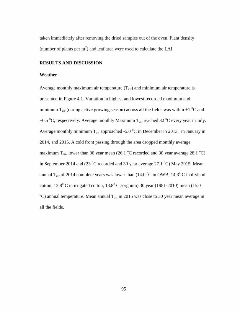
95

taken immediately after removing the dried samples out of the oven. Plant density

(number of plants per m2) and leaf area were used to calculate the LAI.


Weather

Average monthly maximum air temperature (Tair) and minimum air temperature is

presented in Figure 4.1. Variation in highest and lowest recorded maximum and

minimum Tair (during active growing season) across all the fields was within ±1 oC and

±0.5 oC, respectively. Average monthly Maximum Tair reached 32

oC every year in July.

Average monthly minimum Tair approached -5.0 oC in December in 2013, in January in

2014, and 2015. A cold front passing through the area dropped monthly average

maximum Tair, lower than 30 year mean (26.1 oC recorded and 30 year average 28.1

oC)

in September 2014 and (23 oC recorded and 30 year average 27.1

oC) May 2015. Mean

annual Tair of 2014 complete years was lower than (14.0 oC in OWB, 14.3

o C in dryland

cotton, 13.8o C in irrigated cotton, 13.8

o C sorghum) 30 year (1981-2010) mean (15.0

oC) annual temperature. Mean annual Tair in 2015 was close to 30 year mean average in

all the fields.

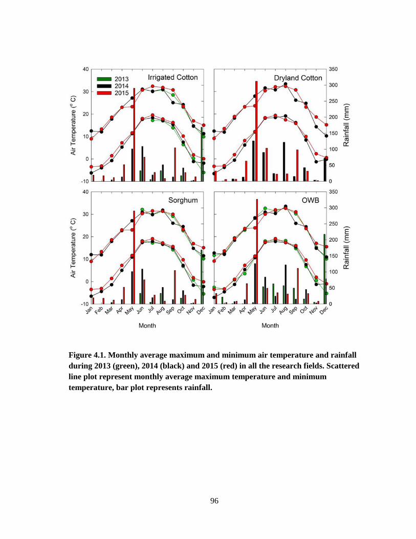
96

Figure 4.1. Monthly average maximum and minimum air temperature and rainfall

during 2013 (green), 2014 (black) and 2015 (red) in all the research fields. Scattered

line plot represent monthly average maximum temperature and minimum

temperature, bar plot represents rainfall.

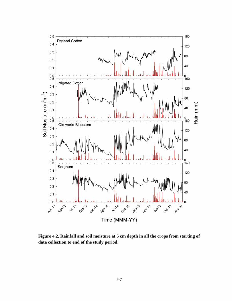
97

Figure 4.2. Rainfall and soil moisture at 5 cm depth in all the crops from starting of

data collection to end of the study period.

98

Figure 4.2 presents soil moisture and rainfall during the entire period of study.

Rainfall received during the study period was greater than long term (2002-2012)

average of 470 mm measured from mesonet station in Plainview. Total annual rainfall

received in dryland cotton field and OWB was 504, 520 and 812 mm in 2013, 2014 and

2015, respectively (Fig. 4.2). Annual rainfall received in sorghum and irrigated cotton

field was about 450 mm in 2013, 520 mm in 2014 and 750 mm in 2015 (Fig. 4.2).

Second quarter of 2013 (April-May), first quarter (January-April) of 2014 and third

quarter (mid-July to September) of 2015 remained relatively dry. Exceptionally high

rainfall was recorded in the area during May (326 mm) of 2015. In fact, 65% of the total

annual rainfall in 2015 was received by July first week.

Biometric Measurements

Figures 4.3 and 4.4 show phenology in sorghum, OWB, irrigated cotton and

dryland cotton. Growing season of OWB was longest among all the crops. Growth of

Old world bluestem started in April last week or May first week and most of the grass

was yellow by the end of October. Sorghum’s growing season was shortest among all

the crops during all growing seasons. Sorghum’s growing season was 140 days in 2013,

147 days in 2014 and 119 days in long 2015. Sorghum plants emerged 4-5 days after

planting of June in 2013, 2014 and 2015. Both irrigated and dryland cotton had second

largest growing season, stretching from June to mid-October when crops were sprayed

with defoliator. Each individual row crop exhibited consistent growing patterns during

all the growing season. Phenological stages of each crop synchronized temporally across

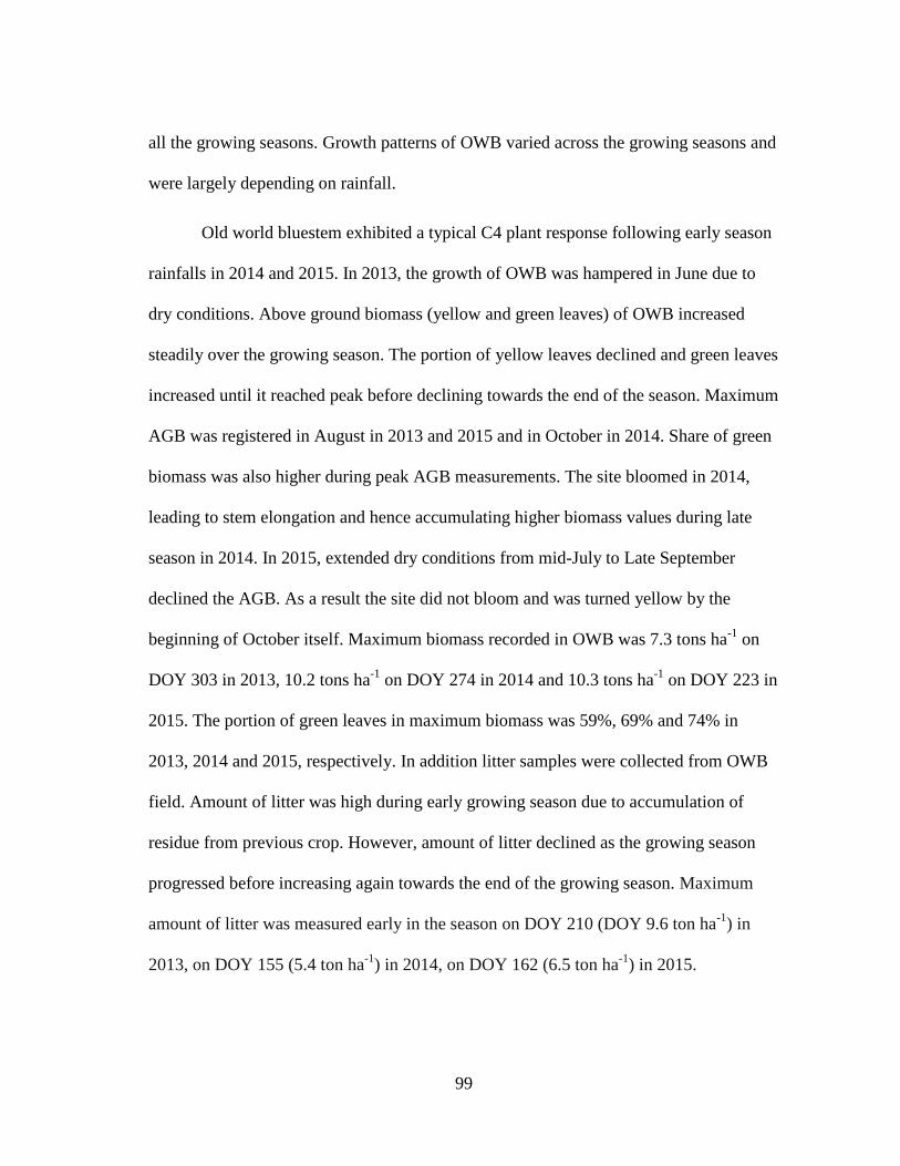
99

all the growing seasons. Growth patterns of OWB varied across the growing seasons and

were largely depending on rainfall.

Old world bluestem exhibited a typical C4 plant response following early season

rainfalls in 2014 and 2015. In 2013, the growth of OWB was hampered in June due to

dry conditions. Above ground biomass (yellow and green leaves) of OWB increased

steadily over the growing season. The portion of yellow leaves declined and green leaves

increased until it reached peak before declining towards the end of the season. Maximum

AGB was registered in August in 2013 and 2015 and in October in 2014. Share of green

biomass was also higher during peak AGB measurements. The site bloomed in 2014,

leading to stem elongation and hence accumulating higher biomass values during late

season in 2014. In 2015, extended dry conditions from mid-July to Late September

declined the AGB. As a result the site did not bloom and was turned yellow by the

beginning of October itself. Maximum biomass recorded in OWB was 7.3 tons ha-1

on

DOY 303 in 2013, 10.2 tons ha-1

on DOY 274 in 2014 and 10.3 tons ha-1

on DOY 223 in

2015. The portion of green leaves in maximum biomass was 59%, 69% and 74% in

2013, 2014 and 2015, respectively. In addition litter samples were collected from OWB

field. Amount of litter was high during early growing season due to accumulation of

residue from previous crop. However, amount of litter declined as the growing season

progressed before increasing again towards the end of the growing season. Maximum

amount of litter was measured early in the season on DOY 210 (DOY 9.6 ton ha-1

) in

2013, on DOY 155 (5.4 ton ha-1

) in 2014, on DOY 162 (6.5 ton ha-1

) in 2015.

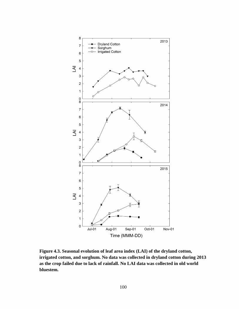
100

Figure 4.3. Seasonal evolution of leaf area index (LAI) of the dryland cotton,

irrigated cotton, and sorghum. No data was collected in dryland cotton during 2013

as the crop failed due to lack of rainfall. No LAI data was collected in old world

bluestem.

101

Figure 4.4. Evolution of above ground biomass (AGB) over the growing season in

dryland cotton, sorghum, old world bluestem (OWB). Dryland cotton failed in

2013, therefore no data was presented for this crops in 2013.

102

Lowest amount of the litter was recorded at the peak growth period on DOY 240 (4.4 ton

ha-1

), DOY 191 (2.5 ton ha-1

) in 2014, and DOY 209 (3.9 ton ha-1

) in 2015. Amount of

litter at final sampling of the season in the field was 6.9 ton ha-1

(DOY 303) in 2013, 6.3

ton ha-1

in 2014 (DOY 317) and 6.8 ton ha-1

in 2015 (DOY 272).

Evolution of AGB was consistent in row crops during all growing seasons,

though differences in biomass accumulation were evident among the crops. However,

the drastic difference between peak AGB were noticed in sorghum across different

growing season. As explained in Chapter II, narrower row spacing in 2014 lead to

significantly higher AGB during that year in comparison to 2013 and 2015. Peak AGB

recorded in sorghum was 18, 21, and 25 tons ha-1

in 2013, 2014 and 2015 respectively.

Maximum biomass in sorghum was recorded in mid-September at physiological

maturity. For cellulosic biofuel production, sorghum biomass is harvested at or before

soft dough stage (Saballos, 2008). In our study, sorghum registered peak biomass of 14,

17, and 12 tons ha-1

of AGB at soft dough stage by mid-August in 2013, 2014, and 2015,

respectively. Similarly, AGB in both dryland and irrigated cotton ascended steadily

during both growing seasons. Peak AGB in irrigated cotton was 14.5 tons ha-1

on DOY

270 in 2013, 12.5 tons ha-1

on DOY 282 in 2014 and 13.3 tons ha-1

on DOY 256 in 2015.

Dryland cotton registered similar AGB of 6.1 tons ha-1

in 2014 and 2015.

In addition to AGB, LAI measurements were taken in row crops. Apparently,

sorghum registered consistently higher LAI than both cotton cropping systems across all

the growing seasons. Maximum LAI registered in sorghum was 4.1 in 2013, 7.1 in 2014

and 5.1 in 2015. As explained in chapter II narrower spacing and relatively high number

103

s of tillers lead to significantly higher LAI In 2014 than 2013 and 2015. Peak LAI in

sorghum was noticed in August around soft dough stage in 2013 and before soft dough

stage in 2014 and 2015. Irrigated cotton registered 2.8 in 2013, 3.1 in 2014 and 2.8 in

2015. Similarly, dryland cotton registered maximum LAI of 1.9 in 2014 and 1.4 in 2015.

Irrigated cotton registered maximum LAI in September during 2014 and 2015 growing

season. Irrigated cotton registered maximum LAI in August in 2013.

Energy Balance

Figure 4.5 represent energy balance of the all the crops during active growing

season. An aggregate energy balance closure of each individual crop was measured

during active growing season (July-August) across all three seasons. Slope of energy

balance in all crops ranged from 0.84 to 0.88, which was within acceptable limits.

Energy balance for individual growing season was not very different from aggregated

energy balance closure. This confirmed the good quality of data for further analysis.

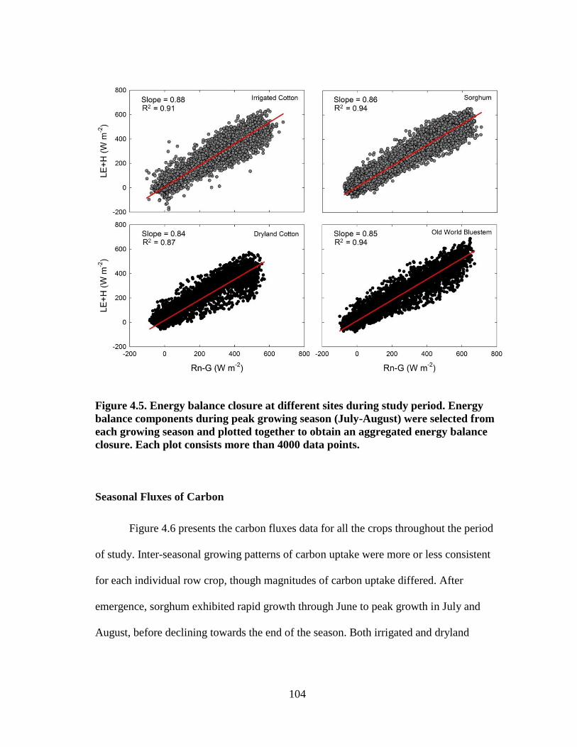
104

Figure 4.5. Energy balance closure at different sites during study period. Energy

balance components during peak growing season (July-August) were selected from

each growing season and plotted together to obtain an aggregated energy balance

closure. Each plot consists more than 4000 data points.

Seasonal Fluxes of Carbon

Figure 4.6 presents the carbon fluxes data for all the crops throughout the period

of study. Inter-seasonal growing patterns of carbon uptake were more or less consistent

for each individual row crop, though magnitudes of carbon uptake differed. After

emergence, sorghum exhibited rapid growth through June to peak growth in July and

August, before declining towards the end of the season. Both irrigated and dryland

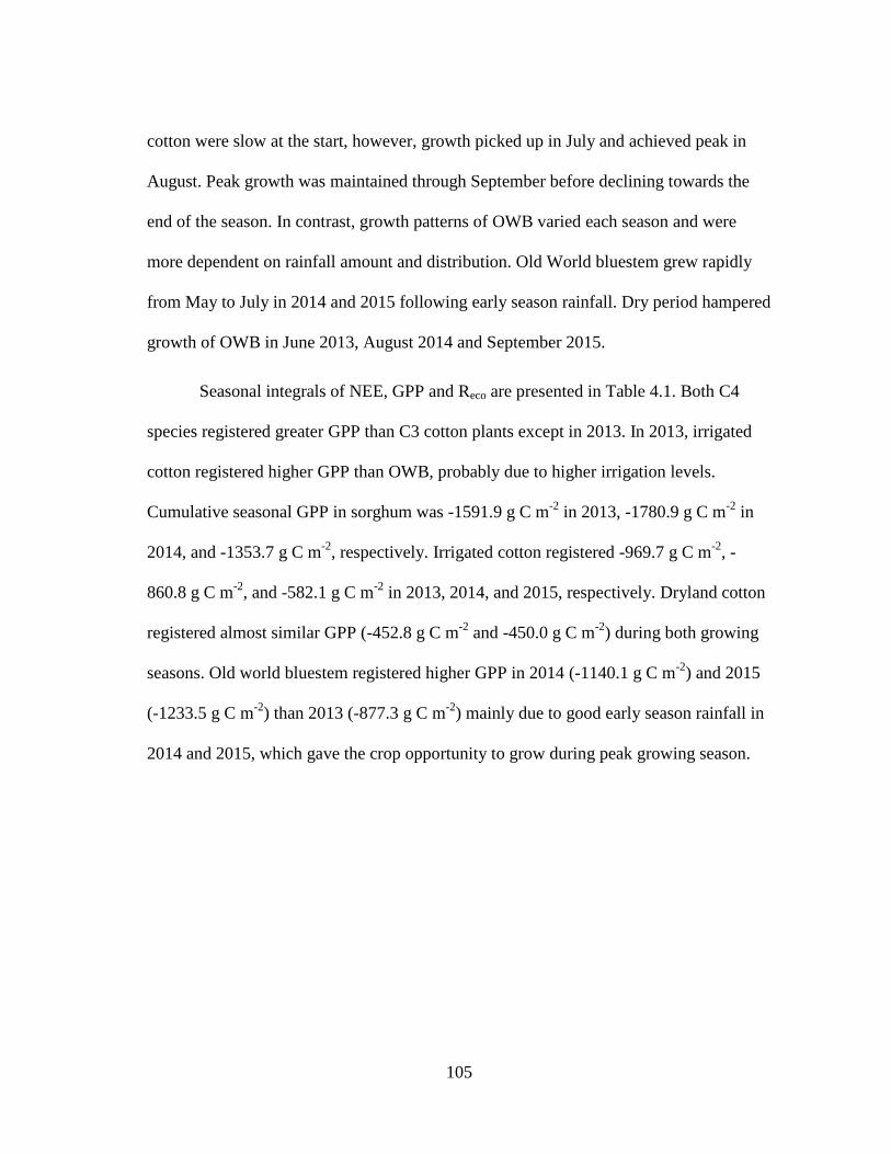
105

cotton were slow at the start, however, growth picked up in July and achieved peak in

August. Peak growth was maintained through September before declining towards the

end of the season. In contrast, growth patterns of OWB varied each season and were

more dependent on rainfall amount and distribution. Old World bluestem grew rapidly

from May to July in 2014 and 2015 following early season rainfall. Dry period hampered

growth of OWB in June 2013, August 2014 and September 2015.

Seasonal integrals of NEE, GPP and Reco are presented in Table 4.1. Both C4

species registered greater GPP than C3 cotton plants except in 2013. In 2013, irrigated

cotton registered higher GPP than OWB, probably due to higher irrigation levels.

Cumulative seasonal GPP in sorghum was -1591.9 g C m-2

in 2013, -1780.9 g C m-2

in

2014, and -1353.7 g C m-2

, respectively. Irrigated cotton registered -969.7 g C m-2

, -

860.8 g C m-2

, and -582.1 g C m-2

in 2013, 2014, and 2015, respectively. Dryland cotton

registered almost similar GPP (-452.8 g C m-2

and -450.0 g C m-2

) during both growing

seasons. Old world bluestem registered higher GPP in 2014 (-1140.1 g C m-2

) and 2015

(-1233.5 g C m-2

) than 2013 (-877.3 g C m-2

) mainly due to good early season rainfall in

2014 and 2015, which gave the crop opportunity to grow during peak growing season.

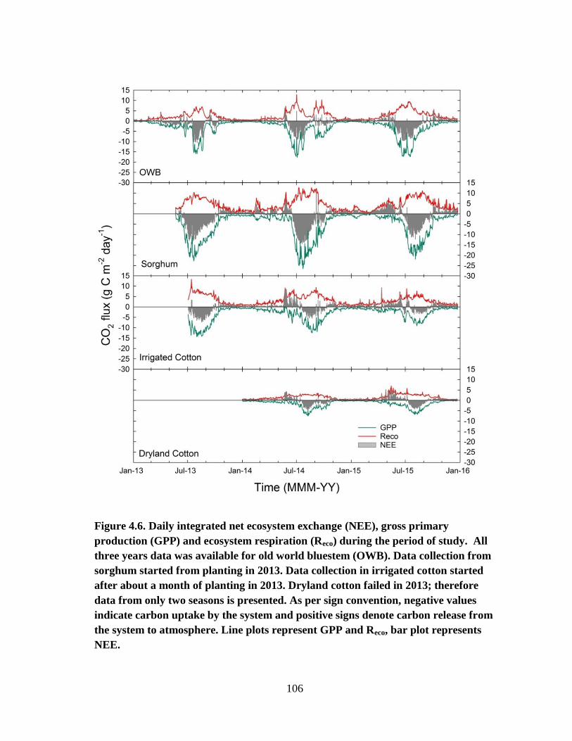
106

Figure 4.6. Daily integrated net ecosystem exchange (NEE), gross primary

production (GPP) and ecosystem respiration (Reco) during the period of study. All

three years data was available for old world bluestem (OWB). Data collection from

sorghum started from planting in 2013. Data collection in irrigated cotton started

after about a month of planting in 2013. Dryland cotton failed in 2013; therefore

data from only two seasons is presented. As per sign convention, negative values

indicate carbon uptake by the system and positive signs denote carbon release from

the system to atmosphere. Line plots represent GPP and Reco, bar plot represents

NEE.

107

Table 4.1. Seasonal integrals of NEE, GPP and Reco in sorghum, old world bluestem

(OWB), irrigated cotton, and dryland cotton. Lower case alphabets alongside mean

values represent the statistical difference at p<0.05.

Crop NEE GPP Reco

g C m-2

2013

OWB -314.5 -877.3 562.8

Sorghum -710.3 -1591.9 872.1

Irrigated

Cotton -305.8 -969.7 663.9

Dryland Cotton - - -

2014

OWB -316.9 -1140.1 823.2

Sorghum -665.2 -1780.9 1138.4

Irrigated

Cotton -81.2 -860.8 766.0

Dryland Cotton -116.9 -452.8 327.2

2015

OWB -373.3 -1233.5 830.3

Sorghum -471.5 -1353.7 882.2

Irrigated

Cotton -21.8 -582.1 560.3

Dryland Cotton -90.7 -450.0 359.3

Mean

OWB -334.9b -1114.4b 638.8b

Sorghum -615.7a -1575.5a 964.2a

Irrigated

Cotton -136.3c -804.2bc 663.4b

Dryland Cotton -104.4c -457.6c 315.3c

Table 4.2. Mean apparent quantum yield (alpha) and mean GPPmax for all the

crops. Rectangular hyperbolic relationship was plotted between GPP and PAR for

5-10 selected clear days during peak photosynthetic activity. Lower case alphabets

besides values indicate significance level at p<0.05.

Crop Mean Alpha Mean GPPmax(umol m-2

s-1

)

Sorghum -0.040a -53.8a

OWB -0.048a -43.9a

Irrigated Cotton -0.045a -28.1b

Dryland Cotton -0.030a -16.1b

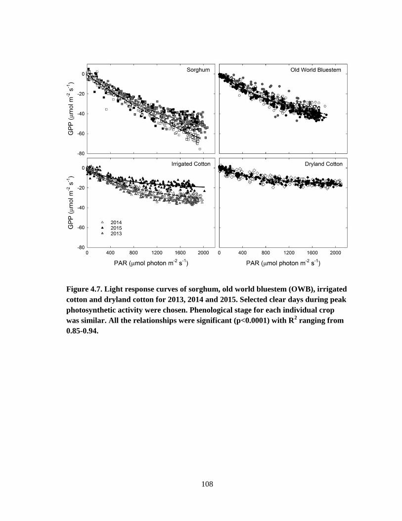
108

Figure 4.7. Light response curves of sorghum, old world bluestem (OWB), irrigated

cotton and dryland cotton for 2013, 2014 and 2015. Selected clear days during peak

photosynthetic activity were chosen. Phenological stage for each individual crop

was similar. All the relationships were significant (p<0.0001) with R2 ranging from

0.85-0.94.

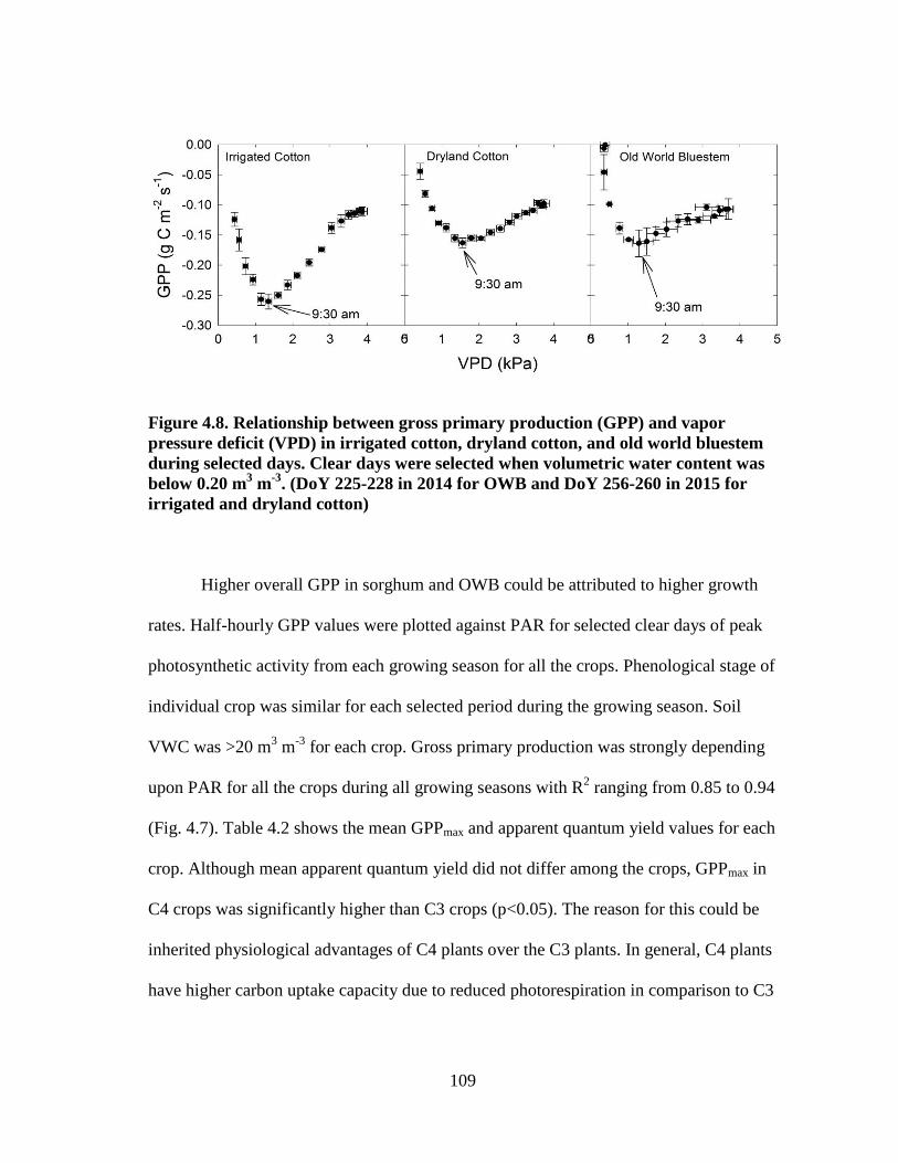
109

Figure 4.8. Relationship between gross primary production (GPP) and vapor

pressure deficit (VPD) in irrigated cotton, dryland cotton, and old world bluestem

during selected days. Clear days were selected when volumetric water content was

below 0.20 m3 m

-3. (DoY 225-228 in 2014 for OWB and DoY 256-260 in 2015 for

irrigated and dryland cotton)

Higher overall GPP in sorghum and OWB could be attributed to higher growth

rates. Half-hourly GPP values were plotted against PAR for selected clear days of peak

photosynthetic activity from each growing season for all the crops. Phenological stage of

individual crop was similar for each selected period during the growing season. Soil

VWC was >20 m3 m

-3 for each crop. Gross primary production was strongly depending

upon PAR for all the crops during all growing seasons with R2 ranging from 0.85 to 0.94

(Fig. 4.7). Table 4.2 shows the mean GPPmax and apparent quantum yield values for each

crop. Although mean apparent quantum yield did not differ among the crops, GPPmax in

C4 crops was significantly higher than C3 crops (p<0.05). The reason for this could be

inherited physiological advantages of C4 plants over the C3 plants. In general, C4 plants

have higher carbon uptake capacity due to reduced photorespiration in comparison to C3

110

plants. Overall, both C4 species assimilated significantly high GPPmax than C3 cotton

(p<0.05). Maximum GPP (GPPmax) was not statistically different among dryland and

irrigated conditions (p<0.05).

In terms of NEE, all the fields were net carbon sinks during growing season (Fig.

4.6). However, the fields remained a net source of carbon during early growing season,

despite initiation of growth. Net ecosystem exchange (carbon uptake) was maximum in

sorghum, despite shorter growing season than other crops. Irrigated cotton registered

maximum growing season carbon uptake (NEE) during 2013 growing season probably

due to greater irrigation during that year. Interestingly, dryland cotton was stronger

carbon sink than irrigated cotton in both 2014 and 2015 years, despite higher GPP in

irrigated cotton. Seasonal NEE for sorghum was -710.3 g C m-2

in 2013, -665.2 g C m-2

in 2014, and -471.5 g C m-2

in 2015. Similarly, OWB registered NEE of -314.5 g C m-2

in 2013, -316.9 g C m-2

in 2014, -373.3 g C m-2

in 2015. Net carbon uptake in irrigated

cotton was -305.8 g C m-2

, -81.2 g C m-2

, and -21.8 g C m-2

in 2013, 2014 and 2015,

respectively.

Lower NEE in sorghum in 2014 despite greater GPP, could be due to higher Reco

during growing season in that year. In sorghum, higher proportion of Reco to GPP in

2014 (63%) and 2015 (65%) lead to lower NEE in 2014 than 2013. In fact, Reco

registered higher proportion of GPP in all crops during 2014 and 2015. The reason for

this could be higher early growing season Reco in all the fields due to heterotrophic

respiration, following early season rainfall events in 2014 and 2015. Precipitation

enhances release of carbon from soil as the water percolating in soil tends to flush out

111

the CO2 from soil as well as increases microbial activity (Franzluebbers 2000, Rochette

et al., 1991, Talmon et al., 2010, Xu et al., 2004; Huxman et al., 2004). Lee et al, (2010)

reported significantly high CO2 flux from a deciduous broad leaf forest on rainy days as

compared to non-rainy days. Harper et al., (2005) reported that the amount and timing of

rainfall events influenced the soil CO2 fluxes in the grassland.

Seasonal Variation in Carbon Fluxes

Seasonal carbon flux trends in sorghum were more or less similar during

different growing seasons, whereas carbon fluxes in OWB varied with growing seasons.

Therefore, seasonal carbon uptake trends of sorghum will not be discussed in this

section. Influence of rainfall amount and its distribution was more evident in OWB than

dryland cotton. Considerable drop in carbon uptake of OWB were noticed during dry

months of the growing season. Similar drops were observed in irrigated and dryland

cotton during September 2015. We plotted GPP for selected clear days during dry period

observed in OWB, dryland cotton and irrigated cotton for both years (Fig. 4.8).

Phenological stage of each crop was similar during each selected period. Gross primary

production increased initially during early morning hours reaching a maximum at 9:30

am, before declining as the day progressed. Wagle et al. (2014) reported similar

observation in sorghum and switchgrass during dry period. The authors concluded that

rising temperatures in the early morning hours increased RuBISCO activity, which

resulted in rapid increase of CO2 assimilation in the early morning hours at lower VPD

levels. The authors further concluded that decline in carbon uptake with rising VPD in

after noon hours could be explained with stomatal closure due to increasing water stress.

112

Vapor pressure deficit is a function of air temperature, therefore similar effects were

observed with rising air temperature in the afternoon hours of the same period (data not

shown). Stomatal closure is coupled with dilution of CO2 concentration at site of

photosynthesis at high temperatures, which enhances RuBISCO reactivity with O2,

resulting in enhanced photorespiration especially in C3 plants. This explains the

observed decline in carbon uptake during afternoon hours in our study during dry

conditions. Despite abiotic limitations of the region to carbon uptake, all the cropping

systems were net carbon sinks at seasonal scale.

Annual Fluxes of Carbon

Table 4.3. Annual net ecosystem exchange (NEE) of the irrigated cotton, sorghum,

dryland cotton, and old world bluestem.

Year OWB Sorghum Irrigated Cotton Dryland Cotton

g C m-2

2013 -301.9 -619.3* -254.3*

2014 -265.6 -444.8 101.3 -19.4

2015 -287.2 -51.4 123.8 56.9

*data from planting to December was available.

Table 4.3 shows the annual carbon budget of all the crops during the study

period. At annual scale both potential bioenergy crops were net sink of carbon, whereas

irrigated cotton acted as carbon source to the atmosphere. Dryland cotton on the other

hand, was a net sink of carbon during 2014 annual cycle, whereas the field was a net

source of carbon in 2015. Large variation was observed in annual sinking capacity of

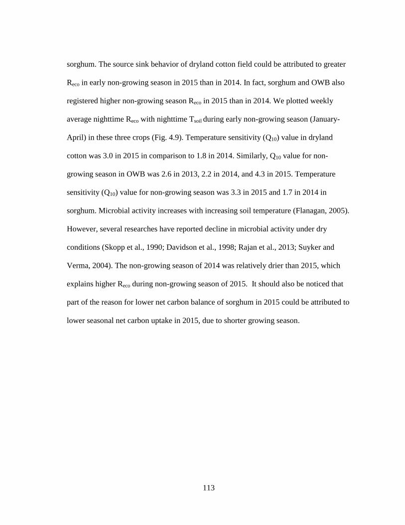
113

sorghum. The source sink behavior of dryland cotton field could be attributed to greater

Reco in early non-growing season in 2015 than in 2014. In fact, sorghum and OWB also

registered higher non-growing season Reco in 2015 than in 2014. We plotted weekly

average nighttime Reco with nighttime Tsoil during early non-growing season (January-

April) in these three crops (Fig. 4.9). Temperature sensitivity (Q10) value in dryland

cotton was 3.0 in 2015 in comparison to 1.8 in 2014. Similarly, Q10 value for non-

growing season in OWB was 2.6 in 2013, 2.2 in 2014, and 4.3 in 2015. Temperature

sensitivity (Q10) value for non-growing season was 3.3 in 2015 and 1.7 in 2014 in

sorghum. Microbial activity increases with increasing soil temperature (Flanagan, 2005).

However, several researches have reported decline in microbial activity under dry

conditions (Skopp et al., 1990; Davidson et al., 1998; Rajan et al., 2013; Suyker and

Verma, 2004). The non-growing season of 2014 was relatively drier than 2015, which

explains higher Reco during non-growing season of 2015. It should also be noticed that

part of the reason for lower net carbon balance of sorghum in 2015 could be attributed to

lower seasonal net carbon uptake in 2015, due to shorter growing season.

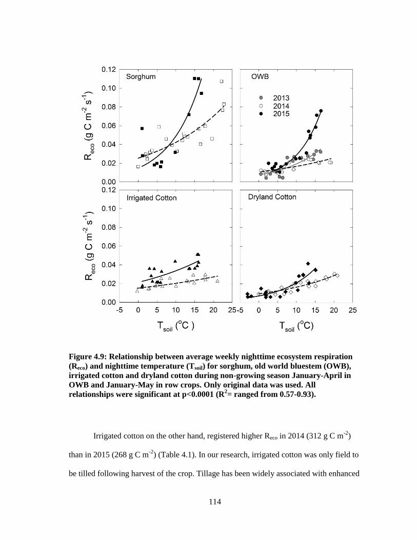
114

Figure 4.9: Relationship between average weekly nighttime ecosystem respiration

(Reco) and nighttime temperature (Tsoil) for sorghum, old world bluestem (OWB),

irrigated cotton and dryland cotton during non-growing season January-April in

OWB and January-May in row crops. Only original data was used. All

relationships were significant at p<0.0001 (R2= ranged from 0.57-0.93).

Irrigated cotton on the other hand, registered higher Reco in 2014 (312 g C m-2

)

than in 2015 (268 g C m-2

) (Table 4.1). In our research, irrigated cotton was only field to

be tilled following harvest of the crop. Tillage has been widely associated with enhanced

115

microbial respiration and release of CO2 from soil. Tillage mixes the plant residue with

soil, thereby increasing the surface area of residue in contact with soil (Lal, 2004). Soil

moisture levels in 2014 were higher as they were in 2015 non-growing season.

Temperature sensitivity of irrigated cotton during non-growing season was close to 1.3

in 2014 and 1.6 in 2015. Seasonal NEE in 2013 was greater than the other two years,

despite almost similar AGB. This suggests that greater amount of carbon was allocated

to below ground biomass in 2013, which may have added to the Reco through

decomposition during 2014 non-growing season following tillage. Lower carbon uptake

and proportionately higher Reco (96% of GPP in 2015 to 90% in 2014) during growing

season in 2015 could have been responsible for lower NEE in that year. Overall, two

complete year (2014 and 2015) integrals of all the row cropping systems yielded a net

carbon sinking of -496.2 g C m-2

in sorghum, 225.2 g C m-2

in irrigated cotton, and 37.4

g C m-2

in dryland cotton. On the other hand, OWB accumulated -854.7 g C m-2

in three

complete years and -552.8 g C m-2

in last two complete years.

Clearly, the annual productivity was higher in bioenergy systems than

conventional cotton cropping systems. Inter-annual variability in net carbon uptake was

largely depending upon Reco during non-growing season and carbon uptake during

growing season. However, the susceptibility of the region to periodic droughts will

determine the fate of rainfed OWB as a bioenergy crops. Previous research by Rajan et

al. (2013) on OWB site has shown transitioning of the site from net sink in a good

rainfall year to a source in a dry year. As mentioned in previous chapter, seasonal NEE

116

of OWB in our study matches well with those of rainfed sorghum reported by Wagle et

al. (2016).

Recall that, poor carbon returns from continuous cotton cropping in Southern

high plains have marginalized the soils by depleting soil organic carbon (Acosta-

Martinez et al., 2010). In our study, the biomass was never removed from OWB and

about 12 inch long stock was left in sorghum field for cattle grazing. Removal of

biomass for biofuel production leads to nutrient removal from soil and leaves poor

carbon return to soil (Propheter and Staggenborg, 2010). This is important, as plant

residue needed to maintain or enhance soil organic carbon could be a constraint for long-

term sustainability of bioenergy production systems (Wilhelm et al., 2007; Powers et al.,

2011). Propheter and Staggenborg (2010) reported greater nutrient removal by the

annual crops (including sorghum bmr cultivar) in comparison to switcgrass and

miscanthus. However, this study was conducted during establishment phase of perennial

crops, when their yields are usually lower than annual crops. Similarly, Blanco-Canqui

and Lal, (2008) reported net nutrient loss in silt loam soils when all the corn stover was

removed from the field, whereas clay loam soils remained unaffected. Cowie et al.

(2006) estimated that soil organic carbon losses are likely to happen in soils with high

carbon concentration and soil with low carbon concentration are likely to accrue carbon

over time. Soil organic carbon in our study was less than 1% in all the fields (data not

shown). Powers et al. (2011) using modelling approach concluded that herbaceous crops

such as switchgrass could be beneficial for soil and water quality perspective in

comparison to traditional corn-soybean cropping systems depending under tillage

117

practices in US corn belt. Cotton et al. (2013) reported increased level of soil organic

carbon under sorghum cropping in high plains soils even after total removal of AGB due

to extensive root system. This suggests that marginalized soils of the Southern High

Plains will benefit from land use change induced by bioenergy cropping systems.

Therefore, bioenergy cropping systems especially perennial cropping systems may prove

sustainable in the long term in terms of soil quality in the Southern High Plains.

However, threshold levels for biomass removal must be optimized in order increase or

maintain the displaced atmospheric carbon levels in the system.

CONCLUSION

On-site carbon balance of two potential bioenergy crops, sorghum and OWB

were compared with conventional cotton cropping system at seasonal and annual scale in

the Southern high Plains. We found that both C4 bioenergy crops were robust carbon

sinks at seasonal scale in comparison to cotton cropping systems. In fact, seasonal

carbon uptake in sorghum was greater than OWB. Seasonal carbon uptake in sorghum

was largely affected by growing season length and phenology. However, when

calculated on annual scale sorghum exhibited greater variation in net carbon capacity

while OWB remained stable. Non-growing seasonal Reco played major role in annual

carbon budget of both bioenergy crops. Wet winters in 2015 led to higher carbon release

into the atmosphere, thereby declining net carbon budget in sorghum. Rainfall

distribution was major controlling factor in growth of OWB. Cotton cropping systems

remained net carbon source of the carbon for combined 2014 and 2015 annual cycles.

Our findings suggest that a shift from conventional cotton cropping systems to bioenergy

118

crops will lead to greater on-site carbon assimilation in the Southern Great Plains.

However, retention of on-site carbon balance will largely depend upon biomass removal,

environmental conditions and agronomic management practices. The Southern High

Plains is susceptible to periodic droughts and is facing water crisis due to declining

water table in Ogallala aquifer. Therefore, sustainability of these bioenergy cropping

systems will largely depend upon the future climatic and irrigation scenarios. We believe

that higher carbon uptake in sorghum in our study was due to irrigation. As such, we

anticipate a decline in carbon uptake capacity of sorghum under dryland conditions.

Therefore, more research is required to assess carbon capacity of sorghum under dryland

conditions to assess the long-term sustainability of these systems under water stressed

scenario in future.

119

CHAPTER V

IMPLICATIONS OF BIOENERGY CROPS INDUCED LAND USE

CHANGE ON ENERGY BALANCE AND EVAPOTRANSPIRATION

IN THE SOUHTERN GREAT PLAINS

INTRODUCTION

Current legislative and regulatory mandates aiming at reducing United States’

dependence on foreign oil imports has driven the rising bioenergy crops production in

the United States. According to US Energy Independence and Security Act of 2007, a

targeted 36 billion gallons of renewable fuel (biofuel) are to be produced by 2022. About

80 billion liters of the total amount will be second generation biofuels, produced from

specific biomass crops. By 2016, about 90 billion liters of renewable fuel was produced

and a target of 95 billion liters has been set for 2017 (RFS, 2017;

https://www.epa.gov/renewable-fuel-standard-program/proposed-renewable-fuel-

standards-2017-and-biomass-based-diesel accessed February 9, 2017). However, in both

years contribution of first generation biofuels has been about 75% of the total renewable

fuels. While the major first generation biofuel crops i.e. corn and soybean production as

bioenergy crops has rapidly increased in the US corn-belt region (Wright and Wimberly,

2013), there still exists a large gap for specific biomass crops to fill, in order to meet the

target for second generation biofuels. As a result, increase in production area of specific

biomass crops for second-generation biofuel production is anticipated in future.

120

Half of the total second generation biofuels are proposed to be produced in the

Southeast United States, including the Southern Great Plains (USDA, 2010). The

Southern Great Plains is a semi-arid region which is susceptible to periodic droughts.

Therefore, agriculture in the Southern Great Plains largely depends upon the water

extracted from the Ogallala Aquifer. Infact, 95% of the water extracted from the aquifer

is used for irrigation, which has depressed the water table in the Ogallala Aquifer.

Introduction to cotton cultivation and central pivot irrigation system as a strategy

(Colaizzi et al., 2009) to reduce water consumption in the Southern Great Plains has

been successful, as the region produces 20-25% of total cotton production in the United

States (Allen et al., 2008). However, with declining Ogallala Aquifer the area is already

witnessing a steady shift from irrigated cotton to dryland cotton. Other major crops of

the region include, sorghum, corn, soybean and wheat. A large scale production of the

bioenergy crops in the region may induce a significant land conversion from

conventional cotton cropping system to bioenergy cropping systems.

Increasing land conversion to bioenergy crops in the world has already shifted

the current scientific research interests towards sustainability of bioenergy cropping

systems. Land required to meet the large scale production of bioenergy crops will come

from existing croplands, marginal lands, grasslands or retired croplands mainly CRP

lands, inducing land use change in many areas (Fargione et al., 2009; Gelfand et al.,

2013; Wright and Wimberly, 2013). Therefore, large scale production of bioenergy

crops will compete with food and fiber crops not only for land but also for water and

other input resources (de Fraiture et al., 2008). This holds true to the Southern Great

121

Plains as well, where a significant competition between bioenergy crops and cotton

cropping systems for land and water is anticipated in future. However, effects of large

scale land conversion to bioenergy crops on ecosystem services including carbon, water

and energy balance at ecosystem scale have not been addressed adequately and should

not be neglected in implementation of production policy (Robertson et al., 2011;

Vanloocke et al., 2012).

Land use change can have major implications on environment as change in

vegetation properties can significantly affect the carbon, water and energy budget of a

region by modifying albedo and energy balance (Pielke et al., 2002; Keuppers et al.,

2007; Twine et al., 2004). Pielke et al. (1998) concluded that land cover is equally

important as anthropogenic activity for earth’s climate as former can significantly

influence weather and climate of a region. Several studies have reported impact of

vegetation type on groundwater recharge, water quality, and evapotranspiration

(Sesmero, 2014; Humphreys et al., 2003; Delucchi, 2010; Green et al., 2011). In general,

environmental implications of conventional annual bioenergy crops are similar to farm

crops, but may differ from perennial crops (Fraiture and Berndes, 2009; Abraha et al.,

2016). For example, groundwater recharge from the perennial crops is usually lower

than annual crops due to greater cumulative ET because of longer growing season

(Schilling, 2008; Trost, 2010; Smith et al., 2013). Perennial crops on the other hand, can

provide ecosystem services in terms of improved soil health, reduced soil erosion, less

agronomic operations, reduced solute leaching to groundwater and improved wildlife

habitat (Trost, 2010).

122

The objective of this research was to assess and compare the water and energy

balance dynamics of an annual and a perennial bioenergy crop with the conventional

cotton cropping systems in the Southern High Plains. For this study, sorghum was the

potential bioenergy crop, which has better potential for established bioenergy cropping

systems over corn due to its lower water and nutrient requirements (Rooney, 2007). The

perennial bioenergy crop for this study was Old World Bluestem (OWB). Old World

bluestem is a resilient drought resistant bunch grass with well-established cropping

systems, have potential to emerge as popular bioenergy cropping systems in the

Southern High Plains. In addition, most of the CRP lands in Texas have been planted

with OWB (Li et al., 2017). We compared sorghum and OWB with conventional

cropping systems of irrigated and dryland cotton using eddy covariance method. Data

from this study will be useful to parameterization of land surface models and remote

sensing models to estimate evapotranspiration and energy balance at regional scale.


Study Site

This study was conducted in four different farmers’ fields fitted with central



miles northeast of Plainview, TX (34°12’34.70’’ N and 101°37’50.85’’ W, 1100 m

elevation). The cultivar planted was Surpass XL bmr (brown midrib). Sorghum was

planted on one half of the field and the remaining half was planted with cotton

(Gossypium hirsutum L.). The farmer practiced crop rotation between these crops on

123

both halves of the field. Management practices prior to planting sorghum included

mowing down of cotton stubbles after harvesting previous cotton crop followed by

tillage in spring and before planting the crop. Total area planted with sorghum each time

was about 25 ha. The crop was planted on 20 May in 2013 and 2014 at a seeding rate of

4.9 kg ha-1

. Heavy rains in late May during 2015 delayed planting, thus the crop was

planted on June 4 in 2015 at the same seeding rate. The row spacing in 2013 and 2015

was 40 inches and 20 inches in 2014. Urea was broadcasted in the field in spring before

planting at a rate of 150 kg N ha-1

. In addition, 30 kg P2O5 ha-1

was also applied prior to

planting. The field was irrigated with low elevation application center-pivot irrigation

system during the crop growth period. For first 40 days the field was supplied with 0.75

inch and for rest of the season it was supplied with 1.5 inch water during each irrigation

event. The field was supplied with about 400 mm of water through irrigation in 2013,

about 400 mm in 2014 and about 270 mm in 2015. Also, the field was cultivated in

between the plant rows to kill weeds twice in June every year when the crop was still

small. The field was harvested for seed on 8 October in 2013, on 14 October in 2014,

and on October 1 in 2015. The growing season was 140, 147, and 119 days long for

2013, 2014, and 2015, respectively. Equipment availability and late season rainfall

affected the timings of harvest. The field remained fallow post-harvest in winter and

spring. The farmer let the remaining stalk grazed by cattle in March 2014 and in January

2015. A fence was put around the tower during the presence of cattle in the field. Since

the crop was grown in rotation with cotton, the new crop was planted on other half of the

field where cotton was produced in previous season. The major soil mapping unit at the

124

study site is Pullman clay loam (a fine, mixed, superactive, thermic Torrertic Paleustoll)

with 0 to 1% slope.


o25’48” W)



Kg seed ha-1



originally from a selection made in India. It is a bunchgrass with an upright growth

habit and has better drought tolerance and water use efficiency than conventional

cropping systems in the Southern Great Plains. Total area of the site is about 42 ha. Until

2011 the field was used for grazing by the cattle or for seed production. This field was

equipped with a center pivot irrigation system; however, no irrigation, nutrient supply or

grazing operation was conducted during the study period (2013-2015). The growing

season for the crop roughly ranged from May to October. Peak growing season occurred

from June to July depending upon precipitation. The grass remained in vegetative state

for most part of the growing season and bloomed in late September/early October. The

field was harvested for seed on November 14, 2014. No seed harvesting was done in

2013 and 2015. The field was never harvested for hay. Major soil mapping unit in the

field was Pullman clay loam with 0-1% slope.

The irrigated cotton field was located adjacent to sorghum field about 4 km

north-east of Plainview in Hale county. In 2013, Cotton was planted in first week of

June. First planting of cotton on May 30 was failed and cotton was replanted on June 9.

125

In 2015, cotton was planted on June 2. Cotton variety planted was Fibermax 2322 at a

seeding rate of 40,000 seeds per acre during all years of study. Cotton was applied with

100 Kg ha-1

of nitrogen (N) and 35 kg ha-1

of P2O5 before planting. Total area of cotton

planted was about 60 acres. Row spacing was 1 m. The field was irrigated using a

center-pivot irrigation system. Cotton was sprayed with defoliator (Ginstar) during last

week of October. Cotton was harvested on November 7-8 each year of study. Cotton

stubbles were mowed down to about 4 inch height after harvest. Irrigated cotton in this

study was rotated with sorghum.

Dryland Cotton field was located about 3 km north of Lockney, TX. Dryland was

planted on June 1 in 2013, 2014 and 2015. The crop failed in 2013 and farmer ploughed

the field to claim crop insurance. In 2015, the farmer decided to plant grain sorghum in

the field. As a result, the tower was moved to a nearby dryland cotton field. The size of

both fields was about 100 acres. The crop was planted with variety Fibermax 2011

during all years of study. Row spacing was 1 m. Crop was planted at seed rate of 26000

seeds per acre. No fertilizer was applied to the field in 2014 and 2015. The field was

sprayed with defoliator (Ginstar) on October 21 in 2014. The field was harvested on

November 6. In 2015, the crop was damaged due to hailstorm on July 7 and 8, but the

crop resumed growth successfully to complete the life cycle. However, late season rains

damaged the cotton bolls and farmer did not harvest the field.




126

in grassland was established in 2010, the tower in sorghum, irrigated cotton, and dryland

cotton was established at planting in 2013. Measurements from irrigated cotton started

about a month after planting. All towers were set up in the middle of the fields, with

fetch of about 150 m from all directions. An integrated sonic anemometer (Model

CSAT-3A, Campbell Scientific) and infra-red gas analyzer (IRGA, Model EC-150,

Campbell Scientific) called the IRGASON was used to measure wind velocity and CO2,

H2O vapor concentration, and H in the ambient atmosphere. In grassland the CO2, H2O

vapor concentration was measured using Li-7500 IRGA (LI-COR Biosciences) and wind

velocity and sensible heat flux were measured using sonic anemometer sonic

anemometer (Model CSAT-3A, Campbell Scientific). The system was installed in

middle of each field with fetch of 150 m or more from all directions. These instruments

were set up facing south-southwest (in the prevailing wind direction) at a height of about

2.1 m from ground surface. The height of the instrument was adjusted in sorghum field

during growing season with increasing crop height to a final height of about 2.6 m from

ground. Other environmental variables measured at both sites included air temperature

(Tair) and relative humidity (RH) (HMP50, Campbell Scientific), net radiation (Kipp &

Zonen NR-Lite net radiometer), photosynthetically active radiation (PAR) (LI-200SL

quantum sensor, LI-COR), solar irradiance (LI-190SB pyranometer, LI-COR),




Campbell Scientific). Self-calibrating soil heat flux plates (HFPSC-01, Hukseflux,

127

Campbell Scientific, Logan, UT) were used to measure soil heat flux at 8 cm depth from

soil surface. Soil heat storage which is the amount of heat stored in 8 cm soil depth over

soil heat flux plates was calculated using the following equation:


𝑡 [5.1]






soil (𝐶𝑑 = 840 𝐽 𝑘𝑔−1𝐾−1):






manufacturers’ guidelines to avoid accumulation of dust. Data from the CSAT3A sonic

anemometer and IRGA system were measured at 10-Hz sampling rate using a CR3000

datalogger (Campbell Scientific). All other environmental variables were measured at 5

seconds interval. The datalogger was programmed to calculate and save 30-min average

values of all environmental variables. The raw 10-Hz wind velocity and EC150/LI-7500

data were saved for further post-processing and analysis of CO2 and energy fluxes.

128













were gap filled. In addition, the physically implausible values in the data were also

filtered and gap filled. Further, the flux is usually underestimated during low turbulence

conditions and therefore, data during low turbulence conditions (when the friction

velocity (u*) was <0.10 m s–1



, 0.33 ms-1

, and 0.31 ms-1



, 0.36 m s-1

, 0.31 m s-1

. After screening the data for out of the

range and above mentioned filtering criteria, the amount of data which was either

missing or did not clear the quality check criteria was about 21%, 8%, and 40% in 2013,

2014, and 2015, respectively. During growing season, 21%, 13 and 3% data was gap-

129

filled in 2013, 2014, and 2015 respectively. The amount of data to be gap filled in









, ±2.5 oC, and ±0.5 kPa,











)*( TsoilB

eco AeR [5.3]


130




NEERGPP eco [5.4]





Quality of eddy covariance data is very important and can be determined the













131

Rn – G = LE + H [5.5]

The sign convention used for Rn and G are positive when the flux is downwards

and negative when the flux is upward. The sign convention used for LE, H and C fluxes

was a positive flux represents flux from the ecosystem to the atmosphere, while a

negative flux represents flux from the atmosphere to the ecosystem.

The 30 min LE data was used to calculate ET using the following equation:

𝐸𝑇 =𝐿𝐸

𝜌𝑤𝜆 [5.6]

where, 𝜌𝑤 density of water (1000 kg m-3

), and 𝜆 is the LE of vaporization (2.5 × 106 J

kg-1

). Ecosystem water use efficiency (EWUE) at monthly and seasonal scales was

calculated by dividing daytime cumulative GPP with daytime cumulative ET at monthly,

and seasonal timescales, respectively.

Biometric Data

Plant dry biomass weight was measured during the growing season. Sorghum

plant samples were taken randomly (3 replications) from the field to measure leaf area

index (LAI), dry leaf mass and dry shoot mass. For grasslands, four random plant

samples (for green, yellow leaves and litter) were taken from quarter of a meter area. No

LAI measurements were done on the grass samples. Plants were stored in an ice chest in

the field and leaf area of sorghum was measured (after separating leaves from shoots)

using a leaf area meter (Model LI-3100, Licor Biosciences, Lincoln, NE) immediately

after they were brought to the laboratory. For grass samples, green and yellow leaves

were separated after samples were brought to the lab. After measuring leaf area, leaves

132

and shoots were stored in paper bags and dried at 65oC for one week. Dry mass of shoot

and leaves was taken immediately after removing the dried samples out of the oven.

Plant density (number of plants per m2) and leaf area were used to calculate the LAI.


Phenology

Phenological parameters are presented in Figure 4.1 and 4.2 in Chapter IV. Leaf

area index and above ground biomass were measured in all the row crops once a

significant crop stand was established. Only above ground biomass and litter

measurements were made in OWB. Sorghum recorded the maximum LAI among the

row crops followed by irrigated cotton and dryland cotton. Maximum LAI ranged from

4.1 in 2013 to 7.1 in 2014 for sorghum, 2.8 in 2013 to 3.1 in 2014 for irrigated cotton

and 1.9 in 2014 to 1.4 in 2015 for dryland cotton. Maximum LAI in all crops occurred

around mid-August across all growing seasons. On the other hand, maximum

aboveground biomass was recorded around physiological maturity of all the crops.

Maximum biomass ranged from 18 tons ha-1

in 2013 to 25 tons ha-1

in 2014 in sorghum,

14.5 tons ha-1

in 2013 to 12.5 in tons ha-1

in 2015 in irrigated cotton and 6.1 tons ha-1

in

dryland cotton during both years of study. Maximum aboveground biomass including

yellow and green leaves in OWB ranged from 7 to 10 tons ha-1

. Detailed discussion on

phenology and weather are provided in chapter 3.

133

Energy Partitioning

Partitioning of available energy i.e. net radiation in different crops is presented in

Fig. 5.1. All three years data was available for OWB (2013-15) and two full (2014 and

2015) year data was available for dryland cotton. Data for irrigated crops was available

from their first planting date in 2013 to December 2015. Available energy was mainly

dispersed between LE and H. Magnitude of G remained lower across all fields

throughout the study period. Sensible heat dominated energy partitioning during non-

growing season (November-April) in all fields. Latent heat was greater in magnitude

than H in January 2015 following snowfall and rain events.

Old world bluestem had the longest growing season (May-October), followed by

cotton (June- mid-October) and sorghum (June-September). Irrigated crops showed

consistent growing season behavior in energy partitioning during all growing seasons.

Latent heat was the major energy dispersal component during active growing (June-

September) season in both irrigated crops followed by sensible heat, and soil heat flux.

Early onset of rainfall in 2015 led to shift in energy dispersion from H to LE in both

fields in May itself. For irrigated cotton, largest monthly LE was observed in August

during all growing seasons. Maximum monthly LE was 177 W m-2

in 2013, 132.6 W m-2

in 2014 and 119 W m-2

in 2015. Maximum monthly H of 80.5 W m-2

and 71.5 W m-2

were observed in April 2014 and 2015 in irrigated cotton. On the other hand, sorghum

recorded largest LE in July of 2013 (141.2 W m-2

) and 2014 (153.2 W m-2

) and in

August of 2015 (140.6 W m-2

). Largest magnitude of H for sorghum was observed in

May (82.1 W m-2

) in 2013, March (57.7 W m-2

) in 2014 and June (67.0 W m-2

) in 2015.

134

Among dryland crops, dryland cotton followed similar patterns of energy

dispersion as in irrigated row crops. LE dominated H from June-October in 2014, and

from May to October in 2015. Sensible heat dominated the energy dispersal for the rest

of the season in dryland cotton. Maximum monthly LE in dryland cotton was observed

in July (86.0 W m-2

) in 2014 and in August (95.5 W m-2

) in 2015. Maximum monthly H

was observed in June (76.1 W m-2

) in 2014 and April (55.6 W m-2

) in 2015. Infact,

magnitude of H was comparable to LE during these months in dryland cotton.

135

Figure 5.1. Energy partitioning in net radiation (Rn), latent heat (LE), sensible heat

(H) and soil heat flux (G) during the study period in different crop fields.

Measurement in sorghum and irrigated cotton started from May and July 2013,

respectively. Dryland cotton failed in 2013 and has not been presented in this data.

136

In contrast, OWB energy partitioning varied between H and LE during active

growing season. Lack of rainfall events kept H the dominant energy component in May

and June 2013 in OWB field. Latent heat remained dominant energy component in July

and August, before H became the dominant component for the rest of the growing

season in 2013. In 2014 growing season, LE remained dominant for June, July,

September and October. In 2015 growing season, LE dominated H from May-August,

following which H dominated for the rest of the growing season. Maximum monthly LE

for OWB was observed in August (95 W m-2

) in 2013, in June (111.4 W m-2

) in 2014

and in July (119.7 W m-2

) 2015. Maximum monthly H in OWB was observed in April in

2013 (81.0 W m-2

) and 2015 (85.1 W m-2

) and in May (76.4 W m-2

) in 2014.

Large portion of energy was partitioned to LE during wet period and to H during

dry period in OWB during active growing season. Similar findings were reported by

Wagle et al (2014) for rainfed switchgrass during active growing season. Wagle et al.

(2014) concluded that energy partitioning was sensitive to both climatic and biological

factors. We plotted daily average Bowen ratio (H/LE) against surface soil moisture in

OWB for all the growing seasons together (Fig. 5.2). Our results show that energy

dispersal among H and LE significantly depended on the soil surface VWC during active

growing season (July-September) (Fig. 5.2). These results suggest that the system was

actively losing energy in form of LE when the soil VWC was greater than 0.20 m3 m

-3,

and in form of sensible heat once the soil moisture dropped this threshold level. It should

be noted that for Pullman clay loam the permanent wilting point is around 0.20 m3 m

-3

(Howell et al., 2004; Rajan et al., 2014). This finding is in good agreement with those

137

reported by Rajan et al. (2015) for the same site during a two year study involving

drought and wet year, and with those reported by Gu et al. (2006). Latent heat is

associated with evapotranspiration, as the water vapor leaving surface carries the amount

of energy equivalent to latent heat of vaporization. Irrigated cotton and sorghum showed

similar behavior, however the LE dominated for most part of the active growing (July-

August) season due to irrigation. Bowen ratio in irrigated cotton was significant function

of soil moisture, while sorghum was not. Dryland cotton just like OWB showed similar

behavior during active growing season, however it was not significantly related to

surface soil moisture.

138

Figure 5.2. Relationship of daily Bowen ratio with daily average soil moisture (5

cm) content. Daily Bowen ratio from all three active growing seasons (June-August)

was plotted together against respective soil moisture. Irrigated Cotton (R2=0.25)

and Old World Bluestem (R2=0.41) had significant relationships. Sorghum and

Dryland Cotton were not significantly related to soil moisture.

Seasonal and Diurnal ET

Figure 5.3 shows the regular seasonal pattern of evapotranspiration in irrigated

crops during all growing seasons. Evapotranspiration largely remained small in January

and February. Average daily ET during this time (January-February) of all years was

similar in sorghum (0.4±0.02 mm, (average ± standard error)), irrigated cotton (0.4±0.02

139

mm) and dryland cotton (0.5±0.03 mm). Old world bluestem registered slightly less ET

(0.3±0.02) during January and February of all years. These ranges of daily ET are

consistent with those (0.5 mm day-1

) reported by Eichelmann et al. (2016) for

switchgrass in Canada, Skinner and Adler, (2010) in north-eastern United States, Wagle

et al. (2014) in Oklahoma, and Wever et al. (2002) for tall prairie. Similarly, average

daily ET from March to May of all years was similar in all the row crop fields (1.3±0.11

mm day-1

in dryland cotton, 1.4±0.11 mm day-1

in irrigated cotton, and 1.5±0.11 mm

day-1

in sorghum) and slightly low (0.9±0.05 mm day-1

) in OWB. March onwards ET

started rising with increasing temperatures, until reached a temporary peak in May 2014

and 2015 following early season rainfalls. Lower ET in OWB during non-growing

season could be attributed to litter accumulation over surface, which may have acted as

insulation to water vapors escaping to atmosphere. Many studies under no-till

management have reported similar behavior of plant residue on ET (Barbieri et al.,

2012).

140

Figure 5.3. Daily evapotranspiration for the complete study period. Old world

bluestem had all three years of data, whereas data collection from irrigated crops

started following planting in 2013. Dryland cotton crop failed due to lack of rainfall

in 2014, thus the data was lost during that year.

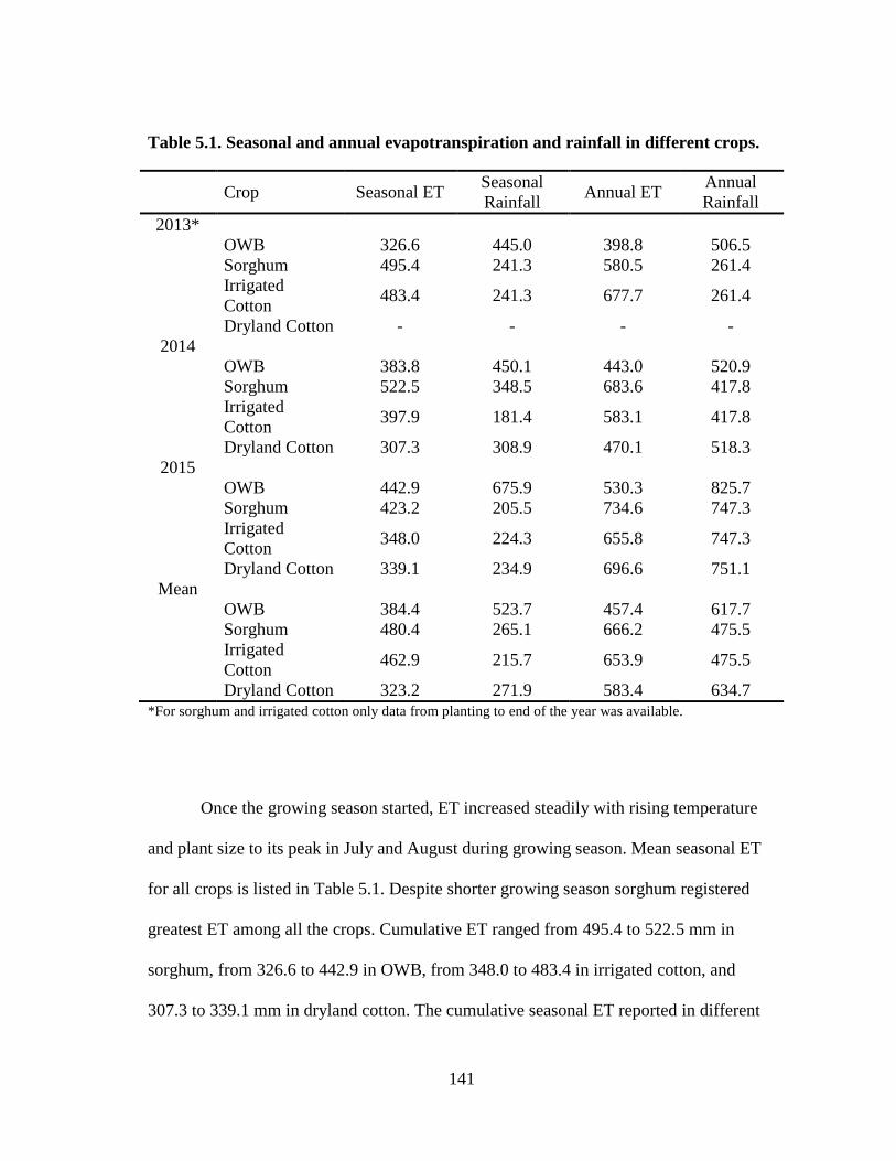
141

Table 5.1. Seasonal and annual evapotranspiration and rainfall in different crops.

Crop Seasonal ET

Seasonal

Rainfall Annual ET

Annual

Rainfall

2013*

OWB 326.6 445.0 398.8 506.5

Sorghum 495.4 241.3 580.5 261.4

Irrigated

Cotton 483.4 241.3 677.7 261.4

Dryland Cotton - - - -

2014

OWB 383.8 450.1 443.0 520.9

Sorghum 522.5 348.5 683.6 417.8

Irrigated

Cotton 397.9 181.4 583.1 417.8

Dryland Cotton 307.3 308.9 470.1 518.3

2015

OWB 442.9 675.9 530.3 825.7

Sorghum 423.2 205.5 734.6 747.3

Irrigated

Cotton 348.0 224.3 655.8 747.3

Dryland Cotton 339.1 234.9 696.6 751.1

Mean

OWB 384.4 523.7 457.4 617.7

Sorghum 480.4 265.1 666.2 475.5

Irrigated

Cotton 462.9 215.7 653.9 475.5

Dryland Cotton 323.2 271.9 583.4 634.7

*For sorghum and irrigated cotton only data from planting to end of the year was available.

Once the growing season started, ET increased steadily with rising temperature

and plant size to its peak in July and August during growing season. Mean seasonal ET

for all crops is listed in Table 5.1. Despite shorter growing season sorghum registered

greatest ET among all the crops. Cumulative ET ranged from 495.4 to 522.5 mm in

sorghum, from 326.6 to 442.9 in OWB, from 348.0 to 483.4 in irrigated cotton, and

307.3 to 339.1 mm in dryland cotton. The cumulative seasonal ET reported in different

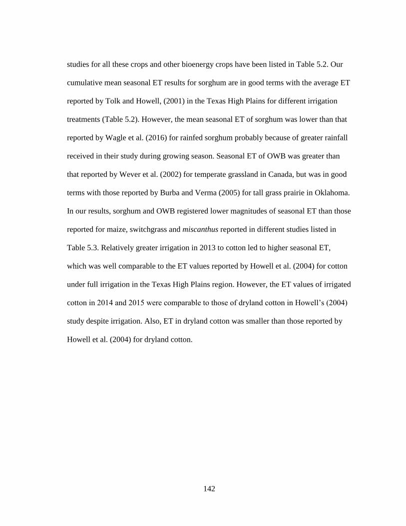
142

studies for all these crops and other bioenergy crops have been listed in Table 5.2. Our

cumulative mean seasonal ET results for sorghum are in good terms with the average ET

reported by Tolk and Howell, (2001) in the Texas High Plains for different irrigation

treatments (Table 5.2). However, the mean seasonal ET of sorghum was lower than that

reported by Wagle et al. (2016) for rainfed sorghum probably because of greater rainfall

received in their study during growing season. Seasonal ET of OWB was greater than

that reported by Wever et al. (2002) for temperate grassland in Canada, but was in good

terms with those reported by Burba and Verma (2005) for tall grass prairie in Oklahoma.

In our results, sorghum and OWB registered lower magnitudes of seasonal ET than those

reported for maize, switchgrass and miscanthus reported in different studies listed in

Table 5.3. Relatively greater irrigation in 2013 to cotton led to higher seasonal ET,

which was well comparable to the ET values reported by Howell et al. (2004) for cotton

under full irrigation in the Texas High Plains region. However, the ET values of irrigated

cotton in 2014 and 2015 were comparable to those of dryland cotton in Howell’s (2004)

study despite irrigation. Also, ET in dryland cotton was smaller than those reported by

Howell et al. (2004) for dryland cotton.

143

Table 5.2. Seasonal ET for different bioenergy crops as well as cotton reported in

different studies.

Author Crop Region Irrigation Seasonal ET

(mm)

Tolk and Howell

(2010)

Sorghum Texas Irrigation 400-490

Wagle et al. (2016) Sorghum Oklahoma Rainfed 553

Wagle et al. (2016) Switchgrass Oklahoma Rainfed 652

Hickman et al. (2010) Switchgrass Illinois - 764

Hickman et al. (2010) Miscanthus Illinois - 954

Hickman et al. 2010 Maize Illinois - 611

Wever et al. (2002) Temperate

Grassland

Canada Rainfed 226-295

Eichelmann et al.

(2016)

Switchgrass Canada Rainfed 562-598

Burba and Verma

(2005)

Prairie Oklahoma Rainfed 480-607

Howell et al. (2004) Cotton Texas Dry 356-415

Howell et al. (2004) Cotton Texas Deficit 619-639

Howell et al. (2004) Cotton Texas Full 739-775

Suyker and Verma

(2009)

Maize Nebraska Irrigated 631

Figure 5.4 presents the diurnal patterns of ET in each month of the growing

season for all crops. Similar to energy partitioning, monthly diurnal courses of ET were

consistent in row crops, while ET in OWB lacked consistency. Peak half-hourly ET

values were observed from 12:00-14:00 hours in all crops during all months of growing

season. In sorghum, highest monthly ET rate was recorded in July and August during all

growing seasons. Irrigated and dryland cotton registered peak monthly ET rate in August

when plants were flowering. Diurnal trends of ET in irrigated cotton were generally

comparable in June, July, and September. Similarly, diurnal trends of ET in dryland

cotton were comparable in June, July, and September, though dryland cotton registered

144

lower peaks than all the other crops during the growing season. Despite August being the

driest month in 2014 and September in 2015, no considerable reduction in ET was

noticed. Infact, half-hourly ET rates in August 2014 were the highest in dryland cotton.

Evapotranspiration rates declined in October in all crops as the plants were senescing.

In OWB, peak average monthly half-hourly ET was recorded in August in 2013,

in June in 2014 and June and July in 2015. In 2013 and 2015, lowest ET was observed in

October as the crops entered senescence. Unlike dryland cotton, lowest ET values were

observed during drier months of May and August in 2014. These findings suggest ET of

the OWB were more sensitive to precipitation than dryland cotton. These results are in

good agreement with those of Rajan et al. (2014), Burba and Verma, (2005) and Wagle

et al. (2014) that suggests role of precipitation distribution is important in ET dynamics

of rainfed perennial grass systems. The drop in ET during drier months in OWB was in

agreement with drop in carbon uptake during these months. However, neither drop in ET

nor reduction in carbon was observed during similar dry months in dryland cotton

(discussed later). These findings suggest that during dry period cotton managed to draw

water from deeper layers.

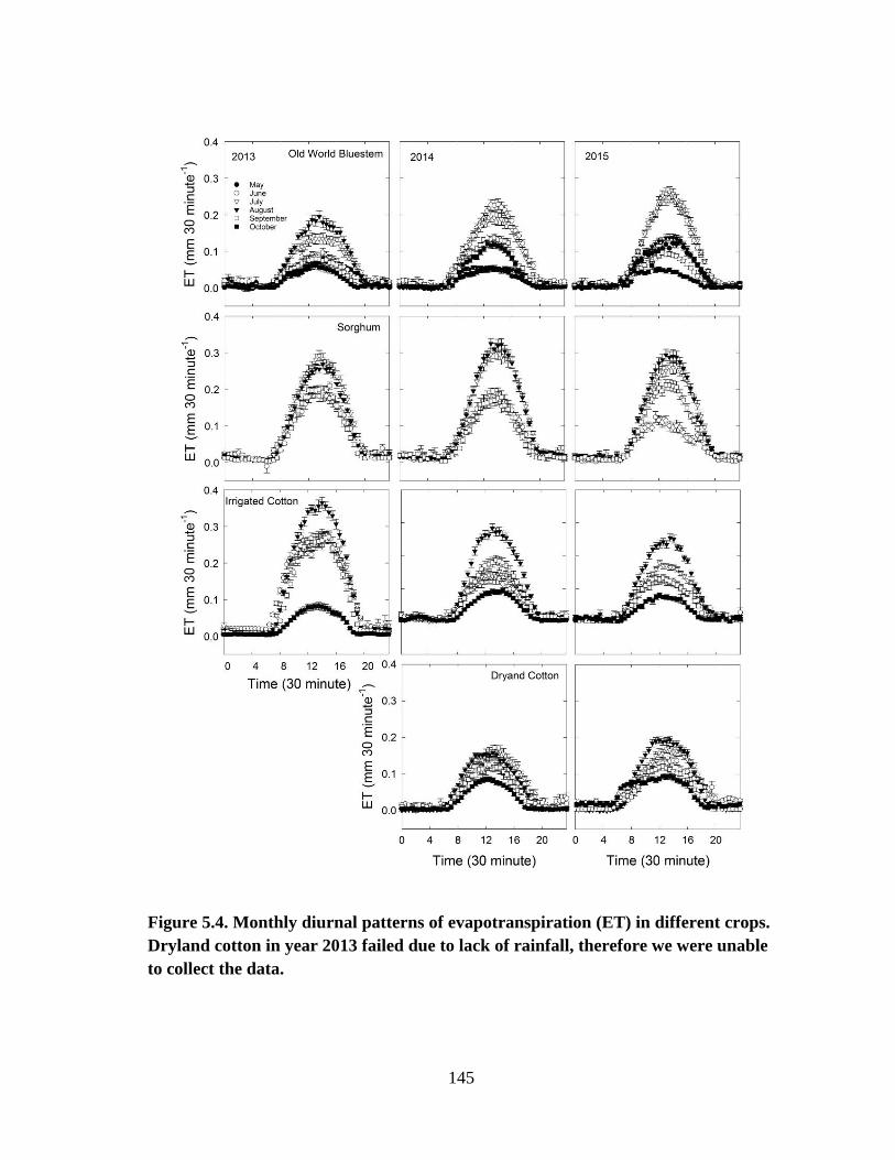
145

Figure 5.4. Monthly diurnal patterns of evapotranspiration (ET) in different crops.

Dryland cotton in year 2013 failed due to lack of rainfall, therefore we were unable

to collect the data.

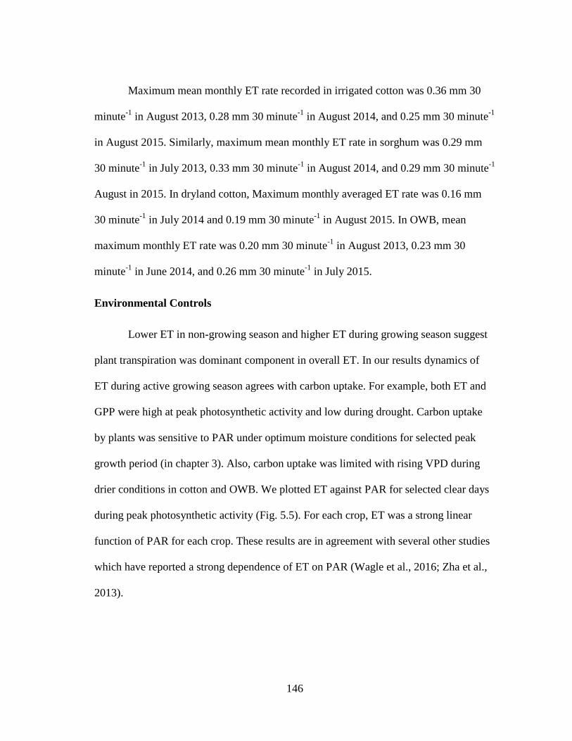
146

Maximum mean monthly ET rate recorded in irrigated cotton was 0.36 mm 30

minute-1

in August 2013, 0.28 mm 30 minute-1

in August 2014, and 0.25 mm 30 minute-1

in August 2015. Similarly, maximum mean monthly ET rate in sorghum was 0.29 mm

30 minute-1

in July 2013, 0.33 mm 30 minute-1

in August 2014, and 0.29 mm 30 minute-1

August in 2015. In dryland cotton, Maximum monthly averaged ET rate was 0.16 mm

30 minute-1

in July 2014 and 0.19 mm 30 minute-1

in August 2015. In OWB, mean

maximum monthly ET rate was 0.20 mm 30 minute-1

in August 2013, 0.23 mm 30

minute-1

in June 2014, and 0.26 mm 30 minute-1

in July 2015.

Environmental Controls

Lower ET in non-growing season and higher ET during growing season suggest

plant transpiration was dominant component in overall ET. In our results dynamics of

ET during active growing season agrees with carbon uptake. For example, both ET and

GPP were high at peak photosynthetic activity and low during drought. Carbon uptake

by plants was sensitive to PAR under optimum moisture conditions for selected peak

growth period (in chapter 3). Also, carbon uptake was limited with rising VPD during

drier conditions in cotton and OWB. We plotted ET against PAR for selected clear days

during peak photosynthetic activity (Fig. 5.5). For each crop, ET was a strong linear

function of PAR for each crop. These results are in agreement with several other studies

which have reported a strong dependence of ET on PAR (Wagle et al., 2016; Zha et al.,

2013).

147

Figure 5.5. Relationship between evapotranspiration (ET) and photosynthetically

active radiation (PAR) for (a) sorghum, (b) old world bluestem (c) irrigated cotton

(d) dryland cotton. Three-five consecutive clear days were selected during peak

photosynthetic activity of growing season in 2013 (grey line), 2014 (dashed line),

and 2015 (solid black line). Phenological stage was similar for each crop and soil

moisture was > 0.20 m3 m

-3. Each crop displayed peak photosynthetic activity

during the selected period. All relationships were significantly linear (p<0.0001).

All the R2 values ranged from 0.88 to 0.94.

Water Use Efficiency

Water use efficiency calculated through different approaches is presented in

Table 5.3. Ecosystem water use efficiency was comparable for each crop during all three

148

growing seasons. Sorghum (3.2-3.4 g C kg-1

H2O) and OWB (2.7-2.9 g C kg-1

H2O)

being C4 plants registered greater seasonal EWUE followed by irrigated cotton (1.6-2.1

g C kg-1

H2O) and dryland cotton (1.3-1.5 g C kg-1

H2O). Our values of EWUE for

sorghum are greater than those for rainfed sorghum (2.5 g C kg-1

H2O) reported by

Wagle et al. (2016) in Oklahoma, but lower than EWUE of 3.8 g C kg-1

H2O corn

reported by Abraha et al. (2016) in Illinois. Ecosystem water use efficiency of OWB was

lower than that of 3.3 to 4.1 g C kg-1

H2O reported by Skinner and Adler (2010) for

switchgrass in northeast United States, 3.6 to 3.8 g C kg-1

H2O observed by Eichelmann

et al. (2016) in Canada, and 3.1 g C kg-1

H2O by Abraha et al. (2016). Lower EWUE of

OWB in comparison to switchgrass in our study than the studies conducted in northern

latitudes could be attributed to lower temperatures and VPD which lead to lower ET for

equal amount of carbon uptake in Northern latitudes (Eichelmann et al., 2016).

However, these values of EWUE fall within the range of 2.5-3.1 g C kg-1

H2O observed

by Wagle et al (2016) for switchgrass in Oklahoma. The EWUE of all the crops in our

study fall within the range of EWUE reported by Beer et al. (2009) (2.1-4.4 g C H2O) for

grasslands and croplands. Comparable EWUE of OWB to switchgrass under similar

environmental conditions (Wagle et al., 2016) suggests similar ecosystem productivity

of OWB to switchgrass. This finding is important as similar ecosystem productivity

suggests relatively equal sustainability of OWB in comparison to switchgrass in the

Southern Great Plains in terms of water use efficiency. Also, it should be noticed that

growing season length of the switchgrass in Wagle et al.’s (2016) study was at least a

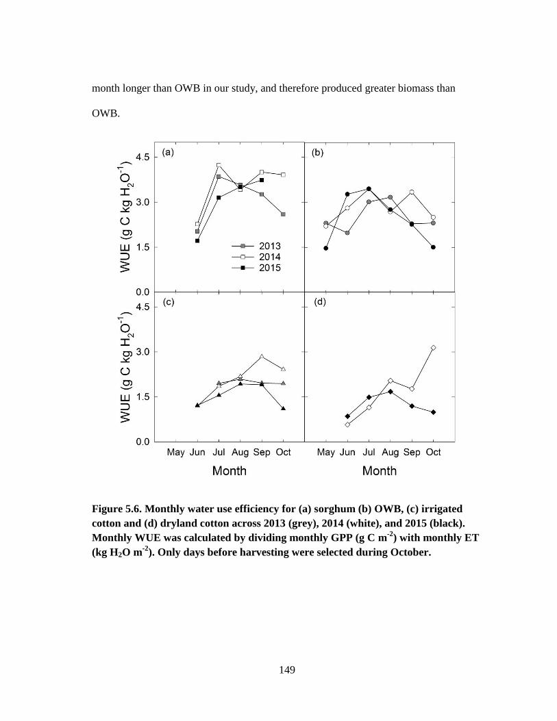
149

month longer than OWB in our study, and therefore produced greater biomass than

OWB.

Figure 5.6. Monthly water use efficiency for (a) sorghum (b) OWB, (c) irrigated

cotton and (d) dryland cotton across 2013 (grey), 2014 (white), and 2015 (black).

Monthly WUE was calculated by dividing monthly GPP (g C m-2

) with monthly ET

(kg H2O m-2

). Only days before harvesting were selected during October.

150

Monthly EWUE are provided in Fig. 5.6. It should be noticed that only those

days were used of the last month when the crop (row crops) was still standing. Peak

monthly EWUE for sorghum was observed in July in 2013 and 2014, and in September

2015. Irrigated cotton recorded highest EWUE in August in 2013 and 2015, and in

September in 2014. In OWB, EWUE was highest during August in 2013 and in June in

2014 and 2015. In OWB, EWUE was smaller during dry month of June in 2013, and

August 2014 and 2015. Dryland cotton registered highest monthly EWUE in August of

2014 and 2015. Ecosystem water use efficiency observed in final month of growing

season was either comparable or higher than first month of growing season. These

findings are in consistence with those of Wagle et al. (2014) and Skinner and Adler

(2010) who reported greater EWUE towards the end of the season due to reduced ET.

Once calculated the mean monthly EWUE was comparable to seasonal EWUE for the

corresponding growing season in all crops.

The monthly WUE irrespective of the crop showed the trade-off between carbon

uptake and ET, as ET was higher during high carbon uptake and low during low carbon

uptake in all the crops (Vanloocke et al., 2010). Basically, months with lower GPP had

lower WUE. This suggests while GPP declined during dry months, while ET did not

decline. We plotted selected clear days from OWB, dryland cotton, and irrigated cotton

from dry periods (Fig. 5.7). Normalized GPP values of these days were plotted against

VPD on a logarithmic scale. The results showed that GPP declined after certain value of

rising VPD (around 9:30 am, see chapter 3), however, ET remained high throughout this

period. This suggests GPP is more likely to be affected by VPD then ET. Similar results

151

have been observed by Cabral et al. (2013) for C3 and C4 crops and Rana et al. (2016)

for canary grass. The possible reason behind this could be added evaporation from soil

and transpiration from cuticle during stomatal closure (Cabral et al., 2013).

Figure 5.7. Relationship of normalized evapotranspiration (ET) and normalized

gross primary production (GPP) with vapor pressure deficit (VPD). Clear days

during dry period were selected for this analysis (DOY 256-260 in 2015 for both

irrigated and dryland cotton; DOY 224-227 in 2014 for dryland cotton). ET was a

significant logarithmic function of VPD for all crops (R2 = 0.67, 0.69 and 0.32 for

irrigated, dryland cotton, and OWB respectively). GPP was not a strong function of

VPD, except in dryland cotton (R2=0.24).

152

Table 5.3. Seasonal ecosystem water use efficiency for different crops during

different study years. Year 2013 does not represent the full cropping season for

Irrigated Cotton as the data collection started about a month after planting.

Year Sorghum OWB Irrigated Cotton Dryland Cotton

2013 3.2 2.7 2.0 -

2014 3.4 3.0 2.2 1.5

2015 3.2 2.8 1.7 1.3

Instantaneous water use efficiency calculated by obtaining linear relationships

between monthly integrals of GPP and monthly integrals of ET across all growing

season. Coefficient of determination and slope of each linear relation ranged from 0.82-

0.97. Slope of this relationship represents the overall mean EWUE. Among all the crops,

sorghum (4.5 g C kg-1

H2O) registered highest slope followed by OWB (3.8 g C kg-1

H2O), irrigated cotton (1.99 g C kg-1

H2O), and dryland cotton (1.4 g C kg-1

H2O). Water

use efficiency of both sorghum and OWB was close, but greater than cotton. Being C4

plants sorghum and OWB have physiological advantages in terms of WUE.

ET vs Rainfall

Cumulative seasonal and annual ET data is presented in Table 5.1. Despite

shorter growing season, annual row crops, especially irrigated crops registered higher

seasonal ET than perennial grassland. Irrigated crops registered highest seasonal ET due

to heavy irrigation during 2013 growing season followed by OWB. In 2014, sorghum

registered highest seasonal ET, followed by irrigated cotton, OWB and dryland cotton.

Old world bluestem registered highest seasonal ET in 2015, among all the crops. In

general, seasonal ET of both irrigated crops was greater than seasonal rainfall. Greater

153

seasonal ET in OWB than dryland cotton was observed in both years, which could be

attributed to longer growing season of OWB. Among non-irrigated crops, the share of

ET in OWB was always lower than cumulative rainfall, than the share of ET in dryland

cotton, which released similar or higher share of precipitation to atmosphere.

Similar to higher seasonal ET than seasonal precipitation in dryland cotton

suggests most of the precipitation in dryland cotton crop was returned back to

atmosphere through ET, leaving smaller portion of water available for groundwater

recharge and runoff (Zeri et al., 2013). Although, determining surface runoff and

drainage was beyond the scope of this study, previous researches have reported better

infiltration capacity of water under established perennial grasslands than annual

croplands due to improved soil health and percolation (Le et al., 2011; Bonin et al.,

2012; Chen et al., 2016). This finding is in good terms with those reported by Chen et

al., (2016) using model simulations for the South High Plains. Chen et al. (2016)

reported improved annual percolation under land use change scenario where annual

crops (cotton) are replaced with perennial (switchgrass) crops. This key finding from this

research is important for future agricultural policies in the area, which will largely

depend upon the status and recharge water table of the Ogallala aquifer.

In contrast, irrigated crops had higher seasonal and annual ET than seasonal and

annual rainfall in first two years of study, respectively. The annual ET was lower in the

2015 for both irrigated crops but was still greater than average long term annual

precipitation. Several researches have reported modification of climate with rising ET.

For example, higher precipitation, lower temperatures, and an increase in thunderstorm

154

activity was reported following 120% rise in ET after conversion of croplands to steppe

in Colorado (Pielke et al., 1998; Baron et al. 1998). Kueppers et al. (2007) reported

reduction in air temperature due to enhanced evapotranspiration with increase in

irrigation intensity in California. These findings suggest higher ET from irrigated

sorghum may have significant implications to local weather patterns, in case irrigated

sorghum replaces conventional cotton cropping systems. A similar conclusion can be

made for irrigated cotton. However, with declining water table and regulation imposed

by regulatory agencies in the high plains will be critical in shaping future scenario.

CONCLUSION

Seasonal and annual energy fluxes, evapotranspiration, and water use efficiency

at different scale was quantified for four different cropping systems during three

different growing seasons. All years received annual rainfall similar to or higher than

long-term annual rainfall. Energy partitioning was dominated by H during non-growing

season in all cropping systems. Latent heat consistently dominated the energy

partitioning in row crops during active growing season. Rainfall distribution and soil

moisture played an important role in energy dispersal among H and LE in OWB. Ground

heat flux remained a minor energy flux component during growing and non-growing

season although some of the data was lost in non-growing season in row crops.

Our findings show greater productivity (EWUE) of the bioenergy systems over

conventional cotton cropping system. The EWUE values of bioenergy crops in our study

were in agreement with those reported for specific bioenergy crops in other studies.

Greater productivity suggests higher sustainability of the bioenergy cropping systems

155

than cotton. However, due to irrigation sorghum crop shared higher seasonal and annual

ET than seasonal and annual rainfall, respectively. Similarly, dryland cotton shared

almost similar or higher seasonal ET than the seasonal rainfall. In contrast, seasonal and

annual ET of OWB was lower than seasonal and annual rainfall. These findings suggest,

OWB has potential of greater percolation and water conservation due to improved soil

conditions and insulation provided by litter, whereas dryland cotton has potential to draw

water from deeper layers. Long-term effects of these findings need further investigation,

as the region of this study is susceptible to periodic droughts, which were absent during

the period of this study.

156

CHAPTER VI

SUMMARY AND CONCLUSION

Current legislative and regulatory mandates aiming at reducing dependence on

foreign oil imports has driven the rising bioenergy crops production in the United States.

The Southern Great Plains have potential to grow bioenergy crops, however the

implication of large scale production of bioenergy crops on carbon, energy and

evapotranspiration (ET) balances of the region are not understood. Therefore, a study

was conducted to assess and compare the carbon, ET and energy balance dynamics of

two potential bioenergy crops with conventional cotton cropping system in the Southern

Great Plains. Sorghum was the potential candidate of annual bioenergy crop and Old

World Bluestem (OWB) was the perennial bioenergy crop. These crops were compared

with irrigated and dryland cotton in the region. All the crops were managed by producers

which gave us an opportunity to conduct research in standard production conditions

followed in the region. Sorghum was irrigated while OWB remained dryland. The

producer practiced annual crop rotation between irrigated cotton and sorghum on

adjacent fields. Continuous measurement of carbon dioxide, ET and energy fluxes were

made in each field using eddy covariance systems. In addition, meteorological variables

157

including rainfall, air temperature, photosynthetically active radiation, soil temperature,

soil moisture, net radiation, soil heat flux, relative humidity, and vapor pressure deficit.

All crops were net sinks of carbon at seasonal scale. Being C4 plants, bioenergy crops

exhibited higher growth rates and greater carbon uptake potential than irrigated and

dryland cotton, which is a C3 plant. Among the bioenergy crops, sorghum recorded

greater carbon uptake than OWB at seasonal scale. This was also manifested in greater

maximum above ground biomass production in sorghum (18-25 tons ha-1

) than OWB (7-

10 tons ha-1

). Irrigated cotton on the other hand, was a greater sink of carbon in 2013

due to higher irrigation levels in that year, while it remained a weak sink in 2014 and

2015. Previous crop’s residues contributed towards greater carbon release from the soil

which reduced the net carbon uptake. Dryland cotton field failed in 2013 due to extended

dry conditions during early months of growth, however field was a weak sink in 2014

and 2015 growing seasons.

On annual scale, sorghum was stronger (-445 g C m-2

) sink in 2014 while it

remained a weak sink (-51 g C m-2

) in 2015. Irrigated cotton remained a net source of

carbon (101 g C m-2

in 2014 and 123 g C m-2

in 2015) on annual scale, while dryland

cotton was a net sink in 2014 (-19 g C m-2

) and a net source (59 g C m-2

) in 2015. In

contrast OWB remained most consistent carbon sink throughout the study, with annual

net carbon uptake ranging from -301 g C m-2

in 2013 to -266 g C m-2

in 2014. Non-

growing season carbon release to atmosphere was higher in 2015 in comparison to 2014,

due to relatively wetter winter in 2015, which may have triggered higher heterotrophic

respiration in 2015 with rising temperature. This explains the lower sinking capacity of

158

the row crops in 2015 which led to lower annual carbon sinking capacity in row crops

than in 2014. Similar, observations were noticed in OWB, greater carbon uptake in 2015

following higher rainfall kept the net carbon sinking of field comparable to other two

years. As such, OWB remained the most stable carbon sink among all the crops in this

study.

The available energy (net radiation) distributed among soil heat flux, latent heat

and sensible heat. Across all the cropping systems, major part of the energy was

distributed among latent heat and sensible heat. Latent heat represents energy lost for

system in form of water and sensible heat represent the energy lost to atmosphere in

form of heat. Apparently, latent heat dominated the energy partitioning in sorghum and

irrigated cotton, as crops were irrigated regularly. In contrast, the energy partitioning

switched from latent heat to sensible heat in OWB during dry periods of the growing

season. Such, patterns were not noticed dryland cotton during dry periods. This

suggested that dryland cotton had access to water in deeper layers during dry period.

Finally, ET of irrigated crops was higher than those of dryland systems. When compared

with seasonal and annual rainfall, irrigated crops had higher ET than cumulative

seasonal and annual rainfall. Dryland cotton had evaporation higher or equivalent to

seasonal rainfall, while OWB registered lower ET in comparison to seasonal rainfall.

Evapotranspiration in dryland cotton was higher during dry period than OWB. This

suggests that dryland cotton may have accesed the water in deeper soil layers during dry

period. Although no runoff measurements were made in the fields, we speculate the

balance of water in OWB may have percolated in the soil indicating groundwater

159

recharging capcity of perennial bioenergy crop. On annual scale both dryland cotton and

OWB registered lower ET than annual rainfall. Further, we calculated ecosystem water

use efficiency (EWUE) of all the crops. Sorghum registered highest EWUE (ratio of

seasonal gross primary production to seasonal ET) ranging from 3.2-3.4 g C kg-1

water,

followed OWB (2.7-3.0 g C kg-1

water), irrigated cotton (1.7-2.2 g C kg-1

water) and

dryland cotton (1.3-1.5 g C kg-1

water).

From the assessment of inter-annual and seasonal on-site carbon, ET and energy budget

of all the these crops wecan make following conclusions.

1. Photosynthetic activity of sorghum are considerably affected by phenology (row

spacing and LAI) and growing season length.

2. Higher growth rates of bioenergy crops make them robust on-site carbon sinks at

seasonal as well as annual time scales in comparison to irrigated cotton cropping

system, which was source of carbon at both scales. Dryland cotton cropping

system can switch between sink and source depending upon climatic factors.

Therefore, land use change induced by bioenergy crops may be more sustainable

in terms of carbon budget than cotton cropping systems.

3. Among bioenergy crops, sorghum had higher annual net carbon uptake (net

ecosystem exchange) than OWB in 2014 and lower in 2015. These findings

suggest that annual net ecosystem exchange of sorghum will be more sensitive to

non-growing season carbon dynamics than OWB, NEE of dryland OWB will be

more sensitve to magnitude and timing of precipitation. Also, inherited benefits

of perennial OWB in terms of no-tillage and no nutrient application may add to

160

the benefits and sustainability of the system. However, sorghum will provide

greater biofuel feedstock than OWB.

4. Water use efficiency of bioenergy crops was higher than those of cotton,

indicating higher sustainability in bioenergy crops than cotton. Higher

sustainability of bioenergy crops may be beneficial in the long run in terms of

value of water spent on these crops.

5. Higher ET from sorghum and irrigated cotton than rainfall may not only have

significant implications on future climate, but may also be detrimental for the

Ogallala Aquifer. On the other hand, lower ET in OWB than cumulative rainfall

is likely to enhance water recharging capacity of soils in the Southern Great

Plains.

6. Higher seasonal ET in comparison to seasonal rainfall in dryland cotton than

OWB, indicated that dryland cotton had access to water from deeper layers.

161

REFERENCES

Abraha, M., I. Gelfand, S.K. Hamilton, C.L. Shao, Y.J. Su, G.P. Robertson, et al. 2016.

Ecosystem water-use efficiency of annual corn and perennial grasslands:

contributions from land-use history and species composition. Ecosystems

19:1001-1012. doi:10.1007/s10021-016-9981-2

Acosta-Martinez, V., G. Burow, T.M. Zobeck and V.G. Allen. 2010. Soil microbial

communities and function in alternative systems to continuous cotton. Soil Sci.

Soc. Am. J. 74:1181-1192. doi:10.2136/sssaj2008.0065

Adler, P.R., S.J. Del Grosso and W.J. Parton. 2007. Life-cycle assessment of net

greenhouse-gas flux for bioenergy cropping systems. Ecol. Appl. 17:675-691.

doi:10.1890/05-2018

Allen, V.G., C.P. Brown, R. Kellison, E. Segarra, T. Wheeler, P.A. Dotray et al. 2005.

Integrating cotton and beef production to reduce water withdrawal from the

Ogallala Aquifer in the Southern High Plains. Agron. J. 97:556-567.

doi:10.2134/agronj2005.0556

Allen, V.G., C.P. Brown, E. Segarra, C.J. Green, T.A. Wheeler, V. Acosta-Martinez, et

al. 2008. In search of sustainable agricultural systems for the Llano Estacado of

the U.S. Southern High Plains. Agric Ecosyst Environ. 124:3-12.

doi:10.1016/j.agae.2007.08.006

162

Anderson-Teixeira, K.J., M.D. Masters, C.K. Black, M. Zeri, M.Z. Hussain, C.J.

Bernacchi, et al. 2013. Altered belowground carbon cycling following land-use

change to perennial bioenergy crops. Ecosystems 16:508-520.

doi:10.1007/s10021-012-9628-x

Andrade, F.H., P. Calvino, A. Cirilo and P. Barbieri. 2002. Yield responses to narrow

rows depend on increased radiation interception. Agron. J. 94:975-980

Atabani, A.E., I.A. Badruddin, H.H. Masjuki, W.T. Chong, T.M.I. Mahlia and K.T. Lee.

2013. Investigation of physical and chemical properties of potential edible and

non-edible feedstocks for biodiesel production, a comparative analysis. Renew.

Sust. Energ. Rev. 21:749-755. doi:10.1016/j.rser.2013.01.027

Attia, A., N. Rajan, G. Ritchie, S. Cui, A. Ibrahim, D. Hays, et al. 2015. Yield, quality,

and spectral reflectance responses of cotton under subsurface drip irrigation.

Agron. J. 107:1355-1364. doi:10.2134/agronj14.0502

Aubinet, M., A. Grelle, A. Ibrom, U. Rannik, J. Moncrieff, T. Foken, et al. 2000.

Estimates of the annual net carbon and water exchange of forests: The

EUROFLUX methodology. Adv. Ecol. Res. 30:113-175

Baldocchi, D., E. Falge, L.H. Gu, R. Olson, D. Hollinger, S. Running, et al. 2001.

FLUXNET: A new tool to study the temporal and spatial variability of

ecosystem-scale carbon dioxide, water vapor, and energy flux densities. Bull.

163

Amer. Meteor. Soc. 82:2415-2434. doi:10.1175/1520-

0477(2001)082<2415:fantts>2.3.co;2

Baldocchi, D.D. 2003. Assessing the eddy covariance technique for evaluating carbon

dioxide exchange rates of ecosystems: past, present and future. Glob. Change

Biol. 9:479-492. doi:10.1046/j.1365-2486.2003.00629.x

Bange, M.P., G.L. Hammer and K.G. Rickert. 1997. Effect of specific leaf nitrogen on

radiation use efficiency and growth of sunflower. Crop Sci. 37:1201-1208

Barbieri, P.A., H. Echeverria, H. Sainz Rozas, and F.H. Andrade. 2008. Nitrogen use

efficiency in maize as affected by nitrogen availability and row spacing effects at

different levels of nitrogen availability and row spacing. Agron. J. 100:1094-

1100. doi:10.2134/agronj2006.0057.

Barbieri, P., L. Echarte, A. Della Maggiora, V.O. Sadras, H. Echeverria and F.H.

Andrade. 2012. Maize evapotranspiration and water-use efficiency in response to

row spacing. Agron. J. 104:939-944. doi:10.2134/agronj2012.0014

Baron, J.S., M.D. Hartman, T.G.F. Kittel, L.E. Band, D.S. Ojima and R.B. Lammers.

1998. Effects of land cover, water redistribution, and temperature on ecosystem

processes in the South Platte Basin. Ecol. Appl. 8:1037-1051.

doi:10.2307/2640959

164

Beer, C., P. Ciais, M. Reichstein, D. Baldocchi, B.E. Law, D. Papale, et al. 2009.

Temporal and among-site variability of inherent water use efficiency at the

ecosystem level. Glob. Biogeochem. Cycles 23:13. doi:10.1029/2008gb003233

Berg, W.A. 1990. Old-world bluestem responses to nitrogen-fertilization. J. Range

Manage. 43:265-270. doi:10.2307/3898687

Berg, W.A. and P.L. Sims. 1995. Nitrogen-fertilizer use efficiency in steer gain on old-

world bluestem. J. Range Manage. 48:465-469. doi:10.2307/4002254

Berndes, G. 2002. Bioenergy and water - the implications of large-scale bioenergy

production for water use and supply. Glob. Environ. Change-Human Policy

Dimens. 12:253-271. doi:10.1016/s0959-3780(02)00040-7

Blanco-Canqui, H. and R. Lal. 2008. No-tillage and soil-profile carbon sequestration: An

on-farm assessment. Soil Sci. Soc. Am. J. 72:693-701.

doi:10.2136/sssaj2007.0233

Blum A., and G.F. Arkin. 1984. Sorghum root growth and water-use as affected by

water supply and growth duration. Field Crops Res. 9:131-142.

Boehmel, C., I. Lewandowski and W. Claupein. 2008. Comparing annual and perennial

energy cropping systems with different management intensities. Agric. Sys.

96:224-236. doi:10.1016/j.agsy.2007.08.004

Bonin, C., R. Lal, M. Schmitz and S. Wullschleger. 2012. Soil physical and hydrological

properties under three biofuel crops in Ohio. Acta Agriculturae Scandinavica

165

Section B-Soil and Plant Science 62:595-603.

doi:10.1080/09064710.2012.679309

Bucholtz, D.L., R.P. Cantrell, J.D. Axtell and V.L. Lechtenberg. 1980. Lignin

biochemistry of normal and brown midrib mutant sorghum. J. Agr. Food Chem.

28:1239-1241. doi:10.1021/jf60232a045

Burba, G.G. and S.B. Verma. 2005. Seasonal and interannual variability in

evapotranspiration of native tallgrass prairie and cultivated wheat ecosystems.

Agric. For. Meteorol. 135:190-201. doi:10.1016/j.agrformet.2005.11.017

Burke, I.C., C.M. Yonker, W.J. Parton, C.V. Cole, K. Flach and D.S. Schimel. 1989.

Texture, climate, and cultivation effects on soil organic-matter content in us

grassland soils. Soil Sci. Soc. Am. J. 53:800-805

Buttrey, E.K., B.W. Bean, F.T. McCollum III, R.E. Brandon, Q. Xue and T.H. Marek.

2011. Yield, water use efficiency, and nutritive value of six warm-season

perennial grasses in response to irrigation level. Forag. Grazingl. 9.

doi:10.1094/fg-2011-1021-01-rs

Cabral, O.M.R., H.R. Rocha, J.H. Gash, M.A.V. Ligo, N.P. Ramos, A.P. Packer, et al.

2013. Fluxes of CO2 above a sugarcane plantation in Brazil. Agric. For.

Meteorol. 182:54-66. doi:10.1016/j.agrformet.2013.08.004

166

Campioli, M., S. Vicca, S. Luyssaert, J. Bilcke, E. Ceschia, F.S. Chapin III et al. 2015.

Biomass production efficiency controlled by management in temperate and

boreal ecosystems. Nat. Geosci. 8:843-846. doi:10.1038/ngeo2553

Carpita, N.C. and M.C. McCann. 2008. Maize and sorghum: genetic resources for

bioenergy grasses. Trends Plant Sci. 13:415-420.

doi:10.1016/j.tplants.2008.06.002

Chandel A.K., O.V. Singh, G. Chandrasekhar, V. Rao, and M.L. Narasu. .2010. Key

drivers influencing the commercialization of ethanol-based refineries. J.

Commerc. Biotechnol. 16:239-257.

Chen, J.M. and T.A. Black. 1992. Defining leaf-area index for non-flat leaves. Plant Cell

Environ. 15:421-429. doi:10.1111/j.1365-3040.1992.tb00992.x

Chen, Y., S. Ale, N. Rajan, C.L.S. Morgan and J. Park. 2016. Hydrological responses of

land use change from cotton (Gossypiumhirsutum L.) to cellulosic bioenergy

crops in the Southern High Plains of Texas, USA. GCB Bioenergy 8:981-999.

doi:10.1111/gcbb.12304

Cherney, J.H., D.J.R. Cherney, D.E. Akin and J.D. Axtell. 1991. Potential of brown-

midrib, low-lignin mutants for improving forage quality. Adv. Agron. 46:157-

198

Cherubini, F., N.D. Bird, A. Cowie, G. Jungmeier, B. Schlamadinger and S. Woess-

Gallasch. 2009. Energy- and greenhouse gas-based LCA of biofuel and

167

bioenergy systems: Key issues, ranges and recommendations. Resour. Conserv.

Recycl. 53:434-447. doi:10.1016/j.resconrec.2009.03.013

Choncubhair, O.N., B. Osborne, J. Finnan and G. Lanigan. 2017. Comparative

assessment of ecosystem C exchange in Miscanthus and reed canary grass during

early establishment. GCB Bioenergy 9:280-298. doi:10.1111/gcbb.12343

Claussen, M., V. Brovkin and A. Ganopolski. 2001. Biogeophysical versus

biogeochemical feedbacks of large-scale land cover change. Geophys. Res. Lett.

28:1011-1014. doi:10.1029/2000gl012471

Cook, B.D., K.J. Davis, W.G. Wang, A. Desai, B.W. Berger, R.M. Teclaw, et al. 2004.

Carbon exchange and venting anomalies in an upland deciduous forest in

northern Wisconsin, USA. Agric. For. Meteorol. 126:271-295.

doi:10.1016/j.agrformet.2004.06.008

Corredor, D.Y., J.M. Salazar, K.L. Hohn, S. Bean, B. Bean and D. Wang. 2009.

Evaluation and characterization of forage sorghum as feedstock for fermentable

sugar production. Appl. Biochem. Biotechnol. 158:164-179. doi:10.1007/s12010-

008-8340-y

Cotton, J., V. Acosta-Martinez, J. Moore-Kucera and G. Burow. 2013. Early changes

due to sorghum biofuel cropping systems in soil microbial communities and

metabolic functioning. Biol. Fertil. Soils 49:403-413. doi:10.1007/s00374-012-

0732-z

168

Cotton, J., G. Burow, V. Acosta-Martinez and J. Moore-Kucera. 2013b. Biomass and

cellulosic ethanol production of forage sorghum under limited water conditions.

Bioenerg. Res. 6:711-718. doi:10.1007/s12155-012-9285-0

Cowie, A.L., P. Smith and D. Johnson. 2006. Does soil carbon loss in biomass

production systems negate the greenhouse benefits of bioenergy? Mitig. Adapt.

Strateg. Glob. Chang. 11:979-1002. doi:10.1007/s11027-006-9030-0

Craine, J.M., D.A. Wedin and F.S. Chapin. 1999. Predominance of ecophysiological

controls on soil CO2 flux in a Minnesota grassland. Plant Soil 207:77-86

Davidson, E.A., E. Belk and R.D. Boone. 1998. Soil water content and temperature as

independent or confounded factors controlling soil respiration in a temperate

mixed hardwood forest. Glob. Change Biol. 4:217-227. doi:10.1046/j.1365-

2486.1998.00128.x

Dalrymple, R.L. 1991. Old World Bluestem stand establishment ad first year production

management. Oklahoma Coop. Ext. Service, Circuar E, 17-44. Noble

Foundation, Ardmore, OK.

de Fraiture, C., M. Giordano and Y.S. Liao. 2008. Biofuels and implications for

agricultural water use: blue impacts of green energy. Water Policy 10:67-81.

doi:10.2166/wp.2008.054

Delucchi, M.A. 2010. Impacts of biofuels on climate change, water use, and land use.

Ann. N.Y. Acad. Sci. 1195:28-45. doi:10.1111/j.1749-6632.2010.05457.x

169

Dien, B.S., G. Sarath, J.F. Pedersen, S.E. Sattler, H. Chen, D.L. Funnell-Harris, et al.

2009. Improved sugar conversion and ethanol yield for forage sorghum

(Sorghum bicolor L. Moench) lines with reduced lignin contents. Bioenerg. Res.

2:153-164. doi:10.1007/s12155-009-9041-2

Drouet, J.L. and J.R. Kiniry. 2008. Does spatial arrangement of 3D plants affect light

transmission and extinction coefficient within maize crops? Field Crop. Res.

107:62-69. doi:10.1016/j.fcr.2007.12.015

Eichelmann, E., C. Wagner-Riddle, J. Warland, B. Deen and P. Voroney. 2016. Carbon

dioxide exchange dynamics over a mature switchgrass stand. GCB Bioenergy

8:428-442. doi:10.1111/gcbb.12259

Falge, E., D. Baldocchi, R. Olson, P. Anthoni, M. Aubinet, C. Bernhofer, et al. 2001.

Gap filling strategies for defensible annual sums of net ecosystem exchange.

Agric. For. Meteorol. 107:43-69. doi:10.1016/s0168-1923(00)00225-2

Fargione, J., J. Hill, D. Tilman, S. Polasky and P. Hawthorne. 2008. Land clearing and

the biofuel carbon debt. Science 319:1235-1238. doi:10.1126/science.1152747

Fargione, J.E., T.R. Cooper, D.J. Flaspohler, J. Hill, C. Lehman, T. McCoy, et al. 2009.

Bioenergy and wildlife: Threats and opportunities for grassland conservation.

Bioscience 59:767-777. doi:10.1525/bio.2009.59.9.8

170

Fargione, J.E., R.J. Plevin and J.D. Hill. 2010. The ecological impact of biofuels. In: D.

J. Futuyma, H. B. Shafer and D. Simberloff, editors, Annual Review of Ecology,

Evolution, and Systematics, Vol 41. Annual Reviews, Palo Alto. p. 351-377.

Flanagan, L.B., L.A. Wever and P.J. Carlson. 2002. Seasonal and interannual variation

in carbon dioxide exchange and carbon balance in a northern temperate

grassland. Glob. Change Biol. 8:599-615. doi:10.1046/j.1365-2486.2002.00491.x

Flanagan, L.B. and B.G. Johnson. 2005. Interacting effects of temperature, soil moisture

and plant biomass production on ecosystem respiration in a northern temperate

grassland. Agric. For. Meteorol. 130:237-253.

doi:10.1016/j.agrformet.2005.04.002

Foken, T. 2008. The energy balance closure problem: An overview. Ecol. Appl.

18:1351-1367. doi:10.1890/06-0922.1

Foken T., M. Aubinet, and R. Leuning . 2012. The eddy covariance method. In: M.

Aubinet, T. Vesala, D. Papale, editors, Eddy Covariance. Springer, Netherlands.

p. 1-19.

Franzluebbers, A.J., R.L. Haney, C.W. Honeycutt, H.H. Schomberg and F.M. Hons.

2000. Flush of carbon dioxide following rewetting of dried soil relates to active

organic pools. Soil Sci. Soc. Am. J. 64:613-623

Gelfand, I., T. Zenone, P. Jasrotia, J.Q. Chen, S.K. Hamilton and G.P. Robertson. 2011.

Carbon debt of Conservation Reserve Program (CRP) grasslands converted to

171

bioenergy production. P. Natl. Acad. Sci. Usa. 108:13864-13869.

doi:10.1073/pnas.1017277108

Gockede, M., T. Foken, M. Aubinet, M. Aurela, J. Banza, C. Bernhofer, et al. 2008.

Quality control of CarboEurope flux data - Part 1: Coupling footprint analyses

with flux data quality assessment to evaluate sites in forest ecosystems.

Biogeosciences 5:433-450

Gould, F.W., 1975. The grasses of texas. Texas A&M University Press, College Station,

Texas.

Goulden, M.L., J.W. Munger, S.M. Fan, B.C. Daube and S.C. Wofsy. 1996.

Measurements of carbon sequestration by long-term eddy covariance: Methods

and a critical evaluation of accuracy. Glob. Change Biol. 2:169-182.

doi:10.1111/j.1365-2486.1996.tb00070.x

Grabowski, J. 2000. Analysis of the potential for using Caucasian Blustem as a biofuel

crop in the Southeastern United States. Technial Report, USDA-NRCS.

Mississippi.

Green, T.R., M. Taniguchi, H. Kooi, J.J. Gurdak, D.M. Allen, K.M. Hiscock, et al. 2011.

Beneath the surface of global change: Impacts of climate change on groundwater.

J. Hydrol. 405:532-560. doi:10.1016/j.jhydrol.2011.05.002

172

Griffith, A.P., F.M. Epplin, S.D. Fuhlendorf, and R. Gillen. 2011. A comparison of

perennial polyculture and monocultures for producing biomass for biorefinery

feedstock. Agron. J. 103:617-627. doi:10.2134/agronj2010.0336

Gu, L.H., T. Meyers, S.G. Pallardy, P.J. Hanson, B. Yang, M. Heuer, et al. 2006. Direct

and indirect effects of atmospheric conditions and soil moisture on surface

energy partitioning revealed by a prolonged drought at a temperate forest site. J.

Geophys. Res.-Atmos. 111. doi:10.1029/2006jd007161

Hallam, A., I.C. Anderson and D.R. Buxton. 2001. Comparative economic analysis of

perennial, annual, and intercrops for biomass production. Biomass Bioenerg.

21:407-424. doi:10.1016/s0961-9534(01)00051-4

Ham, J.M. and J.L. Heilman. 2003. Experimental test of density and energy-balance

corrections on carbon dioxide flux as measured using open-path eddy covariance.

Agron. J. 95:1393-1403

Hao, B.Z., Q.W. Xue, B.W. Bean, W.L. Rooney and J.D. Becker. 2014. Biomass

production, water and nitrogen use efficiency in photoperiod-sensitive sorghum

in the Texas High Plains. Biomass Bioenerg. 62:108-116.

doi:10.1016/j.biombioe.2014.01.008

Harper, C.W., J.M. Blair, P.A. Fay, A.K. Knapp and J.D. Carlisle. 2005. Increased

rainfall variability and reduced rainfall amount decreases soil CO2 flux in a

173

grassland ecosystem. Glob. Change Biol. 11:322-334. doi:10.1111/j.1365-

2486.2005.00899.x

Havlin, J.L., D.E. Kissel, L.D. Maddux, M.M. Claassen and J.H. Long. 1990. Crop-

rotation and tillage effects on soil organic-carbon and nitrogen. Soil Sci. Soc.

Am. J. 54:448-452

Heaton, E., T. Voigt and S.P. Long. 2004. A quantitative review comparing the yields of

two candidate C-4 perennial biomass crops in relation to nitrogen, temperature

and water. Biomass Bioenerg. 27:21-30. doi:10.1016/j.biombioe.2003.10.005

Hickman, G.C., A. Vanloocke, F.G. Dohleman, and C. Bernacchi. 2010. A comparison

of canopy evpotranspiration for maize and two perennial grasses identified as

potential bioenergy crops. GCB Bioenergy 4:157-168. doi: 10.1111/j.1757-

1707.2010.01050.x

Howell, T.A., S.R. Evett, J.A. Tolk and A.D. Schneider. 2004. Evapotranspiration of

full-, deficit-irrigated, and dryland cotton on the northern Texas high plains. J.

Irrig. Drainage Eng-ASCE 130:277-285. doi:10.1061/(asce)0733-

9437(2004)130:4(277)

Humphreys, E.R., T.A. Black, G.J. Ethier, G.B. Drewitt, D.L. Spittlehouse, E.M. Jork, et

al. 2003. Annual and seasonal variability of sensible and latent heat fluxes above

a coastal Douglas-fir forest, British Columbia, Canada. Agric. For. Meteorol.

115:109-125. doi:10.1016/s0168-1923(02)00171-5

174

Hussain, M.Z., T. Grunwald, J.D. Tenhunen, Y.L. Li, H. Mirzae, C. Bernhofer, et al.

2011. Summer drought influence on CO2 and water fluxes of extensively

managed grassland in Germany. Agric. Ecosyst. Environ. 141:67-76.

Doi:10.1016/j.agae.2011.02.013

Huxman, T.E., J.M. Cable, D.D. Ignace, J.A. Eilts, N.B. English, J. Weltzin, et al. 2004.

Response of net ecosystem gas exchange to a simulated precipitation pulse in a

semi-arid grassland: the role of native versus non-native grasses and soil texture.

Oecologia 141:295-305. doi:10.1007/s00442-003-1389-y

Ise, T., C.M. Litton, C.P. Giardina and A. Ito. 2010. Comparison of modeling

approaches for carbon partitioning: Impact on estimates of global net primary

production and equilibrium biomass of woody vegetation from MODIS GPP. J.

Geophys. Res.-Biogeosci. 115. doi:10.1029/2010jg001326

Jackson, R.B., J. Canadell, J.R. Ehleringer, H.A. Mooney, O.E. Sala, E.D. Schulze.

1996. A global analysis of roots distributions for terrestrial biomes. Oecologia

108: 389-411

Janssens, I.A., H. Lankreijer, G. Matteucci, A.S. Kowalski, N. Buchmann, D. Epron, et

al. 2001. Productivity overshadows temperature in determining soil and

ecosystem respiration across European forests. Glob. Change Biol. 7:269-278.

doi:10.1046/j.1365-2486.2001.00412.x

175

Janssens, I.A. and K. Pilegaard. 2003. Large seasonal changes in Q(10) of soil

respiration in a beech forest. Glob. Change Biol. 9:911-918. doi:10.1046/j.1365-

2486.2003.00636.x

Jefferson, P.G. and W.P. McCaughey. 2012. Switchgrass (Panicum virgatum L.) cultivar

adaptation, biomass production, and cellulose concentration as affected by

latitude of origin. ISRN Agron. 2012. doi:10.5402/2012/763046

Johnson, E. 2009. Goodbye to carbon neutral: Getting biomass footprints right. Environ.

Impact Assess. Rev. 29:165-168. doi:10.1016/j.eiar.2008.11.002

Johnson, I.R. and J.H.M. Thornley. 1987. A model of shoot - root partitioning with

optimal-growth. Ann. Bot. 60:133-142

Karmakar, A., S. Karmakar and S. Mukherjee. 2010. Properties of various plants and

animals feedstocks for biodiesel production. Bioresour. Technol. 101:7201-7210.

doi:10.1016/j.biortech.2010.04.079

Kross, A., H. McNairn, D. Lapen, M. Sunohara and C. Champagne. 2015. Assessment

of RapidEye vegetation indices for estimation of leaf area index and biomass in

corn and soybean crops. Int. J. Appl. Earth Obs. Geoinf. 34:235-248.

doi:10.1016/j.jag.2014.08.002

Kueppers, L.M., M.A. Snyder, L.C. Sloan, D. Cayan, J. Jin, H. Kanamaru, et al. 2008.

Seasonal temperature responses to land-use change in the western United States.

Glob. Planet. Change 60:250-264. doi:10.1016/j.gloplacha.2007.03.005

176

Lal, R. 2004. Soil carbon sequestration to mitigate climate change. Geoderma 123:1-22.

doi:10.1016/j.geoderma.2004.01.032

Lasslop, G., M. Reichstein, D. Papale, A.D. Richardson, A. Arneth, A. Barr, et al. 2010.

Separation of net ecosystem exchange into assimilation and respiration using a

light response curve approach: critical issues and global evaluation. Glob.

Change Biol. 16:187-208. doi:10.1111/j.1365-2486.2009.02041.x

Law, B. 2007. AmeriFlux Network aids global synthesis. Eos Trans. AGU 88:286-286.

doi:10.1029/2007EO280003

Le, P.V.V., P. Kumar and D.T. Drewry. 2011. Implications for the hydrologic cycle

under climate change due to the expansion of bioenergy crops in the Midwestern

United States. P. Natl. Acad. Sci. Usa. 108:15085-15090.

doi:10.1073/pnas.1107177108

Lee, M.S., K. Nakane, T. Nakatsubo, W.H. Mo and H. Koizumi. 2002. Effects of rainfall

events on soil CO2 flux in a cool temperate deciduous broad-leaved forest. Ecol.

Res. 17:401-409. doi:10.1046/j.1440-1703.2002.00498.x

Lewandowski, I., J.M.O. Scurlock, E. Lindvall and M. Christou. 2003. The development

and current status of perennial rhizomatous grasses as energy crops in the US and

Europe. Biomass Bioenerg. 25:335-361. doi:10.1016/s0961-9534(03)00030-8

Li, C., L.M. Fultz, J. Moore-Kucera, V. Acosta-Martínez, J. Horita, R. Strauss, et al.

2017. Soil carbon sequestration potential in semi-arid grasslands in the

177

Conservation Reserve Program. Geoderma 294:80-90.

doi:http://dx.doi.org/10.1016/j.geoderma.2017.01.032

McLaughlin, S.J., D. Bouton, B. Bransby, W. Conger,D. Ocumpaugh, C. Parrish, et al.

1999. Developing switchgrass as a bioenergy crop. In: Perspectives on new crops

and new uses. 282

McLauchlan, K.K., S.E. Hobbie and W.M. Post. 2006. Conversion from agriculture to

grassland builds soil organic matter on decadal timescales. Ecol. Appl. 16:143-

153. doi:10.1890/04-1650

Meijerink, G., H. Langeveld, P. Hellegers. 2008. Biofuels and Water: an exploration.

Strategy & Policy Brief. Available at:

http://www.academia.edu/17638207/Biofuels_and_water_an_exploration

Meki, M.N., J.L. Snider, J.R. Kiniry, R.L. Raper and A.C. Rocateli. 2013. Energy

sorghum biomass harvest thresholds and tillage effects on soil organic carbon

and bulk density. Ind. Crop. Prod. 43:172-182.

doi:10.1016/j.indcrop.2012.07.033

Moncrieff, J.B., J.M. Massheder, H. de Bruin, J. Ebers, T. Friborg, B. Heusinkveld, P.

Kabat, S. Scott, H. Soegaard, and A. Verhoef. 1997. A system to measure surface

fluxes of momentum, sensible heat, water vapor and carbon dioxide. J. Hydrol.

188-189:589-611

178

Monteith, J.L. and C.J. Moss. 1977. Climate and the efficiency of crop production in

Britain [and Discussion]. Philos. Trans. R. Soc. London, Ser. B 281:277-294

Moore, J.M., S. Klose and M.A. Tabatabai. 2000. Soil microbial biomass carbon and

nitrogen as affected by cropping systems. Biol. Fertil. Soils 31:200-210.

doi:10.1007/s003740050646

Nagler, P.L., E.P. Glenn, T.L. Thompson and A. Huete. 2004. Leaf area index and

normalized difference vegetation index as predictors of canopy characteristics

and light interception by riparian species on the Lower Colorado River. Agric.

For. Meteorol. 125:1-17. doi:10.1016/j.agrformet.2004.03.008

Naik, S.N., V.V. Goud, P.K. Rout and A.K. Dalai. 2010. Production of first and second

generation biofuels: A comprehensive review. Renew. Sust. Energ. Rev. 14:578-

597. doi:10.1016/j.rser.2009.10.003

Nair, S., S. Maas, C.G. Wang and S. Mauget. 2013. Optimal field partitioning for center-

pivot-irrigated cotton in the Texas High Plains. Agron. J. 105:124-133.

doi:10.2134/agronj2012.0219

Nouvellon, Y., A. Begue, M.S. Moran, D. Lo Seen, S. Rambal, D. Luquet, et al. 2000.

PAR extinction in shortgrass ecosystems: effects of clumping, sky conditions and

soil albedo. Agric. For. Meteorol. 105:21-41. doi:10.1016/s0168-1923(00)00194-

5

179

Oikawa, P.Y., G.D. Jenerette and D.A. Grantz. 2015. Offsetting high water demands

with high productivity: Sorghum as a biofuel crop in a high irradiance arid

ecosystem. GCB Bioenergy 7:974-983. doi:10.1111/gcbb.12190

Owen, K.E., J. Tenhunen, M. Reichstein, Q. Wang, E. Falge, R. Geyer, et al. 2007.

Linking flux network measurements to continental scale simulations: ecosystem

carbon dioxide exchange capacity under non-water-stressed conditions. Glob.

Change Biol. 13:734-760. doi:10.1111/j.1365-2486.2007.01326.x

Parrish, D.J. and J.H. Fike. 2005. The biology and agronomy of switchgrass for biofuels.

Crit. Rev. Plant Sci. 24:423-459. doi:10.1080/07352680500316433

Pielke, R.A., R. Avissar, M. Raupach, A.J. Dolman, X.B. Zeng and A.S. Denning. 1998.

Interactions between the atmosphere and terrestrial ecosystems: influence on

weather and climate. Glob. Change Biol. 4:461-475. doi:10.1046/j.1365-

2486.1998.t01-1-00176.x

Pielke, R.A., G. Marland, R.A. Betts, T.N. Chase, J.L. Eastman, J.O. Niles, et al. 2002.

The influence of land-use change and landscape dynamics on the climate system:

relevance to climate-change policy beyond the radiative effect of greenhouse

gases. Philos. Trans. R. Soc. London, Ser. A 360:1705-1719.

doi:10.1098/rsta.2002.1027

180

Polley, H.W., H.B. Johnson and H.S. Mayeux. 1992. Determination of root biomasses of

3 species grown in a mixture using stable isotopes of carbon and nitrogen. Plant

Soil 142:97-106

Powers, S.E., J.C. Ascough, R.G. Nelson and G.R. Larocque. 2011. Modeling water and

soil quality environmental impacts associated with bioenergy crop production

and biomass removal in the Midwest USA. Ecol. Model. 222:2430-2447.

doi:10.1016/j.ecolmodel.2011.02.024

Prochnow, A., M. Heiermann, M. Plochl, B. Linke, C. Idler, T. Amon, et al. 2009.

Bioenergy from permanent grassland - A review: 1. Biogas. Bioresour. Technol.

100:4931-4944. doi:10.1016/j.biortech.2009.05.070

Propheter, J.L. and S. Staggenborg. 2010a. Performance of annual and perennial biofuel

crops: Nutrient removal during the first two years. Agron. J. 102:798-805.

doi:10.2134/agronj2009.0462

Propheter, J.L., S.A. Staggenborg, X. Wu and D. Wang. 2010b. Performance of annual

and perennial biofuel crops: Yield during the first two years. Agron. J. 102:806-

814. doi:10.2134/agronj2009.0301

Qin, Z., Q. Zhuang, and M. Chen, Impacts of land use change due to biofuel crops on

carbon balance, bioenergy production, and agricultural yield, in the conterminous

United States. GCB Bioenergy 4:277-288. doi:10.1111/j.1757-

1707.2011.01129.x

181

Rajan, N., S.J. Maas, and J.C. Kanthialankal. 2010. Estimating crop water use of cotton

in the Southern High Plains. Agron. J. 102:1641-1651.

Rajan, N., S.J. Maas and S. Cui. 2013. Extreme drought effects on carbon dynamics of a

semiarid pasture. Agron. J. 105:1749-1760. doi:10.2134/agronj2013.0112

Rajan, N., S. Maas, R. Kellison, M. Dollar, S. Cui, S. Sharma, et al. 2015. Emitter

uniformity and application efficiency for centre- pivot irrigation systems. Irrig.

Drain. 64:353-361. doi:10.1002/ird.1878

Rajan, N., S.J. Maas and S. Cui. 2015. Extreme drought effects on summer

evapotranspiration and energy balance of a grassland in the Southern Great

Plains. Ecohydrology 8:1194-1204. doi:10.1002/eco.1574

Rana, G., R.M. Ferrara, D. Vitale, L. D'Andrea and A.D. Palumbo. 2016. Carbon

assimilation and water use efficiency of a perennial bioenergy crop (Cynara

cardunculus L.) in Mediterranean environment. Agric. For. Meteorol. 217:137-

150. doi:10.1016/j.agrformet.2015.11.025

Reichstein, M., E. Falge, D. Baldocchi, D. Papale, M. Aubinet, P. Berbigier, et al. 2005.

On the separation of net ecosystem exchange into assimilation and ecosystem

respiration: review and improved algorithm. Glob. Change Biol. 11:1424-1439.

doi:10.1111/j.1365-2486.2005.001002.x

182

Reichstein, M., D. Papale, R. Valentini, M. Aubinet, C. Bernhofer, A. Knohl, et al. 2007.

Determinants of terrestrial ecosystem carbon balance inferred from European

eddy covariance flux sites. Geophys. Res. Lett. 34. doi:10.1029/2006gl027880

Renewable Fuel Standard. 2016. Fueling a High Octane Future. 2016 Etanol Outlook

Industry Outlook. Available at www.ethanolrfa.org/wp-

content/uploads/2016/.../Ethanol-Industry-Outlook-2016.pdf (accessed January

2017

Robertson, G.P., V.H. Dale, O.C. Doering, S.P. Hamburg, J.M. Melillo, M.M. Wander,

et al. 2008. Agriculture - sustainable biofuels redux. Science 322:49-50.

doi:10.1126/science.1161525

Robertson, G.P., S.K. Hamilton, S.J. Del Grosso and W.J. Parton. 2011. The

biogeochemistry of bioenergy landscapes: carbon, nitrogen, and water

considerations. Ecol. Appl. 21:1055-1067. doi:10.1890/09-0456.1

Rochette, P., R.L. Desjardins and E. Pattey. 1991. Spatial and temporal variability of soil

respiration in agricultural fields. Can. J. Soil Sci. 71:189-196

Rooney, W.L., J. Blumenthal, B. Bean and J.E. Mullet. 2007. Designing sorghum as a

dedicated bioenergy feedstock. Biofuel. Bioprod. Bior. 1:147-157.

doi:10.1002/bbb.15

http://www.ethanolrfa.org/wp-content/uploads/2016/.../Ethanol-Industry-Outlook-2016.pdf

http://www.ethanolrfa.org/wp-content/uploads/2016/.../Ethanol-Industry-Outlook-2016.pdf

183

Rowe, R.L., N.R. Street and G. Taylor. 2009. Identifying potential environmental

impacts of large-scale deployment of dedicated bioenergy crops in the UK.

Renew. Sust. Energ. Rev. 13:271-290. doi:10.1016/j.rser.2007.07.008

Rydsaa, J.H., F. Stordal and L.M. Tallaksen. 2015. Sensitivity of the regional European

boreal climate to changes in surface properties resulting from structural

vegetation perturbations. Biogeosciences 12:3071-3087. doi:10.5194/bg-12-

3071-2015

Saballos, A., W. Vermerris, L. Rivera and G. Ejeta. 2008. Allelic association, chemical

characterization and saccharification properties of brown midrib mutants of

sorghum (Sorghum bicolor (L.) Moench). Bioenerg. Res. 1:193-204.

doi:10.1007/s12155-008-9025-7

Sanderson, M.A., R.L. Reed, S.B. McLaughlin, S.D. Wullschleger, B.V. Conger, D.J.

Parrish et al. 1996. Switchgrass as a sustainable bioenergy crop. Bioresource

Technology 56: 83-93

Sanderson, M.A., P.R. Adler, A.A. Boateng, M.D. Casler and G. Sarath. 2006.

Switchgrass as a biofuels feedstock in the USA. Can. J. Plant Sci. 86:1315-1325

Sattler, S.E., D.L. Funnell-Harris and J.F. Pedersen. 2010. Brown midrib mutations and

their importance to the utilization of maize, sorghum, and pearl millet

lignocellulosic tissues. Plant Sci. 178:229-238.

doi:10.1016/j.plantsci.2010.01.001

184

Schilling, K.E., M.K. Jha, Y.K. Zhang, P.W. Gassman and C.F. Wolter. 2008. Impact of

land use and land cover change on the water balance of a large agricultural

watershed: Historical effects and future directions. Water Resour. Res. 44:12.

doi:10.1029/2007wr006644

Schulze, E.D., F.M. Kelliher, C. Korner, J. Lloyd and R. Leuning. 1994. Relationships

among maximum stomatal conductance, ecosystem surface conductance, carbon

assimilation rate, and plant nitrogen nutrition - a global ecology scaling exercise.

Annu. Rev. Ecol. Syst. 25:629-+. doi:10.1146/annurev.es.25.110194.003213

Searchinger, T.D. 2010. Biofuels and the need for additional carbon. Environ. Res. Lett.

5. doi:10.1088/1748-9326/5/2/024007

Sharratt, B.S. and D.A. McWilliams. 2005. Microclimatic and rooting characteristics of

narrow-row versus conventional-row corn. Agron. J. 97:1129-1135.

doi:10.2134/agronj2004.0292

Shoemaker, C.E. and Bransby, D.I., 2010, September. The role of sorghum as a

bioenergy feedstock. In Sustainable alternative fuel feedstock opportunities,

challenges and roadmaps for six US regions, Proceeedings of the Sustainable

Feedstocks for Advance Biofuels Workshop, Atlanta, GA pp. 28-30

Singh, M.P., J.E. Erickson, L.E. Sollenberger, K.R. Woodard, J.M.B. Vendramini and

J.R. Fedenko. 2012. Mineral composition and biomass partitioning of sweet

185

sorghum grown for bioenergy in the southeastern USA. Biomass Bioenerg. 47:1-

8. doi:10.1016/j.biombioe.2012.10.022

Skinner, R.H. and P.R. Adler. 2010. Carbon dioxide and water fluxes from switchgrass

managed for bioenergy production. Agric. Ecosys. Environ. 138:257-264.

doi:10.1016/j.agee.2010.05.008

Skopp, J., M.D. Jawson and J.W. Doran. 1990. Steady-state aerobic microbial activity as

a function of soil-water content. Soil Sci. Soc. Am. J. 54:1619-1625

Smith, C.M., M.B. David, C.A. Mitchell, M.D. Masters, K.J. Anderson-Teixeira, C.J.

Bernacchi, et al. 2013. Reduced nitrogen losses after conversion of row crop

agriculture to perennial biofuel crops. J. Environ. Qual. 42:219-228.

doi:10.2134/jeq2012.0210

Song, Y., A.K. Jain, W. Landuyt, H.S. Kheshgi and M. Khanna. 2015. Estimates of

biomass yield for perennial bioenergy grasses in the USA. Bioenerg. Res. 8:688-

715. doi:10.1007/s12155-014-9546-1

Steiner, J.L. 1986. Dryland grain-sorghum water-use, light interception, and growth-

responses to planting geometry. Agron. J. 78:720-726

Stoy, P.C., M. Mauder, T. Foken, B. Marcolla, E. Boegh, A. Ibrom, et al. 2013. A data-

driven analysis of energy balance closure across FLUXNET research sites: The

role of landscape scale heterogeneity. Agric. For. Meteorol. 171:137-152.

doi:10.1016/j.agrformet.2012.11.004

186

Suyker, A.E. and S.B. Verma. 2001. Year-round observations of the net ecosystem

exchange of carbon dioxide in a native tallgrass prairie. Glob. Change Biol.

7:279-289. doi:10.1046/j.1365-2486.2001.00407.x

Suyker, A.E., S.B. Verma, G.G. Burba, T.J. Arkebauer, D.T. Walters and K.G. Hubbard.

2004. Growing season carbon dioxide exchange in irrigated and rainfed maize.


Suyker, A.E. and S.B. Verma. 2012. Gross primary production and ecosystem

respiration of irrigated and rainfed maize-soybean cropping systems over 8 years.


Talmon, Y., M. Sternberg and J.M. Grunzweig. 2011. Impact of rainfall manipulations

and biotic controls on soil respiration in Mediterranean and desert ecosystems

along an aridity gradient. Glob. Change Biol. 17:1108-1118. doi:10.1111/j.1365-

2486.2010.02285.x

Teeri, J.A. and L.G. Stowe. 1976. Climatic patterns and distribution of C4 grasses in

North-America. Oecologia 23:1-12

Tilman, D., J. Hill and C. Lehman. 2006. Carbon-negative biofuels from low-input high-

diversity grassland biomass. Science 314:1598-1600.

doi:10.1126/science.1133306

Tolbert, V.R., D.E. Todd, L.K. Mann, C.M. Jawdy, D.A. Mays, R. Malik, et al. 2002.

Changes in soil quality and below-ground carbon storage with conversion of

187

traditional agricultural crop lands to bioenergy crop production. Environ. Pollut.

116:S97-S106. doi:10.1016/s0269-7491(01)00262-7

Tolk J.A., and T.A. Howell. 2001. Measured and simulated evapotranspiration of grain

sorghum grown with full and limited irrigation in three high plains soils. Trans

ASAE 44:1553-1558

Trost, J.R. 2010. Effects of perennial and annual vegetation on a soil water balance and

groundwater recharge. MS. Thesis. University of Minnesota

Turner, N.C., E.D. Schulze, T. Gollan. 1984. 1984. The response of stomata and leaf gas

exchange to vapour pressure deficits and soil water content. Oceologia 63:338-

342.

Twine, T.E., W.P. Kustas, J.M. Norman, D.R. Cook, P.R. Houser, T.P. Meyers, et al.

2000. Correcting eddy-covariance flux underestimates over a grassland. Agric.

For. Meteorol. 103:279-300. doi:http://dx.doi.org/10.1016/S0168-

1923(00)00123-4

Twine, T.E., C.J. Kucharik and J.A. Foley. 2004. Effects of land cover change on the

energy and water balance of the Mississippi River basin. J. Hydrometeorol.

5:640-655. doi:10.1175/1525-7541(2004)005<0640:eolcco>2.0.co;2

USDA. 2010. USDA Biofuels Strategic Production Report. A USDA regional roadmap

top meeting the biofuels goals of the renewable fuels standard by 2022.

188

http://www.usda.gov/documents/USDA_Biofuels_Report_6232010.pdf

(accessed: 15 January 2016)

USEIA. 2015. Monthly Energy Review.

https://www.eia.gov/todayinenergy/detail.cfm?id=21412 (accessed: 15 January

2016)

Vanloocke, A., C.J. Bernacchi and T.E. Twine. 2010. The impacts of Miscanthus x

giganteus production on the Midwest US hydrologic cycle. GCB Bioenergy

2:180-191. doi:10.1111/j.1757-1707.2010.01053.x

VanLoocke, A., T.E. Twine, M. Zeri and C.J. Bernacchi. 2012. A regional comparison

of water use efficiency for miscanthus, switchgrass and maize. Agric. For.

Meteorol. 164:82-95. doi:10.1016/j.agrformet.2012.05.016

Wagle, P. and V.G. Kakani. 2014. Seasonal variability in net ecosystem carbon dioxide

exchange over a young switchgrass stand. GCB Bioenergy 6:339-350.

doi:10.1111/gcbb.12049

Wagle, P., V.G. Kakani and R.L. Huhnke. 2015. Net ecosystem carbon dioxide

exchange of dedicated bioenergy feedstocks: Switchgrass and high biomass

sorghum. Agric. For. Meteorol. 207:107-116.

doi:10.1016/j.agrformet.2015.03.015

http://www.usda.gov/documents/USDA_Biofuels_Report_6232010.pdf

https://www.eia.gov/todayinenergy/detail.cfm?id=21412

189

Wagle, P., V.G. Kakani and R.L. Huhnke. 2016. Evapotranspiration and ecosystem

water use efficiency of switchgrass and high biomass sorghum. Agron. J.

108:1007-1019. doi:10.2134/agronj2015.0149

Wall, G.W. and E.T. Kanemasu. 1990. Carbon-dioxide exchange-rates in wheat canopies

.1. Influence of canopy geometry on trends in leaf-area index, light interception

and instantaneous exchange-rates. Agric. For. Meteorol. 49:81-102.

doi:10.1016/0168-1923(90)90044-7

Webb, E.K., G.I. Pearman, and R. Leuning. 1980. Correction of flux measurements for

density effects due to heat and water vapor transfer. Q. J. R. Meteorol. Soc.

106:85-100.

Wever, L.A., L.B. Flanagan, P.J. Carlson. 2002. Seasonal and interannual variation in

evaporation, energy balance and surface conductance in a northern temperate

grassland. Agric. For. Meteorol. 112:31-49

Whistance, J., W. Thompson and S. Meyer. 2017. Interactions between California's low

carbon fuel standard and the national renewable fuel standard. Energy Policy

101:447-455. doi:10.1016/j.enpol.2016.10.040

Wilhelm, W.W., J.M.E. Johnson, D.L. Karlen and D.T. Lightle. 2007. Corn stover to

sustain soil organic carbon further constrains biomass supply. Agron. J. 99:1665-

1667. doi:10.2134/agronj2OO7.0150

190

Wilson, K., A. Goldstein, E. Falge, M. Aubinet, D. Baldocchi, P. Berbigier, et al. 2002.

Energy balance closure at FLUXNET sites. Agric. For. Meteorol. 113:223-243.

doi:10.1016/s0168-1923(02)00109-0

Wright, A.L., F.M. Hons, R.G. Lemon, M.L. McFarland and R.L. Nichols. 2008.

Microbial activity and soil C sequestration for reduced and conventional tillage

cotton. Appl. Soil Ecol. 38:168-173. doi:10.1016/j.apsoil.2007.10.006

Wright, C.K. and M.C. Wimberly. 2013. Recent land use change in the Western Corn

Belt threatens grasslands and wetlands. P. Natl. Acad. Sci. Usa. 110:4134-4139.

doi:10.1073/pnas.1215404110

Xu, L.K. and D.D. Baldocchi. 2004. Seasonal variation in carbon dioxide exchange over

a mediterranean annual grassland in California. Agric. For. Meteorol. 123:79-96.

doi:10.1016/j.agrformet.2003.10.004

Xu, L.K., D.D. Baldocchi and J.W. Tang. 2004. How soil moisture, rain pulses, and

growth alter the response of ecosystem respiration to temperature. Glob.

Biogeochem. Cycles 18:10. doi:10.1029/2004gb002281

Xu, M. and Y. Qi. 2001. Spatial and seasonal variations of Q(10) determined by soil

respiration measurements at a Sierra Nevadan forest. Glob. Biogeochem. Cycles

15:687-696. doi:10.1029/2000gb001365

191

Yimam, Y.T., T.E. Ochsner and V.G. Kakani. 2015. Evapotranspiration partitioning and

water use efficiency of switchgrass and biomass sorghum managed for biofuel.

Agric. Water Manage. 155:40-47. doi:10.1016/j.agwat.2015.03.018

Zenone, T., I. Gelfand, J.Q. Chen, S.K. Hamilton and G.P. Robertson. 2013. From set-

aside grassland to annual and perennial cellulosic biofuel crops: Effects of land

use change on carbon balance. Agric. For. Meteorol. 182:1-12.

doi:10.1016/j.agrformet.2013.07.015

Zeri, M., K. Anderson-Teixeira, G. Hickman, M. Masters, E. DeLucia and C.J.

Bernacchi. 2011. Carbon exchange by establishing biofuel crops in Central

Illinois. Agric. Ecosys. Environ. 144:319-329. doi:10.1016/j.agee.2011.09.006

Zeri, M., M.Z. Hussain, K.J. Anderson-Teixeira, E. DeLucia and C.J. Bernacchi. 2013.

Water use efficiency of perennial and annual bioenergy crops in Central Illinois.

J. Geophys. Res.-Biogeosci. 118:581-589. doi:10.1002/jgrg.20052

Zhang, Q., S. Manzoni, G. Katul, A. Porporato and D.W. Yang. 2014. The hysteretic

evapotranspiration- Vapor pressure deficit relation. J. Geophys. Res.-Biogeosci.

119:125-140. doi:10.1002/2013jg002484

Zheng, H., Q.F. Wang, X.J. Zhu, Y.N. Li and G.R. Yu. 2014. Hysteresis Responses of

Evapotranspiration to Meteorological Factors at a Diel Timescale: Patterns and

Causes. PLoS One 9. doi:10.1371/journal.pone.0098857

192

Zhou, S., B.F. Yu, Y.F. Huang and G.Q. Wang. 2014. The effect of vapor pressure

deficit on water use efficiency at the subdaily time scale. Geophys. Res. Lett.

41:5005-5013. doi:10.1002/2014gl060741

carbon, evapotranspiration and energy balance dynamics of

Documents

Transcript of carbon, evapotranspiration and energy balance dynamics of