Case Studies of High Wind Events in Barrow, Alaska: Climatological Context and Development Processes

APRIL 2003 719L Y N C H E T A L .

q 2003 American Meteorological Society

Case Studies of High Wind Events in Barrow, Alaska: Climatological Context andDevelopment Processes

AMANDA H. LYNCH

Program in Atmosphere and Oceanic Sciences, and Cooperative Institute for Research in Environmental Sciences,University of Colorado, Boulder, Colorado

ELIZABETH N. CASSANO, JOHN J. CASSANO, AND LEANNE R. LESTAK

Cooperative Institute for Research in Environmental Sciences, University of Colorado, Boulder, Colorado

(Manuscript received 15 May 2002, in final form 15 October 2002)

ABSTRACT

The Beaufort–Chukchi cyclones of October 1963 and August 2000 produced the highest winds ever recordedin Barrow, Alaska. In both cases, winds of 25 m s21 were observed with gusts unofficially reported at 33 ms21. The October 1963 storm caused significant flooding, contaminated drinking water, and interrupted powersupplies. The August 2000 storm caused the wreck of a $6 million dredge, and removed roofs from 40 buildings.Both storms were unusual in that they tracked eastward from the East Siberian Sea into the Chukchi and BeaufortSeas, rather than following a more typical northward track into the Arctic Ocean.

This paper addresses, through modeling and analysis, the development processes of these two storms. TheOctober 1963 system was a long-lived, warm core, zonally elongated cyclone that traversed around the Arcticbasin through the Canadian Archipelago. The August 2000 system was an open-wave cyclone that dissipatedrapidly into a weak, cold core eddy in the Alaskan sector of the Beaufort Sea. Approximating the contributionsto development using terms in a quasigeostrophic omega equation, it was found that both storms were char-acterized by the increasing importance of the convergence of the Q vector (representing differential vorticityadvection and thermal advection) in the midtroposphere, at the expense of forcing by the turbulent fluxes ofheat, moisture, and momentum in the boundary layer. However, the influence of surface turbulent fluxes in theearly stages of development was important, particularly for the August 2000 cyclone, which passed over anextensive coastal lead in the East Siberian Sea. This study concludes that the observed retreat in western Arcticice cover is unlikely to be an important contributor to increasing cyclonic activity in the region, but that iceretreat north of Eurasia could have an impact.

1. Introduction

Barrow, Alaska, is located at the northernmost pointof Alaska, on a broad sloping coastal plain that extendsfrom the Brooks Range to the south to the Arctic Ocean(Fig. 1). The coastline is heavily indented with shallowbays and lagoons, and the continental shelf is relativelynarrow. The coastal region is predominantly low-lyingwetland tundra, dotted by numerous thaw lakes. Sandand gravel barrier islands, island relics of earlier coastalretreat processes, and the unprotected coastline are allsubject to considerable erosion by wave action. Retreat-ing sea ice in the arctic seas (Gloersen et al. 1999)combined with rising sea level and the coastal and hu-man geography may contribute to increased impacts ofmeteorological events on coastal areas, including dam-

Corresponding author address: Dr. Amanda H. Lynch, CooperativeInst. for Research in Env. Sciences, 216 UCB, Boulder, CO 80309-0216.E-mail: [email protected]

ages from high winds, storm surge, flooding, and shore-line erosion. Based on discussions with elders, students,local officials, and the general public, Barrow residentsare concerned that increasing open water may also pro-vide a significant source of energy for the intensificationof cyclones. These meteorological events can alsospawn secondary threats such as hazardous materialsspills, which are particularly damaging to the coastalenvironment at high latitudes.

In this paper we examine the climatological contextand development processes of two severe storms thatcaused high winds (around 25 m s21) and flooding inBarrow. These storms were mesoscale frontal cyclones,rather than ‘‘polar lows’’ (as will be shown later), whichtraversed the Chukchi and Beaufort Seas. Polar lows areviolent subsynoptic cyclones that form poleward of thepolar front, with largely convective cloud systems (Bus-inger and Reed 1989). It has been noted that small vor-tices with extreme winds (.30 m s21) can be embeddedwithin a synoptic system (Rasmussen 1985)—such a‘‘multitype system’’ may be considered a polar low if

720 VOLUME 131M O N T H L Y W E A T H E R R E V I E W

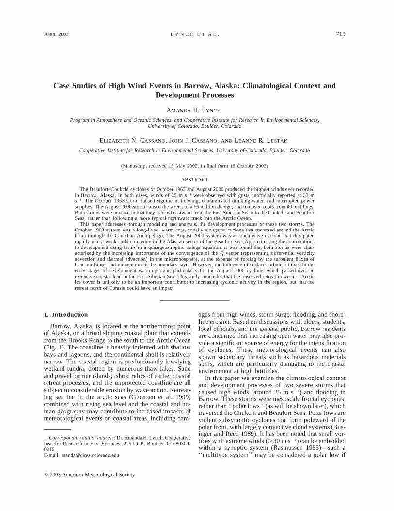
FIG. 1. Storm tracks for the 1963 and 2000 cyclones. (a) Center of the 1963 cyclone (solid line) basedon the NCEP–NCAR reanalysis; center of the 2000 cyclone (dashed line) based on the ECMWF operationalanalysis; and interpolated storm frequencies per year from the storm track center’s dataset generated fromthe six-hourly NCEP–NCAR reanalysis (Serreze 1995) for 1958–96. Each storm track center grid point wasassigned a frequency value, which was then interpolated using splining. The NCEP–NCAR reanalysis datawas not used for the 2000 storm due to errors in the reanalysis from 1997 forward at the time of calculating.(b) A more detailed storm track for the 1963 storm, showing dates and intensities, based on the NCEP–NCAR reanalysis (dashed line) and the Polar MM5 simulation (solid line). (c) A more detailed storm trackfor the 2000 storm, showing dates and intensities, based on the ECMWF analysis (dashed line) and the PolarMM5 simulation (solid line).


surface heat and moisture are crucial for development.True polar lows are considered rare in the Beaufort–Chukchi sector (Parker 1989).

In fact, the sector encompassing the eastern Chukchiand western Beaufort Seas, where these two cyclonesreached their maximum intensity, is a region of lowcyclone frequency (Fig. 1a) and intensity compared toother regions of the Arctic. Keegan (1958) conductedone of the earliest synoptic climatologies for the Arctic,focusing on the 15 winter months of 1952–57. Keegannoted a pronounced minimum of cyclones in this sector,suggesting that orography forms a barrier to the passageof cyclones from the northern Pacific, and cyclones orig-inating over eastern Siberia do not generally track asfar to the east. LeDrew analyzed a dynamic climatologyfor the region for the winters (LeDrew 1985) and sum-mers (LeDrew 1983) of 1975 and 1976, and noted thewinter storm track extending from the Norwegian Seaalong the Eurasian coast to the Kara, Laptev, and EastSiberian Seas [the latter area does not appear in the1952–57 Keegan climatology but does appear in the1957–61 Gaigerov climatology (LeDrew 1985)]. In thesummer analysis, LeDrew (1983) noted regular occur-rences of low pressure in the Laptev Sea with highpressure over the Beaufort Sea. Depressions off theNorth Slope coast of Alaska appear to be very rare inthese climatologies.

Lynch et al. (2002, manuscript submitted to Bull.Amer. Meteor. Soc., hereafter LCBM), Walsh et al.(1996), and Maslanik et al. (1996) use different mea-sures but all conclude that the late 1960s through to themid-1980s had a very different storm climatology com-pared to later records. This is a period of much lowerstorm frequency in general, and in particular in theBeaufort–Chukchi sector, compared to the period fromthe mid-1980s to the present. LCBM focus on Barrowand extend the record back to 1945, showing that thischange is not a linear trend of increasing storms—the1940s through to the early 1960s showed more highwind events than the next two decades. Proshutinskyand Johnson (1997) suggest a cyclic behavior with aperiod of 10–14 yr—in this scheme the Keegan cli-matology encompasses only the cyclonic regime, where-as the Gaigerov and LeDrew climatologies encompassanticyclonic regimes. Hence the differences between theLeDrew and Keegan climatologies are not unexpected.

Serreze et al. (1993, 1995) examined the character-istics of arctic synoptic activity from the early 1950s tothe present. Using data from the National Meteorolog-ical Center (NMC), Serreze et al. (1993) confirmed thatcyclone motion along the Eurasian coast, with the ten-dency for the Laptev, East Siberian, and Chukchi Seasto be common zones of migration into the Arctic Ocean,are more typical than motion farther eastward into theeastern Chukchi or Beaufort Seas (Fig. 1a). Cyclogen-esis often occurs in preferred regions along the Arcticfront—such preferred regions in Siberia are evident insummer and persist into the autumn (Serreze et al.

2001). Using the same dataset to focus on the Beaufort–Chukchi sector, and extending the record to 2001,LCBM note that while cyclone frequency is highly var-iable over long timescales, there is no significant trendin cyclone frequency for any season over the period ofrecord, but that there is a significant increase in theintensity of summer cyclones. Thus, from the early workto the more modern climatologies, the Beaufort–Chuk-chi region is not the home of frequently occurring in-tense cyclones.

A further issue is the influence of these synoptic pat-terns on the evolution of sea ice cover, which in turnhas a strong influence on the harshness of the stormimpacts on the coastal environment. Rogers (1978) as-sociates light ice years with more cyclonic activity inthe East Siberian Sea. Maslanik et al. (1996) noted thatincreased cyclone activity north of Siberia since the late1980s places the East Siberian Sea in the warm sectorof cyclones, leading to more frequent warm southerlywinds and hence ice retreat. The extension of the stormtrack through the Chukchi and Beaufort Seas can beassociated with strong ice retreat in this region [e.g.,Maslanik et al. (1999) for the 1998 Surface Heat Budgetof the Arctic Ocean (SHEBA) year]. Hence, coastal im-pacts are likely to be large in the summer and autumndue to the combined effects of intense cyclonic activityand associated ice retreat.

In section 2 we describe the data and models usedfor the analysis of the two storms on which we focusin this paper. Section 3 places these storms in the cli-matological context described earlier and section 4 pre-sents an analysis of the development processes leadingto the formation and intensification of these storms,based on model simulations. Section 5 presents someconclusions regarding Beaufort–Chukchi region storms.

2. Methodology

a. Polar MM5

The Polar MM5 nonhydrostatic mesoscale atmo-spheric model, version 3.4, is used to simulate the stormevents (Cassano et al. 2001). The Polar MM5 is mod-ified from the standard version of the fifth-generationPennsylvania State University–National Center for At-mospheric Research Mesoscale Model (MM5) (Dudhia1993; Grell et al. 1994) to better represent atmosphericprocesses occurring in the polar atmosphere, as de-scribed in this section. In the Polar MM5, the grid-scalecloud and precipitation processes are represented by theReisner explicit microphysics parameterization (Reisneret al. 1998). This parameterization predicts the mixingratio of cloud water and ice crystals as well as the rainand snow water mixing ratios. Excessive cloud coverwas found to be a problem over the Antarctic in sen-sitivity simulations using an older version of MM5(called MM4; Hines et al. 1997a,b), similar to resultsfound by Manning and Davis (1997) for cold, high


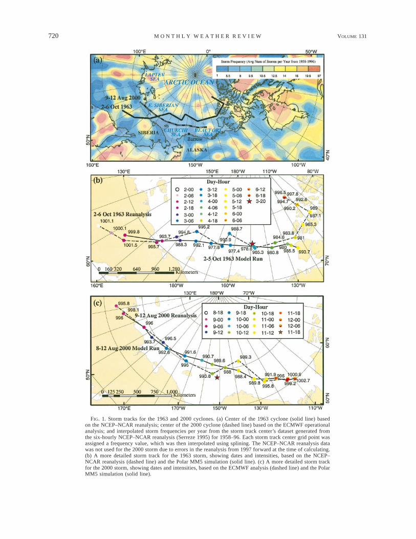
FIG. 2. Mean sea level pressure (hPa) maps showing the Oct1963 storm at its closest approach to Barrow (1800 UTC 3 Oct)from (a) NCEP–NCAR reanalysis data and (b) Polar MM5 sim-ulation. (c) The ‘‘hand analysis’’ for 2000 UTC 3 Oct, reproducedfrom Schafer (1966).

clouds over the continental United States. Replacementof the Fletcher (1962) equation for ice nuclei concen-tration with that of Meyers et al. (1992) in the explicitmicrophysics parameterization, as suggested by Man-ning and Davis (1997), has helped to eliminate thiscloudy bias in polar simulations.

The Polar MM5 uses a modified version of the Na-tional Center for Atmospheric Research (NCAR) Com-munity Climate Model, version 2, (CCM2) radiativetransfer parameterization (Hack et al. 1993) for short-wave and longwave radiation. Since the parameteriza-tion of cloud cover in the original MM5 radiation codetended to significantly overestimate the cloud liquid wa-ter path (Hines et al. 1997a,b), the predicted cloud waterand ice mixing ratios from the explicit microphysicsparameterization are used for determination of cloudradiative properties in the Polar MM5. This allows fora consistent treatment of the radiative and microphysicalproperties of the clouds and for the separate treatmentof the radiative properties of liquid and ice-phase cloudparticles. It should be noted that this method treats cloudparticles as equivalent spheres and has been shown tobe inaccurate for nonspherical ice particles (Grenfell andWarren 1999).

Turbulent fluxes are parameterized using the 1.5-order turbulence closure parameterization used in theNational Centers for Environmental Prediction (NCEP,formerly NMC) Eta Model (Janjic 1994). Other im-provements in the Polar MM5 include modificationsof the thermal properties used in the soil model forsnow and ice surface types (following Yen 1981), anincrease in the number of soil levels, and the additionof a sea ice surface type (Hines et al. 1997b). The seaice surface type allows for the specification of frac-tional sea ice cover in the model initial conditions forany oceanic grid point, and this sea ice distributiondoes not evolve during the model simulation. The sur-face fluxes for the sea ice grid points are calculatedseparately for the open water and sea ice portions ofthe grid point, and then averaged. The sea ice thicknessvaries from 0.2 to 0.95 m and is dependent on thehemisphere and sea ice fraction at the grid point.

The model domain (e.g., Fig. 2) is centered at 688Nlatitude and 1728W longitude and has a horizontal extentof 2820 km 3 2370 km, with a horizontal grid spacingof 30 km. A total of 23 vertical levels are used, of whichfour are located within the lowest 450 m of the atmo-sphere. The lowest sigma level is located at a nominal


height of 38 m above ground level. The model top isset at a constant pressure of 100 hPa. The initial andboundary conditions for the model atmosphere are ini-tialized using European Centre for Medium-RangeWeather Forecasts (ECMWF) Tropical Ocean GlobalAtmosphere (TOGA) analyses for the August 2000 case,and the NCEP–NCAR reanalysis for the October 1963case. Boundary forcing is achieved using linear relax-ation, and fields without boundary values are specifiedto be zero on inflow boundaries and to have zero gra-dient on outflow boundaries. The sea ice concentrationsfor both cases are provided by the National Snow andIce Data Center (NSIDC). For August 2000, the iceconcentrations are derived from the Defense Meteoro-logical Satellite Program (DMSP) Special Sensor Mi-crowave Imager (SSM/I), generated using the bootstrapalgorithm (Comiso 2002). For the October 1963 case,the sea ice concentration was assembled from the Arcticand Southern Ocean Sea Ice Concentrations (Walsh andChapman 2001).

b. Omega equation analysis

An important issue in the analysis of the developmentof these systems are the relative contributions of dif-ferential absolute vorticity advection [term A, Eq. (1a)],thermal advection [term B, Eq. (1a)], and diabatic pro-cesses associated with the atmospheric boundary layerand from latent heat release within the system [term C,Eq. (1a)]. Such a diagnosis can be approximated byusing a diabatic form of the quasigeostrophic omega(vertical velocity) equation (e.g., LeDrew 1988; Roeb-ber 1989; Deveson et al. 2002):

2] v ] 12 2 2¹ (sv) 1 f 5 f v · = ¹ F 1 f0 0 g2 1 2[ ]]p ]p f0

A

]F R2 21 ¹ v · = 2 2 ¹ Hg 1 2[ ]]p pcp

B C

(1a)2] v R

2 2 2¹ (sv) 1 f 5 22= · Q 2 ¹ H, (1b)0 2]p pcp

where all symbols are defined in the appendix. Theright-hand side of Eq. (1b) represents all forcing of thevertical motion in a quasigeostrophic system on an f -plane. In such a system, with no diabatic forcing, ver-tical velocity is forced solely by the divergence of Q(Hoskins et al. 1978). This form of the equation avoidsthe inaccuracies associated with the tendency for thedifferential vorticity advection term and the thermal ad-vection term [terms A and B in Eq. (1a)] to be of similarmagnitude and opposite sign. The diabatic heating rateH is made up of contributions from the surface sensible

heat flux (Hsh), the latent heat release (HIh), and con-vective processes (Hconv):

FsH 5 (2)sh rDZ

L DCyH 5 (3)lh Dt

L Dqy vconvH 5 (4)conv Dt

The equation can be solved as a Poisson equation byspecifying the Polar MM5 vertical velocity at the topand sides of the grid cell of interest, and a friction-induced component of vertical velocity at the bottom ofthe grid cell vfriction 5 (= 3 t0) · k/rf. The diabaticheating rate due to latent heat release is further assumedto be partitioned according to the proportion of watervapor in the grid cell that is horizontally advected com-pared to that which is vertically transported by latentheat fluxes from the surface.

In our application, we focus on the 850-hPa layer toremain above the boundary layer throughout the sim-ulation. The zone of maximum uplift associated withthe cyclone is identified, and for this location, the con-tributions to omega from each term in Eq. (1b) are cal-culated for the 850-hPa grid cell at this location (withdifferencing calculated between the 800- and 900-hPalayers). In this way, it is possible to identify the criticaldevelopment processes at each stage of the cyclone’slife cycle.

3. Case study descriptions

It is often reported that the most severe storm alongthe Beaufort Sea coast occurred from 3 to 5 October1963. This storm caused extensive damage at Barrow:the damage estimate was $3.25 million (about $19 mil-lion in 2001 dollars). Highest observed winds were 25m s21, with gusts unofficially reported at 33 m s21

(Hume and Schalk 1967). Water moved inland 122 mfrom the shore and large chunks of sea ice were washedinland about 4.6 m. Waves were estimated to be 3-mhigh with a storm surge of 3 m. Coastal areas in thevicinity of the Naval Arctic Research Laboratory(around 5 km northeast of Barrow airport) and shore-lines backed by lakes were severely flooded, contami-nating local drinking water. Damage included the de-struction of 19 buildings, destruction of power lines,erosion of bluffs southwest of Barrow by 3 m, and ashoreline retreat of 18 m.

According to the NCEP–NCAR reanalysis data, thestorm originated along the Arctic front over Siberiaaround 145.68E on 2 October 1963 (Figs. 1a,b). Overthe next 24 h it traversed to the coast of the East SiberianSea and continued northward, as is typical for such sys-tems. However, shortly after 0600 UTC 3 October, thestorm turned eastward and commenced a rapid deep-


FIG. 3. Mean sea level pressure (hPa) maps showing the Aug 2000storm at 0000 UTC 11 Aug from (a) ECMWF operational analysisdata and (b) Polar MM5 simulation. (c) AVHRR image of the Aug2000 cyclone at 1200 UTC 11 August.

ening, reaching an analyzed central pressure of 988.7hPa at 1800 UTC 3 October while located in the Beau-fort Sea north of Barrow (Figs. 1b and 2). Based on theNCEP–NCAR reanalysis, the cyclone continued to in-tensify as it traversed eastward, reaching its analyzedpeak intensity of 981.0 hPa when it reached the Ca-nadian Archipelago at 1200 UTC 4 October. It shouldbe noted that it is likely that the minimum central pres-sure of the cyclone was deeper than indicated by theNCEP–NCAR reanalysis. Schafer (1966) shows an ap-proximate synoptic analysis of the storm (reproducedin Fig. 2c) based on surface data from the NationalWeather Service (NWS). This ‘‘hand analysis’’ indi-cated that the storm reached an intensity of 976 hPa, at2000 UTC 3 October. This intensity is more consistentwith the 3-m storm surge observed. The location of theSchafer (1966) analyzed storm center at this time isshown in Fig. 1b—its position to the northeast of Bar-row suggests that the NCEP–NCAR reanalysis showsthe storm moving somewhat too slowly. Further, Schafer(1966) suggests that it is likely that the storm was de-caying by 0000 UTC 4 October, not continuing to deep-en as shown in the NCEP–NCAR reanalysis. Because

of the low spatial resolution, sparse observations, andmodel biases typical of the polar regions (see e.g., Cul-lather et al. 2000; Francis 2002; Walsh et al. 2002) itis not surprising that details of the storm in the NCEP–NCAR reanalysis are not consistent with independentobservations. In any case, the cyclone was of sufficientstrength to cause the extreme winds measured at Barrowas it traversed the Chukchi and Beaufort Seas, partic-ularly because of the presence of strong high pressureover the Aleutian Islands (central pressure 1030 hPa).

The storm of 10–11 August 2000 (Figs. 1c and 3)produced official record wind gusts of 29 m s21 andsustained winds of 25 m s21, according to the NWSanemometer. The peak wind intensity in Barrow oc-curred at 0000 UTC on 11 August 2000. It has beensuggested that the NWS anemometer may have ‘‘peggedout’’—a maximum wind gust of 33 m s21 was reportedat the NOAA Climate Monitoring and Diagnostics Lab-oratory (CMDL) weather station (D. Endres 2001, per-sonal communication) although the official CMDL peak1-s wind was recorded at 31 m s21. Emergency man-agement teams had insufficient notice to mobilize heavyequipment to build temporary protective berms along


the coast. The storm eroded the beach to within 100 mof a main junction location of the underground utilitycorridor, sunk the dredge barge, washed out a boat ramp,and removed roofs from 40 buildings. A tidal gauge atPrudhoe Bay reported a storm surge of 1.46 m, within6 cm of the 100-yr event (A. Morkill 2001, personalcommunication). The final cost of this storm, primarilydue to the damaged dredge barge Qayuutaq, was $7.7million.

The August 2000 storm originated around 145.18Ebut in this case the Arctic front was situated consider-ably closer to the East Siberian Sea coast than the 1963storm (Figs. 1a,c). Twelve hours later, around 0600 UTC9 August 2000, it crossed the coastline at the same lo-cation as the 1963 storm (within the roughly 200-kmresolution of the analyses), then continued directly east-ward. As the cyclone traversed from the Chukchi to theBeaufort Sea it continued to deepen, reaching an inten-sity of 989.3 hPa, 290 km to the north of Barrow, around0000 UTC 11 August, and then dissipating rapidly be-fore reaching the Canadian Archipelago. Figure 3cshows the storm at 1200 UTC 11 August from AdvancedVery High Resolution Radiometer (AVHRR) data, fromthe AVHRR Polar Pathfinder dataset, developed as partof the NOAA–NASA Pathfinder effort (Fowler et al.2000). The image is a 25 km 3 25 km product averagedfrom composited channel-4 (thermal) and channel-2 (re-flectance) 5 km 3 5 km images. From this imagery, thestorm is clearly mesoscale in nature [the organized cloudbands span a diameter of O (400 km) at the time shown],and shows the ECMWF analysis tracks it rather toorapidly (Fig. 1c). It is clear from the storm track cli-matology (Serreze 1995), also shown in Fig. 1a, thatthe trajectories of the October 1963 and August 2000storms were relatively unusual.

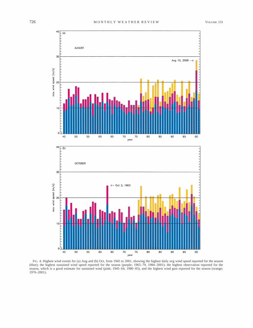
The intensity of Beaufort–Chukchi sector cycloneshas significantly increased over the past 40 yr in sum-mer, but not in other seasons, and the number of cy-clones in this sector has not increased in any seasonLCBM). Not all high wind events in Barrow are asso-ciated with Beaufort–Chukchi cyclones. Barrow highwind events can be linked to a range of different syn-optic conditions, including large, deep Aleutian cy-clones and strong Beaufort–Chukchi ridges. LCBM an-alyzed the occurrence of high wind events in Barrowover the past 55 yr, using available NWS observations.The number of high wind events each year decreasedthroughout the ’50s, ’60s and ’70s, and have increasedthrough the ’80s and ’90s. Average winds have in-creased in winter (significant at the 99% confidence lev-el) and spring (significant at the 95% confidence level),but not in autumn or summer. There is little apparentlinear trend in the highest winds in any season, and thecyclone of August 2000 is a clear outlier in the Augustrecord (Fig. 4a), and in fact in the summer record. Thedaily average winds associated with the October 1963cyclone do not represent such a strong departure fromclimatological intensity (Fig. 4b), and although the high-

est observation is significantly stronger than any otherOctober, several other years have suffered fall stormsin other months with comparable average daily windmaxima (LCBM).

4. Simulation and analysis

a. October 1963 case

Simulation of the October 1963 case study com-menced at 0000 UTC 1 October 1963. The cycloneformed to the southwest of the model domain, and firstappears 24 h after initialization at the domain’s westernboundary, over Siberia. It then travelled very rapidlynortheastward to the coast, crossing the coast around1800 UTC 2 October, just slightly ahead of the analyzedposition (Fig. 1b). Rather than migrating northward, asis typical for such systems, the simulated cyclonetracked eastward over the next day, reaching maximumintensity of 977.3 hPa at 1500 UTC 3 October slightlyto the west of directly north of Point Barrow, whereuponthe system started to dissipate (Figs. 2 and 5). Through-out this period the cyclone was over sea ice, and con-tinued to develop in a confluent region of the large-scaleflow, which is consistent with the zonally elongatedstructure that resulted (Schultz et al. 1998; Sinclair andRevell 2000). The system was strongly steered by the500-hPa wind, and, unusually for cyclones that formalong the Arctic front (Keegan 1958), had formed awarm seclusion by the time it neared Barrow (Fig. 5).The simulated central pressure at maximum intensitywas comparable to analyses performed by Schafer(1966; Fig. 2). In contrast, the NCEP–NCAR analyzedcyclone did not reach as low a central pressure andcontinued to intensify as it continued toward the Ca-nadian Archipelago. As noted, however, the NCEP–NCAR reanalyses should not be considered reliable forthe details of this storm, although the large-scale forcingof the boundaries of the mesoscale model appears to beadequate. The simulated wind at Barrow reached a peakof 24.2 m s21, in good agreement with Hume and Schalk(1967) and NWS observations.

Given that the Polar MM5 simulates adequately thedevelopment and path of the storm, at least up until theclosest approach to Barrow, it is possible to draw con-clusions regarding the mechanisms involved in stormdevelopment, based on the increased information avail-able from the model output (e.g., Giordani and Caniaux2001). Figure 6a shows the 850-hPa vertical velocityand mean sea level pressure simulated by the Polar MM5at the location of maximum uplift in the storm through-out its life cycle, starting at 1300 UTC 2 October. Atthis time, the simulated cyclone is over land, progressingto the coast within the next 6 h. During this early period,simulated vertical velocities are quite strong, up to 2cm s21. As the cyclone progresses across the ChukchiSea, the rapid and consistent deepening of the simulatedcyclone is clear, with uplift between 2 and 3 cm s21


FIG. 4. Highest wind events for (a) Aug and (b) Oct, from 1945 to 2001, showing the highest daily avg wind speed reported for the season(blue); the highest sustained wind speed reported for the season (purple; 1965–79, 1984–2001); the highest observation reported for theseason, which is a good estimate for sustained wind (pink; 1945–64, 1980–83), and the highest wind gust reported for the season (orange;1976–2001).


FIG. 5. The 500-hPa thickness (m, solid lines) and surface relativevorticity (s21, dashed lines) at 1800 UTC 3 Oct from the Polar MM5simulation.

FIG. 6. (a) Time series showing the central sea level pressure (solid bold line), the 850-hPa vertical velocity (open circles) at the locationof max uplift and the 850-hPa vertical velocity (closed circles) calculated using Eq. (1b) in the Oct 1963 cyclone. (b) Time series of verticalvelocities due to each of the contributions of terms in Eq. (1b). The bar at the bottom indicates the surface type: land surface (vertical hash),ice concentration less than 50% (diagonal hash) and greater than 50% (solid gray).

associated with the most intense phase of the storm.Also shown is the vertical velocity as calculated by thequasigeostrophic method described in section 2b usingthe approximation v ø 2w]p/]z, and the contributionsto this velocity from the convergence of Q, the latentheat release from grid-scale and convective processesat 850 hPa, and the contribution from the boundary layerturbulent fluxes of sensible and latent heat. Apart fromthe first 6 h while the cyclone is close to the lateralboundaries, the calculated vertical velocity tracks themodel vertical velocity quite accurately, although itslightly underestimates the magnitude. Inaccuracies inthis method arise from the assumption of small depar-tures from geostrophic flow, the assumption of zero fallvelocity for condensates, truncation and convergencelimitations in the numerical method, and the use of hour-

ly model output for the calculation to compare withinstantaneous vertical velocities.

As the cyclone moves out over the ice (Fig. 6b), themost important sources of uplift in the system are theboundary layer sensible heat fluxes, large-scale hori-zontal convergence of moisture, and subgrid-scale con-vection, consistent with the findings of other authors(e.g., Mak 1998; Kuo et al. 1991; Leslie et al. 1987).During this period, vertical motion forced by the term22= · Q (that is, the adiabatic processes of differentialvorticity advection and thermal advection) actuallydrives subsidence, and initially the effects of this syn-optic environment overwhelm other sources of uplift.As the system continues eastward over sea ice that ap-proaches 100% concentration, the influence of turbulentfluxes and latent heat release progressively diminishes,and the convergence of Q in the middle tropospherebecomes of increasing importance, intensifying the up-lift. Sensible heat fluxes from the surface are of con-sistent, though small, importance until around 1200UTC 3 October, contributing around 15% of the totalvertical velocity throughout this period. Once cyclolysiscommences, the forcing due to differential vorticity andthermal advection diminishes rapidly. It is clear thatdiabatic effects are not sufficient to sustain the cycloneexcept in the earliest phase of cyclogenesis, and hencethis system can be classed as a frontal cyclone ratherthan a polar low.

b. August 2000 case

Simulation of the August 2000 case study com-menced at 0000 UTC 7 August 2000—the simulatedcyclone track is compared to the analyzed track in Fig.1c. The simulated cyclone follows the track of theECMWF analysis very closely. At 1200 UTC 10 Au-gust (Fig. 3) the simulated cyclone is slightly to the


FIG. 7. The 500-hPa thickness (m, solid lines) and surface relativevorticity (s21, dashed lines) at 0000 UTC 11 Aug 2000 from the PolarMM5 simulation.

FIG. 8. (a) Time series showing the central sea level pressure (solid bold line), the 850 hPa vertical velocity (open circles) at the locationof max uplift and the 850-hPa vertical velocity (closed circles) calculated using Eq. (1b) in the Aug 2000 cyclone. (b) Time series of verticalvelocities due to each of the contributions of terms in Eq. (1b). The bar at the bottom indicates the surface type: land surface (vertical hash),ice concentration less than 50% (diagonal hash) and greater than 50% (solid gray).

northwest of the analyzed position, and more intense.The peak intensity near Barrow was 988.0 hPa at 1900UTC 10 August, but central pressures within 0.5 hPaof 988.0 hPa were maintained for 9 h, encompassingthe peak of 989.3 hPa in the 12 hourly ECMWF anal-ysis data at 0000 UTC 11 August (Fig. 3). The locationof the cyclone at this time was identical to the analyzedlocation within the grid spacing of the analysis data.In general, the analyzed cyclone deepens later andmore rapidly than the simulated cyclone. The August2000 cyclone represents a ‘‘classic’’ type of open wavecyclone, which is more typical of this region (Keegan1958; Fig. 7). The cyclone formed on the northern sideof the jet exit region associated with the Arctic front,and intensified as it was steered eastward by the upper-level winds (not shown).

The development of this system was more complexthan the October 1963 cyclone. Figure 8a shows the850-hPa vertical velocity and mean sea level pressuresimulated by the Polar MM5 at the location of maxi-mum uplift in the storm throughout its life cycle, start-ing at 0100 UTC 9 August. At this time, the simulatedcyclone had just entered the domain—12 h later itpassed over the coast and was situated over the coastallead (indicated by diagonal hashes in the timeline, Fig.8b). Also shown is the vertical velocity as calculatedby the quasigeostrophic method described in section2b, and the contributions to this velocity from 22= · Q,the latent heat release from grid-scale and convectivemoist processes at 850 hPa, and the contribution fromthe boundary layer turbulent fluxes of sensible andlatent heat. As noted, the simulated cyclone undergoesconsistent strengthening from the time of cyclogen-esis until it reaches its peak intensity at 1900 UTC10 August (Fig. 8a). Following this, the cyclone grad-ually and consistently weakens. Until a few hoursafter this cyclolysis commences, vertical velocities at850 hPa tend to be above 1 cm s21 , with the mostvigorous vertical motion occurring while the cycloneis at the leading edge of the open water along theSiberian coast, from 0600 to 1700 UTC 9 August 2000.Maximum gradients in the surface heat fluxes are pre-sent at this location (not shown). The quasigeostrophicvertical velocity is quite close to the modeled verticalvelocity and the pattern of development is similar, andagain, given the approximations inherent in the meth-od, the errors are acceptable. Early in the developmentof the cyclone, uplift as strong as 11 cm s21 is simu-lated, associated primarily with convection and alsothe surface fluxes of latent heat. Later, as the cyclonetracks eastward over the ice, which is generally be-tween 50% and 65% concentration, the convergenceof Q is of most consistent importance, with contribu-


FIG. 9. Differences of (a) surface latent heat flux (W m22), (b)surface sensible heat flux (W m22), and (c) sea level pressure (hPa)between the expt using 1990 sea ice and the control case at 1200UTC 9 Aug.

tions of convection, surface sensible heat fluxes, andlatent heat release due to the conversion of horizontallyconverged moisture of minimal importance. Only sur-face latent heat fluxes continue to play a role, albeitsporadically, comparable with the synoptic environ-ment. As the cyclone then weakens, all diabatic termsdrop to near-zero, and the 22= · Q term contributesactively to subsidence for almost 7 h during this phase.Thus, the pattern noted in the October 1963 case isalso seen here, but more dramatically, with surfacefluxes very important during the early intensification,and adiabatic forcing becoming dominant for the mostintense phase of the cyclone. Cyclolysis commenceswhen this additional forcing diminishes, as the systemundergoes a classic frontal cyclone progression (e.g.,Schultz et al. 1998). However, given the importanceof surface fluxes and convection during the initial de-velopment of this cyclone, the system could be con-sidered to be a ‘‘multitype’’ polar low (Rasmussen1985).

Two additional experiments were performed on theAugust 2000 cyclone. The first used the sea ice coverobserved during August 1998, which saw a strong re-treat of sea ice on the Beaufort Sea north of Barrow

(Maslanik et al. 1999). The second experiment usedthe sea ice cover of August 1990, during which timethere was a record retreat of sea ice in the East SiberianSea (Lynch et al. 2001). In the first case, in which seaice cover was reduced later in the development cycleof the system, there was minimal impact on the sim-ulation (not shown). The resulting cyclone followedthe same track and reached the same maximum inten-sity. The position at closest approach to Barrow wasthe same. In the second case, the impact on the sim-ulated cyclone was small but discernible, particularlyin the early stages. The cyclone moved across the coastslightly earlier than the control case. While over thecoastal lead, the surface fluxes were increased by asmuch as 100 W m22 for the sensible heat flux and 75W m22 for the latent heat flux (Fig. 9) and the hori-zontal gradient of surface fluxes also increased mark-edly. During this period, vertical velocity forced bysubgrid-scale convective processes was stronger andpersisted about twice as long, and the influence of thehorizontal convergence of moisture on the forcing ofvertical velocity by latent heating was enhanced. Fur-ther, the propagation of the cyclone slowed while overthe coastal lead. With the additional forcing on vertical


velocity, the cyclone was somewhat deeper at this stage(Fig. 9c). As the cyclone tracked across the ChukchiSea, the importance of the synoptic environment onthe development of the cyclone was preeminent, justas in the control case, and hence the simulation fromthis time forward was very similar to the control. Thispattern of behavior in the presence of low ice concen-trations is consistent with the results of, for example,Angel and Isard (1997). While the closest approach toBarrow occurred at around the same time (0000 UTC11 August), the cyclone was around 1 hPa deeper andaround 50 km closer to Barrow, with concomitantstronger winds at Barrow. Cyclolysis commenced atthe same time, and proceeded at the same rate in boththe control and the experiment simulations.

5. Conclusions

The Beaufort–Chukchi cyclones of October 1963 andAugust 2000 produced the highest winds ever officiallyrecorded in Barrow, Alaska. The October 1963 stormproduced a significant storm surge and caused extensiveflooding, whereas the August 2000 storm caused morelimited flooding, but had a large financial impact dueto the damage to a dredge and the consequent endingof the beach nourishment program (LCBM). The cy-clones also differed in that the October 1963 systemwas a long-lived, warm core, zonally elongated cyclonethat traversed around the Arctic basin through the Ca-nadian Archipelago, whereas the August 2000 systemwas an open wave cyclone, which dissipated rapidlyinto a weak, cold core eddy in the Alaskan sector ofthe Beaufort Sea.

Despite these differences, there were several impor-tant commonalities between the two cyclones. Bothformed along the Arctic frontal zone over Siberia andtraversed northeastward to the East Siberian Sea. At thispoint, rather than tracking into the central Arctic Oceanas is typical for such systems, the cyclones turned in amore eastward direction, steered by the upper-level flow,into the Chukchi Sea and thence to the Beaufort Sea.As they moved from land to ocean, the cyclones inten-sified initially due to surface fluxes and convection overlower-concentration ice, and subsequently as a result ofthermal advection and differential vorticity advectionabove the boundary layer. The August 2000 storm un-derwent more significant intensification associated withthe more open coastal lead in the East Siberian Sea atthis time, and for this reason could be considered to bea ‘‘multitype’’ polar low.

The primary impetus for this analysis is the concernof Barrow residents that retreating sea ice in the Chukchiand Beaufort Seas (Gloersen et al. 1999) may contributeto an increase in the impacts of severe storms on Barrow.This concern arises not only because sea ice serves asa significant protection against storm surge, waves, andcoastal erosion, but also because there is a perceptionthat open water provides a significant source of energy

for the intensification of cyclones. However, concern ismitigated by the additional perception that cyclones inthis region track the ice edge, and hence a retreatingsea ice may cause the few cyclones that track eastwardfrom the East Siberian Sea to shift further north. Thestudy of these two systems does not bear out these per-ceptions completely. Neither cyclone tracked the iceedge—they were steered by a strong upper-level flowon their unusual eastward tracks. While the cyclone ofAugust 2000 did intensify as it passed over the opencoastal lead in the East Siberian Sea, the location of theice edge north of Barrow had little impact on the courseof cyclone development. This is borne out by the ad-ditional experiments that showed that the simulation ofthis cyclone was insensitive to the specification of theice edge in this area. However, retreating sea ice in theEast Siberian Sea had some impact on the cyclone, in-creasing the intensity early in its lifecycle and causingit to track more closely to Barrow in its subsequentdevelopment. This result is consistent with the analysisof Rogers (1978) who found that while the amount ofopen water in late summer and autumn in the East Si-berian Sea is associated with greater cyclonic activity,open water in the Beaufort Sea has little or no influenceupon subsequent local surface winds or the sea levelpressure distribution. Thus, the retreat of sea ice in theBeaufort–Chukchi region will continue to have impli-cations for the impacts of storms on the Alaskan NorthSlope coastal zone, but it is the sea ice retreat in theEast Siberian Sea that should be considered a possibleinfluence on the trends in the number and intensity ofBeaufort–Chukchi cyclones.

Acknowledgments. This paper was much improved bycomments from two anonymous reviewers and partic-ularly through the suggestions of Dr. H. Giordani.Thanks to Mathew Rothstein for contributing to theanalysis of the climatology of Barrow-area high windevents. The satellite data were provided by Jim Maslanikat the National Snow and Ice Data Center. This workwas supported by NSF Grants OPP-0100120 and OPP-9732461.

APPENDIX

List of Symbols

cp specific heat of dry air (J kg21 K21)DC total change of condensate in the 800–900-

hPa-layer grid cell, including cloud waterand cloud ice, assuming a fall velocity ofzero (kg kg21)

f 0 Coriolis parameter, constant for the domain(s21)

Fs sensible heat flux from the surface (Wm22)

H diabatic heating rate (W kg21)Ly latent heat of vaporization (J kg21)


p pressure (Pa)Dqvconv change in water vapor in the 800–900-hPa-

layer grid cell due to subgrid-scale con-vection (kg kg21)

Q [2(]vg/]x) · =(2]F/]p), 2(]vg/]y) ·=(2]F/]p)]

R gas constant for dry air (J kg21 K21)Dt model time step (s)vg geostrophic wind velocity vector (m s21)DZ thickness of the 800–900-hPa layer (m)r density (kg m23)s static stability (m2 Pa22 s22)F geopotential height (m)v vertical velocity, in the form dp/dt (Pa s21)

REFERENCES

Angel, J. A., and S. A. Isard, 1997: An observational study of theinfluence of the Great Lakes on the speed and intensity of passingcyclones. Mon. Wea. Rev., 125, 2228–2237.

Businger, S., and R. J. Reed, 1989: Cyclogenesis in cold air masses.Wea. Forecasting, 4, 133–156.

Cassano, J. J., J. E. Box, D. H. Bromwich, L. Li, and K. Steffen,2001: Evaluation of polar MM5 simulations of Greenland’s at-mospheric circulation. J. Geophys. Res., 106, 33 867–33 890.

Comiso, J., cited 2002: Bootstrap sea ice concentrations for NIMBUS-7 SMMR and DMSP SSM/I. National Snow and Ice Data Center,Boulder, CO. [Available online at http://www.nsidc.colorado.edu/data/catalog.html.]

Cullather, R. I., D. H. Bromwich, and M. C. Serreze, 2000: Theatmospheric hydrologic cycle over the Arctic basin from re-analyses. Part I: Comparison with observations and previousstudies. J. Climate, 13, 923–937.

Deveson, A. C. L., K. A. Browning, and T. D. Hewson, 2002: Aclassification of FASTEX cyclones using a height-attributablequasi-geostrophic vertical-motion diagnostic. Quart. J. Roy. Me-teor. Soc., 128, 93–117.

Dudhia, J., 1993: A nonhydrostatic version of the Penn State–NCARMesoscale Model: Validation tests and simulation of an Atlanticcyclone and cold front. Mon. Wea. Rev., 121, 1493–1513.

Fletcher, N. H., 1962: Physics of Rain Clouds. Cambridge UniversityPress, 386 pp.

Fowler, C., J. Maslanik, T. Haran, T. Scambos, J. Key, and W. Emery,cited 2000: AVHRR Polar Pathfinder twice-daily 5 km EASE-Grid composites. National Snow and Ice Data Center, Boulder,CO. [Available online at http://www.nsidc.colorado.edu/data/catalog.html.]

Francis, J. A., 2002: Validation of reanalysis upper-level winds inthe Arctic with independent rawinsonde data. Geophys. Res.Lett., 29(9), 1315, doi: 10.1029/2001GL014578.

Giordani, H., and G. Caniaux, 2001: Sensitivity of cyclogenesis tosea surface temperature in the northwestern Atlantic. Mon. Wea.Rev., 129, 1273–1295.

Gloersen, P., C. L. Parkinson, D. J. Cavalieri, J. C. Comiso, and H.J. Zwally, 1999: Spatial distribution of trends and seasonality inthe hemispheric sea ice covers: 1978–1996. J. Geophys. Res.,104, 20 827–20 835.

Grell, G. A., J. Dudhia, and D. R. Stauffer, 1994: A description ofthe fifth-generation Penn State/NCAR mesoscale model (MM5).NCAR Tech. Note 3981STR, 122 pp.

Grenfell, T. C., and S. G. Warren, 1999: Representation of nonsphericalice particles by a collection of independent spheres for scatteringand absorption of radiation. J. Geophys. Res., 104, 31 697–31 709.

Hack, J. J., B. A. Boville, B. P. Briegleb, J. T. Kiehl, P. J. Rasch, andD. L. Williamson, 1993: Description of the NCAR communityclimate model (CCM2). NCAR Tech. Note 3821STR, 108 pp.

Hines, K. M., D. H. Bromwich, and R. I. Cullather, 1997a: Evaluating

moist physics for Antarctic mesoscale simulations. Ann. Glaciol.,25, 282–286.

——, ——, and Z. Liu, 1997b: Combined global climate model andmesoscale model simulations of Antarctic climate. J. Geophys.Res., 102, 13 747–13 760.

Hoskins, B. J., I. Draghici, and H. C. Davies, 1978: A new look atthe v-equation. Quart. J. Roy. Meteor. Soc., 104, 31–38.

Hume, J. D., and M. Schalk, 1967: Shoreline processes near Barrow,Alaska: A comparison of the normal and the catastrophic. Arctic,20, 86–103.

Janjic, Z. I., 1994: The step-mountain eta coordinate model: Furtherdevelopments of the convection, viscous sublayer, and turbu-lence closure schemes. Mon. Wea. Rev., 122, 927–945.

Keegan, T. J., 1958: Arctic synoptic activity in winter. J. Meteor.,15, 513–521.

Kuo, Y. H., R. J. Reed, and S. Lownam, 1991: Effects of surface-energy fluxes during the early development and rapid intensi-fication stages of seven explosive cyclones in the western At-lantic. Mon. Wea. Rev., 119, 457–476.

LeDrew, E. F., 1983: The dynamic climatology of the Beaufort toLaptev Sea sector of the Polar Basin for the summers of 1975and 1976. J. Climatol., 3, 335–359.

——, 1985: The dynamic climatology of the Beaufort to Laptev Seasector of the Polar Basin for the winters of 1975 and 1976. J.Climatol., 5, 253–272.

——, 1988: Development processes for five depression systems with-in the polar basin. J. Climatol., 8, 125–153.

Leslie, L. M., G. J. Holland, and A. H. Lynch, 1987: Australian east-coast cyclones. Part II: Numerical modeling study. Mon. Wea.Rev., 115, 3037–3053.

Lynch, A. H., J. A. Maslanik, and W. Wu, 2001: Mechanisms in thedevelopment of anomalous sea ice extent in the western Arctic:A case study. J. Geophys. Res., 106, 28 097–28 106.

Mak, M., 1998: Influence of surface sensible heat flux on incipientmarine cyclogenesis. J. Atmos. Sci., 55, 820–834.

Manning, K. W., and C. A. Davis, 1997: Verification and sensitivityexperiments for the WISP94 MM5 forecasts. Wea. Forecasting,12, 719–735.

Maslanik, J. A., M. C. Serreze, and R. G. Barry, 1996: Recent de-creases in Arctic summer ice cover and linkages to atmosphericcirculation anomalies. Geophys. Res. Lett., 23, 1677–1680.

——, ——, and T. Agnew, 1999: On the record reduction in 1998western Arctic sea-ice cover. Geophys. Res. Lett., 26, 1905–1908.

Meyers, M. P., P. J. DeMott, and W. R. Cotton, 1992: New primaryice-nucleation parameterizations in an explicit cloud model. J.Appl. Meteor., 31, 708–721.

Parker, M. N., 1989: Polar lows in the Beaufort Sea. Polar and ArcticLows, P. F. Twitchell, E. A. Rasmussen, and K. L. Davidson,Eds., A. Deepak, 323–330.

Proshutinsky, A. Y., and M. A. Johnson, 1997: Two circulation re-gimes of the wind driven Arctic Ocean. J. Geophys. Res., 102(C6), 12 493–12 514.

Rasmussen, E. A., 1985: A case study of polar low development overthe Barents Sea. Tellus, 37A, 407–418.

Reisner, J., R. M. Rasmussen, and R. T. Bruintjes, 1998: Explicitforecasting of supercooled liquid water in winter storms usingthe MM5 mesoscale model. Quart. J. Roy. Meteor. Soc., 124,1071–1107.

Roebber, P. J., 1989: The role of surface heat and moisture fluxesassociated with large-scale ocean current meanders in maritimecyclogenesis. Mon. Wea. Rev., 117, 1676–1694.

Rogers, J. C., 1978: Meteorological factors affecting interannual var-iability of summertime sea ice extent in the Beaufort Sea. Mon.Wea. Rev., 106, 890–897.

Schafer, P. J., 1966: Computation of a storm surge at Barrow, Alaska.Arch. Meteor. Geophys. Bioklimatol., 15A, 372–393.

Schultz, D. M., D. Keyser, and L. F. Bosart, 1998: The effect of large-scale flow on low-level frontal structure and evolution in mid-latitude cyclones. Mon. Wea. Rev., 126, 1767–1791.


Serreze, M. C., 1995: Climatological aspects of cyclone developmentand decay in the Arctic. Atmos.–Ocean, 33, 1–23.

——, J. E. Box, R. G. Barry, and J. E. Walsh, 1993: Characteristicsof Arctic synoptic activity, 1952–1989. Meteor. Atmos. Phys.,51, 147–164.

——, A. H. Lynch, and M. P. Clark, 2001: The summer Arctic frontalzone as seen in the NCEP/NCAR reanalysis. J. Climate, 14,1550–1567.

Sinclair, M. R., and M. J. Revell, 2000: Classification and compositediagnosis of extratropical cyclogenesis events in the southwestPacific. Mon. Wea. Rev., 128, 1089–1105.

Walsh, J. E., and W. L. Chapman, cited 2001: Arctic and SouthernOcean Sea Ice Concentrations. National Snow and Ice DataCenter, Boulder, CO. [Available online at http://www.nsidc.colorado.edu/data/catalog.html.]

——, ——, and T. L. Shy, 1996: Recent decrease of sea level pressurein the central Arctic. J. Climate, 9, 480–486.

——, V. M. Kattsov, W. L. Chapman, V. Govorkova, and T. Pavlova,2002: Comparison of Arctic climate simulations by uncoupledand coupled global models. J. Climate, 15, 1429–1446.

Yen, Y. C., 1981: Review of thermal properties of snow, ice, and seaice. CRREL Rep. 81-10, 27 pp.

Case Studies of High Wind Events in Barrow, Alaska: Climatological Context and Development Processes

Documents

Transcript of Case Studies of High Wind Events in Barrow, Alaska: Climatological Context and Development Processes