biomechanical characterization and simulation of the

BIOMECHANICAL CHARACTERIZATION AND SIMULATION OF THE

TRICUSPID VALVE

A Dissertation

Presented to

The Graduate Faculty of The University of Akron

In Partial Fulfillment

Of the Requirements for the Degree

Doctor of Philosophy

Keyvan Amini Khoiy

December 2018

ii

BIOMECHANICAL CHARACTERIZATION AND SIMULATION OF THE

TRICUSPID VALVE

Keyvan Amini Khoiy

Dissertation

Approved: Accepted:

Advisor

Dr. Rouzbeh Amini

Department Chair

Dr. Rebecca K. Willits

Committee Member

Dr. Brian L. Davis

Dean of the College

Dr. Craig Menzemer

Committee Member

Dr. Ge Zhang

Dean of the Graduate School

Dr. Chand K. Midha

Committee Member

Dr. Francis Loth

Date

Committee Member

Dr. Rolando J.J. Ramirez

iii

ABSTRACT

The tricuspid valve, which is located on the right side of the heart, prevents blood

backflow from the right ventricle to the right atrium. Regurgitation in this valve occurs

when its leaflets do not close normally. Tricuspid valve regurgitation is one of the most

common tricuspid valve dysfunctions, often requiring valve repair or replacement. The

long-term success rate of the repair surgeries has not been promising; in many cases,

reoperations are required within a few years after the first surgery. A limiting factor in

understanding the etiology of tricuspid valve repair failure is our lack of knowledge

regarding tricuspid valve biomechanics. In particular, tricuspid valve mechanical behavior

has not been accurately studied. In addition, there is no precise analytical and/or

computerized model to predict the mechanical responses of the valve under normal and

pathological conditions. In the current study, we have used biaxial tensile testing, small

angle light scattering, ex-vivo passive heart beating simulation, and sonomicrometry

techniques to quantify the mechanical characteristics, microstructure, dynamic

deformations, and geometric parameters of the tricuspid valve. We aimed to develop a

more accurate computerized model of the tricuspid valve for simulation purposes. Our

studies are important both for understanding the normal valvular function as well as for

development/improvement of surgical procedures and medical devices.

iv

DEDICATION

To my mother for her loving support and inspiration

v

ACKNOWLEDGEMENTS

I would like to express my sincere appreciation to my supervisor Dr. Rouzbeh

Amini, who consistently and enthusiastically conveyed a spirit of adventure regarding

research, as well as excitement for making progress in all aspects of life. Without his

guidance and persistence, the completion of this work would not have been possible.

I would like to thank my committee members, Dr. Brian L. Davis, Dr. Ge Zhang,

Dr. Francis Loth, and Dr. Rolando J. J. Ramirez, who have demonstrated to me that an

appreciation for global concerns should always outpace all our substantial goals.

I also thank Thomas Decker, Dipankar Biswas, and Anthony Black, whose help

added to the quality and flow of this work, as well as Sheila Pearson, whose grammatical

advice has aided in improving the quality of my publications.

I would also like to thank my roommates, Evan Stern and Gigi Jumbert, as well as

Sharon Stern and Robin Henry. They were in fact my family in the U.S., caring about me

and protecting me so that I would not feel lonely while I was away from my family, who

are living thousands of miles away.

My family are the most important people to me in the pursuit of this study, and

always. I would like to thank them all, specifically my mother, whose love, patience,

diligence, and perseverance has at all times been my inspiration—even though we have not

been able to meet in person for the last four years.

vi

TABLE OF CONTENTS

Page

LIST OF TABELS ............................................................................................................. xi

LIST OF FIGURES ......................................................................................................... xiv

CHAPTERS

I. INTRODUCTION ............................................................................................................1

1.1 Anatomy and Function of the Heart .......................................................... 1

1.2 Tricuspid Valve Anatomy ......................................................................... 2

1.3 Tricuspid Valve Microstructure ................................................................ 5

1.4 Tricuspid Valve Pathophysiology ............................................................. 7

1.5 Tricuspid Valve Mechanical Behavior ...................................................... 9

1.6 Material Models ........................................................................................ 9

1.7 Computerized Simulation ........................................................................ 11

1.8 Open Questions ....................................................................................... 15

II. BIAXIAL MECHANICAL RESPONSE OF THE TRICUSPID VALVE

LEAFLETS ........................................................................................................................19

2.1 Summary ................................................................................................. 19

2.2 Introduction ............................................................................................. 19

2.3 Materials and Methods ............................................................................ 21

2.3.1 Biaxial Tensile Testing Equipment ................................................... 21

2.3.2 Specimen Preparation ........................................................................ 22

2.3.3 Biaxial Tensile Testing Protocols ..................................................... 23

vii

2.3.4 Strain and Stress Calculation ............................................................. 25

2.4 Results ..................................................................................................... 27

2.5 Discussion ............................................................................................... 34

III. QUANTIFICATION OF MATERIAL CONSTANTS FOR A

PHENOMENOLOGICAL CONSTITUTIVE MODEL OF THE TRICUSPID

VALVE LEAFLETS .........................................................................................................36

3.1 Summary ................................................................................................. 36

3.2 Introduction ............................................................................................. 37


3.3.1 Planar Biaxial Tensile Strains and Stresses ....................................... 38

3.3.2 Constitutive Modeling ....................................................................... 39

3.3.3 Average Models ................................................................................ 40

3.4 Results ..................................................................................................... 46

3.4.1 Stress Response Functions ................................................................ 46

3.4.2 Constitutive Modeling Results .......................................................... 47

3.4.3 Average Modeling Results ................................................................ 51

3.5 Discussion ............................................................................................... 59

3.5.1 Constitutive Model ............................................................................ 59

3.5.2 Average Models ................................................................................ 64

3.5.3 Limitations ........................................................................................ 66

3.6 Conclusion ............................................................................................... 67

IV. DYNAMIC DEFORMATIONS AND SURFACE STRAINS OF THE

TRICUSPID VALVE LEAFLETS ....................................................................................68

4.1 Summary ................................................................................................. 68

4.2 Introduction ............................................................................................. 69

viii

4.3 Methods ................................................................................................... 71

4.3.1 Ex-vivo Heart Apparatus ................................................................... 71

4.3.2 Sample Preparation ........................................................................... 75

4.3.3 Strain Calculation .............................................................................. 76

4.3.4 Pressures Data Analysis .................................................................... 77

4.4 Results ..................................................................................................... 78

4.4.1 Pressure ............................................................................................. 78

4.4.2 Deformation ...................................................................................... 79

4.5 Discussion ............................................................................................... 84

V. DYNAMIC DEFORMATIONS OF THE TRICUSPID VALVE ANNULUS,

INTACT AND AFTER CHORDAE RUPTURE ..............................................................90

5.1 Summary ................................................................................................. 90

5.2 Introduction ............................................................................................. 91


5.3.1 Ex-vivo Heart Apparatus ................................................................... 93

5.3.2 Sample Preparation ........................................................................... 94

5.3.3 Data Analysis .................................................................................... 96

5.3.4 Statistical Analysis ............................................................................ 98

5.4 Results ..................................................................................................... 99

5.4.1 Pressure ............................................................................................. 99

5.4.2 Annulus Area, Circumference, and Radius Values ......................... 100

5.4.3 Annulus Dilation Due to the Chordae Rupture ............................... 104

5.4.4 Changes in Annulus Geometry Throughout the Cardiac Cycle ...... 105

5.4.5 Annulus Curve ................................................................................. 109

ix

5.5 Discussion ............................................................................................. 109

VI. EFFECTS OF CHORDAE RUPTURE ON THE SURFACE STRAINS OF THE

TRICUSPID VALVE LEAFLETS ..................................................................................115

6.1 Summary ............................................................................................... 115

6.2 Introduction ........................................................................................... 116

6.3 Materials and Methods .......................................................................... 118

6.3.1 Ex-vivo Heart Apparatus ................................................................. 118

6.3.2 Sample Preparation ......................................................................... 119

6.3.3 Data Acquisition .............................................................................. 119

6.3.4 Pressure Data Analysis .................................................................... 120

6.3.5 Deformation Data Processing and Analysis .................................... 121

6.3.6 Average Model ................................................................................ 121

6.3.7 Statistical Analysis .......................................................................... 122

6.4 Results ................................................................................................... 122

6.4.1 Average Model ................................................................................ 122

6.4.2 Pressures .......................................................................................... 123

6.4.3 Leaflet Deformation and Strain Spatial Distribution ...................... 125

6.4.4 Temporal Distribution of the Strains ............................................... 129

6.5 Discussion ............................................................................................. 130

6.6 Conclusion ............................................................................................. 133

VII. FINITE ELEMENT MODELING AND SIMULATION OF THE TRICUSPID

VALVE ............................................................................................................................135

7.1 Introduction ........................................................................................... 135

7.2 Materials and Methods .......................................................................... 136

x

7.2.1 Modeling the Geometry of the Tricuspid Valve ............................. 136

7.2.2 Finite Element Model of the Tricuspid Valve ................................. 141

7.3 Results ................................................................................................... 144

7.4 Discussion ............................................................................................. 146

VIII. CONCLUSIONS AND FUTURE WORK .............................................................150

8.1 Conclusions ........................................................................................... 150

8.2 Future Work .......................................................................................... 157

BIBLIOGRAPHY ............................................................................................................159

APPENDICES .................................................................................................................182

APPENDIX A. THE DEVELOPED AVERAGE STRESS–STRAIN RESPONSES

FOR THE POSTERIOR AND SEPTAL LEAFLETS (Supplementary Materials to

Chapter III).......................................................................................................................183

APPENDIX B. QUANTIFICATION OF THE SURFACE STRAINS USING FOUR-

DIMENSIONAL SPATIOTEMPORAL COORDINATES OF SURFACE

MARKERS ......................................................................................................................190

B.1 Strain Calculation .................................................................................. 190

B.2 Nomenclature ........................................................................................ 193

APPENDIX C. QUANTIFICATION OF THE MATERIAL CONSTANTS FOR A

PHENOMENOLOGICAL CONSTITUTIVE MODEL OF SMALL BOWEL

MESENTERY (Applications of the Method Developed in Chapters II and III) .............196

C.1 Summary ............................................................................................... 196

C.2 Introduction ........................................................................................... 197

C.3 Material and Methods............................................................................ 198

C.3.1 Biaxial Tensile Testing Equipment ................................................. 198

C.3.2 Specimen Preparation ...................................................................... 199

C.3.3 Planar Biaxial Tensile Testing ........................................................ 200

xi

C.3.4 Strain and Stress Calculation ........................................................... 202

C.3.5 Constitutive Modeling ..................................................................... 203

C.3.6 Average Model Development ......................................................... 205

C.4 Results ................................................................................................... 207

C.4.1 Dimensional Measurements ............................................................ 207

C.4.2 Biaxial Mechanical Responses ........................................................ 207

C.4.3 Response Function Interpretation .................................................... 212

C.4.4 Constitutive Modeling ..................................................................... 213

C.4.5 Average Modeling ........................................................................... 216

C.5 Discussion ............................................................................................. 218

xii

LIST OF TABELS

Table Page

1.1 A list of the material models that have been widely used in the literature to model

the mechanical properties of soft tissue ..................................................................... 11

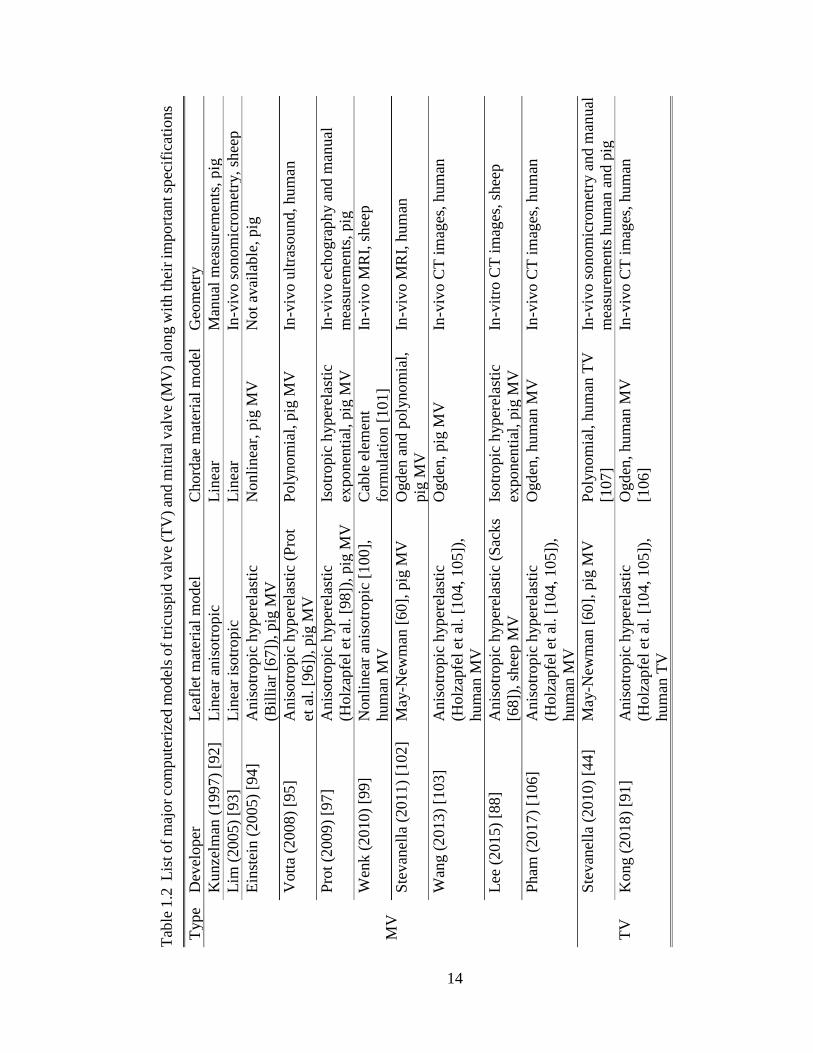
1.2 List of major computerized models of tricuspid valve (TV) and mitral valve (MV)

along with their important specifications .................................................................. 14

1.3 The abbreviations used in this document are listed in this table alphabetically. ....... 18

2.1 Biaxial loadings protocols applied for each specimen ............................................... 24

2.2 Measured thicknesses for the leaflets of all the hearts used during the experiment .. 28

2.3 The average maximum rigid body rotation ωmax, the average maximum shear

angle θmax, and the average of the ratio of the maximum Cauchy shear stress to

the maximum Cauchy normal stress r presented for each loading protocol and

leaflet type (for each protocol and leaflet type the data is averaged over all hearts

and presented in the form of average ± standard error). ............................................ 33

3.1 The maximum membrane tension of each tension-controlled loading protocol for

circumferential c and radial r directions. The tension ratios were kept constant

during the experiments: Tc: Tr = 1: 1, 1: 0.75, 0.75: 1, 1: 0.5, 0.5: 1 ........................ 38

3.2 Material constants along with the R2 of the fit and anisotropy index AI calculated

for individual specimens by fitting the experimental data into the proposed

constitutive model ..................................................................................................... 50

3.3 Material constants for the tension-based average model data (AVG) as well as the

average data minus one standard error (AVG – SE) and average data plus one

standard error (AVG + SE). The corresponding R2 value of the fit and the

anisotropy index AI are also presented. ..................................................................... 55

3.4 Material constants for the first Piola–Kirchhoff-stress–based average model data

(AVG) as well as the average data minus one standard error (AVG – SE) and

average data plus one standard error (AVG + SE). The corresponding R2 value

of the fit and the anisotropy index AI are also presented. ......................................... 55

xiii

3.5 Material constants for the Cauchy-stress–based average model data. The

corresponding R2 value of the fit and the anisotropy index AI are also presented

in the table. ................................................................................................................ 55

5.1 Calculated area at minimum and maximum right ventricular pressure (RVP) for

intact and post chordae rupture (PCR) conditions. The values are presented for all

eight hearts used in the experiments along with the average (AVG) and standard

deviation (STD). Comparing the average values showed an increase in the area

post chordae rupture. ............................................................................................... 101

5.2 Calculated circumference at minimum and maximum right ventricular pressure

(RVP) for intact and post chordae rupture (PCR) conditions. The values are

presented for all eight hearts used in the experiments along with the average

(AVG) and standard deviation (STD). Comparing the average values showed an

increase in the circumference post chordae rupture. ............................................... 103

5.3 Calculated radius using the triangulation method (R) along with the radii

calculated from the area (RA) and circumference (RC), using the assumption of

flat annuli, at minimum and maximum right ventricular pressure (RVP) for intact

and post chordae rupture (PCR) conditions. The values are presented for all eight

experimental hearts along with the average (AVG) and standard deviation (STD).

Comparison between R, RA, and RC showed that the three different methods of

calculating the radius produced the same results. ................................................... 103

5.4 Geometric dilation in area, circumference, and radius of the heart annuli due to

chordae rupture at maximum right ventricular pressure (RVP) calculated using

Equation (5.1) along with the average (AVG) and standard deviation (STD) for

each quantity. ........................................................................................................... 105

5.5 Dilation in the length of annulus anterior segment (AAS), annulus posterior

segment (APS), and annulus septal segment (ASS) due to the chordae rupture at

maximum right ventricular pressure (RVP) calculated using Equation (5.1) along

with the average (AVG) and standard deviation (STD) for each quantity. The

largest dilation occurred at the AAS. ...................................................................... 105

5.6 Average geometric changes at maximum right ventricular pressure (RVP) for

intact and post chordae rupture (PCR) conditions calculated using Equation (5.2).

The last column shows the percentage of the change in geometric parameters with

intact-to-PCR dilation included in calculations. The geometrical parameters at

minimum RVP were selected as the reference to calculate the changes. ................ 108

7.1 The measured perimeter (Prmtr), anterior segment length (ASL), posterior

segment length (PSL), septal segment length (SSL), anterior leaflet height (ALH),

posterior leaflet height (PLH), septal leaflet height (SLH), anteroposterior

commissure height (ACH), posteroseptal commissure height (PCH), and

anteroseptal commissure height (SCH) for three different porcine heart valves.

xiv

The table also includes the normalized values for each valve, the normalized

average (Nrmlzd AVG), and the scaled average values. The scaled average

(AVG) values were used in the modeling of the valve geometry. .......................... 138

7.2 Average (AVG) number of first- and second-order chordae counted based on the

dissected porcine TVs and used in the geometry modeling. ................................... 138

8.1 Parameters of a Fung-type model for human heart valves [42] ................................152

C.1 Five different loading protocols used in the tangential (Tang) and radial directions

during the experiments to evaluate the mechanical response of different regions

of porcine mesentery. .............................................................................................. 202

C.2 Measured thicknesses for the individual specimens of the distal avascular, distal

vascular, and root regions of the porcine mesentery. .............................................. 208

C.3 The average maximum rigid body rotation wmax, the average maximum shear

angle θmax, and the average ratio of the maximum Cauchy shear stress to the

maximum Cauchy normal stress r presented for each loading protocol and

mesentery region (for each protocol and mesentery region the data are averaged

over all samples (n=8) and presented in the form of average ± standard error). ..... 211

C.4 Material parameters computed for individual samples by fitting the experimental

data to the proposed constitutive model along with the fitting R-squared values

(R2) and the anisotropy index (AI). ......................................................................... 214

C.5 Material parameters computed by fitting the averaged stress–strain data to the

proposed constitutive model along with the fitting R-squared (R2) and the

anisotropy index (AI). .............................................................................................. 220

xv

LIST OF FIGURES

Figure Page

1.1 The heart structure and parts. (Image adopted from Cook et al. [2]) ........................... 2

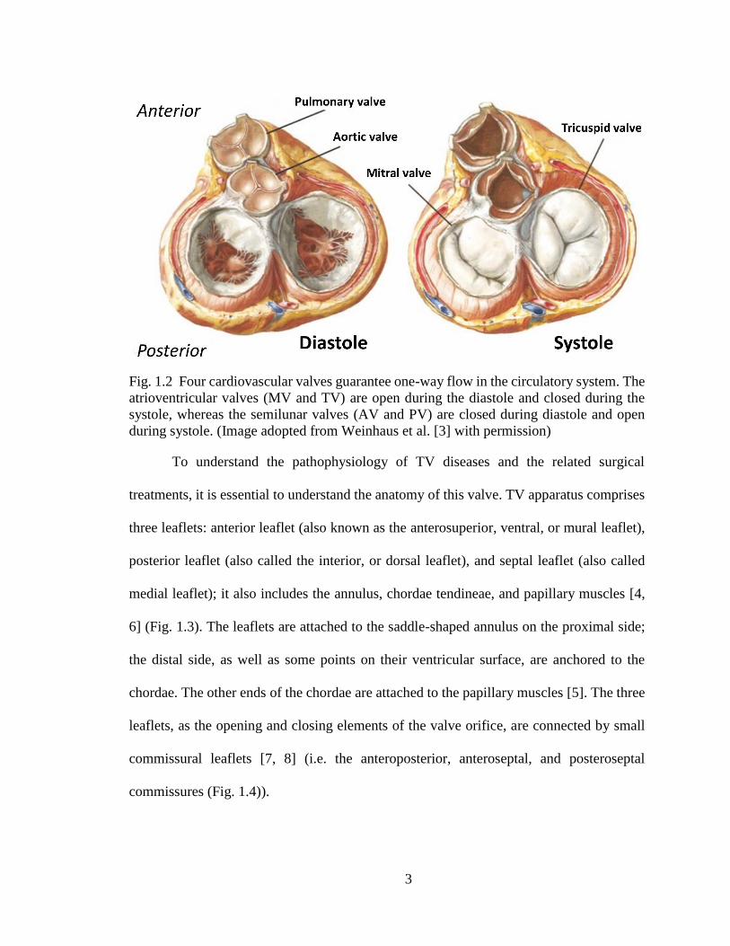
1.2 Four cardiovascular valves guarantee one-way flow in the circulatory system. The

atrioventricular valves (MV and TV) are open during the diastole and closed

during the systole, whereas the semilunar valves (AV and PV) are closed during

diastole and open during systole. (Image adopted from Weinhaus et al. [3]) ............. 3

1.3 TV apparatus comprises of anterior leaflet, posterior leaflet, septal leaflet, annulus,

chordae tendineae, and papillary muscles. (Image adopted from Weinhaus et al.

[3] and Chan [5].) ........................................................................................................ 4

1.4 Illustration of the tricuspid valve leaflets, their connection to each other, and their

attachment to the chordae. (Image adapted from Carpentier et al. [8].) ...................... 5

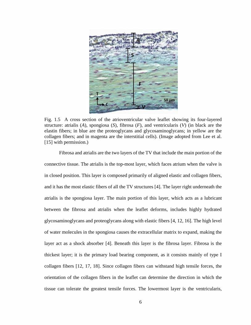
1.5 A cross section of the atrioventricular valve leaflet showing its four-layered

structure: atrialis (A), spongiosa (S), fibrosa (F), and ventricularis (V) (in black

are the elastin fibers; in blue are the proteoglycans and glycosaminoglycans; in

yellow are the collagen fibers; and in magenta are the interstitial cells). (Image

adopted from Lee et al. [15].) ...................................................................................... 6

2.1 Custom-made biaxial tensile testing equipment ........................................................ 22

2.2 a) Specially designed phantom to facilitate the attachment of the leaflets to the

biaxial tensile testing equipment. b) Specimen attached to the equipment using

fishhooks and suture lines. ........................................................................................ 24

2.3 The three leaflets of the tricuspid valve and the position and shape of the

specimens. ................................................................................................................. 27

2.4 The average membrane tension versus stretch ratio for the loading protocols a)

number 1 (equibiaxial), b) number 2, c) number 3, d) number 4, and e) number 5

for the anterior leaflet. The circumferential (Circ) and radial directions are in solid

red and dash-dotted blue, respectively. The bars are standard errors. The green

dashed line shows the maximum physiological tension level (Max Physio), while

the tension level goes up to 100 N/m in case of hypertension. ................................ 30

xvi



for the posterior leaflet. The circumferential (Circ) and radial directions are in

solid red and dash-dotted blue, respectively. The bars are standard errors. The

green dashed line shows the maximum physiological tension level (Max Physio),

while the tension level goes up to 100 N/m in case of hypertension. ...................... 31



for the septal leaflet. The circumferential (Circ) and radial directions are in solid

red and dash-dotted blue, respectively. The bars are standard errors. The green

dashed line shows the maximum physiological tension level (Max Physio), while

the tension level goes up to 100 N/m in case of hypertension. ................................. 32

3.1 Comparison between the accuracy of linear interpolation and exponential fit to

estimate the original data for averaging. ................................................................... 43

3.2 The constant stress contours produced using the response functions of Equation

(2.2) plotted over the strain field for typical leaflets: (a,b) anterior, (c,d) posterior,

and (e,f) septal leaflets. .............................................................................................. 47

3.3 The result of the five-protocol fit along with the experimentally measured

circumferential (Circ) and radial data for typical leaflets: (a) anterior, (b)

posterior, and (c) septal. The numbers represent the protocol numbers listed in

Table 3.1. ................................................................................................................... 49

3.4 The average stress–strain responses developed based on identical tension states

from loading protocols (a) number 1 (equibiaxial), (b) number 2, (c) number 3,

(d) number 4, and (e) number 5 of Table 3.1 for the anterior leaflet. The vertical

axis is the second Piola–Kirchhoff stress, and the horizontal axis is the Green

strain. These data were used to calculate the average material constants presented

in Table 3.3. ............................................................................................................... 52

3.5 The average stress–strain responses developed based on identical first Piola–Kirchhoff stress states from loading protocols (a) number 1 (equibiaxial), (b)

number 2, (c) number 3, (d) number 4, and (e) number 5 of Table 3.1 for the

anterior leaflet. The vertical axis is the second Piola–Kirchhoff stress, and the

horizontal axis is the Green strain. These data were used to calculate the average

material constants presented in Table 3.4.................................................................. 53

3.6 The average stress–strain responses developed based on identical Cauchy stress

states from loading protocols (a) number 1 (equibiaxial), (b) number 2, (c) number

3, (d) number 4, and (e) number 5 of Table 3.1 for the anterior leaflet. The vertical

axis is the second Piola–Kirchhoff stress, and the horizontal axis is the Green

strain. These data were used to calculate the average material constants presented

in Table 3.5. ............................................................................................................... 54

xvii

3.7 The five stress-controlled protocols used to reconstruct the tissue responses based

on the developed average models. The horizontal axis is the circumferential

second Piola–Kirchhoff stress, and the vertical axis is the radial second Piola–

Kirchhoff stress. ........................................................................................................ 56

3.8 Tissue response of the anterior leaflet to five stress-controlled loading protocols

(Fig. 3.7) reconstructed using the material constants of the arithmetic average (A-

B) from Table 3.2, the tension-based average model (T-B) from Table 3.3, the

first Piola–Kirchhoff-stress–based average model (P-B) from Table 3.4, and the

Cauchy-stress–based average model (C-B) from Table 3.5. The vertical axis is the

second Piola–Kirchhoff stress, and the horizontal axis is the Green strain. The

subscripts cc and rr denote the circumferential and radial directions, respectively.

................................................................................................................................... 57

3.9 Tissue response of the posterior leaflet to five stress-controlled loading protocols


B) from Table 3.2, the tension based average model (T-B) from Table 3.3, the





................................................................................................................................... 58

3.10 Tissue response of the septal leaflet to five stress-controlled loading protocols


B) from Table 3.2, the tension based average model (T-B) from Table 3.3, the





................................................................................................................................... 59

3.11 Small-angle light-scattering (SALS) scan of the midsection of a typical tricuspid

valve anterior leaflet. Each arrow shows the main direction of the extracellular

matrix fibers over a 250 μm × 250 μm region. The color map shows the degree

of alignment. The warmest color, corresponding to 1, indicates a network in which

all fibers are in the same direction; the coolest color, corresponding to 0, indicates

a network in which the probability of a fiber existing in any directions is the same.

................................................................................................................................... 62

3.12 Constant strain energy contours plotted over the Green strain field for the (a)

anterior, (b) posterior, and (c) septal leaflets of a typical tricuspid valve. ................ 63

3.13 The strain energy contours plotted over the strain field for posterior leaflet of the

specimen listed as Sample 3 in Table 3.2. The contours are nonconvex, violating

the integrity of the developed constitutive model for this specific leaflet. ............... 64

xviii

4.1 a) Schematic of the ex-vivo beating heart apparatus and b) a picture of the actual

apparatus. ................................................................................................................... 71

4.2 The T-shaped pipefitting connected to the right atrium through a straight barbed

hose fitting (1). The Luer Lok assembly was connected to the other side of the t-

shaped pipe fitting to support the pressure sensor. The other straight barbed hose

fitting (2) connected the right ventricle to the pump. Crystal wires came out

through the inferior vena cava. The umbilical clamp was used to prevent leakage

from the inferior vena cava. ....................................................................................... 74

4.3 Umbilical clamps, cable ties, and worm-drive clamps were used for sealing. .......... 74

4.4 The arrangement of the sonocrystals over the surface of the septal leaflet. The red

lines show the triangular element used for strain calculation. The radial direction

was defined by a vector connecting crystal 4 to crystal 7. ........................................ 76

4.5 Right heart pressure during the cardiac cycle averaged over all of the hearts. The

bars are standard errors (n=8). The vertical lines show the opening and closure of

the pulmonary valve (PV) and tricuspid valve (TV): TV closed at 0.2 s and opened

at 0.54 s; the pulmonary valve opened at 0.29 s and closed at 0.44 s. ...................... 79

4.6 Average peak areal, maximum principal (Max Princ), circumferential (Circ), and

radial strains at the leaflet midpoint measured with respect to reference 1 (Ref1,

minimum RAP) and reference 2 (Ref2, end diastole). The error bars are standard

error (n=8). ................................................................................................................ 81

4.7 The temporal strain variations during the cardiac cycle. (a) The areal, (b)

maximum principal, (c) circumferential, and (d) radial strains at the leaflet

midpoint averaged over all of the hearts. The shaded area shows the standard error

(n=8). Vertical lines show the time points for TV closing, PV opening, maximum

RVP, PV closing and TV opening respectively from left to right............................. 82

4.8 The areal, maximum principal, circumferential, and radial strains at maximum

RVP. The strains are averaged over all the hearts (n=8) and are presented on a

typical septal leaflet. Minimum RAP is used as the reference for strain calculation.

The arrows are showing the direction of the strains at the center of each triangular

surface........................................................................................................................ 83

4.9 Distribution of the maximum principal strain over the leaflet during the septal

entire cardiac cycle. Maximum principal strain is averaged over all of the hearts

(n=8) and showed over a typical septal leaflet during the cardiac cycle. .................. 84

5.1 Eight sonocrystals (2 mm in diameter) sutured around the valve annulus (a) before

the experiment and (b) after the experiment. The pulmonary side of the heart has

been cut open for better visualization of the positions of the crystals....................... 95

xix

5.2 Method used to calculate the area, circumference, and radius of the annulus. A

lower resolution of the original triangulation is presented for illustrative purposes.

................................................................................................................................... 97

5.3 Average right ventricular pressure (RVP), pulmonary artery pressure (PAP), and

right atrial pressure (RAP) measured for the intact and post chordae rupture (PCR)

cases. ........................................................................................................................ 100

5.4 Comparison of the average values of (a) the area, (b) circumference, and (c) radius

between the intact and post chordae rupture (PCR) conditions at minimum and

maximum right ventricular pressure (RVP). The Wilcoxon signed rank test p-

values for area, circumference, and radius were 0.01 at maximum RVP and 0.04

at minimum RAP. The asterisks (*) show significant differences (p < 0.05,

Wilcoxon signed rank test). Error bars show the standard errors. ........................... 102

5.5 Comparison of the dilation (due to the chordae rupture) between annulus anterior

segment (AAS), annulus posterior segment (APS), and annulus septal segment

(ASS) at maximum right ventricular pressure (RVP). The Wilcoxon signed rank

test p-values were 0.55, 0.38, and 0.74 between the AAS and APS, the AAS and

ASS, and the APS and ASS, respectively. No significant differences were

observed (p > 0.05, Wilcoxon signed rank test). Error bars show the standard

errors. ....................................................................................................................... 104

5.6 Changes in (a) area, (c) circumference, and (e) radius as well as the absolute values

of (b) area, (d) circumference, and (f) radius throughout the cardiac cycle

averaged over all the annuli for intact and post chordae rupture (PCR) conditions.

The shaded regions show the standard errors. The temporal position of the

maximum right ventricular pressure (RVP) as well as the opening and closure of

the tricuspid and pulmonary valves for the intact case are shown in the graphs as

a better illustration of the deformations that occur throughout the cardiac cycle. .. 107

5.7 Comparison of the change in the length of the annulus anterior segment (AAS),

annulus posterior segment (APS), and annulus septal segment (ASS) in intact and

post chordae rupture (PCR) conditions at maximum right ventricular pressure

(RVP). The PCR values include the dilation as well. For a comparison of the

change in length between the intact and PCR conditions, the Wilcoxon signed

rank test was used; p-values were 0.02 for AAS and ASS and 0.38 for APS. The

p-values were 0.03, 0.02, and 0.84 for the comparison of the change in length for

the intact case between the AAS and APS, the AAS and ASS, and the APS and

ASS, respectively. The asterisks (*) indicate significant differences (p < 0.05,

Wilcoxon signed rank test). Error bars show the standard errors. ........................... 108

6.1 TV septal leaflet and annulus average geometry at reference frame (minimum

RAP) for normal (blue) and PCR (red) conditions. ................................................. 123

xx

6.2 Average hemodynamic pressures during the cardiac cycle for intact conditions.

The shaded areas show the standard error. .............................................................. 124

6.3 Average hemodynamic pressures during the cardiac cycle for post chordae rupture

(PCR) conditions. The shaded areas show the standard error. ................................ 125

6.4 Spatial distribution of areal, maximum principal (Max Princ), circumferential

(Circ), and radial strains demonstrated over the developed average septal leaflet

geometry at maximum right ventricular pressure (RVP) before (top row) and after

(bottom row) chordae rupture. ................................................................................. 127

6.5 Comparison of the average (over all the hearts) of maximum of the strain’s spatial

average signal (strain is averaged over the leaflet surface throughout the cardiac

cycle). Error bars show the standard error. .............................................................. 128

6.6 Comparison of the maximum of maximum principal strain between intact and post

chordae rupture (PCR) cases for Crystal 1 and Crystal 2, shown in Fig. 6.1. ......... 128

6.7 Calculated average TV septal leaflet maximum principal strain, plotted at different

timepoints to show the deformation of the leaflet throughout the cardiac cycle for

both intact (top row) and post chordae rupture (bottom row) conditions. The color

map shows the distribution of the maximum principle strain. ................................ 129

6.8 Temporal distribution of the spatial average of the strains throughout the cardiac

cycle for intact and post chordae rupture (PCR) conditions averaged for all hearts.

The shaded area shows the standard error. .............................................................. 130

7.1 The important dimensions of the tricuspid valve, which include anterior segment

length (ASL), posterior segment length (PSL), septal segment length (SSL),

anterior leaflet height (ALH), posterior leaflet height (PLH), septal leaflet height

(SLH), anteroposterior commissure height (ACH), posteroseptal commissure

height (PCH), and anteroseptal commissure height (SCH), as measured from

dissected porcine heart valve apparatus. ................................................................. 137

7.2 Reconstructed wireframe used for modeling the tricuspid valve geometry. Refer

to Table 7.1 for abbreviations and dimensions. ....................................................... 140

7.3 The reconstructed TV apparatus geometry used in the finite element analysis. ...... 140

7.4 Finite element mesh for the reconstructed TV geometry......................................... 144

7.5 Maximum in-plane principal strain distribution illustrated over the anterior (A),

posterior (P), and septal (S) valve leaflets at different points in time during the

valve closure simulation. ......................................................................................... 145

xxi

7.6 Distribution of maximum in-plane principal strain over the septal leaflet at

maximum right ventricular pressure. ....................................................................... 146

7.7 Maximum in-plane principal stress distribution illustrated over the anterior (A),

posterior (P), and septal (S) valve leaflets at different points in time during the

valve closure simulation. ......................................................................................... 147

7.8 Comparison of effects of changes in the annulus boundary conditions on the strain

distribution and deformations of the septal leaflet. The top plot shows the result

of the simulation with the moving annulus boundary conditions (as the simulation

of the intact case), and the bottom plot shows the result of the simulation with the

fixed annulus boundary conditions (as the simulation of rigid ring annuloplasty). .148

A.1 The average stress–strain responses developed based on identical tension states


(d) number 4, and (e) number 5 of Table 3.1 (of the main manuscript) for the

posterior leaflet. The vertical axis is the second Piola–Kirchhoff stress, and the


material constants presented in Table 3.3................................................................ 184

A.2 The average stress–strain responses developed based on identical first Piola–

Kirchhoff stress states from loading protocols (a) number 1 (equibiaxial), (b)

number 2, (c) number 3, (d) number 4, and (e) number 5 of Table 3.1 (of the main

manuscript) for the posterior leaflet. The vertical axis is the second Piola–

Kirchhoff stress, and the horizontal axis is the Green strain. These data were used

to calculate the average material constants presented in Table 3.4. ........................ 185

A.3 The average stress–strain responses developed based on identical Cauchy stress


3, (d) number 4, and (e) number 5 of Table 3.1 (of the main manuscript) for the

posterior leaflet. The vertical axis is the second Piola–Kirchhoff stress, and the



A.4 The average stress–strain responses developed based on identical tension states


(d) number 4, and (e) number 5 of Table 3.1 (of the main manuscript) for the

septal leaflet. The vertical axis is the second Piola–Kirchhoff stress and the



A.5 The average stress–strain responses developed based on identical first Piola–

Kirchhoff stress states from loading protocols (a) number 1 (equibiaxial), (b)

number 2, (c) number 3, (d) number 4, and (e) number 5 of Table 3.1 (of the main

manuscript) for the septal leaflet. The vertical axis is the second Piola–Kirchhoff

xxii

stress, and the horizontal axis is the Green strain. These data were used to

calculate the average material constants presented in Table 3.4. ............................ 188

A.6 The average stress–strain responses developed based on identical Cauchy stress


3, (d) number 4, and (e) number 5 of Table 3.1 (of the main manuscript) for the

septal leaflet. The vertical axis is the second Piola–Kirchhoff stress, and the


material constants presented in Table 3.5.................................................................189

C.1 The specimens were excised from (A) the distal avascular region, (B) the distal

vascular region, and (C) the root region of the porcine mesenteries. ...................... 200

C.2 (a) Suture lines are connected to the specimen using fishhooks. (b) Specimen

attached to the specifically-designed carriages of the equipment using suture-

lines.......................................................................................................................... 201

C.3 The average membrane tension versus stretch ratio for the equibiaxial loading

protocol for (a) the distal avascular, (b) the distal vascular, and (c) the root regions

of the porcine mesenteries (n=8, the bars are standard errors). ............................... 210

C.4 The mean stretch values at 40 N ⁄ m measured at three different regions of the

mesentery shown in Fig. C.1 for radial and tangential (Tang) directions. Bars are

the standard error (n=8). .......................................................................................... 210

C.5 The constant stress contours for (a) and (b) the distal avascular, (c) and (d) the

distal vascular, and (e) and (f) the root regions of a typical porcine mesentery

specimens. ............................................................................................................... 212

C.6 The experimentally measured data and the result of the five-protocol fitting for

(a) the distal avascular, (b) the distal vascular, and (c) the root regions of a typical

porcine mesentery specimen. The numbers are associated with the protocol

numbers in Table C.1. ............................................................................................. 215

C.7 Average second Piola–Kirchhoff stress versus Green strain in tangential (Tang)

and radial directions for loading protocols (a) number 1 (equibiaxial), (b) number

2, (c) number 3, (d) number 4, and (e) number 5 of Table C.1 for the distal

avascular region. ...................................................................................................... 216



2, (c) number 3, (d) number 4, and (e) number 5 of Table C.1 for the distal

vascular region......................................................................................................... 217

xxiii



2, (c) number 3, (d) number 4, and (e) number 5 of Table C.1 for the root region. 217

C.10 Constant energy contours plotted over the strain field for typical samples of (a)

the distal avascular, (b) the distal vascular, and (c) the root regions of the porcine

mesentery. ................................................................................................................ 222

C.11 The mechanical responses observed for the root region of the porcine mesentery

did not always follow the same trend. For example, tissue was (a) stiffer in

tangential direction, or (b) had similar stiffness in both directions, noticeably

different from other typical cases in this region (Fig. C.6c). The numbers are

associated with the protocol numbers in Table C.1. ................................................ 223

1

CHAPTER 1I

INTRODUCTION

1.1 Anatomy and Function of the Heart

The heart, one of the most vital organs of the body, is a combination of two separate

pumps that are attached to one another. The right side pumps blood through the pulmonary

circulation in order to transfer oxygen to blood in the lungs. Conversely, the left side pumps

blood into the systemic circulation to provide the organs and tissues of the body with

necessary oxygen and nutrients. Each side of the heart incorporates an atrium and a

ventricle [1] (Fig. 1.1).

A recurrent contraction in the heart muscles provides the force to pump the blood,

and four one-way valves (including two atrioventricular and two semilunar valves) guide

the blood in the appropriate direction in the circulation process (Fig. 1.2). During systole,

the atrioventricular valves—the mitral valve (MV) on the right and the tricuspid valve (TV)

in the left) force—close the valve orifice to prevent blood from the ventricles from back

into the atria. Analogically during diastole, the semilunar valves close to prevent the blood

from flowing back from the aorta (aortic valve (AV)) and pulmonary arteries (pulmonary

valve (PV)). Opening and closure of these four valves are passive procedures (i.e. a

backward pressure gradient closes the valves, and a forward pressure gradient causes them

to open) [1].

2

Fig. 1.1 The heart structure and parts. (Image adopted from Cook et al. [2] with permission)

Each of these valve apparatuses consists of several parts that, in combination with

the other parts of the heart, create a powerful blood pump that can beat an average of more

than three billion times during a human lifetime. In the current study, we are focusing on

the TV; therefore, in the following sections of this chapter, we discuss this apparatus in

more detail.

1.2 Tricuspid Valve Anatomy

The TV, as one of the two atrioventricular valves, is a composite of several

structures located in the right heart between the right atrium and right ventricle, and it has

a roughly triangular orifice. The structures of the TV work together in order to open during

diastole and close during systole to maintain a one-way flow of blood and to prevent blood

backflow from the right ventricle to the right atrium during the systole [4, 5].

3

Fig. 1.2 Four cardiovascular valves guarantee one-way flow in the circulatory system. The

atrioventricular valves (MV and TV) are open during the diastole and closed during the

systole, whereas the semilunar valves (AV and PV) are closed during diastole and open

during systole. (Image adopted from Weinhaus et al. [3] with permission)

To understand the pathophysiology of TV diseases and the related surgical

treatments, it is essential to understand the anatomy of this valve. TV apparatus comprises

three leaflets: anterior leaflet (also known as the anterosuperior, ventral, or mural leaflet),

posterior leaflet (also called the interior, or dorsal leaflet), and septal leaflet (also called

medial leaflet); it also includes the annulus, chordae tendineae, and papillary muscles [4,

6] (Fig. 1.3). The leaflets are attached to the saddle-shaped annulus on the proximal side;

the distal side, as well as some points on their ventricular surface, are anchored to the

chordae. The other ends of the chordae are attached to the papillary muscles [5]. The three

leaflets, as the opening and closing elements of the valve orifice, are connected by small

commissural leaflets [7, 8] (i.e. the anteroposterior, anteroseptal, and posteroseptal

commissures (Fig. 1.4)).

4

Fig. 1.3 TV apparatus comprises of anterior leaflet, posterior leaflet, septal leaflet, annulus,

chordae tendineae, and papillary muscles. (Image adopted from Weinhaus et al. [3] and

Chan [5] with permission.)

Perfect closure relies on the precise coaptation of the three leaflets, which implies

a perfect fit between the surface area and shape of the leaflets and the annulus [9]. The

chordae tendineae, along with the papillary muscles, construct a suspension system for the

leaflets to sit on. This suspension system prevents excessive upward displacement of the

leaflets during the systole and eases the opening of the valve orifice during the diastole.

Papillary muscles, which have contractile properties and are attached to the ventricular wall

at the proximal side, are normally categorized in three groups (anterior, posterior, and

septal, as mentioned previously). The chordae tendineae, which are the intermediate parts

between the papillary muscles and the leaflets, are fibrous cords that possess elastic

properties. Based on their attachment to the leaflet, three types of chordae tendineae can

be distinguished: basal chordae (attached to the base of the leaflets), intermediary or

second-order chordae (attached to the belly of the leaflet at the ventricular side), and

marginal chordae or first-order (attached to the free edge of the leaflets) [8-10]. The

majority of the chordae tendineae branch before inserting into the leaflet. In this

5

dissertation, we use the abovementioned convention for chordae tendineae categorization;

however, other methods of categorization with different approaches also exist [8, 9].

Fig. 1.4 Illustration of the tricuspid valve leaflets, their connection to each other, and their

attachment to the chordae. (Image adapted from Carpetier et al. [8])

The TV apparatus—along with the right atrium, right ventricle, and blood flow—

are interconnected components of the same hemodynamic system, and TV function is

heavily influenced by the operation of all other components [8].

1.3 Tricuspid Valve Microstructure

Different parts of the TV apparatus have different structural components based on

their complex functions. TV leaflets contain interstitial fibroblasts and connective tissue

fibers [11], including collagen and elastin, within an extracellular matrix [4]. They have a

four-layer structure in cross section including atrialis, spongiosa, fibrosa, and ventricularis,

covered by a layer of endothelial cells [4, 12-15] (Fig. 1.5).

6

Fig. 1.5 A cross section of the atrioventricular valve leaflet showing its four-layered

structure: atrialis (A), spongiosa (S), fibrosa (F), and ventricularis (V) (in black are the

elastin fibers; in blue are the proteoglycans and glycosaminoglycans; in yellow are the

collagen fibers; and in magenta are the interstitial cells). (Image adopted from Lee et al.

[15] with permission.)

Fibrosa and atrialis are the two layers of the TV that include the main portion of the

connective tissue. The atrialis is the top-most layer, which faces atrium when the valve is

in closed position. This layer is composed primarily of aligned elastic and collagen fibers,

and it has the most elastic fibers of all the TV structures [4]. The layer right underneath the

atrialis is the spongiosa layer. The main portion of this layer, which acts as a lubricant

between the fibrosa and atrialis when the leaflet deforms, includes highly hydrated

glycosaminoglycans and proteoglycans along with elastic fibers [4, 12, 16]. The high level

of water molecules in the spongiosa causes the extracellular matrix to expand, making the

layer act as a shock absorber [4]. Beneath this layer is the fibrosa layer. Fibrosa is the

thickest layer; it is the primary load bearing component, as it consists mainly of type I

collagen fibers [12, 17, 18]. Since collagen fibers can withstand high tensile forces, the

orientation of the collagen fibers in the leaflet can determine the direction in which the

tissue can tolerate the greatest tensile forces. The lowermost layer is the ventricularis,

7

which consist of sheets of endothelial cells that overlay the elastic and collagen fibers [4].

The thickness of these layers will vary according to their proximity to the annulus.

Proximal to the annulus, the fibrosa is thick and gradually becomes thinner towards the

distal side of the leaflets, vanishing about two-thirds of the way through. In contrast,

spongiosa and atrialis are relatively thin at the proximity of the annulus and increasingly

thicken distally to become the main components at the free edges of the leaflets [4]. The

TV annulus has a fibrous structure, which gradually transitions from the collagen-rich area

at the leaflet’s side to the elastin-rich area towards the myocardium wall [12, 18]. The

chordae tendineae are composed of collagen fibers parallel to the chordae long axis [18];

they provide the necessary strength for the chordae to carry tensile loads when the valve is

pressurized.

1.4 Tricuspid Valve Pathophysiology

Etiologically, TV regurgitation can be divided into two types, functional

regurgitation and organic regurgitation. Functional TV regurgitation (FTR), also known as

secondary TV regurgitation, is the primary reason for TV malfunction. It is the type of

regurgitation that develops after a disturbance in the coordination of the valve elements

without any organic valvular or myocardial lesion [4, 8]. This dysfunction, which could be

reversible, is considered to be functional, as the morphology of the leaflets is normal [5,

19]. MV diseases, right ventricular dysfunction, and pulmonary hypertension diseases are

the main reasons for development of FTR [8]. For example, approximately one half of the

patients suffering from MV regurgitation have at least moderate FTR [20, 21]. In addition,

more than 30% of the patients with MV stenosis have developed moderate to severe FTR

[22, 23].

8

On the other hand, organic TV regurgitation is primarily due to either the

involvement of the TV in certain diseases or a diseased myocardium. No matter what the

etiology of the disease is, it can cause lesions that affect different components including

the annulus (dilatation, abscess), leaflets (excess leaflet tissue, thickening, vegetation,

abscess, perforation, tear), commissures (fusion, thickening), chordae (rupture, elongation,

thickening, shortening, fusion), papillary muscles (rupture, elongation), and/or ventricle

(infarction, fibrosis, dilatation) [8]. Three different types of TV regurgitation have been

defined based on leaflet motion [8]: type I (normal leaflet motion), type II (excessive leaflet

motion or leaflet prolapse), and type III (restricted leaflet motion, including restricted

leaflet opening and restricted leaflet closure). Severe restriction to the leaflet motion as a

result of commissural fusion, leaflet thickening, chordae fusion, and calcification causes a

reduction in blood flow from the atrium to the ventricle; this condition is categorized as

TV stenosis [4, 8].

As one of the most common TV dysfunctions, TV regurgitation often requires TV

repair or replacement [24, 25]. From 1999 to 2008, approximately 150,000 patients

underwent TV repair surgeries [24] in the United States. Overall, TV repair has better

outcomes when compared to TV replacement with prosthetic devices [8, 26, 27]. However,

according to the Society of Thoracic Surgery Database, in terms of morbidity and mortality,

TV surgery is still the most high-risk valve operation [28]. The frequency of TV repair

procedures has been increasing recently, as many investigators are now in favor of more

aggressive surgical approaches to FTR in the absence of any organic TV lesions [24, 29-

31]. Roughly 1.6 million people in the United States suffer secondary TV regurgitation,

raising the number of potential candidates for TV repair [32-34].

9

1.5 Tricuspid Valve Mechanical Behavior

The success level of TV surgeries is highly tied to our knowledge of TV mechanical

properties as, similar to the other cardiovascular valves, TV function is linked to the valve’s

biomechanical behavior and complex geometry. The mechanical behavior of any material,

in turn, is tied to its microstructure. As discussed above, the microstructure of TV

components is extremely complex, complicating the overall mechanical behavior of the

valve. Given the in-situ loading conditions of the desired valve leaflets during the operation

of the heart, biaxial tensile tests have been used to provide precise and realistic data on the

mechanical response of the heart valve leaflets. Many studies have addressed the

mechanical behaviors of soft tissue including the MV and AV [35-42]. May-Newman et

al. studied the biaxial mechanical behavior of the porcine MV [35], and Billiar et al. probed

the biaxial responses of the natural and glutaraldehyde-treated AV cups [36]. Grashow et

al. studied creep and strain relaxation as well as the effect of strain rate on the mechanical

behavior of the anterior leaflet of the MV [37, 38]. Sacks et al. explored the surface strains

of the MV anterior leaflet [39]. However, TV mechanical behavior has been understudied

in comparison to the behavior of other heart valves, and it has not yet been accurately

characterized, leaving it to become known as “the forgotten valve” [43]. For example, the

only available computational model of the TV [44] has been constructed based on a grossly

simplified geometry using the homogenous mechanical properties of the MV.

1.6 Material Models

Mechanical response modeling is an essential step in the accurate quantification of

normal biomechanical behavior of the native valve tissue during the cardiac cycle. Material

models are necessary for a better understanding of the mechanical behavior of the tissue

10

and are designed to model the mechanical responses under a generalized form of loading

in a computerized simulations. For this purpose, researchers develop equations, namely

constitutive models, that can approximate the response of the desired material (i.e. the

strains) to the environmental stimuli (i.e. forces). These models can be derived as the

empirical relationship between the stimuli and the response, which are known as

phenomenological models, or they can be derived based on basic principles and

microstructure of the desired material, which are known as structural models. Several

different phenomenological and structural models have been proposed to represent the

mechanical behavior of different materials [45-49] based on their inherent microstructure

and composition. For example, the Mooney–Rivlin model (developed initially by Mooney

[45] and modified by Rivlin et al. [46]) and the Ogden model (proposed by Ogden [47])

were developed to represent the mechanical behavior of isotropic rubber materials.

Soft tissue materials (including heart valve tissue) are often considered

incompressible. Because of their oriented fibrous structure, they are known to exhibit

anisotropic responses. They express highly nonlinear stress–strain response and undergo

large strains and rotations [12, 50]. All these characteristics induce complexity in their

mechanical behavior and make their accurate modeling highly challenging. Researchers

have proposed different models to represent the mechanical responses of soft tissues,

including heart valves [15, 42, 50-73]. Different variations of a Fung-type model, originally

proposed by Fung [52], have been widely used in modeling mechanical behavior of soft

tissues including skin [53], pericardium [54, 55], abdominal aorta [56], urinary bladder

[57], small intestine [58], coronary artery [59], and heart valves [42]. May-Newman and

Yin proposed a specific phenomenological constitutive model with three material constants

11

to represent the mechanical behavior of the MV [60]. Choi et al. introduced a

phenomenological constitutive model to address orthotropic mechanical properties of the

pericardium [61-63], which was later used by other researchers to model the mechanical

responses of the abdominal aorta [64, 65]. In addition to the phenomenological constitutive

models, structural models have also been widely used to capture the mechanical responses

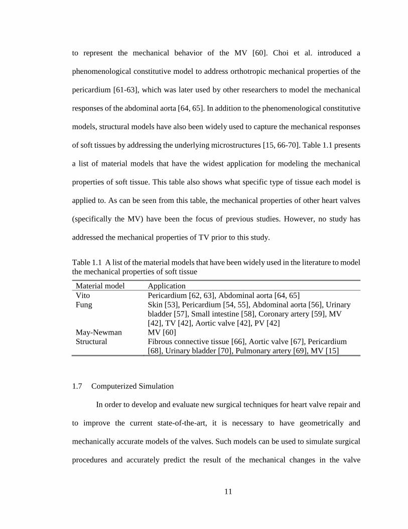
of soft tissues by addressing the underlying microstructures [15, 66-70]. Table 1.1 presents

a list of material models that have the widest application for modeling the mechanical

properties of soft tissue. This table also shows what specific type of tissue each model is

applied to. As can be seen from this table, the mechanical properties of other heart valves

(specifically the MV) have been the focus of previous studies. However, no study has

addressed the mechanical properties of TV prior to this study.

Table 1.1 A list of the material models that have been widely used in the literature to model

the mechanical properties of soft tissue

Material model Application

Vito Pericardium [62, 63], Abdominal aorta [64, 65]

Fung Skin [53], Pericardium [54, 55], Abdominal aorta [56], Urinary

bladder [57], Small intestine [58], Coronary artery [59], MV

[42], TV [42], Aortic valve [42], PV [42]

May-Newman MV [60]

Structural Fibrous connective tissue [66], Aortic valve [67], Pericardium

[68], Urinary bladder [70], Pulmonary artery [69], MV [15]

1.7 Computerized Simulation

In order to develop and evaluate new surgical techniques for heart valve repair and

to improve the current state-of-the-art, it is necessary to have geometrically and

mechanically accurate models of the valves. Such models can be used to simulate surgical

procedures and accurately predict the result of the mechanical changes in the valve

12

apparatus or the boundary conditions. In addition, these models contribute to the

development of new prosthetic valves that are designed to mimic native valve behaviors.

To develop such models accurately and to validate them, one should consider the following

factors:

Appropriate mechanical properties. A computerized model needs to reflect the

realistic mechanical response of the original tissue under a generalized loading condition.

Obtaining such properties can be accomplished by accurately measuring the mechanical

properties of the tissue and using appropriate material models [74, 75].

Accurate geometry and underlying microstructure. Manual measurements or 2D

and 3D imaging can be used to reconstruct the geometry of the TV. Small angle light

scattering (SALS) techniques [76-79] can be used to extract the microstructure of the leaflet

tissues and the distribution of the fiber orientations.

Loading and boundary conditions. In case of the heart valve, loading can be

accomplished by incorporating the transvalvular pressures or the blood flow into the

simulation. In this case, boundary conditions might be the deformation of the annulus and

papillary muscles throughout the cardiac cycle. Sonomicrometry [80-83] or other

techniques [84] can be used to track and record these boundary conditions.

Experimental measurements for validation purposes. A reliable method to evaluate

the accuracy of the developed computerized model is to experimentally measure the

deformations in a specific case and compare them with the results of the computerized

simulation. Sonomicrometry techniques [26, 85], videofluoroscopy [30], or camera

tracking systems [39] can be used to capture the heart valve deformations and extract the

13

mechanical strains [86, 87] while the heart is beating. These strains can be compared to the

simulation results to validate the model.

Such a geometrically and mechanically accurate model, once it has been

experimentally validated, can be used to simulate the heart valve lesions and surgical

procedures as well as evaluate the effects of mechanical alterations on the valve apparatus

and/or develop new prosthetic valves. Lee et al. have recently published a detailed article

regarding such a model that they have developed for the MV [88, 89]. In this study, high-

resolution micro-CT images of MV were used to reconstruct an accurate geometry. The

microstructure of the tissues was characterized using SALS, and the material model

proposed by Fan et al. [90] was used to represent the mechanical behavior of the MV

leaflets. However, by the start of the study described in this dissertation, no accurate

computerized model of TV was available in the literature. The only available model at that

time was established based on a grossly simplified geometry, and a material model for the

MV was used to represent the mechanical properties [44]. Another model later was

proposed by Kong et al. in 2018 [91], was based on a more accurately developed geometry

obtained from CT images, and TV mechanical properties were used to represent the

mechanical responses. However, no data were presented to verify the validity of this model.

Consequently, it was necessary to develop a more accurate and verifiable finite element

(FE) model of the TV to be used in computerized simulations in order to study TV behavior

under different circumstances and environmental changes, including simulation of valvular

lesions and treatments. Table 1.2 summarizes the major computerized models for the MV

and the only two available computerized models for the TV, along with their important

specifications (including the material models).

14

Tab

le 1

.2 L

ist of

maj

or

com

pute

rize

d m

odel

s of

tric

usp

id v

alve

(TV

) an

d m

itra

l val

ve

(MV

) al

on

g w

ith thei

r im

port

ant sp

ecif

icat

ions

Type

Dev

eloper

L

eafl

et m

ater

ial

model

C

hord

ae m

ater

ial

model

G

eom

etry

MV

Kunze

lman

(1997)

[92]

Lin

ear

anis

otr

opic

L

inea

r M

anual

mea

sure

men

ts, p

ig

Lim

(2005)

[93]

Lin

ear

isotr

opic

L

inea

r In

-viv

o s

onom

icro

met

ry,

shee

p

Ein

stei

n (

2005)

[94]

Anis

otr

opic

hyp

erel

asti

c

(Bil

liar

[67])

, pig

MV

Nonli

nea

r, p

ig M

V

Not

avai

lable

, pig

Vott

a (2

008)

[95]

Anis

otr

opic

hyp

erel

asti

c (P

rot

et a

l. [

96])

, pig

MV

Poly

nom

ial,

pig

MV

In

-viv

o u

ltra

sound, hum

an

Pro

t (2

009)

[97]

Anis

otr

opic

hyp

erel

asti

c

(Holz

apfe

l et

al.

[98])

, pig

MV

Isotr

opic

hyper

elas

tic

exponen

tial

, pig

MV

In-v

ivo e

cho

gra

ph

y a

nd m

anual

mea

sure

men

ts, pig

Wen

k (

2010)

[99]

Nonli

nea

r an

isotr

opic

[1

00],

hum

an M

V

Cab

le e

lem

ent

form

ula

tion [

101]

In-v

ivo M

RI,

sh

eep

Ste

van

ella

(2011)

[102]

May

-New

man

[60],

pig

MV

O

gd

en a

nd p

oly

nom

ial,

pig

MV

In-v

ivo M

RI,

hum

an

Wan

g (

2013)

[103]

Anis

otr

opic

hyp

erel

asti

c

(Holz

apfe

l et

al.

[104, 105])

,

hum

an M

V

Ogd

en,

pig

MV

In

-viv

o C

T i

mag

es, h

um

an

Lee

(2015)

[88]

Anis

otr

opic

hyp

erel

asti

c (S

acks

[68])

, sh

eep M

V

Isotr

opic

hyper

elas

tic

exponen

tial

, pig

MV

In-v

itro

CT

im

ages

, sh

eep

Pham

(2017)

[106]

Anis

otr

opic

hyp

erel

asti

c

(Holz

apfe

l et

al.

[104, 105])

,

hum

an M

V

Ogd

en, hum

an M

V

In-v

ivo C

T i

mag

es, hum

an

TV

Ste

van

ella

(2010)

[44]

May

-New

man

[60],

pig

MV

P

oly

nom

ial,

hum

an T

V

[107]

In-v

ivo s

onom

icro

met

ry a

nd m

anual

mea

sure

men

ts h

um

an a

nd p

ig

Kong (

2018)

[91]

Anis

otr

opic

hyp

erel

asti

c

(Holz

apfe

l et

al.

[104, 105])

,

hum

an T

V

Ogd

en,

hum

an M

V

[106]

In-v

ivo

CT

im

ages

, h

um

an

15

1.8 Open Questions

The TV is the most understudied of the four cardiac valves, leaving it to be known

as “the forgotten valve” [43]. While many studies have been conducted to examine the

mechanical characteristics of the MV and AV [35-39], the biaxial mechanical responses of

the TV have not yet been accurately quantified.

Moreover, a large group of researchers has studied the biomechanical behavior and

dynamic deformations of the MV [12, 26, 30, 39, 82, 85, 108, 109], the atrioventricular

valve analogous to the TV on the left side of the heart. In addition, a few studies focus on

TV geometry and annulus deformation [80, 81, 83, 84, 110]. While these studies are

extremely important, they provide no information about the dynamic mechanical strains of

TV leaflets. In terms of experimental techniques, the previous valvular studies can be

categorized into two main groups: in-vivo studies [26, 30, 80-82, 85, 108-110] and in-vitro

studies [39, 111, 112]. In-vivo ovine and porcine studies are frequently used as models

prior to clinical studies [26, 82, 85]. Such studies, however, require surgical operating

rooms and animal care facilities, which are often costly and should be used only prior to

clinical approaches. In-vitro studies, while less costly, were previously conducted only on

excised valves [39, 112]. In these studies, the excised valves are generally mounted on a

prosthetic rigid annulus and subjected to pulsatile pressure in a flow simulator. The

outcome of such studies is limited, since it has been shown that the cardiac valve annulus

is dynamically deforming during the cardiac cycle [82]; thus, valve annulus restriction

could significantly alter the leaflet strains [26]. Recently, an ex-vivo apparatus using the

entire porcine heart (instead of using isolated valves) has been developed to image valve

motion and to study hemodynamics in the left chambers of the heart [113]. Nevertheless,

16

the author did not find any study on the dynamic mechanical strains of the TV in the

literature.

Finally, a few researchers have published studies on accurate development of

computerized models for the MV [88] and AV [114, 115]. However, despite the importance

of computational simulations for the TV, no verified model for the TV is currently

available. The only available computational model at the start of the current study was

developed by Stevanella et al. [44] based on grossly simplified assumptions. In their model,

the geometry was constructed based on the dimensions manually measured from the

excised valves and sonomicrometry data that was available in the literature. Moreover,

without access to accurate TV data, the mechanical responses were estimated using data

available for the MV with the assumption of uniform mechanical properties over all

leaflets.

As such, the following questions are still open:

• Unlike other heart valves (MV and AV), the mechanical properties of TV have not yet

been accurately measured. Do all leaflets of TV have similar mechanical responses and

are these responses the same as the other valves? If yes, to what extent are they are

similar? If no, how will each TV leaflet respond to mechanical loading? Is it possible

to develop a constitutive material model to represent the mechanical properties of TV

leaflets? Which material model can best represent the mechanical properties of TV

leaflets? Is the microstructure of the TV leaflets similar to that of other heart valve

leaflets? The answer to these questions can be found in chapters II and III of the current

document.

17

• The pathophysiology of TV regurgitation is closely related to the dynamic

deformations of the valve annulus and leaflet coaptation [116]. Any alteration in

mechanical environment of the valve (i.e. chordae rupture) can cause long-term valve

regeneration. To understand the mechanism behind these long-term changes, it is

necessary to study normal TV deformations and probe the immediate effects of changes

in the mechanical environment of the valve. Moreover, valve deformations and strain

distributions on the leaflets can be used as boundary conditions as well as validation

data for computerized models. What is the normal deformation on TV leaflets and

annulus during the cardiac cycle? What is the distribution of the strains on the surface

of the TV leaflets and how does it change throughout the cardiac cycle? How do the

valve deficiencies affect the strain distribution and deformation of TV leaflets and TV

annulus? These questions are addressed in detail in chapters IV, V, and VI.

• The only available computerized model for the TV uses poor geometry and the

mechanical properties of another heart valve. Does geometry improvement and

application of realistic TV mechanical properties provide us with a computerized model

that can accurately simulate TV behavior? The answer to this question is provided in

chapter VII.

In the remaining chapters of this document, answers to these questions will be

provided, and a final chapter is dedicated to conclusions and possible future work. All

experiments and measurements in this study are conducted on the porcine heart. The pigs

were female or castrated males ranging from 6 to 8 months in age and weighing around

200 𝑙𝑏𝑠.

18

Table 1.3 The abbreviations used in this document are listed in this table alphabetically.

Abbreviation Full expression

ACH Anteroposterior Commissure Height

ALH Anterior Leaflet Height

ASL Anterior Segment Length

AV Aortic Valve

AVG Average

CTR Chordae Tendinea Rupture

FE Finite Element

FTR Functional Tricuspid Regurgitation

MV Mitral Valve

PAP Pulmonary Artery Pressure

PBS Phosphate Buffered Saline

PCH Posteroseptal Commissure Height

PCR Post Chordae Rupture

PLH Posterior Leaflet Height

PSL Posterior Segment Length

PV Pulmonary Valve

RAP Right Atrial Pressure

RVP Right Ventricular Pressure

SCH Anteroseptal Commissure Height

SE Standard Error

SLH Septal Leaflet Height

SSL Septal Segment Length

STD Standard Deviation

TV Tricuspid Valve

19

CHAPTER 2II

BIAXIAL MECHANICAL RESPONSE OF THE TRICUSPID VALVE LEAFLETS

(The content of this chapter was published in JBME (Aug 2016) as “On the Biaxial

Mechanical Response of Porcine Tricuspid Valve Leaflets” [117].)

2.1 Summary

Located on the right side of the heart, TV prevents blood backflow from the right

ventricle to the right atrium. Similar to other cardiac valves, quantification of TV biaxial

mechanical properties is essential in developing accurate computational models. In the

current study, for the first time, biaxial stress-strain behavior of porcine TV was measured

ex vivo under different loading protocols using biaxial tensile testing equipment. The

results showed a highly nonlinear response including a compliant region followed by a

rapid transition to a stiff region for all of TV leaflets in both the circumferential and radial

directions. Based on the data analysis, all the three leaflets were found to be anisotropic,

and they were stiffer in the circumferential direction in comparison to the radial direction.

It was also concluded that the posterior leaflet was the most anisotropic leaflet.

2.2 Introduction

TV, which is located between the right atrium and the right ventricle of the heart,

prevents blood backflow from the ventricle to the atrium during ventricular systole [1].

Absent the normal closure of TV leaflets, blood flow may regurgitate back into the right

atrium during systole, a condition that may require valvular repair surgery. From 1999 to

20

2008, approximately 30,000 patients have undergone TV repair surgeries [24]. Overall,

TV repair has better outcomes when compared to TV replacement with prosthetic devices

[25, 118, 119]. However, according to the Society of Thoracic Surgery Database, in terms

of morbidity and mortality, TV surgery is still the most high-risk valve operation [120].

The frequency of TV repair procedures has been increasing recently, as many investigators

are now in favor of more aggressive surgical approaches to functional tricuspid

regurgitation (FTR), also known as secondary TV regurgitation, in the absence of any

organic lesions of TV [20, 21, 121, 122]. Although FTR could be caused by diseases

specific to the right side of the heart (e.g. pulmonary hypertension or right atrial tumors),

it frequently develops in the presence of left-sided heart diseases and in particular coexists

with MV lesions. For example, approximately one half of the patients suffering from MV

regurgitation have at least moderate FTR [123, 124]. In addition, more than 30% of

patients with MV stenosis have developed moderate to severe FTR [125, 126]. Roughly

1.6 million people in the United States suffer secondary TV regurgitation, raising the

number of potential candidates for TV repair [32-34].

In order to develop new surgical techniques for TV leaflet repair and to improve

the current state-of-the-art, it is necessary to understand the biomechanical properties of

native TV tissues. Given the in-situ loading conditions of TV leaflets during the operation

of the heart, a biaxial tensile test could provide precise and realistic data on the mechanical

response of the valve leaflets. While many studies have been conducted to examine the

mechanical characteristics of MV and AV[35-39], the biaxial mechanical responses of TV

have not yet been accurately quantified, leaving TV to become known as “the forgotten

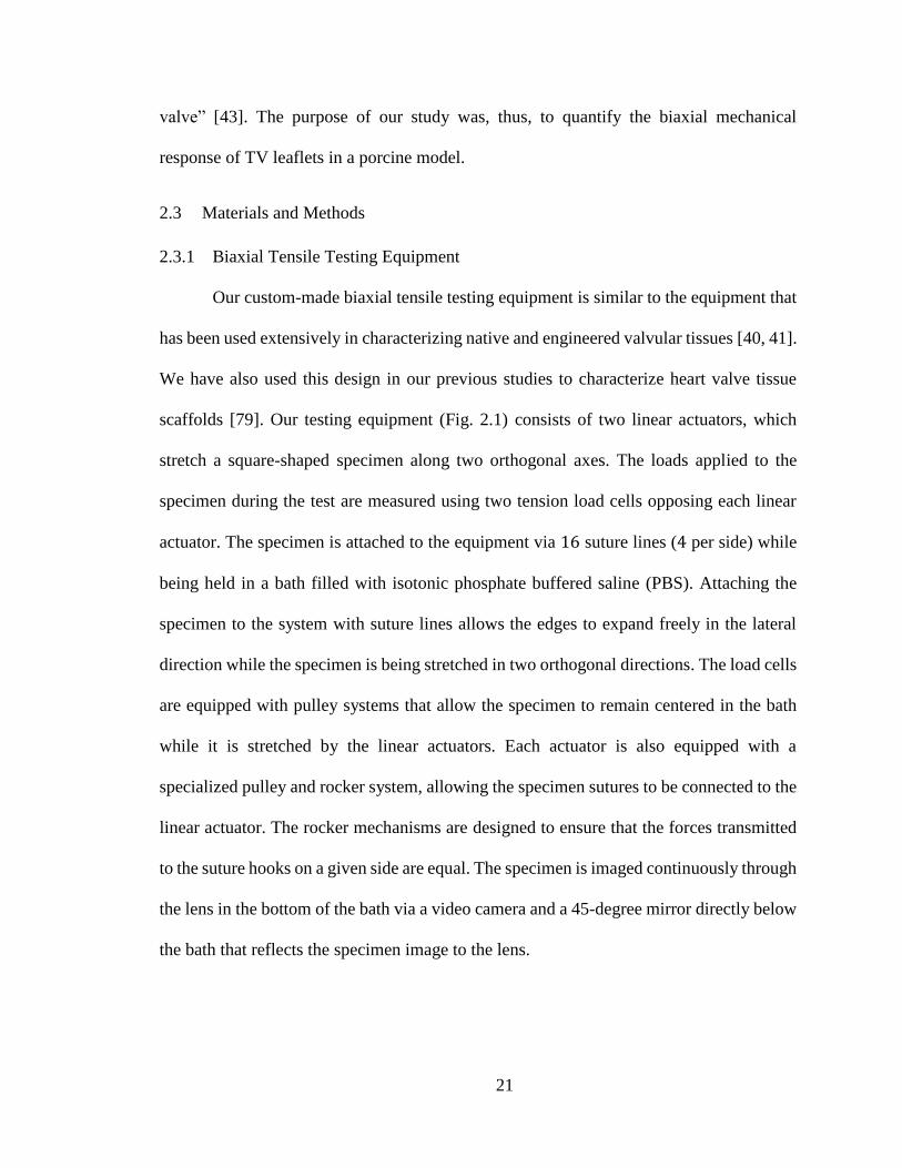
21

valve” [43]. The purpose of our study was, thus, to quantify the biaxial mechanical

response of TV leaflets in a porcine model.

2.3 Materials and Methods

2.3.1 Biaxial Tensile Testing Equipment

Our custom-made biaxial tensile testing equipment is similar to the equipment that

has been used extensively in characterizing native and engineered valvular tissues [40, 41].

We have also used this design in our previous studies to characterize heart valve tissue

scaffolds [79]. Our testing equipment (Fig. 2.1) consists of two linear actuators, which

stretch a square-shaped specimen along two orthogonal axes. The loads applied to the

specimen during the test are measured using two tension load cells opposing each linear

actuator. The specimen is attached to the equipment via 16 suture lines (4 per side) while

being held in a bath filled with isotonic phosphate buffered saline (PBS). Attaching the

specimen to the system with suture lines allows the edges to expand freely in the lateral

direction while the specimen is being stretched in two orthogonal directions. The load cells

are equipped with pulley systems that allow the specimen to remain centered in the bath

while it is stretched by the linear actuators. Each actuator is also equipped with a

specialized pulley and rocker system, allowing the specimen sutures to be connected to the

linear actuator. The rocker mechanisms are designed to ensure that the forces transmitted

to the suture hooks on a given side are equal. The specimen is imaged continuously through

the lens in the bottom of the bath via a video camera and a 45-degree mirror directly below

the bath that reflects the specimen image to the lens.

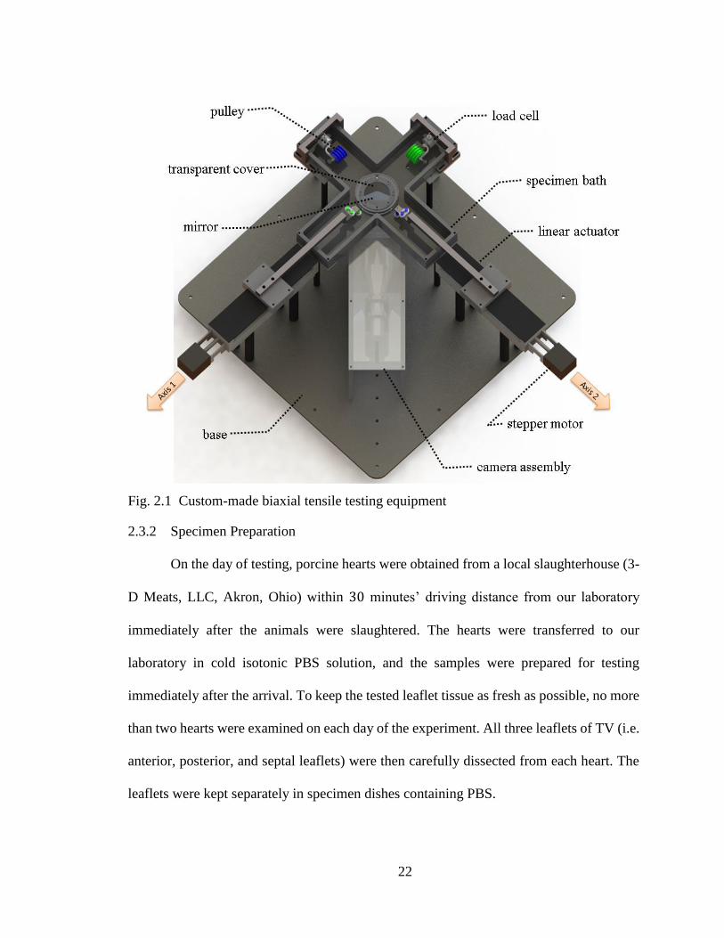
22

Fig. 2.1 Custom-made biaxial tensile testing equipment

2.3.2 Specimen Preparation

On the day of testing, porcine hearts were obtained from a local slaughterhouse (3-

D Meats, LLC, Akron, Ohio) within 30 minutes’ driving distance from our laboratory

immediately after the animals were slaughtered. The hearts were transferred to our

laboratory in cold isotonic PBS solution, and the samples were prepared for testing

immediately after the arrival. To keep the tested leaflet tissue as fresh as possible, no more

than two hearts were examined on each day of the experiment. All three leaflets of TV (i.e.

anterior, posterior, and septal leaflets) were then carefully dissected from each heart. The

leaflets were kept separately in specimen dishes containing PBS.

23

Removing a square-shaped specimen from the leaflet and attaching it to the biaxial

tensile testing equipment was facilitated by a specially designed phantom (Fig. 2.2a). Not

only did the phantom make it much easier and faster to attach the specimen to the system,

it also decreased the probability of damaging the tissue during the preparation process. The

leaflets were carefully positioned between the two halves of the phantom, trimmed using

surgical scissors, and attached to the fishhooks-suture-line setup through the grooves in the

phantom. The grooves facilitated the uniform attachment of the fishhooks, which was

necessary to obtain a uniform strain field. They were designed in 1 𝑚𝑚 distance from each

other on all the edges. These suture lines were then used to mount the specimen on the

testing equipment. The phantom was designed in such a way that it did not put any pressure

on the leaflet and was clamped to the leaflet edges only. Thus, any chance of damage due

to specimen preparation was minimized.

In total, ten sets of TV leaflets were tested, with each set coming from the same

heart. We performed all of the tests within 2 to 6 hours postmortem to eliminate erroneous

results that might be obtained from testing leaflets that had been frozen and thawed. The

dimensions of the trimmed specimens were 11 𝑚𝑚 by 11 𝑚𝑚 and the fishhooks were

attached on the sides of a 7.6 𝑚𝑚 by 7.6 𝑚𝑚 square (center to center). Four small glass

beads (0.5 𝑚𝑚 in diameter) were attached to the specimen in a 2 by 2 array (3 𝑚𝑚 apart

in each direction) as fiducial markers for quantification of the in-plane deformation.

2.3.3 Biaxial Tensile Testing Protocols

Specimens were mounted to the biaxial tensile testing equipment in the specimen

bath containing isotonic PBS at room temperature (Fig. 2.2b) with the circumferential

direction (i.e. commissure-to-commissure direction) aligned with one stretching direction

24

(axis 1 in Fig. 2.1) and the radial direction aligned with the other direction (axis 2 in Fig.

2.1). Before collecting the data, the samples were preconditioned using ten cycles of

equibiaxial loading. Each leaflet then experienced seven different loading protocols

starting with equibiaxial loading, which loaded it up to a maximum of 100 𝑁/𝑚 on each

axis. The other four loading types were non-equibiaxial as shown in the Table 2.1. In all

cases, a tare load of 0.5 𝑔 was first applied [36]. Each loading-unloading cycle took

20 seconds to complete.

Fig. 2.2 a) Specially designed phantom to facilitate the attachment of the leaflets to the

biaxial tensile testing equipment. b) Specimen attached to the equipment using fishhooks

and suture lines.

Table 2.1 Biaxial loadings protocols applied for each specimen

Maximum membrane tension (𝑁/𝑚)

Loading protocol no. Circumferential axis Radial axis

1 100 100

2 100 80

3 80 100

4 100 50

5 50 100

25

2.3.4 Strain and Stress Calculation

The in-plane positions of the fiducial markers were obtained using the camera

setup. Homogeneity of the strain field primarily depends on how uniform and regular the

suture lines are connected around the specimen and how close the connection points are

from the adjacent edges [74, 75]. The aforementioned phantom used to attach the fishhooks

guaranteed the uniform connection of the suture lines to the specimen. Since in our biaxial

testing equipment, four connections (i.e. the fish hooks) are applied on each side of the

specimen, uniform strain field was expected at the region covering 35% of the central area

of the specimen [75]. The fiducial markers were attached on the central area of the

specimen in a 3 𝑚𝑚 by 3 𝑚𝑚 square format. Since total area of the specimen was a

7.6 𝑚𝑚 by 7.6 𝑚𝑚 square (i.e. the area between the fishhooks), fiducial markers were

positioned within the 35% uniform strain field. The positional data were used to calculate

in-plane deformation gradient tensor F using methods explained previously [86, 127]. The

Green strain tensor was then calculated using the following equation:

E =

1

2(C − I) (2.1)

where I is the identity tensor and C, the right Cauchy-Green deformation tensor,

was defined by

C = FTF (2.2)

The thickness of each specimen was measured in six different locations using a dial

micrometer with an accuracy of 25 microns, and the average was calculated. As the square-

26

shaped specimens were cut from the central region of each leaflet, as shown in Fig. 2.3, the

thickness value was not measured beyond this square area.

To calculate the first Piola-Kirchhoff stress tensor P, each axis force was divided

by the cross-sectional area of the specimen normal to that axis. Such cross-sectional area

was calculated as the product of the distance between the fishhooks, which are connected

on two opposite sides of the specimen, and the measured thickness of the specimen. The

normal stresses P11 and P22 were then calculated. Since the specimens were thin enough

and only under planar loads and with the assumption of no shear forces applied [50], all

other components of first Piola-Kirchhoff stress tensor were considered to be zero. The

second Piola-Kirchhoff stress tensor S was then calculated:

S = F−1P (2.3)

The rigid body rotation angles ω were also calculated to determine how much of

the deformation was due to the rigid body rotation during the tests:

ω = tan−1(

𝑅21

𝑅11) (2.4)

where rotation matrix R was given by

R = FU−1 (2.5)

and U was the right stretch tensor:

C = U2 (2.6)

27

Fig. 2.3 The three leaflets of the tricuspid valve and the position and shape of the

specimens.

The tethered mounting configurations, used in the current study, allows for free

lateral displacements which provides more homogeneous stress field based on the applied

boundary loads [74]. As mentioned before, the elements of the first Piola-Kirchhoff stress

tensor are determined based on the assumption that there is no shear stress.

The shear angle θ, a measure of shear deformation, was also calculated using the

following equation:

θ = cos−1(

𝐶12

𝐶11𝐶22) (2.7)

2.4 Results

The thickness values for all of the tested specimens (including average and standard

deviation by leaflet type) are listed in Table 2.2. The Student’s t-test analysis revealed that

there was no significant difference between the thicknesses of the anterior and posterior

28

leaflets (𝑝 = 0.27). The septal leaflet, however, was significantly thicker than the anterior

and posterior leaflets (𝑝 < 10−4 for both cases). Another notable outcome was that the

septal leaflets had the smallest overall standard deviation in measured thickness values.

Table 2.2 Measured thicknesses for the leaflets of all the hearts used during the experiment

Leaflet Thickness (𝜇𝑚)

Heart No Anterior Posterior Septal

1 241 377 440

2 318 271 508

3 406 453 478

4 258 288 411

5 368 406 521

6 300 269 528

7 262 330 587

8 246 386 478

9 432 330 483

10 300 347 479

AVG 313 346 491

STD 68 61 49

The tension-stretch behavior of the specimens for all protocols listed in Table 2.1

was recorded. Fig. 2.4 demonstrates the average membrane tension versus stretch ratio of

the anterior leaflet for each loading protocol (averaged over all of the 10 specimens).

Figures 2.5 and 2.6 show the same graphs for posterior and septal leaflets, respectively.

The bars in these figures are the standard errors. The standard error was from 0.00 to 0.02

for circumferential direction and for radial direction it was from 0.00 to 0.04 for all three

types of leaflets and all the protocols. As shown in Figs. 2.4–2.6 the largest difference

between mechanical responses in the circumferential direction and the radial direction for

the equibiaxial loading was observed for the posterior leaflet, indicating that the posterior

leaflet presented more anisotropic responses than the other two leaflets.

29

The average values of the maximum rigid body rotation angles 𝜔𝑚𝑎𝑥 for each

leaflet type and loading protocol are presented in Table 2.3. In this table, the largest value

of rigid body rotation was less than 3 degrees indicating that the rigid body rotation was

negligible in the current experiment.

The average maximum shear angles θmax for each leaflet type and loading protocol

are also presented in Table 2.3. The largest maximum shear angle (4.2 ± 0.9 degrees) was

calculated for protocol number 5, in which the leaflet experienced one of the two most

anisotropic loading conditions. The shear angles calculated for the other protocols were

around 3 degrees. Table 2.3 also displays the average ratio of the maximum Cauchy shear

stresses to the maximum Cauchy normal stresses r measured for each leaflet type under

different loading protocols. The average maximum shear stress is in the range of 3.5% to

7.2% of the maximum normal stress.

30

Fig. 2.4 The average membrane tension versus stretch ratio for the loading protocols a)

number 1 (equibiaxial), b) number 2, c) number 3, d) number 4, and e) number 5 for the

anterior leaflet. The circumferential (Circ) and radial directions are in solid red and dash-

dotted blue, respectively. The bars are standard errors. The green dashed line shows the

maximum physiological tension level (Max Physio), while the tension level goes up to

100 𝑁/𝑚 in case of hypertension.

31



posterior leaflet. The circumferential (Circ) and radial directions are in solid red and dash-


maximum physiological tension level (Max Physio), while the tension level goes up to

100 𝑁/𝑚 in case of hypertension.

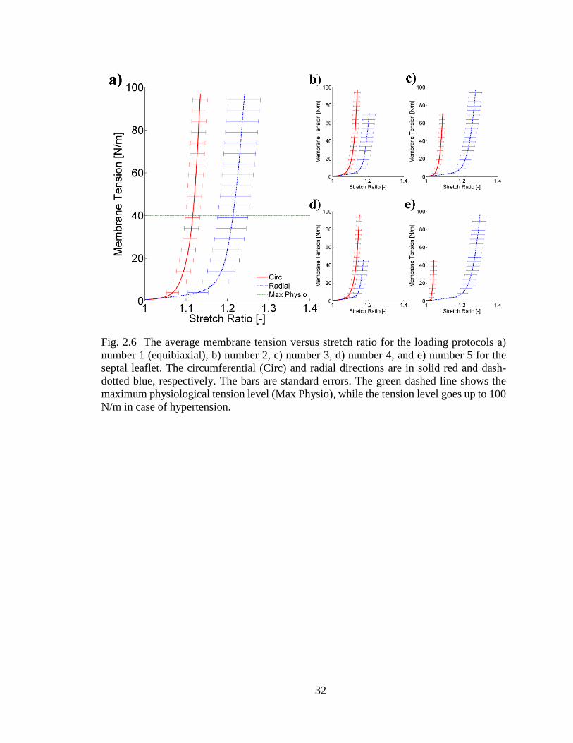
32



septal leaflet. The circumferential (Circ) and radial directions are in solid red and dash-


maximum physiological tension level (Max Physio), while the tension level goes up to 100

N/m in case of hypertension.

33

Tab

le 2

.3 T

he

aver

age

max

imum

rig

id b

od

y r

ota

tion 𝜔

𝑚𝑎

𝑥, th

e av

erag

e m

axim

um

sh

ear

angle

𝜃𝑚

𝑎𝑥, an

d t

he

aver

age

of

the

rati

o o

f

the

max

imum

Cau

chy s

hea

r st

ress

to

the

max

imum

Cau

chy n

orm

al s

tres

s 𝑟

pre

sente

d f

or

each

lo

adin

g p

roto

col

and l

eafl

et t

yp

e (f

or

each

pro

toco

l an

d l

eafl

et t

ype

the

dat

a is

aver

aged

over

all

hea

rts

and p

rese

nte

d i

n t

he

form

of

aver

age

± s

tandar

d e

rror)

.

Load

ing

Pro

toco

l N

o.

Ante

rior

Lea

flet

Post

erio

r L

eafl

et

S

epta

l L

eafl

et

𝜔𝑚

𝑎𝑥

(deg

ree)

𝜃 𝑚𝑎

𝑥

(deg

ree)

r

(%)

𝜔

𝑚𝑎

𝑥

(deg

ree)

𝜃 𝑚𝑎

𝑥

(deg

ree)

r

(%)

𝜔

𝑚𝑎

𝑥

(deg

ree)

𝜃 𝑚𝑎

𝑥

(deg

ree)

r

(%)

1

2.5

3±

0.4

9

3.4

3±

0.8

1

7.2

1±

1.6

9

1.7

9±

0.4

4

2.8

8±

0.7

3

5.5

9±

1.4

3

1.2

3±

0.2

9

3.4

9±

0.6

4

5.8

0±

0.8

4

2

2.3

8±

0.4

5

3.1

9±

0.8

3

7.2

1±

1.8

9

1.6

5±

0.4

8

2.7

5±

0.7

0

5.7

2±

1.6

9

1.4

7±

0.2

6

3.4

6±

0.6

4

5.4

2±

0.9

0

3

2.5

7±

0.4

9

3.5

0±

0.8

1

5.4

7±

1.1

3

1.8

0±

0.4

6

2.9

6±

0.7

6

4.6

8±

1.0

6

1.2

6±

0.2

2

3.1

4±

0.6

6

4.8

1±

0.7

3

4

2.2

7±

0.4

0

3.1

3±

0.9

2

6.5

6±

1.7

5

1.7

0±

0.4

7

2.6

9±

0.7

1

4.5

8±

1.5

2

1.8

8±

0.3

7

3.2

3±

0.5

8

4.3

4±

0.8

9

5

2.8

7±

0.5

4

4.2

0±

0.9

0

4.3

7±

0.6

8

2.0

2±

0.4

9

3.3

0±

0.8

5

3.5

1±

0.7

1

1.6

0±

0.2

1

3.4

3±

0.7

5

3.8

6±

0.7

0

34

2.5 Discussion

In this study, we quantified the biaxial mechanical response of the porcine TV

leaflets. The outcomes of our study are useful for quantification of the mechanical

properties of TV leaflets and for developing FE models because such models rely on the

accurate quantification of the tissue mechanical properties [44].

The peak load values used in biaxial stretching were selected based on the

estimation of maximum stresses on the leaflets both for normal physiological right

ventricular pressure (RVP) and for the case of pulmonary hypertension. The reported

maximum RVP is approximately 30 𝑚𝑚 𝐻𝑔 for a normal heart [128], while during

pulmonary hypertension it can reach as high as 80 𝑚𝑚 𝐻𝑔 [129, 130]. Based on different

anatomical measurements we approximated the mean radius of curvature of TV to be

around 2 𝑐𝑚 [131, 132]. Using these numbers along with the law of Laplace, one can

estimate the maximum tension on TV leaflets to be approximately 40 𝑁/𝑚 and 100 𝑁/𝑚

under normal physiological conditions and in the case of pulmonary hypertension,

respectively. In Figs. 2.4a, 2.5a, and 2.6a the maximum physiological level of loading is

determined with the horizontal green dashed line. Therefore, the presented tension-

deformation data can be referred to both for physiological levels and for hypertensive levels

of loading.

The overall trends of the tension–stretch graph showed a highly nonlinear behavior,

as the leaflets were more compliant at the beginning of the loading (i.e. over the toe region)

and then they rapidly became stiff (i.e. transition to the lockout region) both in the radial

and in the circumferential directions. The latter behavior was not observed in the few

mechanical tests conducted on TV previously due to the small level of strains used in such

35

experiments [133]. In all of the specimens tested, the leaflets were stiffer in the

circumferential direction than the radial direction, a phenomenon observed in other cardiac

valves as well [35-39]. As there was no significant difference between the thicknesses of

the anterior and posterior leaflets, even without using any specific material model, one can

conclude from the tension–stretch data that these two leaflets had the same stiffness in the

circumferential direction. The anterior leaflet, however, was much stiffer than the posterior

one in the radial direction, as the anterior leaflet deforms much less under the same loading

conditions. The septal leaflet was more compliant than the other two leaflets in the

circumferential direction, as it showed nearly the same deformation under the same loading

conditions while being significantly thicker (as discussed previously). For the radial

direction, the septal leaflet deformed slightly more in comparison to the anterior leaflet,

and it also was thicker. Therefore, it can also be concluded that the septal leaflet is more

compliant in the radial direction than the anterior leaflet.

36

CHAPTER 3III

QUANTIFICATION OF MATERIAL CONSTANTS FOR A PHENOMENOLOGICAL

CONSTITUTIVE MODEL OF THE TRICUSPID VALVE LEAFLETS

(The content of this chapter was published in JBME (May 2018) as “Quantification of

Material Constants for a Phenomenological Constitutive Model of Porcine Tricuspid

Valve Leaflets for Simulation Applications” [134].)

3.1 Summary

TV is a one-way valve on the pulmonary side of the heart, which prevents backflow

of blood during ventricular contractions. Development of computational models of TV is

important both in understanding the normal valvular function and in the

development/improvement of surgical procedures and medical devices. A key step in the

development of such models is quantification of the mechanical properties of TV leaflets.

In this study, after examining previously measured five-loading-protocol biaxial stress–

strain response of porcine TVs, a phenomenological constitutive framework was chosen to

represent this response. The material constants were quantified for all three leaflets, which

were shown to be highly anisotropic with average anisotropy indices of less than 0.5 (an

anisotropy index value of 1 indicates a perfectly isotropic response, whereas a smaller

value of the anisotropy index indicates an anisotropic response). To obtain mean values of

material constants, stress–strain responses of the leaflet samples were averaged and then

fitted to the constitutive model (average 𝑅𝟐 over 0.9). Since the sample thicknesses were

37

not hugely different, averaging the data using the same tension levels and stress levels

produced similar average material constants for each leaflet.

3.2 Introduction

TV, a one-way valve that opens and closes in response to changes in ventricular

pressure [135], prevents the backflow of blood from the right ventricle to the right atrium

during ventricular systole [1]. The main malfunctions of TV, namely valvular regurgitation

and stenosis, may require surgical interventions such as total valve replacement or valvular

repair [136, 137]. In the United States, approximately 150,000 patients undergo TV

surgeries annually [24, 25, 138]. While TV repair surgeries have better outcomes when

compared to total TV replacement procedures [32-34], the outcomes of TV repair surgeries

are still not completely satisfying, and TV surgery remains one of the most high-risk valve

procedures [120]. To improve existing surgical techniques and develop more successful

valve repair procedures, accurate quantification of the biomechanical properties of native

TV tissues is essential. Such data are necessary both in the development of tissue-

equivalent biomaterials [79] and as input parameters for generating computational models

of healthy and diseased TVs [44, 89, 139]. Despite the need for data on the mechanical

behavior of this valve, TV has been understudied in comparison to the other valves of the

heart [35, 37-39, 42, 43, 67].

Considering the native loading environment of the cardiac valves, we have

previously used biaxial tensile testing to evaluate the stress–strain response of porcine TV

leaflets [117]. In the current study, we utilized a phenomenological constitutive model to

quantify the anisotropic and nonlinear material properties of the porcine TV leaflets. Since

material properties of porcine TV leaflets were not available, previous FE models relied on

38

material properties derived from the mitral and AVs [44], which are expected to be

different from those of TV. In this study, we aimed to provide material constants that can

be used in the development of TV FE models to mimic its deformation in vivo [81] and ex

vivo [140].


3.3.1 Planar Biaxial Tensile Strains and Stresses

The planar biaxial tensile testing procedure and the strain and stress calculations

are presented in detail in our previous publication [117]. Briefly, a total of 30

(11 𝑚𝑚 × 11 𝑚𝑚) square-shaped samples (i.e., one sample per each TV leaflet of ten

porcine hearts) were freshly excised and mounted on the biaxial tensile testing equipment

[40, 41, 79, 117] with the circumferential and radial directions of the leaflets aligned with

stretching axes of the equipment. Five different tension-controlled loading protocols with

a constant tension ratio of 𝑇𝑐: 𝑇𝑟 = 1: 1, 1: 0.75, 0.75: 1, 1: 0.5, 0.5: 1 were then performed

on each specimen with a maximum tension of 100 𝑁/𝑚 as shown in Table 3.1. The strains

and stresses were subsequently calculated from tension–deformation data. More

information about the stress–strain responses are provided in our previous publication

[117].

Table 3.1 The maximum membrane tension of each tension-controlled loading protocol

for circumferential 𝑐 and radial 𝑟 directions. The tension ratios were kept constant during

the experiments: 𝑇𝑐: 𝑇𝑟 = 1: 1, 1: 0.75, 0.75: 1, 1: 0.5, 0.5: 1

Loading protocol no. 𝑇𝑐,𝑚𝑎𝑥 (𝑁 𝑚⁄ ) 𝑇𝑟,𝑚𝑎𝑥 (𝑁 𝑚⁄ )

1 100 100

2 100 75

3 75 100

4 100 50

5 50 100

39

3.3.2 Constitutive Modeling

Similar to the tissue in other cardiac valves, TV leaflet tissue was assumed to be

incompressible, homogenous, and hyperelastic, undergoing finite deformations within the

small specimen region [60]. Hence, following the concept of pseudoelasticity [141], its

mechanical response was expressed using a strain energy function 𝑊 and the components

of the second Piola–Kirchhoff stress tensor 𝑆𝑖𝑗 were evaluated:

𝑆𝑖𝑗 =

𝜕𝑊

𝜕𝐸𝑖𝑗 (3.1)

where 𝐸𝑖𝑗 were the components of the Green strain tensor and 𝑖 and 𝑗 were dummy indices.

To examine the pseudoelastic response of TV leaflets and choose a suitable form

for the strain energy function, all the stress–strain data were independently fitted to the

following response functions for each directional component [56, 142].

𝑆𝑐𝑐 = 𝑐0 (𝑐1𝐸𝑐𝑐 + 𝑐3𝐸𝑟𝑟 + 𝑐4𝐸𝑐𝑐𝐸𝑟𝑟 +1

2𝑐5𝐸𝑟𝑟

2 + 𝑐6𝐸𝑐𝑐𝐸𝑟𝑟2

+ 2𝑐7𝐸𝑐𝑐3 ) 𝑒𝑄

𝑆𝑟𝑟 = 𝑐0 (𝑐2𝐸𝑟𝑟 + 𝑐3𝐸𝑐𝑐 + 𝑐5𝐸𝑐𝑐𝐸𝑟𝑟 +1

2𝑐4𝐸𝑐𝑐

2 + 𝑐6𝐸𝑐𝑐2 𝐸𝑟𝑟

+ 2𝑐8𝐸𝑟𝑟3 ) 𝑒𝑄

(3.2)

where 𝑐𝑐 and 𝑟𝑟 denote the circumferential and radial directions, respectively, and

𝑄 = (𝑐1𝐸𝑐𝑐2 + 𝑐2𝐸𝑟𝑟

2 + 2𝑐3𝐸𝑐𝑐𝐸𝑟𝑟 + 𝑐4𝐸𝑐𝑐2 𝐸𝑟𝑟 + 𝑐5𝐸𝑟𝑟

2 𝐸𝑐𝑐

+ 𝑐6𝐸𝑐𝑐2 𝐸𝑟𝑟

2 + 𝑐7𝐸𝑐𝑐4 + 𝑐8𝐸𝑟𝑟

4 )

(3.3)

40

It is worth noting that the above equations do not describe a constitutive model.

They are merely a set of response functions that were utilized to interpolate the stress

components over the entire strain field.

Specific forms of the resulting stress surfaces were carefully examined, and an

anisotropic Fung-type strain energy function was subsequently chosen [53, 142]. As shear

stresses were negligible [117], the strain energy function 𝑊 was expressed as:

𝑊 = 𝑐

2(𝑒𝑎1𝐸𝑐𝑐

2 +𝑎2𝐸𝑟𝑟2 +2𝑎3𝐸𝑐𝑐𝐸𝑟𝑟 − 1) (3.4)

where 𝑐 and 𝑎𝑖 were the material constants and 𝐸𝑐𝑐 and 𝐸𝑟𝑟 were the components of the

Green strain tensor in the circumferential and radial directions, respectively. To calculate

the material constants, the measured biaxial stress–strain data for each specimen were fitted

to this model using a custom MATLAB code (MathWorks, Natick, MA) and the Trust-

Region-Reflective algorithm [143]. An anisotropy index 𝐴𝐼 was also calculated [58]:

𝐴𝐼 = 𝑚𝑖𝑛 (

𝑎1 + 𝑎3

𝑎2 + 𝑎3,𝑎2 + 𝑎3

𝑎1 + 𝑎3) (3.5)

3.3.3 Average Models

An important outcome of accurate constitutive modeling of soft tissues is the

application of the resultant material constants in generating computational simulations of

tissue deformation. One approach in performing such simulations is to use sets of

specimen-specific material constants. However, introducing a set of material constants to

represent the generic (average) tissue mechanical behavior could be also beneficial. In such

a case, one could perform parametric studies to identify how each parameter (both material

and geometric parameters) influence the simulation outcomes [144-147].

41

For linear elastic materials, the moduli of elasticity can be calculated by evaluating

the individual specimen-specific moduli of elasticity and then finding the average moduli

by calculating the arithmetic mean. In our study, however, a simple arithmetic mean of the

constitutive model material constants cannot accurately characterize the cumulative

behavior of the tissue due to the nonlinearity of the mechanical behavior and the resultant

choice of a nonlinear constitutive model. As described by other investigators [58, 64], one

way to resolve this issue is to first generate an average curve for each protocol by

calculating the arithmetic mean of experimentally measured strain values for all specimens.

Next, we can fit these average curves into the proposed model to calculate the generic

material constants. Averaging the strains is only appropriate over similar stress (or tension)

states. Our biaxial testing device was set up in such way that the shear components of the

stress tensors were considered to be negligible. As such, in our experiment, a similar stress

(or tension) state simply means that the normal stress (or tension) at each direction must be

equal among all samples being used in the averaging of the strains. Consistent with the

approach of other investigators [58, 64], we used tension control protocols in our

experiments. In the following sections, the procedures for calculating the average values

for similar tension states and similar stress states are described.

Average model development using tension. As our experiments were conducted

using tension-controlled protocol, having a similar tension state was guaranteed for similar

protocols of different samples. In our experiment, duration of the deformation was identical

for each specimen, and the strain data were collected at a similar time interval in all cases.

Although we had a high frequency for collecting the data, strain data were not necessarily

available for each specific tension value. As such, a procedure to approximate the strain

42

data at any specific tension value was necessary. Prior to our study, other investigators had

employed exponential functions to fit each tension–strain curve independently [58, 64] and

used that expression to interpolate the data. The exponential fit, however, cannot efficiently

predict the tension–strain response in cases where the Poisson’s effect induces a drift in the

tension–strain curves. In such cases, discrete mathematical functions are simply unable to

accurately fit the data since (due to the Poisson’s effect) more than one tension value may

exist for a single strain value. To overcome this hurdle in our study, we calculate the strains

at desired tension values by linearly interpolating the original data. As we had performed

our experiments with a relatively high frequency of data collection, we were able to capture

the Poisson’s effect in our estimated values of strains at each specified tension value. In

addition, more accurate estimations of strains—particularly at the lower strain regions—

were obtained in comparison to the exponential fits. The advantages of using the linear

interpolation over the exponential fit in this application is illustrated in Fig. 3.1. As shown

in this picture, the linear interpolation follows the original data accurately while the

exponential fit extremely deviates.

The specified tension values for each protocol were chosen as the average tension

𝑇𝑎𝑣𝑔,𝑖𝑖. For each protocol, the approximated strain values were averaged over the samples

to compute the average strain 𝐸𝑎𝑣𝑔,𝑖𝑖. The subscript 𝑖𝑖 refers to the circumferential 𝑐𝑐 and

radial 𝑟𝑟 directions.

43

Fig. 3.1 Comparison between the accuracy of linear interpolation and exponential fit to

estimate the original data for averaging.

Next, the following equation was used to estimate the normal components of the

average first Piola–Kirchhoff stress tensor 𝑃𝑎𝑣𝑔,𝑖𝑖 [58].

𝑃𝑎𝑣𝑔,𝑖𝑖 =

𝑇𝑎𝑣𝑔,𝑖𝑖

𝑛∑

1

ℎ𝑖

𝑛

𝑖=1

(3.6)

where ℎ𝑖 are the individual leaflet thicknesses and 𝑛 is number of specimens. The diagonal

components of the average deformation gradient tensor 𝐹𝑎𝑣𝑔,𝑖𝑖 were approximated using

the following equation, with the assumption of negligible shear deformations:

𝐹𝑎𝑣𝑔,𝑖𝑖 = √2𝐸𝑎𝑣𝑔,𝑖𝑖 + 1 (3.7)

The normal components of the average first Piola–Kirchhoff stress tensor 𝑃𝑎𝑣𝑔,𝑖𝑖

and deformation gradient tensor 𝐹𝑎𝑣𝑔,𝑖𝑖 were used to assemble their corresponding tensor

44

with the assumption of zero off-diagonal components. These tensors were then used to

calculate the average second Piola–Kirchhoff stress tensor:

𝑺𝑎𝑣𝑔 = 𝑷𝑎𝑣𝑔. 𝑭𝑎𝑣𝑔−𝑇 (3.8)

Finally, to calculate the average material constants, the 𝑺𝑎𝑣𝑔 − 𝑬𝑎𝑣𝑔 data were

fitted into the proposed constitutive model.

Average model development using the first Piola–Kirchhoff stress. The response of

valvular tissues to tension depends on the thickness of the leaflet specimens. As the

thickness of leaflets varies from one specimen to another, in theory, the average model

developed based on the equal tension values could be erroneous. Although this error might

seem to be trivial, in practice, due to the small variations of the thicknesses and

experimental convenience, biaxial testing of the valves has been generally conducted in a

tension-controlled manner [36, 38, 58, 59, 148]. To evaluate the potential errors in using

equal-tension values in the averaging process, we performed a second averaging procedure,

this time based on the first Piola–Kirchhoff stress values. Since for each protocol the ratio

of the tension in the radial direction over the tension in the circumferential direction was

kept constant, after calculating the first Piola–Kirchhoff stresses (by dividing tension over

the individual leaflet thicknesses), we were able to obtain the similar stress states necessary

for the averaging process. While the stress ratios were constant for all specimens for each

protocol, dividing the tensions by the specimen thicknesses resulted in different maximum

values of first Piola–Kirchhoff stresses. As such, it was necessary to truncate the data to

the point where there existed experimental data for all samples. This process led to the loss

of data at the high-tension values for some specimens.

45

Averaging was accomplished by linearly interpolating the first Piola–Kirchhoff

stresses and averaging the strains similar to the method explained above. In particular, for

each protocol, the first Piola–Kirchhoff stress components 𝑃𝑎𝑣𝑔,𝑖𝑖 were directly specified

from the experimental data with the necessary linear interpolation. For each specified stress

value, the strains were averaged over all the samples to obtain the components of average

Green strains 𝐸𝑎𝑣𝑔,𝑖𝑖. As before, the subscript 𝑖𝑖 indicates the circumferential 𝑐𝑐 or radial 𝑟𝑟

direction. Subsequently, Equation (3.7) was used to approximate the average deformation

gradient tensor diagonal components 𝐹𝑎𝑣𝑔,𝑖𝑖. Finally, the average second Piola–Kirchhoff

stress tensor 𝑺𝑎𝑣𝑔 was calculated using Equation (3.8).

Average model development using the predefined constitutive model and Cauchy

stress. As the Cauchy stress is the true stress borne by the tissue during the loading process,

it is probably the best candidate upon which the averaging procedure should be built. Since

the experiments were conducted in a tension-controlled manner, similar Cauchy stress

states were not directly available. Therefore, similar stress states were reconstructed by

choosing (sampling) a set of five-protocol Cauchy stress loadings and evaluating their

corresponding strains using the material constants obtained from the specimen-specific

constitutive modeling. Here, the desired data needed for averaging method based on

Cauchy stress were chosen a priori. Consequently, we used these chosen values as the

components of average Cauchy stress 𝜎𝑎𝑣𝑔,𝑖𝑖 and averaged the calculated strains over all

samples to compute the components of average Green strain 𝐸𝑎𝑣𝑔,𝑖𝑖 for each protocol.

Then, using Equation (3.7), we calculated the components of the deformation gradient

tensor 𝐹𝑎𝑣𝑔,𝑖𝑖. Finally, with the assumption of negligible shear stress and deformation, we

46

assembled the Cauchy stress tensor and deformation gradient tensor and used them to

calculate the average second Piola–Kirchhoff stress tensor:

𝑺𝑎𝑣𝑔 = 𝐽. 𝑭𝑎𝑣𝑔−1 . 𝝈𝑎𝑣𝑔. 𝑭𝑎𝑣𝑔

−𝑇 (3.9)

where 𝐽 is the determinant of 𝑭 which is equal to 1, as the valvular tissue was considered

to be incompressible.

3.4 Results

Detailed explanation of the biaxial mechanical responses of TV leaflets and the

tension–deformation data are presented in our previous publication [117]. Briefly, all three

leaflets responded in an anisotropic manner. Similar to tissues in other cardiac valves, TV

leaflets were more compliant at lower strain values but became stiffer when the strain

increased.

3.4.1 Stress Response Functions

The stress–strain data were fitted to the response functions described in Equation

(3.2) independently for each directional component. The 𝑅𝟐 (mean ± standard deviation)

for these fitted curves were 0.92 ± .06, 0.93 ± .09, and 0.93 ± .07 for the anterior,

posterior, and septal leaflets, respectively. The resulting fitting parameters were used to

plot the constant stress contours over the strain field. As shown in Fig. 3.2, for typical (i.e.,

randomly selected) anterior, posterior, and septal leaflets, the contours were asymmetric

around the 𝐸𝑐𝑐 = 𝐸𝑟𝑟 line for nearly all samples. In a perfectly isotropic material, the

response should be symmetric with respect to this line. Therefore, it was further confirmed

that the mechanical responses were anisotropic for all three leaflets as had been visually

inferred in our previous investigations [117]. The rapid increase in the stress values versus

47

the strains, along with the assumption of negligibility of shear stresses and the anisotropic

nature of the responses observed here, justified the choice of our Fung-type

phenomenological model [53] as well as the specific strain energy function 𝑊 defined in

Equation (3.4).

Fig. 3.2 The constant stress contours produced using the response functions of Equation

(2.2) plotted over the strain field for typical leaflets: (a,b) anterior, (c,d) posterior, and (e,f)

septal leaflets.

3.4.2 Constitutive Modeling Results

All five protocols of the biaxial stress–strain (second Piola–Kirchhoff stress versus

Green strain) data were simultaneously fitted to the Fung-type constitutive model of

Equation (3.4). As shown in Fig. 3.3 for typical anterior, posterior, and septal leaflets, the

results showed a reasonably accurate fit with the average 𝑅𝟐 (mean ± standard deviation)

of 0.92 ± 0.05, 0.89 ± 0.10, and 0.89 ± 0.10 for the anterior, posterior, and septal

48

leaflets, respectively. The material constants resulting from the specimen-specific fitting

method are shown in Table 3.2. The 𝑅2 as well as the anisotropy index 𝐴𝐼 are also presented

in Table 3.2 for each fit. An anisotropy index value of 1 indicates a perfectly isotropic

response, whereas a smaller value of 𝐴𝐼 indicates an anisotropic response [58]. As shown

in Table 3.2, the anisotropy index ranged from 0.22 to 1.00, from 0.09 to 0.58, and from

0.21 to 1.00, for the anterior, posterior, and septal leaflets, respectively.

49

Fig. 3.3 The result of the five-protocol fit along with the experimentally measured

circumferential (Circ) and radial data for typical leaflets: (a) anterior, (b) posterior, and (c)

septal. The numbers represent the protocol numbers listed in Table 3.1.

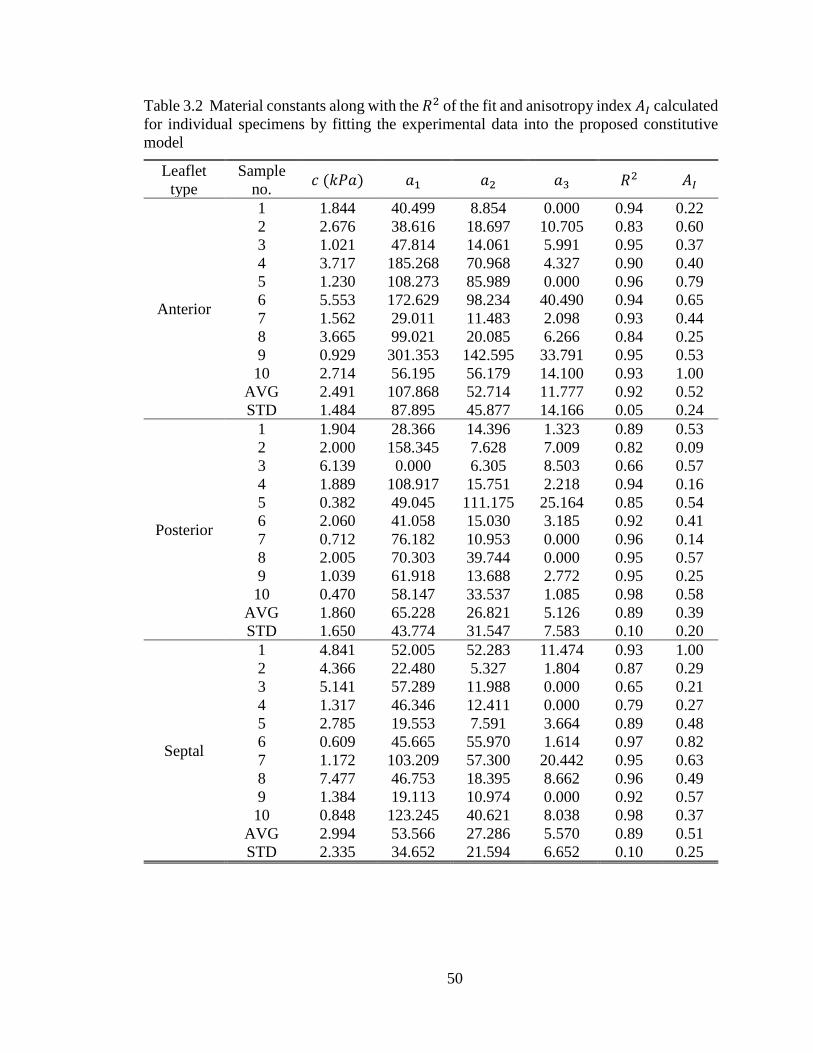
50

Table 3.2 Material constants along with the 𝑅2 of the fit and anisotropy index 𝐴𝐼 calculated

for individual specimens by fitting the experimental data into the proposed constitutive

model

Leaflet

type

Sample

no. 𝑐 (𝑘𝑃𝑎) 𝑎1 𝑎2 𝑎3 𝑅2 𝐴𝐼

Anterior

1 1.844 40.499 8.854 0.000 0.94 0.22

2 2.676 38.616 18.697 10.705 0.83 0.60

3 1.021 47.814 14.061 5.991 0.95 0.37

4 3.717 185.268 70.968 4.327 0.90 0.40

5 1.230 108.273 85.989 0.000 0.96 0.79

6 5.553 172.629 98.234 40.490 0.94 0.65

7 1.562 29.011 11.483 2.098 0.93 0.44

8 3.665 99.021 20.085 6.266 0.84 0.25

9 0.929 301.353 142.595 33.791 0.95 0.53

10 2.714 56.195 56.179 14.100 0.93 1.00

AVG 2.491 107.868 52.714 11.777 0.92 0.52

STD 1.484 87.895 45.877 14.166 0.05 0.24

Posterior

1 1.904 28.366 14.396 1.323 0.89 0.53

2 2.000 158.345 7.628 7.009 0.82 0.09

3 6.139 0.000 6.305 8.503 0.66 0.57

4 1.889 108.917 15.751 2.218 0.94 0.16

5 0.382 49.045 111.175 25.164 0.85 0.54

6 2.060 41.058 15.030 3.185 0.92 0.41

7 0.712 76.182 10.953 0.000 0.96 0.14

8 2.005 70.303 39.744 0.000 0.95 0.57

9 1.039 61.918 13.688 2.772 0.95 0.25

10 0.470 58.147 33.537 1.085 0.98 0.58

AVG 1.860 65.228 26.821 5.126 0.89 0.39

STD 1.650 43.774 31.547 7.583 0.10 0.20

Septal

1 4.841 52.005 52.283 11.474 0.93 1.00

2 4.366 22.480 5.327 1.804 0.87 0.29

3 5.141 57.289 11.988 0.000 0.65 0.21

4 1.317 46.346 12.411 0.000 0.79 0.27

5 2.785 19.553 7.591 3.664 0.89 0.48

6 0.609 45.665 55.970 1.614 0.97 0.82

7 1.172 103.209 57.300 20.442 0.95 0.63

8 7.477 46.753 18.395 8.662 0.96 0.49

9 1.384 19.113 10.974 0.000 0.92 0.57

10 0.848 123.245 40.621 8.038 0.98 0.37

AVG 2.994 53.566 27.286 5.570 0.89 0.51

STD 2.335 34.652 21.594 6.652 0.10 0.25

51

3.4.3 Average Modeling Results

The average stress–strain (second Piola–Kirchhoff stress versus Green strain)

responses developed for the anterior leaflet based on identical tension states are shown in

Fig. 3.4. This figure shows that the same ratio of tension in the radial and circumferential

directions (listed in Table 3.1) does not exist for the second Piola–Kirchhoff stresses. For

example, the tension-controlled equibiaxial protocol does not produce an equibiaxial

second Piola–Kirchhoff stress state. Figures 3.5 and 3.6 show similar graphs for the

average stress–strain responses developed based on identical first Piola–Kirchhoff stress

states and identical Cauchy stress states for the anterior leaflet. Similar graphs for the

posterior and septal leaflets are provided in APPENDIX A.

For each set of average response curves, the proposed phenomenological

constitutive model was also utilized to develop the average material model and calculate

the average material constants for each leaflet type. Table 3.3 shows the material constants

computed for the average response curves developed based on identical tensions along with

the 𝑅2 of the fit and the anisotropy index 𝐴𝐼. The data fitted the model with 𝑅2 of 0.85,

0.95, and 0.94 for anterior, posterior, and septal leaflets, respectively. Tables 3.4 and 3.5

show the same quantities obtained after fitting the average response curves developed

based on identical first Piola–Kirchhoff stresses and Cauchy stresses into the proposed

constitutive model. As expected, the values for the material constants are different from

the arithmetic average of the constants calculated for the individual specimens, as listed in

Table 3.2.

52

Fig. 3.4 The average stress–strain responses developed based on identical tension states

from loading protocols (a) number 1 (equibiaxial), (b) number 2, (c) number 3, (d) number

4, and (e) number 5 of Table 3.1 for the anterior leaflet. The vertical axis is the second

Piola–Kirchhoff stress, and the horizontal axis is the Green strain. These data were used to

calculate the average material constants presented in Table 3.3.

53

Fig. 3.5 The average stress–strain responses developed based on identical first Piola–Kirchhoff stress states from loading protocols (a) number 1 (equibiaxial), (b) number 2, (c)

number 3, (d) number 4, and (e) number 5 of Table 3.1 for the anterior leaflet. The vertical

axis is the second Piola–Kirchhoff stress, and the horizontal axis is the Green strain. These

data were used to calculate the average material constants presented in Table 3.4.

54

Fig. 3.6 The average stress–strain responses developed based on identical Cauchy stress

states from loading protocols (a) number 1 (equibiaxial), (b) number 2, (c) number 3, (d)

number 4, and (e) number 5 of Table 3.1 for the anterior leaflet. The vertical axis is the

second Piola–Kirchhoff stress, and the horizontal axis is the Green strain. These data were

used to calculate the average material constants presented in Table 3.5.

55

Table 3.3 Material constants for the tension-based average model data (AVG) as well as

the average data minus one standard error (AVG – SE) and average data plus one standard

error (AVG + SE). The corresponding 𝑅2 value of the fit and the anisotropy index 𝐴𝐼 are

also presented.

Leaflet type Data type 𝑐 (𝑘𝑃𝑎) 𝑎1 𝑎2 𝑎3 𝑅2 𝐴𝐼

Anterior

AVG - SE 4.137 74.935 31.156 8.438 0.86 0.47

AVG 3.702 60.171 23.129 5.098 0.85 0.43

AVG + SE 3.439 49.372 17.875 3.201 0.85 0.40

Posterior

AVG - SE 0.933 80.526 24.339 4.368 0.95 0.34

AVG 0.946 63.831 18.940 3.279 0.95 0.33

AVG + SE 0.980 51.610 15.099 2.557 0.97 0.33

Septal

AVG - SE 1.980 55.638 23.449 7.281 0.95 0.49

AVG 2.135 45.504 17.610 3.335 0.94 0.43

AVG + SE 2.498 36.945 13.462 1.141 0.91 0.38

Table 3.4 Material constants for the first Piola–Kirchhoff-stress–based average model data

(AVG) as well as the average data minus one standard error (AVG – SE) and average data

plus one standard error (AVG + SE). The corresponding 𝑅2 value of the fit and the

anisotropy index 𝐴𝐼 are also presented.

Leaflet type Data type 𝑐 (𝑘𝑃𝑎) 𝑎1 𝑎2 𝑎3 𝑅2 𝐴𝐼

Anterior

AVG - SE 3.257 78.060 33.025 8.946 0.88 0.48

AVG 2.943 62.608 24.443 5.395 0.87 0.44

AVG + SE 2.758 51.329 18.847 3.379 0.87 0.41

Posterior

AVG - SE 0.780 85.602 25.542 4.152 0.95 0.33

AVG 0.802 67.054 19.926 3.207 0.95 0.33

AVG + SE 0.842 53.680 15.911 2.567 0.96 0.33

Septal

AVG - SE 1.712 57.094 24.531 7.916 0.96 0.50

AVG 1.876 46.460 18.253 3.646 0.94 0.44

AVG + SE 2.234 37.476 13.842 1.296 0.91 0.39

Table 3.5 Material constants for the Cauchy-stress–based average model data. The

corresponding 𝑅2 value of the fit and the anisotropy index 𝐴𝐼 are also presented in the

table.

Leaflet type 𝑐 (𝑘𝑃𝑎) 𝑎1 𝑎2 𝑎3 𝑅2 𝐴𝐼

Anterior 1.961 70.589 27.856 6.473 1.00 0.45

Posterior 1.248 57.783 17.877 1.795 1.00 0.33

Septal 2.321 40.420 16.784 2.954 1.00 0.46

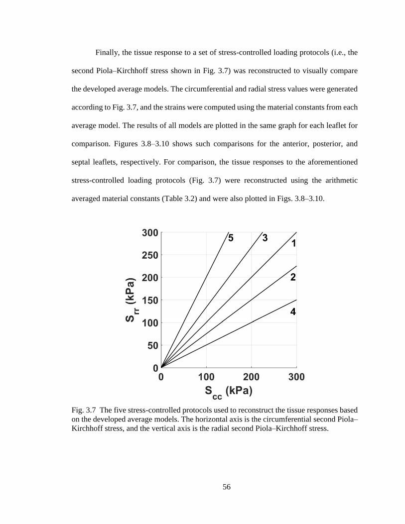
56

Finally, the tissue response to a set of stress-controlled loading protocols (i.e., the

second Piola–Kirchhoff stress shown in Fig. 3.7) was reconstructed to visually compare

the developed average models. The circumferential and radial stress values were generated

according to Fig. 3.7, and the strains were computed using the material constants from each

average model. The results of all models are plotted in the same graph for each leaflet for

comparison. Figures 3.8–3.10 shows such comparisons for the anterior, posterior, and

septal leaflets, respectively. For comparison, the tissue responses to the aforementioned

stress-controlled loading protocols (Fig. 3.7) were reconstructed using the arithmetic

averaged material constants (Table 3.2) and were also plotted in Figs. 3.8–3.10.

Fig. 3.7 The five stress-controlled protocols used to reconstruct the tissue responses based

on the developed average models. The horizontal axis is the circumferential second Piola–

Kirchhoff stress, and the vertical axis is the radial second Piola–Kirchhoff stress.

57

Fig. 3.8 Tissue response of the anterior leaflet to five stress-controlled loading protocols

(Fig. 3.7) reconstructed using the material constants of the arithmetic average (A-B) from

Table 3.2, the tension-based average model (T-B) from Table 3.3, the first Piola–Kirchhoff-stress–based average model (P-B) from Table 3.4, and the Cauchy-stress–based average

model (C-B) from Table 3.5. The vertical axis is the second Piola–Kirchhoff stress, and

the horizontal axis is the Green strain. The subscripts 𝑐𝑐 and 𝑟𝑟 denote the circumferential

and radial directions, respectively.

58

Fig. 3.9 Tissue response of the posterior leaflet to five stress-controlled loading protocols


Table 3.2, the tension based average model (T-B) from Table 3.3, the first Piola–Kirchhoff-stress–based average model (P-B) from Table 3.4, and the Cauchy-stress–based average




59

Fig. 3.10 Tissue response of the septal leaflet to five stress-controlled loading protocols


Table 3.2, the tension based average model (T-B) from Table 3.3, the first Piola–Kirchhoff-stress–based average model (P-B) from Table 3.4, and the Cauchy-stress–based average




3.5 Discussion

3.5.1 Constitutive Model

The constant stress contour plots (Fig. 3.2) led us to choose a Fung-type strain

energy function as our phenomenological constitutive framework. As listed in Table 3.2,

the selected constitutive model fitted the data reasonably well for all samples. The only

exception was a posterior leaflet, listed as heart number 3 in Table 3.2. For this specific

sample, the constant 𝑎1 vanished when fitting was performed with positive-constant

constraints (𝑅2 = 0.66) [149]. Even without enforcement of positive-constant constraints,

the value of 𝑎1 did not change, and the quality of fitting did not improve (𝑅2 = 0.66). In

addition, an 𝑎1 of zero is physically impossible, as it implies that there exists no direct

60

relation between deformation and the stress state in the circumferential direction. As such,

the data for this posterior leaflet, listed as Sample 3 in Table 3.2, were eliminated in the

average models. For a small number of other samples, the constant 𝑎3 vanished when the

positive constant constraints were imposed (Table 3.2). Such results indicated that in these

specific samples, the product of strains in both directions did not influence the calculated

stress values.

To evaluate how effective the model was in predicting the response of the tissue,

we first fitted protocols 1, 2, 4, and 5 (listed in Table 3.1) to the proposed constitutive

model. We then used the parameters obtained from the model to predict the response of the

model to protocol 3 (listed in Table 3.1). The 𝑅2 values for the fitting process were 0.915,

0.893, and 0.886 for the anterior, posterior, and septal leaflets, respectively. The 𝑅2 values

for the comparison between the model prediction and experimentally measured data (i.e.,

protocol 3) were 0.936, 0.875, and 0.907 for the anterior, posterior, and septal leaflets,

respectively. The 𝑅2 values for the prediction of the experimental data were all close to

1.0. Such proximity to 1.0 indicated that parameters obtained from fitting a large portion

of the strain energy space to the constitutive model were reliable for predicting the regions

of the strain energy space not included in the parameter fitting process. After the ability of

the model to predict the tissue response was confirmed, all five-protocol were used in the

fitting process as described in the method section.

The average anisotropy indices were 0.52, 0.39, and 0.51 for anterior, posterior,

and septal leaflets, respectively (Table 3.2). The anisotropy indices were much smaller than

1, confirming that, similar to other cardiac valves, TV leaflet tissue response was

anisotropic [38, 42, 60, 67, 148]. As shown in Fig. 3.11, quantitative analysis of tissue

61

microstructure using small angle light scattering [77, 86, 150-152] confirmed that the main

direction of the extracellular matrix fibers was along the circumferential direction, and TV

leaflets were thus expected to be anisotropic. The porcine leaflets were qualitatively similar

to human tissues, as all three leaflets were stiffer in the circumferential direction in

comparison to the radial direction for both species [42]. The average anisotropy index of

the posterior leaflet was slightly smaller than the other two leaflets; however, the difference

was not significant (𝑝 ≈ 0.1 for both comparisons, Student t-test).

In FE analysis, using a convex strain energy function in the material model is

crucial for the stability of the numerical methods [153]. Hence, supplementary inspections

were performed to validate the integrity of the developed phenomenological constitutive

models by plotting the constant strain energy contours over the strain field using the

calculated material constants. As illustrated in Fig. 3.12, the strain energy contours for

typical TV leaflets were convex in all cases, which further confirmed the reliability of the

developed individual models. The only exception, as initially suspected, was the posterior

leaflet of the sample listed as Sample 3 in Table 3.2. In this specific case, the strain energy

was nonconvex (Fig. 3.13). As such, in future development of FE models of TV, using the

material constants of this specific sample is not recommended. Using similar methods, we

observed that the strain energy functions for the average models were all convex.

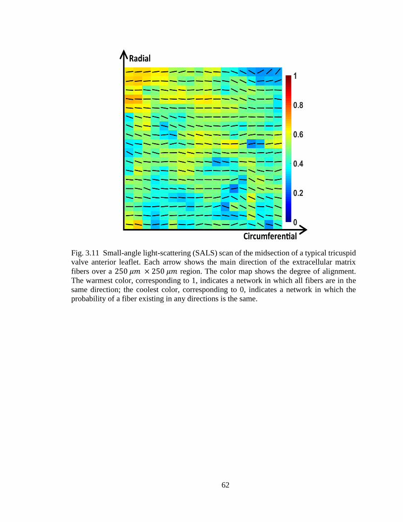
62

Fig. 3.11 Small-angle light-scattering (SALS) scan of the midsection of a typical tricuspid

valve anterior leaflet. Each arrow shows the main direction of the extracellular matrix

fibers over a 250 𝜇𝑚 × 250 𝜇𝑚 region. The color map shows the degree of alignment.

The warmest color, corresponding to 1, indicates a network in which all fibers are in the

same direction; the coolest color, corresponding to 0, indicates a network in which the

probability of a fiber existing in any directions is the same.

63

Fig. 3.12 Constant strain energy contours plotted over the Green strain field for the (a)

anterior, (b) posterior, and (c) septal leaflets of a typical tricuspid valve.

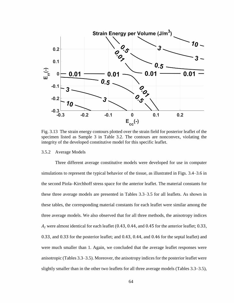
64

Fig. 3.13 The strain energy contours plotted over the strain field for posterior leaflet of the

specimen listed as Sample 3 in Table 3.2. The contours are nonconvex, violating the

integrity of the developed constitutive model for this specific leaflet.

3.5.2 Average Models

Three different average constitutive models were developed for use in computer

simulations to represent the typical behavior of the tissue, as illustrated in Figs. 3.4–3.6 in

the second Piola–Kirchhoff stress space for the anterior leaflet. The material constants for

these three average models are presented in Tables 3.3–3.5 for all leaflets. As shown in

these tables, the corresponding material constants for each leaflet were similar among the

three average models. We also observed that for all three methods, the anisotropy indices

𝐴𝐼 were almost identical for each leaflet (0.43, 0.44, and 0.45 for the anterior leaflet; 0.33,

0.33, and 0.33 for the posterior leaflet; and 0.43, 0.44, and 0.46 for the septal leaflet) and

were much smaller than 1. Again, we concluded that the average leaflet responses were

anisotropic (Tables 3.3–3.5). Moreover, the anisotropy indices for the posterior leaflet were

slightly smaller than in the other two leaflets for all three average models (Tables 3.3–3.5),

65

as were the arithmetic averages (Table 3.2). As shown in Figs. 3.8–3.10, the responses for

the three developed average models were highly similar. One reason for the similarity

could be the small variations in thickness of the different specimens for each leaflet. Had

the tissue thicknesses varied dramatically among the samples, one would have expected

that the average values obtained from the same tension states (thickness-dependent) to be

different from those obtained from same states of first Piola–Kirckhoff stress (thickness-

independent). Our analysis confirmed the fidelity of the tension-controlled biaxial testing

loading protocols and the subsequent averaging procedure in the tension space [36, 38, 58,

59, 148] when there are only small variations in the thickness of the specimens. It is,

however, more reasonable to avoid potential error in future investigations by performing

stress-controlled tests, especially when the tissue thickness varies significantly between the

specimens.

Figures 3.8–3.10 also show the arithmetically averaged material constant

responses. Based on these figures, while the responses of the three models for averaging

the experimental data (i.e., tension-based, first-Piola-Kirchhoff-stess–based, and Cauchy-

stress–based approaches), were notably similar, the responses generated from

arithmetically averaging the material constants were different, especially in the radial

direction. Such differences and similarities can be further investigated by comparing the

material constants for average models from Tables 3.3 and 3.4 with the arithmetic average

of the material constants of the individual fits from Table 3.2. For example, As shown in

these tables for septal leaflet, 𝑐 ranged from 1.876 to 2.321 𝑘𝑃𝑎, 𝑎1 ranged from 40.420

to 46.460, 𝑎2 ranged from 16.784 to 18.253, and 𝑎3 ranged from 2.954 to 3.646 for the

average models, wheras the arithmetically averaged values 𝑐, 𝑎1, 𝑎2, and 𝑎3 for the same

66

leaflet were 2.994 𝑘𝑃𝑎, 53.566, 27.286, and 5.570, respectively. The arithmetically

averaged material constants are all outside of the range of average model material

constants, consistent with our conclusion regarding Figs. 3.8–3.10.

Since stress is a tensor, the large difference between the values, even if it is only in

the radial direction, indicates a completely altered state of stress. This observation further

exemplifies that the arithmetically averaged values of the individual material constants may

not represent the generic tissue responses accurately.

3.5.3 Limitations

While phenomenological constitutive models are powerful in predicting the

responses of the tissue, they do not provide much insight about the mechanical environment

at the underlying extracellular matrix/cellular levels. In other words, model parameters

cannot be quantitatively related to structural components of the tissue, such as extracellular

matrix protein volume fractions or extracellular matrix morphology. Such information is

of particular interest in the field of mechanobiology, for which constitutive frameworks

that include structural components of the tissue are more relevant [66-70]. Another

limitation pertains to the use of porcine tissues. Although many of the conclusions of this

study (e.g. the choice of the averaging method) seemed to be independent of the species,

caution should always be taken when drawing conclusions for human subjects based on

animal studies. Another limitation is that all of the experiments in were conducted at room

temperature, and the response of the tissue might be different at body temperature. Finally,

previous studies have shown that in vivo residual strains are present in ovine MV leaflets,

and they relax after dissection [26]. If such a phenomenon does exist for TV, any change

67

in the deformation should be taken into consideration in the development of future

computational models.

3.6 Conclusion

We used results from biaxial mechanical testing and obtained material constants

for a Fung-type phenomenological model to predict the mechanical response of the porcine

TV leaflet. Similar to other cardiac valves, we observed that TV leaflets were highly

anisotropic. We also conducted a series of studies to identify the most appropriate method

for finding representative material parameters for TV leaflets. Since the thicknesses did not

differ significantly in our sample groups, we found that both tension-based and stress-based

averaging methods provided acceptable outcomes. However, to prevent potential errors

when sample thickness varies more considerably, it is recommended to employ the stress-

based averaging method.

68

CHAPTER 4IV

DYNAMIC DEFORMATIONS AND SURFACE STRAINS OF THE TRICUSPID

VALVE LEAFLETS

(The content of this chapter was published in JBME (Oct 2016) as “Surface Strains of

Porcine Tricuspid Valve Septal Leaflets Measured in Ex Vivo Beating Hearts” [140].)

4.1 Summary

Quantification of TV leaflets mechanical strain is important in order to understand

valve pathophysiology and to develop effective treatment strategies. Many of the

traditional methods used to dynamically open and close the cardiac valves in vitro via flow

simulators require valve dissection. Recent studies, however, have shown that restriction

of the atrioventricular valve annuli could significantly change their in-vivo deformation.

For the first time, the porcine valve leaflets deformation was measured in a passive ex-vivo

beating heart without isolating and remounting the valve annuli. In particular, the right

ventricular apexes of porcine hearts (n = 8) were connected to a pulse-duplicator pump that

maintained a pulsatile flow from and to a reservoir connected to the right atrium and the

pulmonary arteries. This pump provided an RVP waveform that closely matched

physiological values. The pressure environment caused the tricuspid and PVs to open/close

similar to that in vivo. At the mid-section of the valve leaflets, the peak areal strain was 9.8

± 2.0% (mean ± standard error). The peak strain was 5.6 ± 1.1% and 4.3 ± 1.0% in the

circumferential and radial directions, respectively. Although the right ventricle was beating

passively, the leaflet peak areal strains closely matched the values measured in other

69

atrioventricular valves (i.e., MV) in vivo. This technique can be used to measure leaflet

strains with and without the presence of valve lesions to help develop/evaluate treatment

strategies to restore normal valve deformation.

4.2 Introduction

As a one-way valve, TV guides the blood from the right atrium to the right ventricle

during the atrial systole and prevents its backflow during the ventricular systole [1]. During

the process of valve closure, its leaflets undergo complicated dynamic deformation and

loadings. Quantification of such dynamic deformations is important because the

development of treatment strategies for TV dysfunctions relies on a comprehensive

understanding of its normal biomechanical environment. Among TV dysfunctions, TV

regurgitation is one of the most common ones, which in most cases requires TV repair or

total valve replacement [24, 25]. The pathophysiology of TV regurgitation is closely

related to the dynamic deformation of the valve annulus and leaflet coaptation [116].

Accurate quantification of normal biomechanical behavior of TV leaflets during the cardiac

cycle is essential for the development and evaluation of efficient repair strategies and/or

prosthetic valves that aim to mimic native valves.

A large group of researchers have studied the biomechanical behavior and dynamic

deformations of MV [12, 26, 30, 39, 82, 85, 108, 109], the atrioventricular valve analogous

to TV on the left heart. There are also a few studies that focus on TV geometry and annulus

deformation [80, 81, 110]. While these studies are extremely important, they provide no

information about the dynamic mechanical strains of TV leaflets. In terms of experimental

techniques, the previous valvular studies can be categorized into two main groups: in-vivo

studies [26, 30, 80-82, 85, 108-110] and in-vitro studies [39, 111, 112]. In-vivo ovine and

70

porcine studies are frequently used as excellent models prior to clinical studies [26, 82, 85].

Such studies, however, require surgical operating rooms and animal care facilities, which

are often costly and should be used only prior to clinical approaches. In-vitro studies, while

less costly, were previously only conducted on excised valves [39, 111]. In these studies,

the excised valves are generally mounted on a prosthetic rigid annulus and subjected to

pulsatile pressure in a flow simulator. The outcome of such studies is limited since it has

been shown that the cardiac valve annulus is dynamically deforming during the cardiac

cycle [82] and, thus, valve annulus restriction could significantly alter the leafletstrains

[26].

Recently, an ex-vivo approach using the entire porcine heart (instead of using

isolated valves) has been developed to image valve motion and to study hemodynamics in

the left chambers of the heart [113]. In the presented study, we have used a modified ex-

vivo apparatus to open and close cardiac valves in the right side of the heart passively. In

particular, for the first time, we have been able to visualize the dynamic deformations of

TV and measure the mechanical strains on the septal leaflet. Our method has enabled us to

study the intact TVs without mounting them on a rigid annulus. Since porcine tissues are

available within a few minutes after the animals are slaughtered at a local slaughterhouse,

no surgical rooms and animal facilities were required for our experiments.

In the present study, we measured the deformation of porcine TV septal leaflets

using small positional markers while the heart was passively beating in our ex-vivo

apparatus. The measured deformation data were then used to quantify the in-plane ex-vivo

mechanical strains of TV septal leaflet.

71

Fig. 4.1 a) Schematic of the ex-vivo beating heart apparatus and b) a picture of the actual

apparatus.

4.3 Methods

4.3.1 Ex-vivo Heart Apparatus

A schematic of the ex-vivo apparatus and the circulation loop and an image of the

setup are shown in Fig. 4.1. The outlet of a reservoir was connected to the superior vena

cava, and the pulmonary artery was connected to the inlet of the reservoir. A positive

72

displacement pump (SuperPump AR Series, Vivitro Labs Inc., BC, Canada) was connected

to the apex of the right ventricle after an incision was carefully made at this location (as

described in more detail below). This pump is widely used for valve testing [154-158].

The pump setup included a controller unit, which enabled us to control the waveform, the

stroke volume, and the frequency of the beating. The continuous pulsatile flow in the right

side of the heart was initiated as follows:

• When the pump piston moved back (towards the left direction in Fig. 4.1a), it

pulled the fluid from the reservoir into the heart; thus, TV opened and the PV

closed.

• When the pump piston moved forward (towards the right direction in Fig. 4.1b),

due to an increase in the RVP, TV closed; after sufficient pressure had built up,

the PV opened, guiding the fluid back to the reservoir through the pulmonary

artery and the connected tubes.

Flow rate was measured using a transonic flowmeter (T108, Transonic Systems

Inc., Ithaca, NY) at the inflow tube proximal to the heart. Catheter type pressure probes

(SPR-524 and PCU-2000, ADInstruments, Colorado Springs, CO) were used to record

transient right atrial pressure (RAP), RVP, and pulmonary artery pressure (PAP). To

control the back-pressure over the PV, a mechanical valve was placed in the circuit after

the pulmonary artery.

Aluminum profiles (80/20 Inc., Columbia City, IN & Flexaframe™, Fisher

Scientific™, Waltham, MA) and rods were used as the framework for the ex-vivo

apparatus (Fig. 4.1b). All other parts, including a 15 liter reservoir, were assembled over

73

this framework. The reservoir was connected to the superior vena cava using flexible tubes.

To connect the right ventricle to the pump, a hole was created at the right apex using

scalpels and scissors where a straight barbed hose fitting was inserted. The hole was made

with extreme caution to avoid any damage to the papillary muscles and chordae tendineae

such to minimize the effect on valve function. The pulmonary artery was connected back

to the reservoir to complete the hydraulic circuit. To measure the pressure as close to the

right ventricle as possible without disturbing the circulation, a T-shaped pipe-fitting was

placed just after of the straight barbed hose fitting connected to the right ventricle. A

modified Luer Lok connector with a long tail was used to provide a safe passage for the

pressure probe through the T-shaped pipe fitting as it was inserted into the ventricular

chamber (Fig. 4.2). To allow one to visualize the leaflet motion, a backup seal followed by

a dome valve was assembled inside the T-shaped pipe fitting before the Luer Lok assembly.

As such, at any point during the experiment, we were able to remove the Luer Lok assembly

and insert an endoscopic camera without causing any leaks. The same assembly was used

to connect the pressure transducer to the superior vena cava and pulmonary artery as well.

The inferior vena cava and other critical vessels were sealed using umbilical clamps to

prevent leaks (Fig. 4.3). Cable ties or worm-drive clamps were used at the other

connections to prevent leaks. Flexible ¾-inch PVC tubes were used for all the tubing, and

the connections and fittings were selected accordingly.

74

Fig. 4.2 The T-shaped pipefitting connected to the right atrium through a straight barbed

hose fitting (1). The Luer Lok assembly was connected to the other side of the t-shaped

pipe fitting to support the pressure sensor. The other straight barbed hose fitting (2)

connected the right ventricle to the pump. Crystal wires came out through the inferior vena

cava. The umbilical clamp was used to prevent leakage from the inferior vena cava.

Fig. 4.3 Umbilical clamps, cable ties, and worm-drive clamps were used for sealing.

75

4.3.2 Sample Preparation

Fresh porcine hearts were obtained from a local slaughterhouse (3-D Meats, Dalton,

OH) and were transported to our laboratory (in approximately 30 minutes) while

submerged in isotonic PBS and covered with ice immediately after the animals were

slaughtered. The hearts were flushed using PBS to remove blood clots. In order to measure

positional data, a total of 16 sonocrystals (Sonometrics Co., ON, Canada) were sutured to

the valve annulus, septal leaflets, and myocardium (Fig. 4.4). To prevent any damage to

the hearts, the sonocrystal wires were passed into the ventricle through the inferior vena

cava and the suturing process was conducted via the superior vena cava. As shown in Fig.

4.4, two crystals (1 𝑚𝑚) were sutured close to the edge, three (1 𝑚𝑚) at the midsection

and three (2 𝑚𝑚) close to the annulus on the septal leaflet. Five more crystals (2 𝑚𝑚) were

sutured around the annulus. In addition, three crystals (3 𝑚𝑚) were connected outside of

the heart close to the apex in order to define the reference frame for positional

measurements. All crystal wires were passed through the inferior vena cava. PBS with PH

of 7.4 was used as the circulation fluid to help prevent the myocardium, especially the

endocardium, from degenerating rapidly. During preparation and data collection, samples

were submerged in PBS and/or PBS was sprayed on the surfaces exposed to the air to

prevent drying. The sonocrystals were connected to the sonomicrometer device (TRX

Series 16, Sonometrics Co., ON, Canada) to acquire the positional data. The pressure and

flow signals were sent to the sonomicrometer as well as a data acquisition card (6036E,

National Instruments, Austin, TX) directly connected to the computer. The pump controller

provided a standard 70 bpm waveform which was used in the experiment. This waveform

complied with the requirements of the International Standard Organization (ISO 5840) and

76

US Food and Drug Administration guidelines for heart valve testing [159]. After

stabilization of the flow rate and periodic pressure signals, the sonomicrometer

potentiometers were adjusted to maximize signal-to-noise ratio. Finally, an endoscopic

camera (SSVR-710 Snakescope) was inserted into the heart to visualize the leaflet motion

and ensure that the leaflets were coapting properly. The data acquisition was then initiated

with a rate of 100 Hz (according to ISO 5840 requirements) and for a period of 20 seconds

(2000 data points). Eight hearts were tested using the aforementioned procedure.

Fig. 4.4 The arrangement of the sonocrystals over the surface of the septal leaflet. The red

lines show the triangular element used for strain calculation. The radial direction was

defined by a vector connecting crystal 4 to crystal 7.

4.3.3 Strain Calculation

SonoSOFT (Sonometrics Co., ON, Canada) software was used to modify the

recorded displacement and pressure signals. SonoXYZ (Sonometrics Co., ON, Canada)

software was used to calculate the positional coordinates of the crystals during each cardiac

cycle with respect to a defined coordinate system. These positional data were used to

77

calculate the strain tensor based on a previously used method [26, 86, 87]. The triangulation

was done manually according to pattern shown in Fig. 4.4. Since only eight crystals were

sutured on the septal leaflet (the remaining eight crystals were sutured on the annulus and

outside of the heart, as stated previously), their positioning was the same for all eight hearts

and no automated triangulation was necessary.

After calculating the crystal positional data from the recorded raw data, the

positional data were averaged over the 22 recorded beats for all crystals in each heart. The

average positional data were then used to calculate the strains and stretches using the

method explained in APPENDIX B.

4.3.4 Pressures Data Analysis

The sonomicrometer data acquisition system was used to obtain both pressure and

displacement signals. No synchronization process was necessary as the data were already

synchronized for each node and heart. During all of the experiments, the signals of RAP,

RVP, and PAP were monitored and recorded. Before using such data, however, a few

pressure corrections were conducted in the signals from each heart. The first correction

was made to adjust the zero level. In particular, in each heart, there was a height difference

between the free surface of the fluid in the reservoir and the right atrium. To remove the

hydrostatic pressure magnitude in the measurement, the height was measured for each heart

and the equivalent hydrostatic pressure was subtracted from the pressure signals. As a

result, the minimum of the RVP and RAP shifted to a level close to zero. In addition, as

the hearts were assembled vertically, there was a height difference between the bottom of

the ventricle and the pulmonary artery where the pressure sensors were positioned to

measure RVP and PAP, respectively. This height difference was also measured for each

78

heart, and the equivalent hydrostatic pressure was subtracted from the PAP. Although these

heights and their equivalent hydrostatic pressures were small, this correction process was

necessary to obtain a consistent and comparable cardiac pressure graph for all experiments.

In all eight experiments, the recorded pressures and positional data were averaged over all

the 22 recorded beats.

4.4 Results

4.4.1 Pressure

As shown in Fig. 4.5, although the porcine hearts were passively beating, the

recorded pressure compared well with in-vivo human cardiac pressures [160]. The small

standard errors show that despite the variability among the porcine samples, the pressures

for each heart do not deviate much from the average value for the eight hearts. The

measured RVP ranged from values close to zero up to approximately 30 𝑚𝑚 𝐻𝑔, similar

to the reported porcine values (2 to 33 𝑚𝑚 𝐻𝑔 [161-164]). The measured PAP ranged

from approximately 6 to 30 𝑚𝑚 𝐻𝑔. The RAP remained relatively close to zero during

diastole. We were not able to find reliable PAP and RAP values for porcine hearts in the

literature but the measured values for these two signals (Fig. 4.5) were comparable to those

of human [160]. The RVP average signal also shows a small drop right at the beginning of

the diastole. A closer examination of the RVP signal in Fig. 4.5 shows that TV closes at

approximately 0.2 𝑠, where the RVP intersects with the RAP; the PV opens at 0.29 𝑠,

where the RVP meets the PAP; the PV closes approximately at 0.44 𝑠, where the RVP

separates from the PAP; and finally TV opens approximately at 0.54 𝑠, where the RVP

crosses the RAP once more. The average flow rate for all the hearts was 2.63 ±

0.13 𝑙/𝑚𝑖𝑛.

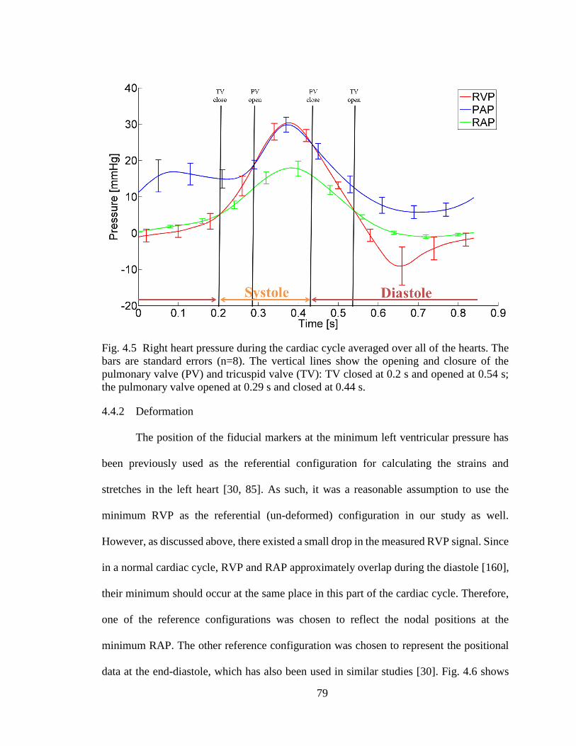
79

Fig. 4.5 Right heart pressure during the cardiac cycle averaged over all of the hearts. The

bars are standard errors (n=8). The vertical lines show the opening and closure of the

pulmonary valve (PV) and tricuspid valve (TV): TV closed at 0.2 s and opened at 0.54 s;

the pulmonary valve opened at 0.29 s and closed at 0.44 s.

4.4.2 Deformation

The position of the fiducial markers at the minimum left ventricular pressure has

been previously used as the referential configuration for calculating the strains and

stretches in the left heart [30, 85]. As such, it was a reasonable assumption to use the

minimum RVP as the referential (un-deformed) configuration in our study as well.

However, as discussed above, there existed a small drop in the measured RVP signal. Since

in a normal cardiac cycle, RVP and RAP approximately overlap during the diastole [160],

their minimum should occur at the same place in this part of the cardiac cycle. Therefore,

one of the reference configurations was chosen to reflect the nodal positions at the

minimum RAP. The other reference configuration was chosen to represent the positional

data at the end-diastole, which has also been used in similar studies [30]. Fig. 4.6 shows

80

the calculated peak areal strain, maximum principal strain, circumferential strain and radial

strain at the center point of the leaflet (point number 4) averaged for all eight hearts using

the two aforementioned references. Fig. 4.6 also shows the strain standard errors for the

eight hearts. There was no significant difference between the strains measured using two

different reference configurations (𝑝 > 0.14 in all cases, paired Student t-test). The same

observation has been reported for MV anterior leaflet [30]. As shown in Fig. 4.6, the peak

areal strain (9.8%) and the peak maximum principal strain (11.2%) were significantly

different (𝑝 < 0.008 in all cases, paired Student t-test) from the peak circumferential strain

(5.6%) and the peak radial strain (4.3%). However, there was no significant difference

(𝑝 ≈ 0.24, paired Student t-test) between the peak circumferential and the peak radial

strains (the numbers quantified using minimum RAP as the un-deformed reference (Ref1

in Fig. 4.6)).

Figure 4.7 shows the temporal strain variations over a cardiac cycle. The strain

values were averaged at the leaflet midpoint for the eight hearts at each time point. The

leaflets experienced positive strain for the majority of the times points during the cardiac

cycle. Comparing the strain graphs with the pressure graph shows that immediately after

TV closed (𝑡 = 0.2 𝑠), all the quantified strains rose rapidly and reached their peaks

values at the maximum RVP (𝑡 ≈ 0.4 𝑠). The strains subsequently dropped, reaching their

minimum values at 𝑡 ≈ 0.65 𝑠, with the exception of the radial strain, which reached the

minimum value at 𝑡 ≈ 0.5 𝑠. Overall, the strain values were extremely small during

diastole and increased during systole. Note that the peak of the means (Fig. 4.6) is always

less than (or ideally equal to) the mean of the peaks (Fig. 4.7) since the maximum values

of the signals for each heart do not necessarily happen exactly at the same time.

81

Fig. 4.6 Average peak areal, maximum principal (Max Princ), circumferential (Circ), and

radial strains at the leaflet midpoint measured with respect to reference 1 (Ref1, minimum

RAP) and reference 2 (Ref2, end diastole). The error bars are standard error (n=8).

Figure 4.8 shows the spatial distribution of the strains over the leaflet at the

maximum RVP. At this pressure level, the strains were averaged over all eight hearts. The

averaged data are illustrated for a typical septal leaflet. As shown in Fig. 4.8, the maximum

principal strain is distributed uniformly over the leaflet at maximum RVP, while the areal

strain is not as uniform. There is much heterogeneity in the spatial distribution of the

circumferential strain and radial strain over the septal leaflet. While higher values for

circumferential strain were observed toward the posterior of the leaflet, the radial strains

reached higher values in areas near the anterior.

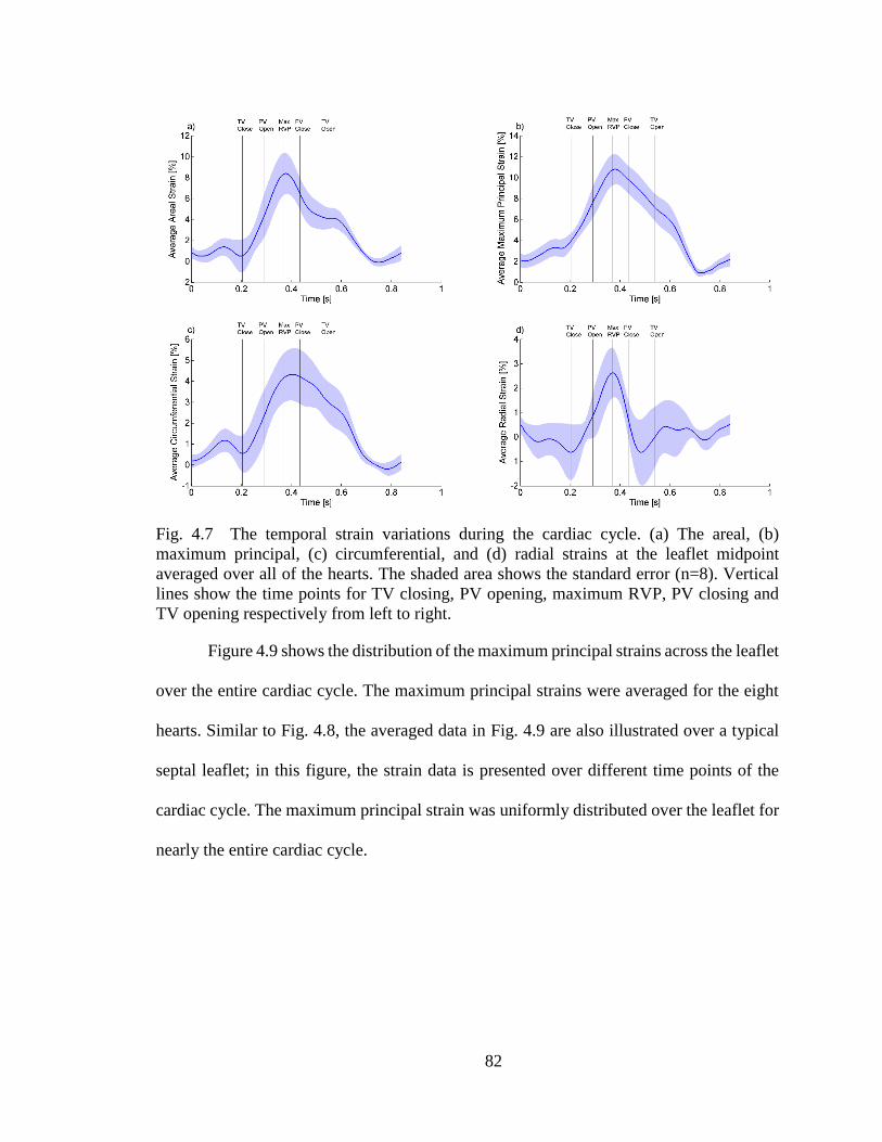
82

Fig. 4.7 The temporal strain variations during the cardiac cycle. (a) The areal, (b)

maximum principal, (c) circumferential, and (d) radial strains at the leaflet midpoint

averaged over all of the hearts. The shaded area shows the standard error (n=8). Vertical

lines show the time points for TV closing, PV opening, maximum RVP, PV closing and

TV opening respectively from left to right.

Figure 4.9 shows the distribution of the maximum principal strains across the leaflet

over the entire cardiac cycle. The maximum principal strains were averaged for the eight

hearts. Similar to Fig. 4.8, the averaged data in Fig. 4.9 are also illustrated over a typical

septal leaflet; in this figure, the strain data is presented over different time points of the

cardiac cycle. The maximum principal strain was uniformly distributed over the leaflet for

nearly the entire cardiac cycle.

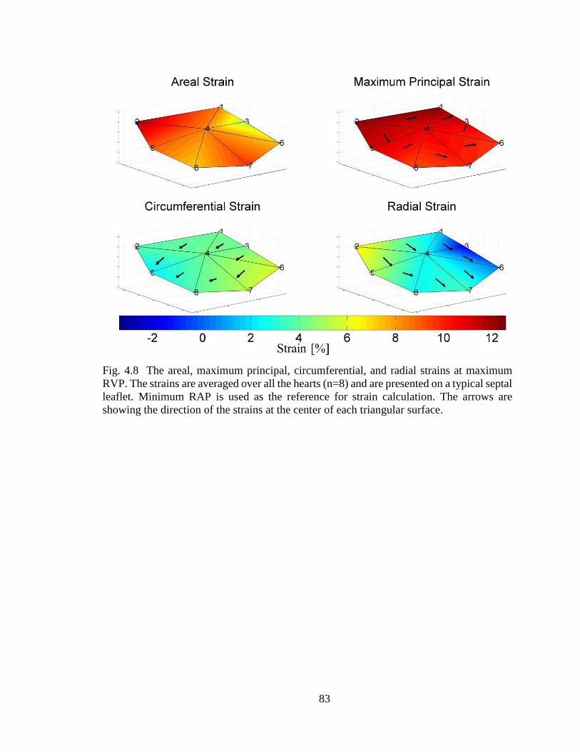
83

Fig. 4.8 The areal, maximum principal, circumferential, and radial strains at maximum

RVP. The strains are averaged over all the hearts (n=8) and are presented on a typical septal

leaflet. Minimum RAP is used as the reference for strain calculation. The arrows are

showing the direction of the strains at the center of each triangular surface.

84

Fig. 4.9 Distribution of the maximum principal strain over the leaflet during the septal

entire cardiac cycle. Maximum principal strain is averaged over all of the hearts (n=8) and

showed over a typical septal leaflet during the cardiac cycle.

4.5 Discussion

Our novel ex-vivo beating heart apparatus was able to produce repeatable data with

high temporal resolution. Using our passive beating heart, we were able to reproduce

ventricular pressure waves that matched the physiological values of an active heart [160].

Porcine hearts are excellent models for valve studies and pressure values at the pulmonary

side are similar in human and porcine hearts. In particular, human RVP ranges

approximately from zero to 30 𝑚𝑚 𝐻𝑔 [128, 160] and porcine RVP ranges roughly from

zero up to around 33 𝑚𝑚 𝐻𝑔 [161-164]. Such a similarity also exists in the system side

of the heart [1, 165].

To our best knowledge, the in-vivo strains in porcine TV leaflets have not yet been

quantified. Thus, it is not possible to compare our deformation results with in-vivo TV

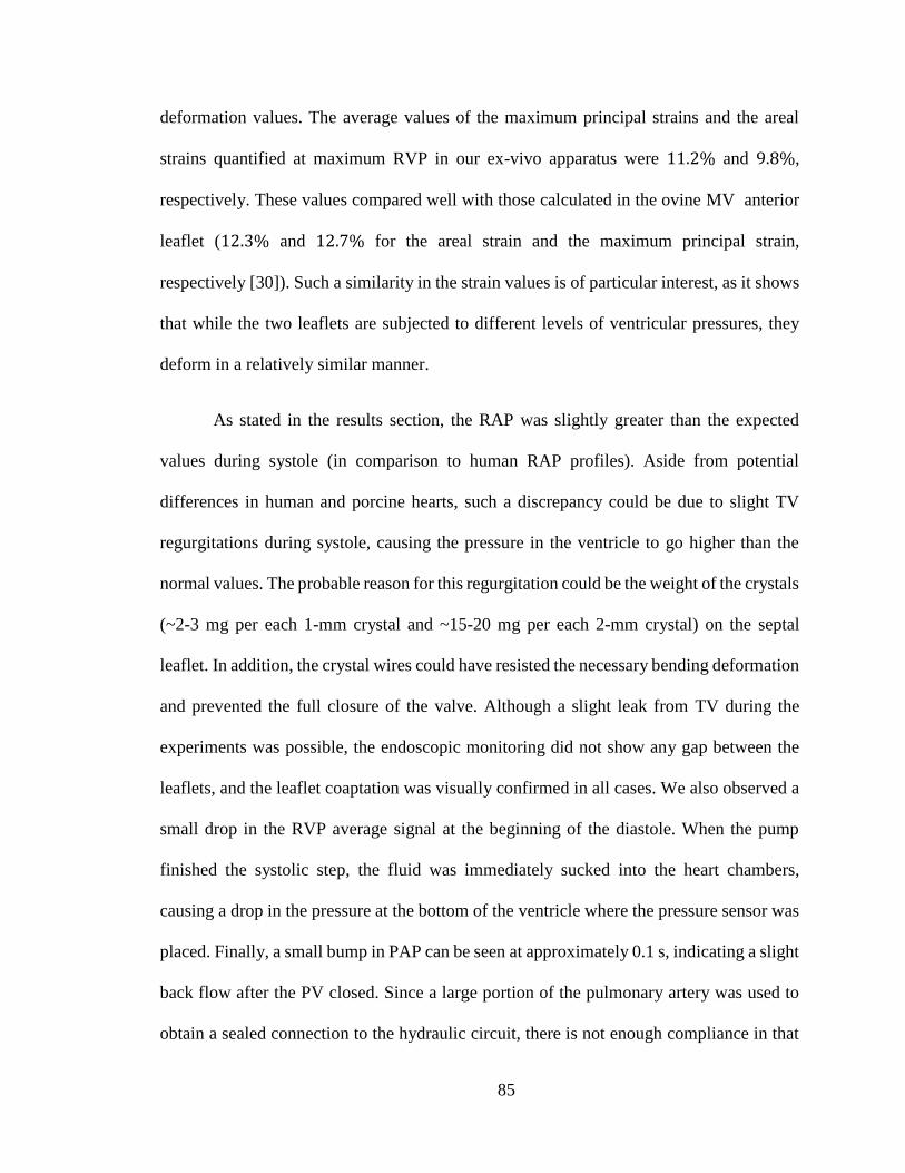
85

deformation values. The average values of the maximum principal strains and the areal

strains quantified at maximum RVP in our ex-vivo apparatus were 11.2% and 9.8%,

respectively. These values compared well with those calculated in the ovine MV anterior

leaflet (12.3% and 12.7% for the areal strain and the maximum principal strain,

respectively [30]). Such a similarity in the strain values is of particular interest, as it shows

that while the two leaflets are subjected to different levels of ventricular pressures, they

deform in a relatively similar manner.

As stated in the results section, the RAP was slightly greater than the expected

values during systole (in comparison to human RAP profiles). Aside from potential

differences in human and porcine hearts, such a discrepancy could be due to slight TV

regurgitations during systole, causing the pressure in the ventricle to go higher than the

normal values. The probable reason for this regurgitation could be the weight of the crystals

(~2-3 mg per each 1-mm crystal and ~15-20 mg per each 2-mm crystal) on the septal

leaflet. In addition, the crystal wires could have resisted the necessary bending deformation

and prevented the full closure of the valve. Although a slight leak from TV during the

experiments was possible, the endoscopic monitoring did not show any gap between the

leaflets, and the leaflet coaptation was visually confirmed in all cases. We also observed a

small drop in the RVP average signal at the beginning of the diastole. When the pump

finished the systolic step, the fluid was immediately sucked into the heart chambers,

causing a drop in the pressure at the bottom of the ventricle where the pressure sensor was

placed. Finally, a small bump in PAP can be seen at approximately 0.1 s, indicating a slight

back flow after the PV closed. Since a large portion of the pulmonary artery was used to

obtain a sealed connection to the hydraulic circuit, there is not enough compliance in that

86

area to dampen the changes in the pressure. A well-tuned compliance chamber might be

useful for eliminating this inertial effect in the PAP signal. Although, more realistic

pressure waveforms can be obtained using a compliance chamber with specific

adjustments, we chose a less complicated approach that will be more easily reproduced by

other researchers.

Unlike MV leaflets, in which significant differences exist between the maximum

strain in the circumferential and radial directions [26, 30, 111], no significant difference

existed between circumferential and radial strains in TV septal leaflet at the maximum

RVP. A potential explanation is that TV septal leaflet has a more isotropic extracellular

matrix microstructural architecture in comparison to MV anterior and posterior leaflets.

The anisotropic nature of MV anterior leaflet has been demonstrated previously [35].

Biaxial mechanical testing and measurement of tissue microstructural architecture (e.g. via

small angle light scattering could identify the degree of anisotropy in TV septal leaflets.

Due to the fact that the number of channels available for sonomicrometry crystals was

limited to 16, we were not able to measure the deformation of TV anterior and posterior

leaflets to make such a comparison among the ex-vivo strain values. Further research is

required to quantify strain values in TV anterior and posterior leaflets in the future [117,

166].

There are many advantages in using porcine hearts in our experiment, as fresh

tissues can be obtained and the biomechanical behavior of the valves is less affected by the

activity of degenerative enzymes in the extracellular matrix. In addition, in comparison to

human cadaverous tissues, younger porcine samples with less variability are available [35].

However, one should always be cautious in drawing conclusions regarding human tissue

87

responses based solely on animal studies [167]. The advantage of our ex-vivo apparatus is

that, if necessary, human cadaverous tissues can be used in conducting similar experiments

without any additional complications.

Sonomicrometry crystals may affect the measured deformations in different ways.

The process of attaching the crystals to the leaflet may cause some localized and permanent

changes to the leaflet structural properties. Although these changes were not measurable in

our setup, much caution was used to prevent damage to the tissue during the suturing

process. In is noteworthy that these changes were presumably restricted to the immediate

vicinity of the crystal. As per potential of error due to buoyancy and/or inertia, the piezo

crystals had same density as that of water or tissue. In addition, the crystals were extremely

small compared to the size of their surrounding tissues. Therefore, their interference with

natural leaflet motion was minimal. Crystals, of course, were connected the

sonomicrometer instrument via wires. One may consider the tethering effects of these

connecting wires as a potential source for leaflet motion restriction. The crystals were

connected to sonomicrometer using 38 gauge copper wires, which were flexible. In order

for the crystal wires to alter the natural motion of the leaflets in any way, the wires should

have been tethered close to the leaflet surface, with little or no out-of-plane slack. As such,

we made sure that the wires had enough slack to prevent physically restraining the natural

motion of the leaflets. Despite its few limitations, sonomicrometry have been used

extensively in the valve studies [26, 81, 82, 167-170].

A major limitation of our experiment is the passive nature of the beating heart. The

contraction of papillary muscles and the activation of ventricular and atrial muscles

potentially change the loading condition on the leaflet annulus and chordae tendineae.

88

Although the ex-vivo passive beating heart is not identical to the in-vivo active hearts,

unlike the in-vitro studies of the excised cardiac valves [39, 111, 112], TV annulus is not

restricted in the ex-vivo apparatus. In-vivo studies of TV motion have shown that TV

annulus size dynamically changes during the normal cardiac cycle [81]. The ex-vivo

beating heart at least maintains the passive component of such deformation in TV annulus.

In short, even though the ex-vivo beating heart experiment is not identical to the in-vivo

heart, it is more realistic than the isolated valve experiments when it comes to the valve

annulus deformation.

There exists a major advantage in using a passive beating heart in the verification

of combined valve and ventricle computational models [171]. In particular, because the

cardiac muscles are not active and the ventricular pressure is the only load applied to the

cardiac tissues, one could use the ex-vivo beating heart to validate combined valve and

ventricle models absent the active stress components of the cardiac tissues. In addition to

detailed pressure and strain measurements, the entire heart can be imaged and segmented

following the experiment to provide a subject-specific computational model.

Although our study was conducted using PBS, there is no limitation in using other

non-clear fluids in our apparatus, as our strain measurement does not rely on visual access

to the valves. Such a capability is of great importance because recent studies have shown

that the flow properties (particularly the transition to turbulence) could be significantly

different in blood in comparison to optically clear viscosity-matched blood substitutes

[172]. Since the transition to turbulence could happen in the proximity of the cardiac

valves, measurements of valve deformation using blood should be conducted in the future.

89

In summary, we developed an experimental setup to measure the dynamic

deformation of the porcine TV septal leaflets. We observed that the leaflet strain values are

similar to those measured in-vivo in leaflets of the other atrioventricular valve (i.e. MV).

In future studies, our experimental model can be used to evaluate mechanical strains on

different TV leaflets. In addition, our experimental setup can be beneficial in studying

primary valve lesions such as chordae rupture, secondary valve lesions such as pulmonary

hypertension, and valve repair procedures such as ring annuloplasty and/or leaflet

resection.

90

CHAPTER 5V

DYNAMIC DEFORMATIONS OF THE TRICUSPID VALVE ANNULUS, INTACT

AND AFTER CHORDAE RUPTURE

(The content of this chapter was published in PLOSE ONE (Nov 2018) as “Dilation of

Tricuspid Valve Annulus Immediately After Rupture of Chordae Tendineae in Ex-vivo

Porcine Hearts” [173].)

5.1 Summary

Chordae rupture is one of the main lesions observed in traumatic heart events that

might lead to severe TV regurgitation. TV regurgitation following chordae rupture is often

well tolerated with few or no symptoms for most patients. However, early repair of TV is

of great importance, as it might prevent further exacerbation of the regurgitation due to

remodeling responses. To understand how TV regurgitation develops following this acute

event, we investigated the changes on TV geometry, mechanics, and function of ex-vivo

porcine hearts following chordae rupture.

Sonomicrometry techniques were employed in an ex-vivo heart apparatus to

identify how the annulus geometry alters throughout the cardiac cycle after chordae

rupture, leading to the development of TV regurgitation.

We observed that TV annulus significantly dilated (~9% in area) immediately after

chordae rupture. The annulus area and circumference ranged from 11.4 ± 2.8 to 13.3 ±

2.9 cm2 and from 12.5 ± 1.5 to 13.5 ± 1.3 cm, respectively, during the cardiac cycle for

91

the intact heart. After chordae rupture, the annulus area and circumference were larger and

ranged from 12.3 ± 3.0 to 14.4 ± 2.9 cm2 and from 13.0 ± 1.5 to 14.0 ± 1.2 cm,

respectively.

In our ex-vivo study, we showed for the first time that TV annulus dilates

immediately after chordae rupture. Consequently, secondary TV regurgitation may be

developed because of such changes in the annulus geometry. In addition, TV leaflet and

the right ventricle myocardium are subjected to a different mechanical environment,

potentially causing further negative remodeling responses and exacerbating the detrimental

outcomes of chordae rupture.

5.2 Introduction

TV guides the blood from the right atrium to the right ventricle and prevents

backflow during ventricular contraction. The leaflets and annulus of TV undergo

complicated dynamic deformations during normal cardiac cycles [80, 81]. Any disturbance

in the normal deformation of the valve leaflets and/or annulus could lead to valvular

regurgitation [174, 175] and changes in the valve’s mechanical response [134, 142]. In

most cases, TV regurgitation—whether it is caused by primary valvular lesions (e.g., due

to congenital malformations [176], trauma [177, 178] or degenerative diseases such as

Marfan syndrome [179, 180]) or takes place as a result of other cardiovascular diseases

(e.g. secondary to pulmonary hypertension [181])—will require surgical intervention

[182].

While TV regurgitation is most often caused by chronic diseases, acute cases could

occur following traumatic events such as vehicular accidents [183, 184]. In the majority of

92

trauma-related cases, chordae rupture is the main lesion present [185]. Many accident

victims also suffer from other injuries such as lacerations, fractures, and closed head

injuries [151]. With these more severe concurrent injuries present immediately after

trauma, the acute TV regurgitation can be easily overlooked when making a diagnosis.

Although advances in diagnostic procedures such as echocardiography have improved in

recent years [186], isolated TV regurgitation is often well tolerated, and most patients

experience few or no symptoms in the weeks and months following the trauma [187, 188].

In fact, the average time from the trauma to the initial diagnosis of TV regurgitation is three

years [189] (with the time to diagnosis ranging from within 15 days of the trauma to as

long as 25 years later). However, early repair of the regurgitative TV following chordae

rupture is of critical importance. Among many benefits, early repair may prevent further

detrimental complications such as thickening and fibrosis of TV leaflets and/or changes in

the sinus rhythm due to right atrial dilation [189].

Previous studies have shown that acute biomechanical changes in cardiac valves

could induce remodeling responses that may negatively affect the valve structure,

mechanical properties, and function [117, 134, 190]. Considering the importance of such

acute events, in this study we aimed to identify how TV regurgitation develops

immediately following chordae rupture. Since normal TV function relies on precise and

complex interactions among the various components (i.e. annulus, leaflets, chordae), it is

expected that chordae rupture disturbs the normal deformation of the valve annulus and

leads to insufficient leaflet coaptation. It has been previously shown that valve

insufficiency can lead to ventricular and annulus dilation due to remodeling responses.

However, based on the assumption that intact chordae tendineae mechanically

93

support/anchor the normal TV annulus, for the first time in this ex-vivo study we have

shown that immediately following chordae rupture, TV annulus dilates in porcine hearts.



We have previously developed an ex-vivo passive beating heart apparatus to mimic

TV deformation without the need to dissect the valve and remount the annulus [140]. The

schematic of this apparatus is shown in Fig. 4.1a. In short, a positive displacement pump

(SuperPump AR Series, Vivitro Labs, Inc., Victoria, BC, Canada) was utilized to induce

passive beating in porcine hearts through pressure differences (without actively engaging

the muscle tissue). The pump, heart, and a fluid reservoir filled with isotonic PBS were

connected together using tubes and tube fittings to build a closed hydraulic circuit, in which

the pump could circulate the fluid from the reservoir into the heart and back to the reservoir.

Backward movement of the pump piston (towards the left in Fig. 4.1a) causes TV to open

and pulls the PBS from the right atrium (which is connected to the reservoir) into the right

ventricle. Forward movement of the pump piston (towards the right in Fig. 4.1a) causes

TV to close and the PV to open by increasing the pressure inside the ventricle, pushing the

PBS back into the reservoir through the pulmonary artery. As such, the pump is able to

circulate the PBS throughout the system and generate movement and deformation of TV

leaflets and annulus. A transonic flowmeter (T108, Transonic Systems, Inc., Ithaca, NY)

was used to monitor the flow rate, and three catheter-type pressure probes (SPR-524 probes

with a PCU-2000 controller, ADInstruments, Colorado Springs, CO) were used to monitor

RAP, RVP, and PAP. Based on the requirements of the heart valve testing procedures

established by the International Standard Organization (ISO 5840) and U.S. Food and Drug

94

Administration guidelines, a standard waveform of the pump with frequency of 70 𝑏𝑝𝑚

was used during the experiment. The other parameters of the pump controller were set to

ensure that the hydrodynamic pressure of the flow would closely match those of a heart

under normal physiological conditions.


Fresh porcine hearts were obtained from a local slaughterhouse (3-D Meats, Dalton,

OH) and were transferred to the laboratory in bags filled with PBS that were covered with

ice. Upon arrival at the lab, the hearts then were flushed out using PBS at room temperature

and checked to ensure that no blood clots were stuck inside the chambers or in the area

around TV apparatus. In order to measure annulus deformation, a total of eight sonocrystals

(Sonometrics Co., London, ON, Canada), 2 𝑚𝑚 in diameter, were carefully sutured around

the valve annulus (Fig. 5.1). The suturing process was conducted through the superior vena

cava, and the crystal wires were passed through the inferior vena cava to prevent any

damage to the heart. To form a reference frame for calculating the positional data, three

more sonocrystals, 3 𝑚𝑚 in diameter, were attached to the outside of the myocardium

close to the apex. A sonomicrometer (TRX Series 16, Somometrics Co., London, ON,

Canada) was used to collect data from the sonocrystals. The pressure and flow signals were

also collected via the sonomicrometer input channels to record all data in a synchronized

manner. After setup of the system but prior to recording any data, an endoscopic camera

(Snakescope SSVR-710) was sent into the right atrium through the superior vena cava to

verify the accurate functionality of the valve apparatus. The positional data of the

sonocrystals were recorded using a sampling rate of 100 𝐻𝑧 for a period of 20 seconds

during each experiment. After recording the data for the intact TV in each experiment, the

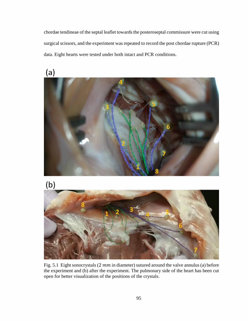
95

chordae tendineae of the septal leaflet towards the posteroseptal commissure were cut using

surgical scissors, and the experiment was repeated to record the post chordae rupture (PCR)

data. Eight hearts were tested under both intact and PCR conditions.

Fig. 5.1 Eight sonocrystals (2 𝑚𝑚 in diameter) sutured around the valve annulus (a) before

the experiment and (b) after the experiment. The pulmonary side of the heart has been cut

open for better visualization of the positions of the crystals.

96

5.3.3 Data Analysis

In order to calculate the area and circumference of the annulus at each moment

during the cardiac cycle, a cubic spline was fitted to the positional data [82, 83] of the

crystals around the annulus (Fig. 5.2). The length of the spline was calculated and

considered as the circumference of the annulus at each moment [83]. The area of the

annulus was approximated as follows:

1- The average of the three-dimensional position vectors collected by the

sonocrystals was calculated as the center of the annulus.

2- A triangulated virtual surface was built by connecting 10,000 equally-spaced

points on the spline representing the annulus to the calculated central point.

3- The sum of the surface areas of all the constructed triangles was calculated as

an approximation for the area of the annulus.

The approximation procedure is illustrated in Fig. 5.2 using a lower resolution of

the points on a typical annulus for better illustrative purposes (24 points for illustrative

purposes in Fig. 5.2; the resolution used in the calculation was 10,001 points). The average

of the measured distance between each point on the spline and the central point was

calculated as the average radius of the annulus. The calculated area and circumference were

also used to calculate the radius for comparison purposes by assuming that the annulus is

a circle on a flat plane.

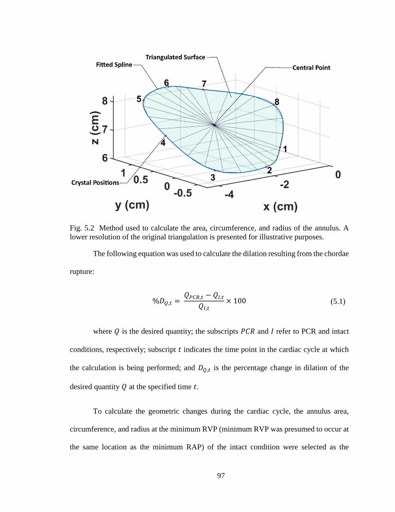
97

Fig. 5.2 Method used to calculate the area, circumference, and radius of the annulus. A

lower resolution of the original triangulation is presented for illustrative purposes.

The following equation was used to calculate the dilation resulting from the chordae

rupture:

%𝐷𝑄,𝑡 =

𝑄𝑃𝐶𝑅,𝑡 − 𝑄𝐼,𝑡

𝑄𝐼,𝑡× 100 (5.1)

where 𝑄 is the desired quantity; the subscripts 𝑃𝐶𝑅 and 𝐼 refer to PCR and intact

conditions, respectively; subscript 𝑡 indicates the time point in the cardiac cycle at which

the calculation is being performed; and 𝐷𝑄,𝑡 is the percentage change in dilation of the

desired quantity 𝑄 at the specified time 𝑡.

To calculate the geometric changes during the cardiac cycle, the annulus area,

circumference, and radius at the minimum RVP (minimum RVP was presumed to occur at

the same location as the minimum RAP) of the intact condition were selected as the

98

reference area (𝐴0), reference circumference (𝐶0), and reference radius (𝑅0), respectively.

Next, using Equation (5.2), we calculated the changes in area, circumference, and radius

for the annulus under both intact and PCR conditions.

%𝐶𝑄 =

𝑄𝑡 − 𝑄0

𝑄0× 100 (5.2)

where 𝑄𝑡 is the desired quantity at the current time, 𝑄0 is the initial (reference)

value of this quantity, and 𝐶𝑄 shows the percentage change. For comparison purposes, we

also calculated the approximate changes in annulus anterior segment (AAS), annulus

posterior segment (APS), and annulus septal segment (ASS) using the position of the

markers attached to each segment.

Finally, we developed an average annulus curve from the measured 3D data to

evaluate its shape. As the data was recorded independently for each TV annulus based on

its own reference frame and coordinate system, registration of marker positional data from

different annuli was necessary to match the corresponding marker positions with a

minimum error for averaging. Therefore, using singular value decomposition, the

measured positional data for all TV annuli were transformed to closely register the

corresponding marker points, and the resulting data points were averaged to develop an

average annulus curve similar to the ones developed in previous studies [83].

5.3.4 Statistical Analysis

All data presented in this paper are reported in the form of mean ± standard

deviation. Although much intervariability was observed among the measured values of

different subjects (more details in this regard can be found in the Results section), the

99

standard deviation due to measurement errors for 22 consecutive cardiac cycles was ~0.1%

of the mean value of the measured quantity. Nevertheless, to minimize the intervariability

due to measurement errors for each sample, the measured data of all 22 consecutive cardiac

cycles were averaged at the corresponding time points in the cardiac cycle and were used

for analysis. The Wilcoxon signed rank test was used for all statistical analysis, where any

result with 𝑝 < 0.05 is considered to be statistically significant.

5.4 Results

5.4.1 Pressure

The average recorded RVP, PAP, and RAP are shown in Fig. 5.3 for the intact and

PCR cases. As illustrated in this figure, the average measured pressures in this ex-vivo

setup closely match the in-vivo ones [160]. The range of pressure values for the intact case

were approximately from 0 to 30 𝑚𝑚 𝐻𝑔 and from 6 to 30 𝑚𝑚 𝐻𝑔 for RVP and PAP,

respectively. However, the pressures for RVP and PAP after chordae rupture ranged from

0 to 25 𝑚𝑚 𝐻𝑔 and from 5 to 24 𝑚𝑚 𝐻𝑔, respectively. The range for the RVP closely

matched the range reported for the porcine RVP in the literature [161-164]. We were not

able to find reported PAP or RAP values for porcine hearts; however, the recorded pressure

values closely matched those measured in human hearts [160].

100

Fig. 5.3 Average right ventricular pressure (RVP), pulmonary artery pressure (PAP), and

right atrial pressure (RAP) measured for the intact and post chordae rupture (PCR) cases.

5.4.2 Annulus Area, Circumference, and Radius Values

The results obtained for the area, circumference, and radius at the minimum and

maximum RVP for intact and PCR ex-vivo porcine hearts are listed in Tables 5.1–5.3.

Throughout the cardiac cycle, in intact hearts, the mean area, circumference, and radius of

the annulus ranged from 11.4 ± 2.8 to 13.3 ± 2.9 𝑐𝑚2, from 12.5 ± 1.5 to 13.5 ± 1.3 𝑐𝑚,

and from 1.9 ± 0.2 to 2.0 ± 0.2 𝑐𝑚, respectively. After chordae rupture, the mean area,

circumference, and radius of the annulus ranged from 12.3 ± 3.0 to 14.4 ± 2.9 𝑐𝑚2, from

13.0 ± 1.5 to 14.0 ± 1.2 𝑐𝑚, and from 1.9 ± 0.2 to 2.1 ± 0.2 𝑐𝑚, respectively. The

numbers provided here are the average of the minimum and maximum values of the

quantities, while Tables 5.1–5.3 list the values at minimum and maximum RVP; thus, there

might be a slight difference between the averages and standard deviations provided here

and those presented in Tables 5.1–5.3. Significant increases in the annulus area,

circumference, and radius were observed following chordae rupture (Fig. 5.4; 𝑝 = 0.01

101

for values measured at maximum RVP and 𝑝 = 0.04 for values measured at minimum

RAP, according to the Wilcoxon signed rank test). A segment-specific statistical analysis

revealed that the APS did not vary significantly after chordae rupture (𝑝 = 0.38 for values

measured at maximum RVP and 𝑝 = 0.64 for those measured at minimum RAP,

according to the Wilcoxon signed rank test), while the AAS and ASS increased

significantly (𝑝 = 0.02 for AAS values measured at maximum RVP, 𝑝 = 0.04 for AAS

values measured at minimum RAP, and 𝑝 = 0.02 for ASS values measured both at

maximum RVP and at minimum RAP, according to the Wilcoxon signed rank test). Table

5.3 also lists the radii estimated from the calculated areas and circumferences (𝑅𝐴 and 𝑅𝐶)

when the annulus was considered as a flat circle. These estimated radii values, especially

those calculated from the areas, were quite similar to those calculated using the previously

explained method.

Table 5.1 Calculated area at minimum and maximum right ventricular pressure (RVP) for

intact and post chordae rupture (PCR) conditions. The values are presented for all eight

hearts used in the experiments along with the average (AVG) and standard deviation

(STD). Comparing the average values showed an increase in the area post chordae rupture.

Area (𝑐𝑚2)

At minimum RVP At maximum RVP

Heart no. Intact PCR Intact PCR

1 12.7 12.7 13.7 14.0

2 8.8 8.7 11.5 12.1

3 8.8 9.9 10.9 12.2

4 13.8 13.9 15.3 15.5

5 8.0 9.4 9.8 11.5

6 16.2 17.7 19.1 20.2

7 11.6 14.7 12.8 15.5

8 11.5 12.0 13.0 13.6

AVG 11.4 12.4 13.3 14.3

STD 2.8 3.0 2.9 2.8

102

Fig. 5.4 Comparison of the average values of (a) the area, (b) circumference, and (c) radius

between the intact and post chordae rupture (PCR) conditions at minimum and maximum

right ventricular pressure (RVP). The Wilcoxon signed rank test p-values for area,

circumference, and radius were 0.01 at maximum RVP and 0.04 at minimum RAP. The

asterisks (*) show significant differences (𝑝 < 0.05, Wilcoxon signed rank test). Error bars

show the standard errors.

103

Table 5.2 Calculated circumference at minimum and maximum right ventricular pressure

(RVP) for intact and post chordae rupture (PCR) conditions. The values are presented for

all eight hearts used in the experiments along with the average (AVG) and standard

deviation (STD). Comparing the average values showed an increase in the circumference

post chordae rupture.

Circumference (𝑐𝑚)

At minimum RVP At maximum RVP

Heart no. Intact PCR Intact PCR

1 13.2 13.2 13.7 13.8

2 11.0 11.0 12.5 12.9

3 10.9 11.7 12.2 12.9

4 13.7 13.8 14.4 14.5

5 10.9 11.8 11.9 12.9

6 14.9 15.5 16.0 16.4

7 12.9 14.2 13.4 14.6

8 12.8 13.0 13.4 13.8

AVG 12.5 13.0 13.4 14.0

STD 1.5 1.5 1.3 1.2

Table 5.3 Calculated radius using the triangulation method (𝑅) along with the radii

calculated from the area (𝑅𝐴) and circumference (𝑅𝐶), using the assumption of flat annuli,

at minimum and maximum right ventricular pressure (RVP) for intact and post chordae

rupture (PCR) conditions. The values are presented for all eight experimental hearts along

with the average (AVG) and standard deviation (STD). Comparison between 𝑅, 𝑅𝐴, and

𝑅𝐶 showed that the three different methods of calculating the radius produced the same

results.

Radius (𝑐𝑚) At minimum RVP At maximum RVP

Heart Intact PCR Intact PCR no. 𝑅 𝑅𝐴 𝑅𝐶 𝑅 𝑅𝐴 𝑅𝐶 𝑅 𝑅𝐴 𝑅𝐶 𝑅 𝑅𝐴 𝑅𝐶

1 2.0 2.0 2.1 2.0 2.0 2.1 2.1 2.1 2.2 2.1 2.1 2.2

2 1.7 1.7 1.8 1.6 1.7 1.8 1.9 1.9 2.0 1.9 2.0 2.1

3 1.7 1.7 1.7 1.8 1.8 1.9 1.9 1.9 1.9 2.0 2.0 2.1

4 2.1 2.1 2.2 2.1 2.1 2.2 2.2 2.2 2.3 2.2 2.2 2.3

5 1.6 1.6 1.7 1.7 1.7 1.9 1.7 1.8 1.9 1.9 1.9 2.1

6 2.3 2.3 2.4 2.4 2.4 2.5 2.4 2.5 2.5 2.5 2.5 2.6

7 2.0 1.9 2.1 2.2 2.2 2.3 2.0 2.0 2.1 2.2 2.2 2.3

8 1.9 1.9 2.0 1.9 2.0 2.1 2.0 2.0 2.1 2.1 2.1 2.2

AVG 1.9 1.9 2.0 2.0 2.0 2.1 2.0 2.1 2.1 2.1 2.1 2.2

STD 0.2 0.2 0.3 0.3 0.2 0.2 0.2 0.2 0.2 0.2 0.2 0.2

104

5.4.3 Annulus Dilation Due to the Chordae Rupture

Table 5.4 shows the increase in area, circumference, and radius of the annuli (i.e.,

a measure of annuli dilation) due to the chordae rupture averaged over all ex-vivo porcine

hearts at maximum RVP. The area of the annuli dilated an average of 8.8% at maximum

RVP. The dilation at this point for both the circumference and the radius was approximately

4% on average. The segment-specific dilations were also calculated and are presented in

Table 5.5 for the AAS, APS, and ASS of the annuli. The largest average dilation in the

circumference of the annuli (6.3%) occurred at the AAS, whereas the lowest average

dilation (2.4%) occurred at the APS. Fig. 5.5 shows a comparison among the average

dilations (at maximum RVP) of three annulus segments. Statistical analyses showed that

there was no significant difference between the dilations in the different segments of the

annuli (Fig. 5.5).

Fig. 5.5 Comparison of the dilation (due to the chordae rupture) between annulus anterior

segment (AAS), annulus posterior segment (APS), and annulus septal segment (ASS) at

maximum right ventricular pressure (RVP). The Wilcoxon signed rank test p-values were

0.55, 0.38, and 0.74 between the AAS and APS, the AAS and ASS, and the APS and ASS,

respectively. No significant differences were observed (𝑝 > 0.05, Wilcoxon signed rank

test). Error bars show the standard errors.

105

Table 5.4 Geometric dilation in area, circumference, and radius of the heart annuli due to

chordae rupture at maximum right ventricular pressure (RVP) calculated using Equation

(5.1) along with the average (AVG) and standard deviation (STD) for each quantity.

Dilation at maximum RVP (%)

Heart no. Area Circumference Radius

1 2.4 1.0 1.1

2 5.2 3.2 2.5

3 11.9 6.4 5.1

4 1.0 0.4 0.9

5 17.1 8.1 8.3

6 5.9 2.6 3.3

7 20.8 8.6 9.3

8 5.9 2.5 2.9

AVG 8.8 4.1 4.2

STD 7.1 3.2 3.2

Table 5.5 Dilation in the length of annulus anterior segment (AAS), annulus posterior

segment (APS), and annulus septal segment (ASS) due to the chordae rupture at maximum

right ventricular pressure (RVP) calculated using Equation (5.1) along with the average

(AVG) and standard deviation (STD) for each quantity. The largest dilation occurred at the

AAS.

Dilation at Maximum RVP (%)

Heart No. AAS APS ASS

1 -1.2 2.3 1.9

2 7.6 -1.8 3.8

3 19.1 -5.2 -0.3

4 0.7 -1.4 5.6

5 10.2 7.6 4.5

6 2.8 1.4 3.8

7 9.2 12.8 2.3

8 1.8 3.5 2.4

AVG 6.3 2.4 3.0

STD 6.6 5.7 1.8

5.4.4 Changes in Annulus Geometry Throughout the Cardiac Cycle

The changes in metrics of each annulus throughout the cardiac cycle were

calculated using Equation (5.2), and the resulting values were averaged over all eight

annuli, as shown in Fig. 5.6. Table 5.6 also shows the average changes (calculated using

106

Equation (5.2)) at maximum RVP for normal and PCR ex-vivo porcine hearts. From the

minimum to the maximum RVP, the annulus area increased by 17 and 18% in intact and

PCR hearts, respectively. However, when accounting for the annulus dilation following

chordae rupture, the maximum change in area was found to exceed 27%. In other words,

the same PCR annuli showed more dilation if the changes were always referenced to the

corresponding intact hearts. The maximum changes in circumference and radius (in both

intact and PCR conditions) ranged roughly from 7.5% to 8.5%. Again, accounting for

chordae rupture–induced annulus dilation, approximately 12% maximum circumferential

and radial changes were calculated. The maximum change in segment-specific

circumferences during the cardiac cycle are also shown in Table 5.6. From this table, it can

be noticed that the AAS of the annulus circumference experienced a larger average change

during the cardiac cycle when compared with APS and ASS. Figure 5.7 shows the change

in the length of three segments of the annulus at maximum RVP for both intact and PCR

conditions. For the intact hearts, the changes in the length of the AAS during the cardiac

cycle were significantly higher than those for the other two segments (𝑝 = 0.03 for the

comparison between AAS and APS, 𝑝 = 0.02 for the comparison between AAS and ASS,

and 𝑝 = 0.84 for the comparison between APS and ASS, according to the Wilcoxon signed

rank test). There was, however, no significant difference between changes in the lengths of

different segments after chordae rupture (The smallest p-value was 0.08, according to the

Wilcoxon signed rank test for each comparison).

107

Fig. 5.6 Changes in (a) area, (c) circumference, and (e) radius as well as the absolute values

of (b) area, (d) circumference, and (f) radius throughout the cardiac cycle averaged over all

the annuli for intact and post chordae rupture (PCR) conditions. The shaded regions show

the standard errors. The temporal position of the maximum right ventricular pressure

(RVP) as well as the opening and closure of the tricuspid and pulmonary valves for the

intact case are shown in the graphs as a better illustration of the deformations that occur

throughout the cardiac cycle.

108

Fig. 5.7 Comparison of the change in the length of the annulus anterior segment (AAS),

annulus posterior segment (APS), and annulus septal segment (ASS) in intact and post

chordae rupture (PCR) conditions at maximum right ventricular pressure (RVP). The PCR

values include the dilation as well. For a comparison of the change in length between the

intact and PCR conditions, the Wilcoxon signed rank test was used; p-values were 0.02 for

AAS and ASS and 0.38 for APS. The p-values were 0.03, 0.02, and 0.84 for the

comparison of the change in length for the intact case between the AAS and APS, the AAS

and ASS, and the APS and ASS, respectively. The asterisks (*) indicate significant

differences (𝑝 < 0.05, Wilcoxon signed rank test). Error bars show the standard errors.

Table 5.6 Average geometric changes at maximum right ventricular pressure (RVP) for

intact and post chordae rupture (PCR) conditions calculated using Equation (5.2). The last

column shows the percentage of the change in geometric parameters with intact-to-PCR

dilation included in calculations. The geometrical parameters at minimum RVP were

selected as the reference to calculate the changes.

Geometrical Change at Maximum RVP (%)

Quantity Intact PCR PCR with dilation

Areal 17.2 18.1 27.6

Circumferential 7.4 7.9 11.9

Radial 8.0 8.6 12.6

Change in AAS 9.0 9.6 16.1

Change in APS 6.3 6.9 8.8

Change in ASS 6.1 6.7 9.3

109

5.4.5 Annulus Curve

The resulting average TV annulus has the shape of a nonplanar saddle curve. The

maximum points of this curve were on the AAS and APS close to the anteroseptal and

posteroseptal commissures, respectively. One of the minimum points, on the other hand,

was approximately placed at the middle of the ASS, and the other was on the AAS close

to the anteroposterior commissure. These observations are consistent with those reported

for the in-vivo TV annulus in an ovine model [80].

5.5 Discussion

The positional data obtained from the sonocrystals sutured around the ex-vivo

porcine heart annulus were used to analyze the annulus deformation during the cardiac

cycle. The effects of the chordae rupture were also investigated on this deformation by

cutting one of the septal chordae proximal to the posterior commissure. The analyses

showed that if we consider the annulus as a flat circle and use the calculated area and

circumference to estimate the radius, the estimated values are comparable to the values for

the radius that were calculated directly from the annulus geometry.

Throughout the cardiac cycle, the geometry of the annulus alters considerably such

that from the minimum RVP to the maximum RVP, the area roughly experiences a 20%

increase, and the circumference extends approximately 8%. Our analysis showed that these

deformations do not occur uniformly along the annulus. For example, the AAS experiences

the largest deformation (about 9% on average). In most TV repair procedures, a prosthetic

annuloplasty ring is used to decrease the annulus size and improve the valve hemodynamics

[8]. Considering the dynamic deformation of TV annulus observed in our study, further

110

research is needed to identify how the valve deformation changes following ring

annuloplasty [26].

Due to the inherent differences between the in-vivo and the ex-vivo cases, the

results reported in this study might not exactly match the in-vivo outcomes. The absence

of muscular contraction (including those of the myocardium and papillary muscles) and

the lack of the interaction between the right and left ventricles in the ex-vivo experiments

might affect the results in comparison to those of the in-vivo cases. As such, much caution

should be taken in interpretation of our results. For example, it has been reported in in-vivo

studies that the annulus dimensions decrease during the systole [81, 83]; for the ex-vivo

case, however, they increase during the systole. In actively beating hearts, the contraction

of the heart muscles decreases the annulus as well. In contrast, in passively beating hearts,

no active contraction is present, and the increased ventricular pressure causes the annulus

to expand during the systole. In particular, unlike our ex-vivo results, Rausch and

colleagues recently observed 7.17 ± 1.93 𝑐𝑚2 as the minima of the annular area during

systole in in-vivo ovine hearts, which was significantly smaller than the annular area during

diastole (i.e., 8.65 ± 1.98 𝑐𝑚2) in the same hearts [83]. A similar trend was also observed

for the measured perimeters in this in-vivo model (i.e., 10.2 ± 1.28 𝑐𝑚 systolic value as

compared to a significantly smaller diastolic value of 11.2 ± 1.27 𝑐𝑚 ). It is worth noting

that quantitative comparison of the in-vivo active beating heart measurements [83] with

our ex-vivo passive beating heart measurements should be conducted with caution due to

the inherent differences in ovine versus porcine models.

In addition, in many different types of soft tissues, even in those that are not as

mechanically active as cardiac muscles, the mechanical properties are different in the ex-

111

vivo setups as compared to those measured in the native in-vivo environment [191]. Such

differences have been attributed to the lack of perfusion and metabolic activities in the ex-

vivo environments. As such, potential differences in the mechanical responses of the

tissues in the in-vivo versus ex-vivo setups should also be considered in the interpretation

of our results. Nevertheless, during the diastole, when the right ventricle is expected to be

at its least active state, the measured ex-vivo area and circumference values (11.4 ±

2.8 𝑐𝑚2 and 12.5 ± 1.5 𝑐𝑚, respectively) closely matched those of the in-vivo

measurements (8.65 ± 1.97 𝑐𝑚2 and 11.1 ± 1.27 𝑐𝑚, respectively) [83]. It should be

noted that since plane projection of the three-dimensional geometry was used to calculate

the area in the aforementioned in-vivo study, the area calculated in our study was slightly

larger, as was expected. Furthermore, Fawzy et al. [81] reported that most changes in

circumference occur in the anterior segment of the annulus in the in-vivo hearts, which is

consistent with the findings of our study (Fig. 5.7).

In atrioventricular valves, the structures of the chordae tendineae and papillary

muscles anchor the valve leaflets and prevent them from billowing into the atrium during

ventricular contraction [8]. As such, one would expect that regurgitation might occur when

such constraints are removed from the leaflet(s) following chordae rupture. However, it is

not just the billowing effects that are prevented by the parachute-like structure of the

chordae tendineae and the papillary muscles. Our experiments showed that there exists a

mechanical interdependency among TV chordae tendineae, leaflets, and annulus. We

observed that immediately after chordae rupture, the dynamic deformation of TV annulus

changed extensively, with a significant increase in the annulus area, circumference and

radius. Annulus dilation, whether it develops over time or occurs acutely (as in the case of

112

trauma-induced chordae rupture), is expected to change the coaptation of the valve leaflets

and induce regurgitation [182]. Our measurements showed that, on average, the flow into

the right atrium decreased by 26% immediately after the septal chordae tendineae close to

the posteroseptal commissure was cut. Moreover, the maximum RVP dropped from 30 mm

Hg to 25 mm Hg, which is a 17% decrease. A similar decrease was observed in the PAP.

These changes show how chordae rupture can alter the hemodynamics of the heart.

Recent ex-vivo studies have shown that TV annulus and leaflets are under tension

[140, 192]. An increase in the annulus area following chordae rupture may change the

annulus tension and alter the homeostatic mechanical environment to which the leaflets

and the myocardium surrounding the annulus are subjected. The homeostatic mechanical

environment is extremely important for the normal function of TV and its surrounding

tissues and can alter its normal mechanical properties [134, 140]. In all types of cardiac

valves, valve interstitial cells reside within the leaflet tissue [193-197]. The valve

interstitial cells, by means of protein synthesis and enzymatic degradation, maintain the

structural integrity of the leaflet tissue. In all types of soft tissues, collagen type I, which is

the main load-bearing protein of the extracellular matrix, scales with tissue stiffness [198].

The in-vivo valve interstitial cells respond to changes in mechanical loading and alter the

tissue stiffness via collagen synthesis or degradation. For example, in murine TVs,

increasing the mechanical load to which the leaflets are subjected led to increased mRNA

amounts of both collagen type I and III as well as to higher collagen turnover [199].

Conversely, in an ovine model, MV collagen content was decreased when the ventricular

pressure (and consequently the mechanical loading on the leaflets) decreased [190].

113

It is worth noting that cells are not the only components that are sensitive to changes

in mechanical loading [86]. While large mechanical strains could increase the rate of

extracellular matrix catabolism in cardiac valves [200], studies have shown that the

extracellular matrix collagen is more stable and degrades more slowly under homeostatic

mechanical strain [78, 201, 202]. Considering such an important influence of the tissue

mechanical milieu on short-term as well as long-term valve responses, it is essential to not

ignore dilation in the annulus following chordae rupture. Surely, further in-vivo animal

studies are necessary to better examine the long-term effects of chordae rupture on TV

function and structure. It is, however, expected that, in addition to the immediate effects of

annulus dilation in generating secondary tricuspid regurgitation, in the long term, changes

in the mechanical environment of TV leaflet and right ventricle myocardium could cause

further negative remodeling responses and exacerbate the detrimental outcomes of chordae

rupture.

In summary, we employed an ex-vivo heart setup and measured the deformation of

porcine TV annuli during simulated cardiac cycles. Regurgitation was induced by cutting

the chordae tendineae of the septal leaflets. For the first time, we observed that TV annulus

dilates immediately after the rupture of the chordae tendineae. Although TV may be

initially asymptomatic, instantaneous annulus dilation following chordae rupture could

lead to exacerbation of TV regurgitation and potentially to mechanically-induced

remodeling responses in TV leaflets, the remaining intact chordae tendineae, the papillary

muscles, and/or the ventricular myocardium. More careful examinations and early surgical

interventions might be necessary to prevent mid-term/long-term negative effects of

114

mechanically-induced remodeling in asymptomatic TVs following the rupture of the

chordae tendineae.

115

CHAPTER 6VI

EFFECTS OF CHORDAE RUPTURE ON THE SURFACE STRAINS OF THE

TRICUSPID VALVE LEAFLETS

(The content of this chapter will be published as a journal paper entitled “Effects of

Chordae Rupture on the Strains of Tricuspid Valve Septal Leaflet: An Ex-vivo Study on

Porcine Hearts”.)

6.1 Summary

Between 2000 and 2012, roughly 40,000 cases of chordae tendinea rupture (CTR)

were reported in the US by the National Inpatient Sample. This lesion is often overlooked,

especially when it comes to CTR of TV. To date, abnormal TV mechanical response in the

presence of CTR is still poorly understood. While recent studies have shown that

significant alteration of in-vivo valve deformation could happen when the conditions in the

atrioventricular valve annuli change, many traditional methods for examining cardiac valve

deformations require dissection of the valve. In the current work, however, porcine valve

leaflet deformation was studied in an intact heart in an ex-vivo setup using sonomicrometry

techniques, and the effects of CTR were examined by severing the septal chordae adjacent

to the posteroseptal commissure.

Following chordae rupture, the maximum RVP dropped from 31 𝑚𝑚 𝐻𝑔 to

25 𝑚𝑚 𝐻𝑔, and the flow rate decreased by 26%, showing that regurgitation occurred

immediately after chordae rupture. The chordae rupture significantly altered the

116

distribution of the strains over the septal leaflet surface. For example, a maximum increase

from 14.64 ± 2.96 to 18.15 ± 3.44 in maximum principal strain was observed after

chordae rupture at the distal edge of the septal leaflet with the p-vale of 0.013.

In this ex-vivo study, we were able to observe the primary regurgitation and record

the immediate decrease in the pressure and flowrate as well as the instantaneous alteration

in the distribution of the strains over the septal leaflet right after CTR. These changes in

the strain distribution shows that, PCR, the tricuspid apparatus and the myocardium could

become exposed to new mechanical loading, potentially resulting in further remodeling

responses and aggravating the negative effects of this lesion.

6.2 Introduction

TV regurgitation arises from a lack of leaflet coaptation that may result from

complications stemming from a few pathologies of the left side of the heart. Chief among

the left side heart diseases is MV regurgitation. TV regurgitation (i.e., non-functional)

poses a greater long-term risk to the patient, since it is well tolerated and the patient may

seem to be asymptomatic [185, 189, 203-205]. Increased morbidity and mortality arises

when the condition is undetected, as right ventricular dysfunction and atrial fibrillation are

likely to lead to chronic heart failure [185]. In many cases involving severe blunt chest

trauma (such as automobile accidents), studies in the literature and various case reports

point to CTR as a likely outcome [189, 204, 206, 207]. In the aforementioned cases, the

rapid compression of the right ventricle induces regurgitation of the atrioventricular valve;

this will result in fatal damage to the heart or, at a minimum, a ruptured chordae tendineae

[208]. In addition to being induced by chest trauma, CTR has also been reported as an

unforeseen outcome of medical procedures such as right heart catherization, where

117

penetrating chest trauma can induce structural disruption of TV structure. Finally, various

cardiovascular pathologies may also play a role in weakening the chordae structure, as can

occur in degenerative valve diseases (myxomatous valve diseases) such as Marfan

syndrome, which can lead to chordae elongation and ultimately to rupture and valvular

insufficiency [209].

Although no definite figure is known for how many cases of CTR in TV have been

documented, its prevalence is likely to be higher than the numbers indicated in the reported

statistics [186, 187]. Between 1999 and 2008, a total of 28,726 operations involving TV

were performed [24], with CTR cited as the most common cause for TV regurgitation (with

one study placing the incidence at 55% of patients). The number of reported cases is likely

to be underestimated for two main reasons [185, 189]. First, as the aforementioned TV

surgery study was limited to participants over the age of 30, it does not account for cases

in younger adults or children. Second, TV regurgitation, whether a result of CTR or not, is

often overlooked during diagnosis [187]. While TV regurgitation can be properly

diagnosed via transthoracic echocardiography and transesophageal echocardiography, it is

usually concurrent with the diagnosis of another condition [203, 210]. The fact that most

individuals with TV regurgitation have been misdiagnosed, were only diagnosed while

physicians were searching for a different indication, or have simply gone undiagnosed

should be cause for alarm [185, 189, 203, 205].

Current techniques to address CTR include reconstruction or replacement. Both of

these options involve the use of chordae implants and may even resort to chordae

transposition, which may not be ideal due to the natural and brittle structure of TV [185].

Because of the risks of undetected and untreated TV regurgitation, coupled with the delay

118

in treatment due to the long time between onset and diagnosis (up to 11 years in some

cases) [177, 211], a proper understanding of CTR is key to developing an approach to either

repair or replace the affected chordae. The abundant insights into CTR and its implications

for the left side of the heart overshadows the detrimental effects on TV apparatus and the

heart as a whole. In this study, we document the behavior of TV septal leaflet mechanics

before and after simulating CTR. Our objective is to examine the changes is the

hemodynamics of TV and alteration of the leaflet strains PCR in an effort to provide

quantitative and comprehensive data that will prove invaluable in determining the best

procedure to address this condition.



In a previously developed ex-vivo passive beating heart apparatus (Fig. 4.1a), a

positive displacement pump (SuperPump AR Series, Vivitro Labs, Inc., Victoria, BC,

Canada) was utilized to beat porcine hearts passively by circulating PBS into the hearts

[140]. The resulting transvalvular pressure from this circulation forces TV to open and

close, imitating the native deformations of intact TV leaflets. The apparatus was developed

in a way that allowed the monitoring and recording of RAP, RVP, PAP, and the mean flow

rate throughout the cardiac cycle. Based on the International Standard Organization (ISO

5840) and U.S. Food and Drug Administration regulations for heart valve testing, the

pump’s standard 70 𝑏𝑝𝑚 waveform was used, and other pump parameters were set to keep

the hydrodynamic pressures in TVs in the test setup consistent with those in a native valve

during the cardiac cycle. More details about this setup can be found in our previous

publication [140].

119


Fresh porcine hearts were transferred to the lab from a local slaughterhouse (3-D

meats, Dalton, OH) in bags filled with PBS that were covered in ice. The right chambers

of the hearts were flushed out with PBS and checked carefully with an endoscopic camera

(an SSVR-710 Snakescope) to ensure that no blood clots were present inside the chambers

or around the valves. Eight sonocrystals (Somometrics Co., London, ON, Canada), 1 or

2 mm in diameter, were then sutured over the septal leaflet in a predefined arrangement

(Fig. 4.4). To eliminate any cutting and patching of the heart chambers, suturing was

performed through the superior vena cava, and the sonocrystal wires were passed through

the inferior vena cava. Umbilical clamps were used to prevent any leakage from the inferior

vena cava and the coronary vein. The heart was then connected to the ex-vivo beating heart

apparatus through the superior vena cava, pulmonary artery, and an incision made at the

bottom of the right apex, as explained in our previous publication [140]. To make a

reference frame for the positional data of the sonocrystals, three 3-mm-diameter

sonocrystals were attached to the outside of the myocardium around the apex.

6.3.3 Data Acquisition

A sonomicrometer (TRX Series 16, Somometrics Co., London, ON, Canada) was

utilized to trigger the sonocrystals and record their signals. The sonomicrometer

communicated with a computer through a USB port using SonoLabDS3 software

(Somometrics Co., London, ON, Canada). To make the data synchronization easier, the

pressure sensors were also connected to analog input channels of the sonomicrometer.

After running the pump, an endoscopic camera (SSVR-710 Snakescope) was sent into the

right atrium — through a probe embedded into the superior vena cava connector [140] —

120

to visually assess the coaptation of the valve leaflets during the beating of the heart. An

oscilloscope (MSO2014B, Tektronix, Beaverton, OR) was used to visualize the signals and

adjust the sensitivity of the sonocrystals to reduce the signal-to-noise ratio. After adjusting

the necessary parameters, the sonocrystal and pressure signals were recorded with a

frequency of 100 Hz for 20 seconds using SonoLabDS3 software. The mean flow rate was

also read from the flowmeter and recorded in each experiment. To model CTR, the chordae

tendineae of the septal leaflet in the proximity of the posteroseptal commissure was cut

using surgical scissors. The experiment was repeated, and the data were recorded for

another 20 seconds with a frequency of 100 Hz. In total, eight successful experiments were

conducted.

6.3.4 Pressure Data Analysis

The hemodynamic pressures (RAP, RVP, and PAP) were recorded during the

cardiac cycle for all experiments for the intact and PCR conditions. As the relative

transvalvular pressures drive the deformation of the valve and the flow, the effects of

hydrostatic pressures on the pressure signals due to the elevation differences between the

pressure probes and the free surface of the liquid (see Fig. 4.1a) were negated by shifting

the average pressure signals. As such, the average RAP and RVP were shifted in such a

way that they are close to zero during the diastole (if a shift was necessary). The PAP was

also adjusted slightly to match these shifts. This process can be interpreted as deducting

the pressure equivalent of the vertical distance between the free surface of the reservoir

fluid and the right atrium, which shifted the diastole portion of the RVP and RAP close to

zero, and the shift in the PAP to compensate for the vertical distance between the bottom

of the right ventricle (where the RVP sensor was located) and entrance of the pulmonary

121

artery (where the PAP sensor was located). As pressure levels are relatively low in the right

side of the heart, the adjustments for these equivalent hydrostatic pressures were necessary

to obtain more consistent pressure curves.

6.3.5 Deformation Data Processing and Analysis

The distance between each pair of sonocrystals was recorded throughout the

experiment. The recorded signals were processed using SonoVIEW software (Sonometrics

Co.) to remove the noise and determine unusable signals (signals with too much noise or

drift). Utilizing SonoXYZ software (Sonometrics Co.), the modified signals were then used

to reconstruct the absolute positional coordinates for each sonocrystal with respect to a

defined coordinate system throughout the entire cardiac cycle. These positional data, which

represent the deformation of the septal leaflet surface during the cardiac cycle, were used

to calculate the strains for both intact and PCR conditions [26, 86, 87, 140]. More

information regarding the triangulation and strain calculation can be found in our previous

publication [140].

6.3.6 Average Model

The measured deformations for all samples were used to develop an average

geometry and deformation model. This average model can provide more insight regarding

the geometry of septal leaflet as well as its deformation throughout the cardiac cycle. As

the recorded data for each sample were in their own reference frame, it was necessary to

represent the data for all the samples in a unique coordinate system for averaging. As such,

the singular value decomposition method [212, 213] was used to transform all the data into

one coordinate system and register the corresponding markers on top of each other with a

minimum cumulative error. The transformed data were then averaged over all samples in

122

a frame-by-frame manner to generate the average geometry and deformation along the

cardiac cycle [83]. This average model was generated for both intact and PCR cases.

6.3.7 Statistical Analysis

The displacement and pressure signals were recorded for 20 seconds, which is

equivalent to approximately 23 cardiac cycles. The standard deviation of the comparison

of these consecutive cardiac cycles was ~0.1% of the mean value of the measured quantity.

Therefore, the signals did not show any significant intervariability among different cardiac

cycles. However, to further reduce noise in the signals, the recorded displacement and

pressure signals were averaged over all cardiac cycles. These average signals were used

for subsequent calculations and analysis. Student’s t-test was used for all statistical

analyses conducted in this study, where any result with 𝑝 < 0.05 was considered to be

statistically significant. Data are presented in the form of mean ± standard deviation,

wherever necessary.

6.4 Results

6.4.1 Average Model

An average model was generated using the measured positional data for all eight

hearts. Figure 6.1 shows this average geometry at the reference frame (minimum RAP) for

normal hearts and PCR cases. This figure shows the position of the markers around the

annulus and across the septal leaflet for both intact and PCR cases simultaneously. Crystals

are numbered in this figure to facilitate tracking of their positions from the intact condition

to the PCR case. In this plot, it can be noticed that Crystal 6 is close to the posteroseptal

commissure and Crystal 8 is near the anteroseptal commissure. To generate the average

model, such a geometry was developed for each frame throughout the cardiac cycle.

123

Fig. 6.1 TV septal leaflet and annulus average geometry at reference frame (minimum

RAP) for normal (blue) and PCR (red) conditions.

6.4.2 Pressures

Figure 6.2 illustrates the average pressure signals for the intact case. This graph

shows that while the experiments were conducted in an ex-vivo setup, the pressure signals

were comparable with those of in-vivo hearts [160]. The RVP, which were mostly close to

zero during the diastole, showed a rise to 31 mm Hg in the peak area of systole. As shown

in Fig. 6.2, a slight drop was observed in the RVP right after the start of the diastole phase.

The PAP ranged approximately from 6 to 31 mm Hg. While the RAP remained close to

zero during diastole, it had a peak of 17 mm Hg during the systole, which does not occur

in a normal human RAP signal. The range of the RVP closely matched those reported for

porcine hearts [161-164]. While we were not able to find reliable PAP and RAP values

reported for porcine hearts in the literature, these signals (Fig. 6.2) closely matched those

124

of human hearts [160]. The standard errors, shown in the shaded areas in Fig. 6.2, were

small—indicating that the pressures measured for different hearts did not deviate much

from the calculated average, despite the variability of the porcine hearts used in the

experiments. A small minimum was observed in the RVP signal right before it plateaued

during diastole after dropping from its peak during systole (Fig. 6.2). As shown in Fig. 6.2,

a closer inspection of the pressure signals showed that RVP and RAP separate at 0.19 s

and come back together at 0.56 s, which indicates TV closure and opening, respectively,

at these time points. Moreover, the signal for the RVP crosses the signal for the PAP at

0.29 s and 0.44 s, indicating the PV opening and closure, respectively, at these points.

Fig. 6.2 Average hemodynamic pressures during the cardiac cycle for intact conditions.

The shaded areas show the standard error.

In Fig. 6.3, pressure signals are presented for the PCR condition. After chordae

rupture, the RVP ranges from close to zero to 25 mm Hg, and the PAP ranges

approximately from 5 to 24 mm Hg. The pressure signals for RVP and PAP intersect first

125

at 0.31 s (when the PV opens), and again at 0.49 s (when the PV closes again). The

pressure signals for RAP, on the other hand, range from close to zero to more than

18 mm Hg.

Fig. 6.3 Average hemodynamic pressures during the cardiac cycle for post chordae rupture

(PCR) conditions. The shaded areas show the standard error.

6.4.3 Leaflet Deformation and Strain Spatial Distribution

The position of the fiducial markers (sonocrystals) were utilized to calculate the

strains over the septal leaflet of TV for both normal and PCR cases. More details regarding

these calculations can be found in our previous publication [140]. To illustrate the spatial

distribution of the strains, the developed average geometry of the septal leaf was used.

Figure 6.4 compares the spatial distribution of areal, maximum principal, circumferential,

and radial strains obtained over the developed average septal leaflet geometry at maximum

RVP before and after chordae rupture. The strains showed in this figure are averaged over

all eight hearts. The bold black edge that connects Crystals 6, 7, and 8 is the annulus side

126

of the leaflet (for a better understanding of the leaflet directions, please refer to Fig. 6.1).

This figure (Fig. 6.4) showed that the spatial distribution of the strains was largely altered

following the chordae rupture. While the strains are more uniformly distributed over the

leaflet surface when the leaflet is intact, they vary widely throughout the leaflet surface

after chordae rupture. From this figure, it can be noticed that the concentration of the strains

moves towards the edge where the chordae has been severed (i.e., toward Crystal 1).

Averaging the strains over the leaflet (spatial average), we obtain a single strain

signal (for each of the areal, maximum principal, circumferential, and radial strains)

throughout the cardiac cycle for each heart. Figure 6.5 presents a comparison of the

maximum of these strain signals averaged over all eight hearts (the error bars show the

standard errors) for different types of strains. Except for the circumferential strain, all

average strains showed an increase after chordae rupture. The maximum principal strain in

this figure increased from 11.19 ± 1.51 for the intact case to 11.95 ± 1.95 for the PCR

case, and the p-value for comparison between these two cases was 0.292. Figure 6.6

presents a comparison of the maximum principal strain averaged over all hearts along with

the standard errors for intact and PCR cases for the sonocrystals located on the distal edge

of the leaflet (Sonocrystals 1 and 2, as shown in Fig. 6.1). An increase from 14.64 ± 2.96

to 18.15 ± 3.44 and 13.15 ± 2.00 to 15.18 ± 2.30 in maximum principal strain was

observed after chordae rupture at the position of Crystals 1 and 2, respectively. The p-value

for this comparison was 0.013 for Crystal 1 and 0.166 for Crystal 2. To see how the heart

deforms throughout the cardiac cycle, the averaged septal leaflet geometry was plotted at

different time points, as illustrated in Fig. 6.7. This figure shows the leaflet deformation

for both intact and PCR cases for comparison purposes. The colormaps in this figure show

127

the distribution of the maximum principal strain over the septal leaflet at different time

points in the cardiac cycle. The change in the valve deformations and the deviation of the

strain distribution was notable following the chordae rupture (Fig. 6.7).

Fig. 6.4 Spatial distribution of areal, maximum principal (Max Princ), circumferential

(Circ), and radial strains demonstrated over the developed average septal leaflet geometry

at maximum right ventricular pressure (RVP) before (top row) and after (bottom row)

chordae rupture.

128

Fig. 6.5 Comparison of the average (over all the hearts) of maximum of the strain’s spatial

average signal (strain is averaged over the leaflet surface throughout the cardiac cycle).

Error bars show the standard error.

Fig. 6.6 Comparison of the maximum of maximum principal strain between intact and post

chordae rupture (PCR) cases for Crystal 1 and Crystal 2, shown in Fig. 6.1.

129

Fig. 6.7 Calculated average TV septal leaflet maximum principal strain, plotted at different

timepoints to show the deformation of the leaflet throughout the cardiac cycle for both

intact (top row) and post chordae rupture (bottom row) conditions. The color map shows

the distribution of the maximum principle strain.

6.4.4 Temporal Distribution of the Strains

To track the changes in the strains throughout the cardiac cycle and compare their

temporal distribution, the spatial average of the strains was calculated at each time point.

This averaging provided a single strain curve for each type of strain, showing the changes

over time for each heart. These signals were averaged for all eight hearts, and the resulting

curves for areal, maximum principal, circumferential, and radial strains before and after

chordae rupture were plotted (Fig. 6.8). Opening and closure of the valves shown in this

graph are based on the intact conditions. These plots showed that, while the spatial

distribution of the strains was significantly altered following chordae rupture (see Fig. 6.4),

the strains, on average, did not change significantly throughout the cardiac cycle and

followed relatively the same shape. Specifically, the spatial average of the maximum

130

principal strain maintained the same shape throughout the cardiac cycle after the chordae

was severed. Based on Fig. 6.8, the rapid growth in strain can be observed immediately

after closure of TV (at 0.2 s). Comparison of the plots in this figure with the pressure plots

in Figs. 6.2 and 6.3 show that the maximum strains occurred at nearly the same time as the

RVP reached its peak (at around 0.4 s). After this peak, the strains rapidly dropped towards

the end of the systole. During the diastole, the strains mostly remained close to zero.

Fig. 6.8 Temporal distribution of the spatial average of the strains throughout the cardiac

cycle for intact and post chordae rupture (PCR) conditions averaged for all hearts. The

shaded area shows the standard error.

6.5 Discussion

Chordae rupture was found to significantly alter TV leaflet strain distribution and

annulus geometry during the cardiac cycle. As such, annulus dilation is an indicator of the

development of TV regurgitation. In addition, alteration in mechanical strains immediately

following CTR may result in remodeling responses that could further influence TV

function/malfunction.

131

Chordae rupture changed the normal geometry of the annulus and septal leaflet

considerably. In addition to the dilation of the annulus, severe alteration occurred after

chordae rupture in the portion of the septal leaflet adjacent to the ruptured chordae (Crystals

1, 2, 3, and 4, as shown in Fig. 6.1). The trajectory of this alteration throughout the cardiac

cycle generates a waveform movement in this area of the septal leaflet in the PCR case that

is not present in the intact leaflet.

Our ex-vivo beating heart apparatus was able to reproduce ventricular pressure

waveforms that closely match those of an active heart [160]. As the hemodynamic

parameters of the pulmonary side are similar in human and porcine hearts, studying porcine

TV deformations can provide significant information regarding the deformations of TV in

a human heart. For example, human and porcine RVP ranges are very close: the RVP

ranges roughly from zero to 30 mm Hg for the human heart and from zero to 33 mm Hg

for the porcine heart [128, 160-164].

The chordae rupture prevented proper coaptation of TV. As such, when the pump

pushed the liquid back into the ventricle during the systole phase, a portion of the liquid

regurgitated back into the right atrium through TV, preventing it from coaptating properly.

Therefore, the average flow rate reduced by approximately 26% after chordae rupture. This

regurgitation following the chordae rupture prevented the pressure from rising to the peak

in the intact condition, and an approximate drop of 6 𝑚𝑚 𝐻𝑔 in the maximum RVP was

observed (Figs. 6.2 and 6.3).

As shown in Fig. 6.2, RAP rises slightly above the normal human pressure profile

during the systole, which may be due to a slight regurgitation during this phase. While the

132

coaptation of the leaflet was verified visually during each experiment, the weight of the

sonocrystals and the resistance of the attached wires to bending could have prevented the

leaflets from closing tightly [140]. The pressure increases after chordae rupture (Fig. 6.3)

confirms that additional regurgitation is occurring due to the chordae rupture.

Closer examination of Figs. 6.2 and 6.3 shows that PV opening was slightly delayed

after chordae rupture. This can be explained by considering the fact that due to the

regurgitation (and reduced flow rate), it takes more time for the pressure to rise high enough

to open the PV. Moreover, the PV closes with a notable delay after chordae rupture in

comparison to the intact case. To explain this delay, we should consider the fact that due

to the regurgitation, the pressure levels during the systole dropped. Thus, during the systole,

the pulmonary artery is subjected to lower pressures, which indicates that this compliant

artery expands less than normal. As a result, when the pressures pass their peak during the

systole, the pulmonary artery pushes against the fluid with a lower force and causes a delay

in the closure of the PV.

The positional data of the sonocrystals sutured to TV septal leaflet of the ex-vivo

beating heart were used to analyze deformations and calculate the strains throughout the

cardiac cycle [140]. By cutting the septal chordae adjacent to the posteroseptal

commissure, it was possible to investigate the effects of chordae rupture on the

deformations and strains. In previous studies, the strains and stretches were calculated

based on the position of the fiducial markers at the minimum left/right ventricular pressure

[30, 85]. However, as a small drop was observed in the measured RVP in the current

study—which creates an artificial global minimum in this RVP signal—the positions of

the sonocrystals at the minimum RAP were chosen as the reference configuration. This

133

was a reasonable choice, since the minimum RVP and RAP show some overlap under

normal conditions [140, 160].

Figure 6.80 shows the spatial average strain signals, which are also averaged over

all the hearts, while Fig. 6.5 shows the average of the maximums of the spatial average

strain signals. It should be noted from these figures that the peak of the means (the peak of

each signal in Fig. 6.8) is always less than (or ideally equal to) the mean of the peaks (the

corresponding value in Fig. 6.5).

The average values for the maximum principal strains and areal strains measured

in this experiment were 11.2% and 9.8%, respectively, before chordae rupture and 12.0%

and 10.0%, respectively, after chordae rupture. While the in-vivo strains in porcine TV

leaflets have not yet been reported in the literature, the values obtained in this study are

comparable to those reported for the anterior leaflet of an ovine MV [30].

6.6 Conclusion

A uniquely developed ex-vivo apparatus to facilitate passive beating of a porcine

heart (Fig. 4.1a) and sonomicrometry techniques were used to examine the effects of CTR

on the deformation of TV septal leaflet [140]. Experiments were conducted on eight intact

porcine hearts as well as on the same hearts after the septal chordae tendineae were severed

at a location adjacent to the posteroseptal commissure. The chordae rupture resulted in

immediate dilation of TV annulus following a drop of 19% in the maximum RVP (Figs.

6.2 and 6.3) and an increase of 26% in the average flow rate. Changes in the pressure levels

and the flowrate revealed the presence of regurgitation immediately following chordae

rupture. The deformation of the leaflet was observed to change right after chordae rupture

134

(Fig. 6.1), and the analysis of the surface strains over the septal leaflet revealed a significant

alteration of the strain distributions over the leaflet surface throughout the cardiac cycle

(Figs. 6.4 and 6.7). Long-term remodeling responses are expected to occur due to changes

in the mechanical environment of the valve apparatus that might alter the normal behavior

of the valve. Finally, we emphasize the limitations inherent in using an ex-vivo setup in

this study. Any application of the results from this study must take the ex-vivo nature of

the results into account.

135

CHAPTER 7VII

FINITE ELEMENT MODELING AND SIMULATION OF THE TRICUSPID VALVE

7.1 Introduction

In order to develop new surgical techniques for TV repair and improve the available

strategies, it is necessary to have an accurate FE model for the TV. Such a model can be

used to simulate surgical procedures and predict the outcomes before the surgery is

performed, helping the surgeon to preplan the procedure so as to maximize the quality of

the result. This model could also be used in the development of new prosthetic heart valves

that can more accurately mimic the behavior of a native valve. Such a development will

facilitate in-silico examination of valve repair techniques and will aid in predicting

alterations in the biomechanical behavior of TV following such surgeries.

To date, the MV has been more widely studied, and a larger number of well-

developed FE models have been proposed to simulate its behavior [10, 42, 88, 89, 92, 214-

219]. In contrast, comparatively few researchers have studied TV [9, 42, 107, 220], and

only one very elementary model had been published [44] before this study due to the lack

of accurate geometrical and mechanical information for this valve. Later, a more accurate

FE model of TV was developed [91]; however, insufficient information was provided for

its outcome to be validated.

In our previous studies (described in chapters II and III, [117, 134]), a material

model was developed to represent the mechanical behavior of the TV in response to

136

estimated environmental strains due to the transvalvular pressures. Moreover, using

sonomicrometry, we were able to measure the annulus deformation and the strain

distributions of the septal leaflet of TV. In this chapter, the information presented in the

previous chapters will be used to establish a more accurate FE model of TV that is able to

simulate the valve mechanical behavior.


7.2.1 Modeling the Geometry of the Tricuspid Valve

A combination of TV dimensions measured using sonomicrometry in the ex-vivo

beating heart system in our previous studies (Chapters IV and V [140]) and the

measurements taken from dissected porcine TVs were used to reconstruct the geometry of

the TV apparatus. To measure the desired dimensions, three porcine TVs were carefully

dissected out of porcine hearts, and anticipated dimensions including annulus perimeter,

annulus segment lengths, leaflet heights, and commissural heights were measured (Fig.

7.1) and recorded (Table 7.1). The number of chordae connected to the free edge (first-

order chordae) and on the ventricular surface (second-order chordae) [10] of each leaflet

were also counted, and the average numbers were calculated for both first- and second-

order chordae, as presented in Table 7.2. The annulus has a complex three-dimensional

saddle-shaped geometry that is not easy to measure from dissected valves except for the

length (which was measured from the dissected valves and is presented in Table 7.1).

Therefore, the average sonocrystal positional data for the annulus obtained using

sonomicrometry were used to reconstruct the three-dimensional geometry of the annulus,

and the other parts of the valve apparatus were reconstructed on top of the annulus

geometry using the measured data. To calculate a set of average values for the measured

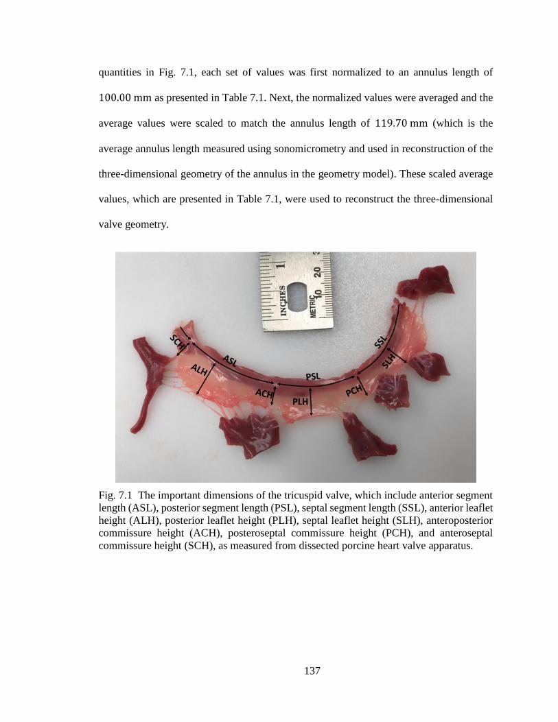
137

quantities in Fig. 7.1, each set of values was first normalized to an annulus length of

100.00 mm as presented in Table 7.1. Next, the normalized values were averaged and the

average values were scaled to match the annulus length of 119.70 mm (which is the

average annulus length measured using sonomicrometry and used in reconstruction of the

three-dimensional geometry of the annulus in the geometry model). These scaled average

values, which are presented in Table 7.1, were used to reconstruct the three-dimensional

valve geometry.

Fig. 7.1 The important dimensions of the tricuspid valve, which include anterior segment

length (ASL), posterior segment length (PSL), septal segment length (SSL), anterior leaflet

height (ALH), posterior leaflet height (PLH), septal leaflet height (SLH), anteroposterior

commissure height (ACH), posteroseptal commissure height (PCH), and anteroseptal

commissure height (SCH), as measured from dissected porcine heart valve apparatus.

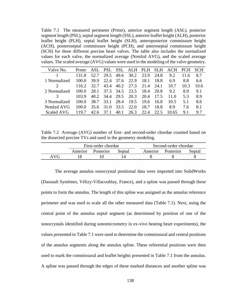
138

Table 7.1 The measured perimeter (Prmtr), anterior segment length (ASL), posterior

segment length (PSL), septal segment length (SSL), anterior leaflet height (ALH), posterior

leaflet height (PLH), septal leaflet height (SLH), anteroposterior commissure height

(ACH), posteroseptal commissure height (PCH), and anteroseptal commissure height

(SCH) for three different porcine heart valves. The table also includes the normalized

values for each valve, the normalized average (Nrmlzd AVG), and the scaled average

values. The scaled average (AVG) values were used in the modeling of the valve geometry.

Valve No. Prmtr ASL PSL SSL ALH PLH SLH ACH PCH SCH

1 131.8 52.7 29.5 49.6 30.2 23.9 24.8 9.2 11.6 8.7

1 Normalized 100.0 39.9 22.4 37.6 22.9 18.1 18.8 6.9 8.8 6.6

2 116.2 32.7 43.4 40.2 27.3 21.4 24.1 10.7 10.3 10.6

2 Normalized 100.0 28.1 37.3 34.5 23.5 18.4 20.8 9.2 8.9 9.1

3 103.9 40.2 34.4 29.5 20.3 20.4 17.5 11.0 5.3 8.9

3 Normalized 100.0 38.7 33.1 28.4 19.5 19.6 16.8 10.5 5.1 8.6

Nrmlzd AVG 100.0 35.6 31.0 33.5 22.0 18.7 18.8 8.9 7.6 8.1

Scaled AVG 119.7 42.6 37.1 40.1 26.3 22.4 22.5 10.65 9.1 9.7

Table 7.2 Average (AVG) number of first- and second-order chordae counted based on

the dissected porcine TVs and used in the geometry modeling.

First-order chordae Second-order chordae

Anterior Posterior Septal Anterior Posterior Septal

AVG 18 10 14 8 8 8

The average annulus sonocrystal positional data were imported into SolidWorks

(Dassault Systèmes, Vélizy-Villacoublay, France), and a spline was passed through these

points to form the annulus. The length of this spline was assigned as the annulus reference

perimeter and was used to scale all the other measured data (Table 7.1). Next, using the

central point of the annulus septal segment (as determined by position of one of the

sonocrystals identified during sonomicrometry in ex-vivo beating heart experiments), the

values presented in Table 7.1 were used to determine the commissural and central positions

of the annulus segments along the annulus spline. These referential positions were then

used to mark the commissural and leaflet heights presented in Table 7.1 from the annulus.

A spline was passed through the edges of these marked distances and another spline was

139

passed through points halfway between the lines that connected the marked points to the

annulus spline (Fig. 7.2). The Surface Loft feature in SolidWorks was used to pass a surface

through all three splines. The TV was assumed to have three papillary muscles

(anteroposterior, anteroseptal, and posteroseptal papillary muscles), each considered as a

single point in which all the chordae of that area merge. The position of these points (e.g.,

the tips of the assumed papillary muscles) were considered to be right under the

commissures at almost the same elevation as the lowest position of the valve leaflets, based

on the observations made for porcine heart TVs. First- and second-order chordae were

modeled in the geometry. First-order chordae (chordae on the edge) were assumed to be

distributed uniformly along the edge for each leaflet. Second-order chordae (chordae

entering to the back of the leaflet) were assumed to be uniformly distributed on the surface

of each leaflet and positioned at a distance about one-third of the total leaflet length from

the leaflet distal (free) edges. The number of chordae used in the model are based on the

chordae counted (presented in Table 7.2). The final developed geometry of the TV

apparatus used in the FE analysis is shown in Fig. 7.3.

140

Fig. 7.2 Reconstructed wireframe used for modeling the tricuspid valve geometry. Refer

to Table 7.1 for abbreviations and dimensions.

Fig. 7.3 The reconstructed TV apparatus geometry used in the finite element analysis.

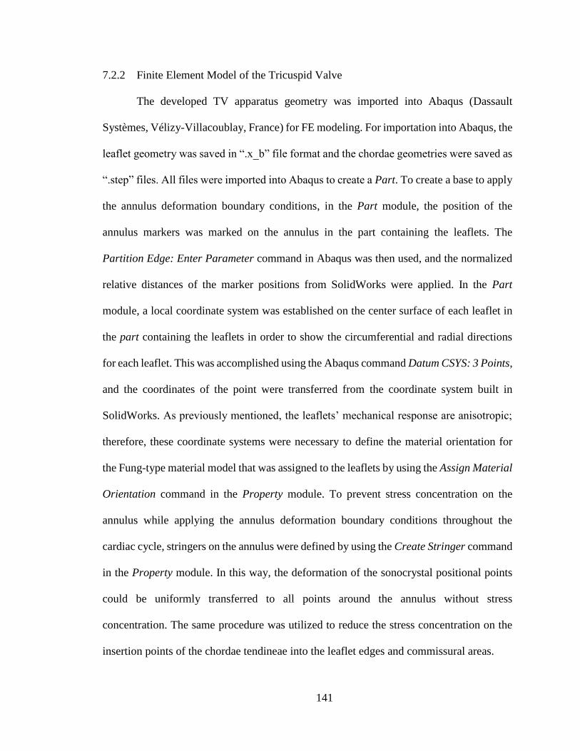
141

7.2.2 Finite Element Model of the Tricuspid Valve

The developed TV apparatus geometry was imported into Abaqus (Dassault

Systèmes, Vélizy-Villacoublay, France) for FE modeling. For importation into Abaqus, the

leaflet geometry was saved in “.x_b” file format and the chordae geometries were saved as

“.step” files. All files were imported into Abaqus to create a Part. To create a base to apply

the annulus deformation boundary conditions, in the Part module, the position of the

annulus markers was marked on the annulus in the part containing the leaflets. The

Partition Edge: Enter Parameter command in Abaqus was then used, and the normalized

relative distances of the marker positions from SolidWorks were applied. In the Part

module, a local coordinate system was established on the center surface of each leaflet in

the part containing the leaflets in order to show the circumferential and radial directions

for each leaflet. This was accomplished using the Abaqus command Datum CSYS: 3 Points,

and the coordinates of the point were transferred from the coordinate system built in

SolidWorks. As previously mentioned, the leaflets’ mechanical response are anisotropic;

therefore, these coordinate systems were necessary to define the material orientation for

the Fung-type material model that was assigned to the leaflets by using the Assign Material

Orientation command in the Property module. To prevent stress concentration on the

annulus while applying the annulus deformation boundary conditions throughout the

cardiac cycle, stringers on the annulus were defined by using the Create Stringer command

in the Property module. In this way, the deformation of the sonocrystal positional points

could be uniformly transferred to all points around the annulus without stress

concentration. The same procedure was utilized to reduce the stress concentration on the

insertion points of the chordae tendineae into the leaflet edges and commissural areas.

142

Although the Fung-type material model developed in chapter III [134] was initially

intended to be used in the model, due to the computational limitations, it was not used in

the final simulations. Instead, a linear elastic model with parameters obtained from the

literature [93] was used. Based on this linear elastic model, the modulus of elasticity for all

TV leaflets was considered to be equal to 0.4 𝑀𝑃𝑎. Considering the fact that the leaflets in

the TV are more fragile than those in the MV, this value is half of the elasticity modulus

reported in the literature for linearly simulated MV leaflets [93]. Moreover, a Poisson’s

ratio of 0.45 was assumed based on values obtained from the literature [93]. Chordae

tendineae mechanical response was modeled using an isotropic hyperelastic Ogden

material model developed for the chordae tendineae of the MV [91, 92, 106]. The same

properties were defined for the stringer on the edge of the leaflets. The stringers on the

annulus, however, were defined to be stronger so that the deformation boundary condition

could adequately and uniformly transfer to all points on the annulus through the movement

of sonocrystal positional points throughout the cardiac cycle. The homogenous shell type

section was used for the anterior leaflet with a thickness of 0.313 mm, and the

corresponding hyperplastic material developed in the previous chapters was assigned to

this section. Similarly, sections were defined for the posterior and septal leaflets as having

a thickness of 0.346 mm and 0.491 mm, respectively, and the corresponding material

properties were assigned to each. Although different average cross-sectional areas have

been reported for the TV chordae tendineae [9, 44, 107], all chordae were assumed to be

unbranched with an initial cross-sectional area of 0.171 mm2 [44, 107], and a general truss

section was defined to represent them. As we did not consider free lengths for the chordae,

their cross-sectional areas were later adjusted during the simulation to ensure coaptation of

143

the leaflets. The same type of section was defined for the edge stringer. To assign beam

sections to the annulus and commissural stringers, circular profiles were defined with radii

of 2 mm and 0.75 mm, respectively. Next, a beam type section was defined by assigning

the corresponding profiles and materials for each stringer. The defined sections were

assigned to the corresponding entities in the parts.

A structured technique was implemented to mesh the leaflets using standard linear

quadratic-shape shell elements with an approximate global size of 0.5 mm (Fig. 7.4). The

chordae were meshed using standard linear truss elements with an approximate global size

of 7 mm (Fig. 7.4). In the Assembly module, the necessary instances were imported into

the assembly using the Create Instance command. In the Step module, a Dynamic Explicit

step was defined to simulate the valve closure period after loading. The closing time was

chosen to be 0.38 second, which is when the average RVP reached its maximum in the ex-

vivo experiments [140].

In the Interaction module in Abaqus, an interaction property was defined to

represent the tangential and normal behavior of the leaflet surfaces in the TV model. The

friction coefficient was chosen to be 0.2 [221, 222], and the contact was defined as hard.

Next, a General Contact was created in the initial step and the above interaction property

was assigned to it. This contact was propagated to the dynamic step. Tie constraints were

used to attach each chorda to the edge or surface of the leaflets. The normalized amplitudes

for the average relative transvalvular pressure and the average positional change for all

sonocrystals on the annulus were imported into the Abaqus model as amplitudes using the

Create Amplitude command. The maximum relative transvalvular pressure (i.e.

~ 14 mm 𝐻𝑔) was uniformly placed on the outer surface of all three leaflets, and the

144

corresponding amplitudes were assigned to it, simulating the smooth pressure change

throughout the valve closure. The papillary muscles were fixed in the initial step and

propagated to the dynamic step. All sonocrystal positions on the annulus were fixed in the

initial step. In the dynamic step, these positions were moved to their corresponding

positions at the maximum RVP (as measured in the ex-vivo experiments), and the

corresponding amplitudes were assigned to simulate the smooth movement at these

points—and thus the deformation of the annulus—throughout the cardiac cycle.

Fig. 7.4 Finite element mesh for the reconstructed TV geometry.

7.3 Results

The developed model was used to simulate closure of TV. In Fig. 7.5, the

deformation of the valve during the closure simulation is illustrated at different time points.

This figure showed that the developed model is able to simulate the valve closure. The

color map in Fig. 7.5 shows the maximum in-plane principal strain distribution. The

145

maximum principal strain was under 25% for most locations based on this figure, and the

strains appeared to be uniform at the belly areas over the surface of the leaflets. The

distribution of the maximum in-plane principal strains on the septal leaflet surface is shown

separately in Fig. 7.6. As can be noticed from this figure, the strains in the belly area range

from approximately 8 to 15%. If we compare this data with the strain values measured for

the same region (belly area) in the ex-vivo experiments shown in Fig. 4.8 (the values of

maximum principal strain in Fig. 4.8 at the belly area range from approximately 9 to 13%.),

we notice a close match between the measured values and the results of this simulation,

further verifying the result of the simulation and the accuracy of the developed model.

Fig. 7.5 Maximum in-plane principal strain distribution illustrated over the anterior (A),

posterior (P), and septal (S) valve leaflets at different points in time during the valve closure

simulation.

146

Fig. 7.6 Distribution of maximum in-plane principal strain over the septal leaflet at

maximum right ventricular pressure.

Figure 7.7 shows the spatial distribution of the maximum in-plane principal stress

at different time points throughout the closure simulation. This stress reached values as

high as 120 kPa. The distribution of the stresses shows that the anterior leaflet experiences

the highest stress, while the septal leaflet experiences the lowest stress. Moreover, a slight

stress concentration can be seen around the area of the annulus. However, there is no

significant stress concentration at the connection points of the chordae on the leaflet

surfaces or at the edges of the leaflets.

7.4 Discussion

By running the FE simulation and applying the transvalvular pressure signal (which

is a function of time), the leaflets began to move toward each other, and coaptation

happened gradually (Fig. 7.5). The progressive change in the shape of the annulus shows

that the improvised annulus stringer perfectly transfers the movement of the sonocrystal

positional data to all the nodes around the annulus, implementing the expected boundary

conditions of the annulus (Fig. 7.5). In Fig. 7.6, the distribution of the maximum in-plane

147

principal strain illustrated over the septal leaflet showed that the levels of maximum in-

plane principal strains at the central area of this leaflet are around 12%, which closely

matches the values measured in the ex-vivo beating heart experiment [140], where the

average of maximum principal strain was roughly 11% (Fig. 4.8).

The level of stresses in the FE model (Fig. 7.7) are comparable to the estimated

values for normal physiological stress levels on the leaflet surfaces [117] from the biaxial

experiments (the values ranged roughly from 80 kPa for the septal leaflet to 130 kPa for

the anterior leaflet). The slight stress concentration observed around the annulus in this

figure might result from imposing the boundary conditions through the annulus stringer.

On the other hand, the stringers improvised into the edges of the leaflets prevented the

strain concentration from occurring at these areas by more uniformly transferring the load

from the chordae to the leaflets and vice versa.

Fig. 7.7 Maximum in-plane principal stress distribution illustrated over the anterior (A),

posterior (P), and septal (S) valve leaflets at different points in time during the valve closure

simulation.

148

Fig. 7.8 Comparison of effects of changes in the annulus boundary conditions on the strain

distribution and deformations of the septal leaflet. The top plot shows the result of the

simulation with the moving annulus boundary conditions (as the simulation of the intact

case), and the bottom plot shows the result of the simulation with the fixed annulus

boundary conditions (as the simulation of rigid ring annuloplasty).

Finally, to show how the results of this study can be used in real applications, we

simulated the ring annuloplasty using the developed FE model to see how valvular

treatments can alter the normal dynamic deformations of the TV. If we assume that the

annulus loses its ability to move as a result of rigid ring annuloplasty, we modeled the ring

annuloplasty by fixing the annulus. In Fig. 7.8, we have compared the strain distribution

and deformations of the septal leaflet from the simulation with a fixed annulus and the

simulation with moving annulus boundary conditions. As shown in this figure, there was a

slight increase in the range of the strains in the belly area. However, in the areas close to

the commissures, the strain distributions and the leaflet deformations were notably altered.

This alteration in the strain distribution and leaflet deformation shows how changing the

149

normal biomechanical environment of TV as a result of valvular treatments can affect the

valve, leading to potential tissue regeneration and long-term valvular failure.

150

CHAPTER 8VIII

CONCLUSIONS AND FUTURE WORK

8.1 Conclusions

Using custom-designed biaxial tensile testing equipment, we measured the biaxial

mechanical responses of the porcine TV leaflets under loading conditions that were

estimated based on physiological pressure levels and approximations of TV structure

geometries [128-132]. The overall trend of the measured tension–stretch data showed a

highly nonlinear behavior both in the radial and in the circumferential directions, as the

leaflets were more compliant at lower strains (i.e. over the toe region) following by a rapid

transition to a stiffer response (i.e. transition to the lockout region). The latter behavior was

not observed in the few mechanical tests conducted on the TV previously due to the small

level of strains used in such experiments [133]. TV leaflets were stiffer in the

circumferential direction, indicating an anisotropic response, a phenomenon that is also

observed in other cardiac valves [35-39]. The largest difference between mechanical

responses in the circumferential direction and the radial direction for the equibiaxial

loading was observed for the posterior leaflet, signifying a more anisotropic response in

this leaflet as compared to the other two leaflets. While no significant difference was

observed between the thicknesses of the anterior and posterior leaflets (𝑝 = 0.27,

Student’s t-test), the septal leaflet was significantly thicker than both of the other leaflets.

The anterior and posterior leaflets had the same stiffness in the circumferential direction,

151

but the anterior leaflet was much stiffer in the radial direction. The septal leaflet was more

compliant than the other two leaflets in the circumferential direction.

Next, we used the experimentally measured mechanical response data from our

biaxial mechanical testing to develop a material model to represent the mechanical

responses of TV leaflets in a general loading condition. The initial analysis of these data

led us to choose a Fung-type strain energy function as the phenomenological constitutive

framework, which was further justified by the high quality of the fitted models to the data.

The calculated anisotropy indices (i.e. 0.52, 0.39, and 0.51 for the anterior, posterior, and

septal leaflets, respectively) revealed that, similar to other cardiac valves [38, 42, 60, 67,

148], TV leaflets were highly anisotropic, further confirming our previous observation.

Quantitative analysis of tissue microstructure using small angle light scattering [77, 86,

150-152] confirmed that the main direction of the extracellular matrix fibers was along the

circumferential direction, and TV leaflets were thus expected to be anisotropic. In terms of

anisotropy, the porcine leaflets were qualitatively similar to human tissues: for both

species, all three leaflets were stiffer in the circumferential direction in comparison to the

radial direction [42].

To develop a set of representative material constants to be used in FE analysis,

average constitutive models were developed considering the nonlinear responses of the

native tissues. Our analysis on the three presented averaging approaches (i.e., tension-

based, first-Piola-Kirchhoff-stress–based, and Cauchy-stress–based approaches)

confirmed the fidelity of the tension-controlled biaxial testing loading protocols and the

subsequent averaging procedure in the tension space [36, 38, 58, 59, 148] when only small

variations in the thickness of the specimens exist. It is, however, more reasonable to avoid

152

potential errors by performing stress-controlled tests, especially when the tissue thickness

varies significantly between the specimens. While the responses of the three average

models were notably similar, the responses generated from arithmetical averaging of the

material constants were completely different. This observation further exemplifies that the

arithmetically averaged values of the individual material constants of a nonlinear model

may not represent the generic tissue responses accurately. Statistical comparison of the

mechanical responses and the material model developed here for the TV using responses

and material models available in the literature for other heart valves is not possible due to

differences in the models that have been used in each case as well as the limited amount of

available data. However, the parameters presented in Table 8.1 are parameters calculated

for human heart valves that are available in the literature [42] for a seven-parameter Fung-

type model, allowing a simple one-to-one comparison to be made.

Table 8.1 Parameters of a Fung-type model for human heart valves [42]

Valve C (𝑘𝑃𝑎) 𝑎1 𝑎2 𝑎3 𝑎4 𝑎5 𝑎6

MV 0.369 188.75 91.80 -2.143 100 -11.37 -12.51

AV 0.132 186.43 74.45 59.84 100 -6.78 -14.49

PV 0.587 43.68 20.66 6.49 10 0.16 -1.38

TV 0.684 59.42 29.05 1.25 10 1.66 -0.29

Additional inspections were also performed to validate the integrity of the

developed phenomenological constitutive models by examining the convexity of their

strain energy functions, as this convexity is crucial for the stability of the numerical

methods in computerized simulations [153].

Next, we developed an experimental setup to measure the dynamic deformation of

the porcine TV complex. Our novel ex-vivo passive beating heart apparatus was able to

153

produce repeatable data with high temporal resolution. Using our passive beating heart

system, we were able to reproduce ventricular pressure waves that matched the

physiological values of an actively beating heart [160]. Due to their excellent similarities

to the human heart in terms of pressure values on the pulmonary side, porcine hearts were

used in this simulation. In particular, human RVP ranges approximately from zero to

30 𝑚𝑚 𝐻𝑔 [128, 160], and porcine RVP ranges roughly from zero up to 33 𝑚𝑚 𝐻𝑔 [161-

164]. Such a similarity also exists in the systemic side of the heart [1, 165]. Using this

simulation apparatus and sonomicrometry techniques [26, 80-83, 85-87], we were able to

visualize the deformations and the strains of the valve septal leaflet and annulus.

The average values of the maximum principal strains and the areal strains

quantified at maximum RVP on the surface of the septal leaflet were 11.2% and 9.8%,

respectively. These values compared well with those calculated for the ovine MV anterior

leaflet (12.3% and 12.7% for the areal strain and the maximum principal strain,

respectively [30]). Such a similarity in the strain values is of particular interest, as it shows

that while the two leaflets are subjected to different levels of ventricular pressure, they

deform in a relatively similar manner. We noticed that the maximum principal strain is

distributed uniformly over the leaflet for nearly the entire cardiac cycle, while the areal

strain is not as uniform. There is much heterogeneity in the spatial distribution of the

circumferential strain and radial strain over the septal leaflet. While higher values for

circumferential strain were observed toward the posterior side of the leaflet, the radial

strains reached higher values in areas near the anterior side. However, unlike MV leaflets,

in which significant differences exist between the maximum strain in the circumferential

and radial directions [26, 30, 111], no significant difference was observed between

154

circumferential and radial strains in the septal leaflet of the TV at the maximum RVP. A

possible explanation for this finding is that the septal leaflet of the TV has a more isotropic

extracellular matrix microstructural architecture in comparison to the anterior and posterior

leaflets of the MV [35].

Positional data obtained from the sonocrystals sutured around the ex-vivo porcine

heart annulus were used to develop an average annulus model and analyze the annulus

shape and deformation throughout the cardiac cycle. The effects of chordae rupture were

also investigated on these deformations and strain distributions by cutting one of the septal

chordae proximal to the posteroseptal commissure. We observed that the geometry of the

annulus is considerably altered during the cardiac cycle such that, from the minimum RVP

to the maximum RVP, the area experiences a roughly 20% increase, and the circumference

extends approximately 8%. Our analysis showed that these deformations do not occur

uniformly along the annulus. For example, the annulus anterior segment (AAS)

experiences the largest deformation (about 9% on average).

Our experiments showed that there exists a mechanical interdependency among the

chordae tendineae, leaflets, and annulus of the TV. We observed that immediately after

chordae rupture, the dynamic deformation of the TV annulus changed extensively, with a

significant increase in the annulus area, circumference and radius. Annulus dilation is

expected to change the coaptation of the valve leaflets and induce regurgitation [182]. Our

measurements showed that the flow into the right atrium decreased by 26% and RVP

dropped by 17%, altering the hemodynamics of the heart immediately after the septal

chordae tendineae was cut. Moreover, the deformation and the strain distribution of the

155

septal leaflet significantly changed throughout the cardiac cycle following the rupture of

the chordae.

Although the TV may be initially asymptomatic, instantaneous annulus dilation and

changes in the leaflets strain distribution following chordae rupture could lead to

exacerbation of TV regurgitation and potentially to mechanically-induced remodeling

responses in the TV leaflets, the remaining intact chordae tendineae, the papillary muscles,

and/or the ventricular myocardium. Hence, careful examination and early surgical

intervention might be necessary to prevent mid-term/long-term negative effects of

mechanically-induced remodeling in asymptomatic TVs following the rupture of the

chordae tendineae.

Finally, a basic model of TV was developed in Abaqus using mechanical properties

of the native TV, microstructure, accurate annulus boundary conditions, and the 3D surface

geometry of TV. This model was used to simulate the closure of the TV during the cardiac

cycle. The distribution of stresses showed that the anterior and septal leaflets experience

the highest and the lowest stresses, respectively. To validate the model, the distribution of

the maximum in-plane principal strain over the septal leaflet from the model was compared

to the corresponding distribution that was measured in experiments using the ex-vivo setup

and sonomicrometry [140]. This comparison revealed that the level of the maximum in-

plane principal strain at the belly area of this leaflet (where we measured strains

experimentally [140]) is around 15%, closely matching the values measured in the ex-vivo

beating heart experiment [140], which were roughly 12% maximum principal strain.

Moreover, the maximum in-plane principal stress in the simulation results reached values

as high as 133.6 𝑘𝑃𝑎 on TV leaflet surfaces. This was comparable to the estimated values

156

of normal physiological stress levels on the leaflet surfaces [117] for the biaxial

experiments (where the values ranged from roughly 80 𝑘𝑃𝑎 for the septal leaflet to

130 𝑘𝑃𝑎 for the anterior leaflet), further validating our developed model.

In summary, in this doctoral research, we obtained important new knowledge of

TV biomechanics including the strain-stress responses, leaflets microstructure, geometry

and dynamic deformations of the annulus, and dynamic deformations and stress

distributions of the septal leaflet throughout the cardiac cycle. In addition, we developed a

computerized model of the TV for simulation applications. Development of such an

accurate and verified model will facilitate in-silico examination of different valve repair

surgeries and provide insight into the possible changes in the biomechanical environment

of the TV following such procedures. With further modifications, verifications, and

validations, our model has the potential to shed light on appropriate modifications for TV

surgical procedures in order for their outcomes to most efficiently mimic the native valve

biomechanics.

Once more, it should be noted that all experiments in the current study were

performed on porcine hearts and porcine valvular tissues. There are many advantages in

using porcine hearts, as fresh tissues can be obtained so the biomechanical behavior of the

valves is less affected by the activity of degenerative enzymes in the extracellular matrix.

In addition, in comparison to human cadaverous tissues, younger porcine samples with less

variability are available [35]. Nevertheless, one should always be cautious in drawing

conclusions regarding human tissue responses based solely on animal studies [167].

157

8.2 Future Work

The findings of the current work can be used as the basis for several other

interesting studies. For example:

Similar to its application in the simulation of chordae rupture, the developed ex-

vivo beating heart apparatus can be used for simulation of the other valvular lesions, such

as valve perforation. Moreover, this apparatus can be used for simulation of valvular

treatments. For example, in most TV repair procedures, a prosthetic annuloplasty ring is

used to decrease the annulus size and improve the valve hemodynamics [8]. Considering

the dynamic deformation of the TV annulus observed in our study, further research can be

accomplished under similar procedures to identify how the valve deformation changes

following ring annuloplasty [26].

Due to the limited number of sonomicrometry crystal channels (16 channels)

employed in this study, we were not able to measure deformation of the anterior and

posterior leaflets of the TV. Further research can be established to quantify strain values in

the anterior and posterior leaflets and compare the results with those for the septal leaflet.

Although our study was conducted using PBS, there is no reason why non-clear

fluids cannot be used in our ex-vivo apparatus, as our strain measurements do not rely on

visual access to the markers. Such a capability is of great importance, because recent

studies have shown that the flow properties (particularly the transition to turbulence) could

be significantly different in blood in comparison to optically clear, viscosity-matched blood

substitutes [172]. Since the transition to turbulence could occur in proximity to the cardiac

valves, measurements of valve deformation using blood can be performed in the future.

158

In addition, the computerized model developed in this study can be improved to

provide more realistic outcomes. For example, while phenomenological constitutive

models are powerful in predicting the responses of the tissue, they do not provide much

insight about the mechanical environment at the underlying extracellular matrix/cellular

levels. In other words, model parameters cannot be quantitatively related to structural

components of the tissue, such as extracellular matrix protein volume fractions or

extracellular matrix morphology. Such information is of particular interest in the field of

mechanobiology, for which constitutive frameworks that include structural components of

the tissue are more relevant [66-70]. Using the experimentally measured mechanical

responses and the mapped microstructure of TV leaflets in the current study, further work

is necessary to develop such structural models that incorporate the microstructure of the

leaflets in the mechanical response.

Moreover, after adequate degrees of verification, the developed computerized

model can also be used in the simulation of valvular lesions and their treatments.

Finally, the data provided in the current work pertain to the use of porcine tissues.

Although many of the conclusions of this study seem to be independent of the species,

further studies can be done on the human heart for better understanding and comparison.

As such, the methods established in the current study can be applied in the same manner

on human cadaveric hearts, as this may provide more accurate insight into the mechanical

behavior of the native human TV and lead to development of more reliable computerized

models.

159

BIBLIOGRAPHY

[1] Hall, J. E., 2015, Guyton and Hall textbook of medical physiology e-Book, Elsevier

Health Sciences.

[2] Cook, M. S., and Weinhaus, A. J., 2015, "Anatomy of the Thoracic Wall,

Pulmonary Cavities, and Mediastinum," Handbook of Cardiac Anatomy,

Physiology, and Devices, P. A. Iaizzo, ed., Springer International Publishing,

Cham, pp. 35-60.

[3] Weinhaus, A. J., and Roberts, K. P., 2005, "Anatomy of the Human Heart,"

Handbook of Cardiac Anatomy, Physiology, and Devices, P. A. Iaizzo, ed.,

Humana Press, Totowa, NJ, pp. 51-79.

[4] Soliman, O. I., Folkert, J., and Cate, T., 2018, Practical Manual of Tricuspid Valve

Diseases, Springer.

[5] Chan, K. M. J., "Functional Mitral and Tricuspid Regurgitation."

[6] Hinton, R. B., and Yutzey, K. E., 2011, "Heart valve structure and function in

development and disease," Annual review of physiology, 73, pp. 29-46.

[7] Joudinaud, T. M., Flecher, E. M., and Duran, C., 2006, "Functional terminology for

the tricuspid valve," The Journal of heart valve disease, 15(3), pp. 382-388.

[8] Carpentier, A., Adams, D. H., and Filsoufi, F., 2011, Carpentier's Reconstructive

Valve Surgery E-Book, Elsevier Health Sciences.

[9] Silver, M. D., Lam, J. H., Ranganathan, N., and Wigle, E. D., 1971, "Morphology

of the human tricuspid valve," Circulation, 43(3), pp. 333-348.

[10] Gunnal, S., Wabale, R., and Farooqui, M., 2015, "Morphological study of chordae

tendinae in human cadaveric hearts," Heart views: the official journal of the Gulf

Heart Association, 16(1), p. 1.

[11] Ushiki, T., 2002, "Collagen fibers, reticular fibers and elastic fibers. A

comprehensive understanding from a morphological viewpoint," Archives of

histology and cytology, 65(2), pp. 109-126.

[12] Sacks, M. S., Merryman, W. D., and Schmidt, D. E., 2009, "On the biomechanics

of heart valve function," Journal of Biomechanics, 42(12), pp. 1804-1824.

160

[13] Schoen, F., 1997, "Aortic valve structure-function correlations: role of elastic fibers

no longer a stretch of the imagination," The Journal of heart valve disease, 6(1), p.

1.

[14] Thubrikar, M., 2018, The aortic valve, Routledge.

[15] Lee, C.-H., Zhang, W., Liao, J., Carruthers, C. A., Sacks, J. I., and Sacks, M. S.,

2015, "On the presence of affine fibril and fiber kinematics in the mitral valve

anterior leaflet," Biophysical journal, 108(8), pp. 2074-2087.

[16] Simionescu, D., Lovekamp, J., and Vyavahare, N., 2003, "Degeneration of

bioprosthetic heart valve cusp and wall tissues is initiated during tissue preparation:

an ultrastructural study," The Journal of heart valve disease, 12(2), pp. 226-234.

[17] Vesely, I., 1997, "The role of elastin in aortic valve mechanics," Journal of

biomechanics, 31(2), pp. 115-123.

[18] Misfeld, M., and Sievers, H.-H., 2007, "Heart valve macro-and microstructure,"

Philosophical Transactions of the Royal Society of London B: Biological Sciences,

362(1484), pp. 1421-1436.

[19] Spinner, E. M., Lerakis, S., Higginson, J., Pernetz, M., Howell, S., Veledar, E., and

Yoganathan, A. P., 2012, "Correlates of tricuspid regurgitation as determined by

3D echocardiography: pulmonary arterial pressure, ventricle geometry, annular

dilatation, and papillary muscle displacement," Circulation: Cardiovascular

Imaging, 5(1), pp. 43-50.

[20] Dreyfus, G. D., Corbi, P. J., Chan, K. M. J., and Bahrami, T., 2005, "Secondary

tricuspid regurgitation or dilatation: which should be the criteria for surgical

repair?," The Annals of Thoracic Surgery, 79(1), pp. 127-132.

[21] Lee, J.-W., Song, J.-M., Park, J. P., Lee, J. W., Kang, D.-H., and Song, J.-K., 2010,

"Long-term prognosis of isolated significant tricuspid regurgitation," Circulation

Journal, 74(2), pp. 375-380.

[22] Fung, Y. C., and Liu, S. Q., 1989, "Change of residual strains in arteries due to

hypertrophy caused by aortic constriction," Circulation research, 65(5), pp. 1340-

1349.

[23] Fung, Y. C., 1991, "What are the residual stresses doing in our blood vessels?,"

Annals of Biomedical Engineering, 19(3), pp. 237-249.

[24] Vassileva, C. M., Shabosky, J., Boley, T., Markwell, S., and Hazelrigg, S., 2012,

"Tricuspid valve surgery: the past 10 years from the Nationwide Inpatient Sample

(NIS) database," The Journal of thoracic and cardiovascular surgery, 143(5), pp.

1043-1049.

161

[25] Guenther, T., Noebauer, C., Mazzitelli, D., Busch, R., Tassani-Prell, P., and Lange,

R., 2008, "Tricuspid valve surgery: a thirty-year assessment of early and late

outcome," European journal of cardio-thoracic surgery : official journal of the

European Association for Cardio-thoracic Surgery, 34(2), pp. 402-409; discussion

409.

[26] Amini, R., Eckert, C. E., Koomalsingh, K., McGarvey, J., Minakawa, M., Gorman,

J. H., Gorman, R. C., and Sacks, M. S., 2012, "On the in vivo deformation of the

mitral valve anterior leaflet: effects of annular geometry and referential

configuration," Annals of Biomedical Engineering, 40(7), pp. 1455-1467.

[27] Chikwe, J., Itagaki, S., Anyanwu, A., and Adams, D. H., 2015, "Impact of

concomitant tricuspid annuloplasty on tricuspid regurgitation, right ventricular

function, and pulmonary artery hypertension after repair of mitral valve prolapse,"

Journal of the American College of Cardiology, 65(18), pp. 1931-1938.

[28] Mahmood, F., Gorman, J. H., Subramaniam, B., Gorman, R. C., Panzica, P. J.,

Hagberg, R. C., Lerner, A. B., Hess, P. E., Maslow, A., and Khabbaz, K. R., 2010,

"Changes in mitral valve annular geometry after repair: saddle-shaped versus flat

annuloplasty rings," The Annals of Thoracic Surgery, 90(4), pp. 1212-1220.

[29] Mahmood, F., Subramaniam, B., Gorman, J. H., Levine, R. M., Gorman, R. C.,

Maslow, A., Panzica, P. J., Hagberg, R. M., Karthik, S., and Khabbaz, K. R., 2009,

"Three-dimensional echocardiographic assessment of changes in mitral valve

geometry after valve repair," The Annals of Thoracic Surgery, 88(6), pp. 1838-

1844.

[30] Rausch, M. K., Bothe, W., Kvitting, J.-P. E., Göktepe, S., Miller, D. C., and Kuhl,

E., 2011, "In vivo dynamic strains of the ovine anterior mitral valve leaflet," Journal

of Biomechanics, 44(6), pp. 1149-1157.

[31] Bothe, W., Kvitting, J.-P. E., Swanson, J. C., Hartnett, S., Ingels, N. B., and Miller,

D. C., 2010, "Effects of different annuloplasty rings on anterior mitral leaflet

dimensions," The Journal of thoracic and cardiovascular surgery, 139(5), pp. 1114-

1122.

[32] Singh, J. P., Evans, J. C., Levy, D., Larson, M. G., Freed, L. A., Fuller, D. L.,

Lehman, B., and Benjamin, E. J., 1999, "Prevalence and clinical determinants of

mitral, tricuspid, and aortic regurgitation (the Framingham Heart Study)," The

American Journal of Cardiology, 83(6), pp. 897-902.

[33] Stuge, O., and Liddicoat, J., 2006, "Emerging opportunities for cardiac surgeons

within structural heart disease," The Journal of thoracic and cardiovascular surgery,

132(6), pp. 1258-1261.

162

[34] Taramasso, M., Vanermen, H., Maisano, F., Guidotti, A., La Canna, G., and Alfieri,

O., 2012, "The growing clinical importance of secondary tricuspid regurgitation,"

Journal of the American College of Cardiology, 59(8), pp. 703-710.

[35] May-Newman, K., and Yin, F. C., 1995, "Biaxial mechanical behavior of excised

porcine mitral valve leaflets," The American Journal of Physiology, 269(4 Pt 2),

pp. H1319-1327.

[36] Billiar, K. L., and Sacks, M. S., 2000, "Biaxial mechanical properties of the natural

and glutaraldehyde treated aortic valve cusp—part I: experimental results," Journal

of Biomechanical Engineering, 122(1), pp. 23-30.

[37] Grashow, J. S., Yoganathan, A. P., and Sacks, M. S., 2006, "Biaixal stress–stretch

behavior of the mitral valve anterior leaflet at physiologic strain rates," Annals of

Biomedical Engineering, 34(2), pp. 315-325.

[38] Grashow, J. S., Sacks, M. S., Liao, J., and Yoganathan, A. P., 2006, "Planar biaxial

creep and stress relaxation of the mitral valve anterior leaflet," Annals of


[39] Sacks, M. S., He, Z., Baijens, L., Wanant, S., Shah, P., Sugimoto, H., and

Yoganathan, A. P., 2002, "Surface strains in the anterior leaflet of the functioning

mitral valve," Annals of Biomedical Engineering, 30(10), pp. 1281-1290.

[40] Boronyak, S. M., and Merryman, W. D., 2012, "Development of a simultaneous

cryo-anchoring and radiofrequency ablation catheter for percutaneous treatment of

mitral valve prolapse," Annals of Biomedical Engineering, 40(9), pp. 1971-1981.

[41] Price, S. L., Norwood, C. G., Williams, J. L., McElderry, H. T., and Merryman, W.

D., 2010, "Radiofrequency ablation directionally alters geometry and

biomechanical compliance of mitral valve leaflets: refinement of a novel

percutaneous treatment strategy," Cardiovascular Engineering and Technology,

1(3), pp. 194-201.

[42] Pham, T., Sulejmani, F., Shin, E., Wang, D., and Sun, W., 2017, "Quantification

and comparison of the mechanical properties of four human cardiac valves," Acta

Biomaterialia, 54, pp. 345-355.

[43] McCarthy, P. M., and Sales, V. L., 2010, "Evolving indications for tricuspid valve

surgery," Current treatment options in cardiovascular medicine, 12(6), pp. 587-597.

[44] Stevanella, M., Votta, E., Lemma, M., Antona, C., and Redaelli, A., 2010, "Finite

element modelling of the tricuspid valve: a preliminary study," Medical

engineering & physics, 32(10), pp. 1213-1223.

163

[45] Mooney, M., 1940, "A theory of large elastic deformation," Journal of applied

physics, 11(9), pp. 582-592.

[46] Rivlin, R., and Saunders, D., 1997, "Large elastic deformations of isotropic

materials," Collected papers of RS Rivlin, Springer, pp. 157-194.

[47] Ogden, R. W., 1972, "Large deformation isotropic elasticity–on the correlation of

theory and experiment for incompressible rubberlike solids," Proc. R. Soc. Lond.

A, 326(1567), pp. 565-584.

[48] Ogden, R. W., 1997, Non-linear elastic deformations, Courier Corporation.

[49] Shahzad, M., Kamran, A., Siddiqui, M. Z., and Farhan, M., 2015, "Mechanical

characterization and FE modelling of a hyperelastic material," Materials Research,

18(5), pp. 918-924.

[50] Sacks, M. S., 2000, "Biaxial mechanical evaluation of planar biological materials,"

Journal of elasticity and the physical science of solids, 61(1-3), pp. 199-246.

[51] Sacks, M. S., and Sun, W., 2003, "Multiaxial mechanical behavior of biological

materials," Annual review of biomedical engineering, 5(1), pp. 251-284.

[52] Fung, Y.-C. B., 1973, "Biorheology of soft tissues," Biorheology, 10(2), pp. 139-

155.

[53] Tong, P., and Fung, Y.-C., 1976, "The stress-strain relationship for the skin,"

Journal of Biomechanics, 9(10), pp. 649-657.

[54] Sacks, M. S., 1999, "A Method for Planar Biaxial Mechanical Testing That

Includes In-Plane Shear," Journal of Biomechanical Engineering, 121(5), pp. 551-

555.

[55] Sun, W., Sacks, M. S., Sellaro, T. L., Slaughter, W. S., and Scott, M. J., 2003,

"Biaxial mechanical response of bioprosthetic heart valve biomaterials to high in-

plane shear," Journal of Biomechanical Engineering, 125(3), pp. 372-380.

[56] Vande Geest, J. P., Sacks, M. S., and Vorp, D. A., 2004, "Age dependency of the

biaxial biomechanical behavior of human abdominal aorta," Journal of

Biomechanical Engineering, 126(6), pp. 815-822.

[57] Gilbert, T. W., Wognum, S., Joyce, E. M., Freytes, D. O., Sacks, M. S., and

Badylak, S. F., 2008, "Collagen fiber alignment and biaxial mechanical behavior

of porcine urinary bladder derived extracellular matrix," Biomaterials, 29(36), pp.

4775-4782.

164

[58] Bellini, C., Glass, P., Sitti, M., and Di Martino, E. S., 2011, "Biaxial mechanical

modeling of the small intestine," Journal of the mechanical behavior of biomedical

materials, 4(8), pp. 1727-1740.

[59] Keyes, J. T., Lockwood, D. R., Utzinger, U., Montilla, L. G., Witte, R. S., and

Vande Geest, J. P., 2013, "Comparisons of Planar and Tubular Biaxial Tensile

Testing Protocols of the Same Porcine Coronary Arteries," Annals of Biomedical

Engineering, 41(7), pp. 1579-1591.

[60] May-Newman, K., and Yin, F. C. P., 1998, "A constitutive law for mitral valve

tissue," Journal of Biomechanical Engineering, 120(1), pp. 38-47.

[61] Choi, H., 1990, "Mechanical properties of canine pericardium."

[62] Choi, H. S., and Vito, R. P., 1990, "Two-Dimensional Stress-Strain Relationship

for Canine Pericardium," Journal of Biomechanical Engineering, 112(2), pp. 153-

159.

[63] Sacks, M. S., and Chuong, C. J., 1998, "Orthotropic Mechanical Properties of

Chemically Treated Bovine Pericardium," Annals of Biomedical Engineering,

26(5), pp. 892-902.

[64] Vande Geest, J. P., Sacks, M. S., and Vorp, D. A., 2006, "The effects of aneurysm

on the biaxial mechanical behavior of human abdominal aorta," Journal of

Biomechanics, 39(7), pp. 1324-1334.

[65] O’Leary, S. A., Healey, D. A., Kavanagh, E. G., Walsh, M. T., McGloughlin, T.

M., and Doyle, B. J., 2014, "The Biaxial Biomechanical Behavior of Abdominal

Aortic Aneurysm Tissue," Annals of Biomedical Engineering, 42(12), pp. 2440-

2450.

[66] Lanir, Y., 1983, "Constitutive equations for fibrous connective tissues," Journal of


[67] Billiar, K. L., and Sacks, M. S., 2000, "Biaxial mechanical properties of the native

and glutaraldehyde-treated aortic valve cusp: part II—a structural constitutive

model," Journal of Biomechanical Engineering, 122(4), pp. 327-335.

[68] Sacks, M. S., 2003, "Incorporation of experimentally-derived fiber orientation into

a structural constitutive model for planar collagenous tissues," Journal of


[69] Fata, B., Zhang, W., Amini, R., and Sacks, M. S., 2014, "Insights into regional

adaptations in the growing pulmonary artery using a meso-scale structural model:

effects of ascending aorta impingement," Journal of Biomechanical Engineering,

136(2), p. 021009.

165

[70] Wognum, S., Schmidt, D. E., and Sacks, M. S., 2009, "On the mechanical role of

de novo synthesized elastin in the urinary bladder wall," Journal of biomechanical

engineering, 131(10), p. 101018.

[71] Lanir, Y., 1979, "A structural theory for the homogeneous biaxial stress-strain

relationships in flat collagenous tissues," Journal of Biomechanics, 12(6), pp. 423-

436.

[72] Lanir, Y., and Fung, Y. C., 1974, "Two-dimensional mechanical properties of

rabbit skin—II. Experimental results," Journal of Biomechanics, 7(2), pp. 171-182.

[73] Lanir, Y., and Fung, Y. C., 1974, "Two-dimensional mechanical properties of

rabbit skin—I. Experimental system," Journal of Biomechanics, 7(1), pp. 29-34.

[74] Zhang, W., Feng, Y., Lee, C.-H., Billiar, K. L., and Sacks, M. S., 2015, "A

generalized method for the analysis of planar biaxial mechanical data using tethered

testing configurations," Journal of Biomechanical Engineering, 137(6), p. 064501.

[75] Eilaghi, A., Flanagan, J. G., Brodland, G. W., and Ethier, C. R., 2009, "Strain

uniformity in biaxial specimens is highly sensitive to attachment details," Journal

of Biomechanical Engineering, 131(9), p. 091003.

[76] Cochran, R., Kunzelman, K., Chuong, C., Sacks, M., and Eberhart, R., 1991,

"Nondestructive analysis of mitral valve collagen fiber orientation," ASAIO

transactions, 37(3), pp. M447-448.

[77] Sacks, M. S., Smith, D. B., and Hiester, E. D., 1997, "A small angle light scattering

device for planar connective tissue microstructural analysis," Annals of Biomedical

Engineering, 25(4), pp. 678-689.

[78] Robitaille, M. C., Zareian, R., DiMarzio, C. A., Wan, K.-T., and Ruberti, J. W.,

2011, "Small-angle light scattering to detect strain-directed collagen degradation in

native tissue," Interface Focus, 1(5), pp. 767-776.

[79] Hobson, C. M., Amoroso, N. J., Amini, R., Ungchusri, E., Hong, Y., D'Amore, A.,

Sacks, M. S., and Wagner, W. R., 2015, "Fabrication of elastomeric scaffolds with

curvilinear fibrous structures for heart valve leaflet engineering," Journal of

Biomedical Materials Research Part A, 103(9), pp. 3101-3106.

[80] Hiro, M. E., Jouan, J., Pagel, M. R., Lansac, E., Lim, K. H., Lim, H.-S., and Duran,

C. M. G., 2004, "Sonometric study of the normal tricuspid valve annulus in sheep,"

Journal of Heart Valve Disease, 13(3), pp. 452-460.

[81] Fawzy, H., Fukamachi, K., Mazer, C. D., Harrington, A., Latter, D., Bonneau, D.,

and Errett, L., 2011, "Complete mapping of the tricuspid valve apparatus using

166

three-dimensional sonomicrometry," The Journal of thoracic and cardiovascular

surgery, 141(4), pp. 1037-1043.

[82] Eckert, C. E., Zubiate, B., Vergnat, M., Gorman Iii, J. H., Gorman, R. C., and Sacks,

M. S., 2009, "In vivo dynamic deformation of the mitral valve annulus," Annals of


[83] Rausch, M. K., Malinowski, M., Wilton, P., Khaghani, A., and Timek, T. A., 2017,

"Engineering Analysis of Tricuspid Annular Dynamics in the Beating Ovine

Heart," Annals of Biomedical Engineering.

[84] Tsakiris, A. G., Mair, D. D., Seki, S., Titus, J. L., and Wood, E. H., 1975, "Motion

of the tricuspid valve annulus in anesthetized intact dogs," Circulation research,

36(1), pp. 43-48.

[85] Sacks, M. S., Enomoto, Y., Graybill, J. R., Merryman, W. D., Zeeshan, A.,

Yoganathan, A. P., Levy, R. J., Gorman, R. C., and Gorman, J. H., 2006, "In-vivo

dynamic deformation of the mitral valve anterior leaflet," The Annals of Thoracic

Surgery, 82(4), pp. 1369-1377.

[86] Amini, R., Voycheck, C. A., and Debski, R. E., 2014, "A Method for Predicting

Collagen Fiber Realignment in Non-Planar Tissue Surfaces as Applied to

Glenohumeral Capsule During Clinically Relevant Deformation," Journal of

Biomechanical Engineering, 136(3), p. 031003.

[87] Filas, B. A., Knutsen, A. K., Bayly, P. V., and Taber, L. A., 2008, "A new method

for measuring deformation of folding surfaces during morphogenesis," Journal of

Biomechanical Engineering, 130(6), p. 061010.

[88] Lee, C.-H., Rabbah, J.-P., Yoganathan, A. P., Gorman, R. C., Gorman Iii, J. H., and

Sacks, M. S., 2015, "On the effects of leaflet microstructure and constitutive model

on the closing behavior of the mitral valve," Biomechanics and modeling in

mechanobiology, 14(6), pp. 1281-1302.

[89] Lee, C.-H., Oomen, P. J., Rabbah, J. P., Yoganathan, A., Gorman, R. C., Gorman,

J. H., Amini, R., and Sacks, M. S., 2013, "A high-fidelity and micro-anatomically

accurate 3D finite element model for simulations of functional mitral valve,"

International Conference on Functional Imaging and Modeling of the Heart,

Springer, pp. 416-424.

[90] Fan, R., and Sacks, M. S., 2014, "Simulation of planar soft tissues using a structural

constitutive model: finite element implementation and validation," Journal of

biomechanics, 47(9), pp. 2043-2054.

[91] Kong, F., Pham, T., Martin, C., McKay, R., Primiano, C., Hashim, S., Kodali, S.,

and Sun, W., 2018, "Finite Element Analysis of Tricuspid Valve Deformation from

167

Multi-slice Computed Tomography Images," Annals of biomedical engineering,

pp. 1-16.

[92] Kunzelman, K., Reimink, M., and Cochran, R., 1997, "Annular dilatation increases

stress in the mitral valve and delays coaptation: a finite element computer model,"

Cardiovascular Surgery, 5(4), pp. 427-434.

[93] Lim, K. H., Yeo, J. H., and Duran, C., 2005, "Three-dimensional asymmetrical

modeling of the mitral valve: a finite element study with dynamic boundaries," J

Heart Valve Dis, 14(3), pp. 386-392.

[94] Einstein, D. R., Kunzelman, K. S., Reinhall, P. G., Nicosia, M. A., and Cochran, R.

P., 2005, "Non-linear fluid-coupled computational model of the mitral valve," J.

Heart Valve Dis, 14(3), pp. 376-385.

[95] Votta, E., Caiani, E., Veronesi, F., Soncini, M., Montevecchi, F. M., and Redaelli,

A., 2008, "Mitral valve finite-element modelling from ultrasound data: a pilot study

for a new approach to understand mitral function and clinical scenarios,"

Philosophical Transactions of the Royal Society of London A: Mathematical,

Physical and Engineering Sciences, 366(1879), pp. 3411-3434.

[96] Prot, V., Skallerud, B., and Holzapfel, G., 2007, "Transversely isotropic membrane

shells with application to mitral valve mechanics. Constitutive modelling and finite

element implementation," International journal for numerical methods in

engineering, 71(8), pp. 987-1008.

[97] Prot, V., Haaverstad, R., and Skallerud, B., 2009, "Finite element analysis of the

mitral apparatus: annulus shape effect and chordal force distribution,"

Biomechanics and modeling in mechanobiology, 8(1), pp. 43-55.

[98] Holzapfel, G. A., Sommer, G., Gasser, C. T., and Regitnig, P., 2005,

"Determination of layer-specific mechanical properties of human coronary arteries

with nonatherosclerotic intimal thickening and related constitutive modeling,"

American Journal of Physiology-Heart and Circulatory Physiology, 289(5), pp.

H2048-H2058.

[99] Wenk, J. F., Zhang, Z., Cheng, G., Malhotra, D., Acevedo-Bolton, G., Burger, M.,

Suzuki, T., Saloner, D. A., Wallace, A. W., and Guccione, J. M., 2010, "First finite

element model of the left ventricle with mitral valve: insights into ischemic mitral

regurgitation," The Annals of thoracic surgery, 89(5), pp. 1546-1553.

[100] Quapp, K., and Weiss, J., 1998, "Material characterization of human medial

collateral ligament," Journal of biomechanical engineering, 120(6), pp. 757-763.

[101] Hallquist, J. O., 2006, "LS-DYNA theory manual," Livermore software

Technology corporation, 3, pp. 25-31.

168

[102] Stevanella, M., Maffessanti, F., Conti, C. A., Votta, E., Arnoldi, A., Lombardi, M.,

Parodi, O., Caiani, E. G., and Redaelli, A., 2011, "Mitral valve patient-specific

finite element modeling from cardiac MRI: application to an annuloplasty

procedure," Cardiovascular Engineering and Technology, 2(2), pp. 66-76.

[103] Wang, Q., and Sun, W., 2013, "Finite element modeling of mitral valve dynamic

deformation using patient-specific multi-slices computed tomography scans,"

Annals of biomedical engineering, 41(1), pp. 142-153.

[104] Gasser, T. C., Ogden, R. W., and Holzapfel, G. A., 2006, "Hyperelastic modelling

of arterial layers with distributed collagen fibre orientations," Journal of the royal

society interface, 3(6), pp. 15-35.

[105] Holzapfel, G. A., Gasser, T. C., and Ogden, R. W., 2000, "A new constitutive

framework for arterial wall mechanics and a comparative study of material

models," Journal of elasticity and the physical science of solids, 61(1-3), pp. 1-48.

[106] Pham, T., Kong, F., Martin, C., Wang, Q., Primiano, C., McKay, R., Elefteriades,

J., and Sun, W., 2017, "Finite element analysis of patient-specific mitral valve with

mitral regurgitation," Cardiovascular engineering and technology, 8(1), pp. 3-16.

[107] Lim, K. O., 1980, "Mechanical properties and ultrastructure of normal human

tricuspid valve chordae tendineae," The Japanese journal of physiology, 30(3), pp.

455-464.

[108] Krishnamurthy, G., Itoh, A., Bothe, W., Swanson, J. C., Kuhl, E., Karlsson, M.,

Miller, D. C., and Ingels, N. B., 2009, "Stress–strain behavior of mitral valve

leaflets in the beating ovine heart," Journal of Biomechanics, 42(12), pp. 1909-

1916.

[109] Krishnamurthy, G., Itoh, A., Swanson, J. C., Bothe, W., Karlsson, M., Kuhl, E.,

Miller, D. C., and Ingels, N. B., 2009, "Regional stiffening of the mitral valve

anterior leaflet in the beating ovine heart," Journal of Biomechanics, 42(16), pp.

2697-2701.

[110] Jouan, J., Pagel, M. R., Hiro, M. E., Lim, K. H., Lansac, E., and Duran, C. M. G.,

2007, "Further information from a sonometric study of the normal tricuspid valve

annulus in sheep: geometric changes during the cardiac cycle," Journal of Heart

Valve Disease, 16(5), p. 511.

[111] He, Z., Ritchie, J., Grashow, J. S., Sacks, M. S., and Yoganathan, A. P., 2005, "In

vitro dynamic strain behavior of the mitral valve posterior leaflet," Journal of


169

[112] He, Z., Sacks, M. S., Baijens, L., Wanant, S., Shah, P., and Yoganathan, A. P.,

2003, "Effects of papillary muscle position on in-vitro dynamic strain on the

porcine mitral valve," The Journal of heart valve disease, 12(4), pp. 488-494.

[113] Leopaldi, A. M., Vismara, R., Lemma, M., Valerio, L., Cervo, M., Mangini, A.,

Contino, M., Redaelli, A., Antona, C., and Fiore, G. B., 2012, "In vitro

hemodynamics and valve imaging in passive beating hearts," Journal of


[114] Jermihov, P. N., Jia, L., Sacks, M. S., Gorman, R. C., Gorman, J. H., and Chandran,

K. B., 2011, "Effect of geometry on the leaflet stresses in simulated models of

congenital bicuspid aortic valves," Cardiovascular engineering and technology,

2(1), pp. 48-56.

[115] Weinberg, E. J., and Mofrad, M. R. K., 2008, "A multiscale computational

comparison of the bicuspid and tricuspid aortic valves in relation to calcific aortic

stenosis," Journal of biomechanics, 41(16), pp. 3482-3487.

[116] Come, P. C., and Riley, M. F., 1985, "Tricuspid anular dilatation and failure of

tricuspid leaflet coaptation in tricuspid regurgitation," The American Journal of

Cardiology, 55(5), pp. 599-601.

[117] Amini Khoiy, K., and Amini, R., 2016, "On the Biaxial Mechanical Response of

Porcine Tricuspid Valve Leaflets," Journal of Biomechanical Engineering, 138(10),

p. 104504.

[118] Navia, J. L., Brozzi, N. A., Klein, A. L., Ling, L. F., Kittayarak, C., Nowicki, E. R.,

Batizy, L. H., Zhong, J., and Blackstone, E. H., 2012, "Moderate tricuspid

regurgitation with left-sided degenerative heart valve disease: to repair or not to

repair?," The Annals of thoracic surgery, 93(1), pp. 59-69.

[119] Singh, S. K., Tang, G. H., Maganti, M. D., Armstrong, S., Williams, W. G., David,

T. E., and Borger, M. A., 2006, "Midterm outcomes of tricuspid valve repair versus

replacement for organic tricuspid disease," The Annals of thoracic surgery, 82(5),

pp. 1735-1741.

[120] Rankin, J. S., Hammill, B. G., Ferguson, T. B., Glower, D. D., O’Brien, S. M.,

DeLong, E. R., Peterson, E. D., and Edwards, F. H., 2006, "Determinants of

operative mortality in valvular heart surgery," The Journal of thoracic and

cardiovascular surgery, 131(3), pp. 547-557.

[121] Desai, R. R., Abello, L. M. V., Klein, A. L., Marwick, T. H., Krasuski, R. A., Ye,

Y., Nowicki, E. R., Rajeswaran, J., Blackstone, E. H., and Pettersson, G. B., 2013,

"Tricuspid regurgitation and right ventricular function after mitral valve surgery

with or without concomitant tricuspid valve procedure," The Journal of thoracic

and cardiovascular surgery, 146(5), pp. 1126-1132. e1110.

170

[122] Chan, V., Burwash, I. G., Lam, B.-K., Auyeung, T., Tran, A., Mesana, T. G., and

Ruel, M., 2009, "Clinical and echocardiographic impact of functional tricuspid

regurgitation repair at the time of mitral valve replacement," The Annals of

Thoracic Surgery, 88(4), pp. 1209-1215.

[123] Cohen, S., Sell, J., McIntosh, C., and Clark, R., 1987, "Tricuspid regurgitation in

patients with acquired, chronic, pure mitral regurgitation. I. Prevalence, diagnosis,

and comparison of preoperative clinical and hemodynamic features in patients with

and without tricuspid regurgitation," The Journal of thoracic and cardiovascular

surgery, 94(4), pp. 481-487.

[124] Koelling, T. M., Aaronson, K. D., Cody, R. J., Bach, D. S., and Armstrong, W. F.,

2002, "Prognostic significance of mitral regurgitation and tricuspid regurgitation in

patients with left ventricular systolic dysfunction," American heart journal, 144(3),

pp. 524-529.

[125] Sagie, A., Freitas, N., Chen, M. H., Marshall, J. E., Weyman, A. E., and Levine, R.

A., 1997, "Echocardiographic assessment of mitral stenosis and its associated

valvular lesions in 205 patients and lack of association with mitral valve prolapse,"

Journal of the American Society of Echocardiography, 10(2), pp. 141-148.

[126] Boyaci, A., Gokce, V., Topaloglu, S., Korkmaz, S., and Goksel, S., 2007, "Outcome

of significant functional tricuspid regurgitation late after mitral valve replacement

for predominant rheumatic mitral stenosis," Angiology, 58(3), pp. 336-342.

[127] Lake, S. P., and Barocas, V. H., 2011, "Mechanical and structural contribution of

non-fibrillar matrix in uniaxial tension: a collagen-agarose co-gel model," Annals

of Biomedical Engineering, 39(7), pp. 1891-1903.

[128] Redington, A. N., Gray, H. H., Hodson, M. E., Rigby, M. L., and Oldershaw, P. J.,

1988, "Characterisation of the normal right ventricular pressure-volume relation by

biplane angiography and simultaneous micromanometer pressure measurements,"

British heart journal, 59(1), pp. 23-30.

[129] Naeije, R., Brimioulle, S., and Dewachter, L., 2014, "Biomechanics of the right

ventricle in health and disease (2013 Grover Conference series)," Pulmonary

circulation, 4(3), pp. 395-406.

[130] Redington, A. N., Rigby, M. L., Shinebourne, E. A., and Oldershaw, P. J., 1990,

"Changes in the pressure-volume relation of the right ventricle when its loading

conditions are modified," British heart journal, 63(1), pp. 45-49.

[131] Anwar, A. M., Geleijnse, M. L., Soliman, O., II, McGhie, J. S., Frowijn, R., Nemes,

A., van den Bosch, A. E., Galema, T. W., and Folkert, J., 2007, "Assessment of

normal tricuspid valve anatomy in adults by real-time three-dimensional

171

echocardiography," The international journal of cardiovascular imaging, 23(6), pp.

717-724.

[132] Tei, C., Pilgrim, J. P., Shah, P. M., Ormiston, J. A., and Wong, M., 1982, "The

tricuspid valve annulus: study of size and motion in normal subjects and in patients

with tricuspid regurgitation," Circulation, 66(3), pp. 665-671.

[133] Heyden, S., Nagler, A., Bertoglio, C., Biehler, J., Gee, M. W., Wall, W. A., and

Ortiz, M., 2015, "Material modeling of cardiac valve tissue: Experiments,

constitutive analysis and numerical investigation," Journal of Biomechanics.

[134] Amini Khoiy, K., Pant, A. D., and Amini, R., 2018, "Quantification of Material

Constants for a Phenomenological Constitutive Model of Porcine Tricuspid Valve

Leaflets for Simulation Applications," Journal of Biomechanical Engineering,

140(9), pp. 094503-094503-094511.

[135] Cooper, T., Napolitano, L. M., Fitzgerald, M. J. T., Moore, K. E., Daggett, W. M.,

Willman, V. L., Sonnenblick, E. H., and Hanlon, C. R., 1966, "Structural basis of

cardiac valvar function," Archives of Surgery, 93(5), pp. 767-771.

[136] Lauten, A., Doenst, T., Hamadanchi, A., Franz, M., and Figulla, H. R., 2014,

"Percutaneous bicaval valve implantation for transcatheter treatment of tricuspid

regurgitation: clinical observations and 12-month follow-up,"

Circulation.Cardiovascular interventions, 7(2), pp. 268-272.

[137] Rodés-Cabau, J., Hahn, R. T., Latib, A., Laule, M., Lauten, A., Maisano, F.,

Schofer, J., Campelo-Parada, F., Puri, R., and Vahanian, A., 2016, "Transcatheter

therapies for treating tricuspid regurgitation," Journal of the American College of

Cardiology, 67(15), pp. 1829-1845.

[138] Kilic, A., Saha-Chaudhuri, P., Rankin, J. S., and Conte, J. V., 2013, "Trends and

outcomes of tricuspid valve surgery in North America: an analysis of more than

50,000 patients from the Society of Thoracic Surgeons database," The Annals of

thoracic surgery, 96(5), pp. 1546-1552.

[139] Lee, C.-H., Amini, R., Sakamoto, Y., Carruthers, C. A., Aggarwal, A., Gorman, R.

C., Gorman III, J. H., and Sacks, M. S., 2015, "Mitral valves: a computational

framework," Multiscale Modeling in Biomechanics and Mechanobiology,

Springer, London, UK, pp. 223-255.

[140] Amini Khoiy, K., Biswas, D., Decker, T. N., Asgarian, K. T., Loth, F., and Amini,

R., 2016, "Surface Strains of Porcine Tricuspid Valve Septal Leaflets Measured in

Ex Vivo Beating Hearts," Journal of Biomechanical Engineering, 138(11), p.

111006.

172

[141] Fung, Y.-c., 2013, Biomechanics: mechanical properties of living tissues, Springer

Science & Business Media, New York.

[142] Amini Khoiy, K., Abdulhai, S., Glenn, I. C., Ponsky, T. A., and Amini, R., 2018,

"Anisotropic and nonlinear biaxial mechanical response of porcine small bowel

mesentery," Journal of the mechanical behavior of biomedical materials, 78, pp.

154-163.

[143] Conn, A. R., Gould, N. I., and Toint, P. L., 2000, Trust region methods, SIAM,

Philadelphia, PA.

[144] Voorhees, A., Jan, N.-J., and Sigal, I., 2017, "Effects of collagen microstructure

and material properties on the deformation of the neural tissues of the lamina

cribrosa," Acta Biomaterialia(58), pp. 278-290.

[145] Voorhees, A., Grimm, J., Bilonick, R., Kagemann, L., Ishikawa, H., Schuman, J.,

Wollstein, G., and Sigal, I., 2016, "What is a typical optic nerve head?,"

Experimental eye research, 149, pp. 40-47.

[146] Gsellman, L., and Amini, R., 2016, "Patients With Intravitreal Gas Bubbles at Risk

of High Intraocular Pressure Without Exceeding Elevation of Surgery: Theoretical

AnalysisVitrectomy, High IOP, and No High Altitude Travel," Investigative

Ophthalmology & Visual Science, 57(7), pp. 3340-3347.

[147] Amini, R., Barocas, V. H., Kavehpour, H. P., and Hubschman, J. P., 2011,

"Computational simulation of altitude change-induced intraocular pressure

alteration in patients with intravitreal gas bubbles," Retina, 31(8), pp. 1656-1663.

[148] Stella, J. A., Liao, J., and Sacks, M. S., 2007, "Time-dependent biaxial mechanical

behavior of the aortic heart valve leaflet," Journal of biomechanics, 40(14), pp.

3169-3177.

[149] Humphrey, J. D., 1999, "An evaluation of pseudoelastic descriptors used in arterial

mechanics," TRANSACTIONS-AMERICAN SOCIETY OF MECHANICAL

ENGINEERS JOURNAL OF BIOMECHANICAL ENGINEERING, 121, pp. 259-

262.

[150] Girard, M. J., Dahlmann-Noor, A., Rayapureddi, S., Bechara, J. A., Bertin, B. M.,

Jones, H., Albon, J., Khaw, P. T., and Ethier, C. R., 2011, "Quantitative mapping

of scleral fiber orientation in normal rat eyes," Investigative ophthalmology &

visual science, 52(13), pp. 9684-9693.

[151] Haskett, D., Johnson, G., Zhou, A., Utzinger, U., and Geest, J. V., 2010,

"Microstructural and biomechanical alterations of the human aorta as a function of

age and location," Biomechanics and modeling in mechanobiology, 9(6), pp. 725-

736.

173

[152] Pant, A. D., Thomas, V. S., Black, A. L., Verba, T., Lesicko, J. G., and Amini, R.,

2018, "Pressure-induced microstructural changes in porcine tricuspid valve

leaflets," Acta Biomaterialia, 67, pp. 248-258.

[153] Federico, S., Grillo, A., Giaquinta, G., and Herzog, W., 2008, "Convex Fung-type

potentials for biological tissues," Meccanica, 43(3), pp. 279-288.

[154] Chaudhury, R. A., Atlasman, V., Pathangey, G., Pracht, N., Adrian, R. J., and

Frakes, D. H., 2016, "A High Performance Pulsatile Pump for Aortic Flow

Experiments in 3-Dimensional Models," Cardiovascular Engineering and

Technology, pp. 1-11.

[155] Evin, M., Guivier‐Curien, C., Pibarot, P., Kadem, L., and Rieu, R., 2016, "Are the

Current Doppler Echocardiography Criteria Able to Discriminate Mitral Bileaflet

Mechanical Heart Valve Malfunction? An In Vitro Study," Artificial Organs.

[156] Trawiński, Z., Wójcik, J., Nowicki, A., Olszewski, R., Balcerzak, A., Frankowska,

E., Zegadło, A., and Rydzyński, P., 2015, "Strain examinations of the left ventricle

phantom by ultrasound and multislices computed tomography imaging,"

Biocybernetics and Biomedical Engineering, 35(4), pp. 255-263.

[157] Rahmani, B., Tzamtzis, S., Ghanbari, H., Burriesci, G., and Seifalian, A. M., 2012,

"Manufacturing and hydrodynamic assessment of a novel aortic valve made of a

new nanocomposite polymer," Journal of Biomechanics, 45(7), pp. 1205-1211.

[158] Cygan, S., Werys, K., Błaszczyk, Ł., Kubik, T., and Kałużyński, K., 2014, "Left

ventricle phantom and experimental setup for MRI and echocardiography–

Preliminary results of data acquisitions," Biocybernetics and Biomedical

Engineering, 34(1), pp. 19-24.

[159] Nolan, S. P., 1994, "The International Standard Cardiovascular implants--Cardiac

Valve Prostheses (ISO 5840:1989) and the FDA Draft Replacement Heart Valve

Guidance (Version 4.0)," The Journal of heart valve disease, 3(4), pp. 347-349.

[160] Mohrman, D. E., and Heller, L. J., 2002, "Cardiovascular physiology."

[161] Greyson, C., Xu, Y., Cohen, J., and Schwartz, G. G., 1997, "Right ventricular

dysfunction persists following brief right ventricular pressure overload,"

Cardiovascular research, 34(2), pp. 281-288.

[162] Greyson, C., Xu, Y., Lu, L., and Schwartz, G. G., 2000, "Right ventricular pressure

and dilation during pressure overload determine dysfunction after pressure

overload," American journal of physiology.Heart and circulatory physiology,

278(5), pp. H1414-1420.

174

[163] Schmitto, J. D., Doerge, H., Post, H., Coulibaly, M., Sellin, C., Popov, A. F.,

Sossalla, S., and Schoendube, F. A., 2009, "Progressive right ventricular failure is

not explained by myocardial ischemia in a pig model of right ventricular pressure

overload," European journal of cardio-thoracic surgery : official journal of the

European Association for Cardio-thoracic Surgery, 35(2), pp. 229-234.

[164] Solomon, S. B., and Glantz, S. A., 1999, "Regional ischemia increases sensitivity

of left ventricular relaxation to volume in pigs," The American Journal of

Physiology, 276(6 Pt 2), pp. H1994-2005.

[165] Hannon, J. P., Bossone, C. A., and Wade, C. E., 1990, "Normal physiological

values for conscious pigs used in biomedical research," Laboratory animal science,

40(3), pp. 293-298.

[166] Billiar, K. L., and Sacks, M. S., 1997, "A method to quantify the fiber kinematics

of planar tissues under biaxial stretch," Journal of Biomechanics, 30(7), pp. 753-

756.

[167] Martin, C., and Sun, W., 2012, "Biomechanical characterization of aortic valve

tissue in humans and common animal models," Journal of Biomedical Materials

Research Part A, 100(6), pp. 1591-1599.

[168] Gorman III, J. H., Jackson, B. M., Enomoto, Y., and Gorman, R. C., 2004, "The

effect of regional ischemia on mitral valve annular saddle shape," The Annals of

thoracic surgery, 77(2), pp. 544-548.

[169] Gorman, J. H., Gorman, R. C., Jackson, B. M., Enomoto, Y., John-Sutton, M. G.

S., and Edmunds, L. H., 2003, "Annuloplasty ring selection for chronic ischemic

mitral regurgitation: lessons from the ovine model," The Annals of Thoracic

Surgery, 76(5), pp. 1556-1563.

[170] Gorman III, J. H., Gupta, K. B., Streicher, J. T., Gorman, R. C., Jackson, B. M.,

Ratcliffe, M. B., Bogen, D. K., and Edmunds Jr, L. H., 1996, "Dynamic three-

dimensional imaging of the mitral valve and left ventricle by rapid sonomicrometry

array localization," The Journal of thoracic and cardiovascular surgery, 112(3), pp.

712-724.

[171] Ge, L., Morrel, W. G., Ward, A., Mishra, R., Zhang, Z., Guccione, J. M., Grossi,

E. A., and Ratcliffe, M. B., 2014, "Measurement of mitral leaflet and annular

geometry and stress after repair of posterior leaflet prolapse: virtual repair using a

patient-specific finite element simulation," The Annals of Thoracic Surgery, 97(5),

pp. 1496-1503.

[172] Biswas, D., Casey, D., Crowder, D., Steinman, D. A., Yun, H. Y., and Loth, F.,

2016, "Characterization of Transition to Turbulence for Blood in a Straight Pipe

under Steady Flow Conditions," Journal of Biomechanical Engineering.

175

[173] Khoiy, K. A., Asgarian, K. T., Loth, F., and Amini, R., 2018, "Dilation of tricuspid

valve annulus immediately after rupture of chordae tendineae in ex-vivo porcine

hearts," PloS one, 13(11), p. e0206744.

[174] Waller, B. F., Moriarty, A. T., Eble, J. N., Davey, D. M., Hawley, D. A., and Pless,

J. E., 1986, "Etiology of pure tricuspid regurgitation based on anular circumference

and leaflet area: Analysis of 45 necropsy patients with clinical and morphologic

evidence of pure tricuspid regurgitation," Journal of the American College of

Cardiology, 7(5), pp. 1063-1074.

[175] Carpentier, A., 1983, "Cardiac valve surgery-the "French correction"," J Thorac

Cardiovasc Surg, 86, pp. 323-337.

[176] Jost, C. H. A., Connolly, H. M., Dearani, J. A., Edwards, W. D., and Danielson, G.

K., 2007, "Ebstein’s anomaly," Circulation, 115(2), pp. 277-285.

[177] Brandenburg, R. O., McGoon, D. C., Campeau, L., and Giuliani, E. R., 1966,

"Traumatic rupture of the chordae tendineae of the tricuspid valve: successful repair

twenty-four years later," The American journal of cardiology, 18(6), pp. 911-915.

[178] Naja, I., Pomar, J., Barriuso, C., Mestres, C., and Mulet, J., 1991, "Traumatic

tricuspid regurgitation," The Journal of cardiovascular surgery, 33(2), pp. 256-258.

[179] Shankar, K. R., Hultgren, M. K., Lauer, R. M., and Diehl, A. M., 1967, "Lethal

tricuspid and mitral regurgitation in Marfan's syndrome∗," The American Journal

of Cardiology, 20(1), pp. 122-128.

[180] Phornphutkul, C., Rosenthal, A., and Nadas, A. S., 1973, "Cardiac Manifestations

of Marfan Syndrome in Infancy and Childhood," Circulation, 47(3), p. 587.

[181] Berger, M., Haimowitz, A., Van Tosh, A., Berdoff, R. L., and Goldberg, E., 1985,

"Quantitative assessment of pulmonary hypertension in patients with tricuspid

regurgitation using continuous wave Doppler ultrasound," Journal of the American

College of Cardiology, 6(2), pp. 359-365.

[182] Rogers, J. H., and Bolling, S. F., 2009, "The tricuspid valve," Circulation, 119(20),

pp. 2718-2725.

[183] Noera, G., Sanguinetti, M., Pensa, P., Biagi, B., Cremonesi, A., Lodi, R., Lessana,

A., and Carbone, C., 1991, "Tricuspid valve incompetence caused by

nonpenetrating thoracic trauma," The Annals of thoracic surgery, 51(2), pp. 320-

322.

[184] Dontigny, L., Baillot, R., Panneton, J., Page, P., and Cossette, R., 1992, "Surgical

repair of traumatic tricuspid insufficiency: report of three cases," Journal of Trauma

and Acute Care Surgery, 33(2), pp. 266-269.

176

[185] Maisano, F., Lorusso, R., Sandrelli, L., Torracca, L., Coletti, G., La, G. C., and

Alfieri, O., 1996, "Valve repair for traumatic tricuspid regurgitation," European

journal of cardio-thoracic surgery: official journal of the European Association for

Cardio-thoracic Surgery, 10(10), pp. 867-873.

[186] Vayre, F., Richard, P., and Ollivier, J., 1996, "Traumatic tricuspid insufficiency,"

Archives des maladies du coeur et des vaisseaux, 89(4), pp. 459-463.

[187] Gayet, C., Pierre, B., Delahaye, J.-P., Champsaur, G., Andre-Fouet, X., and Rueff,

P., 1987, "Traumatic tricuspid insufficiency: an underdiagnosed disease," Chest,

92(3), pp. 429-432.

[188] Croxson, M. S., O'Brien, K. P., and Lowe, J. B., 1971, "Traumatic tricuspid

regurgitation. Long-term survival," British heart journal, 33(5), p. 750.

[189] Ma, W.-G., Luo, G.-H., Sun, H.-S., Xu, J.-P., Hu, S.-S., and Zhu, X.-D., 2010,

"Surgical treatment of traumatic tricuspid insufficiency: experience in 13 cases,"

The Annals of thoracic surgery, 90(6), pp. 1934-1938.

[190] Stephens, E. H., Nguyen, T. C., Itoh, A., Ingels, N. B., Miller, D. C., and Grande-

Allen, K. J., 2008, "The effects of mitral regurgitation alone are sufficient for leaflet

remodeling," Circulation, 118(14 suppl 1), pp. S243-S249.

[191] Guertler, C. A., Okamoto, R. J., Schmidt, J. L., Badachhape, A. A., Johnson, C. L.,

and Bayly, P. V., 2018, "Mechanical properties of porcine brain tissue in vivo and

ex vivo estimated by MR elastography," Journal of Biomechanics, 69, pp. 10-18.

[192] Basu, A., and He, Z., 2016, "Annulus Tension on the Tricuspid Valve: An In-Vitro

Study," Cardiovascular Engineering and Technology, 7(3), pp. 270-279.

[193] Filip, D. A., Radu, A., and Simionescu, M., 1986, "Interstitial cells of the heart

valves possess characteristics similar to smooth muscle cells," Circulation research,

59(3), pp. 310-320.

[194] Messier, R. H., Bass, B. L., Aly, H. M., Jones, J. L., Domkowski, P. W., Wallace,

R. B., and Hopkins, R. A., 1994, "Dual structural and functional phenotypes of the

porcine aortic valve interstitial population: characteristics of the leaflet

myofibroblast," Journal of Surgical Research, 57(1), pp. 1-21.

[195] Mulholland, D. L., and Gotlieb, A. I., 1996, "Cell biology of valvular interstitial

cells," The Canadian journal of cardiology, 12(3), pp. 231-236.

[196] Taylor, P. M., Batten, P., Brand, N. J., Thomas, P. S., and Yacoub, M. H., 2003,

"The cardiac valve interstitial cell," The international journal of biochemistry &

cell biology, 35(2), pp. 113-118.

177

[197] Bairati, A., and DeBiasi, S., 1981, "Presence of a smooth muscle system in aortic

valve leaflets," Anatomy and embryology, 161(3), pp. 329-340.

[198] Swift, J., Ivanovska, I. L., Buxboim, A., Harada, T., Dingal, P. D. P., Pinter, J.,

Pajerowski, J. D., Spinler, K. R., Shin, J.-W., and Tewari, M., 2013, "Nuclear

lamin-A scales with tissue stiffness and enhances matrix-directed differentiation,"

Science, 341(6149), p. 1240104.

[199] Willems, I., Havenith, M. G., Smits, J., and Daemen, M., 1994, "Structural

alterations in heart valves during left ventricular pressure overload in the rat,"

Laboratory investigation; a journal of technical methods and pathology, 71(1), pp.

127-133.

[200] Huang, S., and Huang, H.-Y. S., 2015, "Biaxial stress relaxation of semilunar heart

valve leaflets during simulated collagen catabolism: Effects of collagenase

concentration and equibiaxial strain state," Proceedings of the Institution of

Mechanical Engineers, Part H: Journal of Engineering in Medicine, 229(10), pp.

721-731.

[201] Zareian, R., Church, K. P., Saeidi, N., Flynn, B. P., Beale, J. W., and Ruberti, J.

W., 2010, "Probing collagen/enzyme mechanochemistry in native tissue with

dynamic, enzyme-induced creep," Langmuir, 26(12), pp. 9917-9926.

[202] Flynn, B. P., Bhole, A. P., Saeidi, N., Liles, M., DiMarzio, C. A., and Ruberti, J.

W., 2010, "Mechanical strain stabilizes reconstituted collagen fibrils against

enzymatic degradation by mammalian collagenase matrix metalloproteinase 8

(MMP-8)," PLoS One, 5(8), p. e12337.

[203] Lancellotti, P., Moura, L., Pierard, L. A., Agricola, E., Popescu, B. A., Tribouilloy,

C., Hagendorff, A., Monin, J.-L., Badano, L., Zamorano, J. L., on behalf of the

European Association of, E., Document, R., Sicari, R., Vahanian, A., and Roelandt,

J. R. T. C., 2010, "European Association of Echocardiography recommendations

for the assessment of valvular regurgitation. Part 2: mitral and tricuspid

regurgitation (native valve disease)," European Journal of Echocardiography,

11(4), pp. 307-332.

[204] Lin, S.-J., Chen, C.-W., Chou, C.-J., Liu, K.-T., Su, H.-M., Lin, T.-H., Voon, W.-

C., Lai, W.-T., and Sheu, S.-H., 2006, "Traumatic Tricuspid Insufficiency with

Chordae Tendinae Rupture: A Case Report and Literature Review," The Kaohsiung

Journal of Medical Sciences, 22(12), pp. 626-629.

[205] Yun Yong, J., Jonghwan, M., Sang Hyun, L., Yeo Jin, K., Hyoeun, A., and and

Sung Yong, P., 2016, "Undiagnosed Traumatic Tricuspid Regurgitation Identified

by Intraoperative Transesophageal Echocardiography," J Acute Care Surg, 6(2), pp.

68-70.

178

[206] DOUNIS, G., MATSAKAS, E., POULARAS, J., PAPAKONSTANTINOU, K.,

KALOGEROMITROS, A., and KARABINIS, A., 2002, "Traumatic tricuspid

insufficiency: a case report with a review of the literature," European Journal of

Emergency Medicine, 9(3), pp. 258-261.

[207] Schuster, I., Graf, S., Klaar, U., Seitelberger, R., Mundigler, G., and Binder, T.,

2008, "Heterogeneity of traumatic injury of the tricuspid valve: A report of four

cases," Wiener klinische Wochenschrift, 120(15), pp. 499-503.

[208] 1992, "Blunt chest injuries in 1696 patients," European Journal of Cardio-Thoracic

Surgery, 6(6), pp. 284-287.

[209] Emine, B. S., Murat, A., Mehmet, B., Mustafa, K., and Gokturk, I., 2008, "Flail

mitral and tricuspid valves due to myxomatous disease," European Journal of

Echocardiography, 9(2), pp. 304-305.

[210] Reddy, V. K., Nanda, S., Bandarupalli, N., Pothineni, K. R., and Nanda, N. C.,

2008, "Traumatic Tricuspid Papillary Muscle and Chordae Rupture: Emerging

Role of Three‐Dimensional Echocardiography," Echocardiography, 25(6), pp. 653-

657.

[211] Richard, P., Vayre, F., Sabouret, P., Gandjbakhch, I., and Ollivier, J. P., 1997,

"Outcome of traumatic tricuspid insufficiency, treated surgically. Apropos of 9

cases," Archives des maladies du coeur et des vaisseaux, 90(4), pp. 451-456.

[212] Golub, G. H., and Reinsch, C., 1970, "Singular value decomposition and least

squares solutions," Numerische mathematik, 14(5), pp. 403-420.

[213] De Lathauwer, L., De Moor, B., and Vandewalle, J., 2000, "A multilinear singular

value decomposition," SIAM journal on Matrix Analysis and Applications, 21(4),

pp. 1253-1278.

[214] Kunzelman, K., and Cochran, R., 1990, "Mechanical properties of basal and

marginal mitral valve chordae tendineae," ASAIO transactions, 36(3), pp. M405-

408.

[215] Zuo, K., Pham, T., Li, K., Martin, C., He, Z., and Sun, W., 2016, "Characterization

of biomechanical properties of aged human and ovine mitral valve chordae

tendineae," Journal of the mechanical behavior of biomedical materials, 62, pp.

607-618.

[216] Liao, J., and Vesely, I., 2003, "A structural basis for the size-related mechanical

properties of mitral valve chordae tendineae," Journal of biomechanics, 36(8), pp.

1125-1133.

179

[217] Stevanella, M., Krishnamurthy, G., Votta, E., Swanson, J. C., Redaelli, A., and

Ingels, N. B., 2011, "Mitral leaflet modeling: Importance of in vivo shape and

material properties," Journal of Biomechanics, 44(12), pp. 2229-2235.

[218] Barber, J. E., Kasper, F. K., Ratliff, N. B., Cosgrove, D. M., Griffin, B. P., and

Vesely, I., 2001, "Mechanical properties of myxomatous mitral valves," The

Journal of thoracic and cardiovascular surgery, 122(5), pp. 955-962.

[219] Ritchie, J., Jimenez, J., He, Z., Sacks, M. S., and Yoganathan, A. P., 2006, "The

material properties of the native porcine mitral valve chordae tendineae: an in vitro

investigation," Journal of biomechanics, 39(6), pp. 1129-1135.

[220] Lim, K. O., Boughner, D. R., and Perkins, D. G., 1983, "Ultrastructure and

mechanical properties of chordae tendineae from a myxomatous tricuspid valve,"

Japanese heart journal, 24(4), pp. 539-548.

[221] Rashid, B., Destrade, M., and Gilchrist, M. D., 2012, "Determination of friction

coefficient in unconfined compression of brain tissue," journal of the mechanical

behavior of biomedical materials, 14, pp. 163-171.

[222] Jin, Z., and Dowson, D., 2013, "Bio-friction," Friction, 1(2), pp. 100-113.

[223] Torres, A. M., and Ziegler, M. M., 1993, "Malrotation of the intestine," World

journal of surgery, 17(3), pp. 326-331.

[224] Strouse, P. J., 2004, "Disorders of intestinal rotation and fixation (“malrotation”),"

Pediatric Radiology, 34(11), pp. 837-851.

[225] Pracros, J. P., Sann, L., Genin, G., Tran-Minh, V. A., de Finfe, C. H. M., Foray, P.,

and Louis, D., 1992, "Ultrasound diagnosis of midgut volvulus: the “whirlpool”

sign," Pediatric radiology, 22(1), pp. 18-20.

[226] Applegate, K. E., Goske, M. J., Pierce, G., and Murphy, D., 1999, "Situs Revisited:

Imaging of the Heterotaxy Syndrome," RadioGraphics, 19(4), pp. 837-852.

[227] Malek, M. M., and Burd, R. S., 2005, "Surgical treatment of malrotation after

infancy: a population-based study," Journal of Pediatric Surgery, 40(1), pp. 285-

289.

[228] El-Gohary, Y., Alagtal, M., and Gillick, J., 2010, "Long-term complications

following operative intervention for intestinal malrotation: a 10-year review,"

Pediatric Surgery International, 26(2), pp. 203-206.

[229] Murphy, F. L., and Sparnon, A. L., 2006, "Long-term complications following

intestinal malrotation and the Ladd’s procedure: a 15 year review," Pediatric

Surgery International, 22(4), pp. 326-329.

180

[230] McVay, M. R., Kokoska, E. R., Jackson, R. J., and Smith, S. D., 2007, "The

changing spectrum of intestinal malrotation: diagnosis and management," The

American Journal of Surgery, 194(6), pp. 712-719.

[231] Graziano, K., Islam, S., Dasgupta, R., Lopez, M. E., Austin, M., Chen, L. E.,

Goldin, A., Downard, C. D., Renaud, E., and Abdullah, F., 2015, "Asymptomatic

malrotation: Diagnosis and surgical management," Journal of Pediatric Surgery,

50(10), pp. 1783-1790.

[232] Fung, Y., 1967, "Elasticity of soft tissues in simple elongation," American Journal

of Physiology--Legacy Content, 213(6), pp. 1532-1544.

[233] Savin, T., Shyer, A. E., and Mahadevan, L., 2012, "A method for tensile tests of

biological tissues at the mesoscale," Journal of Applied Physics, 111(7), p. 074704.

[234] D'Amore, A., Yoshizumi, T., Luketich, S. K., Wolf, M. T., Gu, X., Cammarata, M.,

Hoff, R., Badylak, S. F., and Wagner, W. R., 2016, "Bi-layered polyurethane –

Extracellular matrix cardiac patch improves ischemic ventricular wall remodeling

in a rat model," Biomaterials, 107, pp. 1-14.

[235] Kahan, L. G., Guertler, C., Blatnik, J. A., and Lake, S. P., 2017, "Validation of

Single C-Arm Fluoroscopic Technique for Measuring In Vivo Abdominal Wall

Deformation," Journal of Biomechanical Engineering, 139(8), pp. 084502-084502-

084507.

[236] Sigal, I. A., Flanagan, J. G., and Ethier, C. R., 2005, "Factors Influencing Optic

Nerve Head Biomechanics," Investigative Ophthalmology & Visual Science,

46(11), pp. 4189-4199.

[237] Humphrey, J. D., Vawter, D. L., and Vito, R. P., 1987, "Quantification of strains in

biaxially tested soft tissues," Journal of Biomechanics, 20(1), pp. 59-65.

[238] Parekh, A., Cigan, A. D., Wognum, S., Heise, R. L., Chancellor, M. B., and Sacks,

M. S., 2010, "Ex vivo deformations of the urinary bladder wall during whole

bladder filling: Contributions of extracellular matrix and smooth muscle," Journal

of Biomechanics, 43(9), pp. 1708-1716.

[239] Natali, A. N., Carniel, E. L., and Gregersen, H., 2009, "Biomechanical behaviour

of oesophageal tissues: Material and structural configuration, experimental data and

constitutive analysis," Medical Engineering & Physics, 31(9), pp. 1056-1062.

[240] Feola, A., Moalli, P., Alperin, M., Duerr, R., Gandley, R. E., and Abramowitch, S.,

2011, "Impact of Pregnancy and Vaginal Delivery on the Passive and Active

Mechanics of the Rat Vagina," Annals of Biomedical Engineering, 39(1), pp. 549-

558.

181

[241] Miller, E., and Ullrey, D., 1987, "The pig as a model for human nutrition," Annual

review of nutrition, 7(1), pp. 361-382.

182

APPENDICES

183

APPENDIX A

THE DEVELOPED AVERAGE STRESS–STRAIN RESPONSES FOR THE

POSTERIOR AND SEPTAL LEAFLETS (SUPPLEMENTARY MATERIALS TO

CHAPTER III)

The graphs showing the average stress–strain responses developed for the posterior

(Figs. A.1–A.3) and septal (Figs. A.4–A.6) leaflets based on identical tension states (Figs.

A.1 and A.4), identical first Piola–Kirchhoff stress states (Figs. A.2 and A.5), and identical

Cauchy stress states (Figs. A.3 and A.6) are presented here.

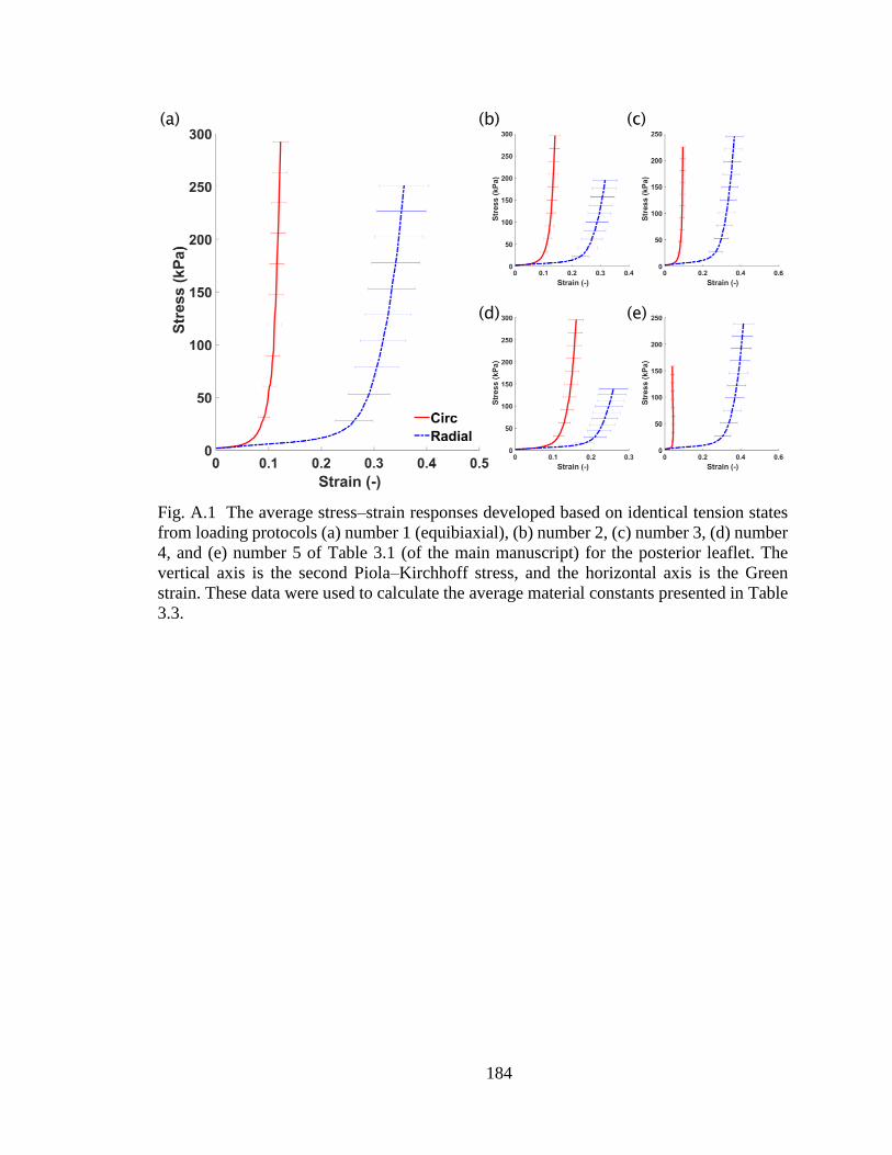
184

Fig. A.1 The average stress–strain responses developed based on identical tension states


4, and (e) number 5 of Table 3.1 (of the main manuscript) for the posterior leaflet. The

vertical axis is the second Piola–Kirchhoff stress, and the horizontal axis is the Green

strain. These data were used to calculate the average material constants presented in Table

3.3.

185

Fig. A.2 The average stress–strain responses developed based on identical first Piola–

Kirchhoff stress states from loading protocols (a) number 1 (equibiaxial), (b) number 2, (c)

number 3, (d) number 4, and (e) number 5 of Table 3.1 (of the main manuscript) for the

posterior leaflet. The vertical axis is the second Piola–Kirchhoff stress, and the horizontal

axis is the Green strain. These data were used to calculate the average material constants

presented in Table 3.4.

186

Fig. A.3 The average stress–strain responses developed based on identical Cauchy stress


number 4, and (e) number 5 of Table 3.1 (of the main manuscript) for the posterior leaflet.

The vertical axis is the second Piola–Kirchhoff stress, and the horizontal axis is the Green


3.5.

187

Fig. A.4 The average stress–strain responses developed based on identical tension states


4, and (e) number 5 of Table 3.1 (of the main manuscript) for the septal leaflet. The vertical

axis is the second Piola–Kirchhoff stress and the horizontal axis is the Green strain. These

data were used to calculate the average material constants presented in Table 3.3.

188

Fig. A.5 The average stress–strain responses developed based on identical first Piola–

Kirchhoff stress states from loading protocols (a) number 1 (equibiaxial), (b) number 2, (c)

number 3, (d) number 4, and (e) number 5 of Table 3.1 (of the main manuscript) for the

septal leaflet. The vertical axis is the second Piola–Kirchhoff stress, and the horizontal axis

is the Green strain. These data were used to calculate the average material constants

presented in Table 3.4.

189

Fig. A.6 The average stress–strain responses developed based on identical Cauchy stress


number 4, and (e) number 5 of Table 3.1 (of the main manuscript) for the septal leaflet.

The vertical axis is the second Piola–Kirchhoff stress, and the horizontal axis is the Green


3.5.

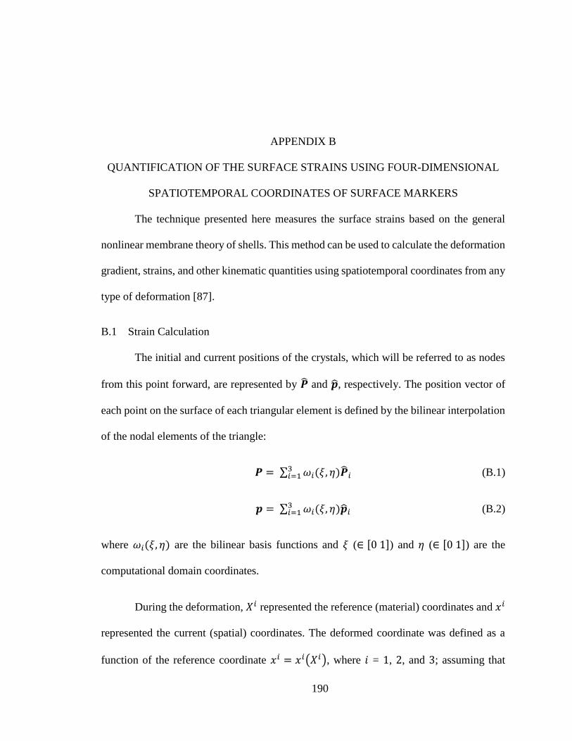
190

APPENDIX B

QUANTIFICATION OF THE SURFACE STRAINS USING FOUR-DIMENSIONAL

SPATIOTEMPORAL COORDINATES OF SURFACE MARKERS

The technique presented here measures the surface strains based on the general

nonlinear membrane theory of shells. This method can be used to calculate the deformation

gradient, strains, and other kinematic quantities using spatiotemporal coordinates from any

type of deformation [87].

B.1 Strain Calculation

The initial and current positions of the crystals, which will be referred to as nodes

from this point forward, are represented by �̂� and �̂�, respectively. The position vector of

each point on the surface of each triangular element is defined by the bilinear interpolation

of the nodal elements of the triangle:

𝑷 = ∑ 𝜔𝑖(𝜉, 𝜂)�̂�𝑖3𝑖=1 (B.1)

𝒑 = ∑ 𝜔𝑖(𝜉, 𝜂)�̂�𝑖3𝑖=1 (B.2)

where 𝜔𝑖(𝜉, 𝜂) are the bilinear basis functions and 𝜉 (∈ [0 1]) and 𝜂 (∈ [0 1]) are the

computational domain coordinates.

During the deformation, 𝑋𝑖 represented the reference (material) coordinates and 𝑥𝑖

represented the current (spatial) coordinates. The deformed coordinate was defined as a

function of the reference coordinate 𝑥𝑖 = 𝑥𝑖(𝑋𝑖), where 𝑖 = 1, 2, and 3; assuming that

191

𝑋3 = 𝑋3(𝑋1, 𝑋2), 𝑥𝑖 was rewritten as 𝑥𝑖 = 𝑥𝑖(𝑋1, 𝑋2) [87]. Therefore, the position vector

of a point at the reference configuration and that of the current configuration is written as:

𝑷 = 𝑋𝛼𝒆𝛼 + 𝑋3(𝑋1, 𝑋2)𝒆3 (B.3)

𝒑 = 𝑥𝛼(𝑋1, 𝑋2)𝒆𝛼 + 𝑥3(𝑋1, 𝑋2)𝒆3 (B.4)

where 𝛼 take values of 1 and 2 and the summation convention on repeated indices is

implied; and where 𝒆𝑖 represents an orthogonal coordinate system. The covariant base

vectors in un-deformed and deformed configurations are:

𝑮𝛼 = 𝑷,𝛼 = 𝒆𝛼 + 𝑋3,𝛼𝒆3 (B.5)

𝒈𝛼 = 𝒑,𝛼 = 𝑥𝛽,𝛼𝒆𝛽 + 𝑥3

,𝛼𝒆3 (B.6)

where 𝛼 and 𝛽 take values of 1 and 2 and the summation convention on repeated indices

is implied; and where ,𝛼 denotes derivative with respect to 𝑋𝛼 (𝜕 𝜕𝑋𝛼⁄ ). The third

covariant base vectors 𝑮3 and 𝒈3 were calculated as described previously [86]:

𝑮3 =𝑮1×𝑮2

‖𝑮1×𝑮2‖ (B.7)

𝒈3 =𝒈1×𝒈2

‖𝒈1×𝒈2‖ (B.8)

The components of the un-deformed metric tensors 𝐺𝑖𝑗 and the deformed metric

tensor 𝑔𝑖𝑗 were calculated using the covariant base vectors in the referential and current

configurations. The elements of the metric tensors are:

𝐺𝑖𝑗 = 𝑮𝑖 . 𝑮𝑗 (B.9)

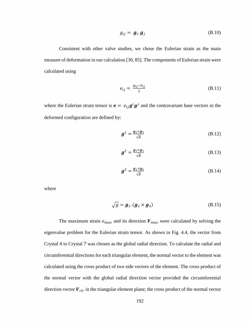
192

𝑔𝑖𝑗 = 𝒈𝑖. 𝒈𝑗 (B.10)

Consistent with other valve studies, we chose the Eulerian strain as the main

measure of deformation in our calculation [30, 85]. The components of Eulerian strain were

calculated using

𝑒𝑖𝑗 = 𝑔𝑖𝑗−𝐺𝑖𝑗

2 (B.11)

where the Eulerian strain tensor is 𝐞 = 𝑒𝑖𝑗𝒈𝑖𝒈𝑗 and the contravariant base vectors in the

deformed configuration are defined by:

𝒈1 =𝒈2×𝒈3

√𝑔 (B.12)

𝒈2 =𝒈3×𝒈1

√𝑔 (B.13)

𝒈3 =𝒈1×𝒈2

√𝑔 (B.14)

where

√𝑔 = 𝒈1. (𝒈2 × 𝒈3) (B.15)

The maximum strain 𝑒𝑚𝑎𝑥 and its direction 𝑽𝑚𝑎𝑥 were calculated by solving the

eigenvalue problem for the Eulerian strain tensor. As shown in Fig. 4.4, the vector from

Crystal 4 to Crystal 7 was chosen as the global radial direction. To calculate the radial and

circumferential directions for each triangular element, the normal vector to the element was

calculated using the cross product of two side vectors of the element. The cross product of

the normal vector with the global radial direction vector provided the circumferential

direction vector 𝑽𝑐𝑖𝑟 in the triangular element plane; the cross product of the normal vector

193

with the local circumferential direction vector provided the local radial direction vector

𝑽𝑟𝑎𝑑 in the triangular element plan. The circumferential and radial strains were then

calculated:

𝑒𝑐𝑖𝑟 = 𝑽𝑐𝑖𝑟 . 𝐞. 𝑽𝑐𝑖𝑟 (B.16)

𝑒𝑟𝑎𝑑 = 𝑽𝑟𝑎𝑑 . 𝐞. 𝑽𝑟𝑎𝑑 (B.17)

where 𝑒𝑐𝑖𝑟 and 𝑒𝑟𝑎𝑑 were circumferential and radial strains, respectively.

Finally, using the Eulerian strain definition, the areal strain was calculated as

𝑒𝑎𝑟𝑒𝑎𝑙 = 1 − 1

𝜆𝑎𝑟𝑒𝑎𝑙 (B.18)

where 𝜆𝑎𝑟𝑒𝑎𝑙, the areal change, was given by

𝜆𝑎𝑟𝑒𝑎𝑙 = √𝑑𝑒𝑡(𝑔𝑖𝑗)

𝑑𝑒𝑡(𝐺𝑖𝑗) (B.19)

B.2 Nomenclature

𝐞 = Eulerian strain tensor

𝑒𝑎𝑟𝑒𝑎𝑙 = Areal change

𝑒𝑐𝑖𝑟 = Circumferential strain

𝒆𝑖 = Orthogonal unit vectors

𝑒𝑖𝑗 = Components of the Eulerian strain tensor

194

𝑒𝑚𝑎𝑥 = Max principal strain

𝑒𝑟𝑎𝑑 = Radial strain

𝑔 = Square value of the scaling factor in the current (deformed) configuration

𝒈𝑖 = Covariant base vectors in the current (deformed) configuration

𝒈𝑖 = Contravariant base vectors in the current (deformed) configuration

𝑮𝑖 = Covariant base vectors in the referential (un-deformed) configuration

𝑔𝑖𝑗 = Components of the deformed metric tensor

𝐺𝑖𝑗 = Components of the un-deformed metric tensor

𝑖, 𝑗 = Dummy indices

𝑝 = p-value of paired student t-test

𝒑 = Position vector in the current (deformed) configuration

𝑷 = Position vector in the referential (un-deformed) configuration

�̂� = Position vector of a node in the current (deformed) configuration

�̂� = Position vector of a node in the referential (un-deformed) configuration

𝑡 = Time

𝑽𝑐𝑖𝑟 = Circumferential direction vector in the triangular element plane

𝑽𝑚𝑎𝑥 = Direction of the maximum principal strain

195

𝑽𝑟𝑎𝑑 = Radial direction vector in the triangular element plane

𝑥𝑖 = Current (spatial) coordinates

𝑋𝑖 = Reference (material) coordinates

,𝛼 = Derivative relative to 𝑋𝛼 (𝜕 𝜕𝑋𝛼⁄ )

𝛼, 𝛽 = Dummy indices (taking values 1 and 2)

𝜂 = Computational domain coordinate

𝜉 = Computational domain coordinate

𝜔 = Bilinear basis function

196

APPENDIX C

QUANTIFICATION OF THE MATERIAL CONSTANTS FOR A

PHENOMENOLOGICAL CONSTITUTIVE MODEL OF SMALL BOWEL

MESENTERY (APPLICATIONS OF THE METHOD DEVELOPED IN CHAPTERS II

AND III)

(The content of this chapter was published in JMBBM (Nov 2017) as “Anisotropic and

Nonlinear Biaxial Mechanical Responses of Porcine Small Bowel Mesentery” [142].)

C.1 Summary

Intestinal malrotation places pediatric patients at the risk of midgut volvulus, a

complication that can lead to ischemic bowel, short gut syndrome, and even death. Even

though the treatments for symptomatic patients of this complication are clear, it is still a

challenge to identify asymptomatic patients who are at a higher risk of midgut volvulus

and decide on a suitable course of treatment. Development of an accurate computerized

model of this intestinal abnormality could help in gaining a better understanding of its

integral behavior. To aid in developing such a model, in the current study, we have

characterized the biaxial mechanical properties of the porcine small bowl mesentery. First,

the tissue stress–strain response was determined using a biaxial tensile testing equipment.

The stress–strain data were then fitted into a Fung-type phenomenological constitutive

model to quantify the tissue material parameters. The stress–strain responses were highly

nonlinear showing more compliance at the lower strains following by a rapid transition into

a stiffer response at higher strains. The tissue was anisotropic and showed more stiffness

197

in the radial direction. The data fitted the Fung-type constitutive model with an average R-

squared value of 0.93. An averaging scheme was used to produce a set of material

parameters which can represent the generic mechanical behavior of the tissue in the

models.

C.2 Introduction

Intestinal malrotation, which occurs approximately in 1 out of 500 live births, is a

congenital disorder that is characterized by incomplete rotation and fixation of the

gastrointestinal tract to the abdominal wall during fetal development [223]. This

developmental arrest may occur during any of the phases of midgut development, resulting

in a wide spectrum of abnormalities, characterized by a narrowed mesenteric base [224].

This narrowed base predisposes a patient to midgut volvulus and possible subsequent

ischemic bowel disease, short gut syndrome and death. Midgut volvulus is one of the most

critical abdominal emergencies in the pediatric population. It is characterized by torsion of

small bowel and mesentery that could lead to blockage of mesenteric blood vessels and

ischemia of the small bowel. Midgut volvulus may lead to intestinal necrosis within a few

hours; thus, it requires immediate surgical intervention [225].

Increased imaging of patients has resulted in more incidental findings of

malrotation during workup for other anomalies [226]. While it is clear how to manage

symptomatic patients with malrotation, managing the treatment of asymptomatic patients

is more difficult because it is not known which patients are at a higher risk of midgut

volvulus. Because of this uncertainty coupled with the high morbidity and mortality

associated with volvulus, it is recommended by some to perform preventative operations

(i.e. a Ladd’s procedure) on all malrotation patients [227]. Others argue that the potential

198

long-term complications after a Ladd’s procedure, specifically future hospitalizations for

small bowel obstructions in 8.7 to 24% of patients, do not outweigh the relatively low risk

of midgut volvulus, and so recommend observation for asymptomatic patients [228-231].

This lack of consensus in the management of incidentally found intestinal

malrotation is likely due to the lack of quality data to support appropriate

recommendations, specifically, the lack of understanding of what degree of malrotation

results in increased propensity to torsion. Development of computational models of the

native and malrotated small bowel is useful to better understand the pathophysiology of

midgut volvulus. Using such models, one could examine how much mechanical torque is

required to deform tissues at different levels of malrotation and how such values compare

with normal cases. An important step in developing such models is the characterization of

the mechanical properties of the small bowel mesentery, which as a member of

gastrointestinal tract, plays an important role in this syndrome. Without accurate

mechanical properties for the small bowl mesentery, it is not possible to develop accurate

three-dimensional FE models of native and malrotated geometries. Previously, the

mechanical response of the mesentery has been quantified using uniaxial extension [232,

233]. In the current study, we used a biaxial mechanical testing equipment to quantify the

biaxial stress–strain response of the small bowel mesentery tissue. We further used a

phenomenological constitutive model to specify tissue material properties.

C.3 Material and Methods

C.3.1 Biaxial Tensile Testing Equipment

In this study, custom-made biaxial tensile testing equipment [40, 41, 117, 234] was

used to stretch specimens in two orthogonal directions under controlled loading. More

199

details about this testing equipment is provided in our previous publication [117]. Briefly,

a load cell measured the force applied in each direction independently. To quantify the

deformation, an optical deformation measurement system was used to track small fiducial

markers attached on the sample surface during the course of the experiment.

C.3.2 Specimen Preparation

On the day of the experiment, porcine mesenteries were obtained from a local

slaughterhouse (Duma Meats Inc., Mogadore, Ohio) within 20 minutes driving distance

from the laboratory. The pigs were about 6 months old and they weighed in approximately

300 𝑙𝑏 when slaughtered. Immediately after the animals were slaughtered, the mesenteries

were placed inside plastic bags filled with isotonic PBS and were covered with ice in a

cooling box for transport. Upon arrival at the lab, the proximal jejunum of the mesentery

was removed and 11 by 11 𝑚𝑚 square-shaped specimens were excised from three

different regions (distal avascular, distal vascular, and root) of the mesentery as shown in

Fig. C.1. The specimens were cut in such a way that the edges were aligned in the radial

and tangential directions of the mesentery. Using a dial micrometer (Anytime Inc., Los

Angeles, CA), the thicknesses were measured in six different locations on each specimen

and the result were averaged. All experiments were conducted at room temperature. Four

small glass beads (< 0.5 𝑚𝑚 in diameter) were glued on the surface of each specimen in

a 2 by 2 array format as the fiducial markers for optical deformation tracking.

200

Fig. C.1 The specimens were excised from (A) the distal avascular region, (B) the distal

vascular region, and (C) the root region of the porcine mesenteries.

C.3.3 Planar Biaxial Tensile Testing

The details of the experimental procedure are similar to those in our previous study

on TV leaflets [117]. In short, before attaching the specimen, the equipment bath was filled

with isotonic PBS at room temperature. Using suture-lines and small fishhooks (O. Mustad

& Son A.S., Gjörvik, Norway), the specimens were attached to the stretching carriages in

such a way that the radial direction was aligned with one axis and the tangential direction

with the other (Fig. C.2). This special technique for connecting samples to the stretching

components and the specific design of the carriages allow free lateral deformation of the

specimen and uniform and shear-free loading, which guarantees the uniform deformation

[117].

Each specimen experienced tension-controlled loading protocols with five different

tension ratios (𝑇𝑡: 𝑇𝑟 = 1: 1, 1: 0.75, 0.75: 1, 1: 0.5, 0.5: 1 with 𝑇𝑡 being the tangential

tension and 𝑇𝑟 being the radial tension). Table C.1 lists the loading protocols for each

specific region of the mesentery. Nine cycles of preconditioning were performed for each

201

loading protocol and data from the tenth cycle were utilized in the analysis. While a

minimum tare load of 0.5 𝑔 was applied for each case, the maximum tensions of 50, 100,

and 130 𝑁/𝑚 were selected for the distal avascular region, the distal vascular region, and

the root region of mesentery, respectively, as the strength of the tissue was not the same at

different regions. These maximum loads were selected experimentally based on the tissue

strength in order to prevent plastic deformation. Our data showed that the mechanical

response of the tissue samples did not change during the experiment with the chosen

maximum tension for each specific region. Each cycle lasted 10 seconds for the loading

step and 10 seconds for the unloading step. Therefore, the loading was quasi-static with

average strain rates of 3.2% and 2.5% per second for tangential and radial directions,

respectively.

Fig. C.2 (a) Suture lines are connected to the specimen using fishhooks. (b) Specimen

attached to the specifically-designed carriages of the equipment using suture-lines.

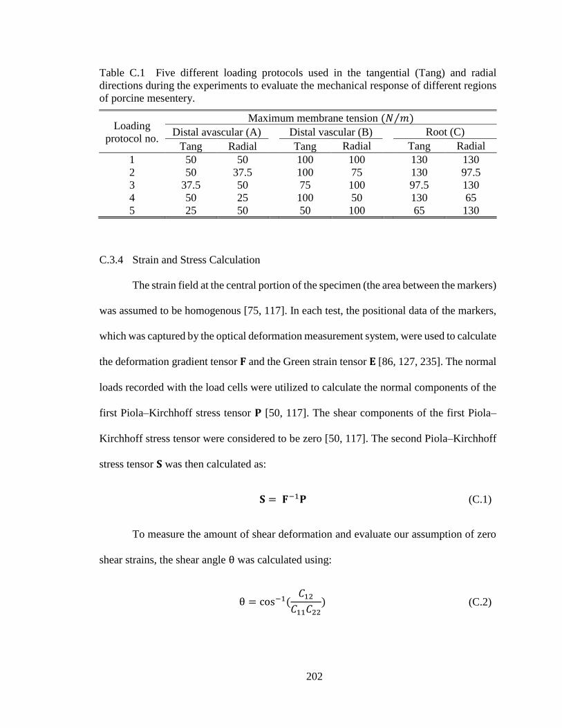
202

Table C.1 Five different loading protocols used in the tangential (Tang) and radial

directions during the experiments to evaluate the mechanical response of different regions

of porcine mesentery.

Loading

protocol no.

Maximum membrane tension (𝑁 𝑚⁄ )

Distal avascular (A) Distal vascular (B) Root (C)

Tang Radial Tang Radial Tang Radial

1 50 50 100 100 130 130

2 50 37.5 100 75 130 97.5

3 37.5 50 75 100 97.5 130

4 50 25 100 50 130 65

5 25 50 50 100 65 130

C.3.4 Strain and Stress Calculation

The strain field at the central portion of the specimen (the area between the markers)

was assumed to be homogenous [75, 117]. In each test, the positional data of the markers,

which was captured by the optical deformation measurement system, were used to calculate

the deformation gradient tensor 𝐅 and the Green strain tensor 𝐄 [86, 127, 235]. The normal

loads recorded with the load cells were utilized to calculate the normal components of the

first Piola–Kirchhoff stress tensor 𝐏 [50, 117]. The shear components of the first Piola–

Kirchhoff stress tensor were considered to be zero [50, 117]. The second Piola–Kirchhoff

stress tensor 𝐒 was then calculated as:

𝐒 = 𝐅−1𝐏 (C.1)

To measure the amount of shear deformation and evaluate our assumption of zero

shear strains, the shear angle θ was calculated using:

θ = cos−1(

𝐶12

𝐶11𝐶22) (C.2)

203

where 𝐶𝑖𝑗 were the components of the right Cauchy–Green deformation tensor 𝐂 defined

by

𝐂 = 𝐅T𝐅 (C.3)

The rigid body rotation angle ω was also calculated [117]:

ω = tan−1(

𝑅21

𝑅11) (C.4)

where rotation matrix 𝐑 was given by

𝐑 = 𝐅𝐔−1 (C.5)

and 𝐔 was the right stretch tensor:

𝐂 = 𝐔2 (C.6)

C.3.5 Constitutive Modeling

At each region, mesentery tissue was assumed to be incompressible, homogenous,

and hyperelastic undergoing finite deformations similar to other soft tissues [42, 53, 57-60,

62, 63, 65]. As such, we assumed that the mesentery tissue samples followed the concept

of pseudoelasticity [141]. The components of the second Piola–Kirchhoff stress tensor

were then evaluated using a strain energy function 𝑊:

𝑆𝑖𝑗 =

𝜕𝑊

𝜕𝐸𝑖𝑗 (C.7)

To determine an appropriate type of the strain energy function, the method

described by Vande Geest et al. [56] were utilized and the stress–strain behavior of the

204

tissue were carefully examined. Based on the Vande Geest et al. method, the stress–strain

data were independently fitted into the following response functions for each direction in

such a way that each normal component of the second Piola–Kirchhoff stress had its own

unique parameters:

𝑆𝑡𝑡 = 𝑐0 (𝑐1𝐸𝑡𝑡 + 𝑐3𝐸𝑟𝑟 + 𝑐4𝐸𝑡𝑡𝐸𝑟𝑟 +1

2𝑐5𝐸𝑟𝑟

2 + 𝑐6𝐸𝑡𝑡𝐸𝑟𝑟2

+ 2𝑐7𝐸𝑡𝑡3 ) 𝑒𝑄

𝑆𝑟𝑟 = 𝑐0 (𝑐2𝐸𝑟𝑟 + 𝑐3𝐸𝑡𝑡 + 𝑐5𝐸𝑡𝑡𝐸𝑟𝑟 +1

2𝑐4𝐸𝑡𝑡

2 + 𝑐6𝐸𝑡𝑡2 𝐸𝑟𝑟

+ 2𝑐8𝐸𝑟𝑟3 ) 𝑒𝑄

(C.8)

where 𝑡𝑡 and 𝑟𝑟 denoted tangential and radial directions, respectively, 𝐸𝑡𝑡 and 𝐸𝑟𝑟 were

the components of the Green strain tensor, and

𝑄 = (𝑐1𝐸𝑡𝑡2 + 𝑐2𝐸𝑟𝑟

2 + 2𝑐3𝐸𝑡𝑡𝐸𝑟𝑟 + 𝑐4𝐸𝑡𝑡2 𝐸𝑟𝑟 + 𝑐5𝐸𝑟𝑟

2 𝐸𝑡𝑡

+ 𝑐6𝐸𝑡𝑡2 𝐸𝑟𝑟

2 + 𝑐7𝐸𝑡𝑡4 + 𝑐8𝐸𝑟𝑟

4 )

(C.9)

It is important to note that the above equations did not represent a constitutive

model but they denoted a set of response functions, which were fitted to the data for each

direction independently allowing us to interpolate the stress components over the strain

field. After careful examination of the result of the fitting outcomes (the details are

explained in section 0

Response Function Interpretation), a Fung-type strain energy function 𝑊 [53] was

chosen to model the mechanical behavior of the mesentery:

205

𝑊 = 𝑐

2(𝑒𝑎1𝐸𝑡𝑡

2 +𝑎2𝐸𝑟𝑟2 +2𝑎3𝐸𝑡𝑡𝐸𝑟𝑟 − 1) (C.10)

where 𝑐 and 𝑎𝑖 were the material parameters and 𝐸𝑡𝑡 and 𝐸𝑟𝑟 were the component

of the Green strain tensor in the tangential and radial directions, respectively. The

experimental data for each specimen were fitted to this model to calculate the material

parameters in each case. To obtain a measure of the anisotropy of the responses, the

anisotropy index 𝐴𝐼 was also calculated for each set of material parameters. The anisotropy

index was calculated as described previously by Bellini et al. [58]:

𝐴𝐼 = 𝑚𝑖𝑛 (

𝑎1 + 𝑎3

𝑎2 + 𝑎3,𝑎2 + 𝑎3

𝑎1 + 𝑎3) (C.11)

C.3.6 Average Model Development

An ultimate goal of soft tissue mechanical characterization is to implement such

mechanical properties in computational models to be developed for simulation of the tissue

deformation. Certainly, one could apply each set of the specimen-specific constitutive

model parameters in subject-specific computational models or, alternatively, conduct

parametric studies to examine a range of mechanical properties [146, 236]. Yet, in many

cases, it is useful to produce a set of parameters representing the generic (average) tissue

mechanical behavior. In the case of linear elastic materials, one could evaluate the elastic

modulus for each specimen and then take the arithmetic mean of all values to obtain a

single average elastic modulus. However, in the presence of nonlinearity in the constitutive

model (similar to the model used in this study), a simple arithmetic average of the model

parameters cannot represent the overall behavior of the tissue. One way to overcome this

problem is to fit the constitutive model to the averaged experimental stress–strain curve

[58, 64]. In the current study, we first averaged the experimental strain values for each

206

protocol over all of the specimens. Clearly, we were only allowed to average the strains

over the same stress (loading) states. In such a case, the corresponding normal components

of stress in each direction had to be equal for all samples used in the averaging process (the

off-diagonal shear components of the stress tensor were supposed to be zero). Since the

biaxial tests were conducted in a tension-controlled manner, the same tension states were

available from similar protocols for all samples. However, it did not necessarily guarantee

that for every specific tension state in each sample, the identical values are available in

other samples. To solve this issue, other investigators [58, 64] had fitted the tension–strain

data into an exponential function for each test and evaluated the strains at the specific

tension values. The problem with using an exponential function is that it does not represent

the Poisson’s effect accurately. Since our data were dense enough, we were able to use an

interpolation method to estimate the tension value at any desired tension state. The

resulting data were then used to calculate the average tensions 𝑇𝑎𝑣𝑔,𝑖 and the average strains

𝐸𝑎𝑣𝑔,𝑖𝑖 were calculated by averaging the strains between all samples (𝑛 = 8) for each

protocol. The subscript 𝑖𝑖 refers to tangential 𝑡𝑡 and radial 𝑟𝑟 directions.

The components of the average first Piola–Kirchhoff stress tensor 𝑃𝑎𝑣𝑔,𝑖𝑖 were then

estimated as suggested by Bellini et al. [58]:

𝑃𝑎𝑣𝑔,𝑖𝑖 =

𝑇𝑎𝑣𝑔,𝑖

𝑛∑

1

ℎ𝑘

𝑛

𝑘=1

(C.12)

where ℎ𝑘 was the 𝑘th sample thickness. With the assumption of negligible shear

deformations, the diagonal components of the average deformation gradient tensor 𝐹𝑎𝑣𝑔,𝑖𝑖

were calculated:

207

𝐹𝑎𝑣𝑔,𝑖𝑖 = √2𝐸𝑎𝑣𝑔,𝑖𝑖 + 1 (C.13)

Finally, the average first Piola–Kirchhoff stress tensor and the average deformation

gradient tensor were used to calculate the average second Piola–Kirchhoff stress tensor:

𝑺𝑎𝑣𝑔 = 𝑷𝑎𝑣𝑔. 𝑭𝑎𝑣𝑔−𝑇 (C.14)

To develop the average constitutive model for each region of the mesentery,

𝑺𝑎𝑣𝑔 − 𝑬𝑎𝑣𝑔 data were fitted to the proposed strain energy function as described above

and the corresponding material parameters were evaluated.

C.4 Results

C.4.1 Dimensional Measurements

In total, twenty-four specimens in eight sets (𝑛 = 8 for each region) were tested.

Each set included one specimen from each region (distal avascular, distal vascular, and

root) of the same animal. All tests were performed within 2 to 6 hours postmortem to

eliminate probable erroneous results associated with the freezing and thawing of the

tissues. The measured thicknesses were 604 ± 279 𝜇𝑚 (mean ± standard deviation) for

the distal avascular, 1195 ± 531 𝜇𝑚 for the distal vascular, and 2162 ± 357 𝜇𝑚 for the

root region of the mesentery. Table C.2 shows the measured thicknesses for all the

specimens and for each region. The Student’s t-test analysis revealed that the thicknesses

were significantly different in all three regions (𝑝 < 0.015 for all comparisons).

C.4.2 Biaxial Mechanical Responses

Figure C.3 shows the average membrane tension versus the stretch ratio in different

regions of the porcine mesentery for the equibiaxial protocol. The maximum standard

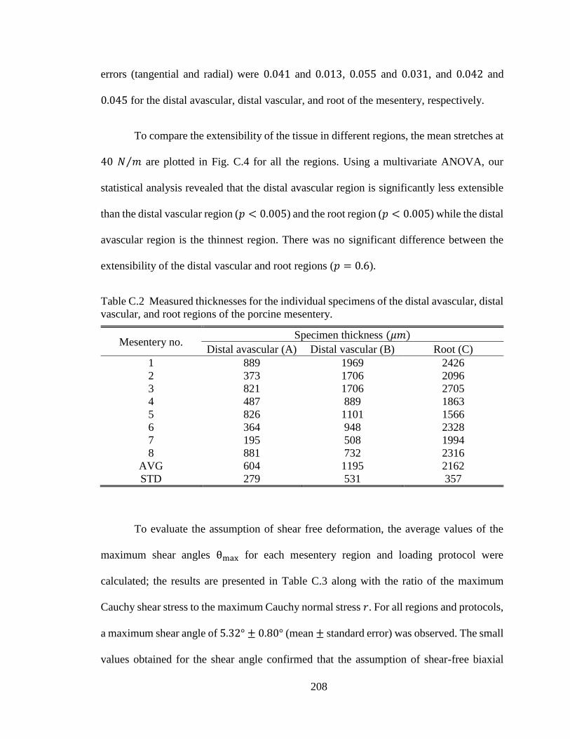
208

errors (tangential and radial) were 0.041 and 0.013, 0.055 and 0.031, and 0.042 and

0.045 for the distal avascular, distal vascular, and root of the mesentery, respectively.

To compare the extensibility of the tissue in different regions, the mean stretches at

40 𝑁 𝑚⁄ are plotted in Fig. C.4 for all the regions. Using a multivariate ANOVA, our

statistical analysis revealed that the distal avascular region is significantly less extensible

than the distal vascular region (𝑝 < 0.005) and the root region (𝑝 < 0.005) while the distal

avascular region is the thinnest region. There was no significant difference between the

extensibility of the distal vascular and root regions (𝑝 = 0.6).

Table C.2 Measured thicknesses for the individual specimens of the distal avascular, distal

vascular, and root regions of the porcine mesentery.

Mesentery no. Specimen thickness (𝜇𝑚)

Distal avascular (A) Distal vascular (B) Root (C)

1 889 1969 2426

2 373 1706 2096

3 821 1706 2705

4 487 889 1863

5 826 1101 1566

6 364 948 2328

7 195 508 1994

8 881 732 2316

AVG 604 1195 2162

STD 279 531 357

To evaluate the assumption of shear free deformation, the average values of the

maximum shear angles θmax for each mesentery region and loading protocol were

calculated; the results are presented in Table C.3 along with the ratio of the maximum

Cauchy shear stress to the maximum Cauchy normal stress 𝑟. For all regions and protocols,

a maximum shear angle of 5.32° ± 0.80° (mean ± standard error) was observed. The small

values obtained for the shear angle confirmed that the assumption of shear-free biaxial

209

loading was reasonable. Moreover, the average maximum values of 𝑟 were 2.7%, 4.4%,

and 10.3% for distal avascular, distal vascular, and root region, respectively. These small

values of 𝑟 (particularly for distal avascular and distal vascular regions) further show the

Cauchy shear stresses in comparison to the Cauchy normal stresses were negligible.

Moreover, the average maximum values of 𝑟 were 2.7%, 4.4%, and 10.3% for distal

avascular, distal vascular, and root region, respectively. These small values of 𝑟

(particularly for distal avascular and distal vascular regions) further show the Cauchy shear

stresses in comparison to the Cauchy normal stresses were negligible.

Table C.3 also represents the maximum rigid body rotation angles 𝜔𝑚𝑎𝑥. The

largest value of rigid body rotation was approximately 3 degrees, indicating minimal rigid

body rotation happened during the experiments.

210

Fig. C.3 The average membrane tension versus stretch ratio for the equibiaxial loading

protocol for (a) the distal avascular, (b) the distal vascular, and (c) the root regions of the

porcine mesenteries (n=8, the bars are standard errors).

Fig. C.4 The mean stretch values at 40 𝑁 ⁄ 𝑚 measured at three different regions of the

mesentery shown in Fig. C.1 for radial and tangential (Tang) directions. Bars are the

standard error (n=8).

211

Tab

le C

.3

The

aver

age

max

imum

rig

id b

od

y r

ota

tion 𝑤

𝑚𝑎

𝑥,

the

aver

age

max

imum

shea

r an

gle

𝜃𝑚

𝑎𝑥,

and t

he

aver

age

rati

o o

f th

e

max

imum

Cau

chy s

hea

r st

ress

to t

he

max

imum

Cau

chy n

orm

al s

tres

s 𝑟

pre

sente

d f

or

each

load

ing p

roto

col

and m

esen

tery

reg

ion

(for

each

pro

toco

l an

d m

esen

tery

reg

ion the

dat

a ar

e av

erag

ed o

ver

all

sam

ple

s (n

=8

) an

d p

rese

nte

d in the

form

of

aver

age

± s

tandar

d

erro

r).

Lo

adin

g

pro

toco

l no.

Dis

tal

avas

cula

r (A

)

Dis

tal

vas

cula

r (B

)

Root

(C)

𝜔𝑚

𝑎𝑥

(°)

𝜃 𝑚

𝑎𝑥

(°)

𝑟

(%)

𝜔

𝑚𝑎

𝑥 (

°)

𝜃𝑚

𝑎𝑥

(°)

r

(%)

𝜔

𝑚𝑎

𝑥 (

°)

𝜃 𝑚𝑎

𝑥 (

°)

r (%

)

1

1.0

±0.2

1.3

±0.2

2.7

±0.6

1.1

±0.2

3.1

±0.7

4.4

±1.1

3.1

±0.6

4.1

±0.7

10.3

±1.7

2

1.1

±0.3

1.4

±0.2

2.6

±0.5

1.1

±0.2

2.9

±0.6

4.0

±0.9

3.1

±0.6

4.6

±0.7

9.3

±1.6

3

1.0

±0.2

1.2

±0.2

2.4

±0.5

1.0

±0.2

3.1

±0.7

3.7

±0.8

3.0

±0.4

4.2

±0.7

10.1

±1.7

4

1.4

±0.3

1.6

±0.2

2.3

±0.4

1.2

±0.2

2.9

±0.7

3.7

±0.8

3.2

±0.8

5.3

±0.8

7.4

±1.2

5

1.2

±0.2

1.3

±0.3

2.1

±0.4

1.2

±0.2

3.2

±0.6

3.6

±0.5

2.9

±0.2

4.2

±0.7

8.7

±1.6

212

C.4.3 Response Function Interpretation

The measured biaxial stress–strain data fitted the response functions of Equation

(C.8) relatively well, with an R-squared value of 0.95 ± 0.05 (mean ± standard deviation).

To facilitate the selection of the strain energy function, graphs of constant stresses were

plotted over the strain field (versus 𝐸𝑡𝑡 and 𝐸𝑟𝑟). For an ideal isotropic material, the

constant stress contours are expected to be symmetric with respect to 𝐸𝑡𝑡 = 𝐸𝑟𝑟 line. As

shown in Fig. C.5 for typical specimens, the stress contours were asymmetric for all three

regions, indicating an anisotropic mechanical response. Moreover, the stress increased in

an exponential manner when strains increased. Such a specific form of the stress surfaces

and the negligibility of the shear stresses was the basis for the selection of an anisotropic

Fung-type [53] strain energy function 𝑊 in Equation (C.10).

Fig. C.5 The constant stress contours for (a) and (b) the distal avascular, (c) and (d) the

distal vascular, and (e) and (f) the root regions of a typical porcine mesentery specimens.

213

C.4.4 Constitutive Modeling

The data from all five biaxial protocols were simultaneously fit to the Fung-type

constitutive model represented by Equations (C.7) and (C.10). The result showed an

acceptable fit with the average R-squared values of 0.96, 0.94, and 0.89 for the distal

avascular, the distal vascular, and the root regions of the mesentery, respectively. Table

C.4 lists the material parameters calculated for each specimen as well as its corresponding

R-squared value for the fitted function. The calculated values for the anisotropy index are

also presented in Table C.4. An anisotropy index equal to 1 represented a perfectly

isotropic material while the smaller values of this index indicated the more anisotropic

response. Fig. C.6 shows the experimental biaxial data as well as the results for the five-

protocol fit for typical specimens from different regions of the mesentery.

214

Table C.4 Material parameters computed for individual samples by fitting the experimental

data to the proposed constitutive model along with the fitting R-squared values (𝑅2) and

the anisotropy index (𝐴𝐼).

Region Sample

no. 𝑐 (𝑘𝑃𝑎) 𝑎1 𝑎2 𝑎3 𝑅2 𝐴𝐼

Distal

avascular

(A)

1 3.857 53.954 72.196 8.801 0.955 0.775

2 11.702 46.903 54.974 22.641 0.986 0.896

3 0.827 75.819 361.473 0.000 0.952 0.210

4 2.654 5.207 39.053 1.814 0.919 0.172

5 1.918 15.547 67.351 6.228 0.957 0.296

6 1.273 39.360 43.100 0.000 0.983 0.913

7 11.974 42.318 37.526 15.170 0.946 0.917

8 2.415 69.101 49.698 20.429 0.975 0.783

AVG 4.578 43.526 90.671 9.385 0.959 0.620

STD 4.573 24.163 110.145 9.063 0.022 0.333

Distal

vascular

(B)

1 0.178 6.695 5.879 3.802 0.926 0.922

2 0.737 25.789 13.146 4.895 0.915 0.588

3 0.712 5.719 27.726 0.917 0.872 0.232

4 0.401 6.287 12.832 3.210 0.956 0.592

5 0.455 2.449 6.107 1.590 0.973 0.525

6 0.555 12.805 15.030 0.000 0.977 0.852

7 2.781 21.028 33.547 2.531 0.966 0.653

8 1.866 17.669 9.374 0.000 0.899 0.531

AVG 0.960 12.305 15.455 2.118 0.936 0.612

STD 0.894 8.410 10.045 1.797 0.038 0.212

Root

(C)

1 1.037 3.584 10.333 0.656 0.953 0.386

2 0.871 49.595 14.884 5.502 0.895 0.370

3 0.559 11.107 3.413 0.528 0.930 0.339

4 0.271 4.877 10.045 2.951 0.963 0.602

5 19.196 1.730 2.500 0.973 0.785 0.778

6 1.133 6.078 4.227 2.399 0.851 0.782

7 0.916 11.839 4.778 2.592 0.787 0.511

8 0.247 9.624 24.819 3.037 0.929 0.455

AVG 3.029 12.304 9.375 2.330 0.877 0.528

STD 6.541 15.497 7.566 1.644 0.071 0.177

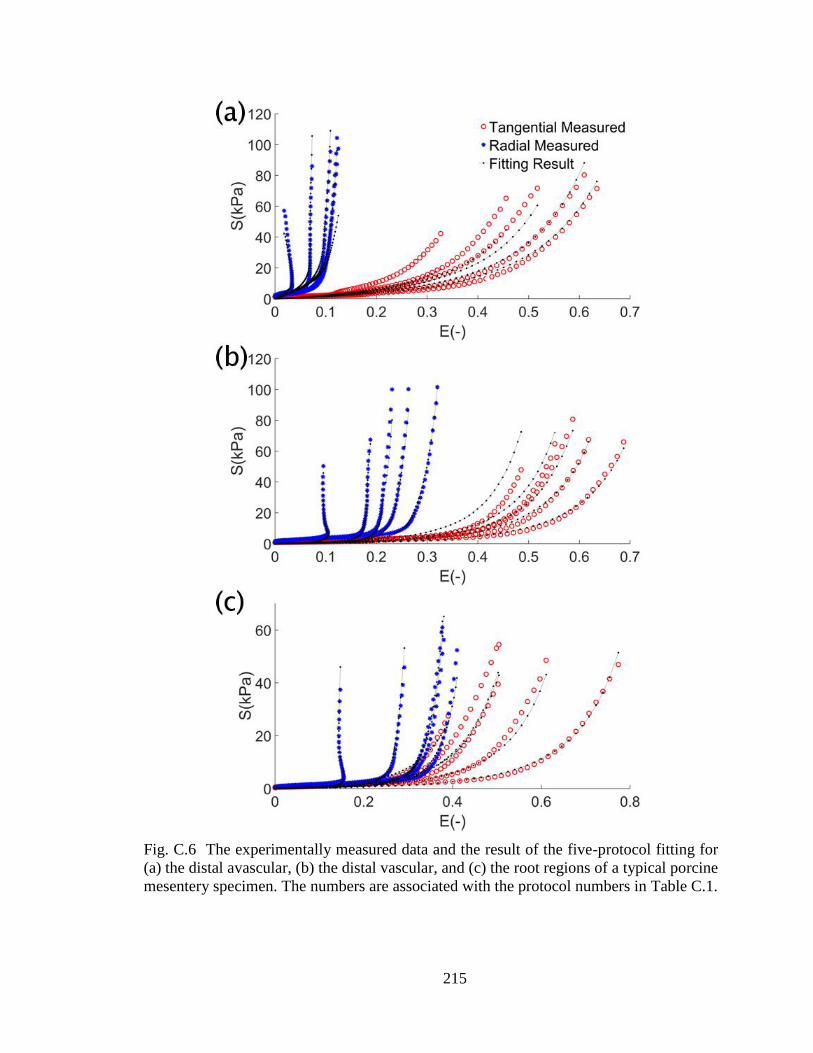
215

Fig. C.6 The experimentally measured data and the result of the five-protocol fitting for

(a) the distal avascular, (b) the distal vascular, and (c) the root regions of a typical porcine

mesentery specimen. The numbers are associated with the protocol numbers in Table C.1.

216

C.4.5 Average Modeling

The developed average stress–strain (second Piola–Kirchhoff stress versus Green

strain) responses are shown in Fig. C.7 for the distal avascular region for all five protocols.

Figures C.8 and C.9 show the same graphs for the distal vascular and root regions of the

mesentery, respectively. The same form of strain energy function was used to develop the

average material model. The averaged data fit the model with R-squared values of 0.97,

0.98, and 0.77 for the distal avascular, distal vascular, and root regions, respectively. The

calculated average material parameters are listed in Table C.5. As expected, these values

are different from the arithmetic average of the parameters calculated for each specimen

(listed in Table C.4). For comparison, Table C.5 also presents the anisotropy index 𝐴𝐼

calculated for the average models using Equation (C.11).

Fig. C.7 Average second Piola–Kirchhoff stress versus Green strain in tangential (Tang)

and radial directions for loading protocols (a) number 1 (equibiaxial), (b) number 2, (c)

number 3, (d) number 4, and (e) number 5 of Table C.1 for the distal avascular region.

217



number 3, (d) number 4, and (e) number 5 of Table C.1 for the distal vascular region.



number 3, (d) number 4, and (e) number 5 of Table C.1 for the root region.

218

C.5 Discussion

Although uniaxial extension can be an acceptable method in mechanical

characterization of tissues under in-situ one-dimensional loading, it has been deemed

insufficient for characterization of the mechanical responses of soft tissues experiencing

multiaxial loading in their native environment [237]. As biological soft tissues are

generally considered incompressible [42, 53, 57-60, 62, 63, 65], planar biaxial testing

provides a two-dimensional stress-state, allowing full characterization of the mechanical

properties of the tissues [50].

The thickness of the tissue varied significantly among the three regions (𝑝 < 0.02

for all comparisons). The thickest region, i.e. the root region, was found to be

approximately 3.5 times thicker than the distal avascular region, which was the thinnest.

These substantial differences among the thicknesses led to the use of different maximum

tensions for each region.

The mesentery tissue showed a highly nonlinear behavior in all three regions with

low stiffness at small strains and dramatically higher stiffness at larger strains, which was

a typical behavior for a soft tissue [69, 238-240]. Both in the avascular region and in the

vascular region of the distal mesentery, the deformation was larger in the tangential

direction in comparison to that of the radial direction indicating an anisotropic tissue

behavior (Fig. C.3). In the root region, however, no notable differences were observed

between the stretch values in the tangential and radial directions.

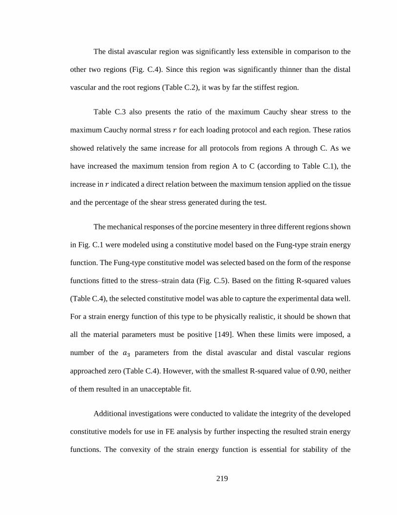
219

The distal avascular region was significantly less extensible in comparison to the

other two regions (Fig. C.4). Since this region was significantly thinner than the distal

vascular and the root regions (Table C.2), it was by far the stiffest region.

Table C.3 also presents the ratio of the maximum Cauchy shear stress to the

maximum Cauchy normal stress 𝑟 for each loading protocol and each region. These ratios

showed relatively the same increase for all protocols from regions A through C. As we

have increased the maximum tension from region A to C (according to Table C.1), the

increase in 𝑟 indicated a direct relation between the maximum tension applied on the tissue

and the percentage of the shear stress generated during the test.

The mechanical responses of the porcine mesentery in three different regions shown

in Fig. C.1 were modeled using a constitutive model based on the Fung-type strain energy

function. The Fung-type constitutive model was selected based on the form of the response

functions fitted to the stress–strain data (Fig. C.5). Based on the fitting R-squared values

(Table C.4), the selected constitutive model was able to capture the experimental data well.

For a strain energy function of this type to be physically realistic, it should be shown that

all the material parameters must be positive [149]. When these limits were imposed, a

number of the 𝑎3 parameters from the distal avascular and distal vascular regions

approached zero (Table C.4). However, with the smallest R-squared value of 0.90, neither

of them resulted in an unacceptable fit.

Additional investigations were conducted to validate the integrity of the developed

constitutive models for use in FE analysis by further inspecting the resulted strain energy

functions. The convexity of the strain energy function is essential for stability of the

220

material model in FE analysis [153]. Hence, the evaluated material parameters for the

proposed constitutive model were used to plot the constant strain energy contours over the

strain field in each case. Investigation of these plots showed that all the estimated material

parameters resulted in convex potentials, as shown in Fig. C.10 for typical specimens of

all three regions of the mesentery, further improving the integrity of the developed model.

An average model was developed that can be used in computer simulations to

predict the average mechanical behavior of the tissue. Figures C.7–C.9 show the averaged

stress-stain data calculated for three regions of the mesentery; the material parameters

computed by fitting these average responses to the proposed constitutive model are listed

in Table C.5. The fitting R-squared value for the distal avascular region was 0.97 and for

the distal vascular regions was 0.98, showing a reliable fit for these data. As expected, the

material parameters computed for average model were different from the arithmetic

averages of the material parameters of individual specimens listed in Table C.4. The

anisotropy index 𝐴𝐼 obtained from the average model (Table C.5) for the distal avascular

and distal vascular regions (0.502 and 0.702, respectively) indicated anisotropic behavior

of the tissue at these two regions, which was consistent with the plots in Figs. C.3, C.7, and

C.8 and also with the averaged 𝐴𝐼 presented in Table C.4 (0.620 and 0.612, respectively).

Table C.5 Material parameters computed by fitting the averaged stress–strain data to the

proposed constitutive model along with the fitting R-squared (𝑅2) and the anisotropy index

(𝐴𝐼).

Region 𝑐 (𝑘𝑃𝑎) 𝑎1 𝑎2 𝑎3 𝑅2 𝐴𝐼

Distal avascular (A) 2.808 29.870 65.742 6.287 0.972 0.502

Distal vascular (B) 0.381 9.741 14.811 2.175 0.975 0.702

Root (C) 1.521 5.528 5.447 2.204 0.765 0.990

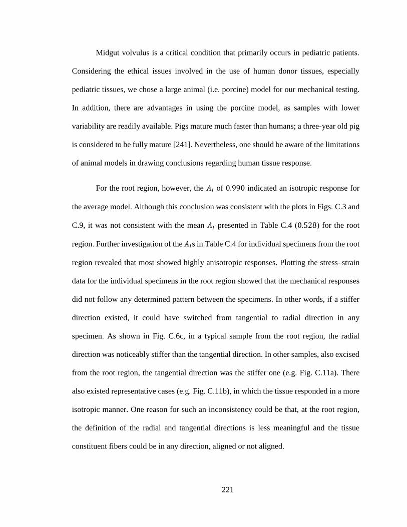
221

Midgut volvulus is a critical condition that primarily occurs in pediatric patients.

Considering the ethical issues involved in the use of human donor tissues, especially

pediatric tissues, we chose a large animal (i.e. porcine) model for our mechanical testing.

In addition, there are advantages in using the porcine model, as samples with lower

variability are readily available. Pigs mature much faster than humans; a three-year old pig

is considered to be fully mature [241]. Nevertheless, one should be aware of the limitations

of animal models in drawing conclusions regarding human tissue response.

For the root region, however, the 𝐴𝐼 of 0.990 indicated an isotropic response for

the average model. Although this conclusion was consistent with the plots in Figs. C.3 and

C.9, it was not consistent with the mean 𝐴𝐼 presented in Table C.4 (0.528) for the root

region. Further investigation of the 𝐴𝐼s in Table C.4 for individual specimens from the root

region revealed that most showed highly anisotropic responses. Plotting the stress–strain

data for the individual specimens in the root region showed that the mechanical responses

did not follow any determined pattern between the specimens. In other words, if a stiffer

direction existed, it could have switched from tangential to radial direction in any

specimen. As shown in Fig. C.6c, in a typical sample from the root region, the radial

direction was noticeably stiffer than the tangential direction. In other samples, also excised

from the root region, the tangential direction was the stiffer one (e.g. Fig. C.11a). There

also existed representative cases (e.g. Fig. C.11b), in which the tissue responded in a more

isotropic manner. One reason for such an inconsistency could be that, at the root region,

the definition of the radial and tangential directions is less meaningful and the tissue

constituent fibers could be in any direction, aligned or not aligned.

222

Fig. C.10 Constant energy contours plotted over the strain field for typical samples of (a)

the distal avascular, (b) the distal vascular, and (c) the root regions of the porcine

mesentery.

223

Fig. C.11 The mechanical responses observed for the root region of the porcine mesentery

did not always follow the same trend. For example, tissue was (a) stiffer in tangential

direction, or (b) had similar stiffness in both directions, noticeably different from other

typical cases in this region (Fig. C.6c). The numbers are associated with the protocol

numbers in Table C.1.

224

Based on our analysis using the response functions, we chose an appropriate form

of a phenomenological Fung-type constitutive model. Predicting tissue responses using

only a few parameters is extremely advantageous, as increasing the number of model

parameters can adversely affect the uniqueness of the fitted values. The phenomenological

models, however, are inherently limited as they provide little or no insight into the micro-

scale mechanical environment. For investigations that require knowledge of extracellular

and/or cellular-level biomechanical responses of the tissues, the use of more complex

structurally-based models is more appropriate [69].

As previously mentioned, development of a computerized model to better

understand the pathophysiology of midgut volvulus is essential. To bring us one step closer

to this goal, in the current study, the biaxial mechanical properties of the small bowel

mesentery, a tissue with major influence in the deformation of small bowel during midgut

volvulus, was characterized. The parameters quantified in this study can be employed in

FE models to simulate the mechanical behavior of the mesentery in different geometries.

biomechanical characterization and simulation of the

Documents

Transcript of biomechanical characterization and simulation of the