Food Policy 37 (2012) 439–451

Contents lists available at SciVerse ScienceDirect

Food Policy

journal homepage: www.elsevier .com/locate / foodpol

Biofuels and the poor: Global impact pathways of biofuels on agricultural markets

Jikun Huang a, Jun Yang a, Siwa Msangi b, Scott Rozelle c,d,⇑, Alfons Weersink e

a Center for Chinese Agricultural Policy, Chinese Academy of Sciences, Chinab International Food Policy Research Institute, United Statesc Stanford University, United Statesd University of Waikato, New Zealande University of Guelph, Canada

a r t i c l e i n f o

Article history:Received 15 August 2011Received in revised form 9 March 2012Accepted 12 April 2012Available online 24 May 2012

Keywords:BiofuelsGlobal marketsDeveloping countriesPrices

0306-9192/$ - see front matter � 2012 Elsevier Ltd. Ahttp://dx.doi.org/10.1016/j.foodpol.2012.04.004

⇑ Corresponding author at: Freeman Spogli InstituStanford University, Encina Hall East, E407 Stanford, C

E-mail address: rozelle@stanford.edu (S. Rozelle).

a b s t r a c t

This study seeks to assess the future impacts of biofuel production on regional agricultural and relatedsectors over the next decade with a specific focus on the vulnerable regions of developing nations. Usinga modification of the GTAP modeling platform to account for the global interactions of regional biofueland food markets, the analysis shows that biofuel production levels depend on the assumption aboutthe future price of energy and the nature of the substitutability between biofuels and petroleum-basedtransport fuels. Low energy prices reduce the demand for biofuels and thus require greater governmentsupport to meet the desired production targets. At the other extreme, when prices are high and there isscope for substituting biofuels for petroleum-based fuels, the volume of biofuels produced will exceedthe mandates. Even when biofuels are being mainly produced in developed countries, our results indicatethat there are impact pathways that extend far beyond the borders of the US, Brazil and the EU. Prices offeedstock and non-feedstock commodities rise in developing countries. There is also a rise in value addedfrom the agricultural sector—a gain that is enjoyed by the owners of land and labor, including unskilled.Hence, to the extent that agriculture is a key sector in getting growth started and addressing povertyneeds, the emergence of biofuels can (in this way at least) be a positive force.

� 2012 Elsevier Ltd. All rights reserved.

Introduction

The food versus fuel debate continues to swirl due partially tothe lack of understanding on the distributional consequencesacross sectors and regions from the expansion in biofuels. Thisexpansion occurred rapidly in the last decade with ethanol levelsincreasing approximately five times over this period to 66.6 mil-lion tons and biodiesel levels growing at an even greater rate to13.5 million tons by 2009 (see Table 1). The growth has been dri-ven by a combination of market developments, such as high fossilfuel prices, and policy levers, such as production mandates. Themotivations for policy intervention to spur biofuel productionrange from enhancement of domestic energy security, to reductionof CO2 emissions, and to increasing value-added from the agricul-tural sector (Linden et al., 2006; Charlesa et al., 2007; FAO, 2008a;OECD, 2008; Tyner, 2008; Westhoff, 2010).

Agricultural commodity prices have risen significantly since2006 and the increasing demand by the biofuel sector for feed-stocks has contributed to that increase (Paarlberg, 2010; Westhoff,2010). The US ethanol industry, as an example, will require almost

ll rights reserved.

te for International Studies,A 94305-6055, United States.

5 billion bushels of corn in 2011, which is approximately 40% of theprevious year’s crop (USDA, 2011). The reduction in supply forfeedstock crops from the US and other major biofuel producers de-creases the supply on world markets and pushes up global prices.These changes in agricultural commodity prices, regardless of thereason for the change, have triggered concerns from governmentsand development agencies about implications for food security andpoverty around the world (FAO, 2008b; IFPRI, 2008; Rosegrantet al., 2008; Tangermann, 2008; Ewing and Msangi, 2009).

The effects of biofuels and the higher prices that their emergencemay cause, however, may not be all bad for developing countries andthe poverty that they face. In the same way that Green Revolutiontechnology (e.g., Otsuka et al., 1994; Pingali and Traxler, 2002) andinternational trade agreements (e.g., Martin and Anderson, 2006)can have differential effects on the populations of developing coun-tries, helping some, while hurting others, biofuels also may havesimilar impacts. In theory, consumers stand to lose the most, espe-cially poor consumers with little ways to offset higher food prices.Many small farmers that produce some, but, buy more than they sell,would also be hurt while farmers who are net-sellers, especially ifthey own land, benefit from the higher crop prices. The higher pricesmay also lead to higher demand for labor. These hypothesizedeffects appear to have been validated at the aggregate level at leastby the occurrence of riots spurred partially by the jump in commod-

Table 1Biofuel production in major countries, 1996–2009 (million ton). Sources: World data are from US Renewable Fuels Association (2010), Earth Policy Institute (2010), BIODIESEL2020 (2008), and F.O. Licht (2009); USA’s data are from US Renewable Fuels Association (2010) and BIODIESEL 2020 (2008); EU’s data are from European Biodiesel Board (2010);Brazil data are from Renewable Fuels Associations (2010); China’s data are from Qiu and Huang (2008) and Renewable Fuels Associations (2010)

1996 2000 2001 2002 2003 2004 2005 2006 2007 2008 2009

EthanolWorld 16.2 15 16.2 18.8 23.7 26.5 35.3 39.8 44.2 59.1 66.6USA 3.6 5.3 5.8 7.0 9.2 11.1 12.8 15.9 21.3 29.5 34.7EU27 n/a 0.2 0.2 0.4 0.4 0.5 0.8 1.5 1.6 2.1 2.9Brazil 12.5 9.2 10 10.9 12.8 13.1 13.9 14.7 16.5 21.3 21.6China – – – 0 0.1 0.2 0.8 1.3 1.4 1.4 1.6

BiodieselWorld 0.5 0.8 1 1.3 1.6 2 3.4 6.6 9 13.3 13.5USA n/a n/a n/a n/a n/a 0.1 0.2 0.8 2.1 2.9 1.8EU27 n/a n/a 0.9 1.1 1.4 1.9 3.2 4.9 5.7 7.8 9.0

n/a: data is not available. –: nearly zero.

440 J. Huang et al. / Food Policy 37 (2012) 439–451

ity prices in food importing countries with a high proportion of ur-ban poor.

Despite these concerns and complexities, there are few system-atic efforts to track the pathways of biofuel production trends fromthe major producing countries to the developing world throughmodels that account for the forces of global supply, demand andtrade (as well as attempt to identify what factors will amplify glo-bal price effects and what factors will attenuate them). There are anumber of high quality modeling efforts that are concerned withbiofuels (e.g., Banse et al., 2008; Birur et al., 2008; Hayes et al.,2009; Fonseca et al., 2010; Hertel et al., 2010; Taheripour et al.,2010; FAPRI, 2011). However, due to shortcomings such as a regio-nal focus (i.e. US or EU) or a partial rather than general equilibriumfocus, or no explicit accounting for a biofuels supply and demandsector, these models do not sufficiently capture the complexitiesof global biofuel and food markets.

This study seeks to assess the future impacts of biofuel produc-tion on regional agricultural and related sectors over the next dec-ade with a specific focus on the vulnerable regions of developingnations. Using a modeling platform created to account for the glo-bal interactions of regional biofuel and food markets, the analysisaims to provide answers for the following questions. First, how willthe rise in demand for biofuels affect food prices, production andtrade at a global level? Second, how will the development of globalbiofuels affect prices, production, trade and the unskilled wage inthe developing countries? Answers to the above questions willbe used to discuss policy recommendations regarding the develop-ment of economically and socially sound biofuels program in theworld.

Our paper, although ambitious, has several limitations. In thispaper we only simulate the impact of the emergence of biofuelsin the three main producing regions—the US, the EU and Brazil.Other countries have plans to develop biofuels, but, since in com-parison to the major producers their volumes of production willbe relatively small, we ignore the emergence of biofuels in allbut the ‘‘big three.’’ In addition, we do not allow for cellulosic orother second generation biofuels. The uncertainty of the produc-tion of biofuels from these technologies is sufficiently large thatwe believe it will not materially affect the world’s biofuels equa-tion in the next decade. Finally, in this paper while we allow forthe expansion of biofuels feedstock crops onto cultivated land thatis currently producing other crops, we do not explicitly allow for itsexpansion. This means, necessarily, that our price effects will be onthe high side, since all of the additional pressure from the in-creased demand for biofuel feedstock crops will have to be metby increased yields.

The next section of the paper provides an overview of biofuelgrowth in the three major production regions and future targets.The third section discusses the methodology developed for assessing

the impact of biofuel development at the country-level along withdefining the base reference scenario and several alternatives basedon policy options, energy prices, and the ability to substitute be-tween biofuels and fossil fuels. The following section presents theresults of our modeling efforts including the impacts of alternativebiofuel development scenarios on world food production and price,national production, and international trade. The last section con-cludes the study with a brief discussion of the policy implicationsof the development of biofuels on food security and poverty and dis-cusses issues for further study.

Biofuel production; past and future developments

The biofuel sector had been in commercial existence for a gen-eration before its rapid rise over the last decade. The United Statesand Brazil started their biofuel development programs in the mid-dle of the 1970s in response to the OPEC-driven increase in fuelprices and the subsequent concern about domestic energy security.In 1975, global ethanol production was only 420 thousand tonsand biodiesel was not available, as commercial manufacturingdid not begin until the early 1990s. By 2000, the annual productionof ethanol and biodiesel had reached a total of 15 and 0.8 mil-lion tons, respectively (Table 1). Biofuel production has increasedsteadily since the beginning of the decade and reached 80.1 mil-lion tons in 2009 with production concentrated in three main re-gions: the United States, Brazil and the European Union. Therapid growth has been spurred partially by the profitability for pro-duction, which is tied to the relative cost of oil and feedstockprices, but largely by government policies (Steenblik, 2007; FAO,2008a; OECD, 2008).

The United States, which now produces more than half of theworld’s ethanol, began its promotion of ethanol production withthe Energy Tax Act of 1978. Biofuel producers were granted fullexemption of the federal gasoline excise tax when they producedgasoline blended with 10% ethanol resulting in an effective subsidyof US 40 cents per gallon of ethanol (UN, 2006). The subsidy wasextended in 1980 to other blend levels including E85 (an etha-nol–gasoline blend which is produced with 85% ethanol). In2007, the United States provided a US 51 cent per gallon tax refundfor blenders of ethanol and a tax credit to biodiesel producers(Yacobucci, 2010). In addition to subsidies, the emerging US biofuelsector was protected through an import tariff on ethanol fromoutside NAFTA (UN, 2006; Tyner, 2008).

The growth in US ethanol production was further spurred by the1990 Clean Air Act that required a minimum percentage of oxygenin gasoline. Initially, this requirement was met through the addi-tion to gasoline of methyl tertiary butyl ether (MTBE). Contamina-tion problems with this highly toxic fuel additive arose and MTBE

1 GTAP is a well-known, multi-country, multi-sector computable general equilib-rium model (Hertel, 1997). The model is based on the neo-classical assumptions thatproducers minimize their production costs and consumers maximize their utilitiessubject to a set of certain common constraints. Supplies and demands of allcommodities clear by adjusting prices in perfectly competitive markets. On theproduction side, firms combine intermediate inputs and primary factors (e.g., land,labor, and capital) to produce commodities with constant-return-to-scale technology.Intermediate inputs are composites of domestic and foreign components with theforeign component differentiated by region of origin (the Armington assumption).

J. Huang et al. / Food Policy 37 (2012) 439–451 441

was gradually banned across the US and replaced by ethanol. Theincrease in demand for ethanol put a premium on its price.Combined with higher gasoline prices, existing subsidy levels andlow feedstock prices, the profitability in ethanol production ledto the rapid construction of corn-based ethanol plants in the USduring the mid-2000s.

The ‘‘Energy Independence and Security Act’’ passed in 2007shifted the US policy emphasis towards mandates (Tyner, 2010).The Renewable Fuel Stands (RFSs) has set ambitious targets forUS’s biofuel production of 15.2 billion gallons in 2012, 30 bil-lion gallons in 2020 and 36 billion gallons in 2022. These volumet-ric mandates are partitioned based on source (conventional,cellulosic, and other) with the target for corn-based ethanol setat 15 billion gallons. Although subsidies and research funding existfor the development of second-generation biofuels, the RFS is nottechnology neutral and is biased toward corn ethanol (Tyner,2010).

Brazil is the second largest producer of ethanol in the worldwith approximately one-third of global production in 2009 (Table1). It was the largest producer until 2006 due partially to thegreater energy efficiency of ethanol produced with sugar cane asopposed to corn. Its growth was stimulated largely by the govern-ment inducing consumers to choose biofuels as a fuel substitute. Inthe 1970s, the government of Brazil established a National FuelEthanol Program to increase the share of domestically producedbiofuel used in the transport sector. This included promoting theavailability of ethanol at most gasoline stations and mandatingthe manufacture of flexible fuel cars capable of using pure gasoline,E25 or pure bio-ethanol. The result is that ethanol comprised 20%of Brazil’s total transport-fuel demand in 2007 (Nass et al., 2007).Although ethanol prices were liberalized in the 1990s, the govern-ment provides other measures of support for the sector including amandatory official blending ratio of ethanol to gasoline, a lowerexcise tax of ethanol than gasoline, and an ad-valorem duty onimported ethanol (Pousa et al., 2007). The goal of the Braziliangovernment is to have ethanol production reach 9.5 billion gallonsby 2012 (31 million tons) and 11.5 billion gallons by 2016(37.7 million tons) (Timilsina and Shrestha, 2010).

The other major producing region for biofuels is Europe withthe bulk of its output in the form of biodiesel produced from rape-seed. The EU accounts for three-quarters of the world’s biodieselwith 5.7 million tons generated in 2007 and this level nearly dou-bled to 9 million tons in 2009. Within the EU, Germany is the lead-ing producer of biodiesel with two-thirds of the world marketshare while France and Italy are the other major producing coun-tries (European Biodiesel Board, 2011).

EU policy makers left the decision to support the productionand use of biofuels to Member States rather than be mandated cen-trally but its 2003 Biofuel Directive suggested a target of 5.75% oftotal petrol and diesel used for transport be provided by biofuels.The share is to increase to 6.25% for 2015. In the mid-2000s, theEU began to direct its Member States to set up the necessary legis-lation to ensure compliance. Tax concessions for the promotion ofbiofuel use were also allowed and part of the reason for the signif-icant growth in German production is the total tax exemption pro-vided to biofuels (Steenblik, 2007). In addition, tariffs are imposedon imported biodiesel, area payments are provided for crops usedin energy production, and minimum blending rates are legislatedby some EU countries (Sorda et al., 2010). The latest EU directivein 2009 increased the mandatory targets for 2010 so that 20% ofenergy is from renewable sources with 10% of transport fuel con-sumption from biofuels. These mandates are based on energy unitsso the choice of technology and feedstock is free for the privatesector to choose as opposed to the volumetric mandates in theUS for first (starch-based) and second (cellulosic-based) biofuels(Tyner, 2010).

Methodology and scenarios

In this section, we present the methodology and scenarios thatare used in this study to assess the implications of global and regio-nal biofuel growth for agriculture and the rest of the economy—including impacts inside and outside countries that have majorbiofuel efforts.

Methodology

To assess the impacts of biofuel development on agriculture andthe rest of the economy, we have built an analytical frameworkbased on the Global Trade Analysis Project (GTAP) platform.1 It isa general equilibrium model and as such is better suited to accountfor the direct and indirect feedback effects of biofuel policies in a glo-bal context (Kretschner and Peterson, 2010). The GTAP platform al-lows us to model the linkages among biofuel production, energyand global agricultural markets. GTAP also allows us to track the im-pacts from world markets to specific countries or regions, includingdeveloping countries. To carry out the impact analysis, we havemade a number of key modifications and improvements to the stan-dard GTAP model.

Introducing biofuels into the GTAP databaseWe use version 7 of the GTAP database in this study. The stan-

dard GTAP database includes 57 sectors of which 20 represent agri-cultural and processed food sectors. Despite the relatively highlevel of disaggregation, many of the biofuels feedstock crops areaggregated with non-feedstock crops. For example, corn is aggre-gated with other coarse grains and rapeseed is part of a broader oil-seeds category. The standard GTAP database also does not have anindustrial sector for the production of either ethanol or biodiesel.

Our model modifies the standard database in three ways. First,we spilt the key biofuels feedstock crops from the broad categorieswhere they currently reside so that they are represented explicitlyin the model database. For example, we disaggregate corn fromcoarse grains along with soybeans and rapeseed from oilseedsusing a ‘‘splitting’’ program (SplitCom) developed by Horridge(2005). In making the split, we used trade data from the United Na-tions Commodity Trade Statistics Database (UNCOMTRADE) andproduction and price data from the FAO. Second, we created fournew industrial sectors for production activities associated withbiofuels: sugar ethanol, corn ethanol, soybean biodiesel and rape-seed biodiesel. Third, our model was adjusted to consider the ef-fects of the by-products from biofuel production. The priceimpacts on feedstocks from ethanol can be reduced since livestockproducers can substitute by-products for feed inputs, such asgrains and oilseed meals (Taheripour et al., 2010).

Linkage between agriculture and energy markets through biofuelsectors

One of the key parts of the modification to the basic GTAPframework is the comprehensive representation of biofuel produc-tion. The manufacturing of the four biofuels depends on the mainfeedstocks plus capital and labor, which are inputs also used incrop production. Consumers in the model are allowed to substitutebetween biofuels and fossil fuels, and since biofuel production uses

2 Since processed feed is included in the processed food sector in GTAP, thesubstitutability between BDBP and processed feed is captured by the substitutionbetween BDBP and processed food.

442 J. Huang et al. / Food Policy 37 (2012) 439–451

crop sector outputs for inputs, an explicit link between agriculturaland energy markets is thereby created.

The linkages were made as realistic as possible with severalmodifications to the original GTAP framework. For example, weextended the standard GTAP model by introducing the energy-capital substitution relationships that are described in the GTAP-E (energy) model, which is widely used for the analysis of energyand climate change policy (Burniaux and Truong, 2002). The sub-stitution between biofuels and fossil fuel is incorporated into thestructure of GTAP-E using a nested CES function between biofuels(ethanol and biodiesel) and petroleum products in a similar way tothe approaches taken by others who have added a biofuel sector tothe GTAP-E model (e.g., Birur et al., 2008; Hertel et al., 2010). Theelasticity of substitution between fossil fuel and biofuels is crucialin our research since it will be an important element that ties theprice of energy to the price of food. Interestingly, in past researchon biofuels in the US, EU and Brazil, the values of the elasticity ofsubstitution are almost all identical to those used by Hertel et al.(2010), who set their substitution parameters for the US, EU andBrazil equal to 3.0, 2.75 and 1.0 respectively. Our assumptions(and the impact of using different substitution parameters on thepredictions of future outcomes) are discussed below.

Allocation of agricultural landAn increase in biofuel production will increase the demand for

feedstock crops but the feasibility of changing land use from onecrop to another may differ significantly by type of land. The stan-dard version of GTAP allocates land using a constant elasticity oftransformation (CET) structure. While this assumption means thatdifferent types of land use are imperfect substitutes for each other(a plausible assumption), all uses have the same degree of substi-tutability. This land-use structure makes it difficult to capture dif-ferences in substitutability that will likely emerge when we see arapid expansion of feedstock crops.

To account for the substitutability problem of crops across landtypes, different land-use modules are incorporated into the stan-dard GTAP model. Birur et al. (2008) use different agro-ecologicalzones (AEZs) to distinguish productive activities within the agricul-tural sector following the methodology outlined in Lee et al.(2005). We do not follow this approach because of the lack of infor-mation on the nature of the substitution parameters between landcurrently under cultivation and land not being cultivated with dif-ferent AEZ scores.

An alternative way to address the issue is to follow the land-usage structure of the OECD PEM model (OECD, 2003). Using thisstructure, Banse et al. (2008) developed a stylized demand struc-ture for land by producers of different crops that allows for differ-ent degrees of substitutability among cultivated land for differentcrops. We use an approach similar to that used in Banse et al.(2008) to capture the different degrees of substitutability betweenagricultural land uses. Unlike the Banse et al. (2008) study, how-ever, we do not allow for an endogenous adjustment of total landsupply as we do not have either necessary information on avail-ability of new land for agricultural production or the nature ofthe response of land supply to shifts in land and agricultural prices.

Multi-output production relationship in biofuel industriesThe standard GTAP model only captures multi-input and single-

output production relationships and does not account for by-prod-ucts of the single output. However, biofuel production generates alarge amount of important by-products, such as dried distillersgrains and soluble (DDGS) and biodiesel by-products (BDBPs), thatcan serve as cost-effective ingredients in livestock rations (Skinneret al., 2012). DDGS and BDBP generate a nontrivial share of the to-tal revenue stream of the biofuel industry. About 15% of a corn-based dry milling ethanol plant’s revenues are derived from DDGS

sales while the share for a typical rapeseed-based (soybean-based)biodiesel producer is about 23% (53%) (Taheripour et al., 2010).

Because of the importance of byproducts, it is essential to intro-duce a multi-output structure in the analysis on the impacts of bio-fuels to account for the full value of production. A constantelasticity of transform (CET) function is adopted to allow for theoptimization of output between biofuel and its byproducts. Be-cause the byproducts are produced at an almost fixed share of theircorresponding biofuel products, the elasticities embedded in theCET function are given small values. Similar to Taheripour et al.(2010), we use �0.005 in both the bio-ethanol and biodiesel indus-trial sectors. If the value were assumed zero, ethanol and its by-product (DDG) would be produced in fixed proportions regardlessof their relative prices.

Substitution between biofuel byproducts and feed inputs in livestockindustries

As discussed above, as biofuel production increases, the supplyof byproducts also increases. For example, the DDGs produced inthe US have grown from 2.7 million tons in 2000 to 23 million tonsin 2008 and the use of DDGs as a protein source has grown corre-spondingly. The substitution between the biofuel by-products andother feed is carefully considered in our model. In contrast to thestandard GTAP model, two-levels of CES functions are used to re-flect such substitution effects in the demand for feed by livestocksectors. In the first level, substitution among various feedstuffs inlivestock production is allowed with an elasticity value set at by0.9, based on the research of Keeney and Hertel (2005). In the stan-dard GTAP model, a Leontief production function is assumed andthere is no substitution among intermediate inputs such as feed in-puts. In the second level, the substitution among DDGs and cornand between BDBP and processed feed are incorporated into ourmodel.2 Although the high correlations among prices provide evi-dence that biofuel by-products and feedstuff are highly substitut-able, there are no direct empirical estimations of these elasticities.In this research, we adopt the same values as used by Taheripouret al. (2010) of 30 for the elasticity of substitution between maizeand DDGS, and 125 for the elasticity of substitution between BDBPand processed feed.

Formulation of scenarios

Major scenariosWe develop three scenarios over the period of 2006–2020 in

this study in order to highlight the way in which the emergenceof biofuels will affect agricultural producers and consumers: onereference and two alternatives. Since the main aim of this studyis to assess the impacts of global biofuel development on the worldfood economy, we assume for the ‘‘reference scenario’’ that globalbiofuels production does not expand beyond the production levelsof 2006; it still exists but it is not allowed to grow.

The projections for the ‘‘reference scenario’’, along with theother two scenarios described below, are solved using a recursivedynamic method. Since the benchmark of GTAP database (version7) is 2004, four periods (2004–2006, 2006–2010, 2011–2015 and2016–2020) were considered and the model solved for each period.During each step, exogenous shocks from macroeconomic param-eters and technological improvements in crop productivity areintroduced. The annual growth rates assumed in the simulationsfor these exogenous parameters are listed by region in AppendixA. The regional growth rates for the macroeconomic variables(GDP, population, labor supply, and capital) for 2004–2010 were

Table 2Biofuel production in the base year (2006) and targeted production in 2020 in majorcountries/regions in reference and policy intervention scenarios.

2006(milliontons)

2020

referencescenario (milliontons)

Policy InterventionScenario (million tons)

GrowthRate (%)

EthanolUSA 15.9 15.9 49.1 209EU 1.5 1.5 21.0 1300Brazil 14.7 14.7 43.2 194

BiodieselUSA 0.8 0.8 6.9 763EU 4.9 4.9 46.4 847

Note: Data for production in 2006 are actual numbers, and data in 2020 in the lastcolumn are the governments’ targeted levels based on the discussions in ‘Biofuelproduction; past and future developments’ of this paper.

J. Huang et al. / Food Policy 37 (2012) 439–451 443

based on historical records obtained mainly from the World Devel-opment Index (WDI) and the World Labor Organization (WLO)while future projections for 2011–2020 were based on other fore-casts (Tongerne and Huang, 2004; Walmsley, 2006; Yang et al.,2011). Annual increases in the yield of the major crops used asfeedstocks for biofuels are based on the International Food PolicyResearch Institute’s (IFPRIs) IMPACT model.

The first of the alternative scenarios is called the ‘‘Market Sce-nario.’’ This scenario is intended to simulate the nature of theemergence of the biofuel sector driven by market forces only. Wedo not include the effect of any of the policy interventions beyondthose in effect prior to 2006. The outcomes from the Market Sce-nario differ from the reference scenario only if biofuel producersdecide to expand biofuel production beyond the 2006 level of pro-duction based solely on relative prices; the expansion occurs be-cause biofuels can compete with fossil fuels without subsidies ormandated targets.

The other alternative scenario is called the ‘‘Policy InterventionScenario’’ and is intended to illustrate the effect of the increasing le-vel of government support expected to affect biofuel production inthe coming decade. To implement this scenario, we force the modelto produce at least enough biofuels to meet the country-specifictargets for biofuel production discussed in the previous section.The actual target levels used in the modeling effort for the PolicyScenario by the different countries are shown in Table 2 and theother policy instruments given in Appendix B. It is important tonote that in the Policy Scenario, the target levels in Table 2 arethe minimum level of production. The biofuel sector may producea higher level of output depending on the profitability of productionas determined by relative output and input prices.

To meet the minimum target levels under the Policy Interven-tion Scenario, the price subsidy to the biofuel industry is endoge-nously determined. When the market solution for biofuelsproduction is less than the volume of biofuels production man-dated by policy, the model provides a subsidy to the producer. Thisprice subsidy is raised increasingly higher until the targeted vol-ume of the production of biofuels is exactly fulfilled. By construc-tion, if the market-guided solution is greater than the policysolution, the price subsidy is zero as it is not necessary to meet tar-get level of production.

Sub-scenariosIn addition to these two major scenarios (the Market Scenario

and the Policy Scenario), we have four sub-scenarios that are builtaround what we believe are two key assumptions: energy priceand the elasticity of substitution between fossil fuels and biofuels.

Energy price directly affects the profitability of biofuel produc-tion and consequently its potential growth and the level of govern-ment support. Two energy price levels are modeled within theReference, Market and Policy Scenarios over the study’s forecastperiod, 2006–2020.3 The Low Energy Price sub-scenario assumesthe price of oil remains at the 2006 level of $60 per barrel, whichis slightly higher than the predicted petroleum price in 2020 fromthe International Energy Agency (IEA) (IEA, 2008). The High EnergyPrice sub-scenario assumes that the price of oil is $120 per barrel,a level that has been reached and exceeded during several periodswithin the last 3 years. Similar values have been projected by otherstudies. For example, forecasts by the USDA, the Energy InformationAdministration (EIA) and the IEA in their most recent outlook as-sumed a crude oil price of approximately $110 per barrel in 2020for their base projections (EIA, 2010; IEA, 2010; USDA, 2011). Much

3 Similar to Birur et al. (2008), we swap the endogenous variable of the price indexfor global crude oil (pxwcom) with the exogenous variable of technology change of oilsector (aosec) in GTAP. The technology adjusts endogenously through the given fuelprice under such a closure.

higher prices have also been forecast for 2020 including a projectionof $169 per barrel by EIA under high global economic growth (EIA,2010) and $185 per barrel by Barclays Capital (Smith, 2011).

The elasticity of substitution between biofuel and petroleumproducts determines the ease at which one fuel can be substitutedfor another and thus the influence of energy prices on the profit-ability of biofuel production. As with the energy price sub-scenario,two values are assumed: a low value of 3 and a high value of 10. Asthe elasticity of substitution rises, we are assuming that there isincreasing substitutability between gasoline and biofuel.

The Low Substitution sub-scenario estimate is based on a his-torical simulation of ethanol and gasoline consumption in the US,EU and Brazil between 2001 and 2006 by Birur et al. (2008). Intheir analysis, the elasticities of substitution were estimated tobe between 1.0 and 3.0. The High Substitution sub-scenario esti-mate of 10 assumes that the substitutability between biofuel-based fuels and conventional petroleum-based fuels will increaseover time. When biofuels are in their infancy and when the infra-structure to allow cars to use either type of fuels is underdevel-oped, the elasticity of substitution may indeed be low. However,we do not believe that the nature of the substitution possibilitiesof biofuels and gasoline in 2020 will necessarily be the same as2000. In Brazil today, for example, drivers act in a way in whichthe substitutability of biofuels and gasoline is very high. Whendrivers pull into a gas station to add fuel to their vehicle, they oftenwill stop to calculate the price of gasoline relative to ethanol. If theprice of ethanol is less (greater) than 0.7 that of gasoline, manydrivers fill up with ethanol (gasoline). Such behavior is consistentwith a high degree of substitutability.

It is not a trivial process, however, that enables an economy tobe transformed into one in which there is greater substitutabilitybetween biofuel-based and petroleum-based transport fuels. Infact, there are at least two (or more) different types of invest-ments/technological changes that are needed. First, there needsto be facilities available at the refueling stations that can provideboth biofuel-based and petroleum-based fuels. Second, driversneed to have vehicles that are able to use either type of fuel (thatis, flex-fuel vehicles). Assuming that the distribution infrastructurealso can provide fuel to the stations in a timely and reliable way,there is no reason to think that the elasticity of substitution wouldnot be substantially above the level that it was at in the 1990s inthe US. Of course, there is no guarantee, because of the potentiallyhigh coordination costs that an economy would shift from a petro-leum fuel-only economy to one offering drivers both fuels, that thetransformation could occur without the intervention of govern-ment policy. However, we believe that if the US government tooksimilar actions as those executed in Brazil (require filling stations

444 J. Huang et al. / Food Policy 37 (2012) 439–451

to add ethanol pumps; encourage flex fuel vehicle production andsales; support or encourage investment in the ethanol distributionsystem) that the level of substitutability between biofuel-basedfuels and petroleum-based fuels would rise.

Other assumptionsThere are a number of other assumptions in our study. For

example, we assume that only first-generation biofuel productiontechnology is adopted during the study period, 2006–2020.Although the second-generation is being invested in, there are nocommercially viable technologies now and we do not want tomake an assumption on when they will be adopted. In addition,we do not model certain first generation technologies due to thelack of data and difficulty in modeling in our framework (that opti-mizes on an annual basis). For example, we do not include jatrophaor oil palm, which are perennial crops.

Results

Biofuel sector

While the world with no biofuels expansion experiences no risein production under all sub-scenarios (by definition of the refer-ence scenario—Table 3, column 2), when it is left to the marketto determine the level of biofuels production (the Market Sce-nario), the results of our model demonstrate that the magnitudeof the rise in biofuel production depends on the assumption aboutthe future price of energy and the nature of the substitutabilitybetween biofuels and petroleum-based transport fuels (Table 3,columns 3 and 4). If energy prices in the future are low, the growthof biofuel production in Brazil, USA and EU is modest (Table 3 col-umn 3, rows 1–8). From 2006 to 2020, ethanol production rises byless than 50% in Brazil and less than 25% in the US. The productionof biodiesel in the US and EU increases by less than 40% over thesame period under the Low Energy Price sub-scenario. The smallincrease in biofuel production relative to the reference scenariois due to the falling prices for agricultural commodities (see nextsection) that increases the profitability of ethanol production eventhough energy prices are low.

Biofuel production levels rise significantly with the High EnergyPrice assumption under the Market Scenario (Table 3, column 4).Instead of rising less than 50% with low energy prices, Brazil’s eth-anol production increases by up to 290%. Similarly, US ethanolproduction would be approximately 10 times greater under higherenergy prices and increase by up to 724% over the forecast period.

Table 3Ethanol and biodiesel production in US, Brazil, and EU under various oil price scenarios a

2006–2020 (% Change)reference scenario

2020 (% Change fro

Market Scenario

Low energy price

Ethanol productionUSA 0

High subst. elasticity 5Low subst. elasticity 22

Brazil 0High subst. elasticity 34Low subst. elasticity 46

Biodiesel productionUSA 0

High subst. elasticity �20Low subst. elasticity 12

EU 0High subst. elasticity 35Low subst. elasticity 39

Biodiesel in the US and the EU would rise even more in percentageterms.

The importance of the elasticity of substitution assumption canbe seen by comparing the difference in the predicted levels of bio-fuels production under the High and Low Substitution Elasticityassumptions in the High Energy Price version of the Market Sce-nario (Table 3, column 4). Brazilian ethanol production rises by290% when the elasticity of substitution between ethanol and gas-oline is high compared to 193% when it is low. The difference iseven greater in the case of US ethanol production, which increasesby over three times the level when the elasticity of substitution be-tween ethanol and gasoline is high as compared to when it is low(724% versus 225%). Biodiesel production levels in the US and EUare also significantly larger under the assumption of a high elastic-ity of substitution. Clearly, the easier it is to substitute between bio-fuel transport fuel and petroleum-based transport fuel, the greaterthe profitability of the biofuel sector and the higher the outputlevels. Note that with a low energy price future under the MarketScenario (Table 3, column 3), that the production under the HighSubstitution sub-scenario is lower than when we assume limitedsubstitution. The reason for this is that the real price of energy in2020 is actually lower than the price during the 2006 baseline withthe Low Energy Price scenario and producers are better able tomove away from biofuels and substitute back into cheaperpetroleum-based transport fuels with the higher elasticity ofsubstitution.

The importance of the role of policy mandates in the future ofbiofuels production is highlighted by comparing the results ofthe Policy Scenario with the results from the reference scenario(and the Market Scenario). One of the most important results isthat future production predictions of ethanol for all major produc-ers are the same under the assumption of Low Energy Price regard-less of the substitutability sub-scenario or under the assumption ofHigh Energy Price with the Low Substitution Elasticity sub-scenario. For example, Brazilian ethanol production in 2020 is pre-dicted to be 194% higher than 2006 levels with low energy pricesregardless of the substitutability of ethanol for gasoline (Table 3,column 5, rows 1 and 2) or if energy price is high and low substi-tutability (Table 3, column 6, rows 2). Similarly, the predicted levelof US ethanol production rises by 209% under the Policy Scenariowhen the energy price is assumed to be low or if the substitutabil-ity between ethanol and gasoline is assumed to stay low.

Comparing the results of Policy Intervention Scenario withthose of the Market Scenario shows that policy matters except ina world characterized by high energy price and high substitutability

nd assumptions on elasticities of substitution between fossil fuels and biofuels.

m reference)

Policy intervention scenario

High energy price Low energy price High energy price

724 209 724225 209 209

290 194 290193 194 194

814 763 814237 763 763

978 847 978313 847 847

J. Huang et al. / Food Policy 37 (2012) 439–451 445

between biofuels and gasoline. Especially under low energy prices,the production of biofuels in the Policy Intervention Scenario in allcountries for both ethanol and biodiesel (Table 3, column 5) is sig-nificantly higher than the production of biofuels under the MarketScenario (Table 3, column 2). This is also true under high energyprices but with low substitutability. The effect of policy on produc-tion levels is particularly evident for biodiesel. Under low energyprices and low substitutability, US (EU) ethanol production in-creases by 763% (847%) over the time period with policy mandatesversus 12% (39%) under a Market Scenario.

While policy mandates have a significant impact on biofuel pro-duction levels under low prices, they have no effect if future energyprices are high and consumers are able to substitute relatively eas-ily between ethanol and gasoline. For example, the policy man-dates require US ethanol production to increase 209% by 2020from the 2006 level. This increase is just obtained under the Mar-ket Scenario with the High Energy Price and Low Substitution Elas-ticity sub-scenarios (225%) whereas it is far exceeded if theelasticity of substitution is assumed high (724%). The changes inbiodiesel production are similar to that for ethanol. Biodiesel pro-duction under the high price and easy substitution Market Scenariowill increase slightly more than the level of mandate (814% versus763%). The relatively low rising extent of biodiesel production isdue to the competition between biodiesel and ethanol productionfor feedstocks (discussed further in the next sub-section) and theeffect of relative output prices. Overall, the results from our analy-sis demonstrate that the policy targets are not binding under ahigh–high scenario with production decisions driven by the mar-ket. A similar result was reported for US biofuels by Hertel andBeckman (2011).

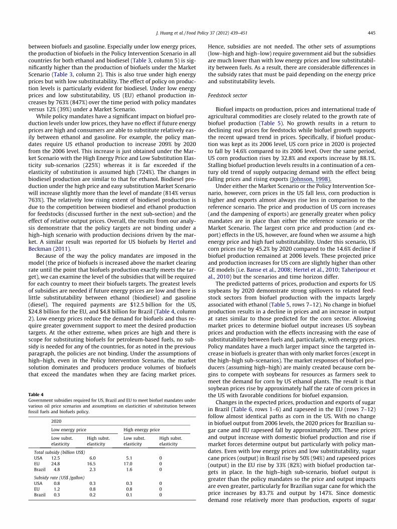
Because of the way the policy mandates are imposed in themodel (the price of biofuels is increased above the market clearingrate until the point that biofuels production exactly meets the tar-get), we can examine the level of the subsidies that will be requiredfor each country to meet their biofuels targets. The greatest levelsof subsidies are needed if future energy prices are low and there islittle substitutability between ethanol (biodiesel) and gasoline(diesel). The required payments are $12.5 billion for the US,$24.8 billion for the EU, and $4.8 billion for Brazil (Table 4, column2). Low energy prices reduce the demand for biofuels and thus re-quire greater government support to meet the desired productiontargets. At the other extreme, when prices are high and there isscope for substituting biofuels for petroleum-based fuels, no sub-sidy is needed for any of the countries, for as noted in the previousparagraph, the policies are not binding. Under the assumptions ofhigh–high, even in the Policy Intervention Scenario, the marketsolution dominates and producers produce volumes of biofuelsthat exceed the mandates when they are facing market prices.

Table 4Government subsidies required for US, Brazil and EU to meet biofuel mandates undervarious oil price scenarios and assumptions on elasticities of substitution betweenfossil fuels and biofuels policy.

2020

Low energy price High energy price

Low subst.elasticity

High subst.elasticity

Low subst.elasticity

High subst.elasticity

Total subsidy (billion US$)USA 12.5 6.0 5.1 0EU 24.8 16.5 17.0 0Brazil 4.8 2.3 1.6 0

Subsidy rate (US$ /gallon)USA 0.8 0.3 0.3 0EU 1.2 0.8 0.8 0Brazil 0.3 0.2 0.1 0

Hence, subsidies are not needed. The other sets of assumptions(low–high and high–low) require government aid but the subsidiesare much lower than with low energy prices and low substitutabil-ity between fuels. As a result, there are considerable differences inthe subsidy rates that must be paid depending on the energy priceand substitutability levels.

Feedstock sector

Biofuel impacts on production, prices and international trade ofagricultural commodities are closely related to the growth rate ofbiofuel production (Table 5). No growth results in a return todeclining real prices for feedstocks while biofuel growth supportsthe recent upward trend in prices. Specifically, if biofuel produc-tion was kept as its 2006 level, US corn price in 2020 is projectedto fall by 14.6% compared to its 2006 level. Over the same period,US corn production rises by 32.8% and exports increase by 88.1%.Stalling biofuel production levels results in a continuation of a cen-tury old trend of supply outpacing demand with the effect beingfalling prices and rising exports (Johnson, 1998).

Under either the Market Scenario or the Policy Intervention Sce-nario, however, corn prices in the US fall less, corn production ishigher and exports almost always rise less in comparison to thereference scenario. The price and production of US corn increases(and the dampening of exports) are generally greater when policymandates are in place than either the reference scenario or theMarket Scenario. The largest corn price and production (and ex-port) effects in the US, however, are found when we assume a highenergy price and high fuel substitutability. Under this scenario, UScorn prices rise by 45.2% by 2020 compared to the 14.6% decline ifbiofuel production remained at 2006 levels. These projected priceand production increases for US corn are slightly higher than otherGE models (i.e. Banse et al., 2008; Hertel et al., 2010; Taheripour etal., 2010) but the scenarios and time horizon differ.

The predicted patterns of prices, production and exports for USsoybeans by 2020 demonstrate strong spillovers to related feed-stock sectors from biofuel production with the impacts largelyassociated with ethanol (Table 5, rows 7–12). No change in biofuelproduction results in a decline in prices and an increase in outputat rates similar to those predicted for the corn sector. Allowingmarket prices to determine biofuel output increases US soybeanprices and production with the effects increasing with the ease ofsubstitutability between fuels and, particularly, with energy prices.Policy mandates have a much larger impact since the targeted in-crease in biofuels is greater than with only market forces (except inthe high–high sub-scenarios). The market responses of biofuel pro-ducers (assuming high–high) are mainly created because corn be-gins to compete with soybeans for resources as farmers seek tomeet the demand for corn by US ethanol plants. The result is thatsoybean prices rise by approximately half the rate of corn prices inthe US with favorable conditions for biofuel expansion.

Changes in the expected prices, production and exports of sugarin Brazil (Table 6, rows 1–6) and rapeseed in the EU (rows 7–12)follow almost identical paths as corn in the US. With no changein biofuel output from 2006 levels, the 2020 prices for Brazilian su-gar cane and EU rapeseed fall by approximately 20%. These pricesand output increase with domestic biofuel production and rise ifmarket forces determine output but particularly with policy man-dates. Even with low energy prices and low substitutability, sugarcane prices (output) in Brazil rise by 50% (94%) and rapeseed prices(output) in the EU rise by 33% (82%) with biofuel production tar-gets in place. In the high–high sub-scenario, biofuel output isgreater than the policy mandates so the price and output impactsare even greater, particularly for Brazilian sugar cane for which theprice increases by 83.7% and output by 147%. Since domesticdemand rose relatively more than production, exports of sugar

Table 5Maize and soybean prices, production and exports in US under various oil price scenarios and assumptions on elasticities of substitution between fossil fuels and biofuels.

2006–2020 (% Change)reference scenario

2020 (% Change from reference scenario)

Market Scenario Policy intervention scenario

Low energy price High energy price Low energy price High energy price

USA maizePrice �14.6

High subst. elasticity 0.7 45.2 15.0 45.2Low subst. elasticity 1.4 12.8 15.0 13.9

Production 32.8High subst. elasticity 1.0 51.3 17.0 51.3Low subst. elasticity 2.1 19.8 17.0 18.6

Exports 88.1High subst. elasticity 1.2 �57.4 �16.6 �57.4Low subst. elasticity �0.3 �8.0 �16.6 �16.4

USA soybeanPrice �11.6

High subst. elasticity 0.4 21.5 12.5 21.5Low subst. elasticity 0.7 6.7 12.5 11.7

Production 31.7High subst. elasticity 0.0 4.7 8.5 4.7Low subst. elasticity 0.3 2.8 8.5 8.7

Exports 48.3High subst. elasticity 0.7 �21.9 �13.3 �21.9Low subst. elasticity 0.1 �3.9 �13.3 �13.3

Table 6Sugarcane and rapeseed prices, production and exports in Brazil and EU under various oil price scenarios and assumptions on elasticities of substitution between fossil fuels andbiofuels.

2006–2020 (% Change)reference scenario

2020 (% Change from reference scenario)

Market Scenario Policy intervention scenario

Low energy price High energy price Low energy price High energy price

Brazil sugarPrice �20.0

High subst. elasticity 6.5 83.7 50.6 83.7Low subst. elasticity 9.1 43.6 50.6 45.7

Production 17.5High subst. elasticity 16.3 147.1 94.1 147.1Low subst. elasticity 22.6 100.1 94.3 99.1

Export 269.0High subst. elasticity �28.7 �95.5 �87.5 �95.5Low subst. elasticity �36.4 �82.4 �87.5 �85.3

EU rapeseedPrice �17.3

High subst. elasticity 1.2 38.0 33.0 38.0Low subst. elasticity 1.4 10.9 33.0 30.5

Production 28.9High subst. elasticity 3.9 95.0 81.6 95.0Low subst. elasticity 4.5 35.7 81.6 84.6

Exporta 294.5High subst. elasticity �4.9 �65.2 �62.8 �65.2Low subst. elasticity �5.3 �32.1 �62.9 �62.3

a The trade of rapeseed inside EU member countries is not included.

446 J. Huang et al. / Food Policy 37 (2012) 439–451

cane (rapeseed) in Brazil (the EU) fell relative to the referencescenario.

In summary, then, the emergence of biofuels from either policymandates requiring minimum levels or due to market-based deci-sions of biofuel refiners are predicted to have profound impacts onthe agricultural economies of the major producing countries.Unlike the past in which prices fell over time, higher biofuel pro-duction from either policy intervention or the market will lead tohigher prices in 2020 than if biofuel output was fixed at the refer-ence level of 2006. However, this rise in prices is not coming fromlower production since output rises sharply. Demand from the bio-fuel plants, in fact, is strong enough that domestic users procureenough of output that exports fall in both the Market Scenarioand the Policy Scenario relative to the base case. In other words,

after the emergence of biofuels there is relatively more corn, sugarand rapeseed being produced, but less of it is going onto worldmarkets.

Developing countries

Agricultural production in developing countries will also be sig-nificantly affected by the emergence of biofuels in the US, Braziland the EU. Because of the price changes (and reduction of exports)due to global biofuel development, world agricultural productionand trade will change remarkably. To show this relatively suc-cinctly, we examine the impact of the emergence of biofuels ondeveloping countries under the assumption of high future energyprices and high substitutability of biofuels and petroleum-based

Table 7The impacts on the price, production, export and self-sufficiency level of selected developing countries in high–high scenario (expressed in% change relative to reference scenario,2020).

East Africa West Africa South Africa India Rest of South Asia

MaizePrice 6.2 4.6 5.4 8.1 8.7Production 4.2 2.0 4.5 2.2 4.3Export 178.8 183.6 44.9 96.5 262.5Self-sufficiency ratio 4.0 1.7 4.6 2.6 4.7

WheatPrice 4.0 4.8 3.3 3.2 3.1Production 1.8 3.5 3.9 0.4 1.4Export 14.1 10.0 12.9 19.1 16.1Self-sufficiency ratio 0.6 0.8 1.4 0.3 1.1

RicePrice 2.4 2.5 4.0 4.9 1.4Production �0.2 0.0 �0.3 0.2 0.1Export 12.9 11.7 4.1 �5.5 30.3Self-sufficiency ratio 0.0 0.7 0.0 0.0 0.2

Beef and MuttonPrice 0.7 0.5 0.5 3.0 1.2Production �0.1 �1.3 2.1 0.3 0.1Export 13.4 9.5 16.0 �0.8 6.0Self-sufficiency ratio 0.4 0.4 1.8 �0.3 0.0

Notes: In the definition of self-sufficiency, the value of 100 indicates that the net export is zero, and the domestic consumption equal to the domestic production. The numbersof self-sufficiency in above table is the difference between the high–high scenario and reference scenario (i.e., the value of self-sufficiency in H–H minus that of thecorresponding reference scenario).High–high refers to high energy price and high elasticity of substitution between biofuels and fossil fuels.

J. Huang et al. / Food Policy 37 (2012) 439–451 447

fuels. This sub-scenario results in biofuel production levels greaterthan the policy targets. We aggregate the effects in developingcountries into region-wide effects, including Eastern Africa,Western Africa, Southern Africa, India and Rest of South Asia (seeAppendix C for regional aggregation).

The increases in feedstock prices predicted for the major biofuelproducing countries are transmitted by global markets to develop-ing countries (Table 7). In the case of corn, the range of the priceincreases from the emergence of biofuels is between 4.6% in WestAfrica to 8.1% in India. These price increases are much less than theapproximate 45% rise predicted for US corn price because of imper-fect price transmission across the boundaries of nations.4 The pre-dicted effects of biofuels would be magnified if the commodity pricechanges more closely matched the price increases previously dis-cussed for developed countries. The higher corn prices in developingcountries causes production to increase by 2% (West Africa) to 4.5%(South Africa). Because of the higher levels of production, exportsrise (or at the very least imports fall) and the net result is an increasein the self-sufficiency ratio of developing countries for corn.

Food consumption is projected to decline under the scenarios ofglobal biofuel development, especially for crops used as biofuelfeedstock. Unfortunately, the impacts on the poor could not be de-rived directly because consumers in the model are not differenti-ated by income. However, many studies have suggested thatrising food prices threaten the caloric consumption and nutritionalintake of the poor (World Bank, 2008; FAO, 2009). Therefore, in-creases in biofuel production globally will likely reduce per capitaconsumption for the poor who are net food purchasers.

4 The pass-through of rising global prices does not translate into a proportionaterise in domestic price levels due to a variety of factors including transaction costs,existence of market power, existence of non-constant returns to scale, degree ofproduct homogeneity, changes of the exchange rates, and effects of border anddomestic policies (Barrett and Li, 2002; Conforti, 2004). Although the domesticagricultural price in developing countries is correlated with movements in the globalprice, actual price transmission is muted in most cases (Keats et al., 2010). Such anincomplete price transmission among countries is mainly reflected in the GTAP modelthrough the price margin between FOB and CIF, and the elasticities of substitutionbetween imported and domestic products (the Armington assumption).

As in the case of biofuel producing nations, rising prices for corn(and sugar and rapeseed) in developing countries have spillover ef-fects on prices of commodities that are not feedstocks. The rise inwheat prices in developing countries (relative to the reference sce-nario) ranges from 3.1% in South Asia (not counting India) to 4.8%in West Africa. Rice and meat prices also rise in all regions.

While non-feedstock commodities prices in developing nationsall rise in the high–high scenario relative to the reference scenario,the impact on production, exports and self-sufficiency is mixed.The pattern of wheat mirrors that of corn. However, the productionof rice and meat fall in most developing countries despite the high-er prices. The reason for the output decline is that the price rises forrice and meat are less than that for maize and wheat; resources areshifted to the crops with higher relative prices. Exports and self-sufficiency ratios are mostly determined by production patterns.

The rise in biofuel production under the assumption of high en-ergy prices and high substitutability has a positive effect on valueadded in the agricultural sectors across all regions (Table 8, PanelA). Agricultural value-added grows most in the major biofuel pro-ducing regions with it rising by 12.5% in the US, 10.2% in the EU,and 15.4% in Brazil relative to the no biofuel production growthscenario. The greatest returns, percentage wise, are enjoyed bythose in the unskilled labor sector and those that own (or get thereturns to) land. Laborers and landowners in developing countriesalso enjoy rising returns due to the higher biofuel production levels(Table 8, Panel B). The overall increase in agricultural value-addedin the developing regions included in our study ranges from 3.2% inSouth Asia (not counting India) to 5.6% in South Africa. The ownersof land resources receive the greatest benefits of the higher valueadded, but both unskilled and skilled laborers also benefit.

In summary, even when biofuels are being mainly produced indeveloped countries, our results indicate that there are impactpathways that extend far beyond the borders of the US, Braziland the EU. Prices of feedstock and non-feedstock commoditiesrise in the developing countries. In the case of maize and wheat,the price rise increases production, increases exports (or reducesimports) and improves self-sufficiency. There is also a rise in valueadded from the agricultural sector—a gain that is enjoyed by the

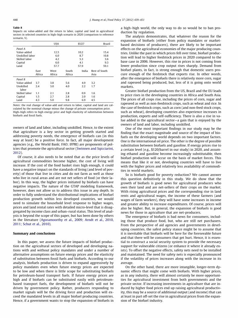
Table 8Impacts on value-added and the return to labor, capital and land in agriculturalsectors in selected countries in high–high scenario in 2020 (comparison to referencescenario, %).

USA EU27 Brazil

Panel AValue-added 12.5 10.2 15.4Unskilled labor 6.0 8.7 10.8Skilled labor 4.2 5.3 3.6Capital 6.0 4.1 9.3Land 57.7 57.9 59.1

EastAfrica

WestAfrica

SouthAfrica

India Rest of SouthAsia

Panel BValue-added 3.7 3.8 5.6 4.9 3.2Unskilled

labor2.4 3.0 4.0 2.2 1.7

Skilled labor 1.1 2.1 2.8 0.9 1.6Capital 1.5 2.7 2.8 2.0 1.6Land 4.3 5.0 9.8 6.9 4.5

Notes: the real change of value-add and return to labor, capital and land are cal-culated by the nominal change minus the change of private consumption price.High–high refers to high energy price and high elasticity of substitution betweenbiofuels and fossil fuels.

448 J. Huang et al. / Food Policy 37 (2012) 439–451

owners of land and labor, including unskilled. Hence, to the extentthat agriculture is a key sector in getting growth started andaddressing poverty needs, the emergence of biofuels can (in thisway at least) be a positive force. In fact, all major developmentagencies (e.g., the World Bank; FAO; IFPRI) are proponents of pol-icies that promote the agricultural sector (Swinnen and Sqicciarini,2012).

Of course, it also needs to be noted that as the price levels ofagricultural commodities become higher, the cost of living willincrease. If the cost of the food basket rises high enough, it couldhave a negative impact on the standards of living (and level of pov-erty) of those that live in cities and do not farm as well as thosewho live in rural areas and are not net sellers of food (or their la-bor). In this way, the higher prices initiated by biofuels can havenegative impacts. The nature of the GTAP modeling framework,however, does not allow us to address this issue in any depth. Inorder to fully understand the distributional implications of biofuelproduction growth within less developed countries, we wouldneed to simulate the household level response to higher wages,prices and land rental rates with detailed micro-level that is disag-gregated by income class and urban–rural status. This level of anal-ysis is beyond the scope of this paper, but has been done by othersin the literature (Agoramoorthy et al., 2009; Arndt et al., 2010,2011; Schut et al., 2010).

Summary and conclusions

In this paper, we assess the future impacts of biofuel produc-tion on the agricultural sectors of developed and developing na-tions with and without policy mandates and under a number ofalternative assumptions on future energy prices and the elasticityof substitution between fossil fuels and biofuels. According to ouranalysis, biofuels production is driven to expand aggressively bypolicy mandates even when future energy prices are expectedto be low and when there is little scope for substituting biofuelsfor petroleum-based transport fuels. If future energy prices arehigh and if biofuels can be substituted easily with petroleum-based transport fuels, the development of biofuels will not bedriven by government policy. Rather, producers responding tomarket signals will be the driving force and production will ex-ceed the mandated levels in all major biofuel producing countries.Hence, if a government wants to stop the expansion of biofuels in

a high–high world, the only way to do so would be to ban pro-duction by regulation.

The analysis demonstrates, that whatever the reason for theexpansion of biofuels (either from policy mandates or market-based decisions of producers), there are likely to be importanteffects on the agricultural economies of the major producing coun-tries. Unlike the past in which prices fell over time, biofuel produc-tion will lead to higher feedstock prices in 2020 compared to thebase case in 2006. However, this rise in prices is not coming fromlower production since crop output rises sharply. Demand frombiofuel plants, in fact, is strong enough that domestic users pro-cure enough of the feedstock that exports rise. In other words,after the emergence of biofuels there is relatively more corn, sugarand rapeseed being produced, but, less of it is going onto worldmarkets.

Greater biofuel production from the US, Brazil and the EU leadsto price rises in the developing countries in Africa and South Asia.The prices of all crops rise, including the prices of corn, sugar andrapeseed as well as non-feedstock crops, such as wheat and rice. Inthe case of feedstock crops, such as corn (and non-feed stock crops,such as wheat), developing countries also experience increases inproduction, exports and self-sufficiency. There is also a rise in va-lue added in the agricultural sector—a gain that is enjoyed by theowners of land and labor, including unskilled.

One of the most important findings in our study may be thefinding that the exact magnitude and source of the impact of bio-fuels on the developing world depends on two important factors.One is the international oil price. The other is the degree of possiblesubstitution between biofuels and gasoline. If energy prices rise toa certain level (e.g., $120/barrel in our study) in 2020, and assum-ing ethanol and gasoline become increasingly substitutable, thenbiofuel production will occur on the basis of market forces. Thismeans that like it or not, developing countries will have to livewith the higher prices and relatively less availability of commodi-ties in world markets.

So is biofuels good for poverty reduction? We cannot answerthis question definitively in this study. We do show that thegrowth of biofuels is good news for agricultural producers whoown their land and are net-sellers of their crops on the market.With rising agricultural prices and the corresponding rise in landrents and agricultural wages, the income of these farmers (andwages of farm workers), they will have some increases in incomeand greater ability to increase expenditures. Of course, prices willalso be higher. But, in general, the expansion of biofuels is goodnews for those in agriculture that are net-producers.

The emergence of biofuels is bad news for consumers, includ-ing those that produce food, but, who are still net purchasers.From the perspective of aid agencies and governments in devel-oping countries, the safest policy stance might be to assume thatit is inevitable that biofuels will be here for the foreseeable futureand that there will be consumers that get hurt. Hence, it is essen-tial to construct a social security system to provide the necessarysupport for vulnerable citizens (or enhance it where it already ex-ists). To offset the negative effects, safety nets need to be installedand maintained. The need for safety nets is especially pronouncedif the volatility of prices increases along with the increase in itsaverage.

On the other hand, there are more intangible, longer-term dy-namic effects that might come with biofuels. With higher prices,as in any industry, there will almost certainly be more opportuni-ties for agricultural investment from both governments and theprivate sector. If increasing investments in agriculture that are in-duced by higher food prices end up raising agricultural productiv-ity, this may be a source of additional output (and income) that canat least in part off-set the rise in agricultural prices from the expan-sion of the biofuel industry.

J. Huang et al. / Food Policy 37 (2012) 439–451 449

Acknowledgment

The authors wish to acknowledge the financial support pro-vided by the Bill and Melinda Gates Foundation and InternationalFund for Agricultural Development (IFAD).

Appendix A

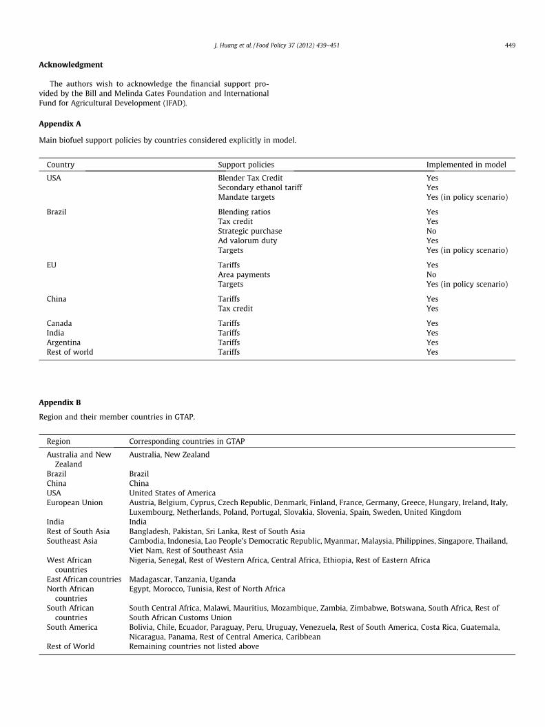
Main biofuel support policies by countries considered explicitly in model.

Country Support policies Implemented in model

USA Blender Tax Credit YesSecondary ethanol tariff YesMandate targets Yes (in policy scenario)

Brazil Blending ratios YesTax credit YesStrategic purchase NoAd valorum duty YesTargets Yes (in policy scenario)

EU Tariffs YesArea payments NoTargets Yes (in policy scenario)

China Tariffs YesTax credit Yes

Canada Tariffs YesIndia Tariffs YesArgentina Tariffs YesRest of world Tariffs Yes

Appendix B

Region and their member countries in GTAP.

Region Corresponding countries in GTAP

Australia and NewZealand

Australia, New Zealand

Brazil BrazilChina ChinaUSA United States of AmericaEuropean Union Austria, Belgium, Cyprus, Czech Republic, Denmark, Finland, France, Germany, Greece, Hungary, Ireland, Italy,

Luxembourg, Netherlands, Poland, Portugal, Slovakia, Slovenia, Spain, Sweden, United KingdomIndia IndiaRest of South Asia Bangladesh, Pakistan, Sri Lanka, Rest of South AsiaSoutheast Asia Cambodia, Indonesia, Lao People’s Democratic Republic, Myanmar, Malaysia, Philippines, Singapore, Thailand,

Viet Nam, Rest of Southeast AsiaWest African

countriesNigeria, Senegal, Rest of Western Africa, Central Africa, Ethiopia, Rest of Eastern Africa

East African countries Madagascar, Tanzania, UgandaNorth African

countriesEgypt, Morocco, Tunisia, Rest of North Africa

South Africancountries

South Central Africa, Malawi, Mauritius, Mozambique, Zambia, Zimbabwe, Botswana, South Africa, Rest ofSouth African Customs Union

South America Bolivia, Chile, Ecuador, Paraguay, Peru, Uruguay, Venezuela, Rest of South America, Costa Rica, Guatemala,Nicaragua, Panama, Rest of Central America, Caribbean

Rest of World Remaining countries not listed above

450 J. Huang et al. / Food Policy 37 (2012) 439–451

Appendix C

Annual growth rates of macroeconomic variables and crop yield by region under reference scenario, 2006–2020 (%).

Macroeconomic variables Crop yield

GDP Population Skilled labor Unskilled labor Capital Maize Sugar Soybean Other oilseeds

Australia and New Zealand 3.4 0.9 0.8 �0.2 3.9 0.5 0.4 0.7 0.6Brazil 4.3 1.2 0.8 3.0 3.5 2.0 1.4 2.0 2.0China 8.0 0.5 0.4 3.0 8.5 1.7 1.1 0.8 1.1USA 2.5 0.8 0.6 �0.1 2.4 0.8 0.6 1.6 1.8European Union 2.0 0.0 �0.1 �0.8 3.0 0.4 0.8 1.3 1.2India 7.0 1.5 1.5 3.9 7.8 2.6 1.3 1.0 1.0Rest of South Asia 5.4 2.0 2.2 3.7 5.4 1.7 1.1 0.8 1.4Southeast Asia 5.4 1.4 1.3 3.8 5.0 1.7 0.9 0.8 0.4West African countries 4.3 2.8 3.1 3.2 4.2 1.9 0.9 1.6 1.2East African countries 5.2 2.7 3.2 3.2 5.3 2.4 2.0 1.8 0.6North African countries 4.4 1.8 1.8 2.4 5.2 1.2 0.9 1.5 1.6South African countries 3.9 2.1 2.5 2.5 4.0 2.4 0.9 1.1 0.6South America 4.3 1.8 1.4 3.5 4.0 1.9 1.6 0.7 0.6

1.5 2.9 1.1 1.1 0.8 1.2

uthors mainly based on research by Tongeren and Huang (2004), Walmsley (2006) andel.

Rest of World 3.4 1.5 1.3

Source: Assumptions on growth rates for macroeconomic parameters estimated by aYang et al. (2011). Annual crop yield values by region are from IFPRI’s IMPACT mod

References

Agoramoorthy, G., Hsu, M.J., Chaudhary, S., Shieh, P., 2009. Can biofuel cropsalleviate tribal poverty in India’s drylands? Applied Energy 86 (S1), 118–124.

Arndt, C., Benfica, R., Tarp, F., Thurow, J., Uaiene, R., 2010. Biofuels, poverty andgrowth: a computable general equilibrium analysis of Mozambique.Environment and Development Economics 15 (1), 81–105.

Arndt, C., Benfica, R., Thurow, J., 2011. Gender implications of biofuels expansion inAfrica: the case of Mozambique. World Development. http://dx.doi.org/10.1016/j.worlddev.2011.02.012.

Banse, M., Van Meijl, H., Tabeau, A., Woltjer, G., 2008. Will EU biofuel policies affectglobal agricultural markets. European Review of Agricultural Economics 35 (2),117–141.

Barrett, C.B., Li, J.R., 2002. Distinguishing between equilibrium and integration inspatial price analysis. American Journal of Agricultural Economics 84 (2), 292–307.

BIODIESEL, 2008. Global Market Survey, Feedstock Trends and Forecasts, second ed.<http://www.emerging-markets.com/biodiesel>.

Birur, D.K., Hertel, T.W., Tyner, W.E., 2008. Impact of Biofuel Production on WorldAgricultural Markets: A Computable General Equilibrium Analysis. GTAPTechnical Paper No. 53. Center for Global Trade Analysis, Purdue University,West Lafayette.

Burniaux, J.M., Truong, T.P., 2002. GTAP-E: An Energy-Environmental Version of theGTAP Model. GTAP Technical Paper No.16. Center for Global Trade Analysis,Purdue University, West Lafayette, January.

Charlesa, M., Ryana, B., Ryanb, R., Oloruntobaa, R., 2007. Public policy and biofuels:the way forward? Energy Policy 35, 5737–5746.

Conforti, P., 2004. Price Transmission in Selected Agricultural Markets. Rome: FAOCommodity and Trade Policy Research Working Paper No. 7.

Earth Policy Institute, 2010. Biofuels Data from World on the Edge. <http://www.earth-policy.org/data_center/C26>.

EIA (US Energy Information Administration), 2010. International Energy Outlook2010. <http://www.eia.gov/oiaf/ieo/index.html>.

European Biodiesel Board, 2011. <http://www.ebb-eu.org/stats.php>.Ewing, M., Msangi, S., 2009. Biofuels production in developing countries: assessing

tradeoffs in welfare and food security. Environmental Science & Policy 12 (4),520–528.

FAO (Food and Agricultural Organization), 2008a. The State of Food and Agriculture,Biofuels: Prospects, Risks and Opportunities, FAO, Rome. <http://www.fao.org/docrep/011/i0100e/i0100e00.htm>.

FAO, 2008b. Soaring Food Prices: Facts, Perspective, Impacts and Actions Required.High-level Conference on World Food Security: the Challenges of ClimateChange and Bioenergy, FAO, Rome, June. <http://www.fao.org/fileadmin/user_upload/foodclimate/HLCdocs/HLC08-inf-1-E.pdf>.

FAO, 2009. The State of Food Insecurity in the World 2008. Rome. <http://www.fao.org/docrep/011/i0291e/i0291e00.htm>.

FAPRI (Food and Agricultural Policy Research Institute), 2011. New Challenges inAgricultural Modeling: Relating Energy and Farm Commodity Prices. FAPRI-MUReport #05-11, May. <http://www.fapri.missouri.edu/outreach/publications/2011/FAPRI_MU_Report_05_11.pdf>.

Fonseca, M.B., Burrell, A., Gay, H., Henseler, M., Kavallari, A., M’Barek, R., Domínguez,Tonini, A., 2010. Impacts of the EU Biofuel Target on Agricultural Markets andLand Use: a Comparative Modeling Assessment. European Commission, Joint

Research Centre, Institute for Prospective Technological Studies, EUR Number:24449 EN, July.

Hayes, D., Babcock, B.A., Fabiosa, J., Tokgoz, S., Elobeid, A., Yu, T.E., Dong, F., Hart, C.,Chavez, E., Pan, S., Carriquiry, M., Dumortier, J.R.F., 2009. Biofuels: PotentialProduction Capacity, Effects on Grain and Livestock Sectors, and Implicationsfor Food Prices and Consumers, FAPRI Working Paper 09-WP 487, Center forAgricultural and Rural Development, Iowa State University, March.

Hertel, T.W., 1997. Global Trade Analysis. Modelling and Applications. CambridgeUniversity Press, New York.

Hertel, T.W., Beckman, J., 2011. Commodity Price Volatility in the Biofuel Era: anExamination of the Linkage between Energy and Agricultural Markets, NBERWorking Paper No. 16824. <http://www.nber.org/papers/w16824.pdf>.

Hertel, T.W., Tyner, W.E., Birur, D.K., 2010. The global impacts of biofuel mandates.Energy Journal 31 (1), 75–100.

Horridge, M., 2005. SplitCom – Programs to Disaggregate a GTAP Sector. Centre ofPolicy Studies, Monash University, Melbourne, Australia. <http://www.monash.edu.au/policy/SplitCom.htm>.

IEA, 2008. World Energy Outlook 2008.IEA (International Energy Agency), 2010. World Energy Outlook 2010.IFPRI (International Food Policy Research Institute), 2008. High Food Prices: the

What, Who, and How of Proposed Policy Actions. IFPRI Policy Brief, IFPRI,Washington DC, May. <http://www.ifpri.org/sites/default/files/publications/foodpricespolicyaction.pdf>.

Johnson, D.G., 1998. Food security and world trade prospects. American Journal ofAgricultural Economics 80 (5), 941–947.

Keats, S., Wiggins, S., Compton, J., Vigneri, M., 2010. Food Price Transmission: RisingInternational Cereals Prices and Domestic Markets. Overseas DevelopmentInstitute (ODI) Project Briefing No. 40. <http://www.odi.org.uk/resources/details.asp?id=5079&title=food-price-transmission>.

Keeney, R., Hertel, T.W., 2005. GTAP-AGR: a Framework for Assessing MultilateralChanges in Agricultural Policies. GTAP Technical Paper No. 24, Center for GlobalTrade Analysis, Purdue University, West Lafayette.

Kretschner, B., Peterson, S., 2010. Integrating bioenergy into computable generalequilibrium models – a survey. Energy Economics 32 (4), 673–686.

Lee, H.L., Hertel, T.W., Sohngen, B., Ramankutty, N., 2005. Towards an IntegratedLand Use Data Base for Assessing the Potential for Greenhouse Gas Mitigation.GTAP Technical Paper No. 25. Center for Global Trade Analysis, PurdueUniversity, West Lafayette.

Lichts, F.O., 2009. World Ethanol and Biofuels Report, vol. 7, No. 18, May 2009.Linden, A., Carlsson-Kanyama, A., Eriksson, B., 2006. Efficient and inefficient aspects

of residential energy behaviour: what are the policy instruments for change?Energy Policy 34 (14), 1918–1927.

Martin, W., Anderson, K., 2006. The Doha agenda negotiations on agriculture: whatcould they deliver? American Journal of Agricultural Economics 88 (5), 1211–1218.

Nass, L., Pereira, P., Ellis, D., 2007. Biofuels in Brazil: an overview. Crop Science 47(6), 2228–2237.

OECD, 2003. Agricultural Policies in OECD Countries: Monitoring and Evaluation2003 – Highlights OECD, Paris. <http://www.oecd.org/dataoecd/25/63/2956135.pdf>.

OECD (Organization for Economic Cooperation and Development), 2008. BiofuelSupport Policies: an Economic Assessment. Directorate for Trade andAgriculture, OECD, Paris. <http://www.oecd.org/document/30/0,3343,en_2649_33785_41211998_1_1_1_37401,00.html>.

J. Huang et al. / Food Policy 37 (2012) 439–451 451

Otsuka, K., Gascon, F., Asano, S., 1994. Second-generation MVs and the evolution ofthe green revolution: the case of central Luzon, 1966–1990. AgriculturalEconomics 10 (3), 283–295.

Paarlberg, R., 2010. Food Politics: What Everyone Needs to Know. Oxford UniversityPress, New York.

Pingali, P.L., Traxler, G., 2002. Changing locus of agricultural research: will the poorbenefit from biotechnology and privatization trends? Food Policy 27 (3), 223–238.

Pousa, P.A.G., Santos, A.L.F., Suarez, P.A.Z., 2007. History and policy of biodiesel inBrazil. Energy Policy 35 (11), 5393–5398.

Qiu, H.G., Huang, J.K., 2008. The Impacts of Biofuel Developments on World FoodPrice and Implications for China’s Agriculture. China Agricultural TradeDevelopment Report 2008. Chinese Agricultural Press, Beijing.

Renewable Fuels Associations, 2010. Ethanol Industry Outlook, various issues.<http://bioconversion.blogspot.com>.

Rosegrant, M., Zhu, T., Msangi, S., Sulser, T., 2008. Global scenarios for biofuels:impacts and implications. Review of Agricultural Economics 30 (3), 495–505.

Schut, M., Slingerland, M., Locke, A., 2010. Biofuel developments in Mozambique.Update and analysis of policy, potential and reality. Energy Policy 38 (9), 5151–5165.

Skinner, S., Weersink, A., deLange, C., 2012. Impact of dried distillers grains withsoluble (DDGS) on ration and fertilizer costs of swine farmers. Canadian Journalof Agricultural Economics 60 (2).

Smith, J.Z., 2011. Crude Awakening: $185 Oil Forecast for 2020. <http://blogs.star-telegram.com/barnett_shale/2011/03/crude-awakening-185-oil-forecast-for-2020.html>.

Sorda, G., Banse, M., Kemfert, C., 2010. An overview of biofuel policies across theworld. Energy Policy 38 (11), 6977–6988.

Steenblik, R., 2007. Biofuels – At What Cost? Government Support for Ethanol andBiodiesel in Selected OECD Countries, Global Subsidies Initiative, InternationalInstitute for Sustainable Development, September.

Swinnen, J.F.M., Sqicciarini, P., 2012. Mixed messages on prices and food security.Science 335, 405–406.

Taheripour, F., Hertel, T.W., Tyner, W.E., Beckman, J.F., Birur, D.K., 2010. Biofuels andtheir by-products: global economic and environmental implications. Biomassand Bioenergy 34, 278–289.

Tangermann, S., 2008. What’s Causing Global Food Price Inflation, VOX, July 22.<http://www.voxeu.org/index.php?q=node/1437>.

Timilsina, G.R., Shrestha, A., 2010. Biofuels: Markets, Targets and Impacts.World Bank Policy Research Working Paper Series, Working Paper No. 5364,July.

Tongerne, F., Huang, J., 2004. China’s Food Economy in the Early 21st Century:Development of China’s Food Economy and Its Impact on Global Trade and onthe EU. Agricultural Economics Research Institute (LEI) Report 6.04.04, Hague,Netherlands.

Tyner, W.E., 2008. The US ethanol and biofuels boom: its origins, current status, andfuture prospects. BioScience 58 (7), 646–653.

Tyner, W.E., 2010. Comparison of the US and EU approaches to simulating biofuels.Biofuels 1 (1), 19–21.

UN (United Nations), 2006. The Emerging Biofuel Market: Regulatory, Trade andDevelopment Implications. United Nations Conference on Trade andDevelopment UNCTAD/DITC/TED/2006/4. <http://www.unctad.org/en/docs/ditcted20064_en.pdf>.

US Renewable Fuels Association, 2010. <http://www.ethanolrfa.org/industry/statistics/>.

USDA, 2011. USDA Agricultural Projection to 2020, Office of the Chief Economist,World Agricultural Outlook Board, US Department of Agriculture. Prepared bythe Interagency Agricultural Projections Committee. Long-term ProjectionsReport OCE-2011-1, February.

Walmsley, T.L., 2006. A Baseline Scenario for the Dynamic GTAP Model. <https://www.gtap.agecon.purdue.edu/resources/res_display.asp?RecordID=2204>.

Westhoff, P.C., 2010. The Economics of Food: How Feeding and Fueling the PlanetAffects Food Prices. FT Press, Upper Saddle River, New Jersey.

World Bank, 2008. Addressing the Food Crisis: the Need for Rapid and CoordinatedAction. Background paper for the Group of Eight meeting of finance ministers,Osaka, Japan, June 13–14.

Yacobucci, B.D., 2010. Biofuels Incentives: a Summary of Federal Programs.Congressional Research Service Reports. Paper 8.

Yang, J., Huang, J.K., Li, N.H., Rozelle, S., Martin, W., 2011. The impact of the Dohatrade proposals on farmers’ incomes in China. Journal of Policy Modeling 33 (3),439–452.