MIT Joint Program on theScience and Policy of Global Change

Biofuels, Climate Policy and theEuropean Vehicle Fleet

Xavier Gitiaux, Sergey Paltsev, John Reilly and Sebastian Rausch

Report No. 176August 2009

The MIT Joint Program on the Science and Policy of Global Change is an organization for research,independent policy analysis, and public education in global environmental change. It seeks to provide leadershipin understanding scientific, economic, and ecological aspects of this difficult issue, and combining them into policyassessments that serve the needs of ongoing national and international discussions. To this end, the Program bringstogether an interdisciplinary group from two established research centers at MIT: the Center for Global ChangeScience (CGCS) and the Center for Energy and Environmental Policy Research (CEEPR). These two centersbridge many key areas of the needed intellectual work, and additional essential areas are covered by other MITdepartments, by collaboration with the Ecosystems Center of the Marine Biology Laboratory (MBL) at Woods Hole,and by short- and long-term visitors to the Program. The Program involves sponsorship and active participation byindustry, government, and non-profit organizations.

To inform processes of policy development and implementation, climate change research needs to focus onimproving the prediction of those variables that are most relevant to economic, social, and environmental effects.In turn, the greenhouse gas and atmospheric aerosol assumptions underlying climate analysis need to be related tothe economic, technological, and political forces that drive emissions, and to the results of international agreementsand mitigation. Further, assessments of possible societal and ecosystem impacts, and analysis of mitigationstrategies, need to be based on realistic evaluation of the uncertainties of climate science.

This report is one of a series intended to communicate research results and improve public understanding of climateissues, thereby contributing to informed debate about the climate issue, the uncertainties, and the economic andsocial implications of policy alternatives. Titles in the Report Series to date are listed on the inside back cover.

Henry D. Jacoby and Ronald G. Prinn,Program Co-Directors

For more information, please contact the Joint Program OfficePostal Address: Joint Program on the Science and Policy of Global Change

77 Massachusetts AvenueMIT E19-411Cambridge MA 02139-4307 (USA)

Location: 400 Main Street, CambridgeBuilding E19, Room 411Massachusetts Institute of Technology

Access: Phone: +1(617) 253-7492Fax: +1(617) 253-9845E-mail: glo balcha nge @mi t .e duWeb site: ht t p://gl o balch ange .m i t .e du /

Printed on recycled paper

Biofuels, Climate Policy and the European Vehicle Fleet

Xavier Gitiaux†, Sergey Paltsev, John Reilly and Sebastian Rausch

Abstract

We examine the effect of biofuels mandates and climate policy on the European vehicle fleet,

considering the prospects for diesel and gasoline vehicles. We use the MIT Emissions Prediction and

Policy Analysis (EPPA) model, which is a general equilibrium model of the world economy. We

expand this model by explicitly introducing current generation biofuels, by accounting for stock

turnover of the vehicle fleets and by disaggregating gasoline and diesel cars. We find that biofuels

mandates alone do not substantially change the share of diesel cars in the total fleet given the current

structure of fuel taxes and tariffs in Europe that favors diesel vehicles. Jointly implemented changes

in fiscal policy, however, can reverse the trend toward more diesel vehicles. We find that harmonizing

fuel taxes reduces the welfare cost associated with renewable fuel policy and lowers the share of

diesel vehicles in the total fleet to 21% by 2030 compared to 25% in 2010. We also find that

eliminating tariffs on biofuel imports, which under the existing regime favor biodiesel and impede

sugar ethanol imports, is welfare-enhancing and brings about further substantial reductions in CO2

emissions.

Contents

1. INTRODUCTION ...................................................................................................................... 1 2. TRENDS AND FORCES SHAPING THE DIESELVEHICLE MARKET .............................. 2 3. THE EPPA MODEL .................................................................................................................. 6

3.1 First generation biofuels ..................................................................................................... 6 3.2 The private transportation sector ...................................................................................... 12

3.2.1 Representation of the fleet turnover ......................................................................... 13 3.2.3 Disagreggation of gasoline fleet and diesel fleet ..................................................... 14 3.2.3 Introducing E85 vehicles in EPPA .......................................................................... 15

3.2 Implementing fuel standards in EPPA .............................................................................. 16 3.4 Scenarios .......................................................................................................................... 17

4. RESULTS ................................................................................................................................ 17 4.1 The vehicle fleet ............................................................................................................... 17 4.2 Welfare, emissions and trade impacts of fuel policies ...................................................... 20

5. SENSITIVITY ANALYSIS ..................................................................................................... 25 6. CONCLUSION ........................................................................................................................ 27 7. REFERENCES ......................................................................................................................... 29

1. INTRODUCTION

Diesel vehicles have strongly entered the European car market especially in the last decade.

They now account for over 50% of new vehicle registrations (ACEA, 2008). The likely reason

for the strong penetration of diesel vehicles is a fuel tax structure that favors diesel. However,

Europe is now seeing a number of new policy developments that could change the cost and

relative prices of fuels. Of particular interest are new renewable fuels mandates. The recently

proposed energy and climate package from the European Commission that would extend the

Emission Trading Scheme (ETS) over the next twenty years also calls for an increase in

† Corresponding author: Xavier Gitiaux (Email: xgitiaux@mit.edu).

MIT Joint Program on the Science and Policy of Global Change, Cambridge, MA, USA.

2

renewable fuels. According to the European Commission (2008) proposal to introduce biofuels

mandates, 5.75% by 2010 and 10% beyond 2020 of renewable fuels (in volume terms) have to be

blended into conventional fuels. This new initiative will interact with an existing tariff and tax

structure that encourages domestic biofuel production and favors diesel imports. The overall

outcome of proposed fuel policies on the diesel market is not immediately clear. At issue with

the renewable fuels requirement are the cost and availability of biodiesel as currently produced

biodiesel and ethanol use different plant feedstocks that lead to different cost and availability of

the fuels. In particular, estimates (IEA, 2004) suggest that biodiesel produced from crops like

rapeseed may be relatively expensive and its availability is limited compared with ethanol.

However, diesel combustion is more efficient and the fuel is subject to lower excise taxes,

possibly offsetting the higher cost of biodiesel. A comprehensive analysis, which takes into

account these factors, is clearly necessary to assess whether proposed fuel policies will

encourage further penetration of diesel vehicles or possibly reverse this trend.

In this paper we augment an existing global energy economic model to study how these

various forces may reshape the structure of the European vehicle fleet over the next twenty years.

We use the MIT Emissions Prediction and Policy Analysis (EPPA) model, which is a recursive

dynamic computable general equilibrium (CGE) model of the world economy with international

trade among regions (Paltsev et al., 2005). Given our interest, we start with the EPPA-ROIL

version of the model that includes a disaggregation of oil production and refining sectors

(Choumert et al., 2006). The resolution required for our focus on the diesel vehicle market leads

us to incorporate several improvements to the model: first, we add a representation of current

technologies for biofuels production as earlier versions of the EPPA model contained explicitly

only a second generation cellulosic technology; second, we disaggregate the private

transportation sector to model the competition between gasoline and diesel vehicles; third, we

treat stock turnover of vehicles to allow a better representation of the inertia of the vehicle fleet

as it affects the penetration of new technologies, and fourth, we represent an advanced vehicle

that is capable of using up to 85% ethanol fuel blends.

The paper is organized as follows. Section 2 reviews recent trends and the main forces driving

the European diesel market. In Section 3 we describe the EPPA-ROIL model and additions we

have made for this study. Section 4 analyzes how interactions between fiscal policy and

renewable fuel standards could change the structure of the European vehicle fleet. Section 5

investigates the sensitivity of these interactions to our modeling assumptions. In Section 6 we

provide conclusions drawn from these simulations.

2. TRENDS AND FORCES SHAPING THE DIESEL VEHICLE MARKET

In 1997, diesel motorization represented 17.5% of the stock of passenger cars in Europe

(EUROSTAT, 2008) and given that diesel vehicles were about 22% of new registrations that

share was drifting only gradually upward. However, starting in 1998 the diesel share of new

vehicle registrations began growing rapidly and by 2007 more than half of the new registrations

in the European Union were diesel fueled vehicles (Figure 1).

3

The increase in diesel vehicles was likely driven by a combination of improved diesel

technology and differences in relative fuel prices (inclusive of fuel taxes). Over the last decade

European car manufacturers have been developing efficient and attractive diesel motors. In 1995,

the consumption of fuel by a new diesel car averaged 6.6 L/100km1 against 7.9 L/100km for a

new gasoline car (Figure 2). Both diesel and gasoline vehicles have improved so that by 2003

diesels consumed on average 5.7L/100 km while gasoline engines consume on average

7.2L/100km. The advantage of diesel vehicles is due in part to the fact that diesel injection

engines are more efficient in terms of fuel consumption and that the energy content of diesel

(35.6 MJ) is greater than that gasoline (32.2 MJ). In addition, manufacturers have succeeded in

designing less noisy motors that emit fewer pollutants, making the newer diesel vehicles more

attractive to consumers.

The higher efficiency comes at an additional cost for purchasing a diesel vehicle. Keefe et al.

(2007) reports an average extra cost of around $2300. Green and Duleep (2004) report an

average of $1750 for a small vehicle (2.0-2.5 L) and up to $2500 for a large vehicle (4.5-5.0 L).

With fuel prices at 1997 level ($0.74/L for diesel and $0.96/L for gasoline at the gas station) and

with a discount rate of 7%, the discounted fuel savings obtained with a diesel vehicle pay for the

additional cost of the engines after 5 years. With higher fuel prices (such as in 2008 with

gasoline price peaking at $2.14/L and diesel price at $1.98/L in Europe) the payback period is

much shorter (around 2 years).

1 A conversion between European and the U.S. units as follows: 1 gallon = 3.785 L, 1 mile = 1.609 km. A

connection between a car performance in terms of MPG (miles per gallon) and L/100km (liters per 100

kilometers) is: (value in MPG) = 235/(value in L/100km).

Figure 1. Share of diesel sales in the new registrations of passenger cars in European

Union. Source: ACEA (2008).

0

10

20

30

40

50

60

Sh

are

(%

)

1994 1996 1998 2000 2002 2004 2006

Year

4

The relative price of gasoline and diesel at the pump is driven in part by the structure of fuel

taxes in Europe that has favored diesel. For 1997 taxes on diesel were on average 31% lower

than those on gasoline when calculated in terms of value per volume and 38% lower when

calculated in terms of value per energy. The absolute difference in the tax rate on diesel and

gasoline has remained a relatively stable over the last ten years, albeit with rising fuel prices the

percentage difference has narrowed, as shown in Figure 3. The result has been lower prices at

the pump for diesel than for gasoline when duties are accounted: in 1997 gasoline cost was

$0.96/L whereas diesel cost was $0.74/L, in 2008 gasoline was $2.14/L and diesel was $1.98/L.

In addition to this tax structure, European fuel policy has called for increased use of biofuels

in the transport fuel market. In 2005, the European Commission set the non binding target of

5.75% biofuels in transportation liquid fuels. In January 2008, in its proposal for Climate Action,

the European Commission (CEC, 2008a) called for a 10% binding target for biofuels by 2020.

Bolstered by such regulatory supports, biofuels have increased their share in the transport fuel

market in recent years, reaching about 2.25% of the gasoline market and 3.5% of the diesel

market (IEA, 2008) in volume terms. Whether these trends will continue depends in part on the

cost of creating additional supply. In the longer term, technologies that convert lignocellulosic

material to fuel have been a major focus of attention, but estimates suggest that those

technologies would not be developed to a level that would allow them to make much of a

contribution until the 2020 to 2030 period (Hamelinck, 2003). Nearer term prospects for biofuels

thus requires more focus on the current technologies for biofuels production including ethanol

from corn, wheat, sugarcane and sugar beet and the production of biodiesel from oil crops

(soybean, rapeseed and palm fruit).

5

5.5

6

6.5

7

7.5

8

1995 1996 1997 1998 1999 2000 2001 2002 2003

Year

L/1

00

km

Diesel motorization

Gasoline motorization

Figure 2. Consumption of fuel to travel 100 km by motorization (European average).

Source: Authors’ calculations based on ACEA (2003).

5

The promotion of these alternative fuels interacts in Europe with a tariff structure that favors

biodiesel imports over ethanol imports and, therefore, protects the domestic production of

ethanol. Jank et al. (2007) reports a high tariff of 0.192 €/L (63% ad-valorem equivalent in 2005)

on non-denaturized ethanol imports and a lower tariff on biodiesel (6.5% ad-valorem equivalent).

However prospects for biodiesel production in Europe are impeded on the one hand by its large

requirement of agricultural feedstock and on the other hand by fuel standards that exclude the

cheapest biodiesel for blended diesel/biodiesel products. The European fuel standards in EN

14214 (CEN, 2008) requires further processing of soy methyl ester to reduce its iodine content

and of palm oil to increase its winter stability. In addition, fuel injection technologies face

greater problems in using biodiesel.

Standards defining automotive gasoline and diesel allow a maximum content of 5% (in

volume terms) of biofuels in conventional fuels (CEN, 2008). Standards that would allow for

10% of biofuels are under consideration. Higher blending rates, such as E85 (containing 85% of

ethanol) would require flex fuel technology that has been developed only for gasoline vehicle

(Intelligent Energy Europe, 2002), since the corrosiveness and the lack of stability of biodiesel

prohibit a high blend rate (Bennett, 2007).

The various policy and technology considerations discussed above work in different

directions in terms of favoring further diesel vehicle penetration. Also, at issue is the cost

Figure 3. Prices before taxes and excise duties in Europe on diesel and gasoline. Prices and

excise duties are nominal prices estimated as an average of prices and duties in France,

Germany, Italy and UK, weighted by their fuel consumption. Source: IEA (2008).

0

0.5

1

1.5

2

2.5

1997 1998 1999 2000 2001 2002 2003 2004 2005 2006 2007 2008

Year

$/L

Tax on diesel

Price of diesel before tax

Tax on gasoline

Price of gasoline before tax

6

efficiency and effectiveness of such policies in a context of carbon dioxide mitigation. To

analyze how interactions among these various forces will reshape the European vehicle fleet over

the next twenty years we augment the EPPA model to represent the cost of different vehicle and

fuel choices.

3. THE EPPA MODEL

Our point of departure is the MIT Emissions Prediction and Policy Analysis (EPPA) model

described in Paltsev et al. (2005). EPPA is a recursive-dynamic multi-regional computable

general equilibrium (CGE) model of the world economy. The economic data from the GTAP

dataset (Hertel, 1997; Dimaranan and McDougall, 2002) are aggregated into the 16 regions and

21 sectors shown in Table 1. The base year of the model is 1997. The EPPA model simulates the

economy outputs recursively at 5-years intervals from 2000 to 2030. The model is written in

GAMS software system and solved using MPSGE language (Rutherford, 1995).

Given our focus on transportation and fuel supply, we use a version of the EPPA model that

relies on additional data to further disaggregate the GTAP data for transportation to include

household transportation (Paltsev et al., 2004) and for the refining sector to include various types

of fuels: gasoline, diesel, liquid petroleum products, heavy fuel oil, petroleum coke and other

petroleum products (Choumert et al., 2006). The modifications we make to this version of the

EPPA model include: representation of first generation biofuels (section 3.1); modeling of the

private transportation sector that accounts for fleet turnover (section 3.2.1); disaggregation of the

vehicle fleet to include separately gasoline and diesel vehicles (section 3.2.2); introduction a an

advanced vehicle capable of using high blend of ethanol (section 3.2.3); and a structure for

modeling renewable fuels standards (section 3.3).

3.1 First generation biofuels

The standard EPPA model includes a “second generation” cellulosic biofuels technology that

in the long run and under climate policy would crowd out the current generation of biofuels

(Reilly and Paltsev, 2007; Gurgel et al., 2008). The representation of current generation biofuels

is, however, only implicit in the standard EPPA model to the extent that those fuels are contained

in aggregate agricultural intermediate inputs into the fuel sector. As current biofuel technologies

are more likely to contribute to meeting near term mandates and will hence play an important

role in shaping the transition to second-generation biofuels, it is necessary to explicitly include

these technologies in the model formulation.

To include these fuels in the EPPA model we add production functions in the agricultural

sector that represent production of the crops to be used as a biofuel feedstock. More specifically,

we include biofuels based on sugar crops (sugar cane and sugar beet), grains (corn), wheat, and

oilseed crops (rapeseed, soybean, palm oil). We utilize data from the GTAP input-output tables

for the production of grain (GRO), wheat (WEA), oilseed (OSD) and sugar crops (C_B). We

further disaggregate oilseeds into soybean, rapeseed and palm fruit, and sugar crops into sugar

beet and sugar cane based on acreage shares of these crops in each EPPA region using FAO data

(FAO, 2008) resulting in the shares shown in Table 2.

7

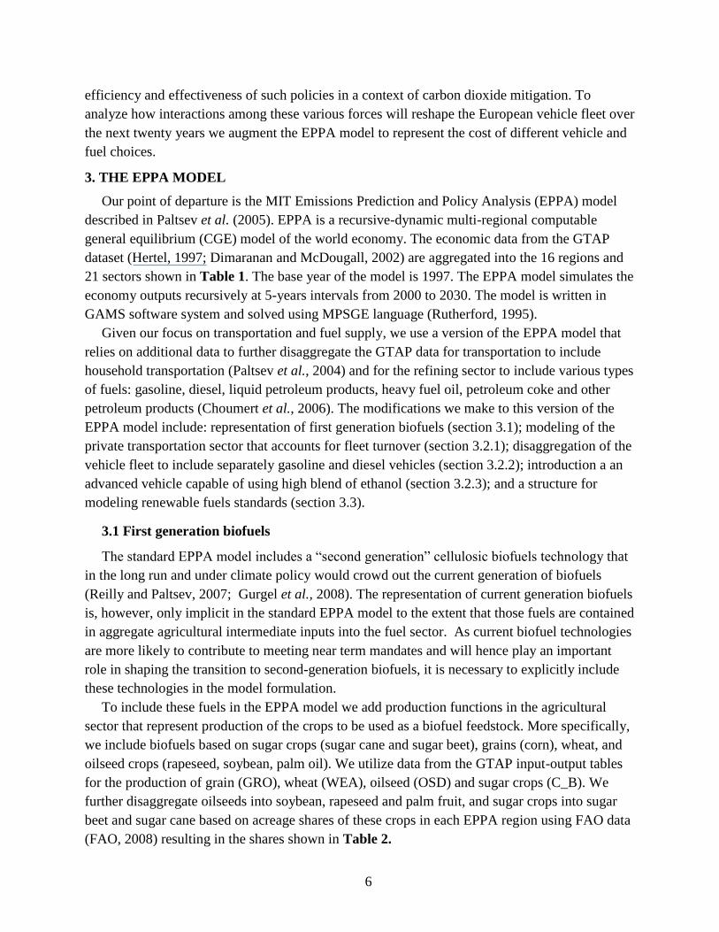
Table 1. Regions and Sectors in EPPA. Detail on the regional and sectoral composition is

provided in Paltsev et al. (2005), and for disaggregated refined oil sector in Choumert et al.

(2006).

Country or Region Sectors Specificity of EPPA-ROIL

Developed Non-Energy

United States (USA) Agriculture (AGRI)

Canada (CAN) Services (SERV)

Japan (JPN) Energy-Intensive Products (EINT)

European Union+ (EUR) Other Industries Products (OTHR)

Australia & New Zealand (ANZ) Transportation (TRAN)

Former Soviet Union (FSU) Household Transportation (HTRN)

Eastern Europe (EET) Energy

Developing Coal (COAL)

India (IND) Crude Oil (OIL)

China (CHN) Refined Oil (ROIL) Disaggregated Refined Oil

Indonesia (IDZ) Natural Gas (GAS) Liquid petroleum Gas (RGAS)

Higher Income East Asia (ASI) Electric: Fossil (ELEC) Gasoline (GSLN)

Mexico (MEX) Electric: Hydro (HYDR) Diesel (DISL)

Central & South America (LAM) Electric: Nuclear (NUCL) Heavy Fuel Oil (HFOL)

Middle East (MES) Electric: Solar and Wind (SOLW) Petroleum Coke (COKE)

Africa (AFR) Electric: Biomass (BIOM) Other Petroleum Products (OTHP)

Rest of World (ROW) Electric: Gas Combined Cycle

Electric: Gas with CCS

Electric: Coal with CCS

Oil from Shale (SYNO)

Synthetic Gas (SYNG)

Liquids from Biomass (BI-OIL)

Production of biofuel crop j (j= grain, wheat, sugar cane, sugar beet, soybean, rapeseed, and

palm fruit) uses capital, labor, land, intermediate inputs supplied by various sectors of economy

(agriculture, energy intensive industries, services, industrial transportation and other industries)

and energy supplied by electricity, gas and refined oil. We derive the share of these inputs from

the GTAP data. We represent crop production with nested CES functions shown in Figure 4.

Land productivity is assumed to improve over time according to an exogenous trend (1% per

year in developed regions and 1.5%-2% in Central and South America (LAM), Indonesia (IDZ),

India (IND), China (CHN) and Africa (AFR)). Note, however, that land productivity (i.e. crop

yields) varies endogenously over time and across the different scenarios as determined by

relative price changes and by the elasticity of substitution between land and the energy-material

bundle, and indirectly with the capital-labor bundle.

8

Table 2. Distribution of acreage between soybean, rapeseed and palm plant production and

between sugar cane and sugar beet in 1997.

GTAP Crop Feedstock for biofuels

USA CAN MEX JPN ANZ EUR EET FSU

Oilseed (OSD)

Soybean 99% 17% 97% 99% 5% 6% 28% 58%

Rapeseed 1% 83% 1% 1% 95% 94% 72% 42%

Palm fruit 0% 0% 3% 0% 0% 0% 0% 0%

Sugar Plant (C_B)

Sugar beet 61% 100% 0% 75% 0% 100% 100% 100%

Sugar cane 39% 0% 100% 25% 100% 0% 0% 0%

GTAP Data Feedstock for biofuels

ASI CHN IND IDZ AFR MES LAM ROW

Oilseed (OSD)

Soybean 37% 56% 48% 41% 18% 100% 98% 0%

Rapeseed 0% 44% 52% 0% 2% 0% 0% 96%

Palm fruit 63% 0% 0% 59% 81% 0% 2% 4%

Sugar Plant (C_B)

Sugarbeet 0% 34% 0% 0% 7% 88% 1% 0%

Sugarcane 100% 66% 100% 100% 93% 12% 99% 100%

Production of biofuel j use as an input biofuel crop j together with energy, intermediate

industrial inputs (from OTHR, EINT, TRAN and SERV sectors of the EPPA model), and capital

and labor, as shown in Figure 5(b). Because the relatively small amounts of biofuel production

that occurred in the base year data are not explicitly represented in the GTAP dataset, we assume

for our revised EPPA model that first generation biofuel technologies enter the market after

2000. For calibrating cost functions we base benchmark value shares on engineering analysis of

their cost of production.2 For ethanol from grain, we follow the estimates for the cost of

production from Tiffany and Edman (2003) and Shapouri and Gallagher (2003). For ethanol

from sugar crops, we use information available from USDA (2005) and IEA (2006). Finally, for

biodiesel from oilseed, we use data from Hass et al. (2005) and Fortenbery (2005). From these

studies we determine the cost components and the 2000 to 2005 average cost of production for

corn ethanol in the United States, sugar cane ethanol in Latin America and biodiesel from

soybean in the United States as provided in Figure 5(a). The cost of feedstock is between one

quarter and one third of the total production cost of ethanol and 80% of the production cost of

biodiesel.

2 The explicit technologies for production thus capture expansion of the industry beyond that amount implicitly

included in the base data set.

9

Figure 4. Production structure of biofuel crop sector j (j= grain, wheat, sugar cane, sugar

beet, soybean, rapeseed, and palm fruit). Vertical lines in the input nest signify a

Leontief or fixed coefficient production structure where the elasticity of substitution is

zero. Figures below the nests relate to the elasticity of substitution.

When adjusted to reflect the lower energy content of biofuels, costs of production range from

$0.39/L for ethanol from sugar cane to $0.55/L for ethanol from corn and to $0.57/L for

biodiesel from soybean. We extend our cost estimates to other regions following the approach

used in Gurgel et al. (2008). We assume that the conversion technology is the same in all regions

but that the feedstock shares vary regionally according to differences in crop prices as reported

by FAO (2008). For example, USA is the reference region for corn ethanol production in our

approach, which means that we normalize input shares in the US to sum to one, while in other

regions they sum to more or less than one depending on the relative price of corn, as provided in

Table 3. In the same fashion, Latin America is the reference region for sugarcane ethanol and

USA for soybean biodiesel. Where there was no crop price information from FAO (e.g. sugar

cane in Canada) we assume that little or none of the crop is grown in that region and we then do

not allow production of that fuel type in that region on basis that the country would need to

import the crop and that transport costs would favor importing the fuel from countries that can

produce the crop rather than the crop itself. We then apply a uniform mark-up multiplier across

regions (1.3 for sugar cane ethanol, 1.9 for corn ethanol and 2.1 for soybean biodiesel) to the

share parameters in the CES production function for all inputs. This ensures that the cost reflects

Biofuel Crop, j

Ressource-Intensive

Bundle

Energy-Materials

Bundle

Land

Intermediate Inputs

Bundle

AGRI EINT SERV TRAN OTHR

Domestic Imports

Value-Added

Capital Labor

Regions: 1 …

n

Energy Aggregate

ELEC Non ELEC

COAL OIL GAS ROIL

… … … …

… … …

…

0.7

0.6

0.3

1

3

5

1.0

10

the bottom up estimates of costs reported above for each biofuel relative to the price of gasoline

or diesel in the reference region for the average 2000 to 2005 data.3

We extend cost structures from Figure 5(a) for wheat and sugar beet ethanol and rapeseed

biodiesel produced in Europe, but we modify the relative weights between the crop and other

inputs bundle to reflect the difference in feedstock prices. A comparison of the European, US

and Brazilian prices for wheat, corn, sugar beet, sugar cane (FAO, 2008) and of rapeseed and

soybean (USDA, 2008) allows us to estimate the 2000-2005 averaged cost of wheat ethanol at

$0.65/L, sugar beet ethanol at $0.77/L and rapeseed biodiesel at $0.68/L. This estimate results in

a mark-up (cost of production relative to refined oil) of 2.2 for wheat ethanol, 2.3 for rapeseed

biodiesel and 2.6 for sugar beet ethanol. Following the approach described above, we extend

these costs of production across all the EPPA regions in which these crops are produced. Table 3

provides the regionally specific data for biomass input shares. For example, for ethanol from

corn the production shares in the US are 0.35 for capital input, 0.03 for labor input, 0.12 for

energy, 0.11 for other industries (OTHR) inputs, and 0.39 for biomass feedstock input. As shown

in Table 3, we use the same input shares across regions, except that for example, in Europe

(EUR), the crop share is now 0.70 instead of 0.39 to reflect the relatively higher cost of corn. The

same is true for other regions and technologies. The mark-up factor is then applied on top of all

inputs.

The cost structure of biodiesel from palm oil and its mark-up factor (which is equal to 1.6) are

evaluated with the same methodology by using the relative price of palm oil compared to soy oil

(USDA, 2008). In addition, as noted previously in Section 2, biodiesel standards in Europe

require products from soybean and palm oil to be further transformed before being injected in

engines. Following Moser et al. (2007), we estimate the cost of these additional process steps at

$0.05 per liter of biodiesel produced and therefore we raise the mark up for imports to Europe:

from 1.6 to 1.8 for biodiesel produced from palm fruit and from 2.1 to 2.2 for biodiesel from

soybean. Elasticities of substitution in Figure 5(b) are taken from the refined oil sector in

Choumert et al., (2006).

3 EPPA follows a standard approach in CGE modeling whereby in the benchmark year all prices are normalized to

1.0 and outputs and inputs are denominated in dollars rather than in gallons, tons, or some other physical unit.

We retain this basic normalization procedure for new technologies, appealing to cost data per physical unit of

new technology relative to the cost of the technology it would replace to estimate the mark-up. This procedure

assures consistency between the economic accounting of the model and supplementary physical accounting for

physical units of energy, emissions, or land use.

11

(a)

(b)

Fuel j

Intermediate Inputs Bundle

EINT SERV TRAN OTHR

Domestic Import

Biofuel crop j

Capital Labor

Regions: 1 …

n

… … …

0.2

3

5

Value

added

…

1.0

Figure 5. Structure for the production of biofuels. (a) Cost structure for biofuel production

(these estimations are established for ethanol from corn in USA, from sugarcane in

Brazil and for biodiesel from soy oil in USA); (b) Structure of first generation biofuels

production function in EPPA. Biofuel crop j=grain, wheat, sugar cane, sugar beet,

rapeseed, soybean or palm fruit. Numbers shown in the figure are the elasticities of

substitution assigned to each input nest. For j=grain, wheat, sugar cane or sugar beet,

fuel j is ethanol that is a perfect substitute for gasoline. For j=soybean, rapeseed or palm fruit, fuel j is biodiesel that is a perfect substitute for diesel.

0% 20% 40% 60% 80% 100%

Percent of total cost of production

Grain

Sugar plant

Oilseed

Feed

sto

ck

Feedstock

Chemicals

Energy

Other

Capital

12

Table 3. Parameters used for the production function of first generation biofuels in EPPA:

mark-up and input shares (*** denotes absence of price information for the feedstock in

the FAO dataset).

Input shares

Technology Mark-up Factor Capital Labor Crop Energy bundle OTHR

Ethanol

from

Corn 1.9 0.35 0.03 0.39 0.12 0.11

Wheat 2.2 0.29 0.02 0.49 0.10 0.10

Sugar Cane 1.3 0.47 0.16 0.26 0.05 0.06

Sugar Beet 2.6 0.27 0.09 0.57 0.02 0.05

Biodiesel

from

Rapeseed 2.3 0.05 0.03 0.84 0.02 0.06

Soybean 2.1 (2.2 for

imports to EU) 0.06 0.03 0.81 0.02 0.08

Palm oil 1.6 (1.8 for

imports to EU) 0.07 0.04 0.77 0.02 0.10

Crop input shares for each technology (regionally specific)

USA CAN ME

X JPN ANZ EUR EET FSU

Ethanol

from

Corn 0.39 0.64 0.73 3.90 0.74 0.70 0.52 0.42

Wheat 0.38 0.33 0.47 4.41 0.47 0.49 0.42 0.54

Sugar Cane 0.58 *** 0.62 3.30 0.37 *** *** ***

Sugar Beet 0.56 0.58 *** 1.84 *** 0.57 0.61 0.42

Biodiesel

from

Rapeseed 1.06 0.76 0.27 9.49 0.88 0.84 0.85 0.32

Soybean 0.81 0.84 0.91 10.61 0.95 0.83 0.66 0.49

Palm oil *** *** 0.79 *** *** *** *** ***

ASI CH

N IND IDZ AFR

ME

S LAM

RO

W

Ethanol

from

Corn 0.66 0.58 0.60 0.69 0.86 1.07 0.52 1.47

Wheat 1.08 0.51 0.49 *** 0.92 1.16 0.56 1.57

Sugar Cane 0.40 *** 1.23 0.40 0.46 *** 0.26 0.73

Sugar Beet *** 0.71 *** *** 0.35 0.80 0.74 2.07

Biodiesel

from

Rapeseed *** 0.92 1.44 *** 1.45 *** 1.13 3.17

Soybean 1.09 1.13 0.93 1.28 1.60 4.85 0.80 2.26

Palm oil 0.75 0.73 *** 0.77 1.19 *** 1.19 3.34

3.2 The private transportation sector

We amend the existing transportation sector in the EPPA model in three ways: (1) We

explicitly treat vehicle fleet turnover, (2) we disaggregate diesel and gasoline vehicles, and (3)

we allow introduction of E85 vehicles. We adopt these modifications in the USA and EUR

region only.

13

3.2.1 Representation of the fleet turnover

The previous approach in EPPA has been consistent with the National Income and Product

Accounts (NIPA) practices that consider the private purchase of vehicles as a flow of current

consumption. That representation underestimates inertia in the own-supplied transportation as

vehicle fleets have a typical lifetime of 15 years. Our revised approach treats vehicles as capital

goods that depreciate while providing a flow of services over their lifetime. NIPA data determine

returns to capital as a residual of the value of the sales less intermediate inputs and labor cost.

By assuming a rate of return and a depreciation rate, it is then possible to impute the level of the

capital. The private transportation sector provides a flow of services that is not directly marketed

and thus, there is no directly comparable data on the gross value of the transportation services

from which intermediate inputs can be subtracted.

We use a cost approach that estimates the value of private transportation services as the sum

of the costs incurred by the owner, including capital cost and operating costs. We first evaluate

the value of the stock of cars from historical sales and then, impute the rental value of the stock

of cars assuming an appropriate depreciation rate δ and a rate of return R on capital. The rental

value of capital is derived from a Jorgenson-type estimation of R, which is the sum of the

depreciation rate and a rate of interest r:

R r .

We use a constant depreciation rate that accounts for the average life of a vehicle. The

European Association of Automobile Manufacturers (ACEA, 2006) provides us with the

distribution of 2006 car stock by age in the EU15 and with new cars registrations since 1979.

The lifetime function deduced from these data characterizes the European stock of cars with a

mean lifetime of about 15 years and an average age of about 8 years. An exponential fit of this

function produces a depreciation rate of about 8%. In addition, we assume that the real rate of

interest is 5% to be consistent with the treatment of other industrial assets in EPPA.

We represent the vehicle fleet as a vintaged capital stock, similar to the representation of

industrial sectors in EPPA (see Paltsev et al., 2005). The total stock of vehicles at time T is:

v

v

T

n

TT KCKCKC

where the superscript n denotes new vehicles, and v=1,...,4 are the multiple vintages of pre-

existing vehicles. For each vintage:

1

1)1( v

T

v

T KCKC

where v = 0 are the new vehicles from the previous period, and because we carry only 4 vintages

there is 100% depreciation of the oldest vintage v=4. Each vintage is represented as a fixed

coefficient production function. Purchasers of vehicles can choose the fuel efficiency and other

characteristics of new vehicle but once they are part of the fleet these characteristics are frozen.

For other industrial sectors we include a share, θ, of new capital that is vintaged, to represent the

possibility of retrofitting pre-existing capital. We represent the vehicle fleet as 100% vintaged;

i.e. there is no possibility to retrofit existing vehicles.

14

We follow the approach of Paltsev et al. (2004) where own-supplied transportation

(OWNTRN) uses inputs from the other industries (purchase of cars), from the services sector

(maintenance, insurance) and from the refinery sector (see Table 4). Because we now consider

the vehicle fleet as a capital stock we remove from household current consumption the payment

for new cars and for used cars. The former is now added to the total of capital goods. Its value is

derived from the value of private consumption of the “manufacture of motor vehicles” sector in

the GTAP dataset. The purchase of used cars is removed from the account for the flow of private

transportation services because in our approach this transaction does not modify the total amount

of capital endowed to the final consumer. Household expenditure surveys on transportation

suggest that used vehicle purchases account for about 14% of the total expenditures for the

private transportation (BEA, 2008). As noted in Paltsev et al. (2005), services inputs in the own-

supplied transportation have a large share because they include not only financial services,

maintenance, insurance but also services related to the distribution of fuel.

Table 4. Input shares in the private transportation sector by type of engine for new

registrations in the benchmark year.

FUEL OTHR SERV

Private transport sector

Paltsev et al. (2004)

USA 0.080 0.220 0.700

EUR 0.240 0.260 0.500

FUEL CAPITAL SERV

Private transportation

sector net of taxes

Gasoline

vehicle

USA 0.127 0.131 0.742

EUR 0.105 0.241 0.655

Diesel vehicle USA 0.083 0.175 0.742

EUR 0.093 0.252 0.655

Private transportation

sector with fuel taxes

Gasoline

vehicle

USA 0.127 0.131 0.742

EUR 0.425 0.137 0.438

Diesel vehicle USA 0.083 0.175 0.742

EUR 0.270 0.292 0.438

3.2.3 Disagreggation of gasoline fleet and diesel fleet

Information derived from EIA (1994) for USA, from the European Commission (CEC,

2008b), and from Bensaid (2005) provide us with an estimate of the stock and the sales of diesel

passenger cars in 1997. Average on-road fuel use per unit of distance (ACEA, 2003) allows us to

estimate the physical share of diesel in the total consumption of fuel for private transportation in

1997. We multiply this share by estimates of relative fuel prices (IEA, 1998) and deduce the

value of diesel expenditure as a share of total expenditures on refined oil products in the private

transportation sector. With these typical fuel economy numbers we also evaluate the total miles

driven in 1997 by diesel and gasoline fleet. Since we assume that one mile driven with a diesel

car provides the same mobility service as one mile driven with a gasoline car, the share of diesel

private transportation in the total flow of private transportation services is equal to the share of

miles driven by diesel engines. Based on this hypothesis, we split the value of the private

15

transportation output (OWNTRN) between diesel (OWNTRNdisl) and gasoline (OWNTRNgsln)

technology.

The higher efficiency of diesel combustion implies a higher input share for the services-

capital bundle in the diesel own-supplied transportation sector. This is not surprising, as we have

noticed in Section 2 that better efficiency comes at an additional cost for purchasing a diesel

vehicle. As we assume that the share of services input is the same in both technologies, we can

fully determine the structure of the diesel and gasoline private transportation, as provided in

Table 4. From shares net of taxes, we can deduce that in Europe, the rental value for a new diesel

vehicle is $100/year more expensive than for a new gasoline vehicle, meaning that given an

interest rate at 5% and a depreciation rate at 8%, the purchase of diesel engine is $600 more

expensive than the purchase of gasoline engine. This number has to be compared with

discounted savings of $500 that are obtained due to the better efficiency of diesel engine with

fuels at 0.25/L (exclusive of taxes) in 1997.

GTAP data do not differentiate taxes on diesel and gasoline. We use data from IEA (2008a),

illustrated previously in Figure 3, to determine the ad-valorem tax on gasoline in the benchmark

year and to establish revenue raised by these excise duties. The excise duty on diesel is then

adjusted to keep the revenue from fuel taxes equal to the revenue accounted in GTAP in 1997.

The elasticity of substitution used in these production sectors are derived from the survey of

econometrics studies in Paltsev et al. (2004), which suggests estimates for short run elasticities

between fuel and other inputs in the range of 0.2-0.5 and for long run elasticities in the range of

0.6-0.8. For the transportation services provided by new vehicles, we use the long run elasticity

of substitution that is assumed to capture the ability to respond to higher fuel prices by

purchasing more efficient vehicles. With the vintaging structure the aggregate short run elasticity

will reflect a weighted average of old vintages with a zero substitution elasticity and the new

vintage with the high elasticity. Persistently high prices will then gradually lead to a vehicle fleet

with greater efficiency. Vintaging captures structurally the observed difference between short

and long run elasticities.

3.2.3 Introducing E85 vehicles in EPPA

Blending more than 10% of biofuels into conventional fuels may damage vehicles that are not

designed to utilize them. Thus, fuel standards limit the blending percentage. In the U.S. the 10%

limit is often referred to as the blending wall, because it would limit biofuel use absent vehicles

that could use a greater percentage. In Brazil, flex-fuel vehicles that can run on any mix of

ethanol and gasoline are popular. They accounted for 84% of new sales at the beginning of 2009

according to ANFAVEA (2009). In the United States E85 vehicles that can run on blends of up

to 85% ethanol have been introduced in response to fuel-economy compliance credits offered by

the Department of Transportation since 2001 (NHTSA, 2001). In 2007, almost 5% of the 17

million new light-duty vehicles sold in the U.S. were E85 vehicles.

In EPPA, we introduce E85 vehicles as an advanced technology that enters the market after

2000 and that is mostly based on the same input shares as the conventional gasoline technology.

16

However, modifications (including a stainless fuel tank and a special sensor to adjust engine

spark timing) add an estimated $200 to the vehicle cost (Keefe et al., 2007). That extra cost

translates to a mark-up of 1.015 on the capital input share in the E85 fleet production function.

The main advantage of including E85 vehicles explicitly is that the vintaging of the vehicle fleet

limits the use of ethanol based on the 10% blending wall on conventional vehicles and the

growth of the stock of E85 vehicles available.

There are also additional costs associated with distribution of E85 fuel. For example, adding

an E85 pump at a service station is estimated to cost approximately $200,000 (Keefe et al.,

2007). IEA (2006) estimates that the total infrastructure changes needed for the transport, storage

and distribution of E85 add about $0.06/gal to the price of ethanol. We add this additional cost

for selling E85 in the services input in the production block of E85.

3.2 Implementing fuel standards in EPPA

There are at least a couple of ways one could represent fuel standards in the EPPA model.

One approach would be to introduce a quantity constraint in the GAMS-MPSGE algorithm used

in the EPPA model. A second approach is to create a system of permits. We use the permit

approach. We implement the permit approach as follows: Firms that produce one unit of

renewable fuel receive one Renewable Fuel Standards (RFS) permit. Every unit of conventional

fuel or of its perfect substitute requires the surrender of a quantity of RFS permits to meet the

renewable fuel mandate, specified as a share, φ, of total fuel. The conventional refiners must

acquire permits from the renewable fuel producers. This approach captures the redistribution of

funds between conventional refiners and biofuels producers, as fuel sellers must pay a premium

(the permit price) to renewable fuel producers.

To capture the 10% blending wall and E85 fuel production we introduce another set of

permits (which we refer to as NORM10 permits) and two blending processes that complement

the conventional refinery sector. The conventional refinery produces conventional fuel. The 10%

blending process is a combination of conventional refinery that is mandated to surrender φ RFS

permits and of biofuels industry that uses as inputs biofuels and NORM10 permits and produces

RFS permits and a perfect substitute for conventional fuel. In this way we allow biofuel

production only up to the amount of NORM10 permits available. The E85 blending process is a

fixed coefficient production function blending 85% biofuels and 15% conventional fuel.

Conventional refineries produce 0.1 NORM10 permits for every unit of fuel produced. This

ensures that the total number of NORM10 permits is only 10% of total fuel production. Use of

E85 is more expensive because of the extra distribution costs and higher vehicle costs. Thus, a

fuel mandate of φ < 10% can be met using the 10% blending process up to that level needed to

meet the target, and even if biofuels are economic without the mandate, they are limited to not

more than 10% unless they overcome extra cost of using E85. A fuel mandate of φ > 10%

requires use of the E85 blending process, and at high enough φ E85 will crowd out the 10%

blending process. The structure of the permit approach is represented in Figure 6.

17

3.4 Scenarios

We use the extended version of the EPPA model to implement four alternative scenarios in

order to investigate interactions between fuel policy in the European transportation sector and the

prospect for diesel vehicles. The first scenario is the no climate policy reference or business-as-

usual (BAU), with the current tax and tariffs structure described in Section 2. The second

scenario (MAND) simulates the European Commission (2008) proposal to introduce mandates

on renewable fuels: 5.75% by 2010 and 10% beyond 2020 (in volume terms) have to be blended

into conventional fuels. The last two scenarios include the biofuel requirements of the MAND

scenario but vary the tax and tariff policy. The MAND_TARIFF scenario removes tariffs on

ethanol and biodiesel imports. The MAND_TAX scenario replaces the differentiated fuel taxes

by a uniform ad-valorem rate on all liquid fuels at the gas station which is set at a level to keep

revenues constant at the BAU level. In fact, to ensure comparability with the reference case, we

endogenize fuel taxes in the MAND and MAND_TARIFF scenarios to keep total tax and tariff

revenues constant at the BAU level. The revenue neutrality requirement is important because we

want to compare welfare cost implications across scenarios, and without a revenue neutrality

assumption the welfare results would depend arbitrarily on where the tax or tariff rate is set. Both

tax and tariff policies are implemented in 2010 jointly with renewable initiatives.

4. RESULTS

Our results focus on the relative penetration of diesel and gasoline vehicles, fuel prices, the

composition and sources of fuels, welfare effects of the policies, CO2 emissions, and trade in

fuels.

4.1 The vehicle fleet

In the BAU case, diesel vehicles continue to penetrate the European vehicle fleet and account

for 34% of all vehicles by 2030 (Figure 7). This growth is driven by a tax system that maintains

RFS permits

φ

Fuel

1.0

Fuel

1.0

RFS permits

1.0

NORM10

Permits

0.1 E85

1

Fuel

1.0

RFS permits

φ

Biofuel

1.0

NORM10

Permits

1.0

RFS permits

φ

Biofuel

0.85

Fuel

0.15

RFS permits

0.85

SERV

0.05

(a) (b) (c)

Figure 6. Implementation of renewable fuels standards in EPPA. (a) Production function of

conventional fuel; (b) Production function of blending of biofuels into conventional

products up to 10%; (c) Production function of E85. Vertical lines in the input nest

signify a Leontief or fixed coefficient production structure where the elasticity of

substitution is zero. Figures below the inputs name are the value of inputs shares. The

φ is the renewable fuel standard.

18

the price of diesel - $5.63/gal by 2030- at the gas station below the price of gasoline - $6.30/gal

by 2030 (Table 5) and by the general increase in oil prices that favors the most efficient

motorization. The share of diesel vehicles drifts upward gradually due to sales of new diesel cars

that stabilize around 33-35% of the new registrations after 2020. These numbers are lower than

the current sales of diesel vehicles in Europe (up to 50%) because the endogenously determined

oil price in the model reaches $50/bbl by 2030, below those levels through 2008 that were

strongly driving the diesel trend in Europe.

A factor behind the gradual leveling off of the diesel share of new vehicles beyond 2020 is

that diesel price is growing somewhat faster than the gasoline price. The diesel price, exclusive

of excise duties, reaches $1.92/gal by 2030 compared with the gasoline price of $1.64/gal.

Therefore, prices inclusive of taxes gradually converge: the gasoline price at the pump is only

12% higher by 2030 than diesel price, while it is one third more expensive in the benchmark

year. The limited ability of the European refineries to respond to the growing demand for diesel

increases the pressure on the supply of diesel. The refinery sector is modeled as a multi-output

production sector where the ability to shift the product share is limited by an elasticity of

transformation of 0.2 between refinery outputs.

The MAND scenario results in somewhat greater penetration of diesel vehicles as they

account for 35% of the passenger cars driven in 2030 (Figure 7). The differentiated tariffs system

on biofuels, favoring biodiesel over ethanol, makes biodiesel from Indonesia (Figure 8) a

somewhat less expensive way to meet the mandate than either domestic ethanol or imported

sugar cane ethanol. The differential tariff structure maintains the gap between diesel price and

gasoline price at the gas station: by 2030 one gallon of diesel costs $5.70 and one gallon of

gasoline $6.39 (Table 5).

The marked trend of penetration of diesel vehicles hinges decisively on the current tax and

tariff regime in Europe. Changes in tax and/or tariffs can reverse this trend as demonstrated in

the MAND_TAX and MAND_TARIFF scenarios. The MAND_TAX scenario leads to a share of

diesel vehicles that falls to 21% by 2030. The MAND_TARIFF scenario has less effect in the

near term but beyond 2020 the diesel vehicle share falls sharply due to the rising price of

conventional gasoline makes sugar ethanol sufficiently competitive to offset additional costs that

are involved in the deployment of E85 fuels and vehicles. The mandatory fuel standards become

irrelevant, the E85 fuel blend is produced, and E85 vehicles crowd out diesel vehicles whose

sales fall to zero by 2030.

19

In the MAND_TARIFF scenario, the shift toward gasoline-ethanol blend, which is more

heavily taxed, leads to lower tax rates on both fuels to satisfy the revenue neutrality condition.

By 2030 excise duties on both gasoline and diesel decrease by 4.7% compared to the MAND

scenario and then prices of fuels inclusive of duties drop as shown in Table 5, which reduces

even further the appeal for diesel vehicles.

Figure 7. (a) Share of diesel vehicles in the European stock of cars and (b) in the

European new registrations.

(a)

0%

5%

10%

15%

20%

25%

30%

35%

40%

1995 2000 2005 2010 2015 2020 2025 2030

Year

Sh

are

of

die

se

l (%

).

BAU

MAND

MAND_TAX

MAND_TARIFF

(b)

0%

5%

10%

15%

20%

25%

30%

35%

40%

1995 2000 2005 2010 2015 2020 2025 2030

Year

Sh

are

of

die

se

l (%

)

BAU

MAND

MAND_TAX

MAND_TARIFF

20

Table 5. Price of fuel at the gas station by 2030 ($/gal).

BAU MAN

D MAND_TAX MAND_TARIFF

Diesel exclusive of duties ($/gal) 1.92 1.94 1.87 1.96

Gasoline exclusive of duties ($/gal) 1.64 1.67 1.79 1.52

Diesel inclusive of duties ($/gal) 5.63 5.70 6.31 5.74

Gasoline inclusive of duties ($/gal) 6.30 6.39 6.06 5.84

4.2 Welfare, emissions and trade impacts of fuel policies

Renewable fuel policies are often motivated by a desire to reduce CO2 emissions on the

assumption that these fuels are cleaner than conventional gasoline and diesel. One might also

hope to achieve these policies at the least cost or for changes in tax policy to improve overall

welfare in the economy. Still another motivation is reductions in fuel imports.

We find that the renewable fuels requirement generates a welfare loss of 0.09% by 2030

relative to the reference case (Figure 9). This is hardly surprising since it increases fuel prices at

the pump. We find, however, that the MAND_TAX actually improves welfare relative to the

reference case. The reason for this is that existing fuel taxes distort fuel choices. The lower tax-

inclusive price diesel leads people to choose more expensive diesel vehicles over gasoline

vehicles, but because the lower price is due to the tax rate there are not a real cost savings from

using the diesel fuel when European consumers are seen as a group. Equating excise taxes on

gasoline and diesel eliminates this relative fuel price distortion, and the welfare gains from that

change outweigh the higher cost of biofuels and the initial shock that such a policy generates in

2010 on the diesel stock that has been previously formed in a fiscal environment favorable for

diesel vehicles. Lowering tariffs on biofuels in the MAND_TARIFF scenario provides access to

lower cost ethanol. The absence of trade barriers makes the renewable requirements costless in

terms of welfare before 2020. After 2020 it generates substantial welfare gain (0.34% by 2030)

by making sugar ethanol, which by this time is less expensive than gasoline, available to the

European market.4

4 Results obtained from simulations that do not impose the revenue neutrality constraint are found to be qualitatively

identical and show only negligible quantitative differences. For example, welfare losses in the MAND scenario

are slightly higher (-0.10%) and welfare gains in the alternative scenarios slightly lower (MAND_TARIFF:

0.29%; MAND_TAX: 0.12%).

21

]

In a context of carbon dioxide mitigation, these welfare changes can also be evaluated in

terms of the resulting reductions in emissions. In our calculations we assume that carbon dioxide

released in the atmosphere by the consumption of biofuels has been previously captured during

the harvest of feedstock, so the net emissions from biofuels are zero. However, energy is used to

grow the crop and produced the biofuels, and there are emissions associated with that use of

energy.5 Looking just at the emissions from the European private vehicle fleet, the renewable

requirement reduces carbon dioxide emissions by 8.2% (MAND scenario) from the 2030 level

without the requirement (Figure 10). The relaxation of tariffs barriers on biodiesel and ethanol

has a much stronger mitigation effect reducing emissions from the private transportation sector

by 45.3% in 2030. The harmonization of fuel taxes in the MAND_TAX scenario has the

opposite effect, dampening slightly the mitigation effect of renewable fuel requirements. By

2030 the European fleet emits only 3.4% less CO2 than in the BAU scenario. This results from

the fact that the harmonized tax rates leads to increased purchases of gasoline vehicles that have

a lower efficiency.

5 There are also potential “indirect” emissions from biofuels that result when the increased demand for land to

produce biofuel crops cause land conversion. If those conversions are from undisturbed land the result can be

significant carbon dioxide emissions. We do not calculate that effect here.

Figure 8. (a) Composition of liquid fuels distributed at the gas stations (EUR) in the

Business-as-Usual scenario, (b) in the mandates scenario, (c) in the mandates

scenario with harmonized excise duties on fuels and (d) in the mandates scenario

without tariffs on biofuels.

(a)

0

50

100

150

200

250

300

1997 2000 2005 2010 2015 2020 2025 2030

Year

Co

nsu

mp

tio

n (

bil

lio

n o

f li

ters

)

Conventional Gasoline

Conventional Diesel

(b)

0

50

100

150

200

250

300

1997 2000 2005 2010 2015 2020 2025 2030

Year

Co

nsu

mp

tio

n (

bil

lio

n o

f li

ters

)

Conventional Gasoline

Conventional Diesel

Biodiesel imported from IDZ

Ethanol domestically

produced

(c)

0

50

100

150

200

250

300

1997 2000 2005 2010 2015 2020 2025 2030

Year

Co

nsu

mp

tio

n (

bil

lio

n o

f li

ters

)

Ethanol domestically

produced

Conventional Diesel

Biodiesel imported from IDZ

Conventional Gasoline

(d)

0

50

100

150

200

250

300

350

1997 2000 2005 2010 2015 2020 2025 2030

Year

Co

nsu

mp

tio

n (

bil

lio

n o

f li

ters

)Biodiesel imported from IDZ

Conventional Diesel

Conventional Gasoline

Ethanol imported from LAM

and AFR

22

-0.1

-0.05

0

0.05

0.1

0.15

0.2

0.25

0.3

0.35W

elf

are

ga

in (

%)

2010 2015 2020 2025 2030

Year

MAND

MAND_TAX

MAND_TARIFFS

Emissions from the private vehicle fleet are, however, not the whole story. Figure 11 shows

for 2020 and 2030 the change in emissions for just the private transportation sector in Europe

(the same information as in Figure 10 but in mega tons of CO2 rather than as a percentage), the

change in private transportation emissions plus emissions from processing biofuels in Europe,

the change in emissions from all sectors in Europe, and the change in global emissions. This

shows leakage and life cycle effects (non including indirect land use change effects).

In the MAND and MAND_TAX scenarios some of the reductions from private vehicles are

offset within Europe by emissions from process emissions from biofuel production. In the

MAND_TARIFF case there is no difference because biofuels are imported and so there are no

process emissions in Europe. European emissions outside the transportation and biofuels

processing sectors are reduced in the MAND case, partially offsetting the process emission

effect, and in the MAND_TARIFF case actually leading to greater emissions reductions because

there are not biofuel process emissions. The main source of this effect is less European refinery

emissions because less conventional fuel is used. For the MAND_TAX scenario the decrease in

diesel vehicles lower the pressure on diesel supply and spurs an increase of diesel consumption

by other sectors of the economy (agriculture, services and industries) especially as the economy

is growing faster than in the BAU scenario. This additional demand for diesel reduces the

emissions benefit further, and actually almost offsets the mitigation effort in 2030. The effect of

renewable initiatives on global emissions is generally reduced further still. The main effect here

Figure 9. European welfare changes obtained in the fuel policy when compared to the

Business-As-Usual scenario.

23

is that reduced conventional fuel demand in Europe (except in the MAND_TAX case) leads to

lower prices for fuel outside of Europe and an increase in fuel use and emissions. Biofuels

imports also have associated emissions but the energy used in biofuels from ethanol is a

relatively small factor because the sugar ethanol generally uses bagasse for process energy.

Energy use is mainly associated with growing and harvesting the crop. In the MAND_TAX

scenario, increased demand for gasoline in Europe drives up gasoline prices outside of Europe

and favors a reduction of gasoline use and emissions: here accounting for leakage effects make

the MAND_TAX scenario almost as effective as the MAND scenario in terms of emissions

reduction.

Trade in liquid fuels is often another motivating factor for a fuel policy. Facing a demand for

diesel that is growing faster than the demand for gasoline, the European refinery industry has

increased its exports of gasoline, mostly to the United States (39% of European gasoline exports

in 1997) and must import diesel, mostly from Russia (66% of European diesel imports in 1997).

In the BAU scenario the growth of the diesel fleet sustains the trend with increasing exports of

gasoline (+35% by 2030 relatively to 1997 exports after peaking at +62% by 2020). Biofuels

mandates amplify this trade pattern further, as they promote the dieselization of the European

fleet (Figure 12): from 1997 to 2030 imports of Russian diesel rise by 2% and exports of

gasoline by 51% (after peaking at +79% by 2020). Both the alternative tax system and fuel trade

policy reduce the size of the diesel fleet by 2030 and, consequently the imports of diesel from

FSU decrease from 1997 to 2030 by 6% (MAND_TARIFF) and by 17% (MAND_TAX).

Equating fuels taxes reverses the trend toward rising exports of gasoline as domestic demand

Figure 10. Reduction of CO2 emissions from the private European transportation sector

relative to the Business-As-Usual scenario. These calculations do not account for

emissions from biofuels processing.

-50

-45

-40

-35

-30

-25

-20

-15

-10

-5

0

CO

2 e

mis

sio

ns r

ed

ucti

on

(%

)

2010 2015 2020 2025 2030

Year

MAND

MAND_TAX

MAND_TARIFFS

24

(b)

-90

-80

-70

-60

-50

-40

-30

-20

-10

0

10

20

MAND MAND_TAX MAND_TARIFFS

Scenarios

Em

issio

ns (

MtC

)

European private transportation

European transportation sector +

biofuel processes in Europe

Europe: all sectors

World

grows. On the contrary, with free biofuels trade, gasoline exports are growing even faster after

2020. European refineries cannot respond rapidly to the dramatic shift toward ethanol; as they

continue to produce diesel especially for sectors beyond the private vehicle fleet (residential,

agriculture, commercial transportation and services sectors) they are unable to shift the refinery

slate and so have significant production of gasoline that has to be exported.

Figure 11. Reduction of the emissions by the European renewable fuels initiatives in (a)

2020 and (b) 2030.

(a)

-12

-10

-8

-6

-4

-2

0

MAND MAND_TAX MAND_TARIFFS

Scenarios

Em

issio

ns (

MtC

)

European private transportation

European transportation sector

+ biofuel processes in EuropeEurope: all sectors

World

25

5. SENSITIVITY ANALYSIS

Previous results emphasize the interactions between fuel policies and the prospects for diesel

vehicles in Europe. In this section we examine the sensitivity of the results to our modeling

assumptions, such as elasticity of substitution and mark-ups.

As the elasticities of substitution are not known with certainty, we test our results by varying

them. Of a particular interest are the elasticities of substitution between outputs in the refinery

sector and between fuel and other inputs in the private transportation sector, because their

Figure 12. Index of (a) gasoline exports from EUR and of (b) diesel imports from FSU to

EUR. Index=1 in 1997.

(a)

0.8

1

1.2

1.4

1.6

1.8

2

2.2

1997 2002 2007 2012 2017 2022 2027

Year

Ra

tio

(=

1 w

ith

ou

t m

an

da

te) BAU

MAND

MAND_TAX

MAND-TARIFFS

(b)

0.8

0.85

0.9

0.95

1

1.05

1.1

1997 2002 2007 2012 2017 2022 2027

Year

Ra

tio

(=

1 w

ith

ou

t m

an

da

te)

BAU

MAND

MAND_TAX

MAND-TARIFFS

26

variations may affect differentially the diesel and gasoline fleets. To examine how changes in

these substitution possibilities would impact the diesel fleet, we separately vary them and show

in Table 6 the share of diesel cars by 2030.

The results for diesel market share are not very sensitive to alternative values of key

parameters. This holds for all the scenarios described in Section 3. The effects of varying the

elasticity of substitution is of a second order compared to the rise in fuel prices that drives the

demand for less fuel intensive technology or for cheapest fuel. Increasing substitution

possibilities between refinery outputs relieves the pressure on the supply of diesel and allows a

further expansion of the diesel fleet, but this effect remains small. The ability to switch between

fuel and other inputs in the own-supplied transportation sector also does not change significantly

the prospects for diesel cars. As diesel vehicles are already more efficient than gasoline-based

cars, additional improvements in technology and easing substitution between fuel and other

inputs favors diesel. But this effect is partly dampened because diesel prices grow faster than

gasoline prices, which encourages further substitution away from fuel (i.e. purchase of vehicles

with greater diesel engine efficiency). In all scenarios, over the 1997-2030 period, the efficiency

of new diesel engines increases more (+ 33% in miles per gallon) than of new gasoline engines

(+19% in miles per gallon).

Among other sources of uncertainties in our modeling assumptions are the mark-ups related to

costs for dispensing E85 and for purchasing an E85 vehicle. According to IEA (2006),

uncertainties on the former are substantial as they range between $0.03 and $0.2 per gallon of

ethanol. Information on the latter are unclear, particularly in the U.S. where automakers are

enticed to sell flex fuel engines because it produces a mileage credit under the Corporate

Average Fuel Economy standards. However Table 6 shows that variations in these parameters do

not change significantly the interactions between fuel policies and diesel fleet. E85 is never sold

even without any additional costs entailed to its distribution infrastructures, unless tariffs on

ethanol are suppressed. In this last scenario the contraction of diesel fleet remains a robust

pattern even if E85 or flex fuel technology turns out to be more expensive than expected. Under

renewable fuels mandates, inexpensive sugar ethanol even blended only up to 10% with

conventional gasoline already reduces the cost of gasoline and makes the gasoline fleet more

attractive.

27

Table 6. Share of diesel vehicle in the European fleet with different elasticities of

substitution for the refinery sector, for the private transportation sector and different costs

assumption for E85 vehicle (* denotes the base case parametrization).

Sector Elasticity of substitution between

BAU MAND

MAND_TAX MAND_TARIFF

S

Refined oil Refinery outputs

0.0 33% 33% 20% 13%

0.2* 34% 35% 21% 13%

0.4 35% 37% 21% 15%

0.6 36% 38% 22% 16%

0.8 36% 38% 22% 17%

Private Transportation

Fuel and other inputs: New cars

0.2 38% 39% 24% 14%

0.4 36% 38% 23% 13%

0.6* 34% 35% 21% 13%

0.8 32% 33% 18% 15%

1.0 30% 31% 16% 15%

Fuel and other inputs: Vintage cars

0.0* 34% 35% 21% 13%

0.1 33% 34% 19% 13%

0.2 33% 35% 20% 13%

0.3 32% 33% 18% 12%

0.4 31% 33% 17% 11%

Sector Mark-up BAU MAND

MAND_TAX MAND_TARIFF

S

Private Transport: flex fuel technology

Distribution of E85

1.000 34% 35% 21% 8%

1.025 34% 35% 21% 10%

1.050* 34% 35% 21% 13%

1.075 34% 35% 21% 17%

1.100 34% 36% 21% 20%

Purchase of flex fuel car

1.000 34% 35% 21% 15%

1.015*

34% 35% 21% 13%

1.030 34% 35% 21% 13%

1.045 34% 35% 21% 13%

1.060 34% 36% 21% 13%

6. CONCLUSION

Favored by the fuel tax structure and by their efficiency, diesel vehicles have substantially

entered the European car market in the last decade. We investigate the sustainability of such a

penetration as Europe is moving toward mandatory standards on biofuels. To examine the

prospect of the diesel fleet under renewable fuels requirement, we augment the EPPA model to

include a representation of the first generation of biofuels. We add seven new backstop

technologies (ethanol from corn, sugar cane, sugar beet and wheat, and biodiesel from rapeseed,

28

palm oil and soybean) that use crops, energy, capital, labor and other intermediate inputs. We

also represent explicitly the production of different crops processed into biofuels. We account

explicitly for CO2 emissions from growing crops and from conversion into bioenergy. On the

downstream side of the fuels market, we treat separately diesel and gasoline vehicles and include

the asymmetry in the European fuel tax system as well as differences in the fuel efficiency.

Based on the consumption of fuel per unit of distance and on the share of diesel vehicles in the

stock of cars, we construct two private transportation functions, which use as inputs, fuel (diesel

or gasoline), services and rent of vehicles. The rental value of the fleet is imputed from historical

sales of cars and appropriate depreciation and interest rates. We also treat stock turnover of

vehicles to allow a better representation of the inertia of the vehicle fleet as it affects the

penetration of new technologies. Finally, we introduce a backstop technology modeling E85

vehicles which given their availability, may be widely commercialized in the near term.

This modeling framework is used to obtain insights into the future of the diesel fleet in

Europe under several fuel policies. By 2030 the share of diesel vehicles increases to 34% in the

BAU scenario given the current tax and tariffs structure. This development is driven primarily by

fuel prices that double over the next twenty years and that spur the emergence of the most

efficient engines and increases in the consumption of the least expensive fuel. Different scenarios

of fuel policy modify the prospect for the diesel fleet. We examine the potential implications of

renewable fuels initiatives by implementing mandates on biofuels that require 10% of ethanol

and biodiesel beyond 2020. We find that despite the potentially limited production for biodiesel,

the diesel fleet is robust to such a policy due to an existing tariffs structure that favors the

imports of biodiesel and that protects the domestic production of ethanol. However combining

biofuel mandates with a policy that harmonizes excise duties on fuels or that eliminates tariffs on

biofuels is shown to reverse the trend toward diesel vehicles. In the case of eliminating tariffs,

diesel vehicles are reduced to 13% of the stock of cars and to 3% of new registrations by 2030.

Renewable fuels standards alone costs 0.09% of welfare in 2030. The harmonization of excise

duties across fuels offsets these costs by reducing the distortionary effect of unequal taxation of

fuels and actually leads to welfare gains of 0.22% by 2030. The elimination of tariffs on biofuels

generates a welfare gain of 0.34% in 2030 as it makes accessible inexpensive sugar ethanol.

The direct effect of renewable fuel standards is to reduce CO2 emissions from the European

vehicle fleet by 8.2% (12.0 MtC). Accounting for emissions during the whole life cycle of

biofuels produced in Europe dampens the mitigation effect of renewable mandates. However, as

demand for biofuels decreases production and emissions from European refineries, emissions

from the production of biofuels are partially offset and the renewable mandate brings about a

reduction of total CO2 emissions in Europe by 10.8 MtC in 2030. This offsetting effect makes

Europe an even larger emitter of carbon when fuels taxes are equalized (+ 6.0 MtC relative to the

business-as-usual). Elimination of tariffs on biofuels imports results in emissions reduction of

80.2 MtC (-45% relative to business-as-usual). Leakages of emissions outside Europe are

substantial, particularly if imports of sugar ethanol constitute a large part of the fuel mix in

Europe. They halve the mitigation gains obtained from the European renewable initiative, unless

29

a harmonization of excise duties in Europe increases the pressure on the global supply of

gasoline and favor a decrease in use of gasoline and emissions outside of Europe.

We have developed a model that examines in a fair amount of detail the demand for fuel in

Europe to study the role of biofuels mandates. The results show a complex inter-relationship of

the gasoline and diesel fleet, fuel tax and tariff policy, and fuel exports and imports. The

interaction of biofuel mandates and fuel and tariff policy strongly affects the cost (or economic

benefits) to the economy and the CO2 emissions implications of the biofuel mandate.

Accounting biofuels as nominally neutral in terms of CO2 emissions within the private

automobile fleet reduces fleet emissions but there are many ways in which this direct effect on

emissions is offset by process emissions domestically or abroad, or through other leakage effects

domestically or abroad. Accurately accounting for biofuel CO2 emissions would need to take

into account these multiple indirect effect.

Acknowledgements

We thank Luc De Marliave and more generally all the experts from TOTAL for their valuable

comments. Development of the EPPA model used here is in part supported by the U.S.

Department of Energy (DOE-Chicago grant # DE-FG02-94ER61937 (ending Dec. 2010) - "An

Integrated Framework for Climate Assessment"), U.S. Environmental Protection Agency (EPA

grant # XA-83240101 (ending June 2010) - "Dynamic Modeling of Emissions from Land

Use Activities" and EPA grant # XA-83344601-0 (ending Dec. 2010) - "Integrated Assessment

of Multiple Greenhouse Gases, Climate Impacts, and Pollution"), U.S. National Science

Foundation (NSF grant # BCS-0410344 (ended Feb. 2009) - "BE/CNH: Global Effects of

Human and Terrestrial Interactions") and the Industry and Foundation Sponsors of the MIT Joint

Program on the Science and Policy of Global Change.

7. REFERENCES

ANFAVEA, 2009, Associacoa Nacional dos Fabricantes de Veiculos Automotores,

www.anfavea.com.

Bennett, J., Ford Company, 2007: Biofuel applications in road vehicles. Royal Society,

http://royalsociety.org/downloaddoc.asp?id=4144.

BEA [Bureau of Eonomic Analysis], 2008: National Income and Product Accounts (NIPA),

http://www.econstats.com/nipa/NIPA2u_2_3_6U_.htm.

Bensaid, Bernard, 2005: Road transports Fuels in Europe: The explosion of Demand for Diesel

Fuel. In: Panorama IFP 2005, available at http://www.ifp.fr/IFP/en/files/cinfo/IFP-

Panorama05_10-CarburantsRoutiersVA.pdf.

CEC [Commission of the European Communities], 2008a: Communication of the Commission to

the European Parliament, the European Economic and Social Committee and the Committee

of the regions, 20 20 by 2020, Europe’s climate change opportunity, http://eur-

lex.europa.eu/LexUriServ/LexUriServ.do?uri=CELEX:52008DC0030:EN:NOT.

CEC [Commission of the European Communities], 2008b: Proposal for a directive of the

European Parliament and the Council on the promotion on the use of energy from renewable

sources,

http://eur-lex.europa.eu/LexUriServ/LexUriServ.do?uri=CELEX:52008DC0030:EN:NOT.

30

CEC [Commission of the European Communities], 2004: Monitoring of ACEA’s Commitment

on CO2 Emissions from Passenger Cars, Joint Report of the European Automobile

Manufacturer’s Association and the Commission Services, Final report, Brussels.

Choumert, F., S. Paltsev and J.M. Reilly, 2006: Improving the refining sector in EPPA, MIT

Joint Program on the Science and Policy of Global Change, Technical Note 9, Cambridge,

Massachusetts, http://globalchange.mit.edu/pubs/abstract.php?publication_id=527.

Dinamranan, B. and R. McDougall, 2002: Global Trade, Assistance and Production: The GTAP5

Data Base. Centre for Global Trade Analysis, Purdue University, West Lafayette, Indiana.

Energy Information administration (EIA), Department of Energy, 1994: Household Vehicles

Energy Consumption Survey, downloaded from

http://ntl.bts.gov/lib/10000/10600/10690/046494.pdf.

European Automobile Manufacturer’s Association - ACEA, 2008.

http://www.acea.be/index.php/news/news_detail/trends_in_new_car_characteristics/.

European Automobile Manufacturer’s Association - ACEA, 2006: European Motor Vehicle Park

2006.

European Committee for Standardization (Centre Européen de Normalisation, CEN): EN 14214:

Automotive fuels - Fatty acid methyl esters (FAME) for diesel engines - Requirements and

test methods, available at

http://www.evs.ee/Checkout/tabid/36/screen/freedownload/productid/164738/doclang/en/pre

view/1/EVS_EN_14214;2009_en_preview.aspx.

EUROSTAT (2008),

http://epp.eurostat.ec.europa.eu/portal/page?_pageid=0,1136228,0_45572945&_dad=portal&_sc

hema=PORTAL.

Food and Agriculture Organization , 2008, FAOSTAT available at

http://faostat.fao.org/site/570/default.aspx.

Fortenbery, T.R., 2005: Biodiesel Feasibility Study: An Evaluation of Biodiesel Feasibility in

Wisconsin, Department of Agricultural and Applied Economies, University of Wisconsin-

Madison, Staff Paper 481.

Green, D.L. and K.G. Duleep, 2004: Future Potential of Hybrid and Diesel Powertrain in the US

Light Duty Vehicle Market, Oak Ridge National Laboratory (ORNL), TM-2004-181.

Gurgel, A., J.M. Reilly and S. Paltsev, 2008: Potential Land Use Implications of a Global

Biofuels Industry, MIT Joint Program on the Science and Policy of Global Change, Report

155, Cambridge, Massachusetts,

http://globalchange.mit.edu/files/document/MITJPSPGC_Rpt155.pdf.

Haas, M.J., A.C. McAloon, W.C. Yee and T.F. Foglia, 2005: A process model to estimate

biodiesel production costs, Bioresources Technology, 97, 671-678.

Hamelinck, C.N., G. Hooijdonk and A.P.C. Faaij., 2003: Prospects for ethanol from

lignocellulosic biomass: techno-economic performance as development progresses, Copernic

Institute, University of Utrecht.

Hertel, T., 1997: Global Trade Analysis: Modeling and Applications, Cambridge University

Press, Cambridge, U.K.

IEA [International Energy Agency], 2004: Biofuels for transport: international perspectives,

http://www.iea.org/textbase/nppdf/free/2004/biofuels2004.pdf.

31

IEA [International Energy Agency], 2008a: Energy prices and taxes, Paris, Organization for

Economic Cooperation and Development.

IEA [International Energy Agency], 2008b: IEA World Energy Statistics and Balances, Energy

balance of OECD countries – Extended Balance, Vol 2008 release 01,

http://puck.sourceoecd.org/vl=4735928/cl=21/nw=1/rpsv/ij/oecdstats/16834240/v285n1/s15/

p1.

Intelligent Energy Europe, 2002: Elaboration and adoption of standards concerning quality

specifications and test methods for bioethanol and to be used as automotive fuel in

concentrations between 0% and 100%,

http://ec.europa.eu/energy/res/sectors/doc/bioenergy/bioethanol/nen_biet_bioethanol.pdf.

Jank, M.J., G. Kutas, L. Fernando do Amaral and A. M. Nassar, 2007: EU and US policies on

biofuels: potential impacts on developing countries, German Marshall Fund of the United

States (GMF).

Keefe, R., J. Griffin and J.D. Graham, 2007: The Benefits and Costs of New Fuels and Engines

for Cars and Light Trucks, Pardee Rand Graduate School, Working Paper, WR-537-PRGS.

Moser, B., M. J. Haas, J. Winkler, M. Jackson and S. Erhan , 2007: Evaluation of Partially

Hydrogenated Methyl Esters of Soybean Oil as Biodiesel, European Journal of Lipid Science

and Technology, Vol. 109, pp 17-24.

National Highway Traffic Safety Administration, 2001: Effect of the Alternative Motor Fuels

Act: CAFÉ Incentives Policy, Report to Congress, Washington, D.C., December 2001.

Paltsev, S., J.M. Reilly, H.D. Jacoby, R.S. Eckaus, J. McFarland, M. Sarofim, M. Asadoorian, and M. Babiker, 2005: The MIT Emissions Prediction and Policy Analysis (EPPA) Model: Version 4, MIT Joint Program on the Science and Policy of Global Change, Report 125, Cambridge, Massachusetts,

http://globalchange.mit.edu/files/document/MITJPSPGC_Rpt125.pdf.

Paltsev, S., L. Viguier, J.M. Reilly, M. Babiker and K.H. Tay, 2004: Disaggregating Household

Transort in the MIT-EPPA model, MIT Joint Program on the Science and Policy of Global

Change, Technical Note 5, Cambridge, Massachusetts,

http://globalchange.mit.edu/files/document/MITJPSPGC_TechNote5.pdf.

Reilly, J.M. and S. Paltsev, 2007: Biomass Energy and competition for land, MIT Joint Program

on the Science and Policy of Global Change, Report 145, Cambridge, Massachusetts,

http://globalchange.mit.edu/files/document/MITJPSPGC_Rpt145.pdf.

Rutherford T., 1995: Demand Theory and General Equilibrium: An Intermediate Level

Introduction to MPSGE, GAMS Development Corporation, Washington, D.C,

http://www.gams.com/solvers/mpsge/gentle.htm.

Shapouri, H. and P. Gallagher, 2003: USDA’s 2002 Ethanol Cost of Production Survey, United

States Department of Agriculture.

Tiffany, D.G. and V.R. Edman, 2003: Factors Associated with Success of Ethanol Producers,

Department of Applied Economy, University of Minnesota, Staff Paper, P03-7.

United States Congress, 2007: Energy Independency and Security Act of 2007, P.L. 110-140,

H.R. 6,

http://frwebgate.access.gpo.gov/cgibin/getdoc.cgi?dbname=110_cong_bills&docid=f:h6enr.t

xt.pdf.

32

United States Department of Agriculture, 2006: The economic feasibility of ethanol from sugar

in the United States,

http://www.usda.gov/oce/reports/energy/EthanolSugarFeasibilityReport3.pdf.

United States Department of Agriculture, 2008, Foreign Agriculture Service: Oilseeds: World

markets and trade, http://www.fas.usda.gov/oilseeds_arc.asp.

White House, 2007: Twenty in Ten: Strengthening America’s Energy Security,

http//:www.whitehouse.gov/stateoftheunion/2007/initiatives/energy.html.

REPORT SERIES of the MIT Joint Program on the Science and Policy of Global Change

Contact the Joint Program Office to request a copy. The Report Series is distributed at no charge.

1. Uncertainty in Climate Change Policy AnalysisJacoby & Prinn December 1994

2. Description and Validation of the MIT Version of theGISS 2D Model Sokolov & Stone June 1995

3. Responses of Primary Production and Carbon Storageto Changes in Climate and Atmospheric CO2

Concentration Xiao et al. October 19954. Application of the Probabilistic Collocation Method

for an Uncertainty Analysis Webster et al. January 19965. World Energy Consumption and CO2 Emissions:

1950-2050 Schmalensee et al. April 19966. The MIT Emission Prediction and Policy Analysis

(EPPA) Model Yang et al. May 1996 (superseded by No. 125)7. Integrated Global System Model for Climate Policy

Analysis Prinn et al. June 1996 (superseded by No. 124)8. Relative Roles of Changes in CO2 and Climate to

Equilibrium Responses of Net Primary Productionand Carbon Storage Xiao et al. June 1996

9. CO2 Emissions Limits: Economic Adjustments and theDistribution of Burdens Jacoby et al. July 1997

10. Modeling the Emissions of N2O and CH4 from theTerrestrial Biosphere to the Atmosphere Liu Aug. 1996

11. Global Warming Projections: Sensitivity to Deep OceanMixing Sokolov & Stone September 1996

12. Net Primary Production of Ecosystems in China andits Equilibrium Responses to Climate ChangesXiao et al. November 1996

13. Greenhouse Policy Architectures and InstitutionsSchmalensee November 1996

14. What Does Stabilizing Greenhouse GasConcentrations Mean? Jacoby et al. November 1996

15. Economic Assessment of CO2 Capture and DisposalEckaus et al. December 1996

16. What Drives Deforestation in the Brazilian Amazon?Pfaff December 1996

17. A Flexible Climate Model For Use In IntegratedAssessments Sokolov & Stone March 1997

18. Transient Climate Change and Potential Croplands ofthe World in the 21st Century Xiao et al. May 1997

19. Joint Implementation: Lessons from Title IV’s VoluntaryCompliance Programs Atkeson June 1997

20. Parameterization of Urban Subgrid Scale Processesin Global Atm. Chemistry Models Calbo et al. July 1997

21. Needed: A Realistic Strategy for Global WarmingJacoby, Prinn & Schmalensee August 1997

22. Same Science, Differing Policies; The Saga of GlobalClimate Change Skolnikoff August 1997

23. Uncertainty in the Oceanic Heat and Carbon Uptakeand their Impact on Climate ProjectionsSokolov et al. September 1997

24. A Global Interactive Chemistry and Climate ModelWang, Prinn & Sokolov September 1997

25. Interactions Among Emissions, AtmosphericChemistry & Climate Change Wang & Prinn Sept. 1997

26. Necessary Conditions for Stabilization AgreementsYang & Jacoby October 1997

27. Annex I Differentiation Proposals: Implications forWelfare, Equity and Policy Reiner & Jacoby Oct. 1997

28. Transient Climate Change and Net EcosystemProduction of the Terrestrial BiosphereXiao et al. November 1997

29. Analysis of CO2 Emissions from Fossil Fuel in Korea:1961–1994 Choi November 1997

30. Uncertainty in Future Carbon Emissions: A PreliminaryExploration Webster November 1997

31. Beyond Emissions Paths: Rethinking the Climate Impactsof Emissions Protocols Webster & Reiner November 1997

32. Kyoto’s Unfinished Business Jacoby et al. June 199833. Economic Development and the Structure of the

Demand for Commercial Energy Judson et al. April 199834. Combined Effects of Anthropogenic Emissions and

Resultant Climatic Changes on Atmospheric OHWang & Prinn April 1998

35. Impact of Emissions, Chemistry, and Climate onAtmospheric Carbon Monoxide Wang & Prinn April 1998

36. Integrated Global System Model for Climate PolicyAssessment: Feedbacks and Sensitivity StudiesPrinn et al. June 1998

37. Quantifying the Uncertainty in Climate PredictionsWebster & Sokolov July 1998

38. Sequential Climate Decisions Under Uncertainty: AnIntegrated Framework Valverde et al. September 1998

39. Uncertainty in Atmospheric CO2 (Ocean Carbon CycleModel Analysis) Holian Oct. 1998 (superseded by No. 80)

40. Analysis of Post-Kyoto CO2 Emissions Trading UsingMarginal Abatement Curves Ellerman & Decaux Oct. 1998

41. The Effects on Developing Countries of the KyotoProtocol and CO2 Emissions TradingEllerman et al. November 1998

42. Obstacles to Global CO2 Trading: A Familiar ProblemEllerman November 1998

43. The Uses and Misuses of Technology Development asa Component of Climate Policy Jacoby November 1998

44. Primary Aluminum Production: Climate Policy,Emissions and Costs Harnisch et al. December 1998

45. Multi-Gas Assessment of the Kyoto ProtocolReilly et al. January 1999

46. From Science to Policy: The Science-Related Politics ofClimate Change Policy in the U.S. Skolnikoff January 1999

47. Constraining Uncertainties in Climate Models UsingClimate Change Detection TechniquesForest et al. April 1999

48. Adjusting to Policy Expectations in Climate ChangeModeling Shackley et al. May 1999

49. Toward a Useful Architecture for Climate ChangeNegotiations Jacoby et al. May 1999

50. A Study of the Effects of Natural Fertility, Weatherand Productive Inputs in Chinese AgricultureEckaus & Tso July 1999

51. Japanese Nuclear Power and the Kyoto AgreementBabiker, Reilly & Ellerman August 1999

52. Interactive Chemistry and Climate Models in GlobalChange Studies Wang & Prinn September 1999

53. Developing Country Effects of Kyoto-Type EmissionsRestrictions Babiker & Jacoby October 1999

REPORT SERIES of the MIT Joint Program on the Science and Policy of Global Change

Contact the Joint Program Office to request a copy. The Report Series is distributed at no charge.

54. Model Estimates of the Mass Balance of theGreenland and Antarctic Ice Sheets Bugnion Oct 1999

55. Changes in Sea-Level Associated with Modificationsof Ice Sheets over 21st Century Bugnion October 1999

56. The Kyoto Protocol and Developing CountriesBabiker et al. October 1999

57. Can EPA Regulate Greenhouse Gases Before theSenate Ratifies the Kyoto Protocol?Bugnion & Reiner November 1999

58. Multiple Gas Control Under the Kyoto AgreementReilly, Mayer & Harnisch March 2000

59. Supplementarity: An Invitation for Monopsony?Ellerman & Sue Wing April 2000

60. A Coupled Atmosphere-Ocean Model of IntermediateComplexity Kamenkovich et al. May 2000

61. Effects of Differentiating Climate Policy by Sector:A U.S. Example Babiker et al. May 2000

62. Constraining Climate Model Properties UsingOptimal Fingerprint Detection Methods Forest et al.May 2000

63. Linking Local Air Pollution to Global Chemistry andClimate Mayer et al. June 2000

64. The Effects of Changing Consumption Patterns on theCosts of Emission Restrictions Lahiri et al. Aug 2000

65. Rethinking the Kyoto Emissions TargetsBabiker & Eckaus August 2000

66. Fair Trade and Harmonization of Climate ChangePolicies in Europe Viguier September 2000

67. The Curious Role of “Learning” in Climate Policy:Should We Wait for More Data? Webster October 2000

68. How to Think About Human Influence on ClimateForest, Stone & Jacoby October 2000

69. Tradable Permits for Greenhouse Gas Emissions:A primer with reference to Europe Ellerman Nov 2000

70. Carbon Emissions and The Kyoto Commitment in theEuropean Union Viguier et al. February 2001

71. The MIT Emissions Prediction and Policy AnalysisModel: Revisions, Sensitivities and ResultsBabiker et al. February 2001 (superseded by No. 125)

72. Cap and Trade Policies in the Presence of Monopolyand Distortionary Taxation Fullerton & Metcalf March ‘01

73. Uncertainty Analysis of Global Climate ChangeProjections Webster et al. Mar. ‘01 (superseded by No. 95)

74. The Welfare Costs of Hybrid Carbon Policies in theEuropean Union Babiker et al. June 2001

75. Feedbacks Affecting the Response of theThermohaline Circulation to Increasing CO2

Kamenkovich et al. July 200176. CO2 Abatement by Multi-fueled Electric Utilities:

An Analysis Based on Japanese DataEllerman & Tsukada July 2001

77. Comparing Greenhouse Gases Reilly et al. July 200178. Quantifying Uncertainties in Climate System

Properties using Recent Climate ObservationsForest et al. July 2001

79. Uncertainty in Emissions Projections for ClimateModels Webster et al. August 2001

80. Uncertainty in Atmospheric CO2 Predictions from aGlobal Ocean Carbon Cycle ModelHolian et al. September 2001

81. A Comparison of the Behavior of AO GCMs inTransient Climate Change ExperimentsSokolov et al. December 2001

82. The Evolution of a Climate Regime: Kyoto toMarrakech Babiker, Jacoby & Reiner February 2002

83. The “Safety Valve” and Climate PolicyJacoby & Ellerman February 2002

84. A Modeling Study on the Climate Impacts of BlackCarbon Aerosols Wang March 2002

85. Tax Distortions and Global Climate PolicyBabiker et al. May 2002

86. Incentive-based Approaches for MitigatingGreenhouse Gas Emissions: Issues and Prospects forIndia Gupta June 2002

87. Deep-Ocean Heat Uptake in an Ocean GCM withIdealized Geometry Huang, Stone & HillSeptember 2002

88. The Deep-Ocean Heat Uptake in Transient ClimateChange Huang et al. September 2002

89. Representing Energy Technologies in Top-downEconomic Models using Bottom-up InformationMcFarland et al. October 2002

90. Ozone Effects on Net Primary Production and CarbonSequestration in the U.S. Using a BiogeochemistryModel Felzer et al. November 2002

91. Exclusionary Manipulation of Carbon PermitMarkets: A Laboratory Test Carlén November 2002

92. An Issue of Permanence: Assessing the Effectiveness ofTemporary Carbon Storage Herzog et al. December 2002

93. Is International Emissions Trading Always Beneficial?Babiker et al. December 2002

94. Modeling Non-CO2 Greenhouse Gas AbatementHyman et al. December 2002

95. Uncertainty Analysis of Climate Change and PolicyResponse Webster et al. December 2002

96. Market Power in International Carbon EmissionsTrading: A Laboratory Test Carlén January 2003

97. Emissions Trading to Reduce Greenhouse GasEmissions in the United States: The McCain-LiebermanProposal Paltsev et al. June 2003

98. Russia’s Role in the Kyoto Protocol Bernard et al. Jun ‘0399. Thermohaline Circulation Stability: A Box Model Study

Lucarini & Stone June 2003100. Absolute vs. Intensity-Based Emissions Caps

Ellerman & Sue Wing July 2003101. Technology Detail in a Multi-Sector CGE Model:

Transport Under Climate Policy Schafer & Jacoby July 2003102. Induced Technical Change and the Cost of Climate

Policy Sue Wing September 2003103. Past and Future Effects of Ozone on Net Primary

Production and Carbon Sequestration Using a GlobalBiogeochemical Model Felzer et al. (revised) January 2004

104. A Modeling Analysis of Methane ExchangesBetween Alaskan Ecosystems and the AtmosphereZhuang et al. November 2003

REPORT SERIES of the MIT Joint Program on the Science and Policy of Global Change

Contact the Joint Program Office to request a copy. The Report Series is distributed at no charge.

105. Analysis of Strategies of Companies under CarbonConstraint Hashimoto January 2004

106. Climate Prediction: The Limits of Ocean ModelsStone February 2004

107. Informing Climate Policy Given IncommensurableBenefits Estimates Jacoby February 2004

108. Methane Fluxes Between Terrestrial Ecosystemsand the Atmosphere at High Latitudes During thePast Century Zhuang et al. March 2004

109. Sensitivity of Climate to Diapycnal Diffusivity in theOcean Dalan et al. May 2004

110. Stabilization and Global Climate PolicySarofim et al. July 2004

111. Technology and Technical Change in the MIT EPPAModel Jacoby et al. July 2004

112. The Cost of Kyoto Protocol Targets: The Case ofJapan Paltsev et al. July 2004

113. Economic Benefits of Air Pollution Regulation in theUSA: An Integrated Approach Yang et al. (revised) Jan. 2005

114. The Role of Non-CO2 Greenhouse Gases in ClimatePolicy: Analysis Using the MIT IGSM Reilly et al. Aug. ‘04

115. Future U.S. Energy Security Concerns Deutch Sep. ‘04116. Explaining Long-Run Changes in the Energy

Intensity of the U.S. Economy Sue Wing Sept. 2004117. Modeling the Transport Sector: The Role of Existing

Fuel Taxes in Climate Policy Paltsev et al. November 2004118. Effects of Air Pollution Control on Climate

Prinn et al. January 2005119. Does Model Sensitivity to Changes in CO2 Provide a

Measure of Sensitivity to the Forcing of DifferentNature? Sokolov March 2005

120. What Should the Government Do To EncourageTechnical Change in the Energy Sector? Deutch May ‘05

121. Climate Change Taxes and Energy Efficiency inJapan Kasahara et al. May 2005

122. A 3D Ocean-Seaice-Carbon Cycle Model and itsCoupling to a 2D Atmospheric Model: Uses in ClimateChange Studies Dutkiewicz et al. (revised) November 2005

123. Simulating the Spatial Distribution of Populationand Emissions to 2100 Asadoorian May 2005

124. MIT Integrated Global System Model (IGSM)Version 2: Model Description and Baseline EvaluationSokolov et al. July 2005

125. The MIT Emissions Prediction and Policy Analysis(EPPA) Model: Version 4 Paltsev et al. August 2005

126. Estimated PDFs of Climate System PropertiesIncluding Natural and Anthropogenic ForcingsForest et al. September 2005

127. An Analysis of the European Emission TradingScheme Reilly & Paltsev October 2005

128. Evaluating the Use of Ocean Models of DifferentComplexity in Climate Change StudiesSokolov et al. November 2005

129. Future Carbon Regulations and Current Investmentsin Alternative Coal-Fired Power Plant DesignsSekar et al. December 2005

130. Absolute vs. Intensity Limits for CO2 EmissionControl: Performance Under UncertaintySue Wing et al. January 2006

131. The Economic Impacts of Climate Change: Evidencefrom Agricultural Profits and Random Fluctuations inWeather Deschenes & Greenstone January 2006

132. The Value of Emissions Trading Webster et al. Feb. 2006133. Estimating Probability Distributions from Complex

Models with Bifurcations: The Case of OceanCirculation Collapse Webster et al. March 2006

134. Directed Technical Change and Climate PolicyOtto et al. April 2006

135. Modeling Climate Feedbacks to Energy Demand:The Case of China Asadoorian et al. June 2006

136. Bringing Transportation into a Cap-and-TradeRegime Ellerman, Jacoby & Zimmerman June 2006

137. Unemployment Effects of Climate Policy Babiker &Eckaus July 2006

138. Energy Conservation in the United States:Understanding its Role in Climate Policy Metcalf Aug. ‘06

139. Directed Technical Change and the Adoption of CO2

Abatement Technology: The Case of CO2 Capture andStorage Otto & Reilly August 2006

140. The Allocation of European Union Allowances:Lessons, Unifying Themes and General PrinciplesBuchner et al. October 2006

141. Over-Allocation or Abatement? A preliminaryanalysis of the EU ETS based on the 2006 emissions dataEllerman & Buchner December 2006

142. Federal Tax Policy Towards Energy Metcalf Jan. 2007143. Technical Change, Investment and Energy Intensity

Kratena March 2007144. Heavier Crude, Changing Demand for Petroleum

Fuels, Regional Climate Policy, and the Location ofUpgrading Capacity Reilly et al. April 2007

145. Biomass Energy and Competition for LandReilly & Paltsev April 2007

146. Assessment of U.S. Cap-and-Trade ProposalsPaltsev et al. April 2007

147. A Global Land System Framework for IntegratedClimate-Change Assessments Schlosser et al. May 2007

148. Relative Roles of Climate Sensitivity and Forcing inDefining the Ocean Circulation Response to ClimateChange Scott et al. May 2007

149. Global Economic Effects of Changes in Crops,Pasture, and Forests due to Changing Climate, CO2

and Ozone Reilly et al. May 2007150. U.S. GHG Cap-and-Trade Proposals: Application of a

Forward-Looking Computable General EquilibriumModel Gurgel et al. June 2007

151. Consequences of Considering Carbon/NitrogenInteractions on the Feedbacks between Climate andthe Terrestrial Carbon Cycle Sokolov et al. June 2007

152. Energy Scenarios for East Asia: 2005-2025 Paltsev &Reilly July 2007

153. Climate Change, Mortality, and Adaptation:Evidence from Annual Fluctuations in Weather in the U.S.Deschênes & Greenstone August 2007

REPORT SERIES of the MIT Joint Program on the Science and Policy of Global Change

Contact the Joint Program Office to request a copy. The Report Series is distributed at no charge.

154. Modeling the Prospects for Hydrogen PoweredTransportation Through 2100 Sandoval et al. February 2008

155. Potential Land Use Implications of a Global BiofuelsIndustry Gurgel et al. March 2008

156. Estimating the Economic Cost of Sea-Level RiseSugiyama et al. April 2008

157. Constraining Climate Model Parameters fromObserved 20th Century Changes Forest et al. April 2008

158. Analysis of the Coal Sector under CarbonConstraints McFarland et al. April 2008

159. Impact of Sulfur and Carbonaceous Emissions fromInternational Shipping on Aerosol Distributions andDirect Radiative Forcing Wang & Kim April 2008

160. Analysis of U.S. Greenhouse Gas Tax ProposalsMetcalf et al. April 2008

161. A Forward Looking Version of the MIT EmissionsPrediction and Policy Analysis (EPPA) ModelBabiker et al. May 2008

162. The European Carbon Market in Action: Lessonsfrom the first trading period Interim ReportConvery, Ellerman, & de Perthuis June 2008

163. The Influence on Climate Change of DifferingScenarios for Future Development Analyzed Usingthe MIT Integrated Global System Model Prinn et al.September 2008

164. Marginal Abatement Costs and Marginal WelfareCosts for Greenhouse Gas Emissions Reductions:Results from the EPPA Model Holak et al. November 2008

165. Uncertainty in Greenhouse Emissions and Costs ofAtmospheric Stabilization Webster et al. November2008

166. Sensitivity of Climate Change Projections toUncertainties in the Estimates of Observed Changesin Deep-Ocean Heat Content Sokolov et al. November2008

167. Sharing the Burden of GHG Reductions Jacoby et al.November 2008

168. Unintended Environmental Consequences of aGlobal Biofuels Program Melillo et al. January 2009

169. Probabilistic Forecast for 21st Century ClimateBased on Uncertainties in Emissions (without Policy)and Climate Parameters Sokolov et al. January 2009

170. The EU’s Emissions Trading Scheme: A Proto-typeGlobal System? Ellerman February 2009

171. Designing a U.S. Market for CO2 Parsons et al.February 2009

172. Prospects for Plug-in Hybrid Electric Vehicles in theUnited States & Japan: A General Equilibrium AnalysisKarplus et al. April 2009

173. The Cost of Climate Policy in the United StatesPaltsev et al. April 2009

174. A Semi-Empirical Representation of the TemporalVariation of Total Greenhouse Gas Levels Expressedas Equivalent Levels of Carbon Dioxide Huang et al.June 2009

175. Potential Climatic Impacts and Reliability of VeryLarge Scale Wind Farms Wang & Prinn June 2009

176. Biofuels, Climate Policy and the European VehicleFleet Gitiaux et al. August 2009