Indiana Biofuels - O'Neill Capstone
238
INDIANA UNIVERSITY – SCHOOL OF PUBLIC AND ENVIRONMENTAL AFFAIRS Indiana Biofuels Opportunity and Challenges V600 Capstone May 1, 2008
-
Upload
khangminh22 -
Category
Documents
-
view
1 -
download
0
Transcript of Indiana Biofuels - O'Neill Capstone

INDIANA UNIVERSITY – SCHOOL OF PUBLIC AND ENVIRONMENTAL AFFAIRS
Indiana Biofuels Opportunity and Challenges
V600 Capstone
May 1, 2008

Page 1 of 238
V600 Capstone in Public and Environmental Affairs
V600 is an interdisciplinary course designed to give students exposure to the realities of the
policy process through detailed analyses of case studies and projects. The course integrates
science, technology, policy, and management. Dr. Clint Oster and Dr. J.C. Randolph instructed
V600 Section 11068 in spring, 2008 and the following School of Public and Environmental
Affairs‘ Master‘s candidates contributed to this study:
Allen, Ashley Nicole Peterson Herbert, Michael Alan
Anderson, Bruce Rene' Hertling, Todd Ryan
Arnold Garraghty, Lori Lynn Miller Jezewski, Laura Marie
Barnwal, Aloke Lavenberg, Daniel Kenneth
Bektassova, Korlan McCarty, Rebecca Sue
Cockrell, Jessica Lee Netherton, Jane Ashley
Cowen, Andra Michelle Newman, Adam Benjamin
Crevey, Robert Joseph O'Connor, Ryan Thomas
Daly, Caroline McCants Paulson, Monica Erin
DeLuce, Andrew Neil Radford, Nicole E
Durkin, Luke Thomas Robertson, Peter James
Enoch, Melissa Lynn Sapargaliyeva, Adel
Gensler, Elizabeth Marie Shutty, Erin
Go, Monica Teresa Spence, Katie Elizabeth
Gogaladze, Khatuna Sugimoto, Ryuzo
Graf, Julie Ann Sullivan-Boivin, Tara Anne
Hamayotsu, Hirobumi Sumner, Jenny Amanda
Hart, Nicholas Roger Terada, Shuhei
Hemly, Lindsey Ann Wozniak, Brandon Michael
Page 2 of 238
Acknowledgments
We would like to thank the following for their contribution to this project:
Mark Bennett
John Clark
Otto Doering
Ron Howe
Bill Jones
Ken Klemme
Kerry Krutilla
Michael Ladish
Todd Royer
Page 3 of 238
Acronyms
AFS: Stoichiometric Air-Fuel Ratio
AQUIRP: Auto/Oil Air Quality Improvement
Research Program
ARS: Agricultural Research Service
ASTM: American Society of Testing Materials
BEA: Bureau of Economic Analysis
BER: Biomass Energy Reserve Program
BIP: Biofuels Innovation Program
BMP: Best Management Practices
BP: British Petroleum
BTE: Brake Thermal Efficiency
BTEX: Benzene, Toluene, Ethylbenzene, and
Xylene
Btu: British Thermal Unit
C-5: Five-Carbon Sugar
C-6: Six-Carbon Sugar (Glucose)
CBP: Consolidated Beioprocessing
CDS: Condensed Distillers' Solubles
CFEIS: Certification and Fuel Economy Information
System
CFPP: Cold filter plug point
CGF: Corn Gluten Feed
CGM: Corn Gluten Meal
CHP: Combined Heat and Power
CO: Carbon Monoxide
CO2: Carbon Dioxide
CPI: Consumer Price Index
CRP: Conservation Reserve Program
CSXT: CSX Transportation
CTL: Coals-to-Liquid
DCGF: Dry Corn Gluten Feed
DDG: Distillers' Dried Grains
DDGS: Distillers' Dried Grains with Solubles
DDS: Distillers' Dried Solubles
DG: Distillers' Grains
DOE: Department of Energy
DS: Distillers' Solubles
DWG: Distillers' Wet Grains
EBI: Environmental Benefits Index
EERE: Office of Energy Efficiency and Renewable
Energy
EIA: Energy Information Administration
EISA: Energy Independence and Security Act of
2007
EPA: Environmental Protection Agency
EPACT: Energy Policy Act of 2005
EQSC: Environmental Quality Service Council
ER: Energy Balance Ratio
ES/EF-B: Enzymatic Hydrolysis-Ethanol
Fermentation Approach
ESCSPP: Energy Security and Climate Stewardship
Platform Plan
ETBE: Ethyl Tert-Butyl Ether
FAO: Food and Agriculture Organization of the
United Nations
FFV: Flex-Fuel Vehicle
FSA: Farm Service Agency
FT: Fischer-Tropsch
GAO: Government Accountability Office
GHG: Greenhouse Gases
GMC: Genetically Modified Crops
GPM: Gallons per Minute
GPY: Gallons per Year
GTL: Gas to Liquids
GWR: Gross Weight on Rail
HC: Hydrocarbons
HEC: Herbaceous Energy Crops
HHV: High Heating Value
IATA: International Air Transport Association
IEDC: Indiana Economic Development Corporation
INDOT: Indiana Department of Transportation
IPCC: Intergovernmental Panel on Climate Change
IPM: Integrated Pest Management
ISDA: Indiana State Department of Agriculture
ISEC: Indiana Sustainable Energy Commission
KHT: Kaldor Hicks Tableau
LHV: Low Heating Value
LIHD: Low-Input High-Density
LORRE: The Laboratory of Renewable Resources
Engineering
MGTM/M: Millions of Gross Ton Miles per Mile
MGY: Million Gallons per Year
MJ/k: Mega-joules per Kilogram
MJ: Mega-joule
MTBE: Methyl Tert-Butyl Ether
MTOW: Maximum Take-Off Weight
NAFTA: North American Free Trade Agreement
NASS: National Agriculture Statistical Service
NEB: Net Energy Balance
NEVC: National Ethanol Vehicle Coalition
NFPA: National Fire Protection Agency
NOx: Nitrogen Oxides
NRCS: Natural Resources Conservation Service
NREL: National Renewable Energy Laboratory
NS: Norfolk Southern
OECD: Organization for Economic Cooperation and
Development
OED: Indiana Office of Energy and Defense
Development

Page 4 of 238
OPEC: Organization of Petroleum Exporting
Countries
ORD: Office of Rural Development
PADD: Petroleum Administration for Defense
District
PAH: Polyaromatic Hydrocarbons
PM: Particulate Matter
ppm: parts per million
REMI: Regional Economic Modeling, Inc.
RFS: Renewable Fuel Standard
RIMS II: Regional Input-Output Modeling System
SARA: Superfund Amendments and Reauthorization
Act
SEPTC: Small Ethanol Producer Tax Credit
SOC: Soil Organic Carbon
SOx: Sulfur Oxides
SRWC: Short-Rotation Woody Crops
SYNFUELS: Synthetic Fuels
TAME: Tertiary Amyl Methyl Ether
TSCA: Toxic Substances Control Act
UIUC: University of Illinois at Urbana-Champagne
USAF-AB: Air Force Advisory Board
USDA: United States Department of Agriculture
USGS: United States Geological Survey
VEETC: Volumetric Excise Tax Credit
VOC: Volatile Organic Compounds
WCGF: Wet Corn Gluten Feed
WVR: Weight-to-Value Ratio
Page 2 of 238
Executive Summary
Biofuels are an important topic for current policy consideration as their use may diversify the US
energy supply and improve air, soil, and water quality. As a key agricultural state, already
equipped with multiple biodiesel and bioethanol plants, Indiana is uniquely positioned to take a
leadership role in biofuels innovation.
This analysis examines Indiana‘s potential in the biofuels market over the next 20 years. It
focuses on production of transportation fuels from agricultural products, and does not take into
consideration the potential for biofuels extraction from animal or other waste products.
Compatibility with current agricultural practices is another key consideration of the report. As
such, the report focuses on corn ethanol, soy biodiesel, and cellulosic ethanol produced from
corn stover and switchgrass. Several feedstocks are more efficient sources of biofuels, but the
timeframe of the analysis precludes more in-depth consideration of these crops. The report looks
at the lifecycle of biofuels in the state of Indiana and takes into consideration a variety of
ecological, technological, social, and economic considerations. Suggested directions for
continued research conclude this summary.
Policy Recommendations Regarding Biofuel Feedstock Selection:
Transition Feedstocks: Neither soy biodiesel nor corn ethanol is an efficient biofuel. Therefore,
production should be transitioned away from these feedstocks to other, more sustainable,
alternatives.
Biodiesel: There is no clear best option feedstock for biodiesel production. However, the
possibilities of using rapeseed following the European model should be considered in the
long term.
Bioethanol: Cellulosic feedstocks (plant material rather than seed material) for bioethanol
are far more ecologically and economically sound than the current feedstock, corn. The
most ideal crops in this regard are grasses such as miscanthus and switchgrass, and
possibly some fast growing trees. However, aside from switchgrass, the technology does
not yet exist to make these feedstocks feasible within the 20-year scope of this analysis.
These crops would also require economic incentives to induce land-use shifts.
Given current land use patterns, technological infrastructure, economic feasibility, and
current legislative environment, the most strategic cellulosic feedstock is corn stover, a
current by-product of corn agriculture. Corn stover can be grown, harvested, baled, and
transported using current knowledge and technology. It is a good transition feedstock to
future use of dedicated biomass crops as it allows farmers to continue growing corn while
the technology for processing cellulosic ethanol develops and thus is less of an
investment risk for farmers.
Note on in-State Variation of Feedstocks: Indiana has two distinct bio-regions due to differences
in glaciations; thus different recommendations are presented for the north and the south of the
state.
Northern Indiana: Continued production of corn ethanol is inevitable, and corn stover
collection is best suited to the flat croplands of northern Indiana. In the long term, we
recommend that future research for fuel feedstocks in northern Indiana place a distinct

Page 3 of 238
emphasis on more productive feedstocks. Research shows rapeseed and miscanthus may
be the best feedstocks for biodiesel and ethanol respectively.
Southern Indiana: Corn stover collection is recommended as means only of providing
feedstock for cellulosic plants only until dedicated crops can reach full productivity.
Since southern Indiana has a great deal of abandoned and reforested agricultural land and
relatively poor soils, switchgrass is a more suitable biofuels crop, particularly as it offers
one of the best input-output energy ratios (540 - 700% more energy produced than is
used to turn it into fuel).
Transition Biofuel Production: Current methods of production for biodiesel and bioethanol are
not optimal. Heading forward, Indiana should consider the following recommendations.
Biodiesel: Rather than producing biodiesel with sub-efficient crops, Indiana should
spearhead initiatives to standardize the quality of biodiesel blends. More importantly,
this move will expand the market for biodiesel since a standardized fuel will encourage
name-brand fuel corporations and engine manufacturers to approve its use.
Bioethanol: The key barrier yet to be overcome for the use of cellulosic crops for biofuels
is the lack of effective technology to convert these materials into fuel. Current
conversion processes (thermo-chemical and bio-chemical by acid hydrolysis) do not
make efficient use of biomass. However, the preferable process of bio-chemical
conversion by enzymatic hydrolysis is still in its infancy. Though breakthrough in
identifying cellulosic enzymes of key utility is expected by 2012, the current
technological capacity to process cellulosic materials is limited.
State Mediation of Transition: In order to further promote the use of transition feedstocks and
production processes discussed above, the State is encouraged to:
Provide property tax exemptions for the first cellulosic ethanol plants.
Consolidate efforts to promote ethanol-blend fuel use. Gas-biofuel blends up to E10
(10% ethanol) are compatible with existing spark-ignition engine technology and can be
stored, transported, and delivered with current gasoline infrastructure. The use of higher
percentages is only feasible in engines designed as ―flex-fuel‖ or engines that have been
modified. Promotion of blends greater than E10 will likely require state encouragement,
such as tax credits for purchases and expansion in the availability of E85 pumps. For this
reason, this report suggests the state focus on the promotion of E10.
Work in tandem with the federal government on joint initiatives including: aggressive
pursuit of research funding incentives for cellulosic ethanol; the creation of a federal-state
pilot program to produce cost competitive corn stover ethanol in Indiana in 2-3 years; and
utilization of Energy Frontier Research Centers and DOE awards to accelerate cellulosic
breakthroughs.
Policy Recommendations to Optimize Broader Societal Impacts of Expanded Biofuel
Production:
Impacts on Employment: The large-scale production of biofuels has the potential to create
employment gains in Indiana. Some studies show that an ethanol plant will produce 19-22 direct,
indirect, and induced jobs per million gallons per year of plant capacity. Though results vary
greatly depending on the projection model used, all models project positive job creation,
especially if:
New ethanol production facilities are required to hire from the local labor pool.

Page 4 of 238
Small-scale/family farmers are protected to prevent job losses as economies of scale in
the biofuel market will tend to favor larger growers.
Impacts on the Environment: It is important to take into account both the impact of
agrochemicals on water and soil quality as well as the carbon sequestration lost when former
fallow land, especially land currently in the Conservation Reserve Program (CRP), is brought
into production to meet biofuel demand. These indirect land use changes may cause effects of
such a significant magnitude that they negate any greenhouse gas reductions from ethanol
consumption relative to fossil fuels. Therefore:
The state should mandate riparian buffers along Indiana‘s waterways, and encourage
planting switchgrass in these zones. This will decrease erosion and chemical runoff from
agricultural fields and will serve as a biological bufferzone to maintain water purity.
Further, if switchgrass is planted, it will eventually provide an additional revenue stream
for farmers as a cellulosic feedstock.
Indiana may want to consider state-level replacement assistance to encourage
conservation of wetlands and grasslands that may lose CRP funding.
Indiana should encourage farmers to implement best management practices that minimize
the environmental footprint of their agricultural production.
Policy Recommendations to Optimize Future Preparedness for Indiana:
Though this report is framed in the context of the most up-to-date available data, the field of
biofuels research is fast evolving and it is likely that some of the recommendations presented
here will be superseded by future research results. For this reason it is vital that, in the interests
of state preparedness, Indiana implement some forward-thinking policies. To this end we
recommend the state:
Support research and development efforts in the field, particularly as it relates to the
development of enzymatic hydrolysis for cellulosic production. Research should also be
supported for other alternative-fuel feedstocks such as animal or municipal wastes as well
as lesser-studied crops such as short-rotation woody crops.
Increase public education initiatives regarding biofuels
Page 5 of 238
Table of Contents
CHAPTER 1: Introduction…………………………………………………………………………….. 13
CHAPTER 2: Current Situation
0H2.1 The Energy Independence Debate ........................................................................................................ 238H14
1H2.2 Threat Number 1: OPEC ....................................................................................................................... 239H15
2H2.3 Threat Number 2: Petrodollars that Threaten Democratic Development ............................................. 240H17
3H2.3 Threat Number 3: Transportation Emissions and Global Climate Change ........................................... 241H18
4H2.4 Alleviating Oil‘s Stronghold ................................................................................................................. 242H18
5H2.5 Indiana‘s Liquid Fuel Situation and Outlook ........................................................................................ 243H19
6H2.6 References for Current Situation ........................................................................................................... 244H21
CHAPTER 3: Feedstock Agriculture
7H3.1 Environmental Background of Indiana ................................................................................................. 245H23
8H3.1.1 Indiana‘s Natural History and Climate .......................................................................................... 246H23
9H3.1.2 Glacial History and Impacts ........................................................................................................... 247H24
10H3.1.3 Soil Type ........................................................................................................................................ 248H24
11H3.1.4 Ecoregions...................................................................................................................................... 249H24
12H3.2 Current Land Use .............................................................................................................................. 250H24
13H3.3 Biofuels and Biofeedstocks ................................................................................................................... 251H25
14H3.3.1 Methodology .................................................................................................................................. 252H25
15H3.3.2 Infeasible Crops ............................................................................................................................. 253H25
16H3.3.3 Feasible Feedstocks ....................................................................................................................... 254H27
17H3.3.3.1 Short-Term Feedstocks ........................................................................................................... 255H27
18H3.3.3.2 Transition Feedstocks ............................................................................................................. 256H27
19H3.3.3.3 Possible Long-Term Feedstocks ............................................................................................. 257H28
20H3.4 Preparing Biofeedstocks for Transportation ......................................................................................... 258H29
21H3.4.1 Corn ............................................................................................................................................... 259H29
22H3.4.2 Soybeans ........................................................................................................................................ 260H29
23H3.4.3 Corn Stover .................................................................................................................................... 261H29
24H3.4.4 Switchgrass .................................................................................................................................... 262H30
25H3.4.5 Woody Biomass ............................................................................................................................. 263H31
26H3.5 Environmental Impacts ......................................................................................................................... 264H31

Page 6 of 238
27H3.5.1 Changes in Land Use ..................................................................................................................... 265H31
28H3.5.2 Corn and Corn Stover .................................................................................................................... 266H32
29H3.5.3 High Energy Crops and Woody Biomass ...................................................................................... 267H33
30H3.5.4 Carbon Sequestration ..................................................................................................................... 268H34
31H3.5.5 Water Demand ............................................................................................................................... 269H35
32H3.5.6 Water Quality ................................................................................................................................. 270H36
33H3.5.7 Fertilizer Inputs .............................................................................................................................. 271H37
34H3.5.8 Pesticide Inputs .............................................................................................................................. 272H38
35H3.5.9 Erosion, Turbidity, and Sedimentation .......................................................................................... 273H39
36H3.6 Hypoxia: Local Decisions Causing National Problems .................................................................... 274H40
37H3.7 Watershed Scale Water Quality Analysis for Potential Agricultural Shifts .......................................... 275H41
38H3.7.1 Introduction .................................................................................................................................... 276H41
39H3.7.2 Methods.......................................................................................................................................... 277H42
40H3.7.3 Results/Discussion ......................................................................................................................... 278H43
41H3.7.4 Groundwater .................................................................................................................................. 279H43
42H3.7.5 Biodiversity .................................................................................................................................... 280H45
43H3.7.6 Invasive Potential of Cellulosic Biofuels Crops ............................................................................ 281H45
44H3.7.7 Genetically Modified Crops (GMCs) ............................................................................................ 282H45
45H3.8 Social and Economic Impacts: The World and Food Security ............................................................. 283H46
46H3.8.1 Food Alarmists ............................................................................................................................... 284H46
47H3.7.5 Biofuels Proponents ....................................................................................................................... 285H47
48H3.8.3 Rising Food Prices ......................................................................................................................... 286H47
49H3.8.4 Economic Impacts .......................................................................................................................... 287H48
50H3.8.4.1. Corn ........................................................................................................................................ 288H48
51H3.8.4.2 Soybeans ................................................................................................................................. 289H50
52H3.8.4.3 Cellulosic Crops ...................................................................................................................... 290H51
53H3.8.4.4 Market Implications from Expanding Biofuels Production .................................................... 291H52
54H3.9 Conclusions ........................................................................................................................................... 292H52
55H3.9.1 Best Management Practices ........................................................................................................... 293H52
56H3.10 References for Feedstock Agriculture ................................................................................................. 294H54

Page 7 of 238
CHAPTER 4: Production
57H4.1 Introduction ........................................................................................................................................... 295H64
58H4.2 Corn Based Ethanol .............................................................................................................................. 296H64
59H4.2.1 Production Process ......................................................................................................................... 297H64
60H4.2.1.1 Dry Milling ............................................................................................................................. 298H64
61H4.2.1.2 Wet Milling ............................................................................................................................. 299H65
62H4.2.2 Production Costs ............................................................................................................................ 300H65
63H4.2.2.1 Dry Milling ............................................................................................................................. 301H65
64H4.2.2.2 Wet Milling ............................................................................................................................. 302H66
65H4.2.3 Closed-Loop Technology ............................................................................................................... 303H66
66H4.2.4 Production By-Products ................................................................................................................. 304H67
67H4.2.4.1 Dry Milling ............................................................................................................................. 305H67
68H4.2.4.2 Wet Milling ............................................................................................................................. 306H68
69H4.2.4.3 Potential Utilization of By-products ....................................................................................... 307H68
70H4.2.5 Ethanol Plant Environmental Issues .............................................................................................. 308H69
71H4.2.5.1 Emissions ................................................................................................................................ 309H69
72H4.2.5.2 Wastewater .............................................................................................................................. 310H70
73H4.2.6 Ethanol Facilities ........................................................................................................................... 311H71
74H4.2.7 Ethanol Yields ................................................................................................................................ 312H71
75H4.3 Biodiesel ............................................................................................................................................... 313H72
76H4.3.1 Feedstocks ...................................................................................................................................... 314H72
77H4.3.2 Biodiesel Production Process ......................................................................................................... 315H73
78H4.3.3 Costs of Production ........................................................................................................................ 316H73
79H4.3.4 By-Products and Emissions ........................................................................................................... 317H74
80H4.4 Cellulosic Ethanol ................................................................................................................................. 318H74
81H4.4.1 Basic Cellulosic Biomass Conversion Technologies ..................................................................... 319H74
82H4.4.2 Biochemical Conversion Processes............................................................................................ 320H75
83HCellulosic Hydrolysis .......................................................................................................................... 321H75
84HFermentation ....................................................................................................................................... 322H76
85HEthanol Recovery ................................................................................................................................ 323H76
86H4.4.3 Advanced Biochemical Processing ................................................................................................ 324H76
87H4.4.4 Thermochemical Conversion Process ............................................................................................ 325H77
Page 8 of 238
88H4.4.5 Utilization of Byproducts of Cellulosic Ethanol Production ......................................................... 326H77
89H4.4.6 Environmental Implications ........................................................................................................... 327H79
90H4.4.6.1 Emissions from Cellulosic Boiler Operations ......................................................................... 328H80
91H4.4.6.1 Water Consumption ................................................................................................................ 329H81
92H4.5 Feedstocks ......................................................................................................................................... 330H81
93H4.5.1 Cornstover .................................................................................................................................. 331H81
94H4.5.2 Switchgrass ................................................................................................................................ 332H81
95H4.5.3 Short Rotation Woody Crops (SRWCs) .................................................................................... 333H81
96H4.6 Cellulosic ethanol plants ................................................................................................................... 334H81
97H4.7 Current Costs and Targeted Costs in 2012 of Cellulosic Ethanol Production .................................. 335H83
98H4.8 Indiana Workforce and Employment Impacts ...................................................................................... 336H84
99H4.9 Conclusions ........................................................................................................................................... 337H86
100H4.10 References for Production ................................................................................................................... 338H87
CHAPTER 5: Engine Compatibility
101H5.1 Introduction ........................................................................................................................................... 339H93
102H5.2 Spark-Ignited Engines and Ethanol ....................................................................................................... 340H93
103H5.2.1 History of Spark-Ignited Internal Combustion Engines ................................................................. 341H94
104H5.2.2 Flex-Fuel Engine Technology ........................................................................................................ 342H94
105H5.2.3Future Possibilities for Flex-Fuel Engine Technology ................................................................... 343H94
106H5.2.4 Problems Associated with Ethanol ................................................................................................ 344H95
107H5.2.5 Current Work at the EPA ............................................................................................................... 345H96
108H52.6 Combustion Engine Emissions ....................................................................................................... 346H96
109H5.3 Diesel Engines ...................................................................................................................................... 347H98
110H5.3.1 History of the Diesel Engine .......................................................................................................... 348H98
111H5.3.2 The Diesel Engine .......................................................................................................................... 349H98
112H5.3.3 The US Diesel Market.................................................................................................................... 350H99
113H5.3.4 Biodiesel‘s compatibility with diesel engines .............................................................................. 351H100
114H5.3.5 Biodiesel Emissions ..................................................................................................................... 352H102
115H5.4 Turbine Engines .................................................................................................................................. 353H102
116H5.4.1 Aviation Fuels .............................................................................................................................. 354H103
117H5.4.2 Alternative Aviation Fuels ........................................................................................................... 355H104
118H5.4.2.1Biodiesel ................................................................................................................................ 356H105

Page 9 of 238
119H5.4.2.2 Ethanol .................................................................................................................................. 357H105
120H5.4.3 Current trends in jet engine design .............................................................................................. 358H105
121H5.5 Implications for Indiana ...................................................................................................................... 359H107
122H5.6 Economic Considerations ................................................................................................................... 360H107
123H5.6.1 E10 Outlook ................................................................................................................................. 361H107
124H5.6.2 E85 Outlook ................................................................................................................................. 362H107
125H5.6.2.1 Flex-Fuel Vehicle Availability .............................................................................................. 363H107
126H5.6.2.2 Fuel Availability and Consumer Demand ............................................................................. 364H108
127H5.6.2.3 Environmental Benefits Associated with Flex-Fuel Vehicles ............................................... 365H109
128H5.6.2.4 Other Cost Considerations .................................................................................................... 366H110
129H5.7 Biodiesel Outlook ............................................................................................................................... 367H110
130H5.8 Conclusions ......................................................................................................................................... 368H111
131H5.9 References for Engines Section .......................................................................................................... 369H112
CHAPTER 6: Logistics
132H6.1 Introduction ......................................................................................................................................... 370H116
133H6.2 Current Rail Infrastructure .................................................................................................................. 371H116
134H6.3 Current Highway Transportation ........................................................................................................ 372H118
135H6.4 Current Maritime Transportation ........................................................................................................ 373H119
136H6.5 Current Transport of Biofuels ............................................................................................................. 374H119
137H6.5 Future Considerations ......................................................................................................................... 375H120
138H6.7 Transportation of Crops ...................................................................................................................... 376H120
139H6.7.1 Transportation of Feedstock from Field to Production Facility ................................................... 377H120
140H6.7.2 Storage between the Field and the Production Plant .................................................................... 378H120
141H6.7.3 Efficient Feedstock Transportation Considerations ..................................................................... 379H121
142H6.7.4 Trucks .......................................................................................................................................... 380H121
143H6.7.5 Rail ............................................................................................................................................... 381H122
144H6.7.6 Viable Feedstock Transportation ................................................................................................. 382H122
145H6.8 Biofuels Distribution ........................................................................................................................... 383H123
146H6.9 Biofuels Transportation Methods........................................................................................................ 384H123
147H6.9.1 Barge ............................................................................................................................................ 385H123
148H6.9.2 Railroads ...................................................................................................................................... 386H123
149H6.7.3 Tanker Truck ................................................................................................................................ 387H124
Page 10 of 238
150H6.7.4 Pipeline ........................................................................................................................................ 388H124
151H6.10 Distribution Considerations .............................................................................................................. 389H125
152H6.11 Petroleum Destination Terminals...................................................................................................... 390H126
153H6.12 Transitioning Gas Stations to Biofuel Retailers ................................................................................ 391H126
154H6.13 Ethanol .............................................................................................................................................. 392H126
155H6.13.1 Limited Availability at Branded Stations ................................................................................... 393H127
156H6.14 Biodiesel ........................................................................................................................................... 394H128
157H6.14.1 Potential Policies to Increase Biofuels Distribution by Fueling Stations ................................... 395H128
158H6.15 Distribution Risks and Benefits ........................................................................................................ 396H129
159H6.15.1 Fire ............................................................................................................................................. 397H129
160H6.15.2 Water Resource Contamination ................................................................................................. 398H129
161H6.15.3 Conventional Fuels Toxicology ................................................................................................. 399H129
162H6.15.4 Biofuels Toxicology ................................................................................................................... 400H130
163H6.16 Conclusions ....................................................................................................................................... 401H132
164H6.17 References for Logistics.................................................................................................................... 402H133
CHAPTER 7: Site Suitability Analysis
165H7.1 Justification ......................................................................................................................................... 403H136
166H7.2 Methods............................................................................................................................................... 404H137
167H7.3 Results ................................................................................................................................................. 405H139
168H7.4 References ........................................................................................................................................... 406H142
CHAPTER 8: Energy Balance of Biofuels
169H8.1 Introduction ......................................................................................................................................... 407H143
170H8.2 Energy Content of Fuels ..................................................................................................................... 408H144
171H8.3 Analytical Process ............................................................................................................................... 409H145
172H8.4 Corn-Based Ethanol Literature Review .............................................................................................. 410H145
173H8.5 Indiana Ethanol Analysis .................................................................................................................... 411H147
174H8.6 Cellulosic Ethanol Literature Review ................................................................................................. 412H149
175H8.7 Biodiesel Literature Review................................................................................................................ 413H150
176H8.8 Conclusions ......................................................................................................................................... 414H150
177H8.9 References for Energy Balance of Biofuels ........................................................................................ 415H152
Page 11 of 238
CHAPTER 9: Costs and Benefits of Biofuels
178H9.1 Introduction ......................................................................................................................................... 416H154
179H9.2 Methods............................................................................................................................................... 417H154
180H9.2.1 Corn Ethanol ................................................................................................................................ 418H156
181H9.2.2 Soy Biodiesel ............................................................................................................................... 419H157
182H9.2.3 Cellulosic Ethanol ........................................................................................................................ 420H158
183H9.3 Results ................................................................................................................................................. 421H159
184H9.3.1 Corn Ethanol ................................................................................................................................ 422H159
185H9.3.2 Soy Biodiesel ............................................................................................................................... 423H160
186H9.3.3 Cellulosic Ethanol ........................................................................................................................ 424H160
187H9.4 Unquantified Considerations............................................................................................................... 425H161
188H9.5 Discussion and Conclusions ............................................................................................................... 426H162
189H9.5.1 Corn Ethanol ................................................................................................................................ 163
190H9.5.2 Soy Biodiesel ............................................................................................................................... 163
191H9.5.3 Cellulosic Ethanol ........................................................................................................................ 164
192H9.6 References for Costs and Benefits of Biofuels ................................................................................... 165
CHAPTER 10: Policy Recommendations
193H10.1 Federal Policy Recommendations ..................................................................................................... 167
194H10.1.1 Federal Agencies ........................................................................................................................ 167
195H10.1.2 Grants for Research, Development, and Demonstration ............................................................ 168
196H10.1.3 Federal Research and Studies .................................................................................................... 168
197H10.1.4 Federal Procurement Policy ....................................................................................................... 168
198H10.1.5 Federal Goal Setting .................................................................................................................. 169
199H10.1.6 Federal Tax Policy and Guaranteed Loan Programs .................................................................. 169
200H10.2 Indiana Policies and Laws Regarding Biofuels ................................................................................ 169
201H10.2.1 Production Tax Credits .............................................................................................................. 170
202H10.2.2 Retailer Tax Credits ................................................................................................................... 170
203H10.2.3 Infrastructure Grants .................................................................................................................. 170
204H10.2.4 Government Use ........................................................................................................................ 170
205H10.2.5 Goal Setting ............................................................................................................................... 171
206H10.2.6 Promotion and Education ........................................................................................................... 171
207H10.2.7 Research ..................................................................................................................................... 171

Page 12 of 238
208H10.3 Indiana‘s Biofuels Incentives and the Dormant Commerce Clause .................................................. 172
209H10.3.1 The Dormant Commerce Clause: An Introduction .................................................................... 172
210H10.3.1.1 Tax Incentives ..................................................................................................................... 173
211H10.3.1.2 Non-Tax Incentives ............................................................................................................. 173
212H10.3.2 Indiana‘s Current Biofuels Incentives: A Cause for Concern? .................................................. 175
213H10.3.3 Assessing the Future .................................................................................................................. 176
214H10.3.3.1 Non-Coercive Tax Incentives ............................................................................................. 176
215H10.3.3.2 Non-Tax Incentives ............................................................................................................. 177
216H10.3.3.3. Congressional Action ......................................................................................................... 177
217H10.3.3.4 Conclusions ......................................................................................................................... 177
218H10.4 Federal Recommendations ................................................................................................................ 178
219H10.4.1 R&D Push for Widespread Commercialization of Corn Stover Cellulosic Ethanol .................. 178
220H10.4.2 Conservation Reserve Program Modifications .......................................................................... 178
221H10.4.3 Use Energy Frontier Research Centers to Advance Cellulosic Biofuels ................................... 179
222H10.4.4 Biodiesel from Alternative Forms of Biomass........................................................................... 180
223H10.4.5 Closing CAFE Standards Loopholes for E-85 Vehicles ............................................................ 180
224H10.4.6 Funding for Comprehensive Environmental Assessments at University Research Centers and
Institutes ................................................................................................................................................ 181
225H10.5 State Recommendations .................................................................................................................... 181
226H10.5.1 Statewide Financial Incentives for Corn Stover Cellulosic Ethanol .......................................... 181
227H10.5.2 Standardized Safety Procedures for Ethanol and Biodiesel Infrastructure and Distribution ..... 182
228H10.5.3 Best Management Practices Outreach and Implementation on Indiana‘s Farmland .................. 182
229H10.5.4 Switchgrass Buffer Strips Bordering Riparian Zones on Indiana Croplands ............................. 183
230H10.5.5 E10 Retailer Tax Credit of $0.02 per Gallon Against the State Gross Retail Tax ..................... 183
231H10.6 Creating an Atmosphere in Support of Biofuels ............................................................................... 184
232H10.6.1 Building a Reputable Coalition .................................................................................................. 184
233H10.6.2 Making Biofuels Proliferation a Public Priority ........................................................................ 186
234H10.6.3 The Messages behind the Marketing Campaign ........................................................................ 186
235H10.7 References for Policy and Legal ....................................................................................................... 188
APPENDICES A-F……………………………………………………………………………………..190

Page 13 of 238
1. Introduction
Energy is a hot topic these days. Rising oil prices and concerns about greenhouse gases and
climate change spark daily debate and provide impetus to examine alternative energy sources.
This has taken the world beyond fossil fuels and towards more environmentally friendly
renewable fuels from sources such as solar, hydropower, geothermal, and wind. Biofuels
represent one potential source in an ever-diversifying national energy portfolio. They have
received increasing attention—both at the federal and state levels. Indiana, with its comparative
advantage in corn and soybeans, is at the forefront of the biofuels push. Increasingly, corn
ethanol and soy biodiesel are fueling the transportation sector just as new production facilities
dot the Indiana landscape. Although it is easy to become excited at the opportunities biofuels
present, it is nevertheless crucial to examine the implications of their production and use. What
are the costs? Are biofuels really cleaner than fossil fuels? Are they more efficient? What will
be the consequences for land use? How will the market and food prices react? Can biofuels
really displace oil consumption? Does Indiana have the technology to make biofuels cost-
competitive with oil? If not, what will it take to get there?
This report seeks to answer such questions and more. While there is, indeed, a future for
biofuels in Indiana over the next 20 years, it is not as simple as growing more corn or soybeans.
Certainly, these crops will play an important role in launching biofuels to the forefront of
national exposure, but by relying solely on them, neither Indiana nor the US will be able to meet
exploding domestic and world demand. Additionally, there are serious environmental and land
use concerns. As such, this report explores the possibility of embracing first-generation
biofuels—like corn ethanol and biodiesel—as a stepping stone to those of the second generation,
which depend on advanced methods to make use of the non-seed, cellulosic components of
crops.
Below, this report describes the current fuel situation and places biofuels in a global, national,
and state context. Second, it highlights popular biofeedstocks and describes some lesser-known
alternative crops, all the while discussing energy efficiencies, land use, and environmental best
management practices. Third, the paper discusses production techniques for corn-based ethanol,
biodiesel, and cellulosic ethanol. Fourth, it outlines engines technology and provides the outlook
for certain biofuels blends and their compatibility with vehicles on the road today. Fifth,
logistical considerations point to the most cost-effective and efficient methods of transporting
and distributing biofuels across Indiana. Sixth, a site suitability analysis reveals premiere
locations for potential cellulosic production plants. Seventh, a net energy balance description
and illustrative cost-benefit analysis follow and provide additional economic considerations for
decision makers. Finally, the report gives policy recommendations and describes the path
forward for Indiana over the next 20 years.
Page 14 of 238
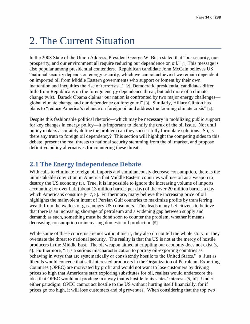
2. The Current Situation
In the 2008 State of the Union Address, President George W. Bush stated that ―our security, our
prosperity, and our environment all require reducing our dependence on oil.‖ [1] This message is
also popular among presidential contenders. Republican candidate John McCain believes US
―national security depends on energy security, which we cannot achieve if we remain dependent
on imported oil from Middle Eastern governments who support or foment by their own
inattention and inequities the rise of terrorists...‖ [2]. Democratic presidential candidates differ
little from Republicans on the foreign energy dependence threat, but add more of a climate
change twist. Barack Obama claims ―our nation is confronted by two major energy challenges—
global climate change and our dependence on foreign oil‖ [3]. Similarly, Hillary Clinton has
plans to ―reduce America‘s reliance on foreign oil and address the looming climate crisis‖ [4].
Despite this fashionable political rhetoric—which may be necessary in mobilizing public support
for key changes in energy policy—it is important to identify the crux of the oil issue. Not until
policy makers accurately define the problem can they successfully formulate solutions. So, is
there any truth to foreign oil dependency? This section will highlight the competing sides to this
debate, present the real threats to national security stemming from the oil market, and propose
definitive policy alternatives for countering these threats.
0B2.1 The Energy Independence Debate With calls to eliminate foreign oil imports and simultaneously decrease consumption, there is the
unmistakable conviction in America that Middle Eastern countries will use oil as a weapon to
destroy the US economy [5]. True, it is impossible to ignore the increasing volume of imports
accounting for over half (about 13 million barrels per day) of the over 20 million barrels a day
which Americans consume [6, 7, 8]. Furthermore, many believe the increasing price of oil
highlights the malevolent intent of Persian Gulf countries to maximize profits by transferring
wealth from the wallets of gas-hungry US consumers. This leads many US citizens to believe
that there is an increasing shortage of petroleum and a widening gap between supply and
demand; as such, something must be done soon to counter the problem, whether it means
decreasing consumption or increasing domestic oil production [5].
While some of these concerns are not without merit, they also do not tell the whole story, or they
overstate the threat to national security. The reality is that the US is not at the mercy of hostile
producers in the Middle East. The oil weapon aimed at crippling our economy does not exist [5,
9]. Furthermore, ―it is a serious mischaracterization to portray oil-exporting countries as
behaving in ways that are systematically or consistently hostile to the United States.‖ [9] Just as
liberals would concede that self-interested producers in the Organization of Petroleum Exporting
Countries (OPEC) are motivated by profit and would not want to lose customers by driving
prices so high that Americans start exploring substitutes for oil, realists would underscore the
idea that OPEC would not produce in a way that is hostile to its states‘ interests [9, 10]. Under
either paradigm, OPEC cannot act hostile to the US without hurting itself financially, for if
prices go too high, it will lose customers and big revenues. When considering that the top two
Page 15 of 238
exporting countries to the US are Canada and Mexico (Saudi Arabia is only third on the list), it is
hard to argue that imported oil presents an immediate threat to national security. Additionally,
non-OPEC countries account for more than five million gallons of daily US-imported oil,
whereas OPEC countries only account for less than five million gallons per day [8]. Interestingly
enough, many Americans believe Iran uses oil as leverage despite the fact that our country does
not import a drop of oil from Iran [10, 11]. Yet, conventional wisdom persists in exaggerating this
US reliance on Middle Eastern oil.
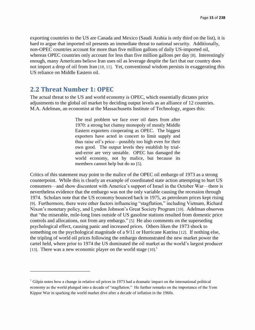
1B2.2 Threat Number 1: OPEC The actual threat to the US and world economy is OPEC, which essentially dictates price
adjustments to the global oil market by deciding output levels as an alliance of 12 countries.
M.A. Adelman, an economist at the Massachusetts Institute of Technology, argues this:
The real problem we face over oil dates from after
1970: a strong but clumsy monopoly of mostly Middle
Eastern exporters cooperating as OPEC. The biggest
exporters have acted in concert to limit supply and
thus raise oil‘s price—possibly too high even for their
own good. The output levels they establish by trial-
and-error are very unstable. OPEC has damaged the
world economy, not by malice, but because its
members cannot help but do so [5].
Critics of this statement may point to the malice of the OPEC oil embargo of 1973 as a strong
counterpoint. While this is clearly an example of coordinated state action attempting to hurt US
consumers—and show discontent with America‘s support of Israel in the October War—there is
nevertheless evidence that the embargo was not the only variable causing the recession through
1974. Scholars note that the US economy bounced back in 1975, as petroleum prices kept rising
[9]. Furthermore, there were other factors influencing ―stagflation,‖ including Vietnam, Richard
Nixon‘s monetary policy, and Lyndon Johnson‘s Great Society Program [10]. Adelman observes
that ―the miserable, mile-long lines outside of US gasoline stations resulted from domestic price
controls and allocations, not from any embargo.‖ [5] He also comments on the superseding
psychological effect, causing panic and increased prices. Others liken the 1973 shock to
something on the psychological magnitude of a 9/11 or Hurricane Katrina [12]. If nothing else,
the tripling of world oil prices following the embargo demonstrated the new market power the
cartel held, where prior to 1974 the US dominated the oil market as the world‘s largest producer
[13]. There was a new economic player on the world stage [10].1
1 Gilpin notes how a change in relative oil prices in 1973 had a dramatic impact on the international political
economy as the world plunged into a decade of ―stagflation.‖ He further remarks on the importance of the Yom
Kippur War in sparking the world market dive after a decade of inflation in the 1960s.
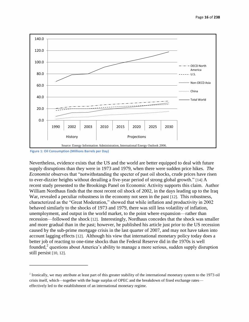
Page 16 of 238
Figure 1: Oil Consumption (Millions Barrels per Day)
Nevertheless, evidence exists that the US and the world are better equipped to deal with future
supply disruptions than they were in 1973 and 1979, when there were sudden price hikes. The
Economist observes that ―notwithstanding the specter of past oil shocks, crude prices have risen
to ever-dizzier heights without derailing a five-year period of strong global growth.‖ [14] A
recent study presented to the Brookings Panel on Economic Activity supports this claim. Author
William Nordhaus finds that the most recent oil shock of 2002, in the days leading up to the Iraq
War, revealed a peculiar robustness in the economy not seen in the past [12]. This robustness,
characterized as the ―Great Moderation,‖ showed that while inflation and productivity in 2002
behaved similarly to the shocks of 1973 and 1979, there was still less volatility of inflation,
unemployment, and output in the world market, to the point where expansion—rather than
recession—followed the shock [12]. Interestingly, Nordhaus concedes that the shock was smaller
and more gradual than in the past; however, he published his article just prior to the US recession
caused by the sub-prime mortgage crisis in the last quarter of 2007, and may not have taken into
account lagging effects [12]. Although his view that international monetary policy today does a
better job of reacting to one-time shocks than the Federal Reserve did in the 1970s is well
founded,2 questions about America‘s ability to manage a more serious, sudden supply disruption
still persist [10, 12].
2 Ironically, we may attribute at least part of this greater stability of the international monetary system to the 1973 oil
crisis itself, which—together with the huge surplus of OPEC and the breakdown of fixed exchange rates—
effectively led to the establishment of an international monetary regime.
0.0
20.0
40.0
60.0
80.0
100.0
120.0
140.0
1990 2002 2003 2010 2015 2020 2025 2030
History Projections
Source: Energy Information Administration, International Energy Outlook 2006.
OECD North America
U.S.
Non-OECD Asia
China
Total World

Page 17 of 238
This concern about supply disturbances returns the focus once again to OPEC, which has been
constraining production ever since its members agreed to cut output in 1973 [5]. Currently,
refinery capacity is woefully inadequate to meet world demand, which is rising dramatically with
the ascent of developing countries like China and India [6, 9].
OPEC—or any non-OPEC exporting country, for that matter—is unlikely to expand capacity
enough to meet the anticipated exponential jump in global demand. As countries in Asia
industrialize, OPEC is quickly losing its power to manipulate oil prices and make them lower by
expanding oil shipments, as it has been able to do more easily in the past. Today, its spare
capacity in the form of proven reserves has decreased to two percent of world demand from 25
percent in 1980, leaving it less able to free reserves as readily [9]. Inconsistent state output
adjustments that attempt to achieve market equilibrium instead distort the world market and
further escalate uncertainty about oil supply, which causes price increases [15]. Because OPEC
earns windfall profits with higher oil prices, it has little incentive to expand capacity or invest in
discovering new reserves. Therefore, there is a great deal of short-term uncertainty about the
ability of supply to meet demand, leaving ample room for wide price fluctuations—this despite
the fact that some economists believe the world‘s oil supply will never be exhausted, or at least
that humans will never fully develop the means to do so [5]. With uncertainty comes speculation,
and with speculation, economic instability. Although the change in oil supply in 1973 was trivial
in size, it nevertheless sparked a buyer‘s panic that had tremendous price effects [5].
2B2.3 Threat Number 2: Petrodollars that Threaten Democratic
Development Like any developing country depending on one commodity for economic growth, countries that
depend on petrodollars tend to lack basic freedoms and veer from the democratic model. This is
the so-called ―oil curse,‖ which lends credence to the ―mounting evidence that resource wealth—
and, by implication, the increase of that wealth through higher resource prices—undermines the
political development of resource-rich countries.‖ [9] Of the 12 OPEC countries, only Indonesia
is ―free,‖ according to Freedom House. While Freedom House considers Kuwait, Venezuela,
and Nigeria ―partly free,‖ the rest of the OPEC countries are ―not free.‖ The average scores for
political rights and civil liberties (where one is ―most free‖ and seven is ―least free‖) are five and
5.1, respectively [17]. These countries do not fare much better with respect to corruption.
According to Transparency International‘s Corruption Perceptions Index 2007, the 12 OPEC
nations average 3.1, on a scale of 1 to 10, where 10 is the least corrupt (the US is at 7.2) [17].
Only those states with small populations seem to escape the oil curse; by contrast, where oil
elites compose a small portion of a large population, equity is conspicuously absent and political
development seems to suffer [9].
In Iraq, corruption and a high natural endowment of oil seem to be linked. Recently, two
members of the Senate Armed Services Committee sent a request to the General Accountability
Office (GAO) to provide a full account of how the Iraqi government is spending a surplus of oil
revenue, which has come as a result of improved security for production and higher oil prices
[18]. Despite revenues that could rise above $56 billion in 2008, GAO believes Iraq had spent
only 4.4 percent of its 2007 reconstruction budget by August of that year [18]. Of course, this

Page 18 of 238
raises grave concerns about the degree of corruption and where the Iraqi government is spending
the money. According to military officials, at least one third of fuel from Iraq‘s largest refinery
in the city of Baiji finds its way to the black market, a pervasive problem across the country.
Much of the money in the black market ends up fueling the insurgency and threatening US and
Iraqi soldiers [19]. The relative increase in the price of oil does not help, as ―oil price movements
and democratic change will move in opposite directions.‖ [9] The curse of oil does threaten US
national security interests, albeit in more indirect ways—through black market cash flows
reaching those who wish to do harm.
3B2.3 Threat Number 3: Transportation Emissions and Global
Climate Change The Energy Information Administration (EIA) believes global oil consumption in 2030 will
almost double from 1990 figures to 118 million barrels per day, an annual increase of 1.4
percent. Two-thirds of this consumption will come from the transportation sector alone.
Clearly, this has enormous implications for carbon dioxide in the atmosphere, which ice core
research reveals is at an all-time high [20]. Among scientists, consensus is emerging that these
heat-trapping gases from fuel combustion—among other sources—are inducing climate change
[6]. As countries like China and India push global oil demand, they will also emit vast quantities
of carbon dioxide and other damaging greenhouse gases (GHG) with increased industrialization,
particularly in the transportation sector. China, for example, has a population of 1.3 billion (four
times the population of the US) and eight automobiles for every one thousand people. When one
contrasts this figure with America‘s 780 vehicles per thousand, it is frightening to imagine the
future scope of the environmental problem [6]. When considering the US alone is responsible for
27 percent of carbon dioxide in the atmosphere, the implications of adding China—which has
already surpassed the US in emissions—to the equation are frightening indeed [21].
There is some evidence questioning global warming causation. For example, the historian Brian
Fagan grants that solar radiation is at its highest level in the past 8,000 years, which accounts for
less than half of the variability in global warming; this implies that humans may not have much
control over the problem [22]. In the long run, however, it seems more prudent to safeguard
against a large magnitude of risk—to address the remaining half of variability that can be
controlled. The Intergovernmental Panel on Climate Change (IPCC) believes ―continued GHG
emissions at or above current rates would cause further warming and induce many changes in the
global climate system during the 21st century that would very likely be larger than those observed
during the 20th
century.‖ [23] Such warming could cause floods displacing 100 million people,
water shortages for one in six people worldwide, extinction of 40 percent of terrestrial animal
species, and droughts affecting tens of millions of humans [24]. With more than half of GHG
emissions between 1970 and 2004 coming from carbon dioxide from fossil fuel use, there are
certainly important national security interests at stake.
4B2.4 Alleviating Oil’s Stronghold How should Americans define energy independence in light of these three primary national
security threats? It does not rely on eliminating oil imports—from the Middle East or anywhere

Page 19 of 238
else—or oil consumption. They cannot be eradicated completely. According to Larry Burns,
Vice President of Research & Development and Strategic Planning at General Motors, the
automobile industry is 98 percent dependent on oil [14]. Thus, a complete transition to alternative
fuels is nowhere near realistic. To satisfy our continuing need for petroleum, US policymakers
should continue to strengthen North American Free Trade Agreement (NAFTA) trade ties.
Canada and Mexico alone—with combined exports of 3.4 million barrels a day in 2006—are
gaining ground on OPEC. Efforts should be made to improve the same types of technology that
made possible drilling 10,000 feet deep offshore in the Gulf of Mexico or extracting oil from
sand deposits in Canada [5]. Greater R&D will spark the innovation that enhances capacity of
proven reserves and diverts petrodollars from the extralegal sectors of OPEC countries wishing
to do the US harm.
With this in mind, oil independence really means avoiding the dependence costs related to the
distorting effects that the OPEC oligopoly has on the market. It should mean reducing US
vulnerability to dependence costs to a low enough level where they have no substantive effect on
economic, military, or foreign policy [13]. Taking this one step further, a measurable goal
suggests that ―the annual economic costs of oil dependence will be less than one percent of GDP,
with 95 percent probability by 2030.‖ [13] America‘s ability to avoid disruption costs that are
less than one percent of GDP entails undermining the market share power of OPEC—and thus
US vulnerability to high oil prices—by challenging the long-term perspective of oil as the only
fuel source. Put simply, the US should improve energy efficiency by finding fuel substitutes and
improving fuel economy [13]. A strategy that will reduce the demand for oil and increase price
elasticity by finding conventional and unconventional substitutes for oil may be effective [13, 25].
Much as a wise investor builds a diverse portfolio of securities, the US must also diversify its
energy portfolio—all the while not neglecting its oil ―inventory.‖ One of the options in a
potentially robust US energy portfolio includes biofuels, an alternative for which the State of
Indiana is particularly well suited.
5B2.5 Indiana’s Liquid Fuel Situation and Outlook There is good reason for Hoosiers to embrace the high cost of oil—realizing the potential for
innovation under market pressure—as it will likely provide incentive to shift toward fuel
alternatives such as biofuels. The collapse of oil prices in the mid-1980s diminished the
economic incentives and political wherewithal to continue investing in energy efficiency [9].
Now, Indiana policy makers can use high prices as a reason to invest in measures that will slow
and reverse consumption, and with it, the damage that GHG emissions are causing to the
environment.
In 2005, Indiana ranked eighth in the United States in per capita energy consumption. The
Hoosier state is also one of the country‘s top consumers of distillate fuels, diesel included [26].
Indiana petroleum consumption in 2005 alone amounted to 2.1 percent (160,785,000 barrels) of
total US consumption. Specifically, the transportation sector‘s needs accounted for 73 percent of
petroleum use in the state [26]. If EIA predictions regarding total future US consumption hold
true, and Indiana‘s share of oil consumption remains roughly at two percent of the US share in
2030, the state can expect an average daily petroleum consumption totaling 552,000 barrels.

Page 20 of 238
Despite tremendous anticipated future consumption, Indiana does have tools to meet this
challenge. For instance, the state is home to a British Petroleum (BP) oil refinery in the city of
Whiting, which hosts a refining plant with the largest processing capacity outside of the Gulf
Coast area. The Whiting plant largely accounts for Indiana‘s crude oil refinery capacity of
433,000 barrels per day, which makes up for Indiana‘s weak crude oil reserves, numbering only
12 million barrels in 2006, or 0.1 percent of the national total [26]. Although plant output is
currently fairly low, BP announced plans in 2006 to invest $3 billion in reconfiguring the plant to
bring greater quantities of heavy crude oil from Canada, which increasingly supplies the
Midwest via a pipeline originating in Alberta [26]. This should ease some of the strain of
importing crude oil from the Gulf Coast region. However, Indiana, as part of the Midwest
region, may also be able to meet a portion of its consumption demand through alternative
renewable energy sources.
World signals and policy mandates have actually encouraged the production of alternative fuel
sources to a substantial degree in the US. For example, ethanol production in the Petroleum
Administration for Defense District (PADD) 2 (the Midwest region) jumped from 38.7 million
barrels of ethanol produced per year in 2000 to 80.6 million barrels in 2004, a 108.3 percent
increase. For comparison, overall ethanol production from 1995-1999 only grew by 10.1 percent
[27]. The PADD 2 Midwest region also accounts for 99.2 percent of all US fuel ethanol
production [27]. In this case, biofuels are largely the focus of the Midwest region that boasts a
great deal of agricultural wealth and capacity.
Indiana, the country‘s fifth-largest corn grower, is turning towards alternative renewable fuels to
meet the state‘s increasing demand [28]. The state shows tremendous potential for producing
ethanol and currently has six operational ethanol plants, with an additional six under construction
and four more proposed [29]. Already, these plants produce an estimated 455 million gallons of
ethanol annually, and those coming on line this year will produce an additional 605 million
gallons [29]. As the fourth-largest soybean state, Indiana also has four biodiesel plants already
producing 108 million gallons annually [29]. Given that the generally agreed maximum amount
of US corn ethanol production is 15 to 16 billion gallons per year—and that the federal
government has mandated the use of 7.5 billion gallons of renewable fuels by 2012—Indiana‘s
anticipated contribution to the national alternative energy supply is impressive [30].
Despite Indiana‘s agricultural capacity to make biofuels a meaningful contributor to the state‘s
energy profile, there are important questions regarding future production, distribution, and use.
Various crops other than corn and soy can be used to produce ethanol and biodiesel. In addition,
different production techniques are needed to process different crops. The logistical concerns of
transporting and distributing biofuels are generally different than those of traditional fuels, and
vehicles themselves may need modifications to use these fuels. It is prudent to consider how
Indiana‘s path towards increased biofuels production could best be shaped over the next twenty
years. From an analytic perspective, economically viable biofuels production must have;
minimal or even positive environmental impacts; a favorable energy balance; and minimal risks
associated with production, including negligible risks to food supply. Systematic analyses of
these and other parameters over the life cycle of biofuels may suggest sound policy
recommendations to better guide Indiana‘s biofuels path over the next twenty years.

Page 21 of 238
6B2.6 References for Current Situation
[1] Bush GW. 2008. 2008 State of the Union
Address by President Bush. White House
Press Release, Washington, DC (2 March
2008;
http://www.state.gov/r/pa/ei/wh/rem/99783.
htm)
[2] McCain J. 2008. John McCain‘s Speech on
Energy Policy. McCain. (2 March 2008;
http://www.johnmccain.com/Informing/New
s/Speeches/13bc1d97-4ca5-49dd-9805-
1297872571ed.htm)
[3] Obama B. 2008. Barack Obama‘s Plan to
make America a Global Energy Leader.
Obama for America. (2 March 2008;
http://www.barackobama.com/issues/pdf/En
ergyFactSheet.pdf)
[4] Clinton HR. 2008. Powering America‘s
Future: New Energy, New Jobs. Hillary for
President. (2 March 2008;
http://www.hillaryclinton.com/issues/energy
/)
[5] Adelman MA. 2004. The real oil problem.
Regulation: 16-21.
[6] Parry IWH, Anderson JW. Petroleum:
Energy independence is unrealistic.
Resources 156: 11-15.
[7] Consumption/Sales of Total Crude Oil and
Petroleum Products. Energy Information
Administration. (5 March 2008;
http://tonto.eia.doe.gov/dnav/pet/pet_cons_p
sup_dc_nus_mbblpd_a.htm)
[8] U.S. Imports by Country of Origin: Total
Crude Oil and Products. Energy Information
Administration. (5 March 2008;
http://tonto.eia.doe.gov/dnav/pet/pet_move_
impcus_a2_nus_ep00_im0_mbbl_m.htm)
[9] Auerswald PE. 2006. The myth of energy
insecurity. Issues in Science and Technology
22: 65-70.
[10] Gilpin R, Gilpin JM. 2001. Global Political
Economy: Understanding the International
Economic Order. Princeton: Princeton
University Press.
[11] Fialka JJ. 2006. Energy Independence: A
Dry Hole. Wall Street Journal.
[12] Nordhaus W. 2007. Who‘s Afraid of a Big
Bad Oil Shock? Prepared for Brookings
Panel on Economic Activity.
[13] Greene DL, Leiby PN, Patterson PD, Plotkin
SE, Singh MK. 2006. Oil Independence:
Achievable National Goal or Empty Slogan?
Office of Energy Efficiency and Renewable
Energy, United States Department of
Energy. TRB 2007 Annual Meeting. 07-
1693.
[14] The Economist. 2007. The drive for low
emissions. The Economist Newspaper Ltd (2
March 2008;
http://www.economist.com/surveys/displays
tory.cfm?story_id=9217898)
[15] Schlesinger JR, Deutch J, Victor DG. 2006.
National Security Consequences of US Oil
Dependency. Council on Foreign Relations.
Independent Task Force Report No. 58.
[16] Freedom House. 2006. Map of Freedom in
the World. (5 March 2008;
http://freedomhouse.org/template.cfm?page
=%20363&year=%202006&country=6983)
[17] Transparency International. 2007.
Corruptions Perceptions Index 2007. (23
March 2008;
http://www.transparency.org/policy_researc
h/surveys_indices/cpi/2007)
[18] Glanz J. 9 March 2008. Senate Committee
Seeks Audit of Iraq Oil Money. The New
York Times Online (5 March 2008;
http://www.nytimes.com/2008/03/09/world/
middleeast/09iraq.html)
[19] Oppel RA. 16 March 2008. Iraq‘s
Insurgency Runs on Stolen Oil Profits. The
New York Times Online (5 March 2008;
http://www.nytimes.com/2008/03/16/world/
middleeast/16insurgent.html)
[20] Black R. 24 November 2005. CO2 Highest
for 650,000 Years. BBC News Online. (2
March 2008;
http://news.bbc.co.uk/2/hi/science/nature/44
67420.stm)
[21] Ang A. 2007. Group: China Tops World in
CO2 Emissions. USA Today Online (2
March 2008;
http://www.usatoday.com/tech/science/2007
-06-20-124188869_x.htm)
[22] Fagan B. 2000. The Little Ice Age: How
Cimate Made History. New York, NY:
Basic Books.
[23] Alley R et al. 2007. Climate Change 2007:
The Physical Science Basis, Summary for
Policymakers. Intergovernmental Panel on
Climate Change. IPCC WGI Fourth
Assessment Report.
Page 22 of 238
[24] BB News. 31 October 2006. Climate
Change Fight Can‘t Wait. BBC News
Online
(http://news.bbc.co.uk/2/hi/business/609608
4.stm)
[25] Sen A. 1999. Development as Freedom.
New York, NY: Random House.
[26] Energy Information Administration. 2008.
Indiana State Energy Profile. Office of
Energy Statistics, United States Government
(3 April 2008;
http://tonto.eia.doe.gov/state/state_energy_p
rofiles.cfm?sid=IN)
[27] Thurau R. Parsons S. Rosales A. Garza E.
Simmons W. 2007. Indiana Energy Report
2007. Indiana University‘s School of Public
and Environmental Affairs and Indiana
Geological Survey. Prepared for the Indiana
Office of Energy and Defense Development.
[28] Indiana State Department of Agriculture.
2007. Background on Bioenergy and
Biofuels. (23 March 2008;
http://ai.org/isda/biofuels/bioenergy-
biofuels-backgrounder-011007%20_2_.pdf)
[29] Abbott D. 2008. Fact Sheet: Biofuels Plants
in Indiana. Indiana State Department of
Agriculture.
[30] Government Accountability Office. 2007.
DOE Lacks a Strategic Approach to
Coordinate Increasing Production with
Infrastructure Development and Vehicle
Needs. GAO-07-713.

Page 23 of 238
3. Feedstock Agriculture
7B3.1 Environmental Background of Indiana
74B3.1.1 Indiana’s Natural History and Climate The state of Indiana lies in the north-central region of the United States, commonly referred to as
the Midwest. It is 275 miles long, approximately 143 miles wide, and spans 36,550 square miles
[1]. The elevation across the state varies, with areas ranging from 581 feet about sea level at
Lake Michigan to more than 1,250 feet above sea level along the eastern border of the state; the
average elevation is 700 feet above sea level [2]. Indiana is unique geologically and has a
significant natural north-south divide due to the glacial history of the state. While most of the
state falls within the Glacial Plains, the southern portion was never glaciated, resulting in
different soil types in the north and the south. Much of the north is prosperous farmland, while
relatively less land is agriculturally productive in the southern half of the state. These different
soils result in different soil nutrient compositions and climates in Indiana‘s 12 uniquely classified
natural regions [3].
Indiana‘s climate is seasonal and
average temperatures range from 22-
103 degrees Fahrenheit. The average
summer temperature is 70-80 degrees
and the average winter temperature is
25-35 degrees Fahrenheit. The first
freeze often occurs in mid-October,
and the last freeze occurs at the end of
April [4]. The number of days below
freezing is approximately 90 in
Northern Indiana and 20 in the
southern part of the state [5, 1]. Mean
annual rainfall ranges from 35 inches
in the north to 45 inches in the south;
the heaviest rains occur during the
spring months. The average annual
snowfall is higher for northern Indiana
with 40 inches total while the south
receives only 15 inches in a good
snowfall year. Drought conditions are
infrequent in Indiana, and most
droughts that do occur are moderate.
The last major drought occurred in the
1930s [6]. The winds predominantly
originate in the southwest with an
Figure 2: Indiana Glacier Coverage [9]

Page 24 of 238
average velocity of 7-10 miles per hour [5, 1].
75B3.1.2 Glacial History and Impacts The Laurentide Glacier reputedly passed over northern Indiana during consecutive periods of
cooling and warming, and the Illinoian Glaciation covered the majority of Indiana [1]. During
this time, ice sheets extended down to the southern border of the state, and only a small stretch of
land in south-central Indiana remained ice free. After the Illinoian ice sheet retreated
approximately 22,000 years ago, the Wisconsinan Glaciation reached its southernmost extent in
Indiana [7]. Both of these glaciations completely covered northern Indiana, flattened out ridges,
and filled in valleys. When the ice sheets over Indiana melted 16,000 years ago, they left
significant glacial deposits of finely ground rocks, which helped create the rich soils of northern
Indiana [7, 8].
76B3.1.3 Soil Type There are 357 soil types in Indiana, and many of these occur over small areas of land. Silt loam
soils dominate Indiana and range from silty clay loam to fine sandy loam. Indiana‘s state soil is
Miami soil, which formed in calcareous, loamy till on the Wisconsin Till Plains. Miami soil is a
brown silt loam on the surface with dark yellowish brown clay loam subsoil; it is fertile and has a
moderate water capacity. These soils are used extensively in agriculture, specifically for corn,
soybean, and winter wheat production. These soils are prime farmland and are responsible for
Indiana‘s productive agriculture. On
steeper areas they are also used as pasture,
hay land, or woodlands [10]. While soils
vary across the state, differences in soil
fertility depend on the mineral content
deposited by glacial movements.
77B3.1.4 Ecoregions Indiana‘s unique natural areas result from
glacial history and subsequent soil types.
A natural area is a generalized unit of a
landscape where a compilation of climate,
soil type, glacial history, topography,
exposed bedrock, pre-settlement
vegetation, flora and fauna distribution,
species composition, and physiography
represent natural characteristics of the
landscape [3]. For additional information
on Indiana‘s ecoregions, see Appendix A.
78B3.2 Current Land Use Of the nearly 23 million acres which
make up Indiana‘s total land area, farms
comprise 15,058,670 acres, of which
12,909,002 acres are in cropland [14, 15].
Figure 3: Current Indiana Land Use [11, 12, 13]

Page 25 of 238
The remainder of farm acreage consists of 1,153,779 acres of woodland, 427,190 acres of
pastureland and rangeland, and 568,699 acres in housing lots and other nonproductive land uses
[15]. Furthermore, as of January 2008, a total of 296,037 acres of cropland were enrolled in
Conservation Reserve Programs (CRP), described in further detail in the Changes in Land Use
section [16].
In 2007, Indiana farmers planted 6,200,000 acres of corn and 5,000,000 acres of soybeans, which
together occupied approximately 87 percent of total cropland [17]. The remainder of cultivated
cropland consisted primarily of hay (660,000 acres), wheat (420,000 acres), and oats (25,000
acres) [18]. Current estimates of 2008 prospective plantings expect corn acreage to decline to
5,700,000 acres and soybean acreage to increase to 5,500,000 acres. Oat and wheat acreage is
also expected to increase (to 30,000 and 550,000 acres, respectively), while hay is predicted to
decline slightly to 650,000 acres [18].
8B3.3 Biofuels and Biofeedstocks
79B3.3.1 Methodology This report considered many sources for biofuels feedstocks. Researchers then narrowed down
potential feedstocks based on their biological feasibility for Indiana‘s climatic and soil
conditions. Further consideration looked into the amount of chemical inputs needed to grow the
crop, invasive potential, and crop establishment in Indiana. Many feedstocks are just beginning
to gather support and little research on them is available. Where little or no conclusive research
exists, researchers cannot make recommendations on the effectiveness of these crops. The
following section lists these crops but does not analyze them in depth.
Biofuels feedstocks for this purpose can be broadly categorized as oil and seed crops, cellulosic
annuals, cellulosic perennials, short rotation woody crops (SRWCs), algae, and waste materials.
The oil and seed crops that were initially considered include corn (Zea mays), soybeans (Glycine
max), sweet sorghum (Sorghum bicolor), grain sorghum (Sorghum spp.), wheat (Triticum spp.),
rapeseed (Brassica napus), and flaxseed (Linum usitatissimum). Cellulosic annuals include the
agricultural residuals from wheat and corn stover. Cellulosic perennials include cordgrass
(Spartina pectinata), switchgrass (Panicum virgatum), and miscanthus (Miscanthus giganteus).
SRWCs considered include poplar (Populus spp.) and willow (Salix spp.). Algae as well as
forestry residue and municipal urban waste were also considered as feedstock sources.
80B3.3.2 Infeasible Crops Insufficient research meant that some of these crops, such as cordgrass and all SRWCs with the
exception of willow and poplar, could not be seriously considered in this report. While further
research and development into these fields may yield more information and efficient planting,
harvesting, and production methods, current research is not sufficient for making
recommendations.
Some crops are less desirable from a biological perspective due to large chemical input
requirements, invasive potential, and relative energy yield inferiority. Biofuels studies currently
use two varieties of sorghum as feedstocks. The sweet sorghum variety produces ethanol from

Page 26 of 238
fermented stalk juice. The seeds or stalks of grain sorghum can produce ethanol, but because the
stalks and seeds mature at different times, they cannot originate from the same planting [19].
Both sweet and grain sorghum have a large genetic base, and some have drought-resistant
hybrids which would grow in Indiana. However, Sorghum bicolor drummondii is a noxious
weed, whose widespread cultivation could result in natural hybridization, high invasive potential,
and significant economic and environmental costs [20, 21]. There is also little agreement on
potential yields [22, 19]. While insecticide and herbicide recommendations vary by region and
circumstance, there is general agreement that grain sorghum has high fertilizer requirements
ranging from 80-100 pounds per acre of nitrogen and up to 80 pounds per acre of phosphorus
and potassium [23, 24]. Sweet sorghum has much lower chemical requirements of only 40 pounds
each of nitrogen, potassium, and phosphorus per acre per year [25]. While these requirements are
lower than large-scale corn production, there are other feedstocks which have lower input
requirements. Sweet sorghum is high in sugar content which increases efficiency in processing;
however, because of the nature of the stalk, the juice must be fermented almost immediately after
harvest [26]. This biological constraint requires multiple small fermenting facilities which may
not be economically and logistically feasible for wide scale biofuels production and use. Neither
variety of sorghum is a feasible feedstock because of the high chemical and production
infrastructure requirements.
Biologically some feedstocks do not produce as much energy as other sources or have biological
limitations preventing their widespread use in Indiana. Wheat and wheat stover have very low
yields compared to similar crops [27]. While farmers can easily grow these crops, there are more
efficient biofuels crops if Indiana plans to change its agricultural practices. While Indiana
farmers can grow both miscanthus and algae, the hybrid miscanthus currently used in feedstocks
has low recruitment after fall planting and colder winters can inhibit plant growth [28]. However,
pilot studies at the University of Illinois are developing miscanthus as a potential biofuels
feedstock in the Midwest, and the future for it appears promising. Further information on this
work can be seen in Appendix B. Flaxseed is a feedstock with significant biological limitations.
Little crop residue remains on the field after harvest which increases runoff and wind erosion of
bare topsoil [29]. It is also susceptible to diseases such as crop rust, a fungus that overwinters in
flax debris, and fararium wilt, a seed and soil-borne fungus that limits flaxseed planting to only
once every three years on the same field [30].
Outdoor production of algae depends either on its close proximity to a large CO2 emitter or the
introduction of CO2 purchased from an alternate source [31]. Outdoor production requires a great
deal of water inputs because evaporation is an ongoing process. Although greenhouses can
mitigate this evaporation, it is prohibitively expensive to enclose the acreage necessary for large-
scale production. Additionally, the duration of favorable weather limits outdoor production.
Outdoor growth also increases the potential for genetically modified species to encroach upon
indigenous species or vice versa. Indoor production of algae is inefficient according to two
separate lines of research. Biological engineering is now the largest hurdle and requires
expensive genetic manipulation to produce an ideal strain [31]. There are also a number of
physical engineering challenges in bioreactor development. Current advances with Light
Emitting Diodes have significantly reduced the energy inputs of bioreactor algal growth but this
technology is not yet widely available [32].

Page 27 of 238
Several firms are currently refining processes for growing mass quantities of algae in desert
environments with minimum inputs [33]. Future algae production could yield biodiesel, ethanol,
and hydrogen with unprecedented efficiency and provide significant potential to mitigate
numerous environmental degradations [32, 34]. Although algae cannot currently yield industrial-
scale benefits, Indiana could consider incorporating algae into its biofuels portfolio in the future.
81B3.3.3 Feasible Feedstocks
199B3.3.3.1 Short-Term Feedstocks
Short-term feedstocks are available for immediate use or are feasible in Indiana within five years
with sufficient policy and economic incentives. Short-term feedstocks have a significant wide
scale ecological footprint. Because corn and soybeans are already well established in the state,
immediate use of these crops may help to initiate widespread biofuels production. Although
corn ethanol production is underway in Indiana and surrounding states, corn is a highly
chemically dependent crop. This increases production costs, decreases land fertility, and
negatively impacts water resources and biodiversity. High chemical application rates increase
costs attributed to equipment, application time, and fuel to cover fields with multiple
applications. However, corn has one of the lowest energy yields, compared to other crops (75 GJ
of biofuel and 15 GJ in co-products) [35].
Soybeans, like corn, are well established within Indiana. While not as chemically intensive, soy
still needs relatively high amounts of insecticides and fertilizers. Studies indicate that farmers
use on average 1.2 kg/ha of insecticide, 10 kg/ha of nitrogen, and 15 kg/ha per year of
phosphorus [35]. The reduced reliance on chemical inputs is a benefit; however, the energy yield
of soy biodiesel is lower than that of corn [35]. Harvesting of soybeans also occurs in the fall and
leaves the ground prone to runoff and wind erosion of topsoil over the winter.
200B3.3.3.2 Transition Feedstocks
Since soy biodiesel and corn ethanol production are not currently energy efficient and create
harmful environmental effects, they should only serve as short-term feedstocks until Indiana
transitions to more environmentally sound and economically lucrative crops. The most efficient
feedstocks, and arguably the most environmentally sound on a large scale, are biomass for
cellulosic ethanol production. However, this production process is still being refined and
production plants are not yet operating in Indiana.
Corn and soy production in Indiana creates a unique opportunity for cellulosic production. The
corn stalk, known as corn stover, normally remains on the field after grain harvest; it either
remains on the surface where it slowly breaks down and sequesters carbon, or it is tilled into the
soil where it breaks down more quickly and facilitates new crop growth during the next growing
period. However, it also emits carbon into the atmosphere [36]. Farmers can remove this
agricultural residue from fields and use it as an initial feedstock for cellulosic ethanol plants.
Cellulosic and grain ethanol production can occur simultaneously since farmers harvest corn and
stover at the same time. Corn stover produces 130 gallons of ethanol per ton of dry corn stover
[36].
While this serves as a good transition crop, it also has environmental drawbacks, including the
same high inputs for corn and increased wind and water erosion [36]. Some states provide

Page 28 of 238
incentive programs or require that a certain amount of stover remains on the ground to
accumulate carbon.
201B3.3.3.3 Possible Long-Term Feedstocks
Sustained long-term projections for Indiana biofuels production will require farmers to switch to
lower input, higher energy yield plants. Cellulosic ethanol feedstocks are the most promising for
long-term biofuels production. Unlike corn, switchgrass and SRWC harvests leave roots in the
field to regenerate from year to year and have major ecological and economic benefits [36]. The
most significant benefits include reduced plowing, planting, and chemical applications, and the
rapid re-growth of perennial crops.
Switchgrass is native to North America and has varieties native to Indiana. Because these plants
evolved in the eco-regions of Indiana, they are highly resistant to fungi and other pests, which
significantly reducing the need for insecticides and fungicides. They also utilize marginal lands
far better than row crops. After planting, switchgrass needs approximately two years to establish
a root system before its first harvest [37]. Once established, there is also little need for herbicides.
The first planting year requires only 2.7 lbs per acre of herbicides, minimal fertilizer, and no
pesticides [28]. Perennial crops, because of their established root systems, significantly decrease
runoff, soil erosion and soil compaction, and increase carbon sequestration [38]. They may also
increase wildlife habitat in the fall and winter seasons, depending on when harvest occurs.
However, switchgrass is a clump grass that—when seeded in high concentrations—creates a
thick, nearly impenetrable mass and may reduce some species‘ ability to take cover [38].
An alternative to cellulosic feedstocks such as switchgrass is fast-growing trees. Willow and
poplar have the most significant amount of research and greatest development potential out of
the 125 tree species examined for biofuels production in Indiana [39]. Both poplar and willow
grow rapidly and accumulate mass quickly. They require far fewer chemical inputs than other
feedstock crops. Poplars require nitrogen inputs every other year throughout their growth cycle,
especially in their fifth and sixth year, to maximize biomass accumulation [40]. Poplar varieties
are extremely sensitive to shade, and herbicides are frequently used in the first two years or until
canopy covers the bare ground [40]. The United States already grows many poplar varieties,
including black cottonwood. While farmers can grow poplar without irrigation and with dry-
land fertilization techniques, optimal harvests may not be regularly achieved by this method.
While both poplar and willow are fast growing, the first harvest occurs seven to ten years after
initial planting [40].
Farmers can harvest the same stand of woody biomass multiple times if harvests occur in the
winter, allowing the roots to regenerate (coppace) [40]. The long growing period and harvest
cycle restrict plots of land to one crop. The land is much harder to convert back to other uses
after harvest because of underground biomass and stumps [40]. This inadvertently makes farmers
less able to respond to changes in market prices for crops since they have to dedicate land for
extended periods of time to poplar production. Grazing of young trees by rodents, deer, and
other mammals poses a serious risk to the viability of a stand of poplar. Antler rubs can kill even
large trees. In many areas, electric fencing or brush fences are effective deterrents. The use of
electric fences raises further environmental as well as economic concerns, stemming from
wildlife impacts and sustained electricity use.

Page 29 of 238
Switchgrass and SRWC provide a long-term alternative for Indiana ethanol production.
Additionally, rapeseed cultivation may be a viable alternative for biodiesel in the future. Canola
oil is a popular product of rapeseed, which grows in Minnesota and Canada. Rapeseed has a
high oil content (40-44 percent) that produces 182 gallons of biodiesel per acre. Like other
alternative crops, it requires fewer chemical inputs. A rapeseed field needs only 1.1 1bs of
herbicide per acre and only one application of phosphorus and nitrogen. Rapeseed has a five-
month long growing season, followed by an annual fall harvest. While infrastructure exists for
planting and harvesting rapeseed, it is not yet widespread in Indiana and would require
investments in both equipment and human capital.
9B3.4 Preparing Biofeedstocks for Transportation Crop harvest and preparation for transportation to a production facility are crucial steps in
biofuels production. Many factors influence the cost of preparing cops for transportation to a
facility. These factors include the material yield and physical properties of the crop, the
sequence of field operations, equipment and other capital costs, work and efficiency rates, and
other costs such as insurance, wages, fuel, taxes, and interest [41]. Traditional crops such as corn
and soybeans utilize conventional harvesting techniques and some biomass crops also have the
ability to use similar processes and equipment.
82B3.4.1 Corn Grain corn serves as the feedstock for the majority of ethanol produced in Indiana. Since Indiana
farmers already grow corn, it is fairly simple to harvest using existing machinery and techniques.
Farmers drive combines with special corn header attachments; this equipment strips the corn
kernels from the stalk and deposits them into a collection bin behind the combine [42]. The corn
is then ready for transportation to storage facilities, usually grain elevators [43].
83B3.4.2 Soybeans Like corn, soybeans are an established crop in Indiana. Consequently, farmers can easily use
equipment they already possess to harvest the crop. In order to harvest soybeans during the fall,
farmers use a combine that separates the beans from the pods, and deposits them into a hopper
behind the combine [44]. Grain elevators then store bushels of soybeans ready for transportation
to a production facility.
84B3.4.3 Corn Stover As Indiana moves its source of biofuels feedstocks away from traditional crops such as corn and
soybeans in favor of cellulosic processes, farmers can easily harvest biomass with traditional or
slightly modified harvesting equipment.
A corn stover harvest requires a variety of different farming techniques including chop
shredding, mowing, raking, and baling [41]. A 2002 study determined that, in Indiana, the cost of
shredding corn stalks is $7.85 per acre. Mowing corn stover with discs and sickle bars costs
$9.72 per acre and $8.50 per acre respectively. Raking corn stover costs considerably less at
$5.03 per acre, while baling in round and rectangular bales costs $3.35 per acre and $3.41 per
acre respectively [41]. Because of the quantity of stover needed to remain on fallow fields to

Page 30 of 238
prevent soil erosion and nutrient loss, the efficiency yield of corn stover is about one-third of the
biomass on the field [41].
Corn stover harvests occur in the fall when the crop is considered dry or has 20-25 percent
moisture. Harvest time can last from several days to several weeks [45]. Farmers can also
harvest corn stover under wet conditions, when the stover has greater than 45 percent moisture
[45]. The two different methods of corn stover harvest depend, in part, on whether farmers prefer
to make one or two complete passes through the field. The typical harvest procedure is to cut the
stalk from its base, shred it, and lay it on the field to dry. Once the stover dries, a raking device
collects the biomass from the field, while a machine compacts the stover into bales for easy
transport [45]. A second method requires only one complete pass through the field. The combine
cuts the stalk from its base and collects it in a windrow behind the machine. The disadvantage of
the one-pass technique is that it requires significantly more drying time because the stover is
tightly packed together. Similar to the previous method, once the stover is collected in the
windrow, a machine collects the biomass and bales it [41].
The baler creates either round or rectangular bales of stover. The bale size of corn stover ranges
from stackers (one half to one ton) to one-ton rectangular bales (four x four x eight feet) to one-
half ton round bales [46]. The study assumed that farmers would store the corn stover at a
distance of five miles from the field, where it would remain until transportation to a production
facility. The stover would be stored in a shed in order to protect the crop from rain, snow, and
freezing temperatures. The harvest estimates did not, however, include storage costs, which
would increase the total cost of corn stover preparation [41].
Recently, Iowa State University researchers created a combine attachment which simultaneously
harvests the corn grain and cuts the stover, depositing it into a wagon behind the combine [42].
The additional cost for the attachment is $10,000-$15,000, which is considerably less than the
cost of a separate combine to harvest corn stover [42].
The choice of corn stover storage technique depends on whether the harvest was wet or dry, and
there is some debate over the preferred method. Farmers can store dry corn stover in bales;
however, large round bales tend to lose 10-23 percent of their contents in storage [45].
Conversely, bales of wet stover result in higher yields and lose less of their contents in storage
[45]. Wet corn stover harvest occurs immediately after the grain harvest, making the process
more efficient [45]. However, these harvests require an anaerobic storage environment to
successfully preserve the crop; wrapping the bale in plastic is one method of achieving this
environment [45].
85B3.4.4 Switchgrass Cellulosic energy crops such as switchgrass can also be harvested to produce biofuels. One
benefit of using switchgrass is that farmers are able to use existing hay equipment to harvest the
feedstock [47]. Once farmers have collected the switchgrass, they bundle it into large round bales
weighing approximately 992 lbs [48]. Switchgrass can either be baled loosely in twine or
wrapped in plastic. Loose bales result in a significant amount of crop loss in transportation.
However, the use of plastic-wrapped bales may have indirect environmental consequences [49].

Page 31 of 238
The Conservation Reserve Program
Enacted in 1985, CRP provides financial
incentives to farmers who retire highly
erodible or ecologically sensitive cropland
from production in order to promote soil
and water conservation. Another
meaningful goal of the program was to
reduce the overproduction of American
commodities [62]. The Farm Service
Agency (FSA) administers CRP and offers
farmers the ability to enroll in several
subprograms with different options. Most
CRP contracts last for 10-15 years and
rental payments are based on the individual
property’s ecological value, measured in
terms of an Environmental Benefits Index
(EBI). Landowners receive assistance in
establishing approved conservation
practices on their land, but incur financial
penalties for early contract termination.
CRP enrollment is capped at 39.2 million
acres, and as of January 2008, there were
34,656,303 acres in active contracts
nationwide [63, 16].
Continuation of CRP depends upon its
renewal with the 2007 Farm Bill, which is
still under consideration in Congress. The
House Agricultural Committee Chairman,
Collin Peterson supports a new 10-year
plan which limits agricultural subsidies.
These changes would decrease agricultural
profits by nearly half and limit CRP to 32
million acres, a reduction of seven million
acres from the 2002 Farm Bill [64].
86B3.4.5 Woody Biomass SRWCs such as poplar and willow serve as additional cellulosic feedstocks. However, since
cellulosic technology is relatively new, little information is available regarding harvesting
methods for these crops. Farmers are able to use existing equipment, but this equipment requires
modifications to cut and chip trees simultaneously [50]. North Carolina State University
researchers are working on the development of a harvesting mechanism for woody biomass. The
machine will cut trees up to six inches in
diameter, chop the logs into chips, and deposit
them into a collection bin [51].
10B3.5 Environmental Impacts
87B3.5.1 Changes in Land Use One of the driving factors behind the growing
interest in renewable transport fuels is concern
over the environmental consequences of
petroleum-based fuel consumption [52].
However, biofuels development is not without
its own suite of environmental impacts. Thus,
determining whether or not biofuels produce
net ecological benefits relative to fossil fuels
requires an evaluation of the potential positive
and negative consequences of changes in land
use, water quality and consumption, soil
erosion and nutrient loss, greenhouse gas
emissions, and biodiversity.
Since the passage of the Renewable Fuel
Standard (RFS) as part of the Energy Policy
Act of 2005, demand for agricultural
feedstocks used in biofuels production has
risen sharply. Initially mandating a supply of
7.5 billion gallons of biofuels per year by
2012, RFS expanded to require 36 billion
gallons per year by 2022, of which 15 billion
gallons must consist of ethanol generated from
corn starch [53, 54]. While RFS also includes
biodiesel and cellulosic biofuels supply
mandates totaling 21 billion gallons per year,
increased corn ethanol production will meet
the majority of biofuels demand since the
majority of new facilities coming online use
corn as a feedstock [54, 55].

Page 32 of 238
88B3.5.2 Corn and Corn Stover Increasing the corn supply to meet projected ethanol demand will require substantial land use
shifts such as altering crop rotations and tillage practices, crop displacement, and bringing new
land into production, potentially including land under contract with CRP [55, 56]. The net
environmental impacts of this land reallocation to corn will depend on the distribution of new
production among these different approaches. Farmers, seeking to increase corn yields on
cropland already in production, may choose to switch some or all of their acreage out of
traditional corn-soybean rotations to shorter rotations of two years of corn, one year of soybeans,
or even into continuous corn production [56]. More intensive corn production will undoubtedly
have yield implications and some farmers may increase nitrogen fertilizer applications and/or
forego conservation tillage in an attempt to compensate for losses in productivity [56]. Such
compensatory measures, in turn, may result in soil erosion, loss of organic carbon, water quality
degradation from nutrient, sediment, and pesticide runoff and infiltration, and air quality
degradation from nitrous oxide emissions from fertilizer application [56, 57].
Corn stover has gained considerable attention as a potential biomass feedstock due to its high
biomass content and abundance; it is likely to be widely adopted for cellulosic energy production
[58, 59]. While it is unlikely that expanded use of corn stover for fuel production would stimulate
an increase in corn acreage, it could indirectly affect the amount of cropland allocated to corn.
Crop residues which remain on the field after harvest help protect soils from erosion and aid in
the maintenance of soil nutrients, organic matter, and microbial communities [60, 58]. Removing
these residues, however, can result in decreased crop yields, increased soil compaction, and soil
and water degradation. These effects may, in turn, stimulate increased reliance on fertilizer and
intensive tillage practices to maintain productivity. It is estimated that roughly 20-30 percent of
corn stover can be removed without introducing these negative impacts [60]. However, crop
yields will likely fall if greater amounts of stover are harvested to meet cellulosic feedstock
demand
In the short term, most of the additional land converted to corn from cropland already in
production will come at the expense of soybeans [57]. Relative to corn, soybean production is
much less environmentally harmful in terms of fertilizer and pesticide impacts on air and water
quality [62]. In the longer term, however, depending on commodity prices and conservation
subsidy trends, farmers may decide to bring marginal land into corn production, including idle
cropland, pastureland, and CRP land.
Corn production on fallow land has a higher net environmental impact than crop displacement or
rotational shifts on active cropland [55]. This is primarily due to significant carbon emissions
from the removal of the existing plant community and losses in soil organic carbon (SOC) during
the first few years of cultivation following tillage [65]. Consequently, these indirect emissions
may be significant enough to negate any GHG reductions from ethanol consumption relative to
fossil fuels. Corn yields on marginal lands may be high (because they have experienced less
nutrient depletion) or low (because they are less productive in general) and therefore, may or
may not require additional inputs. Overall, the increased rates of GHG emissions and soil and
nutrient loss from increased corn cultivation are disproportionately greater than the rate at which
existing cropland and marginal lands are reallocated to corn production [53]. Furthermore, many
marginal lands, particularly those under CRP contracts, are highly erodible or ecologically

Page 33 of 238
sensitive; thus bringing these lands into production would negate the conservation benefits
realized by retiring them from production.
89B3.5.3 High Energy Crops and Woody Biomass In contrast to the overall negative land use and environmental impacts of increased grain corn
cultivation for biofuels production, herbaceous energy crops (HEC) like switchgrass and SRWC
like poplar and willow may have positive environmental benefits, including soil stabilization,
increased soil organic matter and below-ground carbon sequestration, reduced sediment and
pesticide runoff (following initial establishment), and lower cultivation, nutrient, and water
requirements [48, 66, 67]. Thus, if HEC and SRWC replace traditional food crops on existing
cropland, the net land use benefits would tend to be positive. However, in the near term, HEC
and SRWC will have difficulty competing for cropland with conventional food crops like corn
and soybeans. Dedicated energy crops take longer to establish and, at present, involve higher
fuel production costs [59]. Consequently, until cellulosic biofuels production becomes more
commercially viable, the opportunity costs to farmers of growing biomass energy crops on high
quality agricultural land will remain prohibitively high [59].
In the long run, however, HEC and SRWC are likely to become more attractive feedstocks for
biofuel production, and heightened demand for these products could result in an increase in total
cropland acreage [58]. While HEC and SRWC produce many positive environmental benefits
when replacing traditional food crops on existing cropland, an overall increase in cropland
acreage would likely result in an increase in the conversion of natural forests, grasslands, and
wetlands to crop production [58]. This could have important negative impacts on wildlife habitats
and the ecosystem services provided by these natural areas, including water and air quality
regulation and nutrient cycling [58].
HEC and SRWC production may be most successful, initially, on marginal lands [66]. Growing
energy crops on marginal land, particularly highly erodible land (HEL), could reduce land
conversion pressure on high quality agricultural lands and natural ecosystems while contributing
to environmental objectives such as soil and water conservation [58]. Some HEC are already
being grown on marginal lands for conservation objectives under CRP; indeed, perennial grasses
have been planted on millions of acres of CRP land as an erosion control mechanism [48]. At
present, farmers are not permitted to harvest these grasses on CRP land and sell the biomass for
biofuels production. However, the House of Representatives version of the 2007 Farm Bill
contains provisions that would allow farmers with CRP contracts to establish ―biomass energy
reserves‖ of dedicated energy crops for commercial cellulosic biofuels production [68].
Nevertheless, the Senate version of the Bill contains no such provisions, and the two versions
have yet to be reconciled in conference committee.
While it is difficult to speculate as to the land use implications of the Farm Bill before both
houses of Congress approve a final version, it is clear that allowing biomass harvesting on CRP
land could influence a farmer‘s decision whether or not to re-enroll his land in a CRP contract or
to enter into a new contract. While an increase in HEC or SRWC acreage on CRP land could
certainly provide positive environmental benefits compared to traditional food crop cultivation, it
is unclear what sorts of potentially negative impacts (particularly with respect to soil and water
quality and wildlife habitat) might arise from the growth and repeated harvesting of dedicated

Page 34 of 238
energy crops on CRP land, since plantings intended for biomass harvest are managed somewhat
differently than those established for conservation and wildlife benefits [58].
90B3.5.4 Carbon Sequestration The carbon sequestration abilities of agricultural land and farmland are important to consider
when addressing land use changes. The global carbon cycle is the flow of carbon amongst
terrestrial, atmospheric, and oceanic systems [69]. Of particular importance is the terrestrial
component of the cycle and how the production of biofuels affects its sequestration capabilities.
Soils and plant biomass contain approximately 2.7 times more carbon than the atmosphere,
making them the two largest biologically active stores of terrestrial carbon [70]. Hence, their
potential as carbon sinks, as well as sources, has a large impact on the global carbon cycle and
GHG emissions.
Forests and agricultural lands sequester carbon through two means: vegetation and soil
sequestration. Carbon sequestration by vegetation occurs through the process of photosynthesis.
Photosynthesis enables plants to incorporate carbon atoms into their cells [69]. Plants then act as
a carbon sink, retaining the carbon within their biomass. While forests serve as the greatest
terrestrial sinks of carbon, agricultural land is a significant source as well. This is especially true
of lands which experience longer harvest cycles and lower tillage rates.
Soil sequesters carbon from decomposed or partially decomposed vegetation, decomposers
themselves, and plant roots [71]. The available research on soil carbon sequestration is minimal
because the processes involved in the carbon cycle within soil are not readily understood.
However, the amount of carbon storage capacity in soils is determined by what is found in
organic materials [72]. These include plant, animal, and microbial debris in all stages of
decomposition [73]. Some believe the amount of carbon sequestered in soil is greater than that
sequestered in living vegetation [73]. Therefore, converting many types of land, not just forest
land, has the potential to drastically reduce the amount of carbon retained within the terrestrial
system.
Specifically, soils disturbed by cultivation have enhanced conditions for decomposition, which
lead to greater rates of soil respiration [72]. Not only is the amount of carbon in the sink
decreasing because of a loss of biomass, but there is also a forward feedback component
happening in which the tilled soil is experiencing greater nutrient cycling. This allows for
increased decomposition and more carbon release.
Best Management Practices (BMPs) such as reduced tillage and sustainable harvesting cycles
have been introduced to deal with biomass and soil carbon losses. While following BMPs for
growing and harvesting energy crops would alleviate some of the aforementioned concerns with
carbon losses in agricultural land, the larger issue is the amount of land that will be dedicated to
energy crops. Projected increases in the prices of corn, wheat, and soybeans have the potential to
provide incentives to farmers to convert retiring CRP land into agricultural land. The increase in
the amount of land moved into the agricultural sector will enhance the amount of carbon released
into the atmosphere. While using abandoned agricultural or marginal land for growing energy
crops will reduce the impact, biofuels produced from residual or municipal wastes that require
little or no additional land use are most attractive from a carbon perspective.

Page 35 of 238
91B3.5.5 Water Demand The expansion of biofuels production requires an examination of water resource availability.
Water enters the soil through irrigation and precipitation. The plant retains some water, and the
rest leaves the surface soil through runoff, infiltration to the aquifer, and through processes such
as evaporation and evapotranspiration [74]. The average volume of runoff from a specific site is
determined by a runoff coefficient, the average annual amount of precipitation multiplied by the
area of the site itself (R= C*P*A). Runoff coefficients vary by place and depend upon slope, soil
texture, and land use type. Less permeable soil and steep slopes originate more runoff. For
example, hilly cultivated land (10-30 percent slope) with a high concentration of clay (little
permeability) will be characterized with a high runoff coefficient (on average 0.6), while the
runoff coefficient for the flat (0-5 percent slope) woodland with open sandy loam is 0.1 [75]. The
slope varies from 0-8 percent in northern Indiana counties and up to 44 percent in southern
counties [76]. Infiltration in the aquifer is another way water leaves the surface soil. Factors such
as soil composition and moisture conditions near the ground surface affect the infiltration rate,
the measure of the rate at which a particular soil absorbs rainfall and irrigation [77].
Water loss into the atmosphere takes place either through evaporation or evapotranspiration
processes. Evaporation takes place directly from the soil and its rate depends on soil texture,
temperature, moisture, and other climatic conditions. Evapotranspiration is an evaporation
process occurring from plants; water loss through this process depends on plant height, albedo,3
canopy resistance,4 etc [77]. Water balance availability in a specific agricultural site depends
upon a number of factors including climatic conditions, location, type of crop, soil composition,
slope, and the amount of precipitation. Consequently, these factors determine necessary levels of
irrigation.
Indiana is among the least irrigated states in the US due to favorable climatic conditions [74].
According to US Geological Survey (USGS), Indiana‘s estimated total water withdrawal in 2000
amounted to 10.1 billion gallons per day (11,300,000 acre-feet annually), but extracted only 101
million gallons for irrigation purposes [78]. In 2000, Indiana‘s application of 0.45 acre-feet of
water for irrigation was the eighth lowest quantity used in the US [78]. According to the US
Department of Agriculture (USDA) there were only 313,130 acres of irrigated land in Indiana in
2002 out of the 15,058,670 acres of agricultural land [15]. Overall water demand is not as big of a
concern in Indiana.
Different crops require different amounts of water. Corn requires around 642,000 gallons of
water per acre, not including water loss through runoff and aquifer infiltration. This is
approximately 168 gallons per pound of corn produced, and indicates about 23.6 inches of
rainfall is necessary for corn production during the growing season [79]. According to Pimentel
et al., corn can suffer from lack of water even if the annual precipitation is 39.4 inches [79].
Therefore, though precipitation in Indiana is adequate for corn production and existing practices
3 Food and Agriculture Organization (FAO) defines albedo as reflectance of the crop-soil surface. The albedo is
affected by the fraction of ground covered by vegetation and by the soil surface wetness.
4 The resistance of crop to vapor transfer is affected by leaf area (number of stomata), leaf age and condition, etc.

Page 36 of 238
prove this, increased corn production in relatively dry areas of the state may require additional
irrigation infrastructure and additional water withdrawal. Soybeans require approximately
491,000 gallons per acre, but yield per acre is less than half that of corn in weight. As a result,
one pound of soybeans requires approximately 240 gallons of water [79]. Most other crops grown
in Indiana demand less water than corn and soybeans. For example, one pound of wheat or
alfalfa requires about 110 gallons of water, a pound of sorghum requires 130 gallons of water,
and one pound of potatoes requires 60 gallons of water [79]. Although these plants utilize a
relatively small amount of agricultural land in comparison to corn and soybeans, their
replacement with more water intensive crops would result in increased water use.
Switchgrass requires less water and is more drought tolerant than corn [80]. Switchgrass is
climatically adapted throughout most of the United States and it may grow on somewhat dry to
poorly drained, sandy to clay loam, soils [37]. Poplar and willow are both phreatophytes,5 and
intensive users of water. Phreatophytes transpire about 30 inches of groundwater per year, and
are frequently used to extract contaminants from soil or groundwater [81]. Sharma et al.
demonstrated the presence of a three-year old poplar plantation ten feet from the boundary of
wheat field caused 7.5 percent higher water use, increasing to 12.7 percent for a four-year old
plantation 20 feet from the field [82]. While the well adapted root systems of these SRWCs
prevent the need for irrigation, their juxtaposition to other crops will affect water demand of the
adjacent crop. SRWCs require water over a longer growing period than annual crops, and also
create a canopy that may decrease infiltration by interrupting rainfall. Therefore, large
plantations for these feedstocks may affect water storage, especially in drier regions [83].
Although no or very little irrigation is needed for growing switchgrass, poplar, and willow, water
use of these crops requires further research [83].
92B3.5.6 Water Quality The rapid incorporation of biofuels into Indiana‘s energy portfolio has significant impacts on
agricultural production in the state. Increased demand for corn and soybeans as feedstocks for
ethanol and biodiesel impacts the prices farmers receive. As prices increase, more producers
enter the market, and land use changes as a result. Demand for grain ethanol contributed to over
a 17 million acre or 15 percent increase in corn acreage in the US between the 2006 and 2007
[17].
Rapid expansion of corn production leads to land use change in the form of adjustments to crop
rotation, conversion of cropland used as pasture, land in fallow, acreage returning from CRP, and
shifts from other crops [84]. These are just a few of the indirect effects from biofuels production.
Water quality impacts must also be taken into account. Increased corn and soybean production
leads to increases in fertilizer and other agrichemical inputs and exposes more bare ground to
soil erosion and runoff. Fortunately, solutions are available which help mitigate problems
associated with corn and beans and eventually provide environmentally beneficial alternatives to
these feedstocks. BMPs help allay the harmful properties of agricultural inputs until
economically efficient production of cellulosic ethanol is possible.
5 Deep-rooted plants that obtains water from a permanent ground supply or from the water table [81].

Page 37 of 238
93B3.5.7 Fertilizer Inputs Destruction of natural ecosystems in favor of farming operations damages soil quality, throws off
normal nutrient cycling, and disrupts the food web. As a result, farmers must ensure their crops
are receiving adequate nutrients to produce maximum yields. Nitrogen and phosphorous are the
primary fertilizers applied to crops in Indiana, and the low costs associated with them have not
promoted conservative use in the past. To make matters worse, increasing prices for corn and
soybeans give farmers an even greater incentive to over apply these chemicals. From a farmer‘s
perspective, it is a wise investment, but from an ecological perspective, over application can be
highly destructive to the quality of ground, surface, coastal, and estuarine waters.
Aquatic plants, similar to terrestrial plants,
grow better under elevated levels of nitrogen
and phosphorous, and over application of these
chemicals runs off into surface water, creating
problems with excessive algae growth and
oxygen deprivation. Currently, over 60 percent
of coastal rivers and bays in the US are
moderately to severely degraded due to nutrient
loading [85]. Since watersheds like the
Mississippi and Missouri Rivers extend through
great reaches of the country, nutrient loading is
never a localized problem.
Fertilizer treatment is highest for corn,
especially nitrogen inputs. Corn utilizes high
inputs of nitrogen because it is such an
inefficient user of the fertilizer. In fact, 40 to
60 percent of the nitrogen applied to corn
generally runs off into surface waters [86].
Application and loss of fertilizers varies by
agricultural management practices, but on
average corn loses 20-40 lbs per acre of nitrogen and 2-15 lbs per acre of phosphorous, while
soybeans lose 15-30 lbs per acre of nitrogen and 1-8 lbs per acre of phosphorous [87, 88].
Expansion of corn production necessitates increased farm tillage, which results in greater
nitrogen and phosphorous loss per acre [87]. Again, appropriate farming techniques such as the
use of riparian buffers and precision farming can minimize these inputs, but the future of
cellulosic production still looks brightest for water quality.
Switchgrass requires some additional nitrogen and phosphorous for most favorable yields, but
requires far less nitrogen than corn, and generally little phosphorous [87]. While little yield
differential was observed with additions of phosphorous to switchgrass, the addition of nitrogen
to this perennial grass is much more complex [89]. Nitrogen application rates vary from zero to
greater than 350 lbs per acre depending on the use of switchgrass as a cash crop, harvest timing,
and frequency [90]. Late harvesting of switchgrass during late fall or early winter months can
Figure 4: Nitrogen fertilization rates and stream concentrations [74]

Page 38 of 238
reduce the potential for nitrogen and phosphorous runoff and leaching. Although the feedstock
is drier and easier to transport, a late harvest reduces the total biomass harvested [91, 92]. No
specific numbers are available for average nitrogen loss, but the loss of phosphorous from
perennials such as switchgrass and other hay crops is around 0.18 to 1.8 lbs per acre [88]. Not all
nitrogen and phosphorous runoff can be traced to agricultural inputs since these are also naturally
occurring elements in plants.
Nutrient inputs for SRWCs are minimal, and trees such as poplar are highly productive crops
with substantial nutrient requirements. They result in a variety of environmental benefits,
including the absorption of excess nutrient runoff from other crops [93]. The high nutrient
requirements for SWRCs and their frequent use as riparian buffers indicates there would be little
runoff of additional fertilizers from their production. If poplar farming techniques use fertilizers,
nitrogen application is minimal with one to two applications of up to 50 lbs per acre during the
entire lifecycle of the plant [94].
94B3.5.8 Pesticide Inputs
Per definition by the Environmental Protection Agency (EPA), a pesticide is any substance or
mixture of substances intended for preventing, destroying, repelling, or mitigating any pest.
Pests can be insects, mice and other animals, unwanted plants (weeds), fungi, or microorganisms
like bacteria and viruses, or prions.6 Though often misunderstood to refer only to insecticides,
the term pesticide also applies to herbicides, fungicides, and various other substances used to
control pests. Under US law, a pesticide is also any substance or mixture of substances intended
for use as a plant regulator, defoliant, or desiccant [96]. These formal definitions generally
suggest stringent regulation, and agricultural pesticide use is monitored and enforced under the
Federal Insecticide Fungicide and Rodenticide Act (FIFRA). Fortunately, problems with
agrichemicals such as herbicides, insecticides, and fungicides have receded over the past 40
years, but the problem still exists, and expansion of agricultural land to accommodate the
burgeoning biofuels market potentially increases these problems.
6 Prions are proteinaceous particles that lack nucleic acid which can invade and attack the central nervous system
of humans and animals [95].

Page 39 of 238
Corn uses more herbicides and pesticides than any other crop and has the highest rates of runoff
and soil erosion, leading these chemicals straight into surface waters [97]. The variety of
pesticides used in corn production has more environmentally harmful consequences than those
used to grow soybeans and other crops. Corn production involves the use of atrazine, acetochlor,
metalochor, glyphosate, and a small amount of other chemicals, while soybeans only use
glysophate and a small amount of other chemicals [61]. These pesticides have the same effects in
water as they do on the fields; instead of being intentionally used pesticides, they become
unintentional biocides which reduce biodiversity and disrupt natural nutrient cycling and
filtration of water.
Order of magnitude lower application rates of pesticides and lower runoff coefficients make
perennial grass crops much more favorable than corn or soybeans [74]. Poplars generally require
herbicides during the first year to control weeds, but after year two or three, the canopy is
developed enough to shade out competition. Insecticides are applied to poplars only if
necessary, and similar herbicide and insecticide practices are expected with other SRWCs [94].
95B3.5.9 Erosion, Turbidity, and Sedimentation The degree of soil erosion and sedimentation in surface waters depends on soil quality, plant
cover, root structure, precipitation, and slope of the land. Turbidity and sediment buildup in
streams and lakes are not the only problems associated with erosion. Nutrients and pesticides
can also bind to soil particles and make their
way into the water via erosion [74]. High levels
of turbidity from sedimentation result in low
levels of light penetration, which reduces
energy absorption by benthic ecosystems and
can decrease photosynthesis in water, leading
to lower levels of dissolved oxygen content.
High turbidity can also affect respiration of
sensitive species, and overall it decreases water
quality in the stream leading to decreased
biodiversity.
Accelerated erosion is induced by any practice
which denudes the soil of its protective
vegetative cover, and it becomes even more
problematic as the slope of the land increases
[98]. Cultivation of row crops such as corn and
soybeans leaves large proportions of topsoil
exposed. If proper soil conservation practices
are not implemented, then accelerated erosion
will drain the ground of its natural fertility [98].
Annual crops also do not have the potential to develop root systems as sophisticated as perennial
grasses and woody crops. Several studies note that perennial grasses and SRWCs provide
greater water quality benefits than corn and soybeans. Farming these perennial crops stands to
improve soil quality, reduce runoff, and enhance water quality. As a result, grasses and short
rotation trees are often planted along riparian zones to reduce non-point source pollution and
Figure 5 Image: Atrazine application rates and
stream concentrations of atrazine. Source: [74]
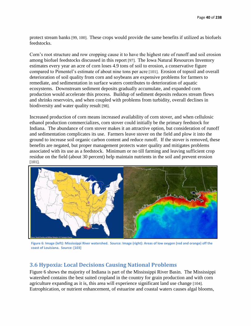
Page 40 of 238
protect stream banks [99, 100]. These crops would provide the same benefits if utilized as biofuels
feedstocks.
Corn‘s root structure and row cropping cause it to have the highest rate of runoff and soil erosion
among biofuel feedstocks discussed in this report [97]. The Iowa Natural Resources Inventory
estimates every year an acre of corn loses 4.9 tons of soil to erosion, a conservative figure
compared to Pimentel‘s estimate of about nine tons per acre [101]. Erosion of topsoil and overall
deterioration of soil quality from corn and soybeans are expensive problems for farmers to
remediate, and sedimentation in surface waters contributes to deterioration of aquatic
ecosystems. Downstream sediment deposits gradually accumulate, and expanded corn
production would accelerate this process. Buildup of sediment deposits reduces stream flows
and shrinks reservoirs, and when coupled with problems from turbidity, overall declines in
biodiversity and water quality result [98].
Increased production of corn means increased availability of corn stover, and when cellulosic
ethanol production commercializes, corn stover could initially be the primary feedstock for
Indiana. The abundance of corn stover makes it an attractive option, but consideration of runoff
and sedimentation complicates its use. Farmers leave stover on the field and plow it into the
ground to increase soil organic carbon content and reduce runoff. If the stover is removed, these
benefits are negated, but proper management protects water quality and mitigates problems
associated with its use as a feedstock. Minimum or no till farming and leaving sufficient crop
residue on the field (about 30 percent) help maintain nutrients in the soil and prevent erosion
[101].
96B3.6 Hypoxia: Local Decisions Causing National Problems Figure 6 shows the majority of Indiana is part of the Mississippi River Basin. The Mississippi
watershed contains the best suited cropland in the country for grain production and with corn
agriculture expanding as it is, this area will experience significant land use change [104].
Eutrophication, or nutrient enhancement, of estuarine and coastal waters causes algal blooms,
Figure 6: Image (left): Mississippi River watershed. Source: Image (right): Areas of low oxygen (red and orange) off the coast of Louisiana. Source: [103]

Page 41 of 238
oxygen depletion, and overall fishery habitat decline
[105, 86, 106]. Nutrient loading from Indiana will
worsen algal blooms in receiving waters. Hypoxia in
the Gulf of Mexico occurs when algae dies, sinks to
the bottom, and decomposes. Algal decomposition
consumes oxygen in the bottom water, creating a
lethal situation for resident plants and animals [74].
Nitrogen is the primary contributor to coastal
hypoxia, but phosphorous loading also leads to
severe degradation of freshwater lakes, rivers, and
some estuarine and coastal waters, especially those
receiving heavy loads of nitrogen as well [107, 108,
109].
Indiana must be cognizant of the interstate
implications of biofuel policies and agricultural
practices. Geo-political boundaries do not confine
environmental problems and decision making
requires an ecosystem management approach.
Effects from nutrient loading in Indiana‘s surface water must be considered in the context of
existing national goals to reduce nitrogen and phosphorous loading in the Mississippi River
Basin by 40 percent or more [110]. The ―dead zone‖ surrounding the Mississippi River Delta is
destroying coastal ecosystems and damaging local economies. Indiana must consider the extent
of eutrophication in the Mississippi River and hypoxia in the Gulf of Mexico when developing
the biofuels market. The state should take similar precautions for northern Indiana watersheds
flowing into the great lakes ecosystem.
11B3.7 Watershed Scale Water Quality Analysis for Potential
Agricultural Shifts
97B3.7.1 Introduction A watershed is any area of land that drains to a common point, and their delineation is important
for studying the ecological implications of human activity at a biologically meaningful scale
[111]. Land use within watershed boundaries directly affects the network of surface waters
capturing runoff from the drainage basin. Point and non-point sources of pollution, including
agricultural inputs, contribute nutrients, bacterial, and chemical contaminants to US waterways
[112]. Watershed scale analysis is used to characterize human, aquatic, and terrestrial features,
conditions, processes, and interactions collectively known as ecosystem elements [111].
Individual watershed analysis allows better estimation of direct, indirect, and cumulative effects
from management practices and land use patterns [111].
Watershed scale analysis is intended to serve as a model for watershed planning that allows for a
variety of human activities while providing for the highest quality water resource attainable.
Figure 7: Middle Fork Creek Watershed, Sullivan County, Indiana [13, 113, 114]

Page 42 of 238
Management at this scale includes
all activities aimed at identifying
and minimizing contaminants to a
water body from its watershed [112].
98B3.7.2 Methods The L-THIA modeling tool is used
to estimate non-point source (NPS)
pollution from a variety of different
land use classifications [113].
Researchers utilized a web-based
version of L-THIA for assessment of
Middle Fork Creek watershed after
it was delineated using the
watershed delineation tool available
with L-THIA [115]. The researchers
selected Middle Fork Creek
watershed based on the broad spectrum of potential land use changes from further development
of biofuels feedstocks. The 2001 land cover data guided the decision, because it revealed
significant acreage of agricultural lands, forest, pasture, and grasslands in the watershed [116].
After delineating the watershed, land use categories are imported into L-THIA to run the NPS
pollution model. Eight different land uses exist in the Middle Fork Creek watershed, and are
also subdivided by soil type. Hydrologic soil groups B and C make up the watershed, and are
described as: B – moderate to well-drained; moderately fine to moderately coarse texture;
moderate permeability; C – poor to moderately well-drained; moderately fine to fine texture; low
permeability [117]. Standard runoff coefficients and NPS pollutant concentrations for each land
use and soil type combination are built into the L-THIA model. L-THIA uses these standard
runoff and pollutant values in conjunction with average annual precipitation to estimate each
land use‘s contribution to NPS pollution in the watershed.
The first scenario represents current land use within the Middle Fork Creek watershed, and
served as the baseline for the analysis. Scenario two illustrates potential watershed impacts if
corn and soybean agricultural land expands. Agriculture makes significant contributions to the
degradation of waters in the United States, and high grain prices resulting in part from the
biofuels boom, are causing farmers to push back tree lines and convert pasture and grassland into
agriculture. Scenario two converts all pasture and grassland and 500 acres of forest into
agriculture in the Middle Fork Creek Watershed. Scenario three looks at the potential impacts
from expanding the production of perennial grasses for the production of cellulosic ethanol. The
L-THIA model groups pasture and grassland together into one land use category, so the inputs
and runoff values in scenario three would be different under a more realistic biofuels scenario.
Fecal coliform runoff would be lower than the output states since much of it comes from the
manure of pasture livestock (there would be no pasture, only expanded grassland), and nitrogen
and phosphorous runoff would be higher since farmers would likely fertilize their perennial grass
crops. Scenario three converted 50 percent of the agricultural land from scenario one into grass
and pasture. This hypothetical conversion is not based on likely scenarios in the near future, but
Land Use Hydrologic
Soil Group
Scenario
One
(acres)
Scenario
Two
(acres)
Scenario
Three
(acres)
Water/Wetlands C 88.4 88.4 88.4
Commercial C 14.8 14.8 14.8
Agricultural B 212.1 248.1 212.1
Agricultural C 10375.2 11410.6 5187.6
High Density Residential B 1.4 1.4 1.4
High Density Residential C 61.7 61.7 61.7
Low Density Residential B 13.8 13.8 13.8
Low Density Residential C 767.1 767.1 767.1
Grass/Pasture B 36 0 36
Grass/Pasture C 535.4 0 5723
Forest B 84.7 84.7 84.7
Forest C 3336.9 2836.9 3336.9
Industrial C 26.9 26.9 26.9
Total Area 15554.4 15554.4 15554.4
Figure 8: Middle Fork Creek Land Use Input Scenarios

Page 43 of 238
illustrates the benefits derived from alternative cropping systems in the event Indiana decides to
promote cellulosic ethanol production from perennial grasses in the long term.
99B3.7.3 Results/Discussion The results table evidences the detrimental impacts of expanding agricultural production in
Indiana, and the potential benefits of pursuing a future in cellulosic ethanol production from
perennial grasses. The results from scenario two show increased losses of all major NPS
pollutants from the watershed (except pesticides since they are not built into L-THIA), and
scenario three shows decreases in the same NPS pollutants.
If corn and soybean agriculture continues to expand in Indiana, the quality of water resources is
expected to decline. However, the implementation of better agricultural management practices
and a shift to perennial crops for cellulosic ethanol production would improve the quality of
water resources. The Middle Fork Creek watershed is a microcosm of the greater web of surface
water in Indiana, and small headwater streams similar to this creek, must be carefully managed
since they are delicate ecosystems and major contributors to NPS pollution. Quality of water
resources has serious implications for human health and the environment alike, and policy
decisions affecting agricultural production must be mindful of these implications. Many
watershed scale projects are now a preferred unit of analysis due to the advantages over classical
land management and protection units artificially defined by manmade boundaries [111]. The
benefits include a defined land area with a unique set of features and the recurring processes
affecting a common array of dependent plants and animals.
Scenario
One
Scenario
Two
Scenario
Three
Total Annual Runoff (acre-feet) 8,675 9,043 7,090
Nitrogen Losses (lbs.) 89,625 97,499 51,412
Phosphorous Losses (lbs) 25,903 28,410 13,602
Suspended Solids Losses (lbs) 2,130,156 2,336,353 1,118,658
BOD Losses (lbs) 118,278 125,562 82,839
Fecal Coliform Losses (millions
of coliform)
53,099,194 52,813,526 28,498,666
*BOD = Biochemical Oxygen Demand (uptake of oxygen from biological organisms)
Figure 9: Middle Fork Creek L-THIA Output
100B3.7.4 Groundwater Microorganisms convert excess nitrogen fertilizer in the soil to nitrate, which is then converted
to nitrite under anaerobic conditions in the soil or groundwater [74]. EPA considers wells
containing over 10 milligrams per liter of combined nitrate and nitrite concentration as impaired,
and recommends the water be treated before it is consumed. When ingested, nitrite binds to
hemoglobin and prevents oxygen transport. Nitrite-induced oxygen depletion is commonly
manifested as ―blue baby syndrome‖ in infants [74].
Similar to nutrient loading of surface water, the quantity of nitrates and nitrites infiltrating
groundwater from different crops is again a product of the crop‘s ability to process the nutrients
and the quantity of fertilizer being applied. One study shows a strong correlation between nitrate

Page 44 of 238
contamination of shallow groundwater and increased nitrogen use, a common situation for well-
drained surficial soils over unconsolidated sand and gravel aquifers in northern Indiana [119].
Vulnerability of Indiana‘s groundwater to nitrate pollution is mapped in Figure 10. The image is
from a study utilizing two modified modeling techniques (DRASTIC and SEEPAGE). The
DRASTIC model shows 58 percent of groundwater systems in Indiana as moderately vulnerable,
and 23 percent under high and very high risk. The SEEPAGE approach indicates 75 percent of
the state has moderate vulnerability [118].
Corn is again the most detrimental feedstock in terms of groundwater contamination. Corn‘s
inefficiency in processing nitrogen along with high application rates allows groundwater
infiltration of nitrogen fertilizer. Soybeans, just as other legumes, have evolved a symbiotic
relationship with nitrogen fixating bacteria which allows them to utilize nitrogen straight from
the air. Nitrogen fixation in beans precludes fertilizer application rates as high as corn.
Application of nitrogen to perennial grasses is high under certain conditions, but their extensive
root systems and ability to store nutrients in their roots over winter make them more efficient
users of nutrients [120]. Moreover, application of nitrogen to grasses is most important during
their establishment, and high application rates during this time increase potential groundwater
contamination. Studies show that nitrogen leaching is low in willow crops even at high
application rates (around 270 lbs per acre once during three to four year rotation), indicating that
nitrate and nitrite groundwater infiltration will not be a major problem from these crops [121, 122].
Similarly, poplars have high nutrient demand and are commonly used as riparian buffers, again
indicating little potential for significant groundwater contamination [93].
Solubility of pesticides determines their potential groundwater infiltration. Similar to nitrogen, a
study shows a strong correlation between pesticide contamination in groundwater, application
rates of pesticide, and presence of highly permeable soils with poor drainage [123]. Application
rates of these chemicals were previously discussed, and are used as a proxy for potential
groundwater contamination, with corn being the worst and the perennial grasses and trees the
best. If crop rotation diminishes, continuous corn persists, and agricultural land expands, then
groundwater contamination becomes more problematic.
Figure 10: Groundwater vulnerability map to nitrate pollution using modified SEEPAGE modeling technique. [124]
Figure 11: Area Map of Contamination Potential [124]
Page 45 of 238
101B3.7.5 Biodiversity
Biodiversity is the overall diversity of life in a given place [125]. While difficult to ascertain,
scholars describe biodiversity by the given number of species in a particular location.
Biodiversity is critical for the proper functioning of healthy ecosystems and can add resilience to
these systems during instances of disturbance. A variety of organisms help maintain ecosystem
functioning and perform important ecosystem services such as watershed protection, nutrient
cycling, and flood control. These ecosystem processes require the participation of myriad
species to make them work. For instance, the seemingly simple process of plant growth requires
an entire host of species, including many decomposers and pollinators [125]. Economic values of
services that species perform are difficult to quantify, yet their loss may be costly.
As human populations increase globally, [126] natural ecosystems and biodiversity sustain large
amounts of degradation due to increased land use. Humans are altering natural ecosystems at an
unprecedented rate. Deforestation, eutrophication, and species extinction are a few examples of
widespread damage to global ecosystems. When biodiversity in an ecosystem is lost, ecosystem
functioning and services begin to degrade, and cascading effects occur, such as the disruption of
the food web. Effects of such degradation may not be evident until after the biodiversity has
been lost, when it may be too late to mitigate the damage [127].
Biofuels production stands to increase the amount of land devoted to agriculture in Indiana.
CRP, forest, grassland, and pasture may be converted to row crops or other cellulosic feedstocks,
thereby decreasing the area of previously existing ecosystems. Agricultural expansion degrades
viable food, shelter, and water for Indiana‘s wildlife. Replacing natural forests and grasslands
with agricultural monocultures decreases the diversity of plants growing in an area, and
consequently fewer animals can then be supported. Biofuels policy, and any potential expansion
of agriculture that results, must be considered in the context of biodiversity and the valuable
services it provides.
102B3.7.6 Invasive Potential of Cellulosic Biofuels Crops Certain cellulosic biofuels crops have traits which increase invasive potential [128]. Once an
invasive species escapes and spreads into larger areas, it is nearly impossible to eradicate [129].
Various species of miscanthus are under consideration as potential biofuels feedstocks.
Miscanthus exhibits several traits that make it potentially invasive including ―the ability to re-
sprout from rhizomes, efficient photosynthetic mechanisms, and rapid growth rates.‖ [129]
Switchgrass has many of the same potentially invasive traits as miscanthus. Therefore, it has the
potential to become a weedy plant and invasive if it outcompetes predators and natural
competitors [129]. Since there is little invasive species research, policymakers should consider
invasive potential when evaluating transitions to alternative biofuels feedstocks.
103B3.7.7 Genetically Modified Crops (GMCs)
GMCs resist insects and weeds, survive harsh environmental conditions, and have increased
yields and nutritional values. Researchers can genetically modify the lignin content of cellulosic
crops to speed up breeding cycles, abate environmental pollution, and enhance landscape
restoration value [130]. Although Indiana does not plant GM poplar, some scientists believe that
poplar may be a good biofuels source. Purdue University researchers are attempting to
genetically modify lignin to release cellulose in fermentable sugars that can be converted to

Page 46 of 238
ethanol [131]. Proponents believe that pest-resistant GMCs are much safer to the surrounding
environment and society than pesticides. According to EPA, 10,000-20,000 cases of pesticide
poisoning in agricultural workers occur annually. Pesticide use kills approximately 70 million
birds annually in the US [132]. According to Halford and Shewry, farmers who grow GMCs
apply less poisonous and rapidly degradable herbicides, which decrease threats to the
environment [133]. Additionally, GMCs may provide food security for the world‘s dramatically
increasing population [132].
Farmers can grow GMCs easily, which creates a comparative advantage over those who rely on
traditional growing methods [33]. Broader GMC cultivation may occur as biofuels crop
production increases. The most popular GMCs are soybeans and corn. Poplar makes up almost
half of GM trees worldwide, and the US engineers 36 percent of poplar biotechnology [134].
Transgenic switchgrass technology is unavailable due to its complexity and lack of research [135].
Indiana‘s application of GMCs has increased during the previous decade. According to the
National Agricultural Statistics Service (NASS) in 2007, 59 percent of corn and 94 percent of
soybeans were GMCs in Indiana [136].
Crop/year 2000 2001 2002 2003 2004 2005 2006 2007
Corn 11% 12% 13% 16% 21% 26% 40% 59%
Soybean 63% 78% 83% 88% 87% 89% 92% 94%
Figure 10: Biotechnological Varieties: Percent of Corn and Soybean GMCs in Indiana [136]
12B3.8 Social and Economic Impacts: The World and Food Security
104B3.8.1 Food Alarmists There is a debate surrounding the impact of biofuels demand on agricultural commodity and food
prices. Historically, food shortages in less-developed countries have resulted from transportation
and equity problems [137]. Although world population has doubled in the past 40 years, food
production has remarkably kept pace with this increase. Today‘s global agricultural system is
capable of producing enough food to supply everyone with a daily caloric intake of 3,200, but
this may change [138]. The Christian Science Monitor reports that ―the era of cheap food is over
and we are going to have to get used to it.‖ [139] The concern is for those 2.7 billion people in
the world who live under the poverty level, for whom increasing food prices can be disastrous.
There are still more than 800 million people around the world who are malnourished and/or
hungry [140]. Food prices are rising in China, India, and the US, countries that contain 40 percent
of the world‘s population [141].
During the past year, basic grain prices for wheat, corn, and soybeans have increased
dramatically. Corn now costs more than $3 per bushel; soybeans more than $9 per bushel.
Because feed grains are a major input for meat, dairy, and poultry production, their price
increases cause retail prices to spike. In the US, 2007 dairy prices were up 13 percent and egg
prices have risen 42 percent [142].

Page 47 of 238
There is also concern about the decrease in the amount of food aid sent abroad. Studies indicate
the 32 million tons of corn converted to fuel in 2004 only amounted to 12 percent of the total US
supply; however, it could have fed 100 million people at average worldwide consumption levels
[143]. The US remains the leading grain exporter, shipping more than Canada, Australia, and
Argentina combined. Thus, what happens to the US grain crop affects the entire world. With the
massive diversion of grain to produce fuel for cars, exports will likely drop [141].
105B3.7.5 Biofuels Proponents
In the other side of the debate, the argument that decreases in US exports will lead to more
hunger in the world is highly exaggerated. According to the Institute for Agriculture and Trade
Policy, most US exports of corn and soybeans go to wealthy countries. Twenty percent of total
US corn is exported directly to 28 Organization for Economic Cooperation and Development
(OECD) countries as animal feed. In 1996, only 0.3 percent of corn exports went to countries
where undernourishment affects at least 20 percent of the population. About one-third of the US
soybean crop is exported, of which OECD countries import 70 percent. In 1998, a year of
record-low soybean prices, the 25 most undernourished countries received less than 0.027
percent of total US soybean exports [144].
Many factors outside of the price of grains influence retail food prices. John Urbanchuk of
LECG, LLC states that ―rising energy prices had a more significant impact on food prices than
did corn‖ Energy prices affect the Consumer Price Index (CPI) two times more than do food
prices [145].
A USDA report shows
labor costs account for 38 cents of every dollar a
consumer spends on food. Packaging, transportation,
energy, advertising, and profits account for 24 cents of
the consumer food dollar. In fact, only 19 cents of every
consumer dollar can be attributed to the actual cost of
food inputs like grains and oilseeds. As an example, a
standard box of corn flakes contains approximately 10
ounces of corn, or about 1/90th of a bushel. Even when
corn is priced at $4 per bushel, a box of corn flakes
contains less than a nickel‘s worth of corn [146].
106B3.8.3 Rising Food Prices Nearly 24 percent of Indiana residents currently live below the poverty line ($20,615 for a family
of four in 2006), and recent trends show increasing numbers [147]. Indiana low-wage worker
incomes have dropped two to four percent since 2000. Medium-income groups lost $4,000 in
annual income since 2000 and by 2006; they earned only 93 percent compared to their national
counterparts. Additionally, in the last six years, Indiana lost 110,000 jobs in the manufacturing
sector [147].
Rising food prices are a substantial burden for those living at or below the poverty level. The US
Department of Labor released Consumer Expenditures 2005, a survey of the percent of income
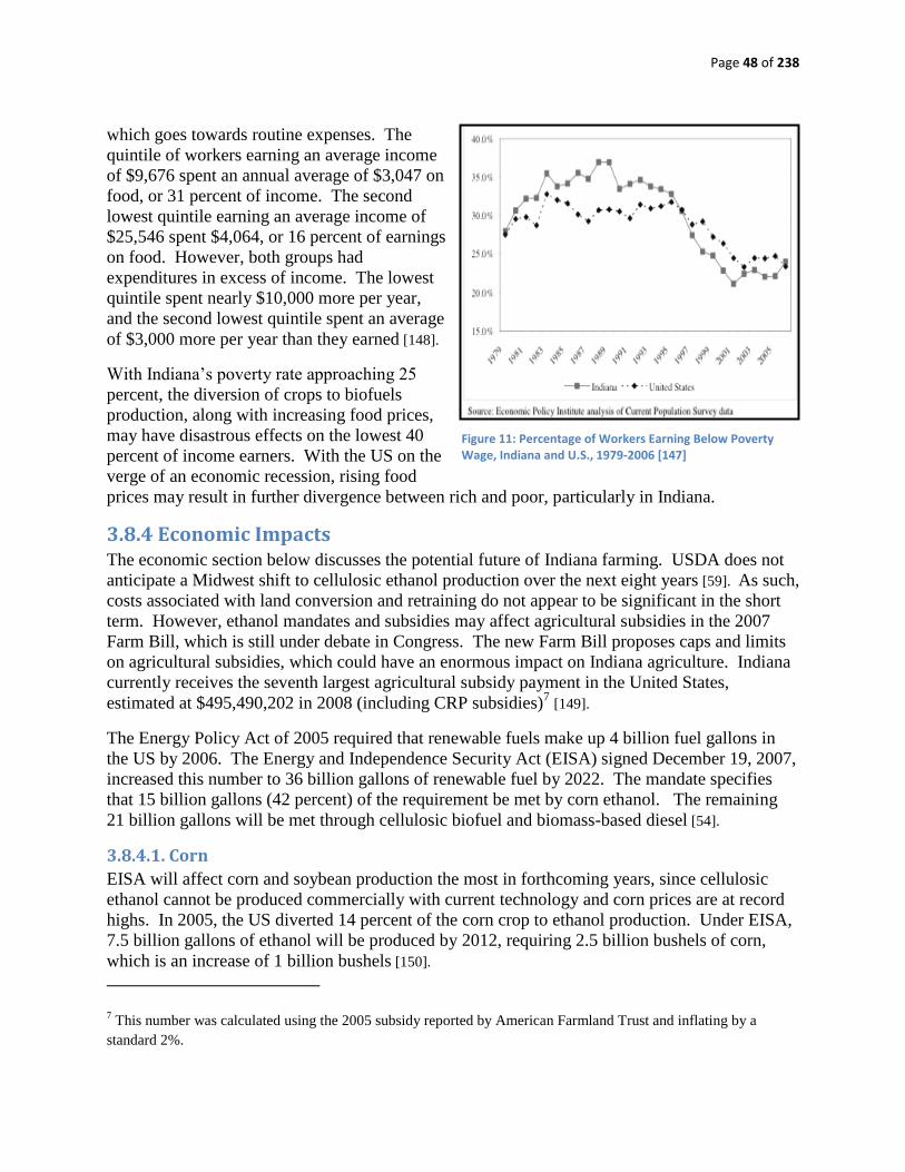
Page 48 of 238
which goes towards routine expenses. The
quintile of workers earning an average income
of $9,676 spent an annual average of $3,047 on
food, or 31 percent of income. The second
lowest quintile earning an average income of
$25,546 spent $4,064, or 16 percent of earnings
on food. However, both groups had
expenditures in excess of income. The lowest
quintile spent nearly $10,000 more per year,
and the second lowest quintile spent an average
of $3,000 more per year than they earned [148].
With Indiana‘s poverty rate approaching 25
percent, the diversion of crops to biofuels
production, along with increasing food prices,
may have disastrous effects on the lowest 40
percent of income earners. With the US on the
verge of an economic recession, rising food
prices may result in further divergence between rich and poor, particularly in Indiana.
107B3.8.4 Economic Impacts
The economic section below discusses the potential future of Indiana farming. USDA does not
anticipate a Midwest shift to cellulosic ethanol production over the next eight years [59]. As such,
costs associated with land conversion and retraining do not appear to be significant in the short
term. However, ethanol mandates and subsidies may affect agricultural subsidies in the 2007
Farm Bill, which is still under debate in Congress. The new Farm Bill proposes caps and limits
on agricultural subsidies, which could have an enormous impact on Indiana agriculture. Indiana
currently receives the seventh largest agricultural subsidy payment in the United States,
estimated at $495,490,202 in 2008 (including CRP subsidies)7 [149].
The Energy Policy Act of 2005 required that renewable fuels make up 4 billion fuel gallons in
the US by 2006. The Energy and Independence Security Act (EISA) signed December 19, 2007,
increased this number to 36 billion gallons of renewable fuel by 2022. The mandate specifies
that 15 billion gallons (42 percent) of the requirement be met by corn ethanol. The remaining
21 billion gallons will be met through cellulosic biofuel and biomass-based diesel [54].
202B3.8.4.1. Corn
EISA will affect corn and soybean production the most in forthcoming years, since cellulosic
ethanol cannot be produced commercially with current technology and corn prices are at record
highs. In 2005, the US diverted 14 percent of the corn crop to ethanol production. Under EISA,
7.5 billion gallons of ethanol will be produced by 2012, requiring 2.5 billion bushels of corn,
which is an increase of 1 billion bushels [150].
7 This number was calculated using the 2005 subsidy reported by American Farmland Trust and inflating by a
standard 2%.
Figure 11: Percentage of Workers Earning Below Poverty Wage, Indiana and U.S., 1979-2006 [147]

Page 49 of 238
In short-term pursuit of profit, farmers will convert acreage to corn to capture the rising market
prices. However, many Midwest farmers plant seasonal rotations between corn and soy
depending on which fetches the highest market price. USDA conducted a 2007 study on the
agricultural effects of EISA. Under the assumption of a 15 billion gallon ethanol mandate, corn
acreage will rise by 2.3 percent in each Midwest state by 2016. USDA also evaluated a 20
billion gallon scenario, which is plausible if market conditions and ethanol subsidies induce the
market to go beyond EISA requirements. With the 20 billion gallon scenario, corn acreage will
increase by 6.8 percent in Midwest states by 2016 [59]. These scenarios are extraordinarily
difficult to predict and are affected by the dollar‘s exchange rate and international supply and
demand for commodities. For instance, with the tumbling dollar and international demand for
soy oil, experts predict soybean prices could go as high as $16 per bushel in 2008 [151].
In 2007, 6,200,000 acres in Indiana were devoted to corn, up from 5,500,000 the previous year
(11 percent increase) [17]. This was coupled by a decline in soybean acreage from 5,700,000
acres in 2006 to 5,000,000 in 2007 (13
percent decline) [17]. Ethanol may induce
higher corn prices in the coming years,
which would result in decreased soybean
production. This low quantity of
soybeans would normally result in rising
soybean prices (a cyclical give and take
between corn and soy); however,
substitute ethanol byproducts such as Dry
Distillers‘ Grains (DDG) from biofuels
production has the potential to actually
reduce the demand for soy. Livestock
ranchers can substitute DDG for
soybean-based feed and do it at a lesser
price [59].
USDA predicts that Corn Belt farmers
will increase corn acreage primarily
through monoculture, reduced production
of other crops, and marginal-land farming.
Therefore, Indiana should not expect extreme shifts in land use patterns over the next 20 years.
Under the 15 billion gallon scenario, Indiana corn acreage would increase to 6,342,600 and the
20 billion gallon scenario would increase acreage to 6,621,600.8 These shifts are not as large as
expected, partially due to the USDA model‘s assumptions of decreasing corn exports, decreasing
feed demand (due to higher prices, lower livestock production, and DDG), and consistency of
CRP funding (an assumption that will likely be false) [59]. Increases in corn acreage come
primarily from a shift away from wheat and other crops.
8 These numbers were calculated with acreage data and growth rates from the pervious page provided by ―An
Analysis of the Effects of an Expansion in Biofuel Production on U.S. Agriculture.‖
Figure 12: Distribution of crop rotations in the corn belt, with percentage change from baseline for each rotation. [59]

Page 50 of 238
In 2007, Indiana corn yields rose to 160 bushels per acre [152, 153] resulting in Indiana corn pre-
subsidy revenues of $3,237,600,000.9 Indiana is the seventh largest recipient of agricultural
subsidies in the United States. The 2002 Farm Bill locked in corn subsidies at $2.63 per bushel
for 2004-2007 [154]. Indiana‘s increase in corn yields led to a $16,306,000 per acre subsidy in
2007. Moreover, warehousing, emergency assistance, farm loans, and other subsidies are
available to Indiana farmers which are significantly more beneficial than the per bushel subsidy.
In 2005, total Indiana corn subsidies amounted to $721,783,401, while in 2004 Indiana corn
subsidies amounted to only $375,308,558 [155]. Since figures are not available for the 2007 crop,
the 2004 figure was compounded at 2 percent inflation to provide a conservative estimate for the
2007 crop at $398,280,444. Thus, the total revenue (not accounting for production costs) of the
2007 Indiana corn crop is approximately $3,635,880,444.
203B3.8.4.2 Soybeans
In 2007, Indiana devoted approximately 5,000,000 acres of land to soybean production [17]. Due
to ethanol production and increasing corn prices, USDA predicts that EISA‘s 15 billion gallon
corn ethanol mandate will induce a 0.7 percent increase in soybean acreage by 2016 [59]. If
market conditions for ethanol improve and agricultural subsidies continue, there is potential for
20 billion gallons of ethanol production by 2016. In this scenario, soybean acreage would
decrease by 0.4 percent [59]. Soybean production will not be significantly harmed in either
scenario due to land diversion from other non-biofuels crops and cattle/poultry farming in the
state over the long run.
Professor Chris Hurt, Editor of the Purdue University Agricultural Economics Report, valued the
2007 soybean crop between $8.25 - $8.50 per bushel at harvest, potentially rising to $10 per
bushel [152]. The $8.50 per bushel figure is used as a conservative estimate for all following
calculations. Indiana soybean
yields in 2007 were 50 bushels
per acre [156].
Revenue from the 2007 Indiana
soybean crop is estimated at
$2,125,000,000.10
The 2004
soybean subsidy was $82,202,338
[149]. Using 2 percent inflation,
the subsidy rises to $87,233,778
in 2007. Thus, the 2007 Indiana
soybean crop revenue is
approximately $2,212,233,778.
These numbers illustrate that
higher corn yields and corn prices
9 These numbers were calculated based on the acreage, price, and yield figures for 2007 previously presented.
10 This number was derived from information previously given in the document.
Figure 13: U.S. Corn and Soybean Planted Average [17]

Page 51 of 238
are forcing farmers to shift away from soybeans in the short-term. This phenomenon is not
unique to Indiana; the national shift towards corn production over the last two years has been
significant. However, as mentioned prior, the low value of the American dollar and reduced soy
production will likely drive the soybean price to all-time highs in 2008, resulting in a future shift
back to soy planting.
204B3.8.4.3 Cellulosic Crops
Cellulosic biofuels add to the complexity of agricultural economics. Technology does not
currently exist to produce fuel from many of these crops, but it is expected that breakthroughs in
identifying cellulosic enzymes could occur within the next four to ten years. This creates a
considerable amount of uncertainty in the market for these crops and land use predictions for
Indiana.
Switching from corn or soy to cellulosic crops depends, in part, on crop profitability.
Complications arise in determining profits for cellulosic crops because they currently have no
market. Several studies have attempted to determine the pricing structure for these crops, which
are highly dependent on mandates, ethanol subsidies, transportation costs, and conservation
program payments [157, 158, 49]. Agricultural subsidies are a significant, if not the only, source of
profit for Indiana farmers. The opportunity cost of a farmer switching to cellulosic crop growth
and losing his or her subsidy is, therefore, substantial. However, two large unknowns could
make it a profitable switch: the 2007 Farm Bill and the renewal of CRP.
Indiana CRP payments increased to $92 per acre in 2008 [159]. As of January 2008, 295,947.4
Indiana acres were enrolled in CRP, with total payments of $27,227,160 [159]. In 2008 26,046
acres of Indiana CRP land will expire [159]. With the forthcoming reduction in the CRP budget,
it is reasonable to assume that it will be increasingly difficult for farmers to be granted new
acreage or renew CRP contracts. Based on CRP reduction, the profitability of harvesting
cellulosic crops depends upon the profitability of the crops themselves.
USDA gathered data concerning switchgrass from two studies completed at the University of
Nebraska and Iowa State University. The Iowa State study found that switchgrass costs ranged
from $121 per acre (yield: 1.5 tons per acre) to $241.16 per acre (yield: 6 tons per acre). The
Nebraska study found switchgrass production costs of $112 per acre (yield: 3.4 tons per acre)
[59]. A similar study was conducted by the Department of Agricultural and Consumer
Economics at UIUC and indicated switchgrass costs at $147 per acre for a yield of 2.58 tons per
acre [158]. Depending on the desired yield, switchgrass costs run between $112 - $241 per acre,
meaning the market price must significantly exceed these costs for farmers to switch to perennial
grasses.
Switchgrass production has both benefits and drawbacks. Benefits include low maintenance, less
prone to external shocks (drought, flooding), environmental improvements (over corn and
soybeans), complementary equipment (between hay and alfalfa), annual harvests, and potentially
reduced per acre costs. The primary drawbacks of switchgrass are storage and transportation.
Iowa State University estimated that hauling 20 tons of switchgrass 30 miles would cost $173.
Storage estimates were an additional $17 per ton [160]. As a result of transportation difficulties,
cellulosic fuel production facilities must be located near switchgrass farms to make them
profitable; Indiana currently has no cellulosic ethanol plants.

Page 52 of 238
Woody residue cellulosic crop growth is unlikely in Indiana. Even if farms could renew CRP
payments, willow can only be harvested every three years and poplar every seven to ten years
[59]. Moreover, farmers would be required to invest in completely new equipment to plant,
harvest, chip, and remove post-harvest tree stumps. This would require farmers to invest
significant upfront capital and forgo revenue for three to ten years before first harvest. Similarly,
transportation and storage issues also occur with woody crops.
It is unlikely that profit potential will induce Indiana farmers to switch to cellulosic fuel crops in
the short term. The construction of cellulosic plants, the advent of new technology, the 2007
Farm Bill, and increasing mandates for cellulosic ethanol could change this situation. However,
market trends indicate that Indiana farmers will convert cropland from soybeans to corn in the
short term and from other crops to corn and soybeans in the long term.
The short-term future of cellulosic ethanol in Indiana likely rests on corn stover, the field residue
from corn harvesting. Stover is free to produce and the farmer only incurs additional costs to
bail, store, and transport the stover, and replenish soil nutrients.
205B3.8.4.4 Market Implications from Expanding Biofuels Production
Corn and soybeans are major inputs for cattle ranching and poultry production. Farmers can use
DDG as a substitute feed. However, DDG has a lower protein count, quality variability, and
shipping and storage issues. Livestock and poultry will be additionally burdened by the rising
value of agricultural land and those who rent land will experience higher rents. Increasing costs
will make small livestock, dairy, and poultry operators particularly vulnerable and favor large-
scale producers who experience economies of scale [59].
Small-scale dairy farming is still a common practice, whereas cattle, poultry, and hog farming
are generally much larger operations. Additionally, dairy cattle are the most sensitive to
fluctuations in feed quality. Poor quality or quantity of feed will affect milk production. As
such, this industry is particularly vulnerable to rising feed prices associated with corn and soy
diversion to biofuels [59].
Ethanol may divert upwards of 47 percent of domestic corn production by 2016, which will
lower exports. Under the 15 billion gallon EISA mandate, corn and soybean exports will
decrease 4.8 percent and 2.8 percent respectively by 2016. If consumer demand and subsidies
increase ethanol production to 20 billion gallons, corn and soybean exports will decline by 12
percent and 5.3 percent respectively [59]. This will offset the US economy to some degree;
however, the higher prices for corn and soybeans will allow US agricultural export value to
increase slightly, despite reductions in quantity.
13B3.9 Conclusions
108B3.9.1 Best Management Practices A strict environmental perspective suggests all agricultural producers in Indiana should stop
growing corn and soybeans and start planting perennial grasses and SRWCs. However, political
and economic influences prevent this from happening. As such, existing and planned biofuels
Page 53 of 238
production necessitates implementation of BMPs for corn and soybeans, and eventual shifts to
perennial grasses and SRWCs are necessary once commercial production of cellulosic ethanol
commences. Production of cellulosic feedstocks provides many long-term benefits including
multiple revenue streams for farmers and a variety of ecosystem services which result in
improved surface and groundwater quality [161].
Agricultural policy goals should include reductions in nutrient loading, pesticide use, and
erosion. More efficient fertilization techniques reduce nutrient loading from existing corn and
soybean operations. Farmers should utilize enhanced efficiency fertilizers that match application
rates to nitrogen uptake patterns of various crops, as well as controlled release fertilizers which
have insoluble coatings to prevent nitrogen dissolution [74]. Injecting fertilizer below the ground
to shield it from wind and water reduces its potential to runoff, and is another BMP option [74].
Similar to fertilizer management, pesticide management is all about efficiency. Efficient
application of agrichemical inputs saves farmers money and prevents undue harm to the
environment. Integrated pest management (IPM) is an increasingly popular management
technique for insects. IPM restricts the use of pesticides to a last resort for insect problems and
focuses on preventive measures. Similarly, herbicides and fungicides should only be applied as
needed. Varying crop densities and planting patterns (alternatives to row cropping) helps
suppress weed development as well as utilization of ground cover (i.e. mulching).
Surface cover and conservation buffers prevent soil erosion most effectively. Crop residue and
winter cover crops are the most popular means of maintaining surface cover throughout the year.
A variety of conservation tillage techniques can help maintain surface cover and the integrity of
the soil. Incentives already exist for ―no till‖ and ―strip till‖ techniques, which are common
alternatives to full-width tillage and will be especially important when corn stover enters the
feedstock market [74]. No till farming is already widely utilized in Indiana and should continue
to be encouraged [162]. Riparian buffers shield surface waters from non-point source runoff, and
development of the market for cellulosic ethanol makes their use more attractive. SRWCs and
perennial grasses are effective riparian buffers since they improve soil and water quality, expand
wildlife habitat, and increase land use diversity [163]. One study shows switchgrass used as a
riparian buffer has eight times the below-ground biomass and up to 55 percent more SOC than
adjacent cropped fields [164]. Promoting the use of perennial grasses and woody crops as
conservation buffers poises farmers to receive new revenue streams once the cellulosic ethanol
market opens.
Protection of Indiana‘s environment will require a broad suite of conservation practices
integrating nutrient, pesticide, and sediment management. Existing crops need more intense
management; superior feedstocks require agricultural incentives, and improved agricultural
technologies require diffusion. Low-input high-density (LIHD) cropping systems, precision
agriculture, and diversified agricultural landscapes are receiving more attention, considering the
variety of feedstocks that produce biofuels [165].

Page 54 of 238
14B3.10 References for Feedstock Agriculture [1] Dryer DR. 1908. Studies in Indiana
Geography. Terre Haute: Inland Publication
Co.
[2] Indiana Geographic Information Council,
Inc. 2005. Indiana Digital Elevation Model.
Indiana Orthophotography (22 February
2008;
http://www.in.gov/igic/projects/indianamap/
index.html)
[3] Homoya MA, Abrell B, Aldrich J, Post, T.
1985. The natural regions of Indiana.
Proceedings of the Indiana Academy of
Science 94: 245-268.
[4] Indiana State Climate Office. 2008.
Department of Agronomy, Purdue, IN (16
February 2008;
http://www.agry.purdue.edu/climate/
facts.asp)
[5] Indiana State Climate Office. 2008.
Department of Agronomy, Purdue, IN (16
February 2008;
http://www.agry.purdue.edu/climate)
[6] Indiana State Climate Office. 2008.
Department of Agronomy, Purdue, IN (16
February 2008;
http://www.agry.purdue.edu/climate/narrativ
e.asp)
[7] Fleming A. 1997. Freeze Frame: The Ice
Age in Indiana. Indiana Geological Survey
(27 February 2008;
http://igs.indiana.edu/Geology/ancient/freez
eframe/)
[8] Bleuer N, DeChurch D. 1999. Flat, but Not
Dull—Understanding the Central Indiana
Glacial Landscape. Indiana Geological
Survey ( 27 February 2008;
http://igs.indiana.edu/geology/topo/centralIn
dLandscape/index.cfm)
[9] Gray HH. 2000. Physiographic divisions of
Indiana: Indiana Geological Survey special
report 61. Digital compilation by Kimberly
H. Sowder.(16 February 2008;
http://igs.indiana.edu/
geology/maps/statephysiography/
physiography.cfm)
[10] Natural Resources Conservation Service.
Miami -- Indiana State Soil. United States
Department of Agriculture, Washington, DC
(26 February 2008; ftp://ftp-
fc.sc.egov.usda.gov/NSSC/
StateSoil_Profiles/ in_soil.pdf)
[11] Like K. 2002. State Boundary of Indiana.
Indiana Geological Survey, 1:24,000
Polygon shapefile. (24 April 2008;
http://129.79.145.7/arcims/statewide_mxd/dl
oad_page/reference.html)
[12] USDA. 2004. Cultivated Areas in Indiana in
2004. United States Department of
Agriculture. National Agriculture Statistics
Service, Fairfax, Virginia (17 April 2008;
http://129.79.145.7/arcims/statewide_mxd/dl
oad_page/reference.html)
[13] Environmental Systems Research Institute.
2006. ArcGIS 9.2. Redlands, California.
[14] National Agricultural Statistics Service.
2007. Fact finding for agriculture. United
States Department of Agriculture,
Washington, DC (16 February 2008;
http://www.nass.usda.gov/Statistics_by_Stat
e/Indiana/Rankings/Data/hilite07.pdf)
[15] National Agricultural Statistics Service.
2004. Indiana State and County Data: 2002
Census of Agriculture. United States
Department of Agriculture, Washington, DC
(16 February 2008;
http://www.nass.usda.gov/census/
census02/volume1/in/ INVolume104.pdf)
[16] Farm Service Agency. Conservation
Reserve Program Monthly Summary---
January 2008. United States Department of
Agriculture, Washington, DC (26 February
2008; http://www.fsa.usda.gov/Internet/
FSA_File/jan2008.pdf)
[17] National Agricultural Statistics Service.
2007. Prospective Plantings. United States
Department of Agriculture, Washington, DC
(21 April 2008;
http://www.usda.gov/nass/PUBS/
TODAYRPT/pspl0308.txt)
[18] National Agricultural Statistics Service.
2008. Prospective Plantings. United States

Page 55 of 238
Department of Agriculture, Washington, DC
(21 Apr. 2008; http://www.usda.gov/nass
/PUBS/TODAYRPT/pspl0308.pdf)
[19] Food and Agriculture Organization of the
United Nations. Crop Water Management:
Sorghum. 2002. AGLW Water Management
Group (9 April 2008;
http://www.fao.org/ag/agl/aglw
/cropwater/sorghum.stm)
[20] National Resources Conservation Service.
Plants Profile for Sorghum Bicolor Ssp.
Drummondii (Sudangrass). United States
Department of Agriculture, Washington, DC
(27 February 2008;
http://plants.usda.gov/java/profile?symbol=
SOBID)
[21] Indiana Department of Natural Resources.
Exotic & Invasive Plants. 2008. Division of
Entomology and Plant Pathology (27
February 2008;
http://www.in.gov/dnr/entomolo
/pestinfo/invasive.htm)
[22] Vermerris W, Rainbolt C, Wright D,
Newman Y. 2007. Production of biofuel
crops in Florida. SS AGR 293. University of
Florida. IFAS Extension (27 February 2008;
http://edis.ifas.ufl.edu/pdffiles/AG/AG2980
0.pdf)
[23] Regehr, D. 1998. Weed control. In: Grain
sorghum production handbook. Manhattan,
Kansas: Kansas State University
Agricultural Experiment Station and
Cooperative Extension Service.
[24] Mask P, Hagan A, Mitchell Jr. C. 1988.
Production guide for grain sorghum.
Alabama Cooperative Extension System.
ANR 502 (28 February 2008;
http://www.aces.edu/pubs/docs/A/ANR-
0502/)
[25] Freeman KC, Broadhead DM, Zummo N.
1973. Culture of sweet sorghum for sirup
production: Agriculture handbook No. 441.
Agricultural Research Service. United States
Department of Agriculture, Washington, DC
(27 February 2008;
http://www.aces.edu/pubs/docs/A/ANR-
0625/)
[26] Oklahoma State University. 2006.
Converting sweet sorghum into ethanol.
Oklahoma State University (26 February
2007; http://osu.okstate.edu/
index.php?option=com_content&task=view
&id=7&Itemid=90)
[27] Blanco M, Azqueta D. 2008. Can the
environmental benefits of biomass support
agriculture? The case of cereals for
electricity and bioethanol production in
Northern Spain. Energy Policy 26: 357-366.
[28] Heaton H, Clifton, Brown J, Voigt T, Jones
M, Long S. 2004. Miscanthus for renewable
energy generation: European Union
experience and projections for Illinois.
Mitigation and Adaptation Strategies for
Global Change 9: 441.
[29] Flax Council of Canada and Saskatchewan
Flax Development Commission. 2002.
Growing Flax: Production, management and
diagnostic guide. Ed 4. p45.
[30] Flax Council of Canada and Saskatchewan
Flax Development Commission. 2002.
Growing Flax: Production, management and
diagnostic guide. Ed 4. p39.
[31] Sheehan J, Dunahay T, Benemann J,
Roessler P. 2008. A Look Back at the U.S.
Department of Energy's Aquatic Species
Program-- Biodiesel from algae. Department
of Energy, National Renewable Energy
Laboratory.
[32] Hankamer B, Lehr F, Repprecht J,
Mussgnug JH, Poston C, Kruse O. 2007.
Photosynthetic biomass and H2 production
by green algae: from bioengineering to
bioreactor scale-up. Physiologia Plantarum
131: 10-21.
[33] Wagner L. 2007. Biodiesel from algae oil.
Research Report, Mora Associates; also in
Bernstein MA. GreenFuel technologies
corporation's emissions-to-biofuels algae
technology: A viable option for biofuel
feedstock. Corporate Technology Report,
GreenFuel Technology.
[34] Brune DE, Yen HW, Schwartz G,
Benemann JR, Massingill MJ, Van Olst JC,
Carlberg JA. 2004. The controlled
eutrophication process; Microalgae for
Page 56 of 238
biofuels production and fertilizer recycling
at the Salton Sea, California. (27 February
2008;
http://www.unh.edu/p2/biodiesel/pdf/algae_
salton_sea.pdf)
[35] Tillman D, Hill J, Lehman C. 2006. Carbon
negative biofuels from low input high
diversity grassland biomass. Science 314:
1599-1600.
[36] Glassner D, Herrenhaus J, Schechinger T.
1998. Corn stover collection project.
BioEnergy‘98: Expanding BioEnergy
Partnerships: 1100-1110 (9 April 2008;
www2.ctic.purdue.edu/core4/bio98paper.pdf
)
[37] National Resources Conservation Service.
2006. Plant Materials Program 2007.
Swithcgrass: plant fact sheet. United States
Department of Agriculture, Washington, DC
(25 January 2008; http://plants.usda.gov/
factsheet/pdf/fs_pavi2.pdf)
[38] Bennett, M. Personal communication.
February 2008.
[39] Tolbert V, Schiller A. 1995. Environmental
enhancement through agriculture:
Proceedings of a conference, Boston
Massachusetts. Center for Agriculture, Food
and Environment, Tufts University,
Medford, MA.
[40] Stanturf. J, van Oosten C, Netzer D,
Coleman M, Portwood C.J. in Stanturf.
2002. Ecology and silviculture of poplar
plantations in poplar culture in North
America. Eds. Isebrands, Eckenwalder and
Richardson. Chapter 5. Ottawa: NRC
Research Press, National Research Council
of Canada: 153-206.
[41] Sokhanasanj S, Turhollow AF. Baseline cost
for corn stover collection. Applied
Engineering in Agriculture 18 (5): 525-530.
[42] Iowa State University. 2006. Iowa State
researchers developing machinery to harvest
corn stalks and leaves. Iowa State University
News Release. (20 March 2008;
http://www.public.iastate.edu/~nscentral/ne
ws/2006/dec/stover.shtml)
[43] Shapouri H, Duffield JA, Wang M. 2002.
The Energy Balance of Corn Ethanol: An
update. United States Department of
Agriculture, Washington, DC (20 March
2008;
http://www.transportation.anl.gov/pdf/AF/2
65.pdf)
[44] North Dakota State University Extension
Service. ProCrop: Soybean harvest. (20
March 2008;
http://www.ag.ndsu.edu/procrop/syb/soybha
r09.htm)
[45] Shinners KJ, Binversie BN, Muck RE,
Weimer PJ. 2007. Comparison of wet and
dry corn stover harvest and storage. Biomass
and Bioenergy 31: 211-221.
[46] Nielsen RL. 1995. Questions relative to
harvesting and storing corn stover.
Department of Agronomy, Purdue, IN (20
March 2008;
http://www.agry.purdue.edu/ext/com/pubs/a
gry.9509.htm)
[47] Vogel KP, Brejda JJ, Walters DT, Buxton
DR. 2002. Switchgrass biomass production
in the Midwest USA: Harvest and nitrogen
management. Agronomy Journal 94: 413-
420.
[48] McLaughlin SB, Walsh ME. 1998.
Evaluating environmental consequences of
producing herbaceous crops for bioenergy.
Biomass and Bioenergy 14 (4): 317-324.
[49] Doering O. 4 March 2008. Economic
perspectives on producing liquid fuels from
plant feedstocks. Indiana Memorial Union,
Bloomington.
[50] Ruark G, Josiah S, Riemenschneider D,
Volk T. February 16, 2006. Perennial crops
for bio-fuels and conservation. Presented at
2006 USDA Agricultural Outlook Forum –
Prospering in Rural America. Arlington,
Virginia (9 April 2008;
http://www.usda.gov/oce/forum/2006%20sp
eeches/PDF%20speech%20docs/Ruark2806.
pdf)
[51] Gregg L. 2007. NC State Researchers
Harvest Biomass to Generate Electricity,
Reduce Forest Fire Risks. North Carolina
State University News Releases. (9 April

Page 57 of 238
2008;
http://news.ncsu.edu/news/2007/10/168biom
assharvesterrelease.php)
[52] Scharlemann JPW, Laurance WF. 2008.
How green are biofuels? Science 319 (4):
43-44.
[53] Marshall L, Greenhalgh S. 2006. Beyond the
RFS: The environmental and economic
impacts of increased grain ethanol
production in the US. WRI Policy Note 1: 1-
6
[54] Economic Research Service. Agricultural
baseline projections: US Crops, 2008-2017.
United States Department of Agriculture,
Washington, DC (12 February 2008;
http://www.ers.usda.gov/Briefing/
Baseline/crops.htm)
[55] Marshall L. 2007. Thirst for corn: What
2007 plantings could mean for the
environment. WRI Policy Note 2: 1-10.
[56] Vyn TJ. 2006. Meeting the ethanol demand:
Consequences and compromises associated
with more corn on corn in Indiana. Purdue
Extension BioEnergy ID-336: 1-4.
[57] Great Lakes Commission. The potential
impacts of increased corn production for
ethanol in the Great Lakes-St. Lawrence
River Region. US Army Corps of Engineers
(18 December 2007;
http://www.glc.org/tributary/pubs/document
s/EthanolPaper 121807FINAL.pdf)
[58] Andrews S, Aschmann S. 2006. Resource
effects of biomass energy production.
USDA Conservation Issue Brief. (27
February 2008;
http://soils.usda.gov/sqi/management/files/
Biomass_Conservation_ Issue_Brief.pdf)
[59] Economic Research Service. 2007. An
analysis of the effects of expansion of
biofuel demand on US agriculture. United
States Department of Agriculture,
Washington, DC (12 February 2008;
http://www.usda.gov/oce/newsroom/news_r
eleases/ chamblissethanol5-8-07)
[60] Wilhelm WW, Johnson JMF, Hatfield JL,
Voorhees WB, Linden DR. 2004. Crop and
soil productivity response to corn residue
removal: A review of the literature.
Agronomy Journal 96.1: 1-17.
[61] Hill J, Nelson E, Tilman D, Polasky S,
Tiffany D. 2006. Environmental, economic,
and energetic costs and benefits of biodiesel
and ethanol biofuels. Proceedings of the
National Academy of Sciences 103.30:
11206-11210.
[62] Dicks MR, Johnson, JB, Hellerstein, DM.
2007. The 2007 Farm Bill: Policy options
and consequences. The Farm Foundation.
2007:1.
[63] Cowan, Tadlock. Conservation Reserve
Program: Status and current issues.
Congressional Research Service (3 January
2008; http://www.nationalaglawcenter.org/
assets/crs/RS21613.pdf)
[64] Farm Bill Developments; USDA Baseline
Projections; 2008 Income Forecast. The
FarmPolicy.com News Summary. 13
February 2008:2.
[65] Righelato R, Spracklen DV. 2007. Carbon
mitigation by biofuels or by saving and
restoring forests? Science 317: 902.
[66] Brown H, Eflin J, Ferguson D. 2002.
Connecting biomass producers with users:
Biomass production on marginal lands in
Indiana. Ball State University (27 February
2008; http://www.bsu.edu/
shapps/nrem/biomass/index.html)
[67] Ranney JW, Mann LK. 1994. Environmental
considerations in energy crop production.
Biomass and Bioenergy 6.3: 211-228.
[68] US House of Representatives, 110th
Congress. H.R. 2419: An Act to Provide for
the Continuation of Agricultural Programs
through Fiscal Year 2012 and for Other
Purposes. Washington: Government Printing
Office. 860 p.
[69] Sedjo RA. 2001. Forest carbon
sequestration: Some issues for forest
investments. Resources for the Future,
Washington, DC (13 March 2008;
http://www.rff.org/Documents/RFF-DP-01-
34.pdf)

Page 58 of 238
[70] Fargione J, Hill J, Tillman D, Polasky S,
Hawthorne P. 2008. Land clearing and the
biofuel carbon debt. Science, 319. 1235.
[71] Gorte RW. 2007. CRS Report for Congress:
Carbon Sequestration in Forests.
Congressional Research Service (11 March
2008;
http://www.ncseonline.org/NLE/CRSreports
/07Apr/RL31432.pdf)
[72] Schlesinger WH, Lichter J. 2001. Limited
carbon storage in soil and litter of
experimental forest plots under increased
atmospheric CO2. Nature 411:466-469.
[73] Post WM, Kwon KC. 2000. Soil carbon
sequestration and land-use change:
processes and potential. Global Change
Biology 6:317-327.
[74] National Academy of Sciences. 2007. Water
implications of biofuels production in the
United States. Committee on Water
Implications of Biofuels Production in the
United States, Washington, DC (23 April
2008;
http://dels.nas.edu/dels/rpt_briefs/biofuels_b
rief_final.pdf)
[75] Schwab GO, Frevert RK, Edminster TW,
Barnes KK. 1981. Soil and water
conservation engineering. Agricultural
Water Management 9(1): 83-84.
[76] National Resources Conservation Service.
2002. Quantifying the change in greenhouse
gas emissions due to natural resource
conservation practice application in Indiana.
United States Department of Agriculture,
Washington, DC (16 February 2008;
http://www.oznet.ksu.edu/ctec/Brenner's_stu
dy/IndianaCarbonStudy/Indiana_Final_Repo
rt.pdf )
[77] Allen RG, Pereira LS, Raes D, Smith M.
1998. Crop evapotranspiration - Guidelines
for computing crop water requirements -
FAO Irrigation and drainage paper 56.
Chapter 2. Food and Agriculture
Organization of the United Nations (17
February 2008;
http://www.fao.org/docrep/X0490E/x0490e0
a.htm#crop%20coefficient%20curve)
[78] Hutson SS, Barber NL, Kenny JF, Linsey
KS, Lumia DS, Maupin MA. 2004.
Estimated use of water in the United States
in 2000. US Geological Survey Circular. US
Geological Survey, Reston, VA (23 April
2008; http://pubs.usgs.gov/circ/2004/
circ1268/)
[79] Pimentel D, Houser J, Preiss E, White O,
Fang H, Mesnick L, Barsky T, Tariche S,
Schreck J, Alpet S. 1997. Water resource:
Agriculture, the environment and society.
BioScience 47(2): 97-106.
[80] Aden A. 2007. Water usage for current and
future ethanol production. Southwest
Hydrology (23 April 2008;
http://www.swhydro.arizona.edu/archive/V6
_N5/feature4.pdf)
[81] Rockwood DL, Naidu CV, Carter DR,
Rahmani M, Spriggs TA, Lin C, Alker GR,
Isebrands JG, Segrest SA. 2004. Short-
rotation woody crops and phytoremediation:
Opportunities for agroforestry? Agroforestry
Systems 61: 51–63, 2004.
[82] Sharma NK, Samrab JS, Singh HP. 2001.
Influence of boundary plantation of poplar
(Populus deltoides M.) on soil–water use
and water use efficiency of wheat.
Agricultural Water Management 51(3): 173-
185.
[83] Powlson DS, Richie AB, Shield I. 2005.
Biofuels and other approaches for
decreasing fossil fuel emissions from
agriculture. Annals of Applied Biology
146:193–201.
[84] Wescott P. 2007. U.S. ethanol expansion
driving changes throughout the agricultural
sector. Amber Waves 5(4).
[85] National Research Council. 2000. Clean
coastal waters: Understanding and reducing
the effects of nutrient pollution. National
Academy Press, Washington DC.
[86] Balkam KS, Blackmer AM, Hansen DJ,
Morris TF, Mallarino AP. 2003. Testing
soils and cornstalks to evaluate nitrogen
management in the watershed scale. Journal
of Environmental Quality 32: 1015-1024.

Page 59 of 238
[87] Simpson T, Pease J, Mcgee B, Smith, MC,
Korcak RF. 2007. Biofuels and Water
Quality: Meeting the challenge and
protecting the environment. MAWQ 07-4.
Agricultural Research Service. United States
Department of Agriculture, Washington,
DC.
[88] Sharpley AN, Rekolainen S. 1997.
Phosphorous in agriculture and its
environmental implications. p.1-54. In H
Tunney et. al. Phosphorous Loss from Soil
to Water. CAB International Press.
Cambridge, England.
[89] Hall KE, George JR, Riedl RR. 1982,
Herbage dry matter yields of switchgrass,
big bluestem, and indiangrass with N
fertilization. Agronomy Journal 75: 47-51.
[90] Parrish DJ, Fike JH. 2005. The biology and
agronomy of switchgrass for biofuels.
Critical Reviews in Plant Science 24: 423-
459.
[91] Madakadze IC, Stewart KA, Peterson PR,
Coulman BE, Smith DL. 1999. Cutting
frequency and nitrogen fertilization effects
on yield and nitrogen concentration of
switchgrass in a short season area. Crop
Science 39: 552-557.
[92] Sanderson MA, Reid RL, Ocumpaugh WR,
Hussey MA, Van Esbroeck G, Read JC,
Tischler C, Hons FM. 1999. Switchgrass
cultivars and germplasm for biomass
feedstock production in Texas. Bioresource
Technology 67: 209-219.
[93] Food and Agricultural Organization of the
United States. 1980. Poplars and willows.
FAO Forestry and Forest Products Studies
No. 12, Rome.
[94] Oak Ridge National Laboratory. Popular
poplars: Trees for many purposes.
Bioenergy Feedstock Information Network
(23 April 2008;
http://bioenergy.ornl.gov/misc/poplars.
html)
[95] United States Environmental Protection
Agency. 2004. Record of Decision by
Principal Deputy AA/OPPTS Regarding
Status of Prions under FIFRA. Washington,
DC: Office of Prevention, Pesticides and
Toxic Substances.
[96] United States Environmental Protection
Agency. 2008. About pesticides. (23 April
2008;
http://www.epa.gov/pesticides/about/#what_
pesticide)
[97] National Research Council. 2003. Frontiers
in Agricultural Research: Food, health,
environment and communities. The National
Academies Press. Washington, DC.
[98] Patton DJ. Soil Conservation, in
AccessScience@McGraw-Hill (13 February
2008; http://bert.lib.indiana.edu: 2339, DOI
10.1036/1097-8542.631800)
[99] McLaughlin SB, De La Torre Ugarte DG,
Garten Jr. CT, Lynd LR, Sanderson MA,
Tolbert VR, Wolf DD. 2002. High value
renewable energy from prairie grasses.
Environmental Science and Technology 36:
2122-2129.
[100] Gochis DJ, Cuenca RH. 2000. Plant water
use and crop curves for hybrid poplars.
Journal of Irrigation and Drainage
Engineering 126: 206-214.
[101] Pimentel D, Patzek T. 2005. Ethanol
production using corn, switchgrass, and
wood; Biodiesel production using soybean
and sunflower. Natural Resources Research
14(1).
[102] Varvel GE, Vogel KP, Mitchell RB, Follet
RF, Kimble JM. 2008. Comparison of corn
and switchgrass on marginal soils for
bioenergy. Biomass and Bioenergy 32: 18-
21.
[103] National Aeronautics and Space
Administration/Goddard Space Flight
Center, Scientific Visualization Studio. In:
The University of Texas at Austin. 2007.
Marine Scientists Funded to Study ‗Dead
Zone.‘ (28 February 2008;
http://cns.utexas.edu/communications/2007/
10/deadzone_noaa.asp)
[104] Alexander RB, Smith RA, Schwartz GE.
2000. Effect of stream channel size on the
delivery of nitrogen to the Gulf of Mexico.
Nature 403: 758-761.
Page 60 of 238
[105] Richardson K. 1997. Harmful of exceptional
phytoplankton blooms in the marine
ecosystem. Advanced Marine Biology 31:
302-385.
[106] Rabalais NN, Turner RE. 2001. Coastal
Hypoxia: Consequences for living resources
and ecosystems. Coastal and Estuarine
Studies 58. American Geophysical Union,
Washington, DC.
[107] Fisher TR, Gustafson AB, Sellner K,
Lacuture R, Haas LW, Magnien R, Karrh R,
Michael B. 1999. Spatial and temporal
variation in resources limitation in
Chesapeake Bay. Marine Biology 133: 763-
778.
[108] Howarth RW, Marino R. 2006. Nitrogen as
the limiting nutrient for eutrophication in
coastal marine ecosystems: Evolving views
over three decades. Limnology and
Oceanography 51: 364-376.
[109] Sylvan JB, Dortch Q, Nelson DM, Maier
Brown AF, Morrison W, Ammerman JW.
2006. Phosphorous limits phytoplankton
growth on the Louisiana shelf during the
period of hypoxia formation. Environmental
Science and Technology 40: 7548-7553.
[110] Mississippi River/Gulf of Mexico
Watershed Nutrient Task Force. 2001.
Action plan for 18 reducing, mitigating, and
controlling hypoxia in the northern Gulf of
Mexico. United States Environmental
Protection Agency, Office of Wetlands,
Oceans, and Watersheds, Washington, DC.
[111] Forest Service, Bureau of Land
Management. 1995. Ecosystem Analysis at
the Watershed Scale. Federal Guide for
Watershed Analysis. Portland, Oregon (23
April 2008;
http://www.reo.gov/library/reports/watershd.
pdf)
[112] National Water Program. 2008. Watershed
management. United States Department of
Agriculture, Washington, DC (3 April 2008;
http://www.usawaterquality.org/themes/wate
rshed/ default.html)
[113] Purdue Research Foundation. 2004. Long
Term Hydrologic Impact Assessment. (9
April 2008;
http://www.ecn.purdue.edu/runoff/index.htm
l)
[114] Like K. 2002. County Boundaries of
Indiana. Indiana Geological Survey.
1:24,000, Polygon shapefile. (24 April 2008;
http://129.79.145.7/arcims/statewide_mxd/dl
oad_page/reference.html)
[115] Choi J, Engel BA. Watershed Delineation
Program. Agricultural & Biological
Engineering Department, Purdue University
(3 April 2008;
http://cobweb.ecn.purdue.edu/~watergen/ma
pserver/mapserv)
[116] United States Geological Survey. 2003.
LC2001USGS_IN: 2001 Land Cover in
Indiana. Derived from the National Land
Cover Database. 2001. by Indiana
Geological Survey. (3 April 2008;
http://129.79.145.7/arcims/statewide
_mxd/dload_page/environment.html)
[117] Engel B. Runoff Coefficients for Rational
Equation. Purdue University (4 April 2008;
http://cobweb.ecn.purdue.edu/~engelb/abe5
26/Runoff/C_table.html)
[118] Navulur KCS, Engel BA. 1997. Predicting
spatial distributions of vulnerability of
Indiana State aquifer systems to nitrate
leaching using a GIS. Purdue University.
[119] Nolan BT, Hitt KJ, Ruddy BC. 2002.
Probability of nitrate contamination of
recently recharged groundwaters in the
conterminous United States. Environmental
Science and Technology 36(10): 2138-2145.
[120] McLaughlin SB, Kszos LA. 2005.
Development of switchgrass (Panicum
virgatum) as a bioenergy feedstock in the
United States. Biomass Bioenergy. 28:515-
535.
[121] Mortensen J, Nielsen KH, Jorgensen U.
1998. Nitrate leaching during establishment
of willow (Salix viminalis) on two soil types
at two fertilization levels. Biomass and
Bioenergy 15(6): 457-466.
[122] Aronsson PG, Bergstrom LF, Elowson SNE.
2000. Long term influence of intensively
cultured short-rotation willow coppice on
nitrogen concentration in groundwater.

Page 61 of 238
Journal of Environmental Management 58:
135-145.
[123] Gilliom RJ, Barbash JE, Crawford CG,
Hamilton PA, Martin JD, Nakagaki N,
Nowell LH, Scott JC, Stackelberg PE,
Thelin GP, Wolock DM. 2006. The quality
of our nation‘s waters – Pesticides in the
nation‘s streams and groundwater, 1992-
2001. U.S. Geological Survey Circular
1291. Reston, VA: U.S. Geological Survey.
[124] Appendix F Indiana Pesticide State
Management Plan. Office of Indiana
Chemist and Seed Commissioner, Purdue
University (23 April 2008;
http://www.isco.purdue.edu/psmp/apendx/ap
endf.htm)
[125] Huston MA, Marland G. 2003. Carbon
management and biodiversity. Journal of
Environmental Management 67(1):77-86.
[126] Krainin D. 2004. Biotech crops, biosafety
protocol: Genetically modified
sustainability? Natural Resources &
Environment 63(1):63-69.
[127] Banks JE. 2004. Divided culture: Integrating
agriculture and conservation biology.
Frontiers in Ecology and the Environment
2(10): 537-545.
[128] Convention on Biological Diversity. 2007.
New and emerging issues relating to the
conservation and sustainable use of
biodiversity: Biodiversity and liquid biofuel
production. United Nations Environment
Program (27 February 2008;
www.cbd.int/doc/meetings/sbstta/sbstta-
12/official/sbstta-12-09-en.pdf)
[129] Raghu S, Anderson RC, Daehler CC, Davis
AS, Wiedenmann RN, Simberloff D, Mack
RN. 2006. Adding biofuels to the invasive
species fire? Science 313: 1742.
[130] Gartland KMA, Crow RM, Fenning TM,
Gartland JS. 2003. Genetically modified
trees: Production, properties, and potential.
Journal of Arboriculture 29(5).
[131] Purdue University. 2006. GM Tree Could be
Used for Cellulosic Ethanol. Fast-Growing
Trees Could Take Root as Future Energy
Source. (23 April 2008;
http://news.mongabay.com/2006/0824-
purdue2.html)
[132] Phipps RH, Park JR. 2002. Environmental
benefits of genetically modified crops:
Global and European perspectives on their
ability to reduce pesticide use. Journal of
Animal and Feed Sciences 11: 1-18.
[133] Halford NG, Shewry PR. 2000. Genetically
modified crops: methodology, benefits,
regulation and public concerns. British
Medical Bulletin 56 (1): 62-73.
[134] Marchadier H, Sigaud P. 2004. Poplars in
biotechnology research. Food and
Agriculture Organization of the United
Nations (27 February 2008;
http://www.fao.org/
docrep/008/a0026e/a0026e09.htm)
[135] Devdatt K. Greenhouse gas profile of a
plastic material derived from a genetically
modified plant. Journal of Industrial
Ecology 4(3).
[136] National Agricultural Statistics Service.
2007. Acreage. U.S. Department of
Agriculture, Washington, DC (23 April
2008;
http://usda.mannlib.cornell.edu/MannUsda/v
iewDocumentInfo.do?documentID=1000)
[137] Nafziger W. 2006. Economic Development.
Fourth Edition. Cambridge: Cambridge
University Press.
[138] Food and Agricultural Organization of the
United Nations. 2003. Agriculture in the
Global Economy. (3 April 2008;
http://www.bread.org/learn/hunger-
reports/hunger-report-2003-download.html)
[139] The Christian Science Monitor. 2007. Why
the era of cheap food is over. (3 April 2008;
http://www.csmonitor.com/2007/1231/p13s0
1-wogi.html?page=1)
[140] United States Department of State. 2007.
Food aid: Reducing world hunger. 12(9) (3
April 2008;
http://usinfo.state.gov/journals/ites/0907/ijee
/ijee0907.htm)
[141] Brown L. 2007. Massive diversion of U.S.
grain to fuel cars is raising world food

Page 62 of 238
prices. Earth Policy Institute (4 April 2008;
http://www.earth-
policy.org/Updates/2007/Update65.htm)
[142] Robertson S. 2007. Food vs. Fuel. The
Washington Post. 12 December, p. A29 (4
April 2008;
http://www.realclearpolitics.com/articles/20
07/12/careless_subsides_hurt_the_poo.html)
[143] Brown L. 2006. Plan B 2.0 rescuing a planet
under stress and a civilization in trouble.
Earth Policy Institute (4 April 2008;
www.earth-
policy.org/Books/PB2/pb2ch2.pdf)
[144] Muller M, Levins R. 1999. Feeding the
world? The upper Mississippi River
Navigation Project. Institute for Agriculture
and Trade Policy (3 April 2008;
http://www.iatp.org/iatp/publications.cfm?ac
countID=421&refID=36106)
[145] Urbanchuk J. 2007. The relative impact of
corn and energy prices in the grocery aisle.
LECG LLC (4 April 2008;
http://www.ethanolrfa.org/objects/document
s/1157/food_price_analysis_-
_urbanchuk.pdf)
[146] National Corn Growers Association. 2007.
US corn growers: Producing food and fuel.
(7 April 2008;
http://www.ncga.com/news/OurView/pdf/20
06/FoodANDFuel.pdf)
[147] Finzell R. 2007. The Status of working
families in Indiana: 2007 update. Indiana
Institute for Working Families (23 April
2008;
http://www.ichhi.org/clientuploads/Indiana_
Institute_For_Working_Families_2007/Statu
s_of_Working_Families_2007_FINAL.pdf)
[148] United States Department of Labor.
Consumer Expenditures in 2005. United
States Department of Labor, Washington,
DC (23 April 2008;
www.bls.gov/cex/csxann05.pdf)
[149] America Farmland Trust. 2007. State
agriculture profile: Indiana. (10 March 2008;
http://www.farmland.org/resources/profiles/
state_profile.asp)
[150] Leer S. 2005. Economists: Ethanol‘s impact
on agriculture a mixed blessing. Purdue
University Department of Agricultural
Economics News Room. (10 March 2008;
http://news.uns.purdue.edu/html3month/200
5/051019.Hurt.ethanol.html)
[151] Hurt, Chris. 2008. Soybean stocks near
crisis: U.S. producers to the rescue! Purdue
University Agricultural Economics (23 April
2008;
http://www.agecon.purdue.edu/extension/pri
ces/grains/soybean.asp?ID=52)
[152] AgAnswers: Business and Science of
Agriculture. 2007. If the Option Exists, Its
Better to Put Soybeans in the Bin. Ohio
State University and Purdue University
Extension (10 March 2008;
http://www.agriculture.purdue.edu/
agcomm/aganswers/story.asp?storyID=4606
)
[153] Hurt C. 2007. Big corn crop and some
harvest problems. Purdue University
Agricultural Economics (10 March 2008;
http://www.agecon.purdue.edu/extension/pri
ces/grains/corn.asp?ID=45)
[154] Demian M. Corn subsidies for wealthy
farmers. Taxpayers for Common Sense. (10
March 2008;
http://www.taxpayer.net/agriculture/learnmo
re/factsheets/corn.html)
[155] Environmental Working Group. 2008. Corn
subsidies in Indiana. Farm Subsidy
Database. (10 March 2008;
http://farm.ewg.org/farm/progdetail.php?fips
=18000&progcode=corn&page=)
[156] Purdue Cooperative Extension Service.
2007. Agricultural Outlook 2007.
September, 2006:13.
[157] Flanders A, McKissick J. 2007. Economic
impact of cellulosic ethanol production in
Treutlen County. The University of Georgia
Center for Agribusiness and Economic
Development.
[158] Khanna M, Dhungana B. 2007. Economics
of alternative feedstocks. In Corn-based
Ethanol in Illinois and the US., A Report
from the Department of Agricultural and

Page 63 of 238
Consumer Economics, University of Illinois,
November, 2007.
[159] Farm Service Agency Conservation. 2008.
Reserve Program Database, 2008. United
States Department of Agriculture,
Washington, DC (10 March 2008;
www.fsa.usda.gov/Internet/FSA_File/crptab
le07.pdf)
[160] Duffy M. 2008. Estimated costs for
production, storage and transportation of
switchgrass. Iowa State University
Extension (10 March 2008;
http://www.extension.iastate.edu/agdm/crop
s/html/a1-22.html)
[161] Jordan N, Boody G, Broussard W, Glover
JD, Keeney D, McCown BH, McIsaac
G,Muller M, Murray H, Neal J, Pansing C,
Turner RE, Warner K, Wyse D. 2007.
Sustainable development of the agricultural
bio-economy. Science 316: 1570-1571.
[162] Indiana State Department of Agriculture.
2005. Indiana‘s Conservation Tillage
Trends, 1990-2004. Division of Soil
Conservation.
[163] Abrahamson LP, Robison DJ, Volk TA,
White EH, Neuhauser EF, Benjamin WH,
Peterson JM. 1998. Sustainability and
environmental issues associated with willow
bioenergy in New York. Biomass and
Bioenergy 15(1): 17-22.
[164] Tufekcioglu A, Raich JW, Eisenhart TM,
and Shultz RC. 2003. Biomass, carbon, and
nitrogen dynamics of multi-species riparian
buffers within and agricultural watershed in
Iowa, USA. Agroforestry Systems. 57:187-
198.
[165] Wallace L, Palmer M. LIHD Biofuels:
Toward a sustainable future. The Ecological
Society of America (22 February 2008;
www.frontiersinecology.org)

Page 64 of 238
4. Production
15B4.1 Introduction This chapter investigates the production technologies utilized in the production of biofuels. The
section is separated into three parts each describing a specific production technology. The
techniques described include ethanol production from starch feedstocks such as corn, biodiesel
production from feedstocks such as soy, and cellulosic ethanol production from feedstocks such
as corn stover and switchgrass. Within each subsection, the current production method is
defined, followed by a description of costs, by-products, and emissions. Ethanol production
from starch feedstocks can use either the dry milling or wet milling technique. Cellulosic
ethanol production describes both the biochemical and thermochemical processes. Finally, the
information highlighted in this section outlines conclusions for the future of biofuels production
within the state. The conclusions are also guided by the information contained in the
Biofeedstocks chapter, in regards to the types of biomass that can be successfully grown in
Indiana.
16B4.2 Corn Based Ethanol In the US ethanol represents 99 percent of the total biofuels market; corn being the predominant
feedstock accounting for 98 percent of ethanol production [1, 2]. In 2006, the US devoted 17
percent of its domestic corn crop to ethanol production, creating 4.6 billion gallons of ethanol [1].
By 2009, ethanol production is projected to exceed 10 billion gallons per year utilizing over 30
percent of the US corn crop [3].
Despite the impressive growth in ethanol production over the past 30 years, ethanol still
comprises only a marginal proportion of US transportation fuel consumption [4]. In 2005,
ethanol displaced two to three percent of the country‘s gasoline, and by 2012 ethanol is expected
to displace approximately eight percent of US gasoline [3].
109B4.2.1 Production Process Production of ethanol uses two techniques; wet milling and dry milling. Currently 82 percent of
ethanol is produced via the dry milling process, with the remaining 18 percent from wet milling
[5]. Wet milling plants are typically larger than dry milling facilities, due to the greater
complexity of the production process. US wet mill production capacity ranges from 50 to 330
million gallons per year (MGY). Existing dry mills have capacities ranging from five to 30
MGY [6]. The majority of new ethanol facilities use the dry milling process [6].
206B4.2.1.1 Dry Milling
The first phase of the dry milling process involves grinding the corn kernels into ―meal.‖ [5]
Manufacturers create a ―mash‖ by combining the meal with water [5]. Enzymes are added to the
mash to convert starch into dextrose [5]. Ammonia is also combined with the mash to control pH
Page 65 of 238
levels. Prior to fermentation, high-temperature cookers process the mash in order to minimize
bacteria levels [5]. After cooking, the mash is then cooled and transferred to fermenters [5]. The
addition of yeast converts the mash to ethanol and several by-products [5]. To facilitate the
fermentation process, the mash is agitated and maintained at a cool temperature [5]. Fermentation
is complete within approximately 40 to 50 hours, transforming the mash into a ―beer.‖
Distillation columns receive the beer where the ethanol is separated from the ―stillage,‖ a by-
product of the fermentation process [5]. Using conventional distillation methods, the ethanol is
distilled to 190 proof [5]. A molecular sieve system dehydrates the 190 proof ethanol to
approximately 200 proof [5]. Finally, a denaturant like natural gasoline is added, making the
ethanol undrinkable, thus preventing application of the beverage alcohol tax which would
unnecessarily increase the cost of ethanol production [5].
207B4.2.1.2 Wet Milling
The wet milling process consists of six steps: ―grain cleaning, steeping, germ separation and
recovery, fiber separation and recovery, gluten separation and recovery, and starch separation.‖
[7] When the corn arrives at the production facility, the first step is to clean the grain and remove
unwanted materials such as stone and grit. Following grain cleaning, the corn steeps in a
solution of water and diluted sulfurous acid for one to two days. This chemical process softens
and breaks down the grain and allows starch separation for milling [7]. Hydrocyclone machines
separate the softened, ground grain from the corn germ. The germ is then washed in water,
dried, and screened.
In order to extract the fiber from the germ, the remaining solids (fiber and the conjoined gluten
and starch) are ground again, washed in water, and separated through a number of tanks and
sieves. The resulting fiber is then recovered and dried. A centrifuge, referred to as a mill-starch
thickener, separates gluten from the mill starch after removal of the fiber [7]. The final step of the
wet milling production process includes starch washing and recovery. Several hydrocyclones
wash the starch in stages, and water carries away waste materials. Water reenters the system
after washing. The final end product of the wet milling process is starch slurry which ferments
into ethanol [5].
110B4.2.2 Production Costs
208B4.2.2.1 Dry Milling
The USDA Office of Energy Policy and New Uses examined corn ethanol production costs
based on a 2002 survey of 21 dry milling facilities in the US. Ethanol production facilities incur
variable and capital costs. Variable production costs include the cost of corn feedstock after
subtracting profits derived from by-products, the operating expenses required to run the
production facility (such as labor, administration, and maintenance), and process inputs (such as
chemicals, yeast, and enzymes). The variable cost per gallon in 2002 for dry milling plants was
$0.96 [6].
In 2002, feedstock costs for corn ethanol production were $0.80 per gallon of ethanol. By-
products reduce the net feedstock costs to $0.39-$0.68 cents per gallon for the dry milling
process. Improvements in by-product technology may continue to offset the net cost of
feedstock [6].

Page 66 of 238
Total cash operating costs, which include utilities, non-feedstock inputs of production (such as
enzymes), and administrative costs were $0.41 per gallon for dry milling plants in 2002 [5].
Energy costs comprise the largest share of the total operating budget, averaging $0.17 per gallon
[5]. The USDA study found that larger production plants saved $0.05 per gallon on energy costs
compared to smaller facilities due to efficiency gains [5]. From 1998 to 2002, total energy costs
for ethanol facilities increased 50 percent. This was due to a 61 percent increase in the price of
natural gas, which is utilized during the production process [5].
The second cost component of ethanol production relates to capital expenditures, such as plant
construction and expansion. USDA found that construction costs for new dry milling plants
varied from $1.05 per gallon to $3.00 per gallon [5]. Comparatively, the cost of expanding
production capacity of current plants was on average $0.50 per gallon, significantly less than
new construction costs [5].
209B4.2.2.2 Wet Milling
Corn ethanol wet milling production costs were not included in USDA‘s 2002 study given a lack
of participation of such facilities. However, data from a previous USDA study in 1998 does
include wet milling production costs [8]. The variable costs for wet milling production facilities,
comprised of net feedstock costs and total cash operating costs, were $0.94 per gallon [8]. Dry
milling variable costs for that same year were $0.95 per gallon of ethanol [8]. Corn feedstock
costs in wet milling plants exceeded corn feedstock costs for dry milling facilities by nine cents
per gallon [8]. Total cash operating costs in 1998 were $0.46 cents per gallon for wet milling
facilities, compared to $0.42 cents per gallon for dry milling plants [8]. Wet milling plants have
lower energy expenditures than dry milling plants given their use of cogeneration but have
higher costs than dry milling plants in every other operating cost category. Capital costs
associated with wet milling production facilities are greater than those of dry milling plants of
equivalent scale.
111B4.2.3 Closed-Loop Technology Given the costly natural gas inputs required to operate ethanol production facilities, E3 BioFuels-
Mead, LLC developed an ethanol production technology called the ―closed-loop system.‖ E3
Biofuels contends the closed-loop system consumes fossil fuels 20 times more efficiently than
traditional ethanol plants [9]. Closed-loop systems produce energy by mixing cattle manure with
a thin stillage, a by-product of ethanol production. An anaerobic digester decomposes the
mixture, resulting in the production of a biogas. The biogas, a combination of methane, carbon
dioxide, and minute levels of other gases, helps power the ethanol production facility. To
complete the loop, cattle feed on wet distillers‘ grain, a by-product of the ethanol production
process [9]. In addition to replacing fossil fuel inputs, closed-loop technology reduces the amount
of methane released into the atmosphere. The first closed-loop plant opened in Mead, Nebraska
in 2007, yielding approximately 25 million gallons of ethanol per year, requiring manure from
28,000 cattle [9].
As of 2004, only two Indiana counties had cattle stocks greater than 28,000 head: Elkhart
(44,000 head) and Lagrange (34,300 head) [10]. The state ranked 36th
in the nation for calve and
cattle inventory (850,000 head), however, the state ranked fifth in hog inventory (3,350,000
head) [10]. The average weight of a hog in Indiana is 264 lbs while the average weight of a steer

Page 67 of 238
is 1,295 lbs [10]. A closed-loop plant with comparable output to Mead‘s would require 140,000
hogs to produce enough manure for operation given the average weight of hogs and steer in
Indiana. Indiana counties such as Carroll (232,653 head), Clinton (182,716 head), and Decatur
(154,586 head) have the hog livestock capacity to generate enough manure to operate a closed-
loop plant comparable to the E3 Biofuels facility [10]. One thousand pounds of hog produces 29
cubic feet of biogas per day, which is comparable to the 30 cubic feet produced by 1000 pounds
of cattle [11]. This suggests closed-loop technology is cost effective and could be a feasible
option in Indiana.
112B4.2.4 Production By-Products
210B4.2.4.1 Dry Milling
The two main by-products of the dry milling process are distillers‘ solubles (DS, also called thin
stillage) and distillers‘ grains (DG). These two by-products are converted into several forms:
Condensed Distillers‘ Solubles (CDS, also called syrup or stillage), Distillers‘ Dried Solubles
(DDS), Distillers‘ Wet Grains (DWG), Distillers‘ Dried Grains (DDG), and Distillers‘ Dried
Grains with Solubles (DDGS).
Distillers‘ Solubles
DS are the liquid removed during the fermentation process. DS typically contain five percent
dry matter including fiber, oil, protein, and yeast cells [12]. DS are dried, reducing the water
content to 55-77 percent, creating CDS. CDS can be sold as cattle feed. However, distribution
may be limited to close proximity because of its high water content. A survey conducted by the
National Agricultural Statistics Service estimates the average price of CDS is $17 per ton [13].
Distillers‘ Grains
DG are the solid by-products of ethanol production, containing all the remaining components of
the corn, except starch. After separation from alcohol in the fermentation/distillation process,
DG are sent to a centrifuge to remove the DS. DWG which are not dried, typically have 50-70
percent water content. Due to their high water content, DWG cannot be stored for more than a
few days without additional treatment, such as mixing with hay. Additional treatments extend
the storage period of DWG from 60 to 200 days, but additional research is needed to determine
appropriate storage time limits [14]. Due to storage issues and high water content, the distribution
of DWG may be limited to local markets.
DDG are produced by drying DG. DDG have a water content of approximately ten percent,
while maintaining similar nutrient values to DWG [15]. DDG are sold widely as livestock feed
for approximately $140 per ton [16].
DDGS are the most valuable and widely sold by-products of dry grind corn ethanol production.
Approximately 71.2 lbs of DDGS are produced per 220 lbs of corn. As its name indicates,
DDGS are a combination of DS and DG, and contain all the nutrients of corn except starch.
Since the moisture content of DDGS (10 percent) is slightly lower than that of corn (13-16
percent), the weight-nutrition ratio of DDGS is significantly higher than whole or dry-rolled
corn, a major component of conventional feed [17, 18].
Page 68 of 238
211B4.2.4.2 Wet Milling
There are three main by-products of the wet milling process; germ, corn gluten feed (CGF), and
corn gluten meal (CGM).
Germ
After the steeping process, the germ (seven to eight percent of a kernel on a dry weight basis) is
separated from the kernel [7]. Germ has high oil content, typically 45 percent on a dry weight
basis, and low protein content of about ten percent dry weight basis [7]. Germ may be sent to
other facilities for oil extraction or the oil can be extracted on-site. After oil extraction, the corn
germ meal can be sold as a high-protein livestock feed or added to corn gluten meal (CGM) [17,
19]. One bushel of corn generates 1.73 lbs of corn oil and 1.83 lbs of corn germ meal [20].
Corn Gluten Feed
Corn Gluten Feed (CGF) is derived from bran that has been separated from the kernel and mixed
with concentrated steep water. This by-product is sold as Wet Corn Gluten Feed (WCGF) or
Dry Corn Gluten Feed (DCGF), feed in which the water is removed. Although the nutrient
composition of CGF varies depending upon the quality of steep water, as well as the ratio of
steep water to corn bran, typical CGF contains 20 percent protein, two percent fat, and seven to
ten percent fiber [15, 17, 20]. Corn generates 5.88 lbs of CGF per bushel, and its average market
price is about $125 per ton [16, 20].
Corn Gluten Meal
After bran removal, the centrifuge separates the gluten from the starch, and removes the
remaining water. CGM typically contains 60 percent protein, two percent fat, and two percent
fiber, and is sold primarily to the swine and poultry industries due to its desirable amino acid
balance [21, 22]. CGM also functions as a bio-herbicide and bio-pesticide on turf grass fields
[23]. One bushel of corn generates 2.55 lbs of CGM, averaging $474 per ton 16, 20]. CGM is
the most valuable of all the by-products of wet milling process.
212B4.2.4.3 Potential Utilization of By-products
Research continues to explore alternative uses for ethanol by-products. One promising
possibility is methane generation. Patrick Hirl, Ph.D., of Stanley Consultants, invented a system
to generate methane from the by-products of dry milling. The methane replaced all the plant‘s
natural gas needs and 75 percent of electricity [24]. Hirl estimates that 5.8 tons of whole stillage
(all solubles and grains), 2.5 tons of DWG, or one ton of DDGS can generate 11.6 million Btu of
biogas, 103 lbs of ammonia (which can be used as fertilizer), and 266 lbs of digested organic
matter in the form of compost or topsoil [25]. Hirl estimates the capital cost of the system for a
100 MGY facility at $46 million [25]. NewBio E Systems created a system that utilizes DS to
generate methane. An advantage of this system is that DG are still usable as livestock feed [26].
This self-sustaining energy input would remove a source of risk associated with ethanol
production, i.e. the unstable price of natural gas.

Page 69 of 238
113B4.2.5 Ethanol Plant Environmental Issues
213B 4.2.5.1 Emissions
Corn ethanol production provides a variety of vectors for air emissions. The process requires
heat sources for drying solid residues and the generation of steam. This heat is most often
generated by combustion of liquid natural gas or coal in on-site cogeneration. This cogeneration
process can release SO2, CO, CO2, and volatile organic compounds (VOC).
Handling and processing of the corn can lead to discharges of particulate matter (PM). This
release is not unique to ethanol production; it also results from most grain elevator operations
[27]. PM is stimulated by physical handling of the corn and can be contained
by modifying grain handling and construction of physical barriers. Examples of these measures
would be reducing the amount of time the corn spends in free fall to minimize kinetic energy
transfers to PMs, and sealing containment areas to reduce air currents for PM transport [27].
These advanced measures are supported by the use of filters and more sophisticated trapping
technology, although they require careful maintenance. Error! Reference source not found.
illustrates the distribution of PM sources in the production process for which EPA has data.
The production process also generates
VOCs and SO2, but the amounts differ,
making quantification difficult. In wet
milling processes, the combustion of fuel
for the drying process is the largest
source of SO2 [27]. The sulfur generated
by the transformation of corn is
suspended in the process water and can
be removed with alkaline solutions.
However, the odor released by the
suspended SO2 necessitates closed
systems and ventilation. These measures
can isolate and intercept the SO2 before it
is released to the atmosphere [27].
The production of heat for drying is also
the greatest source of VOC, although the
amounts and impacts of VOC can be
abated through drying temperature control. Allowing the drying temperature to exceed 800
degrees Fahrenheit will increase odor and blue haze formation [27]. According to the National
Renewable Energy Laboratory (NREL) analysis, the energy requirements of drying consumed
66-69 percent of all energy in dry milling plants. Wet milling plants devote an additional three
percent to drying, necessary for the processing of by-products [29]. The same analysis
determined that dry milling plants use 36,000–52,360 Btu per gallon, while wet milling plants
use 34,000-54,980 Btu per gallon. Wet milling plants are more likely to have cogeneration
facilities because of their need for on-site steam production, whereas dry milling plants use
electricity for nine to fifteen percent of their energy production [29]. The wet milling
Emission Source Type of Control Kg/Mg lb/ton
Grain Receiving Fabric Filter 0.016 0.033
Grain Handling None 0.43 0.87
Grain Cleaning None 0.82 1.6
Grain Cleaning Cyclone 0.086 0.17
Starch Storage Bin Fabric Filter 0.0007 0.0014
Starch Bulk Loadout Fabric Filter 0.00025 0.00049
Gluten Feed Drying
(Direct Fired Rotary Dryer) Cyclone 0.13 0.27
(Indirect Fired Rotary Dryer) Cyclone 0.25 0.49
Starch Drying
(Flash Dryers) Wet Scrubber 0.29 0.59
(Spray Dryers) Fabric Filter 0.08 0.16
Gluten Drying
(Direct Fired Rotary Dryer) Cyclone 0.13 0.27
(Indirect Fired Rotary Dryer) Cyclone 0.25 0.49
Table 1: Filterable Particulate Matter Emissions from a Corn Wet Milling Operation [28]
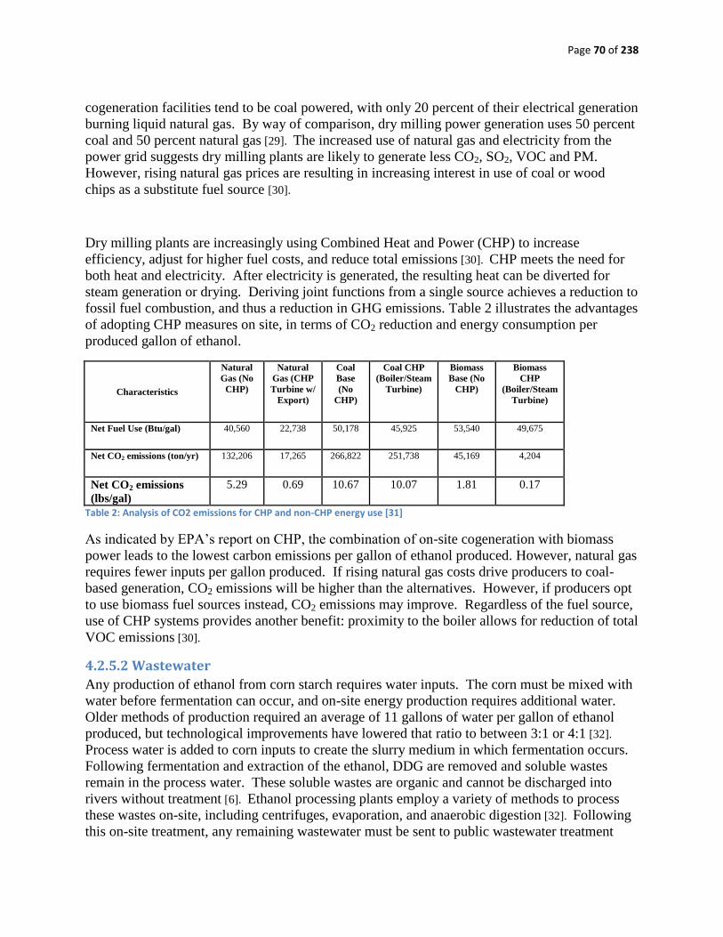
Page 70 of 238
cogeneration facilities tend to be coal powered, with only 20 percent of their electrical generation
burning liquid natural gas. By way of comparison, dry milling power generation uses 50 percent
coal and 50 percent natural gas [29]. The increased use of natural gas and electricity from the
power grid suggests dry milling plants are likely to generate less CO2, SO2, VOC and PM.
However, rising natural gas prices are resulting in increasing interest in use of coal or wood
chips as a substitute fuel source [30].
Dry milling plants are increasingly using Combined Heat and Power (CHP) to increase
efficiency, adjust for higher fuel costs, and reduce total emissions [30]. CHP meets the need for
both heat and electricity. After electricity is generated, the resulting heat can be diverted for
steam generation or drying. Deriving joint functions from a single source achieves a reduction to
fossil fuel combustion, and thus a reduction in GHG emissions. Table 2 illustrates the advantages
of adopting CHP measures on site, in terms of CO2 reduction and energy consumption per
produced gallon of ethanol.
Characteristics
Natural
Gas (No
CHP)
Natural
Gas (CHP
Turbine w/
Export)
Coal
Base
(No
CHP)
Coal CHP
(Boiler/Steam
Turbine)
Biomass
Base (No
CHP)
Biomass
CHP
(Boiler/Steam
Turbine)
Net Fuel Use (Btu/gal) 40,560 22,738 50,178 45,925 53,540 49,675
Net CO2 emissions (ton/yr) 132,206 17,265 266,822 251,738 45,169 4,204
Net CO2 emissions
(lbs/gal)
5.29 0.69 10.67 10.07 1.81 0.17
Table 2: Analysis of CO2 emissions for CHP and non-CHP energy use [31]
As indicated by EPA‘s report on CHP, the combination of on-site cogeneration with biomass
power leads to the lowest carbon emissions per gallon of ethanol produced. However, natural gas
requires fewer inputs per gallon produced. If rising natural gas costs drive producers to coal-
based generation, CO2 emissions will be higher than the alternatives. However, if producers opt
to use biomass fuel sources instead, CO2 emissions may improve. Regardless of the fuel source,
use of CHP systems provides another benefit: proximity to the boiler allows for reduction of total
VOC emissions [30].
214B4.2.5.2 Wastewater
Any production of ethanol from corn starch requires water inputs. The corn must be mixed with
water before fermentation can occur, and on-site energy production requires additional water.
Older methods of production required an average of 11 gallons of water per gallon of ethanol
produced, but technological improvements have lowered that ratio to between 3:1 or 4:1 [32].
Process water is added to corn inputs to create the slurry medium in which fermentation occurs.
Following fermentation and extraction of the ethanol, DDG are removed and soluble wastes
remain in the process water. These soluble wastes are organic and cannot be discharged into
rivers without treatment [6]. Ethanol processing plants employ a variety of methods to process
these wastes on-site, including centrifuges, evaporation, and anaerobic digestion [32]. Following
this on-site treatment, any remaining wastewater must be sent to public wastewater treatment

Page 71 of 238
facilities. However, most new ethanol plants have on-site treatment facilities and discharge no
wastewater to the environment or other facilities. The majority of this treatment is a function of
the anaerobic digesters, which reduce organic solubles by 85-95 percent [6].
The majority of water consumed in the production process is used for energy production. Steam
generation in boilers and cooling systems are the most water-dependent aspects of energy
production. There are evaporative losses from these systems, but some of the water can be
recycled and re-used, depending on the technology employed [32]. Water is also lost in the
exportation of DWG, which are used as feed for livestock [33]. Technology is in development
that could significantly reduce the water consumed in cooling towers, and researchers are
exploring alternative means of distillation and drying in order to reduce evaporative losses [32].
114B4.2.6 Ethanol Facilities As of 2006, there were 116 ethanol production facilities in operation throughout the country [34].
These facilities have an annual production capacity of over 5.4 billion gallons [34]. Additionally,
68 new and expanding production facilities are under construction with an expected increased
capacity of 4 billion gallons by the end of 2008 [34]. Indiana is also experiencing an expansion of
ethanol capacity and Indiana ethanol production could rise 200 percent by 2009 [35].
Table 3: Corn-based ethanol production in Indiana given by existing ethanol plants, plants currently under construction, and those currently proposed [35].
115B4.2.7 Ethanol Yields As a starch crop, corn has a lower relative ethanol production yield compared to other
feedstocks. Corn yields approximately 313 gallons of ethanol per acre of cropland, while
sugarcane produces more than twice the amount, or approximately 652 gallons of ethanol per
Operational ethanol plants Year Town/County
Corn needed
in millions of bushels
Estimated production
level in million gallons
Central Indiana Ethanol 2007 Marion/Grant 15 40
Iroquois BioEnergy 2007 Rensselaer/Jasper 15 40
New Energy 1985 South Bend/St. Joseph 37 100
POET Biorefining 2007 Portland/Jay 24 65
The Andersons 2007 Clymers/Cass 40 110
Verasun 2007 Linden/Montgomery 37 100
168 455
Ethanol plants under construction Town/County
Corn needed
in millions of bushels
Estimated production
level in million gallons
Altra Cloverdale/Putnam 22 60
Aventine Renewable Energy Mt. Vernon/Posey 81 220
Cardinal Ethanol Harrisville/Randolph 37 100
Indiana Bio-Energy Bluffton/Wells 37 100
POET Biorefining Alexandria/Madison 22 60
POET Biorefining North Manchester/Wabash 24 65
223 605
Proposed ethanol plants which
received state incentives Town/County
Corn needed
in millions of bushels
Estimated production
level in million gallons
ASAlliances Biofuels LLC Tipton/Tipton 37 100
Central States Enterprises Inc. Montpelier/Blackford 40 110
Hartford City Bio-energy, LLC Harford City/Blackford 33 88
Rush Renewable Energy Rushville/Rush 22 60
132 358
Page 72 of 238
acre. [36]. Thus, while the United States and Brazil currently produce similar quantities of
ethanol, the US devotes twice the cropland to fuel production.
Ethanol has a heat content of 3.5 million Btu per barrel compared to gasoline‘s 5.25 million Btu
per barrel, giving ethanol only 67 percent of the heat content of gasoline [37]. Based on this
calculation, US ethanol production in 2006 of 4.85 billion gallons was equivalent to only 3.2
billion gallons of gasoline [36]. Given this disparity, even if all 10.5 billion bushels of corn
cultivated in the US in 2006 were devoted to ethanol production, the resultant 18.9 billion
gallons of ethanol would displace only 13.4 percent of total US demand [1]. Furthermore, 137
million acres of cropland would be required to harvest enough corn to displace 50 percent of the
United States‘ petroleum imports [1]. Given that US famers have harvested no more than 76
million acres of corn annually in the past 60 years, corn based ethanol is not a potential
replacement for US gasoline consumption [1].
17B4.3 Biodiesel The military first used the chemical reactions required to make biodiesel during World War II in
order to make biodiesel for heavy-duty machinery and glycerin for explosives [38]. In 2005, 1.5
percent of the US soybean harvest produced 256 million liters of biodiesel. This supplied
approximately 0.09 percent of total diesel demand in the US that year [39].
116B4.3.1 Feedstocks Biodiesel can be made from virtually any oil, including vegetable and seed oils, animal fats, and
waste oils. Soy is the most common feedstock used in American biodiesel production. In
Indiana, soy is the only feedstock grown in sufficient magnitude to produce large quantities of
biodiesel. However, there are other sources that could be utilized to produce biodiesel, such as
waste oil or pork by-products [40].
Oil producers prepare soybeans by removing stems, leaves, dirt, and finally, the hull. Production
facilities then remove oil by crushing the soybean or through solvent extraction. Next, producers
degum the oil by adding water and agitating the mixture at a low heat. The oil is degummed to
remove impurities, to create high quality oil for biodiesel production [41]. Finally, producers add
citric acid. The by-product, lecithin, is edible and typically sold for use in feed [42].
To ease production, most producers typically refine, bleach, and deodorize (RBD) soybean oil.
Refined oil, known as RBD, removes many of the impurities found in production outputs.
Bleached oil allows quality control technicians to recognize problems more easily. Deodorized
oil prevents odors from making production, distribution, and use disagreeable to workers and
consumers. It takes approximately 100 lbs of soybeans and 10 lbs of methanol to produce 100
lbs of biodiesel and 10 lbs of glycerol [42].
Rapeseed is the oilseed that produces canola oil, and is the feedstock of choice in Canada and
Europe, where the climate is more favorable for cultivation. Rapeseed produces more oil per
acre than soy, but does not grow well in Indiana weather conditions [43]. Other crops, such as oil
palm, coconut, and jatropha, also have much higher oil content and a higher oil yield per acre
than soy [44]. Another factor that restricts the use of certain feedstocks is the temperature at

Page 73 of 238
which the oil gels. Soy has a lower gel point than do many other feedstocks [45]. Additionally,
Indiana‘s cold winters restrict feedstock choices, as certain feedstocks require indoor or heated
storage and transportation [46].
117B4.3.2 Biodiesel Production Process The production of biodiesel is a relatively simple chemical reaction known as transesterification.
In this process, biodiesel is made using heat or pressure in combination with a catalyst (such as
sodium hydroxide, sodium methylate, or potassium hydroxide) that transforms oil and methanol
into alkyl esters (biodiesel) and glycerin [42]. The production process requires approximately 87
percent oil, 12 percent alcohol, and one percent catalyst [47]. If the oil contains more than four
percent fatty acids (as is the case with animal oils or waste oils such as used cooking oils from
restaurants), it must be treated and cleaned. Biodiesel must be washed with water to remove
excess catalyst, alcohol, and glycerin [42].
In the United States, biodiesel must conform to American Society of Testing Materials (ASTM)
standards. As of 2001, ASTM approved a standard allowing up to 20 percent blending of
biodiesel [48]. This standard (ASTM D-6751) prescribes several tests for content, flash points,
impurities, and other attributes [49]. In recent years, many producers have opted to participate in
a program called BQ-9000, which is associated with the National Biodiesel Board and aims to
provide quality control measures and promote consumer confidence in biodiesel.
According to the Indiana State Department of Agriculture (ISDA), there are four biodiesel
production facilities in Indiana. All of these facilities are located in the northern half of the state
and all use soybean oil as their primary input. The facilities have capacities ranging from
5,000,000 gallons per annum to 88,000,000 gallons per annum [35].
118B4.3.3 Costs of Production The greatest cost in biodiesel production is the feedstock. According to Pimentel et al. in 2005,
the cost of inputs to produce 2204 lbs of soy biodiesel is $1,212.16, with $1,117.42 of that cost
the soybeans themselves [50]. At the current point in time, biodiesel production costs are not
competitive with conventional diesel. The National Academy of Science stated that the
estimated production costs for soybean biodiesel was $0.145 per diesel energy equivalent gallon
whereas diesel wholesale prices averaged $0.122 per gallon [39].
Biodiesel production technology has already reached maturity. The transesterification process is
already efficient, and researchers do not expect substantial gains in efficiency in the coming
years [40]. However, there are several ways that biodiesel production can be made more cost
efficient.
One way that producers can lower the costs is to increase production scale. The past several
years have seen a trend towards larger producers as it offers several cost advantages [40]. First,
producers can put pressure on input and transportation suppliers. Second, producers can lower
production costs by producing more with equivalent levels of capital and labor. However, there
is a ceiling to these savings, as demand for biodiesel is limited. Without artificial increases in
demand or a drastic change in the economics of biodiesel production, these benefits will not
materialize [51].

Page 74 of 238
Another potential way that producers can lower costs is by purchasing genetically modified
soybeans. Researchers have been working to increase the amount of oil produced per soybean
acre, to lower the gelling point, and to reduce future emissions from soy based biodiesel [52].
119B4.3.4 By-Products and Emissions Biodiesel production is a low air-emissions process. NREL modeling of emissions and
byproducts for the biodiesel conversion process discounts all emissions other than those
associated with steam and electrical generation [53]. As demonstrated in the above discussion of
air emissions associated with corn ethanol production, the quantity of criteria pollutants
associated with steam and electrical generation is dependent on a number of variables including
the nature of the source fuel and whether the power and steam are generated via cogeneration or
purchased from external sources [30].
Heat is required during the transesterification process to improve efficiency. As such, the use of
natural gas or some other source of energy is necessary. Many facilities also refine the fuel and
other by-products using steam, which requires the use of an outside source of energy. It is
theoretically possible for the facilities to burn glycerol or use a diesel generator to produce the
heat required for the production process. However, it is more economically efficient to sell the
diesel and glycerol, since using them as a source of energy would require additional expensive
machinery [40].
Wastewater is another by-product that biodiesel production facilities emit. Water is used to
refine the products of the transesterification process and to transport heat. Efficient facilities
minimize their water losses by reusing water as much as possible, through capturing steam and
the utilization of other methods [40].
Salt is also a typical by-product of transesterification. While salt potentially has many industrial
uses, it is usually not of sufficient purity. Ron Howe, of Integrity Biofuels in Morristown, IN,
stated that the Integrity Biofuels production facility sends excess salt to the landfill. The amount
of salt generated from transesterification is minimal (about 1 lb for every 100 lbs of biodiesel)
[40].
18B4.4 Cellulosic Ethanol
120B4.4.1 Basic Cellulosic Biomass Conversion Technologies Cellulosic biomass is the fibrous, woody portion of a plant that that makes up 75 percent or more
of all plant material [54]. Due to the makeup of cellulosic biomass, the entire plant can be used in
the production process. Therefore, the yield of sugar per unit of land per year is much higher
than corn. Cellulosic biomass can be derived from feedstocks such as corn stover, switchgrass,
and short rotation woody crops including willow and poplar. A joint analysis by DOE and
USDA shows the US could sustainably produce 1.37 billion dry tons of biomass annually for
energy production by the middle of this century and still be able to meet all food, feed, and
export demands [55]. As such, corn ethanol will not be the final biofuel infrastructure; it is
adequate to be the transition to the inarguably more sustainable and beneficial cellulosic ethanol [55].

Page 75 of 238
There are two conversion processes used to break down cellulosic biomass: thermochemical
conversion and biochemical conversion. Both processes are complex due to the fibrous structure
of the plant cell walls [59]. Cellulosic biomass is comprised of three primary components:
cellulose, hemicellulose, and lignin. The proportions of these components vary within each
biomass, and when combined, comprise more than 90 percent of a plant‘s dry mass [60]. These
components make cellulosic biomass more resistant to being broken into simple sugars than
traditional first generation biomass feedstocks [36].
Cellulose is a complex carbohydrate made from six-carbon (C-6) sugars, also known as glucose.
Cellulose is the most common carbohydrate in all forms of biomass; generally it constitutes 40-
55 percent of plant biomass [36]. Hemicellulose is a complex carbohydrate made up of both C-6
and five-carbon (C-5) sugars. Hemicellulose is a major source of carbon comprising between 20
and 40 percent of total biomass [36]. Finally, lignin is a complex polymer that provides the
rigidity and structural integrity in plants and plant cell walls and makes up 10 to 25 percent of
total plant biomass [54].
215B4.4.2 Biochemical Conversion Processes
The biochemical conversion of cellulosic biomass to ethanol involves five basic steps: handling,
pretreatment, hydrolysis, fermentation, and ethanol recovery [54]. Each step is discussed in detail
below.
Biomass handling
The first step in any biomass conversion process is to reduce the size of the raw biomass. This is
done through a grinding or chipping process to make ethanol production more efficient [54].
Pretreatment
During the pretreatment phase, the encapsulating layer of hemicellulose and lignin are broken
down into simple sugars, allowing access to the cellulose [60]. As a result, the remaining
cellulose is more accessible to enzymatic hydrolysis and further processing [59]. The process of
removing lignin from biomass is known as delignification [61]. Various technologies have been
developed for the delignification process and cellulose recovery.
The pretreatment phase is one of the most expensive processing steps with costs as high as $0.30
per gallon of ethanol produced. However, pretreatment shows the greatest potential for
efficiency gains and cost reduction through further research and development [62, 63, 64, 65, 66].
Based on the different chemical compositions and structures of cellulosic biomass feedstocks,
available pretreatment methods can be tailored for efficiency and effectiveness.
The most common pretreatment process used for corn stover and switchgrass is the diluted acid
pretreatment process. However, due to the difference of the proportion of cellulose,
hemicellulose, and lignin components contained in the various cellulosic feedstocks, the optimal
pretreatment conditions (temperature, pH, acid concentration, etc.) may differ [67].
216BCellulosic Hydrolysis
There are two types of cellulosic hydrolysis: acid hydrolysis and enzymatic hydrolysis. Acid
hydrolysis breaks down both hemicellulose and cellulose into simple sugars without the use of
expensive enzymes [55]. This process is commonly used with first generation starchy feedstocks.

Page 76 of 238
However, acid hydrolysis is not recommended for second generation cellulosic biomass because
the acid tends to degrade too large a portion of the hemicellulose sugars before they can be
fermented into ethanol, thus reducing yields [54].
Enzymatic hydrolysis (also referred to as enzymatic sacchrification) is more effective for
cellulosic biomass than acid hydrolysis and has already replaced the acid hydrolysis process for
traditional starch feedstocks in several ethanol facilities in the US [36, 60]. The remainder of this
section will focus on the enzymatic hydrolysis process. In this process, enzymes are used to
break down the remaining cellulose into its component simple sugars (glucose and mannose)
[36]. Since not all of the hemicellulose is broken down in the pretreatment phase, C-5 sugars,
including xylose, still remain at the end of the hydrolysis phase [36].
217BFermentation
The fermentation process can occur in two stages: C-6 glucose fermentation and C-5 pentose
fermentation. In glucose fermentation, yeast or bacteria induce a chemical reaction that converts
simple sugars to ethanol. However, the yeast and bacteria used to ferment C-6 sugars cannot
easily ferment the C-5 sugars contained in the remaining hemicelluloses [36]. Thus, the C-5 sugar
requires customized and genetically engineered bacteria, also called microbes, to enable
conversion to ethanol [36, 54]. Currently, there are no organisms that can efficiently convert both
C-5 and C-6 sugars into ethanol [55]. However, researchers are using genetic engineering to
develop microbes that can do both simultaneously [54]. The Laboratory of Renewable Resources
Engineering (LORRE) is working on genetic transformations that will enable both C-6 sugars
and C-5 sugars to be fermented into ethanol [68].
218BEthanol Recovery
The completed fermentation process produces an ethanol broth. In this step, the ethanol is
separated from the mix of water, microbes, and residue, and is purified through distillation [60].
A final dehydration step removes the remaining water from the ethanol in a manner similar to the
corn ethanol production process [54, 55].
After distillation and ethanol recovery, undigested lignin residue remains because it cannot be
further broken down through fermentation. The lignin residue can be used to produce the
electricity required to power the ethanol production process. Burning residual lignin using the
thermochemical process discussed in the next section creates more energy than is required for the
production process [54]. The demonstrated yield for this process is 60 gallons of ethanol per dry
ton of cellulosic biomass. However, projected yields will be around 80 gallons of ethanol per
dry ton of cellulosic biomass [55].
121B4.4.3 Advanced Biochemical Processing The five steps discussed above complete the basic enzymatic hydrolysis–ethanol fermentation
approach (ES/EF-B). This approach is the most common cellulosic ethanol manufacturing
technology [55]. Researchers are striving to implement an advanced version of the ES/EF-B
approach called Consolidated Bioprocessing (CBP). CBP uses microorganisms that produce all
the necessary enzymes to convert both hydrolyze cellulose into sugar and ferment the C-5 and C-
6 sugar found in hemicellulose to ethanol [36, 55]. Alternatively, the development of modified
enzymes and fermentation organisms will allow for the incorporation of hydrolysis enzyme
production, hydrolysis, and fermentation into a single organism [59]. Projections suggest that this

Page 77 of 238
process could yield over 100 gallons of ethanol per dry ton of biomass [55]. The CBP process
offers the lowest cost in the long run, but is still in the early stages of development [36].
Demonstrated yield in labs and pilot plants is 60 gallons of ethanol per dry ton of cellulosic
biomass. However, projected yields will be around 80 gallons of ethanol per dry ton of
cellulosic biomass [55].
122B4.4.4 Thermochemical Conversion Process There are two main thermochemical pathways for converting biomass into liquid fuel:
gasification and pyrolysis. This section will focus on the gasification process since pyrolysis is
best suited to provide fuel for stationary electric power rather than transportation fuel [36].
In the gasification process, raw biomass travels into a high temperature gasification vessel,
where oxygen levels are kept low to ensure that the resulting gas does not burn [36]. As a result,
all three biomass components are converted into syngas, a synthetic gas made up of hydrogen
and carbon monoxide [36]. The syngas is then cleaned before it is converted to ethanol or
biodiesel using advanced catalytic conversion such as the Fischer-Tropsch (FT) process. This
thermochemical process operates on the same engineering principles that turn coal and natural
gas into liquid fuel [36, 69].
Gasification and FT thermochemical process advantages include accommodation of various
types of plant material, quickness, high theoretical yields, and simple pretreatment [55]. These
techniques can theoretically process batches of different feedstocks and can more easily be
combined with existing coal gasification facilities. They also provide the benefit of being able to
convert high-energy lignin residues into ethanol, a feat enzymes in the biochemical process
cannot yet accomplish alone. The use of the thermochemical process is common for SRWCs
such as poplar and willow because they contain significantly more lignin than other types of
cellulosic biomass [36]. Lastly, gasification and FT synthesis have the potential to produce more
fuel per ton of biomass than the biochemical process.
The thermochemical process is not without disadvantage. First, the gasifiers in the
thermochemical process are difficult to control and are subject to tar formation and intensive gas
clean up, which reduces the ethanol yield [69]. Also, the thermochemical process only yields
about 40 gallons per ton of biomass, making it a much less efficient use of biomass than the
biochemical process [70].
To maximize economic and energy efficiency, an integrated cellulosic biomass refinery will
have the thermochemical and biochemical conversion processes act on the same feedstock.
Ideally, the residual lignin left over after the cellulose and hemicellulose portions of a feedstock
are processed biochemically, can be thermochemically converted into electricity to power the
plant and the conversion process itself, burned for heat, or gasified and converted to FT fuels [59,
69].
123B4.4.5 Utilization of Byproducts of Cellulosic Ethanol Production The main by-product of cellulosic ethanol production is lignin. Lignin is a non-fermentable
amorphous polymer composed of randomly branched building blocks (phenylpropenyl)
connected by carbon-carbon and ether (carbon-oxygen) bonds [71]. The structure of lignin varies

Page 78 of 238
widely across plant species and within the same plant family [71]. Currently, lignin is the main
by-product of paper mills and is burned to produce heat, steam, and electricity to run the pulping
process, which is estimated to be worth $6 per 106 Btu [71].
In October of 2007, Holladay et al. of Pacific Northwest National Laboratory published a
comprehensive report on lignin utilization prepared for DOE that demonstrates the possibilities
of lignin utilization in the short term (three to ten years), medium term (five to 20 years), and
long-term (beyond ten years) [71].
The report identified more than fifty opportunities and narrowed them down based on the
following five criteria: technological degree of difficulty, market size and value, market risk,
building block utility (whether a candidate compound can be a base of a larger group of
derivatives), and mixture (whether a candidate is a lignin-based single compound or a complex
mixture of lignin and other compounds). Three short-term, three medium-term, and four long-
term candidates are summarized below [71].
In the short-term, gasification, pyrolysis, and hydroliquefication are the three most likely feasible
opportunities for the utilization of lignin. Syngas can be produced from lignin through a
gasification process, and is considered to be a well-established process in other industries such as
the steel industry [71]. Syngas can be converted into hydrogen and carbon dioxide with water-
gas-shift technology, green gasoline, or green diesel.
Pyrolysis is a process ―that can convert dry biomass to a liquid product known as pyrolysis oil or
bio-oil.‖ [71] Pyrolysis oil can replace a fraction of imported petroleum and be converted into
green fuels and chemicals; however, certain technological improvements are still needed.
Another opportunity in the short to medium term is hydroliquefication, in which lignin is
converted into reformulated gasoline. NREL and the University of Utah together developed
processes to convert lignin into three kinds of fuel additives through depolymerization and
hydrodeoxygenation [71].
The three medium-term opportunities for lignin utilization are possible through the expansion of
current commercial practices such as concrete admixture, animal feed pellets, dye dispersant,
road binders, and dust control to produce higher-value products [71]. One of the utilization
options is to produce carbon fibers from lignin. If successful, lignin-based carbon fiber can
replace some synthetic polymers such as polyacrylonitrile and can be used in domestic passenger
vehicles in place of steel panels. The second possible high-value product is polymer modifiers.
Currently produced polymer modifiers are used to improve various polymer physical properties,
and modifiers that improve performance properties may be possible in the future [71]. The third
possible utilization revolves around resins, adhesives, and binders. Bio-based resins and
adhesives have great market potential since they can displace formaldehyde, a suspected
carcinogen used in many products such as plywood and fertilizer [72].
The four long-term and more challenging opportunities for lignin utilization could potentially
take place through the development of conversion technologies required for aromatic chemicals.
One of the four goals of this technological development challenge is to produce high-value
aromatic chemicals (BTX chemicals: benzene, toluene, and xylene) through aggressive (non-
selective) depolymerization (C-C and C-O bond rapture) [71]. The aromatic chemicals that are

Page 79 of 238
produced through this process will further expand the opportunity to produce many other
chemicals, such as phenol and xylene that can be used in the petrochemical industry, as fuel
additives [71]. Past works involving hydroliquefaction suggest a strong possibility that the
process can be successful.
The second possible utilization of lignin is to produce other aromatic chemicals, such as
aldehydes, catechols, and cresols, through selective depolymerization [71]. The biggest
advantage of this process may be that those chemicals ―are difficult to make via conventional
petrochemical routes.‖ [71] The third opportunity for lignin utilization is to develop new
technology that can produce low molecular weight aromatics (e.g. aliphatics) or other chemicals
(e.g. acids, diacids, aldehydes, keto acids, etc.) that could be used as fuel additives to syngas,
alkylated gasoline, or propane fuels [71]. The fourth option is to develop fermentation routes
available today ―that use lignin as a nutrition source,‖ but this option requires more research on
viable lignin fermentation processes and it is a ―higher-risk area of research.‖ [71]
As mentioned previously, these long-term options most likely require a significant amount of
time and financial resources for the research and development of new technology; thus, it may
not be realistic to vigorously pursue these options. Rather, they are still subjects to be studied at
research laboratories or academic institutes.
124B4.4.6 Environmental Implications Although there are no commercial cellulosic plants currently operating in the United States, the
indication is that existing processing technologies will keep gaseous emissions well within
EPA‘s New Source Performance Standard limits. The sources of gaseous emissions in the
cellulosic process are all derived from the heat sources necessary for the creation of steam (in the
case of steam explosion pre-treatment), or for the drying of the lignin-rich residue resulting from
the fermentation process. This residue, once dried, can be burned as boiler fuel to provide all
necessary heat for the cellulosic
ethanol production process, with
excess capacity for energy
cogeneration. The quality of this
solid residue obviates the need for
any fossil fuels in the production
process [73].
Fermentation of the biomass itself
produces no gaseous emissions other
than CO2. Due to the potential for
ethanol vapor loss, fermentation
occurs within a closed system, so it is
possible to capture all CO2 emissions
from fermentation and pursue a
variety of means of sequestration [74].
Stover Feedstock 3,144 1.000
Enzymes 25 0.008
Total 3,169 1.008
Combustion Exhaust 1,497 0.476
Ethanol Product 1,066 0.339
Scrubber Vent 532 0.169
Ash 16 0.005
Gypsum 10 0.003
Aerobic Vent 3 0.001
Loss to Atmosphere 4 0.001
Total 3,129 0.995
Carbon Flow
(C kmol/hr)
Ratio to Feedstock Carbon Content
(C kmol basis)
Carbon Inlets
Carbon Outlets
Table 4: Carbon inputs and outputs for the cellulosic ethanol production process Carbon is introduced in the forms of feedstock and enzymes, and is released or captured in the proportions provided by the table. [73]

Page 80 of 238
219B4.4.6.1 Emissions from Cellulosic Boiler Operations
The flue gases resulting from residue combustion are composed primarily of NOx, SOx, and CO.
Following processing of the flue gas, solid residues retain no further use, and will necessitate
disposal (most likely in landfills). Although the flue gas emissions are by nature undesirable,
they contain no components that are inherently hazardous [75]. Furthermore, all emissions levels
are required to be in compliance with New Source Performance Standards limits set forth by the
Clean Air Act [73].
Sulfur is introduced into the ligonocellulosic processing system via hydrogen sulfide created
during wastewater treatment, sulfur contained in the original biomass and residues, and the
neutralization of sulfuric acid. According to NREL, sulfur is generated at a rate of 0.68 kg per
MWhr [73]. All of the sulfur introduced to the combustor is transformed into sulfur dioxide, with
one percent of the resultant SO2 turning into sulfuric acid. Although the amount of sulfur
emitted in the combustor is higher than that generated by combustion of unadulterated biomass,
it is lower than average coal combustion emission rates. Limestone can be introduced to the
system to lower sulfur count, if necessary [73].
Carbon is introduced to the system via biomass and biomass residue. Following consumption,
carbon monoxide is produced at a rate of 0.31 kg per MWhr. There are not many opportunities
for a negative carbon balance with this kind of production because those parts of the biomass not
directly transformed into ethanol (which will eventually combust and release its carbon) are
consumed to produce heat and electricity for the production process. The chief opportunity for
carbon sequestration is the extraction of carbon from flue gases to deposit in landfills or
subterranean carbon sinks. The vast majority of carbon released to the atmosphere is in the form
of CO2 [73].
Table 4 was developed by NREL and
details the carbon balance. The majority of
released carbon is from the combustion
process, followed in quantity by carbon
contained in ethanol and scrubber deposits
[73].
NOx is generated at a rate of 0.31 kg per
MWhr within the ligonocellulosic
processing system, assuming ammonia is
used to control NOX formation. When
ammonia is introduced, combustion can
also produce N2O (nitrous oxide), while
reducing total NOx levels. With ammonia
introduced, NOx production is
commensurate with that associated with
coal combustion. Without ammonia, NOx
levels produced are the same as burning
untreated biomass [73].
Total Flow (kg/hr) Water Flow (kg/hr)
Stover Feedstock 98039 14706
Enzymes 6824 6255
Chemicals & Nutrients 7239 0
Air 310255 3382
Well Water 186649 186649
Inlet Total 609006 210992
-2788
-2736
20035
371
14882
Ethanol Product 24686 122
Evaporative Losses 195993 156291
Vents to Atmosphere 375443 68051
Solids to Landfill 12718 2194
O utlet Total 608840 226658
Water Difference (inputs+consumption+generation-outputs) = -784
Consumption/Generation Total
Process Outlets
Process Inlets
Water Consumption/Generation
Prehydrolysis
Saccharification
Combustion
Wastewater Treatment
Table 5: Water inputs and outputs for the cellulosic ethanol production process. Water is introduced via feedstock, enzymes, chemicals and nutrients, air, and well water, and is released or captured in the proportions provided by the table [73].

Page 81 of 238
220B4.4.6.1 Water Consumption
The hydrolysis process produces wastewater containing complex chemicals that cannot be
released into ground water. However, the compounds can be removed through the use of
treatment facilities that are now often installed on-site at the production plant. This allows the
plants to operate without producing any wastewater that necessitates handling by municipal
water treatment plants. This internal purification process of removing the compounds via
anaerobic decomposition produces methane, but the methane burned for the creation of steam,
the drying of residue, or for assistance in energy cogeneration is not emitted to the atmosphere
[6].
Although new plants are intended to be completely closed systems, some water is inevitably lost
via consumption in hydrolysis or via evaporation and purposeful venting into the atmosphere.
Any water lost is replaced by well water to be used during the hydrolysis process. The following
table was produced by NREL and details total water flow.
125B4.5 Feedstocks
221B4.5.1 Cornstover
Corn stover is a type of lignon cellulosic biomass. It consists of the stalks, leaves, and cobs
remaining above ground after the corn kernels have been harvested [56]. Since no extra
investment is required to produce corn stover, it is considered to be one of the most preferred
sources of feedstock for Indiana cellulosic ethanol production. Corn stover is converted into
ethanol via the biochemical process.
222B4.5.2 Switchgrass
The Bioenergy Feedstock Development Program examined over 30 herbaceous crops during the
1980s, and selected switchgrass in 1991 as an excellent potential crop for bioenergy in the US
because it grows well under a wide range of conditions, prevents land erosion, and can be
harvested by conventional farming methods [57, 58].
223B4.5.3 Short Rotation Woody Crops (SRWCs)
There are many benefits to using SRWCs as biomass feedstocks. Woody biomass possesses a
high lignin content, which is considered attractive for gasification and conversion to ethanol or
synthetic diesel fuel. SRWCs also produce less ash than agricultural residues, which makes them
easier to gasify [36].
126B4.6 Cellulosic ethanol plants In 2007, DOE elected to support six cellulosic ethanol plants with $385 million in federal
funding [76, 77]. In addition, on January 30, 2008, DOE selected three cellulosic plants in which
it will invest over $84 million in the next four years [78]. Table 6 provides additional details
about the nine plants. DOE selected various kinds of plants; some process woody biomass,
while others process agricultural residues and switchgrass. In addition, some plants will use
thermochemical processes to convert biomass to ethanol and the others will use biochemical

Page 82 of 238
processes [76, 77, 78]. The knowledge gained from these projects will provide practical and useful
information for other commercial-scale cellulosic plants.
Company Location
Capacity (million gallons of
ethanol/year)
Construction
Timeline
(Start-
Complete)
Amount
Awarded
(Upper
Limit) Technology Process Feedstock (tons/day)
Abengoa
(facility)
Bioenergy
Biomass of
Kansas, LLC of
Chesterfield, MO
Colwich, KS 11.4; plus power for facility late 2008-late
2011
$76 million Thermochemical;
biochemical
corn stover; wheat; straw; milo
stubble; switchgrass; other (700)
ALICO, Inc. of
LaBelle, FL
LaBelle, FL 13.9; plus 6,255 kilowatts of
electric; 8.8 tons hydrogen/day;
50 tons of ammonia/day
2008 - late 2010 $33 million Thermochemical
gasification /
ermentation
yard; wood; vegetative wastes
(citrus peel); eventually
energycane (700)
BlueFire Ethanol,
Inc. of Irvine, CA
Southern
California
19 mid-2008 - late
2009
$40 million Concentrated acid
hydrolysis
sorted green waste; wood waste
from landfills (700)
Broin Companies
of Sioux Falls,
SD
Emmetsburg,
IA
125; 25% cellulosic ethanol 2007 - 30 mo.
Later
$80 million Biochemical integrated
into corn dry-mill
infrastructure
corn fiber; cobs; stalks (842)
Iogen Biorefinery
Partners, LLC, of
Arlington, VA
Shelley,
Idaho
18 2008 - late 2010 $80 million Biochemical wheat straw; barley straw; corn
stover; switchgrass; and rice
straw (700)
Range Fuels of
Broomfield, CO
Soperton,
GA
40; plus 9 million gallons of
methanol/year
2007 - 2011 $76 million Thermochemical
conversion
wood residues; wood based
energy crops (1,200)
ICM Inc. St. Joseph,
MO
N/A Start 1 year after
receiving funds
$30 million built adjacent to an
existing corn-based
ethanol plant
Corn fiber; corn stover;
switchgrass; sorghum
Lignol
Innovations Inc.
Commerce
City, CO
N/A N/A $30 million Biochem-organisolve Hard and soft wood residues
Pacific Ethanol
Inc.
Boardman,
OR
N/A N/A $24.3 million Using Danish company
BioGasol‘s proprietary
conversion
Agricultural and forest product
residues
Table 6: A summary of the nine cellulosic ethanol plants supported by the US Department of Energy pilot cellulosic biofuels program [76, 77, 78].

Page 83 of 238
127B4.7 Current Costs and Targeted Costs in 2012 of Cellulosic Ethanol
Production Although the biomass feedstocks for
cellulosic ethanol are relatively
inexpensive, the conversion technology is
still quite expensive; one of the largest
costs associated with cellulosic ethanol
production is cost of the enzymes which
convert cellulose to sugar [79]. NREL and
DOE have contracted with the world‘s two
largest enzyme companies, Genecor
International and Novozymes, to reduce the
cost of producing these cellulases [80]. The
goal is to bring the cost of the enzymes
down to about $0.10 per gallon of ethanol
produced, a key factor for the cost
competitiveness of cellulosic ethanol [60].
Novozymes announced in early 2005 that it
had reduced the cost of enzymes to $0.10-
$0.20 per gallon of ethanol, far less than the
previous costs of approximately $5 per
gallon [36].
Over the past decade, the cost of cellulose
per gallon of ethanol has decreased from
about $5 to about $0.50; however, this cost
is approximately 20 times higher than the
cost for enzymes in corn ethanol production
[70]. Table 7 and Table 8 demonstrate the
current costs and targeted costs for the years
2009 and 2012 for each type of cellulosic
conversion technology [79]. Table 7
demonstrates that the largest cost of the corn stover cellulosic production process is pretreatment,
but significant cost reductions can be achieved through the development of bioconversion
technology such as enzymes and fermentation [79]. Table 8 demonstrates that the largest cost
reduction of woody biomass cellulosic ethanol production can be achieved through the
development of synthesis gas clean up and conditioning technologies [79].
As production facilities continue to improve technology, production costs of cellulosic ethanol
will most likely decrease. However, production costs themselves are only one component of
total biofuels costs. The harvest and initial transportation of these feedstocks from the field to
the production facility, and the distribution of fuel from the facilities are important components
of the total cost of biofuel production; these factors can significantly influence the location of
biofuel production facilities.
Process Area
2005 State
of
Technology
2009
Target
2012
Target
Prehydrolysis/treatment 0.44 0.31 0.25
Enzymes 0.32 0.33 0.10
Saccharification& Fermentation 0.31 0.27 0.10
Distillation & Solids Recovery 0.18 0.17 0.15
Balance of Plant 0.34 0.27 0.22
Processing Total 1.59 1.35 0.82
Table 7: Costs (($/gallon in 2007 $s) associated with biochemical conversion of corn stover to ethanol [79].
Process Area
2005 State
of
Technology
2009
Target
2012
Target
Feed Handling and Drying 0.18 0.17 0.16
Gasification 0.14 0.13 0.13
Synthesis gas Cleanup & Conditioning
0.69 0.62 0.43
Fuels Synthesis 0.08 0.05 -0.03
Product Recovery and Purification 0.05 0.05 0.05
Balance of Plant 0.08 0.10 0.08
Processing Total 1.21 1.11 0.82
Table 8: Costs (($/gallon in 2007$s) associated with thermochemical conversion of hybrid poplar to ethanol [79].

Page 84 of 238
19B4.8 Indiana Workforce and Employment Impacts Economic impact analyses of biofuels production must take into account inter-industry
relationships within regions. There are a wide range of input-output models which evaluate the
potential employment benefits for communities that participate in biofuels production. These
modeling systems estimate inter-industry transactions demonstrating the economic impacts of
any changes to the economy. Common mechanisms that estimate the economic effects of
biofuels production include the Regional Input-Output Modeling System (RIMS II), developed
by the US Department of Commerce, and the Minnesota IMPLAN input-output model. An
integrated input-output econometric model developed by Regional Economic Modeling, Inc.
(REMI) can also estimate economic effects. The different models have varying levels of
complexity, with RIMS II being the least complex and REMI being the most complex; the cost
of these models increases with their complexity.
An advantage of RIMS II includes the estimation of regional multipliers without conducting
expensive surveys. The level of industrial detail for RIMS II minimizes aggregation error and a
consistent set of estimating procedures allows for multiplier comparison across areas [81].
Furthermore, empirical analyses show that RIMS II data is accurate within 10 percent of locally
developed industry multipliers based on expensive surveys [81]. IMPLAN, similar to RIMS II, is
calibrated for a specific region, but unlike RIMS II, it uses computer software and can alter
default settings and adjust model specifications before it obtains economic multipliers [81].
While RIMS II and IMPLAN are considered static models, REMI represents a dynamic model or
simulation which provides insight to long-term economic impacts. The REMI model is able to
stimulate how long-run impacts may differ from short-run impacts due to induced changes in
competition for labor, population migration rates, labor or capital substitution, and inflation [82].
When estimating net employment effects, a distinction is made between direct, indirect, and
induced employment effects. Indirect employment effects arise from production input purchases
made by ethanol plants in the regional economy. Major inputs include corn, natural gas, and
electricity, which are only a small fraction of ethanol production inputs [83]. The more purchases
the ethanol plant makes from regional suppliers (transportation, maintenance, accounting and
financial, business, legal services), the higher the potential local economic impact [83]. Thus,
indirect employment effects are jobs created as a result of business-to-business transactions
between the ethanol plant and other businesses. Induced employment, in turn, includes
additional jobs created from activity associated with spending on household goods and services
in the local economy. Direct, indirect, and induced effects give the total effect on employment
that is potentially attributed to the biofuels plant [83].
Several studies attempt to estimate the effects of biofuels production; each suggests that there are
several potential regional economic benefits that could occur as biofuels production increases.
One 2002 study examined the economic benefits to a local community of building and operating
a 40 million gallon-per-year (MGY) dry mill ethanol plant. This study estimated job impacts by
applying final demand multipliers calculated by the US Bureau of Economic Analysis (BEA).
The 2002 study concluded that a 40 MGY ethanol plant will create approximately 41 permanent
new jobs as direct employment and 653 additional jobs throughout the economy as a result of
new demand for local businesses [84]. Thus the total effect on employment is 694 new jobs.
Since the multiplier effect is the ratio obtained by dividing the total value by the direct value, this

Page 85 of 238
study implies that there is an effective jobs multiplier of 17, meaning every job in an ethanol
plant produces 16 other jobs in the regional economy.
As of 2007, Indiana had six operational ethanol plants with an average capacity of 75 MGY (455
MGY total production capacity) and six more are under construction with a total production level
of 605 MGY (average capacity of 100 MGY) [35]. Iowa State University economist David
Swenson conducted an analysis concluding that an ethanol plant‘s direct employment is 35 jobs,
indirect – 76.9, induced – 23.5, implying a multiplier effect of 3.87. That means that for every
job in the ethanol plant, 2.87 jobs are created in the rest of the economy [83]. According to the
Indiana Department of Workforce Development, ten existing and under-construction ethanol
plants create an average of 53.7 direct jobs [85].
Several studies also examine the economic benefits of biodiesel production. Bowman estimated
the total employment impact is 1,240 jobs, 3,020 jobs, and 10,600 jobs for two, five, and 20
percent blends respectively in Kentucky [86]. Another study conducted by the University of
Missouri utilized the IMPLAN model and found a soy diesel plant with annual production of 4.5
MGY in Missouri could create 243 new jobs, 81 of which were direct jobs [86]. Thus, the
multiplier effect is three. Similar to Swenson‘s analysis, the University of Missouri study
assumed that there would be no new agricultural production due to biodiesel manufacturing [86].
Purdue University used the IMPLAN model to conduct another study which estimated the
potential effects of biofuels production on Indiana employment. An average Indiana biodiesel
plant is expected to create 21 direct jobs, and an additional 467 jobs, resulting in a multiplier of
22 [87]. The static IMPLAN model makes projections assuming that all of the necessary
resources are available, prices are constant, and demand for inputs as well as outputs will not
change. According to Purdue University researchers, increased soybean production revenues
come from higher yields, the conversion of non-farmland into soybean acres, or the shift of corn
acreage to soybean production. Since the only data available were revenue effects from a switch
in corn production to soybeans, researchers adjusted the soybean revenue. Reducing Indiana
corn production had a considerable impact on employment effects. Total employment decreased
from 467.3 workers down to 133.1 workers [87]. Thus, the multiplier effect including corn
adjustments decreases from 22 to six.
The results of different studies and analyses differ depending on the models and assumptions
used, but nevertheless all of these studies conclude that ethanol and soy diesel manufacturing are
likely to bring positive employment effects in direct, indirect, and induced employment
opportunities. As of 2007, biofuels production facilities employed and projected to employ 905
workers in 15 biodiesel and ethanol plants (including those under construction) [85]. The
University of Georgia Center for Agribusiness and Economic Development released a study in
2007 concluding that the average earnings for an ethanol plant employee with benefits is
$43,348 [88]. This provides Indiana with a net gain in direct employment revenue of
$39,229,940.

Page 86 of 238
20B4.9 Conclusions Future biofuels production in Indiana will likely incorporate a combination of corn ethanol
production, soy biodiesel production, and cellulosic ethanol production from feedstocks such as
corn stover and switchgrass. Corn ethanol and soy biodiesel production techniques involve
mature production technologies that have already been improved and refined over several
decades. Future efficiency gains in these areas are believed to be limited at best. However,
continued capacity expansion in both areas and the allocation of larger proportions of the total
corn and soy harvest toward biofuels production suggests that both ethanol and biodiesel
produced from these feedstocks will continue. Also, the development of ―closed-loop‖ systems
may significantly reduce the carbon footprint of biofuels production.
If biofuels are to be considered a serious alternative to gasoline, cellulosic production must be
commercialized. Initially the state should focus on cellulosic production using corn stover.
Indiana is one of the nation‘s largest corn producers and, as such, corn stover is readily available.
The creation of ethanol from corn stover requires the use of the biochemical production process.
For this technology to be successfully commercialized, continued research and development
must be conducted to fine-tune enzymatic hydrolysis and reduce the costs of pretreatment.
Enzymatic hydrolysis, the process by which cellulose is broken into simple sugars, depends upon
the creation of new enzymes to improve the efficiency of the production process. Through
continued investment in research and development, it is believed that cellulosic production can
be successful commercialized by 2012. Through the use of tailored incentives toward R&D and
the establishment of production facilities, Indiana can become one of the nation‘s leaders in
cellulosic production. Incentives should be provided for the first commercial cellulosic facility
and the first combination facility, in which corn ethanol and cellulosic ethanol are both produced
at the same site.
Research should also investigate the possibility for switchgrass ethanol production, in particular
with regard to the environmental benefits associated with the feedstock. A transition toward
switchgrass as a cellulosic feedstock is believed to be a longer term solution, due to the need to
transition cropland toward its production.
Finally, although thermochemical production has been discounted to a large extent due to the
timeframe restraints of this research, this production technique may well become viable in the
future. In particular, the ability of this technique to take residual lignin, resulting from the
biochemical process and convert it into starch. By linking the biochemical and thermochemical
processes, a more complete cellulosic market will be possible.

Page 87 of 238
21B4.10 References for Production [1] Yacobucci BD, Schnepf R. 2007. Ethanol
and Biofuels: Agriculture, Infrastructure,
and Market Constraints Related to Expanded
Production. Congressional Research
Service. CRS Report for Congress Order
Code RL33928.
[2] Farrell AE, Plevin RJ, Tuner BT, Jones AD,
O‘Hare M, Kammen DM. 2006. Ethanol can
contribute to energy and environmental
goals. Science 311: 506-508.
[3] Westcott PC. 2007. US ethanol expansion
driving changes throughout the agricultural
sector. AmberWaves 5: 10-15.
[4] Renewable Fuels Association. Industry
Statistics. (21 January 2008;
http://www.ethanolrfa.org/industry/statistics/
#A)
[5] Renewable Fuels Association. How Ethanol
is Made (21 January 2008;
http://www.ethanolrfa.org/resource/made)
[6] Shapouri H, Gallagher P. 2005. USDA‘s
2002 Ethanol Cost-of-Production Survey.
Office of Energy Policy and New Uses,
Office of the Chief Economist, United States
Department of Agriculture. Agricultural
Economic Report Number 841.
[7] Ramirez E, Johnston D, Mcaloon AJ, Yee
WC, Singh V. 2008. Engineering process
and cost model for a conventional corn wet
milling facility. Industrial Crops and
Production 27: 91-97.
[8] Gallagher PW, Shapouri H, Graboski M.
2003. USDA‘s 1998 Ethanol Cost-of-
Production Survey. Office of Energy Policy
and New Uses, Office of the Chief
Economist, United States Department of
Agriculture. Agricultural Economic Report
Number 808.
[9] E3 Biofuels, LLC. Closed Loop vs.
Conventional Ethanol. (16 March 2008;
http://www.e3biofuels.com/technology/etha
nol-methods.php)
[10] Preston G. 2004. Indiana Cattle Highlights.
Indiana Agricultural Statistics Field Office,
National Agricultural Statistics Service,
Iowa State Statistical Office, United States
Department of Agriculture.
[11] Hansen RW. 2007. Methane Generation
from Livestock Wastes. Colorado State
University Cooperative Extension (16
March 2008;
http://www.ext.colostate.edu/pubs/farmmgt/
05002.html)
[12] Boyles S. 2007. Thin Stillage and Corn
Distillers Solubles. BEEF Team Newsletter,
The Ohio State University Extension (22
February 2008;
http://fairfield.osu.edu/ag/beef/beefAgst29.h
tml)
[13] National Agricultural Statistics Service.
2004. 2004 National Distillers Grains
Summary Survey of Ethanol Producers.
Iowa State Statistical Office, United States
Department of Agriculture.
[14] Loy D, Strohbehn D. 2007. Ethanol Feeds:
Feeding Distillers Grains to Beef Cattle:
Long Term Storage of Wet Distillers Grains
and CDS. Iowa State University, University
Extension.
[15] Loy DD. 2007. Ethanol Coproducts for
Cattle: Wet Distillers Feeds for Feedlot
Cattle. Iowa Beef Center, Iowa State
University, University Extension. IBC-19.
[16] Livestock & Grain Market News (LGMN)
Portal: Corn Distillers Dry Grain, Daily
Report. 20 January 2008. Agricultural
Marketing Service, United States
Department of Agriculture.
[17] Schroeder JW. 1997. Corn Gluten Feed:
Composition, Storage, Handling, Feeding
and Value. North Dakota State University
Agriculture and University Extension (4
February 2008;
http://www.ag.ndsu.edu/pubs/ansci/dairy/as
1127w.htm)
[18] Klopfenstein T, Erickson G, Bremer V.
2007. Feeding corn milling byproducts to
feedlot cattle. Veterinary Clinics of North
America: Food Animal Practice 23(2): 223-
245.

Page 88 of 238
[19] Applegate T, Richert B, Maier D. 2006.
Feed Ingredient Co-Products of Ethanol
Fermentation from Corn. Department of
Animal Science and Department of
Agricultural and Biological Engineering,
Purdue University, Purdue Extension
BioEnergy Series. ID-333.
[20] Blasi DA, Brouk MJ, Drouillard J,
Montgomery SP. 2001. Corn Gluten Feed:
Composition and Feeding Value for Beef
and Dairy Cattle. Kansas State University
Agricultural Experiment Station and
Cooperative Extension.
[21] Davis KS. 2001. Corn Milling, Processing
and Generation of Co- Products.
Presentation at the Minnesota Corn Growers
Association Technical Symposium.
Bloomington, MN.
[22] Loy DD, Miller W. 2008. Ethanol
Coproducts for Cattle: The Process and
Products. Iowa State University, University
Extension. IBC-18.
[23] Office of Pesticide Programs. 2002. Corn
Gluten Meal (100137) Fact Sheet. United
States Environmental Protection Agency (25
February 2008;
http://www.epa.gov/oppbppd1/biopesticides/
ingredients/factsheets/factsheet_100137.htm
)
[24] Hirl PJ. 3 January 2008. United States
Patent Applications 20080003654: Process
for Producing Ethanol and for Energy
Recovery. United States Patent & Trade
Office (25 February 2008;
http://appft1.uspto.gov/netacgi/nph-
Parser?Sect1=PTO1&Sect2=HITOFF&d=P
G01&p=1&u=%2Fnetahtml%2FPTO%2Fsr
chnum.html&r=1&f=G&l=50&s1=%22200
80003654%22.PGNR.&OS=DN/200800036
54&RS=DN/20080003654)
[25] Hirl PJ. 2007. Self-Generation of Energy for
Ethanol Production from Distiller‘s Grains
Anaerobic Digestion. Presentation at the
2007 Fuel Ethanol Workshop. St. Louis
MO. 25-28 June 2007. (20 January 2008;
www.bbibiofuels.com/few/2007/FEW07/FE
W07-WS01-Hirl.pdf)
[26] Zeman N. 2007. Coproducts Energy Value
is Rising. Ethanol Producer Magazine,
October 2007 Issue. Grand Forks, ND.
[27] Emissions Factors and Policy Applications
Center. 1995. AP 42 Compilation of Air
Pollutant Emission Factors. 5th
Edition.
Volume 1: Stationary Point and Area
Sources. Chapter 9: Food and Agriculture
Industries. 9.9.7.3: Grain Processing, Corn
Wet Milling, Emissions and Controls.
United States Environmental Protection
Agency.
[28] Emissions Factors and Policy Applications
Center. 1995. AP 42 Compilation of Air
Pollutant Emission Factors. 5th
Edition,
Volume 1: Stationary Point and Area
Sources, Chapter 9: Food and Agriculture
Industries, 9.9.7.3: Grain Processing, Corn
Wet Milling, Emissions and Controls.
Adapted from Table 9.9.7-1 (Particulate
Matter Emission Factors for Corn Wet
Milling Operations), p.9.9.7-7. United States
Environmental Protection Agency.
[29] Wang M, Saricks C, Yu M. 1999.
Greenhouse Gases in the Corn-to-Fuel
Pathway. Center for Transportation
Research, Argonne National Laboratory.
Office of Science, Office of Scientific and
Technical Information, United States
Department of Energy. 98-WP61B.04.
[30] Prepared by Energy and Environmental
Analysis, Inc. 2007. Impact of Combined
Heat and Power on Energy Use and Carbon
Emissions in the Dry Mill Ethanol Process.
Prepared for the Combined Heat and Power
Partnership, United States Environmental
Protection Agency.
[31] Prepared by Energy and Environmental
Analysis, Inc. 2007. Impact of Combined
Heat and Power on Energy Use and Carbon
Emissions in the Dry Mill Ethanol Process.
Adapted from Table 6: CHP Total Energy
Consumption Comparison—Natural Gas,
p.9. Prepared for the Combined Heat and
Power Partnership, United States
Environmental Protection Agency.
[32] Aden A. 2007. Water Usage for Current and
Future Ethanol Production. Southwest
Hydrology. September/October 2007 Issue:
22-23.

Page 89 of 238
[33] National Corn Growers Association. 2008.
Truths About Water Use, Corn and Ethanol.
(25 January 2008;
http://www.grainnet.com/articles/NCGA__T
ruths_About_Water_Use__Corn_and_Ethan
ol_____04_17_2008-55990.html)
[34] Renewable Fuels Association. 2008.
Changing the Climate: Ethanol Industry
Outlook.
[35] Abbott D. 2008. Fact Sheet: Biofuels Plants
in Indiana. Indiana State Department of
Agriculture.
[36] The Worldwatch Institute. 2007. Biofuels
for Transport: Global Potential and
Implications for Energy and Agriculture.
Sterling, Virginia: Earthscan Publications
Ltd. p.24.
[37] Energy Information Administration. April
2008. Monthly Energy Review. Appendix
A: Thermal Conversion Factors. TableA2:
Approximate Heat Content of Petroleum
Production, Imports, and Exports. p.156.
United States Department of Energy.
[38] Knothe G, Van Gerpen JH, Krahl J. 2005.
The Biodiesel Handbook. Champaign, IL:
AOCS Press.
[39] Hill J, Nelson T, Polasky S, Tiffany D. 25
July 2006. Environmental, Economic, and
Energetic Costs and Benefits of Biodiesel
and Ethanol Biofuels. Proceedings of the
National Academy of Sciences of the United
States of America 103(30): 11206-11210.
[40] Howe R. 15 February 2008. Personal
Communication. Integrity Biofuels Plant,
Morristown, Indiana.
[41] Barton N. 2007. The Right Enzymes Can
Boost a Better Diesel Yield. Biodiesel
Magazine. April 2007 Issue (25 January
2008;
http://www.biodieselmagazine.com/article.js
p?article_id=1567)
[42] Van Gerpen J, Shanks B, Pruszko R,
Clements D, Knothe G. 2004. Biodiesel
Production Technology: August 2002-
January 2004. National Renewable Energy
Laboratory, United States Department of
Energy. NREL/SR-510-36244.
[43] Christmas E. 1991. Canola: A Potential New
Crop for Indiana. Purdue University New
Crops News (1 February 2008;
http://www.hort.purdue.edu/newcrop/NewC
ropsNews/91-1-1/canola.html)
[44] Pahl G. 2005. Biodiesel: Growing a New
Energy Economy. White River Junction,
VT: Chelsea Green Publishing Company.
[45] Tyson KS. 2001. Biodiesel Handling and
Use Guidelines. National Renewable Energy
Laboratory, United States Department of
Energy. NREL/TP-580-30004.
[46] Fangrui M, Hanna MA. 1999. Biodiesel
production: a review. Bioresource
Technology 70: 1-15.
[47] National Biodiesel Board. Biodiesel
Production. (1 February 2008;
http://www.biodiesel.org/pdf_files/fuelfacts
heets/Production.PDF)
[48] National Biodiesel Board. Standards and
Warranties. (1 February 2008;
http://www.biodiesel.org/resources/fuelfacts
heets/standards_and_warranties.shtm)
[49] ASTM Standard ASTM D-6751. 2001.
ASTM D6751-07b Standard Specification
for Biodisel Fuel Blend Stock (B100) for
Middle Distillate Fuels. West
Conshohocken, PA: ASTM International
Standards Worldwide.
[50] Pimentel D, Patzek, T. 2005. Ethanol
production using corn, switchgrass, and
wood; Biodiesel production using soybean
and sunflower. National Resources Research
14: 65-76.
[51] Radich A. 2006. Biodiesel Performance,
Costs, and Use. Energy Information
Administration (1 March 2008;
http://tonto.eia.doe.gov/FTPROOT/environ
ment/biodiesel.pdf)
[52] Wang PS, Van Gerpen JH, Thompson J,
Clemente T. 2007. Improving the Properties
of Soy Biodiesel. 2007 American Society of
Agricultural and Biological Engineers
Annual Meeting. 076091.
[53] Sheehan J, Camobreco V, Duffield J,
Graboski M, Shapouri H. 1998. Final

Page 90 of 238
Report: Life Cycle Inventory of Biodiesel
and Petroleum Diesel for Use in an Urban
Bus. Prepared for the United States
Department of Agriculture and United States
Department of Energy. National Renewable
Energy Laboratory, United States
Department of Energy. NREL/SR-580-
24089.
[54] Biomass Program. 2008. ABC‘s of Biofuels.
Office of Energy Efficiency and Renewable
Energy, United States Department of Energy
(25 February 2008;
http://www1.eere.energy.gov/biomass/abcs_
biofuels.html)
[55] Granda CB, Zhu L, Holtzapple MT. 2007.
Sustainable liquid biofuels and their
environmental impact. Environmental
Progress 26(3): 233-250.
[56] Office of Energy Efficiency and Renewable
Energy. 2004. Feedstock Composition
Glossary. United States Department of
Energy (2 February 2008;
http://www.ethanol-
gec.org/information/briefing/19.pdf)
[57] Liebig MA. 2006. Switching to switchgrass
makes sense. Agricultural Research July
2006 Issue: 19.
[58] McLaughlin S, Bouton J, Bransby D,
Conger B, Ocumpaugh W, Parrish D,
Taliaferro C, Vogel K, Wullschleger S.
1999. Developing Switchgrass as a
Bioenergy Crop. Reprinted from:
Perspectives on New Crops and Uses.
Alexandria, VA: ASHS Press.
[59] United States Department of Energy. 2006.
Breaking the Biological Barriers to
Cellulosic Ethanol: A Joint Research
Agenda. Office of Science and Office of
Energy and Renewable Energy, United
States Department of Energy. DOE/SC/EE-
0095.
[60] National Renewable Energy Lab. 2003.
Unraveling the structure of plant life: to
make sustainable fuels and chemicals. 2003
Research Review, 2nd
Edition. United States
Department of Energy. p.10-15.
[61] Roberts MT, Etherington D. 2007.
Delignification. Dictionary of Descriptive
Terminology (20 February 2008;
http://palimpsest.stanford.edu/don/dt/dt0993
.html)
[62] Kohlman KL, Sarikaya A, Westgate PJ,
Weil J, Velayudhan A, Hendrickson R,
Ladisch MR. 1995. Enhanced enzyme
activities on hydrated lignocellulosic
substrates. ACB Symposium Series No.
618: Enzymatic Degradation of Insoluble
Carbohydrates. Washington, DC: ACS
Publishing. p.237-255.
[63] Lee D, Yu AHC, Wong KKY, Saddler JR.
1994. Evaluation of the enzymatic
susceptibility of cellulosic substrates using
specific hydrolysis rates and enzyme
adsorption. Applied Biochemistry and
Technology 45: 407-415.
[64] Lynd LR, Elander RT, Wyman CE. 1996.
Likely features and costs of mature biomass
ethanol technology. Applied Biochemistry
and Biotechnology 57: 741-761.
[65] Mosier NS, Hendrickson R, Dreschel R,
Welch G, Dien BS, Bothast R, Ladisch MR.
2003. Principles and Economics of
Pretreating Cellulose in Water for Ethanol
Production. Paper 103. 225th
American
Chemical Society Meeting. New Orleans,
LA. 26 March 2003.
[66] Mosier NS, Hendrickson R, Welch G,
Dreschel R, Dien B, Ladisch M. 2003. Corn
Fiber Pretreatment Scale-up and Evaluation
in an Industrial Corn to Ethanol Facility.
Oral Presentation 6A-04. 25th
Symposium
on Biotechnology for Fuels and Chemicals.
Breckenridge, CO. 4-7 May 2005.
[67] Diena BS, Jung HJG, Vogel KP, Dasler
MD, Lamb JFS, Iten L, Mitchell RB, Sarath
G. 2006. Chemical composition and
response to dilute-acid pretreatment and
enzymatic saccharification of alfalfa, reed
canarygrass, and switchgrass. Biomass and
Bioenergy 30: 880-891.
[68] Laboratory of Renewable Resources
Engineering (LORRE). 2004. Integrative
Center for Biotechnology and Engineering,
Purdue University (8 Apr. 2008;
http://cobweb.ecn.purdue.edu/~lorre/16/over
view/overview_bioenergy.shtml)

Page 91 of 238
[69] Schubert C. 2006. Can biofuels finally take
center stage? Nature Biotechnology 24(7):
777-784.
[70] Somerville C. 2007. Biofuels: a primer.
Current Biology 17: r115-r119.
[71] Holladay JE, Bozell JJ, White JF, Johnson
D. 2007. Top value-added chemicals from
biomass: Volume II – Results of Screening
for Potential Candidates from Biorefinery
Lignin. Pacific Northwest National
Laboratory, Operated by Battelle for the
United States Department of Energy. PNNL-
16983.
[72] Agency for Toxic Substances and Disease
Registry. 1999. Toxicological Profile for
Formaldehyde. Public Health Service,
United States Department of Health and
Human Services.
[73] Aden A, Ruth M, Ibsen K, Jechura J, Jeeves
K, Sheehan J, Wallace B, Montague L,
Slayton A, Lukas J. 2002. Lignocellulosic
Biomass to Ethanol Process Design and
Economics Utilizing Co-Current Dilute Acid
Prehydrolysis and Enzymatic Hydrolysis for
Corn Stover. National Renewable Energy
Laboratory, United States Department of
Energy. NREL/TP-510-32438.
[74] M‘ollersten K, Yana J, Moreira JR. 2003.
Potential market niches for biomass energy
with CO2 capture and storage: opportunities
for energy supply with negative CO2
emissions. Biomass and Bioenergy 25: 273-
285.
[75] Lynd LR. 1996. Overview and evaluation of
fuel ethanol from cellulosic biomass:
technology, economics, the environment,
and policy. Annual Review of Energy and
the Environment 21: 403-465.
[76] United States Department of Energy. 28
February 2007. DOE Selects Six Cellulosic
Ethanol Plants for Up to $385 Million in
Federal Funding. DOE Press Release (20
February 2008;
http://www.doe.gov/news/4827.htm)
[77] Irwin L. 2007. Cellulosic Wave Set in
Motion. Ethanol Producer Magazine, July
2007 Issue (20 February 2008;
http://www.ethanolproducer.com/article.jsp?
article_id=3025)
[78] Deutscher H. 2008. U.S. DOE Invests $84
Million in Three Cellulosic Ethanol Projects.
Ethanol Producer Magazine, February 2008
Issue (20 February 2008;
http://www.ethanolproducer.com/article.jsp?
article_id=3666)
[79] Office of Biomass Program. 2008. Biomass
Multi-Year Program Plan. Office of Energy
Efficiency and Renewable Energy, United
States Department of Energy.
[80] National Renewable Energy Laboratory.
2007. Research Advances: NREL Leads the
Way: Cellulosic Ethanol. United States
Department of Energy. NREL/BR-510-
40742.
[81] Lynch T. 2000. Analyzing the Economic
Impact of Transportation Projects Using
RIMS II, IMPLAN, and REMI. Prepared for
the Office of Research and Special
Programs, United States Department of
Transportation.
[82] Weisbord G. 1990. Remi and I-O Models
Compared. Cambridge Systematics (617)
354-0167 (1 March 2008;
www.remi.com/support/articles.shtml)
[83] Swenson D. 2005. Model Economic
Analyses: An Economic Impact Assessment
of an Ethanol Production Facility in Iowa.
Department of Economics, Iowa State
University. Staff General Research Papers
No. 12226.
[84] Urbanchuk JM, Kapell J. 2002. Ethanol and
the Local Community. AUS
Consultants/SJH & Company.
[85] inContext. 2007. Is Indiana Ready to be an
Emerging Leader in the Biofuels Industry?
Indiana‘s Workforce and Economy. Indiana
Department of Workforce Development and
Indiana Business Research Center, Kelley
School of Business, Indiana University. p.1-
4.
[86] Bowman K. 2003. Economic Impact of Soy
Diesel in Kentucky. Murray State
University.

Page 92 of 238
[87] Althoff K, Ehmke C, Gray A. 2003.
Economic Analysis of Alternative Indiana
State Legislation on Biodiesel. Center for
Food and Agricultural Business, Department
of Agricultural Economics, Purdue
University.
[88] Flanders A, McKissick J. 2007. Economic
Impact of Cellulosic Ethanol Production in
Treutlen County. Center for Agribusiness
and Economic Development, The University
of Georgia. CR-07-07.

Page 93 of 238
5. Engine Compatibility
22B5.1 Introduction In the United States, spark-ignited internal combustion engines and diesel engines power
vehicles on the road today. The traditional combustion engine can run on conventional gasoline
or a retrofitted combustion engine, a flex-fuel engine, can use up to 100 percent ethanol as fuel.
Currently, almost 700 filling stations nationwide provide E85 blended fuel. Several major car
manufacturers are committed to dedicating half of their production to flex-fuel vehicles by 2012,
which would inevitably increase the demand for E85 filling stations and in turn ethanol-based
biofuels. Compared to traditional combustion engines running on gasoline, current research
indicates that the amount of flex-fuel engine pollutant emissions varies across the range of
particulates. However, these engines result in decreased fuel efficiency.
The majority of buses and medium to heavy trucks on the road today depend on diesel-powered
engines. Currently, manufactures only recommend using between five and twenty percent
biodiesel blends because diesel engines running on higher percentage blends have the potential
to damage engine components. The widespread usage of biodiesel is dependent on resolving the
fuel‘s negative properties, but current research indicates biodiesel decreases pollutant emissions
in most categories.
Biodiesel blended with aviation fuel is a possible alternative for turbine engines, but as with
diesel engines on the road, engineers must combat many negative properties of the fuel.
23B5.2 Spark-Ignited Engines and Ethanol Spark-ignited internal combustion engines operate by
creating an explosion from a mixture of fuel and air
inside a confined space called a combustion chamber,
or cylinder. This exothermic reaction creates gases at
a high temperature and pressure, which expand inside
the chamber. The gases then act upon a piston inside
the chamber pushing it upward. Each piston is linked
to the crankshaft by a connecting rod. When the
combustion chambers fire in succession, they turn the
crankshaft. The crankshaft converts the piston‘s
motion into rotational energy, which is then
transferred through the transmission to turn the wheels
of the vehicle [1].
Figure 14: Internal Combustion Engine [2]
Page 94 of 238
128B5.2.1 History of Spark-Ignited Internal Combustion Engines Spark-ignited engines designed to burn ethanol have been in widespread use for over 100 years.
American inventor Samuel Morey built the first spark-ignited internal combustion engine in the
US in 1826. His design relied on a mixture of turpentine and ethanol and could power a car as
well as a boat [3]. In 1876, German inventor Nikolaus Otto used ethanol to power a modern
internal combustion engine and placed it in the first motorcycle, dubbed the ―Otto Cycle.‖ [4] In
1896, American inventor Henry Ford built his first automobile, the Quadricycle, which also
relied on ethanol. Ford went on to develop the world‘s first flex-fuel vehicle, the 1908 Model T,
designed to run on either ethanol or gasoline [5]. Since then, ethanol engine technology has
improved dramatically [6, 7].
129B5.2.2 Flex-Fuel Engine Technology
Currently, the US automobile fleet contains over six million flex-fuel vehicles. Nearly 700
filling stations offer E85 fuel, which is a blend of 85 percent ethanol and 15 percent gasoline.
Flex-fuel engines are available in a wide range of makes and models. Ford, General Motors, and
Chrysler plan to make half of their production flex-fuel capable by 2012 [8]. Modern flex-fuel
engines operate similarly regardless of fuel type. The payload and acceleration characteristics of
flex-fuel engines are also comparable to their conventionally fueled counterparts. Flex-fuel
engines can operate with any blend of ethanol and gasoline.
The engine‘s fuel system constantly monitors the levels of ethanol and gasoline in the tank
allowing the engine to adapt as the mixture changes [9]. Ethanol can be mixed with water, and
water vapor presents challenges in the fuel system that gasoline does not. Components made of
brass, copper, and aluminum can corrode; therefore, flex-fuel engines cannot utilize these
components [10]. Ethanol can also react with many kinds of rubber and cause obstructions in the
fuel system. Fluorocarbon rubber, Teflon-lined hoses, and stainless steel fuel tanks are
commonly employed in flex-fuel vehicles to counteract this problem [9, 11].
While the conversion of any conventionally fueled vehicle to E85 is technically feasible, only
one conversion kit has been approved for use in the US. Flex-Fuel US received EPA
certification in November 2007 for its ―Flex-Box‖ conversion kit designed for use in the Ford
Crown Victoria [9]. The kit sells for $1,500 plus installation charges and the Chicago Police
Department has installed the kits in a 20-car demonstration project [12]. The Crown Victoria kits
should be commercially available soon, and kits for other makes and models will enter the
market as they complete the EPA certification process.
Flex-fuel vehicles cost slightly more to produce than their conventionally fueled counterparts.
The additional cost to the manufacturer is estimated to be as low as $200 per vehicle [13].
Automotive manufacturers are currently offering flex-fuel vehicles at the same price as
conventionally fueled models [5, 14]. Automakers are allowed to claim Corporate Average Fuel
Economy (CAFE) emissions credits for flex-fuel vehicles so consumers are not directly impacted
by the increased cost of production at the present time [15].
130B5.2.3Future Possibilities for Flex-Fuel Engine Technology Current flex-fuel engines are constrained because they must use both gasoline and E85
interchangeably. This prevents the optimization of ethanol engine design and limits the fuel‘s

Page 95 of 238
potential. An optimally designed engine can exploit several beneficial characteristics of ethanol
such as increased octane, a higher latent heat of vaporization, and improved laminar flame speed
[6, 7].
Higher Octane
Ethanol has a higher octane than gasoline and is often employed as a gas additive to increase
octane. Most E85 pumps advertise a minimum octane of 100. Fuels with higher octane numbers
mean engines running on ethanol can operate at higher compression ratios without pre-ignition
[16]. Increasing the compression ratio can improve performance and maximize the benefits from
ethanol‘s higher octane level [6].
Latent Heat of Vaporization
Ethanol has a higher latent heat of vaporization than gasoline and provides a greater charge
density [17]. The latent heat of a substance is the amount of heat energy released during a change
of phase. Substances change phase when they go from solid to liquid or liquid to gas [18]. Latent
heat of vaporization refers to the energy necessary to convert a unit of the substance from liquid
to gas if pressure and temperature are constant [19]. The latent heat of vaporization for ethanol is
three to five times higher than gasoline, which translates into decreased temperatures in the
intake manifold and increased volumetric efficiency [7].
Laminar Flame Speed
When fuel is mixed with air in a combustion chamber and then ignited, a flame front is created
around the spark. The flame front spreads outward inside the chamber from the point of ignition.
The laminar flame speed is a measure of how fast the flame front moves through the combustion
chamber. Ethanol has a higher laminar flame speed than gasoline which permits ―leaner‖ air-
fuel mixtures [20]. The stoichiometric air-fuel ratio (AFR) for gasoline is 50 to 65 percent higher
than the AFR for ethanol, meaning less air is required for complete combustion with alcohol-
based fuels [7].
131B5.2.4 Problems Associated with Ethanol Cold Starting Issues
In the past, engines running on alcohol fuels experienced problems with cold starting. Below 11
degrees Celsius, ethanol begins to freeze and the fuel-air mixture is not rich enough to support
combustion [21]. Alcohol-based fuels are less volatile than gasoline, which is why they produce
fewer evaporative emissions and why cold starting is an issue [6]. When an engine is designed to
run specifically on alcohol, it can accommodate the different properties of the fuel. Research
suggests that the problems caused by low octane number and vapor pressure can be solved with
higher energy ignition systems or higher compression ratios [6]. Ongoing experiments at EPA‘s
National Vehicle and Fuel Emissions Laboratory have demonstrated consistent starting down to
zero degrees Celsius [22].
Lower Energy Content
One of the major differences between ethanol and gasoline is energy content. The heating value
of alcohol is lower than that of gasoline meaning that it takes more alcohol to achieve the same
energy output in an engine [7]. E85 contains 28 percent less energy per gallon than gasoline, and
most flex-fuel vehicles experience a 20 to 30 percent reduction in fuel economy when running on

Page 96 of 238
E85 [23, 24, 25]. Research has shown that optimizing an engine for ethanol can mitigate reduced
fuel economy; however, such engines are not yet commercially available [5, 22].
132B5.2.5 Current Work at the EPA
According to research from the EPA‘s Clean Automotive Technology Program, the reduced
efficiency associated with ethanol can be prevented through engine optimization. Brake Thermal
Efficiency (BTE) measures how much energy from the fuel is transformed into mechanical work
by the engine. Higher BTE numbers imply more efficient engines. Modern gasoline and diesel
engines have BTEs around 30 percent and 45 percent respectively [26].
With higher compression ratios and modifications to the combustion chamber, port-injected,
spark-ignited ethanol engines can be one-third more efficient than current flex-fuel offerings [7].
EPA test engines have demonstrated up to 42 percent BTE which rivals current diesel technology
[22]. Similar research into engine optimization with E85 demonstrates a 20 percent improvement
in efficiency over standard gasoline engines [20]. Performance and efficiency of engines
optimized for ethanol can exceed conventional gasoline engines and approach the efficiency
levels of today‘s best diesel technology with low emissions [6, 22].
133B52.6 Combustion Engine Emissions
A 2006 EPA comprehensive assessment of
the 2005 Renwable Fuel Standard (RFS)
employed various models to estimate the
emission levels from the combustion of E10.
Comparing results from the MOBILE6.2
modeling tool and various other EPA
predictive models, the study determined
potential emissions differences between E10
and conventional gasoline. A summary of
the results of these models and other studies
cited in the 2006 EPA Assessment is
provided in Table 9 [27].
Ethanol emissions affect ambient
concentrations of pollutants such as carbon
monoxide (CO), nitrogen oxides (NOx),
particulate matter (PM), and volatile organic
compounds (VOC) (as a precursor to ozone). These pollutants are especially important because
EPA has categorized them as criteria pollutants which are regulated by the Clean Air Act. The
EPA models produced varying results while estimating the effects of E10 use. In general, E10
use led to a decrease in VOC and CO emissions and slight increase in NOx emissions [27]. EPA
analyzed three independent studies of the effects of ethanol on PM emissions that produced
widely differing results [27]. The first study from the Colorado Department of Public Health and
Environment compared E10 and conventional gasoline use in 24 vehicles and found a 36 percent
reduction in PM emissions from a cold start using E10, but no significant change in emissions
from a regular start. The second study, from the State of Alaska in conjunction with General
Motors Corporation, studied ten vehicles fueled with E10 and found considerable variability with
Pollutant
Effect
Range (%
Compared
to E0)
Overall
Effect Study Model(s)
CO -11 to –19 Reduction MOBILE6.2
NOx 7.7 Increase EPA
Predictive
VOCs -7.4 Reduction EPA
Predictive
Toxics Various Various EPA Predictive
PM -81 to +84 Inconclusive Colorado DPHE,
Alaska,
EPA
Research
Triangle
Aromatics -0.63 to -
2.39
Reduction AQIRP
Table 9: E10 Exhaust Pollutant Emissions Compared to Conventional Gasoline (E0) [27]

Page 97 of 238
effects ranging from an 81 percent reduction to an 84 percent increase in PM emissions. The
third study, conducted by EPA researchers, found an average one percent increase in PM
emissions with the use of E10, but concluded the study showed ―no clear effect of ethanol on PM
emissions.‖ [27] EPA‘s analysis of these studies concluded that data are too limited to determine a
quantitative estimate of the effect of E10 on PM emissions [27].
Ethanol emissions may also lead to greater levels of toxic gases and aromatics in the air. Toxic
pollutant emissions (formaldehyde, acetaldehyde, benzene, etc.) are important to consider due to
the potential for detrimental health effects. People exposed to toxic pollutants at high
concentrations or over a long duration may have an increased risk of cancer, damage to the
immune system, and neurological, reproductive, developmental, and respiratory health problems
[28]. Effects of E10 use on toxic emissions vary widely, showing both increases and decreases in
emissions depending on the specific toxic gas; however, the effect on one particular toxic gas is
striking. EPA models predict that acetaldehyde emissions increase by 143 percent with E10 use
[27]. The implications of this effect will be discussed further in the section on E85.
Aromatics are pervasive environmental
pollutants formed by incomplete fuel
combustion. They have been identified as a
potential cause of cancer and are also an
important emissions category due to their
potential relevance to PM. EPA cites
emerging research that indicates aromatics
from vehicle emissions contribute to PM
formation in the atmosphere [27, 29]. An
Auto/Oil Air Quality Improvement
Research Program (AQUIRP) test of over
100 vehicles found that E10 use resulted in
aromatics emissions reductions of 0.63
percent to 2.39 percent over conventional
gasoline use.
For higher concentrations of ethanol such as
E85, few data are available largely due to their recent commercial introduction and limited use.
The data that exist are summarized in Table 10. In general, E85 studies consider many of the
same pollutants as E10 studies; however, E85 emissions may have important effects regarding a
pollutant not considered in most E10 studies: non-methane organic gas (NMOG).
A 1993 AQUIRP study and a 2006 EPA Certification and Fuel Economy Information System
(CFEIS) study analyzed NOx and CO emissions. AQUIRP found significant decreases in NOx
emissions with the use of E85 over conventional gasoline in 1988, while CFEIS showed a four
percent increase in NOx emissions [27]. Neither study found significant changes in CO
emissions. Less data exist regarding the impact of E85 on PM emissions, although a 2003
Society of Automotive Engineers study showed a negligible increase in PM emissions from E85;
however, the study only employed one gas blend and one model year in the test [27].
Pollutant
Effect Range
(%
Compared to
E0)
Overall Effect Study
CO No significant
estimates
None AQIRP,
CFEIS
NOx -49 to +4 Inconclusive AQIRP,
CFEIS
NMOG +33 to +56 Increase AQIRP,
CFEIS
Toxics +108 (net) Increase AQIRP,
CFEIS
PM Theoretical
increase
SAE
Aromatics Theoretical
reduction
EPA
Table 10: E85 Exhaust Pollutant Emissions Compared to Conventional Gasoline (E85) [27, 30]

Page 98 of 238
Both the AQUIRP and CFEIS studies showed that increases in NMOG emissions from E85 use
compared to conventional gasoline ranged from 33 to 56 percent [27]. However, most E85
NMOG emissions have lower reactivity than other NMOGs and thus may be less facilitative of
ozone formation.
The effects of E85 use on emissions of toxic air pollutants vary widely; however, EPA data
indicates an aggregate net increase when all toxic gases are considered [27]. This is largely due to
a 2,620 percent increase in acetaldehyde emissions. Other toxic gases decrease with E85 use;
specifically, benzene, 1,3-butadiene, ethylbenzene, hexane, styrene, toluene, mylene, p-xylene,
o-xylene, and naphthalene are projected to decrease 50 to 80 percent [27]. A study on the effects
of E85 use on cancer rates could not determine whether increased toxic gas emissions, especially
acetaldehyde, increased cancer risk compared to conventional gasoline [30].
Overall, biofuels‘ impacts on emissions vary by fuel type. Because of limited data, many of the
effects regarding specific pollutants are inconclusive. Generally, ethanol-based fuels seem to
lead to a net decrease in aromatics emissions and a potential increase in net toxic emissions,
particularly acetaldehyde, which some studies link to negative health effects.
24B5.3 Diesel Engines
134B5.3.1 History of the Diesel Engine The invention of the modern internal combustion engine is largely credited to the work of Rudolf
Diesel. Diesel‘s engine was initially fueled by coal dust and later, by peanut and vegetable oils
[31]. Diesel, an early proponent of biofuels, stated in 1911 that ―the diesel engine can be fed with
vegetable oils,‖ the use of which would ―help considerably in the development of agriculture of
the countries which use it.‖ [31]
In 1924, the Maschinenfabrick Augsburg-Nuerenburg Company incorporated the diesel engine
into a truck and the company exhibited the vehicle at the 1924 Berlin Motor Show [31]. Daimler-
Benz, today known as Mercedes Benz, produced the first diesel engine motor car in 1936, the
Type 260D [31]. Auto manufacturers began producing diesel engines that could run on fossil
fuels during the 1920s, despite the fact that fossil fuels have a lower viscosity than fuels
produced with biomass.
135B5.3.2 The Diesel Engine The diesel engine is an intermittent-combustion piston-cylinder engine [32]. The majority of
diesel engines run on a two-stroke or four-stroke cycle. Diesel engines create energy by burning
fuel under compression with a mixture of hot air inside the engine cylinders. Auto-ignition
occurs when the air temperature within the cylinder is higher than the ignition temperature of the
fuel [32]. At or above the auto-ignition temperature, the fuel spontaneously reacts with oxygen
and burns [32].
Diesel engines incorporate a direct-injection system, whereby fuel is injected into the engine‘s
cylinders. In such a system, the combustion process is heterogeneous, meaning the fuel source

Page 99 of 238
and air are not premixed. The direct-injection system relies on the rapid vaporization of fuel
which is important for successfully igniting the fuel source [32].
The compression ratio is the pre-ignition compression level of the fuel mixture [33]. An engine‘s
compression ratio is determined by the maximum volume of the cylinder with the piston in its
lowest position divided by the volume when the piston is at its highest point or fully compressed.
A larger compression ratio implies higher air temperature within the engine‘s cylinders [33]. The
air temperature in diesel engines is typically above 526 degrees Celsius (979 degrees Fahrenheit)
[32]. Higher compression ratios increase engine efficiency, but may also result in engine
knocking [33].
Engine knocking refers to the phenomenon caused when air/fuel pockets explode outside of
normal combustion resulting in a knocking sound. Knocking causes reduced engine efficiency
and potential engine damage [34]. Direct-injection systems also affect engine efficiency. In
modern diesel engines, fuel is injected directly into the engine‘s cylinders. To promote effective
burning, fuel is injected in a cone spray, with fuel radiating from the nozzle [32]. Many of the
recent improvements in diesel engine technology are the result of new direct-injection systems.
More thorough mixing of the fuel and air significantly improves combustion. Two of the
improved methods used to mix fuel and air are known as ―air swirls‖ and ―radial movement of
the air,‖ otherwise referred to as ―squishing [32].‖
136B5.3.3 The US Diesel Market Table 11 highlights domestic consumption of
transportation energy by mode and fuel type
in 2005. The information has been limited to
purely highway vehicles. All figures are in
trillion British Thermal Units (Btu).
Approximately 2.4 percent of US
transportation energy is consumed by diesel-
fueled light vehicles. Historically, diesel-
fueled cars and light trucks comprised only a
small portion of the total light-vehicle market.
The Alliance of Automobile Manufacturers
estimates that there are now 4.8 million
diesel-powered cars, SUVs, and trucks in the
US [36]. However, demand for diesel-powered
vehicles is expected to rise over the next
decade. Three automotive manufacturers
announced the sale of six new diesel vehicles at the beginning of 2008 and J.D. Power and
Associates estimate that diesel vehicles will represent ten percent of the automobile market by
2015 [36].
Diesel vehicles dominate the bus and medium/heavy trucks categories. Approximately 88
percent of bus journeys in 2005 relied on diesel fuel; in the medium/heavy trucking sector, 89
percent of journeys were powered by diesel fuel [35]. Auto manufacturers currently only
recommend low blends of biodiesel such as B5 and B20. All biodiesel blends must be created
Gasoline Diesel Other* Total
Light Vehicles 16813.5 414.1 47.5 17275.1
Cars 9080 51.2 9 9140.2
Light Trucks 7697.6 362.9 47.5 8108
Motorcycles 26.9 0 0 26.9
Buses 6.5 167.7 16.5 190.7
Transit 0.2 76.3 16.6 93.1
Intercity 0 28.3 0 28.3
School 6.3 63.1 0 69.4
Medium/Heavy Trucks 460 4101.7 15.2 4576.9
Highway 17280 4683.5 79.2 22042.7
Table 11: US Vehicle Market Energy Consumption, 2005 [35]

Page 100 of 238
using neat biodiesel that meets American Society of Testing and Materials (ASTM) D6751
standards to prevent invalidating engine warranties. ASTM D6751 was the first national
standard for biodiesel fuel within the US, and the standard sets out prescriptions for neat
biodiesel blended with gasoline diesel [37]. Table 12 highlights automobile manufacturers‘
current positions on the use of biodiesel blends.
137B5.3.4 Biodiesel’s compatibility with diesel engines The Table 13 below highlights the key
characteristics of typical No.2 diesel and neat
biodiesel. No.2 diesel is the standard petroleum-
based diesel fuel used in motor vehicles, while
neat biodiesel refers to 100 percent biodiesel
(unblended biodiesel fuel). The two fuels have
separate fuel standards, and those for neat
biodiesel are more stringent than regular diesel
fuel.
Fuels derived from vegetable oils, animal fats,
partially reacted oils, and other biologically
derived fuels that do not meet the specifications
set out in the above table, may not be defined as
biodiesel [39]. Backyard biodiesel producers are
unlikely to meet these high standards, in
particular regarding the standards defined for
water and sediment volume [39]. There are also
accreditation programs for biodiesel producers
who meet and exceed the above standards, such
as BQ9000 [40].
Biodiesel‘s octane number is slightly higher than
No.2 diesel while both have similar levels of
viscosity. One of the major issues surrounding
the use of biodiesel in vehicles is the fuel‘s
Company Audi BMW Chrylser LLC
Ford
Motor Co General Motors Honda Hyundai Isuzu
John Deere
Mercedes Benz Nissan Volkswagen Volvo
Biodiesel
Blend
Approval
TBA TBA
B20 (Approved
Government,
Military and Commercial
Vehicles)
B5 B5
B20
(Special
Equipment
Opt. on
the 2008 Chevy
Silverado
and GMC Sierra for
approved
fleets)
B5 TBA TBA B5 B20 B5 TBA B5 B5
Table 12: Automakers’ Support for Biodiesel Blends [38]
Fuel Property Diesel Biodiesel
Fuel Standard
ASTM
D975 ASTM D6751
Lower Heating Value, BTU/gal ~129,050 ~118,170
Kinematic Viscosity @ 40oC 1.3 - 4.1 4.0 - 6.0
Specific Gravity kg/l @60oF 0.85 0.88
Density, lb/gal @ 15oc 7.079 7.328
Water and Sediment, vol% 0.05 max 0.05 max
Carbon, wt % 87 77
Hydrogen, wt % 13 12
Oxygen, by dif. Wt % 0 11
Sulfer, wt % * 0.05 max 0.0 to 0.0024
Boiling Point, oC 180 to 340 315 to 350
Flash Point, oC 60 to 80 100 to 170
Cloud Point, oC -15 to 5 -3 to 12
Pour Point, oC -35 to -15 -15 to 10
Cetane Number 40 - 55 48 - 65
Lubricity SLBOCLE, grams 2000 - 5000 >7000
Lubricity HFRR, microns 300 - 600 <300
Table 13: No.2 Diesel and B100 Biodiesel Fuel Properties [39]

Page 101 of 238
performance in cold temperatures. As the information in Table 13 suggests, the cloud and pour
points of biodiesel occur at higher temperatures than those of regular diesel. These properties
may significantly hamper the use of neat biodiesel within the country‘s northern states during
winter.
The cloud point of a fuel is the temperature at which crystals begin to form and its appearance
becomes cloudy [39]. Clouding of the fuel can reduce the engine‘s performance, clog filters, and
hamper the functioning of other engine components. The cloud point for the majority of
biodiesel falls within the range of -3 degrees Celsius to 12 degrees Celsius (27 degrees
Fahrenheit to 54 degrees Fahrenheit).
Pour point is defined as the temperature
at which the fuel becomes a gel [39].
Upon reaching the pour point, the
engine no longer functions correctly,
and continued vehicle use can damage
both the engine and the fuel system.
Biodiesel‘s cloud and fuel points are
affected by the biomass used in the
production of the fuel. Table 14
highlights these properties.
The cloud and pour points highlighted
in Table 14 refer to neat biodiesel.
Two of the most common biomass
feedstocks used in biodiesel
production, soy and canola (rapeseed),
produce some of the highest cloud and
pour points of any biodiesel fuel. Many of the cold weather issues surrounding the use of
biodiesel can be resolved by blending biodiesel with regular diesel, which improves the cloud
and pour points of the fuel. The most common blends are B20 and B5. Other solutions include
anti-gel fuel additives and fuel-line heater systems. Research suggests that additives in neat
diesel can reduce the pour point by nearly 12 degrees Celsius (54 degrees Fahrenheit), assuming
treatment rates of 10,000 parts per million (ppm). However, typical treatment rates for additives
are 1,000 ppm, which produce an average pour-point reduction of 3 degrees Celsius [39]. Table
14 also highlights the Cold Filter Plug Point (CFPP) of several biomass biodiesels. CFPP is
defined as the temperature at which crystal formation in the fuel can cause test-filter failure [39].
Neat biodiesel is a strong solvent which may cause problems in vehicles that previously
combusted diesel or were manufactured before 1993. DOE recommends all engines be cleaned
before B100 use, as neat diesel may loosen or dissolve sediments left by regular diesel within the
fuel system and engine [39]. B100 can also degrade certain rubber components commonly found
in vehicles manufactured before 1993 [39].
All biofuels face problems with microbial contamination. Certain biological organisms can grow
on the surface of diesel fuels, including aerobic fungus, bacteria, and yeast hydrocarbon-utilizing
Test Method
Cloud Point
ASTM D2500
Pour Point
ASTM D97
Cold Filter
Plug Point IP
309
B100 Fuel oF oC oF oC oF oC
Soy Methyl Ester 38 3 25 -4 28 -2
Canol Methyl Ester 26 -3 25 -4 24 -4
Lard Methyl Ester 56 13 55 13 52 11
Edible Tallow Methyl
Ester 66 19 60 16 58 14
Inedible Tallow Methyl
Ester 61 16 59 15 50 0
Yellow Grease 1 Methyl
Ester -- -- 48 9 52 11
Yellow Grease 2 Methyl Ester
46 8 43 6 34 1
Table 14: Cold temperature properties of Biodiesel fuels [30]

Page 102 of 238
microorganisms [39]. DOE recommends use of biocides in both conventional and biodiesel fuels,
which prevent the aforementioned contamination [39].
138B5.3.5 Biodiesel Emissions Studies of biodiesel emissions primarily examine
B20 because it is the most common biofuel blend.
Use of the soybean-based variety over
conventional diesel fuel is predicted to increase
NOx emissions and decrease PM, hydrocarbon
(HC), and CO emissions [41]. Toxic gas
emissions are predicted to decrease, but results
vary considerably with fuel variety. The
following Table 15 presents EPA-estimated
percentage changes in emissions of B20 over
conventional diesel fuel [41]. Soy-based biodiesel
shows fairly consistent decreases in all pollutants
except NOx.
A B20 blend minimizes many of the
environmental issues related to the use of neat
biodiesel. By blending biodiesel, cold weather
issues are significantly reduced and drivers are
unlikely to notice any detrimental effects from the
use of B20, in terms of power, torque, or fuel efficiency [39].
25B5.4 Turbine Engines The basic parts of a turbine engine are the inlet, compressor, combustion chamber, turbine, and
nozzle (Figure 15). Air flows into the inlet and is compressed. The high-pressure air is forced
into the combustion chamber where it is
sprayed with fuel and ignited. Energy, in the
form of heat, is released past the turbine and
through the nozzle providing thrust. The heat
flow passing the turbine provides power to
rotate the compressor [42].
The modern western commercial aviation
industry uses an updated turbine engine called
a turbofan engine (Figure 15). The basic parts
of the turbine engine are encased in a
covering. The fan draws in air that either
Pollutant
Effect Range
(%
Compared
to B0)
Overall
Effect Study
PM -30.8 to +6.0 Decrease McCormick et al. (2001, 2005),
Souligny et al. (2004), Alam et al. (2004),
EPA (2002)
HC -35 to +13.5 Decrease McCormick et al.
(2001, 2005), Souligny et al. (2004),
EPA (2002)
CO -28.1 to +1.0 Decrease McCormick et al.
(2001, 2005), Souligny et al. (2004),
EPA (2002)
NOx -3.0 to +6.0 Increase McCormick et al.
(2001, 2005), Souligny et al. (2004),
Alam et al. (2004),
EPA (2002)
Toxics Predicted decrease
Table 15: B20 Exhaust Pollutant Emissions Compared to Conventional Diesel [27, 41]
Figure 15: Illustration of Basic Turbofan Engine [44]

Page 103 of 238
enters the inlet or travels outside the casing, bypassing the center. With current technology, 90
percent of the thrust is produced from this ―bypass‖ air driven around the casing at high subsonic
speeds. The fan supplements the total thrust by forcing the air directly into the hot turbine
exhaust [43].
Combustion occurs when, in the presence of a heat source, fuel reacts with an oxidizer. The
oxidizer in this case is air from the atmosphere. Energy is released when the carbon-carbon and
carbon-hydrogen bonds in hydrocarbons are broken and new carbon-oxygen and hydrogen-
oxygen bonds are formed [45]. Thus, as the number of carbon-carbon and carbon-hydrogen
bonds found in the fuel molecule increases, the amount of energy produced during combustion
increases. As more energy is produced, the availability of thrust increases driving propulsion.
139B5.4.1 Aviation Fuels Aviation fuels are graded on gravimetric and
volumetric energy characteristics, thermal
stability, characteristics at high and low
temperatures, and lubricating capabilities [45,
46, 47. 48]. Current aviation fuels absorb excess
heat and act as a hydraulic operating fluid [45].
Besides the combustion energy produced by a
fuel, the amount of energy produced as a
function of the mass and volume of the aviation
fuel is important. Gravimetric energy content
is the amount of energy per unit mass of fuel
expressed as Megajoules per kilogram (MJ/kg).
Each aircraft is certified with a Maximum Take-Off Weight (MTOW), which is the heaviest
weight the aircraft can be while still fulfilling all flight safety requirements. Volumetric energy
content is the amount of energy per unit volume of fuel which determines the maximum flight
range possible with a full load of fuel. Table 16 illustrates how various alternative fuels compare
to current aviation fuels along these two measures.
Petroleum-based hydrocarbon fuels provide a greater amount of energy per mass and volume
compared to almost all alternative fuels. Many potential alternative fuels contain oxygen as part
of the fuel molecule. The oxygen in the molecule does not contribute any energy during
combustion. For example, ethanol contains about 35 percent oxygen by weight whereas
conventional jet fuels contain only trace levels of oxygen [49]. The higher oxygen content results
in ethanol having a lower gravimetric energy content than conventional jet fuels.
The western commercial aviation industry uses two kerosene-type fuels, Jet A-1 and Jet A, to
power jet engines. Jet A is primarily available in the US and Jet A-1 is available internationally.
The International Air Transport Association (IATA) maintains the fuel standards at most
international airports. Jet A-1 meets the requirements of specifications set by IATA, NATO, and
Britain Defense Standard 91-91. In the US, the requirements for commercial aviation jet fuel are
defined by the American Society of Testing and Materials (ASTM) regulation D 1655. The fuel
supply standards set by IATA and ASTM are almost identical but some IATA standards are
slightly more stringent in some areas. For example, the freezing point standard is -40 degrees
Fuel Specific Energy,
MJ/kg
Density
15°C
Energy Density,
MJ/l
FT Synfuel 44.2 0.759 33.6
Jet A/Jet A-1 43.2 0.808 34.9
Liquid
Hydrogen 120 0.071 8.4
Liquid Methane 50 0.424 21.2
Methanol 19.9 0.796 15.9
Ethanol 27.2 0.794 21.6
Biodiesel 38.9 0.87 33.9
Table 16: Specific Energy, Density and Energy Density [45]

Page 104 of 238
Celsius for Jet A and -47 degrees Celsius for Jet A-1. Refineries producing jet fuel must meet
rigorous standards for aviation fuel production, but because jet fuel is a mixture of hundreds of
chemicals, the specifications do not dictate detailed composition of the fuel. The specifications
are performance standards and not composition standards.
Though Jet A and Jet A-1 are primarily kerosene, jet fuel producers must add compounds to
supplement qualities of the fuel. The compounds are added in small amounts, usually measuring
only in ppm. Common additives add a variety of additional characteristics to the fuel. Anti-
knock additives inhibit gasoline from detonating. Anti-oxidants reduce the likelihood of
oxidation of the fuel in storage. Corrosion inhibitors decrease the caustic effects of the fuel on
ferrous metals found in pipelines and fuel storage tanks. Some corrosion inhibitors also provide
lubricating properties for the fuel. Finally, biocide additives help block microbiological growths
in the fuel [50].
140B5.4.2 Alternative Aviation Fuels The purpose of using alternative fuels in aviation is two-fold. First, the use of alternative fuels
should relieve the worldwide demand for petroleum-based aviation fuels. In 2007, alternative
fuel accounted for about 30 percent of the airline industry‘s operating costs, compared with
about ten percent in 2002 [51]. Second, the industry is focusing on decreasing its contribution to
overall carbon emissions. The industry currently contributes two percent of the total carbon
emissions in the world [52]. Due to an expected increase in the number and length of flights,
overall emissions are expected to increase significantly over the coming years [53]. In response,
the industry has committed to decreasing its total carbon dioxide emissions beyond emissions
from burning fuel [54, 55, 56]. Total emissions from the fuel include elements of processing,
supply chain distribution, and engine use.
In the aviation industry, the term ―alternative fuels‖ includes biofuels and synthetic fuels
(synfuels). In May 2006, the US Air Force Advisory Board (USAF-AB) published the Report
on Technology Options for Improved Air Vehicle Fuel Efficiency recommending alternative
aviation fuel options for the not too distant future [57]. USAF-AB recommended coal-to-liquid
(CTL) and gas-to-liquid (GTL) fuels as the ―sole viable short term option [57].‖ In the short term
(five–15 years), alternative fuels derived from oil shale, cellulosic-based ethanol blends, and
biodiesel are possibilities. Because ethanol has a much lower energy content than conventional
jet fuel, ethanol is only viable as a blend in the short term and only if it is widely commercially
available. In the long term, biomass and hydrogen fuels look promising for use in aviation [57].
The current unavailability of any alternative aviation biofuels is based on the individual
characteristics of each fuel, though several challenges are consistent for all the alternate biofuels.
The primary stumbling block for aviation biofuels is their tendency to freeze at normal cruising
altitude temperatures. Also, compared to traditional jet fuel, biofuels have poorer thermal
stability characteristics. Finally, a pure biofuel does not have stable long-term storage
characteristics [47].
Acceptance of alternative fuels is a collaborative process that includes members of the entire
commercial aviation industry, from engine and airframe manufacturers, fuel and additive
suppliers, to national aviation regulatory agencies, and other interested parties. Following
extensive testing in South Africa, GTL-derived synthetic fuel received approval in 1999 from the

Page 105 of 238
South African government for use at the Johannesburg International Airport. To streamline the
approval process for alternative fuels, the industry is currently developing a generic approval
process for CTL and GTL. Other alternative fuels will be subjected to a full review before
approval in the airline industry [58]. The approval process may span years because each engine
type will have to be certified for each fuel type [59].
224B5.4.2.1Biodiesel
The properties for a given biodiesel depend specifically on the feedstock used to produce the
fuel. Regardless of the feedstock, the
main concern with biodiesel is its low
temperature properties (Table 17).
Biodiesel manufactured to current
standards freezes at current jet aircraft
cruise altitudes of 28,000 to 45,000 feet
where temperatures are below -30
degrees Celsius. Even blends of
biodiesel with Jet A or Jet A-1 have
higher freezing points than pure
petroleum based jet fuel. Current
additives decrease the freezing point by
a few degrees Celsius. Any new
additives developed would require
significant testing prior to approval.
Non-blended biodiesel also has poor
high-thermal stability characteristics. As shown in Table 17, pure biodiesel developed from
soybeans has a much higher flashpoint than conventional jet fuel. A 20 percent biodiesel-80
percent Jet A blend has passed thermal stability requirements [47].
225B5.4.2.2 Ethanol
Several properties of ethanol introduce challenges for developing it into a viable alternative jet
fuel. Ethanol is significantly more volatile than jet fuel and boils at 78 degrees Celsius. Ethanol
also has a higher heat of vaporization than conventional jet fuels which affects its behavior in the
combustion chamber. As a strong solvent, ethanol could damage fuel system materials. A 100
percent ethanol jet fuel will require new storage and distribution systems [45]. In addition to
these characteristics, ethanol‘s energy density (MJ/l) and specific energy (MJ/kg) are almost 40
percent less than conventional jet fuel [59].
For these reasons, some researchers conclude that ethanol is unsuitable as an alternative jet fuel [60].
141B5.4.3 Current trends in jet engine design The primary turbofan engine manufacturers are General Electric Aviation, CFM International
(50/50 partnership between Snecma and General Electric Company), Rolls-Royce, and Pratt &
Whitney. These manufacturers are primarily focusing on improving the efficiency of current
Table 17: Comparison of biodiesel and conventional jet fuel properties [45]
Fuel Property Biodiesel (soy) Conventional Jet Fuel
Flash Point, °C 100 40 - 45
Viscosity 40°C, Cst 4.7 1.2
Sulfur, wt% < 0.05 0.05 - 0.15
Net Heat of Combustion,
MJ/kg 36 – 39 43.2
Relative Density, 15°C 0.87 - 0.89 0.80
Freezing Point, °C ~ 0 < -40
Approximate Carbon Number C16 - C22 C8 - C16

Page 106 of 238
engine designs in order to decrease their overall fuel consumption. Table 18 provides
information on each manufacturer‘s advances in engine technology.
The commercial aviation industry has partnered with engine and airframe manufacturers to
conduct ―demonstration‖ flights powered with alternative fuels. On February 1, 2008, Airbus
flew the A380 with one of the older four Rolls-Royce Trent 900 engines running on a mixture of
regular aviation fuel and synthetic fuel processed from natural gas [61]. Later the same month,
Virgin Airlines tested a Boeing 747 with one of the four aircraft engines powered by a 20-
percent mix of coconut and babassu oil and 80 percent conventional aviation fuel. Virgin did not
release the specifics of the General Electric engine used in the test flight [62]. Air New Zealand,
partnered with Rolls-Royce and Boeing,
plans a 747-400 test flight by early 2009.
As with the Virgin Airlines‘ test, one of
the four engines will be powered by a
mix of biofuel and conventional aviation
fuel [63]. Continental Airlines plans to
conduct a biofuels demonstration flight
early 2009 using a Boeing Next-
Generation 737 equipped with the
CFM56-7B engines [64].
In October 2007, a 100 percent biodiesel
fueled flight took place. Flying a
Czechoslovakian-made L-29 aircraft, the
test pilots reached 17,000 feet over Reno,
Nevada without any significant drop in
engine performance. However,
commercial jets regularly cruise at altitudes between 28,000 and 45,000 feet, and the fuels for
them will have to resist more adverse conditions. The Motorlet M701 engine on the L-29
Delphin is rated to fly on a variety of fuels including heating oil. The fuel used on the flight was
produced from restaurant waste oil. Due to the high aromatic quality of the fuel, soot buildup in
the turbine, fuel nozzles, and combustion chamber were found. The chief pilot, who also wrote
and conducted the test program, plans on eliminating the buildup by including additives in the
fuel. Information on any modifications to the engines was not released [65, 66].
Engine manufacturers created partnerships with other industry leaders to develop biofuels that
fuel will act as drop-in alternatives and not require engine modification when mixed with
conventional. Potential industry modifications focus on improved fuel efficiency, engine design,
aerodynamic improvements, and structural materials of the plane. Engine design improvements
include geared turbofan engines with ducted or un-ducted prop fans and inter-cooled,
recuperative engines [47].
Company and
website
New engine Key advances
GE Aviation
Genx
Twin-annular, pre-mixing
swirler combustor, high pressure
ten-stage compressor, and lightweight composite fan case
and fan blades
www.geae.com
CFM International
CFM56-7B
Successfully ground tested with
30/70 mix of vegetable oil methyl ester and Jet A-1 www.cfm56.com
Rolls-Royce Trent 1000
Increased fuel efficiency with
15-20 percent reduction in
carbon emissions www.rolls-royce.com
Pratt & Whitney
www.pw.utc.com
Geared
Turbofan
Successfully ground tested with synthetic and jet fuel mix
Table 18: Key advances in jet engine technology by primary manufacturer

Page 107 of 238
26B5.5 Implications for Indiana The alternative aviation fuel market will not impact Indiana until solutions are found to address
the instable characteristics of biofuels. Once biofuels are viable for aviation use, Indiana can
enter the market by providing the alternative biofuels to regional airports. A representative from
Integrity Biofuels in Morristown, Indiana indicated the company could be ready within the next
five to ten years to provide biodiesel to the Indianapolis Airport for jet fuel blending [67]. A
reduced cost option offered at the Indianapolis, Chicago, or Cincinnati airports will encourage
current stop-over flights to refuel in the Midwest.
27B5.6 Economic Considerations This section focuses on the two main ethanol blends – E10 and E85 – that appear to be feasible
options within Indiana. The following are considerations expanding upon demand for these
biofuels as they relate to vehicle compatibility and availability, as well as other related concerns.
In addition, this section includes a brief summary of the outlook for biodiesel as it relates to fuel
availability and vehicle use.
142B5.6.1 E10 Outlook By far, the most feasible ethanol and gasoline blend is E10, which is compatible with existing
gasoline engines [68]. There are some reductions in fuel economy associated with E10 [68].
However, the Government Accountability Office (GAO) reports this reduction to be
inconsequential since fueling stations can sell E10 at the same price as regular gasoline, and
consumers appear unconcerned by the issue [68].
The Indiana State Department of Agriculture (ISDA) reports the state is projected to meet its
goal of one billion gallons of ethanol production annually in 2008 [69]. In 2001, Indiana
consumed 8.7 million gallons of gasoline per day [70]. Even if this daily projection were raised to
9 million gallons per day and adjusted to an annual figure, Indiana could more than supply
ethanol for a 100 percent E10 scenario within the state. Among other factors, GAO suggests the
E10 market is a limiting factor in the growth of E85 use; if the E10 market becomes saturated,
E85 use would likely grow [68]. If this is true, there would likely be an increase in demand for
flex-fuel vehicles within the state.
143B5.6.2 E85 Outlook
226B5.6.2.1 Flex-Fuel Vehicle Availability GAO reports that three percent of transportation vehicles in the US use some form of biofuels
[68]. According to the Indiana Bureau of Motor Vehicles, there were 6,062,859 registered cars
and trucks in Indiana in 2005 [71]. Based on 2002 data, the Energy Information Administration
(EIA) estimates 6,584 of Indiana vehicles are alternative-fuel vehicles, with 1,670 of these
vehicles equipped for E85 use [71]. As a rough approximation, three percent of registered cars
and trucks in Indiana can use E85 as a fuel source. However, many drivers may own flex-fuel
vehicle models without taking advantage of the flexibility in fuel sources the technology
provides. A study conducted by the Union of Concerned Scientists found that more than 99

Page 108 of 238
percent of all flex-fuel car owners use regular gasoline as a fuel, largely attributable to the lack of
availability of E85 fueling stations in the US [72].
There are more than 4.5 million flex-fuel vehicles in the US, accounting for a mere two percent
of vehicles nationally [68]. For manufacturers, the adjustment cost of manufacturing a flex-fuel
vehicle ranges from $30-$300 per vehicle, with negligible costs passed on to consumers [68].
Auto manufacturers also receive offset credits for the number of flex-fuel vehicles they produce
[72]. This credit is meant to reward manufacturers for the offsets created by anticipated
reductions in gasoline consumption in the US from use of flex-fuel vehicles [72].
According to the National Ethanol Vehicle Coalition (NEVC), there were approximately 49
models of flex-fuel vehicles commercially available in the US from 2003 to 2008 [73]. Of these,
33 percent were cars, 27 percent were sport utility vehicles (SUVs), 22 percent were vans, and
18 percent were pick-up trucks [73]. Daimler-Chrysler, General Motors, and Ford agreed to
increase manufacturing of flex-fuel
vehicles to make up half of their
fleets by 2012 [68].
While flex-fuel vehicles are and will
continue to be available on the
market at affordable prices, one of
the main barriers to their intended use
is the lack of E85 pumps and
distribution infrastructure within the
US [68, 72, 74]. According to NEVC,
there were 93 E85 refueling stations
in Indiana in 2007 [73]. According to
Weiss and Gryll, however, stations
offering E85 only account for
roughly 7 percent of all service
stations in the US [72].
For comparison, ethanol makes up 40
percent of the transportation fuel
utilized in Brazil, and flex-fuel vehicles account for over 70 percent of new auto sales in that
country [74]. Throughout the 1980s, the government in Brazil invested heavily in its ethanol
infrastructure as a means to increase energy independence [74]. Ethanol did not become popular
in Brazil, though, until the government allowed consumers to choose their fuel - gasoline or
ethanol – based on market prices [74].
227B5.6.2.2 Fuel Availability and Consumer Demand According to data collected by DOE, E85 fuel prices have remained relatively lower than
gasoline prices from 2000 to 2006, as evidenced in Table 18 [71]. As of 2006, however, E85
accounted for less than one percent of US ethanol use [68]. GAO attributes this to the prices
producers can charge for ethanol blends [68]. Producers sell lower-blend ethanol such as E10 at
much higher prices than higher blends, generally having to discount the price of E85 due to the
loss of fuel economy [68].
Figure 16: Midwest Regional Natural Gas, Propane, and E85 Prices Relative to Gasoline 2000-2006 (Dollars per Gallon or per Gallon Gasoline Equivalent) [71]

Page 109 of 238
228B5.6.2.3 Environmental Benefits Associated with Flex-Fuel Vehicles
Indiana ranked sixth amongst states in terms of overall state CO2 emissions based on 2001 EIA
data, with 230.2 million metric tons of CO2 emissions versus the national average of 111.9
million metric tons per year [71]. According to 2005 data from EIA, Indiana ranked fifth amongst
states in terms of its per capita CO2 emissions [71]. Biofuels may be one possible strategy to
lower Indiana‘s contribution to greenhouse gas emissions.
While there are varying estimates on the extent of environmental benefits associated with
biofuels, a study by Hill et al. found the life-cycle reduction of greenhouse gases to be 12 percent
for corn-based ethanol and 41 percent for soy-based biodiesel compared to their respective fossil
fuels [75]. GAO estimates that E85 is associated with a roughly 20 percent reduction in
greenhouse gases compared to fossil-fuels combustion, with cellulosic ethanol generating a
purported 70 to 90 percent reduction in greenhouse gases. Interestingly, GAO cites an 85
percent reduction in greenhouse gases for biodiesel relative to regular diesel fuel [68]. While the
estimates and methodologies vary, many studies attribute moderate to significant environmental
benefits to biofuels based on reduced greenhouse gas emissions.
Attributing a monetary value to environmental benefits is difficult due to lack of price signals,
the intangible nature of these benefits, and the cumulative and probabilistic nature of future
environmental impacts. Thus, ranking systems are often used to compare intangible benefits and
costs between alternatives in these cases. EPA offers an online Green Vehicle Guide with fuel
economy standards for domestic automobiles [76]. The guide offers a ranking system for vehicles
based on various vehicle emissions. The Air Pollution Score ranks vehicles on a scale from one
to ten – with ten being the most environmentally friendly – based on emissions of Clean Air Act
criteria pollutants [76]. There is a similar ranking system called the Greenhouse Gas Score
created in an analogous manner.
Using ethanol flex-fuel vehicles as an example, Air Pollution Scores, Greenhouse Gas Scores,
and EPA Fuel Economy Ratings were found for all models of flex-fuel vehicles produced in
2008, according to NEVC data. The results are summarized in Table 19, broken down by
vehicle class category.
Fuel Economy Rating:
City/Highway (miles per gallon)
Air Pollution Score: 1-10
Greenhous Gas Score: 1-10
Min Median: Max
Min Median: Max
Min Median: Max
SUV E
9/12 10/14 11/14
3 7 7
4 5 6
G
12/17 14/19 14/19
3 7 7
2 3.5 4
Vans E 9/12 11/17 12/17 6 6 6 4 6 7
G 12/16 16/23 17/24 6 6 6 2 5 5
Pick-
ups
E
9/12 9/14 11/14
3 6 7
4 4 6
G
12/17 14/19 14/19
3 6 7
2 3 4
Cars E 11/16 13/19 14/21 3 6 6 6 7 8
G 15/23 18/26 19/29 3 6 6 5 6 6
E = Ethanol; G =Gasoline Table 19: U.S. EPA Green Vehicle Guide Data for 2008 Flex Fuel Vehicles [76]

Page 110 of 238
The EPA Green Vehicle Guide does not indicate any reductions in criteria air pollutants
emissions for ethanol. The Greenhouse Gas Score shows significant reduction in greenhouse gas
emissions from ethanol. For ethanol, the rankings range from four to seven, with pick-ups
having the least greenhouse gas benefits across vehicle class categories and cars having the best.
When looking at fuel economy differences, gasoline fares better than ethanol. However, from an
environmental perspective, ethanol provides greater benefits than gasoline.
229B5.6.2.4 Other Cost Considerations Biofuels vehicles have lower fuel economy than their fossil-fuel counterparts. If consumers do
not alter their driving behavior, it will take a larger quantity of biofuels to drive the same
distance as it would with fossil fuels. DOE created an online Flex-Fuel Vehicle Cost Calculator
to compare different models of flex-fuel vehicles [77]. The calculator estimates gallons of
gasoline saved per year and the costs associated with driving the same mileage using E85. The
results are summarized in Table
20, broken down by vehicle
category.
A consumer would need to be
willing to pay an additional
$311.97 to $369.82 per year to
drive a flex-fuel vehicle, based on
median values across categories.
Note, however, that there is some
variability in these numbers. For
example, driving a Chevrolet
Monte Carlo would only cost an
additional $192.19 per year to
drive, while a Mercury Grand
Marquis would cost an additional
$1,999.04 per year to drive [68, 77].
GAO also suggests the corrosive nature of higher-blend ethanol fuels may impact long-term
engine performance [68]. It is unclear whether consumers would be willing to pay these
additional amounts per year.
28B5.7 Biodiesel Outlook As discussed in previous sections, biodiesel is compatible with existing diesel engines.
However, market forces appear to be the main barrier to biodiesel‘s widespread use. According
to 2006 EIA information, biodiesel comprises a mere 0.6 percent of diesel usage in the US and is
projected to remain at this level for the next 15 years [68]. Since soy is the primary feedstock for
biodiesel, competition from other soybean uses makes biodiesel more expensive for producers
[68]. EIA estimates that low demand for biodiesel is largely due to higher fuel prices from this
competition [68]. Biodiesel engines also face performance problems in colder weather, and the
fuel may increase risk of fuel-filter blockage [68]. All these considerations contribute to low
consumer demand for biodiesel.
Gas Saved (gallons/year)
Minimum: 722.69 539.06 707.57 489.14
Median: 747.07 646.37 747.07 559.62
Maximum: 847.01 887.57 869.29 667.86
Extra Cost to Drive Same Mileage Using E-85 ($/year)
Minimum: $226.37 $283.08 $226.37 $192.19
Median: $311.97 $369.82 $333.80 $364.87
Maximum: $818.30 $541.33 $818.30 $1,999.04
Assumptions: Based on 15,000 miles driven per year
Average E85 fuel price $2.29/gallon; average gasoline fuel price $2.72/gal (based on October 2007
Alternative Fuel Price Report)
Based on median fuel economy rating between city and highway driving
Table 20: U.S. Department of Energy Flex Fuel Vehicle Cost Calculator Result for 2008 Flex Fuel Vehicles [77]

Page 111 of 238
29B5.8 Conclusions The lack of widespread availability of biofuels in America is the primary restriction to increased
biofuels use in ground transportation. Car manufacturers are dedicated to increasing production
of flex-fuel vehicles while at the same time keeping the cost to consumers almost equivalent to
the cost of traditionally powered vehicles. With car manufacturers increasing production of flex-
fuel vehicles, demand for E85 filling stations and in turn, ethanol-based biofuels will increase.
Indiana production of ethanol in 2008 is more than sufficient to meet a state 100 percent E10
scenario.
Research results on flex-fuel emissions are contradictory, and a clear picture of emissions is
unavailable. Further studies are needed to assess the potential health risks of exposure to ethanol
emissions.
Though gasoline-powered vehicles dominate the market today in America, diesel powered
vehicles still account for a quarter of the energy consumption by highway vehicles, and demand
is expected to increase over the next decade. Currently, car manufacturers only recommend
using low blends of biodiesel such as B5 and B20 in diesel engines and use of higher
concentrations may invalidate engine warranties. Characteristics of any particular batch of
biodiesel are dependent upon the feedstock and the additives required to meet performance
standards set by ASTM. Finally, levels of emissions depend on the biodiesel feedstock as well.
Overall, particulate matter, hydrocarbons, and carbon dioxide emission decrease, but nitrogen
oxide emissions increase with biodiesel use.
Research indicates biodiesel is the most promising alternative jet fuel. Biodiesel‘s characteristics
closely mirror current jet fuels used in the aviation industry. Similar to the issue of biodiesel in
ground transportation, biodiesel‘s low temperature characteristics makes it unsuitable for jets
flying at normal cruising altitudes. Use of biodiesel in jet engines requires a much lower
freezing point than for ground transportation. Generally, ethanol is not considered as a viable
alternative jet fuel because of its energy content by mass and volume.
Indiana should consider funding additional research on the environmental impacts of biofuels.
Additionally, state-offered rebates for retrofitting fueling stations are useful in correcting the
pervasive lack of availability issue.
Page 112 of 238
30B5.9 References for Engines Section [1] Energy Online. Combustion Engine.
National Council of Educational Research
and Training. (21April 2008;
http://ncert.nic.in/sites/learning%20basket/e
nergy10class/combustion%20engine1.htm)
[2] Encyclopedia Britannica. 2006. Internal-
combustion Engine. Encyclopedia
Britannica Online (21 Apr 2008;
http://www.britannica.com/eb/art/print?id=6
6070&articleTypeId=0)
[3] Lawson SM. 2004. Samuel Morey Inventor
Extraordinary. Kinnexions.com (21 April
2008;
http://kinnexions.com/smlsource/samuel.htm
)
[4] Encyclopedia.com. 2008. Nikolaus August
Otto (21 Apr 2008;
http://www.encycopedia.com/doc/1B1-
374248.html)
[5] Office of Transportation and Air Quality.
E85 and Flex Fuel Vehicles. United States
Environmental Protection Agency (8 March
2007;
http://www.epa.gov/smartway/growandgo/d
ocuments/factsheet-e85.htm)
[6] Brusstar M, Stuhldreher M, Swain D Pigeon
W. 2002. High Efficiency and Low
Emissions from a Port-Injected Engine with
Neat Alcohol Fuels. SAE International. SAE
Paper 2002-01-2743.
[7] Hsieh WH, Chen RH, Wu TL, Lin TH.
2002. Engine performance and pollutant
emissions of an SI engine using ethanol-
gasoline blended fuels. Atmospheric
Environment 36: 403-410.
[8] General Motors. 2008. E85 Ethanol. (10
April 2008;
http://www.gm.com/explore/fuel_economy/
e85/index.jsp?deep=what)
[9] Renewable Fuels Association. 2005. E85.
(10 April 2008;
http://www.ethanolrfa.org/resource/e85/#FA
Q)
[10] Coelho EPD, Moles C, Santos M, Barwick
M, Chiarelli P. 1996. Fuel Injection
Components Developed for Brazilian Fuels.
SAE International SAE Paper 962350.
[11] Naegeli D, Lacey P, Alger M. 1997. Surface
corrosion in ethanol fuel pumps. SAE
International. SAE Paper 971648.
[12] Porter S. 2008. Flex Fuel Kits Offer Green
Alternative to Gasoline. Northern Colorado
Business Report (9 April 2008;
http://www.yourownfranchise.com/pdf_pres
s_releases/Northern%20CO%20Business%2
0Report-Eco%20Green.pdf)
[13] The Economist. 2 June 2007. The Drive for
Low Emissions.
[14] Khosla V. 2007. Imagining the future of
gasoline: Proposals for the US energy
economy. Industrial Biotechnology 2(3):
177-191.
[15] National Highway and Traffic Safety
Administration. Alternative Fuels. National
Highway and Traffic Safety Administration
(21 April 2008;
http://www.nhtsa.gov/cars/rules/rulings/cafe
/alternativefuels/exec-summary.htm)
[16] Radwan MS. 1985. Performance and Knock
Limits of Ethanol-Gasoline Blends in Spark-
Ignited Engines. SAE International. SAE
Paper 850213.
[17] Dodge L, Shouse K, Grogan J, Leone D and
Whitley K. 1998 Development of an
Ethanol-Fueled Ultra-Low Emissions
Vehicle. SAE International. SAE Paper
981358.
[18] Splung.com. Latent Heat. (8 April 2008;
http://www.splung.com/content/sid/6/page/l
atentheat)
[19] Nave CR. 2005. Heat of Vaporization.
Department of Physics and Astronomy
Georgia State University (8 April 2008;
http://hyperphysics.phy-
astr.gsu.edu/hbase/thermo/phase2.html#c3)

Page 113 of 238
[20] Marinov N. 1999. A detailed chemical
kinetic model for high temperature ethanol
oxidation. Int. J. Chemical Kinetics 31(3):
183-220.
[21] Davis, G. 2001. Development of
Technologies to Improve Cold Start
Performance of Ethanol Vehicles Grant
Michigan Department of Consumer and
Industry Services. No. PLA-00-48.
[22] Brusstar M, Bakenhus M. 2005.
Economical, High-Efficiency Engine
Technologies for Alcohol Fuels. National
Vehicle and Fuel Emissions Laboratory, US
Environmental Protection Agency.
[23] Turner JWG, Peck A, Pearson RJ. 2007.
Flex-Fuel Vehicle Development to Promote
Synthetic Alcohols as the Basis for Potential
Negative-CO2 Energy Economy. SAE
International. SAE Paper 2007-01-3618.
[24] Office of Energy Efficiency and Renewable
Energy. Fuel Properties Comparison Chart.
United States Department of Energy (10
April 2008;
http://www.eere.energy.gov/afdc/progs/fuel
_compare.php)
[25] United States Department of Energy and
United States Environmental Protection
Agency. Flex Fuel Vehicles. (10 April 2008;
http://www.fueleconomy.gov/feg/flextech.sh
tml)
[26] Volvo Group. Diesel Engines. Volvo. (9
April 2008;
http://www.volvo.com/group/global/en-
gb/Volvo+Group/ourvalues/environment/pr
oducts/dieselengines.htm).
[27] Office of Transportation and Air Quality.
2006. Renewable Fuel Standard Program
Draft Regulatory Impact Analysis. United
States Environmental Protection Agency.
EPA42D-D-D6-008.
[28] United States Environmental Protection
Agency. 2008. Toxic Air Pollutants. (13 Apr
2008;
http://www.epa.gov/air/toxicair/newtoxics.ht
ml.)
[29] Agency for Toxic Substances and Disease
Registry 1996. Polycyclic Aromatic
Hydrocarbons (PAHs). United States
Department of Health and Human Services.
[30] Jacobson. 2007. Effects of ethanol (E85)
versus gasoline vehicles on cancer and
mortality in the United States.
Environmental Science and Technology
41(11): 4150 – 4157.
[31] Pahl G. 2005. Biodiesel Growing a New
Energy Economy. White River Jct, VT:
Chelsea Green Publishing Company.
[32] Encyclopedia Britannica. 2008. Diesel
Engine. Encyclopedia Britannica Online (23
Mar 2008; http://search.eb.com/eb/article-
9106037.)
[33] Encyclopedia Britannica. 2008.
Compression Ratio. Encyclopedia
Britannica Online (23 Mar 2008;
http://search.eb.com/eb/article-9106037.)
[34] CITGO. Product Questions and Answers.
(25 March 2008;
http://www.citgo.com/Products/QuestionsA
nswers.jsp#Q3).
[35] Davis S, Diegel S. 2007. Transportation
Energy Data Book: Edition 26. Office of
Energy Efficiency and Renewable Energy,
US Department of Energy. ONRL-6978.
[36] National Biodiesel Board. 2008. Biodiesel
and Diesel Vehicle Market: Primed for
Growth. (25 March 2008;
www.biodiesel.org/pdf_files/OEM%20State
ments/Diesels_for_Sale_in_US.pdf)
[37] Biodiesel Net. Biodiesel Fuel. (20 Apr 2008;
http://www.dieselnet.com/standards/us/fuel_
biodiesel.php)
[38] National Biodiesel Board. 2008. OEM
Biodiesel Statements. (25 March 2008;
http://www.biodiesel.org/pdf_files/OEM%2
0Statements/OEM_Statements_Summary.pd
f).
[39] Tyson S, McCormick R. 2006. Biodiesel
Handling and Use Guidelines. Third Edition.
Office of Energy Efficiency and Renewable
Energy, United States Department of
Energy. DOE/GO-102006-2358.
Page 114 of 238
[40] BQ9000 Quality Management Program.
National Biodiesel Accreditation Program.
(25 March 2008; http://www.bq-9000.org.)
[41] Office of Air and Radiation. 2002. A
Comprehensive Analysis of Biodiesel
Impacts on Exhaust Emissions Draft
Technical Report. United States
Environmental Protection Agency. EPA420-
P-02-001.
[42] Blenn Research Center. Turbofan Engine.
National Aeronautics and Space
Administration (19 Mar 2008;
http://www.grc.nasa.gov/WWW/K-
12/airplane/aturbf.html)
[43] Kjelgaard C. 2007. Clean, Quiet, Powerful:
Engines for the New Jets. Aviation (19 Mar
2008;
http://www.space.com/businesstechnology/0
70705_newenginetech.html )
[44] AIRLINERS.NET. High Bypass Turbofan
Engine. (21 Apr 2008;
http://www.airliners.net/uf/536920545/1169
362917TCW1dY.png)
[45] Chevron Corporation. 2006. Alternative Jet
Fuels, Addendum 1 to Aviation Fuels
Technical Review FTR-3/A1.
[46] Daggett D, Hadaller O, Hendricks, R,
Walther R. 2006. Alternative Fuels and
Their Potential Impact on Aviation. National
Aeronautics and Space Administration.
ICAS–2006–5.8.2
[47] Daggett DL, Hendricks RC, Walther R,
Corporan E. 2007. Alternate Fuels for Use
in Commercial Aircraft. The Boeing
Company (5 Feb 2008;
www.boeing.com/commercial/environment/
pdf/alt_fuels.pdf)
[48] CFM International. 2007. CFM Successfully
Tests Ester-based Biofuel on CFM56-7B
Engine. (4 Feb 2008;
http://www.cfm56.com/index.php?level2=bl
og_viewpost&t=395)
[49] Taylor WF. 1997. Aviation Fuels with
Improved Fire Safety: A Proceeding.
Washington, DC: National Academies Press.
[50] Computer Support Group. Aviation Jet Fuel
Information. (5 Feb 2008;
http://www.csgnetwork.com/jetfuel.html)
[51] Decker J. 2007. Flying Green: The Use of
Biofuels for Aviation. Renewable Energy
World (8 Mar 2008;
http://www.renewableenergyworld.com/rea/
news/story?id=51544).
[52] Lee DS, Owen B. Graham A, Fichter C, Lim
LL, Dimitriu D.2005. 2005: International
Aviation Emissions Allocations - Present
Day and Historical. Manchester
Metropolitan University Centre for Air
Transport and the Environment. CATE
2005-3(C)-2.
[53] Ribeiro SK, Kobayashi S, Beuthe M, Gasca
J, Greene D, Lee DS, Muromachi Y,
Newton PJ, Plotkin S, Sperling D, Wit R,
Zhou PJ. Climate Change 2007: Mitigation.
Contribution of Working Group III to the
Fourth Assessment Report of the
Intergovernmental Panel on Climate
Change. New York: Cambridge University
Press.
[54] Esler, D. 2007. Alternative Fuels for Jet
Engines. Aviation Week (10 Mar 2008;
http://www.aviationweek.com/aw/generic/st
ory_generic.jsp?channel=bca&id=news/bca
0907p3.xml)
[55] Federal Aviation Administration. 2008.
Commercial Aviation Alternative Fuels
Initiative: Supporting Solutions for Secure
and Sustainable Aviation. (10 Mar 2008;
http://www.faa.gov/news/fact_sheets/news_
story.cfm?newsId=10112)
[56] Associated Press. 2006. Researchers
Working on Alternative Jet Fuel. MSNBC
(9 Mar 2008;
http://www.msnbc.msn.com/id/13427343).
[57] Karagozian A, Dahm W, Glasgow E, Howe
R, Kroo I, Murray R, Shyu H. 2006.
Technology Options for Improved Air
Vehicle Fuel Efficiency. United States
Airforce Scientific Advisory Board. SAB-
TR-06-04.
[58] Chevron Corporation. 2006. Alternative Jet
Fuels Review. FTR-3/A1.

Page 115 of 238
[59] Air Transport Association. Alternative
Fuels Q&A. (3 Feb 2008;
http://www.airlines.org/economics/energy/al
tfuelsqanda.htm).
[60] Saynor B, Bauen A, Leach M. 2003. The
Potential for Renewable Energy Sources in
Aviation Final Report. Imperial College
Centre for Energy Policy and Technology.
[61] Airbus. 2008. Airbus A380 Commences
Alternative Fuel Test Flight Programme.
Airbus Press Releases (14 Mar 2008; m
http://www.airbus.com/en/presscentre/pressr
eleases/pressreleases_items/08_02_01_alter
native_fuel.html)
[62] BBC. 2008. Airline first in biofuel flight.
BBC News Online (16 Mar 2008;
http://news.bbc.co.uk/go/pr/fr/-
/2/hi/uk_news/7261214.stm).
[63] Associated Press. 2007. Air New Zealand to
Conduct Biofuel Trial Project. MSNBC (2
Feb 2008;
http://www.msnbc.msn.com/id/21034314/).
[64] Continental Airlines. 2008. Continental
Airlines, Boeing and GE Aviation Announce
Plans for Sustainable Biofuels Flight
Demonstration. Continental Airlines News
Releases (16 Mar 2008;
http://www.continental.com/web/en-
us/apps/vendors/default.aspx?i=PRNEWS)
[65] Biello D. 2007. Biodiesel Takes to the Sky.
Scientific American Online (16 Mar 2008;
http://www.sciam.com/article.cfm?id=biodie
sel-takes-to-the-sky)
[66] EEA AirVenture. 2008. L-29 ‗BioJet‘
Coming to AirVenture. (16 March 2008;
http://www.airventure.org/2008/news/08031
3_biojet.html)
[67] Howe R. 15 February 2008. Personal
Communication. Integrity Biofuels Plant,
Morristown, IN.
[68] Government Accountability Office. 2007.
Biofuels: DOE Lacks a Strategic Approach
to Coordinate Increasing Production with
Infrastructure Development and Vehicle
Needs. GAO-07-713.
[69] Indiana State Department of Agriculture.
BioEnergy. (1 Apr 2008;
http://www.in.gov/isda/2871.htm)
[70] Wilmot F. 2005. Indiana: A Petroleum
State? inContext (4 Apr. 2008;
http://www.incontext.indiana.edu/2005/mar-
apr/datacenter.html)
[71] Thurau RG, Parsons SC, Rosales AM, Garza
EL, Simmons WM. 2007. Indiana Energy
Report 2007. Prepared for the Indiana Office
of Energy and Defense Development.
[72] Weiss D, Gryll N. 2007. Flex-Fuel Bait and
Switch. Center for American Progress (3
Mar 2008;
http://www.americanprogress.org/issues/200
7/06/flexfuel.html)
[73] National Ethanol Vehicle Coalition. 2008.
Listing of FFVs. (18 Feb 2008;
http://www.e85fuel.com/e85101/flexfuelveh
icles.php)
[74] Lashinsky A, Schwartz N. 2006. How to
Beat the High Cost of Gasoline. Forever!
CNN Money (2 Mar 2008;
http://money.cnn.com/magazine/fortune/fort
une_archive/2006/02/06/8367959/index.htm
)
[75] Hill J, Nelson E, Tilman D, Polasky S,
Tiffany D. 2006. Environmental, Economic,
and Energetic Costs and Benefits of
Biodiesel and Ethanol Biofuels.
Proceedings of the National Academy of
Sciences 103(30): 11206-11210.
[76] United States Environmental Protection
Agency. Green Vehicle Guide. (16 Mar
2008;
http://www.epa.gov/greenvehicles/Index.do)
[77] Office of Energy Efficiency and Renewable
Energy. 2008. Flexible Fuel Vehicle Cost
Calculator. United States Department of
Energy (16 Mar. 2008;
http://www.eere.energy.gov/afdc/progs/cost
_anal.php?0/E85)

Page 116 of 238
6. Logistics
31B6.1 Introduction Freight traffic in Indiana consists of four modes: rail, highway, air, and maritime (specifically
barge). As much as one-third of all freight traffic neither originates nor terminates within the
state [1, 2]. Indiana‘s geographic location, separating the Eastern states from the Mountain states
and other Midwestern states, makes it a likely thoroughfare for through carriers. Recent
estimates show that truck traffic on Indiana highways is by far the dominant mode of freight
transportation, moving nearly 73 percent of all freight tonnage [1]. The remainder consists of rail
transport at 16 percent of freight tonnage, followed by barge at 11 percent, and air at a nominal
0.1 percent [1].11
32B6.2 Current Rail Infrastructure For rail traffic originating in Indiana, coal is the most
heavily shipped commodity, accounting for 41 percent of
total exports and 75 percent of intrastate rail traffic,
followed by primary metal products (20 percent) and
farm products (17 percent) [2]. Figure 17shows the
current rail system for the state. The system consists of
four major Class I carriers and 37 regional and short-line
railroads [1].12
The two largest Class I carriers, CSX
Transportation, Inc. (CSXT) and Norfolk Southern (NS),
maintain 1,929 route-miles and 1,569 route-miles,
respectively, in Indiana. CSXT and NS focus primarily
on east-west routes connecting major cities such as
Chicago, IL, Indianapolis, IN, St. Louis, MO, and
Cincinnati, OH, although both carriers do maintain routes
which traverse the state north-south [1]. The other Class I
carriers each operate a single line: the Canadian Pacific
line stretches from Chicago, IL to Louisville, KY, and the
Canadian National line passes through northern Indiana
between Chicago, IL and Toronto, Ontario [1]. Class I rail
accounts for 91 percent of all rail lines in Indiana [2]. In
contrast to most short rail lines throughout the Midwest,
11 For the purposes of this discussion, air transport will not be addressed as it is not a viable means of moving
biofuels feedstock or refined biofuels.
12 Class I freight are rail systems with annual operating revenues of $346.8 million or more, line-haul are railroads
operating at least 350 miles of road and/or earning revenue between $40 million and the Class I threshold, and local
or short line railroads smaller than line-haul railroads [9, 10].
Figure 17: Active Rail in Indiana [3, 4, 5, 6, 7]

Page 117 of 238
short rail lines in the state of Indiana are heavily associated with the movement of coal and
metals within and out of the state [2]. The most recent Indiana Department of Transportation
(INDOT) Indiana Rail Plan indicates that the top three short-line operators, which account for
73 percent of short-line carloads, primarily handle commodities such as coal, metals, and
chemicals [2].
While rail is highly dedicated to the coal industry, agricultural transport also benefits from both
Class I and regional rail transporters. In Indiana there are over 180 grain elevators, 152 of which
are served by the two largest Class I operators. CSXT accesses 75 grain elevators and 14 feed
mills while NS accesses 77 grain elevators and 12 processing mills, accounting for around 80
percent of all grain elevators in the state [2]. Nevertheless, short line railroads, comprising 1,269
route-miles, are particularly beneficial for agricultural transport, providing access to Class I
railroads in 62 counties, 15 of which are solely serviced by short lines [2]. The majority of
agricultural rail shipments, originating in Indiana and totaling over 70,000 carloads, reaches
areas in the Southeastern US [1, 2]. Although agricultural transport is a relatively small segment
of the rail freight industry, nearly half of all short lines are financially dependent on the shipment
of crops, specifically grain, for revenue [2]. Figure 19 illustrates this correlation between grain
production and rail lines.
The INDOT 2030 Long Range Transportation Plan assesses the current state of freight rail in
Indiana and forecasts changes in transportation flows. Figure 18, shows the rail traffic density
throughout the state in terms of millions of gross ton miles per mile annually (MGTM/M) [2].
Not surprisingly, rail traffic from major metropolitan areas, particularly along the northern routes
to and from the Chicago area, shows a higher incidence of congestion. The Long Range
Transportation Plan also determines which upgrades are necessary to improve the current rail
infrastructure and decrease potential congestion due to freight increases. Specifically, the plan
suggests increasing the capacity of short-line rail from the current 263,000 lbs to 286,000 lbs
gross weight on rail (GWR), as well as building and upgrading bridges [2]. INDOT estimates the
cost of the proposed upgrades for the state of at $99.5 million, with one-third of the estimated
cost going to upgrade bridges and the remainder to improve track structure [2].
In 2007, Cambridge Systematics, Inc. prepared a National Rail Freight Infrastructure Capacity
and Investment Study for the Association of American Railroads. The report analyzes the current
state of rail infrastructure in the US, forecasts rail use increases and associated travel impacts
through 2035 (based on the US Department of Transportation‘s projected 88 percent increase rail
freight demand), and proposes upgrades to mitigate the expected congestion [12]. This study also
addresses infrastructure upgrades for Class I as well as short-line rail. For Indiana, the study
identifies a potential increase of zero to 30 trains per day by 2035 (from a 2005 baseline) for the
east-west Terre Haute-to-Muncie railway and the north-south Fort Wayne-to-Muncie railway; an
increase of 30-80 trains per day along the east-west Lafayette-to-Fort Wayne railway and the
north-south Evansville railway; as well as a potential increase of 80-200 cars per day along the
Chicago-to-Gary, IN railway [12].
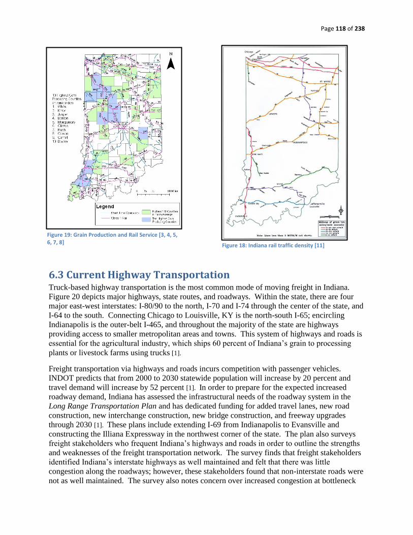
Page 118 of 238
Figure 18: Indiana rail traffic density [11]
33B6.3 Current Highway Transportation Truck-based highway transportation is the most common mode of moving freight in Indiana.
Figure 20 depicts major highways, state routes, and roadways. Within the state, there are four
major east-west interstates: I-80/90 to the north, I-70 and I-74 through the center of the state, and
I-64 to the south. Connecting Chicago to Louisville, KY is the north-south I-65; encircling
Indianapolis is the outer-belt I-465, and throughout the majority of the state are highways
providing access to smaller metropolitan areas and towns. This system of highways and roads is
essential for the agricultural industry, which ships 60 percent of Indiana‘s grain to processing
plants or livestock farms using trucks [1].
Freight transportation via highways and roads incurs competition with passenger vehicles.
INDOT predicts that from 2000 to 2030 statewide population will increase by 20 percent and
travel demand will increase by 52 percent [1]. In order to prepare for the expected increased
roadway demand, Indiana has assessed the infrastructural needs of the roadway system in the
Long Range Transportation Plan and has dedicated funding for added travel lanes, new road
construction, new interchange construction, new bridge construction, and freeway upgrades
through 2030 [1]. These plans include extending I-69 from Indianapolis to Evansville and
constructing the Illiana Expressway in the northwest corner of the state. The plan also surveys
freight stakeholders who frequent Indiana‘s highways and roads in order to outline the strengths
and weaknesses of the freight transportation network. The survey finds that freight stakeholders
identified Indiana‘s interstate highways as well maintained and felt that there was little
congestion along the roadways; however, these stakeholders found that non-interstate roads were
not as well maintained. The survey also notes concern over increased congestion at bottleneck
Figure 19: Grain Production and Rail Service [3, 4, 5, 6, 7, 8]

Page 119 of 238
Figure 20: Major Highways and Roadways in Indiana [3, 6, 7, 13]
locations, as well as the Borman Expressway in
Northwestern Indiana and the intersection of I-465 and
I-69 in Indianapolis [1].
The movement of freight may shift toward truck-based
highway transportation and away from barge and rail.
INDOT believes that trucking will increase from nearly
73 to 75 percent of freight movement, barge will
decrease from 11 to nine percent, and rail freight will
decrease from 16 to 15 percent [1]. While INDOT
recognizes that the use of biofuels will likely increase, it
does not include the potential impact of biofuels on
transportation in the forecasts created to determine
future transportation trends. Consequently, estimates
regarding decreases in rail and barge transport and
increases in trucking may be lower than what will
occur.
34B6.4 Current Maritime Transportation In the extreme north on Lake Michigan and at the southern border along the Wabash and Ohio
Rivers, barges transport primarily steel, mining, petroleum, and agricultural commodities [1].
While barge traffic moves 11 percent of freight by weight, less than two percent of freight
transport value comes from maritime transport [1]. The movement of commodities by barge is
most effective in the warmer months. During the winter, many Indiana ports close due to
maintenance needs or because the waterway freezes and becomes impassable [1]. Ultimately,
barge transportation is not a practical means of moving feedstocks or refined biofuels within
Indiana; this transportation mode is primarily used for interstate commerce and has a very
limited range.
35B6.5 Current Transport of Biofuels Biofuels occupy a relatively small share of current freight transport in Indiana. Of the state‘s
current capacity of 11.7 billion gallons of ethanol and 455 million gallons of biodiesel, 30
percent of biofuels and biofuels end-products transport by rail, 20 percent by truck, and 50
percent by barge [1]. With the anticipated increase from six to 12 ethanol plants within the next
year, the biofuels transportation sector will likely figure more prominently in the freight industry.

Page 120 of 238
36B6.5 Future Considerations Within the last year, five ethanol plants came online, increasing the estimated production of corn
based ethanol from 102 million gallons to 455 million gallons [14]. The Indiana State Department
of Agriculture (ISDA) expects another six plants to be in production by the end of 2008, further
increasing production by an additional 605 million gallons [14]. This expected increase in ethanol
production will likely change the direction of one of the state‘s largest exports, corn. A study by
Purdue University Extension estimates that in the long term, adjustments for increased ethanol
production will decrease exports of corn from 52 percent in 2005 to only 25 percent by 2010 [15].
This decrease in exports will likely coincide with an increase in ethanol production from the
current 102 million gallons per year to one billion gallons per year. As of January 2008, ISDA
estimates that total corn ethanol production will reach 1.06 billion gallons per year by the end of
2008 [14]. The actual number of ethanol plants to emerge in the near future is uncertain;
however, four proposed corn ethanol plants, estimated to produce an additional 358 million
gallons per year, have already received state incentives [14].
Additionally the construction of current and expected biofuels production plants near feedstock
sources (i.e. farms) is expected to increase the traffic and wear and tear on local roadways to and
from biofuels plants. Consequently, there may be a need for an increase in highway maintenance
due to greater truck traffic.
An essential factor in the production and distribution of biofuels is the ability of freight
transportation corridors to provide a route from the farm to the processing plant, from the
processing plant to the product terminal, and on to the final retailer. In order for the network to
work, the final retailer must have the capacity to store and distribute the final product. The next
section outlines the process behind the multi-step coordinated effort required to move biofuels
from the farm to the pump and describes the related economic and environmental considerations
associated with the distribution of biofuels within Indiana.
37B6.7 Transportation of Crops
144B6.7.1 Transportation of Feedstock from Field to Production Facility In Indiana, large semi-trucks, railway trains, and barges are the three modes of transportation
available to move bulk freight such as biofuels feedstocks. Large semi-trucks and flatbed trucks
are the dominant means of crop transportation. Jumbo hopper cars (rail) serve to transport
feedstock out of the state and also cover long distances within the state [1]. Since waterborne
barge transport is only viable in the northwest and southern corridors, barges are not feasible for
mass feedstock transportation throughout the state [1]. Consequently, future transport of
feedstock from farms for use at biofuels production plants will primarily take place via trucks
and railway trains. Before the feedstock arrives at the production plant, it must be stored in
either a grain elevator or on the field for eventual purchase by the plant.
145B6.7.2 Storage between the Field and the Production Plant Biofuels production plants do not have the storage capacity to hold feedstocks on site and
therefore must purchase and ship feedstocks to the plant on a daily basis [16]. Harvested
Page 121 of 238
feedstock storage occurs at either a grain elevator or on the farm. Grain elevators are interim
storage facilities for corn and soy feedstocks before purchase or shipment in state or out of state
by either truck or railway trains [1]. There are over 180 grain elevators in operation serving farms
and distributors throughout the state [2]. Farms located within a 25-mile radius of a grain elevator
use trucks to transport the feedstocks to the elevator after harvest [2]. However, farmers bale
switchgrass and corn stover cellulosic feedstocks and leave the bales in the field rather than
transport the feedstocks to a grain elevator [16]. The storage of corn stover bales occurs, on
average, five miles from the field from which it was harvested [17]. Switchgrass, however,
remains on or near the field [18].
Production plants purchase feedstocks from either the grain elevator or directly from the farmer
and transport the feedstocks to the plant. Ideally, grain elevators or farms are located within a
short distance (less than 75 miles) of the plant [15]. However, it is not unlikely for the
transportation of soybeans to occur over a distance of up to 150 miles, depending on the
popularity of soybean crops around the production plant [19]. Trucks then transport the
feedstocks to the production facility from the grain elevator or the farm.
146B6.7.3 Efficient Feedstock Transportation Considerations While there are a number of factors influencing the most efficient way to transport feedstocks
from the storage facility to the biofuels production plant, the most important element is the
weight-to-value ratio (WVR) of the feedstock. The WVR compares the capacity needed to
transport a feedstock to the monetary value of that feedstock. It allows production facilities to
determine the transportation mode that is most efficient, given hauling capacity and associated
costs. WVRs quantify characteristics including the weight of the feedstock, the volume to
transport at one time, and the cost of the mode of transportation.
The weights and measurements of corn and soy are quantified in bushels. One bushel is equal to
1.25 cubic feet. The weights and measurements of switchgrass and corn stover are in bales,
which are either rectangular or round in shape. The bale size of corn stover ranges from stackers
(one half to one ton) and one-ton bales (four feet x four feet x eight feet) for rectangular bales to
one-half ton round bales [20]. Switchgrass is baled in round bales weighing roughly half a ton
[21].
147B6.7.4 Trucks Standard large semi-trucks transport corn and soybeans from the grain elevator to the production
plant. One of these trucks has a maximum weight capacity of 26 tons and a volume capacity of
910 bushels [2]. Corn weighs 56 pounds per bushel. Thus, given its weight capacity, a standard
semi-truck could transport 1,023 bushels of corn at a time but is limited by its volume capacity to
only 910 bushels [22]. Slightly heavier than corn, soybeans weigh 60 pounds per bushel, limiting
a standard semi-truck to only 955 bushels at a time [22]. Like corn, the volume capacity of the
truck restricts soybean transport to 910 bushels.
A standard flatbed semi-truck transports switchgrass and corn stover bales to the production
facility. One of these trucks has a weight capacity of 23 tons and a volume capacity of 52 feet in
length, 8.5 feet in width, and seven feet in height [23]. Corn stover bales vary in size (rectangular
and round); therefore the quantity that a flatbed semi-truck can transport also varies. If farmers

Page 122 of 238
bale corn stover in rectangular bales (four feet x four feet x eight feet), a flatbed truck can
transport 23 one-ton bales or 46 half-ton bales of corn stover at one time, taking into account the
truck‘s weight capacity. If corn stover is baled in round bales, 17 one-ton bales can be
transported at one time, considering the weight capacity and the standard stacking practice of 12
bales on the bottom and five bales on top [24]. Standard flatbed semi-trucks also transport
rectangular bales of switchgrass. A standard bale of switchgrass is three feet in length by four
feet in width by eight feet in height [21]. Given the weight of switchgrass, a standard flatbed semi
can transport up to 46 bales of switchgrass. However, the volume capacity limits transport to 23
double-stacked rectangular bales of switchgrass.
148B6.7.5 Rail Jumbo hopper cars transport all feedstocks by rail. Each jumbo hopper car has a weight capacity
of 100 tons and a volume capacity of 3,500 bushels or 100 one-ton bales [2]. The size of a
standard jumbo hopper car is 39 to 50 feet in length and 13 to 15.5 feet in height with a volume
capacity 4,600 to 3,750 cubic feet [25]. Accordingly, one jumbo hopper can carry 3,936 bushels
of corn, 3,674 bushels of soy, 200 bales of switchgrass, or 100 bales of corn. However, the
weight capacity of a jumbo hopper car limits the transport of corn and soy to 3,500 bushels per
car. The volume capacity of a jumbo hopper car also limits the transport of corn stover and
switchgrass to around 40 one-ton bales per rail car or 80 half-ton bales, well under the maximum
number of bales given the weight capacity of rail. (See Table 21: Transportation statistics of feasible
crops for Indiana.for a summary of feedstock
transportation statistics.)
Although the average costs of transporting
feedstocks are unavailable, railway train transport is
only efficient for transporting feedstocks over a
minimum distance of 400 to 500 miles; otherwise,
the rail haul of feedstocks is inherently unprofitable
due to the low value of the feedstocks [2]. Ideally,
the maximum distance for transporting feedstocks
from the grain elevator or the field to the biofuels
production plant should not exceed 75 miles. As a
result, trucks are the only cost-effective option in
Indiana for transporting feedstocks from the field to
the grain elevator and from the grain elevator or
field to the biofuels production plant [15]. If a grain elevator is not located within a 75-mile
radius of the plant, or if purchasing from the grain elevator is too expensive, a biofuels
production plant can directly obtain corn and soybean feedstocks from the farmer, bypassing the
grain elevator storage system as it would for the purchase of corn stover and switchgrass.
149B6.7.6 Viable Feedstock Transportation Trucks are the only cost-effective option for transporting biofuels feedstocks in Indiana due to
the fact that rail is not profitable over short distances, including the 75-mile radius limitation for
hauling feedstocks to a production plant. Indiana grain exports will continue to rely on rail, but
in-state transport will shift to trucks. Trucks can easily access farms and existing biofuels
production plants while few rail lines are in close proximity to either. Furthermore, even when
Weight
Amount
Transported
per Truck
Amount
Transported
per Rail
Corn 56
lbs/bushel 910 bushels
3,500
bushels
Soybeans 60
lbs/bushel 910 bushels
3,500
bushels
Corn Stover ~2,000
lbs/bale
23 one ton
bales
40 one ton
bales
Switchgrass ~1,000
lbs/bale
23 half ton
bales
40 half ton
bales
Table 21: Transportation statistics of feasible crops for Indiana.

Page 123 of 238
using rail transport, trucks still need to transport the feedstock from the field to the railway and
from the railway to the production facility. The short distance to either the farm or the grain
elevator makes truck transport the most practical option for Indiana. However, as truck traffic
expands to meet increasing demand for feedstock transportation to biofuels production plants,
negative impacts, such as deteriorating road conditions (particularly on rural roads) and
increased ambient pollution, may occur [2].
38B6.8 Biofuels Distribution Although production costs are the largest component of retail prices, distribution costs can be
significant when transporting biofuels over large distances [26]. According to GAO, DOE lacks a
comprehensive strategic plan to coordinate significantly larger volumes of biofuels production
with the current distribution infrastructure [27]. DOE‘s chosen fuel blend strategy for ethanol
will greatly influence the nation‘s distribution infrastructure. The same equipment used to
transport and store diesel can be used for biodiesel without any modifications, whereas ethanol
requires minor modifications [26].
The current biofuels distribution infrastructure in the US includes rail, truck, and barge.
Geographic location, cost efficiencies, and location of terminal storage facilities determine the
proper mode of transport. The US has yet to use barge transport as a significant component of its
distribution infrastructure due to existing capacity issues [28]. Other countries, such as Brazil and
South Africa, distribute large quantities of biofuels through pipelines [29]. For Indiana, rail and
truck will likely be the most efficient methods of biofuels transportation.
39B6.9 Biofuels Transportation Methods
150B6.9.1 Barge Indiana has three public ports: one on Lake Michigan at Portage and two on the Ohio River at
Jeffersonville and Mount Vernon. Transporting biofuels to distant markets by barge is a
possibility for Indiana [15]. Currently, at the Port of Indiana at Mount Vernon, the state's largest
ethanol production facility at 220 million gallons per year (GPY), Aventine Renewable Energy is
under construction and should come online in 2008 [14]. This facility will be accessible by truck,
rail, and river barge. River barges have a 10,000-gallon capacity and—depending on the market
location—can cost less than rail transportation [30].
151B6.9.2 Railroads Rail transport is typically the most cost effective mode of moving biodiesel and ethanol over
medium to long distances of 300 to 2,000 miles [30]. In fact, ethanol shipments by rail nearly
tripled from 2001 to 2006, when producers moved 106,000 rail cars [28]. Railroad corporations
are now pushing production facilities to transport biofuels via unit trains, which are more
efficient with 75 to 95 tank cars [28]. Each tank car has a capacity of 30,000 gallons [28]. These
unit train cars are capable of discharging 3,000 gallons per minute (GPM), enabling rail
operators to unload 18 cars in four hours, or an entire unit train in one day [30]. This appears to
be a faster, more efficient method of transporting ethanol.

Page 124 of 238
In a 2007 GAO report, railroad officials indicate that there is no spare capacity to support higher
levels of biofuels transport; however, for Indiana, rail is the best method of exporting biofuels
[27]. In 2002, INDOT developed a comprehensive Indiana State Rail Plan, which recommends
funding track improvements for the state‘s 1,200 miles of short-line rail, as well as conducting a
feasibility study on constructing a short-haul line on the I-65 corridor to divert some truck traffic
[2]. Indiana railroads view as unprofitable lines that transport products distances of less than 400
to 500 miles; consequently, trucks will likely become the primary mode of biofuels transport
within the state [2]. Coal is the most shipped item on rail followed by grain. Grain export
shipments originate on short lines, which then connect to Indiana‘s Class I rail road lines. Short
lines predominately serve rural areas and depend upon grain transport for revenue. They can
transport biofuels. Using short lines can greatly reduce truck traffic on country roads and serve
as a network for Class I railroad lines.
152B6.7.3 Tanker Truck Biodiesel and ethanol distribution via tanker truck is cost effective for deliveries of up to 300
miles [30]. Each truck has a capacity of 7,800 to 8,200 gallons and cost for transport via truck
can be as little as a few cents per gallon over short distances [26, 30]. The cost of producing and
moving ethanol is the primary limitation to widespread use. As a result, the largest ethanol fuel
markets have emerged close to feedstock-growing areas and production facilities [26]. In an
interview with Ron Howe of Integrity Biofuels in Morristown, Indiana, he stated that his
company ships 70-80 percent of its product to destinations in Indiana, with the remainder going
to the Chicago area. Howe also stated that to keep costs low, the company only transports
biodiesel distances within 150 miles [19].
Not only do tanker trucks transport biofuels directly from the production facility, but they also
upload ethanol at large petroleum product terminals that have received the fuel by rail. These
trucks then deliver the fuel to regional terminals that are not equipped for rail delivery or lack the
storage capacity for a large quantity delivery [26]. Thus, biofuels production and distribution may
cause an increase in truck traffic on state and local roads [15].
153B6.7.4 Pipeline Generally, pipeline distribution is the most economical mode of fuel transportation [29]. The use
of pipelines for transporting gasoline generates a cost of $0.03-0.05 per gallon, whereas ethanol,
whose main modes of transportation are rail and tanker truck, costs approximately $0.13-0.15 per
gallon [27]. Pipeline distribution of biofuels is operationally prohibitive. The US already has an
extensive existing pipeline infrastructure for petroleum, natural gas, diesel, and jet fuel.
However, the existing infrastructure is not conducive to biodiesel and ethanol transmission. The
infrastructure moves petroleum products from the refineries located on the nation‘s coasts to its
interior [31]. Most ethanol and biodiesel plants are located within the Midwest, and their products
must be shipped in the opposite direction of the current pipeline infrastructure to more populated
areas.
Because of its chemical properties, the US has not installed pipelines for ethanol transportation
and distribution. Ethanol and high-grade alcohols are extremely corrosive on some soft metals
such as zinc, aluminum, brass, and lead [32]. Ethanol also has the tendency to attract water and
other chemicals left in the pipeline, which reduces its ability to blend at higher concentrations

Page 125 of 238
[33]. Contamination of ethanol by water and other chemicals may damage engines, which then
suffer poor performance [32].
Ethanol pipelines in Brazil have been successful, and there is now a project by Petrobras, a state-
owned oil company and the nation‘s largest ethanol producer, to build an approximately 200-
mile pipeline [34]. For the past decade, Brazil has been using polyethylene pipelines to transport
ethanol [35]. However, as of 2007, no major US pipeline has invested in ethanol transport [31]. In
the US, pipelines can be modified in order to support ethanol. This involves using epoxy and
other anti-corrosive substances to coat the inside of pipes, and replacing corrosive-susceptible
components [31]. The cost of constructing ethanol pipelines is approximately $1 million per mile
[27]. However, this may vary dramatically depending on the status of right-of-way. For example,
if ethanol pipelines are built along existing pipeline routes, the cost decreases to approximately
$500,000 per mile [29]. Nevertheless, to be cost effective in the US, ethanol would have to
replace 40 percent of gasoline consumption [29].
Unlike ethanol, biodiesel is not corrosive and does not attract water in pipelines. Since 2006
there have been several B5 biodiesel experimental shipments through existing pipelines.
Country Mark Cooperative, an Indiana-based oil refining and marketing company, successfully
moved 210,000 gallons of B5 through a 238-mile pipeline network (which usually transports
diesel, gas, and heating oil) from their Mount Vernon, IN refinery to their Jolietville, Indiana
terminal facility in July 2006 [36]. There is no pipeline transportation of blends higher than B5
due to the risk of the fuel congealing at low temperatures. Yet, there are still concerns that
biodiesel transmix,13
a mixture of biodiesel with another type of fuel, will not meet biodiesel fuel
specifications or will contaminate other fuels [36].
40B6.10 Distribution Considerations There are many factors to consider in selecting a distribution mode, including the size of the
production facility, shipping costs, customer preferences, shipment size, the capability of the
producer to use rail or barge transport, and distance to the distribution terminals. Very small
production facilities14
usually transport their product exclusively by truck. For small production
facilities, freight rail and trucks are the most cost-effective modes of transportation. Medium-
sized production facilities also ship their product mainly by truck and rail. Large production
facilities move biofuels economically by truck, rail, and barge [30]. While large production
facilities located on navigable waters could transport biofuels via barge, these boats are too slow
to get the fuel to market in a timely manner. Moreover, the majority of production facilities
(including most of those in Indiana) are not located on navigable waters [28].
13 Transmix occurs when different types and grades of fuel are shipped through the same pipeline [36].
14 Very small production facilities are those that produce less than 10 MGY; small facilities are those that produce
10-25 MGY; medium-sized produce 25-50 MGY; and large produce more than 50 MGY.
Page 126 of 238
41B6.11 Petroleum Destination Terminals Before it leaves the facility, producers denature the ethanol by blending 100 percent ethanol with
five percent gasoline for transport as E95. Conversely, producers transport biodiesel as B100
(100 percent biodiesel) [26]. Distributors then store and blend the ethanol with gasoline at
petroleum product terminals [26]. Petroleum terminals dictate the transportation delivery mode
based on both distance from the production facility and its receipt and storage capabilities [30].
Terminals close to a production facility generally receive biodiesel and ethanol by tanker truck.
A terminal‘s receipt capability includes its storage and blending capacity. Large petroleum
terminals are accustomed to receiving fuel via pipeline, so some do not have adequate rail
infrastructure or train unloading capacity [28].
Facility storage tanks must be large enough to maintain an adequate inventory and receive a
minimum shipment size [26]. A 25,000-barrel storage tank costs approximately $500,000 [26].
Additionally, petroleum terminals must install new blending systems or modify existing systems
in order to store ethanol and biodiesel; these systems could cost up to $1 million [26]. While
some petroleum terminals use the ―splash blending‖ method, where ethanol is mixed with
gasoline inside the tanker truck as it is being filled, this method can result in incomplete blending
and high product volatility [26].
42B6.12 Transitioning Gas Stations to Biofuel Retailers In the US in early 2007, approximately 1,050 public fueling stations offered E85, a high-
concentration ethanol blend, and about 325 stations offered biodiesel in 20- to 100-percent
concentrations (B20 to B100) [27]. GAO estimates that E85 was available at about 0.6 percent of
all fueling stations and that biodiesel from B20 to B100 was offered at about one percent of all
diesel stations [27]. In addition to the limited availability of ethanol and biodiesel, the need for
specialized storage and dispensing equipment at fueling stations may further hinder the
widespread public supply of biofuels [27].
43B6.13 Ethanol Many fuel retailers currently blend ethanol with gasoline in order to lower costs, increase the
fuel‘s octane rating, and decrease harmful gasoline emissions [27]. Corn-based ethanol accounts
for 98 percent of the ethanol produced in the US [27]. Gasoline-ethanol blends containing 10
percent or less ethanol (E10) are approved for use in all gasoline vehicles and do not require the
retailer to modify existing or install new storage and dispensing equipment [26, 28]. Higher
concentration blends, such as E85 (85 percent ethanol), can only be used in flex-fuel vehicles
(FFVs) and generally cannot be stored and dispensed without equipment modification [26, 38].
E85, the most popular higher blend of ethanol, may require the use of new or modified
equipment due to its corrosive nature [27, 38]. High-concentration ethanol blends tend to degrade
soft metals such as lead. Terne, a lead-tin alloy, is often used to plate steel gasoline storage tanks
[26]. Other materials like natural rubber, polyurethane, polyvinyl chloride (PVC), and some
plastics also degrade when in contact with ethanol [26]. Most metal underground storage tanks
that meet December 1998 EPA codes and most fiberglass underground storage tanks are suitable

Page 127 of 238
for ethanol storage, but those previously used for gasoline must be cleaned before using the tank
for an ethanol concentration higher than E10 [32]. Particulates in gasoline tend to settle at the
bottom of the tank; adding ethanol—an alcohol—to a dirty tank will place this sludge in
suspension, causing problems in the ethanol user‘s vehicle [32].
Retailers must also ensure that there is no water in the tank and remedy any causes of water
buildup in ethanol storage tanks [37]. Ethanol is susceptible to phase separation. If sufficient
water accumulates in the storage tank, the ethanol in the blend will absorb the water and separate
from the gasoline. This forms two layers in the tank: gasoline on top and ethanol on the bottom.
As it is no longer an ethanol blend, this phase separation can cause problems in vehicles‘ fuel
lines [39].
In addition to storage tanks, all fuel dispenser components must consist of ethanol-compatible
materials, including filters, dispenser hoses, nozzles, fitting, connectors, adapters, and piping [32].
Costs of converting existing or replacing storage tanks and dispensing equipment vary. A GAO
report states that converting existing storage tanks and dispensers to E85 at 64 fueling stations in
Illinois from 2005 to 2006 cost an average of $3,354 per station [27]. Other estimates for
equipment conversion range from $2,500 to $30,000 [40]. A survey by Underwriters
Laboratories, a product safety certification organization that tests products and writes standards
for safety, finds that of 45 stations that cleaned existing equipment for use with E85, none took
into account manufacturer-recommended retrofits [40]. The report states that these ―simplified
cases‖ will likely not meet the Underwriters Laboratories standards for E85 when they are
released [40].
Expenses associated with replacing or adding storage tanks and dispensers exceed those of
converting existing equipment. One project to install a new E85 storage tank and dispensing
equipment at Mammoth Cave National Park in Kentucky in 1998 cost a total of $22,216; the
tank alone cost just over $16,000 [32]. This is relatively low, with other estimates ranging from
$50,000 to $70,000, and one as high as $200,000 [27, 40]. The Energy Policy Act of 2005
provides assistance for fueling stations in converting or replacing equipment to become E85
compatible. The legislation authorizes a tax credit of 30 percent of the expense of installing E85
distribution equipment, up to $30,000 [41]. Indiana also offers grants of up to $5,000 to defray
fueling stations‘ costs of converting to E85 [42].
154B6.13.1 Limited Availability at Branded Stations In addition to the expense associated with modifying or purchasing new storage and dispensing
equipment, liability and branding concerns may limit the availability of E85 at fueling stations.
A GAO report states that Wal-Mart, BP, and Marathon Petroleum representatives cite the lack of
an Underwriter Laboratories-certified E85 dispenser as a greater obstacle to offering E85 at their
fueling stations than equipment costs, and these companies have deferred plans to offer E85 until
an approved dispenser is available [27].
The same report finds that, while 37 percent of fueling stations are under the brand of five major
oil companies (BP America, Chevron Products Company, ConocoPhillips, ExxonMobil, and
Shell Oil Products US), only nine percent of stations selling E85 and eight percent of those
offering higher biodiesel blends are under one of these brands [27]. None of these major oil

Page 128 of 238
companies offers E85 to their stations as a branded product; only in states where it is mandated
by law do they offer biodiesel [27]. Because the brand does not have control over the quality of
the unbranded product, stations must label the E85 and biodiesel they acquire from other sources
differently than branded products and are not allowed to advertise the unbranded biofuels on
their marquees [27].
44B6.14 Biodiesel Like ethanol, biodiesel may be blended with its petroleum counterpart, diesel, for use in vehicles
with diesel engines. Biodiesel may improve engine performance and lubrication, reduce
greenhouse gas emissions, and decrease emissions of other common air pollutants [43]. In the
US, producers use soybean oil to generate 90 percent of biodiesel [44]. Typical blends of
biodiesel are B5 (5 percent biodiesel, 95 percent diesel) and B20 (20 percent biodiesel, 80
percent diesel), though the product can be used in its pure from as B100 [43]. Most diesel engines
can run on biodiesel without modification [43]. Biodiesel in lower concentrations does not appear
to present any significant material compatibility issues with engines or storage and dispensing
equipment [45]. However, some diesel engine companies do not cover biodiesel use in their
warranties [46]. Like ethanol, biodiesel in high concentrations such as B100 may cause problems
when it comes into contact with certain metals (brass, bronze, copper, lead, tin, and zinc) and
other materials (nitrile rubber compounds, polypropylene, polyvinyl, and Tygon) [46]. Vehicles
manufactured before 1993 are more likely to contain engine parts incompatible with B100 [45].
Most diesel fuel storage tanks are made from materials that are compatible with biodiesel and
require only limited modifications to storage tanks and dispensing equipment [44, 45]. The federal
tax credit of up to $30,000 for alternative fuel infrastructure changes at fueling stations
(discussed above for ethanol) also applies to biodiesel blends of B20 or above [41].
155B6.14.1 Potential Policies to Increase Biofuels Distribution by Fueling
Stations As biofuel production and FFV availability increases, ethanol and biodiesel fuels will likely
become more accessible to the public. GAO reports that members of Congress have proposed a
number of policies to increase the availability of biofuels, such as mandating that major oil
companies install at least one E85 dispenser at each of their fueling stations, prohibiting biofuels
marketing restrictions on fueling station franchisees, allowing the public to utilize federal fueling
stations that offer biofuels, and increasing tax credits to fueling stations that install biofuel
infrastructure [27]. The National Governors Association echoes those recommendations and adds
that states might ―boost the adoption of alternative fuels or vehicles‖ by, for example, purchasing
vehicles for state fleets that can run on biofuels, and by investing in research and demonstration
to bring new technologies to market [44].
Page 129 of 238
45B6.15 Distribution Risks and Benefits
156B6.15.1 Fire One major risk associated with biofuels distribution is fire hazard. Both ethanol and biodiesel
are volatile substances and receive a three out of four hazard rating by the National Fire
Protection Association [47].15
Biodiesel fires should be extinguished using foam or dry chemicals as water can splash,
spreading the burning liquid [48]. Biofuels leaks should be contained because runoff to sewers
and drainage systems could cause fire or explosion hazards [48]. Biodiesel should always be
stored in a dry, cool, and well ventilated area.
Ethanol vapors, which have many of the same characteristics as gasoline, are heavier than air;
therefore, they travel easily away from the initial release point. There have been some instances
where fire has started from ethanol vapors traveling a considerable distance from the release
point to an ignition source [48]. Fire suppression of higher ethanol blends such as E85 requires
the use of alcohol-resistant foams. However, any ethanol blend under 10 percent can accept the
same fire suppression foam technology as used for gasoline and other hydrocarbon fuels [48].
157B6.15.2 Water Resource Contamination When motor fuels accidentally spill into environment, they infiltrate groundwater and surface
water supplies. Fueling stations, refineries, and major transportation corridors are potential sites
of contamination, and these areas become more sensitive as human and wildlife population
densities increase. Each type of transportation fuel has a different level of toxicity, and several
federal regulations mandate specific handling requirements for different motor fuels. As
illustrated below, one of the major benefits of displacing conventional motor fuels such as
gasoline and diesel with biofuels is the significant decrease in the health risks associated with the
toxic properties of the fuels.
158B6.15.3 Conventional Fuels Toxicology Gasoline and diesel fuel are derived from the distillation of petroleum and contain mixtures of
hundreds of different hydrocarbon chains. Commercial additives, which improve octane ratings,
oxygen content, and other performance measures, further complicate the toxicology of gasoline
[49]. Furthermore, the refinery streams used to blend gasoline are all on the Toxic Substances
Control Act (TSCA) Chemical Substances Inventory [50]. Additionally, the US regulates
gasoline for acute and chronic health effects under the Superfund Amendments and
Reauthorization Act (SARA), Sections 311 and 312. Some of the potential additives for gasoline
are benzene, ethyl benzene, naphthalene, ethanol, methyl tert-butyl ether (MTBE), tertiary amyl
methyl ether (TAME), and ethyl tert-butyl ether (ETBE) [50]. Many of these are highly toxic,
and are either known or suspected carcinogens.
15 A rating of three is given to materials that are flammable, volatile or explosive at ambient pressures and
temperatures

Page 130 of 238
If accidental releases of gasoline go unnoticed or unchecked, the resulting water contamination
can pose serious threats to local human and wildlife populations. As with all toxicants, the
duration and level of exposure to the chemical constituents of gasoline determine the degree of
associated risk. Although gasoline is minimally soluble in water, many of its toxic constituents
are more highly soluble, and local environmental conditions dictate the rate of biodegradation
and the ultimate fate of the fuel. When gasoline runs off into surface waters, it may be toxic to
aquatic organisms; lab tests reveal that LC50s (concentrations lethal to 50 percent of test
subjects) range from 1.8 milligrams per liter to 8.3 milligrams per liter for a variety of fish and
invertebrates [50].
MTBE is a common gasoline additive which is highly soluble in water, and as its use expanded,
concern over leakage from underground storage tanks increased [49]. EPA has classified MTBE
as a possible human carcinogen; it also causes acute headache, eye, nose, and throat irritation,
cough, nausea, dizziness, and disorientation [49]. As a result, on March 14, 2002, Indiana
initiated a partial ban on MTBE in gasoline, allowing no more than 0.5 percent MTBE by
volume, with a phase-out date of July 24, 2004 [51]. This created a window of opportunity for
ethanol since it is a common substitute for MTBE, but without mandates requiring ethanol use,
other more toxic additives such as TAME and ETBE may still replace MTBE. Furthermore,
given sufficient levels of ethanol in the subsurface environment, gasoline and water become
completely miscible and flow through substrates in a single phase [52]. This can lead to
significant increases in BTEX (benzene, toluene, ethylbenzene, and xylene) concentrations in
groundwater [52].
While diesel‘s composition is different from that of gasoline, both fuels contain common
ingredients and performance-enhancing chemicals that contribute to the toxicity of the fuel. The
US regulates diesel fuel as an acute and chronic health hazard under SARA Sections 311 and 312
[53]. A variety of amines and low-weight polymers are added to stabilize the fuel, prevent
corrosion and buildup, and improve the overall cold properties of diesel. Diesel contains varying
levels of aldehydes, benzene, 1, 3 butadiene, polyaromatic hydrocarbons (PAH), and nitro-PAH
[54]. Benzene poses the most documented threat, and even mixtures containing low levels of
benzene merit due caution. The toxic nature of PAHs caused the federal government to begin
limiting aromatic content in diesel to below 40 percent in 1993 [54].
While acute exposure to diesel fuel causes severe eye and skin irritation and lung damage if
ingested or inhaled, there is little knowledge about chronic exposure to low doses of its
constituents, as would be the case with water contamination [53]. Overall, the National Fire
Protection Agency (NFPA) gives diesel fuel its lowest ranking for health hazards, but many of its
components are known toxins and potential carcinogens, and the substance must be handled
accordingly. Diesel is negligibly soluble and volatile and requires similar emergency response
measures to those of gasoline [53]. Environmental releases of transportation fossil fuels should
be contained and cleaned up immediately, and should be considered a significant threat to human
health and the environment.
159B6.15.4 Biofuels Toxicology Corn ethanol and biodiesel from soybeans are the primary biofuels produced in Indiana and are
intended to displace some gasoline and conventional diesel consumption. While ethanol is a
Page 131 of 238
known toxicant, the majority of the research on its health effects regards its presence in alcoholic
beverages and not its potential environmental impacts [49].
Although the duration of exposure to ethanol from groundwater contamination could be lengthy
if a leaking storage tank went unrepaired, the concentration of ethanol and the total volume
consumed would likely be minimal compared to cases of intentional ingestion. Furthermore,
ethanol biodegrades more quickly in natural environments than the constituents of gasoline, and
it would be unlikely that human exposure to ethanol would be high enough to cause significant
harm [52]. Ethanol is completely water soluble, and if it infiltrates groundwater, its plume travels
at the same speed and in the same direction as groundwater flow [52]. Although ethanol
biodegrades quickly, the process consumes large amounts of oxygen, which can deprive
microorganisms of their oxygen requirements and slow the biodegradation of BTEX in gasoline
if the two are involved in the same accident [52]. Overall, ethanol is a much simpler substance,
biodegrades faster, and poses much less risk to water resources than its petroleum-based
counterpart.
While extensive research on alternative uses of ethanol has to some extent precluded serious
analysis of its toxic potential in its use as a biofuel, the same is not true for biodiesel. Biodiesel
is a relatively new substance, with significantly different chemical properties than its petroleum-
derived counterpart. The manufacturing process converts fats and oils into fatty acid methyl
esters of varying length [45]. Biodiesel is either consumed neat (100 percent biodiesel) or as a 20
percent additive to conventional diesel. It is a legally registered fuel and fuel additive with the
EPA, and is listed under TSCA, but has been found to contain no hazardous materials and is
generally regarded as safe to use [45]. Most laws that regulate the toxicity of petroleum-derived
fuels do not apply to biodiesel. Biodiesel has received a rating of zero (minimal hazard) for
health effects from the Hazardous Material Identification System, and while the oily and
flammable nature of the substance merits concern in remediating accidental releases, it is
completely insoluble in water and responses to leaks and spills are much less urgent than for
conventional diesel [55]. While conventional diesel fuel contains up to 40 percent aromatics,
biodiesel contains none, greatly decreasing its toxicity by comparison [56].
Biodiesel can slightly irritate eyes and mucous membranes if inhaled, but vapors are only present
if the substance is heated. Skin irritation is not likely, and there are no hazards anticipated from
incidental ingestion [45]. In fact, one study sponsored by USDA found that the acute oral LD50
(lethal dose for 50 percent of test subjects) is greater than 17.4 grams per kilogram by body
weight, which is nearly ten time less toxic than ordinary table salt (NaCl) [57]. The mutagenic
effects from exposure to biodiesel are also substantially lower than those of petroleum-based
diesel, and while blends are less mutagenic than conventional diesel, neat biodiesel is by far the
safest [56]. Not only is biodiesel insoluble, but it also biodegrades quickly in comparison to
petroleum-based diesel. One study found that 95 percent of biodiesel had biodegraded after 28
days, while only 40 percent of conventional diesel had degraded under similar conditions [58].
Overall, research on biofuels, along with general toxicology of their chemical constituents,
suggests that petroleum-based transportation fuels are far more toxic than their biofuel
alternatives. Biofuels are less toxic in nature and decompose at much faster rates than fossil
fuels, leading to the conclusion that the transportation, storage, distribution, and use of biofuels
pose much less risk to water resources.

Page 132 of 238
46B6.16 Conclusions In establishing BMPs for the harvest of cellulosic feedstocks such as corn stover and
switchgrass, policymakers should take shipment needs into consideration. Based on current data,
rail transportation of biofuel feedstocks within Indiana will not meet the needs of feedstock
producers, nor will it be cost effective. In order to move feedstock efficiently, biofuels producers
should employ trucks as the primary mode of transportation. Due to the low economic value of
the feedstocks, studies suggest that shipments made in excess of 75 miles will not be
economically efficient. To transport refined biofuels over distances of less than 300 miles,
tanker trucks are the most cost-effective option. The distribution of refined biofuel by rail is a
good alternative, but railway companies require hauling distances of 300-2,000 miles to make
rail travel efficient, and infrastructural adjustments are necessary for this to occur. Maintaining
and improving Indiana‘s short-rail lines offers the possibility for export of biofuels and may
encourage further investment in the state. For this to be effective, production facilities should
located near existing short-rail lines allowing for eventual export via Class I rail. Finally, to
ensure the safe transport and storage of biofuels, emergency service individuals and retail
operators should train in managing biofuels spills and leaks, and in preventative maintenance of
biofuels tankers used for transport and storage tanks. This becomes a greater concern as the
quantity of biofuels in transport increases and the number of vehicles running on biofuels grows.

Page 133 of 238
47B6.17 References for Logistics
[1] Corridor and Long Range Planning Section.
2007. 2030 Long Range Transportation
Plan: 2007 Update. Office of Urban and
Corridor Planning, Indiana Department of
Transportation.
[2] Prepared by PARSONS. 2002. Indiana Rail
Plan. Prepared for the Indiana Department
of Transportation Multi-Modal
Transportation Division. Environmental
Systems Research Institute. 2006. ArcGIS
9.2. Redlands, California.
[3] Keefe VH. 2006. Rail System (INDOT).
Indiana Geological Survey, 1:1,200 Line
shapefile (15 February 2008;
http://129.79.145.7/arcims/statewide_mxd/in
dex.html)
[4] Business Information and Technology
Systems, Indiana Department of
Transportation. 2005. Rail System – Active
and Abandoned (INDOT). Indiana
Department of Transportation, 1:1,200 Line
shapefile. (15 February 2008;
http://129.79.145.7/arcims/statewide_mxd/in
dex.html)
[5] Environmental Systems Research Institute.
2006. U.S. Counties. ESRI SDC Data Set,
1:100,000 Polygon feature (15 February
2008; http://iuware.iu.edu/list.aspx?id=146)
[6] Environmental Systems Research Institute.
2006. U.S. Cities. ESRI SDC Data Set,
1:250,000 Point feature (15 February 2008;
http://iuware.iu.edu/list.aspx?id=146)
[7] Prepared by PARSONS. 2002. Indiana Rail
Plan. Adapted from Figure 2-3 Grain
Production and Rail Service, p.10. Indiana
Department of Transportation.
[8] Policy and Economics Department. 2008.
Class I Railroad Statistics. Association of
American Railroads (18 March 2008;
www.aar.org/PubCommon/Documents/Abo
utTheIndustry/Statistics.pdf)
[9] Federal Railroad Administration. 2006.
Freight Railroads Background (19 March
2008;
http://www.fra.dot.gov/downloads/policy/fre
ight2004.pdf)
[10] Prepared by PARSONS. 2002. Indiana Rail
Plan, Figure 2-1 Railroad Traffic Density in
Indiana, p.5. Indiana Department of
Transportation Multi-Modal Transportation
Division.
[11] Prepared by Cambridge Systematics, Inc.
2007. National Rail Freight Infrastructure
Capacity and Investment Study. Association
of American Railroads.
[12] Business Information and Technology
Systems, Indiana Department of
Transportation. Roads 2005 – INDOT.
Indiana Department of Transportation,
1:100,000 Line shapefile. (15 February
2008;
http://129.79.145.7/arcims/statewide_mxd/in
dex.html)
[13] Abbott D. 2008. Fact Sheet: Biofuels Plants
in Indiana. Indiana State Department of
Agriculture.
[14] Dooley, F. The Effect of Ethanol on Grain
Transportation and Storage. Department of
Agricultural Economics, Purdue University
BioScience Series. ID-329.
[15] Klemme K. 27 March 2008. Personal
Communication. Indiana University School
of Public and Environmental Affairs,
Bloomington, IN.
[16] Sokhanasanj S, Turhollow AF. 2002.
Baseline cost for corn stover collection.
Applied Engineering in Agriculture 18(5):
525-530.
[17] McLaughlin SB, Walsh, ME. 1998.
Evaluation environmental consequences of
producing herbaceous crops for bioenergy.
Biomass and Bioenergy 14(4): 317-324.
[18] Howe R. 15 February 2008. Personal
Communication. Integrity Biofuels Plant,
Morristown, Indiana.

Page 134 of 238
[19] Nielsen RL. 1995. Questions Relative to
Harvesting and Storing Corn Stover.
Agronomy Department, Purdue University.
AGRY-95-09.
[20] Chariton Valley Biomass Project.
Transporting and Storing Switchgrass.
Chariton Valley RC&D (18 March 2008;
http://www.iowaswitchgrass.com/cofiringcy
cle%7Etransporting.html)
[21] Beuerlein J. Bushels, Test Weights, and
Calculations. Department of Horticulture
and Crop Science, Ohio State University (17
March 2008; http://ohioline.osu.edu/agf-
fact/0503.html).
[22] Arab Cartage and Express Company.
Equipment Selection: Flatbed Truck
Specification. (17 March 2008;
http://www.arabcartage.com/equipment.htm
#flatbed?)
[23] Atchinson JE, Hettenhaus JR. 2003.
Innovative Methods for Corn Stover
Collecting, Handling, Storing and
Transporting. National Renewable Energy
Laboratory, United States Department of
Energy. NREL/SR-510-33893.
[24] CSX Corporation, Inc. Carry Type Details:
Jumbo Covered Hopper. (18 March 2008;
http://www.csx.com/?fuseaction=customers.
search_car&n=Jumbo%20Covered%20Hop
per)
[25] Fulton L. 2005. Biofuel Costs and Market
Impacts in the Transport Sector. Energy
Prices & Taxes 2005.1Q: xi-xxvii.
[26] Government Accountability Office. 2007.
DOE Lacks a Strategic Approach to
Coordinate Increasing Production with
Infrastructure Development and Vehicle
Needs. GAO-07-713.
[27] Brat I, Machalaba D. 1 February 2007. Can
Ethanol Get a Ticket to Ride? The Wall
Street Journal. p.B1.
[28] Steiner E. 2003. Ethanol Pathways in the
2050 North American Transportation
Futures Study. National Renewable Energy
Laboratory, United States Department of
Energy, Golden, CO.
[29] Reynolds RE. 2000. The Current Fuel
Ethanol Industry: Transportation,
Marketing, Distribution, and Technical
Considerations. Prepared by Downstream
Alternatives Inc. for the United States
Department of Energy.
[30] Yacobucci BD, Schnepf R. 2007. Ethanol
and Biofuels: Agriculture, Infrastructure,
and Market Constraints Related to Expanded
Production. Congressional Research
Service. CRS Report for Congress Order
Code RL33928.
[31] National Renewable Energy Laboratory,
National Ethanol Vehicle Coalition. 2002.
Handbook for Handling, Storing, and
Dispensing E85. United States Department
of Energy. DOE/GO-1002001-956.
[32] Colona G. 2008. Fire Testing Ethanol Fuels.
NFPA Journal March/April 2008. (18
March 2008;
http://www.nfpa.org/publicJournalDetail.asp
?categoryID=1555&itemID=37924&src=NF
PAJournal&cookie%5Ftest=1)
[33] Fan G. 24 September 2007. Brazil Cosan
Warns Against Petrobras Ethanol Pipline.
Dow Jones Newswires (12 February 2008;
http://www.cattlenetwork.com/content.asp?c
ontentid=162861)
[34] Khalip A. 15 January 2008. Petrobras Offers
Oil Ethanol Expertise at a Price. Reuters (12
February 2008;
http://www.reuters.com/article/GlobalAgric
ultureandBiofuels08/idUSN1554409420080
115)
[35] McElroy AK. 2007. Pipeline Potential.
Biodiesel Magazine August 2007 (18 March
2008;
http://www.biodieselmagazine.com/article.js
p?article_id=1441)
[36] American Coalition for Ethanol. Ethanol
101: What is Ethanol. (18 March 2008;
http://www.ethanol.org/index.php?id=34&p
arentid=8)
[37] National Renewable Energy Laboratory.
2005. Clean Cities Fact Sheet: Low-Level
Ethanol Fuel Blends. United States
Department of Energy. DOE/GO-102005-
2028.

Page 135 of 238
[38] State of Iowa Department of Natural
Resources. 21 November 2006. Converting
Existing Underground Storage Tank (UST)
Systems to Ethanol Compatible.
[39] Johnson C, Melendez M. 2007. E85 Retail
Business Case: When and Why to Sell E85.
National Renewable Energy Laboratory,
United States Department of Energy.
NREL/TP-540-41590.
[40] Energy Policy Act of 2005. Pub. L. No. 109-
58, § 1342, 119 Stat. 1049 (2005).
[41] IND. CODE § 15-9-5 (2007)
[42] SmartWay Transport Partnership. 2006.
Alternative Fuels: Biodiesel. United States
Environmental Protection Agency. EPA420-
F-06-044.
[43] Dierkers G. 2008. Greener Fuels, Greener
Vehicles: A State Resource Guide.
Environment. Environment, Energy &
Natural Resources Division, National
Governors Association Center for Best
Practices, Washington, DC.
[44] Office of Energy Efficiency and Renewable
Energy. 2006. Biodiesel: Handling and Use
Guidelines, Third Edition. United States
Department of Energy. DOE/GO-102006-
2358.
[45] Alternative Fuels & Advanced Vehicles
Data Center. 2008. B20 and B100:
Alternative Fuels. Office of Energy
Efficiency and Renewable Energy, United
States Department of Energy (21 March
2008;
http://www.eere.energy.gov/afdc/fuels/biodi
esel_alternative.html)
[46] Ebert J. 2007. Playing It Safe with
Methanol. Biodiesel Magazine, July 2007
Issue (18 March 2008;
http://biodieselmagazine.com/article-
print.jsp?article_id=1709)
[47] Milke JA, Sunderland PB, Levy KM,
Ontiveros VL, Carey AC. 2007. Fire Safety
of the Traveling Public and Firefighter‘s for
Today‘s and Tomorrow‘s Vehicle Fleet.
Department of Fire Protection Engineering,
University of Maryland. Prepared for The
Fire Protection Research Foundation.
[48] Klaassen CD. 2001. Casarett and Doull‘s
Toxicology: The Basic Science of Poisons.
6th
Edition. Columbus, OH: McGraw Hill.
[49] Chevron Products Company. 2002. Chevron
Regular Unleaded Gasoline: Material Safety
Data Sheet (18 March 2008;
http://www.albina.com/fuel/ChevronRUGas
MSDS.htm)
[50] United States Environmental Protection
Agency. 2004. State Actions Banning
MTBE (Statewide). EPA420-B-04-009.
[51] Buscheck T, O‘Reilly K, Koschal G,
O‘Regan G. 10 & 11 April 2001. Ethanol in
Groundwater at a Northwest Terminal.
Presentation: Workshop on the Increased
Use of Ethanol and Alkylates in Automotive
Fuels in California (18 March 2008; www-
erd.llnl.gov/ethanol/proceed/terminl.pdf)
[52] Phillips Petroleum Company. 2002. MSDS
Summary Sheet: No. 2 Diesel Fuel (18
March 2008;
www.petrocard.com/Products/MSDS-
ULS.pdf )
[53] Hochhause A. 2004. Gasoline and other
motor fuels. Kirk-Othmer Encyclopedia of
Chemical Technology 12: 286-435.
[54] Biodisel Industries, Inc. 2006. Material
Safety Data Sheet: Section 1- Product
Identification, Biodiesel. (18 March 2008;
www.pipeline.to/biodiesel/research/files/BI
%20MSDS.pdf )
[55] 40 C.F.R. pt. 79, §§ 211(b)(2), 211(e)
(1998).
[56] National Biodiesel Board. Environmental
and Safety Information. (18 March 2008;
http://www.biodiesel.org/pdf_files/fuelfacts
heets/Environment_Safety.pdf)
[57] Peterson CL, Reece D. 1994. Toxicology,
Biodegradability and Environmental
Benefits of Biodiesel. Department of
Agricultural Engineering, University of
Idaho (18 March 2008;
www.biodiesel.org/resources/reportsdatabas
e/reports/mar/19940101_mar-002.pdf)

Page 136 of 238
7. Site Suitability Analysis
48B7.1 Justification Corn and crop residues such as corn stover
are appealing feedstocks for biofuel
production because they are readily available
[1]. Furthermore the technology for corn
ethanol (hereafter referred to as ethanol) is
highly developed [2]. There are currently 12
ethanol plants in production or slated for
production within the next year in Indiana [4]
(Figure 1). This analysis uses spatial analyst
tools to address the question: Where are the
most suitable sites to build ethanol
production facilities in Indiana?
Because of resource demands, the
distribution of agricultural land across the
state, and market saturation careful
consideration of future production plant
location is important. If sites are not properly
selected for these facilities, there could be an
inadvertent yet severe impact on land and
water resources. There is also the danger that
ill-sited plants would no longer be
economically efficient after the initial market
boom in production facilities settles down.
Economically, the constraints imposed on
these plants are highly dependent on
transportation costs [6]. The farmer can economically transport their crop up to 25 miles [6]. The
distance from grain elevators to production facilities is the most significant economic constraint
on transportation. Production facilities can get their grain from up to 75 miles away [6]. Further
consideration needs to account for current ethanol facilities‘ locations so as not to saturate the
market.
Ecologically, ethanol plants require large volumes of water, on the scale of four gallons to every
gallon of ethanol produced [7]. Therefore, surface waters and aquifers will be increasingly tapped
to supply a growing water demand. Because groundwater is replenished slowly, facilities would
be more sustainable if they were able to use surface water and return the waters to the rivers and
lakes. Therefore, plants within pumping distance to surface waters would be preferred.
Figure 21: Ethanol facilities funded through state initiatives [3, 4, 5]

Page 137 of 238
However facility location along waterways should not be recommended at the extreme
environmental costs of building the facility within fragile riparian areas. If the site selection does
not account for these water needs, they could threaten the Indiana‘s freshwater supply. Like all
new infrastructure, smart placement is key to the economic and ecological outcomes in the area.
While the push for ethanol has been the main focus for alternative fuels in Indiana [8], relative to
other ethanol feedstocks, corn has a low energy balance. Additionally the technology is mature,
leaving little room for efficiency gains from production methods [9]. These compelling reasons
may lead Indiana to shift focus to cellulosic ethanol production in the near future.
Cellulosic ethanol in Indiana could feasibly be produced from both corn stover and in the future,
switch grass. Currently there are no cellulosic plants in Indiana. However there is widespread
supply of corn stover which may justify the development of cellulosic ethanol in Indiana. The
most suitable sites for cellulosic ethanol production facilities would be largely dependent on
similar constraints to current ethanol plants, with the exception that cellulosic plants would not
be dependent on grain elevators as farmers are likely to store the bales and sell directly to the
production facilities. Therefore, using current trends to predict distances, farmers could travel up
to 25 miles to deliver their product [6]. These production facilities would still be dependent on
high amounts of water and thus, close proximity to major sources of surface water would be
ideal. Availability of roads and slope of the land are also important considerations.
Indiana has a high number of existing ethanol facilities near which cellulosic ethanol could be
produced in rotation with grain feedstocks. Therefore, a co-location of corn ethanol and
cellulosic ethanol plants may be desired. Once cellulosic production becomes more efficient and
profitable, independent cellulosic plants may start to appear across Indiana‘s landscape.
Once cellulosic production facilities are on line, a shift to the more efficient feedstock,
switchgrass, may become appealing. While the cellulosic ethanol process has not yet been
perfected, it is projected to be online by 2012 with large opportunities for increased efficiency in
production. Therefore, Indiana needs to be planning and effectively locating production facilities
taking into consideration economics and the environment.
49B7.2 Methods In order to find the most suitable sites in Indiana for corn and cellulosic ethanol production
facilities, many factors had to be included in this analysis. Additionally, the most suitable sites
for ethanol facilities, because they are largely dependent on location of existing facilities and
grain elevators, provided different results than the site suitability analysis for cellulosic ethanol
production facilities that do not share this constraint. All analyses were conducted using
ArcMap 9.2 [4].
This analysis has a multi-tiered approach. It first focuses on the suitable sites for future and
proposed ethanol plants incorporating the following variables: distance to major grain elevator,
distance to surface water source, distance to highways, and distance from existing plants. All the
Page 138 of 238
following datasets were combined to find developable areas [10, 11, 12, 3]. A Euclidean distance
buffer was used which allowed for areas near grain elevators, surface water and highways and far
from existing facilities to be ranked higher on a scale of one through ten with ten being the most
optimal sites.
Location data was combined with a digital elevation model (DEM) which was converted to slope
for the state of Indiana [13]. Protected areas in Indiana, such as parks, as well as highly
developed areas and wetlands were excluded from analysis by using a mask over the DEM.
Once the slope dataset was masked, the data was reclassified to exclude areas with a slope over
30 percent in the interest of finding more level developable areas. The remaining areas were
assessed to find suitable sites for future ethanol facilities using a weighted overlay analysis. The
inputs were then weighted, with distance to grain elevators as the most important at 30 percent
weight, followed by distance to highways at 25 percent, areas with lower slope at 20 percent,
distance to surface water at 13 percent and finally, the distance to current facilities at 12 percent
weight.
To find the most suitable sites for a future cellulosic ethanol facility location, similar methods of
analysis were used excluding the grain elevator and location of current production facility
restraints. The variables included were distance to surface water, distance to highways and areas
of low slope [11, 12, 13]. These layers were buffered allowing for areas near surface water and
highways with low slope to have a higher ranking than the other alternatives. Using a weighted
overlay the variables were weighted proportionally to the ethanol facility overlay. The distance
to roads was weighted the most at 43 percent, followed by areas of low slope at 35 percent and
distance to streams at 22 percent. A map of the suitable sites for cellulosic production was
created.
The third tier of analysis used the two outputs from the weighted overlays for ethanol and
cellulosic ethanol site suitability analysis and combined them to find areas in which co-location
of a corn ethanol and cellulosic ethanol plant could be constructed. From this map, the top three
existing sites were selected and buffered with a 25 mile buffer (the likely distance a farmer could
transport switchgrass to the production facility). This buffer was overlaid on the current lands
used for agriculture [15] and found the area of productive agricultural lands within the 25 mile
radius of these facilities. The facility with the highest amount of contributing agricultural land in
this area was selected as a possible pilot site for an ethanol-cellulosic ethanol co-production
facility.

Page 139 of 238
50B7.3 Results
Figure 23: Suitable sites in Indiana for ethanol production plant location. Note: there were few areas that were ranked as the highest suitability (marked in red). The rest of the area ranked lower (marked in blue) but is still considered suitable sites.
Figure 22: Suitable sites in Indiana for cellulosic ethanol production plant location. All areas marked in blue were ranked as the highest site suitability. Due to the amount of area included in the top ranking area, the second ranking areas were not included in this analysis
Figure 23
While there are suitable lands
remaining for ethanol facilities, only
one region in the south east corner of
Indiana ranks as the most suitable.
This is largely, but not completely,
due to the number of existing
facilities in Indiana.
Figure 22
Switchgrass, which was not
limited by current facility location,
has more suitable locations

Page 140 of 238
Figure 24: Overlap of suitable areas with current production facilities as well as state and privately funded proposed sites.
Figure 25: Suitable regions without existing production plants
Figure 25
When the first and second most
suitable areas for ethanol
production are overlaid with the
most suitable sites for cellulosic
ethanol, a large area of the state
falls within the parameters used in
this analysis.
Figure 26
It becomes apparent that when state
and privately proposed sites are
shown with the suitable areas, that
many, although not all, match up.
This may mean that local conditions
are still favorable for production
facility construction and operation.
However, in some cases it may
indicate that the locations proposed
may need further analysis.

Page 141 of 238
Figure 27: Top three ranked current ethanol facilities for addition of cellulosic ethanol production facility co-location.
Figure 26: suitable regions without existing production plants.
Figure 28
For preliminary cellulosic production
facilities it may be was to co-locate them
with existing ethanol facilities until it
becomes more cost effective on a wide-
scale. Therefore, when current facilities
are assessed, the facilities that fall within
the most suitable sites would be the best
facilities at which to locate a pilot
cellulosic ethanol production facility.
When a 25 mile radius was assessed for
agricultural land, the site in the middle
contained the most. This may be due to
the fact that agricultural lands in
surrounding states were not assessed in
this analysis. According to these results,
any of the three sites existing sites would
be ideal for a co-located facility.
Figure 27
All remote analyses however, are subject to
error. Spatial GIS analyses results cannot be
assumed accurate without on-the-ground
verification of results. There may be other
conditions at these sites that would restrict
construction of these facilities. Other sites
less suitable in this analysis may be more
suitable when other local conditions are
considered. Only current facilities, either in
production or in construction, were used in
this analysis. This may lead to overlap
between the suitable sites for future facilities
and the locations of proposed sites. Analysis
did not take into account agriculture first;
therefore suitable sites were not selected
because they have the most contiguous acres
of agricultural lands. Area of adjacent
agricultural land was taken into account after
suitable sites were defined.

Page 142 of 238
51B7.4 References [1] Doering O. 4 March 2008. Economic
perspectives on producing liquid fuels
from plant feedstocks. Indiana Memorial
Union, Bloomington.
[2] Yacobucci BD, Schnepf R. 2007. Ethanol
and Biofuels: Agriculture, Infrastructure,
and Market Constraints Related to
Expanded Production. Congressional
Research Service (27 April 2008:
http://www.nationalaglawcenter.org/assets
/crs/RL33928.pdf)
[3] Indiana State Department of Agriculture.
2008. Fact Sheet: Biofuels plants in
Indiana. Indiana Department of
Agriculture (17 April 2008;
http://www.in.gov/isda/)
[4] Environmental Systems Research
Institute. 2006. ArcGIS 9.2. Redlands,
California.
[5] Like K. 2002. County Boundaries of
Indiana. Indiana Geological Survey.
1:24,000, Polygon shapefile. (24 April
2008;
http://129.79.145.7/arcims/statewide_mxd
/dload_page/reference.html)
[6] Dooley F. 2006. The Effect of Ethanol on
Grain Transportation and Storage. ID-329.
Purdue University, Department of
Agricultural Economics.
[7] National Academy of Sciences. 2007.
Water implications of biofuels production
in the United States. Committee on Water
Implications of Biofuels Production in the
United States, Washington, DC (23 April
2008;http://dels.nas.edu/dels/rpt_briefs/bi
ofuels_brief_final.pdf)
[8] United States Department of Energy. 2008.
Biomass Program. (27 April 2008;
http://www1.eere.energy.gov/biomass/)
[9] World Watch Institute. 2007. Biofuels for
Transport: Global Potential and Implications
for Energy and Agriculture. World Watch
Institute. World EarthScan Publications,
Ltd.
[10] All Pages. 2008. Grain Elevators in Indiana.
Geo-coded by Priebe M, Indiana University,
Bloomington (1 April 2008;
http://www.allpages.com/)
[11] Indiana Department of Transportation. 2004.
Highways in Indiana. (17 April 2008;
http://129.79.145.7/arcims/statewide_mxd/dl
oad_page/infrastructure.html)
[12] United States Geological Survey and United
States Environmental Protection Agency.
2002. Canals, Lakes, Streams and Swamps
in Indiana. Compiled by Bernardine
Lochmueller and Associates, Evansville, IN
(17 April 2008;
http://129.79.145.7/arcims/statewide_mxd/dl
oad_page/hydrology.html)
[13] United States Geological Survey. 2001.
National Elevation Dataset. One Arc Second
DEM. (12 April 2008; http://seamless.usgs.
gov/website/seamless/viewer.htm)
[14] United States Department of Agriculture.
2004. Cultivated Areas in Indiana in 2004.
United States Department of Agriculture.
National Agriculture Statistics Service,
Fairfax, Virginia (17 April 2008;
http://129.79.145.7/arcims/statewide_mxd/dl
oad_page/reference.htm

Page 143 of 238
8. Energy Balance of Biofuels
52B8.1 Introduction The notion of energy balance is a crucial element in the debate over biofuel viability. If the
energy availability of a fuel is less than the energy expended during production, the practicality
of widespread use diminishes. Energy balances are frequently provided as ratios of usable energy
to production energy:
If ER is greater than one, the energy balance is positive and thus more energy is available in the
fuel than is expended in the fuel‘s production. If ER is less than one, the energy balance is
negative and less energy is available in the fuel than used in production. Ideally, fuels should
have ratios greater than 1 to be considered viable from a pure energy perspective.
An alternate method for considering energy balance is from the perspective of net energy, or
total energy available less energy consumed in production:
–
Energy balances are unique for each type of fuel and for the feedstocks used to produce various
biofuels. Given the variability of production inputs, these ratios differ spatially and temporally.
Spatially the variations are explained largely by the use of different soil types with divergent
fertility to produce a given feedstock. Temporally, energy balances are affected by weather

Page 144 of 238
conditions that may necessitate greater fertilizer use for feedstock production. The variation in
energy contents necessitates an individual analysis of each feedstock under consideration.
This section seeks to explore existing literature and identify the different methods scholars have
employed to examine the energy in fuel derived from different feedstocks. A unique situation
arises for corn-based ethanol in that suitable data is available to generate Indiana-specific values
for the energy balance and net energy for ethanol produced in the state. Insufficient data,
however, limits the development of localized energy values for other feedstocks.
53B8.2 Energy Content of Fuels All fuels have established amounts of energy
available for use, defined above as Ef.
Energy content is measured by the amount of
heat produced through the combustion of a
fuel. Heating values are measured in two
forms, high and low. A high, or gross, heat
value (HHV) is the amount of heat produced
when a set amount of the fuel fully
combusts. A low heat value (LHV)
removes suppressed heat generated from
water vapor from the HHV (note this is the
same as Ef in the NEV equation above). For
instance, ethanol‘s HHV is 84,000 Btu per
gallon, but its LHV is only 75,700 Btu per
gallon once adjusted for latent heat created
in water vaporization [1].
Table 22 provides the estimated energy content of various fuels. Gasoline contains 125,000 Btu
per gallon at HHV, slightly less than available in various forms of biodiesel [2, 1]. These values
are of particular importance in understanding energy balances because different scholars have
selectively chosen HHV or LHV to present inflated results for ER or NEV. The use of HHV
necessarily overstates the available energy in a fuel because vaporization is not accounted for;
therefore, LHVs are more appropriate for energy balance analysis.
Fuel LHV HHV MJ/gallon
Agricultural
Residues (low
estimate)
4,300
Btu/lb†
Agricultural Residues (high
estimate)
7,300
Btu/lb†
Biodiesel No. 2 140,000 Btu/gallon‡ 126-135
B20 Mix (20/80) 138,000 Btu/gallon‡
Diesel 130,719 138,714 Btu/gallon*
Ethanol 75,700 84,000 Btu/gallon† 80-89
Gasoline 116,515 125,000 Btu/gallon*† 132
* Graboski, M. 2002. [3]
‡ North Dakota State University. 2003. [2]
† Oak Ridge National Laboratory. 2008. [1]
Table 22: Energy Content of Select Fuels

Page 145 of 238
54B8.3 Analytical Process Establishing the amount of energy expended during the production of biofuels is a tremendous
process and, for the most accurate indication of energy available, must include all primary and
secondary input processes. In the literature to be discussed below, the disparity of findings is
largely a function of inconsistent use of system boundaries and accompanying assumptions. An
ideal primary input boundary for biofuel production includes analysis of (1) feedstock planting,
fertilization, and harvest; (2) transportation of feedstock to storage receptacles or processing
plants; (3) feedstock-to-fuel conversion processes; and (4) transportation of fuel to storage
facilities and/or points of distribution (Table 23). Secondary impacts to consider include inputs
such as energy expended for fertilizer and chemical production as well as the output of generated
co-products from the fuel conversion process. For example, newer facilities should benefit from
more efficient conversion processes whereas older facilities constructed near the beginning of a
feedstock‘s development will have lower
conversion rates.
55B8.4 Corn-Based Ethanol
Literature Review Perhaps the most intriguing discussion of
biofuel energy balance occurs in the
literature related to corn-based ethanol
production. At least 15 studies specifically
examining the energy required for the
production of ethanol have been completed
in the past 20 years and found anywhere
from incredibly negative net energy values to extremely positive net energy values.
Chambers et al. (1979) published the first major study examining energy balance of corn-based
ethanol [4]. Their study highlighted a number of the methodological flaws inherent in examining
life-cycle processes, which will become more evident in the subsequent discussion. They
concluded that ethanol‘s energy balance was slightly positive but maintained that when
compared to petroleum, the energy benefits were
unquestioned since many of ethanol‘s energy inputs can
be supplied by non-petroleum sources, such as coal and
natural gas. One decade later, the scholarly
examination of energy balances intensified as articles
became more frequent. Ho (1989) found a negative
NEV and an ER less than one [5]. In short, Ho‘s (1989)
findings suggested that the energy available from corn-
based ethanol was greater than the energy used to
produce the fuel [5]. The study relied on corn yields of
90 bushels per acre and early feedstock conversion
Phase Activities
1. Farming Feedstock planting
Feedstock fertilization
Feedstock harvest
2. Transport off
farm Transportation to storage facility
Transportation to refining facility
3. Fuel Conversion Feedstock-to-fuel conversion
4. Fuel
Transportation Transportation of fuel to storage facility
Transportation of fuel to distribution site
Table 23: Production Phases to Consider for Energy Balance
Descriptive US (bu/acre) Indiana (bu/acre)
Average 104.8 109.4
Median 108.9 112
St. Dev. 13.8 18.8
Maximum 119.8 135
Minimum 81.1 73
Table 24: Characteristics of US and Indiana Corn Yields, 1978-1988 - Authors’ calculation using data from NASS 2008 [7]

Page 146 of 238
processes that produced ethanol with 57,000 Btu per gallon. In the end, Ho (1989) found a NEV
of -3,500 Btu per gall by using the LHV for ethanol [5].
One year later, Marland and Turhollo (1990) published a study that found a positive ER and NEV
but used corn yields of 119 bushels per acre [6]. Marland and Turhollo (1990) calculated ER to
be 1.25 and NEV to be 10,027 Btu per gall [6], drastically different results from Ho (1989) [5].
However, the variation in findings between these two models is largely attributed to two factors:
different yield estimates and different heating values. A higher yield indicates more ethanol is
produced using the same amount of land and that total energy is more broadly distributed among
processes. Ho‘s (1989) estimates understate known yields for the decade immediately preceding
the study, 1978 to 1988, which averaged 105 bushels per acre (Table 24); only two years from
the decade had yields less than 90 bushels per acre [5]. The study from Marland and Turhollo
(1990) relied on an HHV which overstated a positive NEV. If re-calculated based on LHV, their
NEV would be only 1,766 Btu per gall and their ER only 1.15 [6].
One author who has consistently found negative ER and NEV for corn-based ethanol is Pimentel
[8, 9, 10]. Pimentel‘s first study found a negative NEV of 33,517 Btu per gall with an ER of 0.74
even with the use of corn yield of 110 bushels per acre [8]. His second study relied on even
higher yields but still found a negative NEV of 33,562 Btu per gall [9]. In a third study, the yields
still increased as the total energy requirements for production decreased; the final result,
however, remained negative at -22,119 Btu per gall [10]. Pimentel‘s studies provide an analysis
that is all inclusive of primary and secondary inputs that other scholars (Shapouri et al. 1995;
Wang et al. 1999; Wang 2001; Shapouri et al. 2002) argue extend beyond the scope of what a
reasonable analysis should include [11, 12, 13, 14]. One highly criticized inclusion from Pimentel
[8, 9, 10] is the energy expended in the production of farm equipment and facilities which other
scholars tend to omit from their studies.
A number of other studies conducted by scholars linked to the U.S. Department of Agriculture‘s
(USDA) Office of the Chief Economist or organizations tied to the biofuels industry found
positive NEVs with ratios greater than one. In the six identified agency or industry sanctioned
studies from 1995 to 2002, all found positive NEVs and ERs greater than one [11, 12, 15, 13, 14,
3]. The average corn yield in the studies was 126 bushels per acre, and the range of NEVs
spanned from a low of 15,114 Btu per gall calculated by Graboski (2002) to a high of 23,769 Btu
per gall estimated by Wang (2001) [2, 13]. Two of the studies relied on HHVs (Shapouri et al.
1995; Shapouri et al. 2002) and when adjusted to a LHV result in a mean NEV across the five
agency or industry studies of 17,444 Btu per gall [11, 14].
Co-product energy crediting is an area of energy balance with even less consensus than system
boundary application. A frequent method employed in recent studies is that of Shapouri et al.
(2002; 2004) which does apply co-product credits for energy use [14, 16]. Shapouri et al. (2002;
2004) relies on a replacement value estimation technique that sets the credit value equal to the
energy required to produce a substitute of specific co-products [14, 16]. Pimentel (2003) utilized
an earlier version of Shapouri et al.‘s (2004) estimation in his own analysis, but also noted that
credits overstated energy use, crediting approximately 19 percent of the total energy [10, 14].

Page 147 of 238
Pimentel (2003) utilized on a nine percent energy credit [10].
To more realistically compare studies to each other, a consistent heating value must be applied.
This enables a comparison of like NEVs. After applying a LHV of 75,700 Btu/gall, the specific
values for each study alter but none do so significantly enough to alter the authors‘ conclusions
(see Table 1 in Appendix D). Altogether, ten of the studies suggested NEVs were positive and
five found NEVs to be negative for corn-based ethanol.
56B8.5 Indiana Ethanol Analysis An Indiana specific ethanol energy balance analysis requires estimates for all facets of the energy
balance equation specific to Indiana. This type of analysis has benefits in considering the
feasibility of corn-based ethanol production in Indiana because it provides a more localized
analysis. Previous studies focused on substantially larger regions or utilized estimates for the
entire U.S. that relied on corn yields that deviate from the state of Indiana‘s historic production
levels. For instance, since 1990 Indiana corn yields exceeded U.S. yields in two of every three
years and averaged 4.7 bushels per acre higher per year [7]. Since corn yields play a fundamental
role in estimating total energy used to produce corn-based ethanol, significant deviations are an
area of volatility in NEV calculations. Of even greater importance is an ability to isolate the
degree to which the volatility of corn yields will affect the overall NEV for Indiana.
Incorporation of U.S. corn yields may overstate the ability of some regions to perform well based
on better soil fertility or weather conditions, particularly in a year where other states realize poor
yields due to overuse of marginal lands, drought, tornadoes, or other weather-related conditions.
The use of national yields in previous studies normalizes the yields, which fails to take into
account the reality that some areas have low yields in a single year while other areas have
elevated yields.
Shapouri et al. (1995, 2002, 2004) included Indiana as a component of their analysis and also
provided itemized lists of farm
inputs for each study which were
used as a model for this analysis of
Indiana farm inputs (see Table 2 in
Appendix D) [11, 14, 16]. Those
studies, however, inaccurately
portray the current ethanol
production situation in Indiana by
relying on older data and several
faulty assumptions, including one
assumption that applied estimates of
wet-mill facilities to Indiana despite
the fact that no such facilities were
operational in Indiana at the time.
Other faulty assumptions include
-20
-10
0
10
20
30
40
19
90
19
91
19
92
19
93
19
94
19
95
19
96
19
97
19
98
19
99
20
00
20
01
20
02
20
03
20
04
20
05
20
06
20
07
Dif
fere
nce
In Y
ield
s (b
u/a
cre
; US=
0)
Figure 28: Difference Between Standard Annual US Corn
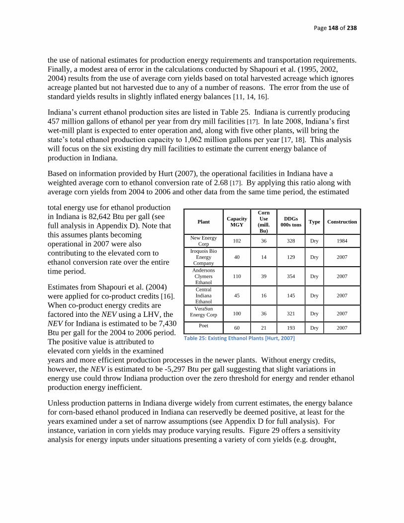
Page 148 of 238
the use of national estimates for production energy requirements and transportation requirements.
Finally, a modest area of error in the calculations conducted by Shapouri et al. (1995, 2002,
2004) results from the use of average corn yields based on total harvested acreage which ignores
acreage planted but not harvested due to any of a number of reasons. The error from the use of
standard yields results in slightly inflated energy balances [11, 14, 16].
Indiana‘s current ethanol production sites are listed in Table 25. Indiana is currently producing
457 million gallons of ethanol per year from dry mill facilities [17]. In late 2008, Indiana‘s first
wet-mill plant is expected to enter operation and, along with five other plants, will bring the
state‘s total ethanol production capacity to 1,062 million gallons per year [17, 18]. This analysis
will focus on the six existing dry mill facilities to estimate the current energy balance of
production in Indiana.
Based on information provided by Hurt (2007), the operational facilities in Indiana have a
weighted average corn to ethanol conversion rate of 2.68 [17]. By applying this ratio along with
average corn yields from 2004 to 2006 and other data from the same time period, the estimated
total energy use for ethanol production
in Indiana is 82,642 Btu per gall (see
full analysis in Appendix D). Note that
this assumes plants becoming
operational in 2007 were also
contributing to the elevated corn to
ethanol conversion rate over the entire
time period.
Estimates from Shapouri et al. (2004)
were applied for co-product credits [16].
When co-product energy credits are
factored into the NEV using a LHV, the
NEV for Indiana is estimated to be 7,430
Btu per gall for the 2004 to 2006 period.
The positive value is attributed to
elevated corn yields in the examined
years and more efficient production processes in the newer plants. Without energy credits,
however, the NEV is estimated to be -5,297 Btu per gall suggesting that slight variations in
energy use could throw Indiana production over the zero threshold for energy and render ethanol
production energy inefficient.
Unless production patterns in Indiana diverge widely from current estimates, the energy balance
for corn-based ethanol produced in Indiana can reservedly be deemed positive, at least for the
years examined under a set of narrow assumptions (see Appendix D for full analysis). For
instance, variation in corn yields may produce varying results. Figure 29 offers a sensitivity
analysis for energy inputs under situations presenting a variety of corn yields (e.g. drought,
Plant Capacity
MGY
Corn
Use
(mill.
Bu)
DDGs
000s tons Type Construction
New Energy
Corp 102 36 328 Dry 1984
Iroquois Bio
Energy Company
40 14 129 Dry 2007
Andersons
Clymers
Ethanol
110 39 354 Dry 2007
Central
Indiana Ethanol
45 16 145 Dry 2007
VeraSun
Energy Corp 100 36 321 Dry 2007
Poet 60 21 193 Dry 2007
Table 25: Existing Ethanol Plants [Hurt, 2007]

Page 149 of 238
flooding, etc.). This analysis indicates that once the corn yield reaches 130 bushels per acre,
energy expended during farm production of corn per gallon of ethanol will remain below 20,000
Btu per gallon. Further improvements in corn yield do not decrease the energy required for farm
production at any significant rate.
The findings of this study, however, are only for data averaged statewide and do not necessarily
mean each individual plant operating in the state is doing so with a positive NEV. For a plant
sited in a low yield county, as is the Poet plant in Jay County, energy balance will yield different
results. Note that each plant obtains corn for production in different manners, whether primarily
by truck or train, and the corn is shipped from varying locations. These logistical and
production-related issues introduce a greater degree of unknown variation in this localized result.
Optimally, energy balance research should be conducted using individual ethanol plants as the
unit of analysis. Until such time as sufficient data becomes available to provide such a localized
and specific analysis, a state-level approach must suffice.
57B8.6 Cellulosic Ethanol Literature Review Ethanol production from cellulosic crops requires individual analyses of each crop.
Unfortunately, few studies exist for each specific crop considered in the feedstock section of this
paper. Instead, what follows is a brief discussion of the available literature related to cellulosic
ethanol production, most of which is purely theoretical. Lynd (1996) identified a base case for
widespread cellulosic ethanol production energy efficiency and estimated efficiency ratios from
4.4 to 10.4, well above the threshold of 1.0 for a strict balance in energy availability and use in
production [19]. Hill et al. identified the efficiency ratio of cellulosic operations as being greater
than 4.0 and called it ―a major improvement over corn grain ethanol‖ and biodiesel [20]. A more
recent study from Schmer et al. (2007) found a NEV for switchgrass in the Great Plains to be
51,971 Btu/gal [21]. Test runs for switchgrass production showed a 0.71 efficiency ratio in the
first year of production, but the ratio became greater than one in the second year of production
and 14.42 by the fourth year [21]. The most
comprehensive of all cellulosic studies to
date estimates life-cycle efficiency ratios for
different types of cellulosic production
processes with all ratios greater than 15; the
study, however, assumes high yield
sorghum would be the primary feedstock
(Granda et al. 2007) [22]. While the authors
concede their estimates are likely slight
overestimates, the benefits relative to corn-
based ethanol in terms of energy appear
substantial. Regardless of the feedstock
used in ethanol production among the
aforementioned studies, the cellulosic
approach offers a definitively greater energy
0
10
20
30
40
50
60
0 50 100 150 200 250
Tho
usa
nd
s B
tu/G
all o
f Et
oh
Corn Yield (bu/acre)Figure 29: Yield Sensitivity Analysis for Energy Required in Indiana Corn Production
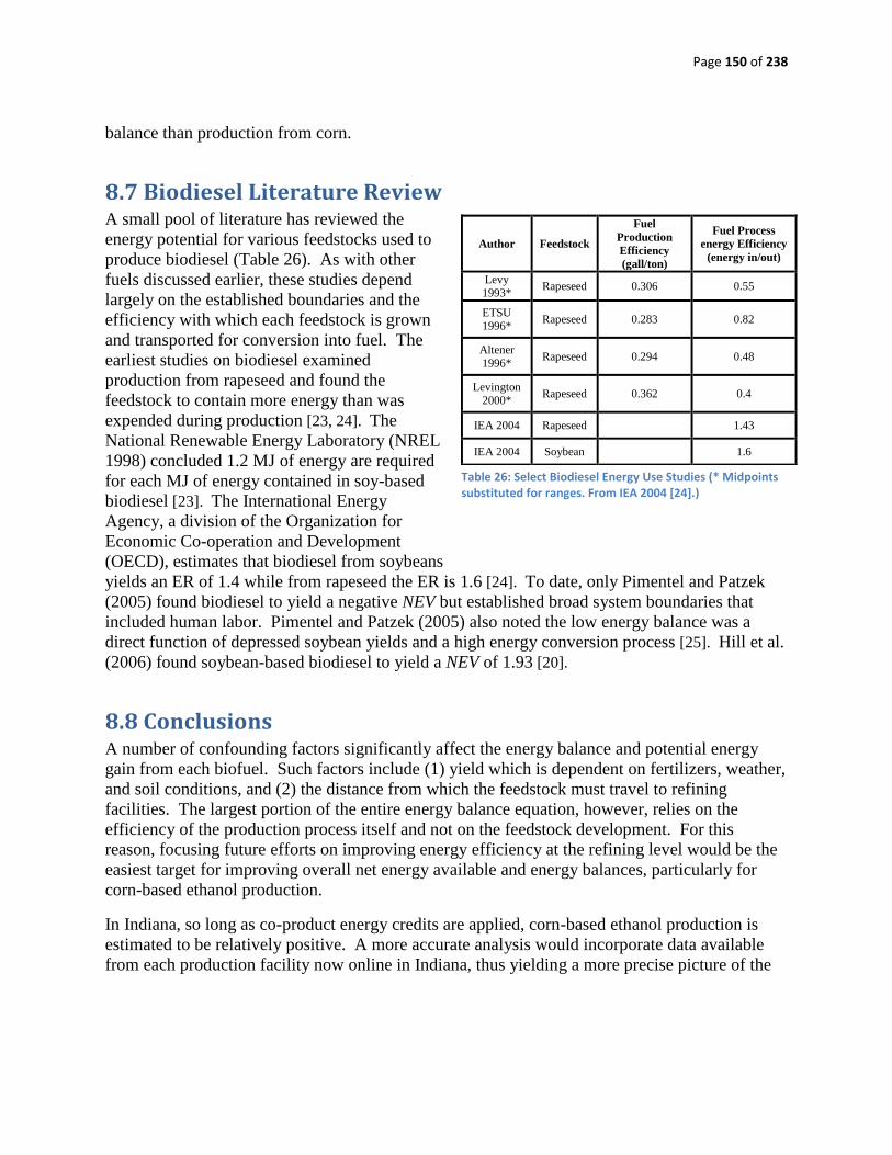
Page 150 of 238
balance than production from corn.
58B8.7 Biodiesel Literature Review A small pool of literature has reviewed the
energy potential for various feedstocks used to
produce biodiesel (Table 26). As with other
fuels discussed earlier, these studies depend
largely on the established boundaries and the
efficiency with which each feedstock is grown
and transported for conversion into fuel. The
earliest studies on biodiesel examined
production from rapeseed and found the
feedstock to contain more energy than was
expended during production [23, 24]. The
National Renewable Energy Laboratory (NREL
1998) concluded 1.2 MJ of energy are required
for each MJ of energy contained in soy-based
biodiesel [23]. The International Energy
Agency, a division of the Organization for
Economic Co-operation and Development
(OECD), estimates that biodiesel from soybeans
yields an ER of 1.4 while from rapeseed the ER is 1.6 [24]. To date, only Pimentel and Patzek
(2005) found biodiesel to yield a negative NEV but established broad system boundaries that
included human labor. Pimentel and Patzek (2005) also noted the low energy balance was a
direct function of depressed soybean yields and a high energy conversion process [25]. Hill et al.
(2006) found soybean-based biodiesel to yield a NEV of 1.93 [20].
59B8.8 Conclusions A number of confounding factors significantly affect the energy balance and potential energy
gain from each biofuel. Such factors include (1) yield which is dependent on fertilizers, weather,
and soil conditions, and (2) the distance from which the feedstock must travel to refining
facilities. The largest portion of the entire energy balance equation, however, relies on the
efficiency of the production process itself and not on the feedstock development. For this
reason, focusing future efforts on improving energy efficiency at the refining level would be the
easiest target for improving overall net energy available and energy balances, particularly for
corn-based ethanol production.
In Indiana, so long as co-product energy credits are applied, corn-based ethanol production is
estimated to be relatively positive. A more accurate analysis would incorporate data available
from each production facility now online in Indiana, thus yielding a more precise picture of the
Author Feedstock
Fuel
Production
Efficiency
(gall/ton)
Fuel Process
energy Efficiency
(energy in/out)
Levy 1993*
Rapeseed 0.306 0.55
ETSU
1996* Rapeseed 0.283 0.82
Altener
1996* Rapeseed 0.294 0.48
Levington 2000*
Rapeseed 0.362 0.4
IEA 2004 Rapeseed 1.43
IEA 2004 Soybean 1.6
Table 26: Select Biodiesel Energy Use Studies (* Midpoints substituted for ranges. From IEA 2004 [24].)

Page 151 of 238
actual energy required for the Indiana biofuels industry. As far as cellulosic and biodiesel energy
availability, little can be conclusively determined from the available information, particularly for
operations specific to Indiana. If the literature accurately portrays the situation in Indiana,
however, the energy balance for most cellulosic fuels and biodiesel is positive.

Page 152 of 238
60B8.9 References for Energy Balance of Biofuels [1] Oak Ridge National Laboratory. 2008.
Bioenergy Conversion Factors. Bioenergy
Feedstock Information Network (BFIN)
Administration Site. United States
Department of Energy (27 April 2008;
http://bioenergy.ornl.gov/papers/misc/energ
y_conv.html)
[2] North Dakota State University. 2003.
Biodiesel Fuel. AE-1240. North Dakota
State University Agricultural Extension (27
April 2008;
http://www.ag.ndsu.edu/pubs/ageng/machin
e/ae1240w.htm)
[3] Graboski M. 2002. Fossil Energy Use in the
Manufacture of Corn Ethanol. National Corn
Growers Association.
[4] Chambers RS, Herendeen RA, Joyce JJ,
Penner PS. 1979. Gasohol: Does it or doesn't
it produce positive net energy. Science
206.4420: 789-95.
[5] Ho SP. 1989. Global Warming Impact of
Ethanol versus Gasoline. National
Conference, Clean Air Issues and America's
Motor Fuel Business. Washington, DC.
[6] Marland G, Turhollow A. 1990. Co Sub 2
Emissions from Production and Combustion
of Fuel Ethanol from Corn: Oak Ridge
National Laboratory, United States
Department of Energy.
[7] National Agricultural Statistics Service.
2008. National Agricultural Statistics
Service. United States Department of
Agriculture (28 April 2008;
http://www.nass.usda.gov/)
[8] Pimentel D. 1991. Ethanol fuels: Energy
security, economics, and the environment.
Journal of Agricultural and Environmental
Ethics 4(1).
[9] Pimentel D. 2001. Limits of biomass
utilization." Encyclopedia of Physical
Science and Technology 2: 159-71.
[10] Pimentel D. 2003. Ethanol fuels: Energy
balance, economics, and environmental
impacts are negative. Natural Resources
Research. 12(2): 127-34.
[11] Shapouri H, Duffield JA, Graboski MS.
1995. Estimating the net energy balance of
corn ethanol. Agricultural Economic Report
271.
[12] Wang M, Saricks C, Wu M. 1999. Fuel-
Cycle Fossil Energy Use and Greenhouse
Gas Emissions of Fuel Ethanol Produced
from U.S. Midwest Corn. Argonne National
Laboratory, United States Department of
Energy.
[13] Wang M. 2002. Fuel choices for fuel-cell
vehicles: Well to wheels energy and
emission impacts. Journal of Power Sources
112.2002: 307-21.
[14] Shapouri H, Duffield JA, Wang M. 2002.
The Energy Balance of Corn Ethanol: An
Update. Office of the Chief Economist,
United States Department of Agriculture.
[15] Agriculture and Agri-Food Canada.
1999. Assessment of Net Emissions of
Greenhouse Gases From Ethanol-Gasoline
Blends in Southern Ontario. Prepared by
Engineering Ltd. #150-12791 Clarke Place,
Richmond, B.C. and (S&T) Consulting Inc.,
J.E. & Associates.
[16] Shapouri H, Duffield JA, McAloon A,
Graboski MS. 2004. The 2001 Net Energy
Balance of Corn-Ethanol. (28 April 2008;
http://www.ethanol-
gec.org/netenergy/NEYShapouri.htm)
[17] Hurt, C. Indiana Ethanol Plants. Lafeyette:
Purdue University, 2007.
[18] Abbott D. 2008. Fact Sheet: Biofuels Plants
in Indiana. Indiana State Department of
Agriculture.
[19] Lynd LR. 1996. Overview and evaluation of
fuel ethanol from cellulosic biomass:
Technology, economics, the environment,
Page 153 of 238
and policy. Annual Review of Energy and
the Environment 21: 403 - 65.
[20] Hill J, Nelson E, Tilman D, Polasky S,
Tiffany D. 2006. Environmental, economic,
and energetic costs and benefits of biodiesel
and ethanol biofuels. Proceedings of the
National Academy of Sciences 103(30):
11206-11210.
[21] Schmer MR, Vogel KP, Mitchell RB, Perrin
PK. 2008. Net energy of cellulosic ethanol
from switchgrass. Proceedings of the
National Academy of Sciences 105(2):465-
469.
[22] Granda CB, Zhu L, Holtzapple MT. 2007.
Sustainable liquid biofuels and their
environmental impact. Environmental
Progress 26(3): 233-50.
[23] National Renewable Energy Laboratory.
1998. Life Cycle Inventory of Biodiesel and
Petroleum Diesel for Use in an Urban Bus.
United States Department of Energy.
[24] International Energy Agency. 2004. Biofuels
for Transport: An International Perspective.
Paris: International Energy Agency(28 April
2008;
http://www.iea.org/textbase/nppdf/free/2004
/biofuels2004.pdf)
[25] Pimentel D, Patzek T. 2005. Ethanol
production using corn, switchgrass, and
wood; Biodiesel production using soybean
and sunflower. Natural Resources Research
14(1).

Page 154 of 238
9. Costs and Benefits of Biofuels
61B9.1 Introduction This report presents various economic, social, technological, and environmental considerations
associated with biofuels. To place these considerations in a more analytical context for Indiana,
analysts evaluated the costs and benefits associated with biofuels. The goal of this analysis is to
identify key drivers that influence the net present value (NPV) of different biofuels, and identify
the impacts on major stakeholders. Recognizing these drivers helps illustrate key concerns in
biofuels policy for the state. The accounting domain is Indiana for the analysis. The time frame
assessed is 2008 to 2030 for corn ethanol and soy biodiesel and 2012 to 2030 for cellulosic
ethanol. Future biofuels consumption is based on GAO projections of national fuel consumption
and a 2006 EPA analysis of current state biofuel consumption (see Appendix E) [1, 2]. Future
biofuels production is based on production capacity of current and planned biofuels plants as
outlined in a recent ISDA fact sheet [3].
The following sub-sections outline the methods, results, unquantified considerations, and
conclusions of analyses of three biofuels: corn ethanol, soy biodiesel, and cellulosic ethanol
using corn stover. Analysts present four different scenarios for each fuel type. The first scenario
is most indicative of the current situation in Indiana: the presence of substantial federal subsidies
and the absence of data on potentially significant environmental impacts. The second scenario
presents a case where federal subsidies are removed and environmental costs are still
unquantified. The third scenario brings federal subsidies back into the picture and adds a limited
number of quantified environmental costs to illustrate the substantial effect on NPV of adding
even one environmental cost consideration. Finally, the fourth scenario modifies the third
scenario by removing federal subsidies.
62B9.2 Methods The accounting domain for analysis is the state of Indiana; therefore, analysts only assessed
impacts that occur within Indiana and are directly related to biofuels production and
consumption in the state. Stakeholders evaluated Indiana government, gas stations, car
manufacturers (regarding E85 only), fuel consumers, agricultural producers, and fuel producers.
The baseline for the analysis compares Indiana biofuels production and consumption under the
parameters outlined in the introduction to a situation in which no biofuels are produced or
consumed in Indiana. It is important to note that the analysis does not directly compare the
production and consumption of biofuels as a direct alternative to conventional fuels. The fuel
types analyzed are blends of biofuels and fossil fuels.
The time frame of the analysis is 2008 to 2030 for corn ethanol and biodiesel, while the time
frame of the analysis for cellulosic ethanol is 2012 to 2030. Current lack of commercial
production and quickly evolving technology delay the time frame for cellulosic ethanol.

Page 155 of 238
Analysts derived per-unit and base values for the benefits and costs from many sources. Table
27 lists the original data employed and corresponding sources. It is important to note that data
included in this analysis may differ from data provided in other sections of the report. Though
data in other sections reflect the broad range of values presented in biofuels research, the data
employed here is in a format more suitable for use in a cost-benefit analysis. Analysts converted
this data to usable values on a variable basis taking the per-unit values and adjusting for inflation
based on the US Department of Labor (DOL) Consumer Price Index – All Urban Consumers [4].
Category Value / Units Source
Savings to Consumers of Gasoline $0.08 / gallon Rajagopal et al. 2007 [5]
Volumetric Ethanol Excise Tax Credit $0.51 / gallon GAO 2007 [1]
Federal Corn Subsidy $0.28 / bushel Farm Security and Rural Investment Act
of 2002 [6]
Ethanol Production Tax Credit $2M max for 40-60 million gallons; $3M max for at least
60 million gallons; $20M for at least 20 million gallons of
cellulosic
Farm Animal Stewardship Purchasing Act
of 2007 [9], Indiana Code 6-3.1-28 [10]
Price of Corn $3.30 / bushel Ag Answers 2007 [11]
Plant Cost - Ethanol $1.90 / gallon of production capacity Doering 2008 [8]
Production Cost - Ethanol $0.66 / gallon Doering 2008 [8]
Sale of By-product - Ethanol $0.38 / gallon Doering 2008 [8]
Transportation Cost - Ethanol $0.054 / gallon US EPA 2006 [2]
Soil Erosion $0.59 / pounds / gallon Sand 2006 [22]
Jobs 675 Abbott 2008 [3]
Opportunity Cost $3.00 / hour /40 hours week / 52 weeks / year Krutilla 2008 [14]
Taxes Paid $43,348 * .034 = $1,473.83 Indiana Department of Revenue 2008 [13]
Taxes to Federal Government $4,220 + 25% over $30,650 = $7,394.50 IRS 2006 [23]
Federal Biofuel Dispenser Tax Credit $30,000 GAO 2007 [1]
Minimal Modification $3,300 GAO 2007[1]
New Dispenser $13,000 GAO 2007 [1]
New Tank, Piping, etc. $62,400 GAO 2007 [1]
Retail Sales - Indiana Ethanol $1.58 / gallon Alexander 2007 [7]
Retail Sales - Exported to Other States $1.58 / gallon Alexander 2007 [7]
Federal Virgin Oil Per Gallon Subsidy $1.00 / gallon GAO 2007 [1]
Biodiesel Retailer Tax Credit $0.01 / gallon Indiana Code 6-3.1-27-10 [18]
Transportation Cost - Biodiesel $0.03 - $0.05 / gallon GAO 2007 [1]
Soybean Price $4.81 / gallon Doering 2008 [8]
Production Cost - Biodiesel $0.47 / gallon Radich 2004 [19]
Plant Cost - Biodiesel $1.04 / gallon Radich 2004 [19]
Retail Sales - Indiana Biodiesel $1.40 / gallon Althoff et al. 2003 [15]
Retail Sales - Exported Biodiesel $1.40 / gallon Althoff et al. 2003 [15]
Glycerin $0.25 / pound Howe 2008 [16]
Plant Cost - Cellulosic Ethanol $250M for 50 million gallon production capacity GAO 2007 [1]
Corn Stover $60 / metric ton Doering 2008 [8]
Production Cost $0.80 other costs + $0.40 enzymes = $1.20 / gallon Doering 2008 [8]
Sale of By-product - Cellulosic Ethanol $0.10 / gallon Doering 2008 [8]
Transportation Cost from Field $35.64 - $41.34 / dry ton Doering 2008 [8]
Reduced Emissions - E10 -1% Greenhouse gases GAO 2007 [1]
Reduced Emissions - E85 -20% Greenhouse gases GAO 2007 [1]
Reduced Emissions - Cellulosic Ethanol -70-90% Greenhouse gases GAO 2007 [1]
Reduced Emissions - Biodiesel -85% Greenhouse gases GAO 2007 [1]
Adjustment Costs for Cars - E85 $30-$300 GAO 2007 [1]
Dedicated Ethanol Pipeline $1M / mile GAO 2007 [1]
Indiana Alternate Fuel Vehicles Tax Credit 15% of investment Indiana Code 6-3.1-31.9 [25]
Firefighting Foam $90-$115 / 5 gallons Blank 2008 [24]
Average Wages for Ethanol Worker $43,348 / year Flanders and McKissick 2007 [12]
Table 27: Data Used in Cost-Benefit Analysis with Applicable Sources
Page 156 of 238
Analysts converted all values to January 2008 Dollars, applied low, medium, and high discount
factors typical in cost-benefit analysis literature to adjust for the time-cost of money, then
multiplied resulting values by the aggregated quantity of fuel and summed to find the net
adjusted, discounted value (See Appendix E for additional details on inflation adjustment and
discounting). Values employed in the analysis relate to gallons of biofuels in their pure form.
The analysis includes costs and benefits associated with different biofuels blends (for example
E10 vs. E85) in terms of 100 percent pure gallons of their constituent biofuels.
160B9.2.1 Corn Ethanol Benefits of both E10 and E85 blends of corn ethanol considered in the analysis include: savings
to consumers, volumetric ethanol excise tax credit, federal corn subsidy, and ethanol exports to
other states. Savings to consumers of gasoline represents the reduced cost of conventional
gasoline that results when biofuels compete with gasoline in the market. A University of
California – Berkley study estimates an inflation-adjusted $0.08 decrease in the 2006 average
price of gasoline when ethanol is added to the market [5]. The volumetric ethanol tax credit is
provided by the federal government to fuel producers at a value of $0.51 per gallon [1]. The
federal government also provides a corn subsidy of $0.28 per bushel of corn to agricultural
producers [6]. Since the accounting domain is limited to Indiana, the costs of credits and
subsidies to the federal government are outside the boundary of analysis. It follows that tax
credits and subsidies provided by the federal government appear as benefits in the analysis rather
than as transfers, the common classification for these elements in cost-benefit analyses. For the
final quantified benefit of exports of corn ethanol from Indiana, analysts multiplied the price of
one gallon of pure ethanol, estimated by Alexander at $1.58 per gallon, by the difference
between Indiana ethanol production and consumption estimates employed in this analysis [7].
Transfers employed in the analysis of E10 and E85 blends of corn ethanol include the sale of
fuel, the sale of byproducts, the state ethanol production tax credit, agricultural inputs, job
creation, and taxes paid. Analysts calculated the sale of ethanol fuel by multiplying the
Alexander figure of $1.58 per gallon by estimated Indiana corn ethanol consumption [7].
Analysts include the value as a transfer from fuel producers to consumers, without consideration
of the intermediate player - gas stations - in order to simplify the analysis. Doering estimates the
value of the sale of byproducts to consumers resulting from the production of corn ethanol as
$0.38 per gallon of ethanol produced [8]. This figure represents an average value taking into
consideration different potential byproducts that result from the various production processes
(for more information on these byproducts, see Section 5). The state ethanol production tax
credit is $0.125 per gallon of ethanol produced to a maximum of $2,000,000 per producer for the
two current or projected plants producing 40 to 60 million gallons of ethanol per year and
$3,000,000 per producer for the 13 plants producing 60 million gallons of ethanol or more [3, 9,
10]. Analysts used a Purdue University estimate of $3.30/bushel for the agricultural inputs [11].
The value of job creation encompasses an estimated 536 jobs created in corn ethanol production
facilities [3] multiplied by the average earnings of an ethanol plant employee including benefits,
$43,348, then adjusted for federal and state taxes to get the figure $34,479.67 [12]. Recipients of
jobs fall under the ―Consumer‖ stakeholder group. Fuel producers pay the corresponding wage
Page 157 of 238
cost. Finally, taxes paid are average state taxes paid by job recipients in the ―Consumer‖
stakeholder group to the Indiana government. The state of Indiana personal income tax is 3.4
percent [13].
Costs associated with E10 and E85 blends of corn ethanol include plant construction, the
additional capital cost associated with interest payments, fuel production costs, transportation
distribution costs, and worker leisure opportunity cost. Analysts employed a plant construction
cost estimate of $1.90 per gallon of ethanol produced and adjusted for production capacity and
an assumed 25-year useful life of each plant [8]. Analysts assumed fuel producers finance plant
construction entirely through borrowing, so employed a capital interest cost of $0.20 per gallon
of ethanol produced and again adjusted for production capacity [8]. Production costs of $0.66 per
gallon of ethanol produced include the costs associated with the corn ethanol production process,
like energy, water, maintenance and others [8]. Transportation distribution costs represent the
average freight cost for shipping corn ethanol from the production facilities to the gas stations.
EPA estimates this at $0.054 per gallon for the Indiana region [2]. Finally, the worker leisure
opportunity cost represents the value of the time given up by workers employed in the
production of biofuels. For simplification, analysts assumed that all workers enter the corn
ethanol production field from a state of unemployment and assign a time value of $3.00 per hour
for 40 hours per week and 50 weeks per year [14]. This is the standard figure employed in cost-
benefit literature.
Analysis of E85 blended form of corn ethanol requires additional considerations, including the
Federal Biofuel Dispenser Tax Credit as a benefit, and modifying existing equipment and
installing new equipment at gas stations as costs. Federal Biofuel Dispenser Tax Credit is
$30,000 to each gas station that provides E85. Recognizing that 97 gas stations in Indiana
currently provide E85 [1], but having no information on which gas stations plan to offer E85 over
the next 22 years, analysts assumed that the number would roughly double to 200 over the time
horizon of the analysis (see Appendix E). To provide E85, each gas station faces the additional
costs of modifying existing equipment ($3,300), installing new fuel dispensers ($13,000), and
installing new tanks and piping ($62,400) [1].
161B9.2.2 Soy Biodiesel Both common blends of biodiesel, B2 and B20, exhibit the same benfits, costs, and transfer
values. Benefits related to soy biodiesel include the Federal Biofuel Dispenser Tax Credit,
Federal Biodiesel Virgin Oil Subsidy, federal soybean subsidy, and soy biodiesel export. The
Federal Biofuel Dispenser Tax Credit of $30,000 is equivalent to the tax credit for corn ethanol
[1]. Recognizing that 61 stations in Indiana currently provide biodiesel [1], but having no
information on which stations plan to offer biodiesel over the next 22 years, analysts assumed
that the number would roughly double to 134 over the time horizon of the analysis (see
Appendix E)The Federal Biodiesel Virgin Oil Subsidy is $1.00 per gallon of biodiesel produced.
The federal government also provides a subsidy of $0.44 per bushel of soybeans to agricultural
producers [6]. For the quantified benefit of soy biodiesel exports from Indiana, analysts
multiplied the price of one gallon of pure biodiesel, estimated by Althoff et al. at $1.40 per
Page 158 of 238
gallon, by the difference between Indiana biodiesel production and consumption estimates
employed in this analysis [15].
Transfers include the sale of fuel, sale of byproducts, Indiana Biodiesel Production Tax Credit,
Indiana Biodiesel Retailer Tax Credit, job creation, taxes paid, and agricultural inputs. Analysts
calculated the sale of biodiesel by multiplying the Althoff et al. figure of $1.40 per gallon by
estimated Indiana biodiesel consumption [15]. The major soy biodiesel byproduct, glycerine,
sells at $0.25 per pound and the typical biodiesel plant produces 1100 pounds of glycerin an hour
[16]. To simplify, analysts included the value as a transfer from fuel producers to consumers,
without consideration of the intermediate player, gas stations. The Indiana Biodiesel Production
Tax Credit is $1.00 per gallon produced up to a maximum of $3,000,000 [17]. Analysts assumed
this subsidy would go to the two biodiesel plants in Indiana that opened in 2007 with capacities
of 3,000,000 gallons per year [3]. The state of Indiana provides gas stations with an Indiana
Biodiesel Retailer Tax Credit of $0.01 per gallon [18]. Job creation and taxes paid relevant to soy
biodiesel employ the same values as corn ethanol job creation, but adjusted for an estimated 134
jobs (see Appendix E) [3]. Analysts assumed soybean oil was the only agricultural input for
biodiesel. Analysts employed Doering‘s estimate of $0.65 per pound, converting pounds to
gallons and assuming one gallon of input oil for each gallon of biodiesel produced [8].
Costs associated with soy biodiesel include plant construction, capital interest cost, fuel
production costs, transportation distribution cost, and worker leisure opportunity cost. Analysts
employed a plant construction cost estimate of $1.04 per gallon of biodiesel produced and
adjusted for production capacity and an assumed 25-year useful life of each plant [19]. Analysts
assumed fuel producers finance plant construction entirely through borrowing and so employed a
capital interest cost of $0.20 per gallon of biodiesel produced adjusting for production capacity
[8]. Analysts used production costs of $0.47 per gallon [19]. Regarding transportation distribution
costs of biodiesel, trial runs of sending biodiesel through existing pipelines have been successful.
Analysts assumed this will be the major distribution method. GAO estimates an average piping
cost of $0.04 per gallon. Finally, the methodology for worker leisure opportunity cost was the
same as for corn ethanol [1].
162B9.2.3 Cellulosic Ethanol Cost, benefit, and transfer figures available for cellulosic ethanol are limited. The benefits
analysts employed are the Volumetric Ethanol Excise Tax Credit and cost savings from
byproduct use. The federal government provides the same $0.51 per gallon tax credit to
cellulosic ethanol producers as to corn ethanol producers. As an indirect benefit, lignin produced
in the cellulosic ethanol production process can be used by fuel producers as a heat source with a
value of $0.10 per gallon of ethanol produced [8].
Transfers considered in the analysis include the Indiana Ethanol Production Tax Credit,
agricultural inputs, and transportation of the feedstock. Indiana provides the same $0.125 per
gallon tax credit for cellulosic ethanol producers as corn ethanol producers, with a maximum tax
credit for all years of $20,000,000 per producer under 60 million gallon capacity. Because no
cellulosic ethanol plants currently operate in Indiana, analysts assumed that ten plants with 50

Page 159 of 238
million gallon capacity each would come into operation over the time frame. Analysts only
considered corn stover for cellulosic production. Corn stover costs $60 per ton [8]. The cost of
transporting corn stover from the field depends on the distance to the production facility.
Analysts assumed production facilities would be sited relatively near corn stover sources to
maximize efficiency. Analysts calculated a weighted average transportation cost of $37.23 per
dry ton of stover based on cost figures provided by Doering for various distances up to 45 miles.
Because the cost of transportation varies with distance, it was assumed that producers would first
buy corn stover close to the production facility (see Appendix E) [8].
Costs considered in the analysis include plant construction, capital interest costs, fuel production,
and transportation distribution. The GAO estimates plant construction costs at $250,000,000
spread over a 25-year useful life of each plant [1]. Doering estimates capital interest costs for
cellulosic ethanol at $0.55 per gallon produced [8]. Analysts employed a fuel production cost of
$1.20 per gallon produced, which includes elements used in production like enzymes, energy,
water, etc [8]. Transportation costs for cellulosic ethanol is the same as for corn ethanol.
63B9.3 Results As mentioned previously, analysts looked at four different biofuels scenarios. The first scenario
is most indicative of the current biofuels situation in Indiana: the presence of substantial federal
subsidies and the absence of data on potentially significant environmental impacts. The second
scenario presents a case where federal subsidies are removed and environmental costs are still
unquantified. The third scenario brings federal subsidies back into the picture and adds a limited
number of quantified environmental costs to illustrate the substantial effect on NPV of adding
even one environmental cost consideration. Finally, the fourth scenario modifies the third
scenario by removing federal subsidies. Table 28 provides a summary of each fuel under all four
scenarios.
A Kaldor-Hicks Tableau (KHT) illustrating the distributional effects of the first scenario is
included for each fuel type below. Analysts chose to present the first scenario, which excludes
environmental considerations, because value data for the vast majority of environmental impacts
do not exist. Environmental value
figures that do exist are presented and
analyzed later in this section. The
tableaus represent results achieved with
a seven percent discount rate, the most
conservative for this analysis.
163B9.3.1 Corn Ethanol A cost-benefit analysis of corn-based
ethanol blended into E10 results in a
positive NPV ranging from $19.8 to
$28.5 billion across discount rates
Fuel Type
r = .03 Scenario 1 Scenario 2 Scenario 3 Scenario 4
Ethanol E10 28,473$ 14,220$ 14,680$ 427$
Ethanol E85 28,469$ 14,216$ 14,676$ 421$
Biodiesel 2,826$ 370$ 2,826$ 370$
Cellulosic Ethanol (3,507)$ (4,790)$ (3,507)$ (4,790)$
r = .05
Ethanol E10 23,530$ 11,749$ 12,130$ 348$
Ethanol E85 23,527$ 11,746$ 12,126$ 343$
Biodiesel 2,367$ 319$ 2,367$ 319$
Cellulosic Ethanol (2,721)$ (3,716)$ (2,721)$ (3,716)$
r = .07
Ethanol E10 19,799$ 9,884$ 10,204$ 289$
Ethanol E85 19,796$ 9,881$ 10,201$ 284$
Biodiesel 2,019$ 279$ 2,019$ 279$
Cellulosic Ethanol (2,131)$ (2,911)$ (2,131)$ (2,911)$
* In millions of dollars
Scenario 1 No environmental costs included
Scenario 2 No federal subsidies and no environmental costs included
Scenario 3 Environmental cost included and federal subsidies included
Scenario 4 No federal subsidies and environmental cost included
Analysis of Costs and Benefits of Biofuels - Summary Results
Net Present Value
Table 28: Cost-Benefit Analysis of Biofuels Summary Table with variable discount rates (in millions of 2008 dollars)
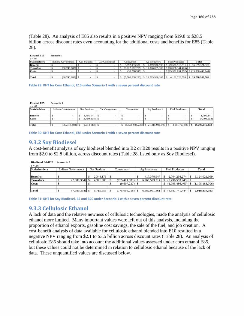
Page 160 of 238
(Table 28). An analysis of E85 also results in a positive NPV ranging from $19.8 to $28.5
billion across discount rates even accounting for the additional costs and benefits for E85 (Table
28).
Table 29: KHT for Corn Ethanol, E10 under Scenario 1 with a seven percent discount rate
Table 30: KHT for Corn Ethanol, E85 under Scenario 1 with a seven percent discount rate
164B9.3.2 Soy Biodiesel A cost-benefit analysis of soy biodiesel blended into B2 or B20 results in a positive NPV ranging
from $2.0 to $2.8 billion, across discount rates (Table 28, listed only as Soy Biodiesel).
Table 31: KHT for Soy Biodiesel, B2 and B20 under Scenario 1 with a seven percent discount rate
165B9.3.3 Cellulosic Ethanol A lack of data and the relative newness of cellulosic technologies, made the analysis of cellulosic
ethanol more limited. Many important values were left out of this analysis, including the
proportion of ethanol exports, gasoline cost savings, the sale of the fuel, and job creation. A
cost-benefit analysis of data available for cellulosic ethanol blended into E10 resulted in a
negative NPV ranging from $2.1 to $3.5 billion across discount rates (Table 28). An analysis of
cellulosic E85 should take into account the additional values assessed under corn ethanol E85,
but these values could not be determined in relation to cellulosic ethanol because of the lack of
data. These unquantified values are discussed below.
Ethanol E10 Scenario 1
r = .07
Stakeholders Indiana Government Gas Stations Car Companies Consumers Ag Producers Fuel Producers Total
Benefits -$ -$ -$ 3,697,933,521$ 1,889,920,996$ 29,571,516,811$ 35,159,371,328$
Transfers (30,740,888)$ -$ -$ (9,227,182,795)$ 19,326,065,109$ (10,068,141,426)$ -$
Costs -$ -$ -$ (38,788,949)$ -$ (15,321,651,792)$ (15,360,440,741)$
Total (30,740,888)$ -$ -$ (5,568,038,223)$ 21,215,986,105$ 4,181,723,593$ 19,798,930,586$
Ethanol E85 Scenario 1
r = .07
Stakeholders Indiana Government Gas Stations Car Companies Consumers Ag Producers Fuel Producers Total
Benefits -$ 1,795,141$ -$ -$ -$ -$ 1,795,141$
Costs -$ (4,709,254)$ -$ -$ -$ -$ (4,709,254)$
Total (30,740,888)$ (2,914,113)$ -$ (5,568,038,223)$ 21,215,986,105$ 4,181,723,593$ 19,796,016,473$
Biodiesel B2/B20 Scenario 1
r = .07
Stakeholders Indiana Government Gas Stations Consumers Ag Producers Fuel Producers Total
Benefits -$ 2,344,178$ -$ 417,378,647$ 2,704,298,274$ 3,124,021,099$
Transfers (7,989,364)$ 4,371,380$ (765,401,981)$ 6,265,573,214$ (5,496,553,249)$ -$
Costs -$ -$ (9,697,237)$ -$ (1,095,486,469)$ (1,105,183,706)$
Total (7,989,364)$ 6,715,558$ (775,099,218)$ 6,682,951,861$ (3,887,741,444)$ 2,018,837,393$
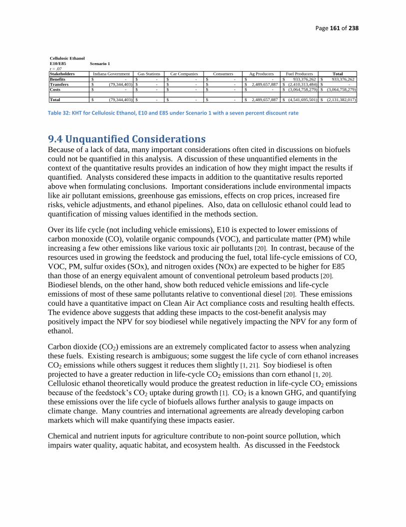
Page 161 of 238
Table 32: KHT for Cellulosic Ethanol, E10 and E85 under Scenario 1 with a seven percent discount rate
64B9.4 Unquantified Considerations Because of a lack of data, many important considerations often cited in discussions on biofuels
could not be quantified in this analysis. A discussion of these unquantified elements in the
context of the quantitative results provides an indication of how they might impact the results if
quantified. Analysts considered these impacts in addition to the quantitative results reported
above when formulating conclusions. Important considerations include environmental impacts
like air pollutant emissions, greenhouse gas emissions, effects on crop prices, increased fire
risks, vehicle adjustments, and ethanol pipelines. Also, data on cellulosic ethanol could lead to
quantification of missing values identified in the methods section.
Over its life cycle (not including vehicle emissions), E10 is expected to lower emissions of
carbon monoxide (CO), volatile organic compounds (VOC), and particulate matter (PM) while
increasing a few other emissions like various toxic air pollutants [20]. In contrast, because of the
resources used in growing the feedstock and producing the fuel, total life-cycle emissions of CO,
VOC, PM, sulfur oxides (SOx), and nitrogen oxides (NOx) are expected to be higher for E85
than those of an energy equivalent amount of conventional petroleum based products [20].
Biodiesel blends, on the other hand, show both reduced vehicle emissions and life-cycle
emissions of most of these same pollutants relative to conventional diesel [20]. These emissions
could have a quantitative impact on Clean Air Act compliance costs and resulting health effects.
The evidence above suggests that adding these impacts to the cost-benefit analysis may
positively impact the NPV for soy biodiesel while negatively impacting the NPV for any form of
ethanol.
Carbon dioxide (CO2) emissions are an extremely complicated factor to assess when analyzing
these fuels. Existing research is ambiguous; some suggest the life cycle of corn ethanol increases
CO2 emissions while others suggest it reduces them slightly [1, 21]. Soy biodiesel is often
projected to have a greater reduction in life-cycle CO2 emissions than corn ethanol [1, 20].
Cellulosic ethanol theoretically would produce the greatest reduction in life-cycle CO2 emissions
because of the feedstock‘s CO2 uptake during growth [1]. CO2 is a known GHG, and quantifying
these emissions over the life cycle of biofuels allows further analysis to gauge impacts on
climate change. Many countries and international agreements are already developing carbon
markets which will make quantifying these impacts easier.
Chemical and nutrient inputs for agriculture contribute to non-point source pollution, which
impairs water quality, aquatic habitat, and ecosystem health. As discussed in the Feedstock
Cellulosic Ethanol
E10/E85 Scenario 1
r = .07
Stakeholders Indiana Government Gas Stations Car Companies Consumers Ag Producers Fuel Producers Total
Benefits -$ -$ -$ -$ -$ 933,376,262$ 933,376,262$
Transfers (79,344,403)$ -$ -$ -$ 2,489,657,887$ (2,410,313,484)$ -$
Costs -$ -$ -$ -$ -$ (3,064,758,279)$ (3,064,758,279)$
Total (79,344,403)$ -$ -$ -$ 2,489,657,887$ (4,541,695,501)$ (2,131,382,017)$
Page 162 of 238
Agriculture section of this report, these problems contribute directly to eutrophication of surface
waters and degradation of groundwater. Soil erosion and resulting sedimentation also degrade
surface waters, and diminish soil quality. Runoff of agrichemicals and infiltration to
groundwater cause serious problems, which may require remedial action. The costs associated
with dredging large sediment deposits and treating contaminated well water play into these
considerations, but the overall contribution of agricultural practices in Indiana to these problems
remains uncertain. Cellulosic feedstocks discussed in this report provide the most optimistic
mitigation of these problems.
Since the market does not yet exist, many cellulosic ethanol impacts remain unquantifiable.
Some benefits of cellulosic ethanol may include additions to ethanol export, job creation, and
environmental benefits like reduced agricultural chemical use. Transfers may include state tax
breaks and fuel sales. Costs may include worker opportunity costs, soil erosion from corn stover
removal, and soil compaction. Data does not exist on the number of jobs that could be created,
the potential amount of cellulosic ethanol that may be added to the market, or even the ethanol
price that will result when cellulosic ethanol production begins. These values will only
materialize once cellulosic ethanol becomes competitive.
65B9.5 Discussion and Conclusions Care should be taken when formulating a comprehensive biofuels policy in Indiana. It was
impossible to incorporate all important considerations associated with biofuels into this analysis.
Biofuels may have unexpected consequences, such as the costs of equipment and training for
emergency responses to ethanol fires. The market for cellulosic ethanol is non-existent, and the
provision of E85 is still in its infancy, but the development of these markets will eventually
present clearer costs and benefits associated with them.
Necessary infrastructure adjustments and the demand for biofuels also remain highly uncertain.
Estimated costs for converting vehicles to flex fuel models that can utilize high ethanol blends
are $50-$300 per vehicle, but it is unclear to what extent this will happen [1]. Transportation
concerns will also become more important as increased traffic takes its toll on Indiana roads.
Future considerations are the expansion of railroads and the possibility of a dedicated ethanol
pipeline, but such ideas represent significant costs for the state. One study estimates the cost of
such a pipeline at $1,000,000 per mile [1]. In addition, Indiana provides two means of monetary
support to gas stations that provide E85: the Indiana Tax Credit for Fueling Stations and the
Indiana Gas Station Grant. Information was not available for these investments, but as markets
expand for higher ethanol blends, the associated transactions will certainly increase.
Other stakeholders will also face additional considerations outside of the scope of this analysis.
Consumers may hesitate to adopt ethanol blends such as E85 as a fuel source because of its
lower fuel economy. Agricultural producers have a strong tradition of corn and soybean rotation
and may need extra encouragement to gather corn stover or to plant other cellulosic crops.
Furthermore, the analysis does not include all potential stakeholders; for instance livestock
Page 163 of 238
producers, wheat and other commodity growers, and car manufacturers may be affected by
biofuels production and consumption. However, as an overall tool, the calculations presented
provide a good conceptual basis for the impacts on a variety of stakeholders and for a number of
different biofuels over the next 20 years.
166B9.5.1 Corn Ethanol The overall NPV of corn ethanol is positive across all discount rates for two primary reasons:
federal subsidies/tax breaks and ethanol exports. Exports are an especially key consideration and
could benefit Indiana substantially in the long-term. However, Indiana should consider the
impact of future removal of federal corn and ethanol subsidies on the state. Recalling the
discussion in the Methods sub-section, federal subsidies appear in the analysis as benefits
because they are transfers entering from outside the accounting domain. The NPV of corn
ethanol, E10 at a seven percent discount rate decreases from $19,799 million to $9,884 million
when federal subsidies are removed (Table 28). Additionally, the state of Indiana is projected to
pay over 35 million dollars (NPV) in tax breaks over the next 20 years. Indiana policy makers
must decide whether this is sustainable.
Agricultural and fuel producers are the real winners in the corn ethanol analysis, benefiting from
tax breaks, subsidies, high crop prices, the sale of byproducts, and high fuel prices. Consumers,
on the other hand, show an extremely negative NPV. The negative NPV for consumers is
primarily due to the purchase of products like fuel and animal feed (from byproducts). Their
negative NPV represents the value they receive from using these goods. Even though the impact
of jobs in the analysis is large, ethanol production is a small business compared to other
industries and will not create a relatively large number of new jobs in the state.
Additional costs and benefits of E85 primarily affect gas stations through tax credits, grants, and
capital modification costs. The impact of the cost of preparing gas stations to provide E85
results in a negative NPV for gas station owners (Note: the profit margin from selling fuel was
not included in the analysis). Consequently, if policy makers decide to promote E85 in the state,
they should be aware that gas station owners may need greater incentives to add E85 to their
stations. Indiana could make efforts to reduce the substantial costs of retrofitting gas stations for
E85 use.
The very limited environmental costs available have a huge effect on the NPV of corn ethanol,
namely the cost of soil erosion (see Appendix E for more details) [22]. Looking at Table 2,
moving from Scenario 1 to 3 in the analysis of corn ethanol, E85 at a seven percent discount
level results in a decrease in NPV from $19,796 to $10,201 million. This leads to two
conclusions: first, efforts to reduce soil erosion could be a major cost saver in regards to corn
ethanol; second, environmental impacts can significantly affect the value of biofuels and warrant
extensive additional research.
167B9.5.2 Soy Biodiesel As with corn ethanol, the overall NPV of biodiesel is positive primarily due to exports and
federal incentives. The NPV of soy biodiesel at a seven percent discount rate decreases from
Page 164 of 238
$2,019 million to $279 million when federal subsidies are removed. Again, Indiana policy
makers must be conscious of the effects of removing federal support. Another policy concern is
the state will pay 10 to 12 million dollars (NPV) in tax breaks over the next 20 years for
biodiesel.
While agricultural producers are substantially benefitting in the biodiesel analyses, fuel
producers experience negative net values. If this continues to be the case, fuel producers will no
longer be willing to produce soy biodiesel. Redirecting tax credits from gas stations to fuel
producers or finding ways to reduce the cost of soybean oil could mitigate the effect on fuel
producers. One potential way to reduce the cost of soybean oil is to encourage alternative
sources, like waste oil or rapeseed, which may compete with and drive down the price of
soybeans.
The negative NPV consumers experience for biodiesel also results from their purchases, but
again this is a proxy for their value derived. Gas stations experience positive values with
biodiesel compared to corn ethanol because no equipment modifications are required and
existing pipelines can be used for biodiesel transportation. Note that the data set employed did
not include any figures for environmental impacts of biodiesel. Hence the NPVs in Table 2 do
not change for biodiesel when moving from Scenario 1 to Scenario 3.
168B9.5.3 Cellulosic Ethanol As mentioned previously, it is difficult to quantify many of the parameters of interest for
cellulosic ethanol. Cellulosic ethanol production should lead to greater greenhouse gas
emissions reductions. However, collection of corn stover may also lead to greater erosion and
soil compaction from harvesting [8]. Substantial research is needed to quantify these and other
effects. Incorporating the quantified values into an analysis will significantly clarify the value of
cellulosic ethanol.
For cellulosic ethanol to be economically viable, efficiency gains through technological advances
must be made in the fuel‘s production process. Several considerations make the future of
cellulosic ethanol look promising: the replacement of food-based crops with dedicated biomass
crops, the effect of removing federal subsidies, and the potential gains in energy balance. In
addition, there are less environmental impacts associated with cellulosic sources (aside from corn
stover) in comparison with corn and soy. It is difficult to tell whether quantifying these
considerations will bring cellulosic ethanol into the positive NPV range, but prospects seem
promising. There is huge potential for expanded production if competitive production
technology is developed.

Page 165 of 238
66B9.6 References for Costs and Benefits of Biofuels [1] Government Accountability Office. 2007.
DOE Lacks a Strategic Approach to
Coordinate Increasing Production with
Infrastructure Development and Vehicle
Needs. GAO-07-713.
[2] United States Environmental Protection
Agency. 2006. Renewable Fuel Standard
Program, Draft Regulatory Impact Analysis.
EPA420-D-06-008.
[3] Abbott D. 2008. Fact Sheet: Biofuels Plants
in Indiana. Indiana State Department of
Agriculture.
[4] United States Department of Labor. 2008.
Bureau of Labor Statistics. Consumer Price
Index – All Urban Consumers 1913-Present.
(16 Apr. 2008;
ftp://ftp.bls.gov/pub/special.requests/cpi/cpi
ai.txt)
[5] Rajagopal D, Sexton SE, Roland-Holst D,
Zilberman D. 2007. Challenge of biofuel:
filling the tank without emptying the
stomach? Environmental Research Letters 2:
1-9.
[6] Farm Security and Rural Investment Act of
2002. Pub. L. No. 107–171.
[7] Alexander C. 2007. Indiana agriculture.
Indiana Business Review 82(4).
[8] Doering O. 4 March 2008. Economic
Perspectives on producing liquid fuels from
plant feedstocks. Indiana University
Memorial Union. Bloomington, IN.
[9] Farm Animal Stewardship Purchasing Act
of 2007. H.R. 1726.
[10] IND. CODE § 6-3.1-28 (2008).
[11] Ag Answers: If the Option Exists, It's Better
to Put Soybeans in the Bin. 2007. Purdue
University, Lafayette, IN (24 Mar. 2008;
http://www.agriculture.purdue.edu/agcomm/
aganswers/story.asp?storyID=4606)
[12] Flanders A, McKissick J. 2007. Economic
Impact of Cellulosic Ethanol Production in
Treutlen County. Center for Agribusiness
and Economic Development, University of
Georgia. CR-07-07.
[13] Indiana Department of Revenue. 2008. Tax
Types / Various Rates. (24 Mar. 2008;
http://www.in.gov/dor/taxtypes/)
[14] Krutilla K. 21 February 2008. Cost-Benefit
Analysis. Lecture. School of Public and
Environmental Affairs, Indiana University,
Bloomington, IN.
[15] Althoff K, Ehmke C, Gray AW. 2003.
Economic analysis of alternative Indiana
state legislation on biodiesel. Center for
Food and Agricultural Business Report,
Purdue University.
[16] Howe R. 15 February 2008. Personal
Communication. Integrity Biofuels Plant,
Morristown, Indiana.
[17] IND. CODE § 6-3.1-27-8 (2008).
[18] IND. CODE § 6-3.1-27-10 (2008).
[19] Radich A. 2004. Biodiesel Performance,
Costs, and Use. Energy Information
Administration, United States Department of
Energy (24 Mar. 2008;
http://www.eia.doe.gov/oiaf/analysispaper/b
iodiesel/)
[20] Hill J, Nelson E, Tilman D, Polasky S,
Tiffany D. 2006. Environmental, economic,
and energetic costs and benefits of biodiesel
and ethanol biofuels. Proceedings of the
National Academy of Sciences 103.30:
11206-11210.

Page 166 of 238
[21] Pimentel D. 2003. Ethanol fuels: energy
balance, economics, and environmental
impacts are negative. Natural Resources
Research 12(2): 127-134.
[22] Sand D. 2006. Erosion Cost for Grant
Bioenergy. Iowa Natural Heritage
Foundation.
[23] Internal Revenue Service. 2006. Federal Tax
Rate Schedules. United States Department
of Treasury.
[24] Blank C. 2008. Ethanol fire risk: fires
require special firefighting foam. Associated
Press. 26 Feb 2008.
[25] IND. CODE § 6-3.1-31.9 (2008).

Page 167 of 238
10. Policy Recommendations
67B10.1 Federal Policy Recommendations Biofuels policy at the federal level focuses on promoting research, development, and deployment
of new technologies for production and distribution, as well as creating incentives for the
production and consumption of biofuels. Federal policy is not a coherently coordinated set of
initiatives, but rather a patchwork of different agency initiatives created by several statutes
passed during the last decade. These initiatives include grants, tax credits, and research
initiatives to encourage development of new technologies, bioenergy crop production, and
expansion of the biofuels distribution network. This section identifies the major federal agencies
that administer programs related to biofuels and explains the key federal initiatives and tax
incentives aimed at promoting the production, distribution, and use of cost-competitive biofuels.
169B10.1.1 Federal Agencies The Office of Energy Efficiency and Renewable Energy (EERE) is a $1.25 billion agency
located within DOE. EERE has jurisdiction over R&D for most renewable energy sources,
including solar, wind, geothermal, biomass, and hydroelectric. EERE programs work closely
with the US National Laboratories, where a great deal of alternative energy research takes place.
The EERE Biomass Program is the center of DOE efforts related to research, development, and
demonstration of biofuels technology. The mission of the Biomass Program is ―to develop and
transform our domestic, renewable, and abundant biomass resources into cost-competitive, high
performance biofuels, bioproducts, and biopower through targeted research, development, and
delivery leveraged by public and private partnerships [1].‖ There are three major budgetary
components of the program, including:
o Feedstock Infrastructure—to support the development and reduce the cost of
biomass resources for energy use
o Platforms R&D—to support the conversion of biomass feedstocks into cost-
competitive energy sources
o Utilization of Platform Outputs Research, Development and Delivery—to test the
network of technologies for development, production, and distribution of biomass
energy sources [2].
IRS has jurisdiction of the administration of the US federal tax code including federal tax credits
and exemptions. The Tax Policy subsection below lists and describes biofuels-related tax
incentives.
Several offices in USDA also oversee programs related to federal biofuel policy. The
Agricultural Research Service (ARS) manages over 1,000 research programs including the
Bioenergy and Energy Alternatives National Program [3]. The Office of Rural Development
(ORD) oversees the Bio-based Products and Bioenergy Program, which finances development of
technologies used to convert biomass into energy, and the Rural Development Business and
Cooperative Program offers guaranteed loans to businesses for this purpose [4].

Page 168 of 238
EPA has regulatory oversight for some energy programs, including the Renewable Fuel Standard
(RFS). EPA administers the Biodiesel Emissions Analysis Program to research the air pollution
effects of various blends of biodiesel [5]. EPA works with DOE to coordinate some federal
studies. Other federal studies, such as the Sugar Cane Ethanol Pilot Program established by the
Energy Policy Act of 2005 (EPACT), are under the exclusive jurisdiction of EPA [6].
170B10.1.2 Grants for Research, Development, and Demonstration The federal government funds the majority of R&D related to biofuels, especially advanced
biofuels(renewable fuels other than ethanol derived from corn starch). Funding mechanisms
include grants to R&D bodies and public-private ventures that develop new technologies, and
financial assistance to local government entities for the purchase of items that further an
advantage in the biofuels industry.
EPACT directs DOE to establish a competitive grant pilot program through the Clean Cities
Program for the provision of grants to state and local governments that purchase alternative fuel
vehicles [7].
The Energy Independence and Security Act of 2007 (EISA) authorized $25,000,000 in biofuels
R&D grants for states with low ethanol production and $50,000,000 in grants for cellulosic
ethanol and biofuels research [8, 9]. EISA also expands certain R&D provisions of EPACT to
include cellulosic and other feedstocks that are less resource and land intensive when converted
to fuels. Additionally, the University-Based Research and Development Grant Program
authorized $25,000,000 in competitive grants for institutions of higher education to conduct
renewable energy R&D [10].
171B10.1.3 Federal Research and Studies The federal government conducts a great deal of R&D pertaining to biofuels. These projects can
take place in the National Laboratories, the National Academies of Science, and within federal
departments like DOE and USDA. The goals of this research are diverse and include studies on
biocrop development, the efficiency of production and refinement techniques, best practices for
increasing fuel efficiency, increasing the use of certain biobased products, etc.
EPACT directs DOE and USDA to steer R&D efforts towards the development of technologies
that facilitate the conversion of cellulosic biomass to biofuels [11]. EISA requires DOE to submit
to Congress a report detailing the challenges involved with increasing biodiesel consumption in
the US [12]. EISA also requires DOE to study the feasibility of commercial applications that
increase the energy efficiency of bio-refinery facilities and develop retrofit technologies that
would allow existing bio-refineries to process different forms of biomass, including ligno-
cellulosic feedstocks [13]. Another requirement directs DOE to study the effects of various
biodiesel blends on the performance and durability of engines [14].
172B10.1.4 Federal Procurement Policy Procurement is a very powerful tool the federal government can utilize to shape policy. The
Energy Policy Act of 1992 requires federal agencies to purchase alternative-fuel vehicles for the
federal fleet. As of 1999, 75 percent of the federal fleet must be alternative-fuel vehicles [15].
Page 169 of 238
173B10.1.5 Federal Goal Setting The federal government encourages producers and consumers to invest voluntarily in greater
production and consumption of biofuels through goal setting. EPACT established RFS, which
set a national goal of producing 7.5 billion gallons of renewable fuels by 2012 [16]. EISA
amended EPACT 2005, doubling the 2012 target to 15.2 billion gallons and setting the 2022
target at 36.0 billion gallons. EISA also mandates that 2.0 billion gallons of the target be met
with advanced biofuels by 2012, and 21.0 billion gallons by 2022. This act also set targets for
cellulosic biofuels and biomass-based biodiesel [17].
174B10.1.6 Federal Tax Policy and Guaranteed Loan Programs Federal legislation has established several tax credits for biofuels production. These tax
incentives are designed to decrease the consumer cost of biofuels, making them more cost-
competitive with traditional fuels. The Small Ethanol Producer Tax Credit (SEPTC) was first
introduced in the 1990 Omnibus Budget Reconciliation Act and was strengthened by the JOBS
Act and EPACT. Any facility with a production capacity of less than 60 million gallons is
eligible for a $0.10 per gallon tax credit for the first 15 million gallons produced annually. This
credit is also limited to one credit per owner (owning multiple facilities does not entitle multiple
credits) [18].
EPACT establishes the Small Agri-Biodiesel Producer Tax Credit, which offers an income tax
credit to producers of agri-biodiesel (biodiesel created exclusively from virgin oils). This small
producer credit is also $0.10 per gallon annually for the first 15 million gallons of qualified agri-
biodiesel. The same production capacity limitations of the Small Producer Credit apply to this
credit [19].
The 2004 JOBS Act created the Volumetric Excise Tax Credit (VEETC) to replace the existing
ethanol tax credit. VEETC offers a $0.51 per gallon credit for ethanol mixtures [20].
EPACT also establishes a credit for the installation of alternative fuel stations under which
taxpayers can claim up to a 30 percent credit for the cost of installing clean-fuel vehicle refueling
equipment. This credit is limited to $30,000 per station [21].
At the time of this report, the 2007 Farm Bill is considering loan guarantees for the construction
of biofuels production and refinement facilities. Half of the loan guarantees would cover loans
of less than $100 million and half would cover loans up to $250 million [21].
68B10.2 Indiana Policies and Laws Regarding Biofuels The state incentive package for Indiana biofuels currently focuses on production and retail tax
credits. These types of policies work together with infrastructure grants, government purchase of
biofuels, goal setting, promotion and education, and biofuels research. However, the current mix
of state policies lacks the ability to move Indiana towards the next phase of cleaner biofuels
development.

Page 170 of 238
175B10.2.1 Production Tax Credits Ethanol
Indiana provides an ethanol production tax credit to producers of $0.125 per gallon. Of Midwest
states offering ethanol production tax credits, Minnesota, Missouri, and South Dakota all offer
$0.20 per gallon while Iowa, Illinois, and Ohio all lack a production tax credit [27, 28].
This tax credit applies to both cellulosic and grain ethanol. The total amount of credit per
producer varies depending on the amount of ethanol produced.
For production of 40-60 million gallons of grain ethanol, a maximum credit of $2 million
is available.
For production of 60+ million gallons of grain ethanol, a maximum credit of $3 million is
available.
For production of 20+ million gallons of cellulosic ethanol, a maximum credit of $20
million is available [29].
Biodiesel
The Indiana Biodiesel Production Tax Credit gives $1 per gallon of pure biodiesel produced in
Indiana [23]. In order to receive the tax credit, the producer must file an application with the
Indiana Economic Development Corporation (IEDC) [23]. The amount of the tax credit cannot
exceed $3 million dollars per year, unless approved by the IEDC [24]. Upon IEDC approval, the
credit can be extended up to $5 million dollars per year [24].
The state also provides a production tax credit of $0.02 per gallon of blended biodiesel produced
in Indiana, and biodiesel producers who use their own fuel do not have to pay the $0.16 per
gallon license tax, provided that it is a blend of at least 30 percent [25, 26].
176B10.2.2 Retailer Tax Credits Retailers distributing E85 can receive a credit of $0.18 per gallon against the state Gross Retail
Tax, up to a maximum of $1 million [29]. Retailers distributing blended biodiesel can receive a
credit of $0.01 per gallon; however, this credit is contingent upon annual state funding [30].
177B10.2.3 Infrastructure Grants ISDA administers Indiana infrastructure grants and limits them to E85 fueling stations.
Individual grants of up to $20,000 are available for new E85 fueling stations or the retrofitting of
existing equipment [31]. This is an increase from the previous maximum available grant of
$5,000 and is intended to promote E85 pumps along the I-65 corridor [32]. ISDA approves grant
applications and allocates a total of $1 million to fueling stations and municipal governments
[33].
178B10.2.4 Government Use Ethanol
For gasoline-fueled vehicles, government entities are required to use an ethanol blend of at least
ten percent whenever possible [34]. Executive Order 05-21 (2005) mandates that state fleet
vehicles based in Indianapolis use E85 (if capable) [35].

Page 171 of 238
Political subdivisions (municipal corporations or other special taxing districts) can receive a
monthly incentive payment for using E85 in FFVs equal to $33.33 per vehicle. However, the
vehicles must have been purchased in the last five years [26].
Biodiesel
Government entities are required to use a blend of at least two percent biodiesel whenever
possible [34]. Indiana also sets purchasing requirements for state government and state
educational institutions [37]. The purchasing requirements are specified by price preference. For
example, if a price preference of ten percent is set, the state is required to purchase biofuels that
cost less than ten percent more than the alternative. Indiana sets a price preference of ten percent
for purchases by governmental bodies and state educational institutions for fuels that are at least
20 percent biodiesel, or ―are primarily esters derived from biological materials, including
oilseeds and animal fats, for use in compression and ignition engines [37].‖
179B10.2.5 Goal Setting While not clearly aimed at changing policy, goals set by Indiana have the power to impact future
policies. ISDA completed a strategic plan in 2004 that details ethanol and biodiesel production
and use goals through 2025. The plan aims for 300 million gallons of ethanol production by
2010 and 350 million gallons by 2025. The plan also sets goals for ten percent ethanol usage (as
a percent of total fuel usage) by 2010 and 20 percent by 2025. Additionally, the plan calls for
100 million gallons of biodiesel production by 2010, and biodiesel usage (as a percent of total
fuel usage) of 20 percent by 2025 [38].
Indiana has also signed onto the Energy Security and Climate Stewardship Platform Plan
(ESCSPP) with Iowa, Kansas, Michigan, Minnesota, Ohio, South Dakota, and Wisconsin. While
the plan sets many goals for the region, it is unclear how large a role Indiana will play in
implementing each goal. ESCSPP sets goals to have commercially available cellulosic ethanol
by 2012, increase the availability of E85 to 15 percent of stations by 2015, ―reduce the amount of
fossil fuel that is used in the production of biofuels 50 percent by 2025,‖ and to have ―by 2025,
at least 50 percent of all transportation fuels consumed by the Midwest [to] be from regionally
produced biofuels and other low-carbon transportation fuels [23].‖
180B10.2.6 Promotion and Education Indiana‘s biofuels promotion and education is limited to efforts undertaken by ISDA. ISDA is
charged with promoting E85 to retailers, auto manufactures, and consumers [39].
181B10.2.7 Research The federal government exclusively funds nearly all government research on biofuels. However,
the state of Indiana does have limited research and planning efforts underway, including the
Environmental Quality Service Council (EQSC), Biomass Feasibility Study Grant Program,
Twenty-First Century Research and Technology Fund, and a Strategic Energy Plan for Biofuels.
Indiana established EQSC to conduct studies and produce findings and recommendations
concerning the implementation of EPACT‘s RFS [40]. As of 2008, EQSC has failed to produce
any findings or recommendations, but has requested that the Indiana Sustainable Energy
Commission (ISEC) be convened to make recommendations on state policies over the next five,

Page 172 of 238
ten, 20, 50, and 100 years. Similarly, EQSC also requested that the director of ISDA prepare a
comprehensive biofuels plan for the next ten, 20, and 50 years. Thus far, neither of these
agencies has produced recommendations for the state [41, 42].
Indiana‘s Office of Energy and Defense Development (OED) operates the Biomass Feasibility
Study Grant Program, which offers $100,000 to qualifying applicants for research related to the
conversion of biomass to energy [43]. The Indiana Twenty-First Century Research and
Technology Fund provides grants and loans for alternative fuel technologies, provided that they
support economic development [44].
In 2006, OED released Indiana‘s Strategic Energy Plan also known as ―Hoosier Homegrown
Energy.‖ The plan encourages the growth of Indiana‘s economic sector through the development
of electricity, natural gas, and transportation fuels. Governor Daniels envisions Indiana as ―the
nation‘s biofuels capital‖ and calls for cellulosic ethanol R&D as a way to move beyond grain
ethanol [45]. Governor Daniels also encourages investment by the private sector in development
of biofuels plants and infrastructure with support from the state through tax incentives, loan
guarantees, and regulation [45].
69B10.3 Indiana’s Biofuels Incentives and the Dormant Commerce
Clause As noted above, Indiana has adopted both tax and non-tax incentives to support the state‘s
growing biofuels industry. It is likely that Indiana will continue to offer several of its current
incentives into the future, and will create new incentives to encourage new technologies and
support emerging trends. However, because Congress has specifically been granted power to
regulate interstate commerce, dormant Commerce Clause issues arise when state-created
incentives demonstrate favoritism towards in-state actors. This section will provide background
information on the development of the dormant Commerce Clause and an analysis of how the
dormant Commerce Clause applies to Indiana‘s current biofuels incentive schemes.
Additionally, this section will offer several incentives options to states that may overcome the
dormant Commerce Clause hurdle.
182B10.3.1 The Dormant Commerce Clause: An Introduction Through the Commerce Clause, the US Constitution grants Congress the power ―[t]o regulate
Commerce . . . among the several states [46].‖ In addition to granting Congress the power to
regulate interstate commerce, the Commerce Clause also restricts the states‘ power to regulate if
the regulations ―place[]an undue burden on interstate commerce [47].‖ This restrictive doctrine is
known as the dormant Commerce Clause (DCC). The Court has explained:
The [DCC], directly limiting the States‘ power to
discriminate against interstate commerce, prohibits
economic protectionism - that is, regulatory measures
designed to benefit in-state economic interests by
burdening out-of-state competitors. Thus, state statutes that
clearly discriminate against interstate commerce are
Page 173 of 238
routinely struck down . . . unless the discrimination is
demonstrably justified by a valid factor unrelated to
economic protectionism [48].
If a state regulation or tax discriminates against interstate commerce on its face or by intent
based on in-state or out-of-state distinctions, a ―strict scrutiny‖ standard is applied [49]. In such a
circumstance, the likelihood of invalidation is great (unless the state is able to present a strong
and legitimate state interest that can be advanced in a no less burdensome manner) [49]. If a state
is acting under its normal jurisdiction and is not discriminating based on geographic location, but
the state action creates a discriminatory burden on interstate commerce, courts apply a balancing
test that weighs the state‘s interest against the burden on commerce [49]. If the state‘s interest
outweighs the burden on commerce, the action will be deemed constitutional [49].
Not only does the DCC prevent states from enforcing direct prohibitions (e.g., taxes, tariffs, or
regulations) that discriminate against interstate commerce, it also prevents states from
effectuating certain incentives that have discriminatory effects [49]. While the Supreme Court has
made clear that states are able to use tax systems and subsidies to encourage economic
development, it has also invalidated tax incentives and subsidies with that purpose because the
incentives discriminated against out-of-state investments and activities [47]. For example, in
Westinghouse Electric Corporation v. Tully, the Court held that a New York tax credit for a new
type of corporate entity was unconstitutional because New York tied the amount of the credit to
the amount of export activity occurring within New York [50]. The result was that if the
corporate entities increased export activity within New York, they received larger tax credits [50].
The Court found that New York‘s efforts to encourage local economic activity discriminated
against interstate commerce [50].
The Court has generally analyzed incentives differently, depending on whether the incentives are
tax based (e.g., credits, exemptions, or abatements) or non-tax based (e.g., cash grants, loans and
financing, etc.).
230B10.3.1.1 Tax Incentives
The Supreme Court has clearly established that a state is prohibited from creating a
discriminatory sales or use tax on out-of-state products to benefit in-state producers or to lure
industries into constructing in-state facilities [51]. Additionally, the Court has held that certain
state tax incentives are unconstitutional if they discriminate against the free flow of interstate
trade. In New Energy Co. of Indiana v. Limbach, Ohio created a motor fuel tax credit for each
gallon of ethanol sold as part of gasohol [48]. However, the credit only applied if the ethanol was
produced in Ohio or in a state providing reciprocal tax credits to ethanol produced in Ohio [48].
The Court explained that the tax credit was ―in effect, taxing a product made by [Indiana]
manufacturers at a rate higher than the same product made by Ohio manufacturers, without . . .
justification for the disparity [48].‖ The Court held that the Ohio tax scheme facially
discriminated against out-of-state producers, and thus, interstate commerce, by differentiating
between in-state and out-of-state producers [48].
10.3.1.2 Non-Tax Incentives
Although the Court held in New Energy Co. that discriminatory tax credits are unconstitutional,
the Court also stated that ―direct subsidization of domestic industry does not ordinarily run afoul

Page 174 of 238
of [the discriminatory action] prohibition‖ under the DCC [48]. This ―loophole‖ for direct
subsidization results from two factors: (1) the market participant exemption and (2) the general
allowance of cash subsidies.
This first factor is the market participant exemption, a Court doctrine that exempts a state from
the DCC limitation when the state is deemed a market participant [47]. The exemption was
applied in Hughes v. Alexandria Scrap Corp., where the court upheld Maryland‘s abandoned
automobile processing subsidy program, which required less-stringent documentation
requirements for in-state processors [52]. The Court explained that Maryland had entered the auto
hulk market to increase the price of auto hulks, and that such actions can be distinguished from
―[interference] with the natural functioning of the interstate market either through prohibition or
through burdensome regulation [52].‖ As a result, if a state enters the market (e.g., buying or
selling goods), it can constitutionally create the same locally beneficial results as it might
through a discriminatory—and likely unconstitutional—tax or tax incentive. This exception
promotes the idea that states should have a choice in how they allocate their resources when
carrying out state business activities and demonstrates recognition of state independence in
economic development [47].
The second factor is simply that the Court has thus far refused to consider invalidation of
discriminatory cash subsidies to in-state industries [51]. While the Court has noted that it has
―never squarely confronted the constitutionality of subsidies,‖ it has mentioned direct payment
subsidies in dicta on several occasions [53]. In New Energy Co., the Court mentioned Indiana‘s
cash subsidy program for in-state ethanol producers as an alternative to Ohio‘s tax credit. Justice
Scalia noted that although the Indiana scheme may have been as equally discriminatory as the
Ohio scheme, ―[t]he Commerce clause does not prohibit all state action designed to give its
residents an advantage in the marketplace, but only action of that description in connection with
the State’s regulation of interstate commerce [48].‖ Additionally, such subsidies were mentioned
in South-Central Timber Development, Inc. v. Wunnicke, and in C & A Carbone, Inc. v Town of
Clarkston, although neither case spoke directly to the subsidy [54, 55].
However, a caveat exists in West Lynn Creamery v. Healy. In that case, Massachusetts required
every milk dealer selling in Massachusetts to pay a ―premium payment‖ into the ―Massachusetts
Dairy Equalization Fund [53].‖ The amount paid in was determined by the amount of milk sold in
the state. On a monthly basis, the fund‘s proceeds were distributed to in-state milk producers in
shares proportionate to the producers‘ in-state production of raw milk [53]. While out-of-state
producers paid into the fund, they were ineligible to receive producer payments taken out of the
fund [53].
The Court held Massachusetts‘s subsidy to be unconstitutional, stating that ―the imposition of a
differential burden on any part of the stream of commerce--from wholesaler to retailer to
consumer--is invalid, because a burden placed at any point will result in a disadvantage to the
out-of-state producer [53]. Although the direct burden (the premium payment) placed on
producers appeared to burden equally in-state and out-of-state producers, the combination of the
payment with the in-state producer subsidy offset the burden placed on in-state producers. The
Court explained that while a ―pure subsidy‖ coming out of the general revenue ―poses no burden
on interstate commerce‖ and is an acceptable means of assisting local business, the

Page 175 of 238
Massachusetts payment and subsidy scheme was equal to an ―ordinary tariff‖ on out-of-state
producers [53].
183B10.3.2 Indiana’s Current Biofuels Incentives: A Cause for Concern? As the section on Indiana‘s policies and laws regarding biofuels describes, Indiana currently has
several tax-based incentives directed at the promotion of biofuels. These incentives are primarily
focused on in-state production, and due to that focus, raise several red flags when considered in
light of the DCC.
The Biodiesel Production Tax Credit, which is equal to $1 per gallon of Indiana-produced
biodiesel used to create blended biodiesel, can be applied to state tax liability [56]. State tax
liability is a taxpayer's total tax liability that is incurred under the state gross retail and use tax,
the adjusted gross income tax, the financial institutions tax, and the insurance premiums tax [56].
Indiana also provides a blended biodiesel production credit for blended-biodiesel producers in
the state [25]. The credit is equal to $0.02 per gallon of blended biodiesel produced in Indiana,
and may be applied to the state gross retail and use tax, the adjusted gross income tax, the
financial institutions tax, and/or the insurance premiums tax [25].
A third production-based tax credit is Indiana‘s Ethanol Production Tax Credit. This credit,
similar to the biodiesel production tax credit, provides a tax credit to ethanol production facilities
located in Indiana [57]. The credit is equal to $0.125 per gallon of ethanol produced at an Indiana
facility, and it is made available to two types of facilities: (1) those able to produce 40 million
gallons of ethanol per year, and (2) pre-existing facilities that increase their capacity by at least
40 million gallons per year [57, 58].
As noted above, incentives based on geographic location have never fared well under the
dormant Commerce Clause. The Indiana biodiesel production credit, the blended biodiesel
production tax credit, and the ethanol production tax credit are all provided only to in-state
biofuels producers. If an out-of-state producer of either biodiesel or ethanol is subject to one or
more of the Indiana state taxes noted under the applicable sections of the Indiana Code,
providing the biodiesel and ethanol tax credits solely to in-state producers is facially in violation
of the DCC. Because the tax credits favor local producers, they all have the potential to
overburden out-of-state producers by taxing them at effectively higher rates than the in-state
biodiesel and ethanol producers receiving the credit. Much like the tax credit in New Energy
Co., the Indiana tax credits, if litigated, would likely be found to ―explicitly deprive[] certain
products of generally available beneficial tax treatment because they are made in certain other
States, and thus on [their] face [the tax incentives] appear[] to violate the cardinal requirement of
nondiscrimination [48].‖
While Indiana has not appropriated funds for corn-based ethanol or biodiesel production in
recent years, a tax credit is still available for in-state cellulosic ethanol production. If cellulosic
ethanol production increases in the future and a national or Midwest market emerges, there is no
doubt that frequent interstate sales transactions (especially between Indiana and its bordering
states) will take place. In such a circumstance, if an out-of-state producer determines that the
burden caused by the discriminatory tax credit outweighs the burden imposed by undertaking
litigation against Indiana, a lawsuit is likely to result.
Page 176 of 238
184B10.3.3 Assessing the Future Indiana‘s reasoning behind its in-state biodfuels tax credits seems evident. Indiana has entered
the race to become a national biofuels leader, and by offering only in-state tax incentives,
Indiana hopes to: (a) influence the location decisions of potential biofuels producers (with the
ultimate goal of luring potential producers to invest in in-state production facilities), (b) increase
the competitiveness of local producers by reducing their tax burden, and therefore, their overall
cost, or (c) both [51].
If Indiana is solely attempting to influence producer location decisions, constitutionality aside,
the state may want to reconsider the soundness of the ―smokestack chasing‖ approach.
Empirical data and business executive surveys demonstrate that location decisions are more
frequently based on the state‘s business climate and other state advantages such as ―wages,
employee skill levels, availability of raw materials, strength of markets, and regulatory
stringency [47].‖ Alternatively, if two states offer competing subsidies, each subsidy may offset
the other, causing producers to make the decision it would have if neither subsidy were offered
[51].
However, if all other factors between two states are equal and subsidies are not, it is possible for
a subsidy to serve as a ―tie-breaker‖ in location decisions [51]. If that is the case or if the state is
attempting to make local production more competitive (or both), the Court, while not providing a
direct decision to rely on, seems to have provided states with two ways to maneuver around the
DCC. The first is non-coercive tax incentives and the second is non-tax incentives. Additionally,
a state can advocate for Congress to enact legislation that allows a state to provide subsidies that
interfere with interstate commerce, thus, circumventing the DCC problem.
231B10.3.3.1 Non-Coercive Tax Incentives
In every case in which the Court has invalidated a tax incentive, the tax incentive has held
coercive power. This means that the tax incentive had the ability to force an entity to pay a
higher effective tax to the taxing state unless the entity located the respective
operation/transaction in-state [59]. Essentially, in the invalidated cases, the state was saying:
You are already subject to our taxing power because you
engage in taxable activity in this state. If you would like to
reduce your tax burdens, you may do so by directing
additional business activity into this state. Should you
decline our invitation, we will continue to exert our taxing
power over you as before, and your tax bill might even go
up [59].
Although many tax incentives hold coercive power, there are some that do not. These include
tax incentives ―framed not as exemptions from or reductions of existing state tax liability but
rather as exemptions from or reductions of additional state tax liability to which the taxpayer
would be subjected only if the taxpayer were to engage in the targeted activity in the state [59].‖
An example of such an incentive would be a real property tax exemption for new construction.
When offering a non-coercive tax incentive, the state essentially says: ―Come to our state and
we will not saddle you with any additional property tax burdens. Moreover, should you choose
not to accept our invitation, nothing will happen to your tax bill - at least nothing that depends on

Page 177 of 238
our taxing regime [59].‖ By utilizing non-coercive tax incentives rather than coercive tax
incentives, states such as Indiana may be able to achieve the same goals while potentially
avoiding DCC constitutionality issues.
232B10.3.3.2 Non-Tax Incentives
An additional way to sidestep DCC problems may be to avoid utilizing a tax scheme all together.
Rather, a state can provide non-tax incentives to business entities it favors, such as biofuels
producers. As earlier noted, non-tax subsidies such as ―direct payment subsidies, funded out of
the general treasury, supply of infrastructure, provision of low-interest loans, assistance in job-
training or recruitment, and granting of land, are largely immunized from dormant Commerce
Clause scrutiny [51].‖ By focusing on non-tax incentives, a state can still encourage local
economic development and favor certain businesses or industries, but it significantly reduces its
chances of being held in violation of the DCC. Additionally, by focusing on non-tax incentives,
a state may be able to further develop some of the other factors businesses consider when making
location decisions, such as labor force training or the provision of land located near biofuels
crops of choice.
233B10.3.3.3. Congressional Action
Congressional consent is another safeguard for states wishing to implement subsidies that burden
interstate commerce. Through a grant of authority, Congress can allow discriminatory subsidies,
such as tax credits, to stand, despite their violation of the DCC. For example, EPACT explicitly
authorizes tax incentives for coal mined in a state if the state utilizes clean coal technologies,
stating such incentives shall ―be considered a reasonable regulation of commerce; and . . . not be
considered to impose an undue burden on interstate commerce or to otherwise impair, restrain, or
discriminate, against interstate commerce [60].‖ If Indiana is able to secure congressional consent
for in-state cellulosic ethanol production tax incentives, Indiana will no longer be in danger of
being held in violation of the DCC.
234B10.3.3.4 Conclusions
State-offered incentives can provide Indiana with a means to encourage growth and development
in biodiesel and ethanol; however, Indiana needs to consider incentive design implications to
ensure that the incentives will withstand DCC scrutiny. While the courts do not take issue with
in-state promotion of economic development, they will quickly invalidate any tax, regulation, or
incentive that burdens interstate commerce by discriminating against out-of-state entities. By
carefully designing incentive schemes to avoid DCC restrictions, or by securing Congress‘s
approval, Indiana can provide the biofuels incentives necessary to ―Fuel Indiana‘s Future.‖

Page 178 of 238
70B10.4 Federal Recommendations
185B10.4.1 R&D Push for Widespread Commercialization of Corn Stover
Cellulosic Ethanol Rationale Behind Proposal
Corn stover is Indiana‘s best cellulosic biofuels option for the foreseeable future. Indiana is one
of the nation‘s top corn producers; therefore, utilizing the by-product from current harvesting
techniques is both preferable and efficient. However, as stated earlier, corn stover cellulosic
ethanol is not yet available for widespread commercial production. Therefore, it is important to
infuse the R&D community with funding, so it can further refine the corn stover cellulosic
ethanol process.
Proposal
Indiana‘s Washington delegation should introduce legislation that encourages increased short-
term (two to three years) funding for corn stover cellulosic commercialization so that the process
can become a significant contributor to the US energy portfolio over the next 20 years. Indiana
senators and representatives should lobby for funding in one of two ways:
Specifically draft legislation that provides funding incentives for private
entrepreneurial entities that conduct corn stover commercialization R&D.
Create federal-state pilot programs that build corn stover cellulosic ethanol facilities
that fine-tune the enzyme, production, and transportation processes so that corn stover
cellulosic ethanol can become a cost-effective energy option for Indiana in the
immediate future.
186B10.4.2 Conservation Reserve Program Modifications Rationale Behind Proposal
As crop prices have risen, fueled by increased demand for corn and other bioenergy crops, many
farmers have incentive to remove lands from CRP and place them into agricultural production.
Some interest groups have proposed allowing farmers to leave CRP contracts early in order to
grow bioenergy crops such as corn.
Proposal
The federal government should not encourage the removal of land from conservation programs.
Many of these lands are marginal for crop growth or contain sensitive ecosystems and wildlife
populations. Instead, federal efforts should focus on high-energy yield crops, such as
switchgrass, that represent the future of the biofuels market and preclude further CRP
encroachment.
There are several proposals to create such a reserve program. At this time, the House version of
the 2007 Farm Bill includes a Biomass Energy Reserve Program (BER) [61]. This program
would establish a biomass energy reserve ―to encourage production of dedicated energy crops in
a sustainable manner that protects the soil, air, water, and wildlife of the United States…‖
(renewable fuels other than ethanol derived from corn starch) [61]. The program offers financial
Page 179 of 238
support and technical assistance to landowners who wish to produce crops for the bioenergy
industry. Though the bill language identifies sustainability as a priority, it does not specify land
and crop eligibility requirements.
The National Wildlife Federation‘s Biofuels Innovation Program proposal (BIP) is similar to
BER and identifies the specific land and crop types that are eligible under the program. BIP
would allow up to five million acres of land to be placed under the control of the Natural
Resources Conservation Service (NRCS) in order to establish a base of support for advanced
biomass energy production. Farmers would submit a proposal that identifies the characteristics
and amount of land to be enrolled under the program, as well as the type and mix of crops.
Farmers will be eligible for a range of incentives including reimbursement for costs related to
converting the land and incentive payments for growing certain crops. BIP prioritizes those
proposals having the greatest benefits to the environment, bioenergy crop production, and crop
diversification.
187B10.4.3 Use Energy Frontier Research Centers to Advance Cellulosic
Biofuels Rationale Behind Proposal
The newly modified RFS calls for the production of 36 billion gallons of biofuels annually by
2022 [62]. Congress expects that 21 billion gallons of this amount will consist of advanced
biofuels (renewable fuels other than ethanol derived from corn starch), of which 16 billion
gallons will be derived from cellulosic biofuels [62, 63]. Moreover, these biofuels must satisfy
greenhouse emissions standards based on lifecycle studies which consider all emissions resulting
from fuel production, from field to tank, including emissions from changes in land use [63]. As a
result, the Office of the Biomass Program (OBP) within Department of Energy (DOE) is striving
to make the production of cellulosic ethanol cost competitive by 2012, a goal which has been
endorsed by Governor Daniels [64, 65].
Meeting EISA goals will require the joint efforts of federal and state governments, industrial and
agricultural communities, and finance and business entrepreneurs. Coordination of
multidisciplinary scientific and engineering expertise from academia and the National
Laboratories will be critical to building a strong technology foundation. Programs within DOE
are therefore entering partnerships with industry, academia and the National Laboratories in
order to leverage their resources [8, 9, 66, 67, 68].
Proposal
DOE‘s Office of Basic Energy Sciences (BES) recently announced that it plans to establish
Energy Frontier Research Centers (EFRCs) ―to accelerate the rate of scientific breakthroughs
needed to create advanced energy technologies for the 21st century [69].‖ BES expects that an
annual $2-5 million will be available during an initial five-year period, after which, $100 million
will be available for multiple EFRC awards starting in 2009. BES will issue a Funding
Opportunity Announcement (FOA) during FY2008 to request applications [69].
The research program of an EFRC applicant must have several ―distinguishing attributes.‖ An
example of a ―research focus area‖ which would meet BES expectations is how biological feed
Page 180 of 238
stocks are converted into portable fuels, specifically research into the cause of current
―bottlenecks‖ in cellulosic biofuels production [69].
188B10.4.4 Biodiesel from Alternative Forms of Biomass Rationale Behind Proposal
Like ethanol, biodiesel production enjoys government subsidies and tax credits that make it price
competitive with petroleum-based diesel. Nevertheless, there are only a few alternatives for the
diesel fuel and, consequently, only a relatively small market exists for biomass-derived biodiesel
from oil seed crops such as soybeans or rapeseed, or from waste oils.
Moreover, biodiesel from these feedstocks has significant drawbacks. Soy crops need relatively
high amounts of insecticides and fertilizers while producing, per acre, only one-sixth the amount
of biofuel produced from corn ethanol (See Section 4.3). Biodiesel from soy and rapeseed may
cause engine problems with blends higher than 20 percent. Waste oil may contain impurities that
create emissions which are detrimental to the environment. As a result, it remains unlikely that
biodiesel from these feedstocks will substantially displace the use of conventional biodiesel [70].
However, just as cellulosic ethanol represents a more promising long-term alternative to gasoline
than corn-based ethanol, newer technologies are emerging that can produce clean low-sulfur
synthetic diesel fuels from alternative forms of biomass and other organic materials. One of the
more promising technologies can utilize a wide variety of organic wastes as feedstocks [70].
Proposal
Because drivers are unlikely to notice any detrimental impact, Indiana should encourage use of
B20 in all vehicles throughout the state. However, Indiana should provide funding and
incentives towards research and investment in technology for converting biomass and organic
wastes into high-quality, environmentally sound, and economically lucrative diesel fuels which
are compatible with existing vehicle technologies and can be readily integrated into existing
distribution infrastructure.
189B10.4.5 Closing CAFE Standards Loopholes for E-85 Vehicles Rationale Behind Proposal
The federal government‘s CAFE program currently provides credits to auto manufacturers for
producing dual-fuel vehicles that run on conventional gasoline as well as unconventional fuels
such as ethanol. The purpose of these incentives is to support the use of alternative fuels that
decrease carbon emissions. In reality, however, there is little consumer demand for these
vehicles; the vehicle engines are less efficient than conventional engines, and many consumers
never use alternative fuels in them [71].
Proposal
Because there is insufficient demand for alternative fuels, the result of the CAFE dual fuel credit
is lower overall fuel economy for vehicle fleets [72]. The Government Accountability Office has
recommended in several reports to Congress that CAFE be eliminated. The federal government
Page 181 of 238
should not offer incentives for the production of dual-fuel vehicles at this time. This ―dual-fuel
loophole‖ should be closed until there is sufficient demand for alternative fuels.
190B10.4.6 Funding for Comprehensive Environmental Assessments at
University Research Centers and Institutes Rationale Behind Proposal
Beneficial and detrimental environmental effects are among the most important qualitative
factors that must be considered in Indiana‘s assessment of biofuels. However, few studies have
been conducted to quantify or comprehensively analyze the environmental impacts of biofuels.
Major areas of uncertainty include, but are not limited to, the following;
o The pollution impacts of cellulosic ethanol production facilities (e.g., emissions,
effluent discharges, etc.)
o Indiana‘s carbon inventory and how land use changes resulting from biofuels
production affect state carbon storage and emissions
o The extent and value of CO2 emission reductions from biofuels engines compared
to their fossil fuel counterparts
o The invasive potential of biofuels crops
o The extent to which various biofuels blends (including E10 and E85) would
provide environmental benefits
Proposal
Federal funding should be directed to university research centers and institutes to model,
measure, valuate, and comprehensively analyze the environmental impacts of biofuels in Indiana
within a time period of five years. By obtaining and analyzing these data, economic analyses of
biofuels in Indiana will provide more realistic and reliable results that can be used to inform
long-term biofuels investment and policy decisions.
71B10.5 State Recommendations
191B10.5.1 Statewide Financial Incentives for Corn Stover Cellulosic Ethanol Rationale Behind Proposal
The market for corn stover ethanol is only emerging, and if Indiana desires to be a national
leader in this sector, the state must create an economically favorable landscape for
entrepreneurial businesses. Since Indiana has comparative advantages in geography and
climate, it should provide financial incentives to lure corn stover cellulosic ethanol producers to
the state. The goal is to promote corn stover ethanol as an integral part of the state‘s energy
portfolio. Since the state believes that corn ethanol and biodiesel are ready to compete in a
market without special incentives, incentives for corn stover cellulosic ethanol may be allotted
from currently funded fuel initiatives.

Page 182 of 238
Proposal
Although cellulosic ethanol from corn stover is not yet cost effective on a large scale, Indiana
should legislate proactively by 2009 to ensure the state is prepared to support this technology.
Indiana‘s General Assembly should therefore, pass the following measures:
Subsidize property tax exemptions for the first corn stover and the first combination corn
stover/switchgrass cellulosic ethanol plants built in Indiana. Localities, driven by
potential job creation, will vigorously compete for the new plants, and private
entrepreneurial companies will be able to select optimal locations for their facilities.
Encourage the growth of corn stover cellulosic ethanol production by transferring all
remaining production credit incentives from biodiesel to corn stover initiatives.
Additionally, the General Assembly should appropriate additional production credit
funding opportunities for corn stover cellulosic ethanol (above and beyond the transferred
funds), thus signaling that corn stover ethanol is clearly in the best interests of Indiana‘s
long-term future.
192B10.5.2 Standardized Safety Procedures for Ethanol and Biodiesel
Infrastructure and Distribution Rationale Behind Proposal
Ethanol and biodiesel are volatile substances that are flammable or explosive at ambient
pressures and temperatures [73]. Ethanol vapors travel easily through the air and biodiesel vapors
travel easily through water. Both have the potential to cause fires and explosions. A biodiesel
fire requires the use of foam or dry chemicals, and higher ethanol blends such as E85 require the
use of alcohol-resistant foams [74].
Best management practices (BMPs) that include safety procedures and emergency response
plans can help reduce the incidence of fires or explosions. BMPs regarding storage, containment
areas, and safety precautions are needed to ensure these volatile substances will not cause harm.
The state should develop safety material, formulate emergency procedures, designate emergency
program teams, and coordinate emergency response. Indiana has no mandate for best
management safety procedures concerning ethanol and biodiesel facilities, distribution
infrastructure (such as terminals and tankers), or distribution facilities (i.e., gasoline stations).
Proposal
The state of Indiana should mandate BMPs in all ethanol and biodiesel production facilities,
distribution infrastructure, and distribution facilities. The BMPs should focus on accident
prevention and safety techniques. BMPs will help to reduce the likelihood of fires and
explosions and ensure personnel and infrastructure are properly equipped and trained to handle
an emergency situation.
193B10.5.3 Best Management Practices Outreach and Implementation on
Indiana’s Farmland Rationale Behind Proposal
Indiana‘s ground and surface waters will be detrimentally affected by changing land use patterns
associated with increased biofuels production. Potential negative consequences include

Page 183 of 238
increased sedimentation, increased nutrient loading from fertilizer usage, and greater water
toxicity resulting from increased pesticide, herbicide, and fungicide inputs (See Section 4.5.6).
To mitigate the detrimental effects of land use change, Indiana farmers must utilize BMPs such
as integrated pest management, riparian buffer zones, winter cover crops, no-till farming,
diversified agricultural landscapes, and nutrient management (See Section 4.5.6). Such practices
must not only be promoted by state officials. Indiana farmers should also receive training on
how to implement and sustain BMPs.
Proposal
Indiana should develop an outreach, education, and implementation program for BMPs on its
agricultural acreage. This program should be undertaken by a state organization that already has
a well-developed presence in the agriculture industry and a working relationship with Indiana
farmers. Potential organizations include the Purdue University Cooperative Extension Service or
Indiana‘s Soil and Water Conservation Districts. If additional incentive is required, the state can
provide performance subsidies to farmers utilizing BMPs that result in short-term economic
losses (e.g., lower yields, increased inputs, etc.). By establishing BMPs throughout Indiana, the
detrimental effects of sedimentation, increased chemical inputs, and poor soil quality will be
significantly reduced and the long-term health of Indiana‘s farmland will be maintained.
194B10.5.4 Switchgrass Buffer Strips Bordering Riparian Zones on Indiana
Croplands Rationale Behind Proposal
The growth of cellulosic feedstocks (such as perennial grass) results in significant water quality
benefits over corn ethanol production. By encouraging production of cellulosic crops on
marginal lands—such as those immediately adjacent to riparian zones—Indiana will receive
substantial water quality benefits, and the state will have a supply of feedstocks to accommodate
cellulosic production facilities once the technology becomes commercially viable.
Proposal
Indiana should mandate that a certain portion of riparian cropland acreage near Indiana waters
(e.g., 30 ft. from the ordinary high water mark) be taken or left out of crop production.
Additionally, a supplemental program should be developed that allows farmers with land falling
under the mandate to enroll in a program, similar to CRP, that pays farmers rent for planting
portions of the mandated acreage in punctuated switchgrass strips. A state department or
organization such as ISDA should establish program specifications best able to preserve stream
bank integrity, protect riparian biodiversity, allow wildlife access to water supplies, and promote
the growth and harvesting of cellulosic feedstocks in Indiana.
195B10.5.5 E10 Retailer Tax Credit of $0.02 per Gallon Against the State Gross
Retail Tax Rationale Behind Proposal
E10 should be encouraged in Indiana because it is a blended fuel that all vehicles can use, in
contrast to E85. E10 can be sold at the retail level without retrofitting or installing new
infrastructure. E10 only requires that fuel storage tanks be cleaned, and this can be done at

Page 184 of 238
minimal cost. The current producer incentive for E85 is a credit of $0.18 per gallon against the
State Gross Retail Tax [29].
Proposal
This proposal seeks to increase the amount of E10 sold within the state of Indiana. By providing
retailers a credit against the state gross retail tax, retailers will be encouraged to clean tanks and
increase the availability of E10.
This incentive is favorable to an E10 mandate because it gives retailers flexibility. Retail
mandates implemented in Hawaii, Minnesota, Missouri, Montana, and Oregon offer limited
exemptions for retailers and unreasonably force the market towards E10. By offering E10
incentives, retailers may choose on an individual basis whether or not it is economically efficient
to offer E10.
ISDA estimates that the state will produce more than one billion gallons of ethanol after
construction of the six new plants is complete. This is more than enough ethanol for the entire
state of Indiana to offer E10, and still retain export capability.
72B10.6 Creating an Atmosphere in Support of Biofuels Successful policy entrepreneurs realize that ―windows of opportunity‖ play an important role in
determining which policy issues become a priority for the public (first) and lawmakers (in
response to public demand). Public, private, and nonprofit parties with a vested interest in
Indiana biofuels proliferation therefore face two options: 1) wait for a window of opportunity to
present itself, or 2) take an active role in creating the window of opportunity. Since it is
impossible to predict the former, stakeholders should take action and persuade the public that
biofuels proliferation is a top priority for the state. Creating a favorable political landscape for
biofuels proliferation is a multi-stage process. To realize maximum success, the Governor‘s
Office should wholeheartedly adopt the following coalition building and marketing plan that
promotes biofuels proliferation as one of the most important statewide issues by 2009.
196B10.6.1 Building a Reputable Coalition There are currently dozens of public, private, and non-profit organizations within Indiana that
have a vested interest in the proliferation of biofuels. With the exception of the Biofuels Indiana
Initiative (a six-organization coalition with little influence), there have been no significant
attempts to build a public-private biofuels coalition that would be able to effectively disseminate
information to consumers, lawmakers, farmers, and producers. Therefore, the Governor‘s Office
should initiate the formation of the Hoosier Homegrown Energy Coalition.
The Hoosier Homegrown Energy Coalition will serve as the organization that disseminates a
unified message regarding the proliferation of biofuels. The Coalition will be a public-private
partnership that unites Indiana‘s stakeholders in order to create a successful biofuels industry
with supportive consumers, lawmakers, farmers, and producers. The Coalition will be
responsible for the creation and implementation of a six-month marketing campaign (to be
discussed in greater detail in Appendix F that will provide the support needed for Indiana
biofuels proliferation in the immediate future.

Page 185 of 238
It is important that the Coalition be comprised of individuals from government, private industry,
non-profit organizations, and academia. The goal of the Coalition is to bring together ideas from
a variety of stakeholders to ensure that Indiana biofuels have a successful future. Ideally, the
Coalition will be limited to 20 member organizations to facilitate effective communication of all
members‘ ideas and goals. Potential members should include representatives from the following
organizations:
Indiana Office of Energy and Defense Development
Indiana Department of Agriculture
Indiana Department of Natural Resources
Indiana Department of Environmental Management
Indiana Governor‘s Office
Indiana Chamber of Commerce
South Shore Clean Cities Coalition
Central Indiana Clean Cities Organization
Richard G. Lugar Center for Renewable Energy
Purdue University Department of Agricultural Economics
Indiana University School of Public and Environmental Affairs
Agribusiness Council of Indiana
Indiana Corn Growers Association
Indiana Soy Bean Alliance
In addition to the above stakeholders, there should be one or two representatives from the
Indiana automobile manufacturing industry (i.e. General Motors and/or Toyota) to address FFV
issues and other automobile technologies related to biofuels. Finally, a representative of an
Indiana biofuels plant and a representative from a farmer cooperative are essential if the
Coalition hopes to achieve maximum effectiveness.
The Coalition will meet quarterly to discuss biofuels proliferation issues within the state.
However, it may be necessary to meet monthly immediately following the Coalition‘s formation
in order to jumpstart the six-month marketing campaign. The Coalition‘s first order of business
should be the acquisition of a marketing consultant to serve as the moderator during meetings
and (more importantly) as the overseer of the Coalition‘s marketing campaign. The Marketing
Consultant‘s office will serve as the central meeting location for the Coalition and will ideally be
located in Indianapolis or the surrounding area. One individual from each of the representative
organizations will be required to attend all Coalition meetings. Each representative will serve as
the liaison between his/her organization and the Coalition, and each individual will ideally serve
at least a one-year term with the Coalition so as to maintain consistency.
A total of three committees will manage each of the three audience-specific marketing messages
focused on consumers, lawmakers, and farmers/producers. These committees will each meet one
time between each Coalition quarterly meeting and will ensure the delivery of each audience-
specific message. The combined efforts of the committees and the overall Coalition will ensure
a unified message for the biofuels proliferation movement.

Page 186 of 238
The Hoosier Homegrown Energy Coalition represents the first step in a process that will
ultimately achieve Governor Daniels‘ goal of transforming Indiana into ―the nation‘s biofuels
capital [45].‖ The Coalition will provide the oversight and leadership needed to ensure that
Indiana bolsters its economy and job creation efforts through the proliferation of the biofuels
industry.
197B10.6.2 Making Biofuels Proliferation a Public Priority Alternative energy issues are increasingly important to the public, but it is still unknown if or
when they will trump other public policy issues (such as property, sales, or income taxes) as a
top priority. Biofuels stakeholders clearly recognize this reality as most of the organizations
contained within the proposed Coalition have attempted to promote the importance of biofuels to
consumers using one or more communications mediums. However, these well-intentioned (but
disaggregate) attempts often projected a vague and conflicting biofuels agenda to the public.
The successful formation of the Coalition is an important first step in adding credibility and
coherence to the biofuels proliferation movement, but the six-month biofuels marketing
campaign (Appendix F) will ultimately ensure citizen and lawmaker interest in passing
innovative biofuels legislation during the 2009 legislative session.
The six-month marketing campaign provides the Coalition with a plan that, if fully implemented,
will generate maximum success for the biofuels movement. However, budgetary realities will
likely be a relevant consideration for organizations within the Coalition—particularly public
entities. The marketing consultant overseeing the entire campaign must prioritize so as to create
the most cost-efficient and effective marketing plan possible.
Regardless of cost constraints, the Coalition should adhere to the six-month marketing timeframe
that begins in mid-October (when bills are first eligible for filing by state legislators) and ends in
mid-March (the conclusion of the legislative session). Concentrated advertising in the early
stages of the marketing campaign will ensure public and government biofuels interest when bills
are written. The Coalition will then continue to build support for the passage of biofuels bills
after they have been submitted (although public attention will automatically increase once the
bill is introduced on the General Assembly floor). A culminating rally at the Capitol that
includes all supporters of biofuels legislation will emphatically demonstrate to lawmakers that
there is a high electoral demand for passage of biofuels legislation.
198B10.6.3 The Messages behind the Marketing Campaign Different parties respond to messages in different ways, and the Hoosier Homegrown Energy
Coalition should therefore utilize carefully tailored messages when disseminating biofuels
information to particular audiences. An overall message will also appear on all Coalition
publications to ensure that the organization remains cohesive and readily identifiable to all
Hoosiers. The following is a breakdown of the specific messages that will be repeated
throughout the marketing campaign:
Hoosiers Homegrown Energy Coalition
o Organizational Message (always appears under the Coalition‘s name)
“Fueling Indiana‘s Future.‖

Page 187 of 238
o Audience-specific Messages (message choice depends upon the intended
audience)
Consumer-specific
―Home is where the fuel is. Indiana Biofuels: Good for your
family. Good for your finances. Good for your future.‖
Lawmaker-specific
―An opportunity to stand out. Indiana Biofuels: Leading the US
into an age of energy security and economic prosperity.‖
Farmer/Producer-specific
―Investing in America‘s energy future. Indiana Biofuels:
Promoting smart business practices through the advancement of
renewable energy resources.‖
Note: To better understand how specific messages are utilized within the six-month marketing
campaign, consult the “Biofuels Marketing Campaign” located in Appendix F

Page 188 of 238
73B10.7 References for Policy and Legal [1] Office of Energy Efficiency and Renewable
Energy. 2007. Biomass Program Overview.
United States Department of Energy (26
April 2008;
www1.eere.energy.gov/biomass/pdfs/Bioma
ss%202007%20Overview_Web.pdf)
[2] Office of Energy Efficiency and Renewable
Energy. 2008. Fiscal Year 2009 Budget-In-
Brief. United States Department of Energy
(26 April 2008;
http://www1.eere.energy.gov/ba/pba/pdfs/F
Y09_budget_brief.pdf)
[3] Agricultural Research Service. 2007. Action
Plan for Bioenergy and Energy Alternatives
National Program. United States Department
of Agrigulture (6 April 2008;
http://www.ars.usda.gov/research/programs/
programs.htm?np_code=307&docid=281)
[4] Office of Rural Development. 2008.
Biobased Products and Bioenergy Program.
United States Department of Agriculture (6
April 2008;
http://www.rurdev.usda.gov/rbs/biomass/bio
mass.htm)
[5] Office of Transportation and Air Quality.
2008. Biodiesel Emissions Analysis
Program. United States Environmental
Protection Agency (6 April 2008;
http://www.epa.gov/OMS/models/biodsl.ht
m)
[6] Energy Policy Act of 2005. Pub. L. No. 109
58, § 208(b), 119 Stat. 656 (2005).
[7] Energy Policy Act of 2005. Pub. L. No. 109-
58, § 721, 119 Stat. 818 (2005).
[8] Energy Independence and Security Act of
2007. Pub. L. No. 110-140, § 223, 121 Stat.
1533 (2007).
[9] Energy Independence and Security Act of
2007. Pub. L. No. 110-140, § 230, 121 Stat.
1536 (2007).
[10] Energy Independence and Security Act of
2007. Pub. L. No. 110-140, § 234, 121 Stat.
1538 (2007).
[11] Energy Policy Act of 2005. Pub. L. No. 109-
58, § 941, 119 Stat. 873 (2005).
[12] Energy Independence and Security Act of
2007. Pub. L. No. 110-140, § 221, 121 Stat.
1536 (2007).
[13] Energy Independence and Security Act of
2007. Pub. L. No. 110-140, § 224, 121 Stat.
1533 (2007).
[14] Energy Independence and Security Act of
2007. Pub. L. No. 110-140, § 226, 121 Stat.
1534 (2007).
[15] Federal Energy Management Program.
2008. Federal Fleet Requirements. Office of
Energy Efficiency and Renewable Energy,
United States Department of Energy (6 April
2008;
http://www1.eere.energy.gov/femp/about/fle
et_requirements.html)
[16] Energy Policy Act of 2005. Pub. L. No. 109-
58, § 1501, 119 Stat 1067 (2007).
[17] Energy Independence and Security Act of
2007. Pub. L. No. 110-140, § 202, 121 Stat.
1521 (2007).
[18] Renewable Fuels Association. 2006. The
Enhanced Small Ethanol Producer Tax
Credit. (27 April 2008;
http://www.ethanolrfa.org/policy/regulations
/federal/septc/documents/SEPTCPublication
0601.pdf)
[19] Energy Policy Act of 2005. Pub. L. No. 109-
58, § 1345, 119 Stat 1052 (2005).
[20] American Jobs Creation Act of 2004.
Pub. L. No. 108-357, § 301, 118 Stat
1459 (2004).
[21] Energy Policy Act of 2005. Pub. L. No.
109-58, § 1342, 119 Stat. 1049(2005).
[22] Farm Security and Rural Investment Act of
2002. H.R. 2419, § 9003, amends Section
9003 of, 7 USC 8103 (2002).
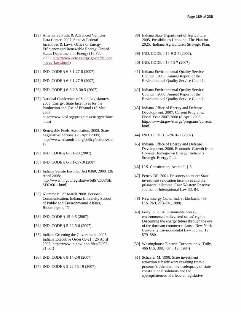
Page 189 of 238
[23] Alternative Fuels & Advanced Vehicles
Data Center. 2007. State & Federal
Incentives & Laws. Office of Energy
Efficiency and Renewable Energy, United
States Department of Energy (18 Feb.
2008; 236Hhttp://www.eere.energy.gov/afdc/ince
ntives_laws.html)
[24] IND. CODE § 6-3.1-27-8 (2007).
[25] IND. CODE § 6-3.1-27-9 (2007).
[26] IND. CODE § 6-6-2.5-30.5 (2007).
[27] National Conference of State Legislatures.
2005. Energy: State Incentives for the
Production and Use of Ethanol (16 Mar.
2008;
http://www.ncsl.org/programs/energy/ethinc
.htm)
[28] Renewable Fuels Association. 2008. State
Legislative Actions. (26 April 2008;
http://www.ethanolrfa.org/policy/actions/stat
e)
[29] IND. CODE § 6-3.1-28 (2007).
[30] IND. CODE § 6-3.1-27-10 (2007).
[31] Indiana Senate Enrolled Act 0360. 2008. (26
April 2008;
http://www.in.gov/legislative/bills/2008/SE/
SE0360.1.html)
[32] Klemme K. 27 March 2008. Personal
Communication. Indiana University School
of Public and Environmental Affairs,
Bloomington, IN.
[33] IND. CODE § 15-9-5 (2007).
[34] IND. CODE § 5-22-5-8 (2007).
[35] Indiana Greening the Government. 2005.
Indiana Executive Order 05-21. (26 April
2008; http://www.in.gov/idoa/files/EO05-
21.pdf)
[36] IND. CODE § 8-14-2-8 (2007).
[37] IND. CODE § 5-22-15-19 (2007).
[38] Indiana State Department of Agriculture.
2005. Possibilities Unbound: The Plan for
2025. Indiana Agriculture's Strategic Plan.
[39] IND. CODE § 15-9-2-4 (2007).
[40] IND. CODE § 13-13-7 (2007).
[41] Indiana Environmental Quality Service
Council. 2005. Annual Report of the
Environmental Quality Service Council.
[42] Indiana Environmental Quality Service
Council. 2006. Annual Report of the
Environmental Quality Service Council.
[43] Indiana Office of Energy and Defense
Development. 2007. Current Programs:
Fiscal Year 2007-2008 (8 April 2008;
http://www.in.gov/energy/programs/current.
html)
[44] IND. CODE § 5-28-16-2 (2007).
[45] Indiana Office of Energy and Defense
Development. 2006. Economic Growth from
Hoosier Homegrown Energy: Indiana‘s
Strategic Energy Plan.
[46] U.S. Constitution, Article I, § 8.
[47] Petrov DP. 2001. Prisoners no more: State
investment relocation incentives and the
prisoners‘ dilemma. Case Western Reserve
Journal of International Law 33: 84.
[48] New Energy Co. of Ind. v. Limbach, 486
U.S. 269, 273–74 (1988).
[49] Ferry, S. 2004. Sustainable energy,
environmental policy, and states‘ rights:
Discerning the energy future through the eye
of the dormant commerce clause. New York
University Environmental Law Journal 12:
579–580.
[50] Westinghouse Electric Corporation v. Tully,
466 U.S. 388, 407 n.12 (1984)
[51] Schaefer M. 1998. State investment
attraction subsidy wars resulting from a
prisoner‘s dilemma: the inadequacy of state
constitutional solutions and the
appropriateness of a federal legislative

Page 190 of 238
response. New Mexico Law Review 28
(1998): 324)
[52] Hughes v. Alexandria Scrap Corp., 426 U.S.
794, 806 (1976).
[53] West Lynn Creamery v. Healy, 512 U.S.
186, 199 n.15 (1994).
[54] South-Central Timber Development, Inc. v.
Wunnicke, 467 U.S. 82 (1984).
[55] C & A Carbone, Inc. v. Town of Clarkston,
511 U.S. 383 (1994).
[56] IND. CODE § 6-3.1-27-6 (2007).
[57] IND. CODE § 6-3.1-28-7 (2007).
[58] IND. CODE § 6-3.1-28-3 (2007).
[59] Hellerstein W, Coenen DT. 1996.
Commerce clause restraints on state
business development incentives. Cornell
Law Review 81: 806–07.
[60] 42 U.S.C. § 16491 (2005).
[61] HR 2419 EH1S, section 9017.
[62] Energy Independence and Security Act of
2007. Pub. L. No. 110-140, § 202, 121 Stat.
1533 (2007).
[63] Energy Independence and Security Act of
2007. Pub. L. No. 110-140, § 201, 121 Stat.
1533 (2007).
[64] Office of Energy Efficiency and Renewable
Energy. 2007. Biomass Program. United
States Department of Energy (27 April
2008;
http://www1.eere.energy.gov/biomass/about.
html)
[65] Midwestern Governors Association. 2007.
Energy Security and Climate Stewardship
Platform for the Midwest (27 April 2008;
http://www.midwesterngovernors.org/resolu
tions/Platform.pdf)
[66] Energy Independence and Security Act of
2007. Pub. L. No. 110-140, § 207, 121 Stat.
1533 (2007).
[67] Energy Independence and Security Act of
2007. Pub. L. No. 110-140, § 234, 121 Stat.
1533 (2007).
[68] Energy Independence and Security Act of
2007. Pub. L. No. 110-140, § 244, 121 Stat.
1533 (2007).
[69] Office of Basic Energy Sciences. 2008.
Energy Frontier Research Centers. United
States Department of Energy (27 April
2008; www.sc.doe.gov/bes/EFRC.html)
[70] Holdren J. 2004. Ending the Energy
Stalemate: A Bipartisan Strategy to Meet
America‘s Energy Challenges. The National
Commission on Energy Policy.
[71] United States Government Accountability
Office. 2007. DOE lacks a strategic
approach to coordinate increasing
production with infrastructure development
and vehicle needs. (Publication No. GAO-
07-713).
[72] Government Accountability Office. 2007.
DOE Lacks a Strategic Approach to
Coordinate Increasing Production with
Infrastructure Development and Vehicle
Needs. Washington, DC. GAO-07-713.
[73] Ebert J. 2007. Playing It Safe with
Methanol. Biodiesel Magazine, July 2007
Issue. (18 March 2008;
http://biodieselmagazine.com/article-
print.jsp?article_id=1709)
[74] Milke JA, Sunderland PB, Levy KM,
Ontiveros VL, Carey AC. 2007. Fire Safety
of the Traveling Public and Firefighter‘s for
Today‘s and Tomorrow‘s Vehicle Fleet.
Department of Fire Protection Engineering,
University of Maryland. Prepared for The
Fire Protection Research Foundation,
Quincy, MA.

Page 191 of 238
Appendix A: Feedstock Agriculture
Region Name of Natural
Region
Description
1 Lake Michigan Entirely aquatic, Indiana‘s portion of Lake Michigan
2 Northwestern
Morainal
Previously Glaciated Area formed by Wisconsinan Ice sheet.
Knob and kettle to rolling hills topography. Poor agricultural
lands with well drained calcareous. Home to the eastern
deciduous forest, tallgrass prairie, northern forest and
wetlands.
3 Grand Prairie Glaciated plain of unconsolidated deposits of sediments
including sands, lacustrine sediments, outwash plain
sediments and till from the WisconsinanGlaciation. Soils are
within silty clay loam variations. Historically the dominate
ecosystem in this area was tallgrass prairie.
4 Northern Lakes Glaciated by Wisconsinan ice sheet this region is identified by
numerous freshwater glacial lakes. The area is covered with
thick and complex deposit of glacial materials. Soils range
from loamy to neutral clayey to sandy loams. The natural
communities include bogs, fens, marshes, prairies, sedge
marshes, swamps and deciduous forests.
5 Central Till Plain Largest natural region in Indiana. Formally forested plain of
Wisconsinan till in central Indiana. Forms major divide
between communities with strong northern affinities and
communities with strong southern affinities. Characterized
by three sections: Entrenched Valley Section, Tipton Till
Section and Bluffton Till Plain. Soils range from thick loess
to loamy to clayey respectively. Predominant ecosystem was
mixed forest communities.
6 Black Swamp Western part of large lacustrine plain that was once covered
by ancient glacial melt water lake. Naturally poorly drained
deep clay and silt loam soils. This ecosystem used to be
dominated by swamp forest but is largely non-existent today
due to extensive drainage for agriculture expansion.
7 Southwestern
Lowlands
Most of this region was glaciated by the Illinoian ice sheet. It
is characterized by low relief and aggraded valleys. Area is
nearly level, undissected with poorly drained soils. Mostly
forests with some barren areas and prairie where the ice
sheets did not cover.

Page 192 of 238
8 Southern Bottomlands Half of this region was once glaciated; however this had little
effect on these low-lying bottomlands along rivers and larger
streams in southern Indiana. Soils are mostly silt loams and
dominant ecosystems previously included swamp, pond,
slough, marsh and prairie. Much of this has been converted to
agriculture lands.
9 Shawnee Hills Not glaciated, this area is the only contiguous belt of rugged
hills. Sandstone forms distinct cliffs. Consists of well drained
silt loam soils. The dominant plant community is upland
forest with patches of limestone glades and barrens.
10 Highland Rim Unglaciated except for relatively unmodified glaciated areas
along edges. Karst topography with well drained silty loams
derived from loess and weathered limestone. Dominant
natural communities pre-settlement were forest, glades and
barrens.
11 Bluegrass Similar to the Kentucky bluegrass region. This entire region
was covered by pre-Wisconsinan ice sheets. The northern
boundary is where the southern edge of the Wisconsinan ice
sheet ended. This area, while glaciated, only has a thin layer
of till with bedrock outcroppings. Soils are silt loams. This
region was originally forested.
Source: [1]

Page 193 of 238
Appendix B: Feedstock Agriculture
Although some reports have suggested Miscanthus may not be viable in Indiana‘s climate, a
project at the University of Illinois in Champaign Urbana (UIUC) has demonstrated markedly
positive results under similar conditions. As a C4 photosynthesizing species, Miscanthus is a
superiorly efficient convertor of sunlight to biomass, and rare for temperate climates [2].
UIUC‘sMiscanthus plots have yielded up to three times more biomass than Switchgrass, in
several different parts of the state. Despite initial concerns that Midwestern climates might suffer
temperatures cold enough to kill Miscanthus crops over winter, UIUC‘s crops have survived
temperatures as low as -10 oF without loss [3]. Remaining concerns could hinge on the necessity
of cellulosic ethanol production to derive fuel from Miscanthus, and its current lack of
production plants in Indiana.
Many objections to industrial production of Miscanthus can stem from the difficulty of its
propagation. The most suitable species for biofuel purposes, Giant Miscanthus, is a hybrid of two
distinct species of Miscanthus (M. sinensis and M. sacchariflorus) and is sterile, incapable of
normal reproduction. Although this alleviates concerns of invasive species potential, it does
complicate wide-spread adoption of the crop. Currently, the optimal planting process is to divide
rhizomes (underground storage organs) and individually plant them. It is theoretically possible to
replicate Miscanthus via tissue culture and rooted cuttings from adult plants, but these methods
have a high failure rate in the field environment [3]. At the time of writing, there are no
commercial means of planting Miscanthus rhizomes; they must be manually inserted
individually. Europeans have had some success with modifying existing farm equipment for
mechanized planting, but the resources do not currently exist in the United States. However, the
potential of Miscanthus may justify American research and development of such equipment.
Miscanthus can be harvested with conventional forage/herbage harvesters [2]. After initial
planting, the established plants will naturally spread out underground and form dense coverage.
With the exception of replacing any rhizomes that fail following the initial planting, Miscanthus
does not require periodic replanting, and adult plants can serve as a source of rhizomes for
establishing future crops [3].
Once Miscanthus is planted, it might require irrigation during dry periods, as there is a
correlation between water availability and crop yield. However, UIUC‘s research indicates
typical Illinois summer conditions are sufficiently moist to produce high yields, suggesting that
native Indiana conditions should likewise suffice. UIUC‘s research indicates maximum yields
can be expected within three years of initial planting, but could be delayed by an additional two
to three years in inferior soil. Miscanthus is capable of fixing its own Nitrogen; UIUC‘s research
shows no significant yield increase from application of Nitrogen fertilizer, which reduces
potential economic and ecological costs. However, European practice is to apply Nitrogen,
Phosphorous and Potassium following the second year of establishment (40-100kg ha-1
of N and
K, 10-20 kg ha-1
of P, depending on yield and soil conditions [2].
Although the freshly planted Miscanthus may require herbicidal weed treatment in its first year,
it is sufficiently established by the second year to suppress weeds without assistance. The
Nitrogen fixation and nutrient reclamation services provided by Miscanthus yield additional

Page 194 of 238
ecological and economic benefits in soil replenishment.Miscanthus also requires minimal efforts
before its land can be converted back to conventional crops, as opposed to trees and short
rotation woody crops [2].
UIUC‘s project found it preferable to plant approximately 4,850 rhizomes per acre in the first
year, although it is to be expected that some rhizomes fail and require replanting in the second or
third years. Once established, Miscanthus is harvested in the beginning of winter, when the
plants have withdrawn minerals and moisture to their root systems. This not only prepares them
for the coming spring, it minimizes impurities in the processing and combustion of fuel. As an
additional benefit, harvesting later in the year obviates the need for costly heating and drying of
the material, positively affecting Miscanthus‘ net energy balance. The majority of the fuel
potential comes from the stems of the grass, which can reach twelve feet of height in one
growing season.
UIUC‘s unfertilized plots yielded biomass averages of 9.8 tons per acre in Northern Illinois, 15.5
tons per acre in Central Illinois and 15.8 tons per acre in Southern Illinois (averaged over a three
year period from 2004-2006). By way of comparison, UIUC‘s data for unfertilized Switchgrass
planted in 2002 shows 2.2 tons per acre in Northern Illinois, 5.2 tons per acre in Central Illinois,
and 2.7 tons per acre in Southern Illinois (Table 1) [3]. According to information from UIUC,
Miscanthus vastly outperforms corn, yielding 168% of corn‘s biomass per hectare. With an
annual yield of 2,960 gallons of ethanol per hectare, Miscanthus would require only 9.3% of
America‘s harvested cropland in order to provide an annual quantity of 35 billion gallons of
ethanol. To achieve that quantity of ethanol, corn would require 14.8% of harvested cropland [4]. Table 1: All Numerical values represent tons of biomass produced per acre in a single growing season.
Region Miscanthus Switchgrass
Northern Illinois 9.8 2.2
Central Illinois 15.5 5.2
Southern Illinois 15.8 2.7

Page 195 of 238
Appendix C: Additional site suitability considerations
Source: [5, 6, 7]

Page 196 of 238
Source: [6, 7, 8]

Page 197 of 238
Source: [7, 9, 10]

Page 198 of 238
Source: [5, 7, 11, 6]

Page 199 of 238
Appendix D: Energy Balance Appendix
Table 1. Energy Balance Studies for Corn Ethanol (adjusted LHVs for all studies).
Year Author Corn Yield (bu/acre)+
Corn ethanol
conversion rate
(gal/bu)
Ethanol conversion
process (Btu/gal)
Total Energy
use (Btu/gal)
Coproducts energy credits
(Btu/gal)
Calc. NEV
(Btu/gal) Calc.
EB
1989 Ho [12] 90 NR 57000 90000 10000 -4300 0.95
1990 Marland and Turhollow [13] 119 2.50 50105 73934 8127 9893 1.13
1991 Pimentel [14] 110 2.50 73687 131017 21500 -33817 0.74
1992 Morris and Ahmed (Industry Avg)[15] 120 2.56 49380 75811 24950 24839 1.33
1992
Morris and Ahmed (Industry Best)[15] 120 2.56 36232 57979 32693 50414 1.87
1992 Keeney and DeLuca [16] 119 2.56 48470 91196 8078 -7418 0.92
1995 Lorenz and Morris [17] 120 2.55 53956 81909 27579 21370 1.26
1995 Shapouri et al. [18] 122 2.53 53277 82824 15056 7932 1.10
1999 Wang et al. [19] 125 2.55 40850 68450 14950 22200 1.32
1999 Argi. And Agri-Food Canada [20] 116 2.69 50415 68450 14055 21305 1.31
2001 Pimentel [21] 127 2.50 75118 131062 21500 -33862 0.74
2001 Wang [22] 125 2.58 39067 66564 14333 23469 1.35
2002 Shapouri et al. [23] 125 2.66 51779 77228 14372 12844 1.17
2002 Graboski (baseline 2000) [24] 140 2.65 55049 77497 14829 13032 1.17
2002 Graboski (2002 new plants) [24] 140 2.73 47937 70551 12880 18029 1.26
2002 Graboski (2002 industry) [24] 140 2.68 52513 75020 14134 14814 1.20
2002 Graboski (2012 projection) [24] 154 2.80 45768 64479 10062 21283 1.33
2003 Pimentel [25] 137 2.60 54171 99119 0 -23419 0.76
2004 Shapouri et al. [26] 139 2.66 49733 72052 26250 29898 1.41
2008 v600 Calculations - INDIANA 155.7 2.68 50002 82642 14372 7430 1.09
* Original citations from Graboski 2002,Shapouri et al. 2002, or original authors; total energy use confirmed in primary sources + Note that all yields are standard yields except for this study which uses a planted yield calculation.

Page 200 of 238
Indiana Energy Balance Analysis for Corn-Based Ethanol Production
The Indiana-specific energy balance estimates use the four phrase process outlined in the text:
farming, feedstock transportation, fuel conversion, and fuel transportation. Energy estimates
were created for each phase to the best degree possible, many of which rely on data from
Shapouri et al. (2002) as discussed below [23].
The time frame for this analysis is 2004 to 2006 for which corn production and acreage data was
obtained from the USDA (NASS 2008) [27]. Statewide standard average yields of corn based on
harvested acreage amounted to 159.6 bushels per acre. The average yield based on the total
planted acreage from 2004 to 2006 was slightly lower at 155.7 bushels per acre.
Phase I: Farming
Farm inputs include all processes outlined by Shapouri et al. (2002) with updates where possible
from USDA Farm Census data (see Table 2 below) [23, 27].
Table 2. Farm Inputs for Indiana Corn Production
Input Unit IN Source
Seed Kernels/acre 28,281 Shapouri 2004est
Fertilizer:
.Nitrogen Pounds/acre 147 USDA 2008
.Potash Pounds/acre 124 USDA 2008
.Phosphate Pounds/acre 77 USDA 2008
.Lime Pounds/acre 20 Shapouri 2002 est
Energy:
.Diesel Gallons/acre 4.6 Shapouri 2002 est
.Gasoline Gallons/acre 2.1 Shapouri 2002 est
.LPG Gallons/acre 3.2 Shapouri 2002 est
.Electricity kWh/acre 28.3 Shapouri 2002 est
.Natural Gas
Cubic
ft/acre 144.2 Shapouri 2002 est
Custom
Work Dol./acre 7.8 Shapouri 2002 est
Chemicals Dol./acre 3.19 Shapouri 2002 est
Custom
Drying Dol./acre 2 Shapouri 2002 est

Page 201 of 238
These estimates are then converted to a Btu per bushel of corn estimate using the following
formula:
The above equation yields results as presented in Table 3.
Table 3. Farm Inputs for Indiana Corn Production (Btu/bu)
Input Est. EI
Btu/bu
Seed .841 718
.Nitrogen 24500 23,133
.Potash 4000 3,186
.Phosphate 4175 2,065
.Lime 620 80
.Diesel 137202 4,054
.Gasoline 125073 1,687
.LPG 91538 1,881
.Electricity 12356 2,264
.Natural Gas 1021 946
Custom work 28500 1,428
Chemicals 150000 3,156
Total energy per bushel 44,597
Btu/gall
Total energy per gallon 16,668
The total energy as Btu per Bushel is then converted to Btu per gallon of ethanol using a
weighted conversion factor of 2.68 calculated from Hurt (2007) [28].
Phase II: Corn Transportation
The transportation of corn energy estimates assume corn is transported from the farm to either a
storage facility or a plant at an average of 25 miles OR taken directly to a plant at an average of
75 miles. These estimates dismiss the use of trains to transport corn to ethanol facilities since
active ethanol plants in Indiana are sited in areas with high production of corn. Using truck size
estimates from Lee (2007) and Benson and Bullen (2007) and fuel efficiency estimates from Fuel

Page 202 of 238
Charger (2008), average energy per gallon of ethanol was calculated (see Tables 4 and 5) [29,
30, 31].
Note that corn transport estimates used in this analysis are 1,000 Btu/gall less than provided in
Shapouri et al. (2002), a likely source of error in the estimation techniques incorporated into this
study [23].
Table 4. Corn Transportation to Granaries
PART I
Average distance to plant 25 miles
Average truck haul 547 bushels
Est. MPG 5 mi/gall fuel
Total needed bushels per year 163000000 Bu/yr
Total truck loads 297989 loads/yr
Total truck load miles 7449725.777 miles/yr
Total gallons of fuel 1489945.2 gall/yr
Energy per gallon of diesel fuel 139000 Btu/gall
Total energy for transport 207,102,376,600 Btu TOTAL
Average energy per bushel 1270.566728 Btu/bu of corn
Average energy per gallon Etoh 474.9 Btu/gall Etoh

Page 203 of 238
Table 5. Corn Transportation to Refineries
PART II
Average distance to plant 75 miles
Average truck haul 875 bushels
Est. MPG 5.5 mi/gall fuel
Total needed bushels per year 163000000 bu/yr
Total truck loads 186285.7 loads/yr
Total Truck load miles 13971428.6 miles/yr
Total gallons of fuel 2540259.7 gall/yr
Energy per gallon of diesel fuel 139000 Btu/gall
Total energy for transport 353,096,103,896 Btu TOTAL
Average energy per bushel 2166.2 Btu/bu of corn
Average energy Per gallon Etoh 809.64 Btu/gall Etoh
Table 6. Total of Corn Transportation to Granaries and Refineries
Total
Total average energy per gallon 1284.52 Btu/gall Etoh
Phase III: Production
Estimates for production originate from a survey conducted by the USDA and reprinted in
Graboski 2002 [24]. Unlike the estimates provided in Shapouri et al. (2002), only dry mill
facilities are included in this analysis (see Table 7) [23]. The available results included one
plant, presumably a smaller facility, with reported low thermal and electrical use. This plant was
dropped from the facility average shifting the average thermal energy use from 37,410 Btu per
gal to 38,804 Btu per gal and electrical use from 1.11 kwh per gal to 1.10 kwh per gal. Electrical
use was converted by its HHV (8,625 Btu per kwh) and added to thermal energy‘s HHV for an
estimated production energy use of 50,001 Btu per gal of ethanol produced. Except for removal
of the low producing plant in the analysis, this is precisely the method utilized by Graboski
(2002) [24].
Note that reliance on the survey may provide poor estimates of production energy. The survey
was originally conducted in 2001 and does not include newer production facilities, as are most of
the facilities in Indiana. However, the potential for overestimation is partially offset by potential
survey error from respondents who may have underreported total energy use in the initial survey. Table 7. Dry Mill Energy Requirements
Graboski 2002 [24] This study
Averagethermal energy use (Btu/gal) 39,031 40,485
Averageelectrical use (Kwh/gal) 1.11 1.10
Total estimated energy (Btu/gal) 48,539 50,002

Page 204 of 238
Phase IV: Ethanol Transportation
Similar to corn transportation, energy use per gallon of ethanol transported was calculated (see
Table 8). An average trucked distance of 100 miles was assumed for transportation of ethanol to
retail distribution sites using the fuel efficiency and loading estimates from Phase II-Part 2. Table 8. Ethanol Transportation to Distribution Sites
Distance 100 miles
Haul 8000 gallons
Total EtOH
457,000,000 gall/yr
Truck loads
57,125 loads
Truck miles
5,712,500 mi
Total diesel fuel
1,038,636 gall/yr
Energy PG
139,000 Btu/gall fuel
Average energy per gallon Etoh
315.9 Btu/gallon Etoh

Page 205 of 238
Total Energy
Estimates from previous tables are summarized in Table 7. Also included are co-product energy
credits extracted directly from Shapouri et al. (2002) [23]. No attempt to re-estimate co-products
was made for this analysis; however, this estimate does fall within a mid-range of credits applied
in previous studies (see Table 1).
Table 10summarizes the key values integrated into the energy balance equation for Indiana. Table 9. Energy Requirements for Corn-Based Ethanol Production in Indiana (Btu/gal)
Phase Btu/gal Source
I. Corn production 16,668.3 Table 3
II. Corn transport 1,284.52 Table 4
III. Ethanol conversion 50,001.7 BBI International Survey (2001) of Ethanol Plants from appendix of Graboski 2002 [24]
IV. Ethanol transport 315.9 Table 6
Co-products 14,372.0 Shapouri et al 2002 [23]
TOTAL 82,642.4
Table 10. Key Values for Indiana NEV
Planted corn yield (bu/acre) 155.6889
Corn ethanol conversion rate (gal/bu) 2.675562
Ethanol conversion process (Btu/gal) 50001.66
Total energy use (Btu/gal) 82642.38
Adjusted NEV (Btu/gal) 7429.618
Adjusted EB 1.089901

Page 206 of 238
Appendix E: Technical Appendix for Cost-Benefit Analysis
Methodology
As mentioned in the Analysis of Costs and Benefits of Biofuels section, the accounting domain
for this analysis is the state of Indiana. Only those impacts that occur within the state of Indiana
have been included. The baseline for this analysis is a ―no biofuels‖ alternative, a world where
biofuels are not being produced or consumed in Indiana. Only those values that are a direct result
of biofuel production and consumption in Indiana and its consequences have been included in the
analysis.
The time frame for the analysis is from 2008-2030 for ethanol and biodiesel and 2012-2030 for
cellulosic ethanol.
Transfer, cost, and benefit values were calculated on a variable basis, taking the per unit value
and adjusting for inflation based on the Consumer Price Index – All Urban Consumers (United
States Department of Labor [32]. All values have been adjusted for inflation by converting to
January 2008 Dollars.
Adjusting for Inflation
To adjust for inflation, it is necessary to take the current January 2008 CPI index value
and divide it by the prevailing index value when the value was produced.
For example, to convert 2007 Dollars to January 2008 Dollars:
Inflation adjustment factor = (January 2008 CPI / 2007 annual average CPI)
Inflation adjustment factor = (211.080/207.342)
The values were then multiplied by chosen discount factors to adjust for the time-cost of money.
Discounting
The discount rates used in this analysis are three percent, five percent, and seven percent.
The discount factors were calculated using the following equation:
Discount factor = 1/ (1 + discount rate) ^ year
For example, to calculate the discount factor for a five percent discount rate:
Discount factor = 1/ (1.05) ^ year
The final values were then multiplied by the appropriate dollar amounts and summed over all
years to find the total inflation adjusted, discounted value.

Page 207 of 238
Table 1.Demand Schedules for the United States and Indiana
GAO Gasoline Projections for United States Consumption
Year Barrels Gallons
2004 4,800,000,000 201,600,000,000
2030 6,800,000,000 285,600,000,000
Year Consumption in United States Consumption in Indiana Percentage
2004 201,600,000,000 3,059,000,000 1.52%
2005 204,830,769,231 3,113,427,692 1.52%
2006 208,061,538,462 3,162,535,385 1.52%
2007 211,292,307,693 3,211,643,077 1.52%
2008 214,523,076,924 3,260,750,769 1.52%
2009 217,753,846,155 3,309,858,462 1.52%
2010 220,984,615,386 3,358,966,154 1.52%
2011 224,215,384,617 3,408,073,846 1.52%
2012 227,446,153,848 3,457,181,538 1.52%
2013 230,676,923,079 3,506,289,231 1.52%
2014 233,907,692,310 3,555,396,923 1.52%
2015 237,138,461,541 3,604,504,615 1.52%
2016 240,369,230,772 3,653,612,308 1.52%
2017 243,600,000,003 3,702,720,000 1.52%
2018 246,830,769,234 3,751,827,692 1.52%
2019 250,061,538,465 3,800,935,385 1.52%
2020 253,292,307,696 3,850,043,077 1.52%
2021 256,523,076,927 3,899,150,769 1.52%
2022 259,753,846,158 3,948,258,462 1.52%
2023 262,984,615,389 3,997,366,154 1.52%
2024 266,215,384,620 4,046,473,846 1.52%
2025 269,446,153,851 4,095,581,539 1.52%
2026 272,676,923,082 4,144,689,231 1.52%
2027 275,907,692,313 4,193,796,923 1.52%
2028 279,138,461,544 4,242,904,615 1.52%
2029 282,369,230,775 4,292,012,308 1.52%
2030 285,600,000,000 4,341,120,000 1.52%
Gasoline Consumption

Page 208 of 238
Gasoline consumption in the United States was based on Government Accountability Office
(GAO) projections [33]. One barrel is equal to 42 gallons and so these estimates were converted
from barrels to gallons by multiplying by 42.
U.S. gasoline consumption 2004 = 4,800,000,000 barrels * 42 gallons = 201,600,000,000 gallons
U.S. gasoline consumption 2030 = 6,800,000,000 barrels * 42 gallons = 285,600,000,000 gallons
United States gasoline consumption was assumed to grow linearly between projection years.
Total Gasoline consumption in Indiana was 3,059,000,000 gallons in 2004 [34].
In order to project future Indiana gasoline consumption, it was necessary to find Indiana‘s
percentage of national gasoline consumption.
Indiana gasoline consumption in 2004 / U.S. gasoline consumption in 2004:
3,059,000,000 / 201,600,000,000 = 1.52%
It was assumed that Indiana‘s future gasoline consumption would be stable as a percentage of
total gasoline consumption and has been projected by multiplying the forecasted United States
consumption by 0.0152.

Page 209 of 238
Table 2. Corn Ethanol Consumption
Consumption of ethanol in Indiana in 2004 was 4.84 percent of U.S. gasoline consumption in
2004 [43]. Future Indiana ethanol consumption is projected linearly at 4.84 percent of total U.S.
gasoline consumption.
Year Consumption in Indiana Production in Indiana Bushels Needed to Produce
2008 157,820,337 1,060,000,000 392,592,593
2009 160,197,150 1,060,000,000 392,592,593
2010 162,573,962 1,060,000,000 392,592,593
2011 164,950,774 1,060,000,000 392,592,593
2012 167,327,586 1,060,000,000 392,592,593
2013 169,704,399 1,418,000,000 525,185,185
2014 172,081,211 1,418,000,000 525,185,185
2015 174,458,023 1,418,000,000 525,185,185
2016 176,834,836 1,418,000,000 525,185,185
2017 179,211,648 1,418,000,000 525,185,185
2018 181,588,460 1,418,000,000 525,185,185
2019 183,965,273 1,418,000,000 525,185,185
2020 186,342,085 1,418,000,000 525,185,185
2021 188,718,897 1,418,000,000 525,185,185
2022 191,095,710 1,418,000,000 525,185,185
2023 193,472,522 1,418,000,000 525,185,185
2024 195,849,334 1,418,000,000 525,185,185
2025 198,226,146 1,418,000,000 525,185,185
2026 200,602,959 1,418,000,000 525,185,185
2027 202,979,771 1,418,000,000 525,185,185
2028 205,356,583 1,418,000,000 525,185,185
2029 207,733,396 1,418,000,000 525,185,185
2030 210,110,208 1,418,000,000 525,185,185

Page 210 of 238
Corn Ethanol Production
Ethanol production in Indiana is based on ethanol production facilities currently operating and
planned production facilities estimated to be in operation in 2013 [35]. The bushels needed to
produce value was projected by taking the total production of ethanol within the state of Indiana
and dividing by 2.7, assuming that one bushel of corn yields 2.7 gallons of ethanol. Table 3. GAO biodiesel projections for United States consumption
Year Gallons
2006 287,000,000
2012 308,000,000
2030 395,000,000
Table 4. Soy Biodiesel Consumption
Biodiesel consumption in the United States is based on GAO projections [33]. It was assumed
that demand would grow linearly between projection years.
Year Consumption (Gallons) Consumption in Indiana Production in Indiana Bushels needed to produce
2006 287,000,000 31,888,889 10,000,000 6,711,409
2007 290,500,000 32,277,778 108,000,000 72,483,221
2008 294,000,000 32,666,667 108,000,000 72,483,221
2009 297,500,000 33,055,556 108,000,000 72,483,221
2010 301,000,000 33,444,444 108,000,000 72,483,221
2011 304,500,000 33,833,333 108,000,000 72,483,221
2012 308,000,000 34,222,222 108,000,000 72,483,221
2013 312,833,333 34,759,259 108,000,000 72,483,221
2014 317,666,667 35,296,296 108,000,000 72,483,221
2015 322,500,000 35,833,333 108,000,000 72,483,221
2016 327,333,333 36,370,370 108,000,000 72,483,221
2017 332,166,667 36,907,407 108,000,000 72,483,221
2018 337,000,000 37,444,444 108,000,000 72,483,221
2019 341,833,333 37,981,481 108,000,000 72,483,221
2020 346,666,667 38,518,519 108,000,000 72,483,221
2021 351,500,000 39,055,556 108,000,000 72,483,221
2022 356,333,333 39,592,593 108,000,000 72,483,221
2023 361,166,667 40,129,630 108,000,000 72,483,221
2024 366,000,000 40,666,667 108,000,000 72,483,221
2025 370,833,333 41,203,704 108,000,000 72,483,221
2026 375,666,667 41,740,741 108,000,000 72,483,221
2027 380,500,000 42,277,778 108,000,000 72,483,221
2028 385,333,333 42,814,815 108,000,000 72,483,221
2029 390,166,667 43,351,852 108,000,000 72,483,221
2030 395,000,000 43,888,889 108,000,000 72,483,221

Page 211 of 238
Reliable estimates of biodiesel consumption in Indiana are not available. It was assumed that the
majority of biodiesel consumption occurs in the Midwest close to the feedstock. As a result,
biodiesel consumption in Indiana is estimated as one ninth of total biodiesel consumption in the
United States.
Soy Biodiesel Production
Production in Indiana is based on production facilities currently operating [35]. The bushels
needed to produce value was projected by taking the total production of biodiesel within the state
of Indiana and dividing by 1.49, assuming that one bushel of soybeans yields 1.49 gallons of
biodiesel. Table 5. Cellulosic Ethanol Production
Cellulosic ethanol is a developing technology and no plants are currently operating in Indiana.
The first plant is assumed to become operational in 2012, with a production capacity of 50
million gallons per year. The growth in the number of plants is presented in Table 5. All plants
are assumed to have a production capacity of 50 million gallons per year. The tons of corn
stover needed to produce value was calculated by taking the total projected cellulosic ethanol
production within the state of Indiana and dividing by 60, assuming that one ton of corn stover
yields 60 gallons of ethanol [36].
Year Production in Indiana Number of Plants Tons of Corn Stover Needed to Produce
2012 50,000,000 1 833,333
2013 50,000,000 1 833,333
2014 50,000,000 1 833,333
2015 50,000,000 1 833,333
2016 100,000,000 2 1,666,667
2017 100,000,000 2 1,666,667
2018 100,000,000 2 1,666,667
2019 100,000,000 2 1,666,667
2020 200,000,000 4 3,333,333
2021 200,000,000 4 3,333,333
2022 200,000,000 4 3,333,333
2023 200,000,000 4 3,333,333
2024 300,000,000 6 5,000,000
2025 300,000,000 6 5,000,000
2026 300,000,000 6 5,000,000
2027 300,000,000 6 5,000,000
2028 500,000,000 10 8,333,333
2029 500,000,000 10 8,333,333
2030 500,000,000 10 8,333,333

Page 212 of 238
Calculations
Due to the large number of calculations involved and the fact that all of the calculations follow
the same format, Table 6 illustrates basic process used to produce all of the calculations.
Detailed calculations are available from the authors upon request. Table 6. Sample Template of Calculations
Each value is calculated using the same formula:
Sum of (value * inflation adjustment factor * discount factor * quantity) for all years
Savings to Consumers of Gasoline
Year Value Year Discount Factor Total Adjusted Discounted Value Total Value
2008 0.08$ 0 1 0.08$ 273,126,695.39$
2009 0.08$ 1 0.970873786 0.08$ 269,165,096.34$
2010 0.08$ 2 0.942595909 0.08$ 265,202,566.76$
2011 0.08$ 3 0.915141659 0.08$ 261,242,521.62$
2012 0.08$ 4 0.888487048 0.07$ 257,288,177.75$
2013 0.08$ 5 0.862608784 0.07$ 253,342,562.50$
2014 0.08$ 6 0.837484257 0.07$ 249,408,522.00$
2015 0.08$ 7 0.813091511 0.07$ 245,488,729.21$
2016 0.08$ 8 0.789409234 0.07$ 241,585,691.56$
2017 0.08$ 9 0.766416732 0.06$ 237,701,758.32$
2018 0.08$ 10 0.744093915 0.06$ 233,839,127.70$
2019 0.08$ 11 0.722421277 0.06$ 229,999,853.66$
2020 0.08$ 12 0.70137988 0.06$ 226,185,852.42$
2021 0.08$ 13 0.68095134 0.06$ 222,398,908.79$
2022 0.08$ 14 0.661117806 0.06$ 218,640,682.14$
2023 0.08$ 15 0.641861947 0.05$ 214,912,712.24$
2024 0.08$ 16 0.623166939 0.05$ 211,216,424.81$
2025 0.08$ 17 0.605016446 0.05$ 207,553,136.83$
2026 0.08$ 18 0.587394608 0.05$ 203,924,061.70$
2027 0.08$ 19 0.570286027 0.05$ 200,330,314.15$
2028 0.08$ 20 0.553675754 0.05$ 196,772,914.92$
2029 0.08$ 21 0.537549276 0.05$ 193,252,795.35$
2030 0.08$ 22 0.521892501 0.04$ 189,770,801.68$
Total 5,302,349,907.83$
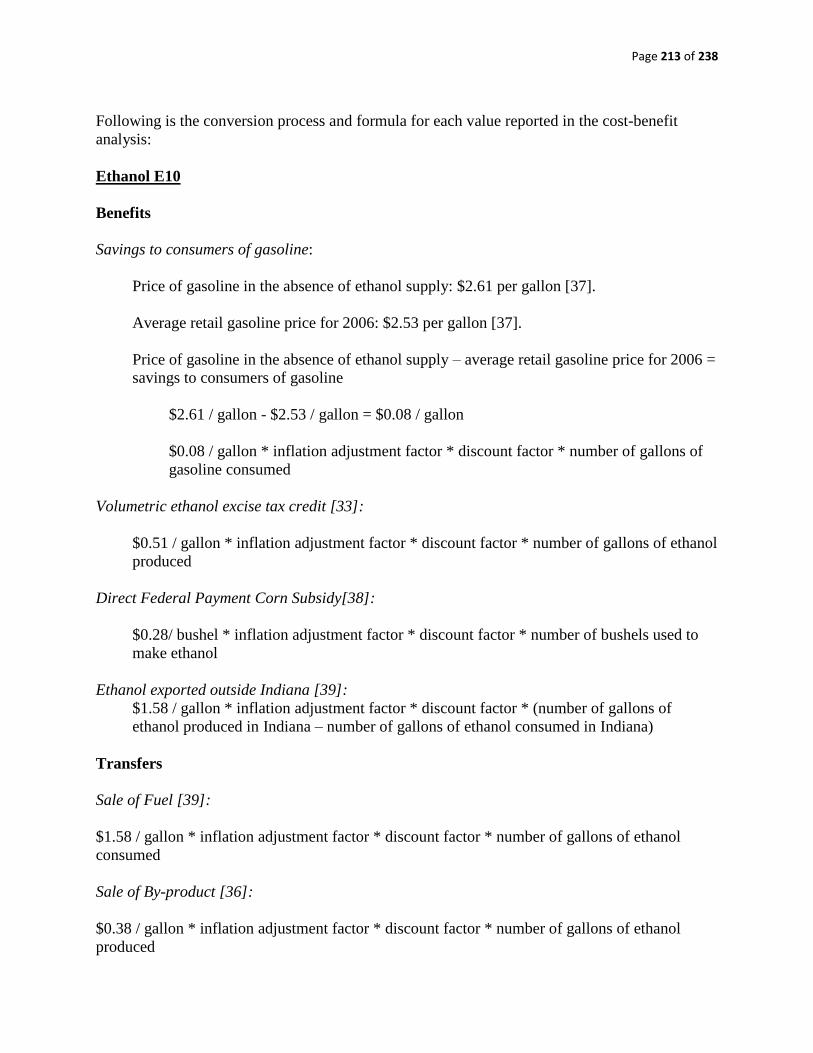
Page 213 of 238
Following is the conversion process and formula for each value reported in the cost-benefit
analysis:
Ethanol E10
Benefits
Savings to consumers of gasoline:
Price of gasoline in the absence of ethanol supply: $2.61 per gallon [37].
Average retail gasoline price for 2006: $2.53 per gallon [37].
Price of gasoline in the absence of ethanol supply – average retail gasoline price for 2006 =
savings to consumers of gasoline
$2.61 / gallon - $2.53 / gallon = $0.08 / gallon
$0.08 / gallon * inflation adjustment factor * discount factor * number of gallons of
gasoline consumed
Volumetric ethanol excise tax credit [33]:
$0.51 / gallon * inflation adjustment factor * discount factor * number of gallons of ethanol
produced
Direct Federal Payment Corn Subsidy[38]:
$0.28/ bushel * inflation adjustment factor * discount factor * number of bushels used to
make ethanol
Ethanol exported outside Indiana [39]:
$1.58 / gallon * inflation adjustment factor * discount factor * (number of gallons of
ethanol produced in Indiana – number of gallons of ethanol consumed in Indiana)
Transfers
Sale of Fuel [39]:
$1.58 / gallon * inflation adjustment factor * discount factor * number of gallons of ethanol
consumed
Sale of By-product [36]:
$0.38 / gallon * inflation adjustment factor * discount factor * number of gallons of ethanol
produced

Page 214 of 238
Ethanol production tax credit [40, 41]:
The tax credit is $0.125 / gallon of ethanol produced. The maximum tax credit for all years is
$2,000,000 per producer for a plant producing 40 to 60 million gallons of ethanol per year and
$3,000,000 per producer for a plant producing 60 million gallons of ethanol or more. The below
calculation was used until each cellulosic production facility received the appropriate maximum
nominal payment. These payments were adjusted into real dollars. The New Energy ethanol
plant in South Bend was excluded from the calculation because it entered production well before
the tax credit was initiated [35].
$2,000,000 * inflation adjustment factor * discount factor * 2 ethanol production facilities
$3,000,000 * inflation adjustment factor * discount factor * 13 production facilities
Agricultural Input (Corn) [42]:
$3.30 / bushel * inflation adjustment factor * discount factor * number of bushels needed to
make the quantity of ethanol produced
Job creation [35]:
Employment is estimated at 536 jobs for all ethanol production facilities in the state of Indiana.
This value was derived by taking the number of jobs estimated to be created in the state of
Indiana for all biofuel production, 670, and dividing it by the 20 current and planned ethanol and
biodiesel production facilities [35]. This number was then multiplied by the 16 current and
planned ethanol production facilities, which yields 536 jobs [35]. The average earnings of an
ethanol plant employee, with benefits, is $43,348 [43]. The wages have been adjusted for tax
payments [44, 45].
Federal taxes paid are a loss to the accounting domain.
Federal income tax payment = $4,220 + 25% over $30,650 = $7,394.50 [45].
Salary – federal taxes – state of Indiana taxes = Adjusted income
$43,348 - $7,394.50 -$1,473.83 = $34,479.67
$34,479.67 / year * inflation adjustment factor * discount factor * 536 jobs

Page 215 of 238
Taxes paid [44]:
The state of Indiana personal income tax is 3.4 percent.
Taxes paid = $43,348 * 0.034 = $1,473.83
$1,473.83 * discount factor * 536 jobs
Costs
Plant construction cost [36]:
The plant construction cost is variable and is based on production capacity. The cost of the plant
is spread out over the useful life of the plant, which is assumed to be twenty-five years. The
plant cost does not include the cost of borrowed capital, which is included in the capital cost
value.
(($1.90 / gallon) / 25 years) * discount factor * production capacity
All of the values for each plant currently operating in Indiana and planned facilities are then
summed to produce a total value.
Capital cost [36]:
An additional capital cost considered is the interest paid on a loan. It is assumed all of the plants
are financed through borrowing and that an interest payment must be captured in the producer‘s
cost. Otto Doering estimates that ethanol producers have a capital interest cost of $0.20 / gallon
[36].
$0.20 / gallon * discount factor * production capacity
Production cost [36]:
Based on Otto Doering‘s ―Economic Perspectives on Producing Liquids Fuels from Plant
Feedstocks‖ [36]:
Other costs: $0.62 / gallon
Enzymes: $0.04 / gallon
Production cost = other costs + enzymes
Production cost = $0.62 + $0.04 = $0.66
$0.66 / gallon * inflation adjustment factor * discount factor * number of gallons of ethanol
produced

Page 216 of 238
Transportation distribution cost [34]:
$0.054 / gallon * inflation adjustment factor * discount factor * number of gallons of ethanol
produced
Worker leisure opportunity cost [46]:
The worker leisure opportunity cost uses a value of $3, which is standard in the literature.
($3 * 40 hours / week * 50 weeks / year) * discount factor * 536 jobs
Soil erosion [47]:
The soil loss is estimated in the following way:
soil loss = 21 lbs. / gallon
topsoil = $0.028 / lb.
topsoil = $0.59 / gallon
$0.59 / gallon * inflation adjustment factor * discount factor * number of gallons of ethanol
produced
Qualitative
Reduced Emissions [33]:
-1% greenhouse gases
Ethanol E85
Benefits
Federal biofuel dispenser tax credit [33]:
The federal biofuel dispenser tax credit was calculated in the following way:
Currently, there are 97 gas stations in Indiana that offer E85. It was assumed that this number
would roughly double to 200 stations due to increased demand for E85 by consumers and the
increased production of ethanol within the state. It was assumed that this increase would occur
gradually from 2014 to 2018. Finally, it was assumed that all stations currently offering E85 had
claimed the tax credit.

Page 217 of 238
Table 7. Assumed Increase in New Stations Offering E85 by Year
$30,000 / station * inflation adjustment factor * discount factor * number of new stations
offering E85
Costs
Minimal modification [33]:
$3,300 / station * inflation adjustment factor * discount factor * number of new stations offering
E85
New dispenser [33]:
$13,000 / station * inflation adjustment factor * discount factor * number of new stations
offering E85
New tank, piping, etc. [33]:
$62,400 / station * inflation adjustment factor * discount factor * number of new stations
offering E85
Qualitative Reduced emissions [33]:
-20% greenhouse gases
Firefighting foam [48]:
$90-$115 / 5 gallons
Adjustment cost for cars [33]:
$30 - $300 / car
Indiana Alternate Fuel Vehicles Tax Credit [49]:
Year Number of new stations
2014 13
2015 20
2016 20
2017 25
2018 25

Page 218 of 238
15% of qualifying investment
Dedicated Ethanol Pipeline [33]:
$1,000,000 / mile
Indiana Tax Credit for Fueling Stations [50]:
$0.18 / gallon, with a maximum of $1,000,000 for all retailers
Indiana Gas Station Grant [51]:
$5,000 / retailer, with a maximum of $1,000,000 for all retailers
Biodiesel
Benefits
Federal biodiesel virgin oil subsidy [33]:
$1.00 / gallon * inflation adjustment factor * discount factor * number of gallons of biodiesel
produced
Federal biodiesel dispenser tax credit [33]:
Currently, there are 61 gas stations in Indiana that offer biodiesel. It was assumed that this
number would roughly double to 134 stations due to increased demand for biodiesel by
consumers and the increased production of biodiesel within the state. It was assumed that this
increase would occur gradually from 2008 to 2012. Finally, it was assumed that all stations
currently offering biodiesel had claimed the tax credit. Table 8. Assumed Increase in New Stations Offering Biodiesel by Year
$30,000 / station * inflation adjustment factor * discount factor * number of new stations
offering biodiesel
Direct federal payment soybean subsidy [38]:
Year Number of new stations
2008 14
2009 29
2010 15
2011 15
2012 14
Page 219 of 238
$0.44/ bushel * inflation adjustment factor * discount factor * number of bushels used to make
biodiesel
Export of biodiesel to other states [53]:
Iowa State University estimates a tax exclusive price of biodiesel of $1.30 - $1.50 / gallon [53].
The value used in this analysis is simply the median value of this range.
$1.40 / gallon * inflation adjustment factor * discount factor * (number of gallons of biodiesel
produced – number of gallons of biodiesel consumed in Indiana)
Transfers
Biodiesel production tax credit:
All biodiesel producers in the state of Indiana are entitled to a subsidy from the state of Indiana
equal to $1.00 per gallon produced, subject to a maximum of $3 million [53]. It was assumed
that all plants opening prior to 2007 had claimed the tax credit. Two plants opened in 2007 and
will be eligible for the tax credit in 2008 [35]. These plants each have a capacity in excess of
three million gallons a year and will exhaust the tax credit in 2008.
Biodiesel retailer tax credit: (237HIndiana Code 6-3.1-27-10).
$0.01 / gallon * inflation adjustment factor * discount factor * number of gallons of biodiesel
produced
Taxes paid [44]:
The state of Indiana personal income tax is 3.4 percent.
Taxes paid = $43,348 * 0.034 = $1,473.83
$1,473.83 * discount factor * 134 jobs
Job creation [35]:
Employment is estimated at 134 jobs for all biodiesel production facilities in the state of Indiana.
This value was derived by taking the number of jobs estimated to be created in the state of
Indiana for all biofuel production, 670, and dividing it by the 20 current and planned ethanol and
biodiesel production facilities [35]. This number was then multiplied by the 4 current biodiesel
production facilities, which yields 134 jobs [35]. The average earnings of an ethanol plant
employee, with benefits, is $43,348 [43]. The wages have been adjusted for tax payments[44,
45]
Federal taxes paid are a loss to the accounting domain.
Federal income tax payment = $4,220 + 25% over $30,650 = $7,394.50 [45].

Page 220 of 238
Salary – federal taxes – state of Indiana taxes = Adjusted income
$43,348 - $7,394.50 -$1,473.83 = $34,479.67
$34,479.67 / year * inflation adjustment factor * discount factor * 134 jobs
Sale of fuel [52]:
$1.40 / gallon * inflation adjustment factor * discount factor * number of gallons of biodiesel
consumed in Indiana
Agricultural input (soybean oil) [36]:
The soybean input value was calculated in the following way:
$0.65 / pound
7.4 pounds = 1 gallon
$0.65 * 7.4 = $4.81 / gallon
$4.81 * discount factor * number of gallons of biodiesel produced
Sale of Glycerin by-product [55]:
The typical biodiesel plant produces 1100 pounds of glycerin an hour.
($0.25 / pound * 1100 pounds an hour * 24 hours / day * 7 days / week * 50 weeks / year) *
discount factor * number of plants producing biodiesel
Costs
Plant construction cost [56]:
The plant construction cost is variable and is based on production capacity. The cost of the plant
is spread out over the useful life of the plant, which we assume to be twenty-five years. The
plant cost does not include the cost of borrowed capital, which is included separately in the
capital cost value.
(($1.04 / gallon) / 25 years) * inflation adjustment factor * discount factor * number of gallons of
biodiesel produced
All of the values for each plant currently operating in Indiana are then summed to produce a total
value.

Page 221 of 238
Capital cost [36]:
The capital cost is interest paid on a loan. It is assumed that all of the plants are financed
through borrowing and that an interest payment must be captured in the producer‘s cost. Otto
Doering estimates that ethanol producers have a capital cost of $0.20 / gallon [36]. It is assumed
that biodiesel producers make the same interest payment as ethanol producers.
$0.20 / gallon * discount factor * production capacity
Production cost [56]:
$0.47 / gallon * inflation adjustment factor * discount factor * number of gallons of biodiesel
produced
Transportation distribution cost [36]:
Trial runs of biodiesel through existing pipelines have been successful and so it was assumed
that biodiesel would be distributed through existing pipelines. The transportation cost for these
pipelines ranges from $0.03 to $0.05 / gallon. This range was averaged, yielding a value of
$0.04 / gallon.
$0.04 / gallon * inflation adjustment factor * discount factor * number of gallons of biodiesel
produced
Worker leisure opportunity cost [46]:
The worker leisure opportunity cost uses a value of $3, which is standard in the literature.
($3 * 40 hours / week * 50 weeks / year) * discount factor * 134 jobs
Biodiesel B20
Qualitative
Reduced emissions [36]:
-78% greenhouse gases
Cellulosic ethanol E10
Benefits
Volumetric ethanol excise tax credit [36]:
$0.51 / gallon * inflation adjustment factor * discount factor * number of gallons of cellulosic
ethanol produced

Page 222 of 238
Use of by-products in production process:
Cellulosic ethanol produced from corn stover yields lignin as a by-product that can be used to
generate heat in the production process. Otto Doering estimates the value of this benefit at $0.10
per gallon [36].
$0.10 / gallon * inflation adjustment factor * discount factor * number of gallons of ethanol
produced
Transfers
Ethanol production tax credit [40, 41]:
The maximum tax credit for all years is $20,000,000 per producer. The below calculation was
used until each cellulosic production facility received the maximum nominal payment. These
payments were adjusted into real dollars.
($0.125 / gallon * 50 million gallon production capacity) * inflation adjustment factor * discount
factor * number of production facilities
Agricultural input (corn stover) [36]:
$60 / dry ton of corn stover * inflation adjustment factor * discount factor * number of tons of
corn stover needed to make quantity of cellulosic ethanol produced
Transportation from field [36]:
The cost of transporting corn stover from the field depends on the distance. The value used in
the calculation was based on estimates from Otto Doering [36]. Because the cost of
transportation varies with distance, it was assumed that producers would first buy corn stover
close to the production facility. This is reflected in the weighted value calculated in Table 9.
Table 9. Weighted Value Calculation for Cost of Transportation
(($37.23 / dry ton) / 60 gallons / dry ton) * inflation adjustment factor * discount factor * number
of gallons of cellulosic ethanol produced
Distance Percetage Cost Weighted Cost
5 miles 30% 35.64$ 10.69$
15 miles 30% 36.09$ 10.83$
25 miles 20% 38.34$ 7.67$
35 miles 15% 39.84$ 5.98$
45 miles 5% 41.34$ 2.07$
Total 37.23$

Page 223 of 238
Costs
Plant construction cost [33]:
The plant construction cost is assumed to be $250,000,000 [33]. The cost of the plant is spread
out over the useful life of the plant, which we assume to be twenty-five years. The plant cost
does not include the cost of borrowed capital, which is included separately in the capital cost
value.
($250,000,000 / 25 years) * inflation adjustment factor * discount factor * number of production
facilities
Capital cost [36]:
The capital cost is interest paid on a loan. It is assumed that all of the plants are financed
through borrowing and that an interest payment must be captured in the producer‘s cost. Otto
Doering estimates that cellulosic ethanol producers would have a capital cost of $0.55 / gallon
[36].
$0.55 / gallon * discount factor * production capacity
Production cost [36]:
The production cost is based on Otto Doering estimates.
Production cost = other costs + enzymes
Other costs = $0.80 / gallon
Enzymes = $0.40 / gallon
Production cost = $0.80 + $0.40 = $1.20 / gallon
$1.20 / gallon * inflation adjustment factor * discount factor * number of gallons of cellulosic
ethanol produced
Transportation distribution cost [34]:
$0.054 / gallon * inflation adjustment factor * discount factor * number of gallons of cellulosic
ethanol produced

Page 224 of 238
Qualitative
Reduced emissions [33]:
-70 to -90 % greenhouse gases
Cellulosic Ethanol E85
Qualitative
Firefighting foam [48]:
$90-$115 / 5 gallons
Adjustment cost for cars [33]:
$30 - $300 / car
Indiana Alternate Fuel Vehicles Tax Credit [49]:
15% of qualifying investment
Dedicated Ethanol Pipeline [33]:
$1,000,000 / mile

Page 225 of 238
Appendix F: Hoosier Homegrown Energy Coalition
Introduction
The following campaign outline provides the Hoosier Homegrown Energy Coalition with a
marketing plan that ensures biofuels proliferation as a top priority at the Capitol in 2009. The
Coalition must realize that other energy interests (i.e. clean coal technology) also desire to
become a top priority among lawmakers and the public. However, the biofuels marketing
campaign will create a level of organizational unity and message coherence unmatched by other
organizations, thus opening the requisite window of opportunity at the Capitol, resulting in the
successful biofuels proliferation throughout the state.
The campaign outlined in this manual is six months in duration and will require active
involvement and financial support from all organizations within the Hoosier Homegrown Energy
Coalition. While it may be cost prohibitive to implement every aspect of the biofuels marketing
plan, it is nonetheless important to realize the following: 1) a concentrated, six-month marketing
effort will achieve a degree of legislative progress that individual organizations would be unable
to realize individually; and 2) political realties are such that it is possible for biofuels to
otherwise remain a ‗backburner‘ issue in Indiana for the foreseeable future.
Multiple communications mediums will be utilized to raise awareness (first) and more
importantly, interest in biofuels proliferation. Television, radio, print sources, and the Internet
all offer various communicative advantages and ensure that the campaign targets a wide range of
population demographics. This campaign outline provides a brief overview, desired objective,
specific message, and target audience for each medium. The specific design of each
advertisement is beyond the scope of this document. The Coalition should therefore identify and
hire a consultant that will oversee all marketing efforts and provide the detail that is ultimately
required.
In addition to advertising through multiple mediums, the Coalition will also utilize audience-
specific messages to ensure maximum success among different demographics. The Coalition
will always include the message ―Fueling Indiana‘s Future‖ for consistency purposes, but will
differentiate more specific portions of the message depending upon the intended audience
(consumers, producers/farmers, or lawmakers). The following is a breakdown of those specific
messages:
Hoosier Homegrown Energy Coalition
o Organizational Message (always appears under the Coalition‘s name)
“Fueling Indiana‘s Future.‖
Photo Property of Asia Cleantech

Page 226 of 238
o Audience-specific Messages (message choice depends upon the intended
audience)
Consumer-specific
―Home is where the fuel is. Indiana Biofuels: Good for your
family. Good for your finances. Good for your future.‖
Lawmaker-specific
―An opportunity to stand out. Indiana Biofuels: Leading the US
into an age of energy security and economic prosperity.‖
Farmer/Producer-specific
―Investing in America‘s energy future. Indiana Biofuels:
Promoting smart business practices through the advancement of
renewable energy resources.‖
The remainder of this document divides the marketing campaign into three phases (October,
November-February, and March) and provides a skeleton outline for the marketing activity that
should occur within each time frame. The organizations that are interested in Indiana biofuels
proliferation must realize that it is necessary to make the biofuels issue important at the Capitol
in 2009. By adhering to and expanding on this campaign outline, the Hoosier Homegrown
Energy Coalition will ultimately achieve success for each of its member organizations that would
not have been possible without collective action and a unified message.
Phase I – The Introduction
(October)
Press Conference
WHAT: Press conference hosted by the Governor or Lieutenant Governor that introduces
the Coalition and the importance of biofuels for the future of Indiana.
OBJECTIVE: Organize an event that will be covered by print and television media and
signal the beginning of the biofuels marketing campaign.
SPECIFIC MESSAGE: Focus on the overall message of the Coalition: ―Fueling
Indiana‘s Future.‖
INTENDED AUDIENCE: Morning/evening news viewers and newspaper readers.
Television
WHAT: Begin with advertisements that introduce the Coalition and the member
organizations. Ideally, the Governor will be featured to enhance credibility. The ads
should be more ―personal interest‖ in design in lieu of specific biofuels facts.
OBJECTIVE: Ensure that all Indiana residents are familiar with the Hoosier Homegrown
Energy Coalition member organizations (Promote understanding that the Coalition is a
public-private initiative that deserves the trust and support of all Hoosiers).

Page 227 of 238
SPECIFIC MESSAGE: ―Home is where the fuel is. Indiana Biofuels: Good for your
family. Good for your finances. Good for your future.‖
INTENDED AUDIENCE: Families (run ads during evening sitcoms) and news viewers
(run ads during the evening news hour).
Radio
WHAT: Focus on talk-show stations that cater to politically active individuals. Be sure
progressive and conservative radio shows are covered equitably.
OBJECTIVE: Focus on why biofuels are important for Indiana‘s future, while again
stressing that a Coalition is behind the biofuels initiative.
SPECIFIC MESSAGE: ―Home is where the fuel is. Indiana Biofuels: Good for your
family. Good for your finances. Good for your future.‖
INTENDED AUDIENCE: Middle-aged, middle-upper class, politically motivated
individuals.
WHAT: Public ads in major papers (print and online) in Indianapolis, Fort Wayne,
Evansville and South Bend (so as to cover all geographic regions of the state). The ads
should be simple in design and clearly display the Coalition‘s logo, slogan, and message.
OBJECTIVE: Increase familiarity with the Coalition‘s overall message and goals (do not
provide specific facts about biofuels but instead lead interested individuals to information
disseminated through other mediums).
SPECIFIC MESSAGE: ―Home is where the fuel is. Indiana Biofuels: Good for your
family. Good for your finances. Good for your future.‖
INTENDED AUDIENCE: Middle-aged, working and middle-upper class, socially
interested individuals.
WHAT: Ads in the Farmer‘s Almanac and seed/farm equipment catalogs that are read by
Indiana farmers.
OBJECTIVE: Increase familiarity with the Coalition‘s overall message and be sure that
farmers know their interests are being represented by the Coalition.
SPECIFIC MESSAGE: ―Investing in America‘s energy future. Indiana Biofuels:
Promoting smart business practices through the advancement of renewable energy
resources.‖
INTENDED AUDIENCE: Indiana farmers and other potential producers of
biofuelsfeedstocks.
Page 228 of 238
WHAT: Mailings/brochures to state politicians and Indiana‘s federal representatives.
Send materials to central offices and send Coalition representatives to every member‘s
office to personally distribute biofuels information.
OBJECTIVE: 1.) Ensure the candidates realize that biofuels will be the most publicized
issue during the upcoming legislative session; and 2.) Ensure the candidates realize the
Coalition represents a wide array of voters throughout the state (and that voters will be
responsive to the Coalition‘s final assessment of the upcoming legislative session).
SPECIFIC MESSAGE: ―An opportunity to stand out. Indiana Biofuels: Leading the U.S.
into an age of energy security and economic prosperity.‖
INTENDED AUDIENCE: All Indiana General Assembly members and Indiana‘s
House/Senate delegation to the U.S. Congress.
Internet
WHAT: Hoosiers Homegrown Energy Coalition webpage that provides information and
legislative updates to interested citizens. The webpage will be integral throughout the
six-month campaign and should therefore remain up-to-date at all times and provide links
to contact local legislators.
OBJECTIVE: Maintain a source of up-to-date information that allows interested
farmers/producers, consumers, and lawmakers to learn more about biofuels and the
current state of biofuels legislation during the 2009 session.
SPECIFIC MESSAGE: All three audience-specific messages will be included within
segments of the webpage.
INTENDED AUDIENCE: Farmers/producers, consumers, and lawmakers that are
interested in learning more about Indiana biofuels and legislative progress (the webpage
is a secondary source of information – individuals will likely hear about the Coalition
from another source before going online).
Phase II – The Crescendo
(November – February)
Note: Increase the frequency of advertisements during January-February and push the March
1st Celebration Rally at the Capitol.
Town Hall Meetings
WHAT: Ten-city tour (with a mix of both urban and rural locations) by the Coalition‘s
marketing consultant to inform citizens about biofuels and their future in Indiana‘s

Page 229 of 238
economy. These meetings will be a significant contributor to stakeholder mobilization
and information-dissemination efforts.
OBJECTIVE: Educate and mobilize a grassroots effort by consumers and
farmers/producers in important rural and urban constituencies.
SPECIFIC MESSAGE: ―Home is where the fuel is. Indiana Biofuels: Good for your
family. Good for your finances. Good for your future.‖ AND ―Investing in America‘s
energy future. Indiana Biofuels: Promoting smart business practices through the
advancement of renewable energy resources.‖
INTENDED AUDIENCE: Consumers and farmers/producers
Television
WHAT: Run ‗dichotomous choice‘ ads that explain that there are multiple energy options
currently available, but that citizens should choose biofuels whenever possible so as to
ensure the best future for Indiana.
OBJECTIVE: Recognize that biofuels are currently similar in price to other energy
alternatives and they will soon be the best option in Indiana (consumers should support
biofuels proliferation in the short term to prosper in the long term).
SPECIFIC MESSAGE: ―Home is where the fuel is. Indiana Biofuels: Good for your
family. Good for your finances. Good for your future.‖
INTENDED AUDIENCE: Families (run ads during evening sitcoms) and news viewers
(run ads during the evening news hour).
Radio
WHAT: Run ―dichotomous choice‖ ads that explain that there are multiple energy
options currently available, but that farmers/producers should choose biofuels whenever
possible so as to ensure the best future for Indiana (and themselves). Run the ads on local
farm programs.
OBJECTIVE: Convince farmers/producers that the demand for biofuels will continue to
rapidly increase.
SPECIFIC MESSAGE: ―Investing in America‘s energy future. Indiana Biofuels:
Promoting smart business practices through the advancement of renewable energy
resources.‖
INTENDED AUDIENCE: Indiana farmers and other potential producers of
biofuelsfeedstocks.
WHAT: Interview the Coalition‘s marketing consultant on news talk shows throughout
Indiana. Speak with as many talk show hosts as possible about the Coalition‘s objectives.
OBJECTIVE: Provide more in-depth information about biofuels and their importance for
Indiana‘s future.
Page 230 of 238
SPECIFIC MESSAGE: ―Home is where the fuel is. Indiana Biofuels: Good for your
family. Good for your finances. Good for your future.‖
INTENDED AUDIENCE: Middle-aged, middle-upper class, politically motivated
individuals.
WHAT: Bus ads in all major Indiana cities with public transportation.
OBJECTIVE: Increase familiarity with the Coalition‘s logo and basic messages. Clearly
direct interested individuals to the Coalition‘s website for additional information about
biofuels and future mobilization efforts.
SPECIFIC MESSAGE: ―Home is where the fuel is. Indiana Biofuels: Good for your
family. Good for your finances. Good for your future.‖
INTENDED AUDIENCE: Middle to upper class urban citizens that see the bus ads while
commuting to and from work.
WHAT: Billboard ads on all major trucking highway segments located between Indiana
cities.
OBJECTIVE: Increase familiarity with the Coalition‘s logo and basic messages. Clearly
direct interested individuals to the Coalition‘s website for additional information about
biofuels and future mobilization efforts.
SPECIFIC MESSAGE: 50% of ads: ―Home is where the fuel is. Indiana Biofuels: Good
for your family. Good for your finances. Good for your future.‖ 50% of ads: ―Investing
in America‘s energy future. Indiana Biofuels: Promoting smart business practices
through the advancement of renewable energy resources.‖
INTENDED AUDIENCE: Rural citizens, commuters between cities, and truckers that are
potential distributors of biofuels.
Phase III – The Exclamation Point
(March)
March 1stBiofuels Celebration Rally at the Capitol
WHAT: A gathering of all biofuels stakeholders (consumers, farmers/producers, and
lawmakers) and the Hoosier Homegrown Energy Coalition at the steps of the Capitol to
celebrate the successful culmination of the biofuels marketing campaign and (hopefully)
the passage of biofuels legislation during the 2009 session. Media members will also be
invited en masse.

Page 231 of 238
OBJECTIVE: The event will provide incentive for legislators to pass biofuelslegislation
for two reasons: 1.) All legislators that supported biofuels legislation will receive a
significant amount of positive media coverage due to the rally (and that will surely aid in
future re-election campaigns); and 2.) If biofuels legislation is not passed by March 1st,
the rally will instead become an event that laments legislative inaction and provides an
opportunity for negative media coverage directed toward the General Assembly.
SPECIFIC MESSAGE: The new biofuels legislation, endorsed by the broad-based
Hoosier Homegrown Energy Coalition, will surely ―Fuel Indiana‘s Future.‖ Broadcast
public appreciation to stakeholders and lawmakers that supported the biofuels
proliferation movement.
INTENDED AUDIENCE: Indiana consumers, farmers/producers, and lawmakers. The
rally should have broad-based appeal that informs as many Hoosiers (and potential
voters) as possible about the success of the Coalition‘s biofuels proliferation initiative.
Page 232 of 238
References for Appendices
[1] Homoya MA, Abrell B, Aldrich J, Post, T.
1985. The natural regions of Indiana.
Proceedingsof the Indiana Academy of
Science 94: 245-268.
[2] Heaton E, Clifton-Brown J, Voight T, Jones
M, Long SP. 2004. Miscanthus for
renewable energy generation: European
Union experience and projections for
Illinois. Mitigation and Adaptation
Strategies for Global Change 9: 433-451.
[3] Pyter R, Voigt T, Heaton E, Dohleman F,
Long S. Growers Guide: Growing Giant
Miscanthus in Illinois. University of Illinois.
(1 March 2008; http://miscanthus.uiuc.edu/)
[4] Voigt T. 2008. Energy Biosciences Institute:
Feedstock Production/Agronomy Program.
Poster provided by Voigt T. University of
Illinois at Urbana-Champaign.
[5] Abbott D. 2008. Fact Sheet: Biofuels plants
in Indiana. Indiana Department of
Agriculture. Geocoded by Priebe M. Indiana
University, Bloomington (17 April 2008;
http://www.in.gov/isda/)
[6] Like K. 2002. County Boundaries of
Indiana. Indiana Geological Survey.
1:24,000, Polygon shapefile. (24 April 2008;
http://129.79.145.7/arcims/statewide_mxd/dl
oad_page/reference.html)
[7] Environmental Systems Research Institute.
2006. ArcGIS 9.2. Redlands, California.
[8] All Pages. 2008. Grain Elevators in Indiana.
Geo-coded by Priebe M, Indiana University,
Bloomington (1 April 2008;
http://www.allpages.com/)
[9] Sowder, K. 2006. Alternative Fuel Retail
Fueling Sites in Indiana.Indiana Geological
Survey (17 April 2008;
http://129.79.145.7/arcims/statewide_mxd/dl
oad_page/infrastructure.html)
[10] Indiana Department of Transportation. 2004.
Highways in Indiana. (17 April 2008;
http://129.79.145.7/arcims/statewide_mxd/dl
oad_page/infrastructure.html)
[11] GrainNet. 2007. Map of Indiana‘s Proposed
and Existing Ethanol Plants. Adapted from
and Geocoded by Priebe M. Indiana
University, Bloomington IN (12 April 2008;
http://ethanol-news.newslib.com/story/6938-
21402/)
[12] Ho SP. 1989. Global Warming Impact of
Ethanol versus Gasoline. National
Conference, Clean Air Issues and America's
Motor Fuel Business. Washington, DC,
1989.
[13] Marland G, Turhollow A. 1990. Co Sub 2
Emissions from Production and Combustion
of Fuel Ethanol from Corn. Oak Ridge
National Laboratory, United States
Department of Energy.
[14] Pimentel D. 1991. Ethanol fuels: Energy
security, economics, and the environment.
Journal of Agricultural and Environmental
Ethics 4(1).
[15] Morris D, Ahmed I. 1992. How Much
Energy Does It Take to Make a Gallon of
Ethanol? Institute for Local Self-Reliance
(28 April 2008;
http://www.eere.energy.gov/afdc/pdfs/0039.
pdf)
[16] Keeney DR, Deluca TH. 1992. Biomass as
an energy source for the Midwestern U.S.
American Journal of Alternative Agriculture
7(3): 137-144.
[17] Lorenz D, Morris D. 1995. How Much
Energy Does it Take to Make a Gallon of
Ethanol? Institute for Local Self-Reliance
(28 April 2008;
http://www.carbohydrateeconomy.org/librar
y/admin/uploadedfiles/How_Much_Energy_
Does_it_Take_to_Make_a_Gallon_.html)
[18] Shapouri H, Duffield JA, Graboski MS.
1995. Estimating the net energy balance of
corn ethanol. Agricultural Economic Report
271.
[19] Wang M, Saricks C, Wu M. 1999. Fuel-
Cycle Fossil Energy Use and Greenhouse
Gas Emissions of Fuel Ethanol Produced
from U.S. Midwest Corn. Argonne National
Laboratory, United States Department of
Energy.
[20] Agriculture and Agri-Food Canada.
1999. Assessment of Net Emissions of
Greenhouse Gases From Ethanol-Gasoline
Blends in Southern Ontario. Prepared by
Engineering Ltd. #150-12791 Clarke Place,
Richmond, B.C. and (S&T) Consulting Inc.,
J.E. & Associates.
Page 233 of 238
[21] Pimentel D. 2001. Limits of biomass
utilization. Encyclopedia of Physical
Science and Technology 2: 159-71.
[22] Wang M. 2002. Fuel choices for fuel-cell
vehicles: Well to wheels energy and
emission impacts. Journal of Power Sources
112.2002: 307-21.
[23] Shapouri H, Duffield JA, Wang M. 2002.
The Energy Balance of Corn Ethanol: An
Update. Office of the Chief Economist,
United States Department of Agriculture.
[24] Graboski M. 2002. Fossil Energy Use in the
Manufacture of Corn Ethanol. National Corn
Growers Association.
[25] Pimentel D. 2003. Ethanol fuels: Energy
balance, economics, and environmental
impacts are negative. Natural Resources
Research. 12(2): 127-34.
[26] Shapouri H, Duffield JA, McAloon A,
Graboski MS. 2004. The 2001 Net Energy
Balance of Corn-Ethanol. (28 April 2008;
http://www.ethanol-
gec.org/netenergy/NEYShapouri.htm)
[27] National Agricultural Statistics Service.
2008. National Agricultural Statistics
Service, United States Department of
Agriculture. (28 April 2008;
http://www.nass.usda.gov/)
[28] Hurt C. 2007. Corn Crop and Some Harvest
Problems. Agricultural Economics, Purdue
University (10 March 2008;
http://www.agecon.purdue.edu/extension/pri
ces/grains/corn.asp?ID=45)
[29] Lee GD. 2007. The Economic Impact of
Errors in Moisture Measurements Part 2
Grain Moisture Meter Series. National
Institute of Standards and Technology (28
March 2008;
http://ts.nist.gov/WeightsAndMeasures/uplo
ad/C_006-2.pdf)
[30] Bullen G, Benson G. 2007. Break-Even
Soybean and Corn Harvesting Yields. North
Carolina State University Cooperative
Extension (10 March 2008;
http://www.ces.ncsu.edu/disaster/drought/So
ybeanBreakeven.pdf)
[31] FuelCharger. 2008. Diesel Performance
Calculator for Single Trucks. Empower
Marketing, Inc. (15 February 2008;
http://www.fuelcharger.cc/calculators/howm
anyfreemiles-2.htm)
[32] United States Department of Labor. 2008.
Bureau of Labor Statistics. Consumer Price
Index – All Urban Consumers 1913-Present.
(16 Apr. 2008;
ftp://ftp.bls.gov/pub/special.requests/cpi/cpi
ai.txt)
[33] Government Accountability Office. 2007.
DOE Lacks a Strategic Approach to
Coordinate Increasing Production with
Infrastructure Development and Vehicle
Needs. GAO-07-713.
[34] United States Environmental Protection
Agency. 2006. Renewable Fuel Standard
Program, Draft Regulatory Impact Analysis.
EPA420-D-06-008.
[35] Abbott D. 2008. Fact Sheet: Biofuels Plants
in Indiana. Indiana State Department of
Agriculture.
[36] Doering O. 4 March 2008. Economic
Perspectives on producing liquid fuels from
plant feedstocks. Indiana University
Memorial Union, Bloomington, IN.
[37] Rajagopal D, Sexton SE, Roland-Holst D,
Zilberman D. 2007. Challenge of biofuel:
filling the tank without emptying the
stomach? Environmental Research Letters 2:
1-9.
[38] Farm Security and Rural Investment Act of
2002. Pub. L. No. 107–171.
[39] Alexander C. 2007. Indiana agriculture.
Indiana Business Review 82(4).
[40] Stewardship Purchasing Act of 2007. H.R.
1726.
[41] IND. CODE § 6-3.1-28 (2008).
[42] Ag Answers: If the option exists, it's better
to put soybeans in the bin.2007. Purdue
University (24 Mar. 2008;
http://www.agriculture.purdue.edu/agcomm/
aganswers/story.asp?storyID=4606)
[43] Flanders A, McKissick J. 2007. Economic
Impact of Cellulosic Ethanol Production in
Treutlen County. Center for Agribusiness
and Economic Development, University of
Georgia. Report CR-07-07.
[44] Indiana Department of Revenue. 2008. Tax
Types / Various Rates. (24 Mar. 2008;
http://www.in.gov/dor/taxtypes/)
[45] Internal Revenue Service. 2006. Federal Tax
Rate Schedules. United States Department
of Treasury.
[46] Krutilla K. 21 February 2008.Cost-Benefit
Analysis. Lecture. School of Public and
Environmental Affairs, Indiana University,
Bloomington, IN.
[47] Sand D. 2006. Erosion Cost for Grant
Bioenergy. Iowa Natural Heritage
Foundation.
Page 234 of 238
[48] Blank C. 2008. Ethanol fire risk: fires
require special firefighting foam. Associated
Press. 26 Feb 2008.
[49] IIND. CODE § 6-3.1-31.9 (2008).
[50] IND. CODE § 6-2.5-7-5 (2008).
[51] IND. CODE § 15-9-5 (2008).
[52] Althoff K, Ehmke C, Gray AW.
2003.Economic analysis of alternative
Indiana state legislation on biodiesel. Center
for Food and Agricultural Business Report,
Purdue University.
[53] IND. CODE § 6-3.1-27-8 (2008).
[54] IND. CODE § 6-3.1-27-10 (2008).
[55] Howe R. 15 February 2008. Personal
Communication. Integrity Biofuels Plant,
Morristown, Indiana.
[56] Radich A. 2004. Biodiesel Performance,
Costs, and Use. Energy Information
Administration, United States Department of
Energy(24 Mar. 2008;
http://www.eia.doe.gov/oiaf/analysispaper/b
iodiesel/)