PROPERTIES, PERFORMANCE AND

EMISSIONS OF BIOFUELS IN BLENDS WITH

GASOLINE

By

Farshad Eslami

A thesis submitted to

The University of Birmingham

For the degree of

DOCTOR OF PHILOSOPHY

The University of Birmingham

School of Engineering

May 2013

University of Birmingham Research Archive

e-theses repository This unpublished thesis/dissertation is copyright of the author and/or third parties. The intellectual property rights of the author or third parties in respect of this work are as defined by The Copyright Designs and Patents Act 1988 or as modified by any successor legislation. Any use made of information contained in this thesis/dissertation must be in accordance with that legislation and must be properly acknowledged. Further distribution or reproduction in any format is prohibited without the permission of the copyright holder.

I

ABSTRACT

The emission performance of fuels and their blends in modern combustion systems

have been studied with the purpose of reducing regulated and unregulated emissions,

understanding of exhaust products of fuels such as Gasoline, Ethanol and 2,5-

Dimethylfuran and comparison of results. A quantitative analysis of individual

hydrocarbon species from exhaust emissions of these three fuels were carried out

with direct injection spark ignition (DISI) single cylinder engine. The analysis of

hydrocarbon species were obtained using gas chromatography-mass spectrometry

(GCMS) connected on-line to SI engine. During this project, novel works have been

done including the set up of on-line exhaust emission measurement device for

detection and quantification of individual volatile hydrocarbons. Setting of a reliable

gas chromatography mass spectrometry measurement system required definition and

development of a precise method. Considerable work has been done for development

of analysis method, suitable for detection of specific individual hydrocarbon species.

Conventional Gasoline, Ethanol and 2,5-Dimethylfuran were used as fuels in single

cylinder direct injection spark ignition engines for the purpose of analysis on

regulated and unregulated exhaust emissions using online measurement method.

Engine operating conditions can be used to reduce the amount of many species in

engine exhaust. This revealed that aromatic compounds such as Toluene and

Benzene give higher concentrations from DMF addition than from Ethanol addition.

The most common exhaust emissions hydrocarbons for the two different engine

operating modes are Propylene, 1-Butene, Benzene and Toluene.

Significant reductions in THC and CO were observed for E10 and E30 compared

with DMF blends for Gasoline The engine operation modes used are very important

II

for production of many hydrocarbon species such as 1, 3 – Butadiene. At high load,

concentration of 1, 3-Butadiene was decreased significantly in exhaust emissions.

The concentrations of heavy hydrocarbons were found to be higher at lower engine

loads. Benzene and Toluene were found to be the major components of engine

exhaust regardless of engine operating conditions and fuels used. These aromatics

were significantly reduced by addition of Ethanol.

Lubricity characteristics of biofuels and Gasoline were investigated using High

Frequency Reciprocating Rig (HFRR). Results showed great enhancing lubricity

characteristics of biofuels when added to conventional Gasoline. 2, 5-Dimethylfuran

was found to be the best among the fuels used, addition of this fuel to Gasoline also

showed better result compared with Ethanol addition. Aging of the fuels also

investigated during this analysis. Aging was also found to be a good lubricity

enhancer compared with non-aged fuel blends. Friction coefficient of DMF and

Ethanol remained roughly constant during the experiments, in contrast this value

showed an increasing trend when Gasoline was used (resulting in poor lubricity of

Gasoline).

III

ACKNOWLEDGMENT

I would like to thank Professor Miroslaw L. Wyszynski for his help and guidance

during my PhD course, it was greatly appreciated.

I would like to dedicate this thesis to soul of my lovely father, with my love and

respect for his help and encouragement in all of my academic aspiration.

To my beloved wife and family, without their support this would not have been

possible.

IV

Table of Contents

CHAPTER 1 ................................................................ 1

1. INTRODUCTION ............................................................................................. 1

1.1. Research Outline ............................................................................................ 2

1.2. Aims and Objectives .................................................................................. 3

1.3. Objectives and Approaches ........................................................................ 3

1.4. Thesis Outline ............................................................................................ 4

Chapter 2-Literature Review ...................................................................................................... 4

Chapter 3-Experimental Setup and Techniques ......................................................................... 4

Chapter 4-Experimental Investigation on Lubricity of 2, 5-Dimethylfuran blends with

Gasoline and Ethanol ................................................................................................................. 4

Chapter 5- GC-MS Speciation and Quantification of 1, 3 Butadiene and Other C3-C7 in SI

engine Exhaust at 3.5 and 8.5 Bar IMEP .................................................................................... 5

Chapter 6- Volatile Hydrocarbon (C3-C7) Speciation and Quantification of Engine Exhaust

Running on 2, 5-Dimethylfuran and Ethanol in blends with Gasoline ....................................... 5

Chapter 7-Conclusions ............................................................................................................... 5

CHAPTER 2 ................................................................ 6

2. LITERATURE REVIEW ............................................................................... 6

2.1. Automobile Traffic ......................................................................................... 6

2.2. Emission Legislation .................................................................................. 7

2.3. Composition of Gasoline ......................................................................... 12

2.3.1. Sources of Emissions in Spark ignition Gasoline Engines ........................ 14

V

2.3.1.1. Carbon monoxide (CO) ..................................................................................... 14

2.3.1.2. Hydrocarbon emission (HC) ............................................................................. 15

2.3.1.3. Oxides of Nitrogen (NOx) ................................................................................. 18

2.3.1.4. Carbon Dioxide (CO2) ...................................................................................... 19

2.3.1.5. Unregulated Engine-out Emissions ............................................................................. 19

2.3.1.5. Ozone Formation ............................................................................................... 20

2.4. Developments in Speciation and Quantification of Hydrocarbons

(review) ............................................................................................................... 23

2.5. Investigations on Lubricity of fuels using HFRR (review) .......................... 28

2.6. Summary ...................................................................................................... 31

CHAPTER 3 .............................................................. 32

3. EXPERIMENTAL SETUP .......................................................................... 32

3.1. Lubricity experimental setup ........................................................................ 32

3.1.1. HFRR (High Frequency Reciprocating Rig) .................................................................. 32

3.2. Exhaust Emission Measurement .............................................................. 38

3.2.1. Single Cylinder Engine .......................................................................................... 38

3.2.1.1. Combustion System .......................................................................................... 40

3.2.1.2. Crankshaft Encoder Assembly .......................................................................... 41

3.2.1.3. Variable Cam Timing ........................................................................................ 41

3.2.1.4. Fuel System ....................................................................................................... 42

3.2.1.5. Lambda Meter System ...................................................................................... 42

3.2.1.6. Control .............................................................................................................. 43

3.2.2. Gas Chromatography ............................................................................................. 43

VI

3.2.2.1. Carrier Gas ........................................................................................................ 45

3.2.2.2. Sample Inlet Injection ....................................................................................... 46

3.2.2.3. Liquid Sample Inlet ........................................................................................... 46

3.2.2.4. Gaseous Sample Inlet ........................................................................................ 48

3.2.2.5. The GC Column ................................................................................................ 50

3.2.2.6. Thermostatic Oven ............................................................................................ 51

3.2.2.7. The GC Detectors .............................................................................................. 52

3.2.3. Mass Spectrometry ................................................................................................ 53

3.2.4. Gas Chromatography-Mass Spectrometry (GCMS) .............................................. 54

3.2.4.1. Calibration of Gas inlet GC-MS........................................................................ 55

3.2.4.2. Species Identification ........................................................................................ 57

3.2.4.3. Calibration Procedures ...................................................................................... 58

3.3. Fuel Used in this Research ....................................................................... 62

3.4. Summary ...................................................................................................... 64

CHAPTER 4 .............................................................. 65

4. LUBRICITY OF FUELS ................................................................................. 65

4.1. Introduction .................................................................................................. 65

4.2. Results and Discussions ........................................................................... 66

4.2.1. DMF Blends with Gasoline and Ethanol ............................................................... 68

4.3. Validation of Results .................................................................................... 75

4.4. Summary ...................................................................................................... 76

VII

CHAPTER 5 .............................................................. 77

5. GC-MS QUANTIFICATION OF C3-C7 HYDROCARBONS IN SI

ENGINE EXHAUST FUELLED WITH ETHANOL, DMF, GASOLINE AND

ISOOCTANE-TOLOUENE BLEND .................................................................. 77

5.1. Introduction .............................................................................................. 77

5.2. Results and Discussions ........................................................................... 78

5.3. Validation ................................................................................................. 92

5.3.1. Validating the Experimental Process ..................................................................... 92

5.3.2. Validating the analysis of the Results .................................................................... 93

5.4. Summary ...................................................................................................... 94

CHAPTER 6 .............................................................. 95

6. VOLATILE HYDROCARBON (C3-C7) SPECIATION AND

QUNATIFICATION OF ENGINE EXHUST RUNNING ON 2, 5-

DIMETHYLFURAN AND ETHANOL IN BLENDS WITH GASOLINE ..... 95

6.1. Introduction .............................................................................................. 95

6.2. Fuels and their blends ................................................................................... 95

6.3. Results and Discussion ................................................................................. 96

6.3.1. CO Emissions ................................................................................................................. 96

6.3.2. CO2 emission .................................................................................................................. 98

6.3.3. THC Emissions .............................................................................................................. 99

6.3.4. NOx Emissions ............................................................................................................. 100

6.3.5 Speciation of C3-C7 Hydrocarbons ............................................................................... 101

VIII

6.3.6. Further discussion on C3-C7 hydrocarbon speciation ................................................... 107

6.3.6.1. Alkanes .................................................................................................................. 107

6.3.6.2. Alkenes, (Propylene, 1-Butene)............................................................................. 108

6.3.6.3. 1, 3-Butadiene ....................................................................................................... 108

6.3.6.4. Aromatics .............................................................................................................. 109

6.4. Summary .................................................................................................... 110

CHAPTER 7 ............................................................ 111

7. CONCLUSION AND FUTURE WORK ...................................................... 111

7.1. Main Contribution ...................................................................................... 111

7.1.2. Lubricity of fuels .......................................................................................................... 112

7.1.3. GC-MS Quantification of C3-C7 Hydrocarbons in SI Engine Exhaust Fuelled with

Ethanol, DMF, Gasoline and Isooctane-Toluene Blend ......................................................... 113

7.1.4. Volatile Hydrocarbon (C3-C7) Speciation and Quantification of Engine Exhaust

Running on 2, 5-Dimethylfuran and Ethanol in blends with Gasoline ................................... 114

7.2. Recommendations and Future Work .......................................................... 115

AUTHOR’S PUBLICATION ................................. 116

8. LIST OF REFERENCES .................................... 117

IX

List of Tables

Table 2.1-Emission Standards Tests ............................................................................ 9

Table 2.2- Emissions Legislation (Delphi 2011) ......................................................... 9

Table 2.3-US Gasoline engine exhaust emission standards summary 1966 to 1993 . 10

Table 2.4- Progression of US exhausts emission standards for light-duty Gasoline-

fuelled vehicles........................................................................................................... 11

Table 2.5 Typical Composition of Gasoline by % Volume, It was obtained from

Future and Fuel Laboratory at University of Birmingham (Ritchie Daniel, PhD

Research Student, University of Birmingham) .......................................................... 13

Table 2.6-Hydrocarbon sources and their relative magnitude in SI engine (Cheng et

al. 1993)...................................................................................................................... 16

Table 2.7-Maximum incremental reactivity factor for selected Hydrocarbon species

(Carter 1998) .............................................................................................................. 22

Table 3.1-HFRR Test Conditions .............................................................................. 34

Table 3.2-Basic Engine Geometry ............................................................................. 38

Table 3.3-Column Specifications ............................................................................... 51

Table 3.4-GCMS Operating Parameters.................................................................... 61

Table 3.5-Standards Species Retention Time.............................................................61

Table 3.6-Fuel chemical and physical properties.......................................................63

Table 4.1- Pure Fuels Wear Scar Sizes......................................................................66

Table 4.2-Test results for 2, 5-Dimethylfuran (DMF) and Gasoline blends .............. 69

Table 4.3-2, 5- Dimethylfuran and Ethanol blend test results ................................... 71

X

Table 5.1-Measured emissions from exhaust at different loads (octane numbers

should be given – earlier info does not mention Isooctane-Toluene) ........................ 79

Table 5.2-Individual hydrocarbon concentrations for each fuel at low and high

engine load (all in ppm) ............................................................................................. 83

Table 6.1- Indicated specific regulated emissions at different loads ....................... 101

Table 6.2-Hydrocarbons C3-C7 concentrations in engine exhaust at 1500 rpm (λ=1)

.................................................................................................................................. 106

List of Figures

Figure 2.1-Emission Regulations (Delphi 2009) ....................................................... 7

Figure 2.2-Combined EU Test Driving Cycle (DieselNet, 2000) ................................ 8

Figure 3.1-HFRR Schematic Diagram ....................................................................... 33

Figure 3.2-HFRR instrument (PCS Instrument Company) ........................................ 33

Figure 3.3-Acceptable Test Conditions (ISO 12156 -1) ............................................ 35

Figure 3.4-HFRR Atmosphere Control Cabinet (PCS Instrument Company) .......... 36

Figure 3.5-Wear Scar Measurement after HFRR Test ............................................... 36

Figure 3.6-Microscope...............................................................................................37

Figure 3.7-Gasoline Conversion Kit (PCS Instrument Company).............................37

Figure 3.8- Schematic of the laboratory setup used this study...................................39

Figure 3.9-Layout of combustion system...................................................................40

Figure 3.10-Six Port Valco Valve Assembly……………………………………….48

Figure 3.11-GCMS Sampling Set..............................................................................49

Figure 3.12-PoraPLOT Q Column.............................................................................51

XI

Figure 3.13-Gas Chromatography-Mass Spectrometry Instrument...........................54

Figure 3.14-Fundamental Component of GC-MS......................................................55

Figure 3.15- MassLab Software Tuning Page screenshot..........................................56

Figure 3.16-Standard Hydrocarbons Chromatogram................................................60

Figure 4.1-Friction coefficient comparison of pure fuels during experiment (75

minutes) ...................................................................................................................... 67

Figure 4.2-Lubrication film comparison of pure fuels during experiment (75

minutes) ...................................................................................................................... 68

Figure 4.3-Friction coefficient and lubrication film coverage - effect of DMF and

Gasoline Blends ......................................................................................................... 69

Figure 4.4- Effect of DMF and Ethanol blends on friction coefficient and lubrication

film ............................................................................................................................. 71

Figure 4.5-Inverse Relationship of Friction Coefficient and Lubrication Film

coverage ..................................................................................................................... 72

Figure 4.6-Comparison of friction coefficient of Non-Aged DMF and aged DMF .. 73

Figure 4.7-Comparison of lubrication film coverage of Non-Aged DMF and Aged

DMF ........................................................................................................................... 74

Figure 4.8- Illustration of error percentage in friction coefficient of DMF blends with

Gasoline...........................................................................................................75

Figure 5.1-Measured hydrocarbon species for different fuels (a) Gasoline, (b)

Ethanol, (c) DMF and (d) Isooctane-Toluene Blend ................................................. 82

Figure 5.2-Comparison of individual hydrocarbon concentrations for different fuels

at low and high engine load (a) Benzene, (b) 1, 3-Butadiene, (c) Propylene, (d) n-

Heptane, (e) Toluene, (f)Iso-butane ........................................................................... 87

XII

Figure 5.3-Percentage of total emissions decrease between 3.5 and 8.5 bar IMEP

engine loads ................................................................................................................ 90

Figure 6.1- Indicated specific emissions of carbon monoxide (CO) for three

percentage contents (volumetric) of DMF (D0, D10, D30) and Ethanol (E0, E10,

E30) at two different loads (3.5 and 8.5 bar IMEP) ................................................... 97

Figure 6.2- Indicated specific emissions of carbon dioxide (CO2) for three

percentage contents (volumetric) of DMF (D0, D10, D30) and Ethanol (E0, E10,

E30) at two different loads (3.5 and 8.5 bar IMEP) ................................................... 98

Figure 6.3- Indicated specific emissions of carbon dioxide (CO2) for three

percentage contents (volumetric) of DMF (D0, D10, D30) and Ethanol (E0, E10,

E30) at two different loads (3.5 and 8.5 bar IMEP) ................................................... 99

Figure 6.4- Indicated specific emissions of oxides of nitrogen (NOx) for three

percentage contents (volumetric) of DMF (D0, D10, D30) and Ethanol (E0, E10,

E30) at two different loads (3.5 and 8.5 bar IMEP) ................................................. 100

Figure 6.5-C3-C7 hydrocarbons speciation (a) E10, D10 at 3.5 bar (b) E10, D10 at

8.5 bar (c) E30, D30 at 3.5 bars and (d) E30, D30 at 8.5 bar................................... 105

XIII

List of Abbreviations

CAD Crank Angle Degrees

CAI Controlled Auto-Ignition

CI Compression Ignition

CO Carbon Monoxide

CO2 Carbon Dioxide

DX X% by volume DMF in Gasoline-DMF Blend

DI Direct Injection

DISI Direct Injection Spark Ignition

DMF 2, 5-Dimethylfuran

EGR Exhaust Gas Recirculation

ETH Ethanol

EX 10% by volume Ethanol in Gasoline/ Ethanol Blend

FID Flame Ionisation Detector

GAS Gasoline

GC Gas Chromatography

GCMS Gas Chromatography Mass Spectrometry

H/C Hydrogen Carbon Ratio

HFRR High Frequency Reciprocating Rig

HMF 5-Hydroxymethhylfurfural

IC Internal Combustion

IMEP Indicated Mean Effective Pressure

LCV Lower Calorific Value

LHV Heat of Combustion

XIV

MS Mass Spectrometry

NOx Oxides of Nitrogen

PFI Port Fuel Injection

RON Research Octane Number

RPM Engine speed, Revolutions per Minute

SI Spark Ignition

ULG Unleaded Gasoline

VOC Volatile Organic Compounds

°aTDC Crank angle degrees after Top Dead Centre of Combustion

°bTDC Crank angle degrees before Top Dead Centre of Combustion

1

CHAPTER 1

1. INTRODUCTION

Road vehicles are major contributors to air pollution and this is why significant

attentions and concerns are being paid to emission from internal combustion (IC)

engines. Due to harmful effects of internal combustion emissions, various emissions

legislations have been introduced to reduce emissions of greenhouse gases and air

pollution. The road vehicles produce large quantities of carbon monoxide (CO),

nitrogen oxides (NOx), hydrocarbons (HC), carbon dioxide (CO2), sulphur oxides

(SOx) and many other carcinogen and toxic substances such as Benzene,

acetylaldehyde, formaldehyde, 1, 3-Butadiene and Toluene. Each of these emitted

emissions can cause serious adverse effects on human health and environment. Due

to growth of number of motor vehicles and resulting emissions, it is believed that

human health has been damaged significantly in developed countries and this

concern is being increased in most of the cities in the world. There are many factors

affecting the quantities of these toxic emissions such as properties of fuels being

burnt in the engines. Various properties of the fuels used nowadays were found to be

the key factor defining the nature of the engine emissions, although there are many

other important factors including the combustion conditions. Physical and chemical

properties of biofuels make them excellent choice for altering the conventional fossil

fuels.

2

1.1. Research Outline

The research presented in this thesis was carried out at University of Birmingham to

investigate effect of chemical and physical properties of Gasoline, Ethanol and 2, 5-

Dimethylfuran and their blends on lubricity and also influence of fuels and their

blends on exhaust emissions at different engine operating conditions of spark-

ignition direct-injection single cylinder engine.

The research is divided into three parts. The first part of this research explains the

lubricity properties of Gasoline and its blends with alternative fuels such as Ethanol

and 2, 5-Dimethylfuran using a HFRR lubricity test rig. Second part deals with effect

of different single cylinder engine operating modes on individual hydrocarbon in

exhaust emissions of Gasoline, Ethanol, 2, 5-Dimethylfuran and Isooctane-Toluene

(2:1). Third part of this research deals with influence of addition of different

percentage (Vol %) of Ethanol and 2, 5-Dimethylfuran in blends with Gasoline on

individual hydrocarbon and regulated emissions of exhaust emission at low/high

load in spark-ignition direct-injection single cylinder engine.

The regulated emissions such as CO, CO2, THC and NOx were measured for all fuel

blends in each test. All research in this project was carried out on a single cylinder

spark-ignition direct-injection engine which represents similar technology as multi-

cylinder Jaguar V8 engine.

3

1.2. Aims and Objectives

The main goal of this project is to assess concentrations of individual hydrocarbons

in exhaust emissions from SI engines for different fuels and their blends. This may

assist in production of cleaner fuels with lower level of impurity and toxicity in

future. The 2, 5-Dimethylfuran was used due to similar physical properties to

unleaded Gasoline.

The other part of this study are to evaluate lubricity property of different fuels and

their blends, this is important since introduction of direct-injection Gasoline fuel

pump with high injection pressure becoming closer to diesel pumps. Another

1.3. Objectives and Approaches

To achieve the aims of this study, following objectives must be investigated:

Comparison of lubricity property of fuels Gasoline, Ethanol and 2, 5-

Dimethylfuran.

The beneficial effects of 2, 5-Dimethylfuran and Ethanol addition to Gasoline

on lubricity property of Gasoline.

The influence of various engine operating modes on individual species (C3-

C7) of exhaust emission fuelled with Gasoline, Ethanol, DMF and Isooctane-

Toluene (2:1).

The effect of addition of different percentages of Ethanol and DMF to

Gasoline on regulated emissions such as CO, CO2, THC and NOx.

The influence of Ethanol and DMF addition to Gasoline on individual

hydrocarbons from exhaust emission at different engine operating conditions.

4

1.4. Thesis Outline

This thesis consists of eight chapters that consider the effect of fuel blends with

Gasoline on lubricity property and behaviour of individual hydrocarbons at different

engine operating modes. A brief description of each chapter is explained below:

Chapter 2-Literature Review

This chapter represents literature review of this study and many significant points are

mentioned about author findings and achievements. Main attention is paid to

combustion and speciation of fuels and their blends in SI engines. However, lubricity

property of fuels and their blends also has been reviewed.

Chapter 3-Experimental Setup and Techniques

The engine, gas chromatography-mass spectrometry and other measuring equipment

applied in this research are described comprehensively including their setup method.

Chapter 4-Experimental Investigation on Lubricity of 2, 5-

Dimethylfuran blends with Gasoline and Ethanol

This chapter investigates the lubricity of conventional 95 RON Gasoline and

compares it with Ethanol and 2.5-Dimethylfuran. Also different blends of Gasoline-

biofuel were examined to investigate the effect of biofuels addition in detail.

5

Chapter 5- GC-MS Speciation and Quantification of 1, 3 Butadiene

and Other C3-C7 in SI engine Exhaust at 3.5 and 8.5 Bar IMEP

The influence of using bio (oxygenated) fuels on regulated and unregulated

emissions in Direct Injection Spark Ignition (DISI) engine is investigated in this

chapter. Ethanol and 2, 5-Dimethylfuran as conventional and novel biofuels were

tested using the same conditions. Results were compared to 95 RON Gasoline. In

order to extend the study on effect of fuel type on exhaust emission, Isooctane and

Toluene were blended with the ratio of 2:1 respectively. The blending ratio was set

to 2:1 as fuel composition in this ratio is very close to Gasoline.

Chapter 6- Volatile Hydrocarbon (C3-C7) Speciation and

Quantification of Engine Exhaust Running on 2, 5-Dimethylfuran

and Ethanol in blends with Gasoline

Volatile hydrocarbon speciation of exhaust emission running on various fuel blends

(95 RON Gasoline, 2, 5-Dimethylfuran and Ethanol) is investigated and compared

with the results from 95 RON Gasoline in this chapter. The effect of blending

percentages is the main investigation in this chapter.

Chapter 7-Conclusions

According to the results, the conclusions are achieved for each chapter and also

recommendations for further studies were mentioned.

6

CHAPTER 2

2. LITERATURE REVIEW

2.1. Automobile Traffic Throughout the world, the number of motor vehicles has been gradually increasing

and this is considered as global threat due to the large amount of pollutants they emit

in the atmosphere daily. It is well known that vehicle emissions are a contributor to

global warming and can constitute a risk to human health (Andrews et al. 2007).

Europe, Japan and the United States have the largest amount of traffic, nearly 250

million light vehicles in the United States and Canada in 2002 (MacLean and Lave

2003). China has the fourth place in the largest light vehicle producers ranking and

has been ranked as third largest consumer. The number of vehicles and motorcycles

was 24.21 million and 59.29 million correspondingly and predictions confirm that

this amount will reach 90 million and 192 million by 2020 (Deng 2006).

Fossil fuels are the most common source of the world’s transportation fuel and two

major transportation fuels are Gasoline and diesel. In 2004, estimations demonstrate

that 2.5 x 1012

litres of Gasoline were devoted to world’s transportation (Wallington

et al. 2006). The major environmental concern in automotive industry is to reduce

concentration of exhaust emission components.

7

2.2. Emission Legislation

Motor vehicles are the major contributors for the environmental pollution and global

warming (Andrews et al. 2007). Therefore, vehicle emissions should be regulated

and car manufacturers must comply with sustained reductions. The countries such as

United States, Europe and Japan regulate emissions standards strictly (Delphi 2009).

Although the most important plan is to reduce emissions from engines, different

standards applied in each of these areas. Europe has introduced two different types of

standards, the Economic Commission for Europe (ECE) and the European Union

(EU). The emissions regulations are compulsory for countries in the European Union

(EU) and all countries must obey these regulations, the other non-European Union

countries must follow ECE (Delphi 2009). Figure 2.1 illustrates an overview of the

main regulations.

Figure 2.1-Emission Regulations (Delphi 2009)

The main aim of this project is to investigate spark ignition engine emissions.

Compression ignition (CI) engines do have the emission regulations for heavy duty

and large passenger vehicles (Delphi 2009).

8

In this section, only European Union will be studied due to the similarities between

ECE and EU emission regulations. Emissions regulations have been tightened since

Euro1 in 1993 and that is why emissions tests are performed and it is not limited

only to tail pipe emission tests. Nowadays, the following approvals must be carried

out in emission tests before vehicles meet the emissions standards that are as follows

(Delphi 2009). Table 2.1 demonstrates the emission standards tests. Limitations of

emissions were described in 1970 (No 1970) and also adjusted for a drive cycle: the

New European Drive Cycle (NEDC). The limitations of regulated emissions are

presented in Table 2.2 from 2000 to 2015. Figure 2.2 illustrates present combined

driving cycle for testing.

Figure 2.2-Combined EU Test Driving Cycle (DieselNet, 2000)

9

Table 2.1-Emission Standards Tests

Type I Tailpipe emissions after a cold start

Type II CO emission test at idling speed

Type III Emissions of crankcase gases

Type IV Evaporative emissions

Type V Durability of anti-pollution devices

Type VI Low Temperature Test

---------- On Board Diagnostics (OBD)

Table 2.2- Emissions Legislation (Delphi 2011)

Emissions Unit Euro III

2000

Euro IV

2005

Euro V(a)

2011

Euro

v(b/b+)

2013

Euro VI

2015

HC

mg/km

200 100 100 100 100

NOx 150 80 60 60 60

CO 2300 1000 1000 1000 1000

PM (mass) - - 5 4.5 4.5

In Euro 5, emission legislation has not been restricted to only the total hydrocarbon

emissions but also has certain limitations for non-methane hydrocarbons. The term

“hydrocarbons” refers to molecules which contain hydrogen and carbon. It also

includes the hydrocarbon oxides and other HC based molecules.

To create new regulations, emissions are tested through the normal driving process

using vehicles. For European legislation, emission experiments are performed using

the combined driving cycle, which contains European extra urban driving cycle and

ECE urban driving cycle.

It is believed that the motor vehicles emissions are the reason of 55-58% of human

cancer in the USA (US-EPA 1990b). The first smog formation observation due to

10

motor vehicle traffic was reported in LA in 1943. Haagen-Smit (1952) proved that

the smog issues in the LA originate from reactions between NOx and hydrocarbons,

resulting in photochemical smog and it is appeared during combustion process in

vehicle engines. Analysing the smog formation experiences in Los Angeles has made

state of California governors to legislate new emission standards for motor vehicle

engines (Krier and Ursin 1977). The United Stated government followed the new

emission standards for engines in the state of California and then different standards

were introduced into the European countries and Japan (see Table 2.3). To respect

these legislations and regulations, researchers must do more investigation on

improvement of combustion modes and exhaust catalysts.

Table 2.3-US Gasoline engine exhaust emission standards summary 1966 to 1993

Year

Federal (g/mi) California (g/mi)

HCs CO NOx HCs CO NOx PM

1965 - - - 10.6 84 4.1 -

1968 6.3 51 6.0 6.3 51 6.0 -

1971 4.1 34 6.0 4.1 34 4.0 -

1972 3.0 28 6.0 2.9 34 3.0 -

1974 3.0 28 3.0 2.9 34 2.0 -

1977 1.5 15 2.0 0.41 9.0 1.5 -

1980 0.41 7.0 2.0 0.39 9.0 1.0 -

1984 0.41 7.0 1.0 0.39 3.4 0.4 0.6

1990 0.41 7.0 1.0 0.39 3.4 0.4 0.08

1993 0.41 3.4 1.0 0.25 3.4 0.4 0.08

11

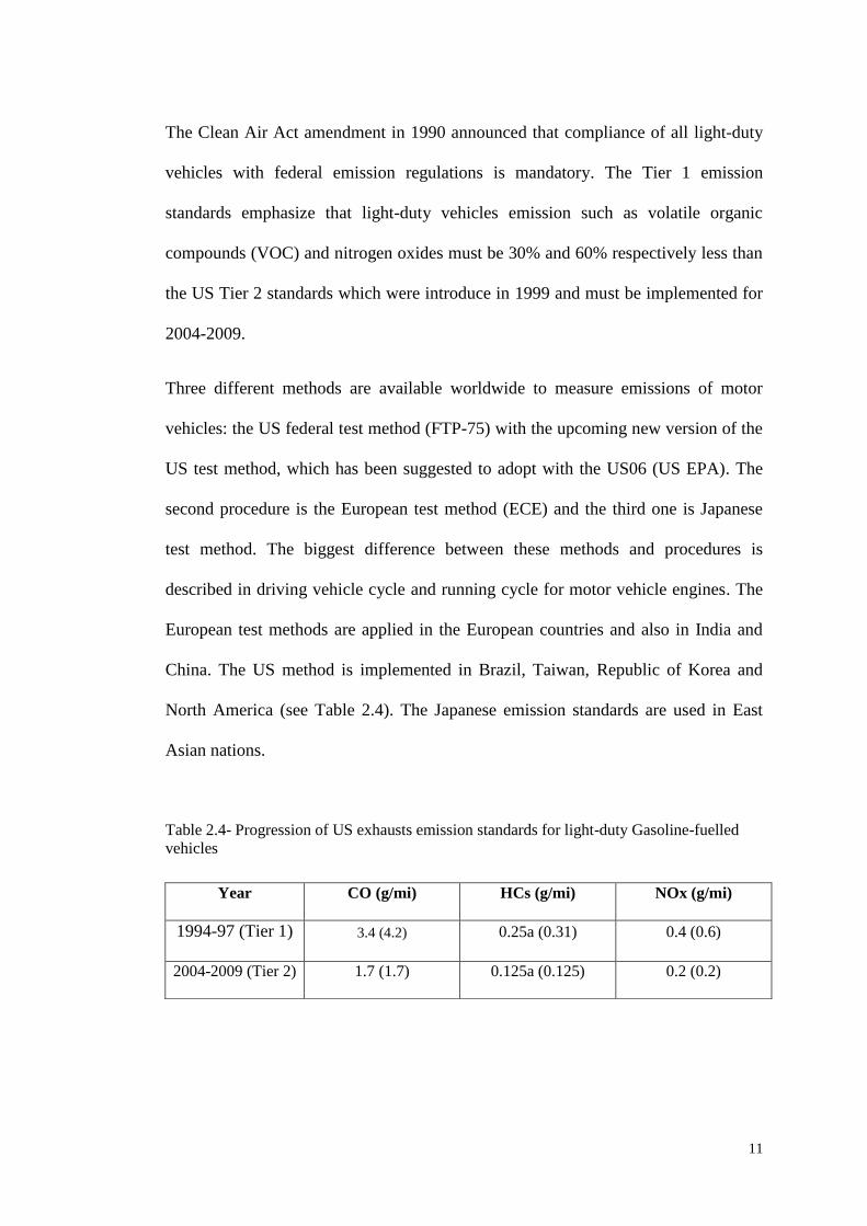
The Clean Air Act amendment in 1990 announced that compliance of all light-duty

vehicles with federal emission regulations is mandatory. The Tier 1 emission

standards emphasize that light-duty vehicles emission such as volatile organic

compounds (VOC) and nitrogen oxides must be 30% and 60% respectively less than

the US Tier 2 standards which were introduce in 1999 and must be implemented for

2004-2009.

Three different methods are available worldwide to measure emissions of motor

vehicles: the US federal test method (FTP-75) with the upcoming new version of the

US test method, which has been suggested to adopt with the US06 (US EPA). The

second procedure is the European test method (ECE) and the third one is Japanese

test method. The biggest difference between these methods and procedures is

described in driving vehicle cycle and running cycle for motor vehicle engines. The

European test methods are applied in the European countries and also in India and

China. The US method is implemented in Brazil, Taiwan, Republic of Korea and

North America (see Table 2.4). The Japanese emission standards are used in East

Asian nations.

Table 2.4- Progression of US exhausts emission standards for light-duty Gasoline-fuelled

vehicles

Year CO (g/mi) HCs (g/mi) NOx (g/mi)

1994-97 (Tier 1) 3.4 (4.2) 0.25a (0.31) 0.4 (0.6)

2004-2009 (Tier 2) 1.7 (1.7) 0.125a (0.125) 0.2 (0.2)

12

2.3. Composition of Gasoline

The composition of Gasoline changes considerably and quickly in the world and

even for different seasons Gasoline must be enhanced with different types of

additives. For instance, in winter, various additives must be added to Gasoline to

prevent the fuel freezing and to keep its capability to combust at lower temperatures

(Elghawi 2009).

Gasoline is divided into various “grades” and the most known types of Gasoline are

RON 97 and RON 95 in the United Kingdom, where RON is the Research Octane

Number. The Research Octane Number (RON) demonstrates capability of fuel for

resisting knock or uncontrolled auto ignition in the engine during compression. It is

essential to identify composition of Gasoline therefore behaviour of each individual

component of fuels can be considered and analysed for different applications.

Table 2.5 illustrates an example of volume percentages of different components in

Gasoline; it was obtained from Future and Fuel Laboratory at University of

Birmingham (Ritchie Daniel, PhD Research Student, University of Birmingham). As

it is shown, aromatics are considered as the major component in the Gasoline

composition. It is essential to mention that aromatics have a Benzene ring and due to

carbon-carbon double bonds they are very stable. Investigations (Kaiser et al. 1983)

tested a certified Gasoline which contained 60% aromatics and 40% paraffins and

speciation was carried out for this composition. Toluene (Methyl-Benzene) is

considered as the most suitable to represent the aromatics fraction of blend, as it is

the most significant component of aromatics in Gasoline, namely 13% (Elghawi

2009). As shown in Table 2.5, Gasoline composition contain 46% of alkanes

13

including iso-alkanes and 14.43% of alkenes which means over 60% volume of

composition of Gasoline constitute of alkanes and alkenes. it can be concluded that

95% of Gasoline by volume are aromatics, alkanes and alkenes. One of the main

components is used to characterize alkanes and alkenes is the iso-octane (2,2,4

thrimethylpentane). It is recognized as an appropriate alkane fraction in certification

test of Gasoline (Kaiser et al. 1991). The Gasoline composition in Table 2.5 is

different from that reported by (Elghawi 2009) of 98% being aromatics, alkanes and

alkenes for winter grade Gasoline. This illustrates modifications that can happen in

Gasoline composition. Nevertheless, both Gasoline compositions demonstrate

aromatics, alkanes and alkenes as the major and main components of Gasoline.

Table 2.5 Typical Composition of Gasoline by % Volume, It was obtained from Future and

Fuel Laboratory at University of Birmingham (Ritchie Daniel, PhD Research Student,

University of Birmingham)

Component % Volume

Alkanes 11.57

Iso-Alkanes 34.30

Alkenes (including dienes) 14.43

Dienes 0.18

Naphthenes 4.01

Aromatics 34.96

Oxygenates 0.00

Unknowns 0.55

Total 100.00

14

2.3.1. Sources of Emissions in Spark ignition

Gasoline Engines

Different pollutants generated by engine are called engine emissions, which are

typically divided into main components such as carbon monoxide (CO), carbon

dioxide (CO2), Hydrocarbons (HC), Nitrogen Oxides (NOx), and Particulate Matter

(PM). The main aim of this project is to analyse individual hydrocarbons at different

engine conditions

2.3.1.1. Carbon monoxide (CO)

Carbon monoxide is produced during incomplete combustion in the engine. The

process of fuel conversion into carbon monoxide can be explained as conversion of

fuel to small hydrocarbons, then oxidation of these hydrocarbons and finally

conversion to carbon monoxide and also due to dissociation of carbon dioxide at

higher temperatures. Incomplete combustion is due to lack of sufficient oxygen in

the air/fuel mixture during combustion. During the combustion, there is no enough

oxygen to fully oxidise the carbon atoms and convert them into carbon dioxide

(CO2). The higher H/C ratio results in lower concentration of carbon monoxide

(Harrington and Shishu 1973).

By adjusting air/fuel ratio in the cylinder, CO emissions can be controlled in the SI

engine. Valério et al. (2004), invented a model to obtain the kinetic formation rate of

carbon monoxide in a spark ignition engines and also the validation of the model.

15

2.3.1.2. Hydrocarbon emission (HC)

Hydrocarbon emissions are produced from two types of sources which are unburned

hydrocarbons and partially burned hydrocarbons. Unburned HCs can be described as

fuel that passes through the chamber and appears in the exhaust emission in its

original form. These types of hydrocarbons are usually in a range of C5 to C12

(Elghawi 2009). Partially burned HCs are defined as hydrocarbons that are not fully

burnt or combusted in the cylinder and have created chain HCs and carbon dioxide

and water (Elghawi 2009).

In this project, analysis of individual hydrocarbons was carried out along with total

hydrocarbons (THC) that contain the main hydrocarbons such as alkenes, alkanes

and aromatics. The main structure of alkanes consists of single carbon-hydrogen

bond that is not able to have additional hydrogen atoms; this kind of hydrocarbons is

recognized as a fully saturated structure. Alkanes may include different side chains

such as iso-alkanes and it will still appear as saturated structure CnH2n+2 where ‘n’

stands for the number of atoms in a molecule. Alkenes structure also has carbon and

hydrogen atoms, but it includes one carbon-carbon double bond. This is known as

unsaturated hydrocarbon and its structure is CnH2n. Aromatics contain a ring of

carbon atoms with double carbon-carbon bonds that are very stable (Hill and Holman

2000). The most abundant main aromatic hydrocarbons in Gasoline is Toluene.

Andrews et al. (2007) reported that most of the HCs in fuel are fully combusted in

the combustion chamber. However, small quantity of hydrocarbons is partially

burned during combustion and that will result in lower molecular hydrocarbons and

oxidized compounds such as aldehydes appearing in emissions. Aromatics such as

Benzene and Toluene may survive process and are emitted in exhaust as unburned

16

hydrocarbons. If combustion does not proceed in a proper way such as when a

misfire happens, huge amount of HCs are emitted in exhaust from the combustion

chamber. Composition of these hydrocarbons depends on engine design, fuel

composition and different operation modes.

There are many different sources of hydrocarbon emissions; the most significant one

that produces major amount of HCs in exhaust under fully warmed engine condition

is combustion chamber crevice volumes. Cheng (Cheng et al. 1993) classified

sources of hydrocarbons emissions according to their relative importance.

Combustion chamber crevices produce 38% of the hydrocarbon emissions. Table 2.6

presents estimation of hydrocarbons sources. Nevertheless, (Alkidas et al. 1995)

estimated that 50% of emitted HCs originates from combustion chamber crevices.

Table 2.6-Hydrocarbon sources and their relative magnitude in SI engine (Cheng et al. 1993)

Source % HC

Combustion-chamber crevices 38

Single-wall flam quenching 5

Oil film layers 16

Combustion-chamber deposits 16

Exhaust-valve leakage 5

Liquid fuel 20

Largest source of hydrocarbon emission result from unburned fuel stored in chamber

crevice volumes in the engine cylinder and propagation of flame is not possible for

narrow entrances into crevice volumes and stored fuel is not combusted and remains

unburned. This is inevitable for all operating modes and conditions. During

expansion stroke, major amounts of hydrocarbons are converted into carbon

monoxide (CO) and carbon dioxide (CO2) in the hot combusted gases in the cylinder

17

and exhaust system. The rest of emissions that are part of stored hydrocarbons in

crevice volumes, are divided into organic products and unburned fuel which are

produced from partial combustion (Kaiser et al. 1994). Combustion of stored

hydrocarbons in the exhaust system plays vital role in concentration of emitted

hydrocarbon species.

Fuel films are produced by wall wetting liquid which is not evaporated and

combusted in the cylinder when flame is passing. Fuel films are evaporated during

cylinder gases cooling, which cause hydrocarbon emission increase. However, wall

wetting does not produce any hydrocarbon emission when the engine is fully warm

(Kaiser et al. 1994).

Combustion chamber deposits can have significant effect on production of HC

emission. Hydrocarbons are pushed into pores during air/fuel mixture compression.

Therefore, when combustion happens, the fuel does not burn. Nevertheless, during

exhaust stroke, these hydrocarbons are emitted into the exhaust stream (Kaiser et al.

1994).

Wall quenching occurs as the combustion flame front burns up to the relatively cool

walls of the combustion chamber. This cooling extinguishes the flame before all

fuels are burned in the cylinder and allows HCs to be emitted through the exhaust

valve. The main source of hydrocarbon emission originates from this phenomenon in

four-stroke engines.

Over the past 30 years, the main focus of all research throughout the world was to

reduce the HCs emissions from spark ignition engines. The oxidation catalyst

produced significant reductions of HC emissions in tailpipe in 1970s. In conclusion,

18

as many articles mentioned during decades, any element that cause to have more

oxygen or the temperature rise to the post flame region result in less hydrocarbon

emission.

2.3.1.3. Oxides of Nitrogen (NOx)

High temperatures combustion flame cause production of nitrogen oxides (NOx)

during combustion. In spark ignition engines, nitric oxide (NO) is considered as the

main part of these oxides along with tiny amount of nitrogen diooxide (NO2).

Oxides of nitrogen are considered as NOx when nitric oxide (NO) and nitrogen

dioxide (NO2) appear together. Usually above 90% of the NOx consists of nitric

oxide (NO) (Stone 1985).

The most part of NOx production is obtained from oxidation of atmospheric nitrogen

originated from reaction with oxygen atoms:

O + N2 → NO + N (1)

N + O2 → NO + O, and (2)

N + OH → NO + H. (3)

This method is identified as the Zeldovich mechanism (Zeldovich 1946). Production

of nitric oxides (NO) increases dramatically with temperature when oxygen atoms

are formed via the thermal decomposition of molecular oxygen.

To limit NOx production from engine, it is necessary to decrease the combustion

temperature. One of the best methods to reduce NOx emissions is the exhaust gas

recirculation (EGR), which introduces part of the exhaust emission to the intake

manifold. The influence of dilution and the use of CO2 and H2O exhaust gases

19

instead of air cause temperature reduction in combustion process and finally less

production of NOx.

2.3.1.4. Carbon Dioxide (CO2)

One of the main combustion components is carbon dioxide (CO2), which is a

greenhouse gas. It is also one of the most important components responsible for

global warming through the greenhouse effect. However, most of emission

limitations require a decrease of carbon dioxide (CO2) emissions from automobiles

(Johnson 2010). Although Carbon dioxide emissions are proportional to fuel

consumption and combustion efficiency, in an optimised engine the effects on CO2

are inversely related. Higher combustion efficiency will result in higher carbon

dioxide emissions and decreasing fuel consumption will cause lower carbon dioxide

emissions. Investigations show that oxygenated fuels produce more carbon dioxide

emissions (Owen and Coley 1995) and the reason is explained in having higher

combustion efficiency and lower low heating value, which results in higher fuel

consumption.

2.3.1.5. Unregulated Engine-out Emissions

Toxic components such as 1, 3-Butadiene, Benzene and aldehydes are emitted from

the spark ignition engines. 1, 3-Butadiene is recognized as a product of partial

combustion and originates from the aromatic and alkane components of fuel (Filser

and Bolt 1984). Many articles have presented carcinogenic properties of 1,3-

Butadiene, which cause human cancer (Huff et al. 1985). One of the main

20

components in the Gasoline engine exhaust is Benzene. Benzene is originated from

de-alkylation of aromatic compounds such as Toluene.

Both of these hydrocarbons are considered as carcinogens. According to

epidemiological evidence, International Agency for Research on Cancer (IARC) has

introduced Benzene as a human carcinogen group 1 (IARC 1987). Many studies in

the United States has shown that motor vehicles are the main reason for human

exposure to toxic pollutants such as Benzene and 1,3-Butadiene (US-EPA 1990b).

Aldehydes are those types of HCs, which contain additional oxygen atoms. These

hydrocarbons appear during combustion process of fuel with high oxygen content.

Incomplete combustion and also thermal decomposition are the main reasons of

aldehydes formation in the cylinder. Formaldehyde forms 50-75% of aldehydes in

exhaust emission of Gasoline fuel and are considered as one of the most reactive

organic chemicals. For alcoholic fuels such as Ethanol and Methanol, due to

oxidation reactions in acetaldehydes, formaldehyde and benzaldehyde, significant

concentration of these carcinogen components in the exhaust emissions are expected.

2.3.1.5. Ozone Formation

Concerns about air pollution have generated special attention to research about fuels

and engine effects on emissions. A critical component of these investigations is to

fully understand atmospheric impact of emitted hydrocarbons from motor vehicles.

The atmosphere contains 79% nitrogen and 21% oxygen by volume and is extremely

oxidizing environment. Oxidization of engine exhaust components is carried out in a

various series of reactions in atmosphere.

21

Ozone plays a vital role in the earth atmosphere and it is considered as a pollutant at

ground altitude. Existing oxygen, nitrogen oxides and hydrocarbons help to form

ozone in atmosphere under sun radiation effects. Carter et al. (1998) have introduced

a method to measure ozone formation potential of hydrocarbons. Two methods have

been discovered, chemical kinetic models and smog chamber experiments.

Maximum incremental reactivity is a measure of the increase in ozone formation per

unit weight of a hydrocarbon when added to the atmosphere. Each of exhaust

emission hydrocarbons demonstrates various photochemical reactivities. Table 2.7

illustrate hydrocarbons with their maximum incremental reactivity (MIR) that was

developed by Carter (1998). The speciation factors of individual hydrocarbons

multiplication by maximum incremental reactivity (MIR) scale makes this possibility

to avoid calculation of ozone formation potential of exhaust emissions. The negative

amount of MIR demonstrates ability of oxidation compounds for reacting with NO2

and it eliminates NOx from the exhaust system. The low maximum incremental

reactivity means lower reaction.

22

Table 2.7-Maximum incremental reactivity factor for selected Hydrocarbon species (Carter

1998)

Compounds MIR [g ozone/ g HC]

Methane 0.01

Ethane 0.35

n-Butane 1.44

n-Pentane 1.74

n-Hexane 1.69

n-Heptane 1.43

n-Octane 1.24

Iso-butane 1.56

Iso-pentane 1.93

Iso-Octane 1.69

Ethylene 9.97

Propylene 12.44

1-Butene 10.8

1-Pentene 8.16

1-Hexene 6.3

Iso-Butene 6.81

1,3-Butadiene 13.09

Formaldehyde 9.12

Acetaldehyde 7.27

Acrolein 8.09

Benzaldehyde -0.5

m-,o-,p- Tolualdehyde -0.44

Benzene 1

Toluene 4.19

Ethyl benzene 2.97

Styrene (vinyl benzene) 2.52

m-Xylene 11.06

o-Xylene 7.83

p-Xylene 4.44

1,3,5-Trimethyl benzene 11.1

Naphthalene 3.05

Furan 17.25

23

2.4. Developments in Speciation and Quantification

of Hydrocarbons (review)

The major source of high atmospheric hydrocarbon release is motor engines in many

urban areas. This poses serious environmental and health hazards in the society.

Photochemical smog is an example of health hazards emerging from the higher

concentration of exhaust gases released by the combustion engines (Loh et al. 2007).

In a research study, it was reported that 48 to 54 % of cancer prevalent in USA is due

to the presence of high amounts of toxic gases in the environment (US-EPA 1990b).

In recent years, most of the energy used in the world originates from fossil fuels and

due to high cost of fossil fuels; clean energy demands have been increasing rapidly

(Mousdale 2008). Studies have shown other renewable sources of energy such as

vegetable oil, biogas, biofuels and natural gas besides the traditional fossil fuels

sources (Bechtold 1997). These studies have shown Ethanol obtained from the

biomass as a potential alternative of fossil fuels. It is considered as the most efficient

fuel because of its high heat of evaporation and octane number, which improves the

engine operation and reduces exhaust gases release (Das L.M 1996, Yücesu et al.

2006). High miscibility of Ethanol is observed with water in contrast to Gasoline

(Kelly et al. 1996, Koç et al. 2009).

Many studies have been conducted to produce more efficient biofuels e.g. 2,5-

dimethyfuran (Román-Leshkov et al. 2007). Conversion of fructose and glucose to

5-hydroxymethhylfurfural and 2,5-Dimethylfuran were made through a novel

catalytic biomass liquid process and fuel showed improved efficiency and yield

(Dumesic et al. 2007). Some more studies reported the production of high yields of

24

HMF with non-acid conversion bioprocess (Zhao et al. 2007). Cellulose can also be

converted to 5-(chromethyl) furfural and later upon homogenization it can be further

converted to DMF fuel. Due to improved manufacturing process of DMF, it has

shown a considerable potential to substitute Gasoline in automobile industry (Mascal

and Nikitin 2008).

DMF exhibit volumetric energy density (31.5 MJ/l) which is the same as Gasoline

and it is 40% greater than the one exhibited by Ethanol (23 MJ/l). The DMF feature

which makes it an ideal alternative of Gasoline in comparison with Ethanol is its

high boiling point (92oC) as it confers low volatility and thus makes it a potential

alternative fuel.

Due to the newly discovered and currently being developed production methods of

DMF, it has become more attractive biofuel candidate. Higher energy density and

octane number of DMF compared with Ethanol lead to higher compression ratio,

improvement in fuel consumption and engine performance makes this fuel an

alternative for Ethanol. Furthermore, DMF has practically zero water solubility,

which eliminates the water absorption problem. (Rothamer and Jennings 2012).

Suitable Gasoline alternatives and their compositions can be identified via

hydrocarbon speciation process. Individual study on each hydrocarbon can impart

photochemical effect and toxicities. Compound which is studied up till now through

new regulatory mechanisms is 1,3- Butadiene and aldehyde (Kao 1994).

Gas chromatography was reported to be the most effective process for individual

hydrocarbon study as mentioned by Jensen et al. (1992) and Siegl (1993) and

25

through this method 140 hydrocarbons have been analyzed up till now (Jensen et al.

1992, Siegl et al. 1993).

Kaiser studied the impact of some of the fuels on environment due to their emission

and he also investigated the effect of unburned hydrocarbons on total HC released.

The fuels he used were six paraffin fuels, two naphtene fuels, two aromatic fuels and

also unleaded and olefin fuels. The aromatic emissions from both naphtene fuels

contribute significantly to the emitted hydrocarbons and the experiments

demonstrate that substantial quantities of aromatic species were observed from non-

aromatic fuels. However, for olefin fuels, four alkenes such as ethylene, 1-Butene, 1-

hexene and di-isobutylene were used as fuels in a single cylinder engine and the

results illustrates that the total hydrocarbons emissions increased with increasing the

molecular weight of the fuel as was investigated previously for alkanes.(Kaiser et al.

1991, Kaiser et al. 1992, Kaiser et al. 1993, Andrews et al. 2007).

In many countries, increasing air pollution and greenhouse gas emissions caused by

fossil fuels has encouraged the use of alternative fuels. The reasons such as depletion

of world’s crude oil and its increasing wholesale price as well as the energy crisis

have created an incentive to use alcohols as alternative fuels (Wagner et al. 1980,

Mielenz 2001 and Al-Baghdadi 2003). This trend is motivated by three primary

factors: global climate change, energy security, and economics. To improve engine

performance and exhaust emissions, many additives can be added to fuel.

Oxygenates are one family of additives that can be used to enhance engine efficiency

and exhaust emissions (Jia et al. 2005). Biofuels play an increasingly vital role in the

supply of renewable energy and can help to reduce greenhouse gas emissions. The

renewable energy demands will increase in the future with the development of new

26

generation biofuels which are more efficient and do not compete with the food chain.

Due to these developments, 2,5-Dimethylfuran (DMF) is assumed as an alternative

fuel (Aden and Foust 2009).

In the United States, large-scale production of Ethanol has made it possible to exceed

the 10% Ethanol content requirements for Gasoline blend nationwide. In recent

years, use of larger percentage of Ethanol (up to 15%) in blend with Gasoline is

allowed by US Environmental Protection Agency (EPA) in new light duty vehicles.

Higher percentage of Ethanol requires an EPA waiver in terms of emissions and

performance considerations (US-EPA 1990b).

Among various oxygenates, Ethanol is the most suitable fuel for spark ignition

engines (SI) and the main benefit of Ethanol as an SI engine biofuel is that it can be

produced from renewable energy source such as sugar cane, cassava and various

types of waste biomass materials (Bayraktar 2005, Topgül et al. 2006).

Most attractive properties of Ethanol over Gasoline as a fuel are high evaporation

heat, high octane number and flame speed which allow positive effect on the engine

efficiency and higher compression ratios. Nowadays, Ethanol-Gasoline blends are

more desirable fuels, with better anti-knock characteristic than pure Gasoline

(Yücesu et al. 2006) which allows increasing the compression ratios. Moreover, the

main advantages of using Ethanol and Gasoline blends are reduction of CO, volatile

organic compounds (VOC) and unburned hydrocarbons emissions (Topgül et al.

2006).

Blending Gasoline with low levels of Ethanol has the advantage of no need for

changes on current engines. Also it offers increase in overall octane number of the

27

fuel blend; this increase in octane number can result in increase in efficiency by

advancing spark timing (Rothamer and Jennings 2012).

Recently, Ethanol is used mostly as alternative liquid biofuel (Agarwal 2007, Fatih

Demirbas 2009). In some regions like Brazil, Ethanol is used as a neat engine fuel or

in different blends with Gasoline (Román-Leshkov et al. 2007, Mousdale 2008).

Daniel et al. (2011) investigated the performance and emissions of DMF compared

with Ethanol and commercial Gasoline. They reported that all of the standard

emissions were reduced for Ethanol and slightly decreased for DMF. Rothamer et al.

(2012) reported the effect of DMF and Ethanol in blends with Gasoline on

combustion properties and emissions, their findings were in agreement with Daniel’s

work. Also they reported that for direct injection operation Ethanol is more effective

than DMF for reducing engine knock for the same blend percentages.

Graham et al. (2008) found that 10% Ethanol blend has considerably increased

acetaldehyde emissions (108%) and produced insignificant changes in formaldehyde

emissions. Hsieha et al. (2002) tested Ethanol-Gasoline blend with various blended

rates (0%, 5%, 10%, 20% and 30% by volume). Furthermore, the influence of

Ethanol content on the exhaust emissions from SI engines has been studied. Addition

of Ethanol decreased CO and total hydrocarbon (THC) significantly; NOx emissions

are dependent on engine operating condition rather than on Ethanol content.

Al-Hasan (2003) studied effect of using unleaded Gasoline-Ethanol blends on engine

performance and exhaust emission. The results indicated that CO and HC emissions

reduced approximately 46.5% and 24.3% respectively. The study mentioned that

20% Ethanol addition to Gasoline had the best results of the exhaust emissions.

28

Hasan et al. (2011) investigated the effect of composite after treatment catalyst on

hydrocarbon speciation from Gasoline engine; they found that hydrocarbon

speciation is heavily dependent on engine operation and combustion mode. Elghawi

et al. (2009) reported the same concept as Hasan et al. Also they have reported that

for SI mode about one half to two thirds of total HC emissions comes from the C6-

C12 range.

2.5. Investigations on Lubricity of fuels using HFRR

(review)

Exposure of the fuel to the fuel pump and internal combustion injection system

provides lubrication of these components. Aeronautical industry was the first to

report the problems of insufficient lubricity problems of fuels in the 60s (Margaroni

1998). The same problem was reported when low sulphur fuel was fed to light-duty

diesel engine The literature shows highly polar fuel compounds were found as the

causes of good lubrication due to the formation of protective layer on the surface of

metal (Safran 1994). This investigation shows the protection could increase for the

fuels containing nitrogen and oxygen. Anti-wear additives are used to improve the

lubricity properties of the fuel because the fuel processing may lead to elimination of

surface active polar compounds (Nikanjam 1992, Barbour and Elliott 2000).

The necessities of lubricity improvement for diesel fuels are much higher than

Gasoline counterparts due to high pressure operation of diesel fuel’s pumps. There

have been some reports on failure of fuel pumps in Gasoline; some of these failures

are reported to be because of poor Gasoline lubricity (Spikes et al. 1996, Wei et al.

1996, Rovai et al. 2005).

29

To enhance the catalyst life and performance in Gasoline engines, the reduction of

fuels compounds such as sulphur contents were considered as a requirement for high

pressure injections pumps of direct injection Gasoline engines, therefore the

investigation of lubricity property of Gasoline fuels became a significant issue

(Eleftherakis et al. 1994). Fuels must provide adequate lubrication of the moving

parts in the fuel supply system, thus research on the effect of specification of fuel

compositions on lubricity is of paramount importance (Danping and Spikes 1986).

In engine fuel systems components such as fuel pumps, flow-control valves and

injectors, fuel lubricity is important for the lubricating behaviour of the fuel itself.

There are many investigations published on diesel and biodiesel fuel lubricity

characteristics, but there is lack of data on lubricity of Gasoline and Gasoline type

bio-fuels. Most Gasoline fuel injection systems inject fuel into the inlet port

upstream of the inlet valves; consequently the operation is at much lower pressure

compared to diesel pumps (Heywood 1985, Aden and Foust 2009). This reduction

in operation pressure results in lower lubricity requirements for Gasoline compared

with diesel (Ping and Korcek 1996). It was discovered that Gasoline which has

higher sulphur content, has good lubricity. It is believed that this good lubricity is a

result of polar-type compounds which absorb themselves into the alloy and form a

protective film coating (Childs and Stobart 2004).

Ping et al. (1996) was the first groups researching the lubricity of Gasoline. They

modified the High Frequency Reciprocating Rig (HFRR) which is mainly used as

the instrument for measuring the lubricity of diesel fuel for testing the Gasoline.

They reported that the Gasoline without additives gave higher wear than highly

refined Class I diesel fuels. Also they reported that adding detergent additives to

30

Gasoline decreases the wear. Lapuerta et al. (2009) reported that adding Ethanol to

biodiesel blends resulted in loss of lubricity at high concentrations of Ethanol in

blend. Agudelo et al. (2011) reported that adding different percentages of Ethanol to

Gasoline (E20-E85) did not impact significantly the blend lubricity, but that addition

of hydrated Ethanol slightly improved blend lubricity in comparison with adding

anhydrous Ethanol.

31

2.6. Summary

In summary, the literature review discusses the regulated and unregulated exhaust

emissions. The major areas contain the discussion of different sources of emission in

spark ignition engines and the effect of composition of fuels on emission of

individual hydrocarbons.

The effect of new alternative oxygenated fuels in SI engines also discussed. The

main concentration of the literature review is on 2, 5-Dimethylfuran (DMF) that has

become popular as a biofuel candidate among researchers due to newly developed

production methods. Advances in production of DMF, conversion of fructose using a

catalytic biomass liquid process have created this possibility for DMF to be

considered as an alternative for Gasoline. Nowadays, many investigations have

reported the anti-knock characteristics of DMF which makes properties of biofuel

similar to Gasoline. The effect of oxygenated fuels blends with Gasoline on

regulated and unregulated emissions were discussed. Ethanol reduces the amount of

CO and THC significantly due to oxidisation of unburned hydrocarbons.

The effect of lubricity of diesel and Gasoline fuel’s pump in SI engines explained.

The diesel engines require more attention for lubrication of moving parts in fuel

system due to high pressure of operation in diesel fuel’s pump. Lack of publications

in lubricity of Gasoline and oxygenated fuels give an incentive to investigate about

this property of fuels.

The major motivation of thesis was introduced in the literature review, which is to

describe comparison of regulated and unregulated emissions of different fuels and

their blends in single cylinder spark ignition engine.

32

CHAPTER 3

3. EXPERIMENTAL SETUP

3.1. Lubricity experimental setup

Over the decades, various experimental methods have been applied to investigate

and study the lubricants and lubricity of fuels. The most two common test

procedures are as follows:

High frequency reciprocating rig (HFRR) ASTM D 6079-99 and ISO 12156-1

Scuffing Load Ball on Cylinder Lubricity Elevator (SBOLCE) ASTM 6078-99

Due to high repeatability of HFRR method, it is more popular than SBOLCE and it

was used in this study.

3.1.1. HFRR (High Frequency Reciprocating Rig)

The high frequency reciprocating rig (HFRR) experiment is performed according to

European standards for the measurement of lubricity. In short, HFRR rig use a metal

ball to scratch on a metal plate with constant frequency while it is immersed in the

fuel. Figure 3.1 shows schematic diagram of High Frequency Reciprocating rig

(HFRR). After the experiment, the wear scar appears on the metal ball and must be

measured in accordance with the BS EN 590. To obtain accurate and consistent

results for lubricity of different fuels, some factors and parameters requires to be

constant and must be within a permitted range. The HFRR rig is controlled by a

computer and provides reliable analysis of lubricity results. The HFRR rig is

33

attached to a controller/processor (see Figure 3.2) and this processor communicates

with a PC as the interface between the user and the device.

Figure 3.1-HFRR Schematic Diagram

Figure 3.2-HFRR instrument (PCS Instrument Company)

34

At the first stage, the HFRR must be calibrated to confirm accurate functioning of

the test rig. It is recommended that the device to be calibrated after every five

experiment to achieve reliable and repeatable results for the future experiment. To

attain the best performance for the rig, the wear scar for high and low lubricity

reference fuel must be measured.

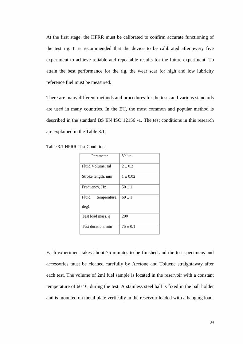
There are many different methods and procedures for the tests and various standards

are used in many countries. In the EU, the most common and popular method is

described in the standard BS EN ISO 12156 -1. The test conditions in this research

are explained in the Table 3.1.

Table 3.1-HFRR Test Conditions

Parameter Value

Fluid Volume, ml 2 ± 0.2

Stroke length, mm 1 ± 0.02

Frequency, Hz 50 ± 1

Fluid temperature,

degC

60 ± 1

Test load mass, g 200

Test duration, min 75 ± 0.1

Each experiment takes about 75 minutes to be finished and the test specimens and

accessories must be cleaned carefully by Acetone and Toluene straightaway after

each test. The volume of 2ml fuel sample is located in the reservoir with a constant

temperature of 60° C during the test. A stainless steel ball is fixed in the ball holder

and is mounted on metal plate vertically in the reservoir loaded with a hanging load.

35

The vibrating motion is carried out by the HFRR machine with stroke length of 1mm

and a frequency of 50 Hz.

The atmosphere condition during the test has significant effect on the result of the

experiment and the wear scar. The acceptable ranges of atmosphere conditions and

relative humidity percentage are shown in Figure 3.3.

Figure 3.3-Acceptable Test Conditions (ISO 12156 -1)

The HFRR Humidity Controlled Cabinet (HFRHCAB) is applied as an accessory for

the HFRR to permit the experiments to be performed at constant room temperature

and relative humidity. The humidity control cabinet increases repeatability and

reliability of the tests (see Figure 3.4).

36

Figure 3.4-HFRR Atmosphere Control Cabinet (PCS Instrument Company)

Figure 3.5 demonstrates the wear scar measurement under the microscope. The wear

scar was measured using a microscope (see Figure 3.6). The wear scar diameter is

observed in both X and Y directions. Mean wear scars were calculated as follows:

Figure 3.5-Wear Scar Measurement after HFRR Test

37

Figure 3.6-Microscope

In order to prevent evaporation of fuels such as Gasoline, Ethanol and DMF,

Gasoline Conversion Kit has been used (see Figure 3.7).

Figure 3.7-Gasoline Conversion Kit (PCS Instrument Company)

38

3.2. Exhaust Emission Measurement

This chapter provides information on equipment applied in this research, including

equipment setup and operation. The Gas Chromatography Mass Spectrometry

method development for different applications is described in this section.

3.2.1. Single Cylinder Engine

The single cylinder four-stroke engine used in this research is fitted with a four

valves spray guided direct injection cylinder head. The basic engine specifications

are shown in the Table 3.2. In order to even-out the pressure in the intake and

exhaust ducts, it is required that the engine is connected to both the intake and

exhaust plenums. The engine is connected to a DC dynamometer, which in the

experiments presented here has a constant speed of 1500 RPM. When engine

operates at stable condition, the speed can be maintained within ±20 RPM but it

reaches to ±200 RPM at unstable operation. Before any research is carried out, the

engine must be warmed up at low load in SI mode until water and oil operating

temperature reaches to 95±3 °C and 85±3 °C respectively. Figure 3.8 shows

schematic diagram of single cylinder engine used in this study which is connected to

the GCMS using heated line.

Table 3.2-Basic Engine Geometry

Bore (mm) 90.0

Stroke (mm) 88.9

Swept Volume (cm3) 565.5

Connecting Road Length (mm) 160.0

Compression Ratio 11.5:1

39

Figure 3.8- Schematic of the laboratory setup used this study

40

3.2.1.1. Combustion System

As demonstrated in Figure 3.9 the combustion system of this engine contains a

centrally fitted injector having six injection holes; the spark plug is connected next to

the injector at an angle of 18 degrees relative to the axis of the cylinder. The pattern

of the nozzle contains two groups of three holes and the symmetric line of these

holes is coincident with the crankshaft axis.

Figure 3.9-Layout of combustion system

41

3.2.1.2. Crankshaft Encoder Assembly

The timing signal produced by the crankshaft encoder must be precisely recognized

as it is utilized by the engine control software package and the variable valve timing

software for spark timing. The timing of this signal (relative to combustion TDC) is

acquired by adjusting a spark timing of 0º bTDC in the engine software, and

evaluating the real location of the spark by operating a stroboscope and the one

degree markings on the flywheel of engine. Once this balance is achieved it can be

inserted into the engine control software therefore the 0º bTDCCOMB spark appears

at TDC. The one/degree markings on the engine flywheel are confirmed by

measurement of the piston location (relative to TDC) at different positions and

evaluating the angular distance from the crankshaft geometry.

3.2.1.3. Variable Cam Timing

The variable cam timing system (VCT) attached to the single cylinder engine applies

lubricating oil pressure to modify the camshaft offset relative to the camshaft pulley.

The camshaft timing may be delayed up to 50 crank angle degrees for both

camshafts (intake and exhaust). A LABVIEW program is used to control variable

cam timing system, the software shows the camshaft location once a cycle and every

two revolutions for crankshaft and performs adjustments to the cam timing by

modifying the signal pulse width which is sent to Variable Camshaft Timing Oil

Control Solenoid. Generally, for maintaining stable engine condition and operation,

the camshaft position must be kept within ±0.1 CAD.

42

3.2.1.4. Fuel System

The single cylinder engine applied in this research is connected to direct injection

(DI) system and a port fuel injection system (PFI). The PFI system is used to warm

up the engine, but it can be applied to evaluate the mixture preparation performance

of direct injection system. The DI system is constructed with a free piston

accumulator. An electric pump helps to deliver fuel from day-tank to the volume in

the top of accumulator, which is located above the piston. The DI injector is attached

to top of the cylinder. Using oxygen-free nitrogen supplied by BOC, the area under

the piston is pressurized. The system is equipped with a circuit to return all unused

fuel to the tank, with ability to flush the entire system using the nitrogen cylinder.

The system is made of ¼ inch stainless steel tube and fittings; the fuel pressure in all

experiments is 150 bar gauge.

3.2.1.5. Lambda Meter System

The lambda meter system applied in the experiments is an ETAS Lambda Meter

(Model LA3) with Bosch heated wide-band oxygen sensor. This special lambda

meter device permits the preprogrammed fuel properties to be modified to match the

fuel in the engine. These fuel properties are stoichiometric air fuel ratios, H/C and

O/C ratios. These properties and parameters become important when oxygenated

fuels are applied to the engine. The lambda control must be open loop where engine

operator sets the injection pulse width to obtain appropriate value.

43

3.2.1.6. Control

The LABVIEW software controls all parameters such as injection and spark timing

in the engine using a National Instruments counter timer card (model 6602). While

the engine is running at stable operating condition, the injection and spark timing can

be adjusted in real time. The software has the potential of monitoring two separate

injections with different pulse width per cycle.

Load settings for SI are obtained by adjusting a butterfly throttle valve that is located

in the inlet. The indicated mean effective pressure (IMEP) is measured online from

in-cylinder pressure using high-speed data acquisition program and IMEP also is

measured using a Kistler water-cooled pressure transducer type 6041A, flush

connected to the cylinder head wall, attached to the data acquisition system by a

Kistler 5011 charge amplifier.

The intake and exhaust temperatures and other temperatures such as engine oil and

coolant were all obtained by type “K” thermocouples. The engine coolant

temperature is adjusted with Proportional Integral Derivative (PID) to control

solenoid valve that set the cold water flow through a heat exchanger.

3.2.2. Gas Chromatography

The main aim of gas chromatography is to separate and detect individual

components of a mixture that are gas or liquid. To analyze the exhaust gas samples,

GCMS is connected to an engine exhaust outlet. To vaporize the liquid sample, the

sample inlet (injection point of the sample) must be heated.

The gas chromatograph is divided into five main parts (McNair and Miller 2011),

which are as follows:

44

Carrier Gas

Sample inlet

Column

Thermostatic Oven

A Detector

All gas chromatographs contain these five main parts and they are the same for both

gas and liquid sampling.

Separation process (chromatography) of solute mixture is done by distribution of

mixture into mobile and stationary phases. The stationary phase is solid and is

packed within the column and it is described with a large surface area that includes

particles with 150μm diameters or less, creating a porous surface and finally

providing absorption (Elghawi 2009). The mobile phase contains a carrier gas that

pushes the vaporized components in the column and into the mass spectrometer

detector. Each compound travels across the column in a specific time due to its

unique molecular structure (McNair and Miller 2011). The certain time for each

compound to leave the GC is called its retention time.

The gas chromatograph applied in this study contains an automatic oven temperature

control that performs precise control of the oven and consequently column

temperature. The gas chromatograph has the capability of different temperature

ramping profiles therefore temperature can be modified at various preset rates.

A chromatogram is always generated by the gas chromatographs and form of

chromatograms can be slightly different due to different type of detectors that can be

used. It is important to mention that all chromatograms in this research have the

same layout. The X-axis illustrates retention times for each compound, while the Y-

45

axis demonstrates the percentage of signal intensity that has been received by the

detector for each compound. The signals have the form of Gaussian shape on the

chromatograms. To perform quantitative analysis of the sample, the peaks are used

to identify each components existing in the original sample. For the quantitative

analysis, the relative areas under the peaks must be calculated to find out how much

of a specific component exists in the original sample. However, the quantification of

components requires calibration of gas chromatography mass spectrometry (GCMS)

using mixture of pure gases with a certain quantities.

3.2.2.1. Carrier Gas

The main aim of the carrier gas is to transfer the injected sample through the column

and push into the mass spectrometer. The carrier gas selection is important and it

must be chosen correctly, depending upon the compounds that need to be analyzed,

the temperature profiles and the detector that is going to be used. A wrong carrier gas

could directly affect the separation process of components, detector performance and

finally results. The carrier gas can be helium or hydrogen but other available gases

such as nitrogen and argon can be used. The most appropriate carrier gas for use in

this research is helium as a carrier gas since all compounds present in this study

contain hydrogen. A hydrogen carrier gas could interfere with separation and

detection process of compounds. Helium is pumped away easily by mass

spectrometer vacuum pump and the sensitivity of detector is low for the helium; in

general, helium reduces its effect on the analysis of results.

The flow rate of carrier gas has significant importance in separation of components.

For the best separation of compounds, the optimum flow rate must be chosen. The

46

flow rate of carrier gas depends on the inlet pressure at head of gas chromatograph

column.

Flow control is essential in GCMS, and the flow rate should be maintained at

constant pressure during components separation to prevent fluctuations of

chromatogram baseline, which affect quantitative analysis of results. The reason of

these fluctuations during temperature programming of GC is due to changes of flow

rate, as viscosity of helium will increase with temperature. However, decrease in

flow rate affects appropriate separation of components and their retention times. The

changes in retention time result in some difficulties for identification of compounds.

Controlling of flow to keep the constant flow rate within temperature profile is

essential.

3.2.2.2. Sample Inlet Injection

The exhaust gas sample injection to the GC column head has significant importance

in having accurate results. This must be obtained rapidly without having any

contamination and directly into the column. The gas samples are introduced by

sampling valves and loops while liquid samples are introduced into the GC using

septum seal.

3.2.2.3. Liquid Sample Inlet

Sample inlet must be heated for injection of liquid samples to vaporise the sample

immediately and mix it with carrier gas flow. To create sharp peaks of compounds

on chromatogram, the liquid sample injection must be performed quickly. Slow

injection of the sample will produce wider peaks, which could cause some

47

difficulties in identification of compounds. The introduction of sample to the GC is

performed by micro syringe as small amount of sample is needed due to expansion

of the sample when it is vaporised from liquid to gas. Sample volumes are usually

only a few micro litres (μL). It is also essential not to overheat the sample since it

causes decomposition of components that affect in appropriate detection of the

components.

Liquid injection is divided into two different techniques that are:

Split Injection- after injection and vaporization of the sample, only small

quantity of the sample enters the column. This phenomenon is carried out by

split or purge valve to determine what proportion of the sample enters into

the column and how much is purged from the sample. This technique is

performed due to having high-resolution separation of peaks for more

accurate analysis of the results. This method also determines ratios in the

range of 10:1 to 1000:1, but these extremes are unlikely to be used (Elghawi

2009). The major advantage of this technique is explained when the split

ratio needs easily to be adjusted by a valve and the disadvantage of the split

injection is that the detector may not be able to detect and identify the

compounds as only small quantities of the sample are injected into the

column.

In Split-less Injection the injection is made as in split injection but the sample

is not purged, it means that the entire injected sample enters into the column.

This method is used to improve sensitivity of components with low

concentration.

48

3.2.2.4. Gaseous Sample Inlet

Gaseous samples are injected directly into column using a sampling loop. Figure

3.10 demonstrates a schematic diagram of six port Valco switching valve that was

used in this study. When the Valco valve is in the LOAD position, the gas sample is

introduced into the sample loop. In the LOAD position, sample flows through the

loop and then is vented through the atmosphere and helium as a carrier gas enters

into the gas chromatograph directly. The other position is the VENT position in

which the excess sample will flow out through the vent port directly and helium gas

will push the samples within the loop toward the column. Figure 3.11 shows the six

port Valco valve used in this study.

Figure 3.10-Six Port Valco Valve Assembly

LOAD Position VENT Position

49

Figure 3.11-GCMS Sampling Set

Many different experiments were performed using different volumes of loops (1 ml

and 100 μL) to improve the sensitivity of the gas chromatography analysis. Small

sample size will result in lower concentration of compounds, weaker peaks in

chromatogram and also cause minor compounds of the sample to become

undistinguishable from the column bleed and column coating.

In general, the Valco valve mechanism has the capability of reducing carrier gas

pressure fluctuations as the valve switches to INJECT position when helium enters

into the column via six-port valve.

50

3.2.2.5. The GC Column

One of the most important parts of the gas chromatography instrument is the column.

It contain stationary phase that cause separation of different compounds in the

sample. Usually, there are two different types of column that can be applied in the

GC which are: the conventional packed columns with diameter of 2 to 4 mm and

with the length of 0.6 to 4 meters and packed with appropriate adsorbent

(Braithwaite et al. 1985). The other type of column is the open tubular column that is

produced from fused silica (McNair and Miller 2011). Internal diameter of this

column ranges from 100 μm to 500 μm and with 10m to 100m long. The open

tubular column is divided into two different categories of (a) Porous Layer Open

Tube (PLOT) and (b) Walled Coated Open Tube (WCOT).

Many parameters must be considered for choosing the appropriate column since the

type of the column has a direct effect on retention times of the sample in the column.

Longer columns can provide better separation of compounds within the column but

also the analysis time of the GCMS becomes longer (McNair and Miller 2011).

Other factors such as column temperature and carrier gas flow rates can help the

column to be optimised for the sample (Elghawi 2009). Hasan et al. (2011) used this

column to do speciation of hydrocarbons in his investigation.

After many experiments, the column may be contaminated when the sample passes

through it. Therefore, there is a need to bleed the column with the high temperature

of 220 ⁰C and leave it for a day or less to clean any contaminants of the column and

to keep the accuracy of the column during the experiments. In this study the highest

appropriate temperature for bleeding the column is 220°C. Columns have limited life

and after a while must be replaced, but column bleeding can help to increase the life

51

of the column. The column used in this study is PoraPlot Q type (see Figure 3.12).

The column specifications were shown in Table 3.3.

Figure 3.12-PoraPLOT Q Column (PerkinElmer Company)

Table 3.3-Column Specifications

Column PoraPLOT Q

Length (m) 25

Internal Diameter (mm) 0.32

Film (μm) 10

3.2.2.6. Thermostatic Oven

One of the most important factors for better separation of the components is the

temperature of the GC column. The GC oven controls the column temperature

precisely and it can be varied in range of 25°C to 350°C. The GC oven is

programmed to heat up temperature with time. It increases the programmed

52

temperature profile at a linear rate. All temperature settings are adjusted by the users.

For adjusting the oven temperature, the oven must be set at 35°C firstly; it must be

held at this temperature for two minutes; when temperature starts to rise the carrier

gas expands. Then temperature increases at a certain rate (in these experiments the

rate is 8°C/minute) and it heats up until the temperature reaches 220°C and at the

final stage it remains at 220°C for few minutes to flush the column. Finally the oven

is cooled down to 35°C again to before any subsequent experiment is carried out.

A slower temperature increase rate will generally perform better separation of

components in the sample but it takes a longer time to carry out the analysis.

3.2.2.7. The GC Detectors

There are different types of detectors that are applied to perform identification of

sample components. The most common detectors are:

Catalytic combustion detector (CCD)

Electron capture detector (ECD)

Flame ionization detector (FID)

Thermal conductivity detector (TCD)

Helium ionization detector (HID)

Electrolytic conductivity detector (ELCD)

Fourier Transform Infrared (FTIR)

Mass Spectrometer (MS)

In this research, mass spectrometer detector has been used to detect hydrocarbon

compounds.

53

3.2.3. Mass Spectrometry

Mass spectrometry analysis is described as dominant method that performs

identification of HC components in different applications such as engine exhaust

emission analysis, drugs and pharmaceuticals, clinical chemistry, petroleum and oil

products, environmental investigations. A mass spectrometry performs ionization of

the sample when it enters into the MS source in gaseous phase. The MS source

applies the electron impact principle of operation to create fragment and molecular

ions for each compound as a small quantity of gaseous sample at low presser of 10-4

mm Hg using the vacuum pump. The electron beam is placed perpendicular to

gaseous sample entrance. The filament temperature controls number of electrons

accurately and the electrons are conducted to the body of chamber using positive

charged beam. A source of mass spectrometry operates at 70 V and supplies enough

energy to ionize the fragments of molecules. Fragmentation of molecules helps to

identify the unknown components and can be in large or small scale of the original

molecules. The fragments masses divided by their electrical charge are called mass

to charge ratio (M/Z). The acceleration of ions is required before passing through a

quadrupole mass-charge filter. The detection and identification of unknown

compounds are obtained by measurement of the charge of the ion and the mass is

related to that ion. Very small potential differences of the electrons make it necessary

to use an amplifier in order to produce measurable current for the detectors.

54

3.2.4. Gas Chromatography-Mass Spectrometry (GCMS)

The gas chromatography (GC) for separation of components and the mass

spectrometer (MS) for detection of compounds are combined to produce very

powerful instrument for identification of present components in each sample. Figure

3.13 shows the GCMS used in this study. It is not easily possible to use these

instruments individually for different applications. Heated transfer line is used to

prevent condensation of sample while it reaches the GCMS. The main concern is the

carrier gas pressure during the experiment in the GC and MS. When the sample exits

the GC the pressure must be at vacuum in the MS inlet (McNair and Miller 2011).

This is achieved on the Fisons MD8000 instrument using the vacuum pump. Figure

3.14 illustrate the basic components of GCMS.

Figure 3.13-Gas Chromatography-Mass Spectrometry Instrument

55

Figure 3.14-Fundamental Component of GC-MS

To have very accurate and reliable results, mass spectrometer is combined with an

online gas chromatograph. For the precise identification of various compounds using

mass spectrometer, the GCMS must be calibrated.

3.2.4.1. Calibration of Gas inlet GC-MS

The first step to calibrate GCMS is to apply the tuning process that contains

adjustments for mass spectrometer (MS) to scan reference components (internally

located in the MS). These components have the molecular masses of 69, 264, 502

and 614. This is used to optimize ion source parameters such as voltage and

temperature. The tuning process can be acquired manually for the best intensity for

ion peaks. The tuning page screenshot is illustrated in Figure 3.15. There are four

peaks at the bottom of the page. Figure 3.15 shows that all peaks are completely

tuned for MS and display best intensity. Changing the “Gain” for each peak can

56

modify peak’s intensity and shape. The peak size increased as the gain will rise.

Mass spectrometer over sensitivity will appear if the gain is too large and peak size

is beyond the window. If the gain value is too small and the peak size is really small,

low sensitivity will appear in comparison with the ideal tuning process.

However, the MS tuning process can be performed automatically using MassLab if

the manual tuning is not possible and this option is named “Auto Tune” that is

shown in Figure 3.15. The MS Autotuning concentrates on the adjustment and

optimization of mass spectrometer for the reference components to provide ideal

intensity of the peaks.

Figure 3.15- MassLab Software Tuning Page screenshot

57

During the optimization of mass spectrometer, two parameters of stability and

sensitivity of the peaks must be considered accurately. To perform accurate

quantitative analysis and obtain repeatability for the results, stability is needed.

There is a possibility to maximize sensitivity of the MS, but for performing

identification of species and not for quantifications. This research is concerned with

both quantification and identification of different species; therefore, the MS must be

tuned for the ideal intensity of peaks to have the accurate results for both

identification and quantification.

3.2.4.2. Species Identification

The gas chromatography mass spectrometry is attached to a PC and is controlled

using the MassLab software. The software has the capability of controlling

temperature profile and ramps in the GC and also provides manual and automatic

tuning process for the MS. The Masslab creates a real time chromatograph while

connected to the mass spectrometer. However, it is possible to analyze different

peaks of chromatogram in the mass sepctra page. The mass spectrum contains a

graph of “Mass/Charge ratio (M/Z)” in the X-axis against “Abundance Percentage”

in the Y-axis. The software allows identifying of different components using scans

of mass spectrum in the library. The four existing libraries in the GCMS are as

follows:

National Institute of Standards and Technology (NIST)

Wiley

NBS

Libtx

58

Various factors must be considered during scanning process, but the main technique

is to find the highest six peaks and then it scans the peaks in the MS library.

Furthermore, the MassLab provides a list of 18 to 20 probable components related to

the MS fragmentation in order of highest probability for possible matches. It is

possible for the user to compare the real spectra with the components in the library

and find the best possible matches as recognized by MassLab.

3.2.4.3. Calibration Procedures

This research has focused on 14 hydrocarbon species C3-C7 presented in the exhaust

emissions from various fuels in an SI engine.

In order to prepare the equipment for experiments, a best method must be provided

to have the repeatable and consistent results. This includes the development of

temperature profile for the flow rates and the column. To have good separation of

components, best temperature program and ramping must be established.

The best capillary column that permits the good separation of volatile hydrocarbons

is the PoraPLOT Q with the specification of 25 meter long x 0.32 mm i.d and 10 μm

film thickness. The PoraPLOT Q allows the detection and identification of both

polar and non-polar components at the same time.

The capillary column is connected to the GC and column head pressure is adjusted to

11 psi. The GCMS parameters applied in this research are shown in Table 3.4. The

temperature profile and ramping method used in this project is the best possible

method for the separation of hydrocarbons from C3-C7. In order to perform

quantitative and qualitative analysis, the standard gas bottle must be used which

59

contains alkanes and alkenes mixture from C3 to C7 with a certain concentrations.

The equipment must be calibrated daily using the standard gas mixture bottle to

maintain the device in a good condition. The certified standard gas bottle was

supplied by AirLiquid Company.

Each experiment takes 29 minutes to be completed and all hydrocarbons were

detected by their retention times (Table 3.5). The area of each peak in chromatogram

demonstrates the concentration of each hydrocarbon component related to that peak.

Figure 3.16 illustrates the standard components in C3 to C7 range applied in this

study and this chromatogram was used as a reference to identify and perform

quantitave analysis of individual hydrocarbons from exhaust emission. The MS

detector used in this research is Fisons MD800. The MassLab provides the gas

chromatographic data for each experiment.

60

Figure 3.16-Standard Hydrocarbons Chromatogram

61

Table 3.4-GCMS Operating Parameters

Table 3.5-Standards Species Retention Time

Instrument

Parameters

MD800mass spectrometry/GC8000 gas chromatograph

Column

PoraPLOT Q

25 m; 0.32 mm ID; 10 μm film

Detector MS, MD800-1 Source 200 oC ; 10:150 amu

Oven ramp

ramp 35 oC initial; 2 minutes hold

8 oC /minute to 220

oC

4 minute final hold (Flush)

Flow rate 6 ml / minute; He

Peak number Compound Retention time (min)

1 Propylene (C3H6) 5.802

2 Propane (C3H8) 6.182

3 Iso-butane(C4H10) 10.215

4 1-Butene(C4H8) 10.532

5 1,3-Butadiene (C4H6) 11.178

6 n-Butane (C4H10) 11.238

7 3-Methyl-1-Butane (C5H12) 14.225

8 Iso-pentane (C5H12) 14.798

9 n-Pentane (C5H12) 15.425

10 n-Hexane (C6H14) 19.085

11 Benzene (C6H6) 19.786

12 n-Heptane (C7H16) 22.245

13 Toluene (C7H8) 23.264

62

3.3. Fuel Used in this Research

The chemical and physical properties of fuels used in this study are listed in Table

3.6. It must be mentioned that when the fuels such as Ethanol and 2, 5-

Dimethylfuran are blended with Gasoline no effort is applied to keep the original

properties of the unleaded Gasoline such as octane number. It must be mentioned

that DMF provided in this research is produced from crude-oil rather than a bio-

source, but it still has the same properties of the bio-derived fuel. The test fuels used

in this study were 97 research octane number (RON) Commercial Gasoline and the

Bio-Ethanol both supplied by Shell Global Solutions UK. The DMF with purity of

99.8% was provided by Shijiazhuang Lida Chemical Co. LTD in China. Also, the

experiments were carried out with blending of Isooctane (C8H18) and Toluene

(C6H5CH3) in volumetric fraction (2:1 blending ratio). The Isooctane was chosen as

a primary reference fuel and it is representative of alkanes and supplied by ACROS

Company. The Toluene was chosen as a representative of aromatics and supplied by

Fisher Chemicals.

63

Table 3.6-Fuel chemical and physical properties

Properties DMF Ethanol Gasoline Isooctane Toluene

Chemical formula C6H8O C2H6O C2-C14 C8H18 C6H5.CH3

Molecular mass

(kg/kmol) 96.13 46.07 100-105 114.23 92.14

H/C ratio 1.333 3 1.795 2.25 1.14

O/C ratio 0.167 0.5 0 0 0

Gravimetric oxygen

content (%) 16.67 34.78 0 0 0

Density at 20°C

(kg/m3) 889.7

a 790.9

a 744.6 692 870

Research Octane

Number (RON)

reported

119b

101.3c

106 96.8 100 121

Stoichiometric air-

fuel ratio (kg/kg) 10.72 8.95 14.46 15.02 13.41

LHV (MJ/kg) 33.7 a 26.9

a 42.9 - -

LHV (MJ/l) 30 a 21.3

a 31.9 - -

Heat of vaporization

(kJ/kg) 332 840 373 308 351

Initial Boiling Point(⁰C) 92 78.4 32.8 99 110.6

a. Measured at University of Birmingham

b. Román-Leshkov, Barrett et al. (2007), Yanowitz, Christensen et al. (2011)

c. Wang, Xu et al. (2012)

64

3.4. Summary

In summary, this chapter describes the experimental test facilities applied in this

research. All experiments were performed in single cylinder spark ignition engine

with compression ratio of 11.5:1 and variable valve timing (intake and exhaust)

system.

The gas chromatography mass spectrometry (GCMS) was used to identify individual

hydrocarbons. The GCMS must be calibrated by performing the tuning process that

includes adjustments for MS to scan reference components with molecular masses of

69, 264, 502 and 614.

An appropriate method was developed to separate and detect standard calibration

hydrocarbons with maximum sensitivity in the GCMS. The PoraPLOT Q column

has been chosen to detect volatile organic compounds (VOC) and the temperature

profile was used to obtain best separation of components.

The six port valco valve was used to inject 1ml exhaust emission sample into the

GCMS. The volume of sample is 1ml to get strong peaks.

Finally, the test facilities were discussed in detail. The each experiment was carried

out in three times to validate reliable and repeatable results.

65

CHAPTER 4

4. LUBRICITY OF FUELS

4.1. Introduction

Spark ignition engines fuelled with alternative fuels are the topic of many studies. As

alternatives for Gasoline, Ethanol and recently 2, 5 - Dimethylfuran (DMF) have

been investigated for their different properties. Lubricity analysis of fuels in fuel

systems is vital because of the lubricating role of fuel in the fuel pumps and

injectors. Lubricity of Gasoline and its alternatives became important since

introduction of direct-injection Gasoline fuel pump with high injection pressure

becoming closer to diesel pumps. Therefore, this work examines the lubricity

properties of Gasoline and its blends with alternative fuels using a HFRR lubricity

test rig. Results of lubricity experiments showed that DMF as an additive to Gasoline

improved the lubricity of blends; this effect was increasing with the percentage of

DMF. These results can be compared with DMF-Ethanol blends which displayed the

same pattern but with lower enhancing role of DMF. The DMF fuel was kept in

storage for seven months and then the same experiments were repeated (DMF

Ageing). Smaller wear scar and better lubricity effects were achieved by using the

aged DMF. These results highlight the potential of DMF to become an additive for

Gasoline and its alternatives.

66

4.2. Results and Discussions

In the HFRR lubricity test, for pure DMF, Ethanol and Gasoline results have been

obtained after 75 minutes of test and by measuring wear scar under the microscope;

the results show that the largest wear scar is for Gasoline - 714µm and the lowest

one is for DMF - 238.5µm (see Table 4.1). Therefore, DMF has the best lubricity in

comparison with Ethanol and Gasoline.

Table 4.1- Pure Fuels Wear Scar Sizes

Figures 4.1 and 4.2 illustrate how friction coefficient and lubrication film of DMF,

Ethanol and Gasoline change with time at 35-45% relative humidity and 25˚C. The

friction coefficient values and lubrication film percentages data were transferred to

the computer software using data acquisition system and all analysis were carried out

by data stored on computer.

The study of pattern of changes of the friction coefficient of fuel during the HFRR

test is one of the most important factors in the test in order to investigate how

properties of fuel can have an effect on the wear scar and lubricity of fuel. The graph

in Figure 4.2 illustrates the behaviour of friction coefficient of the three fuels during

test. Among the tested fuels, Gasoline displays biggest changes and large

fluctuations in friction coefficient during the test, and this is why it has the largest

wear scar.

Pure Fuels Wear Scar (µm)

DMF 238.5

Ethanol 596

Gasoline 714

67

The friction coefficients of DMF are relatively stable and constant during the

experiment in comparison with Gasoline and Ethanol which display increasing

trends, particularly visible for Ethanol.

Figure 4.1 demonstrates that the average friction coefficient of DMF is 0.271 which

is almost 42% lower than that of Gasoline (0.466) and over 20% lower than that of

Ethanol (0.355). That is why DMF has the best lubricity among three fuels. Also, the

average percentage of lubrication film coverage of the three fuels has been illustrated

in Figure 4.2 where DMF average lubrication film coverage is 68% while this value

is 53% and 46% for Gasoline and Ethanol respectively. High film coverage of DMF

can result in smaller wear scar. Highest value of film coverage for DMF is 83%

during experiment.

Figure 4.1-Friction coefficient comparison of pure fuels during experiment (75 minutes)

68

Figure 4.2-Lubrication film comparison of pure fuels during experiment (75 minutes)

4.2.1. DMF Blends with Gasoline and Ethanol

Figures 4.3 demonstrate the effect of DMF concentration in blends with Gasoline on

the values of friction coefficient and lubrication film coverage. It can be seen that

friction coefficient decreases gradually for larger percentages of DMF and

lubrication film coverage has an increasing trend with larger concentration of DMF

in the blends. For 0% to 70% DMF blends, some irregularities can be seen in the

lubrication films results since DMF is oxygenated fuel, reaction may take place at

high temperature and can enhance Gasoline lubricity property; these kinds of errors

can have a direct effect on the lubrication film coverage. It can be concluded that

there is a decreasing trend in wear and friction coefficient at low concentration of

DMF in blends with Gasoline. By addition of 10% of DMF the wear scar size is

reduced by almost 34% to 472m from 714m at 0% DMF. Larger concentrations of

DMF in blends can further decrease the wear scar size. At 90% DMF, the wear scar

size reduced to 278m. Table 4.2 shows the results of DMF blending with gasoline.

69

Figure 4.3-Friction coefficient and lubrication film coverage - effect of DMF and Gasoline

Blends

Table 4.2-Test results for 2, 5-Dimethylfuran (DMF) and Gasoline blends

Fuel Blend

Average

Wear

Scar(µm)

Average

Friction

Coefficient

Average

Lubrication

Film

Coverage

100GAS 714 0.466 53%

10DMF90GAS 472 0.274 28%

30DMF70GAS 539.5 0.311 20%

50DMF50GAS 429 0.302 41%

70DMF30GAS 322 0.283 44%

90DMF10GAS 278 0.235 41%

100DMF 238.5 0.271 68%

70

Figure 4.4 indicates friction coefficient and lubrication film coverage of different

percentages of DMF and Ethanol blends. It was realized that by increasing the

percentage of DMF, the friction coefficient and lubrication film coverage varied

differently and as percentage of DMF was increased the friction coefficient of blends

changed slightly. This friction coefficient remained relatively constant by increasing

the concentration of DMF in the blend. Investigation on lubrication film coverage

and friction coefficient in DMF Ethanol blends showed better lubricity properties

and wear scar by increasing percentages of DMF in blends. There is a reduction in

wear scar and friction coefficient in lower DMF concentration of blends with

Ethanol. Also, DMF concentration in blends with Gasoline enhanced lubricity more

than Ethanol blends.

The lubrication film coverage was decreased by 28% upon addition of 10% DMF

after which it fluctuates upon further addition. In DMF and Ethanol blends, 10%

DMF reduced the wear by 12% from 596 m to 521.5 m compared to the 38%

reduction in Gasoline. Also by adding more percentages of DMF, the wear scar was

decreased to 447 m at 90% DMF. It is obvious that increase in DMF concentration

in blends with Ethanol resulted in better wear scar compared with Gasoline blends.

The analysis of results indicates that small amount percentages of DMF to Gasoline

can improve the lubricity of Gasoline more significantly than that of Ethanol. Table

4.3 demonstrate the results obtained for DMF blends with Ethanol.

71

Figure 4.4- Effect of DMF and Ethanol blends on friction coefficient and lubrication film

Table 4.3-2, 5- Dimethylfuran and Ethanol blend test results

Fuel Blend

Average

Wear

Scar(µm)

Average

Friction

Coefficient

Average

Lubrication

Film

Coverage

100ETH 596 0.355 46%

10DMF90ETH 521.5 0.282 33%

30DMF70ETH 515.5 0.265 26%

50DMF50ETH 485 0.286 25%

70DMF30ETH 534.5 0.27 22%

90DMF10ETH 447 0.261 48%

100DMF 238.5 0.271 68%

72

In general, the study of friction coefficient of DMF in blends with Ethanol and

Gasoline illustrates important role of DMF for enhancement of Gasoline lubricity

properties. As it is illustrated in the results, DMF has better effect on Gasoline

lubricity properties in comparison with the effect on Ethanol. Figure 4.5 represents

inverse relationship of lubrication film coverage and friction coefficient in DMF

Ethanol blend (50DMF 50ETH). As the friction coefficient is increased, the

percentages of lubrication film coverage is decreased and this issue proves that

lubrication film and friction coefficient of fuel have inverse relationship.

Figure 4.5-Inverse Relationship of Friction Coefficient and Lubrication Film coverage

73

2, 5-Dimethylfuran was stored in a dark cupboard at atmospheric condition for seven

months to investigate on changes of lubricity properties of fuel after storage. Results

on same DMF after seven months showed that the DMF lubricity properties were

changed during storage. Results demonstrate lower average wear scar which means

better lubricity properties for DMF. Figures 4.6 and 4.7 illustrate the friction

coefficient and lubrication film percentage of the non-aged and aged sample of DMF

with respect to time at 35–45% relative humidity and 25 ˚C.

Figure 4.6-Comparison of friction coefficient of Non-Aged DMF and aged DMF

74

Figure 4.7-Comparison of lubrication film coverage of Non-Aged DMF and Aged DMF

The average lubrication film coverage has varied slightly from 65% to 68% and the

average friction coefficient has decreased considerably by almost 30% after the

seven months storage. The main reason for these chemical properties changes is

likely to be the high volatility of DMF and also the effect of air-trapped in the bottle

in which the DMF was stored. The wear scar was improved after seven months and

for the aged DMF it is 28% smaller than for the non-aged DMF.

75

4.3. Validation of Results

In order to have report the correct data from the experiments all tests have been done

three times and the average of the data was reported as the main result. Percentage of

the error in the data was set to less than 5% and if the data from each test was out of

the range the experiment was repeated. For illustration results of friction coefficient

from DMF and Gasoline blends obtained from three different tests are shown in

Figure 4.8. As it is illustrated the percentage of error is less than 5% and data were

acceptable for report.

Figure 4.8-Illustration of error percentage in friction coefficient of DMF blends with

Gasoline

Results obrained from experiments at University of Birmingham are in very good

agreement with the results reported by Agudelo et al. (2011). They reported all tested

Gasoline fuels had a wear scar diameter in the range of 700-850 µm and Ethanol

wear scar diameter is 605 µm which are really close to the results obtained at

University of Birmingham.

0.2

0.3

0.4

0.5

0 20 40 60 80 100

Fric

tion

Coeff

icie

nt

Percentage of DMF in blend

Test 1

Test 2

Test 3

Average

76

4.4. Summary

This chapter investigates comparison of lubricity of different fuels such as Gasoline,

Ethanol and 2, 5-Dimethylfuran using High Frequency Reciprocating Rig (HFRR).

Moreover, the effect of addition of different percentages of DMF (by volume) as a

biofuel to Gasoline and Ethanol on lubricity property of these fuels were carried out

The results illustrate that DMF has the best lubricity among three fuels and friction

coefficient was almost constant for pure DMF and Ethanol during the experiment.

The friction coefficient has an increasing trend for the Gasoline during the lubricity

experiment that confirms poor lubricity of Gasoline.

Additions of DMF and Ethanol have improved lubricity of Gasoline drastically due

to being oxygenated fuels. The DMF has enhanced lubricity of Gasoline more than

Ethanol.

Inverse relationship between friction coefficient and lubrication film percentages

was observed.

Aging of fuels were studied for their influence on lubricity. The aging of biofuels

improved the lubricity more than non-aged fuels in the blends.

77

CHAPTER 5

5. GC-MS QUANTIFICATION OF C3-C7

HYDROCARBONS IN SI ENGINE EXHAUST

FUELLED WITH ETHANOL, DMF,

GASOLINE AND ISOOCTANE-TOLOUENE

BLEND

5.1. Introduction

This chapter is focused on the impact of pure fuels which are used in engine for

combustions such as Ethanol, DMF, unleaded Gasoline, Ethanol and Isooctane-

Toluene blend The gases emitted on their combustion and their impact were

extensively investigated and the engine used for this study was a single cylinder four

stroke spark engine at two different indicated mean effective pressures i.e. 3.5 and

8.5 bar. The speed of engine was set at 1500 rpm and the engine was run at

stoichiometric condition of λ=1. Quantitative analyses of gases were performed

using gas chromatography/ mass spectrometry techniques and the species

investigated were Propylene, Iso-Butene, 1-Butene, 1,3-Butedine, n-Butane, 3-

Methyl-1Butane, Iso-pentane, n-Pentane, n-Hexane, Benzene and Toluene. A

HORIBA-7100DEGR gas tower was used to identify the NOx and THC

concentrations presence in the exhaust gas. Exhaust samples were taken 0.3 m

downstream of the exhaust valve and pumped via a heated line (maintained at 191

⁰C) to the analyzer.

78

Direct connection using a heated line to engine was made with GC/MS for exhaust

gas sample transfer and an online method was employed. Changes of concentration

of individual hydrocarbons (C3-C7) observed in results from various engine

conditions and fuels used.

5.2. Results and Discussions

In Table 5.1, it is possible to see the illustrations of the NOx, total hydrocarbons

(THC) and CO engine out emissions that were obtained for different fuels in two

engine loads. By conducting repeated experiments, it was possible to extract reliable

and constant HC emissions. The various kinds of fuels fed at operating engine

conditions have the ability to affect the amount of total hydrocarbons. The lowest

hydrocarbons emission can be observed for Ethanol at the two operating conditions.

More NOx is produced if the combustions temperatures are set higher (Stone 1985)

which is why it is believed that higher engine loads have the ability to produce

higher isNOx (indicated specific NOx) (Payri et al. 2009).

The results also indicate that lower levels of isNOx are produced by Ethanol as

compared to DMF and Gasoline. This is because of lower temperature levels and

burning rate that takes place in the engine. The DMF has the ability to burn at a

higher rate than Ethanol along with having a high combustion temperature which

then produces isNOx emissions for 2, 5- Dimethylfuran which are near to those from

Gasoline fuelling. The H/C ratio and isNOx amount could also prove to have an

inverse relationship with each other. The lowest H/C ratio is present in DMF, which

is why it could produce the highest levels of isNOx. On the other hand, Ethanol has

79

been found to have the highest H/C ratio. Harrington and Shishu are the first

researchers who came across this issue and reported it (Harrington and Shishu 1973).

Table 5.1-Measured emissions from exhaust at different loads (octane numbers should be

given – earlier info does not mention Isooctane-Toluene)

In the results that have been obtained for DMF, indicated specific total hydrocarbon

emissons (isTHC) are very similar to those of Gasoline. Meanwhile, the isTHC

emissions for Ethanol are much lower because of higher oxygen content in

comparison with DMF which helps in oxidation of unburned hydrocarbons. Due to

increased combustion temperature, the isTHC is reduced with increase of load from

3.5 to 8.5 bar IMEP for Ethanol. The only way possible to increase the efficiency of

combustion is through the high rate of oxidation of hydrogen and carbon molecules.

The results indicate that the trends of isTHC are similar to those of specific carbon

monoxide (isCO2), as a conclusion it can be mentioned that as load increases, the

isCO2 emissions become lower. Lower isCO emissions are produced due to high

oxygen content present in Ethanol.

Fuel IMEP

(bar)

CO

(%)

isCO

(g/kWh)

CO2

(%)

isCO2

(g/kWh)

HC

(ppm)

isHC

(g/kWh)

NOx

(ppm)

isNOx

(g/kWh)

ETH 3.561 0.563 21.697 14.420 860.872 291.724 1.846 412.407 1.816

8.594 0.678 23.531 14.1 768.365 313.599 1.786 1452.573 5.757

ULG 3.554 0.731 33.645 15.813 825.564 615.275 7.685 1205.380 6.882

8.461 0.721 30.856 14.630 758.661 488.636 5.215 1654.595 9.058

DMF 3.604 0.744 26.899 16.668 947.058 458.874 5.689 1120.103 4.630

8.623 1.081 35.193 16.240 831.062 339.153 3.787 2504.388 9.320

Iso tol 3.565 0.723 27.197 14.822 876.176 537.553 14.877 559.683 2.406

8.632 0.903 30.420 14.548 770.183 452.710 11.220 2781.131 10.707

80

Carbon dioxide is a non-toxic gas, but it has the ability to affect global warming.

Hence it is considered essential to analyze isCO2 during the experiment. CO2

emissions are reduced if load is increased and the biofuels can produce larger isCO2

emissions as compared to Gasoline.

The n-Hexane, Propylene and n-Butane are the common compounds present in all

the samples (Figure 5.1). Due to the fact that the exhaust gas has higher temperature

at higher loads, the presence of 1-ButeneButene and 1, 3-Butadiene has been found

there at lower levels. For lower loads, the NOx emissions are reduced and due to

incomplete combustion, the HC emissions increase to a large extent.

It is generally believed that Benzene emissions are carcinogenic. Hence it is

important to thoroughly analyze this component during the experiment. When engine

load has been increased from 3.5 to 8.5 bar, the Benzene concentration present in the

exhaust is reduced for all fuels. This can be clearly observed in Figure 5.1. The

Ethanol usually produces lower level of Benzene emissions compared to ULG.

When compared to other kinds of fuels, it was found for the Ethanol combustion that

Iso-pentane, n-Heptane, n-Hexane and n-Butane components have the lowest

concentration level. When the load was increased, it is observed that nearly all

components in emissions are reduced. However, the 3-Methyl-1-Butane and n-

Hexane remained constant. Propylene and Toluene have shown high levels of

concentration compared to other hydrocarbons for emissions from this fuel, which is

present at both 3.5 and 8.5 engine loads. Table 5.2 presents individual hydrocarbon

concentratios for each fuel at different engine conditions.

81

0

20

40

60

80

100

Con

cen

trati

on

(p

pm

)

Emissions from ULG

3.5 bar

8.5 bar

0

5

10

15

20

25

30

Con

cen

trati

on

(p

pm

)

Emissions from Ethanol

3.5 bar

8.5 bar

a

b

82

Figure 5.1-Measured hydrocarbon species for different fuels (a) Gasoline, (b) Ethanol, (c)

DMF and (d) Isooctane-Toluene Blend

0

5

10

15

20

25

30

35 C

on

cen

trati

on

(p

pm

)

Emissions from DMF

3.5 bar

8.5 bar

0

100

200

300

400

500

600

Con

cen

trati

on

(p

pm

)

Emissions from Isooctane-toluene blend

3.5 bar

8.5 bar

c

d

83

Table 5.2-Individual hydrocarbon concentrations for each fuel at low and high engine load (all in

ppm)

The DMF tests that have been carried out show that for a 3.5 bar IMEP load highest

levels of concentration were present for Propylene, 1-Butene, Benzene and Toluene.

On the other hand, for 8.5 bar IMEP the lowest levels of concentration were present

for n-Butane and 3-Methyl-1-Butene. Generally, the Toluene and Propylene

concentrations were highest in the exhaust gas, followed by 1-Butene, n-Pentane and

n-Heptane components at both loads.

The highest concentrations of individual hydrocarbons in exhaust gas were present

with Gasoline fuelling, which is the most common fuel for petrol engines. It is

observed in the results that this fuel generates higher levels of most individual HC

gaseous emissions as compared to others. A downward trend is observed when the

engine load is increased and a 46% decrease is observed in the emission of n-

Heptane and Iso-pentane components.

Ethanol DMF ULG

Isooctane-Toluene

blend

3.5 bar 8.5 bar 3.5 bar 8.5 bar 3.5 bar 8.5 bar 3.5 bar 8.5 bar

Propylene 21.437 12.973 24.670 14.858 29.468 19.480 36.563 27.845

Iso-butane 2.294 0.579 3.498 3.378 3.919 3.471 0.716 0.651

1-Butane 8.408 4.159 10.962 6.469 14.013 12.057 55.526 47.195

1,3-Butadiene 5.737 1.565 7.573 3.813 12.811 11.943 4.347 2.833

n-Butane 1.010 0.686 4.99 2.573 4.466 3.7693 2.138 1.213

3-Methyl-1-

Butane 1.807 1.792 2.279 2.053 2.366 2.238 1.290 0.913

Iso-pentane 1.274 0.632 6.405 5.297 11.000 5.897 2.336 0.737

n-Pentane 3.286 0.814 9.909 7.554 13.125 11.213 46.462 22.043

n-Hexane 1.363 1.223 7.523 5.467 10.668 6.380 1.629 0.845

Benzene 3.117 1.239 10.997 3.212 11.564 7.083 8.9633 8.018

n-Heptane 1.193 1.098 10.078 4.572 15.475 8.372 2.671 2.415

Toluene 23.925 16.911 29.624 21.421 82.176 69.457 497.267 308.752

84

The Toluene concentration in the Isooctane-Toluene blend was much higher than the

rest of the fuels.

The incomplete combustion of alkanes in the fuel causes an increase in alkenes like

Propylene and 1-Butene in the exhaust. The results provided by Hasan et al. (2011)

explain that due to higher combustion temperatures, the concentrations of Propylene

at 8.5 bar were greater than during 3.5 bar engine load. This is because of the higher

temperatures that cause the transformation of the paraffinic species into olefins by

the abstracting of the H-atom.

A by-product of partial HC oxidation is the 1, 3-Butadiene. The 1, 3-Butadiene is a

photo-chemically reactive unregulated hydrocarbon. This reactivity is a unique

property of it as other hydrocarbons do not display it.

Figure 5.2 demonstrate comparison of concentrations of hydrocarbons for different

fuels and operating conditions.

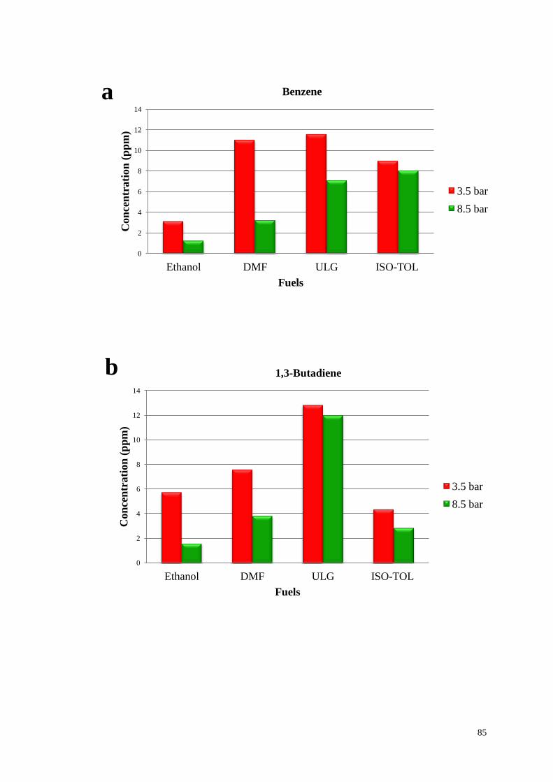
85

0

2

4

6

8

10

12

14

Ethanol DMF ULG ISO-TOL

Con

cen

trati

on

(p

pm

)

Fuels

Benzene

3.5 bar

8.5 bar

0

2

4

6

8

10

12

14

Ethanol DMF ULG ISO-TOL

Con

cen

trati

on

(p

pm

)

Fuels

1,3-Butadiene

3.5 bar

8.5 bar

a

b

86

0

5

10

15

20

25

30

35

40

Ethanol DMF ULG ISO-TOL

Con

cen

trati

on

(p

pm

)

Fuels

Propylene

3.5 bar

8.5 bar

0

2

4

6

8

10

12

14

16

18

Ethanol DMF ULG ISO-TOL

Con

cen

trati

on

(p

pm

)

Fuels

n-Heptane

3.5 bar

8.5 bar

c

d

87

Figure 5.2-Comparison of individual hydrocarbon concentrations for different fuels at low

and high engine load (a) Benzene, (b) 1, 3-Butadiene, (c) Propylene, (d) n-Heptane, (e)

Toluene, (f)Iso-butane

0

100

200

300

400

500

600

Ethanol DMF ULG ISO-TOL

Con

cen

trati

on

(p

pm

)

Fuels

Toluene

3.5 bar

8.5 bar

0

0.5

1

1.5

2

2.5

3

3.5

4

4.5

Ethanol DMF ULG ISO-TOL

Con

cen

trati

on

(p

pm

)

Fuels

Iso-Butane

3.5 bar

8.5 bar

e

f

88

This photo-chemical reactivity of 1,3-Butadiene is a unique property of it as other

unregulated hydrocarbons does not possess it (Filser and Bolt 1984). In the engine

exhaust, 90% of the 1, 3-Butadiene comes from general alkanes and aromatic content

present in the fuel. According to the classification by the US environmental

protection agency (EPA), the 1,3-Butadiene is considered as a probable human

carcinogen because it is grouped as B2 carcinogen (US-EPA 1990b). The alkenes are

not effectively oxidised or decomposed when combustion temperature is relatively

low. Therefore, the maximum 1,3-Butadiene evolved during the lower engine load

operation as the temperatures of combustion were comparatively lower at 8.5 bar

IMEP load.

The incomplete combustion of Toluene, alkylbenzenes and xylenes results in

dealkylation which produces Benzene (Johnson et al. 2007). The chances of acute

myeloid leukaemia increases when 1-5 ppm is exposed for many years in ambient

air according to the conclusion of the risk assessment conducted by Johnson and his

team (2007). Benzene is said to be a human carcinogen (group 1), taking into the

consideration the epidemiological evidence by IARC, the international agency for

research on cancer (IARC 1987). Higher post-flame oxidation results in highest

concentrations of Benzene. Therefore, at higher loads Benzene formation is

preferential for Toluene combustion (Johnson et al. 2007). This is proven by the

evidence that in the engine operating at 3.5 bar, engine fuelled with Gasoline, the

Benzene concentration ranged from 1 ppm to 11.5 ppm (shown in Table 5.2, as the

post-flame oxidation increased. This concentration is the highest for such an engine

operation (Villinger et al. 2002).

89

The influences over health of short-term exposure for Toluene are not yet identified,

however, long-term exposure effects are well-recognized (Kostrzewski and

Piotrowski 1991). As the structure of Toluene is similar to that of aromatic structure,

thus its formation is generally related to Benzene, despite the fact that Toluene is a

non-carcinogen (category: 3A). Evidence by Schuetzle (1994) supports it as when

the Toluene or Xylene is added to the Gasoline fuel, the Benzene emissions are

witnessed.

The Toluene quantities in emissions ranged between 17 ppm and 497 ppm. These

highest and lowest points of the Toluene emissions were observed in the Isooctane-

Toluene blend at 3.5 bar and Ethanol at 8.5 bar, respectively. As compared to the

other compounds of this group, the concentration of Toluene remained constantly

higher throughout various tests.

The quantities of every constituent of the exhaust helped in calculating the

percentage changes of the sum of speciated 12-components emissions in various

fuels at 3.5 bar and 8.5 bar engine load. The outcomes for fuels were 30% decrease

for unleaded Gasoline, with 70%, 60% and 56% decrease for Ethanol, DMF and

Isooctane-Toluene blend respectively. Therefore, it shows that for Ethanol, the

alteration of the engine load is of greater significance compared to other fuels (see

Figure 5.3).

90

Figure 5.3-Percentage of total emissions decrease between 3.5 and 8.5 bar IMEP engine

loads

At lower loads, Ethanol produces low amounts of CO. The level of CO emissions

trend is similar for DMF. At higher engine load as the heating value of Ethanol is

relatively lower (and enthalpy of vaporization is much greater) , thus, greater time is

required to mix large quantity of Ethanol with air, otherwise the mixture of Ethanol

and air will not be of good quality. A thorough mixing is required within a short span

of time when the fuel is injected. The mixing process with even more Ethanol

remains poorer due to weak turbulence level in the cylinder at low engine speeds

(1500) and low loads (Zhong et al. 2010). This has been observed by many

researchers (Zhong et al. 2010, Daniel et al. 2011). However, the emissions by

Ethanol were the lowest, throughout the tests. Lower combustion temperature

produces lower THC emissions indicating complete combustion. The importance of

using oxygenated biofuels is shown in Table 5.1 by the level of CO emissions. The

CO emitted level of Gasoline is higher than that of the DMF.

0

10

20

30

40

50

60

70

80

Ethanol DMF ULG ISO-TOL

Per

cen

tage

of

Dec

reas

e

Fuels

91

Lower emissions of engine running on Ethanol can be expressed by the fact that the

combustion temperature is lower and it is more complete.

Also lower indicated specific CO level was measured compared with Ethanol when

oxygenated biofuel (DMF) was applied As mentioned before, lower total

hydrocarbon (THC) emissions were measured at low engine loads when Ethanol was

used this can be compared with the result from Gasoline and DMF. These numbers

increased rapidly by increase in engine load. Increase in engine load will result in

higher in-cylinder temperature and subsequently oxidation of unburned Gasoline and

DMF compounds. Lower HC level in exhaust emission when using Ethanol can be

expressed by more complete combustion and promoted oxidation reaction which are

because of excess oxygen in the fuel. As DMF contains 16.67% oxygen by mass, the

level of total unburned hydrocarbons in the exhaust is between Gasoline and

Ethanol. High combustion temperatures result in the formation of NOx. Table 5.1

shows the NOx emissions for the DMF, Gasoline and Ethanol. The total HC

emissions and NOx emissions are inversely related to each other.

The overall temperature behavior in the experiment finally results in the engine-out

NOx emission (Zhong et al. 2010). Low NOx emissions are produced by the Ethanol

combustion in the overall full-load range. The higher NOx emissions are a result of

the lower heat of vaporization of the DMF when compared to Ethanol. Thus

according to Table 5.1, the lower NOx concentration is related to the lower cylinder

pressures and exhaust temperatures associated with Ethanol.

92

5.3. Validation

It is essential that the experiments are performed in a way in which the obtained

results and conclusions drawn can be considered acceptable and reliable.

5.3.1. Validating the Experimental Process

The procedure of obtaining the results has been comprehensively described within

the sections of this project; still there is a possibility that errors may occur. Extra care

was taken to make sure that fuel samples did not become contaminated with more

impurities or combined with other fuels. Compressed air was used to clean all of the

equipment. The contamination of the fuel used within the engine was more difficult

to prevent because the engine lab could not be controlled as easily. The reason can

be explained as the engine being used for various types of fuel testing. The adverse

impact of the fuel would be within injectors and cylinder of the engine as this area

was unreachable for nitrogen purging and evaporation of fuel using the compressed

air. However, as fuel was pressurized when using the GDI system, these impurities

and remaining fuels would not be able to travel back along the pipe to reach the fuel

source within the tank. For that reason, as the engine was run for more than ten

minutes prior to each test being carried out, any remained fuel within these areas

would already passed through pipes and burn in the engine and would have been

pumped out of the exhaust manifold. Therefore, contamination of the fuel is very

unlikely, and any corruption that did occur would not have affected the results.

Moreover, prior to each test, the heated line and sample loop and the multiport Valco

valve were cleaned to remove pervious test samples. Before injecting the sample in

GC-MS,5 minute delay was used considered to be sufficient for all heated line and

93

sample loop areas to become full of the tested exhaust gas sample. Due to mentioned

reasons, the results obtained are considered to be accurate and valid.

5.3.2. Validating the analysis of the Results

Much care considered to ensure correct identification of the mass spectra as

misidentification could result in inaccurate conclusions being drawn from the

experiment. The most accurate and popular method is the use of a reference gas

(calibration gas), this would contain known compounds (13 compounds) and of

known quantities (50 ppm of each).

This would be quick and reliable way to identify compounds through comparison of

retention times; moreover, it would enable quantitative analysis as exact quantities of

the various compounds within the reference gas would be known. Thus prior to each

daily test, the GC-MS was calibrated by using standard gas bottle with known

components.

In general, it is considered that all of the compounds that were identified so correctly

as shown in Figure 3.17. The main reason for this is use of the most reliable method

that is using a reference gas and comparing retention times.

94

5.4. Summary

This chapter highlights comparison of the regulated and unregulated emission of

different fuels such as Gasoline, Ethanol, 2, 5-Dimethylfuran and isooctane toluene

blend (2:1) in single cylinder spark ignition engines.

The results showed that regulated emissions of pure Gasoline such as CO, CO2 and

THC were really similar to DMF emissions. Higher oxygen content of Ethanol

results in oxidization of unburned hydrocarbons and lower HC. The most important

factors in production of highly toxic hydrocarbons are engine operating modes.

The results demonstrate that at higher load individual species such as Benzene, 1-

Butene and 1, 3-Butadiene were present in emitted hydrocarbons with concentrations

up to 30ppm.

Aromatics have a ring structure with carbon-carbon double bond that makes them

stable during combustion process and aromatics components such as Toluene

remains unburned fuel in exhaust emission.

The major hydrocarbons at lower load are alkanes and the main components at

higher load are alkene. Aromatics or heavier hydrocarbons such as Toluene and

Benzene were found to be more stable at lower load due to lower combustion

temperature.

The results were validated using standard gas bottle, reliable and repeatable method.

95

CHAPTER 6

6. VOLATILE HYDROCARBON (C3-C7)

SPECIATION AND QUNATIFICATION OF

ENGINE EXHUST RUNNING ON 2, 5-

DIMETHYLFURAN AND ETHANOL IN

BLENDS WITH GASOLINE

6.1. Introduction

The purpose of this part of the study is to experimentally investigate the effect of

Ethanol and 2, 5-Dimethylfuran (DMF) addition to Gasoline on regulated and

unregulated exhaust emissions from single cylinder direct-injection spark ignition

engine. Experiments were conducted with blends containing 10 and 30 volume

percentages of Ethanol or DMF. The single cylinder engine was operated at low and

high loads (3.5 and 8.5 bar IMEP), constant speed of 1500 rpm and stoichiometric

air/fuel ratio for each blend. This study has mainly focused on speciation and

quantitative analysis of individual hydrocarbons in the range C3-C7 in exhausts

emissions using gas chromatography-mass spectrometry (GC-MS).

6.2. Fuels and their blends

Table 3.5 presents the properties of fuels in this study. The test fuels used in this

study were 97 research octane number (RON) commercial Gasoline and the bio-

Ethanol both supplied by Shell Global Solutions UK. The DMF with purity of 99.8%

was provided by Shijiazhuang Lida Chemical Co. LTD in China. The blends tested

include DMF blends of 10% and 30% by volume (denoted as D10 and D30), and

96

Ethanol blends of 10% and 30% (E10 and E30). The fuels used are all relatively

high-octane. The octane number of Ethanol used in this study is reported to be larger

than Gasoline around 106. Blend octane number generally decreases with increasing

octane number of the base fuel and with increasing blend percentage of the additive

(Nisbet 1946). The experiments were performed at constant injection timing of 280

⁰bTDC and stoichiometric air/fuel ratio (λ=1) and fixed valve timing (see Table 3.2).

In this study, free piston accumulator, which was used to deliver the fuel, was

pressurized to150 bar with nitrogen (oxygen free) bottle. The ETAS LA4 lambda

meter is used to set fuel stoichiometric AFR, H/C and O/C ratios as mentioned in

Table 3.5.

6.3. Results and Discussion

6.3.1. CO Emissions

Generally, the indicated specific carbon monoxide emissions (isCO) decrease as load

increases. At 8.5 bar IMEP, the Ethanol-Gasoline blends (for all contents of Ethanol)

have the lowest isCO emissions in comparison with 2, 5-Dimethylfuran (DMF) at

the same load, this is due to higher oxygen content and combustion efficiency of

Ethanol (Daniel et al. 2011). Figure 6.1 illustrates the indicated specific (is) CO

emissions for three different percentage contents of Ethanol and DMF in the

Gasoline, investigated in both low and high engine load (3.5 and 8.5 bar IMEP). It is

obvious from Figure 6.1 that the isCO (in g/kWh) decreases with increase in content

of DMF and Ethanol percentage. As shown in Figure 6.1, the CO emissions at low

load using D10, D30, E10 and E30 decreased by 10.76%, 15.06%, 13.91% and

18.60% respectively in comparison with Gasoline. At high engine load (8.5 bar

97

IMEP) the isCO emissions of D10, D30, E10 and E30 decreased by 8.27%, 9.45%,

14.61% and 15.98%, respectively.

Table 6.1 illustrates the results for indicated specific emissions of CO, CO2, THC

and NOx measured using Horiba MEXA 7100 and recalculated for g/kWh (indicated

work).

Figure 6.1- Indicated specific emissions of carbon monoxide (CO) for three percentage

contents (volumetric) of DMF (D0, D10, D30) and Ethanol (E0, E10, E30) at two different

loads (3.5 and 8.5 bar IMEP)

98

6.3.2. CO2 emission

Carbon dioxide is not considered as a toxic gas and pollutant engine emission, but it

is one of the main components that contribute to greenhouse effect. At 3.5 bar IMEP,

The isCO2 emissions of DMF-Gasoline blends decreased with increasing content of

DMF and Ethanol. Figure 6.2 represents the relation between the isCO2 emissions

and three different percentages (Vol%) of Ethanol and DMF blended with Gasoline.

It is evident from Figure 6.2 that, the specific isCO2 emissions decrease as the

Ethanol and DMF percentage in fuel blends increases. At low engine load, the isCO2

emissions for D10, D30, E10 and E30 decrease by 0.6%, 3.4%, 2.61% and 4.58%,

respectively.

The indicated specific CO2 emissions at high load (8.5 bar IMEP) using D10, D30,

E10 and E30 blends are reduced by 1.5%, 2.89%, 2.61% and 7.64%, respectively.

Figure 6.2- Indicated specific emissions of carbon dioxide (CO2) for three percentage

contents (volumetric) of DMF (D0, D10, D30) and Ethanol (E0, E10, E30) at two different

loads (3.5 and 8.5 bar IMEP)

99

6.3.3. THC Emissions

Ethanol contains higher oxygen content compared with DMF and that is why

Ethanol-Gasoline blends caused to produce the lowest isTHC emissions. The THC

emissions decrease with increase of load; this is due to higher combustion

temperature at higher load. HC emissions for three different percentage contents of

DMF and Ethanol in Gasoline, at both low and high engine load are illustrated in

Figure 6.3. It can be seen that when the Ethanol and DMF percentages increase, the

specific emissions of unburned HC decrease. As illustrated in Figure 6.3, HC

emissions at low load using D10, D30, E10 and E30 decreased by 3.75%, 5.87%,

9.32% and 19.5%, respectively in comparison with pure Gasoline.

The HC concentrations at high load using D10, D30, E10 and E30 decreased by

3.43%, 13.05%, 9.69% and 24.79%, respectively relative to pure Gasoline.

Figure 6.3- Indicated specific emissions of carbon dioxide (CO2) for three percentage

contents (volumetric) of DMF (D0, D10, D30) and Ethanol (E0, E10, E30) at two different

loads (3.5 and 8.5 bar IMEP)

100

6.3.4. NOx Emissions

It is obvious that NOx production increases with load. The isNOx emissions are

directly associated with combustion temperature. (Laowagul and Yoshizumi 2009).

At each load the addition of Ethanol caused to produce lowest isNOx emissions due

to lower combustion temperature of Ethanol.in comparison to Gasoline and DMF.

Ethanol decreased NOx emission for E10 and E30 by 2.96% and 6.21%,

respectively, in comparison to Gasoline. Considering the NOx emission from DMF

blends, Figure 6.4 demonstrates that the isNOx emissions increase with the increase

of DMF percentage in the blend. Indicated specific NOx emissions increase with

load. The specific NOx emissions at low load using D10 and D30 DMF blends are

increased by 3.97%, 11.26% respectively compared with pure Gasoline. The NOx

emissions at high load using D10 and D30 are increased by 7.65% and 11.99%

respectively relative to Gasoline. In contrast, E10 and E30 decreased isNOx

emissions by 1.33% and 4.10% respectively. Table 6.1 illustrate indicated specific

regulated emissions at 3.5 and 8.5 bar IMEP.

Figure 6.4- Indicated specific emissions of oxides of nitrogen (NOx) for three percentage contents

(volumetric) of DMF (D0, D10, D30) and Ethanol (E0, E10, E30) at two different loads (3.5 and

8.5 bar IMEP)

101

Table 6.1- Indicated specific regulated emissions at different loads

6.3.5 Speciation of C3-C7 Hydrocarbons

Figure 6.5(a) compares the concentration of hydrocarbons species for Gasoline, D10

and E10 blends for low engine load (approximately 3.5bar). It is clear that addition

of 10% DMF to Gasoline decreased the concentration of all individual hydrocarbons

(the results were noticeably below those for Gasoline). The highest reduction occurs

for n-Pentane by approximately 16.5% and the lowest decrease was for Toluene

(nearly 4.44%). According to results presented in Figure 6.5(a), the concentrations of

exhaust species dropped significantly for the 10% Ethanol-Gasoline blend as

compared with Gasoline. The highest decrease happened for n-Pentane - by 68.11%

and the lowest was for 3-methyl-1Butane (approximately 1.35%). Figure 6.5(b)

illustrates the results of hydrocarbon speciation in emissions for the same fuel blends

at higher engine load (8.5 bar IMEP). These results present the effect of engine

conditions on exhaust hydrocarbon speciation. It is found that the concentrations of

all individual hydrocarbons for the 10% DMF-Gasoline blend diminish significantly

when compared with Gasoline. The biggest reduction occurs for n-Pentane with

reduction of 48.92% and the lowest decrease is for 1-Butene (about 3.78%).

Fuel

blends

isCO (g/kWh) isCO2 (g/kWh) isTHC (g/kWh)) isNOx (g/kWh)

3.5 bar 8.5 bar 3.5 bar 8.5 bar 3.5 bar 8.5 bar 3.5 bar 8.5 bar

Gasoline 33.64512 30.85642 875.5640 792.6615 7.64541 6.81545 6.85452 8.68111

E10 28.96282 26.34583 852.6275 771.9443 6.93264 6.15496 6.65133 8.56536

E30 27.38481 25.92282 835.4582 732.0734 6.15451 5.12565 6.42815 8.32475

D10 30.02227 28.30268 869.7878 781.1364 7.35807 6.58607 7.12648 9.345485

D30 28.57543 27.93979 845.6275 769.7445 7.19604 5.92559 7.62666 9.72212

102

Adding 10% Ethanol to Gasoline resulted in dramatic reduction in concentration of

all hydrocarbons; the highest reductions happen for Toluene and n-Pentane with the

amount of 71.36% and 69.48% respectively and the lowest decrease is for n-Butane

and n-hexane (just under 8%). It was concluded that for both high and low engine

loads addition of Ethanol and DMF resulted in change of concentrations in

hydrocarbon species. Both the DMF and Ethanol blends decreased concentration of

all hydrocarbons for low and high loads. Reductions in concentrations were more

significant with the addition of Ethanol to the blends and it was found that for high

engine loads these concentrations decreased even more compared with results from

low engine loads. Addition of just 10% DMF to the blends was found to be less

effective in terms of reduction of speciated hydrocarbons.

Figure 6.5(c) represents the concentration of hydrocarbons for Gasoline, D30 and

E30 blends at low engine load (3.5bar IMEP). It can be observed that by adding 30%

DMF to Gasoline the concentration of all individual hydrocarbons fall noticeably,

except for n-Butane, which displays a rise of 14.6%. The biggest reductions occur

for Propylene, Iso-pentane and n-Pentane with 42% drop and the lowest decrease is

for 3-methyl-1Butane (approximately 11.76%).

The concentrations of same hydrocarbons for the 30% Ethanol-Gasoline blend

reduced considerably compared with those for Gasoline fuelling. The highest

decreases happen for 1-Butane and Benzene with the amount of 96% and 94.5%

respectively (the values of concentrations of these hydrocarbons changed to almost

zero in exhaust), and the lowest reduction is for 3-methyl-1Butane (approximately

22.44%).

103

Figure 6.5(d) demonstrates the results of speciation for blends of 30% DMF and

30% Ethanol with Gasoline at high engine load. Addition of DMF resulted in a slight

decrease in concentration of hydrocarbons with the exception of n-Butane which

shows an increase of 9.4%. The largest change was seen for n-Pentane with a

reduction of 58.26% and lowest decrease was an almost negligible change for

Benzene. Adding 30% Ethanol to Gasoline caused the concentration of all

hydrocarbons to drop dramatically, the highest decreases happened for 1-Butane and

Benzene with the amounts of 98% and 95.3% respectively, and the lowest decrease

was for n-hexane (nearly 27%). In conclusion, addition of higher percentage of DMF

does not have significant effect as compared with adding 10%. But Ethanol as an

additive to Gasoline showed great reduction in concentration of each hydrocarbon;

as it was shown before some of these hydrocarbons almost disappear in the exhaust

of engine running on high percentages of Ethanol. Table 6.2 shows the concentration

of hydrocarbon species for different fuels and operating engine conditions.

104

105

Figure 6.5-C3-C7 hydrocarbons speciation (a) E10, D10 at 3.5 bar (b) E10, D10 at 8.5 bar (c) E30,

D30 at 3.5 bars and (d) E30, D30 at 8.5 bar

,

106

Table 6.2-Hydrocarbons C3-C7 concentrations in engine exhaust at 1500 rpm (λ=1)

Compound

Gasolin

e at 3.5

bar

(ppm)

Gasoli

ne at

8.5 bar

(ppm)

E10 at

3.5 bar

(ppm)

E10 at

8.5 bar

(ppm)

E30 at

3.5 bar

(ppm)

E30 at

8.5 bar

(ppm)

D10 at

3.5 bar

(ppm)

D10 at

8.5 bar

(ppm)

D30 at

3.5 bar

(ppm)

D30 at

8.5 bar

(ppm)

Propylene 29.46 19.48 24.62 16.28 7.39 4.18 27.29 18.48 17.07 14.20

Iso-

butane

3.91 3.47 3.15 2.35 2.54 1.35 3.66 3.14 2.98 2.64

1-Butene 14.01 12.05 9.34 8.10 0.55 0.23 12.23 11.60 10.26 9.49

1,3-

Butadiene 13.82 13.82 10.05 8.81 8.21 7.66 11.81 11.24 12.81 10.94

n-Butane 4.46 3.76 4.40 3.45 2.29 2.12 4.37 3.52 5.12 4.12

3-Methyl-

1-Butane 2.36 2.23 2.13 1.62 1.83 1.01 2.15 1.80 2.08 2.03

Iso-

pentane

11.00 5.89 5.67 3.18 1.64 0.52 9.40 3.88 6.27 3.24

n-Pentane 13.12 11.21 4.18 3.42 2.71 3.45 10.95 5.72 7.54 4.68

n-Hexane 10.66 6.38 8.21 5.86 4.82 4.63 9.92 6.01 8.48 5.36

Benzene 11.56 7.08 7.42 5.42 0.62 0.33 9.81 6.03 8.48 7.050

n-

Heptane 15.47 8.37 8.35 6.16 5.15 4.12 14.51 7.53 12.39 8.19

Toluene 82.17 69.45 46.26 19.88 28.18 17.06 78.52 61.03 69.33 55.95

107

6.3.6. Further discussion on C3-C7 hydrocarbon speciation

6.3.6.1. Alkanes

Engine-out emissions of propane, Iso-butane, n-Butane, Iso-pentane, n-Pentane, n-

hexane and n-Heptane were all within the range of 0–12 ppm for engine running on

pure Gasoline at 8.5 bar IMEP engine load. The concentrations of these saturated

hydrocarbons increased as the engine load and combustion temperatures were

reduced (0-16 ppm for engine load of 3.5 bar IMEP and Gasoline as the main fuel).

By introducing even the low percentages of Ethanol (10%) to engine fuel, the

concentrations of most of these species were reduced to less than 7ppm for high

engine loads (8.5 bar IMEP), presumably as a result of higher oxygen content of the

fuel enhancing the oxidation of unburned hydrocarbons. Decrease in engine load

resulted in an increase of concentration of these hydrocarbons, although changes

were moderate between the two engine loads. Increase in percentage of Ethanol in

fuel blends (to 30%) resulted in significant reductions of total hydrocarbons and

specially alkanes in engine exhaust.

As an alternative to Gasoline DMF was introduced to the engine at low blends (D10

and D30). Alkanes in the exhaust of engine running on DMF-Gasoline blends

showed slight changes compared with pure Gasoline. It is clear that all of these

hydrocarbons were decreased for both engine conditions, but these changes were not

as big as changes in hydrocarbons when Ethanol was added to the blends.

It can be summarised that adding DMF to Gasoline showed lower reduction in

alkanes compared with Ethanol (particularly at higher blends 30%).

108

6.3.6.2. Alkenes, (Propylene, 1-Butene)

Concentration of Propylene followed the same pattern as total hydrocarbons

(decrease in concentration was found as a result of increase in load). Also the

addition of Ethanol showed significant change in concentration of Propylene,

particularly for higher blends. These changes were present for DMF addition as well

but were less significant, 1-Butene as another alkene present in engine exhaust

showed reduction in concentration for increased engine load and with addition of

DMF and Ethanol. Again changes in concentration when adding DMF were very

small and even at high percentages the results were close to those for pure Gasoline,

but significant change was noticed when concentration of Ethanol in the blends was

increased to 30%. In this case the amount of 1-Butene in exhaust dropped to around

zero for both the low and high engine loads.

6.3.6.3. 1, 3-Butadiene

The 1, 3-Butadiene is considered the most toxic hydrocarbon among volatile organic

compounds (VOCs) and it has low reactivity with ozone in air in comparison to

other alkenes. Investigation on mechanisms of 1, 3-Butadiene carcinogenicity

showed that it may increase cancer risks in humans. The highest trace of 1, 3-

Butadiene was detected when DMF was added to the fuel blends and changes in

engine load did not have major effect on the concentration. 1, 3-Butadiene is

considered as highly reactive and hazardous pollutant which is transformed into

reaction quickly and produces toxic pollutants. (Duffy, Nelson et al. 1998, Bond and

Medinsky 2001, Laowagul and Yoshizumi 2009).

109

6.3.6.4. Aromatics

Benzene is considered as one of the most toxic substance of exhaust gases and

carcinogenicity of Benzene generates particular concern, which causes a range of

health problems. Inhalation exposure to Benzene may cause leukaemia risks in

occupational environments. Generally, main source of Benzene emission is

considered as dealkylation product of alkylbenzene, Toluene and xylene while

incomplete combustion occurs. (Stone 1985, Kaiser et al. 1991, Kaiser et al. 2005).

In this study, the concentration of Benzene ranged from almost 0 ppm to 12 ppm

with the highest concentration being for the engine operating with pure Gasoline and

at low loads due to the increased post-flame oxidation, which describes the reason of

preference of Benzene formation in SI engines over Toluene (Johnson et al. 2007).

The concentration of Benzene in exhaust was significantly reduced by addition of

high percentages of Ethanol to the fuel blends (Concentrations decreased to almost

zero for both engine loads).

In this work, Toluene was present at relatively high concentrations compared with

the rest of the measured compounds in this group. The highest and lowest Toluene

traces of 83 ppm and 17 ppm were found in engine running on pure Gasoline at

3.5bar IMEP and E30 at 8.5 bar IMEP engine load respectively.

110

6.4. Summary

In summary this chapter demonstrated the effect of addition of oxygenated fuels such

as Ethanol and 2, 5-Dimethylfuran to Gasoline on regulated and unregulated exhaust

emission from spark ignition engines.

Higher heat of evaporation and oxygen content of Ethanol have reduced total

hydrocarbon emission (THC) and carbon monoxide (CO) considerably for both E10

and E30 in comparison with DMF blends.

The engine operating conditions play vital role in concentrations of individual

hydrocarbons. 1, 3-Butadiene concentration was decreased in exhaust emission by

increasing the load.

At higher load, alkanes concentrations were decreased. Concentrations of heavier

hydrocarbons were decreased at higher load.

Regardless of engine operating modes, Benzene and Toluene were main components

of exhaust emissions. Addition of Ethanol reduced concentration of aromatics

drastically.

111

CHAPTER 7

7. CONCLUSION AND FUTURE WORK

7.1. Main Contribution

7.1.1. Methodology Concept

In order to investigate the fuels lubricity properties the well known HFRR rig was

used. The process is discussed in details in Chapter 3 of this thesis. Also in order to

prevent any data loss and inappropriate reporting of the results all of the experiments

were repeated three times in the same condition (same day) and any results with

more than 5 percent error were deleted and average data of all experiments were

reported as the final results in this thesis. Also for data validation, results obtained

from Gasoline and Ethanol were compared with the literature and as they were in

very good agreement with them, results were accepted and reported in this thesis.

For study on emissions and the possible effect of fuels properties on engine exhaust,

novel works have been done. For measurement of regulated emissions commercial

cutting edge equipments in this field have been used. For analysis of unregulated

hydrocarbons in engine exhaust gas chromatography equipped with mass

spectrometer have been modified. Engine exhaust was transferred directly from

engine into the measurement point using heated lines at elevated temperature to

prevent any hydrocarbon loss due to leakage and condensation in the pipes. Special

112

valve (six port Valco valve) was employed with the capability of control on the

injected sample using sampling loop. Another main effort during this project was to

apply a proper method of analysis on GCMS. This method was developed over long

period of time with several runs. And finally after getting the desired peaks of

chromatogram, a special calibration gas bottle with 13 types of hydrocarbons have

been used to quantify the results. As the concentration of each hydrocarbon in the

gas bottle is set to a known value.

7.1.2. Lubricity of fuels

The vital role of fuels lubricating characteristics in new spark ignition engines was

analyzed using the HFRR for conventional 95 RON Gasoline and other biofuels as

additives.

Friction coefficient as an important factor in lubricity analysis maintained almost

constant value during the 75 minute tests for pure 2,5-Dimethylfuran and Ethanol,

but this value showed an increasing trend for Gasoline confirming poor lubricity of

Gasoline compared with these biofuels.

Addition of 2, 5-Dimethylfuran and Ethanol to Gasoline enhanced the lubricity of

the blend significantly. This increase was clearer for DMF.

Inverse relation of lubrication film coverage and friction coefficient was clearly

observed.

Aging of the fuels was also investigated for their effect on the lubricity; it was found

that ageing of biofuels enhanced the lubricity even more than using non-aged fuels in

the blends.

113

7.1.3. GC-MS Quantification of C3-C7 Hydrocarbons in SI Engine

Exhaust Fuelled with Ethanol, DMF, Gasoline and Isooctane-

Toluene Blend

Regulated emissions of engine exhaust running on pure fuels showed that for 95

RON Gasoline emissions of CO, HC and NOx were similar to those for DMF. Lower

CO was measured using Ethanol as the fuel due to lower maximum in-cylinder

temperature and complete combustion, also higher oxygen content of Ethanol

resulted in complete combustion and lower HC. NOx emission showed reduction

when Ethanol was used.

Engine operating conditions found to be very important in production of highly

carcinogenic species. At higher loads it was found that species like Benzene, 1-

Butene and 1,3-Butadiene were present in the exhaust in concentrations up to 30

ppm.Due to high stability of the aromatic structure of Toluene there was high

fraction of unburned fuel in the engine exhaust compared with iso-octane.

Alkanes were found to be the major components in the exhaust at lower loads and

alkenes were found to be the major component for higher loads, again confirming the

important role of engine operating conditions on exhaust. Heavier hydrocarbons such

as Toluene, n-Heptane and Benzene found to be more prominent at lower engine

load.

114

7.1.4. Volatile Hydrocarbon (C3-C7) Speciation and Quantification

of Engine Exhaust Running on 2, 5-Dimethylfuran and Ethanol in

blends with Gasoline

The significant reduction in total hydrocarbons (THC) and carbon monoxide (CO)

emission were generally observed for both E10 and E30 in compared with DMF

blends with Gasoline and this is due to higher heat of evaporation and oxygen

content of Ethanol addition.

The engine operation modes used are very important for production of many

hydrocarbon species such as 1, 3 – Butadiene. At high load, concentration of 1, 3-

Butadiene was decreased significantly in exhaust emissions, which is believed to be

due to its high reactivity in presence of NOx emission.

Alkanes such as propane, Isobutane, n-Butane, Iso-pentane, n-Pentane, n-hexane

and n-Heptane were found to reduce in concentration with increase the engine load.

The concentrations of heavy hydrocarbons were found to be higher at lower engine

loads.

Benzene and Toluene were found to be the major components of engine exhaust

regardless of engine operating conditions and fuels used. Concentrations of

aromatics significantly reduced by addition of Ethanol.

115

7.2. Recommendations and Future Work

Further analysis of lubricity of fuels can be carried out by changing the test

conditions. New additives can be added to the fuels for further enhancement of

lubricity o the blends (Specially Gasoline).

Exhaust emission speciation can be expanded to heavier hydrocarbons in the range

of C7+ using a new set of standard gases, giving a better idea of the nature of engine

exhaust for various engine conditions and fuels.

Monocyclic aromatic hydrocarbons (MAH) and even Polycyclic aromatics

hydrocarbons (PAH) for both vapour phase and particulate matter can be

investigated for the same conditions using liquid chromatography and

thermogravimetric analysis (TGA).

Exhaust emission analysis can be extended to carbonyls using other measurement

devices (HPLC)

It would also be beneficial to analyse the fuels in liquid form before the combustion

and compare the hydrocarbons with those in the exhaust emissions.

116

AUTHOR’S PUBLICATION

F. Eslami, M.L.Wyszynski, A. Tsolakis, H. Xu, S. Norouzi, K. Dearn, Experimental

Investigation on Lubricity of 2, 5 –Dimethylfuran Blends, Combustion Engines

PTNSS Kongress 2012- 1/2012 (148)

F. Eslami, M.L.Wyszynski, Ch. Wang, H. Xu, S. Norouzi, A. Tsolakis, F. Eslami,

Volatile Hydrocarbon (C3-C7) Speciation and Quantification of Engine Exhaust

Emissions Running on 2,5-Dimethylfuran and Ethanol in blends with Gasoline

(submitted in Elsevier Fuel Journal)

S. Norouzi, F. Eslami, A. Tsolakis, M.L. Wyszynki, Corrosion Effects of RME in

Blends with ULSD on aluminium and Copper, Fuel Processing Technology Elsevier

104 (2012) 204–210

F. Eslami, M.L.Wyszynski, S. Norouzi, A. Tsolakis, F. Eslami, H.

Vafamehr,Speciation and Quantification of individual hydrocarbons of Gasoline,

Ethanol and 2, 5 Dimethylfuran in Spark Ignition Single Cylinder Engine using GC-

MS (Preparation)

117

8. LIST OF REFERENCES

Aden, A. and T. Foust (2009). "Technoeconomic analysis of the dilute sulfuric acid

and enzymatic hydrolysis process for the conversion of corn stover to Ethanol."

Cellulose 16(4): 535-545.

Agarwal, A. K. (2007). "Biofuels (alcohols and biodiesel) applications as fuels for

internal combustion engines." Progress in energy and combustion science 33(3):

233-271.

Agudelo, J., et al. (2011). "The lubricity of Ethanol-Gasoline fuel blends." Revista

Facultad de Ingeniería Universidad de Antioquia(58): 9-16.

Al-Baghdadi, M. (2003). "Hydrogen–Ethanol blending as an alternative fuel of spark

ignition engines." Renewable Energy 28(9): 1471-1478.

Al-Hasan, M. (2003). "Effect of Ethanol–unleaded Gasoline blends on engine

performance and exhaust emission." Energy Conversion and Management 44(9):

1547-1561.

118

Alkidas, A., et al. (1995). "Effects of piston crevice geometry on the steady-state

engine-out hydrocarbon emissions of a SI engine." sAE Paper 952537.

Andrews, G., et al. (2007). "Condensable and Gaseous Hydrocarbon Emissions and

Their Speciation for a Real World SI Car Test." SAE Technical Paper: 01-0062.

Barbour, R. and N. G. Elliott (2000). "Understanding diesel lubricity." 134-141.

Bayraktar, H. (2005). "Experimental and theoretical investigation of using Gasoline–

Ethanol blends in spark-ignition engines." Renewable Energy 30(11): 1733-1747.

Bechtold, R. L. (1997). "Alternative Fuels Guidebookc."

Bond, J. A. and M. A. Medinsky (2001). "Insights into the toxicokinetics and

toxicodynamics of 1, 3-Butadiene." Chemico-Biological Interactions 135: 599-614.

Braithwaite, A., et al. (1985). Chromatographic methods, Chapman and Hall.

Carter, W. P. L. (1998). "UPDATED MAXIMUM INCREMENTAL REACTIVITY

SCALE FOR REGULATORY APPLICATIONS."

119

Cheng, W. K., et al. (1993). "An overview of hydrocarbon emissions mechanisms in

spark-ignition engines."

Childs, P. R. N. and R. Stobart (2004). Proceedings of the 3rd IMechE Automobile

Division Southern Centre Conference on Total Vehicle Technology: Finding the

Radical, Implementing the Practical: 26-27th April 2004, University of Sussex,

Brighton, UK, Professional engineering publ.

Daniel, R., et al. (2011). "Effect of spark timing and load on a DISI engine fuelled

with 2, 5-Dimethylfuran." Fuel 90(2): 449-458.

Danping, W. and H. Spikes (1986). "The lubricity of diesel fuels." Wear 111(2):

217-235.

Das L.M, R. Y. V. R. (1996). "Evaluation of alternative fuels for internal combustion

engine." International Energy and Environment Symposium: 951–958.

Delphi (2009). "Worldwide Emissions Standards: Passenger Cars and Light Duty

Trucks,."

Delphi (2011). "Worldwide Emissions Standards - Passenger Cars and Light Duty

Vehicles."

120

Deng, X. (2006). "Economic costs of motor vehicle emissions in China: A case

study." Transportation Research Part D: Transport and Environment 11(3): 216-226.

Duffy, B., et al. (1998). "Emissions of benzene, Toluene, xylenes and 1, 3-Butadiene

from a representative portion of the Australian car fleet." Atmospheric Environment

32(14-15): 2693-2704.

Dumesic, J. A., et al. (2007). "Catalytic process for producing furan derivatives from

carbohydrates in a biphasic reactor." US: World Intellectual Property.

Eleftherakis, J. G., et al. (1994). Development of a benchtop fuel lubricity

assessment method.

Elghawi, U. (2009). Speciation and quantification of individual hydrocarbons during

fuel reforming and in exhaust emissions from a Gasoline (SI/HCCI) engine,

University of Birmingham.

Fatih Demirbas, M. (2009). "Biorefineries for biofuel upgrading: a critical review."

Applied Energy 86: S151-S161.

Ferguson, C. R. (1985). "International combustion engines; Applied

thermosciences."

121

Filser, J. and H. Bolt (1984). "Inhalation pharmacokinetics based on gas uptake

studies." Archives of toxicology 55(4): 219-223.

Graham, L. A., et al. (2008). "Emissions from light duty Gasoline vehicles operating

on low blend Ethanol Gasoline and E85." Atmospheric Environment 42(19): 4498-

4516.

Haagen-Smit, A. (1952). "Chemistry and physiology of Los Angeles smog."

Industrial & Engineering Chemistry 44(6): 1342-1346.

Harrington, J. and R. Shishu (1973). A Single-Cylinder Engine Study of the Effects

of Fuel Type, Fuel Stoichiometry, and Hydrogen-to-Carbon Ratio on CO, NO, and

HC Exhaust Emissions, Society of Automotive Engineers.

Hasan, A., et al. (2011). "Effect of composite aftertreatment catalyst on alkane,

alkene and monocyclic aromatic emissions from an HCCI/SI Gasoline engine." Fuel

90(4): 1457-1464.

Heywood, J. "1988, Internal Combustion Engine Fundamentals, McGraw-Hill, New

York."

Hill, G. and J. Holman (2000). Chemistry in context, Nelson Thornes.

122

Hsieh, W. D., et al. (2002). "Engine performance and pollutant emission of an SI

engine using Ethanol–Gasoline blended fuels." Atmospheric Environment 36(3):

403-410.

Huff, J., et al. (1985). "Multiple organ carcinogenicity of 1, 3-Butadiene in B6C3F1

mice after 60 weeks of inhalation exposure." Science (New York, NY) 227(4686):

548.

IARC (1987). Overall evaluations of carcinogenicity: an updating of IARC

monographs volumes 1 to 42: this publication represents the views and expert

opinions of an IARC ad-hoc Working Group on the Evaluation of Carcinogenic

Risks to Humans, which met in Lyon, 10-18 March 1987, World Health

Organization, International Agency for Research on Cancer.

Jensen, T. E., et al. (1992). Advanced emission-speciation methodologies for the

Auto/Oil Air Quality Improvement Research Program. 1. Hydrocarbons and ethers,

Environmental Protection Agency, Research Triangle Park, NC (United States).

Atmospheric Research and Exposure Assessment Lab.

Jia, L. W., et al. (2005). "Influence of Ethanol-Gasoline blended fuel on emission

characteristics from a four-stroke motorcycle engine." Journal of hazardous materials

123(1): 29-34.

123

Johnson, E. S., et al. (2007). "A critique of benzene exposure in the general

population." The Science of the total environment 374(2-3): 183.

Johnson, T. V. (2010). "Review of Diesel Emissions and Control 2010-01-0301."

Review of Diesel Emissions and Control 1: 0301.

Kaiser, E., et al. (1983). "The effect of fuel and operating variables on hydrocarbon

species distributions in the exhaust from a multicylinder engine." Combustion

science and technology 32(5-6): 245-265.

Kaiser, E. W., et al. (2005). "Detailed hydrocarbon species and particulate emissions

from a HCCI engine as a function of air-fuel ratio." SAE transactions 114(4): 1404-

1414.

Kaiser, E. W., et al. (1994). Fuel Structure and the Nature of Engine-Out Emissions,

Society of Automotive Engineers.

Kaiser, E. W., et al. (1994). "Time-resolved measurement of speciated hydrocarbon

emissions during cold start of a spark-ignited engine." sAE Paper 940963.

Kaiser, E. W., et al. (1992). "Effect of fuel structure on emissions from a spark-

ignited engine. 2. Naphthene and aromatic fuels." Environmental science &

technology 26(8): 1581-1586.

124

Kaiser, E. W., et al. (1993). "Effect of fuel structure on emissions from a spark-

ignited engine. 3. Olefinic fuels." Environmental science & technology 27(7): 1440-

1447.

Kaiser, E. W., et al. (1991). "Effect of fuel structure on emissions from a spark-

ignited engine." Environmental science & technology 25(12): 2005-2012.

Kao, A. S. (1994). "Formation and removal reactions of hazardous air pollutants."

Air & Waste 44(5): 683-696.

Kelly, K. J., et al. (1996). "Federal test procedure emissions test results from Ethanol

variable-fuel vehicle Chevrolet Luminas." SAE transactions 105: 698-717.

Koç, M., et al. (2009). "The effects of Ethanol–unleaded Gasoline blends on engine

performance and exhaust emissions in a spark-ignition engine." Renewable Energy

34(10): 2101-2106.

Kostrzewski, P. and J. Piotrowski (1991). "Toluene determination in capillary blood

as a biological indicator of exposure to low levels of Toluene." Polish journal of

occupational medicine and environmental health 4(3): 249.

125

Krier, J. and E. Ursin (1977). Pollution and Policy, Berkeley: University of

California Press.

Laowagul, W. and K. Yoshizumi (2009). "Behavior of benzene and 1, 3-Butadiene

concentrations in the urban atmosphere of Tokyo, Japan." Atmospheric Environment

43(12): 2052-2059.

Lapuerta, M., et al. (2009). "Lubricity of Ethanol-biodiesel-diesel fuel blends."

Energy & Fuels 24(2): 1374-1379.

Loh, M. M., et al. (2007). "Ranking cancer risks of organic hazardous air pollutants

in the United States." Environmental Health Perspectives 115(8): 1160.

MacLean, H. L. and L. B. Lave (2003). "Evaluating automobile fuel/propulsion

system technologies." Progress in energy and combustion science 29(1): 1-69.

Margaroni, D. (1998). "Fuel lubricity." Industrial Lubrication and Tribology 50(3):

108-118.

Mascal, M. and E. B. Nikitin (2008). "Direct, High‐Yield Conversion of Cellulose

into Biofuel." Angewandte Chemie 120(41): 8042-8044.

126

McNair, H. M. and J. M. Miller (2011). Basic gas chromatography, Wiley-

Interscience.

Mielenz, J. R. (2001). "Ethanol production from biomass: technology and

commercialization status." Current Opinion in microbiology 4(3): 324-329.

Mousdale, D. M. (2008). Biofuels: biotechnology, chemistry, and sustainable

development, CRC.

Nikanjam, M. (1992). "Lubricity of low aromatics diesel fuel."

Nisbet, H. B. (1946). "THE BLENDING OCTANE NUMBERS OF 2: 5-

DIMETHYLFURAN." Journal of the Institute of Petroleum 32: 162.

No, D. (1970). "70/156/EEC of the European Parliament of the Council on the

approximation of the laws of the member states relating to the type-approval of

motor vehicles and their trailers." Official Journal EC.

Owen, K. and T. Coley (1995). "Automotive fuels reference book."

Payri, F., et al. (2009). "Hydrocarbon emissions speciation in diesel and biodiesel

exhausts." Atmospheric Environment 43(6): 1273-1279.

127

PCS Instruments Company Website- Tribology test equipment, traction machines,

testing fuels provided by PCS Instruments.

Ping, W. D. and S. Korcek (1996). "Comparison of the Lubricity of Gasoline and

Diesel Fuels."

Román-Leshkov, Y., et al. (2007). "Production of Dimethylfuran for liquid fuels

from biomass-derived carbohydrates." Nature 447(7147): 982-985.

Rothamer, D. A. and J. H. Jennings (2012). "Study of the knocking propensity of 2,

5-Dimethylfuran–Gasoline and Ethanol–Gasoline blends." Fuel.

Rovai, F. F., et al. (2005). "Wear and corrosion evaluation of electric fuel pumps

with Ethanol/Gasoline blends." SAE transactions 114(4): 1123-1134.

Safran, S. A. (1994). Statistical thermodynamics of surfaces, interfaces, and

membranes, Addison-Wesley Reading, MA.

Schuetzle, D., et al. (1994). "The relationship between Gasoline composition and

vehicle hydrocarbon emissions: a review of current studies and future research

needs." Environmental Health Perspectives 102(Suppl 4): 3.

128

Siegl, W. O., et al. (1993). Improved Emissions Speciation Methodology for Phase II

of the Auto/oil Air Quality Improvement Research Program: Hydrocarbons and

Oxygenates, Society of Automotive Engineers Warrendale, PA.

Spikes, H., et al. (1996). The lubricating properties of Gasoline fuel. Proceedings of

Fuel Symposium.

Stone, R. (1985). "Introduction to internal combustion engines."

Topgül, T., et al. (2006). "The effects of Ethanol–unleaded Gasoline blends and

ignition timing on engine performance and exhaust emissions." Renewable Energy

31(15): 2534-2542.

US-EPA, U. E. P. A. (1990b). "Cancer Risk from outdoor Exposure to Air Toxics."

Office of Air Quality Planning Standards, Research Triangle Park 1(450/1-90-004a).

Valério, M., et al. (2004). "Improvement of a model for calculation of oxides of

nitrogen emissions from spark ignition engines." sAE Paper: 01-3001.

Villinger, J., et al. (2002). "Comparative Study of Butadiene and B, T, X Tailpipe

Emissions for Gasolines of Different Octane Levels." SAE Technical Paper: 01-

1643.

129

Wagner, T., et al. (1980). "Practicality of alcohols as motor fuel." SAE Prog.

Technol.;(United States) 19.

Wallington, T., et al. (2006). "Automotive fuels and internal combustion engines: a

chemical perspective." Chem. Soc. Rev. 35(4): 335-347.

Wang, C., et al. (2012). "Combustion characteristics and emissions of 2-methylfuran

compared to 2, 5-Dimethylfuran, Gasoline and Ethanol in a DISI engine." Fuel.

Wei, D., et al. (1996). "Comparison of the lubricity of Gasoline and diesel." SAE

paper 962010: 62-69.

Yanowitz, J., et al. (2011). "Utilization of renewable oxygenates as Gasoline

blending components." Contract 303: 275-3000.

Yücesu, H. S., et al. (2006). "Effect of Ethanol–Gasoline blends on engine

performance and exhaust emissions in different compression ratios." Applied

thermal engineering 26(17): 2272-2278.

Zeldovich, Y. B. (1946). "The oxidation of nitrogen in combustion and explosions."

Acta Physicochimica URSS 21(4): 577-628.

130

Zhao, H., et al. (2007). "Metal chlorides in ionic liquid solvents convert sugars to 5-

hydroxymethylfurfural." Science 316(5831): 1597-1600.

Zhong, S., et al. (2010). "Combustion and emissions of 2, 5-Dimethylfuran in a

direct-injection spark-ignition engine." Energy & Fuels 24(5): 2891-2899.