ClickHere

for

FullArticle

Characterization of emissions from South Asian biofuelsand application to source apportionment of carbonaceousaerosol in the Himalayas

Elizabeth A. Stone,1,2 James J. Schauer,1 Bidya Banmali Pradhan,3 Pradeep Man Dangol,3

Gazala Habib,4 Chandra Venkataraman,5 and V. Ramanathan6

Received 9 February 2009; revised 24 October 2009; accepted 30 October 2009; published 16 March 2010.

[1] This study focuses on improving source apportionment of carbonaceous aerosol inSouth Asia and consists of three parts: (1) development of novel molecular marker–basedprofiles for real‐world biofuel combustion, (2) application of these profiles to a year‐longdata set, and (3) evaluation of profiles by an in‐depth sensitivity analysis. Emissionsprofiles for biomass fuels were developed through source testing of a residential stovecommonly used in South Asia. Wood fuels were combusted at high and low rates, whichcorresponded to source profiles high in organic carbon (OC) or high in elemental carbon(EC), respectively. Crop wastes common to the region, including rice straw, mustard stalk,jute stalk, soybean stalk, and animal residue burnings, were also characterized. Biofuelprofiles were used in a source apportionment study of OC and EC in Godavari, Nepal. Thissite is located in the foothills of the Himalayas and was selected for its well‐mixed andregionally impacted air masses. At Godavari, daily samples of fine particulate matter(PM2.5) were collected throughout the year of 2006, and the annual trends in particulatemass, OC, and EC followed the occurrence of a regional haze in South Asia. Maximumconcentrations occurred during the dry winter season and minimum concentrationsoccurred during the summer monsoon season. Specific organic compounds unique toaerosol sources, molecular markers, were measured in monthly composite samples. Thesemarkers implicated motor vehicles, coal combustion, biomass burning, cow dung burning,vegetative detritus, and secondary organic aerosol as sources of carbonaceous aerosol. Amolecular marker–based chemical mass balance (CMB) model provided a quantitativeassessment of primary source contributions to carbonaceous aerosol. The new profiles werecompared to widely used biomass burning profiles from the literature in a sensitivityanalysis. This analysis indicated a high degree of stability in estimates of sourcecontributions to OC when different biomass profiles were used. The majority of OC wasunapportioned to primary sources and was estimated to be of secondary origin, whilebiomass combustion was the next‐largest source of OC. The CMB apportionment of EC toprimary sources was unstable due to the diversity of biomass burning conditions in theregion. The model results suggested that biomass burning and fossil fuel were importantcontributors to EC, but could not reconcile their relative contributions.

Citation: Stone, E. A., J. J. Schauer, B. B. Pradhan, P. M. Dangol, G. Habib, C. Venkataraman, and V. Ramanathan (2010),Characterization of emissions from South Asian biofuels and application to source apportionment of carbonaceous aerosol in theHimalayas, J. Geophys. Res., 115, D06301, doi:10.1029/2009JD011881.

1. Introduction

[2] Atmospheric aerosols reflect or absorb sunlight anddirectly impact climate by changing the amount of solar

radiation reaching the Earth’s surface. Aerosols also indirectlyimpact climate by causing changes in cloud compositionand physics by forming smaller, yet more numerous, clouddroplets, resulting in longer cloud lifetimes and enhanced

3International Centre for Integrated Mountain Development, Kathmandu,Nepal.

4Department of Civil Engineering, Indian Institute of TechnologyDelhi, New Delhi, India.

5Department of Chemical Engineering, Indian Institute of TechnologyBombay, Mumbai, India.

6Center for Clouds, Chemistry and Climate, Scripps Institute ofOceanography, University of California, SanDiego, La Jolla, California, USA.

1Environmental Chemistry and Technology Program, University ofWisconsin‐Madison, Madison, Wisconsin, USA.

2Now at Environmental and Organic Chemistry, Carlsbad EnvironmentalMonitoring and Research Center, Institute of Energy and the Environment,New Mexico State University, Carlsbad, New Mexico, USA.

Copyright 2010 by the American Geophysical Union.0148‐0227/10/2009JD011881

JOURNAL OF GEOPHYSICAL RESEARCH, VOL. 115, D06301, doi:10.1029/2009JD011881, 2010

D06301 1 of 14

cloud albedo [Ramanathan et al., 2005; Sun and Ariya,2006]. In Asia, heavily polluted atmospheres have beenobserved in recent decades and were associated with long‐term dimming over the continent [Ramanathan et al., 2005].Long‐term climatic impacts of the haze may also includechanges to hydrology and agriculture [Centers for Cloud,Chemistry, and Climate, 2002]. The impacts of atmosphericaerosols on climate relate to their chemical composition:light absorption is dominated by dark‐colored particles likeelemental carbon (EC), also called black carbon or soot,whereas organic carbon (OC) and sulfate aerosols are highlyreflective [Ramanathan et al., 2001].[3] The composition of aerosols at a point location is a

function of aerosol sources and their strengths. Chemical sig-natures can be used to identify aerosol sources and to quanti-tatively understand relative source contributions. Molecularmarkers are organic species present in the ambient atmospherethat come from specific aerosol source categories, are stablein the atmosphere, and can be used quantitatively in sourceapportionment [Schauer and Cass, 2000]. Chemical massbalance (CMB) modeling apportions carbonaceous aerosol toprimary sources using chemically defined source profiles[Watson et al., 1984]. The CMB model has been used instudies of ambient aerosol worldwide [Chowdhury et al.,2007; Schauer et al., 2002; Stone et al., 2008; Zheng et al.,2006] and its results have been used in air resources manage-ment to understand pollution sources [Watson et al., 2008].[4] Effective receptor‐based source apportionment requires

source profiles that are representative of the emissionsimpacting the receptor. In the case of biomass burning, the typeof fuel burned and combustion conditions affect the chemicalcomposition of particulate matter generated [Simoneit, 2002].This presents a significant challenge in the selection of bio-mass source profiles since fuel type and burn conditions canvary considerably by region. Previous studies have charac-terized the organic composition of particulate matter gener-ated by fireplace combustion of oak and pine [Schauer et al.,2001], modern‐stove combustion of major tree species foundin the United States [Fine et al., 2004a], wood‐stove emis-sions of common Austrian leaves [Schmidl et al., 2008a] andfuelwoods [Schmidl et al., 2008b], modern‐stove combustionof biomasses indigenous to Bangladesh [Sheesley et al.,2003], open burning of a pine forest [Lee et al., 2005], stoveburning of straw [Zhang et al., 2007], and others. Thesestudies have demonstrated that biomass emissions havechemical signatures distinct from other aerosol sources: bio-mass emissions contain large amounts of levoglucosan, plantsterols which vary by plant species, and other organic com-pounds [Simoneit, 2002]. Detailed organic species can also beused to differentiate between the different types of biomassesburned.[5] A study of the emissions from biofuels burned in a

traditional single‐pot mud stove widely used for cooking foodin South Asia produced aerosols with chemical propertiesdifferent from previous studies of biomass. Habib et al.[2008] demonstrated that biofuel burn rates (mass of fuelburned per hour, kg h−1) significantly influence aerosol com-position and that these stoves produced aerosol containingmore EC than OC. Due to the widespread use of biomassfuels in South Asia and the chemical nature of these emis-sions, biofuel use was consequently estimated to be the largestcontributor to ambient EC in the region [Venkataraman et al.,

2005]. In this study, emissions from these South Asian bio-fuels were characterized bymolecular marker species to aid inthe creation of biofuel source profiles for use with sourceapportionment studies of ambient aerosol in the region.[6] A contemporary approach to the development of novel

source profiles includes their immediate application andassessment. Such an approach was taken by Lee et al.[2005] in the chemical characterization of particulate mattergenerated by open forest burning and by Lough et al. [2007]in the development and application of molecular marker–based motor vehicle profiles. The combination of profiledevelopment with application demonstrates profile efficacy,documents caveats, and conveys their intended uses. Addi-tionally, the comparison of new profiles to those docu-mented in the literature further enhances the understandingof how biomass burning emissions vary across differentregions and fuel types. The variability of biomass profilesand uncertainty of apportionment results can be evaluatedusing sensitivity analysis [Robinson et al., 2006; Sheesleyet al., 2007], which compares apportionment results acrosssolutions using different profiles.[7] This study applies the newly developed South Asian

biofuel profiles in a study of the sources of carbonaceousparticulate matter (PM2.5) collected in Godavari, Nepallocated in the foothills of the Himalayas on the southernedge of the Kathmandu Valley. The Godavari site wasselected because it is representative of regional aerosol inSouth Asia where biofuel combustion is the dominant formof biomass burning according to emissions inventories[Streets et al., 2003b].[8] The Himalayan region is subject to heavily light‐

absorbing aerosols that cause significant reductions in surfaceradiation, particularly during winter months [Ramana et al.,2004]. Himalayan radiative forcing is among the greatest inthe world and may cause alternations of the region’s hydro-logic cycle [Ramanathan and Ramana, 2005]. A previousstudy of Himalayan aerosol composition was carried out byShrestha et al. [2000] at a remote site (4100 m altitude)and a rural Middle‐Mountain site (1900 m altitude) andshowed seasonal trends in water‐soluble ion concentrationsthat were attributed to large‐scale circulation patterns; aerosolconcentrations were lowest during the summer monsoon,elevated during the dry winter, and highest during the pre-monsoon season. Aerosol species were highly intercorrelatedand thought to be part of a thoroughly mixed air mass thatmay have traveled a long distance. A study during the pre-monsoon and monsoon seasons at the Pyramid Observatoryin the Himalayas (5100 m altitude) in 2006 recorded fineparticle concentrations elevated in comparison to the back-ground atmospheric conditions and noted temporal consis-tency between elevated fine particle mass, EC, and ozone[Bonasoni et al., 2008].[9] On a regional scale, Adhikary et al. [2007] demon-

strated that typical air masses impacting the Godavari sitewere westerly for dry months and southeasterly (from theBay of Bengal) for the period of the monsoon. During periodsof high organic and black carbon, air masses originated in thenorthwestern states of India. Several other studies of fineparticle transport to the Kathmandu Valley have pointedtoward long‐range transport of pollution from Terai region[Hindman andUpadhyay, 2002; Shrestha et al., 2000], whichincludes the Himalayan foothills in southern Nepal and the

STONE ET AL.: APPORTIONMENT OF SOUTH ASIAN AEROSOL D06301D06301

2 of 14

Indian state of Uttar Pradesh. Local meteorology in theKathmandu Valley was studied by Panday and Prinn [2009],who documented daily ventilation of the basin during thedaytime and a build‐up of anthropogenic pollutants duringthe morning and night. Emissions from within the valleyrecirculated within the basin during the morning and impactedthe surrounding mountains during times of ventilation.

2. Methods

2.1. Source Sampling

[10] The biofuel and biomass samples discussed in thispaper were collected during the study of primary aerosolsfrom biofuel combustion by Habib et al. [2008] wheresampling methods are described in detail. Biofuels wereselected to represent important fuels in India and are sum-marized in Table 1. Fuels were burned in a single‐pot mudstove and emissions were collected isokinetically using adilution sampler with dilution ratio of 10–40 and chamberresidence time of 200–300 s. Fuel woods, like acacia andmango woods were burned at low and high rates of approx-imately 1 kg and 2 kg of fuel per hour, respectively.

2.2. Ambient Sampling

[11] Fine particulate matter (PM2.5) was collected dailyat the Integrated Centre for Integrated Mountain Devel-opment (ICIMOD) Godavari Training and DemonstrationSite (27.59°N, 85.31°E, elevation: 1600 m), located on thesouthern edge of the Kathmandu Valley in the foothills of theHimalayas. This rural/near‐urban site is part of the regionalnetwork of Atmospheric Brown Cloud (ABC) observatories[Ramanathan et al., 2007]. Godavari is located within 20 kmof Kathmandu, Bhaktapur, and Patan, the three largest citiesin the Kathmandu Valley. Within the Valley is Nepal’sgreatest concentration of brick kilns, numbering approxi-mately 125 kilns at the time of this study. A map of the studysite in relation to the surrounding cities, brick kilns, and landuses is shown in Figure S1 in auxiliary material Text S1.1

Many aerosol sources were expected to contribute to ambientparticulate matter at Godavari, that included urban emissionsfrom nearby cities, transportation (diesel vehicles and motorbikes are common to the area), residential biofuel use (wood,dung, crop wastes), agricultural waste burning, and brickkilns (that burn coal, wood, and biomass briquettes made ofcrop wastes in unknown quantities).[12] A PM2.5 sampler was used to collect ambient

particulate matter. The sampler consisted of a sampleinlet, a cyclone used to select particles less than 2.5 mmin aerodynamic diameter, and filter holders, which wereall composed of Teflon‐coated aluminum (URGCorporation,Chapel Hill, North Carolina). Airflow through the PM2.5

cyclone was 16 L per minute (lpm), which was initiated bya vacuum pump and was controlled by critical orifices.Airflow through the filter holders was measured by a cali-brated Rotometer before and after sample collection. From1 January 2006 to 24November 2006, the sampling devicewashoused in a hand‐built casing made of wood. An identical,commercially available, sampling device (URG‐3000 ABC)was used from 25 November 2006 to 31 December 2006,which had the advantage of collecting both PM2.5 andPM10. The commercially available sampler operated at aflow of 64 lpm split between two PM2.5 inlets operating at16 lpm each and a PM10 inlet operating at 32 lpm. The hand‐built and commercially available samplers were operatedconcurrently for a period of 1 month to demonstrate consis-tency in collection, after which the hand‐built version wasdiscontinued from use.[13] Particulate matter was collected on two types of

substrates: quartz fiber filters (47 mm, Tissuquartz, Pall LifeSciences, East Hills, New York) and Teflon filters (47 mm,Teflo Membrane, 2.0 mm pore size, Pall Life Sciences).Throughout the study, filters were prepared in the laboratoryprior to sample collection and were managed using clean‐handling techniques [Stone et al., 2007]. Field blanks werecollected every fifth day, daily samples began at 1000–1100 local time, and the sample duration was approximately23.5 h. Samples were not collected from 28 August to8 September and 27 September to 8 October, which corre-sponded to sampler cleaning and maintenance. Samples wereshipped frozen in a cooler to the laboratory in Madison,Wisconsin, where all chemical measurements were made.

2.3. Chemical Analysis

[14] The mass of PM2.5 was measured gravimetricallyusing a high‐precision scale (Mettler Toledo, Inc., Colombus,Ohio) [Stone et al., 2007], for which the uncertainty wasestimated at 10%. The OC and EC content of PM wasdetermined with a thermal‐optical instrument (Sunset Labo-ratory, Forest Grove, Oregon) using the base case ACE‐Asiamethod [Schauer et al., 2003]. The OC and EC measure-ments used in the biofuel source profiles were collectedby the University of Wisconsin‐Madison as part of thelaboratory intercomparison presented by Habib et al.[2008] in order to promote consistency with ambient aero-sol measurements.[15] Organic species were measured in aerosol collected

in Nepal and in biofuel combustion samples following astandard extraction and quantification protocol [Stone et al.,2008]. Ambient measurements were made in composite sam-ples of quartz fiber filters that consisted of equal filter portions

Table 1. Summary of Indian Biomasses Burn Conditions andEmission Factors Discussed in This Studya

BiofuelBurn Rate(kg h−1)

PM2.5 EmissionFactor (g kg−1)

Carbon Content(% PM2.5)

WoodAcacia

low burn rate 0.9 3 36high burn rate 2.1 3.8 53

Mangolow burn rate 1 2 59high burn rate 1.8 5.9 56

Animal and Crop WastesCow dung cake 1.3 5.4 47Rice straw 1.9 9.9 52Mustard stalk 1.4 10.9 50Jute stalk 1.1 1.7 55Soy stalk 1.6 9.7 52

aFuels were burned in a traditional single mud pot stove, commonly usedin India. Carbonaceous aerosol represents the sum of elemental and organiccarbon. Values are summarized from Habib et al. [2008].

1Auxiliary materials are available in the HTML. doi:10.1029/2009JD011881.

STONE ET AL.: APPORTIONMENT OF SOUTH ASIAN AEROSOL D06301D06301

3 of 14

from sampling days in a given month. Filters were spikedwith isotopically labeled recovery standards that included thefollowing compounds: pyrene‐D10, benz(a)anthracene‐D12,coronene‐D12, cholestane‐D4, eicosane‐D42, tetracosane‐D50, triacontane‐D62, dotriacontane‐D66, cholesterol‐D6,and levoglucosan‐13C6. Filters were extracted by soxhletsusing 250 mL dichloromethane followed by 250 mLmethanol. Extracts were reduced in volume using rotaryevaporation under vacuum followed by evaporation undernitrogen. The extract was derivatized in two ways: first bymethylation with diazomethane and then by silylation(with N,O‐bis‐(trimethylsilyl)trifluoroacetamide with 1%Trimethylchlorosilane). Derivatized extracts and externalcalibration standards were injected into a gas chromatographmass spectrometer, GC(6890)‐MS(5973) (Agilent Technol-ogies, United States), for quantification of a wide range oforganic compounds that included n‐alkanes, hopanes, poly-aromatic hydrocarbons (PAH), aromatic acids, levoglucosan,and sterols. The analytical uncertainty of organic speciesmeasurement was estimated to be twenty percent, based onthe recovery of standard compounds and the standard devi-ation of field blank concentrations.

2.4. Source Apportionment and Sensitivity Analysis

[16] Primary source contributions to carbonaceous aerosolin Godavari were calculated using chemical mass balance(CMB) modeling software available from the United StatesEnvironmental Protection Agency (EPA‐CMB version 8.2).This program solved the effective‐variance, least squaressolution to a linear equation of ambient measurementsequated to primary sources and their relative contributions toOC, EC, and fitting species [Watson et al., 1984]. The modelassumed that input species were stable in the atmospherebetween source and receptor, which has been shown to be areasonable assumption based on comparison of CMB resultswith colocated measurements and other source apportion-ment techniques [Docherty et al., 2008; Jaeckels et al.,2007].[17] The organic species included in the model were the

molecular markers observed at Godavari: nonacosane,triacontane, hentriacontane, dotriacontane, tritriacontane,17‐a(H)‐21‐b(H)‐hopane, picene, levoglucosan, and cam-pesterol. The source profiles used in this study were consid-ered to be the best available at the time of the experiment andwere drawn from the region of study when possible. Motorvehicle profiles were developed in the United Statesthrough a large and comprehensive study of diesel emissionsfrom engines of various ages, weights, and driving cycles[Lough et al., 2007]. While the control technologies requiredfor diesel engines vary by location, the composition of fuelsand motor oils are relatively consistent and yield comparableemissions. The coal combustion profile was collected inChina from a small boiler and was considered to be the mostrelevant to the study region [Zhang et al., 2008]. The veg-etative detritus profile [Rogge et al., 1993] is the only one ofits kind available and was not expected to change signifi-cantly across locations. Biomass profiles not generated inthis study included fireplace oak combustion in California[Schauer et al., 2001], open pine forest burning in Georgia[Lee et al., 2005], burning of rice straw in China [Zhang etal., 2007], and modern‐stove combustion of Bangladeshicow dung and biomass briquettes [Sheesley et al., 2003]. The

difference between carbonaceous aerosol attributed to primarysources and the total measured concentration is referred to asbeing from ‘other sources’ and is discussed in sections 3.3and 3.4. A sensitivity test was used to investigate theimpact of biomass source profiles on the apportionment ofOC and EC in Godavari, similar to a previous CMB study[Sheesley et al., 2007], in which biomass profiles weresystematically varied while molecular marker species andother source profiles were held constant.

3. Results and Discussion

3.1. Development of Source Profiles

[18] This study characterized South Asian biofuels burnedunder real‐world conditions in a residential cooking stovecommonly found in the region; fuels are summarized inTable 1. The bulk chemical, microphysical, and opticalproperties of the aerosol generated in source testing was thesubject of a previous publication [Habib et al., 2008] andrevealed an important distinction between burning high andlow rates, in which the latter produced more EC than OC[Venkataraman et al., 2005]. These results were differentfrom those of previous studies of biomass burning that indi-cated OC was the dominant form of carbon in biomassemissions. The chemical composition of emissions is relevantto the radiative properties of aerosols. EC is of particularinterest because it is light‐absorbing and plays a key role inatmospheric heating, surface cooling, and climate forcing[Ramanathan et al., 2007].[19] The biofuel emissions contained varying concentra-

tions of carbonaceous aerosol, which varied considerablywith burn rate. PM2.5 generated by acacia burning at lowrates comprised 9% EC and 27% OC, compared to high ratesthat produced emissions that were 15% EC and 38% OC.The PM generated by mango wood burning at low rates was37% EC and 22% OC, compared to at high rates whenemissions were 11% EC and 45% OC. On average, crop andcow dung burning produced PM2.5 that was 5% EC and 45%OC, with the exception of emissions from jute straw burningthat consisted of 14% EC and 41% OC. The concentrationsof EC normalized to OC (or EC to OC ratio) for fuelscharacterized in this biofuel study are shown in Figure 1a.As previously documented, these values demonstrate a largerange across different biofuel emissions [Habib et al., 2008].For mango wood, this ratio was 1.6 for the low rate com-pared to 0.2 for the high rate, whereas acacia wood at lowand high rates were 0.3–0.4. Emissions from crop and animalwastes had generally lower EC concentrations relative toOC, ranging from 0.04 for rice straw, 0.13–0.15 formustard and soybean stalks and cow dung, to 0.3 for jutestalk. The EC concentrations observed in this study arehigher than those observed in previous studies of biomassesin a modern stove by Sheesley et al. [2004] (0.01 for cowdung and 0.02 for rice straw burned in a modern stove) andZhang et al. [2007] (0.06 for rice straw burning in a Chinesestove). The variability of EC to OC ratios in these profilesdemonstrates that biomass emissions vary significantly byburn conditions and that EC:OC ratios alone cannot be usedto differentiate between combustion sources [Habib et al.,2008; Venkataraman et al., 2005].[20] Biofuels were characterized by molecular marker

species, which are compounds unique to aerosol source

STONE ET AL.: APPORTIONMENT OF SOUTH ASIAN AEROSOL D06301D06301

4 of 14

categories, present in the aerosol phase, and relatively stablein the atmosphere such that they can be used for sourceapportionment of ambient aerosol [Schauer et al., 1996]. Themolecular marker species measured in biofuels emissionswere levoglucosan, animal sterols (stigmastanol, coprostanol),plant sterols (stigmasterol, b‐sitosterol, campesterol), andC21‐C32 n‐alkanes. Semivolatile species (e.g., PAH) werenot reported because of their high potential for samplingartifacts when low dilution ratios are used in source testing.Concentrations of molecular markers, OC, and EC in biofuelsare summarized in Table S1 in auxiliary material Text S1.[21] A key molecular marker is levoglucosan, which is a

major component of biomass burning aerosol. Plant cellu-lose breaks down by one of two temperature dependantpathways; at temperatures greater than 300°C, pyrolysisoccurs and levoglucosan is the major product [Simoneit,

1999]. Levoglucosan concentrations observed in this studyranged from 200 to 290 mg mgOC−1 for woods at high burnrates compared to 60–120 mg mgOC−1 for the same woodsat low burn rates, as shown in Figure 1b. The observedtrend is that the emissions rates for levoglucosan and OCdecreased at low burn rates compared to high burn rates.The differences in levoglucosan concentrations at differentburn rates were likely related to combustion temperatures,which ranged from 370 to 470 for low‐rate burns and 630–670 for high‐rate burns [Habib et al., 2008]. A similar shiftin levoglucosan concentrations was documented in a pre-vious study that compared emissions from fireplace to woodstoves under catalytic and noncatalytic modes [Fine et al.,2004a]. Levoglucosan concentrations ranged from 25 to140 mg mgOC−1 for crop and animal wastes. Woody stalksfrom mustard and soybean crops had higher concentrations

Figure 1. Concentrations of (a) elemental carbon and (b–e) molecular markers in aerosols generated bythe combustion of South Asian biomasses.

STONE ET AL.: APPORTIONMENT OF SOUTH ASIAN AEROSOL D06301D06301

5 of 14

than rice straw or hollow jute stalks. Previous studies havereported similar levoglucosan concentrations in emissionsfrom various types of biomass burning: 230–260 mg mgOC−1

in the emissions from fireplace wood burning [Schauer etal., 2001], 95 mgOC−1 in an open burn of an pine forest[Lee et al., 2005], 110–410 mgOC−1 from woodstove com-bustion of common American woods [Fine et al., 2004a], and20–100 mgOC−1 in stove burning of Bangladeshi biomasses[Sheesley et al., 2003]. The results of this study and com-parison to previous ones demonstrate a trend in which theburn type and conditions play a larger role in determiningthe bulk chemical composition, especially EC, and primarymolecular marker concentrations, namely levoglucosan,than does the type of wood or crop waste burned.[22] The presence or absence of molecular markers can

provide information about specific fuel type in a broadcategory like biomass burning. Several animal sterols,stigmastanol and coprostanol were proposed by Sheesley etal. [2003] to be unique markers of cow dung burning. Thisstudy confirmed previous results when cow dung markerswere observed only in aerosol from this source, as shown inFigure 1c. Plant sterols, including stigmasterol, b‐sitosterol,and campesterol, are shown in Figure 1d and are producedby vegetation in varying ratios, which can be useful indifferentiating between types of biomasses [Simoneit, 2002].Previous studies have shown campesterol to primarily beassociated with grasses [Simoneit, 2002]; in this study,however, it was observed in every wood burning sample,albeit at lower concentrations than in rice straw, mustardstalks, and soybean stalks. The presence of plant sterols incow dung emissions probably reflects the animal’s diet[Sheesley et al., 2003] or the mixing of plant materials likestraw during formation of dung patties. Biomass emissionsalso contain a homologous series of n‐alkanes with an odd‐carbon preference originating from plant waxes that canalso be released to the atmosphere directly through abrasionof leaf surfaces as vegetative detritus [Simoneit, 2002]. Theconcentrations of n‐alkanes shown in Figure 1e demonstratevariability with fuel type and were expectedly low in woodburning tests. Source profiles for biofuels were developedbased on EC and molecular marker concentrations normalizedto OC and are intended for use with source apportionmentmodeling in regions where biofuel combustion is prevalent.

3.2. Aerosol Composition and Seasonal Variation

[23] Monthly average PM2.5 mass, organic matter, andelemental carbon concentrations in Godavari, Nepal areshown in Figure 2. The yearly average PM2.5 concentration(±1 standard deviation), calculated from 24 h measurements(n = 326), was 26 ± 19 mg m−3. The 24 h average massconcentrations ranged from a maximum in mid‐January of120 ± 10 mg m−3 to a minimum in August of < 0.8 mg m−3.The annual average mass concentration in Godavari weresimilar to a nearby rural Himalayan site [Bonasoni et al.,2008], but were elevated with respect to pristine locations.Levels were on par with suburban sites in South Asia[Hopke et al., 2008] and were several times lower than inIndian megacities [Chowdhury et al., 2007]. On average,carbonaceous aerosol accounted for 40 ± 2% of PM2.5, whenOC was converted to organic matter using a factor of 2.0 toaccount for the weight of other elements (oxygen, nitrogen,hydrogen, etc.) associated with organic carbon [Turpin andLim, 2001]. The yearly average OC and EC concentrations(±1 standard deviation) were 4.8 ± 4.4 mgC m−3 and 1.0 ±0.8 mg m−3, respectively. Over the course of the year,24 h average OC concentrations ranged from 0.30 ± 0.15 to33.0 ± 1.7 mgC m−3 while EC concentrations ranged from< 0.05 mg m−3 to 4.1 ± 0.7 mgC m−3. The remaining PM2.5

mass was expected to include dust and other inorganic con-stituents identified in Himalayan aerosol by Shrestha et al.[2000], such as sulfate, nitrate, ammonium, potassium, andcalcium.[24] The seasonal trends of PM2.5 observed in Godavari

were similar to previous studies in the Himalayas [Bonasoniet al., 2008; Shrestha et al., 2000], where mass concentra-tions were greatest in the dry winter months and were lowestduring the summer monsoon. Carbonaceous aerosol con-centrations peaked in late March and early April during thedry premonsoon season. Similar annual trends have beenobserved in urban areas in India [Chowdhury et al., 2007]and in Maldives during periods of transport of polluted airmasses from South Asia [Stone et al., 2007]. The seasonalvariation and aerosol loadings observed in Godavari wereconsistent with the annually occurring a regional haze in SouthAsia [Ramanathan et al., 2007]. A pollution episode occurredmid‐June, well into the monsoon season, that caused levels of

Figure 2. PM2.5 concentrations in Godavari, Nepal, in 2006.

STONE ET AL.: APPORTIONMENT OF SOUTH ASIAN AEROSOL D06301D06301

6 of 14

PM2.5 to exceed 40mgm−3 for 5 days. These pollution episodes

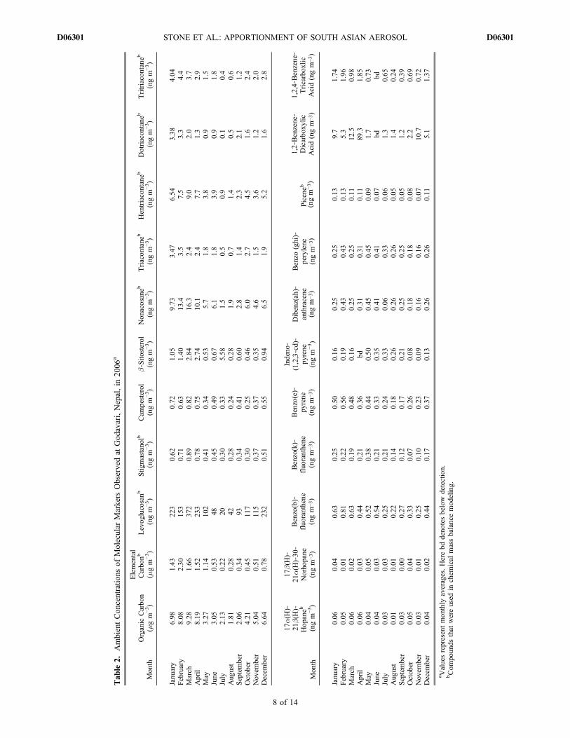
in 2006 were also observed at the ABC Pyramid site in thehigher Himalayas by Bonasoni et al. [2008].[25] Molecular markers for primary aerosol sources were

quantified in composite samples and monthly concentrationsare presented in Table 2 for the purpose of identifying andquantifying aerosol sources. The presence of elemental carbonand PAH were generic indicators that combustion of carbo-naceous fuels contributed to ambient aerosol. As previouslydiscussed, the presence of levoglucosan at concentrations20–370 ng m−3 indicated the presence of biomass burningaerosol. Stigmastanol, an indicator of cow dung, was observedin every composite sample at concentrations of 0.3–0.9 ngm−3.A homologous series of n‐alkanes with odd‐carbon prefer-ence indicated the presence of modern biomass material,namely plant wax [Simoneit, 1999]. One or more hopanes in aseries of three were observed in each sample from Godavari.Hopanes are associated with combustion of geologically agedfuels, which include coal combustion, fuel oil burning, andmotor vehicles [Simoneit, 1999] while picene, a specific PAHwith concentrations of 0.05–0.13 ngm−3 was a direct indicatorof the presence of emissions from coal‐burning [Oros andSimoneit, 2000]. The seasonal variability of molecular mar-kers generally followed that of OC. Specifically, levoglucosan,sterols, n‐alkanes, and hopanes were at peak levels in Marchand April, whereas PAHwere at highest levels in January andFebruary. Minimum molecular marker concentrations wereobserved in the summer months when aerosol loadings werelowest.[26] Carboxylic acids were observed in relatively high

concentrations in Godavari, although they are typically notconsidered molecular markers because they are not sourcespecific. They have been associated with emissions from pri-mary aerosol sources [Simoneit, 1985] and secondary sourcesvia diurnal trends in urban areas [Fine et al., 2004b] andseasonal trends in remote locations [Sheesley et al., 2004].In Godavari, wintertime concentrations of 1,2‐benzenedicarboxylic acid ranged from 5 to 13 ng m−3 while 1,2,4‐benzenetricarboxylic acid ranged from 0.72 to 2.0 ng m−3.Maximum carboxylic acid concentrations occurred in Aprilat levels of 90 and 1.9 ng m−3 that were so high in comparisonto other months that it was expected they were impacted bylocal point sources. Aromatic acid concentrations weremarkedly lower during the summermonsoon season andwerenot detectable in June. Aromatic carboxylic acids were notedto be in high concentrations in a polluted air mass affectingthe South Asian region in the wintertime of 2004–2005[Stone et al., 2007], which suggested that these compoundsmay be characteristic of regional air pollution in South Asia.

3.3. Base Case Source Apportionment of OrganicCarbon

[27] Chemical mass balance (CMB) modeling was used toapportion fine particle OC and EC in Godavari, Nepal, toprimary sources. The base case source apportionment resultsfor OC are shown in Figure 3 and summarized in Table 3.EC apportionment is discussed in section 3.4. Primary sourcesincluded in the model were biomass burning, cow dungburning, coal combustion, vegetative detritus, and motorvehicles (i.e., diesel engines). The category “other” representedsources not included in the model, which could have beenunidentified primary and/or secondary sources. The acacia

low‐rate profile was selected as the base case for biomassburning for several reasons. This tree species was commonlyfound in the tropical regions of Nepal and India, whichwere expected to have produced air masses that impactedGodavari. This profile had EC concentrations in betweenother high‐ and low‐rate profiles and provided an inter-mediate solution representative of both high‐EC emissionsfrom residential stoves and high‐OC emissions from openburning. Similarly, it had average levoglucosan concentrationsthat embodied a diverse range of burning conditions. Theacacia low profile was found to be the most representative ofresidential biofuel use and the open burning of biomasses andagricultural wastes, which were all expected to be relevantsources in the region surrounding Godavari.[28] The base case CMB source apportionment results

for Godavari in 2006 indicated that biomass combustionaccounted for 21 ± 2% of OC (average ± standard error).Diesel engines made a smaller contribution to OC with 3.9 ±0.8 and coal combustion contributed 3.0 ± 0.3%. Brick kilns,the only known industry to burn coal in the vicinity ofGodavari, were expected to be the source of these emissions.Vegetative detritus accounted for 3.9 ± 0.3% of OC, whilecow dung contributed less than 1%. Primary source con-tributions followed the same annual trends as their keymolecular markers. The percent contribution of biomassburning to OC was lowest at the height of the summermonsoon (7–19%) and was greatest in March (31%) andSeptember (35%) prior to and following the monsoon. Dieselengines and coal combustion had temporal trends in whichpercent contributions were greatest during the summermonsoon, which indicated that these anthropogenic sourcesdid not vary seasonally like biomass burning.[29] Other sources of OC, which correspond to the differ-

ence between modeled primary sources and total measuredOC, were significant; they accounted for 54–84% of OC bymonth. Meanwhile, all of the measured EC was apportionedby the model. Other sources of aerosol, then, contained OCbut not EC, and this suggested that other sources were notcombustion‐related. Previous studies of ambient aerosol haveassociated SOA with OC unapportioned to primary sourcesby the CMB model [Sheesley et al., 2004; Stone et al.,2008] and by related techniques [Engling et al., 2006]. Theassumption that other sources are SOA was used to estimateSOA in Godavari and can be considered valid when all pri-mary sources are identified and well characterized.[30] The hypothesis that unapportioned OC is SOA was

supported by the high levels of aromatic carboxylic acidspreviously discussed and consistency with previous studiesin which SOA was considered to be an important contributorto PM2.5. Table 4 presents a summary of results from CMBsource apportionment studies and aromatic carboxylic acidconcentrations from Hong Kong [Zheng et al., 2006], anurban and peripheral site in Mexico City, Mexico [Stone etal., 2008], Michigan’s Upper Peninsula in the United States[Sheesley et al., 2004], suburban Pensacola, Florida [Zheng etal., 2002], rural [Schauer et al., 2002] and urban [Dochertyet al., 2008] locations in Southern California, and Maldivesin the Northern Indian Ocean [Stone et al., 2007]. Thecomparison of the results from Godavari to these studiesdemonstrates that a large fraction of OC in nonurban areasis not apportioned to primary sources. Also, these data showthat elevated concentrations of carboxylic acids generally

STONE ET AL.: APPORTIONMENT OF SOUTH ASIAN AEROSOL D06301D06301

7 of 14

Tab

le2.

AmbientCon

centratio

nsof

Molecular

Markers

Observedat

God

avari,Nepal,in

2006

a

Mon

thOrganic

Carbo

n(mgm

−3)

Elemental

Carbo

nb

(mgm

−3)

Levog

lucosanb

(ngm

−3)

Stig

mastano

lb

(ngm

−3)

Cam

pesterol

(ngm

−3)

b‐Sito

sterol

(ngm

−3)

Non

acosaneb

(ngm

−3)

Triacon

tane

b

(ngm

−3)

Hentriacontaneb

(ngm

−3)

Dotriacon

tane

b

(ngm

−3)

Tritriacontaneb

(ngm

−3)

Janu

ary

6.98

1.43

223

0.62

0.72

1.05

9.73

3.47

6.54

3.38

4.04

February

8.08

2.30

153

0.71

0.63

1.40

13.4

3.5

7.5

3.3

4.4

March

9.28

1.66

372

0.89

0.82

2.84

16.3

2.4

9.0

2.0

3.7

April

8.19

1.52

233

0.78

0.75

2.74

10.1

2.4

7.7

1.3

2.9

May

3.27

1.14

102

0.41

0.34

0.53

5.7

1.8

3.8

0.9

1.5

June

3.05

0.53

480.45

0.49

0.67

6.1

1.8

3.9

0.9

1.8

July

2.13

0.22

200.30

0.33

5.58

1.5

0.5

0.9

0.1

0.4

Aug

ust

1.81

0.28

420.28

0.24

0.28

1.9

0.7

1.4

0.5

0.6

September

2.06

0.34

930.34

0.41

0.60

2.8

1.4

2.3

2.1

1.2

Octob

er4.21

0.45

117

0.30

0.25

0.46

6.0

2.7

4.5

1.6

2.4

Nov

ember

5.04

0.51

115

0.37

0.37

0.35

4.6

1.5

3.6

1.2

2.0

Decem

ber

6.64

0.78

232

0.51

0.55

0.94

6.5

1.9

5.2

1.6

2.8

Mon

th

17a(H

)‐21

b(H)‐

Hop

aneb

(ngm

−3)

17b(H)‐

21a(H

)‐30‐

Norho

pane

(ngm

−3)

Benzo(b)‐

fluo

ranthene

(ngm

−3)

Benzo(k)‐

fluo

ranthene

(ngm

−3)

Benzo(e)‐

pyrene

(ngm

−3)

Indeno

‐(1,2,3‐cd)‐

pyrene

(ngm

−3)

Dibenz(ah)‐

anthracene

(ngm

−3)

Benzo

(ghi)‐

perylene

(ngm

−3)

Piceneb

(ngm

−3)

1,2‐Benzene‐

Dicarbo

xylic

Acid(ngm

−3)

1,2,4‐Benzene‐

Tricarbox

licAcid(ngm

−3)

Janu

ary

0.06

0.04

0.63

0.25

0.50

0.16

0.25

0.25

0.13

9.7

1.74

February

0.05

0.01

0.81

0.22

0.56

0.19

0.43

0.43

0.13

5.3

1.96

March

0.06

0.02

0.63

0.19

0.48

0.16

0.25

0.25

0.11

12.5

0.98

April

0.06

0.03

0.44

0.21

0.36

bd0.31

0.31

0.11

89.3

1.85

May

0.04

0.05

0.52

0.38

0.44

0.50

0.45

0.45

0.09

1.7

0.73

June

0.04

0.03

0.54

0.21

0.33

0.35

0.41

0.41

0.07

bdbd

July

0.03

0.03

0.25

0.21

0.24

0.33

0.06

0.33

0.06

1.3

0.65

Aug

ust

0.01

0.01

0.22

0.14

0.18

0.26

0.26

0.26

0.05

1.4

0.24

September

0.03

0.00

0.27

0.12

0.17

0.21

0.25

0.25

0.05

1.2

0.39

Octob

er0.05

0.04

0.33

0.07

0.26

0.08

0.18

0.18

0.08

2.2

0.69

Nov

ember

0.03

0.01

0.25

0.10

0.23

0.09

0.16

0.16

0.07

10.7

0.72

Decem

ber

0.04

0.02

0.44

0.17

0.37

0.13

0.26

0.26

0.11

5.1

1.37

a Valuesrepresentmon

thly

averages.Herebd

deno

tesbelow

detection.

bCom

poun

dsthat

wereused

inchem

ical

massbalancemod

eling.

STONE ET AL.: APPORTIONMENT OF SOUTH ASIAN AEROSOL D06301D06301

8 of 14

increase along with other sources of OC, suggesting a com-mon origin, presumably SOA. The seasonal trends in othersources at Godavari were similar to other Asian locations,specifically a rural site in Hong Kong where wintertimeconcentrations were greatest and summertime lowest. Theseseasonal trends were distinctly different from those observedin the United States where aromatic carboxylic acids andother sources were greatest in summer and autumn. Theobserved trends in Asia are partially governed by the sum-mertime monsoon that corresponds to lowest aerosol con-centrations and may also be related to the availability ofphotochemically active precursor and/or transport of pollu-tion to Godavari.

3.4. Sensitivity to Biomass Profile

[31] The stability of the source apportionment at Godavariwas assessed by comparing the CMB source apportionmentresults when different biomass profiles were used. Theexamined profiles included six biomass profiles generatedin this study and four profiles from the literature: fireplacecombustion of oak [Schauer et al., 2001], open burning ofa pine forest [Lee et al., 2005], stove combustion of ricestraw [Zhang et al., 2007], and stove burning of biomassbriquettes [Sheesley et al., 2003]. The biomass profiles gen-erated in this study were limited to the base case (acaciaburning at a low rate), acacia at a high rate, mango at a highrate, rice straw, mustard stalk, and soy stalk. Mango wood

burning at a low rate was assessed separately and is discussedbelow. While all other variables were held constant, thebiomass source profile was systematically varied and thesource contributions to OC in Godavari using various bio-mass profiles are presented in Figures 4a–4b. The sensitivityof the model results were assessed for 2 months in contrastingseasons: January in the wintertime and August during thesummer monsoon. Most estimates of biomass contributionsto OC were clustered around the base case result whichwas 25% (1.7 ± 0.5 mg m−3) in January and 19% (0.33 ±0.10 mg m−3) in August. The open burn profile yielded thehighest estimates of biomass contributions to OC in bothwintertime (53%) and summertime (36%). Low‐end esti-mates were produced by profiles for acacia burning at a highrate, mustard stalk, and fireplace combustion of oak andranged from 9 to 14% in the wintertime and from 7 to 10%in the summertime. When the four extreme cases wereexcluded, the average across the remaining cases was 25 ±6% (±1 standard deviation) in the wintertime and 19 ± 4%in the summertime. These results indicated that biomasscontributions to OC were self‐consistent when variousbiomass profiles were used and most solutions were instrong agreement with the base case result. It was expectedthat the Godavari site was impacted by both biofuel burningand open burning in 2006 and that actual contribution fellin between these two extremes and within the projecteduncertainty.

Figure 3. Source contributions to PM2.5 organic and elemental carbon representing the base case conditions.

Table 3. Base Case Source Contributions Calculated by Molecular Marker Chemical Mass Balance Modeling to Ambient OrganicCarbon at Godavari, Nepal, in 2006a

MonthDiesel Engines(mgC m−3)

Coal Combustion(mgC m−3)

Vegetative Detritus(mgC m−3)

Cow Dung(mgC m−3)

Biomass Burning(mgC m−3)

Other(mgC m−3) R2 c2

January 0.32 ± 0.11 0.20 ± 0.04 0.32 ± 0.06 0.005 ± 0.006 1.71 ± 0.50 4.41 ± 0.73 0.86 4.06February 0.72 ± 0.13 0.16 ± 0.04 0.36 ± 0.06 0.013 ± 0.006 1.20 ± 0.35 5.62 ± 0.67 0.87 4.31March 0.28 ± 0.14 0.18 ± 0.04 0.38 ± 0.07 0.005 ± 0.010 2.85 ± 0.83 5.58 ± 1.04 0.90 3.10April 0.35 ± 0.12 0.19 ± 0.04 0.29 ± 0.05 0.009 ± 0.007 1.82 ± 0.53 5.53 ± 0.78 0.91 2.39May 0.33 ± 0.06 0.13 ± 0.03 0.15 ± 0.03 0.006 ± 0.004 0.80 ± 0.23 1.86 ± 0.40 0.90 3.61June 0.15 ± 0.04 0.12 ± 0.02 0.15 ± 0.03 0.011 ± 0.004 0.37 ± 0.11 2.24 ± 0.33 0.89 2.97July 0.06 ± 0.02 0.10 ± 0.02 0.03 ± 0.01 0.008 ± 0.002 0.15 ± 0.05 1.79 ± 0.27 0.90 2.03August 0.06 ± 0.03 0.04 ± 0.01 0.05 ± 0.01 0.006 ± 0.002 0.33 ± 0.10 1.32 ± 0.27 0.84 3.79September 0.03 ± 0.04 0.08 ± 0.02 0.09 ± 0.02 0.005 ± 0.003 0.73 ± 0.21 1.12 ± 0.34 0.86 3.41October 0.05 ± 0.06 0.15 ± 0.03 0.21 ± 0.04 0.002 ± 0.003 0.90 ± 0.26 2.91 ± 0.45 0.84 3.87November 0.08 ± 0.06 0.11 ± 0.02 0.16 ± 0.03 0.004 ± 0.004 0.90 ± 0.26 3.80 ± 0.49 0.90 2.45December 0.07 ± 0.09 0.16 ± 0.03 0.24 ± 0.04 0.002 ± 0.006 1.77 ± 0.52 4.40 ± 0.75 0.89 2.58

aValues in bold are statistically significant.

STONE ET AL.: APPORTIONMENT OF SOUTH ASIAN AEROSOL D06301D06301

9 of 14

[32] The amount of OC apportioned to biomass burningsources directly impacted the OC represented by other sources.In the sensitivity analysis, the estimated contribution ofother sources in January was 63% (4.4 ± 0.7 mg m−3) andthe average across all other solutions was 65 ± 14%. InAugust, the base case contribution from other sources was73% (1.3 ± 0.3 mg m−3) while the average across othersolutions was 75 ± 9%. Other source contributions to OCwere consistent across the different source apportionmentsolutions and clustered closely to the base case solution. Aspreviously discussed, other sources were found to be con-sistent with SOA and the magnitude of its estimated con-tributions to OC in Godavari warrants further study of SOAprecursors and formation mechanisms in South Asia.[33] The selection of biomass profile had relatively small

impacts on other sources. Diesel contributions to OC were7 ± 1% in January and 5 ± 1% in August whereas coalcombustion contributions were relatively stable at 2–3% inboth months. Contributions from cow dung burning wereconsistently less than 1%, when either the cow dung profilegenerated in this study or that of Sheesley et al. [2004] wasused. The selection of biomass profile affected the estimationof contributions from vegetative detritus and cow dung, sinceall of these sources were associated with n‐alkanes. Thebiomass profiles for open burning and cropwastes (rice straw,mustard stalk, and soy stalk) were associated with decreasedcontributions from vegetative detritus and cow dung as aresult of this colinearity, also noted by Sheesley et al. [2007].

[34] The apportionment of EC to biomass burning inGodavari exhibited a high degree of instability when differentbiomass profiles were used as shown in Figures 4c–4d. Thebase case EC contribution from biomass burning in Januarywas 38% (0.53 ± 0.05 mg m−3) while the range of othersolutions was 3–23% with an average and standard devi-ation of 15 ± 11%. Similar instability was observed for themonth of August when the base case EC contribution frombiomass was 37% (0.10 ± 0.01 mg m−3) and other solutionsranged from 3 to 22% with an average of 13 ± 11%. The basecase profile represented the upper estimate of biomass con-tributions to EC, but was considered to be reasonable basedon the moderate EC to OC ratio compared to other low burnrate profiles and prevalence of biofuel use in the region[Venkataraman et al., 2005]. Diesel engines accounted forthe majority of EC not apportioned to biomass, contributing81 ± 11% in January and 78 ± 11% in August. Coal com-bustion consistently contributed 3–4% of EC.[35] The upper limit of biomass contributions to EC were

explored using the biomass profile for mango wood burningat a low rate. This profile represented an extreme case withan EC to OC ratio of 1.6. The only other profile in the modelwith an EC to OC ratio greater than one was diesel engineswith a ratio of 2.6 [Lough et al., 2007]. When profiles forlow‐rate mango wood burning and diesel engines were bothincluded in the CMB model, the diesel engine contributionwas forced to be negative. A statistically significant negativesource contribution was considered physically impossible

Table 4. Summary of Ambient Aromatic Carboxylic Acid Concentrations and Organic Carbon Unapportioned to Primary AerosolSources From a Number of Source Apportionment Studies When Secondary Organic Aerosol was Considered to be an Important Sourceof Ambient Organic Carbona

Site Season (Date of Study)

1,2‐benzene‐dicarboxylicacid (ng m−3)

1,2,4‐benzene‐tricarboxylicacid (ng m−3)

CMB Other(mg OC m−3)

CMB Other(% OC) Study

Godavari, Nepal(near‐urban)

Dry Season (Jan–Mar 2006) 5.3–12.5 1.0–2.0 4.4–5.6 64 this studyMonsoon Season (May–Aug 2006) >1.0–1.7 <0.2–0.7 1.3–2.2 72 this studyDry Season (Oct–Dec 2006) 2.2–10.7 0.7–1.4 2.9–4.4 70 this study

Hok Tsui, Winter (2000–2001) 17.93 nm 1.8 36 Zheng et al. [2006]Hong Kong (rural) Spring (2001) 2.26 1.2 44 Zheng et al. [2006]

Summer (2001) nm 1.2 67 Zheng et al. [2006]Fall (2001) 0.39 2.1 57 Zheng et al. [2006]

Mexico CityUrban Site Springtime (17–30 Mar 2006) 3.9–27 <0.3–2.4 1.7–6.4 38 Stone et al. [2008]Peripheral Site Springtime (17–30 Mar 2006) 1.1–5.3 <0.3–1.6 1.1–4.6 49 Stone et al. [2008]

Upper Peninsula,Michigan (rural)

Summertime (May–Aug 2002) 0.3–1.5 0.1–2.0 0.5–3.1 81 Sheeley et al. [2004]Wintertime (Dec 2001 to Mar 2002) nm nm 0–0.3 32 Sheeley et al. [2004]

Pensacola, Florida(suburban)

Springtime (Apr 1999) 0.43 0.03b 1.2 60 Zheng et al. [2002]Summer (Jul 1999) 1.79 2.34 1.4 68 Zheng et al. [2002]Autumn (Oct 1999) 5.2 3.09 2.0 63 Zheng et al. [2002]Winter (Jan 2000) 2.11 0.36 0.2 9 Zheng et al. [2002]

Kern NWR (rural) Wintertime (26–28 Dec 1995) 4.7 3.6b 3.7 82 Schauer et al. [2002]

Riverside, California(urban)

Summertime (26 Jul to 7 Aug 2005) <1.2–53 nm 4.2–7.6 79 Docherty et al. [2002]

Hanimaadhoo,Maldives (remote)

Transition (Aug–Oct 2004) <0.1 <0.1 nm Stone et al. [2007]Dry Season (Dec 2004 to Jan 2005) 3.5 1.2 Stone et al. [2007]

aAbbreviations: OC, organic carbon; CMB, primary aerosol sources; nm, not measured.bSum of several benzenetricarboxylic acid isomers.

STONE ET AL.: APPORTIONMENT OF SOUTH ASIAN AEROSOL D06301D06301

10 of 14

and rejected. In order to assess what fraction of biomasscombustion could have been associated with biomass emis-sions high in EC relative to OC, weighted‐average profiles ofmango wood at low and high rates were assembled rangingfrom 0 to 40% low burn rate, by 10%. When the low burnrate emissions profile exceeded 40%, biomass contributionsto OC and EC incrementally increased while diesel con-tributions were forced to be negative, providing unviablesolutions. Source apportionment results for these profiles areshown in Figure 5. The maximum model‐predicted EC

contribution from biomass under these conditions was esti-mated to be 93% in the wintertime and 88% in the summer-time, while minimum diesel engine contributions were 2%and 3%, respectively. From this, we confirm that the sourceapportionment of EC in Godavari is highly unstable due tothe diversity of biomass burn conditions in the region. Whilethe newly developed biofuel profiles contribute to a betterestimate of biofuel contributions to ambient OC in SouthAsia, they could not improve the apportionment of EC.The biofuel emissions high in EC relative to OC may have

Figure 4. Sensitivity of source contributions to organic and elemental carbon in wintertime (January)and during the summer monsoon (August) using various biomass profiles. The base case is marked witha star.

STONE ET AL.: APPORTIONMENT OF SOUTH ASIAN AEROSOL D06301D06301

11 of 14

accounted for a significant portion of ambient EC, as sug-gested by previous studies based on emissions inventories[Streets et al., 2003a; Venkataraman et al., 2005] and impliedby the wide range of viable solutions in this study.

4. Conclusions

[36] Aerosol sources impacting Godavari in 2006 werediverse and expectedly came from a mixture of many sourcecategories present within the South Asian region. CMBmodeling provided an approach to quantitatively assess the

current understanding of source contributions from biomassburning and fossil fuel combustion to carbonaceous aerosol(OC and EC) at the receptor location. Source profiles wereselected to represent important sources in the region ofinterest, and included profiles for residential biofuel use andopen biomass burning. The best estimate or base case resultindicated that biomass burning and SOA were importantsources of ambient OC whereas biomass burning and fossilfuel combustion were significant sources of EC. The sys-tematic comparison of a range of possible solutions revealedthat primary sources and SOA contributions to OC wereclustered together among different model solutions andindicated a high stability in apportionment results. However,source contributions to EC were variable when differentbiomass profiles were used and revealed that source con-tributions to EC could not be reconciled with molecularmarker CMB modeling in regions like South Asia, wherebiomass burning emissions high in EC relative to OC wereexpectedly important. To improve understanding of OCsources in remote Asian locations, studies should target SOAtracer compounds linked to biogenic and anthropogenicprecursors [Kleindienst et al., 2007] and further character-ization of water‐soluble OC components. Further reconcili-ation of EC sources in South Asia should rely upon otherapportionment techniques, such as multivariate analysis[Stone et al., 2007] and stable‐isotope analysis [Gustafsson etal., 2009], which provide more constrained approaches todistinguishing between fossil and modern sources of EC.

[37] Acknowledgments. This research was supported through Atmo-spheric Brown Cloud (ABC) grants from the National Oceanic and Atmo-spheric Administration (NOAA). We thank the Wisconsin State Laboratoryof Hygiene and scientists Jeff DeMinter and Brandon Shelton for assistancewith chemical analysis and University of Wisconsin‐Madison studentsCatherine Kolb andMarya Orf for technical support. We also thank BhupeshAdhikary at the University of Iowa for helpful communications and theMENRIS division at ICIMOD for producing the map of the KathmanduValley. We appreciate the contributions of the Nepal Ministry of Environ-ment and the United Nations Environmental Program Regional ResourceCenter for Asia and the Pacific for their support to the observatory pro-gram in Nepal.

ReferencesAdhikary, B., G. R. Carmichael, Y. Tang, L. R. Leung, Y. Qian, J. J. Schauer,E. A. Stone, V. Ramanathan, and M. V. Ramana (2007), Characterizationof the seasonal cycle of south Asian aerosols: A regional‐scale modelinganalysis, J. Geophys. Res., 112, D22S22, doi:10.1029/2006JD008143.

Bonasoni, P. et al. (2008), The ABC‐Pyramid Atmospheric Research Obser-vatory in Himalaya for aerosol, ozone and halocarbon measurements, Sci.Total Environ., 391, 252–261, doi:10.1016/j.scitotenv.2007.10.024.

Centers for Cloud, Chemistry, and Climate (2002) The Asian brown cloud:Climate and other environmental impacts, executive summary, Environ.Sci. and Pollut. Res., U.N. Environ. Prog., Nairobi. (Available at http://rrcap.unep.org/abc/impactstudy/)

Chowdhury, Z., M. Zheng, J. J. Schauer, R. J. Sheesley, L. G. Salmon,G. R. Cass, and A. G. Russell (2007), Speciation of ambient fine organiccarbon particles and source apportionment of PM2.5 in Indian cities,J. Geophys. Res., 112, D15303, doi:10.1029/2007JD008386.

Docherty, K. S. et al. (2008), Apportionment of primary and secondaryorganic aerosols in southern California during the 2005 Study of OrganicAerosols in Riverside (SOAR‐1), Environ. Sci. Technol., 42, 7655–7662,doi:10.1021/es8008166.

Engling, G., P. Herckes, S. M. Kreidenweis, W. C. Malm, and J. L. Collett(2006), Composition of the fine organic aerosol in Yosemite NationalPark during the 2002 Yosemite aerosol characterization study, Atmos.Environ., 40, 2959–2972, doi:10.1016/j.atmosenv.2005.12.041.

Fine, P. M., G. R. Cass, and B. R. T. Simoneit (2004a), Chemical charac-terization of fine particle emissions from the wood stove combustion of

Figure 5. Sensitivity of source contributions to organic andelemental carbon in wintertime (January) and during thesummer monsoon (August) using weighted‐average profilesof mango wood burned at low and high rates.

STONE ET AL.: APPORTIONMENT OF SOUTH ASIAN AEROSOL D06301D06301

12 of 14

prevalent United States tree species, Environ. Eng. Sci., 21, 705–721,doi:10.1089/ees.2004.21.705.

Fine, P. M., B. Chakrabarti, M. Krudysz, J. J. Schauer, and C. Sioutas(2004b), Diurnal variations of individual organic compound constituentsof ultrafine and accumulation mode particulate matter in the Los Angelesbasin, Environ. Sci. Technol., 38, 1296–1304, doi:10.1021/es0348389.

Gustafsson, O., M. Krusa, Z. Zencak, R. J. Sheesley, L. Granat, E. Engstrom,P. S. Praveen, P. S. P. Rao, C. Leck, and H. Rodhe (2009), Brownclouds over South Asia: Biomass or fossil fuel combustion?, Science,323, 495–498, doi:10.1126/science.1164857.

Habib, G., C. Venkataraman, T. C. Bond, and J. J. Schauer (2008), Chemical,microphysical and optical properties of primary particles from the combus-tion of biomass fuels, Environ. Sci. Technol., 42, 8829–8834, doi:10.1021/es800943f.

Hindman, E. E., and B. P. Upadhyay (2002), Air pollution transport in theHimalayas of Nepal and Tibet during the 1995–1996 dry season, Atmos.Environ., 36, 727–739, doi:10.1016/S1352-2310(01)00495-2.

Hopke, P. K. et al. (2008), Urban air quality in the Asian region, Sci. TotalEnviron., 404, 103–112, doi:10.1016/j.scitotenv.2008.05.039.

Jaeckels, J. M., M. S. Bae, and J. J. Schauer (2007), Positive matrix factor-ization (PMF) analysis of molecular marker measurements to quantify thesources of organic aerosols, Environ. Sci. Technol., 41, 5763–5769,doi:10.1021/es062536b.

Kleindienst, T. E., M. Jaoui, M. Lewandowski, J. H. Offenberg, C. W.Lewis, P. V. Bhave, and E. O. Edney (2007), Estimates of the contribu-tions of biogenic and anthropogenic hydrocarbons to secondary organicaerosol at a southeastern US location, Atmos. Environ., 41, 8288–8300,doi:10.1016/j.atmosenv.2007.06.045.

Lee, S., K. Baumann, J. J. Schauer, R. J. Sheesley, L. P. Naeher, S. Meinardi,D. R. Blake, E. S. Edgerton, A. G. Russell, and M. Clements (2005),Gaseous and particulate emissions from prescribed burning in Georgia,Environ. Sci. Technol., 39, 9049–9056, doi:10.1021/es051583l.

Lough, G. C., C. C. Christenson, J. J. Schauer, J. Tortorelli, E. Bean,D. Lawson, N. N. Clark, and P. A. Gabele (2007), Development of molec-ular marker source profiles for emissions from on‐road gasoline and dieselvehicle fleets, J. Air Waste Manage. Assoc., 57, 1190–1199.

Oros, D. R., and B. R. T. Simoneit (2000), Identification and emission ratesof molecular tracers in coal smoke particulate matter, Fuel, 79, 515–536,doi:10.1016/S0016-2361(99)00153-2.

Panday, A. K., and R. G. Prinn (2009), Diurnal cycle of air pollution in theKathmandu Valley, Nepal: Observations, J. Geophys. Res., 114, D09305,doi:10.1029/2008JD009777.

Ramana, M. V., V. Ramanathan, I. A. Podgorny, B. B. Pradhan, andB. Shrestha (2004), The direct observations of large aerosol radiativeforcing in the Himalayan region, Geophys. Res. Lett., 31, L05111,doi:10.1029/2003GL018824.

Ramanathan, V., and M. V. Ramana (2005), Persistent, widespread, andstrongly absorbing haze over the Himalayan foothills and the Indo‐Gangetic Plains, Pure Appl. Geophys., 162, 1609–1626, doi:10.1007/s00024-005-2685-8.

Ramanathan, V. et al. (2001), Indian Ocean Experiment: An integratedanalysis of the climate forcing and effects of the great Indo‐Asian haze,J. Geophys. Res., 106, 28,371–28,398, doi:10.1029/2001JD900133.

Ramanathan, V., C. Chung, D. Kim, T. Bettge, L. Buja, J. T. Kiehl, W. M.Washington, Q. Fu, D. R. Sikka, and M. Wild (2005), Atmosphericbrown clouds: Impacts on South Asian climate and hydrological cycle,Proc. Natl. Acad. Sci. U. S. A., 102, 5326–5333, doi:10.1073/pnas.0500656102.

Ramanathan, V. et al. (2007), Atmospheric brown clouds: Hemisphericaland regional variations in long‐range transport, absorption, and radiativeforcing, J. Geophys. Res., 112, D22S21, doi:10.1029/2006JD008124.

Robinson, A. L., R. Subramanian, N. M. Donahue, A. Bernardo‐Bricker,and W. F. Rogge (2006), Source apportionment of molecular markersand organic aerosol. 2. Biomass smoke, Environ. Sci. Technol., 40,7811–7819, doi:10.1021/es060782h.

Rogge, W. F., L. M. Hildemann, M. A. Mazurek, G. R. Cass, and B. R. T.Simoneit (1993), Sources of fine organic aerosol. 4. Particulate abrasionproducts from leaf surfaces of urban plants, Environ. Sci. Technol., 27,2700–2711, doi:10.1021/es00049a008.

Schauer, J. J., and G. R. Cass (2000), Source apportionment of wintertimegas‐phase and particle‐phase air pollutants using organic compounds astracers, Environ. Sci. Technol., 34, 1821–1832, doi:10.1021/es981312t.

Schauer, J. J., W. F. Rogge, L. M. Hildemann, M. A. Mazurek, and G. R.Cass (1996), Source apportionment of airborne particulate matter usingorganic compounds as tracers, Atmos. Environ., 30, 3837–3855,doi:10.1016/1352-2310(96)00085-4.

Schauer, J. J., M. J. Kleeman, G. R. Cass, and B. R. T. Simoneit (2001),Measurement of emissions from air pollution sources. 3. C1–C29 organic

compounds from fireplace combustion of wood, Environ. Sci. Technol.,35, 1716–1728, doi:10.1021/es001331e.

Schauer, J. J., M. P. Fraser, G. R. Cass, and B. R. T. Simoneit (2002),Source reconciliation of atmospheric gas‐phase and particle‐phase pollu-tants during a severe photochemical smog episode, Environ. Sci. Tech-nol., 36, 3806–3814, doi:10.1021/es011458j.

Schauer, J. J. et al. (2003), ACE‐Asia intercomparison of a thermal‐opticalmethod for the determination of particle‐phase organic and elemental car-bon, Environ. Sci. Technol., 37, 993–1001, doi:10.1021/es020622f.

Schmidl, C., H. Bauer, A. Dattler, R. Hitzenberger, G. Weissenboeck,I. L. Marr, and H. Puxbaum (2008a), Chemical characterisation of particleemissions from burning leaves, Atmos. Environ., 42, 9070–9079,doi:10.1016/j.atmosenv.2008.09.010.

Schmidl, C., L. L. Marr, A. Caseiro, P. Kotianova, A. Berner, H. Bauer,A. Kasper‐Giebl, and H. Puxbaum (2008b), Chemical characterisationof fine particle emissions from wood stove combustion of commonwoods growing in mid‐European Alpine regions, Atmos. Environ.,42, 126–141, doi:10.1016/j.atmosenv.2007.09.028.

Sheesley, R. J., J. J. Schauer, Z. Chowdhury, G. R. Cass, and B. R. T.Simoneit (2003), Characterization of organic aerosols emitted fromthe combustion of biomass indigenous to South Asia, J. Geophys.Res., 108(D9), 4285, doi:10.1029/2002JD002981.

Sheesley, R. J., J. J. Schauer, E. Bean, and D. Kenski (2004), Trends in sec-ondary organic aerosol at a remote site in Michigan’s Upper Peninsula,Environ. Sci. Technol., 38, 6491–6500, doi:10.1021/es049104q.

Sheesley, R. J., J. J. Schauer, M. Zheng, and B. Wang (2007), Sensitivity ofmolecular marker‐based CMBmodels to biomass burning source profiles,Atmos. Environ., 41, 9050–9063, doi:10.1016/j.atmosenv.2007.08.011.

Shrestha, A. B., C. P. Wake, J. E. Dibb, P. A. Mayewski, S. I. Whitlow,G. R. Carmichael, and M. Ferm (2000), Seasonal variations in aerosolconcentrations and compositions in the Nepal Himalaya, Atmos. Environ.,34, 3349–3363, doi:10.1016/S1352-2310(99)00366-0.

Simoneit, B. R. T. (1985), Application of molecular marker analysis tovehicular exhaust for source reconciliations, Int. J. Environ. Anal.Chem., 22, 203–233, doi:10.1080/03067318508076422.

Simoneit, B. R. T. (1999), A review of biomarker compounds as sourceindicators and tracers for air pollution, Environ. Sci. Pollut. Res., 6,159–169, doi:10.1007/BF02987621.

Simoneit, B. R. T. (2002), Biomass burning—A review of organic tracersfor smoke from incomplete combustion, Appl. Geochem., 17, 129–162,doi:10.1016/S0883-2927(01)00061-0.

Stone, E. A., G. C. Lough, J. J. Schauer, P. S. Praveen, C. E. Corrigan, andV. Ramanathan (2007), Understanding the origin of black carbon in theatmospheric brown cloud over the Indian Ocean, J. Geophys. Res., 112,D22S23, doi:10.1029/2006JD008118.

Stone, E. A., D. C. Snyder, R. J. Sheesley, A. P. Sullivan, R. J. Weber, andJ. J. Schauer (2008), Source apportionment of fine organic aerosol inMexico City during the MILAGRO experiment 2006, Atmos. Chem.Phys., 8, 1249–1259.

Streets, D. G. et al. (2003a), An inventory of gaseous and primary aerosolemissions in Asia in the year 2000, J. Geophys. Res., 108(D21), 8809,doi:10.1029/2002JD003093.

Streets, D. G., K. F. Yarber, J. H. Woo, and G. R. Carmichael (2003b), Bio-mass burning in Asia: Annual and seasonal estimates and atmosphericemissions, Global Biogeochem. Cycles, 17(4), 1099, doi:10.1029/2003GB002040.

Sun, J. M., and P. A. Ariya (2006), Atmospheric organic and bio‐aerosolsas cloud condensation nuclei (CCN): A review, Atmos. Environ., 40,795–820, doi:10.1016/j.atmosenv.2005.05.052.

Turpin, B. J., andH. J. Lim (2001), Species contributions to PM2.5mass con-centrations: Revisiting common assumptions for estimating organic mass,Aerosol Sci. Technol., 35, 602–610, doi:10.1080/02786820152051454.

Venkataraman, C., G. Habib, A. Eiguren‐Fernandez, A. H. Miguel, andS. K. Friedlander (2005), Residential biofuels in south Asia: Carbona-ceous aerosol emissions and climate impacts, Science, 307, 1454–1456,doi:10.1126/science.1104359.

Watson, J. G., J. A. Cooper, and J. J. Huntzicker (1984), The effective var-iance weighting for least‐squares calculations applied to the mass balancereceptor model, Atmos. Environ., 18, 1347–1355, doi:10.1016/0004-6981(84)90043-X.

Watson, J. G., L. W. A. Chen, J. C. Chow, P. Doraiswamy, and D. H.Lowenthal (2008), Source apportionment: Findings from the US Super-sites program, J. Air Waste Manage. Assoc., 58, 265–288, doi:10.3155/1047-3289.58.2.265.

Zhang, Y. X.,M. Shao, Y. H. Zhang, L.M. Zeng, L. Y. He, B. Zhu, Y. J.Wei,and X. L. Zhu (2007), Source profiles of particulate organic matters emit-ted from cereal straw burnings, J. Environ. Sci., 19, 167–175, doi:10.1016/S1001-0742(07)60027-8.

STONE ET AL.: APPORTIONMENT OF SOUTH ASIAN AEROSOL D06301D06301

13 of 14

Zhang, Y. X., J. J. Schauer, Y. H. Zhang, L. M. Zeng, Y. J. Wei, Y. Liu,and M. Shao (2008), Characteristics of particulate carbon emissions fromreal‐worldChinese coal combustion,Environ. Sci. Technol., 42, 5068–5073,doi:10.1021/es7022576.

Zheng, M., G. R. Cass, J. J. Schauer, and E. S. Edgerton (2002), Sourceapportionment of PM2.5 in the southeastern United States using solvent‐extractable organic compounds as tracers, Environ. Sci. Technol., 36,2361–2371, doi:10.1021/es011275x.

Zheng, M., G. S. W. Hagler, L. Ke, M. H. Bergin, F. Wang, P. K. K. Louie,L. Salmon, D. W. M. Sin, J. Z. Yu, and J. J. Schauer (2006), Compositionand sources of carbonaceous aerosols at three contrasting sites in HongKong, J. Geophys. Res., 111, D20313, doi:10.1029/2006JD007074.

P. M. Dangol and B. B. Pradhan, International Centre for IntegratedMountain Development, GPO Box 3226, Khumaltar, Kathmandu, Nepal.(info@icomod.org)

G. Habib, Department of Civil Engineering, Indian Institute ofTechnology Delhi, Hauz Khas, New Delhi 110016, India. (gazalahabib@gmail.com)V. Ramanathan, Center for Clouds, Chemistry and Climate, Scripps

Institute of Oceanography, University of California, San Diego, 9500Gilman Drive, MC 0221, La Jolla, CA 92093‐0221, USA. (vram@ucsd.edu)J. J. Schauer, Environmental Chemistry and Technology Program,

University of Wisconsin‐Madison, 660 N. Park St., Madison, WI 53706,USA. (jjschauer@wisc.edu)E. A. Stone, Environmental and Organic Chemistry, Carlsbad

Environmental Monitoring and Research Center, Institute of Energy andthe Environment, New Mexico State University, 1400 University Dr.,Carlsbad, NM 88220, USA. (betsy.stone@gmail.com)C. Venkataraman, Department of Chemical Engineering, Indian Institute

of Technology Bombay, Powai, Mumbai 400076, India. (chandra@che.iitb.ac.in)

STONE ET AL.: APPORTIONMENT OF SOUTH ASIAN AEROSOL D06301D06301

14 of 14