Lifecycle Analyses of Biofuels - eScholarship

Year 2006 UCD-ITS-RR-06-08

Lifecycle Analyses of Biofuels

Draft Report (May be cited as draft report)

Mark A. Delucchi

Institute of Transportation Studies ◊ University of California, Davis

One Shields Avenue ◊ Davis, California 95616

PHONE: (530) 752-6548 ◊ FAX: (530) 752-6572

WEB: http://its.ucdavis.edu/

DRAFT WORKING MANUSCRIPT

LIFECYCLE ANALYSES OF BIOFUELS

Draft manuscript

(may be cited as draft manuscript)

Mark A. Delucchi

Institute of Transportation Studies

University of California, Davis

One Shields Avenue

Davis, CA 95616

May, 2006


1

OVERVIEW

This manuscript on lifecycle analysis (LCA) of biofuels for transportation has three major parts: I. An analysis of greenhouse-gas emissions from biofuels, estimated using the Lifecycle

Emissions Model (LEM).

II. A review of recent LCAs of biofuels.

III. A comprehensive conceptual framework for doing LCAs of biofuels.

I. ANALYSIS OF GREENHOUSE-GAS EMISSIONS FROM BIOFUELS

The LEM analysis of lifecycle GHG emissions from biofuels is organized as follows:

• A short overview of the Lifecycle Emissions Model (LEM).

• Brief, general descriptions of the basic technical processes as they are represented in

the LEM.

• Estimates of CO2-equivalent GHG emissions from biofuels at three different levels of

aggregation: at the level of the farm (e.g., land-use and cultivation emissions per

hectare); for the whole upstream fuel lifecycle (also known as “well-to-tank”), and for

the entire fuel and vehicle-use lifecycle (in grams/mile; sometimes called “well-to-

wheel,” but in this case also including the vehicle lifecycle). These will be produced for

selected biofuel and other pathways in the LEM.

• The ratio of process energy inputs to fuel outputs, for selected fuelcycles.

• Emissions of individual pollutants by stage, for selected fuelcycles.

• A brief, general discussion of the differences in LEM results by country and year.

• A brief discussion of the differences between using the CO2-equivalency factors

(CEFs) in the LEM and the “Global Warming Potentials” (GWPs) of the

Intergovernmental Panel on Climate Change (IPCC).


2

The analysis of lifecycle GHG emissions from biofuels was performed using the

Lifecycle Emissions Model (LEM). The LEM has been developed over a number of

years by Dr. Delucchi and colleagues. Complete documentation of the LEM is available

on Dr. Delucchi’s web page.

For economy of presentation, the main results of the lifecycle analysis (LCA) of biofuels

and vehicles are reported for the U. S. for the year 2010, using LEM CEFs. As

mentioned above, we do present and discuss some results for different years and

different countries, for the IPCC GWPs as opposed to the LEM CEFs.

Overview of the LEM

The LEM uses lifecycle analysis (LCA) to estimate energy use, criteria air-pollutant

emissions, and CO2-equivalent greenhouse-gas emissions from a wide range of energy

and material lifecycles. It includes lifecycles for passenger transport modes, freight

transport modes, electricity, materials, heating and cooling, and more. For transport

modes, it represents the lifecycle of fuels, vehicles, materials, and infrastructure. It

calculates energy use and lifecycle emissions of all regulated air pollutants plus so-called

greenhouse gases. It includes input data for up to 30 countries, for the years 1970 to

2050, and is fully specified for the U. S.

For motor vehicles, the LEM calculates lifecycle emissions for a variety of combinations

of end-use fuel (e.g., methanol), fuel feedstocks (e.g., coal), and vehicle types (e.g., fuel-

cell vehicle). For light-duty vehicles, the fuel and feedstock combinations included in the

LEM are shown in Table 0.


3

TABLE 0. FUEL, FEEDSTOCK, AND VEHICLE COMBINATIONS IN THE LEM

Fuel -->

↓ Feedstock

Gasoline Diesel Methanol Ethanol Methane (CNG, LNG)

Propane (LPG)

Hydrogen (CH2) (LH2)

Electric

Petroleum ICEV, FCV

ICEV ICEV BPEV

Coal ICEV ICEV ICEV, FCV

FCV BPEV

Natural gas ICEV ICEV, FCV

ICEV ICEV ICEV, FCV

BPEV

Wood or grass ICEV, FCV

ICEV, FCV

ICEV FCV BPEV

Soybeans ICEV

Corn ICEV

Solar power ICEV, FCV

BPEV

Nuclear power ICEV, FCV

BPEV

Notes: ICEV = internal-combustion-engine vehicle; FCV = fuel-cell vehicle; BPEV = battery-powered electric vehicle.

The LEM has similar but fewer combinations for heavy-duty vehicles (HDVs), mini-

cars, and motor scooters.

As indicated in Table 0, the LEM includes the following biofuel lifecycles:

• corn to ethanol

• soybeans to biodiesel

• switchgrass to ethanol

• wood to ethanol

• wood to methanol

• wood to synthetic natural gas

• switchgrass to hydrogen


4

Fuel, material, vehicle, and infrastructure lifecycles in the LEM

The LEM estimates the use of energy, and emissions of greenhouse gases and urban air

pollutants, for the complete lifecycle of fuels, materials, vehicles, and infrastructure for

the transportation modes listed above. For fuels and electricity, these lifecycles are

constructed as follows:

• end use: the use of a finished fuel product, such as gasoline, electricity,

or heating oil, by consumers.

• dispensing of fuels: pumping of liquid fuels, and compression or

liquefaction of gaseous transportation fuels.

• fuel distribution and storage: the transport of a finished fuel product to

end users and the operation of bulk-service facilities. For example, the

shipment of gasoline by truck to a service station.

• fuel production: the transformation of a primary resource, such as

crude oil or coal, to a finished fuel product or energy carrier, such as

gasoline or electricity.

• feedstock transport: the transport of a primary resource to a fuel

production facility. For example, the transport of crude oil from the

wellhead to a petroleum refinery. A complete country-by-country

accounting of imports of crude oil and petroleum products by country

is included in the LEM.

• feedstock production: the production of a primary resource, such as

crude oil, coal, or biomass. Based on primary survey data at energy-

mining and recovery operations, or survey or estimated data for

agricultural operations.


5

For materials, the lifecycle is:

• crude-ore recovery and finished-material manufacture: the recovery

and transport of crude ores used to make finished materials and the

manufacture of finished materials from raw materials.

• the transport of finished materials to end users.

For vehicles, the lifecycle is:

• materials use: see the “lifecycle of materials”.

• vehicle assembly: assembly and transport of vehicles, trains, etc.

• operation and maintenance: energy use and emissions associated with

motor-vehicle service stations and parts shops, transit stations, and so

on;

• secondary fuel cycle for transport modes: building, servicing, and

providing administrative support for transport and distribution modes

such as large crude-carrying tankers or unit coal trains.

Lifecycle of infrastructure:

• energy use and materials production: the manufacture and transport of

raw and finished materials used in the construction of highways,

railways, etc., as well as energy use and emissions associated with the

construction of the transportation infrastructure.


6

Sources of emissions in LEM lifecycles

The LEM characterizes greenhouse gases and criteria pollutants from a variety of

emission sources:

• Combustion of fuels that provide process energy (for example, the

burning of bunker fuel in the boiler of a super-tanker, or the

combustion of refinery gas in a petroleum refinery);

• Evaporation or leakage of energy feedstocks and finished fuels (for

example, from the evaporation of hydrocarbons from gasoline storage

terminals);

• Venting, leaking, or flaring of gas mixtures that contain greenhouse

gases (for example, the venting of coal bed gas from coal mines);

• Fugitive dust emissions (for example, emissions of re-entrained road

dust from vehicles driving on paved roads);

• Chemical transformations that are not associated with burning process

fuels (for example, the curing of cement, which produces CO2, or the

denitrification of nitrogenous fertilizers, which produces N2O);

• Changes in the carbon content of soils or biomass, or emissions of non-

CO2 greenhouse from soils, due to changes in land use.


7

Pollutant tracked in the LEM

The LEM estimates emissions of the following pollutants:

• carbon dioxide (CO2) • total particulate matter (PM)

• methane (CH4) • particulate matter less than 10 microns

diameter (PM10), from combustion

• nitrous oxide (N2O) • particulate matter less than 10 microns

diameter (PM10), from dust

• carbon monoxide (CO) • hydrogen (H2)

• nitrogen oxides (NOx) • chlorofluorocarbons (CFC-12)

• nonmethane organic compounds

(NMOCs), weighted by their ozone-

forming potential

• hydrofluorocarbons (HFC-134a)

• sulfur dioxide (SO2) • the CO2-equivalent of all of the

pollutants above

Ozone (O3) is not included in this list because it is not emitted directly from any

source in a fuel cycle, but rather is formed as a result of a complex series of chemical

reactions involving CO, NOx, and NMOCs.

The LEM estimates emissions of each pollutant individually, and also converts all of the

pollutant into CO2-equivalent greenhouse-gas emissions. To calculate total CO2-

equivalent emissions, the model uses CO2-equivalency factors (CEFs) that convert mass

emissions of all of the non-CO2 gases into the mass amount of CO2 with an equivalent

effect on global climate. These CEFs are conceptually related, broadly, to the “Global

Warming Potentials” (GWPs) used by the Intergovernmental Panel on Climate Change


8

(IPCC). The CEFs are discussed in Appendix D of the LEM documentation (available on

Delucchi’s faculty web page, www.its.ucdavis.edu/people/faculty/delucchi/).

Biofuel conversion processes in the LEM

All biofuel pathways have the same basic steps: cultivation and harvest of biomass,

transport of biomass to the biomass-to-fuel conversion facility, conversion of the

biomass to a finished biofuel, distribution of the finished biofuel to stations, dispensing

of the biofuel, and use of the fuel in vehicles. These steps are illustrated in Figure 1,

which shows the corn-to-ethanol pathway, and Figure 2, which shows the the soybean-

to-biodiesel pathway.

The biomass-to-fuel conversion step is different for each biofuel pathway:

Corn to ethanol (dry mill process) (www.ethanolresearch.com/about/). To produce

ethanol from corn, the starch portion of the grain is exposed and mixed with water to

form a mash. The mash is heated and enzymes are added to convert the starch into

glucose. Next, yeast is added to ferment the glucose to ethanol, water, and carbon

dioxide. This fermentation product, called “beer,” is boiled in a distillation column to

separate the water, resulting in ethanol.

A variety of highly valued feed co-products, including gluten meal, gluten feed and

dried distillers grains, are produced from the remaining protein, minerals, vitamins and

fiber and are sold as high-value feed for livestock.

Soybeans to biodiesel (Appendix A of the LEM documentation).The production of

biodiesel from raw vegetable material requires several steps. First, raw oil must be

extracted from the rapeseed or soybean feedstock. Once obtained, the raw oil is filtered,

collected in a tank, and then periodically pumped into an agitating transesterfication

reactor. In the reactor, the oil is heated to 60-70 °C, and gradually brought into contact

with a mixture of chemicals. After transesterfication, the product is transferred to the


9

finishing reactor, where various chemicals and processes are used to neutralize or

remove fats, soaps, and solids. The result is a liquid fuel similar to diesel fuel derived

from crude oil.


emissions

Corn cultivationRail transport

emissions

Refueling station Vehicle operationEthanol plantTruck distribution

emissions

Corn production

emissionsemissionsemissions

FIGURE 1. DIAGRAM OF CORN-TO-ETHANOL PATHWAY

emissions

Soybean farmingRail transport

emissions

Refueling station Vehicle operationBiodiesel plantTruck distribution

emissions

Soybean production

emissionsemissionsemissions

FIGURE 2. DIAGRAM OF SOY TO BIODIESEL PATHWAY


11

Switchgrass or wood to ethanol.

(www.harvestcleanenergy.org/enews/enews_0505/enews_0505_Cellulosic_Ethanol.ht

m). To produce ethanol from cellulosic biomass, such as switch grass or wood, the

fermentable sugars must be extracted from the feedstock (just as is done with ethanol

from corn). This is more difficult with cellulosic feedstocks than with grain feedstocks

because the sugars in cellulose and hemicellulose are locked in complex carbohydrates

called polysaccharides.

The fermentable sugars are extracted with either acid hydrolysis or enzymatic

hydrolysis. With acid hydrolysis, acid breaks down the complex carbohydrates into

simple sugars. With enzymatic hydrolysis, the feedstock first is pre-treated to make it

more accessible to hydrolysis. After pretreatment, enzymes are added to convert the

cellulosic biomass to fermentable sugars. In either case, in the final step the sugars are

fermented to produce ethanol and carbon dioxide.

A key difference between grain-to-ethanol processes and cellulose-to-ethanol processes

is that the former use fossil fuels to produce heat during the conversion process,

whereas the latter use the unfermentable parts of the original biomass feedstock (such

as lignin) for process heat.

Wood or grass to methanol, synthetic natural gas, or hydrogen

(www.ieiglobal.org/ESDVol1No5/biomasstransport.pdf). The production of liquid

methanol or gaseous fuels (hydrogen or synthetic natural gas) from biomass involves

several steps. The feedstock is first gasified (by heating it to above 700 ºC in the

presence of little or no oxygen) into a synthesis gas (syngas) consisting of CO, H2, CO2,

H2O(g), and in some cases CH4 and small amounts of other hydrocarbons. There are a

number of different gasification technologies, with slightly different operating

conditions, energy requirements, and costs; see the reference cited at the start of this

paragraph for a good discussion.


12

The syngas exiting the gasifier is cooled and then quenched with a water spray to

remove particulates and other contaminants. Additional cleanup of sulfur compounds

(especially important with coal) is needed to prevent poisoning of downstream

catalysts. The syngas then undergoes a series of chemical reactions that lead to the

desired end-product (methanol, hydrogen, or synthetic natural gas). (The equipment

downstream of the gasifier for conversion to methanol is the same as that used to make

methanol or hydrogen from natural gas feedstock.)

In these processes, the biomass feedstock supplies the energy for process heat. Some

external electricity may be purchased.

Three levels of lifecycle emission estimates for biofuels in the LEM

In this section we present LEM estimates of CO2-equivalent GHG emissions from

biofuels at three different levels of aggregation: at the level of the farm (e.g., land-use

and cultivation emissions per hectare); for the whole upstream fuel lifecycle (also

known as “well-to-tank”), and for the entire fuel and vehicle-use lifecycle (in

grams/mile; sometimes called “well-to-wheel,” but in this case also including the

vehicle lifecycle).

Emissions from land use and cultivation. The LEM produces a comprehensive

accounting of GHG emissions related to the cultivation of biomass feedstocks. Table 1

shows the contribution of each land-use and cultivation emission category to total CO2-

equivalent emissions per bushel (corn, soybeans) or dry ton (grass, wood).


13

TABLE 1. BREAKDOWN OF CO2-EQUIVALENT EMISSIONS FROM CULTIVATION AND LAND-USE (U. S. YEAR 2010) (G/BU [CORN, SOY] OR G/DRY-TON [WOOD, GRASS])

Cultivation or land-use emission category Corn Grass crop

Wood SRIC Soy

N2O related to input of synthetic fertilizer N (on-site and off-site) 4,262 47,506 9,209 330

N2O related to input animal manure N (on-site and off-site) 137 0 0 0

N2O related to input of biologically fixed atmospheric N (on-site and off-site) 0 0 0 11,311

N2O related to crop residue N (on-site and off-site) 1,250 5,668 1,216 4,452

Emissions related to incremental use of synthetic N fertilizer induced by incremental use of manure-N fertilizer 55 0 0 0

Credit for emissions foregone from displaced alternative uses of animal manure 108 0 0 0

Credit for synthetic N displaced by leftover N made available to co-rotated crops 0 0 0 (2,143)

Emissions from use of synthetic N that substitutes in generic ag. for leftover N "stolen" away by recipient crop E in question 515 0 0 0

N2O from cultivation, independent of N input (on-site only) 58 1,840 1,704 201

NOX related to all N inputs (except deposition and leftover) (includes NH3 emissions) (on-site and off-site) (3,090) (31,719) (6,628) (12,838)

CH4 soil emissions related to all N inputs (except deposition and leftover) (on-site and off-site) and CH4 emissions independent of fertilizer use 65 2,965 1,030 236

CO2 sequestered in soil due to all N inputs (except deposition and leftover) (on-site only). Includes discounted re-emission of CO2 at end of life. (4) (360) (14) (333)

CO2 sequestered in soil and biomass due to fertilization of off-site ecosystems by all N (except deposition and leftover) leached from field of application. Includes discounted re-emission of CO2 at end of life. (1,589) (11,646) (1,974) (2,853)

CO2 sequestered in soil, due to cultivation (on-site only). Includes discounting of C lifetimes. 4,595 33,241 116,878 19,447

CO2 sequestered in biomass, due to cultivation (on-site only). Includes discounting of C lifetimes. 258 14,456 (179,827) 2,922

Non- CO2 GHGs from burning of agricultural residues 106 443 670 121

TOTAL 6,725 62,393 (57,737) 20,855

Source: LEM calculations (see LEM model documentation for details).


14

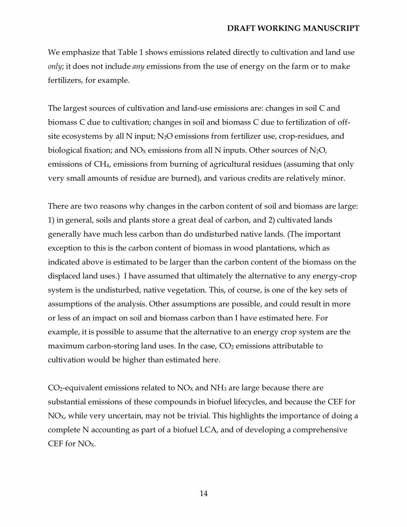
We emphasize that Table 1 shows emissions related directly to cultivation and land use

only; it does not include any emissions from the use of energy on the farm or to make

fertilizers, for example.

The largest sources of cultivation and land-use emissions are: changes in soil C and

biomass C due to cultivation; changes in soil and biomass C due to fertilization of off-

site ecosystems by all N input; N2O emissions from fertilizer use, crop-residues, and

biological fixation; and NOX emissions from all N inputs. Other sources of N2O,

emissions of CH4, emissions from burning of agricultural residues (assuming that only

very small amounts of residue are burned), and various credits are relatively minor.

There are two reasons why changes in the carbon content of soil and biomass are large:

1) in general, soils and plants store a great deal of carbon, and 2) cultivated lands

generally have much less carbon than do undisturbed native lands. (The important

exception to this is the carbon content of biomass in wood plantations, which as

indicated above is estimated to be larger than the carbon content of the biomass on the

displaced land uses.) I have assumed that ultimately the alternative to any energy-crop

system is the undisturbed, native vegetation. This, of course, is one of the key sets of

assumptions of the analysis. Other assumptions are possible, and could result in more

or less of an impact on soil and biomass carbon than I have estimated here. For

example, it is possible to assume that the alternative to an energy crop system are the

maximum carbon-storing land uses. In the case, CO2 emissions attributable to

cultivation would be higher than estimated here.

CO2-equivalent emissions related to NOX and NH3 are large because there are

substantial emissions of these compounds in biofuel lifecycles, and because the CEF for

NOX, while very uncertain, may not be trivial. This highlights the importance of doing a

complete N accounting as part of a biofuel LCA, and of developing a comprehensive

CEF for NOX.


15

CO2-equivalent N2O emissions are large because of the large CEF for N2O and the

careful, comprehensive accounting in the LEM of all sources of N2O. In this respect, the

very large N2O emissions from N inputs to soy farming merit further discussion.

Further analysis (reported in the LEM documentation) indicates that our model

estimates are consistent with the range of measurements reported in the literature. Still,

the large impact of this source N2O on lifecycle CO2-equivalent emissions from soy

farming, and the uncertainty in actual measurements of emissions suggests that we

need more research in this area.

As we will see in the next section, emissions related to cultivation and land use are a

substantial percentage – typically around ±30% -- of total “upstream” emissions from

biofuel lifecycles. Thus, our analysis of emissions related to cultivation and land use

clearly illustrates that these may be significant sources of emissions in biofuel lifecycles,

and hence that it is important to perform a comprehensive accounting of N flows and

the impacts of cultivation in biofuel lifecycles.

Emissions from the entire upstream lifecycle of biofuels. Table 2 shows the contribution

of emissions from different stages to total CO2-equivalent emissions from the entire

lifecycle of biofuels excluding end use (and excluding the vehicle lifecycle). The gasoline

lifecycle is shown for comparison.


16

TABLE 2. BREAKDOWN OF “UPSTREAM” FUELCYCLE CO2-EQUIVALENT EMISSIONS, BY STAGE (U. S. YEAR 2010) Fuel ------> RFG Methanol Ethanol Ethanol SCG Biodiesel CH2

Feedstock ------> oil wood corn grass wood soy wood

Fuel dispensing 2% 3% 1% 1% 22% 0% 64%

Fuel distribution and storage 5% 11% 2% 5% 5% 1% 2%

Fuel production 61% 57% 50% 39% 33% 29% 11%

Feedstock transmission 10% 14% 3% 8% 14% 2% 10%

Feedstock recovery 20% 32% 14% 21% 32% 26% 23%

Land-use changes, cultivation 0% -32% 33% 25% -33% 81% -23%

Fertilizer manufacture 0% 16% 18% 23% 16% 24% 11%

Gas leaks and flares 2% 0% 0% 0% 10% 0% 3%

CO2, H2S removed from NG 0% 0% 0% 0% 0% 0% 0%

Emissions displaced 0% 0% -22% -23% 0% -64% 0%

Total (g-CO2-eq/106 BTU) 20,778 18,960 89,668 34,494 14,309 132,242 25,174

Notes: RFG = reformulated gasoline; SCG = synthetic compressed gas; CH2 = compressed hydrogen.

The largest sources of emissions in the upstream lifecycle of biofuels are land-use

changes and cultivation, fuel production, feedstock recovery, fertilizer manufacture,

and “displaced” emissions, which sometimes are referred to unwisely as “coproduct

credits.” Emissions related to feedstock transmission, fuel distribution, and liquid-fuel

dispending are relatively small, but emissions related to dispensing gaseous fuels can be

substantial, an account of the energy required to compress gaseous fuels.

The large contribution of land-use and cultivation emissions is notable because they are

treated cursorily or not at all in most other biofuel LCAs. (Note that for the wood-

based fuelcycles, land-use changes and cultivation result in “negative” emissions, or net

C sequestration. As indicated in Table 1, this is because the C content of the biomass in

wood plantations is estimated to greatly exceed C content of the biomass on the

displaced land uses.)


17

Table 3 shows much of the same information as Table 2, but also includes end-use

fuelcycle emissions and vehicle-lifecycle emissions, and shows results for biofuel light-

duty vehicles (LDVs), biofuel heavy-duty vehicles (HDVs) and fuel-cell LDVs .

In contrast to many other studies, this analysis finds that corn ethanol does not not

have significantly lower GHG emissions than does gasoline, and that cellulosic ethanol

has only about 50% lower emissions (Table 3 Part A). The main reasons for this

difference are that we estimate relatively high emissions from feedstock and fertilizer

production, from land use and cultivation, and from emissions of non-CO2 GHGs from

vehicles.

Table 3 Part C presents results for biofuel HDVs. This table includes biodiesel from

soybeans, a biofuel not included in Table 3 Part A. Perhaps surprisingly, the LEM

estimates that soy biodiesel has higher lifecycle GHG emissions than does conventional

diesel. This is because of the large (and usually overlooked) N2O emissions from

soyfields, and the large (and again usually overlooked) emissions of carbon due to

changes in land use (Table 2).


18

TABLE 3. TOTAL FUELCYCLE CO2-EQUIVALENT EMISSIONS, BY STAGE (U. S. YEAR 2010)

Part a. Biofuel LDVs

General fuel --> Ethanol Ethanol Methanol Natural gas

Fuel specification --> E90 (corn) E90 (grass) M85 (wood) CNG (wood)

Vehicle operation: fuel 343.8 343.8 331.7 269.5

Fuel dispensing 2.5 2.0 2.4 14.6

Fuel storage and distribution 8.3 8.4 8.8 3.4

Fuel production 198.1 65.0 55.0 22.4

Feedstock transport 14.3 12.8 12.3 9.6

Feedstock and fertilizer production 122.6 66.5 37.7 32.6

Land use changes and cultivation 124.7 36.8 (22.3) (22.2)

CH4 and CO2 gas leaks and flares 0.2 0.2 0.4 7.0

C in end-use fuel from CO2 in air (282.9) (282.9) (232.9) (251.8)

Emissions displaced by coproducts (81.1) (33.3) 0.0 0.0

Sub total (fuelcycle) 450.6 219.3 193.1 85.2

% changes (fuelcycle) -2.4% -52.5% -58.2% -81.6%

Vehicle assembly and transport 19.2 19.2 19.2 20.4

Materials in vehicles 55.9 55.9 56.0 59.2

Road dust, tire wear, brake wear PM 0.2 0.2 0.2 0.2

Lube oil production and use 4.5 4.5 4.5 2.3

Refrigerant (HFC-134a) 9.2 9.2 9.2 9.2

Grand total 539.8 308.5 282.3 176.5

% changes (grand total) -2.0% -44.0% -48.7% -67.9%

Note: percentage changes are relative to conventional gasoline LDVs.


19

Part b. Fuel-cell LDVs

General fuel --> Gas MeOH MeOH EtOH H2 H2 H2 H2

Fuel spec (feedstock) --> RFG (crude)

M100 (NG)

M100 (wood)

E100 (grass)

CH2 (water)

CH2 (NG)

CH2 (wood)

CH2 (coal)

Vehicle operation: fuel 203.8 180.9 180.9 195.5 0.2 2.8 3.3 3.3

Fuel dispensing 1.2 2.0 1.5 1.2 33.0 33.0 33.0 33.0

Fuel storage and distribution 2.8 7.1 5.9 5.3 1.4 0.0 1.0 1.2

Fuel production 36.4 48.6 30.7 39.0 7.7 145.3 5.5 61.8

Feedstock transport 6.3 3.2 7.5 7.8 0.0 7.7 5.2 2.4

Feedstock & fertilizer production 11.9 9.9 25.3 43.9 0.0 6.2 17.7 3.5

Land use changes and cultivation 0.0 0.0 (17.3) 25.3 0.0 0.0 (12.1) 0.1

CH4 and CO2 gas leaks and flares 1.1 8.5 0.0 0.0 1.7 13.6 1.6 10.2

C in end-use fuel from CO2 in air 0.0 0.0 (180.4) (194.8) 0.0 0.0 (3.0) 0.0

Emissions displaced by coproducts 0.0 0.0 0.0 (22.9) 0.0 0.0 0.0 0.0

Sub total (fuelcycle) 263.4 260.4 54.2 100.2 44.0 208.6 52.2 115.6

% changes (fuelcycle) -43.0% -43.6% -88.3% -78.3% -90.5% -54.8% -88.7% -75.0%

Vehicle assembly and transport 18.2 18.3 18.3 18.2 18.0 18.0 18.0 18.0

Materials in vehicles 60.6 61.1 61.1 60.9 62.9 62.9 62.9 62.9 Road dust, tire wear, brake wear PM 0.2 0.2 0.2 0.2 0.2 0.2 0.2 0.2

Lube oil production and use 0.0 0.0 0.0 0.0 0.0 0.0 0.0 0.0

Refrigerant (HFC-134a) 9.2 9.2 9.2 9.2 9.2 9.2 9.2 9.2

Grand total 351.6 349.2 143.0 188.8 134.4 298.9 142.5 205.9

% changes (grand total) -36.2% -36.6% -74.0% -65.7% -75.6% -45.7% -74.1% -62.6%

Note: percentage changes are relative to conventional gasoline LDVs.


20

Part c. Biofuel HDVs

General fuel --> Diesel Biodiesel Ethanol Ethanol Methanol

Fuel specification --> LSD SD100 (soy) E100 (corn) E100 grass M100 (wood)

Vehicle operation: fuel 3,523.3 3,651.4 3,447.1 3,447.1 3,280.6

Vehicle operation: refrigerant 0.0 0.0 0.0 0.0 0.0

Fuel dispensing 14.3 18.0 23.4 17.8 23.1

Fuel storage and distribution 33.5 61.2 79.2 80.2 90.5

Fuel production 267.0 1,821.5 1,968.7 587.5 474.3

Feedstock transport 104.0 116.2 133.6 117.3 115.5

Feedstock and fertilizer production 197.3 3,108.0 1,243.9 662.1 391.6

Land use changes and cultivation 0.0 5,004.7 1,294.6 382.0 (266.7)

CH4 and CO2 gas leaks and flares 17.6 0.0 0.0 0.0 0.0

C in end-use fuel from CO2 in air 0.0 (3,477.3) (2,937.8) (2,937.8) (2,788.3)

Emissions displaced by coproducts 0.0 (3,942.9) (841.7) (346.0) 0.0

Sub total (fuelcycle) 4,157.0 6,361.0 4,411.0 2,010.2 1,320.7

% changes (fuelcycle) -0.0% 53.0% 6.1% -51.7% -68.2%

Vehicle assembly and transport 65.2 65.9 65.5 65.5 65.7

Materials in vehicles 131.1 132.4 131.6 131.6 132.0

Road dust, tire wear, brake wear PM 1.4 1.4 1.4 1.4 1.4

Lube oil production and use 39.2 48.9 39.2 39.2 39.2

Refrigerant (HFC-134a) 8.7 8.7 8.7 8.7 8.7

Grand total 4,402.5 6,618.3 4,657.4 2,256.6 1,567.7

% changes (grand total) -0.1% 50.2% 5.7% -48.8% -64.4%

Note: percentage changes are relative to conventional diesel HDVs.

Table 3 Part B presents results for biofuel and fossil fuel-cell LDVs. Methanol from

wood, hydrogen from wood, and hydrogen from wood offer the largest reductions in

lifecycle GHG emissions compared with conventional gasoline ICEVs: about 90% on a

fuelcycle basis, and 75% on a fuel+vehicle lifecycle basis.


21

Other results: energy use and pollutant emissions

In this section we present LEM estimates of energy use and individual pollutant

emission in selected biofuel lifecycles.

Table 4 shows BTUs of process energy consumed per BTU of net fuel output to end

users, for selected biofuel lifecycles. Although for some fuelcycles there is a decent

correlation between energy use and greenhouse-gas emissions, for biofuels there is not

because on the one hand a substantial part of lifecycle biofuel emissions is essentially

unrelated to energy use (e.g., emissions from land-use changes and cultivation), but on

the other much of the input energy is from the biomass itself which sequesters

approximately as much CO2 as it emits.

TABLE 4. ENERGY INTENSITY OF BIOFUEL LIFECYCLES (BTU-IN /BTU-END USE) (U. S. YEAR 2010)

Fuel --> Methanol SCG Ethanol Ethanol Biodiesel CH2

Feedstock ----> wood wood wood/grass corn soy wood

Fuel dispensing 0.0037 0.0221 0.0028 0.0028 0.0021 0.0855

Fuel distribution, storage 0.0176 0.0411 0.0150 0.0135 0.0100 0.0399

Fuel production 1.8395 1.3945 2.1231 0.5108 0.4057 1.7085

Feedstock transmission 0.0190 0.0147 0.0194 0.0285 0.0185 0.0182

Feedstock recovery 0.0331 0.0255 0.0402 0.0849 0.2032 0.0317

Ag. chemical manufacture 0.0170 0.0131 0.0789 0.1891 0.4138 0.0163


22

The Table 5 series shows emissions of individual pollutants (without the CO2-

equivalency weights) by stage of the upstream lifecycle of biofuels. The largest sources

of CO2 and CH4 emissions are fuel production, land-use changes and cultivation,

fertilizer manufacture and feedstock recovery. The largest source of N2O emissions, of

course, is land-use changes and cultivation. The largest sources of CO emissions are

feedstock recovery (due to tractors), fuel production, and land-use changes and

cultivation. The largest sources of NO2 and NMOC emissions are land-use changes and

cultivation, fuel production, and feedstock recovery. The largest sources of SO2 and PM-

black carbon emissions are feedstock recovery and fuel production.

TABLE 5. INDIVIDUAL POLLUTANT EMISSIONS, BY STAGE (NO CEFS) (U. S. YEAR 2010) (G-POLLUTANT/106-BTU-FUEL) Part A. CO2

Fuel ------> RFG Methanol Ethanol Ethanol SCG Biodiesel CH2


Fuel dispensing 395 543 560 413 3,267 414 17,169

Fuel distribution and storage 967 2,045 1,734 1,777 575 1,279 441

Fuel production 12,491 9,688 44,294 12,252 4,233 38,242 1,921

Feedstock transmission 1,278 2,452 3,295 2,502 1,890 2,342 2,348

Feedstock recovery 4,217 4,556 10,400 5,530 3,511 26,300 4,362

Land-use changes, cultivation 0 (6,939) 14,496 4,943 (5,348) 95,954 (6,644)

Fertilizer manufacture 0 2,656 13,049 6,461 2,047 31,433 2,543

Gas leaks and flares 249 0 0 0 (711) 0 12

CO2, H2S removed from NG 0 0 0 0 0 0 0

Emissions displaced 0 0 (12,852) (8,371) 0 (84,278) 0

Total 19,597 15,001 74,976 25,507 9,465 111,684 22,152


23

Part B. CH4



Fuel dispensing 0.7 1.1 1.1 0.9 6.7 0.8 33.0

Fuel distribution and storage 2.0 5.2 4.3 4.5 13.8 3.2 5.0

Fuel production 47.0 33.8 146.4 54.5 18.2 146.9 6.4

Feedstock transmission 70.1 6.1 7.8 6.3 4.7 5.8 5.9

Feedstock recovery 24.7 12.1 33.6 14.7 9.3 80.4 11.6

Land-use changes, cultivation 0.0 6.9 29.3 23.3 5.3 41.5 6.6

Fertilizer manufacture 0.0 4.8 52.3 23.0 3.7 95.5 4.6

Gas leaks and flares 76.7 0.0 0.0 0.0 63.7 0.0 1.1

CO2, H2S removed from NG 0.0 0.0 0.0 0.0 0.0 0.0 0.0

Emissions displaced 0.0 0.0 (38.6) (17.3) 0.0 0.0 0.0

Total 221.2 70.1 236.3 109.8 125.7 374.1 74.2

Part C. N2O



Fuel dispensing 0.0 0.0 0.0 0.0 0.1 0.0 0.5


Fuel production 0.3 1.3 1.1 1.8 0.9 1.6 1.0








Total 0.6 7.8 84.3 37.5 6.2 274.7 7.7


24

Part D. CO



Fuel dispensing 0.2 0.3 0.2 0.2 1.9 0.2 7.3


Fuel production 13.0 61.5 33.3 70.8 37.5 43.6 56.4








Total 59.2 183.5 341.7 207.4 493.5 1,017.6 178.3

Part E. NO2



Fuel dispensing 0.7 1.1 1.0 0.8 6.7 0.8 31.7


Fuel production 25.4 67.6 100.6 70.7 32.6 109.3 27.3



Land-use changes, cultivation 0.0 45.6 950.8 289.8 35.1 3,789.2 43.6





Total 80.3 178.2 847.1 418.8 134.4 4,186.8 157.0


25

Part F. NMOCs



Fuel dispensing 8.2 2.5 3.4 3.4 0.4 0.0 0.8


Fuel production 2.6 6.4 203.5 6.7 3.0 40.6 44.9








Total 42.1 26.7 239.6 31.3 11.8 115.6 55.5

Part G. SO2



Fuel dispensing 0.8 1.2 1.2 0.9 7.1 0.9 38.1


Fuel production 13.1 19.5 51.8 20.7 10.3 38.6 5.1








Total 52.9 32.5 75.5 17.1 25.7 104.2 52.5


26

Part H. PM (black carbon)



Fuel dispensing 0.0 0.0 0.0 0.0 0.0 0.0 0.1


Fuel production 0.2 1.7 0.9 1.9 0.8 0.6 0.7







Emissions displaced 0.0 0.0 -1.2 -0.1 0.0 0.0 0.0

Total 0.5 3.6 3.5 4.1 2.3 9.2 2.5

Note: see notes to Table 2.

LEM results for different target years, different CEFs, and different countries. The LEM can perform lifecycle analyses for up to 30 different countries, and for any

target year between 1970 and 2050. The Tables 1-5 show results for the U. S. for the

year 2050. In this section, we briefly examine how the results change for different target

years and countries.

Results for different target years. Table 6 shows lifecycle emissions summary results for

biofuels for LDVs and HDVs, for different years from 1970 to 2050.


27

TABLE 6. LIFECYCLE EMISSIONS FOR BIOFUEL VEHICLES, U. S., 1980, 2010, AND 2040 Year 1980 Year 2010 Year 2040

LDVs (versus 26 mpg LDGV) fuelcycle fuel+veh fuelcycle fuel+veh fuelcycle fuel+veh

Baseline: Gasoline (CG) (g/mi) 482.7 596.4 461.8 550.7 439.1 504.1

Ethanol (E90 (corn)) -11% -9% -2% -2% -11% -9%

Ethanol (E90 (grass)) -23% -18% -53% -44% -81% -71%

Methanol (M85 (wood)) -52% -42% -58% -49% -65% -57%

Natural gas (CSNG (wood)) -71% -57% -82% -68% -92% -79%

HDVs (versus 3 mpg HDDV) fuelcycle fuel+veh fuelcycle fuel+veh fuelcycle fuel+veh

Baseline: Diesel (LSD) (g/mi) 5,694.8 5,985.9 4,158.2 4,405.1 3,671.4 3,869.8

Biodiesel (SD100 (soy)) 61% 59% 53% 50% 17% 16%

Ethanol (E100 (corn)) -30% -28% 6% 6% -8% -7%

Ethanol (E100 (grass)) -41% -39% -52% -49% -92% -87%

Methanol (M100 (wood)) -76% -72% -68% -64% -84% -80%


Notes: LDGV = light-duty gasoline vehicle; HDDV = heavy-duty diesel vehicle; mpg = miles per gallon; CG =

conventional gasoline, E90 = 90% ethano/10% gasoline; M85 = 85% methanol/15% gasoline; CSNG = compressed

synthetic natural gas; LSD = low-sulfur diesel; SD100 = 100% soydiesel; fuel+veh = lifecycle of fuels and lifecycle of

vehicles. For baseline LDGV and baseline HDDV, total lifecycle CO2-equivalent emissions are shown; for alternatives,

percentage changes relative to basline are shown.

Two general results are noteworthy. First, the emissions from the baseline gasoline and

diesel vehicles decline over time, even though the baseline vehicle fuel economy is held

constant. This is because in the LEM emissions of non-CO2 criteria pollutants are

projected to decline over time, and because some (but not all) upstream and vehicle

lifecycle processes are assumed to become more energy efficient overtime.

Second, in all cases except one the percentage change for alternatives compared with

the baseline also declines, which implies that lifecycle CO2-equivalent emissions from

alternatives decline faster than do emissions from the baselines. There are several

reasons for this. First, the fuel economy of the alternatives relative to the fixed fuel

economy of the baseline is projected to increase. Second, almost all important processes

in alternative-fuel lifecycles are projected to become more efficient, whereas petroleum


28

refining is not, because any technical efficiency gains in refining are assumed to be

nullified by the declining quality of crude oil input on the one hand and increasingly

stringent product requirements on the other. Third, major sources of emissions unique

to biofuel lifecycles, such as those related to the N cycle, are projected to decline over

time.

The exception mentioned above is corn ethanol, which has relatively low emissions in

1980, then higher emissions in 2010, and then relatively low emissions again in 2040.

Table 7 shows the breakdown of emissions from corn ethanol by target year and stage

of the lifecycle.

TABLE 7. CORN ETHANOL LIFECYCLE EMISSION BY STAGE AND TARGET YEAR (G/MI)

1970 1980 1995 2000 2010 2025 2040

Vehicle operation: fuel 341 338 355 354 344 335 334

Fuel dispensing 0 1 2 3 3 3 2

Fuel storage and distribution 12 10 9 9 8 7 7

Fuel production 131 153 188 197 198 190 181

Feedstock transport 21 18 16 16 14 13 11

Feedstock and fertilizer production 148 142 137 137 123 105 96

Land use changes and cultivation 166 154 139 134 125 113 100

CH4 and CO2 gas leaks and flares 2 2 1 0 0 (0) (1)

C in end-use fuel from CO2 in air (282) (282) (282) (283) (283) (283) (283)

Emissions displaced by coproducts (118) (108) (96) (92) (81) (67) (57)

Sub total (fuelcycle) 421 428 469 475 451 415 392 % changes (fuelcycle) -17% -11% -3% -1% -2% -7% -11%

Vehicle assembly and transport 23 21 21 21 19 17 14

Materials in vehicles 68 63 59 59 56 50 43

Road dust, tirewear, brakewear PM 0 0 0 0 0 0 0

Lube oil production and use 9 7 5 5 5 4 4

Refrigerant (HFC-134a) 30 22 14 12 9 6 4

Grand total 552 542 569 573 540 492 457 % changes (grand total) -14% -9% -2% 0% -2% -6% -9%

In the case of corn ethanol, total fuelcycle emissions actually increase from 1970 to

about 2000, and then begin to decrease. The increase is due mainly to an increase in


29

CO2-equivalent emissions from the fuel-production stage and a decrease in the “credit”

from emissions displaced by co-products. CO2-equivalent fuel-production (and vehicle

tailpipe) emissions increase because of reductions in emissions of NO2 and SO2, which

have negative (i.e., “cooling”) CEFs. The co-product emissions-displacement credit

decreases because the co-products are assumed to displace soy products, and the

lifecycle emissions from the soy products decrease over time.

Results for different countries. Table 8 shows fuel lifecycle emissions summary results

for biofuels for LDVs and HDVs, for six different countries, including the U. S., for the

year 2010. The table shows CO2-equivalent fuelcycle emissions for the gasoline and

diesel vehicles (in grams/mile) and the percentage difference from the baseline for the

alternatives.

TABLE 8. FUELCYCLE EMISSIONS FOR BIOFUEL VEHICLES IN DIFFERENT COUNTRIES (YEAR 2010)

LDVs (versus 26 mpg LDGV) U. S. China India S. Africa Chile Japan

Baseline: Gasoline (CG) (g/mi) 461.8 454.3 373.0 594.8 471.1 457.5

Ethanol (E90 (corn)) -2% 17% 10% 0% -6% 1%

Ethanol (E90 (grass)) -53% -36% -47% -53% -56% -45%

Methanol (M85 (wood)) -58% -50% -53% -59% -65% -61%


HDVs (versus 3 mpg HDDV) U. S. China India S. Africa Chile Japan

Baseline: Diesel (crude oil) (g/mi) 4,158.2 1,713.1 1,767.1 2,600.6 2,695.9 4,920.0

Biodiesel (SD100 (soy)) 53% 183% 183% 78% 38% 54%

Ethanol (E100 (corn)) 6% 16% 12% 2% 4% -8%

Ethanol (E100 (grass)) -52% -44% -55% -61% -56% -53%

Methanol (M100 (wood)) -68% -69% -71% -78% -78% -77%


Table 8 shows that lifecycle emissions from biofuels, both in absolute terms and relative

to emissions from gasoline, can vary from one country to another. Differences are

particularly pronounced for corn ethanol and soy diesel in China or India versus the U.


30

S. (By contrast, there is relatively little difference in percentage changes when wood is

the feedstock.) As indicated in Table 9, the differences between China, India and the U.

S. in the case of soy diesel are due almost entirely to differences in emissions related to

land use and cultivation, which in turn are due to differences in land types used for

crops and in the amount and efficiency of fertilizer use. Some of the difference also is

due to the higher emissions from fertilizer manufacture, which result from the greater

N intensity. This highlights, once again, the importance of assumptions regarding the

types of land uses displaced by biofuel plantations.

TABLE 9. SOY DIESEL UPSTREAM EMISSION BY STAGE AND COUNTRY (G/106 BTU)

U. S. China India S. Africa Chile Japan

Fuel dispensing 386 380 561 461 187 231 Fuel distribution and storage 1,309 1,279 1,426 1,400 1,125 1,306 Fuel production 38,933 39,332 45,694 41,071 32,266 36,105 Feedstock transmission 2,484 2,419 2,516 2,602 2,325 2,710 Feedstock recovery 34,365 34,002 35,247 35,662 32,792 34,112 Land-use changes, cultivation 106,975 213,625 206,766 131,679 100,577 123,944 Fertilizer manufacture 32,068 39,127 42,366 36,324 32,235 32,921 Gas leaks and flares 0 0 0 0 0 0 CO2, H2S removed from NG 0 0 0 0 0 0 Emissions displaced (84,278) (84,278) (84,278) (84,278) (84,278) (84,278)

Total 132,242 245,885 250,298 164,920 117,229 147,049

Differences between using LEM CEFs and IPCC GWPs CO2-equivalency factors (CEFs), which convert gases other than CO2 to the amount of

CO2 with some equivalent effect on climate or the global economy, are an integral part

of the calculation of CO2-equivalent lifecycle emissions. Appendix D of the LEM

documentation details the development of the CEFs used in the LEM (hereinafter

referred to as “LEM CEFs”).

The LEM CEFs differ in a number of important respects from the widely used CEFs –

called “Global Warming Potentials,” or GWPs – adopted by the Intergovernmental


31

Panel on Climate Change (IPCC). The most important difference is that the IPCC has

not formally estimated CEFs (qua GWPs) for CO, NMOCs, NOX, SOX, PM and H2 (apart

from accounting for the effect of CO and C in NMOCs oxidizing to CO2), whereas we

have. Table 10 shows the LEM CEFs and the IPCC 100-year GWPs.

TABLE 10. LEM CEFS USED IN THIS ANALYSIS AND IPCC 100-YEAR GWPS

Pollutant LEM CEFs (yr. 2010) IPCC 100-yr. GWPs

NMOC-C 3.664 3.664

NMOC-03/CH4, SOA 4.8 not estimated

CH4 18.8 23

CO 2.9 1.6

N2O 251 296

NO2 -15.5 not estimated

SO2 -52.4 not estimated

PM (black carbon) 1,410 not estimated

PM (organic matter) -161.8 not estimated

PM (dust) -2.9 not estimated

H2 5.6 not estimated

SF6 126,617 22,200

CFC-12 12,369 8,600

HFC-134a 1,275 1,300

CF4 32,782 5,700

C2F6 69,933 11,900

HF 2000 not estimated

In addition, the IPCC GHG accounting methods ignore temporary carbon

sequestration or emission due to changes in land use, whereas we do not. This of course

matters greatly in the estimation of lifecycle emissions from biofuels.

How important are the differences between the LEM CEFs and the IPCC GWPs? In this

section, we compare results from the LEM using LEM CEFs with results using IPCC

GWPs, for a selected number of biofuel lifecycles.


32

Table 11 presents this comparison for the U. S, for the year 2010. The table shows the

percentage change in the g/mi emissions going from the IPCC g/mi results to the LEM

CEF g/mi results, and two different measures of the percentage change in emissions

relative to gasoline. As one would expect, there are significant differences in using IPCC

GWPs rather than LEM CEFs in those cases where there are significant differences in

emissions of the pollutants for which LEM CEFs differ significantly from IPCC GWPs –

mainly PM, SO2, and NO2 – or else significant emissions associated with changes in land

use (which are counted in the LEM CEF case but not in the IPCC GWP case).

TABLE 11. FUELCYCLE EMISSIONS WITH LEM CEFS AND WITH IPCC 100-YEAR GWPS (U. S., YEAR 2010)

LEM CEFs IPCC GWPs IPCC GWPs vs. LEM CEFs

g/mi % ch. g/mi % ch. ∆ g/mi ∆ rel. ∆ abs.

Baseline LDGV 462 n.a. 492 n.a. -6.1% n.a. n.a.

Baseline HDDV 4,158 n.a. 4,100 n.a. 1.4% n.a. n.a.

ICEV, diesel (low-sulfur) 350 -24% 357 -27% -2% -11% 3%

ICEV, natural gas (CNG) 345 -25% 370 -25% -7% 2% -1%

ICEV, LPG (P95/BU5) 347 -25% 370 -25% -6% 0% -0%

ICEV, ethanol (corn) 451 -2% 479 -3% -6% -7% 0%

ICEV, ethanol (grass) 219 -53% 225 -54% -2% -3% 2%

ICEV, methanol (wood) 193 -58% 234 -52% -17% 11% -6%

ICEV, soy diesel (vs. HDDV) 6,361 53% 4,603 12% 38% 332% 41% Notes: %/ch. is percentage change in g/mi emissions relative to gasoline or diesel baseline; ∆ g/mi is the percentage difference between the IPCC and the LEM-based g/mi estimates; ∆ rel. is the percentage change in the IPCC-based % ch. relative to the LEM-based %ch.; ∆ abs is the difference between IPCC % ch. and LEM % ch.

For a few biofuel lifecycles there can be significant differences between using the LEM

CEFs and the IPCC GWPs. In general, there are two reasons for these differences. First,

biofuel lifecycles can emit substantial amounts of NO2, and this has a significant CEF in

the LEM but is not counted as an IPCC GWP. The importance of differences in the CO2-


33

equivalent effect of NO2 is shown in Table 12, which provides a breakdown of lifecycle

CO2-equivalent emissions by pollutant.

TABLE 12. BREAKDOWN OF LIFECYCLE CO2-EQUIVALENT EMISSIONS BY POLLUTANT, BIOFUEL PATHWAYS (U. S., YEAR 2010)

General fuel --> RFG Ethanol Ethanol Methanol Natural gas Biodiesel

Fuel specification --> crude oil E90 (corn) E90 (grass) M85 (wood) CNG (wood) SD100 (soy)

Net CO2 from vehicles 60% 8% 8% 15% 0% 0%

Lifecycle CO2 93% 82% 44% 44% 22% 124%

CH4 4% 5% 3% 3% 5% 8%

N2O 3% 19% 10% 4% 4% 76%

CO 3% 3% 3% 3% 4% 5%

NMOC 1% 1% 1% 1% 0% 1%

NO2 -4% -13% -8% -5% -4% -74%

SO2 -4% -5% -3% -3% -3% -6%

PM (BC+OM) 2% 4% 4% 4% 3% 17%

PM (dust) -0% -0% -0% -0% -0% -0%

H2 0% 0% 0% 0% 0% 0%

SF6 0% 0% -0% 0% 0% 1%

HFC-134a 2% 2% 2% 2% 2% 0% Notes: Net CO2 from vehicles is equal to tailpipe CO2 less any “credit” for C fixed by biomass used to make biofuel. All

pathways for LDVs except biodiesel, which is for HDVs.

The second reason for any differences in Table 11 is that the IPCC GWP method

effectively ignores carbon emissions related to land use, whereas our method does not

(this is discussed more fully in the next paragraph). I note, however, that in general the

two differences – the counting of the climate impacts of NOX and land use changes in

the LEM CEF case but not the IPCC GWP case – work in opposite directions, because

the CEF for NOX actually is negative. This means that in the LEM, the effect of NOX can

tend to offset the effect of land-use changes. As a result, in some biofuel pathways there

actually little difference between the LEM CEF case and the IPCC GWP case (Table 11). I


34

note, though, that the CEF for NOX is uncertain, and might even be positive, in which

case the NOX effect and the land-use effect would work in the same direction, and there

would be significant differences between the LEM CEF case and the IPCC GWP case for

all biofuel pathways.

Treatment of land-use changes. Our methods for estimating GHG emissions related to

land-use changes are similar to those recommended by the IPCC except for this key

difference: we use a time-varying discount rate with a very long time horizon, whereas

the IPCC apparently assumes a zero discount rate and a 100-year time horizon (IPCC,

1997, 2000, 2003). Our methods and the IPCC methods both assume that any initial

change in land use – say, the clearing of forest to plant crops – eventually is reversed

when the program that gave rise to the initial change (planting crops, in our example) is

abandoned. Following abandonment, the carbon content of the soils and biomass

begins a gradual return to the original values (in our example, those of a forest). If the

discount rate is zero and the carbon content after reversion is the same as the original

carbon content – and if the complete reversion occurs within the time horizon – 100

years in the IPCC recommendations – then the net carbon emission due to the

program is zero. However, if the discount rate is not zero, then the present value of the

future carbon gain following reversion is less than the value of the carbon loss at the

start of the program, resulting in a non-zero net emission due to the program. As a

result, whether one uses the LEM CEFs (which incorporate a non-zero discount rate,

and hence count emissions related to land-use changes) or the IPCC GWPs (which

ignore emissions related to changes in land use) can have a big impact on absolute and

relative emissions in biofuel lifecycles.


35

II. REVIEW OF LIFECYCLE ANALYSES OF BIOFUELS

Overview

Recently, several good reviews of major biofuel lifecycle analyses have been published.

(Fleming et al., 2006; Farrel et al., 2006; Hammerschlag, 2006; Larson, 2005; Wang,

2005a, 2005b; International Energy Agency, 2004). In addition, several other recent

reports provide more general summaries of a large number of biofuels studies

worldwide (e.g., Quirin et al., 2004).

These recent summaries and comparisons of biofuel lifecycle analyses have identified

many of the major areas of uncertainty, disagreement, and incompleteness in the

existing literature. However, all of these areas, and others, have been discussed

qualitatively in Delucchi’s (2004) white paper on conceptual, methodological, and data

issues in lifecycle analysis, much of which is included as Part III of this report.

Moreover, our own analyses as part of the development of the LEM have begun to

address some of the issues raised in the recent literature reviews.

Because on the one hand there already are comprehensive, up-to-date reviews of the

major biofuels lifecycle analyses, and on the other hand we have a good conceptual

framework and have begun to address some of the major problems in existing studies,

we decided that rather than create yet another typical review and comparison of

biofuels studies, we would begin where the current reviews leave off and our own

work has started: with a focus on the major areas of uncertainty, disagreement, and

incompleteness in the existing literature. These areas include:

• treatment of lifecycle analyses within a dynamic economic-equilibrium framework;

• major issues concerning energy use and emission factors; and

• incorporation of the lifecycle of infrastructure and materials.

• representation of changes in land use;

• treatment of market impacts of co-products;


36

• development of CO2 equivalency factors for all compounds;

• detailed representation of the nitrogen cycle and its impacts;

In this part, we present a summary of the findings of the recent published reviews of

major biofuel LCAs, including results from the LEM. Then, in the next part, we examine

the areas of uncertainty, disagreement, and incompleteness listed above, within the

context of a comprehensive conceptual framework for biofuel LCAs.

Summary of reviews of major biofuel LCAs

As mentioned above, a number of excellent reviews of major biofuel LCAs have been

published recently, including Farrel et al. (2006), Hammerschlag (2006), Fleming et al.

(2006), Larson (2005), Wang (2005a, 2005b), the International Energy Agency (2004), and

Quirin et al. (2004). These studies are not themselves original biofuel LCAs, but rather

are reviews of a number of such original LCAs. The original biofuel LCAs considered

by four review papers are shown in Table 13.


37

TABLE 13. ORIGINAL BIOFUEL LCAS INCLUDED IN RECENT REVIEW PAPERS

Review article Original biofuel LCAs reviewed (post-2000 only)

Biofuel pathways in original

Farrel et al. (2006) Patzek (2004) ethanol from corn

Pimentel and Patzek (2005) ethanol from corn, switchgrass, and wood; biodiesel from soy and sunflower

Shapouri and McAloon (2004) ethanol from corn

Graboski (2002) ethanol from corn

Wang (2001) ethanol from corn and cellulosic; biodiesel from soybeans

De Oliveira et al. (2005) ethanol from corn, sugarcane

Hammerschlag (2006) Graboski (2002) ethanol from corn

Shapouri et al. (2002) ethanol from corn


Kim and Dale (2005a) ethanol from corn

Lynd and Wang (2004) ethanol from corn, cellulose

Sheehan et al. (2004) ethanol from corn stover

Fleming et al. (2006) Ahlvik and Brandberg (2001) hydrogen, ethanol, and FTL from lignocellulose

General Motors et al. (2001) ethanol from lignocellulose

General Motors et al. (2002) hydrogen, ethanol, and FTL from lignocellulose; ethanol from corn and/or sugar beet

European Council for Automotive R&D (CONCAWE et al., 2004)

hydrogen, ethanol, or FTL from lignocellulose; ethanol from corn and/or sugar beet

GREET model (Fleming et al. runs of GREET model)

ethanol from lignocellulose; ethanol from corn

GHGenius model (Fleming et al. runs of GHGenius model)

hydrogen and ethanol from lignocellulose; ethanol from corn and/or sugar beet


38

Wang (2005a) Delucchi et al. (2003) ethanol from corn, switchgrass, and wood; biodiesel from soy; methanol from wood; CNG from wood

Delucchi (2001) ethanol from corn, switchgrass, and wood

Graboski (2002) ethanol from corn

Kim and Dale (2005a) ethanol from corn

Kim and Dale (2002) ethanol from corn

Natural Resources Canada (2005) ethanol from corn, wheat, switchgrass, and wood

Patzek et al. (2005) ethanol from corn

Pimentel (2003) ethanol from corn


Shapouri and McAloon (2004) ethanol from corn

Shapouri et al. (2002) ethanol from corn

Wang et al. (2003) ethanol from corn

Note: FTL = Fischer-Tropsch liquids.

Although Table 13 does not include Larson’s (2005) review, I note that it also is an

excellent and comprehensive review.

Table 14 summarizes the lifecycle GHG emissions results presented in the review

papers mentioned above, and compares the results with those from the LEM.

TABLE 14. APPROXIMATE TYPICAL OVERALL RESULTS OF LIFECYCLE GHG-EMISSION ANALYSES OF BIOFUELS

Source Ethanol from corn

Ethanol from cellulose

biodiesel from soy

GREET (see various papers by Wang and GM et al.) GHGenius (see web site), Kim and Dale, De Oliveira, LBST (GM et al. 2002a), CONCAWE et al., Spatari et al. (2005), and others

- 50% to -10% -100% to -40% - 80% to -40%

LEM estimates -30% to + 20% -80% to -40% 0% to +100%


39

The LEM typically estimates higher lifecycle GHG emissions from biofuel pathways

than do other studies. (Studies by Pimentel and Patzek [see P&P, Table 15] also estimate

high non-renewable energy use and hence implicitly high CO2 emissions, but Farrel et

al. [2006] and Hammerschlag [2006] have identified several shortcomings with those

studies.) The main reasons have to do with treatment of the nitrogen cycle, land-use

changes, CO2 equivalency factors, co-products, and market impacts.

In the following sections we first delineate the structure and assumptions of major,

original biofuel LCAs (including the LEM), and then analyze biofuel LCAs within a

general conceptual framework.

Structure, general methods, and assumptions of original LCAs of biofuels

Table 15 shows the structure, general methods, and key assumptions of several original

biofuel LCAs.


TABLE 15. STRUCTURE, GENERAL METHODS, AND KEY ASSUMPTIONS OF ORIGINAL BIOFUEL LCAS. Study set #1.

LEM GREET GM –LBST Europe Kim & Dale (KD) GHGenius

Region Can represent up to 30 countries. Most detail for U. S.

United States. Europe. United States North America

Time frame Any year from 1970 to 2050 (built in projections of energy and material use and emissions).

Near term or long term.

Year 2010. Apparently near term.

Any year from 1970 to 2050 (built in projections of energy and material use and emissions).

Biomass pathways

Ethanol from corn, switchgrass, and wood; biodiesel from soybeans; methanol, SNG and hydrogen from wood.

Ethanol from corn and cellulosic biomass; biodiesel from soybeans.

Ethanol from sugar beet, crop residue, wood; hydrogen, methanol, and SNG from wood; biodiesel from rape seed.

Ethanol from corn grain and corn stover; biodiesel from soybeans.

Ethanol from corn, wood, grass, and wheat; methanol and SNG from wood; biodiesel from soybeans; hydrogen from wood, corn, and wheat.

Fuel lifecycle model

Detailed, original internal model.

Detailed, original internal model.

LBST E2 I-O model and data base.

No model per se; own calculations based on literature review and analysis.

Detailed internal model (built on 2001 version of LEM).

Fuel production

Input-output representation based on review and analysis of literature.

Review and analysis of literature.

Detailed process descriptions based on review and analysis of literature.

Literature review. Input-output representation based on review and analysis of literature (similar to LEM).


41

Study set #1 continued.


Treatment of coproducts

DDGS (corn to ethanol) displaces corn grain and soybeanns; excess electricity (wood to ethanol) displaces grid power; soybyproducts displace glycerin.

DDGS (corn to ethanol) displaces corn and soy; excess electricity (wood to ethanol) displaces grid power.

Sugar beet pulp displaces US soybeans; rape seed byproducts displace glycerin.

System of linear equations for corn ethanol co-product displacement; soy byproducts displace solvents; excess electricity (stover to ethanol) displaces grid power.

DDGS (corn to ethanol) displaces corn and soy; excess electricity (wood to ethanol) displaces grid power; soybyproducts displace glycerin. (Expanded and refined version of LEM treatment.)

Crop production

Detailed analysis of primary USDA and other data on energy and fertilizer inputs.

Detailed review and analysis of USDA and other data sources on energy adn fertililizer inputs.

Review of literature on energy use; review and analysis of N requirements.

Review and analysis of USDA and other sources of data (such as GREET).

Review and analysis of literature and government data.

Fertilizer and pesticide production

Complete lifecycle of fertilizer based on primary survey data (U. S. national average). Pesticide use based on literature review.

Detailed review and analysis of literature.

Review of literature. Own calculations based on literature data.

Based on the LEM.

Land use changes

Comprehensive accounting of changes in land use associated impacts on soil and plant carbon.

USDA analysis of land-use changes combined with 1998 LEM estimates of C sequestration rates.

Discussed but not included (GM et al., 2002b, p. 292).

Not included. (DAYCENT model used to simulate soil-carbon changes on site due to tillage practices.)

Based on 2003 version of LEM, but with different assumptions regarding displaced land uses.

Nitrogen cycle Complete accounting of N flows, fates, and impacts.

Not included. (Review and analysis of some literature pertinent to N2O emissions.)

Partial treatment of N requirements, N sources, and associated N2O emissions.

Not included per se, but DAYCENT model used to simulate N2O and soil carbon.

Partial accounting of N-related emissions, based on improved version of 2003 LEM.


42



GHGs and CO2-equivalency factors

LEM CEFs (Table 10). (But IPCC GWPs can be specified.)

IPCC GWPs for CO2, CH4, and N2O; other pollutants represented as non-GHGs.

IPCC GWPs for CO2, CH4, and N2O.


ca. 2000 version of LEM CEFs, or 100-year IPCC GWPs.

Vehicle energy-use modeling, including drive cycle

Assumed fuel economy for baseline vehicles, simple model of energy use of alternatives relative to baseline. U. S. combined city/highway driving.

Assumed fuel economy values for baseline vehicles, % change in fuel use for alternatives relative to baseline.

GM simulator, European Drive Cycle (urban and extra-urban driving).

Assumed fuel economy values.

Based on the LEM.

Vehicle and materials lifecycle

Comprehensive, detailed internal model based on detailed literature review and analysis

Not included. Not included. Not included. Based on LEM treatment.

Infrastructure Crude representation. Not included. Not included. Not included. Not included.

Price effects A few simple quasi-elasticities.

Not included. Not included. Not included. Not included?

Documentation Delucchi (2003). Wang (1999, 2001, 2005a, 2005b); Wang et al. (1999, 2003).

GM et al. (2002a, 2002b, 2002c).

Kim and Dale (2002, 2004, 2005a, 2005b).

(S&T)2 Consulting (2005a).


43

Study set #2.

Graboski USDA Pimentel & Patzek (PP) STELLA U. Toronto

Region United States. United States. United States United States and Brazil.

Ontario, Canada

Time frame 2000 and 2012 About year 2000. Roughly 2000. About year 2000. Near term (2010) and mid term (2020).

Biomass pathways

Ethanol from corn. Ethanol from corn. Ethanol from corn, switchgrass, and wood; biodiesel from soy

Ethanol from corn (U. S.); ethanol from sugarcane (Brazil).

Ethanol from switchgrass and corn stover.

Fuel lifecycle model

Own detailed analysis of lifecycle stages.

Some stages based on GREET model.

No model per se; own calculations based on literature review and analysis.

STELLA systems modeling framework used with data assumptions based on literature reviews.

Developed own life-cycle modules based on literature review and analysis.

Fuel production Detailed review and analysis of literature.

Assumptions based on an industry survey.

Literature review. Literature review. Literature review.

Treatment of coproducts

Original, detailed analysis of products displaced by co-products of dry mills and wet mills.

Assumes soymeal is replacement product.

Co-products assumed either to have no market value, or else small value as soy protein substitute.

Not included. (See Farrel et al. [2006] supporting online material p. 10.)

Excess electricity sold to regoinal power grid.

Crop production Detailed analysis of primary USDA and other data on energy and fertilizer inputs.

Detailed analysis of primary USDA and other data on energy and fertilizer inputs.

Analysis and review of USDA and other data.

Literature review (e.g., Shapouri et al. 2002).

Literature review.

Fertilizer and pesticide production

Original analysis of stages of fertilizer lifecycle; review of data on pesticide production.

Fertilizer estimates from industry expert; pesticide data from GREET.

Literature review of energy for fertilizer, pesticide, and seed production.

Literature review (e.g., Shapouri et al. 2002).

Literature review.


44


Graboski USDA Pimentel & Patzek (PP) STELLA U. Toronto

Land use changes

Not included. Not included. Not included. Not included. (However, they do assume that tillage practices result in soil C sequestration.)

Discussed but assumed no impact.

Nitrogen cycle Not included. Not included. Not included. Not included. Not included.

GHGs and CO2-equivalency factors

Not included. (Graboski analyzes lifecycle fossil energy use only.)

Not included. (USDA analyzes lifecycle energy use only.)

Not included. (P&P analyze energy use only.)

Not included. (Analysis of CO2 emissions only.)


Vehicle energy-use modeling, including drive cycle

Not included. (Graboski analyzes lifecycle fossil energy use only.)


Not included. (P&P analyze energy use only.)

2001 Ford Taurus 26 mpg Chevy Impala combined city/highway driving; 3% efficiency advantage on ethanol.

Vehicle and materials lifecycle

Analysis of energy embodied in farm equipment and ethanol plants.


Includes an estimate of embodied in farm equipment.

Not included. Not included.

Infrastructure Not included. Not included. Not included. Not included. Not included.

Price effects Not included. Not included. Not included. Not included. Not included.

Documentation Graboski (2002) Shapouri et al. (1995, 2002); Shapouri and McAloon (2004).

Pimentel (2003); Pimentel and Patzek (2005); Patzek (2004); Patzek et al. (2005)

De Oliveira et al. (2005).

Spatari et al. (2005)


45

In the next part we examine the important aspects of biofuel LCAs within the context

of a comprehensive conceptual framework for doing LCAs of biofuel pathways.

III. A COMPREHENSIVE CONCEPTUAL FRAMEWORK FOR DOING LCAS OF BIOFUELS.

Conceptual framework for biofuel LCA: current practice

Brief historical background. Current LCAs of transportation and climate change can be

traced back to “net energy” analyses done in the late 1970s and early 1980s in response

to the energy crises of the 1970s, which had motivated a search for alternatives to

petroleum. These were relatively straightforward, generic, partial “engineering”

analyses of the amount of energy required to produce and distribute energy feedstocks

and finished fuels. Their objective was to compare alternatives to conventional gasoline

and diesel fuel according to total fuelcycle use of energy, fossil fuels, or petroleum.

In the late 1980s, analysts, policy makers, and the public began to worry that burning

coal, oil, and gas would affect global climate. Interest in alternative transportation fuels,

which had subsided on account of low oil prices in the mid 1980s, was renewed.

Motivated now by global (and local) environmental concerns, engineers again analyzed

alternative transportation fuelcycles. Unsurprisingly, they adopted the methods of their

“net-energy” engineering predecessors, except that they took the additional step of

estimating net CO2 emissions, based on the carbon content of fuels. By the early 1990s

analysts had added other GHGs (methane and nitrous oxide) weighted by their “Global

Warming Potential” (GWP) to come up with fuelcycle CO2-equivalent emissions for

alternative transportation fuels. Today, most LCAs of transportation and global climate

are not appreciably different in general method from the analyses done in the early

1990s. And although different analysts have made different assumptions and used

slightly different specific estimation methods, and as a result have come up with


46

different answers, few have questioned the validity of the general method that has

been handed down to them.

The problem with the pedigree. LCAs of transportation and climate in principle are

much broader than the net-energy analyses from which they were derived, and hence

have all of the shortcomings of net-energy analyses plus many more. If the original net-

energy analyses of the 1970s and 80s could be criticized for failing to include economic

variables, on the grounds that any alternative-energy policy would affect prices and

hence uses of all major sources of energy, then the lifecycle GHG analyses they

spawned can be criticized on the same grounds, but even more severely, because in the

case of lifecycle GHG analyses we care about any economic effect anywhere in the

world, whereas in the case of net-energy analysis we cared about economic effects only

in the country of interest. Beyond this, lifecycle GHG analysis encompasses additional

areas of data (such as emission factors) and additional systems (such as the global

climate) which introduce considerable additional uncertainty.

The upshot is that LCAs of transportation and climate are not built on a carefully

derived, broad, theoretically solid foundation, but rather are an ad-hoc extension of a

method -- net-energy analysis -- that was itself too incomplete and theoretically

ungrounded to be valid on its own terms and which could not reasonably be extended

to the considerably broader and more complex problem of global climate change. And

although recent LCAs of transportation and climate have been been made to be

consistent with LCA “guidelines” established by the International Organization for

Standardization (ISO; see the ISO web site, www.iso.ch/iso/en/iso9000-

14000/iso14000/iso14000index.html), the ISO guidelines have only recently properly

addressed some of the issues discussed here, and have not yet developed a proper

policy/economic conceptual framework. (See the Main Report of the LEM

documentation for further discussion.)


47

Comparison of current practice with an ideal model

Indeed, when we begin to examine the development and application of lifecycle models

for transportation we find right away that often it is not even clear what precise

questions the models are supposed to answer. This turns out to be a serious flaw,

because if we don’t know what question a model is meant to answer, we cannot

comprehend the answers (outputs) the model provides. In the case of LCAs of

transportation and global climate, we are forced often to infer a question from the

nature of the outputs and the methods used. What we find, generally, is an unrealistic

and irrelevant research question and a limited modeling method.

The strengths of weaknesses of current LCAs applied in transportation can be seen best

by comparing current practice with an ideal model. An ideal model, of course, would

replicate reality. In this major section, I first outline an ideal LCA model of reality, and

then compare actual conventional LCA with this ideal.

Figure 3 shows a conceptual flow chart of an ideal model, one which replicates reality.

The ideal, shown on the left side of Figure 3, comprises several components, in boxes,

with arrows showing relationships between components. Across from each

component, on the right side, is a yellow box that discusses whether and how the

component is treated in conventional LCA. I begin by discussing the ideal model.


48

Figure 3. Ideal versus conventional LCA


49

An ideal model of LCA of transportation and climate change

In principle, LCAs of transportation and climate change are meant to help us

understand the impact on global climate of some proposed transportation action. Let us

call the proposed action to be evaluated a “policy,” and refer generally to the impacts of

the policy on “environmental systems.” Hence, in Figure 3, the model starts with the

specification of a policy, and ends with the impacts on environmental systems. In

between are a series of steps that constitute the conceptual components of our model of

reality.

In reviewing these components, it is easiest to work backwards from the output of

interest, the impact on environmental systems. The state of an environmental system –

the ultimate output of interest -- is determined by the magnitude and quantity of

emissions and by other environmental variables. Hence, in Figure 3, an “emissions”

component is shown affecting the “environmental systems” output component.

Emissions, in turn, are related to the production and consumption of energy and

materials and the use of land (PCEM); hence, Figure 3 shows an arrow from the PCEM

box to the emissions box. But emissions also may be affected directly by policy

measures; this is indicated by the arrow directly from the policy box to the emissions

box.

Thus far the main aspects of our model of reality is that changes in PCEM result in

changes in emissions which result in changes in environmental systems. This much

generally appears in conventional LCA. But the next and critical question is: what

affects changes in PCEM? Here the ideal model has an important component that as we

shall see is missing from conventional LCAs of transportation. Changes in PCEM can be

related directly to policy, which is what most conventional LCAs assume – but usually

only implicitly – and which is shown by the arrow from the policy box to the PCEM box.

But changes in PCEM also are related to changes in prices of major goods and services

throughout the global economy. Prices, in turn, are affected directly by policies, but also


50

by – and here is the nub – indirectly by changes in PCEM. There is thus a circular

feedback between changes in PCEM, changes in prices, and further changes in PCEM.

Our conclusion, then, is that economic systems, whose states are determined partly by

prices, are an inextricable part of the real world. As a result, prices are a necessary part

of an ideal model of the impact of policy on climate change. Unfortunately,

conventional LCAs of transportation and climate change do not consider prices or other

aspects of economic systems. This omission introduces an error of unknown but

potentially large magnitude, and thereby may render the results of conventional LCAs

virtually meaningless.

Comparing conventional LCAs of transportation and climate change with the ideal

model: policy

Conventional LCAs of transportation and climate change typically do not analyze a

specific policy. Indeed, conventional LCAs typically do not even posit a specific question

for analysis. The implicit questions of conventional LCA must be inferred from the

conclusory statements and the methods of analysis. In transportation, the conclusory

statements of lifecycle analysis typically are of the sort: “the use of fuel F in light-duty

vehicles has X% more [or less] emissions of CO2-equivalent GHG emissions per mile

than does the use of gasoline in light-duty vehicles”. The method of analysis usually is a

limited input-output representation of energy use and emissions for a relatively small

number of activities linked together to make a lifecycle, with no parameters for policies

or the function of markets. Recalling that CO2-equivalent emissions (which typically are

part of the conclusory statements, as mentioned above) are equal to emissions of CO2

plus equivalency-weighted emissions of non-CO2 gases, where the equivalency

weighting usually is done with respect to temperature change over a 100-year time

period, we then can infer that the question being addressed by most LCAs of GHG

emissions in transportation is something like:


51

“What would happen to climate forcing over the next 100 years if we

simply replaced the set of activities that we have defined to be the

‘gasoline lifecycle’ with the set of activities that we have defined to be the

‘fuel F lifecycle,’ with no other changes occurring in the world”?

The problem here is that this question is irrelevant, because no action that anyone can take

in the real world will have the net effect of just replacing the narrowly defined set of ‘gasoline

activities with the narrowly defined set of ‘fuel-F activities’. Any action that involves fuel F –

any action – will have complex effects on production and consumption activities

throughout the world, via global political and economic linkages. These effects will

occur, and a priori cannot be dismissed as insignificant. To omit them, therefore, is to

introduce into the analysis an error of unknown sign and magnitude.

To recap, in the real world one evaluates specific policies, but conventional LCAs do not

evaluate specific policies, they evaluate implicit, unrealistic questions. As a consequence,

it is difficult if not impossible to relate the results of conventional LCAs to any actual

policy actions we might be considering.

Now, one cannot conceive of any potential use of the results of an LCA apart from the

evaluation of policy. And the details of the specification of the policy are important,

because different policies will have different effects on climate. For example,

considering the case of ethanol from corn, a policy to increase (or eliminate) the

ethanol subsidy will have a different impact on climate than will a policy to mandate

ethanol vehicles, mainly because different policies affect people, prices, and choices

differently. One thus cannot make heads or tails of an analysis that not only is unrelated

to any particular policy, but, what’s worse, does not even have any important policy

relevant variables, such as price, supply, or other market parameters. In order to

analyze the impacts of a particular policy, or indeed of any conceivable policy, one

must, include all of the variables affected directly by policy. Many of these are economic

variables, which are conspicuously absent from conventional transportation LCAs.


52

A related deficiency of conventional LCA is the failure to specify clearly the

counterfactual, or alternative world, with which a specific policy (say, a specific policy

regarding ethanol) is being compared. It is conceptually impossible to evaluate a fuel

such as ethanol “by itself;” rather we must estimate the difference between doing one

thing rather than another. These differences between alternative worlds are a function

of the initial conditions in each world, the initial perturbations (or changes), and

dynamic economic, political, social, and physical forces. Yet no transportation fuelcycle

study, old or new, has any sort of serviceably modeled counterfactual, or alternative

world -- most likely because such a model requires something like general economic

equilibrium analysis, at the least, and fuelcycle analysts are not familiar with general

equilibrium models.


model: production and consumption of energy and materials, and use of land

(PCEM).

Although virtually all LCAs of transportation and climate have focused intensively on

the energy and to a much lesser extent the materials part of PCEM, and data and

methods of analysis in this area have improved over the past 15 years, there remain

serious omissions and oversimplifications, which by themselves undermine any claims

of definitive knowledge of the effects of transportation policies on climate.

Energy-use data. There are many sources of primary, basic data on the energy intensity

of various feedstock production and transport processes (e.g., oil recovery, coal mining,

natural gas transport, and petroleum shipments) yet no analysis makes use of all of

them, and many analyses make use of few or none of them. On the basis of results

from my Lifecycle Emissions Model (LEM), and the work of others, I surmise that the

difference between using primary data in an appropriately detailed input/output flow

model, and using literature-review estimates in a more aggregated approach, can

amount to a percent or two of simple, first-order, fuelcycle GHG emissions.


53

More uncertain, and more important, are estimates of the energy intensity of fuel

production (e.g., petroleum refining, ethanol production) and the energy efficiency of

motor vehicles. Most analysts acknowledge the latter, and even check the sensitivity of

their results to assumptions regarding the relative efficiency of motor vehicles. Many

analysts, too, are aware of the importance of assumptions regarding the energy

intensity of, say, corn-to-ethanol production. But even though there are plenty of

analyses and models of, for example, refinery input and output and refinery energy

usage, under different economic scenarios, no recent transportation LCA, as far as I

know, uses such models, or even the results of the such models run specifically for

fuelcycle policy evaluation. This weakness may again have a nontrivial impact on the

results. For example, my analysis suggests that uncertainty as regards refinery energy

production is at least three absolute percentage points in the fuelcycle analysis.

Generally, the LEM uses national-average input-output data for energy use and

emissions. These data typically are estimated on the basis of a detailed review of

primary survey data or of the relevant technical literature. The data are specified for a

base year, and then projected into the future, generally assuming that the use of energy

materials becomes more efficient and that emission factors decrease. Thus, to some

extent, the LEM avoids the problem of relying on out-dated data sources.

Most estimates of energy use and emission factors in the LEM are broadly similar to

those in other comprehensive LCA models, such as GREET. In any event, whatever

differences remain among LCA modelers concerning the appropriate assumptions for

major energy-using processes, such as ethanol production from corn, are not

completely resolvable without further analysis of policy and economic factors. This is

because decisions such as which fuels to use and how much technological efficiency and

emission control to invest in depend on anticipated prices of fuel and capital,

government policies, world economic conditions, and other factors. Without an explicit

analysis or at least discussion of these factors, it can be difficult to make a case for one

set of assumptions over another.


54

Materials and infrastructure. More seriously, many recent studies have ignored energy

and materials associated with building and maintaining fuel production and distribution

infrastructure, transportation equipment, farm equipment, and so on, even though

some analyses indicate that such energy and materials usage might be a non-trivial

fraction of total fuelcycle energy and material usage. For example, my own recent

analysis suggests that the simple, first-order GHG emissions associated with building

and servicing pipelines, ships, trucks, and tractors -- but not fuel-production facilities --

might be about 3% of the total, simple, first-order GHG emissions in the corn/ethanol

fuelcycle. Whether or not these are included can make a difference of two to three

absolute percentage points in the comparison of ethanol with gasoline. In addition, a

few studies indicate that emissions associated with the fuel-production facilities might

be of the same order of magnitude, although there is much uncertainty. Thus, all told,

emissions associated with construction and maintenance of facilities might be on the

order of 5% of fuelcycle GHG emissions, and shift the standing of ethanol, for example,

relative to gasoline, by as much as five percentage points (although this appears to be a

maximum, and 3% might be more likely).

The LEM contains a detailed, original, comprehensive representation of the lifecycle of

materials used in light- and heavy-duty vehicles, but relatively simple representations

of the lifecycle of materials, infrastructure, and repair for things like tractors and

ethanol production facilities. Pimentel and Patzek (2005) estimate the energy embodied

in farm machinery, but the estimates are not well documented. Graboski (2002)

provides a much lower estimate of embodied energy, but based partly on farm

expenditure data. LEM estimates appear to be between these two, but closer to

Pimentel and Patzek’s. This is an area for further research.

Land use changes. Finally, but of potentially great quantitative significance,

conventional transportation LC models ignore (or treat too simply) changes in land use

related to the establishment of biomass grown to make biofuels. The replacement of

native vegetation with biofuel feedstocks and the subsequent cultivation of the biomass

can significantly change the amount of carbon stored in biomass and soils, and thereby


55

significantly change the amount of CO2 removed from or emitted to the atmosphere

compared with the no-policy alternative. An ideal representation of land-use changes

would involve an integrated model of land-use characteristics, land productivity, and

commodity prices, constraints on use of land, and other factors. To my knowledge no

transportation LCA embodies such a model. The LEM’s relatively simple but

conceptually comprehensive treatment of the impact of land-use changes suggests that

a proper treatment of land-use changes could change CO2-equivalent emissions from

transportation lifecycles by ten or more percentage points in some cases (see for example

Tables 1 and 2 here). It thus becomes of paramount importance to conduct biofuel

LCAs within the context of a global economic model of land use and production and

consumption of crops, wood products, and substitutes.

Now, some analysts have suggested that in some cases the production of a biofuel

feedstock, such as corn, will not bring new land into production and hence will not

cause any change in land uses because the incremental production of the biocrop will be

“supplied” by increases in crop yield (Graboski, 2002, p. 72; (S&T)2 Consulting, 2005a, p.

286) As demonstrated next, this argument depends logically on an implausible

assumption.

In order for there to be no expansion of total land in corn production as a result of

incremental corn production, the argument must be that the increase in demand for

corn spurs increases in per-acre corn yields that would not otherwise occur. If, to the

contrary, the increases in corn yield would have occurred anyway, it is easy to see that

incremental corn production must require “new” land relative to the no-incremental

production baseline. If corn yield is independent of corn output, then in the no-

incremental-production baseline, the amount of land devoted to corn production will

decrease by exactly the rate of increase in yield. With respect to this baseline, any

incremental corn production must be on new or additional land; it cannot be on any of

the old land because that land already is yielding at the assumed (increased) rate. Now,

it may well be that the new land brought into production for the incremental corn will

about balance the amount of old land taken out of production due to the increase in


56

yield, but it would be an unambiguous error to assume that because the total amount

of land in production remained roughly the same, the incremental corn production did

not require incremental land. The correct comparison is with the no-incremental-corn

baseline in which the amount of land in production decreases, and with respect to which

a constant amount of land in production represents an increase in total land in

production.

The logical kernel of this demonstration can be put as follows: if corn yield does not

depend on corn output, then any incremental corn production must always occur on

new land because all other land already is yielding at the assumed, output-independent

rate.


model: prices

All energy and environmental policies affect prices. Changes in prices affect

consumption, and hence output. Changes in consumption and output change

emissions. Price effects are ubiquitous.

Research done by the U. S. Department of Energy (DOE) and Oak Ridge National

Laboratory indicate which kinds of price effects are likely to be important. First and

foremost, perhaps, are those that involve the price of oil. The substitution of a non-

petroleum fuel for gasoline probably will reduce the price of crude oil. A reduction in

the world price of oil will stimulate increased consumption of petroleum products, for

all end uses, worldwide. Analyses by DOE have shown that the additional worldwide oil

consumption induced by the lower prices is quite large compared to the initial

substitution in the U. S. transportation sector.

Whatever the exact magnitude of these price effects, they are potentially important

enough that they ought to be taken seriously in an evaluation of the impact of

transportation policies on climate. There is no way to escape this conclusion. We cannot


57

dismiss the effects because they occur outside of the U. S., or outside of the

transportation sector, because in an analysis of global warming, we care about all

emissions, everywhere. We cannot dismiss price effects on the grounds that a policy

will not really affect price, because in principle even the smallest change has a nonzero-

probability of leading to a nonzero affect on price. (In any event, if the price effects

really are so small, then the policy must be so unimportant or ineffective as to have no

affect on climate worth worrying about anyway.) And we certainly cannot argue that

all such price effects are likely to be substantially “similar” for all policies, and hence of

no importance in a comparison of alternatives, because this clearly is not the case: policies

related to LPG, which can be made from crude oil, may have an effect different from

policies related to natural gas, which is a substitute for oil, and different again from

policies related to new fuels derived from biomass, which has little to do with oil.

The economic modelers will be quick to remind us that the web is even more complex.

For example, a large price subsidy, such as is enjoyed by corn ethanol, ultimately causes

a deadweight loss of social welfare, on account of output being suppressed below

optimal levels due to the inefficient use of [tax] resources. This loss of output probably

is associated ultimately with lower greenhouse gas (GHG) emissions. Thus, in this case,

a subsidy policy may have countervailing effects: on the one hand, there will be an

increase in GHG emissions caused by increased use of petroleum due to the lower price

of oil due to the substitution of ethanol, but on the other, there will be a decrease in

GHG emissions due to the reduction in output caused by the economic deadweight loss

from the subsidy. By contrast, an R & D policy that succeeds in bringing to market a

new, low-cost fuel, will, on account of the more efficient use of energy resources,

unambiguously improve social welfare. (This is another argument in favor of

stimulating the development of low-cost biofuels from cellulosic materials.)

It is easy to go on. For example, economists have pointed out that price effects might

eliminate and even reverse the environmental benefits of EVs as estimated in simple

fuelcycle analyses: if EVs are mandated, but are really quite costly, the resultant increase


58

in the cost of vehicles will cause car buyers to delay purchase of new, clean, efficient

vehicles -- to the possible detriment of the local and global environment.

As a final example, changes in prices are an important determinant of equilibrium uses

of different types of land. The extent to which a new biofuel program displaces native

vegetation, existing agricultural production, unproductive set-aside land, or something

else, matters a great deal in analyses of lifecycle CO2-equivalent emissions, because of

the different carbon-storage characteristics of these ecosystems. In the real world, this

displacement ultimately is determined strongly by prices of land and commodities

derived from land.

Prices in the context of “joint production.” Nearly as important are price effects in cases

of joint production. It is well known that corn-ethanol plants, for example, produce

goods other than ethanol. A policy promoting ethanol therefore is likely to result in

more output of these other goods, as well as more production of ethanol. What is the

impact on climate of the production of the other goods? The only way to answer this

question is to model the market for the other goods to see, in the final equilibrium,

what changes in consumption and production occur in the world with the ethanol

policy. If the production of the other goods is large compared with the production of

ethanol, then we reasonably may expect that the effect on climate of the production of

the other goods is not trivial compared to the “first order” effect of using or making

ethanol.

Note that what is required is a general-equilibrium model of the markets affected by

co-products, not an analysis that assumes that, say, the co-products of ethanol

production simply displace alternative products (such as soy meal). Fundamentally, this

is because we reasonably may expect that the introduction of low-cost co-products to

world markets will shift supply curves downward and induce additional consumption

as well as simply displace alternative sources. To the extent that co-products induce

additional consumption rather than displace alternatives, an analysis that assumes 100%

displacement will overestimate the emissions “credit” impact of co-products.


59

No transportation LCA done to date has used a full global equilibrium model to

determine the impact of coproducts on world markets. Although the best recent biofuel

LCAs do at least adopt the correct “displacement” or “system expansion” approach to

estimating the consequences of joint production (Graboski, 2002; Kim and Dale, 2002),

they do not consider the impact of co-products on prices, and hence overestimate the

“displacement credit.” (The LEM uses simple quasi-elasticities to account for the impact

of price changes on co-product markets.)

The same issue of joint production arises in petroleum refineries. But even though these

sorts of effects are well known and widely studied, no engineering fuelcycle analyst has

done, or incorporated, an appropriate economic analysis of these effects, in any

fuelcycle. Many analyses have used so-called “apportioning” schemes, which bear no

real formal relation to the general equilibrium analysis of alternative policies.

Minor effects of prices. Finally, there are a practically infinite number of what are likely

to be relatively minor effects of price changes. For example, different fuelcycles use

different amounts of steel, and hence have different effects on the price and thereby the

use of steel in other sectors. The same can be said of any material, or of any process

fuel, such as coal used to generate electricity used anywhere in a fuelcycle. It might be

reasonable to presume that in these cases the associated differences in emissions of

GHGs are a second-order effect on a second-order process (e.g., that the price effect of

using steel use is no more than 10% of the “first-order” or direct effect of using steel,

which itself probably is less than 10% of fuelcycle emissions), and hence relatively small.

On the other hand, we might be surprised, and sometimes many individually quite

small effects add up (rather than cancel each other). For these reasons, it would be wise

for fuelcycle analysts to investigate a few classes of these apparently minor price effects.

(It is possible that some input-output [I/O]energy analysts have done this already,

although most if not at all I/O studies used in LCA assume that prices are fixed.)


60


model: emissions and the climate environmental systems

The ultimate objective of LCAs of GHG emissions in transportation is to determine the

effect of a particular policy on global climate. This requires a number of steps beyond

the macro-economic modeling of commodity production and consumption discussed

above: identification of gases that are emitted from fuelcycles and can affect climate

directly or indirectly; identification of sources of emissions of the identified direct and

indirect GHGs; estimation of emission factors for the identified sources; modeling the

effect of “indirect” GHGs on “direct” GHGs; and representation of the effect of direct

GHGs on climate. None of these steps are as well characterized as one might like, and

as a result one might reasonably have little confidence in the soundness of the overall

representation of the climatic effect of a particular policy.

i). Identification of emitted GHGs. The more researchers study climate, the more they

learn about the gases that affect climate. As a result, the list of identified GHGs has

grown considerably since early fuelcycle analyses, and can be expected to continue to

grow.

The authors of the early studies of net fuelcycle CO2 emissions were well aware that

other gases, emitted at various stages in fuelcycles, affect climate. Shortly after the early

fuelcycle CO2 fuelcycle studies were done, other fuelcycle analysts began to include

other GHGs, first methane (CH4), then nitrous oxide (N2O). These three are referred to

as “direct” GHGs, because they affect climate directly, as themselves, rather than

indirectly via an effect on other gases. Ozone (O3) also affects climate directly, but is not

emitted as such from fuelcycles; rather, its concentration is influenced by other gases

that are emitted from fuelcycles: nitrogen oxides (NOx), carbon monoxide (CO),

nonmethane organic compounds (NMOCs), hydrogen (H2), and others. By 1990 NOx,

CO, and NMOCs had been identified as “indirect” GHGs because of their effects on

ozone. In 1993, I included them in my first LCA model (the forerunner of the LEM),

weighting them by the IPCC’s “global warming potential” (GWP) factors.


61

More recently, aerosols have been identified as direct and indirect GHGs, and work is

proceeding to identify which kinds or components of aerosols affect climate most. The

most recent research indicates that sulfate aerosols tend to cause global cooling, but that

the black-carbon (BC) component of aerosols has a very strong global warming effect.

[The latest version of my Lifecycle Emissions Model (LEM) includes BC and sulfate from

particulate matter (PM). See Table 10 here.] The list of GHGs undoubtedly will continue

to grow as researchers identify more GHGs, direct and indirect.

ii) Identification of sources of GHGs. Not surprisingly, the more we look for sources of

GHGs, the more we find. Sometimes the newly identified or quantified sources are

surprisingly significant. For example, in the case of the soy/biodiesel lifecycle, emissions

of N2O from nitrogen fixation by soybeans may be enormous – on a par with CO2

emissions from fuel combustion. In fact, including these emissions in an LCA of

biodiesel may result in biodiesel emitting considerably more CO2–equivalent fuelcycle

emissions than petroleum diesel, rather than considerably less as is estimated in

conventional LCAs. Although this source has been identified and even quantified in

IPCC emission-inventory guidelines for years, it has not been included in any biodiesel

LCAs performed to date (other than my own).

iii) Estimation of emission factors. In many cases, data on GHG emissions are lacking or

of poor quality. For example, even if one identifies N2O emissions from nitrogen

fixation by soybeans, one still is faced with considerable uncertainty regarding the

appropriate emission factor for this source.

Because CH4 emissions typically are multiplied by a CEF of on the order of 10 to 30, and

N2O emissions by a factor of 250 to 350, a doubling or having of assumed emissions of

these gases can have a large impact on the calculated CO2-equivalent total.

Unfortunately, in many cases there are so few real emissions data that we are happy if

we have reason to believe that we know emissions to within a factor of two. For

example, nitrous oxide emissions from vehicles might contribute as little as 3% or as


62

much as 10% of simple, first-order fuelcycle emissions. (Only a year or so ago, this

range might have been about 2% to 15% -- so we do make progress!) Moreover,

virtually all analysts assume that all vehicles emit the same amount of N2O, even

though in many cases this assumption probably will prove to be appreciably in error.

Another often poorly characterized source of emissions is changes in carbon

sequestration in biomass and soils as a result of changes in land use related to the

establishment of biomass used as a feedstock for biofuels. Generic data on the carbon

contents of soils and plants are available, but there can be much variation about these

generic means from site to site. The uncertainty inherent in carbon-storage factors

related to land use can change lifecycle CO2-equivalent emissions by several percentage

points.

Finally, there has been less research into emission factors for newly identified (but

potentially important) GHGs, such as black carbon (BC). First-cut comprehensive

emission-factor databases and emissions inventories for BC have been published only

recently. In many cases, the uncertainty in BC emission-factors is 50% or more. Given

the possibly quite large CO2-equivalency factor for BC (on a mass basis, it may be well

over 1000 – Table 10), this degree of uncertainty in emission-factor estimates translates

directly into a large uncertainty in the effect of BC emissions on climate.

iv) The effects of indirect GHGs on direct GHGs. The difficulties with emission factors

may be serious, but at least they are familiar to most fuelcycle modelers. By contrast,

this fourth step -- modeling the environmental flows and fates of the emissions – is

unfamiliar to most fuelcycle modelers. The problem is not that nothing is known about

these flows and fates, for indeed quite bit is known; rather, the problem is that nobody

seems to have the complete, integrated picture of all of the interactions that ultimately

affect climate.

The complexity and possible importance of these environmental interactions are nicely

illustrated by the nitrogen cycle, one of the more complex of the


63

pollutant/environment/climate pathways. Virtually all fuelcycles produce very large

amounts of NOX. Some biomass fuelcycles -- particularly the corn/ethanol cycle -- also

produce large amounts of inorganic nitrate. These nitrogen compounds undergo a

number of transformations, in a variety of media, and have several different kinds of

effects on climate. These effects are discussed and quantified in Appendix D of the LEM

documentation. In summary:

i) NOX participates in a series of atmospheric chemical reactions that involve CO,

NMOCs, H2O, OH-, O2, and other species, and which affect the production of

tropospheric ozone, which in turn has two kinds of effects:

i-a) a direct radiative-forcing effect;

i-b) an indirect effect on carbon sequestration in plants and soil.

ii) In the atmospheric chemistry mentioned in i), NOX affects the production of the

hydroxyl radical, OH, which oxidizes methane and thereby affects the lifetime of

methane.

iii) As nitrate, NOX deposits onto soils and oceans and then denitrifies or nitrifies into

N2O (a strong, long-lived direct climate-change gas) and NO (which oxidizes back to

the indirect GHG NO2 that was the source of the deposited N in the first place), and also

affects soil emissions of CH4.

iv) As nitrate, it fertilizes terrestrial and marine ecosystems and thereby stimulates plant

growth and carbon sequestration in nitrogen-limited ecosystems.

v) NOX forms particulate nitrates, which as aerosols probably have a net negative

radiative forcing (see the section on aerosols).

vi) As deposited nitrate, NOX can increase acidity and harm plants and thereby reduce

CO2 sequestration.


64

As shown in Table 10, we estimate that the CEF for NOX may be negative. Tables 12

shows that the in biofuel lifecycles, the climate impact of NOX emissions can be

significant. These LEM results indicate that the climatic effect of changes to the nitrogen

cycle may be on the order of 5% of fuelcycle CO2-equivalent emissions of CO2, CH4,

and N2O for fossil-fuel lifecycles, and 10% or more for biofuel lifecycles. This 5% to 10%

excludes the impact of N2O from the use of fertilizer, which itself is roughly another 3-

4% in the some fuelcycles.

Given the large nitrogen flows in some biomass fuelcycles, and the possibility that the

nitrogen cycle will have a total effect equivalent to more than 10% of fuelcycle

emissions, it is evident that a complete analysis of the climate impacts of energy policies

ought to include a total nitrogen-cycle balance, with all of the relevant fates (especially

nitrogen fertilization, and denitrification to N2O), fully specified. The LEM traces most of

these effects of nitrogen but in some cases only crudely and with poor data.

By comparison, the pathways for CH4, CO, NMOCs, and N2O are at least a bit simpler

(the N2O cycle appears to be quite simple). However, the aerosol (PM) pathways are

quite complex and, as we shall see momentarily, potentially quite important in LCAs of

CO2-equivalent GHG emissions.

v) The effect of direct GHGs on climate. Once we have estimated the final, net changes

in emissions of climate-relevant gases, we either can run global climate models to

estimate the effect of the emissions on climate (this is most accurate but also the least

convenient and the most costly), or else we can convert non- CO2 emissions to an

“equivalent” amount of CO2, in essence using the results of simplified climate models.

Most fuelcycle analysts have used the IPCC’s global-warming potentials (GWPs), which

tell us the grams of a gas that produce the same integrated radiative forcing, over a

specified period of time, as one gram of CO2, given a single pulse of emissions of each

gas. Typically, analysts use the GWPs for a 100-year time horizon.


65

But as some economists, and indeed some of the original developers of GWPs

themselves pointed out, the IPCC GWPs should not be used in any analysis that

purports to be, or contribute to, anything like a cost-benefit evaluation. The 100-year

GWPs give radiative forcing 99 years from now the same weight as radiative forcing

tomorrow, but give no weight at all to radiative forcing 101 years from now. Neither

ordinary people, let alone cost-benefit analysts, evaluate the future in this way; rather,

people and analysts weigh the future against the present by discounting the future at

some typically nonzero rate. Intuitively and analytically useful CEFs should incorporate

a discount rate. (Again, some of the original analysts in this area also developed GWP

expressions with a discount rate.)

Furthermore, because we do not care about the radiative forcing or even the mean

global temperature per se, but rather about the actual physical, economic, social, and

biological impacts of climate change, CEFs ideally should be estimated on the basis of

equivalent impacts, rather than equivalent temperature change. The most natural

numeraire for impacts, of course, is their dollar value1.

Thus, if one does not run a model of climate and climate-impacts to estimate the effects

of changes in emissions of “greenhouse” gases, for each policy scenario to evaluated,

one should use CEFs that equilibrate on the present dollar value of the impacts of

climate change. Ideally, these present-value CEFs would be derived from runs of

climate-change models for generic but explicitly delineated policy scenarios.

Researchers have begun to develop such CEFs, and the simple ones developed so far

(including some developed for the LEM; see Table 10) can differ from the IPCC 100-

year GWPs by more than 10%. I would not be surprised if sophisticated present-value

1 In addition to these problems of incorporating an arbitrary time cutoff and defining equivalence with respect to radiative forcing rather than with respect to impacts, the IPCC GWPs have the problem of estimating equivalence for a one-time unit emission of a gas given constant concentrations of all gases, as opposed to considering a more realistic pattern of emissions changes over time.


66

CEFs, developed with advanced climate and economic models, differed from the IPCC

GWPs by 20% – a potentially important difference.

More importantly, as discussed above, estimating and applying CEFs for gases for

which the IPCC has not developed GWPs can have a significant effect on lifecycle CO2-

equivalent emissions.

Towards a more comprehensive model

This overview has identified major deficiencies in the development and application of

conventional LCAs of transportation and climate. In this concluding section, I delineate

a more comprehensive and accurate model.

If we wish the results of lifecycle analysis of transportation to be interpretable and

relevant, then lifecycle models must be designed to address clear and realistic questions.

In the case of lifecycle analysis comparing the energy and environmental impacts of

different transportation fuels and vehicles, the questions must be of the sort: “what

would happen to [some measure of energy use or emissions] if somebody did X instead

of Y,” where – and here is the key – X and Y are specific and realistic alternative courses of

actions. These alternative courses of actions (“actions,” for short) may be related to

public policies, or to private-sector market decisions, or to both. Then, the lifecycle

model must be able to properly trace out all of the differences – political, economic,

technological -- between the world with X and the world with Y. Identifying and

representing all of the differences between two worlds is far more complex than simply

representing the replacement of one narrowly defined set of engineering activities with

another.

As noted above, current lifecycle models do not put the questions they address clearly,

and are not capable of tracing out all of the effects of clearly put questions. A major part

of the problem is that there always will be economic differences between world X and


67

world Y that do affect energy and emissions but that present lifecycle models do not

account for.

To begin to develop a more realistic lifecycle evaluation framework, we must

understand how public or private actions regarding transportation fuels might affect

prices and ultimately emissions. In general, actions may affect prices directly, for

example by changing tax rates, or indirectly, by affecting the supply of or demand for

commodities2 used in transportation. In an integrated and complex global economy,

changes in the prices of important commodities ultimately will affect production and

consumption of all commodities in all sectors throughout the world. In the final

equilibrium of prices and quantities, there will be a new global pattern of production

and consumption. Associated with this new pattern of production and consumption

will be a new pattern of emissions of criteria pollutants and greenhouse gases. The

difference between the global emissions pattern associated with the transportation

action being evaluated and the global emissions pattern without the action may be said

to be the “emissions impact” of the action being evaluated.

Hence, I propose that rather than ask what would happen if we replaced one very

narrowly set of defined activities with another, and then use a technology lifecycle

model to answer the question, we instead ask what would happen in the world were to

take one realistic course of action rather than another, and then use an integrated

economic and engineering model to answer the question. This juxtaposition reveals

three key differences between what we current conventional approach and the

expanded approach that I believe is likely to be more accurate (Table 16):

2 Actions may affect demand or cost functions directly, for example by mandating production or consumption, or indirectly, for example by affecting incomes and hence household consumption decisions.


68

Table 16. Comparison of the conventional lifecycle approach in transportation with

an expanded approach

Issue conventional approach Expanded approach

The aim of the

analysis

Evaluate impacts of replacing

one limited set of

“engineering” activities with

another

Evaluate worldwide impacts of

one realistic action compared with

another

Scope of the

analysis

Narrowly defined chain of

material production and use

activities

All major production and

consumption activities globally

Method of analysis Simplified input/output

representation of technology

Input/output representation of

technology with dynamic price

linkages between all sectors of the

economy

Ideally, then one would construct a model of the world economy, with sectoral and

geographic detail where we think it is most important for evaluating energy policies

(e.g., world oil production and demand; vehicle production in the U. S.; agricultural

markets for crops and biomass). Within the sectors we would have detailed

input/output data and emission factors for the processes now modeled in fuelcycle

analyses.

One could do this either by expanding an economic/policy-evaluation model into an

integrated economic/fuelcycle/climate model, suitable for the all-in-one evaluation of

the impact of energy policies on climate, or by adding to an engineering fuelcycle

model demand and supply functions or simple price, quantity, and elasticity

parameters. Either way -- whether starting from “economic” or from “engineering-

fuelcycle” models -- it is a formidable project.


69

The policy-manipulable inputs to such an integrated economic/engineering model

might be things like projections of the cost of fuels or vehicles, taxes or subsidies on

fuels and vehicles, mandates regarding the supply of certain types of vehicles or fuels,

demand side restrictions or inducements, environmental constraints, demographic and

macroeconomic variables, and representations of consumer preferences. The major

outputs of interest might be emissions, energy use, vehicle travel, GNP, and the like. In

principle, all emissions could be monetized, and a total change in social welfare

estimated. If one chose not to monetize all of the outputs, then one simply would

report all of the different outputs, and leave commensurability and overall evaluation

for someone else. In this case, one would make compound statements of this sort:

“policy-option 1 results in lower greenhouse-gas emissions than does policy-option 2,

but also lower vehicle miles of travel and lower GNP”.

REFERENCES AND BIBLIOGRAPHY ADAS Consulting Ltd., Energy Use in Organic Farming Systems, MAFF project OF0182, for the Ministry of Agriculture, Fisheries, and Food, London, Great Britain (2000). www.defra.gov.uk/science/project_data/DocumentLibrary/OF0182/OF0182_181_FRP.pdf. A. Aden, M. Ruth, K. Ibsen, J. Jechura, K. Neeves, J. Sheehan, B. Wallace, L. Montague, A. Slayton, and J. Lukas Lignocellulosic Biomass to Ethanol Process Design and Economics Utilizing Co-Current Dilute Acid Prehydrolysis and Enzymatic Hydrolysis for Corn Stover, NREL/TP-510-32438, National Renewable Energy Laboratory, Golden, Colorado, June (2002). www.nrel.gov/docs/fy02osti/32438.pdf. P. Ahlvik and A. Brandberg, Well to Wheels Efficiency for Alternative Fuels from Natural Gas or Biomass, Publication 2001: 85, Swedish National Road Administration, October (2001). D. Andress, Comparison of Ethanol Fuel Cycles in the GHG Models Developed by Michael Wang and Mark Delucchi, prepared Lockheed Martin Energy Systems and the U. S. Department of Energy, David Andress and Associates Inc., Kensington, Maryland, November (1998).


70

J. E. Atchison and J. R. Hettenhaus, Innovative Methods for Corn Stover Collecting, Handling, Storing, and Transporting, NREL/SR-510-33893, National Renewable Energy Laboratory, Golden, Colorado, April (2004). www.nrel.gov/docs/fy04osti/33893.pdf. S. Bernesson, Farm-Scale Production of RME and Ethanol for Heavy Diesel Engines, Doctoral Thesis, Department of Biometry and Engineering, Swedish University of Agricultural Sciences, Uppsala, Sweden (2004). http://diss-epsilon.slu.se/archive/00000698/01/Agraria497.pdf.

N. Brinkman, M. Wang, T. Weber, and T. Darlington, Well-to-Wheels Analysis of Advanced Fuel/Vehicle Systems – A North American Study of Energy Use, Greenhouse Gas Emissions, and Criteria Pollutant Emissions, General Motors Corporation and Argonne National Laboratory, May (2005). www.transportation.anl.gov/pdfs/TA/339.pdf. E. Brown, R. N. Elliott, and S. Nadel, Energy Efficiency Programs in Agriculture: Design, Success, and Lessons Learned, Report Number IE051, American Council for an Energy-Efficient Economy, Washington, D. C., January (2005). www.aceee.org/pubs/ie051full.pdf. E. Brown and R. N. Elliott, On-Farm Energy Use Characterizations, Report Number IE052, American Council for an Energy-Efficient Economy, Washington, D. C., March (2005). www.aceee.org/pubs/ie052full.pdf. E. Brown and R. N. Elliott, Potential Energy Efficiency Savings in the Agriculture Sector, Report Number IE053, American Council for an Energy-Efficient Economy, Washington, D. C., April (2005). www.aceee.org/pubs/ie053full.pdf. E. Brown, R. N. Elliott, and S. Nadel, Energy Efficiency Programs in Agriculture: Design, Success, and Lessons Learned, Report Number IE051, American Council for an Energy-Efficient Economy, Washington, D. C., January (2005). www.aceee.org/pubs/ie051full.pdf. The Canadian Agricultural Energy End-Use Data Analysis Center (CAEEDAC), Energy Consumption in the Canadian Agricultural and Food Sector, Final Report for Agriculture and Agri-Food Canada, by CAEEDAC, College of Agriculture, University of Saskatchewan, Canada, November 30 (1998). www.usask.ca/agriculture/caedac/PDF/energy_95.PDF. K. G. Cassman, “Impact of New Agricultural Practices and Technologies on Corn Production Efficiency and Yield,” Renewable Biofuels Forum, Washington D. C., August 23 (2005). www.ncga.com/ethanol/pdfs/KenCassman.pdf. CONCAWE, EUCAR (European Council for Automotive Research and Develoment), and ECJRC (European Commission Joint Research Centre), Well-To-Wheels Analysis of Future Automotive Fuels and Powertrains in the European Context, Well-to-Wheels Report,


71

Version 1b, January (2004). Available on the web at http://ies.jrc.cec.eu.int/Download/eh. M. A. Delucchi, Conceptual and Methodological Issues in Lifecycle Analyses of Transportation Fuels, UCD-ITS-RR-04-45, Institute of Transportation Studies, University of California, Davis, October (2004). www.its.ucdavis.edu/people/faculty/delucchi/. M. A. Delucchi, “A Lifecycle Emissions Analysis: Urban Air Pollutants and Greenhouse-Gases from Petroleum, Natural Gas, LPG, and Other Fuels for Highway Vehicles, Forklifts, and Household Heating in The U. S.,” World Resources Review 13 (1): 25-51 (2001). M. A. Delucchi et al., A Lifecycle Emissions Model (LEM): Lifecycle Emissions from Transportation Fuels, Motor Vehicles, Transportation Modes, Electricity Use, Heating and Cooking Fuels, and Materials, UCD-ITS-RR-03-17, Institute of Transportation Studies, University of California, Davis, December (2003). www.its.ucdavis.edu/people/faculty/delucchi/. M. E. D. De Oliveira, B. E. Vaughan, and E. J. Rykiel Jr., “Ethanol as Fuel: Energy, Carbon Dioxide Balances, and Ecological Footprint,” BioScience 55: 593-602 (2005). V. Dornburg, I. Lewandowski, and M. Patel, “Comparing the Land Requirements, Energy Savings, and Greenhouse-Emissions Reduction of Biobased Polymers and Bioenergy,” Journal of Industrial Ecology 7 (3-4): 93-116 (2004). M. A. Elsayed, R. Matthews, and N. D. Mortimer, Carbon and Energy Balances for a Range of Biofuel Options, Project Number B/B6/00784/REP, Resources Research Unit, Sheffield Hallam University, United Kingdon, March (2003). www.dti.gov.uk/renewables/publications/pdfs/bb600784.pdf. A. E. Farrell, R. J. Plevin, B. T. Turner, A. D. Jones, M. O’Hare, and D. M. Kammen, “Ethanol Can Contribute To Energy and Environmental Goals,” Science 311: 506-508 (2006). J. S. Fleming, S. Habibi, H. L. MacLean, “Investigating the Sustainability of Lignocellulosic-Derived Fuels for Light-Duty Vehicles,” Transportation Research D 11: 146-159 (2006). Food and Agricultural Policy Research Institute, Implications of Increased Ethanol Production for U. S. Agriculture, FAPRI-UMC Report #10-05, College of Agriculture, Food and Natural Resources, University of Missouri, Columbia, Missouri, August 22 (2005). www.fapri.missouri.edu/outreach/publications/2005/FAPRI_UMC_Report_10_05.pdf. G. Forsberg, “Biomass Energy Transport: Analysis of Bioenergy Transport Chains Using Lifecycle Inventory Method,” Biomass and Bioenergy 19: 17-30 (2000).


72

P. Gallagher, M. Dikeman, J. Fritz, E. Wailes, W. Gauthier, and H. Shapouri, “Supply and Social Cost Estimates for Biomass from Crop Residues in the United States,” Environmental and Resource Economics 24: 335-358 (2003).

S. O. Gärtner, G. A. Reinhardt, and J. Braschkat, Lifecycle Assessment of Biodiesel: Update and New Aspects, Final Report, Project No. 530/025, Institute for Energy and Environmental Research, Heidelberg, Germany, May (2003). www.ifeu.org/landwirtschaft/pdf/rme-2003-study-ifeu.pdf. General Motors, Argonne National Lab, et al., Well-toWheel Energy Use and Greenhouse Gas Emisions of Advanced Fuel/Vehicle Systems, in three volumes, published by Argonne National Laboratory, June (2001). www.transportation.anl.gov/software/GREET/index.html. General Motors et al., GM Well-to-Wheel Analysis of Energy use and Greenhouse Gas Emissions of Advanced Fuel/Vehicle Systems – A European Study, L-B-Systemtechnik GmbH, Ottobrunn, Germany, September 27 (2002a). Available from www.lbst.de/gm-wtw. General Motors et al., Annex “Full Background Report”—Methodology, Assumptions, Descriptions, Calculations, Results – to the GM Well-to-Wheel Analysis of Energy use and Greenhouse Gas Emissions of Advanced Fuel/Vehicle Systems – A European Study, L-B-Systemtechnik GmbH, Ottobrunn, Germany, September 27 (2002b). Available from www.lbst.de/gm-wtw. General Motors et al., Annex to Chapter 3 of Annex “Full Background Report” to the GM Well-to-Wheel Analysis of Energy use and Greenhouse Gas Emissions of Advanced Fuel/Vehicle Systems – A European Study, L-B-Systemtechnik GmbH, Ottobrunn, Germany, September 27 (2002c). Available from www.lbst.de/gm-wtw GHGenius, A model for lifecycle assessments of transportation fuels, documentation reports, available on the web at www.ghgenius.ca/reports.php. D. Gielen, J. Fujino, S. Hashimoto, and Y. Moriguchi, “Modeling of Global Biomass Policies,” Biomass and Bioenergy 25: 177-195 (2003). M. S. Graboski, Fossil Energy Use in the Manufacture of Corn Ethanol, for the National Corn Growers Association, Colorado School of Mines, August (2002). www.ncga.com/ethanol/pdfs/energy_balance_report_final_R1.PDF. N. Greene, Growing Energy: How Biofuels Can Help End America’s Oil Dependence, Natural Resources Defense Council, New York, December (2004). www.bioproducts-bioenergy.gov/pdfs/NRDC-Growing-Energy-Final.3.pdf.


73

M. Gulati, K. Kohlmann, M. R. Ladisch, R. Hespell, and R. J. Bothast, “Assessment of Ethanol Production Options for Corn Products,” Bioresource Technology 58: 253-264 (1996). R. Hammerschlag, “Ethanol’s Energy Return on Investment: A Survey of the Literature 1990 – present,” Environmental Science and Technology 40: 1744-1750 (2006). D. Hart, A. Bauen, A. Chase, J. Howes, Liquid Biofuels and Hydrogen from Renewable Resources in the UK to 2050: A Technical Analysis, for the UK Department of Transport, E4teck Ltd., December (2003). www.dti.gov.uk/energy/sepn/biointro-2.pdf. M. C. Heller, G. A. Keoleian, and T. A. Volk, “Life Cycle Assessment of a Willow Bioenergy Cropping System,” Biomass and Bioenergy 25: 147-165 (2003). M. A. J. Huijbregts et al., “Is Cumulative Fossil Energy Demand a Useful Indicator for the Environmenttal Performance of Products?,” Environmental Science and Technology 40: 641-648 (2006). Institute of Agriculture and Natural Resources, University of Nebraska, The Ethanol Industry in Nebraska, Relevant Research Results from IANR, Briefing to Members of the Unicameral, February 8 (2005). http://ianrnews.unl.edu/timelyTopics/ethanol.pdf. Intergovernmental Panel on Climate Change, IPCC National Greenhouse Gas Inventories Programme, Good Practice Guidance for Land Use, Land-Use Change and Forestry, Institute for Global Environmental Strategies, Japan (2003). Available on the internet at www.ipcc-nggip.iges.or.jp/public/gpglulucf/gpglulucf_contents.htm. Intergovernmental Panel on Climate Change, Land Use, Land-Use Change, and Forestry, A Special Report of the Intergovernmental Panel on Climate Change, ed. by. R. T. Watson, I. R. Noble, B. Bolin, N. H. Ravidranath, D. J. Verardo, and D. J. Dokken, Cambridge University Press, Cambridge (2000). Available on the internet at www.grida.no/climate/ipcc/land_use/. Intergovernmental Panel on Climate Change, Revised 1996 IPCC Guidelines for National Greenhouse Gas Inventories, Volume 3: The Greenhouse Gas Inventory Reference Manual, Intergovernmental Panel on Climate Change, United Nations Environment Programme, Organization for Economic Cooperation and Development, International Energy Agency, Paris, France (1997). Available on the internet at www.iea.org/ipcc/invs6.htm. International Energy Agency, Biofuels for Transport, Organization for Economic Cooperation and Development, Paris, France, April (2004). www.iea.org/books.


74

K. L. Kadam, L. H. Forrest, and W. A. Jacobson, “Rice Straw as a Lignocellulosic Resource: Collection, Processing, Transportation, and Environmental Aspects,” Biomass and Bioenergy 18: 369-389 (2000). M. Kaltschmittt, G. A. Reinhard, and T. Seltzer, “Life Cycle Analysis of Biofuels Under Different Environmental Aspects,” Biomass and Bioenergy 12: 121-134 (1997). H. S. Kheshgi, R. C. Prince, and G. Marland, “The Potential of Biomass Fuels in the Context of Global Climate Change,” Annual Review of Energy and the Environment 25: 199-244 (2000). S. Kim and B. E. Dale, “Environmental Aspects of Ethanol Derived from No-Tilled Corn Grain: Nonrenewable Energy Consumption and Greenhouse-Gas Emissions,” Biomass and Bioenergy 28: 475-489 (2005a). S. Kim and B. E. Dale, “Life Cycle Assessment of Various Cropping Systems Utilized for Producing Biofuels: Bioethanol and Biodiesel,” Biomass and Bioenergy 29: 426-439 (2005b). S. Kim and B. E. Dale, “Cumulative Energy and Global Warming Impact from the Production of Biomass for Biobased Products,” Journal of Industrial Ecology 7 (3-4): 147-162 (2004). S. Kim and B. E. Dale, “Allocation Procedure in Ethanol Production System from Corn Grain,” International Journal of Lifecycle Assessment 7: 237-243 (2002). M. Kojima and T. Johnson, Potential for Biofuels for Transport in Developing Countries, Energy Sector Management and Assistance Programme, The World Bank, Washington, D. C., October (2005). http://wbln0018.worldbank.org/esmap/site.nsf/pages/Reports05. E. F. Lambin et al., “The Causes of Land-Use and Land-Cover Change: Moving Beyond the Myths,” Global Environmental Change 11: 261-269 (2001). E. D. Larson, “Liquid Biofuel Systems for the Transport Sector: A Background Paper,” GEF/STAP Workshop on Liquid Biofuels, August 29 – September 1, New Delhi, India (2005). www.unep.org/stapgef/documents/Wshop_docs/liquid_biofuels_2005/Back%20Ground%20Papers/BackGround%20Paper%201St.pdf. J. Lauer, “Does It Pay to Cut Corn Seed Costs?,” Integrated Pest and Corop Management Program, University of Wisconsin (2004). http://ipcm.wisc.edu/wcm/pdfs/2004/LauerAug5.pdf. R. Leemans, A. van Amstel, C. Battjes, E. Kreilemann, and S. Toet, “The Land Cover and Carbon Cycle Consequences of Large-Scale Utilizations of Biomass As an Energy Source,” Global Environmental Change 6: 335-357 (1996).


75

D. Lorenz and D. Morris, How Much Energy Does It Take to Make a Gallon of Ethanol?, Institute for Local Self Reliance, Washington, D. C., June (1995). L. R. Lynd and M. Q. Wang, “A Product-Nonspecific Framework for Evaluating the Potential of Biomass-Based Products to Displace Fossil Fuels,” Journal of Industrial Ecology 7 (3-4): 7-32 (2004). L. R. Lynd, “Overview and Evaluation of Fuel Ethanol from Cellulosic Biomass: Technology, Economics, the Environment, and Policy,” Annual Review of Energy and the Environment 21: 403-465 (1996b). I. de Carvalho Macedo, M. R. L. Verde Leal, and J. E. A. Ramos da Silva, Assessment of Greenhouse Gas Emissions in the Production and Use of Fuel Ethanol in Brazil, Secretariat of the Environment, Government of the State of Sao Paulo, Brazil, April (2004). www.unica.com.br/i_pages/files/pdf_ingles.pdf. M. Marquevich, G. W. Sonnemann, F. Castels, and D. Monante, “Life Cycle Inventory Analysis of Hydrogen Production by the Steam-Reforming Process: Comparison Between Vegetable Oils and Fossil Fuels as Feedstocks,” Green Chemistry 4: 414-423 (2002). P. Mazza and E. Heitz, The New Harvest: Biofuels and Windpower for Rural Revitalization and National Energy Security, The Energy Foundation, San Francisco, California, November (2005). www.ef.org/documents/AgEnergyFinal.pdf. (S&T)2 Consulting, Inc., Documentation for Natural Resource Canada’s GHGenius Model 3.0, prepared for Natural Resources Canada, Office of Energy Efficiency, by (S&T)2 Consulting, Ottawa, Canada, September (2005a). http://ghgenius.ca/reports/DocumentationforExcelGHGenius.pdf. (S&T)2 Consulting, Inc., Ethanol GHG Emission Using GHGenius: an Update, prepared for Natural Resources Canada, Office of Energy Efficiency, by (S&T)2 Consulting, Ottawa, Canada, March (2005b). www.ghgenius.ca/reports/NRCanEthanolUpdate.pdf. R. G. Nelson, “Resource Assessment and Removal Analysis for Corn Stover and Wheat Straw in the Eastern and Midwestern United States -- Rainfall and Wind-Induced Soil Erosion Methodology,” Biomass and Bioenergy 22: 349-363 (2002). R. A. Ney and J. L. Schnoor, “Incremental Life Cycle Analysis: Using Uncertainty Analysis to Frame Greenhouse Gas Balances from Bioenergy Systems for Emission Trading,” Biomass and Bioenergy 22: 257-269 (2002). R. K. Niven, “Ethanol in Gasoline: Environmental Impacts and Sustainability Review Article,” Renewable and Sustainable Energy Reviews 9: 535-555 (2005).


76

T. W. Patzek, “Thermodynamics of the Corn-Ethanol Biofuel Cycle,” Critical Reviews in Plant Sciences 23 519-567 (2004). T. W. Patzek, S-M. Anti, R. Campos, K. W. Ha, J. Lee, B. Li, J. Padnick, and S.-A. Yee, “Ethanol from Corn: Clean Renewable Fuel for the Future, or Drain on Our Resources and Pockets?,” Environment, Development, and Sustainability 7: 319-336 (2005). R. D. Perlack, L. L. Wright, A. Turhollow, R. L. Graham, B. Stokes, and D. C. Erbach, Biomass as Feedstock for a Bioenergy and Bioproducts Industry: The Technical Feasibility of a Billion-Ton Annual Supply, ORNL/TM-2005/66, Oak Ridge National Laboratory, Oak Ridge, Tennesse, April (2005). http://www1.eere.energy.gov/biomass/pdfs/final_billionton_vision_report2.pdf. D. Pimentel, “Ethanol Fuels: Energy Balance, Economics, and Environmental Impacts Are Negative,” Natural Resources Research 12: 127-134 (2003). D. Pimentel and T. Patzek, “Ethanol Production Using Corn, Switchgrass, and Wood; Biodiesel Production Using Soybean and Sunflower,” Natural Resources Research 14: 65-76 (2005). S. E. Powers, Quantifying Cradle-to-Farm Gate Lifecycle Impacts Associated with Fertilizer Used for Corn, Soybean, and Stover Production, NREL/TP-510-37500, National Renewable Energy Laboratory, Golden, Colorado, May (2005). M. Quirin, S. O. Gärtner, M. Pehnt, and G. A. Reinhardt, CO2 Mitigation Through Biofuels in the Transport Sector, Status and Perspectives, Main Report, Institute for Energy and Environmental Research, Heidelberg, Germany, August (2004). www.ufop.de/downloads/FVV_IFEU_Study_engl.pdf, www.ifeu.org/landwirtschaft/pdf/co2mitigation.pdf. H. Shapouri, J. A. Duffield, and M. S. Graboski, Estimating the Net Energy Balance of Corn Ethanol, Agricultural Economic Report Number 721, Economic Research Service, United States Department of Agriculture, Washington, D. C., July ( 1995). www.ethanol-gec.org/corn_eth.htm. H. Shapouri, J. A. Duffield, and M. Wang, The Energy Balance of Corn Ethanol: An Update, Agricultural Economic Report Number 813, Office of Energy Policy and New Use, U. S. Department of Agriculture, Washington, D. C., July (2002). www.transportation.anl.gov/pdfs/AF/265.pdf. H. Shapouri and A. McAloon, The 2001 Net Energy Balance of Corn-Ethanol, U. S. Department of Agriculture, Office of the Chief Economist, Washington, D. C. (2004). www.usda.gov/oce/reports/energy/net_energy_balance.pdf.


77

J. Sheehan, A. Aden, K. Paustian, K. Killian, J. Brenner, M. Walsh, and R. Nelson, “Energy and Environmental Aspects of Using Corn Stover for Fuel Ethanol,” Journal of Industrial Ecology 7 (3-4): 117-146 (2004). S. Spatari, Y. Zhang, and H. L. Maclean, “Life Cycle Assessment of Switchgrass- and Corn Stover-Derived Ethanol-Fueled Automobiles,” Environmental Science and Technology 39: 9750-9758 (2005). P. L. Spath and M. K. Mann, Biomass Power and Conventional Fossil Systemms with and without CO2 Sequestration – Comparing the Energy Balance, Greenhouse Gas Emissions, and Economics, NREL/TP-510-32575, National Renewable Energy Laboratory, Golden, Colorado, January (2004). www.nrel.gov/docs/fy04osti/32575.pdf. S. K. Tyson, C. J. Riley, and K. K. Humphries, Fuel Cycle Evaluations of Biomass -- Ethanol and Reformulated Gasoline, NREL/TP-463-4950, National Renewable Energy Laboratory, Golden, Colorado, October (1992). http://devafdc.nrel.gov/pdfs/2380.pdf. University of California Cooperative Extension, No-Till Wheat and Barley Production in California, CEC-400-1995-900, prepared for the California Energy Commission, Sacramento, California (1995). http://www.energy.ca.gov/process/agriculture/ag_pubs/CEC-400-1995-900.PDF. P. Venturi and G. Venturi, “Analysis of Energy Comparisons for Crops in European Agricultural Systems,” Biomass and Bioenergy 25: 235-255 (2003). M. Wang, various publications and presentations on the use of GREET to estimate fuelcycle emissions. See www.transportation.anl.gov/software/GREET/publications.html. M. Wang, “Updated Energy and Greenhouse Gas Emission Results of Fuel Ethanol,” presented at the 15th International Symposium on Alcohol Fuels, San Diego, California, September 26-28 (2005a). www.transportation.anl.gov/pdfs/TA/354.pdf. M. Wang, “The Debate on Energy and Greenhouse-Gas Emissions Impacts of Fuel Ethanol,” Energy Systems Division Seminar, Argonne National Laboratory, August 3 (2005b). www.transportation.anl.gov/pdfs/TA/347.pdf. M. Wang, Development and Use of GREET 1.6 Fuel-Cycle Model for Transportation Fuels and Vehicle Technologies, ANL/ESD/TM-163, Center for Transportation Research, Argonne National Laboratory, Argonne, Illinois, June (2001). www.transportation.anl.gov/pdfs/TA/153.pdf. M. Wang, GREET 1.5 – Transportation Fuel-Cycle Model, Volume 1: Methodology, Development, Use, and Results, ANL/ESD-39, Vol. 1, Argonne National Laboratory, Argonne, Illinois, August (1999).


78

M. Wang, C. Saricks, and H. Lee, Fuel-Cycle Energy and Emissions Impacts of Ethanol-Diesel Blends in Urban Buses and Farming Tractors, prepared for the Illinois Department of Commerce and Economic Opportunity, Center for Transportation Research, Argonne National Laboratory, Argonne, Illinois, July (2003). www.transportation.anl.gov/pdfs/TA/280/.pdf. M. Wang, C. Saricks, and D. Santini, Effects of Fuel Ethanol Use on Fuel-Cycle Energy and Greenhouse-Gas Emissions, ANL/ESD-38, Center for Transportation Research, Argonne National Laboratory, Argonne, Illinois, January (1999). www.transportation.anl.gov/pdfs/TA/58/.pdf. World Fuels Today, “Researchers, Scientists Debate Ethanol’s Net Energy Balance Face to Face,” Hart publications, p. 1, August 25 (2005). www.worldfuels.com. Y. V. Wu, R. Rosati, D. J. Sessa, and P. Brown, “Utilization of Protein-Rich Ethanol Co-Products from Corn in Tilapia Feed,” Journal of the American Oil Chemists Society 71: 1041-1043 (1994). M. Wu, Y. Wu, and M. Wang, Mobility Chains Analysis of Technologies for Passenger Cars and Light-Duty Vehicles Fueled with Biofuels: Application of the GREET Model to the Role of Biomass in America’s Energy Future (RBAEF) Project, Center for Transportation Research, Argonne National Laboratory, Argonne, Illinois, May (2005). www.transportation.anl.gov/pdfs/TA/344.pdf C. E. Wyman, “Biomass Ethanol:Technical Progress, Opportunities, and Commercial Challenges,” Annual Review of Energy and the Environment 24: 180-226 (1999).

Lifecycle Analyses of Biofuels - eScholarship

Documents

Transcript of Lifecycle Analyses of Biofuels - eScholarship