UC BerkeleySustainable Infrastructures

TitleA Linear Power Flow Formulation for Three-Phase Distribution Systems

Permalinkhttps://escholarship.org/uc/item/7pd2h1rq

JournalIEEE Transactions on Power Systems, 31(6)

AuthorsAhmadi, HamedMartı´, José Rvon Meier, Alexandra

Publication Date2016-02-29 Peer reviewed

eScholarship.org Powered by the California Digital LibraryUniversity of California

5012 IEEE TRANSACTIONS ON POWER SYSTEMS, VOL. 31, NO. 6, NOVEMBER 2016

A Linear Power Flow Formulation forThree-Phase Distribution Systems

Hamed Ahmadi, Member, IEEE, José R. Martı́, Life Fellow, IEEE, and Alexandra von Meier, Member, IEEE

Abstract—Power flow analysis is one of the tools that is requiredin most of the distribution system studies. An important charac-teristic of distribution systems is the load unbalance in the phasesand a three-phase power flow analysis is needed. In this paper, athree-phase linear power flow (3LPF) formulation is derived basedon the fact that in a typical distribution system, voltage angles andmagnitudes vary within relatively narrow boundaries. The accu-racy of the proposed 3LPF is verified using several test cases. Po-tential applications of the proposed method are in distribution sys-tems state estimation and volt-VAR optimization.Index Terms—Unbalanced power flow, voltage dependence.

NOMENCLATURE

Network admittance matrix.Network conductance matrix.Network susceptance matrix.Active/reactive power demand.Load equivalent current injection.Real/imaginary parts of nodal voltages.ZIP load model parameters.Tap position for voltage regulators.

I. INTRODUCTION

A. Motivation

T HE modern Distribution Management System (DMS)provides decision support in near-real-time to optimize

the performance of the system. Many of the computations doneinside the DMS, such as state estimation, power flow analysis,volt-VAR optimization, network reconfiguration, etc., requirepower flow solutions. Since these computations need to bedone at near-real-time, a fast and robust power flow solution

Manuscript received September 08, 2015; revised December 29, 2015; ac-cepted February 15, 2016. Date of publication February 29, 2016; date of currentversion October 18, 2016. This work was supported by the National Science andEngineering Research Council (NSERC) of Canada. Paper no. TPWRS-01267-2015.H. Ahmadi and J. R. Martı́ are with the Department of Electrical and Com-

puter Engineering, The University of British Columbia, Vancouver, BC V6T1Z4, Canada (e-mail: hameda@ece.ubc.ca; jrms@ece.ubc.ca).A. von Meier is with the California Institute for Energy and Envi-

ronment, University of California, Berkeley, CA 94704 USA (e-mail:vonmeier@ berkeley.edu).Color versions of one or more of the figures in this paper are available online

at http://ieeexplore.ieee.org.Digital Object Identifier 10.1109/TPWRS.2016.2533540

method is needed. The authors have previously proposed theLinear Power Flow (LPF) formulation, assuming a balancednetwork [1]. This formulation is suitable for some of the op-timization problems controlling three-phase equipment. Forinstance, when optimizing the network configuration, avail-able switches are opened/closed to alter the network topology[2]. Since distribution system switches are often three-phaseunits (gang-operated), the LPF is an efficient alternative toother power flow analysis methods, e.g., the Newton-Raphsonmethod, which are nonlinear and non-convex. In some cases,however, the unbalance between the phases cannot be ne-glected. For example, some of the voltage regulators areindependent units installed on each phase. Distribution systemstate estimation (DSSE) also requires a full consideration ofunbalances in the system model. In such cases, a three-phasepower flow solution is needed.The main purpose of this paper is to extend the application of

the LPF method to unbalanced distribution systems. The 3LPFsource codes are available to the power systems communityunder the GNU General Public License agreement at [3].There are several well-known methods for power flow anal-

ysis in the literature. Newton-Raphson and Fast Decoupled arethe most common methods for transmission systems, while theBackward/Forward Sweep is one of the widely usedmethods fordistribution systems. There are, however, some key differencesbetween transmission systems and distribution systems, suchsmaller ratios, mixed overhead-underground cable sec-tions, shorter lengths, phase unbalances, and often radial config-uration and single point of supply. These special characteristicssometimes cause difficulties in applying conventional powerflow analysis methods developed for transmission systems todistribution systems. Often, a balanced case is considered in dis-tribution systems planning since the unbalances may not highlyaffect the decisions in the long-term planning stage. In addition,the computation time may not be an important factor in systemplanning studies. Therefore, the nonlinear and non-convex for-mulation of the balanced power flow problem is sufficient formost of the cases in system planning.When it comes to the near-real-time analysis and optimization, on the other hand, computa-tion time and robustness become binding factors. The proposed3LPF algorithm in this paper addresses these needs.

B. Related Literature

A three-phase version of the Newton-Raphson power flowanalysis was formulated in [4] in complex form. Comparing thesolution proposed in [4] with the balanced case revealed thatthis method takes 6 iterations to converge when the maximum

0885-8950 © 2016 IEEE. Personal use is permitted, but republication/redistribution requires IEEE permission.See http://www.ieee.org/publications_standards/publications/rights/index.html for more information.

AHMADI et al.: A LINEAR POWER FLOW FORMULATION FOR THREE-PHASE DISTRIBUTION SYSTEMS 5013

tolerance is , while the balanced case takes only 4 itera-tions to reach the same tolerance. Normally, optimization algo-rithms have difficulties with complex numbers and having theequations in complex form may not be suitable for optimizationroutines. The Fast-Decoupled method, when applied to distri-bution systems, may not perform well due to high ratiosin some cases. A method was proposed in [5] that uses a com-plex impedance base, as opposed to the conventional magni-tude base, to calculate the per-unit impedances. By doing so,the ratio can be deliberately altered to avoid convergenceproblems. This method has been shown to work for balancednetworks in [5]. Sequence networks, namely the positive, neg-ative, and zero sequences, were adopted in [6] and [7] to solvethe unbalanced power flow. Sequence networks have some ad-vantages in modeling DGs and transformers of various config-urations [8] in the power flow framework.The Backward/Forward Sweep method, originally developed

for radial systems, was improved in [9] and [10] to account fornetworks with loops and laterals. A load-stepping technique wasproposed in [11] to address the convergence issue of sweep-based methods in heavily loaded feeders. It should be noted thatthe sweep-based methods do not admit a closed form formu-lation of the power flow problem to be embedded in an opti-mization algorithm. Three methods were compared in [12] interms of computational burden, namely the Newton, DishonestNewton, and Fixed-Point Iteration (FPI) methods. A modified-augmented-nodal analysis method was used to construct thesystem of power flow equations. It was shown that the FPImethod is faster than other competitors, especially the Forward/Backward Sweep method. In the FPI method of [12], loads arefirst represented as parallel R-L elements at the nominal voltageand in the consecutive iterations, appropriate current injectionsare added to the right-hand side to compensate for themismatch.The implicit Gauss method was introduced in [13] for

power flow analysis. Loads and capacitor banks are replaced byequivalent current injections and a fixed admittance matrix isthen factorized once to find the solution of a system of linearequations for which only the right-hand side changes at eachiteration. Branch voltages, i.e., the difference between the volt-ages at the two ends of a branch, were taken as state variablesto form the power flow equations in [14]. By doing so, the au-thors of [14] reached better performance than the implicitmethod.The current injection method (CIM) for power flow analysis

was previously proposed by the authors of [15] for single-phasebalanced systems and was extended to the three-phase unbal-anced cases in [16]. The CIM was adopted in [17], consid-ering loops in the network instead of nodes, to form the powerflow equations. The CIM was also employed in [18] and theimpedance matrix was formed using an upper triangular matrixthat relates the branch currents to nodal current injections.There have been a few linear approximations of power

flow equations in the literature. One linear approximation isthe so-called DC power flow, in which all voltage magnitudesare assumed to be one per-unit, line resistances are ignored,and voltage angles are assumed to be small. In a DC powerflow model, only active power flows can be approximated

and reactive power flows are not considered [19]. The as-sumptions of DC power flow does not hold for a typical dis-tribution system since the resistive and reactive parts of theline impedances are comparable. One recent study proposedthe linearization of the nonlinear power flow manifold [20].The power flow equations are linearized around the no-loadsolution using a first-order approximation method in [20]. Alinear power flow approximation for a balanced distributionsystem was proposed in [21] which introduces a relativelylarge error in the solution but provides an upper and lowerbound on nodal voltages.In this paper, two methods are discussed for power flow anal-

ysis. The first method, which is based on the fixed-point iterationmethod, was obtained by slight modifications to the previouslyproposed current injection method and is discussed for compar-ison purposes only. The second method, called the 3LPF, is themain contribution of this paper and is a linear approximation ofthe first method. Amodified version of the CIM is described thatdoes not require the formation and updating of the coefficientmatrix at every iteration. This method is used later as a referenceto determine the error of the 3LPF. The modified version of theCIM used here was inspired by the implicit method of [13].The algorithm starts by replacing loads by their equivalent com-plex current injection. At every iteration, the corresponding cur-rent injections are updated according to the nodal voltages cal-culated in the previous iteration. This way, the coefficient matrixof the system of linear equations is constant at all iterations and,therefore, the computational requirements are reduced. This isan FPI method for solving the power flow problem using theCIM. The FPI-based CIM is used as a reference to calculate theerror of the 3LPF solution proposed in this paper.The rest of the paper is organized as follows. In Section II,

the FPI-based CIM for three-phase power flow analysis is de-scribed. The derivation of the 3LPF is explained in Section III.Simulation results are provided in Section IV, demonstrating theaccuracy of the 3LPF solution. The main findings of this studyare summarized in Section VI.

II. THE CLASSICAL CURRENT INJECTION METHOD

A. Branch ModelsDistribution systems involve three-phase, double-phase, and

single-phase branches and loads. Four-wire sections can bereplaced by their three-phase equivalent obtained by applyingKron's reduction technique [13]. The branch admittance matrixcan be found by taking the inverse of the branch impedancematrix. The line capacitance (also referred to as line charging)can be considered based on the -model representation of theline. Half of the line total capacitance is added to one end andthe other half to the other end.

B. Load ModelsThe analysis in this paper is limited to the primary distribution

system, i.e., from the substation transformer to the distributiontransformers. There is usually minimal information available tothe utilities regarding the secondary distribution system in termsof exact load values, length and type of service cables, etc. A

5014 IEEE TRANSACTIONS ON POWER SYSTEMS, VOL. 31, NO. 6, NOVEMBER 2016

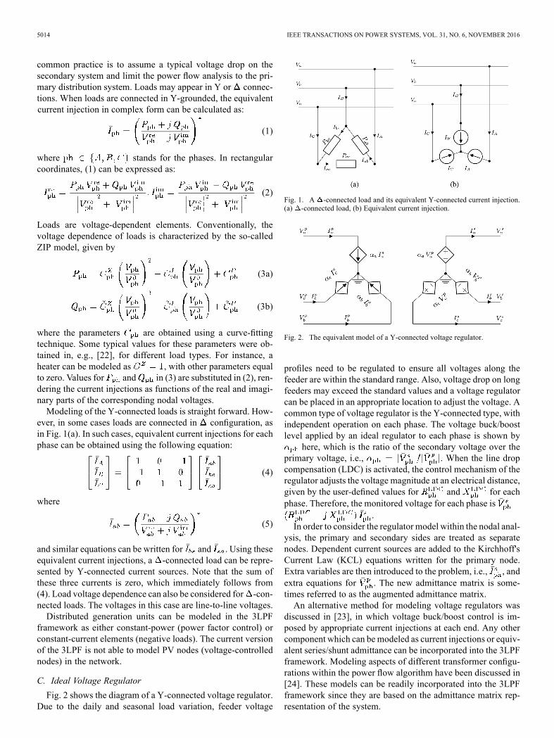
common practice is to assume a typical voltage drop on thesecondary system and limit the power flow analysis to the pri-mary distribution system. Loads may appear in Y or connec-tions. When loads are connected in Y-grounded, the equivalentcurrent injection in complex form can be calculated as:

(1)

where stands for the phases. In rectangularcoordinates, (1) can be expressed as:

(2)

Loads are voltage-dependent elements. Conventionally, thevoltage dependence of loads is characterized by the so-calledZIP model, given by

(3a)

(3b)

where the parameters are obtained using a curve-fittingtechnique. Some typical values for these parameters were ob-tained in, e.g., [22], for different load types. For instance, aheater can be modeled as , with other parameters equalto zero. Values for and in (3) are substituted in (2), ren-dering the current injections as functions of the real and imagi-nary parts of the corresponding nodal voltages.Modeling of the Y-connected loads is straight forward. How-

ever, in some cases loads are connected in configuration, asin Fig. 1(a). In such cases, equivalent current injections for eachphase can be obtained using the following equation:

(4)

where

(5)

and similar equations can be written for and . Using theseequivalent current injections, a -connected load can be repre-sented by Y-connected current sources. Note that the sum ofthese three currents is zero, which immediately follows from(4). Load voltage dependence can also be considered for -con-nected loads. The voltages in this case are line-to-line voltages.Distributed generation units can be modeled in the 3LPF

framework as either constant-power (power factor control) orconstant-current elements (negative loads). The current versionof the 3LPF is not able to model PV nodes (voltage-controllednodes) in the network.

C. Ideal Voltage RegulatorFig. 2 shows the diagram of a Y-connected voltage regulator.

Due to the daily and seasonal load variation, feeder voltage

Fig. 1. A -connected load and its equivalent Y-connected current injection.(a) -connected load, (b) Equivalent current injection.

Fig. 2. The equivalent model of a Y-connected voltage regulator.

profiles need to be regulated to ensure all voltages along thefeeder are within the standard range. Also, voltage drop on longfeeders may exceed the standard values and a voltage regulatorcan be placed in an appropriate location to adjust the voltage. Acommon type of voltage regulator is the Y-connected type, withindependent operation on each phase. The voltage buck/boostlevel applied by an ideal regulator to each phase is shown by

here, which is the ratio of the secondary voltage over theprimary voltage, i.e., . When the line dropcompensation (LDC) is activated, the control mechanism of theregulator adjusts the voltage magnitude at an electrical distance,given by the user-defined values for and for eachphase. Therefore, the monitored voltage for each phase is

.In order to consider the regulator model within the nodal anal-

ysis, the primary and secondary sides are treated as separatenodes. Dependent current sources are added to the Kirchhoff'sCurrent Law (KCL) equations written for the primary node.Extra variables are then introduced to the problem, i.e., , andextra equations for . The new admittance matrix is some-times referred to as the augmented admittance matrix.An alternative method for modeling voltage regulators was

discussed in [23], in which voltage buck/boost control is im-posed by appropriate current injections at each end. Any othercomponent which can bemodeled as current injections or equiv-alent series/shunt admittance can be incorporated into the 3LPFframework. Modeling aspects of different transformer configu-rations within the power flow algorithm have been discussed in[24]. These models can be readily incorporated into the 3LPFframework since they are based on the admittance matrix rep-resentation of the system.

AHMADI et al.: A LINEAR POWER FLOW FORMULATION FOR THREE-PHASE DISTRIBUTION SYSTEMS 5015

D. Fixed-Point Iteration

The current injection method (CIM) is based on applying theKCL at each node in the system. The sum of the currents drawnfrom a node by the loads should be equal to the sum of thecurrents injected into that node from the rest of the network.Using load equivalent current injections, the following generalformulation can be reached for a systemwith nodes (includingall the existing phases):

(6)

where is the admittance matrix; isthe load equivalent current injections as a nonlinear functionof the nodal voltages . Starting from an initial guess, under the condition that is invertible, (6) can be treated

as a fixed-point iteration (FPI) problem. The iteration method isdescribed in Algorithm 1. The process continues until the dif-ference between the two consecutive solutions is less than thepredefined tolerance .

Algorithm 1 CIM using Fixed-Point Iteration

1: procedure FIXED-POINT ITERATION2:3: while do4: Update current injections5: Solve for6:7:8: end while9: end procedure

The nodal voltages in the unloaded case are considered asthe initial guess, i.e., all the voltages are equal to the substationvoltage. The FPI algorithm used here is different from the oneused in [12] in the sense that loads are converted to R-L equiva-lents in [12] while they are considered as equivalent current in-jections here. As reported in [12], the FPI method is about threetimes faster than the Newton method and about two times fasterthan the Dishonest Newton method for the IEEE 8500-Nodesystem.

III. THE LINEAR POWER FLOW METHOD

The CIM, compared to the Newton-Raphson equations, takesthe complexity and nonlinearities from the power flow equa-tions and places them in the load modeling part. It is more ef-fective to perform linearization on the load models where theimpacts on the solution accuracy are relatively small. Having acloser look at (6) reveals that the only nonlinearity arises fromthe right-hand side of the equations, i.e., the equivalent currentinjections . Since (6) is written in complex form, a decom-posed version is considered here which is in the real form:

(7)

in which and are the real and imaginaryparts of the augmented admittance matrix and

are the real and imaginary parts of the three-phasenodal voltages , respectively; and arethe real and imaginary parts of the three-phase nodal currentinjections , respectively. The terms in the right-hand sideof (7) were derived in (2) for Y-connected loads and can besimilarly derived for -connected loads using (4) and (5). Usingthese equivalents for and , all the nonlinear terms turn outto be functions of and . Substituting the correspondingvalues of and from (3) into (2), and assumingp.u., the relations in (8a) and (8b), shown at the bottom of thepage, can be derived.Depending on the load voltage dependence characteristics,

four nonlinear terms appear in (8), as follows:

(9a)

(9b)These nonlinear functions can be approximated with theirlinear equivalents using a curve-fitting technique when and

vary within a certain range. The approximated linear func-tions are then expressed as

(10)

(8a)

(8b)

5016 IEEE TRANSACTIONS ON POWER SYSTEMS, VOL. 31, NO. 6, NOVEMBER 2016

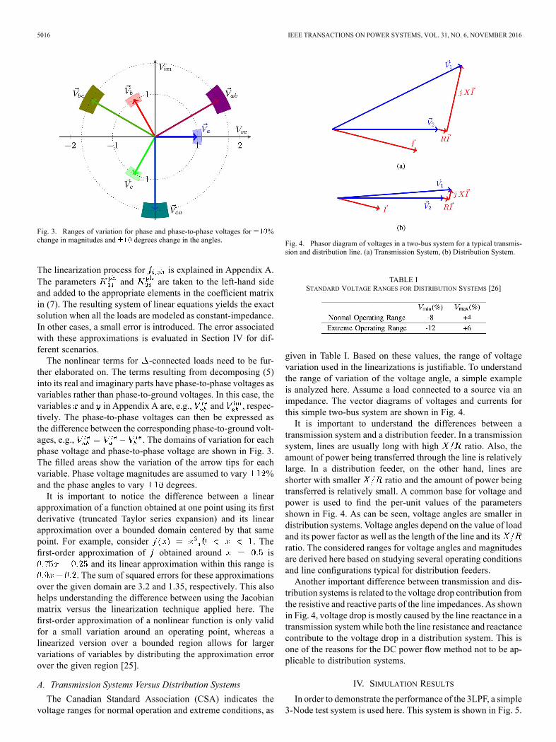
Fig. 3. Ranges of variation for phase and phase-to-phase voltages for %change in magnitudes and degrees change in the angles.

The linearization process for is explained in Appendix A.The parameters and are taken to the left-hand sideand added to the appropriate elements in the coefficient matrixin (7). The resulting system of linear equations yields the exactsolution when all the loads are modeled as constant-impedance.In other cases, a small error is introduced. The error associatedwith these approximations is evaluated in Section IV for dif-ferent scenarios.The nonlinear terms for -connected loads need to be fur-

ther elaborated on. The terms resulting from decomposing (5)into its real and imaginary parts have phase-to-phase voltages asvariables rather than phase-to-ground voltages. In this case, thevariables and in Appendix A are, e.g., and , respec-tively. The phase-to-phase voltages can then be expressed asthe difference between the corresponding phase-to-ground volt-ages, e.g., . The domains of variation for eachphase voltage and phase-to-phase voltage are shown in Fig. 3.The filled areas show the variation of the arrow tips for eachvariable. Phase voltage magnitudes are assumed to vary %and the phase angles to vary degrees.It is important to notice the difference between a linear

approximation of a function obtained at one point using its firstderivative (truncated Taylor series expansion) and its linearapproximation over a bounded domain centered by that samepoint. For example, consider . Thefirst-order approximation of obtained around is

and its linear approximation within this range is. The sum of squared errors for these approximations

over the given domain are 3.2 and 1.35, respectively. This alsohelps understanding the difference between using the Jacobianmatrix versus the linearization technique applied here. Thefirst-order approximation of a nonlinear function is only validfor a small variation around an operating point, whereas alinearized version over a bounded region allows for largervariations of variables by distributing the approximation errorover the given region [25].

A. Transmission Systems Versus Distribution SystemsThe Canadian Standard Association (CSA) indicates the

voltage ranges for normal operation and extreme conditions, as

Fig. 4. Phasor diagram of voltages in a two-bus system for a typical transmis-sion and distribution line. (a) Transmission System, (b) Distribution System.

TABLE ISTANDARD VOLTAGE RANGES FOR DISTRIBUTION SYSTEMS [26]

given in Table I. Based on these values, the range of voltagevariation used in the linearizations is justifiable. To understandthe range of variation of the voltage angle, a simple exampleis analyzed here. Assume a load connected to a source via animpedance. The vector diagrams of voltages and currents forthis simple two-bus system are shown in Fig. 4.It is important to understand the differences between a

transmission system and a distribution feeder. In a transmissionsystem, lines are usually long with high ratio. Also, theamount of power being transferred through the line is relativelylarge. In a distribution feeder, on the other hand, lines areshorter with smaller ratio and the amount of power beingtransferred is relatively small. A common base for voltage andpower is used to find the per-unit values of the parametersshown in Fig. 4. As can be seen, voltage angles are smaller indistribution systems. Voltage angles depend on the value of loadand its power factor as well as the length of the line and itsratio. The considered ranges for voltage angles and magnitudesare derived here based on studying several operating conditionsand line configurations typical for distribution feeders.Another important difference between transmission and dis-

tribution systems is related to the voltage drop contribution fromthe resistive and reactive parts of the line impedances. As shownin Fig. 4, voltage drop is mostly caused by the line reactance in atransmission system while both the line resistance and reactancecontribute to the voltage drop in a distribution system. This isone of the reasons for the DC power flow method not to be ap-plicable to distribution systems.

IV. SIMULATION RESULTSIn order to demonstrate the performance of the 3LPF, a simple

3-Node test system is used here. This system is shown in Fig. 5.

AHMADI et al.: A LINEAR POWER FLOW FORMULATION FOR THREE-PHASE DISTRIBUTION SYSTEMS 5017

Fig. 5. The 3-Node test system.

Fig. 6. Relative error of the 3LPF for different feeder loadings.

The branch impedances and loads are given in Appendix C. Sev-eral parameters can affect the accuracy of the 3LPF, includingthe ratio, length of the lines, feeder loading , loadpower factor , and load voltage dependence ( , and

portions). The errors associated with the 3LPF results arecalculated with respect to the results obtained using the CIMmethod. Let the voltage magnitudes obtained by the 3LPF be

and those obtained by the CIM be . The relativeerror, in %, is then calculated as

(11)

In each simulation, only one factor is altered and other param-eters are fixed at the original values given in Appendix C. Thefirst parameter to be considered is the feeder loading, which isaltered by scaling the load and by a factor . Fig. 6 showsthe errors for each node in the system. In the same figure, thesystem minimum voltage is also shown on the right verticalaxis. The loads are scaled up until the minimum voltage fallsbelow 0.90 per-unit. The maximum error in this case is less than0.24%, associated with Phase A at Node 3. With normal feederloading, i.e., , the maximum error is less than 0.05%.It is worthwhile mentioning that the unbalance caused by thenon-existing phase C at Node 3 contributed significantly to thevoltage unbalance, about 5% difference in magnitudes in phasesA and B, urging the application of a three-phase analysis.The effect of the load power factor, , is shown in Fig. 7.

Here, the value of load active power is kept fixed and the reac-tive power is determined based on the value of in Fig. 7. For

Fig. 7. Relative error of the 3LPF versus loads power factor.

instance, , and correspond tolagging, and leading, respectively. The max-

imum error in this case is about 0.09%. As the load becomesmore capacitive (negative values for ), the voltage magnitudesget closer to 1 p.u., increasing the accuracy of the 3LPF solution.Loads are voltage-dependent elements, i.e., the amount of ac-

tive and reactive power demand changes as the voltage levelvaries. In the standard IEEE test systems, loads are modeled asconstant-impedance (Z), constant-current (I), or constant-power(PQ) [27]. The errors of the 3LPF solution for these three casesare shown in Fig. 8. All loads, including their active and reactivepower components, are assumed to have the same voltage de-pendence in these simulations. Note that the 3LPF is capable ofmodeling any combinations of components of the ZIPmodel de-scribed in (3). The highest error occurs for the constant-powerload model and the error of the constant-impedance model iszero.The ratio of the branches varies in distribution systems,

depending on the phase arrangement, type of conductors, over-head lines or underground cables, voltage levels, etc. The valuesfor are kept constant in the test system and the values forare calculated based on the ratio. It should be noted that allthe 9 elements of the three-phase resistance matrices are scaledby the given factor. The impact of the ratio on theerror of the 3LPF solution is shown in Fig. 9. The maximumerror in this case is about 0.11%.The feeder length is another important factor that can impact

the error of the 3LPF solution. The effect of the feeder lengthon the accuracy of the 3LPF solution is shown in Fig. 10. Thefeeder length is increased to the point that the maximum voltagedrop almost exceeds the standard limits. In this case, the max-imum error is about 0.16%. Due to the relatively large hypothet-ical values chosen for the line parameters, the voltage limits arereached at 6 km. This happens while the voltage angles deviatefrom the nominal values, i.e., , by less than3 . Adding a voltage regulator brings the voltage magnitudeswithin the standard limits, and the voltage angles may growlarger. In our approximations, is considered for voltageangles, which was derived based on numerous analyses of realand hypothetical distribution systems.The IEEE 13-Node, the IEEE 123-Node, and the IEEE 8500-

Node test systems, described in [27] and [28], are also used

5018 IEEE TRANSACTIONS ON POWER SYSTEMS, VOL. 31, NO. 6, NOVEMBER 2016

Fig. 8. Relative error of the 3LPF versus loads voltage dependence.

Fig. 9. Relative error of the 3LPF versus ratio of lines.

Fig. 10. Relative error of the 3LPF versus feeder length.

here to evaluate the accuracy of the 3LPF solution. The fol-lowing modifications are made to the IEEE 13-Node system:Transformer XFM-1 is replaced by a 3000 ft long L602 line;The distributed load between Nodes 632 and 671 is assumedto be connected at Node 632. The power flow solution for thistest system is provided in Table II. The histogram of errorgiven by (11), considering all the phases and nodes, is shown inFig. 12. The error in this case is less than 0.03%. This systemwas also adopted in [20] to numerically evaluate their proposedlinearization method, referred to as the 1st Order method here.A comparison is made in terms of the solution accuracy betweenthe 3LPF and the 1st Order method. Fig. 11 shows the error foreach node and phase. In the first scenario, shown in Fig. 11(a),

Fig. 11. Relative error of power flow solutions obtained by the 1st Ordermethod of [20] and the 3LPF for the IEEE 13-Node system. (a) Tap changerset at , (b) Tap changer set at .

the voltage regulator taps are adjusted at [1.0625, 1.05, 1.0687].The maximum relative errors in this case for the 1st Ordermethod and the 3LPF are 0.57% and 0.03%, respectively. In thesecond scenario, shown in Fig. 11(b), the tap changer is set at[1, 1, 1]. The maximum in this case is 1.44% and 0.21% forthe 1st Order method and the 3LPF, respectively.In the IEEE 123-Node system, the transformer between nodes

61 and 610 is removed. The histogram of error for this systemis shown in Fig. 12. The error in this case does not exceed0.025%.The IEEE 8500-Node system is described in [28]. The total

load in the system is about 10.8 MW 2.7 MVAR. This systemconsists of the primary network (12.47 kV), single-phase dis-tribution transformers (7.2 kV/120 V/120 V), and a 50-ft ser-vice cable that connects the loads to the customer service trans-formers. In this study, only the primary network is considered.The primary network consists of about 3680 nodes. The cus-tomer service transformers are replaced by the equivalent loadconnected to them. Voltage regulators are set at tap 1.02 on allphases and are kept fixed. There are four capacitor banks, all ofwhich are assumed to be connected since the given loading is forpeak load conditions. The histogram of error for this system isshown in Fig. 12. The error in this case does not exceed 0.06%.

AHMADI et al.: A LINEAR POWER FLOW FORMULATION FOR THREE-PHASE DISTRIBUTION SYSTEMS 5019

Fig. 12. Histogram of relative error of the 3LPF solution for the IEEE 13-,123-, and 8500-Node systems, considering all phases at each node.

TABLE IIPOWER FLOW SOLUTION FOR THE IEEE 13-NODE

TEST SYSTEM OBTAINED BY THE 3LPF

The CIM is an iterative solution method. The maximum errorat each iteration for the three test cases introduced above isshown in Fig. 13. As can be seen, the maximum error for the3LPF is slightly lower than the error for the CIM at its seconditeration. In other words, it takes the CIM up to three iterationsto exceed the accuracy of the 3LPF solution. At its first itera-tion, the error of the CIM is about an order of magnitude largerthan the 3LPF method.

V. POTENTIAL APPLICATIONS OF THE 3LPFWhile the 3LPF is directly useful in power flow analysis,

its major advantages are more evident when embedded inoptimization routines., where computational efficiency is of theessence. This becomes especially pressing for on-line appli-cations that are required to produce fast and robust solutions.Distribution system state estimation (DSSE) is an importantcase, which has received considerable attention due to thenew developments in the advanced metering infrastructure. Ithas been shown that the presence of unbalances can signifi-cantly affect the accuracy of the DSSE [29] and, therefore, athree-phase model of the system should be used. The DSSE hasmany applications in the tools provided by the modern DMS,e.g., volt-VAR control methods [30]. One of the challenges in

Fig. 13. Maximum error in voltage magnitudes per iteration for the CIM solu-tion for the IEEE 13, 123, and 8500-Node test systems. The 3LPF error is shownusing a red dashed line.

the DSSE is the lack of sufficient measurements, which leadsto an unobservable system and causes convergence issues inthe DSSE algorithm. Methods have been proposed to generatepseudo-measurements to address this issue, e.g., [31]. Sincethe conventional power flow equations are nonlinear andnon-convex, the DSSE problem is numerically intensive tosolve [32]. Computational challenges arising from the inclusionof pseudo-measurements are likely to be alleviated substan-tially by the 3LPF method.Another challenge in DSSE is the presence of discrete

variables, e.g., status of switches, fuses, capacitor banks, andvoltage regulator taps. Besides, introducing integer variables tothe DSSE optimization problem creates a practically intractableproblem. It is expected that the proposed 3LPF formulationpaves the path for including the discrete variables within theDSSE. With the 3LPF, the resulting optimization problem canbe solved using commercially available mixed-integer pro-gramming solvers. Normally, in a typical distribution feeder,there exist only a few number of voltage regulators and/orcapacitor banks. Also, most of the distribution feeders areradial, which facilitates the idea of decomposing the probleminto several independent sub-problems, each dealing only witha single feeder. These specific features of distribution systemsmake it possible to take advantage of the fast mixed-integerprogramming methods.The optimal placement of new measurement devices for

DSSE has been a subject of research in several studies [33],[34]. This problem can be formulated as a mixed-integer pro-gramming problem, where the existence of a measuring devicecan be modeled as a binary variable. The 3LPF formulation al-lows for the introduction of integer variables to the optimizationproblem of meter placement. In addition, the volt-VAR opti-mization problem in distribution system requires three-phasepower flow analysis when voltage regulators and/or capac-itor banks with single, double, and independently-operatedthree-phase units are present. The LPF has been successfullyapplied to this problem for a balanced case in [35]. The pro-posed 3LPF formulation can be directly applied to unbalancedcases. It should be noted that the 3LPF is still applicable even if

5020 IEEE TRANSACTIONS ON POWER SYSTEMS, VOL. 31, NO. 6, NOVEMBER 2016

voltages are outside the standard limits, although the associatederror may be slightly higher.Due to the probabilistic and intermittent nature of some

renewable energy resources, e.g., wind and solar, probabilisticpower flow methods have been developed to find the expectedvalue and variance of the system state variables [36], [37].There are also elements of uncertainty in load values as well asload models in a distribution system. The proposed 3LPF is anefficient alternative to nonlinear formulations for probabilisticpower flow analysis. The probabilistic power flow analysisprovides a bound for the nodal voltages and branch currents forgiven bounds on the expected load/generation scenarios. Thisis useful to ensure, with some definable probability, that thesystem will operate within the standard limits under differentscenarios. The ever-increasing penetration of distributed energyresources calls for these types of studies.The error values reported in Section IV are acceptable for the

targeted applications mentioned above.

VI. CONCLUSION

The current injection method for a three-phase distributionsystem was described and the fixed-point iteration method wasused to solve the resulting power flow equations. A three-phaselinear power flow (3LPF) formulation was derived based onthe fact that the nodal voltages vary within a bounded range.The error associated with the 3LPF solution for various systemparameters was illustrated. An important application of the3LPF is in distribution system optimization routines, such asvolt-VAR optimization, and distribution system state estima-tion. With this linear set of equations, it is possible to includeinteger variables to represent switches status, tap position forvoltage regulators, etc.

APPENDIX ALINEAR APPROXIMATION OF A TWO-VARIABLE FUNCTIONAssume a nonlinear function defined on and

. A linear approximation of on the specified compactdomain is . Assume evenly distributedpoints in the function domain, i.e., . In order to findthe best coefficients for that closely matches , the followingleast-square problem should be solved:

(12)

Applying the Karush-Kuhn-Tucker conditions to the aboveproblem yields the following solution:

(13)

Note that this has to be solved for the four nonlinear functionsin (9) and for each phase separately. Therefore, in (10) rep-resents for , and Phase .

APPENDIX BCALCULATED FOR LINEAR APPROXIMATIONS

APPENDIX CPOWER-FLOW DATA FOR THE 3-NODE TEST SYSTEM

is in is in ; active power is in(MW); reactive power is in MVAR; lengths are in miles.

From To Load Length

REFERENCES[1] J. R. Marti, H. Ahmadi, and L. Bashualdo, “Linear power flow formu-

lation based on a voltage-dependent load model,” IEEE Trans. PowerDel., vol. 28, no. 3, pp. 1682–1690, Jul. 2013.

[2] H. Ahmadi and J. R. Martı́, “Distribution system optimization basedon a linear power flow formulation,” IEEE Trans. Power Del., vol. 30,no. 1, pp. 25–33, Feb. 2015.

[3] H. Ahmadi, “Linear power flow source codes,” Dec. 2015 [Online].Available: http://www.ece.ubc.ca/hameda/downloads.htm.

[4] H. L. Nguyen, “Newton-Raphson method in complex form,” IEEETrans. Power Syst., vol. 12, no. 3, pp. 1355–1359, Aug. 1997.

[5] O. L. Tortelli, E.M. Lourenco, A. V. Garcia, and B. C. Pal, “Fast decou-pled power flow to emerging distribution systems via complex pu nor-malization,” IEEE Trans. Power Syst., vol. 30, no. 3, pp. 1351–1358,May 2015.

AHMADI et al.: A LINEAR POWER FLOW FORMULATION FOR THREE-PHASE DISTRIBUTION SYSTEMS 5021

[6] M. Abdel-Akher, K. M. Nor, and A. H. A. Rashid, “Improved three-phase power-flow methods using sequence components,” IEEE Trans.Power Syst., vol. 20, no. 3, pp. 1389–1397, Aug. 2005.

[7] I. Dzafic, H.-T. Neisius, M. Gilles, S. Henselmeyer, and V. Lan-derberger, “Three-phase power flow in distribution networks usingFortescue transformation,” IEEE Trans. Power Syst., vol. 28, no. 2,pp. 1027–1034, May 2013.

[8] M. Z. Kamh and R. Iravani, “Unbalanced model and power-flow anal-ysis of microgrids and active distribution systems,” IEEE Trans. PowerDel., vol. 25, no. 4, pp. 2851–2858, Oct. 2010.

[9] D. Shirmohammadi, H.W. Hong, A. Semlyen, and G. X. Luo, “A com-pensation-based power flow method for weakly meshed distributionand transmission networks,” IEEE Trans. Power Syst., vol. 3, no. 2,pp. 753–762, May 1988.

[10] C. S. Cheng and D. Shirmohammadi, “A three-phase power flowmethod for real-time distribution system analysis,” IEEE Trans. PowerSyst., vol. 10, no. 2, pp. 671–679, May 1995.

[11] M. Dilek, F. De León, R. Broadwater, and S. Lee, “A robust mul-tiphase power flow for general distribution networks,” IEEE Trans.Power Syst., vol. 25, no. 2, pp. 760–768, May 2010.

[12] I. Kocar, J. Mahseredjian, U. Karaagac, G. Soykan, and O. Saad, “Mul-tiphase load-flow solution for large-scale distribution systems usingMANA,” IEEE Trans. Power Del., vol. 29, no. 2, pp. 908–915, Apr.2014.

[13] T.-H. Chen, M.-S. Chen, K.-J. Hwang, P. Kotas, and E. A. Chebli,“Distribution system power flow analysis—A rigid approach,” IEEETrans. Power Del., vol. 6, no. 3, pp. 1146–1152, Jul. 1991.

[14] J.-H. Teng and C.-Y. Chang, “A novel and fast three-phase load flowfor unbalanced radial distribution systems,” IEEE Trans. Power Syst.,vol. 17, no. 4, pp. 1238–1244, Nov. 2002.

[15] V. M. Da Costa, N. Martins, and J. R. L. Pereira, “Developments in theNewton Raphson power flow formulation based on current injections,”IEEE Trans. Power Syst., vol. 14, no. 4, pp. 1320–1326, Nov. 1999.

[16] P. A. N. Garcia, J. L. R. Pereira, S. Carneiro, Jr., V. M. Da Costa, andN. Martins, “Three-phase power flow calculations using the current in-jection method,” IEEE Trans. Power Syst., vol. 15, no. 2, pp. 508–514,May 2000.

[17] T.-H. Chen and N.-C. Yang, “Loop frame of reference based three-phase power flow for unbalanced radial distribution systems,” Elect.Power Syst. Res., vol. 80, no. 7, pp. 799–806, 2010.

[18] P. M. De Oliveira-De Jesus, M. A. Alvarez, and J. M. Yusta, “Distri-bution power flow method based on a real quasi-symmetric matrix,”Elect. Power Syst. Res., vol. 95, pp. 148–159, 2013.

[19] A. J. Wood and B. F. Wollenberg, Power Generation, Operation, andControl. New York, NY, USA: Wiley, 2012.

[20] S. Bolognani and F. Dorfler, “Fast power system analysis via implicitlinearization of the power flowmanifold,” in Proc. 53rd Annu. AllertonConf. Commun., Control, and Comput., 2015.

[21] S. Bolognani and S. Zampieri, “On the existence and linear approxima-tion of the power flow solution in power distribution networks,” IEEETrans. Power Syst., vol. 31, no. 1, pp. 163–172, Jan. 2016.

[22] L. M. Hajagos and B. Danai, “Laboratory measurements and models ofmodern loads and their effect on voltage stability studies,” IEEE Trans.Power Syst., vol. 13, no. 2, pp. 584–592, May 1998.

[23] A. Gómez-Expósito, E. Romero-Ramos, and I. Džafić, “Hybrid real-complex current injection-based load flow formulation,” Elect. PowerSyst. Res., vol. 119, pp. 237–246, 2015.

[24] T.-H. Chen et al., “Three-phase cogenerator and transformer modelsfor distribution system analysis,” IEEE Trans. Power Del., vol. 6, no.4, pp. 1671–1681, Oct. 1991.

[25] H. Ahmadi, J. R. Martı́, and A. Moshref, “Piecewise linear approxima-tion of generators cost functions using max-affine functions,” in Proc.IEEE PES General Meeting, Vancouver, BC, Canada, 2013, pp. 1–5.

[26] Preferred Voltage Levels for AC Systems, 0 to 50,000 V, Std. CAN3C235-83, Canadian Standard Association (CSA), 2010.

[27] W. H. Kersting, “Radial distribution test feeders,” IEEE Trans. PowerSyst., vol. 6, no. 3, pp. 975–985, Aug. 1991.

[28] R. F. Arritt and R. C. Dugan, “The IEEE 8500-node test feeder,” inProc. IEEE PES T& D Conf. Expo., 2010, pp. 1–6.

[29] C. W. Hansen and A. S. Debs, “Power system state estimation usingthree-phase models,” IEEE Trans. Power Syst., vol. 10, no. 2, pp.818–824, May 1995.

[30] M. Biserica, Y. Besanger, R. Caire, O. Chilard, and P. Deschamps,“Neural networks to improve distribution state estimation-volt varcontrol performances,” IEEE Trans. Smart Grid, vol. 3, no. 3, pp.1137–1144, Sep. 2012.

[31] E. Manitsas, R. Singh, B. C. Pal, and G. Strbac, “Distribution systemstate estimation using an artificial neural network approach for pseudomeasurement modeling,” IEEE Trans. Power Syst., vol. 27, no. 4, pp.1888–1896, Nov. 2012.

[32] L. Schenato, G. Barchi, D. Macii, R. Arghandeh, K. Poolla, and A. VonMeier, “Bayesian linear state estimation using smart meters and PMUsmeasurements in distribution grids,” in Proc. IEEE Int. Conf. SmartGrid Commun., 2014, pp. 572–577, IEEE.

[33] R. Singh, B. C. Pal, and R. B. Vinter, “Measurement placement in dis-tribution system state estimation,” IEEE Trans. Power Syst., vol. 24,no. 2, pp. 668–675, May 2009.

[34] M. G. Damavandi, V. Krishnamurthy, and J. R. Martı́, “Robust meterplacement for state estimation in active distribution systems,” IEEETrans. Smart Grid, vol. 6, no. 4, pp. 1972–1982, Jul. 2015.

[35] H. Ahmadi, J. R. Martı́, and H. W. Dommel, “A framework forvolt-VAR optimization in distribution systems,” IEEE Trans. SmartGrid, vol. 6, no. 3, pp. 1473–1483, May 2015.

[36] M. Ding and X. Wu, “Three-phase probabilistic power flow in dis-tribution system with grid-connected photovoltaic systems,” in Proc.APPEEC, Mar. 2012, pp. 1–6.

[37] H. Ahmadi and H. Ghasemi, “Probabilistic optimal power flow incor-porating wind power using point estimate methods,” in Proc. EEEIC,May 2011, pp. 1–5.

Hamed Ahmadi (M’15) received the B.Sc. andM.Sc. degrees in electrical engineering from theUniversity of Tehran in 2009 and 2011, respectively,and the Ph.D. degree in electrical and computer en-gineering from the University of British Columbia,Vancouver, BC, Canada. He was a postdoctoralfellow at the University of British Columbia fromApril to August 2015, working on a joint projectwith BC Hydro. He is currently an Engineer atGeneration and Transmission Division, BC Hydro,Burnaby, BC. His research interests include distri-

bution systems analysis, optimization algorithms, power system stability andcontrol, smart grids, and high voltage engineering.

José R.Martı́ (M’80–SM’01–F’02–LF’15) receivedthe Electrical Engineering degree from Central Uni-versity of Venezuela, Caracas, in 1971, the Masterof Engineering degree in electric power (M.E.E.P.E.)from Rensselaer Polytechnic Institute, Troy, NY, in1974, and the Ph.D. degree in electrical engineeringfrom the University of British Columbia, Vancouver,BC, Canada in 1981. He is known for his contribu-tions to the modeling of fast transients in large powernetworks, including component models and solutiontechniques. Particular emphasis in recent years has

been the development of distributed computational solutions for real-time sim-ulation of large systems and integrated multisystem solutions. He is a Professorof electrical and computer engineering at the University of British Columbiaand a Registered Professional Engineer in the Province of British Columbia,Canada.

Alexandra “Sascha” von Meier (M’12) received aB.A. in physics in 1986 and a Ph.D. in energy andresources in 1995 from University of California atBerkeley. She is presently an Adjunct Professor inthe Department of Electrical Engineering and Com-puter Science at UC Berkeley, and Director of Elec-tric Grid Research at the California Institute for En-ergy and Environment (CIEE). Her research focuseson Smart Grid issues, the use of advanced sensing andmonitoring capabilities such as synchrophasor datafor power distribution systems, and the integration of

renewable resources. She was previously a professor of energy management anddesign at Sonoma State University.