
'" N - eScholarship
259
LBL-4264 c .1 - . "I ESTIMA TION OF THE DYNAMICAL PARAMETERS OF THE CALVIN PHOTOSYNTHESIS CYCLE, OPTIMIZA TION, AND 111 CONDITIONED INVERSE PROBLEMS Jaime Mils tein (Ph. D. thesis) September 1975 Prepared for the U. S. Energy Research and Development Acministration under Contract W -7405-ENG-48 For Reference Not to be taken from this room tJj I '" N . 0' ......
-
Upload
khangminh22 -
Category
Documents
-
view
3 -
download
0
Transcript of '" N - eScholarship

LBL-4264
c .1 ~: -
. "I
ESTIMA TION OF THE DYNAMICAL PARAMETERS OF THE CALVIN PHOTOSYNTHESIS CYCLE,
OPTIMIZA TION, AND 111 CONDITIONED INVERSE PROBLEMS
Jaime Mils tein (Ph. D. thesis)
September 1975
Prepared for the U. S. Energy Research and Development Acministration under Contract W -7405-ENG-48
For Reference
Not to be taken from this room
~ tJj
~ I
~
'" N . 0' ...... ~

DISCLAIMER
This document was prepared as an account Of work sponsored by the United States Government. While this document is believed to contain correct information, neither the United States Government nor any agency thereof, nor the Regents of the University of California, nor any of their employees, makes any warranty, express or implied, or assumes any legal responsibility for the accuracy, completeness, or usefulness of any information, apparatus, product, or process disclosed, or represents that its use would not infringe privately owned rights. Reference herein to any specific commercial product, process, or service by its trade name, trademark, manufacturer, or otherwise, does not necessarily constitute or imply its endorsement, recommendation, or favoring by the United States Government or any agency thereof, or the Regents of the University of California. The views and opinions of authors expressed herein do not necessarily state or reflect those of the United States Government or any agency thereof or the Regents of the University of California.

\.
!\
O 0.·" ,. ':0
{.,J
In memory of my mpther,' Rachel, and
my father, Samuel whose eternal light
has guided me through the labyrinths
of life.
1.

Acknowledgments
It is a pleasure to express my deeply felt gratitude
to my mentor and friend, Professor Hans J. Bremermann, for
his warm encouragement, thoughtful guidance, countless
insights, and unlimited generosity throughout the making of
this thesis.
I wish to thank the other members of the committee,
Professors B. Parlett and Dr. A. J. Bassham, for their
patience~ coristructive criticism, and helpful discussions.
I am indebted to Professors J'. A. Bassham and M. Calvin
and tbe members of the Biodynamic Laboratory for their excel
lent assistance and their many hours spent to obtain experi-
mental data.. Dr. Clifford Risk and Dr. Joel Swartz have
provided invaluable suggestions and encouraging support
throughout this work.
I extend many thanks to Myron Katz, who was especially
helpful in making the introductions and general text easier
to understand, and to Said Doss, Pat Gilmer, David Krumme,
Stan Zietz 'and Bob Miller for their valuable comments and
suggestions.
I am very grateful to my sister, Monica,my brother
in-law, Chaim, and their children, Naama, Eial and Yuval,
who have been my inspiration in all personal endeavors and
whose affection has always given me personal strength to '.
overcome many difficult years. I wish to thank my aunts and
ii

f- ,
o 0 4 o 9 3·
uncles, Helena, Piri, Simon and Moshe, for their moral and
spiritual support. I give special thanks to my close friend,
Shoshana, for her great understanding.
The acknowledgments would not be complete without
extending thanks to many clos~.frierids, Carmela and Sam,
Tova and Avi, Naftaly, and Dalia and Shmulik, to name a few,
for their understanding and companionship throughout the
difficult moments of my work.
Last but not least, I want to express my deep apprecia-
tion to Nora Lee, for her patience, warmth~and the wonderful
job she has don~ in typing this.manuscript.
iii

INTRODUCTION
This thesis is concerned with the determination of the
dynamic rate ccinstants of the carbon reduction cycle (Calvin
Cycle) and with the mathematical and comp~tational tools
required. The rate constant problem has been an Dpen problem
for over twenty years.
The dynamics of photosynthesis can be described by a
system of eighteen ordinary non-linear differential equations·
which contain twenty-two unknown parameters -- the rate
constants.
Determination of these constants from observable data
1S the concern of this thesis. Mathematically, it reduces
to a non-lirtear fitting problem which in turn reduces to
optimizing a transcendental function that is not known 1n
closed form, but it can be evaluated pointwise through
(laborious) computation.
The literature on optimization 15 vast and many algorithms
are 1n use. The problem at hand can only be solved if a
powerful, computationally efficient, non-stagnating optimi
zation algorithm is used.
Thus the first part of the thesis is concerned with
the comparison of different optimization algorithms and
their performance on a variety of test problems. This is
a mathematical-numerical problem in its own right which in
turn is closely related to the problem of root finding for
systems of polynomials and transcendental functions in many

00 o :2 2
variables. The research showed that the optimizatiQn algorithm
by H. Brmermann ,outperformed all others t~sted.
In applying the optimization algorithm to the photo
synthesis problem another problem was encountered. The dynamic
equations that describe photosynthesis turned out t6 be
very stiff and standard integration algorithms (Runge-Kutta)
failed. Rate constants determination is an iterative process
that requires repeated integration.of the dynamic equations
and a special stiff method (Gear's method) had to be
adapted to the problem.
The earliel:' work of J. Swartz [ 83] which solves
similar but smaller and simpler parameter determination
problems showed the importance of an error analysis. Due
to the intrinsic nature of the parameter determination problem, L'·
noise in the (experimental) data can result in a percentage
error that can vary greatly (by orders of magnitude) between
parameters. Hence an error analysis of the expected variance
of the parameters is required if the results are to be
meaningful. In the case of photosynthesis, this analysis
involves matrices of partial derivatives of the system's
equations with so many terms, that even a very'small
probability of making a mistake during symbol manipulation,
results in a virtual certainty of erroneous terms in the
complete matrices. Since, ln this case, human error ln
symbol manipUlation cannot be made small enough, automation
of symbol manipUlation proved necessary. To this end we
v

used a new experimental language called ALTFAN (Algebra
Translator). ALTFAN is a language and system for performing
symbolic computations on algebraic data. The basic
capability of the language is to perform operations on
rational expressions in one or more indeterminants. The
system is designed to handle very large problems involving
such data,with considerable efficiency.
Our mathematical description of the kinetic of the
Calvin Cycle is a non-linear system of ordinary differential
equations. ·Determination of the rate constants. (kinetic
parameters) is based on the knowledge of the trajectories
of the intermediates of the system (the concentration of
the intermediates change with time). A problem for which
the trajectories are known and the parameters have to be
determined is called an "inverse problem". Experimental
error can cause errors in the observation of the trajectories
which in turn can cause large errors in the determination of
the parameters. Such a problem is called "ill-condi'tioned".
Parameter identification of the Calvin Cycle turned out to
be an ill-conditioned problem if only one set of initial
conditions is usad. To overcome the ill-conditioned nature
of our model it is necessary to obtain accurate experimental
data using several initial conditions, that is, performing
several experiments with different initial concentration.
The experiments to obtain accurate data are elaborate,
costly and require a substantial amount of time. M. Calvin,
vi
....

o 0 o 2 ? ... 9 /'
J. A. Bassham and co-workers at the Chemical Biodynamics
Laboratory at the University of California, Berkeley, will
furnish sufficient experimental data for use in the parameter
identification problem.
vii

Table of Contents
ACKNOWLEDGMENTS
INTRODUCTION
ABSTRACT
PART I: NON-LINEAR OPTIMIZATION
1.0 INTRODUCTION TO PART I
1.1 OPTIMIZATION KEY TO PARAMETER DETERMINATION.
1.2 UNCONSTRAINED OPT'IMIZATION
1.3 COMPUTATIONAL DIFFICULTIES IN OPTIMIZATION
1.4 SURVEY OF METHOD OF UNCONSTRAINED, OPTIMIZATION
1.4.1 1.4.2 1.4.3 1.4.4 1. 4.5 1.4.6 1.4.7 1.4.8 1. 4;. 9 1.4.10 1.4.11 1.4.12 1.4.13 1. 4.14 1.4.15
1.4.16
Direct Search Methods Pattern Sea~ch Method: Hooke-Jeeves [1961J Method of Rotating Coordinates Simplex Method: NeIder & Mead Random Method Descent Techniques Lagrangian Multipliers Descent Directions Gradient Descent Methods Techniques Using Conjugage Directions Powell' s Algorithm Without Using'D,erivatives Conjugate Gradient Techniques Fletcher and Reeves Algorithm [1964J Variabl~ Metric Techniques Davidon-Fletcher-Powell Variable Metric Technique Other Algorithms Considered
1.5 BREMERMANN'SALGORITHM (The "Optimizer") 1970
1.6 TEST PROBLEMS
1.6.1
1.6.2 1.6.3 1.6.4 1.6.5 1. 6.6
Algorithms Used in the Comparison with the "Optimizer" Discussion Effects of the Computer on the Results Test Procedure Results Obtained with Bremermannis Optimizer The Comparison of Bremermann's Optimizer with other Algorithms
viii
Page
ii
lV
xiii
2
4
4
5
5
5 6 9
12 15 16 19 20 22 24 27 29 30 32
33 35
'" 36
39 <.;
44 46 48 48 51
65
o Ou U 4 4 0 ~ 2 9 8
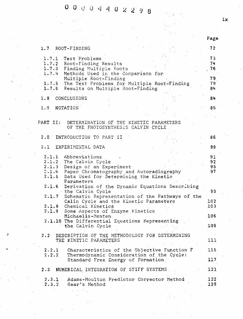
1.7 ROOT-FINDING
1.7.1 1.7.2 1.7.3 1.7.4
1.7.5 1.7.6
Test Problems Root-Finding Results Finding Multiple Roots Methods Used in the Comparison for Multiple Root-Finding The T~st Problems for Multiple Root-Finding Results on Multiple rtoot-Finding
1.8 CONCLUSIONS
1.9 NOTATION
PART II: DETERMINATION OF THE KINETIC PARAMETERS OF THE PHOTOSYNTHESIS CALVIN CYCLE
2.0 INTRODUCTION TO PART II
2.1 EXPERIMENTAL DATA
2.1.1 2.1.2 2.1. 3 2.1.4 2.1.5
2.1.6
2.1.7
2.1.8 2.1.9
2.1.10
Abbreviations The Calvin Cycle Design of an Experiment Paper Chromatography and Autoradiography Data Used for Determining the Kinetic Parameters Derivation of the Dynamic Equations Describing the Calvin Cycle Schematic Representation of the Pathways of the Ca1in Cycle and the Kinetic Parameters Chemical Kinetics Some ASpects of Enzyme Kinetics Michaelis-Menten The Differential Equations Representing the Calvin Cycle
2.2 DESCRIPTION OF THE METHODOLOGY FOR DETERMINING THE KINETIC PARAMETERS
2.2.1 2.2.2
Characteristics of the Objective Function F Thermodynamic Consideration of the Cycle: Standard Free Energy of Formation .
2.3 NUMERICAL INTEGRATION OF STIFF SYSTEMS.
2.3.1 2.3.2
Adams-Moulton Predictor Corrector Method Gear's Method
Page
72
73 74 76
79 79 84
84
85
86
89
91 92 95 97
99
102 103
106
109
III
·115
117
121
122 129
ix

Implementation of the r.;rror 2Ancii-y's~s:::' (>J'~' ,
Technique on the tyn~~ib~f~E~GJ~~6~SJ8f~ the Ca;~~n ~I~~i;e ~~~:)~.:r~~/t ~~~~~ \~~!;; .":~~:,~,~~i;~l";
,.'v ~.~ I' ;, .. \ '-. J.~
Page
144 (~ ;' , .- . C' 2. 5 ILL"7~ON.PITIONED SYSTEM ,OFctQUArrtO'N~ c) ,,<)::7 L;::: 147 e \', ;~~ J': 1.1)11:r :[ ~ ~J"C) O/J "3 .!; q .f :r 1 ~/! 'J '1 () :~ :::JTI~' .j. ,:,1 0:-1 < ~,~- (.~ :, S _~'1 :. e. '" ',~ ~ . i. +18 ... ~ · ... i~· h,'i t· r-.r , •.. ,', ',:" I'~ r- ~'.- :. .... r ~ r .... ~ .~', "._;. 1· r J 'k'':' -:;: -2 .. \' !1..r 2.5.1 Il1-Cond~tIoh:·"Eri")Exarhp1e-·L'i.." 1.'.: .::J,C.,.:':,;:' 152
2.5.2 Geometric Inierpretation of the G9D~~~~Qn~r, ~:g, Number of nxn Matrix A ' __ .•. t: ~.t.".'-.JI)·':, d ,,,1155
aB .. ,.:r,~-,-r-·-rlf\.~ri·f~ C . .I 2.6 TEST OF NUMERICAL HACHINERY USED IN THE" ,,'j.~ .... Vfi
PARAMETER IDENTIFICATION PROBLEM 161
2.6.1 2.6.2 2.6.3
~)<;r':r"-:l~:ri\-'ft:,,~ 6.t.7 t"\'r'7~I'·-"'r,-1'''''~ ~f.J(":" '~::r~ :.Ii.'·.-~- rfl,"', ~.~, ~/f.~::"'''''1',r~j,''''r . ... -ri Im15:retfi~·tl~a:;e itin~·.c\ f;: the·:Nun\~r.l:'cFtL :Machinet-y . .1.'
Graphi22i1 y rh~pi~Y.Jo~·: R~s6i{~C: l ',)L'~ .1:"',' :1.1)
Using Real Experiment1? ~~~~ O'f ~i'.;:;:r:)~)(l~:'(:T':tiI
'I.'5IA162 171
,) ,,189 • .1., )..
~'B 2.7
Jf 3.1
SUHMARY
CONCLUSION
r \,,190 . ~,.. ~ .~,
190
3.3
30J
r t r' • .l ... • 1 .... t~
~o Dal~5~~s2~~0~,·, ~.:~~~0ri~2 ~lj0niX ~~t b~~ 2I~~~ nils)
"1 11.0 .. t I:J nl') !.~ !?J 'v j: :t.,~) ::~ t {j C: ::;. rlj ~:'. c', ~~~) _l: J E .. [ f): 9 j' :-}/:S':r.b cf~;
; f3j:~)\::J Sf!} 10 n.o~t:tr)"1~)Lll;'3!.!():J ~)j~.Jl"L;::l[:{\~t:or!f"~.:.~.rlif ,[lr)j':~J-£'Inry():I '-;c- '1/.J2. i :rt:",n:: ~9r~''''1 t1ilE,t~[LET2
borl~sM ~Q1~9~~OJ ~o~~10~~q nG!luo~-2msbA f) (: ~1. j" t:d -: c~ ~ :1. 17", G ~)
p ~ 1· .. ;'~
c!.~.r~,~:
~~ t" ",.,
\ ... 1- ~ :::0
" ;" ".. . ... L .. ~,: :.' ;:.,
191
"

1.0
1.1
1.2
1.3
1.4
1.5
1.6
1.7
1.8
1.9
1.10
1.11
1.12
1.13
1.14
1.15
o .~ ~) .. , .... 9 9
Tables
Comparison of Central Processing Time (in seconds) when Bremermann's Optimizer is used on a Variety of Problems with Various Computers
Results Obtained on Two 50-Dimensional Test Problems {Rosenbrook "Banana" Type and "Bowl" Type
Graphic Representation of Table 1.1
Results Obtained Using Bremermann's Optimizer on Severa1 Test Problems:
Page
49
52
55
Rosenbrook 1960 56
Rosenbrook 1960 (Different Initial Values) 57
Beale 1958 58
Engvall .1966 (2-Dimensional) 59
Zangwi11 1967 (2-Dimensional) 60
Zangwill 1967 (3-Dimensional) 61
Engva1l 1966 (3-Dimensional) 62
Fletcher & Powell 1963 63
Powell Singular 1964 64·
.Results of Bremermann's Optimizer on 50-Dimensional Problems· Tested on a CDC 6400 Computer 66
Comparative Results on the 50-Dimensional Rosenbrook Type "Banana" 67
Comparative Results on the 50-Dimensional Function "Bowl" Type 6 8
Results for Test Problem with up to 4~variables .Using Bremermann's Optimizer on a CDC-6600 Computer 69
xi
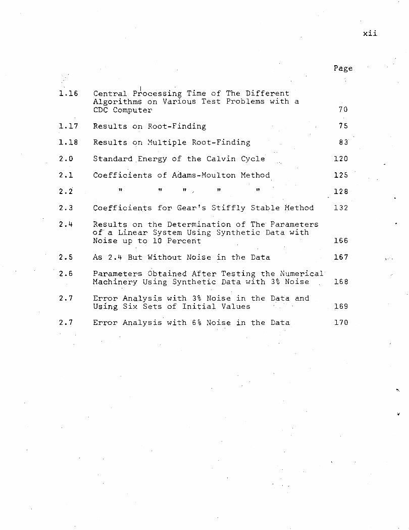
1.16
1.17
1.18
2.0
2.1
2.2
Central Pfocessi~g Time of The Different Algorithms on Various Test Problems with a CDC Computer
Results on Root-Finding
Results on Multiple Root-Finding
Standard Energy of the Calvin Cycle
Coefficients of Adams-Moulton Method
" " " " "
Page
70
75
83
120
125
128
2.3 Coefficients for Gear's Stiffly Stable Method 132
2.4 Results on the Determination of The Parameters of a Linear System Using Synthetic Data with Noise up to 10 Percent 166
2.5 As 2.4 But Without Noise ln the Data 167
2.6 Parameters Obtained After Testing the Numerical Machinery Using Synthetic Data with 3% Noise 168
2.7 Error Analysis with 3% Noise in the Data and Using Six Sets of Initial Values 169
2.7 Error Analysis with 6% Noise in the Data 170
xii

o 0
Abstract
This thesis is concerned with the determination of
kinetic parameters of the Calvin photosynthesis cycle and
the numerical tools required. A mathematical model with
seventeen non-linear ordinary differential equations des-
cribing this cycle is presented; its unknown parameters are /
to be determined using data from observations of the state
variables and an optimization technique developed herein.
This method for p~rameter identification involves a non-
linear optimization algorithm, first developed by Hans
Bremermann, a computer routine for numerical integration
of stiff systems and an error analysis technique, based on
a method of Rosenbrook and StQrey which was implemented and
tested by Joel Swartz. Bremermann's optimization algorithm
is tested and compared to other techniques frequently used
xiii
on optimization and root-finding problems. Finally, in order
to test both the mathematical model and parameter identifica-
tion technique, an arbitrary choice of parameter-values was
designated as the correct or exact parameter values and the
technique was implemented using simulated "observational"
data.

<0 ;I. 3 01 1
(
PART I: NON-LINEAR OPTIMIZATION
1.0 INTRODUCTION TO PART I
The first chapter of this thesis will center on dis
cussing the problem of non-linear optimization. A survey
on different methods is carried out with the aim of obtaining
an unde~~tanding of the difficulties encountered while
optimizing a real value function of many variables. Of
central importance to this' study is the performance of an
algorithm as it depends on the dimensionality; i.e., the
number of independent variables of the function whose extremum
is so~ght. There is no theory which determines how th~ number
of variables will affect the performance of an algorithm~
Moreover the preparation of an algorithm to be used in a
computer may turn out to be a very laborious task. . Some
algorithms require a subroutine cont~ining the Jacobian or
the Hessian matrix; if a real valued function of three
variables is being optimized then the calculation of the
Jacobian matrix will involve three formal differentiation of
the function with respect to the variables, ,in that case,
the Hessian will require nirie differentiations. This computa
tion can accurately be performed in a reasonable amount of
time, but a fifty dimensional problem requires fifty
formal differentiations ~o obtain the Jacobia~ and 2500 to
obtain the Hessian. With only fifty variables this task is
humanly impossible. As the dimensionality of a function
increases the calculation of a Hessian matrix grows
quadratically. Furthermore, some algorithms require the
inversion or diagonalizationof large dimensional linear
2

I'
o 0 0',' .::d. A ~'J' , "'1 ~ :c:: J 0 2
systems and these tasks are cumbersome and require a signifi-
cant amount of computing time.
Because of the difficulties mentioned above there exists
,a gap in the understanding of the perforr,nance of algorithms
on problems of large dimensionality. As the field of non
linear optimization evolved, the per:formance of an algorithm
was tested not on theoretical grounds but rather by applying
the algorithm to some "test" problems for which success or
failure could be easily determined.
In this Chapter a comparison of Bremermann's optimizer,
which has evolved as an algorithm to simulate'the process of , '
evolution, and some of the prominent algorithms found in the
literature is made. Initially we compared their performances
on functions having up to four variables and then on fifty
dimensional problems.
The preparation of subroutines for use in an algorithm
has to be considered. Since Bremermapn's algorithm does not
require any special subroutine except one that evaluates a
function, we will see that Bremermann's optimizer is easy
to implement.
The literature of non-linear optimization is' vast and
therefore it is difficult to describe all the methods which
deal with the optimization problem. We extra~ted from the
literature a representative set of algo~ithms and discussed
their main features with the sole purpose of acquiring a basic
knowledge of the methods and difficulties encountered in
their use.
3

1.1 OPTIMIZATION: KEY TO PARAMETER DETERMINATION
In the next Chapter, non linear optimization will be
used in determining the kinetic parameters of the carbon
reduction cycle (Calvin Cycle). Because of the many kinetic
parameters included in the Calvin Cycle and because derivatives
cannot readily be computed, many optimization algorithm
fail on this problem, in any case an optimization process for
this many parameters is costly and computa:tionally demanding
Thus, the principal purpose of this Chapter is to explore
different algorithms considered prominent in the literature.
We shall discuss the main features of these methods and compare
their actual perforinance with Bremermann' s optimization
algorithm In solving several "tests" problems.
1.2 UNCONSTRAINED OPTIMIZATION
.-"--
The unconstrained minimization problem can be stated as
follows:
Minimize rex] for x E JRn
where r[x] 1S a nonlinear function in n-variables; -x is
an n-dimensional vector, i.e., and JIf
is the n-dimensional Euclidean space.
Definition: The function rEx] for which a minimum value
is sought is called the objective function.
Definition: A point x* is said to be a solution of the
unconstrained minimization problem if
..

o 0
5
VxErrf
and x* does not have to satisfy any constraints.
1.3 COMPUTATIONAL DIFFICULTIES IN OPTIMIZATION
Given an objective function F[i] the task of finding
a global optimum Casolution to the optimization problem),
in general is nontrivial. The comp.utional difficulties can
be classified into several categories:
1) Convergence properties of the method
2) Sensitivity of the method to initial guesses
3) Computational cost
In the next section we shall survey the main features of
methods in optimization which are most widely used.
1. 4 SURVEY OT METHODS OF UNCONSTRAINED OPTIMIZATION
The methods most widely used can be classified into two
broad categories:
1) Direct search methods
2) Descent techniques
1.4.1 Direct Search Methods
Direct search methods do not requlre the calculation of
. derivatives but rather the evaluations of the objective
function. Some examples of search methods follow:
1.4.2 Pattern Search Method: Hooke-Jeeves [1961]
.This method consists of two kinds of moves: exploratory
and pattern moves. In an exploratory move, the algorithm
examines the local behavior of the function trying to locate
a decrease in the objective function. When the value of
the objective function decreases, there is ~n indication that
a "valley" is present. A pattern move utilizes the infor-
mation obtained from an exploratory move by progressing
along such a "valley".
The 'Exploratory Move. This move conslsts of the
following procedure: A steplength A is chosen arbitrarily.
Starting from the current itenate, x = (xl' ... , x ) , a . n
single step is taken along the direction of one coordinate
(by adding preset increment, A, to the particular
coordinate considered). If the value of the objective
function at this point decreased or remained unchanged
compared with its initial value, then this step is considered
successful, if its value increases the step is considered
unsuccessful and that choice is not used. When an unsuccessful
step is present, replace A by ~A and check if the new
value of the objective function 1S smaller. If it increases
the value then it is unsuccessful;, choose another coordinate
and perform the previous procedure. If in this exploration
a point y = (Yl' ... , Yn ) is found for which F[y] ~ F[x]
-then y will be retained as a new initial point. When all
n-coordinate directions have been tried the exploratory move
is complete.
6
..

O· '0" .. " (.1 o
We should note that the point -y obtained by the
exploratory move mayor may not be distinct from the initial
point -x . If this is the case, it can be understood that
either we are very clo~e to the minimum or that the steplenth
~ is too big to succeed 1n reducing the value of the
objective function F. Thus a reduction of the steplenth
is desirable and furthe~ explorations can be continued.
Mathematically the exploratory move 1S as follows: Let
io = (xl' ... , xn) be an initiai guess; a =x. J
for
1 ~ j ~ n , j an integer,be the current coordinate being A A
considered; X = (xl'.··' xn ) the vector sought by an
exploratory move; F(xl, ... ,xn ) is our initial value of
the objective function:
The basic iteration of the exploratory move is:
1) Initialize J lee. J = 1
2) a = x. J
7
3) if [F(~l' •.. ;~j_l' Xj+~, ... ,xn) ~ F(~l' •.• '~j_l' xj, ... ,xn )]
then set a = x. +~, go to Step 5. Otherwise go to ]
Step 4 but if you have been to Step 4 for the same J
go to Step 5.
4) Set A to -~. and go to Step 3.
5)
6)
'" x. = a go to Step 6. J
j = j+l go to Step 2.
When all n-coordinates directions x. j = 1, ... , n have J
been tried the exploratory move is complete.and we will
have arrived at a new point A '" '"
X =. (Xl' ••• , xn) .

r.
The Pattern Move: :y '.") ;,
This, mov~r,consists of a s~!lgle,:
From the p'oin~ X obtained-. '--f' L i'_ ... '-; ,_
st~p from the present point A
X • • .. ,', . '.
by taking a step along tpe approximate gradient direction ~l . ,~'~-'- " . ..". . 't. ,.~~.,.~~.
- . S; l.e.
-,w'.: X +'" s ..
.. _~:; ~~." J ;~ . . _ .
where s = (x - x) '''.',''''',- '/''J ;'\' _ ...
A ,,"
" .. ~ {(~l. -., x l ?:"2,(;X:f -; ~2,\··;r (Pn -: Xn)_}
t J~ '. ': . . ...
, . . .. J:'
The interaction of Exploratory and Pattern Moves. "\" _.," J
The method is iterative: '<"';- ,.'. ~
.;....... ~ ".- ~
1) Exploratory. Move -+ 2) Pattern Move-+ 3) Exploratory:·Move.
. -. ~. " ...... comparison of the value of the 'objective function at the
points obtained by consecutive exploratory moves is made.
': .. ":1, L '-,·''''''';,1.("': ,.. I, :" c· ,,' ,,' .' .'- \~I
obtained Let x be the point In 1) or. e - :'* ., ., .•.
" ,.' .. .. " Let x 'be the point obtained In 3)
Then .... -. :'" ~ \. J '.
,','
* a) If rex] < r[~] go to b. Other.wise., go to.StepC
'* ; .....
b) Perform a new Pattern Move (using tpe Poiqt x),
followed by an Exploratory Move. Return to Step 1.
c) 1 = 1/2. Start an Exploratory Move around,the Point.~ .:·~"''; .. 1 ".: .... " :- i ~ ~ :' .' ( ":" . '... '.., ~ \. '.~' -
~~~" ~~~~~~:, i~~: c~~'J,~..:::?a:tternand, Exploratory "Mov~. " "','
Then go t,o .a). "'
8

o 0 o o 5
The iterative scheme is terminated when the size of the step-
length A 1S less than a given value y •
1.4.3 METHOD or ROTATING COORDINATES
It was first suggested by-Rosenbrook [1960J that the
coordinate s~stem be rotated,from the current poiht of itera-
tion, in such a way that one axis is oriented toward the
"locally estimated direction of a·local minimum" and the
other axes are normal to it and mutually orthogonal.
The iteration steps of the algorithm
1) Let S = {sl' s2' s3' ... sn} be an arbitrary orthogonal
set of vectors In JRn . Let A = (A l , ... , A ) be an n
arbitrary n-tuple of numbers which will be used as the
initial steplengths. Let -x = (xl' ... , Xn) be an
n-tuple of real numbers representing a vector in JRn
where - - is the initial x = xls l + . x 2·s 2
+ ... + x nSn' x
guess. Let r; IR* .. JR be the function to be minimized.
2) This step is called "a sequence of minimizations". Its
primary object is to obtain a new vector
i = (il
, i2
, ... , in) which satisfies r[iJ ( rei] .
A secondary effect of this step is to provide information
about "successful steplengths" ("successful" will be
defined below).
9

If I X_j' sJ'] 2 F [ I x. S ·1 j=2 j=l J ] then
Al is successful. Try Al = 2Al ' repeat until you a~e no
longer successful then x = 1 Change to the next
coordinate. Otherwise (i.e.
F[ I x.s.]) j = 1 ] ] 1
unsuccessful. Try Al = 1/2 Al repeat until you are
successful. Then x = xl + Al change to next coordinate.
For the j-th coordinate: if
,. x.s. + (x. + A.)s. +
1 1 ] ] ]
x.s. + 1 1
n
l. k=J
is
Then A . J
is successful. Try A. = 2A. ] ]
repeat until you are
'" no longer successful then x. = x. + A. , change to next ] ] ]
coordinate. Otherwise A. ]
is unsuccessful. Try
repeat until you are successful then '" x. = x. + ] ]
to next coordin~te.
A. = 1/2. A. ] ]
A. , change ]
3) Let 8. d~note the sum 6f all the successful steplengths 1
in the· direction s· 1
(note: 8. ~ 0). 1
4) Calculate a set of independent directions.
10
,.

Note:
o 0 J 0 4 4 0 2 ~ 0 6
If 3 1 :3 e. = /0 1
e n
the procedure lS terminated.
5) Using Gram-Schmidt orthogomalization proceduregerierate
a new set of orthogonal directions.
Let wI = PI i
[<Pi)T. Tj ] and w. = p. - I T. 1 1 j=l J
i = 1, ... , n
w. where T. 1 1, = rw:T 1 = ... , n
J 1
will be the new search directions.
'" 6) Repeat the procedure from Step 1, using the point x
found in Step 2 and the new orthogonal directions, T,
found In. Step 5.
The search for the minimum is terminated when:
1) Either A is smaller than a predetermined tolerance y
or
2) The magnitude IIpoll of the progress of several steps is
less than a predertimined minimum value.
11

1.4-.4- Simplex Method: NeIder ~ Mead [1965J
For the purpose of this method we use the following
d f' . . )\ e l.nl.tl.on :
Definition: "sim121ex" l.n JRn is a set of n+l vectors
X- { -1 -2 -3 -n -n+ll in :rn.n = x , x x , ... , x , x j ,
The mal.n feature of the simplex method is that at each
iteration we change a simplex (the current iterate) by
operations called: reflection, expansion, contraction (defined
below). The~e operations change only one of the vectors at
a time.
The one changed is usually that for which the objective
function
Let
F[xJ
-h x
is the greatest.
be the vector corresponding to the maximum
value of F on X, l..e.
Let
= max F[xl.] i
-t x be the vector corresponding to the ml.nl.mum
value of F on X, i.e.:
= ml.n i
~Within the context of topology a simplex is defined differentely, see Spanier, Algebraic Topology [80 J. In the context of optimization theory (constrained and unconstrained) the above definition is sufficient.
12
•

O· :..,' ~J 0 7
Let .;.0 X be the centroid of {X~· I i#h} , i.e.:
a 1 n+1 L -1
X = - x n i=l
i#h
The three basic operations of the simplex method are
defined below, where a, y, B are arbitrary real nuniliers.
Reflection: -h r x 1S replaced by x defined by
a > 0
(This corresponds to reflection through an opposite faceR)
Expansion: -r x is replaced by -e x
-e ~r -0 x = yx + (l-y) x y > 1
(This corresponds to expanding the
-r x xO)
Contraction: -h is replaced by x
defined by:
simplex in the
-c defined by: x
o < B < 1
direction
(This corresponds to contracting the simplex by effectively
reducing
Melder and Mead found that "good" values for the constants
are a = 1, y. = 2, B = . 5 .
The stopping criterion is based on the comparison of
the standard deviation bf r at the (n+l) vectors with
a preselected tolerance L > a i.e.
n
-0 2}1/2 r[x ]] < L
13

The following flowchart describes the entire process:
( Initialize
~ r ° h x = (l+a)x -~x +--@
Compute M(x )
Yes
xe = xr+(l_Y)xO
e Compute H(x )
Yes
Yes
h r x by x
No
h r Replace x by x
XC = xh+(l-13 )xO
Compute M(x~)
Yes
i Replace x by 1 i
.2"(x +x) all i
Replace xh by xe 1 +
r:\ No 0.;---<
Is convergence criterion satisfied?
Yes )-----+ Ex! t
Further development on this method was done by Paviani,
Himmelblau [1969].
14

~ .. o
1.4.5 Random Methods
Th~se methods have the property that random searches
do not require derivatives which may be difficult to compute
if functional evaluation is a bit noisy.
Random Jumping
Let F: JRn ... JR be an obj ective functiOn for which a
minimum x* E JRn is sought.
initial guess.
Define a hypercube by
a. < x· < b. ~ 1. ~
Let be the
where a., b. E JR and are lower and upper bound of x. for 1. 1. 1.
each 1. • In what follows, -s = . . . , s ) n
is called a
random vector because each component, s. , is a random number 1.
uniformly distributed between 0 and 1 .
The basic iteration is as follows:
1) k = 1
2) Find a point ~ = (~l' ... , x ) E JRn; pick a random n .
vector, s, then
x· = (b. - a.)s. + a. ~ . 1. ~ 1. 1.
1. = 1, ... , n
15
3) IfF[x] < F[xk ] go to Step 4. Otherwise find a new random
4)
vector "-
. • ., 5 ). n
Set
S = (81
,
-k+l " and x = x -k+l x
to Step 5.
Go to Step 2.
is the new estimate of x*. Go

5) If < £ where, £ is a predetermined
tolerance. Terminate the procedure. Otherwise go to
Step 1.
Random Direction Stepping
The iteration step for this method is:
1) k = 0 , xO E JR.n is the initial guess
2) Choose a set ... , of steplengths, n any
positive integer.
3) Find a vector k k k s = (sl' ... , sn) whose components are
-random numbers between 0 and 1.
4) A new point is determined by
-k+l -k -k x = x + ).:s for
where F[xk + Ask] = min FIxk Aisk] l<l<k
5) If two consecutive values of F differ by less than
a predetermined value ~ terminate the procedure.
Otherwise go to Step 6.
6) If k = n stop. Otherwise go to Step 3.
1.4.6 DescentTechniques
These techniques use the gradient of F[x] , which is
the vector normal to the local contour surface and is
denoted by ~ F[x]. Its components are the first order
partial derivatives of a differentiable function F[x] E Cl ;
that is
16
"'" J

- (dF ~)T 'l F[x] = . dXl
' ... , dXn
where T indicates the transpose.
Since the gradient vector VF[i] points ln the
direction in which the function decreases most rapidly. It
seems reasonable to follow the gradient in order to reach
a minimum. Gradien,t methods implement this idea. They
require repeated evaluation of partial derivatives of the
objective function F[i] .
Let k denote the kth iteration of a process;
sk E :mn be a direction. in :mn ; xk E:mn a point
in the n-dimensional space.
A unit vector -k s
UskU is said to be a descent
direction with respect to F[xk ] at the point xk E :mn
i a scalarA O > 0 V scalars A satisfying
we have
<
if F is differentiable, sk 1S a descent direciton if
-k -k] r[ik ] lim F[xt as -k = dF_k(x ) Cl+O
Cl s
-k -VF[ik ] < 0 = s
where VF[ik ] denotes the gradient of rei] evaluated at
the point (ik ). Note that by definition the product
if
17

-k -k] (s )-\7F[x i~ nothing other than the directional derivative
of F[x] In the direction of -k s evluated at -k x· If this
directional derivative exists and is negative then
descent direction.
-k s
Now we are ready to demonstrate a typical descent
iteration:
Let
iteration
-k x be the point obtained from the k_th
a) compute, according to some rule, a descent direction
-k k k s = (sl' ••. , sn)
lS a
b) Compute, according to some rule, a descent steplength
).k
c) obtain a new point using
A sequence of k-descent steps ~tarting from a point
xo to the point xk is given by
-k x =
= k-l
Xo + I i=O
-l !:1x
-i (-i+l -i) where !:1x = x - x •
At the k~th iteration defines the matrix !:1xk
= [ -0 -1 -k-l] !:1x , !:1x , ••• , !:1x
18

o a o
Le. the columns of ~xk are the k-descent steps
-0 .. -1 -k-l /J.x , /J.x , ••• , /J.x preceding -k /J.x •
The literature describes numerous descent techniques
which differ in the rules for computing
which differ 1n the use of sk, Ak and
sk and ,k d 1\ .an
We shall
consider some representatives of this class~ but before this,
we shall discu$S some preliminary concepts.
1.4.7 Lagranglan Multipliers
Suppose we want to find the minimum of the objective
function F[x] constrained by g[x] (a constraint is a
condition that an objective function must satisfy).
m L(x,u) = F[x] r u), g) ,ex) 1S defined to be Lag~angian
j=l
Function corresponding to the constrained minimization
problem
min x
(F[x] U [g,(x) > 0 )
j = 1, ... , m]}
The components of -u are called the Lagrange
Multipliers.
Defin~tion. A pair of points (x*, u*) such that
L(x*,u) < L( -.f, -~,.) < L(x,u*) - - n V x,u E lR x .... ,u,n,
will be called a saddle point of the Lagrangian.
ular if our problem is:
In part·ic-
19

Find the min F[x]
subject to the equality constraint
g(x) =0
i.e. min {F[x] n [g(x) = oJ} , then the saddle point
(x*,u*) is characterized by:
where
v L(x" u*) = 0 x '
and V L(x*,u*) = 0 u
V and x V u are the gradients of x and -u
respectively. These result~ will be used 1n the following
section. [1.4.8]
1.4.8 Descent Directions
Definition: The distance between two.points 1n llin , the
n-dimensional space, is defined as:
( - -) [(- x-2
)T A(x-l
- x-2
)]1/2 d x l ,x2 = x l -
where the superscript T on the vector (Xl - x2 ) denotes
the transpose and A 1S a·positive definite nxn symmetric
matrix. We assume A to be positive definite to assure
Once distance, d, 1S defined on llin a metric is
established then the role of the matrix A is to introduce
a new metric relative to the old coordinate system. Keeping
the matrix A fixed during an iterative process will fix
the metric. For example, if A is the n-dimensional
20
'.

identity matrix d(~l' i 2 ) = Euclidean Metric.
Changing the matrix A 1S equivalent to rescaling the /'
variables, and by doing so we generate a new metric relative
to the old coordinates.
Clearly, . the locus of points at a distance d from
a point ~k E JRn is given by" the n-dimensionql ellipsoid
with center -k x
Now let us consider a step -k b.x from ~k x onto this
ellipsoid suth that the value of F is the least, in
other i-lords:
F can be expanded 1n a first order Taylor approximation
around
slnce
finding
-k x to get
is conStant, we can reduce our problem to
The saddle point can be found by the method of Lagrange
multipliers:
and at the saddle point
21

(1) aL ~F[xk] . k
= - 211A[~x ] = 0 ax
aL [~xk]TA[~xk] 3il = (2) - d 2
= 0
From the first condition
which indicates that the step -k ~x 15 taken in the direction·
of A-l~F[xk] .. The Lagrangian multiplier can be found by
solving (1) and (2).
Thus the direction of locally steepest descent is
given_ by
(3 ) -k s --
The matrix A has been denoted by Ak to indicate that this
matrix may change from step to step. Now Ak was taken to
be positive definite and syrrunetric, and if ~F[xkJ i- 0 then
Since the inverse of a positive definite matrix is also
positive definite, the directions sk as defined by (3)
are descent directions.
1.4.9 Gradient Descent Methods
Gradient descent techniques differ 1n the choice of Ak
The simplest choice of Ak 1S the nXn dimensional
identity matpix In n' that is, Ak = I Vk" For this choice
of Ak we have
22

-k [-k] s = - 'VF x
This clearly is a descent direction since
This method is termed the steepest descent technique, and its
iMplementation involves only fi~st order differentiation.
For further discussion on some specific algorithms
see Forsythe and Motzkim [1951] and Gradient Partan
("Parallel Tange'nts") Shah, et al [1964].
Second Order Gradient Technique
This technique is very well known as Newton's Method.
In this method the matrix Ak is chosen to be the Hessian
[x- k ] The Hess is defined as the matrix
whose elements are the second partial derivatives of a ")
twice differentiable function (i.e. F E C~):
Hess[x] = where h .. = lJ
a2F[x] dX. ax. . l ]
Note: The Hessian is the second order t~rm of the Taylor
series expansion of F at -k x
Now, since F is a C2 function the Hessian is a
symmetric matrix. If In addition the Hessian is positive
definite and non singular, then we have:
23

The direction, -k s ,defines 1n this way a descent
direction since
The vector -k s 1S called a "second order gradient direction".
Among the vast number of methods using second
derivatives we shall mention some of the prominent tech-
niques which are most often quoted in the literature
(for reference see [30], [36], [53]). Some examples follow:
Greenstadt's Method [1967], Fiacco and MacCormick [1968J,
Marquardt-Levenberg [1963], [1944], Mathews and Davies
[1969] and [1971].
1.4.10 Techniques Using Conjugate Directions
The search directions in second order gradient
techniques are generated using the Hessian matrix, but In
many cases the derivatives of the objective function are
not available in an explicit form and in such cases we would
like to generate the search direction without the use of
derivatives. To this end we shall consider the conjugate
method without calculating derivatives.
Conjugate Direction Techniques
Definition. Given two vectors - - -v and w we say that v
-and ware "conjugate" with respect to some positive
24

o 0
25
definite symme.tric matrix A if:
vT Aw = 0
Definition. A set A of nonzero vectors which are pairwise
conjugate with respect to the same matrix A. will be
called a set of conjugate dire~tions, l.e. A ~ {vI' ... ~ vn } ,
where v.Av.:: a 1 ]
for i # j. Note that the n-conjugate
directions are linearly independent.
Definition. If an objective function is quad~atic then
the method is said to have quadratic convergence if it finds
the exact minimum in a finite number of iterations.
Note. Second order gradient techniques, discussed
previously, h~ve quadratic convergence.
The theory of conjugate methods deals primarily with
quadratic functions. This particular characteristic is due
to the fact that if an objective function F[~J 1S quadra~ic
i.e.
A E GL (n), ~ E lRn [1. oJ
where A is any positive definite symmetric matrix, 15
an n-vector and c 1S a constant.
It is possible to find the exact minimum by using
conjugate directions in a finite number of iterations.
The conjugate directions are obtained as follows:
pick arbitrarily in , find -x· 1
satisfying
.. ",".

x. E s. = {x I x 1. 1.
-oJ. _ = x'; + a.v} 1.
and F[x.] < F[x] 1. -
v xEs. 1.
then a.. 1.S a steplength satisfying x. = x~ + a..v 1. 1. 1. 1.
for 1. = 0,1 thereby obtaining Then the direction
-w defined by
-1.S conjugate to v , 1..e. V Aw = 0 . Since:
Theorem: If the minimum of F[x] 1.n the subspace
s. = {x E mn 1.
-
_ _.t .. ·. X = xi + a.v 2 ' a. E JR }
is at x. , for 1. 1. = 0,1 then is conjugate
-to v, with respect to A.
-Proof. For 1. = 0,1 and the definition of x. VIe obtain 1.
Taking the partial derivatives with respect to A and
substituing x. + AV 1. -for x in Equation [1.0]
obtain
aF - -] ax [xi + AV =
The right expression implies
and considering
-T-v (AxO. - b) = 0
-T -v (Axi - b) = 0
this expression for . i = 0 and 1
and -T -v (Axl
- b) respectively.
we
we get
26
DOw 044 u 2 ~ , 4
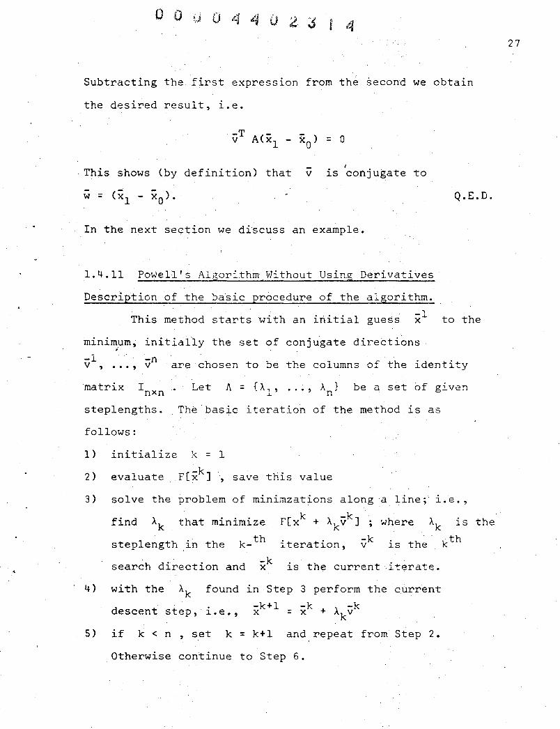
Subtracting the first expreSSlon from the ~econd we obtain
the desired result, l.e.
-v J
is conjugate to . This sho~s (by definition) that
W = (xl - xO). Q.E.D.
In the next section we discuss an example.
1.4.11 Powell's Algorithm Without Using Derivatives
Description of the ba~ic pr6cedure of the algorithm.
This method starts with an initial guess -1 x to the
minimum, initially the set of conjugate directions , -1 -n v , •.. , v are chosen to be the columns of the identity
matrix Inxn' Let A = 0.'1' ••• , An} be a set of gi. ven
steplengths. The'basic iteration of the method is as
follows:
1) initialize k = 1
) ~t[x-kJ , . 2 evaluate save thlS value
3) solve the problem of minimzations along aline; i.e.,
, 4)
find Ak that minimize
steplength in the k_th
search direction and xk
[ k -k J F x + AkV ; where Ak 1S
. . -k. h'· th lteratlon, v lS t e K
is the current iterate.
with the Ak
descent step,
found in Step 3 perform the current
-k+l -k -k i.e., x = x + AkV
5) if k < n ,set k = k+l and repeat from Step 2.
Otherwise continue to Step 6.
the
27

6) if I xr: - x. I < €. , i = 1, ... , n where € . are l l l l
predetermined m~nlmum steplength values, terminate the
iteration. Otherwise continue to Step 7.
7) find the integer j , 1 ~ j ~ n such that
=
9) if either
10)
F3 ~ Fl or
The present n-directions -1 v ,
and used in the next iteration.
... , Set
-n v will be retained
-1 -n x = x ,k = 1
repeat from Step 2. Otherwise continue to Step 10. A
set v =
" A such s '" of >.. s
(-n -1) " A
x -x v = (V l '
that -n " " F[x +>.. v ] s s . is
set
-1 x n "" = x + A·v s s
" ... , v ) n and find
a minimum with this value
11) determine the new set of conjugate directions, l.e.
{-l v , fool ••• , v , ... , n-l " v ,v}
The current direction v j for J found in Step 7 is
discarded, and a new direction, v obtained In Step 10
is added set k = 1 and repeat from Step 2.
28

0 ... 0'.'. . n .0., .. 1 . i.P u '~ '1 (J 'I ~4:."<' d!. \J
The above.method was first implemerited by Powell [1964J
It turned out that this procedure generates linearly
dependent directions, which causes difficulties in the
implementation of the algorithm. Powell [1944], Zangwill
[1967] and Brent [19}3] modified the algorithm to overcome
this problem.
1.4.12 Conjugate Gradient Techniques
The conjugate gradient techniques result from
combining the conjugate method with first order gradient
methods.
These techniques use a sequence of descent steps
rather than individual steps. The gradient of rei] , VF[iJ,
is used to generate conjugate directions. The method is
designed for quadratic objective functions or for
algebraic functions that can be approximated by a
quadratic function. Thus the method will generate mutually
conjugate directions with respect to any po~itive definite
matrix A, corresponding to the quadratic function
[ -J -T- 1 -T -F x = a + b x : 2 x Ax
where a lS a constant - _. n x,b E JR , A E GL(n). The minimum
sought i* will have to satisfy
Hence the problem of finding the unlque solution i* of
Ax + b = a is equivalent to finding the
29

min [1.1]
It turned out that finding -.'. X" by solving the linear system
is much more computational demanding than to minimize [1.1],
since [l.U is only a local approximation of F and
-a and b as well as A vary with x.
We shall examine now the process of solving the
minimization problem when F[xJ is quadratic, using
conjugate and gradient directions. There exist several
methods using this general approach: first a me-thod
developed by Fletcher a~d Reeves [1964], secOnd, the
"supermemory gradient method", Miele and Cantrell [1969],
Gragg and Levy [1969] and third, the "projected gradient
method", Myers [1968J, Pearson [1969], Sorenson [1969].
Since the method of Fletcher and Reeves [1964] has
been tested intensively we will outline the basic iteration
of the technique.
1.4.13 Fletcher and Reeves Algorithm [1964]
The descent direction of the method:
Let -0 -1 -k-l . -k .s , s , .•• , s ,s be conjugate directions
defined by the recurrence formula:
where
-0 s VF[x]
-k -s = - VF[x] + k . I s1-
i=l
i-I s
Si are chosen to be scalars such that -k s is
conjugate to all previously used descent directions,
30

-0 s , . . . , -k-l s The formula for
6
1 "'· u •
31
ak = [VF[xkJJTVF[xkJ
[VF[xk-1JJTVF[xk-1J [1.2J
The iteration pf the method is,:
1)
2)
3)
Let Ik, = {,k ,k} H 1\1' ••• ,1\ n, be a set of given steplengths,
-0 '-0 glven x ,evaluate F[x J, set k = O.
find the gradient at -k -k J x ,i.e. VF[x
if 'k OVF[x]ll less than the predetermined' toler~nce.
Terminate the iteration. Otherwise continue to Step 4.
4) find the descent direction for the kthiteration, i.e.
6)
-k -k J ~ k-l s = - VF[x + a s
ak is found from formula [1. 2J
normalize -k s ,l.e.
k-k use A s found in Step 5 to perform a descent steep
i.e.
-k+l x =
7) evaluate F[xk+1J
8) if < E E a predetermined improvement
value and'nAk~kU < T T a predeterminedsteplength.
Terminate the iteration. Otherwise go to Step 9.
9) A t th " "t x-k +l ,and l"f k' < n ,set ccep e pOln k = k+l
otherwise set -0 -k+l x = x ; k = 0 ; in both cases repeat
from Step 2.

1.4.14 Variable Metric Techniques
These methods involve finding conjugate directions that
under certain conditions approach second order gradient
directions (see page 23). They are referred to in
the literature as quasi-second order or quasi-Newton tech~
niques. An impoytant contribution in the area of descent
techniques was made by Davidon [1959J and extended by
Fletcher and Powell [1963J. Good references dealing with the
theoretical and practical aspects of these techniques have
been published by Adachi [1971J, Huang [1970], Huang and
Levy [1970J, Pearson [1969J.
As we mentioned earlier, the gradient techniques
differ basically in the choice of the matrix Ak , The variable
metric techniques start with an arbitrary positive definite
matrix; in most cases AO = I, the nXn dimensional identity
.... 1 T matrix and ln each of the following stepsAk = Ak +l of
the matrix is updated.
The basic iteration procedure is:
a) given a point -0 x and a positive definite m<;itrix. AO
(in most cases AO = I) , set k = 0 and compute -0 J VF[x .
b) Obtain new point -k+l from the point ·-k obtained a x x
from the k_th iteration according to
where we have to find Ak that minimizes
-k T -k F[x - AA VF[x ]]. K
32

..
0 0 t"j 0 jl;i t1 0 "11 3 , 7 ! €.
c) Compute the gradient at -k+l x , l.e.
d) Update inverse of the matrix to obtain Ak +l • The
various methods in this class differ in the manner
in which they update Ak .
e) Set k = k+l repeat from Step b.
The descent direction -k s
metric techniques are computed by
-k s
used in the variable
As we mentioned earlier the method by Davidon Fletcher
and Powell is of major importance hence we will outline
the main iteration step of their technique.
1.4.15 Davidon-Fletcher-Powell Variable Ivletric Techniq~
The basic iteration of the method consists of:
a) Obtain the value of the objective function F[xO] at
a given point -0 set k 0 x =
b) Compute the gradient at the point -k i. e. x ,
'V F[xk]
c) Compute the matrix Hk , (where Hk is the inverse of
the matrix ~k)
c l ) For the initial step HO = I, the n n identity matrix.
Go to Step d. For k > 0 go to c 2 •
c2
) The updating of Hk lS obtained using
33

where
and where
-k+l = x
( -k)T-k AX Y
-k x and
-k -k T (Hky )(Hky )
(yk)T Hkyk
d) Compute the descent direction sk according to
and normalize
-k s
e) Calculate the normalized derivative of the objective
f)
r[x- k ] function in the descent direction
If
Tk = l(sk)T vr[xk]1 AV r[xkJII
terminate iteration.
(E l , E2 are predetermined tolerances). Otherwise
go to g.
g) If (sk)T V r[xk ] > 0 set sk - - sk and reset Hk
to Hk = Inxn
h) Solve the problem of minimization along ~he line
i)
xk + Ask l.e. find Ak that minimizes rexk + Ask]
Define -k -k-k AX = A s
j) Obtain a new point according to
-k+l x =
34

k)
m)
0 0 ';) 0 .(Ii 1 &:;i
'i 0 4£ ~'·.l
.;) 8
Evaluate the objective function at the point
i.e. F[Xk +l ].
-k+l x
terminate
the iteration. (e l is predetermined minimal improve-
ment of the function and 82 ~s
lengtl"!) • Otherwise go to m.
Accept the point -k+l and if x
otherwise ~et k = a , xO -k+l = x
a predetermined step-
k < n set k = k+l;
Repeat from Step b.
There exist variants of the variables metric methods
and some of those have been proposed by Broyden [1967J,
[1970], Huang [1970], Pearson [1969], Greenstadt [1970a,bJ,
Goldfarb [1970J, an~ Murtach and Sargeant [1970].
In general the variable metric techniques perform
better for general non-quadratic functions than many other
quadratically convergent methods.
These methods have the advantage of fast convergence
near the minimum.
1.4.16 Other Algorithms Considered
A) Two prominent algorithms have recently been the
subject ofa paper by E. Polack [ 70 J. In that paper
a comparison of his method, a gradient secant method, with
the Brents~Shananskii discrete Newton algorith is made.
Two fifty dimensional problems are discussed. It is of
interest to compare their results with the'performance of
Bremermann's optimizer on problems having many variables.
To this end we are introdu~ing these two algorithms. The
.35
full descriptions of these methods can be found Vla the
aforementioned paper.
B) Since root-finding for algebraic objective
functions is a special case of minimization we would like
to mention a new technique developed by S. Smale. He has
developed "A Global Newton Ralphson" method for.finding
a zero of a system of non-linear algebraic equations.
The algorithm is still in its early developments and it
isa very promising method on the basis of its performance
on some. test problems. The algorithm views a system of
non-linear algebraic equations as a system of non-linear
ordinary differential equations, and using concepts of
global analysis it is able to follow the trajectories which . .
will lead to a zero of the system.
1.5 BREMERMI\.NN'S ALGORITHM (THE "OPTIMIZER") [1970]
This method was developed by Bremermann and grew
out of simulation of biological evolution as a search and
optimization process.
Bremermann observed that the computa.tional cost of
elaborate choices of search or descent directions often
exceeds the benefits derived from it. He observed that by
searching along randomly chosen directions (rather than
along computed directions) the overall speed ofconvergenc~
(in computer time) is faster than when he searched along
gradients. In the following material we will investigate
36
this phenomena, not only in comparison with gradients but
with respect to a representative sample of all the methods
described so far.
This method finds the global maximum or minimum
of an objective functi6n with a polynomial of degree four
or less of many variables. The method is iterative and
theoretically guaranteed to converge for polynomials of
several variables up to the fourth degree. A detailed
theo~etical analysis of the optimizer's convergence
properties, and other theoretical considerations can be
found in [llJ.
Description of the Method
1) F is evaluated for the initial estimate -(0) x
2) A random direction R is chosen. The probability
3)
distribution of the R is an n-dimensional Gaussian
wi th a 1 = a 2 =. a. is the standard 1
deviation of the ith coordinate.
On the line determined by -(0) x and R the restriction
of F to this line is approximated by five-point
Lagrangian interpolation, centered at x(O) and
equidistant with distance H, the preset step length
parameter.
4) The Lagrangian interpolation of the restriction of F
is a fourth-degree polynomial in a parameter A
describing the line xO + AR • (It describes F
exactly, up to round-off errors, if F 15 a fourth-
order function.) The five coefficients of the Lagrangian
37

interpolation polynomial are determined.
5) The derivative of the interpolation polynomial is a
third-degree polynomial. It has one or three real
roots. The roots are computed by Cardan's formula.
6) If there is one root ~O ' the procedure is iterated
from the point x(O) +~OR with a new random direction
provided that F(x(O) + ~OR) 2 F(x(O». If the latter
inequality does not hold, then the method is iterated
from -0 x with a new random direction.
7) When there are three real roots ~l' ~2 ' ~3 ,then
the pOlynomial (or F ) is evaluated at
-(0) ~ R x(O) - -(0) x + + ~2R , and x + ~3R . Also 1 I
considering the value F(x(O» , the procedure lS
iterated from the point where F has the smallest value
(if F has a minimum value at'more than one point, then
the procedure chooses one of them).
8) When a predetermined number of iterations has been run,
the method is stopped and the value of F and the value
of -x are printed.
A FORTRAN program implementing the procedure is
listed in the Appendix.
Features of the optimizer
1) Preparation of a problem for use with Bremermann's
optimizer is easy. It consists of:
a) the optimizer requires a subroutine that
evaluates F at any desired point.
38

o 0 U 2: o
b) Very few changes have to be made to optimize
different functions (i.e., number of variables,
number of iterations, a steplength parameter)
besides providing a routine that computes the
objectivefuhction F[il.
2) It does not require close initial estimates for
convergence to the global minimum.
3) It does not require the gradient or Hessian of an
objective function. Hence the optimizer can be
applied with a minimum of effort.
1.6 TEST PROBLEMS
When developing an algorithm we have to be concerned
with the theoretical as well as with the practical properties
of the method. The best way to verify how well it
performed is to actually try to solve specific problems.
In the field of optimization some functions having
pathological properties were formualted with the intention
of determining how well an algorithm is able to overcome
various difficulties. Examples of difficulties include:
local minima, number of variables, slow speed of conver-
gence, accuracy of the result obtained, singular Jacobian
or Hessian and ill conditioned problems.
Historically these functions carry the name of their
originators or the name of the particular difficulty inherent
39

in the problem. (e.g. Rosenbrook 1960, Singular Powell 1964).
The purpose of formulating these functions is to test how
robust is an algorithm in a wide range of different Droblems.
To this erid we have compiled eleve~ known test problems
which, in the literature, are considered difficult to
optimize.
The test p~oblems in this Chapter were obtained from
a) D. M. Himmelblau's paper "A uniform evaluation of
unconstrained optimization techniques"; b) Richard Brent's
book, "Algorithm for minimization without derivatives"; and
c) E. Polak's paper, "A modified secant method for
unconstrained minimization".
40

o a 044 0 ~ ~ 2
The Test Problems are:
1. Rosenbrook 1960:
Descent methods tend to fall into a parabolic valley
2.
before reaching the true minimum at (1,1).
Beale 1956: F[x] = 3 • 2 I [c o -x
l(1-x 1
2 )] .0 1 1 1=
where c 1 = 1.5 , c 2 = 2.25 , c 3 = 2.626
minima is F[x] = 0 at x = (3, 1/2).
The global
[ -] 4 + 4 + 2 2 3. Engwall 1966: F x = xl x 2 2xl x 2
The global minima is F[x] = ° at -. x = (1,0).
4. Zangwill 1967: F[x] = (1/15) [16xi + 16X~ - 8x1 x 2 - 56xl -
The global minima is
5. Zangwill 1967: F[x]
The global minima is
6. Engvall 1966: F[x]
flex) 2 + 2
= Xl x 2
f2~x) 2 + x 2 = Xl 2
f3(x) = Xl + x
2
f4
(x) = Xl + x2
fs(x) 3 2 = Xl + 3x2
2S6x. + 991] 1
F[x] = -18.2 at the point
F[ x] = ° -at x = (0,0,0) .
5 2 -= I fi(x) where
i=l
+ 2 -1 x3
+ (x3-2) 2 - I
+ x3 I
- x3 + 1
2 36 + (Sx3-x
l+l) -
-x = (4,9).
41

Global minima lS F[i] = ° at x = (0,0,1) .
7. Fletcher and Powell 1964:
8 .
1
x global minima is F[x] = 3
0.78547, 0.78547).
Wood:
+ exp
-at x = (0.78547,
3· (1-x3
) +
This function has a local minima that may interfere in
finding the global one. Global minima is F[x] = ° -at x = (1,1,1,1) .
9. Singular (Powell 1962):
. 2 244 F(x) = (xl
+lOx2
) + 5(x3-x4 ) + (x2-2x 3) + lO(xl-x4 )
In this function most of the known algorithms failed
to pass the stopping criterion since the Hessian at the
-.minimum value 0 lS doubly singular. Global mlnlmum
lS rex] = ° x = (0,0,0,0)
10. Rosenbrook: 50 dimensional "banana"
42

o 0
43
+
+ 2 24 2 I (x. - x~+l) . +
i=20 ~ .40
+ +
+ 3 I9 [X. i= 30 . ~
+
20 4 + 2 I (x.-xSl_·)
i=l ~ ~
25 4 I (x,-xSl_o)
i= 21 ~ ~ +
Global minima is F[x] = 0 -at x = 0
11. "Bowl" Type. 50 dimensional
. F(x) (1 -0 xII 2 /100 )' = - e
Global minima is F[x] = 0 -at x = 0 .
1.6.1 Algorithms .Used ln the Comparison with the Optimizer
For the purpose of comparing the optimizer performance
on the test problem, having up to 4-variables we have
chosen IS prominent algorithms. Our basis for the comparison
will be the results obtained by D. M. Himmelblau in his
paper, "A uniform evaluation of uncons"trained optimization
techniques"
Detailed descriptions of each technique are not
included and the reader is referred to proper references
at the end of this chapter.
The IS algorithms will be classified into two
categories:
a) Algorithms using analytical derivatives
b) Derivative free algorithms
Algorithms uSlnganalytical derivatives
The algorithm used were:
1) DPF Davidon-Fletcher-Powell Rank 2 (Fletcher, Powell 1963)
2) B Broyden (Rank 1) 1965
3) P2 Pearson No.2 (1969) without reset
4) P3 Pearson No.3 (1969) without reset
5) PN Projected Newton (Pearson) 1969
6) FR Fletcher Reeves (1964) reset each n+l iteration
7) CPContinued Partan (Shah et. a. 1964)
8). IP Iterated Partan (Shah et. a1. 1964)
9) GP Goldstein-Price 1967
10) F Fletcher 1970
44

O 0\ '.~ '. ~
45
Derivatives Free Algorithms
11) HJ Hooke-Jeeves (1961)
12) NM NeIder-Mead (1965)
13) P Powell (1964)
14) R Rosenbrook (19~0)
15) S Stewa~t (DPF with numerical derivatives) 1967
All algorithms in the comparison performed by Himmelblau 'V1
were tested ln a CDC 6600 computer. Bremermann's optimizer
performance on the test problems was also tested on a CDC 6600
computer, though ina different facility.
In using the optimizer on large dimensional problems,
we chose to compare it with the ~esults obtained by E. Polak
ln his paper "A modified secant method for unconstrained
minimization" [1973]. In this paper a new gradient-secant
method is presented, and its performance on two 50-dimensional
problems is compared with Brent-Shamanskii's discrete
Newton Algorithm
E. Polak shows that his algorithm is superior to most
of the various conjugate gradient methods described ln the
literature; he also has a heuristic argument to justify his
method's superiority over the variable metric techniques.
Morever, the paper compares the Brent-Shamanskii algorithm
with his method and he concludes that the new gradient-
secant method will emerge "as one of the more efficient
methods for the solution of certain classes of unconstrained
optimization problems". A full theoretical discussion of
both methods is given in

The methods., compared by E. Polak wer,e .'~e8t~d ~:.on a CDC '.' ""': ........ - ~.-~p
6400 in the computer facility of U.C. Berkeley. " "
Our comparison with Polak's results were obtained uSlng
the same computer and facilities.
1.6.2 Discussion .. "-; ?- *./ ~ ." ,':} ...
In order to compare Bremermann's optimizer with other
algori thms:;'it is: n.ecessary to. det,epmine a criterion bY,whic,h
all the:algorithms:, lcan;rb.e;,fairly,compar;ed~',
, In the literature.' [581, .[59J, [71J, the most ['.
conunon points for comparison ,are:
1) The ,number of ; function ':eval Uq:t ionsreq uired to-obtain
the:~iriimum'withirtta'predeterm~ned accuracy
2) How robustris>the.'method (correct ~ol,ution on a.wide
number of test~problems).
3) Number of iterations.
4) 'Total computational time required to obtain the desired
optimum value.
'i, ' !
) j .,.~ r," .,;:' _ ...... .: .
l).Function.Evaluations. (] ,"'to '.' ~.' •
This criterion ~as different .- ~ .
meanings for different.authors. Some consider the evaluation . .,' J •• " ~ •• ~"J ' '; '-:; ---r :", .. ': !j ~ :. J ~. • r c·
of a Jacobian 91' Hessian as one f~nction evaluation, while ln ,~ ., .
fact a nxl Jacobian requlres. ~ function evaluations and a ~ : :.) '- : 0: ;'. r" • ... oJ ~ I
nxl Hessian+r~q~ires n2
function evaluation. Furthermore, J,. .'" r ....
"
it is po~sibl~.to re9~ce :hei~umber of functions evaluation
by a diff~rep~,~im~~consuming,~est, such as: matrix operations,
heuristic operations, numerical derivatives, etc. Therefore t
1 ,
46

0 0 ~ ~ :~.Ji 0 4 "I 0 ~ J :2 .f,;,~
47
we should be very cautious when considering function evalua-
tion as the sole criterion for a comparison.
2) To determine how robust an algorithm is, it is
necessary to test it in a wide range of problems. Each of
these problems exhibits a particular difficulty which an
algorithm must overcome. The algorithms used for the comparison
including the optimizer, were applied to eleven test problems,
which are considered as "classics" in the literature. It is
important to emphasize that eVen though an algorithm might
solve all eleven of the test problems, it is very possible
that there are pathological objective functions for that algo-
rithm.
3) The criterion for comparison based on number of
,> iterations is very misleading since it means search directions
in variable metric techniques and conjugate methods, but has
a different meaning in the others. In particular an iteration
step in methods using conjugate directions will have a substep
of minimizing along a line k -k x + AS ,i. e. Ak such
. ... F[x-k + 's-k] . . that m1n1m1ze A, wh1le other methods, llke
Bremermann's optimizer, consider such a line minimization to
be a single iteration of the procedure, therefore, when we
interprete results in the literature we should always understand
what is meant by the "number of iterations" required to obtain
the global minimum in any comparison between algorithms.
4) By the total computational time: we mean the actual
time required to run an algorithm on a specified computer.
This time will include the time for: function evaluations,

derivatives evaluations, matrix inversions, and. Heuristic
operations, etc. It is of interest to note that in 1968,
A. R. Colville after comparing thirty different algorithms on
eight optimization problems found that totoal computational
time is a more valid performance index than the number of
function evaluations alone.
1.6.3 Effects of the Computer on the Results
When comparing distinct algorithms, we should be avlare
that the numerical results were possibly obtained on different
computers having different machine precision. To determine
the effect on the results, due to such computer differences 0e
tested Bremermann~s optimizer on a CDC 6400, 'CDC 6600 and
CDD 7500 computers. All of these have the same precision.
The results of this comparison are recorded in Table [l.OJ.
Central processing time is used for comparing the
performance of various algorithms on different computers.
The purpose of this comparison is to show that the time i.e.
central processing time, can be varied over a large ~ange
simply by varying the computer; in later sections, we use
central processing time on the ~ computer as a tool for'
comparison of optimization algorithms.
1.6.4 Test Procedure
a) Dimensionality of the Problems
In the literature of optimization comparison among
algorithms has concentrated primarilly on test functions of
48

..
Table 1.0
Comparison of Central Processing Time (in seconds) when Bremermann's Optimizer is Used on a Variety of Problems with Various Computers
COMPUTER PROBLEM
50 Dimensional 50 Dimensional 2 DIM . 2 DIM Fletcher & "Banana" Type "Bowl" Type Zangwi11 Rosenbrook Beale Engwall Zangwi11 Engwall Singu1a! Powell
(1967) (1960) (1958) (1966) (1967) (1966)
CDC 6400 15.345 9.809 0.032 0.295 0.196 ! 0.167 0.136 0.923 Computer
CDC 6600 4.110 2.378 0.008 0.076 0.039 0.038 0.023 0.180 Computer
CDC 7600 0.688 0.432 Computer
The termination criteria are given in page 5 O.
The number of iterations for a particular problem did,not vary from computer to computer.
(1962)
0.056
0.023
(1963)
0.041
0.013
~ ill
0
0
' , c &-
.tL
C
r'< "", CA~
B\.:;;
0':

a few variables, usually less than five. When a particular
algorithm is applied to problems of a few variables we elude
the difficulty of dimensionality. For example, in methods
where second derivatives are required, the process for
obtaining analytical derivatives may be humanly impossible,
(for n = 100 the Hessian has 10.000 terms) while numerical
differentiation may introduce errors. Furthermore, the
inversion of a Hessian matrix can be time consuming and
inaccurate, in particular, if the process is iterative and
at each iteration an inversion of Hess[i] is performed.
To take into account the problem of dimensionality we
shall consider the following two classes of optimization
problems:
a) Problems with up to four variables
b) 50 dimensional problems
b) Termination Criteria
Each class of problems will have the same termination
criteria. For functions of up to four variables termination
will occur when both of the following conditions are
satisfied:
if x* ~s the true minimum then
and
where k denotes the k_th iteration.
50

o 0 u ") ·6·· "-
51
These conditions were set by Himmelblau wheri comparing its
leading algorithms on test problems with up to four
variations. For functions of 50 variables, termination will
occur when:
and
These conditions were set by Polak when he compared his method,
Ita new secant method ll, with Brent-Shamanskii algorithm.
1.6.5 Results Obtained with Bremermann's Optimizer
The results on functions of 50-variables were obtained
using a CDC-6400 computer in the Computer Center of the
University of California at Berkeley.
The·results are recorded in the following tables.

Table 1.1
RESULTS OBTAINED ON T\!JO 50 DIMENSIONAL TEST PROBLEHS
USING BREl1EFl1ANN I S OPTIMIZER
ON THE CDC 6400 COMPUTER
ROSENBROOK 50- DIMENS IONAL BANk\JA TYPE
INITIAL FUNCTION VALUE -. F.[xO] = 1019,004 .
FINAL FUNCTIOi"! VALU2 = F[x] = 55,736 E-20 ,,¢
OBTAINED
GLOBAL 11AX I I1lJ ;-1 SOUGHT = F[x] = 0
Iteration # F[x] Iteration # I F[x]
20 I 49,400 180 2,3092 E-8 i 40 ! 2,492 200 I 9,611 E-l0
I !
60 1,690 E-l 220 ! 1,654 E-l1 I
i
80 2,575 E-2 240 1,526 E-12
100 3,566.E-3 260 4,500 E-15
120 4,235 E-4 280 3 ) 17 5 E-18
140 4,917 E-5 300 6,573 E-20
160 1,641 E-6
*In this and the following tables E-n, n any integer,
will denote 10-n for example 65,736x-20 = 65,736 x lO- 20
52
I I
53
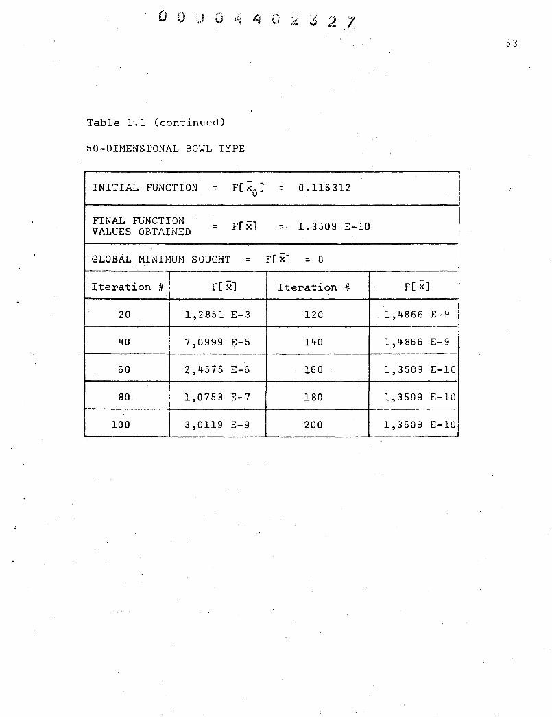
Table 1.1 (continued)
50-DIMENSIONAL BOWL TYPE
INITIAL FUNCTION = F[xO
] = 0.116312
FINAL. FUNCTION = F[ x] 1.3509 E-10 VALUES OBTAINED - ,
GLOBAL MIHIMUM SOUGHT = F[ x] = 0
Iteration # F[ x1 Iteration # F[ x]
20 1,2851 E-3 120 1,4866 E-9
40 7,0999 E-5 140 1,4866 E-9
60 2,4575 E-6 160 1,3509 E-IO
80 1,0753 E-7 180 1,3509 E-I0
100 3,0119 E-9 200 1,3509 E-I0

F U N C T I 0 N
V A ,. !..I
U E
0 B T A I N E D
104
10 3
10 2
10 1
10
1
10-1
10- 2
10- 3
10-4
10- 5
10- 6
10- 7
10- 8
10-9
10- 10
10-11
10- 12
10-13
10-14
10-15
10-16
10-17
10-18
10-19
10- 20
FUNCTION VALUE OBTAI~ED VS. NUHBER OF ITE?ATION FOR T':JO 50 DHiENSIONAL PROBLEMS
I
~ \
I I
! \ I
I I I
., ~ '" .. i I.-
(' 'I"~JL
I
.~ ~.\. I :....
~~, 1 ~, ! i I ! I !
~ --:
~j[, I i 1 i h !
\.~~ ~~.I i i h
~~ I
-/I~~ I I
I 1 I i , 1 !
,
., I 1\ I
0/1\ , :
i i l I
\ I \~ ,
I : > ,--" •• ,. _ ... -.-.~ .... - .-.- - "1 i
I. I \ 1\ :
i I ., I
, I ... -h i
I . h r:\. .~-. "'.
1 '-I ~ ! \\1 I
1 .. , I
" , .. 1 :'\ A !
.. ' . .. · .. · .. ··1 ' . . - .. ... ;.r .. .... y
·N - ...
I I I I , ~
l i I
I I i I
I
I
i I !
I
I I I
I
I ! I 1
"
i· I
!
i
i
I~. "O~ i ~ '1 /N -....... .. " .... -- . .. ... - .. ...
1 I
I I I i I I
r,
i I
I I
I i I I
, I i I i I ,
I I j ,
I I ! I
! ! I I i 1
I I I
I I ! !
I ! i ,
J : I ,
I ! I I I
54
I I I
I I ! !
I
I
I I
I 1 : ! I I i I I
I 1 1 I
I I I
L I i I , i
, I
I I ! \
! I
I ! , , . i
i I
l ! ." !
i ! i I ]
1 I
I i I
I I
I .. 'I "
I
! , ! !
\ i j i :
\~ i !
I
! " : i I !
i \ I ! \ I \1
, ! i
---/
I \ I \\
o 20 40 60 80 100 120 140 160 180 200 220 240 260 280 300
NUMBER OF ITERATION
x - "Banana" Type o - "Bowl" Type
Table 1.2 Graphic Representation of Table 1.1

PROBLEMS PRESENTED
1. Zangwill (1967)
2. FLETCHER-POWELL (1963)
3. POWELL SINGULAR (1962)
~. ZANGWILL (1966)
5. BEALE (1958)
6. ROSENBROOK INITIAL VALUES (-1.2, 1)
7. ROSENBROOK WITH INITIAL VALUES (3.2, 5.1)
8. ENGVALL (1966)
9. WOOD
80 100
NUMBER OF ITERATIONS
Table 1.2: Graphic Representation of Table 1.1.
Results obtained using Bremermann's optimizer on several test problems.
5S

Table 1. 3
Rosenbrook (1960)
Initial Values
Final Values Obtained
True Values
Iteration No.
o 20
40
60
80
100
Function Values
10
10- 3
.10- 6
10-9
Xl = 1.0000000240
= 1.0000004770·
X = 1 1
Objective Function Value
F[x]
24.2
0.534
3.621 E'" -,)
5.576 E~6
4.771 E-9
5.863 E-12
j i ,
i I I
·1 I I
I I I
I I
-I
I i I I I , j-
lO-12~ __ ~ __ ~ ____ ~ __ ~ ____ ~ __ ~
o 20 40 60 90 100 Iteration
· 56
\

Function Values
0 j,':'-""
,,) 0 <iiI di U li
Table 1.4
Rosenbrook (1960)
Initial Value
Final Values Obtained
True Values
Iteration No.
0
20
40
60
80
100
It 1 u
2 ! 0
1 0
-1 1 0
10-3
-6 1 0
.. 7 1 0
-I ! 0
-I 1 ! 0
20 It 0
0 «',I ~-.i
:2 9 '" V s;~
57
- (-3 . 2 ,5 .1) x =
x- = 0.99999995710 1
x2 = 099999986980'
xl = 1 x = 1 2
Objective Function Value F[x]
2646.8
0.512
1.467 E-2
5.931 E-4
1.522 ... E-S
1.S67 E-ll
60 80 1 II 0 Iterations

Table 1. 5
Beale (1958)
Initial Values
,-
Final Values Obtained
True Values
Iteration No.
0
20
40
60
80
100
Function I Values
1
10-6
10-9
10-12
20 "'4
58
-x = (I,8)
xl = 3.0000000026
x2
-. 4.9999999922
xl = 3 x 2 = 2.5
Objective Function Value F[x]
9.828869
0.149
7.,027
1.796
2.117
2.111
Iterations

DOl) Ot.~
Table 1.6
Engvall (1966)
Initial Values -- (5,2) x =
Final Values xl .. =' 10000003008 Obtained x 2 = 0.0000640257
True Values xl = 1
'X2 = 0
Iteration Objective Function Number Value
F[x]
0 19.0625
20 3.375 E-3
40 3.165 E-4
60 1.647 . E-4
SO S.295 E-6
100 8.199 E-6
Function Values 102
1
10-2
10-4
10-6 ~~--~--~----~--~----~------o 20 40 60 80 100
Iterations
59

Table 1. 7
Zangwill (1967)
I Initial Values - ( 3 ,8 ) x = !
Final 3.9999992813 Values xl = Obtained
,x 2 9 . 00000'3345 .-
True Values x = l~' 1
x2 = 9
Iteration Objective Function Number Value
0 -16.6
10 -18.2
Function Values
-16.2
I -18.2---~~~~4~O---~--~---~----------
Iterations
60

Function Values
o 0 ',i1
Table 1.8
Zangwill (1967)
Initial Values - (100,-1,2.5) x = ,
Final Values xl = -1+.5963931176 E-8 Obtained x2 = -3.952316521+6 E-9
x3 = 7.61+03466058 E-9
True Values xl = 0 ~ = a X3 = 0
Iteration Objective Function Value F[xJ Number
0
20
1+0
60 "-
1
10- 3
10-6
10-9
10-12
29,726
9,496 E-7
1,455 E-12
6,959 E-15
10-1~5~ __ ~ ____ ~ __ ~ __ ~ ____ ~ __ _ o 1+0 60 100
Iterations
61

Table 1.9
Engvall (19.6 6 )
Initial Values
Final Values Obtained
True Values
J
0
40
80
120
160
200
Function Values -1
10
10- 3
10- 5
10- 7
10--g
- (1,2 ;0) x =
xl = 0.0000063
x2 = 0.0000007
x3 = 1.0000032
- (0 ,0 ,1) x =
F[x]
2.424 £-2
8.302 E-3
1.482 E-3
4.101 E-5
7.891 £-8
1. 007 £-11
I ,
I I
i .!
10-11 ~0----~----~----~~--~1~6~0~~~2~0~0----
Iterations
62

Table 1.10
Fletcher
Initial Values
Final Values Obtained
True Values
J
0
9
Function Values
&
63
Powell '(1963)
xl = -1
x 2 = a
x3 = a
Xl = 1
x 2 = a I I
I x3 = a I
I i
- (1,0,0) I X = I
i !
F[x] 1 I
" I 2500
0
40 60 80
Iteration

TableL 11
Powell Singular (1964)
Initial Values
Final Values Obtained
True· Values
J
0
20
Function Values 10 3
1
10 -: 3 -
-6 ~ 10
-9 10 -
.-
- (3,-1,0,1) x =
Xl = -1,00065692829
x 2 1,00065692869
x3 = ° x 4 = -2,7535001022
Xl = a X2 = ° x3 = 0 x
4 = 0
F[x]
215
4.816
10 -15 '-. ---..lIF-----+-----+-~1-o 20 40 60 80
Iterations
64
E-4
I E-5
E-8

o 0
1.6.6 The Comparison of Bremermann's Optimizer with
other Algorithms
A. In the comparison on the 50-dimensional problems,
Bremermann's optimizer clearly performed better than the
Brent-Shamanskii method and the new gradient-secant
method.
The Rosenbrook Banana Type (Tables 1.12, 1.13)
in central processing time (C.P.U.) on the CDC 6400 computer,
the optimizer is twice as fast as the Brent Shamanskii method,
and three times faster than the new gradient~secant method.
The optimizer needed 16,044 fewer function evaluations
than the Secant method and 8,050 less than the Brent-Shamanskii
method. (Note: Here clearly furiction evaluation is not a
good criteria for comparison.)
The 50-Dimensional Bowl Type (Tables 1.12, 1.14)
Here again the optimizer performed better in terms of
both time and number of function evaluations. The optimizer
needed 1,043 function evaluations compared to 9,093 and 9,771
for the Brent Shamanskii method and the new Secant method,
respectively.
B. In the problems with up to 4 variables the optimizer
proved itself a robust method on the given-test problems.
It was a little slower than Fletcher's method in terms of
time comparison, but in all problems was comparable to those
algorithms which are generally classified in the literature
as "good algorithms", Himmelblau [1973]. The results are
65

Tablel.12 RESULTS OF OPTIMIZER ON SO~DIMENSIONAL PROBLEMS TESTED ON A CDC 640D COMPUTER
. All proble~s satisfied the stopping criteria, i.e. F[ x]<::_ '10-:-10 I x k -xk+ 11.s.'10- 6
Function
Rosenbrook 50-dimensional type "Banana"
50-dimensional Bowl type
I ,.
Number of Variables
50
50
Initial Function Value
Fex} = 1.019
F[x] = 0.1163
",
Number of Iterations
199
149
Computat ional Processing Time (in seconds)
15.3
9.8
Solution
X. = 0, ). .
i=1, ... ,50
X. = 5 ). . , i = 1, ... ,50
<J)
(J)

Tab1f> 1.13 COMPARATIVE RESULTS ON THE 50-DIMENSIONAL ROSENBROOK TYPE "BANANA"
Method
Brent-Shamanskii (B-S)
New Secnnt Method (SEC)
Bremermann's Optimizer
(OPTIM)
Method
B-S
SFC
OPTIM
Number of Iterations
58
170
199
Initial Value of NF[xo]B
441
441
1.019 x 10 3
Number of Function Evaluations
9,,443
17,537
1,393
Computation was Terminated when
D - U - 9 . 'V'F [ x . ] < 10 . ~
i = 1, ... , 50
H\7F[x.]11 < 10- 9 ~
i = 1, ... ,50
UF[x]ll <10- 9
and
Ixk-xk +1 ' < 10-6
C.P.U. Second
37.5
48.25
15.34
(j;
-.J
o c
Ct
.i~
~
Ci
F'I..:
<A
c,;..:
t.~., ~111,1,;.

Table 1.14 COMPARATIVE RESULTS ON THE 50-DIMENSIONAL FUNCTION "BOWL" TYPE
.Method
B-S
SECANT
OPTIM
Method
B-S
SEC
OPTIM
Number of Iterations
98
93
149
.Initia1 Value of "F[ioJH.
0.0047
0.0047
0.0116
Nuwber of Function Evaluations
9,093
9,771
1,043
Computation was Terminated when
HV'F[i.]II < 10- 9 1
HV'F[i.]11 < 10.,..9 1
HF[ii JIl < 10-10
and
I xk-x I· < 1 - 6 k+1 0
C.P.U. Second
, C
. ?' .. '~: ~'.
3 9c~ 7-7
16.5
9.809
(j)
ro

PROBLEM CHARACTERISTICS:
Function Number of Initia.l Values Number of Total Time Exact Valves Name Variables Chosen Iterations in Seconds Sought
Rosenbrook 2 (-1.2,1) 91 0.066 (1,1)
2 (3.2,5.1) 94 0.071 (1,1)
Engval1 (1966) 2 ( 5,2 ) 46 0.032 (1,0)
Zangwil1 (1967) 2 (3,8) 11 0.008 (4,9)
Beale (1958) 2 (1,8) 53 0.030 ( 3 ,5)
Zangwil1 (1967) 3 (100,-1,2.5) 35 0.020, (0,0,0)
Fletcher & Powell (1967) 3 (-1,0,0) 9 0.013 (1,0,0)
Engvall 3 (1,2,0) 115 0.098 (0,0,1)
Powell (1962) 4 (3,-1,01) 25 0.023 (0,0,0,0)
Wood 4 (-3,-1,-3,-1) 0.5 (1,1,1,1)
Table 1.15
Results for Test Functions with up to 4-variables using Bremermann's Optimizer
on a CDC-6600 Computer. All the problems satisfied the stopping criteria, . [-] - 5 1- I - 5 th. . 1.e., F x < 10 and xk-xk +1 2 10 , (where k denotes the k 1terat10n)
C) ill
0
C
'.r.:~
C
.. f::.
..h,
,rt'i.,.,' ",-.
r ... : CA.:
CN
u:

Table 1.16 Central Processing Time of the Different Algorithms on Various Test Problems With a CDC-6600 Computer (Dimension < 4)*
PROBLEM
Method Zangwill Rosenbrook Beale Using 1967 1960 1958 Derivatives
Davidon Fletcher Powell
Broyden
Projected Newton (Pearson)
Fletcher Reeves
Continued Spartan
2
.006
.008
.007
.010
(Shah et all .009
Goldstein Price
F.letcher
.007-
.004
2
.030
.031
.043
.047
.043
.027
.022
2
F**
F**
.031
.033
.041
.024
.013
Powell Fletcher Engvall Zangwill Engvall Singular & Powell
1966 1967 1966 1963 1963
Number of Variables
2
.016
.017
.017
.019
.020
.020
.008
3
.010
.017
.032
.021
.017
.019
.004
3
.028
.056
.073 .
.154
.489
.044
.022
4
.079 .r
.112
.125
.691
.536
.065
.062
4
.047
.047
.134
.222
.256
.061
.036
Wood
4
.085
.089
F**
.330
.410
.089
.024
*All the alKoJ;'ithms except Bremermann's optimizer were tested by H. Himmelblau at another -J
location. l59] 0
** F = Failed

Table 1.16 (Continued)
Z~ngwil1 Rosenbrook Beale Derivatives 1967 . 1960 1958
... .0 Free
i'? Methods
1~~~ 2 2 2
. ::"J
0 Hooke & ~ Teeves .009 .056 .024
/IV Melder & i::;;'
Mead .024 .035 .029
~'" Powell .010 .038 .021 ' ...... "'-
0 Rosenbrook .018 .053 .052
a Stewart .008 .02'6 .024
Bremermann's Optimizer .008 .066 .030
r
Powell Fletcher Engva11 Zangwi11 Engva11 Singular & Powell,
1966 1967 1966 1963 1967
Number of Variables
2 3 3 4 4
.008 .014 .012 .015 .214
.025 .096 .087 .153 .118
.017 .014 .052 .114 .017
.026 .067 .114 .183 .146
.016 .020 .048 .230 .090
.032 .020 .098 .023 .013
Wood
4
0.152
0.154
0.041
0.378
0.171
0.151
--J f-J

recorded ~n Tables
1.7 ROOT-FINDING
Given an objective function F: ]Rn-+ IR; a vector
-x = ... , Finding a minimum of F involves
soiving
aF = 0 ax:-].
i = 1, ..• , n
To find the critical point of this system, ].n particular
if this system consists of non-linear algebraic equations,
the critical point is a "zero" of the system. Hence optimi-
zation is closely related to root-finding of non-linear
algebraic equations.
The root finding problem can be stated as follows:
Given n-non-linear algebraic equations f. 1 = 1, ... , n 1
find the value x* of the n-dimensional vector x such
that
f.[x*J = 0 ].
i = 1, ... , n
There exist an extensive and detailed literature dealing
with the root-finding problem on non-linear algebraic
equations. In particular, all methods which minimize a
function in n-variables can be used for solving such systems
by minimizing ari objective F[i] such that
72

73
where the global minimum 1S obtained where F[x*] = 0
1. e . , f. [x*] = 0 1 . i = 1, .. " n . Good references can
be found in [19], and [73].
In previous sections we have compared Bremermann's
optimizer performance with fifteen prominent minimization
algorithms, We can consider a minimization procedure a
root finding algorithm,
We have further investigated the performance of
Bremermann's optimizer on various test problems including
root finding.
The following test problems were kindly furnished by
S. Smale.
1.7.1 The Test Problems were:
'J
fl[xl,x2,x3,x4'xS] = " xl + alxlxS + a
2
f2[xl,x2,x3,x4'xS] 3 + b
lx 2x S
+ b2 = x 2
f3[xl,x2,x3'~4'xS] 3 + + c2x S = x3 c l x 2x 3
f4[xl,x2,x3,x4'xS] 3 2 2 d 2x S = x 4 + dl(xl + x
3) +
fS[xl,x2,x3,x4'xS] 3 = Xs + Plxl~3 + P2x 2x 4
The initial guesses ~nd coefficients values are as follows:
Case I:
Coefficients: a l = -10, a 2 = 1, b l = 10, b2 = -1,
c I = 7 , c2 = 0, d l = -2, <12 = 0,
PI = -7, P2 = 8

74
Initial Values:
Set 1: = (1,2,3,4,5)
Set 2: " = (5,4,3,2,1)
Case II:
Coefficients: a 1 + -11, a 2 = 1, b 1 = -12, b 2 = 2,
c 1 = -13, c 2 = 3
d1 = -14, d 2 = 4, Pl = -15, P2 = 5
Initial Values:
Set 1: (xl,x2,x3,x4,x5) = (40,40,30,40,30)
" 2 : " :: ( 5 , -5, 5 , ,.. 5 ) -;:>,
" 3 : " = (-5, -5, -5, -5, -5)
" 4 : " = '( -1, 1, -1, 1, -1)
" 5 : " = (-11, -12, -13, -14, -15)
" 6 : " = (-1, 2, -4, 7 , 36)
It 7 : " = (1, 1, 1, 1, 1)
Case III:
Coefficients: a l = -0.11, a 2 = 0.1, b 1 -, -0.12, b 2 = o • 2
c 1 = -0.13, c 2 = o . 3 , d1 = -0.14, d 2 = 0.4
P1 = -0.15, P 2 = o • 5
Initial Values: Set 1 to Set 7 will have the same initial
values as th~ ones in Case II.
1.7.2 Root Finding Results
The'resultsobtained by using the optimizer are recorded
on Table 1.17.

Total Final Values Execution Time of the Objec-(in seconds) tive Function
Case I:
Set 1 2.2 [- -25 F x] < 10 and
Set 2 2.1 ,- -,. . -14 x k +1-xk .2 10
co r"l
Case II: .;0') Set 1
~"'il Set 2
o Set 3 All sets F[x] < 10-25
''f' Set 4 together' took and
-~ Set 5 13.1 sec Ixk +1 - xk l < 10-12
.......... " Set 6 '" .... I~1f
Set 7
o Case III
'0 Set 1
Set 2
Set 3 All sets F[x] < 10-25
Set 4- together took and
Set 5 4.4 sec IXk +l - xkl < 10-12
Set 6
Set 7
Table 1.17 RESULTS ON ROOT-FINDING
Root Found
I xl = -0.054 x 2 = 4.31
x =0 3 x = 4 .18
x5 = -1. 84
-x = (0.18, 0.34, 0.33, 0.47, 0.49) - (10.5, 11.02, 11.8, 15.1, 10.1) x = - (-8.9, 0.023, -2.8, 10.6, 7.2) x = - (0.2~, -2.1, -0.03, 0.016,0.3) x = - (0.18, 0.34, 0.33, 0.47, 0.49) x = - (10.5, 11.02, 11.8, 15.1, 10.1) x = - ( - 8 . 9, O. 0 2.3, - 2 . 8, 10. 6, 7. 2) x =
Xl = -0.47
x 2 = -0.59
x = -0.22 3 . x 4 = -0.05
x5 = 0.09
-.J U1

When optimization of F finds a root, this, .in general,
will be one of many roots (a system of th p- order poly-
nornials in n-variables has up to n p roots). In one
variable, when a root x o
has been found, then the poly-
nornial can be divided by x-x O and a root of the remalnlng
pOlynomial can be found, etc. This method is not available
for several variables. However, multiple roots can be found
by optimization·combined with the method of deflation. We
shall now discuss the different aspects of finding multiple
roots of a non-linear algebraic system.
1.7.3 Finding Multiple Roots
Bremermann's optimizer was used to find mUltiple roots
of a given non-linear system. In this context, we use the
deflation techniques that have been studied in the one
dimensional case by J. H. Wilkinson [1963J.
Basically deflation techniques work so that once a root
r of the system Q has been found, a new system is formed.
This new system has the same roots of the original system
except for the root r. (A good discussion of deflation
techniques can be found in the paper of K. Brown and W.
Gearhart [19J.
Deflation Matrices
Let F be a system of N real non-linear algebraic
equations in n-unknowns. Let mn denote the n-dimensional
Euclidean space.
76

Definition:
For each element 15 E JRn let N = N(x,p): Pxd r- ]Rn -+]Rn2 '-,
matrix JRn where - 'belongs &' of JRn on x to an open set
and P 1.S the closure of such a set. We will call the
function, N, a Deflation Matrix iffo~ any differentiable
function F.: IRn -+' JRn such that F[P] = 0 and F'[~] 1.S
nonsingular, we have
lim Inf UN(x. ,p)eF[X.l ll · > 0 1. 1.
for any sequence --x. ~ P 1.
where -x. 1.
E&
Definition:
Let G = N(x,P) F[x] then we shall tall G the
"Deflated Function" or the function obtained from F by
"deflating out" the simple zero - -x = r .
If we apply an iterative proc~dure to find additional
roots the function G will have the following representation:
where we deflated-out K-simple roots PI' ..• , Pk
b Three basic methods of deflation are found in the
literature:
1) norm deflation
2) inner product deflation
3) gradient deflation
(In the following, the subscripted vector
found. )
6 (' (.\ (:; (', t?' ~ 0 p f~ ;-~ '-7-<1
P. is the ith root 1.-
(1 J" :0
77

1) In the norm deflation the ith deflation matrix
NiCi;~.) is-taken to be: 1
2)
3)
i C- - ) N· x,P. = - 1
A
lIi-p.1I l
where A is nonsingular matrix of mn and the norm II U
can be any well defined vector norm.
In the inner product deflation the ith i - -N (x,P) matrix
is always a diagorial matrix and the j_th diagonal
element of i - -N (x,Pi) 1sgiven by
1 N .. =
JJ « (i)
a. J
where (i)
a 1 , ... , Ci) a n
are nonzero vectors belonging
to mn , i = 1, ... , k and < > denotes the
inner product.
If the above (i) a. J
are chosen to be
a~_i) = 'V'F[p.] J 1
1 = 1, ... , k
The method 1S called gradient deflation. And the
components of-the function G will be denoted by:
. th ]-
k II
F. [x] J
J = 1, ... ,i<: -
i=l < VF.[P.], x-P. >
J 1 1
78

1.7.4 Methods Used in the Comparison for Multiple Root Finding:
In the paper of K. M. Brown andW. B.'Gearhart [19J
two methods were used to find multiple roots of 4 different
systems. The methods were
1) discretized form of Newton's method
2) a quadratically convergent method due to K. M. Brown
In the comparisbn all three deflation techniques were used
by.each of the above algorithms.
For the purpose of comparing the algorithms performance
with the optimizer, the best of the deflation technique for
each method was chosen, while the optimizer used the same
norm, i.e. II (a l , .•. , an) II = max (lall, la2 1, ... , Ian\)
for three of the test problems and the euclidean norm for
the fourth problem.
1.7.5 The Test Problems for Multiple Root-Finding
The test problems used for finding multiple roots were
formulated by K. M. Brown and W. B. Gearhart
The test problems used were
1) The cubici parabola
F[x,yJ
G[x,yJ
3 = yx .- 3x - Y 2 = x - y
The system has three roots:
P 2 = .( 0,0) P3 = (-0.75, 0.5625)
79

x
This system has a "magnetic zerO.", with respect to'
NewtO.n's methO.d, which is defined as a zero. fO.r which
a particular methO.d tends to' cO.nverge, irrespectively
O.f the starting" guess.
The existence O.f magnetic zero. tO.gether with the tech-
nique used in finding multiple rO.O.ts will determine a
regiO.n O.f cO.nvergence. For different methO.ds the
regiO.n O.f cO.nvergence can vary, hence it is pO.ssible that
O.ne technique will be able to' find all the rO.O.ts O.f the
system while anO.ther will fail to' O.btain sO.me O.f these
rO.O.ts.
2) The fO.ur cluster
F(x,y) = (x_y2) (x-sin y)
G(x,y) = (cO.sy -x) (y-cO.s x)
has fO.ur rO.O.ts:
80

Y,
I 1
• 5
o
PI :::
P2 :::
P3 :::
P4 :::
2 x=Y
(0.68, 0.82)
(0.64, 0.80)
(0.71, 0.79)
(0.69, 0.77)
x=cosY
• 5 1 x
This system has distinct roots nearly close together in
the first quadrant of the x-y plane. Here round-off
errors and the region of convergence of a particular
technique may cause that not all of the roots can be
found.
3) The Hyperbola Circle
F[x,y] = xy - 1
G[x,y] = x 2 + y2 4
has four zeros,
o n 0 v
81

4)
PI = (0.517, 1. 93)
P2 = (1.93, 0.517)
P3 = (-1.93, -0:.517)
P4 = (-0.517, -1.93)
2 2 x +y =4
III
3Y
1
-1
IV \
'-3 I
This system has the "bad" property, that some algorithms
might diverge to infinity on the first attempt to find
·a root. The "right" combination of both, the deflation
technique and the method used in finding the roots will
determine the extent of success in finding all ~oots of
this system.
The 3x3 svstem ,(
F[x,y,z] = x 2 + 2y2 ~ 4
G[x,y,z] = x 2 ~ y2 + z - 8
H[x,y,z] = (x_I)2 + (2y_~)2 + (z_5)2 - 4
has two roots:
PI = (0, 12, 6)
P2 = (2, 0, 4)
82

N
7;';J"
7'?
::'\i
.::):
c;r
'\~
(.;:)
0
0:
Table 1.18 ROOT FINDING: RESULTS OF COMPARISON
BROWN'S !1ETHOD DISCRETIZE NEWTON'S
METHOD
#-OF Number of Deflation
PROBLEMS ROOTS Roots Found Method
1
I Cubic 3 3 Uniform
I Parabola Norm
2 The Four 4 2 Euclidean Cluster Norm .
3 Hyperbola Euclidean
4 4 & Uniform Circle Norm
4 The 3x3 2 2
Euclidean System Norm
_L-.
INITIAL POINTS FOR ALL PROBLEMS IN THE COMPARISON WERE THE SAME; THE POINTS WERE:
Number of Roots Found
2
2
2
2
*DEPENDS ON INITIAL POINT; FOUND 3 ROOTS FROM SAME INITIAL POINT AS OTHER METHODS BUT FOUND ALL 4 ROOTS WHEN ALLOWED TO START AT ANOTHER INITIAL POINT.
Deflation !1ethod
With all 3 types of deflection only 2 roots were found
Euclidean Norm
Gradient Norm
Euclidean Norm
PROBLEM
1
2
3
4
BREMERMANN'S OPTIMIZER
Nwnber of Deflation Roots Found l1ethod
3 IN ALL
PROBLEMS
4 WE USED I
)', THE 3 or 4
MAXIMUM I
2 N O}~M _ !
. I
STARTING POINT
Xo = <0.8,0.55)
Xo = (0. 9 ,1)
Xo = (0,1)
Xo = (1,0.7,5)
co w

84
These systems will increase the computational difficulty
and will cause difficulties when applying the inner product
or gradient norms.
1.7.6 Results on Multiple Root-Finding
All four problems were tested with a CDC 6400 computer
and all roots were found to within 12 digits accuracy. The
results of the comparison are recorded ln Tabl~ [l.lSl.
1.8 CONCLUSIONS
In this Chapter we tried for the first "time to evaluate
the performance of the Bremermann optimizer. We can
conclude the following:
1) The Bremermann optimizer has performed well compared to
15 leading algorithms ln solving test problems involving
4 or fewer variables.
2) The Bremermann optimizer performed very well on n-
dimensional problems; in our case, 50-dimensional.
3) The Bremermann optimizer is a good algorithm to be used
in finding a root as well as multiple roots of nonlinear
systems.
4) There is a need to continue to investigate the different
multipliers and steplength strategies.
5) Execution time is small and preparation of a problem for
use with Bremermann's optimizer is easy, facts that few
algorithms can claim.

..
6) The optimizer can be applied with a mlnlffium of effort
slnce it does not require the Hessian or Jac6bian
of an objective function. Furthermore very few changes
have to be made to optimize different functions.
1.9 NOTATION
A = matrix
AK = matrix (the K index indicates that this matrix may
change from step to step.
I = identity matrix
J = Jacobian matrix
J = iteration
L = Lagrangian function
F = objective function
T = superscript refering to the transpose' ofa vector or matrix
i,j = indexes used for variables
K = superscript refering to iteration number
n = number of variables
S = vector (Sl' ... , Sn) . indicating direction
X = vector (Xl' ... , Xn) of variables
A = steplenght
'iJ gradient [e.g. VF(Xl ,··· ,Xn ) ( ar ar E.L)T = = ax' aX 2 , ... ,
aXn 1
d = distance in n-dimensional space
h = elements of Hessian
r,p = root
U,V = vectors
-NeX,p) = matrix on N2 E used for finding mUltiple roots
o 0
85

PART II: DETERHINATION OF THE KINETICPARAHETERS OF THE
PHOTOSYNTHESIS CALVIN CYCLE

2.0 INTRODUCTION TO PART II
All life on earth is dependent on photosynthesis by
plants, the process by which carbon dioxide, CO 2 , in the
presence of light is fixed and reduced to organic matter.
Photosynthesis is.carried out by both procaryotic and
eurayotic cells. The procaryotes include the blue green
algae.and.some bacteria; the eucaryotes include higher green
plants, red, green and brown algae, dimoflagellates, and
diatons.
Photosythesis consists of two processes, a light
dependent phase (light reactions), and a light-independent
ph~se (dark reactions). In the light reactions, light energy,
photons, are converted into chemical energy, stored in ATP
(ademosine-5'-triphosphate) and NADPH (reduced nicotinamide
adenine dinucleotide phosphate). The dark reactions, on the
other hand, refer to the enzymatic reactions in which CO 2 is
incorporated into reduced carbon compounds previously
encountered in carbohydrate metabolism.
The pathway whereby CO 2 is reduced to carbohydrates
and other organlc compounds was first discovered by M. Calvin,
J. A. Bassham et al [3].
Although the pathway of the pentose phosphate cycle
(Calvin cycle) has been known since 1954, knowledge of the
dynamic changes (kinetics) of its intermediates has remained
incomplete. The cycle involves seventeen intermediates which
conversion to each other is mediated by different enzymes.
Each step from one intermediate to another can be described
86

mathematically by seventeen non-linear, first order differential
equations which contain twenty-two kinetic parameters. These
parameters determine the kinetics; their calculation will
be the object of this Chapter. There are major difficulties
in this calculation, since the parameters must be determined
simultaneously for the following reasons:
a) some intermediates are involved in several reactions
b) some reactions reach equilibrium too fast for accurate
measurement when tested in isolation from the rest of
the reaction of the cycle.
c) the reactions depend on the ~nzymes p~esent whose
activitie$, in turn, are affected by other metabolite
pool sizes in the cycle.
Though the data of' t.he cycle has been available for
a number of years, the mathematical computation has
remained beyond reach for five main reasons:
a) the system was too large for computational techniques;
b) poWerful computers to handle large scale problems were
not available;
c) the set of available data was incomplete to determine
the kinetics of pool size changes;
d) there were no adequate techniques for labelling the
intermediates of the cycle;
e) only receritly have good teChniques for handling stiff
equations (differential equations that are difficult
to integrate numerically) become available.
h fv n 0
87

However, rec~nt ad~ances in experimental and computational
techniques have brought the problem within reach.
The determination of the kinetic parameters lS known
mathematically as "systems identification" or "parameter"
identification.
Previously to our attempt, Heinmets [45 ] evolved
a large non-linear model formualted for an enzyme induction
system through automatic computarized parameter identifica
tion. Roth and Roth [76 J used Bellman's method of quasi
linearization for testing Heinmets model. The attempt was
unsuccessful and it pointed to the need for investigating
the numerical problems involved.
Such an inve~tigation of these numerical problems
was carried out by Joel SiiiJart z [83 J. He implemented
many methods proposed by Bremermann [10 J, [9 J and,
based upon the method of Rosenbrook and Storey [ 75] ,
deve16pedand tested a theory of how experimental errors
affect the accuracy of determination of parameters.
With work done in the area of numerical analysis one of
our tasks was the gathering of reliable biochemical data.
We were interested in determining the pool sizes of inter
mediat~s of the Calvin cycle under certain biochemical
conditions and after disturbance of such a system. With this
information we should be able to determine simultaneously the
kinetic parameters of all reactions involved in the cycle.
88
" .
., ./
2.1 EXPERIMENTAL DATA
With the discovery of C14
, a radioactive isotope of
carbon, it was recognized the usefulness of this isotope as
a label for the identification of compounds in biological
processes •. In 1946, M. Calvin, J. A. Bassham et al set out
to trace the path of carbon in photosynthesis using C140 2 as
one of their principal tools.
Early experiments were conducted with leaves of plants
in a closed chamber containing carbon dioxide labelled with
C14 . After photosynthesis was allowed in a leaf for a glven
period, biochemical activity was halted by immersion in
alcohol. The alcohol inactivates the enzymes which are
needed for the creation of various intermediates, without
which "the reactions musi stop. Because it was recognized
that in this technique even a very small delay in alcohol
immersion would lead to misinteI'pretation of the results,
a new method was needed through which more reliable data could
be obtained.
To obtain greater precision In this respect a single-
cell green algae -- chlorella pyrenoidoisa -- was adapted
as the subject for many ,experiments. Data about metabolic
changes under various conditions were obtained as follows:
chlorella was grown under steady-state conditions. At time
14 14 zero, unlabelled CO 2 was replaced by C 02 and C -labelled
bicarbonate Was injected into the culture medium to effect
a step function switch from unlabelled to labelled carbon in
the CO 2 uptake of the system. Aliquots were killed, i.e.
Ci fI' (to ;.": 0 "- f>;" f" t1; 0 6 , < .... -~ ,f.,... L/'
89

immersed in alcohol, at an interval of one to several mi.nutes t\ r ~~ ..... j .. ;:. "Y", ;'L~~: 1 J .>: ~~ '1/': .~ ;- -: :-:
._:a~t/~;:r;: . <;lqdi 1=~sn. r o\~, ,£1~02 ;: . ,The. a~.~,-<ll;lo~s. rW,e~e;j s~l?c~~quently ~, .. ' . _ .. , _. ' ...... c .. ,"... .. " ,-' .,.' ~ . ... ,J .tt .,
analyzed by paper chromatographY,and autoradiogrq.phy (pp 21:. ~<':)/~';"~' ~~ '~r. f r ... ,",J~;·:~)fl.~l ~~.>.c:l' '';'L'~'f [.:'~':::,J:~~ .. )' .. :'~'''~ '''";;,' .. ; ~~''': .. ~:C.l.rlh::J
~L,?,f_.s02.:, };o~i"tl~L~ix,~t~~,n ~ t!~.}~.e) ~f.d~7.7.1 LS~,~te • ~~~~gar)~~os
dr, ~~at~s 111~~~ ~~~: ~~~~:~;r;~~tO~;: 0;.):~7;~ a~~e~~_~~ ~~;}S7.~ ~ ~n the
Caivin Cycle.
The first s,teps along the path are the r~act~,on of ~~:1't1::;~t~G ":tCl r~~\}5;:)04. f!I.LW f)'; .... ~~)JJ~)~"I>(. f'" .. j:::}d ,-~~rfT~':'!i~i:'I~~q~:'C;} V: .. f'J:'~~.J,
d.:r:~b~~9~; ,.{~i,ph~~phate [.~~~D~ ),,"!~ -S~ .. C~2,~ '.~ ~~;'i~ r~s~l t ~.~~ ~r()quct 5 '< _" _.'~ __ .3 .• ___ 91.- .. I{Or0 '~" ,JJ ,," _ ... ''-'_'.,.. ._ .... "r, .. '." .'_ ~ •••.
are two molecules.of 3-p~osphoglyceric acid, PGA._.This_~tep (i9 '\.'" .f ~, : F "'i J t ~ .5 [; ,1. E.> !1.i !J ~1 W ( ,:_ .l r- .3 E ~~. 2 ,.t.. ,~: ::j ~. -.i ' ~ \ '~ '.J .. : c.) 1 --: (f :. ~J J 1 ~~ , .~ I
is called the.carb9xy~ation phase. The reduction phase, is rJ '1:):,,::JC:~frrr;1.~ \ ..... ) ~·J.J;~£l .. {:'d:'-.'oh:" ,"~:"-, r:;.~u .. :--, .... , .... ·>~u ~ >J.~l";"{:},
the step along the path where PGA combines with adenosine-';; :, £, ;" __ [0~ t,.J :.::~ j,Tr~: .' ' "~ :~J r:, j.l ~T . ", ~;J J L, v ,1, :: :-'! :.-z n .t ~ (I t: : ,~:' L ij _ ~ ,'~rr " J ~:; (.I, .: .. ,t"
5'-triphosphate to produce.diphosphoglycbrat~, (DPG~), and :7:jf.~~_C'1 J,1\/./ ,{,:': '~'Jnl. ~~ ". ·:-' ..... r" .. ,Jf1 ,: ~L!.) ~t"f. ... \,,'r ':(': '1C)i:~: ':h':'::~ ~),~~. : S_J __ .,~ ~~ ~
adenosine-5'-dyphosphate, ADP~ DPGA in turn combines with , .. ~:s..!. il:
J <>~,;""'r ~:~j'~<'t"; TL 9;::~J;.:)t)E';d 1> (; :~Jr .! ;:~.JI~ 'N:~ ~ ... ~",~>.~ .,.:~. ~,c.~" ii· ... 'L:::':.-·.:
reduced n~cotinanide aderiine dinucleotid~ phosp~ate, NADPH, .~ ()[t.:·: c, f) 1! _~ "'{&.J. ~}L l...l£i~1~: y"-r~J\i ,r:, j.~, t..l\:-·~ 1..; ... ' .... rr: ~1':j9 --:- '~.{ (~ .... ' l"'r ( :J C·'"'~-r-
and.the resulting p~oducts ar~ glycer~ldehyde-3-phosphat~, GAL, t ~~J:;J.!':3~)·:'1- ~9rf.} ·.i() ;l"'~·J:~j·J;.:: ""·1c-£r'(~)'J·rl .. ~-~:: ,:'1, :",:;~ :·.~t,."',~ ':';,,~,~."'};/; i.: .. ~,...L ~:'"',:':"n:~."
and nicotinanide adenine dinucleotide phosphate, N,~P+. The ,:,' i~ i,' ... ,:: ~ \ t3 ;- !,t~ <'.f. c~ L,,~;.., 1 ~,~ .. ~ ~}'"! Oft': ~'f:) 1: ri v} r ~ "-, ,.J '~)'rt"f j r," 1) -:) ~'''' i: '. ,J:S i~/ bc, ,"1 ,I c_, ;1: l:.,~' f~ f
v
chloroplasts of higher green plants contain the NADP+ specific , . . f ... · ,,;, 1, 1.£ b:- :-() ~i"~
enzyme. ·--s.l.sr:f(~ ~
Moreover in these two reactions the NADPH and j',)9~:;~~' r 21:11 :~ rr· .... t~~if)L:,1.C. ::.;; 'f.) 'C" r"Jf~~\':C ()T
ATP are utilized to drive the carbon reduction cycle. t ... :) :~ '~J.:sl::;?) ;: ;.:., ~\I .. ~, j,_}C ~ .u·~ C)~) ~t 0 n :3~VC~ f~';.~ 9'! c.r ;~ ) ,~, ",.f F,' ~5 04. t i -;- >,~~ ~" -:':~~ 1. f. ~):.-
. . The remainder of the reactions accomplispes the '::'_~.:.,\.,~('.,b~:&JI:1 J'l}C:C!.f~ f.,]~cC ~8:j>1~-=',I~L''":;.)q:x·~ '(:':6£r' I~ j _':}[dLt 8 ~ .. .;[Lt ~:~.
reg~~eratio.n of ribulose dipho?phate, RUDP, necessary to '. ,~., ,(Ij,. ~01 :..:.:~ ;')::)(. :'r';J"d:) ~::;'1~ .. "I#,<' 20., cI.r~),r;-~~I"') ;J;...! ~;.~:"-!.b\/ r,·r~.'· ;11) ~:':;)'~n;~)t~:)
keep the cycl~, operating, this phase is called the ~1r'x ~ ~;;'l, ~,J~~C:, .. , ~ .r.~-',:~,··.:.. ,. ! "~ .... 'i~)r-!'~I, 't~~"1'·.' ;,\,,~.:,.. -='. ,~ .. 2·1,"·f '=1.:: ':~':1:i()1.ff""';l
,. re~eneration phase.,., J
..J!; . .l.Jt)\.·LJ~."'" : .... ;;,~' j ~ A
rd
, ,', . ,-... \
90

2.1.1 Abbreviations
The fol16wing are the intermediates of the Calvin
Cycle and the abbreviations that will be used in the state
equations;
CO 2
RUDP
PGA
GAL
rDP
F6P
ERY
SDP
S7P
XYL
Ru5P
ADP
ATP
NADP+
NADPH
G6P
DHAP
R5P
P~-1.
Carbon-Dioxide
Ribulose - 1,5 - Diphosphate
3- Phosphoglyceric Acid
Glyceraldehyde-3 - Phosphate
Fructose - 1,6 - Diphosphate
Fructose - 6 - Phosphate
Erythrose ~ 4 - Phosphate
Sedoheptulose - 1,7 - Diphosphate
Sedoheptulose - 7 - Phosphate
Xylulose - 5 - Phosphate
Ribulose - 5 - Phosphate
Adenosine - 5' - Diphosphate
Adenosine - 5' - Triphosphate
Nicotinamide Adenine Dinucleotide Phosphate
Reduced Nicotinamide Adenine Dinucleotide Phosphate
Glucose - 6 - Phosphate
Dihydroxy Ace~one Phosphate
Ribose - 5 - Phosphate
Inorganic Phosphate
Hydrogen Proton
91

ATP ADPG~
~G6P
STARCH
THE CALVIN CYCLE
F6P
/ FOP
GAL C02 :\.
" NADP+ " "............ ADP .... ~PGA
NADPH..... .". - -~ \. . DPGA~p . "'---+ FATTY ACIDS
AMINO ACIDS
PROTEINS
XBL758-4226
.to
"This intermediate is not being considered in the mathematical model (see page 104)
The dark lines represent regulatory points of the cycle where the reaction proceeds only in the direction of the arrow. The rest of the reactions are consice~ej to be reversible.
92

As a result of many experiments, it was found that
carbohydrates ar~ not the sole organic product of photo-
synthesis but serve for further biosynthesis of fats, amlno
acids and proteins.
After the main intermediates and enzymes of the Calvin
Cycle were found, interest concentrated on the regulation of
the enzymes involved in this cycle. Sinc~ whole leaves and
chlorella turned out to be a very complex syste~ to study
regulatory sites, attempts were made to isolate the choroplast,
the compar~ment where the reductive pentose phosphate cycle
is located and operating.
In 1966 J. A. Bassham and R. G. Jensen [54 ]
developed a new technique for-isolating chlor~plast. The
isolated chlorophast became the subject for study regulatory
sites of the Calvin Cycle. In this new system photosynthetic
reactions could be isolated from reactions of the cytoplasm,
and the cell wall could be eliminated as a barrier to the
assimilation of various added metabolites and chemicals.
This new characteristic greatly facilitated the study of
the mechanisms of enzymic transformation and metabolic
control in the reactions of photosynthesis.
When isolated chloroplasts were studied a special
difficulty arose. Initially the measurements of CO 2 fixation
of whole spinach leaves was far greater than the corresponding
~ate in isolated chloroplats. However, as- a result of
improvements made in the isolation procedures, the rate of
CO 2 fixation by isolated chloroplats gradually rose until
o o
93

it reached 50% or more of the rate for intact spinach
leaves [ 6 J.
To further eliminate problems of chemical tranSDort
across the chloroplast membrane and to enhance more metabolic
control over the Calvin Cycle, J. Bassham and co-workers
developed a new technique useful in studies of regulatory
mechanisms of photosynthesis. The new technique consists of
fracturing the chloroplast and combining its contents with
soluble components from lysed chloroplast. This is called
a reconstituted chloroplast system. Hhen phtosynthesis is
allowed in this sytem the resulting products are principally
intermediate compound of the Calvin Cycle.
When whole leaves or chloroplasts are used the
observed radioactivity comes from a mixture of unlabelled,
partially labelled and fully labelled compounds. This
mixture cannot be untangled for conversion into concentration
data necessary for solving the parameter identification
problem. However the new technique of fracturing chloro-
plasts and reconstituting the photosynthetic system in
vitro eliminates the problem of partial labelling because
of the following reasons:
a) After CO 2 is removed <nitrogen gas is flushed
through the flask, for several minutes), the system is
reactivated by introduction of one or several of the
following substances:
lLf 1) NaHC 03' radioactive sodium bicarbonate
2) C14
0 2 radioactive carbon dioxide
94

95
3) P32 d· . h h· ra loactlve p osp ate
4) labelled prlmers such as, labelled PGA, and labelled
glucose
b) Endogenous metabolite concentration are small due
to dilution of chloroplast volume into flask volume and
therefore the specific activity by adding a primer with known
s . A. ( l-I c I l-I mo 1 e ) does not change hence by knowing the
radioactivity in a labelled compound the metabolites is
directly convertible into concentrations. New methods of
counting and automatic collection of radioactivity counts
have contributed to a greater accuracy of the data~ This
data can be ~sed for determination of the kinetic parameters~
The enzymes in the reconstituted system are also
diluted in the flask, but the concentrations are sufficiently
high to maintain high rates of photosynthesis.
For the cycle to be operative at sati~factory level
1/10 of a millimolar of ADP and NADP is added to the flasK.
Furthermore in the flasK, the ratio of the soluble part of
chloroplasts to the chloroplast membrane system (lamellae)
is increased by fourteen to one (14:1) compared to whole
chloroplasts.
2.1.3 Design of an Experiment
The following technique was applied to obtain kinetic
data from the reconstituted system.
Two batches bf spinach chloroplasts were isolated
according to the method of Jensen and Bassham [ 54 ] •
o b

96
The leaves were cut into small pieces and placed in a
solution. The leave pieces and the solution are cooled to
0°, and are blended for five seconds at high speed. The
slurry was filtered through several layers of cheesecloth
and the resulting juice was centrifuged for fifty seconds.
Each chloroplast was susp~nded in a solution and
cooled to 0°.
To fracture the chloroplasts the pellets of both
batches were suspened ln a solution cooled to 0°. After
ten minutes the suspension was centrifuged and the su~er-
natant solution containing soluble components from the
chloroplast was stored at 0° until the reconstitution of
the system.
The pellet was resuspended in a solution and washed.
After ten minutes was centrifuged and stored at 0°.
The resuspended green pellet and the soluble solution
were placed into a flask.
Further additions were made, i.e., PGA as the prlmer,
NADP, ADP. Photosynthesis is carried out in flasks
stoppered with a serum cap. The flasks are mounted on a rack
which holds 16 flasks and moves in a circular motion ih the
horizontal plane. This swirling distributes the suspension
of chloroplast uniformly in the flask.
The flasks are held in a water bath and are illuminated
through the transparent bottom of the bath.
Nitrogen is flushed through the flask to remove any alr
CO 2 " The system was "starved" of CO 2 for five minutes. Then

14 14 labelle.d primer (C ,PGA, or C -glucose d P 32). .. d an lS In]ecte'
through the serum cap. Lamellae are injected and a pre
illumination period follows. After preillumination NaHC14 0 3
or C140 2 lS injected to the system and ph6tosynthesis proceeds.
The shaking device is frequently stopped to allow sampling
from the flasks. These samples are killed in a methanol
solution and thus stopping the biochemical reaction.
The aliquots are analyzed by using two dimensional
paper chromatography and radioautography.
2.1.4 Paper Chromatography and Autoradiog~aphy
For the identification of the intermediate of the
Calvin Cycle the te6hnique of two dimensio~ai paper chroma
tography was used. This 'technique allows to separate
individual components of a mixture by their ~ize and charge.
The principle of this technique is based on the distribution
of compounds between a stationary phase (the paper) and a
moving phase (organic, inorganic solvents which move by
capillap forces or gravity through the paper). The different
affinity and solubility to the stationary phase and the moving
phase, respectively, sepa,rate the individual components from
each other. The method is described as folliows:
A sample of the solution killed in mehanol and containing
the labelled intermediates of the Calvin Cycle is applied to
a sheet of chromatography paper (stationary phase) near one
corner. An edge of the paper adjacent to the corner is
immersed in an organic solvent (moving phase); the whole
6 o
97

assembly is placed in a vapor tight box. \fuile the solvents
are moving through the paper separation occurs. As a result,
the compounds will be distributed in a row in one dimensional.
Depending on the solubility of the compounds and the nature
of the solvent used, some compounds may still overlap one
another. Repeating the same procedure with a different
solvent travelling orthogonal to the first direction will
separate the compounds in a second dimension.
Since most of the compounds are colorless, special
techniques are required to locate them on the paper. And
Slnce the compounds are labelled with either C14, p32 or
both, the technique of radioautography is applied.
The chromatography paper is placed in contact with a
sheet of X-ray film for a few days. The compounds that are
radioactive will appear as "foot print~on the X-ray film.
Further comparison between chromatographs and radiographs
will identify the compounds and their exact location on the
paper. The spots that contain a specific compound are then
cut out from the paper and mounted on a tape for automatic
. ·C f d" f C14 p32 countlng. ounts 0 the ra 10actlve decay 0 or _
are recorded automatically and entered into a computer, where
the counts per compound are converted as amounts in ~ moles/mg
chlorophyl.
98

2.1.5 Data Used For Determining The Kinetic Parameters
The data used for determining the kinetic parameters lS
obtained from experim~nts with the r~constituted system.
The success in obtaining "reliable data" has not been
able to be predicted from experimental experiments. (Some
experiments have led to consistent results which in turn
define what is meant by reliable data.) Therefore it is
not unusual to perform several experiments until satisfactory
kinetic data can bebbtained. One difficulty in obtaining
such data lies 'in the fact that such experim~nts are very
costly and ~eq~ire substantial amounts of time (sometimes
one or two months).
In this thesis one set, of data will b~ used. In a
later section (2.5.1) we shall discuss th~ need for several
sets of data ,to deter:-mine accurately the kinetic parameters.
,2.1.6 Derivation of the Dynamic Equations Describing the
Calvin Cycle
Given any arbitrary chemical reaction
C + D
where A,B,C and D are compounds; k l , k2 are kinetic para
meters of this reaction; the arrows indicate the direction
of the flux. It is possible to describe the rate of change
of a particular compound in the following way:
o 00
99

The rate of formation of a compound, say A, lS glven by
the flux enteritig the pool of this compound, i.e.
The rate of decomposition lS given by the flux leaving the
p601 of A and is glven by
The total rate of change of co~pound A lS the net result
of the forward flux given by kl[A][B] and the backward flux
given by K2 [C][DJ, i.e.
dA where dt denotes the rate of change of compound A with
respect to time. By a similar way we obtain,
dA _ dB = dt - dt
dC - dt = dD
- dt . Using the schematic repre~entation
(on page 102) of the Calvin Cycle we'can apply the same
procedure over all the reactions. Thus obtaining the rate
of change with respect to time of each of the intermediates
of the cycle.
The calculation of these equations lS crucial for the
success and validity of our results., Therefore it is
important not to err while deriving the equations since a
missing term or a wrong sing can give equations that belong
to a completely different system. We derived the equations
100

101
several times with great care, but afterwards, when checking
we found each time a missing term or a wrong sign. To be
sure that our description 1S without mistakes we decided
to generate the equations automatically by computer. This
is possible because of the logical structure inherent ln
the derivations of the ~quations. To this end I adapted
a computer program written in machine language (COMPASS),
by Keith Davenport as a joint term project for a course
1n computer science and a course in biomathematics, to
derive the rate equations (differential equations),
describing the Calvin Cycle. This program will generate
any system of differential equations which satisfies
the mass action laws.
o o 0

102
2.1.7 Schematic ReDresentation of the •
Pathways of the r , . ~a.~ Vln
C:icle and the Kinetic Parameters
(The arrows denote the direction of the reaction)
a) CO 2 @ RUDP k1
2 PGA II
b) PGA @ ATP + NADPH k2
ADP + GAL + NADP~ r?-• + .. k3
l
c) GAL kS
DHA -.. ' k4
d) GAL @ DBA k7
FDP .. • k6
e) FDP ka
F6P II
f) @ GAL kg
ERY @ XYL F6P II - kID
g) ERY @ DBA k12
SDP • .. kI1
h) SDP k I3 S7P II<
i) S7P @ GAL k14
R5P (f) XYL .. <4 k 1S
j) RSP k16 RU5P • 4
k17

K) XYL kJ.9 RUSP -.... K18
1) RU5P @ AT? K20 RUDP @ ADP -
m) F6P - GSP
2.1.8 Chemical Kinetics
Given any chemical reactions we can describe them by
rate equations of the form:
where
the
• xi = f i (xl' -... , 1 .- 1 = 1, •.• , n
X. 1
1S the concentration of the .th d 1 specles; an
f. are polynomials in the x. 1 1
The degree of the
polynomial f. is the order of the reaction. 1
When two mole-
cules unite to form a product, a second order term arises.
When a molecule decomposes into parts, a linear term arises.
When three molecules combine a third order term appears
in f i ; however, usually three molecules first combine lTI a
pair, forming an intermediate product which then reacts with
the third molecule. Thus third order rate equations are a
simplification of second order equations with an additional
intermediate product.
The Calvin Cycle will be described by seventeen non-
linear, first-order differential equations, which contain
(" (; 0 i1 ~ f"e~ '('" 0 0
~ 5 ~) ;~
<' 1'",
103

twertty-two kirietic parameters. The polynomials in the rate
equations are mostly of second degree. The equations have
the form
= L. K~x. + 1 1
1 L
i,j
1 K .. x.x. lJ 1 J
dx n
dt = t n I. K.x. + ,,' 1 1 I 'Kn .'.x.x. 1 i,j lJ 1 J
where x. represents the state variables (measured as con-1
centrations) of the system; l.e. the seventeen intermediates
of the cycle, and K~and 1
n K .. lJ
are the kinetic parameter
of the system. The concentrations x· 1
i = 1, .•. , n vary
with time and will be of major importance in the determina-
tion of the parameters K. and K ... 1 1J
104
Note: Some.of the equations will have third or fourth order
reactions due to a simplification of the path from th~ inter
mediate PGA to the intermediate GAL. The reason for this
simplification 1S that there exists an intermediate, 1-3
phosphoglycerate, (DPGA), whose half-life is very small;
therefore, it is difficult to measure its concentration.
Hence the reactions
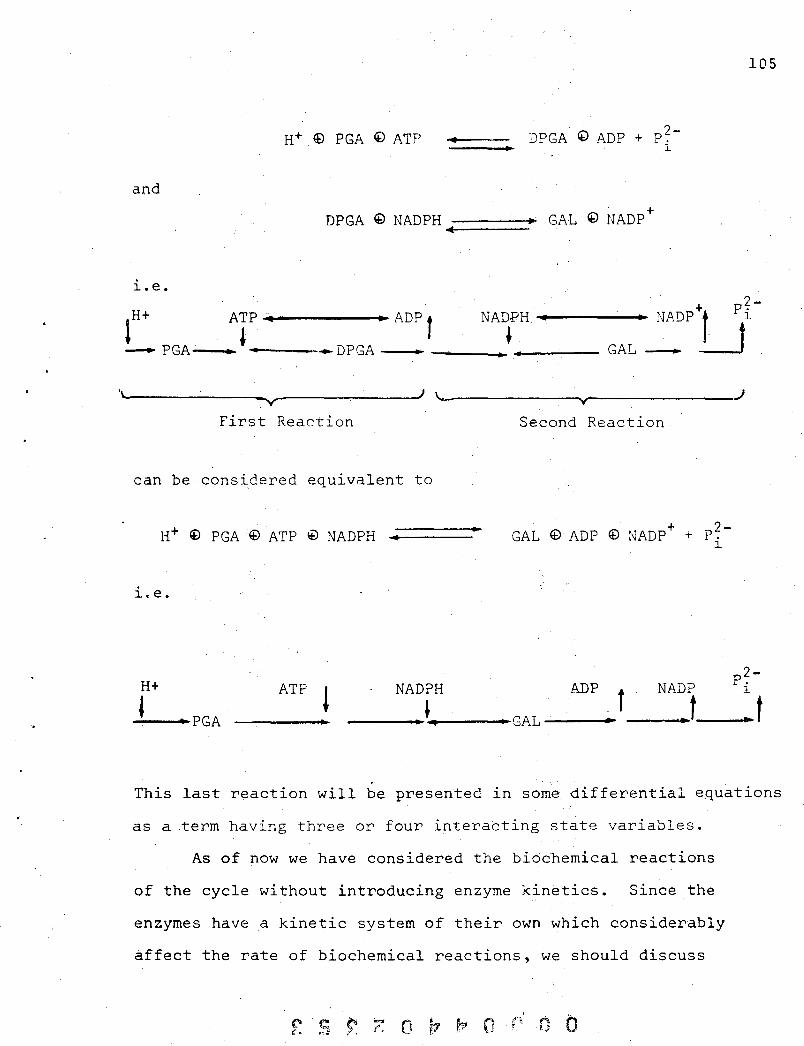
and
l..e.
H+ . @ PGA @ ATP DPGA @ ADP + ?~-------_.~ l ..
DPGA@ NADPH -===='!"~. GAL@NADP+ .~.
105
. . + p?-lH+ AT? ~ .. ADP f NADPH ..... -----.... NADP t l.
- PGA--.~l-.. ---_DPGA • ____ .~ •• ---- GAL _ U . '\ J ~---------------_V_----------------~ ~----------------~vr-----------------
First Reaction Second Reaction
can be considered equivalent to
H+ ~ PGA @ ATP @ NADPH •
i. e.
H+
-~--"~PGA ATP l p~-
NADPH ADP . f NADP l
____ .~~""'I .. ~----~. GAL - ___ .... ___ ..... ~t_--~.~t
This last reaction will be presented in some differential equations
as a term having three or four interacting state variables.
As of now we have considered the bib~hemical reactions
of the cycle without introducing enzyme kinetics. Since the
enzymes have a kinetic system of their own which considerably
affect the rate of biochemical reactions, we should discuss
(\ e r;.. ~ O.! r,·... r.:.'f.' r .... ] t.... 1-;':; ~.~-"' 00

discuss the basic characteristics of such a system.
2.1.9 Some Aspeots of Enzyme Kinetics Michaelis-Menten
An enzyme is a protein that functions as a catalyst
for a biochemical reaction. In any enzymatic reaction we
encounter the phen?menon of saturation with substrate
(compound which is being transformed). This phenom~non can
be described as follows: with a fixed enzyme concentration,
an increase of substrate will result at first in ~ ve~y rapid
rise in reaction rate. As the substrate concentration
continues to increase, the reaction rate begins to decrease
until, with a large substrate concentration, no further
change in the reac~ion rate is observed. The reaction rates.
at low substrate concentrations are known as the "first
order kinetics"; when the reaction rate starts to decrease
due to the increase of substrate we have a "mixture of zero
and first-order kinetics"; and finally when n~ change in
the rate of reaction occurs this stage is called "zero
order kinetics".
106

The mathematical equation that defines the quantitative rela-
tionship between the rate of an enzyme reaction and the
substrate concentration is the Michaelis-Menten equation.
Vmax [sJ V = KM + [8 ]
[2.1]
where V is the observed velocity (rate of change) at a
glven substrate concentration [8J; KM is the Michaelis
constant expressed in units of concentration (mole/liter);
and V is the maximum velocity at saturating concentra-max
tion of substrate.
Any typical enzyme-reaction involves the formation of
an enzyme-substrate complex (E8) which eventually breaks
down to form the enzyme E and the product P. Thus
E + 8 k3
-----~E + p -where k l , k2' k3' k4 are the rate constants for each
reaction.
The Michaelis Menten constant Km is defined to be:
The maximum velocity V max is attained when the total enzyme
concentration [EJ In the system 15 present as the [E8] complex.
In that case, the initial rate V of an enzymatic reaction
o rL L, ,~ o 0
107

is proportional to the concentration of the IS complex we
can write
v = k3 [ES]
In particular when the total enzyme concentration, [E], 15
in ES complex form, then the rate of reaction is at its
maximum and
Vmax =
If we have the case that V = 1/2 V ,then from the max
Michaelis-Menteri equation we can easily derive that
which implies that KM is numerically equal to the substrate
concentration at which the velocity is half the maximal
velocity.
Furthermore, if we let the concentration of the
substrate be very large in Equation [2.1]
be neglected and the rate of change V lS equal to the
maximai velocity, l.e.
V = V max
which lS an indication of a zero order reaction.
So far, we have considered enzymes that possess
independent substrate binding siZes, i.e. the binding of one
molecule of substrate has no effect on the structural
or electronic changes of the vacant site. If such changes
108

-'
occur, the velocity curve will not follow the Michaelis-
Menten kineiics, and the enzyme will be -classified as an
"allosteric" or "regulatory" enzyme. These enzymes show
signoid kinetics <and S-shaped curve).
Some of the enzymes reacting in the Calvin Cycle are
allos teric., [5]. Hence along the pathways of the cycle
we will encounter regulatory points. At these points the
enzymes act as "valves" regulating the speed of the biochemical-
reactions.
In the reconsituted system, however, it was possible
to obtain steady state conditions [4] , i.e. the "valve"
maintains th~ flux through the regulatory points at constant
rate. Hence the kinetic parameters, k l , ... , k22 ' of the
mathematical model [2.1.10] will be assumed to be constant
throughout the cycle. Having discussed the enzymes and the
general biochemical aspects of the Calvin Cycle, we shall
now introduce our mathematical model.
2.1.10 The Following are the Differential Equations that
Describe the kinetics of the Calvin Cycle
Kl to K22 are the parameters that are being determined, H+ 1S
. .-1 a constant and 1tS value 1S 10 in pH 7.
d(RUDP)/dt = +K(20)CATP)(RU5P) - K(1)(RUDP)-
dCPGA)/dt = +K(3)(GAL)(ADP)(NADP+) (P?-) 1
K(2) (PGA) (ATP) CNADPH) (H+) + K(l) (RUDP) (C02
)
dCATP)/dt = -K(20)(ATP)(RU5P) + K(3)CGAL)(ADP)(NADF+)(P?-) 1
- K(2)CPGA)(ATP)CNADPH)(H+)
'0, -0-~. \J
109

dCADP)/dt - +K(20)(ATP)(RU5P) - K(3)(GAL)CADP)(NADP+) (pf-)
+ K(2)(PGA)(ATP)(NADPH)(N+)
d(NADPH)dt = +K(3)(GAL)(ADP)(NADP+)(P?-) l
-K(2)(PGA)(ATP)(NADPH)(H+)
d(NADP+)/dt = -K(3)(GAL)(ADP)(NADP+)(P?-) l
+K(2)(PGA)(ATP)(NADPH)(H+)
d(GAL)/dt = +K(6)(FDP) - K(S)(GAL) +K(4)(DHA)
110
- K(3)(GAL)(ADP)(NADP+)(P?-)+K(2)(PGA)CATP)(NADPH)(H+) l
+ K(lS)(XYL)(RSP) - K(14)(S7P)(GAL)
+ K(lO)CXYL)CERY) - K(9)(GAL)(F6F) - K(7)(GAL)(DHA)
d(DHA)/dt = +K(ll)(SDP) - K(7)(GAL)(DHA) + K(6)(FDP)
+K(S)(GAL) - K(7)(DHA) - K(12)(DHA)(ERY)
dCFDP)/dt = -K(8)(FDP) + K(7)(GAL)(DHA) - K(6)(FDP
d(f6P)/dt = +K(22)(G6P) - K(21)(F6P) + K(lO)(XYL}(ERY)
-K(9)(GAL)(F6P)
d(ERY)/dt = -K(12)(DHA)(ERY) + K(ll)(SDP)
-K(lO)(XYL)(ERY) + K{9)(GAL)(F6P)
d(XYL)/dt = +K(18)(RUSP) - K(lS)(XYL)(RSP) + K(14)(S7P)(GAL)
-K(lO)(XYL)(ERY) + K(9)(GAL)(F6P) - K(19)(XYL)
d(SPI;l)/dt K(13)(SDP) + K(12)(DHA)(ERY) ~ K(ll)(SDP)
d(S7P)/dt = + K(lS)(XYL)(RSP) - K(14)(S7P){GAL) + K('13)(SPD)
d(RSP)/dt = K(17)(RSP) + K(16)(RUSP) - K(lS)(XYL)(RSP)
+ K(14)(S7P)(GAL)
d(RUSP)/dt = K(17)(RSP) - K(16)(RUSP) + K(19)(XYL)
d(G6P)/dt
- K(lS)(RUSP) - K(20)(RUSP)(AYP)
K(22)(G6P) + K(2l)(F6P)

2.2 DESCRIPTION OF THE METHODOLOGY FOR DETERMINING
THE KINETIC PARAMETERS
The following assumptions and notations will be used·
a) We have a system of non-linear ordinary differential
equations • x = f(x,k,t) x(O) = c
where x = (xl' .•• , xn) E:mn , is the vector of the,
state variables; f = (f l , .•. , fn) is the n-dimensional
vector function describing the system;
k = (k1 , ••• , k p ) E:mP is the vector of parameters;
t E:m is a real variable representing tlme. A solution,
x, of the system lS a function of k and t , i.e.
x = xCk,t).
b) The points observed in the experiments will be denoted
by yet) = (Yl(t), .•. , ynCt» E:mn
,t = (t l , ... , t n )
These points are subject to an error n , l.e.
yet) = xCt) + n
where y. (t. ) 1 J
1S the observed concentration of the ith
intermediate at time· t = t. . J
The methodology
Let us integrate, numerically, the system of differential . equations x- fCx,k,t) , i(o) = c , using an assumed set
of parameters, k. Let us define a new function F[k] where
F is obtained by summing over the square of the discrepancies
between the measured values yet) = x(t) + n and the
o
III

computed values obtained in the above integration, then:
F[K] = JJ;,;T(trl - XT(K,trl} Wr {Y(trl - X(K,trl}
[2.2J
where ~(tr) is the measured value at time tr; i(K,t r )
the computed value at time tr and Wr lS a symmetric
positive matrix (for which there are different choices,
the choice of Wr used in our technique will be discussed
in Section 2.4 We are interested in minimizing
F[K] over the space of parameters, i.e. we wish to obt~in A
a value, R, such that
A
F[R] < F[R] . 'if R E JRP
The procedure will consist of several parts:
a) Make an initial guess, K - (k - l' ••• , k p ) , of the
-parameters K = (k l , ••• , kp )'
b) Integrate numerically the non-linear system·[ 2.2 ],
using the parameters values obtained in Step a, and
one set of initial conditions i(O) = c l
representing the first set of initial
values).
c) Apply Bremermann's optimizer discussed in Chapter I.
To minimize the function F[K] as d~scribed previously
the new parameters values, say
obtained after the optimization will be considered
a ~ first approximation to the value K sought.
112

d) For the system ; = fCi, kG, t) , choose several
different initial values i(O) = Cl , iCO) = c~ -() 3 -C 4 -e) 5 -() 6 x 0 = C , x 0) = C , x 0 = C , x 0 = C • eThe
number of initial values were chosen ·arbi trarily. For
example we can choose different values for some
intermediates of the' Calvin Cycle by taking twice the
initial concentration of one, half the concentration
of another and son on.)
e) Integrate the system mentioned In Step d from each of
the different initial values.
f) Obtain the experimental data of the Calvin Cycle
-1 . Y , 1 = 1~2,3,4,5,6 uS1ng each of the initial values
mentioned inStep d •.
g) Reform the function F:
h) Minimize F[KO] uS1ng Bremermann's optimizer over the
space of paramet~rs ~nd obtain the best value of ~ '* K, K •
i) Determine the accuracy of the parameters in relation
tci the assumed errors n in the data, using an error
analysis technique, a la J. Schwartz and based upon
the methods of Rosenbrook and Storey.
L S r:o ~ f1 ~ rJ 0 ~ .. n 0 I.';. d P
!'". , \\., .. -
!
113

114
The procedure described above has three major numerical
tasks:
1. Non-linear optimization
2. Numerical integration
1. Error analysis evaluation
1. In our first Chapter we discussed many aspects of
non-linear optimization. We observed that many of the
prominent techniques use descent techniques for which,
first and second partial derivatives are required. This re-
quirement implicitly assumes that the objective function
is in closed· form and derivatives can be obtained. But
since the objective function F of our procedur~ is given
point-wise rather than in closed form, this characteristic
eliminates the use of techniques involving derivatives.
Furthermore the minimization of F has to be performed over
twenty-two kinetic parameters. Very few algorithms which
do not require derivatives have beeri used in large scale
problems, and those that had gave unsatisfactory results [ 58 J.
Therefore it was a natural choic~ to use Bremermann's
optimizer since it does not require derivatives of the
objective function F. Our comparison, in Chapter I, has
shown that the algorithm is for large dimensional problems
(50-dimensional) faster convergent than any other algo
rithm tested.
2. The function F depends on the solution of the
. .!. - -system x = f(x,k,t). The solution, i = i(~,t), is
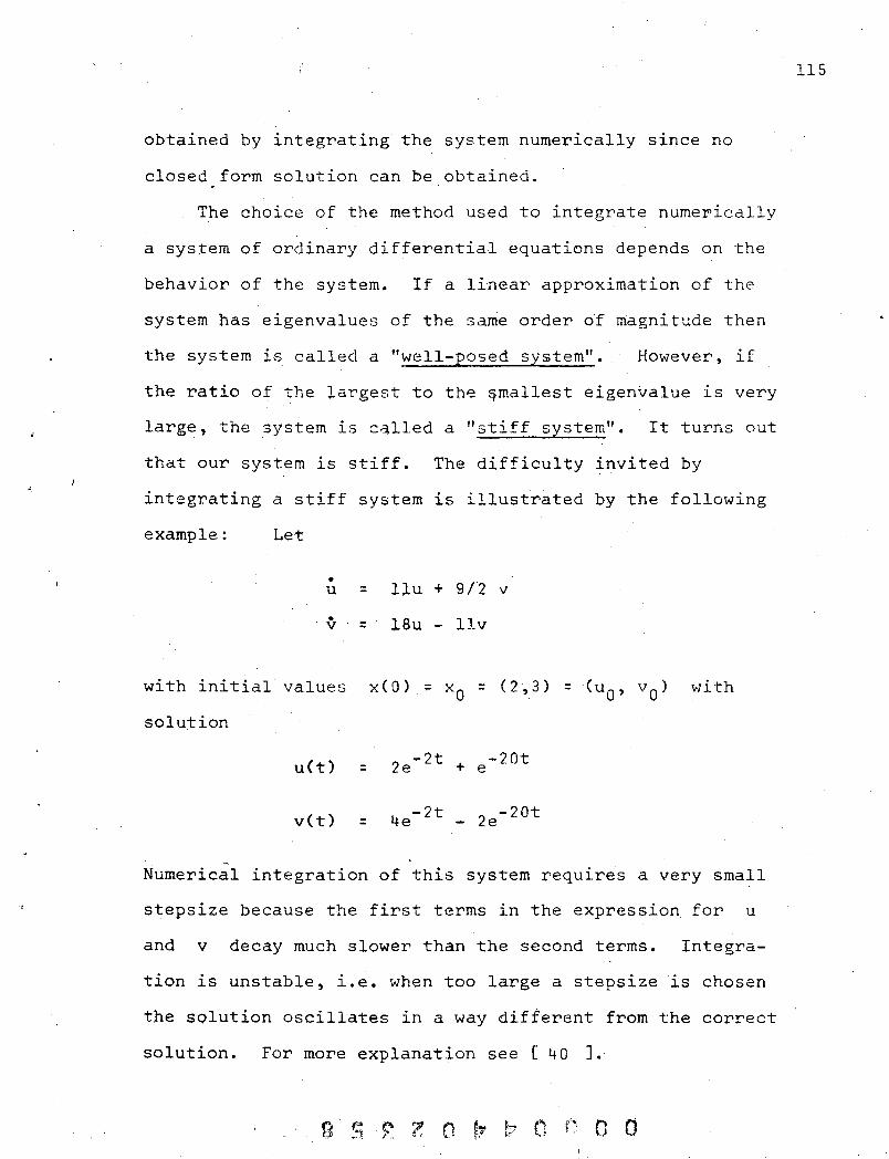
obtained by integrating the system numericallY since no
closed form solution can be obtained. ,
The choice of the method used to integrate numerically
a system of ordinary differential equations depends on the
behavior of the system. If a linear approximation of the
system has eigenvalues of the same order of magnitude then
the system is called a "well-posed system". However, if
the ratio of the largest to the ~mallest eigenvalue is very
large, the system is called a "stiff system". It turns out
that our system is stiff. The difficulty invited by
integrating a stiff system is illustrated by th~ following
example: Let
• u :;:: llu + 9/1 v
v = 18u Ilv
with initial values x(O) :;:: xa :;:: (2,3) :;:: (u O' va) with
solution
u(t) -2t -20t :;:: 2e + e
v(t) -2t 2e -20t :;:: 4e -
~
Numerical integration of this system requlres a very small
stepsize because the first terms in the expression for u
and v decay mUch slower than the second terms. Integra-
tion is unstable, i.e. when too large a stepsize lS chosen
the solution oscillates in a way different from the correct
solution. For more explanation see [40 J.
B. , (1 f~ 0 0 I:
115

We 'have chosen an elaborate integration technique, Gear's Hethcd,
since it is accurate and stable over a larger domain than
the standard methods. We shall discuss with more details
the aspects of integration in Section [2.3J.
3. Error analysis of the results is a very important
feature of the method. Because we want t6 find a measure
of the error on the best set of parameters found, 1n
relationship to errors in the experimental data.
An inverse problem for which small errors in the data
can lead to very large errors in the parameters is called
an "ill-conditioned system" <and example of a linear
ill-conditioned system is given in Section
Since the inverse problem associated with the Calvin
Cycle is potentially ill-conditioned we should be very care
ful when interpreting our results. Therefore, an error
analysis is required to check the validity of the kinetic
parameters obtained by our method.
The error analysis performed herein, based upon the
methods of Storey and Rosenbrook and implemented and tested
for small systems by J. Swartz, Section [2.4] 15
entirely devoted to a the6retidal analysis of this technique.
2.2.1 Characteristics of the Objective Function F
The objective function F will have to satisfy the
following,criteria:
a) The state variables of the system are non-negative
This is due to the fact that the state variables
116

Xi' i = 1, •.• , n of the mathematical model represent the
. concentrations of the intermediates of the Calvin Cycle.
These concentrations have to be non-negative to be
meaningful.
b) The system (modelled by F) satisfies nine linear
relations between the parameters.
By considering the thermodynamics of the Calvin Cycle
we are able to find a linear relation between the parameters
for the forward direction, KF , and backward direction,
KB ' of a particular reversible reaction. (In the schematic
representation in Section [2.1.7] the forward reaction was
denoted by an arrow pointing to the right, ~ , and the
backward reaction by an arrow pointing to the left, .-- .)
These linear relations allow us to optimize over fewer
parameters -~ thirteen, instead of twenty~two. Once we have
determined thirteen of them we obtain the other nlne from
the linear relations.
In the next section we shall discuss thermodynamical
properties used to obtain the li~ear relations between
reversible reactions.
2.2.2 -Thermodynamic -Considerations of the Cycle
Standard free energy of formation:
It is customary to define, for each element at one
atmospher~ of pressure, an arbitrary standard state in either
the solid, liquid, or diatomic gas phase. When this is
defined, the standard free energy of formation of a compound
r'~ o o
117

~G', ~s defined as the difference in free energy between
one mole of the compound at one atmosphere pressure at a
particular temperature and the total free energies of its
elements in their standard states at the same temperature.
Suppose we have a system composed of four species
reacting according to:
The steady state free energy, ~G, change is given by
1) ~G
where ~Gr is the standard free energy, R is the universal
gas constant, T is the temperature in degrees Kelvin,
[AJ, [BJ, [eJ, [DJ, are the concentrations of the species.
When the concentrations of these four compounds are at
equilibrium the steady state free energy ~G is equal to
zero. Thus
When ~G = 0
Equation 1) becomes:
~G'
118

since [C]c[DJ d
[AJa[B]b represents the proportion between the
concentrations at equilibrium, this expression has a constant
value knoWn as the equilibrium const~lt,.k
reaction; i.e.
2 ) b.G' = -RT tri K •
of the
The equilibrium constant K represents the net value of
the forward reaction KF KB
and the backward reaction ~~--~--
l..e. These forward and backward reactions are
the parameters of the dynamical system.'
Therefore, if we know b.G' then we can determine a
linear relation b~tween KF and KB ; from 2) we get
3) f b.Gf] Exp - RT
The values of b. G' were obtained by [5] and
are recorded in Table [2.0].
Note: The standard free energy b.G' is a constant which
does not change under different experimental conditions
or in different systems. Therefore, its value is the same
inside of the reconsituted system as well as inside of a
system with whole leaves or chloroplasts.
'. "
o 9 { ", , , F , o o
119

120
Table 2.0
Standard Free Energy of the Calvin Cvcle
Reaction t.G' Reaction t.G'
A -8.4 R H -3.4 R
B +4.3 U I +0.1 U
C -1.8 U J +0.5 1)
D -5.2 U K +0.2 U
E -3.4 R L -5.2 Rl
F +1.5 U M -0.5 U
G -5.6 U
Abbreviations A through M: See Section [2.1.7J
R, probable sites of met~bolic regulation
Rl, possible sites of " " U, unregulated and freely "reversible" reactions
The following are the linear relation, between the forward
and backward reactions using the parameters In Section
<. 701 x 10- 3 ) K3 = K2 (.844) Kls = K14
<. 209 x 10 2 ) K4 = Ks (.429) K17 = K16
<. 651 x 10 4 ) K6 = K7 (.713) K18 = K19
(.794 x 10~1) KIO = Kg (.232 x 10 1 ) K22 = K21
(.128 105) Kll - K12

2.3 NUMERICAL INTEGRATION OF STIFF SYSTEt-IS
A system of non-linear differential equations lS called
"stiff" if it lS a system whose linearization has eigen-
values of very different magnitudes. For example ,consider
the equation
with solution y =
dy = dt
At ce
For values of A < 0
by a factor -1 e in time
AY y(O) = 0
y decays exponentially, i.e.
-l/A , the last ~xpression is
called the time constant. The "stiffness" of the system
lS due to the existence of greatly diffe~ing ti~e constants.
In a system y = F[y] different components decay at
different rates (especially in physical and biological
problems). These decay rates are related locally to the
partial derivatives ~~ ; if some reactions- are s low and
others are fast, the fast ones will control the stability
of the method of integration, and the slow ones will determine
the magnitude of the truncation error.
The mathematical model of the Calvin Cy~le lS a sti£f ,-
system of differential equations. Theref6r~, the integra-
tion of our system will be a major step in the process of
obtaining the kinetic parameters.
After each successful iterative step of our optimiza-
tion we obtain a new set of parameters. Using these
parameters, we integrate our system; at this point we may
9 0, 0
121

find that with the new set of parameters our system becam~
more stiff. Thus, a good and reliable method of integration
is required to obtain the desired result. To this end,
iriitially we tried a 4th-order Runge Kutta Method; but the
method is not suitable for our problem because of its
com~utational instability as well as inaccuracy for a
reasonably small step size h.
Finally we settled on a combination of two methods:
the Adams-Moulton prediction corrector method and Gear's
th method up to 6 order. This is a package developed and
implemented by Clifford Risk at the University of California
Berkeley Computer Center.
2.3.1 The Adams Moulton Predictor Corrector Method
For th~ purposes of clarity consider a single
differential equation. These results can be easily extended
to systems. Suppose we have the initial value problem
y = f(x,y), yeO) = c [2.3J
where f(x,y) is defined and continuous in the strip
a < x < b _00 < y < 00 , a, b are finite; and the equation
satisfies a Lipshitz condition.
This equation satisfies the identity
JX+d
yex+d) - y(x) = f(t,yCt»dt [2.4 J x
122

For any two points x and x+d In [a,b].
The Adams-Moulton method is based on'replacing the
function fex,y(x», which is unknown, by ~n interpolating
polynomial, P(x) , having the values f :;: f{x n'Yn ) on a
n
set of points x where y has alrea.dy been computed. n n
Let us assume that x :;: xo + ph where h 1S a p ,
constant and p 1S an integer. The first backward difference
of a function
'ilf P
f(x) at the point
f p _1 ' where
x :;: x p is defined to be:
f :;: f·{x ) p . p
A q-order backward difference is obtairted from:
also by definition :;: f P
NOW, by induction we can obtain the following representa
tion for Vqf in terms of the function values f
where
p
:;: r m=O
f p-m
q :;: 0,1,2,3, .....
(~) is the binomial coefficient and
q(q-l)(q-2) ... q-m+l 1,2,m
o
m :;: 1,2,3 ....
123

If we require~ rj ,teo! find a-representation", for th~ values-~ of
iOn tern-iS- '·bf-, -differences, Vqf ,we use .mathematical p
~~ '.) .; -"
o ,1, 2 , 3 , ~: '.
2 ;:"5 ;.J~~, and ·~assuming we. have the inter:po)ating
points, x, x l' P p-••• , x ,we can form the interpolating p-q
I ...... _
polynomial" } -pex).:
where x-x
s = ------E. h
q
I m=O
-, .. ) '- . , '.
o < q < 6 " . \
Then Equation [2.4.. Ie becomes
-.. - .... ~ .;" ~. ',} ~ ,
Yp ... ~p:-l = JP ., ,_ ~ T._ x 1
' .'- )P- .. I;. , , ,
= h
where h 18 a 8tep1ength chosen and r ... ·
r '-
"'" ;:.. F-
" '.,j''\.
P(x)dx
[2.7]
124

x
* Ym = (_l)m h- l r (-:) dx [2.8]
x p-l
= (_l)ln r (:) ds
0
* Numerical values of Ym
are given In Table 2.17.
m o 1 2
1 1 1 -"2 - IT
Table 2.1
3
1 -"24
19 - 720
5
3 - 160
6
863 60480
Now assuming that we know an approximation (the
subscript ( ) denotes the approximation) of a solution of
Equation [ 2.7 ] , we calculate f; 0 ) = f(x p ,Y ~ 0 » and
form the differences
f p-l
Then, a better approximation
'If l' p-
is obtained from
125

[2.9 J
Following the same procedure, we can improve the value of
In general a sequence (v)
yP ,v = 0, 1, 2,
of approximations is obtained recursively from the relation
q (v+l)
Yp = Y + h p-l I
m=O [2.10J
where
These sequences of numbers
will converge to yp for sufficiently small values of h
and this solution is unique (Henrici 1962, pp. 216). In actual
numerical computation, there is no need to evaluate [ 2.7 J
at each iteration step. We can subtract two consecutive
expressions and obtain
q
I m=j
and s~nce
becomes
=
q
L m=O
y* (f-ev) m p
and if set v8 + Y~ + Y~ + ••• + y~ = Bm
Then
[2.l1J
Equation [2.11J
[2.1 ]
m = 0, 1, 2, ..••
126

The solution of [ J is now obtained by summing
up the terms of the series
+ .,.,.
Practically, the computation 1S stopped when
£ > 0
where £ 1S a preselected small value. Since in this
procedure there is no need to carry differences explicitly
'.lsing [ 2.7 ] we can express differences in terms of function
values. Thus; Equation [ 2.7J becomes:
where
q
= h l: p=O
.!f.
S·· qP
f p-p
.'. (q) ... } Y .. 1 + ••• + p Yq" p+
q = 0, 1, 2,3, .•• , p=O,l, ••• ,q.
Some numerical values for S ~': qp are recorded 1n Table 2.2
127

128
Table 2.2 Coefficients of A~ac5-Mouiton ~ethod
p o 1 2 3 5
28"( lp 1 1
* 128·· 2p 5 81 -1
2413:~ 3p 9 19 -5 1
* 72013 4p 251 646 -264 106 -19
1440 B:': 5p 47S 1427 -798 482 -173 27
Note: A formula which ~rovides a first approximation
(0) . . . f for y ,lS called a pn-·d lct::Jr fOt'mula and a ormula
like [2.l~ is called a corr~c~or formula. Furthermore
since the new value is obtained by solving a non-
linear equation that involves rhe function f the method
is called an implicit ~ethorl • .

2.3.2 Gears Method
In this section we shall discuss' some characteristics
of Gear's method. Further details· can be found in [40J
Let h be a fixed positive real number and A complex
number with negative real part. Then:
Definition: A multistep method of integration lS absolutely
stable for those values of hA ~uch that roots of the
characteristic equation
P(~) + hA Q(~) = 0
are <1 in absolute value. Where
P(~) = k I k-i
~ and i=O
k l. s. c: k - i
• '0 l l=
[2.13J
[2.14 ]
Definition (Gear 1964), a method is stiffly stable if in the
region Rl = {hAl Re(hA) < D < O} it is absolutely stable,
and in the region R2~' {hAID < Re(hA) < a, a > 0 , and
Il~(hA)1 < e} it is accurate.
o o 0
129

Gears method has all the characteristic roots, ~,
equal to zero at Ah = 00 only. The x-step methods of order
k with Q(~) = sk are shown to be stiffly stable for
k < ,for some D, a and a. To obtain this result it
is required to compute P(r,) from Q(s) so as to get an
order k-method
Fo~ a stiffly stable method, Q(s) has to be a poly-
nomial of degree at least equal to the degree of PCr,) •
Otherwise, one root at hA = 00 is 00 This property
implies that stiffly methods are implicit, therefore it lS
necessary to solve a corrector equation.
Gears method calculates the solution of a stiff system
according to the following_corrector equation
k v . = .\ a. y . + hBOf ~ P f.. 1. p-1. P
1.=1
The values of a i and BO for the method are glven in
Table 2.3.
If we consider the characteristic equation
[2.15]
p(r;) + Ah Q(s) = 0 , the locus Ah wi ttl roots ia 1;; = e of
modulus 1 is given by a continuous closed curve:
Ah = P(r;;) QTf) o < a < 2'IT [2.16]
These curve~ will describe the region of absolute stability
of the method.
130

",0
...0.
;,?
~.~~
o ::;;.r
"'.:t'.
r-"~ ' . ....r
'r.-~
'.OJ..'
o a
Figure [ ] Region of absolute stability for stiffly stable methods of order one through six.
------~--------------~---------------+--------------_t 1·-----
6 6
6 ----- ...... W f-'

132
Table 2.3
Coefficients of Gear's Stiffly Stable Method
k 1 2 3 4 5 6
So ,'; 2/3 6/11 12/25 60/137 60/147
a 1 * 413 18/11 48/25 300/137 360/147
(l ~'; -113 -9/11 -36/25 -300/137 -450/147 2
a 3 * 2/11 16/25 200/137 400/147
a * -3125 -75/137 -225/147 4
as ,'; 12/137 72/147
a 6 * -10/147
* For k = 1 we obtain the backward Euler method i.e.
Yp = Y 1 + hfCy ) + OCh2) p- P

2.4 ERROR ANALYSIS OF THE KINETIC PARAHETERS
As earlier studies have shown, J. Swartz [83J
it 1S necessary to estimate the expected error of the
kinetic parameters from ~he measurement errors in the data.
To this end we will discuss the error analysis technique,
a la J. Swartz, which is based upon Storey and Rosenbrook
[ 75 ],
Note: Although we followed the main ideas of Storey and
Rosenbrook, gaps in their presentation made it necessary
to give an independent derivation of the error analysis.
Error Analysis
The purpose of the error analysis is to verify the
accuracy of the parameters found after applying the optimi-
zation and integration procedure. By having a measure of
the error in the parameters we shall obtain an insight into
the following points:
1) Consistency of the model and the data
2) The estimated error of the parameters due to errors
in the data.
To this end let us consider a.dynamica~ system of the
form:
.:. x = f(x,k,t) x(O) = c
The following assumptions will be used: 1:
[2.l7J
a) The parameters values, k, obtained at the end of the
optimization procedur~ are in reasonably good agree-
- -ment with actual values, k of k
a 0
133

134
,.. b) Let ~ = i(t,~) denote a solution of [ 2.17] , where
'" k is a particular value of K. Denote by zeal a
solution of [ 2.17 ] depending on a E JRP such that
i(a) = i(t,k+a). Denote by rea) the error In X
which resulTS from an error, a , in k, i.e.
e:(a) - -= z - x '"
A
= x(t,k+a) x(t,k)
c) A first order Taylor expansion of f = f(x,~,t) around ,..
the point (x,k,t) lS
A A
fCi+£, K+a, t+~t) = f(i,~,t) + f_£ + f_ a + x k
A
similarly for x = i(k,t) at (k,t) ..
x(k+a,t+~t) A
= i(k,t) + xK
a + Xt~t + O«a+~t)2)
where
af. af. af. ax. ax. f l f l f t
l - l l = ax. = = at. xl< = Xt = 3t· x i< ai<. aie. J J
J J J
In all that follows we are only interested in the case
when ~t = 0 and only considering the first order terms
In E ·and a.
~';
Ok - kll < a for some sufficiently small a E JR+

Now, consider a system on non-linear ordinary
differential equations
. x = f(x,k,t) , x(O) = c
Let x =x(t,k) be a general solution of this system, then
-varying k slightly wo~ld only change a particular
solution slightly; i.e. we will obtain a solution
x + e: = x(t,k+cx)
-where e: is the perturbation of x due to small changes a
l.n k. This is equivalent to saying that the general
solution of[ 2.17] is a continuous function of the
parameter k. This is certainly true locally Sl.nce
Theorem. Let Equations [2.17] be given where
f(x,k,t) and f.
l. x.
1.
If
are defined and continuous in domain,
.J... belongs to B (k is a value
of k) , then there exist positive numbers rand q such
that:
1) Given ...., k
solution
such that -4 J,.
Uk - kft < q , there exist a unl.que
-i x = x(t,k) of [2.17 ] defined for
It - tol < r ~
and satisfying x(to,k) = Xo
2) The solution is a continuous function of t and K.
A proof of this theorem can be found in [77].
0'0
135

Now that we established that small perturbations In
- -k will generate small errors In x we are interested in
finding:
a) A time relation describing the dependence of -x
= variations a of k around k , and
b) a relation describing the dependence of a upon
variations n around x(t) •
llpon
Therefore; given a solution x(t,k+a) a first order
approximation is glven by:
x(t,k+a) ax -= x(t,k)+ a _ (t,k) [2.18] ak
set x(t,k+) - 'x(t,k) = e: (t) , ax -- (t,k) = D(t) and ak
a ax (t,k) e;(t) = -ak
• ax - •
a-= (t,k) = e:(t) ak
• • •
136
IDx(t,k) = £(t) ax + y at , for some y E :ffil , [2.19]
where ID
becomes:
for t = t I'
denotes the total derivatives. Then Equation [2.18]
[2.20]
=

where Dr is a 'nxp matrix which gives the dependence of
-x(t,k) upon variations ~a of ~ around k. Since we
wish to find the changes of D with tim~. let us introduce
the errors E and a into Equation [ 2.17] and obtain:
• • -x + £ = f(t,x+E , k+a) x(O) = c
£(0) = 0 [2.21]
By kee'ping t fixed and expanding this expreS:3lon 1E a
Taylor series using onlY first terms and considering [ 2.19]
we get
!. • -x + £ = f(to,x,k) + AE + Ba [2.22J
and
• £ = AE + Ba [2.23]
where
af. "--A (A .. ) 1 (x,k,t o ) = = 1J ax.
J
af. " B (B .. ) 1 (x,k,t O) = = . 1J ak.
J
Both matrices are functions of t but not of £ or a ,
also A 1S nxn and B is nxp. Since the above
calculations do not depend on to ' differentiate Equation
[ 2.20 ] with respect to time and substitute the result
into Equation [ 2.23 ] , then:
6 9 ('> .7: (} i?' ~~ r; I 0 0 1':" t'-" '-.,1
137

-Da = ADa + Ba [2.24 ]
since a lS a scalar, cancelling it we obtain:
OCt) = ACt)-D(t) + B(t) [2.25J
DCO) = 0
The nXp matrix net) will contain all the informa-
tion pertaining to the dependence of the solu~ion x(t) on
errors in the parameters.
Equation [2.25 J is called "the variational equation"
of the system [ 2.17J, for further properties of this
equation, see [44], [50J, [77J.
At this point we are ready to determine the relation
between the error n in the observation (data) and a
In the parameters. Consider the function F described
In Section [ 2. 2 ] By minimizing F over the space
-of parameters k, we will obtain a set of' parameters
-which is an estimate of the value k of k. Let = k+a be such a set for which F[k+aJ lS a minimum. Then
Equation [ 2.2 J becomes
M 'f r[k+aJ - L . r=l
and at the mlnlmum
-T y (t )
r
-k+a
aF -aa [k+aJ = o
W+,;<tr)-X<k+C<, t r )1
L2.26J
138

J
or
a '~{-T (t ) ~ 1 Y, r ]. r=
or
or
a an.
].
M
= a 1: an. 1 ]. r=
D n r I = 0
= 0
This is a scalar equation. Hence when taking the partial
derivatives with respect to the ith component of the
vector we get
+
. .th f S].nce the ]. component 0 a vector an~ transpose are the
same we get that
b • t'" f~ 0',', 0' o 1'<" tp ~,)
139

M
r = o r=l
or
M M
r = r r=l r=l
Let H = then
[2.27J
When: the symmetric matrix H is non-singular,
Equation [ 2.27 ] gives the relation between n and a
sought.
At this point we are ready to calculate the expected
error a due to error n in the observations (data).
It is reasonable to assume that the error vectors
{n·} corresponding to different sets of measurements will 1
be statistically independent, i.e.
i -;. J
where denotes the "expectation values" of n. , and 1
[2.28]
is the operation of taking the average over a large number
140

of similar experiments. In contrast the individual components
of each vector n are not assumed to be independent. Then
the expectation values are represented by a matrix called
the covariance matrix l.e;
H. 1
where M lS the covariance matrix.
The expectation value of a lS zero, (since its
components are independent) therefore we are interested
[2.29J
in finding the covariance matrix of the components of a ,
that is, the expected value, p, of a. Assuming that
the expectation values are known, it follows from Equation
[ 2.28] that:
H
I [2.30J r=l
Let P be the covarlance matrix representing the expected
values of a i.e.
= P .. 11
and o ' P .. =O,i~j lJ
i ~ 1
Then since the expectation of each component ln Equation [2.30J
is well defined we obtain:
l o o a
141

. /
HPH = M
L r=l
DTH M W D r r r r r
[2.31J
Wr -- (Mr)-l . If we choose to be the we1ghting matrix, for
each r,Wr has the following representation
1 2 cr lr 0 . . . 0
W = r 1
0 . . . . cr2 nr
where 2 the variance of a.(t) cr. = 1 1
and Equation [2.31 ] becomes
M
HPH = L r=l
The right side of this equation 1S defined equal to H
thus
HPH = H
If H is non-singular then
which determines P.
P _1
= H
[2.32J
[2.33]
[2 • 34 ]
142

From Equation [2.27] we observe that a lS a linear
function of Its probability density will be Gaussian
[66 ], and is given by
1
(21T)P/2IfPf
and, the expected varlance
direction b is given by
=
-
-T b
[2.35J
for the parameters in the
-Pb [2.36J
where b 1S a unit p-vector in the parameters space. By
143
By choosing b parallel to the direction of one of the parameters,
1.e. b. = 1, b. = 0, i "/. j 1 J
we obtain the variance of this
parameter, i.e.
2 (J. = P ..
1 11 [2.37J
This result is of central importance because it determines
the relationship between a measurement of experimental
error in the data and a measurement of error in the calculated
parameters. Furthermore it indicates how well the data
fits the model.
o

2.4.1 Implementation of the Error Analysis Technique
on the Dynamical Equation of the Calvin Cycle
The main difficulty in implementing the error analysis
is the d~lculation of Equation [2.25 ] , i.e .
• D = AD + B
in spite of the nlce analytical represetnation, this
calculation can run into a major difficulty, which is,
the calculation of the matrices
A = B = af.
1
ak. J
(x ,k, t)
If we try to obtain the partial derivatives by formally
differentiating, the task is almost humanly. impossible,
since the dimension of A is l7x17 and B is 17 x 2 2
the chances for human mistakes while taking derivatives
is very high. This is especially true since each entry
of these matrices has many terms. Furthermore forming the
product, A·B, requires over 7000 multiplications of the
entries. Since ali entries have five terms on the average;
the 35000 mUltiplication required makes the existence of
a mistake a virtual certainty.
This computational problem is simply a result of the
size of the system of equations. For a smaller problem
analytic differentiation can be performed by hand and
checked efficiently.
144

We have overcomed this problem by employing the
computer itself to perform analytical differentiationuslng
a new experimental computer language called ALTRAN
(Algebra Translator). - -- '
ALTRAN is a language and system for performing
symbolic computations on algebraic data. The basic capability
of the language is to'perform operations on rational
expressions 1.n one·or more indeterminants. The system l5
designed to handle very large problems involving such
data, with considerable efficiency.
Operations on integers rational and real (floating
point) data are also included together with computer
procedures for dealing with truncated power series and
systems of linear equations.
The ALTRAN language is still an experimental language
in its early development and only few iristitutions have it
in operational form in their computer installations.
The usefullness of the ALTRAN language can be
stressed by considering the following aspect in the •
calculation of the matrix D. The matrix D is equal to:
where A =
• D(t) = A(t) D(t) + B(t)
af. l.
ax. )
B = af. 1. ak. '
) D =
ax. 1. ak.
J
A is (17x17), B is (17x22) ,and D is (17x22) •
o 0
145

Now, let us consider what is the probdbility of making
no mistakes in the actual computation of these partial
derivatives, when it is not done by a computer.
Let p be the probability of making a mistake when
taking the partial derivatives of a term in an entry of
matrix B, then I-p is the probability of not making a
mistake. Since each time we take a derivative we can make
a mistake, we can consider that each time is an independent
event.
Assume that each entry of the matrix B has an average
of five terms then we get that the probability of making
no mistakes is:
if 1 P = 100 l..e. one out of 100, then
1 20
(l-p)P ~ e-2000p
which i~plies that it is almost impossible to compute it
by hand.without having a mistake unless -4 P < 10 . By
a similar computation and assumptions for the matrix A we
get that
or
_lSOOp e
146

If we note that our matrix D ~s the result of the computation
of matrix A and B then we can conclude that if we have a
large system and we try to compute the matrix D by hand,
then we almost certainly will make a mistake in the
computation since for most people the error rate is much
larger than 10-4 [46J, [87J.
To avoid an almost certain error, we obtained the
matrix D, by writing and implementing a computer program
written in the ALTRAN language. The matrix D so obtained
has 82 nonzero entries. Each entry contains on the average,
about 15 algebraic terms.
From our experience ~n deriving the matrix D, we can
conclude that the error analysis could not be implemented
unless we used the ALTRAN system. It is interesting to note
that in our initial attempts in trying to obtain the matrix
D, by performing formal differentiation by hand, we found
that we always generated mistakes. Thus the reader should
be aware that the use of ALTRAN as a new tool is of utmost
importance.
2.5 ILL-CONDITIONED SYSTEM OF EQUATIONS
In our previous section we discussed the theoretical
aspects of an error analysis. Our main result was a measure
of the expected error in the kinetic parameters due to error
2 in the data. The variance, 0 ,was represented by a matrix
P, the matrix equation D = AD + B required the calculation
of the matrix A and B. The nature of these matrices was
o , .~~
p ~-. - o o
147

never discussed. Thus it 1S of interest to determine how
errors in the data affect such matrices. To this end we
shall carefully analyse the behavior of the solution x,
of a typical linear system Mi = E ,M is an invertible
nxn matrix, when variations are made 1nthe value of M and
-b. When large changes in x result from small changes in
-M and b \<le speak of the matrix M as "ill-conditioned"
or the system as "ill conditioned". In this section we
present standard results on this topic. We also give a
geometric interpretation of the results by ~pplying them
to the matrix P.
Sensitivity of a Linear System to Perturbations
Let Mx = b be a linear system, where M 1S a
nonsingular matrix of order n, b is an n~dimensional
vector and -x is the n-dimen~ional solution of the system.
We are interested in finding some kind of measure of
the error affecting the solution -x resulting from
-errors 1n the vector b , and the dependence of errors
-1n x on ~rrors 1n M;
The "norm" of a matrix M; II Mil , 1S a number which
measures the magnitude of a matrix. The norm satisfies
the following properties:
1) OMO > 0 , II Mil = 0 iff A = 0 -2) DcMO = I c I ilNI! where c E :rn. I
3) HH+QII < II Mil + IIQII
4) IIMQII < IIMII·UQU
148
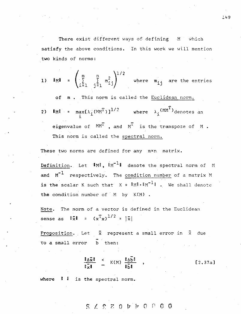
There exist different ways of defining M which
satisfy the above conditions. In this work we will mention
two kinds of norms:
n 1) 8MO = (m . L r m: .y/2
where m .. are the entries
2)
~=l j=l
of m • This norm
=
eigenvalue of
1J
is called the
where
1]
Euclidean norm.
A. (MMT) denotes 1
and is the transpose of
This norm is called the spectral norm.
These two norms are defined for any mxn matrix.
an
M •
Definition. LetHMn, OM-In denote the spectral norm of M
and -1 M respectively. The condition number of a matrix 'M
is the scalar K such that K = UMO.OM-In We shall denote
the condition number of M by K(M) •
Note. The norm of a vector is defined in the Euclidean
sense as nin = (xTx)1/2 = Iii
Proposition. Let
to a small error
- -x represent a small error 1n x due
b then:
< n6bD K(M)
ObO , [2.37a]
where n 0 ~s the spectral norm.
{, 0'" O' r·
149

150
- -Proof. Since M(x+~x) = (b+~b) , and Mx = b by definition
then
[2.38J
taking norms on both sides
[2.39J
we also have
RbO < UM" UxU
Now mUltiplying Expression [ 2.38 ] by Expression [2. 39 J
we get
<
and dividing by Obn.uxO we obtain our result
n~xn -- < DxU
Q.E.D.
Notice that this result depends on the choice of the
norm. For the spectral norm the condition number k(M)
of a matrix M turns out to be given by:

151
The condition number k(M) lS a me.asure of the maximum
distortion which the linear ~ransformation M makes on
the unit sphere. The expression represents the
relative error In the vector b , and is the
relative error In the vector soluiion -x due to error In
the vector b.
So far we considered the matrix M as if it were known
precisely. We now look at the system Mx = b when j
an error t.-.M ln M and b is also known precisely. Again.
as in Proposition 1 we are interested in det~rmining how
t.-.M affects the solution vector -x •
Let (x+t.-.x) = (M+t.-.M)-l b. be given
Proposition. If M is the matrix representing the error
in the matrix M and X results from this error then
Dt.-.xD < K(M) Bt.-.MR Ux+t.-.xU n M 0
Proof. Clearly
or
This equality can be'rewritten as
= [2.40]

152
Now since (i+~i) = (M+6M)-1 ; Equation [ 2.40J becomes
Taking norms on both sides we get
or
[2.41J Ox+!\xl1 -
which is the desired result.
Q.E.D.
Expression [ 2-41] means that the relative error in
the vector solution -x is bounded by the rel~tive ~rro~
in the matrix M times the condition number of K(M) .
2.5.1 Ill-Condition: An Example
After discussing sensitivity properties of a matrix
M consider an example of an ill-conditioned linear
system: M 1S a real symmetric matrix such that:
1 .99
M =
.99 .98

The eigenvalues Al , A2 , of M are found by taking
the determinant of M and solving a quadratic equation, i.e.
-l-A 1 .99
= .99 .98-A 2
We find that Al - - .00005 and A2 = 1.98005. The
condition. number of M
K(M) =
=
is given by
A T maxMM A. MMT m1.n
(1.9005)2 2 (-.00005)
= 39.600
So K(M) 1.S a very large number. Now consider the problem
of finding the point of intersection of two lines:
= 1.99
.99xl + .98x2
= 1.97
Th~ solution to this system is Xl = 1 x 2 = 1 but for
Xl = 3 and x 2 = -1.0203 we obtain
Xl + .99x2 = 1.989903
. 99x l + .98x2 = 1.970106
153

--.000097
Therefore a change ~b =
+.000106
+2.0000
can give -x
-2.0203
Now, we can calculate n~xll and obtain lI!lxU ~ 212
Similarly II xU = 12 , thus n~xn
II x II
since
Hence, using
lI~xll
D x II <
2 <
and IIbU ~ 212 , then IIlltll
II b 1/
lI~bll K(M) II b n
10-4 K(M) -2-
we see that
For this to be true K(M) has to be at least ~O.OOO Slnce
we found that K(M) 39,600, we found approximately the worst
case. Therefore if b 1S known to have an error of above
.00001, then the vector x can only be known to within
two units of each of its components. This system is an
example of a very ill-conditioned problem. Geometrically
154

this means that the point of intersection of these two
lines is hard to determine, i.e. the lines are 'practically
coincident.
2
l~---~
1
2.5.2 Geometric Interpretation of the Condition Number
of a nXn matrix A
The condition number 1S a measure of the maximum
distort1onwhich the linear transformation with matrix A
makes on the unit sphere.
Using the spectral norm, assume that A is a real
symmetric matrix and the condition number K(A) is one.
This implies that we have an undistorted sphere, and A
and A-I stretch all directions by the same factor. Since
the eigenvalues, Ai of A are all equal in magnitude, i.e.
IAII = IA21 = ••• = IAn l it will be impossible for A-I.
-to stretch 6b more than b itself, in other words, the
relative uncertainty of the vector solution -x 1S the
same as that of b. However, when K(A) 1S 1010 A-I
stretches one direction 10 10 times as much as another
n I (' t,'",.. b. ~,'; {) f~ 0'.]', O· 'I'"J ,,~ , (: ~" I" • ~"
155

- -direction, In this case if b gets the short stretch, ~b
may 'get the long one, and 8~xB
D x D
10 would be 10
times lI~bn
U b U and our original unit sphere becomes distorted
into a hyperellipsoid. Hhen the deformed sphere is very
elongated the implication lS that our matrix is nearly
singular. The closer the ellipsoid is to a sphere the
farther it is from singular and the eigenvalues <associated
with the coordinates of this ellipsoid) would be similar in
magnitude.
In our discussion of the error analysis our main
result,
2 -T -(J_ = b Pb
b
represents the variance of the parameters K. l
In the E
direction. P is a real symmetric matrix, hence its
eigenvalu~s are real, and its eigenvectors are real and
orthogonal.
[2.42J
Now consider the hyperellipsoid Z having the eigen-
vectors of P as the directions of the principal axes and.
the length of each principal semidiameter is equal to the
square-root of the corresponding eigenvalues.
-In any direction b the distance from the origin to
the hyperellipsoid is If P is already a
diagonalized matrix, the diagonal entries are the eigen-
values, Ai' and the axes of the ellipsoid Z have length
156

equal to I'f7 i = 1, •.• , n' •. 1
The geometric interpretation of [ 2.42 ] l.e. for the
matrix P, implies
[2.43]
Thus the expected error of the parameters is between
and If the ratio between the larger to the
smaller eigenvalue is very large our ellipsoid would be
very elongated. This will imply that some parameters are
poorly determined and they might be very sensitive to the
noise in the data, or equivalently the expected error ln
some parametem is very large.
Now, suppose we have a set of parameters found by our
technique using one set of initial values, and suppose
that after the error analysis some parameters are poorly
determined, i.e. K(P) is very large. Then the following
question arises: What can be done to make P better
conditioned? Or equivalently, how can we better determine
our poorly determined parameters?
To consider this question let us reconsider the badly
ill-conditioned problem discussed in [ 2.5.U:
"Find the point of intersection of the lines
-Xl + .99x2 = 1.99
.99xl + .98x2 = 1.97 represented by Mx = bIt
o 0
157

If instead of having only one piece of data 1.e.
=
which we have shown to satisfy
(
1.989903)
1.970106
Mx = b for x = ( 3.0000)"
-1.0203
Suppose ~e have two data points, that is, suppose we have
__ (1.989999) b 1 as above and b 2
1.970050
If we use both data points the problem is no longer
linear but it lS better conditioned in the following sense.
Our motive is to obtain the best value of x from the data
given. One optimization scheme is described by:
1) " R2 Find the vector x E which minimizes
UMx - b 02 +. UMx - b U2 1 2
[2.44]
The question of ill-condition revolves around the
concept: what accuracy ln the data (where t.b lS
the error in b) lS required to lnsure a desired accuracy
in the answer, IIllxll
II x R (where t.x lS the error ln x)?
158

The ratio of the mean to the square
root of the variance (standard deviation),
= C1 is defined to be the signal
to noise r~tio of the data.
Thus the data rea~ly contains information corresponding
to in the statisticaly form: C1
Ibn
The previously mentioned optimization scheme utilizes
this information. Therefore, we can infer that statistical
knowledge of H~xB
H x I is better when two data points are
utilized than only one is used. In other words: the signal-
to-noise ratio or accuracy of x can be predicted via
[2.37a] i.e.
l~xD
I x a < K(A) C1
abo [2.45]
using hI and b 2 we obtain 0'2 = 6.176
l~xB < K(A) I x U -
3.6x.785
212
.9
(J6.176 X IO- 9 )
212
o 0
159

which is an improvement over the expected accuracy, 1.8,
when only one piece of data is used.
Using this idea we were able to "better condition"
the parameter identification problem. Consider Step g
Section 2.2. Now for each x(O) (initial value) we ~an
get a set of parameters for our dynamical system. This
set would contain some poorly determined parameters. Thib
means that for each set of parameters lS very
large and more information is needed to determine these
parameters. Clearly the union of the sets Ki contains
more information about our system than each individual set.
Therefore it is natural to consider the sum F and
minimize over the space of parameters to get a set of
parameters which best satisfies our system under several
initial conditions.
In our dynamical model for the Calvin cycle, we were
unable to recover our exact parameters, with reasonable
error, with one or three different initial values (though
there was a big improvement from one initial value to three).
But we were able to recover all of the parameters with
some reasonable error bounds with six initial conditions
[2.6].
When calculating the variance of the kinetic parameters
of the Calvin cycle due to six percent e~ror in the data,
it was found that, when using only one initial value the
160

parameters were poorly determined and their variance
from 10-4 to 10 9 . Wh'l h ' ",' 1 1 range 1 e w en uS1ng S1X 1n1t1a va ues
the parameters found were well determined, and their
variance range from 10- 5 to 10 4 -- see Table 2.7.
Clearly the matrix P, obtained by uSing the best
parameters found is still ill condition, but the ratio
between the maximal to the minimal variance in the para-
meters has imporved by six order of magnitude. This
improvement indicates that we were able to better determine
the values of some parameters and therefore reduce the
value of the expected errors significantly enough so as
to improve the condition numb.er of P.
2.6 TEST OF THE NUMERICAL MACHINERY USED IN THE PARAMETER
IDENTIFICATION PROBLEM
We will now perform a test of our numerical machinery
in order to double check. that it really works and 1n
order to test our error estimates. The computation of the
error estimates involves linearization and is valid strictly
only for small errors in the kinetic parameters.
The idea of this test is as follows:
We do not know the dynamics of the actual system,
,however, if our method really works, then our equations with
the parameters values that we have developed should be a
161

good approximation of the real system. If this lS the case
we can generate simulated data (synthetic data, this will
be ~efined in Section 2.61 ) from our equations. We
then feed this data to our numerical machinery and compute
parameter values from the simulated data. To make this
process realistic we should also simulate experimental
error. This can easily be done by adding noise (from a .
random number generator) to the simulated data. Then we
should perform the errOr analysis and see whether the
computed parameter values are within the error bounds. If
this is not the case then our numerical machinery cannot
be trusted. If repeated tests (with different simulated
experimental error) give the expected result it still
does not absolutely prove that our computed values are
the true rate constants of the Calvin cycle, but it is a
strong indication that the values are reliable. The
ultimate test must be prediction of experimental results.
2.6.1 Implementation of the Numerical Machinery
Definition: The set of integrated values of a dynamical
system~ having the exact parameters will be called
"synthetic data", "generated data" or "perfect data".
In this Section we _wilf discuss how all the parts
previously considered, performed under simulated conditions.
The main procedure involves the optimization and
integration routines. We first started with the assumption
162

that our technique should be able to perform well on a
small linear system, before considering the larger non-
linear one. To that end we chose the following test problem
dYl 4Y2 dt = Yl -
dY2 + Y2 at = -Yl
with closed form solution
Yl<O) = 1
Y2(0) = a
-t 3t e - e
4
[2 .46 ]
This solution is the source for our synthetic data. The
technique was implemented as follows: Using the set of
parameters kl = 1, k2 = 4, k3 = 1, k4 = 1 we integrated
the system uSlng our integration routines. We took four
intermediate points on the trajectory <solution curve).
These points will b~ considered "perfect data". We perturbed
the data uniformly by 10% noise using the following
formula
where -0 x
- -0 2P x = x 1 + (R-.5) 100
is the exact data point; -x is the perturbed
data point; R is a random number uniformly distributed
between a and 1 generated by the random number generator
{~ O· 0 . . " .
163

on the CDC 6400 computer at the University of California,
Berkeley; P is the maXlmum percenta~e noise in the data
(in our case 10%). , In order to begin optimization we chose our first
iterate by perturbing our original set of
uniformly by 100%.
k. l
i = 1,2,3,4
The task is to recover the original parameters, i.e.
kl = 1, k2 = 4, k3 = 1, k4 = 1. We started with one initial
condition ylCO) = 1, Y2(0) = 0 after 1000 iterations.
Using Bremermann's optimizer we were able to recover only
. -2 two of the parameters wlth 10 accuracy. We stopped the
procedure due to the amount of time consumed and the little
progress toward the recovery of all the parameters.
Normally, the set af parameters found after such a
computation is used as a starting guess for our multi
initial value procedure. But in this case we chose to
start with our original guess and use multi-initial values.
We chose two different initial values such that the
two sets are not a scalar.multiple of each other. The
sets chosen were
Again, performing our technique, but with two simultaneous
initial values, we succeeded in recovering three of the four
-3 parameters within 10 accuracy. This was achieved after
300 iterations using Bremermann's optimizer. Consequently
164

we tried the technique with 3-initial values
1 = 2"
After 150 iterations we, succeeded to recover all the
.. -6 T parameters sought wlthln 10 accuracy. hese results
are recorded in Table 2.4.,
At this stage we were ready to perform the technique
on our dynamical model describing the Calvin cycle.
This system is large, non-linear, and stiff. Forthis
purpose we generated'synthetic data by integrating the
system for a specified initial condition and a set of
parameters chosen arbitrarily as "perfect parameters".
We followed the same steps tried in the 2x2 system
but this time we started with on~ initial condition,
continued with three and six initial conditons.
With six initial conditions we recovered all the 22
parameters after 72 iterations and with accuracy up to 1-
10% error of the initial parameters, clearly we could
have recovered all of them with better accuracy if we
would have run our program for longer time. The results
are recorded in Table
165

Table 2.4: Results on the Determination of the Parameters of System [2.46] Usin~
Synthetic Data with up to 10% Noise.
Perfect parameters value 1.0
Initial parameters values .23
After 150 iteractions Calculated parameters values .984
After 300 iterations Calculated parameters values 1.000002
Final function value
( 0 0) -9 after 300 lnteratlons was ~F = .702 10
3 4 CAy Yo-Yo ~Here F = I I. ~ 1
j=l i=l Yi
3 is the number of distinct initial values
4 is the number of time intervals
4.0 1.0 1.0
7.19 1.47 . 1. 71
3.967 .998 1.02
3.999999 .999999 .99999
Total C.P.U. time (in a
C.D.C. 6400) 320 seconds
Yi is the synthetic data
Yi the integrated data
(It is interesting to compare these results with the results obtained using perfect
data without noise and using the initial guess, perturbation of 100% in the exact parameters.)
I-' en en

Table 2.5
Perfect parameters values 1.0
"~r IInitial parameters values • 13
CO After 150 iterations
:? I Calculated parameters values .6159
.-"" . IAfter 300 iter~tions • '1
. Calculated parameters values .9986 0
~.
~ Final function value
;:'J .(after 300 iterations) was *F = .803 10-6
0
0; 3 4 (Ar *Here F = L L Yi~:i j=l i=l
3 is the number of distinct initial values
4 is the number of time intervals
4.0
3.189 .
4.112
4.0009
-y. ~
,.. y. ~
1.0 1.0
1. 811 .356
1. 042 1. 022
1. 00005 .99913
Total C.P.U. time (in a
C.D.C. 6400} 340 seconds
is the synthetic data
the integrated data
f-' (J)
-..J

.'.
Table 2.6: Parameters Obtained After Testing The Numerical Machinery Using Synthetic
Parameter*
K(l)
K(2)
K(S)
K(7)
K(8)
K(9)
K(12)
K(13)
K(14)
K(17)
K(19)
K(20)
K(21)
Data With 3% Noise
Exact Values
.68
1. 99
1. 38
1.83
.096
21. 27
22.85
.12
4.46
11.52
6.91
100.58
.83
Initial Values
.28
1. 79
2.29
1. 04
.12
29.28
38.96
.11
8.63
17.14
6. 5
130.18
.68
Values Found
.68
1. 97
1.1+ 8
1. 81
.099
22.01
24.59
.12
3.99
11. 71
7.00
101.21
.84
Function Value 1t *
Initial F =
284.87
Final F =
1.66
(CDC 7600> C.P.V.Time
400
Number of Iterations
120
~These thirteen parameters were obtained by our procedure. The other nine are obtained by using the linear relations in Section [2.2.2J.
6 14 F = I L
j=l i=l (- A)2 Y~:Yi uSlng 6 different initial values and 14 times intervals.
~i is the perturbed data (i.e. 3% noise) Y is the integrated values.
~ O'l 00

169

170
Table 2.7: continued
Error Analysis wi th o~~ Noise in the Data
.,
Expected Expected Error with error
Percentage ! Value Found o·ne set of y;ith six I
Para- When Actual Initial Initial of absolute i meter Exact Value F = 4.1 * Error Values Values error ** i
I
3 XlO-4 .9;<10-5 I
1 .68 .68 0 I I
2 1.99 1.52 .47 • 32X10-3 .7 xIO-4 :::::; 24% I I
3 2835.85 2166.0 .667 103 .13 xI04 .32 xl03 ::::::: 23~{ I
4 .066 .064 .002 .5 x 10-3 .25 x10-5 ::::::: 3% I I
! 5 1.38 1.34 .04 .36 .17 xI0-2 ::::::: 2.5% i
.94 x10-4 .18 xIO-5 I 6 .00028 .00025 .00003 ::::::: 10%
I 7 1.83 1.6 .23 .5 xlO-1 • 85 xlO-3 ::::::: 12%
8 .096 .09 .006 .5 xlO-3 .28 xIO-5 ~ 6% I I
.2xl02 I
9 21.27 19.5 1.77 .16 ::::::: 8% I 10 267.78 245.70 22.08 lXI0 7 .34 x104 ::::::: 8%
.25 X10-3 .29XlO-6 I 11 .0017 .0015 .0015 ::::::: 11% I
12 22.85 21.2 1.65 1x101 .2 ::::::: ]''' I 10
13 .12 .12 0 .4x10-5 .52 xl0-6
\ 14 4.46 5.5 1.04 .17 x102 . 86xlO-1 ::::::: 26~~
115 5.26 6.4 1.14 .31 x109 .59 xI04 ::::::: 21%
\16 26.72 26.9 .1S .22xl03 6. ::::::: .9%
11.52 11. 7 .18 .28x102 .93 ::::::: 1. 7% 117 9.67 9.5 .55x103
118 .17 .16 ::::::: 1.3%
19 6.91 6.84 .07 .23 x102 .34xl0-1 ::::::: 1%
20 100.58 105.4 5.18 .75x101 .10xlOl ::::::: 5.2%
21 .83 .64 .19 • 69 xl0-2 .5sx10-3 ::::::: 22%
22 .34 .27 .07 .14xI0-2 .12x l0-3 ~ 20%
* The mean of the error is 9.7% •

171
2.6.2 Graphical Display of Results
In this Section we will present the graphs of each
intermediate of the Calvin cycle. These graphs were
obtained using the best set of parameters found by using
our numerical machinery (Table 2.7 ) For graphical
representation we have written a computer subroutine
which implements the task of graphing any set of data "lith
great accuracy.
Each graph will represent:
a) The trajectory of an intermediate uSlng an initial
guess of the parameters.
b) The trajectory of an intermediate uSlng the exact
parameter values. This is a set chosen arbitrarily
and considered to be the "exact" para.meter.
c) The trajectory of an intermediate using the best
parameters found after applying our numerical
machinery.
9 o a

." , ~
.''''0'
••••• 00
.. " ... ! .010000
• • ..... 00 ... .. C • .. .. :: .o •• aGa · • ..
• 131'00
•• aoaoo
.010000
R U 0 P
o Z.O '.0 '.0 '.0 I D. a S2.0 It.O 1'.0 11.0 T'"' t ...... UTI'
~.AJECTa.y alTAINfO us ••• erST 'A.A"fT~'1 'DUID
~'A~ltTOay O,TAI.fD UI'.' INITIAL Gur" or 'AIA"fTrl VALUrS
172
10.0 21.0 Z •• a U.O ZI.O 30. a
XBL 759·8012

• C .. · !
• SfOOOO
.n ••• o
.ni ...
~. nooOl J:
• • · to C • ......... • .. .. · •
• •• 0 •• 0 '.0 ••• .0.0
PGA
".0 .t.D .'.0 11.0 TI"C ,_ "'.UTI.
6T8A.aCtTOa., OlTA1JIIla U·S ••• EXACT 'AIA"ITr. 'AI.Ura
~.A .. ctTD'Y aeTA,_eO US, •• '.lTIAL GUll' 0' 'AIAftITC. 'ALuea
I. t. " l'
173
".0 11.0 at.o 11.0 n.o JO.O
XBL 759·8011 ,e
"
o o

• c ...
·.uu ..
• z ... oo
.15 ....
• UlOOI
~ .nuoo
• .unoo o l-e · l-· :: • ,1000 · • ..
• HllOO
.z .....
ATP
z.o <.0 ' •. 0 1.0 11.0 1'.0 ".0 te.o J'.O TJ"f .eI ""MUTII
6T.A~fCTO.Y OITAlafD USia, flACT 'AIA"'T,. VALUei
*T."oIltTO'Y alTAJlleD us.,. .. I(ST 'AIA"[T'I' '0'''110
~.AJICTO'Y a.TAlaCD UI.a, 'atTIAl IUfSI 0' 'AIA",T'. 'ALUII
174
zo.a ·u.a Z4.0 21.0 21.0 JO ••
XBL 759-801 0

· c ~ · "'
!
.1 .....
. tuoa •
. ,nooo
• . "001 • .. .. '" · .. · .. .. · · ..
. lUI ..
• 11000
ADP
.IIIOIOL-~ __ ~ __ 4-~ __ ~ __ ~~~~ __ ~ __ ~~ __ ~ __ ~~~~ __ ~ __ ~~ __ ~ __ 4-~ ______ ~~~~ __ ~ __ ~~--~~
I 1.1 t.' 1.0 I.G 10 .• "., .t.O .1.0 .1 .• TI"f .1 "l.uTes
bT.A~ltTO.Y O.T~I.(O UI.I, '_ACT PAaA"tTEI .Aluea
()
10.0 11.0 t •. o 11.0 :10.0
XBL 759·8009
o
175

.• n ...
.• nlO •
• 0IUOO
.u ....
! • .01'10.0
.. • · .. · :: .. 010000 · · ~
.. o,a.l •
..... 00
.,,0"0
NADPH
.'11000~-A __ ~ __ ~~~-A __ ~ __ ~~~ ____ ~ __ ~-4 __ ~ __ 6-~. ______ ~ __ ~-A __ ~ __ 6-~ ______ ~~~~ __ ~ __ L-~ __ ~
• a •• 0.0 1.0 1.0 10.0 11.' ••• 0 11.0 ".0 10.0 I J. 0 It.O 11 .. 0 1'.0 '0.0 TI", J. "I .. UTe.
6T.A~ICTO'Y ,ITAI.CD U,._C flACT 'AIA",TII WAluri
XBL 759-80()8
176

• c .. · I: ..
.......
.......
....... c ~ , ••••• !
· o .. ! ....... .. · .. .. · •
... n ..
.. ., ...
. "15"
NAOP
• '1.0 .t.O .1.' '1.0 TI"I' I. ",."TE'
AT.A~rtTO.Y aITAIM(a UIJ.' (IACT ~A.A"rTr. 'Alues
I •• t.' '.0 ..0 to ••
o .. , '- 'j , .
10 •• 11 •• If ••
o
177
21.1 It .• '0.0
XBL 759·8007

.. , ....
•••••••
· ~ ...... . · so
! · ....... o .. < • .. · .. .. : .•••• '0 ..
• 07 ....
.......
DHA
• I.' ... '.0 '.0 10.0 II.' ,4.0 S'.O " .• TI .. , '1 pU.UTeS
6,TeA.CCTOIY ·.ITAI.CD "I.'U eXACT 'AIAMITt. VAl.Ue,
~.AJeCTO'Y OITAI_CD USI.c leST 'AIA",TC'I rOUMO
~~~~CCTO'1 OITAIMCD UI ••• '1ITIAl CUISI 0' 'A'APtCT!. VALUe.
178
11.0 II .• 24.0 21. a 21.0 3D. a
XBL 759-80011

· c .. · I:
.......
. 11'"
.1 .....
• .IUOIO · .. C
~ • .. .. • ·
.1 •••••
• 1 .....
GAL
. 1'1'.'~~ __ ~ __ ~~ __ -L _______ ~~ __ ~ __ 4-~ __ -4 _____ ~ __ ~ __ ~ __ ~ ____ ~ __ ~~ __ ~ __ ~ __ ~ ____ ·~ __ ~~--~--~
I a •• t.1 1.1 1.0 .0.1 12.0 .t.O .1.0 ".0 TI"E 'M "._UTlS
AT'A~ICTO.Y aITAI.IO us,_, I:I~(T 'A.~"fTI' _~Lur •
• T'AJICTO~Y aITAI_,O ~II.G I'IT 'AIA",T, •• ,o~ •• ~'AJCCTO'Y DITAIM'D UII., 'MITIAl" CUrs, 0' 'A'A"ITCI 'ALUII
bo I .•
(}
1 D •• II. I '4.0 U.I 11.0 10.0
XBL 759·8005
o a
179

• c .. • I:
." ....
..... 10
~ ...... . It
!
~
c • ~ •• nooo a .. .. a .. ..
.• n ...
•• 11 ...
FOP
.1.0 t.O 1.0 1.0 10.1 12.0 ' •• 0 .1.0 11.D TI"I. II .... UTfS
6T.A~ICTO.~ O.TAI_CD US •• , flACT 'AIA"fTEI 'AlUfl
180
zo. a H.b 1.,0 t •. O 28.0 ,O.!)
XBL 759-8004
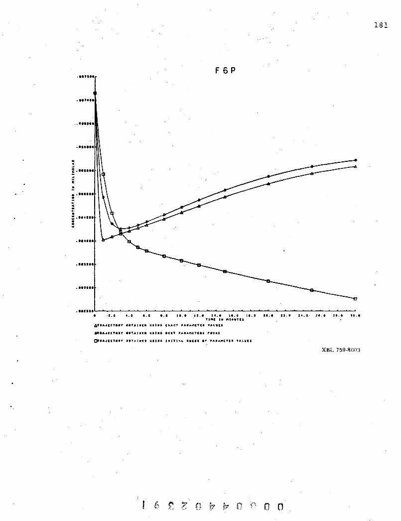
. '
• c ..
... ,. ..
.• u ...
•• ••••••
....... ~ ....... ! · ...... . • .. c • .. · :: . ',fll • • • .. ....... ... ,. .. . "" ..
• ·Z.D •• 0 1.0 I.' 11.0
F 6 P
II.' 't.1 '1.0 '1.0 . TI"' •• "JIYTC5
AY.A~ICT'.Y O'T~J.fD uS.le ,'ACT 'A'A~ITI. YAlUC'
6·
181
11.0 11.0 Z t. 0 la.o 21. Q JO.O
XBL 759·8003
o o
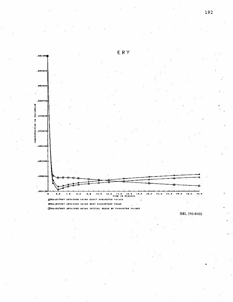
· C 4 · I: ..
.•• ue
.......
.......
. ".,00
r .000.0 •
.. · ... : .000500 ... • w .. · · .. .......
... ouo
.......
ERY
: . "41 •• L-~ __ ~ __ ~~~~ __ ~ __ ~~~~ __ ~ __ ~~ __ ~ __ ~~ __ ~ __ ~ __ ~-4 __ ~ __ ~~ __ ~ __ ~ __ ~~ __ ~--~~--~
• I •• ... •• 0 '.0 1 C. 0 12.0 It.O a •• D 11.0 10.0 1 •• 0 te.o :I 0.0 TJltC I. "I.UTI!
~T.A~ICTO.Y •• TAIM!. bill' I!:IACT ,A.A"CTE. WAlU!1
XBL 759·8002
182
•

· c ..
.......
.......
~ .... I .. .. I:
! & · .. c · .. & = .•••• 00 · • ..
.......
R reu L 5 p
,,1 . ~~~~~~--~~--~~--~~~~~~~--~--~~~~~~--~~--~~--~~~~~~~ • I .. ' '. 0 •• 0 •• 0 '0,.,0. 1·1;. ,0; ·1 •• 0 ••• 0 i •. 0 fl'''' 'a ."'.UTfl
10.0 fa.. 0 I'.' "Z'.O '0.0
". ", . ',:J ,6TIA..fICl'OIV .ITAltltO tJI.,.' fiAtT 'AIAI1fTr. ""lue,
*T.,.. ... I'CTO." O,TAIAfD UI'" 'IIT 'A.A,.CTI •• ··";~(u ... ' ~", 'I
; J "/., :'1
~'A~ICTO"Y "TAla,O Ult., 'aITIAL CUI.' 0' 'AIA"(1'I. VAL~r.
XBL 739·7998
o o o
183

.. c .. • c ..
•••••••
• 8.,S •
••••• ee
i .S .. 500
! • · ~ : • '0 ••• 0 ~
• .. u · ·
.I.,SOI
.......
... asoo
SOP
• z.e ' .. 1.0 '.0 10.1 &1.. ,f.O '1.0 11.0 TI"f 1_ "I.UTES
AT.A~(CTC.Y '.TAI_tD uat_, flACT 'AIA",rrl .AlUfS
184
to.o t t .. 0 If.O 2&.0 21 .. 0 '0. a
XBL 759-800:

.......
•••••••
.... ,.. • ! .... ,.. • " ... c ! · ...... . · .. c • .. • .. .. : .......
. ""11
... " ..
• I.' t.' ••• •• 1 10.0
XYL
"., .t., 1'.1 '1.0 TI"I 'I "I_UTI.
AT'.~"T"Y O.TAI.,O •• , •• 'I.,T 'AI.ft,T'1 'ALur, ",.A""TOIV "DeTAI.CD ..... , aCIT ,.IA"fTr:I, 'OU ••
CW.A~ICT •• Y oaTAI_CD VI'I' i_ITIAl cuel' 0' 'AI""fTII 'ALUI.
o
185
to.o H.' 1: ••• .. .. 1'.0 JO.O
X8L 759·8000
o

.Ott .. O
•• 13 ...
• IlIIOO
· ~.'ll0'O o C
• .01 oeoo co .. < & .. · .. .. : .101000
.0.1000
... "00
GLU 6 p
• 1.0 t.o 1.0 1.0 10.0 a2.O 't.O 11.0 11.0 ·'0.0 TU'I: .w "l"U~r:5
6TIA.lt:CTOIY OITAI .. !D USI_C fl"CT PA,,,"t:Tf'. 'fAlut:1
186
22.0 2t.O 21.0 ZI.D
XBL 759-7999

• c ... • ! ... C • -
S7P .......
.......
.......
· ...... . • .. c • .. • .. .. • • .. .......
•••••••
• I.·' . .. ••• • •• 'I .• 11.0 If.' ".0. 'I.a TJ"' •• "I.UTE.
6T.AJICT.'~ 'ITAI.'. UII.' fIAtT PAIA"CTCI 'ALUla
~.A~fCT •• Y ',fAIIID US'I' .,IT PAIA"ITC •• 'OU_'
arl", .. CCT •• V .•• TAIIEO UI!I' .IITtAL.lvel' or "AIAftCT'1 '''LUII
o r"'
187
10 •• n .• 1 •. • II .• n.' H.O
XBL 759·80) 3
o

• c .. • r:
!
.......
...... 0
•• 0 •• 00
• .0"'00 • ~
" · ~ · .. .. • · ..
.... tOO
.""00
RIB 5 p
1.0 '.1 1.0 1.0 .. 0.0 ar.o ,t.O 11.0 11.0 TI"( ._ "'IMUT(S
6T.A~CCTO.Y OITAI_tO UII.' r_ACT PA.A"ITCI YAlur.
1'88
' .
JO.O 22.0 11.0 21.0 '0.0
XBL 759-7997

2.6.3 Using Real Experimental Data
As we mentioned earlier'in Section 2.1, the process
by which experimental data is. obtained is very laborious
and costly. After the initial success of our methodology
in January of 1975, A. Bassham's laboratory did various
experimertts which, if successful would have given us data
for an accurate determination of the parameters. Unfor-
tunately these did not give useful data because either some
impurities were present in the reconstituted system or good
steady-state concentration levels of the intermediates could
not be obtained. The reader should be aware that usually
when an experiment fails to obtain its objective, results are
discarded and many days (even months) of research py several
scientists are wasted.
Since an experiment requires much time (including
fracturing the chloroplast, paper chromatography, auto-
radiography, computer outputs, graphs preparation, etc) data
is not yet available for use in this problem. We expect that
the needed data will soon be available and that implementation
will then be complete.
s (, f1 0 0
189

2 • 7 SUMMA.RY
By implementing our technique using synthetic data,
our purpose was
1) How well can we determine our set of parameters assuming
we had good experimental data (for this purpose we ) .
generated synthetic data).
2) How could. we make our ill condition~d problems
"better conditioned".
3)· Can we recover the original parameters.
After applying our numerical machinery we can certainly
state that given a good set of data (about 10% noise)
with several initial conditions, our technique will make
the problem a "better conditioned" and by doing so we
can rec6ver the set of parameters that govern the dynamic
sy~tem with better accuracy.
3.1 CONCLUSION
Our general task was the identification of the kinetic
p~rameters of the Calvin cycle. To this end we used synthetic
data and a set 'of parameters (arbitrarily chosen) to check
the performance of our numerical machinery. The results
indicate that our technique is a reliable tool for para-
meter identification and ln particular for the determination
of the parameters of the Calvin cycle. -The numerical routines,
though elaborate, can be adapted fairly easy to systems of
a different nature than the Calvin cycle. An extension
190

of our methodology to other biochemical and metabolic
systems should be fairly straightforH'ard and of direct
biological importance.
lri the process of developing our method we have put
together the pieces ofa very complex system using informa-
tiort from different fields of science; such as non-linear
optimization, numerical integration of stiff systems,
algebraic ~anipulation with computers, error analysis of
the results, biochemical kinetics, thermodynamics properties
of the system and the chemical pathway of the Calvin cycle.
For the first time we have obtained an approximation
of the parameters value which determine the kinetics of
the C~lvincycle.
The results justify our encouragement for further·
investigation in the following areas: ~
1) Determination of more accurate parameters value
from better data.
2) The incorporation of the enzyme kinetic of the Calvin
cycle to our mathematical model.
3) The analytical investigation of the multi-initial
value problem.
~) The introduction of controls into the system.
Once the kinetic parameters are known we can introduce
new control parameters that would determine the maximum
output desired by "steering" the system toward such an
output.
o o o
191

FROGRAN MATH(INPUT,OUTPUT,PUNCH,TAPf6s 0UTPUT' C*.... PPOGRAN MATH IS THE NAIN PPCGP.M,IT CONTAINS ERfMERMAN_S C..... ALGORITHN. MATH CALLS FUNCTION FeZ). THIS FUNCTION IS THE C..... FU~CTION DESCRIAED IN SECTION 2.2. C..... FUNCTION F(Z) CALLS THf INTEG~ATION ROUTINE ,ORIVES_ WHICH c***.. IS TH~ IMPLEMENTATJONQPF GEAR~ ~ETHOO DISCUSSED IN SEC. 2.3.2. C* •• *. YNI~ INITIAL CONDITIONS FOR THE DYNAMICAL SYSTE~S • C**.*. E = ARRAY ~n~TAINING THF DATA PC[NTS (SY~THeT[C,C~EXPER[~ENTAL) c** •• * n~ = ARRAY CC~TAI~I( THE INTEGRATEO VALUES OBTAINED BY USING c****. GEARS M~THdD. c***** K3 = NUMAER OF SETS EACH OF _HICH CONTAINS 17 INITIAL VALUES. c***** K2 = NUMEER CF nATA POINTS (=13' c** •• * Kl.: NU~'3EP OF STATE VARIAE.'LES (THE 17 INTEI<,..IDIATES OF THE c***** CALVIN CYCLf ) C IT = NUMPER OFI1ERA1IONS C N = NU~BER ~F VAPIABLES C x = ARRAY OF VARIAEL~S C--RUOP ~-~-F6P----OHAP----FGA----ADP----ATP---FDP-----SDP----G6.----S7P C---XYL--~5P~---IU5P-----GALP~------NERY-------NADP--~-- --NADPH--------
C
2
30')
11
J24
SOl
502
COhlMON CZ(I~' CO~M8N/JAIME/FCI7,13,f',Kl,K2,K3 CO~~ON IEIN/OPC17,13),XCI3',~ CO,,",MON /DOG/YN I ( 11, I ,6' CC~MC~/FIS"'/PIC I:!), lEa DI~f~510N X)((13) D I 14E '" S ION vAL C I :!) DI~E~~ION HHHCQ6) O(ME .... SION R(200) LOG I CAL WARN nATA KI,K2,KJ/17,13,11 nATA HHH/24C.OOI,.002,.01,.I"
REAn lOO,N P!: 40 300, I r FOFiMATCI6' r.; EA D2 , ( ( Y N I e I , 1 ,L , , I = 1 , K 1 ) ,L =1 ,K 3 » FO~MAT(~FIO.9,/,8FIC.~",FIO.9» REAl) 17,X FORM_T(lCPFIO.A/),5FIC.8. FF<INT 3?4,CX(J), t=l,~) FO~MAT (13)1, * CZ PAPAMETEr.;S VALUES .///(IX,6(E20.10, IX'//', p E ./1 0 50 1 , ( ( ( F ( I , .J , K ) , .1= 1 ,K 2 , , I = I ,K I ) ,K:: 1 , K J , FORMAT(qFIO.Q,I,5FIO.~' PRINT 50?,«((F( I,J,K) ,J=t,K2) ,1=I,KI),K=I,1(3' FO~MAT( * DATA POINTS *//(lX, 8(Fl0.6,SX)",IH ,S(FIO.6,5X"//) PU~CH E96,(((Fel,J,K) ,J=I ,K2),I=I,KI),tc=I,K3' CO 2 ~ I.:: 1 , N X( I) =It,L(J(j(X ( I)' XX(IJ=X(I)
21 COI'.TI\jUE FO=F(Z' PQINT :Ul, FO
311 FOP>llt,r ( * INITIAL FU"CTI0~ VALUf • , E20.10'
.. ~ to tV

i'....
C'-
:~")
:"l
':::,)
~--
'f'
~'::)
':~
0
'0
c C
C C C C C
1'-l
40 C c c c
l5 4 I
4::?
4 3
44
c
AEGINNING OF T~E OPTI~llATla~ KG = 0 K5'=0 DC 10 J :: I, IT (. RA~OCM OIR~CTI~~ GENf~ATOR Q IINF (~, WE'TUJ-tNS A RANOO~ NUMBER UN IFORMLY OISTR.IRUTEO BETIIEE ..
Z~RO Af\,O ~N~ AT FACH CALL ' , . ~(I) HAS' GAUSSIA~ OISI~IPUTICN
K (, = (\ KG :; I<G + GO 40 I :: I, N XV :; -ALfJG(lUNf(Ol' vv = -ALC'C;(RANF(O'. IF (YV.LI.C.5*(XY-I.O) •• Z.GC TO 39 w(l) =SIG~(XY.~ANF(O) -.~) n( I )::~( ()*XX( I) CC"TlNt-1:
FCr.~~TICN CF fCURT~ C~OE~ PCLYNCNJAL
~ :; ')ISTA~CF ~ET~EFN THE POINTS OF LAGRAf\,GIAf\, INTERPOLATION K~~::I<';A+ I IF(~S~.GT.4C)KSA=1
t1 = HI~H ( K SA) 1)0 4 \ , ;:: " N X(I):: XXCI).?" r:(J)" H f? :: F(n r.n I, 2 I :: I, N X(I':; x)C(n + I<(I).H Fl = F(Z) ~n 4 ~ I -= 1. N '(II) :: XX(I) - f.'(['" I~ t-~, ." Fll) I") IJ If 4 I :: " N '( ( I) :: X X ( I) - -;. • P( I) .. H t-'III;' :; f(l) " :: ( r 2 • F~? ) / f: • + F (l-2 •• ( F I + F "'I • / ] • r~ :: (F~-FO,1;»/4.-(fl-F"'1 )/2. c :; 4.t(f'I'F:'oIl'/3.-!'i •• FO/2.~cFc+r"'?)/12. i) :; ;>.*(r \-F\lIl )/1.-(F~-f"'2)/12. 1"(At-'')(4'.C''.1.f-20. GUIO ~<)
el.I "It: ~;~ Srll, LJ TI (J~I C
c
Y I :; - .) I ( GO T.l ~1
c ('Life :::()LU11'I~j
C C r~: ~~~1
C 5) P (/1-~~.~/(1 •• 4 •• ~'
~ to W

c
Q = O/A-A*C/(3.*A**?'i2.*S.*3/C27.*A**J' DELTA :: 4.*~.*J +21~ *0.*2 [_F (~E L T A • L!: • C., GO TO 6 C ~COT =SORTCO[LTA/I08.' AA =-:Q/2. +'HlOT eA=-O/2.-RCGT Vl=SIGN(AnS(AA)*.( 1./!.),AA)+S[G~(ABS(BA' •• '1./3~),eA.-B/(3 •• A' IFtAf~S(VI).GT.5CO. , GO .10 83 .
51 Dr: ':2 1= 1,"-5 2 x ( I) -:; x x( I) + '( I * U (1' * H
FLNC = ~(Z) GO TI) 70
C TH~fc peOTS c
c
60 PHI = ASIN«SORT(Z1.,*Q)/(2 •• P*SOHT(-P)t' /3. U = SQRI(-P/~.) * 2. V '" - P /(~. ,. AI ~ = SIN ( r>H I , CS = COS(PHI) * SORT(!.) / 2. VI = IJ * (C 5 .. 0.5 * 5) .. V '(2 = -U ,. ~ + V '(J = -U • (CS -00.5 • 5' + V IF(AAS(YII.GT.500. ) GO Te 84 IFIA~5(V2'.GT.5CC.' GC Te 84 IF(AeSIY31.GT.500.' GO TO 84
C ~INt~UM OF T~E FCLYNOMIAL C
C C C
61
6~ 62
65 63
70
~o
A2
FFI = A/4. ,. VI**4 • A/3. ,. VI •• 3 +-C/2. * v,**2 + 0 • VI + FO FF2 = A/4. ,. V2**4 • e/3. ,. V2*.3 + C/2 •• V2 •• 2 + 0 • V2 + FO FF! = A/4. * '(1**4 + e/3 •• Yl**J + C/2 •• Vl •• 2 + 0 • Y3 + FO H- ((FFI.LE.FF2l.ANO.(FFI.LE.FFJ') GO TO 65 IF «FF2.LE.FFl).A~D.(Ff2.LE.FF3» GO TO 6. 00 6 I I = 1, N X(I) = xx(1) + Y3 * RII' • H FUN( = F(Z) GO I'J 70 nc 62 I = I, N X(I):: XX(I) + '(2 * R(I'. H FUNC = feZ) GO T i) 7 C on 6 31 ~ 1, N X ( I I = x x ( I I .. Y 1 * P (I) '" H F UNC =f' I l , CCI';TPHJE
FU"IC IS THE FUNCTICN VALUE AT THE END OF E~CH ITERATION
IF (FUNC - Fr) Fa = FlJNt" Dr) R2· 1:.::1,1\. xXII) C= XCI' GO TO 72
eO,AI,8l
~ to -+=

.~ "'i e4
~ °1 -'? ~
:f). I?
c \"',J" c
r. 0
71 3:>;>
-~
1 '. .~
60~
.c.~ ~ .... ,~..; I.,
P.9'l
::J
0
(C",ll'HI' c:I' .... 'l·H .. ;C
,,'1 fC 7;.> P"(r-;T ~'.~"~
~(J .. W/lf( ~T"'(~ FIJNCflr:'" I~LCc:r: * • I~(J.~C.IT) GO Tn 71 . IF(~r,."c.3) GC' Tn I·~ .
.... (~., (' If ~'" T
:::.; (" r .•. ) ? , J , f" ('
r-';"'Ar(~' J 1"'"(:, I?, 1J)(, * FlJIIIC, IS *, "20.1,)' KG = :") IF('''2~(J.J).fC.~) c~ TO l~ IF( J.'~I .1 T) C.O Tt: 1(' ((J,,' I H:F "~ I ' I, I) "I f . = I ." V A I. ( ( ) =- :~,,!) ( :0: (f ) , ~ ~ ( r~ T .~ ~ I,. ( V A L ( I ) • I :: 1, II; ,
(n'I' I 'HI'"". P Q II'. r " ~ ? , ( ( ') ':' ( I , J ) , J:: I, K c) ,I = 1 t K I ) P l. !\ r '-1 €-I ':I'"} , ( (f'''' ( 1 , J ) • J = 1 .11.2 ) • f :: I ,K , ) F ~ll< 10' 1\ l( 1 C. )t • 7f' 1 Q • to , /, f ~ Ie. t. ) ..,u .... r ... 17,VAL ~1r:(:1
f. " .;
~ w (TI

FUII.(TlON FU. C***** F = 1~f. FU~CTIr.N TC BE C~TIMIZEn. C****. C1 = ARnAY ~ONTAI~I~u 22 KINETIC PARANETE~S,TH[IR OETF.RNINATION C ••••• IS ou~ ~.I" Cfl,JF.CTIVF.
(0'<11010111 C l( 13) CO 't1 M'l N / j A I ~ r::/ f U 7, 1 J , f • , K 1 , I< 2 , K J CC~MC~ /FI,,/nR(17,11),X(13).'" cc~~o~ /OCG/YNI(17,1,~)
C*o*.. T = ARRAY CONTAI"I( T~E lJ TIME INTERVALS. n I VF" S ION' T ( 1 3 I
c***** ·~'),T(,.TLA<;T.Y,~O,FPS,~F,KFLAG,'I'MAX,ERRO~.Pw.FSAVE A~E c***** "0 = Nn. OF STAff v~nIAHLES. c***** TO = INITIAL TI~F c* •• ** TLA~T-TC = INTEAV~L O~ INTEGRATION. c**o** ~F ~~FFOS Tn TH~ ~~THOO CF I"'TEGRATIO~. C***** 'Io1F = 10' 15 IIDA""5-"'C;uLTO" • MF ;; 22 IS GEARS "'E'T,",OD. C**.** FP5 IS LC(Al A((U~A(Y CF I"TFG~ATIO~. C***f.:* '(FL\G,FnRf}k,FSAVE,Pw ARE AR~AYS DESCRI8111.G SCflAE III.TEJONAL C***** P"Ac~I\"'[T[I<'i UF T,,"E INTEGRATI"'G ROUTINFS. c**.** Y~I\~ = UPPfP AOUI\n eN THE STATE VA~IA8LES.·
P filL Y ( 1 7 , 1 .] I REAL Y""II.X(17"E~"'O~(171,P"{306),FSAVE(J4. CO '~MfjN /F I SH/P I ( 1 :a) , lEe D A TAT / 5. , A • , 9 • , 1 0 ., 1 ~ • , 1.6 • , ;:.1 • , 2 0\ • , 2 7 • , ~ I •• 3!: •• J e. , 4 , • / e(":IC~J::I,~ . CZ(JI-= [XP{x(JJJ
IO~ CC"ll"1lJr: . F::J.
I) 0 ~ 'J L:: I , I< .., DO ;> ,(=1,1<1 y«,IJ=Y"II(~,I,L. V"'Axlr<J=.f>
2 co '11 P~lJt= fI.W=;:>.? 1\('=1<1 HC=.::::OOCCO,)CC5 'CP:;=.1 T~=O. 0'1 .].) M=l ,I<~ I£,C="I TL4ST'-'T("1.
C •••• * ~OUTrNF OQIVES INTE(RATES T~E C1FFEqENTIAL EQUATIONS. CALL ~RIVFS(NO,TC,TLAST,y,~O,EPS,~F.KFLAG,YMA •• E~ROR,P.,FSAVEl TO-=TL"ST on 30 1<.=1,1<1 r)Q 1"',"4) =Y(J<, l' (=r.P(~,~I/[{I<,~,L. F=F+(l.-C)**2
~o eriNT l"IllF P:Tui<'-j FN!J
t-J to 0'1

:-;.'
.; ..
. ,0'
~J"
:'-.., ~
',:)
V
'~
o
. ~.:>
'0
SURqOUTINE CIFFU~'N,T'YfYDOT' .. c..... ·S~3qCUTINE nIFFU~ CC~TAr~S ECUATIO~S TO AE INTEGRATFO WITH C ••••• CURREN~ P~RANETER ESTI~~'ES. IT ALSO CQNTAI~S THE. LINEAR C ••••• -·- REL~TlONS AfTWfEN Ttoe PARAMETERS. THESE RELAJlOlltSAAE C..... oaUINEO USllliG THE THE,"NOOY~AMIC DATA CISCUSSED lilt S~C. 2.2.2.
COMMO~ CC'll) .. .. Ct.... CZ = ARRAY CO~'AIN1~G 22 KINETIC PARAMeTERs,f~EIR OETERMllltATION C..... IS ~UQ NAIN 08JECTIVE. .
OIMEI\SIOfll C1(22) C ••••• YOOl(l) TO YOO'(17) ARE 'HE OE~IVA'IVES OF T~f STATf VA~IABLES.
RfA.L YOOT(l7),V(17,I.'!) , .. CON~aN'FIS~'PI(13).IEC ClI I )=<:C( I. c: Z ( J., = CC ( 2 , <:Z(4,=CC(J. CZ'61=CC(4) C Z(fU.= (C( 5' CZ(IC'=CC&.6, (111":((7' (ZeIJ'=(C(8' czeI5'=CCCC;' C:ZH71=CC(lO. (Z ( I·~·t :::CCC II ) (Z(2e)=cC( 12) CZ(lH=C(CIJ, ("Z( 2' :(l( ~' •• OOC7 (Z('5'=("Z(4).20.9 CZ(7'=<"ZI6,.6510. ('.Z(9)=(1(IC'·.0794 CZ(12,=eZ(II'·12AOO. el(1~)~Cl(le' •• e44 C 1 { 1 h »'=.: Z ( 17 , •• 429 C:l{I~):el(1~'·.71J CI'21'~(ZCi2'.2.J~ V01nn= -(ZII'.Y(., +CZ(20).Y'3).Y'16' . VOCt(4)=-CZ(?).'(e]'.Y(4).YC2)+CZC3).YC6'.YC7).YC~) ,(001(2'-= '(OOT(4' + CZ( I).yea) ~OCfl].=VCOf(4)-(l(20'.Y(16).Y(3' . yntll( 5' =-YDOT( 4 )+ezc 20' .Y(16).VC 3' YCIlT(7)=-VDOT(4, YDCf(h):-CZ(1).Y(b).V(7).V(5'-(Z(S).V(6)+Cl(4'.Y(8)-ClC7'.YC6'.YC8 l'+CI(b'*Y(~' +Cl(2).Y(3'.Y(4'.VI2)-ClIQ).YC10).V(6)+ClC10).Y(II'.Y 2eI2'+CI'15'.Y'15'.v(12)-Cl(14).Y(14).y~6)
YDOT(S,=-CZ(4).YI8)+CZIS'.V(E'+CZ(6'.YC9" -Cl(7).YC6).YC8)+CZ(II'. lye 13)-f:Z( 12'.Y' Il,.ovlt:, ,
YOCf(Q)= -Cllf'.V'9' iC/(7).Y(61*V(8l-CZI8'.Y(9) Y D n T( 1 cJ ) = - CZ I <;) • v, Ie) * Y ( 0 ) + C Z ( I ') , • V, I 1 ,. Y (I 2 ,. C Z ( 8' • Y ( 9' - C Z ( 2 I ,. y
1'11'+C"?2'*Y( 11' . ' yelf( Il'=-CZIIO).V(II'.V(12,+ClIQ).Y(IO).Y(b)+(Zell).Y(13'-eZ(12).
lye 11 H"(! H'! yon f ( I 2 , '" C I ( 9 ) * Y ( 1 ('\ , • Y ( 0 ) - ( Z ( 1 0 ) • Y ( 1 I ) • y( I 2 , + C 1 ( 14'. Y ( I.). V ( 6 , - e Z (
Il~'*'( I':)$y( 12)+CI(·leUY( Ib,-eze 19'.YI 12' . 'fun f ( I J) = - C 1 ( I I ) • y ( 1 ~ ) +C I' 12 ,. Y ( 1 1 ) • Y ( 8' - (l' I J, • Y ( 13'
..... !D ~

¥OCT(14'=-CZ(14'.V(14).V(6'+CZ(t~).V(t5'.Y(12'+CZ(13'.YCll' vonTC151=-CLCI5).YC15).Y(12)+Cl(14).YCI4'.V(6)-Cl(17).Y(15)+CZC16)
I·Y(t6) YOCT(I~)=.CZ(17).Y(t5'-CZ(t6'.Y(t6'+Cl(19).Y(12)-ClC18).V(16'-CZC2
IO).V(16).Y(!' ~OnT(17)=-C.l(?2).Y(t1'+CZ(21).Y(IO' IF(T.fO.4t)GO TO 13 GO TO 14
13 p~INr 1',((1(}),1=1,22' 12 r~~~AT (13X, * Cl PARAMFTfPS VALLES ."'(IX,6(E20.10, IX)")' t. CONT1~UE
RE'UR~ ENO
...... <.0 (X)

,0
~:)
-::ii
7\J
':)
''''T
::;r.
'~:::1t
o a
suaA~ullNF CATCX' . c..... THIS SUnpOUTINE WILL PERTU~~ T~E EX_Cr DATA ORlAINEO USING C..... AN EXACT SET OF PARANETE~S t ov A P~EDETEANINF.C PERCENTAGE.
CO~NON'JAIME'£'11.13.E'tKt.K2,K3 . PER=.·'6 no 1 K=I,KJ 00 ? 1::.1. K 1 DC ) J=2,KtI 51~=iUNF(O)-.5 E (I ,J • 10.: F ( I , J I j( t. ( , • • S I "C PE R ,
J COIIIY l"IUt: 2 CC"fINUF 1 C C" 1 I "IUE RE'Uq~ ENe
t-' W W

5LOROUTINF NOISECX) c..... r~15 SUBPOUTINE WILL PERTURB AN EXACT SET OF PARAMETERS C..... (AR8ITRARLY CHC5EN, BY A PREOETERMINED PERCENTAGE ACCOROING TO C..... THE FORMULA DISCUSSEO I~ SECTICN 2.6.1.
DI~E"SION X(t3J PE4=2. , DO 3 I I:;: I "I J SI~=r.ANF(O)-.5 )( ( () = )( ( I) • II. • S [ R. PE R J
31 COl\TI"IUE J;E TUQ"I EN/)
'" o o
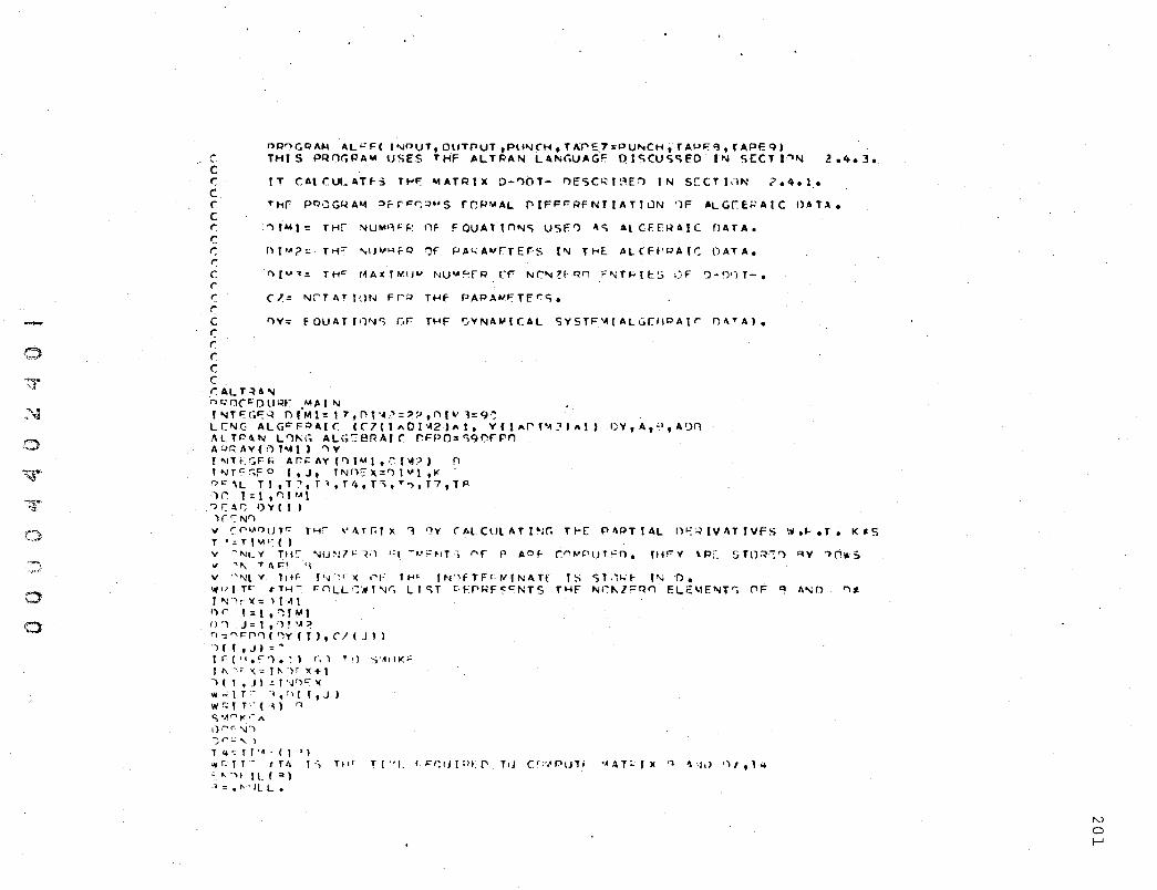
,0
7? "';
:'\l
,"'"' ':.:.Iloiji
~.' ""'3-
~ .. ',*
o
o o
npr'lGI:IAt-I AL;:F( I "JOUT, OUTpUT ,PU"lCH. T A,.., E7 =PU"<CH. r AP~". rAPE Q, THI 5 pqOr,PA~ USES THF ~LTPAN L4N(,U~G!" OISCUS<;ED I'" SECT F''''
IT CAtCULAT,.:; Tt-'F: MATRIX D-')OT- I')ESC~lc~[n IN S[CTI.1N <'.A.l .•
2.4.3. c c r: c C': THf' PQoJG4AM ::>F:r~r.~"s rcp .... AL (,)IFFr.RfNrlllTltJN "F ALGEEr:AIC f)AT~.
C r: r:
~IM1: TH[ ~UM~~R OF FOUATynNS USE') ~s ALCEf~AIC OATA.
r: DT~?::. Trl" "'IJV<4f-Q 'Jr PA\,;Av["TEf'S I'" THE. ALCFf'PAIC DATA. r: c 1"'11"''':: THe I~A(ll\f.tW NU .... r~rR (T Nr"'~t··qn FI\IT~II:S I)F ')-'YJT-. r r (1= f\ji'Tl\fIUN Fr~ THF PAP"w'F:TI:r.S. r: C ')V: fOUArr,.''''''' ,.F THF I)VNA~ICAL C;VSTF'oi(ALGEflPAlr nI\TA). r: r: r: c C r AL T~A 'Ij nGnC':~Ot"~~- MAl f\j I'ljT~GC::~ n(·Ml=17,f't·4:>=::>~.nl"'l=9~ LC"I( ALG~FOAIC «(7(1"DI"2'I'I, Y'I"r"~~'AlI)Y,A,",A~n hLTP~f\j Ln~~ ALG:eRAI( ~FPO::S9Qr~n A O r.:AV(:)T'11' "IV I "IT".(;Ff; Ar.j:AY(')IMl.~I"?' fl , "J r c: r,F 0 I, J , T f\! IV::: ~:: ') I .... 1 ,'" Q "'\L T 1 ,T :'. r -, • T I., T', , T"). T 7, T F'I ') r 1:0 1 ,n I 'A 1 "'r:~~f)Y(11 'IC' I\j')
V (:r",.ADUTC TI-i' \'ATr.lx '1 r~y ("lCUlATI~J(, TI-E P4PTIAL n<:RIVATfVFS \~.~.T. Kes T':TIM":() V '-"'LY Tile '\jU~U<'-~;) "I -''''''~'T') ror- r AO~ r:""~r>UT<=n. TIf;'Y \ Pi_ ~Tn~:-:') qy 'l('j~S
..; '" T 1\ ere 'i v "'\iL V T I H' I '~ r' r l( ,., F T I-' C IN') f T f r: w rNA T (' I S <; T ,~I-.; t- ,'-J f).
"t·JITcc kTH"7 J:IlLLI:'Jjl'.r, LIST C:E""RF~<=NT5 THF NI;I'.z:::qn ELEI.1ENT<; r"'F ~ A"lO ,,~
r "",'le.",) 1',,\1 I) r t:: 1 , ~ r U J 1)'1 J=I,'!'A,;) ~:~FP~(~Y(T),Cl(J') -)(r,JI=~
r r (r,.r,). ~ I r,) "-'1 :;·.111K". I "~';'(= II\)r-':+l ') ( , , .J I = I 'Jf)C' )(
'II ... IT" , • '1 ( T t J 'II";! r'-(q r> C;.~r'"\t<'i-I\
l)rc'lC)
"")rt.:' )
14'" r I ",. (1 » "" r. ! 1 'C t f 4 I '-, Til r T!" t _ I- >= r: 1 J I :; F [' T 11 C .. c',, P lJ 11 " AT:" r)( q 1\ --1" l) I , 1 4 O~,rIL(")
-~ = • f'\.l It L •
tv o f-J

v r:"""nUTr T!I'- \l4T)'< 1\ "V (/,LCIILATI'jG Tur nAP 1 1AL r.r~IIIATlllr'l flr .IV v ALL TI.e ::L~"·,Frl.T<; (f ,. IIrH" !'.TflRr "v R""",S r:I\ TAF~ 0 " T 1 = fl" t": ( ,
~~'1'= -tft.~; f-'nLI.':tl'jr. LI<;T ;"fPP~!:;-".:T"! Tlfr ·~"'j7~::.r: ""L'-:"'=.'IT'; 'F ,.., ;)" 1=1 ,nl \.'1
nr'" J=l,')t~l A :I"\J- ('r)( r:v (I ) , Y ( J ) rWPIT<=(ql A If(A.f('J.")) C." T"' ~:I\T
',l/P( Tr ',J,A CAT", f)cr~1")
I)l1f 11\')
T?=T'''':=IT\I ~PIT= tT? IS TY~ TI~r c~CUI~~n Tn CO~pYT~ "~TRr~ ~ "T:> A=."JULL. f 0.,:1"' r" I L ( "~ , v ~ll"ln"1 cL~"'AC~l''; '-'. I"V [N(.(,YI-'AT IHlf FOJ;'.4AT f) n I '>If) ~ 'I = I, r) , 'I 1 w(')!Tr- 1"If)FX,"VC r"l!)~'1' ~1~'T-:(7) t",n'"'x,I~V(IN"I':'X' f):"," t.,j')
wrnTr tr:LI"~f-"IT:'; ("11'" '~A,!"r.'IX Al/:I)+~ -t P r: w 1 "If) ( ~ I QCW ['~n( ~I I ",')cX=llT~l T7=T!\!::CI I") n ,= I , .~ I '~ 1. v n Y I '; 1I ~ I" r 1 n ::; T' )'. C' " f" 1")\0/ n F A I") n J = 1 , r, I ... 1 REhCl(QI ")YfJ' I")Cf" III") ')n J=l,-lf~:>
I F ( f) (I , .II • f" () • .; 1 .-,f) T G r~ l ~ Dn
l"II'r v = I ".')f '1+ 1 v "A~"I"' 'jrXT ""'1N:lI:P"l rL~'~INT nF A f.' ~ A r ( q I II n', n (" I< = 1 , '") I 'I 1 I F ( I") ( K , J) • '" '). : •• n ~ • I") Y ( I( ) • F o. C ) ('.n T " C Q Y ACr=A~q+f)V(K'~V(I")(~,J') CqVA OnrN,) WPITf I.J,r~''''\f:x,\n'' W~IT~'''') r",I)":"X,A,)~
'i.lf"')", r) ry N,) OC""r") Tr.=ll~::'T"Y1 NPITF tT'} IS Tlo: TI~r '"('OUIPFO ~ C"""'f"UTf IAATQI)( A*f)+A AND OUTPIIT *,Trl F ",f) ."'nF C ALr, .. r-r.>AtC GATII
-CIClPV(l' +CZ(?,'HrY'"H*"V(16' - r. 7 ( "~ ) lI" V ( ~, I(: Y , 4 ,::< Y ( ? I +C l' ~) '" y ( ... , >!l '( ( 7)'" Y ( c., , + r: z ( 1 , ,: V ( 1 , " -C7(?'*V(1'*Y(4).V(?'.Cl(J)*Y(A'*Y(7'*Y(~'-Cl(?~.~Y(16'.V('
~ , N o N

-.:'\f
o ":r ;-'.1
;:,)
7,.;r
~y
C)
, .. :-.... ,·t·"'~~
a 0:
:3 )
" ) y ( 12)
v (l ~ ~
14'
-Cl(2).Y(3)*V(4'~Y(2ItCl(3'.Y(~)*Y(1'*Y(5) CZ(2'~V(J).Y(4)~Y(2'-CZ( ~'.Y(61~Y(7'.Y(S)trZ('O'*Y(lb)*Y(
-CZ(1'*Y(6'*Y(7)*Y(~)-Cl(5'*Y(F'''Cl(4)~V(~I-Cl(7'*V(~' *V( tr: I ( 6 , *y ( q, .. (" )1'( 2 , r. V ( 3 , .. y ( " ) ~'Y ( l • - C 1 ( 9 I * V ( 1 0 , I< Y ( f': , t C. Z ( 1 'J ) '" Y ( 1 1 ) '"
+C 1 ( 1 c; I ,~ v ( 1 ~ ) .. y ( 1 2 ) -C l( 1 4 );: y ( 14 I .. Y ( !> ) C Z ( ? , *' y ( ~ ) * Y ( 4 ) lit Y ( <' ) -c Z ( J) .• Y ( 6 ) .. Y ( 7 ) * Y ( c:, ,
- C 1 (4 , "V ( R ) .. (' 7 ( 5 ) *v ( (, ) + r: , ( (- ) '" Y ( C) - (" 1 ( 7 I 'l< V ( 6 ) '" v ( R ) .. C l ( 1 1 ) 'l< V ( i ~ ) -C 1 ( 1 2 ) '" ~ ( 1 1 ) * Y ( A )
- C 7 ( f- , .. y ( q) +(' 1 ( 7, .. V ( ,., , '* Y I Q , - (" l I 1") ~ Y ( '~ I - C 1 ( 9 ) ~, V ( 1 0 ) * y (( ) .. C 1 ( 1 ~. ) '" Y ( I 1 ) "Y ( 1 2·' .. C 1 ( " , (: y ( ~) - C 7 I .> 1 , :~
"Cl(2?) «V( 1">' -(l(lCI*vll1 '''YIl?)+C7(91*YI)( ,¢V(6).'.l( 11)'.'V(I"q-C'112)"<
Y(111*V('1) r: 1 ( <) I ~: Y ( 1 C ) '" Y ( f., ) - C 1 ( 1 C ) ~ v I 1 1 I~: y ( 1 2 ) .. (" 7 ( 1 4 1 .. Y ( 1 4 ) ~: V (r) I - C .7 (
.. v ( 1 '~I '* Y ( 1 .3 ) .. C 7 ( 1 R I~' Y lIto 1 - C 1 ( 1 q ) to Y ( I 2 ) - r: 1 I 1 1 1 -I- Y ( 1 ... ) .. C Z ( 1 2 ) ''(: V ( 1 1 ) .. v ( Q , - r 1 (·1 ] , If: V ( 1 :0 ) - C ! ( 1 4 I ~ y ( 1 4 ) ... Y (t ) .. ( 1 ( 1" H· y ( 1 ~ ) .:. y ( 1 ~ ,.. C 1 ( 1 :!) .. Y ( t 1) - r: 7 I t 5 I oX Y ( 1 ') ) * v ( I? ) .. C l ( 1 4 ) * Y I 1 " ) i Y . (t I - (" Z ( 1 7 ) .', V ( 1 5 I +<' :' (
1("*V(I"-'
2~' r I ( 1 7 I "Y ( l~) ) - (" 1 ( t (, I .. Y ( t " I +, 7 ( 1 Q ) '" V I 1.2 ) - i .1 ( .~ I "V (1 f: ) - ell
*VCtA)·VI1) , - <. 7 I ~ 21 "v ( t 7 I +C 1 ( " 1 ) ,.,v ( Ie)
• F. nF
IV o w

12.43.40 C4,IC/75 8UTPUT
C C C C C C C C C C C C C C C C c: C C C C C C C C C C C C C
1 2
PRaG~~~ PLCTCf~PUT,uuTPUT,TAPE9q) THIS IS ~ FlCTTt~G ~OUTr~E _HtC~ CAN ee IMFLEMENTEC AT THE COMPU
TE~ rENTf~ OF T~E UNiVERSITY OF CALIFO~NIA eFRKE~EY.
5PECS,AR[ PARAMETEPS CF THE GRAPHICAL DISPLAY SYSTE~,THEY SPECIFY
Tt-<F. LE·NGTH cr A COOI<CINAT[ SYSTEW,NUMiJER OF SUBCIVISIONS,TYPE OF C
COr.OINATCS (~nLA~,~~C1A~GULAR),A~O ETC.
THE P,WGRAM ~[OUfRF.S THAT THf TRAJECTORIES OF THE SOLUTION AND fXP
F k I'" [lIlT AL CAT A e E c: f V EN •
l,ZI,l2 A~E T~F POINTS R[PRESENTING 1) A~ EXFf~I~E~TAL DATA FeiNT
2) AN I~TFGHATEO DATA PCIN1, 3) A POI~T Ch T~E T~AJfCTO~Y W~EN US.
~G A~ INITIAL GUESS Cf PA~AMETERS VALUES.
~= NUMACR OF INTE~MECIATES OF THE CALVIN CYCLE.
N= N'JMElF.R CF DATA POI"TS(OR T[ME INTff.lVALS).
DIMf"5fGN SPFCS(3C), lIl4),Zl( 14).Tf 14) ,CC 11. I)J¥IO"SION Z2041 . U I-.oCNS ION E( 17,.4' ,DR (1 7,14' ,TR C 17,14·, ~IMEN5IUN P'UFX(500),~UFY(500) o f ME" S I a h L I NF ( 1 7 » CI~E"SION L~OC(2)> OI~E~SfON GIVE"(1, nAT A T /0 •. , e. , ~ • ,9. ,Ie., 12. , 16. ,21. ,2". ,27. , ] 1 • ,35. ,38. ,41 • / /oA=17 N=14 LAt3C(2}=O REAl) ""I,(LI""'(I,,·I-=l,'"
~ FOR~AT(2(aAIO,),IAIC) READ 1,«E(I,.Jl,J=I,N ),1=1,"0 PEA f) 1., ( ( 0 R ( I , J ) , J = I, ~) ,I = 1 , ., ) REAn l,(TR(I,J),J-=I,"),I=I,M) FC~~Ar(HflO.A~/rbFl0.8) Fo,n~Ar (2(eFIC.('/),IFIO.6) SPFCS(I)=1.5 ~PF:C~(?)=I .5 ~p F. C ~ ( J) :: 4 1 • 5PFC5(4)=O.
\
N a ~

1'1)
0>
c::r :-'1
:::)
.. ~ ?1
.~
'0
0'
0
::PEC~(t"'=C. SPEC5C71=IO. 5PEC~C8'=9. 5PECS(9)-=30. SPECSCIO)= 10. SPECSeI2)::<;9 5P E C S ( I J , :: I .SPEC~(14 1::1. SPFCS(151=1. S p t:: (.S C I') ) = 0 • SPFCS(20)::O. SPEC ~ (21) :: 1.
M:) DC 2!J J=I,JI SPECS(l7)=.1 ~PECS(18):01 SPfOC::(25)=O.O 0=1. C::O. CO 21 (=l,N ZI(f)=fCJ,() I ( I ) :: l>r~ ( J , I ) 12111~TRIJ,() IF(Zlll).GT.C)C=ZlCI' JFIICI).GT.C)C=Zel) IF ( Z 2( I ) • G T • C , C:: Z ;> e 1 , IF(ZICI).Ll.D)D=ll(I' lFCI( l'.LT.D)O=Z( I) lFCL2(1'.lT.D)D=Z2el) CONT INUF SFECS(24)=O.1 SPfC5(26)::0. SPf-'"CS( It,)::l. SI=ECS(ll ':oJ. GIVF~Cl'::C GIVE"I(2)=D GIVFN(J)=lO. CALL FAALIY(GI~~N,SPECS) CALL AXLllJeSPECS) SPECS(2A,:t. CALL NCDLIPe5PECS) CALL T1TLfE(15t-TI~E 1I'1II1"UTf.S,SPECSJ SPFCS(2HI=n. CALL NLOLIL{SPfCSJ CALL TrTLrl(?7H(ONCE~TRATICN IN wILLIMQLA~,SPECSJ S P lc C ,~( 1 7 ) = • ) SF[CS(11J1=.3 LM:C( 1,=L I f'..F ( J 1 CALL TlfLET(LhAC,SPEC::' ~PfC':;(171=.1 S PEe S ( I tl ) = • 1 CALL PSLILICl,Z,SPECS' ChLL PFLILI(T,l,HUFX,EUFV,SPECS) 5PEC5(22)~1.5
N o en

50EC5(23'=.9 RULE=I •. CALL SYMKEYlRULE,.8HT~AjECTCRY CBTAINEO USING EXACT PARAMETER VALU
lES,SPF:CS' SPECS(l6)=13 CALL PSLILllT,ZI,SPECe, CALL PFLILllT,ZI,AUFX,BUFY,SPECS' SPECS(C:J)=.C5 CALL SYMKEY(RULF,47HT~AJECTCRY DeTAINED USING BEST PARAMET6RS FOUN
10, ~PECS) SPECSllt)=!: CALL PSLILI(T,Z2,SPECS) CALL PFLILI(T,l2,B~FX,BUFY,SPECS) SPFCS(23)=.3 . CALL SYMKEY(~ULE,59~T~AJECTCRV OETAIN~C USING INITIAL ~UESS OF PAR
lAMETEQ VALUES,SPEC5' IFIJ.EO.M)(O TO 20 CALL ~XTFR~(SPECS)
20 CONTI~UE . CALL GD~[NC(SPfCS) STOP EI\O
IV o en

~
~:J
~.
~"'j
o "i:JJ'"
"W
<:') ""l, .. ,:,. .. -'
c') o
PR(JGH 4-4 t:.WOR ( INPUT ,OUT PUT. [lUNCH. 'AP[o =OUT?UT I C*".·. THIS ~I.lCGRAM GIV£"S AN ESTII\IlATE CF THF. EXPECTEO £:RiW,-~ IN THi: c***** PARA ... rTF.~C; tiU[ TI) ERRCfO IN Tr1E DATA. C ••••• 1f30' Ie; T:iE Flk~T ,)ATA r>UI""T. C.*.** IhlP IS T11£: LAS1 i.)ATA POINT.
CO .. "MJN C 1 ( I.H CUMMeN 'l,lH, vIMf:NSION Y"ICl7,I,6' U I Mf f',j~) i fjN H ( 2 £' , ~ 2' , DE. ( ;'? , ;>~. I, E ( I ., , I 4 ,6 I . o I 'He ,'oJ ') IU N 11 ( 2~' • 2 ~ , • p ( .~ ;- ) • P I ( 2 c I • E I V U ( "2 I • P P ( 22 J .) I Wf I\' S I I ~ N h (?? .;:>?) • T ( ?;>. ?? , , '-. ( ~' ,? , 2 2 ) Cllllr I\SlCN AIN\i (:'2,22) ,A( 22,,,,,, U I ~t." ,; [rl'~ "" t< All EA ( ') 72) [)(MI~~',I(lN I) UM "-I 'I' ( ?2.~?1 l) A T h r</ <'? / , \1/ 1 7/ • I .i oj T /1 / , I Tn r> / I J / • I<. I /6/ 1<1- A Lo I'. (( Y N I ( I , 1 ,L 1 • 1;;'1 • ,01 I, L = I , «. 1 ,
11 r d IH .... ' T (<' ( >;. Ie. t> / I , riO. t,) PIAu 1,>,(CIIII,I-=I,I.SI
16 F L~~,l T ( ~r Ie. (,' /, 5/1 J • 0 I P fAG 'l ,) I , ( ( ( f· ( I. J , " ) , .1 = 1 , I r. I PI. I = 1 ",", , , K = I , I( 1 ,
5C I r I) r;~.' AT (') r lb. 1', / ,,,;/. 1 '). I l, /, jf 1 t, • I .i I . Du ,..,0 I;;I,K on 7~O J=I,K H( I. J I:; u
750 ·(0'-11 I f',jllr
0[, 2 I ..: .... = 1 ,<. 1 on I I = I , I(
Dr) 1 J-=I,o< ... ( I. J 1=(; Dl: ( I ,J 1 "0 C. rt~ll ""u!-_ lI(1 ? L;; FlllT, I tuP
C"."'It* I ~IT~i-IL ;; A ~U['f:r)UT INf- TU .tF IISI::I) TO f 1,,.1> THt: VA'~ I &oNCf 'Jr- .THf-. C" ••• " PA'~A\1L1[,~5.
(ALL I:-.r(.;~L("1\! I.L,!:., IIH'T,K,"',I<.'<" [)C ~I 1=1,·"
C.:.",·p.<", CXX=THt: ,I~TI' A S';·) III Ir.(, 06 PL,~(U·j.T l~flI5[ (" IT c.xx=I./(£.(I,L, .... O<')"L( I,L.t<K)) CXA=Cxx*100JO./lh. ClJ " I. J = I ,I(
5 ( 1. j j = C 11.]1.. ~ I lie ( I • J I f-( J ,1).:.)1 ( I, J)
tll (ONTI "''-I. 14=K I II ;;1,';
1(=1<
c.*t**.: 5u\;"jdTI·4·': r~AMUL PI~krf';hv.·j"A"HX '~LJLTIPL1CAT1·I"'S. (. ALL /IIIA~.' UL ( 'l • ':. , I A , 1 oJ, 1 (. , T ) G(I 41 \"1,1< r.r. 41 )'-'1,;(
C~~,**,' (:"'LCJl·q lr.N fW ftll- "'AT'dx 11 (·)j';(u·'S'-,) I'~ SL:. 2.' •• 1. h(I,J).~ 1,(/ ,J) t T( I,JI A( I,J):"I( I,.JI I:' ( 1 , J ) -= ,'1 ( 1 , .J) / h •
41 c.nNll NU" <! (lll\ll\t.,)r
N o ~

21 C G '" T II\j·Jf. 1)0 10C J:.l, t< 00 ,JJO 1:1,1< PP I NT 1 1 , J, I, .... ( J, I )
11 FfJHMAT(ll1 ,1~.r~,r.16.tlJ 100 COM 11\:);:
M> 1 M:?i' N=2? NuY'[:.:1)
CIOtIC<.*. 11(11;1'(: RI)UTI NE HI t-' INe) r: IGENV'\LUt~~ IlF MATHIX P. (ALL HQUR(~,NUIM.N,~IV~,NUYES,OU~~Y' 00 304 1:1,1( E I II (, ( I I = 1. 0 I'f- I II LJ ( I )
304 CLi>llINUt , p PIN T j 02. (to I \lL ( I ),1 = 1 ,1(, J0 2 f () R~ A' ( f,)( , fr t- I (,~ N VAL lJfo S UF [' CC "/ /, l.l( , t.': 20. Ie, 1 )(' /.1 J
N:.K IA:f(. . II)(;f=0
c****o(: LINV~f:: IOuTIN': Tn liND THF= II\Vf:r./c;r: fJ~ rl (ilIHleH IS Tt-r: "ATRIX C***** P OISCIJ>'.itu IN ''if-('TI(~I\ ~.4.1.)
.: /I L L i... I N 1/ 2 f ( A ,I'o,j , g, ,\ 1 N 1/, [[):i T , .", 0<. A.f~ E A, I t. IJ ) ur: 'I " I ;: 1 , K ", ( I ) :: A 1 Nil ( I , 1 ) DO <)<) J= 1 ,I( P~INT 11,I,J,AINV(I,J)
Q<l COl\ll I Nuf DO <.J7 1:[,0<. P I ( J I.:,~ ( 1 I
97 CUNT INJ~ PI.INT iO?, (PH 1),1=1 ,I(J ,
lOb fORMAf(ul(, '" "ARIANC:~ .ITH "ill( UdTIAL VALUES *.I//(lX,6t.20.10,IX'/ I/)
N=K IA=K ID(;T=O CAL L L I 1\ ,,? t' ( n , N , I A, ,\ 1 N 1/, I D G T ,W K A !ll A , I f:: n J Dn 101 I:I,K PP ( ( ):: 1\ I Nil ( 1 ,I J 001::>1 J:::I,K PHI N, Til ,I ,J, A 1 Nil ( 1, J J
101 CtJ"TI I\1)f: C •• *** PIHNT OUT '),- THE IIAI·HA"lCE IJF P. (Tt-E l,{PfCTEO fr~HaR l'~ THt: c.* ••• PA~A~~T~RS.'
PP IN f !J 5, ( PP ( 1 ) , (= 1 • K I 305 FL~MI\f(t>X,~, \(AR(ANC~ Gf' J:"'foIAW~TL,lS "'//I(I)(,oE~iJ.II),IX'I/)
S luI> ' . END SU8kGUTINE: MAMULIB,S,IA,IB, (C,T) DIMEN5(O~ ~(?~,22),r(22,22),S(22,221 Of) 1 I=I,IA DO 1 J =' 1 ,Ie T(r,JI=0 C ONT I NLJr Do 2 I = 1 , 1 A on 2 Jecl,IC
N a (X)

;.0'
o -'~.
~.,,\,
.::)
'i\l-'
;;;;as
(:)
a
DO 2 LK=I, Pi TC f,J.= r( f,J' .. III f ,LlO*S(LK,J)
2 (OI'llTINuE RE rUIlN END SU'1~()UTI,4E YOllT(N')tY,rLASr.T.~.,\oIt"') COMMONISTCO~2/M,Nq.H PEAL Y(NO,I H RfTu'H~
FNO S 1I '1 ill) uri NF I N r G P L ( Y 1'4 I ,L ,E , I tl 'J T , I( , "" 0( I( ) CU'-1M(]N CZ(ll) ClI· ... ,~tlN :i, DE UI"'[~SICN ~(~?,22),C~(22,~2) Ol ..... CNShIN Y;'l1(17,l.6~,t(17,14."JI DI",r,,,"sr.JN T(ljl '
<.**('** YOLol( 10j) TO Yf)OT(I3?1 ARE TIi~ NON lE>lfl ~Lt:MENTS OF THI: ENrERIC'; C**"'** or T"It': J-"'AHH x Dl:,;CuSSCI) IN SCCTlU"4 (».4.1.
PLAlV(>i2,IJ) RC.~L Y'A,\X(<i?) ,ERRJk(-i2I,~"(/)dCo),F51'''f:( 1')4' DA r '\ T /1 ., ,,- • , 1 • ,' •• ,'~. , b • • '3. , I J • , I 2 • , 1 'j. , 2 C • , :~~:; •• ] J • I MU''''''32 00 1') L =1 ,'»I\")"4 V~A,(II'-I.
I <J Cl1'J TI N ur: II'(l-I'lUT)I,I,2 (.!INTINU,' 00 , 1=1'1,"'[;,"1 Yel, 1)-=0.
3 (.flNTINv[ DU ~ 1 [= I , M '1'(1 ,I)=VN[( I,I,KI()
21 I':LNTINUI' DO 4 I = I , K Dr. '. j=I,1( Dt ( 1 , j , :: 0
4 ClJNJI"-i'JL 1\0 = t.t"l"', HO=0.001 lP'3:;;0.·)f)1 ro=o. MF -= 22
2 (CNTLN·,JE TL AS T:: T (L ) (. A LL [)" I v t:: S (1'4 C'. TO, TL AS T , Y • H~ ,i:;l:; • /Wr , 0('= L A ~" V M A X • fe ~q '1 ~ , p '- , .-'5 .. w r: ) DLl ~0 1 = 1 • '04 L ( I. L ,<,K.) =y ( 1 I I )
30 (ON r I r,u:, Gf ( 1 • 1 ) = '1'( 1 ~ ) ('I:- ( 1 , 2 C ):: 'f ( 1 q ) LJI. ( ,-' I 1 I = '1'( ? ') I IJ£ (,I,? I = v ( 2 1 I r'L ( t' , ,I ) ~ v ( ;' ? I (; t (j,.) I ~ y ( .? S I C f. ( j ,I 1= Y ( :> ~ I [) [. ( \ ,:> ) I :' Y ( ." ".> )
IV -0 1O

DE(~,2);;;Y(26J DE(~,J • .:Y(27) DEC'5,Z):Y(lc' [) '::: ( 5 , 3) -: Y ( :")' ()E( 5,20J:Y( JO) DE.. (6, 21 .: Y ( .J I ) DE:(6,J)=Y(32) 01: ( b, 4' : Y ( :U, D F. ( (, , ::. 1 ;;; y. ( .~ 4 • Of: C ~, Co );;; y ( 3 ~ ) OE(6,71-=Y(]0' DL ( 6. S I" Y ( 3 7) DE ( 0, I') ) ::: Y ( 3 ~ ) DE ( u, 14 ) := Y ( C")) DE ( 6, 1 5) = ..... ( (.0) DC (7. <') = Y ( 4 1 ) DE ( 7, ] 1 = Y ( 4? , DE (3, 4) -= Y ( ,.,~ ) DE ( '3, :, I = 'I ( 44 I Cf:: ( 'i, b I = V ( 4 ~ •• DE. (,'\, 7 ) = 'I ( 4 (. 1 OL ( e, 1 1 ) = Y ( 4 7 ) Dt: ( >3 , 1 2 , =y ( 4 e • 01: (q,t: I=Y{4'1' D[(~,7)=V(50) 01: ('I, H);;;Y(SI) DEC 10,-3):.'1(52) DE: (l 0, I) = '( C 5 J , u£: ( I 0, 1 ) ) == V( ')l, J [II: ( I 0 ,.) I ) := y ( ,; '3 , DE ( 1 G, :~::!)= Y (St» Ol ( I 1 ,";., = Y ( ~ 7 I Of: ( 1 1 , 1) ) := Y ( 51:\ J ul: ( lit I t I: y ( ::; 'I ) liE ( t 1 ,1 2 I -:. Y ( 60 ) D[ ( 1 2, ,) ) = Y ( 6 t ) DE. ( I 2 • 1 J ,:. y'( 6:.! 1 Ol( 12,141-=Y(6.3» Of. ( 1 2 , 1 j I = Y ( (~/, ) u( (I£' ,I'oj) :Y( o..J' uF.:( 13,11 )=Y(on) DE. ( 1 J, I? ) = Y ( () 7 ) DE Cl 3 , 1 1 ) "v (6;j ) DI: ( I 4, 1 'j 1= Y ( 6 ("i ) D!- ( II, ,14 I = Y ( I J ) o [ ( 1 '+ , 1 .~ ) =- y ( 1 I 1 Qt. ( I:) , I 4) = Y ( 1? ) ()[- ( 1 :, , I ',> ) = V ( l J 1 Of.. ( I:), 1 t: ) = Y ( 7!1 ,
DI (1:',1" =V (I'" Of-' ( 1 t, 1 t: ) = Y ( 7,.» Ul ( 1"> , I 7 , = ¥ ( '771 [; L ( If-.. 1 .1) 'C. " ( 7 --, 1 o l ( 10 , t .~ ) = y ( ! , , PC ( I', , ":-; ) "- y ( '-1 c' ) Oi:: ( 1 1, c! I ) =- Y ( ,\ I )
.N ..... o

....0
.. ,.."" "-'::;r
'~l
.::>
~
~~,.
~ . .. ~ . ...,.
~'C:!>,.
,-3
0
0
DE ( 1 7 , 22 ):::: Y ( 82 ) RETURN END SUBROUTINE DIFFUh(N,T,V,VD~T) CO,,",,>40N ee( 13) DI~'ENSION eZ(221 #< E AL Y DO T ( A 2 , , V ( 82, I 3 , Cln '::::CC(1 , (1(2'.:CC{Z) (ZC~)=CC(3)
Cl(7'=«:(4) C1Co'::::(((5. Cl(~)=CC(td
Cl( 12' =CC( 7) CZ(l3)=CC(i1, Cl(14'=CC(9) Cl (l 7) ::::(CCl 0 I Cl( 1 Q)=CC( II. elUO):CC( 12) Cl(21)::::CC(l3' (1(3)= Cl(?)*14?5.05 Cl(4)::::Cl'~)*.047dJ CZ(&'=C1(7'*.000153 (" Z ( I 0 , = C 1( 9' '" 1 2 • 59 (Z(II )=CleI2.*.00007~ eZ(I~':CZ( 14)*1.18 CZ(I~·)=Cl(17'*2.j2 Cle It:! )=Cl( 1 Q)*1.4 e 1 (.? 2 ) = C 7C ;:> l' '" • 4 2
c***** YIH.iT= IJt:ldVATI VES OF TH( STATE IIARIABLES. vuor( 1)= -el( I'*V( I) +CI(20'*Y(~I.V( 161 VD 0 r ( 4 ) = -C 1 (2' "/f. V ( j, '" Y ( 4) *v ( 2 I+ez, 3) • Y (6 ) *V ( 7 I.V ( 5) V .),1 r ( ;:> ).:; Y lHIT ( 4 ) + e I ( 1 , '" Y ( 1 » vu 0 T ( J ) :::: yon T (4) - C Z ( 20'. V ( 16 ».V ( J ) V 00 T ( 5 ) = - Y f) C T ( 0\ ) .. C I ( 20 , * y ( I ti) • Y ( 3 » VD Cl T ( 7 ) =-Y DOT ( 4) YDOr(h)=-Cl(3).Y(6)*Y(7'*Y(5)-Cl(~).y(~, .. el(4)"'V(a»-CI(7).Y(61.Y(8
1 ) + Cl ( (.I r Y ( q) + L 1 ( 2 , * Y ( :t , *y (4 • *y e 2 J- C Z ( q ) .Y ( I 0) '" Y (t, » • C I ( 10)" Y ( lit .. Y 2 (l ;> HC l( 15 ) (0 Y ( I">'. Y' ( 12. -c Z ( I 4 , '" Y ( 14 » '" Y (6 I
Y DllT ( 13 ,:-C Z ( 4 , * Y ( 8 , .. C Z (5' * Y ( b' .. C 1 ( f , • Y ( Ii) -C I C 7 , *y (6 ) *y (8 ) + CZ ( I 1 » • I" C I j, -C 1 ( 12' * Y( 11 ) * Y t 8.
YDOre9'= -Cl(oH,\,(QI +c:Z( n*Y(o'.Y(/j'-C1CIi'.Y(91 YOOf(lO'=-Cl(<;'*Y(lOI*y(ol+Cl(IO).Y(11 '*Y( 1~)+Cl(R'*T(9' -CZ(211*,
1 (IO)+Cl(2;:>'*Y( 171 Y t) () T ( , I I:::: -r. .l ( I 0 I * Y ( I 1 ) .. Y ( 1 2 ) .. C I ( <; , * v ( 1 0 , • Y ( 6 , "C I ( 1 I , *v ( 13) - C I e I 2 I •
IY(11H''f('H YO (J 1 ( 1 2 , =c·z ( 9 , « y ( 1 0 , * Y ( b ) - C L ( I 0 ). y ( 1 I ) '* Y ( .- 2 ) + C Z ( 1 4 ) • V C I 4) .. Y ( 6) - c Z (
114l"'1'( 1:.>1*Y' ( 13) +Cl( 1 el*Y(1bl-CL(1 n*Y( 1~1 Y D '1 r { 1 ] .:::: -(. 1. ( I 1 • )~ Y ( I 1 ) + C Z ( 1 2 ) * Y ( I I ) ')Y ( >j • -C I ( I :\ ) * Y ( I)>> Y DO T C 1 41 = - r. / ( 1 '. ) .. Y ( I 4 I « Y ( (, )+ C l ( .1 5 , ... Y ( t r~ ).y ( 1 2 1 +C I ( 1 J I fit Y ( I J} Yl) I j r ( l~). '" - 'J ( 1 ~) * Y ( I 5 I*' Y (I;> ) + C I ( 1 ,. ) .. Y ( 14 , « Y' ( t. ) - C 1 ( 1 7) * Y ( 1 ~ I ~ C 1 ( 1 6 ,
1*'1'(16) Y Oll r ( 1 t, , = .. C L ( 1 7 ) « V( I J ,-, I ( 1 (, I *v ( 1 6' + C l ( 1 -I P Y ( 1 2) -C l ( 1 f> I « '1' ( 1 b' - C 1 ( :~
10 ) *Y ( I 6) « Y ( .q Y 0,-1 f ( I 7' = - C l ( .!;> ) >I< Y ( I I , + C 1 e 2 I ) ,.. y ( 1 0 , YO 0 r ( I 'i I ,~
t>..) I-' .-.

c*'~*",l« fA(r .. )f- Trf. fJLL:;ioIlt\r, ':CLATLJ,,;, IS <\ ~dN-lH~C f-1~f~V ;j,= TH'2 C *.~ *' III '" ioU. T fI I x ').
I - (" Z ( I • * V ( 1 ~) - Y( 1 1 Y I) r.T ( 1 ,,~ I '"
1 - C1(IPY( l~' t ('l(~OIO::y(jI'~Y(JO) tell 201*Y(I!JPY(?.)' • Y(ll*YI 1 161
YOOTI2!)1= 1 C I ( 1 • ,j: V ( 1 ,~) - (Z I '" , *y I.'J ) « Y (4 ,~, Y( 7.0 t • Y ( 1 ,
YO OT ( ~ 1 J:: 1 - (, l ( '» '" V ( C ) ~ Y ( "l , >It Y ( 2 .. 1 - C 1 (,J) ". Y ( ;c 1 <tv ( Ii) » Y ( 2 J 1 - C Z (2 ) • Y ( ,i) * Y ( 4 , 1 • Y (? I I '.. (L I ) ) * Y ( 'j 1 ,;;. Y ( ::- 1 >Coy ( '. I) • : 1 ( ) • " v ( ~". t" Y ( 7"~ Y ( :3 1 1 1 'I' ( :~ ) ~ y ( ., I iT- Y «(. 1 .. ( 1 ( .3) * Y ( (, ) "'v ( 7) '" Y ( ? 'i 1
YUll T (r~') ) ;
1 - L l (;.: ) '" v ( .? I * Y I J ) ,~v ( ?, I - (1 ( C' I " Y ( 2 , ... v ( .. , t: Y ( ;>,. 1 - (l ( t! '''' v ( )' * Y, 4 , I 1(: Y ( ?,!., .. C l. ( ill,: Y I c~ , .:' Y (t> , '~Y ( '. 2 I • C ,~( j 1 * Y ( ~ 1 « Y ( 7 , « Y ( j? , 1 .. V(.')I>ltY(hH'Y(7J"Cl(.n*V(bH'Y(7)*Y(29,
YDOfI2])= 1 - ( l I:::! I *v ( ;» * Y( ] ) * Y, 2 t;, - (Z (? 1 >I< Y ( 2 He Y ( 4' ,~ Y( 2 31 - C l ( ~ I • y ( j I 'IlC V (4 ) I*Y(;~I' .. r:Z(]H:V(:"»:':Y((d'~Y(41) .. CLC1,t.:Y(::>I*Y(7,t,:Y(H' . 1 - C 1 ( ? C 1 ~: '(( I t>l * Y(.? J, - Y ( <:, ':: t ( J H: Y ( 4 )tel ( l' « Y ( 6 I ~Y ( 7 '''' Y ( 281
YOCT( ;~~ I:: 1 -C I. ( £> H' Y ( .~ , * Y ( j I '" Y (2 7) - C Z ( ~ 1 ... v ( 2 , .~ '(( '+ I * Y ( , .. , - C l ( 2 I « Y ( 3 , "'V, .. , I * Y ( ;>;> 1 .. C I ( 31 '" '( ( 5) "Y ( (-. 1 * '( ( 4 ? 1 .. (z () • * V (5 I. Y (7 , *V ( 3 ~ , I - (l ( 20 ) ¥ Y ( 10 , * y ( 24' + Y ( ~ , .. y ( 6 ) * Y (7) + C l ( 3' oj< v ( 6) 9 Y ( 7 , * v ( 2 '·H
Y I)n f ( 2 '.;' :: 1 - Cl(.~'*V(~')~V(lq"'Y(c:;'1 + CZ(,I)*Y(oHv(7''''VtJCO; l-CI.(~(;HY(lt'~'Y(2r:.) - Y()'*Y(h.~Cl(20)~'Y(l'«Y(~OI
V,) r: f ( :' ,. • :: 1 - Clc:~'(tY(2)"'V(J)"'Y(2t" - CZ(?).V(?HY(4'*Y(211 - CZ(2I*V(~"'.<Y(4) 1 '" Y ( 2 IJ .. C 1 ( ] 1 ;~ v ( ':.d f.: Y, td * Y ( 4 1 1 .. ( Z ( 3 1 ¢ Y ( 5 ) * Y ( 7 , * Y ( 1I , 1 - Y ( :-! 1 ~,y ( :l I >:< Y ( 4' .. C 7 ( ]",~ t ( ., ) • Y ( 1 •• Y (2 d I
YDO T ( 27. = 1 - ClPI*Y(21*Y(.1)*V(27) - (Z(2).Y(21*V(4)*Y(?4) - Cl(2).V(J'.Y(4) l*V(~.:'1 + CZ(3'.V(!'JI*V(u,*Y(4') • Cl(31*VI51*Y(7J*VD2) 1 .. v ( ~) * Y ( 61 * v ( 7' .e 1 ( :1 1 ,. Y (6' * Y ( 71'" Y ( 2:J 1
YDOTC:!J):: . I (l(21~1'(2)*Y(.i)*V(2t>l .. (l(?"'~Y(~)~'V(41«VI231 I -C Z ( .·i I ~ v ( 5 • * y ( u 1 ,~ l' ( 41 1 - C Z( '3 ) * Y ( C) ) '~Y ( 7 • * v ( .1 1 1 1" ( l ( 20 1 * Y ( I 6 ) ., Y ( ~.i' + -- (2 1 )~ Y ( :') '" Y ( 4 1 fC Z ( 2 ) « yl 3 ) '" V ( ~ 1 * v (2 1 , -1(1(3)~V(JI*Y(41*Y(211
Y!.HH (2·~)= 1 C I ( ? 1 .;: l' ( ;> ) * l' ( ~ 1::'< Y ( 2 " .. C 1 , 2 1 )~ Y ( ? ) ". Y ( II • .,.Y ( 24' 1 -<.; 1 ( j , ,~ v (oj ) ,: Y ( 6 ) * Y ( 4? - (Z ( 3 • ';: Y ( 5 ) ,'Y ( 7 , * Y ( j 2' .. 'Z(231*V( 11_)<lV(24, - l'(~)I*Y(6PY(7J+(l(;?I*Y(~I*Y(4'*V(221-lCZ(J)~'Y (I':>,*V( 7)*"V(29)
YOOT()C.= 1 Cl(2.>;<Y(2)'~Y(4)('Y(2S) - (Z()'''Y(0)*,((7I*Y(301 • Cl(20'*Y(H"'V(~O) 1"C7(~CH'V(161)~Y(?'5) .. Y()I*V(ltd
VCoUTIJI)= 1 C l ,,~ ) )~ Y (2) ':' l' ( 3' '" Y ( 2 6 I + C l ( 2 ) * Y ( 2 ) * Y ('+ •• Y ( 2 3 , I.. C '- ( ;:: ) ,) V ( j I ~: Y ( ... ) * y ( 2 1) - (l ( ~ I~: Y ( 6 ) * Y ( '7 ) * 'r ( 2 d, . 1 -C L (3 I *. v ( "I ~'Y ( /: 1* Y ( 41) - C Z ( 3 , ~: Y ( ~) '" Y ( 7) * Y ( 31 J l-C/(JI"'Y(II)- Cl(71*Y(~)*V(31) - l:l('lH'Y(IO'*Y(Jll - Ll(1")*Y(141 1 * Y ( J 1) .. "( ( .~ ) * Y ( .1 ) * v ( 4 1
YOOT (32 I = 1 C I( :>. I', Y ( ? ) 'I Y ( ~ ) ,~ v ( ? 7' + C I ( 2 )" '( ( ? I ~,y ( I~J * Y ( 24 )
tv t-' tv

i".. ,....,. "-;~
:'1
.'.."J.
'T
4i~_
b
0;
o
1-(Z(3,*VI5'*Y(6.*V(42' - Cl(3)~YI5)*V(7'.Y(32' 1+(Z(2'~Y(3'*Y(4'*V«22'-CZ(3'*y(u)*Y(1'.YC22' 1-(Z(5P't(32) - CZ(7).YCR).Y(J2' - (Z(<<;'."(10'.Y"'2' - (Z(14).V(14) I*Y(32) - Y(5'.Y(6'*Y(7.
VOOT(3:i )= 1 - Cl(3'.V(~).YI7"·Y(j3' + (Z(4)*t(41) - CZ(5'.V(.JJ) -1 (Z(7'.\,,(8'.Y(33' - eZ(Q'.Y(10,.'r(J.l) - Cl(l4'.V(l4,.Y(3:H + Y(8) 1-(z( n*V(b).Y(4"3)
YO()f( 34)= 1- (IC]l*Y(5)t;Y(7)*YI34) + Cl(4).V(44' - C1(5'.YI14'-1 Cl(n~i(I1)*'((]4' - CZ(9'*V(10'.Y(34).- C7(14)*\'(14'*"1'(34) - V(6) 1-C 7 (7'*Ylf '*Vi44'
Y("LT():.>'= 1 - C 1 ( j ) * '( ( (~ , * Y C 7 ) ,. V ( _15' + C 1 «'. , ', ... ' ( 'I ~ , - C 1 ( ~ ) * Y ( 15) + (l (ti ) • Y (4' Jt I-C.;! ( l'*Y(I>'*Y(45) - CZ( 7)*(( .'\)*'1'(35) - el(-,I,.Y( 10'*VLl';) -1 (l( 14)*y(l4'*Y(j~)+Y(9)
yon T( 30) = 1 - cz(n*Y(;J,*VI7).Y(36) + ClCo+,.YI4b' - Cl(~'*Y(3~' + Cl(G'.Y(50) I-C~(7)*Y(6'*Y(4€' - Cl(7)lC'l'(8,*YIJ6'- CZ('l'.(IIO).YIlb' -1 C l ( 14)';' Y [ 1'+ , * v 1 3b) - Y ( f>' * Y 1 8 »
YO'J r ( 37 ) = 1 - Cl(3''''Y(5'*Y(1)>O<Y(]7) - el(~"'.Y(J7) - Cl.I7'I\CY(d'>O<YC31) 1 - ClI9'*V(IO'*Y(37t + CI(10H'V(1, ).Y(bl' -1 C 1 ( 1 4 , * y ( 1 4' * Y 1 .3 7 , + C 1 ( 1 5 ) • Y ( 1 :, t * Y 1 6 l' - Y ( b ) *Y ( 1 0 , I-ClC9'*YCb).YI5J'+CZ( 10'*V( IZHV( 57)
Y DO r ( 3d' = 1 - <.. 1 «-U * y ('5 I * v ( 1) >0< Y( ] e t - C Z ( ~ ) • 'Y (l 'j) - C Z ( 7) h' ( I'd" Y ( 3 ~ ) 1 - Cl(QI*V(IO'*YI3~1 • CI.( lOI~Y( 11 )*YI6~' I -C I ( I '+ , * Y C 1 4 , >;< Y 1 ::'I fI , - .. C 1 ( I :. , * Y 1 1 ;;) t; y 1 b 2' + v ( 1 1 I *y ( 1 2 ) 1 -(Z(9)"IY(6)*Y(54' +C1(IOJ$Y(I~'~Y('~8)
VCOT( ~Q'= 1- CZ(3)OY(5'*V(7J*YI39) - CZ(~).Y(l~' - CZ(7'>O<Yld'*V(]q, 1 .. CZflOI*Ylll''::Y(t»' - CZ(I .. '>O<Y(61* .. (70' I+ClIl~'*Y(l2'>O<V(7:n .. CZ(l~'.Y(15)~Y(63) - YCCd*Y( 14' I -CI(C;;)*Y(tO'*Y(J..J) - CZ(14,::rY{14'*"'li'~)
YV(iT 1 4'.l1 = 1 - Ll(~I*Y(5'*YI7'.Y(40' - (115'.Y(40, - CI(7)*YI~'*V(40) I - (1(14)*VI6'*V(111 - CL(14)t1'(14'~Y(40) 1 -c 1 ( Q I * V ( 1 0 , * Y ( 4 0) .. C Z 1 1 ~ , * Y ( • 2 , • '( ( 7 3 , + Y 1 1 2 • * Y ( 1 5 , ,VOOT(41)-
1 CZ(2'*YI2'*VI31*vC2td • (ZIZ)*V(2I*YI4)*Y(23' 1 C 1 1 .J) '" '( ( 5) • 'I' ( b , * Y ( 4 1 1 - C Z ( J , *" Y ( 5 , • Y ( 7 , * y 1 3 1 t + I (1 1 2 I *V ( J). Y ( 4 ). Y ( 2 l' - C 1 ( ] ) * 'I' ( 6 ) • Y C 7 , * ., ( 28 J + Y ( 2 ) • v 1 3 , • y ( '+ )
YOnT (,. 2';; . 1 (Z(2'*Y(.",.Y(],*V(271 + CZ(,2)*Y(2'*YI4'.Y(2~) l-CL(j)":<Y(~""'V(L)~~Y(42' - :::Z(1'*Y(::,I;'Y(71*Y(J2) 1 +C:~(~'*"'(3l*·Y(4'.y(22) - Cl(.1H'Y(td*"n7l*V(2'n - Y(';)*'((0$Y(7)
v IJO T( 4 3 ) = . I - C I (4) * v ( 4 .1) .. (1 ( 51 * Y ( .J J) - C I ( -, ) *., ('6 , (- ( ( 4 ~ 1 - C 1 ( ". Y ( ~,. Y (J 3 ) l-LZ(12''''Y(111'''Y{4J) - Yeo)
YOJ T 1 44' -= 1 - -':Z(4)-,,'((44) .. CZ(!:.I*y(,141 - <":l(1)~'i'(t,)*,(44) - CI(1I*vce,>O<Y(341 1- C 1 C 1 2 I ".-y C 1 1 ) * y, 4 4 I + Y ( 6 ,
'fOI) T ('.'" :: 1- Cz(41*Y(451 + (Z('>I*Y(3S, + Cl((""'Y(4-~' -'CZ(7)*V(bl"Y(45)-1 (1 ( 7 I ~ 'Y ( Ii , * Y ( 3':>. - e Z (1 2 I * Y ( I 1 , * Y (4 ;) I .. v ( '41
N ...... w

YOOTl46.-" 1 - cze.).V(46) • ~Z'5'.Y(361 + Cl'~'.V(50' - CZe7'$Y(6,.V(46, -1 C I ( 7 ) *V ( A HV ( 36' - C I (1 2 ) • Y (1 1) * Y ( Il U - Y ( 6 , • Y ( 8 ,
YOOT147)= ' 1 - Cl(4)lllY(4n - CZ(7).Y(h'.Ye,,7 •• Cl(11HV(66. I (l(l2'.Yill).Y(471 + Y(ll' -~l(ll)lllY(H"'Y(5(H YDOT(4~)= '
1 - CZ(4).Y(48. - CZ(7,*V(b).V(4J) • CI(ll •• V(b7. 1 C l ( \ 2 ) '" V ( II , ... Y (4 d ) - V ( 1'\,. Y ( II , -C l (l Z ) '" V ( ~ , .. Y ( b 0 •
YOOT(4'1)= 1 - Cl(b)*Y(49) • CZ(7.*V(h'*V(4j) • Cl(7).Y(8 •• Y(~5) - CZ(a'$Y(49. 1 - Y ( I~ ,
YDOT( 5;) I :: 1- Cl(',,*Y('.>O' • Cl(1In'(t:,l(t,(4!..». Cl,7'*'(8'.Y(JIJJ - CZ('tn*y(SO' 1 .Y ( ti , .Y , Ii ,
YOOT (") l' :: 1 - Cl(6.*V(51) CZ(8)'*Y(51. - y(c"
YOJ T( 5l' = 1 C,(ti'*Y(5I' - CZ(~I>l<Y( t:).Y(5?) - Cl(21 )*Y(52 •• '((9.
Y0!1T[:>3)= 1 - C l ,,~ ) • Y ,~) ) * Y ( '.;:~) - c Z ( 9 ). Y, 1 0 ) ~ Y ( 17 I • C 1 ( 10 HI Y ( I 1 , ... ., ( «: I 1 • I, Cl(10 ).Y(12).Y(57) - Cl(cl)*V(~3) - Y(fd.Y(lO, Yi.)GT(J~):: '
1 - Cl('H*V(ol*Y(54) CZ(q'*Y(lO).V(]!iI" CZ(10'.Y(I1I.Y(<<:2' • 1 C7(lOH'Y(l2'.Y(5HI - (1(211"Y(;)4' .. ,((ll).Y(12'
YO rt T ( ~;., , = 1 - Cl(S)*Y(b'*Y(55) - Cl(21'.V(i5, .. Cl(22,>l<V(Hl) - Y(lOI VOnT(5~1= . '
1 - Cl('1'.V(f),*n56) Cl(21,OY(St>t .. Cl(?2'*Y(b:?' .. Y(1l1 yoOT(::,7J=
I CZ(.':;)*Y(td~Y(S]) • c..l(q'~Y(10)"'Y(:171 - CZllO'*Y(lU*V(611 -1 CZ(10)¥Y(l?".Y(57) - Cl(121)).,(/1'.Y('571 ... Y(6)*VllO'
YO') T ( S t I = I (Z(Q'*V(6'*V(54' .. Cl(91J11Y(101.Y(J8) - Cl(ln,tV(11,*.,(621 -1 Cl(101"'( 12'*\'(5e, - Cl(121*Y('i).Y(5<t1 - V( 11 ,oky( 12'
.. D OT ( 5, I:: 1 - CL(II)Hn(I?Ii.:'f(~)Q'. Cl(IH>;<V'(b61 - C.l(l2)\<Y(dl*y(~gl (l(ln .... lY(II)*Y(~7) .. V( IJ)
VOuT(6C,= 1 - C l ( I,) ) *V ( I? I * V ( .... 0' .. C Z ( I 1 H: Y ( 67 t - C Z ( 1 2)1t: V ( 1]' f.t Y ( 601 - CZ (l 2 I '" lY( 11 '*Y(48, - Y(>i"~Y(llJ
'1'00 T ( " l) = • I c;>(n.Y(t"'~Y(~>1) .. (7('H~:V(lO':~Y(:171 - C7(.IO'*'(11H:Y(ul'-1 C.! ( 1 In ... , Y ( I ? J (: v ( , 7) .. C 1 ( 1 4 ) • ., ( 14 ) i, Y ( 1 7' - C l ( 1 'H '* Y (t; 1) .. Y ( f> I '" Y ( 1 1 0 )
Y DCT (u.~ 1= 1 C l ('.i) ,~'( ( t;) * '( (':1141 ... C Z ( 9' ::: V (l 0 ) ~: Y CO I - C 1 ( 10 , f.t '( ( I 1 , *' 'f (o~ I -1 C l ( I 0 ) * 'f ( I 2 I '" 'I' ( ~ A , • C 1 ( 1 4 1 ~ '( ( 1 '. ) * 'I ( j 'I' - C l ( 1')) f.t V ( f.?, - Y ( 1 1 , * Y ( I 12)
Y OtJ T ( 6 I ) = I C l ( ') ) " .... , 1 0 ) * 'I ( 1'1) - C l ( Ie) '~'I ( I 1 ) ::' V ( t: J ) ... C l ( I 4 ) ::: Y ( 'd ., Y ( 7 0) -lC7(I',)>,<"(131>;<Y( 72) .. CZ(l'll*Y(l'I''-'Y(I'H - (l(1"P:Y("jl+'f(t,)~y(14) I - Y (I ~) ':q' ( I'> ,
Y I), ) f ( t> II , ::
1 - Cl,(10)'''Y(111*V(04)''' r:Z(\!,)):,'V(7'3) - CZ(J'H:;<Y(,".). '1'(1'_" YO'lT( v:" =
N ~ -'=

.. t'O
.t.~
-;r
-:-'14
,::t
~
~a'
::)
':~
o o
1 - Cl(lO''''Y(tl'.V(b5, + CZ(18'*Y(7~' - CZ(19'*Y(65' - Y(12) ~OUr(6&1= .
1 - CZ(111*V(06, + CZ(12" .. Y(t:'*Y(!jQ, + Cl(l2H'Y(IU*Y(471 CI(131. 1 Y , 66 I - Y ( I :i I
VDOT(h7,= 1- (L(II'*Y(u71 + CI{I.2'*V(t:I~Y(60) + CZ(l21*V(l1I*Y(4A) - CZll3,. IV(h71 + V(8J~Y( 111
Y!) LlT ( b .! , = 1 - (l(111~Y(681 - CZ(1.J).Y(68) - Y(IJ, ~DOT (691 =
I Cl(131~v(be) - CZ(14,,:rY(61*Y(tH .. Y(13' VOOT(701=
1 - C! ( 1 4 1 ,... Y ((, I :jt y ( 70 I - C Z ( 1 14 ) * V ( I .. , • V ( J 9 I '+ C 1 ( 15' • Y ( I 2 , • Y ( 72' . + 1 Cl(l!::'<;V(l5)>;<Y(f») - '(61-"Y(14' .
VUI)T(i'l)= 1 - Cl(I /·II')Y(6'.V(7I' - C1(14,.V(14).Y(40, + CZ(lS'.V(12'.Y(73) .. 1 'I'U~H'Y(15'
YI)OT ( 7:? 1= I (Z(14)~Y(b'*Y(70) .. CZ(l41*Y(14''::'I'(19' - C1(15'.'((121*V(72, -1 ._lll:d'~V(I:"H:'I'(631 - (Z(17'*V(721" Y(t=.,(lY(141
V our ( 7 U = I CI( 141*\"(01*V( 111 .. Cl( 1I"*V(14)'-'Y(40' - ez( 15'.V( 12,.Y( 731 I Cl(l7H'Y(711 - Y(12'*Y(151 YUUf(74) =
1- (.l(151<:Y(12)*Y(74, .. (l(I~)*Y(76) - CZ(l7H·Y(741 + Y(lt' YOOT ( 75' =
I - Cl(l~11"'Y'(I~)*Y'(7:" .. (1(16)*V(771 - CZ(I71'H'(7!:' - YIlS' YUOT (76 I.;
1- Cl(10'*V(7u) .. Cl(17'.Y(741 - (Z(l81C:Y(76J - CZ(20,.YC.H*V(76, 1 -'(Ib)
" CO T ( 7 7 1 = I - (Z(I .. '*Y(77, .. C1(17).Y(75' - Cll1AI.Y(77) C1(20)*Y(.1)*V(77, I .. f I 1 ~) )
V DO T ( 7 ·i ) = 1- (J(16)*'((78) (1(181"'Y(16) ... Cl(I'H'I<Y(64) - c..Z(20)*V(]'.V/78) I-Yl1'>1
Yl)(JT{19)", 1·- (L{lt')*V(19) - C1(ld'>I<Y(IY) ... Cl(1'))*Y'(651 - Cl(20).VC:H*Y(7'11 I+Y(12)
Y;)OT(AO'''' 1 - (il IbHVldOJ - c..lClti).Y(tlO, - Cl(2C'*Y(3''''V(80' - CZ(~O'*V(l6). lY(?51 - Y(31.Y(16)
V O;J r ( e 1 ) = 1 ClI211>l<Y(55J - Cl(22).Y(81) ... V(10,
"',)0 T ( 'V ,.~ 1 C2L'lP"'I")(d Cl(?Z')*Y(d?) - Y(ln
I<f: TlJ:~N ENO
tv
I-' (T1

12.42.37 09/10/75 OUTPUT
C C C C C C C C C C C C C C C C C C C
PROGRAM MOONAK (INPUT,OUTPUT) THIS PROGRA'" WILL GENERATE , ... e DYNAMIC EQ\;ATlCNS USING THE AELAnC
NS DISCUSSEO IN SECTICN 2.1.4.
THE PROGRAM I~ SET uP TCGENERATE .UP TC 100 OIFFERENT INTERACTIO
THE PROGRAM IS _RITTE~ I~ FORTRAN AND COMPASS(MACt4INE LANGUAGE'.
TO GENERATE THF EQUATIONS T ... E FOLLOWING DATA IS REQUIRED:
THE NAMES OF THE INTERACTI~G SPECIES(OENOTEO AS TnREE ALPHANUMERIC
CHARACtERS) •
THE SPECIES I~TERACTICN EQUATIONS.T ... IS EQUATIONS FaLLa. THE LOGICA
L STRUCTURE OF T~E SC~E~ATIC REPRESENTATION OF SECTION 2.1.4.
REAL ~(100),XC20"DIFFXC20' INTEGER CHARAC(80),LCCATF.,~TERMS,NERRORS,SPETAe2C20) COMMON /COM2/LOCATE,NTERMS /COM3/SPETAB2
1000 FO~MATC1Hl ,*MATt4EMATICAL MODEL.,/' 10'1 FORMATC8A10) 1002 FO~~ATI80Rl' le03 FORMAT(/lX,BAIO) 1004 FO~MATC1X,80Rl' 1005 FCRMAT(/lX,*SPECIE~ LIST OVERFLO •• /) 1006 FORMATC/1X,*INTERACTICN LIST OVEAFLO_*/, 1007 FO~MATClx,*UNCEFINEO SPECIES./) 1008 FORMAT(/lX,*CONTROL CARD ERROR, JOB TF.RMINATEC*) 1009 FOkMAT(1X,*SYNTAX ERRCRt/) . 1010 FOhMAT(/lX,*CIFFERENTIAL EQUATION TOC LA~GE, JOB TERMINATEO.) 1011 FORMAT(lX,.NUM~ER OF ERRORS IS *,14,* JOB TER"INATEO*, . 1012 FCRMAT(/lX,*O(*,A3,*'/DT = *,5(Rl,.K(*,13,.'.~AIO,2X),C/14X.5(Al ••
1 K ( *. 1.1 ,* , • , A I 0 , 2 x , , ,. _ 1013 FO~MAT(/lx,.PPOGRA'" O'olERFLCW, JOR TERMINATED.) 1014 FORM~T(EI2.5) 1015 FORMAT(/(IX,*PATE CO~~TA~T K(*,13,.) = *,eI2.~» 1016 FO~MAT(/llx,A3,. ; *,E12.S»
·1011 FCRMAT(/(lX,*O(*,A3,."DT = *,EI2.5" C
00 9()0 1=1,2 PRINT 1000 NERRORS=O READ lOOl,(CHAIHC(I" 1=1,8' IF(CHAPAC( 1) .EO. 10H~PECIES LI .• AND. C"'ARAC(2) .EO. IOHST
l' GO TO 1 PF<INT IOOB STOP PR(~T l003,(CHARAC(I), 1=1,8' REAi> -I002,01ARAC
N
tV f-J O'l

.~
rO
'q"
i:"J
o "d'
. ~ .~
.~J
o 0:
PRINT I004,CHARAC CALL ~CDI(CHAR'C'
2 IF(CHARAC(]) .fe. 0) GO TO .1 IF(Ct<ARAC( I) .EC. 0) GO TO 5 IF(CHU<AC(2' .fC. 0) GO TC. RE:AO I002,CHARAC F~INr IC04,CHARAC CALL ALTl(CHA~AC) GO Tn ?
3 Ff'IjI"T 1005 ~f~RORS=NFQRnpS+l GC 1.) 5
4 PRINT !uQ9 "EHROqS:N[~RnpS+I
5 nF_C IOOl,(Ct-iAIUC((), 1=1,8) IF(CHAPAC( I) .eo. lOHSPECIES IN .ANO. CHARACC2) .EO. 10.,TERACTION
I .ANI). CHARAC(3) .FQ. lOt<LIST ) GO TO 6 Pf.lIIIoT IOO~ STOP
6 PRINT IOC3,(Ct-iMIAC([), 1=1,8' READ 100~,CHARAC PRINT lOC4,Ct-iARAC CA~L ~G02(CHARAC'
1 IF(CHAnAC( 1) .M:. C) GO TO 8 IF(Cl-tARACUd .EC. C, GO TO lZ If(L(X'TE .Ea. 101)1' <:0 TC 14 IF(Ct-iAPA(2) ."E. C, GO TO 9 F~I"'T 1004 jl"E~RORS=NE~RC~S+1
9 IF(CHARAC(:!) .NE. C, GO TO 10 P~INT 1007 . "F.~R~RS=NfRROPS+l
10 IF((HARA((4' .Nf:. 0' GO TO II PRINl lOOt, "EnqaQS=NERPORS+I
1 1 IF ( CH A r.I A( ( 5) ." F. 0) ~o TeA PR1!llT 1013 .
8 ~EAD 1002,CHA~AC PRINT lC04,Ct-iARAC CALL ALT2(CHA~AC' GO TO. 7
12 IF(NEIHlnRS .GT. 0' C;C fC 16 N:l CALL ~cn3~CHAPAC,,,)
I~ PPINl lOI2,(CHARAC(J', I=I,NTERNS) IF(LOCATF .Ea. <;<;9) GC TO 15 "::"'.1 CALL ALT3(CHAPAC,N' GO TO 13
I <\ Pi~ I N T I 0 I C ST:l~ STep
15 GO TO (Ql,~2,<;3,~4,~CC,9CCj, ')1 M::]
N ..,... -..l
:.~

92
93
94
99
900
111=8 GO TO q9 M=2 IIII=t GO TO 99 ~=3 N=8 GO TO 99 .. =,3 N=8 ~E_O l014,IKCJ'1 J-1,III"IXCJt, ~sa,Mt PRINT l015,(J,~ J', J=l,~) . P~INT l016,CSPETAB2(J),X(Jt. J-a,M, CALL ~ODELA(K,X,OIFFX' P~INT l017,(SPETAB2CJ',OIFFX(J', J=I,Mt CONTINUE STOP
16 PRINT lOll,NERRO~S STOP END
IV I-' Q)

BINARY CONT~OL CARDS.
lDENT MODl
BLeCKS
J:f.lOG,"AM* COMl CO"'3
END
TYPE
LOCAL CO~"'ON CONNON
EhT~Y PO INTS •
MOCl
tX1ERNAL SY"A~LS.
DUMPFCE'G
SPE'TAP.l INTAO AVAIL II.UNSI= ,,"UMfN raJ:
SPETA8?
o
IOENT ENTRY USF ass ASS ass BSS BSS P.SS USE USE ASS USE MACRO AXl B·X~EG2 AX3 1·XREG2 e·x~E:G~ END ...
ADDRESS
o o o
o ALTl
MOD 1 MOC1,ALTl I'COM11' 96 401 laC 1 1 1
* /COOI' 20
LENGTH
61 1130
24
7
* HAS~,NAME,XREG1,XREG2 )(REGl ~!:~lC3 12 X3+XREG2 XRE':i2*)(S
o 0
219

(:
~A"A
•
:.4I1CfH) SAl ZR 8X3 AX 3 Zp S)(3 I:lX 4 S·RfGd JP Er..D'4
if~~C~,~A~A,R[GX,~~~~,Pl,P? ~["e.SPETAel X 1 ,PI XI-RFGX H. l(.:',P2 iU CP.5 )(3*X5 )(4
NA""A
• ~fGISTER ~I HOLes T~[ AUDPF.SS OF CHA~AC(I) *REGJSTER 02 CUUNTS THE ~UMH£R OF SPECies *~fr,JSTF~ P.3 HOLC~ TH~ NU~~ER 20 *~EGJ~TER ~4 SERVFS VARICUS PU~POSES *~[GISTfP R~ 3ERV~S AS A FLAG *REGISTE~ A6 15 AN INCcX I *R~GIST[R A7HOLDS THE NUMOER Be *nFGISTEP XO 5fRVFS VAklCUS PURPr.SES *Rt:GISTE~S )(·),)(2,)("l,X4,(~ SEfIV!::. VARICUS Pt)~POSES *qfGISTCR XI HCLDS CHARAC(I) *nfGlST:::.- X~ H'JLOS A 5-'1[T, RIGHT JI)SlIFIED "IIISI( ep~G[5TER X7 H8LDS lH~ N~~P~Q 550
•
, ,/
)
*T~C A-REGISTERS S~~VE ONLY TO PUT TH~ P~OPER VALUES I~TO THE X-~fGlSTERS * . MOCl *FIRST
IILPH~
+ ilL Tl
I~r T.I\
95Sl C.LEAR rHf
SB2 SXI' SH2 SA6 GT SA6 SA 1 0)(6 S~6 JP P.SSl SA '5 SB2 583 Sfl5 SR6 SB7 S)(,': S)( 7 sr :) EO SA 1
*nt:lER"4INf WH~T
1 AR~"Y SPf'TAB'l
32 t) ,12-1 '3t'+,,"PETABI iJ2,BO,ALPHA f'iUMSf'l ~nCl x I "L T1 *+2 1 NUNSi=J ,(5 "0 ')
- 1 ') :)
.HI:! j5~
'io + 1 ~c,!37,NU '31 +A6
TYP~ OF SYMHOL
SF.T FLA.G DOwN
SfT 5-dIT, nIG~T-JUSTIFIE~ ,..ASK l~ x5 S50 OISPLAY CCOE Fnq 8LANK
lEST FO~ END OF CARD LOAn CHARAC( I)
CHA~A« It 1 S
N N a

sxo NG sxO ZR PL SXO ZR NG JP
.FI~ST Ct",ARACTEP GAtr.NA NE
SXO PL SA4 SB5 A)(2 JP
XI-4SA XO,GANiI4A )(1 .... 510 XO,PEqrOO XO,ERRORI XI-55R XO.BE1A XO,EPRORI CO lIiIi14 A
ILLEGAL CHARACTER CHECK
ILLEGAL C~ARACTEQ Ct"ECK
IN SPECIES NAME il4UST ~~ A LFTT~~ !::IO,85,CELTA XI-338 XO,ERRORl 3 1 Xl '3ETA
S~T FLAG UP
*A SOE'ClfS NA ... E *FORMATION OF A
CAN ~,AVE A ~AX[MUM CF ONLY 3 CHAPACT~qS SPECIES NAME
nELTA Sf'4
·SPECIES If"TA LPI
• THETA
LX2 BX2 GT RJ SX~ RJ SA~ JP Ea SB5
LIST Ea 584 EQ LX2 8X2 .lP
"'4-1 6 Xl+)(2 B4,EO,BETA =l(OU~FREG o =XCUMPRFG '31+1 ALTl BO,A5,~fTA
EPqOR llIi SYNTAX
o SET FLAG DOWN CAN t"AVE A ~AXI~UM OF 20 NA~~S
"!2,B3,F:RROR2 134-1 B4,~O,THETA 6 X2+X7 LPI
HASH S84 LX?'
STa~E HASH VALUE I~ ~4
.HASH ICTA *PLACE "FIRST KAPPA
SEARCH SEAqCH X2.84,K~PPA,OETA
SOECIE~ ~A~E , WITH PO[NTE~S, INTO SPECIES PCINTEK IS ITS [ND~~ NUMBER IN SP€TAH2
BX6 )(2 SAE B2+SPETAB2 SX3 ~2 AX4 X3 LX" 1 P. BX~ X2+X3 ax~ XE+X4 SA~ B4+SPETABI
TA'3LES
221

222
582 ·82+1
• • COMMA,~~RIO~,ENU-OF-CARD CHECK EQ ~5,eO,AfTA LT H5,PO,MU
LA~OA SX6 0 SA6 91
~U SX~ 12 SA6 "IU"'5P JP AL T I
PERloe eQ ao,Bs,LAMDA SBS I JP lETA
~u EQ OO,85,~u SB5 -I JP ZE TA
r-~~cP? SX6 1 ~PECIES LIST OvEnFLO* SA6 "11 +2 JP AL T 1 END

aLeCKS
~ROG~A~* LI TE~ALS>t' COMt COM3
AIN4~Y CONTRCL CAPOS.
ICENT M002 ENO
TYPE ACCReSS
LOCAL I) LOC~L Ie!: cnfl.:-tON 0 COMMON 0
E~THY PO INTS.
"'CD? 1 ALl?
223
LENGTI1
tti5 2
1130 24
12
n o 0

224
[DENT ~OO2 ENTRy ~OC2,ALT2
• USE I'CC"411' SPETAel ass ~6 INTAe ",ss 4Cl .. VAIL ess 100 Nli"4SP ass 1 NUNIN ass' I TOF ess 1
I.iSE >01
USF I'CC'IJI' SPET"E'2 ass 20
USE • SINHOLC RSSZ 1
* MACHO HASH,~AME,XREG1,XREG2 IItAME ex 3 l(REGl
e. XREG2 X~.)C3 AX3 12 1·)(~EG2 X3+XREG2 e.XREG2 XREG2.x5 ENCI\4
• MACRO SEARC~,NAI\4A.R~Gx,QF.GB,Pl,~2 .... AMA SAl "f'GE+SPETABl
ZR XI,PI eX3 XI-REGX AX3 J~ ZA l(~,P2 S)(3 RF<:E+5 ax. X3.)(5 s·REGe X4 JP !I. .. a.A ENOI\4
>Or
"CO2 BSSZ
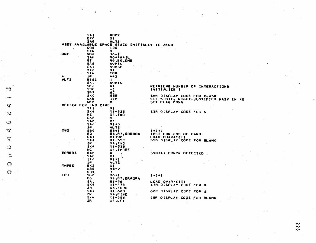
1"")
'~
."'. ,'4
0
~'
T
.;:)
.~. ,""'F<"
0
a
SA 1 ~OC2 8X6 Xl SA6 ALT2
*SET AVAILABLE SPACE !:TACK INITIALLV TC ZE~O SB6 100 SX6 0
ONE SB6 B6-1 SA6 R6+AVAIL GT R6,BO,ONE SA6 NU.-tN SAl NU~SP BX6 l( I SA6 TOF
+ JP- *+2 ~LT2 BSSZ 1
SA I NUr-IN SA2 XI RETPIEVE NU~BER OF INTERACTIONS SB6 -.1 INITIALIZE I SB7 ac SxO see 5513 DISPLAY CODE FOR eLA~K SX5 37P. SET S-BIT, RIGHT-JUSTIFIED MASK SB!: 0 SET FLAG DOWN
.c~eCK FeR ENe CARD SA 1 Al SX4 )(1-538 5313 DISPLAY CODE FOR S NZ )(4,T.0 sxe 0 SAt. BI SA«5 131+5 JP 4L T2
TWO SB6 86+1 1=1+1 EQ 86,R7,ERAORA TEST FOR ENO OF CARD SAl B I+-Bf LOAD CHARACCI) SX4 )(1-558 55R DISPLAV CODe FOR BLANK ZR )(4, HIO SX4 )(1-338 NG X4,rt1REE
ERRORA 5X6 0 SYNTAX ERRCR DETECTED SA6 SI SA6 R, +. JP 4LT2
THREE B)(2 XI SB5 RS+2 SB" 3
LPI SB6 86+' 1=1+1 Ea ~ t t B 7 , ER~ OR A SAl 8,+86 LOAD CHAIUCCI' SX4 XI-476 47B DISPLAV CODE FeR • IR )(4,FOUR S)(4 Xl-608 608 CISPLAY CODE FOR ZR )(4 ,F I VE SX4 Xl-55t! 5~R DISPLAY CO~E FOR BLANK ZR )(4 ,u: 1
I~ 1(5
N N U1

sx. PL sa.
.SPECIES NAME CAN LX2
FOUR
LP2
8X2 JP SX 1 NZ 5B5 SB4 EO LX2 BX2 JP
Xl-.58 X4,ERRORA 84-1
IS CHARAcel' A LETTER OF! A NUNBER
HAVE A MAXIMUM OF CNLV 3 CHARACTERS 6
')(2 .. XI LPl 85-2 XI,ERRORA I 64-1 B4,BO,SIX 6 X2+XO LPc
.LP2 FILLS OUT TME SPECIES NANE WITH BLANKS 85-1 FI \IE SX I
SIX
.HASH SE\lEtIi EIGMT
II<I"e
ZR JP HASH SP.4 LX2
SEARCH 'SEARCM S)(3 PL AX 7 JP SB) EO ZR
*CCNSTFlUCTlON OF MX2 ax) LX:! BX4 LX4 B)(6 SA3 BX6 583 SA6
.CONSTRUCTION OF LX2 B)(3 B,X4 AX4 Axt 58) SA6 JP
.C(NSTRUCT ION OF TEN MX 2
)(I,ERRURA LP2 X2,)(4 X4 42
X2,E4,ERRORe,EIGHT B5-2 )C),NINE XI HIO ICO B2,P.3,ERRORC )(J,TEN
INTERACTION LIST OVERFLOW
EINA~Y I~TEFIACTION LAeEL OF FORM CXXX)(XX~' le X7.X~
54 )(1.~2 24 )(4+)(3
MASK INTO X3 1ST SPECIF.~ hAM!
~ASK INTO )(4 2NO SPECIES NAME
=-ct7777772526771777258 ()() )(6+X3 ~LACE PARENTHESES ARaUNC LABEL fH+10l B3+INTAB STURE LABEL INTO INTAB
BINARY I .. TERACTIO .. CCDf. .O~D 36 )(7*x2 )(1*"2 18 X~+X4 A2tl e3+1"'A8 ELEVE~
CODe ,WCRD FO~MEO IN )(6
STO~E CODE _aRC INTO INTAH
UNA~Y INTERACTION LABEL OF fORM (XXX) 18
N N m

~
~:;r'
.':\1.
l~""""'-~""f1o':t-
~
","~,
'q
;;:::11
~
a
~
BX3 XI.X2 LX3 ~ .. SA. =-2~7777772522222222228 C ) axe. X3+X" FLACE PARENTHESES AROUNC LABEL S83 82+101 SA6 B\Htf\TAB STORE LABEL INTO INTAB
.eONSTRueTION OF ~NAR~ IhTERACTloN CODE WORD LXZ 3~ eX3 XUX2 SX4 7711~B 8X6 X3+X4 ceDE WORD FORMEC INTO INTAB SB3 A2+1 SA6 A3+INTAB
ELEVEfli .SB6 86+1 1= 1+1 EO 86,R7,OUT TEST FOR END OF CARD
TwELVE SAl 81.~6 LOAD CHAPACC I) SX7 Xl-551'3 55B DISPLAY COnE FOR ELANK. ZR X7,ELEVEN SX7 Xl-578 DISPLAY CODE FOR • ZR X1,OUT SX7 x 1-4~e 4tR DISPLAY CODe FOR ZR X7,THTEEN S)(7 xl-4~8 "SA DISPLAY CODE FOR + Nl X7,E~RORA S)(t; 0 SA6 Sl"t-OLD SRS 0 JP FORTFEN
THTEEN SX6 10coe SA6 SIr-HOLD SB5 0
FofHEEN SB6 A6U 1==1+' EO B~,B7,SlxTeEN TEST FOR END OF CARD SAl Bl+E6 LOAD CHARACC I) S)(7 )(1-55~ 55B DISPLAY eOCE FO~ BLANK ZR )(7,FORTEEN SX7 XI-57E' 578 DISPLAY eOOE FOR • ZR X7,SIXTEEN SX7 XI-46E 46B DISPLAY CODE FOR -ZR X7,SDTEEN SX7 XI-45E? 45A DISPLAY CODE FOR + ZR X7,SIXTEFN PL X7,E:RRORA GT- 8S,"lO,FIFTEEN SX7 XI-33E? IS T ... E CHARACTER A LETTER PL X7,FRRORA SB5 1 SA4 J BX2 Xl JP FOf.;TEE"
*FORMATION OF SPECl,",!,; "A"'E FIFTEEN S84 A4-1
EO R4,P.O,E~RORA
N N -..J

SIXTEEN
SEVTEEN
E lTTEEN NlfIoTEEN
.PLACE TWENTY
LX2 BX2 JP ZR SB4 EQ LX2 BX 2 JP HASH SB4 LX2 SE_qC." SX2 BX3 SA4 LX2 BX7 AX7 5'1.7 SB5 SA2 BX" SX2 ax,,' LX" SB5 eo LX7 axt' '"'x 2 Bx2 BX6 SAo ext SA6 LT JP
""00 IF lED SA2 AX7 SB5 GT Bx6 SAt MX2 Bx6 AXf; SA6 SX7 SA 7 JP LT
6 )(~+)Cl FOJ;TEEN 85,ERfiORA B4-1 B4,eo,SEVTEEN 6 )(2+)(0 FILL SPECIES WITH BLA"'KS 5 I )IlfEIIi X2,X" X" "2 X2,B",ERRORe,NINTEEN _ 177B FCR~ 7-BIT , RIGHT-JUSTIFIEO NASK IN X2 Xl.)(2 ""ASK LOCATION POINTER ''''Te )(3 X3+AVAIL II XltX2 MASK POSITION POINTER INTC X7 15 X7+1 X7 SINHOLO X4+)(2 83 )(4+)12 PACK SIGN AND PCINTER (hTC BEAD FIELD to "'5-5 B~,AO,lWENT" 15 X7t)(3 PACK PC~TERS IhTC OhE WCRD 42 X2. x I xttX2 REPACK SPfTABI _ORO A4+SPETABI X4 X~+AVAIL B6,e7,TWELVE OUT
LIST EE~C EACK INTO AVAIL rCF x2 X7-Q9 8~,BO,ERRORO ERROR IF AVAIL OVERFLCWS X7+)(4 X3tAVAIL 42 XI.)(? XtitX7 Fl4tSPETABI X7+, I"'C~E~F"'T TOP TOP TWELVE 86,B7,T\toELVE
r-..> r-..> CD

:,{)
t:.:r
:""-1
'0'
"'7
:~
.~ 'L~,-#
-'~
>.,,'"
:::>
o
OUT SX6 SA6 JP
ERRORe SXf SA6 SAt: .IP ,
ERRDRC SX6 SA~ SA6 JP
ERRORD SX6 SA6 SAt JP ENO
STCRAGE NEEOED f4CO ECS ASSE~BLY
A2+l NU"IN AL T2 0 f.'Il 81 +2 ALT2 ()
'H 81+3 ALT2 0 FH At •• AL T2
'UNDEFINEC SPECIES
INTERACTION LIST OVERFLOW
PROGRAM OVERFLCIII
265 STATE~ENTS 1.038 SECO"'OS
o SY~BOLS o REFERE"'CES
1 ERROR IN •••••••
~ INTERNAL TABLE NavES
I'V I'V I.D

BI~A~Y CCNT~OL CARDS.
lDENT a40C3 ENe
8L~CICS TYPE ACCRESS LENGTtI
PR()G~Aa4. LOCAL 0 117 CODE COMMON 0 4304 COMI COMa40N 0 1130 COM3 CO "',... CN 0 24 CO"'2 CO"'MON 0 2
ENTRY POINTS.
101003 11 ALT3 51
IDENT MOC3 ENTRY MOC3~"LT3 USE I'CCD I'
STORE. BSSZ 30 I MOCEL BSSZ 194\3
USE • LOADX MACRO (NSTR,XREG,N SA4 INSTR BX6 )(REG+)(4\ bup N, 1 LX6 30 SA6 A 3H400EL SB3 fel3+1 INCREMENT LOCATION COU~'ER END'" • USE I'C(""I/
SPETABI BSS q6 [NTAB ass 401 AVAIL BSS ICO "u,",sp ess 1 I\U.-[" ess 1 TOP BSS I
USE •
N W o

-,0
---·1.,:r
:,1 ;:::.:)
~.
·7
t:J!
o 0;
SPETAS2
LCCATE "'TERMS
TYPE 1
TYPE24 TVPE28 lYPE2C. TYPE20
* TYPE3B TYPE3C
* TYPE4 TYPES TYPE6 TYPE7
•
USE BSS USE USE BSSZ essz USE' VFD
vFO VfO VFO VFO
VFO VFD
VFO VFC "FO VFO
.~
/CCMJ/ 20 • /CCM2/ 1 1
* 12/6140B,18/STORE.30/46COC46000e
10/2415146000A,30/5111000C008 lO/242~246CCOBt30/5122CCOCOOa 30/24353406120,30/5132C000008 30/46000406638,30/51640000008
30/2425~40612Bt30/5122CCOCCOB JC/46~CC460COR,30/5164CCOCCOA
3,/1160CC2000P.,30/?066C46COOB 30/~o~e124656Ht30/5114CCOCCOB 30/4600C46~00B,30/5163COOCCOB 12/C2COB,18/~ODEL,3c/oe
~CD~ O~Sl 1 SAl TYFEI 8xe Xl SA3 1 5A6 R].~CDEL 583 2 B31S A LOCAlIC'" CCL~TER M)( 0 1 a LXO Ie SAl NU"'IN 5Bl Xl e7 ~OLDS ~UM~E~ OF lNT~RACTIONS SB6 1
LPl· SAl A6.INT~E fJX2 Xl*)(C A)(l If' SX3 ~6-1 SX1 77775R 1)(7 X2-X7 I.R Xl,ABE
*LOAC CODE FeR COMPUTING R4T~ CONSTANT.BIN4~Y I~TER4CTIC~ fACTOR LOACX TVFE2A,X3,1 . LUADx TYFE2~,Xl,t LOADX TYP~2C,X2,1 LGADX TYPE2l,X3,O SA t: 136+1 LE Ob,F7,LPl JP ARE S
.LCAC COCE FeR CO~PUTING RATE CONSlANT*LNA~Y INTERAC~IC~ FArTC~ ARE LOADX TYPF2A,X3,1
LOADx TYFE3f3,Xl,1 LO~CX TYFE~(,X],O
tV W ......
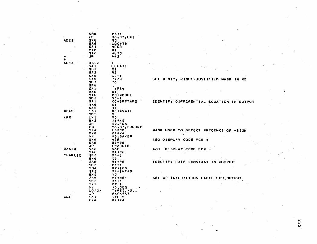
ABfS
+ • ALlJ
AALE
L.P2
8At(ER
Ct-ARLIE
r.uc:;
SBb LE 5)(6 SAl! SA I BX6 SA6 JP
8SSl SA I SA3 SA2. SXO SX5 587 SA6 SA I 8X6 SA6 SB3 SAl AX6 SA6 SA 1 SAe LXI BX2 ZH EO SX4 8XO Nl SXfSAt> JP SX6 SA6 S8f eX6 SA6 S8f Sf'4 SA3 BX. f SA6 SH t' SX2 NZ LO/lOX JP SA4 eX4
e6 .. B6,A7,U:I· ~~ LOC~lE Netl )(1 AL TJ *+:;
I LOCATE XI '32 X2-1 7778 76 I TYPE4 XI P.3+fooIOOI::L A 3+ 1 XO+SPETAA2 XI ~I XO+AVAIL c; 50 Xl·)l5 X2,FOX '36,e7,ERRORF Iocca XltX4 XC,BAKER 4!:P. 81+E6 O'ARL IE 46E 81+86 86+1 X2 I31+E6 Af+l X2+100 134+INTAB )(~
Al+86' At+l X 2-1 XO,DOG TYFE5,x2,1 EAf;,...EST TYFE5 Xc'X4
SET 9-B IT. R IGHT-J.UST IF lEO MASK IN X5
10ENTIFV OIFFEAENTIAL EQUATION IN OUTPUT
NASK USED TO OETECT p~eOENCE OF -SIGN
4.50 01 SPLAY COOE FCIof +
4fA DISPLAV COOE FeR -
I DENT IFY F< AT E CaNST A"'T IN OUTPUT
SET UP INTERACTION LABEL FOR OUTPUT
N W N
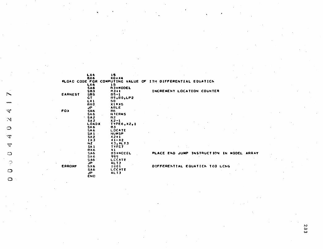
l'..
~~;;r
:'\.!
.;::)
.~ .. ~ ~
t:;>
0
0
<:
LX" 15 BX6 XOt)( •
• LOAC CODE FOR CO~PUTING VALUE OF LX6 15 SA6 B 3+MOOEL SB3 AJta
EARNEST 585 85-1 GT 8!:,BO,LP2 L)(1 50 8)(0 )(1.)(5 JP AeLE
FO)! SX6 B6 SA6 NlERNS SA2 B2 SX2 )(2-1 LOAOX T'\'PE6,x2,1 SX6 B3 SA6 LOCATE SA 1 NU"SP S)(2 X2tl IXJ X1-)(2 NI )(~,AL'3 SA 1 TYFE7 BX6 Xl SA6 B3 HoICCEL SX6 9CjjC; SA6 LCeATE JP ALl:!
ERRORF SX6 1001 SA6 Lee ATE JP ALT] END.
ITH DIFFERENTIAL EQU.TIC~
INCREME~T LOCATION COUNTER
PLACE Efl.O JUMP INSTqUCTIO"",, IN MODEL ARRAY
OIFFEREhTIAL EQUAT1C~ TCO LC~G
N W W

·,
BINA~Y CONT~OL CARDS.
IDENT END
BLeCKS TYFE
FROGf:A"'* LOCAL CODE CO~MON
ENT~Y POINTS.
PIIODELIo
STORE MeDEL
MODELA
lDENT ENTRY USE RSSZ essz USE BSSZ RJ JP ENC
o
MODELA
ActRESS
o o
MOtELA MaCE-LA ICCDEI 101 94~ • 1 "'ceEL ~COELIo
LeNGT~
3 2024
N W -l=

II
REFERENCES AND BIBLIOGRAPHY
1. Adachi, N., "On variable metric algorithms". Journal of O~timization Theory and Applications, vol. 7, 391 t 971).
2. Balakrishnan, A. V., Techniques of Optimization. Academic Press, N'ew York and London (1972).
3. Bassham, J. A., "Control of photosynthetic carbon metabolism". Science, New York, 172, 526-534.
4. , Gerri Levine and John FordeI' III, "Photosynthesis in vitro. I. Achievements of High Rates". Plant sCT. Ltrs. 2, 15-21 (1974).
5. and G. H. Krause, "Free energy changes and metabolic regulation in steady state photosynthetic carbon reduction". Biochem. Biophys. Acta 189, 207-.2 21 ( 19 6 9 ) •
235
6. and M. Kirk, "Dynamics of the photosynthe-sis of carbon compounds. I. Carboxylation reactions". Biochem. Biophys. Acta 43, 447-464 (1960).
7. Bellman, R. and R. Kalaba, Qtiasilinearization and nonlinear boundary-value problems. American Elsevier, New York (1965).
8. , J. Jacquez, R.Kalaba andS. Schwimmer, ----.t't":tQ~u-a-s ..... ilinearization and the estimation of chemical-
rate constants from raw kinetic data". Math. Biosci. 1, 71-76 (1967).
9. Bremermann, H. J., "Computation of equilibria and kinetics of chemical systems with many species". Quantitative Biology of Metabolism, 3rd International Symposium, Biologische Anstalt Helgoland, Sept. 26-29, 1967, Springer-Verlag (1967).
'10. , "Identification of rate constants in chemical cycles of known structure".. IE.EE Symposium on Adaptive Processes,- Decision and Control, pp. xxiii. 2.1 - xxIII. 23 (1970).
11. , "A method of unconstrained global optimization". Math. Biosci. 9, 1-15 (1970).
12. and L. S. Lam, "Analysis of spectra with nonlinear superposition". Math. Biosci. 8, 449-460 (1970).

13. Blum, E. K., Numerical Analysis and and Practlce. Addlson-l.]es1ey
l'heor
14-. Box, M. J., D. Davies and W. H. SWann, "Nonlinear Optimization Techniques ll
• rCI Ltd., Monograph No.5, Oliver and Boyd, Edinburgh (1969).
15. Brent, R. P., "On Maximizing the Efficiency of Algorithms for Solving Systems of Nonlin~ar Equations". Report RC 3725, IBM, Yorktown Heights (1971).
16. , "An algori thm with guaranteed convergence for finding a zero of a function". Compo J. 14, 4-22-425 (1971).
17. , Algorithms for Minimization without Deriv------a~t~i~v-e-s--. Prentice Hall (1973).
18. Brown, K~ M .. and J. E. Dennis, "On Newton-like iteration functions: general convergence theorems and a specific algorithm". Numer. Math. 12, 186-191 (1968).
19. and W. B. Gearhart, "Deflation techniques for the calculation of further solutions of a nonlinear system". Numerische Math. 16, 334-342, Springer-Verlag (1971).
20. , "A -quadratically convergent Newton-like method based upon Gaussian eliminations". SIAM J. Numer. Anal. 6, 560-569 (1959).
21. Brown, W. S., Al tran User's Manual. Bell Laboratories (1973).
22. Broyden, C. G., "Quasi-Newton methods and their applications to function minimization". Math. of Computation, Vol. 21, 368 (1967).
23. , "The convergence of a class of double------r-a--n~k--m-l~·n--imization algorithms: 1. General consider
ations, and 2. The new algorithm". J. Inst. Math. Appls., vol. 6, 76 and 222 (i9 70).
24-. Colville, A. R., "A comparative study on nonlinear programming codes". Report No.· 320-2949, IBM, Yorktown Heights (1968).
25. Conn, Eric E. and P. K. Turnpf, Outlines of Biochemistry. John Wiley and Sons, Inc. (1972).
26. Coppell, W. A., "Stability and asymptotic behavior of differential equations ll
• Heath Mathematical Monographs (1965).
236
'.

\ ,
\I
27. Cragg, E. E. and A. V. Levy, "Study on a supermemory gradient method for the minimization of functions". J. of Optimization Theory and Applications, vol. 4-, 191 (1969).
28. Davidson, W. C., "Variable metric method for minimization". Reyort P.J~L-5990, AEC Research and Development (1959 •
29. Eason, E. D. and R. G. Fenton, "A comparison of numerical optimization methods for engineering design". Paper No. 73-DET-17, ASME Publication (1973).
30. Eigen, M. and L. deMaeyer, "Theoretical basis of relaxation spectrometry". In Techniques of Chemistry, vol. 6, part 2, ed. by A. Weissberg and Gordon Hammes, John Wiley and Sons, Inc., New York (1973).
31. Engvall, J. L., '.'Numerica1 algorithm for solving overdetermined systems of nonlinear equations". NASA Document N70- 3 56 0 0 (1966).
32. Fiacco, A. V. and G. P. McCormick, "Computational aspects of unconstrained minimization algorithms". Chapter 8.i~ ~onl~near Pro~ramming: Seq";1ential Unconstrained M1nlmlzatl0n Technlques, John Wlley and Bons, Inc., New York (1968).
33. Fletcher, R., "Function minimization without evaluating derivatives -- a r·eview i '. Computer Journal, vol. 8, 33 (1965).
34.· , "A new approach to metric variable algo-ritlUIls". Computer Journal 13, 317-322.
3S.and M. J. D. Powell, "A rapidly convergent descent method for minimization". Computer Journal, vo 1. 6, 16 3 ( 19 6 3 ) •
36. and C. M. Reeves, "Function minimization by conjugate gradients". Computer Journal, vol. 7, 149 (1964).
37. Forsythe, George and Cleve B. Moler, Com~uter Solution of Lin~ar Algebraic Systems. Prentlce Hall, Inc. (1967 ).
38. and T. S. Motzkin, "Asymptotic proper-ties of the optimum gradient method {abstract)" .. American Mathematical Society Bulletin, vol. 57, 183 (1951).
237

·39. Garfinkel, D., nSim~lation of glycoli tic systems". Concets and Models of Biomathematics, F. Heinmetz, ed., Marcel Dekker, New York, 1-74 1969).
40. Gear, C. WiLliam, Numerical Initial Value Problems In Ordinary Differential Eauations. Prentice Hall, Inc. (i971).
41. Goldfarb, D., "Sufficient conditions for the convergence of a variable metric algorithm". In Optimization, R. Fletcher, ed., Academic Press, Inc., New York, 273 (1969).
42. Goldstein, A. A. and J. F. Price, "An effective algorithm for minimization". Numerische Mathematik, vol. 10, 184 (1967).
238
43. Greenstadt, J., "On the relativ~ efficiencies of gradient methods". Math. of Computation, vol. 21,360 (1967).
44. Hartman, Philip, Ordinary Differential Equations. John Wiley and Sons, Inc. (1973).
45. Heinmetz, F., "Analog computer analysis of a model system for the induced enzyme synthesis". J. Theoret. BioI. 6, 60-75 (1964).
46. Henneman, R. and L. S. Reid, "Memorandum on the conditions determining complex task proficiency". Psychological Laboratory, University of Virginia (1952).
47. Henrici, Peter, Discrete Variable Methods inOr~in~ry Differential Equations. John Wiley and Sons, Inc. (1962).
48.
49.
Himmelblau, D. M., ArPlied Nonlinear Programming. Hill, New York 1972).
McGraw-
, "Dete~mination of rate constants for ---c-o-m-p ..... i,..-e-x--,k ....... i-n-etic models". Ind. Eng. Chem. Fund. 6,
539 (1967).
50. and Stephen Smale, Differential and Linear Al ebra.
19 4 .
51. Hooker, R. and T. A. Jeeves, "Direct search solution of numerical and statistical problems". Journal of the ACM, vol. 8, 212 (1961).
..

52. Huang, H. Y. and A. V. Levy, "Numerical experiments on quadratically convergent algorithms for function minimization". Journal of Optimization Theory and Applications, vol. 6, 269 (1970).
53. Jacoby, S. C. S., .J. S. Kowalik and J. T. Pizzo, Iterative Methods for Nonlinear Optimization Problems. Prentice Hall (1972).
54 •. Jensen,R. G. and J. A. Bassham, Biochem.· Biophys.· Acta 153, 227 (1968). .
S5. Kowalk, J. and M. R. Osborne, Methods for Unconstrained 0itimization Problems. American Elsevier, New York, C 968).
56. , "Descent Methods". Chapter 3, 29, i~ Methods for Unconstrainea ° timization Problems, Amer~can Elsev~er, New York 1968 .
57. Lanczos, C., Applied Analysis. Prentice Hall (1956).
58. Leon, A., "A comparison among eight known optimizing procedures". In Recent Advances in Optimization Techniques, ed. by A. Lavi and T. P. Vogl, John Wiley and Sons, Inc., New York (1966) . .
59. Lootsma, F. A., Numerical Methods for Nonlinear OptimiZation. Academic Press (1973).
60. Marquardt, D. W., !iAn algorithm for least squares estimation of nonlinear parameters". SIAM Journal, vol. 11, 431 (1963).
61. Miele, A. and J. W •. Cantrell, "Study on a memory gradient method for the minimization of functions". Journal of 0ttimization Theory and Applications, vol. 3, 459 1969).
62. Murray, W., ation.
o timiz-
63. Murtach, B. A. arid R. W. H. Sargent, "Computational experience with quadratically convergent minimization methods". Computer Journal, vol. 13, 185 (1970).
64.· Myers, G. E., "Properties of the conjugate gradient and . Davidon methods". Journal of Optimization Theory and Applications, vol. 2, 209 (1968).
O '7 , ("
239

240
65. NeIder, J. A. and R. Mead, "A simplex method for function minimization". Computer Journal, vol. 7, 308 (1965) •
. ' ,
"6'6. Noel, Paul, Introduction To Mathematical Statistics. John Wiley and Sons, Inc. (1963).
67. Paviani, D. A. and D. M. Himmelblau, "Constrained nonlinear optimization by heuristic programming". Journal of ORSA, vol. 17, 872 (1969).
68. Pearson, J. D., "Variable metric methods of minimization". Computer Journal, vol. 12, 171 (1969).
&9. Pedersen, T. A., Martha Kirk and J. A. Bassham, "Lightdark transients in levels of intermediate comnounds during photosynthesis in air-adapted Chlorell;;'''. Physiol. Plantarum 19, 219-231 (1966).
70. Polack, E., "A modified second method for unconstrained minimization". (To be published.)
71. Powell, M. J. D., "An efficient method for finding the minimum of a function of several variables without calculating derivatives". Computer Journal, vol. 7, 155 (1964).
72. Quisthoudt, Godelieve, De Optmering van Thermodynamische en Kinetische Parameters bij Chemische Relaxtiemetingen. Thesis, Catholic University, Leuven, Belgium (1973).
73. ~Ralston, A., A First Course In Numerical Analysis. McGraw-Hill (1965).
74. Rosennbrock, H. H., "An automatic method for finding the greatest or least value of a function". Computer Journal, vol. 3, 175 (1960).
75. and C. Storey, Computational Techniques for Chemical Engineers. Pergamon Press~ Oxford (1966).
76. Roth, R. S. and Micheline M. Roth, "Data unscrambling and the analysis of inducible enzyme synthesis". Math. Biosci. 5, 57-92 (1969).
77.· Sanchez, David A., Ordinal' Stability Theo~r~y~.~~W~.~~~~~~~~~~~~~~---
78. Shah, B. V., R. J. Buehler and O. Kempthorne, "Some algorithms for minimizing a function of several variables". SIAM Journal, vol. 12, 74 (1964).
,
7ge Smale, Stephen, "A global Newton Rapshom algorithm" . . (Personal communication.)
80. Sorenson, H. W., "Comparison of some conjugate direction pr·ocedures for function minimization". Journal of the Franklin Institute., vol. 288, 421 (1969>-
·81. Spanier, E., Algebraic Topology. McGraw-Hill, New York . (1966).
82. Stewart, G. W. III, 1tA modification of Davidson's minimization method to accept difference approximations of derivatives". Journal of the ACM, vol. 14, 72 (1967).
83.
84.
85.
86.
87.
88.
Strehlow, H. and J. Jen, "On the accuracy of chemical re1axation.measurements". Chern. Instr. 3, 47-69 (1971).
Swartz, J., Parameter Estimation In Biological Systems. Thesis, University of California, Berkeley (1973).
and H. J. Bremermann, "Discussion of parameter estimation in biological modelling: algorithms for estimation and evaluation of the estimates". J. Math. Biol. (1975).
Van Zeggeren, F. and S. H. Storey, The Computati_on of Chemical E'(uilibria. Cambridge University Press, Cambridge 1970).
Wallace, Simaiko H., Selected Papers on Human Factors in the Design and Use of Control Systems. Dover Publications (1961).
Wilkinson, J. H., Roundint Errors in Algebraic Processes. Prentice Hall, Inc. 1963).
89. Zangwill, W. I., "Minimizing a function without calculating derivatives". Computer Journal, vol. 10, 293 (1967).·
90. , "Unconstrained problems". Chapter 5 in Nonlinear pro~amming, A Unified Approach, PrenticeHail,· Inc. (1 69).
241

.-________ LEGAL NOTICE-----------.
This report was prepared as an account of work sponsored by the United States Government. Neither the United States nor the United States Energy Research and Development Administration, nor any of their employees, nor any of their contractors, subcontractors, or their employees, makes any warranty, express or implied, or assumes any legal liability or responsibility for the accuracy, completeness or usefulness of any information, apparatus, product or process disclosed, or represents that its use would not infringe privately owned rights.
-.... ( . . .., n

TECHNI(;J-l.L INFORMATION DIVISION
LAWRENCE BERKELEY LABORATORY
UNIVERSITY OF CALIFORNIA
BERKELEY, CALIFORNIA 94720
.... ' ~
""