UNIVERSITY OF CALIFORNIARIVERSIDE

Efficient and Secure Management of Warehouse-Scale Computers

A Dissertation submitted in partial satisfactionof the requirements for the degree of

Doctor of Philosophy

in

Electrical Engineering

by

Mohammad Atiqul Islam

December 2018

Dissertation Committee:

Dr. Shaolei Ren, ChairpersonDr. Nael Abu-GhazalehDr. Daniel Wong

Copyright byMohammad Atiqul Islam

2018

The Dissertation of Mohammad Atiqul Islam is approved:

Committee Chairperson

University of California, Riverside

Acknowledgments

I would like to convey my heartiest gratitude to my advisor Prof. Shaolei Ren for

his continuous supervision and guidance in my Ph.D. research. This dissertation would not

have been possible without his support and motivation. Besides my advisor, I would also

like to thank my dissertation committee: Prof. Nael Abu-Ghazaleh and Prof. Daniel Wong,

for their insightful comments and suggestions to improve this dissertation.

My sincere appreciation goes to all the co-authors of my research papers which form

the core of this dissertation. In particular, I would like to thank Prof. Adam Wierman for

his active involvement and contribution in my most representative papers. It was a source of

immense encouragement and inspiration to work alongside such an accomplished academic.

I thank my lab mates and fellow graduate students at UC Riverside for their

thought-provoking comments during numerous discussions. A special thanks goes to Hasan

Mahmud who helped me take my initial steps in system building.

Finally, nothing would be possible without the constant support from my family:

my parents, my brother, and sisters. Most importantly, thanks to my wife Shanjida who

bear through all the responsibilities of raising our daughter while I was pursuing my dream.

Content from published work and contributions

The text of this dissertation, in part or in full, is a reprint of the material as

it appears in list of publications below. The co-author Dr. Shaolei Ren listed in that

publication directed and supervised the research which forms the basis for this dissertation.

iv

1. M. A. Islam, H. Mahmud, S. Ren, and X. Wang, “Paying to Save: Reducing Cost

of Colocation Data Center via Rewards”, IEEE Intl. Symp. on High Performance

Computer Architecture, Burlingame, 2015. doi: 10.1109/HPCA.2015.7056036

Added to the dissertation as Chapter 2. M. A. Islam is the major contributor of the

project. H. Mahmud assisted in setting up the experiment testbed, while X. Wang

provided guidance and advice in preparing the manuscript.

2. M. A. Islam, X. Ren, S. Ren, and A. Wierman, “A Spot Capacity Market to In-

crease Power Infrastructure Utilization in Multi-Tenant Data Centers”, IEEE Intl.

Symp. on High Performance Computer Architecture, Vienna, 2018, pp. 776-788. doi:

10.1109/HPCA.2018.00071

Added to the dissertation as Chapter 3. M. A. Islam is the major contributor of the

project. Other co-authors, X. Ren and A. Wierman, provided guidance and advice in

preparing the manuscript.

3. M. A. Islam, S. Ren, and A. Wierman, “Exploiting a Thermal Side Channel for Power

Attacks in Multi-Tenant Data Centers”, ACM Conference on Computer and Commu-

nications Security, Dallas, 2017. doi: https://doi.org/10.1145/3133956.3133994

Added to the dissertation as Chapter 4. M. A. Islam is the major contributor of the

project. A. Wierman provided guidance and advice in preparing the manuscript.

4. M. A. Islam, L. Yang, K. Ranganath, and S. Ren, “Why Some Like It Loud: Timing

Power Attacks in Multi-Tenant Data Centers Using an Acoustic Side Channel”, Proc.

v

ACM Meas. Anal. Comput. Syst. Volume 2, Issue 1, Article 6 (April 2018). doi:

https://doi.org/10.1145/3179409.

Added to the dissertation as Chapter 5. M. A. Islam is the major contributor of

the project. Other co-authors, L. Yang and K. Ranganath, assisted in the evaluation

experiments.

5. M. A. Islam and S. Ren, “Ohm’s Law in Data Centers: A Voltage Side Channel

for Timing Power Attacks”, ACM Conference on Computer and Communications

Security, Toronto, 2018. DOI: https://doi.org/10.1145/3243734.3243744

Added to the dissertation as Chapter 6. M. A. Islam is the major contributor of the

project.

vi

Dedicated to

my parents Mohammad Safikul Islam and Ambia Khatun,

and

my wife Shanjida.

vii

ABSTRACT OF THE DISSERTATION

Efficient and Secure Management of Warehouse-Scale Computers

by

Mohammad Atiqul Islam

Doctor of Philosophy, Graduate Program in Electrical EngineeringUniversity of California, Riverside, December 2018

Dr. Shaolei Ren, Chairperson

Warehouse-scale computers or data centers are booming both in numbers and sizes.

Consequently, data centers have been receiving major research attention in the recent years.

However, prior literature primarily focuses on Google-type hyper-scale data centers and

overlook the important segment of the multi-tenant colocation data centers where multiple

tenants rent power and space for their physical servers while the data center operator

manages the non-IT infrastructure like the power and cooling. Multi-tenant data centers

are widely used across various industry sectors and hence efficient management of multi-

tenant data centers is crucial.

However, many existing efficient operation approaches cannot be applied in multi-

tenant data centers because the IT-equipment (e.g., servers) are owned by different tenants

and therefore the data center operator has no direct control over them. In this disserta-

tion research, I propose market-based techniques for coordination between the tenants and

the operator towards efficient data center operation. Specifically, I propose an incentive

framework that pays tenants for energy reduction such that the operator’s overall cost is

viii

minimized. I also propose a novel market design that allows tenants to temporarily acquire

additional capacity from other tenants’ unused capacity for performance boosts.

Further, the criticality of the hosted services makes data centers a prime target

for attacks. While data center cyber-security has been extensively studied, the equally

important security aspect - data center physical security - remained unchecked. In this

dissertation, I identify that an adversary disguised as a tenant in a multi-tenant data cen-

ter can launch power attacks to create overloads in the power infrastructure. However,

launching power attacks requires careful timing. Specifically, an attacker needs to estimate

other tenants’ power consumption to time its malicious load injection to create overloads. I

identify the existence of multiple side channels that can assist in attacker’s timing. I show

that there exists a thermal side channel due to server heat recirculation, an acoustic side

channel due to server fan noise, and a voltage side channel due to Ohm’s Law that can

reveal the benign tenants’ power consumption to an attacker. I also discuss the merits and

challenges of possible countermeasures against these attacks.

ix

Contents

List of Figures xiv

List of Tables xix

1 Introduction 11.1 Efficiency of multi-tenant data centers . . . . . . . . . . . . . . . . . . . . . 3

1.1.1 Cost efficiency through rewards . . . . . . . . . . . . . . . . . . . . . 41.1.2 Performance boosting using spot capacity . . . . . . . . . . . . . . . 4

1.2 Security of multi-tenant data centers . . . . . . . . . . . . . . . . . . . . . . 51.2.1 A thermal side-channel due to heat recirculation . . . . . . . . . . . 61.2.2 An acoustic side-channel due to server noise . . . . . . . . . . . . . . 71.2.3 A voltage side-channel due to Ohm’s Law . . . . . . . . . . . . . . . 7

2 Paying to Save: Reducing Cost of Colocation Data Center via Rewards 92.1 Introduction . . . . . . . . . . . . . . . . . . . . . . . . . . . . . . . . . . . . 92.2 Preliminaries . . . . . . . . . . . . . . . . . . . . . . . . . . . . . . . . . . . 13

2.2.1 Peak power demand charge . . . . . . . . . . . . . . . . . . . . . . . 132.2.2 Limitations of colocation’s current pricing models . . . . . . . . . . . 14

2.3 Mechanism and Problem Formulation . . . . . . . . . . . . . . . . . . . . . 172.3.1 Mechanism . . . . . . . . . . . . . . . . . . . . . . . . . . . . . . . . 172.3.2 Problem formulation . . . . . . . . . . . . . . . . . . . . . . . . . . . 18

2.4 RECO: Reducing Cost via Rewards . . . . . . . . . . . . . . . . . . . . . . . 202.4.1 Modeling cooling efficiency and solar energy . . . . . . . . . . . . . . 202.4.2 Tracking peak power demand . . . . . . . . . . . . . . . . . . . . . . 232.4.3 Learning tenants’ response to reward . . . . . . . . . . . . . . . . . . 242.4.4 Feedback-based online optimization . . . . . . . . . . . . . . . . . . 26

2.5 Experiment . . . . . . . . . . . . . . . . . . . . . . . . . . . . . . . . . . . . 282.5.1 Colocation test bed . . . . . . . . . . . . . . . . . . . . . . . . . . . 282.5.2 Tenants’ response . . . . . . . . . . . . . . . . . . . . . . . . . . . . . 302.5.3 Benchmarks . . . . . . . . . . . . . . . . . . . . . . . . . . . . . . . . 332.5.4 Experiment result . . . . . . . . . . . . . . . . . . . . . . . . . . . . 33

2.6 Simulation . . . . . . . . . . . . . . . . . . . . . . . . . . . . . . . . . . . . . 35

x

2.6.1 Setup . . . . . . . . . . . . . . . . . . . . . . . . . . . . . . . . . . . 352.6.2 Tenants’ response . . . . . . . . . . . . . . . . . . . . . . . . . . . . . 372.6.3 Results . . . . . . . . . . . . . . . . . . . . . . . . . . . . . . . . . . 39

2.7 Related Work . . . . . . . . . . . . . . . . . . . . . . . . . . . . . . . . . . . 432.8 Conclusion . . . . . . . . . . . . . . . . . . . . . . . . . . . . . . . . . . . . 44

3 A Spot Capacity Market to Increase Power Infrastructure Utilization inMulti-Tenant Data Centers 453.1 Introduction . . . . . . . . . . . . . . . . . . . . . . . . . . . . . . . . . . . . 453.2 Opportunities for Spot Capacity . . . . . . . . . . . . . . . . . . . . . . . . 50

3.2.1 Overview of Data Center Infrastructure . . . . . . . . . . . . . . . . 503.2.2 Spot Capacity v.s. Oversubscription . . . . . . . . . . . . . . . . . . 513.2.3 Potential to Exploit Spot Capacity . . . . . . . . . . . . . . . . . . . 53

3.3 The Design of SpotDC . . . . . . . . . . . . . . . . . . . . . . . . . . . . . . 553.3.1 Problem Formulation . . . . . . . . . . . . . . . . . . . . . . . . . . 563.3.2 Market Design . . . . . . . . . . . . . . . . . . . . . . . . . . . . . . 583.3.3 Implementation and Discussion . . . . . . . . . . . . . . . . . . . . . 65

3.4 Evaluation Methodology . . . . . . . . . . . . . . . . . . . . . . . . . . . . . 693.4.1 Testbed Configuration . . . . . . . . . . . . . . . . . . . . . . . . . . 703.4.2 Workloads . . . . . . . . . . . . . . . . . . . . . . . . . . . . . . . . . 703.4.3 Power and Performance Model . . . . . . . . . . . . . . . . . . . . . 713.4.4 Performance Metrics . . . . . . . . . . . . . . . . . . . . . . . . . . . 73

3.5 Evaluation Results . . . . . . . . . . . . . . . . . . . . . . . . . . . . . . . . 743.5.1 Execution of SpotDC . . . . . . . . . . . . . . . . . . . . . . . . . . 743.5.2 Evaluation over Extended Experiments . . . . . . . . . . . . . . . . 763.5.3 Other Demand Functions . . . . . . . . . . . . . . . . . . . . . . . . 793.5.4 Sensitivity Study . . . . . . . . . . . . . . . . . . . . . . . . . . . . . 80

3.6 Related Work . . . . . . . . . . . . . . . . . . . . . . . . . . . . . . . . . . . 843.7 Conclusion . . . . . . . . . . . . . . . . . . . . . . . . . . . . . . . . . . . . 85

4 Exploiting a Thermal Side Channel for Power Attacks in Multi-TenantData Centers 874.1 Introduction . . . . . . . . . . . . . . . . . . . . . . . . . . . . . . . . . . . . 874.2 Identifying Power Infrastructure Vulnerabilities . . . . . . . . . . . . . . . . 93

4.2.1 Multi-tenant Power Infrastructure . . . . . . . . . . . . . . . . . . . 934.2.2 Vulnerability to Power Attacks . . . . . . . . . . . . . . . . . . . . . 954.2.3 Impact of Power Attacks . . . . . . . . . . . . . . . . . . . . . . . . . 97

4.3 Exploiting a Thermal Side Channel . . . . . . . . . . . . . . . . . . . . . . . 1014.3.1 Threat Model . . . . . . . . . . . . . . . . . . . . . . . . . . . . . . . 1014.3.2 The Need for a Side Channel . . . . . . . . . . . . . . . . . . . . . . 1044.3.3 A Thermal Side Channel . . . . . . . . . . . . . . . . . . . . . . . . 1054.3.4 Estimating Benign Tenants’ Power from a Thermal Side Channel . . 1094.3.5 Attack Strategy . . . . . . . . . . . . . . . . . . . . . . . . . . . . . . 116

4.4 Experimental Evaluation . . . . . . . . . . . . . . . . . . . . . . . . . . . . . 1184.4.1 Methodology . . . . . . . . . . . . . . . . . . . . . . . . . . . . . . . 118

xi

4.4.2 Evaluation Results . . . . . . . . . . . . . . . . . . . . . . . . . . . . 1214.5 Defense Strategy . . . . . . . . . . . . . . . . . . . . . . . . . . . . . . . . . 130

4.5.1 Degrading Thermal Side Channel . . . . . . . . . . . . . . . . . . . . 1304.5.2 Other Countermeasures . . . . . . . . . . . . . . . . . . . . . . . . . 133

4.6 Related Work . . . . . . . . . . . . . . . . . . . . . . . . . . . . . . . . . . . 1344.7 Concluding Remarks . . . . . . . . . . . . . . . . . . . . . . . . . . . . . . . 136

5 Timing Power Attacks in Multi-tenant Data Centers Using an AcousticSide Channel 1375.1 Introduction . . . . . . . . . . . . . . . . . . . . . . . . . . . . . . . . . . . . 1375.2 Opportunities for Power Attacks . . . . . . . . . . . . . . . . . . . . . . . . 143

5.2.1 Multi-tenant Power Infrastructure . . . . . . . . . . . . . . . . . . . 1435.2.2 Opportunities . . . . . . . . . . . . . . . . . . . . . . . . . . . . . . . 145

5.3 Threat Model and Challenges . . . . . . . . . . . . . . . . . . . . . . . . . . 1485.3.1 Threat Model . . . . . . . . . . . . . . . . . . . . . . . . . . . . . . . 1485.3.2 Challenges for Power Attacks . . . . . . . . . . . . . . . . . . . . . . 150

5.4 Exploiting An Acoustic Side Channel . . . . . . . . . . . . . . . . . . . . . . 1525.4.1 Discovering an Acoustic Side Channel . . . . . . . . . . . . . . . . . 1525.4.2 Filtering Out CRAC’s Noise . . . . . . . . . . . . . . . . . . . . . . . 1595.4.3 Demixing Received Noise Energy . . . . . . . . . . . . . . . . . . . . 1625.4.4 Detecting Attack Opportunities . . . . . . . . . . . . . . . . . . . . . 169

5.5 Evaluation . . . . . . . . . . . . . . . . . . . . . . . . . . . . . . . . . . . . . 1715.5.1 Methodology . . . . . . . . . . . . . . . . . . . . . . . . . . . . . . . 1715.5.2 Results . . . . . . . . . . . . . . . . . . . . . . . . . . . . . . . . . . 175

5.6 Defense Strategies . . . . . . . . . . . . . . . . . . . . . . . . . . . . . . . . 1815.7 Related Work . . . . . . . . . . . . . . . . . . . . . . . . . . . . . . . . . . . 1835.8 Concluding Remarks . . . . . . . . . . . . . . . . . . . . . . . . . . . . . . . 184

6 Ohm’s Law in Data Centers: A Voltage Side Channel for Timing PowerAttacks 1866.1 Introduction . . . . . . . . . . . . . . . . . . . . . . . . . . . . . . . . . . . . 1866.2 Preliminaries on Power Attacks . . . . . . . . . . . . . . . . . . . . . . . . . 190

6.2.1 Overview of Multi-Tenant Data Centers . . . . . . . . . . . . . . . . 1916.2.2 Vulnerability and Impact of Power Attacks . . . . . . . . . . . . . . 1936.2.3 Recent Works on Timing Power Attacks . . . . . . . . . . . . . . . . 195

6.3 Threat Model . . . . . . . . . . . . . . . . . . . . . . . . . . . . . . . . . . . 1966.4 Exploiting A Voltage side channel . . . . . . . . . . . . . . . . . . . . . . . 200

6.4.1 Overview of the Power Network . . . . . . . . . . . . . . . . . . . . . 2006.4.2 ∆V -based attack . . . . . . . . . . . . . . . . . . . . . . . . . . . . . 2026.4.3 Exploiting High-Frequency Voltage Ripples . . . . . . . . . . . . . . 2046.4.4 Experimental validation . . . . . . . . . . . . . . . . . . . . . . . . . 2106.4.5 Tracking Aggregate Power Usage . . . . . . . . . . . . . . . . . . . . 2146.4.6 Timing Power Attacks . . . . . . . . . . . . . . . . . . . . . . . . . . 216

6.5 Evaluation . . . . . . . . . . . . . . . . . . . . . . . . . . . . . . . . . . . . . 2186.5.1 Methodology . . . . . . . . . . . . . . . . . . . . . . . . . . . . . . . 218

xii

6.5.2 Results . . . . . . . . . . . . . . . . . . . . . . . . . . . . . . . . . . 2226.6 Extension to Three-Phase System . . . . . . . . . . . . . . . . . . . . . . . . 229

6.6.1 Three-Phase Power Distribution System . . . . . . . . . . . . . . . . 2296.6.2 Evaluation Results . . . . . . . . . . . . . . . . . . . . . . . . . . . . 232

6.7 Defense Strategy . . . . . . . . . . . . . . . . . . . . . . . . . . . . . . . . . 2346.8 Related work . . . . . . . . . . . . . . . . . . . . . . . . . . . . . . . . . . . 2376.9 Conclusion . . . . . . . . . . . . . . . . . . . . . . . . . . . . . . . . . . . . 238

7 Conclusions 239

Bibliography 241

xiii

List of Figures

1.1 Multi-tenant colocation data center infrastructure. . . . . . . . . . . . . . . 2

2.1 (a) Estimated electricity usage by U.S. data centers in 2011 (excluding smallserver closets and rooms) [120]. (b) Colocation revenue by vertical market [30]. 10

2.2 Normalized power consumption of Verizon Terremark’s colocation in Miami,FL, measured at UPS output from September 15–17, 2013. . . . . . . . . . 15

2.3 (a) pPUE variation with outside ambient temperature [35, 176]. (b) Snap-shot of weekly pPUE during Summer and Winter in San Francisco, CA, in2013. . . . . . . . . . . . . . . . . . . . . . . . . . . . . . . . . . . . . . . . . 21

2.4 (a) Solar prediction with ARMA. Model parameters: p = 2, q = 2, (A1, A2) =(1.5737,−0.6689) and (B1, B2) = (0.3654,−0.1962). (b) Periodogram fordifferent workloads using FFT. . . . . . . . . . . . . . . . . . . . . . . . . . 22

2.5 System diagram of RECO. . . . . . . . . . . . . . . . . . . . . . . . . . . . . 272.6 Workload traces normalized to maximum capacity. . . . . . . . . . . . . . . 302.7 Processing capacity under different power states. . . . . . . . . . . . . . . . 302.8 Energy consumption under different power states. . . . . . . . . . . . . . . . 312.9 Response to reward under different workloads. . . . . . . . . . . . . . . . . 322.10 Comparison of different algorithms. . . . . . . . . . . . . . . . . . . . . . . . 342.11 Cost and savings under different algorithms. . . . . . . . . . . . . . . . . . . 352.12 Tenant response and fitting. . . . . . . . . . . . . . . . . . . . . . . . . . . . 372.13 (a) Response function for a day’s first time slot. (b) Predicted and actual

power reduction. . . . . . . . . . . . . . . . . . . . . . . . . . . . . . . . . . 392.14 Grid power and reward rate w/ different algorithms. . . . . . . . . . . . . . 402.15 Monthly cost savings for colocation and tenants. . . . . . . . . . . . . . . . 412.16 Impact of changes in tenants’ behaviors. . . . . . . . . . . . . . . . . . . . . 422.17 Cost savings in different locations. . . . . . . . . . . . . . . . . . . . . . . . 43

3.1 Overview of a multi-tenant data center. . . . . . . . . . . . . . . . . . . . . 503.2 (a) Illustration of spot capacity in a production PDU [169]. (b) CDF of

tenants’ aggregate power usage. (c) A tenant can lease power capacity inthree ways: high reservation; low reservation; and low reservation + spotcapacity. “Low/high Res.” represent low/high reserved capacities. . . . . . 52

xiv

3.3 (a) Piece-wise linear demand function. The shaded area represents StepBid.(b) Aggregated demand function for ten racks. StepBid-1 bids (Dmax, qmin)only, and StepBid-2 bids (Dmin, qmax) only. . . . . . . . . . . . . . . . . . . . 60

3.4 Demand function bidding. (a) Optimal spot capacity demand and biddingcurve. (b) 2D view. . . . . . . . . . . . . . . . . . . . . . . . . . . . . . . . . 64

3.5 System diagram for SpotDC. . . . . . . . . . . . . . . . . . . . . . . . . . . . 653.6 Timing of SpotDC for spot capacity allocation. . . . . . . . . . . . . . . . . 663.7 (a) PDU power variation in our simulation trace. (b) Market clearing time

at scale. . . . . . . . . . . . . . . . . . . . . . . . . . . . . . . . . . . . . . 683.8 Power-performance relation at different workload levels. . . . . . . . . . . . 713.9 Performance gain versus spot capacity allocation. . . . . . . . . . . . . . . . 733.10 A 20-minute trace of power (at PDU#1) and price. The market price in-

creases when sprinting tenants participate (e.g., starting at 240 and 720 sec-onds), and decreases when more spot capacity is available (e.g., starting at360 seconds). . . . . . . . . . . . . . . . . . . . . . . . . . . . . . . . . . . . 74

3.11 Tenants’ performance. Search-1 and Web meet SLO of 100ms, while Count-1and Graph-1 increase throughput. . . . . . . . . . . . . . . . . . . . . . . . 76

3.12 Comparison with baselines. Tenants’ performance is close to MaxPerf with amarginal cost increase. . . . . . . . . . . . . . . . . . . . . . . . . . . . . . . 77

3.13 CDFs of market price and aggregate power. (a) Sprinting tenants bid and alsopay higher prices than opportunistic tenants. (b) SpotDC improves powerinfrastructure utilization. . . . . . . . . . . . . . . . . . . . . . . . . . . . . 79

3.14 Comparison with other demand functions under different spot capacity avail-abilities. . . . . . . . . . . . . . . . . . . . . . . . . . . . . . . . . . . . . . . 80

3.15 Impact of spot capacity availability. With spot capacity, the market pricegoes down, the operator’s profit increases, and tenants have a better perfor-mance. . . . . . . . . . . . . . . . . . . . . . . . . . . . . . . . . . . . . . . . 81

3.16 Impact of bidding strategies. With price prediction, sprinting tenants getmore spot capacity and better performance. . . . . . . . . . . . . . . . . . . 82

3.17 Impact of spot capacity under-prediction. . . . . . . . . . . . . . . . . . . . 833.18 Impact of number of tenants. (a) Operator’s profit. (b) Tenants’ cost. (c)

Tenant’s performance. . . . . . . . . . . . . . . . . . . . . . . . . . . . . . . 84

4.1 Tier-IV data center power infrastructure with 2N redundancy and dual-corded IT equipment. . . . . . . . . . . . . . . . . . . . . . . . . . . . . . . 93

4.2 Infrastructure vulnerability to attacks. (a) Power emergencies are almostnonexistent when all tenants are benign. (b) Power emergencies can occurwith power attacks. (c) The attacker meets its subscribed capacity constraint.The shaded part illustrates how the attacker can remain stealthy by reshapingits power demand when anticipating an attack opportunity. . . . . . . . . . 94

4.3 Circuit breaker trip delay [133]. . . . . . . . . . . . . . . . . . . . . . . . . . 984.4 Cooling system overview. (1) Hot recirculated air. (2) Return air. (3)

Perforated tile. (4) Hot aisle. (5) Cold aisle. . . . . . . . . . . . . . . . . . 1064.5 Adoption of heat containment techniques [157]. . . . . . . . . . . . . . . . . 106

xv

4.6 CFD simulation result. (a) Temperature distribution after 10 seconds of a10-second 60kW power spike at the circled racks. (b) Temperature trace atselect sensors. . . . . . . . . . . . . . . . . . . . . . . . . . . . . . . . . . . . 107

4.7 Breakdown of readings at sensor #1 (Fig. 4.6(a)). . . . . . . . . . . . . . . . 1094.8 Temperature-based power attack. All attacks are unsuccessful. . . . . . . . 1104.9 Summary of temperature-based power attacks. The line “Launched Attacks”

represents the fraction of time power attacks are launched. . . . . . . . . . . 1124.10 Finite state machine of our attack strategy. Pest is the attacker’s estimated

aggregate power demand (including its own), and Pth is the attack triggeringthreshold. . . . . . . . . . . . . . . . . . . . . . . . . . . . . . . . . . . . . 117

4.11 Data center layout. . . . . . . . . . . . . . . . . . . . . . . . . . . . . . . . . 1194.12 The attacker’s heat recirculation model: zone-wise temperature increase at

sensor #1 (Fig. 4.6(a)). . . . . . . . . . . . . . . . . . . . . . . . . . . . . . 1224.13 Error in the attacker’s knowledge of heat recirculation matrix Hb, normalized

to the true value. . . . . . . . . . . . . . . . . . . . . . . . . . . . . . . . . . 1224.14 Robustness of Kalman filter performance. (a) The Kalman filter response to

large power spikes. (b) Power estimation error versus error in the attacker’sknowledge of heat recirculation matrix. . . . . . . . . . . . . . . . . . . . . . 123

4.15 A snapshot of the actual and estimated power. . . . . . . . . . . . . . . . . 1234.16 (a) Frequency of power attacks versus the attack triggering threshold. (b)

True positive and precision rates versus the attack triggering threshold. . . 1254.17 Attack success rates for different timer values. . . . . . . . . . . . . . . . . . 1264.18 Comparison with random attacks. . . . . . . . . . . . . . . . . . . . . . . . 1274.19 (a) Statistics of attack opportunity and attack success. (b) Expected annual

loss due to power attacks incurred by the data center operator and affectedtenants (200kW designed capacity oversubscribed by 120%). (c) Even withheat containment, the thermal side channel can still assist the attacker withtiming power attacks. . . . . . . . . . . . . . . . . . . . . . . . . . . . . . . 128

4.20 Illustration of different attack scenarios. . . . . . . . . . . . . . . . . . . . . 1304.21 Degrading the thermal side channel. . . . . . . . . . . . . . . . . . . . . . . 1314.22 True positive and precision rates of different defense strategies. “Low”/“high”

indicates the amount of randomness in supply airflows. “x%” heat contain-ment means x% of the hot air now returns to the CRAH unit directly. . . . 133

5.1 Loss of redundancy protection due to power attacks in a Tier-IV data center. 1435.2 Infrastructure vulnerability to attacks. An attacker injects timed malicious

loads to create overloads. . . . . . . . . . . . . . . . . . . . . . . . . . . . . 1465.3 Noise tones created by rotating fan blades [28]. . . . . . . . . . . . . . . . . 1535.4 Inside of a Dell PowerEdge server and a cooling fan. The server’s cooling fan

is a major noise source. . . . . . . . . . . . . . . . . . . . . . . . . . . . . . 1555.5 The relation between a server’s cooling fan noise and its power consumption

in the quiet lab environment. (a) Server power and cooling fan speed. (b)Noise spectrum. (c) Noise tones with two different server power levels. . . . 156

5.6 (a) Sharp power change creates noise energy spike. (b) Relation betweennoise energy and server power. . . . . . . . . . . . . . . . . . . . . . . . . . 157

xvi

5.7 Server noise and power consumption in our noisy data center. (a) Noisespectrum. (b) Cutoff frequency of high-pass filter. The ratio is based on thenoise of 4kW and 2.8kW server power. (c) Noise energy and server power. . 160

5.8 Noise energy mixing process. . . . . . . . . . . . . . . . . . . . . . . . . . . 1635.9 Illustration: NMF converts the 15 noise sources into 3 consolidated sources. 1655.10 State machine showing the attack strategy. . . . . . . . . . . . . . . . . . . 1685.11 Layout of our data center and experiment setup. . . . . . . . . . . . . . . . 1725.12 Illustration of power attacks. . . . . . . . . . . . . . . . . . . . . . . . . . . 1755.13 Impact of attack triggering threshold Eth. The legend “Attack Opportunity”

means the percentage of times an attack opportunity exists. . . . . . . . . . 1765.14 Impact of high-pass filter cutoff frequency. . . . . . . . . . . . . . . . . . . . 1775.15 Impact of attacker size. “x%” in the legend means the attacker subscribes

x% of the total subscribed capacity. . . . . . . . . . . . . . . . . . . . . . . 1785.16 Without energy noise spike detection, the attacker launches many unsuccess-

ful attacks. . . . . . . . . . . . . . . . . . . . . . . . . . . . . . . . . . . . . 1795.17 Detection statistics for different attack strategies. . . . . . . . . . . . . . . . 180

6.1 Data center power infrastructure with an attacker. . . . . . . . . . . . . . . 1926.2 Circuit of data center power distribution. . . . . . . . . . . . . . . . . . . . 2016.3 (a) 12-hour voltage traces at the UPS (grid) and PDU. (b) Probability of

temporal variation of the UPS voltage. . . . . . . . . . . . . . . . . . . . . . 2036.4 A server with an AC power supply unit [17]. An attacker uses an analog-to-

digital converter to acquire the voltage signal. . . . . . . . . . . . . . . . . . 2056.5 Building blocks of PFC circuit in server’s power supply unit. . . . . . . . . 2066.6 (a) Wave shape of PFC current at different power levels. (b) Current ripples

from the PFC switching. . . . . . . . . . . . . . . . . . . . . . . . . . . . . . 2076.7 High-frequency voltage ripples at the PDU caused by switching in the server

power supply unit. . . . . . . . . . . . . . . . . . . . . . . . . . . . . . . . . 2106.8 High-frequency PSD spikes in PDU voltage caused by the server power supply

unit. . . . . . . . . . . . . . . . . . . . . . . . . . . . . . . . . . . . . . . . . 2116.9 (a) PSD at different server powers. (b) Server power vs. PSD aggregated

within the bandwidth of 69.5 ∼ 70.5kHz for the 495W power supply unit. (c)(b) Server power vs. PSD aggregated within the bandwidth of 63 ∼ 64kHz forthe 350W PSU. (d) PMF shows the PFC switching frequency only fluctuatesslightly. . . . . . . . . . . . . . . . . . . . . . . . . . . . . . . . . . . . . . . 212

6.10 (a) The aggregate PSD for different numbers of servers. The aggregate PSDsare normalized to that of the single server at low power. (b) Power spectraldensity of all servers in our testbed showing three distinct PSD groups, eachcorresponding to a certain type of power supply unit. . . . . . . . . . . . . . 213

6.11 A prototype of edge multi-tenant data center. . . . . . . . . . . . . . . . . . 2196.12 Detection of power shape of different server groups. . . . . . . . . . . . . . . 2216.13 Power vs. PSD plot of different server groups. . . . . . . . . . . . . . . . . . 2226.14 Illustration of power attack. . . . . . . . . . . . . . . . . . . . . . . . . . . . 2236.15 Impact of attack triggering threshold Pth. The legend “Attack Opportunity”

means the percentage of times an attack opportunity exists. . . . . . . . . . 224

xvii

6.16 Cost and impact of attacker size. x% in the legend indicates the “%” capacitysubscribed by the attacker. The tiers specify the infrastructure redundancies,from Tier-I with no redundancy up to Tier-IV with 2N full redundancy. . . 225

6.17 Detection statistics for different attack strategies. . . . . . . . . . . . . . . . 2276.18 (a) Impact of the attack strategy (e.g., Thold) on true positive rate. (b) ROC

curves showing the accuracy of detection of attack opportunities. . . . . . . 2286.19 3-phase power distribution with 2-phase racks. . . . . . . . . . . . . . . . . 2306.20 Performance of voltage side channel for a three-phase 180kW system. . . . . 2336.21 DC power distribution with DC server power supply unit that has no PFC

circuit. . . . . . . . . . . . . . . . . . . . . . . . . . . . . . . . . . . . . . . . 235

xviii

List of Tables

2.1 A 10MW data center’s electricity cost for selected locations (in U.S. dollars). 14

3.1 Testbed Configuration. . . . . . . . . . . . . . . . . . . . . . . . . . . . . . . 69

4.1 Estimated impact of power emergencies (5% of the time) on a 1MW-10,000sqftdata center. . . . . . . . . . . . . . . . . . . . . . . . . . . . . . . . . . . . 97

5.1 Data center outage with power attacks. . . . . . . . . . . . . . . . . . . . . 1475.2 Cost impact of power attack 3.5% of the time on a 1MW-10,000 sqft data

center. . . . . . . . . . . . . . . . . . . . . . . . . . . . . . . . . . . . . . . . 147

6.1 Server configuration of our experiments. . . . . . . . . . . . . . . . . . . . . 220

xix

Chapter 1

Introduction

Warehouse-scale computers or data centers have emerged as one of the most im-

portant cyber-physical systems in the wake of the age of the Internet. They are the physical

home to the cloud and host numerous mission-critical services. Power-hungry data centers

have been rapidly expanding in both number and scale, placing an increasing emphasis on

optimizing data center operation. In the U.S., electricity consumption by data centers in

2013 reached 91 billion kilo-watt hours (kWh) [120].

However, existing efforts have been predominantly concentrating on owner oper-

ated (Google type) data centers [97, 173], missing out on the critical segment of colocation

or multi-tenant data centers. Unlike the owner-operated data centers where a single entity

(e.g., Google) has full control over the entire data center, in multi-tenant data centers, the

data center operator only manages the support infrastructure such as cooling and power

system (as shown in Fig. 1.1). The tenants rent space and power from the multi-tenant

1

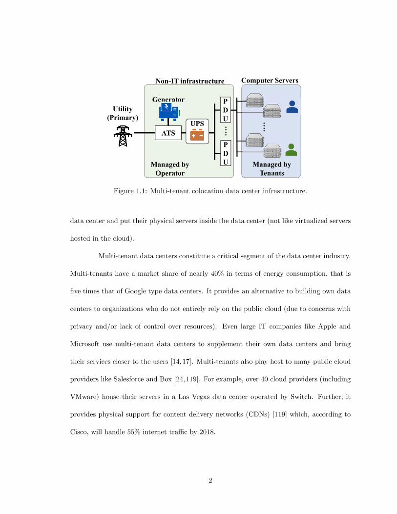
Managed byTenants

Managed byOperator

Non-IT infrastructure

Utility(Primary)

Generator

UPSATS

PDU

PDU

1

Computer Servers

Figure 1.1: Multi-tenant colocation data center infrastructure.

data center and put their physical servers inside the data center (not like virtualized servers

hosted in the cloud).

Multi-tenant data centers constitute a critical segment of the data center industry.

Multi-tenants have a market share of nearly 40% in terms of energy consumption, that is

five times that of Google type data centers. It provides an alternative to building own data

centers to organizations who do not entirely rely on the public cloud (due to concerns with

privacy and/or lack of control over resources). Even large IT companies like Apple and

Microsoft use multi-tenant data centers to supplement their own data centers and bring

their services closer to the users [14,17]. Multi-tenants also play host to many public cloud

providers like Salesforce and Box [24,119]. For example, over 40 cloud providers (including

VMware) house their servers in a Las Vegas data center operated by Switch. Further, it

provides physical support for content delivery networks (CDNs) [119] which, according to

Cisco, will handle 55% internet traffic by 2018.

2

1.1 Efficiency of multi-tenant data centers

Multi-tenant data centers offer unique data center solutions to a wide range of

tenants and with its already high market share it is critical to make multi-tenant data

centers more energy-efficient. Data center operators aspire efficient operation for reasons

such as improved infrastructure utilization, lowered electricity bill, reduced carbon emission,

etc. However, in multi-tenant data centers, the tenants manage their own servers, and the

operator does not have any control over them. As a result, many existing techniques that

require a centralized operation and operator’s access to the servers cannot be used in the

multi-tenant data center [97, 173]. For example, it has been commonly proposed in the

literature to slow down CPUs, put servers in low-power modes, or even temporarily shut

them down to reduce power consumption. They utilize the workload information to decide

which servers to be slowed down or turned off with minimum performance impact (e.g.,

a server/cluster with a low workload is a suitable candidate for power reduction). These

techniques cannot be applied to multi-tenant data centers because, first, the operator does

not have any information on tenants’ workload, and second, it also does not control the

tenants’ servers. In addition, due to subscription-based pricing, the tenants usually do not

get to reap the benefits of the efficient operation (e.g., reduced electricity bill). Hence,

there exists an “incentive gap” between the operator and tenants. In my research, I try

to bridge this gap. I propose market based frameworks that establish coordination and

communication between operator and tenants toward their mutual benefit.

3

1.1.1 Cost efficiency through rewards

Electricity bill takes a significant portion of the data center’s operation cost. How-

ever, due to the lack of control mentioned before, multi-tenant operators cannot coordinate

the server power consumption toward cost efficiency. As detailed in Chapter 2, we propose

an incentive framework called RECO (REward for COst reduction) that enables coordinated

power management of tenants’ servers. RECO pays (voluntarily participating) tenants for

energy reduction such that the colocation operator’s overall cost is minimized. In RECO,

the operator announces reward for power reduction and the participating tenants reduce

power to get financial compensation. The operator proactively learns tenants’ response to

optimize the offered reward. The proposed framework also incorporates time-varying oper-

ation environment (e.g., cooling efficiency, intermittent renewables) and addresses the peak

power demand charge.

1.1.2 Performance boosting using spot capacity

The aggregate power demand of data centers fluctuates over time, often leaving

large unused capacities resulting in a low average utilization of the power infrastructure.

As presented in Chapter 3, we propose to tap into the variable unused-capacity or “spot

capacity” to temporarily boost performance. There are tenants who would benefit from

these temporary speedups. Spot capacity even allows cost-conscious tenants to conserva-

tively purchase power capacity from the data center and relying on spot capacity during

their infrequent high workload periods. We propose a novel market called SpotDC (Spot

capacity management in Data Center) that allows tenants to bid for spot capacity using an

4

elastic demand function (unlike spot instance of Amazon and preemptible VMs from Google

without price-demand elasticity). SpotDC is win-win for operator and tenants, as the op-

erator makes extra profit by selling the unused capacity and the tenants get performance

boost (1.2x∼1.8x) at a marginal cost increase.

1.2 Security of multi-tenant data centers

Due to the sheer volume of data and criticality of hosted services, data centers

are emerging as a prime target for malicious attacks. While securing data centers in the

cyber space has been widely studied, a complementary and equally important security

aspect — data center physical infrastructure security — has remained largely unchecked

and emerged to threaten the data center uptime. In my research, I make contribution to

data center security by enhancing the physical infrastructure security, with a particular

focus on mitigating the emerging threat of “power attacks” in multi-tenant data centers.

In multi-tenant data centers, operators oversubscribe the power infrastructure by

selling more capacity to tenants than available by exploiting the statistical multiplexing at

aggregate. Oversubscription is a commonly used technique to increase the utilization of the

expensive power infrastructure. We identify that it also makes the data center vulnerable to

“power attacks” that target the power infrastructure and intent to create capacity overloads

leading to data center outage. A malicious tenant or an attacker in the multi-tenant data

center can increase its own power consumption at times when the aggregate power is high

and push the power beyond the capacity to create overloads. While there are safeguards

in place to handle capacity overloads like infrastructure redundancy, I find that the outage

5

probability can increase by as much as 280 times during an overload. Hence, power attacks

can significantly increase the downtime of a data center and cause millions of dollars of

financial loss to both the tenants and the operator.

To launch successful power attacks that creates capacity overloads, an attacker

needs to recognize the attack opportunities, i.e., when the other tenants have high power.

But the attack opportunities are intermittent as they depend on different tenants’ power

consumption. There are no direct ways (e.g., access to power meter) for an attacker to know

the other tenants’ power. We identify that there exist side-channels in the multi-tenant data

centers that can leak the tenants’ power usage information to the attacker. My dissertation

work focuses on identification of such possible side channels.

1.2.1 A thermal side-channel due to heat recirculation

Heat recirculation is a universal phenomenon in data centers with commonly used

open airflow cooling. It refers to the recirculation of the hot exhaust air from one server to

the inlet of other servers. As server heat is proportional to its power usage, heat recirculation

constitutes a thermal side-channel that reveals the server’s power usage. In Chapter 4, we

show that an attacker in a multi-tenant can place temperature sensors in its servers/racks

and detect the temperature changes due to heat-recirculation. The attacker then can use

this information to estimate other tenants’ power consumption using a Kalman filter, and

hence identify the aforementioned attack opportunities. We find that using the thermal

side-channel an attacker can launch successful power attacks with a high accuracy.

6

1.2.2 An acoustic side-channel due to server noise

Physical computer servers in operation make acoustic noises. Among different

noise generating components in a server, the cooling fans are the dominant contributor.

Typical server fans create high pitched sound with frequency components that depends on

the fan speed. When servers generate a high heat due to high power consumption, the fans

also run faster to pass more air through the servers to carry away the heat. Hence, noise

is a good indicator of server power. In Chapter 5, we show that an attacker can listen

to server noises in the data center using microphones placed inside its servers/racks and

use blind-source-separation (BSS) techniques to detect other tenants’ high-power periods

(i.e., attack opportunities). Our experiments show that using the acoustic side channel the

attacker can create many capacity overloads and significantly increase data center outage

probability.

1.2.3 A voltage side-channel due to Ohm’s Law

Due to power infrastructure sharing in multi-tenant data centers, several tenants’

racks are typically connected to the same power equipment (e.g., PDU). Now according

to Ohm’s Law, there is a small voltage drop in the power cable connecting a PDU to the

higher level power equipment (e.g., UPS). This voltage drop is proportional to the PDU’s

total current which in turn depends on the tenants’ server currents. Therefore, an attacker

connected to the same PDU can measure the voltage and try to infer the PDU load (e.g.,

low voltage means high voltage drop due to high PDU load). However, due to random

voltage fluctuations caused by the power grid, the voltage drop due to PDU current/load is

7

practically undetectable. In Chapter 6, we identify that the power supply units in computer

servers generate high frequency (∼60kHz) current ripples which can be detected in PDU

voltage without interference from the grid fluctuation. The current ripples vary with the

server’s power consumption, and hence form a voltage side channel that reveals the PDU

load to an attacker. The attacker then can use this information to precisely time its power

attacks.

8

Chapter 2

Paying to Save: Reducing Cost of

Colocation Data Center via

Rewards

2.1 Introduction

Power-hungry data centers have been quickly growing to satiate the exploding

information technology (IT) demands. In the U.S., electricity consumption by data centers

in 2013 reached 91 billion kilo-watt hours (kWh) [120]. The rising electricity price has

undeniably placed an urgent pressure on optimizing data center power management. The

existing efforts, despite numerous, have centered around owner-operated data centers (e.g.,

Google), leaving another data center segment — colocation data center (e.g., Equinix) —

much less explored.

9

Figure 2.1: (a) Estimated electricity usage by U.S. data centers in 2011 (excluding smallserver closets and rooms) [120]. (b) Colocation revenue by vertical market [30].

Colocation data center, simply called “colocation” or “colo”, rents out physical

space to multiple tenants for housing their own physical servers in a shared building, while

the colocation operator is mainly responsible for facility support (e.g., power, cooling).

Thus, colocation significantly differs from owner-operated data centers where operators

fully manage both IT resources and data center facilities.

Colocation offers a unique data center solution to a wide range of tenants (as shown

in Fig. 2.1), including financial industries, medium cloud providers (e.g., Salesforce) [24,119],

top-brand websites (e.g., Wikipedia) [1], content delivery providers (e.g., Akamai) [119], and

even gigantic firms such as Amazon [11]. The U.S. alone has over 1,200 colocations, and

many more are being constructed [27]. According to a Google study [17], “most large

data centers are built to host servers from multiple companies (often called colocation, or

10

‘colos’).” The global colocation market, currently worth U.S.$25 billion, is projected to

U.S.$43 billion by 2018 [3]. Excluding tiny-scale server rooms/closets, colocation consumes

37% of the electricity by all data centers in the U.S. (see Fig. 2.1), much more than hyper-

scale cloud data centers (e.g., Amazon) which only take up less than 8%. Hence, it is at

a critical point to make colocations more energy-efficient and also reduce their electricity

costs. Towards this end, however, there is a barrier as identified below: “uncoordinated”

power management.

A vast majority of the existing power management techniques (e.g., [97, 173]) re-

quire that data center operators have full control over IT computing resources. However,

colocation operator lacks control over tenants’ servers; instead, tenants individually man-

age their own servers and workloads, without coordination with others. Furthermore, the

current pricing models that colocation operator uses to charge tenants (e.g., based on power

subscription [31, 123]) fail to align the tenants’ interests towards reducing the colocation’s

overall cost. We will provide more details in Section 2.2.2. Consequently, colocation oper-

ator incurs a high energy consumption as well as electricity cost.

In this paper, we study a problem that has been long neglected by the research

community: “how to reduce the colocation’s operational expense (OpEx)?” Throughout the

paper, we also use “cost” to refer to OpEx wherever applicable. Our work is distinctly differ-

ent from a majority of the prior research that concentrates on owner-operated data centers

(e.g., Google). We propose RECO (REward for COst reduction), using financial reward as a

lever to shift power management in a colocation from uncoordinated to coordinated. RECO

pays voluntarily participating tenants for energy saving at a time-varying reward rate ($

11

per kWh reduction) such that the colocation operator’s overall cost (including electricity

cost and rewards to tenants) is minimized. Next, we highlight key challenges for optimizing

the reward rate offered to tenants.

Time-varying operation environment. Outside air temperature changes over time,

resulting in varying cooling efficiency. Further, on-site solar energy, if applicable, is also

highly intermittent, thus calling for a dynamic reward rate to best reflect the time-varying

operation environment.

Peak power demand charge. Peak power demand charge, varied widely across util-

ities (e.g., the maximum power demand measured over each 15-minute interval), may even

take over 40% of colocation operator’s total electricity bill [103,166,178]. Nonetheless, peak

power demand charge cannot be perfectly known until the end of a billing cycle, whereas

the colocation operator needs to dynamically optimize reward rate without complete offline

information.

Tenants’ unknown responses to rewards. Optimizing the reward rate offered to

incentivize tenants’ energy reduction requires the colocation operator to know how tenants

would respond. However, tenants’ response information is absent in practice and also time-

varying.

RECO addresses these challenges. It models time-varying cooling efficiency based

on outside ambient temperature and predicts solar energy generation at runtime. To tame

the peak power demand charge, RECO employs a feedback-based online optimization by

dynamically updating and keeping track of the maximum power demand as a runtime state

value. If the new (predicted) power demand exceeds the current state value, then additional

12

peak power demand charge would be incurred, and the colocation operator may need to

offer a higher reward rate to incentivize more energy reduction by tenants. RECO also

encapsulates a learning module that uses a parametric learning method to dynamically

predict how tenants respond to colocation operator’s reward.

We evaluate RECO using both scaled-down prototype experiments and simula-

tions. Our prototype experiment demonstrates that RECO is “win-win” and reduces the

cost by over 10% compared to no-incentive baseline, while tenants receive financial rewards

for “free” without violating their respective Service Level Agreements (SLA). Complement-

ing the experiment, our simulation shows that RECO can reduce the colocation operator’s

overall cost by up to 27% compared to the no-incentive baseline case. Moreover, using

RECO, tenants can reduce their costs by up to 15%. We also subject RECO to a varying

environment, showing that RECO can robustly adapt to sheer changes in tenants’ responses.

To sum up, our key contribution is uniquely identifying and formulating the prob-

lem of reducing colocation’s operational cost, which has not been well addressed by prior

research. We also propose RECO as a lever to overcome uncoordinated power management

and effectively reduce colocation’s overall cost, as demonstrated using prototype experi-

ments and simulations.

2.2 Preliminaries

2.2.1 Peak power demand charge

As a large electricity customer, colocation operator is charged by power utilities

not only based on energy consumption, but also based on peak power demand during a

13

Table 2.1: A 10MW data center’s electricity cost for selected locations (in U.S. dollars).

Data Center Power Utility Demand Energy Demand ChargeLocation (Rate Schedule) Charge Charge (% of total)

Phoneix, AZ APS (E-35) 186,400 253,325 42.39%Ashburn, VA Dominion (GS-4) 153,800 207,360 42.59%Chicago, IL ComED (BESH) 110,000 276,480 28.46%

San Jose, CA PG&E (E-20) 138,100 332,398 29.35%New York, NY ConEd (SC9-R2) 314,400 1,099,008 22.24%

billing cycle, and such peak power demand charge is widely existing (e.g., all the states

in the U.S.) [103, 145, 166, 178]. Peak power demand charge is imposed to help power

utilities recover their huge investment/costs to build and maintain enough grid capacities

for balancing supply and demand at any time instant. The specific charge for peak power

demand varies by power utilities. For example, some are based on the maximum power

measured over each 15-minute interval, while others are based on two “peak power demands”

(one during peak hours, and the other one during non-peak hours).

Next, we consider a data center with a peak power demand of 10MW and an almost

“flat” power usage pattern (by scaling UPS-level measurements at Verizon Terremark’s NAP

data center during September, 2013, shown in Fig. 2.2). Table 2.1 shows the data center’s

monthly cost for selected U.S. data center markets. It can be seen that, as corroborated by

prior studies [103, 166, 178], peak power demand charge can take up over 40% of the total

energy bill, highlighting the importance of reducing the peak power demand for cost saving.

2.2.2 Limitations of colocation’s current pricing models

There are three major pricing models in colocations [31, 36], as shown below.

Pricing for bandwidths and other applicable add-on services is not included.

14

Figure 2.2: Normalized power consumption of Verizon Terremark’s colocation in Miami,FL, measured at UPS output from September 15–17, 2013.

Space-based. Some colocations charge tenants based on their occupied room space,

although space-based pricing is getting less popular due to increasing power costs [31,36].

Power-based. A widely-adopted pricing model is based on power subscription

regardless of actual energy usage (i.e., the amount of power reserved from the colocation

operator before tenants set up their server racks, not the actually metered peak power). In

the U.S., a fair market rate is around 150-200$/kW per month [19,36,163].

Energy-based. Energy-based pricing charges tenants based on their actual energy

usage and is indeed being adopted in some colocations [31, 36]. This pricing model is

more common in “wholesale” colocations serving large tenants, typically each having a

power demand in the order of megawatts. In addition to energy usage, tenants are also

charged based on power subscription (but usually at a lower rate than pure power-based

pricing), because colocation operator needs to provision expensive facility support (e.g.,

cooling capacity, power distribution) based on tenants’ power reservation to ensure a high

reliability.

Clearly, under both space-based and power-based pricing, tenants have little in-

centive to save energy. We show in Fig. 2.2 the power consumption of Verizon Terremark’s

15

colocation in Miami, FL, measured at the UPS output (excluding cooling energy) from

September 15–17, 2013, and further normalized with respect to the peak IT power to mask

real values. Verizon Terremark adopts a power-based pricing [163]. It can be seen that

the measured power is rather flat, because of two reasons: (1) tenants’ servers are always

“on”, taking up to 60% of the peak power even when idle [17]; and (2) the average server

utilization is very low, only around 10-15%, as consistent with other studies [51,98,120].

Even under energy-based pricing, tenants still have no incentives to coordinate

their power management for reducing colocation operator’s electricity cost. For example,

with intermittent solar energy generation available on-site (which is becoming widely popu-

lar [13,38]), the colocation operator desires that tenants defer/schedule more workloads to

times with more solar energy (i.e., “follow the renewables”) for maximizing the utilization

of renewables and reducing the cost, but tenants have no incentives to do so. For illustration

purposes, we consider a hypothesis scenario by supposing that Verizon Terremark employs

energy-based pricing. We extract the variations in measured power usage, and then scale

the variations to demonstrate the situation that tenants are saving their energy costs via

energy reduction (e.g., “AutoScale” used in Facebook to dynamically scale computing re-

source provisioning [173]). Fig. 2.2 shows that the intermittent solar power may be wasted

(shown as shaded area), because of the mis-match between solar availability and tenants’

power demand. Further, tenants do not have incentives to avoid coinciding their own peak

power usage with others, potentially resulting in a high colocation-level peak power usage.

Note that it is not plausible to simply adopt a utility-type pricing model, i.e.,

tenants are charged based on “energy usage” and “metered peak power” (not the pre-

16

determined power subscription). While this pricing model encourages certain tenants to

reduce energy and also flatten their own power consumption over time, some tenants (e.g.,

CDN provider Akamai) have time-varying delay-sensitive workloads that cannot be flat-

tened. Further, time-varying cooling efficiency and intermittent solar energy, if applicable,

desire a power consumption profile (e.g., “follow the renewables”) that may not be consistent

with this pricing model.

To sum up, to minimize colocation operator’s total cost, we need to overcome

the limitations associated with the current pricing models in colocations and dynamically

coordinate power management among individual tenants.

2.3 Mechanism and Problem Formulation

This section presents RECO, using reward as a lever for coordinating tenants’ power

consumption. We first describe the mechanism and then formalize the cost minimizing

problem.

2.3.1 Mechanism

Widely-studied dynamic pricing (e.g., in smart grid [113]) enforces all tenants to

accept time-varying prices and hence may not be suitable for colocations where tenants

sign long-term contracts [177, 190]. Here, we advocate a reward -based mechanism: first,

colocation operator proactively offers a reward rate of r $/kWh for tenants’ energy reduc-

tion; then, tenants voluntarily decide whether or not to reduce energy; last, participating

17

tenants receive rewards for energy reduction (upon verification using power meters), while

non-participating tenants are not affected.

When offered a reward, participating tenants can apply various energy saving

techniques as studied by prior research [46, 97, 173]. For example, a tenant can estimate

its incoming workloads and then dynamically switch on/off servers subject to delay perfor-

mance requirement. This technique has been implemented in real systems (e.g., Facebook’s

AutoScale [173]) and is readily available for tenants’ server power management.

2.3.2 Problem formulation

We consider a discrete-time model by dividing a billing cycle (e.g., one month)

into T time slots, as indexed by t = {0, 1, · · · , T −1}. We set the length of each time slot to

match the interval length that the power utility uses to calculate peak power demand (e.g.,

typically 15 minutes) [5,103,166,178]. At the beginning of each time slot, colocation operator

updates the reward rate r(t) for energy reduction (with a unit of dollars/kWh). Then,

tenants voluntarily decide if they would like to reduce energy for rewards. As discussed in

Section 2.4.3, the amount of energy reduction by a tenant during a time slot is measured

by comparing with a pre-set reference value for that tenant.

We consider a colocation data center with N tenants. At any time slot t, for a

reward rate of r(t), we denote the total energy reduction by tenants as ∆E(r(t), t), where the

parameter t in ∆E(·, t) indicates that the tenants’ response to offered reward is time-varying

(due to tenants’ changing workloads, etc.). We denote the reference energy consumption

by tenant i as eoi (t). Thus, the total energy consumption by tenants’ servers at time t can

18

be written as

E(r(t), t) =N∑i=1

eo(t)−∆E(r(t), t). (2.1)

Considering electricity price of u(t), power usage effectiveness of γ(t) (PUE, ratio

of total data center energy to IT energy) and solar energy generation of s(t), colocation

operator’s electricity cost and reward cost at time slot t are

Cenergy(r(t), t) = u(t) · [γ(t) · E(r(t), t)− s(t)]+ , (2.2)

Creward(r(t), t) = r(t) ·∆E(r(t), t), (2.3)

where [ . ]+ = max{ . , 0} indicates that no grid power will be drawn if solar energy is

already sufficient. Following the literature [103], we consider a zero-cost for generating

solar energy, but (2.2) is easily extensible to non-zero generation cost.

The colocation pays for its peak energy demand during a billing cycle. Power

utilities may impose multiple peak demand charges, depending on time of occurrence. For

J types of peak demand charges, we use Aj for j = {1, 2, · · · , J} to denote the set of time

slots during a day that falls under time intervals related to the j-th type of demand charge.

Utilities measure peak demand by taking the highest of the average power demand during

pre-defined intervals (usually 15 minutes) over the entire billing period. We write the peak

demand charge as follows

Cdemand =J∑j=1

dj ·maxt∈Aj [γ(t) · E(r(t), t)− s(t)]+

∆t, (2.4)

19

where E(r(t), t) is servers’ energy consumption given in (2.1), ∆t is the duration of each

time slot, and dj is the charge for type-j peak demand (e.g., ∼ 10$ per kW [103,145,178]).

Next, we present the colocation operator’s cost minimizing problem (denoted as

P-1) as follows

minT−1∑t=0

[Cenergy(r(t), t) + Creward(r(t), t)] + Cdemand.

Solving P-1 and obtaining the optimal reward rate r(t) faces unknown and uncertain offline

information. First, cooling efficiency (which significantly affects PUE) and solar energy

generation both vary with the outside environment. Second, the total cost contains demand

charge which is only determined after a billing cycle. Last but not least, tenants’ response

to reward (i.e., how much energy tenants reduce) is unknown. The next section will address

these challenges.

2.4 RECO: Reducing Cost via Rewards

This section presents how RECO copes with three major technical challenges in

optimizing the reward: time-varying environment, peak power demand charge that will not

be perfectly known until the end of a billing cycle, and tenants’ unknown responses. Then,

we show the algorithm for executing RECO at runtime.

2.4.1 Modeling cooling efficiency and solar energy

Now, we provide details for modeling time-varying cooling efficiency and predicting

on-site solar energy generation.

20

20 40 60 80 1001

1.1

1.2

1.3

1.4

1.5

Temerature (oF)

pPU

E

MeasurmentsFitting

pPUE = 1.6576e−5 θ2 + 0.0018599 θ + 0.98795

(a)

1 24 48 72 96 120 144 1681.15

1.2

1.25

1.3

1.351.35

Hour

pPU

E

Winter pPUESummer pPUE

(b)

Figure 2.3: (a) pPUE variation with outside ambient temperature [35, 176]. (b) Snapshotof weekly pPUE during Summer and Winter in San Francisco, CA, in 2013.

Cooling efficiency. Cooling energy is a non-trivial part of data center’s total en-

ergy usage [176]. Data centers, including colocations, may improve cooling energy efficiency

using air-side economizer (i.e., outside cold air for cooling).

As a concrete example, we model the cooling energy efficiency based on a commercially-

available cooling system manufactured by Emerson Network Power [35, 176]. This cooling

system operates in three different modes: pump, mixed and compressor. Given a return air

temperature of 85oF , it runs in the pump mode for ambient temperature lower than 50oF .

It runs in the mixed mode for ambient temperature between 50oF and 60oF , and in the

compressor mode when ambient temperature exceeds 60oF . Based on manufacture-reported

measurements, we model partial PUE (pPUE) as1

pPUE = 1.6576× 10−5θ2 + 0.0018599θ + 0.98795, (2.5)

where θ is the ambient temperature in Fahrenheit [35,176]. Then, runtime overall PUE γ(t)

can be calculated by including pPUE and the fraction of other non-IT power consumption

1pPUE is defined asPowerIT+PowerCooling

PowerIT, without including other non-IT power consumption such as

losses in power supply system.

21

1 24 48 72 96 120 144 1680

250

500S

olar

Pow

er (

KW

)

Hour

Actual Predicted

(a)

0

0.2

0.4

Pow

er

0 24 48 72 960

0.2

0.4

Period (Hour)

Pow

er

0 24 48 72 96Period (Hour)

Gmail MSN

Wikipedia University

(b)

Figure 2.4: (a) Solar prediction with ARMA. Model parameters: p = 2, q = 2,(A1, A2) = (1.5737,−0.6689) and (B1, B2) = (0.3654,−0.1962). (b) Periodogram for dif-ferent workloads using FFT.

(e.g., energy loss in power supply). The measured data points and fitted model are shown

in Fig. 2.3(a), while the pPUE calculated using (2.5) is shown in Fig. 2.3(b) for a snapshot

of outside air temperature in San Francisco, CA.

Solar energy. On-site solar energy, a popular form of renewable energy, has been

increasingly adopted by colocations (e.g., Equinix). Here, we consider that the colocation

has photovoltaic (PV) panels to harvest solar energy on-site.

Solar energy generation is intermittent and depends on solar irradiance and weather

conditions. Recent literature [68] shows that autoregressive moving average (ARMA) model

based on historic data can predict solar generation with a reasonable accuracy.

We only require short-term solar energy prediction (as shown in Section 2.4.4).

Thus, as an example, we use ARMA-based prediction method because of its lightweight

implementation and good accuracy [68]. Specifically, our ARMA model is built with sum

of weighted auto-regressive (AR) and moving-average (MA) terms. The predicted solar

generation at time slot t using ARMA can be expressed as s′(t) =p∑i=1

Ai · s′(t− i) +q∑j=1

Bj ·

ε(t−j), where s′(t) is the predicted solar energy, ε(t−j) is white noise with zero mean, p and

22

q are the orders, and Ai and Bj are the weight parameters learned a priori. In Fig. 2.4(a),

we show predicted and actual solar generation of 7 days based on solar energy data from

California ISO [4]. In the prediction, we have a Mean Absolute Error (MAE) of 18kW,

which is less than 2.5% of the considered peak generation of 750kW. More sophisticated

models, e.g., incorporating weather forecast [141], can improve prediction and be plugged

into RECO for areas where solar generation is not as regular as California.

2.4.2 Tracking peak power demand

The peak power demand is determined at the end of a billing cycle, and hence it

cannot be perfectly known at runtime. To address this, we propose to keep track of the

peak power demand value, denoted by Qj(t), which indicates the j-th type of peak power

demand up to the beginning of time slot t. Intuitively, if the new power demand in the

upcoming time slot is expected to exceed Qj(t), the colocation operator needs to offer a

higher reward rate to better encourage tenants’ energy saving for reducing demand charge.

The colocation operator updates Qj(t) online, if time t belongs to the time interval

for type-j peak power demand, as follows

Qj(t+ 1) = max

[[γ(t) · E(r(t), t)− s(t)]+

∆t, Qj(t)

], (2.6)

where [γ(t)∗E(r(t),t)−s(t)]+∆t is the average power demand during time t. We initialize Qj(0)

using an estimated peak power demand for the upcoming billing cycle (e.g., based on the

peak demand of the previous cycle). The tracked peak power demand Qj(t) serves as a

23

feedback value to determine whether it is necessary to offer a high reward rate to tame the

peak power demand.

2.4.3 Learning tenants’ response to reward

Naturally, optimizing the reward rate r(t) requires the colocation operator to ac-

curately predict how tenants would respond to the offered reward, but tenants’ response

information is absent in practice. To address this challenge, we propose a learning-based

approach that predicts how tenants respond to the offered reward based on history data.

We model the tenants’ aggregate response (i.e., aggregate energy reduction) using a pa-

rameterized response function ∆E(r): if offered a reward rate of r $/kWh, tenants will

aggregately reduce servers’ energy consumption by ∆E(r). We will explain the choice of

∆E(r) for tenants’ response in Section 2.6.2.

Tenants’ energy reduction naturally depend on their SLA constraints, and thus

varies with workloads. However, IT workload exhibits diurnal patterns, which can be lever-

aged to greatly reduce the learning complexity. To validate this point, in Fig. 2.4(b), we

show the periodogram of time-series data of four different real-life workload traces (also

used in our simulations) using Fast Fourier Transform (FFT). The peak at 24 hours in-

dicates that workloads have a strong correlation over each 24 hours (i.e., daily repetition

of workload). Thus, the colocation operator can just learn the diurnal response function:

assume that the response functions for the same time slot of two different days are the same,

and then update it incrementally at runtime. That is, if there are K time slots in a day, the

24

Algorithm 1 RECO-LTR: Learning Tenants’ Response

1: Input: Set of previous I observations X ′ = {(r′i, y′i) :r′i and y′i are reward and energy reduction in observation i} for i = 1, 2, · · · I (largerindex represents older data); new observation (r0, y0)

2: Set X = {(r0, y0), (r′i, y′i) : i = 1, 2, · · · , I − 1}

3: Update parameters for response function ∆E(r) to minimize∑I−1

i=0 (yi −∆E(ri))2

colocation operator learns K different response functions, and we denote them as ∆Ek(r)

where k = {0, 1, · · · ,K − 1}.

We employ non-linear curve fitting based on least square errors to learn the re-

sponse function. We use a sliding window with a predetermined number of previous obser-

vations (i.e., energy reduction and reward) to determine the unknown parameters in our

parameterized response function. At the end of a time slot, the new observation replaces the

oldest one, thus avoiding using too old information. RECO-LTR (RECO-Learning Tenants’

Response) in Algorithm 1 presents our curve fitting algorithm to update the response func-

tion online. In our simulation, Fig. 2.13(b) demonstrates that the proposed learning-based

method can reasonably accurately learn tenants’ response over time.

We next note that as in typical incentive-based approaches (e.g., utility incentive

programs [161]), a reference usage for the no-reward case needs to be chosen in order to

calculate each tenant’s energy reduction. Thus, when the colocation operator announces

reward rate r, it also notifies each participating tenant of its reference energy usage, such

that tenants can determine on their own whether and how much energy to reduce. In our

study, we can set reference usage based on tenants’ energy consumption history (when no

reward was offered) and/or calculate the diurnal reference energy usage based on the learnt

response function evaluated at zero reward.

25

Algorithm 2 RECO

1: Initialize: For t = 0, ∀j set Qj(0) = P oj , where P oj is the estimated type-j peak powerdemand based on previous billing cycle or expectation.

2: while t ≤ T − 1 do3: Input: Electricity price u(t) and predicted solar generation s′(t).4: Optimize: Solve P-2 to find r(t).5: Measurement: Measure energy reduction ∆E(r(t), t) (based on reference usage),

and solar generation s(t).6: Update peak power demand: For all j ∈ Aj , update Qj(t) according (2.6).7: Update tenants’ response function: Using RECO-LTR (Algorithm 1), update

∆Ek(r) with {r(t),∆E(r(t), t)}, where k = t mod K.8: t = t+ 1

2.4.4 Feedback-based online optimization

We break down the original offline problem P-1 into an online optimization prob-

lem (denoted as P-2). Specifically, we remove the total demand charge part and replace

it with the cost increase associated with increase in peak power demand (hence demand

charge). The new objective is to optimize reward rate r(t) for minimizing

P-2: Cenergy(r(t), t) + Creward(r(t), t)

+∑j

dj ·[γ(t) · E(r(t), t)− s′(t)

∆t−Qj(t)

]+

· It∈Aj ,

(2.7)

where Cenergy(r(t), t) and Creward(r(t), t) are the energy cost and reward cost given by (2.2)

and (2.3), respectively,[γ(t)·E(r(t),t)−s′(t)

∆t −Qj(t)]+

indicates whether the new (predicted)

power demand during t will exceed the currently tracked value of Qj(t) for type-j demand

charge, and It∈Aj is the indicator function equal to one if and only if time t falls into the

time interval Aj for type-j demand charge (defined by the power utility).

We formally describe the feedback-based online optimization in Algorithm 2. At

the beginning of each time slot, RECO takes the tracked peak power demand, electricity price

26

Figure 2.5: System diagram of RECO.

u(t), predicted tenants’ response function and solar generation s′(t) as inputs, and yields

the reward rate r(t) $/kW by solving P-2. At the end of each time slot, RECO updates the

peak demand queues Qj using the actual power consumption. RECO also records the actual

response of the tenants to the reward ∆E(r, t), and updates the corresponding response

function using RECO-LTR with the new observation. The whole process is repeated until

the end of a billing cycle.

We show the system diagram of implementing RECO in Fig. 2.5. On the colocation

operator side, RECO can be implemented as a complementary/additional control module

alongside any existing control systems (e.g., cooling control). Tenants, on the other hand,

only need a very lightweight software to communicate with the operator for receiving the

reward rate online. Upon receiving the reward information, tenants can decide at their own

discretion whether and how to reduce energy subject to SLA for rewards.

27

2.5 Experiment

This section presents a prototype to demonstrate that RECO can effectively reduce

colocation’s cost by more than 10%. We show that the tenants can save their colocation

rental cost without violating SLAs, while the colocation can save on both energy and demand

charges. We first describe our colocation test bed, and then present the experiment results.

2.5.1 Colocation test bed

Hardware.

We build a scaled-down test bed with five Dell PowerEdge R720 rack servers. Each

server has one Intel Xeon E5-2620 Processor with 6-cores, 32GB RAM and four 320 GB

hard drives in RAID 0 configuration. One server (called “I/O Server”) is equipped with a

second processor and four additional hard disks, and used to host the database VMs. We

use Xen Server 6 as the virtualization platform and Ubuntu Server 12.04.4 as the hosted

operating system in each VM. As a rule of thumb, we allocate at least one physical core

to each VM. We use a separate HP tower server to implement RECO and communicate

with tenants using Java sockets. WattsUp Pro power meters are used to monitor power

consumption of the tenants’ Dell PowerEdge servers.

Tenants.

We have two tenants in our prototype, one running delay-tolerant Hadoop jobs

and the other one processing key-value store (KVS) workload which resembles a realistic

multi-tiered website such as social networking. The Hadoop system is built on 12 VMs

28

hosted on 2 servers. We configure 11 worker nodes and 1 master node for the Hadoop

system. A custom control module is used to consolidate and/or reconfigure the Hadoop

servers to trade performance for energy. For Hadoop workload, we perform sort benchmark

on randomly generated files of different sizes using RandomTextWriter (Hadoop’s default).

Our implementation of KVS workloads has four tiers: front-end load balancer,

application, memory cache, and database. The load balancer receives jobs from the gener-

ator and routes the requests to the application servers. The application tier processes the

key and sends request to back-end database to get values. The back-end database is imple-

mented in two tiers: replicated memory cache and database. We use three Memcached VMs

and three database VMs, and put them in the I/O server. There are 15 application VMs in

total (12 on two application servers and the other three on the I/O server). There are 100

million key-value entries in the database, and each key-value request returns multiple keys

and the process repeats until the exit condition (e.g., number of iteration) is met. The KVS

tenant can reconfigure the cluster and switch off up to two application servers (hosting 12

application VMs) to reduce energy.

Other settings.

We use the workload traces from Microsoft Research (MSR) as Hadoop workloads,

and Gmail workload traces as KVS workloads [2, 154]. Fig. 2.6 shows the workload traces

of the tenants normalized to their maximum processing capacity. Length of each time slot

in our experiment is 15 minutes, and we run the experiment for 192 time slots (48 hours).

We use the electricity price of PG&E [5]. Due to the relatively short experiment, we

consider that RECO has already learned the response function before the experiment starts,

29

1 48 96 144 1920

0.2

0.4

0.6

0.8

1W

orkl

oad

Time Slot

Hadoop KeyValueStore

Figure 2.6: Workload traces normalized to maximum capacity.

1 2 3 40

2

4

6

8

Jobs

per

Tim

e S

lot

Power State

File Size = 1 GBFile Size = 2 GBFile Size = 3 GB Low capacity

High power

(a) Hadoop tenant

0 1 2 3 40

50

100

Req

uest

per

Sec

ond

Power State

Low capacityHigh power

(b) KVS tenant

Figure 2.7: Processing capacity under different power states.

but we will examine the learning capability of RECO via simulations. Due to prototype’s

limitation, we do not consider cooling efficiency or availability of solar energy, which will

be incorporated in the simulation section.

2.5.2 Tenants’ response

We consider that the Hadoop tenant has a SLA on job’s maximum completion time

of 15 minutes, while the KVS tenant has a SLA of 500 ms on the 95% delay (as similarly

considered in prior research [46]). Each server is set to have three power states: high speed

(H), low speed (L), and deep sleep/shut-down (Z). High and low speed settings correspond

to all CPU cores running at 2 GHz and 1.2 GHz, respectively.

30

0 1 2 3 40

20

40

60

80E

nerg

y (w

att−

hour

)

Power State

No FilesSize=2GBSize=3GBSize=4GB

(a) Hadoop tenant

0 1 2 3 40

50

100

150

200

Ene

rgy

(wat

t−ho

ur)

Power State

No Request10 Req./s30 Req./s60 Req./s

(b) KVS tenant

Figure 2.8: Energy consumption under different power states.

There are five combinations of power states for the Hadoop tenant with two servers,

and we index the power states from 0 to 4: (serverH1, serverH2) = {(Z,Z), (L,Z), (H,Z),

(L,L), (H,H)}. The KVS tenant with three servers also has five possible power states,

because we keep the database server hosting the Memcached and database VMs unchanged.

The server power state combinations are from the set (serverK1, serverK2, serverK3) =

{(Z,Z,H), (Z,L,H), (Z,H,H), (L,L,H), (H,H,H)}. The first two servers are application

servers and the last one is the I/O server. Note that, power state 0 corresponds to lowest

speed and thus maximum energy reduction, while power state 4 means the system is running

at its maximum capacity. Fig. 2.7 shows tenants’ processing capacities subject to SLA

constraints under different power states. We see that power state 3 for both tenants has a

lower processing capacity but consumes more power.

In Fig. 2.8, we show the energy consumption associated with each power state for

different workload. If a certain workload cannot be processed given a power state, then its

energy consumption at that power state is omitted from the figure. Fig. 2.8(a) shows the

energy consumption of the Hadoop tenant during a time slot. We see that, the same file

consumes more energy when processed in a higher power state, indicating a waste of energy

31

0 5 10 15 200

1

2

3

4

5P

ower

Sta

te

Reward (cents/kWh)

No WorkloadFile Size < 3 GBFile Size < 5 GB

(a) Hadoop tenant

0 5 10 15 200

1

2

3

4

5

Pow

er S

tate

Reward (cents/kWh)

Req./s <15Req./s <20Req./s <30

(b) KVS tenant

Figure 2.9: Response to reward under different workloads.

when the system has a low workload. We also see that large files (e.g., 4GB) cannot be

processed at low power states because of the SLA constraint. In Fig. 2.8(b), we show the

energy consumption by KVS tenant’s servers for different request rates. Similar to that of

Hadoop tenant, low request rates can be processed at a low power state with low energy

consumption, while high request rates (e.g., 60 requests/second) require the use of higher

power states and also more energy. The key observation in Fig. 2.8 is the energy saving

opportunity for processing workloads subject to SLA.

We consider the tenants’ response to rewards in such a way that it resembles the

response used in simulations (detailed in Section 2.6.2). Fig. 2.9 shows the tenants’ response

to different rewards under different workload conditions. Because of less capacity but more

power/energy at power state 3, tenants do not use this state. We also see that because of

SLAs, tenants cap their energy reduction given high incoming workloads and do not run

their systems in very low power states (thus low capacity). The KVS tenant can use power

state 0 for non-zero workloads, because it has three application VMs hosted on the I/O

server that is always on.

32

2.5.3 Benchmarks

We consider two benchmarks to compare RECO with.

BASELINE. This is the baseline case where the colocation adopts a power-based

pricing, without using any rewards. The tenants keep all their servers running.

EPR (Electricity Price-based Reward). In this case, the colocation directly offers

electricity price as reward, without accounting for time-varying cooling efficiency or solar

energy availability. This is equivalent to energy-based pricing.

2.5.4 Experiment result

We first compare the performance of the tenants’ workloads in Fig. 2.10. We see

that both tenants can reduce energy without SLA violation, showing the potential of RECO

in real-life systems. In Fig. 2.10(c), we show the energy consumption, demonstrating that

RECO and EPR have a significantly lower energy consumption compared to BASELINE.

In some time slots, EPR has lower energy consumption than RECO, because EPR provides

a higher reward equal to electricity price.

Throughout the evaluation, we focus on the comparison of colocation operator’s

cost (including energy cost, peak power demand cost, and reward cost if applicable).2

Fig. 2.11(a) shows the colocation’s total cost for different algorithms. As we run the ex-

periment for 48 hours, we scale down the monthly demand charge by PG&E to 48 hours

based on a pro-rated charge. We see that RECO has the lowest total cost. BASELINE does

not incur any reward cost, but has significantly higher energy and demand costs. EPR has

2We consider the commonly-used power-based pricing as the baseline case, and RECO is applied on topof this baseline. Hence, the colocation’s revenue, i.e., tenants’ power-based rent (excluding power-irrelevantbandwidth charges, etc.), is pre-determined and isolated from our study.

33

1 24 48 72 96 120 144 168 1920

400

800

1200

Com

plet

ion

Tim

e (s

)

Time Slot

SLA BASELINE EPR RECO

(a) Job completion time for Hadoop tenant

1 24 48 72 96 120 144 168 1920

200

400

600

800

95%

Del

ay (

ms)

Time Slot

SLA BASELINE EPR RECO

(b) 95% delay of KVS tenant

1 24 48 72 96 120 144 168 19250

100

150

Ene

rgy

(wat

t−ho

ur)

Time Slot

BASELINE EPR RECO

(c) Energy consumption

Figure 2.10: Comparison of different algorithms.

the lowest energy and demand charges, but gives a significant portion of the cost saving as

reward, thus resulting a total cost higher than RECO.

In Fig. 2.11(b), we show the total cost savings of the colocation opeator and

tenants by using RECO and EPR compared to BASELINE. RECO has more than 10% cost

saving, and the Hadoop tenant and KVS tenant save 6.5% and 3.5% of their colocation

34

BASELINE EPR RECO0

1

2

3

4

5T

otal

Cos

t ($)

Energy CostDemand CostReward Cost

(a) Colocation’s cost

0

5

10

15

20

Sav

ing

(%)

Colocation HadoopTenant

KVSTenant

EPRRECO

(b) Cost savings

Figure 2.11: Cost and savings under different algorithms.

rental cost3, respectively. EPR only saves less than 3% of the total cost for the colocation

operator, although both tenants save around 10% of their rental costs.

2.6 Simulation

In this section, we present a trace-based simulation, complementing the prototype

experiment. We show that using RECO, colocation operator can reduce the monthly cost

by up to 27%, while the tenants can get as much as 16% of their monthly rent as reward.

We first present our setup and then results.

2.6.1 Setup

We consider a colocation located in San Francisco, California (a major market serv-

ing Silicon Valley) [27]. The colocation has 15 tenants, each having 2,000 servers and a peak

power subscription of 500 kW. We collect the traces from Google, Microsoft, Wikipedia,

Verizon Teremark and University (FIU) as the tenants’ workload traces. In particular, we

3The rental cost is calculated based on pro-rated for 48 hours with a rental rate of 147$/kW per month(a fair market rate for colocation service [19]), considering that Hadoop and KVS tenants have powersubscriptions of 240W and 340W, respectively.

35

take the U.S. traffic data for Google services: Gmail, Search, Maps and Youtube from [2].

Microsoft traces are collected from [154], which consist of traces from Hotmail, Messenger

and MSR. The Wikipedia traces are from [160], and contain traffic for Wikipedia (English).

We collect the Verizon Teremark and University traces through our direct collaboration

with them. Verizon Teremark traces are collected from multiple flywheel UPS measure-

ments at one of their colocations, whereas the university trace contains HTTP requests to

its website. The workloads are scaled to have a 15% average server utilization for each

tenant, which is consistent with public disclosure [51, 120]. Note that tenants need to turn

on more servers than the minimum-required capacity, such that workloads do not overload

servers and can satisfy SLA. We predict the solar energy generation based on the traces

collected from [4] using ARMA, and scale it to have a peak solar generation of 750 kW

(10% of critical peak power of the colocation). The colocation is connected with PG&E,

and registers as a large commercial customer under PG&E’s electric schedule E-20 [5]. Be-

sides monthly service charges, the colocation is subject to peak power demand charge and

energy charge [5]. We collect the temperature data for San Francisco, CA, from [7] for 2013,

and use it to determine the colocation’s cooling efficiency using (2.5).

We use a discrete-time simulator, which is a common evaluation method for re-

search. It simulates the colocation operator’s decision and tenants’ responses at runtime.

The simulator for colocation operator takes renewable energy and temperature traces as

inputs, executes RECO, and communicates with the tenant simulator using function calls.

The tenant simulator uses workload traces and reward information as inputs, and outputs

36

0 5 10 15 200

30

60

90In

divi

sual

Red

uc. (

kWh)

Reward (cents/kWh)

Tenant #1Tenant #2Tenant #3

(a) Threshold-based response

0 5 10 15 200

250

500

750

1000

Agg

rega

te R

educ

. (kW

h)

Reward (cents/kWh)

Tenant ResponseSigmoid Fitting

(b) Fitting

0 5 10 15 200

30

60

90

Indi

visu

al R

educ

. (kW

h)

Reward (cents/kWh)

Tenant #1Tenant #2Tenant #3

(c) Profit-based response

0 5 10 15 200

250

500

750

1000

Agg

rega

te R

educ

. (kW

h)Reward (cents/kWh)

Tenant ResponseSigmoid Fitting

(d) Fitting

Figure 2.12: Tenant response and fitting.

the servers’ energy reduction. In each time slot, all the decisions (e.g., reward, tenants’

energy reduction) are logged.

2.6.2 Tenants’ response

Upon receiving the reward information, as shown in Fig. 2.5, tenants can voluntar-

ily choose their power management, depending on workloads and SLAs. Here, we consider

that tenants will dynamically switch off servers (a variant of AutoScale being used in Face-

book’s production system [173]) while ensuring that their active servers’ utilization will not

exceed 50% for satisfying SLA.

We use Sigmoid function f(r) = a1+c·e−br for tenants’ response, which exhibits

two interesting properties: (1) given a low reward, tenants are reluctant to commit energy

37

reduction; and (2) when the energy reduction approaches their maximum possible amount,

tenants become less willing to reduce resource provisioning and energy.

To justify our choice of Sigmoid function, we consider two different cases of tenants’

response to rewards, and show that the aggregate energy reductions can be approximated

using Sigmoid functions. In the first case, we consider tenants’ threshold-based binary

response, where a tenant turns off the maximum number of servers subject to SLA when

the reward rate is more than a cost threshold. Fig. 2.12(a) shows a sample of responses by

three tenants (out of 15) who have different cost thresholds and SLA constraints. In the

second case, we consider a profit-based response: turning off a server incurs a switching cost

and also performance cost (due to possible performance degradation), and with the reward

information, a tenant determines the optimal number of servers to turn off to maximize

its net profit following a similar approach in [97]. We show a sample of profit-maximizing

responses of three tenants in Fig. 2.12(c). In both cases, tenants try to maximize their

own net profits, consistent with prior studies that focus on energy cost saving [101]. From

Fig. 2.12(b) and 2.12(d), we see that in both cases, Sigmoid function can be used to estimate

the aggregate response (i.e., total energy reduction by all tenants) with a high accuracy.

Note that while we use Sigmoid function for evaluation, our methodology also applies to

alternative response functions.

The colocation operator constructs a set of diurnal response functions, each corre-

sponding to a different time slot of a day. Fig. 2.13(a) shows tenants’ response to different

reward rates for the first time slot of a day. The error bars represent the deviation of ac-

tual response from the learnt/predicted value. We consider that before simulation begins,

38

0 5 10 15 200

250

500

750

1000

Reward (cents/kWh)Ene

rgy

Red

uctio

n (k

Wh)

(a)

1 200 400 600 800 10000.3

0.4

0.5

0.6

0.7

Red

uctio

n (M

Wh)

Timeslot

PredictedActual

(b)

Figure 2.13: (a) Response function for a day’s first time slot. (b) Predicted and actualpower reduction.

the colocation operator already has the response functions based on one month’s learning,

which is sufficient as we will show later in Fig. 2.16 that the colocation can adapt to large

changes in tenants’ responses within one month.

2.6.3 Results

Below, we present our results based on the above settings. We examine the exe-

cution of RECO and show the performance comparison in terms of cost savings. Then, we

demonstrate the applicability of RECO in different scenarios. The simulations are done for

one year and each time slot is 15-minute, matching PG&E’s peak power demand account-

ing [5].

Performance comparison

The colocation operator minimizes the cost by optimally choosing the reward rate

based on the response function and using Algorithm 2. Because of prediction error (as

shown by error bar in Fig. 2.13(a)), the actual energy reduction may be different from the

predicted value. However, Fig. 2.13(b) shows the actual and predicted energy reduction

39

1 200 400 600 800 10000

2

4

6

8

Grid

Pow

er (

MW

)

Time Slot

BASELINE EPR RECO

(a) Grid power

1 200 400 600 800 100056789

101112

Rew

ard

(cen

ts/k

Wh)

Time Slot

EPR RECO

(b) Reward rates

Figure 2.14: Grid power and reward rate w/ different algorithms.

for a snapshot period, matching each other fairly well. The average deviation between the

actual and predicted energy reduction for the whole year is less than 1%.

Fig. 2.14 shows a snapshot of colocation’s grid power consumption and reward

rates. In Fig. 2.14(a), we see that BASELINE has the highest grid power consumption

because tenants are charged based on power subscription and have no incentives to reduce

any energy. RECO and EPR have much lower grid power consumption compared to BASE-

LINE, saving 41% and 54% of average power consumption, respectively. Fig. 2.14(b) shows

the reward rates provided to tenants. We see that RECO offers lower reward rates (average

7 ¢/kWh) compared to EPR (average 9.7 ¢/kWh), because RECO is optimizing the reward

rate to minimize the colocation’s cost and giving a higher reward will increase energy re-

duction but the corresponding reward cost will increase the overall cost. Because of the

lower reward rate offered by RECO, power consumption of RECO is higher than EPR, but

the overall cost is reduced, which is the metric that RECO focuses on.

We show the cost savings of EPR and RECO in Fig. 2.15, compared to BASELINE

that offers no reward. The error bars in Fig. 2.15(a) represent the range of tenants’ cost

savings. We see that RECO has a more than 19% cost saving compared to BASELINE,

40

Jan Mar May Jul Sep Nov0

10

20

30

40

Cos

t Sav

ing

(%)

EPR RECO

(a) Colocation’s monthly cost saving

Jan Mar May Jul Sep Nov0

10

20

30

40

Ten

ant S

avin

g (%

)

EPR RECO

(b) Tenants’ average monthly saving

Figure 2.15: Monthly cost savings for colocation and tenants.

while reaching up to 27% during the summer months. The increased cost savings during

summer months are because PG&E has higher energy and demand charges during summer,

thus increasing the potential of cost saving via rewards. EPR has a cost saving of around

15% during winter and 20% during summer. While RECO saves more than EPR in terms

of colocation’s costs, it gives less reward to tenants and keeps some energy cost saving for

the colocation operator. Nonetheless, tenants can still get back an average of more than

15% of their colocation costs.4

Adaptation of RECO

To demonstrate that RECO can adapt to large changes in tenants’ power manage-

ment, we increase the value of b in Sigmoid function for all the tenants’ responses at the

start of May, making the tenants less willing to reduce energy. We change back b to its

initial value at the start of September. Fig. 2.16(a) shows the impact caused by the sudden

changes in tenants’ behaviors on the response function. We see the sudden spikes in energy

reduction prediction errors when the changes occur, and then the error gradually goes down,

showing the adaptability of RECO. The similar pattern occurs again when the response set-

4Based on a fair market rate of 147$/kW per month for colocation [19].

41

1 30 60 90 120 150 180 210 240 270 300 330 360−1

−0.5

0

0.5

1

Pre

dict

ion

Err

or (

MW

h)

Hour

0

5

10

15

20

Rew

ard

(cen

ts/K

Wh)

Prediction ErrorReward Rate

(a) Prediction error in energy reduction and reward rate

Jan Feb Mar Apr May Jun Jul Aug Sep Oct Nov Dec0

10

20

30

40

Sav

ing

(%)

Cost Saving Tenant Saving

(b) Colocation’s cost and tenants’ monthly saving

Figure 2.16: Impact of changes in tenants’ behaviors.

ting is changed back to its initial value. Positive prediction error indicates over-prediction

of energy reduction, while negative prediction error indicates under-prediction. We also see

that higher reward rate is offered when the tenants become less willing to participate in

RECO. However, as shown in Fig. 2.16(b), the tenants also have lower savings when they

are less willing to reduce energy and correspondingly, cost saving for the colocation also

decreases. We take the liberty that tenants will become more willing to shed energy (for

rewards), as power management is being increasingly adopted and tenants (e.g., Apple and

Akamai) are pressured by the public for energy efficiency [9, 13].

Finally, we show in Fig. 2.17 the cost savings by RECO and EPR, compared to

BASELINE, in different U.S. colocation markets. The error bar indicates the range of

different tenants’ savings. The results are consistent with our above findings: by using

RECO, colocation operator achieves the lowest cost, while tenants are also able to save some

42

SF Atlanta NYC Chicago0

10

20

30

40

Cos

t Sav

ing

(%)

EPR RECO

(a) Colocation’s monthly cost saving

SF Atlanta NYC Chicago0

10

20

30

40

Ten

ant S

avin

g (%

)

EPR RECO

(b) Tenants’ average monthly saving

Figure 2.17: Cost savings in different locations.

costs. The variations in cost savings across locations are mainly because of the location-

specific electricity rates and colocation rental rates.

2.7 Related Work

Data center power management has been well explored by many prior studies.

Notably, power proportionality [59, 94, 97], has been well investigated and also applied in

large systems (e.g., Facebook’s AutoScale [173]). In geo-distributed data centers, several

studies explore spatio-temporal diversity, e.g., electricity price [101, 130, 132], carbon effi-

ciency [47, 87], and renewable availability [186]. Power over-subscription [167], hardware

heterogeneity [60], and thermal energy storage [188] are also effective to reduce operator’s

total cost of ownership and improve performance. Recently, taming data center’s peak power

demand has been studied by using, e.g., workload scheduling [166], load shedding [178], and

jointly optimizing IT and facility resources [103]. These studies, however, are applicable for

owner-operated data centers; they cannot be used directly and/or effectively for colocations

due to the operator’s lack of control over tenants’ servers.

43

In the context of colocations, [138] investigates colocation demand response to

aid power grid stability, while [74] proposes a bidding-based mechanism to let tenants

“compete” for a limited budget for minimizing carbon footprint (rather than cost). These

studies, however, suffer from tenants’ untruthfulness, i.e., if tenants report falsified values

to gain benefits, the solutions will collapse. By contrast, in our study, the colocation

operator proactively learns tenants’ response without relying on tenants’ self-reporting,

thus avoiding tenants’ cheating. Further, our study focuses on cost minimization and also

differs from [74, 138] in: (1) we capture peak power demand charge; (2) we incorporate

the effect of outside temperature and solar energy availability; and (3) we propose a new

feedback-based online algorithm to optimize reward rate for cost minimization, shifting

power management in a colocation from “uncoordinated” to “coordinated”.

2.8 Conclusion

This paper focused on reducing operational cost for colocation and addressed the

lack of coordination among tenants’ power consumption, which has been neglected by prior

research. We proposed RECO, which learns tenants’ response to rewards and dynamically

sets the reward rate to reduce colocation’s cost using feedback-based online optimization.

We evaluated RECO via a scaled-down prototype and also simulations, showing that RECO

can save up to 27% of the operational cost while the tenants may save up to 15% of their

colocation rent subject to SLA.

44

Chapter 3

A Spot Capacity Market to

Increase Power Infrastructure

Utilization in Multi-Tenant Data

Centers

3.1 Introduction

Scaling up power infrastructures to accommodate growing data center demand is

one of the biggest challenges faced by data center operators today. To see why, consider

that the power infrastructure (e.g., uninterrupted power supply, or UPS), along with the

cooling system, incurs a capital expense of US$10-25 per watt of IT critical power delivered

to servers, amounting to a multi-million or even billion dollar project to add new data

45

center capacities [42, 167, 174]. Further, other constraints, such as local grid capacity and

long time-to-market cycle, are also limiting the expansion of data center capacities.

Traditionally, when deciding the capacity, data center operators size the power

infrastructure in order to support the servers’ maximum power demand with a very high

availability (often nearly 100%). Nonetheless, this approach incurs a considerable cost,

since the power demands of servers rarely peak simultaneously. More recently, data cen-

ter operators have commonly used capacity oversubscription to improve utilization, i.e., by

deploying more servers than what the power and/or cooling capacity allows and apply-

ing power capping to handle emergencies (e.g., when the aggregate demand exceeds the

capacity) [45,107,174].

While oversubscription has proven to be effective at increasing capacity utilization,

data center power infrastructure is still largely under-utilized today, wasting more than

15% of the capacity on average, even in state-of-the-art data centers like Facebook [17,

169, 174]. This is not due to the lack of capacity demand, as many new data centers are

being constructed. Instead, the reason this under-utilization remains is that, regardless

of oversubscription, the aggregate server power demand fluctuates and does not always

stay at high levels, whereas the infrastructure is provisioned to sustain a high demand in

order to avoid frequent emergencies that can compromise data center reliability [45,75,174].

Consequently, there exists a varying amount of unused power capacity, which we refer to as

spot (power) capacity and illustrate in Fig. 3.2(a) in Section 3.2.

Spot capacity is common and prominent in data centers, and has increasingly

received attention. For example, some studies have proposed to dynamically allocate spot

46

capacity to servers/racks for performance boosting via power routing [126] and “soft fuse”

[55].

Importantly, all the prior research on exploiting spot capacity has focused on an

owner-operated data center, where the operator fully controls the servers. In contrast, our

goal is to develop an approach for exploiting spot capacity in multi-tenant data centers.

Multi-tenant data centers (also commonly called colocation) are a crucial but

under-explored type of data center that hosts physical servers owned by different tenants

in a shared facility. Unlike typical cloud providers that offer virtual machines (VMs),

the operator of a multi-tenant data center is only responsible for non-IT infrastructure

support (like power and cooling), and each tenant manages its own physical servers. Multi-

tenant data centers account for five times the energy consumed by Google-type owner-

operated data centers altogether [120]. Most tenants are medium/large companies with

advanced server management. For example, both Microsoft and Google have recently leased

capacities in several multi-tenant data centers for global service expansion, while Apple

houses approximately 25% of its servers in multi-tenant data centers [14].

In a multi-tenant data center, power capacity is typically leased to tenants in

advance without runtime flexibility. Traditionally, tenants reserve/subscribe a sufficiently

large capacity to meet their maximum demand, but this is very expensive (at US$120-

250/kW/month) and results in a low utilization of the reserved capacity. More recently, an

increasingly larger number of cost-conscious tenants have begun to reserve capacities that

are lower than their peak demand [123,158]. This is similar to the common practice of under-

provisioning power infrastructure (equivalently, oversubscribing a given infrastructure) for

47

cost saving in owner-operated data centers [42,169]. In fact, even Facebook under-provisions

its power infrastructure [174]. Thus, when their demand is high, tenants with insufficient

capacity reservation need to cap power (e.g., scaling down CPU [45, 71, 174]), incurring a

performance degradation.

Spot capacity complements the traditionally fixed capacity reservation by intro-

ducing a runtime flexibility, which is aligned with the industrial trend of provisioning more

elastic and flexible power capacities. Concretely, spot capacity targets a growing class of

tenants — cost-conscious tenants with insufficient capacity reservation upfront — and, on

a best-effort basis, provides additional power capacities to help them mitigate performance

degradation (or equivalently improve performance) during their high demand periods. More

importantly, utilizing spot capacity incurs a negligible cost increase for participating ten-

ants (as low as 0.3%, shown by Fig. 3.12 in Section 3.5.2). In addition, without power

infrastructure expansion, the operator can make extra profit by offering spot capacity on

demand. However, exploiting spot capacity is more challenging and requires a significantly

different approach in multi-tenant data centers than in owner-operated data centers because

the operator has no control over tenants’ servers, let alone the knowledge of which tenants

need spot capacity and by how much.

Contributions of this work. In this paper, we propose a novel market approach,

called Spot Data Center capacity management (SpotDC), which leverages demand bidding

and dynamically allocates spot capacity to tenants to mitigate performance degradation.

Such flexible capacity provisioning complements the traditional offering of guaranteed ca-

pacity, and is aligned with the industrial trend.

48

Our work is motivated by other spot markets (e.g., cognitive radio [64] and the

Amazon cloud [10]). However, market design for spot power capacity is quite different,

facing a variety of multifaceted challenges. First, the operator does not know when/which

racks need spot capacity and by how much. Even without changing workloads, tenants’

rack-level power can vary flexibly to achieve different performances [104], and extracting

elastic spot capacity demand at scale can be very challenging, especially in a large data

center with thousands of racks. In addition, practical constraints (e.g., multi-level power

capacity) mean that the operator needs a new way to set market prices. Finally, rather than

being restricted to only bid the total demand as considered elsewhere (like Amazon [10]),

tenants bid for spot capacity differently — bid a demand vector for their racks which need

spot capacity and can jointly affect the workload performance (Section 3.3.2).

Our design of SpotDC addresses each of these challenges. First, it has a low over-

head: only soliciting four bidding parameters for each rack that needs spot capacity. Second,

it quickly computes spot capacity allocation under practical constraints, without compro-

mising reliability. In addition, we provide a guideline for tenants’ spot capacity bidding to

avoid performance degradation (or improve their performance). Finally, as demonstrated by

experiments, SpotDC is “win-win”: tenants improve performance by 1.2–1.8x (on average)

at a marginal cost increase compared to the no spot capacity case, while the operator can

increase its profit by 9.7% with any capacity expansion.

The novelty of our work is that SpotDC is a lightweight market approach to dy-

namically exploit spot capacity in multi-tenant data centers, complementing fixed capacity

reservation. This is in stark contrast with the prior research that has focused on improv-

49

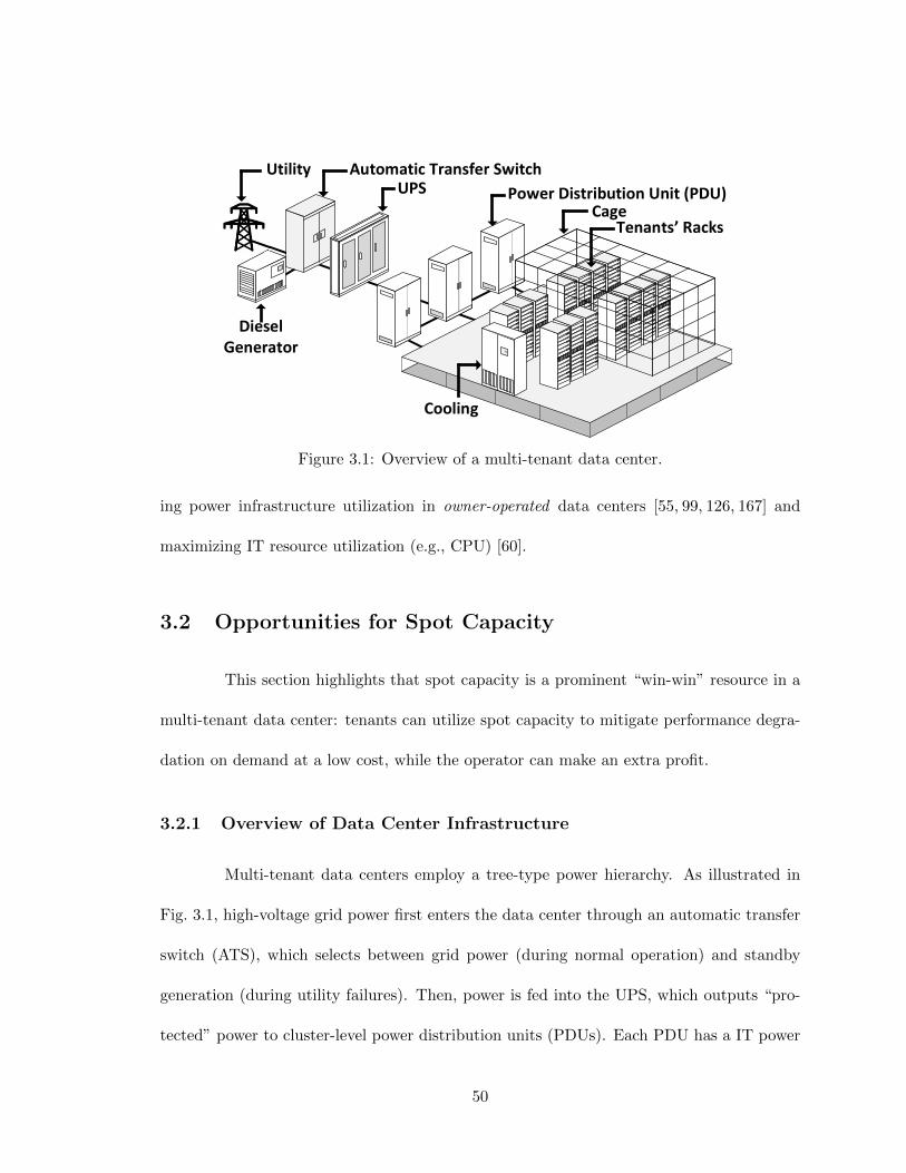
Tenants’ RacksPower Distribution Unit (PDU)UPSAutomatic Transfer SwitchUtility

Diesel Generator

Cooling

Cage

Figure 3.1: Overview of a multi-tenant data center.

ing power infrastructure utilization in owner-operated data centers [55, 99, 126, 167] and

maximizing IT resource utilization (e.g., CPU) [60].

3.2 Opportunities for Spot Capacity

This section highlights that spot capacity is a prominent “win-win” resource in a

multi-tenant data center: tenants can utilize spot capacity to mitigate performance degra-

dation on demand at a low cost, while the operator can make an extra profit.

3.2.1 Overview of Data Center Infrastructure

Multi-tenant data centers employ a tree-type power hierarchy. As illustrated in

Fig. 3.1, high-voltage grid power first enters the data center through an automatic transfer

switch (ATS), which selects between grid power (during normal operation) and standby

generation (during utility failures). Then, power is fed into the UPS, which outputs “pro-

tected” power to cluster-level power distribution units (PDUs). Each PDU has a IT power

50

capacity of 200-300kW and supports roughly 50-80 racks/cabinets. At the rack level, there

is a power strip (also called rack PDU) that directly connects to servers. In a typical (retail)

multi-tenant data center, tenants each manage multiple racks and share PDUs.

The capacities at all levels must not be exceeded to ensure reliability. Typically,

the UPS and cluster PDUs handle power at a high or medium voltage and hence are very

expensive, costing US$10-25 per watt (along with the cooling system and backup generator)

[42,75]. Nonetheless, the rack-level PDU has a lower voltage and is very cheap (e.g., US¢20-

50 per watt) [12,126]. Thus, the capacity bottleneck is at the shared UPSes/PDUs, not at

individual tenants’ racks. In fact, 20% rack-level capacity margin is already in place [45],

and additional over-provisioning is increasingly more common for flexible power distribution

to racks (e.g., power routing [126]).

3.2.2 Spot Capacity v.s. Oversubscription

Like in owner-operated data centers, power capacity is under-utilized in multi-

tenant data centers. Fig. 3.2(b) plots the cumulative density function (CDF) of measured

power at a PDU serving five tenants in a commercial data center over three months. The

CDF is normalized to the maximum power and shown as the left-most curve. Suppose

that the PDU capacity is provisioned at the maximum power demand. Ideally, if the PDU

is always 100% utilized, the power usage CDF would become a vertical line, as shown in

Fig. 3.2(b), which highlights a large gap between the measured CDF and the ideal case.

To improve infrastructure utilization, data center operators commonly oversub-

scribe the capacity, as tenants typically do not have peak power at the same time. To

illustrate oversubscription, we keep the same PDU capacity and add another two tenants,

51

0 6 12 18 24Hour

0.80

0.85

0.90

0.95

1.00

1.05N

orm

. P

ow

er

Spot Capacity

Power UsagePower Budget (Assumed)

(a)

0.60 0.80 1.00 1.15Power Normalized to Capacity

0.0

0.5

1.0

CD

F

A C

B

w/o Oversubscription Oversubscription

(b)

0 6 12 18 24Hour

0.6

0.7

0.8

0.9

1.0

Norm

. P

ow

er

PowerHigh Res.

Low Res.High Demand

Spot Capacity

(c)

Figure 3.2: (a) Illustration of spot capacity in a production PDU [169]. (b) CDF oftenants’ aggregate power usage. (c) A tenant can lease power capacity in three ways:high reservation; low reservation; and low reservation + spot capacity. “Low/high Res.”represent low/high reserved capacities.

resulting in a new CDF (dotted line in Fig. 3.2(b)) which is closer to the ideal case than

the original CDF. The improved capacity utilization is indicated by the area “A”. However,

oversubscription may occasionally trigger an emergency when power capacity is exceeded

(indicated by the area “B”). This has been well understood, and many power capping

solutions have been proposed to handle emergencies [45,75,167,174].

To avoid frequent emergencies, the shared UPS/PDUs must be sized to sustain

a high aggregate power demand [42, 45, 75, 174]. Consequently, even when some tenants

have reached their capacities, other tenants may still have low power usage, possibly re-

sulting in spot capacity at the shared PDU/UPS. The existence of spot capacity is also

visualized by the gap (area “C”) between the actual and idealized CDFs in Fig. 3.2(b).

52

Importantly, spot capacity can be allocated to those tenants to improve performances on

demand (Section 3.2.3).

Therefore, exploiting spot capacity and power oversubscription are complementary

to increasing data center infrastructure utilization: oversubscription is decided over a long

timescale and requires power shaving during emergencies [45, 75, 174], whereas spot capac-

ity is dynamically exploited based on the runtime availability to deliver additional power

budgets to tenants (with insufficient capacity reservation) for performance improvement.

3.2.3 Potential to Exploit Spot Capacity

Even with the same servers/workloads, a tenant’s power usage can be elastic and

can vary significantly depending on power control and/or workload scheduling [104]. Thus,

given a server deployment, a tenant’s power capacity subscription can vary widely.

Traditionally, each tenant reserves a sufficiently large capacity of the shared PDU

with a high availability guarantee (a.k.a. guaranteed capacity) to support its maximum

power demand, which is illustrated as “High Res” (high reservation) in Fig. 3.2(c). The

guaranteed capacity subscription, at US$120-250/kW/month, is a major fraction of tenants’

cost and can even exceed 1.5 times of the metered energy charge [58, 75]. Furthermore,

tenants rarely fully utilize their large guaranteed capacities.

More recently, the shrinking IT budget has placed a growing cost pressure on

tenants. A 2016 survey shows that 40% of tenants end up paying more than what they

anticipate for their power subscription [158]. Thus, studies on reducing tenants’ power

costs have been proliferating [73,123,165]. Notably, cost-conscious tenants have commonly

reserved capacities lower than their maximum power demand to reduce costs [123]. This is

53

illustrated by “Low Res” (low reservation) in Fig. 3.2(c), and similar to under-provisioning

power infrastructures in owner-operated data centers such as Facebook [169, 174]. Then,

when their demand is high, tenants with insufficient capacity reservation need to apply

power capping, incurring a performance degradation; otherwise, heavy penalties will be

applied.

As illustrated in Fig. 3.2(c), spot capacity helps tenants with insufficient capacity

reservation mitigate performance degradation when their power demand is high. Specif-

ically, when a tenant with insufficient capacity reservation has high workloads, the oper-

ator can allocate spot capacity, if available, to this tenant’s racks as an additional power

budget to mitigate performance degradation. The rack-level PDU capacity is not a bottle-

neck [55, 126], and the operator can dynamically adjust it at runtime, which is already a

built-in functionality in many of today’s rack-level PDUs [12]. More importantly, utilizing

spot capacity incurs a negligible cost for participating tenants (as low as 0.3% and much

lower than reserving additional guaranteed capacities, shown in Section 3.5.2).

Spot capacity v.s. guaranteed capacity. Spot capacity is dynamically al-

located based on demand function bidding (Section 3.3.2). But, once spot capacity is

allocated, it can be utilized over a pre-determined time slot (e.g., 1-5 minutes) in the same

way as guaranteed capacity,1 with the exception that it may be unavailable in the next time

slot. This differs from the Amazon spot market where allocated VMs may be evicted at

any time.

In practice, tenants with insufficient capacity reservation often run delay-tolerant

workloads (e.g., batch processing), which exhibit large scheduling flexibilities and are run

1Section 3.3.3 discusses how to guarantee spot capacity for one slot.

54

on 50+% servers (with roughly 50% power capacity) in data centers [17, 169]. Note that,

for a tech-savvy tenant with advanced power control, insufficient capacity reservation can

even apply for delay-sensitive workloads (e.g., web service), as is being done by large com-

panies [42, 169, 174]. In this paper, we use opportunistic and sprinting tenants to refer

to tenants which use spot capacity to mitigate slowing down of delay-tolerant and delay-

sensitive workloads, respectively. Thus, a tenant can be both opportunistic and sprinting.

In any case, with the help of spot capacity, a tenant with insufficient capacity reserva-

tion can temporarily process its workloads without power capping (or cap power less fre-

quently/aggressively than it would otherwise).

Importantly, spot capacity targets cost-conscious tenants with insufficient capacity

reservation and does not affect the revenue of guaranteed capacity. Even without cost-

effective spot capacity, these tenants already choose insufficient capacity reservation; they

would not pay the high cost and reserve a sufficiently large amount of guaranteed capacity

to meet their maximum power demand. On the other hand, tenants running mission-

critical workloads will likely continue reserving a sufficient guaranteed capacity without

using intermittent spot capacity.

3.3 The Design of SpotDC

Our main contribution is a new market approach for exploiting spot capacity,

SpotDC, which leverages a new demand function bidding approach to extract tenants’ rack-

level spot capacity demand elasticity at runtime and reconcile different objectives of tenants

and the operator: tenants first bid to express their spot capacity demand, and then the oper-

55

ator sets a market price to allocate spot capacity and maximize its profit. With SpotDC, the

operator makes extra profit, while participating tenants mitigate performance degradation

(or improve performance) at a low cost.

3.3.1 Problem Formulation

To design SpotDC, we consider a time-slotted model, where each dynamic spot

capacity allocation decision is only effective for one time slot. The duration of each time

slot can be 1-5 minutes [126].

Model. Consider a data center with one UPS supporting M cluster PDUs indexed

by the set M = {m | m = 1, · · · ,M}. There are R racks indexed by the set R = {r | r =

1, · · · , R}, and N tenants indexed by the set N = {n | n = 1, · · · , N}. Denote the set of

racks connected to PDU m as Rm ⊂ R. Note that racks are not shared among tenants in

a multi-tenant data center, while a tenant can have multiple racks.

The operator continuously monitors power usage at rack levels [45, 126, 174]. For

time slot t = 1, 2, · · · , the predicted available spot capacity at the upper-level UPS is denoted

by Po(t), and the available spot capacity at PDU m is denoted by Pm(t), for m = 1, 2, · · · .

How to predict the available spot capacity is discussed in Section 3.3.3. At the rack level, the

physical capacity is over-provisioned beyond the guaranteed capacity to support additional

power budgets (i.e., spot capacity). The maximum spot capacity supported by rack r is

denoted as PRr .

The operator sells spot capacity at price q(t), with a unit of $/kW per time slot.

The set of racks that requests spot capacity is denoted by S(t) ⊆ R, and the actual spot

capacity allocated to rack r ∈ S(t) is denoted by Dr (q(t)).

56

Objective. The operator incurs no extra operating costs for offering spot capacity,

since tenants pay for metered energy usage (and otherwise a reservation price can be set to

recoup energy costs). Thus, the operator’s profit maximization problem at time t can be

formalized as:

maximizeq(t)

q(t) ·∑r∈S(t)

Dr (q(t)) . (3.1)

Constraints. We list the most important power capacity constraints for spot

capacity allocation, from rack to UPS levels, as follows:

Rack : Dr (q(t)) ≤ PRr , ∀r ∈ S(t) (3.2)

PDU :∑

r∈S(t)∩Rm

Dr (q(t)) ≤ Pm(t), ∀m ∈M (3.3)

UPS :∑r∈S(t)

Dr (q(t)) ≤ Po(t) (3.4)

Other constraints, such as heat density (limiting the maximum cooling load, or server power,

over an area) and phase balance (ensuring that the power draw of each phase should be

similar in three-phase PDUs/UPSes), can also be incorporated into spot capacity allocation

following the model in [126], and are omitted for brevity.

In SpotDC, spot capacity allocation is at a rack-level granularity, since tenants

manage their own racks while the operator controls upstream infrastructures like PDU and

UPS. Note that with a tenant-level spot capacity allocation, the operator would have no

knowledge of or control over how a tenant would distribute its received spot capacity among

its racks. This can create capacity overloading and/or local hot spots if multiple tenants

concentrate their received spot capacity over a few nearby racks served by a single PDU.

57

Finally, rack-level spot capacity allocation does not require a homogeneous rack setup. Dif-

ferent tenants can have different racks with different configurations, and even a single tenant

can have diverse rack configurations.

3.3.2 Market Design

A key challenge for maximizing the operator’s profit is that, due to its lack of

control over tenants’ servers, the operator does not know tenants’ demand function: which

tenants need spot capacity and by how much. This is private information of individual ten-

ants. Prediction is a natural solution to the challenge — the operator first predicts tenants’

responses and then sets a profit-maximizing price for tenants to respond. However, due to

the capacity constraints at different levels in Eqns. (3.2), (3.3) and (3.4), prediction needs to

be done rack-wise and there can be hundreds or even thousands of racks with dynamic work-

loads. Most importantly, with prediction-based pricing, spot capacity allocation is decided

by the tenants (passively through their responses to the market price set by the operator).

This can lead to dangerous capacity overloads in the event of under-predicting tenants’

spot capacity demands (i.e., setting a too low price). Thus, prediction-based pricing is not

suitable for spot capacity allocation. In contrast, an alternative to prediction is to solicit

tenants’ demand through bidding, called demand function bidding: each participating ten-

ant first reports its own spot capacity demand to the operator through a bidding process,

and then the operator allocates spot capacity by setting a market price while meeting all

the capacity constraints.

58

Demand function

The core of demand function bidding is to extract users’ demand through a func-

tion (called demand function), which can capture how the demand varies as a function of

the price. In our context, there can be up to thousands of racks, and even without reducing

the workloads, server power can vary to achieve different performances (e.g., with a granu-

larity of watt by Intel’s RAPL) [104]. Thus, our goal is to design a demand function that

can extract tenants’ rack-level elastic spot capacity demand reasonably well yet at a low

complexity/overhead.

A straightforward approach is to solicit each tenant’s complete rack-level demand

curve under all possible prices. We illustrate in Fig. 3.3(a) an example demand curve

(labeled as “Reference,” and Section 3.4.3 explains how to derive it). The actual demand

curve can be even more complex and multi-dimensional (for multiple racks, as shown in

Fig. 3.4(a)), thus incurring a high overhead to extract. In addition, bidding the complete

demand curve is difficult for participating tenants, as they must evaluate their demand

under many prices. For these reasons, soliciting the complete demand curve is rarely used

in real markets [10,80].

In practice, parameterized demand function bidding is commonly applied when

the buyers’ demand is unknown to the seller a priori. For example, a step demand function

illustrated in the shaded area in Fig. 3.3(a) is used by Amazon spot VM market [10] and

means that a user is willing to pay up to a certain price for a fixed amount of requested

VMs. We refer to this demand function as StepBid. While it has a low overhead, StepBid

can be very different from tenants’ actual demand curve (“Reference”) shown in Fig. 3.3(a).

59

(a) (b)

Figure 3.3: (a) Piece-wise linear demand function. The shaded area represents StepBid. (b)Aggregated demand function for ten racks. StepBid-1 bids (Dmax, qmin) only, and StepBid-2bids (Dmin, qmax) only.

Moreover, with StepBid, the operator cannot flexibly allocate spot capacity: a tenant’s spot

capacity demand can only be either 100% or 0% satisfied. Thus, StepBid cannot capture a

tenant’s rack-level spot capacity demand elasticity. As illustrated in Fig. 3.3(b), even at the

shared PDU level, StepBid cannot extract the aggregate demand elasticity of multiple racks,

thus resulting in a lower profit for the operator (Section 3.5.3). The reason is that, although

StepBid can extract the aggregate demand elasticity over a large number of racks, spot

capacity allocation is subject to several localized constraints (e.g., shared PDU capacity)

that each cover only up to a few tens of racks. This is in sharp contrast with Amazon spot

market where the unused VMs are pooled together and allocated to a large number of users

without restricting one user’s demand to any particular rack.

Piece-wise linear demand function. We propose a new parameterized de-

mand function which, as illustrated by “Linear Bid” in Fig. 3.3(b), approximates the actual

demand curve using three line segments: first, a horizonal segment: tenant specifies its

maximum spot capacity demand for a rack as well as the market price it is willing to

60

pay; second, a linearly decreasing segment: the demand decreases linearly as the market

price increases; and third, a vertical segment: the last segment indicates tenant’s maximum

acceptable price and the corresponding minimum demand.

As shown in Fig. 3.3(a), our linear demand function for rack r is uniquely deter-

mined by four parameters:

br = {(Dmax,r, qmin,r), (Dmin,r, qmax,r)} (3.5)

where Dmax,r and Dmin,r are the maximum and minimum spot capacity demand, and qmin,r

and qmax,r are corresponding prices, respectively. We also allow Dmax,r = Dmin,r or qmin,r =

qmax,r, which reduces to StepBid.

We choose our linear demand function for its simplicity and good extraction of

the demand elasticity. It also represents a midpoint between StepBid (which is even simpler

but cannot extract spot capacity demand elasticity) and soliciting the complete demand

curve (which is difficult to bid and rarely used in practice [80]). Moreover, the experiment

in Section 3.5.3 shows that, using our demand function, the operator’s profit is much higher

than that using StepBid and also fairly close to the optimal profit when the complete demand

curve is solicited, thus further justifying the choice of our demand function.

Spot capacity allocation

The following three steps describe the spot capacity allocation process, which is

also described in Algorithm 3.

61

Algorithm 3 SpotDC— Spot Capacity Management

1: Continuously monitor rack power2: for t = 0, 1, · · · do3: Each participating tenant analyzes workloads and submits bids4: Collect bids br and predict spot capacity5: Decide price q(t+1), send market price and spot capacity allocation to participating

tenants, and re-set rack capacity via intelligent rack PDU6: Each tenant manages its power subject to the allocated spot capacity effective for

time t+ 1

Step 1: Demand function bidding. Participating tenants, at their own discretion, decide

their rack-wise bidding parameters based on their anticipated workloads and needs of spot

capacity for the next time slot.

Step 2: Market clearing. Upon collecting the bids, the operator sets the market price q(t) to

maximize profit, i.e., solving (3.1) subject to multi-level capacity constraints (3.2)(3.3)(3.4).

This can be done very quickly through a simple search over the feasible price range.

Step 3: Actual spot capacity allocation. Given the market price q(t) plugged into the

demand function, each tenant knows its per-rack spot capacity and can use additional

power up to the allocated spot capacity during time t.

Tenant’s bidding for spot capacity

For a tenant, the power budgets for multiple racks jointly determine the appli-

cation performance (e.g., latency of a three-tier web service, with each tier housed in one

rack). Thus, a key difference from spot VM bidding in Amazon [10] is that, in our con-

text, each participating tenant needs to bid a bundled demand for all of its racks that need

spot capacity. Nonetheless, the bidding strategy is still at the discretion of tenants in our

context, like in Amazon spot market. It can follow a simple strategy for each rack: bid

62

the needed extra power (i.e., total power needed minus the reserved capacity) as spot ca-

pacity demand with Dmax,r = Dmin,r, and set the amortized guaranteed capacity rate (at

US$120-250/kW/month) as maximum price. Tenants routinely evaluate server power under

different workloads prior to service deployment [167,169,174], and thus can determine their

needed power based on estimated workloads at runtime.

On the other hand, advanced tenants with detailed power-performance profiling

can also bid holistically for their racks in need of spot capacity. Below, we provide a

guideline for spot capacity bidding to highlight how advanced tenants may approach this

task, although our focus is on the operator’s side — setting up a market for spot capacity

allocation.

Given each price, there exists an optimal spot capacity demand vector for a ten-

ant’s racks. The optimality can be in the sense of maximizing the tenant’s net benefit (i.e.,

performance gain measured in dollars,2 minus payment), maximizing performance gain (not

lower than payment), or others, which tenants can decide on their own. Consider web ser-

vice (as described in Section 3.4.2) on two racks as an example. As illustrated in Fig. 3.4(a),

tenant identifies its demand curve by first evaluating performance gains resulting from spot

capacity (Section 3.4.3) and then finding optimal demand vectors under different prices.

In general, the relation between rack-1 demand and rack-2 demand may be non-

linear, as shown in Fig. 3.4(b). Nonetheless, spot capacity allocated to both racks are

determined by the same price and may not follow the optimal demand curve. For example,

one rack’s spot capacity allocation may change linearly in the other’s. Consequently, the

2The monetary value for performance gain [47] is quantified by tenants as described in Section 3.4.3.

63

Rack-1

(kW

)0.10.5

1.0Rack-2 (kW)

0.10.5

1.0

Pri

ce (

$/W

)

0.0

0.5

1.0

Optimal DemandBid

(a)

0.0 0.2 0.4 0.6 0.8 1.0Rack-1 (kW)

0.0

0.2

0.4

0.6

0.8

1.0

Rack-2

(kW

)

Optimal DemandBid

(b)

Figure 3.4: Demand function bidding. (a) Optimal spot capacity demand and biddingcurve. (b) 2D view.

tenant needs to approximate the optimal demand curve using, e.g., a line shown as “Bid” in

Fig. 3.4(a). We also present the top-down perspective of bidding curve in Fig. 3.4(b), which

indicates the relation between the two racks’ actual spot capacity demand. In Fig. 3.4(a),

the bidding demand curve includes all the needed parameters: the maximum and minimum

demand pairs for the two racks, as well as the corresponding bidding prices (the same qmin

and qmax for the two racks).

A tenant can bid similarly ifK of its racks need spot capacity: decide the maximum

and minimum bidding demand vectors (Dmax,1, · · · , Dmax,K) and (Dmin,1, · · · , Dmin,K), which

are joined in an affine manner to approximate the optimal K-dimensional demand, and then

decide the two corresponding bidding prices.

Finally, it is important to note that tenants can bid freely without their own

strategies. Thus, the resulting bidding profile and spot capacity allocation can be signifi-

cantly different from the theoretical equilibrium point at which each participating tenant’s

net benefit is maximized (given the other tenants’ bids) [80]. In fact, even under a set of

simplified assumptions (e.g., concave utility for each tenant, no tenant forecasts the market

64

Rack i

Power AnalyzerSpotCapPred(…)

Rack 1

Workload AnalyzerLoadPred(…)PwrToPerf(…)

Workload AnalyzerLoadPred(…)PwrToPerf(…)

Tenant Operator

SpotDCMarketPrice(b,…)SetPowerCap(…)HeartBeat(…)

��

Demand BiddingBid(bi,…)HeartBeat(��,…)

Power MeterPower(…)

PDU

��

Demand BiddingBid(b1,…)HeartBeat(��,…)

Power Management

DVFS(…)Sleep(…)

Migrate(…)AdmnCtrl(…)LoadBal(…)

�Power BudgeterPowerCap(�,…)

Figure 3.5: System diagram for SpotDC.

price, etc.), it is non-trivial to derive the theoretical equilibrium point [80], since a tenant’s

spot capacity demand involves multiple racks and hence is multi-dimensional. Further,

given tenants’ strategic behaviors and lack of information about each other, how to reach

an equilibrium is a theoretically challenging problem [80]. Thus, we focus on the operator’s

spot capacity market design and resort to case studies to show the benefit of exploiting

spot capacity (Section 3.5), while leaving the theoretical equilibrium bidding analysis as

our future work.

3.3.3 Implementation and Discussion

We now illustrate the implementation for SpotDC in Fig. 3.5, where the applica-

tion program interfaces (APIs), as highlighted in shaded boxes, facilitate communications

between the operator and tenants using a simple network management protocol. In our

time-slotted model, the data center operator and participating tenants are synchronized by

periodically exchanging HeartBeat(· · · ) signals. As suggested by [126], each time slot can

65

1

2

4

Demand Bidding1

Spot Capacity Prediction2

Market Clearing3

Using Spot Capacity4

3

� − � �

Figure 3.6: Timing of SpotDC for spot capacity allocation.

be 1-5 minutes in practice. To conclude the design of SpotDC, it is important to discuss a

few remaining practical issues.

Timing. We show in Fig. 3.6 the timing of different stages leading to and during

spot capacity allocation in time slot t. For using spot capacity during time slot t, tenants

need to submit their demand bids (marked as “1”) during time slot t − 1. The gradient

color is to emphasize that most bids are expected to be received closer to time slot t.

Then, the operator predicts the available spot capacity (marked as “2”) before clearing the

market. The market clearing time (marked as “3”) is very small (less than a second), and

the clearing price is broadcast to the tenants. Finally, from their demand functions, tenants

determine their rack-level spot capacity allocation and use it (marked as “4”) during time

slot t. Note that participating tenants have an entire time slot to decide and send their

bids to the operator for using spot capacity in the next time slot. Thus, the communication

delay (in the order of hundreds of milliseconds) is insignificant even when tenants submit

bids remotely.

Spot capacity prediction. The operator can predict spot capacity by taking the

current aggregate power usage as a reference and subtracting it from the physical PDU/UPS

66

capacity. For racks that are currently using spot capacity or request it for the next time slot,

the guaranteed rack-level capacity will be used as their reference power usage. Collecting the

power readings can be done near instantaneously as a part of the routine power monitoring.

The key concern here is how accurate the prediction of spot capacity is. We note that, due

to statistical multiplexing, the cluster-level PDU power only changes marginally within a

few minutes (e.g., less than ±2.5% within one minute for 99% of the times) [126,169,174]. In

Fig. 3.7(a), we show the statistics of PDU-level power variations in our experimental power

trace (Section 3.5) and see that it is consistent with the results in [169]: the PDU-level power

changes slowly across consecutive time slots. Moreover, in almost all cases, spot capacity

is not completely utilized due to the operator’s profit-maximizing pricing and multi-level

capacity constraints (as seen in Fig. 3.10). The operator can also conservatively predict (i.e.,

under-predict) the available spot capacity without noticeably affecting its profit or tenants’

performance (Fig. 3.17). Finally, any unexpected short-term power spike can be handled by

circuit breaker tolerance, let alone the power system redundancy in place. Therefore, even

with inaccurate spot capacity prediction, the availability of spot capacity can be guaranteed

for one time slot almost highly as the normal power capacity provisioning.

Applicability. SpotDC targets a growing class of tenants — cost-conscious ten-

ants with insufficient capacity reservation (even Facebook under-provisions power capacity

in its own data center [174]) — and helps them mitigate performance degradation on a

best-effort basis. Utilizing spot capacity is even easier than otherwise: with spot capacity,

a tenant caps power less frequently/aggressively than it would otherwise. Moreover, spot

capacity bidding is at the discretion of tenants: it can be either as simple as bidding the

67

(a)

0 5000 10000 15000Number of Racks

0.0

0.2

0.4

0.6

0.8

1.0

Avera

ge M

ark

et

Cle

ari

ng

Tim

e (

s) Step: 0.1 ¢/kW

Step: 1 ¢/kW

(b)

Figure 3.7: (a) PDU power variation in our simulation trace. (b) Market clearing time atscale.

needed power at a fixed price, or as sophisticated as holistically bidding for multiple racks

in need of spot capacity (Section 3.3.2). There is no application/workload requirement for

tenants to participate in SpotDC, as long as they can control power subject to dynamic spot

capacity allocation.

Scalability. The design of SpotDC is highly scalable since only four parameters

are solicited for each rack in need of spot capacity; no bids are required for racks that do

not need extra power demand beyond the reserved capacity. Additionally, our proposed

uniform clearing price only requires a scan over feasible prices subject to the infrastructure

constraints. Therefore, the market clearing is very fast. We show in Fig. 3.7(b) the average

market clearing time for different numbers of server racks and different search step sizes

in our large-scale simulation (Section 3.5.4) on a typical desktop computer. We see that

even with 15000 racks, the average clearing time is less than a second for a step size of 0.1

cents/kW. For a step size of 1 cent/kW, the average clearing time is below 100ms. Further,

it takes almost no time for the operator to reset rack-level power budgets (e.g., 20+ times

per second for our PDU [12] without any timeouts).

68

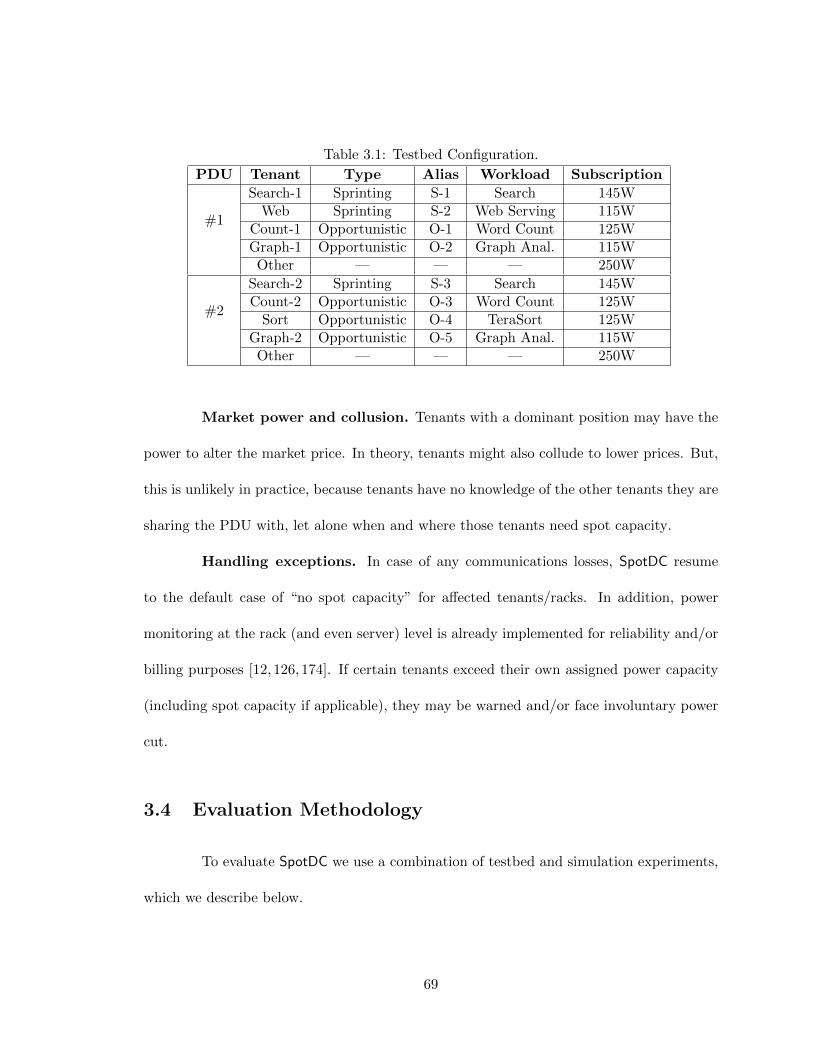
Table 3.1: Testbed Configuration.

PDU Tenant Type Alias Workload Subscription

#1

Search-1 Sprinting S-1 Search 145WWeb Sprinting S-2 Web Serving 115W

Count-1 Opportunistic O-1 Word Count 125WGraph-1 Opportunistic O-2 Graph Anal. 115WOther — — — 250W

#2

Search-2 Sprinting S-3 Search 145WCount-2 Opportunistic O-3 Word Count 125W

Sort Opportunistic O-4 TeraSort 125WGraph-2 Opportunistic O-5 Graph Anal. 115WOther — — — 250W

Market power and collusion. Tenants with a dominant position may have the

power to alter the market price. In theory, tenants might also collude to lower prices. But,

this is unlikely in practice, because tenants have no knowledge of the other tenants they are

sharing the PDU with, let alone when and where those tenants need spot capacity.

Handling exceptions. In case of any communications losses, SpotDC resume

to the default case of “no spot capacity” for affected tenants/racks. In addition, power

monitoring at the rack (and even server) level is already implemented for reliability and/or

billing purposes [12, 126, 174]. If certain tenants exceed their own assigned power capacity

(including spot capacity if applicable), they may be warned and/or face involuntary power

cut.

3.4 Evaluation Methodology

To evaluate SpotDC we use a combination of testbed and simulation experiments,

which we describe below.

69

3.4.1 Testbed Configuration

Like in the literature [75, 167], we build a scaled-down testbed with Dell Pow-

erEdge servers connected to two PDUs, labeled as PDU#1 and PDU#2, respectively. In

our scaled-down system, each server is considered as a “rack”. We show our testbed config-

uration in Table 3.1, where the subscription amounts (i.e., guaranteed capacity) are based

on corresponding tenant’s power usage in our experiment. We use two off-the-shelf PDUs

(AP8632 from APC [12]) with per-outlet metering capabilities. Each PDU has four par-

ticipating tenants and one group of “other” tenants representing non-participating tenants.

The total leased capacities of PDU#1 and PDU#2 are 750W and 760W, respectively. We

assume that the two PDUs have a capacity of 715W and 724W, respectively, to achieve 5%

oversubscription (e.g., 750W=715W*105%) [75]. We also consider a common oversubscrip-

tion by 5% at the upper UPS, and hence the total power usage need to be capped at 1370W

(= 715W+724W105% ).

3.4.2 Workloads

We consider a mixture of workloads in our experiments. Each workload is repre-

sentative of a particular class of tenants in multi-tenant data centers, and they are typical

choices in the prior studies [75,167,169].

Search. We implement the web search benchmark from CloudSuite [44] in two

servers, each virtualized into three VMs. It is based on a Nutch search engine which

benchmarks the indexing process. Our implementation uses one front-end and five index

serving VMs.

70

Figure 3.8: Power-performance relation at different workload levels.

Web serving. We use the web serving benchmark from CloudSuite [44] that

implements a Web 2.0 social-event application using PHP. The front-end is implemented

using a Nginx web sever, while the back-end is implemented using MySQL database on a

separate server.

Word count and TeraSort. We implement both WordCount and TeraSort

benchmarks based on Hadoop 2.6.4 with one master node and seven data nodes, hosted

on eight VMs. In our experiment, WordCount processes a 15GB input file, while TeraSort

sorts 5GB of data.

Graph analytics. We implement PowerGraph [105] on two servers (16GB mem-

ory each). A Twitter data set consisting of 11 million nodes from [182] is used as the

input.

3.4.3 Power and Performance Model

To participate in SpotDC, a tenant needs to assess the the performance improve-

ment resulting from spot capacity. Towards this end, we first run the workloads at different

power levels and workload intensities. Fig. 3.8 shows the power-performance relation of

71

Search-1, Web and Count-1 for selected workload intensities. The other workloads also

exhibit similar power-performance relations and are omitted for brevity.

The power-performance relation gives the potential performance improvement

from spot capacity. To determine the bidding parameters, performance improvement needs

to be converted into a monetary value. A tenant participating in SpotDC can decide the

monetary value at its own discretion without affecting our SpotDC framework. For eval-

uation purposes, we convert the performance into monetary values following the prior re-

search [47,75]. Specifically, for sprinting tenants (Search and Web), we consider the following

model: ctenant = a · d if d ≤ dth, and ctenant = a · d + b · (d − dth)2 otherwise, where ctenant

measures the equivalent monetary cost per job, a and b are modeling parameters, and d

is the actual performance (e.g., 99-percentile, or p99, latency for Search and p90 latency

for Web) and dth is the service level objective (SLO, 100ms for all sprinting tenants). The

model indicates that the cost increases linearly with latency below the SLO threshold, and

quadratically when latency is greater than the SLO to account for penalties of SLO viola-

tion. For opportunistic tenants running Hadoop and graph analytics, we use throughput

(inverse of job completion time) as the performance metric and employ a linear cost model

ctenant = ρ · Tjob, where ρ is a scaling parameter and Tjob is the job completion time.

Tenants can first estimate their performance “costs” with and without spot ca-

pacity, respectively, and then the difference is the performance gain (in dollars) brought by

spot capacity. In our experiments, the cost parameters are chosen such that spot capacity

will not cost more than directly subscribing guaranteed capacity. Further, we assume that

Search tenants bid the highest price, Web tenants bid a medium price, and opportunistic

72

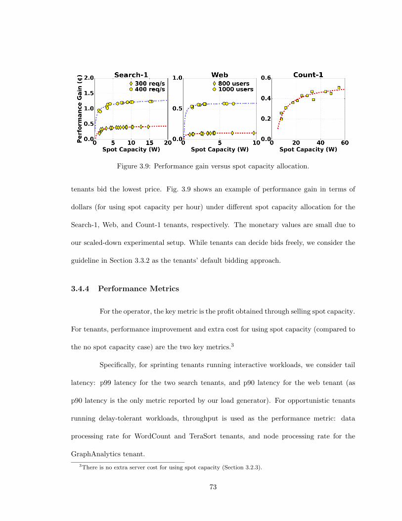
Figure 3.9: Performance gain versus spot capacity allocation.

tenants bid the lowest price. Fig. 3.9 shows an example of performance gain in terms of

dollars (for using spot capacity per hour) under different spot capacity allocation for the

Search-1, Web, and Count-1 tenants, respectively. The monetary values are small due to

our scaled-down experimental setup. While tenants can decide bids freely, we consider the

guideline in Section 3.3.2 as the tenants’ default bidding approach.

3.4.4 Performance Metrics

For the operator, the key metric is the profit obtained through selling spot capacity.

For tenants, performance improvement and extra cost for using spot capacity (compared to

the no spot capacity case) are the two key metrics.3

Specifically, for sprinting tenants running interactive workloads, we consider tail

latency: p99 latency for the two search tenants, and p90 latency for the web tenant (as

p90 latency is the only metric reported by our load generator). For opportunistic tenants

running delay-tolerant workloads, throughput is used as the performance metric: data

processing rate for WordCount and TeraSort tenants, and node processing rate for the

GraphAnalytics tenant.

3There is no extra server cost for using spot capacity (Section 3.2.3).

73

Figure 3.10: A 20-minute trace of power (at PDU#1) and price. The market price increaseswhen sprinting tenants participate (e.g., starting at 240 and 720 seconds), and decreaseswhen more spot capacity is available (e.g., starting at 360 seconds).

3.5 Evaluation Results

In this section, we present the evaluation results based on our testbed and sim-

ulations. Our results highlight that spot capacity can greatly benefit both the operator

and tenants: compared to the no spot capacity case, the operator can earn an extra profit

by 9.7%, and tenants can improve performance by 1.2–1.8x (on average) while keeping the

additional costs low (as low as 0.5%).

3.5.1 Execution of SpotDC

For our first experiment, we execute SpotDC in our testbed for 20 minutes divided

evenly into 10 time slots. For clarity, we only show the results for tenants served by PDU#1.

To show variations of spot capacity availability over the 10 time slots, we create a synthetic

trace with a higher volatility for the non-participating tenants’ power. Sprinting tenants bid

for spot capacity when they would otherwise have SLO violations due to high workloads,

while opportunistic tenants process data continuously and would like spot capacity to speed

up processing.

74

Spot capacity allocation and market price

Fig. 3.10 shows the traces of spot capacity allocation (top figure) and market

price (bottom figure). As the synthetic power trace is more volatile than the actual usage

[169, 174], spot capacity prediction is assumed to be perfect. Later, we will predict spot

capacity as presented in Section 3.3.3.

We see that, whenever sprinting tenants participate, they receive most of their

requested spot capacity, while opportunistic tenants may be priced out. The reason is that

spring tenants need spot capacity more urgently to meet their SLOs and hence bid a higher

price. This is also reflected in the market price trace, from which we see that the sprinting

tenants’ participation drives up the price given the same spot capacity availability (e.g., 120–

240 seconds versus 240–360 seconds). In addition, the market price decreases when more

spot capacity is available (e.g., 0–120 seconds versus 120–240 seconds). Lastly, we notice

that the actual spot capacity allocation is less than the available capacity due to multi-level

capacity constraints. This also confirms that, even without conservative prediction, using

spot capacity does not introduce additional power emergencies.

Tenant performance

We show the performance trace in Fig. 3.11. We see that the Search-1 and Web

tenants can successfully avoid SLO (i.e., 100ms in our experiment) violations by receiving

additional power budgets from the spot capacity market. Meanwhile, Count-1 and Graph-1

tenants can also opportunistically improve their throughput (by up to 1.5x).

75

Figure 3.11: Tenants’ performance. Search-1 and Web meet SLO of 100ms, while Count-1and Graph-1 increase throughput.

3.5.2 Evaluation over Extended Experiments

Our next set of experiments seek to assess the long-term cost and performance. To

do this, we extend our 20-minute experiment to one year via simulations. We use the scaled

power trace collected from a large multi-tenant data center as the non-participating tenants’

power usage. We also collect and scale the request arrival trace from Google services [53] for

sprinting tenants, and back-end data processing trace collected from a university data center

for opportunistic tenants (anonymized for review). We consider that the sprinting tenants

need spot capacity during high traffic periods for around 15% of the times. Opportunistic

tenants only lease guaranteed capacity to keep minimum processing rates, and need spot

capacity for speed-up for around 30% of the time slots. We keep an average of approximately

15% of the total guaranteed capacity subscription as spot capacity, while we will vary the

settings later. To evaluate SpotDC, we consider comparisons to the following two baselines.

PowerCapped: No spot capacity is provisioned, and tenants cap their power below

the guaranteed capacity at all times. This is the status quo, and we use it as a reference to

normalize cost, profit, and performance.

76

(a) Power subscription cost (b) Normalized performance

(c) Spot capacity usage

Figure 3.12: Comparison with baselines. Tenants’ performance is close to MaxPerf with amarginal cost increase.

MaxPerf: In this case, the data center operator fully controls all the servers as

if in an owner-operated data center, and allocates spot capacity to maximize the total

performance gain (as in [126]). There is no payment between the tenants and operator in

MaxPerf.

Cost and performance

We show in Fig. 3.12(a) the total cost for tenants (baseline cost under PowerCapped

plus extra spot capacity cost), while Fig. 3.12(b) shows the resulting performance of using

spot capacity normalized to that with PowerCapped. Tenants’ cost includes spot capacity

payment and the increased energy bill. We use inverse of tail latency/job completion time

to indicate tenants’ performance. The performance is averaged over all the time slots

whenever tenants need spot capacity. We see that by using SpotDC, tenants can achieve a

77

performance very close to MaxPerf while the cost increase is only marginal (no more than

than 0.5% for sprinting tenants). Opportunistic tenants have a higher percentage of cost

increase, because they demand more spot capacity and bid more frequently (30% of the

times).

Fig. 3.12(c) shows each tenant’s maximum and average spot capacity usage, in

percentage of their guaranteed capacity subscriptions (Table 3.1). In general, sprinting ten-

ants receive less spot capacity (in percentage), because they are more performance-sensitive

and hence do not oversubscribe their guaranteed capacity as aggressively as opportunistic

tenants. However, if PowerCapped is used without spot capacity, tenants’ capacity sub-

scription costs will increase by 10-40% in order to maintain the same performance, because

tenants have to reserve enough capacity to support their maximum power usage (e.g., 10%

more capacity for Search-1).

Finally, we note that spot capacity is provisioned at no additional cost for the

data center operator, except for the negligible capital expense for over-provisioning rack-

level capacity to support additional power budgets. In our calculation, we set US$0.4 per

watt for rack capacity and amortize it over 15 years [12,126]. We find that, by using SpotDC,

the operator’s net profit increases by 9.7% compared to the PowerCapped baseline.

Market price and power utilization

Fig. 3.13(a) shows the CDF of market prices for participating tenants in PDU#1.

As expected, opportunistic tenants bid and have lower prices than sprinting tenants, al-

though both types of tenants can avoid high costs of leasing additional guaranteed capacity.

78

(a) Market price (b) Aggregate power usage

Figure 3.13: CDFs of market price and aggregate power. (a) Sprinting tenants bid and alsopay higher prices than opportunistic tenants. (b) SpotDC improves power infrastructureutilization.

In our setting, opportunistic tenants will not bid higher than the amortized cost of guaran-

teed capacity (around US$0.2/kW/hour), while sprinting tenants are willing to pay more

to avoid SLO violations.

In Fig. 3.13(b), we show the CDF of UPS-level power consumption normalized to

the designed UPS capacity. SpotDC can greatly increase the power infrastructure utilization

compared to PowerCapped. Since both the PDUs and UPS are oversubscribed in our setting,

there exist occasional power emergencies (i.e., exceeding the UPS capacity), but these are

handled through separate mechanisms [75] beyond our scope. In any case, spot capacity

does not introduce additional emergencies, because it is offered only when there is unused

capacity at the shared PDUs and UPS.

3.5.3 Other Demand Functions

An important design choice in SpotDC is the demand function. To understand

its impact, we consider two alternatives: StepBid, where tenants bid a step function for

79

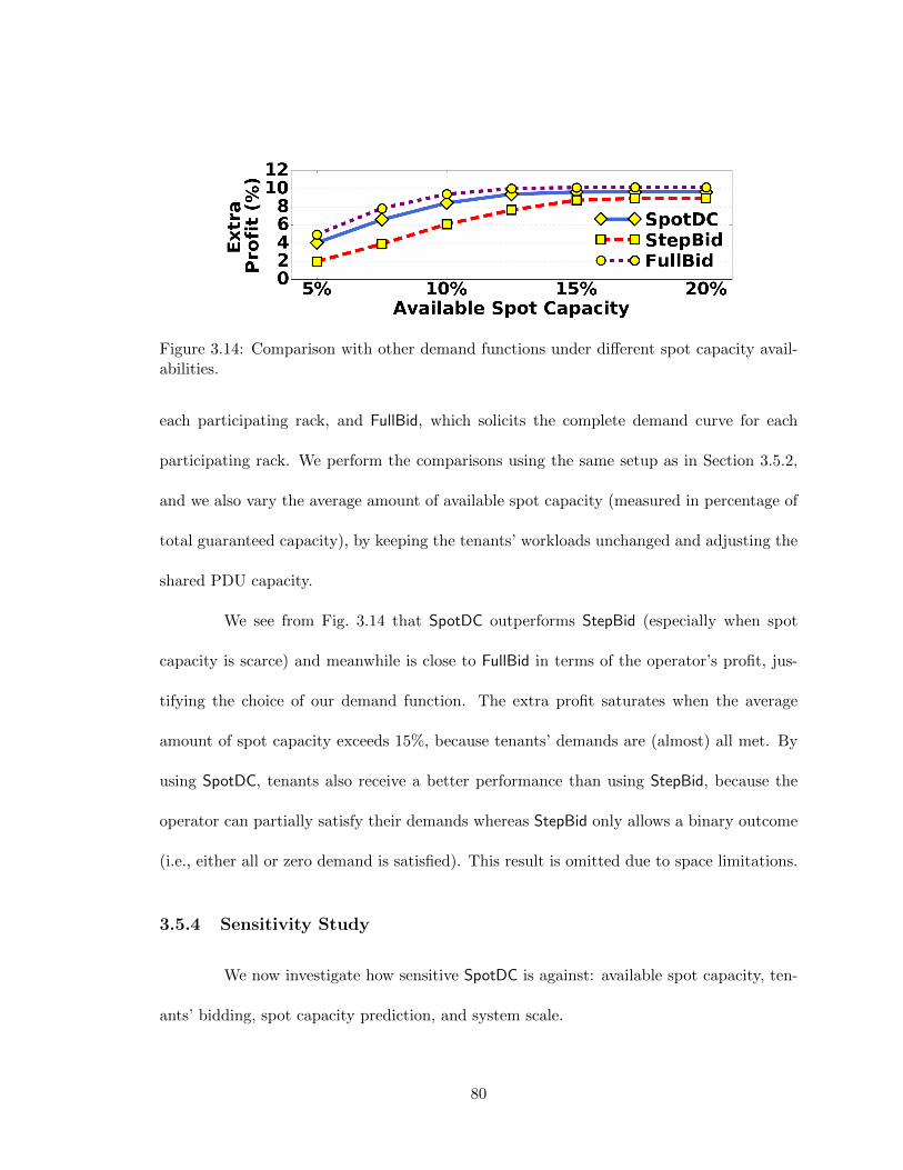
Figure 3.14: Comparison with other demand functions under different spot capacity avail-abilities.

each participating rack, and FullBid, which solicits the complete demand curve for each

participating rack. We perform the comparisons using the same setup as in Section 3.5.2,

and we also vary the average amount of available spot capacity (measured in percentage of

total guaranteed capacity), by keeping the tenants’ workloads unchanged and adjusting the

shared PDU capacity.

We see from Fig. 3.14 that SpotDC outperforms StepBid (especially when spot

capacity is scarce) and meanwhile is close to FullBid in terms of the operator’s profit, jus-

tifying the choice of our demand function. The extra profit saturates when the average

amount of spot capacity exceeds 15%, because tenants’ demands are (almost) all met. By

using SpotDC, tenants also receive a better performance than using StepBid, because the

operator can partially satisfy their demands whereas StepBid only allows a binary outcome

(i.e., either all or zero demand is satisfied). This result is omitted due to space limitations.

3.5.4 Sensitivity Study

We now investigate how sensitive SpotDC is against: available spot capacity, ten-

ants’ bidding, spot capacity prediction, and system scale.

80

(a) Operator’s extra profit (b) Tenants’ perfromance

Figure 3.15: Impact of spot capacity availability. With spot capacity, the market price goesdown, the operator’s profit increases, and tenants have a better performance.

Available spot power

In Fig. 3.15 we study the impact of amount of available spot capacity. For this, we

keep the tenants’ setup unchanged, and vary the operator’s oversubscription at the PDUs to

alter the available spot capacity. The spot capacity availability is measured in percentage

of the total subscribed capacity. In Fig. 3.15(a), we show that the operator’s extra profit

increases with spot capacity availability, as the operator can get more money by selling

more spot capacity. Fig. 3.15(b) shows tenants’ performance increases with spot capacity

availability.

Tenants’ bidding strategy

Tenants can bid for spot capacity on demand differently. For example, tenants may

predict the price and set their bids accordingly. As illustrated in Fig. 3.16(a), we assume

that sprinting tenants bid with a perfect knowledge of market price. The way opportunistic

tenants bid remain the same. We see from Figs. 3.16(b) and 3.16(c) that through a more

81

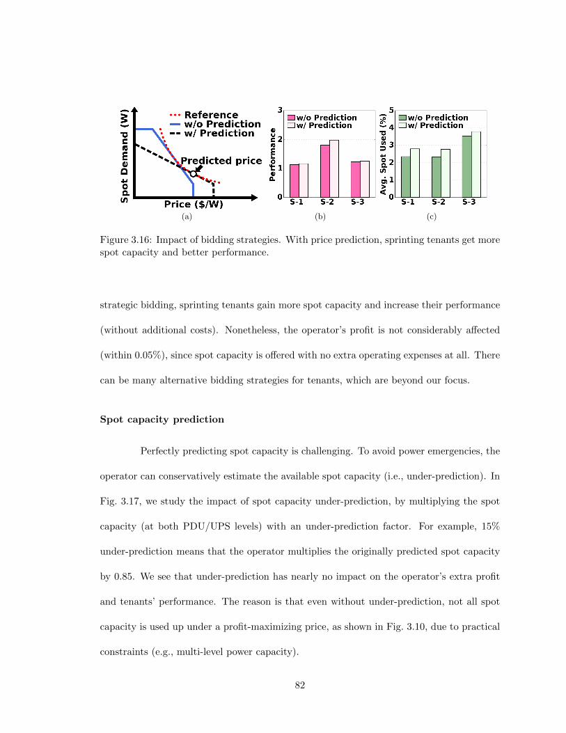
(a) (b) (c)

Figure 3.16: Impact of bidding strategies. With price prediction, sprinting tenants get morespot capacity and better performance.

strategic bidding, sprinting tenants gain more spot capacity and increase their performance

(without additional costs). Nonetheless, the operator’s profit is not considerably affected

(within 0.05%), since spot capacity is offered with no extra operating expenses at all. There

can be many alternative bidding strategies for tenants, which are beyond our focus.

Spot capacity prediction

Perfectly predicting spot capacity is challenging. To avoid power emergencies, the

operator can conservatively estimate the available spot capacity (i.e., under-prediction). In

Fig. 3.17, we study the impact of spot capacity under-prediction, by multiplying the spot

capacity (at both PDU/UPS levels) with an under-prediction factor. For example, 15%

under-prediction means that the operator multiplies the originally predicted spot capacity

by 0.85. We see that under-prediction has nearly no impact on the operator’s extra profit

and tenants’ performance. The reason is that even without under-prediction, not all spot

capacity is used up under a profit-maximizing price, as shown in Fig. 3.10, due to practical

constraints (e.g., multi-level power capacity).

82

Figure 3.17: Impact of spot capacity under-prediction.

Larger-scale simulation.

We now extend our evaluation to a larger-scale simulation by increasing the number

of tenants to up to 1,000 (a hyper-scale data center). We keep the same tenant composition

as shown in Table 3.1. Tenants’ power subscriptions and the PDU/UPS capacity are both

scaled up proportionally to those listed in Table 3.1. For the newly added tenants, we

randomly scale up/down workloads and performance cost models by up to 20% to reflect

tenant diversity.

The results are normalized to those obtained using PowerCapped (without offering

spot capacity) and shown in Fig. 3.18. For clarity, we only show the results averaged

over all the participating tenants. We see that as the number of tenants increases, the

normalized results are fairly stabilized and consistent with our scaled-down evaluation:

compared to PowerCapped, SpotDC increases the operator’s profit by 9.7%, while tenants

improve performance (by 1.4x on average) at a marginal cost.

83

(a) (b) (c)

Figure 3.18: Impact of number of tenants. (a) Operator’s profit. (b) Tenants’ cost. (c)Tenant’s performance.

3.6 Related Work

Data center energy management has received considerable attention in the last

decade. For example, numerous techniques have been proposed to improve server energy

proportionality [97, 109], to jointly manage IT and non-IT systems [107, 143], and to ex-

ploit spatial diversities [91, 101, 130]. In addition, renewable-powered data centers are also

emerging to cut carbon footprint [52,92].

Maximizing data center infrastructure utilization is another focal point of research.

The prior work focuses on power oversubscription e.g., [99,168,169,174]. Other work looks

at handling cooling emergencies through geographic load balancing [107] and phase changing

materials [143]. Further, recent work also seeks to improve infrastructure utilization through

dynamic power routing [126], soft fuse [55], among others.

Additionally, computational sprinting is emerging to boost performance. Initially

proposed for processors [131], it is also studied at a data center level [189]. More recently,

sprinting is extended to a shared rack to coordinate sprinting activities using game theory

84

[41]. It allows the aggregate power demand to temporarily exceed the shared capacity (area

“B” in Fig. 3.2(b)), whereas we exploit spot capacity (area “C” in Fig. 3.2(b)) based on

demand function bidding.

Our work focuses on multi-tenant data centers and significantly differs from the

work above. In particular, the key challenge our work addresses is to coordinate spot

capacity allocation at scale, leading to a new market approach.

Market-based resource allocation has been studied in other contexts, such as pro-

cessor design [60,170], power markets [80], wireless spectrum sharing [63,64], among others.

These studies focus on different contexts with different design goals/constraints than our

work (e.g., fairness for server/processor sharing [60,170]).

Much of the research on multi-tenant data centers focuses on incentive mechanisms

for energy cost saving [73,165], demand response [185], and power capping [75]. In all these

works, tenants are incentivized to cut tenant-level power and hence incur a performance

loss, whereas we focus on improving performance by exploiting spot capacity.

3.7 Conclusion

In this paper, we show how to exploit spot capacity in multi-tenant data centers to

complement guaranteed capacity and improve power infrastructure utilization. We propose

a novel market, called SpotDC, that leverages demand function bidding to extract tenants’

demand elasticity for spot capacity allocation. We evaluate spot capacity based on both

testbed experiments and simulations: compared to the no spot capacity case, the operator

85

increases its profit (by 9.7%), while tenants improve performance (by 1.2–1.8x on average,

yet at a marginal cost).

86

Chapter 4

Exploiting a Thermal Side Channel

for Power Attacks in Multi-Tenant

Data Centers

4.1 Introduction

The explosion of cloud computing and the Internet of Things has generated a

huge demand for multi-tenant data centers (also called “colocation”), resulting in a double-

digit annual growth rate [3]. There are already nearly 2,000 multi-tenant data centers in the

U.S. alone, accounting for five times energy of Google-type data centers combined altogether

[73,120]. Unlike a multi-tenant cloud platform that offers virtual machines (VMs), a multi-

tenant data center is a shared facility where multiple tenants co-locate their own physical

servers and the data center operator only manages the non-IT infrastructure (e.g., power

87

and cooling). It serves almost all industry sectors, including top-brand IT companies (e.g.,

Apple houses 25% of its servers in multi-tenant data centers [14]).

The growing demand for multi-tenant data centers has created an increasingly high

pressure on their power infrastructure (e.g., uninterrupted power supply, or UPS), which is

very costly to scale up due to the high availability requirement (e.g., 99.9+%) and already

approaches the capacity limit in many cases [146]. The capital expense for data center

infrastructure is around U.S.$10-25 for each watt delivered to the IT equipment, exceeding

1.5 times of the total energy cost over its lifespan [42,58,174].

As a result, maximizing the utilization of the existing infrastructure in order to

defer and/or reduce the need for expansion is a key goal for data center operators. To

accomplish this, operators of multi-tenant data centers typically oversubscribe their power

infrastructure by selling power capacity to more tenants than can be supported, counting

on tenants not to have peaks in their power consumption simultaneously [83]. The industry

standard is to oversubscribe the power capacity by 120% (yielding 20% more revenue for the

operator at no extra cost) [66, 88]. This is also a common practice in owner-operated data

centers (e.g., Facebook [174]) for improving power capacity utilization, and recent research

has begun to suggest even more aggressive oversubscription [57,93].

Power oversubscription is a powerful tool for increasing utilization and reducing

capital cost, but it can potentially create dangerous infrastructure vulnerabilities. In partic-

ular, the designed power capacity can be overloaded (a.k.a. power emergency) when the

power demand of multiple tenants peaks simultaneously. While data center infrastructure

can tolerate short-term spikes, prolonged overloads over several minutes will make circuit

88

breakers trip and result in power outages that are costly and may take hours or days to

recover from [75, 127, 167, 169]. For example, Delta Airlines incurs a US$150 million loss

due to a 5-hour power outage in its data center [22].

Although infrastructure redundancy is common in data centers and can absorb

some overloads, they are not as reliable as desired. In fact, power equipment failures have

now topped cyber attacks and become the most common reason for data center outages

[127]. More importantly, such redundancy protection is lost during power emergencies,

which is extremely dangerous and increases the outage risk by 280+ times compared to a

fully-redundant case [23]. In fact, according to the data center tier classification (a higher

tier means a better availability and hence higher construction cost) [23, 159], even though

power emergencies only occur and compromise redundancy protection for 5% of the time,

the expected downtime for a Tier-IV data center can increase by nearly 14 times to a similar

level as a Tier-II data center, effectively resulting in a capital loss of 50% for the data center

operator (Sec. 4.2.3).

Given the danger of power emergencies, an owner-operated data center operator

can apply various power capping techniques (e.g., throttling CPU as done by Facebook [174])

to eliminate power emergencies. However, a multi-tenant data center operator cannot follow

similar approaches since it does not have the ability to control tenants’ servers. In particular,

a power emergency may occur while all tenants are operating within their own subscribed

power capacities due to the operator’s power oversubscription. In such cases, the data

center operator cannot forcibly cut power supplies to tenants’ servers without violating the

89

contract; thus multi-tenant data centers are more vulnerable to power emergencies than

owner-operated data centers [75].

As a consequence, multi-tenant data center operators have taken alternative pre-

cautions. They typically impose contractual terms to restrict tenants’ “normal” power

usage to be below a certain fraction of their subscribed capacities (e.g., 80%), only allowing

tenants to make limited use of the full subscribed capacities. Non-compliant tenants may

face involuntary power cuts and/or eviction [8, 72]. This effectively avoids most, if not all,

severe power emergencies, enabling the operator to safely oversubscribe its power capacity

with a reasonably low risk of (usually mild) emergencies [66, 156]. As such, despite the

common power oversubscription, power supply to tenants’ servers has long been considered

as safe in a multi-tenant data center [157].

Contributions of this paper. This paper focuses on an emerging threat to

data center availability — maliciously timed high power loads (i.e., power attacks) — and

highlights that multi-tenant data centers are vulnerable to power attacks that create power

emergencies if power infrastructure oversubscription is exploited. In particular, we demon-

strate that, through observation of a thermal side channel, a malicious tenant (i.e., attacker)

can launch well-timed power attacks with a high chance of successfully creating power emer-

gencies that can potentially bring down the data center facility.

More specifically, although power emergencies are almost nonexistent under typical

operation due to statistical multiplexing of the servers’ power usage across benign tenants,

a malicious tenant (which can be a competitor of the target multi-tenant data center) can

invalidate the anticipated multiplexing effects by intentionally increasing its own power load

90

up to its subscribed capacity at moments that coincide with high aggregate power demand

of the benign tenants. This can greatly increase the chance of overloading the shared power

capacity, thus threatening the data center uptime and damaging the operator’s business

image.

In order to create severe power emergencies, the attacker must precisely time its

power attacks. This may seem impossible because the attacker cannot use its full subscribed

capacity continuously or too frequently, which would lead the attacker to be easily discovered

and evicted due to contractual violations. Further, the attacker does not have access to the

operator’s power meters and does not know the aggregate power usage of benign tenants

at runtime.

The key idea we exploit is that the physical co-location of tenants’ servers in a

shared facility means the existence of an important side channel — a thermal side channel

due to heat recirculation.

Concretely, almost all server power is converted into heat, and some of the hot air

exiting the servers may recirculate and travel a few meters to other server racks, (due to

the lack of heat containment [157] in many data centers as shown in Section 4.3.3), which

impacts the inlet temperature of those other racks [81, 115]. Heat recirculation constitutes

an important side channel that the attacker can exploit to estimate the power of nearby

tenants sharing the same power infrastructure. Nonetheless, since servers housed in different

racks have different impacts on the attacker’s server inlet temperature, detection of a high

temperature does not necessarily mean a high aggregate power usage of benign tenants.

91

To exploit the thermal side channel for timing power attacks, we propose a novel

model-based approach: the attacker can build an estimated model for heat recirculation

and then leverage a state-augmented Kalman filter to extract the hidden information about

benign tenants’ power usage from the observed temperatures at its server inlets. By doing so,

the attacker can control the timing of its power attacks without blindly or continuously using

its maximum power: attacks are only launched when the aggregate power of benign tenants

is also high. Our trace-based experiments demonstrate that, with the aid of our proposed

Kalman filter, an attacker can successfully capture 54% of all the attack opportunities with a

precision rate of 53%, which significantly outperforms random attacks and represents state-

of-the-art timing accuracy. We also discuss possible defense strategies to safeguard the

data center infrastructure, e.g., randomizing cooling system operation and early detection

of malicious tenants (Sec. 5.6).

In conclusion, the key novelty of this paper is that it is the first study on power

attacks in multi-tenant data centers by exploiting a thermal side channel. Our work is

different from the existing data center security research that has mostly focused on cyber

space, such as exhausting the IT resources (e.g., bandwidth via distributed denial of ser-

vice, or DDoS, attacks [111, 181]) and co-residency attacks in the cyber domain (e.g., VM

co-residency attacks [114, 187]). Moreover, in sharp contrast with the small but quickly

expanding set of papers [48,93,180] that attempt to create power emergencies in an owner-

operated data center, our work focuses on a multi-tenant setting and exploits a unique

co-residency physical side channel — the thermal side channel due to heat recirculation —

to launch well-timed power attacks.

92

Utility(Primary)

Generator

UPS

UPS PDU

PDUBenignTenant

Tenant Racks

Malicious Tenant

Utility(Secondary)

ATS

Managed by Operator

PDU

PDU

Figure 4.1: Tier-IV data center power infrastructure with 2N redundancy and dual-cordedIT equipment.

4.2 Identifying Power Infrastructure Vulnerabilities

This section highlights why and how power oversubscription happens in multi-

tenant data centers. Additionally, it shows that if exploited by a malicious tenant through

well-timed power attacks, power oversubscription can lead to emergencies, significantly

compromising the data center availability.

4.2.1 Multi-tenant Power Infrastructure

A multi-tenant data center typically delivers protected power to tenants’ servers

through multiple stages following a hierarchical topology. First, a UPS system takes utility

power as its input and then outputs conditioned power to one or more power distribution

units (PDUs). Next, each PDU steps down its input voltage and delivers power to a few tens

of server racks at a suitable voltage. Finally, each rack has a power strip (also called rack

PDU) that supports a whole rack of servers. All the power equipment have circuit breakers,

which will trip to prevent more serious consequences in case of a prolonged overload.

93

0 6 12 18 24Time (H)

120

140

160

180

200

220P

ow

er

(kW

)Power Capacity Others Attacker

(a) Power trace under normal circumstances.

0 6 12 18 24Time (H)

120

140

160

180

200

220

Pow

er

(kW

)

Power Cap. Opportunity Others Attacker

0s 720s 1440s180

200

220

(b) Power trace with power attacks.

0 6 12 18 24Time (H)

05

101520253035

Att

aker

Pow

er

(kW

) Subscription Power Gradual change

(c) Attacker’s power trace.

Figure 4.2: Infrastructure vulnerability to attacks. (a) Power emergencies are almost nonex-istent when all tenants are benign. (b) Power emergencies can occur with power attacks. (c)The attacker meets its subscribed capacity constraint. The shaded part illustrates how theattacker can remain stealthy by reshaping its power demand when anticipating an attackopportunity.

The power delivered to the IT equipment is also called critical power. Additionally,

cooling system is needed to remove server heat, and its capacity is sized based on the critical

power (i.e., cooling load). Thus, although data center capacity includes both power and

cooling infrastructure capacities, it is often measured in the amount of total designed power

capacity — total critical power supported by the power infrastructure subject to a certain

availability requirement. In this paper, we follow this convention and use “(designed) power

capacity” to refer to data center capacity. That is, overloading the designed power capacity

also implies overloading and stressing the designed cooling capacity. Note that cooling

system is connected to the utility substation through a separate path different from the

servers.

94

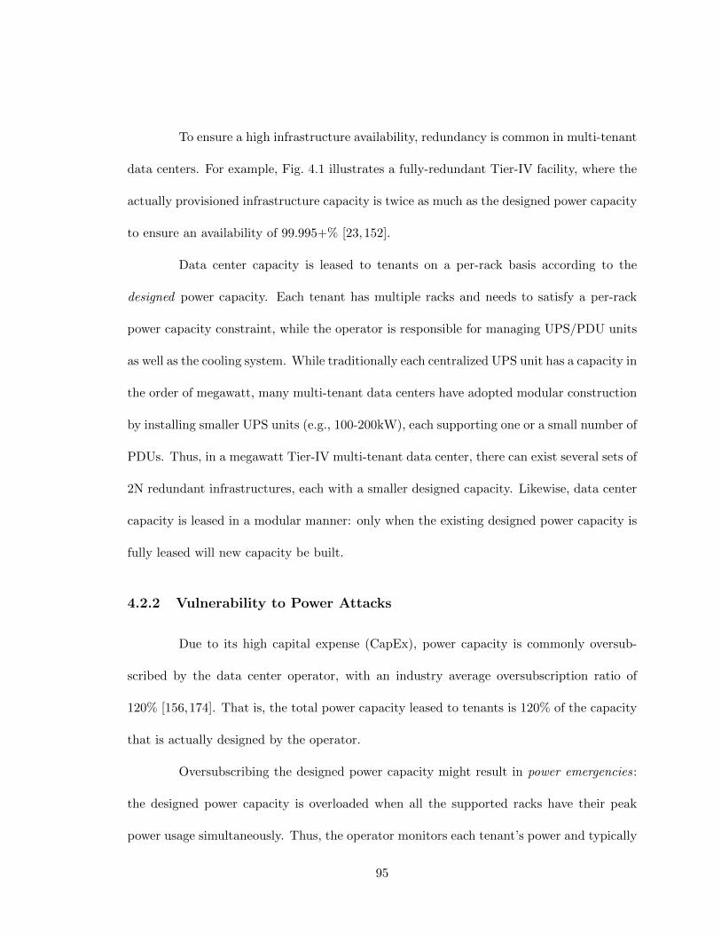
To ensure a high infrastructure availability, redundancy is common in multi-tenant

data centers. For example, Fig. 4.1 illustrates a fully-redundant Tier-IV facility, where the

actually provisioned infrastructure capacity is twice as much as the designed power capacity

to ensure an availability of 99.995+% [23,152].

Data center capacity is leased to tenants on a per-rack basis according to the

designed power capacity. Each tenant has multiple racks and needs to satisfy a per-rack

power capacity constraint, while the operator is responsible for managing UPS/PDU units

as well as the cooling system. While traditionally each centralized UPS unit has a capacity in

the order of megawatt, many multi-tenant data centers have adopted modular construction

by installing smaller UPS units (e.g., 100-200kW), each supporting one or a small number of

PDUs. Thus, in a megawatt Tier-IV multi-tenant data center, there can exist several sets of

2N redundant infrastructures, each with a smaller designed capacity. Likewise, data center

capacity is leased in a modular manner: only when the existing designed power capacity is

fully leased will new capacity be built.

4.2.2 Vulnerability to Power Attacks

Due to its high capital expense (CapEx), power capacity is commonly oversub-

scribed by the data center operator, with an industry average oversubscription ratio of

120% [156,174]. That is, the total power capacity leased to tenants is 120% of the capacity

that is actually designed by the operator.

Oversubscribing the designed power capacity might result in power emergencies:

the designed power capacity is overloaded when all the supported racks have their peak

power usage simultaneously. Thus, the operator monitors each tenant’s power and typically

95

imposes contractual terms to limit its normal usage to a fraction of the subscribed power

capacity (e.g., 80%), while only allowing occasional and temporary usage of the full capacity

[8,72]. The contractual constraint can effectively make the tenants’ aggregate power demand

stay well below the designed power capacity, thus achieving a high availability.

To illustrate this point, we show a 24-hour trace of power usage by four tenants in

Fig. 4.2(a). The total designed power capacity is 200kW, but sold as 240kW because of the

120% oversubscription.1 When all four tenants are benign, we see in Fig. 4.2(a) that power

emergencies are almost nonexistent: there is no overload for the designed power capacity in

our 24-hour snapshot. Indeed, even when a power emergency occurs due to coincident peak

power usage of benign tenants, the overload is typically transient (because of the operator’s

contractual constraint) and can be well absorbed by the power infrastructure itself [133].

In contrast, if a tenant is malicious, well-timed power attacks can successfully

create prolonged power emergencies (e.g., overloading the designed capacity for several

minutes). To see this point, we consider the same power trace as in Fig. 4.2(a), but inject

power attacks by increasing the power usage of one tenant (i.e., attacker, which subscribes

a total of 30kW power capacity) to its full capacity for 10 minutes whenever the designed

capacity can be overloaded. The aggregate power demand and attacker’s power usage

are shown in Fig. 4.2(b) and Fig. 4.2(c), respectively. In contrast to the benign case in

Fig. 4.2(a), we see that five overloads of the designed power capacity occur over a 24-hour

period in the presence of an attacker, while the attacker only uses its full power occasionally

without continuously peaking its power or violating the operator’s contract [8]. In fact, even

a benign tenant may have such usage patterns, but unlike malicious attacks, such benign

1More details of the power trace are provided in Section 4.4.1.

96

Table 4.1: Estimated impact of power emergencies (5% of the time) on a 1MW-10,000sqftdata center.

Classification SpecificationOutage

(hours/Yr)

Outagew/ Attack(hours/Yr)

IncreasedOutage Cost(mill. $/Yr)

CapitalLoss

(mill. $/Yr)

TotalCost

(mill. $/Yr)

Tier-I(Availability: 99.671%)

No redundacy 28.82465.36

(Availability: 94.688%)8.57 NA 8.57

Tier-II(Availability: 99.741%)

N+1 redundancy(generator/UPS/chiller)

22.69366.36

(Availability: 95.818%)22.11 0.1 (9+%↓) 22.22

Tier-III(Availability: 99.982%)

N+1 redundancy(all non-IT equipment)

1.5825.46

(Availability: 99.709%)11.15 1.0 (50%↓) 12.15

Tier-IV(Availability: 99.995%)

2N redundancy(all non-IT equipment)

0.446.59

(Availability: 99.925%)3.42 1.1 (50%↓) 4.52

peak power usage is not intentionally timed to create power emergencies and hence is much

less harmful than malicious attacks (see Fig. 4.18 for a comparison between malicious attacks

and random peaks).

The previous examples illustrate that the way that today’s multi-tenant data cen-

ters are managed is highly vulnerable: a malicious tenant can intentionally time its high

power usage when the demand of benign tenants is also high, thus overloading the designed

power capacity (shared by multiple tenants) much more often than otherwise would be.

4.2.3 Impact of Power Attacks

Data centers are classified into four tiers based on the degree of infrastructure

redundancy in accordance with TIA-942 standard and the Uptime Institute certification

[152, 159]. Next, we highlight that power emergencies created by malicious power attacks

are very dangerous and significantly compromise the data center availability.

Tier-I. A basic Tier-I data center has no infrastructure redundancy: the actual

provisioned capacity is the same as the designed capacity. Thus, it is cheaper to build

($10/Watt capacity), but only has an availability of 99.671% which translates into an ex-

pected outage time of 28.80 hours per year [23,155]. While power infrastructure can tolerate

97

1 1.5 2Normalized to Rated Current

100

101

102

103

104

Tri

p D

ela

y (

s)

Tripped

NotTripped

Tolerance band

Figure 4.3: Circuit breaker trip delay [133].

short-term spikes, prolonged overloads over a few minutes will alert the system and make

the circuit breakers trip in order to prevent more catastrophic consequences (e.g., fire) [133].

Fig. 4.3 shows the tripping time for a standard circuit breaker. Therefore, an overload of

the designed capacity created by a successful power attack can easily bring down a Tier-I

data center.

Tier-II/-III. A Tier-II/-III data center has “N+1” redundancy: if N primary

non-IT units are needed for the designed capacity, then 1 additional redundant unit is also

provisioned [23,155]. Thus, overloading the designed capacity may not cause a data center

outage, but will compromise the desired redundancy protection. For example, when any of

the N + 1 units fails, overloading the designed capacity will bring down the remaining N

infrastructure.

Tier-IV. A Tier-IV data center is fully 2N redundant: duplicating each needed

non-IT unit, as illustrated in Fig. 4.1 [23, 155]. The redundant infrastructure may equally

share the IT power loads with the primary infrastructure (“sharing” mode), or stand by

and take over the loads when the primary infrastructure is overloaded or fails (“standby”

98

mode) [134]. In either case, during an emergency that overloads the designed power capacity,

such redundancy protection is lost: if with an emergency, a power outage can occur when

either the primary or secondary infrastructure fails, but otherwise, it only occurs when both

the primary and secondary infrastructures fail.

We now summarize the impact of power attacks in Table 4.1, by assuming that

malicious power attacks result in emergencies (each lasting for 10 minutes) for 5% of the

time. We first show the data center availability and corresponding expected outage time

per year for each tier [23]. The outage time only includes unplanned infrastructure failures,

while other types of outages, e.g., caused by human errors and cyber/network attacks, are

excluded. While best operational practices may further improve availability, the availability

value in Table 4.1 is representative for each tier based on real-world site measurement

[23,155].

Naturally, with power attacks, the expected outage time increases due to overloads

of the designed capacity. For a Tier-1 data center, an overload of a few minutes will cause

an outage as the circuit breakers will trip to prevent more serious consequences [133]. For

a Tier-II/-III data center, we calculate the expected outage probability as “95% · (1− pa) +

5% · pf”, where pa is the availability without overloads and pf is the failure rate of the

redundant system. As redundancy increases the availability from pa,I to pa (when there

is no overload), we estimate pf = 1−pa1−pa,I , where pa,I is primary system availability (using

Tier-I availability value). For a fully-redundant Tier-IV data center, we assume that the

primary and redundant systems are completely independent [23], each having a failure rate

of√

1− pa without overloads. Thus, with emergencies occurring for 5% of the time, the

99

outage probability can be estimated as “95% · (1−pa) + 5% ·[2√

1− pa − (1− pa)]”. Then,

we show the expected outage time with attacks per year, as well as the new availability

values. A higher-tier data center is more costly to build, e.g., the capital expense for each

watt of critical power for a Tier-IV data center is twice as much as a Tier-II data center [155].

Nonetheless, due to the increased outage time exceeding the tier standard, the intended tier

classification may not apply anymore. Such tier downgrading essentially means a capital

loss for the operator (i.e., higher cost for a lower tier), which is also shown in Table 4.1

based on the power capacity cost data in [155]. It will also damage the operator’s business

image in the long term and result in a customer turnover.

In addition, power attacks also lead to increased outage costs borne by affected

tenants (compared to the no-attack case). For example, even a power outage in a single

data center can cost millions of dollars, as exemplified by the recent British Airways data

center outage [139]. Although application-level redundancy across geo-distributed data

centers may retain service continuity during outages in a single location, the workload

performance of affected tenants can be significantly degraded due to traffic re-routing and

migration [128,175]. We estimate the average outage cost per sqft per minute based on [127],

excluding service losses due to recovery after an outage. The outage costs are 0.033, 0.1073,

0.7783 and 0.93 (all in “$/sqft/min”), for Tier-I to Tier-IV data centers, respectively. The

total outage cost increase is shown in Table 4.1, which is even higher than the operator’s

amortized capital loss.

100

In conclusion, even if emergencies only occur for 5% of the time due to power

attacks, data center availability is significantly compromised, resulting in a huge financial

loss for both the operator and benign tenants.

4.3 Exploiting a Thermal Side Channel

The previous section highlighted the danger of maliciously timed power attacks

that can compromise long-term data center availability. In this section, we exploit a thermal

side channel to estimate the aggregate power usage of benign tenants and, thus, guide an

attacker to time its attacks against the shared power infrastructure.

4.3.1 Threat Model

We consider an oversubscribed multi-tenant data center where a malicious tenant,

i.e., attacker, houses physical servers and shares a designed power capacity of C with several

other benign tenants. The attacker’s servers can be divided into groups and deployed under

multiple accounts in different locations inside the target data center (to better estimate

the power consumption of nearby benign tenants as shown in Sec. 4.3.4). While it may be

possible that the attacker hides advanced weapons/bombs in its modified servers to phys-

ically damage the facility, such attacks are orthogonal to our work. Instead, we focus on

an unexplored threat model: an attacker aims to compromise the data center infrastruc-

ture availability by maliciously timing its peak power usage. That is, the attacker behaves

normally as other benign tenants, except for that it launches power attacks to create power

101

emergencies by intentionally using its full subscribed power capacity when it anticipates a

high aggregate power of benign tenants.

We consider an attack successful if “pa+pb ≥ C” is satisfied over a continuous time

window of at least L minutes (L = 5 in our default case and is enough to trip an overloaded

circuit breaker [133]), where pa is the attacker’s power and pb is the aggregate power of

benign tenants. Accordingly, we say that there is an attack opportunity if a successful

attack can be possibly launched by the attacker, regardless of whether an attack actually

occurs.

• What the attacker can do. We assume that the attacker knows the shared

power capacity (as advertised by the operator) and can subscribe to a certain amount of

capacity at a fairly low price (e.g., monthly rate of U.S.$150/kW [19]). Then, when an

attack opportunity arises, the attacker can generate malicious power loads almost instantly

by running simple CPU-intensive workloads.2 As servers are merely used to launch power

attacks, the attacker does not need to run any useful workloads and can install any low-cost

(even second-hand) high-power servers in its racks. In order to stay stealthy, the attacker

can gradually increase power and also reshape its power demand when it anticipates a power

attack opportunity, as illustrated in solid color in Fig. 4.2(c). Further, we assume that the

attacker conceals temperature sensors at its server inlets and can perform computational

fluid dynamics (CFD) analysis, which is a standard tool for modeling data center heat

recirculation and easy to use for anyone with a good knowledge of data center operation

(see Autodesk tutorial [15]).

2If some benign tenants offer web-based services open to the public, the attacker may also remotely sendmore requests to these benign tenants’ servers to increase their power consumption when it detects an attackopportunity.

102

• What the attacker cannot do. In our model, the attacker cannot hide

destructive weapons inside its servers for attacks, which may not even pass the move-in

inspection by the operator and can be held legally liable. Neither can the attacker mod-

ify its off-the-shelf servers to, for example, generate transient power spikes/pulses. These

spikes/pulses may trip the attacker’s own rack circuit breaker and/or be detected by the

operator’s power monitoring system.

Given the attacker’s access to the target data center, there may exist other attack

opportunities to bring down a data center, such as congesting the shared bandwidth, which

are complementary to our focus on attacking the shared non-IT infrastructure and compro-

mising its designed availability. Moreover, we do not consider remotely hacking the data

center infrastructures or manually tampering with the power infrastructures (all tenants’

visits to a multi-tenant data center are closely monitored and escorted). These may be

possible, but are orthogonal to our study.

•Who can be the attacker? The attacker’s cost (i.e., server cost plus data cen-

ter leasing cost) is only a small fraction of the benign tenants’ financial loss or operator’s

capital loss (between between 1.44% and 15.88%, Sec. 4.4.2), thus providing a sufficient

motivation for the attacker. For example, the attacker can be a competitor of the target

multi-tenant data center, which not only results in the victim’s capital loss but also signif-

icantly damages its business image. Note that power outages result in power cut for both

benign tenants and the attacker (which does not run useful workloads), and these are what

the attacker is aiming to create.

103

To summarize, we focus on malicious power attacks to overload the shared power

infrastructure in a multi-tenant data center and compromise its availability. Towards this

end, an attacker intentionally creates power emergencies by using its peak power when

the benign tenants’ aggregate power demand is high. Meanwhile, the attacker’s power

consumption still meets the operator’s contractual constraint.

4.3.2 The Need for a Side Channel

As illustrated in Fig. 4.2(b), attack opportunities exist intermittently due to the

fluctuation of benign tenants’ power usage. Thus, a key question is: how does the attacker

detect an attack opportunity?

Naturally, an attack opportunity arises when the aggregate power of benign tenants

is sufficiently high. But, the benign tenants’ power usage is only known to themselves and

to the data center operator (through power meters) — not to the malicious tenant.

A naive attacker may try to always use the maximum power allowed by its sub-

scribed capacity in order to capture all attack opportunities. But, this is not realistic since

the attacker may face power supply cut (due to violation of contractual terms) and be

evicted [8, 72]. Similarly, blindly or randomly launching attacks at random times is not

likely to be successful (Fig. 4.18 in Sec. 4.4.2).

Another naive strategy for the attacker would be to simply select a coarse op-

portunity window to launch attacks. For example, the attacker may choose peak hours.

Nonetheless, the multiplexing of independent tenants that run diverse workloads means

that the aggregate peak power usage can occur more randomly and outside of expected

peak hours. Alternatively, with dual power supply in a Tier-IV data center illustrated in

104

Fig. 4.1, the attacker can detect the loss of infrastructure redundancy protection when see-

ing that only one cord is supplying power (which may take several hours to correct); then,

it can launch power attacks in order to bring down the data center. But, such dual power

supply may not be available in all data centers (especially lower-tier data centers [23]).

Even though a coarse opportunity window exists (e.g., peak hours occur regularly

or failure of the secondary infrastructure is detected) and helps the attacker locate the attack

opportunities within a smaller time frame, the actual attack opportunity is intermittent

and may not last throughout the entire coarse window, as shown in Fig. 4.2(b). Thus, the

attacker needs a precise timing in order to launch successful attacks with a higher chance.

For this reason, side channels that leak (even noisy) information about the benign tenants’

power usage at runtime are crucial for the attacker.

4.3.3 A Thermal Side Channel

An important observation is that the co-residency of the attacker and benign

tenants in a shared physical space means that a thermal side channel exists. To see why,

let us look at how the cooling system works in a typical multi-tenant data center.

Cooling System Overview

A cooling system is essential for conditioning the server inlet temperature (between

65 and 81 [144]) and maintaining data center uptime [116]. Most multi-tenant data centers,

especially medium and large ones, adopt a raised-floor design and use computer room

air handlers (CRAHs) in conjunction with outdoor chillers to deliver cold air to server

105

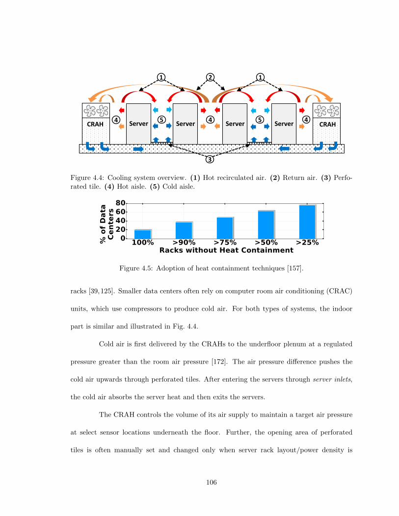
Co

ld A

isle

Ho

t A

isle

ServerCRAH CRAHServer Server Server

1 2

3

1

4 5 4 5 4

Figure 4.4: Cooling system overview. (1) Hot recirculated air. (2) Return air. (3) Perfo-rated tile. (4) Hot aisle. (5) Cold aisle.

100% >90% >75% >50% >25%Racks without Heat Containment

020406080

% o

f D

ata

Cen

ters

Figure 4.5: Adoption of heat containment techniques [157].

racks [39,125]. Smaller data centers often rely on computer room air conditioning (CRAC)

units, which use compressors to produce cold air. For both types of systems, the indoor

part is similar and illustrated in Fig. 4.4.

Cold air is first delivered by the CRAHs to the underfloor plenum at a regulated

pressure greater than the room air pressure [172]. The air pressure difference pushes the

cold air upwards through perforated tiles. After entering the servers through server inlets,

the cold air absorbs the server heat and then exits the servers.

The CRAH controls the volume of its air supply to maintain a target air pressure

at select sensor locations underneath the floor. Further, the opening area of perforated

tiles is often manually set and changed only when server rack layout/power density is

106

Sensor #2

Sensor #1

(a) Temperature distribution.

0 20 40 60 80 100Time (s)

60.0

60.5

61.0

Read

ing

(oF) Sensor #1

Sensor #2Power Spike Window

(b) Temperature trace.

Figure 4.6: CFD simulation result. (a) Temperature distribution after 10 seconds of a10-second 60kW power spike at the circled racks. (b) Temperature trace at select sensors.

changed [82,116]. As such, there is not much frequent variation in the flow rate of cold air

entering the data center room.

For delivering cold air dynamically to accommodate variable demands and im-

proving efficiency, heat containment (e.g., seal cold/hot aisles to decrease heat recircula-

tion) is needed [135]. Nonetheless, heat containment needs a high level of homogeneity in

server rack layout, and some tenants may be concerned with the potential risks (e.g., fire

safety) [108,119]. Thus, as illustrated in Fig. 4.4, many multi-tenant data centers rely on an

open airflow path to serve multiple tenants. This is also confirmed by a recent Uptime Insti-

tute survey covering 1,000+ large/medium data centers [157] which, as plotted in Fig. 4.5,

shows that nearly 80% data centers have at least 25% of racks without heat containment

and that 20% data centers do not have any heat containment at all.

In our experiment (Fig. 4.19(c)), we will investigate how different levels of heat

containment will affect the timing accuracy of power attacks.

107

Heat Recirculation

Although most hot air directly returns to the CRAHs to be cooled down, some

hot air can travel a few meters to other server racks in the shared open space and impact

their inlet air temperature [81, 95, 115]. To better illustrate this phenomenon (called heat

recirculation), we run industry-grade CFD simulations to model the data center airflow [16].

With all the servers at deep sleep states consuming nearly zero power, we generate a 10-

second 60kW power load evenly distributed among 12 server racks (marked with circles)

in Fig. 4.6(a). Ten seconds after the power spike, the data center temperature distribution

is shown in Fig. 4.6(a), where blue and red surfaces represent low and high temperatures,

respectively. It can be clearly seen that the temperature of nearby racks is affected by the

power spike. The detailed temperature changes at two select sensor locations are also shown

in Fig. 4.6(b). We also show the breakdown of temperature readings monitored at sensor

#1 in Fig. 4.7.Note that the breakdown is for demonstrating the impact of benign tenants’

power usage on the attacker’s server inlet temperature, while it is not accurately known to

the attacker in practice. We see that the benign tenants’ servers have a noticeable impact

on the attacker’s server inlet temperature, potentially leaking the benign tenants’ power

usage information to the attacker at runtime.

Heat recirculation is generally undesirable for efficiency reasons [81, 95]; our work

shows that it is undesirable for security reasons too, since it constitutes a thermal side

channel that an attacker can use to launch well-timed power attacks. Concretely, the

attacker’s server inlet temperature contains some, albeit not accurate, information of benign

108

0 3 6 9 12 15 18 21 24Time (H)

60

65

70

75

80

85S

en

sor

Read

ing

(oF)

Attacker Other Tenants Noise

Figure 4.7: Breakdown of readings at sensor #1 (Fig. 4.6(a)).

tenants’ power usage: if a server of a benign tenant consumes more power, it will result in

a higher temperature increase at the attacker’ server inlets.

4.3.4 Estimating Benign Tenants’ Power from a Thermal Side Channel

Given the impact of the benign tenants’ power usage at the attacker’s server in-

let temperature, the attacker may use this information to obtain (noisy) estimates of the

aggregate power usage and launch well-timed power attacks.

An intuitive, but naive, approach is to launch power attacks based on a tempera-

ture threshold (which we call temperature-based power attack): attack when the tempera-

ture reading is higher than a threshold. Nonetheless, temperature-based power attacks are

hardly better than launching attacks at random times.

To illustrate this point, we run CFD analysis (details in Section 4.4.1) and present

a snapshot in Fig. 4.8.In our experiment, the attacker launches a 10-minute attack whenever

its average temperature reading exceeds 76.3 for at least 1 minute, but the snapshot shows

that all attacks are unsuccessful. We further vary the temperature threshold for power

attacks and show the result in Fig. 4.9(a). As expected, with a lower temperature threshold,

109

0 2 4 6 8 10 12 14 16 18 20 22 24Time (H)

160

170

180

190

200

210P

ow

er

(kW

)TemperatureActual Power

CapAttack Opportunity

Successful AttackUnsuccessful Attack

0 2 4 6 8 10 12 14 16 18 20 22 2465

70

75

80

Tem

pera

ture

(oF)

Figure 4.8: Temperature-based power attack. All attacks are unsuccessful.

the attacker attacks more frequently (e.g., 45+% of the times given a temperature threshold

of 74) and can capture more attack opportunities, but the precision (i.e., the percentage of

successful attacks among all the launched attacks) still remains very low. In practice, the

attacker cannot use its full capacity too frequently due to contractual constraints. Thus,

for practical cases of interest (e.g., launching attacks for no more than 10% of the times),

the attacker can hardly capture any attack opportunities. We also consider power attacks

based on the maximum temperature reading, and similar results are shown in Fig. 4.9(b).

The reason temperature-based power attacks have a poor detection of attack op-

portunities is that heat recirculation is spatially non-uniform (i.e., more significant among

racks closer to each other), and hence different servers can result in drastically different

temperature impacts on the attacker’s temperature sensors. Moreover, the attacker’s own

power usage (as well as noise) also greatly impacts the temperature readings. Thus, tem-

perature does not accurately reflect the benign tenants’ aggregate power usage, motivating

us to study alternative approaches to making a better use of the prominent thermal side

channel.

110

Modeling Heat Recirculation

As heat recirculation is spatially non-uniform, the same server, if placed in different

racks, can have very different impacts on the attacker’s server inlet temperature. Thus, to

better estimate the benign tenants’ power usage, the attacker needs to further attribute its

server inlet temperature increase to different servers. Such information can be extracted by

the attacker with the help of a heat recirculation model, which relates a server’s power usage

to the inlet temperature increase at the attacker’s servers. In what follows, as proposed

in [81,151], we present a simple yet accurate linear model of heat recirculation and quantify

how an individual server’s power usage affects the attacker’s server inlet temperature.

Note that the actual heat recirculation model is unknown to the attacker; instead,

the attacker only has limited and imprecise knowledge of how heat recirculates in the data

center, which can deviate significantly from the actual process (Sec. 4.3.4 and Fig. 4.13).

But, our experiments in Sec. 4.4.2 show that even imprecise knowledge of the heat recircu-

lation model can assist the attacker time its power attacks with a high accuracy.

We consider a discrete time-slotted model, where the attacker has M sensors (in-

dexed by m = 1, 2, · · · ,M) and reads its temperature sensors once every time slot (e.g.,

every 10 seconds). There are N servers (indexed by n = 1, 2, · · · , N) owned by benign

tenants. Meanwhile, the attacker owns J servers indexed by n = N + 1, N + 2, · · · , N + J .

We denote the (average) power consumption of server n during time slot t as pn(t).

The attacker’s temperature sensor reading can be affected by a server’s power over

the previous K time slots, because it takes time for hot air generated by a server to travel

to the attacker’s server inlet (e.g., up to 100 seconds in our CFD simulations) [81]. Prior

111

74 75 76 77 78Temperature Threshold (oF)

0

10

20

30

40

50P

erc

en

tag

e (

%)

LaunchedAttacks

TruePositive

Precision

(a) Based on avg. temperature

76 77 78 79 80Temperature Threshold (oF)

0

10

20

30

40

50

Perc

en

tag

e (

%)

LaunchedAttacks

TruePositive

Precision

(b) Based on max. temperature

Figure 4.9: Summary of temperature-based power attacks. The line “Launched Attacks”represents the fraction of time power attacks are launched.

research [81, 151] has shown that, given a particular airflow pattern, the heat recirculation

process can be modeled as a finite-response linear time-invariant system whose inputs and

outputs are a server’s power usage and the temperature increase at a sensor, respectively.

Concretely, the cumulative temperature increase at sensor m caused by server n

at time t can be expressed as ∆Tm,n(t) = pn(t) ∗hm,n(t) =∑K−1

τ=0 pn(t− τ) ·hm,n(τ), where

“∗” is the convolution operator and hm,n(t) is the system impulse response function (i.e.,

hm,n(t) denotes the temperature increase at sensor m at time t if server n consumes a unit

power at time 0). Note that hm,n(t) = 0 for t < 0 (due to system causality) and t ≥ K

(since the hot air generated at a server only contributes to the sensor temperature increase

for up to K time slots).

Next, we sum up the temperature impact caused by all the servers in the data

center and express the m-th temperature sensor reading at time t as

Tm(t) = Tsup(t) +

N+J∑n=1

K−1∑τ=0

pn(t− τ) · hm,n(τ) + rm(t), (4.1)

112

where Tsup(t) is the supply air temperature and rm(t) is the noise capturing random dis-

turbances. For notational convenience we use ~pb,t = {p1(t), · · · , pN (t)} to denote the vector

of the power usage for benign tenants’ N servers at time t. We also use a column vector

xt = [~pb,t, ~pb,t−1, · · · , ~pb,t−K+1]T, where “T” denotes the transpose, to include all the benign

tenants’ power usage values over the past K time slots. Similarly, for the attacker, we

denote ~pa,t = {pN+1(t), · · · , pN+J(t)} and use yt = [~pa,t, ~pa,t−1, · · · , ~pa,t−K+1]T.

Next, we rewrite the model in (4.1) as follows

zt = Tt − Tsup(t) · I−Hayt = Hbxt + rt, (4.2)

where Tt = [T1(t), · · · , TM (t)]T is the vector of temperature readings, I = [1, 1, · · · , 1]T is an

N×1 identity vector, rt = [r1(t), · · · , rM (t)]T, and Ha and Hb are heat recirculation matrices

containing all the system impulse functions that relate server power of the attacker and the

benign tenants to the temperature increase at the attacker’s sensors, respectively. In particu-

lar, the m-th row of Ha is [hm,N+1(0), · · · , hm,N+J(0), · · · , hm,N+1(K−1), · · · , hm,N+J(K−

1)], while the m-th row of Hb is [hm,1(0), · · · , hm,N (0), · · · , hm,1(K − 1), · · · , hm,N (K − 1)].

A State-Augmented Kalman Filter

Kalman filters are a classic tool to estimate hidden states from noisy observations

in many applications, such as power grid state estimation and aircraft control [65]. Here,

we apply a Kalman filter to estimate benign tenants’ runtime power usage, which is not

directly observable but is contained in the thermal side channel.

113

Design of a Kalman filter. The observation model can be specified using the

heat recirculation model in (4.2). As the current temperature reading is affected by the

servers’ power usage over the past K time slots, we use xt = [~pb,t, ~pb,t−1, · · · , ~pb,t−K+1]T as

the augmented state. We also view zt = Tt−Tsup(t) · I−Hayt as the equivalent observation

(or measurement), because the Tsup(t) is known (e.g., by placing an additional sensor at

the perforated tile) and Hayt is the temperature increase due to the attacker’s own power

usage that is known to itself.

In addition, the attacker needs a process model to characterize the dynamics of

benign tenants’ power usage (i.e., state) over time, which is unknown to the attacker. Thus,

for simplicity, the attacker assumes that the benign tenant’s server power is driven by a

noise process, i.e., pn(t+1) = pn(t)+qn,t, where qn,t is the random noise. Thus, the process

model can be written as

xt+1 = Fxt + qt. (4.3)

In the model, qt = [q1,t, q2,t, · · · , qN,t, 0, · · · , 0] is a NK × 1 column vector with Q being

its covariance matrix, and F = [ IN×N , 0N×N(K−1); IN(K−1)×N(K−1), 0N(K−1)×N ] is a

NK ×NK matrix governing the state transition, where In×n is an n× n diagonal matrix

with 1 along the diagonal and 0 in all other entries and 0m×n is an m× n zero matrix.

The thermal side channel is then fully characterized by combining the observation

model in (4.2) and process model in (4.3). Thus, the attacker can apply a Kalman filter to

estimate xt, which includes the benign tenants’ power ~pb,t = {p1(t), · · · , pN (t)} at time t.

114

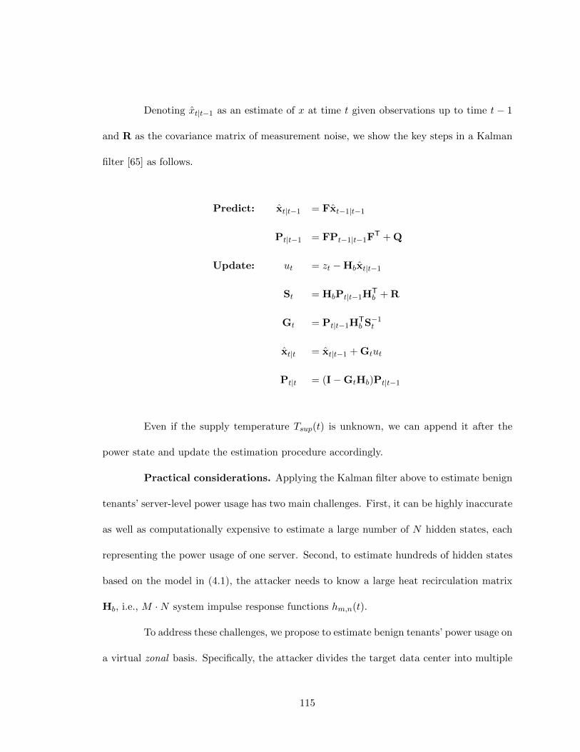
Denoting xt|t−1 as an estimate of x at time t given observations up to time t − 1

and R as the covariance matrix of measurement noise, we show the key steps in a Kalman

filter [65] as follows.

Predict: xt|t−1 = Fxt−1|t−1

Pt|t−1 = FPt−1|t−1FT + Q

Update: ut = zt −Hbxt|t−1

St = HbPt|t−1HTb + R

Gt = Pt|t−1HTb S−1

t

xt|t = xt|t−1 + Gtut

Pt|t = (I−GtHb)Pt|t−1

Even if the supply temperature Tsup(t) is unknown, we can append it after the

power state and update the estimation procedure accordingly.

Practical considerations. Applying the Kalman filter above to estimate benign

tenants’ server-level power usage has two main challenges. First, it can be highly inaccurate

as well as computationally expensive to estimate a large number of N hidden states, each

representing the power usage of one server. Second, to estimate hundreds of hidden states

based on the model in (4.1), the attacker needs to know a large heat recirculation matrix

Hb, i.e., M ·N system impulse response functions hm,n(t).

To address these challenges, we propose to estimate benign tenants’ power usage on

a virtual zonal basis. Specifically, the attacker divides the target data center into multiple

115

virtual zones (each containing one or more tenants) and estimates the power for each zone of

racks as a single entity, rather than for each individual server. In fact, estimating zone-level

power usage already suffices, because the attacker only needs to know the aggregate power

usage of benign tenants.

To construct the zone-level heat recirculation matrix, the attacker can visit the

data center (as any tenant can) and visually inspect its layout. Then, following the indus-

try practice and as described in Section 4.4.1, the attacker can perform CFD analysis to

construct a zone-level heat recirculation model with the assumption that all the servers in

one zone yield the same temperature increase impact on the attacker’s sensors.

Naturally, the zone-level heat recirculation model only approximates the detailed

server-level model (4.1), and the attacker cannot exactly know the data center layout from

a visual inspection. Thus, the attacker only has an estimate of the actual heat recirculation

model. Despite this limitation, we show in Section 4.4.2 that the attacker can still estimate

the benign tenants’ aggregate power usage with high accuracy (e.g., only 3% error on

average), capturing 54% of the attack opportunities.

4.3.5 Attack Strategy

In a typical multi-tenant data center, a tenant is allowed to use power up to α ·Ct

continuously, where Ct is the power capacity subscribed by the tenant and α < 1 is the

threshold (usually 80%) set by the operator [8,72]. A tenant can also use its full capacity Ct

occasionally, but continuously using it can result in an involuntary power cut and eviction.

We now discuss how the attacker can make use of the estimation procedure above in order

to time its attacks while meeting the operator’s contractual constraint.

116

Idle Wait𝑇𝑤𝑎𝑖𝑡 starts

Attack𝑇𝑎𝑡𝑡𝑎𝑐𝑘 starts

Hold𝑇ℎ𝑜𝑙𝑑 starts

2

12

→ 𝑃𝑒𝑠𝑡 ≤ 𝑃𝑡ℎ

→ 𝑃𝑒𝑠𝑡> 𝑃𝑡ℎ

→ 𝑇𝑤𝑎𝑖𝑡 expires

→ 𝑇𝑎𝑡𝑡𝑎𝑐𝑘 expires

→ 𝑇ℎ𝑜𝑙𝑑 expires

1

2

3

4

5

3

4

5

Figure 4.10: Finite state machine of our attack strategy. Pest is the attacker’s estimatedaggregate power demand (including its own), and Pth is the attack triggering threshold.

We consider a simple strategy where the attacker keeps on using its maximum

power for a fixed time of Tattack, when it anticipates a high aggregate power usage of

Pest ≥ Pth (called triggering threshold). The triggering threshold Pth is an important choice

parameter for the attacker: the smaller Pth, the more attacks. Before launching an attack,

the attacker should wait for its estimate of benign tenants’ usage to stay high for some time

Twait, in order to reduce unsuccessful attacks when the estimate of benign tenants’ power

is only transiently high. Depending on the operator’s contractual constraint, we also set a

hold time of Thold before the attacker launches its next attack and impose a constraint on

its triggering threshold Pth ≥ Pth. In our experiments (Sec. 4.4.2), we will vary how long

and how frequently the attacker is allowed to fully use its subscribed capacity.

We illustrate our attack strategy using a finite state machine in Fig. 4.10. More

advanced strategies are left as future work, as the current one is already quite effective.

117

4.4 Experimental Evaluation

To demonstrate the danger of power attacks by malicious tenants, we evaluate

how well the attacker can detect attack opportunities based on the thermal side channel.

Our experimental results highlight that, with the aid of a Kalman filter and by launching

attacks no more than 10% of the time, the attacker can successfully detect 54% of all attack

opportunities (i.e., true positive rate) with a precision of 53%.

Although these values may vary depending on the specific settings, our results offer

an important support to the broad implication: the attacker can extract useful information

about benign tenants’ runtime power usage from the thermal side channel and launch well-

timed successful power attacks against the power infrastructure.

4.4.1 Methodology

Because of the destructive nature of power attacks and the practical difficulty in

accessing mission-critical data center facilities, we use an industry-grade simulator, Au-

todesk CFD [16], to perform CFD analysis and simulate heat recirculations driven by a

real-world workload trace. The accuracy of CFD analysis has been well validated [81,151],

and many data centers, including Google [54], use CFD analysis to predict temperature

distributions [81,151,172]. Thus, before any demonstration in industrial multi-tenant data

centers is planned, the CFD-based simulation provides us with an important understanding

of the possibility and danger of power attacks timed through a thermal side channel. Our

default settings are described below.

118

CRAH

Server Racks

CRAH

CRAH

CRAH

PerforatedTiles

Virtual Zone 3Virtual Zone 2

Virtual Zone 1Attacker

Figure 4.11: Data center layout.

Data center layout. We consider a modular infrastructure design where a large

data center is constructed using multiple independent sets of non-IT infrastructures, each

having a smaller designed capacity. Specifically, the total designed capacity under consider-

ation is 200kW and, according to the industry average [156], oversubscribed by 120%. We

follow the design by HP Labs [172] and show the indoor part of our considered data center

space in Fig. 4.11.To get an idea of the heat recirculation process, the attacker divides the

shared data center space into four different virtual zones (three for benign tenants and one

for the attacker), while we note that the attacker’s zone division is not unique. Zones 1 and

2 have 12 server racks each. Zone 3 has 18 server racks, while the attacker occupies the 4th

zone with 6 racks. Each rack has 20 servers and a power capacity of 5kW. There are four

CRAH units that supply cold air to servers through perforated tiles.

119

CFD analysis. We port our data center layout shown in Fig. 4.11 into Autodesk

CFD to quantify the heat recirculation process [16]. The physical components, such as

servers, racks, raised floor and CRAH, are designed in Autodesk Inventor based on its data

center simulation guideline [15]. Nonetheless, as CFD is computationally prohibitive, it can-

not be used for simulations with month-long power traces. Thus, to calculate the attacker’s

temperature, we follow the literature [81, 151] and use the server-level heat recirculation

model in (4.1), where the system impulse response function hmn(t) is derived by generating

a power spike over one time slot (10 seconds) for server n and getting the temperature at

sensor m through the CFD analysis on Autodesk. This process is repeated for all the servers

and sensors. The accuracy of the linear model in (4.1) has been extensively validated against

real system implementations [81, 95, 151, 172]. Thus, the model has been widely applied to

guide temperature-constrained runtime resource management [81, 95, 151]. Here, we use it

for a new purpose — assisting the attacker with timing its power attacks.

Power trace. We collect a representative composition of four different power

traces for the four virtual zones (Fig. 4.11), following the practice of prior studies [75, 93].

Specifically, two power traces are collected from Facebook and Baidu production clusters

[169,174] and used for virtual zones 1 and 2, respectively. We also collect two request-level

batch workload traces (SHARCNET and RICC logs) from [43,124], and, based on the power

model validated against real systems [42], convert them into the power usage of the third

virtual zone and the attacker. All the power usage are scaled to have an average utilization

of 75% (for the 3 virtual zones) and 60% (for the attacker), normalized with respect to the

120

tenant’s subscribed capacity. Fig. 4.15 shows a 24-hour snapshot of the synthetic aggregate

power trace, which has a consistent pattern with real measurements [169,174].

Attacker. The attacker has 6 racks in one row as illustrated in Fig. 4.11. It

has six sensors placed evenly along the top of its six racks, and reads the sensors once

every 10 seconds (one time slot). The attacker’s sensor noise includes two parts: random

disturbance/random noise following a Gaussian distribution N (0, 0.5) with a unit of , and

additional noise modeled as a variable that has a mean of 0.5 and scales proportionally

with the power trace in [169] (capturing the impact of servers that are served by other

infrastructures but housed in the same room). Following the strategy in Sec. 4.3.5, after

detecting an attack opportunity and waiting for Twait = 1 minute, the attacker increases

its power to the full capacity for Tattack = 10 minutes. By default, the attacker does not

attack consecutively or more than 10% of the time each day, and sets Thold = 10 minutes.

Note that if available, a coarse timing (e.g., daily peak hours, see Sec. 5.3.2) may

help the attacker focus on a narrower time frame for attacks, but it is still inadequate due

to the short duration of intermittent attack opportunities. In contrast, we focus on fine-

grained precise timing by exploiting a thermal side channel, on top of the complementary

coarse timing.

4.4.2 Evaluation Results

Our evaluation results highlight that our proposed Kalman filter can extract rea-

sonably accurate information about benign tenants’ power usage and guide the attacker to

launch successful attacks.

121

0

0.005

1001

oF

/kW

80

0.01

Time (s)

Zones

60240

3 200

Figure 4.12: The attacker’s heat recirculation model: zone-wise temperature increase atsensor #1 (Fig. 4.6(a)).

0s 10s 20s 30s 40s 50s 60s 70s 80s 90s 100s

-75%-50%-25%0%25%50%75%

Figure 4.13: Error in the attacker’s knowledge of heat recirculation matrix Hb, normalizedto the true value.

Kalman Filter Performance

The attacker constructs a zone-level heat recirculation matrix for its Kalman filter

(Section 4.3.4) and hence, only has an inaccurate knowledge of the actual heat recirculation

matrix Hb in (4.2). Given this limitation, let us first examine the Kalman filter performance.

In our experiment, we consider three zones for the benign tenants as illustrated in

Fig. 5.11. We show the attacker’s estimate of zone-based temperature increase impact at

one of its sensors in Fig. 4.12. Further, we show in Fig. 4.13 the attacker’s error normalized

with respect to the true heat recirculation matrix Hb, i.e., the values ofhm,n(t)−hm,n(t)

hm,n(t) ,

122

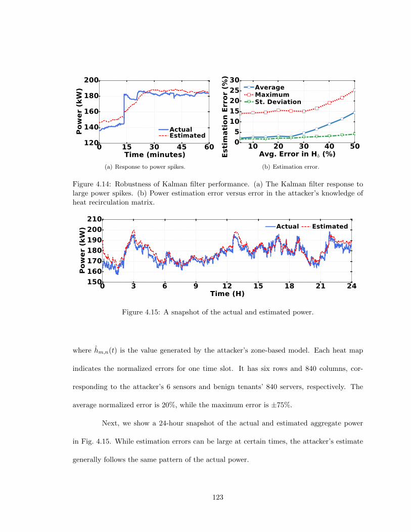
0 15 30 45 60Time (minutes)

120

140

160

180

200P

ow

er

(kW

)

ActualEstimated

(a) Response to power spikes.

10 20 30 40 50Avg. Error in Hb (%)

0

5

10

15

20

25

30

Esti

mati

on

Err

or

(%)

AverageMaximumSt. Deviation

(b) Estimation error.

Figure 4.14: Robustness of Kalman filter performance. (a) The Kalman filter response tolarge power spikes. (b) Power estimation error versus error in the attacker’s knowledge ofheat recirculation matrix.

0 3 6 9 12 15 18 21 24Time (H)

150

160

170

180

190

200

210

Pow

er

(kW

) Actual Estimated

Figure 4.15: A snapshot of the actual and estimated power.

where hm,n(t) is the value generated by the attacker’s zone-based model. Each heat map

indicates the normalized errors for one time slot. It has six rows and 840 columns, cor-

responding to the attacker’s 6 sensors and benign tenants’ 840 servers, respectively. The

average normalized error is 20%, while the maximum error is ±75%.

Next, we show a 24-hour snapshot of the actual and estimated aggregate power

in Fig. 4.15. While estimation errors can be large at certain times, the attacker’s estimate

generally follows the same pattern of the actual power.

123

We now examine the Kalman filter robustness. The process model (4.3) assumes

that the benign tenants’ power is driven by a noise, but this may not hold in practice.

Thus, we create an artificial large power spike (unlikely in practice) and see how the filter

responds. It can be observed from Fig. 4.14(a) that the filter can fairly quickly detect the

sudden power spike (within 15 minutes) and then produce good estimates again. Next, we

investigate the filter performance by varying the average error in the attacker’s knowledge

of the actual heat recirculation matrix. Specifically, we scale the errors in our default case

(20% average error, as shown in Fig. 4.13) and show the average error, maximum error,

and standard deviation in the attacker’s power estimation in Fig. 4.14(b). We see that if

the attacker’s assumed heat recirculation matrix does not deviate too much from the actual

one, its power estimation is quite accurate (e.g., only 5% average power estimation error,

given 30% average error in the attacker’s knowledge of Hb). The low estimation error is

partly because the benign tenants’ power has a large fixed portion, while the attacker only

needs to detect temporal variations for timing attacks.

To conclude, despite the attacker’s imperfect observation and process models, the

Kalman filter can estimate the benign tenants’ power at runtime reasonably well.

Power Attacks

Next, we present our experimental result on how well the Kalman filter can help

the attacker time its attacks.

True positive and precision rates. As the attacker cannot launch attacks too

frequently (no more than 10% of the time in our default case), true positive and precision

124

97 99 101 103 105Triggering Threshold (% Capacity)

0

10

20

30%

of

Tim

eAttack OpportunitySuccessful AttacksUnsuccessful Attacks

(a) Frequency of attacks.

97 99 101 103 105Triggering Threshold (% Capacity)

0

20

40

60

80

100

Perc

en

tag

e (

%)

True PositivePrecision

(b) True positive and precision rates.

Figure 4.16: (a) Frequency of power attacks versus the attack triggering threshold. (b) Truepositive and precision rates versus the attack triggering threshold.

rates are important metrics to consider. True positive rate is defined as the percentage

of available attack opportunities captured by the attacker, while precision is the percentage

of successful attacks among all the launched attacks. By default, we consider an attack

successful if the designed power capacity is overloaded for at least 5 minutes.

We first show the frequency of power attacks in Fig. 4.16(a) by varying the at-

tacker’s triggering threshold. When the attacker sets a lower triggering threshold, it will

attack more frequently, detecting more attack opportunities and meanwhile launching more

unsuccessful attacks. Thus, as shown in Fig. 4.16(b), this results in a higher true positive

rate but a lower precision rate. To keep the power attacks under 10% of the total time,

the attacker can set its triggering threshold at 101% of the designed capacity shared with

benign tenants, resulting in a true positive rate of 54% and precision rate of 53%. This

represents a significant improvement, compared to the temperature-based attack that only

captures 3.9% of the attack opportunities with a precision of 2.1% (Fig. 4.9(a)).

125

0 15 30 45Attack Time (min)

0

20

40

60

80

100P

erc

en

tag

e (

%) True Positive

Precision

(a) Successful attacks.

0 15 30 45Hold Time (min)

0

20

40

60

80

100

Perc

en

tag

e (

%) True Positive

Precision

(b) Successful attacks.

Figure 4.17: Attack success rates for different timer values.

Impact of Tattack and Thold values. The operator’s power contracts vary by

data centers, and thus the attacker can adjust its attack strategy parameters (Sec. 4.3.5).

Here, we study the effect of varying Tattack and Thold on the attack success rates in Fig. 4.17.

Specifically, we vary one value while keeping the other as default, and set the triggering

threshold to launch attacks for no more than 10% of the time. With an increased Tattack,

the attacker will peak its power for a longer time and intuitively should yield better attack

success rates. This holds for Tattack ≤ 25 minutes. However, the true positive and precision

rates may decrease as Tattack continuously increases, because the attacker may keep on

attacking even though the attack opportunity is gone. On the other hand, with an increased

Thold, the attacker will wait longer before re-launching an attack, even though an attack

opportunity may appear sooner. Hence, we see in Fig. 4.17(b) that the attack success rates

decrease as Thold increases.

Comparison with random attacks. Without a (thermal) side channel, the at-

tacker may launch random attacks, possibly within a narrower time frame if coarse timing

is available (Sec. 5.3.2). Random attacks can also capture a benign tenant which uninten-

126

0 5 10 15 20 25 30Attack (% Time)

0

20

40

60

80

100Tru

e P

osit

ive (

%)

Random AttackTimed Attack

(a) Successful attacks.

0 5 10 15 20 25 30Attack (% Time)

0

20

40

60

80

100

Pre

cis

ion

(%

) Random AttackTimed Attack

(b) Successful attacks.

Figure 4.18: Comparison with random attacks.

tionally peaks its power usage. We now compare our timed attack with random attack

on a yearly trace in Fig. 4.18. Intuitively, randomly attacking for X% of the time should

capture X% of the available attack opportunities, with a fixed precision rate that is the

same as the probability of attack opportunities. This can be seen from Fig. 4.18, where the

small disturbances are due to empirical evaluations. Nonetheless, our timed attack signifi-

cantly outperforms random attacks, especially for limited attacking time less than 10% of

the time. This highlights the necessity of a (thermal) side channel as well as the danger of

maliciously timed power attacks. Note that after an initial increase, the true positive rate of

our timed attacks remains saturated even when the attacker attacks more frequently (which

also means a lower precision rate). This is because the total available attack opportunities

are the same and some of them can span a relatively longer (e.g., 20 minutes), but we do

not allow the attacker to attack consecutively (Sec. 4.3.5).

Impact of the attacker size. Naturally, a larger attacker with a higher capac-

ity subscription can launch more successful attacks and make the power infrastructure less

127

5 10 15 20 25Attacker's Size (% of Sold Capacity)

0

20

40

60

80

100P

erc

en

tag

e (

%)

Attack OpportunityTrue PositivePrecision

(a) Frequency of attacks.

5 10 15 20 25Attacker's Size (% of Sold Capacity)

0

2

4

6

8

10

12

Tota

l C

ost

(mill.

$)

Tier-II Data CenterTier-III Data CenterTier-IV Data Center

(b) Cost impact of attack.

None Zone-1 Zones-1&2 AllHeat Containment

0

20

40

60

Perc

en

tag

e (

%)

True PositivePrecision

(c) Impact of heat containment

Figure 4.19: (a) Statistics of attack opportunity and attack success. (b) Expected annualloss due to power attacks incurred by the data center operator and affected tenants (200kWdesigned capacity oversubscribed by 120%). (c) Even with heat containment, the thermalside channel can still assist the attacker with timing power attacks.

reliable. In Fig. 4.19(a), we show the impact of attacker size on the available attack oppor-

tunities and its attack success rates. We keep the benign tenants’ total capacity fixed and

scale up the attacker’s capacity to the different percentages of total subscribed capacity. We

also keep the total attacking time at the default 10%. Naturally, the number of attack op-

portunities increases with the attacker size, as the attacker can create higher power spikes.

We also see that as the attacker has more servers, the true positive rate can go down while

the precision increases. This is because, although there are more attack opportunities, the

total attacking time remains the same, thus possibly resulting in a lower true positive rate.

At the same time, as there are more opportunities, the precision rate goes up.

128

Next, in Fig 4.19(b), we show the annual cost impact (following Sec. 4.2.3) with

varying sizes of the attacker. The attacker needs to pay more as rent when its subscribed

capacity is larger, with an annual cost of $48.8k at 5% size up to $308.9k at 25% size

(assuming a capacity leasing cost of $150/kW/month, energy cost of 10 cents/kWh, and

server cost of $1500 per 250W server amortized over 3 years). But these costs are just a

fraction (varying between 1.44% and 15.88% depending on the attacker size and data center

tier) of the total cost borne by the operator and affected tenants due to the compromised

data center availability. On the other hand, a larger attacker can create more emergencies

and cause more damages to the data center. We see that, by spending in the order of 100

thousand dollars per year, the attacker can cost the target data center an annual loss in the

order of millions of dollars.

Impact of heat containment. While full heat containment is rare in multi-

tenant data centers, it may be partially implemented (see Fig. 4.5). Here, we study the im-

pact of different degrees of heat containment on the timing accuracy of attacks. We consider

three different cases, where one, two and three zones have heat containment, respectively.

As heat containment can reduce, but not completely eliminate, heat recirculation [125], we

consider that the corresponding heat recirculation impact is reduced by 90% when a zone

has heat containment. We see in Fig. 4.19(c) that heat containment reduces both the true

positive rate and precision. Nonetheless, this is still higher than random attacks.

Illustration of different attack scenarios. Finally, we show a snapshot of the

power attack trace in Fig. 4.20 to illustrate what would happen had attacks been launched

based on the strategy described in Sec. 4.3.5. We see some successful attacks that can

129

0 2 4 6 8 10 12 14 16 18 20 22 24Time (H)

160170180190200210220

Pow

er

(kW

) 1 22 1 2 111 2

ActualEstimated

CapacityAttack Opportunity

Successful Attack (1)Unsuccessful Attack (2)

Figure 4.20: Illustration of different attack scenarios.

create prolonged overloads of the shared capacity. Note that an actual outage may not

always occur after a capacity overload due to infrastructure redundancy, but if it does

occur, the power trace will differ after the outage incident. There are also unsuccessful

attacks in Fig. 4.20 due to overestimates of the benign tenants’ aggregate power demand,

which fails to overload the designed capacity. In addition, there are missed opportunities

around the 19-th hour.

4.5 Defense Strategy

Given the danger of power attacks, a natural question follows: how can a multi-

tenant data center operator better secure its power infrastructure against power attacks? In

this section, we discuss a few possible defense strategies.

4.5.1 Degrading Thermal Side Channel

Since the thermal side channel resulting from heat recirculation is instrumental to

time power attacks, the first natural defense strategy would be degrading the side channel.

This can make the attacker estimate the benign tenants’ power usage with more errors,

130

Cold

Ai

sle

Hot

Aisl

e

Server Server Server Server60F 60F

Random Supply Air Temperature

Random Airflow with Adaptive Vent Tiles

Cold Aisle Containment Reducing Recirculation

Figure 4.21: Degrading the thermal side channel.

thus misguiding the attacker’s power attacks. Towards this end, the data center can either

randomize the cooling system set point or reduce heat recirculation through heat contain-

ment.

Randomizing supply air temperature. Supply air temperature Tsup(t) is an

important parameter for the attacker’s observation model in (4.2), and its randomization

might confuse the attacker. However, the attacker can easily set Tsup(t) as a new state

to estimate along with the states of benign tenants’ power consumption in the Kalman

filter, and estimate it fairly accurately. Thus, randomizing Tsup(t) does not offer a good

protection against power attacks. Further, it can decrease the cooling efficiency (due to,

e.g., unnecessarily low temperature settings).

Randomizing supply airflow. Another approach is to make the actual heat

recirculation process more uncertain to the attacker. In particular, randomizing the supply

airflow can make the attacker’s knowledge of the heat recirculation matrix more erroneous.

This requires the data center operator install adaptive vent tiles and carefully adjust their

opening without server overheating, incurring a high control complexity [172]. Moreover, as

131

the attacker only needs to know the benign tenants’ aggregate power rather than individual

power, the Kalman filter performance is still reasonably good in the presence of supply

airflow randomization, making this strategy only moderately effective.

Heat Containment. While container-based design (e.g., enclosing tenants’ servers

in a shipping container) can isolate thermal recirculation across tenants [129], it is costly to

implement and rarely used in multi-tenant data centers [148]. Instead, the data center oper-

ator typically decreases heat recirculation by sealing the cold or hot aisles [40,116]. Cold/hot

aisle containment has a reasonably low capital expense but, due to tenants’ heterogeneous

racks, only has limited adoption in multi-tenant data centers (especially existing ones) as

shown in Fig. 4.5 [157]. Nonetheless, once heat containment is successfully installed, only

very little hot air can recirculate and there is no control needed at runtime. Thus, heat

containment can be effective with a low capital expense.

We illustrate the aforementioned defense strategies in Fig. 4.21. We also quan-

tify the effectiveness of different defense strategies by investigating their impacts on the

attacker’s true positive and precision rates of successful attacks. The results are shown in

Fig. 4.22, where “Baseline” is the current status quo without our discussed defenses. For

all the defenses, the attacker uses the same attack strategy as discussed in Section 4.3.5.

We see that heat containment is the most effective strategy, while randomizing the supply

air temperature has little effect in preventing power attacks. In particular, with 99% heat

containment (i.e., only 1% hot air recirculates), the attacker’s timing accuracy through the

thermal side channel is only marginally better than random attacks.

132

BaselineRandom

Supply Temp. Random

Airflow (Low) Random

Airflow (High)

90% Heat

Containment99% Heat

Containment

0

20

40

60

Perc

en

tag

e (

%)

True Positive Precision

Figure 4.22: True positive and precision rates of different defense strategies. “Low”/“high”indicates the amount of randomness in supply airflows. “x%” heat containment means x%of the hot air now returns to the CRAH unit directly.

We recommend heat containment as the “best” defense strategy due to its high

effectiveness, low cost and zero management at runtime. Thus, besides efficiency [116],

securing the power infrastructure against power attacks now becomes another compelling

reason for multi-tenant data centers to adopt heat containment.

4.5.2 Other Countermeasures

There also exist other countermeasures to secure a multi-tenant data center against

power attacks. A straightforward approach is to not oversubscribe the power infrastructure,

thus eliminating the vulnerabilities and attack opportunities. But, this comes at a signif-

icant revenue loss for multi-tenant data center operators and installing extra capacity can

be particularly challenging in existing data centers. Another approach is to increase the

level of redundancy. Nonetheless, the attacker can still compromise the long-term designed

availability, which essentially translates into a capital loss for the operator (Table 4.1).

It is also important to detect the malicious attacker as early as possible and then

evict it. While the power usage illustrated in Fig. 4.2(c) does not violate the operator’s

contract and can be a benign tenant’s power pattern, continuously having such a usage

133

pattern may be suspicious. Concretely, the operator may pay special attention to the high

aggregate power periods and closely monitor which tenant has the highest contribution to

those periods.

Finally, the operator can take other measures or implement a combination of the

above strategies to secure its infrastructure against power attacks. This is an interesting

research direction for our future study.

4.6 Related Work

Power oversubscription is economically compelling but can result in occasional

emergencies that require power capping to handle [42]. For example, well-known power

capping techniques include throttling CPU frequencies [95, 174], reducing workloads [169],

among others. Unfortunately, these approaches cannot be applied by a multi-tenant data

center operator due to the operator’s lack of control over tenants’ servers.

There have been many studies on making the cyber part of a data center more

secure. For example, defending data center networks against DDoS attacks [111, 181] and

protecting user privacy against side channel attacks [61, 84, 114, 187] have both received

much attention.

In parallel, data center physical security has been gaining attention quickly in

recent years. For example, [150] studies defending servers against human intrusion and

attacks. More recently, [93, 180] attempt to intentionally create power emergencies in an

owner-operated data center through VMs. Nonetheless, malicious VM workloads may not

134

all be placed together to create high and prolonged spikes, and the operator can use server

power and VM placement control knobs in place to safeguard the power infrastructure [114].

In contrast, we consider a multi-tenant data center where a malicious tenant can

subscribe enough power capacity to create extended and severe power emergencies. Further,

the data center operator has no control of tenants’ servers and thus, cannot apply power

capping to mitigate power attacks. More importantly, unlike [48, 93, 180], we exploit a

co-residency thermal side channel resulting from the unique heat recirculation to launch

well -timed power attacks. Thus, our work represents the first effort to defend multi-tenant

power infrastructures against power attacks.

Our work also makes contributions to the literature on multi-tenant data center

power management. Concretely, the existing studies have all been efficiency-driven, such as

reducing energy costs [73], increasing power utilization [75] and minimizing social cost for

demand response [21]. In contrast, our work focuses on the power infrastructure security, a

neglected but very important issue in multi-tenant data centers.

Finally, we discuss if the attacker can alternatively exploit other side channels. In

general, when workload increases, the server power also increases and so does the latency

[17]. Thus, request response time might be a cyber side channel: a higher response time

might indicate that the tenant is having a higher workload and hence, power usage, too.

Nonetheless, many tenants do not even have any services open to the public [17,30]. Thus,

the measured response time contains little, if any, information about the aggregate power

usage of multiple benign tenants. Further, the attacker might infer the benign tenants’

power usage based on its detected voltage/current changes. However, a multi-tenant data

135

center delivers highly conditioned power to tenants’ servers, and the internal wiring topology

(e.g., Fig. 4.1) may not be known to the attacker. In any case, we make the first effort to

study power attacks in multi-tenant data centers by exploiting a thermal side channel, which

can complement other side channels (if any) and assist the attacker with timing its attacks

more accurately.

4.7 Concluding Remarks

In this paper, we study a new attack — maliciously timing peak power usage

to create emergencies and compromise the availability of a multi-tenant data center. We

demonstrate that an oversubscribed multi-tenant data center is highly vulnerable to mali-

ciously timed high power loads. We identify a thermal side channel due to heat recirculation

that contains information about the benign tenants’ power usage and design a Kalman filter

guiding the attacker to precisely time its attacks for creating power emergencies. Our exper-

iments show that the attacker can capture 54% of all attack opportunities with a precision

rate of 53%, highlighting a high success rate and danger of well-timed power attacks.

136

Chapter 5

Timing Power Attacks in

Multi-tenant Data Centers Using

an Acoustic Side Channel

5.1 Introduction

The exploding demand for cloud services and ubiquitous computing at the Inter-

net edge has spurred a significant growth of multi-tenant data centers (also referred to as

“colocation”). The U.S. alone has nearly 2,000 multi-tenant data centers, which are expe-

riencing a double-digit annual growth rate and account for about 40% of all data center

energy consumption [3,73,120]. Unlike a multi-tenant cloud platform where users rent vir-

tual machines (VMs) on shared servers owned by the cloud provider, a multi-tenant data

center offers shared non-IT infrastructures (e.g., power and cooling) for multiple tenants to

137

house their own physical servers. It serves as a cost-effective data center solution to almost

all industry sectors, including large IT companies (e.g., 25% of Apple’s servers are housed

in multi-tenant data centers [14]).

Naturally, it is extremely important to provide a highly reliable power supply to

tenants’ servers in a multi-tenant data center. To accomplish this, data center operators

have typically employed backup power and infrastructure redundancy (e.g., duplicating

each power supply equipment, or 2N redundancy, as illustrated in Fig. 5.1), safeguarding

multi-tenant data centers against random power equipment faults and utility power out-

ages. For example, power availability in a multi-tenant data center with state-of-the-art 2N

redundancy can exceed 99.995% [23,152,155].

The high availability of data center power infrastructures comes at a huge cost: the

capital expense (CapEx) is around U.S.$10-25 for delivering each watt of power capacity to

the IT equipment, taking up 60+% of a data center operator’s total cost of ownership over

a 10-year lifespan [58,75,126,174]. Thus, in order to reduce and/or defer the need for infras-

tructure expansion, a common technique is power oversubscription: similarly as in other

industries (e.g., airline), a multi-tenant data center operator sells its available data center

infrastructure capacity to more tenants than can be supported. The rationale of power

oversubscription is that different tenants typically do not have peak power consumption at

the same time. The current industry average is to have a 120% oversubscription (yielding

20% extra revenue without constructing new capacities) [66, 156]. Moreover, power over-

subscription is also commonly found in owner-operated data centers (e.g., Facebook [174]),

and more aggressive oversubscription [56,93] has been advocated.

138

Despite the compelling economic benefit, power oversubscription is not risk-free

and can potentially create dangerous situations. Concretely, although generally uncom-

mon, tenants’ aggregate power demand can exceed the design power capacity (a.k.a. power

emergency) when their power consumption peaks simultaneously. Power emergencies com-

promise infrastructure redundancy protection (illustrated in Fig. 5.1) and can increase the

outage risk by 280+ times compared to a fully-redundant case [23]. Moreover, data center

power infrastructures are not as reliable as desired. In fact, compared to cyber attacks,

power equipment failures are even more common reasons for data center outages, for which

overloading the design power capacity is a primary root cause [34, 127]. For example, de-

spite backup power equipment and redundancy, a power outage recently occurred in British

Airways’s data center and cost over U.S.$100 million [139].

As a consequence, the significant outage risk associated with power emergencies

has prompted active precautions. Concretely, due to the lack of control over tenants’ servers,

a multi-tenant data center operator typically restricts tenants’ “normal” power usage to be

below a fraction (usually 80%) of their subscribed capacities as stipulated by contractual

terms. That is, tenants may only use their full subscribed capacities in limited occasions,

and non-compliant tenants may face power cuts and/or eviction [8, 72]. Thus, this can

effectively eliminate most, if not all, severe power emergencies, thus achieving the designed

availability.

While power oversubscription has been regarded as safe due to safeguard mecha-

nisms, recent studies [76,77,93,180] have demonstrated an emerging threat — power attacks,

i.e., malicious power loads that aim at overloading the shared capacity — which could cre-

139

ate frequent power emergencies and compromise data center availability. Although there

are only limited attack opportunities as illustrated in Fig. 5.2, the impact of power attacks

is devastating. As shown in Table 5.2, even if power attacks can create power emergencies

for only 3.5% of the time, multi-million-dollar losses are incurred by both the operator and

affected tenants.

In a multi-tenant data center, a malicious tenant (i.e., attacker) must precisely

time its peak power usage in order to create successful power attacks without violating

the operator’s contract: the attacker only uses its full subscribed capacity when the power

demand of other benign tenants’ is high. In the existing research [76], such precise timing

is achieved through the help of a thermal side channel resulting from heat recirculation —

benign tenants’ server heat, which can recirculate to the attacker’s temperature sensors,

is a good indicator of their power usage. Nonetheless, exploiting the thermal side channel

has several key limitations. First, heat containment techniques are increasingly common

in modern data centers to improve cooling efficiency and thus can effectively mitigate, or

even eliminate, the thermal side channel. Second, in order to time its power attacks, the

attacker must be able to construct a data center heat recirculation model, which can deviate

significantly from the actual environment and lower the timing accuracy. Last but not least,

it may take a long time (> 1 minute) for the heat generated by distant servers to affect

the attacker’s temperature sensor, rendering the estimation possibly outdated. All these

factors would contribute to the limited applicability of the thermal side channel in practice.

Contributions of this paper. This paper focuses on the emerging threat of

power attacks in multi-tenant data centers and exploits a novel side channel — acoustic

140

side channel resulting from servers’ noise generated by cooling fans — which assists an

attacker with timing its power attacks. Concretely, the key idea we exploit is that the

energy of noise generated by a server’s cooling fans increases with its fan speed measured in

revolutions per minute (RPM), which is well correlated with the server power (Section 5.4.1).

Thus, through measurement of the received noise energy using microphones, an attacker

can possibly infer the benign tenants’ power usage and launch well-timed power attacks,

which significantly threaten the data center availability. Nonetheless, there are three key

challenges to exploit the acoustic side channel.

• How to filter out the computer room air conditioner’s (CRAC’s) fan noise? In

a data center, the volume of CRAC’s fan noise is often significantly greater than that of

servers’ fan noise, thus making the servers’ fan noise undetectable.

• How to relate the received aggregate noise energy with benign tenants’ aggregate

power consumption? There are many noise sources (e.g., servers) in a data center, all

arriving at the attacker’s microphones through different attenuation paths. Thus, the mixed

noise energy measured by the attacker has a rather poor correlation with benign tenants’

aggregate power usage.

• How to detect real attack opportunities? As various types of disturbances can

create spikes in the attacker’s received noise energy, the attacker must be able to avoid these

fake attack opportunities and launch attacks at the right moments.

In this paper, we address all these challenges (Section 5.4). First, we investigate

differences between servers’ fan noise and the CRAC’s fan noise in terms of frequency

characteristics, and then propose a high-pass filter that can filter out most of the CRAC’s

141

fan noise while preserving the acoustic side channel. Second, we propose an affine non-

negative matrix factorization (NMF) technique with sparsity constraint, which helps the

attacker demix its received aggregate noise energy into multiple consolidated sources, each

corresponding to a group of benign tenant’s server racks that tend to have correlated fan

noise energy. Thus, when all or most of the consolidated sources have a relatively higher

level of noise energy, it is more likely to have an attack opportunity. More importantly,

noise energy demixing is achieved in a model-free manner: the attacker does not need to

know any model of noise propagation. Third, we propose an attack strategy based on a

finite state machine, which guides the attacker to enter the “attack” state upon detecting

a prolonged high noise energy.

We run experiments in a real data center environment to evaluate the effectiveness

of our proposed acoustic side channel in terms of timing accuracy. In addition, we com-

plement the experiments with simulation studies over a longer timescale. Our results show

that the attacker can successfully capture 54% of the attack opportunities with a precision

rate of 48%, potentially creating a million-dollar financial loss yet spending a small fraction

(between 3% and 23%) of the created loss. Moreover, our achieved timing accuracy is com-

parable to the best-known result reported by the existing research [76]. Finally, we discuss

a possible set of common defense strategies to safeguard the data center infrastructure,

such as increasing infrastructure resilience, mitigating the acoustic side channel, and early

detecting malicious tenants (Section 5.6).

142

PDUPDU

Capacity200 kW

Capacity200 kW

UPS UPS

IT Load200 kW

DesignCapacity200 kW

Benign Tenants

200 kW

Fault

No Outage

Switchover

(a) Without power attacks

PDUPDU

Capacity200 kW

Capacity200 kW

UPS UPS

IT Load220 kW

DesignCapacity200 kW

Benign Tenants MaliciousTenant

220 kW

Fault

Outage

Switchover

(b) With power attacks

Figure 5.1: Loss of redundancy protection due to power attacks in a Tier-IV data center.

To facilitate future research on data center acoustic side channels by other re-

searchers, we have also made our noise recordings along with server measurements, such as

power and fan speeds, publicly available at [112].

5.2 Opportunities for Power Attacks

We here discuss the multi-tenant data center power infrastructure vulnerability,

and show opportunities for well-timed power attacks.

5.2.1 Multi-tenant Power Infrastructure

As illustrated in Fig. 5.1, a multi-tenant data center typically has a hierarchical

power infrastructure with the uninterrupted power supply (UPS) sitting at the top. The

UPS acts as a buffer between the grid electricity and downstream equipment, providing

143

conditioned power and facilitating seamless switch-over to backup generators during grid

failures. Each UPS is connected to one or multiple power distribution units (PDUs) which

supply power to the server racks. Each rack also has its own power strip (often called rack

PDU) to connect the servers. All the power equipment have circuit breakers to protect

against power surges as well as to isolate faulty equipment from the rest.

An important notion in data centers is “design capacity” (also called critical power

budget/capacity), indicating the capacity of conditioned power supplied to IT equipment

(e.g., servers). The cooling system taking away the heat from servers is also sized based on

the designed power capacity. Data center capacity, therefore, is often measured based on

the total designed power capacity, while it also includes the matching cooling capacity.

Most data centers have some levels of redundancy to handle random equipment

failures. Specifically, data centers are classified into four tiers [152, 159]: a Tier-I data

center does not have any redundancy, a Tier-II data center has N+1 redundancy only for

the UPS and backup generators, while Tier-III and Tier-IV data centers have N+1 and 2N

redundancy for the entire power infrastructure, respectively. Fig. 5.1 shows a Tier-IV data

center with 2N redundancy.

A multi-tenant data center leases rack-wise power capacity to tenants based on its

design capacity, and all tenants are required to meet per-rack capacity constraints. While

megawatt UPSes are not uncommon, data centers often install multiple smaller UPSes

(∼200-300kW), each serving one or two PDUs. For example, a large Tier-IV data center

may have multiple independent sets of 2N redundant infrastructures. In addition, power

144

capacity is also deployed on an as-needed basis: new capacity is added only when existing

capacity is exhausted.

5.2.2 Opportunities

Vulnerability to power attacks. While power oversubscription is common

[93, 156, 180], multi-tenant data center operators use contractual restrictions to prohibit

tenants from using their full capacities all the time (e.g., a tenant’s normal power usage

cannot exceed 80% of its subscribed capacity) [8,72]; involuntary power cuts and/or eviction

may apply to non-compliant tenants. Thus, this can keep the typical aggregate power

demand well below the designed capacity, achieving the designed availability.

We illustrate this point in Fig. 5.2, where we show aggregate power trace of four

tenants subscribing a total capacity of 15.6 kW while the designed capacity is 13 kW

with a 120% oversubscription.1 In normal situations, the total power remains below the

design capacity throughout our 12-hour trace. Note that our power trace includes common

workloads such as data processing and web services housed in a multi-tenant data center

[75,100,169].

The safeguards, however, are ineffective and vulnerable to well-timed malicious

power attacks. As shown in Fig. 5.2, an attacker can intentionally inject malicious loads by

increasing power to its maximum subscribed capacity when the other benign tenants also

have a high power demand. Consequently, in contrast to the benign case, we see two power

emergencies in the 12-hour trace. Here, the attacker’s peak power only lasts for 10 minutes

at a time, thereby not violating the contract yet enough to trip the circuit breaker. Note

1The capacity setting is based on our experimental setup in Section 5.5.1.

145

0 1 2 3 4 5 6 7 8 9 10 11 12Time (H)

89

101112131415

Pow

er

(kW

)Capacity Normal Load Malicious Load Attack Opportunity

0min 15min 30min12

13

14

Figure 5.2: Infrastructure vulnerability to attacks. An attacker injects timed maliciousloads to create overloads.

that, even a benign tenant may occasionally reach its full subscribed capacity, but unlike in

the malicious case, these random peaks do not necessarily coincide with the peak of other

tenants.

Impact of power attacks. The immediate impact of power attacks is overloading

the design capacity and compromising the infrastructure redundancy, which is extremely

dangerous. We use a state-of-the-art Tier-IV data center with 2N redundancy to illustrate

this point in Fig. 5.1. Specifically, Fig. 5.1(a) shows a design capacity of 200kW and,

because of the 2N redundancy design, there are two independent power paths each having

a capacity of 200kW. The total IT load is equally shared by the two independent paths.

Without a power attack, even though one of the power paths fails, the load is switched to

the alternate path without outage. Hence, random single path failures are handled by the

redundancy design. Now, suppose that a power attack overloads the design capacity by

10% and that the total IT load is 220kW. As shown in Fig. 5.1(b), with a power attack, an

actual outage occurs followed by a single power path failure.

Thus, we see that the data center loses its redundancy protection when it is under

successful power attacks, which can increase the outage risk by 280 times compared to the

146

Table 5.1: Data center outage with power attacks.

ClassificationAvailibility

(%)Outage

(hours/Yr.)

Availibilityw/ Attack

(%)

Outagew/ Attack

(hours/Yr.)

Tier-I 99.671 28.82 96.182 334.41

Tier-II 99.741 22.69 96.995 263.26

Tier-III 99.982 1.58 99.791 18.3

Tier-IV 99.995 0.44 99.946 4.74

Table 5.2: Cost impact of power attack 3.5% of the time on a 1MW-10,000 sqft data center.

ClassificationOutage

Cost($/hour/sqft)

IncreasedOutage Cost(mill. $/Yr.)

CapitalLoss

(mill. $/Yr.)

TotalCost

(mill. $/Yr.)

Tier-I 1.98 6 n/a 6

Tier-II 6.4 15.5 0.1 15.6

Tier-III 46.7 7.8 0.9 8.7

Tier-IV 55.6 2.4 1.1 3.5

redundant case [23, 159]. We can draw similar conclusions for Tier-II and Tier-III data

centers with N+1 redundancy, although the degree of redundancy loss is even worse than

a Tier-IV data center. For Tier-I data center without redundancy protection, a successful

prolonged power attack (e.g., 10 minutes) can lead to an outage.

As shown in Table 5.2, even if redundancy protection is compromised by power

attacks for only 3.5% of the time, multi-million-dollar losses are incurred, let alone the loss

of customers for the victim data center operator.

In summary, despite the infrastructure redundancy and contractual safeguards in

place, a multi-tenant data center with power oversubscription opens up abundant opportu-

nities for well-timed power attacks that can result in significant financial losses.

147

5.3 Threat Model and Challenges

We now introduce the threat model and show challenges faced by an attacker for

successful attacks.

5.3.1 Threat Model

Tenants typically sign yearly leases in multi-tenant data centers. Our threat model

consists of a malicious tenant (i.e., attacker) that has its servers housed in a multi-tenant

data center with oversubscribed power infrastructure. The target data center includes

one or more sets of modular “UPS→PDU” power paths (possibly with redundancies). The

attacker leases a certain amount of power capacity (e.g., at a monthly rate of U.S.150$/kW)

and shares one such power path with several other benign tenants. It also installs several

microphones on its server covers and/or rack assemblies.

Liberties and limitations of the attacker. We now discuss what the attacker

can and cannot do in our threat model. For power attacks, the attacker can peak its

power usage quickly by launching CPU intensive tasks. More importantly, the attacker

launches power attacks by maliciously timing its peak power usage within the operator’s

contractual constraint: the attacker poses as a normal tenant, but it intentionally creates

power emergencies by peaking its power usage when benign tenants’ power usage is also high.

There may exist other types of attacks, such as igniting explosive devices, phys-

ically tampering with the data center infrastructures, and modifying server power supply

units to create power surges beyond the attacker’s leased capacity (which will first trip the

attacker’s rack-level circuit breakers and isolate the attacker from other tenants). These

148

are all beyond our scope. Moreover, attacking the (possibly shared) network infrastructures

are well-studied threats [111,181] and also orthogonal to our study.

Finally, the attacker may create multiple tenant accounts (i.e., sub-attackers),

each exploiting an acoustic side channel (Section 4.1) within a local range of a few meters

to infer power usage of corresponding benign tenants. Nonetheless, we do not consider

multiple attackers that belong to different and possibly competing entities, which is left as

interesting future work.

Successful attack. We consider a power attack successful when pa + pb ≥ P cap

is satisfied for a continuous time window of at least L minutes (L = 5 minutes in our

evaluation and enough for a circuit breaker to trip [133]), where pa is the attacker’s power,

pb is the aggregate power of the benign tenants, and P cap is the capacity of the shared

power infrastructure under attacks. Accordingly, an attack opportunity is said to arise if

there could be a successful power attack (i.e., the attacker’s peak power can result in a

capacity overload for L+ minutes), regardless of whether the attacker actually launches an

attack. Fig. 5.2 illustrates the attack opportunities in solid bars.

Note that a successful power attack may not always cause an outage; instead, it

compromises the data center availability and, over a long term, the outage time in a multi-

tenant data center significantly increases, resulting in million-dollar losses (Table 5.2).

Motivations for attacker. Although geo-redundancy techniques may prevent

certain advanced tenants’ service dis-continuity, a successful power attack, even in a single

data center, can still lead to service outages for affected tenants and cost them million-dollar

losses (see the recent example of JetBlue [149]). Meanwhile, tier classification is downgraded

149

(e.g., a Tier-IV data center becomes a Tier-II one) due to infrastructure redundancy pro-

tection loss, effectively wasting the data center operator’s huge CapEx for achieving a high

availability. Additionally, power outages significantly damage the operator’s business rep-

utation. On the other hand, the attacker can create such severe impacts by spending only

a fraction of the resulting loss (3∼23%) borne by the tenants and the operator. Thus, the

attacker can be a competitor of the tenant(s) and/or the data center operator, or just any

criminal organization creating havoc.

5.3.2 Challenges for Power Attacks

While multi-tenant data centers are vulnerable to power attacks, the actual attack

opportunities are intermittent due to fluctuation of benign tenants’ power usage.

Naturally, attack opportunities depend on benign tenants’ aggregate power de-

mand at runtime, which is unknown to the attacker. Additionally, the attacker does not

have access to the operator’s power meters to monitor tenants’ power usage for billing pur-

poses. The attacker might hack into the operator’s power monitoring system to gain the

power usage information, but this is safeguarded in the cyber space and orthogonal to our

study.

A naive attacker may try to attack the data center without any knowledge of other

tenants’ power usage by simply maintaining its maximum power all the time. Nonetheless,

this kind of power usage violates the operator’s contractual requirement, leading to invol-

untary power cut and/or eviction. Alternatively, the attacker may try to launch random

power attacks in hopes of capturing some attack opportunities. This, however, is also not

150

effective and has a poor success rate (Fig. 5.17 in Section 5.5.2), since attack opportunities

are intermittent.

The attacker may also refine its strategy by choosing a smaller window (e.g.,

anticipated peak hours) to launch attacks. Nonetheless, a successful power attack needs a

precise timing due to the intermittency of attack opportunities, which cannot be located by

simply zooming into a smaller time window in the order of hours. Alternatively, the attacker

may launch attacks whenever it sees one of the power paths is down (due to equipment fault

or maintenance shut-down). Again, intermittency of attack opportunities mandates precise

timing for an attack to be successful. Moreover, detecting the loss of a power path requires

a dual-corded connection, which may not apply in all data centers (e.g., a Tier-II data

center) [152].

Limitation of the thermal side channel. In order to achieve a precise timing

for power attacks, a recent study [76,77] has proposed to use a thermal side channel resulting

from heat recirculation to estimate benign tenants’ power. However, heat containment

techniques that reduce (even eliminate) the thermal side channel are expected to be adopted

widely in the modern data centers. In addition, exploiting the thermal side channel in [76]

requires modeling the heat recirculation in the target data center. Although a low sensitivity

to model errors is reported in [76], the attacker needs to know the data center layout to

build the model and any changes in the layout (e.g., new tenants move in) will require

remodeling. Last but not least, it may take >1 minute for the heat generated by distant

servers to reach the attacker’s temperature sensor, rendering the estimated benign tenants’

151

power usage information possibly outdated. Thus, the thermal side channel may not be as

widely applicable as desired by the attacker.

In summary, a key challenge faced by the attacker is how to precisely time its power

attacks at the moments when the benign tenants’ aggregate power demand is also high.

5.4 Exploiting An Acoustic Side Channel

A key observation we make in this paper is that there exists an acoustic side channel

which results from servers’ cooling fan noise and carries information of benign tenants’ power

usage at runtime. In this section, we first show through experiments on commercial servers

how the noise is generated and its relation to server power. Then, we present our approaches

to address the following three challenges in order to exploit the acoustic side channel for

timing power attacks in a practical multi-tenant data center environment.

• How to filter out the air conditioner noise?

• How to estimate benign tenants’ power from the mixed noise?

• How to detect real attack opportunities?

5.4.1 Discovering an Acoustic Side Channel

Theoretical Support

The main sources of noise in data center servers are cooling fans, hard drives

with spinning disks, and electrical components such as capacitors and transformers [28].

However, the dominant noise comes from the cooling fans, which draw cold air from

152

Blad

e

Measurementpoint

Time

Pulses when blade passes

= tones

Figure 5.3: Noise tones created by rotating fan blades [28].

the data center room into servers.2 The rotating blades in a server’s cooling fans cre-

ate pulsating variations in air pressure levels, thus generating high-pitched noise with fre-

quency components that depends on the fan speed. The relationship between the noise

major tone frequency and fan speed in RPM (revolutions per minute) is governed by:

Frequency (Hz) = 160 ×Fan RPM×Number of Blades. Fig. 5.3 illustrates how the rotating

blades creates the noise tones [28]. The fans also generate broadband white noise due to

the friction of airflow with the electrical components inside the server. Among other less

significant noise sources, hard disks create low-pitched humming noise, while the transform-

ers and capacitors create tapping noise due to mechanical stress caused by the alternating

current.

More importantly, a server’s fan speed increases with its power consumption, serv-

ing as a good indicator of the server power. In a server, most of the power consumption

converts into heat, which needs to be removed through cold air flowing through the server

2Air cooling is dominant in multi-tenant data centers. Liquid cooling, i.e., using liquid inside a server toremove heat, is typically used in high-performance computing centers (a different type of data center [120])due to their ultra-high power density.

153

to maintain the temperature of internal components below a safe operating temperature

threshold. As data center rooms operate in a conditioned temperature with little to no

variation [107, 116], the amount of heat carried away from a server is directly proportional

to the cold air flow rate which, according to the fan law [153], is directly proportional to

the fan speed for a given server. Hence, the relationship between server power consumption

p and fan speed r can be approximated as follows r ≈ k1 · p, where k1 is a proportionality

constant that depends on the server’s airflow impedance, data center air density, operating

temperature, among others. In addition, following the empirical formula presented in [106]

for a two-dimensional passage (e.g., a server case), the noise signal energy resulting from fan

rotations is proportional to the fifth power of the air-flow rate, which in turn is proportional

to the fan speed as well as the server power. This gives us the following relation between

the noise signal energy L and the server power (electricity) consumption p: L ≈ k2 · p5,

where k2 is a server-specific proportionality constant. Therefore, this relation provides us

with a theoretical support that the server fan noise energy serves as a good side channel that

can reveal the server power usage information.

Experimental Validation

We now run experiments on a set of four Dell PowerEdge 1U rack servers (a

popular model used in data centers) to validate the relation between the server noise and

power consumption. To minimize the disturbances from external sources, we put our servers

in a quiet lab environment with the room temperature conditioned at 72oF. We vary the

power consumption of the servers by running CPU intensive loads at different levels. We

154

5

Airflow

4 3 4 3 4

2

1

1 Storage 2 Fan 3 CPU

4 Memory 5 Power supply

Server Noise Recording Setup

Server ComponentsSingle Fan Unit

Fan Array

Figure 5.4: Inside of a Dell PowerEdge server and a cooling fan. The server’s cooling fan isa major noise source.

record the server noise using a Samson Meteor studio microphone (with a sampling rate of

8k/sec) placed in front of the server inlet. We also monitor the servers’ power consumption,

fan speeds, inlet and exhaust air temperatures. Fig. 5.4 shows the picture of internal

components of the server with a close-up picture of one cooling fan and the noise recording

setup.

The first thing to notice is that there is an array of cooling fans in the server

spanning the entire width. This type of fan placement facilitates cold airflow through all

the components in the server and is widely used in today’s servers. By default, these fans

are dynamically controlled by the server based on the temperature sensor readings from

different internal components (e.g., CPU). In our servers, there are seven fans, which are

regulated individually by Dell’s built-in fan control algorithm based on the need of the fan’s

155

0 1 2 3 4Time (hour)

400

500

600

700

800

900P

ow

er

(W)

PowerMean Fan SpeedIndividual Fan Speed

0 1 2 3 41. 52. 02. 53. 03. 54. 04. 5

Fan

Sp

eed

(rp

m)£103

(a)

0 1 2 3 4Time (hour)

0

1

2

3

4

Fre

qu

en

cy (

kH

z)

0. 0

2. 5

5. 0£10−4

(b)

0 1000 2000 3000 4000Frequency (Hz)

0

1

2

3

4

Am

plitu

de

£10−3

Low Power (560W)High Power (800W)

400 450 5000. 0

0. 5

1. 0

1. 5£10−3

(c)

Figure 5.5: The relation between a server’s cooling fan noise and its power consumption inthe quiet lab environment. (a) Server power and cooling fan speed. (b) Noise spectrum.(c) Noise tones with two different server power levels.

designated cooling zone inside the server to achieve an exhaust hot air temperature below

a safety threshold [29].

Fig. 5.5(a) shows the server power consumption and one server’s cooling fan speed.

Both individual fan speeds and the mean fan speed are shown. It can be seen that the mean

fan speed closely matches the server power consumption, thereby corroborating that the

server fan speed is a good side channel for server power consumption. Next, in Fig. 5.5(b)

we show the recorded noise frequency spectrum based on FFT (Fast Fourier Transform)

each having a 10-second window. We see that the effect of changes in server’s power is

clearly visible: with a high power, the noise frequency components also increase and there

are more high-frequency components. The lower frequency components are mainly due

to the background noise in the lab. We further take two sample points in time from the

156

0 5 10 15Time (min)

200

400

600

800

1000

1200P

ow

er

(W) Power

Noise

0 5 10 150. 0

0. 2

0. 4

0. 6

0. 8

1. 0

Nois

e E

nerg

y

£10−2

(a)

300 500 700 900Power (W)

0. 0

0. 2

0. 4

0. 6

0. 8

1. 0

Nois

e E

nerg

y

£10−3

Data pointsFitting

(b)

Figure 5.6: (a) Sharp power change creates noise energy spike. (b) Relation between noiseenergy and server power.

frequency spectrum, representing high and low server power respectively, and show them

in Fig. 5.5(c). We confirm that a high server power generates higher-intensity noise across

the entire frequency spectrum (especially for high-frequency spectrum). Additionally, in

the zoomed-in figure, we see that there are additional frequency components in the server

noise between 400Hz and 500Hz. These frequency components clearly show the impact of

changed fan speeds in the noise tone. Note that, because there are multiple fans that are

separately controlled to run at different fan speeds (Fig. 5.5(a)), we do not see one single

prominent tone in the server noise spectrum.

Relation between noise energy and server power. To quantify the volume of

the server’s cooling fan noise, we use the notion of “noise energy” (or noise signal energy),

which is the sum of the square of each frequency component after performing FFT on the

recorded noise signal over a 10-second window. Equivalently, noise energy is also the same

as the square of time-domain noise signal amplitudes over the same 10-second window due

to the Parseval’s theorem. Note the difference between “noise energy” and ”server power”

that are frequently used in this paper: noise energy means the recorded noise signal energy

157

over a certain time window (not the real energy and hence a scaler without units), whereas

server power is the real power in our conventional notion.

In Fig. 5.6(a), we show that a sudden change in server power creates a noise energy

spike, which then gradually slows down to a stable value as the server power stabilizes. This

is due to the internal fan control algorithm used by the Dell serversfor reacting to a sudden

change in power and heat: the fans try to bring down the suddenly increased temperature to

a safe range as quickly as possible, thus running at an exceedingly high speed and generating

a noise energy spike. Note that such noise energy spikes may not represent a real attack

opportunity and needs to be detected by the attacker in order to improve its timing accuracy

(Section 5.5.2).

We also see from Fig. 5.6(a) that there is a time lag in the fan speed response. It is

mainly because the fan control algorithm directly reacts to the server’s internal temperature

change, rather than the server power change. Hence, the time lag is due to the temperature

build-up time plus the fan reaction time (for increasing fan speed). The temperature build-

up time depends on the magnitude of server power change, and a higher power change

results in a quicker temperature increase. In our experiment, the time lag is about 60

seconds for the maximum power change from 230W to 845W, while in practice the time lag

is shorter since server power often varies within a smaller range. Moreover, the generated

fan noise almost instantly reaches the attacker’s servers due to the high speed of sound. In

contrast, using the thermal side channel reported in [76], it can take around 100 seconds

for the heat generated by the benign tenants’ servers to travel to the attacker’s server inlet.

158

Thus, the acoustic side channel can reveal benign tenants’ server power consumption in a

more timely manner than the thermal side channel.

In Fig. 5.6(b), we show the relationship between the noise energy and server power

consumption. For this figure, we run the server at different power levels, each for 20 minutes

to reach the steady state. We see that the noise energy increases exponentially with the

increasing server power consumption, following the approximated relation: noise-energy =

10−23 · (server-power)6.8. It deviates slightly from the theoretical relationship because the

server also has other weaker noise sources like capacitors.

To sum up, our experiment corroborates the theoretical investigation that a server’s

cooling fan noise energy serves as a good side channel to indicate the server power consump-

tion: a server’s cooling fan noise energy increases with its speed, which in turn increases

with the server power consumption. Nonetheless, there exist multifaceted challenges to

exploit the prominent acoustic side channel in a practical data center environment, thus

motivating our studies in the subsequent sections.

5.4.2 Filtering Out CRAC’s Noise

We have yet to show the existence of our discovered acoustic side channel in a

practical data center environment. For this purpose, we run the same experiment inside

our school data center with our server rack consisting of 20 Dell PowerEdge servers. The

details of our data center are provided in Section 5.5.1. We run the same stress in all the

servers such that they all have the same power consumption (and hence similar fan speeds),

and record the noise in front of the server inlet in the middle of the rack. In Fig. 5.7(a),

159

0 1 2 3 4Time (hour)

0

1

2

3

4Fre

qu

en

cy (

kH

z)

0. 00

0. 25

0. 50

0. 75

1. 00£10−2

1.0 1.5 2.00.00

0.25

0.50

(a)

0 100 200 300 400 500Lower Cutoff (Hz)

1.0

1.5

2.0

Nois

e E

nerg

y R

ati

o

Noise energy ratioAbsolute noise energy

0 100 200 300 400 5000. 0

0. 5

1. 0

Ab

s.

Nois

e E

nerg

y£10−2

(b)

0 1 2 3 4Time (hour)

2

3

4

5P

ow

er

(kW

) PowerSound Energy

0 1 2 3 40

2

4

6

8

Nois

e E

nerg

y

£10−3

(c)

Figure 5.7: Server noise and power consumption in our noisy data center. (a) Noise spec-trum. (b) Cutoff frequency of high-pass filter. The ratio is based on the noise of 4kW and2.8kW server power. (c) Noise energy and server power.

we apply 10-second FFT on the recorded noise signal and show the frequency spectrum,

from which we see that unlike in a quiet lab environment, the low-frequency background

noise inside the data center overwhelms the sound spectrum and changes in servers’ cooling

fan noise are hardly visible. We have also varied the blower setpoint of computer room air

conditioner (CRAC), and found the same result. In fact, as shown in Fig. 5.7(b), if we do

not filter out the low-frequency components, the recorded noise energy is nearly the same

(i.e., with a ratio close to 1) even though we vary the server power significantly (2.8kW

versus 4kW); nonetheless, even for fewer servers, the distinction in noise energy at two

different power levels is very clear in a quiet lab environment (Fig. 5.6(b)).

While some low-frequency components of the background noise come from servers

owned by others, their impact is relatively insignificant since most of the servers in our

160

experimental data center are idle with minimum fan speeds; instead, most of the low-

frequency noise comes from the CRAC that provides cold air to the servers through large

blowers (e.g., fans). Fortunately, the CRAC fan noise has different frequency tones from

servers: a majority of the CRAC noise is within a lower frequency range compared to servers’

cooling fan noise, because the blower fan speed in a CRAC is often smaller than a server’s

cooling fan. Therefore, if we apply a high-pass filter to remove low-frequency components in

the recorded noise, the CRAC’s noise impact may be mitigated.

We validate the idea of using a high-pass filter for recovering the acoustic side

channel and investigate the effect of the cutoff frequency of the high-pass filter in Fig. 5.7(b).

We specifically look at the ratio of noise energy given a high server power (4kW) to that

given a low server power (2.8kW). A higher ratio means that the noise energies between

high server power and low server power are more different and hence more distinguishable

(i.e., a better acoustic side channel). We also show the absolute noise energy recorded in the

high server power case. We see that the ratio sharply rises up to 200Hz and remains around

1.7, while the absolute sound energy decreases significantly. While a high ratio is desirable

to have a larger variation in the noise energy as the server power changes, a too low absolute

noise energy is not effective since we need to have a detectable noise trace. Here, we choose

200Hz as the cutoff frequency for the high-pass filter, which gives a high ratio of noise

energy given different server power levels and also a moderately high absolute noise energy.

In general, the choice of “optimal” cutoff frequency that yields the best timing accuracy

may vary with data centers and CRACs. However, in our experiments in Section 5.5.2,

we find that the timing accuracy is not significantly affected over a wide range of cutoff

161

frequencies (200Hz–600Hz), demonstrating a good robustness of our filtering approach. In

Fig. 5.7(c), we further show the server power and filtered noise energy in the data center.

We see that after filtering out the low-frequency components (mostly due to the CRAC

noise), the recorded noise energy closely follows the changes in server power consumption,

although the noise energy variation is not as sharp as in a quiet lab environment (shown in

Fig. 5.6(b)) and there are more random disturbances (addressed in Section 5.4.4).

To conclude, in a practical data center environment, the acoustic side channel can

be recovered using a high-pass filter. In later sections, all noise signals will pass through the

high-pass filter unless otherwise stated.

5.4.3 Demixing Received Noise Energy

Up to this point, we have demonstrated an acoustic side channel resulting from

servers’ cooling fan noise in a set of servers that have the same power consumption. This can

be viewed as a set of correlated noise sources. Although the attacker may create multiple

tenants throughout the data center room, it is not possible for the attacker to monitor each

single noise source by placing a microphone near every rack. Thus, the noise recorded by

the attacker’s microphones will have multiple nearby server racks’ noises mixed together

(plus the CRAC noise which, as shown in Section 5.4.2, can be largely filtered out via a

high-pass filter).

In the time domain, amplitudes of noise signals from different tenants vary rapidly

and get constructed/destructed over time at the attacker’s microphones. Nonetheless, statis-

tically, there is little correlation between each other. Therefore, the noise energies generated

by different tenants are additive at the attacker’s microphones and can be captured using a

162

(𝑴×𝑲)

𝒂𝟏𝟏

𝒂𝑴𝑵

𝒂𝟐𝟐

𝒂𝟐𝟏

𝒂𝟐𝑵

𝒂𝟏𝟐𝒂𝟏𝑵

𝒂𝑴𝟐

𝒂𝑴𝟏

𝒙𝟏(𝒕)

𝒙𝟐(𝒕)

𝒙𝑵(𝒕)

𝒚𝟏(𝒕)

𝒚𝟐(𝒕)

𝒚𝑴(𝒕)

Noise sources Noise mixing Microphone

𝒆𝟏(𝒕)

𝒆𝟐(𝒕)

𝒆𝑴(𝒕)

(𝑵×𝑲) (𝑴×𝑵) (𝑴×𝑲)

Unknown Measurements

Figure 5.8: Noise energy mixing process.

linear mixing model. In what follows, we directly work on the energy of noise signals (with

low-frequency components filtered out by a high-pass filter).

Noise Energy Mixing Model

We consider a time-slotted model where each time slot lasts for 10 seconds. The

generated noise energy (after a high-pass filter) over one time slot is considered as one

sample of noise energy signal in our mixing model. There are M microphones and N noise

sources. Fig. 5.8 illustrates the noise energy mixing process. Each server/rack can be a noise

source, and the attenuation matrix A = [am,n] ∈ RM×N+ includes the attenuation coefficient

of each path from a source n to a microphone m.3 The matrix X = [xn,k] ∈ RN×K+

3The attacker’s own noise energy can be excluded, as it is known to the attacker itself.

163

represents the noise energy generated by the sources over K time slots. Y = [ym,k] ∈

RM×K+ is corresponding received noise energy in the microphones over K time slots, and

E = [em,k] ∈ RM×K+ denotes random disturbing energy. Next, the noise energy mixing

process can be expressed as Y = AX + E.

Noise Energy Demixing

The mixing model in Section 5.4.3 helps us understand how different noise sources

impact the attacker’s microphones, but the model is blind to the attacker. Concretely,

obtaining the attenuation matrix A is very challenging, if not impossible, because of the

complex nature of acoustic transmission channels (e.g., reverberation effects) as well as

equipment/obstacles in between. Moreover, even the number of noise sources (i.e., N) is

unknown to the attacker.

In a blind environment, a naive strategy would be to simply look at the noise

energy received at the attacker’s microphones and then launch attacks upon detecting a high

received noise energy. We refer to this strategy as microphone-based attack. Nonetheless,

this strategy is ineffective and would lead to a poor timing, because of the “near-far”

effect: a noise source closer to the microphone will have a bigger impact on the noise energy

received by the attacker than a more distant source, whereas under the microphone-based

attack strategy, the attacker simply considers the entire data center environment as a single

noise source without accounting for location differences of different servers/racks. We will

further study the microphone-based attack and show its ineffectiveness in our evaluation

section (Fig. 5.17).

164

Source #1

Mixed Noise NMF

Source #2

Source #3

Noise Sources Consolidated Sources

Figure 5.9: Illustration: NMF converts the 15 noise sources into 3 consolidated sources.

To mitigate near-far effects, the attacker can demix its received noise energy into

multiple sub-components, each representing a consolidated noise source (e.g., a set of servers

generating correlated noise energies). While near-far effects can still exist within each

consolidated noise source demixed by NMF, they tend to be less significant in general

compared to those when viewing all the benign servers as a single source, which is attested

to by our evaluation results under various settings. Hence, if a consolidated noise source has

a high noise energy, then we see based on the acoustic side channel that the corresponding

servers are likely to have a high power usage. Therefore, if all or most of the consolidated

noise sources have a high noise energy level, then it is likely that the aggregate power of

benign tenants is also high and an attack opportunity arises.

Our proposed noise energy demixing falls into the problem of blind source separa-

tion (BSS), which decomposes the received signals in a model-free manner [183]. Concretely,

in our context, BSS can separate the mixed noise energy signals into multiple less-correlated

components, each representing a consolidated noise source. We illustrate the key idea of

BSS in Fig. 5.9, where the actual noise sources on the left side, mixed together in the data

165

center, are demixed into several consolidated sources. Note that demixing is in general

non-deterministic and hence, there is no “wrong” demixing.

Among various BSS techniques, we choose to use affine NMF (non-negative matrix

factorization) with sparsity constraint [33, 86]. NMF was introduced as a low-rank factor-

ization technique and utilized in unsupervised learning of hidden features [89,90,122]. Note

that the goal of our proposed NMF-based approach is not to group servers in such a way

that matches exactly with the actual physical layout; instead, it is to mitigate the “near-

far” effect, which would otherwise be more significant and lead to a bad timing accuracy

for power attacks when viewing all the benign servers as a single source.

Concretely, the attacker obtains at time t the noise energy signals yt = [y1,t,

y2,t · · · yM,t]T through itsM microphones (as before, all the noise signals have passed through

a high-pass filter to filter out the CRAC noise), where T is the transpose operator. We

use L to denote the number of consolidated noise energy signals zt = [z1,t, z2,t · · · zL,t]T,

each representing the sum of a group of servers’ noise energy. The value of L is chosen

by the attacker (e.g., usually L < M). The attenuation matrix for these L consolidated

noise sources are B = [bm,l] ∈ RM×L. To apply NMF, the attacker has to collect enough

signal samples in order to exploit the statistical attributes. Here, the attacker applies

NMF over the past K samples, and we use the notations Yt = [yt−K+1, yt−K · · · , yt], Zt =

[zt−K+1, zt−K · · · , zt], and Et = [et−K+1, et−K · · · , et] with et = [e1,t, e2,t · · · eM,t]T being the

random disturbances.

Formally, the problem at hand can be stated as: given Yt and Yt = BZt + Et,

the attacker blindly estimates Zt without knowing the attenuation matrix B. For a better

166

estimation, we impose a sparsity constraint on Zt, i.e., Zt becomes very sparse with non-zero

elements only when the noise energy of consolidated sources is sufficiently high. This is good

for our purpose, because the attacker only needs a good estimation for the high power (hence,

high noise energy) periods. Thus, we rewrite Yt = BZt+Et as Yt ∼= BZt+BoIT +Et, where

Bo ∈ RM×1 is the static part in the received noise energy signals, I is a K×1 unit vector, and

Zt is the sparse version of the consolidated noise energies Zt. With the disturbing matrix

Et modeled as having i.i.d. white Gaussian entries, estimating Zt and B can be formulated

as a minimization problem with a Euclidean cost plus a sparsity target/regularization as

follows:

F (B, Zt, B0) =1

2‖ Y − BZt −B0I

T ‖2F +λ∑l,k

zl,k (5.1)

subject to all entries in B, Zt, B0 being non-negative. In (5.1), note that || · ||F is the

Frobenius norm, B =[B1||B1|| ,

B2||B2|| · · ·

BL||BL||

]in which Bl is the l-th column of B, and λ ≥ 0 is

a weight parameter that controls the degree of sparsity. Note that the column normalization

of B is to make sure the sparsity constraint does not become irrelevant in the cost function:

since the sparsity part of the cost function (5.1) is strictly increasing, B needs to normalized

after every update; otherwise, the solution can lead to very high values of B and small values

of Zt [67].

The objective function in (5.1) is not jointly convex in B, Zk, and B0. Thus, we use

alternating least squares (ALS) with gradient descent and derive the following multiplicative

167

Idle Attack𝑇𝑎𝑡𝑡𝑎𝑐𝑘 starts

Wait𝑇𝑤𝑎𝑖𝑡 starts

Hold𝑇ℎ𝑜𝑙𝑑 starts

State Number: Low-0, Alert-1, Wait-2, Attack-3, Hold-4, Resume-5

Resume𝑇𝑟𝑒𝑠𝑢𝑚𝑒 starts

→ 𝑬𝒆𝒔𝒕 > 𝑬𝒕𝒉

→ 𝑬𝒆𝒔𝒕≤ 𝑬𝒕𝒉

→ Rate of change ≤ 𝚫𝒕𝒉

→ Rate of change > 𝜟𝒕𝒉

→ Time-out

1

2

3

4

12

2 2

1 3

14

11

5

5

5

55

5

Figure 5.10: State machine showing the attack strategy.

update rules in a compact matrix form based on [33,86]:

Zt ← Zt �BT(Y −BoIT)

BTY + λ+ ε(5.2)

B ← B � (Y −BoIT)ZTt

BZtZTt + ε

(5.3)

Bo ← Bo �ITY

IT(BZt +BoIT)

(5.4)

where ε is a small positive number added to the denominator to avoid division by zero, and �

is the Hadamard (components-wise) product. The above update rules yield fast convergence

to a (possibly local) optimum [33]. Note that reaching a unique global optimum is not

guaranteed for NMF (due to number of unknown variables greater than the observations)

and remains an open problem, which is beyond our scope.

168

5.4.4 Detecting Attack Opportunities

To detect periods of benign tenants’ high power usage based on estimates of noise

energy generated by different (consolidated) sources, we propose an online estimation pro-

cess as well as a state machine to guide its attacks, as explained below.

Online Noise Energy Dimixing

At each time t, the attacker performs NMF once over its received noise energies

over the past K time slots. While the sparse version of noise energy Zt throughout the

entire look-back window with K samples gets demixed (as shown in (5.1)), only the latest

demixed value zt is useful and employed by the attacker for detecting attack opportunities.

Since the attacker does not know which set of racks correspond to which consolidated noise

source and the scale of zt is not preserved in NMF [33,86], we need re-scaling to make use

of zt. In our study, re-scaling is done to ensure that, for each consolidated source n, the

sparse version of demixed noise energy has a normalized average value of 0.5 throughout

the entire look-back window: 1K

∑tk=t−K+1 zl,k = 0.5, for all l = 1, 2 · · ·L.

Finally, we note that the NMF itself converges very quickly due to its matrix-based

update rules and hence produces a fast online estimation for the attacker. In our evaluation,

demixing noise energy over a 12-hour look-back window takes less than a second in Matlab

run on a typical desktop computer.

Launching Attacks

Although demixed noise energy is re-scaled (to have the same average for all con-

solidated sources), an attack opportunity is more likely to arise if the latest demixed noise

169

energy is high for all consolidated sources. Thus, we propose a threshold-based attack

strategy in which the noise energy demixed online is continuously fed to the attacker for

detecting attack opportunities. Specifically, at time slot t, the attacker considers there is an

attack opportunity when Eest > Eth, where Eest =∑L

l=1 zl,t is the aggregate estimated noise

energy (i.e., sum of the latest normalized demixed noise energy of all consolidated sources,

after re-scaling as discussed in Section 5.4.4) and Eth is the attack triggering threshold. The

attacker may tune the threshold Eth at runtime based on how often it can launch attacks

(e.g., lower Eth to launch more attacks and vice versa).

In addition, to avoid attacking transient noise energy spikes caused by a sudden

change in server power (Fig. 5.6(a)), the attacker waits for Twait minutes before launching

an attack if the rate of change in Eest across two consecutive time slots is higher than a

preset threshold ∆th.

As per the operator’s contract, the attacker can keep its power high for only Tattack

minutes each time. If Eest falls below Eth during an attack (i.e., before Tattack expires),

instead of reducing power immediately, the attacker waits for Tressume minutes to see if

Eest becomes high again. After each attack, the attacker waits for Thold minutes before

re-launching an attack.

We further illustrate the attack strategy using a state machine in Fig. 5.10, where

the shaded boxes are the attack states (i.e., the attacker uses its full power). Using this

strategy, the attacker can already achieve a reasonably high attack success rate (∼50%,

comparable to the best-known value [77]), although more sophisticated attack strategies

can be interesting future work.

170

5.5 Evaluation

We run experiments in a real data center environment and conduct simulations,

in order to evaluate the effectiveness of our discovered acoustic channel and study how well

it can assist an attacker with timing power attacks in a multi-tenant data center. The

evaluation results show that, by using the NMF-based noise energy demixing and attack

strategy proposed in Section 5.4.4, the attacker can detect 54% of all attack opportunities

with a 48% precision, representing state-of-the-art timing accuracy.

5.5.1 Methodology

We conduct experiments in a real data center located on our university campus.

The data center has 14 server racks mainly for archive and research purposes. These servers

are owned by different research groups and idle nearly all of the time (as shown by the PDU

reading). As we do not control these server racks except for our own, these racks are

excluded from our experiment and they mainly generate background noises to provide us

with a real data center environment (e.g., some servers housed together with the attacker

may have almost no power variations). Note that the effective range of an acoustic side

channel is only a few meters in practice and that the noise generated by servers far away

from the attacker’s microphones is mostly viewed as background noise. Thus, if it tries to

launch power attacks in a large data center room, the attacker may create multiple tenant

accounts (i.e., sub-attackers), each exploiting a local acoustic side channel.

In our experiment, we consider three benign tenants and one attacker sharing the

same “UPS-PDU” power distribution path as illustrated in Fig. 5.1. Due to limited server

171

CRAC-1CRAC-2PDU

Rack-1

Server Shelf

Rack-5

Rack-6

Rack-7

Rack-8

Rack-9

Rack-10

Rack-11

Rack-12

Rack-13

Rack-14

Rack-15

Storage Area(spare parts, empty boxes,

tools, etc.)

Entrance

SpeakerTenant#1

Attacker’sMicrophones

Tenant#3 Tenant#2

38'- 6"

17'-

6"

Attacker’s Racks (#2,#3,#4)

Figure 5.11: Layout of our data center and experiment setup.

racks under our control, we use speakers that can reliably reproduce the server noise as

two of the benign tenants’ server noise sources (#2 and #3). Our own server rack is used

as another benign tenant (#1), while we consider another rack as the attacker and place

four microphones to record the noise. Using the same setup as in Section 5.4.1, we record

two 24-hour server noise traces in our quiet lab space and use them to emulate two benign

tenants. We place the two speakers playing the two noise traces inside the data center,

along with our server rack. The speaker locations mimic tenants’ location inside a real data

center. We show the data center layout with the locations of the speakers, our server rack,

and the attacker’s microphones in Fig. 5.11. While scaled-down, our data center captures

the acoustic environment of a real data center. Even in a large multi-tenant data center,

since the acoustic side channel typically spans up to 10+ meters, the attacker needs to create

multiple tenant accounts, each exploiting the side channel to detect high power usage of

benign tenants within a local range. Moreover, our experimental data center has a similar

size with edge multi-tenant data centers that are quickly emerging to accommodate the

172

growing demand of Internet of Things applications [32]. Finally, we also test our timing

approach in larger data centers by using online sources of data center noise and simulating

a different data center layout.

For each noise energy demixing (Section 5.4.4), we use the past 12-hour noise

recording. Thus, although we run the experiment for 24 hours, there is no noise energy

demixing or attack opportunity detection within the first 12 hours, and our figures only

show results for the second 12 hours.

Tenant sizes. Due to equipment constraints, we perform scaled-down experi-

ments as in prior studies [75, 100]. Our own server rack (i.e., the first tenant in our ex-

periment) consists of 20 servers and has a maximum total power of 4.4 kW. We amplify

the server noise played in the speakers to have a noise level comparable to an actual rack.

With a maximum amplification of the speakers’ volume, we get roughly five times the noise

energy of the original recording inside our office space. With this scaling factor of five, ten-

ants #2 and #3 each have an equivalent size of 4.5 kW (similar as our server rack or tenant

#1), while the attacker’s size is 2.2 kW. The total capacity of the power infrastructure with

the three benign tenants and one attacker is 13kW, while the total subscribed capacity is

15.6kW due to 120% oversubscription. Thus, the three benign tenants under consideration

and the attacker occupy about 86% and 14% of total subscribed capacities, respectively.

Power trace. We use four different power traces for the three benign tenants

and the attacker. Two of the benign tenants’ traces are taken from Facebook and Baidu

production clusters [169, 174]. For the other two traces, we use the request-level logs of

two batch workloads (SHARCNET and RICC logs) from [43, 124] and convert them into

173

power consumption traces using real power models [42]. All the benign tenants’ and the

attacker’s power traces are scaled to have 75% and 65% average power capacity utilization,

respectively. Fig. 5.12 shows the aggregate power trace of all four tenants. Instead of

considering that the attacker only consumes power during attacks, we use a real-world

power trace for the attacker since an actual attacker would like to have a power consumption

pattern similar to the benign tenants in order to stay stealthy.

Extended simulation. To evaluate the effectiveness of our discovered acoustic

side channel and proposed attack strategies under different scenarios, we perform a year-

long simulation by extending the 24-hour experiment in the data center. The key point in

the extended simulation is to preserve the noise mixing process of different sources inside

the data center. For this, we divide the 24-hour microphone recordings into 48 half-hour

pieces. We then create the 1-year microphone trace by combining the 48 pieces in a random

order. Overall, there exist attack opportunities for 6.7% of the times.

Other settings. The recording mode of the microphones is set to 16-bit mono

with a sampling rate of 8kHz. We do not use higher sampling rates for the recording since

most of the frequency components of interest are well below 4kHz. The attacker uses the

attack strategy described in Section 5.4.4 with Twait = 2 minutes, Tattack = 10 minutes,

Thold = 10 minutes and Tressume = 2 minutes. In the default case, the attacker does not

attack more than 7.5% of the time.

174

0 1 2 3 4 5 6 7 8 9 10 11 12Time (H)

89

101112131415

Pow

er

(kW

)PowerCapacity

Attack OpportunitySuccessful Attack

Unsuccessful AttackDemixed Noise Energy

0 1 2 3 4 5 6 7 8 9 10 11 1205101520253035

Dem

ixed

Nois

e E

nerg

y

Figure 5.12: Illustration of power attacks.

5.5.2 Results

We first show the results from our experiment inside the data center, and then

present statistics of timing accuracy based on the acoustic side channel over a 1-year ex-

tended simulation. Our results highlight that the acoustic side channel is prominent for the

attacker to launch well-timed attacks.

Demonstration of power attacks. The microphone recordings inside the data

centers are converted to noise energy traces after filtering out frequencies lower than 200Hz.These

noise energy traces are applied in NMF to demix the noise energy traces, based on which

the attacker detects the periods of benign tenant’s high power usage and launches power

attacks. Fig. 5.12 shows the timing of power attacks by exploiting the acoustic side channel.

We see that there are two attack opportunity windows, one between hours 6 and 7, and

the other between hours 9 and 10. The attacker launches two successful attacks in the

attack windows. However, it also launches unsuccessful attacks due to false alarms when

the benign tenants’ actual power consumption is low. Further, there is one short-duration

overload around hour 9, but this is deemed unsuccessful because it does not last long enough

to reach our threshold of 5 minutes (to consider an attack successful).

175

1 2 3 4 5Triggering Threshold (Eth)

0

5

10

15%

of

Tim

eAttack OpportunitySuccessful AttacksUnsuccessful Attacks

(a)

1 2 3 4 5Triggering Threshold (Eth)

0

20

40

60

80

100

Perc

en

tag

e (

%)

True PositivePrecision

(b)

Figure 5.13: Impact of attack triggering threshold Eth. The legend “Attack Opportunity”means the percentage of times an attack opportunity exists.

Detection statistics. We look into two important metrics to evaluate the timing

accuracy: true positive rate and precision. The true positive rate measures the percentage of

attack opportunities that are successfully detected by the attacker, while precision measures

the percentage of successful attacks among all the launched attacks. The attacker would

seek to have both high true positive rate and high precision. Naturally, how often the

attacker would launch attacks depends on the attack triggering threshold. Fig. 5.13(a)

shows that, with a lower threshold, the attacker launches more attacks but many of them are

unsuccessful, while with a higher triggering threshold, the attacker launches fewer attacks

but with a better precision (since it launches attacks only when it is quite certain about an

attack opportunity).

Fig. 5.13(b) shows the resulting true positive rate and precision with different

triggering levels. We see that the precision goes up as the triggering threshold increases,

while the true positive rate slightly goes down (because the attacker launches attacks less

frequently). In our default setting, we use a triggering threshold Eth = 2, which results in

attacks for a little over 7% of times with 54% true positive rate and 48% precision. An

attacker would decide its triggering threshold mostly based on how often it is allowed to

176

4 6 8 10 12 14 16Attacks (% Time)

40

45

50

55

60Tru

e P

osit

ive (

%)

Cutoff - 200HzCutoff - 400HzCutoff - 600Hz

(a)

4 6 8 10 12 14 16Attacks (% Time)

20

30

40

50

60

70

80

Pre

cis

ion

(%

) Cutoff - 200HzCutoff - 400HzCutoff - 600Hz

(b)

Figure 5.14: Impact of high-pass filter cutoff frequency.

use its full capacity (i.e., launch attacks). Attacking too frequently can result in contract

violation/eviction.

Impact of high-pass filter cutoff frequencies. Applying a high-pass filter

is crucial to filter out undesired CRAC noise while preserving the desired server noise.

Thus, an important parameter to set is the cutoff frequency, below which the frequency

components will be eliminated from the recorded noise. We vary the cutoff frequency and

show the corresponding detection statistics in Fig. 5.14, while using the default settings for

other parameters as specified in Section 5.5.1. The results show that the true positive and

precision rates are relatively insensitive to the choice of cutoff frequencies within a fairly

wide range of interest.

Impact of attacker size. The attacker launches power attacks by increasing

its power to the maximum subscribed capacity. Hence, the subscription amount (i.e., the

size of the attacker) plays an important role. Specifically, a larger attacker is more capable

of launching a harmful attack, as it can cause a larger increase in the aggregate power.

In Fig. 6.16(a), we study the impact of attacker size on available attack opportunity, true

positive rate, and precision. Here, we increase the attacker’s capacity while keeping the

177

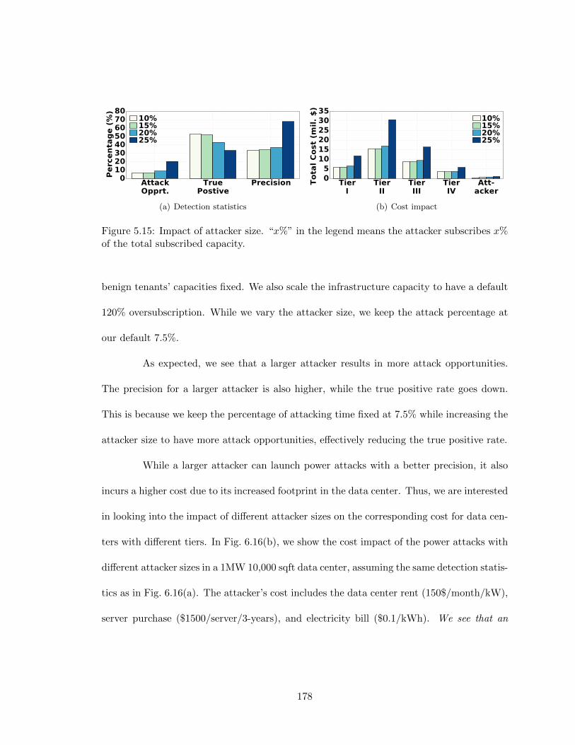
AttackOpprt.

TruePostive

Precision0

1020304050607080

Perc

en

tag

e (

%)

10%15%20%25%

(a) Detection statistics

TierI

TierII

TierIII

TierIV

Att-acker

05

101520253035

Tota

l C

ost

(mil.

$)

10%15%20%25%

(b) Cost impact

Figure 5.15: Impact of attacker size. “x%” in the legend means the attacker subscribes x%of the total subscribed capacity.

benign tenants’ capacities fixed. We also scale the infrastructure capacity to have a default

120% oversubscription. While we vary the attacker size, we keep the attack percentage at

our default 7.5%.

As expected, we see that a larger attacker results in more attack opportunities.

The precision for a larger attacker is also higher, while the true positive rate goes down.

This is because we keep the percentage of attacking time fixed at 7.5% while increasing the

attacker size to have more attack opportunities, effectively reducing the true positive rate.

While a larger attacker can launch power attacks with a better precision, it also

incurs a higher cost due to its increased footprint in the data center. Thus, we are interested

in looking into the impact of different attacker sizes on the corresponding cost for data cen-

ters with different tiers. In Fig. 6.16(b), we show the cost impact of the power attacks with

different attacker sizes in a 1MW 10,000 sqft data center, assuming the same detection statis-

tics as in Fig. 6.16(a). The attacker’s cost includes the data center rent (150$/month/kW),

server purchase ($1500/server/3-years), and electricity bill ($0.1/kWh). We see that an

178

0 1 2 3 4 5 6 7 8 9 10 11 12Time (H)

0

5

10

15

20D

em

ixed

Nois

e E

nerg

y Estimation Attack

Figure 5.16: Without energy noise spike detection, the attacker launches many unsuccessfulattacks.

attacker can create million-dollar losses, by spending only a fraction (between 3% and 23%)

of the total cost borne by the data center and affected tenants.

Impact of noise energy spike detection. Here, we test the effectiveness of the

noise energy spike detection mechanism in our attack strategy in Section 5.4.4. Concretely,

we show in Fig. 5.16 that without the spike detection mechanism, the attacker launches

power attacks (unsuccessful) upon detecting short-duration energy spikes (e.g., around hours

1, 6, 10 and 11) that possibly result from a fan RPM spike in case of a rapid server power

change (Fig. 5.6(a)). In contrast, as shown in Fig. 5.12, the attacker can effectively avoid

such unsuccessful attacks by waiting for the demixed energy noise to become stable.

Comparison with other attack strategies. We examine two alternatives:

the simple microphone-based power attack (Section 5.4.3) and peak-aware random power

attacks (Random-P). In microphone-based power attacks, we take the average of the noise

energy recorded by the four microphones (also with a high-pass filter applied) and compare

it against an attack triggering threshold: if higher than the threshold, then attack. In

Random-P, the attacker is assumed to have the knowledge of the probability of attack

opportunities during different hours of a day, although this information is rarely available

179

4 6 8 10 12 14 16Attacks (% Time)

0

20

40

60

80

100Tru

e P

osit

ive (

%)

NMF-basedMic-basedRandom-P

(a)

4 6 8 10 12 14 16Attacks (% Time)

0

20

40

60

80

100

Pre

cis

ion

(%

) NMF-basedMic-basedRandom-P

(b)

Figure 5.17: Detection statistics for different attack strategies.

in practice. Then, the attacker distributes its total number of attacks (i.e., total amount of

time it attacks) to each hour in proportion to the probability of attack opportunities during

that hour.

Fig. 5.17(a) shows the true positive rate at different percentages of attack times.

We see that our proposed strategy significantly outperforms both microphone-based and

random attack strategies. In Fig. 5.17(b), we see similar results for the precision of power at-

tacks. Note that, while significantly worse than our proposed attack strategy, the microphone-

based attack still has a reasonable true positive rate and precision. This is mainly because

our experiment only has three benign tenants and hence the attenuation coefficients between

different noise sources and the microphones do not differ very significantly.

Finally, we note that the prior research [76] discovers a thermal side channel result-

ing from heat recirculation in data centers with raised-floor designs where benign tenants’

server heat can recirculate to the attacker’s temperature sensors. It proposes a model-based

estimation algorithm based on Kalman filter to infer benign tenants’ runtime power usage

and time power attacks, achieving a timing precision of about 50%. Nonetheless, our uni-

versity data center does not use perforated tiles and has a completely different setup than

180

the one considered in [76]; we cannot place a large number of heat sources to emulate heat

recirculation in our university data center either. Thus, we do not provide a side-by-side

comparison with [76] in terms of timing accuracy, although our model-free approach achieves

a comparable accuracy with the reported values in [76].

5.6 Defense Strategies

Given the danger of power attacks timed using the acoustic side channel, we briefly

discuss possible defense strategies.

Power infrastructure resilience. Naturally, attack opportunities can be de-

creased by lessening the oversubscription ratio, but this comes at a significant revenue loss

for the operator. Another approach is to increase power infrastructure resilience against

power attacks. This, however, requires expensive infrastructure installation and/or up-

grades, and more so for multi-tenant data center operators whose entire investment is the

data center infrastructure. Additionally, tapping into stored energy (e.g., battery) during an

attack may not mitigate cooling overloads, since the actual cooling load (i.e., server power)

is not reduced (Section 5.2.1). In any case, an attacker can still launch timed attacks to

compromise data center availability, albeit to a less severe extent.

Acoustic side channel. Power attacks can be potentially mitigated by weakening

the acoustic side channel. Towards this end, low noise servers and/or noise-proof server racks

can be used [118]. However, these are developed mainly to operate in small-scale (e.g.,

one/two racks) placed inside or in close proximity to office spaces, not for multi-tenant data

centers. In addition, because of foam-sealed doors, special cooling arrangements are required

181

for noise canceling server racks which are difficult to retrofit in multi-tenant data centers.

Another approach is to destroy the correlation between server noise energy and server power

consumption by running the cooling fans at maximum speed all the time. But, this results

in a huge energy/cost wastage [96, 171], and is not decided by the data center operator

due to its lack of control over tenants’ servers. Finally, the data center operator may

place noise-generating speakers, mimicking server noise to decrease the attacker’s timing

accuracy. However, it is still difficult to completely eliminate the acoustic side channel and

de-correlate the attacker’s received noise energy from the benign tenants’ power usage by

adding speaker-generated noise, because the attacker is stealthy and its microphone location

is unknown to the data center operator.

Attack detection. A more proactive approach would be to find the malicious

tenant(s). The data center operator can increase vigilance in its power monitoring to detect

suspicious power usage patterns and pay close attention to that tenant. Then, the operator

may take additional safety measures. Alternatively, the operator may revise its contract

terms to prohibit certain power usage patterns that are likely malicious power attacks.

Server inspection. The attacker can conceal very small-sized or even invisible

microphones (e.g., spying microphone) on its servers or racks that cannot be easily detected

via visual inspection. Thus, on top of today’s routine visual inspection, the data center

operator may need to use advanced microphone detection devices to protect the data center

facility against unauthorized listening devices.

Note that installing per-server circuit breakers (which are already available in

some data centers) is not very helpful for defending against power attacks. The reason

182

is that the attacker does not violate the operator’s contractual constraint and hence, the

operator cannot forcibly/arbitrarily cut power supply to any particular tenant (including

the attacker) when power emergencies occur due to either coincident peaks or well-timed

power attacks. While the data center operator may sign some contracts with certain tenants

in advance for guaranteed power reduction in case of an emergency, it would have to pay a

high reward to involved tenants.

In conclusion, the above defense strategies (or a combination) may improve data

center infrastructure security in multi-tenant data centers. A more comprehensive investi-

gation and evaluation of different defense strategies are warranted as future work.

5.7 Related Work

Although common in data centers, oversubscription of power infrastructure re-

quires power capping techniques to avoid outages, including CPU speed throttling [95,174],

workload migration [169], energy storage discharging [56, 123, 168], among others. These

techniques, however, are inapplicable for multi-tenant data center operators due to their

lack of control over tenants’ servers or workloads.

While cyber security has long been a focus of research (e.g., mitigating distributed

denial of service attacks [111, 181], and stealing private information through covert side

channels [62]), power attacks to compromise data center physical security have also been

recently demonstrated [77, 93, 180]. In particular, [93, 180] propose to use virtual machines

(VMs) to create capacity overloads in cloud platforms. Nonetheless, VM-based attacks

require co-residence of many malicious VMs to create prolonged harmful power spikes.

183

Additionally, attackers do not directly control the power consumption of their launched

VMs; instead, the cloud operator has many control knobs to migrate and/or throttle the

VM power consumption across the cloud data center [114], safeguarding against VM-based

power attacks. Our work, in contrast, focuses on multi-tenant data centers where a malicious

attacker has its own physical servers, controls its server power consumption, and has the

capacity to directly overload the shared power infrastructures.

Another recent study [77] exploits a thermal side channel for timing power attacks

in a multi-tenant data center, whose limitations are discussed in Section 5.3.2. Compared

to [77], we exploit a novel acoustic side channel which is more universally applicable, utilized

using a model-free approach, and still produces a comparable (even better) timing accuracy.

Finally, our work adds to the recent literature on energy/power management

in multi-tenant data centers and multi-tenant clouds. The recent works predominantly

have been efficiency-driven, such as electricity cost reduction [73, 117, 165], improving in-

frastructure utilization [75], and reducing the cost of participation in utility demand re-

sponse [21, 102]. In contrast, our work studies an under-explored adversarial setting in

multi-tenant data centers.

5.8 Concluding Remarks

This paper studies power attacks in a multi-tenant data center. We discover a

novel acoustic side channel that results from servers’ cooling fans and helps the attacker

precisely time its power attacks at the moments when benign tenants’ power usage is high.

In order to exploit the acoustic side channel, we propose to: (1) employ a high-pass filter to

184

filter out the air conditioner’s noise; (2) apply NMF to demix the received aggregate noise

and detect periods of high power usage by benign tenants; and (3) design a state machine to

guide power attacks. Our results show that the attacker can detect more than 50% attack

opportunities, representing state-of-the-art timing accuracy.

185

Chapter 6

Ohm’s Law in Data Centers: A

Voltage Side Channel for Timing

Power Attacks

6.1 Introduction

In the age of cloud computing and Internet of Things, data centers have experi-

enced an exponential growth at all scales and undeniably become mission-critical infrastruc-

tures without which our society cannot function. In fact, even a single data center outage

can egregiously affect our day-to-day life. For example, an outage in Delta Airlines’ data

center in 2016 stranded tens of thousands of passengers in transit, costing more than 150

million U.S. dollars [22]. Moreover, a recent survey shows that unplanned data center-wide

186

outages caused by malicious attacks have increased by 11 times from 2010 to 2016 [127].

Thus, securing data centers against attacks has been of paramount importance.

While data center’s cyber security has been extensively investigated [111,181,187],

a much less studied security aspect — power infrastructure security — has also emerged as

an equally, if not more, important concern. Even worse, besides being afflicted with random

system failures, data center power infrastructures are also increasingly becoming a target

for malicious attacks due to the criticality of their hosted services [85, 127]. Concretely,

recent studies [49,76,79,93,180] have found and successfully demonstrated that an attacker

can inject malicious power loads (referred to as power attacks) to overload the data center

power infrastructure capacity, thus creating more frequent data center outages. Such power

attacks are achieved by increasing the attacker’s own server power usage [76, 79] and/or

sending more workloads to the target data center [93,180].

The primary reason for data centers’ vulnerability to power attacks stems from

the common practice of power capacity oversubscription. Data center power infrastruc-

tures are very expensive (and sometimes impossible because of local grid capacity or other

constraints) to build to accommodate the growing demand, costing 10 ∼ 25 dollars per

watt of power capacity delivered to servers and taking up 25 ∼ 60% of an operator’s total

cost of ownership over a 15-year lifespan [17, 75, 167, 174]. As a consequence, to maximize

utilization of existing power infrastructures, data centers (even Facebook and Google data

centers [42, 174]) commonly oversubscribe their power capacity by housing more servers

than can be supported. The current industry average is to oversubscribe the infrastructure

by 120% (i.e., provisioning 100kW power capacity to servers whose total power can reach

187

120kW) [76,88], and recent research [93,167,174] has suggested even more aggressive over-

subscription. The rationale for oversubscription is statistical multiplexing: not all servers

peak their power usage simultaneously. Additionally, various techniques (e.g., throttling

CPU and halting services [45, 71, 75, 174]) have been proposed to handle the very rare,

albeit possible, power capacity overload resulting from oversubscription.

Nonetheless, power attacks, especially maliciously timed attacks [49, 76, 79], can

alter the servers’ total power usage and create frequent power capacity overloads. Despite

safeguards (e.g., infrastructure redundancy), power attacks at best invoke power capping

more often than otherwise, significantly degrading application performances (due to, e.g.,

CPU throttling [93,174]). More importantly, they significantly compromise the data center

availability and create more frequent outages, which can lead to catastrophic consequences

(see Delta Airlines’ example [22]).

In this paper, we focus on the emerging threat of power attacks in a multi-tenant

colocation data center (also called colocation or multi-tenant data center), an important

but less studied type of data centers [120]. A multi-tenant data center is a shared data

center facility, in which multiple companies/organizations (each as a tenant) houses their

own physical servers and the data center operator is responsible for providing reliable power

and cooling to tenants’ servers. Even large companies, like Google and Apple [14,147], lease

multi-tenant data center capacities to complement their own data centers.

Compared to an owner-operated data center whose operator can perform power

capping/throttling to mitigate power attacks, a multi-tenant data center is more vulnerable

to power attacks, because the data center operator has no control over tenants’ power usage.

188

Alternatively, the operator of a multi-tenant data center sets contractual constraints: each

tenant can continuously use a certain fraction (usually 80%) of its subscribed power capacity,

but can only use its full subscribed power capacity on an occasional basis; non-compliance

can result in forcible power cuts [72, 76]. Therefore, to launch successful power attacks

while meeting the contractual constraint in a multi-tenant data center, a malicious tenant

(attacker) must precisely time its power attacks: it needs to increase its server power to the

full capacity only at moments when the benign tenants are also using a high power [76,79].

Nonetheless, a key challenge for the attacker to precisely time its power attacks is that it

does not know benign tenants’ power usage at runtime. Importantly, attack opportunities

(i.e., benign tenants’ high power usage moments) are highly intermittent, making random

attacks unlikely to be successful (Fig. 6.17 in Section 6.5.2).

In order to achieve a good timing of power attacks, we discover a novel physical

side channel — voltage side channel — which leaks information about benign tenants’ power

usage at runtime. Concretely, we find that a power factor correction (PFC) circuit is almost

universally built in today’s server power supply units to shape server’s current draw follow-

ing the sinusoidal voltage signal wave and hence improve the power factor (i.e., reducing

reactive power that performs no real work) [121]. The PFC circuit includes a pulse-width

modulation (PWM) that switches on and off at a high frequency (40 ∼ 100kHz) to regulate

the current. This switching operation creates high-frequency current ripples which, due to

the Ohm’s Law (i.e., voltage is proportional to current given a resistance) [18], generate

voltage ripples along the power line from which the server draws current. Importantly, the

high-frequency voltage ripple becomes more prominent as a server consumes more power

189

and can be transmitted over the data center power line network without interferences from

the nominal grid voltage frequency (50/60Hz). As a consequence, the attacker can easily

sense its supplied voltage signal and extract benign tenants’ power usage information from

the voltage ripples.

We build a prototype that represents an edge multi-tenant data center [32] to

demonstrate the effectiveness of our discovered voltage side channel in terms of timing at-

tacks. Our results show even though the attacker restricts itself from launching continuous

attacks to meet the data center operator’s contractual limit, it can still successfully utilize

more than 64% of the available attack opportunities with a precision rate of 50%. If attacks

can be launched consecutively, the attacker can even detect 80+% of attack opportunities.

Importantly, the attacker’s total cost is just a small fraction (3% ∼ 16% in our study) of

the resulting financial loss. Next, we extend our study to a three-phase power distribution

system used in large multi-tenant data centers. Finally, we highlight a few defense strate-

gies (including direct current power distribution, jamming signals, power infrastructure

resilience, and attacker identification) and discuss their limitations in practice.

6.2 Preliminaries on Power Attacks

In this section, we provide preliminaries on power attacks, highlighting the im-

portance of multi-tenant data center, the vulnerability and impact of power attacks, and

limitations of the prior work.

190

6.2.1 Overview of Multi-Tenant Data Centers

Importance of multi-tenant data centers

Multi-tenant colocation data centers, also commonly called multi-tenant data cen-

ters or colocations, are a critical segment of the data center industry, accounting for as

much as five times the energy consumption by Google-type owner-operated data centers

combined altogether [120].

A multi-tenant data center significantly differs from a multi-tenant cloud: in a

multi-tenant cloud (e.g., Amazon), the cloud operator owns the physical servers while rent-

ing out virtualized resources (e.g., virtual machines) to cloud users; in a multi-tenant

data center, the data center operator only owns the data center facility and physical

power/cooling infrastructures, whereas tenants manage their own physical servers in shared

spaces.

There are more than 2,000 large multi-tenant data centers in the U.S. alone, serving

almost all industry sectors that even include large IT companies (e.g., Apple, which houses

25% of its servers in leased multi-tenant data centers) [14,27]. Importantly, the multi-tenant

data center industry is experiencing a double-digit growth to meet the surging demand [6].

Moreover, many emerging Internet of Things workloads, such as augmented re-

ality and assisted driving, are hosted in geo-distributed edge multi-tenant data centers in

proximity of the data sources for latency minimization. For example, Vapor IO, a data

center operator, plans to build thousands of edge multi-tenant data centers in wireless

towers [26,162].

191

UPSPDU

ATS

Utility

Generator Attacker

BenignTenants

Figure 6.1: Data center power infrastructure with an attacker.

Data center power infrastructure

Typically, data centers employ a tiered power infrastructure as illustrated in

Fig. 6.1. An uninterrupted power supply (UPS) takes the grid voltage as input and outputs

voltage to the lower-tier power distribution unit (PDU). The PDU acts as a local power

distribution hub and delivers power to server/racks. Each infrastructure has a power ca-

pacity protected by a circuit breaker. An automatic transfer switch (ATS) will switch to

the backup generator (if any) during grid outages.

The power infrastructure shown in Fig. 6.1 represents an edge multi-tenant data

center where the total power capacity is small (usually in the order of 10+kW or less) and

each tenant houses a few servers in a shared server rack. In Section 6.6, we also show (three-

phase) power infrastructures used in large multi-tenant data centers where an individual

tenant houses at least one dedicated server rack and the data center operator oversubscribes

its more expensive upper-level PDUs each with 40 ∼ 200kW capacity.

192

6.2.2 Vulnerability and Impact of Power Attacks

As stated in Section 6.1, the common practice of power capacity oversubscription

improves the utilization of power infrastructures, but meanwhile also leaves data centers

vulnerable to malicious power attacks that result in more frequent and costly power outages.

Current safeguards

First of all, a data center operator leverages infrastructure redundancy to handle

random system failures [152]. Depending on the level of redundancy, data centers are

classified into four tiers, from Tier-I that has no redundancy to Tier-IV that duplicates all

power/cooling systems (so-called “2N” redundancy) [23, 152]. While a power attack may

not lead to an actual power outage due to infrastructure redundancies, such redundancy

protection is compromised due to malicious power loads, exposing the impacted data center

in a very dangerous situation. For instance, with power attacks, the outage risk for a

fully-redundant Tier-IV data center increases by 280+ times than otherwise [76,152].

Moreover, since multi-tenant data center operators cannot control or arbitrarily cut

tenants’ power usage (unless a tenant is found in violation of the contract), they typically

impose contractual constraints on each tenant’s continuous power usage (limited to 80%

of a tenant’s subscribed power capacity), while only allowing tenants to use up their full

power capacity occasionally [72, 76]. By doing so, the tenants’ aggregate power usage can

stay below the actual power infrastructure capacity at almost all times. Nonetheless, these

safeguards are highly vulnerable to well-timed power attacks that are launched at moments

when tenants’ power usage is also high (see Fig. 5.12 for illustration) [76,79].

193

In addition, tenants themselves may employ software-based fault tolerance to with-

stand power outages. Nonetheless, power outages can induce correlated server failures that

are challenging to survive through [140]. For example, even a power outage in a single

facility cost Delta Airlines over 150 million U.S. dollars [22].

The above discussion highlights that, despite several safeguards, multi-tenant data

centers are still highly vulnerable to (well-timed) power attacks [76,79].

Cost impact of power attacks

While not every power attack can lead to an actual outage, power attacks result

in more frequent capacity overloads and hence significantly compromise the data center

availability over a long term. For example, the outage risk for a fully-redundant Tier-IV

data center increases by 280+ times than otherwise [76, 152]. Based on a conservative

estimate [79], even for a medium-size 1MW data center experiencing power attacks for only

3.5% of the time, a total financial loss of 3.5 ∼ 15.6 million U.S. dollars can be incurred per

year. The financial loss is incurred not only by tenants which experience service outages,

but also by the data center operator which loses its capital expense in strengthening the

infrastructure resilience (let alone the reputation damage and high customer churn rate).

More importantly, the attacker only needs to spend a tiny fraction (as low as 3%)

of the total loss, thus providing strong motivations for malicious tenants (e.g., organized

crime groups that try to bring down services and create societal chaos, the victim data

center’s competitor, etc.) [79]. Interested readers are referred to [76, 79] for a detailed cost

analysis of power attacks.

194

6.2.3 Recent Works on Timing Power Attacks

In a multi-tenant data center, a key challenge for an attacker is that the actual

attack opportunity lasts intermittently (Fig. 5.12 in Section 6.5.2). For timing power attacks

in a multi-tenant data center, the prior research has considered a thermal side channel (due

to the heat recirculation resulting from servers’ heat) [76] and an acoustic side channel (due

to noise propagation from servers’ cooling fan noise) [79]. Nonetheless, as confirmed by our

discussion with a large data center operator, they suffer from the following limitations.

First, both the thermal and acoustic side channels utilize air as the medium.

Hence, they have only a limited range (e.g., 5 ∼ 10 meters) and are highly sensitive to

disturbances (e.g., supply cold air temperature and human voice disturbances). Moreover,

because it takes time (1 minute or even longer) for server heat to reach the attacker’s tem-

perature sensor and for server’s cooling fans to react to server power changes, these side

channels cannot provide real-time information about benign tenants’ power usage. In addi-

tion, exploiting a thermal side channel requires an accurate modeling of heat recirculation,

whereas the acoustic side channel needs complex signal processing techniques to mitigate

near-far effects (i.e., the attacker’s received noise level is dominate by its neighbors) [79].

Last but not least, the thermal side channel requires a raised-floor data center layout with-

out heat containment, whereas the acoustic side channel requires servers have conventional

fan speed controls.

In sharp contrast, a distinguishing feature of our discovered voltage side channel

(Section 6.4.3) is that it is insensitive to external disturbances (because of the wired power

line transmission) and can carry benign tenants’ power usage information throughout the

195

power network. The voltage side channel also provides real-time information about benign

tenants’ power usage (with a delay of 1 second for frequency analysis). More importantly,

the voltage side channel is based on the high-frequency voltage ripples generated by PFC

circuits that are universally built in servers’ power supply units, and can be exploited

without any specific models about the data center power network. Finally, while the settings

for our experiments and [76,79] are different, our results show that given 10% attack time,

the voltage side channel can achieve 80+% true positive for detecting attack opportunities

(Fig. 6.18(a)) whereas [76,79] only achieve around or below 50%. This translates into ∼2x

successful attacks by using our voltage side channel. Therefore, our voltage side channel

presents a more significant threat in real systems.

6.3 Threat Model

As illustrated in Fig. 6.1, we consider a malicious tenant (i.e., attacker) that houses

its own physical servers in a multi-tenant data center, sharing the power infrastructure with

benign tenants.

Attacker’s capability. The attacker subscribes a fixed amount of power capac-

ity from the data center operator. It behaves normally as benign tenants, except for its

malicious intention to overload the shared power infrastructure and create more power out-

ages. Thus, for stealthiness, the attacker only occasionally uses power up to its capacity,

which is allowed by the operator’s power usage contract [72]. Physically tampering with

the shared power infrastructure or placing explosive devices can be easily found/detected

and is orthogonal to our work.

196

The attacker launches power attacks by running power-hungry applications (e.g.,

computation to maximize CPU utilization) at moments when the aggregate power usage of

benign tenants is sufficiently high. Note that the attacker may also remotely send additional

requests to benign tenants’ servers during power attacks if benign tenants offer public

services (e.g., video streaming). This complementary attack method can further increase

the aggregate server power consumption. In this paper, we focus on attacks by using the

attacker’s own server power as in [76,79].

To exploit a voltage side channel for timing power attacks, the attacker acquires the

supplied voltage by placing an analog-to-digital converter (ADC) circuit inside the power

supply unit (Fig. 6.4) in one of its servers.1 The ADC samples the incoming continuous-time

voltage signals at a rate of 200kHz or above, and the sampled voltage signals are stored for

further processing (Section 6.4). Note that in a multi-tenant data center, the attacker owns

its physical servers, instead of renting them from the data center operator. Furthermore,

while a multi-tenant data center has a more rigorous inspection for tenants than a public

cloud platform, the data center operator will not disassemble tenant servers’ power supply

units during the routine inspection due to intrusiveness. Thus, a coin-size or even smaller

voltage ADC can be easily placed inside the power supply unit before the attacker moves

its servers into the target multi-tenant data center. In modern power supply units, a high-

speed voltage ADC is already in place as part of the PFC design, and in this case, the

attacker can simply read the ADC’s output without placing an additional ADC circuit.

1ADC circuits often operate over a low voltage range (e.g., 5V) and hence, a voltage divider may benecessary to scale down the incoming voltage to an appropriate range.

197

Successful attack. Power attacks compromise the data center availability over

a long term. Thus, we consider a power attack successful as long as the combined power

usage of the attacker and benign tenants continuously exceeds the power infrastructure

capacity for at least L minutes (e.g., L = 5 is enough to trip a circuit [79,142]), even though

an actual outage does not occur due to infrastructure redundancy. Instead of targeting a

specific tenant, power attacks compromise the availability of shared power infrastructures

and hence significantly affect the normal operation of both data center operator and benign

tenants.

Other threat models for power attacks. Next, we highlight the differences

between our threat model and other relevant models for power attacks.

• Power attacks in public clouds. Some studies [49,93,180] propose to use malicious

virtual machines (VMs) to create power overloads in public clouds like Amazon. For tripping

the circuit breaker and successful attacks, the attacker needs to launch a large number of

VMs co-residing in the same PDU. Nonetheless, this is nontrivial and can be difficult to

accomplish in practice, because the cloud operator frequently randomizes its VM placement

(to prevent co-residency side channel attacks [114,187]). In addition, the cloud operator has

numerous knobs (e.g., CPU scaling) to throttle the VM power consumption for defending

its power infrastructure against a power attack. More recently, [50] considers a related

attack model but aims at using VMs to generate excessive heat for overloading the cooling

capacity.

In contrast, our model focuses on a multi-tenant data center where an attacker

can house its own physical servers to inject large power loads, tripping the circuit breaker of

198

a shared PDU more easily. The data center operator, as discussed in Section 6.2.2, cannot

control or forcibly cut a tenant’s power usage unless a tenant violates its power contract.

Compared to using VMs for power attacks in a public cloud [93,180], an attacker

in a multi-tenant data center can incur more costs (e.g., for purchasing servers). At the

same time, however, power attacks in our model are also more devastating due to the

attacker’s capability of injecting large power loads on a single PDU. Importantly, in our

model, the attacker’s total cost is just a small fraction (3% ∼ 16% in Section 6.5.2) of the

resulting financial loss. Moreover, while VMs can be launched remotely without revealing

the attacker’s identity [93,180], it is also difficult to identify and/or prosecute the attacker in

our attack scenario, because: (1) data center outages are caused by the operator’s capacity

oversubscription as well as the aggregate high power of multiple tenants; and (2) the attacker

does not violate any contractual constraints. Even though its servers are detected, the

attacker’s loss is minimum (e.g., only a few servers) because it likely uses fake/counterfeit

identities when moving into the target data center. Finally, we focus on precise timing of

power attacks for stealthiness, while the crucial timing issue is neglected in [93,180].

• Power attacks in multi-tenant data centers. Our model builds upon those consid-

ered in two recent studies [76,79]. In these studies, the attacker needs to install temperature

sensors and microphones in order to exploit a thermal side channel [76] and an acoustic side

channel [79], respectively, for timing power attacks. Both thermal sensors and microphones

are exposed to the outside of the servers and hence may be detected more easily. In con-

trast, our model is more stealthy as the attacker only places a small ADC circuit (if not

available yet) inside its server’s power supply unit, without exposing any hardware to the

199

outside. More comparisons (e.g., practical limitations and timing accuracy) are provided in

Section 6.2.3.

6.4 Exploiting A Voltage side channel

The key novelty of our work is to exploit a voltage side channel to track benign

tenants’ aggregate power usage at runtime for timing power attacks in a multi-tenant data

center.

Concretely, we discover that the PFC circuit inside each server’s power supply unit

is controlled by a switch to regulate the server’s current draw for improving power factor.

Because of the Ohm’s Law, this design creates high-frequency voltage ripples which, without

interference from the nominal 50/60Hz frequency of the gird voltage, exist along the power

lines supplying voltage to servers. Thus, by sensing the supplied voltage and extracting the

frequency components associated with the ripples, the attacker can track benign tenants’

power usage and launch well-timed power attacks.

6.4.1 Overview of the Power Network

Before presenting our voltage side channel, we show in Fig. 6.2 an overview of

the equivalent electrical circuit of a data center power network, where one PDU delivers

power to N servers. For better understanding, we focus on a single-phase system that each

serves a few tens of servers and best represents an edge multi-tenant data center (hosting

200

Attacker’s measurement 𝐕𝐍 = 𝐕𝐏𝐃𝐔 − 𝐈𝐍 ⋅ 𝐑𝐍

𝐈𝟏

𝐑

𝐕𝐔𝐏𝐒 𝐕𝐏𝐃𝐔

𝐑𝐍

= 𝐕𝐔𝐏𝐒 − 𝐈 ⋅ 𝐑 − 𝐈𝐍 ⋅ 𝐑𝐍

Attacker

Affected by grid and UPS

NegligibleAffected by total server power

𝐈 = ∑𝑰𝒏

VServer

V

𝐈𝟐

𝐈𝐍

Figure 6.2: Circuit of data center power distribution.

workloads such as augmented reality and assisted driving) [25, 26]. In Section 6.6, we will

extend to more complex three-phase systems used in large multi-tenant data centers.

As shown in Fig. 6.2, the PDU distributes alternating current (AC) to servers

using a parallel circuit. We denote the UPS output voltage and the PDU voltage by VUPS

and VPDU , respectively. The power line connecting the UPS to the PDU has a resistance

of R, and the total current flowing from UPS to PDU is denoted by I =∑N

n=1 In, where

In is the current of server n. Without loss of generality, we let server N be the one with

attacker’s ADC circuit, while the attacker can own multiple other servers. Thus, the voltage

measured by the attacker is denoted by VN .

Constraint on current measurement. Power is the product of voltage and

current, and servers operate at a relatively stable voltage. Thus, had the attacker been able

to sense the total current I =∑N

n=1 In, it would know the aggregate power usage of all

201

tenants and easily time its power attacks. Due to the power line constraint, however, the

attacker can only measure the current flowing into its own servers.

Line voltage drop. We observe that the voltage supplied to each individual

server is affected by all the servers. Concretely, the current flowing from the UPS to PDU

results in a voltage drop ∆V along the power line. The phenomenon of voltage drop is

also common in our daily life, e.g., dimming of a light when starting a power-consuming

appliance in the same house. Then, following the Ohm’s Law, the voltage measured by the

attacker is expressed as VN = VUPS − I · R − IN · RN ≈ VUPS − I · R = VPDU , which can

be rewritten as

VN = VPDU = VUPS −R ·N∑n=1

In, (6.1)

where, for better presentation, we replace the approximation with equality given the fact

that the voltage drop IN · RN between the PDU and attacker’s server is negligible due to

the much smaller current IN compared to I =∑N

n=1 In and small line resistance RN . Even

when IN ·RN is non-negligible, the attacker can lower its server’s power (i.e., decrease IN )

to make IN ·RN sufficiently small.

6.4.2 ∆V -based attack

We now present an intuitive strategy — ∆V -based attack — that times power

attacks directly based on the attacker’s voltage measurement VN . Importantly, we will

show that this seemingly effective strategy results in a rather poor timing of power attacks.

202

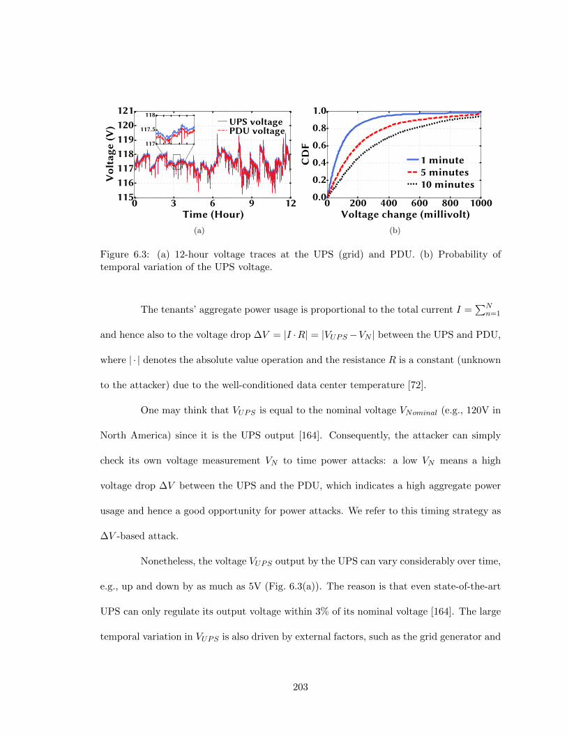
0 3 6 9 12Time (Hour)

115116117118119120121

Vol

tage

(V) UPS voltage

PDU voltage117

117.5

118

(a)

0 200 400 600 800 1000Voltage change (millivolt)

0.0

0.2

0.4

0.6

0.8

1.0

CD

F

1 minute5 minutes10 minutes

(b)

Figure 6.3: (a) 12-hour voltage traces at the UPS (grid) and PDU. (b) Probability oftemporal variation of the UPS voltage.

The tenants’ aggregate power usage is proportional to the total current I =∑N

n=1

and hence also to the voltage drop ∆V = |I ·R| = |VUPS−VN | between the UPS and PDU,

where | · | denotes the absolute value operation and the resistance R is a constant (unknown

to the attacker) due to the well-conditioned data center temperature [72].

One may think that VUPS is equal to the nominal voltage VNominal (e.g., 120V in

North America) since it is the UPS output [164]. Consequently, the attacker can simply

check its own voltage measurement VN to time power attacks: a low VN means a high

voltage drop ∆V between the UPS and the PDU, which indicates a high aggregate power

usage and hence a good opportunity for power attacks. We refer to this timing strategy as

∆V -based attack.

Nonetheless, the voltage VUPS output by the UPS can vary considerably over time,

e.g., up and down by as much as 5V (Fig. 6.3(a)). The reason is that even state-of-the-art

UPS can only regulate its output voltage within 3% of its nominal voltage [164]. The large

temporal variation in VUPS is also driven by external factors, such as the grid generator and

203

other loads sharing the same grid. More importantly, the attacker cannot measure VUPS to

calculate ∆V = |I ·R| = |VUPS −VN | because it cannot place its ADC circuit at the output

of the UPS which is owned by the data center operator. On the other hand, compared to

the VUPS variation, the variation in voltage drop ∆V = |I · R| caused by tenants’ power

usage is much smaller (in the order of a few millivolts) because of the small line resistance.

In Fig. 6.3(a), we show a 12-hour trace of the voltage output by our CyberPower

UPS and PDU voltage supplied to servers. The voltage drop between the UPS an PDU is

negligible compared to the UPS voltage variation itself. In Fig. 6.3(b), we show the cumula-

tive distribution function of the UPS output voltage at different timescales, demonstrating

that the UPS output voltage can vary much more significantly than the line voltage drop

due to server load.

To conclude, the change of VN is predominantly driven by the variation in the

UPS voltage VUPS , rather than the actual line voltage drop ∆V = |I · R| caused by the

tenants’ power usage. Thus, without knowing time-varying VUPS, the ∆V -based strategy

cannot precisely time power attacks (Fig. 6.17 in Section 6.5.2).

6.4.3 Exploiting High-Frequency Voltage Ripples

Given the ineffectiveness of the ∆V -based attack, we present our key idea: the PFC

circuit inside each server’s power supply unit generates high-frequency voltage ripples that

have a strong correlation with the servers’ power, which can reveal the aggregate power usage

information at runtime. Next, we will first show the root cause of why the PFC generates

high-frequency voltage ripples, and then validate the ripples through experiments.

204

Voltage Regulator

AC/DC

Power Factor

Correction(PFC)

DC/DC

Power Supply Unit (PSU)

Server

380V 12VAC100/240V

Analog to Digital Converter

Figure 6.4: A server with an AC power supply unit [17]. An attacker uses an analog-to-digital converter to acquire the voltage signal.

Overview of server’s power supply unit

We first provide an overview of server’s power supply unit to facilitate the readers’

understanding. All the internal components of a server/computer, such as CPU, run on

DC power at a regulated voltage (usually 12V), provided by an internal power supply unit.

Fig. 6.4 shows a block diagram of a server.

In the first step, the sinusoidal AC voltage supplied by the PDU is passed through

an AC to DC full-bridge rectifier which inverts the negative part of the sine wave and

outputs a pulsating DC (half-sine waves). Then, a power factor correction (PFC) circuit

outputs an elevated voltage at 380V which is then fed to a DC to DC converter to lower

it to 12V supplied to server’s internal components. An important concept is power factor,

which is a scalar value between 0 and 1 measuring the fraction of total delivered power

that is actually used. The power factor goes down when the voltage or current becomes

non-sinusoidal, which creates power waste and other detrimental effects [121]. Thus, to

205

Power Factor Correction (PFC)

PWMControl

Outputvoltagesample

Input voltagesample

Rectifier

Inductor Diode

MOSFET

Bulkcapacitor

Figure 6.5: Building blocks of PFC circuit in server’s power supply unit.

improve server’s power factor, a PFC circuit is required and also mandated by international

regulations [37,69].

Voltage ripples generated by PFC circuit

The purpose of the PFC circuit is to improve power factor by shaping the current

drawn by the power supply unit to match the sinusoidal source voltage.2 The working

principle is to draw more current when the input voltage (pulsating AC at the rectifier

output) is high and draw less current when the input voltage is low. Fig. 6.5 shows the

basic block diagram of the most commonly-used boost-type PFC with an inductor, a diode,

a switch (MOSFET), and the pulse width modulation (PWM) control circuit [70,110,121].

The PWM control circuit repeatedly closes and opens the switch at a high frequency to

control the current through the inductor to shape it like a sine wave while also maintaining

a stable DC voltage at the output. The current wave shapes of the inductor controlled by

a server’s PFC circuit are illustrated in Fig. 6.6(a).

2The voltage signal coming from the PDU is not perfectly sinusoidal; instead, it has voltage ripples dueto current ripples along the UPS-PDU line (Fig. 6.7).

206

Time

PFC

Cur

rent

High powerLow power

(a)

𝒐𝒏 𝒐𝒇𝒇 𝒐𝒏 𝒐𝒇𝒇

ActualCurrent

ReferenceCurrent

(b)

Figure 6.6: (a) Wave shape of PFC current at different power levels. (b) Current ripplesfrom the PFC switching.

A prominent side effect of the PWM circuit’s rapid switching is the rapid change

in the current (i.e., high-frequency ripple) drawn from the source. Hence, the PFC circuit

in the power supply unit creates high-frequency current ripples flowing through the power

line between the UPS and PDU, which in turn result in voltage ripples along the line due

to the Ohm’s Law.

Importantly, a key observation is that the voltage ripples are at a much higher

frequency (40 ∼ 100kHz) than the 50/60Hz nominal grid frequency as well as the UPS

output voltage frequency. Thus, the voltage ripple signal and UPS output voltage VUPS

signal are orthogonal in the frequency domain. In fact, this is also the fundamental principle

for power line communications that leverage power networks as the transmission medium

(e.g., recent studies [20] have proposed to install special transmitters and leverage data

center power lines to send control command signals for server network management).

In summary, while the PFC circuit is mandated for improving the power factor [37],

its usage of PWM-based switching design creates high-frequency ripple voltage signal that

207

is transmitted over the data center power lines without interference from the UPS output

voltage.

Impact of server’s power usage on voltage ripples

A natural follow-up question is: do the voltage ripples carry information about

server’s power usage?

Note first that if we apply a band-pass filter to keep frequency components within a

certain range around the PFC switching frequency (e.g., ∼70kHz), the UPS output voltage

VUPS signal becomes approximately zero and the voltage relation in Eqn. (6.1) reduces to

VN = VPDU ≈ −R ·N∑n=1

In (6.2)

where x represents a filtered version of x that only keeps frequency components around the

PFC switching frequency. Thus, the attacker’s filtered voltage measurement VN essentially

only contains the voltage ripple signal. It is possible that the UPS output voltage VUPS

itself also has some high-frequency components (due to, e.g., grid input), but these frequency

components are rather weak because of fading over a long distance and hence can be viewed

as background noise (Fig. 6.8(a)).

There are three basic conduction modes for PFC designs: continuous, discontin-

uous and critical conduction modes [121]. In both discontinuous and critical conduction

modes, the current ripple decreases to zero during each switching cycle and the hence peak

current can be exceedingly high (twice as much as the average current). Thus, they are

mostly designed for low-power devices. In today’s servers, power supply units are most

208

commonly designed with a fixed-frequency PFC operating under the continuous conduc-

tion mode where the current ripple does not decrease to zero during each PWM-controlled

switching cycle (as shown in Fig. 6.6(a)). We take a closer look at the PFC current ramps

in Fig. 6.6(b). The current goes up when the switch is “ON” (i.e., the MOSFET is turned

on), and goes down when the switch is “OFF”. The “ON” and “OFF” times are designated

as Ton and Toff in Fig. 6.6(b), where the period is T = Ton + Toff and the duty cycle is

D = TonT . The duty cycle is regulated within each cycle to ensure that the average current

follows the reference current shown in dashed line in Fig. 6.6(b). The reference current is

set based on the sampled input voltage to make the resulting current follow the voltage

shape (i.e., improve the power factor to close to 1).

To accommodate the server power change, the current changes and there is a

multiplier applied to the current reference sampled from the input voltage. Consequently,

as shown in Fig. 6.6(a), we have a taller current wave when the power is higher and vice

versa. Intuitively, the current waves we show in Fig. 6.6(b) need to rise faster when the

server consumes more power, as the current ramp needs to reach higher values. It also

needs to drop faster from a higher current to follow the sinusoidal voltage wave. On the

other hand, the PFC switching frequency is relatively fixed with a small temporal variation

shown in Fig. 6.9(d). Therefore, when a server consumes more power, the current ripple

needs to change faster (i.e., increasing/decreasing faster) within one switching period, and

vice versa. Correspondingly, based on the Ohm’s Law in Eqn. (6.2), we expect to see a

more prominent high-frequency voltage ripple.

209

Figure 6.7: High-frequency voltage ripples at the PDU caused by switching in the serverpower supply unit.

To quantify the intensity of the voltage ripple, we use aggregate power spectral

density (PSD), i.e., the sum of PSD components over a 1kHz band centered around the

PFC switching frequency. We choose 1kHz as our default frequency band, and we will later

vary the frequency band (Fig. 6.12(d)).

In summary, the high-frequency voltage ripple created by a server is expected to be

more significant when it consumes more power.

6.4.4 Experimental validation

We now seek experimental validation on real servers to corroborate our discussion

in Section 6.4.3. Here, we only present the results, while the experimental setup is described

in Section 6.5.1.

Single server. We first run only one server with a 495W-rating power supply

unit. Fig. 6.7 shows two zoom-in oscilloscope screenshots that reveal the voltage ripples

caused by the server’s power supply unit. We further run frequency analysis on the collected

210

0 20 40 60 80 100Frequency (kHz)

10-6

10-5

10-4

10-3

10-2

10-1

100PS

D (W

/Hz)

(a) Without a server

0 20 40 60 80 100Frequency (kHz)

10-6

10-5

10-4

10-3

10-2

10-1

100

PSD

(W/H

z)

69 70 7110-6

10-5

10-4

(b) With a server

Figure 6.8: High-frequency PSD spikes in PDU voltage caused by the server power supplyunit.

voltage signals over each one-second segment. We show the resulting power spectral density

(PSD) with and without the server, in Figs. 6.8(a) and 6.8(b), respectively. We see that

the server produces a PSD spike around 70kHz, presenting a concrete proof of the voltage

ripples observable in the power line network.

We then run the server at different power levels and show the PSD around the

server’s PFC switching frequency in Fig. 6.9(a). We see that the PSD is higher when

the server power consumption is higher, matching with our expectation. We next show the

server power vs. aggregate PSD in Fig. 6.9(b), by summing up all the frequency components

within a 1kHz band (69.8 ∼ 70.8kHz). In Section 6.4.5, we provide an algorithm to identify

the frequency band over which the PSD is aggregated. We see that the aggregate PSD

monotonically increases with the server power. We also conduct similar experiments with a

350W power supply unit and show the results in Fig. 6.9(c). We note that given a certain

server power, the resulting aggregate PSD varies little, because of the high-frequency ripple

211

70.1 70.20. 00. 20. 40. 60. 81. 01. 21. 4

PSD

(W/H

z)£10−5

86W

70.1 70.2Frequency (kHz)

0. 00. 20. 40. 60. 81. 01. 21. 4£10−5

115W

(a)

70 80 90 100 110 120Power (W)

4. 054. 104. 154. 204. 254. 30

Agg

rega

te P

SD (W

) £10−5

MeasurementsFitting

(b)

40 50 60 70 80 90Power (W)

0. 00. 20. 40. 60. 81. 01. 21. 4

Agg

rega

te P

SD (W

) £10−5

Data pointsFitting

(c)

70.0 70.1 70.2 70.3Switching Frequency (kHz)

0.000.020.040.060.080.100.120.140.16

PMF

(d)

Figure 6.9: (a) PSD at different server powers. (b) Server power vs. PSD aggregated withinthe bandwidth of 69.5 ∼ 70.5kHz for the 495W power supply unit. (c) (b) Server power vs.PSD aggregated within the bandwidth of 63 ∼ 64kHz for the 350W PSU. (d) PMF showsthe PFC switching frequency only fluctuates slightly.

signal transmission over power lines without much interference. Finally, we also identify

that the switching frequency remains relatively fixed as shown in Fig. 6.9(d).

Multiple servers with identical power supply units. Next, we run four

servers, each with a 495W power supply unit. We turn on the servers one by one, record the

voltage readings for three different power levels, and calculate the aggregate PSD. Instead

of using the absolute value, we show in Fig. 6.10(a) the relative aggregate PSD normalized

with respect to the lowest value when only one server is running. It can be seen that the

212

Low Medium HighPower Level

0.81.01.21.41.61.82.0

Nor

m. A

ggr.

PSD 1 server

2 servers3 servers4 servers

(a)

62 64 66 68 70 72Frequency (kHz)

0. 0

0. 5

1. 0

1. 5

2. 0

PSD

(W/H

z)

£10−6

(b)

Figure 6.10: (a) The aggregate PSD for different numbers of servers. The aggregate PSDsare normalized to that of the single server at low power. (b) Power spectral density of allservers in our testbed showing three distinct PSD groups, each corresponding to a certaintype of power supply unit.

aggregate PSD becomes greater as we run more servers and/or increase their power usage,

which is consistent with our discussion in Section 6.4.3.

Multiple servers with different power supply units. We run all of our 13

servers that have different configurations and power supply units. Table 6.1 shows the

server configuration. We show the PSD of the resulting voltage in Fig. 6.10(b). We observe

three distinct groups of PSD spikes, each corresponding to one type of power supply unit.

Based on our individual server experiments, we identify that the PSD spikes around 64kHz

are caused by 350W power supply units. The PSD spikes around 66kHz and 70kHz are

both created by servers with the 495W power supply units. Despite the same capacity,

the two types of 495W power supply units are from different generations and hence have

distinct switching frequencies. In addition, each group consists of several spikes because dif-

ferent power supply units of the same model and generation may still have slightly different

switching frequencies.

213

In summary, our experiments have found and validated that: (1) the power supply

unit designs of today’s servers create high-frequency voltage ripples in the data center power

line network; and (2) these ripples carry information about servers’ power usage at runtime.

Note that, like in today’s mainstream systems [121], the PFC circuits in our servers operate

under the continuous conduction mode which, as shown in Fig. 6.10(b), causes line voltage

ripples with narrow spikes in the frequency domain. For certain high-power servers (close

to 1kW or even higher), two PFC circuits may be connected in tandem (a.k.a. interleaving

PFC) to meet the demand of large current flows while reducing voltage ripples. Compared

to a single-stage PFC, the two individual PFC circuits in an interleaving PFC design operate

with a certain time delay between each other and result in line voltage ripples with shorter

but wider spikes in the frequency domain [121, 184]. Albeit over a wider range, the high-

frequency components in line voltage ripples resulting from PWM switching still become

more prominent as a server consumes more power [184]. Therefore, our finding holds broadly

regardless of a single-stage or interleaving PFC design.

6.4.5 Tracking Aggregate Power Usage

Now, we study how the attacker can track the tenants’ aggregate power usage

based on its measured voltage signal.

Calculating group-wise aggregate PSD

In a multi-tenant data center with servers from different manufacturers, we shall

expect to see several groups of PSD spikes in the voltage signal, each group consisting of

214

Algorithm 4 Calculating Group-wise Aggregate PSD

1: Input: PSD data P (f), frequency band F (e.g., 1kHz), frequency scanning lower/upperbounds Flb/Fub

2: Output: Group-wise aggregate PSD P1, P2, · · · , PM .3: Find grid frequency Fo ← max45Hz≤f≤65Hz P (f)4: for f from Flb to Fub do5: Cf ← P (f−Fo)+P (f+Fo)

2

6: Keep Cf spikes and discard others (i.e., power line noise)7: Generate bands B[i] = [f − F

2 , f + F2 ] for each Cf spike

8: Merge B with overlapping frequency bands9: Number of groups M ← number of separate bands in B

10: for each item B[i] ∈ B do11: Pi ←

∑f∈B[i] P (f)

12: Return group-wise aggregate PSD Pi for i = 1, 2, · · · ,M .

the PSD spikes from similar power supply units (and likely from servers owned by the same

tenant). Likewise, we can also divide servers into different groups according to their PFC

switching frequencies.

In general, within each group, the aggregate PSD increases when the servers in

that group consume more power (Fig. 6.10(a)). Nonetheless, even given the same aggregate

PSD, servers in one group may have very different power usage than those in the other

group because they have different power supply units and are also likely to have different

configurations (e.g., different CPUs). Thus, the total PSD over all the groups may not

be a good indicator of the servers’ total power consumption; instead, we should consider

group-wise aggregate PSD.

We leverage the frequency domain segregation and use Algorithm 4 to identify

PSD groups. We use the insight from our experiment that each server creates a pair of PSD

spikes separated by twice the nominal power line frequency (i.e., 60Hz in the U.S.) and

215

centered around its PFC switching frequency. Further, the spikes are significantly greater

than the power line background noise.

Tracking tenants’ aggregate power usage

To launch successful power attacks, the attacker only needs to identify the moments

when the tenants’ aggregate power is sufficiently high. Thus, knowing the shape of the

aggregate power usage is enough.

Given the group-wise aggregate PSD P1, P2, · · · , PM at runtime, the attacker can

track the total power usage of servers in each group (i.e., a high aggregate PSD means a high

power in that group). Nonetheless, the attacker does not know the corresponding absolute

server power given a certain aggregate PSD value. Intuitively, however, if all or most group-

wise aggregate PSDs are sufficiently high, then it is likely that the tenants’ aggregate power

usage is also high (i.e., an attack opportunity). Thus, based on this intuition, we first

normalize each group-wise aggregate PSD (with respect to its own maximum over a long

window size, e.g., 24 hours) and denote the normalized values by P1, P2, · · · , PM . Then,

we sum them up P =∑M

m=1 Pm and use it as an approximate indicator of the tenants’

aggregate power usage.

6.4.6 Timing Power Attacks

To time power attacks based on the voltage side channel, we propose a threshold-

based strategy based on the sum of normalized group-wise aggregate PSDs P . Specifically,

we set four different states — Idle, Wait, Attack, and Hold — and the attacker transitions

216

Algorithm 5 Timing Power Attacks Using Voltage Side Channel

1: Input: attack threshold Pth, timer thresholds for Twait, Tattack, and Thold2: Initiation: current state Sc ← idle, next state Sn ← idle Twait ← 0, Tattack ← 0, andThold ← 0

3: loop at regular intervals (e.g., every 10 seconds)4: Use Algorithm 4 to get the aggregate PSDs5: Use historical data to get normalized PSD, P1, P2, · · · , PM6: P ←

∑Mm=1 Pm

7: if Sc = idle then8: if P < Pth then9: Sn ← idle

10: else Sn ← wait, start Twait

11: else if Sc = wait then12: if P ≥ Pth then13: if Twait is expired then14: Sn ← attack, start Tattack, stop and reset Twait15: else Sn ← wait

16: else Sn ← idle, stop and reset Twait

17: else if Sc = attack then18: if Tattack is expired then19: Sn ← hold, start Thold, stop and reset Tattack20: else Sn ← attack

21: else22: if Thold is expired then23: if P ≥ Pth then24: Sn ← attack, start Tattack, stop and reset Thold25: else Sn ← idle, stop and reset Thold

26: else Sn ← hold

27: Sc ← Sn

from one state to another by periodically (e.g., every 10 seconds) comparing P against a

threshold Pth.

•Idle : This is the default state. If P ≥ Pth is met, the attacker moves to Wait

and starts a Twait timer.

•Wait : To avoid attacking during transient spikes of P , the attacker stays in

Wait until Twait expires. Then, if P ≥ Pth still holds, the attacker moves to Attack and,

otherwise, back to Idle.

217

•Attack : In this state, the attacker uses its maximum power consumption for

attacks. The attacker stays in Attack for Tattack time, after which it starts a Thold timer

and moves to Hold.

•Hold : To avoid suspiciously consecutive attacks, the attacker stays in this state

until Thold expires. Then, if P ≥ Pth is still met, it moves back to Attack and otherwise to

Idle.

Finally, we present the formal algorithm description in Algorithm 5.

6.5 Evaluation

This section presents our evaluation results of exploiting the voltage side channel

for timing power attacks in a scaled-down multi-tenant data center. We focus on how well

the attacker can track tenants’ aggregate power usage at runtime and how well it can time

its power attacks. Our experimental results demonstrate that, by launching non-consecutive

attacks no more than 10% of the time, the attacker can successfully detect 64% of all attack

opportunities (i.e., true positive rate) with a precision of 50%.

6.5.1 Methodology

As shown in Fig. 6.11, we set up 13 Dell PowerEdge servers connected to a single-

phase 120V APC8632 rack PDU for our experiments. This setup represents an edge colo-

cation data center, an emerging type of data center located in distributed locations (e.g.,

wireless towers) [26].

218

1 Oscilloscope

1

2

3

45

6

2 Network Switch

3 PowerEdge Servers

4 UPS

5 APC PDU

6 Voltage Sampling

Figure 6.11: A prototype of edge multi-tenant data center.

The server configuration is shown in Table 6.1. The PDU is powered by a Cyber-

Power UPS that is plugged into a power outlet in our university server room. We use a Rigol

1074Z oscilloscope to measure the voltage at a sampling rate of 200kHz. The oscilloscope

probe is connected to the PDU through a power cable with polarized NEMA 1-15 plug.

While we use an oscilloscope to collect the voltage signal (as we cannot open the power

supply unit for lab safety), the attacker can place a small ADC circuit inside its power

supply unit to achieve the same purpose in practice.

Tenants. As shown in Table 6.1, we divide the 13 servers among the four tenants.

There are three benign tenants and one attacker (tenant #4). The total capacity of the

three benign tenants is 1,300W and the capacity of the attacker is 200W (i.e., 13% of

219

Table 6.1: Server configuration of our experiments.

Tenant CPU/MemoryPowerSupplyRating

PFCSwitchingFrequency

Numberof

Servers

SubscribedPower

#1 Xeon/32GB 350W ∼63kHz 4 360W

#2 Dual Xeon/32GB 495W ∼66kHz 2 460W

#3 Xeon/32GB 495W ∼70kHz 4 480W

#4 Pentium/32GB 350W ∼63kHz 3 200W

the total capacity subscription). The data center power capacity is 1,250W with 120%

oversubscription (i.e., sold as 1,500W) [76,88].

Workload traces. Like in the prior research [76, 79], the four tenants’ server

power usage follows four different power traces. Traces for two of the benign tenants are

collected from Facebook and Baidu workloads [169,174], while the other two power traces are

generated offline using workload traces (SHARCNET and RICC logs) from [43,124]. These

power traces are scaled to have 75% utilization for the benign tenants and 65% utilization

for the attacker. We assign a real workload trace to the attacker so that it behaves normally

as benign tenants and stays stealthy. The tenants’ total power consumption is shown in

Fig. 6.14. While we use these power traces to reflect the temporal variation in tenants’

power usage for our evaluation, our approach to timing power attacks also applies for any

other power traces.

Duration. We run the experiment for 12 hours and record the power consumption

and voltage readings. We also run simulation studies by extending our 12-hour experiment

into one year. Specifically, we split the 12-hour data into 10-minute pieces and randomly

order them into yearly voltage signals and corresponding power readings. In our yearly trace,

the attack opportunities take up 7.5% of the time, consistent with the settings in [76, 79].

Note that, because they are transmitted over power lines, the voltage ripples do not vary

220

0 4 8 12Time (Hour)

250

300

350

400Po

wer

(W)

Corr. Coeff. = 0.98Power PSD

1

2

3

4

Agg

rega

te P

SD (W

)£10−6

(a) Tenant #1 (63 ∼ 64 kHz)

0 4 8 12Time (Hour)

100

200

300

400

500

Pow

er (W

)

Corr. Coeff. = 0.97Power PSD

0. 6

0. 8

Agg

rega

te P

SD (W

)£10−5

(b) Tenant #2, (65.5 ∼ 66.5 kHz)

0 4 8 12Time (Hour)

200

300

400

500

Pow

er (W

)

Corr. Coeff. = 0.9Power PSD

6

7

8

Agg

rega

te P

SD (W

)£10−6

(c) Tenant #3, (69.5 ∼ 70.5 kHz)

#1 #2 #3Tenant

0.60.70.80.91.01.11.2

Cor

rela

tion

Coe

ff.

0.3kHz0.5kHz

1kHz1.5

(d) Impact of frequency band size (F )

Figure 6.12: Detection of power shape of different server groups.

significantly over time given a certain power level. Thus, our extended trace still preserves

the voltage signal patterns that we would otherwise see in real experiments and hence

suffices for our purpose of evaluating the timing accuracy.

Others. By default, in Algorithm 5, we set the frequency band as F = 1kHz,

and the scanning lower and upper bounds as Flb =55kHz and Fub =80kHz, respectively.

We set Twait=2 minutes, Tattack=10 minutes, and Thold=10 minutes. We perform frequency

analysis of the voltage signal over each one-second segment.

221

100 150 200 250 300 350 400 450Power (W)

0. 00. 20. 40. 60. 81. 0

Agg

rega

te P

SD (W

) £10−5

Tenant #1Tenant #2Tenant #3

Figure 6.13: Power vs. PSD plot of different server groups.

6.5.2 Results

We first focus on how well the attacker can track tenants’ aggregate power usage

at runtime based on the voltage side channel, and then turn to how well the attacker can

time its power attacks.

Tracking tenants’ power usage. We apply Algorithm 4 to detect groups of

PSD spikes (i.e., different tenants in our case) and see how well the per-group aggregate

PSD represents the corresponding servers’ power consumption. As the attacker knows its

own power usage, we separate its own spikes from the PSD scanning process. Fig. 6.12

shows the three benign tenants’ power usage and the corresponding group-wise aggregate

PSD from our 12-hour experiment. We see that the aggregate PSDs and the power usage

have a strong correlation for all tenants (with correlation coefficient ranging from 0.9 to

0.98), demonstrating the effectiveness of the voltage side channel in extracting the power

usage of benign tenants.

Fig. 6.13 shows the power vs. aggregate PSD plot for the three benign tenants

from our 12-hour experiment. This figure is based on the same results of Fig. 6.12. Instead

222

0 1 2 3 4 5 6 7 8 9 10 11 12Time (Hour)

90010001100120013001400

Pow

er (W

)PowerCapacity

Attack OpportunitySuccessful Attack

Unsuccessful AttackSpectral Power

0 1 2 3 4 5 6 7 8 9 10 11 120.51.01.52.02.53.03.5

Nor

mal

ized

PSD

, ~ P

Figure 6.14: Illustration of power attack.

of plotting all data points from the 12-hour trace, we randomly choose 500 data points for

this figure. It reveals that for the same power level, tenant #1’s servers have a smaller

aggregate PSD than the other two tenants. This supports our choice of treating each group

of spikes separately.

Next, we study the impact of the choice of frequency band F in Algorithm 4 on

the power-PSD relation. We see from Fig. 6.12(d) that the correlation between the power

usage and the resulting aggregate PSD is not quite sensitive to the choice of F , provided

that it is higher than 0.5kHz (to include all the PSD spikes).

Illustration of power attacks. Section 6.4.6 and Algorithm 5 guide the attacker

to time power attacks based on the sum of group-wise aggregate PSD of its measured voltage

signal. We now illustrate in Fig. 6.14 a 12-hour trace in our experiment. Concretely,

Fig. 6.14 includes the aggregate power usage (without power attacks), sum of group-wise

aggregate PSD, malicious power loads injected by the attacker, and attack opportunities.

There are three attack opportunities in 12 hours, each lasting less than 30 minutes and

emphasizing the need for precisely timing attacks. We see that two successful attacks are

223

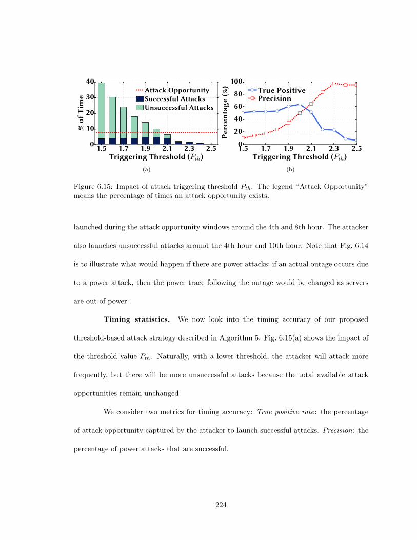
1.5 1.7 1.9 2.1 2.3 2.5Triggering Threshold (Pth)

0

10

20

30

40%

of T

ime

Attack OpportunitySuccessful AttacksUnsuccessful Attacks

(a)

1.5 1.7 1.9 2.1 2.3 2.5Triggering Threshold (Pth)

020406080

100

Perc

enta

ge (%

) True PositivePrecision

(b)

Figure 6.15: Impact of attack triggering threshold Pth. The legend “Attack Opportunity”means the percentage of times an attack opportunity exists.

launched during the attack opportunity windows around the 4th and 8th hour. The attacker

also launches unsuccessful attacks around the 4th hour and 10th hour. Note that Fig. 6.14

is to illustrate what would happen if there are power attacks; if an actual outage occurs due

to a power attack, then the power trace following the outage would be changed as servers

are out of power.

Timing statistics. We now look into the timing accuracy of our proposed

threshold-based attack strategy described in Algorithm 5. Fig. 6.15(a) shows the impact of

the threshold value Pth. Naturally, with a lower threshold, the attacker will attack more

frequently, but there will be more unsuccessful attacks because the total available attack

opportunities remain unchanged.

We consider two metrics for timing accuracy: True positive rate: the percentage

of attack opportunity captured by the attacker to launch successful attacks. Precision: the

percentage of power attacks that are successful.

224

AttackOpprtunity

TruePostive

Precision01020304050607080

Perc

enta

ge (%

) 5%10%15%20%

(a)

TierI

TierII

TierIII

TierIV

Att-acker

020406080

100120140

Nor

mal

ized

Cos

t 5%10%15%20%

(b)

Figure 6.16: Cost and impact of attacker size. x% in the legend indicates the “%” capacitysubscribed by the attacker. The tiers specify the infrastructure redundancies, from Tier-Iwith no redundancy up to Tier-IV with 2N full redundancy.

Fig. 6.15(b) shows the evaluation results under different attack thresholds Pth.

We see that the true positive rate is high when the attacker sets a lower threshold and

launches more attacks, consequently capturing more attack opportunities. Nonetheless, the

true positive rate may not always increase by lowering the threshold. This is because of

the attack strategy in Algorithm 5: with a low triggering threshold, the attacker sometimes

launches an attack prematurely and hence misses on actual attack opportunity that follows

immediately, due to the holding time Thold (to meet contractual terms and stay stealthy)

before launching another attack. When the triggering threshold is higher, the attacker is

more conservative and launches attacks only when it anticipates a sufficiently high aggregate

power by benign tenants. Thus, the precision rate increases as the threshold increases.

Impact of attacker size. For stealthiness, the attacker behaves as a benign

tenant and launches attacks by increasing its power only to its subscribed capacity (i.e.,

allowed power limit). Now, we show the impact of the attacker’s size (i.e., its subscribed

power capacity) on the detection statistics in Fig. 6.16(a). For this, we keep the benign

225

tenants’ capacity fixed and increase both the attacker and data center capacity while we also

limit the total attacks under 10% of the time. Naturally, there are more attack opportunities

if the attacker has a larger power capacity as it can more easily elevate the aggregate power

by itself to create capacity overloads. We also see that true positive rate goes down while

the precision goes up when the attacker’s power capacity becomes larger. This is because

we keep the attack time percentage fixed at 10%. As a result, even with more attack

opportunities, the attacker cannot launch more frequent attacks and hence misses more

attack opportunities (i.e., lower true positive rate) while its chance of capturing an actual

attack opportunity increases (i.e., higher precision).

Although increasing the attacker’s power capacity allows the attacker to launch

successful power attacks more easily, the attacker also needs to spend more money for its

power capacity subscription and equipment. We now study the cost impact of power attacks.

All the costs are normalized with respect to the attacker’s own cost when it subscribes 5%

of the total subscribed power capacity. We estimate the cost based on the method provided

in [76]. The results are shown in Fig. 6.16(b), demonstrating that the attacker only needs

to spend a tiny fraction (3% ∼ 16% in our study) of the total resulting losses for the data

center operator and other benign tenants. Our findings are similar to those in [76, 79]. In

practice, these normalized values correspond to tens of million dollars even for a relatively

small data center with only 1MW power capacity [76].

Comparison with other attack strategies. We now compare the timing the

power attacks with two other attack strategies.

226

5 10 15 20 25Attacks (% Time)

020406080

100120

True

Pos

itiv

e (%

)Voltage side channelPeak-aware random¢V based

(a)

5 10 15 20 25Attacks (% Time)

020406080

100120

Prec

isio

n (%

) Voltage side channelPeak-aware random¢V based

(b)

Figure 6.17: Detection statistics for different attack strategies.

• Peak-aware random attack : This strategy is an improved version of purely ran-

dom attacks and assumes that the attacker knows the probability of when attack oppor-

tunities arise per hour and allocate its total attack times to maximize its overall success

rate.

• ∆V -based attack : As described in Section 6.4.2, the attacker simply checks its

voltage reading (in RMS) for attacks.

We compare these different attack strategies in terms of their true positive rates

and precisions and show the results in Fig. 6.17. We see that our proposed approach

to timing attacks significantly outperforms the peak-aware random attack and ∆V -based

attack under our default total attack time of 10%, demonstrating the need of a precise timing

for attacks. Importantly, the voltage reading in RMS can be misleading for indicating attack

opportunities, since it is predominantly affected by the UPS output voltage VUPS rather

than the line voltage drop. Note that if the attacker attacks more frequently, the peak-aware

random attack and our approach come closer to each other in terms of the timing accuracy.

227

5 10 15 20 25Attacks (% Time)

0

20

40

60

80

100Tr

ue P

osit

ive

(%)

No restrictionWith attack strategy

(a)

0.0 0.2 0.4 0.6 0.8 1.0False Positive Rate

0.0

0.2

0.4

0.6

0.8

1.0

True

Pos

itiv

e R

ate

Voltageside channelRandom¢V based

(b)

Figure 6.18: (a) Impact of the attack strategy (e.g., Thold) on true positive rate. (b) ROCcurves showing the accuracy of detection of attack opportunities.

Nonetheless, frequent attacks are not only prohibited by contracts [72], but also will likely

be detected as suspicious behavior.

Detection accuracy. Finally, we show the effectiveness of our voltage side chan-

nel in detecting attack opportunities when the attacker can attack consecutively without

any restriction (e.g., Thold). Fig. 6.18(a) shows the true positive rates for the cases with

and without consecutive attack restrictions. The gap between the two lines indicates that

although the voltage side channel can identify attack opportunities, the holding time before

launching a new attack for stealthiness and contract constraints can result in a few miss-

ing opportunities. Fig. 6.18(b) shows that our voltage side channel can identify most of

the attack opportunities with a low false positive rate. By comparison, the random attack

strategy performs rather poorly, and the ∆-based attack is even worse because the mea-

sured voltage VN is mostly affected by the grid and UPS operations rather than tenants’

aggregate power (Section 6.4.2).

228

6.6 Extension to Three-Phase System

Our previous sections focus on a single-phase power distribution that is mostly

used in edge multi-tenant data centers. Next, we extend our study to a three-phase system

that is commonly used in large-scale multi-tenant data centers [136].

6.6.1 Three-Phase Power Distribution System

All large data centers use three-phase AC distributions to deliver power at high

efficiency [137]. Each PDU supports 40 ∼ 200kW of server power (10 ∼ 50 server racks)

and is oversubscribed by the data center operator, and each tenant typically houses at least

one full dedicated server rack. Here, we consider an attacker with multiple server racks

sharing one oversubscribed PDU with benign tenants.

There are a few different ways to connect servers in a three-phase system. We show

in Fig. 6.19 the most widely-used three-phase systems, where the servers are connected to

two of the phases with a supply voltage at 208V [137]. This is also the most complicated

case since each server/server rack is connected to and hence also affected by two different

phases.

Voltage equations in a three-phase system

As illustrated in Fig. 6.19, all the server racks connected to the same two phases

are considered as one cluster. We represent the total load of each server cluster using their

combined current Iab, Ibc, and Ica, respectively. Like in Section 6.4, because the voltage

229

𝑹𝑳 𝑽𝒂 = 𝑽𝑨 − 𝑰𝑨𝑹𝑨𝑽𝑨

𝑰𝒂𝒃,𝟏

𝑰𝒃𝒄 = 𝑰𝒃𝒄,𝟏 + ⋯ + 𝑰𝒃𝒄,𝑵𝒃𝒄

𝑰𝑨

𝑹𝑳𝑽𝑩𝑰𝑩

𝑹𝑳𝑽𝑪𝑰𝑪

𝑽𝒂𝒃

𝑰𝒂𝒃,𝑵𝒂𝒃

𝑽𝒂𝒃

𝑰𝒃𝒄,𝟏

𝑽𝒃𝒄

𝑰𝒃𝒄,𝑵𝒃𝒄

𝑽𝒃𝒄

𝑰𝒄𝒂,𝑵𝒄𝒂

𝑽𝒄𝒂

𝑰𝒄𝒂,𝟏

𝑽𝒄𝒂

𝑰𝒂𝒃 = 𝑰𝒂𝒃,𝟏 + ⋯ + 𝑰𝒂𝒃,𝑵𝒂𝒃𝑰𝒄𝒂 = 𝑰𝒄𝒂,𝟏 + ⋯ + 𝑰𝒄𝒂,𝑵𝒂𝒃

𝑰𝑨 = 𝑰𝒂𝒃 − 𝑰𝒄𝒂

𝑰𝑩 = 𝑰𝒃𝒄 − 𝑰𝒂𝒃

𝑰𝑪 = 𝑰𝒄𝒂 − 𝑰𝒃𝒄

𝑽𝒃 = 𝑽𝑩 − 𝑰𝑩𝑹𝑩

𝑽𝒄 = 𝑽𝑪 − 𝑰𝑪𝑹𝑪

3 phase UPS3 phase PDU

Current equations

Figure 6.19: 3-phase power distribution with 2-phase racks.

levels are relatively fixed (apart from some temporal variations around the nominal levels),

the current flowing into each server cluster are a good indicator of the cluster’s power usage.

A distinguishing feature of the three-phase connection is that each server rack is

connected to two phases. For each phase, the line voltage drop is affected by the current

flowing from the UPS output to the PDU. As shown in the current flow equations in

Fig. 6.19, the line current for each phase jointly depends on two server clusters.

Next, by ignoring the practically negligible line voltage drop between the PDU

and servers, we write the voltage Vab, which is supplied by the PDU to the server cluster

connected to phase A and phase B, as follows:

Vab = Va − Vb = VA − IA ·RL − (VB − IB ·RL)

= VAB −RL · (IA − IB)

= VAB −RL · (2Iab − Ibc − Ica),

230

where the last step follows from IA = Iab − Ica and IB = Ibc − Iab. Similarly we can also

write

Vbc = VBC −RL · (−Iab + 2Ibc − Ica)

Vca = VCA −RL · (−Iab − Ibc + 2Ica).

Exploiting the voltage side channel in a three-phase system

Like in the single-phase system (Section 6.4.3), we apply a high-pass filter to keep

the high-frequency voltage ripples introduced by servers’ PFC circuits, while removing the

nominal UPS output voltage frequencies and harmonics. Thus, with a high-pass filter, the

line voltage components VAB, VBC , and VCA becomes almost zero. Next, by using x to

represent the filtered version of x that only keeps frequency components around the servers’

PFC switching frequencies, we get the following relations:

Vab ≈ −RL · (2Iab − Ibc − Ica)

Vbc ≈ −RL · (−Iab + 2Ibc − Ica)

Vca ≈ −RL · (−Iab − Ibc + 2Ica).

Thus, by collecting the Vab, Vbc and Vca signals using its voltage probes, the attacker can

easily solve the above equation set and extract the high-frequency voltage ripple signals

(i.e., RL · Iab, RL · Ibc, and RL · Ica) resulting from the server clusters’ power usage.

231

Consequently, based on the approach proposed in Section 6.4, the total power usage

of each server cluster at runtime can be tracked and, when combined together, provides the

attacker with an estimate of the total PDU-level power usage for timing its attacks.

In summary, even in the most complicated three-phase power distribution system,

the benign tenants’ aggregate power usage can be extracted by the attacker through our

discovered voltage side channel for precisely timing its attacks.3

6.6.2 Evaluation Results

In Section 6.6.1, we have provided a theoretical foundation for timing power attacks

based on a voltage side channel in three-phase data centers. Next, we evaluate the timing

accuracy of the voltage side channel.

Methodology

We only have a limited access to a large multi-tenant data center with three-

phase power distribution and cannot perform experiments due to the destructing nature

of our research. Hence, we re-use the experimental results from our servers that have

three different types of power supply units. Concretely, we generate three different sets

of server power and voltage signal traces based on experiments done on our single-phase

server setup with 13 servers. To simulate a large three-phase system, we make 50 copies for

each set of trace and add 10% randomness in the power load and PFC switching frequency

for each copy. The randomness accounts for the heterogeneity in servers’ power supply

3To exploit the voltage side channel in the three-phase system illustrated in Fig. 6.19, the attacker needsto house at least one server rack in each of the three server clusters (e.g., by pretending to be three tenants)to measure cluster-wise voltage signals.

232

1.5 1.7 1.9 2.1 2.3 2.5Triggering Threshold (Pth)

01020304050

% o

f Tim

eAttack OpportunitySuccessful AttacksUnsuccessful Attacks

(a)

1.5 1.7 1.9 2.1 2.3 2.5Triggering Threshold (Pth)

020406080

100

Perc

enta

ge (%

) True PositivePrecision

(b)

Figure 6.20: Performance of voltage side channel for a three-phase 180kW system.

units and PFC switching frequencies in large systems. Hence, each set of server power and

voltage signal traces obtained through our experiments are essentially scaled up by 50 times,

and represent the power loads and voltage signals of one server cluster in the three-phase

system. Therefore, the three-phase system under consideration has 650 servers (50 times of

our single-phase experiment) in each of the three clusters.

In our simulation, the attacker has at least one server rack in each cluster and can

measure the phase-to-phase voltages (Vab, Vbc, and Vca). Since each server rack is connected

to two different phases and the phase voltages are affected by multiple server clusters (hence,

multiple power-voltage traces), we use the three-phase voltage equations in Section 6.6.1

to generate the attacker’s voltage measurements (Vab, Vbc, and Vca). Note that, while we

consider the UPS supplies a balanced three-phase voltage (i.e., VAB = VBC = VCA, with a

120◦ phase difference), the supplied voltage is eliminated from the filtered voltages (Vab, Vbc,

and Vca) which the attacker uses for extracting the server clusters’ power usage. The benign

tenants and attacker are scaled proportionally according to the composition in Table 6.1.

The resulting attack opportunities take up 7.5% of the time.

233

Results

Due to the space limitation, we only show the most important results — timing

accuracy. Specifically, Fig. 6.20 shows the true positive and precision rates under different

triggering thresholds. We see that, compared to the results in Fig. 6.15, the timing accuracy

is still reasonably good although it becomes a bit worse in the three-phase system. This is

mainly due to the randomness added in the power and PSD data when scaling up our edge

data center to a large multi-tenant data center, and also due to the fact the attacker needs

to track the power usage of three server clusters rather in a three-phase system.

Our results demonstrate the effectiveness of the voltage side channel in terms of

timing power attacks in a three-phase system. This matches with our expectation, because

the high-frequency voltage ripples generated by servers’ PFC circuits exist both in single-

phase and three-phase systems and these voltage ripple signals can be transmitted over the

data center power line network.

6.7 Defense Strategy

To mitigate the threat of well-timed power attacks, we highlight a few possible

defense strategies to degrade the voltage side channel and, more generally, against power

attacks.

DC power distribution. The PFC circuit universally built in today’s server

power supply units is the root cause for high-frequency voltage ripple signals that leak

server power usage information through the power lines (i.e., voltage side channel). Thus,

the voltage side channel may be eliminated by adopting DC power distributions where the

234

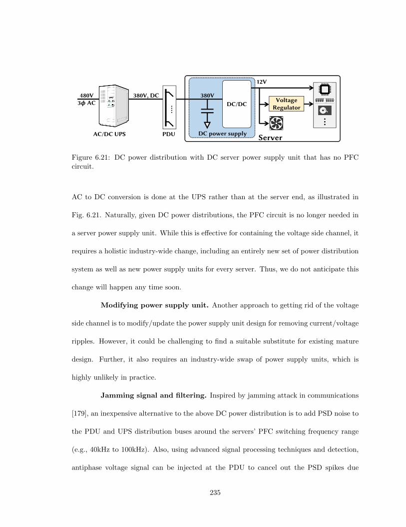
Voltage RegulatorDC/DC

DC power supplyServer

380V

12V

380V, DC

AC/DC UPS PDU

480V3𝝓 AC

Figure 6.21: DC power distribution with DC server power supply unit that has no PFCcircuit.

AC to DC conversion is done at the UPS rather than at the server end, as illustrated in

Fig. 6.21. Naturally, given DC power distributions, the PFC circuit is no longer needed in

a server power supply unit. While this is effective for containing the voltage side channel, it

requires a holistic industry-wide change, including an entirely new set of power distribution

system as well as new power supply units for every server. Thus, we do not anticipate this

change will happen any time soon.

Modifying power supply unit. Another approach to getting rid of the voltage

side channel is to modify/update the power supply unit design for removing current/voltage

ripples. However, it could be challenging to find a suitable substitute for existing mature

design. Further, it also requires an industry-wide swap of power supply units, which is

highly unlikely in practice.

Jamming signal and filtering. Inspired by jamming attack in communications

[179], an inexpensive alternative to the above DC power distribution is to add PSD noise to

the PDU and UPS distribution buses around the servers’ PFC switching frequency range

(e.g., 40kHz to 100kHz). Also, using advanced signal processing techniques and detection,

antiphase voltage signal can be injected at the PDU to cancel out the PSD spikes due

235

to server loads. Nonetheless, this may require modification/upgrade of the existing power

distribution equipment. In addition, adding jamming signals may reduce the overall power

factor of the data center and incur more power losses. Another approach is to install low-pass

filters to prevent high-frequency voltage ripple signals from entering the data center power

network but, if improperly chosen, the filters may also block legitimate communications

(e.g., for network management [20]). Moreover, in practice, filters can reduce the strengths

of high-frequency voltage ripples but not completely eliminate them.

Infrastructure reinforcement. Since power attacks target to exploit the data

center power infrastructure vulnerability (due to the common practice of oversubscription

[75, 88, 174]), another natural approach is to strengthen the infrastructure against power

attacks. Toward this end, additional investment can be made to increase the infrastructure

redundancy (e.g., installing extra UPSes), but this comes at a great capital expense and

can be especially challenging for existing data centers. Moreover, it is a passive defense:

attackers can still launch attacks to compromise the desired data center availability, though

actual outages may occur less frequently.

Attacker identification. A more proactive approach is to identify attackers

inside the data center and evict them in the first place. For example, high-granularity

monitoring and rigorous analysis of tenants’ power usage can expose a tenant’s malicious

intention. The main challenge here is to distinguish an attacker from benign tenants because

the attacker also follows all contractual limits and can behave like a benign tenant in terms

of power usage. In addition, it is even more difficult to identify an attacker if the attacker

houses its servers in different racks (pretending to be multiple different benign tenants)

236

and/or launches well-timed power attacks by increasing benign tenants’ power usage through

request flooding (instead of only relying on the attacker’s own power capacity).

To conclude, it is non-trivial to defend data center power infrastructures against

power attacks timed through a voltage side channel. Thus, effective and inexpensive defense

strategies are one of the future research directions in data center power security [49,76,79,

93,180].

6.8 Related work

Power capping. Power infrastructure oversubscription has been extensively ap-

plied for increasing capacity utilization. To handle the ensuing possible capacity over-

loads, power capping has been proposed, such as throttling CPU [45,174], rerouting work-

loads [169], and partially offloading power demand to energy storages [56,123,168]. However,

these techniques cannot be applied in multi-tenant data centers due to the operator’s lack of

control over tenants’ servers. While [75] proposes a market approach for handling capacity

overloads in multi-tenant data centers, the market assumes that all tenants are benign and,

more crucially, broadcasts the data center’s high-power periods (i.e., attack opportunities)

unsuspectingly to all tenants including possibly an attacker.

Data center security. Securing data centers in the cyber domain has been widely

studied to defend against attacks such as DDoS [111, 181], and data stealing and privacy

breach [61, 84, 114, 187]. Meanwhile, an emerging attack vector has been malicious power

loads that target the oversubscribed data center power infrastructures to create outages.

Studies [49,50,93,180] investigate how VMs can be used to create power overloads in cloud

237

data centers. Another two recent works [76, 79] exploit physical side channels in multi-

tenant data centers to time power attacks. In contrast, we propose a novel voltage side

channel that is not sensitive to external disturbances, does not require any offline modeling,

does not suffer from time lag, and can accurately track power shapes of multiple tenants. A

detailed comparison between our work and these related studies is provided in Sections 6.2.3

and 6.3.

Power management in multi-tenant data centers. Finally, our work furthers

the growing literature on power management in multi-tenant data centers. While the recent

studies have predominantly focused on improving power/energy efficiency and reducing

cost [73, 75, 78, 117, 165], we focus on the complementary aspect of its physical security

against devastating power attacks.

6.9 Conclusion

In this paper, we consider the emerging threat of power attacks in multi-tenant

data centers. We discover a novel voltage side channel resulting from the high-frequency

switching operation in the PFC circuit of a server’s power supply unit. The voltage side

channel can accurately track benign tenants’ power usage and helps the attacker precisely

time its power attacks. Our experiment results on a prototype edge data center show that

an attacker can effectively use the voltage side channel to utilize 64% of the power attack

opportunities. We also highlight a few defense strategies and extend to more complex

three-phase power distribution systems.

238

Chapter 7

Conclusions

This dissertation summarizes the major novel contributions made toward the ef-

ficient and secure operation of multi-tenant colocation data centers. Multi-tenant data

centers are very important yet underexplored segment of the data center industry. In this

dissertation, I presented my work on the two important expect of data center operation -

efficiency and security.

The key challenge addressed here toward the efficient operation of multi-tenant

data centers is the lack of coordination between the operator and tenants. Since the operator

does not have any control or knowledge of workload running in the tenants’ servers, many

efficient operation techniques that require a centralized control cannot be applied directly

to multi-tenant data centers. Further, due to the predominant flat-rate pricing structure,

the tenants do not have any incentive for efficient operation. In my research, I bridged

the coordination gap by proposing markets where the operator passes the incentive to the

tenants as rewards for their efficient server management. I also proposed a spot capacity

239

market where the operator sells unused infrastructure capacity to tenants for a temporary

performance boost. Using this market the operator can increase the utilization of the

expensive infrastructure while cost-conscious tenants can conservatively subscribe capacity

and rely on the spot market to acquire additional capacity in the rare time when its capacity

is exhausted.

On the secure data center operation, I focused on data center physical security. I

showed that the widely used oversubscription of infrastructure capacity makes data center

vulnerable to power attacks. A power attack on data center aims at creating overload by

injecting malicious power load leading to data center outage. However, exploring the power

attack vulnerability due to oversubscription is not trivial and require careful timing since the

attack opportunities (i.e., when an overload can be created) are intermittent. Specifically,

an attacker needs to estimate the data center power consumption (i.e., the benign tenants’

power consumption). However, no tenants (and hence the attacker) have no access power

meters in the data center. Nonetheless, I identified the existence of physical side channels

in multi-tenant data centers that leak other tenants’ server power consumption. I showed

that there exists a thermal side channel due to server heat recirculation, an acoustic side

channel due to server fan noise, and a voltage side channel due to Ohm’s Law. I showed

that an attacker can launch stealthy power attacks using these side channels and cause huge

financial loss to data center operator and tenants. I also identified and presented possible

countermeasures against such power attacks.

240

Bibliography

[1] “Wikimedia’s data center search ends with cyrusone,”http://www.datacenterknowledge.com/archives/2014/05/05/wikimedias-data-center-search-ends-cyrusone/.

[2] “Google transparency report,” http://www.google.com/transparencyreport/traffic/explorer.

[3] “Colocation market - worldwide market forecast and analysis (2013 - 2018),” http://www.marketsandmarkets.com/ResearchInsight/colocation.asp.

[4] “California ISO open access same-time information system,” http://www.oasis.caiso.com.

[5] http://www.pge.com/.

[6] “Colocation market by solutions, end users, verticals & region - worldwide marketforecast and analysis (2013 - 2018),” http://www.researchandmarkets.com/research/pxndbm/colocation market.

[7] “Historical Weather,” http://www.wunderground.com/.

[8] 365DataCenters, “Master services agreement,” http://www.365datacenters.com/master-services-agreement/.

[9] Akamai, “Environmental sustainability policy,” http://www.akamai.com/html/sustainability/our commitment.html.

[10] Amazon, “EC2 spot instances,” http://aws.amazon.com/ec2/spot-instances/.

[11] Amazon, https://aws.amazon.com/about-aws/globalinfrastructure/.

[12] APC, “Metered-by-outlet with switching rack PDU,” http://goo.gl/qvE8NV.

[13] Apple, “Environmental responsibility report,” 2014, http://images.apple.com/environment/reports/docs/Apple Environmental Responsibility Report 2014.pdf.

[14] ——, “Environmental responsibility report,” 2016.

241

[15] Autodesk, “CFD simulations of data centers,” http://auworkshop.autodesk.com/library/cfd-aec/cfd-simulations-data-centers.

[16] ——, “Computational fluid dynamics,” http://www.autodesk.com/products/cfd/overview.

[17] L. A. Barroso, J. Clidaras, and U. Hoelzle, The Datacenter as a Computer: AnIntroduction to the Design of Warehouse-Scale Machines. Morgan & Claypool, 2013.

[18] H. W. Beaty and D. G. Fink, Standard handbook for electrical engineers. McGraw-Hill New York, 2007.

[19] CBRE, “Q4 2013: National data center market update,” 2013.

[20] L. Chen, J. Xia, B. Yi, and K. Chen, “Powerman: An out-of-band managementnetwork for datacenters using power line communication,” in NSDI, 2018.

[21] N. Chen, X. Ren, S. Ren, and A. Wierman, “Greening multi-tenant data centerdemand response,” in IFIP Performance, 2015.

[22] CNN, “Delta: 5-hour computer outage cost us $150 million,” Sep. 07 2016 (http://money.cnn.com/2016/09/07/technology/delta-computer-outage-cost/).

[23] Colocation America, “Data center standards (Tiers I-IV),” 2017, https://www.colocationamerica.com/data-center/tier-standards-overview.htm.

[24] CyrusOne, “Colocation: The logical home for the cloud,” 2012, http://resources.idgenterprise.com/original/AST-0050996 CyrusOne wp0926.pdf.

[25] DatacenterKnowledge, “Can edgeconnex disrupt incumbent data centerproviders?” http://www.datacenterknowledge.com/archives/2016/09/13/can-edgeconnex-disrupt-incumbent-data-center-providers/.

[26] ——, “Vapor IO to sell data center colocation services at celltowers,” http://www.datacenterknowledge.com/archives/2017/06/21/vapor-io-to-sell-data-center-colocation-services-at-cell-towers.

[27] DatacenterMap, “Colocation USA,” http://www.datacentermap.com/usa/.

[28] C. E. P. Dell, “Dell enterprise acoustics,” 2011, https://www.dell.com/downloads/global/products/pedge/en/acoustical-education-dell-enterprise-white-paper.pdf.

[29] Dell Product Group - Server Engineering, “Cooling options for thermal control indell poweredge servers,” 2015, http://en.community.dell.com/techcenter/extras/m/white papers/20441060/download.

[30] J. dePreaux, “Wholesale and retail data centers - North America and Europe - 2013,”IHS, Jul. 2013, https://technology.ihs.com/api/binary/492570.

[31] R. A. Dines, “Build or buy? the economics of data center facilities,” in ForresterResearch, 2011, http://www.io.com/wp-content/uploads/2013/04/build-or-buy.pdf.

242

[32] EdgeConnex, http://www.edgeconnex.com/.

[33] J. Eggert and E. Korner, “Sparse coding and NMF,” in IJCNN, 2004.

[34] Emerson Network Power, “Addressing the leading root causes of downtime,” 2013,http://goo.gl/b14XaF.

[35] ——, “Liebert DSE precision cooling system,” http://www.emersonnetworkpower.com/documentation/en-us/products/precisioncooling/largeroomcooling/documents/sl-18927.pdf.

[36] Enaxis Consulting, “Pricing data center co-location services,” 2009, http://enaxisconsulting.com.

[37] Energy Star, “Computers specification version 7.0,” 2018, https://www.energystar.gov/products/spec/computers specification version 7 0 pd.

[38] Equinix, www.equinix.com.

[39] T. Evans, “Fundamental principles of air conditioners for information technology,”Schneider Electric WHite Paper #57, March 2015.

[40] ——, “The different technologies for cooling data centers,” http://www.apcmedia.com/salestools/VAVR-5UDTU5/VAVR-5UDTU5 R2 EN.pdf.

[41] S. Fan, S. M. Zahedi, and B. C. Lee, “The computational sprinting game,” in ASP-LOS, 2016.

[42] X. Fan, W.-D. Weber, and L. A. Barroso, “Power provisioning for a warehouse-sizedcomputer,” in ISCA, 2007.

[43] D. G. Feitelson, D. Tsafrir, and D. Krakov, “Experience with using the parallel work-loads archive,” Journal of Parallel and Distributed Computing, vol. 74, no. 10, pp.2967–2982, 2014.

[44] M. Ferdman, A. Adileh, O. Kocberber, S. Volos, M. Alisafaee, D. Jevdjic, C. Kaynak,A. D. Popescu, A. Ailamaki, and B. Falsafi, “Clearing the clouds: A study of emergingscale-out workloads on modern hardware,” in ASPLOS, 2012.

[45] X. Fu, X. Wang, and C. Lefurgy, “How much power oversubscription is safe andallowed in data centers,” in ICAC, 2011.

[46] A. Gandhi, M. Harchol-Balter, R. Raghunathan, and M. A. Kozuch, “Autoscale: Dy-namic, robust capacity management for multi-tier data centers,” ACM Trans. Com-put. Syst., vol. 30, no. 4, pp. 14:1–14:26, Nov. 2012.

[47] P. X. Gao, A. R. Curtis, B. Wong, and S. Keshav, “It’s not easy being green,”SIGCOMM Comput. Commun. Rev., 2012.

[48] X. Gao, Z. Gu, M. Kayaalp, D. Pendarakis, and H. Wang, “ContainerLeaks: Emergingsecurity threats of information leakages in container clouds,” in DSN, 2017.

243

[49] ——, “ContainerLeaks: Emerging security threats of information leakages in containerclouds,” in DSN, 2017.

[50] X. Gao, Z. Xu, H. Wang, L. Li, and X. Wang, “Reduced cooling redundancy: A newsecurity vulnerability in a hot data center,” in NDSS, 2018.

[51] J. Glanz, “Power, pollution and the internet,” in The New York Times, Sep. 22, 2012.

[52] I. Goiri, W. Katsak, K. Le, T. D. Nguyen, and R. Bianchini, “Parasol and greenswitch:managing datacenters powered by renewable energy,” in ASPLOS, 2013.

[53] Google, “Cluster workload traces,” https://code.google.com/p/googleclusterdata/.

[54] ——, “Google’s Data Center Efficiency,” http://www.google.com/about/datacenters/.

[55] S. Govindan, J. Choi, B. Urgaonkar, and A. Sivasubramaniam, “Statistical profiling-based techniques for effective power provisioning in data centers,” in EuroSys, 2009.

[56] S. Govindan, D. Wang, A. Sivasubramaniam, and B. Urgaonkar, “Leveraging storedenergy for handling power emergencies in aggressively provisioned datacenters,” inASPLOS, 2012.

[57] ——, “Aggressive datacenter power provisioning with batteries,” ACM Trans. Com-put. Syst., vol. 31, no. 1, pp. 2:1–2:31, Feb. 2013.

[58] A. Greenberg, J. Hamilton, D. A. Maltz, and P. Patel, “The cost of a cloud: Researchproblems in data center networks,” SIGCOMM Comput. Commun. Rev., vol. 39,no. 1, Dec. 2008.

[59] B. Guenter, N. Jain, and C. Williams, “Managing cost, performance and reliabilitytradeoffs for energy-aware server provisioning,” in INFOCOM, 2011.

[60] M. Guevara, B. Lubin, and B. C. Lee, “Navigating heterogeneous processors withmarket mechanisms,” in HPCA, 2013.

[61] M. Guri, M. Monitz, Y. Mirski, and Y. Elovici, “Bitwhisper: Covert signaling chan-nel between air-gapped computers using thermal manipulations,” in IEEE ComputerSecurity Foundations Symposium, 2015.

[62] M. Guri, Y. A. Solewicz, A. Daidakulov, and Y. Elovici, “Fansmitter: Acoustic dataexfiltration from (speakerless) air-gapped computers,” CoRR, vol. abs/1606.05915,2016. [Online]. Available: http://arxiv.org/abs/1606.05915

[63] S. Ha, S. Sen, C. Joe-Wong, Y. Im, and M. Chiang, “Tube: time-dependent pricingfor mobile data,” in SIGCOMM, 2012.

[64] S. Haykin, “Cognitive radio: Brain-empowered wireless communications,” IEEE J.Sel.A. Commun., vol. 23, no. 2, pp. 201–220, Sep. 2006.

244

[65] S. S. Haykin, Kalman Filtering and Neural Networks. New York, NY, USA: JohnWiley & Sons, Inc., 2001.

[66] Hornbaker Group, “Determining kilowatt capacity ofdata center space,” http://www.hornbakergroup.com/pdf/Considerations-when-leasing-Data-Center-space-by-the-kilowatt.pdf.

[67] P. O. Hoyer, “Non-negative sparse coding,” in NNSP, 2002.

[68] R. Huang, T. Huang, R. Gadh, and N. Li, “Solar generation prediction using the armamodel in a laboratory-level micro-grid,” in SmartGridComm, 2012, pp. 528–533.

[69] IECEE, “IEC 61000-3-2:2018: Electromagnetic compatibility (EMC) - part 3-2,” http://www.onsemi.com/pub/Collateral/HBD853-D.PDF.

[70] Infineon Technologies AG, “PFC boost converter design guide,” https://goo.gl/MePNFj.

[71] Intel, “Rack scale design: Architectural requirement specifications,” Document Num-ber: 332937-003, Jul. 2016.

[72] Internap, “Colocation services and SLA,” http://www.internap.com/internap/wp-content/uploads/2014/06/Attachment-3-Colocation-Services-SLA.pdf.

[73] M. A. Islam, H. Mahmud, S. Ren, and X. Wang, “Paying to save: Reducing cost ofcolocation data center via rewards,” in HPCA, 2015.

[74] M. A. Islam, S. Ren, and X. Wang, “GreenColo: A novel incentive mechanism forminimizing carbon footprint in colocation data center,” in IGCC, 2014.

[75] M. A. Islam, X. Ren, S. Ren, A. Wierman, and X. Wang, “A market approach forhandling power emergencies in multi-tenant data center,” in HPCA, 2016.

[76] M. A. Islam, S. Ren, and A. Wierman, “Exploiting a thermal side channel for powerattacks in multi-tenant data centers,” in CCS, 2017.

[77] ——, “A first look at power attacks in multi-tenant data centers,” in GreenMetrics,2017.

[78] M. A. Islam, X. Ren, S. Ren, and A. Wierman, “A spot capacity market to increasepower infrastructure utilization in multi-tenant data centers,” in HPCA, 2018.

[79] M. A. Islam, L. Yang, K. Ranganath, and S. Ren, “Why some like it loud: Tim-ing power attacks in multi-tenant data centers using an acoustic side channel,” inSIGMETRICS, 2018.

[80] R. Johari and J. N. Tsitsiklis, “Parameterized supply function bidding: Equilibriumand efficiency,” Oper. Res., vol. 59, no. 5, pp. 1079–1089, Sep. 2011.

[81] M. Jonas, R. R. Gilbert, J. Ferguson, G. Varsamopoulos, and S. K. Gupta, “A tran-sient model for data center thermal prediction,” in IGCC, 2012.

245

[82] D. Kennedy, “Optimizing capacity and efficiency in a diverse and variable load envi-ronment,” TATE, August 2010.

[83] B. Kleyman, “Knowing when dedicated data centers are just not enough,” Data Cen-ter Frontier, December 2015.

[84] P. C. Kocher, J. Jaffe, and B. Jun, “Differential power analysis,” in CRYPTO, 1999.

[85] M. Korolov, “Data center infrastructure, the often-overlooked security risk,” in Dat-aCenterKnowledge, April 2018.

[86] H. Laurberg and L. K. Hansen, “On Affine Non-negative Matrix Factorization,” inICASSP, 2007.

[87] K. Le, R. Bianchini, J. Zhang, Y. Jaluria, J. Meng, and T. D. Nguyen, “Reducingelectricity cost through virtual machine placement in high performance computingclouds,” in SuperComputing, 2011.

[88] Leagle.com (Case No. 5:13-cv-03093-PSG), “Layton v. Terremark North America,LLC,” June 2014.

[89] D. D. Lee and H. S. Seung, “Learning the parts of objects by non-negative matrixfactorization,” Nature, vol. 401, no. 6755, p. 788, 1999.

[90] ——, “Algorithms for non-negative matrix factorization,” in NIPS, 2001.

[91] S. Lee, R. Urgaonkar, R. Sitaraman, and P. Shenoy, “Cost minimization using renew-able cooling and thermal energy storage in CDNs,” in ICAC, 2015.

[92] C. Li, Y. Hu, L. Liu, J. Gu, M. Song, X. Liang, J. Yuan, and T. Li, “Towardssustainable in-situ server systems in the big data era,” in ISCA, 2015.

[93] C. Li, Z. Wang, X. Hou, H. Chen, X. Liang, and M. Guo, “Power attack defense:Securing battery-backed data centers,” in ISCA, 2016.

[94] C. Li, R. Zhou, and T. Li, “Enabling distributed generation powered sustainablehigh-performance data center,” in HPCA, 2013.

[95] L. Li, W. Zheng, X. D. Wang, and X. Wang, “Coordinating liquid and free air coolingwith workload allocation for data center power minimization,” in ICAC, 2014.

[96] S. Li, T. Abdelzaher, and M. Yuan, “Tapa: Temperature aware power allocation indata center with map-reduce,” in IGCC, 2011.

[97] M. Lin, A. Wierman, L. L. H. Andrew, and E. Thereska, “Dynamic right-sizing forpower-proportional data centers,” in INFOCOM, 2011.

[98] H. Liu, “A measurement study of server utilization in public clouds,” in DASC, 2011.

246

[99] L. Liu, C. Li, H. Sun, Y. Hu, J. Gu, T. Li, J. Xin, and N. Zheng, “Heb: Deploying andmanaging hybrid energy buffers for improving datacenter efficiency and economy,” inISCA, 2015.

[100] Z. Liu, Y. Chen, C. Bash, A. Wierman, D. Gmach, Z. Wang, M. Marwah, andC. Hyser, “Renewable and cooling aware workload management for sustainable datacenters,” in SIGMETRICS, 2012.

[101] Z. Liu, M. Lin, A. Wierman, S. H. Low, and L. L. Andrew, “Greening geographicalload balancing,” in SIGMETRICS, 2011.

[102] Z. Liu, I. Liu, S. Low, and A. Wierman, “Pricing data center demand response,” inSIGMETRICS, 2014.

[103] Z. Liu, A. Wierman, Y. Chen, B. Razon, and N. Chen, “Data center demand re-sponse: avoiding the coincident peak via workload shifting and local generation,” inSIGMETRICS, 2013.

[104] D. Lo, L. Cheng, R. Govindaraju, L. A. Barroso, and C. Kozyrakis, “Towards energyproportionality for large-scale latency-critical workloads,” in ISCA, 2014.

[105] Y. Low, J. Gonzalez, A. Kyrola, D. Bickson, C. Guestrin, and J. M. Hellerstein,“Graphlab: A new parallel framework for machine learning,” in Uncertainty in Arti-ficial Intelligence (UAI), 2010.

[106] R. H. Lyon and A. E. Bergles, “Noise and cooling in electronics packages,” IEEETransactions on Components and Packaging Technologies, vol. 29, no. 3, pp. 535–542, 2006.

[107] I. Manousakis, I. n. Goiri, S. Sankar, T. D. Nguyen, and R. Bianchini, “Coolprovision:Underprovisioning datacenter cooling,” in SoCC, 2015.

[108] R. McFarlane, “Controversial hot aisle containment practices,” Techtarget, June 2014.

[109] D. Meisner, C. M. Sadler, L. A. Barroso, W.-D. Weber, and T. F. Wenisch, “Powermanagement of online data-intensive services,” in ISCA, 2011.

[110] Microchip, “Switch mode power supply (SMPS) topologies,” http://ww1.microchip.com/downloads/en/AppNotes/01114A.pdf.

[111] J. Mirkovic and P. Reiher, “A taxonomy of DDoS attack and ddos defense mecha-nisms,” SIGCOMM Comput. Commun. Rev., vol. 34, no. 2, pp. 39–53, Apr. 2004.

[112] Mohammad A. Islam, “Server noise trace,” https://sites.google.com/site/mdatiqislam1985/server noise trace.

[113] H. Mohsenian-Rad, V. W. S. Wong, J. Jatskevich, R. Schober, and A. Leon-Garcia,“Autonomous demand side management based on game-theoretic energy consumptionscheduling for the future smart grid,” IEEE Trans. Smart Grid, vol. 1, no. 3, pp. 320–331, Dec. 2010.

247

[114] S.-J. Moon, V. Sekar, and M. K. Reiter, “Nomad: Mitigating arbitrary cloud sidechannels via provider-assisted migration,” in CCS, 2015.

[115] J. Moore, J. Chase, P. Ranganathan, and R. Sharma, “Making scheduling “cool”:Temperature-aware workload placement in data centers,” in USENIX ATC, 2005.

[116] D. L. Moss, “Dynamic control optimizes facility airflow delivery,” Dell White Paper,March 2012.

[117] N. Nasiriani, C. Wang, G. Kesidis, B. Urgaonkar, L. Y. Chen, and R. Birke, “On fairattribution of costs under peak-based pricing to cloud tenants,” in MASCOTS, 2015.

[118] NENS, “How to reduce the noise from your servers,” 2017, https://www.nens.com/reduce-noise-servers/.

[119] J. Novet, “Colocation providers, customers trade tips on energy savings,” Nov. 2013,http://www.datacenterknowledge.com/.

[120] NRDC, “Scaling up energy efficiency across the data center industry: Evaluating keydrivers and barriers,” Issue Paper, Aug. 2014.

[121] On Semiconductor, “Power factor correction (PFC) handbook,” http://www.onsemi.com/pub/Collateral/HBD853-D.PDF.

[122] P. Paatero and U. Tapper, “Positive matrix factorization: A non-negative factormodel with optimal utilization of error estimates of data values,” Environmetrics,vol. 5, no. 2, pp. 111–126, 1994.

[123] D. S. Palasamudram, R. K. Sitaraman, B. Urgaonkar, and R. Urgaonkar, “Usingbatteries to reduce the power costs of internet-scale distributed networks,” in SoCC,2012.

[124] Parallel Workloads Archive, http://www.cs.huji.ac.il/labs/parallel/workload/.

[125] S. V. Patankar, “Airflow and cooling in a data center,” Journal of Heat Transfer, vol.132, no. 7, p. 073001, July 2010.

[126] S. Pelley, D. Meisner, P. Zandevakili, T. F. Wenisch, and J. Underwood, “Powerrouting: Dynamic power provisioning in the data center,” in ASPLOS, 2010.

[127] Ponemon Institute, “2016 cost of data center outages,” 2016, http://goo.gl/6mBFTV.

[128] Q. Pu, G. Ananthanarayanan, P. Bodik, S. Kandula, A. Akella, P. Bahl, and I. Stoica,“Low latency geo-distributed data analytics,” in SIGCOMM, 2015.

[129] A. Qouneh, C. Li, and T. Li, “A quantitative analysis of cooling power in container-based data centers,” in IISWC, 2011.

[130] A. Qureshi, R. Weber, H. Balakrishnan, J. Guttag, and B. Maggs, “Cutting theelectric bill for internet-scale systems,” in SIGCOMM, 2009.

248

[131] A. Raghavan, Y. Luo, A. Chandawalla, M. Papaefthymiou, K. P. Pipe, T. F. Wenisch,and M. M. K. Martin, “Computational sprinting,” in HPCA, 2012.

[132] L. Rao, X. Liu, L. Xie, and W. Liu, “Reducing electricity cost: Optimization ofdistributed internet data centers in a multi-electricity-market environment,” in IN-FOCOM, 2010.

[133] Raritan, “Data center power overload protection,” White Paper, 2016.

[134] N. Rasmussen, “Overload protection in a dual-corded data center environment,” APCWhite Paper 206, 2014.

[135] ——, “Guidelines for specification of data center power density,” Schneider ElectricWhite Paper 120.

[136] ——, “High-efficiency ac power distribution for data centers,” Schneider ElectricWhite Paper Library, http://www.apc.com/salestools/nran-6cn8pk/nran-6cn8pk r2en.pdf.

[137] ——, “Efficiency and other benefits of 208 volt over 120 volt input for it equip-ment,” Schneider Electric White Paper Library, http://www.apc.com/salestools/SADE-5TNQZ7/SADE-5TNQZ7 R3 EN.pdf.

[138] S. Ren and M. A. Islam, “Colocation demand response: Why do I turn off my servers?”in ICAC, 2014.

[139] Reuters, “British Airways $100M outage was caused by worker pulling wrong plug,”Jun. 02 2017.

[140] M. Sedaghat, E. Wadbro, J. Wilkes, S. D. Luna, O. Seleznjev, and E. Elmroth,“Diehard: Reliable scheduling to survive correlated failures in cloud data centers,” inCCGrid, 2016.

[141] N. Sharma, P. Sharma, D. Irwin, and P. Shenoy, “Predicting solar generation fromweather forecasts using machine learning,” in SmartGridComm, 2011, pp. 528–533.

[142] M. Sheppy, C. Lobato, O. V. Geet, S. Pless, K. Donovan, and C. Powers, “Reducingdata center loads for a large-scale, low-energy office building: NREL’s research supportfacility,” Nov. 2011.

[143] M. Skach, M. Arora, C.-H. Hsu, Q. Li, D. Tullsen, L. Tang, and J. Mars, “Thermaltime shifting: Leveraging phase change materials to reduce cooling costs in warehouse-scale computers,” in ISCA, 2015.

[144] R. A. Steinbrecher and R. Schmidt, “Data center environments: Ashrae’s evolvingthermal guidelines,” ASHRAE Technical Feature, pp. 42–49, December 2011.

[145] STEM, “Demand charges,” 2014, http://www.stem.com/resources/learning.

249

[146] Y. Sverdlik, “Silicon valley: A landlord’s data center market,” in DataCenterKnowl-owedge, February 2015.

[147] ——, “Google to build and lease data centers in big cloud expansion,” in DataCen-terKnowledge, April 2016.

[148] ——, “Microsoft moves away from data center containers,” in DataCenterKnowledge,April 2016.

[149] ——, “Verizon data center outage delays JetBlue flights,” in DataCenterKnowledge,January 2016.

[150] J. Szefer, P. Jamkhedkar, Y.-Y. Chen, and R. B. Lee, “Physical attack protection withhuman-secure virtualization in data centers,” in Dependable Systems and NetworksWorkshops (DSN-W), 2012.

[151] Q. Tang, S. K. S. Gupta, and G. Varsamopoulos, “Energy-efficient thermal-awaretask scheduling for homogeneous high-performance computing data centers: A cyber-physical approach,” IEEE Trans. Parallel Distrib. Syst., vol. 19, no. 11, pp. 1458–1472,Nov. 2008.

[152] Telecommunications Industry Association, “Data center standards overview,” TIA942, 2005 (amended in 2014).

[153] The New York Blower Company, “Fan laws and system curves,” http://www.nyb.com/pdf/Catalog/Letters/EL-02.pdf.

[154] E. Thereska, A. Donnelly, and D. Narayanan, “Sierra: a power-proportional, dis-tributed storage system,” Tech. Rep. MSR-TR-2009-153, 2009.

[155] W. P. Turner, J. H. Seader, and K. G. Brill, “Tier classifications define site infras-tructure performance,” Uptime Institute White Paper 17, 2006.

[156] United States District Court, “Layton v. Terremark North America, LLC,” 2014.

[157] Uptime Institute, “Data center industry survey,” 2014.

[158] ——, “Data center industry survey,” 2016.

[159] ——, “Tier certifications,” https://uptimeinstitute.com/TierCertification/.

[160] G. Urdaneta, G. Pierre, and M. Van Steen, “Wikipedia workload analysis for decen-tralized hosting,” Computer Networks, 2009.

[161] U.S. EPA, “Utility guide for designing incentive programs focused on data centerefficiency measures,” Nov. 2012.

[162] Vapor IO, “The edge data center,” https://www.vapor.io/.

[163] Verizon Terremark, “Pricing plan,” http://www.terremark.com/landing-pages/colocation-promo-group3/.

250

[164] Vertiv, “Flexible, efficient scalable UPS for room or row-based applications,” LibertyAPS Product Brocure, 2016.

[165] C. Wang, N. Nasiriani, G. Kesidis, B. Urgaonkar, Q. Wang, L. Y. Chen, A. Gupta,and R. Birke, “Recouping energy costs from cloud tenants: Tenant demand responseaware pricing design,” in eEnergy, 2015.

[166] C. Wang, B. Urgaonkar, Q. Wang, and G. Kesidis, “A hierarchical demand responseframework for data center power cost optimization under real-world electricity pric-ing,” in MASCOTS, 2014.

[167] D. Wang, C. Ren, and A. Sivasubramaniam, “Virtualizing power distribution in dat-acenters,” in ISCA, 2013.

[168] D. Wang, C. Ren, A. Sivasubramaniam, B. Urgaonkar, and H. Fathy, “Energy storagein datacenters: what, where, and how much?” in SIGMETRICS, 2012.

[169] G. Wang, S. Wang, B. Luo, W. Shi, Y. Zhu, W. Yang, D. Hu, L. Huang, X. Jin, andW. Xu, “Increasing large-scale data center capacity by statistical power control,” inEuroSys, 2016.

[170] X. Wang and J. F. Martinez, “ReBudget: Trading off efficiency vs. fairness in market-based multicore resource allocation via runtime budget reassignment,” in ASPLOS,2016.

[171] Z. Wang, C. Bash, N. Tolia, M. Marwah, X. Zhu, and P. Ranganathan, “Optimalfan speed control for thermal management of servers,” in InterPACK, Berkeley, CA,USA, 2009.

[172] Z. Wang, A. McReynolds, C. Felix, C. Bash, C. Hoover, M. Beitelmal, and R. Shih,“Kratos: Automated management of cooling capacity in data centers with adaptivevent tiles,” in ASME International Mechanical Engineering Congress and Exposition,2009.

[173] Q. Wu, “Making facebook’s software infrastructure more energy efficient with au-toscale,” 2014.

[174] Q. Wu, Q. Deng, L. Ganesh, C.-H. R. Hsu, Y. Jin, S. Kumar, B. Li, J. Meza, andY. J. Song, “Dynamo: Facebook’s data center-wide power management system,” inISCA, 2016.

[175] Z. Wu, M. Butkiewicz, D. Perkins, E. Katz-Bassett, and H. V. Madhyastha,“Spanstore: Cost-effective geo-replicated storage spanning multiple cloud services,”in SOSP, 2013.

[176] H. Xu, C. Feng, and B. Li, “Temperature aware workload management in geo-distributed datacenters,” in ICAC, 2013.

[177] H. Xu and B. Li, “Dynamic cloud pricing for revenue maximization,” IEEE Trans.Cloud Comput., vol. 1, no. 2, pp. 158–171, Jul. 2013.

251

[178] ——, “Reducing electricity demand charge for data centers with partial execution,”in e-Energy, 2014.

[179] W. Xu, W. Trappe, and Y. Zhang, “Anti-jamming timing channels for wireless net-works,” in WiSec, 2008.

[180] Z. Xu, H. Wang, Z. Xu, and X. Wang, “Power attack: An increasing threat to datacenters,” in NDSS, 2014.

[181] S. Yu, Y. Tian, S. Guo, and D. O. Wu, “Can we beat ddos attacks in clouds?”IEEE Transactions on Parallel and Distributed Systems, vol. 25, no. 9, pp. 2245–2254, September 2014.

[182] R. Zafarani and H. Liu, “Social computing data repository at ASU,” 2009. [Online].Available: http://socialcomputing.asu.edu

[183] V. Zarzoso and A. Nandi, “Blind source separation,” in Blind Estimation UsingHigher-Order Statistics. Springer, 1999, pp. 167–252.

[184] J. Zhang, J. Shao, P. Xu, F. C. Lee, and M. M. Jovanovic, “Evaluation of inputcurrent in the critical mode boost pfc converter for distributed power systems,” inIEEE Applied Power Electronics Conference and Exposition.

[185] L. Zhang, S. Ren, C. Wu, and Z. Li, “A truthful incentive mechanism for emergencydemand response in colocation data centers,” in INFOCOM, 2015.

[186] Y. Zhang, Y. Wang, and X. Wang, “Greenware: Greening cloud-scale data centers tomaximize the use of renewable energy,” in Middleware, 2011.

[187] Y. Zhang, A. Juels, M. K. Reiter, and T. Ristenpart, “Cross-vm side channels andtheir use to extract private keys,” in CCS, 2012.

[188] W. Zheng, K. Ma, and X. Wang, “Exploiting thermal energy storage to reduce datacenter capital and operating expenses,” in HPCA, 2014.

[189] W. Zheng and X. Wang, “Data center sprinting: Enabling computational sprintingat the data center level,” in ICDCS, 2015.

[190] H. Zhong, L. Xie, and Q. Xia, “Coupon incentive-based demand response: Theoryand case study,” IEEE Trans. Power Systems, vol. 28, no. 2, pp. 1266–1276, May2013.

252