Benefits and costs of liquidity regulation - European Central ...

Working Paper Series Benefits and costs of liquidity regulation

Discussion Papers

Marie Hoerova, Caterina Mendicino, Kalin Nikolov, Glenn Schepens,

Skander Van den Heuvel

Disclaimer: This paper should not be reported as representing the views of the European Central Bank (ECB). The views expressed are those of the authors and do not necessarily reflect those of the ECB.

No 2169 / July 2018

Discussion papers Discussion papers are research-based papers on policy relevant topics. They are singled out from standard Working Papers in that they offer a broader and more balanced perspective. While being partly based on original research, they place the analysis in the wider context of the literature on the topic. They also consider explicitly the policy perspective, with a view to develop a number of key policy messages. Their format offers the advantage that alternative analyses and perspectives can be combined, including theoretical and empirical work. Discussion papers are written in a style that is more broadly accessible compared to standard Working Papers. They are light on formulas and regression tables, at least in the main text. The selection and distribution of discussion papers are subject to the approval of the Director General of the Directorate General Research.

ECB Working Paper Series No 2169 / July 2018 1

Abstract

This paper investigates the costs and benefits of liquidity regulation. We find that

liquidity tools are beneficial but cannot completely remove the need for Lender of

Last Resort (LOLR) interventions by the central bank. Full compliance with current

Liquidity Coverage Ratio (LCR) and Net Stable Funding Ratio (NSFR) rules would

have reduced banks’ reliance on publicly provided liquidity during the global financial

crisis without removing such assistance altogether. The paper also investigates the

output costs of introducing the LCR and NSFR using two macro-financial models. We

find these costs to be modest.

JEL Classification Codes: E44, E58; G21; G28

Keywords: Banking; Liquidity regulation; Capital requirements; Central bank;

Lender-of-last-resort


Non-Technical Summary

The prudential regulation of banks has changed dramatically since the global financial

crisis. While the Basel III reforms of the quantity and quality of bank capital have been the

most prominent, a number of other policy initiatives have also been pursued with the aim of

making banks safer and avoiding future crises. In this paper, we focus on one of these

initiatives - a new regime of bank liquidity regulation - and examine if and how it can be

beneficial for financial stability, at what cost, and how it interacts with other financial policy

tools such as capital requirements and the Lender of Last Resort.

More specifically, we provide an empirical assessment of the benefits of liquidity

regulation and a quantification -- based on macro-financial models and euro area data -- of its

long-run macroeconomic costs. We also aim to shed light on the interactions with capital

regulation and LOLR, and take these interactions into account in our evaluation of benefits

and costs.

First, with the help of a simple conceptual framework and drawing on the academic

literature, we explain how, in principle, liquidity requirements can make individual banks and

the financial system as a whole safer. We argue that capital is best in dealing with solvency

risk while, under idealized conditions, the LOLR is best in dealing with liquidity risk. When

capital requirements can make banks perfectly safe or the LOLR can perfectly distinguish

between insolvent and illiquid banks, liquidity regulation is redundant.

However, in reality, capital requirements are costly and information about the true

quality of bank balance sheets is imperfect. LOLR interventions on the scale required to

eliminate liquidity risk may end up inadvertently bailing out some insolvent banks, thus

encouraging excessive risk taking ex ante. Liquidity requirements then arise naturally as a

‘second best’ solution to address the costs associated with large-scale LOLR use. Asking

banks to hold their own liquidity buffers reduces LOLR reliance and saves on some of the

distortions of public liquidity backstops.

In the end, the usefulness of liquidity tools in the optimal financial policy mix is

determined by three main factors: (1) the size of LOLR distortions, (2) the effectiveness of

liquidity policy instruments in alleviating liquidity stress and (3) the cost of liquidity policy

instruments themselves. Our empirical work takes as a point of departure that unlimited

LOLR interventions are costly and focuses on providing guidance on the quantitative

importance of the last two factors.

The second part of the paper provides an empirical assessment of the benefits of

liquidity regulation. It investigates the extent to which the two main liquidity ratios (the


Liquidity Coverage Ratio, (LCR) and the Net Stable Funding Ratio, (NSFR)) might have

been effective in reducing liquidity take-up by European banks during the post-Lehman crisis

as well as the European Sovereign Debt crisis. During the 2008-2009 crisis period, European

banks in our sample on average used a total of 460 billion euros of public liquidity. Our

estimates suggest that, had these banks fully complied with the LCR (NSFR) ratio, this would

have reduced liquidity take-up by 32 (110) billion euros. The proposed policy tools therefore

had a statistically and economically significant negative impact on liquidity take-up during

the most recent crisis.

Nevertheless, the evidence also suggests that liquidity regulations (at least as currently

specified) would not have prevented the need for large public liquidity assistance for

European banks. Our empirical results therefore provide a note of caution against expecting

the end of LOLR interventions due to the application of the current liquidity policy tools.

In the third part of the paper, we estimate the cost for banks of complying with the

LCR and NSFR. These costs turn out to be non-trivial but small, especially when compared

with the costs of capital requirements. When we simulate the introduction of the LCR and

NSFR in two structural macro-financial models (Van den Heuvel (2016) and 3D model as in

Mendicino et al. (2016)), we find that the regulations would lead to relatively modest declines

in lending and real activity. Our analysis therefore suggests that while the LCR and NSFR do

not have financial stability benefits on a par with bank capital requirements, they are still

useful due to their relatively low cost.


1 Introduction

The prudential regulation of banks has changed dramatically since the global financial

crisis. While the Basel III reforms of the quantity and quality of bank capital have been the

most prominent, a number of other policy initiatives have also been pursued with the aim

of making banks safer and avoiding future crises. In this paper, we focus on one of these

initiatives - a new regime of bank liquidity regulation - and examine if and how it can be

beneficial for financial stability, at what cost, and how it interacts with other financial policy

tools such as capital requirements and the Lender of Last Resort (LOLR).

More specifically, we provide an empirical assessment of the benefits of liquidity regulation

and a quantification – based on macro-financial models and euro area data – of its long-run

macroeconomic costs. We also aim to shed light on the interactions with capital regulation

and LOLR, and take these interactions into account in our evaluation of benefits and costs.

First, with the help of a simple conceptual framework and drawing on the academic

literature, we explain how, in principle, liquidity requirements can make individual banks

and the financial system as a whole safer. We argue that capital is best in dealing with

solvency risk while, under idealized conditions, the LOLR is best in dealing with liquidity

risk. When capital requirements can make banks perfectly safe or the LOLR can perfectly

distinguish between insolvent and illiquid banks, liquidity regulation is redundant.

However, in reality, capital requirements are costly and information about the true quality

of bank balance sheets is imperfect. LOLR interventions on the scale required to eliminate

liquidity risk may end up inadvertently bailing out some insolvent banks, thus encouraging

excessive risk taking ex ante. Liquidity requirements then arise naturally as a ’second best’

solution to address the costs associated with large-scale LOLR use. Asking banks to hold

their own liquidity buffers reduces LOLR reliance and saves on some of the distortions of

public liquidity backstops.

In the end, the usefulness of liquidity tools in the optimal financial policy mix is de-

termined by three main factors: (1) the size of LOLR distortions, (2) the effectiveness of

liquidity policy instruments in alleviating liquidity stress and (3) the cost of liquidity policy

instruments themselves. Our empirical work takes as a point of departure that unlimited


LOLR interventions are costly and focuses on providing guidance on the quantitative impor-

tance of the last two factors.

The second part of the paper provides an empirical assessment of the benefits of liquidity

regulation. It investigates the extent to which the two main liquidity ratios (the Liquidity

Coverage Ratio (LCR) and the Net Stable Funding Ratio (NSFR)) might have been effective

in reducing liquidity take up by European banks during the post-Lehman crisis as well as

the European Sovereign Debt crisis. During the 2008-2009 crisis period, European banks in

our sample on average used a total of 460 billion euros of public liquidity. Our estimates

suggest that, had these banks fully complied with the LCR (NSFR) ratio, this would have

reduced liquidity take-up by 32 (110) billion euros. The proposed policy tools therefore had

a statistically and economically significant negative impact on liquidity take-up during the

most recent crisis.

Nevertheless, the evidence also suggests that liquidity regulations (at least as currently

specified) would not have prevented the need for large public liquidity assistance for European

banks. Our empirical results therefore provide a note of caution against expecting the end

of LOLR interventions due to the application of the current liquidity policy tools.

In the third part of the paper, we estimate the cost for banks of complying with the

LCR and NSFR. These costs turn out to be non-trivial but small, especially when compared

with the costs of capital requirements. When we simulate the introduction of the LCR and

NSFR in two structural macro-financial models (Van den Heuvel (2016) and 3D model as

in Mendicino et al. (2016)), we find that the regulations would lead to relatively modest

declines in lending and real activity. In summary, our analysis suggests that while the LCR

and NSFR do not have financial stability benefits on a par with bank capital requirements,

they are still useful due to their relatively low cost.

The rest of this paper is organized as follows. In Section 2 we explain the impact of

the LCR and NSFR with the help of a simple bank balance sheet model and a selective

survey of the wider academic literature on liquidity regulation. Then, in Section 3 we

use the ECB’s Individual Balance Sheet Items (IBSI) data to quantify the benefits of the

LCR and NSFR in reducing the need for emergency liquidity assistance. In Section 4 we

estimate the costs of the two regulatory instruments to individual banks and simulate their


macroeconomic impact in two macro-financial models. Section 5 discusses other important

aspects of liquidity regulation and Section 6 concludes.

2 Liquidity and capital regulation, and the Lender of

Last Resort: Conceptual issues

Regulation of banking has grown enormously over the past 100 years. Deposit insurance,

capital and liquidity regulation as well as extensive supervision are used throughout the

world to keep banks safe. This is in stark contrast to the treatment of ordinary corporations

for whom failure risk is seen as a vital source of market discipline.

Banks are rarely allowed to fail because their insolvency leads to significant negative

externalities for the wider economy. The possibility of contagion via asset prices and broader

depositor confidence makes larger banks especially systemic. And the international evidence

shows clearly that once a crisis becomes systemic, its economic and fiscal costs can be

enormous (Laeven and Valencia (2013), Reinhard and Rogoff (2009)). To make matters

worse, banks that are ‘too big’ or ‘too systemic to fail’ have the perverse incentive to pursue

risky lending strategies in the knowledge that their systemic significance will force the state

into bailing them out when they get into trouble (Kareken and Wallace (1978)).

Regulation therefore has twin goals. First, it aims to make banks resilient to unavoidable

risks that arise out of banks’ risky lending and maturity transformation. Second, by imposing

certain minimum standards on the banks’ asset and liability structure, regulation aims to

align banks’ private risk-taking incentives with the wider social interest.

In the rest of this section, we focus on the role of capital and liquidity regulation in

achieving these twin goals. We start in Section 2.1 with a simple balance sheet model of

an individual bank in order to understand how capital and liquidity tools reduce the bank’s

vulnerability to liquidity and solvency risk. Then, in Section 2.2, we draw on the literature

on the way capital and liquidity tools interact with the LOLR.


2.1 A stylized bank balance sheet model

We start with a simple bank balance sheet model to assess the effects of capital and

liquidity requirements on bank default and liquidity risk.1 In what follows we take very

much a microprudential perspective, taking the entire environment facing the bank as given

and examining how different regulations affect its resilience to exogenous risks as well as its

own risk-taking incentives.

Table 1 presents a stylized bank balance sheet. On the asset side, the bank holds riskless

liquid assets m and risky loans l, which generate a stochastic return and are costly to

liquidate. On the liability side, the bank finances itself by raising short-term deposits d

and long-term bonds b, as well as equity e. Equity is a residual claim on bank profits and

therefore acts as a loss-absorbing buffer. Short-term deposits can be withdrawn on demand,

generating a possibility of a ‘run’ on the bank.

The bank defaults if the realization of the loan return is not sufficient to repay its depos-

itors and bondholders. This happens either if the risky loan return turns out to be low or

because the loans have been liquidated during a bank run.

Assets Liabilities

Liquid assets m (HQLA) Deposits d (short-term, runnable)

Loans l (illiquid, risky) Bonds b (long-term, stable)

Equity e

Using the balance sheet above, we can define the regulatory capital and liquidity require-

ments as follows. The Capital Ratio (hereafter CR) postulates that bank equity e must

exceed a specified fraction of risk-weighted assets, so that e ≥ φ(ψm + l) where ψ is the

risk-weight on the liquid asset and where the risk weight on loans has been normalized to

unity.

The Liquidity Coverage Ratio (hereafter LCR) requires banks to hold enough high-

quality liquid assets (HQLA) m to cover a fraction θ of outflows of short-term funding,

1Cecchetti and Kashyap (2018) also present a simplified framework in which multiple capital and liquidity

requirements are related to a small set of fundamental bank balance sheet characteristics. They examine

which requirements are likely to bind and how they affect banks’ business models, and they conclude that

the two liquidity requirements almost surely will never bind at the same time.


m ≥ θd.

The Net Funding Stable Ratio (hereafter NSFR) restricts the bank’s share of long-

term stable funding b and e to cover a fraction υ of the illiquid assets l, b+ e ≥ υl.2

As already discussed, the bank faces risks coming from the asset side (solvency risk)

as well as from the liability side (liquidity risk). In addition, these risks are to a large

extent endogenous and determined by the risk-taking behaviour of the bank. The goal of

regulation is to build the bank’s resilience to exogenous asset and liability risks as well as to

incentivise it to refrain from taking excessive risk.

Using the framework developed above, we now examine the impact of higher capital and

liquidity requirements on these sources of risk. The question we ask is why both of these

regulatory tools are needed in the regulatory toolkit. We focus here on describing the insights

and providing some intuition. In Appendix A, we provide a more detailed exposition of the

underlying bank balance sheet model and present proofs of the results we discuss below.

2.1.1 Mitigation of solvency risk

A high capital ratio is the most direct and well-understood way to ensure the bank’s

solvency. It gives the bank capacity to withstand loan losses thus reducing default risk of

the bank.

Liquidity requirements, in contrast, have a more complex and indirect impact on solvency

risk. The LCR in particular may increase the bank’s capital (as the risk weight on some

HQLA assets is non-zero) which would tend to increase the bank’s resilience (provided the

risk in HQLA assets is minimal compared to its risk weight).3 That said, increasing capital

requirements would be a more direct way to achieve an increase in bank capital.

However, both the LCR and NSFR would tend to reduce the bank’s profitability (all else

2In practice, stable funding corresponds not only to long maturity liabilities but also to household and

corporate deposits which are unlikely to be withdrawn quickly.3In a canonical Merton (1977) framework, higher liquidity buffers can reduce default risk by decreasing

asset volatility, for a given leverage level. Calomiris (2012) points out that, for a given leverage ratio, liquidity

holdings reduce bank vulnerability to unexpected credit risk shocks as liquid asset holdings are safe and free

from credit risk.


equal), leading to higher failure risk.4 Whether this happens depends on some key financial

spreads.

• In the case of the LCR, bank profits are eroded whenever the return on HQLA assets

is lower than the cost of deposits.

• In the case of NSFR, bank profits are eroded whenever the cost of stable funding is

higher than the cost of deposit funding.

We will return to these spreads – between HQLA assets and deposits and between bank

bonds and deposits – to measure the costs of these regulations in Section 4.

2.1.2 Mitigation of liquidity risk

All regulatory instruments we consider potentially reduce liquidity risk. If bank runs hap-

pen due to solvency concerns (Calomiris and Kahn (1991), Goldstein and Pauzner (2005)),

higher capital can actually reduce both solvency and liquidity risk.In addition, since equity is

a ‘stable liability,’ it can also make the bank less vulnerable to a loss of depositor confidence

provided the bank achieves a higher capital ratio by reducing short-term runnable deposits

(as opposed to long-term debt, for example).

In the Diamond and Dybvig (1983) framework that is traditionally used to analyze liq-

uidity risk it is rational for an individual depositor to run on the bank when (i) a sufficiently

large number of others are running and when (ii) attempting to satisfy all depositors at

once leads to large losses from ‘fire-selling’ the bank’s assets. Liquidity regulation aims to

counteract both of the above conditions for a bank’s vulnerability to runs. A higher NSFR

reduces the likelihood of runs by reducing liabilities that are withdrawable on demand (point

(i) above) while the LCR forces the bank to hold liquid assets that can be liquidated without

a ‘fire sale’ loss during a depositor run (point (ii)).

4Of course, in general equilibrium, the regulation may lead to higher lending rates with broadly unchanged

failure risk. We will return to this issue later on.


2.1.3 Mitigation of ex ante risk-taking incentives

Another important factor to consider is the impact of higher capital and liquidity require-

ments on bank ex ante risk-taking incentives. A well-known rationale for capital regulation

is that it creates better incentives to manage risks through ‘skin-in-the-game’ on the part of

bank shareholders. As risk-taking increases the probability of bank default and the loss of

shareholder equity, shareholders with enough at stake will, in theory at least, be motivated

to favour prudent risk choices (e.g., Karaken and Wallace (1979), Gianmarino, Lewis and

Sappington (1993)).

In Calomiris, Heider and Hoerova (2015) the bank has an unobservable loan monitoring

choice which can reduce the bank’s failure risk. However, there is moral hazard: the bank

will only monitor when it is in its own interest. Both capital and liquidity regulation can

induce the bank to undertake the socially optimal loan monitoring and avoid taking excessive

risk.

The impact of the NSFR on risk-taking incentives depends on how it affects bank prof-

itability. Since a higher NSFR erodes bank profits, this lowers the payoff from monitoring

and, in turn, increases bank risk-taking incentives. Differently put, to the extent that the

NSFR reduces the franchise value of the bank, it could make the bank more willing to take

on risks.

The impact of the LCR is more complex. Similarly to the NSFR, it lowers profitability

and reduces the bank’s incentives to monitor. However, there is a positive incentive effect,

too. Since HQLA are safe and do not have to be monitored, the LCR saves on monitoring

costs. This increases the payoff from monitoring effort and decreases risk-taking incentives.

Moreover, both the NSFR and the LCR make it harder for a bank to take on more risk

through excessive liquidity and maturity transformation.

2.1.4 Mitigation of ex post risk-taking incentives

In addition to disciplining banks in normal times, the literature has shown that liquid

assets can be extremely useful at incentivising prudent behaviour by banks during stressed

periods. When depositors are worried that insolvent banks will engage in ’gambling for


resurrection’, they would like to observe a credible signal of prudent behaviour by financial

institutions. In normal times, the bank’s capital ratio performs this role but in stressed times

bank equity may be particularly hard for outsiders to value correctly.

Calomiris, Heider and Hoerova (2015) have shown that the ratio of HQLA to total bank

assets may actually be better than equity in providing such a signal of prudent behaviour.

HQLA are always transparent and safe and, as argued above, they can also work like ‘skin-

in-the-game’ that incentivises banks not to take excessive risk. Hence liquidity buffers may

be important complements to capital buffers in particular during a crisis when bank equity

is hard to value accurately and new issuance is extremely costly.

The authors point out that the location of liquidity buffers may matter: liquid asset

holdings induce good behaviour if they are observable and not subject to moral hazard -

e.g., when they are held as reserves at the Central Bank. In contrast, liquid assets held on

the bank balance sheet may worsen incentive problems since they can be quickly used to

purchase risky assets (Myers and Rajan, 1998).

2.1.5 Summary

The key point from the preceding discussion are that both capital and liquidity can help

ensure that banks are solvent, liquid and not in pursuit of excessive risk. In this sense,

capital and liquidity are substitutes. Even so, capital requirements are the most direct and

robust tool to control solvency risk and to provide incentives not to take on excessive risk,

whereas liquidity requirements are especially useful to reduce the risk of damaging runs or

liquidity stress, and to decrease the incidence of ‘fire-sales’.5 Moreover, since illiquidity can

all too easily result in insolvency for banks, these benefits of liquidity also mitigate this

particular risk to solvency and make one path to excessive risk taking –through excessive

liquidity transformation– less accessible.

5In Vives’ (2015) framework with strategic complementarity among investors’ actions, the solvency and

liquidity requirements are also partial substitutes, and both must be set while accounting for the level of

disclosure. The reason why capital and liquidity are not perfectly substitutable is that a capital ratio is more

effective in controlling the probability of insolvency, whereas a liquidity ratio is more effective in controlling

the probability of illiquidity.


All this suggests that capital and liquidity requirements are to some extent substitutes in

the optimal policy mix, albeit imperfect ones. Because of the degree of substitutability, the

question of the relative costs of these requirements becomes more relevant. If one of the tools

is much less costly than the other, that could shift the optimal policy mix in the direction of

that tool, even though our framework suggests there are limits to this substitution (especially

to reducing capital). We provide a quantitative analysis of the relative costs of the two tools

in Section 4.

2.2 Interaction with the Lender of Last Resort (LOLR)

In the previous section we saw that capital and liquidity tools are costly but have benefits

in terms of lower liquidity risk. However, it is important to consider another intervention that

can address liquidity risk in banking: the LOLR function of a central bank. Although it was

left out from our simple model to separate the issues more clearly, in reality, a central bank

can supply liquidity to illiquid but solvent financial institutions and thus prevent inefficient

bank failures. Indeed, in the absence of imperfect information, runs on illiquid but solvent

banks can be eliminated costless by a LOLR standing ready to lend to such banks. In such a

stylized world, it is sufficient for capital regulation to keep banks solvent and for the LOLR

to make sure they are always liquid. There is no need for liquidity regulation in that world.

In order to motivate a role for liquidity tools, this section turns to the frictions that make

the LOLR and capital insufficient or excessively costly. We depart from our simple conceptual

framework above in order to survey the academic literature on the costs of excessive LOLR

reliance. The existence of these costs are the reason why liquidity regulation in particular

has a place in the financial policy toolkit.

Several considerations argue against an excessive reliance on the LOLR.

2.2.1 Distinguishing liquidity from solvency problems is difficult and takes time

Illiquid bank assets are famously opaque. Asymmetric information about their fundamen-

tal value is the norm. If the LOLR cannot value bank assets perfectly, it will end up backing

the deposits of some insolvent banks and make losses, or it will not back deposits of illiquid


but solvent banks (Rochet and Vives, 2004). The anticipation of lending to insolvent banks

also creates a moral hazard problem (e.g., Acharya, Shin, and Yorulmazer, 2011; and Farhi

and Tirole, 2012). It may induce banks to invest in riskier or more opaque assets while hold-

ing fewer liquid assets (Repullo, 2005). Even though liquidity assistance by central banks is

often collateralized, the opaqueness of non-HQLA bank assets means that it is difficult to

eliminate all risk to the central bank, although clearly much can be done to minimize it.

On the other hand, the failure to lend to illiquid but solvent banks –the other potential

mistake by the LOLR– would results in inefficient bank failures. Either way, the LOLR

intervention is no longer costless and unconditionally efficient. Complementing the LOLR

function with liquidity regulation then becomes attractive, since higher buffers of liquid assets

should reduce the likelihood of LOLR interventions and their associated costs (Rochet and

Vives, 2004).6 The empirical evidence that we present in Section 3 confirms that higher

holdings of liquid assets reduce banks’ reliance on central bank liquidity.

Another argument for liquidity requirements is that they can buy time for the lender of

last resort. Imposing an LCR requirement will give banks higher liquidity buffers so that

they can pay out to withdrawing depositors for a longer period before they have to start

liquidating loans which is very costly and may lead to contagion. Liquid buffers therefore give

time to a LOLR to perform more careful due diligence, find out which banks are solvent and

which are not, and arrange the appropriate response. These benefits of liquidity regulation

has been emphasized in several recent papers (e.g., Carlson, Duygan-Bump and Nelson,

2015; Santos and Suarez, 2015; Stein, 2012).

2.2.2 Avoiding losses on LOLR interventions is not enough

One misguided argument in favour of large-scale LOLR interventions is that they are usu-

ally highly collateralized and therefore avoid losses for the central bank. In fact, collateralized

loans to an insolvent bank encumber its assets with two adverse effects.

First, other uninsured and unsecured creditors have an even stronger incentive to ’run’

on the bank since the Loss-Given-Default of the bank’s privately held liabilities increases as

6Diamond and Kashyap (2015) also present a framework in which combining liquidity requirements and

LOLR may be beneficial. We summarize their arguments in Section 5.2.


the bank’s good assets become increasingly pledged to the LOLR. This will tend to make

LOLR interventions less effective at stemming runs.

Second, if the LOLR routinely lends to insolvent banks, this will be highly distortionary

even if high collateralization ensures no losses for the central bank. The LOLR could allow

’zombie’ banks to survive for some time and engage in socially costly ’gambling for resur-

rection’ for example through ’zombie lending’ (the practice of lending to bankrupt firms in

order to avoid recognizing losses). This would deepen losses for other creditors (e.g. long

term bond holders) as well as misallocate resources. This is why Bagehot originally called for

only lending to ’solvent but illiquid’ banks. Even if collateral makes LOLR loans safe, banks

will create excessive amounts of opaque and risky loans when they expect to shift losses on

to other creditors or society at large.

2.2.3 It may be too costly to completely eliminate solvency risk with capital

requirements

The preceding arguments against relying on the LOLR to solve liquidity problems would

lose their strength if capital requirements were set at such a high level so as to completely

eliminate any solvency risk for banks. The LOLR would not have to be concerned about

lending to insolvent banks and the resulting moral hazard. Any bank that suffers illiquidity

would be supported and the problem would be solved costlessly.

However, the levels of capital requirements needed to eliminate, or even to almost elimi-

nate, all solvency risk would be very high, if it is possible at all. For example Dagher et. al.

(2016) show that more than 20% of capital would have been needed for banks to withstand

the effects of the recent financial crisis without any failures. As we show in Section 4, capital

requirements entail significant macroeconomic costs, making this a costly path to financial

stability. If it turns out that eliminating bank risk through higher capital is excessively

expensive, liquidity risk will remain and will have to be managed in a cost-efficient manner

using a combination of LOLR interventions and liquidity buffers.


2.2.4 What is the evidence on the costs from LOLR interventions?

While plausible theoretical arguments for the costs of the LOLR exist, quantitative em-

pirical evidence on these costs is harder to find. Drechsler et. al. (2016) examine the moral

hazard created by LOLR interventions. They find that banks with ex ante more risky and

lower quality assets were more likely to borrow from the central bank during the 2008-11

crisis. This is strongly suggestive of LOLR-related distortions, though not conclusive since

riskier assets are more likely to suffer from illiquidity in stressed times.

Also highly suggestive is the evidence by Caballero, Hoshi and Kashyap (2008) who exam-

ine the costs of ’zombie’ lending in Japan. The authors showed that undercapitalized (’zom-

bie’) banks supported insolvent (’zombie’) firms by rolling over their loans on favourable

terms in order to avoid the recognition of losses. This had very significant negative effects

on aggregate economic activity by impeding the necessary transfer of factors of production

from less to more productive firms. While Caballero, Hoshi and Kashyap (2008) do not

make the link to LOLR, the only way insolvent ’zombie’ banks can continue to operate is by

accessing public funding on favourable terms. This points to LOLR facilities as the policy

instrument used to keep them afloat.

Finally, it is worth remembering the compelling evidence in Friedman and Schwartz (1963)

for the enormous costs of insufficient LOLR use during the Great Depression. The LOLR is

a powerful and useful policy instrument that has a role to play in crisis management despite

its costs.

2.2.5 Summary

In summary, LOLR interventions are very effective at dealing with illiquidity but carry

potential costs that can only be eliminated by avoiding loans to insolvent banks. While

careful supervisory oversight and high capital ratios can reduce the probability that liquidity

support is given to insolvent banks, it is unrealistic to assume that this probability will ever

be driven to zero. Liquidity regulation therefore has a role to play in limiting liquidity risk

and in buying time for a careful bank due diligence by the LOLR.


3 The benefits of liquidity and capital: an empirical

assessment

The previous section argued that liquidity regulation should reduce liquidity risk for banks

and may also reduce some risks to their solvency. Thus, the benefits of liquidity regulation

should lead to reduced reliance on LOLR funding during crisis episodes as well as, potentially,

a lower probability of bank failure.

In this section we set out to quantify the size of these benefits using data on Euro Area

banks from 2008 until the present day. We document the evolution of the liquidity position

of European banks over time and investigate the relation between a bank’s liquidity position

and its reliance on central bank liquidity and probability of failure. We create proxies for

the Liquidity Coverage Ratio (LCR) and the Net Stable Funding Ratio (NSFR), document

how they evolved since the ‘08-‘09 financial crisis and analyse whether banks with better

liquidity positions are less reliant on central bank liquidity during crisis periods.

3.1 Data description

Given that liquidity regulation is a relatively new concept (the LCR, for example, is being

gradually phased-in since 2015), data to study the relation between liquidity requirements

and bank behaviour is scarce. To circumvent this problem, we calculate a historical proxy

for the LCR and the NSFR based on monthly data from the ECBs Individual Balance Sheet

Items (IBSI) database. This database contains balance sheet data for Monetary Financial

Institutions (MFIs) in the euro area. IBSI data is not as detailed as the regulatory data that is

needed to calculate the exact LCR or NSFR, but has the advantage that we can create bank-

level time series going back to January 2008.7 Additionally, for the period 2014Q4-2016Q2

we can use regulatory data to calculate the actual LCR and NSFR ratio and subsequently use

7We are able to calculate such proxies for 197 MFIs from 13 euro area countries. The countries included

in the sample are Austria, Belgium, Cyprus, Finland, Germany, Greece, Ireland, Italy, Portugal, Slovakia,

Slovenia, Spain and The Netherlands. At the time of writing, we did not have sufficiently detailed info for

French banks available to calculate the proxies.


these to benchmark our proxies.8 Unreported tests show a correlation of 0.55 (0.53) between

the actual NSFR (LCR) and our proxy. When comparing the distribution of our proxies

with the distribution of the actual values, we find that our estimates are on the conservative

side, as we tend to underestimate the actual value of the ratios. A Kolmogorov-Smirnov

test, however, indicates that there is no statistical difference between the distribution of

both series. For the remainder of the empirical analysis, we will rely on the estimated ratios,

as they allow us to analyze the relation between bank liquidity and bank behavior over a

prolonged period of time.

We also construct two additional balance sheet measures that should capture a bank’s

liquidity situation. First, we construct a liquidity ratio defined as the total amount of cash

and government bonds on a bank’s balance sheet divided by its total assets. The idea is that

these two asset classes are the most liquid ones and thus provide good buffers in times of

stress situations. Second, we construct a ratio that also takes the net reliance on interbank

funding into account. This liquidity gap ratio is defined as the sum of cash, government bonds

and interbank loans, divided by interbank liabilities. The idea is that interbank liabilities

are potentially more prone to runs than other funding sources, and hence it is important to

have sufficient liquid assets available relative to this funding source. Summary statistics for

all variables included in the regression analysis can be found in Table 3.

Figure 1 shows the evolution of the different liquidity measures over time. Each panel

illustrates the distribution of either the LCR, NSFR, liquidity ratio or liquidity gap ratio at

three different points in time (2008, 2012 and 2016). The distribution of the LCR and NSFR

shifts to the right over time, indicating a gradual improvement in the liquidity position of

banks. For the LCR there is a sharp drop in the probability to observe a very low ratio. The

evolution for the NSFR is somewhat less outspoken, but a t-test indicates that the mean in

2016 is significantly higher (at the 1% level) than in 2008. Similarly, a Kolmogorov-Smirnov

test does confirm that the distribution of the NSFR in 2016 is different from the one in 2008.

Panels (c) and (d) of Figure 1 indicate that the liquidity ratio and the liquidity gap ratio

also increase over time.

8A detailed overview of how the proxies are calculated can be found in Table 1 and 2 below.


3.2 Bank liquidity and reliance on the LOLR

In this part, we empirically analyse the relation between our different liquidity measures

and liquidity take-up at the ECB around the ’08-’09 financial crisis and during the sovereign

debt crisis. Our main equation of interest looks as follows:

ln(Liq.take− up)bt = β1 ∗ Liquidityb,t−1 + β2 ∗Xb,t−1 + αb + γt + εbt (1)

The dependent variable is the natural logarithm of the total amount of liquidity take-up

scaled by a bank’s total assets. Liquidityb,t−1 is one of our four liquidity proxies (LCR,

NSFR,liquidity gap ratio or liquidity ratio). The control variables Xb,t−1 include a capital

ratio (total capital over total assets), a loan ratio (total loans over total assets) and bank

size (log of total assets). All regression also include bank and time fixed effects.

The first four columns of Table 4 show the results for the sample period January 2008

until September 2009. The results in column 1 show a strong negative relation between the

LCR and liquidity take-up, implying that banks with a higher LCR were relying less on

central bank liquidity during the ’08-’09 crisis. A 10 percentage points increase in the LCR

on average leads to a 1% reduction in total liquidity take-up the next month. Additionally,

we investigate whether this effect is equally strong for all banks or whether it depends on

the ex-ante size of the LCR. Arguably, one might expect that a 10 percentage point increase

in the LCR is more relevant for banks with a very low LCR than for bank with a high one.

In order to answer this question, we re-estimate equation 1, but also include a squared term

for the LCR:

ln(Liq.take− up)bt = β1 ∗Liquidityb,t−1 + β2 ∗Liquidity2b,t−1 + β3 ∗Xb,t−1 + αb + γt + εbt

(2)

This setup allows us to evaluate the impact of a change in the LCR for different values

of the LCR (β1 + 2 ∗ β2 ∗ Liquidityb,t−1). Panel (a) of Figure 2 indicates that the impact is

non-linear and particularly strong for banks with a low LCR: a 10 percentage points increase

will lead to a reduction in liquidity take-up of 2% for banks with an LCR of 60%, while the

impact is negligible for banks with an LCR above 200. Panel (a) of Figure 3 shows the

predicted average liquidity take-up that corresponds with these changes. The predictions


are again based on equation 2. They show a strong decrease in expected take-up depending

on the value of the LCR. While a bank with an LCR of around 50 % is expected to have

a liquidity take-up (scaled by total assets) of around 1.25 %, this drops to 0.8 % for banks

with an LCR of around 200 %.

Column 2 of Table 4 illustrates the impact of the NSFR. As for the LCR, we find a strong

negative relation between the NSFR and liquidity take-up. A 10 percentage point increase in

the NSFR on average leads to a 10% decrease in total liquidity take-up during the following

month. In contrast with the LCR, the impact of a change in NSFR is independent of the

current level of the NSFR (Panel (b) of Figure 2). In other words, a change in the NSFR has

a similar impact on liquidity take-up for banks with a high NSFR as for banks with a low

NSFR. As for the LCR, Panel (b) of Figure 3 shows the predicted average liquidity take-up

that corresponds with these changes in NSFR. While banks with an NSFR of around 50 %

have an expected take up of 2.4 %, this drops to 0.26 for bank with an NSFR of 150 %.

Columns 3 and 4 of Table 4 present the results for two alternative liquidity ratios. The

liquidity ratio is calculated as the sum of cash and government bonds held by the bank

over total assets. The liquidity gap ratio is defined as the sum of cash, government bonds

and interbank assets scaled by interbank liabilities. The advantage of these ratios is that

they are very easy to calculate. The disadvantage is that they are very crude measures and

thus might lack information that is contained in the more sophisticated LCR and NSFR.

The results show that there is no significant relation between the liquidity ratio and bank

liquidity take-up (column 3 of Table 4), while the impact of the liquidity gap ratio (column

4) is similar to the impact of the LCR. A 10 percentage point increase in the liquidity gap

ratio on average leads to reduction in liquidity take-up of about 1%. As for the LCR, panel

(c) of Figure 2 illustrates that the impact is stronger for banks that have a lower liquidity

gap ratio.

The second part of Table 4 (columns 5 to 8) shows fairly similar results during the sovereign

crisis (January 2011 until July 2012). As during the ’08-’09 crisis a higher LCR and NSFR

lead to a reduction in liquidity take-up. The impact of the liquidity gap ratio is again

similar to the impact of the LCR. The main difference between both periods is the role

of bank capital. A higher capital ratio (defined as total capital over total assets) had a


strong negative impact on liquidity take-up during the ’08-’09 crisis. A one percentage point

increase led to a reduction in liquidity take-up of around 4%. In contrast, there was no

significant relation between capital and liquidity take-up during the sovereign crisis.

Finally, we investigate what the aggregate liquidity take-up during the ’08-’09 financial

crisis would have looked like if all banks would have had a an LCR or NSFR of at least 100%.

We use the estimated coefficients from equation 2 and calculate the predicted liquidity take-

up if either the LCR or the NSFR would have been 100% for banks that had a ratio below

100%. For the banks with a ratio above 100, we do not change anything. Figure 4 illustrates

the results of this exercise. The black line show the actual aggregate liquidity take-up,

mounting to over 500 bn. EUR at the end of 2008. The figure indicates that the liquidity

take-up would have been lower if all banks would have had an NSFR (blue line) or an LCR

(red line) of at least 100%. More specifically, the average take-up between September 2008

and December 2009 would have been 25% (7%) lower if all bank would have had an NSFR

(LCR) of at least 100%. This indicates that better liquidity positions for banks can help in

reducing the aggregate reliance on the LOLR during crisis times. At the same time, they

cannot completely replace the LOLR.

3.3 Bank Liquidity and Default Risk

In Table 5 we analyze the relation between the different liquidity measures and bank

default risk. We again do the analysis for both the ’08-’09 crisis and for the sovereign

crisis. Bank default risk is measured by the Moody‘s KMV distance-to-default measure.

This measure is defined as the number of standard deviations of the market value of assets

that the bank is away from its default point.9 Given that this measure is only available for

listed banks, this reduces our sample from 197 to 38 MFIs. Although the coefficients for the

liquidity measures are almost always positive, we find no significant relation between these

measures an a bank‘s distance-to-default. However, the lack of a significant effect could in

9The default point is the point where the market value of assets becomes smaller than the book value of

liabilities.


fact reflect the success of the LOLR in preventing bank failures due to liquidity stress.10 In

contrast, more capital always significantly reduces default risk. For example, during the ’08-

’09 crisis, a one percentage point increase in the capital ratio reduced the distance-to-default

by around 0.12. Given that the median bank in that period had a distance-to-default of 5.6,

this corresponds with a reduction of around 2 % for the median bank.

Overall, the results in Table 4 and 5 lead to a number of interesting insights. First, they

indicate that both regulatory liquidity measures are negatively correlated with reliance on

the LOLR. If reliance on the LOLR is a negative signal about a banks’ liquidity position,

then this finding illustrates a potential benefit of liquidity regulation. Second, while better

liquidity positions reduce reliance on the LOLR, they cannot completely replace the LOLR.

Our counterfactual analysis in Figure 4 clearly illustrates that even when all banks have

an LCR or NSFR of at least 100 %, reliance on the LOLR is still substantial during crisis

periods. Third, better liquidity positions in terms of the LCR and NSFR do not necessarily

reduce the default risk of a bank, although that might reflect the success of the LOLR

operations. Capital buffers, on the other hand, are always negatively related with default

risk. Finally, the negative correlation between bank capital levels and reliance on the lender-

of-last-resort during the ’08-’09 crisis indicates that being well-capitalized might also help

to reduce liquidity problems. Keep in mind, however, that the relative cost of higher capital

versus higher liquidity requirements might be quite different.

4 The costs of liquidity and capital regulation: a quan-

titative evaluation

4.1 Where does the cost of liquidity regulation come from?

Safe, liquid assets have important and competing uses. For example, there is demand for

such assets from money funds, pension funds, insurance companies, and large corporations,

as well as from banks. Such assets are viewed as desirable not only as safe and liquid

10Related, evidence from a sample of European and North American banks suggests that a high NSFR

ratio reduced the likelihood of state aid (BoE Staff working paper No. 602).


investments, but also as collateral that is readily accepted for many financial transactions.

Because the supply of genuinely high-quality liquid assets is not unlimited, the demand for

these assets tends to bid up their prices and lower their yields.

Several studies have argued that these low yields reflect a ‘money premium’ or ‘conve-

nience yield’ on safe, liquid assets, which lowers their return even beyond what would be

expected based on the usual positive relation between risk and expected return. For exam-

ple, Krishnamurthy and Vissing-Jorgensson (2012), Greenwood, Hansen and Stein (2015)

and Carlson et al. (2016) provide evidence regarding safe, sovereign bonds. These studies

find that a reduced supply of public safe assets not only lowers their yields as expected, but

also appears to spur more private issuance of collateralized short-term debt, such as repo

and ABCP. These private ‘money-like’ instruments may serve as an (imperfect) substitute

for the public safe assets. Accordingly, private issuers appear to take advantage when yields

on such assets are especially low, although this may raise financial stability concerns as it

is often associated with increased maturity and liquidity transformation (see also Gorton,

Lewellen and Metrick (2012)).

The combination of considerable demand and limited supply of high-quality, liquid assets

has important repercussions for the cost of liquidity regulation of banks. To see this, suppose

instead that high-quality liquid assets were abundantly available or in perfectly elastic supply.

In that world, imposing liquidity requirements on banks would entail little or no costs. Social

costs would be small, because any crowding out of competing uses of these sought-after assets

would be minor with an abundant or elastic supply. In addition, those same conditions would

result in lower prices and thus higher yields on high-quality liquid assets, at least compared

to a situation of limited supply. Indeed, the yields would likely be relatively close to banks’

typical financing costs for holding such assets, so that private costs of liquidity requirements

would be small as well.

However, as noted, in reality, the supply of genuinely high-quality liquid assets is not

unlimited and these assets do have important competing uses, besides their use in satisfying

banks’ liquidity requirements, resulting in their relatively low yields. For banks this means

that such assets are not usually a profitable investment, as banks’ typical financing costs

for holding such assets are often above their yields. Banks may still decide to hold some of


these assets for reasons of liquidity management, as well as (for larger banks) for trading

and market making. But liquidity regulation that would require banks to hold more than

their ‘natural’ demand would be likely to reduce banks’ profitability. Similarly, from a social

perspective, the benefits of liquidity regulation have to be weighed against their cost in terms

of crowding out the competing uses of such assets.

4.2 Measuring the cost of capital and liquidity tools to the indi-

vidual bank

The low yield on liquid assets implies that liquidity regulation can be costly for banks.

More specifically, as noted in the discussion of the stylized bank model in Section 2, whether

this happens depends on some key financial spreads: In the case of NSFR, bank profits are

eroded whenever the cost of stable funding is higher than the cost of deposit funding. In the

case of the LCR, bank profits are eroded whenever the return on HQLA assets is lower than

the cost of deposits.

Chart 5 illustrates this by showing a spread that can indicate whether the LCR is costly

to banks. The blue line is the average interest rate on total deposits of households and

non-financial corporations in euro area banks, and the red line is the average yield on 1-year

sovereign bonds of non-stressed euro area countries, as a proxy for the yield on (level 1)

HQLA assets. The interest rate on deposits is adjusted to include an estimate of the non-

interest cost of servicing deposits.11 As can be seen in the chart, the cost of deposits has

typically been higher than the government bond yield. Since 2000, the spread averages 74

basis points, suggesting a positive cost of complying with the LCR for banks, on average

over this period. Interestingly, the spread has been relatively high in recent years, compared

to the pre-crisis years.

11Total non-interest costs are the sum of Administration costs and Fee commission expenses net of Fee

commission income (source: SDW). Van den Heuvel (2017) estimates that 56% of non-interest costs can

be attributed to servicing depositors (the rest being due to lending and other activities). Based on that

estimate, the total non-interest costs of servicing deposits are calculated as one half of the total non-interest

costs, and are then expressed as percent of total deposits when added to the interest rate on total deposits.


The NSFR and Long-Term Loans

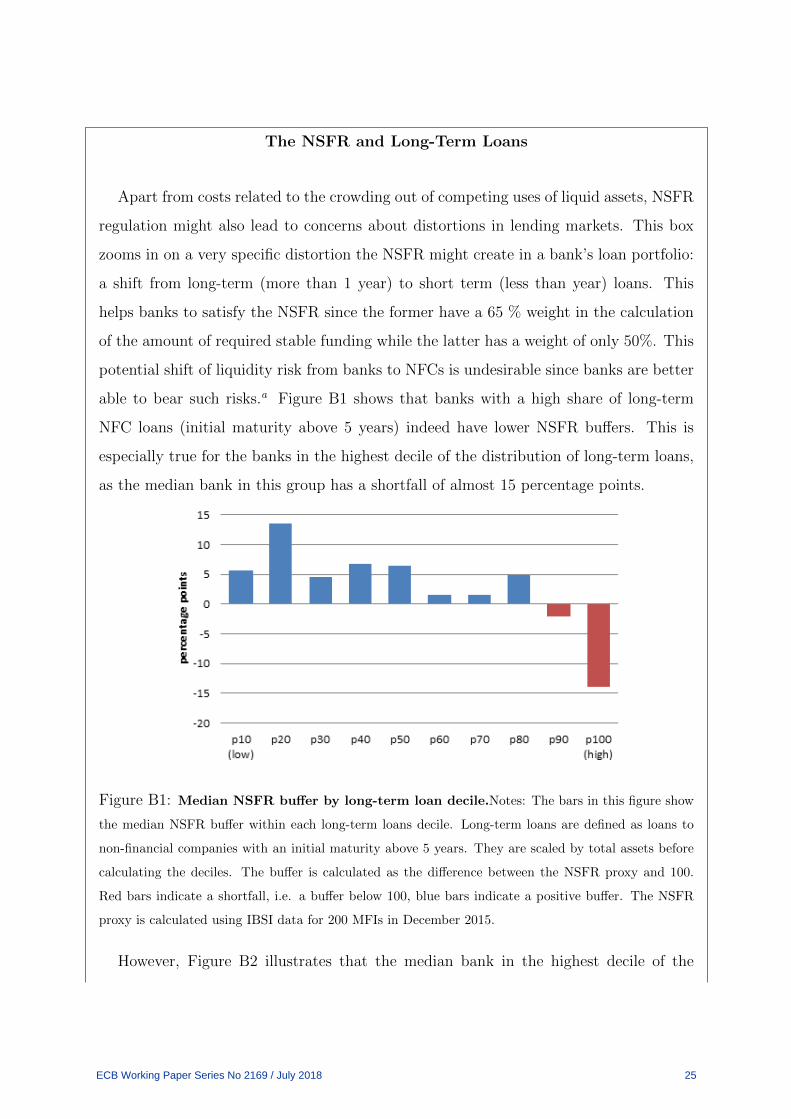
Apart from costs related to the crowding out of competing uses of liquid assets, NSFR

regulation might also lead to concerns about distortions in lending markets. This box

zooms in on a very specific distortion the NSFR might create in a bank’s loan portfolio:

a shift from long-term (more than 1 year) to short term (less than year) loans. This

helps banks to satisfy the NSFR since the former have a 65 % weight in the calculation

of the amount of required stable funding while the latter has a weight of only 50%. This

potential shift of liquidity risk from banks to NFCs is undesirable since banks are better

able to bear such risks.a Figure B1 shows that banks with a high share of long-term

NFC loans (initial maturity above 5 years) indeed have lower NSFR buffers. This is

especially true for the banks in the highest decile of the distribution of long-term loans,

as the median bank in this group has a shortfall of almost 15 percentage points.

Figure B1: Median NSFR buffer by long-term loan decile.Notes: The bars in this figure show

the median NSFR buffer within each long-term loans decile. Long-term loans are defined as loans to

non-financial companies with an initial maturity above 5 years. They are scaled by total assets before

calculating the deciles. The buffer is calculated as the difference between the NSFR proxy and 100.

Red bars indicate a shortfall, i.e. a buffer below 100, blue bars indicate a positive buffer. The NSFR

proxy is calculated using IBSI data for 200 MFIs in December 2015.

However, Figure B2 illustrates that the median bank in the highest decile of the


distribution of LT loans also has the smallest amount of available stable funding (depicted

as a percentage of total assets). If this bank would increase its available stable funding

to the average level in the other groups, then the shortfall depicted in Figure B1 would

already be cut in half.

In practice, profit maximising banks will likely take the least costly course of action.

Since the difference between the available stable funding weights on wholesale and retail

funding is much larger than the difference between the required stable funding weights

on long and short term loans, adjusting the liability side of banks balance sheets is by

far the more effective way to reduce a potential NSFR shortfall. Indeed, a recent study

by the EBA indicates that the increase in the NSFR of European banks since the crisis

was mainly driven by an increase in available stable funding and not by a reduction in

required stable funding.b It is thus unlikely that the introduction of the NSFR would

lead to large changes in the maturity structure of a banks’ loan portfolio.

Figure B2: Median available stable funding by long-term loan decile. Note: The bars in this

figure show the median available stable funding (as a percentage of total assets) within each long-term

loans decile. Long-term loans are defined as loans to non-financial companies with an initial maturity

above 5 years. They are scaled by total assets before calculating the deciles. Available stable funding is

a proxy for the numerator of NSFR, depicted as a percentage of total assets. All variables are calculated

using IBSI data for 200 MFIs in December 2015.

aOne of the key functions of banks is maturity and liquidity transformation.bEBA (2016). CRD IV-CRR/ Basel III Monitoring exercise Results based on Data as of 31 December

2015. EBA report.


https://www.eba.europa.eu/-/eba-publishes-results-of-the-crdiv-crr-basel-iii-monitoring-exercise-as-of-31-december-2015

4.3 The macroeconomic costs and benefits of capital and liquidity

regulation: insights from macro models

The presence of private costs of liquidity regulations does not necessarily imply the pres-

ence significant social costs. This does not happen, for example, if the private costs to

banks are a gain for other investors, or if financial intermediation can shift – without cost

or unwelcome side effects – to institutions that are not affected by the rules.

In order to assess the macroeconomic, social costs of liquidity regulation, we rely on struc-

tural general equilibrium models. Specifically, we employ two structural macro-financial

models and combine them with euro-area data to estimate the overall long-run macroeco-

nomic costs (including their welfare costs). We first present results based on a model by Van

den Heuvel (2017) and then turn to a quantitative version of the 3D model as in Mendicino

et al. (2016). The two models were developed at the European Central Bank and the Federal

Reserve Board.

Van den Heuvel (2017): ”The Welfare Effects of Bank Liquidity and Capital Re-

quirements” The first model we use, Van den Heuvel (2017), embeds the role of liquidity

creating banks in an otherwise standard general equilibrium growth model.12 Besides banks,

the model also features firms and households, who own the banks and the firms. Because of

the preference for liquidity on the part of households and firms, liquid assets, such as bank

deposits and government bonds, command a lower rate of return than illiquid assets, such

as bank loans and equity. The spread between the two is the convenience yield of the liquid

instrument.

The model incorporates a rationale for the existence of both capital and liquidity regula-

tion, based on a moral hazard problem created by deposit insurance (see Appendix B for a

more detailed summary of the model). But these regulations also have costs, as they reduce

the ability of banks to create net liquidity. Capital requirements directly limit the fraction

of assets that can be financed with liquid deposits, while liquidity requirements reduce net

12Liquidity creation has long been recognized as one of the key social functions of banks (see for example

Freixas and Rochet, 1997). The model extends Van den Heuvel (2008) to include liquidity stress and liquidity

regulation.


liquidity transformation by banks by removing HQLA from non-banks.

Requiring banks to hold more HQLA crowds out other users of these assets, such as by

money funds, insurers, pension funds, etc., increasing scarcity of safe assets. At the same

time, it has the effect of making financial intermediation by banks more costly, potentially

reducing credit. The total macroeconomic costs consist of costs from reduced access to

liquidity, reduced credit and, consequently, potential reductions in investment and output.

The model tells you what financial spreads to look at to gauge the total macroeconomic

cost of these requirements. Consistent with the predictions of the simple framework presented

in Section 2, the cost-revealing financial spreads for an LCR-style liquidity requirement is

the spread between the average interest rate on bank deposits and the yield on HQLA. For

the capital requirement, the model implies that the macroeconomic costs depend primarily

on the spread between risk-adjusted required return on equity and the average interest rate

on bank deposits. According to the theory, both spreads must be adjusted for non-interest

costs of deposits and, of course, scaled by the size of the banking sector in the economy (see

Appendix B for the exact formulas).

To quantify the long-run macroeconomic costs, the results from the model are combined

with euro area data from SDW.13 For equity, the risk adjustment follows Hanson, Kashyap,

and Stein (2011), but adapted for the euro area. Formally, the macroeconomic cost is

measured as the welfare cost, a summary measure of all present and future cost due to lost

production and reduced liquidity, expressed as a percent of GDP.

The main finding is that the macroeconomic costs of liquidity requirements are non-zero,

but modest, and smaller than for capital requirements. For a liquidity requirement similar

to the LCR, the gross macroeconomic cost is estimated at 0.05 percent of euro area GDP

(5-13 billion euros per year), although it is slightly higher if estimates are based on the most

recent years (0.013 percent). By comparison, based on the same model, the cost of a 10

p.p. increase in capital requirements is about 0.3-1.0 percent of GDP (30-100 billion euros

per year). (The range reflects choices about the risk-adjustment to the required return on

equity.)

Naturally, these costs must be weighed against the financial stability benefits of these

13See the previous subsection for details.


tools. In the model, both capital and liquidity requirements are helpful to limit excessive

risk taking by banks, which they can engage in through credit risk or liquidity risk. It

turns out that, because of its positive effect on incentives, capital requirements have broader

financial stability benefits; that is, it addresses both types of risk taking. That said, liquidity

regulation tackles liquidity risks at lower cost and so are part of the optimal policy mix,

complementing capital. Indeed, the model suggests a simple division of labour: It socially

optimal for the liquidity requirement to address liquidity risk and for the capital requirement

to deal with credit risk.

3D model - Mendicino et al. (2016) The 3D model is a macroeconomic model that

emphasizes financial intermediation and bank default and their consequences for macroeco-

nomic outcomes and welfare. The model considers households who borrow to buy houses

and firms who borrow in order to invest in productive projects. Banks are essential to in-

termediate funds between savers and borrowers in this economy so financial instability and

bank failures have a large negative impact on lending and economic activity.

For the purposes of this paper, the quantitative version of the 3D model as in Mendicino

et al. (2016) has been extended to consider the impact of liquidity regulation tools on the

cost of providing loans.14 The model does not feature liquidity risk and therefore the only

effect of increasing the NSFR/LCR is to increase the costs for banks of providing loans to

business and households. Hence, the 3D model is suitable for analysing the costs of the

regulation but not the benefits that arise more from the mitigation of liquidity risk.

The NSFR imposes a cost on banks because the long term bonds that qualify for the

regulation carry higher interest rates compared to shorter term funding. For the LCR, this

is because the high-quality liquid assets (HQLA) that qualify for the LCR pay interest rates

that are lower than banks’ deposit funding cost. How big the impact of a given increase in

the NSFR or in the LCR depends on the two crucial spreads which we calibrate from the

data – (i) the spread between bank bonds and bank deposits (this is the cost of the NSFR)

14Mendicino et al. (2016) extend the original 3D model in Clerc et al. (2015) in several dimensions and,

in order to provide quantitative results, it is properly calibrated to match first and second moments of key

Euro Area macroeconomic and banking data.


and (ii) the spread between the return on HQLA and the return on bank deposits (this is

the cost of the LCR). These spreads are clearly indicated in the legend of Figure 6.

Both the NSFR and the LCR impose costs on the economy. Total credit declines by up

to 0.8% in the long run for the former and by 0.4% for the later. The difference is clearly

explained by the difference in the costs of the two regulations. The bank bond-bank deposit

spread is approximately twice as big as the HQLA-bank deposit spread which explains why

the NSFR has an impact that is twice as big.

The transmission of the policy is standard. Hardest hit are credit dependent activities

such as business investment (down by around 0.2-0.3% depending on the policy instrument).

Consumption (not shown) falls very gently in line with lower economic activity. Total GDP

sees a modest decline of around 0.1%.

Finally, it is important to acknowledge that our simulations miss any benefit for uninsured

debt bank funding costs that may arise out of a reduced probability of bank failure due to

liquidity risk. Such a reduction in bank fragility would tend to reduce loan interest rates

(since funding costs would be lower), making the cost of the regulation in terms of real

economic activity even smaller. Overall, the model simulations suggest that the NSFR and

LCR would have only a modest negative impact on real economic activity.

Insights from other macro models Covas and Driscoll (2014) quantify the macroeco-

nomic impact of a minimum liquidity standard introduced on top of existing capital require-

ments using a nonlinear dynamic general equilibrium model with a banking sector. In the

baseline calibration, imposing a liquidity requirement would lead to a steady-state decrease

of about 3 percent in the amount of loans made, an increase in banks’ holdings of securities

of at least 6 percent, a fall in the interest rate on securities of a few basis points, and a

decline in output of about 0.3 percent. The results are sensitive to the supply of safe assets:

the larger the supply of such securities, the smaller the macroeconomic impact of introduc-

ing a minimum liquidity standard for banks. They find that the general equilibrium effects

of new regulations on bank loans and securities are considerably smaller than the partial

equilibrium effects. Therefore, partial equilibrium approaches may overstate the impact of

the new regulations on the macroeconomy.


De Nicolo, Gamba and Lucchetta (2014) study the quantitative impact of capital, liquid-

ity and resolution regulatory policies on bank lending, efficiency and welfare. In their model,

which focuses on the microprudential aspects of the regulations in a dynamic partial equi-

librium model of banking, liquidity requirements unambiguously reduce lending, efficiency,

and welfare because they severely hamper banks’ maturity transformation. Moreover, liquid-

ity regulation cam make capital regulation more pro-cyclical. Liquidity requirements force

banks to use retained earnings to build up liquidity buffers rather than invest in lending, in

both upturns and downturns. Therefore, capital ratios become inflated in upturns.

5 The macroprudential dimension of capital and liq-

uidity regulation

In our simple conceptual framework and in our empirical analysis, we took the perspective

of a single bank. This clarified how different policy instruments affect financial institutions

but took the overall economic environment as given. In particular, the distribution of loan

returns and the liquidation value of loans was treated as exogenous.

Since the crisis, financial regulation has shifted to an increasingly macroprudential per-

spective which recognizes that much of the risk facing banks is endogenous systemic risk.

In order to understand the impact of regulation on systemic risk, the academic literature has

developed a raft of new General Equilibrium models which explicitly analyse the feedbacks

between banks and the wider economy. In this section we survey this literature.

5.1 Systemic risk management and systemic risk externalities

One of the most well understood spillovers (or externalities) occur when individual banks

are forced to liquidate their assets due to pressure from their short-term lenders. Such ‘fire

sales’ can depress prices very considerably leading to contagion and multiple bank failures.

A number of papers have analysed this issue (Korinek and Jeanne (2011), Brunner-

meier and Sannikov (2014), Gertler, Kiyotaki and Queralto (2015), Gertler, Kiyotaki and

Prestipino (2015)) and conclude that the presence of these undesirable spillovers require


higher capital ratios than individual banks would choose for themselves. The main prescrip-

tion of these papers is to have capital ratios in normal times that ensure that banks’ capital

constraints do not bind very often. Gertler and Kiyotaki (2015) in addition show that the

possibility of bank runs greatly magnifies the risks facing banks, necessitating even higher

capital ratios.

Liquidity buffers can be as effective as capital in preventing contagious failures in the

presence of fire-sales (Cifuentes, Ferrucci and Shin 2005). Moreover, liquidity requirements

(and Pigouvian taxes) can help internalize the systemic fire-sale externalities induced by

financial intermediaries’ overexposure to short-term funding (Perotti, and Suarez, 2011).

In Boissay, Collard and Smets (2015) and Boissay and Collard (2016) capital and liquidity

regulation help to control the build-up of aggregate excess liquidity and the associated decline

in lending quality. The authors show that the optimal policy is to use these tools to eliminate

the probability of an interbank market collapse that would trigger a banking crisis in their

framework.

Kashyap, Vardoulakis and Tsomocos (2014) also argue for the use of liquidity and capital

tools in order to eliminate the possibility of inefficient bank runs. In their ’global games’

framework (Morris and Shin, 1998), bank runs are endogenous and can be reduced by higher

capital ratios as well as tools that resemble the LCR or the NSFR. Individual banks fail to

take the socially optimal decisions due to incomplete contracting that allows bank manage-

ment to change the bank’s risk and liquidity profile in an unobservable manner. Optimal

regulation limits the scope for bank moral hazard and it involves changes in both liquidity

and capital tools.

A very interesting aspect of the framework of Kashyap, Vardoulakis and Tsomocos (2014)

is that the costs of the different regulatory instruments are fully endogenous and driven

by the incomplete nature of asset markets. Bank equities and bank deposits are the main

financial assets available to households in the model and changes in their overall supply and

riskiness will affect the cost of these liabilities for banks permanently. For example, higher

capital ratios will reduce the cost of equity as predicted by Modigliani-Miller. However,

the corresponding reduction in the supply of deposits should lead to a fall in their cost for

banks. Equally, higher liquidity requirements will increase the cost of providing deposits


while reducing the cost of issuing equity. In the end, the optimal regulation trades off the

social costs and benefits of different aspects of the bank’s balance sheet. As a result, both

capital and liquidity tools end up being an integral part of the optimal policy mix.

5.2 Should the LCR be drawn down in a crisis?

Having discussed the role of capital and liquidity tools in mitigating individual bank and

systemic risk, we turn briefly to an interesting and current issue in the policy debate: ‘Should

the LCR be drawn down in a crisis or should it be maintained at the required minimum level

at all times?’. The answer to this question crucially depends on whether one takes a macro

or microprudential perspective and the surrounding discussion therefore illuminates nicely

some of the issues we have discussed above.

Goodhart (2010) famously argued that a minimum requirement which cannot be used is

not effective at preventing asset liquidations. A buffer is only a buffer when the bank can

use it in stressed conditions instead of fire-selling its illiquid assets. Goodhart (2010) draws

a parallel between a minimum liquidity requirement and the ‘last taxi’ problem whereby a

traveller arriving at a station late at night is overjoyed to see one taxi remaining. She hails

it, only for the taxi driver to respond that he cannot help her, since local bye-laws require

one taxi to be present at the station at all times.

Similarly, Stein (2013) highlights a bank’s private incentives to draw down the LCR in

a pure quantity-based system of regulation: if a bank is held to an LCR standard of 100

percent in normal times, it may be reluctant to allow its ratio to fall below 100 percent when

facing large outflows for fear that doing so might be seen by market participants as a sign

of weakness. Yet, it may be important to prevent fire-sales. That is, for macroprudential

purposes, it is important to have mechanisms in place that would allow banks to temporarily

fall below 100% LCR ratio in the stress situation. Stein advocates the usage of a Committed

Liquidity Facility provided by the central bank. Access to such facility could be counted

towards satisfying the LCR requirement in the stress situation and would be equivalent to

a liquid asset drawdown without signalling distress to the market.

The ‘buying time’ motivation for the LCR (e.g., Santos and Suarez, 2015) would also call

for the LCR to be drawn down in a crisis. If it were not, a bank which is subject to a run


would need to engage in costly liquidations and may become insolvent in the process even

though it would have been solvent in the absence of a run.

In sum, in the situation when a bank run or fire-sale dynamic is under way, running down

the LCR appears to be a useful crisis management tool.15

However, if one considers microprudential benefits of liquidity requirements as well as

their benefits in preventing runs, it may be that the ‘last taxi’ must remain at the station.

In Calomiris, Heider and Hoerova (2015), observable liquidity buffers tame a bank’s risk-

taking incentives and stem depositors’ incentives to run in the bad state. Releasing liquidity

buffers is therefore not advisable from the microprudential perspective.

Diamond and Kashyap (2015) consider liquidity regulation as a tool to deter bank runs.

They study a modification of the Diamond and Dybvig (1983) model in which the bank

may hold a liquid asset, some depositors see sunspots that could lead them to run, and

all depositors have incomplete information about the bank’s ability to survive a run. The

incomplete information means that the bank is not automatically incentivized to always

hold sufficient liquidity to survive runs. As long as bank loans are very illiquid and their

liquidation costly, capital requirements alone cannot deter runs, and liquidity requirements

are necessary. Regulation similar to the LCR and the NSFR can change the bank’s incentives

so that runs are less likely. When the regulator has less information than the bank, additional

excess (and unusable) liquidity must be required to provide incentives to hold the proper

amount of liquidity; that is, the last taxi must remain at the station. However, integrating

liquidity requirements with a lender of last resort policy can do better. Banks may be allowed

to use their liquidity buffers and to access liquidity from the lender of last resort. This

would effectively violate the liquidity requirement but liquidity borrowed from the LOLR

could deter a run. To provide incentives to banks to hold sufficient liquidity, penalties must

be imposed, such as reduced executive compensation and a limitation on dividends. This

is similar to allowing the last taxi to leave the station but imposing a penalty on the taxi

company.

15In a calibrated general equilibrium model with banks, Covas and Driscoll (2014) show that relaxing

the liquidity requirement under a situation of financial stress dampens the response of output to aggregate

shocks.


6 Conclusion

This paper clarifies and quantifies the role of liquidity regulation in the optimal prudential

regulatory policy mix. We use the ECB’s IBSI data to investigate the extent to which

liquidity and capital ratios succeeded in making European banks more stable during the

Global Financial Crisis and the European Sovereign Debt Crisis. Our empirical analysis

suggests an intuitive division of labour: the leverage ratio was effective at reducing bank

failures while the LCR and NSFR limited significantly the emergency liquidity take-up by

European banks. However, we find that even if European banks had fully complied with the

Basel III liquidity standards, they would have still required very substantial central bank

liquidity assistance. This suggests that eliminating LOLR interventions would necessitate

much higher liquidity requirements.

In the end, our evidence suggests that capital requirements and LOLR interventions are

both essential in managing solvency and liquidity risk. Liquidity regulation is also useful

since it is effective at managing liquidity stress and its macroeconomic costs are very modest

compared to capital regulation.


References

[1] Acharya, V. V., H. S. Shin, and T. Yorulmazer (2011). “Crisis Resolution and Bank

Liquidity,” Review of Financial Studies 24(6), 2166-2205.

[2] Boissay, F., and F. Collard (2016). “Macroeconomics of Bank Capital and Liquidity

Requirements,” BIS Working Paper No. 596.

[3] Boissay, F., F. Collard, and F. Smets (2016). “Booms and Banking Crises,” Journal of

Political Economy 124(2), 489-538.

[4] Brunnermeier, M. K., and Y. Sannikov (2014). “A Macroeconomic Model with a Finan-

cial Sector,” American Economic Review 104(2), 379-421.

[5] Bucalossi, A., C. Coutinho, K. Junius, A. Luskin, A. Momtsia, I. Rahmouni-Rousseau,

B. Sahel, A. Scalia, S. W. Schmitz, R. Soares, F. Schobert and M. Wedow (2016), “Basel

III and Recourse to Eurosystem Monetary Policy Operations,” ECB Occasional Paper

171.

[6] Calomiris, C. W., and C. M. Kahn (1991). “The Role of Demandable Debt in Structuring

Optimal Banking Arrangements,” American Economic Review 81(3), 497-513.

[7] Calomiris, C. W., F. Heider, and M. Hoerova (2015). “A Theory of Bank Liquidity

Requirements,” Columbia Business School Research Paper No. 14-39.

[8] Carlson, M. A., B. Duygan-Bump, and W. Nelson (2015). “Why Do We Need Liquidity

Regulations and a Lender of Last Resort? A Perspective from Federal Reserve Lending

During the 2007-09 US Financial Crisis,” BIS Working Paper No. 493.

[9] Cecchetti, S. and Kashyap, A. (2018). “What Binds? Interactions between Bank Capi-

tal and Liquidity Regulations” in Philipp Hartmann, Haizhou Huang and Dirk Schoen-

maker eds. The Changing Fortunes of Central Banking, Cambridge University Press.

[10] Clerc, L., A. Derviz, C. Mendicino, S. Moyen, K. Nikolov, L. Stracca, J. Suarez, and

A.P. Vardoulakis (2015). “Capital Regulation in a Macroeconomic Model with Three

Layers of Default,” International Journal of Central Banking 11(3), 9-63.


[11] Cifuentes, R., G. Ferruci, and H. S. Shin (2005). “Liquidity Risk and Contagion,”

Journal of the European Economic Association 3(2-3), 556-566.

[12] Covas, F., and J. C. Driscoll (2014). “Bank Liquidity and Capital Regulation in General

Equilibrium, ” Finance and Economics Discussion Series of the Federal Reserve Board

No. 2014-85.

[13] De Nicolo, G., A. Gamba, and M. Lucchetta (2014). “Microprudential Regulation in a

Dynamic Model of Banking,” Review of Finanical Studies 27(7), 2097-2138.

[14] Diamond, D. W., and P. H. Dybvig (1983). “Bank Runs, Deposit Insurance, and Liq-

uidity,” Journal of Political Economy 91(3), 401-419.

[15] Diamond, D. W., and A. K. Kashyap (2016). “Liquidity Requirements, Liquidity Choice

and Financial Stability,” NBER Working Paper No. 22053.

[16] Farhi, E., and J. Tirole (2012). “Collective Moral Hazard, Maturity Mismatch, and

Systemic Bailouts,” American Economic Review 102(1), 60-93.

[17] Gertler, M., and N. Kiyotake (2015). “Banking, Liquidity, and Bank Runs in an Infinite

Horizon Economy,” American Economic Review 105(7), 2011-2043.

[18] Gertler, M., N. Kiyotaki, and A. Queralto (2012). “Financial crises, Bank Risk Exposure

and Government Financial Policy,” Journal of Monetary Economics 59, 17-34.

[19] Gertler, M., N. Kiyotaki and A. Prestipino (2015). “Wholesale Banking and Bank Runs

in Macroeconomic Modelling of Financial Crises,” Handbook of Macroeconomics 2,

1345-1425.

[20] Giammarino, R. M., T. R. Lewis, and D. E. M. Sappington (1993). “An Incentive

Approach to Banking Regulation,” Journal of Finance 48(4), 1523-1542.

[21] Goldstein, I., and A. Pauzner (2005). “Demand-Deposit Contracts and the Probability

of Bank Runs,” Journal of Finance 60(3), 1293-1327.

[22] Goodhart, C. (2010), “The future of Finance: The LSE Report,” Chapter 5 in A. Turner

and others, London School of Economics and Political Science.


[23] Gorton, G., and G. Ordonez (2014). “Collateral Crises,” American Economic Review

104(2), 343-378.

[24] Greenwood, R., S. G. Hanson, and J. C. Stein (2015). “A Comparative-Advantage

Approach to Government Debt Maturity,” Journal of Finance 70(4), 1683-1722.

[25] Kareken, J., and N. Wallace (1978). “Deposit Insurance and Bank Regulation: A

Partial-Equilibrium Exposition,” Quarterly Journal of Economics 69(2), 207-222.

[26] Kashyap, A. K., D. P. Tsomocos, and A. P. Vardoulakis (2014). “How Does Macropru-

dential Regulation Cchange Bank Credit Supply?,” NBER Working Paper No. 20165.

[27] Korinek, A., and O. Jeanne (2013). “Macroprudential Regulation Versus Mopping Up

After the Crash,” NBER Working Paper No. 18675.

[28] Krishnamurthy, A., and A. Vissing-Jorgensson (2012). “The Aggregate Demand for

Treasury Debt,” Journal of Political Economy 120(2), 233-267.

[29] Laeven, L., and F. Valencia (2013). “Systemic Banking Crises Database,” IMF Economic

Review 61 (2), 225–270.

[30] Mendicino, C., Nikolov, K., Suarez, J. and D. Supera (2016). ”Optimal Dynamic Capital

Requirements” forthcoming Journal of Money Credit and Banking.

[31] Myers, S. C., and R. G. Rajan (1998). “The Paradox of Liquidity,” Quarterly Journal

of Economics 113(3), 733-771.

[32] Perotti, E., and J. Suarez (2011). “A Pigovian Approach to Liquidity Regulation,”

International Journal of Central Banking 7(4), 3-41.

[33] Reinhart, C. M., and K. S. Rogoff (2009). “The Aftermath of Financial Crisis,” Amer-

ican Economic Review 99(2), 466-472.

[34] Repullo, R. (2005). “Liquidity, Risk-Taking, and the Lender of Last Resort,” Interna-

tional Journal of Central Banking 1, 47-80.


[35] Rochet, J.-C., and X. Vives (2004). “Coordination Failures and the Lender of Last

Resort: Was Bagehot Right After All?,” Journal of the European Economic Association

2(6), 1116-1147.

[36] Santos, J. A. C., and J. Suarez (2015). “Liquidity Standards and the Value of an In-

formed Lender of Last Resort,” mimeo.

[37] Stein, J. C. (2012). “Monetary Policy as Financial-Stability Regulation,” Quarterly

Journal of Economics 127(1), 57-95.

[38] Stein, J.C. (2013). “Liquidity Regulation and Central Banking,” speech at the 2013

Credit Markets Symposium, Charlotte, North Carolina.

[39] Van den Heuvel, S. (2008). “The Welfare Cost of Capital Requirements,” Journal of

Monetary Economics 55(2), 298-320.

[40] Van den Heuvel, S. (2017). “The Welfare Cost of Bank Liquidity and Capital Require-

ments,” ECB mimeo.


Tables and Figures

Table 1: LCR proxy

HQLA Weights

Cash 1

Deposits at central bank 1

Government debt 0.85 * encumbrance coefficient

Corporate debt 0.85*encumbrance coefficient

Equity securities 0.5

Expected Outflow Weights

Overnight household deposits 0.05

Household deposits - redeemable at notice 0.05

Rest of world deposits 0.1

Overnight NFC deposits 0.25

NFC deposits - redeemable at notice 0.25

Government deposits 0.4

MFI deposits 1

OFI deposits 1

Expected Inflow 0.7*Expected Outflow

LCR = HQLA / Net inflow

Notes: This table shows the variables and the corresponding weights that are

used for calculating the LCR proxy. We use MFI level IBSI data for 197 euro

area banks to calculate a monthly LCR proxy for each Monetary Financial

Institution (MFI). The LCR is defined as the ratio of High Quality Liquid

Assets (HQLA) over Net Inflow. The Net Inflow is defined as the difference

between the Expected Outflow and the Expected Inflow. NFC is short for

non-financial corporation, OFI stands for other financial institution.


Table 2: NSFR proxy

Required Stable Funding Available Stable Funding

Item Weights Item Weights

Cash 0 Debt< 1y 0

Deposits at central banks 0 MFI deposits 0

Government debt 0.05 OFI deposits 0

MFI loans 0.15 CCP repo 0

Corporate debt 0.15 Other liabilities 0

Government loans 0.5 NFC deposits - overnight 0.5

Household loans < 1y 0.5 Government deposits 0.5

Household mortgages < 1y 0.5 NFC deposits > 3m 0.9

NFC loans < 1y 0.5 NFC deposits redeemable at notice 0.9

Household mortgages < 5y 0.65 NFC deposits at agreed maturity < 1y 0.9

Household mortgages > 5y 0.65 Household deposits - overnight 0.9

Household loans < 5y 0.85 Household deposits at agreed maturity < 1y 0.95

Household loans > 5y 0.85 Household deposits redeemable at notice 0.95

NFC loans < 5y 0.85 Household deposits row 0.95

NFC loans > 5y 0.85

Other equity securities 0.85 Capital 1

MFI debt 1 Debt> 1y 1

MFI equity 1 Debt> 2y 1

Equity securities row 1 Household deposits at agreed maturity > 1y 1

Loans row 1 Household deposits at agreed maturity > 2y 1

Debt securities row 1 NFC deposits at agreed maturity > 1y 1

Loans to OFI 1 NFC deposits at agreed maturity > 2y 1

Other assets 1

NSFR = ASF / RSF

Notes: This table shows the variables and the corresponding weights that are used for calculating the

NSFR proxy. We use MFI level IBSI data for 197 euro area banks to calculate a monthly LCR proxy

for each Monetary Financial Institution (MFI). The NSFR is defined as the ratio of Available Stable

Funding over Required Stable Funding. NFC is short for non-financial corporation, OFI stands for

other financial institution.


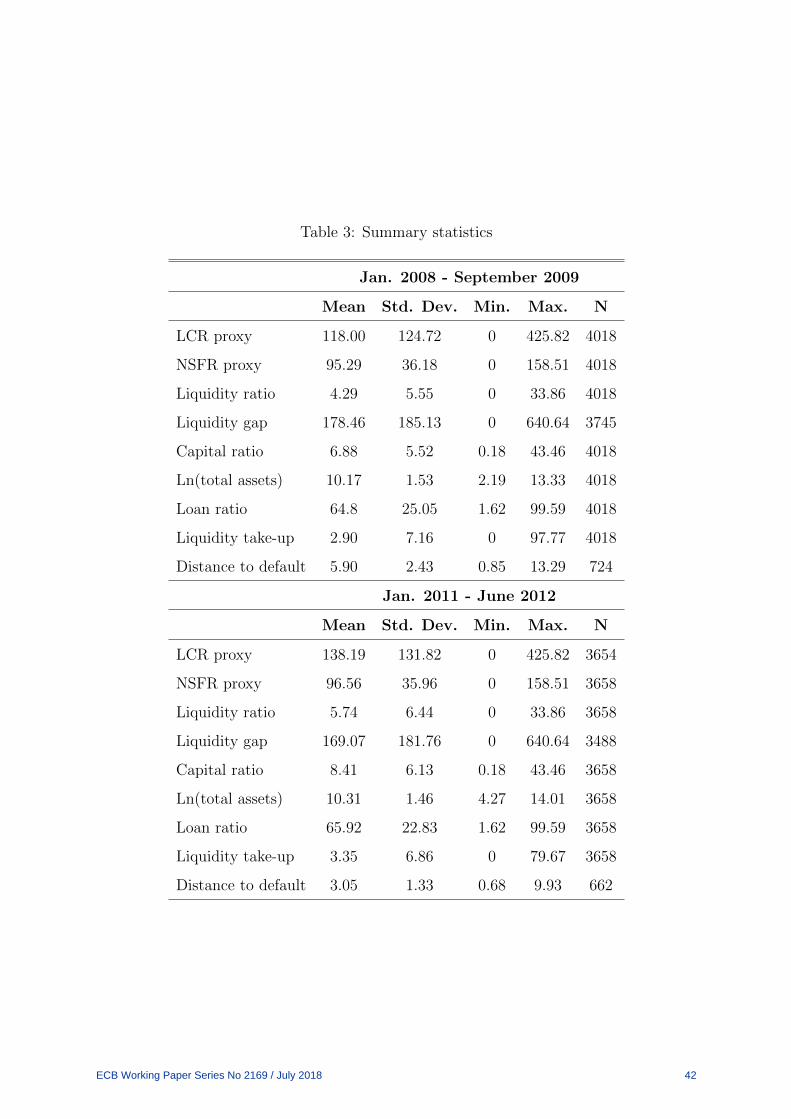
Table 3: Summary statistics

Jan. 2008 - September 2009

Mean Std. Dev. Min. Max. N

LCR proxy 118.00 124.72 0 425.82 4018

NSFR proxy 95.29 36.18 0 158.51 4018

Liquidity ratio 4.29 5.55 0 33.86 4018

Liquidity gap 178.46 185.13 0 640.64 3745

Capital ratio 6.88 5.52 0.18 43.46 4018

Ln(total assets) 10.17 1.53 2.19 13.33 4018

Loan ratio 64.8 25.05 1.62 99.59 4018

Liquidity take-up 2.90 7.16 0 97.77 4018

Distance to default 5.90 2.43 0.85 13.29 724

Jan. 2011 - June 2012

Mean Std. Dev. Min. Max. N

LCR proxy 138.19 131.82 0 425.82 3654

NSFR proxy 96.56 35.96 0 158.51 3658

Liquidity ratio 5.74 6.44 0 33.86 3658

Liquidity gap 169.07 181.76 0 640.64 3488

Capital ratio 8.41 6.13 0.18 43.46 3658

Ln(total assets) 10.31 1.46 4.27 14.01 3658

Loan ratio 65.92 22.83 1.62 99.59 3658

Liquidity take-up 3.35 6.86 0 79.67 3658

Distance to default 3.05 1.33 0.68 9.93 662


Tab

le4:

Ban

kL

iqu

idit

y,C

ap

ital

an

dL

OL

R

Dep

enden

tva

riab

le=

ln(t

otal

CB

liquid

ity

take

-up

/T

A)

Jan

.20

08-

Sep

t.20

09Jan

.20

11-

Jul.

2012

(1)

(2)

(3)

(4)

(5)

(6)

(7)

(8)

LC

R-0

.000

904*

*-0

.001

48**

(0.0

0045

2)(0

.000

647)

NSF

R-0

.010

6***

-0.0

121*

**

(0.0

0262

)(0

.003

84)

Liq

uid

ity

rati

o0.

0073

30.

0401

*

(0.0

194)

(0.0

217)

Liq

uid

ity

gap

-0.0

0099

0***

-0.0

0159

***

(0.0

0025

8)(0

.000

500)

Cap

ital

rati

o-0

.046

2**

-0.0

402*

**-0

.047

2**

-0.0

401*

*-0

.001

920.

0018

0-0

.003

67-0

.029

9

(0.0

200)

(0.0

143)

(0.0

197)

(0.0

202)

(0.0

253)

(0.0

226)

(0.0

231)

(0.0

258)

ln(S

ize)

0.24

1**

0.10

40.

193*

0.22

7*0.

450*

**0.

475*

**0.

322*

*0.

398*

*

(0.1

22)

(0.1

51)

(0.1

15)

(0.1

31)

(0.1

71)

(0.1

64)

(0.1

50)

(0.1

98)

Loa

nra

tio

-0.0

124*

**-0

.003

85-0

.012

8***

-0.0

0969

***

-0.0

113

-0.0

0363

-0.0

0918

-0.0

176*

**

(0.0

0299

)(0

.003

72)

(0.0

0312

)(0

.003

20)

(0.0

0713

)(0

.006

84)

(0.0

0703

)(0

.005

92)

Obse

rvat

ions

4,01

84,

018

4,01

83,

745

3,65

43,

658

3,65

83,

488

R-s

quar

ed0.

734

0.74

00.

732

0.74

10.

738

0.74

50.

739

0.74

8

Ban

kF

EY

YY

YY

YY

Y

Tim

eF

EY

YY

YY

YY

Y

Not

es:

All

righ

t-han

dsi

de

vari

able

sar

eca

lcula

ted

usi

ng

mon

thly

dat

afr

omE

CB

sIn

div

idual

Bal

ance

Shee

tIt

ems

(IB

SI)

dat

abas

efo

r19

7M

onet

ary

Fin

anci

alIn

stit

uti

ons

(MF

Is)

inth

eeu

roar

ea.

The

sam

ple

per

iod

inth

efirs

tfo

ur

colu

mns

is

Jan

uar

y20

08-

Sep

tem

ber

2009

.T

he

sam

ple

per

iod

inth

ela

stfo

ur

colu

mns

isJan

uar

y20

11-

July

2012

.T

he

dep

enden

t

vari

able

isth

enat

ura

llo

gari

thm

ofa

ban

k‘s

liquid

ity

take

-up

atth

ece

ntr

alban

ksc

aled

by

tota

las

sets

.L

CR

isou

rpro

xy

for

the

ban

k‘s

liquid

ity

cove

rage

rati

o(i

n%

).N

SF

Ris

our

pro

xy

for

the

ban

k‘s

net

stab

lefu

ndin

gra

tio

(in

%).

Liq

uid

ity

rati

ois

the

sum

ofca

shan

dgo

vern

men

tse

curi

ties

scal

edby

tota

las

sets

(in

%).

Liq

uid

ity

gap

isth

esu

mof

cash

,go

vern

men

tse

curi

ties

and

inte

rban

kas

sets

scal

edby

inte

rban

kliab

ilit

ies

(in

%).

Cap

ital

rati

ois

defi

ned

asto

tal

capit

alov

erto

tal

asse

ts(i

n%

).

ln(S

ize)

isth

enat

ura

llo

gari

thm

ofto

tal

asse

ts.

Loa

nra

tio

isth

era

tio

ofto

tal

loan

sov

erto

tal

asse

ts(i

n%

).R

obust

stan

dar

d

erro

rs(c

lust

ered

atth

eban

kle

vel)

are

inpar

enth

eses

.


Table 5: Bank Liquidity, Capital and Default Risk

Dependent variable = Distance to Default

Jan. 2008 - Sept. 2009 Jan. 2011 - Jul. 2012

(1) (2) (3) (4) (5) (6) (7) (8)

LCR 0.00300 0.00163

(0.00196) (0.00184)

NSFR 0.0202 0.0148

(0.0186) (0.0121)

Liquidity ratio -0.0826 0.00645

(0.0569) (0.0380)

Liquidity gap 0.00161* 0.00202

(0.000874) (0.00170)

Capital ratio 0.121* 0.122* 0.138** 0.123* 0.282** 0.262** 0.287** 0.285**

(0.0674) (0.0696) (0.0637) (0.0668) (0.127) (0.127) (0.131) (0.128)

ln(Size) 4.253*** 4.445*** 4.177*** 4.178*** 0.526 0.450 0.477 0.545

(1.200) (1.524) (1.163) (1.213) (1.067) (1.114) (0.999) (1.024)

Loan ratio 0.0454 0.0200 0.00866 0.0217 0.0226 0.0175 0.0226 0.0207

(0.0282) (0.0207) (0.0231) (0.0225) (0.0159) (0.0160) (0.0145) (0.0146)

Observations 724 724 724 724 662 662 662 662

R-squared 0.885 0.885 0.886 0.885 0.759 0.760 0.758 0.761

Bank FE Y Y Y Y Y Y Y Y

Time FE Y Y Y Y Y Y Y Y

Notes: All right-hand side variables are calculated using monthly data from ECBs Individual Balance Sheet

Items (IBSI) database for 38 Monetary Financial Institutions (MFIs) in the euro area. The sample period in the

first four columns is January 2008 - September 2009. The sample period in the last four columns is January 2011

- July 2012. The dependent variable is a bank‘s distance to default. Distance to default is provided by Moody‘s

and only available for 38 out 197 MFIs in our sample. LCR is our proxy for the bank‘s liquidity coverage ratio

(in %). NSFR is our proxy for the bank‘s net stable funding ratio (in %). Liquidity ratio is the sum of cash and

government securities scaled by total assets (in %). Liquidity gap is the sum of cash, government securities and

interbank assets scaled by interbank liabilities (in %). Capital ratio is defined as total capital over total assets

(in %). ln(Size) is the natural logarithm of total assets. Loan ratio is the ratio of total loans over total assets

(in %). Robust standard errors (clustered at the bank level) are in parentheses.


(a)

LC

R(b

)N

SF

R

(c)

Liq

uid

ity

gap

(d)

Liq

uid

ity

rati

o

Fig

ure

1:E

volu

tion

of

Liq

uid

ity

Pro

xie

s.S

ourc

e:M

FI

leve

lIB

SI

dat

afo

r19

7eu

roar

eab

anks

and

own

calc

ula

tion

s.N

otes

:T

he

figu

res

show

the

evol

uti

onof

our

liqu

idit

yp

roxie

s(L

CR

,N

SF

R,

Liq

uid

ity

gap

and

Liq

uid

ity

rati

o)ov

erti

me.

Th

egr

ayli

ne

show

sth

ed

istr

ibu

tion

ofea

chra

tio

in20

08,

the

bla

ckli

ne

show

sth

ed

istr

ibu

tion

in20

12an

dth

eb

lue

lin

esh

ows

the

dis

trib

uti

onin

2016

.


(a)

LC

R(b

)N

SF

R

(c)

Liq

uid

ity

gap

(d)

Cap

ital

rati

o

Fig

ure

2:Im

pact

of

Ban

kL

iqu

idit

yan

dC

ap

ital

on

LO

LR

Reli

an

ce:

2008-2

009

Sou

rce:

MF

Ile

vel

IBS

Id

ata

for

197

euro

area

ban

ks

an

d

own

calc

ula

tion

s.N

otes

:T

hes

efigure

ssh

owth

eim

pac

tof

ach

ange

inou

rli

qu

idit

yp

roxie

s(L

CR

,N

SF

Ran

dth

eL

iqu

idit

yga

pra

tio)

and

ach

an

ge

inth

eC

apit

alra

tio

onli

qu

idit

yta

ke-u

pb

ased

oneq

uat

ion

2.E

ach

blu

ed

otre

pre

sents

the

imp

act

ofa

10p

erce

nta

gep

oint

(LC

Ran

dL

iqu

idit

ygap

rati

o)or

a1

per

centa

gep

oint

(NS

FR

and

Cap

ital

rati

o)ch

ange

onli

qu

idit

yta

ke-

up

(y-a

xis

)fo

ra

spec

ific

valu

eof

the

rati

o(x

-axis

).T

he

gray

are

a

ind

icat

esth

e90

%co

nfi

den

cein

terv

al.


Appendix A A Simple Balance Sheet Model

A.1 Capital requirements

We assume a bank that raises external funds using equity (e) and short term deposits

(d) in order to invest in risky illiquid loans (l). We analyse the model in partial equilibrium

and assume that the distribution of returns to all these assets are exogenously given. The

ex post return to loans is ωRL where ω is a random variable with an expected value equal

to unity and a distribution function F (ω).

The bank’s balance sheet is

e+ d = l

while its profits are given by

π = max[ωRLl −Rdd, 0

]where Rd is the interest rate on short term deposits. The profit is truncated at zero due to

limited liability.

Let φ denote the bank’s leverage as a fraction of loans

e = φl

Then we can easily show that the bank’s failure threshold ω is a function of leverage:

ω =Rd (1− φ)

RL

Higher leverage is associated with a lower value of ω, meaning that the bank fails more often.

To analyse the bank’s vulnerability to runs, assume, following Diamond and Dybvig (1983)

that loans pay out the full return ωRL only at the end of the model period. Early liquidation

of the bank’s loans carry a proportional cost λ.

In addition, we suppose that a fraction χ of depositors can withdraw early after observing

the loan return ωRL. Depositors are served by the bank on the first-come first-served basis.

It is an optimal strategy for a depositor to withdraw funds early if they think the other

depositors will withdraw early whenever the liquidation value of assets is not sufficient to

cover the early withdrawals:

ωRL (1− λ) l < Rdχd (3)


In this situation, those depositors who are slow to withdraw will not be repaid in full. When

the above condition holds, a panic-based “run” is an equilibrium to the deposit game.

The panic-based run equilibrium exists for banks whenever the loan return falls below the

following “run” threshold:

ω =χRd (1− φ)

(1− λ)RL

=χ

(1− λ)ω

We already showed that banks with ω below ω are insolvent. For a depositor in such a

bank, it is a dominant strategy to withdraw funds from the bank as soon as ω is observed, and

regardless of what other depositors do. Insolvent banks are therefore subject to fundamental

runs. Banks with ω ∈ (ω, ω) are solvent but potentially illiquid and are therefore subject to

self-fulfilling, panic runs in the spirit of Diamond and Dybvig (1983). Banks with ω above

ω are very well capitalised and are therefore immune to any runs.

Leverage affects a bank’s vulnerability to runs: more leveraged banks are more vulnerable

to runs since ω is decreasing in bank leverage φ. They are also more likely to fail due to

abnormally low loan returns.

The above analysis shows that capital regulation which controls the bank’s leverage is

capable of making banks more resilient to solvency as well as liquidity risk. In the next sec-

tion, we introduce liquidity regulation tools and see how they affect the fragility of financial

institutions.

A.2 Liquidity requirements

We consider two policy instruments - the Liquidity Coverage Ratio (LCR) and the Net

Stable Funding Ratio (NSFR). We ask how these two policies impact bank solvency risks

from fundamental factors such as the volatility of the its assets as well as the risk of a bank

run. For the purposes of the LCR we add liquid assets while for the purposes of the NSFR

we add illiquid (or stable) liabilities. To keep the analysis tractable, we add these two policy

instruments one by one rather than at the same time.


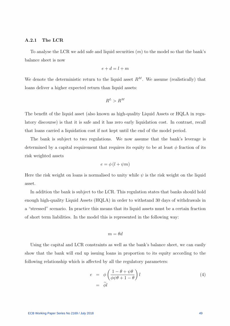
A.2.1 The LCR

To analyse the LCR we add safe and liquid securities (m) to the model so that the bank’s

balance sheet is now

e+ d = l +m

We denote the deterministic return to the liquid asset RM . We assume (realistically) that

loans deliver a higher expected return than liquid assets:

RL > RM

The benefit of the liquid asset (also known as high-quality Liquid Assets or HQLA in regu-

latory discourse) is that it is safe and it has zero early liquidation cost. In contrast, recall

that loans carried a liquidation cost if not kept until the end of the model period.

The bank is subject to two regulations. We now assume that the bank’s leverage is

determined by a capital requirement that requires its equity to be at least φ fraction of its

risk weighted assets

e = φ (l + ψm)

Here the risk weight on loans is normalised to unity while ψ is the risk weight on the liquid

asset.

In addition the bank is subject to the LCR. This regulation states that banks should hold

enough high-quality Liquid Assets (HQLA) in order to withstand 30 days of withdrawals in

a “stressed” scenario. In practice this means that its liquid assets must be a certain fraction

of short term liabilities. In the model this is represented in the following way:

m = θd

Using the capital and LCR constraints as well as the bank’s balance sheet, we can easily

show that the bank will end up issuing loans in proportion to its equity according to the

following relationship which is affected by all the regulatory parameters:

e = φ

(1− θ + ψθ

φψθ + 1− θ

)l (4)

= φl


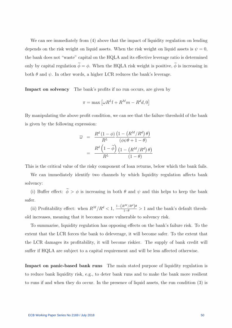
We can see immediately from (4) above that the impact of liquidity regulation on lending

depends on the risk weight on liquid assets. When the risk weight on liquid assets is ψ = 0,

the bank does not “waste” capital on the HQLA and its effective leverage ratio is determined

only by capital regulation φ = φ. When the HQLA risk weight is positive, φ is increasing in

both θ and ψ. In other words, a higher LCR reduces the bank’s leverage.

Impact on solvency The bank’s profits if no run occurs, are given by

π = max[ωRLl +RMm−Rdd, 0

]By manipulating the above profit condition, we can see that the failure threshold of the bank

is given by the following expression:

ω =Rd (1− φ)

RL

(1−

(RM/Rd

)θ)

(φψθ + 1− θ)

=Rd(

1− φ)

RL

(1−

(RM/Rd

)θ)

(1− θ)

This is the critical value of the risky component of loan returns, below which the bank fails.

We can immediately identify two channels by which liquidity regulation affects bank

solvency:

(i) Buffer effect: φ > φ is increasing in both θ and ψ and this helps to keep the bank

safer.

(ii) Profitability effect: when RM/Rd < 1,1−(RM/Rd)θ

1−θ > 1 and the bank’s default thresh-

old increases, meaning that it becomes more vulnerable to solvency risk.

To summarise, liquidity regulation has opposing effects on the bank’s failure risk. To the

extent that the LCR forces the bank to deleverage, it will become safer. To the extent that

the LCR damages its profitability, it will become riskier. The supply of bank credit will

suffer if HQLA are subject to a capital requirement and will be less affected otherwise.

Impact on panic-based bank runs The main stated purpose of liquidity regulation is

to reduce bank liquidity risk, e.g., to deter bank runs and to make the bank more resilient

to runs if and when they do occur. In the presence of liquid assets, the run condition (3) is


modified as follows:

ωRL (1− λ) l +RMm < Rdχd (5)

The above expression already shows how the LCR helps to deter bank runs or to make them

less costly if they do occur. Conditional on a run, liquidity increases the resources at the

bank’s disposal since RM > ωRL (1− λ). Hence even though liquid assets do not pay high

returns on average, they have a stable value in stressed funding conditions thereby making

the bank more resilient to runs.

Manipulating the run condition allows us to derive a run threshold below which depositors

will withdraw from the bank:

ω =Rd (1− φ)

(1− λ)RL

(χ−

(RM/Rd

)θ)

(φψθ + 1− θ)

=1

(1− λ)

(χ−

(RM/Rd

)θ)

(1− (RM/Rd) θ)ω

Again, banks with ω ∈ (ω, ω) are solvent but potentially illiquid and the main impact of

LCR regulation is to shrink the size of this region even if this does come at the expense of

making the bank slightly less profitable thereby increasing ω. Whether the bank’s fragility

is reduced by the LCR depends on which effect dominates. When holding liquidity is not

overly costly (i.e. RM/Rd is not too far below 1, the LCR leads to a reduction in the bank’s

probability of failure.

A.2.2 The NSFR

To analyse the NSFR, we now change our balance sheet model by abstracting from liquid

assets and by introducing long-term illiquid debt liabilities (b).

e+ d+ b = l

We think of b as “long term debt” which cannot be withdrawn on demand and is not subject

to runs. In contrast, d continues to denote short term deposits which can be run upon. The

bank’s profits next period are given by

π = max[ωRLl −Rdd−Rbb, 0

]


where Rd is the cost of short term deposits while Rb > Rd is the cost of long term debt.

This time, in addition to the capital constraint, the bank faces an NSFR constraint which

states that stable funding (bonds + equity) must be a certain fraction of illiquid assets

(loans)

e+ b = υl

Impact on solvency The failure threshold of the bank ω is the realisation of the loan

return shock ω below which the bank is insolvent. It is implicitly defined by the relation

below:

ωRLl −Rdd−Rbb = 0

Using the NSFR constraint, the capital constraint and the bank’s balance sheet, we can

derive the following expression for the failure threshold as a function of the policy parameters

and rates of return.

ω =Ra (1− φ)

RL

where

Ra =

[Rd (1− υ)

(1− φ)+Rb (υ − φ)

(1− φ)

]is the weighted average cost of debt funding for banks under the binding NSFR requirement.

The introduction of long term debt changes the expression for the threshold because

the bank’s weighted average cost of debt funding Ra is greater than Rd under the realistic

assumption that maturity transformation is profitable and Rb > Rd. Hence the NSFR regu-

lation reduces the bank’s profitability and other things equal increases its failure probability.

Impact on panic based-bank runs Of course, just as for the LCR, the primary reason

for the introduction of the NSFR is to prevent bank runs. To analyse the impact of the

NSFR on bank runs, we again suppose that a fraction χ of short term depositors d can

withdraw early after observing the loan return ωRL. Then loans must be liquidated at cost

λ.

The run exists whenever the liquidation value of the bank’s assets fails to cover the

potential withdrawals:

ωRL (1− λ) l < χRdd


Using the NSFR and the capital constraints we can compute the loan return shock threshold

below which depositors find it optimal to run:

ω =Rd (1− φ)

RL (1− λ)

χ (1− υ)

(1− φ)

Since υ = φ and χ 5 1, χ(1−υ)(1−φ)

< 1 and the NSFR makes the bank less likely to experience a

run compared to the no NSFR case. This is because the introduction of the NSFR replaces

runnable liabilities (deposits) with “stable” debt funding and this reduces the fragility of the

bank. Of course, as this example also makes abundantly clear, the way the bank becomes

more stable is by doing less maturity transformation.

A.3 Incentive effects of the LCR, NSFR and CR

In the simply model considered so far, the risk of bank assets was exogenously given. In

reality, bank actions affect the risk that the bank faces. For example, the bank can screen

loans to make sure to grant loans to the most creditworthy borrowers, the bank monitors

loans to maximize chances loans are repaid, or the bank scrutinizes the quality of other

assets it invests in. In this subsection, we extend the model above the make bank risk

endogenous, following Calomiris, Heider and Hoerova (2015). Specifically, we assume that

if a bank monitors its loans, then they yield return ωRL with probability 1. If a bank does

not monitor its loans, then the return is ωRL with probability p and it is zero otherwise.

There are two future states of the economy (denoted by s), good (g) or bad (b), s = {g, b}.

If a bank does not monitor loans, it derives a private benefit Bs per unit of loans in state s.

We assume that Bb > Bg, which captures the fact that it is more difficult to generate a high

loan return when the state of the economy is bad. The state is revealed after the makes its

funding and asset allocation decisions but before the makes its effort choice. After the state

s is revealed, the bank can choose to liquidate some of the loans and turn those into liquid

assets, ∆ms. This entails a per-unit cost of l. We assume that 1) monitoring is efficient so

that, for a given ω, ωRL > pωRL + Bb and 2) whether or not a bank monitors loans is not

observable to outsiders. Since the bank is protected by limited liability so that it can walk

away from its obligations when in default, a moral hazard problem ensues.

To ensure that a bank monitors loans in state s, a bank has to have an incentive to do


so, i.e., the expected profit from monitoring must be higher than the expected profit under

no monitoring or:

RL

(l − ∆ms

1− l

)+RM (m+ ∆ms)−Rdd−Rbb ≥

p

[RL

(l − ∆ms

1− l

)+RM (m+ ∆ms)−Rdd−Rbb

]+

(1− p) max[RMm− Rdd− Rbb, 0

]+Bs

(l − ∆ms

1− l

)where the bank can increase its liquid asset holdings by ∆ms after the state s is revealed, by

liquidating the amount ∆ms

1−l of its loans. To maximize a bank’s incentives, when zero returns

on loans are observed (implying that the bank did not monitor), it is optimal to distribute

all remaining assets RMm among bank creditors so that RMm = Rdd+ Rbb.

The incentive constraint in state s writes as

(1− p)[RL

(l − ∆ms

1− l

)+RM (m+ ∆ms)−Rdd−Rbb

]≥ Bs

(l − ∆ms

1− l

)It can be re-written as follows:(

RL − Bs

1− p

)(l − ∆ms

1− l

)+RM (m+ ∆ms) ≥ Rdd+Rbb

or, using the balance sheet identity,(RL − Bs

1− p

)(l − ∆ms

1− l

)+RM∆ms ≥ Rd (l − e) +

(Rd −RM

)m+

(Rb −Rd

)b

The expression in brackets on the left-hand side is also known as “pledgeable return”

(Holmstrom and Tirole, 1997) or a return that can be pledged to bank creditors without

jeopardizing a bank’s incentive to monitor. Note that loans are pledgeable at the return

that is lower than their physical expected return RL while liquid assets are pledgeable at

their full return RM since there is no monitoring associated with the liquid asset holdings.

In other words, cash holdings are impervious to moral hazard and they are fully pledgeable.

The incentive effects of capital and liquidity are as follows:

(i) Higher equity holdings e relax the incentive constraint.

(ii) When the pledgeable return on loans is lower than the return on safe assets, RL− Bs

1−p <

RM , liquidating loans and turning them into liquid assets relaxes the incentive constraint.


(iii) Higher bond holdings b tightens the constraint if bonds are more expensive than

deposits (profitability effect).

(iv) Higher liquid asset holdings m tightens the constraint if the yield on liquid assets RM

is lower than the cost of deposits (profitability effect).

Calomiris, Heider and Hoerova (2015) show that the incentive constraint in the bad state,

not in the good state, is binding. The way the bank can help relax this constraint is to scale

back his loan portfolio: liquidate some of the loans and turn them into cash. It will entail a

per-unit liquidation cost l to turn loans into cash. But the gain is that cash may be more

pledgeable than risky loans. Such liquidation is the optimal decision when the moral hazard

problem is sufficiently severe (Bb is high), the liquidation costs are moderate (l is low) and

if the bad state is ex ante sufficiently unlikely.

Appendix B Brief description of the macroeconomic

models used

B.1 Van den Heuvel (2017): “The Welfare Effects of Bank Liq-

uidity and Capital Requirements”

Banks create liquidity. They do this by funding relatively illiquid loans to firms and

households with liquid and relatively safe deposits. While borrowers get financing, depositors

get a combination of payment services, easy access to funds, and interest income. This

social function of banks has long been recognized in the literature. The model of Van den

Heuvel (2017) embeds the role of liquidity creating banks in an otherwise standard general

equilibrium growth model. Besides banks, the model also features firms and households, who

own the banks and the firms, as well as a government that can impose regulations. Because

of the preference for liquidity on the part of households and firms, liquid assets, such as bank

deposits and government bonds, will command a lower rate of return than illiquid assets,

such as bank loans and equity. The spread between the two is the convenience yield of the

liquid instrument.

For banks, this spread implies that the capital requirement binds, as deposit finance is


less expensive than equity, a deviation from the Modigliani-Miller benchmark. The liquidity

requirement, which requires banks to hold a fraction of deposits in the form of government

bonds, will bind if the convenience yield on government bonds exceeds the convenience

yield on bank deposits (net of the noninterest cost of servicing those deposits). Because of

competition, banks pass on the cheap deposit funding to borrowers in the form of a lower

lending rate, boosting investment. However, if binding, both the capital requirement and

the liquidity requirement limit the reduction in the lending rate.

Both capital and liquidity regulation do provide benefits in the model. These ultimately

derive from a moral hazard problem created by deposit insurance (which can be interpreted

more broadly as explicit or implicit government guarantees). Due to deposit insurance banks

shareholders do not internalize all the potential losses when they make choices about risk.

This can lead to excessive risk taking, which banks can engage in by making excessively risky

loans and/or by holding insufficient liquid assets to guard against liquidity shocks due to

early withdrawals by depositors. Limiting this behaviour is desirable for two reasons. First,

making excessively risky loans to firms is distortionary and results in lower productivity.

Second, excessive risk taking results in elevated bank failure rates – a banking crisis – which

entails negative externalities, including deadweight resolution costs.

As bank supervision can only detect excessive risk taking imperfectly, a capital require-

ment is helpful in limiting the moral hazard problem by ensuring that shareholders internalize

more potential losses, be it from lending or from liquidity stress. A liquidity requirement is

also helpful, though the model suggests that it only ameliorates the second manifestation of

the moral hazard problem, excessive liquidity risk. Thus, the financial stability benefits of

the capital requirement are broader. However, liquidity regulation addresses the problem of

liquidity risk more directly – and, it turns out, at lower cost – so it is still part of the optimal

policy mix. Indeed, the model suggests a simple division of labour: in the optimal policy

mix the liquidity requirement addresses liquidity risk and the capital requirement deals with

credit risk.

At the same time, liquidity and capital regulations also impose important costs according

to the model: they reduce the ability of banks to create net liquidity through the transfor-

mation of illiquid loans into liquid deposits. After all, capital requirements directly limit


the fraction of bank loans that can be financed by issuing deposit-type liabilities. Liquidity

requirements force banks to hold safe, liquid assets against deposits, limiting their liquidity

transformation by restricting the asset side of their balance sheet. This is costly because

safe, liquid assets are necessarily in limited supply and may have competing uses. In the

model, this is captured by assuming that government bonds, like bank deposits, are liquid.

A key contribution of the paper is to derive simple formulas for the macroeconomic costs

of the two regulations that can be taken to the data. These costs depend crucially on the

value of the banks’ liquidity creation and the liquidity of government bonds. Fortunately,

the model shows that equilibrium asset returns reveal the strength of these preferences for

liquidity. Using this, the marginal cost of increasing the liquidity requirements is derived as:

d

c

(RD −RB + n

)(1− λ)−1

where d/c is ratio of aggregate deposits to consumption, RD − RB is the spread between

bank deposits and government bonds, which is adjusted for the noninterest cost of servicing

deposits (n), and λ is the LCR-style liquidity requirement.

The logic is simple: from the perspective of the other agents, the liquidity requirement

effectively forces banks to transform some government bonds into deposits, both instruments

prized for their liquidity. Thus, imposing a liquidity requirement entails a social cost only to

the extent that the liquidity services of deposits are, at the margin and net of the noninterest

cost of creating these services, valued less than those of Treasuries; only then is there a costly

net reduction in liquidity available to investors. The deposit-Treasury spread, adjusted for

the noninterest cost of deposits, reveals whether this is true or not.

A similar formula for the marginal cost of raising the capital requirement is provided in

Van den Heuvel (2017). It is particularly simple when the liquidity requirement is set to

zero. In that case, the marginal cost of the capital requirement is:

L

c

(RE −RD − n

)where L/c is the ratio of total loans to consumption, RE − RD is the spread between the

(risk-adjusted) required return on equity and deposits, and n is again the noninterest cost

of servicing deposits. An increase in the capital imposes a cost by constraining the ability


of banks to issue deposit-type liabilities, which are valued by households for their liquidity.

The spread between the return on bank equity and deposits reveals the strength of liquidity

preferences with respect to deposits. Further, the paper shows that, all else equal, a binding

liquidity requirement lowers the welfare cost of the capital requirement.

B.2 The 3D Model

B.2.1 Main Model Features

The 3D model is a macroeconomic model that was initially designed for the analysis of

capital regulation. Its main distinguishing feature is the emphasis on bank default and its

consequences for macroeconomic outcomes and welfare. For the purposes of this paper, the

model has been extended to include liquidity regulation tools.

The model considers an economy populated by saving households and borrowing house-

holds that consume, supply labour to the production sector and invest in housing. House-

holds belong to two dynasties of ex ante identical infinitely lived agents that differ in terms

of the subjective discount factor. In equilibrium, patient households save and impatient

households borrow to finance their housing investment. The total mass of households is

normalized to one, of which an exogenous fraction are savers and the remaining fraction are

borrowers.

Entrepreneurs own the capital used in the production technology. Capital purchase is

financed with entrepreneurial wealth and bank loans. Capital and housing production face

adjustment costs. All borrowers, including banks, operate under limited liability. External

financing is modelled in the form of non-contingent (non-recourse) debt. Borrowers optimally

decide to default when the return on their assets is lower than their debt. Default hits the

balance sheet of lenders, affecting loan pricing and credit supply.

Banks are essential to intermediate funds between savers and borrowers in this economy.

They raise equity from banks shareholders and deposits from households, to finance their

loans. Deposits are partially insured by a deposit insurance (DI) agency funded with lump

sum taxes. Banks default when the return on their loan portfolio is insufficient to cover


deposit repayments.16

In particular, default by household and/or firms hits the balance sheet of banks with two

effects: (i) lower bank capital (ii) higher bank risk and higher bank funding costs. Both lead

to a reduction in the supply of credit.

The key distortions in the model are related to:

• Limited liability of banks and safety net guarantees (total or partial DI): these insulate

banks from the effect of their risk taking on the cost of deposits.

• The risk premium on uninsured debt is based on average (rather than individual) bank

risk behavior: this further reduces the incentive of any individual bank to limit leverage

and failure risk because it will get no funding cost benefit when uninsured debt holders

are uninformed.17

• Limited participation to the equity market: this makes equity scarce and their use

more expensive than debt.

As a result of the first two types of distortions banks have an incentive to take as much

risk as possible by leveraging up to the regulatory limit. Banks’ excessive leverage has three

effects in equilibrium: (i) a higher bank default probability and hence higher bank funding

costs (through a higher risk premium on uninsured bank debt; (ii) higher bailout subsidy

which attenuates the increase in bank funding costs; (iii) less usage of expensive equity which

lowers overall funding costs. The net effect on economic activity depends on whether bank

funding costs go up or down as a result of excessive leverage. When bank failure risk is

high, the effect of the higher risk premium on uninsured debt dominates and high leverage

depresses economic activity. When bank failure risk is low, the traditional effect dominates.

In that case, economising on expensive equity reduces overall bank funding costs and higher

bank leverage increases economic activity.

16Upon default, depositors do suffer some costs despite the presence of deposit insurance. This feature is

in the model in order to provide a link between bank risk and banks’ funding costs. The average probability

of bank default is used as a proxy to assess the degree of financial (in)stability.17This aims to capture the fact that banks are opaque and it is difficult for even relatively expert investors

to understand the true nature of risks on their balance sheets.


B.2.2 The Macroeconomic Impact of Liquidity Tools

The 3D model is silent on the benefits of liquidity regulation that work through the

prevention of bank runs. Its main strength is on quantifying the macroeconomic costs of

liquidity tools as well as the impact of liquidity tools on the bank’s solvency risk that is

unrelated to bank runs.

The LCR ratio is modelled in the 3D by imposing an additional regulatory requirement.

Banks need to hold government bonds as a certain proportion of their deposits. Government

bonds in the model are safe assets which pay the risk-free rate. Since the risk-free rate is

lower than the rates on bank deposits and on loans, banks make losses on government bonds

and would not hold them voluntarily. In addition, the government bonds may be subject to

a capital requirement. In the baseline, we assume zero weights on government bonds.

Impact on credit supply and the cost of credit. When the risk weight on government

bonds is zero, the only impact of the liquidity requirement is to force banks to hold a loss-

making asset, depressing their profitability. In the long run , the bank’s rate of return

on equity needs to be high enough so that bank capital is stable despite regular dividend

payments. Lower profitability due to banks’ bond holdings must therefore be made up by

increasing loan rates. Credit declines although the impact is not quantitatively large.

The credit supply contraction is greater when bonds attract a positive risk weight. Then,

in addition to their impact on bank profitability, the liquidity requirements directly crowd

out loans from bank portfolios. Therefore, the increase in lending spreads and the decline in

loans are even greater.

Impact on bank solvency. Liquidity requirements affect bank profitability and, to the

extent that bond holdings attract a capital charge, they also affect bank leverage. Both of

these factors have an impact on the probability that the bank becomes insolvent due to poor

loan return realisations.

It turns out that, once we take general equilibrium effects into account, banks’ profitability

does not suffer very much. Higher loan rates offset the costs of the bond holdings and, thus,

solvency risk is little changed. When HQLA attract a capital charge, a higher LCR also


induces a decline in overall bank leverage. This, other things equal, leads to a decline in the

probability of bank default due to a standard ‘buffer effect’.

Appendix C Description of the LCR and NSFR

C.1 LCR

The Liquidity Coverage Ratio (LCR) became effective in the EU in October 2015.18 The

ratio equals a credit institution’s liquidity buffer divided by its net liquidity outflows over a

30 calendar day stress period.

The liquidity buffer is defined as the stock of unencumbered high-quality liquid assets

(HQLA) that a bank holds. The exact calculation of HQLA is complex and relies on a

weighting scheme for a bank‘s assets.19 Bank assets are divided in three broad groups;

Level 1 assets, Level 2 assets and Level 2B assets. Level 1 assets are very liquid assets such

as cash and marketable securities that are assigned a zero risk-weight under the Basel II

Standardized Approach for credit risk. These assets count for 100% towards the stock of

HQLA. Level 2 and Level 2B assets comprise various (government and corporate) securities

and are subject to a haircut before being added to the HQLA stock. They cannot take up

more than 40% of HQLA.

Net liquidity outflows are defined as the expected cash outflows over the next 30 days

minus the total expected inflows, with the restriction that expected inflows are capped at

75% of the outflows. Expected outflows are calculated by multiplying outstanding balances

of various types of liabilities and off-balance sheet commitments with expected run-off rates.

Retail deposits covered by deposit insurance, for example, are subject to an expected run-off

rate of 3% or higher20, non-insured deposits are subject to a minimum expected run-off rate

off 10%.

18See Commission Delegated Regulation (EU) 2015/61 of 10 October 2014 to supplement Regulation (EU)

No 575/2013 of the European Parliament and the Council with regard to liquidity coverage requirement for

Credit Institutions.19See BIS (2013) for a detailed explanation of the calculation of both the HQLA and the net outflows.203% is the minimum that should be applied to these deposits, but local regulators can decide to implement

higher expected run-off rates.


From January 2018 onwards, the ratio will have to be above 100%. Until then, the

regulation allows for a phase-in period, with the minimum requirement set to 60% in 2015,

70% in 2016 and 80% in 2017.

C.2 NSFR

The Net Stable Funding Ratio (NSFR) compares the amount of available stable funding

with the amount of required stable funding. In contrast with the LCR, it does not focus

on the short-term resilience of a bank but instead aims to reduce funding risk over a 1-year

horizon.

The calculation of the amount of available stable funding relies on a weighting scheme a

bank‘’s funding sources. A bank‘s capital and liabilities are divided in 5 broad categories.

Each category receives a specific weight (ranging between 0 and 100 %) and the total amount

of stable funding is calculated as the weighted sum of the different categories. Regulatory

capital (excluding Tier 2 instrument with a residual maturity below 1 year), for example,

receives a 100 % weighting factor, while insured deposit will receive a weight of 90 or 95%.

Required stable funding is based on the characteristics of a bank’s assets and off-balance

sheet exposures. As with the calculation of the available stable funding, assets and off-

balance sheet exposures are divided in different categories that all get a specific weight. The

weighting scheme is based on the residual maturity or liquidity value of an exposure, where

exposures with a higher residual maturity or a lower liquidity value get a higher weight.

Additionally, assets that are encumbered for one year or more automatically receive a 100

% weighting factor. Assets that are assigned a 0 % weight are for example cash and central

bank reserves.


(a) LCR

(b) NSFR

Figure 3: Impact of LCR and NSFR on LOLR Reliance: Average Take-up in ’08-’09 Source:

MFI level IBSI data for 197 euro area banks and own calculations. Notes: This figure shows the predicted

liquidity take-up of banks with different levels of the LCR (panel (a)) or NSFR (panel (b)) during a crisis

period. The predicted values are based on equation 2, which is estimated using monthly data for 197 euro

area MFIs between January 2008 and September 2009. Liquidity take-up is defined as the total reliance on

central bank liquidity scaled by total assets. Blue dots represent predictions that are statistically significant

at the 10 % level, red dots indicate insignificant predictions at the 10 % level.


Figure 4: What if All Banks Had an LCR Above 100? Source: Own calculations using MFI level

IBSI data and liquidity take-up data for 197 euro area banks. Notes:The sample period is January 2008

to December 2009. The black line represents the actual liquidity take-up of all MFIs in our sample. The

estimated LCR (red line) and NSFR (blue line) take-up is estimated in two steps. First, we estimate equation

2 for both ratios. Next, we put the LCR and NSFR values to 100 for all banks that have an LCR and NSFR

below 100 and subsequently calculate the predicted take-up for each bank, using the estimated coefficients

from equation 2. We then aggregate the individual estimates to get the final estimated take-up.


Figure 5: Rates on Deposits and Government Bond Yields. Source: SDW and authorsae calcu-

lations. Notes: The blue line is the average interest rate on total deposits of households and non-financial

corporations in euro area banks. The red line is the average yield on 1-year sovereign bonds of non-stressed

euro area countries, as a proxy for the yield on (level 1) HQLA assets. The interest rate on deposits is

adjusted to include an estimate of the non-interest cost of servicing deposits.

Figure 6: Cost of LCR and NSFR in the 3D model


Acknowledgements This paper was written while Skander Van den Heuvel was on leave from the Federal Reserve Board. We would like to thank seminar participants at the ECB, Federal Reserve Board, as well as Luc Laeven, Philipp Hartmann, Simone Manganelli and Michael Wedow for helpful comments and suggestions. The views expressed in this paper do not necessarily reflect those of the ECB, the Eurosystem or the Federal Reserve Board. Marie Hoerova European Central Bank, Frankfurt am Main, Germany; email: [email protected] Caterina Mendicino European Central Bank, Frankfurt am Main, Germany; email: [email protected] Kalin Nikolov European Central Bank, Frankfurt am Main, Germany; email: [email protected] Glenn Schepens European Central Bank, Frankfurt am Main, Germany; email: [email protected] Skander Van den Heuvel Federal Reserve Board, Washington DC, United States; email: [email protected]

© European Central Bank, 2018

Postal address 60640 Frankfurt am Main, Germany Telephone +49 69 1344 0 Website www.ecb.europa.eu

All rights reserved. Any reproduction, publication and reprint in the form of a different publication, whether printed or produced electronically, in whole or in part, is permitted only with the explicit written authorisation of the ECB or the authors.

This paper can be downloaded without charge from www.ecb.europa.eu, from the Social Science Research Network electronic library or from RePEc: Research Papers in Economics. Information on all of the papers published in the ECB Working Paper Series can be found on the ECB’s website.

PDF ISBN 978-92-899-3274-5 ISSN 1725-2806 doi:10.2866/805891 QB-AR-18-049-EN-N

mailto:[email protected]





http://www.ecb.europa.eu/

http://www.ecb.europa.eu/

http://ssrn.com/

https://ideas.repec.org/s/ecb/ecbwps.html

http://www.ecb.europa.eu/pub/research/working-papers/html/index.en.html

Benefits and costs of liquidity regulation - European Central ...

Documents

Transcript of Benefits and costs of liquidity regulation - European Central ...