THE ANCILLARY HEALTH BENEFITS AND COSTS OF GHG MITIGATION: SCOPE,SCALE, AND CREDIBILITY

by Devra DAVIS, Alan KRUPNICK and George THURSTON

Section 899 of the Code of Criminal Procedure for the State of New York, opens with the statementthat “persons pretending to foresee the future shall be deemed disorderly...”

1. Introduction

Climate change mitigation policies will bring with them ancillary or secondary benefits and costs inaddition to those directly associated with avoided temperature changes. The ancillary public healtheffects of air pollutant emission changes (such as in reductions in particulate matter (PM)) have beenthe focus of some research attention. However, none of the major economic models of climateimpacts has incorporated these ancillary impacts into their analyses. The extent and scale of ancillaryimpacts will vary with the particular Greenhouse Gas (GHG) mitigation policy chosen. Theconsideration of ancillary benefits can be of critical importance for devising optimal mitigationstrategies. To assist in the assessment of ancillary benefits, this paper examines literature relevant tothe assessment of ancillary benefits for public health of GHG policies and offers criteria for evaluatingthis work.

A broad array of tools is required for the conduct of public health evaluations of ancillary costs andbenefits, and such tools are readily available. Energy scenarios can be employed to produce scenariobased risk assessments, which rely on emission inventories and air pollution and dispersion models.Estimated changes in concentrations and exposures from these scenarios can then be linked in order toestimate incremental changes in public health that could result from various GHG policies (Burtrawet al., 1996, Cropper and Oates, 1992, Holmes et al., 1995, Jorgenson et al., 1995, Viscusi et al., 1994,Burtraw and Toman, 1997, and Burtraw et al., 1999). In addition, a global assessment has been madeof the impacts on public health that could arise between 2000 and 2020 under current policies, andunder the scenario proposed by the European Union (EU) in 1995. (Working Group on Fossil Fuels,1997, Davis, 1997). Country-wide assessments of GHG mitigation policies on public health have alsobeen produced for Canada (Last et al., 1998) and for China (World Bank, 1997), under differingbaseline assumptions.

In addition, there are numerous cost-benefit analyses that have been used to assess the public healthbenefits of proposed environmental regulatory strategies (e.g., U.S. EPA, 1999, Thurston, et al, 1997).Indeed, such cost-benefit analyses are required in the U.S. by Executive Order for major newregulations. The public health effects of emissions changes in GHG co-pollutants is only one class ofmany potential ancillary effects of GHG reduction policies. To estimate the entire array of ancillarypublic health cost and benefits of alternative GHG mitigation strategies, a wide body of knowledgeand practice has been developed for potential application

At the same time, both the public health and the economics literatures are rife with ongoingcontroversies. These include: the concentration-response functions being used (the appropriatepollutants, the nature of and uncertainty about the functional relationships (e.g., whether thresholdsexist)) and, the valuation of various health endpoints (the appropriate estimates for the value of astatistical life or statistical life year, for instance). Ideally, such cost-benefit studies should includepollutants emitted into all environmental media, including air, water, and land. For instance, waterand soil pollution can arise from the deposition of combustion products from fossil fuels, such asreactive sulfur and nitrogen compounds, which interact with naturally occurring humic materials,phytochemicals and byproducts of chlorination to yield highly potent and reactive byproducts (Wuet al., 1999). These byproducts can exacerbate water pollution and worsen water quality, causingadverse impacts on human health.

Nevertheless, judging by the many past cost-benefit analyses of the effects of energy use on theenvironment and health, the largest quantifiable category of ancillary benefits or costs is related to airpollution and health effects. Of these, the largest contributor to the quantifiable monetary valuation ofhealth benefits involves mortality risks, while the numbers of estimated adverse effects are dominatedby less severe health outcomes.

While recognizing that air pollution is but one example of the potential auxiliary changes that willaccompany GHG mitigation policies, this paper attempts to clarify the weight of the evidence on theimportant relationship between air pollution and health on the one hand, and health and economicvalues on the other. Annex I presents a discussion of basic epidemiologic and economic concepts.The body of this manuscript investigates, from the perspective of the health effects literature and thevaluation literature, several key aspects of this relationship:

• the scope of ancillary effects (Section 2) —which categories of health are likely to be affectedwhen carbon reduction policies are put in place, including both quantified and non-quantifiedhealth effects, and which of these have been expressed in monetary terms;

• the scale of ancillary effects and benefits/costs (Section 3 for health effects, Section 5 forvaluation):

− – How large are these effects likely to be?

− – What is the population at risk?

− – How large are the monetary values of these effects?

• The credibility of these estimates (Section 4 for health effects; Section 6 for valuation). Whatare the strengths, weaknesses, limitations and uncertainties characterizing the relationshipsbetween pollution and health and for the various methods of estimating the economicvaluation of these effects?

We close with recommendations to policymakers and modelers on the appropriate role of ancillaryhealth benefits and costs in the climate change mitigation debate and supporting modeling. As part ofthese recommendations, we also identify a number of public health and economic related researchtopics that require clarification in order to promote the more effective conduct of ancillary benefitsassessments with respect to GHG mitigation policies. See Annex I for a discussion of basicepidemiologic and economic concepts.

2. Scope of ancillary benefits

2.1 Health effects

Most of the research that has quantified health effects linked with air pollution extends across theentire human age range. Considerable numbers of human studies have been conducted for thecommonplace “community” air pollutants. As a result, there is a large and rapidly growing number ofstudies linking air pollution with both mortality and morbidity throughout the world. A broadconsensus has emerged over the past 5 decades showing that ambient levels of pollution in developedcountries today are linked with measurable impacts on public health. Public health disasters, such asthe episodes that occurred in London, 1952 and Donora, 1948, provided unambiguous proof of thedamaging potential of high levels of air pollution for public health.

More recently, sophisticated time series analyses of daily pollution patterns, along with cross-sectionaland cohort studies of differences in rates of chronic and acute illness, have provided a consistentpicture of the extent to which ambient levels of air pollution affect severe health outcomes, includingmortality and hospital admissions. But, as displayed in Figure 1 for the city of New York, theseroutinely recorded severe health outcomes represent only the “tip of the iceberg” of adverse effectsassociated with this pollutant. They are best viewed as indicators of the much broader spectrum ofadverse health effects, such as increased restricted activity days and doctors visits, being experiencedby the public as a result of air pollution exposures. Although these outcomes have much lower“monetary valuations” than the more severe impacts, their presence is important to recognize whengauging the scope of air pollution’s impact on society.

Figure 1. Pyramid of New York City, NY Annual Adverse Ozone Impacts avoided by theimplementation of the proposed new standard (vs. “AsIs”)*

3,500 Respiratory ED Visits/yr

180,000 Asthma Attacks/yr

(i.e. , person-days during which notably inc reased asthma s ymptoms, e.g.,

requiring extra medication, are experienced)

240265

75 Deaths/yr

Non-asthma Respiratory Hospital Admissions/yr

Asthma Hospital Admissions/yr. (0.01% of all adverse impact cases)

930,000 Restricted Activity Days/yr

(i.e., person-days on which activities are restricted due to illness )

2,000,000 Acute Respiratory Symptom Days/yr

(i.e., person-days during which respiratory symptoms such as chest discomfort, coughing, wheezing, doctor diagnosed flu, etc.

are experienced)

*Figure section sizes not drawn to scale.Source: Ozone and Particulate Matter Standards: Hearings on the Clean Air Act Before theSubcommittee on Clean Air, Wetlands, Private Property and Nuclear Safety and the Comm.on Env’t and Public Works, 105th Congress (1997).

A summary of the presently quantifiable and the suspected effects of ambient air pollution on humanhealth are summarized in Table 1. From this table, it can be seen that any air pollution impactassessment, especially in terms of numbers of health effects, will not be able to quantify the full rangeof changes in health effects that will result from changes in the levels of ambient air pollution.

The very young, older adults, and persons with pre-existing respiratory and cardio-vascular disease areamong those thought to be most strongly affected by air pollution. Airway inflammation induced byozone and PM is especially problematic for children and adults with asthma, as it makes them moresusceptible to having asthma attacks, consistent with recent asthma camp results (Thurston,et al., 1997). For example, controlled human studies (e.g., Molfino et al., 1991) have indicated thatprior exposure to ozone enhances the reactivity of asthmatics to aeroallergens, such as pollens, whichcan trigger asthma attacks. In addition, ozone increases inflammation and diminishes immunefunction the lungs. This can make older adults more susceptible to pneumonia, a major cause ofillness and death in this group.

Table 1. Scope of health effects

Human Health Effects of Air Pollution

Quantifiable Health Effects Non-quantified/Suspected Health Effects

Mortality*Bronchitis - chronic and acuteAsthma attacksRespiratory hospital admissionsCardiovascular hospital admissionsEmergency room visits for asthmaLower respiratory illnessUpper respiratory illnessShortness of breathRespiratory symptomsMinor restricted activity daysAll restricted activity daysDays of work lossModerate or worse asthma status

Neonatal and post-neonatal mortalityNeonatal and post-neonatal morbidityNew asthma casesFetus/child developmental effectsNon-bronchitis chronic respiratory diseasesCancer (e.g., lung)Behavioral effects (e.g.,.learning diabilities)Neurological disordersRespiratory cell damageDecreased time to onset of anginaMorphological changes in the lungAltered host defense mechanisms (e.g., increased susceptibility to respiratory infection)Increased airway responsiveness to stimuliExacerbation of allergies

Source: Adapted from: The Benefits and Costs of the Clean Air Act 1990 to 2010, U.S. EPA,EPA-410-R-99-001 1999).

It is well established that both asthma mortality and asthma hospital admissions increased during the1980’s in the U.S. and other developed nations (e.g., Buist and Vollmer, 1990; Taylor andNewacheck, 1992). The highest rates are associated with inner city residence (Carr et al, 1992; Weissand Wagener, 1990), and Latino or African-American origin (Carter-Pokras and Gergen,1993; Coultas et al, 1993; Weiss and Wagener, 1990). Conventional air pollutants do not appear tobe the driving force behind the global increase in the prevalence of asthma, since levels ofconventional pollutants have generally declined while the asthma prevalence has increased. However,because more persons are acquiring asthma, an ever increasing number in the population will beaffected by the aggravating effects of air pollution, especially among the economically disadvantaged.In many different regions of the world, studies have found a higher rate of hospitalizations for asthmain more polluted zones. For example, the chance of being hospitalized with asthma on days followinghigh air pollution in New York City is much greater than in the surrounding suburbs, probably becausethe city has a much larger minority and low-income population (Thurston et al., 1992, Saldiva et al.,1996). In the words of Weiss and Wagener (1990), “whatever the reason for the increases, bothasthma mortality and hospitalization continue to affect non-whites, urban areas, and the poordisproportionately. For example, the hospitalization rate for asthma is higher in New York City thananyplace else in the U.S. (Carr et al., 1992).

Among the factors that may increase the susceptibility of residents of low-income urbanneighborhoods to air pollution are:

i. Enhanced individual susceptibility of minority populations to pollutioneffects (i.e., more compromised health status, due to genetic predisposition,impaired nutritional status, or severity of underlying disease);

ii. Exposures to atmospheric pollution in center cities may be greater thanthose of the general population, due to higher local pollutant emissionscombined with a lower prevalence of protective air conditioning;

iii. Potentially enhanced exposures to a variety of residential risk co-factorssuch as cockroaches, dust mites, and indoor pollution sources (e.g., gas stovesused for space heating purposes); and/or

iv. A greater likelihood of poverty, which is associated with reduced access toroutine preventive health care, medication, and health insurance.

A number of studies suggest that the very young represent an especially susceptible sub-population,although the precise magnitude of the effects of specific levels of air pollution can be expected to varywith other underlying conditions. Lave and Seskin (1977) found mortality among those 0-14 years ofage to be significantly associated with levels of total suspended particulates (TSP). More recently,Bobak and Leon (1992) studied neonatal (ages less than one month) and post-neonatal mortality (ages1-12 months) in the Czech Republic, finding significant and robust associations between post-neonatalmortality and PM10, even after considering other pollutants. Post-neonatal respiratory mortalityshowed highly significant associations for all pollutants considered, but only PM10 remainedsignificant in simultaneous regressions. Woodruff et al. (1997) used cross-sectional methods tofollow-up on the reported post-neonatal mortality association with outdoor PM10 pollution in a U.S.population. This study involved an analysis of a cohort consisting of approximately 4 million infantsborn between 1989 and 1991 in 86 U.S. metropolitan statistical areas (MSAs). After adjustment forother covariates, the odds ratio (OR) and 95% confidence intervals for total post-neonatal mortality forthe high exposure versus the low exposure group was 1.10 (CI=1.04-1.16). In normal birth weightinfants, high PM10 exposure was associated with mortality for respiratory causes (OR = 1.40,CI=1.05-1.85) and also with sudden infant death syndrome (OR = 1.26, CI=1.14-1.39). Among lowbirth weight babies, high PM10 exposure was associated, but not significantly, with mortality fromrespiratory causes (OR = 1.18, CI=0.86-1.61).

This study was recently corroborated by a more elegant follow-up study by Bobak and Leon (1999),who conducted a matched population-based case-control study covering all births registered in theCzech Republic from 1989 to 1991 that were linked to death records. They used conditional logisticregression to estimate the effects of suspended particles, sulfur dioxide, and nitrogen oxides on risk ofdeath in the neonatal and post-neonatal period, controlling for maternal socioeconomic status and birthweight, birth length, and gestational age. The effects of all pollutants were strongest in thepost-neonatal period and were specific for respiratory causes. Only particulate matter showed aconsistent association when all pollutants were entered in one model. Thus, populations withrelatively high percentages of children may have higher air pollution effects than in populations instudy areas with fewer children (e.g., studies conducted more developed nations).

2.2 Scope for valuation

The literature reviewed above indicates that a wide variety of possible health endpoints could beaffected ancillary to climate change mitigation policies. Some of these have not been quantified, andsome of the effects listed as non-quantified may be related physiological expressions of those that arequantified. Of the quantified endpoints, Table 2 provides information about whether they have been(or could be) monetized, based on our understanding of the literature. We also consider the status ofmonetization for some of the non-quantified health effects. For each of these effects, we list thetechniques used to provide monetary values. Willingness to Pay studies (WTP) are those that provideestimates of preferences for improved health that meet the theoretical requirements of neoclassicalwelfare economics. Cost of Illness (COI) is a technique that involves totaling up medical and other outof pocket expenditures. “Consensus” refers to the way in which these values were determined. Theydo not have much of an evidentiary basis. Each of these approaches and endpoints are discussed inmore detail in Section 6.

The valuation literature for neonatal mortality, children, and cancer is very limited at the present time,but there is much interest in better valuing these endpoints in the U.S. Cancer valuation is discussed inSection 6. Valuing reduced mortality risks for newborns or children is one of the most challengingtasks in the field because children are generally not the key decision makers over their own health andsafety. They are part of a family unit that makes choices for them. For this reason, some economistsare devising household production function models to address these valuation questions (Tolley,1999; Dickie, 1999) and devising novel strategies for measuring revealed preferences for improvingchild safety and health (such as examining the types of vehicles or bicycle helmets purchased).However, this literature has not yet matured.

In addition, we add here placeholders for two potentially important linkages that go from economiceffects of GHG policies to health effects rather than the reverse. The linkage from unemployment tohealth refers to the possibilities that GHG policies might raise or lower unemployment rates from whatthey would otherwise be. A number of studies have linked unemployment to increased suicides,domestic violence, and alcohol and drug abuse. While this linkage is quite controversial in the healthbenefits literature, it has the potential to introduce a large, new set of ancillary benefits (or costs) tosuch studies. The second linkage — from lower incomes to lower health status — is of a similar type.GHG policies may lower incomes below BAU levels. A number of studies have shown how income ispositively correlated with health status. Thus, if incomes fall or do not rise as fast as a result of aGHG policy, health may worsen absolutely or relative to what it would have been in the absence of aGHG policy. Again, this linkage is quite controversial, and is included here because of its potential tochange thinking on the ancillary benefits/costs issue.

Table 2. Status of valuation of quantified and suspected health endpoints

Health Effects ValuationEstimatesAvailable?

Basis

QUANTIFIED EFFECTSMortality: Adults Y WTP (caveats)Chronic Bronchitis Y WTP (caveats)Acute Bronchitis Y COIHospital Admissions Y Hospital CostsEmergency room visits Y Emergency room costsLower respiratory illness Y WTP (caveats)Upper respiratory illness Y WTP (caveats)Respiratory symptoms Y WTPMRAD Y ConsensusRAD Y ConsensusWLD Y WageAsthma Day Y WTPChange in asthma status NNON-QUANTIFIED/SUSPECTED EFFECTSMortality: Neonatal/fertility

Y WTP; Number ofstudies on-going

Mortality: Children Soon Number of WTPstudies on-going

Cancer Mortality andMorbidity (various types)

Y COI; WTP

LINKS FROM ECONOMIC EFFECTS TO HEALTHHealth effects linked tounemployment

? ?

Health effects linked tolower incomes

? ?

3. Scale of health effects

Observational epidemiology studies - both long-term and acute exposure studies - have showncompelling and remarkably consistent evidence of air pollution associations with adverse humaneffects, including: decreased lung function, more frequent respiratory symptoms, increased numbersof asthma attacks, more frequent emergency department visits, additional hospital admissions, andincreased numbers of daily deaths. While not all of these impacts represent major financial impacts onthe society, they often involve decreases in quality of life, and also provide additional weight ofevidence of air pollution associations with the most serious effects, such as mortality.

In studies to date, the health effects associated with particulate matter (PM) and ozone (O3) haveconsistently been found. Particulate matter consists of two types of particles: primary and secondaryparticles. Primary particles come directly out of the tailpipes and stacks, and those are primarilycarbonaceous particles. Secondary particles are formed in the atmosphere from gaseous pollutants,such as sulfates from sulfur dioxide and nitrates from nitrogen oxides (NOx). Ozone (O3) is aninvisible irritant gas that is formed in the atmosphere in the presence of sunlight and other airpollutants. These ozone precursor pollutants, nitrogen oxides and hydrocarbons, as well as SO2, comefrom a variety of sources, including diesel automobiles (diesel contains more sulfur than gasoline),power plants, and industry.

As shown in Figures 2-5, there have been numerous studies published in recent years indicatingconsistent associations between both PM and O3 exposures and both daily mortality and morbidity. Itis interesting to note that the inclusion of PM along with ozone in the model has little effect on theO3-mortality effect, indicating that these associations are likely to be largely independent of oneanother.

Figure 2. Ozone mortality effect estimates across localities, with and without simultaneousinclusion of PM

Mor

talit

y R

elat

ive

Ris

k (p

er 1

00 p

pb)

And

erso

n et

al.,

1996

1.0

1.2

1.3

1.4

1.1

0.9

0.8

Ozone OnlyWith Co-pollutant

Ito

& T

hurs

ton,

199

6

Kel

sall

et a

l.,19

97

Hoe

k et

al.,

1996

Tou

lou

mi e

t al.,

1997

All

5 P

M-i

nclu

ded

Mod

els

All

5 O

zone

-onl

y M

odel

s

Source: Thurston and Ito, 1999.

Figure 3. PM

mortality effect estim

ates across localities

AmsterdamAthensBirminghamChicagoCincinnatiDetroitErfurtKingston, TNLos AngelesMinneapolisPhiladelphiaProvoSantiagoSanta ClaraSteubenville St. LouisSao PauloOVERALLWinter Cities only

Relative Risk (RR) of Death fora 100ug/m3 Increase in PM10

1.0

1.2

1.4

1.6

Source: S

chwartz, 1997.

Figure 4. Ozone m

orbidity effect estimates across localities

Relative Risk (RR) of RespiratoryHospital Admissions for a

100 ug/m3 Increase in Ozone

1.0

1.5

2.5

All R

espiratoryA

dm

issionsC

OPD

Ad

missions

Pneumonia

Ad

missions

2.0

Buffalo Ontario New Haven New York Spokane TacomaWeighted Average

Birmingham

Detroit

Minneapolis

Philadelphia

Weighted Average

Birmingham

Detroit

Minneapolis

Philadelphia

Weighted Average

Source: Schwartz, 1997.

Figure 5. PM morbidity effect estimates across localitiesR

elat

ive

Ris

k (R

R) o

f Res

pira

tory

Ad

mis

sion

s fo

r a

100u

g/m

3 In

crea

se in

PM

10

1.0

1.5

2.5 All RespiratoryAdmissions

COPDAdmissions

PneumoniaAdmissions

2.0

Bu

ffal

o

Ont

ario

N

ew H

aven

N

ew Y

ork

S

pok

ane

Tac

oma

Wei

ghte

d A

vera

ge

B

arce

lona

B

arce

lona

B

irm

ingh

am

D

etro

it

Ont

ario

Phi

lad

elph

ia

Wei

ghte

d A

vera

ge

Bir

min

gham

Min

neap

olis

Det

roit

Ont

ario

P

hila

del

phia

Wei

ghte

d A

vera

ge

Min

neap

olis

Source: Schwartz, 1997.

Three recent studies: the Harvard Six Cities study (Dockery et al., 1993) the American CancerSociety (ACS) study (Pope III et al., 1995)and the Health Effects Institute reassessment of otherstudies (Samet et al., 2000), have shown significant associations between long-term exposure to airpollution and human mortality. This work confirms earlier cross-sectional results (e.g., Lave andSeskin, 1977, Ozkaynak and Thurston, 1988). While the magnitude of the chronic effects of airpollution is not definitively known, cohort and cross-sectional studies suggest that air pollution effectsare significant and may cause as many as 30 000-60 000 deaths annually in the United States alone.As a percentage of death rates, a 10 ug/m3 reduction in average daily levels of PM10 has been found toreduce mortality by 0.5 per cent (Samet et al., 2000) to as much as 7 per cent (Dockery et al., 1993).This range is a product of a variety of factors, including varying reasearch methods, as well as forunexplained reasons, but the major difference is due to the fact that the lower estimates include onlythe effects of day-to-day acute air pollution exposure effects, while the higher estimates also includecumulative effects associated with longer-term (i.e., lifetime) air pollution exposures. For example,U.S. death rates over the last decade were about 800 per 100 000, thus a 10 ug/m3 reduction (say froman average daily mean of 75 ug/m3) could result in 4 to 56 fewer premature deaths annually per100 000 people. Calculations in Davis et al (1997) found that controlling air pollution from fossil fuelcombustion in transportation, residential use, energy, and industry in order to reduce greenhouse gasemissions might reduce as many deaths in the U.S. each year as currently occur due to traffic crashesor HIV. Globally, reductions in air pollution tied with mitigating greenhouse gases could reduce4.4-11.9 million excess deaths by 2020. Additional burdens on public health from morbidityassociated with these exposures would be expected to be diminished as well, although these are notreadily calculated on a global scale.

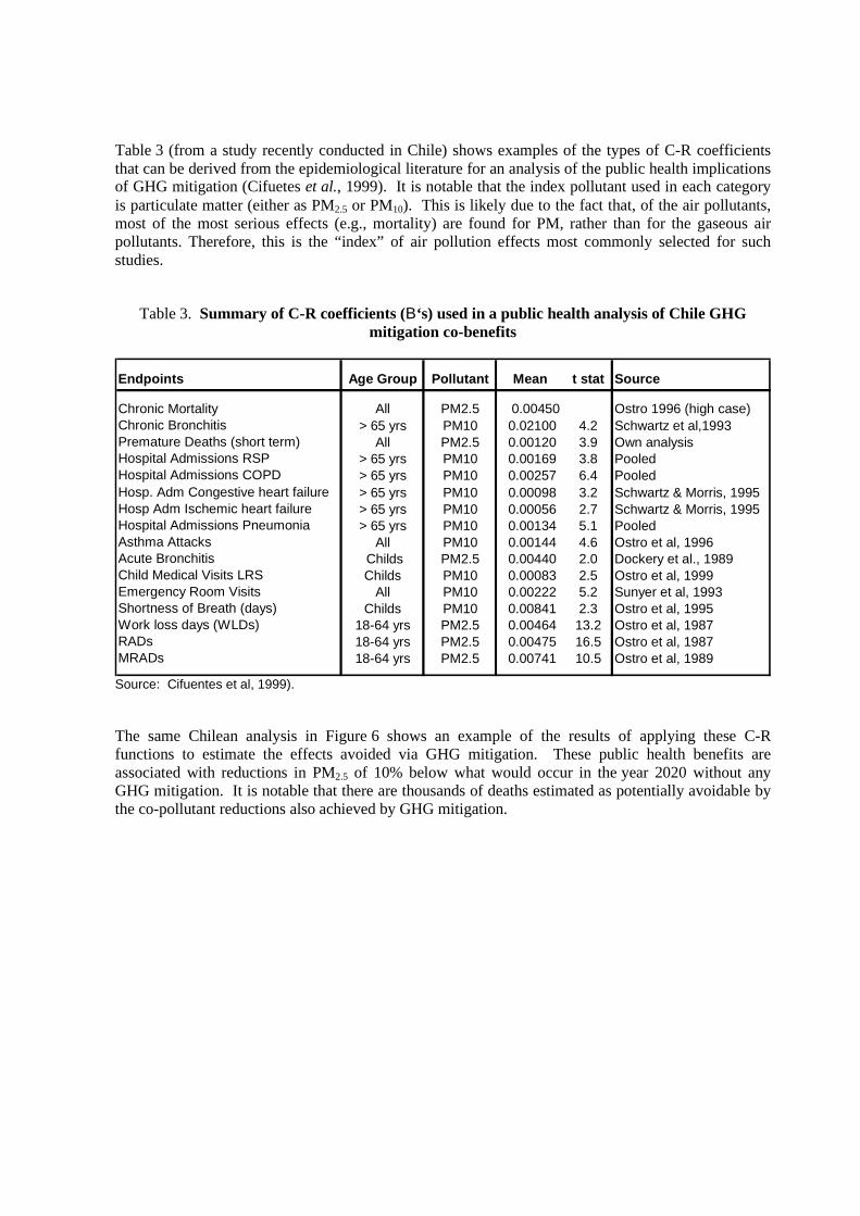
Table 3 (from a study recently conducted in Chile) shows examples of the types of C-R coefficientsthat can be derived from the epidemiological literature for an analysis of the public health implicationsof GHG mitigation (Cifuetes et al., 1999). It is notable that the index pollutant used in each categoryis particulate matter (either as PM2.5 or PM10). This is likely due to the fact that, of the air pollutants,most of the most serious effects (e.g., mortality) are found for PM, rather than for the gaseous airpollutants. Therefore, this is the “index” of air pollution effects most commonly selected for suchstudies.

Table 3. Summary of C-R coefficients (Β‘s) used in a public health analysis of Chile GHGmitigation co-benefits

Endpoints Age Group Pollutant Mean t stat Source

Chronic Mortality All PM2.5 0.00450 Ostro 1996 (high case)Chronic Bronchitis > 65 yrs PM10 0.02100 4.2 Schwartz et al,1993 Premature Deaths (short term) All PM2.5 0.00120 3.9 Own analysisHospital Admissions RSP > 65 yrs PM10 0.00169 3.8 PooledHospital Admissions COPD > 65 yrs PM10 0.00257 6.4 PooledHosp. Adm Congestive heart failure > 65 yrs PM10 0.00098 3.2 Schwartz & Morris, 1995Hosp Adm Ischemic heart failure > 65 yrs PM10 0.00056 2.7 Schwartz & Morris, 1995Hospital Admissions Pneumonia > 65 yrs PM10 0.00134 5.1 Pooled Asthma Attacks All PM10 0.00144 4.6 Ostro et al, 1996Acute Bronchitis Childs PM2.5 0.00440 2.0 Dockery et al., 1989Child Medical Visits LRS Childs PM10 0.00083 2.5 Ostro et al, 1999Emergency Room Visits All PM10 0.00222 5.2 Sunyer et al, 1993Shortness of Breath (days) Childs PM10 0.00841 2.3 Ostro et al, 1995Work loss days (WLDs) 18-64 yrs PM2.5 0.00464 13.2 Ostro et al, 1987RADs 18-64 yrs PM2.5 0.00475 16.5 Ostro et al, 1987MRADs 18-64 yrs PM2.5 0.00741 10.5 Ostro et al, 1989

Source: Cifuentes et al, 1999).

The same Chilean analysis in Figure 6 shows an example of the results of applying these C-Rfunctions to estimate the effects avoided via GHG mitigation. These public health benefits areassociated with reductions in PM2.5 of 10% below what would occur in the year 2020 without anyGHG mitigation. It is notable that there are thousands of deaths estimated as potentially avoidable bythe co-pollutant reductions also achieved by GHG mitigation.

Figure 6. Total estimated effects avoided in Chile during the period 2000 to 2020

����������

���������

�������

�������

������

������

�����

1 100 10,000 1,000,000 100,000,000

Restricted Activity Days

Asthma Attacks & Bronchitis

Emergency Room Visits

Child medical visits

Hospital Admissions

Chronic Bronchitis

Premature Death

Excess Effects

Source: Cifuentes, et al., 1999.

Most of the available air pollution studies used in such quantifications of air pollution effects havebeen conducted in developed countries. A series of recent studies indicate that assessing thecoefficients of mortality tied with various pollutants may not completely reflect the relativeimportance of pollutants in all countries. For any society, deaths that occur at earlier ages are deemedmore important than those that occur later in life, as they result in more years of life lost. For instance,one study in Delhi, India, found that children under 5 and adults over age 65 were not determined tobe at mortality risk from air pollution. Perhaps this was because other causes of death (notablyinfectious diseases) predominated in those who survive to reach these age groups, or because ofinadequate power to detect such effects (Cropper et al, 1997). However, persons between the ages of15-45 were found to be at increased risk of death from air pollution. The reason that the Relative Risk(RR) estimates from this study are lower than found in Philadelphia is not known. This may be due todifferences in pollution mix (e.g., PM composition), but it could also be due to a higher infantmortality rate that removes a potentially susceptible sector from the adult population. Because thepopulation distribution in India includes many more persons, the net impact on the country from airpollution measured in terms of years of life lost is considerable. Although the percentage increase islower in India than in more developed nations, the cumulative effect (i.e., attributable risk) in India isas high (Table 4). Thus, the mortality effects of air pollution in developing nations can be animportant factor in GHG considerations.

Table 4. Percentage increase in mortality and years of life lost per 100 ug/m3 increase inTSP: Delhi vs. Philadelphia1

Mortality End PointDelhi

(% changeper

100 ug/m3)

Philadelphia(% Change

per 100 ug/m3)

Years of Life Lost

Delhi Philadelphia

By selected cause \ Total deaths CVDRespiratory

2.34.33.1

6.79.2

10.2 (Pneumonia)17.8 (COPD)

51,403 51,108

Source: 1 Cropper et al, “The Health Benefits of Air Pollution Control in Delhi,” Amer. J.Agr. Econ. 79 (5,1997): 1625-29.

Similar assessments can be made with respect to morbidity and disability tied with a “base,” orreference case. Disability years of life lost can be estimated by considering the average age at whichspecific disabilities known to be worsened by air pollution, such as asthma and other chronic lungdiseases, occur. This then provides a baseline against which to estimate likely reductions of directlabor productivity, or some other measure of output, associated with this disability. WHO has derivedestimates of DALY (disability adjusted life years) from various major causes for 1990 and future years(Murray and Lopez, 1996). Respiratory diseases, which can be associated with air pollution, rankwithin the top 5 causes of deaths worldwide for adults and were the leading causes of deaths inchildren (WHO, 1996).

4. Credibility of health effects linkages

Uncertainties characterize many parts of the process by which information is obtained on the airpollution-public health consequences of GHG mitigation policies. Among the important issues thatrequire clarification are:

• the credibility of dose-response relationships between specific pollutants and specific types ofmortality;

• the transferability of coefficients of these relationships derived in more developed countries toless developed ones;

• the extent to which morbidity can be quantified for specific pollutants and mixtures ofpollutants and the reliability of this quantification;

• the mix of chronic and acute impacts for which quantification can and should be undertaken;

• the credibility of methods for expressing preferences for health improvements in money (orother) terms.

For any given health outcome, the size of the estimated health risk is often at issue and is usuallyexpressed as the increase in risk per increase unit of exposure. While some monitors exist in manycities of the world, there remain serious problems with exposure misclassification. Where models areemployed to estimate exposure, these are also quite limited by gaps in the availability of model inputs,such as accurate emissions source data. Recent assessments also indicate that the relative importanceof indoor and outdoor air varies substantially in developed and developing countries (Wang andSmith, 2000). The use of experimental models and animal studies for the estimation of human risks isalso a point of contention. Where they exist, epidemiological studies are usually relied upon for RRestimates.

Although air pollution, and especially PM air pollution, has been compellingly linked with excessmortality by a substantial body of epidemiological research, there are aspects of this association thatare still uncertain. There is always concern that some confounder, another variable not adjusted for inthe analysis but correlated with the exposure and causally related to the effect, might actually beresponsible for an association found by an epidemiological study. This is especially of concern whenthere is no known biological plausibility of the effects noted. However, in the case of air pollution, theeffects are certainly biologically plausible, based on controlled studies and past documented episodes,such as the London Fog of 1952. In addition, health effects from air pollution have been documentedat so many locales and in so many different populations. The main question today is whetherpreviously documented mortality effects can be experienced at more routine ambient levels. Otheruncertainties in these analyses include the following issues:

4.1 Causality

Because the epidemiological studies alone cannot definitively prove causation, other evidence shouldbe brought to bear, such as toxicological studies. For example, clinical studies have demonstrateddecreased lung function, increased frequencies of respiratory symptoms, heightened airwayhyper-responsiveness, and cellular and biochemical evidence of lung inflammation in exercising adultsexposed to ozone concentrations at exposures as low as 80 parts per billion for 6.6 hours (e.g.,Folinsbee et al., 1988, and Devlin et al, 1991). Airway inflammation in the lung is among the seriouseffects that have been demonstrated by controlled human studies of air pollution at ambient levels.Airway inflammation is especially a problem for children and adults with asthma, as it makes themmore susceptible to having asthma attacks. For example, recent controlled human studies haveindicated that prior exposure to ozone can enhance the reactivity of asthmatics to aeroallergens, suchas pollens, which can trigger asthma attacks (Molfino et al., 1991). Thus, air pollution exposures mayindirectly exert their greatest effects on persons with asthma, by increasing inflammation in the lung,which then heightens the responsiveness of asthmatics’ lungs to all other environmental agents thatmay cause an exacerbation. The precise mechanism(s) by which air pollution could cause thepollution-mortality associations indicated by epidemiologic studies are not fully understood. Theabsence of understanding of mechanisms is also the case with respect to cigarette smoking and themany diseases known to be associated with it. For air pollution, the epidemiological results aresupported by a large body of data from controlled exposure studies in animals and humans thatconsistently demonstrate pathways by which pollution can damage the human body when it isbreathed (e.g., US EPA, PM Criteria Document, 1999).

4.2 Other pollutants

PM concentrations are often correlated spatially and over time with the concentrations of otherambient pollutants, making it more difficult to unambiguously separate the effects of the individualpollutants. Thus, it is unclear how much each pollutant may individually influence elevated mortalityrates. As a result, most cost-benefit studies choose one index air pollutant, rather than estimatingeffects for multiple air pollutants individually and then adding their effects to get a total air pollutioneffect. This focus on a single pollutant provides a conservative approach to estimating air pollutioneffects. In fact, several recent analyses (e.g., Thurston and Ito, 1999) suggest that ozone and PM airpollution effects are relatively independent, since controlling for one pollutant has only modest effectson the relative risk (i.e., the C-R function) of the other (see Figure 2). Thus, the use of a single indexpollutant in Cost-Benefit Analyses underestimates the overall public health effects and monetaryvaluations of air pollution changes. However, this use of a single pollutant may overestimate theeffect assigned to a particular pollutant if it is only serving as an index of effects actually caused bythe overall mixture of pollutants.

4.3 Differences between central site and personal pollution exposures

It has been pointed out that central site monitoring station measurements are poorly related to thepersonal exposures of individuals, which introduce some error into the air pollution-health effectsrelationship. While this is true on an individual level, it is not always so on an aggregate (i.e.,population average) level, as shown by Mage and Buckley, 1995). In making estimates of thepersonal exposure of individuals to outdoor air pollution (the type of air pollution under considerationfor change), the measurements from a central site monitoring station may actually be more appropriatethan measurements made indoors, or even than personal samplers collecting all particles in the air,including those of indoor origins. Recent studies (e.g., Leaderer et al., 1999) show significantcorrelations between central site monitors of PM2.5 and the ambient concentrations of PM2.5 outside thehomes of individual study participants. Moreover, fine particles of outdoor origins permeate readily tothe indoors. This is exemplified by sulfates, a common outdoor fine particle component that is usuallynot confounded by indoor sources, and which showed high correlations (r=0.88) between outdoormeasurements and personal exposures during the P-Team study (Ozkaynak et al, 1996). Conversely,total personal PM2.5 exposure measurements can be greatly influenced by indoor sources (e.g., due todusts, molds, side-stream cigarette smoke, etc.), but these are not the focus of government regulationsor of the health effects epidemiology used to develop C-R functions.

If personal samples of PM2.5 were in fact collected and used in an epidemiologic study of the mortalityeffects of PM2.5 of outdoor origins, for example, the exposure data would be confounded by the PMcontribution from indoor sources, which would then need to be separated out prior to theepidemiologic analyses of the effects of outdoor air pollution on health. Central site measurements arecorrelated with community outdoor concentrations. Therefore, community-based measurements arealso correlated with the contribution of outdoor air pollution to indoor exposures. The use of outdoormeasurements actually avoids potential confounding by indoor PM pollution.

4.4 Shape of the C-R function

The shape of the true air pollution C-R function is uncertain. Most recent analyses assumes the C-Rfunction to have a log-linear form throughout the relevant range of exposures. If this is not the correctform, or if certain scenarios predict concentrations well above the range of concentration under whichthe C-R function developed, then avoided public health effects may be miss-estimated. The choice ofwhether to assume that there is a threshold of effects will also influence the effect estimates. Theexistence of a level below which there are absolutely no effects of air pollution exposure has not beendocumented in the literature, so there is at this time no definitive basis upon which to set a threshold ofeffects. However, alternative threshold assumptions can be investigated as part of a sensitivityanalysis.

4.5 Regional and country-to-country characteristic differences

While air pollution epidemiology studies indicate a general coherence of results, variability exists inthe quantitative results of different air pollution studies (i.e., the RR’s per ug/m3 of pollution). Thisvariability may in part reflect region-specific C-R functions resulting from regional differences inpotentially important factors such as socio-economic conditions, age-distribution of the population,population racial composition, and health care practices. If true regional differences exist, applyingthese C-R functions to regions other than the study location could result in miss-estimation of effectsin these regions. The scientific literature does not presently allow for a region-specific estimation ofhealth benefits in many areas. However, the use of relative risks based upon local rates of disease(rather than absolute numbers of effects per ug/m3 of pollution) could minimize miss-estimationresulting from the use of uniform C-R functions across localities.

4.6 PM composition

In the case of PM pollution, factors such as the physical and chemical composition of particles in theambient air can be expected to vary its toxicity, which would change the C-R function for this keypollutant. Some things, however, can be tentatively concluded about the relative toxicity of differentPM from various types of sources. For example, an analysis of 1980 cross-sectional variations inmortality across the U.S. by Ozkaynak and Thurston (1987) found that coal-combustion and industrialprocess-derived particles were more strongly associated with mortality than were oil combustion,gasoline auto emissions, or soil-derived (i.e., wind blown) particles. In addition, recent analysesindicate that fine particles (i.e., da <2.5 um) are more strongly associated with adverse health effectsthan are coarser particles (i.e., da <2.5 um) (e.g., Thurston et al., 1994).

Recent studies also suggest that diesel emissions may contain especially toxic particles. Indeed, in thepublished literature, diesel exhaust particles have been associated with a worsening of respiratoryproblems. Recent epidemiological studies indicate that respiratory problems are worsened inresidential areas closer to diesel truck traffic (de Hartog et al., 1997) (Brunekreef, et al., 1997a).Furthermore, clinical studies confirm that diesel particles can increase asthma responsiveness bycausing a skewing of the immune response towards increased Immunoglobulin E (IgE) production, inturn causing allergic inflammation. Recent experimental studies in animals and humans have shownthat diesel particulate, through its effects on cytokine and chemokine production, which are known tobe associated with an increased inflammatory response, enhances this IgE production (e.g., see: Nelet al., 1998). Thus, exposure to diesel air pollution may well act by increasing an asthma patient’sgeneral responsiveness to any and all allergens and pollens to which they are already allergic. Thiswould increase the chance that acute asthma problems will be experienced in a given population ofpersons with asthma.

Thus, PM from different emission source categories may have different health implications. Thiswould suggest that the health consequences of GHG mitigation are sensitive to how GHGs arereduced. Technologies that resulted in more reductions of fine particulates from coal combustion,industrial processes, or diesel fuel combustion would result in greater health benefits.

4.7 Exposure/Mortality lags

It is presently not known whether there is a delay between changes in air pollution exposures andchanges in health effects (e.g., mortality rates) in chronic (long-term) air pollution-health effectsrelationships. This is not a concern in acute studies, however. The existence of such a delay could beimportant for the estimation of health and monetary benefits. Although there is no specific scientificevidence of the existence of an effects lag, current evidence on adverse health effects of smokingsuggests that effects might well be delayed a matter of years (U.S. DHHS, 1990). If this is shown toalso be the case for air pollution, a lag structure of the non-acute portion of the air pollution effectscould be incorporated into a Cost-Benefit analysis.

4.8 Cumulative effects

Cross-sectional and long-term cohort studies (e.g., Pope et al., 1995) are thought to relate primarily toPM-associated cumulative damage, as they are larger than the short-term mortality estimates reportedfrom time-series studies. However, the relative roles of acute and chronic air pollution exposures arenot defined at this time, and it is not yet possible to separate them out in Cost-Benefit Analyses (e.g.,by using differing life-shortening implications).

4.9 Life-shortening

The public health burden of mortality associated with exposure to ambient PM depends not only onthe increased risk of death, but also on the length of life-shortening that is attributable to those deaths.The most recent U.S. EPA PM Criteria Document concluded that “Confident qualitative determinationof years of life lost to ambient PM exposure is not yet possible; life-shortening may range from daysto years.” (U.S. EPA, 1996). A new analysis has now provided a first estimate of the life-shorteningassociated with chronic PM exposure. Brunekreef (1997) reviewed the available evidence of themortality effects of long-term exposure to particulate matter air pollution and, using life table methods,derived an estimate of the reduction in life expectancy that is associated with those effect estimates.

Based on the results of Pope et al (1995) and Dockery et al. (1993), a relative risk of 1.1 per 10 µg/m3

exposure over 15 years was assumed for the effect of particulate matter air pollution on men25-75 years of age. A difference of 1.11 years was found between the “exposed” and “clean air”cohorts’ overall life expectancy at age 25. Looked at another way, this would imply that theexpectation of the life span of the persons who actually died from air pollution was reduced by morethan 10 years, since they represent a small percentage of the entire cohort population.

The above study of air pollution’s effect on life expectancy considered only deaths among adultsabove 30 years of age, but deaths among children can logically have the greatest influence on apopulation’s overall life expectancy. As discussed above, some of the older cross-sectional studiesand the more recent studies by Bobak and Leon (1992, 1999) and Woodruff et al. (1997) suggest thatinfants may be among the sub-populations that are especially affected by long-term PM exposure.Although it is difficult to quantify, any premature air pollution-associated mortality that occurs amongchildren due to long-term pollution exposure, would significantly increase the overall population life-shortening. This is because all other estimates of life-shortening have been based solely on theimpacts of long-term pollution exposures to adults 30 years and older. Therefore, considerableuncertainty remains as to the amount of life-shortening associated with long-term exposure to airpollution.

5. Scale of values

Much of the justification for environmental rulemaking rests on estimates of the benefits to society ofhealth improvements. Within this set of effects, reductions in risk of death are usually the largestcategory of benefits, both within the health category and compared to other categories. For instance,mortality risk reductions are arguably the most important benefit underlying many of the USEPA’slegislative mandates, including the Safe Drinking Water Act, CERCLA, the Resource Conservationand Recovery Act and the Clean Air Act. In the most recent analysis of the benefits and costs of airquality legislation, The Benefits and Cost of the Clean Air Act Amendments of 1990 (USEPA, 1999),reductions in premature mortality are valued at $100 billion annually out of $120 billion in totalbenefits, compared to costs of about $20 billion. Even though health costs/benefits of air pollutionchanges are harder to identify and quantify than those for control costs, European and Canadianstudies similarly find that mortality risk reductions dominate any analysis of pollution reductions(EXTERNE, 1999; AQVM, 1999).

Next to reductions in mortality risk, reductions in the probability of developing a chronic respiratorydisease have been estimated to be the most valued, recognizing that values for other types of diseasesare sparse. Reductions in various acute effects are lower valued. It is recognized that reducedpollution may lead to decreased acute consequences of disease, such as an emergency room or a dailyhospital visit. Reductions in these endpoints tend to be far more highly valued than the avoidance of aday of acute symptoms as defined in standard health benefits analysis, i.e., coughs, sneezes, and thelike. Nevertheless, the former are based on medical costs, while the latter are based on willingness topay (WTP)—the appropriate measure of preferences for health improvements (see Section 6).

Table 5 provides a small sample of the midpoint values typically used by practitioners of healthbenefits analyses, as well as ranges of these values. We picked the unit values for health endpointschosen by four major studies or models in the U.S., Canada and Europe, ordered from highest tolowest based on the first of these studies-the U.S. study on the Costs and Benefits of the 1990 CleanAir Act Amendments-and put them in common currency and constant dollars.

The willingness to pay for reducing risks of mortality and chronic morbidity is expressed, forconvenience, in terms of the value of a statistical life (VSL) and the value of a statistical case ofchronic disease (VSC). It is important to note that this term is merely a shorthand for the WTP for agiven risk reduction divided by that risk reduction. This relationship is convenient because the VSLsor VSCs can be multiplied by estimates of the “lives saved” or “chronic cases saved” to obtainbenefits.

The table shows quite close agreement on the size of the best or midpoint VSLs and VSCs. Thedifferences that do exist may be explained partly by currency conversions and partly by researchersnot always adjusting such values over time for inflation. Also, the rank ordering of preferences notedabove is found to be very similar across the studies, although not every study considers the same set ofhealth endpoints. The low VSLs for TAF and AQVM result from adjustments to the VSL for ageeffects. ExternE takes the VSL and converts it to a value of a life-year for subsequent analysis. Inother analyses, EPA and TAF have done the same thing (see Section 6 for more information).1 Theseefforts have yielded values ranging from $50 000 to $300 000 a life year.

In our judgment, this close agreement is the result of several factors, including replicability of findingsin original studies in different locations (i.e., independent choices made by different research teams),and the consensus reached by research teams on a common pool of studies, results and interpretations.We believe that the social cost of electricity studies in the U.S. and the ExternE effort in Europe havesomething to do with this commonality (see Lee et al, 1995 and Markandya et al, 1996). In addition,the Canadian studies have been informed by the AQVM model developed by Bob Rowe and otherswho have been active participants in the U.S. social costing debate as well (Hagler Bailly, 1995).Many studies in the U.S. pre-date and presage these efforts.

1 Other adjustments to VSLs have been made for latency (ExternE), for health status (basically the

“harvesting” issue) (Markandya, 1999) and for a range of attributes, such as dread and voluntariness(US EPA, 2000).

Table 5. Comparison of unit values used in several major studies or models. ($1990).

Values US

EPAa

US

TAFb

Canada

AQVMc

Europe

ExternEd

Low Central High Low Central High Low Central High Central

Mortality 1560000 4800000 8040000 1584000 3100000 6148000 1680000 2870000 5740000 3031000

Chronic Bronchitis - 260000 - 59400 260000 523100 122500 186200 325500 102700

Cardiac Hosp. Admissions - 9500 - - 9300 - 2940 5880 8820 7696

Resp. Hosp. Admissions - 6900 - - 6647 - 2310 4620 6860 7696

ER Visits 144 194 269 - 188 - 203 399 602 218

Work Loss Days - 83 - - - - - - - -

Acute Bronchitis 13 45 77 - - - - - - -

Restricted Activity Days 16 38 61 - 54 - 26 51 77 73

Resp. Symptoms 5 15 33 - 12 - 5 11 15 7

Shortness of Breath 0 5.3 10.60 - - - - - - 7

Asthma 12 32 54 - 33 - 12 32 53 36

Child Bronchitis - - - - 45 - 105 217 322 -a. The Costs and Benefits of the Clean Air Act Amendments of 1990. Low and high estimates are estimated to be 1 standard deviation below and above the

-mean of the Weibull distribution for mortality. For other health outcomes they are the minimums and maximums of a judgmental uniform distribution.b. Air Quality Valuation Model Documentation, Stratus Consulting for Health Canada. Low, central, and high estimates are given respective probabilities of 33%,

34%, and 33%.c. Tracking and Analysis Framework, developed by a consortium of U.S. institutions, including RFF. Low and high estimates are the 5% and 95% tails of the

distribution.d. ExternE report, 1999. Uncertainty bounds are set by dividing (low) and multiplying (high) the mean by the geometric standard deviation (2).

22

The ranges around these estimates are all somewhat different, seemingly without pattern. This resultperhaps could be expected since there is no treatment of uncertainty that is universally accepted. TheEPA mortality results are based on one standard deviation from the distribution (the Weibull) that bestfit the mean WTP estimates from 26 studies. The Canada results are based on a representation ofuncertainty as a three-point probability distribution, which includes expert judgment. The TAFdistributions are Monte Carlo-based, assuming, unless otherwise indicated by the original studies, thaterrors about mean estimates are normally distributed, with variances given in theconcentration-response and valuation studies relied upon for the underlying estimates. Bounds aredefined as 5th and 95th per centile. Error bounds in the latest EXTERNE report are established as onehalf (low) and twice (high) the geometric mean.

It is worth noting that the endpoints being valued are not all comparable to one another. The unitvalues for mortality risk, chronic lung disease risk, and acute symptoms all are derived from awillingness-to-pay approach that may be thought of as capturing, however imperfectly, the full valueto the individual of reducing the risk or the symptom. The other values are only partial, mainly relyingon cost of illness techniques. They are meant to capture the more severe manifestations of either acuteevents or chronic states and may, without proper adjustments, double count WTP benefits or providesignificant underestimates of the WTP to reduce such effects. Indeed, it is fairly common practice toadjust such COI estimates by a factor to bring them up to a WTP estimate, so as to eliminate suchunderestimation. AQVM (1999), for instance, recommends using a factor of 2-3 to make thisadjustment. The evidentiary basis for the generality of this adjustment across endpoints is quite weak.

6. Credibility of valuation estimates

So far, we have presented some idea of the range of “best” estimates for avoiding health effects orreducing their risks as taken from a variety of major studies or models in developed countries. Now,we describe their uncertainties and assess the state of the information available for making thesevaluations.

In this section, we first delve into the details of the various valuation estimation procedures and theirlimitations, tackling mortality risk valuation first and then chronic and acute morbidity valuation. Atthe end of each of these subsections, tables are presented that summarize the state of the literature. Wethen address the issue of valuation in a developing country context, examining the literature onbenefits transfers and indigenous valuation.

There are obviously many ways to make such assessments. This assessment is only intended toprovide a comparison among the various estimation approaches for each endpoint, rather than anabsolute assessment of accuracy. We use three criteria for making such a judgement: (i) the degree towhich methods of estimation are based on preferences for such health improvements (which we take tobe synonymous with following welfare economics principles); (ii) the number of studies that havefollowed this technique (being an imperfect measure of degree of consensus and attractiveness of thetechnique to researchers); and (iii) additional major limitations of the technique (to capture otherlimitations of the approach, such as data limitations). Based on our subjective judgement, we thenprovide a rating of the reliability of the different approaches to estimating the value for the endpoint inquestion: A (very reliable) to D (unreliable)

23

6.1 Concepts for valuing health

Underlying any attempt to attach an economic value to health effects is the idea that individuals havepreferences that extend over environmental quality and its implications as well as over market goods(and other non-market goods besides environmental goods). If this assumption is accepted then, inprinciple, it is possible to deduce how individuals trade off environmental quality or their healthagainst other services they value. This assessment can be made by attempting to measure how muchin the way of other services individuals are willing to give up in order to enjoy health benefits.2 Theexpression of these values in money terms is just a convenient shorthand for what people are willing togive up in alternative real consumption opportunities. In the aggregate, this measure is given by thesum of individuals combined willingness to pay for the specified improvement.

6.2 Mortality risk valuation

6.2.1 Evaluating estimation approaches

We have identified five approaches to estimating preferences for reducing mortality risks andexpressing these preferences in monetary terms: the human capital approach, various revealedpreference approaches (most importantly the hedonic labor market approach, but also the consumerproducts approach), and stated preference techniques that address health and that do not.

The original approach to valuing mortality risk reductions was the human capital approach. It viewedthe value of a person’s life as their productive value, adding up the lost productivity from prematuredeath as a measure of loss. It was generally recognized that this measure was quite partial andproblematic, not reflecting people’s preferences for reducing death risks, and basically assigningnon-workers a zero value. But, it was easy to calculate and was thought to be better than nothing.Because, at least in developed countries, superior alternatives are available, this approach is no longerused.

2 The notion that such individual tradeoffs fully describe society’s interest in environmental quality is

by no means universally accepted, particularly among non-economists who are highly critical ofeconomic valuation in general and benefit-cost analysis in particular. For an excellent summary of theeconomic argument see Freeman (1993). Even if one accepts that WTP is an acceptable measure ofindividual valuation, distributional effects will complicate the effort. These complications arisebecause changes in environmental quality or health often will themselves change the real income(utility) distribution of society, taking into account both non-market and market benefits. It isimportant to recognize that a valuation procedure that adds up individual WTP is not capturingindividual preferences about changes in the income distribution, even though these clearly do matterfrom a policy perspective. This is a complicated issue that is beyond the scope of this paper toaddress.

24

The two most common approaches for estimating willingness to pay for health improvements includehedonic labor market studies and stated preference methods, such as contingent valuation surveys.The former statistically relate wage differentials to mortality or morbidity risk differences acrossoccupations and industrial/commercial sectors, under the theory that in competitive labor markets,workers in risky jobs should receive wage premiums equal to the value they place on avoidingincreased mortality or morbidity risks. One study asks workers their perception of the death risks theyface in order to address the issue of whether their behavior would be consistent with perceived risksrather than actual risks and that these two types of risks might diverge. These studies are numerousand form the foundation for most VSL estimates. However, they are problematic when applied toassessing the willingness to pay to avoid health effects of air or other pollutants. In particular,epidemiological studies suggest that reducing air pollution lowers death rates primarily among personsover 65. These benefits, furthermore, are more likely to accrue to people with chronic heart or lungdisease and may occur with a lag. 3 There is a growing consensus that the appropriate, if challenging,valued “commodity” is an increase in the probability of surviving to all future ages given a shift in thesurvival function.

Attempts have been made to adjust estimates of risk reductions from the labor market literature for ageand latency. Under certain strong assumptions, one can convert the value of a statistical life from alabor market study (or other source) into a value per life-year saved (Moore and Viscusi, 1988). Thevalue of a life-year can then be multiplied by discounted remaining life expectancy to value thestatistical lives of persons of different ages. To illustrate this calculation, suppose that the value of astatistical life based on compensating wage differentials is $5 million, and that the average age ofpeople receiving this compensation is 40. If remaining life expectancy at age 40 is 35 years and theinterest rate is zero, then the value per life year saved is approximately $140 000. If, however, theinterest rate is 5 per cent, then discounted remaining life expectancy is only 16 years, and the value perlife-year saved rises to approximately $300 000. 4

Markandya et al have recently developed another, relatively ad hoc approach to adjusting VSLs for avariety of shortcomings. The elaborate set of adjustments to the standard VSL ($2.4m) illustrates theproblems with this standard probably more than it increases certainty about what the “true” VSL is.The authors start from a standard VSL of $2.4m. The upper bound estimate is 70% of the VSL($1.7m), adjusted because the affected group is elderly. For the mid and low estimates, the highestimate is adjusted further to account for shorter life expectancy (assumed to be 12 times shorterbased on an interpretation of the short-term mortality studies) and the worse health status of thoseaffected relative to others their age. This is $130 000. For the low estimate, larger adjustments aremade for the same reasons, to yield a VSL of only $3,100.

3 The delay in the realization of risk reductions could occur either because the installation of pollution

control equipment today will not benefit young people until they become susceptible to the effects ofpollution (the air pollution case described above), or because the program reduces exposure today to asubstance that increases risk of death only after a latency period (e.g., asbestos).

4 Similar adjustments can be made to account for the effect of latency periods. According to thelife-cycle model, a 40-year-old’s WTP to reduce his probability of dying at age 60 should equal whathe would pay to reduce his current probability of dying at age 60, discounted back to age 40.

25

There is also a small literature of consumer preference studies (generally and unfortunately ignored)that attempts to estimate the WTP to reduce death risks from purchase or other actual decisions byconsumers, say in purchasing smoke detectors (Dardis, 1980) and in driving behavior under differentspeed limits (Greenstone and Ashenfelter, 1999). These studies tend to find lower VSLs. Forinstance, Greenstone and Ashenfelter find a VSL of $1.56 million in $1999. One problem with someof these studies is statistically separating the mortality risk-reducing attribute from other attributes ofvalue to individuals.5

The stated preference approaches, of which contingent valuation and conjoint analysis are the twomost prominent, are survey approaches that set up choice situations. These methods ask individuals tochose among various hypothetical choices. For instance, they ask whether individuals are willing topay some amount, or to vote yes on a referenda, or to prefer one package of attributes over another, inorder to acquired reductions in mortality risk. The ability of conjoint analysis to recover preferences isa matter of debate. Also, both of these approaches may suffer from a variety of their own biases, andtheir results have been shown to be very sensitive to question wording and ordering. They are capableof being molded to whatever population and context are appropriate, however. And respondents canbe tested for their cognition and understanding of the issues being examined in the survey. (seeHammitt and Graham (1999) for a detailed discussion of the CV-mortality risk valuation literature).

Some of the best known CV studies for mortality risks (Jones-Lee et al, 1985; Hammitt and Graham,1999) look at traffic fatalities rather than deaths in a pollution context, hence we make a distinctionbetween these two types of CV studies. One study used conjoint analysis to examine WTP forreduced mortality risks in a pollution-type context (Desvousges et al, 1998) but it was assumed that aproduct could deliver a certain improvement in lengthening of life, rather than a probabilistic one.Several studies have used CV approaches to examine WTP in a context applicable to mortality riskreductions from pollution: Johannesson and Johansson (1995) and Krupnick et al (2000).

Johannesson and Johansson were the first to test for WTP for an increased life expectancy (one year inexpectation) added between ages 75 and 85. They find implied VSLs ranging from $70 000-$110 000for the sample surveyed by phone in Sweden. This study is problematic, however, as it does notprovide any indication of whether respondents understood the complex scenario, and it offersrespondents what is actually an unrealistically huge reduction in risk.

5 We ignore here the large body of literature using an hedonic property value approach. His approach

provides a revealed WTP for air pollution reductions but is dependent on housing market perceptionsabout pollution and links to all types of effects, health being only one. It has the advantage (somewould say disadvantage) of not using any concentration-response information. See Smith (1999) for arecent example.

26

The most recent study that may be useful for understanding WTP of groups at risk from air pollutionin the context of the nature of this risk is Krupnick et al (2000). The WTP estimates from thiscontingent valuation survey imply values of a statistical life (VSLs) considerably lower than those inthe standard literature. The estimates of mean WTP imply a VSL of approximately $800 000 to$2 million (US dollars).6 They also find that annual WTP for a risk reduction of comparable size issignificantly lower ($200 000) when the risk reduction takes place later in life (at age 70, occurringover 10 years, instead of beginning now and taking place over the next ten years). Further, they findthat age has a relatively minor effect on the VSL and that physical health status has no effect.However, mental health affects VSL, with more “mentally” healthy individuals being willing to paymore for a given risk reduction. An individual’s vision for their future health was found to also affecttheir current WTP for a future risk reduction.

There are two studies in the literature that estimate the WTP to reduce cancer mortality risk. Inaddition, EPA has produced an unpublished paper that adjusts the standard VSLs to account for uniqueelements of the cancer risk, such as dread. Magat, Viscusi and Huber (1996) use conjoint analysis todetermine the tradeoff between the risk of dying in an auto accident and the risk of dying fromterminal lymphoma. They found that risks traded at one-to-one, implying equal VSLs to that found inthe auto-accident context. Hamilton, Viscusi, and Gayer (1999) conducted an hedonic property valuestudy near a Superfund site to estimate the WTP to reduce risks from that site. They found VSLsaround $4.5 million. The EPA adjustment procedures lead to a range of one-half to three times thebenefits using the “standard” U.S.EPA’s VSL of $5.8 million ($1999).

The willingness to pay measures will be theoretically superior to the “supply-side” measures of healthdamage that are usually used when WTP measures are unavailable. These measures include the valueof productivity lost or expenditures on avoidance and amelioration (e.g., medical costs). WTPmeasures are preferred because they theoretically capture the complete value of such effects, including“pain and suffering.” Out of pocket medical expenditures, for instance, are likely to provide a lowerbound on willingness to pay (particularly if medical costs are partly or completely paid by insurance or“the State”), since they do not include any of the intangible costs of reduced health, such as reductionsin quality of life suffered by the ill person and any caregivers (just as the total expenditure on food isnot a complete measure of the value people place on sustenance).7

Ideally, the out-of-pocket expenditure data can be supplemented or replaced by cost data that reflectthe opportunity costs of resources on avoidance or amelioration. In a developing country, what dataare available on costs may reflect wages and other inputs to medical services that are distorted throughgovernment policies, such as minimum wage laws. In such cases, cost data will not reflect socialopportunity costs, and further adjustments are desirable.

6 These estimates are, however, in line with some revealed preference studies based on consumer

behavior (Viscusi 1992; Greenstone and Ashenfelter 1999).

7 Regulatory constraints may cause amelioration expenditures to overstate damages if very strictregulatory standards apply.

27

Part of the VSL literature has taken a very different approach than that discussed so far. Carrothers,Graham, and Evans (1999) use a QALY approach to estimate a VSL appropriate to the “short-term” or“time-series” air pollution-mortality studies. They both discount the life years lost because peoplewho die prematurely are not in good health and assume that only a few “days to years” are lostbecause of exposure to air pollution. Then, they convert the QALY to a money metric using $50 000per QALY, a commonly accepted cost benchmark for medical interventions, although not necessarilythe appropriate number in this air pollution context. The result is a VSL less than 10 per cent of thatused by EPA ($4.8 million, $1990). Note that while the assumption of losing only a few days to yearsmay be appropriate for the time-series studies, it does not hold up well for the long-term or prospectivestudies that follow people for eight years and record when they die. Note also that Krupnick et al(2000) find that poor physical health does not reduce WTP, which calls into question the discountingof future life years for ill health.

The authors also argue that pollution exposures may lead to morbidity effects that exceed those pickedup by the time series studies. This could happen if the effects on risks of non-fatal heart attacks whichlater induces premature death add up to more life expectancy loss than those from direct fatalities.This speculation requires more research.

6.2.2 How credible are the VSL estimates from these approaches?

The ideal situation for reducing uncertainty about the use of the estimates from one or more of theseapproaches would be to have a set of unambiguous theoretical predictions borne out by a complete andunambiguous set of empirical findings. As Table 6 shows, the body of literature varies from this ideal.

Neoclassical welfare economics, in particular, the life-cycle utility model, lies at the heart of thetheoretical modeling. Its predictions about the effects of various factors on WTP are provided in thefirst row of the table. WTP should clearly increase with the size of the risk change; indeed, subject tosome minor caveats, the life cycle model predicts a proportional relationship. This implies that theVSL would be constant for any risk change. The model also implies that the further in time any riskchange begins, the lower WTP should be. The effect on WTP of baseline risk has been very recentlystudied by Pratt and Zeckhauser, who show that those facing higher baseline risks should be willing topay more for a given risk reduction (the “dead anyway” effect). Higher incomes or wealth should berelated to higher WTP. The age effect varies depending on whether the individual can borrow againstfuture earnings. With borrowing, the predicted relationship is an inverted U-shape, peaking, accordingto these studies, at around 40. Finally, the models do not make a prediction on health status.

These predictions have not always been matched by the model results. Rarely have most studies eventested for sensitivity of the WTP for different risk changes provided to separate samples (the externalscope test), let alone passed them. The recent CV study by Krupnick et al (2000) passes this test butfails the more stringent proportionality test. The same study (as noted above) is the only one to test forthe WTP for future risk reductions in a survey also testing the WTP for contemporaneous reductions.This study found the former to be from 15-30% of the latter for average futurity of 19 years, and withan average perceived probability of making it to 70 (when the risk reduction would begin) of about75%. The empirical studies have all found income effects as expected but have had difficultyseparating baseline risk from age, because the two move together. Also, all studies have had verylimited participation of older individuals. An exception is Krupnick et al (1999) which had one-thirdof their sample over 60 years old (up to 75), finding the expected inverted-U relationship, which wassteeper than that of Jones-Lee at al (1985); confidence intervals were wide. Finally, only theKrupnick et al study explicitly addresses the effect of health status on WTP. Further improvementsare required.

28

29

Table 6. Theoretical predictions and empirical results of studies estimating WTP for mortalityrisk reductions

Study RiskChange

Future RiskChange

BaselineRisk

Income(or proxies)

Age Health Status

Life cyclemodel: Theory

+,proportional

- +a + -b

+ then -cindeterminate

EmpiricalStudies Compensating Wage

+ NA -d + - NA

Other Revealed Preference

+ NA ? + + NA

CVM +, notproportional

- Varies + + then -;+;-

0 (one study)

Source: Hammitt and Graham (1999) and authors.a. Small “dead anyway” effect.b. With borrowing against future earnings.c. Inverted U with no borrowing.d. Self selection by risk tolerant workers.

6.2.3 Ratings

Based on the above discussion, as shown in Table 7, none of the approaches for estimating preferencesfor reducing mortality risks in monetary terms is fully satisfactory (i.e., given an A rating). The latestattempts to use CV approaches designed to fit the “commodity” being valued represent a potentiallymore credible literature if the results hold up to scrutiny and are replicated.

30

Table 7. Credibility ratings for the air concentrations � Mortality valuation pathway

CriteriaApproach

Welfare Theoretic (Y/N) Numbers of Studies(Many/ Some/Few)

Limitations

Rating

Human Capital N M (not recent) Undervaluesnon-workers

D

COI Not usually; in principlecould beIf separate estimatesavailable for pain andsuffering

M Usually underestimate C

Revealedpreference: Hedonic LaborMarket; others

Y M Inappropriatecommodity/Population sampled.Many ad hocapproaches to adjust.

B

CVM: non-health Y S Inappropriatecommodity/Population

B

CVM (andconjoint): health

Y (restrictive conditionsfor conjoint)

F Needs peer review andreplication

B

QALYs N. Based on medical costto reduce a QALY

F At least recognizesthat life-years maymatter

C

6.3 Valuing chronic health

6.3.1 Evaluating estimation approaches

We have identified only two types of approaches that have been used to estimate preferences forreducing chronic morbidity risks and expressing these preferences in monetary terms: the cost ofillness approach and stated preference techniques.

The cost of illness approach breaks down the consequences of illness into its component parts andattempts to place values on each part. The ideal WTP measures would capture all the medical costs,pain and suffering, time loss, productivity loss and fear of an illness (see Harrington and Portney(1987) for the basic model). This approach has a welfare theoretic basis but is basically a stop-gap touse when other approaches fail. For instance, Hartunian (1985) uses a model of the progress of cancerand (separately) of respiratory disease to estimate the medical costs from having these diseases overone’s lifetime. Cropper and Krupnick (1998) have estimated the consequences of having variouschronic diseases on wages and labor force participation. Ultimately, such measures founder on theirinability to capture the pain and suffering that are likely to arise from chronic illness.

31

Conjoint analysis has been used by two studies to value the WTP to reduce risks of developing chronicrespiratory disease, and several studies have addressed the WTP to reduce cancer morbidity risks.Viscusi, Magat, and Huber (VMH) (1991) and Krupnick and Cropper (KC) (1992) used conjointanalysis to examine the WTP to reduce the risks of chronic respiratory disease. This analysis involvedasking subjects to choose between two cities to live in, where both are preferred to their present city,and the cities differ in the risk of developing chronic bronchitis (or respiratory disease in general) andin one other characteristic: the probability of dying in an automobile accident or the cost of living. Aninteractive computer program changes the magnitudes of these differences to drive the subject to apoint of indifference between the two cities. At this point, the tradeoff between automobile-relateddeath and chronic bronchitis is known, and a statistical case of chronic bronchitis can be monetized byusing a value of a statistical life. Alternatively, the tradeoff can be posed as being between chronicbronchitis and the cost of living, allowing the value of a case of chronic bronchitis to be obtaineddirectly. The two studies use the same protocol, except that KC chose a sample of subjects who hadrelatives with chronic respiratory disease and asked a second set of questions to obtain WTP to reducerisks of a chronic respiratory disease with symptoms just like their relatives.

Because the former study (which surveyed 300 people stopped in a NC shopping mall) is thought tocapture a more random sample than the latter study, the former is used as the starting point of the VSCcalculation in many cost-benefit analyses. However, because this study described a case of chronicbronchitis that was quite severe and the KC study asked people to describe the severity of the casesthey were familiar with, the latter study’s case severity is thought to be more representative of reality.Thus, the VMH estimate is modified using results from the KC study. The adoption of these studiesby EPA for valuation of this endpoint in its key cost-benefit studies has been criticized (OMB memo,September 1999) for basing its choice on two “pilot” studies that are unrepresentative of thepopulation at risk, and for using interesting, but largely unreplicated, approaches for valuation.

Dickie and Gerking (1996) use a household production model to address WTP to avoid skin cancer.This study might be useful to estimate a particular ancillary cost of climate change mitigation policy,i.e., reductions in ambient ozone have been linked hypothetically to increased UV-B radiation, whichis linked to skin cancer. In the behavioral model in this paper, people combine consumption goods,goods to reduce harmful effects of sunlight, and time spent in the sun to produce utility. The model isformulated to permit risk perceptions to influence averting behavior, which then influences WTP. In acontingent behavior survey of 300 people eliciting WTP for a lotion that reduced skin-cancer risks,average WTP varied by perceived baseline risk and income, from $30 to $50 for a 5% reduction inlifetime skin-cancer risk. At the true risk level (1 in 7), this value is $44, or $6,160 ($44/0.007) for astatistical case (in 1988 dollars).

There is also a literature providing QALY estimates for chronic diseases, converting to dollars usingsome arbitrary cost figure or benchmark, e.g., $50 000.

32

6.3.2 Ratings

As for mortality risk valuation, the literature has gaps here as well (Table 8), with very few studieseven addressing the topic of valuing chronic illness.

Table 8. Credibility ratings for the air concentrations � Chronic morbidity valuation pathway

CriteriaApproachWelfare Theoretic

(Y/N)Numbers of Studies(Many/ Some/Few)

Other LimitationsRating

COI Notusually; Hospitalization; sometimes laborproductivity (whichis a revealedpreference approach)

M: medical coststudiesF: labor productivitystudies

Pricing medicalservices can bedifficult wheremedical care issocialized orsubsidized

C-B

Conjoint: health Y (restrictiveconditions forconjoint)

F Small,non-representativesamples

B

CVM: Health Y F Usual issues BQALYs Under very

restrictiveconditions; but notin practice

S Can’t compare withcosts; not sensitiveto severity

C

6.4 Acute health valuation

6.4.1 Evaluating estimation approaches

The ideal WTP measures for WTP to avoid acute health effects8 would capture all of the medicalcosts, pain and suffering, time loss, and fear of an acute illness (see Harrington and Portney, 1987, forthe basic model). In principle, the stated-preference approach can come closest to reaching the ideal.Three contingent-valuation (CV) studies (Loehman et al., 1979; Tolley et al., 1986a; Dickie et al.,1987) are the original studies of this type. They used bidding procedures to elicit estimated values forrespiratory-symptom days, with average estimates ranging from $5 to $25, depending on the symptom,its severity, and whether a complex of symptoms is experienced.

All those studies have drawbacks, related mainly to their methodology-the CV studies were performedbefore many of the most important advances in CV techniques. But they offer consistent ranges ofestimates for WTP to avoid a particular type of symptom.

One of the only European studies on the WTP to avoid acute health effects is also a very recent one(Navrud, 1997). Over 1 000 Norwegians were interviewed in-person to ascertain their WTP to avoid avariety of acute health effects (one more day over their usual annual frequency and 14 days over theirusual frequency). The values for avoiding symptom effects (in $1990) are slightly smaller than thosefound in the older U.S. studies, but the asthmatic values are far larger.

8 This literature uniformly treats acute health effects in a deterministic rather than a probabilistic

context.

33

34

A more recent study is that of Alberini, Cropper, and Krupnick (1997), which surveys a sample of 832Taiwanese about their WTP to avoid their most-recent episode of acute respiratory illness. Thisapproach differs from that of some of the other studies which describe the symptoms and duration ofthe episode for the person. Statistical techniques are used to relate the Alberini-Cropper-Krupnickvalues to the duration and severity of the episode and other variables. The authors find that avoiding aone-day episode of a cold like they had recently experienced is valued at about $20 (1992$) with themarginal value of avoiding longer episodes falling rapidly to $6 at 5-days. For non-cold episodes, thevalue for a day was $31. The results also are compared with those of the older studies. Even thoughthe Taiwanese have lower incomes than the US people participating in the US studies, the TaiwaneseWTP bracketed the Taiwan WTP estimate without any adjustment for per capita income differentials.This not only raises a question about benefit transfers adjusted for income differentials but raisesanother problem: when there is more than one study from the source country to use in a benefitstransfer, and the studies have different results, how does one choose the studies to make the transfer?

There are several non-CVM alternative approaches to valuing acute health effects. One-thecost-of-illness approach-attempts to tally the various out-of-pocket costs associated with illness. Bymissing “pain and suffering,” this approach necessarily underestimates costs (benefits).Hospitalization, emergency room, doctor, and drug costs (including charges paid by insurancecompanies), the value of nonwork time spent in these activities and being sick, and the value of worklost as a result of illness are the categories of costs most often estimated.

Another, less-used approach-the averting-behavior method-attempts to infer the WTP to avoid a healtheffect by observing and placing a value on behavior used to avoid the health effect. For instance, ifsomeone stays indoors with the air conditioner on all day because of high pollution, the added costs ofthe electricity bill might be related to the WTP to avoid the health effect. For this approach to yielddefensible estimates of value requires a number of stringent assumptions, e.g., the air conditioner hasno other attributes than cleaning the air. In practice, it is little used, particularly in an acute-healthcontext.

6.4.2 Ratings

Here again, the valuation studies leave much to be desired (Table 9)—a particularly distressing state ofaffairs, given how relatively easy a study of this type of endpoint would be to mount. Work on theseendpoints in Europe may revitalize the field. However, unless health scientists find far larger effectsof pollution on acute health than found so far, the value gained from many more valuation studies maybe quite limited.

35

Table 9. Credibility ratings for the air concentrations � Acute morbidity valuation pathway

CriteriaApproachWelfare Theoretic

(Y/N)Numbers of Studies(Many/ Some/Few)

Other LimitationsRating

COI No M Pricing medicalservices can bedifficult; May notneed any

C

Revealedpreference(averting behavior)

Y (under restrictiveconditions)

F B

Conjoint: health Y (restrictiveconditions forconjoint)

F B

CVM: health (old) Y S Oldmethods/studies; some ad hocestimates; smallsamples

B

CVM (new) Y F ? ?QALYs In theory, under very

restrictiveconditions; rarely inpractice

M Scores not verysensitive to severity

C

7. Developing country issues

7.1 Valuation

Probably the most controversial aspect of estimating ancillary benefits is the link between healtheffects and valuation in developing countries. Indeed, previous IPCC assessments have sparked greatcontroversy, because they have presented non-market values for health improvements in developingcountries that, under some assumptions, appeared to value lives of populations in such countries lowerthan those in developed countries.

Many of the criticisms of such valuations are criticizing valuation itself, as much as its application todeveloping countries. Nevertheless, health improvements can be thought of as commodities in thebroadest sense. That is, we buy health improvements (or risk reductions) in our everyday life. Webuy medicines and medical procedures, we spend time exercising, preparing low calorie meals, etc.As we do for commodities, we trade-off income or time against health commodities. We speed on thehighway to save time, when we know it will cost us a bit in gas and raise our risk of injury, propertydamage and death. Thus, thinking of health improvements and risk reductions as a commodity, it iseasy to imagine that people have a willingness to pay for this commodity, i.e., it has price sensitivity,where WTP varies depending on how large the risk reduction is.

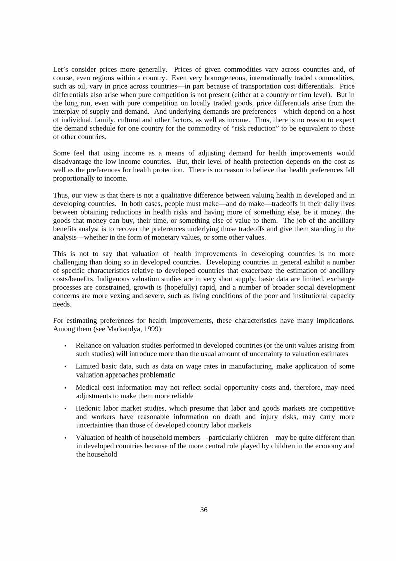
36

Let’s consider prices more generally. Prices of given commodities vary across countries and, ofcourse, even regions within a country. Even very homogeneous, internationally traded commodities,such as oil, vary in price across countries—in part because of transportation cost differentials. Pricedifferentials also arise when pure competition is not present (either at a country or firm level). But inthe long run, even with pure competition on locally traded goods, price differentials arise from theinterplay of supply and demand. And underlying demands are preferences—which depend on a hostof individual, family, cultural and other factors, as well as income. Thus, there is no reason to expectthe demand schedule for one country for the commodity of “risk reduction” to be equivalent to thoseof other countries.

Some feel that using income as a means of adjusting demand for health improvements woulddisadvantage the low income countries. But, their level of health protection depends on the cost aswell as the preferences for health protection. There is no reason to believe that health preferences fallproportionally to income.

Thus, our view is that there is not a qualitative difference between valuing health in developed and indeveloping countries. In both cases, people must make—and do make—tradeoffs in their daily livesbetween obtaining reductions in health risks and having more of something else, be it money, thegoods that money can buy, their time, or something else of value to them. The job of the ancillarybenefits analyst is to recover the preferences underlying those tradeoffs and give them standing in theanalysis—whether in the form of monetary values, or some other values.

This is not to say that valuation of health improvements in developing countries is no morechallenging than doing so in developed countries. Developing countries in general exhibit a numberof specific characteristics relative to developed countries that exacerbate the estimation of ancillarycosts/benefits. Indigenous valuation studies are in very short supply, basic data are limited, exchangeprocesses are constrained, growth is (hopefully) rapid, and a number of broader social developmentconcerns are more vexing and severe, such as living conditions of the poor and institutional capacityneeds.

For estimating preferences for health improvements, these characteristics have many implications.Among them (see Markandya, 1999):

• Reliance on valuation studies performed in developed countries (or the unit values arising fromsuch studies) will introduce more than the usual amount of uncertainty to valuation estimates

• Limited basic data, such as data on wage rates in manufacturing, make application of somevaluation approaches problematic

• Medical cost information may not reflect social opportunity costs and, therefore, may needadjustments to make them more reliable

• Hedonic labor market studies, which presume that labor and goods markets are competitiveand workers have reasonable information on death and injury risks, may carry moreuncertainties than those of developed country labor markets

• Valuation of health of household members –-particularly children—may be quite different thanin developed countries because of the more central role played by children in the economy andthe household

37

• Rapid economic growth means preferences are changing as well, raising the questions aboutthe applicability of indigenous studies several years hence. Perhaps, benefits transfers becomemore legitimate over time.

It used to be the case that valuing health improvements in developing countries would requireperforming a benefits transfer—using concentration-response and valuation information from adeveloped country (usually the U.S.) where such studies had been mounted and applying them,sometimes with adjustments, sometimes not, to the developing country. This practice is the one thatled directly to the controversy noted above. However, the process is much more broadly applied,being used to “transfer” benefit estimates from one part of a country to another and from onedeveloped country to another developed country, as well as to a developing country.

Moreover, as we show in Annex I, environmental economists and others have begun to performprimary valuation research in developing countries, which has revealed that preferences for healthimprovements, conditioned on income as they must be, are not terribly different between developedand developing countries. Furthermore, comparisons between values obtained through benefitstransfer and values obtained directly from the people in the country reveal that such transfers are notparticularly reliable. Thus, benefit transfer techniques may be gradually supplanted by direct analyses.

The above phrase “conditioned on income as they must be” highlights one of the more controversial,basic elements of modern welfare economics—that equity considerations should be kept separate fromefficiency. See Krupnick, Burtraw and Markandya (2000) for a discussion.

7.2 Transfer Uncertainty

The idea behind benefit transfers is to fill in gaps in the availability of information on, in this case, thepreferences of individuals in a country for health improvements. The underlying theory is inDesvousges et al (1985, WRR), where a hierarchy of approaches is suggested. They begin with simplyusing, say, a value of statistical life estimate in the source country and applying it to a receivingcountry’s population. Simple types of adjustments, for example, income differentials, characterize thenext approach, moving to more complicated adjustments that incorporate a host of differences betweenthe source and receiving country, such as education levels, baseline risks, age distributions, healthstatus, and the like. The income adjustment is usually made by using an income elasticity ofwillingness to pay for the improvement. Using an elasticity of 1.0 would change the WTP in thereceiving country proportionally to the relative per capita income differentials across the twocountries. An elasticity of zero would mean that no adjustment was made for income differentials.

A number of health valuation studies have used income differentials within their sample to calculateincome elasticities of WTP. Surprisingly, these studies find relatively small elasticities, ranging from0.2 to 0.6 (Mitchell and Carson, 1986; Alberini, et al, 1997; Loehman et al., 1979).

Using an elasticity of 0.3, for example, to adjust WTP across countries would imply that the WTP of areceiving country with a tenth of the per capita income (in purchasing power parity terms) of thesource country would be 73 per cent of that of the source country’s WTP. For the example above, the$100 WTP in the U.S. is translated into a $73 WTP in Ukraine when the elasticity is 0.3. Theappropriate translation of the willingness-to-pay (WTP) from the study country (S) to the targetcountry (T) is given by:

38

WTPT = WTPS (1- εWTP,Y (YS – YT)/ YS)

Where ε is the income elasticity of WTP with respect to per capita income, and YT is the income ofpeople in the target country.

There are a number of concerns about using this approach. First, it ignores many other factors thatmight make WTP different across countries—cultural factors as much as more measurable variables,such as age distribution. Second, it uses individual variation in incomes within what is usually abasically wealthy source country to estimate WTP for a country with low average incomes. This is outof sample and ignores differences in income distribution.

In principle, the more complex adjustment approach can be parameterized by using a single study,estimating the variation in WTP as a function of a number of appropriate regressors, such aseducation, etc., although for many such studies, microdata of this nature is not generally available.The CV studies generally can provide such estimates.

Because of the lack of microdata for many of the original valuation studies, some benefit transferstudies have used the valuation studies in a meta-analysis. By treating each study’s results as anobservation, group data (say on average education levels in the country where the study wasperformed) can be used to estimate the effect of variables on WTP. Bowland and Beghin (1998) forinstance, use 33 labor market studies to estimate the marginal effect of risk differences, income,education, age, and various labor market descriptors on WTP for mortality risk reductions and applythe estimated equation to estimating benefits of fine particulate reductions in Santiago. They find thatthe implied VSL is about $740 000 U.S. in $1992, adjusted for PPP, compared to the U.S. standardVSL figure of $4.8 million ($1990).

This study has some problems—many of the observations use the same labor market/mortality dataset,key variables to help explain WTP differences (such as health status) are missing, and the studies aremostly for the U.S., so those have insufficient variation in many of the variables. More importantly,one of the key results—that the income elasticity of WTP is well over 1.0—is much at odds with therest of the literature. Chilean income is assumed (in this 2010 analysis) to be about half of U.S.income. But the high income elasticity (plus other differences between the countries) serves to widenthe gap to a ratio of 1 to 7.

Another literature “kills two birds with one stone,” by estimating values directly from an indigenousstudy and then using benefit transfer techniques to test for whether these techniques can come close toreplicating the values from the indigenous study. One example is a comparison of a series of wagecompensation studies done in India and Taiwan compared to transferred values from U.S. studies(Simon, Cropper, Alberini, and Arora, 1999) (Table 10).

39

The authors cite Shanmugan (1977) as the first study to examine the Indian manufacturing industry,although focused on one metropolitan area and restricted to blue collar males working in industriesdescribed at the “two-digit” level. He estimates a VSL of $400 000 on an exchange rate basis. Simon,Cropper, Alberini, and Arora (1999) take a broader, more comprehensive look at Indian labor markets.They examine blue-collar workers, both male and female, in all of India’s manufacturing industry andat the three-digit level, using risk data at the industry, rather than the occupational level. They findthat the implied VSL is between $150 000 and $360 000 on an exchange rate basis ($1990). Theycompare the VSLs across countries by computing the ratio of the VSL to the present value of foregoneearnings implied by a unit change in occupational death risk—i.e., to the values derived using thehuman capital approach. They find that, using their original study, the VSL is from 20 to 48 timeslarger than the value of foregone earnings. The implication is that a benefit transfer assuming a unitaryincome elasticity of WTP would underestimate the VSL for India by 50-60%.

They also cite Liu, Hammitt, and Liu, who used five years of wage and accident data fromnonagricultural sectors and the three-digit industry level, using risk measures by industry. They findVSLs that range from $135 000 to $589 000 ($1990) depending on the year of the data, and averageabout $410 000. These authors also present results of a meta-analysis using the VSL estimatesreported by Viscusi (1993) with per capita income and annual fatality risk as arguments. Using thislog linear equation, which features an income elasticity of about 0.5 (insignificant) and a risk elasticityof -0.27 (which is significant) yields a VSL of $1.4 million. The implication is that a benefit transferusing a unitary income elasticity of WTP and accounting for baseline mortality risk differences wouldoverestimate a VSL for Taiwan by 3-4 times.

Table 10. Wage compensation studies in U.S., India, and Taiwan and benefit transfercomparisons

Country/Transfer VSL ($) GDP per Capita

(1995 US$)*

VSL/GDP

Per Capita

VSL/PDV

foregone income

USA 4,800 000 26,037 184.35 8-23

India (Shanmugan, 1977) 400 000 365 1096 73

India (Simon, et al, 1999) 150 000-

360 000

365 411-986 20-48

Taiwan 410 000 11,276 36.4 7-8

USA to TaiwanFunction Transfer(Viscusi, 1993)

1,400 000 11,276 124.2 24-27

* - Statistics for USA and India from the United Nations “World Statistics Pocketbook, 1995.” Statistics for Taiwanfrom Directorate General of Budget, Accounting, and Statistics, Republic of China.

40

Another example is Chestnut, Ostro and Vithit-Vadakan (1997), who administered a contingentvaluation survey to 141 adults (half nurses) in Bangkok to estimate their willingness to pay foravoiding one respiratory-symptom day of three alternative types (no activity restriction, partial activityrestriction, and work loss day). Using an exchange rate conversion (25 baht/$), mean estimates were$16, $30, and $63 for no restrictions, partial restrictions and work loss respectively, while the mediansare $4, $12, and $26, respectively. Standard median estimates used in U.S. studies (Table 6 above) fora symptom-day with no restrictions range from $12 to $15, while restricted activity days range from$30 to $50. With U.S. median incomes from 3 to 4 times larger than those of respondents in theBangkok sample, it is not clear that benefits transfer based on unitary income elasticities would be apoor proxy for actual WTP.

On balance, though, the main conclusion of these comparisons is that benefit transfers assuming theincome elasticity of WTP is 1.0 or even making other adjustments do not appear to be reliable forvaluing mortality and morbidity risks in developing countries.

8. Conclusions

The IPCC is charged with assessing current technical knowledge about likely physical, social andeconomic changes that will occur as a result of climate modification over the next century. The matterof how various climate policies will affect public health has remained beyond the purview of climatemodels and has received little attention in the Special Reports on Emission Scenarios. In addition, thisaspect of climate change policies has yet to rise to prominence in international climate mitigationpolicy negotiations. Although some have suggested that the size of potential ancillary benefits couldbe as great as some of the costs associated with climate change mitigation policies, others findrelatively small effects relative to costs (Grubb, 1999).

Estimating the ancillary public health consequences of greenhouse gas mitigation policies is achallenging, multidisciplinary task, drawing upon expertise in economics, emission inventories, airpollution modeling, and public health. This task is made easier by recognizing that such estimates arechiefly conducted in order to compare to the costs of various proposed greenhouse gas mitigationstrategies. Both ancillary benefits and mitigation costs are contemporaneous and may, in the firstinstance, be analyzed at a country-level.

Based on available information to date, the estimated improvements in public health linked withvarious reductions in air pollution reductions appear to be significant-both in developed and othercountries. However, these estimates are uncertain and do not reflect the full array of pollutants that arelikely to be involved, nor do they address myriad other pathways potentially affecting public healthbeyond those tied with air pollution. Notwithstanding these uncertainties, the analyses of ancillaryhealth benefits can provide useful information to the policy debate about the scope, design, and timingof climate policy.

We want to emphasize that it is one thing to link changes in air pollution and health and another thingto link greenhouse gas mitigation policies with specific changes in air pollution. Our paper hasfocused only on the former.

41

In summary, we offer the following major points:

1. While the public health benefits of GWG co-pollutant reductions are ancillary to thedirect weather effects of GWG’s, they are more immediate in time than the climatechanges (i.e, mostly begin as soon as emissions are reduced), and therefore they gainincreased importance when effects are viewed on a Net Present Value basis.

2. In terms of monetized ancillary benefits, the air-mortality pathway is the dominantpathway in analyses to date. An annual unit (ug/m3) reduction in PM2.5, for instance, cangenerate benefits of about $250 per person based on the Pope study and the standardVSL. Further, there is relatively low statistical uncertainty around this estimate.However, the dominance of air pollution-mortality monetary valuations may not remainonce a broader assessment can be conducted.

3. There is a need to recognize the broad array and large number of adverse health effectsthat are associated with air pollution, many of which are not yet quantifiable from eithera health effects or valuation perspective. Also, it should be noted that, if non-monetaryvaluation metrics, such as numbers of effects or quality of life changes are considered,less severe outcomes will dominate the costs/benefits.

4. PM is the air pollutant that most recent studies indicate has the greatest public healthconsequences. But PM composition and size is heterogeneous across sources. There issome evidence that PM from different emission source categories may have differenthealth implications. GHG mitigation strategies that lead to lower emissions of fineparticulates, and that result in reductions in coal combustion, industrial processes, ordiesel fuel combustion may lead to greater ancillary benefits than those that reduce largerparticles or are achieved via reductions in low PM sources, such as natural gascombustion.

5. However, there remain uncertainties with respect to the PM-mortality relationship. Ofthese, probably the greatest uncertainty is associated with the question of the possiblecontribution of co-pollutants to the PM effect estimates (i.e., to what extent PM isserving as an index of air pollution, in general), and the potency of specific PMcomponents.

6. The air-chronic respiratory disease pathway is an additional important pathway. There isan emerging epidemiological literature on this endpoint, with substantial modeluncertainty. Model and statistical uncertainties are especially large in the valuationliterature regarding these endpoints.

7. The standard VSL is drawn from labor market studies, which may be inappropriate forthis pathway. Contingent valuation approaches have the potential to yield appropriateestimates. However, these methods have had difficulty meeting the theoreticalexpectation that WTP should increase proportionally with greater risk reductions. Eventhe best studies suffer from this problem. Valuation of children’s health and estimationof the WTP for improvements in other people’s health are active areas of research.

8. Although uncertainties in valuation are large, there is fairly broad consensus over thevalues to be used in air pollution-health benefits analyses, as evidenced in Table 5.

42

9. No matter what approach is taken to estimate the public health consequences of airpollution reductions, benefits are likely to be substantial. In order to conduct the mostrobust and uncontroversial analyses, we recommend relying on the most defensible,transparent methods, even if they are recognized as being deficient to the conceptuallycorrect methods. In other words, a strategy of retreating to defensible borders seemsappropriate. For example, such measures may indeed be the standard VSLs from labormarket studies, although they probably overestimate benefits/costs. Still better would beto make some adjustments for age and health status or wait for the new CV literature todevelop further. In some cases, the human capital approach might ultimately be the mostdefensible. These approaches may all be superior to benefit transfers.

Overall, though still a work in progress, the present techniques available for the analyses of theancillary public health costs and benefits are adequate and appropriate for implementation by thosecomparing the relative merits of various GHG mitigation policies. The public health changesassociated with GHG mitigation strategies should be considered as a key factor in the choice of GHGmitigation strategies made by the nations of the world in the next few years.

43

REFERENCES

Alberini, Anna, Maureen Cropper, Tsu-Tan Fu, Alan Krupnick, Jin-Tan Liu, Daigee Shaw, andWinston Harrington. (1997). “Valuing Health Effects of Air Pollution in DevelopingCountries: The Case of Taiwan,” Journal of Environmental Economics34(2, October): 107-126.

Alderman, Harold, and Victor Lavy. (1996). “Household Responses to Public Health Services: Costand Quality Tradeoffs,” The World Bank Research Observer 11(1, February): 3-22.

Barker, Terry, and Knut Einar Rosendahl. (2000). “Ancillary Benefits of GHG Mitigation inEurope: SO2, NOx and PM20 Reductions from Policies to Meet Kyoto Targets Using the E3MEModel and EXTERNE Valuations. Draft. Paper presented at the Expert Workshop onAssessing the Ancillary Benefits and Costs of Greenhouse Gas Mitigation Strategies, March27-29, 200, Washington, DC.

Bobak M., Leon D.A. (1992). Air pollution and infant mortality in the Czech Republic, 1986-88.Lancet. 340(8826):1010-1014

Bobak M, Leon DA. (1992). The Effect Of Air Pollution On Infant Mortality Appears Specific ForRespiratory Causes In The postneonatal Period.. Epidemiology. 1999 Nov;10(6):666-70.

Bowland, Brad J., and John C. Beghin. (1998). “Robust Estimates of Value of a Statistical Life forDeveloping Economies: An Application to Pollution and Mortality in Santiago. Draft (Raleigh,NC: North Carolina State University, February.

Brunekreef B, et al. (1997a). Air pollution from truck traffic and lung function in children living nearmotorways. Epidemiology. May;8(3):298-303

Brunekreef B. (1997b). Air pollution and life expectancy: is there a relation? Occup Environ Med.Nov; 54(11): 781-784.

Buist AS, Vollmer VM. (1990). Reflections on the rise in asthma morbidity and mortality. J Am MedAssoc.; 264:1719-1720

Carr W, Zeitel LKimuta , Weiss K. (1992). Variations in asthma hospitalizations and deaths in NewYork City. Am J Public Health; 82:5965.

Carrothers, T. J., John D. Graham, and John Evans. (1999). “Valuing the Health Effects of AirPollution,” Risk in Perspective (Harvard Center for Risk Analysis) 7(5, July).

Carter-Pokras, O.D. and Gergen, P.J. (1993). Reported asthma among Puerto Rican,Mexican-American, and Cuban children, 1982 through 1984. Am. J. Pub. Hlth. 83:580-582.

44

Chestnut, Lauraine G., Bart D. Ostro, and Nuntavarn Vichit-Vadakan. (1997). “Transferability of AirPolllution Control Health Benefits Estimates from the United States to DevelopingCountries: Evidence from the Bangkok Study,” American Journal of Agricultural Economics79(5): 1630-1635.

Choe, KyeongAe, Dale Whittington, and Donald T. Lauria. (1996). “The Economic Benefits ofSurface Water Quality Improvements in Developing Countries: A Case Study of Davao,Philippines,” Land Economics 72(4, November): 519-537.

Cifuentes, L., Sauma, E, Soto,F, and Jorquera, H. (1999). Preliminary estimation of the potentialco-control benefits for Chile. School of Engineering. P. Catholic University of Chile. Santiago.

Coultas DB, Gong H Jr, Grad R, Handler A, McCurdy SA, Player R, Rhoades ER, Samet JM,Thomas A, Westley M. Respiratory diseases in minorities of the United States. Am J RespirCrit Care Med 1993; 149:S93-S131.

Cropper, Maureen L., Mitiku Haile, Julian A. Lampietti, Christine Poulos, and Dale Whittington.(1999). “The Value of Preventing Malaria in Tembien, Ethiopia.” Draft (Washington,DC: The World Bank).

Cropper, Maureen L. and Alan J. Krupnick. (1990). “The Social Costs of Chronic Heart and LungDisease,” Resources for the Future Discussion Paper QE89-16-REV (Washington,DC: Resources for the Future).

Cropper, M., N. Simon, A. Alberini, S. Arora, P.K. Sharma. (1997). “The Health Benefits of AirPollution Control in Delhi.” American Journal of Agricultural Economics, 79(5), 1625 –1629.

Dardis, Rachel. (1980). “The Value of a Life: New Evidence from the Marketplace,” AmericanEconomic Review, 70: 1077-1082.

de Hartog JJ, et al.. Relationship between air pollution due to traffic, decreased lung function andairway symptoms in children. Ned Tijdschr Geneeskd. 1997 Sep 20;141(38):1814-8.

Desvousges, W. H., F. Reed Johnson, S. P. Hudson, S. R. Gable, and M. S. Ruby. (1996). UsingConjoint analysis and Health-State Classifications to Estimate the Value of Health Effects ofAir Pollution (Research Triangle Park, NC: Triangle Economic Research).

Devlin RB, McDonnell WF, Mann R, Becker S, House DE, Schreinemachers D, Koren HS. (1991).Exposure of humans to ambient levels of ozone for 6.6 hours causes cellular and biochemicalchanges in the lung. Am J Respir Cell Mol Biol. Jan;4(1):72-81.

Dickie, M. and S. Gerking. (1996). “Genetic Risk Factors and Offsetting Behavior: The Case of SkinCancer” (Laramie, WY: University of Wyoming, College of Business).

Dickie, M., et al. (1987). “Reconciling Averting Behavior and Contingent Valuation BenefitEstimates of Reducing Symptoms of Ozone Exposure (draft),” in Improving Accuracy andReducing Costs of Environmental Benefit Assessments (Washington, DC: U.S. EnvironmentalProctection Agency, February).

45

Diener et al. (1998). Health Canada..in Economic Appraisal.

Dockery, D. W.; Pope, C. A., III; Xu, X.; Spengler, J. D.; Ware, J. H.; Fay, M. E.; Ferris, B. G.,Jr.; Speizer, F. E. (1993). An association between air pollution and mortality in six U.S. cities.N. Engl. J. Med. 329 (24): 1753-1759.

ExternE. (1999). Externalities of Energy, Volume 7: Methodology 1998 Update. Lead Author forChapter 12 (Brussels: European Commission), 518pp.

Folinsbee LJ, McDonnell WF, Horstman DH. 1988 Pulmonary function and symptom responses after6.6-hour exposure to 0.12 ppm ozone with moderate exercise. JAPCA.. Jan;38(1):28-35.

Freeman, A. Myrick, III. (1993). The Measurement of Environmental and Resource Values: Theoryand Methods (Washington, D.C., Resources for the Future).

Georgiou, Stavros, Dale Whittington, David Pearce, and Dominic Moran. (1997). Economic Valuesand the Environment in the Developing World (Cheltenham, UK: Edward Elgar).

Gertler, Paul J., and Jeffrey S. Hammer. (1997). “Strategies for Pricing Publicly Provided HealthServices.” Draft (Washington, DC: The World Bank).

Gertler, Paul, and Jacques van der Gaag. (1990). The Willingness to Pay for Medical Care: Evidencefrom Two Developing Countries (Baltimore and London: Johns Hopkins University Press forThe World Bank).

Greenstone, M., and O. Ashenfelter. (1999). Using Mandated Speed Limits to Measure the Value of aStatistical Life. Mimeo (Princeton, NJ: Princeton University, May).

Hagler Bailly Consulting, Inc. (1995). The New York State Externalities Cost Study (Dobbs Ferry,NY: Oceana Publications).

Hamilton, James T., W. Kip Viscusi, and Ted Gayer. (1999). “Market Reactions to Site Risks,” inJames T. Hamilton and W. Kip Viscusi (eds.)

Hammitt, James K. (1999). “Valuing Mortality Risk: Theory and Practice.” Draft (Cambridge,MA: Harvard University, June).

Hammitt, James K., and John D. Graham. (1999). “Willingness to Pay for HealthProtection: Inadequate Sensitivity to Probability,” Journal of Risk and Uncertainty18(1, April): 33-62.

Harrington, W. and P. Portney. (1987). “Valuing the Benefits of Health and Safety Regulations,”Journal of Urban Economics 22: 101-112.

Hartley, et al. (1999). Economic Appraisal of the Health Effects of Air Pollution, report to UKDepartment of Health from the Ad Hoc Group

Holland, M., J. Berry and D. Foster (eds) “ExternE: Externalities of Energy Volume 7: Methodology1998 Update” (Belgium: European Commission).

46

Johannesson, Magnus and Per-Olov Johansson (1996), “To Be, or Not to be, That Is the Question: AnEmpirical Study of the WTP for an Increased Life Expectancy at an Advanced Age,” Journal ofRisk and Uncertainty, 13, 163-174.

Jones-Lee, M.W., M. Hammerton and P.R. Phillips. (1985). “The Value of Safety: Results of aNational Sample Survey,” Economic Journal 95: 49-72.

Krupnick, Alan J., and Maureen Cropper. (1992). “The Effect of Information on Health RiskValuation,” Journal of Risk and Uncertainty, no. 5, pp. 29-48.

Krupnick, Alan, Anna Alberini, Maureen Cropper, Nathalie Simon, Bernie O’Brien, Ronald Goeree,and Martin Heintzelman. (2000). “What Are Older People Willing to Pay to Reduce Their Riskof Dying.” Draft.

Künzli, N., R. Kaiser, S. Medina et al. N.D. (forthcoming 2000). “Health Costs of Outdoor andTraffic-related Air Pollution: A Tri-national European Assessment, Lancet, in press.”

Lanoie, Paul. (1999). “The Value of Life and Health.” Draft (Montreal: Institute of AppliedEconomics, École des Hautes Études Commerciales).

Lave, L.; and Seskin, E.P. (1977). Air pollution and human health. Baltimore, MD: The JohnsHopkins University Press.

Lavy, Victor, and John M. Quigley. (1991). “Willingness to Pay for the Quality and Intensity ofMedical Care: Evidence from Low Income Households in Ghana.” Working Paper No. 91-178(Berkeley, CA: University of California at Berkeley, Department of Economics, September).

Leaderer, B. Naeher, L., Jankum, T., Balenger, K., Holford, T.R., Toth, C., Sullivan, J., Wolfson, J.M.,and Koutrakis, P. (1999). Indoor, outdoor, and regional summer and winter concentrations ofPM10, PM2.5, SO4

=, H+, NH4+, NO3

-, NH3 and HONO in homes with and without kerosene spaceheaters. Accepted for publication in Environ. Hlth. Perspectives.

Lee, R., et al. (1995). Estimating the Externalities of Electricity Fuel Cycles (Washington, DC:McGraw-Hill/Utility Data Institute).

Liu, Jin-Tan, James K. Hammitt, and Jin-Long Liu. (1997). “Estimated Hedonic Wage Function andthe Value of Life in a Developing Country,” Economics Letters 57(3): 353-358.

Loehman, E. T., et al. (1979). “Distributional Analysis of Regional Benefits and Cost of Air QualityControl,” Journal of Environmental and Economic Management, 6, pp. 222-243.

Mage, D. and Buckley, T.J. (1995). The relationship between personal exposures and ambientconcentrations of particulate matter. 95-MP 18.01. Proceedings of the 1995 Meeting of the Airand Waste Management Association. Pittsburgh, PA.

Markandya, A. (1998). The Indirect Costs and Benefits of Greenhouse Gas Limitation. Economics ofGHG Limitations. Handbook Series. UNEP Collaborating Centre on Energy and Environment,Risø National Laboratory Denmark..

47

McConnell, Kenneth E., and Marcia A. Rosado. (1999). “Valuing Discrete Improvements in DrinkingWater Quality Through Revealed Preferences.” Draft (College Park, MD: University ofMaryland, Department of Agricultural and Resource Economics, May 3).

Ministry of Health of Great Britain. (1954). Report on Pub. Health and Med. Subjects: Mortality andMorbidity During the London Fog of December 1952 (Her Majesty’s Stationary Off., London.

Mitchell, R. C., and R.T. Carson. (1986). Valuing Drinking Water Risk Reductions Using theContingent Valuation Method: A Methodological Study of Risks from THM and Giardia.Report for the U.S. Environmental Protection Agency, Washington, D.C.

Molfino, N.A., Wright, S.C., Katz, I., Tarlo, S., Silverman, F., McClean, P.A., Szalai, J.P., Raizenne,M., Slutsky, A.S., and Zamel, N. (1991). Effect of low concentrations of ozone on inhaledallergen responses in asthmatic subjects. Lancet 338:199-203.

Moore, Michael J., and W. Kip Vicusi. (1988). “The Quantity-Adjusted Value of Life,” EconomicInquiry 26: 369-388.

Moore, M. J., and W. K. Viscusi. (1989). “Rates of Time Preference and Valuations of the Durationof Life,” Journal of Public Economics 38: 297-317.

Murray, Christopher J. L., and Alan D. Lopez, eds. (1996). The Global Burden of Disease: AComprehensive Assessment of Mortality and Disability from Diseases, Injuries, and RiskFactors in 1990 and Projected to 2020 (Cambridge, MA: The Harvard School of Public Healthon behalf of The World Health Organization and The World Bank, distributed by HarvardUniversity Press).

Navrud, S. (1997). “Valuing Health Impacts From Air Pollution in Europe: New Empirical Evidenceon Morbidity.” Working Paper (Norway: Agricultural University of Norway).

Nel AE, Diaz-Sanchez D, Ng D, Hiura T, Saxon A. Enhancement of allergic inflammation by theinteraction between diesel exhaust particles and the immune system. J Allergy Clin Immunol.1998; Oct.102 (4 Pt 1): 539-54)

Neuman et al (1997)

North, J. H., and C. C. Griffin. (1993). “Water Source as a Housing Characteristic: Hedonic PropertyValuation and Willingness to Pay for Water,” Water Resources Research 29(7,July): 1923-1929.

OMB Memo (Sept. 1999)

Ortúzar, J de D., L. A. Cifuentes, and H. C. W. L. Williams. N.D. “On the Valuation of TransportExternalities: Application of Willingness-to-Pay Methods in Less Developed Countries.” Draft(Santiago, Chile: Pontificia Universidad Católica de Chile).

Özkaynak, H., and Thurston, G. D. (1987). Associations between 1980 U.S. mortality rates andalternative measures of airborne particle concentration. Risk Anal. 7: 449-461.

48

Ozkaynak H, Xue J, Spengler J, Wallace L, Pellizzari E, Jenkins P. 1996. Personal exposure toairborne particles and metals: results from the Particle TEAM study in Riverside, California. JExpo Anal Environ Epidemiol. Jan-Mar;6(1):57-78.

Pearce, David W. (1997). “Benefit-Cost Analysis, Environment, and Health in the Developed andDeveloping World,” Environment and Development Economics 2(2, May): 210-214.

Pope, C. A., III; Thun, M. J.; Namboodiri, M. M.; Dockery, D. W.; Evans, J. S.; Speizer, F.E.; Heath, C. W., Jr. (1995). Particulate air pollution as a predictor of mortality in aprospective study of U.S. adults. Am. J. Respir. Crit. Care Med. 151: 669-674.

Pratt, John W., and Richard J. Zeckhauser: Willingness to Pay and the Distribution of Risk andWealth,” Journal of Political Economy 4(104, August): 747-762.

Ray, A. 1984. Cost Benefit Analysis: Issues and Methodologies (Baltimore, MD: John HopkinsUniversity Pres).

Samet, Jonathan, Francesca Dominici, and Scott Zeger. (2000). “Combining Evidence on AirPollution and Daily Mortality from 20 Largest US Cities,” Health Effects Research Report94(May): 61-74.

Schwartz , J. (1997). Health Effects of Air Pollution From Traffic: Ozone and Particulate Matter inHealth at the Crossroads: Transport Policy and Urban Health (T. Fletcher & A.J. McMichaeleds., John Wiley & Sons).

Schwartz, J. (2000). Harvesting and long term exposure effects in the relation between air pollutionand mortality. Am J Epidemiol. Mar 1;151(5):440-8.

Shaunmugam, K. R. (1997). “Compensating Wage Differentials for Work Related Fatal and InjuryAccidents,” The Indian Journal of Labour Economics 40(2).

Simon, Nathalie B., Maureen L. Cropper, Anna Alberini, and Seema Arora. (1999). “ValuingMortality Reduction in India: A Study of Compensating Wage Differentials.” Draft(Washington, DC: The World Bank).

Stratus Consulting, Inc. 1999. Air Quality Valuation Model Documentation, for Health Canada.

Taylor WR, Newacheck PW. (1992). Impact of childhood asthma on health. Pediatrics; 90:657-662.

Thurston, G.D., Ito, K., Kinney, P., and Lippmann, M. (1992). A multi-year study of air pollution andrespiratory hospital admissions in three New York State metropolitan areas: Results for 1988and 1989 summers. J. Expos. Anal. Environ. Epidemiol. 2:429-450.

Thurston, G.D., Ito, K., Lippmann, M., and Bates, D.V. (1994). Respiratory hospital admissions andsummertime haze air pollution in Toronto, Ontario: Consideration of the role of acid aerosols.Environ. Res 65:271-290.

Thurston, G.D., Lippmann, M., Scott, M.B., and Fine, J.M. (1997). Summertime haze air pollutionand children with asthma. Am. J. Respir. Crit. Care Med. 155:654-660.

49

Thurston, G. (1997). Testimony on the Health Effects of Ozone. Clean Air Act: Ozone andParticulate Matter Standards..Hearings on the Clean Air Act Before the Subcommittee on CleanAir, Wetlands, Private Property and Nuclear Safety and the Comm. on Environment and PublicWorks, 105th Congress. U.S. GPO. ISBN 0-16-055638-4. Washington, D.C.

Thurston, G, Bates, D, Burnett, R., Lipfert, F., Ostro, B, Hale, B, Krupnick, A, Rowe, B, Ireland, D.and Jessiman, B. (1997). Health and Environmental Impact Assessment Report, JointIndustry/Government Study of Sulphur in Gasoline and Diesel Fuels, June 25, 1997, HealthCanada, Ottawa.

Thurston, G.D. and Ito, K. (1999). Epidemiological studies of ozone exposure effects. In: AirPollutants and Effects on Health (ed.: S. Holgate and H. Koren). Academic Press. London. pp.485-510.

Tolley, G. S., et al. (1986a). Valuation of Reductions in Human Health Symptoms and Risks, FinalReport for the U.S. Environmental Protection Agency, Grant #CR-811053-01-0, University ofChicago, January.

Tolley, George, et al. (1994). “State-of-the-Art Health Values,” in Tolley, Kenkel and Fabian (eds.)Valuing Health for Policy: An Economic Approach (Chicago, IL: University of Chicago).

United Kingdom Department of Health, Ad-Hoc Group on the Economic Appraisal of the HealthEffects of Air Pollution. (1999). Economic Appraisal of the Health Effects of Air Pollution(London: The Stationery Office).

U.S. Department of Health and Human Services (U.S. DHHS). (1990). The Health Benefits ofSmoking Cessation. A Report of the Surgeon General. DHHS Pub. No. (CDC) 90-8416. U.S.Government Printing Office, Washington, D.C.

U.S. Environmental Protection Agency (U.S. EPA). (1996). Air quality criteria for Particulate Matter.Volume III. Research Triangle Park, NC: Office of Health and Environmental Assessment,Environmental Criteria and Assessment Office; EPA report no. EPA/600/P-95/001cF.Available from: NTIS, Springfield, VA.

U.S. EPA, (1999). The Benefits and Costs of the Clean Air Act 1990 to 2010, U.S. EPA, Report No.EPA-410-R-99-001. Available from: NTIS, Springfield, VA.

U.S. Environmental Protection Agency (USEPA). (2000). “Valuing Fatal Cancer Risk Reductions.”Scientific Advisory Board Draft (Washington, DC: USEPA, March).

Viscusi, Kip. (1992). Fatal Tradeoffs. Public and Private Responsibilities for Risk. (Oxford: OxfordUniversity Press).

Viscusi, W. Kip. (1993). “The Value of Risks to Life and Health,” Journal of Economic LiteratureXXXI: 1912-1946.

Viscusi, W. K., W. A. Magat, and J. Huber. (1991). “Pricing Environmental Health Risks: SurveyAssessments of Risk-Risk and Risk-Dollar Trade-Offs for Chronic Bronchitis,” Journal ofEnvironmental Economics and Management 21(1, July).

50

Wang, Hua, and Dale Whittington. (N.D.). “Willingness to Pay for Air Quality Improvement inSofia, Bulgaria.” Draft (Washington, DC: The World Bank).

Weiss KB, Wagener, DK. (1990). Changing patterns of asthma mortality. Identifying targetpopulations at high risk. J Am Med Assoc; 264:1683-1687.

WHO. 1995. Update and revision of the air quality guidelines for Europe. The Netherlands: WHORegional Office for Europe.Meeting of the working group “Classical” air pollutants.

Woodruff T.J., Grillo J., Schoendorf K.C. (1997). The relationship between selected causes ofpostneonatal infant mortality and particulate air pollution in the United States. Environ HealthPerspect 1997 June; 105(6):608-612.

51

ANNEX I

SOME RELEVANT EPIDEMIOLOGIC AND ECONOMIC BASICS

Epidemiological concepts

Epidemiology is the study of the distribution of determinants of disease frequency in humanpopulations over time and in specific areas. Epidemiological studies statistically evaluate changes inthe occurrence of adverse health effects in a single population as it undergoes varying real-lifeexposures to pollution over time, or across multiple populations experiencing different exposures fromone place to another. There are two types of epidemiologic studies: 1) experimental studies, whichinvolve the deliberate application or withholding of a supposed cause and observation for thesubsequent appearance or lack of appearance of effect (eg., intervention studies), and; 2)observational (non-experimental) studies, in which nature determines the exposure in real-worldsituations. In most cases, past analyses of ancillary benefits of energy policy or regulatory actions haverelied primarily on available observational epidemiological studies to derive quantitative relationshipsbetween changes in environmental conditions and changes in public health.

Within observational studies, two major types of effects have been looked at in assessment ofenvironment-health effects relationships: long-term (chronic) exposure studies, and: short-term(acute) exposure studies. The former compare individuals or populations over long periods of time sothat they provide information about the cumulative effects of pollution, but they are challenging toconduct, and can be confounded by differences in other characteristics (e.g., socio-economicconditions) across individuals or populations. Individual-level studies are preferable topopulation-based cross-sectional studies, because it is easier to control for potential confounders on anindividual level. Most published studies of the effects of air pollution, however, have looked at acuteeffects using time-series methods, which follow the exposure and health effects of a population overtime. Time-series studies have the major advantage that many potentially confounding factors incross-sectional studies, such as socio-economic status, are relatively constant over time, and thepopulation under study serves as its own “control”. This obviates the need to separately analyze acomparison population, and all their respective associated (and potentially confounding) differences incharacteristics. However, time-series models have their own challenges, foremost of which is thatthey are often complicated by the fact that other environmental factors, such as seasonal variations,may confound the results, if not addressed in the statistical analysis. Thus, epidemiological analysesare complex, but can provide among the most useful and relevant information available regarding therelationship between environment and health.

52

Most of the recent studies linking air pollution and health have applied multivariate methods, such asPoisson models, that statistically address major potential confounders. In such models, the mean ofthe daily effects (Y) is modeled as an exponential function of the explanatory variables (X):

( ) [ ]XYE ∗= βexp

The relative risk (RR) associated with a change in the air pollutant concentrations (one of the Xvariables) is given by:

RR ∆P( )= exp β ∗ ∆ P[ ]

The slope coefficient, β, is a measure of the health effect per unit pollution, and ∆P is the change inair pollutant concentrations from a reference concentration, CO (e.g., a no GHG mitigation caseprojection). The relative risk shown above can be applied to the base rate of effects (Ro) in apopulation of interest that is being exposed to air pollution (e.g., number of deaths per 100 000 personsduring a baseline year) in order to estimate the projected effect of a pollution concentration change.Therefore, as discussed in Cifuentes et al. (1999), in the case where no threshold of effects applies, foran increase in concentrations ∆ P from CO to C, the change in health effects (E)(e.g., in deathsper year) is given by:

∆E( )[ ] = exp β ∗ C − C0( )( )-1[ ]⋅ R0 ⋅ Pop )

where R0 refers to the number of effects at concentration CO, and is generally obtained from availablepublic health statistics data. For short-term effects analyses, like the daily time series studies, theabove formula applies to daily effects, and the health effects rate should be expressed as the number ofeffects per day. To obtain the number of excess effects in a year, it is necessary to add the effects forall days of the year, assuming that short-term “harvesting” of deaths is not a major component of theacute air pollution effect (Schwartz, 2000).

Economic concepts

Definitions

Ancillary benefits and costs are changes in social welfare that arise as a result of (1) externalities and(2) government and other market failures when undertaking GHG mitigation programs. Socialwelfare is, in the abstract, the summation of all the things that members of a society see ascontributing to the quality of their lives, individually and collectively-without enumerating what thosefactors might be. Social welfare is meant to be a yardstick that permits us to look at our society inalternative states of the world and choose the state in which we are best off. Positive changes in socialwelfare are called benefits; negative changes are called social costs.

The social cost of producing a good or service is given by the opportunity cost of all the resourcesthat go into producing it. Some of these may not involve financial payments. Hence the financial costmay not be equal to the social cost. The financial cost is equal to the private cost if all resourcesprovided by the party responsible for the good or service are paid for in money.

53

For instance, the financial cost of supplying electricity generated from a coal-fired power station willinclude payments to labour, capital and raw materials. This will not equal the social cost, however, if(a) the payments are not based on the opportunity costs of the labour, capital etc., say because thepower plant operates in a country where labour markets are not competitive; and (b) resources such asclean air and water have been used up in the production of the electricity and payment is not made tothose affected by the loss of those resources, based on its opportunity cost. The financial cost can alsobe referred to as the private cost of supplying the electricity if all resources under the control of thesupplier are paid for in financial terms. If some resources (e.g. own labour) are not so paid for, thefinancial cost may differ from the private cost.

One of the most important reasons why the financial or private cost may differ from the social cost isthe presence of external effects or externalities. Externalities are said to arise when the production orconsumption of something has an impact on welfare which has not been fully taken into account bythose responsible for production or consumption decisions. In the above example, the welfare costsof air and water pollution from the generation of the electricity may not be taken into account by thesuppliers of electricity. To account fully for this welfare effect, persons affected by the loss of air andwater quality would have to agree to the losses based on their WTA payment. This presumes that theyare fully informed about the nature of these losses and that this information is well established andpublicly accessible.

The discussion so far has been about externalities, or situations where missing markets cause adivergence between private and social costs. Such divergences can also arise, however, for otherreasons. Prominent among them are:

• Government subsidies and taxes.

• Government controls that restrict, in one form or another, the supply for demand for aparticular input or output.

• Market imperfections such as monopoly or monopsony power.

All these factors result in market prices deviating from marginal social costs. Hence in making aproper assessment of the social cost this divergence has to be allowed for. The following are someimportant examples of divergences and how they may be addressed.

Adjustments for deviations between private costs and opportunity costs in labour and capital marketsare made through the use of ‘shadow prices’. As an example, if the wage paid to a worker is $30/dayand the opportunity cost of his or her time is only $15 a day, a shadow price of 0.5 is applied to theactual wage to get the social cost of that input. The underlying imperfection in this case may be unionpower which keeps the wage artificially high, or macroeconomic failure, which prevents the labourmarket from clearing. Likewise, where capital markets are distorted, the market price of capital maynot reflect its true scarcity. This would imply the need to apply a shadow price to capital of greaterthan one; something which is routinely done in project appraisal by public sector investors. Thedetails of how such premia can be calculated are discussed in standard treatments of the subject (see,for example, Ray (1984)).

54

The standard assumption for social cost pricing of all goods and services is to take the internationalprices9 for all tradable commodities. This assumes that international prices are indeed free marketprices. If that is not the case, an adjustment must be made to the international price to reflect anydivergence from social cost. Note that such adjustments will mean that all inputs and outputs will bevalued net of any taxes or subsidies.

Alternative to Money Metric: QALYs

A measure is needed for expressing preferences for health improvements. Otherwise, we have no wayof judging whether one state of nature is more desirable than another state of nature. Owing to itsconvenience and familiarity, money is the standard numeraire for expressing preferences for healthimprovements and aggregating over different health improvements. But it needn’t be the only one.Recently, the Quality Adjusted Life year (QALY) and a close relative, the Disability AdjustedLife year (DALY) have gained popularity as a way of expressing preferences and adding up overalternative health effects.10

The Quality Adjusted Life years (QALY) approach assigns numeric values to various health states, sothat morbidity effects can be combined with mortality effects to develop an aggregated measure ofhealth burdens. Although there are variations to the QALY approach, there is agreement on basicelements. Health states are measured on 0-1 scale, usually with 1 representing a year of completelyhealthy life and 0 representing death. A year of suffering some specified illness is weightedsomewhere between 0 and 1. For example, a year of extreme pain may be valued at 0.5. A basicassumption is that the QALY values are additive, so that a treatment that eliminates extreme pain forone year for two individuals (2 x 0.5), is equivalent to a treatment that adds one healthy year of life.Life years are treated equally for all individuals, so that a single healthy year is weighted the sameregardless of age or income (this is knows as the “egalitarian assumption”). Weights can be based onthe preferences of individuals (through rating scales, standard gamble, and time trade-off approaches),but a recent survey of QALY studies found that this has often not been the case; in many studies,physician judgments have substituted for individual preferences (Neuman et al, 1997). Both thestandard gamble and time trade-off approaches are consistent with utility theory as long as some fairlyrestrictive assumptions are met.11,12

9 The relevant prices are the international price f.o.b. from the country concerned for goods that are

exports or potential exports, and c.i.f. to the country for goods that are imports or import substitutes.Where goods are not tradable, shadow prices are estimated using the costs of production with inputspriced at international prices.

10 The National Institutes of Health have examined whether their allocation of research dollars iscorrelated with DALYs from different diseases and conditions. [ ] QALYs have been used as the basisfor an EPA sponsored study of the risk-risk trade-offs of improving drinking water quality. TheGlobal Burden of Disease is a study by the Harvard School of Public Health that attempted acomprehensive assessment of mortality and disability from diseases, injuries and risk factors in 1990and projected to 2020 using DALYs (Murray and Lopez, 1996).

11 Constant proportional trade-off (if an individual is indifferent between 30 years of perfect health and40 years of illness, they are also indifferent between 15 years perfect health and 20 years of illness)and utility independence (the ratio of utilities in two health states is independent of the time framechosen).

12 A variant of the QALY, the disability-adjusted life-year (DALY) has been developed by researchers atHarvard University to estimate the global burden of disease (cite). There are two importantdifferences from the QALY.

55

56

The Damage Function Approach

The standard approach to estimating health benefits of changes in pollutants is the Damage FunctionApproach (DFA). In the health context, this approach involves deriving a mathematical relationshipbetween pollution concentrations that affect health,13 and the various types of health effects andbetween the health effect and individual (or social) preferences for reducing the risk or the incidenceof this effect. Thus, the estimation of health benefits of changes in pollution requires an understandingand careful integration of health science with economics. This integration involves matching asclosely as possible the starting point of the valuation analysis to the end point provided by healthscience-a health response (such as a symptom-day or an increase in mortality risk) or a healthconsequence (such as a hospitalization or a bed-disability day). In addition, it requires knowledge ofthe population by cohorts that map into the health endpoints (e.g., asthmatics) and information aboutthese populations (such as mortality rates).

13 The step from emissions to concentrations precedes this step and is not unique to health. However, to

go beyond this step requires that the pollution concentrations be of the appropriate type and timemeasure (average of the daily one-hour peaks, annual average, etc.) to link to theconcentration-response functions.

57

ANNEX II

VALUATION STUDIES IN DEVELOPING COUNTRIES

Labor Market Estimates of WTP for Mortality Risk Reduction. (see text above)

WTP for reduced respiratory symptom-days. See Chestnut, Ostro and Vithit-Vadakan (1997) andAlberini et al. above.

WTP and COI for vaccinations against malaria. Cropper et al (1999) estimate the willingness to payto protect against malaria for a year using a contingent valuation approach and comparing this to costof illness measures. The COI measures include treatment and drug costs, transportation costs, workdays lost and losses associated with household labor substitution to arrive at a cost of from $4-$24(1997$) per episode, $9-$31 per household annually. In contrast, annual household WTP forpreventing malaria $36 (median of $25), which is about 15 per cent of annual income. Under a rangeof assumptions, WTP is from 2-3 times larger than COI. The income elasticity of vaccine demand is0.4. The authors also estimated the WTP for bednets, which provide partial protection from malaria.They find the WTP is about 70 per cent of the WTP for a vaccine promising complete protection. Thecomparison may be a bit misleading however, because the bednets would normally provide protectionover several years.

WTP for Medical Care. Gertler and Hammer report estimates of price elasticities for medical servicesfrom 10 developing countries and 12 separate studies. These elasticities vary for low income and highincome households, the former being about twice the latter, suggesting that, first, the poor’s demandfor medical care is sensitive to price and second, that the rich are less sensitive to price than the poor.A number of these studies used travel costs to measure price variation as medical services to the poorare often offered for free. This literature (for instance, Lavy and Quigley, 1991; Alderman and Lavy,1996) also finds that the poor are willing to pay for more accessible and reliable health care and drugs,although are willing to pay less than the rich for equivalent health care.

58

WTP for Improved drinking water quality. Diarrheal disease is one of the major causes of childhoodmortality in developing countries. Therefore, observing the steps parents take to improve the qualityof their drinking water provides some indication of the WTP to reduce child mortality risks (of course,it also embeds the WTP to reduce the morbidity associated with diarrheal disease. In the U.S., thereare a variety of studies examining the WTP for drinking water improvements. Household WTP toreduce organic chemicals in groundwater, for instance, which could reveal a WTP to reduce cancerrisks, is over $1 000, gauged by their averting behavior expenditures. A very different measure ofaverting behavior comes from Harrington, et al who find that costs to treat water contaminated bygiardia range from $1.13 to $3.60 per person per day. Households in Korea were found to be willingto pay $3.28 per month for a device on their public water supply to provide early warning of chemicalcontamination. McConnell and Rosado (1999) find for a sample of Brazilian households thatwillingness to pay for filters to make the water safer (a lower bound measure) is about $10 per monthper household.

WTP for air pollution reductions. Whittington and Wang surveyed 514 people in Sofia, Bulgaria toassess their WTP for reductions in air pollution (“most air pollutants would be reduced byapproximately 75%). They were told that respiratory illness would be reduced (no specified amount),700 lives per year would be saved out of 1000 who die from health problems related to air pollution),and a variety of other improvements would occur, such as reduced materials damage, improvedvisibility, and lower damage to trees and plants, and that these benefits would be realized “in afew years time.” Mean WTP was estimated in several ways, the highest WTP being about 4.2 per centof income. Income elasticity of WTP was about 0.27, in line with other studies. The complexity ofthe “commodity” being valued and the large benefits being hypothesized makes these estimates notcomparable to those of studies that focus on the health effects themselves and use much smaller riskreductions. The bid elicitation method, which asks for the probabilities that the individual would voteyes given a large number of alternative monthly payments, also makes this study difficult to comparewith others.

Demand for Water. Observing the demand for water in rural areas of developing countries is anindication that even the poorest people have a willingness to pay for important commodities. A largenumber of studies estimate the demand for water in poor rural communities in developing countriesand find that people are willing to pay for better water. North and Griffin (WRR, 1993) used datafrom rural households in the Philippines to estimate a hedonic property value model for thewillingness to pay a private versus a public water source. Households were divided into low, middleand high income households. Households in all income groups were willing to pay “about half theirmonthly imputed rent for piped water in their house.” This finding suggests that income may not bethe best surrogate measure for benefits transfers. WTP is actually largest for middle incomehouseholds: $2.25 per month (1978$ at 7.4 peso/$) versus $1.95 for high income households.Quigley (1992) found that low income households in El Salvador were willing to pay 10% of their rentfor piped water. Whittington et al (1990) found benefits to rural Kenyans of piped water of 2.5% oftheir income, based on savings in time from not hauling water.

59

Human Capital/Cost of illness measures of death

PWGM report on studies using cost of illness measures. Hospitalization costs in Brazil wereestimated to be $5600 per death. Foregone output costs divided them by number of deaths yielded a“VSL” of $5 000 to $25 000 (p. 98).

Ortuzar, Cifuentes, and Williams (1999) note that human capital estimates in Chile were recentlyupdated from $42 000 (1989$) to $60,900 because of income increases.

There is probably little need for extending analyses of health benefits/costs outside of the air-mortalitypathway. Based on the current literature, best estimates are clearly large. An annual unit (ug/m3)reduction in PM2.5, for instance, can generate benefits of about $250 per person based on the Popestudy and the standard VSL. Further, there is little statistical uncertainty around this estimate.

However, there are major model uncertainties with respect to the size and composition of PMconstituents that are affecting health and how other pollutants should be treated to avoiddouble-counting. Some strategies for reducing carbon are likely to reduce all conventional pollutantsin roughly proportional amounts, making this uncertainty moot. Other strategies could result inchanging the proportions of different types of pollutants or, with the class of particulates, the sizes oftypes, having unexpectedly larger or smaller effects on health.