JOURNAL OF MECHANICS OF MATERIALS AND STRUCTURESVol. 4, No. 10, 2009

BENDING OF LAMINATED PLATES WITH MIXED BOUNDARY CONDITIONSBASED ON HIGHER-ORDER SHEAR DEFORMATION THEORY

MOJGAN YAGHOUBSHAHI AND HOSSEIN RAJAIE

The bending of laminated plates is considered using higher-order transverse shear deformation theory.The principle of virtual work is used to derive a new set of seven governing equations and correspondingboundary conditions. These equations, combined with eighteen relationships between the resultant stressand displacement components, compose a system of first-order partial differential equations that is solvedby the generalized differential quadrature method. Numerical results for laminated plates with a varietyof mixed boundary conditions are calculated using the proposed method, and good agreement is foundwith the corresponding solutions obtained using ANSYS.

1. Introduction

Fiber-reinforced laminated composite materials are widely used in a variety of engineering fields, suchas aerospace, civil, marine, mechanical, nuclear, and petrochemical engineering. Such materials arepopular for industrial applications due to high strength-to-weight ratios, long fatigue life, good stealthcharacteristics, and enhanced corrosion resistance. A number of theories describing laminated compositeplates exist in the literature.

Classical plate theory is based on the Kirchhoff kinematic hypothesis that straight lines normal tothe undeformed midsurface remain straight and normal to the middle surface after deformation andundergo no thickness stretching. Neglecting transverse shear effects, this theory produces unacceptableapproximations in the analysis of even thin laminated plates and shells. Surveys of various classic shelltheories can be found in [Naghdi 1956; Bert and Francis 1974; Bert and Chen 1978].

The development of plate theories with transverse shear effects has improved the accuracy of resultsconsiderably. The refined theories are of different orders, based on discretization of the transverse sheareffects and the number of terms included in the assumed displacement field. Reissner [1945] was thefirst to develop a plate theory that included transverse shear deformation for static analysis. Mindlin[1951] then expanded Reissner’s theory for dynamic analysis. Both approaches rely on first-order sheardeformation theory (FSDT). Reissner’s theory is stress-based, whereas Mindlin’s is displacement-based.These theories do not satisfy the condition of zero transverse shear stress at the top and bottom surfacesof the plate, and consider a uniform transverse shear stress distribution across the thickness of the plate.Therefore they require the use of a shear correction factor to increase the precision of the results.

Later a set of theories, generally known as higher-order shear deformation theories (HSDT), has beendeveloped by a number of researchers. Basset [1890] appears to have been the first researcher to suggestthat displacement fields can be expanded in a power series of the thickness coordinate. The higher-order

Keywords: laminated plates, higher-order transverse shear deformation theory, mixed boundary conditions, generalizeddifferential quadrature method.

1771

1772 MOJGAN YAGHOUBSHAHI AND HOSSEIN RAJAIE

theory presented by Reddy and Liu [1985] is based on a displacement field in which the displacementsin the surface of the shell are expanded as a quadratic function of the thickness coordinate. Actually, thehigher-order theories require additional computation with respect to the first-order theories.

Employing such theories results in systems of highly coupled partial differential equations. Severalmethods exist for obtaining solutions for such systems. Among those numerical studies, the differentialquadrature (DQ) method, introduced by Bellman et al. [1972], is an efficient method for obtaining accu-rate numerical results using a few grid points. DQ approximates the spatial derivative of a function withrespect to a given coordinate at a discrete point as the weighted linear sum of all functional values inthe domain of that coordinate direction. Two methods were proposed by those authors for obtaining theweighting coefficients of the first-order derivative: the first method solves a system of algebraic equationsto determine the weighting coefficients, and the second utilizes a simple algebraic formulation, providedthat the coordinates of grid points are chosen to be the roots of the shifted Legendre polynomial. Thefirst method is simpler to apply, but the second is more efficient. For the first method, in which thecoordinates of grid points are arbitrarily chosen, Quan and Chang [1989] used Lagrange interpolationpolynomials as test functions to develop explicit formulations for determining the weighting coefficientsfor the first- and second-order derivative discretization.

A generalized differential quadrature (GDQ) method was introduced in [Shu and Richards 1990; Shu1991]. It generalized all current methods via analysis of a higher-order polynomial approximation andanalysis of a linear vector space. In GDQ, the weighting coefficients of the first derivatives are deter-mined by a simple algebraic formulation, and there is no restriction on the coordinates of the grid points.The weighting coefficients of the second and higher-order derivatives are determined by a recurrencerelationship.

Bert et al. [1988] were the first to apply the DQ method to structural mechanics problems. Subse-quently, a number of researchers utilized this method to solve a variety of structural problems relevant tothin plate theory [Striz et al. 1988; Bert et al. 1989; Sherbourne and Pandey 1991]. A bending analysisof thin/thick laminated plates with various boundary conditions based on first-order shear deformationtheory was described in [Aghdam et al. 2006]. The DQ method was used in [Li and Cheng 2005;Tornabene and Viola 2008] to solve for the vibration of plates and shells. In [Malekzadeh and Setoodeh2007], large deformation of laminated plates on a nonlinear elastic foundation was analyzed by the DQmethod.

The present study deals with the bending analysis of thin/thick laminated plates with various boundaryconditions based on the higher-order shear deformation theory, in which the displacement field presentedby Reddy and Liu [1985] is considered. Introducing two new unknown functions wi (i = 1, 2) forcomputational purposes, a new set of seven governing equations and corresponding boundary conditionsfor each edge are derived. Applying the wi allows the governing equations and boundary conditions to beeasily obtained from the virtual work formulation. These equations, together with eighteen relationshipsbetween the resultant stress and displacement components, form a system of 25 first-order partial differen-tial equations. Solving a set of 25 equations simultaneously enables one to apply boundary conditions inthe HSDT more accurately and conveniently. In the HSDT of Reddy and Liu, the governing equations aresecond-order partial differential equations, and the boundary conditions are first-order partial differentialrelationships. By applying this technique, the governing equations convert first-order and boundaryconditions into linear algebraic relationships. Application of linear algebraic relationships as boundary

BENDING OF LAMINATED PLATES WITH MIXED BOUNDARY CONDITIONS BASED ON HSDT 1773

conditions is much easier, and the number of grid points required for convergence in the GDQ methodis reduced.

In this paper, plates with free edge and mixed boundary conditions are considered. The results arecompared with those obtained ANSYS version 5.4. Numerical results are presented to understand thecomplex deformation behavior of symmetric and antisymmetric cross ply plates.

2. Formulation

A rectangular plate with different boundaries in the α1 and α2 directions is considered. The principle ofvirtual work for the equilibrium of a body with surface S and volume V requires satisfaction of∫

V

3∑i=1

3∑j=1

σi j δεi j dV −∫

SδWext ds = 0, (1)

where σi j denotes the stress components, δεi j the variation of virtual strain components caused by virtualdisplacements, and δWext the variation in virtual work performed by the external forces. Employing ahigher-order shear deformation theory, the displacement components, in terms of functions specifyingthe deformation of the middle surface of the plate, may be approximated as [Reddy and Liu 1985]

Ui (α1, α2, ζ )= ui (α1, α2)+ ζϕi (α1, α2)+ ζ2ψi (α1, α2)+ ζ

3θi (α1, α2), i = 1, 2

W (α1, α2, ζ )= w(α1, α2),(2)

where, ζ , ranging from −h/2 to h/2, is the variable in the thickness direction.

Convention. Henceforth, unless otherwise stated, we use the subscript n to refer to the normal direction(i.e., n = 3) and i, j are distinct indices ranging over the in-plane directions (i.e., i = 1, 2 and j = 3− i).

One may assume, without loss of generality, that shear stress is absent from the top and bottom surfacesof the plate. Therefore,

τin

(α1, α2,±

h2

)= 0. (3)

Hooke’s law for a laminated plate composed of orthotropic layers implies that (3) is equivalent to

γin

(α1, α2,±

h2

)= 0. (4)

The strain-displacement relationships in the principal coordinates of a plate are

εi i =∂Ui

∂αi, εnn =

∂W∂ζ

, γi j =∂U j

∂αi+∂Ui

∂α j, γin =

∂W∂αi+∂Ui

∂ζ. (5)

Substitution of (2) into (5) yields

γin =∂w

∂αi+ϕi + 2ζψi + 3ζ 2θi . (6)

Application of (4) to (6) gives the four equations{∂w/∂αi +ϕi + hψi +

34 h2θi = 0

∂w/∂αi +ϕi − hψi +34 h2θi = 0

i = 1, 2. (7)

1774 MOJGAN YAGHOUBSHAHI AND HOSSEIN RAJAIE

Solving the system of algebraic equations (7) yields

ψi = 0, θi =−4

3h2

(∂w∂αi+ϕi

). (8)

Substituting (8) into (2) gives the displacement components in the thickness direction in terms of dis-placements of the middle surface of the plate:

Ui (α1, α2, ζ )= ui + ζϕi − ζ3 4

3h2

(∂w∂αi+ϕi

), W (α1, α2, ζ )= w(α1, α2). (9)

The strain-displacement equations (7), in view of (9), give

εi i = ε0i + ζκ

0i + ζ

3κ2i , γin = λ

0i + ζ

2η1i ,

εnn =∂w∂ζ, γi j = γ

0i + ζµ

0i + ζ

3µ2i + γ

0j + ζµ

0j + ζ

3µ2j ,

(10)

where we have set

ε0i =

∂ui∂αi

, κ0i =

∂ϕi∂αi

, κ2i =−

43h2

∂∂αi

(wi +ϕi ), λ0i =

∂w∂αi+ϕi ,

γ 0i =

∂u j

∂αi, µ0

i =∂ϕ j

∂αi, µ2

i =−4

3h2∂∂αi

(w j +ϕ j ), η1i =−

4h2 (wi +ϕi ).

(11)

Here we have introduced two new unknown functions, wi =∂w∂αi

. The stress resultants are defined as[Ni Ni j Nin Mi Mi j Min Pi Pi j Pin Si Si j

]T

=

∫ h/2

−h/2

[σi i τi j τin ζσi i ζ τi j ζ τin ζ 2σi i ζ

2τi j ζ2τin ζ 3σi i ζ

3τi j]T

dζ, (12)

where T is the transpose of a vector. The applied load per unit area of the middle surface of a plate istaken as q = q1e1+ q2e2− qnen , where e1, e2, and en are unit vectors in the directions of the principalaxes (α1, α2) and thickness direction (n), respectively. Let σ̄i i , τ̄i j , and τ̄in be the components of appliedtraction on the edges αi = constant. The virtual work done by external loads on the plate is

δwext =

∫α1

∫α2

(q1δu1+ q2δu2− qnδw) dα1 dα2+

∮α j

∫ h/2

−h/2(σ̄i iδUi + τ̄i jδU j + τ̄inδW ) dζ dα j , (13)

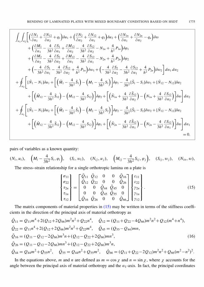
where the second integral should be taken across the boundary of the plate. Substituting (9) into (13)and (10) into (1), employing (12), setting σn = 0, and carrying out the required manipulations, leads tothe overall variational equation in the box on the next page.

From the first four lines of the boxed equation we derive seven governing differential equations:

∂Ni

∂αi+∂Ni j

∂α j+ qi = 0,

∂Mi

∂αi+∂Mi j

∂α j− Nin = 0,

∂Nin

∂αi+∂N jn

∂α j− qn = 0,

∂Si

∂αi+∂Si j

∂α j− 3Pin = 0.

(14)

The remaining terms in the boxed equation lead to the boundary conditions for a plate. The boundarydata on each edge αi = constant are prescribed by selecting one member of each of the following seven

BENDING OF LAMINATED PLATES WITH MIXED BOUNDARY CONDITIONS BASED ON HSDT 1775

∫α1

∫α2

[(∂N1

∂α1+∂N12

∂α2+ q1

)δu1+

(∂N2

∂α2+∂N12

∂α1+ q2

)δu2+

(∂N1n

∂α1+∂N2n

∂α2− qn

)δw

+

(∂M1

∂α1−

43h2

∂S1

∂α1+∂M12

∂α2−

43h2

∂S12

∂α2− N1n +

4h2

P1n

)δϕ1

+

(∂M2

∂α2−

43h2

∂S2

∂α2+∂M12

∂α1−

43h2

∂S12

∂α1− N2n +

4h2

P2n

)δϕ2

+

(−

43h2

∂S1

∂α1−

43h2

∂S12

∂α2+

4h2

P1n

)δw1+

(−

43h2

∂S2

∂α2−

43h2

∂S12

∂α1+

4h2

P2n

)δw2

]dα1 dα2

+

∮α2

[[N̄1− N1]δu1+

[(M̄1−

43h2

S̄1

)−

(M1−

43h2

S1

)]δϕ1−

43h2[S̄1− S1]δw1+ [N̄12− N12]δu2

+

[(M̄12−

43h2

S̄12

)−

(M12−

43h2

S12

)]δϕ2+

[(N̄1n +

43h2

∂ S̄12

∂α2

)−

(N1n +

43h2

∂S12

∂α2

)]δw

]dα2

+

∮α1

[[N̄2− N2]δu2+

[(M̄2−

43h2

S̄2

)−

(M2−

43h2

S2

)]δϕ2−

43h2[S̄2− S2]δw2+ [N̄12− N12]δu2

+

[(M̄12−

43h2

S̄12

)−

(M12−

43h2

S12

)]δϕ1+

[(N̄2n −

43h2

∂ S̄12

∂α1

)−

(N2n −

43h2

∂S12

∂α1

)]δw

]dα1

= 0.

pairs of variables as a known quantity:

(Ni , ui ),(

Mi −4

3h2 Si , ϕi

), (Si , wi ), (Ni j , u j ),

(Mi j −

43h2 Si j , ϕ j

), (Si j , w j ), (Nin, w),

The stress–strain relationship for a single orthotropic lamina on a plate isσ11

σ22

τ2n

τ1n

τ12

=

Q̄11 Q̄12 0 0 Q̄16

Q̄12 Q̄22 0 0 Q̄26

0 0 Q̄44 Q̄45 00 0 Q̄45 Q̄55 0

Q̄16 Q̄26 0 0 Q̄66

ε11

ε22

γ2n

γ1n

γ12

. (15)

The matrix components of material properties in (15) may be written in terms of the stiffness coeffi-cients in the direction of the principal axis of material orthotropy as

Q̄11 = Q11m4+2(Q12+2Q66)m2n2

+Q22n4, Q̄12 = (Q11+Q22−4Q66)m2n2+Q12(m4

+n4),

Q̄22 = Q11n4+2(Q12+2Q66)m2n2

+Q22m4, Q̄45 = (Q55−Q44)mn,

Q̄16 = (Q11−Q12−2Q66)m3n+(Q12−Q22+2Q66)mn3,

Q̄26 = (Q11−Q12−2Q66)mn3+(Q12−Q22+2Q66)m3n,

Q̄44 = Q44m2+Q55n2, Q̄55 = Q44n2

+Q55m2, Q̄66 = (Q11+Q22−2Q12)m2n2+Q66(m2

−n2)2.

(16)

In the equations above, m and n are defined as m = cosχ and n = sinχ , where χ accounts for theangle between the principal axis of material orthotropy and the α1-axis. In fact, the principal coordinates

1776 MOJGAN YAGHOUBSHAHI AND HOSSEIN RAJAIE

of a plate differ from the material principal axes. The material principal axes make an angle χ with theprincipal coordinates of the plate. In terms of engineering constants, the material properties in (16) arederived as

Q11 =E11

1, Q12 =

E11ν21

1, Q22 =

E22

1, Q44 = G23, Q55 = G13, Q66 = G12, (17)

where 1= 1− ν12ν21. However, if the equations in (10) are substituted into (15), the resultant equationsare substituted into (12), and the integration in the thickness direction is carried out, we arrive at thefollowing equations for the stress resultants:

N1

N12

N2

=C1

11 C116 C1

12 C116

C116 C1

66 C126 C1

66

C112 C1

16 C122 C1

26

ε0

1γ 0

1ε0

2γ 0

2

+C2

11 C216 C2

12 C216

C216 C2

66 C226 C2

66

C212 C2

16 C222 C2

26

κ0

1µ0

1κ0

2µ0

2

+C4

11 C416 C4

12 C416

C416 C4

66 C426 C4

66

C412 C4

16 C422 C4

26

κ2

1µ2

1κ2

2µ2

2

,

M1

M12

M2

=C2

11 C216 C2

12 C216

C216 C2

66 C226 C2

66

C212 C2

16 C222 C2

26

ε0

1γ 0

1ε0

2γ 0

2

+C3

11 C316 C3

12 C316

C316 C3

66 C326 C3

66

C312 C3

16 C322 C3

26

κ0

1µ0

1κ0

2µ0

2

+C5

11 C516 C5

12 C516

C516 C5

66 C526 C5

66

C512 C5

16 C522 C5

26

κ2

1µ2

1κ2

2µ2

2

,

P1

P12

P2

=C3

11 C316 C3

12 C316

C316 C3

66 C326 C3

66

C312 C3

16 C322 C3

26

ε0

1γ 0

1ε0

2γ 0

2

+C4

11 C416 C4

12 C416

C416 C4

66 C426 C4

66

C412 C4

16 C422 C4

26

κ0

1µ0

1κ0

2µ0

2

+C6

11 C616 C6

12 C616

C616 C6

66 C626 C6

66

C612 C6

16 C622 C6

26

κ2

1µ2

1κ2

2µ2

2

,

S1

S12

S2

=C4

11 C416 C4

12 C416

C416 C4

66 C426 C4

66

C412 C4

16 C422 C4

26

ε0

1γ 0

1ε0

2γ 0

2

+C5

11 C516 C5

12 C516

C516 C5

66 C526 C5

66

C512 C5

16 C522 C5

26

κ0

1µ0

1κ0

2µ0

2

+C7

11 C716 C7

12 C716

C716 C7

66 C726 C7

66

C712 C7

16 C722 C7

26

κ2

1µ2

1κ2

2µ2

2

,{

N1n

N2n

}=

[C1

55 C154

C145 C1

44

]{λ0

1

λ02

}+

[C3

55 C354

C345 C3

44

]{η1

1

η12

},

{M1n

M2n

}=

[C2

55 C254

C245 C2

44

]{λ0

1

λ02

}+

[C4

55 C454

C445 C4

44

]{η1

1

η12

},

{P1n

P2n

}=

[C3

55 C354

C345 C3

44

]{λ0

1

λ02

}+

[C5

55 C554

C545 C5

44

]{η1

1

η12

},

where

C pi j =

1p

N∑k=1

(Q̄i j )k(hpk−h p

k−1), p ∈ {1, 2, . . . , 7}, (18)

BENDING OF LAMINATED PLATES WITH MIXED BOUNDARY CONDITIONS BASED ON HSDT 1777

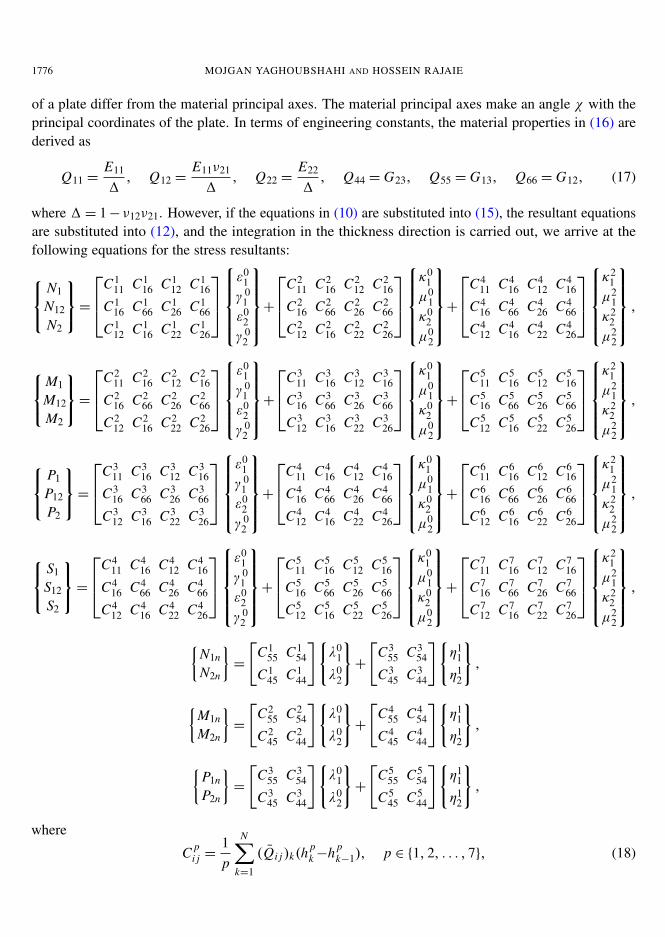
and hk − hk−1 is the thickness of the k-th layer. Substitution of (11) into the equations on page 1776yields the stress resultants in terms of the displacement components. These equations, combined with(14), form a system of 25 first-order partial differential equations for displacements and stress resultants:

[K ]{u1, u2, w, ϕ1, ϕ2, w1, w2, N1, N12, N2,M1,M12,M2,

P1, P12, P2, S1, S12, S2, N1n, N2n,M1n,M2n, P1n, P2n}T= {−q1,−q2, qn, 0, . . . , 0}T . (19)

The coefficients of the matrix K are given in the box below (19). A numerical solution for (19) can beachieved by means of the GDQ method. The method is detailed, for example, in [Shu 1991; Bert et al.1988], and its application to first-order differential equations is summarized here. In the GDQ method,

Nonzero entries of K referenced by row and column

Rows 1 to 7:

1,8 :∂

∂α11,9 :

∂

∂α22,9 :

∂

∂α12,10 :

∂

∂α23,20 :

∂

∂α13,21 :

∂

∂α2

4,11 :∂

∂α14,12 :

∂

∂α24,20 : −1 5,13 :

∂

∂α25,12 :

∂

∂α15,21 : −1

6,17 :∂

∂α16,18 :

∂

∂α26,24 : −3 7,19 :

∂

∂α27,18 :

∂

∂α17,25 : −3

Rows 8 to 19:

k,k : −1

k,1 : A′1∂

∂α1+C ′1

∂

∂α2k,4 :

(A′2−

43h2

A′4)∂

∂α1+

(C ′2−

43h2

C ′4)∂

∂α2k,6 : − 4

3h2A′4

∂

∂α1−

43h2

C ′4∂

∂α2

k,2 : B ′1∂

∂α2+C ′1

∂

∂α1k,5 :

(B ′2−

43h2

B ′4)∂

∂α2+

(C ′2−

43h2

C ′4)∂

∂α1k,7 : − 4

3h2B ′4

∂

∂α1−

43h2

C ′4∂

∂α2

where

for k ∈ {8, 11, 14, 17}, n = 13 (k− 8), A′l = Cn+l

11 , B ′l = Cn+l12 , C ′l = Cn+l

16 ;

for k ∈ {9, 12, 15, 18}, n = 13 (k− 9), A′l = Cn+l

16 , B ′l = Cn+l26 , C ′l = Cn+l

66 ;

for k ∈ {10, 13, 16, 19}, n = 13 (k− 10), A′l = Cn+l

12 , B ′l = Cn+l22 , C ′l = Cn+l

16 ,

Rows 20 to 25:

k,k : = −1 k,4 : = A′1−4h2

A′3 k,6 : = − 4h2

A′3

k,3 : = A′1∂

∂α1+ B ′1

∂

∂α2k,5 : = B ′1−

4h2

B ′3 k,7 : = − 43h2

A′3

where

for k ∈ {20, 22, 24}, n = 12 (k− 20), A′l = Cn+l

55 , B ′l = Cn+l45 ,

for k ∈ {21, 23, 25}, n = 12 (k− 21), A′l = Cn+l

45 , B ′l = Cn+l44 .

1778 MOJGAN YAGHOUBSHAHI AND HOSSEIN RAJAIE

the derivative of a function at any discrete point in a given direction is approximated by the weightedlinear sum of the function values at all sampling points in that direction,

d F(xk)

dx=

N∑l=1

Ckl F(xl), k ∈ {1, 2, . . . , N }, (20)

where N denotes the number of sampling points selected in the x-direction and Ckl are the weightingcoefficients of the first derivative with respect to the variable x . Taking the Lagrange interpolationpolynomials as test functions, the coefficients in (20) result in

Ckl =M(xk)

(xk − xl)M(xl), k, l = 1, 2, . . . , N , k 6= l,

Ckk =−

N∑l=1l 6=k

Ckl, k = 1, 2, . . . , N ,(21)

where M(xk)=N∏

l=1l 6=k

(xk − xl). The sampling points are chosen in the form of a cosine distribution as

xk =a2

[1− cos

( k−1N−1

π)], k = 1, 2, . . . , N , (22)

where a is the length in x-direction. Differentiating (19) with respect to α1 and α2 and using (20) togetherwith the boundary conditions (see page 1775) leads to an overdetermined system of algebraic equationsfor displacements and stress resultants at the sampling points. These equations are then solved usingleast-squares minimization methods.

3. Numerical results

To verify the methodology developed in this study, the bending of symmetric ([0/90/0] and [90/0/90])and antisymmetric [0/90] cross ply square plates, subjected to uniformly distributed transverse loads,were considered. A material with the following properties was used in these numerical calculations:

E1

E2= 25,

G12

E2=

G13

E2= 0.5,

G23

E2= 0.2, ν12 = 0.25,

in which E1 and E2 are the in-plane Young’s modulus in the α1 and α2 coordinate directions. G12 is thein-plane shear modulus, G13 and G23 are the transverse shear modulus in the α1− n and α2− n planes,respectively, whereas ν12 is the major Poisson’s ratio in the α1-α2 plane. The quantities w∗ and M∗1 are

w∗ =−103 E2h3

qna4 w, M∗1 =103 Mi

qna2 .

Here, ‘a’ is the length of the edges of the square, and qn denotes the uniformly distributed transverseload. In this study, three models with various boundary conditions were considered. The first model,called (S-S-S-S), is a plate with an SS2-type simply supported boundary condition on all edges. Thesecond model, called (S-S-S-SF), is a plate with SS2-type simply supported boundary condition on threeedges, and the fourth edge, corresponding to the edge α1 = a, is a mixed boundary condition of free and

BENDING OF LAMINATED PLATES WITH MIXED BOUNDARY CONDITIONS BASED ON HSDT 1779

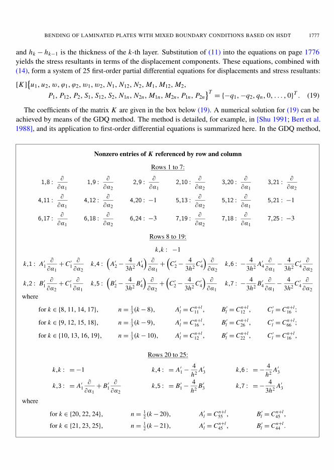
!Figure 1. The models used in the present study with their various boundary conditions.

SS2-type simply supported boundary conditions, as shown in Figure 1. (S-S-S-F) is the last model andhas three edges subjected to the SS2 boundary condition, and the edge corresponding to the edge α1 = ais free.

The SS2-type simply supported boundary conditions and free edge defined on the edge αi = constantare as follows:

SS2 type: ui = 0, Mi = 0, Si = 0, Ni j = 0, ϕ j = 0, w j = 0, w = 0.

Free edge: Ni = 0, Mi = 0, Si = 0, Ni j = 0, Mi j = 0, Si j = 0, Nin = 0.

In all models, the displacements and moments are computed at the center of the plate. Because thebending of a plate with mixed boundary conditions has not been extensively investigated, we comparedthe models to simulations performed with the ANSYS version 5.4 finite element software. The finiteelement mesh is composed of 400 SHELL99 elements with identical dimensions.

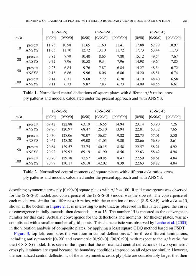
Table 1 compares the normalized central deflections of antisymmetric [0/90] and symmetric [0/90/0]and [90/0/90] cross ply square plates, characterized by four different a/h ratios, for the three models,computed using our approach versus ANSYS. In each direction, fifteen grid points are used for model(S-S-S-S), 17 for model (S-S-S-SF), and 19 for model (S-S-S-F). Table 2 shows the analogous comparesfor central moments.

The maximum w∗ discrepancy between the two sets of results is observed for the (S-S-S-SF) modelwith a [0/90/0] lamination and a/h= 10. In comparing the results with FE, we mention that the boundaryconditions used in the present approach are not identical to those in ANSYS. Therefore, we expect somediscrepancies between the results. Nonetheless, discrepancies should not be more than 11%.

The discrepancies of the normalized central moments, M∗1 , between the two sets of results can beattributed to the fact that ANSYS calculates moments on grid points by extrapolating the moment calcu-lated over the Gaussian points. Therefore, this method produces some approximations in the calculationof moments on grid points.

In the [90/0/90] lamination, the normalized central deflections of (S-S-S-SF) are larger than those of(S-S-S-F). A finite element analysis with 1600 elements (a/h = 10) was performed. The value of w∗,in the center of both (S-S-S-SF) and (S-S-S-F) models, is 11.73.

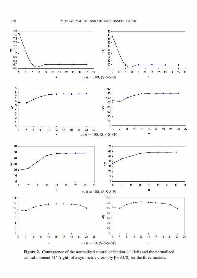
The first three rows of Figure 2 display the convergence (with n1 = n2 = n) of normalized transversedisplacements w∗ and normalized moments M∗1 for the (S-S-S-S), (S-S-S-SF), and (S-S-S-F) models

1780 MOJGAN YAGHOUBSHAHI AND HOSSEIN RAJAIE

a/h = 100, (S-S-S-S)

a/h = 100, (S-S-S-SF)

a/h = 100, (S-S-S-F)

a/h = 10, (S-S-S-SF)

Figure 2. Convergence of the normalized central deflection w∗ (left) and the normalizedcentral moment M∗1 (right) of a symmetric cross ply [0/90/0] for the three models.

BENDING OF LAMINATED PLATES WITH MIXED BOUNDARY CONDITIONS BASED ON HSDT 1781

(S-S-S-S) (S-S-S-SF) (S-S-S-F)a/h [0/90] [0/90/0] [0/90] [0/90/0] [90/0/90] [0/90] [0/90/0] [90/0/90]

10present

ANSYS11.7311.63

10.9811.70

11.6512.72

11.6013.10

11.4111.72

17.8817.73

52.7953.44

10.9711.73

20present

ANSYS9.829.72

7.797.96

10.4010.58

8.659.34

7.807.96

15.1214.98

49.5449.64

7.677.85

50present

ANSYS9.239.18

6.846.86

9.769.96

7.878.06

6.846.86

14.2714.20

48.5448.51

6.726.74

100present

ANSYS9.149.11

6.716.73

9.689.87

7.727.83

6.706.73

14.1014.09

48.4048.55

6.586.61

Table 1. Normalized central deflections of square plates with different a/h ratios, crossply patterns and models, calculated under the present approach and with ANSYS.

(S-S-S-S) (S-S-S-SF) (S-S-S-F)a/h [0/90] [0/90/0] [0/90] [0/90/0] [90/0/90] [0/90] [0/90/0] [90/0/90]

10present

ANSYS69.4269.96

122.88120.97

63.1968.47

116.55125.10

14.9413.94

23.1422.81

53.9053.32

7.267.65

20present

ANSYS70.3070.67

128.06128.20

70.0769.08

136.87141.03

9.829.80

22.7322.66

57.0156.89

5.505.61

50present

ANSYS70.6470.92

129.57129.93

73.7569.19

140.15141.90

8.588.56

22.5722.63

58.2158.42

4.924.94

100present

ANSYS70.7070.97

129.78130.17

72.5769.18

140.85142.02

8.478.39

22.5922.63

58.6158.82

4.844.84

Table 2. Normalized central moments of square plates with different a/h ratios, crossply patterns and models, calculated under the present approach and with ANSYS.

describing symmetric cross ply [0/90/0] square plates with a/h = 100. Rapid convergence was observedfor the (S-S-S-S) model, and convergence of the (S-S-S-SF) model was the slowest. The convergence ofeach model was similar for different a/h ratios, with the exception of model (S-S-S-SF), with a/h = 10,shown at the bottom in Figure 2. It is interesting to note that, as observed in this latter figure, the curveof convergence initially ascends, then descends at n = 15. The number 15 is reported as the convergencenumber for this case. Actually, convergence for the deflections and moments, for thicker plates, was ac-complished with a smaller number of grid points. This characteristic was observed by Lanhe et al. [2005]in the vibration analysis of composite plates, by applying a least square GDQ method based on FSDT.

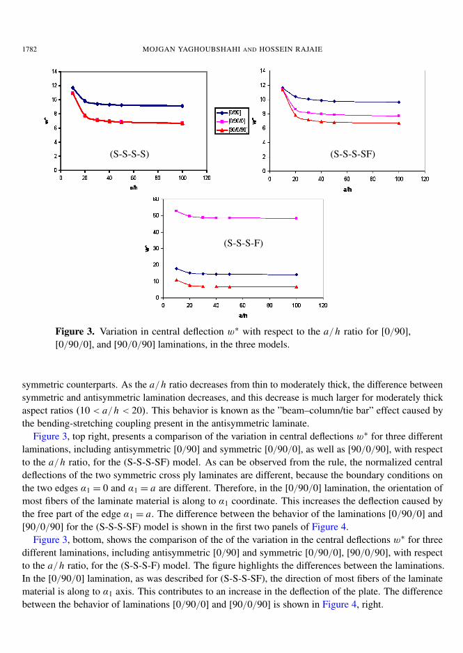
Figure 3, top left, compares the variation in central deflections w∗ for three different laminations,including antisymmetric [0/90] and symmetric [0/90/0], [90/0/90], with respect to the a/h ratio, forthe (S-S-S-S) model. It is seen in the figure that the normalized central deflections of two symmetriccross ply laminates are equal because the boundary conditions imposed on all edges are similar. However,the normalized central deflections, of the antisymmetric cross ply plate are considerably larger that their

1782 MOJGAN YAGHOUBSHAHI AND HOSSEIN RAJAIE

(S-S-S-S) (S-S-S-SF)

(S-S-S-F)

Figure 3. Variation in central deflection w∗ with respect to the a/h ratio for [0/90],[0/90/0], and [90/0/90] laminations, in the three models.

symmetric counterparts. As the a/h ratio decreases from thin to moderately thick, the difference betweensymmetric and antisymmetric lamination decreases, and this decrease is much larger for moderately thickaspect ratios (10< a/h < 20). This behavior is known as the ”beam–column/tie bar” effect caused bythe bending-stretching coupling present in the antisymmetric laminate.

Figure 3, top right, presents a comparison of the variation in central deflections w∗ for three differentlaminations, including antisymmetric [0/90] and symmetric [0/90/0], as well as [90/0/90], with respectto the a/h ratio, for the (S-S-S-SF) model. As can be observed from the rule, the normalized centraldeflections of the two symmetric cross ply laminates are different, because the boundary conditions onthe two edges α1 = 0 and α1 = a are different. Therefore, in the [0/90/0] lamination, the orientation ofmost fibers of the laminate material is along to α1 coordinate. This increases the deflection caused bythe free part of the edge α1 = a. The difference between the behavior of the laminations [0/90/0] and[90/0/90] for the (S-S-S-SF) model is shown in the first two panels of Figure 4.

Figure 3, bottom, shows the comparison of the of the variation in the central deflections w∗ for threedifferent laminations, including antisymmetric [0/90] and symmetric [0/90/0], [90/0/90], with respectto the a/h ratio, for the (S-S-S-F) model. The figure highlights the differences between the laminations.In the [0/90/0] lamination, as was described for (S-S-S-SF), the direction of most fibers of the laminatematerial is along to α1 axis. This contributes to an increase in the deflection of the plate. The differencebetween the behavior of laminations [0/90/0] and [90/0/90] is shown in Figure 4, right.

BENDING OF LAMINATED PLATES WITH MIXED BOUNDARY CONDITIONS BASED ON HSDT 1783

! ![0/90/0] [90/0/90] [0/90/0] [90/0/90]

(S-S-S-SF) (S-S-S-F)

Figure 4. Displacement contours of a plate with laminations [0/90/0] and [90/0/90]for two of the models.

Figure 5 compares the central deflection of the (S-S-S-S) and (S-S-S-SF) models, for [0/90], [0/90/0],and [90/0/90] laminations. The maximum difference between (S-S-S-S) and (S-S-S-SF) is observed inthe [0/90/0] lamination, and the minimum difference is observed in the [90/0/90] lamination. Thiseffect can be understood from the explanation given for Figure 4, left.

[0/90] [0/90/0]

[90/0/90]

Figure 5. Variation in central deflection w∗ with respect to the a/h ratio for [0/90],[0/90/0], and [90/0/90] laminations, in the (S-S-S-S) and (S-S-S-SF) models.

1784 MOJGAN YAGHOUBSHAHI AND HOSSEIN RAJAIE

[0/90] [0/90/0]

[90/0/90]

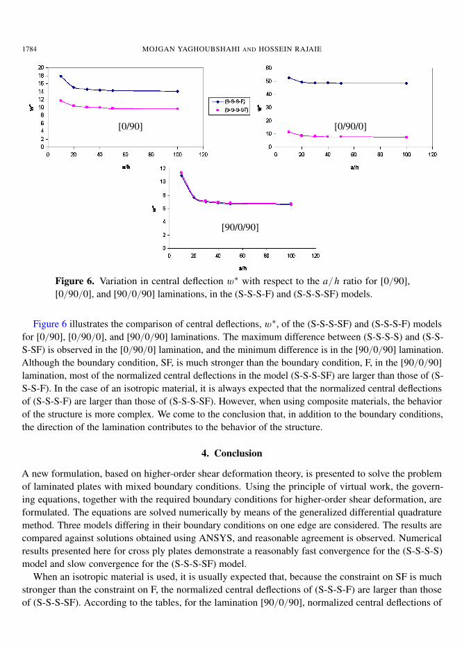
Figure 6. Variation in central deflection w∗ with respect to the a/h ratio for [0/90],[0/90/0], and [90/0/90] laminations, in the (S-S-S-F) and (S-S-S-SF) models.

Figure 6 illustrates the comparison of central deflections, w∗, of the (S-S-S-SF) and (S-S-S-F) modelsfor [0/90], [0/90/0], and [90/0/90] laminations. The maximum difference between (S-S-S-S) and (S-S-S-SF) is observed in the [0/90/0] lamination, and the minimum difference is in the [90/0/90] lamination.Although the boundary condition, SF, is much stronger than the boundary condition, F, in the [90/0/90]lamination, most of the normalized central deflections in the model (S-S-S-SF) are larger than those of (S-S-S-F). In the case of an isotropic material, it is always expected that the normalized central deflectionsof (S-S-S-F) are larger than those of (S-S-S-SF). However, when using composite materials, the behaviorof the structure is more complex. We come to the conclusion that, in addition to the boundary conditions,the direction of the lamination contributes to the behavior of the structure.

4. Conclusion

A new formulation, based on higher-order shear deformation theory, is presented to solve the problemof laminated plates with mixed boundary conditions. Using the principle of virtual work, the govern-ing equations, together with the required boundary conditions for higher-order shear deformation, areformulated. The equations are solved numerically by means of the generalized differential quadraturemethod. Three models differing in their boundary conditions on one edge are considered. The results arecompared against solutions obtained using ANSYS, and reasonable agreement is observed. Numericalresults presented here for cross ply plates demonstrate a reasonably fast convergence for the (S-S-S-S)model and slow convergence for the (S-S-S-SF) model.

When an isotropic material is used, it is usually expected that, because the constraint on SF is muchstronger than the constraint on F, the normalized central deflections of (S-S-S-F) are larger than thoseof (S-S-S-SF). According to the tables, for the lamination [90/0/90], normalized central deflections of

BENDING OF LAMINATED PLATES WITH MIXED BOUNDARY CONDITIONS BASED ON HSDT 1785

(S-S-S-SF) are larger than those of (S-S-S-F). This result illustrates that when a composite material isused, the behavior of the structure is more complex, and we can come to the conclusion that, in additionto the boundary conditions, the direction of the lamination contributes to the behavior of the structures.

The direction of fibers in the [0/90/0] and [90/0/90] laminations has a significant effect, especially formodels (S-S-S-SF) and (S-S-S-F). When the direction of most of the fibers is perpendicular to the freeedge, the central deflections of the plates are larger than when it’s parallel. The effect of the transverseshear deformation is described by the conceptual bending-stretching coupling effect, a characteristic ofantisymmetric laminates. This characteristic is obvious in the model (S-S-S-S).

References

[Aghdam et al. 2006] M. M. Aghdam, M. R. N. Farahani, M. Dashty, and S. M. Rezaei Niya, “Application of generalizeddifferential quadrature method to the bending of thick laminated plates with various boundary conditions”, Appl. Mech. Mater.5–6 (2006), 407–414.

[Basset 1890] A. B. Basset, “On the extension and flexure of cylindrical and spherical thin elastic shells”, Phil. Trans. R. Soc.A 181 (1890), 433–480.

[Bellman et al. 1972] R. Bellman, B. G. Kashef, and J. Casti, “Differential quadrature: a technique for the rapid solution ofnonlinear partial differential equations”, J. Comput. Phys. 10:1 (1972), 40–52.

[Bert and Chen 1978] C. W. Bert and T. L. C. Chen, “Effect of shear deformation on vibration of antisymmetric angle-plylaminated rectangular plates”, Int. J. Solids Struct. 14:6 (1978), 465–473.

[Bert and Francis 1974] C. W. Bert and P. H. Francis, “Composite material mechanics: structural mechanics”, AIAA J. 12:9(1974), 1173–1186.

[Bert et al. 1988] C. W. Bert, S. K. Jang, and A. G. Striz, “Two new approximate methods for analyzing free vibration ofstructural components”, AIAA J. 26:5 (1988), 612–618.

[Bert et al. 1989] C. W. Bert, S. K. Jang, and A. G. Striz, “Nonlinear bending analysis of orthotropic rectangular plates by themethod of differential quadrature”, Comput. Mech. 5:2–3 (1989), 217–226.

[Lanhe et al. 2005] W. Lanhe, L. Hua, and D. Wang, “Vibration analysis of generally laminated composite plates by the movingleast squares differential quadrature method”, Compos. Struct. 68:3 (2005), 319–330.

[Li and Cheng 2005] J.-J. Li and C.-J. Cheng, “Differential quadrature method for nonlinear vibration of orthotropic plateswith finite deformation and transverse shear effect”, J. Sound Vib. 281:1–2 (2005), 295–309.

[Malekzadeh and Setoodeh 2007] P. Malekzadeh and A. R. Setoodeh, “Large deformation analysis of moderately thick lami-nated plates on nonlinear elastic foundations by DQM”, Compos. Struct. 80:4 (2007), 569–579.

[Mindlin 1951] R. D. Mindlin, “Influence of rotatory inertia and shear on flexural motions of isotropic, elastic plates”, J. Appl.Mech. (ASME) 18:1 (1951), 31–38.

[Naghdi 1956] P. M. Naghdi, “A survey of recent progress in theory of elastic shells”, Appl. Mech. Rev. (ASME) 9:9 (1956),365–388.

[Quan and Chang 1989] J. R. Quan and C. T. Chang, “New insights in solving distributed system equations by the quadraturemethods, I: Analysis”, Comput. Chem. Eng. 13:7 (1989), 779–788.

[Reddy and Liu 1985] J. N. Reddy and C. F. Liu, “A higher-order shear deformation theory of laminated elastic shells”, Int. J.Eng. Sci. 23:3 (1985), 319–330.

[Reissner 1945] E. Reissner, “The effect of transverse shear deformation on the bending of elastic plates”, J. Appl. Mech.(ASME) 12:2 (1945), 69–77.

[Sherbourne and Pandey 1991] A. N. Sherbourne and M. D. Pandey, “Differential quadrature method in the buckling analysisof beams and composite plates”, Comput. Struct. 40:4 (1991), 903–913.

[Shu 1991] C. Shu, Generalized differential quadrature integral quadrature and application to the simulation of incompressibleviscous flows including parallel computation, Ph.D. thesis, University of Glasgow, 1991.

1786 MOJGAN YAGHOUBSHAHI AND HOSSEIN RAJAIE

[Shu and Richards 1990] C. Shu and B. E. Richards, “High resolution of natural convection in a square cavity by general-ized differential quadrature”, pp. 978–985 in Numerical methods in engineering: theory and appreciations (NUMETA 90)(Swansea, 1990), vol. 2, edited by G. N. Pande and J. Middleton, Elsevier, London, 1990.

[Striz et al. 1988] A. G. Striz, S. K. Jang, and C. W. Bert, “Nonlinear bending analysis of thin circular plates by differentialquadrature”, Thin-Walled Struct. 6:1 (1988), 51–62.

[Tornabene and Viola 2008] F. Tornabene and E. Viola, “2-D solution for free vibrations of parabolic shells using generalizeddifferential quadrature method”, Eur. J. Mech. A Solids 27:6 (2008), 1001–1025.

Received 27 Feb 2009. Revised 9 Apr 2009. Accepted 23 Jun 2009.

MOJGAN YAGHOUBSHAHI: moyaeng@gmail.comDepartment of Civil and Environmental Engineering, Amirkabir University of Technology, 424 Hafez Avenue, Tehran 15914,Iran

HOSSEIN RAJAIE: rajaieh@aut.ac.irDepartment of Civil and Environmental Engineering, Amirkabir University of Technology, 424 Hafez Avenue, Tehran 15914,Iranhttp://www.aut.ac.ir/official/main.asp?uid=rajaieh