Bank of England

Working Paper no. 305

August 2006

Bank capital, asset prices and monetary policy

David Aikman and Matthias Paustian

Bank capital, asset prices and monetary policy

David Aikman�

and

Matthias Paustian��

Working Paper no. 305

� Conjunctural Assessment and Projections Division, Bank of England, Threadneedle Street,London, EC2R 8AH.

�� Department of Economics, Bowling Green State University, Bowling Green OH, United States.

The views expressed in this paper are those of the authors, and not necessarily those of the Bankof England. We would like to thank Jan Vlieghe for encouraging us to pursue this project, and formany helpful discussions on its direction. We would also like to thank Peter Andrews, AlexBowen, Tim Fuerst, Reint Gropp, Jürgen von Hagen, Gabriel Sterne and Haiping Zhang for usefulcomments. We thank conference and seminar participants at the European Winter Meeting of theEconometric Society in Stockholm, DIW Berlin, the Bank of England, the Bundesbank, BowlingGreen State University, the University of Munich, the University of Würzburg, and the Center forEuropean Integration Studies at the University of Bonn. All errors are our own. This paper was�nalised on 4 July 2006.

The Bank of England's working paper series is externally refereed.

Information on the Bank's working paper series can be found atwww.bankofengland.co.uk/publications/workingpapers/index.htm.

Publications Group, Bank of England, Threadneedle Street, London, EC2R 8AH; telephone+44 (0)20 7601 4030, fax +44 (0)20 7601 3298, email mapublications@bankofengland.co.uk.

c Bank of England 2006ISSN 1749-9135 (on-line)

Contents

Abstract 3

Summary 4

1 Introduction 6

2 Structure of the model 9

3 The �nancial contract 18

4 Monetary policy 20

5 Equilibrium 20

6 Functional forms and calibration 22

7 The economy's response to exogenous shocks 23

8 How should monetary policy be conducted in the face of this �nancial friction? 27

9 Conclusion 33

Appendix A: The no moral hazard reference model 35

Appendix B: Charts 36

References 41

2

Abstract

We study a general equilibrium model in which informational frictions impede entrepreneurs'

ability to borrow and banks' ability to intermediate funds. These �nancial market frictions are

embedded in an otherwise-standard dynamic New Keynesian model. We �nd that exogenous

shocks have an ampli�ed and more persistent effect on output and investment, relative to the case

of perfect capital markets. The chief contribution of the paper is to analyse how these �nancial

sector imperfections � in particular, those relating to the banking sector � modify our

understanding of optimal monetary policy. Our main �nding is that optimal monetary policy

tolerates only a very small amount of in�ation volatility. Given that similar results have been

reported for models that abstract from banks, we conclude that assigning a non-trivial role for

banks need not materially affect the properties of optimal monetary policy.

Key words: Banks; moral hazard; credit market frictions; price rigidities; optimal monetary policy.

JEL classi�cation: E44; E32; E52.

3

Summary

Do weak banks affect the transmission mechanism of monetary policy? Does bank lending merely

re�ect general macroeconomic conditions, or are there important feedback effects from banks to

other macro variables? More generally, how should �nancial sector conditions in�uence the

conduct of monetary policy? These questions are of long-standing interest to policymakers and

they form the motivation for this paper. In order to study them, we develop a framework that

explicitly models the role of banks in intermediating credit �ows, and takes into account some

possible frictions that are likely to exist between depositors, banks and borrowers.

In our model, the amount of capital held by banks and the creditworthiness of borrowers are both

important ingredients in transmitting shocks throughout the economy. To see why, suppose that an

unanticipated tightening of monetary policy (or some other adverse shock) leads to a decline in

output, which then lowers the pro�tability of �rms, triggers a fall in asset prices, and causes loan

losses for banks. The accompanying reductions in borrower net worth and bank capital will have

two effects. First, banks will be less willing to lend to borrowers whose creditworthiness has

declined. And second, depositors will view banks as riskier institutions, and will readjust their

portfolios out of bank deposits. We show by simulation that these effects are able to generate a

signi�cant second-round cutback in the �ow of lending which exacerbates the initial downturn.

Intuitively, we might expect there to be a role for monetary policy in mitigating the second-round

effects generated by these frictions. For instance, by aggressively cutting interest rates in a

downturn, the central bank might be able to check the falls in asset prices and net worth associated

with the shock, thereby partly cushioning the impact on aggregate demand. The cost of acting in

this way, however, is higher in�ation � at least in the short term. A key question for policymakers

is therefore: how much of an increase in in�ation volatility should be tolerated in order to reduce

the volatility of output growth in this way?

The chief contribution of this paper is to tackle this question. We proceed in two steps. First, we

assess the performance of monetary policy strategies that respond in a mechanical way to

`�nancial' variables such as asset prices or credit �ows over-and-above consumer price in�ation.

It turns out that these simple monetary policy rules perform poorly if the goal of policy is

maximising the wellbeing of economic agents in the model. Second, we use numerical techniques

4

to analyse the properties of the `optimal' monetary policy implied by the model. Our main �nding

is that a central bank acting in this optimal way will tolerate only a very small amount of in�ation

volatility. Furthermore, the `trade-off' implied by our model is very steep in the sense that the

reduction in output growth volatility achieved by allowing in�ation to become more volatile is

very small. Given that similar results have been reported for models that abstract from banks � and

in fact credit market imperfections altogether � we conclude that assigning a non-trivial role for

these frictions need not materially affect optimal monetary policy. This suggests that policies that

work well in `normal' times are likely to continue working well in a situation where weak banks

are limiting the expansion of credit.

5

`Traditionally, most economists have regarded the fact that banks hold capital as at best a

macroeconomic irrelevance and at worst a pedagogical inconvenience.' Friedman, B (1991).

1 Introduction

The current generation of workhorse models used for monetary policy analysis typically abstract

from imperfections in �nancial markets. Firms and households can borrow freely at riskless

interest rates. And �nancial intermediaries, if they are explicitly modelled, are nothing more than

a veil. In this paper, we relax these assumptions and study an environment in which informational

frictions impede the smooth functioning of �nancial markets. These frictions generate an

important role for banks in ensuring the ef�cient allocation of funds. We use the framework to

analyse the implications of this bank-centric view of the economy for the design of monetary

policy.

A common justi�cation for abstracting from banks is that the increasing sophistication of �nancial

markets have made borrowers less intermediary-dependent in recent years. One counter-argument

to this is that banking crises, when they occur, are typically extremely costly events. Hoggarth,

Reis and Saporta (2002) for instance estimate that average cumulative output losses following

crises are in the order of 15%-20% of annual GDP. Some authors have found that loan supply

disturbances affect real activity in more normal times too. Peek and Rosengren (1997) for instance

�nd that capital shortages at Japanese banks adversely affected US real estate investment in the

early 1990s. The evidence, however, is not clear-cut: Driscoll (2004) for example �nds little

connection between shifts in bank loan supply and US states' personal income. (1) Yet another set

of studies have found cross-sectional patterns in bank behaviour that are dif�cult to reconcile with

theories based on perfect capital markets. For example, Kashyap and Stein (1995, 2000)

demonstrate that lending by `small' banks is more sensitive to a change in monetary policy than

lending by their larger counterparts. The presumption is that, with less liquid balance sheets, small

(1) The macroeconomic impact may be a non-linear function of the magnitude of the shock to loan supply. Ashcraft(2005a), for instance, �nds little relationship between state-level real income and loan supply following a shock tomonetary policy. When focusing on bank failures, however, he �nds signi�cant and apparently permanent effects onreal activity (see Ashcraft (2005b)).

6

banks are less able to shield their lending from such shocks. (2)

In this paper, we develop a small quantitative general equilibrium model in which banks serve a

meaningful role in intermediating credit. And we use the model to study the properties of a range

of alternative monetary policies. The exercise requires us to take a stand on three key questions:

� First, what frictions are banks helping to overcome?

� Second, what drives feedback between the �nancial system and real economic activity?

� And third, what frictions give the central bank leverage over the real economy?

The role for banks in our model stems from an asymmetric information problem between

borrowers and lenders: borrowers, we assume, are tempted to divert resources towards privately

bene�cial activities (like engaging in unpro�table takeovers, appointing family and friends to key

positions in the �rm etc). By monitoring borrowers' actions, banks can mitigate the deadweight

losses imposed by this agency problem. (3)

The net worth of borrowers and the amount of capital held by banks both matter for real activity in

our model. The need to hold capital/net worth also emanates from an asymmetric information

problem. Only entrepreneurs with enough capital at stake will be motivated to act diligently. And

likewise for banks: monitoring is a costly activity, so banks will be tempted to devote fewer

resources to it than is required. Only those banks with suf�cient capital at stake will be trusted to

be conscientious monitors. (4) Fluctuations in capital/net worth therefore feed back onto real

investment and output.

(2) Ashcraft (2005a) �nds that af�liation with a multi-bank holding company signi�cantly lowers the sensitivity ofloans to monetary policy. Similarly, Ehrmann and Worms (2004) caution against the use of size as a proxy forliquidity in �nancial systems where bank networks are prominent (eg Germany).Other studies exploit cross-sectional differences in bank capitalisation as an identi�cation device. For instance,Kishan and Opiela (2000) report evidence that loan growth of highly leveraged banks is more responsive to monetarypolicy than the loan growth of well-capitalised banks.(3) The focus on monitoring clearly abstracts from a host of other important functions served by the banking sector(such as liquidity provision, payment services etc). We follow this approach for reasons of tractability, rather thanfrom a belief that monitoring is more important than these other functions per se.(4) This follows the framework of Holmstrom and Tirole (1997). Notice that the need for banks to hold capital in thismodel has nothing to do with regulatory policy.

7

Our model builds on earlier work by Chen (2001). (5) The �rst contribution of this paper is to

extend this work in order for it to be suitable for monetary policy analysis. The standard

framework for monetary policy research in recent years has been dynamic general equilibrium

models with nominal rigidities. We follow that approach here and assume that the real effects of

monetary policy derive from frictions in adjusting goods prices.

The paper proceeds as follows. After running through the details of the model, we use impulse

response analysis to analyse how credit frictions in�uence its dynamic properties. We �nd that

credit constraints bring about an ampli�ed, and more persistent response of macroeconomic

variables (notably output) to technology, monetary and net worth shocks, relative to the

benchmark of perfect capital markets. Ampli�cation is not a universal result in the literature on

�nancial frictions. Bernanke et al (2000), for instance, report a similar degree of output

ampli�cation as we do. But Carlstrom and Fuerst (1996, 2001) �nd that credit frictions dampen

the initial impact on output, but generate greater persistence thereafter. As we discuss below, these

differences can be traced to the greater volatility of asset prices in our model and Bernanke et al's.

We then turn to the normative question of how monetary policy should be conducted in this

model. We approach this question in two steps. First, we ask whether simple Taylor-type rules

augmented to include `�nancial' variables such as asset prices or credit growth provide a sensible

way of conducting monetary policy in the model. In line with the conclusions drawn by Bernanke

and Gertler (2001), Gilchrist and Leahy (2002) and others, we �nd that they do not: mechanically

responding to asset prices and/or credit growth is detrimental to welfare relative to a policy of

strict price stability. Second, we search within a broad family of rules for the optimal monetary

policy that maximises the representative household's expected utility. We �nd that optimal

monetary policy does not fully stabilise the price level following a real disturbance. Rather, it

takes a slightly countercyclical stance, smoothing through some of the inef�cient �uctuations that

arise from such shocks. Quantitatively, however, the amount of in�ation tolerated by the optimal

policy is very small and roughly comparable to what is found by Collard and Dellas (2005) for the

case of tax distortions. Furthermore, the volatility of real variables under the optimal rule is

quantitatively very similar to that under full price stability.

(5) Meh and Moran (2004) study a general equilibrium model with banking sector frictions similar in spirit to ours.These authors show how the banking frictions outlined in the text can generate countercyclical capital-asset ratios asobserved in the data.

8

Our paper is related to a recent study by Faia and Monacelli (2005), who study the performance of

simple rules in the �nancial accelerator model of Bernanke et al (2000). They �nd strict in�ation

targeting to be the welfare maximising policy in that model. Our approach differs from theirs in

that the class of rules that we consider is much more general. In particular, we allow the central

bank to respond to all the relevant state variables of the economy. Nevertheless, our results are

complementary to theirs in that we �nd only very small deviations from full price stability under

the optimal policy. Assigning a non-trivial role for banks, therefore, need not materially affect the

properties of optimal monetary policy. Another paper which shares a similar motivation to ours is

Vlieghe (2005), which examines optimal monetary policy in a monetised, sticky price version of

Kiyotaki (1998). The degree of in�ation volatility found by Vlieghe (2005) under the optimal

Ramsey plan is similar to that found here. But, in contrast to our �ndings, this small amount of

in�ation volatility is associated with much lower volatility in output than under full price stability.

The rest of the paper is organised as follows. Section 2 introduces the model environment. Section

3 explains the structure of �nancial contracts. Section 4 outlines a baseline monetary policy rule

used in the initial part of the paper. Section 5 discusses aggregation issues and lists the model's

equilibrium conditions. Section 6 details our calibration. Section 7 analyses impulse responses

from the model following shocks to bank capital, monetary policy, and technology. Section 8

analyses optimal monetary policy. Finally, Section 9 concludes.

2 Structure of the model

2.1 Overview

We begin with a brief overview of the basic structure of our model. There are four agents:

households/depositors, entrepreneurs, �nancial intermediaries (`bankers'), and wholesalers.

Households, bankers and entrepreneurs have distinct preferences over the economy's consumption

good. (6) The production of this good involves two tiers. At the initial tier, entrepreneurs and

households use capital to produce an `intermediate' good. Entrepreneurs, we assume, are more

skilled at doing this than households. But imperfections in the economy's credit market imply that

entrepreneurs end up holding too little of the capital stock in equilibrium. By implication, the

fraction of the capital stock held by entrepreneurs at any point in time has a �rst-order effect on

(6) Treating households, bankers and entrepreneurs as distinct from one another is a simpli�cation that facilitates themodelling of a credit market.

9

the economy's productive capacity. (7)

At the second tier we introduce price stickiness. In the New Keynesian literature, it is

commonplace to assume that producers of the intermediate good are imperfect competitors. This

is a useful assumption because imperfect competitors face non-trivial pricing decisions � clearly a

necessary ingredient in any coherent theory of price stickiness. However, assuming imperfect

competition between entrepreneurs would signi�cantly complicate the structure of our model. To

get round this problem, we borrow an idea from Bernanke, Gertler and Gilchrist (2000) and

assume that imperfect competition and price rigidity occurs one level down the supply chain, at

the wholesale level. Wholesalers purchase the intermediate good from households and

entrepreneurs, differentiate it (eg paint it different colours), and sell it on at a markup over

marginal cost to a competitive retail sector. Retailers then simply aggregate the differentiated

goods into �nal output, which is then either consumed or invested. Neither wholesalers nor

retailers play any further role in the model.

At the end of each period, new capital goods are produced by competitive capital-goods

producers. Capital producers use a concave technology to transform inputs of �nal output

(`investment') and rented capital into new capital goods. The concavity of their production

function is analogous to assuming convex costs of adjusting the capital stock. And it implies that

the relative price of new capital goods may deviate from unity in the short run.

We now proceed by describing the decision problems of each agent in more detail.

2.2 Households

Households are in�nitely lived and have preferences over consumption Ch , leisure 1� N and real

money balances m. (8) The objective of the representative household is to maximise the lifetime

(7) This dual sector set-up is somewhat stylised, but may be thought of as corresponding to the following scenario.The less productive but unconstrained production by households resembles that of large, well-established companieswho can borrow cheaply in �nancial markets. Conversely, the high-return but constrained production by entrepreneursresembles that of small �rms and start-ups, who typically have greater trouble accessing �nance.(8) We take H .m/ to be small. This is intended to capture the idea that cash is used for very few transactions in thesteady state. This `cashless limiting economy' (see Woodford (1998)) is an attractive approach in a model such asours, where bank deposits form a signi�cant fraction of households' portfolios.

10

utility:

E01XtD0

� t

24�Cht �1� 1�

1� 1�

C�

1C .1� Nt/1C C H .m t/

35 (1)

where � is the time discount factor.

In any period t , the representative household receives the following income �ows: a wage of !tper unit of labour Nt supplied; a gross real interest rate of r dt�1 on its deposits of the previous

period Dt�1; a price of vt per unit of intermediate good G�K ht�1

�sold to wholesalers; lump-sum

pro�ts from the monopolistic wholesaler 5t ; plus a real transfer trt from the central bank. The

household may also have cash holdings carried over from the previous period. These resources are

either consumed, or used to augment the household's holdings of capital, deposits or cash. This

constraint on the �ow-of-funds is formalised as follows:

qt�K ht � .1� �/K

ht�1�C Dt C Cht C m t D

r dt�1Dt�1 C !tNt C vtG�K ht�1

�C5t C trt C

m t�1� t

� here denotes the depreciation rate of physical capital, and � t denotes the gross in�ation rate

Pt=Pt�1 (Pt being the aggregate price index).

The �rst-order conditions with respect to K ht ; Dt and Nt are as follows:

qt�Cht�� 1

� D �Et�ChtC1

�� 1�

h.1� �/qtC1 C vtC1G

0 �K ht �i (2)�Cht�� 1

� D �Etr dt�ChtC1

�� 1� (3)

�.1� Nt/ D !t�Cht�� 1

� (4)

In the analysis that follows, the central bank is assumed to use the short-term nominal interest rate

as its policy instrument. We therefore omit the �rst-order condition for cash holdings from the list

of equilibrium conditions, as in this model, it merely serves to recursively record the supply of

money required to support the desired interest rate of the central bank.

11

2.3 Entrepreneurs

There is a continuum of risk-neutral entrepreneurs. At the beginning of period t , entrepreneurs

have access to a stochastic constant-returns-to-scale production technology that transforms capital

into intermediate goods in t C 1. An initial outlay of one unit of capital returns R units of the

intermediate good if the project is successful, and zero otherwise. (9) Capital is assumed to

depreciate by � in the former case, and fully in the latter.

Investment is subject to moral hazard in that the entrepreneur privately chooses the probability of

his or her project succeeding. The entrepreneur can choose to be either diligent, or to `shirk'. If

the entrepreneur acts diligently, the probability of the project succeeding is high and denoted by p.

If the entrepreneur shirks, however, the probability of the project succeeding falls to p0

(p � p0 � 1p > 0). Enterpreneurs are nevertheless tempted to shirk to enjoy private bene�ts. (10)

We assume there are two grades to shirking: low-level shirking yields private bene�ts of b (per

unit of capital under the entrepreneur's control), whereas high-level shirking offers higher private

bene�ts B (B > b). For simplicity, we assume that the distribution of returns is unaffected by

which type of shirking the entrepreneur engages in. So all else equal, entrepreneurs will always

prefer high-level shirking to the low-level variety. The table below summarises the options open to

the entrepreneur.

PROJECT DETAILS

project probability of success private bene�ts

I p 0

II p0 b

III p0 B

We assume that this technology is only socially worthwhile when in the hands of an entrepreneur

who is acting diligently. To see how �nancial contracts implement this outcome, denote by ft the

(9) Returns in this model are veri�able at zero cost.(10)Private bene�ts capture the idea that the entrepreneur gets some kind of non-monetary return from some projects.A common interpretation is that they capture effort. Lower effort is clearly a bene�t to the entrepreneur, but leads to alower probability of success.

12

expected per unit return that is pledged to �nanciers. (11) The utility an entrepreneur can expect

from acting diligently is pEt .vtC1R � ft C .1� �/ qtC1/. While the expected utility from

high-level shirking is p0Et.vtC1R � ft C .1� �/qtC1/C B. The entrepreneur will choose not to

shirk, therefore, if and only if:

pEt.vtC1R � ft C .1� �/ qtC1/ � (5)

p0Et.vtC1R � ft C .1� �/qtC1/C B

Rearranging, we �nd the maximum return that can be pledged to outsiders without destroying

entrepreneurial incentives:

ft � f t � Et .vtC1R C .1� �/qtC1/�B1p

(6)

This condition simply states that entrepreneurs who attempt to pledge `too much' of the expected

project return will be viewed as not having a suf�cient �nancial interest in the success of their

projects. Notice that higher expected asset prices and/or intermediate goods prices relax the

constraint (ie f t goes up). Entrepreneurs can therefore pledge more and hence borrow more in

`good times'. (12)

The lifespan of entrepreneurs is uncertain: they face a constant probability � e of surviving to the

next period. (13) Dying entrepreneurs are replaced by new entrepreneurs in every period so that the

mass of entrepreneurs remains constant. The lifetime utility of a typical entrepreneur is linear in

the sum of his or her consumption cet and the private bene�ts B 2 f0; b; Bg he or she enjoys:

E01XtD0

� t�cet C Bket�1

�(7)

where ket�1 denotes the entrepreneur's holdings of physical capital at the beginning of period t .

Each period, surviving and newborn entrepreneurs receive an endowment of �nal output, ee. (14)

(11)Note that agents in the economy are assumed to have limited liability. This implies (a) that no payment can bemade if the project fails, and (b) that ft can be no larger than vtC1R C .1� �/qtC1.(12) It is instructive to compare this expression to that found in Kiyotaki and Moore's (1997) model. The limitedability of entrepreneurs to commit in that model means they can pledge no more than the expected value of theircollateral, ie f t � .1� �/ EtqtC1.(13)The purpose of this assumption is to preclude the possibility that the entrepreneurial sector as a whole willeventually accumulate suf�cient net worth to become self-�nancing (see Carlstrom and Fuerst (1996)).(14)The role of the endowment is to provide some own funds for those entrepreneurs who would otherwise have none(ie newly born entrepreneurs and entrepreneurs whose projects failed in the previous period). This allows thoseentrepreneurs to begin operations. The calibrated value of the endowment is extremely small, however, and plays norole in the dynamics of the model.

13

The net worth of a typical entrepreneur in period t is given by:

wt D

8<: vtRket�1 C .1� �/ qtket�1 � ft�1ket�1 C ee

eeif successful in t

otherwise

Surviving entrepreneurs use their own wealth wt and a loan lt from the bank to fund purchases of

new physical capital:

qtket D wt C ldt (8)

With linear preferences, the entrepreneur only cares about the present discounted value of her

consumption. In the neighbourhood of a steady state in which the credit constraint binds, the

agency problem implies that the expected rate of return from accumulating capital exceeds the

discount factor. (15) Entrepreneurs therefore choose to postpone consumption and accumulate net

worth until the period in which they die. They then consume their entire resources before exiting.

2.4 Banks

We assume a large number of risk-neutral banks. Banks play a distinct role in the model because

of their ability to monitor. By spending a certain amount of resources c proportional to the project

scale under their supervision, they can distinguish B-projects from the others. Monitoring is

valuable to entrepreneurs because it reduces their opportunity costs of acting diligently by B � b.

Lower opportunity costs raise f t , the maximum pledgeable per unit return:

ft � f t � Et .vtC1R C .1� �/qtC1/�b1p

(9)

All else equal, this raises the amount by which entrepreneurs can leverage their projects.

Banks, however, also face a moral hazard problem in that depositors cannot observe whether

monitoring actually takes place. In order to ensure that it does, a second incentive constraint must

be satis�ed, this time regulating the share of the return that must be paid to the bank, 0 < Rbt < 1:

pRbt ft � c � p0Rbt ft (10)

Rearranging, we �nd the following expression for Rbt :

Rbt �c

1p ft(11)

(15)To see this de�ne, � � p .vR C .1� �/q � f / as the return an entrepreneur can expect in the economy's steadystate. In the aggregate, the expected rate of return on entrepreneurial capital is therefore �K e

� e�K eCee . Since ee � 0 the

return on entrepreneurial net worth is 1=�e. Provided that �e is suf�ciently small relative to �, therefore,entrepreneurs will want to postpone consumption until death in the steady state.

14

The intuition here is analogous to that behind equation (9): in order to be induced to carry out

costly monitoring, the bank must have a suf�cient �nancial interest in the success of the project.

All else equal, this acts to lower the amount entrepreneurs can borrow against their projects.

The choice between direct �nance (ie no monitoring) and indirect �nance (ie being monitored) is

determined by the magnitude of c relative to B � b. For monitoring to exist in equilibrium, it must

be the case that the gains from intermediated �nance � lower opportunity costs of not shirking �

outweigh the delegation costs of providing the bank with the necessary incentives to monitor.

Banks can lower the delegation costs by injecting some of their own net worth (or `capital') into

projects they monitor. (16) We calibrate the model in such a way that banks must do this for there to

be a cost advantage in monitoring.

Like entrepreneurs, bankers are also taken to face an uncertain horizon. A typical banker

maximises the following lifetime utility:

E01XtD0

� t�cbt � ck

et�

(12)

where cbt is the banker's consumption.

Banks offer risk-free deposits to the household sector. For a deposit of dt in period t the household

sector will receive p.1� Rbt / ftket in repayment in t C 1. In order for this to be consistent with the

assumption that each bank's assets are perfectly correlated, we follow Carlstrom and Fuerst (1996)

by assuming the existence of a mutual fund that diversi�es the idiosyncratic risk inherent in the

project technology. (17)

Each period, surviving and newborn banks receive an endowment of �nal output, eb. The net

worth of a typical bank in t is given by:

at D

8<: Rbt�1 ft�1ket�1 C eb

ebif project successful in t

otherwise

(16)Diamond (1984) shows that if banks hold perfectly diversi�ed loan portfolios, delegation costs asymptotically fallto zero as the number of projects being monitored increases. In this case, banks can be induced to monitor withoutholding any own capital. We implicitly make the extreme opposite assumption: that project returns within a bank'sloan portfolio are perfectly correlated.(17)This works in the following way. Households make deposits at the mutual fund. The mutual fund transfers theseresources to the banking sector for use in credit extension. By the law of large numbers, a certain fraction p of thebanking sector's assets will yield a positive return. This return is then paid to the mutual fund, who in turn distributesit back to households.

15

Banks �nance loans lst to entrepreneurs with their own net worth (net of monitoring costs) and

deposits from households:

lst D at � cket C dt (13)

Finally, like entrepreneurs, banks also �nd it optimal to postpone consumption and accumulate net

worth until the period in which they exit the economy. Note that bankers can accumulate net worth

over time without holding the durable good (capital) in our economy. The fact that entrepreneurs'

projects are funded in t and mature in period t C 1 allows bankers to accumulate wealth over time

by �nancing these projects period after period.

2.5 Wholesalers, retailers and price-setting

There is a continuum of imperfectly competitive wholesalers indexed by z. Wholesale �rms

transform intermediate goods Mt.z/ and labour Nt.z/ into differentiated wholesale products Yt.z/.

The production function they employ is subject to exogenous, serially correlated variations in

technology Tt :

Yt.z/ D TtMt.z/ Nt.z/1� (14)

log Tt D � log Tt�1 C vt (15)

Cost minimisation by �rm z gives rise to the following �rst-order conditions:

!t DX t .1� /Tt�Mt.z/Nt.z/

� (16)

vt DX t Tt�Mt.z/Nt.z/

� �1(17)

where X t denotes real marginal cost. Since all �rms optimise against the same vector of input

prices, marginal cost must be equal across wholesalers.

A competitive `retailer' uses these varieties Yt.z/ as inputs into production of a homogeneous �nal

output good Y . The production function of the retailer is given by the Dixit-Stiglitz index:

Yt D�Z 1

0Yt.z/

��1� dz

� ���1

(18)

where � > 1.

We introduce price stickiness by following a widely used modelling convention devised by Calvo

(1983). In any given period, wholesale �rms are permitted to reset their prices only with

16

probability 1� � . This probability is constant, and independent of when the �rm last reset its

price. Firms that are not permitted to post new prices in t are required to maintain prices they were

quoting in t � 1. A �rm which is free to choose a new price P�t .z/ in t will do so to maximise

expected real pro�ts:

maxP�t .z/E

Et1XiD0.��/i

�ChtCi

�� 1�

(�P�t .z/PtCi

�1��YtCi � X tCi

�P�t .z/PtCi

���YtCi

)(19)

The �rms that adjust their price in t face identical decision problems. So all choose the same P�t :

P�t D�

� � 1�EtP1

iD0.��/i �ChtCi�� 1

� X tCi P�tCiYtCi

EtP1

iD0.��/i�ChtCi

�� 1� P��1tCi YtCi

(20)

As is well known, the consumption-based price index Pt in this case evolves according to:

Pt Dh� P1��t�1 C .1� �/

�P�t�1��i 1

1�� (21)

2.6 The capital-goods producing sector

New capital goods are produced at the end of each period. This production is carried out by a

continuum of competitive capital-goods producing �rms indexed by j . The production of new

capital goods requires inputs of existing undepreciated capital (rented from households and

entrepreneurs), and �nal output (`investment') It . j/. The production function is concave in

investment:

Y kt . j/ D �It . j/� ..1� �/ K t�1 . j//1��

where 0 < � < 1, and � is a constant.

Firm j chooses how much to invest, and how much of the existing capital stock to rent (at rate zt )

in order to maximise pro�ts, qtY kt . j/� zt ..1� �/ K t�1 . j//� It . j/. The �rst-order conditions

for this problem are: (18)

1 D�qt��

It . j/.1� �/ K t�1 . j/

���1(22)

zt D .1� �/qt�t�

It . j/.1� �/ K t�1 . j/

��(23)

The concavity of the production function gives rise to a variable price of capital qt that is

increasing in the investment to capital ratio.

(18) In general equilibrium, the rental rate on capital zt �ows to the owners of the capital stock each period, iehouseholds and entrepreneurs. Given that zt is close to zero in equilibrium, however, we ignore it here in order tostreamline the description of the model.

17

Due to the linear homogeneity of the production function, all �rms choose the same ratio of

investment to capital. The aggregate capital stock therefore evolves according to:

K t D �It� ..1� �/ K t�1/1�� C .1� �/ K t�1 (24)

3 The �nancial contract

In order to keep the model tractable, we follow Carlstrom and Fuerst (1996) by assuming that

there exists enough anonymity between agents that only one period contracts are feasible. The

contract speci�es what each of the participants invests in the project, and how the project return is

divided among these parties, contingent on the project outcome.

We limit attention to a contract that maximises the entrepreneur's return subject to incentive

constraints of entrepreneurs (9) and bankers (11), as well as a participation constraint for

depositors:

r dt �pH .1� Rbt / ftK et

Dt(25)

If we think of households as also being able to trade in an alternative riskless asset (eg short-term

government debt in zero net supply), then (25) can then be interpreted as a constraint governing

household participation in the �nancial contract. (19)

The contract we focus on has the following structure: entrepreneurs invest all their net worth w;

banks invest a; and households put up the difference .q C c/ ke � w � a. If the project succeeds,

the per unit return is divided so that the constraints (9), (11), and (25) bind:

ft D Et�vtC1R C .1� �/.qtC1 C ztC1/

��b1p

(26)

Rbt Dc

1pFt(27)

r dt DpH .1� Rbt / ftK et

Dt(28)

If the project fails, none of the parties receives payment.

Notice that under the terms of this contract, entrepreneurs bear the entire aggregate risk inherent in

the project, ie the payment ft is the same regardless of the realised values of vtC1 or qtC1. In

(19)A similar participation constraint has to hold for bankers. In the steady state, our model implies that bankersobtain a rate of return which exceeds the rate of return on their outside option. Therefore, the participation constraintfor bankers is non-binding in the neighbourhood of the steady state and can be dropped.

18

consequence, households earn a risk-free return on their deposits. (20) Combining (28) with (8),

(13), (26) and (27) gives:

ket Dat C wt4t

(29)

where 4t is de�ned as:

4t � qt C c �pr dt

�f t �

c1p

�

(29) is a key equation in the model. It relates equilibrium purchases of capital by an entrepreneur

to the sum his or her net worth and the capital invested in his or her project by the banker. 4t > 0

is clearly a necessary condition for credit constraints to be binding. The intuition is that 4t is the

difference between the per-unit cost of investing (qt C c), and the maximum discounted return that

can be pledged to depositors without destroying incentives. Were 4t to be negative, depositors

would be willing to �nance the �rst best allocation without the need for entrepreneurs' and banks'

own funds. The economy would then behave as if all agents had perfect information. In the

analysis that follows, we restrict ourselves to parameter choices in which 4t is strictly positive and

suf�ciently large so that entrepreneurs are unable to �nance their desired capital holdings in the

steady state.

The timing of events within a given period t can be summarised as follows.

1. Projects installed in period t � 1 succeed or fail. Project returns are shared according to the

contract.

2. Aggregate shocks are realised.

3. Final goods are produced and factor payments for labour and intermediate goods input are

made.

4. New capital goods are produced.

5. Some entrepreneurs and bankers receive a signal to exit the economy. These agents consume all

their net worth prior to exiting.

6. The new generation of entrepreneurs and bankers enters the economy. Bankers and

entrepreneurs receive their endowments.

7. Households decide how much to consume, how much to save, and how to allocate their savings.

(20)Since households' labour income is risky, a state-contingent return on households' deposits that is negativelycorrelated with labour income would be strictly preferred to the non-contingent pay-off received here. We do notpursue this here, however, as deposit contracts observed in practice are typically non-contingent.

19

8. Financial contracts are signed.

9. Entrepreneurs choose project type. Banks choose whether to monitor or not.

4 Monetary policy

In part of the analysis that follows, we make the simplifying assumption that the central bank

adjusts the nominal interest rate via the following simple Taylor-type rule: (21)

r nt D�1�

�1��r �r nt�1

��r � .1��r /.1C�/t eut (30)

In log-linear form, rules of this type have been employed in a number of studies. The degree of

inertia in the rule is controlled by the parameter �r . .1C �/ gives the long-run response of the

nominal interest rate to a change in in�ation. ut denotes a monetary policy shock. A standard

Fisher equation links the policy instrument to the real rate of return on deposits.

5 Equilibrium

Aggregating across individual agents is straightforward here because we have been careful to

make assumptions that ensure agents have decision rules that are linear in their net worth. So,

despite there being substantial heterogeneity in banks' and entrepreneurs' net worth, all that

matters is the aggregate quantity of each.

We use upper-case letters to denote economy-wide aggregate quantities. Aggregating equation

(29) across entrepreneurs and bankers gives:

K et DAt CWt4t

(31)

Aggregate entrepreneurial consumption and net worth (denoted by upper-cases) are given by:

Cet D .1� �e/ p

�vtR C .1� �/qt � ft�1

�K et�1 (32)

Wt D� e p�vtR C .1� �/qt � ft�1

�K et�1 C e

e (33)

Similarly, aggregate consumption and net worth by bankers is given by:

Cbt D�1� � b

� �p ft�1K et�1 � r

dt�1Dt�1

�(34)

At D�b�p ft�1K et�1 � r

dt�1Dt�1

�C eb (35)

(21)This is not meant to imply that simple feedback rules of this sort are an accurate description of how monetarypolicy is set in the United Kingdom or elsewhere. Rather, such rules offer a convenient benchmark with which toanalyse one's model given their widespread use in the literature.

20

To close the model, we specify market-clearing conditions for consumption goods, capital goods,

intermediate goods and credit:

Yt C eb C ee � cK et D Cet C C

bt C C

ht C It (36)

K t D K et C Kht (37)

Mt D pRK et�1 C G.Kht�1/ (38)

qtK et �Wt D At C Dt � cKet (39)

We end the discussion of equilibrium with a comment on the production function for �nal output.

As �rst pointed out by Yun (1996), the following relation between aggregate factor inputs Mt , Ntand aggregate output Yt must hold:

Yt ��Z 1

0Yt.z/

��1� dz

� ���1

DTtQPtM t N

1� t (40)

where QPt is a `price dispersion' term, capturing the ef�ciency costs of that follow from our

assumption that only a fraction of wholesalers are permitted to reset their prices in any given

period. (22) QPt evolves as:

QPt D .1� �/�P�tPt

���C �

�Pt�1Pt

���QPt�1 (41)

General equilibrium in this model is a price systemnPt�1; P�t ; QPt�1; !t ; qt ; vt ; r dt ; r nt�1

o1tD0and an

allocation�X t ; Yt ; Nt ;Mt ; It ;Cht ;Cet ;Cbt ; Dt ; ft�1; Rbt ; K t�1; K et�1; K ht�1; At ;Wt

1tD0 that satisfy

the following equations: (2), (3), (4), (16), (17), (20), (21), (22), (24), (26), (27), (30), (31), (32),

(33), (34), (35), (36), (37), (38), (39), (40), (41), plus the Fisher equation and transversality

conditions for households' asset holdings.

Finally, we de�ne two key �nancial variables for use later on: �rms' leverage qtK et =Wt and banks'

capital-asset ratios At=.L t C cK et /.

(22)Paustian (2005) argues that the use of Calvo contracts to introduce staggered price-setting may overestimate thewelfare costs of in�ation. Preliminary results based on a commonly used alternative scheme due to Rotemberg (1982)gave similar results however.

21

6 Functional forms and calibration

We calibrate the model using steady-state values for the deterministic version of the economy. We

take one period to be a quarter, and set � to 0:99, consistent with a gross real interest rate of 1:04.

The household production function takes the form G.K ht / D�"

�K ht�1

�". Capital is assumed todepreciate at the rate � D 0:025 per period. Household utility is taken to be logarithmic in leisure

and consumption, implying that D �1 and � D 1. This assumption, together with an

assumption that households work for one third of their available time (as governed by � ), yields a

Frisch elasticity of labour supply of � 1�N N D 2. The capital share is set at 0:35. The technology

process is calibrated with � D 0:9, and the standard deviation of the innovation set at � u D 0:007.

As in Bernanke et al (2000), we require �rms' leverage to be roughly 2 in the steady state. The

fraction of total capital held by entrepreneurs in the steady state is set to 0:5. Banks' capital-asset

ratios are taken to be 10%. Steady-state monitoring costs per dollar of extended credit amount to

roughly 6 cents. This is in line with the �ndings of Harrison et al (1999), who report average costs

of 5:85 cents for banks in 48 US states for the period 1982-94. The annualised return to bank

capital is calibrated to be 10%. To match these features, we set " D 0:5, c D 0:03 and � D 1. The

per-unit net return R is set at 22:5 and b D 0:35 . We follow Carlstrom and Fuerst (1996) and set

the quarterly failure rate at 1%, requiring p D 0:99. The difference in success probabilities, 1p; is

taken to be 0:35. (23) We choose � such that the elasticity of the price of physical capital with

respect to the investment to capital ratio is 0:75. This is in line with empirical estimates for OECD

countries obtained by Eberly (1997) ranging from 0:51 to 1:51.

We calibrate � D 7, implying a markup of 16:66%, roughly consistent with the evidence in Basu

and Fernald (1993) for US manufacturing. The average duration of price contract is calibrated to

be 2 quarters, ie � D 12 . This is in line with the evidence in Bils and Klenow (2004), who �nd an

average frequency of price adjustment of roughly 6 months when excluding temporary sales.

Finally, inertia in the monetary policy rule �r is set to 0:9 and the in�ation response 1C � D 1:5.

The full set of parameter values are reported in the table below.

(23)Given that shirking never occurs in the equilibrium of our model, it is impossible to calibrate 1p by looking atdata. We therefore experimented with lower values for this parameter.With less difference between the average returnsof acting diligently and shirking, the steady-state pay-offs to entrepreneurs and bankers ( f and Rb) go up. This hadlittle effect on the model's dynamics, however.

22

PARAMETER VALUE

Preferences:

Subjective discount factor � 0:99

Frisch labour supply elasticity 1�N N 2

Death probabilities � e; �b 0:64; 0:6

Private bene�ts b 0:35

Entrepreneurs' Technology:

Probability of high return if diligent p 0:99

Fall in probability of high return if shirking 1p 0:35

High return R 22:5

Households' Technology:

Elasticity of household capital w.r.t. user cost " 0:5

Scale factor � 1

Bankers' Technology:

Monitoring cost c 0:03

Wholesalers' Technology:

Capital share 0:35

Price reoptimisation probability � 0:5

Capital Producers' Technology:

Curvature parameter � 0:25

Depreciation rate � 0:025

Final Goods Producers' Technology:

Demand elasticity � 7

7 The economy's response to exogenous shocks

To illustrate the general properties of the model, it is instructive to consider how the economy

responds to unexpected shocks. We consider three speci�c shocks: an exogenous fall in bank

capital; an unanticipated monetary policy tightening; and an unanticipated fall in total factor

productivity. To clarify the role played by the �nancial frictions in the model, we also plot the

23

responses of model variables with �nancial frictions `switched off'. (24)

7.1 A shock to bank capital

We �rst consider an exogenous one-off fall in bank capital, ie a fall in bank capital that is not

brought about endogenously by movements in supply and demand. Such a shock could be the

result of a fall in the value of a bank's foreign assets. It could also result from a discovery of fraud.

More generally, our interest in this shock stems from a desire to isolate the incremental role played

by the banking sector in generating the model's dynamics. We calibrate the shock to generate a

decline in the banking sector's capital-asset ratio from 10% (its steady-state value) to 7:5% for

constant loan supply. (25) Impulse responses to this shock are displayed in Chart 1 in Appendix B.

All else equal, the reduction in banks' net worth reduces the funds available for project �nance. If

bank frictions were turned off, (26) households would be willing to meet this �nancing shortfall by

raising their deposits. So the shock would have no effect on the real allocation of resources. When

bank frictions are binding however, depositors require that banks do not become over-leveraged,

and banks as a result are forced to curtail their lending. The squeeze on credit means that

entrepreneurs are able to buy less capital for use in the following period. And as entrepreneurs use

the capital stock more ef�ciently than households, this shift lowers expected future returns,

depressing the current price of capital. This reduces the value of entrepreneurs' current net worth,

and as in Kiyotaki and Moore (1997), there is a negative feedback effect from net worth to asset

prices, and then back from asset prices to net worth which greatly magni�es the impact of the

initial shock.

The redistribution of capital acts as a supply shock to intermediate goods production. So the lower

output of intermediate goods is accompanied by higher prices. This raises wholesalers' marginal

costs of production. And given that higher marginal costs are expected to persist, those �rms that

can charge higher prices do so. The result is upward pressure on in�ation as these �rms attempt to

restore their markups. The policy rule followed by the central bank dictates a persistent rise in

(24)This frictionless reference model is sketched in Appendix A. The model's deep parameters are left unchanged.The sole difference is that the reference model assumes that monitoring and project choice are observable andcontractable.(25)Because banks are highly leveraged institutions, this corresponds to a relatively large fall in bank net worth, ie theshock is in the region of a 25% drop in bank net worth relative to steady state.(26)This could be a scenario in which monitoring by banks can be costlessly observed. It could also correspond to ascenario in which monitoring involves no resource cost for the bank.

24

nominal interest rates to contain this in�ationary pressure. And after an initial fall, there is a

prolonged rise in the real interest rate.

The variation in asset prices following this shock directly affects banks' incentives to monitor and

entrepreneurs' incentives to put in high effort. For example, the high price of intermediate goods v

along the transition path means that banks can be induced to monitor with a smaller promised

return Rb. Banks are therefore permitted to hold lower capital-asset ratios during this period. High

expected intermediate goods prices also make entrepreneurs less willing to misbehave, but the

effect of this is partly offset by lower expected asset prices q. Overall, entrepreneurs �nd they can

pledge a greater portion of their projects' expected returns to outsiders and this partly cushions the

adverse effect of the shock.

Output falls by 0:6% at its trough. (27) And although the shock only lasts for one quarter, it takes

roughly 10 further quarters for the effect of the shock to die away. These effects are broadly

comparable to those reported by authors who have examined wealth redistribution shocks between

households and entrepreneurs. (28)

7.2 Monetary policy shock

We next consider an expansionary monetary policy shock that corresponds to a 25 basis points

reduction of the annualised nominal interest rate. Chart 2 in Appendix B illustrates the impulse

responses of several variables to this shock.

The monetary expansion immediately increases nominal aggregate demand. Given that some

�rms cannot adjust their prices, in�ation erodes their markup and they increase production to meet

this demand. That generates a sharp increase in labour demand, which drives up the marginal

productivity and hence relative price of intermediate goods. Entrepreneurs' projects therefore

become more valuable. And this boosts both their own net worth and the net worth of banks,

leading to an expansion in loan supply. Loan supply is boosted further by the reduction in the real

interest rate. The lower opportunity cost draws deposits into the �nancial system, increasing the

(27) It should be noted that large variations in bank capital are necessary to generate sizable �uctuations inmacroeconomic variables in this model. For further discussion of this property of the model, see Aikman and Vlieghe(2004).(28)For example, Carlstrom and Fuerst (1996) �nd that a 0:1% redistribution of the steady-state capital stock in theirmodel from households to entrepreneurs yields a 1:4% increase in output that lasts for approximately 10 quarters.

25

resources available for entrepreneurial �nance. From this point on, the shock is propagated in a

qualitatively similar way to the bank capital shock described earlier.

The output effect of the monetary shock is both ampli�ed and more persistent (as measured by the

half life) in the full model relative to the frictionless benchmark. In particular, the initial response

of output to the monetary impulse is about 50% greater when the credit constraint is binding.

Bernanke et al (2000) report a similar degree of ampli�cation based on their model. Clearly the

model does not provide a complete theory of the transmission mechanism however. The major

point of discrepancy is that the peak responses of consumption and output occur immediately,

whereas VAR studies typically �nd hump-shaped responses of these variables (see for instance

Christiano, Eichenbaum and Evans (2005)). Given the simplicity of the real side of the model,

however, this is hardly surprising.

7.3 Technology shock

Impulse responses to an unanticipated 1% fall in total factor productivity Tt are displayed in Chart

3 in Appendix B. The immediate effect of the adverse shock to technology is to lower the demand

for intermediate goods, and with it, their price. Investment projects installed in t � 1 are therefore

less productive than anticipated. The net worth of all investing agents suffers as a result. From this

point on, the shock is propogated in a qualitatively similar way to the previous shocks examined.

And as in those cases, the second-round effects generated by the �nancial frictions embedded in

this model both amplify and add persistence to the response of output to the shock.

It should be noted that the ampli�cation of shocks is not a universal result in the literature. In

particular, Carlstrom and Fuerst (2001) �nd that credit frictions initially dampen the response of

output to technology and monetary shocks, but generate greater persistence thereafter. The

proximate cause of these differing results is that the net worth of constrained agents is much more

volatile in our framework than in Carlstrom and Fuerst's. This in turn can be traced to the

behaviour of asset prices, which are an order of magnitude more volatile here than in Carlstrom

and Fuerst's model. This feature of our model derives from the assumed degree of concavity in the

26

technology for producing new capital goods, as controlled by the parameter �. (29) As �! 1, the

ampli�cation effect in our model vanishes and the dynamics of our model following a productivity

disturbance resemble those in Carlstrom and Fuerst (2001).

8 How should monetary policy be conducted in the face of this �nancial friction?

The above analysis illustrated the gap between the ef�cient behaviour of our economy and its

behaviour with �nancial frictions turned on. This inef�ciency gap gives rise to a potential role for

monetary policy. In particular, it might be bene�cial (in terms of a welfare criterion corresponding

to the utility of agents in the model) for monetary policy to use its leverage over real activity to

smooth through some of the inef�cient �uctuations arising from the credit constraint. While the

central bank obviously cannot directly in�uence the origins of the moral hazard problems faced by

agents in the economy, it may be able to in�uence incentive constraints indirectly. For instance, by

stimulating nominal demand in the face of an adverse productivity shock, the central bank can

mitigate the fall in asset prices, and therefore much of the `second-round' effects associated with

this shock. The cost of acting in this way, however, is higher in�ation, which is detrimental to the

welfare of agents in the economy because of its distortionary effect on the retailer's input demands

(see equation (18)).

The literature on welfare-based monetary policy in models with sticky prices has made a case for

price stability. Khan et al (2003) analyse a monetary model in a cash-credit goods set-up, with

staggered price-setting and no capital accumulation. They show that optimal monetary policy

tolerates only very small departures from full price stability in an environment with several

distortions. Collard and Dellas (2005) reach a similar conclusion analysing a monetary model

with tax distortions and capital accumulation. Here, we ask: do the large cyclical variations in the

`inef�ciency gap' (ie the gap between actual and ef�cient levels of real activity) that are induced

by moral hazard in �nancial contracts give rise to more signi�cant departures from price stability

than were found in the aforementioned studies?

To study this question, we proceed in two steps. First, we analyse the welfare implications of

(29)Our assumption that entrepreneurs have access to a linear technology is also important for generating persistence.As discussed by Cordoba and Ripoll (2004), concave production technologies impose a natural limit on ampli�cation.Ampli�cation requires large productivity differences between constrained and unconstrained agents. Such aproductivity gap can only appear if constrained agents hold a small fraction of the collateral in the economy, implyingthat their share of total production must be small.

27

appending certain �nancial variables to the simple policy rule considered thus far. Second, we

compare how a rule that perfectly stabilises the in�ation rate fares in welfare terms relative to an

`optimal' rule that maximises the welfare of the representative household.

8.1 Computing welfare

A standard way of measuring the welfare effect of a policy change from, say, A to B is by the

`equivalent variation' of B, ie the amount of extra consumption an agent would need under policy

B to be indifferent between A and B. To illustrate how equivalent variations can be calculated in

our model, let monetary policy rule i yield welfare of V i . And let the sequences of consumption

and labour supply associated with i be denoted as�C it ; N it

1tD0, i D A; B. The equivalent variation

� of the consumption sequence under A, that makes the household at least as well off as under the

B, is implicitly given by:

V B D E01XtD0

� t�.1C �/C At

�1� 1�

1� 1�

C�

1C �1� N A

t�1C

Under logarithmic utility, this simpli�es to V B D log.1C�/1�� C V A. It follows that

� D exp..1� �/.V B � V A//� 1.

To compute V i , we use the numerical solution techniques described in Schmitt-Grohé and Uribe

(2004b) and Collard and Juillard (2001). These techniques are based on a second-order Taylor

approximation of the model equations around the deterministic steady state.

8.2 Simple instrument rules

In this section, we analyse the welfare effects of simple monetary policy rules of the following

log-linear form:

Or nt D .1� �0/.�1 O� t CJXjD2� j Og j t/C �0 Or nt�1

where g j t represents additional variables that the central bank might wish to respond to over and

above in�ation. A prominent question in the literature is whether monetary policy should respond

to �nancial variables such as asset prices or credit aggregates. While Bernanke and Gertler (2001)

and Gilchrist and Leahy (2002) argue that a response to asset prices in an interest rate rule is not

warranted, they do not formally analyse the welfare performance of such rules based on an explicit

model-consistent welfare measure. Here, we consider the implications of including asset prices

28

and the growth rate of credit into the central bank's reaction function. Similar conclusions were

obtained using the level of credit instead of its growth rate.

Chart 4 in Appendix B plots the percentage gain in welfare under our proposed simple rule,

relative to a rule that completely stabilises in�ation (our V B from the preceding section).

Conditional on the parameters �1 and �0, a mechanical response to credit growth and/or asset

prices is detrimental to welfare relative to a policy of fully stabilising in�ation. The welfare loss

stems from the dispersion of output across producers of differentiated goods as indicated by

equation (40). Our formal welfare analysis therefore supports the position taken by Gilchrist and

Leahy (2002): the presence of �nancial frictions does not suf�ce to imply that optimal policy can

be well approximated by a simple Taylor-type rule augmented with asset prices and/or credit

growth.

8.3 Optimal instrument rules

How does a rule that fully stabilises in�ation fare relative to an `optimal' rule that maximises the

welfare of the representative household? We take up this question in this section. We de�ne an

optimal rule as one that responds log-linearly to all the state variables in the model. Given that all

endogenous variables are functions of the state variables, our approach is quite general and similar

in spirit to that taken by Collard and Dellas (2005). (30) The optimal rule maximises the welfare

measure by choosing coef�cients in the following reaction function:

Or nt D c0 O� t CJXjD1c j OS j;t�1 C cJC1et

According to this rule, the nominal interest rate reacts to current in�ation, to all endogenous state

variables S j;t�1, and to the current period exogenous shock et . (31)

For all computed welfare measures, we study a decomposition into mean and variance based on

(30)These authors also allow for a reaction to crossproducts of the states. We experimented with crossproducts andfurther lags of the states and this generated only a very small gain in welfare relative to the rule considered above. Wetherefore chose to ignore these terms in order to save on computational time. Another difference between ourapproach and that of Collard and Dellas (2005) is that we optimise the coef�cients of our rule for each shock, whereasCollard and Dellas (2005) �nd a rule which is optimal given the full variance-covariance matrix of the disturbances.(31)The response to in�ation is added to ensure determinacy and for numerical stability. We impose that c0 D 10.This ensures that the optimisation is initialised in a promising region of the parameter space. This is not a bindingrestriction, however, as the optimisation routine is free to `undo' too strong a response to in�ation via an appropriatereaction to the states.

29

the following second-order Taylor approximation to household expected utility:

E fU .Ct ; Nt/g D a1E(C)� a2VAR.C/� a3E.N /� a4VAR.N /CO.jj� jj3/

Here a1; :::; a4 are coef�cients and O.jj� jj3/ denotes constants and terms of higher than secondorder in the amplitude of the exogenous shocks. We decompose welfare into means and variances

of consumption and labour, as in Collard and Dellas (2005) and compute welfare for three

monetary policy rules: full price stability (henceforth FPS); our baseline monetary rule (BMR) �

equation (30) with the variance of the shock process set to zero; and the optimised monetary rule

(OMR).

The following table depicts the welfare effects of shocks to bank's net worth and to technology

under the three aforementioned monetary policy rules. (32) We also report the standard deviation

(SDV) of in�ation in order to measure the departure from full price stability in each case. The last

column expresses the welfare gain relative to a policy of full price stability:

WELFARE COMPONENTS

SD.C/ SD.N / E .C/ E .N / SD .�/ �100�

Bank net worth shocks:

BMR 0:00229 0:00060766 1:0442545 0:3228945 0:00086 �0:0007

FPS 0:00304 0:00071266 1:0442657 0:32289514 0 0

OMR 0:00283 0:00065809 1:0442736 0:32289759 0:00035 0:0002

Technology shocks:

BMR 0:022147 0:00063566 1:0444055 0:32289436 0:0036 �0:0413

FPS 0:024036 0:00034722 1:0445947 0:32289365 0 0

OMR 0:024051 0:00045403 1:0446017 0:32289759 0:00025 0:0002

Two broad conclusions can be drawn from these results. First, the simple baseline rule (BMR)

yields a very similar level of welfare to the rule that completely stabilises in�ation (FPS). This is

in line with �ndings of Schmitt-Grohé and Uribe (2004a) who �nd that whether the central bank

(32)Bank capital shocks are modelled as innovations to (35) with a standard deviation of 0:007. This calibrationimplies that output is largely driven by technology shocks: only 5% of the forecast error variance decomposition isdue to bank net worth shocks. Financial variables are more strongly affected by this shock. Roughly 12% of forecasterror variance is due to the net worth shock.

30

targets in�ation strongly or weakly has only small effects on welfare, provided the rule yields a

determinate equilibrium. Second, while optimal policy tolerates some deviation of in�ation from

its steady-state rate, these departures tend to be extremely small. (33)

This point can be made a different way by comparing the impulse responses to a bank capital

shock under the FPS and OMR rules. As Chart 5 in Appendix B shows, the optimal response to

the bank capital shock is for the central bank to induce a very modest amount of in�ation on

impact. Thereafter, in�ation undershoots its steady-state level. This feature of optimal policy

under commitment is familiar from the studies of Steinsson (2003) and Woodford (2003). The

initial rise in in�ation implies a lower real interest rate, which stimulates spending and strengthens

labour demand relative to the case where in�ation is fully stable. Asset prices therefore fall by

less. This helps mitigate the adverse effect of the shock on entrepreneurs' incentives, allowing

them to pledge a greater fraction of their projects' expected returns to outsiders. Quantitatively,

however, the differences between the OMR and FPS rules are barely noticeable for most of the

variables in the model.

This �nding is complimentary to the results of Faia and Monacelli (2005), who argue that a policy

of strict in�ation targeting is the welfare maximising policy in the �nancial accelerator model of

Bernanke et al (2000). (34) Assigning a non-trivial role for banks need not therefore materially

affect the properties of optimal monetary policy. Another paper which shares a similar motivation

to ours is Vlieghe (2005), which examines optimal monetary policy in a monetised, sticky price

version of Kiyotaki (1998). The degree of in�ation volatility found by Vlieghe (2005) under the

optimal Ramsey plan is similar to that found above. But, in contrast to what we �nd, this small

amount of in�ation volatility is associated with much lower volatility in output than under full

price stability.

(33)The table shows that it is crucial to account for the average levels of consumption E.C/ and labour E.N / whencapturing the welfare effects of monetary policy rules. For shocks to bank capital, both the BMR and OMR induce asmaller standard deviation of consumption and labour relative to full price stability. However, it is the fact the optimalrule increases the average level of consumption and the baseline rule decreases the average level of consumption thataccounts for the welfare ranking.(34)Note that unlike Faia and Monacelli (2005), however, we do not limit ourselves to a grid search over theparameters in a simple interest rate rule responding to in�ation, asset prices and output.

31

8.4 Sensitivity analysis

The policy prescriptions from calibrated models may be sensitive to speci�c modelling

assumptions and the particular choice of parameter values that have been adopted. In this section,

we therefore consider two sensitivity exercises. The �rst pertains to the measure of social welfare

adopted by the policymaker. The second to the severity of the moral hazard problem in the

banking sector.

The choice of social welfare function in a model with heterogenous agents is non-trivial. Here, we

consider the implications of allowing for non-zero weights on entrepreneurs' and bankers' utilities

in the social welfare function. The table below summarises our results, with !h , !e and !bcorresponding to the welfare weights attached to households', entrepreneurs' and bankers'

respective utilities. For each set of weights, we recompute the optimal monetary policy rule,

assuming that the dynamics of the model are driven solely by bank capital shocks. The �nal

column reports the standard deviation of in�ation for some arbitrarily chosen weights. (35) Our

results suggest that the desirability of low in�ation volatility in this economy is robust to

alternative con�gurations of the social welfare function. Only in the extreme case where bankers'

utility is the sole argument of the social welfare function does the optimal volatility of in�ation

increase signi�cantly.

SENSITIVITY TO WELFARE WEIGHTS

case !h !e !b SD .�/

baseline 1 0 0 0:0004

1 1 0:2 0:05 0:0004

2 1 0:4 0:1 0:0004

3 1 0:8 0:2 0:0004

4 1 1 1 00005

5 0 0 0 00015

We next consider how the severity of the moral hazard problem in the banking sector affects our

(35)Recall that, unlike households who are assumed to be risk-averse, both entrepreneurs and bankers haverisk-neutral preferences. Risk neutrality implies that these agents care only about the expected value of theirconsumption strips.

32

results. We calibrate higher moral hazard by increasing the monitoring cost parameter c. The logic

of our model implies that a high moral hazard banking sector will be required to hold a bigger

�nancial stake in the projects they are monitoring. And we �nd that raising the cost of monitoring

from 3% to 5% of the scale of the project increases the required capital-asset ratio in the banking

sector from 10% to 15% (in steady state). This has a neglible impact on the dynamics of in�ation,

however: the standard deviation of in�ation under the recomputed optimal rule remains at 0:0004.

9 Conclusion

We have studied an economy in which information frictions give rise to a non-trivial role for

banks in intermediating funds, and for bank capital as a key determinant of overall loan supply.

These credit market frictions are embedded in a dynamic general equilibrium setting with nominal

price rigidities. These frictions are shown to have a signi�cant impact on the dynamic properties

of the model, relative to the benchmark of a standard sticky price model. In particular, shocks to

productivity, bank net worth, and monetary policy have an ampli�ed and more persistent effect on

output than in the case where credit market frictions are switched off.

The main results of the paper are as follows. First, the model provides little rationale for targeting

either asset prices or credit growth. We �nd that simple rules augmented to include a response to

these variables perform poorly in welfare terms, relative to a policy of strict in�ation targeting.

Second, the optimal monetary policy � de�ned as the policy which maximises the expected

welfare of the representative household � does not fully stabilise in�ation in response to shocks to

technology and bank net worth. However, the amount of in�ation volatility tolerated under the

optimal policy is extremely small. This suggests that policies that work well in normal times are

likely to continue working well in a situation where weak banks are limiting the expansion of

credit. These results were derived from a stylised macroeconomic model that was calibrated to

match certain features of the UK economy, however. And as with any such exercise, the results

should be interpreted with caution.

One may wonder therefore to what extent the results are due to the particular calibration of the

model. One response to this is that the near optimality of perfect price stability arises despite a

calibration that arguably overstates the adverse impact of credit constraints. For instance, we have

calibrated the model such that households hold one half of the capital stock in the steady state.

33

That allocation is far from the �rst best. It implies, for instance, that households' marginal product

is roughly 20 times smaller than that of entrepreneurs. A more important concern would be that

the framework on which this model is based � that of Holmstrom and Tirole (1997) � is incapable

of generating really severe outcomes following shocks to bank capital. The relatively large shocks

we consider in Sections 7 and 8 generated only a moderate decline in output. Whether or not our

results are robust to alternative frameworks that feature a more prominent role for banks remains

an open question that we wish to pursue in future research.

34

Appendix A: The no moral hazard reference model

In this appendix, we brie�y describe a version of the model with �nancial frictions `switched off',

ie agents have complete information. Credit markets in this case equalise the marginal products of

capital in the entrepreneurial and household sectors. Technically, giving agents symmetric

information allows us to drop the incentive compatibility constraints (9) and (11) from the list of

equilibrium conditions. Like households, banks and entrepreneurs in this case receive an expected

return that is just suf�cient to satisfy their participation constraints. The incentive to continually

postpone consumption and accumulate net worth is therefore eliminated. And given linear utility,

the exact time path of consumption and savings is indeterminate. Without loss of generality, we

focus on the extreme case in which both the bank and entrepreneur accumulate zero net worth and

consume just their endowments each period. The equilibrium conditions in this case are:

qt�Cht�� 1

� D�Et�ChtC1

�� 1�

h.1� �/qtC1 C vtC1G

0 �K t � K et �i��K t � K et

���1D pR�

Cht�� 1

� D�Etr dt�ChtC1

�� 1�

�.1� Nt/ D X tTt.1� /�MtNt

� �Cht�� 1

�

vt D TtX t �NtMt

�1� Pt D

h� P1��t�1 C .1� �/

�P�t�1��i 1

1��

QPt D .1� �/�P�tPt

���C �

�Pt�1Pt

���QPt�1

TtM t N

1� t DCht C It

Mt D�

�

�K t�1 � K et�1

��C pRK et�1

r nt D�1�

�1��r �r nt�1

���.1��r /.1C�/t eut

1 D�qt��

It.1� �/ K t�1

���1K t D�I �t ..1� �/ K t�1/1�� C .1� �/ K t�1

P�t D�

� � 1�EtP1

iD0.��/i �ChtCi�� 1

� X tCi P�tCiYtCi

EtP1

iD0.��/i�ChtCi

�� 1� P��1tCi YtCi

35

Appendix B: Charts

Chart 1: Dynamic responses to a bank capital shock

Notes: Responses to an exogenous 25% fall in bank capital. Responses are expressed as percentage

deviations from the steady state. One time period is a quarter, such that the in�ation rate corresponds to the

quarterly change in the price level. We plot the deviations of the annualised nominal interest rate. The

shock occurs in quarter 1.

36

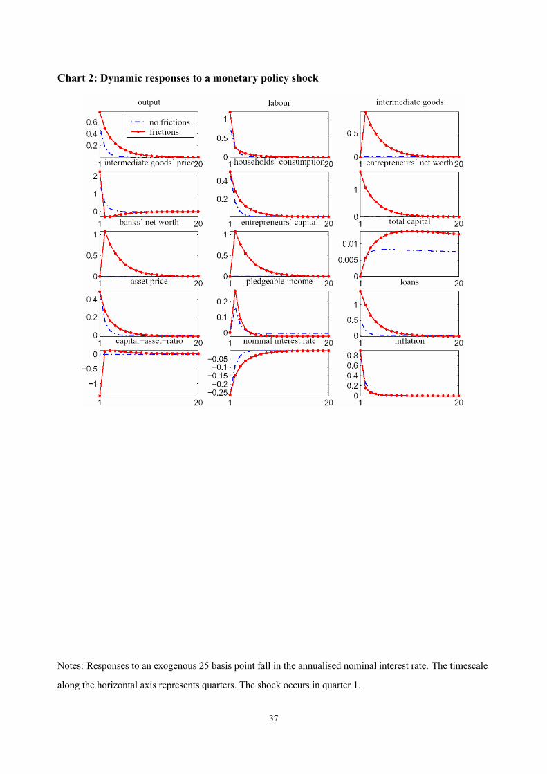
Chart 2: Dynamic responses to a monetary policy shock

Notes: Responses to an exogenous 25 basis point fall in the annualised nominal interest rate. The timescale

along the horizontal axis represents quarters. The shock occurs in quarter 1.

37

Chart 3: Dynamic responses to a technology shock

Notes: Responses to an exogenous 1% fall in the level of technology, with an autocorrelation of 0:9. The

timescale along the horizontal axis represents quarters. The shock occurs in quarter 1.

38

Chart 4: Welfare effects of targeting asset prices and credit growth

Notes: The chart plots�100� as a function of the coef�cients on credit growth and asset price growth in

the central bank's policy rule.

39

Chart 5: Dynamic responses to a bank capital shock under the optimal rule and the pricestability rule

Notes: Responses to a 25% fall in bank capital. The timescale along the horizontal axis represents quarters.

The shock occurs in quarter 1.

40

References

Aikman, D and Vlieghe, G (2004), `How much does bank capital matter?', Bank of England

Quarterly Bulletin, Spring, pages 48-58.

Ashcraft, A (2005a), `New evidence on the lending channel', Journal of Money, Credit and

Banking, forthcoming.

Ashcraft, A (2005b), `Are banks really special? New evidence from the FDIC-induced failure of

healthy banks', American Economic Review, forthcoming.

Basu, S and Fernald, J (1993), `Constant returns and small markups in U.S. manufacturing',

Center for Research on Economic and Social Theory and Department of Economics, University of

Michigan, 1993-19.

Bernanke, B, Gertler, M and Gilchrist, S (2000), `The �nancial accelerator in a quantitative

business cycle framework', in Taylor, J and Woodford, M (eds), Handbook of macroeconomics,

Vol. 1C, pages 1,341-93, Elsevier.

Bernanke, B and Gertler, M (2001), `Should central banks respond to movements in asset

prices?', American Economic Review Papers and Proceedings, Vol. 91(2), pages 253-57.

Bils, M and Klenow, P (2004), `Some evidence on the importance of sticky prices', Journal of

Political Economy, Vol. 112, No. 5, pages 947-85.

Calvo, G (1983), `Staggered price setting in a utility-maximizing framework', Journal of

Monetary Economics, Vol. 12, pages 383-98.

Carlstrom, C and Fuerst, T (1996), `Agency costs, net worth and business �uctuations: a

computable general equilibrium analysis', Federal Reserve Bank of Cleveland Working Paper no.

9602.

41

Carlstrom, C and Fuerst, T (2001), `Monetary shocks, agency costs, and business cycles',

Carnegie-Rochester Conference Series on Public Policy, Vol. 54, Issue 1, pages 1-27.

Chen, N-K (2001), `Bank net worth, asset prices and economic activity', Journal of Monetary

Economics, Vol. 48(2), pages 415-36.

Christiano, L, Eichenbaum, M and Evans, C (2005), `Nominal rigidities and the dynamic

effects of a shock to monetary policy', Journal of Politicial Economy, Vol. 113 (February), pages

1-45.

Collard, F and Dellas, H (2005), `Tax distortions and the case for price stability', Journal of

Monetary Economics, Vol. 52, pages 249-73.

Collard, F and Juillard, M (2001), `Accuracy of stochastic perturbation methods: the case of

asset pricing models', Journal of Economic Dynamics and Control, Vol. 25, pages 979-99.

Cordoba, J C and Ripoll, M (2004), `Credit cycles redux', International Economic Review,

November, Vol. 45(4), pages 1,011-46.

Diamond, D (1984), `Financial intermediation and delegated monitoring', Review of Economic

Studies, Vol. 51, pages 393-414.

Driscoll, J (2004), `Does bank lending affect output? Evidence from the U.S. states', Journal of

Monetary Economics, Vol. 51(3), pages 451-71.

Eberly, J (1997), `International evidence on investment and fundamentals', European Economic

Review, Vol. 41, pages 1,055-78.

Ehrmann, M and Worms, A (2004), `Bank networks and monetary policy transmission', Journal

of the European Economic Association, Vol. 2(6), pages 1,148-71.

Faia, E and Monacelli, T (2005), `Optimal monetary policy rules, asset prices and credit

frictions', Working Paper no. 279, IGIER, Bocconi University.

42

Friedman, B (1991), `Comment on �The credit crunch�', Brookings Papers on Economic Activity,

Vol. 2, pages 240-47.

Gilchrist, S and Leahy, J (2002), `Monetary policy and asset prices', Journal of Monetary

Economics, Vol. 49, pages 75-97.

Harrison, P, Sussmann, O and Zeira, J (1999), `Finance and growth: theory and new evidence',

Finance and Economics Discussion Series, Board of Governors of the Federal Reserve System.

Hoggarth, G, Reis, R and Saporta, V (2002), `Costs of banking system instability: some

empirical evidence', Journal of Banking and Finance, Vol. 26, pages 825-55.

Holmstrom, B and Tirole, J (1997), `Financial intermediation, loanable funds, and the real

sector', Quarterly Journal of Economics, Vol. 112(3), pages 663-91.

Kashyap, A and Stein, J (1995), `The impact of monetary policy on banks balance sheets',

Carnegie-Rochester Conference Series on Public Policy, Vol. 41, pages 151-95.

Kashyap, A and Stein, J (2000), `What do one million observations on banks have to say about

the transmission mechanism?', American Economic Review, Vol. 90(3), pages 407-28.

Khan, A, King, R and Wolman, A (2003), `Optimal monetary policy', Review of Economic

Studies, Vol. 70, pages 825-60.

Kishan, R and Opiela, T (2000), `Bank size, bank capital, and the bank lending channel',

Journal of Money, Credit and Banking, Vol. 32(1), pages 121-41.

Kiyotaki, N (1998), `Credit and business cycles', Japanese Economic Review, Vol. 49, No. 1,

pages 18-35.

Kiyotaki, N and Moore, J (1997), `Credit cycles', Journal of Political Economy, Vol. 105, pages

221-48.

43

Meh, C and Moran, K (2004), `Bank capital, agency costs, and monetary policy', Bank of

Canada Working Paper 2004-6.

Paustian, M (2005), `The role of contracting schemes for the welfare costs of nominal rigidities

over the business cycle', Bundesbank Discussion Paper Series 1: Economic Studies, No. 22/2005.

Peek, J and Rosengren, E (1997), `International transmission of �nancial shocks: the case of

Japan', American Economic Review, Vol. 87, pages 495-505.

Rotemberg, J J (1982), `Sticky prices in the United States', Journal of Political Economy, Vol.

90(6), pages 1,187-211.

Schmitt-Grohé, S and Uribe, M (2004a), `Optimal �scal and monetary policy under sticky

prices', Journal of Economic Theory, Vol. 114, pages 198-230.

Schmitt-Grohé, S and Uribe, M (2004b), `Solving dynamic general equilibrium models using a

second-order approximation to the policy function', Journal of Economic Dynamics and Control,

Vol. 28, pages 755-75.

Steinsson, J (2003), `Optimal monetary policy in an economy with in�ation persistence', Journal

of Monetary Economics, Vol. 50, pages 1,425-56.

Vlieghe, G (2005), `Optimal monetary policy in a model with credit market imperfections',

Chapter 4 of Ph.D. thesis Credit market imperfections: macroeconomic consequences and

monetary policy implications, London School of Economics and Political Science.

Woodford, M (1998), `Doing without money: controlling in�ation in a postmonetary world',

Review of Economic Dynamics, Vol. 1(1), pages 173-219.

Woodford, M (2003), Interest and prices: foundations of a theory of monetary policy, Princeton

University Press.

Yun, T (1996), `Nominal price rigidity, money supply endogeneity, and business cycles', Journal

44

of Monetary Economics, Vol. 37, pages 345-70.

45