K.7

Asset Price Learning and Optimal Monetary Policy Caines, Colin and Fabian Winkler

International Finance Discussion Papers Board of Governors of the Federal Reserve System

Number 1236 August 2018

Please cite paper as: Caines, Colin and Fabian Winkler (2018). Asset Price Learning and Optimal Monetary Policy. International Finance Discussion Papers 1236. https://doi.org/10.17016/IFDP.2018.1236

Board of Governors of the Federal Reserve System

International Finance Discussion Papers

Number 1236

August 2018

Asset Price Learning and Optimal Monetary PolicyColin Caines and Fabian Winkler

NOTE: International Finance Discussion Papers are preliminary materials circulated to stimulate dis-cussion and critical comment. References to International Finance Discussion Papers (other than anacknowledgment that the writer has had access to unpublished material) should be cleared with theauthor or authors. Recent IFDPs are available on the Web at www.federalreserve.gov/pubs/ifdp/. Thispaper can be downloaded without charge from Social Science Research Network electronic library atwww.ssrn.com.

Asset Price Learning And Optimal Monetary Policy

Colin Caines∗ & Fabian Winkler† §

Abstract: We characterize optimal monetary policy when agents are learning about endogenous as-set prices. Boundedly rational expectations induce inefficient equilibrium asset price fluctuations whichtranslate into inefficient aggregate demand fluctuations. We find that the optimal policy raises interestrates when expected capital gains, and the level of current asset prices, is high. The optimal policy doesnot eliminate deviations of asset prices from their fundamental value. When monetary policymakers areinformation-constrained, optimal policy can be reasonably approximated by simple interest rate rulesthat respond to capital gains. Our results are robust to a wide range of belief specifications as well asto the inclusion of an investment channel.

Keywords: Optimal Monetary Policy, Natural Real Interest Rate, Learning, Asset Price Volatility,Leaning Against The Wind

JEL classifications: E44, E52

∗ The author is a staff economist in the Division of International Finance, Board of Governors of the FederalReserve System, Washington, D.C. 20551 U.S.A. The email address of the author is colin.c.caines@frb.gov.† The author is a staff economist in the Division of Monetary Affairs, Board of Governors of the Federal ReserveSystem, Washington, D.C. 20551 U.S.A. The email address of the author is fabian.winkler@frb.gov.§ The views in this paper are solely the responsibility of the authors and should not be interpreted as reflectingthe views of the Board of Governors of the Federal Reserve System or of any other person associated with theFederal Reserve System. The authors would like to thank Chris Gust, Damjan Pfajfar, Chris Erceg, Kevin Lans-ing, Thomas Mertens, Robert Tetlow, Pei Kuang, and seminar participans at the Chicago Fed, the San FranciscoFed, Drexel University, the 2018 Midwest Macro conference, the 2018 Canadian Economics Assocation Meetings,the 2018 Econometric Society Summer Meeting and the University of Birmingham for helpful comments.

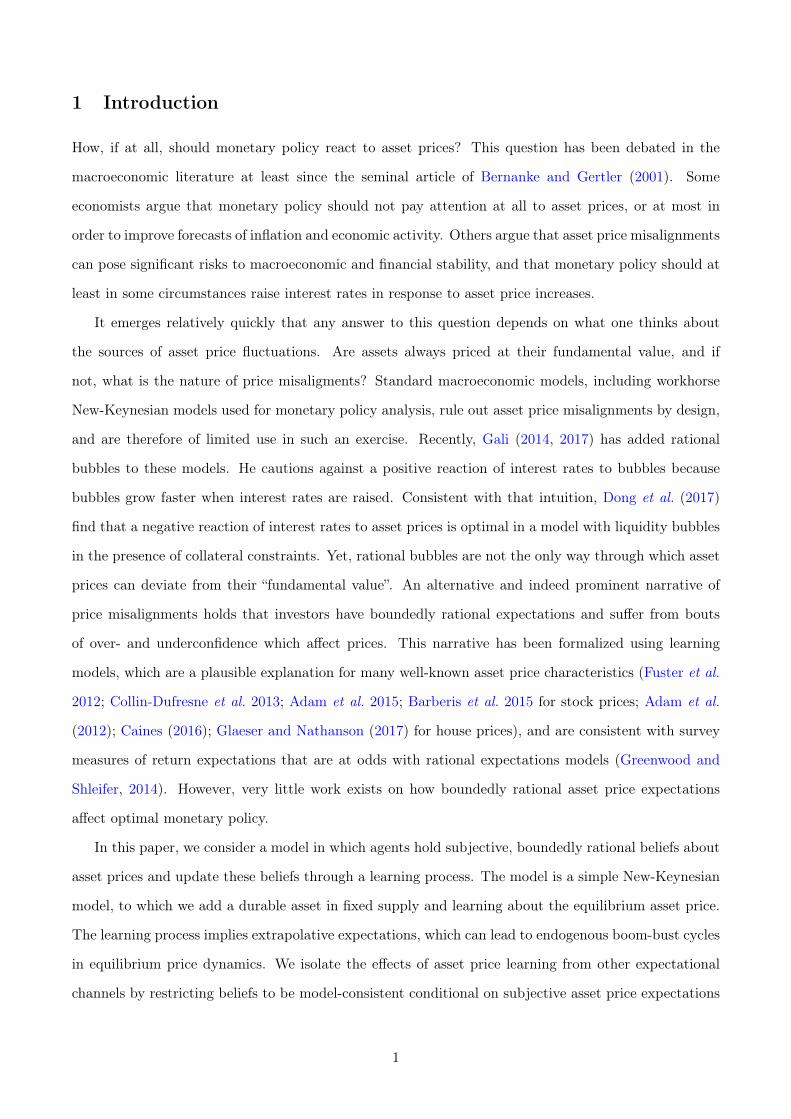
1 Introduction

How, if at all, should monetary policy react to asset prices? This question has been debated in the

macroeconomic literature at least since the seminal article of Bernanke and Gertler (2001). Some

economists argue that monetary policy should not pay attention at all to asset prices, or at most in

order to improve forecasts of inflation and economic activity. Others argue that asset price misalignments

can pose significant risks to macroeconomic and financial stability, and that monetary policy should at

least in some circumstances raise interest rates in response to asset price increases.

It emerges relatively quickly that any answer to this question depends on what one thinks about

the sources of asset price fluctuations. Are assets always priced at their fundamental value, and if

not, what is the nature of price misaligments? Standard macroeconomic models, including workhorse

New-Keynesian models used for monetary policy analysis, rule out asset price misalignments by design,

and are therefore of limited use in such an exercise. Recently, Gali (2014, 2017) has added rational

bubbles to these models. He cautions against a positive reaction of interest rates to bubbles because

bubbles grow faster when interest rates are raised. Consistent with that intuition, Dong et al. (2017)

find that a negative reaction of interest rates to asset prices is optimal in a model with liquidity bubbles

in the presence of collateral constraints. Yet, rational bubbles are not the only way through which asset

prices can deviate from their “fundamental value”. An alternative and indeed prominent narrative of

price misalignments holds that investors have boundedly rational expectations and suffer from bouts

of over- and underconfidence which affect prices. This narrative has been formalized using learning

models, which are a plausible explanation for many well-known asset price characteristics (Fuster et al.

2012; Collin-Dufresne et al. 2013; Adam et al. 2015; Barberis et al. 2015 for stock prices; Adam et al.

(2012); Caines (2016); Glaeser and Nathanson (2017) for house prices), and are consistent with survey

measures of return expectations that are at odds with rational expectations models (Greenwood and

Shleifer, 2014). However, very little work exists on how boundedly rational asset price expectations

affect optimal monetary policy.

In this paper, we consider a model in which agents hold subjective, boundedly rational beliefs about

asset prices and update these beliefs through a learning process. The model is a simple New-Keynesian

model, to which we add a durable asset in fixed supply and learning about the equilibrium asset price.

The learning process implies extrapolative expectations, which can lead to endogenous boom-bust cycles

in equilibrium price dynamics. We isolate the effects of asset price learning from other expectational

channels by restricting beliefs to be model-consistent conditional on subjective asset price expectations

1

(Winkler, 2016), implying that expectations are consistent with all equilibirum conditions other than

asset market clearing.1 This restriction greatly reduces the degrees of freedom in boundedly rational

expectations and also renders the analysis of the learning model particularly transparent. In particular,

it implies that agents fully understand the policy strategy followed by the central bank. We then solve

analytically for optimal monetary policy under learning.

We show that the optimal policy requires the policy rate to respond positively to asset prices,

separately from its reaction to fundamental shocks. The reason is that the natural real rate of interest

under learning is no longer a function of just technology and preferences, but depends on subjective

asset price beliefs. If agents expect larger capital gains on their assets, then the real interest rate must

rise also for the bond market to clear, even if expectations aren’t rational. When prices are rigid, setting

the interest rate below this “perceived natural rate” inefficiently raises aggregate demand and inflation.

The central bank therefore needs to raise interest rates when asset prices are high in order to stabilize

inflation. While the optimal interest rate policy is different under learning, the optimal target criterion

is not: Because price rigidities are the only distortion in our baseline model, flexible inflation targeting

remains optimal. We also numerically evaluate simple Taylor-type interest rate rules which include a

reaction to asset prices. We find that this reaction generally mitigates the distortions from non-rational

beliefs and stabilizes asset price fluctuations. This latter finding is in direct contrast to Gali (2014) and

Dong et al. (2017): Higher interest rates increase the size of rational bubbles, but decrease subjective

price expectations under learning.

The model predicts positve comovement between the natural real interest rate and realized asset

prices. Such comovement seems to be present in the data as well, as Figure 1 shows. The figure plots

the 20-quarter change in the well-known Laubach and Williams (2016) natural rate estimate against

the 20-quarter change in both the FHFA house price index for the United States as well as the Shiller

CAPE ratio2. House prices and the natural real rate are positively correlated in both cases.

In our baseline version of the model, non-rational asset price expectations cause distortions because

they affect perceived household wealth and therefore aggregate demand. There are of course other,

and potentially more important channels through which asset prices can affect the real economy, e.g.

credit frictions (Bean, 2004). We see the wealth effect channel in this paper as a stand-in for these

more complex transmission channels of asset prices. The advantage of this simplification is that we

are able to obtain closed form solutions for optimal monetary policy in the presence of learning. But1The concept has also been applied in Caines (2016) and Gandré (2017).2We thank Kevin Lansing for pointing out this relationship to us.

2

Figure 1: 20-Quarter Change in the Natural Rate of Interest & Asset Prices.

1980 1985 1990 1995 2000 2005 2010 2015 2020

year

-4

-3

-2

-1

0

1

2

-0.2

0

0.2

0.4

r∗, Laubach-Williams one-sided

FHFA House Price

1980 1985 1990 1995 2000 2005 2010 2015 2020

year

-4

-3

-2

-1

0

1

2

-10

0

10

20

r∗, Laubach-Williams one-sided

CAPE

we also consider an extension of our model in which asset supply is elastic. In this case, subjective

belief distortions also cause inefficient fluctuations in real investment. Numerical simulations indicate

that interest rate rules still need to respond to asset prices in this case; and moreoever, that even the

optimal target criterion features “leaning against the wind”, in the sense that the central bank tolerates

a downward departure of inflation from the target at times when asset prices are high.

Our baseline model also assumes a particular process of expectation formation in which agents think

that asset prices are a random walk with a small time-varying drift. This simple process has been

shown to lead to good asset pricing properties in equilibrium (Adam et al., 2017), but our results are

not confined to the use of this process. We show that our results carry through to more general class of

subjective beliefs, which include for example “natural expectations” (Fuster et al., 2012) and “diagnostic

expectations” (Bordalo et al., 2018).

The remainder of this paper is structured as follows. After discussing the related literature in Section

2, we begin by describing the model in Section 3, and our notion of a learning equilibrium in Section

4. We characterize the linearized equilibrium under rational expectations and learning in Section 5.

Optimal policy is analyzed in Sections 6, while Section 7 discusses how well certain simple interest rate

rules approximate the optimal policy. Sections 8 and 9 discuss extensions to more general beliefs and

an invenstment channel, respectively. Section 10 concludes.

3

2 Related literature

Our paper shares a number of features with Adam and Woodford (2018), who study so-called robustly

optimal policy with house prices. Their model is very similar to ours, but instead of learning they

study belief distortions to the fundamentals of the economy and let the policymaker choose a policy

that maximizes welfare for the worst possible combination of these distortions.3 The appeal of such an

analysis is that the policymaker cannot systematically exploit distorted expectations to its advantage,

because the class of possible distortions is large and the policymaker does not know which of these

is realized. In our setup, the policymaker could in principle achieve outcomes that are far better

than those under rational expectations with a suitable, highly non-linear policy. Because we judge

such sophisticated manipulation of beliefs to be unrealistic, we restrict the set of admissible policies

to simple linear targeting and instrument rules. Moreover, our results are derived at the fully efficient

steady state. By contrast, Adam and Woodford find a tightening reaction of monetary policy to rising

asset prices to be beneficial only when the steady state is distorted in a particular direction.

Our analysis also shares some features with Christiano et al. (2010), who study the optimal policy

reaction to news shocks about future productivity. In their model, news shocks cause asset prices to rise,

and also increase the natural real rate of interest, so that monetary policy should optimally respond by

raising interest rates. In this paper, the natural real rate fluctuates in response to endogenous changes

in subjective expectations that can be entirely independent of productivity.

Dupor (2005) and Mertens (2011), among others, have argued that monetary policy should react

to asset prices in environments that depart from rational expectations. In these papers, distortions to

beliefs about asset prices have real effects through investment channels. Monetary policy that reacts to

asset prices can then counteract these effects. In this paper we present an argument for leaning against

the wind even in the absence of distortions of this kind. Our results are only strengthened if we include

an investment channel.

Our paper focuses on learning about asset prices but keeps expectations conditionally model-

consistent otherwise. This is not to say that learning or other belief distortions in expectations of

other variables doesn’t matter; rather, it allows us to isolate the effects of asset prices learning from

other such distortions. In so doing, we complement a small but growing number of papers studying

monetary policy prescriptions in models with learning about inflation. Fully optimal policy has recently3One important difference between the different concepts of belief distortions is that our asset prices can deviate from

the discounted sum of expected fundamentals, whereas in Adam and Woodford (2018) only expectations of fundamentalsare distorted.

4

been studied in a two-equation model with learning by Molnar and Santoro (2014) and Eusepi and

Preston (2016). Airaudo (2016) aguments the standard New Keynesian model with a stock market and

infinite-horizon learning (as in Preston (2006)) to study conditions under which the rational expecta-

tions equilibrium is learnable, but stops short of characterizing optimal policy.4 Eusepi et al. (2015)

introduce drift in long-run expectations to a New Keynesian model and show that such beliefs introduce

an intertemporal trade-off in policy between stablizing current inflation and anchoring long-horizon

beliefs.

3 Model description

Our model is a standard New-Keynesian model in which the representative household also holds a stock

of an asset that yields utility. The supply of the asset in the economy is fixed. One can think of the

asset as a stock of housing, but we will refer to it as a generic durable asset. Because the asset is in fixed

supply, the dynamics of inflation and output are unaffected by its presence under rational expectations.

Under learning, however, we will get non-trivial effects of asset prices on allocations.

We first describe the model for a general description of expectations. A representative household

provides labor and owns firms. It can also hold nominal bonds promising a nominal return it. In

addition, the household owns the durable asset. The household’s problem is

EP∞∑t=0

βt

(C1−γt

1− γ− N1+φ

t

1 + φ+ χ

H1−θt

1− θ

)

s.t. Ct = WtNt + Πt + Tt −Qt (Ht −Ht−1) +Bt −1 + it−1

1 + πtBt−1.

Here, Ct is the household’s utility from consuming final consumption goods, Nt is the household’s labor

supply, and Tt are lump-sum taxes. Πt are the profits received from firms. The quantity of the asset

owned by the household is denoted Ht and trades at the price Qt. Bt are government bonds which are

in zero net supply. The price level is Pt and πt = Pt/Pt−1 − 1 is the inflation rate. The expectational

operator EP has a superscript indicating that agents’ expectations are evaluated under a subjective

probability measure P that need not coincide with rational expectations.4Outside of the learning literature, Gabaix (2016) develops a particular form of myopia and studies optimal policy under

commitment. In his model, agents have attenuation bias and underestimate the persistence of economic fluctuations. Inthis paper, agents instead overestimate their persistence, at least along the dimension of asset prices. As a result, theoptimal policy needs to react aggressively to the extrapolative bias, while Gabaix finds that policy can afford to be lessaggressive in the presence of attenuation bias.

5

The first order conditions are:

Wt = Cγt Nφt (1)

1 = βEPt(

CtCt+1

)γ 1 + it1 + πt+1

(2)

Qt = χCγtHθt

+ βEPt(

CtCt+1

)γQt+1. (3)

On the production side, a representative intermediate goods producer transforms household labor

into intermediate goods using the decreasing returns to scale technology

Yt = AtNαt . (4)

It has to hire labor at the real wage rate wt and sells its goods at the real price Mt. Its first-order

condition is

Wt = αMtAtNα−1t . (5)

There is a contiuum of wholesalers indexed by i ∈ [0, 1] who transform the undifferentiated interme-

diate good into differentiated goods using a one-for-one technology. They face a standard Dixit-Stiglitz

demand function and a Calvo price setting friction. When producer i is able to set a price Pit for its

output Yit, it solves:

maxPit

EPt∞∑s=0

(s∏

τ=1

ξΛt,t+τ

)((1 + τt)Pit −Mt+sPt+s)Yit+s

s.t. Yit =

(PitPt

)−σYt,

where σ is the demand elasticity of substitution between varieties, Λt,t+τ = βτCγt C−γ+τ is the household

discount factor between times t and t + τ , ξ is the probability of not being able to adjust the price in

the futureAny profits are distributed to households. The first-order conditions are standard and give

rise to the New-Keynesian Phillips curve.

The term τt is a time-varying government subsidy to revenue. Shocks to the subsidy will act as cost-

push shocks. The steady-state value of the subsidy is set such that it eliminates mark-up distortions.

Our steady state is therefore fully efficient.

A representative retailer buys differentiated goods from wholesalers at the price Pit and transforms

them back into a homogenous final consumption good. The final good sells at price Pt and is produced

6

according to the technology

Yt =

(∫ 1

0(Yit)

σ−1σ di

) σσ−1

. (6)

The first order condition gives rise to a constant elasticity of substitution σ between varieties. The price

level can be expressed as Pt =∫ 1

0 PitYit/Yt.

The government transfers a lump sum real amount to households

Tt = τt

∫ 1

0PitYitdi (7)

to finance the subsidies to final good producers and offset the tax on stock holdings. Profits and

government transfers sum up to Πt+Tt = Yt−WtNt. Finally, the central bank sets the nominal interest

rate.

We allow for productivity and cost-push shocks which follows first-order autoregressive processes:

logAt = (1− ρa) log A+ ρa logAt−1 + εat (8)

τt = (1− ρτ ) τt + ρττt−1 + ετt (9)

The innovations are independent white noise with variances σ2A and σ2

τ .

Market clearing in the final goods market requires Yt = Ct. Bonds are in zero net supply and the

market clearing condition is therefore Bt = 0. Finally, the supply of the durable is fixed at unity, so

that asset market clearing requires Ht = 1.

4 Equilibrium

The equilibrium under rational expectations is standard—it is the textbook New Keynesian model.

The asset price Qt is redundant because the durable asset is in fixed supply. Agents with rational

expectations never expect to buy or sell the asset, not because they expect to be unable to to do

so—they are price takers in a competitive market—but because they expect the price in every state of

the world to be such that they will not ever want to change their asset holdings.

Let’s recall the formal definition of a rational expectations equilibrium. Let yt ∈ RN denote the

collection of all endogenous model variables—including prices, allocations, and strategies—and by ut ∈

RM the collection of all exogenous model variables at time t, which I will call “fundamentals”. Stochastic

processes for yt and ut are defined on the spaces Ωy = Π∞t=0RN and Ωu = Π∞t=0RM , respectively. Further,

7

denote by Ω(t)u the set of all possible histories of exogenous variables up to period t, and its elements by

u(t) ∈ Ω(t)u . Finally, let Pu denote the true probability measure for the exogenous variables defined on

(Ωu,S (Ωu)), where S (·) is the Borel sigma-algebra on a metric space. The topological support of Pu is

denoted bysupp (Pu).

Definition 1. A rational expectations equilibrium is a sequence of mappings gt : Ω(t)u 3 u(t) 7→ yt ∈

RN , t = 0, 1, 2, . . . such that, for all t and u(t) ∈ supp (Pu):

1. the choices contained in yt solve the time-t decision problem of each agent in the economy, condi-tional on decision-relevant5 past and current outcomes contained in u(t) andy(t) =

(g0

(u(0)

), . . . , gt

(u(t))), and evaluating the probability of future external decision-relevant

outcomes under the probability measure P implied by Pu and the mappings (gt)∞t=0;

2. the allocations contained in yt = gt(u(t))clear all markets.

Under learning, we assume that agents are not endowed with the knowledge of the equilibrium asset

price process. Intuitively, they do not know whether only the representative household is investing in

the asset, or whether other investors exist who trade in unknown ways, causing seemingly random price

fluctuations. Faced with this lack of knowledge, agents forecast prices using a subjective belief system.

As we show in Section 8, this subjective belief system can be made quite general, but here we confine

ourselves to our preferred specification which follows Adam et al. (2017). Agents think that the asset

price is a simple random walk model with a time-varying drift:

∆ logQt = µt−1 + εt (10)

µt = ρµµt−1 + νt. (11)

where the shocks εt ∼ N(0, σ2

ε

)and νt ∼ N

(0, σ2

ν

)are iid white noise, independent of the rest of

the economy. Since these two shocks are not observable, agents have to use the Kalman filter to form a

belief about the hidden state µt. The asset price can equivalently be written just in terms of observables

and the filtered state:

∆ logQt = µt−1 + zt (12)

µt = ρµµt−1 + gzt (13)

Here, µt is the belief about µt ; g is the weight agents place on new data when updating their beliefs,5A variable is decision-relevant if it enters the agents’ decision problem, and a decision-relevant variable is external if

its value is taken as given by the agent, while it is internal if the variable is part of the solution of the agents’ decisionproblem. For example, wholesalers need to get information on current and future aggregate demand Yt (decision-relevantand external) to set prices Pit (decision-relevant and internal), while they do not need to forecast wages since their onlyproduction input is the intermediate good.

8

which is a function of the perceived variances of εt and νt; and zt ∼ N(0, σ2

z

)is the forecasting error in

the filtering problem. This forecasting error is exogenous normally distributed white noise under agents’

subjective expectation, the variance of which is decreasing in the signal-to-noise ratio σ2ν/σ

2ε . In order

to avoid complications arising from simultaneity in the determination of outcomes and beliefs, we follow

Adam et al. (2012) and Caines (2016) and assume that in period t agents make choices conditional on

µt−1, and update their beliefs according to (12) at the end period.

In order to determine expectations about the remaining variables of the model, including inflation,

we follow Winkler (2016) in assuming that agents have so-called “conditionally model-consistent expec-

tations”. This is a restriction on expectations that effectively allows us to isolate the effects of asset

price learning from other potential sources of learning in the economy. Conditionally model-consistent

expectations are consistent with all equilibrium conditions of the model, except those that would convey

knowledge of the price that clears the asset market.

Formally, let (Ωz,S (Ωz) ,Pz) be the probability space that defines the subjective beliefs for zt (i.e.,

the zt are iid normally distributed with mean zero and variance σ2z). Agents’ subjective beliefs depend on

this perceived stochastic forecast error even though in equilibrium, model outcomes are a function only

of fundamentals ut. The subjective probability measure P is defined by a mapping from fundamentals

ut and the subjective forecast error zt to model outcomes yt.

Definition 2. Conditionally model-consistent expectations (CMCE) are a sequence of mappings ht :

Ω(t)u × Ω

(t)z 3

(u(t), z(t)

)7→ yt ∈ RN , t = 0, 1, 2, . . . such that, for all t and

(u(t), z(t)

)∈ supp (Pu,z):

1. the choices contained in yt solve the time-t decision problem of each agent in the economy, condi-tional on decision-relevant past and current outcomes contained in u(t) andy(t) =

(h0

(u(0), z(0)

), . . . , ht

(u(t), z(t)

)), and evaluating the probability of future decision-relevant

outcomes under the probability measure P implied by Pu ⊗ Pz and the mappings (ht)∞t=0;

2. the allocations contained in yt = ht(u(t), z(t)

)clear all markets except the markets for assets and

final consumption goods;

3. asset prices under P follow the law of motion given by (12)–(13).

The definition of the mappings ht defining expectations is almost identical to the definition of a

rational expectations equilibrium, except that asset market equilibrium is not part of the conditions, and

instead the price Qt evolves according to subjective beliefs. Conditional model consistency restricts the

subjective belief P to have the maximum degree of consistency with the model given agents’ misspecified

belief about asset prices. In analogy to the adaptive learning literature, we call the mappings ht defining

beliefs the perceived law of motion (PLM).

Computing the learning equilibrium is an easy two-step procedure: First, compute the PLM

9

ht(u(t), z(t)

); second, compute the ALM gt

(u(t)). Both steps are no more complicated than solving the

rational expectations equilibrium.

While under P, demand for the durable asset does not have to be equal to supply, in equilibrium

the market still has to clear:

Definition 3. An equilibrium with conditionally model-consistent expectations is a sequence of map-pings rt : Ω

(t)u 3 u(t) 7→ zt ∈ R and gt : Ω

(t)u 3 u(t) 7→ yt ∈ RN , t = 0, 1, 2, . . . such that, for all t and

u(t) ∈ supp (Pu):

1. g(u(t))

= h(u(t),

(r0

(u(0)

), . . . , rt

(u(t))))

;

2. the allocations contained in yt = gt(u(t))clear the asset market.

Market clearing is brought about by finding the right value of the price Qt that clears the housing

market. We call the resulting equilibrium mappings gt the actual law of motion (ALM). This mapping

implies a particular path for zt, the subjective house price forecast error. In equilibrium, zt will be a

function of the states and the shocks of the model, while under P it is perceived as an unforecastable

exogenous disturbance. It is precisely in this way that P violates the rational expectations hypothesis.

Agents endowed with conditionally model-consistent expectations may not know the equilibrium

pricing function, but they make the smallest possible expectational errors consistent with their subjective

view about the evolution of stock prices. This way of setting up expectations is very tractable and can

be readily applied in a variety of models, as we have shown in previous papers (Caines, 2016; Winkler,

2016). It also allows us to transparently solve the linearized version of the model.

5 Linearized equilibrium

The analysis in this paper will focus entirely on the linearized version of the model. The conditionally

model-consistent expectations under learning imply that the learning equilibrium can be linearized in

much the same way as its rational expectations counterpart.

10

5.1 Rational expectations equilibrium

Under rational expectations, we can linearize around the non-stochastic steady state to obtain:

yt = at + αnt (14)

πt = βEtπt+1 +(1− ξ) (1− βξ)

ξ(wt − at + (1− α)nt) + ηt (15)

wt = γyt + φnt (16)

it = γ (Etyt+1 − yt) + Etπt+1 (17)

qt = γyt − βγEtyt+1 + βEtqt+1. (18)

Here, lower-case variables denote log-linearizations around the zero-inflation steady state, except for it

which is the difference of the nominal interest rate from its steady-state level, and ηt = (1−ξ)(1−βξ)ξ (τ − τt)

is the cost-push shock process. The model is simply the textbook New-Keynesian model with an extra

equation for the price of housing. Note that it still has to be closed with an equation describing the

conduct of monetary policy, such as an interest rate rule. Note that asset holdings ht are known to

be constant in equilibrium. As a result, ht does not even enter the rational expectations equilibrium

conditions.

An important special case of the model obtains when prices are fully flexible and there are no cost-

push shocks (ξ = 0 and ηt = 0). In this case, the allocation in the rational expectations equilibrium

is first-best efficient everywhere. Output and the real interest rate are independent of the conduct of

monetary policy and are given by:

yn,REt =φ+ 1

φ+ 1− α (1− γ)at (19)

rn,REt = − γ (φ+ 1)

φ+ 1− α (1− γ)(1− ρa) at. (20)

These quantities are also called the natural level of output and the natural real rate, respectively.

As is well known, the equilibrium with sticky prices can be expressed in terms of the deviation from

this efficient equilibrium. To this end, denote the output gap by yt = yt − yn,REt . The sticky price

equilibrium can be summarized with the standard two equations:

πt = βEtπt+1 + κyt + ηt (21)

Etyt+1 − yt =1

γ

(it − Etπt+1 − rn,REt

). (22)

11

where κ = (1− ξ) (1− βξ) (1 + φ− α+ αγ) /ξα. These equations are the standard New-Keynesian

Phillips curve and the IS equation.

5.2 Learning equilibrium

In order to solve the learning equilibrium, we have to proceed in two steps. The first is to solve for

the agents’ policy functions given their beliefs P; the second is to impose market clearing in the asset

market to back out the equilibrium asset price.

It is easy to verify that the equilibrium under learning has the same non-stochastic steady state as

the rational expectations equilibrium, and we take this as our linearization point. The expectations of

agents as well as their optimal choices under the subjective measure P are expressed as the solution to

a “perceived law of motion” (PLM) that, in its linearized form, consists of the following equations:

yt = at + αnt (23)

πt = βEPt πt+1 +(1− ξ) (1− βξ)

ξ(wt − at + (1− α)nt) + ηt (24)

wt = γct + φnt (25)

it = γ(EPt ct+1 − ct

)+ EPt πt+1 (26)

qt = γct − (1− β) θht − βγEPt ct+1 + βEPt qt+1 (27)

ct = yt −QH

Y(ht − ht−1) (28)

qt = qt−1 + µt−1 + zt (29)

µt = ρµµt−1 + gzt (30)

This system can be solved as if it were a rational expectations model. However, under P, there is an

additional shock, the asset price forecast error zt, that is absent under rational expectations. This shock

will be predictable in equilibrium, but under under P agents believe it to be unforecastable. The first

stage of the solution has to take this into account. Just as under rational expectations, one still needs to

add an equation describing the conduct of monetary policy, such as an interest rate rule, for the above

system to be fully determined.

Having solved for expectations and optimal choices given P, the equilibrium under learning (also

called “actual law of motion” or ALM) is then found by imposing market clearing in the market for

housing. This condition simply reads

ht = 0. (31)

12

This equation implicitly defines the equilibrium realizations of zt. Contrary to agents’ beliefs, this

forecast error is not an exogenous shock in equilibrium, but an endogenous variable. It is precisely in

this sense that expectations are not rational in this model.

5.2.1 Flexible price PLM

As before, we first describe the flexible price equilibrium (ξ = 0 and ηt = 0). We find the flex-price

PLM by solving (23)–(30) under subjective beliefs P. The learning model has two additional state

variables compared to its rational expectations counterpart, qt and µt−1. We guess and verify that the

asset demand function has the following form:

hn,PLMt = kaat + khhn,PLMt−1 − kqqt + kµµt−1 (32)

where the coefficients satisfy kh ∈ (0, 1), ka, kq, kµ > 0. Exact expressions can be found in the appendix.

Asset demand under learning is increasing in productivity, decreasing in the asset price, and increasing

in expectations of future asset price growth.

We can also solve for the values of output and the real interest rate under flexible prices. Under

subjective expectations, these are functions of the fundamental, last period’s asset holdings, the asset

price which is perceived as exogenous, and price growth expectations. Below, we write output and the

real rate in deviation from their rational expectations counterpart:6

yn,PLMt = yn,REt +αγκ1

1 + φ− α

(kaat − (1− kh)hn,PLMt−1 − kqqt + kµµt−1

)(33)

rn,PLMt = rn,REt + γκ1

(ka (2− ρa − kh) at − (1− κh)2 hn,PLMt−1 − kq (1− kh) qt

)+ γκ1 ((2− ρµ − kh) kµ + kq) µt−1. (34)

where the constant κ1 is

κ1 =1 + φ− α

1 + φ− α (1− γ)

QH

Y> 0.

This natural rate is increasing in the price growth belief µt−1. Agents’ subjective expectations about

output under flexible prices are affected by the choice of asset holdings (which are not constant in

agents’ minds). An increase in expected asset price growth will increase asset demand, and households6Since the PLM includes asset holdings ht as an endogenous state variable, there are two possible definitions of a

natural real rate and natural level of output (Neiss and Nelson, 2003; Woodford, 2003). One can either define them asconditional on the actual level of asset holdings ht−1 under sticky prices, or as conditional on the level of asset priceshn,PLMt−1 that would obtain had prices been flexible in the past as well, given the history of exogenous shocks. Here, weopt for the latter definition.

13

will increase their labor supply in order to finance their purchase of the asset, thereby increasing the

level of output.

The natural real rate under subjective expectations can be understood by the arbitrage relationship

between the return on the durable asset and the return on bonds. Combining the two asset pricing

equations (26) and (27), we obtain:

rn,PLMt =1− ββ

(γct − θht − qt) + EPt qt+1 − qt

The expected return on the two assets has to be equal up to first order. An increase in expected durable

asset price growth µt−1 = EPt qt+1 − qt increases the expected return to the durable asset, and the real

interest rate on bonds therefore has to rise as well.

5.2.2 Flexible price ALM

To find the flex-price equilibrium under learning, i.e. the actual law of motion, one has to impose ht = 0.

From the housing demand function (32), one can then immediately solve for the equilibrium asset price

and the realization of the subjective forecast error:

0 = kaat − kqqt + kµµt−1

⇔ qt =kaat + kµµt−1

kq. (35)

That is, the equilibrium asset price is increasing in both productivity and house price growth expecta-

tions. This is intuitive. The demand function (32) is downward-sloping, and so an increase in demand

due to either higher productivity (i.e. higher income) or higher expected capital gains has to be met

with an increase in the price to bring about equilibrium in the asset market.

It becomes clear that the forecast error zt is every

thing but unforecastable:

zt =1

kqkaat − qt−1 +

(kµkq− 1

)µt−1.

This is precisely the way in which rational expectations break in this model. If agents had the correct

belief about zt, then owing to their conditionally-model consistent expectations, their beliefs would be

correct and their expectations would be rational.

Substituting the equilibrium price (35) into Equations (33) and (34), we obtain the realized level of

14

output and the real rate under flexible prices:

yn,ALMt = yn,REt (36)

rn,ALMt = rn,REt + γκ1 ((1− ρa) kaat + ((1− ρµ) kµ + kq) µt−1) . (37)

Under learning and flexible prices, the equilibrium level of output is the same as under rational

expectations. This coincidence arises because, under flexible prices, output is determined entirely by

intratemporal conditions that are independent of expectations. Nonetheless, the real interest rate does

depend on expectations, and its natural level under learning is therefore different from rational expec-

tations. In particular, it is increasing in subjectively expected house price growth.

5.2.3 Sticky prices

Just as under rational expectations, the sticky price equilibrium under learning can be expressed in

deviation from the flexible price allocation, which greatly helps our analysis. One only has to be careful

in keeping apart the flexible price allocations under the PLM and the ALM. We will use tildes for

the former and hats for the latter: That is, ht = ht − hn,PLMt denotes the difference of asset holdings

from their flex-price level under the PLM, while the difference with the ALM flex price level is denoted

ht = ht − hn,ALMt . The same notation applies to consumption and output. Then the sticky price

equilibrium in the PLM can be summarized with three equations:

πt = βEPt πt+1 + κ(ct + κ1∆ht

)+ ηt (38)

ct = EPt ct+1 −1

γ

(it − EPt πt+1 − rn,PLMt

)(39)

ht =γ

θ (1− β)

(ct − βEPt ct+1

)(40)

The first equation is the familiar Phillips curve, but where the output gap is replaced by the consumption

gap, augmented by asset purchases ∆ht.7 The intuition is that asset purchases are financed by an

increase in labor supply, which drives down firms’ marginal cost of production and therefore reduces

inflation. The second equation is the familar IS equation, where again the output gap is replaced by the

consumption gap since the two are not equal under agents’ subjective expectations. The third equation

is the Euler equation for housing demand, rewritten in gap form.

Notice that the asset price qt itself does not appear in the Euler equation for asset holdings in gap7Even though in equilibrium (in the ALM) there can be no housing purchases as the supply of housing is fixed, one

cannot simply set ∆ht = 0 to compute the equilibrium, since agents are not aware of this restriction.

15

form. Agents perceive it to be an exogenous process, and therefore to be independent of the degree of

price stickiness. It therefore drops out of the gap between flexible and sticky prices, and what is left

are those variations in asset demand that are due to variations in the household’s discount factor. The

asset price still implicitly enters equation (40) through the natural rate rn,PLMt .

To find the actual law of motion under sticky prices, one imposes ht = hn,PLMt + ht = 0 and solves

for qt. The equilibrium depends crucially on the behavior of the nominal interest rate it, which we have

not specified yet.

5.3 Numerical illustration

We illustrate the properties of the learning model using a simple calibration in which we interpret

the durable asset as housing. We set the labor share in output equal to α = 0.7 and the discount

factor β equal to 0.995. The coefficient of relative risk aversion is set to γ = 1.39 (Gandelman and

Hernández-Murillo, 2014) and the inverse Frisch elasticity of labor supply is set to φ = 0.33. The

utility scaling parameter χ is set to 0.01005 in order to achieve a steady state ratio of asset wealth

to output of QH/Y = 2.01, which corresponds to the US ratio of real estate holdings over GDP in

2016. The parameter governing the price elasticity of demand for consumption varieties is set to σ = 6

as in Christiano et al. (2010), while price stickiness is set to the standard valueκ = 0.75. We follow

Billi (2017) and set the autocorrelation of both the technology and cost-push shocks to 0.8. Finally,

we calibrate the remaining four parameters (σA, στ , θ, g) to jointly match the volatilities of output

growth σ (∆Yt) = 0.64%, inflation σ (πt) = 0.82%, house price growth σ (∆Qt) = 1.51% and real wage

growth σ (∆wt) = 0.10%.The resulting parameter values are σA = 0.83%, σp = 0.75%, θ = 0.0068 and

g = 0.0041.

We first document the effect of learning under flexible prices. Here, learning has no effect on

equilibrium allocations relative to rational expectations, but manifests itself only in the realized asset

price and interest rate process. Figure 2 plots the response of asset prices Qt and the real interest

rate it to a technology shock εA under rational expectations and learning. The effect of learning on

Qt is typical for self-referential asset price learning models. Initially, the asset price Qt rises on impact

because higher wage wage income raises asset demand, as under rational expectations. But the initial

increase now causes a subsequent revision in beliefs µt through the learning mechanism. The household

believes that the shock has some long-run impact on house price growth and responds by increasing its

demand for housing above the rational expectations demand. This response drives a further increase

in Qt in the next period and the shock continues to propagate through belief updating thereafter. At

16

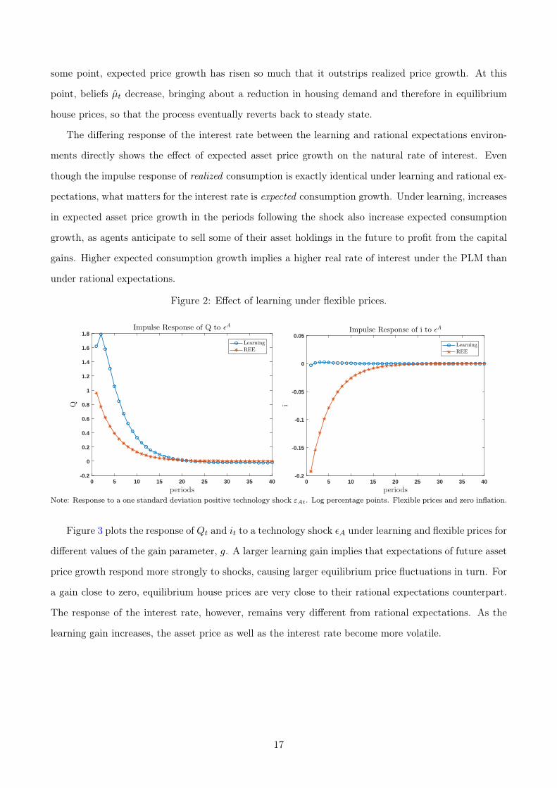
some point, expected price growth has risen so much that it outstrips realized price growth. At this

point, beliefs µt decrease, bringing about a reduction in housing demand and therefore in equilibrium

house prices, so that the process eventually reverts back to steady state.

The differing response of the interest rate between the learning and rational expectations environ-

ments directly shows the effect of expected asset price growth on the natural rate of interest. Even

though the impulse response of realized consumption is exactly identical under learning and rational ex-

pectations, what matters for the interest rate is expected consumption growth. Under learning, increases

in expected asset price growth in the periods following the shock also increase expected consumption

growth, as agents anticipate to sell some of their asset holdings in the future to profit from the capital

gains. Higher expected consumption growth implies a higher real rate of interest under the PLM than

under rational expectations.

Figure 2: Effect of learning under flexible prices.

0 5 10 15 20 25 30 35 40

periods

-0.2

0

0.2

0.4

0.6

0.8

1

1.2

1.4

1.6

1.8

Q

Impulse Response of Q to ǫA

Learning

REE

0 5 10 15 20 25 30 35 40

periods

-0.2

-0.15

-0.1

-0.05

0

0.05

i

Impulse Response of i to ǫA

Learning

REE

Note: Response to a one standard deviation positive technology shock εAt. Log percentage points. Flexible prices and zero inflation.

Figure 3 plots the response of Qt and it to a technology shock εA under learning and flexible prices for

different values of the gain parameter, g. A larger learning gain implies that expectations of future asset

price growth respond more strongly to shocks, causing larger equilibrium price fluctuations in turn. For

a gain close to zero, equilibrium house prices are very close to their rational expectations counterpart.

The response of the interest rate, however, remains very different from rational expectations. As the

learning gain increases, the asset price as well as the interest rate become more volatile.

17

Figure 3: Role of the learning gain g, flexible prices.

0 5 10 15 20 25 30 35 40

periods

-1

-0.5

0

0.5

1

1.5

2

2.5

3

Q

Impulse Response of Q to ǫA

g = 0.01

g = 0.008

g = 0.002

0 5 10 15 20 25 30 35 40

periods

-5

0

5

10

15

20

i

×10-3 Impulse Response of i to ǫA

g = 0.01

g = 0.008

g = 0.002

Note: Response to a one standard deviation positive technology shock εAt. Log percentage points. Flexible prices and zero inflation.

6 Optimal Policy

6.1 Welfare functions

We provide second-order approximations to the expected discounted sum of utility in our model. Under

learning, an important distinction has to be made whether welfare is evaluated under the subjective law

of motion (in which asset supply is variable and prices are a random walk) or under the actual law of

motion (in which asset supply is fixed and prices are functions of the model fundamentals).

If we evaluate welfare under the actual law of motion, then welfare can be approximated by

−∑∞

t=0 E0Lt up to second order, terms independent of policy, and a multiplying positive constant.

The period loss function is given by

Lt = λπ2t + y2

t . (41)

where λ = 2σαξ (1− ξ)−1 (1− βξ)−1 (1 + φ− α (1− γ))−1 and yt = yt−yn,REt is the deviation of output

from its flex-price level. This loss function is identical to that of the standard rational expectations New

Keynesian model. It penalizes deviations of inflation from zero as well as deviations of output from the

natural rate of output under rational expectations (19). This natural rate of output is first-best efficient

under the ALM.

By contrast, the welfare function under the PLM takes a quite different form. Welfare is approxi-

18

mated by −∑∞

t=0 βtEP0 LPLMt , where the period loss function is given by

LPLMt = λπ2t + c2

t

+1− α+ φ

1 + φ− α (1− γ)

(QH

Y∆ht

)2

+ 2ct

(QH

Y∆ht

)− (1− β) θα

1 + φ− α (1− γ)

QH

Yh2t . (42)

where ct and ht are the deviations of consumption and asset holdings from their PLM-flexible price

levels. Here, the period loss takes the form of deviations from the flexible price allocations under the

PLM, and also includes terms for asset holdings. Those terms do not appear in the ALM loss function

because asset holdings are constant in equilibrium.

6.2 Optimal policy without cost-push shocks

We now solve for the optimal monetary policy, first under the assumption that there are no cost-push

shocks. For exposition, we start by reviewing the optimal policy under rational expectations. As the

flexible price equilibrium under rational expectations is first-best efficient, monetary policy is optimal if

it manages to replicate the flexible price allocation in the presence of nominal rigidities. This amounts

to closing the output gap and completely stabilizing the price level at the same time, as can be seen

from the loss function (41). Without cost-push shocks, the “divine coincidence” holds and complete

stabilization is achievable. The optimal policy implements

πt = 0. (43)

From the Phillips curve (21), it immediately follows that yt = 0. The optimal policy can be

implemented with the following rule:

it = rn,REt + φππt (44)

where φπ can be any number satisfying the Taylor principle φπ > 1. The interest rate has to track the

natural real rate and react more than one-for-one to inflation, i.e. satisfy the Taylor principle.

Under learning, the question is which welfare criterion to use. Should the central bank aim to

maximize agents’ subjectively expected discounted utility and minimize the loss function 42 under the

PLM? Or should it aim to maximize average realized utility and minimize the loss function 41 under

the ALM? Fortunately, both welfare criteria prescribe the same optimal outcome here.

19

Proposition 1. The optimal monetary policy under learning implements πt = 0 and yt = yn,REt , regard-

less of whether welfare is evaluated under the ALM or the PLM. The optimal policy can be implemented

with the rule it = rn,PLMt + φππt, where φπ > 1.

Proof. Suppose that the central bank implemented πt = 0. The PLM Phillips curve (38) then reduces

to the relationship

yt =γα

1 + φ− α (1− γ)

QH

Y∆ht. (45)

Substituting into the housing demand equation (40), we obtain a second-order difference equation of

the form

(1− β)θ

γht = −κ1

(∆ht − βEPt ∆ht+1

). (46)

It is easily verified that the only solution to this equation is ht = 0. But this implies that we implement

the flexible price allocation. From the subjective perspective of agents, the flexible price allocation is

first-best efficient. Therefore, strict inflation targeting is optimal from the subjective perspective of

agents. Moreover, the actual equilibrium in this economy has πt = 0 and yt = yn,REt , as was shown

in the last section. This allocation is also first-best efficient under model-consistent expectations, and

therefore optimal under model-consistent expectations as well.

It might seem at first that the presence of learning does not alter the prescriptions of optimal policy

because the target criterion strict inflation targeting is unchanged. But the implementation of this

target requires a different reaction function under learning. The nominal interest rate has to track the

natural real interest rate rn,PLMt as agents perceive it under subjective expectations. This natural rate

is very different from the one under rational expectations. Whereas rn,REt is a function of productivity

at only, rn,PLMt depends additionally on beliefs µt, prices qt and the asset holdings ht−1. In particular,

the real rate rises when expected asset price growth µt increases. In equilibrium, the asset price qt

depend positively on expected price growth, and it is in this sense that the optimal monetary policy

leans against the wind: In times of high prices, the interest rate has to be high to track the perceived

natural real rate.

The equilibrium realization of the nominal rate under the optimal policy is the expression rn,ALMt

derived in (37). However, an instrument rule that prescribes it = rn,ALMt +φππt would fail to implement

the optimal policy. The equilibrium natural rate rn,ALMt only coincides with the perceived natural rate

when ht = 0. While this must be the case in equilibrium, agents under P contemplate other possible

realizations of the house price for which they plan on choosing ht 6= 0. These off-equilibrium states of

20

the world enter into agents’ expectations of future marginal costs. Therefore, the central bank must

promise to stabilize inflation even in these off-equilibrium states. Tracking only the equilibrium natural

rate is insufficient: It must track the perceived natural rate.

As an illustration, Figure 4 shows impulse responses for the learning model with three interest rate

equations:

it = rn,PLMt + 1.05πt (47)

it = rn,ALMt + 1.05πt (48)

it = rss + 1.5πt + 0.125yt. (49)

The first equation (47) implements strict inflation targeting as per Proposition 1. The only difference

of the second equation (48) is that the monetary authority reacts to the equilibrium process of the natural

rate instead of the perceived process. Figure 4 shows how using the ALM natural rate of interest in the

the policy rule does not yield a zero inflation outcome. As discussed in the last section, the central bank

must promise to stabilize inflation even in those states that are never reached in equilibrium—that is,

when the housing market doesn’t clear—but contemplated by agents under their subjective expectations.

Using the ALM natural rate in the policy rule fails to do so. Due do their beliefs about the process

governing Qt, agents under the PLM do not account for the effect of the technology shock on future

asset price growth. Consequently, the initial response of consumption is smaller than under rational

expectations. From the standpoint of an agent under the flex price ALM on the other hand, the

technology shock has an anticipated positive impact on the path of Qt due to expected asset demand.

As a result, the initial consumption response and subsequent consumption decline will be greater. The

ALM natural rate of interest declines more upon the impact of the shock than does the PLM natural

rate of interest. When a monetary authority uses the ALM natural rate in its policy rule as in (48),

then, the nominal interest does not increase sufficiently to prevent an inflationary response.

Finally, the third equation is a standard Taylor rule. Figure 4 shows that this rule performs somewhat

better in terms of outcomes, but is still far from the optimal policy. It is worth notint that the nominal

interest rate is more volatile under the Taylor rule than under the optimal rule (47), which reacts to

asset prices. The reason is of course that the stabilization benefits of reacting to asset prices make

equilibrium nominal rates more stable as well.

21

Figure 4: Optimal policy and alternatives after a technology shock.

0 5 10 15 20 25 30 35 40

periods

-0.05

0

0.05

0.1

0.15

0.2

0.25

0.3

pi

Impulse Response of pi to ǫA

Learning, r∗ = r∗

PLM

Learning, r∗ = r∗

ALM

Learning, Taylor (1993)

0 5 10 15 20 25 30 35 40

periods

-0.15

-0.1

-0.05

0

0.05

0.1

0.15

0.2

0.25

0.3

Ygap

Impulse Response of Ygap to ǫA

Learning, r∗ = r∗

PLM

Learning, r∗ = r∗

ALM

Learning, Taylor (1993)

0 5 10 15 20 25 30 35 40

periods

-0.5

0

0.5

1

1.5

2

2.5

3

Q

Impulse Response of Q to ǫA

Learning, r∗ = r∗

PLM

Learning, r∗ = r∗

ALM

Learning, Taylor (1993)

0 5 10 15 20 25 30 35 40

periods

-0.05

0

0.05

0.1

0.15

0.2

0.25i

Impulse Response of i to ǫA

Learning, r∗ = r∗

PLM

Learning, r∗ = r∗

ALM

Learning, Taylor (1993)

Note: Response to a unit standard deviation positive technology shock εAt under sticky prices. Log percentage points. The interestrate rules used are given in Equations (47)–(49).

6.3 Optimal policy with cost-push shocks

The presence of cost-push shocks breaks the so-called “divine coincidence” under rational expectations,

so that the first-best allocation is not feasible. Here, we will show first that in principle, a sophisticated

policymaker with knowledge of the precise nature of the belief distortions under learning can restore the

first-best outcome by twisting private sector expectations to its advantage through a highly non-linear

policy. This is clearly the optimal policy, but we do not see it as relevant in practice. Instead, we restrict

the set of admissible policies to a known class of linear targeting rules and show that it is possible to

replicate the allocations of the RE-optimal policy under discretion and commitment. As in the case

without cost-push shocks, implementing these policies requires the nominal interest rate to track the

natural rate of interest under the PLM, which is increasing in asset price expectations.

Proposition 2. With cost-push shocks and learning, it is possible to implement the first-best allocation

22

with the targeting rule πt = − (βρη)−1 ηt + btzt, where bt is a non-linear state-dependent coefficient.

Proof. See the appendix.

Clearly, this is the optimal policy with cost-push shocks, but we see this result as somewhat prob-

lematic. First, the policy implies a high degree of belief manipulation by the central bank that is

particularly vulnerable to the Lucas critique. This problem was anticipated by Woodford (2010) who

wrote that one “might even conclude that the optimal policy under learning achieves an outcome better

than any possible rational-expectations equilibrium, by inducing systematic forecasting errors of a kind

that happen to serve the central bank’s stabilization objectives”. Moreover, it is difficult to see how

such a highly non-linear policy would be credible in the first place.

Here, we will alleviate this problem by restricting the set of admissible policies to those that are

familiar from the New-Keynesian literature, and that do not rely on a systematic exploitation of agents’

systematic forecast errors. Under rational expectations, it is well known that the optimal discretionary

policy seeking to minimize the loss function (41) satisfies (e.g. Woodford, 2003):

πt = ζηt (50)(yt − yn,REt

)= −1− ζ (1− βρ)

κζπt (51)

where the sensitivity ζ of inflation to the cost-push shock is given by ζdisc =(1− βρ+ λκ2

)−1. It is

also possible to solve for the weight ζ∗ that minimizes the loss function (41) within the class of policies

implementing πt = ζηt. This optimal weight is given by ζ∗ =(1− βρ+ λκ2/ (1− βρ)

)−1. The interest

rate rule that implements this policy is given by

it = rn,REt +

(ρ+ γ (1− ρ)

1− ζ (1− βρ)

κ

)1

ζπt. (52)

Under learning, we obtain the following result:

Proposition 3. The allocation in (50)–(51) is attainable under learning for any value of ζ in the ALM.

The nominal interest rate that implements the allocation follows

it = rn,PLMt + a1 + φ− ακ1α

yt

+

(ρ+ γ (1− ρ)

1− ζ (1− βρ)

κ

((1 +

κ1γ (1− βρ)

θ (1− β) + γβa

)−1

+ a1 + φ− α

κ1ακγ (1− ρ)

))1

ζπt. (53)

where the coefficient a ∈ (0, 1) is defined in the appendix.

23

In particular, the optimal discretionary policy outcome under RE is attainable under learning with

ζ = ζdisc. Moreover, within the class of policies of the form (50), the weight ζ = ζ∗ maximizes ALM

welfare under learning. The expression for the nominal interest rate shows that the equilibrium interest

rate path depends on inflation and the perceived output gap as well as the natural rate. The natural

rate is increasing in the level of asset prices as well as the subjective expectation of future asset price

growth. Therefore, the nominal interest rate in (88) is effectively reacting to asset prices.

7 Simple rules

Implementing optimal policy in the learning environment requires knowledge of the natural rate of

interest under the PLM. In particular, it implies that the monetary authority knows the agents’ beliefs

about µt, which in part determine rn,PLM in equilibrium. An obvious concern is that beliefs that are

subjective and privately held are hard to measure. In this section, we show that incorporating a positive

reaction to asset prices into a standard interest rate rule can allow a monetary authority who does not

observe beliefs to approximate optimal policy under learning. This result is not a natural consequence

of the optimal policy analysis, because simple rules can be quite far from the optimal policy. A reaction

to asset prices will tend to be beneficial in a rule if periods of elevated asset prices coincide with excess

aggregate demand under that particular rule. For our calibrated model and the standard Taylor rule,

that turns out to be the case.

We re-compute the model under the assumption that the monetary authority is following a Taylor-

type rule of the form:

it = ρiit−1 + (1− ρi) ·

(rss + φπ · πt + φy · yt + φq ·

∞∑s=0

ωs∆ logQt−s

). (54)

The rule depends on inflation and the output gap, and has an additional term for asset prices: a moving

average of past price changes, with a weight on past observations that decays at the rate ω ∈ (0, 1).

In what follows, we keep the coefficient on inflation at φπ = 1.5 and find the tuples (ρi, φy, φq, ω) that

minimize either (41) under the equilibrium probability measure, or (42) under the subjective probability

measure.8 We impose the constraint 0 ≤ ω ≤ 0.999. Table 1 shows the optimized rule coefficients and

compares them to the outcome of the optimal target criterion from Section 6.2.8If one also optimizes over the coefficient and inflation, then the optimal policy under rational expectations is given

by φπ → ∞ and φy/φπ → ζ > 0 (Boehm and House, 2014). The outcomes of this limit policy are also attainable underlearning with a similar policy that also responds infinitely strongly to inflation and the ouput gap. In this section, werule out infinite rule coefficients by keeping the inflation coefficient fixed, and focus only on the tradeoff of reacting to theoutput gap and asset prices.

24

Table 1: Performance of optimized simple rules.

Rational Expectations σ (πt) σ (yt) σ (∆qt) L

(1) it = rss + 1.5πt + 0.125 · yt 0.349 0.451 0.801 3.315

(2) it = ρ∗i it−1 + (1− ρ∗i ) ·(rss + 1.5πt + φ∗y · yt

)0.249 0.472 0.515 1.888

ρ∗i , φ∗y = 0.844, 0.331

(3) πt = ζ∗ηt 0.050 0.492 1.098 0.577ζ∗ = 0.040

Learning σ (πt) σ (yt) σ (∆qt) L

(4) it = ρ∗i it−1 + (1− ρ∗i ) ·(rss + 1.5πt + φ∗y · yt

)0.051 0.476 1.741 0.559

ρ∗i , φ∗y = 0, 0.041

(5) πt = ζ∗ηt 0.050 0.492 1.879 0.577ζ∗ = 0.040

(6) it = ρ∗i it−1 + (1− ρ∗i ) · (rss + 1.5πt) 0.014 0.541 1.911 0.656ρ∗i = 0

(7) BG (1999) w/ asset priceit = ρ∗i it−1 + (1− ρ∗i ) ·

(rss + 1.5πt + φ∗q · log qt−1

)0.013 0.541 1.912 0.656

ρ∗i , φ∗q = 0, 3.6× 10−5

(8) BG (2001) w/ asset priceit = ρ∗i it−1 + (1− ρ∗i ) ·

(rss + 1.5πt + φ∗q · log qt

)0.012 0.541 1.911 0.655

ρ∗i , φ∗q = 0, 7.5× 10−4

(9) it = ρ∗i it−1 + (1− ρ∗i ) ·(rss + 1.5πt + φ∗q ·

∑∞s=0 ω

∗s∆ logQt−s)

0.025 0.531 1.792 0.645ρ∗i , φ∗q , ω∗ = 0, 0.010, 0.268

(10) FM (2007) w/ asset priceit = ρ∗i it−1 + (1− ρ∗i ) ·

(rss + 1.5πt + φ∗y · yt + φ∗q · log qt

)0.045 0.441 1.700 0.476

ρ∗i , φ∗y , φ∗q = 0.405, 0.064, 0.012

(11) it = ρ∗i it−1 + (1− ρ∗i ) ·(rss + 1.5πt + φ∗y · yt + φ∗q ·

∑∞s=0 ω

∗s∆ logQt−s)

0.045 0.442 1.701 0.477ρ∗i , φ∗y , φ∗q , ω∗ = 0.408, 0.064, 0.012, 0.999

25

The first three rows show results under rational expectations. Row (1) shows our baseline policy

rule while Row (2) shows the optimized values of persistence and the output gap coefficient, holding

constant the coefficient on inflation. This rule is more aggressive than the standard Taylor rule and

leads to welfare gains from output gap stabilization. Alowing for a non-zero asset price response in

the optimization leads to φq = 0: There is no benefit from leaning against the wind under rational

expectations.9 Row (3) also shows the outcomes from the optimal target rule derived in Section 6.2.

This target rule dramatically improves welfare, mainly by reducing inflation volatility.

Under learning, the picture is quite different. Row (4) repeats the baseline policy rule, with both

interest rate persistence ρi and the output gap response φy set to their optimized value. The resulting

rule displays zero interest rate persistence and has a less aggresive output gap response than the stan-

dard Taylor rule. Nevertheless, inflation volatility is lower than under rational expectations, thereby

improving welfare. Row (5) shows the outcomes from the optimal target rule derived in 6.2. As was

shown in Section 6.2, the allocations induced by this rule are identical to those in Row (3). Rows (6) -

(8) show the effect of including the asset price level in a rule that does not have an output response as

in Bernanke and Gertler (1999) or Bernanke and Gertler (2001). In each case the optimal asset price

response is near-zero, with no gain in welfare. The situation is somewhat different when a weighted

average of past asset price growth is included instead (Row (9)). The optimal asset price response is

positive, with a slight decrease in output gap volatility driving a 1.7 percent gain in welfare. The gains

to reacting to asset prices are more pronounced when an output gap response is included in the simple

rule. Row (11) shows the results when the model is simulated under the simple rule specified in (54) with

optimized coefficient values. Once again reacting to the asset price is optimal. The optimal coefficient

on the output gap is positive, and the optimal ω is set very close to one. With this value its dynamics

are closer to the subjective belief µt, which itself is a moving average of past price changes. The reaction

to the asset price stabilizes the output gap and lowers the volatility of asset prices, resulting in a near-15

percent welfare gain. The results are similar when the asset price level is included in the rule instead of

the weighted average, as in Faia and Monacelli (2007). It is important to highlight that under learning

the simple interest rate rules outperform the optimal target criterion when a reaction to both asset

prices and the output gap is present. It is also worth noting that the optimized interest rate rules do

not reduce asset price volatility to its level under rational expectations. The reason is of course that

asset price volatility does not enter the loss function directly, and so the central bank cares only about

the effects of asset price movements on inflation and the output gap.9In fact, the optimal coefficient on asset prices would be slightly negative had we not imposed φq ≥ 0.

26

To get a better idea of the effects of monetary policy reactions to asset prices and the output gap

under learning, we compute loss function values as well as the volatilities of inflation, the output gap

and asset prices over a range of parameters. We fix the moving average weight to ω = 0.9, the interest

rate persist to ρi = 0, and vary the magnitude of the response coefficients φy and φq on the output gap

and inflation.10 Figure 5 contains the results as surface plots.

Figure 5: Loss values and volatilities for different output gap and asset price coefficients.

(a) Inflation volatility.

0 0.01 0.02 0.03 0.04 0.05 0.06 0.07 0.08 0.09 0.1

φy

0

0.002

0.004

0.006

0.008

0.01

0.012

0.014

0.016

0.018

0.02

φq

σ(π)

0.4

0.6

0.8

0.8

1

1

1

1.2 1.2

1.2

1.4

1.4

1.4

1.4

1.6

1.6

1.6

1.8

1.8

1.8

2

2

2.2

0.987

(b) Output gap volatility.

0 0.01 0.02 0.03 0.04 0.05 0.06 0.07 0.08 0.09 0.1

φy

0

0.002

0.004

0.006

0.008

0.01

0.012

0.014

0.016

0.018

0.02

φq

σ(y-yn,RE

)

0.9

2

0.9

2

0.9

4

0.9

4

0.9

60.9

6

0.9

80.9

8

11

1.0

2

1.0

2

1.0

4

1.0

41.0

6

1.0

61.0

8

1.0

81.1

1.1

1.1

2

0.965

(c) Asset price volatility.

0 0.01 0.02 0.03 0.04 0.05 0.06 0.07 0.08 0.09 0.1

φy

0

0.002

0.004

0.006

0.008

0.01

0.012

0.014

0.016

0.018

0.02

φq

σ(∆ q)

0.8

80.9

0.9

0.9

2

0.9

20.9

4

0.9

40.9

6

0.9

60.9

8

0.9

81

11.0

2

1.0

21.0

4

1.0

4

1.0

6

1.0

8

0.954

(d) Loss function.

0 0.01 0.02 0.03 0.04 0.05 0.06 0.07 0.08 0.09 0.1

φy

0

0.002

0.004

0.006

0.008

0.01

0.012

0.014

0.016

0.018

0.02

φq

L

1

1

1

1

1

1.1

1.1

1.1

1.2

1.2

1.31.

4

0.936

Note: Unconditional standard deviation of inflation πt, house price growth ∆qt and output gap yt under the ALM, and loss functionL, as a function of φy and φq , keeping ω = 0.9 throughout. All values are reported relative to the rule in Row (5) of Table 1. Redlines denote contour lines at unity, i.e. the value attained by the optimal coefficient φy with φq = 0. Black dots denote the valueattained under the unrestricted optimal coefficients, reported in Row (6) of Table 1.

The effect of changes in the output gap coefficient are as expected: They lower the volatility of the

output gap itself, but increase the volatility of inflation. This trade-off arises because the model has10Our results are qualitatively robust to changes in the moving average weight ω. In particular, a positive reaction to

asset prices φq > 0 always reduces asset price volatility.

27

cost-push shocks in it. A reaction to the output gap also lowers asset price volatility in this model.

But the asset price coefficient also plays an important role. The volatility of asset prices is decreasing

in the asset price response φq. The volatility of the output gap is only little affected by the asset price

response, but the volatility of inflation is reduced significantly with φq > 0. Therfore, the loss function

is minimized at a strictly interior point at which the central bank reacts to both the output gap and

asset price growth.

Importantly, a reaction to asset prices always decreases asset price volatility (regardless of the value

of ω). This is in stark contrast to the rational bubbles of Gali (2014, 2017). Rational bubbles grow at

the rate of interest, and so raising rates when a bubble is growing makes it grow even faster, causing

more volatility. By contrast, raising rates in the learning model here has the effect of lowering the house

price today: A higher real rate requires a higher expected return on housing. For a given expected

capital gain µt, a higher return needs to be brought about by a lower price today. The reduction in the

house price today then reduces optimism about future price growth.

8 Extension: General Asset Price Beliefs

One might wonder whether our results hinge in any way on our assumption that agents’ subjective

beliefs about asset prices are given by a simple random walk with drift. In this section, we show that

this is not the case. All our results so far extend to a very general form of beliefs about asset prices

that encompass extrapolative as well as attenuating beliefs relative to rational expectations, “natural

expectations” (Fuster et al., 2012), “diagnostic expectations” (Bordalo et al., 2018) and other forms of

non-rational beliefs. The only assumptions we have to retain are that expectations are conditionally

model-consistent in the sense of Definition 2, and that the subjective law of motion for asset prices is

independent of policy. While this second assumption is admittedly somewhat limiting, an environment

in which agents do think that monetary policy can curb asset price booms probably provides an even

stronger rationale for reacting to asset prices than what we discuss here.

We replace the subjective law of motion for asset prices in (12)–(13) with a general belief of the

form:

qt = A (L) zt +B (L)ut. (55)

where A and B are arbitrary lag polynomials. Subjective beliefs can depend in an arbitrary way on the

fundamental shocks ut (i.e. productivity and cost-push shocks) as well as a subjective forecast error zt.

The general formula nests rational expectations, our baseline belief system, and a multitude of other

28

forms of subjective beliefs.

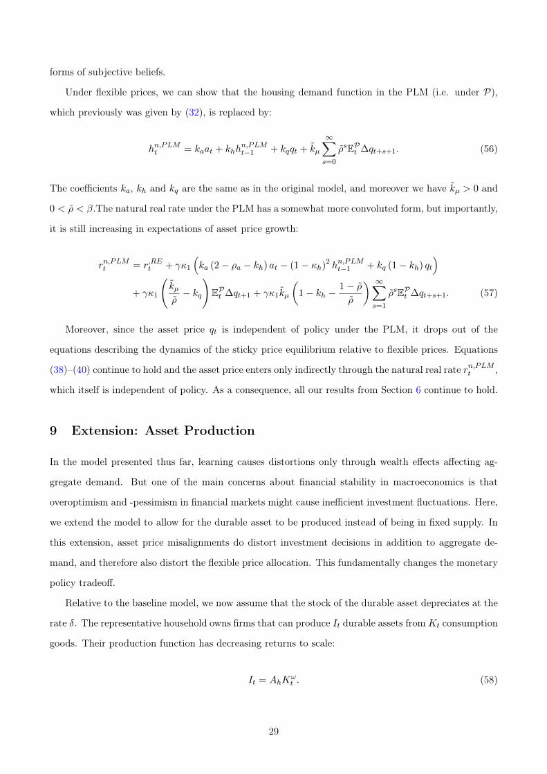
Under flexible prices, we can show that the housing demand function in the PLM (i.e. under P),

which previously was given by (32), is replaced by:

hn,PLMt = kaat + khhn,PLMt−1 + kqqt + kµ

∞∑s=0

ρsEPt ∆qt+s+1. (56)

The coefficients ka, kh and kq are the same as in the original model, and moreover we have kµ > 0 and

0 < ρ < β.The natural real rate under the PLM has a somewhat more convoluted form, but importantly,

it is still increasing in expectations of asset price growth:

rn,PLMt = r,REt + γκ1

(ka (2− ρa − kh) at − (1− κh)2 hn,PLMt−1 + kq (1− kh) qt

)+ γκ1

(kµρ− kq

)EPt ∆qt+1 + γκ1kµ

(1− kh −

1− ρρ

) ∞∑s=1

ρsEPt ∆qt+s+1. (57)

Moreover, since the asset price qt is independent of policy under the PLM, it drops out of the

equations describing the dynamics of the sticky price equilibrium relative to flexible prices. Equations

(38)–(40) continue to hold and the asset price enters only indirectly through the natural real rate rn,PLMt ,

which itself is independent of policy. As a consequence, all our results from Section 6 continue to hold.

9 Extension: Asset Production

In the model presented thus far, learning causes distortions only through wealth effects affecting ag-

gregate demand. But one of the main concerns about financial stability in macroeconomics is that

overoptimism and -pessimism in financial markets might cause inefficient investment fluctuations. Here,

we extend the model to allow for the durable asset to be produced instead of being in fixed supply. In

this extension, asset price misalignments do distort investment decisions in addition to aggregate de-

mand, and therefore also distort the flexible price allocation. This fundamentally changes the monetary

policy tradeoff.

Relative to the baseline model, we now assume that the stock of the durable asset depreciates at the

rate δ. The representative household owns firms that can produce It durable assets fromKt consumption

goods. Their production function has decreasing returns to scale:

It = AhKωt . (58)

29

Production takes place within one period. The profits of the investment firms are:

Πt = QtIt −Kt (59)

and profit maximization leads to the first order condition:

It = Ah (ωQtAh)ω

1−ω . (60)

The budget constraint of the household becomes

Ct +Qt (Ht − (1− δ)Ht−1) +1 + it−1

1 + πtBt−1 = WtNt + Πt + Tt +Bt. (61)

Market clearing in the durable asset market now requires

Ht = (1− δ)Ht−1 + It. (62)

The equilibrium is defined analogously to section 4. Agents do not know the market clearing con-

dition (62), but instead hold subjective beliefs that the asset price follows equations (12)–(13). Beliefs

about the hidden state µt are updated using the Kalman filter as before, and expectations about the

remaining equilibrium objects satisfy conditional model consistency as defined in section 4.

9.1 Linearized equilibrium

We relegate the complete description of the linearized equilibrium to the appendix. Importantly, the

natural real rate of interest in the model with asset production continues to be increasing in the asset

price belief µt. As before, we can write the PLM under sticky prices in deviation from the flexible price

PLM:

πt = βEPt πt+1 + κ(ct + κ1

(ht − (1− δ) ht−1

))+ ηt (63)

it = γ (Etct+1 − ct) + Etπt+1 + rn,PLMt (64)

θht = γct − β (1− δ) γEtct+1. (65)

30

9.2 Welfare functions

We can derive a quadratic approximation of welfare to evaluate different policies. If we evaluate welfare

under the actual law of motion, then welfare takes the form −∑∞

t=0 E0Lt, where the period loss function

is given by

Lt = 2σξ

1− ξ1

1− βξπ2t +

(γC

Y+

1− α+ φ

α

C2

Y 2

)c2t + (1− β (1− δ)) θ QH

Yh2t

+

(1− α+ φ

α

Q2H2

Y 2+ (1− ω)

QH

Y

)(ht − (1− δ) ht−1

)2

+ 21− α+ φ

α

C

Y

QH

Y

(ct − cn,REt

)(ht − (1− δ) ht−1

). (66)

Compared to the standard New Keynesian model, we have to take into account variation in the asset

stock ht that the household owns, as well as variations in asset investment ht. As before, the rational

expectations equilibrium under flexible prices is first-best efficient, and the loss function can therefore

be written in deviations from it.

By contrast, under the PLM, welfare is approximated by −∑∞

t=0 EP0 LPLMt , where the period loss

function is given by

LPLMt = 2σξ

1− ξ1

1− βξπ2t +

(γY

C+

1− α+ φ

α

C2

Y 2

)c2t − (1− β (1− δ)) θ QH

Yh2t

+1− α+ φ

α

(QH

Y

)2 (ht − (1− δ) ht−1

)2

+ 2

(γY

C+

1− α+ φ

α

)C

Y

QH

Yct

(ht − (1− δ) ht−1

). (67)

9.3 Numerical results

We illustrate the dynamics of the model with a simple calibration. We take the same parameters as in

the baseline model, and in addition set ω = 0.636, corresponding to an elasticity of housing supply of

1.75, as estimated by Saiz (2010). The rate of depreciation of the asset is set to δ = 0.007, corresponding

to 2.8% yearly depreciation of housing (Harding et al., 2007).

Figure (6) illustrates that learning has real effects in this model with production even under flexible

prices. It compares the flexible price-responses to a productivity shock under rational expectations and

learning. As before, learning increases asset price volatility. But asset production now responds to asset

demand, diverting resources away from consumption in an asset price boom.

As was the case with the baseline model, strict inflation targeting requires the policymaker to track

31

Figure 6: Effect of learning under flexible prices, with asset production.

0 5 10 15 20 25 30 35 40

periods

-0.5

0

0.5

1

1.5

2

Q

Response of Q to ǫA

Learning

REE

0 5 10 15 20 25 30 35 40

periods

-0.18

-0.16

-0.14

-0.12

-0.1

-0.08

-0.06

-0.04

-0.02

0

0.02

i

Response of i to ǫA

Learning

REE

0 5 10 15 20 25 30 35 40

periods

0

0.02

0.04

0.06

0.08

0.1

0.12

0.14

H

Response of H to ǫA

Learning

REE

0 5 10 15 20 25 30 35 40

periods

-0.1

0

0.1

0.2

0.3

0.4

0.5

0.6

0.7

Y

Response of Y to ǫA

Learning

REE

Note: Response to a one standard deviation positive technology shock εAt. Log percentage points. Flexible prices and zero inflation,with asset production.

movements in the natural rate of interest in the PLM; but this is no longer optimal. This is illustrated

in figure 7, which shows responses to a one standard deviation productivity shock for rules 47–49. The

figure shows that when the central bank sets interest rates according to the perceived natural rate of

interest rn,PLMt , it achieves strict inflation targeting as before, and therefore implements the flexible

price allocation under learning. But this allocation is inefficient because of the investment decisions

taken under non-rational expectations and the housing gap ht is not closed. Tracking the equilibrium

(ALM) process of the natural rate delivers even worse outcomes. The standard Taylor rule, by contrast,

manages to keep the housing gap relatively small following a technology shock, but does not stabilize

inflation and also does not close the consumption gap ct as much as rule 47. Therefore, this extension

of the model features a non-trivial policy tradeoff even without cost-push shocks.

With an investment channel present, learning does not only change how monetary poloicy has to be

implemented, but also the optimal target criterion. In Table 2, we compare strict inflation targeting in

32

Figure 7: Inflation targeting vs Taylor rule, with asset production.

0 5 10 15 20 25 30 35 40

periods

-0.05

0

0.05

0.1

0.15

0.2

0.25

pi

Response of pi to ǫA

Learning, r∗ = r∗

PLM

Learning, r∗ = r∗

ALM

Learning, Taylor (1993)

0 5 10 15 20 25 30 35 40

periods

-0.15

-0.1

-0.05

0

0.05

0.1

0.15

0.2

0.25

0.3

Cgap

Response of Cgap to ǫA

Learning, r∗ = r∗

PLM

Learning, r∗ = r∗

ALM

Learning, Taylor (1993)

0 5 10 15 20 25 30 35 40

periods

-0.5

0

0.5

1

1.5

2

2.5

3

Q

Response of Q to ǫA

Learning, r∗ = r∗

PLM

Learning, r∗ = r∗

ALM

Learning, Taylor (1993)

0 5 10 15 20 25 30 35 40

periods

0

0.05

0.1

0.15Hgap

Response of Hgap to ǫA

Learning, r∗ = r∗

PLM

Learning, r∗ = r∗

ALM

Learning, Taylor (1993)

Note: Response to a unit standard deviation positive technology shock εAt under sticky prices and with asset production. Logpercentage points. The interest rate rules used are given in Equations (47) (using the PLM natural rate with asset production) and(49).

the absence of cost-push shocks with a targeting rule that explicitly “leans against the wind”, in that

it tolerates inflation below target at times when asset prices are high. This targeting rule would be

suboptimal under rational expectations, but turns out to be welfare-increasing under learning.

We also compute optimal simple rules of the form (53) for our calibration of the model with cost-

push shocks, as in section 7. The results are tabulated in Table 3. As can be seen in rows (7)–(9),

in the absence of an outgap gap response the optimal rule has a negative coefficient on the asset price

term. This a result of the allocative inefficiency that learning introduces under asset production. The

optimal choice of φq in this case is driven by the need to control of inefficient under/over investment

under learning. As was the case with fixed asset supply, however, the optimal simple rule exibits a

positive response to both asset prices and the output gap, with optimal rule coefficients prescribing a

more aggressive reaction to both the otput gap and asset prices under learning than in the case with

fixed asset supply.

33

Table 2: “Leaning against the wind” with asset production.

Rational Expectations σ (πt) σ (yt) σ(

∆ht

)σ (∆qt) L

πt = 0 0.000 0.000 0.000 0.930 0

Learning σ (πt) σ (yt) σ(

∆ht

)σ (∆qt) L

πt = 0 0.000 0.037 4.413 1.661 31.67πt = −.311µt−1 0.389 0.026 4.369 1.659 31.31

Table 3: Performance of optimized simple rules, with asset production.

Rational Expectations σ (πt) σ (ct) σ(ht)

σ (∆qt) L

(1) it = rss + 1.5πt + 0.125 · yt 0.342 0.470 0.000 0.759 0.779

(2) it = ρ∗i it−1 + (1− ρ∗i ) ·(rss + 1.5πt + φ∗y · yt

)0.365 0.271 0.000 0.675 0.475

ρ∗i , φ∗y = 0.723, 1.207

(3) πt = ζ∗ηt 0.299 0.296 0.000 0.968 0.401ζ∗ = 0.214

Learning σ (πt) σ (ct) σ(ht)

σ (∆qt) L

(4) it = ρ∗i it−1 + (1− ρ∗i ) ·(rss + 1.5πt + φ∗y · yt

)1.024 0.512 0.193 1.078 6.207

ρ∗i , φ∗y = 0.098, 0.819

(5) πt = ζ∗ηt 0.566 0.034 0.494 1.662 32.413ζ∗ = 0.399

(6) it = ρ∗i it−1 + (1− ρ∗i ) · (rss + 1.5πt) 0.045 0.602 0.747 1.923 60.771ρ∗i = 0

(7) BG (1999) w/ asset priceit = ρ∗i it−1 + (1− ρ∗i ) ·

(rss + 1.5πt + φ∗q · log qt−1

)1.735 0.693 0.744 0.778 46.412

ρ∗i , φ∗q = 0,−0.241

(8) BG (2001) w/ asset priceit = ρ∗i it−1 + (1− ρ∗i ) ·

(rss + 1.5πt + φ∗q · log qt

)0.697 0.596 0.742 1.925 59.715

ρ∗i , φ∗q = 0,−0.072

(9) it = ρ∗i it−1 + (1− ρ∗i ) ·(rss + 1.5πt + φ∗q ·

∑∞s=0 ω

∗s∆ logQt−s)

0.618 0.598 0.744 1.927 59.956ρ∗i , φ∗q , ω∗ = 0,−0.064, 0.999

(10) FM (2007) w/ asset priceit = ρ∗i it−1 + (1− ρ∗i ) ·

(rss + 1.5πt + φ∗y · yt + φ∗q · log qt

)0.638 0.559 0.096 0.927 2.131

ρ∗i , φ∗y , φ∗q = 0.330, 3.548, 1.077

(11)* it = ρ∗i it−1 + (1− ρ∗i ) ·(rss + 1.5πt + φ∗y · yt + φ∗q ·

∑∞s=0 ω

∗s∆ logQt−s)

0.646 0.570 0.095 0.923 2.155ρ∗i , φ∗y , φ∗q , ω∗ = 0.329, 3.106, 0.974, 0.999

34

10 Conclusion

In this paper, we have characterized optimal monetary policy in a model in which agents are learning

about asset prices. Our model is the standard New-Keynesian model with a durable asset in fixed supply.

Agents form expectations about asset price in an extrapolative fashion. However, their expectations

remain model-consistent conditional on their beliefs about house prices, which allows us to isolate the

effects of learning about asset prices from the many other ways in which distorted beliefs can affect the

economy. Learning amplifies asset price fluctuations in the model, and leads to perceived wealth effects

that create inefficient fluctuations in aggregate demand.

We gave an analytical solution to the optimal policy in the linearized model with learning, and

have showed that inflation targeting remains optimal. However, inflation targeting requires a very

different prescription for the nominal interest rate under learning. The interest rate has to increase with

asset prices and subjective expectations of future asset price growth. We then showed using numerical

simulations that the optimal policy can be reasonably well approximated by simple rules that responds

to inflation and a moving average of asset price growth. A reaction to asset prices always reduces asset

price volatility, but too much of a reaction can increase inflation volatility. Nonetheless, the optimal

weight on asset prices is strictly positive for the rules we considered.

We have also shown that our theoretical results are robust to the specification of subjective beliefs,

encompassing a wide range of belief specifications. Another extension of our model showed that the

case for reacting to asset prices is strengthened further when investment decisions are affected by asset

prices. With an investment channel, it becomes beneficial to include a reaction to asset prices in the

targeting rule of monetary policy. This “leaning against the wind” policy effectively curbs inefficient

investment fluctuations.

35

References

Adam, K., Kuang, P. and Marcet, A. (2012). House price booms and the current account. NBERMacroeconomics Annual, 26 (1), 77–122.

—, Marcet, A. and Beutel, J. (2017). Stock price booms and expected capital gains. AmericanEconomic Review, 107 (8), 2352–2408.

—, — and Nicolini, J. P. (2015). Stock market volatility and learning. Journal of Finance.

— and Woodford, M. (2018). Leaning Against Housing Prices as Robustly Optimal Monetary Policy.Working Paper 24629, NBER.

Airaudo, M. (2016). Monetary Policy and Asset Prices with Infinite-Horizon Learning. Tech. rep.

Barberis, N., Greenwood, R., Jin, L. and Shleifer, A. (2015). X-CAPM: An extrapolative capitalasset pricing model. Journal of Financial Economics, 115 (1), 1–24.

Bean, C. R. (2004). Asset prices, financial instability, and monetary policy. The American EconomicReview, 94 (2), 14–18.

Bernanke, B. S. and Gertler, M. (1999). Monetary policy and asset price volatility. EconomicReview – Federal Reserve Bank of Kansas City, Q IV, 17–62.

— and — (2001). Should central banks respond to movements in asset prices? American EconomicReview, 91 (2), 253–257.

Billi, R. M. (2017). Price Level Targeting and Risk Management. Working Paper Series 302, SverigesRiksbank.

Boehm, C. E. and House, C. L. (2014). Optimal Taylor Rules in New Keynesian Models. WorkingPaper 20237, NBER.

Bordalo, P., Gennaiola, N. and Shleifer, A. (2018). Diagnostic expectations and credit cycles.Journal of Finance, 73 (1), 199–227.

Caines, C. (2016). Can Learning Explain Boom-Bust Cycles In Asset Prices? An Application to theUS Housing Boom. International Finance Discussion Papers 1181, Board of Governors of the FederalReserve System (U.S.).

Christiano, L., Ilut, C., Motto, R. and Rostagno, M. (2010). Monetary policy and stock marketbooms. Proceedings , Jackson Hole Economic Policy Symposium, pp. 85–145.

Collin-Dufresne, P., Johannes, M. and Lochstoer, L. A. (2013). Parameter Learning in GeneralEquilibrium: The Asset Pricing Implications. NBER Working Papers 19705, National Bureau ofEconomic Research, Inc.

Dong, F., Miao, J. and Wang, P. (2017). Asset Bubbles and Monetary Policy. Working paper.

Dupor, B. (2005). Stabilizing non-fundamental asset price movements under discretion and limitedinformation. Journal of Monetary Economics, 52 (4), 727 – 747.

Eusepi, S., Giannoni, M. and Preston, B. (2015). The Limits of Monetary Policy with Long-termDrift in Expectations. Working paper.

— and Preston, B. (2016). The science of monetary policy: an imperfect knowledge perspective. StaffReports 782, Federal Reserve Bank of New York.

36

Faia, E. and Monacelli, T. (2007). Optimal interest rate rules, asset prices, and credit frictions.Journal of Economic Dynamics and Control, 31 (10), 3228–3254.

Fuster, A., Hebert, B. and Laibson, D. (2012). Natural expectations, macroeconomic dynamics,and asset pricing. In D. Acemoglu and M. Woodford (eds.), NBER Macroeconomics Annual 2011,NBER Chapters, vol. 26, National Bureau of Economic Research, pp. 1–48.

Gabaix, X. (2016). A Behavioral New Keynesian Model. NBER Working Papers 22954, National Bu-reau of Economic Research, Inc.

Gali, J. (2014). Monetary policy and rational asset price bubbles. American Economic Review, 104 (3),721–752.

— (2017). Monetary Policy and Bubbles in a New Keynesian Model with Overlapping Generations.Working Paper 959, Barcelona GSE.

Gandelman, N. and Hernández-Murillo, R. (2014). Risk Aversion at the Country Level. Workingpaper series, Federal Reserve Bank of St. Louis.

Gandré, P. (2017). Learning, house prices and macro-financial linkages. Working paper.

Glaeser, E. L. and Nathanson, C. G. (2017). An extrapolative model of house price dynamics.Journal of Financial Economics.

Greenwood, R. and Shleifer, A. (2014). Expectations of returns and expected returns. Review ofFinancial Studies, 27 (3), 714–746.

Harding, J. P., Rosenthal, S. S. and Sirmans, C. (2007). Depreciation of housing capital, mainte-nance, and house price inflation: Estimates from a repeat sales model. Journal of Urban Economics,61 (2), 193 – 217.

Laubach, T. and Williams, J. C. (2016). Measuring the natural rate of interest redux. BusinessEconomics, 51, 257–267.

Mertens, T. M. (2011). Volatile Stock Markets: Equilibrium Computation and Policy Analysis. Work-ing paper, Federal Reserve Bank of San Francisco.

Molnar, K. and Santoro, S. (2014). Optimal monetary policy when agents are learning. EuropeanEconomic Review, 66, 39 – 62.

Neiss, K. S. andNelson, E. (2003). The real-interest-rate gap as an inflation indicator.MacroeconomicDynamics, 7 (2), 239–262.

Preston, B. (2006). Adaptive learning, forecast-based instrument rules and monetary policy. Journalof Monetary Economics, 53 (3), 507 – 535.

Saiz, A. (2010). The geographic determinants of housing supply. Quarterly Journal of Economics,125 (3), 1253–1296.

Winkler, F. (2016). The Role of Learning for Asset Prices, Business Cycles, and Monetary Policy.Finance and Economics Discussion Series 2016-019, Federal Reserve Board of Governors.

Woodford, M. (2003). Interest and prices: Foundations of a theory of monetary policy. PrincetonUniversity Press.

— (2010). Robustly optimal monetary policy with near-rational expectations. American Economic Re-view, 100 (1), 274–303.

37

A Appendix: Details on the derivations

A.1 Asset demand in the model with fixed asset supply

The coefficients in the asset demand function (32) are:

kh =1

2β

1 + β +θ

γκ1(1− β)−

√(1 + β +

θ

γκ1(1− β)

)2

− 4β

∈ (0, 1) (68)

ka =1 + φ

1 + φ− α (1− γ)

1− βρaκ1 + (1− β) θγ + βκ1 (1− kh − ρa)

> 0 (69)

kq =1

γ

1− β(1− β) θγ + κ1 (1− βkh)

> 0 (70)

kµ =β/γ

(1− β) θγ + κ1 (1− βρµ + β (1− kh))

(1 + β) θγ + κ1β (1− kh)

(1 + β) θγ + κ1 (1− βkh)> 0 (71)

A.2 Asset demand with extended beliefs

The coefficients kµ and ρ read as follows:

kµ =1

γ

β

(1− β) θγ + κ1 (1 + β − βkh)

(1 + β) θγ + κ1β (1− kh)

(1 + β) θγ + κ1 (1− βkh)> 0 (72)

ρ =β

β + (1− β) θγκ1

+ (1− βkh)∈ (0, 1) . (73)

A.3 Attaining the first-best allocation with cost push shocks under learning

Substituting the policy πt = − (βρη)−1 ηt + btzt into the Phillips curve (38), we obtain:

πt = − (βρη)−1 ηt + btzt = κ

(ct + κ1∆ht

). (74)

We will find bt such that πt = 0 a.s. under the ALM. In this case, κ(ct + κ1∆ht

)= yt−yREt = 0 under

the ALM as well, and the first-best allocation is attained.

In order to solve for bt, then, we need to compute the equilibrium value of zt, which amounts to

solving for the equilibrium price qt. To do this, we first need to derive the demand function for the asset

under the PLM. Let xt = ct + κ1∆ht. In analogy to the computations of the flexible-price equilibrium,

38

we can compute the asset demand function as the solution to the following system of equations:

(1− β) θht = γct − qt − βEPt [γct+1 − qt+1] (75)

(1 + φ− α+ αγ) ct = αxt + (1− α) at − (1 + φ− α)QH

Y∆ht. (76)

With xt =(btzt − (βρη)

−1 ηt

)/κ, we can solve:

ht = khht−1 + kaat − kqqt + kµµt−1 + kbzbtzt + kηηt. (77)

Here, the coefficients kh, ka, kq and kµ are the same as in the flexible-price demand function (32). The

coefficients kη and kbz are given by:

kη = − khβρηκ

1− βρη1− khβρη

Y

QH

α

1 + φ− α(78)

kz,t = −khκ

Y

QH

α

1 + φ− α(79)

Now the ALM is found by imposing ht = 0, and this condition leads to the ALM expression for zt:

zt =kq

kq − kbzbt

(1

kq(kaat + kµµt−1 + kηηt)− qt−1 − µt−1

)(80)

Imposing βρηbtzt = ηt then leads to:

bt =

(kbzkq

+βρηkq

(kaat + kµµt−1 + kηηt)− βρη (qt−1 + µ)

)−1

ηt. (81)

A.4 Replication of RE-optimal policy with cost push shocks under learning

The solution undear learning must be obtained again by first solving the PLM and then imposing

equilibrium. We start by imposing (50) as a targeting rule in the PLM. We can make use of the

fact that we can represent the equilibrium conditions of the PLM by the three equation (38)–(40).

Substituting the targeting rule yields:

ct = −1− ζ (1− βρ)

κηt − κ1∆ht (82)

ht = − γ

θ (1− β)βEPt ∆ct+1. (83)

39

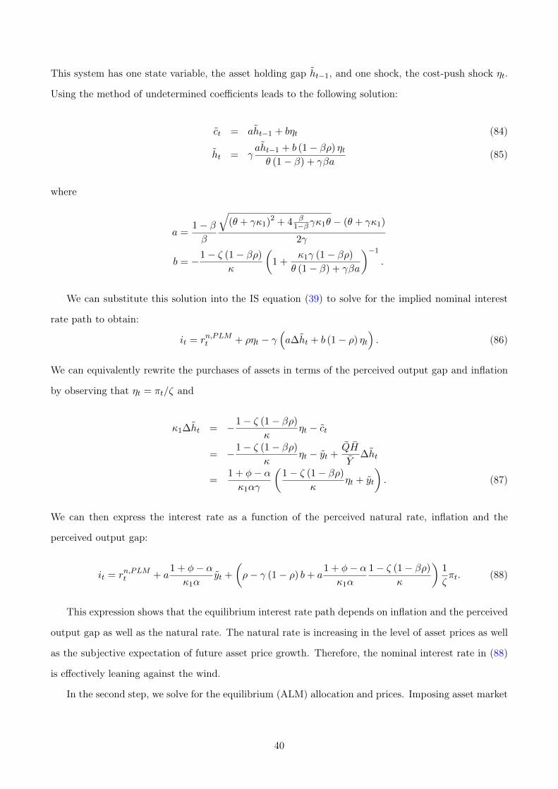
This system has one state variable, the asset holding gap ht−1, and one shock, the cost-push shock ηt.

Using the method of undetermined coefficients leads to the following solution:

ct = aht−1 + bηt (84)

ht = γaht−1 + b (1− βρ) ηtθ (1− β) + γβa

(85)

where

a =1− ββ

√(θ + γκ1)2 + 4 β

1−βγκ1θ − (θ + γκ1)

2γ

b = −1− ζ (1− βρ)

κ

(1 +

κ1γ (1− βρ)

θ (1− β) + γβa

)−1

.

We can substitute this solution into the IS equation (39) to solve for the implied nominal interest

rate path to obtain:

it = rn,PLMt + ρηt − γ(a∆ht + b (1− ρ) ηt

). (86)

We can equivalently rewrite the purchases of assets in terms of the perceived output gap and inflation

by observing that ηt = πt/ζ and

κ1∆ht = −1− ζ (1− βρ)

κηt − ct

= −1− ζ (1− βρ)

κηt − yt +

QH

Y∆ht

=1 + φ− ακ1αγ

(1− ζ (1− βρ)

κηt + yt

). (87)

We can then express the interest rate as a function of the perceived natural rate, inflation and the

perceived output gap:

it = rn,PLMt + a1 + φ− ακ1α

yt +

(ρ− γ (1− ρ) b+ a

1 + φ− ακ1α

1− ζ (1− βρ)

κ

)1

ζπt. (88)

This expression shows that the equilibrium interest rate path depends on inflation and the perceived

output gap as well as the natural rate. The natural rate is increasing in the level of asset prices as well

as the subjective expectation of future asset price growth. Therefore, the nominal interest rate in (88)

is effectively leaning against the wind.

In the second step, we solve for the equilibrium (ALM) allocation and prices. Imposing asset market

40

clearing requires ht = 0, which can be rewritten as

hn,PLMt = −ht. (89)

Substituting this into the expression for asset demand (32), we can solve for the equilibrium price:

−ht = kaat − khht−1 + kqqt + kµµt−1

⇒ qt = − 1

kq

(kaat + kµµt−1 + ht − khht−1

). (90)

Finally, we solve for the equilibrium output gap. We first rewrite Equation (33) in terms of housing

purchases under flexible prices:

yn,PLMt = yn,REt +αγκ1

1 + φ− α

(hn,PLMt − hn,PLMt−1

)(91)

and use this relationship to arrive at the main result in this section:

yt = ht + yn,PLMt − yn,REt

= ct +QH

Y∆ht + yn,PLMt − yn,REt

= ct +

(QH

Y− αγκ1

1 + φ− α

)∆ht

= ct + κ1∆ht

= −1− ζ (1− βρ)

κηt. (92)

That is, the equilibrium path of the output gap is identical to that under rational expectations.

A.5 Linearized equilibrium conditions and natural rate in the model with asset

production

Under rational expectations, the following set of equations describe the linearized equilibrium (up to a

monetary policy rule):

41

yt = at + αnt (93)

πt = βπt+1 +(1− ξ) (1− βξ)

ξ(wt − at + (1− α)nt) + ηt (94)

wt = γct + φnt (95)

Y yt = Cct + QH (ht − (1− δ)ht−1) (96)

ht = (1− δ)ht−1 +ωδ

1− ωqt (97)

it = γ (Etct+1 − ct) + Etπt+1 (98)

qt = γct − (1− β (1− δ)) θht − β (1− δ) γEtct+1 + βδEtqt+1. (99)

We can eliminate the asset price, wages, labor and output from this to get a three-equation system:

πt = βEtπt+1 +(1− ξ) (1− βξ)

ξ·(

γct +

(1 + φ− α

α

)(C

Yct +

QH

Y(ht − (1− δ)ht−1)

)− 1 + φ

αat

)+ ηt (100)

it = γ (Etct+1 − ct) + Etπt+1 (101)(1− β

)θht = γct −

1− ωωδ

(ht − (1− δ)ht−1)− βγEtct+1 + β1− ωωδ

Et (ht+1 − (1− δ)ht) (102)

where we introduced β = β (1− δ) to ease notation.

Under learning, we can do a similar exercise. We first tackle the PLM. All we do is to replace the

market clearing condition with the subjective law of motion for asset prices:

yt = at + αnt (103)

πt = βEPt πt+1 +(1− ξ) (1− βξ)

ξ(wt − at + (1− α)nt) + ηt (104)

wt = γct + φnt (105)

Y yt = Cct + QH (ht − (1− δ)ht−1) (106)

it = γ(EPt ct+1 − ct

)+ EPt πt+1 (107)

qt = γct − (1− β (1− δ)) θht − β (1− δ) γEPt ct+1 + βδEPt qt+1 (108)

qt = qt−1 + µt−1 + zt (109)

µt = ρµµt−1 + gzt. (110)

42

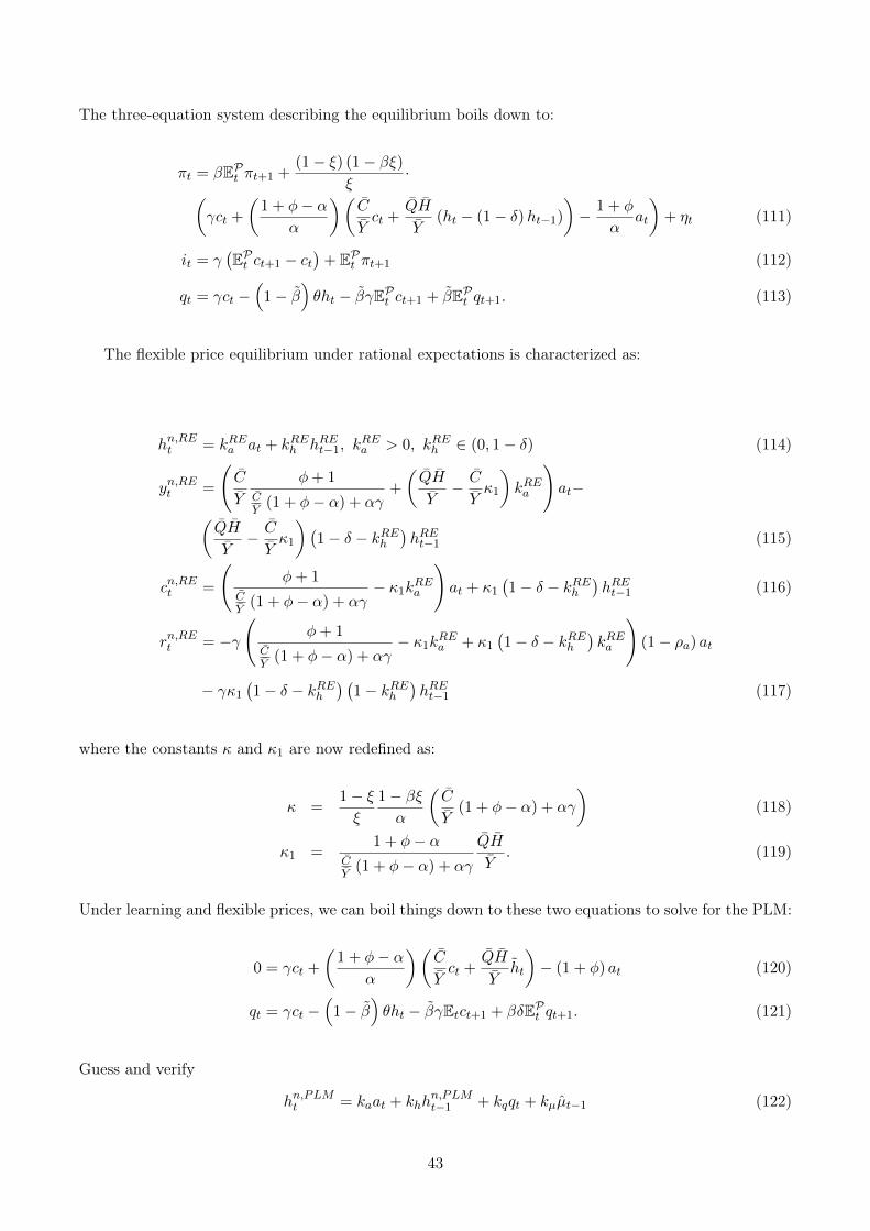
The three-equation system describing the equilibrium boils down to:

πt = βEPt πt+1 +(1− ξ) (1− βξ)

ξ·(

γct +

(1 + φ− α

α

)(C

Yct +

QH

Y(ht − (1− δ)ht−1)

)− 1 + φ

αat

)+ ηt (111)

it = γ(EPt ct+1 − ct

)+ EPt πt+1 (112)

qt = γct −(

1− β)θht − βγEPt ct+1 + βEPt qt+1. (113)

The flexible price equilibrium under rational expectations is characterized as:

hn,REt = kREa at + kREh hREt−1, kREa > 0, kREh ∈ (0, 1− δ) (114)

yn,REt =

(C

Y

φ+ 1CY

(1 + φ− α) + αγ+

(QH

Y− C

Yκ1

)kREa

)at−(

QH

Y− C

Yκ1

)(1− δ − kREh

)hREt−1 (115)

cn,REt =

(φ+ 1

CY

(1 + φ− α) + αγ− κ1k

REa

)at + κ1

(1− δ − kREh

)hREt−1 (116)

rn,REt = −γ

(φ+ 1

CY

(1 + φ− α) + αγ− κ1k

REa + κ1

(1− δ − kREh

)kREa

)(1− ρa) at

− γκ1

(1− δ − kREh

) (1− kREh

)hREt−1 (117)

where the constants κ and κ1 are now redefined as:

κ =1− ξξ

1− βξα

(C

Y(1 + φ− α) + αγ

)(118)

κ1 =1 + φ− α

CY

(1 + φ− α) + αγ

QH

Y. (119)

Under learning and flexible prices, we can boil things down to these two equations to solve for the PLM:

0 = γct +

(1 + φ− α

α

)(C

Yct +

QH

Yht

)− (1 + φ) at (120)

qt = γct −(

1− β)θht − βγEtct+1 + βδEPt qt+1. (121)

Guess and verify

hn,PLMt = kaat + khhn,PLMt−1 + kqqt + kµµt−1 (122)

43

where the coefficients are given by:

kh =1

2β

(1 + β (1− δ) +

θ

γκ1

(1− β

)−√(

1 + β (1− δ) +θ

γκ1

(1− β

))2

− 4β (1− δ)

)∈ (0, 1− δ) (123)

ka =1 + φ

CY

(1 + φ− α) + αγ

1− βρaκ1 +

(1− β

)θγ + βκ1 (1− δ − kh − ρa)

> 0 (124)

kq = −1

γ

1− β(1− β

)θγ + κ1

(1− βkh − βδ

) < 0 (125)

kµ =β/γ(

1− β)θγ + κ1

(1− βρµ + β (1− δ − kh)

)(

1− β)θγ + κ1β (1− δ − kh)(

1− β)θγ + κ1

(1− βkh − βδ

) > 0 (126)

where β = (1− δ)β. We can characterize the flex-price PLM consumption, output and interest

rates:

cn,PLMt − cn,REt

κ1= −

(ka − kREa

)at −

(kh − kREh

)ht−1+(

1− δ − kREh) (hn,PLMt−1 − hn,REt−1

)− kqqt − kµµt−1 (127)

yn,PLMt − yn,REtQHY− C

Yκ1

= −cn,PLMt − cn,REt

κ1(128)

−rn,PLMt − rn,REt

γκ1= −

((1− kh) (1− δ − kh)−

(1− kREh

) (1− δ − kREh

))ht−1

−(1− kREh

) (1− δ − kREh

) (hn,PLMt−1 − hn,REt−1

)+(ka (2− δ − ka − ρa)− kREa

(2− δ − kREa − ρa

))at

+ (kµ (2− δ − kh − ρµ)− kq) µt−1 + kq (1− δ − kh) qt (129)

In order to find the ALM under flexible prices, we impose market clearing for the durable asset and

obtain:

(1− δ)ht−1 +ωδ

1− ωqt = kaat + khht−1 + kqqt + kµµt−1

⇔ qt =1

ω1−ω δ − kq

(kaat + kµµt−1 − (1− δ − kh)ht−1) . (130)

The equilibrium price is increasing in productivity, increasing in asset price beliefs, and decreasing in

the existing stock of housing.

44

When the equilibrium asset price qt from equation (130) is substituted into the expression for the

natural rate rn,PLMt , the natural real rate in the ALM rn,ALMt is increasing in asset price expectations

µt−1, just as in the baseline model. The sign of the other coefficients are ambiguous and depend on the

parameterization.

45