Autonomous adaptive sensorless controller of inverter-based islanded-distributed generation system

256

& T

www.ietdl.org

Published in IET Power ElectronicsReceived on 24th January 2008Revised on 23rd June 2008doi: 10.1049/iet-pel.2008.0029

ISSN 1755-4535

Autonomous adaptive sensorless controllerof inverter-based islanded-distributedgeneration systemK.H. Ahmed A.M. Massoud S.J. Finney B.W. WilliamsDepartment of Electrical and Electronic Engineering, Strathclyde University, 204 George Street, Royal College Building,Glasgow G1 1XW, UKE-mail: [email protected]

Abstract: A control method for inverter operation in an islanded-distributed generation system is presented. Thecontroller provides sufficient active and reactive power to match the connected load, therein providing highpower quality. Control in this mode is based on voltage and frequency droops. Detailed analysis, based on theconcept of harmonic impedance, establishes the appropriateness of inductor current feedback againstcapacitor current feedback, with respect to inverter output power quality. Steepest descent adaptive control isembedded to estimate the output voltage for sensorless operation, which enhances system robustness andperformance. To compensate the DSP calculation delay, a modified Kalman filter design is discussed.Simulation and experimental results demonstrate the validity of the proposed control method.

1 IntroductionDistribution networks have been designed to deliver powerfrom the network to the end customer. Distributedgeneration (DG), however, requires more active distributionnetworks that allow bidirectional electricity to flow to theelectricity user for consumption at homes or businesses,and into the network when the user is exporting excessgeneration capacity [1]. Processing speeds have increased,facilitating improved flexibility, reliability and complexity ofcontrol algorithms. In an islanded mode, the DG unit isthe source of power. Hence, it should be able to feed thelocal network with the appropriate voltage and frequency.Frequency and voltage control in island networks, suppliedby single or several inverters in parallel, can be obtained bymeans of various control methods, with or without anintercommunication link. The common control methodsfor single inverter operation are derived from UPSoperation [2, 3]. Many control methods for the paralleloperation of inverter-based systems have been proposed[4–7]. Paralleled operation of voltage source inverters isdifficult to achieve. If the output voltages or impedancesare mismatched, circulating currents arise. Perfect matchingis not possible and even small mismatches cause large

he Institution of Engineering and Technology 2009

circulating currents. Therefore a means of ensuring currentsharing is essential. Nested control loops are used to forcevoltage source inverters to follow a current reference. Thesecurrent sources are then used within a voltage control loopto provide a reference for the network voltage. Althoughmany methods exist for controlling inverters, there is nosatisfactory method to achieve a truly distributed powersupply system. Most techniques need some form of inverterinterconnection. These interconnections not only restrictthe location of the inverter units, but can also act as asource of noise and failure. The system is therefore nottruly distributed and does not offer redundancy.Techniques without control interconnection are presentedin [8–10], which are based on the frequency and voltagedroop concept to achieve load sharing. These techniques,however, only function well for linear and mostly resistiveloads. When the load is nonlinear, the load harmoniccomponents cannot be properly shared. Furthermore, lineimpedance impacts significantly on reactive power sharing,an issue not addressed. For sensorless operation, differentestimation schemes have been considered [11–14]. In [11],adaptive estimation estimates simultaneously in real timethe interfacing parameters and grid voltage. In [12], analgorithm for predicting the line voltage vector is proposed.

IET Power Electron., 2009, Vol. 2, Iss. 3, pp. 256–266doi: 10.1049/iet-pel.2008.0029

IETdoi

www.ietdl.org

In [13], a new control method for a PWM rectifier system,based on a direct power control approach, is reported. In[14], an input current model-based observer is used forboth input current estimation and control feedback inPWM converters.

In this paper, a control method is proposed for a PWMinverter operating in an islanded DG system. The controlsystem is based on voltage and frequency droops when theinverter is the source of power, like a synchronousgenerator. Different feedback state variables are investigatedto obtain robust designs that are readily evaluable. Thecontrollers use an outer voltage control loop and an innercurrent control loop. The outer loop ensures steady-statereference tracking performance and the inner loop providesfast dynamic compensation to system disturbances.Detailed analysis, based on a harmonic impedance concept,establishes the appropriateness of the capacitor currentfeedback against other feedback current control variableswith respect to inverter power quality. The influence of thecontrol strategy on low-order current harmonic distortiongenerated by an inverter connected to a distorted load isinvestigated through a combination of simulation andexperimentation. To compensate a DSP calculation delay, amodified Kalman filter design is introduced. The estimatedstate control variables are incorporated into the controldesign to reduce system measurement and costrequirements, and to increase reliability. Simulation andexperimental results demonstrate the validity of theproposed control method.

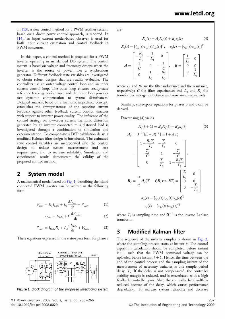
2 System modelA mathematical model based on Fig. 1, describing the islandconnected PWM inverter can be written in the followingform

VIabc ¼ R1ILabc þ L1

dILabc

dtþ VCabc (1)

ILabc ¼ IOabc þ CdVCabc

dt(2)

VCabc ¼ IOabcR2 þ L2

dIOabc

dtþ VOabc (3)

These equations expressed in the state-space form for phase a

Figure 1 Block diagram of the proposed interfacing system

Power Electron., 2009, Vol. 2, Iss. 3, pp. 256–266: 10.1049/iet-pel.2008.0029

are

_X a(t) ¼ AaXa(t)þ Baua(t) (4)

Xa(t) ¼ [iLa(t)vCa(t)iOa(t)]T, ua(t) ¼ [vIa(t)vOa(t)]T

A ¼

�R1

L1

�1

L1

0

1

C0 �

1

C

01

L2

�R2

L2

26666664

37777775

, B ¼

1

L1

0

0 0

01

L2

266664

377775

where L1 and R1 are the filter inductance and the resistance,respectively; C the filter capacitance; and L2 and R2 thetransformer leakage inductance and resistance, respectively.

Similarly, state-space equations for phases b and c can bederived.

Discretising (4) yields

Xa(kþ 1) ¼ Ad Xa(k)þ Bd ua(k) (5)

Ad ¼ =�1[(sI� A)�1] ’ Iþ ATs

¼

1�R1Ts

Lt

�Ts

L1

0

Ts

C1 �

Ts

C

0Ts

L2

1�R2Ts

L2

26666664

37777775

,

Bd ¼

ðT

0

Ad (T � t)Bdt ’ BTs ¼

Ts

L1

0

0 0

0 �Ts

L2

266664

377775

Xa(k) ¼ [iLa(k)vCa(k)iOa(k)]T

ua(k) ¼ [vIa(K )vOa(k)]T

where Ts is sampling time and =21 is the inverse Laplacetransform.

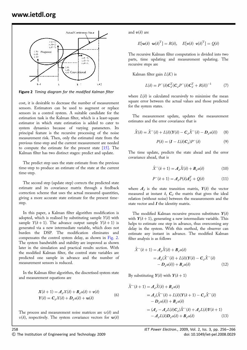
3 Modified Kalman filterThe sequence of the inverter samples is shown in Fig. 2,where the sampling process starts at instant k. The controlalgorithm calculation should be completed before instantkþ 1 such that the PWM command voltage can beuploaded before instant kþ 1. Hence, the time between theend of the control process and the sampling instant of themeasurement of necessary variables is one sample perioddelay, Ts. If the delay is not compensated, the controllerstability margin is reduced, and is exacerbated with a highfeedback controller gain. Also, the controller bandwidth isreduced because of the delay, which causes performancedegradation. To increase system reliability and decrease

257

& The Institution of Engineering and Technology 2009

258

&

www.ietdl.org

cost, it is desirable to decrease the number of measurementsensors. Estimators can be used to augment or replacesensors in a control system. A suitable candidate for theestimation task is the Kalman filter, which is a least-squareestimator in which state estimation is added to cater tosystem dynamics because of varying parameters. Itsprincipal feature is the recursive processing of the noisemeasurement risk. Then, only the estimated state from theprevious time-step and the current measurement are neededto compute the estimate for the present state [15]. TheKalman filter has two distinct stages: predict and update.

The predict step uses the state estimate from the previoustime-step to produce an estimate of the state at the currenttime-step.

The second step (update step) corrects the predicted stateestimate and its covariance matrix through a feedbackcorrection scheme that uses the actual measured quantities,giving a more accurate state estimate for the present time-step.

In this paper, a Kalman filter algorithm modification isadopted, which is realised by substituting sample Y (k) withsample Y (kþ 1). The advance output sample Y (kþ 1) isgenerated via a new intermediate variable, which does notburden the DSP. The modification eliminates andcompensates the control system delay, as shown in Fig. 2.The system bandwidth and stability are improved as shownlater in the simulation and practical results section. Withthe modified Kalman filter, the control state variables arepredicted one sample in advance and the number ofmeasurement sensors is reduced.

In the Kalman filter algorithm, the discretised system stateand measurement equations are

X (kþ 1) ¼ Ad X (k)þ Bd u(k)þ v(k)

Y (k) ¼ Cd X (k)þDd u(k)þw(k)(6)

The process and measurement noise matrices are w(k) andv(k), respectively. The system covariance vectors for w(k)

Figure 2 Timing diagram for the modified Kalman filter

The Institution of Engineering and Technology 2009

and v(k) are

E[w(k) w(k)T] ¼ R(k), E[v(k) v(k)T] ¼ Q(k)

The recursive Kalman filter computation is divided into twoparts, time updating and measurement updating. Therecursive steps are

Kalman filter gain L(K ) is

L(k) ¼ P�(k)CTd (Cd P�(k)CT

d þ R(k))�1 (7)

where L(k) is calculated recursively to minimise the meansquare error between the actual values and those predictedfor the system states.

The measurement update, updates the measurementestimates and the error covariance that is

X̂ (k) ¼ X̂�(k)þ L(k)(Y (k)� Cd X̂�(k)�Dd u(k)) (8)

P(k) ¼ (I � L(k)Cd )P�(k) (9)

The time update, predicts the state ahead and the errorcovariance ahead, that is

X̂�(kþ 1) ¼ Ad X̂ (k)þ Bd u(k) (10)

P�(kþ 1) ¼ Ad P(k)ATd þ Q(k) (11)

where Ad is the state transition matrix, Y (k) the vectormeasured at instant k, Cd the matrix that gives the idealrelation (without noise) between the measurements and thestate vector and I the identity matrix.

The modified Kalman recursive process substitutes Y (k)with Y (kþ 1), generating a new intermediate variable. Thishelps to estimate one step in advance, thus overcoming anydelay in the system. With this method, the observer canestimate any instant in advance. The modified Kalmanfilter analysis is as follows

X̂�(kþ 1) ¼ Ad X̂ (k)þ Bd u(k)

¼ Ad (X̂�(k)þ L(k)(Y (k)� Cd X̂�(k)

�Dd u(k))þ Bd u(k) (12)

By substituting Y (k) with Y (kþ 1)

X̂�(kþ 1) ¼ Ad X̂ (k)þ Bd u(k)

¼ Ad (X̂�(k)þ L(k)(Y (kþ 1)� Cd X̂�(k)

�Dd u(k))þ Bd u(k)

¼ (Ad � Ad L(k)Cd )X̂�(k)þ Ad L(k)Y (kþ 1)

� Ad L(k)Dd u(k)þ Bd u(k) (13)


IETdoi

www.ietdl.org

To remove Y (kþ 1) from the observer equations,intermediate variable M(k) is used

M(k) ¼ X̂�(k)� Ad L(k� 1)Y (k) (14)

M(kþ 1) ¼ X̂�(kþ 1)� Ad L(k)Y (kþ 1) (15)

M(kþ 1) ¼ (Ad � Ad L(k)Cd )(M(k)þ Ad L(k� 1)Y (k))

þ (Bd � Ad L(k)Dd )u(k)

The system estimated states are

X̂�(k) ¼M(k)þ Ad L(k� 1)Y (k) (16)

This method can be generalised to estimate n-samples inadvance by cascading the output from each modifiedKalman filter, and practically n is limited by the total delaysamples to be compensated.

4 Control systemThe proposed control system observer is shown in Fig. 3. Thecontrol part consists of output voltage estimation, voltagecontrol, current control and steady-state cancellation control.

4.1 Adaptive sensorless controller

The aim of the controller in Fig. 4 is to predict theinstantaneous output voltage to eliminate measurementsensors. Steepest descent adaptive control is embedded inthe control system to estimate the output voltage. Themethod searches for the minimum of a function of manyvariables [16]

eOa(k) ¼ iOa(k)� i�Oa(k) (17)

v�Oa(kþ 1) ¼ v�Oa(k)� lrf (k) (18)

i�La(kþ 1)v�Ca(kþ 1)i�Oa(kþ 1)

24

35 ¼ Ad

i�La(k)v�Ca(k)i�Oa(k)

24

35þ Bd

vIa(k)v�Oa(k)

� �(19)

where l is a positive adaptation gain, which controls the


speed of convergence and rf (k) is the gradient of the costfunction with respect to the output voltage.

The quadratic cost function is

f (k) ¼1

2e2

Oa(k) ¼1

2(iOa(k)� i�Oa(k))2 (20)

and the gradient is

rf (k) ¼@f (k)

@v�Oa(k)¼@f (k)

@i�Oa(k)

@i�Oa(k)

@v�Oa(k)¼

Ts

L2

eOa(k)

v�Oa(k) ¼ v�Oa(k� 1)� lTs

L2

eOa(k) (21)

The adaptive gain l is selected to maintain the controllersystem stable and give fast convergence. There is a trade-offbetween fast convergence and system stability margin. Theselection of the adaptive gain l and its impact on stabilitycan be assessed with the Lyapunov direct method orLyapunov second method. Then, the stability analysis isindirect via the analysis of the time behaviour of a scalarfunction, which is defined for the given system. Theproposed Lyapunov function is

V (k) ¼ Y T(k)Y (k) (22)

In the proposed system, from the cost function the Lyapunov

Figure 4 Adaptive estimation algorithm

Figure 3 Proposed control algorithm

259


260

&

www.ietdl.org

function can be

V (k) ¼ e2Oa(k) (23)

where eOa(k) is the error because of the adaptation process.The Lyapunov method criterion must be satisfied.

i. V(k) . 0, the squaring process in (23) satisfies thiscondition.

ii. DV (k) , 0.

where DV (k) ¼ V (kþ 1)� V (k) is the change in theLyapunov function.

The term DV (k) is given by

DV (k) ¼ e2Oa(kþ 1)� e2

Oa(k) (24)

Using (19) with the adaptation law in (18), the change inDeOa(k) is given by

DeOa(k) ¼ eOa(kþ 1)� eOa(k)

¼ (iOa(kþ 1)� i�Oa(kþ 1))� (iOa(k)� i�Oa(k))

(25)

Rearranging (19) gives

iOa(kþ 1)

i�Oa(kþ 1)

� �¼ 1�

R2Ts

L2

� �iOa(k)

i�Oa(k)

� �

þTs

L2

1 0 �1 0

0 1 0 �1

� � vCa(k)

v�Ca(k)

vOa(k)

v�Oa(k)

26664

37775 (26)


vCa(k) and v�Ca(k) are

vCa(k)

v�Ca(k)

� �¼

vIa(k)

vIa(k)

� ��

L1

Ts

� �iLa(kþ 1)

i�La(kþ 1)

� �

þL1

Ts

� �1�

R1Ts

L1

� �iLa(k)

i�La(k)

� �(27)

DeOa(k) is given by (28) (shown at the bottom of the page)

Comparing the sampling time with the change in the gridfrequency allows the change in the grid voltage to beneglected. To simplify the analysis, the inductor current IL

is taken to be equal to the output current Io. Assume alsothat, R1Ts/L1 and R2Ts/L2 ¼ 0, since these assumptionsare used in obtaining these results.

The change in the error is

DeOa(k) ¼ �l 1þL1

L2

� ��1Ts

L2

� �2

eOa(k) (29)

The form of change in the final error is

DeOa(k) ¼�lT 2

s

L2(L1 þ L2)

!eOa(k) (30)

By substituting (30) into (24), DV (k) becomes

DV (k) ¼ eOa(k)þ DeOa(k)� �2

�e2Oa(k)

¼ e2Oa(k)þ 2eOa(k)DeOa(k)þ De2

Oa(k)� e2Oa(k)

¼ e2Oa(k)

�2lT 2s

L2(L1 þ L2)þ

�lT 2s

L2(L1 þ L2)

!20@

1A

¼ �e2Oa(k)

lT 2s

L2(L1 þ L2)

!2�

lT 2s

L2(L1 þ L2)

!

(31)

DeOa(k) ¼ 1�R2Ts

L2

� �iOa(k)� i�Oa(k)� (iOa(k� 1)� i�Oa(k� 1))�

þTs

L2

vIa(k)�

L1

Ts

iLa(kþ 1)� 1�R1Ts

L1

� �iLa(k)

� ��

� vOa(k)� vIa(k� 1)þL1

Ts

iLa(k)� 1�R1Ts

L1

� �iLa(k� 1)

� �� þ vOa(k� 1))� vIa(k)

þL1

Ts

i�La(kþ 1)� 1�R1Ts

L1

� �i�La(k)

� �� þ v�Oa(k)þ vIa(k� 1)�

L1

Ts

i�La(k)� 1�R1Ts

L1

� �i�La(k� 1)

� ��

� v�Oa(k� 1)

!(28)


IETdoi

www.ietdl.org

To satisfy the second criterion in the Lypanouv theory, theadaptation gain l is chosen as

l , 2L2(L1 þ L2)

T 2s

(32)

4.2 Voltage control loop

Output voltage control is achieved with a resonant controller,which introduces an infinite gain at the fundamentalfrequency, and hence achieves a zero steady-state error [17].The system is in the stationary frame and phases aredecoupled. The controller can be applied to single-phase andthree-phase systems. The controller transfer function is (33)

G(s) ¼ KP þ2Kis

s2 þ v2o

(33)

Practically, the infinite gain at the resonant frequency cannotbe achieved in a digital system. Also, a slight displacementbetween the reference signal frequency and the measuredsignal resonant frequency can lead to performancedeterioration. To solve the problem, a modified resonantcontroller is used as follows [18]

G(s) ¼ KP þ2Kivcs

S2 þ 2vcs þ v2o

(34)

where, vc is the low-frequency cut-off of the integrator.

For DSP implementation, the discrete-time transferfunction can be obtained through the Tustin transformation

G(z) ¼a2 þ a1z�1

þ a0z�2

b2 þ b1z�1 þ b0z�2(35)

a2 ¼4Kp

T 2þ

4vc(Kp þ Ki)

Tþ Kpv

2o a1 ¼ 2Kpv

2o �

8Kp

T 2

a0 ¼4Kp

T 2�

4vc(Kp þ Ki)

Tþ Kpv

2o b2 ¼

4

T 2þ

4vc

Tþ v2

o

b1 ¼ 2v2o �

8

T 2b0 ¼

4

T 2�

4vc

Tþ v2

o

where T is the switching period.

In the steady state, resonant control has an infinite gain atthe fundamental frequency (vo) without any need to estimatethe system parameters. However, the gain of the resonantcompensator is greatly reduced at other frequencies; hence,it is not adequate to eliminate harmonic influences causedby the load.

For example, with the following typical specifications forthe proposed application:


Kp ¼ 1, Ki ¼ 50, K ¼ 20, vo ¼ 314 rad/s andvc ¼ 10 rad/s, the controller in the s-domain is

G(s) ¼ 1þ1000s

s2 þ 20s þ 98596(36)

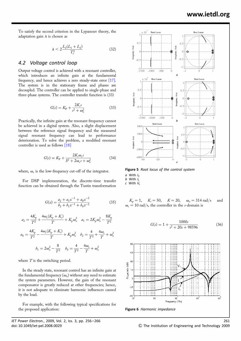
Figure 5 Root locus of the control system

a With ICb With ILc With VL

Figure 6 Harmonic impedance

261


262

& T

www.ietdl.org

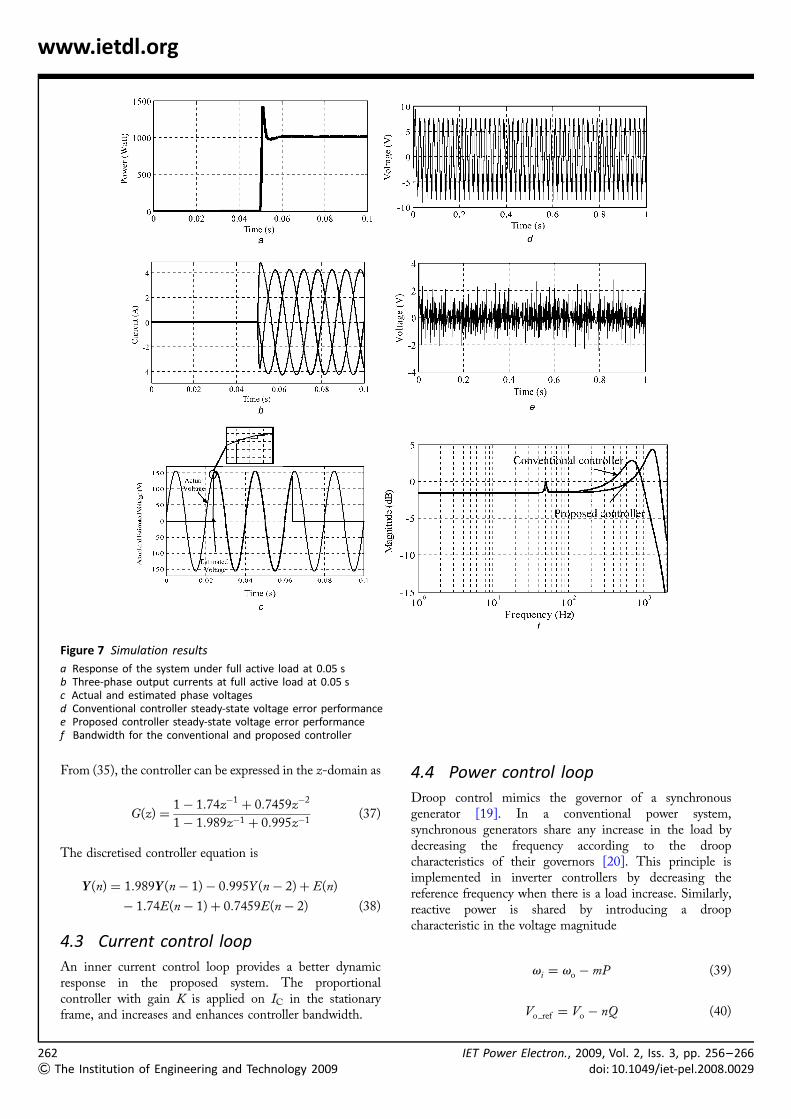
Figure 7 Simulation results

a Response of the system under full active load at 0.05 sb Three-phase output currents at full active load at 0.05 sc Actual and estimated phase voltagesd Conventional controller steady-state voltage error performancee Proposed controller steady-state voltage error performancef Bandwidth for the conventional and proposed controller

From (35), the controller can be expressed in the z-domain as

G(z) ¼1� 1:74z�1

þ 0:7459z�2

1� 1:989z�1 þ 0:995z�1(37)

The discretised controller equation is

Y (n) ¼ 1:989Y (n� 1)� 0:995Y (n� 2)þ E(n)

� 1:74E(n� 1)þ 0:7459E(n� 2) (38)

4.3 Current control loop

An inner current control loop provides a better dynamicresponse in the proposed system. The proportionalcontroller with gain K is applied on IC in the stationaryframe, and increases and enhances controller bandwidth.

he Institution of Engineering and Technology 2009

4.4 Power control loop

Droop control mimics the governor of a synchronousgenerator [19]. In a conventional power system,synchronous generators share any increase in the load bydecreasing the frequency according to the droopcharacteristics of their governors [20]. This principle isimplemented in inverter controllers by decreasing thereference frequency when there is a load increase. Similarly,reactive power is shared by introducing a droopcharacteristic in the voltage magnitude

vi ¼ vo � mP (39)

Vo ref ¼ Vo � nQ (40)


IETdoi:

www.ietdl.org

m ¼vo � v̂

P̂, n ¼

Vo � V̂

Q̂

V̂ is the maximum voltage at the maximum inductive load Q̂,Vo the nominal voltage for zero reactive load demand, v̂ theminimum frequency at the maximum active load P̂, vo thenominal frequency for no-load demand.

5 Stability and harmonicimpedance analysisControl system dynamics are investigated by using the rootlocus method. There are three control variables: filtercapacitor current (IC), filter inductor voltage (VL) andcurrent (IL). To control the output voltage, Vo is the outer-loop control variable, whereas the inner-loop controlvariable can either be IL, IC or VL. The control systemtransfer function is a function of the output referencevoltage and load current. The choice of the inner controlledvariable depends on the stability and power quality aspects.Equation (41) is the closed-loop transfer function with itsroot locus plot shown in Fig. 5a, when an outer resonantvoltage loop (Vo) and an inner proportional current loop(Ic) are used

Vo ¼KKps2

þ KKis þ KKpv2o

a4s4 þ a3s3 þ a2s2 þ a1s þ a0

V �o

� L2s þ R2 þL1s3þ R1s2

þ L1v2os þ R1v

2o


!ILoad

(41)

a4 ¼ L1C, a3 ¼ (R1 þ K )C , a2 ¼ L1Cv2o þ KKp þ 1

a1 ¼ (R1 þ K )Cv2o þ KKi, a0 ¼ (1þ KKp)v2

o

Fig. 5b shows the root locus of another transfer function,(42), for an outer resonant voltage loop (Vo) and an innerproportional current loop (IL)

Vo ¼KKps2

þ KKis þ KKpv2o


V �o

� L2s þ R2 þ

L1s3þ (R1 þ K )s2

þL1v2os þ (R1 þ K )v2

o


0BBB@

1CCCAILoad

(42)

a4 ¼ L1C, a3 ¼ (R1 þ K )C , a2 ¼ L1Cv2o þ KKp þ 1

a1 ¼ (R1 þ K )Cv2o þ KKi, a0 ¼ (1þ KKp)v2

o

Power Electron., 2009, Vol. 2, Iss. 3, pp. 256–26610.1049/iet-pel.2008.0029

Equation (43) is for an outer resonant loop (Vo) and aninner control loop (VL), and Fig. 5c shows the rootlocus for this transfer function. In the proposed controlsystem, the inner controlled variable depends on thestability and power quality aspects. The root loci in Fig. 5confirm that the capacitor and inductor currents give thebest degree of stability

Vo ¼KKps2

þKKisþKKpv2o

a4s4þ a3s3þ a2s2þ a1sþ a0

V �o

� L2sþR2þ

L1(I þK )s3þR1(I þK )s2

þv2oL1(1þK )sþv2

oR1(1þK )

a4s4þ a3s3þ a2s2þ a1sþ a0

0BBB@

1CCCAILoad

(43)

a4 ¼ L1C(1þK ), a3 ¼ R1C(1þK ),

a2 ¼ (1þK )v2oL1C þKKpþ 1

a1 ¼ (1þK )v2oR1C þKKi, a0 ¼ (1þKKp)v2

o

5.1 Harmonic impedance

The harmonic impedance is the second criteria that can beused to compare the performance of the three controlmethods. To minimise the harmonic voltage distortionfrom the inverter under distorted load conditions, theharmonic impedance should be ideally zero. That is, theinverter should produce zero harmonic voltage for allharmonic load currents. Fig. 6 shows a Bode magnitudeplot comparing the harmonic impedance for the inductorand capacitor currents, and inductor voltage feedback. Atlow frequencies, the harmonic impedances are

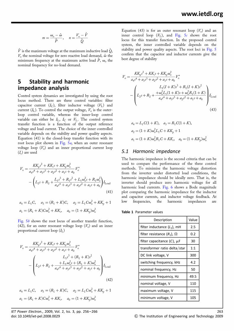
Table 1 Parameter values

Description Value

filter inductance (L1), mH 2.5

filter resistance (R1), V 0.2

filter capacitance (C ), mF 30

transformer ratio delta/star 1:1

DC link voltage, V 300

switching frequency, kHz 4.2

nominal frequency, Hz 50

minimum frequency, Hz 49.5

nominal voltage, V 110

maximum voltage, V 115

minimum voltage, V 105

263


264

&

www.ietdl.org

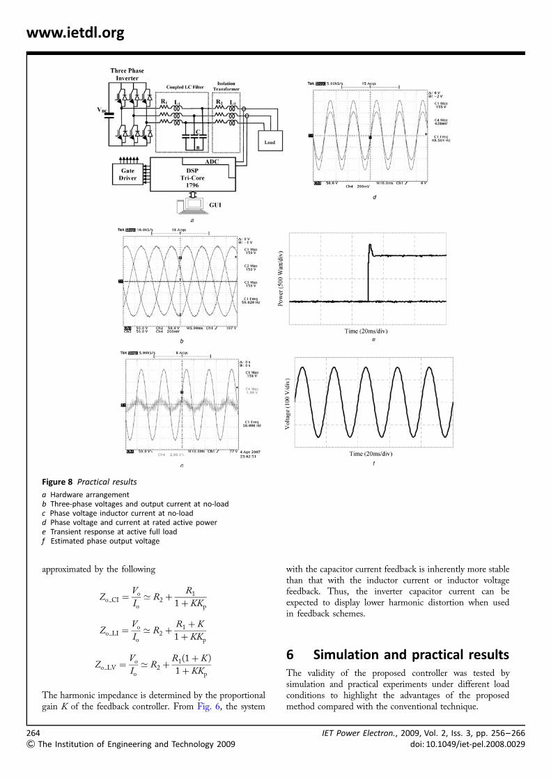
Figure 8 Practical results

a Hardware arrangementb Three-phase voltages and output current at no-loadc Phase voltage inductor current at no-loadd Phase voltage and current at rated active powere Transient response at active full loadf Estimated phase output voltage

approximated by the following

Zo CI ¼Vo

Io

’ R2 þR1

1þ KKp

Zo LI ¼Vo

Io

’ R2 þR1 þ K

1þ KKp

Zo LV ¼Vo

Io

’ R2 þR1(1þ K )

1þ KKp

The harmonic impedance is determined by the proportionalgain K of the feedback controller. From Fig. 6, the system


with the capacitor current feedback is inherently more stablethan that with the inductor current or inductor voltagefeedback. Thus, the inverter capacitor current can beexpected to display lower harmonic distortion when usedin feedback schemes.

6 Simulation and practical resultsThe validity of the proposed controller was tested bysimulation and practical experiments under different loadconditions to highlight the advantages of the proposedmethod compared with the conventional technique.


IETdoi:

www.ietdl.org

6.1 Simulation experiments

The performance of the proposed control algorithm isinvestigated using MATLAB/SIMULINK simulations.The control algorithm accounts for the sample and holdcircuit, measurement and computational delays, andquantisation effects. Fig. 7a shows the response of thesystem at full active load, whereas the corresponding three-phase output currents are shown in Fig. 7b. Fig. 7c illustratesthe actual and estimated phase output voltages, which showsthat estimation adaptation converges within 0.7 ms. Thesimulation results use the system parameters in Table 1.

The steady-state performance of the conventionalresonant controller without delay compensation, usingfilter capacitor current feedback, is shown in Fig. 7d.There is a slight steady-state error between the referencevoltage and the output voltage, because of the lowfeedback gain used to maintain system stability. There is atrade-off between the bandwidth and the stability limits.It can be concluded that the measurement delay in thecalculation of the control algorithm decreases feedbackgain to maintain stability, which reduces controllerbandwidth. The steady-state performance of the proposedcontroller shown in Fig. 7e has a lower steady-state error.This results because of the delay compensation techniqueused to overcome and enhance the controller bandwidthlimitation. The controller feedback gains are selected bysimulations to achieve the required performance. Thecontroller bandwidth was assessed from the Bode plot ofthe closed-loop transfer function for both the controllers,as shown in Fig. 7f. The proposed delay compensationtechnique enhances the bandwidth compared with theconventional controller.

6.2 Practical implementation

The experimental platform is shown in Fig. 8a. The commoncontrol algorithm was verified experimentally using a three-phase digitally controlled VSI with an LC filter andisolating transformer (to ensure zero DC current injection).The experimental system was implemented with the samesystem parameters as used in the simulation studies, shownin Table 1. An Infineon TriCoreTM TC1796 is used toimplement the algorithm. Fig. 8b shows the three-phaseoutput voltages and currents at no-load, whereas Fig. 8cshows the phase output voltage and inductor current at no-load Fig. 8c. The phase output voltage and output currentat full active power of 1 kW are shown in Fig. 8d. Fig. 8epresents the system transient response of the controllerunder a change in the active load step. The phase estimatedoutput voltage at full active load of 1 kW from the DSP isshown in Fig. 8f.

7 ConclusionThis paper proposes a sensorless method to control a DG inverterin an islanded mode. The controller structure with the different

Power Electron., 2009, Vol. 2, Iss. 3, pp. 256–26610.1049/iet-pel.2008.0029

control loops was investigated. An adaptive control algorithmwas embedded in the controller to estimate the output voltage.The selection of the system control variable is based on the twocriteria: root locus method and harmonic impedance.Simulation and experimental results demonstrated that thecontroller operates correctly, thus improving the power qualityand performance of DG inverter-based systems.

8 References

[1] BULL S.R.: ‘Renewable energy today and tomorrow’,Proc. IEEE, 2001, 89, (0018–9219), pp. 1216–1226

[2] KUKRER O.: ‘Deadbeat control of a three-phase inverterwith an output LC filter’, IEEE Trans. Power Electron.,1996, 11, pp 16–23

[3] MATTAVELLI P.: ‘An improved deadbeat control for UPSusing disturbance observers’, IEEE Trans. Ind. Electron.,2005, 52, pp. 206–212

[4] MARWALI M.N., JUNG J.W., KEYHANI A.: ‘Control of distributedgeneration systems – Part II: load sharing control’, IEEETrans. Power Electron., 2004, 19, pp. 1551–1561

[5] TULADHAR A., JIN H., UNGER T., MAUCH K.: ‘Control of parallelinverters in distributed ac power systems withconsideration of line impedance effect’, IEEE Trans. Ind.Appl., 2000, 36, pp. 131–138

[6] CHIANG S.J., LIN C.H., YEN C.Y.: ‘Current limitation control formulti-module parallel operation of UPS inverters’, IEE Proc.,Electr. Power Appl., 2004, 151, (6, 7), pp. 752–757

[7] SUN X., LEE Y.S., XU D.: ‘Modeling, analysis, andimplementation of parallel multi-inverter systems withinstantaneous average current sharing scheme’, IEEE TransPower Electron., 2003, 18, (3), pp. 844–856

[8] GUERRERO J.M., DEVICUNA L.G., MATAS J., CASTILLA M., MIRET J.:‘Output impedance design of parallel-connected UPSinverters with wireless load-sharing control’, IEEE Trans.Ind. Electron., 2005, 52, pp. 1126–1135

[9] DE BRABANDERE K., BOLSENS B., KEYBUS J.V.D., WOYTE A., DRIESEN J.,BELMANS R.: ‘A voltage and frequency droop control methodfor parallel inverters’, IEEE Trans. Power Electron., 2007,22, pp. 1107–1115

[10] GUERRERO J.M.: ‘A wireless controller to enhancedynamic performance of parallel inverters in distributedgeneration systems’, IEEE Trans. Power Electron., 2004,19, (5), pp. 1205–1213

[11] MOHAMED Y.A-R.I., EL-SAADANY E.F., EL-SHATSHAT R.A.: ‘Naturaladaptive observers-based estimation unit for robust grid-voltage sensorless control characteristics in inverter-based

265


266

&

www.ietdl.org

DG units’. IEEE Power Engineering Society General Meeting,2007, pp. 1–8

[12] AGIRMAN I., BLASKO V.: ‘A novel control method of a VSCwithout AC line voltage sensors’, IEEE Trans. Ind. Appl.,2003, 39, (2), pp. 519–524

[13] MALINOWKSI M., KAZMIERKOWSKI M.P., HANSEN S., BLAABJERG F.,MARQUES G.: ‘Virtual flux based direct power control ofthree-phase PWM rectifiers’, IEEE Trans. Ind. Appl., 2001,37, (4), pp. 1019–1027

[14] BHOWMIK S., ZYL A.V., SPEE R., ENSLIN J.H.R.: ‘Sensorlesscurrent control for active rectifiers’, IEEE Trans. Ind. Appl.,1997, 33, pp. 765–772

[15] GIRGIS A.A., CHANG W.B., MAKRAM E.B.: ‘A digital recursivemeasurement scheme for on-line tracking of powersystem harmonics’, IEEE Trans. Power Deliv., 1991, 6, (3),pp. 1153–1160


[16] HAYKIN S.: ‘Adaptive filter theory’ (Prentice-Hall, 1995,3rd edn.)

[17] ZMOOD D.N., HOLMES D.G.: ‘Stationary frame currentregulation of PWM inverters with zero steady-state error’,IEEE Trans. Power Electron., 2003, 18, pp. 814–822

[18] LOH P.C., NEWMAN M.J., ZMOOD D.N., HOLMES D.G.:‘A comparative analysis of multi-loop voltageregulation strategies for single and three-phase UPSsystems’, IEEE Trans. Power Electron., 2003, 18, (5),pp. 1176–1185

[19] KUNDUR P.: ‘Power system stability and control’(McGraw-Hill, New York, 1994)

[20] LI Y., VILATHGAMUWA D.M., LOH P.C.: ‘Design, analysis andreal-time testing of a controller for multibus microgridsystem’, IEEE Trans. Power Electron., 2004, 19, (5),pp. 1195–1204


Autonomous adaptive sensorless controller of inverter-based islanded-distributed generation system

Documents

Transcript of Autonomous adaptive sensorless controller of inverter-based islanded-distributed generation system