Hydrogeochemistry and Remote Sensing Yellowstone National Park
Upload
khangminh22Category
view
1download
0
Assessment of Irrigation
Performance by Remote Sensing
in the Naivasha Basin, Kenya
SAMMY MUCHIRI NJUKI
February, 2016
SUPERVISORS:
Dr. Zoltan Vekerdy
Dr. Ir. R. van der Velde


Thesis submitted to the Faculty of Geo-Information Science and Earth
Observation of the University of Twente in partial fulfilment of the
requirements for the degree of Master of Science in Geo-information Science
and Earth Observation.
Specialization: Water Resources and Environmental Management
SUPERVISORS:
Dr. Z. Vekerdy
Dr. Ir. R. van der Velde
THESIS ASSESSMENT BOARD:
Prof. Dr. Z. Su (Chair)
Dr. A. (Alain) Frances (External Examiner, National Laboratory for Energy
and Geology)
Assessment of Irrigation
Performance by Remote Sensing in
the Naivasha Basin, Kenya
SAMMY MUCHIRI NJUKI
Enschede, The Netherlands, February, 2016

DISCLAIMER
This document describes work undertaken as part of a programme of study at the Faculty of Geo-Information Science and
Earth Observation of the University of Twente. All views and opinions expressed therein remain the sole responsibility of the
author, and do not necessarily represent those of the Faculty.
i
ABSTRACT
Irrigation performance assessment is vital for effective water management especially in water-scarce areas.
In addition, it provides information needed to monitor crop water use and related productivity in irrigation
command areas. However, irrigation performance assessment is hampered by lack of necessary ground data
more so in developing countries. Advances in remote sensing technology and its applications have reduced
over reliance on ground data. This has led to a tremendous improvement in irrigation performance
assessment and monitoring in ground data scarce areas.
This research utilizes information derived from remote sensing to assess irrigation performance in the
commercial irrigation farms in the Naivasha basin, Kenya for the year 2014. It aims at quantifying irrigation
consumption by crops by use of remote sensing derived actual evapotranspiration. Consequently, irrigation
efficiency is assessed based on the derived irrigation consumption and irrigation water abstraction data.
The Surface Energy Balance System (SEBS) model was used together with MODIS land surface
temperature, variables derived from Landsat 8, meteorological data and MODIS monthly
evapotranspiration product to obtain monthly evapotranspiration estimates at 30 m spatial resolution. On
the other hand, CHIRPS rainfall product was combined with gauge rainfall data and information derived
from land use and land cover to derive monthly effective precipitation maps. Monthly irrigation
consumption was then computed from the difference between the two maps. Monthly irrigation efficiency
was finally obtained by comparing the monthly irrigation consumption to the monthly water abstraction
data.
Four farms were considered and the total amount of irrigation consumption in the year 2014, was found to
be 4 364 680 m3. The highest amount of irrigation consumption (471 147 m3) was obtained in July and the
lowest (275 467 m3) in September. Irrigation efficiency was computed for Vegpro Gorge farm only. An
average irrigation efficiency of 71% was obtained for 2014. Highest irrigation efficiency (88.5%) was in
March with the lowest (44.1%) being in September. High irrigation efficiencies were obtained for the wet
and the dry months with low efficiencies being obtained for the transition months between wet and dry
seasons.
It was concluded that reliance on rainfall data only in irrigation scheduling led to low irrigation efficiencies
during transition months. This is because the effect of soil moisture storage is not taken into account in
irrigation scheduling thus excess irrigation water is supplied. It is recommended to incorporate indicators
such as the aridity index in irrigation scheduling to improve the efficiency of the irrigation system.
KEY WORDS: Irrigation performance assessment, remote sensing, SEBS, Naivasha, irrigation efficiency,
Landsat 8, MODIS, CHIRPS.

ii
ACKNOWLEDGEMENTS
I take this opportunity to thank the Dutch Government, for financing my MSc studies through the NFP
scholarship scheme.
I express special gratitude to my supervisors Dr. Zoltan Vekerdy and Dr. Ir. Rogier van der Velde for their
unrelenting support throughout the period of this research. Special thanks to Dr. Zoltan for the help in
conceptualizing this research, valuable advice throughout the course of the research and positive criticism
of my work. You were always at my service even when I popped into your office without notice. To Dr
Rogier van der Velde, your help in image processing and valuable input into my research is highly
appreciated. I am greatly indebted sir.
Special thanks to Prof Wim Bastiaanssen, who through the meeting organized by Dr. Zoltan at Delft played
a key role in the conceptualization of this research.
I also acknowledge all the staff from the WREM department who shaped me academically. Without the
knowledge you imparted on me this fete would not have been achieved.
I sincerely thank Vincent Odongo for providing the flux tower data, land cover map and for the valuable
knowledge on working with the data. Special thanks to Dr. Joost Hoedjes for the help in facilitating my
field visits to the irrigation farms in Naivasha. Your help in obtaining data from the farms made this work
a success. I also appreciate the help accorded to me by Dominic Wambua, Henry Munyaka and other staff
at WRMA Naivasha in obtaining the necessary data for this research. I also thank my classmate Kingsley
Kwabena for his assistance during fieldwork.
To Kasera, Daniel, Kisendi, Amos, Lilian, Linus, Kibet, Mohammed, Kuzivakwashe, Asseyew, thank you
for your help in this research.
I also acknowledge my classmates, friends and the Kenyan community at ITC for the fun moments that we
shared during my stay in the Netherlands.
Last but not least, I acknowledge my family and Uncle Patrick’s family for their support and encouragement
throughout the course of my study. A big thank you, it is finally done.

i
TABLE OF CONTENTS
1. INTRODUCTION .............................................................................................................................................. 1
1.1. Background ...................................................................................................................................................................1 1.2. Problem statement ......................................................................................................................................................1 1.3. Objectives .....................................................................................................................................................................2 1.4. Research questions ......................................................................................................................................................2 1.5. Justification ...................................................................................................................................................................2
2. THEORETICAL BACKGROUND ................................................................................................................ 3
2.1. Irrigation performance assessment ..........................................................................................................................3 2.2. Evapotranspiration ......................................................................................................................................................4 2.3. Downscaling of evapotranspiration .........................................................................................................................7 2.4. Effective precipitation ................................................................................................................................................8
3. STUDY AREA AND DATA COLLECTION .............................................................................................. 9
3.1. Study area ......................................................................................................................................................................9 3.2. Fieldwork and data collection ................................................................................................................................ 10
4. SATELLITE DATA AND PROCESSING ................................................................................................ 15
4.1. Landsat 8 multispectral images .............................................................................................................................. 15 4.2. Downward shortwave surface flux ........................................................................................................................ 16 4.3. MODIS products ..................................................................................................................................................... 16 4.4. Shuttle Radar Topography Mission (SRTM DEM) ........................................................................................... 18 4.5. CHIRPs rainfall product ......................................................................................................................................... 18 4.6. ECMWF ERA-Interim Data .................................................................................................................................. 18
5. RESEARCH METHOD.................................................................................................................................. 19
5.1. Evapotranspiration computation ........................................................................................................................... 19 5.2. Computation of Irrigation Consumption ............................................................................................................. 28 5.3. Computation of Irrigation efficiency .................................................................................................................... 30
6. RESULTS AND DISCUSSIONS .................................................................................................................. 31
6.1. Evapotranspiration computation ........................................................................................................................... 31 6.2. Computation of irrigation consumption .............................................................................................................. 38 6.3. Irrigation efficiency .................................................................................................................................................. 43
7. CONCLUSION AND RECOMMENDATIONS ..................................................................................... 45
7.1. Conclusion ................................................................................................................................................................. 45 7.2. Recommendations .................................................................................................................................................... 45
ii
LIST OF FIGURES
Figure 1: Schema for SEBS model ............................................................................................................................. 7
Figure 2: Location of the study area ........................................................................................................................... 9
Figure 3: Drip irrigation system at Vegpro Gorge farm to the left and a centre pivot irrigation system at
Delamere Manera farm to the right .......................................................................................................................... 11
Figure 4: Daily rainfall totals to the left and the monthly rainfall totals for the four stations used in this
research ......................................................................................................................................................................... 12
Figure 5: Location of the MODIS tile H21V09 in the MODIS sinusoidal grid projection. Source (NASA,
2015). ............................................................................................................................................................................. 17
Figure 6: Flow chart of the research method .......................................................................................................... 19
Figure 7: Land use and land cover in the study area. Source (Vincent Odongo). ............................................ 23
Figure 8: SEBS interface in ILWIS showing the model inputs as applied for MODIS satellite overpass on
23/01/2014 .................................................................................................................................................................. 25
Figure 9: Hargreaves method derived reference ET ............................................................................................. 31
Figure 10: Energy balance closure for the flux tower in Naivasha ..................................................................... 32
Figure 11: ET derived using uncorrected latent heat flux to the left and the one obtained after correction
to the right .................................................................................................................................................................... 32
Figure 12: Original MODIS LST map to the left and the downscaled LST map to the right........................ 33
Figure 13: Plot showing the sensitivity of SEBS ET to the meteorological variables...................................... 34
Figure 14: Scatter plot between SEBS estimates and flux tower ET to the left and SEBS estimates and ET
crop to the right ........................................................................................................................................................... 35
Figure 15: Annual total ET map ............................................................................................................................... 36
Figure 16 Scatter plots between SEBS estimates and the flux ET to the left and SEBS estimates and ET
crop to the right ........................................................................................................................................................... 37
Figure 17: Monthly ET maps .................................................................................................................................... 38
Figure 18: Scatter plots of the daily gauge rainfall versus the daily CHIRPS rainfall estimates for the four
stations. ......................................................................................................................................................................... 39
Figure 19: Scatter plots between the monthly total gauge rainfall and the monthly total CHIRPS estimates
........................................................................................................................................................................................ 40
Figure 20: Line plots of the monthly total gauge rainfall and the monthly total CHIRPS estimates ............ 40
Figure 21: Decomposed CHIRPS biases for the four gauge stations in 2014 .................................................. 41
Figure 22: Comparison between irrigated area and the irrigation consumption per farm .............................. 43
Figure 23: Comparison between irrigation consumption and the aridity index ................................................ 43
Figure 24: Comparison between irrigation supply and the aridity index in Vegpro Gorge farm ................... 44
Figure 25: Relationship between rainfall and irrigation supply in Vegpro Gorge farm ................................... 44

iii
LIST OF TABLES
Table 1: Summary of irrigation data obtained from the farms ............................................................................ 11
Table 2: Satellite data products used and their sources ........................................................................................ 15
Table 3: Data used for Atmospheric correction and their sources..................................................................... 16
Table 4: Roughness parameter values associated with the land use map .......................................................... 24
Table 5: SEBS ET sensitivity analysis results ......................................................................................................... 34
Table 6: Statistical results of the error analysis on daily SEBS estimates .......................................................... 35
Table 7: Statistical results of the downscaled monthly ET .................................................................................. 37
Table 8: Statistical results of the analysis on the performance of the CHIRPS product ................................ 41
Table 9: Decomposed CHIRPS biases for the four gauge stations in 2014 ..................................................... 41
Table 10: Monthly irrigation consumption obtained for each of the four farms ............................................. 42
Table 11: Monthly irrigation efficiency in Vegpro gorge farm in 2014 ............................................................. 43

iv
LIST OF ABBREVIATIONS
AOT Aerosol Optical Thickness
CHIRPS Climate Hazards Group Infrared Precipitation with Station data
CMORPH Climate Prediction Centre Morphing Method
DEM Digital Elevation Model
DSSF Downward Shortwave Surface Flux
ECF Eddy Covariance Flux
ECMWF European Centre for Medium-Range Weather Forecasts
ET Evapotranspiration
EUMETSAT European Organization for the Exploitation of Meteorological Satellites
FAO Food and Agriculture Organization
FEWS NET Farming Early Warning System Network
GDAL Geospatial Data Abstraction Library
GIS Geographic information system
GPS Global Positioning System
HDF Hierarchical Data Format
IDL Interactive Data Language
ILWIS Integrated Land and Water Information System
ISOD In Situ and Online Data
ITCZ Inter-tropical Convergence Zone
KWSTI Kenya Wildlife Training Institute
LSA SAF Land Surface Analysis Satellite Applications Facility
LST Land surface temperature
MODIS Moderate Resolution Imaging Spectroradiometer
MSG METEOSAT Second Generation
NDVI Normalized Difference Vegetation Index
NetCDF Network Common Data Form
NIR Near-infrared
OLI Operational Land Imager
PBL Planetary Boundary Layer
PERSIANN Precipitation Estimation from Remotely Sensed Information using
Artificial Neural Networks
PET Potential evapotranspiration
RFE Rainfall Estimates
SEBAL Surface Energy Balance Algorithm for land
SEBS Surface Energy Balance System

v
SEVIRI Spinning Enhanced Visible and Infrared Imager
SMAC Simplified Model for Atmospheric Correction
SRTM Shuttle Radar Topography Mission
SZA Solar Zenith Angle
TAMSAT Tropical Applications of Meteorology using Satellite data and ground-
based observations
TIFF Tagged Image File Format
TIRS Thermal Infrared Sensor
TOA Top of Atmosphere
TRMM Tropical Rainfall Measuring Mission
USGS United States Geological Survey
WGS World Geodetic System
WRMA Water Resources Management Authority


ASSESSMENT OF IRRIGATION PERFORMANCE BY REMOTE SENSING IN THE NAIVASHA BASIN KENYA
1
1. INTRODUCTION
1.1. Background
Irrigation is the greatest consumer of the freshwater budget in the world. However, mainly due to poor
management of irrigation systems the cost benefit effects of irrigation especially in water-scarce
environments have been put into question (Perry, Steduto, Allen, & Burt, 2009).
Demand for more food production as a result of population growth has resulted in an increase in land under
irrigation especially in the arid and semi-arid areas. In these areas, irrigation represents the main water use
(Akdim et al., 2014). Most of the surface water sources in these areas are inadequate and are poorly
replenished leading to overexploitation of available ground water resources (Simons et al, 2015). As such,
assessment and monitoring of irrigation water use and practices is vital for effective water resources
management. However, lack of enough ground data in most areas hampers effective irrigation performance
assessment and consequently leads to poor management of water resources. Remote sensing approaches
require less ground data thus suited for applications in data poor areas.
Use of remote sensing in irrigation management started in the 1980’s due to challenges in obtaining the
necessary ground data continuously (Akdim et al., 2014). However, despite the huge potential offered by
this technology, it is largely underutilized in this field (Singh et al., 2013). Remote sensing has the ability to
provide the required data regularly and at the required spatial distribution for application in water resources
management.
Akdim et al. (2014) notes that, most of the early applications of remote sensing in irrigation focused on
relating the water allocations to the area under irrigation. Advances in technology and research have seen
the scope of application widen to other areas such as estimation of crop water requirements (Akdim et al.,
2014), water use mapping in irrigation (Gumma et al., 2011), estimation of crop coefficients (Gontia &
Tiwari, 2009), irrigation performance assessment (Bastiaanssen, et al, 1999), among others.
Irrigation performance assessment has traditionally been derived from information on water flow in canals
an approach which is very limited in terms of the scale of its application (Bastiaanssen & Bos, 1999). On the
other hand, evapotranspiration from an irrigated field provides a more representative picture of overall water
consumption by crops on the field at different scales. This is essential in effective management of irrigated
fields. Research nowadays is focused on the use of remote sensing to obtain some of the irrigation
performance indicators which can directly be related to evapotranspiration.
1.2. Problem statement
Lake Naivasha is an economically and ecologically important freshwater lake in the Kenyan Rift Valley. It is
the second Ramsar site in Kenya, signifying its importance to the delicate ecosystem it supports (van Oel
et al., 2013). Being a freshwater lake, coupled with a good agricultural environment, the lake supports a wide
range of agricultural activities through irrigation, the most prominent being horticulture. In addition, the
lake is used as a source of water for domestic and industrial use.
The horticultural industry in this area has experienced tremendous growth over the last decade. This has led
to an influx of people into Naivasha as a result of new income generating opportunities(Odongo et al.,

ASSESSMENT OF IRRIGATION PERFORMANCE BY REMOTE SENSING IN THE NAIVASHA BASIN KENYA
2
2014). Consequently, significant land use and land cover changes have occurred in the area over the same
period. All these factors have put a serious stress on the water resources of the lake. These have led to
dwindling water levels in the lake, a situation aggravated by climate change and the delicate dynamics
associated with lakes in the East African Rift system (Bergner et al., 2009).
According to van Oel et al. (2013), water abstractions for irrigation use have adverse effects on the
water resources of Lake Naivasha. Odongo et al. (2014) argue that irrigation and domestic water
use account for 71% of water abstracted from the lake either directly or indirectly from the aquifer connected
to the lake. In recent periods, the Water Resources Management Authority (WRMA) has been forced to
impose serious restrictions on water abstractions as a consequence of water scarcity. Although, such critical
decisions should be based on reliable information, WRMA suffers from shortage of data sound enough for
effective management of water resources (van Oel et al., 2013).
Efforts to improve on irrigation-related data collection have been made since the year 2008, with WRMA
making it mandatory for all the farmers to have metered water abstractions. However, acquiring data on
irrigation consumption and efficiency of water use remains a challenge for WRMA. As such, data on
irrigation performance is vital for the management of the water resources of the lake.
1.3. Objectives
The main objective of this research is to assess irrigation performance in commercial farms in Naivasha
basin (Kenya) using remote sensing.
The specific objectives of the research are to:
Determine actual evapotranspiration from open irrigated commercial farms in Naivasha basin from
remote sensing images
Compute the irrigation water consumption
Determine the irrigation efficiency
1.4. Research questions
Based on the objectives above, the research questions were as follows:
Does the remote sensing derived actual evapotranspiration match the evapotranspiration defined
from in-situ measurements?
How much of the actual evapotranspiration is from irrigation?
What is the efficiency of the irrigation system?
1.5. Justification
Efficient monitoring of irrigation water consumption and other aspects related to irrigation performance
using traditional methods is expensive and challenging (Bastiaanssen & Bos, 1999). Accurate estimation of
evapotranspiration (ET) at a relatively low cost by use of remote sensing is increasingly improving
monitoring of irrigation at the regional and field scale and more so in data poor areas (Singh, Senay, Velpuri,
Bohms, & Verdin, 2014). This research exploits the availability of free remote sensing imagery to help
improve access to information on irrigation consumption and efficiency of systems in use in commercial
farms in Naivasha. The outcome of this research will help WRMA in the implementation of efficient
management of the water resources of Lake Naivasha. The methodology used in this research can also be
adopted both by WRMA and the farmers for monitoring of irrigation performance thus improving on
decision making. In addition, information derived from the irrigation performance assessment is essential
in the implementation of best irrigation practices by the farmers hence improving on water use efficiency
and crop productivity.
ASSESSMENT OF IRRIGATION PERFORMANCE BY REMOTE SENSING IN THE NAIVASHA BASIN KENYA
3
2. THEORETICAL BACKGROUND
This chapter discusses the underlying principles of the methodology adopted in this research, as presented
in various literature sources. In addition, opinions of various researchers on the concepts and the results of
their applications are discussed in brief.
2.1. Irrigation performance assessment
Traditionally, irrigation performance indicators have been generated from data related to water flow into
irrigation command area obtained from flow measurement devices (Bastiaanssen & Bos, 1999). This limits
the number of indicators that can be derived from classical flow measurements since other sources of water
such as uptake from saturated zones cannot be quantified using this approach. In addition, irrigation
performance indicators related to crop growth are impossible to quantify based on measurements of
discharge into command area since the flow measurements do not account for other variables such as
fertility, salinity, soil moisture and farming practices (Bastiaanssen & Bos, 1999). Moreover, in most
irrigation command areas data necessary for quantifying irrigation performance is rarely collected and in the
few cases where it is available, its reliability is not guaranteed (Murray - Rust, 1994).
Most of the traditional as well as a host of other new indicators can be obtained from estimates of
evapotranspiration via remote sensing (e.g. Menenti, Visser, Morabito, & Drovandi, 1989; Bastiaanssen &
Bos, 1999; Er-Raki et al, 2010).
Adequacy, which is defined as the relative evaporation, is a good irrigation indicator on the water stress.
Bastiaanssen, Van der Wal, & Visser, (1996) successfully quantified adequacy, based on evaporative fraction
from remote sensing in the Nile delta in Egypt.
Equity is another important indicator that has been determined from remote sensing approaches. It is
determined by observing the spatial variation in the latent heat flux over the irrigated fields. Alexandridis,
Asif, & Ali (1999) used the actual ET derived from remote sensing to determine equity of water supply
between farmers in Fordwah, Pakistan.
Water productivity, which Bastiaanssen & Bos (1999) define as the amount of yield per unit volume of water
consumed is another indicator that has been derived from remote sensing. Droogers, Kite, & Bastiaanssen
(1999) were able to derive this indicator on a field scale and river basin scale in Turkey from remote sensing
as well.
Irrigation water use efficiency is another important indicator that has been evaluated widely using remote
sensing data. It is defined as the ratio of the yield of crop to the volume of irrigation supply (Perry, Steduto,
Allen, & Burt, 2009; Salama, Yousef, & Mostafa, 2015). Some of its applications are discussed extensively
in (Wu, et al, 2015, Bashir, et al, 2009, Bastiaanssen et al., 1996 and Akdim et al., 2014).
Irrigation efficiency as a performance indicator has been widely adopted in the field of irrigation
management. Jensen (1967) defined irrigation efficiency as the ratio of irrigation water consumption (the
volume of irrigation water lost through transpiration by plants, evaporation from the soil surface in irrigated
areas and evaporation of intercepted irrigation water) to the total volume of water supplied as irrigation.
Van Eekelen et al. (2015) refer to the difference between the irrigation water consumption and the total
ASSESSMENT OF IRRIGATION PERFORMANCE BY REMOTE SENSING IN THE NAIVASHA BASIN KENYA
4
volume of water supplied as incremental ET. They argue that conveyance losses, loss of water in the form
spray, run off of irrigated water and deep percolation account for the difference between incremental
evapotranspiration and the volume of water supplied for irrigation. As such, van Eekelen et al. (2015) define
irrigation efficiency as the ratio of incremental ET to the volume of water irrigated. Perry et al. (2009) and
Reinders, van der Stoep, & Backeberg (2013) use the term consumed fraction as an alternative to irrigation
efficiency. In the computation of irrigation efficiency by use of remote sensing the volume of water
consumed by crops is estimated directly from remote sensing and compared with the volume of irrigation
supply (van Eekelen et al., 2015).
2.2. Evapotranspiration
Evapotranspiration is defined as the sum of evaporation (direct conversion of water into vapour from wet
surfaces such as soil, water bodies and plant leaves) and transpiration (loss of water from the soil through
the leaves of plants) released into the atmosphere (Perry et al., 2009).
2.2.1. Reference evapotranspiration (ET0)
Allen, Pereira, Raes, & Smith (1998) define reference evapotranspiration as the evapotranspiration from a
reference surface, usually well watered grass with a height of 0.12 m. The recommended standard method
for the computation of reference evapotranspiration is the FAO Penman-Monteith method (Allen et al.,
1998). However, due to the large set of data needed to compute ET0 using this method, its applications is
limited in data scarce areas (Trajkovic, 2005). Various temperature-based empirical methods such as the
Blaney-Criddle, Thornwaite and the Hargreaves equation have been developed to compute ET0 in data
scarce environments. However, most of these methods require local calibration to be applicable in a wide
range of environments but the Hargreaves method, which shows good estimates of ET0 throughout a range
of global environments (Allen et al., 1998).
2.2.2. Potential evapotranspiration (PET)
Potential evapotranspiration of a particular crop refers to the reference evapotranspiration adjusted to the
characteristics of the crop (Perry et al., 2009). The characteristics of each crop are defined by the KC factor
as presented in Allen et al. (1998). Potential evapotranspiration thus defines the maximum amount of water
that a specific crop can evaporate under the prevailing environment with no limitations in water supply.
2.2.3. Actual evapotranspiration (ETa)
Actual evapotranspiration is defined as the actual amount water that is lost to the atmosphere from vegetated
surfaces. Under conditions of full water supply such as in fully irrigated surfaces or during wet seasons the
actual evapotranspiration is equal to the potential evapotranspiration (Perry et al., 2009).
Actual evapotranspiration from remote sensing can be estimated from either thermal or visible and NIR
remote sensing images. In visible/NIR remote sensing, indicators such as the NDVI are used together with
crop coefficients in equations such as the Penman-Monteith to obtain crop evapotranspiration (Akdim et
al., 2014). In thermal remote sensing, land surface temperature is derived and used in energy balance models
to estimate the turbulent fluxes of the energy balance equation. Some of the commonly used energy balance
models for the estimation of evapotranspiration based on thermal imagery are, SEBS (Z. Su, 2002), SEBAL
(Bastiaanssen, et al, 1998), furthermore, included but not limited to the TSEB, METRIC, Alexi, SEBI and
ETWatch models discussed in Karimi, Bastiaanssen, Molden, & Cheema (2013).
2.2.3.1. SEBS model
The Surface Energy Balance System, SEBS is a single source energy balance model used for the estimation
of turbulent energy fluxes based on the general energy balance equation (Su, 2002). It is widely used in the
ASSESSMENT OF IRRIGATION PERFORMANCE BY REMOTE SENSING IN THE NAIVASHA BASIN KENYA
5
modelling of evapotranspiration in data scarce environments since it mainly relies on remotely sensed inputs.
Su (2002) developed and applied the model on cotton data in Arizona, grasslands in Kendall and in Barrax,
Spain, where the model simulated the evaporative fraction and the turbulent fluxes with uncertainties
comparable to the ones observed with in situ measurements. Su, McCabe, Wood, Su, & Prueger (2005),
report that the model can quantify evapotranspiration with uncertainties within the range of 10-15% of in-
situ measurements. This is also supported by the work of Liou & Kar (2014) where the accuracy of most
energy balance models is reported to be within the range of 30% of the measured ET. The model was also
found to simulate evapotranspiration fairly well in the mainly agricultural area of the Nile delta (Elhag,
Psilovikos, Manakos, & Perakis, 2011). In the irrigated Mahidasht plains of Iran, SEBS, SEBAL and
lysimeter-based evapotranspiration were compared and SEBS estimates were found to match the
evapotranspiration derived from the lysimeter fairly well (Bansouleh, Karimi, & Hesadi, 2015).
However, according to Elhag et al. (2011) the model just like most of the other energy balance approaches
performs poorly over some large regions due to a mix of topographic effects and meteorological
inconsistencies. The model has also been found to overestimate ET in dry sparsely vegetated areas under
water limited conditions (Gokmen et al., 2013, Huang, et al., 2015, van der Kwast et al., 2009).
The model consists of tools for determining physical parameters of the land surface such as vegetation
coverage, leaf area index and height of vegetation based on spectral reflectance and radiances from remote
sensing observations. In addition, it also incorporates a model for estimating the roughness length for heat
transfer (Su, 2002). Based on these, the model estimates the evaporative fraction from a surface subject to
energy balance limiting conditions which are the wet and dry cases respectively. From the evaporative
fraction, daily evapotranspiration is calculated.
Based on Su (2002), the model principally comprises of the following main equations. Equation 2-1 is the
energy balance equation, which represents the energy balance terms of the system.
𝑅𝑛 = 𝐺0 + 𝐻 + 𝜆. 𝐸 2-1
Where, 𝑅𝑛 is the net radiation, 𝐻 is the sensible heat flux, 𝜆𝐸 is the latent heat flux and 𝐺0 is the ground
heat flux.
The ground heat flux (𝐺0) is heavily reliant on vegetation cover. As such, a ratio of the net radiation to the
ground heat flux is used in the parameterization of the ground heat flux term. It ranges between 0.05 for
full vegetation coverage (Γ𝑐) and 0.315 in bare land (Γ𝑠) (Kustas & Daughtry, 1990). Based on these
limiting ratios and the fractional vegetation coverage (𝑓𝑐) the ground heat flux term is calculated using
Equation 2-2.
𝐺0 = 𝑅𝑛. [𝛤𝑐 + (1 − 𝑓𝑐). (𝛤𝑠 − 𝛤𝑐)] 2-2
Where, 𝑓𝑐 is the fractional canopy coverage and Γ𝑐 𝑎𝑛𝑑 Γ𝑠 is the ratio of the ground heat flux to the net
radiation for full vegetation coverage and bare soil respectively.
To obtain the turbulent energy fluxes in Equation 2-1, the evaporative fraction needs to be estimated. To
achieve this, limiting wet and dry conditions must be defined. Evaporation is at its maximum under the
limiting wet conditions whereas the sensible heat flux tends to minimum. This situation is mathematically
defined by Equation 2-3.

ASSESSMENT OF IRRIGATION PERFORMANCE BY REMOTE SENSING IN THE NAIVASHA BASIN KENYA
6
𝐻𝑤𝑒𝑡 = 𝑅𝑛 − 𝐺0 − 𝜆𝑤𝑒𝑡 2-3
Where, 𝐻𝑤𝑒𝑡 𝑎𝑛𝑑 𝐻𝑑𝑟𝑦 is the sensible heat flux at limiting wet and dry conditions respectively and 𝜆𝑤𝑒𝑡 is
the latent heat of vaporization at limiting wet conditions
On the other hand, latent heat under the limiting dry conditions is almost negligible whereas the sensible
heat is at its maximum. This is formulated as shown in Equation 2-4.
𝐻𝑑𝑟𝑦 = 𝑅𝑛 − 𝐺0 2-4
As such, the evaporative fraction is deduced from the limiting wet conditions and the latent heat and is as
presented in Equation 2-5.
𝛬 =
𝜆𝐸
𝜆𝐸𝑤𝑒𝑡= 1 −
𝜆𝐸𝑤𝑒𝑡 − 𝜆𝐸
𝜆𝐸𝑤𝑒𝑡 2-5
Where, 𝜆𝐸𝑤𝑒𝑡 is the turbulent latent heat flux at limiting wet conditions and Λ is the evaporative fraction
On combining Equations 2-1, 2-2, 2-3, 2-4 and 2-5, the evaporative fraction can be derived from Equation
2-6.
𝛬 = 1 −
𝐻 − 𝐻𝑤𝑒𝑡
𝐻𝑑𝑟𝑦 − 𝐻𝑤𝑒𝑡 2-6
The evaporative fraction is assumed constant over the day and as such, based on equation 7, daily
evapotranspiration can be computed.
𝐸𝑑𝑎𝑖𝑙𝑦 = 𝛬24 × 8.64 × 107 ×
𝑅𝑛 − 𝐺0
𝜆𝜌𝜔 2-7
Where, 𝜌𝜔 is the density of water, Λ24 is the daily evaporative fraction and 𝐸𝑑𝑎𝑖𝑙𝑦 is the daily
evapotranspiration.
Detailed explanation and formulations of the SEBS model is presented in Su, (2002).
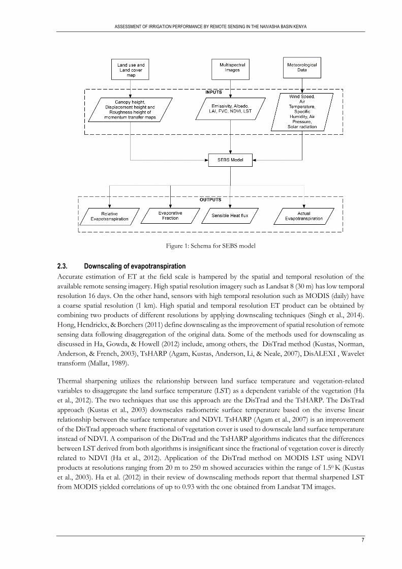
The schema of the model is shown in Figure 1.
ASSESSMENT OF IRRIGATION PERFORMANCE BY REMOTE SENSING IN THE NAIVASHA BASIN KENYA
7
Figure 1: Schema for SEBS model
2.3. Downscaling of evapotranspiration
Accurate estimation of ET at the field scale is hampered by the spatial and temporal resolution of the
available remote sensing imagery. High spatial resolution imagery such as Landsat 8 (30 m) has low temporal
resolution 16 days. On the other hand, sensors with high temporal resolution such as MODIS (daily) have
a coarse spatial resolution (1 km). High spatial and temporal resolution ET product can be obtained by
combining two products of different resolutions by applying downscaling techniques (Singh et al., 2014).
Hong, Hendrickx, & Borchers (2011) define downscaling as the improvement of spatial resolution of remote
sensing data following disaggregation of the original data. Some of the methods used for downscaling as
discussed in Ha, Gowda, & Howell (2012) include, among others, the DisTrad method (Kustas, Norman,
Anderson, & French, 2003), TsHARP (Agam, Kustas, Anderson, Li, & Neale, 2007), DisALEXI , Wavelet
transform (Mallat, 1989).
Thermal sharpening utilizes the relationship between land surface temperature and vegetation-related
variables to disaggregate the land surface temperature (LST) as a dependent variable of the vegetation (Ha
et al., 2012). The two techniques that use this approach are the DisTrad and the TsHARP. The DisTrad
approach (Kustas et al., 2003) downscales radiometric surface temperature based on the inverse linear
relationship between the surface temperature and NDVI. TsHARP (Agam et al., 2007) is an improvement
of the DisTrad approach where fractional of vegetation cover is used to downscale land surface temperature
instead of NDVI. A comparison of the DisTrad and the TsHARP algorithms indicates that the differences
between LST derived from both algorithms is insignificant since the fractional of vegetation cover is directly
related to NDVI (Ha et al., 2012). Application of the DisTrad method on MODIS LST using NDVI
products at resolutions ranging from 20 m to 250 m showed accuracies within the range of 1.50 K (Kustas
et al., 2003). Ha et al. (2012) in their review of downscaling methods report that thermal sharpened LST
from MODIS yielded correlations of up to 0.93 with the one obtained from Landsat TM images.
ASSESSMENT OF IRRIGATION PERFORMANCE BY REMOTE SENSING IN THE NAIVASHA BASIN KENYA
8
2.4. Effective precipitation
Jensen (1967) defines effective precipitation in the context of irrigation applications as the fraction of the
total precipitation that is available for use by crops. It refers to the total precipitation less the amount of
water lost as run off and deep percolation. Evaporation of water from wet soil surface and interception
from crop canopy is assumed beneficial to the crop. Bos, et al., (2009) define effective precipitation as the
fraction of the total precipitation available to meet the transpiration demand within a cropped area. Some
of the widely used methods in the estimation of effective precipitation for irrigation management include
the USDA method and the Curve Number method discussed in details in Bos, et al (2009). In addition to
these methods, various other empirical methods used in the estimation of effective precipitation are
discussed in Patwardhan, Nieber, & Johns (1990).
Another empirical method for computing effective precipitation was proposed by van Eekelen et al, (2015).
In this method, effective precipitation is computed from the ratio between actual ET from natural land use
classes and precipitation. This ratio represents the fraction of the total precipitation that is available for
consumption by natural vegetation. The method was successfully implemented to quantify incremental ET
as a result of irrigation and ground water abstractions in the Incomati basin, South Africa (van Eekelen et
al., 2015). The main advantage of this method is that effective precipitation is quantified based purely on
remote sensing thus very applicable in areas with limited ground data availability.
ASSESSMENT OF IRRIGATION PERFORMANCE BY REMOTE SENSING IN THE NAIVASHA BASIN KENYA
9
3. STUDY AREA AND DATA COLLECTION
3.1. Study area
3.1.1. Location
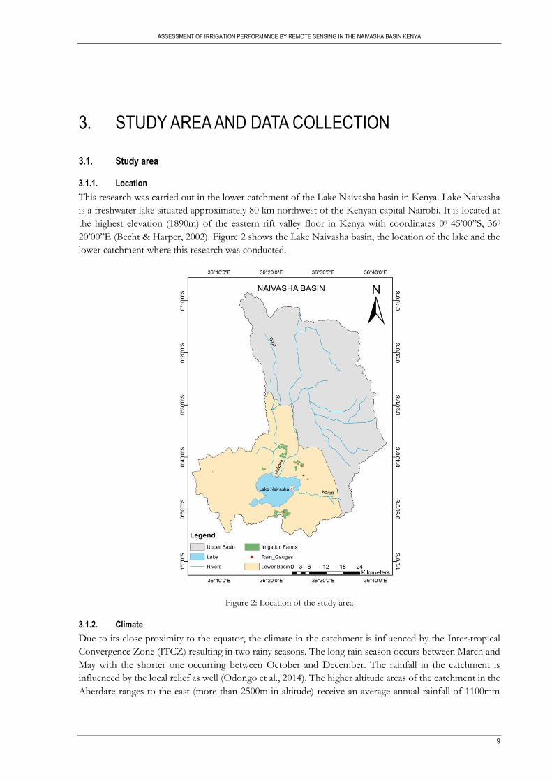
This research was carried out in the lower catchment of the Lake Naivasha basin in Kenya. Lake Naivasha
is a freshwater lake situated approximately 80 km northwest of the Kenyan capital Nairobi. It is located at
the highest elevation (1890m) of the eastern rift valley floor in Kenya with coordinates 00 45’00’’S, 360
20’00’’E (Becht & Harper, 2002). Figure 2 shows the Lake Naivasha basin, the location of the lake and the
lower catchment where this research was conducted.
Figure 2: Location of the study area
3.1.2. Climate
Due to its close proximity to the equator, the climate in the catchment is influenced by the Inter-tropical
Convergence Zone (ITCZ) resulting in two rainy seasons. The long rain season occurs between March and
May with the shorter one occurring between October and December. The rainfall in the catchment is
influenced by the local relief as well (Odongo et al., 2014). The higher altitude areas of the catchment in the
Aberdare ranges to the east (more than 2500m in altitude) receive an average annual rainfall of 1100mm

ASSESSMENT OF IRRIGATION PERFORMANCE BY REMOTE SENSING IN THE NAIVASHA BASIN KENYA
10
compared to an annual average of 600mm at the lake (Becht & Harper, 2002). The daily mean temperature
varies from 80 C in the upper parts of the catchments to 300 C at the lake.
3.1.3. Hydrology
Lake Naivasha is a shallow lake, 6-8 m deep that covers a surface area of 139km2. The total catchment area
of the basin is approximately 3400 km2.The main inflow of water into the lake is from rivers Malewa and
Gilgil which are perennial and originate from the upper wetter catchment areas in the Aberdares. Several
other streams flow seasonally towards the lake with Karati the only one reaching the lake during periods of
intense rain (Odongo et al., 2014). The lake has no visible surface water outlet and its freshness is attributed
to ground water outflow towards the southwest, feeding into the Olkaria hot springs (Ojiambo, Poreda, &
Lyons, 2001).
3.1.4. Irrigation
In the last three decades, the basin has experienced tremendous growth in horticultural farming (Mekonnen,
Hoekstra, & Becht, 2012). The upper catchment of the basin consists of small scale farmers who primarily
rely on rainfall for farming. The lower parts of the catchments, particularly the areas around the lake, are
occupied by large scale commercial irrigation farms. They mainly rely on freshwater from the lake for
irrigation and their produce is mainly for export. According to Mekonnen et al. (2012) the commercial farms
under irrigation occupy an area of 4,450 ha of which cut flowers occupy 43% of the area (characteristically
in greenhouses), followed by vegetables with 41% and the rest is mainly fodder crop (Musota, 2008).
Vegetables and fodder are mainly grown in open irrigation farms.
3.2. Fieldwork and data collection
For this research, a fieldwork was conducted between September 21 and October 9, 2015 in view of
obtaining the necessary primary as well as secondary data. The fieldwork comprised of the following
activities
Collecting of data on open commercial irrigation farms in the lower catchment of the Naivasha
basin.
Obtaining data on water abstraction from the Lake and connected aquifers by the open commercial
irrigation farms
Collecting meteorological data
Land use and land cover mapping in the lower catchment
3.2.1. Data on open commercial irrigation farms
The fieldwork data collection exercise was aimed at acquiring irrigation data from open commercial
irrigation farms in the lower catchment. Some of these farms are Vegpro K. Ltd, Finlays Kingfisher farm,
Delamere Manera farm, Loldia farm and Marula farm, among others. However, fieldwork was carried out
in Loldia farm, Delamere Manera farm and the two farms belonging to Vegpro K. Ltd (Vegpro Gorge farm
and Vegpro Delamere Pivots) only. Authority to carry out fieldwork in Marula farm and Finlays Kingfisher
farm was denied.
During the field work, GPS positions of the various irrigation blocks per farm were taken for identification
on the GIS system and subsequent digitizing of the farms. The crop types as well as the irrigation systems
in use per block on each farm were also identified. Data on the irrigated area, the type of irrigation systems
in use as well as the source of water in each farm was obtained as well. An overview of the data obtained
from the farms is shown in Table 1. Detailed data on crops grown in the farms is presented in the
appendices.

ASSESSMENT OF IRRIGATION PERFORMANCE BY REMOTE SENSING IN THE NAIVASHA BASIN KENYA
11
Table 1: Summary of irrigation data obtained from the farms
Farm Total
Area (ha)
Drip Irrigated
Area (ha)
Pivot Irrigated
Area (ha)
Crops Grown Water
Source
Vegpro Gorge
Farm
503 301 202 Assorted
Vegetables
Lake
Vegpro
Delamere
Pivots
179 32 147 Assorted
Vegetables
Borehole
Delamere
Manera Farm
127 0 127 Fodder crops Borehole
Loldia Farm 74 0 74 Assorted
Vegetables
Lake and
Boreholes
The two types of irrigation systems used in the farms are shown in the images shown in Figure 3.
Figure 3: Drip irrigation system at Vegpro Gorge farm to the left and a centre pivot irrigation system at Delamere Manera farm to the right
3.2.2. Water abstraction data
Water abstraction data was obtained from both the farms and WRMA Naivasha offices. The source of water
for each of the farm is indicated in Table 1. Full water abstraction records for the year 2014 were available
for Vegpro Gorge farm and Loldia farm only. However lease of water to other farmers by Loldia farm made
it difficult to ascertain the actual amount of water supplied to their farm. Vegpro Delamere pivots on the
other hand did not have reliable water abstraction records since some of their meters occasionally
experienced breakdowns. As such, water abstraction from some of their boreholes was unmetered in some
months. This was attributed to silt in the borehole water which led to constant mechanical failure in the
metering systems. As for Delamere Manera farm, water abstraction records were unavailable owing to
breakdown in their metering system. The monthly water abstraction records for each of the farms are shown
in the appendix.
3.2.3. Precipitation data
Precipitation data was collected for the rain gauge stations within the lower catchment. Data was obtained
for both the stations managed by WRMA and the farms. In addition, rainfall data from the gauge station at
the eddy covariance flux (ECF) tower site at the Kenya Wildlife Training Institute (KWSTI) was also
ASSESSMENT OF IRRIGATION PERFORMANCE BY REMOTE SENSING IN THE NAIVASHA BASIN KENYA
12
collected. All the farms were found to use manual rain gauges for recording rainfall. On the other hand,
WRMA was found to use both manual and telemetric rain gauges to record rainfall. The stations for which
data was collected, their location and type of rain gauge used are shown in the appendix.
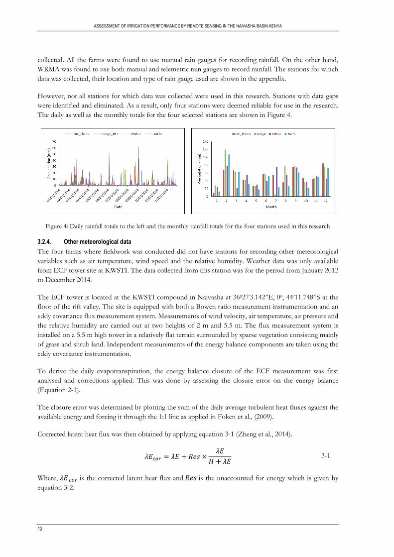
However, not all stations for which data was collected were used in this research. Stations with data gaps
were identified and eliminated. As a result, only four stations were deemed reliable for use in the research.
The daily as well as the monthly totals for the four selected stations are shown in Figure 4.
Figure 4: Daily rainfall totals to the left and the monthly rainfall totals for the four stations used in this research
3.2.4. Other meteorological data
The four farms where fieldwork was conducted did not have stations for recording other meteorological
variables such as air temperature, wind speed and the relative humidity. Weather data was only available
from ECF tower site at KWSTI. The data collected from this station was for the period from January 2012
to December 2014.
The ECF tower is located at the KWSTI compound in Naivasha at 36027’3.142’’E, 00, 44’11.748”S at the
floor of the rift valley. The site is equipped with both a Bowen ratio measurement instrumentation and an
eddy covariance flux measurement system. Measurements of wind velocity, air temperature, air pressure and
the relative humidity are carried out at two heights of 2 m and 5.5 m. The flux measurement system is
installed on a 5.5 m high tower in a relatively flat terrain surrounded by sparse vegetation consisting mainly
of grass and shrub land. Independent measurements of the energy balance components are taken using the
eddy covariance instrumentation.
To derive the daily evapotranspiration, the energy balance closure of the ECF measurement was first
analysed and corrections applied. This was done by assessing the closure error on the energy balance
(Equation 2-1).
The closure error was determined by plotting the sum of the daily average turbulent heat fluxes against the
available energy and forcing it through the 1:1 line as applied in Foken et al., (2009).
Corrected latent heat flux was then obtained by applying equation 3-1 (Zheng et al., 2014).
𝜆𝐸𝑐𝑜𝑟 = 𝜆𝐸 + 𝑅𝑒𝑠 ×
𝜆𝐸
𝐻 + 𝜆𝐸 3-1
Where, 𝜆𝐸 𝑐𝑜𝑟 is the corrected latent heat flux and 𝑅𝑒𝑠 is the unaccounted for energy which is given by
equation 3-2.

ASSESSMENT OF IRRIGATION PERFORMANCE BY REMOTE SENSING IN THE NAIVASHA BASIN KENYA
13
𝑅𝑒𝑠 = 𝑅𝑛 − (𝐻 + 𝜆𝐸 + 𝐺0) 3-2
This energy balance closure correction approach is based on the assumption that the Bowen ratio is correctly
measured by the ECF system and the closure error is associated with turbulent energy fluxes and not the
available energy (Zheng et al., 2014).
Evapotranspiration was then derived from the corrected latent heat flux using equation 3-3.
𝐸𝑇 = (
𝜆𝐸
𝜆) 3-3
Where, 𝜆𝐸 is the latent heat of vaporization (2.45 MJ kg-1).


ASSESSMENT OF IRRIGATION PERFORMANCE BY REMOTE SENSING IN THE NAIVASHA BASIN KENYA
15
4. SATELLITE DATA AND PROCESSING
Various satellite data and products were used as inputs to the SEBS model as well as in the downscaling of
SEBS derived ET estimates and for obtaining spatially distributed rainfall estimates. These satellite data and
products were downloaded free of charge from open source databases. The satellite data and products
downloaded are shown in Table 2.
Table 2: Satellite data products used and their sources
Product Source
Landsat 8 images http://earthexplorer.usgs.gov.
MODIS MOD11A1 LST https://lpdaac.usgs.gov/data_access/data_pool
MODIS MOD16A2 ET product http://www.ntsg.umt.edu/project/mod16#data-product
LSA SAF DSSF https://landsaf.ipma.pt/products/prods.jsp
CHIRPS Rainfall product http://chg.geog.ucsb.edu/data/index.html
SRTM DEM http://earthexplorer.usgs.gov.
Planetary boundary layer height http://apps.ecmwf.int/datasets/data/interim-full-daily/levtype=sfc/
Sunshine hours http://apps.ecmwf.int/datasets/data/interim-full-daily/levtype=sfc/
4.1. Landsat 8 multispectral images
Fourteen Landsat 8 images with less than 10% cloud cover corresponding to path 169 and row 60 were
downloaded for the year 2014. These images were in unsigned 16 bit digital number format. They were then
converted into reflectance and radiances. Finally, the area of study was extracted by creating a sub map in
ILWIS using the coordinates of the bounding box of the catchment shape file.
4.1.1. Conversion to TOA reflectance and radiance
Conversion of the images into TOA reflectance and radiances for the VIS/NIR and the TIRS bands
respectively was implemented using equations 4-1, 4-2 and 4-3 (USGS, 2015b).
𝐿𝜆 = 𝑀𝐿𝑄𝑐𝑎𝑙 + 𝐴𝐿 4-1
𝜌𝜆′ = 𝑀𝜌𝑄𝑐𝑎𝑙 + 𝐴𝜌 4-2
𝜌𝜆 =
𝜌𝜆′
𝑐𝑜𝑠 (𝜃𝑠𝑧) 4-3
Where, 𝐿𝜆 is the TOA spectral radiance (W m-2.srad-1.μm-1), 𝑀𝐿 is the band specific radiance multiplicative
rescaling factor, 𝐴𝐿 is the radiance additive rescaling factor, 𝑄𝑐𝑎𝑙 is the DN value, 𝜌𝜆′ is the TOA
reflectance (-) uncorrected for the influence of the solar angle, 𝑀𝜌 is the band specific reflectance

ASSESSMENT OF IRRIGATION PERFORMANCE BY REMOTE SENSING IN THE NAIVASHA BASIN KENYA
16
multiplicative rescaling factor, 𝐴𝜌 is the reflectance additive rescaling factor, 𝜌𝜆 is the TOA reflectance (-)
corrected for the solar angle and 𝜃𝑠𝑧 is the local solar zenith angle.
The scale factors were obtained from the metadata file downloaded together with the images.
4.1.2. Atmospheric correction
To obtain the reflectance at the surface, the effects of atmospheric absorption and scattering were removed.
This was achieved by applying the SMAC algorithm (Rahman & Dedieu 1994) to the radiometrically
calibrated visible and near infra-red bands. Data on the aerosol optical thickness (AOT) at 550nm, ozone
content, water vapour as well as the sensor coefficient file used in the process of atmospheric correction
were obtained from the sites presented in Table 3. The atmospheric correction process was implemented
via the SMAC extension in ILWIS.
Table 3: Data used for Atmospheric correction and their sources
Atmospheric Correction Data Source
AOT 550 nm http://aeronet.gsfc.nasa.gov/.
Ozone content [atm.cm] http://macuv.gsfc.nasa.gov/.
Water vapour [gm.cm-2] http://giovanni.gsfc.nasa.gov/giovanni/
Sensor coefficients http://www.cesbio.ups-tlse.fr/fr/smac_telech.htm
4.2. Downward shortwave surface flux
To compute the net radiation, SEBS model requires an input of the instantaneous down-welling shortwave
radiation. The downward shortwave surface flux (DSSF), product used in this research is derived from three
shortwave bands, in the visible, near infra-red and the shortwave infra-red of the SEVIRI instrument aboard
the Meteosat Second Generation (MSG) weather satellite (EUMETCAST, 2015). The DSSF product is
available at the full coverage of the MSG disc at a temporal resolution of 30 minutes. The spatial resolution
of the product at the equator where the study area for this research lies is 3 km. The algorithm used to derive
the DSSF product is discussed in details in Geiger et al. (2008) .
The product was downloaded in the HDF 5 file format and an IDL script1 was used to convert the files into
Geo TIFF format. The converted files were then imported into ILWIS raster formats. A sub map of the
study area was then created for each file. The files were then resampled to the spatial resolution of Landsat
8 (30 m) using the bilinear interpolation method.
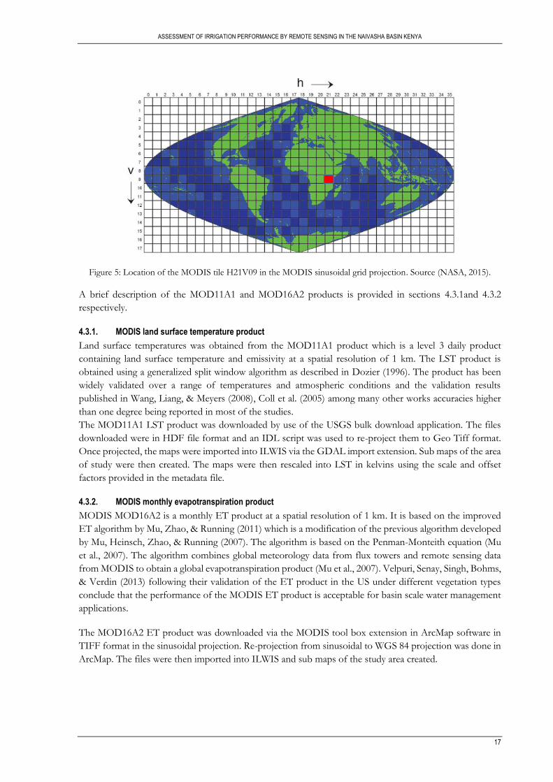
4.3. MODIS products
The two MODIS products used in this research were downloaded from the sites indicated in Table 2. Both
products were obtained for the MODIS tile H21V09 within which the study area lies as indicated in Figure
5. Both products were downloaded in sinusoidal projection.
1 Obtained from van der Velde, R.
ASSESSMENT OF IRRIGATION PERFORMANCE BY REMOTE SENSING IN THE NAIVASHA BASIN KENYA
17
Figure 5: Location of the MODIS tile H21V09 in the MODIS sinusoidal grid projection. Source (NASA, 2015).
A brief description of the MOD11A1 and MOD16A2 products is provided in sections 4.3.1and 4.3.2
respectively.
4.3.1. MODIS land surface temperature product
Land surface temperatures was obtained from the MOD11A1 product which is a level 3 daily product
containing land surface temperature and emissivity at a spatial resolution of 1 km. The LST product is
obtained using a generalized split window algorithm as described in Dozier (1996). The product has been
widely validated over a range of temperatures and atmospheric conditions and the validation results
published in Wang, Liang, & Meyers (2008), Coll et al. (2005) among many other works accuracies higher
than one degree being reported in most of the studies.
The MOD11A1 LST product was downloaded by use of the USGS bulk download application. The files
downloaded were in HDF file format and an IDL script was used to re-project them to Geo Tiff format.
Once projected, the maps were imported into ILWIS via the GDAL import extension. Sub maps of the area
of study were then created. The maps were then rescaled into LST in kelvins using the scale and offset
factors provided in the metadata file.
4.3.2. MODIS monthly evapotranspiration product
MODIS MOD16A2 is a monthly ET product at a spatial resolution of 1 km. It is based on the improved
ET algorithm by Mu, Zhao, & Running (2011) which is a modification of the previous algorithm developed
by Mu, Heinsch, Zhao, & Running (2007). The algorithm is based on the Penman-Monteith equation (Mu
et al., 2007). The algorithm combines global meteorology data from flux towers and remote sensing data
from MODIS to obtain a global evapotranspiration product (Mu et al., 2007). Velpuri, Senay, Singh, Bohms,
& Verdin (2013) following their validation of the ET product in the US under different vegetation types
conclude that the performance of the MODIS ET product is acceptable for basin scale water management
applications.
The MOD16A2 ET product was downloaded via the MODIS tool box extension in ArcMap software in
TIFF format in the sinusoidal projection. Re-projection from sinusoidal to WGS 84 projection was done in
ArcMap. The files were then imported into ILWIS and sub maps of the study area created.
ASSESSMENT OF IRRIGATION PERFORMANCE BY REMOTE SENSING IN THE NAIVASHA BASIN KENYA
18
4.4. Shuttle Radar Topography Mission (SRTM DEM)
In this research, a digital elevation model was used as one of the inputs into SEBS. The, SRTM DEM with
a spatial resolution of 30m (1 arc second) was used. The DEM comes already void filled by use of
interpolation techniques and other sources of elevation data as described in USGS (2015a). The DEM was
downloaded as a Geo TIFF. It was then imported into ILWIS where the area of study was extracted by
creating a sub map using the corner coordinates of the catchment shape file.
4.5. CHIRPs rainfall product
The Climate Hazard Group Infrared Precipitation with Station (CHIRPS) rainfall product is a 0.050 spatial
resolution quasi-global product (Funk et al., 2015). The rainfall product is available on a daily, five days and
monthly temporal resolutions. To derive this product, thermal infra-red cold cloud duration (CCD) derived
rainfall estimates are calibrated with monthly climatology precipitation derived from gauge data (Funk et al.,
2015).
Toté et al. (2015)compared the performance of CHIRPS, TAMSAT and FEWS NET RFE in Mozambique
where they found the CHIRPS product to outperform the rest especially under intense rainfall events.
However they note that the product was not performing well under periods of light rain. Ceccherini,
Ameztoy, Hernández, & Moreno (2015) tested downscaled TRMM 3B43, PERSIAN CDR, CMORPH,
CHIRPS, RFE and TAMSAT in South America and West Africa and found the downscaled CHIRPS
product to have the best performance statistics for both regions.
Selection of the product was mainly based on its high spatial resolution (approximately 5 km) compared to
the rest e.g. approximately 25 km for TRMM. Also, based on literature the performance of the product
especially in tropical regions appears reasonably good.
Daily CHIRPS rainfall maps were downloaded via the ISOD toolbox in ILWIS for the African region for
the year 2014. A sub map of the area of study was then created for each daily map using the corner
coordinates of the catchment shape file in ILWIS. Map lists of the daily sub maps were then created for
each month. The map list statistics function in ILWIS was then used to sum the maps in each map list to
obtain the monthly total precipitation maps. The annual total precipitation map was then obtained by
summing the twelve monthly total precipitation maps.
4.6. ECMWF ERA-Interim Data
Data on Planetary boundary layer height (PBL) and the number of sunshine hours per day was obtained
from the European Centre for Medium-Range Weather Forecasts (ECMWF). The datasets were obtained
from the publicly accessible ECMWF Interim Reanalysis (ERA-Interim) data set which is available as a
continuously updated reanalysis of the global atmosphere (ECMWF, 2015). Description of the model,
datasets used and the performance of the various model outputs are extensively discussed in (Dee et al.,
2011).
Both datasets were downloaded in the Network Common Data Format (NetCDF) in grids of 0.1250
resolution. The datasets were then converted into Geo Tiff format by use of IDL scripts. The files were
then imported into ILWIS where a sub map of the study area was created.
ASSESSMENT OF IRRIGATION PERFORMANCE BY REMOTE SENSING IN THE NAIVASHA BASIN KENYA
19
5. RESEARCH METHOD
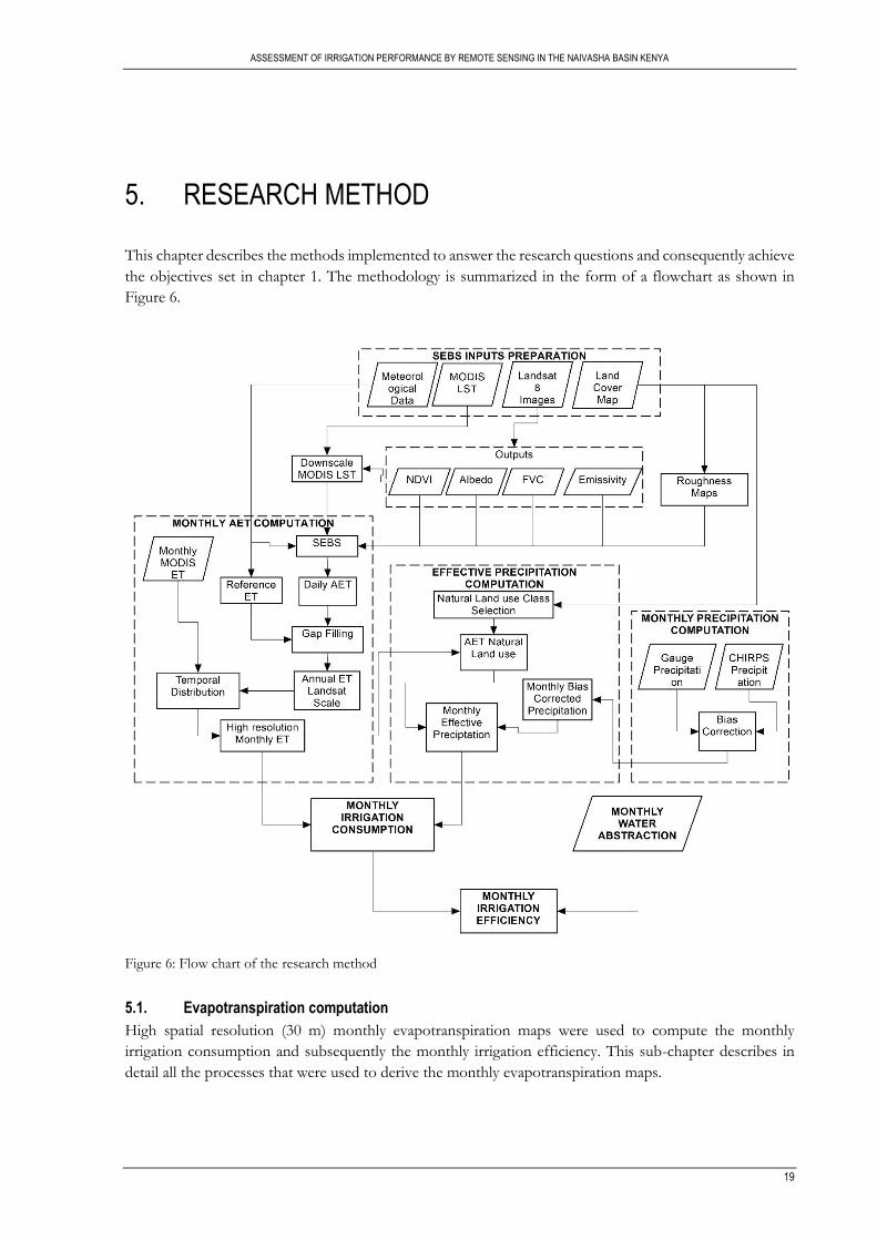
This chapter describes the methods implemented to answer the research questions and consequently achieve
the objectives set in chapter 1. The methodology is summarized in the form of a flowchart as shown in
Figure 6.
Figure 6: Flow chart of the research method
5.1. Evapotranspiration computation
High spatial resolution (30 m) monthly evapotranspiration maps were used to compute the monthly
irrigation consumption and subsequently the monthly irrigation efficiency. This sub-chapter describes in
detail all the processes that were used to derive the monthly evapotranspiration maps.
ASSESSMENT OF IRRIGATION PERFORMANCE BY REMOTE SENSING IN THE NAIVASHA BASIN KENYA
20
5.1.1. Preparation of SEBS model inputs
SEBS model requires three sets of inputs to accurately model evaporative fraction on a pixel at the time of
satellite overpass and consequently the daily evapotranspiration.
The first set consists of inputs derived from remote sensing images. Remote sensing inputs are obtained
from the visible, near infra-red and thermal infra-red bands of multispectral images. The variables derived
include land surface temperature, emissivity, NDVI, albedo and the FVC.
The second set of inputs is meteorology-related data. These data are derived from observations made at
weather stations. The meteorological inputs required are air temperature, air pressure, wind speed and the
specific humidity all measured at a reference height. In addition, data on short wave incoming radiation,
sunshine hours in a day and the planetary boundary layer height are also necessary inputs into the model.
The third set consists of inputs derived from land use and land cover maps. Land use and land cover maps
are needed to derive parameters related to surface roughness. These include the canopy height, the
displacement height and the roughness height maps. This set of inputs is important since the parameters
defined from it highly influence the turbulent heat fluxes and to a great extent the accuracy of the derived
evapotranspiration maps.
The preparation of each of the inputs is described in the following sections.
5.1.1.1. Normalized Difference Vegetation Index
The Normalized Difference Vegetation Index was computed from band 4 and 5 of the radio metrically
calibrated and atmospherically corrected OLI bands (Equation 5-1). Band 4 and 5 are the Red and NIR
bands of the Landsat 8 OLI sensor respectively.
𝑁𝐷𝑉𝐼 =
𝜌5 − 𝜌4
𝜌5 + 𝜌4 5-1
Where, 𝜌5 is the reflectance of the Near Infra-red band and 𝜌4 is the reflectance of the red band.
5.1.1.2. Fraction vegetation cover
The NDVI derived in Equation 5-1 was used to derive the fraction of vegetation cover maps based on
Equation 5-2. This equation requires representative NDVI values for bare soil and fully vegetated cover.
𝐹𝑉𝐶 =
𝑁𝐷𝑉𝐼 − 𝑁𝐷𝑉𝐼𝑠
𝑁𝐷𝑉𝐼𝑣 − 𝑁𝐷𝑉𝐼𝑠 5-2
Where 𝑁𝐷𝑉𝐼𝑣 is the representative NDVI of full vegetation coverage and 𝑁𝐷𝑉𝐼𝑠 is the representative
NDVI of bare soil.
The values of NDVIs and NDVIv were chosen to be 0.15 and 0.9 respectively based on the work of Jiménez-
Muñoz et al. (2009) on the application of the methodology on high spatial resolution imagery.
5.1.1.3. Land surface emissivity
Broad band land surface emissivity was calculated empirically using Equation 5-3, which was proposed by
Sobrino, Jiménez-Muñoz, & Paolini (2004) for Landsat imagery.
휀 = 0.004 × 𝐹𝑉𝐶 + 0.986 5-3
ASSESSMENT OF IRRIGATION PERFORMANCE BY REMOTE SENSING IN THE NAIVASHA BASIN KENYA
21
5.1.1.4. Albedo
The shortwave albedo was computed from bands 2 to 7 of the OLI sensor which span the entire visible and
near-infrared spectrum based on Equation 5-4 (Liang, 2001).
𝛼𝑠ℎ𝑜𝑟𝑡 = 0.3562𝜌2 + 0.130𝜌4 + 0.373𝜌5 + 0.085𝜌6 + 0.072𝜌7 − 0.0018 5-4
Where, 𝛼𝑠ℎ𝑜𝑟𝑡 is the shortwave albedo and 𝜌𝑖 is the reflectance of bands 2, 4, 5, 6 and 7.
5.1.1.5. Land surface temperature
The USGS has raised concerns about the quality of the thermal bands in Landsat 8 and the consequent
quality of LST derived from these bands particularly when using the split window algorithm. USGS, (2015b)
notes that the quality of the thermal bands 10 and 11 is affected by stray light from neighbouring pixels
especially for band 11.
Based on these considerations, MODIS LST product was used in this research as the source of LST for
input into SEBS model. However, due to the coarse spatial resolution (1 km) of the MODIS LST product,
downscaling of the product was done. This was achieved by applying the principle of thermal sharpening
(Kustas et al., 2003). Selection of the MODIS LST maps to be sharpened was based on the assumption that
NDVI within a ten day period remains fairly unchanged. As such, cloud free MODIS LST maps were
selected within a period of five days before and after the Landsat 8 day of satellite overpass. NDVI obtained
from Landsat 8 at the corresponding day of overpass was then used to downscale the selected MODIS LST
maps.
The downscaling process involved the aggregation of the 30 m NDVI maps to the spatial resolution of the
LST (1 km) by applying a 33 by 33 averaging filter on the NDVI map. The aggregated NDVI image was
then classified into classes consisting of bare soil, sparsely vegetated and fully vegetated pixels. Water pixels
were masked out since they do not conform to the NDVI-LST relationship. Pixels with NDVI values of
0.2 and below were considered to be bare soil, 0.2 to 0.5 as mixed pixels and above 0.5 as fully vegetated
based on recommendations presented in Kustas et al., (2003). From each class, 25 % of the pixels with the
lowest coefficient of variation were then used to determine the relationship to be used for downscaling the
LST (Kustas, et al, 2003).
A first order linear regression was then derived by fitting the selected pixels to their corresponding LST.
LST as a function of NDVI was obtained using the derived linear regression equation as shown in Equation
5-5.
𝐿𝑆𝑇𝑁𝐷𝑉𝐼 = 𝑎 + 𝑏𝑁𝐷𝑉𝐼 5-5
Where, 𝐿𝑆𝑇𝑁𝐷𝑉𝐼 is the LST derived as a function of NDVI and 𝑎 & 𝑏 = are the coefficients of the linear
regression equation.
This regression equation was then applied on both the native NDVI map and the aggregated NDVI map
to obtain the LST as a function of NDVI at both the 30 m resolution and the 1 km resolution. A temperature
change map was then obtained by use of equation 5-6.
∆𝐿𝑆𝑇 = 𝐿𝑆𝑇𝑚 − 𝐿𝑆𝑇𝑁𝐷𝑉𝐼𝑎 5-6
Where ∆𝐿𝑆𝑇 is the LST difference map, 𝐿𝑆𝑇𝑚 is the LST from MODIS, and 𝐿𝑆𝑇𝑁𝐷𝑉𝐼𝑎 is the LST derived
from equation using the aggregated NDVI map. This change map accounts for the differences that may

ASSESSMENT OF IRRIGATION PERFORMANCE BY REMOTE SENSING IN THE NAIVASHA BASIN KENYA
22
exist due to other factors not captured in the NDVI-LST relationship such as differences in spatial scale,
viewing geometry and the differences in the sensitivity of the sensors
Finally, the downscaled LST was derived from equation 5-7.
𝐿𝑆𝑇30𝑚 = 𝐿𝑆𝑇𝑁𝐷𝑉𝐼𝑛+ ∆𝐿𝑆𝑇 5-7
Where, 𝐿𝑆𝑇30𝑚 is the LST at 30 m resolution, 𝐿𝑆𝑇𝑁𝐷𝑉𝐼𝑛 is the LST derived from applying equation 5-5 on
the native NDVI map and 𝑁𝐷𝑉𝐼𝑛 is the Native NDVI map (30 m) spatial resolution.
This procedure was applied for each LST scene since the relationship varies from scene to scene (Kustas et
al., 2003).
5.1.1.6. Meteorological data
Data on air temperature, pressure, wind speed and the relative humidity was obtained from the flux tower
measurements located at the KWSTI compound. This data represents point measurements but was assumed
to be representative to the study area (lower catchment) since the tower and the farms lie on the floor of
the rift valley where differences in elevation are minimal. The tower lies within a radius of approximately 15
kilometres to the irrigation farms.
Specific humidity was derived from the measurements of air temperature, pressure and relative humidity
measured at a height of 2 m at the flux tower. This was based on the relationship between these variables
and the specific humidity as described in Brutsaert (2005). Hence, specific humidity was computed from
equation 5-8.
𝑞 =𝜌𝑣
𝜌⁄ 5-8
Where 𝑞 is the specific humidity (-), 𝜌𝑣 is the density of water vapour (kg m-3), 𝜌 is the total air density (dry
and moist air in kg m-3).
The density of water vapour was computed from equation 5-9.
𝜌𝑣 =
0.622𝑒
𝑅𝑑𝑇 5-9
Where, 𝑒 is the vapour pressure in kPa, 𝑅𝑑 is the specific gas constant of dry air (286 J kg-1 K-1), 𝑇 is the
air temperature in K.
The total air density was derived from equation 5-10.
𝜌 =
𝑃
𝑅𝑑𝑇(1 −
0.378𝑒
𝑃) 5-10
And 𝑃 is the air pressure in Pascal’s.
The saturated vapour pressure was then calculated using equation 5-11.
ASSESSMENT OF IRRIGATION PERFORMANCE BY REMOTE SENSING IN THE NAIVASHA BASIN KENYA
23
𝑒𝑠 = 0.6108. 𝑒𝑥𝑝 (
17.27𝑇𝑎
237.3 + 𝑇𝑎) 5-11
Where, 𝑒𝑠 is the saturated vapour pressure in kPa and 𝑇𝑎 is air temperature in 0C.
Finally, vapour pressure was derived from the relationship between the relative humidity and saturated
vapour pressure as shown in equation 5-12.
𝑅𝐻 = 𝑒𝑒𝑠⁄ 5-12
Where, 𝑅𝐻 is the relative humidity (-) and 𝑒𝑠 is the saturated vapour pressure in kilo Pascal.
Inputs of sunshine hours and the planetary boundary layer height were obtained from the maps prepared
from downloads from the ECMWF site. Maps derived from the LSA SAF DSSF product were used as
inputs into the model for the shortwave incoming radiation.
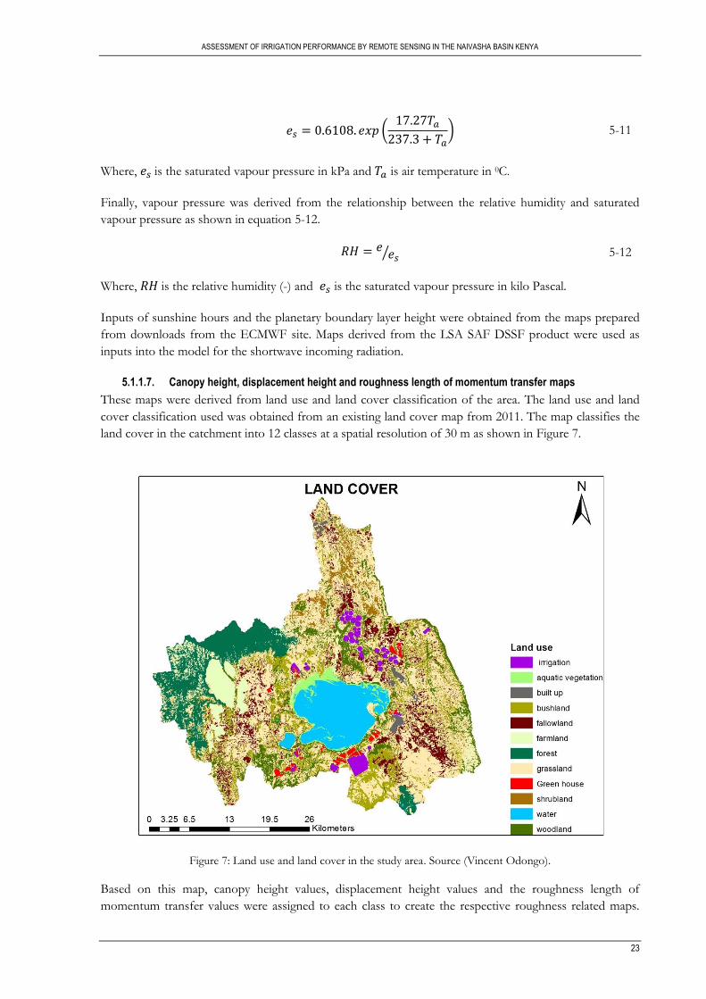
5.1.1.7. Canopy height, displacement height and roughness length of momentum transfer maps
These maps were derived from land use and land cover classification of the area. The land use and land
cover classification used was obtained from an existing land cover map from 2011. The map classifies the
land cover in the catchment into 12 classes at a spatial resolution of 30 m as shown in Figure 7.
Figure 7: Land use and land cover in the study area. Source (Vincent Odongo).
Based on this map, canopy height values, displacement height values and the roughness length of
momentum transfer values were assigned to each class to create the respective roughness related maps.
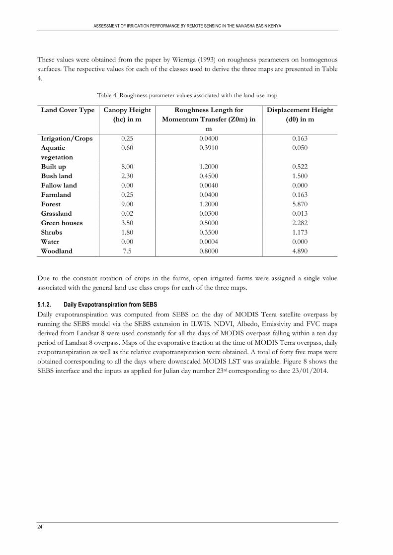
ASSESSMENT OF IRRIGATION PERFORMANCE BY REMOTE SENSING IN THE NAIVASHA BASIN KENYA
24
These values were obtained from the paper by Wiernga (1993) on roughness parameters on homogenous
surfaces. The respective values for each of the classes used to derive the three maps are presented in Table
4.
Table 4: Roughness parameter values associated with the land use map
Land Cover Type Canopy Height
(hc) in m
Roughness Length for
Momentum Transfer (Z0m) in
m
Displacement Height
(d0) in m
Irrigation/Crops 0.25 0.0400 0.163
Aquatic
vegetation
0.60 0.3910 0.050
Built up 8.00 1.2000 0.522
Bush land 2.30 0.4500 1.500
Fallow land 0.00 0.0040 0.000
Farmland 0.25 0.0400 0.163
Forest 9.00 1.2000 5.870
Grassland 0.02 0.0300 0.013
Green houses 3.50 0.5000 2.282
Shrubs 1.80 0.3500 1.173
Water 0.00 0.0004 0.000
Woodland 7.5 0.8000 4.890
Due to the constant rotation of crops in the farms, open irrigated farms were assigned a single value
associated with the general land use class crops for each of the three maps.
5.1.2. Daily Evapotranspiration from SEBS
Daily evapotranspiration was computed from SEBS on the day of MODIS Terra satellite overpass by
running the SEBS model via the SEBS extension in ILWIS. NDVI, Albedo, Emissivity and FVC maps
derived from Landsat 8 were used constantly for all the days of MODIS overpass falling within a ten day
period of Landsat 8 overpass. Maps of the evaporative fraction at the time of MODIS Terra overpass, daily
evapotranspiration as well as the relative evapotranspiration were obtained. A total of forty five maps were
obtained corresponding to all the days where downscaled MODIS LST was available. Figure 8 shows the
SEBS interface and the inputs as applied for Julian day number 23rd corresponding to date 23/01/2014.
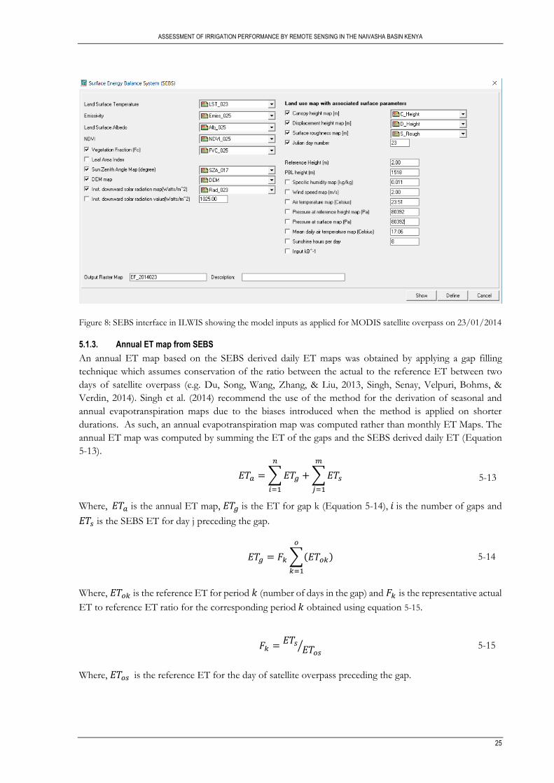
ASSESSMENT OF IRRIGATION PERFORMANCE BY REMOTE SENSING IN THE NAIVASHA BASIN KENYA
25
Figure 8: SEBS interface in ILWIS showing the model inputs as applied for MODIS satellite overpass on 23/01/2014
5.1.3. Annual ET map from SEBS
An annual ET map based on the SEBS derived daily ET maps was obtained by applying a gap filling
technique which assumes conservation of the ratio between the actual to the reference ET between two
days of satellite overpass (e.g. Du, Song, Wang, Zhang, & Liu, 2013, Singh, Senay, Velpuri, Bohms, &
Verdin, 2014). Singh et al. (2014) recommend the use of the method for the derivation of seasonal and
annual evapotranspiration maps due to the biases introduced when the method is applied on shorter
durations. As such, an annual evapotranspiration map was computed rather than monthly ET Maps. The
annual ET map was computed by summing the ET of the gaps and the SEBS derived daily ET (Equation
5-13).
𝐸𝑇𝑎 = ∑ 𝐸𝑇𝑔
𝑛
𝑖=1
+ ∑ 𝐸𝑇𝑠
𝑚
𝑗=1
5-13
Where, 𝐸𝑇𝑎 is the annual ET map, 𝐸𝑇𝑔 is the ET for gap k (Equation 5-14), 𝑖 is the number of gaps and
𝐸𝑇𝑠 is the SEBS ET for day j preceding the gap.
𝐸𝑇𝑔 = 𝐹𝑘 ∑(𝐸𝑇𝑜𝑘)
𝑜
𝑘=1
5-14
Where, 𝐸𝑇𝑜𝑘 is the reference ET for period 𝑘 (number of days in the gap) and 𝐹𝑘 is the representative actual
ET to reference ET ratio for the corresponding period 𝑘 obtained using equation 5-15.
𝐹𝑘 =𝐸𝑇𝑠
𝐸𝑇𝑜𝑠⁄ 5-15
Where, 𝐸𝑇𝑜𝑠 is the reference ET for the day of satellite overpass preceding the gap.
ASSESSMENT OF IRRIGATION PERFORMANCE BY REMOTE SENSING IN THE NAIVASHA BASIN KENYA
26
Reference evapotranspiration was calculated using the Hargreaves method (Hargreaves, 1989) whose
formulation is presented in equation 5-16. This method was used due to gaps in the radiation data from the
flux tower which limited the application of the recommended Penman method.
𝐸𝑇0 = 0.0023𝑅𝑎(𝑇𝑚𝑎𝑥 − 𝑇𝑚𝑖𝑛)0.5 (
𝑇𝑚𝑎𝑥 + 𝑇𝑚𝑖𝑛
2+ 17.8) 5-16
Where, 𝑇𝑚𝑎𝑥 is the maximum air temperature of the day, 𝑇𝑚𝑖𝑛 is the minimum air temperature of the day
in degrees Celsius and 𝑅𝑎 is the extra-terrestrial radiation calculated based on the formulations in the
appendix.
5.1.4. Monthly ET maps
To compute monthly irrigation consumption, monthly ET maps at the Landsat 8 spatial scale were used.
These maps were obtained using equation 5-17 (Singh et al., 2014). In this algorithm, coarse spatial
resolution ET maps at a high temporal resolution are used to introduce temporal variability in fine spatial
resolution ET maps with poor temporal resolution. This results in a final ET map with both high spatial
and temporal resolutions. The algorithm is based on the assumption that a linear relationship exists between
evapotranspiration derived from coarse resolution imagery and fine resolution imagery (e.g Hong,
Hendrickx, & Borchers, 2011, Singh et al., 2014).
In this research, MODIS monthly ET maps were used to introduce the temporal variability in the total
annual ET map derived from SEBS.
𝐿(𝑥, 𝑦, 𝑡𝑚) =
𝑀(𝑥, 𝑦, 𝑡𝑚)
𝑀(𝑥, 𝑦, 𝑡𝑎) × 𝐿(𝑥, 𝑦, 𝑡𝑎) 5-17
Where, 𝐿(𝑥, 𝑦, 𝑡𝑚) is the monthly evapotranspiration at the Landsat 8 spatial scale for pixel (x, y),
𝑀(𝑥, 𝑦, 𝑡𝑚) is the monthly MODIS evapotranspiration for pixel (x, y), 𝑀(𝑥, 𝑦, 𝑡𝑎) is the annual MODIS
evapotranspiration for pixel (x, y), 𝐿(𝑥, 𝑦, 𝑡𝑎) is the annual Landsat 8 derived evapotranspiration for pixel
(x, y) and pixel (x, y) is at the Landsat 8 spatial scale.
5.1.5. Validation of evapotranspiration
SEBS derived daily ET maps as well as the monthly downscaled evapotranspiration maps were validated for
both irrigated and non-irrigated pixels within the study area.
Since no measurements of actual ET were available in the irrigated fields, validation was carried out by
comparing the SEBS estimate with potential ET calculated using a crop coefficient and the reference ET.
This was based on the assumption that under irrigated conditions, optimal conditions for evapotranspiration
exists. As such, the potential ET of the crops is approximately equal to the actual ET of the crops. Actual
ET for the crops was then calculated using equation 5-18.
𝐸𝑇𝐶𝑟𝑜𝑝 = 𝐸𝑇0 × 𝐾𝑐 5-18
Where 𝐸𝑇𝑐𝑟𝑜𝑝 is the actual ET for the crop under irrigation, 𝐸𝑇0 is the reference ET and 𝐾𝑐 is the crop
coefficient for the particular crop.
ASSESSMENT OF IRRIGATION PERFORMANCE BY REMOTE SENSING IN THE NAIVASHA BASIN KENYA
27
The pixel considered for the calculation of ET crop is located in the Delamere Manera farm with coordinates
00 40’ 40.79”S, 360 25’ 02.92”E. The crop grown in this pixel is Lucerne whose KC value is presented in the
appendices. Delamere Manera farm was chosen since no crop rotation is carried out in the farm. This was
done so as to ensure that the pixel chosen would be under optimal water supply conditions throughout the
study period. In addition, an average KC value would be more applicable for a perennial crop rather than
seasonal crops with rapidly varying KC values. This was done to ensure that a reliable estimate of ET crop
would be obtained. However, it should be noted that ET crop may be unreliable when the crop is harvested
since the KC value will change as a result.
Validation in the non-irrigated pixel was done using the ECF ET for the pixel where the flux tower is
located. The ET was derived based on the corrected latent heat flux as described in section 3.2.4.
The statistical measures of accuracy used to assess the performance of the SEBS estimates are the coefficient
of determination (R2), mean absolute error (MAE), root mean square error (RMSE) and the Bias. The
formulation of the MAE, RMSE and the Bias are presented in Equations 5-19, 5-20 and 5-21 respectively.
𝑅𝑀𝑆𝐸 = √∑ (𝑋𝑚,𝑖 − 𝑋𝑜,𝑖)𝑛
𝑖=1
𝑛
2
5-19
𝑀𝐴𝐸 =
∑ [𝑎𝑏𝑠(𝑋𝑚,𝑖 − 𝑋𝑜,𝑖)]𝑛𝑖=1
𝑛 5-20
𝐵𝑖𝑎𝑠 = [
∑ 𝑋𝑚 − ∑ 𝑋𝑜𝑛𝑖=1
𝑛𝑖=1
∑ 𝑋𝑜,𝑖𝑛𝑖=1
]
5-21
Where, 𝑋𝑚,𝑖 is the modelled variable, 𝑋𝑜,𝑖 is the observed variable and 𝑛 is the number of observations.
5.1.6. Sensitivity analysis of SEBS derived evapotranspiration
Though SEBS is sensitive to all the input variables (Van der Kwast et al., 2009), sensitivity analysis was
carried out for the meteorological variables only. Meteorological variables were selected for sensitivity
analysis since they were used as point inputs. The sensitivity analysis aimed at analysing the uncertainty
which would be introduced in case of spatial variations in the meteorological variables.
Sensitivity analysis was carried out by first running the SEBS model under the normal conditions at the time
of satellite overpass for the Julian day number 23 corresponding to the 23rd of January 2014. The
corresponding daily evapotranspiration was then noted. The inputs were then varied between the ranges of
-20 to 20 percent at intervals of 10 percent. The sensitivity of SEBS derived ET was then computed using
equation 5-22.
𝑆 =
𝑋−+ − 𝑋0
𝑋0× 100 5-22
Where, S is the sensitivity (%), 𝑋−+ is the ET obtained after varying each variable by +20 % to -20 % at
intervals of 10 % and 𝑋0 is the original ET.
ASSESSMENT OF IRRIGATION PERFORMANCE BY REMOTE SENSING IN THE NAIVASHA BASIN KENYA
28
5.2. Computation of Irrigation Consumption
To compute the monthly irrigation consumption, maps of monthly incremental ET as a result of irrigation
were used. These maps were computed using equation 5-23.
𝐸𝑇𝑖𝑟𝑟,𝑚 = 𝐸𝑇𝑚 − 𝑃𝑒,𝑚 5-23
Where, 𝐸𝑇𝑖𝑟𝑟,𝑚 is the monthly incremental ET due to irrigation in mm, 𝐸𝑇𝑚 is the monthly ET in mm and
𝑃𝑒,𝑚 is the monthly effective precipitation in mm.
Irrigation consumption per farm was then obtained by masking out the monthly incremental ET maps with
the digitized shape files of the farms. The volume of irrigation consumption per pixel was then obtained as
a product of the monthly irrigation depth (m) and the pixel area (m2). Finally, the total irrigation
consumption volume per farm was computed by summing all the volumes for the irrigated pixels within
each farm during the month.
5.2.1. Computation of effective precipitation
Monthly effective precipitation was computed by applying the method proposed by van Eekelen et al.,
(2015). In this method, the ratio between evapotranspiration from natural land use classes and rainfall is
computed. This ratio represents the fraction of total rainfall over the period that is consumed by plants
assuming no uptake from ground water zone. The method assumes equal effective precipitation for natural
land use classes and cropped areas assuming no irrigation. Effects of land treatment and the differences in
characteristics of individual plants and their response to evapotranspiration are ignored.
However, some of the assumptions made in the method were reviewed. The effective root zone depth of
the natural vegetation in comparison with crops was introduced so as to select the natural vegetation class
best representative of the crops grown in the farms. After the selection of the natural land use class, effective
precipitation was then computed using equation 5-24.
𝑃𝑒,𝑖 = (
𝐸𝑛𝑙,𝑖𝑃𝑖
⁄ ) 𝑥 𝑃𝑖 5-24
Where 𝑃𝑒,𝑖 is the effective precipitation for the period i.e. month, season or year, 𝐸𝑛𝑙,𝑖 is the
evapotranspiration from natural land use classes for the period under consideration and 𝑃𝑖 is the
precipitation over the period under consideration.
First, maps of monthly ratios of the actual evapotranspiration to the precipitation were prepared. Pixel
values for the selected natural land use classes were extracted. These values were then interpolated to create
maps of monthly ratios between evapotranspiration from the selected natural land use class and
precipitation. Finally, the maps were multiplied with the respective monthly rainfall maps to obtain the
monthly effective precipitation maps.
5.2.2. Selection of natural land use classes
The land cover map presented in Figure 7, was used to identify all the natural land use classes in the area.
GPS points of the natural land use classes collected during the fieldwork exercise were used to verify the
natural vegetation classes within the study area as presented in the land cover map. All the natural land use
classes were then assigned representative effective root zone depth values derived from literature sources.
On the other hand, data on crop type from the farms was used to derive the effective root zone depth for
each crop based on the guidelines presented in the FAO 56 report on crop evapotranspiration and crop
ASSESSMENT OF IRRIGATION PERFORMANCE BY REMOTE SENSING IN THE NAIVASHA BASIN KENYA
29
water requirements (Allen et al., 1998). A representative average effective root zone depth was then
computed for all the crops. This average root zone depth was then compared to the effective root zone
depth from the natural land use classes to obtain the class that best matched the crops.
On average, the effective root zone depth for crops grown in the commercial farms ranged from a minimum
of 0.45 m for onions to a maximum of 1.5 m for Lucerne as presented in in the appendices. The average
effective root zone depth was found to be approximately 0.9 m. On comparison, grass was found to be
more representative of the cropped area on average with effective root zone depth ranging from 0.5 m to
1.5 m depending on the grass type as documented in the FAO 56 report.
However, due to the close proximity to the lake and wetland areas further analysis was needed to eliminate
grass fields which extract water from the saturated zone. A ratio between the annual evapotranspiration to
the annual precipitation was computed for the grass fields. All the fields with an annual ratio greater than
one were excluded since at an annual scale the ratio should be less than one if no groundwater uptake is
present. The average and the standard deviation of the remaining sample were then calculated. The average
of the sample was found to be 0.79 with a standard deviation of 0.025. Using these statistics, the range of
pixels to be included in the computation of the effective precipitation was fixed between 0.74 and 0.84 by
taking the range of inclusion as twice the standard deviation from the mean.
5.2.3. Precipitation
To derive effective precipitation maps for the catchment, CHIRPS rainfall product was used. However, the
performance of the CHIRPS precipitation product was first evaluated against the gauge-measured data prior
to its application. This was achieved by extracting daily pixel values from the CHIRPS rainfall product
corresponding to each of the rain gauges and analysing for various statistical measures of accuracy.
The statistical measures for which the product was evaluated are the Bias, Root mean square error (RMSE)
and the Mean absolute error (MAE). The formulations for the RMSE, MAE and the Bias are presented in
section 5.1.5. In addition, the total bias was disaggregated into individual component biases namely the hit
rain bias, missed rain bias and false rain bias. Hit rain bias is defined as the event in which both the satellite
and the gauge record rainfall while the missed rain bias occurs in the event when the gauge records but the
satellite does not detect rainfall. On the other hand, false rain bias occurs in the event when the satellite
detects rainfall and the gauge does not record any rainfall. These definitions as well as their mathematical
formulations are as presented in Habib, Larson, & Graschel (2009) and Haile, Habib, & Rientjes (2013).
The formulation of these three bias components is presented in the following equations.
𝐻𝑖𝑡 𝑏𝑖𝑎𝑠 = ∑(𝑃𝑠,𝑖
𝑛
𝑖=1
− 𝑃𝑔,𝑖)|(𝑃𝑠 > 0 & 𝑃𝑔 > 0) 5-25
𝑀𝑖𝑠𝑠𝑒𝑑 𝑟𝑎𝑖𝑛 𝑏𝑖𝑎𝑠 = ∑ 𝑃𝑔,𝑖
𝑛
𝑖=1
|(𝑃𝑠 = 0 & 𝑃𝑔 > 0) 5-26
𝐹𝑎𝑙𝑠𝑒 𝑟𝑎𝑖𝑛 𝑏𝑖𝑎𝑠 = ∑ 𝑃𝑠,𝑖
𝑛
𝑖=1
|(𝑃𝑠,𝑖 > 0 & 𝑃𝑔,𝑖 = 0) 5-27
Where, 𝑛 is the number of days, 𝑃𝑠 is CHIRPS derived precipitation and 𝑃𝑔 is gauge precipitation.

ASSESSMENT OF IRRIGATION PERFORMANCE BY REMOTE SENSING IN THE NAIVASHA BASIN KENYA
30
Based on the results of the statistical evaluation, the satellite product was corrected for Bias on a monthly
time step. This was achieved by computing the monthly bias factors for each station. The computation of
the bias factors and the subsequent bias correction procedure followed the formulations presented in Habib,
Haile, Sazib, Zhang, & Rientjes, (2014).
𝐵𝐹𝑇𝑆𝑉 =
∑ 𝑃𝑠,𝑖𝑛𝑖=1
∑ 𝑃𝑔,𝑖𝑛𝑖=1
5-28
Where, 𝐵𝐹𝑇𝑆𝑣 is the time and space varying bias factor.
Once the bias factors for all the stations were computed, maps of monthly bias correction factors were
derived. An inverse distance weighted interpolation technique was adopted to generate monthly bias
correction factor maps. Bias correction was then implemented by multiplying the monthly CHIRPS
precipitation maps with the inverse of the bias correction factor maps of the respective months. Due to the
inability of multiplicative bias correction approaches to correct for zero values in the satellite rainfall, the
pixels in the bias corrected maps with values less than those of gauge derived rainfall maps were replaced
by values of the gauge derived rainfall map. Monthly gauge derived rainfall maps were obtained by
interpolating the monthly gauge rainfall totals for the respective months.
5.3. Computation of Irrigation efficiency
Irrigation efficiency was computed on a monthly basis for Vegpro Gorge farm since this was the only farm
with reliable irrigation water abstraction data. Irrigation efficiency was computed using equation 5-29.
𝐼𝐸 =
𝐼𝐶
𝐼𝐴× 100 5-29
Where, 𝐼𝐸 is the irrigation efficiency (%), 𝐼𝐶 is the volume of irrigation consumption (m3) and 𝐼𝐴 is the
volume of irrigation water abstraction (m3).
The computed irrigation efficiency as well as the irrigation consumption was evaluated by use of an indicator
of aridity computed as a ratio between the precipitation and the reference ET using equation 5-30.
𝐴𝐼 =
𝑃
𝐸𝑇0 5-30
Where, 𝐴𝐼 is the aridity index (mm), 𝑃 is precipitation in mm and 𝐸𝑇0 is the reference ET computed from
Hargreaves equation (mm).
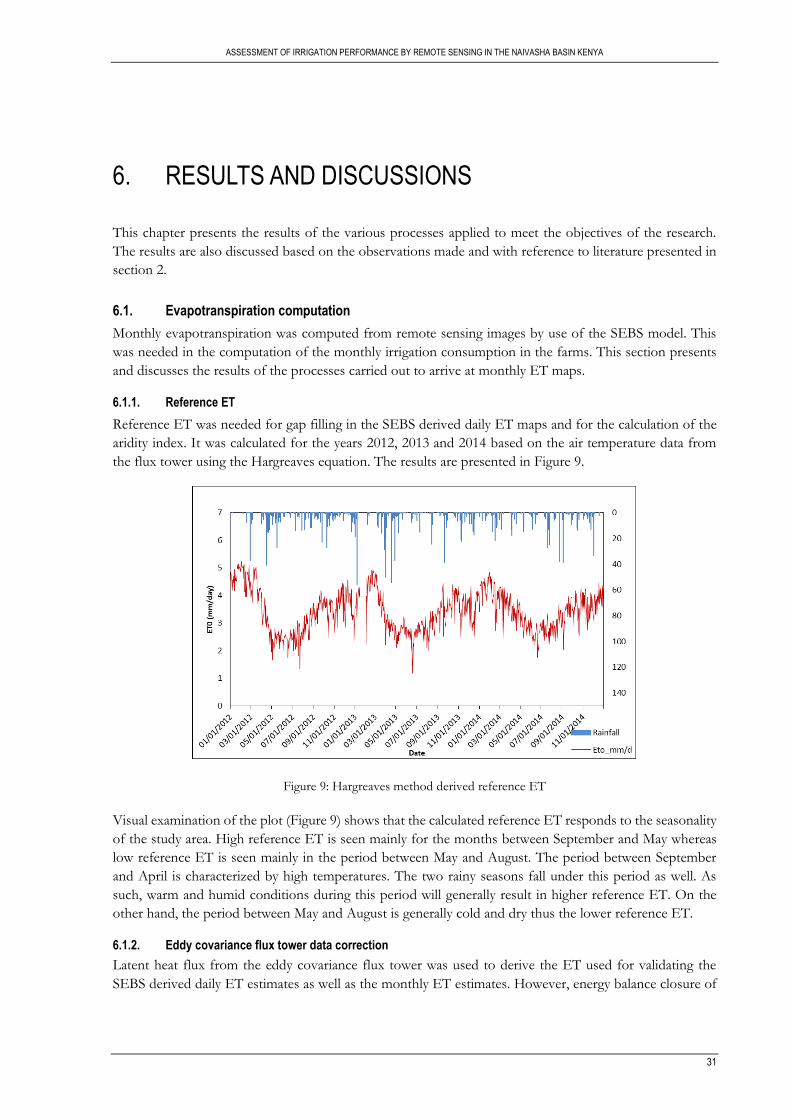
ASSESSMENT OF IRRIGATION PERFORMANCE BY REMOTE SENSING IN THE NAIVASHA BASIN KENYA
31
6. RESULTS AND DISCUSSIONS
This chapter presents the results of the various processes applied to meet the objectives of the research.
The results are also discussed based on the observations made and with reference to literature presented in
section 2.
6.1. Evapotranspiration computation
Monthly evapotranspiration was computed from remote sensing images by use of the SEBS model. This
was needed in the computation of the monthly irrigation consumption in the farms. This section presents
and discusses the results of the processes carried out to arrive at monthly ET maps.
6.1.1. Reference ET
Reference ET was needed for gap filling in the SEBS derived daily ET maps and for the calculation of the
aridity index. It was calculated for the years 2012, 2013 and 2014 based on the air temperature data from
the flux tower using the Hargreaves equation. The results are presented in Figure 9.
Figure 9: Hargreaves method derived reference ET
Visual examination of the plot (Figure 9) shows that the calculated reference ET responds to the seasonality
of the study area. High reference ET is seen mainly for the months between September and May whereas
low reference ET is seen mainly in the period between May and August. The period between September
and April is characterized by high temperatures. The two rainy seasons fall under this period as well. As
such, warm and humid conditions during this period will generally result in higher reference ET. On the
other hand, the period between May and August is generally cold and dry thus the lower reference ET.
6.1.2. Eddy covariance flux tower data correction
Latent heat flux from the eddy covariance flux tower was used to derive the ET used for validating the
SEBS derived daily ET estimates as well as the monthly ET estimates. However, energy balance closure of
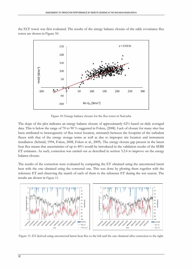
ASSESSMENT OF IRRIGATION PERFORMANCE BY REMOTE SENSING IN THE NAIVASHA BASIN KENYA
32
the ECF tower was first evaluated. The results of the energy balance closure of the eddy covariance flux
tower are shown in Figure 10.
Figure 10: Energy balance closure for the flux tower in Naivasha
The slope of the plot indicates an energy balance closure of approximately 62% based on daily averaged
data. This is below the range of 70 to 90 % suggested in Foken, (2008). Lack of closure for many sites has
been attributed to heterogeneity of flux tower location, mismatch between the footprint of the turbulent
fluxes with that of the energy storage terms as well as due to improper site location and instrument
installation (Schmid, 1994, Foken, 2008, Foken et al., 2009). The energy closure gap present in the latent
heat flux means that uncertainties of up to 40% would be introduced in the validation results of the SEBS
ET estimates. As such, correction was carried out as described in section 3.2.4 to improve on the energy
balance closure.
The results of the correction were evaluated by comparing the ET obtained using the uncorrected latent
heat with the one obtained using the corrected one. This was done by plotting them together with the
reference ET and observing the match of each of them to the reference ET during the wet season. The
results are shown in Figure 11.
Figure 11: ET derived using uncorrected latent heat flux to the left and the one obtained after correction to the right
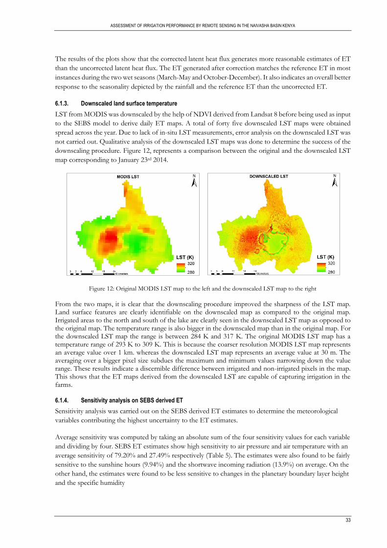
ASSESSMENT OF IRRIGATION PERFORMANCE BY REMOTE SENSING IN THE NAIVASHA BASIN KENYA
33
The results of the plots show that the corrected latent heat flux generates more reasonable estimates of ET
than the uncorrected latent heat flux. The ET generated after correction matches the reference ET in most
instances during the two wet seasons (March-May and October-December). It also indicates an overall better
response to the seasonality depicted by the rainfall and the reference ET than the uncorrected ET.
6.1.3. Downscaled land surface temperature
LST from MODIS was downscaled by the help of NDVI derived from Landsat 8 before being used as input
to the SEBS model to derive daily ET maps. A total of forty five downscaled LST maps were obtained
spread across the year. Due to lack of in-situ LST measurements, error analysis on the downscaled LST was
not carried out. Qualitative analysis of the downscaled LST maps was done to determine the success of the
downscaling procedure. Figure 12, represents a comparison between the original and the downscaled LST
map corresponding to January 23rd 2014.
Figure 12: Original MODIS LST map to the left and the downscaled LST map to the right
From the two maps, it is clear that the downscaling procedure improved the sharpness of the LST map. Land surface features are clearly identifiable on the downscaled map as compared to the original map. Irrigated areas to the north and south of the lake are clearly seen in the downscaled LST map as opposed to the original map. The temperature range is also bigger in the downscaled map than in the original map. For the downscaled LST map the range is between 284 K and 317 K. The original MODIS LST map has a temperature range of 293 K to 309 K. This is because the coarser resolution MODIS LST map represents an average value over 1 km. whereas the downscaled LST map represents an average value at 30 m. The averaging over a bigger pixel size subdues the maximum and minimum values narrowing down the value range. These results indicate a discernible difference between irrigated and non-irrigated pixels in the map. This shows that the ET maps derived from the downscaled LST are capable of capturing irrigation in the farms.
6.1.4. Sensitivity analysis on SEBS derived ET
Sensitivity analysis was carried out on the SEBS derived ET estimates to determine the meteorological
variables contributing the highest uncertainty to the ET estimates.
Average sensitivity was computed by taking an absolute sum of the four sensitivity values for each variable
and dividing by four. SEBS ET estimates show high sensitivity to air pressure and air temperature with an
average sensitivity of 79.20% and 27.49% respectively (Table 5). The estimates were also found to be fairly
sensitive to the sunshine hours (9.94%) and the shortwave incoming radiation (13.9%) on average. On the
other hand, the estimates were found to be less sensitive to changes in the planetary boundary layer height
and the specific humidity
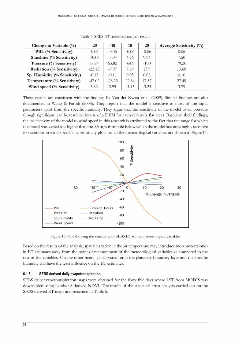
ASSESSMENT OF IRRIGATION PERFORMANCE BY REMOTE SENSING IN THE NAIVASHA BASIN KENYA
34
Table 5: SEBS ET sensitivity analysis results
Change in Variable (%) -20 -10 10 20 Average Sensitivity (%)
PBL (% Sensitivity) -0.06 -0.06 -0.06 -0.06 0.06
Sunshine (% Sensitivity) -10.06 -5.04 4.96 9.94 7.50
Pressure (% Sensitivity) 87.94 63.82 -64.9 -100 79.20
Radiation (% Sensitivity) -23.15 -9.97 7.69 13.9 13.68
Sp. Humidity (% Sensitivity) -0.17 -0.11 0.03 0.08 0.10
Temperature (% Sensitivity) -47.02 -23.23 22.34 17.37 27.49
Wind speed (% Sensitivity) 5.82 2.95 -3.15 -3.25 3.79
These results are consistent with the findings by Van der Kwast et al. (2009). Similar findings are also
documented in Wang & Parodi (2008). They, report that the model is sensitive to most of the input
parameters apart from the specific humidity. They argue that the sensitivity of the model to air pressure
though significant, can be resolved by use of a DEM for even relatively flat areas. Based on their findings,
the insensitivity of the model to wind speed in this research is attributed to the fact that the range for which
the model was varied was higher than the 0.5 m/s threshold below which the model becomes highly sensitive
to variations in wind speed. The sensitivity plots for all the meteorological variables are shown in Figure 13.
Figure 13: Plot showing the sensitivity of SEBS ET to the meteorological variables
Based on the results of the analysis, spatial variation in the air temperature may introduce more uncertainties
in ET estimates away from the point of measurement of the meteorological variables as compared to the
rest of the variables. On the other hand, spatial variation in the planetary boundary layer and the specific
humidity will have the least influence on the ET estimates.
6.1.5. SEBS derived daily evapotranspiration
SEBS daily evapotranspiration maps were obtained for the forty five days where LST from MODIS was
downscaled using Landsat 8 derived NDVI. The results of the statistical error analysis carried out on the
SEBS derived ET maps are presented in Table 6.
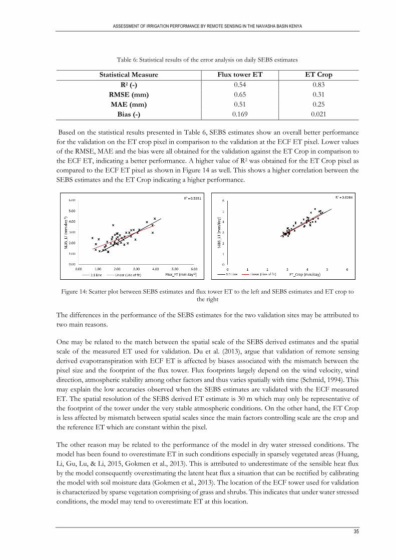
ASSESSMENT OF IRRIGATION PERFORMANCE BY REMOTE SENSING IN THE NAIVASHA BASIN KENYA
35
Table 6: Statistical results of the error analysis on daily SEBS estimates
Statistical Measure Flux tower ET ET Crop
R2 (-) 0.54 0.83
RMSE (mm) 0.65 0.31
MAE (mm) 0.51 0.25
Bias (-) 0.169 0.021
Based on the statistical results presented in Table 6, SEBS estimates show an overall better performance
for the validation on the ET crop pixel in comparison to the validation at the ECF ET pixel. Lower values
of the RMSE, MAE and the bias were all obtained for the validation against the ET Crop in comparison to
the ECF ET, indicating a better performance. A higher value of R2 was obtained for the ET Crop pixel as
compared to the ECF ET pixel as shown in Figure 14 as well. This shows a higher correlation between the
SEBS estimates and the ET Crop indicating a higher performance.
Figure 14: Scatter plot between SEBS estimates and flux tower ET to the left and SEBS estimates and ET crop to the right
The differences in the performance of the SEBS estimates for the two validation sites may be attributed to
two main reasons.
One may be related to the match between the spatial scale of the SEBS derived estimates and the spatial
scale of the measured ET used for validation. Du et al. (2013), argue that validation of remote sensing
derived evapotranspiration with ECF ET is affected by biases associated with the mismatch between the
pixel size and the footprint of the flux tower. Flux footprints largely depend on the wind velocity, wind
direction, atmospheric stability among other factors and thus varies spatially with time (Schmid, 1994). This
may explain the low accuracies observed when the SEBS estimates are validated with the ECF measured
ET. The spatial resolution of the SEBS derived ET estimate is 30 m which may only be representative of
the footprint of the tower under the very stable atmospheric conditions. On the other hand, the ET Crop
is less affected by mismatch between spatial scales since the main factors controlling scale are the crop and
the reference ET which are constant within the pixel.
The other reason may be related to the performance of the model in dry water stressed conditions. The
model has been found to overestimate ET in such conditions especially in sparsely vegetated areas (Huang,
Li, Gu, Lu, & Li, 2015, Gokmen et al., 2013). This is attributed to underestimate of the sensible heat flux
by the model consequently overestimating the latent heat flux a situation that can be rectified by calibrating
the model with soil moisture data (Gokmen et al., 2013). The location of the ECF tower used for validation
is characterized by sparse vegetation comprising of grass and shrubs. This indicates that under water stressed
conditions, the model may tend to overestimate ET at this location.
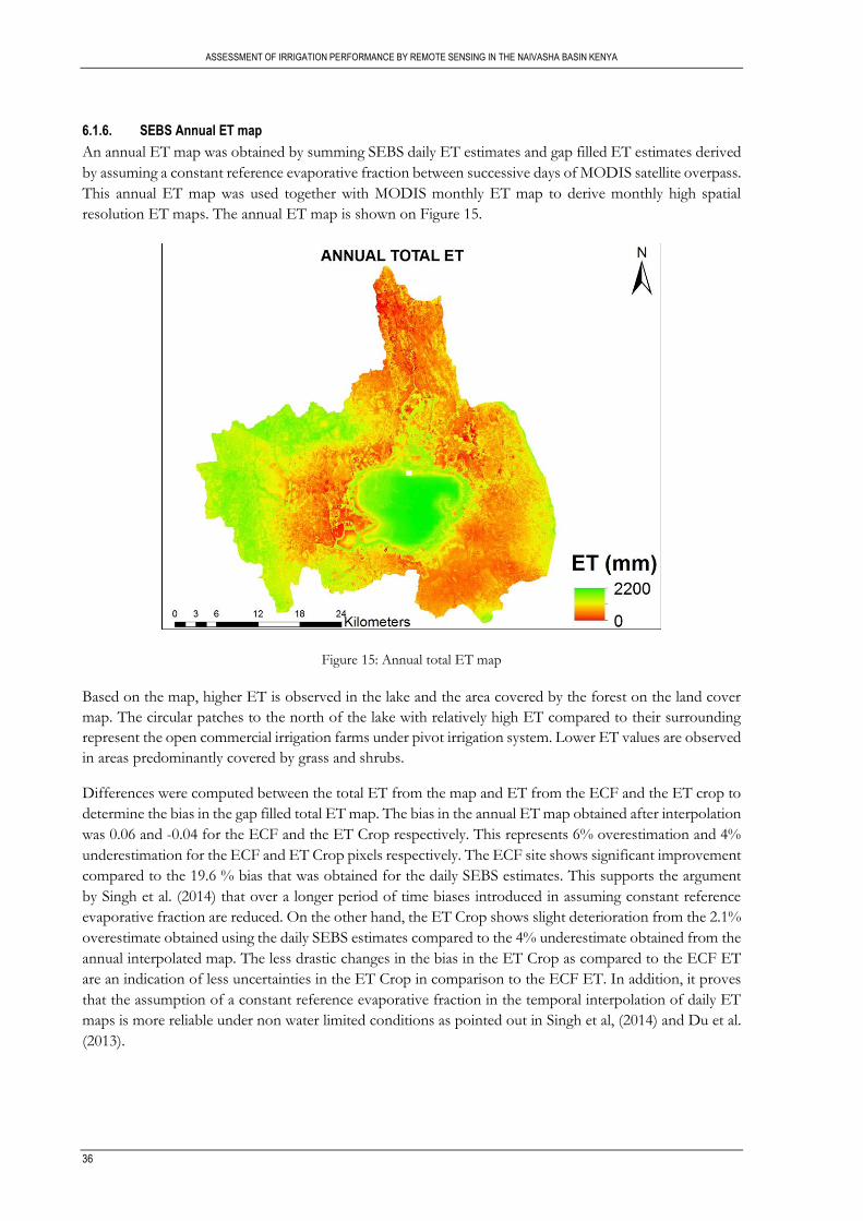
ASSESSMENT OF IRRIGATION PERFORMANCE BY REMOTE SENSING IN THE NAIVASHA BASIN KENYA
36
6.1.6. SEBS Annual ET map
An annual ET map was obtained by summing SEBS daily ET estimates and gap filled ET estimates derived
by assuming a constant reference evaporative fraction between successive days of MODIS satellite overpass.
This annual ET map was used together with MODIS monthly ET map to derive monthly high spatial
resolution ET maps. The annual ET map is shown on Figure 15.
Figure 15: Annual total ET map
Based on the map, higher ET is observed in the lake and the area covered by the forest on the land cover
map. The circular patches to the north of the lake with relatively high ET compared to their surrounding
represent the open commercial irrigation farms under pivot irrigation system. Lower ET values are observed
in areas predominantly covered by grass and shrubs.
Differences were computed between the total ET from the map and ET from the ECF and the ET crop to
determine the bias in the gap filled total ET map. The bias in the annual ET map obtained after interpolation
was 0.06 and -0.04 for the ECF and the ET Crop respectively. This represents 6% overestimation and 4%
underestimation for the ECF and ET Crop pixels respectively. The ECF site shows significant improvement
compared to the 19.6 % bias that was obtained for the daily SEBS estimates. This supports the argument
by Singh et al. (2014) that over a longer period of time biases introduced in assuming constant reference
evaporative fraction are reduced. On the other hand, the ET Crop shows slight deterioration from the 2.1%
overestimate obtained using the daily SEBS estimates compared to the 4% underestimate obtained from the
annual interpolated map. The less drastic changes in the bias in the ET Crop as compared to the ECF ET
are an indication of less uncertainties in the ET Crop in comparison to the ECF ET. In addition, it proves
that the assumption of a constant reference evaporative fraction in the temporal interpolation of daily ET
maps is more reliable under non water limited conditions as pointed out in Singh et al, (2014) and Du et al.
(2013).
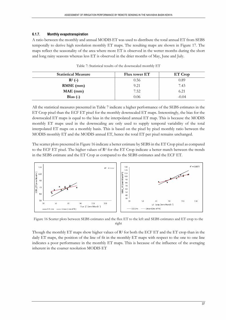
ASSESSMENT OF IRRIGATION PERFORMANCE BY REMOTE SENSING IN THE NAIVASHA BASIN KENYA
37
6.1.7. Monthly evapotranspiration
A ratio between the monthly and annual MODIS ET was used to distribute the total annual ET from SEBS
temporally to derive high resolution monthly ET maps. The resulting maps are shown in Figure 17. The
maps reflect the seasonality of the area where more ET is observed in the wetter months during the short
and long rainy seasons whereas less ET is observed in the drier months of May, June and July.
Table 7: Statistical results of the downscaled monthly ET
Statistical Measure Flux tower ET ET Crop
R2 (-) 0.56 0.89
RMSE (mm) 9.21 7.43
MAE (mm) 7.52 6.21
Bias (-) 0.06 -0.04
All the statistical measures presented in Table 7 indicate a higher performance of the SEBS estimates in the
ET Crop pixel than the ECF ET pixel for the monthly downscaled ET maps. Interestingly, the bias for the
downscaled ET maps is equal to the bias in the interpolated annual ET map. This is because the MODIS
monthly ET maps used in the downscaling are only used to supply temporal variability of the total
interpolated ET maps on a monthly basis. This is based on the pixel by pixel monthly ratio between the
MODIS monthly ET and the MODIS annual ET, hence the total ET per pixel remains unchanged.
The scatter plots presented in Figure 16 indicate a better estimate by SEBS in the ET Crop pixel as compared
to the ECF ET pixel. The higher values of R2 for the ET Crop indicate a better match between the trends
in the SEBS estimate and the ET Crop as compared to the SEBS estimates and the ECF ET.
Figure 16 Scatter plots between SEBS estimates and the flux ET to the left and SEBS estimates and ET crop to the right
Though the monthly ET maps show higher values of R2 for both the ECF ET and the ET crop than in the
daily ET maps, the position of the line of fit in the monthly ET maps with respect to the one to one line
indicates a poor performance in the monthly ET maps. This is because of the influence of the averaging
inherent in the coarser resolution MODIS ET
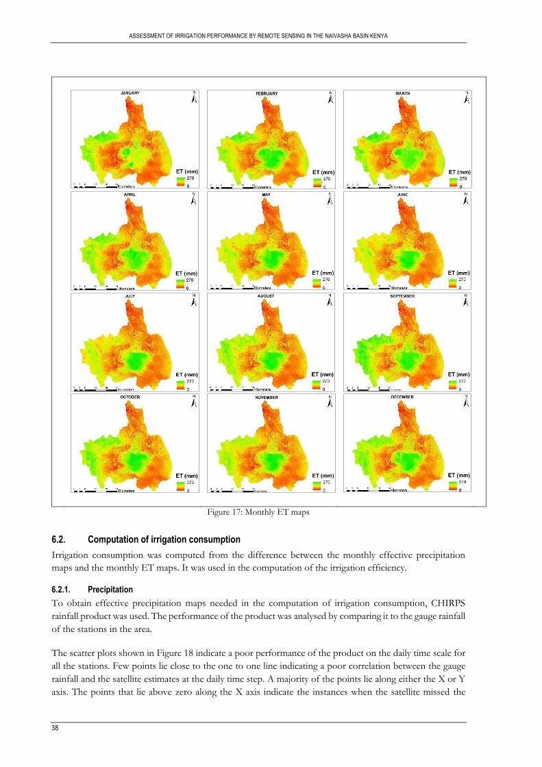
ASSESSMENT OF IRRIGATION PERFORMANCE BY REMOTE SENSING IN THE NAIVASHA BASIN KENYA
38
Figure 17: Monthly ET maps
6.2. Computation of irrigation consumption
Irrigation consumption was computed from the difference between the monthly effective precipitation
maps and the monthly ET maps. It was used in the computation of the irrigation efficiency.
6.2.1. Precipitation
To obtain effective precipitation maps needed in the computation of irrigation consumption, CHIRPS
rainfall product was used. The performance of the product was analysed by comparing it to the gauge rainfall
of the stations in the area.
The scatter plots shown in Figure 18 indicate a poor performance of the product on the daily time scale for
all the stations. Few points lie close to the one to one line indicating a poor correlation between the gauge
rainfall and the satellite estimates at the daily time step. A majority of the points lie along either the X or Y
axis. The points that lie above zero along the X axis indicate the instances when the satellite missed the
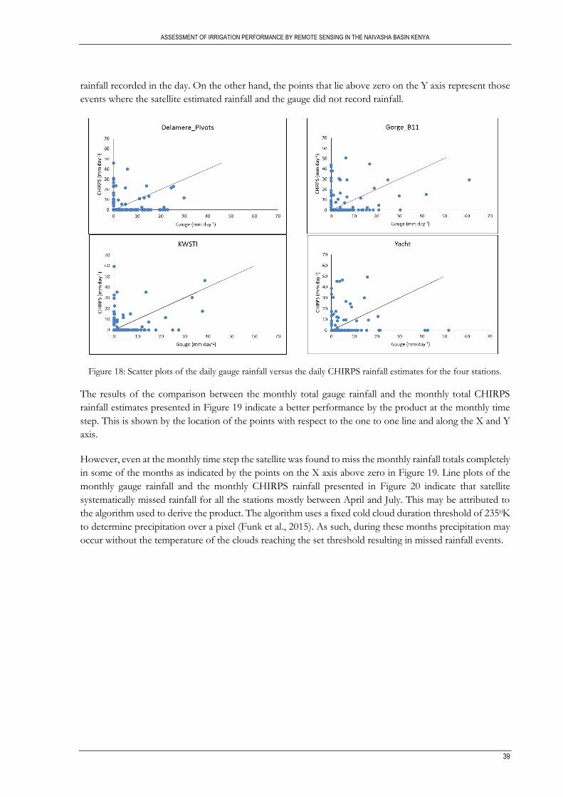
ASSESSMENT OF IRRIGATION PERFORMANCE BY REMOTE SENSING IN THE NAIVASHA BASIN KENYA
39
rainfall recorded in the day. On the other hand, the points that lie above zero on the Y axis represent those
events where the satellite estimated rainfall and the gauge did not record rainfall.
Figure 18: Scatter plots of the daily gauge rainfall versus the daily CHIRPS rainfall estimates for the four stations.
The results of the comparison between the monthly total gauge rainfall and the monthly total CHIRPS
rainfall estimates presented in Figure 19 indicate a better performance by the product at the monthly time
step. This is shown by the location of the points with respect to the one to one line and along the X and Y
axis.
However, even at the monthly time step the satellite was found to miss the monthly rainfall totals completely
in some of the months as indicated by the points on the X axis above zero in Figure 19. Line plots of the
monthly gauge rainfall and the monthly CHIRPS rainfall presented in Figure 20 indicate that satellite
systematically missed rainfall for all the stations mostly between April and July. This may be attributed to
the algorithm used to derive the product. The algorithm uses a fixed cold cloud duration threshold of 2350K
to determine precipitation over a pixel (Funk et al., 2015). As such, during these months precipitation may
occur without the temperature of the clouds reaching the set threshold resulting in missed rainfall events.
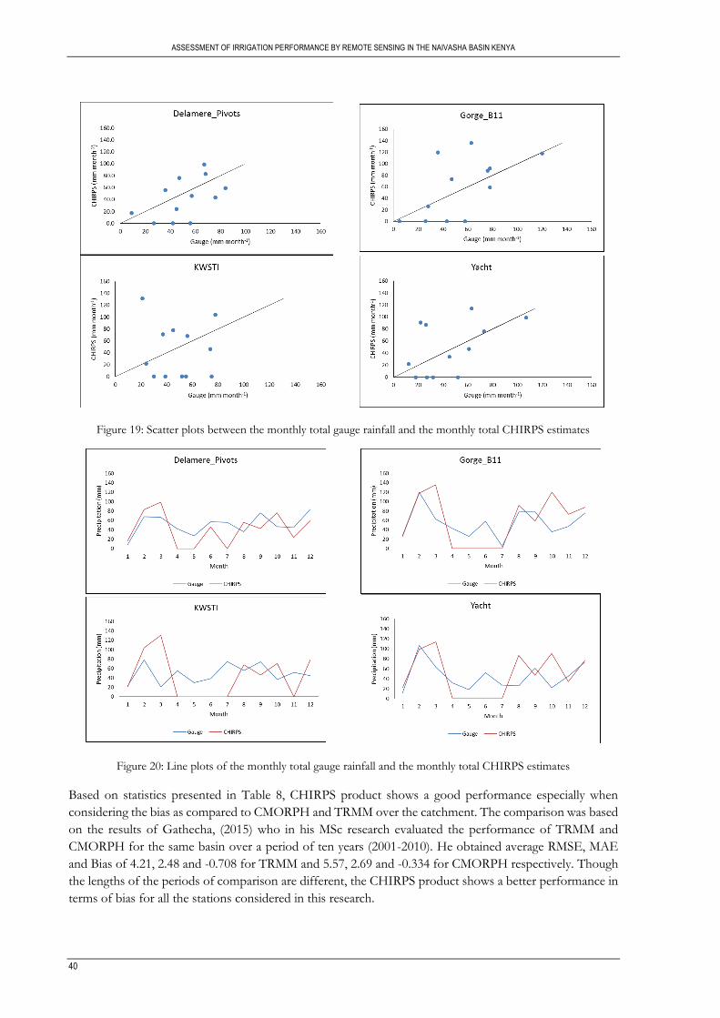
ASSESSMENT OF IRRIGATION PERFORMANCE BY REMOTE SENSING IN THE NAIVASHA BASIN KENYA
40
Figure 19: Scatter plots between the monthly total gauge rainfall and the monthly total CHIRPS estimates
Figure 20: Line plots of the monthly total gauge rainfall and the monthly total CHIRPS estimates
Based on statistics presented in Table 8, CHIRPS product shows a good performance especially when
considering the bias as compared to CMORPH and TRMM over the catchment. The comparison was based
on the results of Gathecha, (2015) who in his MSc research evaluated the performance of TRMM and
CMORPH for the same basin over a period of ten years (2001-2010). He obtained average RMSE, MAE
and Bias of 4.21, 2.48 and -0.708 for TRMM and 5.57, 2.69 and -0.334 for CMORPH respectively. Though
the lengths of the periods of comparison are different, the CHIRPS product shows a better performance in
terms of bias for all the stations considered in this research.
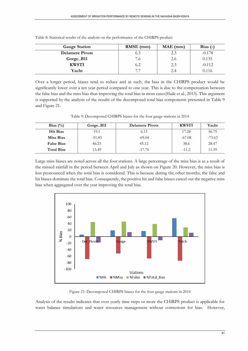
ASSESSMENT OF IRRIGATION PERFORMANCE BY REMOTE SENSING IN THE NAIVASHA BASIN KENYA
41
Table 8: Statistical results of the analysis on the performance of the CHIRPS product
Gauge Station RMSE (mm) MAE (mm) Bias (-)
Delamere Pivots 6.3 2.3 -0.178
Gorge_B11 7.6 2.6 0.135
KWSTI 6.2 2.3 -0.112
Yacht 7.7 2.4 0.116
Over a longer period, biases tend to reduce and as such, the bias in the CHIRPS product would be
significantly lower over a ten year period compared to one year. This is due to the compensation between
the false bias and the miss bias thus improving the total bias in most cases(Haile et al., 2013). This argument
is supported by the analysis of the results of the decomposed total bias components presented in Table 9
and Figure 21.
Table 9: Decomposed CHIRPS biases for the four gauge stations in 2014
Bias (%) Gorge_B11 Delamere Pivots KWSTI Yacht
Hit Bias 19.1 6.13 17.28 56.75
Miss Bias -51.83 -69.04 -67.08 -73.63
False Bias 46.23 45.12 38.6 28.47
Total Bias 13.49 -17.76 -11.2 11.59
Large miss biases are noted across all the four stations. A large percentage of the miss bias is as a result of
the missed rainfall in the period between April and July as shown on Figure 20. However, the miss bias is
less pronounced when the total bias is considered. This is because during the other months, the false and
hit biases dominate the total bias. Consequently, the positive hit and false biases cancel out the negative miss
bias when aggregated over the year improving the total bias.
Figure 21: Decomposed CHIRPS biases for the four gauge stations in 2014
Analysis of the results indicates that over yearly time steps or more the CHIRPS product is applicable for
water balance simulations and water resources management without corrections for bias. However,
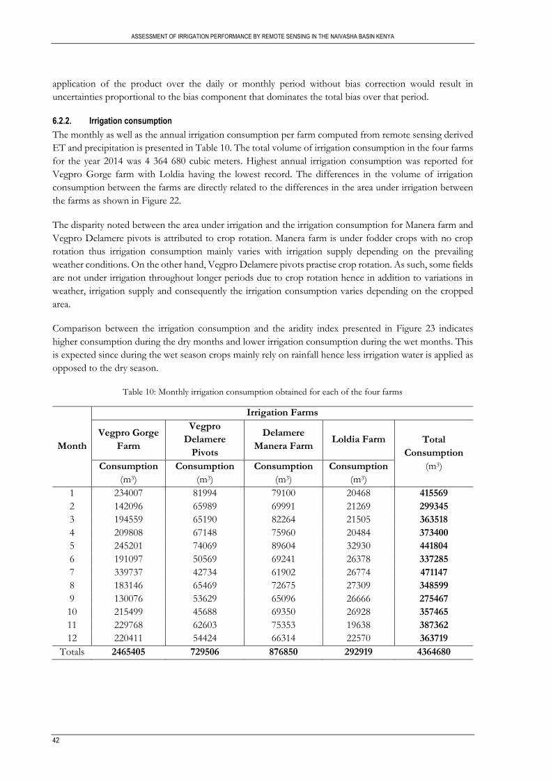
ASSESSMENT OF IRRIGATION PERFORMANCE BY REMOTE SENSING IN THE NAIVASHA BASIN KENYA
42
application of the product over the daily or monthly period without bias correction would result in
uncertainties proportional to the bias component that dominates the total bias over that period.
6.2.2. Irrigation consumption
The monthly as well as the annual irrigation consumption per farm computed from remote sensing derived
ET and precipitation is presented in Table 10. The total volume of irrigation consumption in the four farms
for the year 2014 was 4 364 680 cubic meters. Highest annual irrigation consumption was reported for
Vegpro Gorge farm with Loldia having the lowest record. The differences in the volume of irrigation
consumption between the farms are directly related to the differences in the area under irrigation between
the farms as shown in Figure 22.
The disparity noted between the area under irrigation and the irrigation consumption for Manera farm and
Vegpro Delamere pivots is attributed to crop rotation. Manera farm is under fodder crops with no crop
rotation thus irrigation consumption mainly varies with irrigation supply depending on the prevailing
weather conditions. On the other hand, Vegpro Delamere pivots practise crop rotation. As such, some fields
are not under irrigation throughout longer periods due to crop rotation hence in addition to variations in
weather, irrigation supply and consequently the irrigation consumption varies depending on the cropped
area.
Comparison between the irrigation consumption and the aridity index presented in Figure 23 indicates
higher consumption during the dry months and lower irrigation consumption during the wet months. This
is expected since during the wet season crops mainly rely on rainfall hence less irrigation water is applied as
opposed to the dry season.
Table 10: Monthly irrigation consumption obtained for each of the four farms
Month
Irrigation Farms
Vegpro Gorge
Farm
Vegpro
Delamere
Pivots
Delamere
Manera Farm Loldia Farm Total
Consumption
(m3) Consumption
(m3)
Consumption
(m3)
Consumption
(m3)
Consumption
(m3)
1 234007 81994 79100 20468 415569
2 142096 65989 69991 21269 299345
3 194559 65190 82264 21505 363518
4 209808 67148 75960 20484 373400
5 245201 74069 89604 32930 441804
6 191097 50569 69241 26378 337285
7 339737 42734 61902 26774 471147
8 183146 65469 72675 27309 348599
9 130076 53629 65096 26666 275467
10 215499 45688 69350 26928 357465
11 229768 62603 75353 19638 387362
12 220411 54424 66314 22570 363719
Totals 2465405 729506 876850 292919 4364680
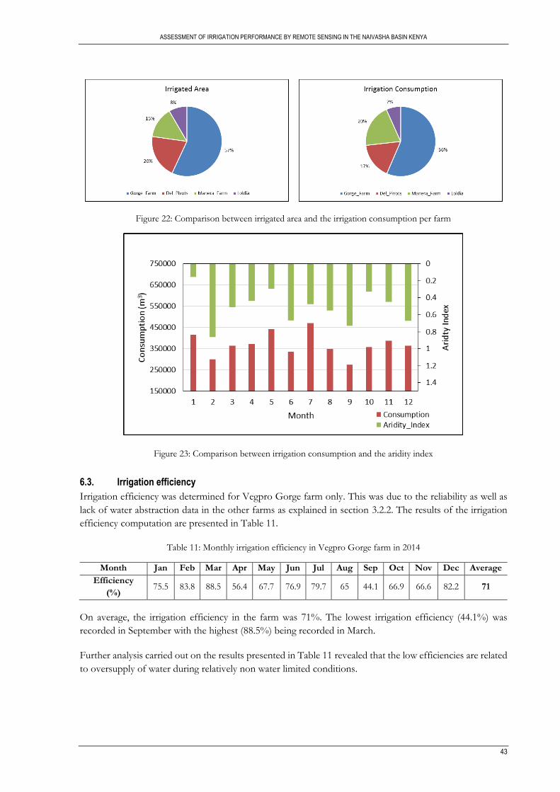
ASSESSMENT OF IRRIGATION PERFORMANCE BY REMOTE SENSING IN THE NAIVASHA BASIN KENYA
43
Figure 22: Comparison between irrigated area and the irrigation consumption per farm
Figure 23: Comparison between irrigation consumption and the aridity index
6.3. Irrigation efficiency
Irrigation efficiency was determined for Vegpro Gorge farm only. This was due to the reliability as well as
lack of water abstraction data in the other farms as explained in section 3.2.2. The results of the irrigation
efficiency computation are presented in Table 11.
Table 11: Monthly irrigation efficiency in Vegpro Gorge farm in 2014
Month Jan Feb Mar Apr May Jun Jul Aug Sep Oct Nov Dec Average
Efficiency
(%) 75.5 83.8 88.5 56.4 67.7 76.9 79.7 65 44.1 66.9 66.6 82.2 71
On average, the irrigation efficiency in the farm was 71%. The lowest irrigation efficiency (44.1%) was
recorded in September with the highest (88.5%) being recorded in March.
Further analysis carried out on the results presented in Table 11 revealed that the low efficiencies are related
to oversupply of water during relatively non water limited conditions.
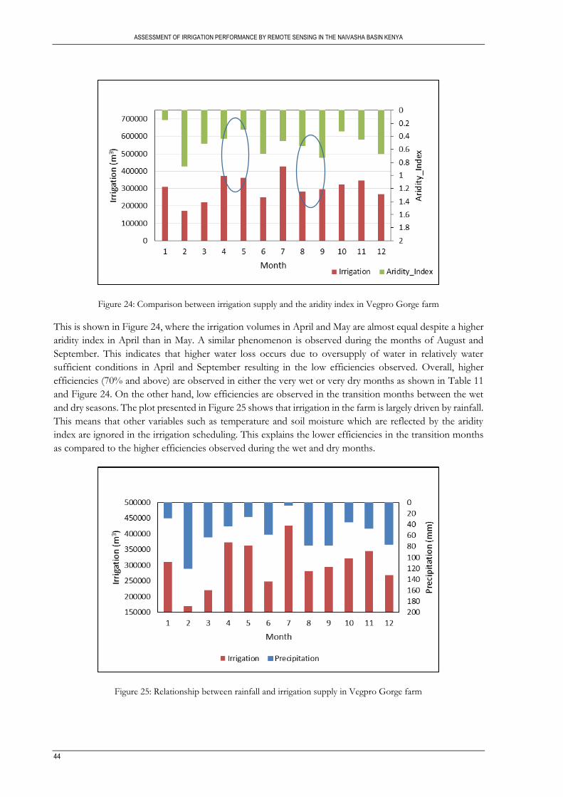
ASSESSMENT OF IRRIGATION PERFORMANCE BY REMOTE SENSING IN THE NAIVASHA BASIN KENYA
44
Figure 24: Comparison between irrigation supply and the aridity index in Vegpro Gorge farm
This is shown in Figure 24, where the irrigation volumes in April and May are almost equal despite a higher
aridity index in April than in May. A similar phenomenon is observed during the months of August and
September. This indicates that higher water loss occurs due to oversupply of water in relatively water
sufficient conditions in April and September resulting in the low efficiencies observed. Overall, higher
efficiencies (70% and above) are observed in either the very wet or very dry months as shown in Table 11
and Figure 24. On the other hand, low efficiencies are observed in the transition months between the wet
and dry seasons. The plot presented in Figure 25 shows that irrigation in the farm is largely driven by rainfall.
This means that other variables such as temperature and soil moisture which are reflected by the aridity
index are ignored in the irrigation scheduling. This explains the lower efficiencies in the transition months
as compared to the higher efficiencies observed during the wet and dry months.
Figure 25: Relationship between rainfall and irrigation supply in Vegpro Gorge farm
ASSESSMENT OF IRRIGATION PERFORMANCE BY REMOTE SENSING IN THE NAIVASHA BASIN KENYA
45
7. CONCLUSION AND RECOMMENDATIONS
7.1. Conclusion
The main objective of this research was to quantify irrigation performance in the commercial farms in
Naivasha basin, Kenya by use of remote sensing. The irrigation performance aspects evaluated are irrigation
consumption and irrigation efficiency. The main remote sensing inputs used to achieve the objective of this
research are Landsat 8 imagery, MODIS products and the CHIRPS rainfall product.
The conclusions drawn from this research are as follows;
Thermal sharpening of MODIS LST by use of Landsat 8 derived NDVI improved the spatial
resolution of the LST maps to the 30 m resolution of Landsat 8 enabling the computation of actual
evapotranspiration at the field scale. LST at a fine spatial scale is a key requirement for effective
quantification of evapotranspiration from farms such as the ones in Naivasha which are
characterized by small farming units with frequent crop rotation.
Daily SEBS ET estimates performed better in the irrigated pixels than in the non-irrigated pixels.
The values of R2 obtained were 0.83 and 0.54 whereas the percent bias was 2.1% and 16.9% upon
comparison between the SEBS estimates and the measured ET for the irrigated and non-irrigated
pixel respectively.
High resolution monthly ET maps obtained from remote sensing show consistency with the
seasonality of the study area. The values of R2 obtained for the monthly ET maps after validation
were 0.89 and 0.56 while the bias was -4% and 6% for the irrigated and non-irrigated pixel
respectively. This shows an acceptable error range for application in irrigation monitoring.
Variations in the volume of irrigation consumption between farms depend mainly on the area under
irrigation in each farm. However, other farming practices such as crop rotation were found to
contribute to these variations.
Monthly irrigation application in Vegpro Gorge farm is driven by the monthly rainfall received
which results in low irrigation efficiencies in transition months between the wet and dry seasons
where aridity index is relatively high despite low monthly rainfall amounts.
7.2. Recommendations
Errors in the downscaled LST maps should be quantified by comparing with measured LST to
understand their implications on the derived ET.
Soil moisture data should be incorporated in the SEBS model to improve on ET estimates during
the dry season.
SEBS ET estimates should be up scaled to match the foot print of the flux tower for better
quantification of the errors in the ET estimates in the non-irrigated areas.

47
LIST OF REFERENCES
Agam, N., Kustas, W. P., Anderson, M. C., Li, F., & Neale, C. M. U. (2007). A vegetation index based technique for spatial sharpening of thermal imagery. Remote Sensing of Environment, 107(4), 545–558. doi:10.1016/j.rse.2006.10.006
Akdim, N., Alfieri, S., Habib, A., Choukri, A., Cheruiyot, E., Labbassi, K., & Menenti, M. (2014). Monitoring of Irrigation Schemes by Remote Sensing: Phenology versus Retrieval of Biophysical Variables. Remote Sensing (Vol. 6). doi:10.3390/rs6065815
Alexandridis, T., Asif, S., & Ali, S. (1999). Water performance indicators using satellite imagery for the Fordwah Eastern Sadiqia (South) Irrigation and Drainage Project. International Water Management Institute.
Allen, R. G., Pereira, L. S., Raes, D., & Smith, M. (1998). Crop evapotranspiration - Guidelines for computing crop water requirements - FAO Irrigation and drainage paper 56. Rome: Food and Agriculture Organization of the United Nations. Retrieved from http://www.fao.org/docrep/x0490e/x0490e04.htm#evapotranspiration (et)
Bansouleh, B., Karimi, A., & Hesadi, H. (2015). Evaluation of SEBAL and SEBS Algorithms in the Estimation of Maize Evapotranspiration. International Journal of Plant & Soil Science, 6(6), 350–358. doi:10.9734/IJPSS/2015/15711
Bashir, M. A., Tanakamaru, H., & Tada, A. (2009). Remote Sensing for Diagnosing Actual Depeletion and Water Use Efficiency. In Thirteenth International Water Technology Conference.
Bastiaanssen, W. G. M., & Bos, M. G. (1999). Irrigation Performance Indicators Based on Remotely Sensed Data: a Review of Literature. Irrigation and Drainage Systems, 13(4), 291–311. doi:10.1023/A:1006355315251
Bastiaanssen, W. G. M., Menenti, M., Feddes, R. A., & Holtslag, A. A. M. (1998). A remote sensing surface energy balance algorithm for land (SEBAL). 1. Formulation. Journal of Hydrology, 212-213, 198–212. doi:10.1016/S0022-1694(98)00253-4
Bastiaanssen, W. G. M., Thiruvengadachari, S., Sakthivadivel, R., & Molden, D. J. (1999). Satellite Remote Sensing for Estimating Productivities of Land and Water. International Journal of Water Resources Development, 15(1-2), 181–194. doi:10.1080/07900629949005
Bastiaanssen, W. G. M., Van der Wal, T., & Visser, T. N. M. (1996). Diagnosis of regional evaporation by remote sensing to support irrigation performance assessment. Irrigation and Drainage Systems, 10(1), 1–23. doi:10.1007/BF01102762
Becht, R., & Harper, D. M. (2002). Towards an understanding of human impact upon the hydrology of Lake Naivasha, Kenya. Hydrobiologia, 488, 1–11. doi:10.1023/A:1023318007715
Bergner, A. G. N., Strecker, M. R., Trauth, M. H., Deino, A., Gasse, F., Blisniuk, P., & Dühnforth, M. (2009). Tectonic and climatic control on evolution of rift lakes in the Central Kenya Rift, East Africa. Quaternary Science Reviews, 28(25-26), 2804–2816. doi:10.1016/j.quascirev.2009.07.008
Bos, M.G, Kselik, R.A.L, Allen, R.G, Molden, D. (2009). Water Requirements for Irrigation and the Environment. Dordrecht: Springer Netherlands. doi:10.1007/978-1-4020-8948-0
Brutsaert, W. (2005). Hydrology: An Introduction. New york: Cambridge University Press. Retrieved from https://books.google.nl/books/about/Hydrology.html?id=yX_xS55xxyoC&pgis=1
Ceccherini, G., Ameztoy, I., Hernández, C., & Moreno, C. (2015). High-Resolution Precipitation Datasets in South America and West Africa based on Satellite-Derived Rainfall, Enhanced Vegetation Index and Digital Elevation Model. Remote Sensing, 7(5), 6454–6488. doi:10.3390/rs70506454
Coll, C., Caselles, V., Galve, J., Valor, E., Niclos, R., Sanchez, J., & Rivas, R. (2005). Ground measurements for the validation of land surface temperatures derived from AATSR and MODIS data. Remote Sensing of Environment, 97(3), 288–300. doi:10.1016/j.rse.2005.05.007
Dee, D. P., Uppala, S. M., Simmons, A. J., Berrisford, P., Poli, P., Kobayashi, S., … Vitart, F. (2011). The ERA-Interim reanalysis: configuration and performance of the data assimilation system. Quarterly Journal of the Royal Meteorological Society, 137(656), 553–597. doi:10.1002/qj.828
Dozier, J. (1996). A generalized split-window algorithm for retrieving land-surface temperature from space. IEEE Transactions on Geoscience and Remote Sensing, 34(4), 892–905. doi:10.1109/36.508406
Droogers, P., Kite, G., & Bastiaanssen, W. G. M. (1999). Integrated basin modeling to evaluate water productivity. Retrieved from https://cgspace.cgiar.org/handle/10568/37573
Du, J., Song, K., Wang, Z., Zhang, B., & Liu, D. (2013). Evapotranspiration estimation based on MODIS products and surface energy balance algorithms for land (SEBAL) model in Sanjiang Plain, Northeast China. Chinese Geographical Science, 23(1), 73–91. doi:10.1007/s11769-013-0587-8
48
ECMWF. (2015). ERA-Interim | ECMWF. Retrieved February 1, 2016, from http://www.ecmwf.int/en/research/climate-reanalysis/era-interim
Elhag, M., Psilovikos, A., Manakos, I., & Perakis, K. (2011). Application of the Sebs Water Balance Model in Estimating Daily Evapotranspiration and Evaporative Fraction from Remote Sensing Data Over the Nile Delta. Water Resources Management, 25(11), 2731–2742. doi:10.1007/s11269-011-9835-9
Er-Raki, S., Chehbouni, A., & Duchemin, B. (2010). Combining Satellite Remote Sensing Data with the FAO-56 Dual Approach for Water Use Mapping In Irrigated Wheat Fields of a Semi-Arid Region. Remote Sensing, 2(1), 375–387. doi:10.3390/rs2010375
EUMETCAST. (2015). Downward Surface Shortwave Flux Products description. Retrieved November 11, 2015, from https://landsaf.ipma.pt/algorithms.jsp?seltab=1&starttab=1
Foken, T. (2008). THE ENERGY BALANCE CLOSURE PROBLEM: AN OVERVIEW. Ecological Applications, 18(6), 1351–1367. doi:10.1890/06-0922.1
Foken, T., Mauder, M., Liebethal, C., Wimmer, F., Beyrich, F., Leps, J.-P., … Bange, J. (2009). Energy balance closure for the LITFASS-2003 experiment. Theoretical and Applied Climatology, 101(1-2), 149–160. doi:10.1007/s00704-009-0216-8
Funk, C., Peterson, P., Landsfeld, M., Pedreros, D., Verdin, J., Shukla, S., … Michaelsen, J. (2015). The climate hazards infrared precipitation with stations—a new environmental record for monitoring extremes. Scientific Data, 2, 150066. doi:10.1038/sdata.2015.66
Gathecha, H. M. (2015). RECONSTRUCTION OF STREAMFLOW INTO LAKE NAIVASHA USING CREST MODEL AN D REMOTE SENSED RAINFALL AND EVAPOTRANSPIRATION. University of Twente. Retrieved from http://www.itc.nl/library/papers_2015/msc/wrem/gathecha.pdf
Geiger, B., Meurey, C., Lajas, D., Franchistéguy, L., Carrer, D., & Roujean, J.-L. (2008). Near real-time provision of downwelling shortwave radiation estimates derived from satellite observations. Meteorological Applications, 15(3), 411–420. doi:10.1002/met.84
Gokmen, M., Vekerdy, Z., Lubczynski, M. W., Timmermans, J., Batelaan, O., & Verhoef, W. (2013). Assessing Groundwater Storage Changes Using Remote Sensing–Based Evapotranspiration and Precipitation at a Large Semiarid Basin Scale. Journal of Hydrometeorology, 14(6), 1733–1753. doi:10.1175/JHM-D-12-0156.1
Gontia, N. K., & Tiwari, K. N. (2009). Estimation of Crop Coefficient and Evapotranspiration of Wheat (Triticum aestivum) in an Irrigation Command Using Remote Sensing and GIS. Water Resources Management, 24(7), 1399–1414. doi:10.1007/s11269-009-9505-3
Gumma, M. K., Thenkabail, P. S., Hideto, F., Nelson, A., Dheeravath, V., Busia, D., & Rala, A. (2011). Mapping Irrigated Areas of Ghana Using Fusion of 30 m and 250 m Resolution Remote-Sensing Data. Remote Sensing, 3(12), 816–835. doi:10.3390/rs3040816
Ha, W., Gowda, P. H., & Howell, T. A. (2012). A review of downscaling methods for remote sensing-based irrigation management: part I. Irrigation Science, 31(4), 831–850. doi:10.1007/s00271-012-0331-7
Habib, E., Haile, A., Sazib, N., Zhang, Y., & Rientjes, T. (2014). Effect of Bias Correction of Satellite-Rainfall Estimates on Runoff Simulations at the Source of the Upper Blue Nile. Remote Sensing, 6(7), 6688–6708. doi:10.3390/rs6076688
Habib, E., Larson, B. F., & Graschel, J. (2009). Validation of NEXRAD multisensor precipitation estimates using an experimental dense rain gauge network in south Louisiana. Journal of Hydrology, 373(3-4), 463–478. doi:10.1016/j.jhydrol.2009.05.010
Haile, A. T., Habib, E., & Rientjes, T. (2013). Evaluation of the climate prediction center (CPC) morphing technique (CMORPH) rainfall product on hourly time scales over the source of the Blue Nile River. Hydrological Processes, 27(12), 1829–1839. doi:10.1002/hyp.9330
Hargreaves, G. H. (1989). Accuracy of Estimated Reference Crop Evapotranspiration. Journal of Irrigation and Drainage Engineering, 115(6), 1000–1007. doi:10.1061/(ASCE)0733-9437(1989)115:6(1000)
Hong, S.-H., Hendrickx, J. M. H., & Borchers, B. (2011). Down-scaling of SEBAL derived evapotranspiration maps from MODIS (250 m) to Landsat (30 m) scales. International Journal of Remote Sensing, 32(21), 6457–6477. doi:10.1080/01431161.2010.512929
Huang, C., Li, Y., Gu, J., Lu, L., & Li, X. (2015). Improving Estimation of Evapotranspiration under Water-Limited Conditions Based on SEBS and MODIS Data in Arid Regions. Remote Sensing, 7(12), 16795–16814. doi:10.3390/rs71215854
Jensen, M. E. (1967). Evaluating Irrigation Efficiency. IRRIGATION AND DRAINAGE DIVISION Proceedings of the American Society of Civil Engineers, ((IR1)), 83–98.
Jiménez-Muñoz, J. C., Sobrino, J. A., Plaza, A., Guanter, L., Moreno, J., & Martínez, P. (2009).

49
Comparison Between Fractional Vegetation Cover Retrievals from Vegetation Indices and Spectral Mixture Analysis: Case Study of PROBA/CHRIS Data Over an Agricultural Area. Sensors (Basel, Switzerland), 9(2), 768–93. doi:10.3390/s90200768
Karimi, P., Bastiaanssen, W. G. M., Molden, D., & Cheema, M. J. M. (2013). Basin-wide water accounting based on remote sensing data: an application for the Indus Basin. Hydrology and Earth System Sciences, 17(7), 2473–2486. doi:10.5194/hess-17-2473-2013
Kustas, W. P., & Daughtry, C. S. . (1990). Estimation of the soil heat flux/net radiation ratio from spectral data. Agricultural and Forest Meteorology, 49(3), 205–223. doi:10.1016/0168-1923(90)90033-3
Kustas, W. P., Norman, J. M., Anderson, M. C., & French, A. N. (2003). Estimating subpixel surface temperatures and energy fluxes from the vegetation index–radiometric temperature relationship. Remote Sensing of Environment, 85(4), 429–440. doi:10.1016/S0034-4257(03)00036-1
Liang, S. (2001). Narrowband to broadband conversions of land surface albedo I. Remote Sensing of Environment, 76(2), 213–238. doi:10.1016/S0034-4257(00)00205-4
Liou, Y.-A., & Kar, S. (2014). Evapotranspiration Estimation with Remote Sensing and Various Surface Energy Balance Algorithms—A Review. Energies, 7(5), 2821–2849. doi:10.3390/en7052821
Mallat, S. G. (1989). A theory for multiresolution signal decomposition: the wavelet representation. IEEE Transactions on Pattern Analysis and Machine Intelligence, 11(7), 674–693. doi:10.1109/34.192463
Mekonnen, M. M., Hoekstra, A. Y., & Becht, R. (2012). Mitigating the Water Footprint of Export Cut Flowers from the Lake Naivasha Basin, Kenya. Water Resources Management, 26(13), 3725–3742. doi:10.1007/s11269-012-0099-9
Menenti, M., Visser, T., Morabito, J. A., & Drovandi, A. (1989). Appraisal of irrigation performance with satellite data and georeferenced information [: the Rio Tunuyan Irrigation Scheme]. Retrieved from http://agris.fao.org/agris-search/search.do?recordID=GB9101219
Mu, Q., Heinsch, F. A., Zhao, M., & Running, S. W. (2007). Development of a global evapotranspiration algorithm based on MODIS and global meteorology data. Remote Sensing of Environment, 111(4), 519–536. doi:10.1016/j.rse.2007.04.015
Mu, Q., Zhao, M., & Running, S. W. (2011). Improvements to a MODIS global terrestrial evapotranspiration algorithm. Remote Sensing of Environment, 115(8), 1781–1800. doi:10.1016/j.rse.2011.02.019
Murray - Rust, D. H. (1994). Irrigated agriculture beyond 2000: institutional adaptation and transformation. IIMI Review.
Musota, R. (2008). Using WEAP and Scenarios to Assess Sustainability of Water Resources in a Basin. Case study for Lake Naivasha Catchment-Kenya. ITC-University of Twente.
NASA. (2015). MODIS Land Team. Retrieved February 12, 2016, from http://modis-land.gsfc.nasa.gov/MODLAND_grid.html
Odongo, V. O., Mulatu, D. W., Muthoni, F. K., van Oel, P. R., Meins, F. M., van der Tol, C., … van der Veen, A. (2014). Coupling socio-economic factors and eco-hydrological processes using a cascade-modeling approach. Journal of Hydrology, 518, 49–59. doi:10.1016/j.jhydrol.2014.01.012
Ojiambo, B. S., Poreda, R. J., & Lyons, W. B. (2001). Ground Water/Surface Water Interactions in Lake Naivasha, Kenya, Using δ18O, δD, and 3H/3He Age-Dating. Ground Water, 39(4), 526–533. doi:10.1111/j.1745-6584.2001.tb02341.x
Patwardhan, A. S., Nieber, J. L., & Johns, E. L. (1990). Effective Rainfall Estimation Methods. Journal of Irrigation and Drainage Engineering, 116(2), 182–193. doi:10.1061/(ASCE)0733-9437(1990)116:2(182)
Perry, C., Steduto, P., Allen, R. G., & Burt, C. M. (2009). Increasing productivity in irrigated agriculture: Agronomic constraints and hydrological realities. Agricultural Water Management, 96(11), 1517–1524. doi:10.1016/j.agwat.2009.05.005
Rahman, H., & Dedieu, G. (1994). SMAC: a simplified method for the atmospheric correction of satellite measurements in the solar spectrum. International Journal of Remote Sensing, 15(1), 123–143. doi:10.1080/01431169408954055
Reinders, F. B., van der Stoep, I., & Backeberg, G. R. (2013). IMPROVED EFFICIENCY OF IRRIGATION WATER USE: A SOUTH AFRICAN FRAMEWORK. Irrigation and Drainage, 62(3), 262–272. doi:10.1002/ird.1742
Salama, M. A., Yousef, K. M., & Mostafa, A. Z. (2015). Simple equation for estimating actual evapotranspiration using heat units for wheat in arid regions. Journal of Radiation Research and Applied Sciences, 8(3), 418–427. doi:10.1016/j.jrras.2015.03.002
Schmid, H. P. (1994). Source areas for scalars and scalar fluxes. Boundary-Layer Meteorology, 67(3), 293–318. doi:10.1007/BF00713146
50
Simons, G. W. H. (Gijs), Bastiaanssen, W. G. M. (Wim), & Immerzeel, W. W. (Walter). (2015). Water reuse in river basins with multiple users: A literature review. Journal of Hydrology, 522, 558–571. doi:10.1016/j.jhydrol.2015.01.016
Singh, R., Senay, G., Velpuri, N., Bohms, S., Scott, R., & Verdin, J. (2013). Actual Evapotranspiration (Water Use) Assessment of the Colorado River Basin at the Landsat Resolution Using the Operational Simplified Surface Energy Balance Model. Remote Sensing, 6(1), 233–256. doi:10.3390/rs6010233
Singh, R., Senay, G., Velpuri, N., Bohms, S., & Verdin, J. (2014). On the Downscaling of Actual Evapotranspiration Maps Based on Combination of MODIS and Landsat-Based Actual Evapotranspiration Estimates. Remote Sensing, 6(11), 10483–10509. doi:10.3390/rs61110483
Sobrino, J. A., Jiménez-Muñoz, J. C., & Paolini, L. (2004). Land surface temperature retrieval from LANDSAT TM 5. Remote Sensing of Environment, 90(4), 434–440. doi:10.1016/j.rse.2004.02.003
Su, H., McCabe, M. F., Wood, E. F., Su, Z., & Prueger, J. H. (2005). Modeling Evapotranspiration during SMACEX: Comparing Two Approaches for Local- and Regional-Scale Prediction. Journal of Hydrometeorology, 6(6), 910–922. doi:10.1175/JHM466.1
Su, Z. (2002). The Surface Energy Balance System (SEBS) for estimation of turbulent heat fluxes. Hydrology and Earth System Sciences, 6(1), 85–99.
Toté, C., Patricio, D., Boogaard, H., van der Wijngaart, R., Tarnavsky, E., & Funk, C. (2015). Evaluation of Satellite Rainfall Estimates for Drought and Flood Monitoring in Mozambique. Remote Sensing, 7(2), 1758–1776. doi:10.3390/rs70201758
Trajkovic, S. (2005). Temperature-Based Approaches for Estimating Reference Evapotranspiration. Journal of Irrigation and Drainage Engineering, 131(4), 316–323. doi:10.1061/(ASCE)0733-9437(2005)131:4(316)
USGS. (2015a). Shuttle Radar Topography Mission (SRTM) 1 Arc-Second Global | The Long Term Archive. Retrieved February 1, 2016, from https://lta.cr.usgs.gov/SRTM1Arc
USGS. (2015b). Using the USGS Landsat 8 Product. Retrieved January 20, 2016, from http://landsat.usgs.gov/Landsat8_Using_Product.php
van der Kwast, J., Timmermans, W., Gieske, A., Su, Z., Olioso, A., Jia, L., … de Jong, S. (2009). Evaluation of the Surface Energy Balance System (SEBS) applied to ASTER imagery with flux-measurements at the SPARC 2004 site (Barrax, Spain). Hydrology and Earth System Sciences, 13(7), 1337–1347. doi:10.5194/hess-13-1337-2009
van Eekelen, M. W., Bastiaanssen, W. G. M., Jarmain, C., Jackson, B., Ferreira, F., van der Zaag, P., … Luxemburg, W. M. J. (2015). A novel approach to estimate direct and indirect water withdrawals from satellite measurements: A case study from the Incomati basin. Agriculture, Ecosystems & Environment, 200, 126–142. doi:10.1016/j.agee.2014.10.023
van Oel, P. R., Mulatu, D. W., Odongo, V. O., Meins, F. M., Hogeboom, R. J., Becht, R., … van der Veen, A. (2013). The Effects of Groundwater and Surface Water Use on Total Water Availability and Implications for Water Management: The Case of Lake Naivasha, Kenya. Water Resources Management, 27(9), 3477–3492. doi:10.1007/s11269-013-0359-3
Velpuri, N. M., Senay, G. B., Singh, R. K., Bohms, S., & Verdin, J. P. (2013). A comprehensive evaluation of two MODIS evapotranspiration products over the conterminous United States: Using point and gridded FLUXNET and water balance ET. Remote Sensing of Environment, 139, 35–49. doi:10.1016/j.rse.2013.07.013
Wang L, Parodi G. N, S. Z. (2008). SEBS MODULE BEAM: A PRACTICAL TOOL FOR SURFACE ENERGY BALANCE ESTIMATES FROM REMOTE SENSING DATA. In Proceedings of the second MERIS I (A) ATSR user workshop. Frascati, Italy. Retrieved from http://citeseerx.ist.psu.edu/viewdoc/summary?doi=10.1.1.226.5606
Wang, W., Liang, S., & Meyers, T. (2008). Validating MODIS land surface temperature products using long-term nighttime ground measurements. Remote Sensing of Environment, 112(3), 623–635. doi:10.1016/j.rse.2007.05.024
Wiernga, J. (1993). Representative roughness parameters for homogeneous terrain. Boundary-Layer Meteorology, 63(4), 323–363. doi:10.1007/BF00705357
Wu, X., Zhou, J., Wang, H., Li, Y., & Zhong, B. (2015). Evaluation of irrigation water use efficiency using remote sensing in the middle reach of the Heihe river, in the semi-arid Northwestern China. Hydrological Processes, 29(9), 2243–2257. doi:10.1002/hyp.10365
Zheng, D., van der Velde, R., Su, Z., Booij, M. J., Hoekstra, A. Y., & Wen, J. (2014). Assessment of Roughness Length Schemes Implemented within the Noah Land Surface Model for High-Altitude Regions. Journal of Hydrometeorology, 15(3), 921–937. doi:10.1175/JHM-D-13-0102.1
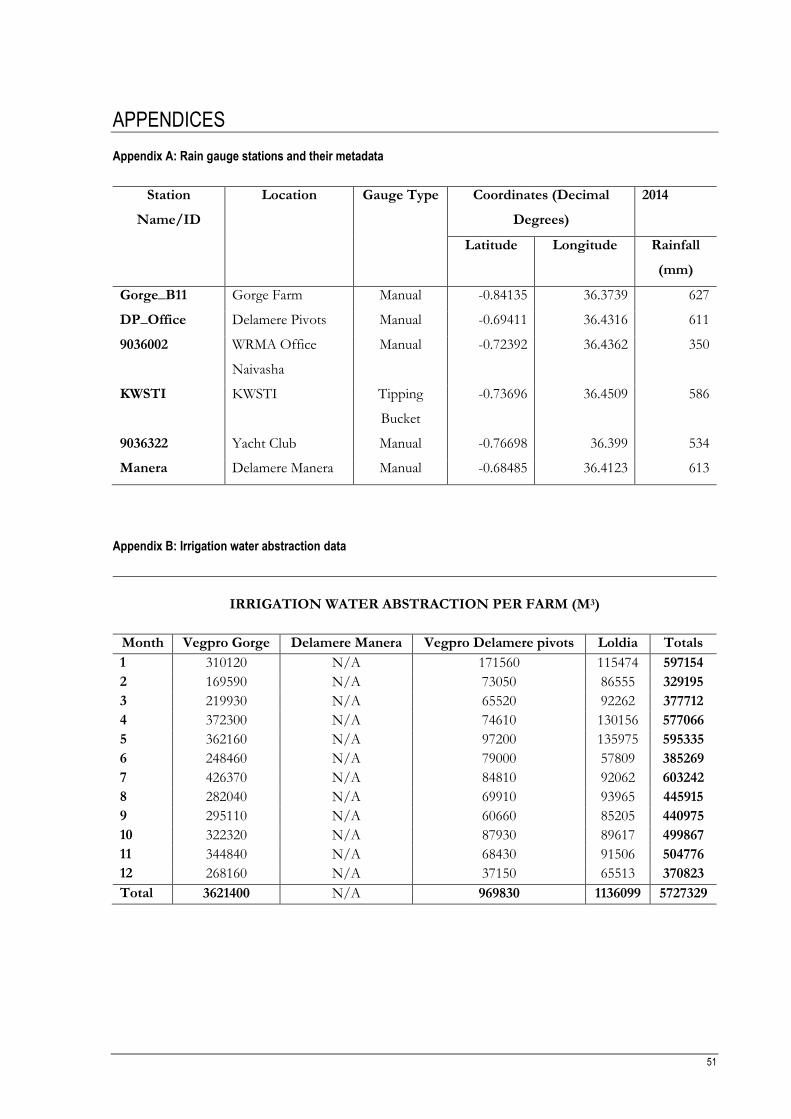
51
APPENDICES
Appendix A: Rain gauge stations and their metadata
Station
Name/ID
Location Gauge Type Coordinates (Decimal
Degrees)
2014
Latitude Longitude Rainfall
(mm)
Gorge_B11 Gorge Farm Manual -0.84135 36.3739 627
DP_Office Delamere Pivots Manual -0.69411 36.4316 611
9036002 WRMA Office
Naivasha
Manual -0.72392 36.4362 350
KWSTI KWSTI Tipping
Bucket
-0.73696 36.4509 586
9036322 Yacht Club Manual -0.76698 36.399 534
Manera Delamere Manera Manual -0.68485 36.4123 613
Appendix B: Irrigation water abstraction data
IRRIGATION WATER ABSTRACTION PER FARM (M3)
Month Vegpro Gorge Delamere Manera Vegpro Delamere pivots Loldia Totals
1 310120 N/A 171560 115474 597154
2 169590 N/A 73050 86555 329195
3 219930 N/A 65520 92262 377712
4 372300 N/A 74610 130156 577066
5 362160 N/A 97200 135975 595335
6 248460 N/A 79000 57809 385269
7 426370 N/A 84810 92062 603242
8 282040 N/A 69910 93965 445915
9 295110 N/A 60660 85205 440975
10 322320 N/A 87930 89617 499867
11 344840 N/A 68430 91506 504776
12 268160 N/A 37150 65513 370823
Total 3621400 N/A 969830 1136099 5727329

52
Appendix C: Formulation of the extra-terrestrial radiation
Extra-terrestrial radiation (Ra) used in the Hargreaves equation was computed using Equation 7-1 (Allen et
al., 1998).
𝑅𝑎 =
24 × 60
𝜋𝐺𝑠𝑐𝑑𝑟[𝜔𝑠 𝑠𝑖𝑛(𝜑) 𝑠𝑖𝑛(𝛿) + 𝑐𝑜𝑠(𝜑) 𝑠𝑖𝑛(𝜔𝑠)] 7-1
Where, 𝐺𝑠𝑐 is the solar constant (0.0820 MJm-2min-1), 𝑑𝑟 is the inverse relative distance Earth-sun, 𝜔𝑠 is the
sunset hour angle, 𝜑 is the latitude in radians and 𝛿 is the solar declination, which is the latitude at which
the sun is directly overhead.
The inverse relative distance Earth-sun is calculated using Equation 7-2
𝑑𝑟 = 1 + 0.033 cos (
2𝜋
365𝐽) 7-2
Where, 𝐽 is the Julian day of the year
Sunset hour angle is calculated using Equation 7-3.
𝜔𝑠 = 𝑎𝑟𝑐𝑐𝑜𝑠[−𝑡𝑎𝑛(𝜑) 𝑡𝑎𝑛(𝛿)] 7-3
Where, 𝜑 is latitude in radians and must be negative for the southern hemisphere
Solar declination is computed using Equation 7-4.
𝛿 = 0.409 sin (
2𝜋
365𝐽− 1.39) 7-4
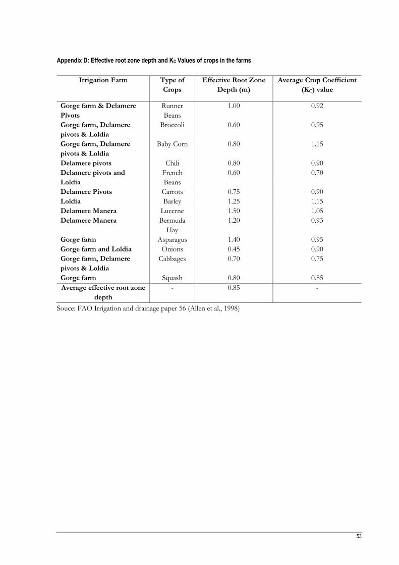
53
Appendix D: Effective root zone depth and KC Values of crops in the farms
Irrigation Farm Type of
Crops
Effective Root Zone
Depth (m)
Average Crop Coefficient
(KC) value
Gorge farm & Delamere
Pivots
Runner
Beans
1.00 0.92
Gorge farm, Delamere
pivots & Loldia
Broccoli 0.60 0.95
Gorge farm, Delamere
pivots & Loldia
Baby Corn 0.80 1.15
Delamere pivots Chili 0.80 0.90
Delamere pivots and
Loldia
French
Beans
0.60 0.70
Delamere Pivots Carrots 0.75 0.90
Loldia Barley 1.25 1.15
Delamere Manera Lucerne 1.50 1.05
Delamere Manera Bermuda
Hay
1.20 0.93
Gorge farm Asparagus 1.40 0.95
Gorge farm and Loldia Onions 0.45 0.90
Gorge farm, Delamere
pivots & Loldia
Cabbages 0.70 0.75
Gorge farm Squash 0.80 0.85
Average effective root zone
depth
- 0.85 -
Souce: FAO Irrigation and drainage paper 56 (Allen et al., 1998)
Copyright © 2022 FDOKUMEN