ASSESSMENT AND MANAGEMENT OF THE IMPACT OF PLATINUM MINING ON

WATER QUALITY AND SELECTED AQUATIC ORGANISMS IN THE HEX RIVER,

RUSTENBURG REGION, SOUTH AFRICA.

By

SABELO VICTOR GUMEDE

Submitted in partial fulfillment of the requirements for the degree of

Doctor of Philosophy: Aquatic Health

in the Department of Zoology, Faculty of Science.

University of Johannesburg

Supervisor: Professor J.H.J. Van Vuren

Co-Supervisor: Professor V. Wepener

May 2012

i

DECLARATION

I declare that this thesis which I submitted for the degree of Doctor of Philosophy (PhD)

in the Department of Zoology, Faculty of Science at University of Johannesburg is

original and has not been submitted by me for a degree at any institution. All assistance

that I received has been fully acknowledged.

___________________ ___________________

Sabelo Victor Gumede Date

ii

ABSTRACT

Mining operations significantly influence the environment due to direct and indirect

discharges of waste products into the aquatic systems. The primary aim of this study

was to assess the current situation in the platinum mining area and develop a

management plan to ensure that existing and potential environmental impacts caused

by platinum mining and processing are mitigated.

To do this, an assessment was carried out to investigate changes in critical aquatic

invertebrate and fish community distributions and assess how they relate to measured

environmental factors. Five sites were selected, one reference site which is upstream of

heavy mining activities and four sites within heavy mining and processing activities.

Standard techniques for water, sediment, invertebrate and fish sampling were used.

Macro-invertebrates sampled were identified to family level whereas fish were identified

to species level.

Multivariate analysis used was cluster analysis by non-metric multidimensional scaling

(NMDS) for both macro-invertebrates and fish. Three methods of ordination were used

to analyze the biotic and abiotic data namely N-MDS, Correspondence Analysis (CA)

and Canonical Correspondence Analysis (CCA).

Cluster analysis of macro-invertebrates data revealed three major groups based on

sampling period (low flow or high flow) and the last cluster according to the locality.

Multidimensional scaling ordination of high and low flow for macro-invertebrate

communities confirmed the groupings detected by cluster analysis. Cluster analysis for

fish communities revealed two groups at 50% similarity; the first group is the

combination of reference and exposure sites for both high and low flow sampling

regimes. No fish were sampled at site 4 during both low and high flow regimes.

Multidimensional scaling ordination of high and low flow fish communities confirmed the

groupings detected by cluster analysis. Analysis using a similarity profile (SIMPROF)

test indicated that fish communities are statistically (p=5%) the same. It was found that

macro-invertebrates and fish respond differently to environmental variables. The macro-

iii

invertebrate and fish community structure indicated no clear-cut distinction between

exposure and reference sites. CCA indicated that metals in sediment and water appear

to have a stronger relationship with macro-invertebrate community structure than fish

community structure. On the other hand, the metal accumulation in fish liver and muscle

tissue did not show any relationship with the environmental variables. Similarity

percentages (SIMPER) for cluster analysis was used to determine indicator species to

the trend and this revealed that Tabanidae, Oligochaeta and Corixidae were the major

contributors to the separation of macro-invertebrate groups which are pollution tolerant

families. It was found that macro-invertebrate community distribution is influenced more

by contaminants in the sediment than sediment particle size. Furthermore, it was found

that that non-core mining activities negatively affect the fish communities of the Hex

River. The results indicated that site four is highly impacted by mining activities in terms

of water and sediment quality.

The study was thus able to provide data and co-ordinate resources towards the

development of the management plan to ensure that changes in the macro-invertebrate

and fish community distributions due to water and sediment qualities are detected in

time and mitigation measures put in place. It is expected that a management plan will

be used to conduct the Hex River rehabilitation process, which is a commitment in the

Environmental Management Programme Report (EMPR) for Rustenburg Platinum

Mines (RPM).

iv

ACKNOWLEDGEMENTS

The co-operation and support of many people have contributed to the successful

completion of this research.

My most sincere and heartfelt appreciation goes to the following persons who, during

the course of this study, extended their support and assistance in many ways–

• My supervisor, Professor Johan van Vuren for his help and for exposing me to

aquatic health environment and for his invaluable guidance and interest in this

work.

• Professor Victor Wepener who is gratefully acknowledged for his guidance and

input in the study.

• Dr. Martin Ferreira and Mr. Wynand Malherbe for their assistance during

sampling and their interest in the study.

• Ms Eve Fisher for assisting with the laboratory work.

• Dr. Richard Greenfield for his support and guidance in the study.

• My family for their love and patience. My dear wife, Likhapha; daughters,

Silindile, Enhle and Elihle are thanked for their moral support and for allowing me

to follow my heart.

• A special note of thanks to my mother Mrs. N.R. Gumede my late father, my

brothers Mpumelelo, Nhlanhla, sisters Nosipho and Bongiwe for their continuous

prayers.

• A number of individuals not mentioned here, whose contributions to the

successful completion of this study are highly appreciated.

Finally, I am grateful to the Almighty God for answering my prayers.

v

LIST OF ACRONYMS

AQMS Air Quality Management System

BOD Biochemical Oxygen Demand

CA Correspondence Analysis

CANOCO Canonical Community Ordination

CCA Canonical Correspondence Analysis

DACE Department of Agriculture, Conservation and Environment

DEAT Department of Environmental Affairs and Tourism

DMR Department of Mineral Resources

DWA Department of Water Affairs

DWAF Department of Water Affairs and Forestry

EIA Environmental Impact Assessment

EMPR Environmental Management Programme Report

EMS Environmental Management Systems

EPA Environmental Protection Agency

GDP Gross Domestic Product

GSM Gravel, Sand and Mud

HQI Habitat Quality Index

HRMC Hex River Management Committee

HRMP Hex River Management Plan

ICP Inductively Coupled Plasma

IDP Integrated Development Plan

IWUL Integrated Water Use License

LEL Lowest Element Level

MMSD Mining Mineral and Sustainable Development

MPRDA Mineral and Petroleum Resources Development Act

NEMA National Environmental Management Act

PGM Platinum Group Metals

RBMR Rustenburg Base Metals Refinery

RLM Rustenburg Local Municipality

vi

RPM Rustenburg Platinum Mines

RPMR Rustenburg Precious Metals Refinery

RVI Riparian Vegetation Index

SASS South African Scoring System

SEL Severe Effect Level

SLP Social and Labour Plan

SIMPER Similarity Percentages

SIMPROF Similarity Profile

TEL Threshold Element Level

TWQR Target Water Quality Range

WHO World Health Organisation

WWTW Waste Water Treatment Works

vii

LIST OF FIGURES

Figure 2.1 Location of the study area, showing sampling sites in the Hex River System. 17 Figure 4.1. Total number of species and individuals of macro-invertebrates sampled per

sampling site, at both high flow (HF) and low flow (LF). 36 Figure 4.2 Total number of individuals and species of fish sampled per sampling site at

both high flow (HF) and low flow (LF). 37 Figure 4.3 Diversity indices of macro-invertebrates per sampling site, at both high flow

(HF) and low flow (LF). 37 Figure 4.4 Diversity indices of fish per sampling site, at both high flow (HF) and low flow

(LF). 38 Figure 4.5 Dendrogram of macro-invertebrate communities, at both high and low flow

sampling sites. The red lines indicate the similarity profile (SIMPROF) test. 40 Figure 4.6 Dendrogram of fish communities at both high and low flow sampling sites. The

red lines indicate the similarity profile (SIMPROF) test. 40 Figure 4.7 Non-Metric Multi-dimensional scaling (MDS) ordination of macro-invertebrate

communities, at both high and low flow sites. 41 Figure 4.8 Non-Metric Multi-dimensional scaling (NMDS) of fish communities at both high

and low flow sites. 41 Figure 4.9 Correspondence Analysis (CA) for fish species (triangles) and sampling sites

(circles), at high and low flow sampling sites during 2005. Data were log (x+1) transformed. Axis 1 is horizontal, and axis 2 is vertical. 60

Figure 4.10 Correspondence Analysis (CA) for fish species (triangles) and sampling sites (circles), at high and low flow sampling sites during 2006. Data were log (x+1) transformed. Axis 1 is horizontal, and axis 2 is vertical. 61

Figure 4.11 Correspondence Analysis (CA) for Macro-invertebrates families (triangles) and sampling sites (circles) (data square root transformed) at both high and low flow during 2005. Axis 1 is horizontal and axis 2 vertical. 62

Figure 4.12 Correspondence Analysis (CA) for Macro-invertebrates families (triangles) and sampling sites (circles) (data square root transformed) at both high and low flow during 2006. Axis 1 is horizontal and axis 2 vertical. 63

Figure 4.13 Canonical Correspondence Analysis of Fish species (triangles), sampling sites (circles) and sediment quality (arrows), at high and low flow during 2005. Axis 1 is horizontal and axis 2 is vertical. 65

Figure 4.14 Canonical Correspondence Analysis of Fish species (triangles), sampling sites (circles) and sediment quality (arrows), at high and low flow during 2006. Axis 1 is horizontal and axis 2 is vertical. 66

Figure 4.15 CCA of macro-invertebrate species (triangles), sampling sites (circles) and sediment quality variables (arrows), at high (HFS) and low (LFS) flow during 2005. Axis 1 is horizontal and axis 2 is vertical. 70

Figure 4.16 CCA of macro-invertebrate species (triangles), sampling sites (circles) and sediment quality variables (arrows), at high (HFS) and low (LFS) flow during 2006. Axis 1 is horizontal and axis 2 is vertical. 71

Figure 4.17 CCA of fish species (triangles); sampling sites (circles), and water quality variables (arrows) at high and low flow during 2005. Axis 1 is horizontal and axis 2 is vertical. 77

viii

Figure 4.18 CCA of fish species (triangles); sampling sites (circles), and water quality variables (arrows) at high and low flow during 2006. Axis 1 is horizontal and axis 2 is vertical. 78

Figure 4.19 CCA of macro-invertebrate species (triangles), sampling sites (circles) and water quality variables (arrows), at high and low flow during 2005. Axis 1 is horizontal and axis 2 is vertical. 82

Figure 4.20 CCA of macro-invertebrate species (triangles), sampling sites (circles) and water quality variables (arrows), at high and low flow during 2006. Axis 1 is horizontal and axis 2 is vertical. 83

Figure 4.21 CCA of fish species (triangles), sampling sites (circles) and sediment grain size variables (arrows), at high and low flow during 2005. Axis 1 is horizontal and axis 2 is vertical. 88

Figure 4.22 CCA of fish species (triangles), sampling sites (circles) and sediment grain size variables (arrows), at high and low flow during 2006. Axis 1 is horizontal and axis 2 is vertical. 89

Figure 4.23 CCA of macro-invertebrate families (triangles), sampling sites (circles) and sediment grain size variables (arrows), at high (HFS) and low (LFS) flow during 2005. Axis 1 is horizontal and axis 2 is vertical. 93

Figure 4.24 CCA of macro-invertebrate families (triangles), sampling sites (circles) and sediment grain size variables (arrows), at high (HFS) and low (LFS) flow during 2006. Axis 1 is horizontal and axis 2 is vertical. 94

Figure 4.25 Mean cobalt (Co) concentration (µg/g) in fish liver and muscle, per sampling site. n= 48 and 52 for 2005 and 2006, respectively. 99

Figure 4.26 Mean aluminium (Al) concentration (µg/g) in fish liver and muscle, per sampling site. n= 48 and 52 for 2005 and 2006, respectively. 99

Figure 4.27 Mean copper (Cu) concentration (µg/g) in fish liver and muscle, per sampling site. n= 48 and 52 for 2005 and 2006, respectively. 100

Figure 4.28 Mean zinc (Zn) concentration (µg/g) in fish liver and muscle per sampling site. n= 48 and 52 for 2005 and 2006, respectively. 100

Figure 4.29 Mean manganese (Mn) concentration (µg/g) in fish liver and muscle, per sampling site. n= 48 and 52 for 2005 and 2006, respectively. 101

Figure 4.30 Mean Nickel (Ni) concentration (µg/g) in fish liver and muscle, per sampling site. n= 48 and 52 for 2005 and 2006, respectively. 101

Figure 4.31 Mean cadmium (Cd) concentration (µg/g) in fish liver and muscle, per sampling site. n= 48 and 52 for 2005 and 2006, respectively. 102

Figure 4.32 Mean lead (Pb) concentrations (µg/g) in fish liver and muscle, per sampling site. n= 48 and 52 for 2005 and 2006, respectively. 103

Figure 4.33 Mean chromium (Cr) concentrations (µg/g) in fish liver and muscle, per sampling site. n= 48 and 52 for 2005 and 2006, respectively. 103

Figure 5.1 Schematic outlay of the hydrological cycle of a tailing disposal facility (Witt et. al., 2005). 122

Figure 6.1 Management structure of the Hex River Management system. 159 Figure 6.2 RPM proposed change management procedure for approval of projects (RPM,

2011). 162 Figure 6.3 Regional setting of sampling sites in the Hex River system. 166

ix

Figure 6.4 Environmental data management process 181 Figure 6.5 Example of a monthly report to stakeholders on incidents that may contribute

to a decline in aquatic health in the Hex River. 187 Figure 6.6 Example of a monthly ‘one pager’ used for employee environmental

awareness in the operations. 188

x

LIST OF TABLES

Table 4.1 Similarity percentage contribution of macro-invertebrate species in the 2005 survey within the cluster with sampling sites HFS3, HFS5, HFS1, HFS2 (average similarity = 81.52), where Av. Abund = average abundance within group, Av. Sim = average similarity, contrib% = percentage contribution, and cum% = cumulative percentage contribution. 45

Table 4.2 Similarity percentage contribution of macro-invertebrate species within the cluster with sampling sites LFS3, LFS5, LFS1 and LFS2 (average similarity = 87.72), where Av. Abund = average abundance within group, Av. Sim = average similarity, contrib% = percentage contribution, and cum% = cumulative percentage contribution. 2005 survey. 46

Table 4.3 Similarity percentage contribution of macro-invertebrate species within the cluster with sampling sites HFS4 and LFS4 (average similarity = 42.28), where Av. Abund = average abundance within group, Av. Sim = average similarity, contrib% = percentage contribution, and cum% = cumulative percentage contribution. 2005 survey. 46

Table 4.4 Dissimilarity percentage contribution of macro-invertebrate species between the 1st cluster (HFS3, HFS2, HFS1 and HFS2) and 2nd cluster (LFS3, LFS5, LFS1 and LFS2) (the average dissimilarity between the two clusters = 54.96), where Av. Abund = average abundance within group, Av. Diss = average dissimilarity, contrib% = percentage contribution, and cum% = cumulative percentage contribution. 47

Table 4.5 Dissimilarity percentage contribution of macro-invertebrate species between the 1st cluster (HFS3, HFS2, HFS1 and HFS2) and 3rd cluster (HFS4 and LFS4) (average dissimilarity between the two clusters = 86.55), where Av. Abund = average abundance within group, Av. Diss = average dissimilarity, contrib% = percentage contribution, and cum% = cumulative percentage contribution. 2005 survey. 48

Table 4.6 Dissimilarity percentage contribution of macro-invertebrate species between the 3rd cluster (HFS4 and LFS4) and 2nd cluster (LFS3, LFS5, LFS1 and LFS2) (average dissimilarity between the two clusters = 83.15), where Av. Abund = average abundance within group, Av. Diss = average dissimilarity, contrib% = percentage contribution, and cum% = cumulative percentage contribution. 2005 survey. 49

Table 4.7 Similarity percentage contribution of fish species within the cluster with sampling sites LFS2, LFS5, LFS3, HFS3, LFS1, HFS5, HFS1, HFS2 (average similarity = 49.39), where Av. Abund = average abundance within group, Av. Sim = average similarity, contrib% = percentage contribution, and cum% = cumulative percentage contribution. 2005 survey. 50

Table 4.8 Similarity percentage contribution of macro-invertebrate species within the cluster with sampling sites HFS1, HFS2, HFS3, HFS5 (average similarity = 71.06), where Av. Abund = average abundance within group, Av. Sim = average similarity, contrib% = percentage contribution, and cum% = cumulative percentage contribution. 2006 survey. 53

xi

Table 4.9 Similarity percentage contribution of macro-invertebrate species within the cluster with sampling sites LFS1, LFS2, LFS3 and LFS4 (average similarity = 87.26), where Av. Abund = average abundance within group, Av. Sim = average similarity, contrib% = percentage contribution, and cum% = cumulative percentage contribution. 2006 survey. 54

Table 4.10 Similarity percentage contribution of macro-invertebrate species within the cluster with sampling sites HFS4 and LFS4 (average similarity = 40.11), where Av. Abund = average abundance within group, Av. Sim = average similarity, contrib% = percentage contribution, and cum% = cumulative percentage contribution. 2006 survey. 54

Table 4.11 Dissimilarity percentage contribution of macro-invertebrate species between the 1st cluster (HFS3, HFS2, HFS1 and HFS2) and 2nd cluster (LFS4, HFS4) (the average dissimilarity between the two clusters = 79.28), where Av. Abund = average abundance within group, Av. Diss = average dissimilarity, contrib% = percentage contribution, and cum% = cumulative percentage contribution. 55

Table 4.12 Dissimilarity percentage contribution of macro-invertebrate species between the 1st cluster (HFS3, HFS2, HFS1 and HFS2) and 3rd cluster (LFS1 and LFS2) (average dissimilarity between the two clusters = 47.79), where Av. Abund = average abundance within group, Av. Diss = average dissimilarity, contrib% = percentage contribution, and cum% = cumulative percentage contribution. 2006 survey 56

Table 4.13 Dissimilarity percentage contribution of macro-invertebrate species between the 3rd cluster (HFS4 and LFS4) and 2nd cluster (LFS1, LFS2) (average dissimilarity between the two clusters = 78.09), where Av. Abund = average abundance within group, Av. Diss = average dissimilarity, contrib% = percentage contribution, and cum% = cumulative percentage contribution. 2006 survey. 57

Table 4.14 Similarity percentage contribution of fish species within the cluster with sampling sites LFS2, LFS5, LFS3, HFS3, LFS1, HFS5, HFS1, HFS2 (average similarity = 58.89), where Av. Abund = average abundance within group, Av. Sim = average similarity, contrib% = percentage contribution, and cum% = cumulative percentage contribution. 2006 survey. 58

Table 4.15 Summary of weightings of the first two axes of Correspondence Analysis for fish species (data log (x+1) transformed) and macro-invertebrate species (data square root transformed), at both high and low flow. 63

Table 4.16 Summary of weightings of the first two axes of CCA for fish species and sediment quality variables, at both high and low flow for 2005 and 2006 surveys. Variances explained by the two axes are given. Monte Carlo probability test of significance is shown for the first axis and all four axes. *p≤0.05. 67

Table 4.17 Intra- and inter-set correlations between each of the sediment quality variables and CCA axes for fish species, at both high and low flow for 2005 and 2006 surveys. 68

Table 4.18 Summary of weightings of the first two axes of CCA for macro-invertebrate species and sediment quality variables, at both high and low flow for 2005 and 2006 surveys. Variances explained by the two axes are given. 72

xii

Table 4.19 Intra- and inter-set correlations between each of the sediment quality variables and CCA axes, for macro-invertebrate species at both high and low flow for 2005 and 2006 surveys. 73

Table 4.20 Mobility of trace metal concentrations (mg/kg) in sediment of the Hex River at the sampling sites, during high and low flow in 2005. 74

Table 4.21 Mobility of trace metal concentrations (mg/kg) in sediment of the Hex River at the sampling sites, during high and low flow in 2006. 75

Table 4.22 Summary of weightings of the first two axes of CCA for fish species and water quality variables, at both high and low flow for 2005 and 2006 surveys. Variances explained by the two axes are given. Monte Carlo probability test of significance is shown for the first axis and all four axis. *p≤0.05. 79

Table 4.23 Intra- and inter-set correlations between each of the water quality variables and CCA axes for fish species at both high and low flow for 2005 and 2006 surveys. 80

Table 4.24 Summary of weightings of the first two axes of CCA for macro-invertebrate species and water quality variables, at both high and low flow during 2006. Variances explained by the two axes are given. Monte Carlo probability test of significance is shown for the first axis and all four axis. *p≤0.05. 84

Table 4.25 Intra- and inter-set correlations between each of the water quality variables and CCA axes for macro-invertebrate species at both high and low flow for 2005 and 2006 surveys. 85

Table 4.26 Metal concentrations (µg/l) in water sampled in the Hex River at the sampling sites, during low flow for 2005 and 2006 surveys. 85

Table 4.27 Metal concentrations (µg/l) in water sampled in the Hex River at the sampling sites, during high flow. 86

Table 4.28 Summary of weightings of the first two axes of CCA for fish species and grain size variables, at both high and low flow during for 2005 and 2006 surveys. Variances explained by the two axes are given. Monte Carlo probability test of significance is shown for the first axis and all four axis. *p≤0.05. 90

Table 4.29 Intra- and inter-set correlations between each of the grain size variables and CCA axes for fish species, and at both high and low flow for 2005 and 2006 surveys. 91

Table 4.30 Summary of weightings of the first two axes of CCA for macro-invertebrate species and grain size variables, at both high and low flow. Variances explained by the two axes are given. Monte Carlo probability test of significance is shown for the first axis and all four axis. *p≤0.05. 95

Table 4.31 Intra- and inter-set correlations between each of the grain size variables and CCA axes for macro-invertebrate species, at both high and low flow. 96

Table 4.32 and 4.33 show water quality results for 2005 and 2006. Water pH was generally lower during low flow as compared to high flow survey. Whereas, Oxygen concentration levels were higher during high flow and lower during low flow. Conductivity and COD concentration levels wre lower during flow and higher in high flow surveys, whereas Kjeldahl nitrogen was higher in the low flow regime as compared to high flow.

Table 4.32 Water quality results for low flow and high flow survey in 2005. 97 Table 4.33 Water quality results for low flow and high flow survey in 2006. 98

xiii

Table 4.34 Mean and Standard deviation in fish musle and liver for 2005 and 2006. Significance level between different tissues is shown. 104

Table 5.1 Sediment Quality Guideline concentration levels (mg/kg) of measured metals, as determined by the EPA (1999), OMEE (1998) and CCME (2002). 115

Table 6.1 A summary of terrestrial environmental aspects in the Hex River system. 156 Table 6.2 A summary of aquatic environmental aspects in the Hex River system. 157 Table 6.3 RPM baseline risk assessment summary. 158 Table 6.4 Category of invertebrates with their given level of pollution tolerance (Gerber &

Gabriel, 2002). 171 Table 6.5 Objectives, output, actions and indicators to be used to test effectiveness of

the management plan. 175 Table 6.6 Data management roles and responsibilities 184

xiv

CONTENTS

DECLARATION ........................................................................................................................... i

ABSTRACT ................................................................................................................................. ii

ACKNOWLEDGEMENTS .......................................................................................................... iv

LIST OF ACRONYMS ................................................................................................................. v

LIST OF FIGURES ................................................................................................................... vii

LIST OF TABLES ........................................................................................................................ x

CHAPTER 1 ............................................................................................................................... 1

GENERAL INTRODUCTION ...................................................................................................... 1

1. Introduction .............................................................................................................. 1

1.1 Background information and motivation ................................................................... 2

1.1.1 Water quality ............................................................................................................ 2

1.1.2 Sediment ................................................................................................................. 3

1.1.3 Macro-invertebrates ................................................................................................. 5

1.1.4 Fish .......................................................................................................................... 6

1.2 Management plan .................................................................................................... 6

1.3 Rationale ................................................................................................................. 7

1.4 Aim .......................................................................................................................... 8

1.4.1 Objectives ................................................................................................................ 8

1.5 References .............................................................................................................10

CHAPTER 2 ..............................................................................................................................16

LOCALITY DESCRIPTION .......................................................................................................16

2.1 Description of study area ........................................................................................16

2.1.1 Geology ..................................................................................................................18

2.1.2 Climate ...................................................................................................................18

2.1.3 Topography ............................................................................................................19

2.1.4 Soil .........................................................................................................................19

2.1.5 Natural vegetation ...................................................................................................19

2.1.6 Surface Water .........................................................................................................20

2.1.7 Air quality ................................................................................................................20

2.2 Selection of sampling sites......................................................................................20

2.3 References .............................................................................................................22

CHAPTER 3 ..............................................................................................................................23

MATERIALS AND METHODS ..................................................................................................23

3.1. Introduction .............................................................................................................23

xv

3.1.1 Field Work ..............................................................................................................23

3.1.1.1 Sampling of macro-invertebrates ............................................................................23

3.1.1.2 Sampling of fish ......................................................................................................24

3.1.1.3 Sampling of environmental variables ......................................................................24

3.1.2 Laboratory analyses................................................................................................24

3.1.2.1 Water ......................................................................................................................25

3.1.2.1a Organic nitrogen and ammonium nitrogen ..............................................................25

3.1.2.1b Chemical oxygen demand.......................................................................................26

3.1.2.2 Sediment ................................................................................................................26

3.1.2.2a Metals .....................................................................................................................26

3.1.2.2b Sediment particle size .............................................................................................27

3.1.2.3 Fish muscle and liver metal accumulation analysis .................................................28

3.1.3 Data analysis ..........................................................................................................28

3.1.3.1 Univariate methods .................................................................................................28

3.1.3.2 Multivariate Methods ...............................................................................................29

3.1.3.2a Cluster analysis ......................................................................................................29

3.1.3.2b Simper analysis ......................................................................................................30

3.1.3.2c Ordination ...............................................................................................................30

3.1.3.2c (i) Non-Metric Multi-dimensional scaling (NMDS) ......................................................30

3.1.3.2c (ii) Correspondence Analysis (CA) ..............................................................................31

3.1.3.2c (iii) Canonical Correspondence Analysis (CCA) .....................................................31

3.2 References .............................................................................................................32

CHAPTER 4 ..............................................................................................................................35

RESULTS ……………………………………………………………………………………………...35

4.1 Introduction .............................................................................................................35

4.2 Species indices .......................................................................................................35

4.2.1 Spatial distribution pattern of sampling sites ...........................................................38

4.3 Species contribution to spatial distribution within dendrogram clusters in 2005 .......41

4.3.1 Macro-invertebrate indicator species ......................................................................42

4.3.2 Fish indicator species .............................................................................................44

4.4 Species contribution to spatial distribution within dendrogram clusters in 2006 .......50

4.4.1 Macro-invertebrate indicator species ......................................................................50

4.4.2 Fish indicator species .............................................................................................58

4.5 Fish and macro-invertebrate distribution within sampling sites ................................58

4.5.1 Correspondence Analysis 2005 ..............................................................................59

4.5.2 Correspondence Analysis 2006 ..............................................................................59

xvi

4.6 Species distribution trend with respect to environmental variables. .........................64

4.6.1 Distribution with respect to sediment quality ...........................................................64

4.6.2 Distribution with respect to water quality measurements .........................................76

4.6.3 Distribution of species with respect to sediment grain size ......................................87

4.7 Metals concentration in fish liver and muscle tissue per sampling site ....................98

4.8 References ........................................................................................................... 105

CHAPTER 5 ............................................................................................................................ 106

DISCUSSION.......................................................................................................................... 106

5.1 Background .......................................................................................................... 106

5.2 Macro-invertebrate community patterns ................................................................ 107

5.2.1 Indicator species ................................................................................................... 108

5.2.2 Linking macro-invertebrate community patterns to measured environmental variables ............................................................................................................... 109

5.2.2.1 Water quality ......................................................................................................... 109

5.2.2.2 Sediment quality ................................................................................................... 114

5.2.2.3 Sediment grain size .............................................................................................. 120

5.3 Fish community patterns ....................................................................................... 123

5.3.1 Indicator species ................................................................................................... 123

5.3.2 Linking fish community patterns to measured environmental variables ................. 124

5.3.2.1 Water quality ......................................................................................................... 125

5.3.2.2 Sediment quality ................................................................................................... 127

5.3.2.3 Sediment grain size .............................................................................................. 130

5.3.2.4 Metal accumulation in fish ..................................................................................... 131

5.4 References ........................................................................................................... 138

CHAPTER 6 ............................................................................................................................ 153

THE MANAGEMENT PLAN .................................................................................................... 153

6.1 Introduction ........................................................................................................... 153

6.1.1 Objectives and performance criteria ...................................................................... 159

6.1.2 Water quality ......................................................................................................... 160

6.1.3 Sediment quality ................................................................................................... 160

6.1.4 Riparian Vegetation .............................................................................................. 160

6.1.5 Macro-invertebrates .............................................................................................. 161

6.1.6 Fish ....................................................................................................................... 161

6.2 Statistical methods and hypotheses ...................................................................... 163

6.2.1 Water quality ......................................................................................................... 163

6.2.2 Sediment quality ................................................................................................... 163

6.2.3 Riparian vegetation ............................................................................................... 164

xvii

6.2.4 Macro-invertebrates .............................................................................................. 165

6.2.5 Fish ....................................................................................................................... 167

6.3 Analytical methods and alternative designs .......................................................... 168

6.3.1 Water quality ......................................................................................................... 168

6.3.2 Sediment .............................................................................................................. 169

6.3.3 Riparian vegetation ............................................................................................... 170

6.3.4 Macro-invertebrates .............................................................................................. 170

6.3.5 Fish ....................................................................................................................... 172

6.4 Monitoring and evaluation ..................................................................................... 173

6.5 Data and information management ....................................................................... 180

6.5.1 Data quality assurance ......................................................................................... 180

6.5.2 Quality control ....................................................................................................... 181

6.5.3 Information management ...................................................................................... 182

6.5.4 Communicating program results ........................................................................... 186

6.5.4.1 Internal stakeholders ............................................................................................. 186

6.5.4.2 External stakeholders ........................................................................................... 188

6.6 References ........................................................................................................... 190

CHAPTER 7 ............................................................................................................................ 194

CONCLUSIONS AND RECOMMENDATIONS ........................................................................ 194

7.1 Conclusions .......................................................................................................... 194

7.2 Recommendations ................................................................................................ 198

7.3 References ........................................................................................................... 199

1

CHAPTER 1

GENERAL INTRODUCTION

1. Introduction

Over the past few years, large-scale urbanization of previously rural populations,

coupled with growing industrialization and rapid socio-economic changes, have

increased both the demand for water and the extent of impacts on the quality of water

resources in South Africa (Roux et al., 1997).

The promulgation of the National Water Act (Act 36 of 1998) resulted in the natural

environment regarded as an integral part of the water resources, as well as being one of

the competing water users. Hence, the biota, physical and chemical in-stream habitats

and processes, which link biota and habitat, are considered inseparable parts of the

water resource. Section 26 (1) of the Act provides for the development of regulations,

to, among others:

1. Require that the use of water from a water resource be monitored, measured

and recorded;

2. Regulate or prohibit any activity in order to protect a water resource or in-

stream or riparian habitat; and

3. Prescribe the outcome or effect, which must be achieved through

management practices for the treatment of waste, or any class of waste,

before it is discharged into or allowed to enter a water resource.

Successful mitigation of the effects of anthropogenic activities on aquatic ecosystems

requires a clear understanding of the factors (i.e. pollutants, habitats or flows) and

mechanisms, by which these factors degrade aquatic systems (Morley & Karr, 2002).

Once the significance of these factors is known, environmental management agencies

can take remedial action to address the primary issues of concern. Biological surveys,

usually using macro-invertebrates and fish as bioindicators, can provide the necessary

information in the condition of the aquatic system (Sharley et. al., 2008).

2

South Africa has more than 80% of the world’s platinum reserves and is the largest

producer of platinum group metals (PGM). The platinum group of metals has shown one

of the highest long-term growths in production of the numerous mineral commodities

over the past 50 years, due to their unique physical and chemical properties, which

make them ideal for a wide variety of technologies. The North West Province of South

Africa hosts the Bushveld complex, a large igneous complex which is about 370 km

east-west and up to 240 km north-south. Demand for platinum group metals has shown

strong growth in recent years, nearly tripling since 1990. The environmental cost of

platinum group metals production is significant, but appears to be mainly related to

production levels, and given the projected demand in the future, the cumulative

environmental costs in such a concentrated region, provide both a major challenge and

opportunity with respect to sustainability (Mudd & Glaister, 2009).

The North West Province is regarded as an arid province, with increasing demands on

water resources. Rainfall in the province is highly variable, in both space and time, often

resulting in severe droughts and extreme flooding. In all the catchments within the North

West Province, evaporation exceeds rainfall. Mining places significant negative

pressure on the province’s water resources. This is because most mines need large

volumes of water for production, and then dispose of waste products into the used

water, which is then discharged as effluent into the rivers and other surface waters

(North West Province, 2002).

Water quality changes are widely considered the most significant consequence of

mining activities. This is due to the wide variety of undesirable contaminants that are

derived from mining operations, and the frequency and persistence of these

contaminants (MMSD, 2001).

1.1 Background information and motivation

1.1.1 Water quality

Water quality can be defined as the combined effects of the physical attributes and the

chemical constituents of an aquatic ecosystem (Palmer et. al., 1996). Both

anthropogenic pressures and natural processes account for degradation in surface

3

water and groundwater quality (Carpenter et al., 1998). Adverse changes in biological

communities may be attributed either to deterioration in water quality or to habitat

degradation, or to both (DWAF, 1997). Mining activities are serious and important

sources of contamination within the natural environment (Spellman & Drinan, 2000).

Water quality degradation world-wide is due mainly to anthropogenic activities, which

release pollutants into the environment, thereby having an adverse effect upon aquatic

ecosystems (Fatoki et al., 2001). In North West Province, very little is being done in the

Rustenburg Platinum Mines (RPM) region, to monitor the water quality coming from

different mining-related water users (DACE, 2002).

Integrated water quality management plans are very important in ensuring sustainability

of different stakeholder efforts at local level. They can in turn ensure that there is an

improvement in water accountability, so that the Department of Water Affairs’ strategic

goals are achieved.

1.1.2 Sediment

Sediment affects a greater length of rivers than any other pollutant (Parkhill & Gulliver,

2002). Together with salinity and nutrients, sediment is one of the top three causes of

river contamination (Lovette et al., 2007). Sediments are generated by natural erosion

and many anthropogenic activities, including agriculture, grazing, forestry, gravel roads,

mining and construction. High sedimentation in rivers has adverse effects on freshwater

macro-invertebrates by increasing drift downstream (Doeg & Milladge, 1991) and

reducing the ability of drifting invertebrates to re-attach to the stream bed (Bilotta &

Brazier, 2008). Further adverse effects of the drift downstream include decreasing the

feeding efficiency of filter-feeders and algal grazers by burying habitat and the in-filling

of space in gravel spawning grounds, and the clogging and abrasion of gills which leads

to decreased immunity to disease and osmotic dysfunction (Bilotta & Brazier, 2008).

Impacts of sediments in lotic systems depend on flow regimes (Kefford et al., 2010).

During low flow, there is a high level of suspended sediment concentration, although

this may be natural. Equally, during low flow, passive drift of macro-invertebrates is

likely to transport benthic macro-invertebrates for shorter distances than during high

4

flow. The effect of increased drift from sedimentation may thus be less important during

low flow. Additionally, the beds of rivers during low flow are often dominated by fine

particles (sand, silt and clay) and the burial or in-filling of spaces by sediment is thus

unlikely to play an important role in any effects of sediment on aquatic biota (Kefford et

al., 2010). Metals bound on sediments have no direct danger to the ecosystem, as long

as they remain bound. Dangers only arise when changes occur in environmental

conditions such as pH, salinity, temperature or redox potential. This allows bound

metals to be released back into the aquatic environment (Van Vuren et al., 1994). Trace

elements in aquatic systems may be attributed to the geology of the area, or to past and

existing land uses (Varkouhi, 2007).

Mining activities have caused the physical environment to become increasingly polluted

with metals, as aquatic environments are proving to be deposition sites for mobilized

metals (Langston & Bebianno, 1998). Metals can be divided into two groups, esential

like cobalt (Co), copper (Cu), manganese (Mn), molybdenum (Mo) and Zinc (Zn), and

non-essetial like cadmium (Cd), mercury (Hg) and lead (Pb). The latter are potentially

toxic in low concentration, and have become widely distributed due to various human

activities (Dallas & Day, 2004). Because of the prevailing neutral or slightly alkaline

conditions, metal contaminants in rivers are generally not present in water-soluble

forms, but are instead associated with suspended bedded sediment, and yet elevated

levels of metals in biota suggest that they are potentially bioavailable (Tarras-Wahlberg

et al., 2001).

Grain size influence both chemical and biological variables, and plays an important role

in the transport and availability of nutrients and contaminants (Walling & Moorehead,

1989). Furthermore, the diversity and abundance of invertebrate assemblages

increases along with increasing sediment particle size (Hill, 2005). Brown et al., (2000)

showed that macro-invertebrate community structure is more closely related to

sediment contaminant concentrations than sediment grain size.

The literature study reveled that, despite the above characteristics and impacts of

sediment on aquatic biota, there is no known correlation between biota and sediment

5

characteristics in the Hex River. However, the Hex River continues to receive

contaminated sediments from platinum mining and processing activities and changes in

infrastructure in and around the mining lease area.

1.1.3 Macro-invertebrates

Macro-invertebrates are usually abundant, ubiquitous, and have a high diversity and a

range of sensitivities. Therefore, these organisms are extensively used to assess

pollution in freshwater environments (Jones et al., 2010; Jones et al., 2011). Equally,

Rosenberg and Resh (1993) and Fonseca and Esteves (1999) emphasized that macro-

invertebrate communities are abundant and occur throughout the environment. They

stated that the methodology for the sampling of macro-invertebrate communities is well

established; that they exhibit a long life cycle and are known to develop differential

responses to environmental fluctuations, and furthermore they argued that these factors

are important characteristics for use in projects of biomonitoring in aquatic

environments. Macro-invertebrates may also demonstrate the effects of past and

present pollution incidents in terms of the way species have established themselves

(Jeffries & Mills, 1990).

Changes in the macro-invertebrate community structure are widely used in pollution

assessment studies (Bollmohr & Schulz, 2009). Community composition is influenced

by an array of anthropogenic and non-anthropogenic factors, and direct causal

relationships are typically not evident (Long & Chapman 1985; Gaston & Edds 1994).

Recent research indicates that family level identification provides sufficient taxonomic

resolution to detect community responses to human disturbance (Warwick 1988a,

1988b; Bowman & Bailey 1997: Heino, 2008). Advantages of macro-invertebrate

sampling include the ability to identify taxa at various levels of taxonomic classification,

and allows for cheap, straightforward and rapid on-site identification (Newson, 2005).

Hill (2005) confirmed that integration of biological indicators (e.g. aquatic macro-

invertebrates) with chemical (e.g. metals) and physical (e.g. sediment) indicators

ultimately provides information on the ecological state of a river. Recent studies in the

6

Hex River (North West Province) indicated a noticeable decrease in biotic integrity

(Clean Stream Environmental Services, 2005).

1.1.4 Fish

There are a number of other proposed organisms that can be used as indicators of

environmental integrity or health and, to date, no clear favourite has emerged. Fish

communities and individuals have various qualities that make them useful in biological

monitoring (Kotze et al., 2004). This includes the fact that fish are relatively long-lived

and reflect changes in the condition of a river system (River Health Program, 2005).

Morgan (2002) found that habitat plays a fundamental role in feeding, reproduction, and

survival of fish, by effecting their physiology, behavior and genetics.

It is widely known that long-term exposure to environmental stressors such as pollution

or low oxygen values causes detrimental effects on important fish features, such as

metabolism, growth, resistance to diseases, reproductive potential, and, ultimately, the

health, condition, and survival (Barton et al., 2002). The effects at the individual and

community levels depend on the intensity and duration of stress exposure and species-

specific features (Adams & Greeley, 2000). Though there are a number of human

activities in the Hex River, there is however, very little information on factors influencing

fish health and community structures in this area.

1.2 Management plan

The National Environmental Management Act (NEMA, 1998) stipulates that

development must be environmentally, socially and economically sustainable. The

United States Environmental Protection Agency (US-EPA) proposed a risk-based

approach for ecosystem assessment and management (US-EPA, 1992), which

considers social, environmental and economic aspects. Risk management refers to the

activities of identifying and evaluating alternative options, deciding on a course of

action, and implementing the decisions. It is not possible to eliminate all risks

associated with anthropogenic activities. Tradeoffs (which may be based on risk-benefit,

cost-benefit or risk-risk benefit) are typically part of risk management (Stern & Fineberg,

7

1996). In the current context, the proposed Hex River Management Plan (HRMP) will

seek to ensure the integrity of the river ecosystem, address all current impacts, and

promote the utilization of the river in a sustainable way.

Different water users continue to develop and implement short-term and site-specific

plans to mitigate their impact on the watercourse. These plans have proved to be

unsustainable, as there is a lack of integration and accountability in executing them.

Greenfield (2004) proposed a conceptual framework to be used when designing a

monitoring program. A detailed management plan is developed and discussed in

chapter six of this thesis.

1.3 Rationale

The town of Rustenburg has grown significantly in the last ten years, due to the

presence of platinum and chrome mining activities, resulting in pressure to the

infrastructure, which ultimately influences the Hex River system (van der Walt et. al.,

2005).

RPM continues to open new shafts and process PGM near the Hex River. There has

been a number of audit findings, and legal non-conformances, that have indicated a

significant deterioration in source water quality. Furthermore, there has been a lack of

understanding about the total impact on the physical, chemical and biological properties

of receiving water environments. Assessment of the macro-invertebrate and fish

community structure in this area may provide a useful and cost-effective management

approach towards concurrent rehabilitation of the Hex River. Full understanding of the

root cause behind changing community patterns, if any, will assist RPM to follow a risk-

based approach in the rehabilitation efforts.

Based on this background and reasons, a study was conducted to assess the extent of

disturbance in the Hex River, by analyzing fish, macro-invertebrates and selected

abiotic variables. The result of this investigation was used to develop a management

plan. It was therefore hypothesized that mining activities negatively affect the water

8

quality, and affect the macro-invertebrate and fish community structure in the Hex River

during low and high flow regimes.

1.4 Aim

The aim of this study was to assess the impact of platinum mining on the water quality

and selected aquatic organisms in the Hex River System, and to develop a

management plan to mitigate identified risks.

1.4.1 Objectives

In order to achieve the aim of this study, the main objectives were:

1. To compare macro-invertebrate and fish community structure between

exposure and reference sites in the Hex River system.

2. To determine various environmental perturbations affecting macro-

invertebrates and the fish community structure in the Hex River System.

3. To identify areas impacted by mining activities.

4. To develop a management plan.

To reflect the main elements of the research, the thesis is structured into seven

chapters, as follows:

• Chapter 1 is the general introduction to the research, describing the

hypothesis, objectives, background and content of the study.

• Chapter 2 outlines the locality description and provides information on the

selection of the sites.

• Chapter 3 outlines the methods that were used for sampling, laboratory

analysis and data analysis.

• Chapter 4 provides the results of the study analysis. Two complementary

multivariate methods, namely hierarchical agglomerative clustering, and

ordination techniques, were used to present the community data in a

graphical form, which is easily interpreted.

• Chapter 5 discusses the results and articulates the response of fish and

macro-invertebrates to physical and chemical factors.

9

• Chapter 6 is the management plan that will be used to mitigate identified

risks in all operations of Anglo Platinum.

• Chapter 7 summarizes the overall conclusions of the study, and provides

recommendations.

10

1.5 References

Adams, S.M. and Greeley, M.S. 2000. Ecotoxicological indicators of water quality: Using

multi-response indicators to assess the health of aquatic ecosystems. Water, Air and

Soil Pollution 123: 103-115.

Barton, J.S., Poff, N.L., Angermeier, P.L., Dahm, C.N., Gleick, P.H., Hairston, N.G.,

Jackson, R.B., Johnston, C.A., Richter, B.D. and Steinman, A.D. 2002. Meeting

ecological and societal needs for freshwater. Ecological Applications 12: 1247-1260.

Bilotta, G.S. and Brazier, R.E. 2008. Understanding the influence of suspended solids

on water quality and aquatic biota. Water Research 42: 2849-2861.

Bollmohr, S. and Schulz, R. 2009. Seasonal changes of macroinvertebrates in a

Western Cape river, South Africa, receiving non-point source insecticide pollution.

Environment. Toxicology and. Chemistry 28 (4): 809-817.

Bowman, M.F. and Bailey, R.C. 1997. Does taxonomic resolution affect the multivariate

description of the structure of freshwater benthic macro-invertebrate communities?

Canadian Journal of Fisheries and Aquatic Science. 54: 1802-1807.

Brown, S.S., Gaston, GR., Rakocinski, C.F., Heard, R.W. and Summers, J.K. 2000.

Effects of sediment contaminants and environmental gradients on macrobenthic

community trophic structure in Gulf of Mexico estuaries. Estuaries 23: 411-424.

Carpenter, S.R., Caraco, N.F., Correll, D.L., Howarth, R.W., Sharpely, A.N. and Smith,

V.H. 1998. Nonpoint pollution of surface waters with Phosphorus and Nitrogen.

Ecological Applications 8: 559-568.

Clean Stream Environmental Services. 2005. Rustenburg Platinum Mines: Integrated

Surface Water Quality, Biomonitoring and Toxicity Testing. Report No. RPM/Q1/2005.

Dallas, H.F. and Day, J.A. 2004. The effect of water quality variables on aquatic

ecosystems: A review. WRC Report No TT 224/04. Water Research Commission,

Pretoria. 240 pp.

11

Department of Water Affairs and Forestry (DWAF). 1997. National Aquatic Ecosystem

Biomonitoring Programme. Overview of the Design Process and Guidelines for

implementation. Pretoria.

Doeg, T.J. and Milladge, G.A. 1991. Effects of experimental increasing concentrations

of suspended sediment on macroinvertebrate drift. Australian Journal of Marine and

Freshwater Research 42: 519-526.

Fatoki, O.S., Muyima, N.Y.O. and Lujiza, N. 2001. Situational analysis of water quality in

the Umtata River catchment. Water South Africa 27 (4): 467-473.

Fonseca, JJL and Esteves, FA. 1999. Influence of Bauxite tailings on the structure of

the benthic macroinvertebrate community in an Amazon Lake (Lago Batata, Para -

Brazil). Revista. Brasileria de Biologia. 59 (3): 397-405.

Gaston, G.R. and Edds, K.A. 1994. Long term study of benthic communities on the

continental shelf off Cameron, Louisiana: A review of brine effects and hypoxia. Gulf

Research Report. 9: 57-64.

Greenfield, R. 2004. An assessment protocol for water quality integrity and

management of the Nyl Wetland system. Unpublished PhD thesis. Johannesburg:

University of Johannesburg.

Heino, J. 2008. Influence of taxonomic resolution and data transformation on biotic

matrix concordance and assemblage - environment relationships in stream

macroinvertebrates. Boreal Environment Research. 13: 359-369.

Hill, L 2005. Elands Catchment Comprehensive Reserve Determination Study,

Mpumalanga Province. Ecological Classification and Ecological Water requirements

(quantity) Workshop Report, Contract Report for SAPPI-Ngodwana, Submitted to the

Department of Water Affairs and Forestry, by the Division of Water, Environment and

Forestry Technology, CSIR, Pretoria. Report No. ENV-P-C 2004-019 pp 1-98.

Jeffries, M. and Mills, D. 1990. Freshwater Ecology. Belhaven Press. London.

12

Jones, J.I., Davey-Bowker, J., Murphy, J.F. and Pretty, J.L. 2010. Ecological monitoring

and assessment of pollution in rivers. In Ecology of industrial pollution, Batty, L.C. and

Hallberg, K.B. (eds). Cambridge University Press. Cambridge pp. 126-146.

Jones, J.I., Murphy, J.F., Collins, A.L., Sear, D.A., Naden, P.S. and Armitage, P.D.

2011. The impact of fine sediment on macro-invertebrates. River Research and

Applications. doi: 10/rra.1516.

Kefford, B.J., Zalizniak, L., Dunlop, J.E., Nugegoda, D. and Choy, S.C. 2010. How are

macroinvertebrates of slow flowing lotic systems directly affected by suspended and

deposited sediments? Environmental Pollution 158: 543-550.

Kotze, P.J., Steyn, G.J., du Preez, H.H. and Kleynhans, C.J. 2004. Development and

application of a fish based sensitivity - weighted index of biotic integrity for use in the

assessment of biotic integrity of the Klip River, Gauteng, South Africa. African Journal of

Aquatic Science 29 (2): 129-143.

Langston, W.J. and Bebianno, M.J. 1998. Metal mobilization in aquatic environments.

Chapman and Hall. London.

Long, E.R. Chapman, P.M. 1985. A sediment quality triad: Measure of sediment

contamination, toxicity, and infaunal community composition in Puget Sound. Marine

Pollution Bulletin 16: 405-415.

Lovett, S., Price, P. and Edgar, B. (eds). 2007. Salt, nutrient, sediment and interactions:

Findings from the National River Contaminants Program. Land and Water Australia.

Canberra.

MMSD Southern Africa. 2001. Mining, minerals and sustainable development in

Southern Africa. Draft MMSD report.

Morgan, M.N. 2002. Habitat associations of fish assemblages in the Sulphur River,

Unpublished PhD Thesis. Texas A&M University, College Station. pp 58.

13

Morley, S.A. and Karr, J.R. 2002. Assessing and restoring the health of urban streams

in the Puget Sound Basin. Conservation Biology 16: 1498-1509.

Mudd, G.M. and Glaister, B.J. 2009. The environmental cost of Platinum-PGM Mining:

An excellent case study in sustainable mining. Canadian Metallurgical Society. Sudbury,

Ontario, Canada.

Newson, M. 2005. Hydrology and the river environment. Oxford University Press.

Oxford

North West Province DACE (Department of Agriculture, Conservation and

Environment). 2002. North West state of the environment report. DEAT. Pretoria.

Palmer, C.G., Goetsch, P.A., O’Keeffe, J.H. 1996. Development of a recirculating

artificial stream system to investigate the use of macroinvertebrates as water quality

indicators. WRC Report No 475/1/96. Water Research Commission, Pretoria.

Parkhill, K.L. and Gulliver, J.S. 2002. Effect of inorganic sediment on whole-stream

productivity. Hydrobiologia 47: 5-7.

Republic of South Africa. 1998. National Environmental Management Act (NEMA), Act

107 of 1998. Government Gazette. No 19519.

Republic of South Africa. 1998. National Water Act (NWA), Act 36 of 1998. Government

Gazette. No 19182.

River Health Program 2005. State of Rivers Report. Monitoring and managing the

ecological state of rivers in the Crocodile (West) Marico Water Management Area.

DEAT. Pretoria.

Rossenberg, D.M. and Resh, V.H. 1993. Freshwater biomonitoring and benthic macro-

invertebrates. Chapman & Hall. New York.

Roux, D.J., Kempster P.L., Kleynhans, C.J., and Vliet, H.R. 1997. Integrating

environmental concepts regarding stressor and response monitoring into a resource-

14

based water quality assessment framework. Division of Water, Environment and

Forestry Technology, CSIR, Pretoria.

Sharley, D.J., Hoffmann, A.A. and Pettigrove, V. 2008. Effects of sediment quality on

macroinvertebrates in the Sunraysia region of the Murray-Darling Rivers, Australia.

Environmental Pollution 156: 689-698.

Spellman, F.R. and Drinan, J. 2000. The drinking water handbook. Technomic

Publishing. Basel.

Stern, P. and Fineberg, H. (eds). 1996. Understanding risk: Informing decision in a

democratic society. National Academy Press. Washington, DC.

Tarras-Wahlberg, N.H., Flachier, A., Lane, S.N and Sangfors, O. 2001. Environmental

impacts and metal exposure of aquatic ecosystems in rivers contaminated by small

scale gold mining: the Puyango basin, southern Ecuador. Science of the Total

Environment. 278 (1-3): 329-361.

USEPA (United States Environmental Protection Agency). 1992. Guidelines for

exposure assessments: EPA/600/Z-92/001. Risk Assessment Forum. U.S.

Environmental Protection Agency. Washington, DC.

Van der Walt, M., Marx, C., Fouche‘, L., Pretorius, N. and St. Arnaud, J. 2005. Turning

the sewage tide around, a good news case study about the Hex River catchment.

Unpublished study. Rustenburg Local Municipality. Rustenburg.

Van Vuren, J.H.J., du Preez, H.H. and Deacon, A.R. 1994. Effects of pollutants on the

physiology of fish in the Olifants River (Eastern Transvaal). WRC Report No 350/1/94.

Water Research Commission. Pretoria. 214 pp.

Varkouhi, S. 2007. Geochemical evaluation of lead trace elements in streambed

sediment. Proceedings of the WSEAS International Conference on Waste management

and Water Pollution, Air Pollution, and Indoor Climate. Archachon, France, October 14-

16, 2007.

15

Walling, DE and Moorhead, PW. 1989. The particle size characteristics of fluvial

suspended sediment: An overview: Hydrobiologia . 176/177: 125-149.

Warwick, R.M. 1988a. The level of taxonomic description required to detect pollution

effects on marine benthic communities. Marine Pollution Bulletin 19: 259-268.

Warwick, R.M. 1988b. Analysis of community attributes of the macrobenthos of

Friefjord/Langesundfjord at taxonomic levels higher than species. Marine Ecology

Progress Series. 46: 167-170.

16

CHAPTER 2

LOCALITY DESCRIPTION

2.1 Description of study area

The study was carried out in the Rustenburg area situated in North West Province of

South Africa (Figure 2.1). To obtain a better understanding of the Hex River system it

was important to describe where the study area is located, and what are other activities

with possible impacts are taking place in the vicinity. RPM consists of nine shafts, five

concentrators, one smelting plant, and one base metal and precious metal refineries.

These activities extend over a distance of 27 km with all associated infrastructure.

17

Figure 2.1 Location of the study area, showing sampling sites in the Hex River System.

18

2.1.1 Geology

The RPM lease area is underlined by a layered sequence of mafic rocks, referred to as

the Rustenburg Layered suite of the Bushveld complex. This suite includes the

economically important Merensky Reef, mined for PGMs (van der Merwe, 2008).

Layering in the mafic sequence dips northwards in the eastern half of the Rustenburg

area, changing gradually to north-eastward in the western half. Well-developed joint

sets have been noted in the mafic rock of the mine area. Near the eastern boundary of

the mine lease area, the mafic sequence is displaced by a fault, which has the same

orientation as one of the joint sets, as do the three syenite dykes emplaced in tensional

structures east of the precious metals refinery (PMR). A thick sequence of gabbro-norite

assigned to the main zone of the Bushveld Complex overlies the Merensky Reef to the

north-north east of Rustenburg (White, 1994).

2.1.2 Climate

Rustenburg is in a semi-tropical region with reasonably high summer and winter

daytime temperatures. It is warm to hot, with moist humid summers and cool, dry

winters. The wind class of the region is the calm category, meaning wind speed is

relatively low. Frost may occur during winter, the area is fog-free and hailstorms are

very rare (ARC, 1998). According to the River Health Programme (2005), climatic

conditions within the Crocodile (West) Marico water management area is temperate,

semi-arid in the east to dry in the west. Variations in temperature in the area are

minimal and thus the Hex River and its tributaries will not experience significant

variations in temperature unless additional heat or cold is added by anthropogenic

activities. Summer temperatures range from 22°C to 35°C and winter 2°C and 20°C.The

Hex River catchment is situated in the Crocodile West and Marico catchment area

management agency. The natural mean annual runoff of the Crocodile West Marico

River area, is 855 million m3/annum (River Health Programme, 2005).

19

2.1.3 Topography

RPM is bordered by the Magalies Range to the south, Rustenburg to the west, Bospoort

dam to the north, and Lynranties Ridge to the east. The RPM lease area is masked by a

blanket soil cover (>90%) with generally only local development of low flat rock outcrop.

Rock outcrop shape is dominantly a function of the structural characteristics of the rock,

principally the presence of fracturing and layering. These features influence the rate of

weathering, which is greatest along joints with production of friable weathered material.

Subsequent removal of friable, weak cohesive material by erosion leaves behind

indurate rock outcrop. Three categories of outcrop shape can be distinguished: (1) low

whaleback outcrops, (2) low boulder-type outcrops and (3) castle outcrops. The river

valley is subjected to industrial development (process plants) and storage (tailings

dams, slag, waste rock dumps and soil stockpiles) facilities (EMPR, 2000).

2.1.4 Soil

The soils are mostly deep, black clays (montmorillonite) of the Arcadian form,

characteristically developed as a residual soil over gabbro-norite rocks, under partly

water-logged conditions. Arcadia soils are characterized by base saturation and high

cation exchange, and high shrink and swell capacity. Deep, red sandy clay soils of the

Shortlands form occur in certain areas (ARC, 1998).

2.1.5 Natural vegetation

Rustenburg is situated in the Savanna Biome, which is the largest biome in southern

Africa, occupying 46% of its area, and covering over one-third the area of South Africa

(Low & Rebelo, 1996). The environmental factors delimiting the biome are complex:

altitude ranges from sea level to 2000 m; rainfall varies from 235 to 1 000 mm per year;

frost may occur from 0 to 120 days per year; and almost every major geological and soil

type occurs within the biome (Rutherford & Westfall, 1986). The plant list obtained from

the computerized database of the National Herbarium (PRECIS) comprised 4029

records, which represented 1339 species in 625 genera. Thirty of these are red data

20

species, eight of which are threatened, five are insufficiently known, and 17 are

considered not threatened (Balkwill et al., 1999)

2.1.6 Surface Water

The RPM lease area has a number of licenced river diversions near the mines and

processing plants. All storm water from the platinum processing plants is collected into

pollution control dams, before being recycled into the concentrators. These are linked

into the RPM water circuit. Under normal operating conditions, no polluted water is

discharged on site, as any spillage and rainfall run off is collected to these dams. All

sites are above the 1:100 year floodline, or are protected against such a storm event by

retaining flood defense berms. There are no major wetlands; however, the Klipfontein

Spruit bed forms a natural pool to the west of the smelter (EMPR, 2000).

2.1.7 Air quality

The RPM smelter contributes 30 to 70% of the atmospheric sulphur dioxide levels within

the mine lease area. Significantly, high levels of ambient sulphur dioxide have been

observed in the Rustenburg region above the recommended DEAT guidelines of 30

ppb. Measured particulate matter (PM10) concentrations comprised between 20 and

50% of the DEAT guideline of 180 µg/m3 and 60 µg/m3 for highest daily and annual

averaging periods, respectively (Guest, 1998). The operational smelters in the vicinity

have a very low contribution relative to RPM smelter due to their distance from it

(EMPR, 2000).

2.2 Selection of sampling sites

The biomonitoring sites were selected to be accessible, of high value to the study, and

were as representative of as many habitats as possible. Five sites were selected along

the Hex River, representing upstream and downstream conditions of RPM activities.

One site (Site 1) was selected to be upstream from current RPM activities, but adjacent

to and downstream from future mining activities where an approved prospecting license

is in place. This was done to also provide baseline information if the mining license is

granted, and a need to mine exists in future. This site was taken as the reference site in

21

the current study. The second site (Site 2) was selected to be downstream from site 1,

where there is high mineral extraction and waste rock dumping, but it is upstream from

heavy platinum processing activities. This site was selected so that a comparison could

be made between mineral extraction and the platinum processing impact made. The

third site (Site 3) was selected downstream of site 2, where there is a combination of

mineral extraction and tailing dam accumulation from platinum processing. This area

was selected to do an assessment of the impact of the combined effect of these mining

activities. The fourth site (Site 4) was selected downstream of site 3, where there are

mostly tailings dams, slag stockpiles and discharges from processing plants. This site

was chosen because the information derived from it is of high value to the current study,

as the site serves as the direct receiving point from the tailings dam and pollution

control dams discharge. The fifth site (Site 5) was the most downstream of all sites, and

falls outside the mine lease area, where there are no mining related activities. This site

was selected to measure the extent of the combined effect of mining activities associate

with these sites and to determine if there is downstream recovery in the Hex River

system. The positions of the sampling sites are shown in figure 2.1. From each of the

selected sites, samples of water, sediment, macro-invertebrates and fish were taken

between January 2005 and November 2006 covering high and low flow events in both

years.

Three letters and a number represent each sampling event and sampling site. The first

two letters represents the sampling event, the third letter represents the site, and the

last number is a site number out of five. As an example, LFS3 means the sample taken

during the low flow event at site 3. Periodical samples are denoted by their initials, for

example, LF and HF represent low flow and high flow, respectively.

22

2.3 References

Agricultural Research Council (ARC). Institute for Soil, Climate and Water. 1998. Soil

quality assessment. Report No. GW/A/98/103. Pretoria.

Balkwill, K., Campbell-Young, G. and McCallum, D.A. 1999. RPM preliminary botanical

report. Wits University. Johannesburg.

Environmental Management Programme. 2000. Rustenburg Platinum Mines. Process

Division, Environmental Department.

Guest, M. 1998. Air quality monitoring in the vicinity of Rustenburg. Overall Report.

Eskom.

Low, A. and Rebelo, A.G. 1996. Vegetation of South Africa, Lesotho and Swaziland. A

comparison to the vegetation map of South Africa, Lesotho and Swaziland. Department

of Environmental Affairs and Tourism. Pretoria.

North West Province DACE (Department of Agriculture, Conservation and Environment.

2002. North West state of the environment report. DEAT. Pretoria.

River Health Program 2005. State of Rivers Report. Monitoring and managing the

ecological state of rivers in the Crocodile (west) Marico Water management area.

DEAT. Pretoria.

Rutherford, M.C. and Westfall, R.H. 1986. The biomes of Southern Africa - an objective

categorization. Memoirs of the Botanical Survey of South Africa 54: 1-98.

Van der Merwe, J.M. 2008. The geology and structure of the Rustenburg Layered Suite

in the Potgietersrus/Mokopane area of the Bushveld Complex, South Africa. Miner

Deposita 43: 405-419.

White, J.A. 1994. The Potgietersrus Project - geology and exploration history.

Proceedings of the 15th CMMI Congress, South African Institute of Mining and

Metallurgy, Marshaltown, pp 173-181.

23

CHAPTER 3

MATERIALS AND METHODS

3.1. Introduction

Prior to undertaking the current study, consultations and site visits were undertaken,

and an assessment of the environment was conducted to ensure that all study

objectives would be met and recommendations accepted by all key stakeholders. The

key stakeholders were Rustenburg Platinum Mines (RPM), the Department of Water

Affairs (DWAF), Department of Agriculture, Conservation and Environment (DACE),

Landowners, Rustenburg Local Municipality (RLM), Kroondal Environmental Forum

(KEF) and Mfidikwe Environmental Forum (MEF). After the workshop in 2005, the Hex

River Management Committee (HRMC) was established.

After consulting with key stakeholders, the sampling design and strategy were

developed. A decision was taken on the critical parameters to use, that would ensure

focus and allow for the development and practical implementation of the management

plan, as discussed in chapter five of this study. Sampling started in January 2005.

3.1.1 Field Work

Field work was conducted during low flo and high flow which included the sampling of

macro-invertebrates, fish, sediment and water.

3.1.1.1 Sampling of macro-invertebrates

Macro-invertebrate samples were taken at all five sampling sites following the SASS 5

procedure described by Dickens and Graham (2002). There are three main biotopes:

(1) Stones: refers to stones in and out of the current and bedrock, (2) Vegetation: refers

to the aquatic vegetation, whether it is marginal or submerged, and (3) GSM (gravel,

sand and mud): refers to fine stones, silt or sediment deposited over time, as well as

mud. Not all biotopes were present except for the GSM, which was consistent

throughout the five sampling sites. After sampling each biotope using the standard

24

SASS net (1 mm mesh size and dimensions of 30 cm x 30 cm x 30 cm), samples were

placed in an identification tray for identification using an invertebrate field guide (Gerber

& Gabriel, 2002). After sampling, macro-invertebrate identification was limited to 15

minutes per biotope of a given sampling site.

3.1.1.2 Sampling of fish

Fish were sampled using the electro-shocking technique at all sites, except at Site 4,

due to the lack of proper habitat and access to sampling as determined by Kleynhans

(1999). The technique was applied for 20-30 minutes per site, depending on the

availability of habitat. The combined distance sampled was 27 km. All fish specimens

were identified to the lowest taxonomic level possible in the field and released, and

some (10 to 18 per site of different species) were preserved for muscle and liver metal

bioaccumulation analysis in the laboratory. Fish identification was conducted using a

guide described by Skelton (1993).

3.1.1.3 Sampling of environmental variables

In situ water quality measurements of dissolved oxygen concentration (mg/L), oxygen

saturation (%), pH, temperature (0C) and conductivity (µS/cm) were taken using a WTW

340i Multimeter. At the same time water samples were collected in triplicate directly into

acid pre-washed polythene bottles at each sampling site and preserved for laboratory

measurements of metals. Bottom sediment samples were collected and processed in

line with standard protocols of the United States Environmental Protection Agency

(USEPA) (2001). Three core sediment samples were taken to a depth of 5 cm across

the river at each sampling site, and were thoroughly mixed into acid pre-washed

polythene bottles, and retained for physical and chemical analysis in the laboratory.

3.1.2 Laboratory analyses

All samples that could not be analysed in the field were taken to different laboratories

for the analysis of all required variables for this study.

25

3.1.2.1 Water

A volume of each water sample was filtered through pre-weighed 0.45 µm cellulose

nitrate membrane filters, according to the method described by Singh et al. (1988). The

filtrate was retained and stored in amber bottles while the membrane filters were placed

in a drying oven at 60 °C for 24 hours. Dried filter papers were weighed before being

placed in falcon tubes for acidification. Three ml of nitric acid and 30 µl hydrogen

peroxide (H2O2) were added to each tube and allowed to digest overnight at room

temperature. Further digestion, where required, was carried out in a fume cabinet, using

a 800 W microwave oven. Both filtered water and digested membranes were stored in a

cool dark cupboard until undergoing metal analysis using Inductively Coupled Plasma

Mass Spectrophotometry (ICP-MS) methods. It was necessary to measure organic

nitrogen and ammonium nitrogen as nitrogen is found in many forms in water whereas

phosphorus is available in lowest amounts. Equally, Chemical Oxygen demand (COD)

was measured because it does not differentiate between biologically available and inert

organic matter and measures the total quantity of oxygen required for oxidation. It takes

few hours to measure as compared to Biochemical Oxygen Demand (BOD).

3.1.2.1a Organic nitrogen and ammonium nitrogen

An organic nitrogen standard was prepared by dissolving 1 547 g/l Bactopeptone in

1000 ml distilled Milli Q water. The concentration is equal to 250 mg/l organic-N. 20 ml

of the standard was added into the digester tubes. 4 to 6 bumping stones and 2 ml of

the digestion mixture was added to each sample. In a fume cupboard, the digestion

block was set at 150 °C, and was allowed to boil for 1.5 hours (during this time the water

in the mixture evaporated so that mainly concentrated H2SO4 remained). The

temperature was set at 340 °C, which took approximately 60 minutes to attain. After

reaching this temperature, it was kept for 30 minutes, after which the rack with tubes

was removed and allowed to cool until the acid mixture was warm. A standard

procedure was followed for this analysis (Nicholls, 1975).

In order to prepare samples for analysis on the Technicon AutoAnalyser 40 ml of NaOH

neutralizing solution was added to the tube and mixed well. Digested samples were

26

analyzed using a Technicon AutoAnalyser II. For Kjeldahl Nitrogen, a complexing agent

was used. The concentration of tri-sodium citrate was kept the same, while NaOH was

added to raise the pH of the sample to the 12.8 to 13.0 range, in order that all free

ammonia is complexed. The result was calculated by measuring each peak and

entering results in the laboratory worksheet. The average of the two reagent blanks was

subtracted from each sample peak. The concentration of the standard was divided by

the average peak height of the three standards, to give a conversion factor. This factor

was then multiplied by each net sample peak height, to give the concentration in µg/l.

This method is in line with APHA (1992) standards.

3.1.2.1b Chemical oxygen demand

All samples were analyzed for the amount of oxygen needed to oxidize organic and

inorganic material contained in each of them. A Hach Model 45600 COD Reactor was

preheated to 150 °C. The cap was removed from the COD digestion vial, of the desired

range. The vial was held at an angle of 45° and 2 ml of standard solution was pipetted

into the vial. The vial cap was replaced and the content mixed thoroughly. The vials

were placed in the preheated COD reactor. After 120 minutes, the vials were kept for an

additional 20 minutes, before they were removed whilst still warm. The vials were

allowed to cool to room temperature. A Hach Model DR 2010 spectrophotometer was

used. The concentration of COD in each sample was calculated from the absorbance

value obtained, by reference to the calibration curve obtained by plotting concentration

of the standard solutions against their corresponding absorbance. This method is in line

with APHA (1992) standards.

3.1.2.2 Sediment

3.1.2.2a Metals

Sediment samples were chemically analyzed by using the technique proposed by the

BCR (Ure et al., 1993). This technique is a sequential extraction scheme (SES) in which

the metals are divided into acid soluble, reducible and oxidizable fractions (Gomez Ariza

et al., 2000). Basically, it is intended that each step expose the sediment sample to the

action of an extractant, which solubilizes a specific component of sediment according to

27

its associated metals. In this project, one gram of sediment was subjected to extraction

in 50 ml acid-washed falcon tubes.

The first stage involved the addition of 40 ml of 0.11 M acetic acid. The samples were

allowed to extract for 16 hours and the residue was separated from the extract by

decanting. Samples were stored in amber bottles until metal analysis was undertaken

using the ICP method. In the second stage, 40 ml of 0.1 M hydroxylamine hydrochloride

was added to the residue, and from there on the same process was followed as in stage

one. The third stage involved the addition of 10 ml of 30% hydrogen peroxide. Tubes

were covered with a watch glass and digested first at room temperature for 1 hour, and

then at 85 °C in a hot bath for a further hour. Aft er digestion, the watch glasses were

removed and the content reduced by evaporation to a few millilitres. At this point, 50 ml

of 1 M ammonium acetate was added and extracted for 16 hours. Once complete, the

tubes were centrifuged at 3000 rpm and the supernatant removed and made up to 100

ml with Milli Q water. Samples were stored in amber bottles for later analysis using the

ICP method. The final stage involved Aqua regia digestion (3:1 ratio of nitric and

hydrochloric acid) of the remaining sediment. Samples were cold-digested and stored

for later metal analysis using the ICP method.

3.1.2.2b Sediment particle size

In the laboratory, sediment samples were thawed and dried in an oven at 60 °C. Drying

was allowed for a period of 24 hours. Sediment grain size was determined by sub-

sampling a portion of 80 g and placing it in an Endecott EFL 2000/1 mechanical sieve,

with sieve racks of 4000 µm, 2000 µm, 500 µm, 212 µm and 53 µm. Samples were

sieved for 20 minutes and each fraction was weighed to the nearest 0.001 g. The

average percentage of each fraction was then calculated (Cyrus et al., 2000).

Grain size categories, as described by Cyrus et al., (2000), were applied as follows:

• > 4000 µm - Gravel

• 4000 µm - 2000 µm - Very coarse sand

• 2000 µm - 500 µm - Coarse sand

• 500 µm - 212 µm - Medium sand

28

• 212 µm - 53 µm - Very fine sand

• <53 µm - Mud (clay)

3.1.2.3 Fish muscle and liver metal accumulation analysis

The muscle and liver samples of fish from each sampling site were allowed to defrost at

room temperature. Digestion of tissue method described by Bervoets and Blust (2003)

was followed. The 2 cm3 was sectioned out and placed into 25 ml falcon tubes. The

tubes and samples were placed in the drying oven for 3-7 days. 0.5 g of the dried

samples was weighed off and placed in Teflon bombs. Seven ml of 65% nitric acid and

1 ml of 30% H2O2 were added to each sample. These samples were digested in a

Milestone Ethos microwave oven, and made up to 50 ml using 500 µl Indium de-ionised

water and 1 % nitric acid. The samples were filtered using 0.45 µm filter paper, and

placed in 15 ml falcon tubes for later ICP analysis.

3.1.3 Data analysis

Data collected from the five sampling sites were combined for the two sampling events

(high and low flow). They were analyzed using univariate and multivariate methods

contained in the statistical software packages PRIMER V6 (Clarke & Gorley, 2006;

Clarke & Warwick, 2001) and CANOCO for Windows 4.5 (ter Braak & Smilauer, 2002).

3.1.3.1 Univariate methods

These methods were used to analyze the biotic data and include the use of single

numbers as measures of some attribute of community structure in a sample (sampling

sites). The total number of individuals and species per sampling site were calculated,

but these measures are not dimensionless quantities and therefore tend to be less

informative. As a result, diversity indices such as Margalef’s index, the Shannon index

and Pielou’s evenness were calculated for each sampling site. These indices describe

species richness or the equitability components of diversity. The Shannon diversity

index, H’, expresses the proportion of the total species count arising from a single

species in a sampling site. Species richness is often given as a total number of species,

but this is dependent on sample size where the bigger the sample, the more species.

29

Alternatively, Margalef’s index d’ was calculated to express species richness. This index

incorporates the total number of individuals (n) and is a measure of the number of

species present for a given number of individuals. Species equitable distribution was

expressed as Pielou’s evenness J’. All univariate analysis were done using the program

DIVERSE in PRIMER. The results were then presented graphically for all the sampling

sites at both high and low flow events.

3.1.3.2 Multivariate Methods

The inherent flexibility of multivariate methods is shown by the range of options

available for prior treatment of data. The choice of transformation and the similarity

coefficient affects the relative contributions of each species to the overall analysis (Field

et al., 1982). Macro-invertebrate and fish community data were square root and (log

x+1) transformed, respectively (Clarke & Warwick, 2001). These methods were used to

analyze both the biotic and abiotic data, and include cluster analysis and ordination

methods.

3.1.3.2a Cluster analysis

This aims to find ‘natural groupings’ of sites, such sites that within a group, are

generally, more similar to each other than sites in different groups. Cluster analysis can

be used to define assemblages, i.e. groups of species that tend to co-occur in a same

manner across sites. The clustering method used was a hierarchical agglomerative

method, in which sites group and the groups themselves form clusters at lower levels of

similarity. These usually take a triangular similarity matrix as a starting point and

successively fuse the sampling sites into groups, and the groups into larger clusters.

This starts with the highest mutual similarities, and then gradually lowers the similarity

level at which groups are formed. The process ends with a single cluster containing all

sampling sites. Cluster analysis were perfomed only for the biotic data using PRIMER

V6, and the results represented by a tree diagram or dendrogram with the X-axis

representing the full set of sampling sites and the Y-axis defining a similarity level at

which two sites or groups are considered to have fused (Clarke & Warwick, 2001).

30

3.1.3.2b Simper analysis

This analysis composes the Bray-Curtis similarities among sampling sites within a

cluster on the dendrogram, or decomposes the Bray-Curtis dissimilarities between all

pairs of sampling sites, one from each cluster, into percentage contributions from each

species, listing the species in decreasing order of such contributions. This analysis was

performed using PRIMER V6 (Clarke & Gorley, 2006).

3.1.3.2c Ordination

Cluster analysis attempts to group sampling sites into discrete clusters, not displaying

their inter-relation on a continuous scale, especially where there is a steady gradation in

community structure across sites perhaps in response to strong environmental factors.

Ordination is a map of the sampling sites, usually in 2 or 3 dimensions, in which the

placement of sampling sites reflects their biological communities. In other words,

distances between sampling sites on the ordination attempt to match the corresponding

dissimilarities in community structure: closer points have very similar communities, and

sampling sites which are far apart have few species in common or the same species at

very different levels of abundance (Gray et al., 1988). Thus, ordination was preferable in

these situations.

Three methods of ordination were used to analyze the biotic and abiotic data, namely

Non-Metric Multi-dimensional scaling (NMDS), Correspondence Analysis (CA) and

Canonical Correspondence Analysis (CCA).

3.1.3.2c (i) Non-Metric Multi-dimensional scaling (NMDS)

Non-Metric Multi-dimensional scaling (NMDS) constructs a map or configuration in a

specified number of dimensions (in this case two dimensions), such that sites with

higher similarity are placed closer on the map. The adequacy of an NMDS is based on

stress value or superimposition of clusters on the N-MDS. A stress value of < 0.05 gives

an excellent representation with a value of < 0.1 gives a good ordination with a value of

< 0.2 should be interpreted by superimposition of cluster groups, and stress > 0.3

implies higher dimensional ordinations and should be examined. A low value represents

31

confidence that the two-dimensional plot is an accurate representation of the sample

relationships. Superimposition of the clusters on an ordination plot will allow any

relationship between the graphs to be more informatively displayed and agreement

between the two representations strengthens the adequacy of both. Only the biotic data

were analyzed by N-MDS using PRIMER V6, because of many zeros in the biotic data,

and because N-MDS require very few assumptions.

3.1.3.2c (ii) Correspondence Analysis (CA)

Correspondence Analysis (CA), as an ordination technique operates on site and

species data matrix and represents it on a two-dimensional plane. It uses a site-by-

species scores data matrix and summarizes in such a way that increasing distance

between sites on the ordination plane means decreasing similarity in the species

assemblages at the respective sites. Conversely, from a species-by-site matrix, CA

ordinates the data in a way that the closer two species are to one another on the same

ordination plane, the greater the likelihood that they will occur at the same or similar

sites, and vice versa (Greenacre, 1993).

3.1.3.2c (iii) Canonical Correspondence Analysis (CCA)

Canonical Correspondence Analysis (CCA) was used to relate species and site score to

underlying environmental variables. The length of an arrow representing an

environmental variable, is equal to the rate of change in the weighted average as

inferred from the tri-plot, and is therefore a measure of how much the species

distribution differs along that environmental gradient. Important environmental gradients

therefore tend to be represented by longer arrows than less important ones (Leps &

Smilauer, 2003). Correspondence analysis and canonical correspondence analysis

were done using the statistical software CANOCO (Canonical Community Ordination)

and CanoDraw version 4.5.

32

3.2 References

APHA (American Public Health Association) 1992. Standard methods for the

examination of water and wastewater, 18th edition. American Water Works Association

Water Environment Federation. Washington D.C.

Bervoets, L. and Blust, R. 2003. Metal concentration in water, sediment and gudgeon

(Gogio gobio) from a pollution gradient: Relationship with fish condition factor.

Environmental Pollution 126: 9-19.

Clarke, K.R. and Gorley, R.N. 2006. Primer v6: User Manual/Tutorial. PRIMER-E:

Plymouth.

Clarke, K.R., and Warwick, R.M. 2001. Change in marine communities: an approach to

statistical analysis and interpretation, 2nd edition. PRIMER-E: Plymouth.

Cyrus, D.P., Wepener, V., Mackay, C.F., Cilliers, P.M., Weerts, S.P. and Viljoen, A.

2000. The effect of interbasin transfer on the hydrochemistry, benthic invertebrates and

ichthyofauna of the Mhlathuze Estuary and Lake Nsenzi. WRC report No. 722/1/00.

Water Research Commission. Pretoria.

Dickens, C.W.S. and Graham, P.M. 2002. The South African Scoring System (SASS),

Version 5, Rapid bioassessment method for rivers. African Journal of Aquatic Science

27: 1-10.

Field, J.G., Clarke, K.R. and Warwick, R.M. 1982. A practical strategy for analysing

multispecies distribution patterns. Marine Ecology Progress Series 8: 37-52.

Gerber, A. and Gabriel, M.J.M. 2002. Aquatic Invertebrates of South African Rivers.

First edition. Resource Quality Services, Department of Water Affairs. Pretoria.

Gomez Ariza, J.L., Giraldes, I., Sanchez-Rodas, D. and Morales, E. 2000. Comparison

of the feasibility of three extraction procedures for trace metal partitioning in sediment

from South West Spain. The Science of the Total Environment 246: 271-283.

33

Gray, J.S., Ashan, M., Carr, M.R., Clarke, K.R., Green, R.H., Pearson, T.H., Rosenberg,

R. and Warwick, R.M. 1988. Analysis of community attributes of the benthic macrofauna

of Frierjord/Langesundfjord and in mesocosm experiment. Marine Ecology Progress

Series. 46: 151-165.

Greenacre, M.J. 1993. Correspondence analysis in practice. Academic Press. London.

Kleynhans, C.J. 1999. The development of a fish index to assess the biological integrity

of South African rivers. Water South Africa (25)3: 265-278.

Kleynhans, C.J. and Louw, M.D. 2007. Module A: Ecoclassification and ecostatus

determination in river ecoclassification: Manual for ecostatus determination (version 2).

Joint Water Research Commission and Department of Water Affairs and Forestry

Report.

Kleynhans, C.J., Louw, M.D. and Moolman, J. 2007. Reference frequency of occurrence

of fish species in South Africa. Report produced for the Department of Water Affairs and

Forestry (Resource Quality Services) and the Water Research Commission.

Leps, J. and Smilauer, P. 2003. Multivariate analysis of ecological data using CANOCO.

Cambridge University Press. United Kingdom.

Nicholls, K.H. 1975. A Single Digestion Procedure for Rapid Manual Determinants of

Kjel-N and Total P in Natural Waters. Analytical Chemistry Acta. 76: 208-212.

Singh, K.P., Chandra, H., Modak, D.P. and Ray, P.K. 1988. Determination of chromium

speciation in water. In: Kruif, H.A.M., De Zwart, D., Viswanatham, P.N. and Ray, P.K.

(eds), Manual on aquatic ecotoxicology. Kluwer Academic Publishers. Dordrecht. pp.

279-283.

Skelton, P.H. 1993. A complete guide to the freshwater fishes of Southern Africa.

Halfway House, South Africa, Southern Life Book Publishers.

34

Ter Braak, C.J.F. and Smilauer, P. 2002. CANOCO reference manual and CanoDraw

for Windows user’s guide: Software for Canonical Community Ordinations (Version 4.5).

Microcomputer Power. Ithaca, New York.

Ure, A.M., Quevauviller, P.H., Muntau, H. and Griepink, B. 1993. Speciation of heavy

metals in soils and sediments. An account of the improvement and harmonization of

extraction techniques undertaken under the auspices of the BCR of the Commission of

the European Communities. International Journal of Environmental Analytical Chemistry

51: 135-151.

USEPA (United States Environmental Protection Agency) 2001. Methods for collection,

storage and manipulation of sediments for chemical and toxicological Analysis:

Technical manual. EPA 823-B-01-002. U.S. Environmental Protection Agency, Office of

Water. Washington, DC.

35

CHAPTER 4

RESULTS

4.1 Introduction

It is convenient to categorize analyses broadly into four main stages: (1) representing

communities by graphical description of the relationships between the biota in the

various samples, (2) discriminating between sites or conditions on the basis of their

biotic composition, (3) assessing levels of ‘stress’ or disturbance, by attempting to

construct biological measures from the community data which are indicative of disturbed

conditions, and (4) relating biotic patterns to environmental variables. Field et al. (1982),

Warwick et al. (1990), Clarke and Gorley (2006) and Clarke et. al. (2008) presented a

strategy for analyzing biological survey data and relating the biotic patterns to

environmental data. The inherent flexibility of the multivariate method is shown by the

range of options available for prior treatment of the data. The choice of transformation

and the similarity coefficient affect the relative contributions of each species to the

overall analysis.

This chapter presents the results of data analysed using different statistical techniques

for water quality, sediment quality and macro-invertebrate and fish community patterns.

4.2 Species indices

The 2005 and 2006 results of univariate diversity analysis for macro-invertebrates

revealed that there is a high number of species (S) in sampling sites LFS1 and LFS2,

and a low number of species (S) in LFS4 and HFS4 surveys (Figure 4.1). The number

of individuals (N) in the low flow sites was higher than in the high flow sites with

sampling sites LFS1, LFS2 and LFS5 having the highest number, whereas sites HFS3,

HFS4 and HFS5 had the lowest numbers (Figure 4.1). Due to lack of proper habitat for

fish and sampling equipment, no fish were sampled at sites HFS4 and LFS4 (Figure

4.2). Figure 4.2 equally shows that the number of species (S) and the number of

36

individuals (N) were generally higher in the high flow sites than in the low flow sites.

This trend was evident in both surveys.

Figure 4.3 shows that 2005 and 2006 survey low flow sites have higher Margalef

species richness (d) than the high flow sites with LFS2 and LFS3 having the highest

richness, whereas HFS4 and LFS4 have the lowest. Both high and low flow sites have

almost the same Pielou’s species evenness (J’) (Figure 4.3). The Shannon Diversity

Index (H) of species shows that LFS1, LFS2 and LFS3 have the highest diversity,

whereas LFS4 and HFS4 have the lowest (Figure 4.3). Generally, the 2006 high flow

survey showed the highest numbers of Margalef’s species richness (d), Pielou’s species

evenness (J’) and Shannon Diversity index (H’) compared to 2005 high flow surveys.

This trend was not evident in the low flow sites. Figure 4.4 show that the diversity

indices for fish distribution with LFS5 and HFS5 for 2005 and HFS1, HFS5 and LFS5 for

2006, have the highest Margalef’s species richness (d), whereas HFS1 for 2005 and

LFS2 for 2006 has the lowest. Pielou’s species evenness (J’) is the same for all other

sampling sites. The Shannon Diversity index (H’) is low for all sampling sites, is almost

the same except for HFS1 and LFS2 for 2005 and 2006, respectively.

Figure 4.1. Total number of species and individuals of macro-invertebrates sampled per sampling site, at both high flow (HF) and low flow (LF).

18 19 12 6 20 25 28 24 7 22 22 20 25 13 19 28 28 25 7 22

363

284

164220 222

656

492

269 272

395 373

241168

211

303

675

517

268 255

405

HF

S1

HF

S2

HF

S3

HF

S4

HF

S5

LFS

1

LFS

2

LFS

3

LFS

4

LFS

5

HF

S1

HF

S2

HF

S3

HF

S4

HF

S5

LFS

1

LFS

2

LFS

3

LFS

4

LFS

5

Total species, S Total individuals, N

2005 2006

37

Figure 4.2 Total number of individuals and species of fish sampled per sampling site at both high flow (HF) and low flow (LF).

Figure 4.3 Diversity indices of macro-invertebrates per sampling site, at both high flow (HF) and low flow (LF).

8 9

0

8 6 5 70

611 9 10

0

10 95 7

0

8

64

55

75

0

35

20 18

30

0

9

43 43

62

0

38

2215

27

0

HF

S1

HF

S2

HF

S3

HF

S4

HF

S5

LFS

1

LFS

2

LFS

3

LFS

4

LFS

5

HF

S1

HF

S2

HF

S3

HF

S4

HF

S5

LFS

1

LFS

2

LFS

3

LFS

4

LFS

5

Total species, S Total individuals, N

2

200520052005 2006

0

0.5

1

1.5

2

2.5

3

3.5

4

4.5

5

HF

S1

HF

S2

HF

S3

HF

S4

HF

S5

LFS

1

LFS

2

LFS

3

LFS

4

LFS

5

HF

S1

HF

S2

HF

S3

HF

S4

HF

S5

LFS

1

LFS

2

LFS

3

LFS

4

LFS

5

Margalef species richness, d

Pielou's evenness, J'

Shannon diversity index, H' (loge)

2005 2006

38

Figure 4.4 Diversity indices of fish per sampling site, at both high flow (HF) and low flow (LF).

4.2.1 Spatial distribution pattern of sampling sites

Figure 4.5 shows the dendrograms of 2005 and 2006 sampling sites from the square

root transformation of macro-invertebrate data, using the Bray-Curtis measure of

similarity and group average sorting. The dendrogram of both years identifies 3 main

clusters at 40% and 50% Bray-Curtis similarity. These clusters are LFS3, LFS5, LFS1

and LFS2; HFS3, HFS5, HFS1 and HFS2; and HFS4 and LFS4. A similarity profile

(SIMPROF) test for 2005 samples shows that the communities at sites HFS4 and LFS4

are statistically (p = 5%) the same as the communities of sites HFS5, HFS1 and HFS2,

and sites LF1 and LF2. Equally, a similarity profile (SIMPROF) test for 2006 samples

shows that the communities at sites HFS4 and LFS4 are statistically (p = 5%) the same

as the communities of sites HFS5, HFS1 and HFS2 and HFS3, and sites LF1 and LF2 .

Figure 4.6 shows the dendrograms of 2005 and 2006 sampling sites from log (x+1)

transformation of fish data, using the Bray-Curtis measure of similarity and group

average sorting. The dendrogram identifies one cluster at 40% Bray-Curtis similarity,

made up of sampling sites LFS2,LFS5, LFS3, HFS3, LFS1, HFS5, HFS1 and HFS2.

0

0.5

1

1.5

2

2.5

3

HF

S1

HF

S2

HF

S3

HF

S4

HF

S5

LFS

1LF

S2

LFS

3LF

S4

LFS

5

HF

S1

HF

S2

HF

S3

HF

S4

HF

S5

LFS

1LF

S2

LFS

3LF

S4

LFS

5

Margalef species richness, d

Pielou's evenness J'

Shannon diversity index, H'(loge)

2005 2006

39

The SIMPROF test shows that the communities of these sites are statistically (p = 5%)

the same. Sampling sites LFS4 and HFS4 have no similarity, as there were no fish

sampled at these sites. Patterns for both years were the same.

Figure 4.7 shows results of the 2005 and 2006 Non-Metric Multi-dimensional scaling

(NMDS) of macro-invertebrates, at both high and low flow sites. The ordination is

plotted from the Bray-Curtis resemblance matrix derived from square-root transformed

data. The ordination confirms the three clusters in the dendrogram (Figure 4.5), and

shows that macro-invertebrate communities in low flow sites are similar, except for

sampling site LFS4. Therefore, all low flow sites are grouped together on the ordination

diagram. Equally, macro-invertebrate communities in all high flow sites are similar,

except for HFS4. Thus, all high-flow sampling sites are grouped together in the

ordination diagram. These groupings were similar for both 2005 and 2006 surveys.

Figure 4.8 shows the results of the 2005 and 2006 NMDS of fish communities at high

and low flow sites. The ordination is plotted from the Bray-Curtis resemblance metrix

derived from log (x+1) transformed data and shows that both high and low flow sites

have similar fish communities (see dendrogram for fish communities (Figure 4.6). Thus,

both low and high flow sites are grouped together in the diagram. The low stress value

of 0.01 for macro-invertebrate and fish N-MDS suggests the two ordinations are an

excellent representation of the data. These groupings were similar for both 2005 and

2006 surveys.

40

Figure 4.5 Dendrogram of macro-invertebrate communities, at both high and

low flow sampling sites. The red lines indicate the similarity profile (SIMPROF) test.

Figure 4.6 Dendrogram of fish communities at both high and low flow sampling sites. The red lines indicate the similarity profile (SIMPROF) test.

LFS

5

LFS

3

LFS

1

LFS

2

HF

S3

HF

S2

HF

S1

HF

S5

HF

S4

LFS

4

Sampling Sites

100

80

60

40

20P

erce

nta

ge S

imila

rity

LFS

3

LFS

5

LFS

1

LFS

2

HF

S3

HF

S5

HF

S1

HF

S2

HF

S4

LFS

4

Sampling Sites

100

80

60

40

20

0

Per

cent

age

Sim

ilarit

y

LFS

4

HF

S4

LFS

2

LFS

5

LFS

3

HF

S3

LFS

1

HF

S2

HF

S1

HF

S5

Sampling Sites

100

80

60

40

20

0

Per

cent

age

Sim

ilarit

y

LFS

4

HF

S4

LFS

2

LFS

5

LFS

1

HF

S1

HF

S5

LFS

3

HF

S2

HF

S3

Sampling Sites

100

80

60

40

20

0

Pe

rce

ntag

e S

imila

rity

2006

2005 2006

2005

41

Figure 4.7 Non-Metric Multi-dimensional scaling (MDS) ordination of macro-invertebrate communities, at both high and low flow sites.

Figure 4.8 Non-Metric Multi-dimensional scaling (NMDS) of fish communities at both high and low flow sites.

4.3 Species contribution to spatial distribution within dendrogram

clusters in 2005

The dendrogram of macro-invertebrate communities within the high and low flow sites

(Figure 4.5) showed three main clusters with the first cluster made up of sampling sites

HFS3, HFS5, HFS1, HFS2; the second cluster made up of sampling sites LFS3, LFS5,

HFS1HFS2HFS3

HFS4

HFS5LFS1

LFS2LFS3

LFS4

LFS5

2D Stress: 0.01

HFS1HFS2HFS3HFS4

HFS5LFS1LFS2LFS3

LFS4LFS5

2D Stress: 0.01

HFS1HFS2HFS3 HFS4HFS5

LFS1LFS2LFS3 LFS4LFS5

2D Stress: 0.01

HFS1HFS2HFS3

HFS4

HFS5LFS1LFS2LFS3

LFS4

LFS5

2D Stress: 0.01

2005 2006

2005 2006

42

LFS1, LFS2; and the third cluster made up of sampling sites HFS4 and LFS4. The

dendrogram of fish communities (Figure 4.6) shows one main cluster comprising the

sampling sites LFS2, LFS5, LFS3, HFS3, LFS1, HFS5, HFS1 and HFS2. Table 4.7

shows the similarity percentage contribution of fish species to this cluster. It is therefore,

necessary to determine how composition of these clusters contributes to the community

structure.

4.3.1 Macro-invertebrate indicator species

The average Bray-Curtis similarity of all sampling sites within the first cluster is 81.52,

following similarity percentages (SIMPER) analysis (Table 4.1). At 9% contribution level,

this similarity is made up of 10.86 from Tabanidae, 9.51 from Gomphidae, 8.52 from

Lepidoptera, and 8.06 from Elmidae (Table 4.1). The contribution of Tabanidae is

13.32% of the total, Gomphidae gives 11.66% of this total, Lepidoptera 10.45% of this

total and Elmidae 9.88% of the total (Table 4.1). The average abundance from the

square-root transformed data of 7.92 for Tabanidae, 6.3 for Gomphidae, 7.07 for

Lepidoptera and 5.13 for Elmidae , 4.55 for Caenidae and 4.52 for Coenagrionidae

(Table 4.1). These families are therefore typical of this cluster.

Table 4.2 shows the similarity percentage of macro-invertebrate species within the

second cluster of figure 4.5, which is made up of the sampling sites LFS3, LFS5, LFS1

and LFS2. The average Bray-Curtis Similarity within this cluster is 87.72. At 5.9 %

contribution level, this comprises average similarities of 5.33 from Hydropsychidae sp2,

5.33 from Chironomidae, 5.26 from Hydropsychidae sp1, 5.26 from Hydropsychidae sp1

and 5.26 from Ceratopogonidae. The percentage contribution of Hydropsychidae sp2 is

6.08%, Chironomidae is 6.08%, Hydropsychidae sp1 is 5.99%, and Ceratopogonidae is

5.99% of the total. The average abundance from square-root transformed data of

Hydropsychidae sp2 is 7.0, Chironomidae is 7.39, Hydropsychidae sp1 is 6.35, and

Ceratopogonidae is 6.2. These families are thus typical of this cluster.

Table 4.3 shows the similarity percentage contribution of macro-invertebrate species

within the third cluster of figure 4.5, made up of the sampling sites HFS4 and LFS4. The

average Bray-Curtis similarity within this cluster is 42.28. This comprises average

43

similarities of 18.48 from Baetidae sp3, 13.63 from Oligochaeta, 5.45 from Turbellaria

and 4.72 from Diptera sp. The Baetidae sp3 contribution is 43.72 %, the contribution of

Oligochaeta is 32.23%, that of Turbellaria is 12.89% and the contribution of Diptera sp

is 11.16% of the total. The average abundance from the square-root transformed data

of Baetidae sp3 is 7.66, Oligochaeta is 6.59, Turbellaria is 5.15, and Diptera is 3.74.

These families are therefore typical of this cluster.

Table 4.4 shows the dissimilarity percentage contribution of macro-invertebrate species

between the first cluster, made up of sampling sites (HFS3, HFS5, HFS1, HFS2) and

the second cluster, made up of sampling sites (LFS3, LFS5, LFS1 and LFS2) in figure

4.5. The average Bray-Curtis dissimilarity between all pairs of sampling sites (one from

each cluster) is 54.96. At 6 % contribution level, this comprises average dissimilarities of

4.53 from Tabanidae, 4 from Hydropsychidae sp2, 3.63 from Hydropsychidae sp1, 3.56

from Gomphidae, 3.56 from Elmidae, 3.39 from Baetidae sp3, and 3.32 from Gerridae.

The Tabanidae contribution is 8.24%, Hydropsychidae sp2 gives 7.27%,

Hydropsychidae sp1 gives 6.61, Notonectidae gives 6.48, Ceratopogonidae gives 6.48,

Baetidae sp3 gives 6.16, and Gerridae gives 6.06 of the total of 54.96%. The average

abundance from the square-root transformed data of each of the species in each of the

clusters is also given. For example, Tabanidae is present in the first cluster but absent

in the second, whereas Hydropsychidae sp2 and Hydropsychidae sp1 are present in the

second cluster, but absent in the first.

Table 4.5 shows the dissimilarity percentage contribution of macro-invertebrate species

between the first cluster (sampling sites HFS3, HFS2, HFS1 and HFS2) and the third

cluster (sampling sites HFS4 and LFS4) of Figure 4.5. The average Bray-Curtis

dissimilarity between all pairs of sampling sites (one from each cluster) is 86.55. At 65%

contribution level, this comprises average dissimilarities of 7.99 from Tabanidae, 7.47

from Baetidae sp3, 7.11 from Gomphidae, 6.4 from Lepidoptera, and 5.21 from

Elmidae. The Tabanidae contribution is 9.23%, Baetidae sp3 is 8.63%, Gomphidae is

8.21%, Lepidoptera is 7.4%, and Elmidae is 6.02% of the total of 86.55%. The average

abundance from the square-root transformed data of each species in each cluster is

also given. For example, Tabanidae and Simuliidae are present in the first but absent in

44

the third cluster, while Baetidae sp3 is more abundant in the third cluster than in the

first.

Table 4.6 shows the dissimilarity percentage contribution of macro-invertebrate species

between the third and second clusters of figure 4.5. The average Bray-Curtis

dissimilarity between all pairs of sampling sites (one from each cluster) is 83.15. At 5%

contribution level, this comprises average dissimilarities of 4.92 from Chironomidae,

4.67 from Hydropsychidae sp2, 4.25 from Hydropsychidae sp1, 4.17 from

Ceratopogonidae and 4.17 from Notonectidae. The Chironomidae contribution is 5.92%,

Hydropsychidae sp2 is 5.62%, Hydropsychidae sp1 is 5.11%, Ceratopogonidae is

5.01% and Notonectidae is 5.01%, of the total of 83.15%. The average abundance from

the square-root transformed data of each species, in each of the clusters, is also given.

For example, Chironomidae, Hydropsychidae sp2, Hydropsychidae sp1,

Ceratopogonidae and Notonectidae are present in the second cluster, but absent in the

third cluster, where as Turbellaria and Diptera are present in the third cluster, but absent

in the second.

4.3.2 Fish indicator species

The average Bray-Curtis similarity of all sites within the cluster is 49.86. This comprises

mainly 14.99 of Barbus paludinosus with a contribution of 30.66%, 6.12 of

Pseudocrenilabrus philander with a contribution of 12.40%, 5.92 of Barbus trimaculatus

with a contribution of 12.00%, 5.88 of Labeo cylindricus with a contribution of 11.91%,

5.29 of Oreochromis mossambicus with a contribution of 10.71%, 4.13 of Clarias

gariepinus with a contribution of 8.36%, and 3.00 of Barbus unitaeniatus with a

contribution of 6.07% of a total of 49.39% (Table 4.7).

45

Table 4.1 Similarity percentage contribution of macro-invertebrate species within the cluster with sampling sites HFS3, HFS5, HFS1, HFS2 (average similarity = 81.52), where Av. Abund = average abundance within group, Av. Sim = average similarity, contrib% = percentage contribution, and cum% = cumulative percentage contribution. 2005 survey.

Species Av. Abund Av. Sim Contrib % Cum. % Tabanidae 7.92 10.86 13.32 13.32 Gomphidae 6.3 9.51 11.66 24.98 Lepidoptera 7.07 8.52 10.45 35.44 Elmidae 5.13 8.06 9.88 45.32 Caenidae 4.55 6.61 8.11 53.43 Coenagrionidae 4.52 6.61 8.11 61.54 Corixidae 2.76 4.27 5.23 66.77 Baetidae sp 2 2.5 3.72 4.56 71.33 Dytiscidae 2.59 3.46 4.24 75.57 Oligochaeta 2.28 3.18 3.9 79.47 Potamonautidae 1.63 2.46 3.01 82.48 Trichoptera 1.72 2.45 3.01 85.49 Hemiptera spp. 1.72 2.44 3 88.49 Hydracarina 1.67 2.13 2.61 91.1

46

Table 4.2 Similarity percentage contribution of macro-invertebrate species within the cluster with sampling sites LFS3, LFS5, LFS1 and LFS2 (average similarity = 87.72), where Av. Abund = average abundance within group, Av. Sim = average similarity, contrib% = percentage contribution, and cum% = cumulative percentage contribution. 2005 survey.

Species Av.

Abund Av. Sim Contrib % Cum. % Hydropsychidae sp 2 7 5.33 6.08 6.08 Chironomidae 7.39 5.33 6.08 12.15 Hydropsychidae sp 1 6.35 5.26 5.99 18.14 Ceratopogonidae 6.2 5.26 5.99 24.14 Gerridae 5.79 5.1 5.82 29.95 Notonectidae 6.23 5.1 5.82 35.77 Baetidae sp 3 6.26 5.03 5.73 41.5 Veliidae 5.52 4.7 5.36 46.86 Coenagrionidae 5.19 4.44 5.06 51.92 Gomphidae 5.14 4.26 4.86 56.78 Corixidae 4.94 4.17 4.75 61.53 Hydracarina 4.69 4.07 4.64 66.17 Caenidae 5.42 3.87 4.41 70.58 Belostomatidae 4.72 3.77 4.3 74.88 Annelida spp 4.11 3.32 3.79 78.67 Simuliidae 3.46 3.08 3.51 82.18 Elmidae 2.64 2.18 2.48 84.66 Lepidoptera 2.72 2.18 2.48 87.14 Leeches 2.62 1.99 2.26 89.4 Baetidae sp 2 2.5 1.78 2.03 91.43

Table 4.3 Similarity percentage contribution of macro-invertebrate species

within the cluster with sampling sites HFS4 and LFS4 (average similarity = 42.28), where Av. Abund = average abundance within group, Av. Sim = average similarity, contrib% = percentage contribution, and cum% = cumulative percentage contribution. 2005 survey.

Species Av. Abund Av. Sim Contrib % Cum. % Baetidae sp 3 7.66 18.48 43.72 43.72 Oligochaeta 6.59 13.63 32.23 75.94 Turbellaria 5.15 5.45 12.89 88.84 Diptera spp. 3.74 4.72 11.16 100

47

Table 4.4 Dissimilarity percentage contribution of macro-invertebrate species between the 1st cluster (HFS3, HFS2, HFS1 and HFS2) and 2nd cluster (LFS3, LFS5, LFS1 and LFS2) (the average dissimilarity between the two clusters = 54.96), where Av. Abund = average abundance within group, Av. Diss = average dissimilarity, contrib% = percentage contribution, and cum% = cumulative percentage contribution.

Species 1st cluster Av. Abund

2nd cluster Av. Abund Av. Diss Contrib % Cum. %

Tabanidae 7.92 0 4.53 8.24 8.24 Hydropsychidae sp 2 0 7 4 7.27 15.51 Hydropsychidae sp 1 0 6.35 3.63 6.61 22.12 Gomphidae 0 6.23 3.56 6.48 28.6 Elmidae 0 6.2 3.56 6.48 35.07 Baetidae sp 3 0.33 6.26 3.39 6.16 41.23 Gerridae 0 5.79 3.32 6.04 47.27 Veliidae 0 5.52 3.16 5.75 53.02 Annelida spp. 0 4.11 2.35 4.27 57.29 Simuliidae 7.07 3.46 2.05 3.72 61.01 Belostomatidae 1.24 4.72 1.98 3.61 64.62 Hydracarina 1.67 4.69 1.74 3.16 67.78 Lepidoptera 0 2.72 1.56 2.83 70.61 Leeches 0 2.62 1.51 2.74 73.36 Notonectidae 2.76 5.14 1.35 2.46 75.82 Chironomidae 5.13 7.39 1.27 2.31 78.12 Libellulidae 0 2.12 1.22 2.21 80.34 Baetidae sp 1 2.32 3.1 1.11 2.01 82.35 Oligochaeta 2.28 0.5 1.01 1.84 84.19 Trichoptera 1.72 0 0.98 1.79 85.98 Potamonautidae 1.63 0 0.93 1.7 87.68 Naucoridae 1.46 2.8 0.9 1.64 89.32 Corixidae 6.3 4.94 0.78 1.41 90.73

48

Table 4.5 Dissimilarity percentage contribution of macro-invertebrate species between the 1st cluster (HFS3, HFS2, HFS1 and HFS2) and 3rd cluster (HFS4 and LFS4) (average dissimilarity between the two clusters = 86.55), where Av. Abund = average abundance within group, Av. Diss = average dissimilarity, contrib% = percentage contribution, and cum% = cumulative percentage contribution. 2005 survey.

Species 1st cluster Av. Abund

3rd cluster

Av. Abund Av. Diss Contrib % Cum. % Tabanidae 7.92 0 7.99 9.23 9.23 Baetidae sp 3 0.33 7.66 7.47 8.63 17.86 Gomphidae 7.07 0 7.11 8.21 26.07 Lepidoptera 6.3 0 6.4 7.4 33.47 Elmidae 5.13 0 5.21 6.02 39.49 Turbellaria 0.94 5.15 4.66 5.38 44.87 Caenidae 4.55 0 4.61 5.32 50.19 Coenagrionidae 4.52 0 4.57 5.28 55.48 Leeches 0 4.58 4.49 5.18 60.66 Oligochaeta 2.28 6.59 4.32 4.99 65.65 Diptera spp. 0 3.74 3.72 4.3 69.95 Baetidae sp 2 2.5 3.08 3.15 3.64 73.59 Corixidae 2.76 0 2.81 3.25 76.84 Baetidae sp 1 2.32 2.74 2.77 3.2 80.03 Dytiscidae 2.59 0 2.61 3.01 83.05 Veliidae 0 1.73 1.82 2.1 85.15 Trichoptera 1.72 0 1.75 2.02 87.17 Hemiptera spp. 1.72 0 1.73 2 89.17 Hydracarina 1.67 0 1.68 1.94 91.11

49

Table 4.6 Dissimilarity percentage contribution of macro-invertebrate species between the 3rd cluster (HFS4 and LFS4) and 2nd cluster (LFS3, LFS5, LFS1 and LFS2) (average dissimilarity between the two clusters = 83.15), where Av. Abund = average abundance within group, Av. Diss = average dissimilarity, contrib% = percentage contribution, and cum% = cumulative percentage contribution. 2005 survey.

Species

3rd cluster

Av. Abund

2nd cluster Av. Abund

Av. Diss

Contrib %

Cum. %

Chironomidae 0 7.39 4.92 5.92 5.92 Hydropsychidae sp 2 0 7 4.67 5.62 11.54 Hydropsychidae sp 1 0 6.35 4.25 5.11 16.65 Ceratopogonidae 0 6.2 4.17 5.01 21.67 Notonectidae 0 6.23 4.17 5.01 26.68 Oligochaeta 6.59 0.5 4.05 4.87 31.55 Gerridae 0 5.79 3.88 4.67 36.22 Caenidae 0 5.42 3.61 4.34 40.57 Turbellaria 5.15 0 3.51 4.22 44.79 Coenagrionidae 0 5.19 3.48 4.19 48.97 Gomphidae 0 5.14 3.44 4.14 53.11 Corixidae 0 4.94 3.32 4 57.11 Belostomatidae 0 4.72 3.16 3.8 60.9 Hydracarina 0 4.69 3.14 3.78 64.69 Leeches 4.58 2.62 3.05 3.66 68.35 Annelida spp. 0 4.11 2.75 3.3 71.65 Veliidae 1.73 5.52 2.51 3.02 74.67 Diptera spp. 3.74 0 2.48 2.98 77.65 Simuliidae 0 3.46 2.33 2.8 80.45 Baetidae sp 2 3.08 2.5 2.08 2.5 82.95 Naucoridae 0 2.8 1.9 2.29 85.23 Baetidae sp 1 2.74 3.1 1.84 2.22 87.45 Lepidoptera 0 2.72 1.82 2.19 89.64 Elmidae 0 2.64 1.78 2.14 91.78

50

Table 4.7 Similarity percentage contribution of fish species within the cluster with sampling sites LFS2, LFS5, LFS3, HFS3, LFS1, HFS5, HFS1, HFS2 (average similarity = 49.39), where Av. Abund = average abundance within group, Av. Sim = average similarity, Contrib% = percentage contribution, and cum% = cumulative percentage contribution. 2005 survey.

Species Av. Abund Av. Sim Contrib % Cum. % Barbus paludinosus 3.14 14.99 30.36 30.36 Pseudocrenilabrus philander 1.93 6.12 12.40 42.76 Barbus trimaculatus 1.39 5.92 12.00 54.76 Labeo cylindricus 1.45 5.88 11.91 66.66 Orechromis mossambicus 1.31 5.29 10.71 77.37 Clarias gariepinus 0.98 4.13 8.36 85.73 Barbus unitaeniatus 1.36 3.00 6.07 91.80

4.4 Species contribution to spatial distribution within dendrogram

clusters in 2006

The dendrogram of macro-invertebrate communities within the high and low flow sites

(Figure 4.5) showed three main clusters with the first cluster made up of sampling sites

HFS3, HFS5, HFS1, HFS2; the second cluster made up of sampling sites LFS3, LFS5,

LFS1, LFS2; and the third cluster made up of sampling sites HFS4 and LFS4. The

dendrogram of fish communities (Figure 4.6) shows one main cluster comprising the

sampling sites LFS2, LFS5, LFS3, HFS3, LFS1, HFS5, HFS1 and HFS2. Table 4.14

shows the similarity percentage contribution of fish species to this cluster.It is therefore,

necessary to determine how composition of these clusters contributes to the community

structure.

4.4.1 Macro-invertebrate indicator species

The average Bray-Curtis similarity of all sampling sites within the first cluster is 71.06,

following similarity percentages (SIMPER) analysis (Table 4.8). At 8% contribution level,

this similarity is made up of 9.45 from Simulide, 9.04 from Tabanidae, 6.76 from

Caenidae, 6.14 from Corixidae and 5.84 from Coenagrionidae (Table 4.8). The

contribution of Simulidae is 13.30%, Tabanidae is 12.72%, Caenidae is 9.51%,

51

Corixidae is 8.65% and Coenagrionidae is 8.22% of the total of 71.06. The average

abundance from the square-root transformed data shows that these families are

therefore typical of this cluster.

Table 4.9 shows the similarity percentage of macro-invertebrate species within the

second cluster of Figure 4.5, which is made up of the sampling sites LFS3, LFS5, LFS1

and LFS2. The average Bray-Curtis Similarity within this cluster is 87.26. At 5.2%

contribution level, this comprises average similarities of 5.26 from Hydropsychidae sp 1,

4.91 from Notonectidae, 4.84 from Baetidae sp 3, 4.84 from Hydropsychidae sp2, 4.69

from Gerridae, 4.69 from Chironomidae, 4.54 from Corixidae. The percentage

contribution of Hydropsychidae sp 1 is 6.03%, Notonectidae is 5.63%, Baetidae sp 3 is

5.55%, Hydropsychidae sp2 is 5.55, Gerridae, 5.63%, Chironomidae is 5.38 and

Corixidae 5.20%. The average abundance from square-root transformed data of

Hydropsychidae sp1 is 6.80, Notonectidae is 6.34, Baetidae sp 3 is 5.91 and

Hydropsychidae sp2 is 7.00, and Gerridae is 5.61. These families are thus typical of this

cluster.

Table 4.10 shows the similarity percentage contribution of macro-invertebrate species

within the third cluster of figure 4.5, made up of the sampling sites HFS4 and LFS4. The

average Bray-Curtis similarity within this cluster is 40.11. This comprises average

similarities of 17.34 from Baetidae sp3, 12.65 from Oligochaeta, 5.06 from Turbellaria

and 2.53 from Diptera sp. The Baetidae sp3 contribution is 43.24 %, the contribution of

Oligochaeta is 31.53%, that of Turbellaria is 12.61 and the contribution of Diptera sp is

6.31 of the total of 40.11%. The average abundance from the square-root transformed

data of Baetidae sp3 is 7.70, Oligochaeta is 6.17, Turbellaria is 4.71, and Diptera is

3.46. These families are therefore typical of this cluster.

Table 4.11 shows the dissimilarity percentage contribution of macro-invertebrate

species between the first cluster, made up of sampling sites (HFS3, HFS5, HFS1,

HFS2) and the second cluster, made up of sampling sites (LFS3, LFS5, LFS1 and

LFS2) in figure 4.5. The average Bray-Curtis dissimilarity between all pairs of sampling

sites (one from each cluster) is 54.96. At 5.5 % contribution level, this comprises

52

average dissimilarities of 6.67 from Baetidae sp 3, 4.01 from Tabanidae, 3.25 from

Simulidae, 2.62 from Corixidae and 6.88 from Caenidae. The Baetidae sp 3

contributions is 8.67%, Tabanidae is 8.56%, Simulidae is 8.00%, Corixidae is 5.68%

and 5.53% from Caenidae. The average abundance from the square-root transformed

data of each of the species in each of the clusters is also given, confirming that these

species are therefore typical of this cluster. For example, Tabanidae is present in the

first cluster but absent in the second, whereas Diptera is present in the second cluster,

but absent in the first.

Table 4.12 shows the dissimilarity percentage contribution of macro-invertebrate

species between the first cluster (sampling sites HFS3, HFS2, HFS1 and HFS2) and the

third cluster (sampling sites HFS4 and LFS4) of Figure 4.5. The average Bray-Curtis

dissimilarity between all pairs of sampling sites (one from each cluster) is 47.79. At 6%

contribution level, this comprises average dissimilarities of 3.85 from Hydropsychidae

sp2 3.84 from Tabanidae, 3.50 from Natonectidae 3.47 from Hydropsychidae sp1, 2.88

from Baetidae sp1 and 2.83 from Ceratopogonidae. The average abundance from the

square-root transformed data of each species in each cluster is also given. For

example, Tabanidae is present in the first but absent in the third cluster, while

Natonectidae is present in the third cluster and absent in the first.

Table 4.13 shows the dissimilarity percentage contribution of macro-invertebrate

species between the third and second clusters of figure 4.5. The average Bray-Curtis

dissimilarity between all pairs of sampling sites (one from each cluster) is 78.09. At 5%

contribution level, this comprises average dissimilarities of 4.40 from Hydropsychidae

sp2, 4.29 from Hydropsychidae sp1 and 4.28 from Chironomidae, 4.00 from

Notonectidae. The Hydropsychidae sp2 contribution is 5.63%, Hydropsychidae sp1 is

5.49%, Chironomidae 5.48%, and Notonectidae is 5.13%, of the total of 78.05%. The

average abundance from the square-root transformed data of each species, in each of

the clusters, is also given. For example, Chironomidae, Hydropsychidae sp2,

Hydropsychidae sp1 and Notonectidae are present in the second cluster, but absent in

the third cluster, where as Diptera is present in the third cluster, but absent in the

second.

53

Table 4.8 Similarity percentage contribution of macro-invertebrate species in the 2006 survey within the cluster with sampling sites HFS1, HFS2, HFS3, HFS5 (average similarity = 71.06), where Av. Abund = average abundance within group, Av. Sim = average similarity, contrib% = percentage contribution, and cum% = cumulative percentage contribution.

Species Av. Abund Av. Sim Contrib % Cum. % Simulidae 7.42 9.45 13.30 13.30 Tabanidae 6.98 9.04 12.72 26.01 Caenidae 4.43 6.76 9.51 35.53 Corixidae 5.19 6.14 8.65 44.17 Coenagrionidae 4.03 5.84 8.22 52.40 Gomphidae 3.08 3.87 5.44 57.84 Chironomidae 3.75 3.52 4.95 62.79 Oligochaeta 2.12 2.77 3.90 66.69 Hydracarina 2.57 2.51 3.54 70.23 Baetidae sp 2 1.87 2.43 3.42 73.65 Dytiscidae 2.21 2.43 3.42 77.06 Potamonautidae 1.68 2.23 3.14 80.20 Elimidae 1.60 2.09 2.94 83.14 Plecoptera 1.47 1.93 2.85 85.99

54

Table 4.9 Similarity percentage contribution of macro-invertebrate species in the 2005 survey within the cluster with sampling sites LFS1, LFS2, LFS3 and LFS4 (average similarity = 87.26), where Av. Abund = average abundance within group, Av. Sim = average similarity, contrib% = percentage contribution, and cum% = cumulative percentage contribution.

Species Av.

Abund Av. Sim Contrib % Cum. % Hydropsychidae sp 1 6.80 5.26 6.03 6.03 Notonectidae 6.34 4.91 5.63 11.66 Baetidae sp 3 5.91 4.84 5.55 17.21 Hydropsychidae sp 2 7.00 4.84 5.55 22.76 Gerridae 5.61 4.69 5.38 28.13 Chironomidae 6.82 4.69 5.38 33.51 Corixidae 5.56 4.54 5.20 38.71 Hydracarina 5.28 4.21 4.83 43.54 Caenidae 4.95 4.13 4.73 48.27 Ceratopogonidae 5.47 3.95 4.53 52.80 Coenagrionidae 5.47 3.95 4.53 57.33 Simuliidae 5.16 3.86 4.43 61.75 Anelida spp 4.30 3.57 4.10 65.85 Gomphidae 4.35 3.47 3.98 69.93 Belostomatidae 4.93 3.47 3.98 73.81 Dytiscidae 4.81 3.26 3.74 77.55

Table 4.10 Similarity percentage contribution of macro-invertebrate species in

the 2006 survey within the cluster with sampling sites HFS4 and LFS4 (average similarity = 40.11), where Av. Abund = average abundance within group, Av. Sim = average similarity, contrib% = percentage contribution, and cum% = cumulative percentage contribution.

Species Av. Abund Av. Sim Contrib % Cum. % Baetidae sp 3 7.70 17.34 43.24 43.24 Oligochaeta 6.17 12.65 31.53 74.77 Turbellaria 4.71 5.06 12.61 87.39 Diptera spp. 3.46 2.53 6.31 93.69

55

Table 4.11 Dissimilarity percentage contribution of macro-invertebrate species between the 1st cluster (HFS3, HFS2, HFS1 and HFS2) and 2nd cluster (LFS4, HFS4) (the average dissimilarity between the two clusters = 79.28), where Av. Abund = average abundance within group, Av. Diss = average dissimilarity, contrib% = percentage contribution, and cum% = cumulative percentage contribution.

Species 1st cluster Av. Abund

2nd cluster Av. Abund Av. Diss Contrib % Cum. %

Baetidae sp 3 0.68 7.70 6.67 8.67 8.67 Tabanidae 6.98 0.00 4.01 8.56 17.23 Simulidae 7.42 0.87 3.25 8.00 25.23 Corixidae 5.19 0.50 2.62 5.68 30.91 Caenidae 4.43 0.00 6.88 5.53 36.44 Turbelleria 0.35 4.71 1.46 5.39 41.82 Leeches 0.25 4.30 0.99 5.35 47.18 Oligochaeta 2.12 6.17 2.70 5.07 52.25 Chironomidae 3.75 0.00 1.58 4.51 56.76 Diptera 0.00 3.46 1.30 4.30 61.06 Coenagrionidae 4.03 0.87 3.13 3.89 64.96 Baetidae sp 2 1.87 3.08 2.07 3.83 68.78 Baetidae sp 1 2.21 2.87 1.78 3.57 72.35 Gomphidae 1.83 0.00 1.86 3.27 75.62 Hydracarina 2.57 0.00 1.52 3.15 78.77 Dytiscidae 2.21 0.00 2.62 2.67 81.84 Velidae 1.83 0.00 1.45 2.24 83.67

56

Table 4.12 Dissimilarity percentage contribution of macro-invertebrate species between the 1st cluster (HFS3, HFS2, HFS1 and HFS2) and 3rd cluster (LFS1 and LFS2) (average dissimilarity between the two clusters = 47.79), where Av. Abund = average abundance within group, Av. Diss = average dissimilarity, contrib% = percentage contribution, and cum% = cumulative percentage contribution. 2006 survey

Species

1st cluster Av. Abund

3rd cluster Av. Abund Av. Diss Contrib % Cum. %

Hydropsychidae sp 2 0.00 7.00 3.85 8.05 8.05 Tabanidae 6.98 0.00 3.84 8.02 16.07 Natonectidae 0.00 6.34 3.50 7.32 23.40 Hydropsychidae sp 1 0.50 6.80 3.47 7.27 30.67 Baetidae sp 1 0.68 5.91 2.88 6.02 36.69 Ceratopogonidae 0.35 5.47 2.83 5.93 42.62 Geriidae 1.47 5.61 2.32 4.86 47.48 Annelida spp 0.25 4.35 2.26 4.73 52.21 Velidae 1.83 5.56 2.07 4.34 56.54 Belostomatidae 1.62 4.81 1.74 3.65 60.19 Chironomidae 3.75 6.82 1.73 3.62 63.82 Simulidae 7.42 4.30 1.69 3.53 67.35 Lepidoptera 0.25 3.26 1.65 3.44 70.79 Hydracarina 2.57 4.95 1.45 3.03 73.82 Libellulidae 0.25 2.53 1.28 2.67 76.49 Leechee 0.25 2.55 1.27 2.65 79.14 Gomphidae 3.08 4.93 1.10 2.29 81.44

57

Table 4.13 Dissimilarity percentage contribution of macro-invertebrate species between the 3rd cluster (HFS4 and LFS4) and 2nd cluster (LFS1, LFS2) (average dissimilarity between the two clusters = 78.09), where Av. Abund = average abundance within group, Av. Diss = average dissimilarity, contrib% = percentage contribution, and cum% = cumulative percentage contribution. 2006 survey.

Species

3rd cluster

Av. Abund

2nd cluster Av. Abund

Av. Diss

Contrib %

Cum. %

Hydropsychidae sp 2 0.00 7.00 4.40 5.63 5.63 Hydropsychidae sp 1 0.00 6.80 4.29 5.49 11.12 Chironomidae 0.00 6.82 4.28 5.48 16.61 Notonectidae 0.00 6.34 4.00 5.13 21.73 Gerridae 0.00 5.61 3.55 4.55 26.28 Velidae 0.00 5.56 3.52 4.51 30.79 Ceratopogonidae 0.00 5.47 3.48 4.46 35.25 Caenidae 0.00 5.47 3.44 4.41 39.66 Oligochaeta 6.17 1.12 3.17 4.06 43.72 Hydracarina 0.00 4.95 3.13 4.01 47.73 Corixidae 0.50 5.28 3.04 3.89 51.62 Gomphidae 0.50 4.93 2.79 3.57 55.19 Annelidae spp 0.00 4.35 2.75 3.52 58.71 Leeches 4.30 2.55 2.72 3.49 62.20 Coenagrionidae 0.87 5.16 2.71 3.47 65.67 Belostomatidae 0.50 4.81 2.70 3.46 69.13 Turbelleria 4.71 0.71 2.55 3.26 72.40 Diptera spp 3.46 0.00 2.19 2.81 75.20 Simulidae 0.87 4.30 2.18 2.79 77.99 Naucoridae 0.00 3.12 2.00 2.56 80.55 Baetidae sp 1 3.08 2.99 1.95 2.50 83.05 Dytiscidae 0.00 3.07 1.94 2.48 85.53 Elmidae 0.00 3.46 1.82 2.33 87.86

58

Table 4.14 Similarity percentage contribution of fish species within the cluster with sampling sites LFS2, LFS5, LFS3, HFS3, LFS1, HFS5, HFS1, HFS2 (average similarity = 58.89), where Av. Abund = average abundance within group, Av. Sim = average similarity, contrib% = percentage contribution, and cum% = cumulative percentage contribution. 2006 survey.

Species Av. Abund Av. Sim Contrib % Cum. % Barbus paludinosus 1.63 13.02 22.11 22.11 Barbus trimaculatus 1.04 7.02 11.91 34.02 Tilapia sparrmanii 1.14 6.21 10.54 44.57 Oreochromis mossambicus 1.03 5.88 9.99 54.55 Labeo cylindricus 1.02 5.83 9.91 64.46 Pseudocrenilabrus philander 1.09 5.50 9.35 73.81 Barbus unitaeniatus 1.02 4.92 8.35 82.16 Clarias gariepinus 0.77 3.97 6.74 88.90 Labeobarbus marequensis 0.65 2.50 4.24 93.14

4.4.2 Fish indicator species

The dendrogram of fish communities, (Figure 4.6), showed one main cluster comprising

the sampling sites LFS2, LFS5, LFS3, HFS3, LFS1, HFS5, HFS1 and HFS2. Table 4.14

shows the similarity percentage contribution of fish species to this cluster. The average

Bray-Curtis similarity of all sites within the cluster is 58.89. This comprises mainly 13.02

of Barbus paludinosus with a contribution of 22.11%, 7.02 Barbus trimaculatus with a

contribution of 11.91%, 6.21 of Tilapia sparrmanii with a contribution of 10.54%, 5.88 of

Orechromis mossambicus with a contribution of 9.99%, 5.83 of Labeo cylindricus with

acontribution of 9.91% and 5.50 of Pseudocrenilabrus philander with a contribution of

9.35% (Table 4.14). The average abundance from the log(x+1) transformed data of

Barbus paludinosus within this group is 1.63 higher than the other species. This species

is thus typical of this cluster.

4.5 Fish and macro-invertebrate distribution within sampling sites

Figures 4.9 to 4.12 shows Correspondence Analysis of fish and macro-invertebrate

sampled during 2005 and 2006.

59

4.5.1 Correspondence Analysis 2005

Correspondence Analysis (CA) ordination of fish species and sampling sites (Figure

4.9), shows that the high flow sites had a slightly different pattern from sites sampled

during low flow, since LFS1 was highly related to the sites during high flow; HFS1,

HFS2 and HFS5 as they occur together on the ordination diagram. The ordination

shows that LFS1, HFS1, and HFS5 shared similar species such as Barbus paludinosus

(Bar pal), Barbus trimaculus (Bar tri), Labeo cylindricus (Lab cyl) and Clarias gariepinus

(Cla gar). Labeo molybdinus (Lab mol) was common at LFS3. CA ordination of macro-

invertebrate species and sampling sites (Figure 4.11), shows that but for LFS4 and

HFS4, low flow sites had a different pattern of species distribution to high flow sites.

LFS1, LFS2, LFS3 and LFS5 shared species such as Veliidae, Ancylidae, Libellulidae,

Annelida, Hydracarina, and Elmidae, whereas HFS1, HFS2, HFS3 and HFS5 shared for

example the species Hemiptera, Simuliidae, Amphipoda and Chironomidae. LFS4 and

HFS4 share common species such as Turbellaria and Oligochaeta (Figure 4.11). The

Eigenvalues of axes one and two of CA (Table 4.15) ordinations, show that axis one for

CA of fish and macro-invertebrates, was more important than axis two. The cumulative

percentage variance of the first two axes for fish species was 70 and for macro-

invertebrates was 64.6 (Table 4.15).

4.5.2 Correspondence Analysis 2006

Equally, the Correspondence Analysis (CA) ordination of fish species and sampling

sites (Figure 4.10), shows that the high flow sites had a slightly different pattern from

sites sampled during low flow, since LFS1 was highly related to the sites sampled

during high flow; HFS1, and HFS5 as they occur together on the ordination diagram.

The ordination shows that LFS1, HFS1, and HFS5 shared similar species such as T.

sparrmanii ( Til spa), Pseudocrenilabrus philander ( Pse phi), Synodontis zambesensis

( Syn zam) and Chiloglanis pretoriae ( Chi pre). CA ordination of macro-invertebrate

species and sampling sites (Figure 4.12), shows that but for LFS4 and HFS4, low flow

sites had a different pattern of species distribution to high flow sites. LFS1, LFS2, LFS3

and LFS5 shared species such as Veliidae, Notonectidae Libellulidae, Annelida,

60

Hydracarina, and Elmidae, whereas HFS1, HFS2, HFS3 and HFS5 shared for example

the species Hemiptera, Simuliidae, Amphipoda and Chironomidae. LFS4 and HFS4

share common species such as Turbellaria and Oligochaeta (Figure 4.12). The

Eigenvalues of axes one and two of CA (Table 4.15) ordinations, show that axis one for

CA of fish and macro-invertebrates, was more important than axis two. The cumulative

percentage variance of the first two axes for fish species was 63 and for macro-

invertebrates was 65.7 (Table 4.15).

Figure 4.9 Correspondence Analysis (CA) for fish species (triangles) and

sampling sites (circles), at high and low flow sampling sites during 2005. Data were log (x+1) transformed. Axis 1 is horizontal, and axis 2 is vertical.

-1.0 1.0

-0.6

1.0

Bar pal

Bar tri

Bar uni

Clar garLab cyl

Lab mol

Lab mar

Mes bre Ore mos

Pse phi

Sch int

Syn zam

Til spa

HFS1

HFS2

HFS3

HFS5LFS1

LFS2

LFS3

LFS5

61

Figure 4.10 Correspondence Analysis (CA) for fish species (triangles) and sampling sites (circles), at high and low flow sampling sites during 2006. Data were log (x+1) transformed. Axis 1 is horizontal, and axis 2 is vertical.

-0.6 1.0

-0.6

1.0

Amp ura

Bar palBar tri

Bar uniChi pre

Clar gar

Lab cylLab mol

Lab mar

Mes bre

Ore mos

Pse phi

Sch int

Syn zam

Til spaHFS1

HFS2

HFS3

HFS5LFS1

LFS2

LFS3

LFS5

62

Figure 4.11 Correspondence Analysis (CA) for Macro-invertebrates families (triangles) and sampling sites (circles) (data square root transformed) at both high and low flow during 2005. Axis 1 is horizontal and axis 2 vertical.

-0.4 1.0

-0.4

0.6

Amphipod

Annelida

Oligocha

Leeches

Elmidae

Dytiscid

Hydracar

Plecopte

Baeti spBaeti sp

Baeti sp

CaenidaeCoenagri

Gomphida

LibellulLepidopt

Hemipera

Belostom

Corixida

Gerridae

Naucorid

Natonect

Velidae

Tricopte

Hydro spHydro sp

Ancylida

Turbelle

Diptera

Ceratopo

Chironom

Simulida

Tabanida

Potamona

HFS1HFS2

HFS3

HFS4

HFS5

LFS1 LFS2LFS3

LFS4

LFS5

63

Figure 4.12 Correspondence Analysis (CA) for Macro-invertebrates families (triangles) and sampling sites (circles) (data square root transformed) at both high and low flow during 2006. Axis 1 is horizontal and axis 2 vertical.

Table 4.15 Summary of weightings of the first two axes of Correspondence Analysis for fish species (data log (x+1) transformed) and macro-invertebrate families (data square root transformed), at both high and low flow.

Fish

2005

Fish

2006

Macro-invertebrate

2005

Macro-invertebrate

2006

Axes 1 2 1 2 1 2 1 2

Eigenvalues 0.29 0.221 0.238 0.173 0.447 0.325 0.364 0.236

CPVS 1 39.7 70 36.5 63 37.4 64.6 39.8 65.7

1 Cumulative percentage variance for species data.

-0.2 1.0

-0.3

0.5

Amphipod

Annelida

Oligocha

Leeches

Elmidae

Dytiscid

Hydracar Plecopte

Baeti sp

Baeti sp

Baeti sp

CaenidaeCoenagri

Gomphida

Libellul Lepidopt

Hemipera

Belostom

Corixida

GerridaeNaucorid

Natonect

Velidae Hydro sp

Hydro sp

TurbelleDiptera

Ceratopo

Chironom

Simulida

Tabanida

Potamona

HFS1

HFS2

HFS3 HFS4

HFS5

LFS1 LFS2

LFS3

LFS4

LFS5

64

4.6 Species distribution trend with respect to environmental variables.

Canonical Correspondence Analysis (CCA) showed patterns of the relationships

between measured environmental variables, sampling sites and biotic communities in a

triplot diagram.

4.6.1 Distribution with respect to sediment quality

Figures 4.13 and 4.14 shows 2005 and 2006 measured sediment quality variables,

sampling sites and fish species triplot. The triplot shows that the variables Hg, Ni, Cu,

Fe, Mn, and Cr explained the variation in the distributive trends for fish species within

the sampling sites in both 2005 and 2006 surveys. Other variables measured, but not

included on the ordination, had high variance inflation factors (>20). This implied that

these variables were perfectly correlated with the other variables and thus indicated

multicollinearity amongst variables. As such, they had no contribution to the canonical

ordination. Therefore, these variables do not merit interpretation, and thus were deleted

from the CCA. Figure 4.13 shows that LFS3 was dominated by higher concentration of

Hg as opposed to the other sites. Nickel was found in LFS1, HFS1, and HFS5, with the

fish species B. paludinosus, B. trimaculatus, L. cylindricus and C. gariepinus. These

species are negatively correlated with increasing concentration of Fe (Figure 4.13). For

2006 (Figure 4.14) LFS3 was dominated by increasing amounts of Hg, Mn and Fe as

opposed to the other sites. Thus it can be deduced that the species L. marequensis and

L. molybdinus are associated with high concentrations of these metals. Also, Ni was

found in LFS1, HFS1, and HFS5, with the fish species T. sparrmanii, Pseudocrenilabrus

philander, Synodontis zambesensis and Chiloglanis pretoriae. These species are

negatively correlated with increasing concentration of Fe (Figure 4.14).

The Eigenvalues of axes one and two of CCA for 2005 and 2006 (Table 4.16)

ordinations, show that axis one was more important than axis two. The cumulative

percentage variance of the first two axes for fish species was 67.5 and 61.2 for 2005

and 2006, respectively (Table 4.16) for fish-species CCA with sediment quality

variables. Species-environment correlation coefficients were very strong for CCA

ordination of fish species with sediment quality variables with values of 0.983 and 0.987

65

for 2005 and 0.981 and 0.999 for 2006 (Table 4.16), for axes one and two respectively.

Intra- and inter-set correlations of sediment quality with axes (Table 4.17), showed that

Cr and Cu were highly correlated with axis one of the intra-set correlations, whereas Ni

was highly correlated with axis one of the inter-set correlations. Equally, Fe was highly

correlated with axis two of both intra and inter-set correlations. Therefore, both axis one

and two were very important in accounting for the observed species distributive trend in

CCA ordination for fish species and sediment quality variables.

Figure 4.13 Canonical Correspondence Analysis of Fish species (triangles), sampling sites (circles) and sediment quality (arrows), at high and low flow during 2005. Axis 1 is horizontal and axis 2 is vertical.

-0.8 1.0

-0.6

1.0

Bar pal Bar tri

Bar uni

Clar gar Lab cyl

Lab mol

Lab mar

Mes bre Ore mos

Pse phi

Sch int

Syn zam

Til spa Cr

Cu

Fe

Hg

Zn

NiHFS1

HFS2

HFS3

HFS5

LFS1

LFS2

LFS3

LFS5

66

Figure 4.14 Canonical Correspondence Analysis of Fish species (triangles), sampling sites (circles) and sediment quality (arrows), at high and low flow during 2006. Axis 1 is horizontal and axis 2 is vertical.

-0.8 1.0

-0.6

1.0

Amp ura

Bar pal Bar tri

Bar uni Chi pre

Clar gar

Lab cyl Lab mol

Lab mar

Mes bre

Ore mos

Pse phi

Sch int

Syn zam

Til spa

Cr

Cu

Fe

Hg

Zn

Ni HFS1

HFS2

HFS3

HFS5

LFS1

LFS2

LFS3LFS5

67

Table 4.16 Summary of weightings of the first two axes of CCA for fish species and sediment quality variables, at both high and low flow for 2005 and 2006 surveys. Variances explained by the two axes are given. Monte Carlo probability test of significance is shown for the first axis and all four axes. *p ≤≤≤≤0.05.

2005 Axes Weightings

CCA All Axes

Axes Ax1 Ax2 Eigenvalues 0.278 0.215

Sp-EnC 2 0.983 0.987

CPVS 3 38.0 67.5

CPVS-EN 4 41.2 73.1

F- ratio 0.614 2.018 P-Value *0.045 *0.015

2006 Axes Weightings

CCA All Axes

Axes Ax1 Ax2 Eigenvalues 0.227 0.172

Sp-EnC 5 0.981 0.999

CPVS 6 34.7 61.2

CPVS-EN 7 38.1 67.0

F- ratio 0.532 1.737 P-Value *0.049 *0.010

2 Species–environmental variable correlation. 3 Cumulative percentage variance for species data. 4 Cumulative percentage variance of species–environmental variables’ relations. 5 Species–environmental variable correlation. 6 Cumulative percentage variance for species data. 7 Cumulative percentage variance of species–environmental variables’ relations.

68

Table 4.17 Intra- and inter-set correlations between each of the sediment quality variables and CCA axes for fish species, at both high and low flow for 2005 and 2006 surveys.

2005 Variables Intra -set Inter -set

Ax 1 Ax2 Ax1 Ax2 Cr 0.8104 -0.200 0.824 -0.202 Cu -0.416 -0.242 -0.423 0.245 Fe -0.381 0.551 -0.387 0.558 Hg 0.017 0.870 0.017 0.881 Zn 0.166 0.293 0.168 0.297 Ni 0.162 -0.331 0.164 -0.335

2006 Variables Intra -set Inter -set

Ax 1 Ax2 Ax1 Ax2 Cr -0.643 0.502 -0.656 0.502 Cu 0.260 -0.467 0.625 -0.467 Fe 0.823 0.056 0.839 -0.056 Hg 0.457 0.576 0.466 0.577 Zn 0.444 0.244 0.453 0.245 Ni -0.407 -0.151 -0.415 -0.152 Figure 4.15 and 4.16 shows 2005 and 2006 measured sediment quality variables,

sampling sites and macro-invertebrate species’ triplot. The triplot shows that the

variables , Cromium (Cr), Copper (Cu), Iron (Fe), Mercury (Hg), Cobalt (Co) and Lead

(Pb) explained the variation in the distributive trends for macro-invertebrate species

within the sampling sites. Other variables measured, but not included on the ordination,

had high variance inflation factors (>20). This implied that these variables were perfectly

correlated with the other variables and thus indicated multicollinearity amongst

variables. As such, they had no unique contribution to the canonical ordination.

Therefore, these variables do not merit interpretation, and thus were deleted from the

CCA. Figure 4.15 shows that Cu, Co and Fe were components for LFS4 and HFS4 with

the macro-invertebrate species Diptera, Tubellera and Oligochaeta. In addition, Hg and

Cr were important variables for LFS1 and LFS2, with species such as Velidae, Annelida

and Hydrocariana (Figure 4.15).

In 2006, figure 4.16 shows that HFS4 and LFS4 are associated with Cu, Fe and Co as

opposed to the other sites, and thus it can be deduced that species of Baetidae,

Oligochaeta and Turbellaria are associated with high concentrations of these metals.

69

Equally, Cr and Pb were vital components for LFS2 with the macro-invertebrate species

Annelida, Gomphidae and Gerridae.

The Eigenvalues of axes one and two of CCA (Table 4.18) ordinations, show that axis

one was more important than axis two. The cumulative percentage variance of the first

two axes for macro-invertebrate species was 33.5 and 55.2 for 2005 and 36.8 and 59.2

for 2006, respectively. Species-environment correlation coefficients were very strong for

CCA ordination of macro-invertebrate species with sediment quality variables with

values of 0.961 and 0.897 for 2005 and 0.972 and 0.927 for 2006 (Table 4.18), for axes

one and two respectively. Intra- and inter-set correlations of sediment quality with axes

(Table 4.19), showed that Cr and Cu were highly correlated with axis one of both intra-

and inter-set correlations. Therefore both axis one and two were important in accounting

for the observed species distributive trend in CCA ordination for macro-invertebrate

species and sediment quality variables.

70

Figure 4.15 CCA of macro-invertebrate species (triangles), sampling sites

(circles) and sediment quality variables (arrows), at high (HFS) and low (LFS) flow during 2005. Axis 1 is horizontal and axis 2 is vertical.

-0.4 1.0

-0.8

0.8

Amphipod

Annelida

Oligocha

Leeches Elmidae

Dytiscid

Hydracar

Plecopte

Baeti sp Baeti sp

Baeti sp

Caenidae Coenagri

Gomphida

Libellul

Lepidopt

Hemipera

Belostom

Corixida

Gerridae

Naucorid

Natonect

Velidae

Tricopte

Hydro sp

Hydro sp

Ancylida

Turbelle Diptera

Ceratopo

Chironom

Simulida

Tabanida

Potamona

Cr

Cu

Fe

HgPb

Co

HFS1

HFS2

HFS3

HFS4

HFS5

LFS1

LFS2

LFS3

LFS4

LFS5

71

Figure 4.16 CCA of macro-invertebrate species (triangles), sampling sites (circles) and sediment quality variables (arrows), at high (HFS) and low (LFS) flow during 2006. Axis 1 is horizontal and axis 2 is vertical.

-0.4 1.0

-0.8

0.6

Amphipod

Annelida

Oligocha

Leeches

Elmidae

Dytiscid

Hydracar

Plecopte

Baeti sp Baeti sp

Baeti sp Caenidae

Coenagri

Gomphida

Libellul Lepidopt

Hemipera

Belostom

Corixida

Gerridae Naucorid

Natonect

Velidae

Hydro sp

Hydro sp

Turbelle

Diptera

Ceratopo

Chironom

Simulida

Tabanida

Potamona

Cr

Cu

Fe

HgPb

Co

HFS1

HFS2

HFS3

HFS4

HFS5

LFS1

LFS2

LFS3

LFS4

LFS5

72

Table 4.18 Summary of weightings of the first two axes of CCA for macro-invertebrate species and sediment quality variables, at both high and low flow for 2005 and 2006 surveys. Variances explained by the two axes are given.

2005

Axes Weightings

CCA All Axes

Axes Ax1 Ax2 Eigenvalues 0.401 0.259

Sp-EnC 8 0.961 0.897

CPVS 9 33.5 55.2

CPVS-EN 10 47.7 78.5

F- ratio 1.514 1.187 P-Value *0.014 *0.026

2006 Axes Weightings

CCA All Axes

Axes Ax1 Ax2 Eigenvalues 0.337 0.205

Sp-EnC 11 0.972 0.927

CPVS 12 36.8 59.2

CPVS-EN 13 46.1 74.2

F- ratio 1.749 1.985 P-Value *0.056 *0.014

8 Species–environmental variable correlation. 9 Cumulative percentage variance for species data. 10 Cumulative percentage variance of species–environmental variables’ relations. 11 Species–environmental variable correlation. 12 Cumulative percentage variance for species data. 13 Cumulative percentage variance of species–environmental variables’ relations.

73

Table 4.19 Intra- and inter-set correlations between each of the sediment quality variables and CCA axes, for macro-invertebrate species at both high and low flow for 2005 and 2006 surveys.

2005 Variables Intra -set Inter -set

Ax 1 Ax2 Ax1 Ax2 Cr -0.259 -0.564 -0.269 -0.628 Cu 0.727 0.391 0.756 0.436 Fe 0.674 0.171 0.701 0.191 Hg 0.382 -0.167 0.398 -0.186 Pb -0.030 -0.142 -0.032 -0.158 Co 0.705 0.060 0.734 0.074

2006 Variables Intra -set Inter -set

Ax 1 Ax2 Ax1 Ax2 Cr -0.278 -0.576 -0.286 -0.622 Cu 0.761 0.303 0.782 0.327 Fe 0.664 0.079 0.683 0.086 Hg 0.681 -0.114 0.701 -0.123 Pb -0.052 -0.160 -0.537 -0.173 Co 0.629 -0.019 0.712 -0.021

74

Table 4.20 Mobility of metal concentrations (mg/kg) in sediment of the Hex River at the sampling sites, during high and low flow in 2005.

Cd Co Cr Cu Hg Mn Ni Pb Zn Al Fe Site 1 Fraction 1 H bdl 7.2 3.44 6.52 bdl 83.12 16.11 8.35 bdl 121.22 47.38

L bdl 7.41 2.6 8.75 1.24 84.29 15.18 9.82 1.83 95.88 57.33 Fraction 2 H bdl 6.21 2.8 6.16 bdl 146.35 21.12 15.23 14.35 146.22 155.98

L bdl 7.38 3.64 7.01 1.21 178.25 21.26 18.75 12.16 142.39 152.95 Fraction 3 H bdl 5.59 3.96 21.98 bdl 174.56 12.15 bdl 13.38 319.21 103.83

L bdl 4.69 5.22 27.28 bdl 188.72 11.28 1.92 11.14 362.38 113.75 Fraction 4 H bdl 2.93 2.66 5.27 bdl 124.52 8.47 2.29 bdl 92.24 39.58

L bdl 3.86 3.58 9.17 bdl 123.47 11.42 3.76 1.95 98.55 43.11 Site 2 Fraction 1 H bdl 7.14 2.98 9.15 0.42 419.13 10.22 9.56 bdl 192.31 65.72

L bdl 8.12 2.21 9.97 2.11 419.74 10.48 8.25 1.99 166.32 74.55 Fraction 2 H bdl 7.17 2.51 8.22 bdl 978.25 17.22 21.06 17.29 281.11 174.15

L bdl 8.68 4.13 9.71 0.62 983.80 27.35 23.96 21.55 292.77 172.14 Fraction 3 H bdl 4.36 2.61 33.14 bdl 103.97 13.69 2.89 9.62 245.62 92.31

L bdl 4.68 3.58 28.47 bdl 119.72 14.02 3.78 9.61 247.45 96.35 Fraction 4 H bdl 3.62 4.51 9.76 bdl 186.68 9.56 2.05 bdl 77.26 59.57

L bdl 3.78 4.87 8.74 bdl 178.25 9.44 3.36 2.39 75.44 69.38 Site 3 Fraction 1 H 2.89 6.16 3.12 8.9 0.54 170.12 11.36 7.36 2.58 176.26 97.62

L bdl 7.15 2.33 8.59 1.68 194.33 15.63 6.91 3.95 108.45 121.21 Fraction 2 H bdl 6.28 3.28 9.12 0.79 333.5 27.12 32.15 22.42 228.16 129.36

L bdl 7.53 2.91 10.15 0.54 410.47 28.22 33.12 21.15 298.33 132.21 Fraction 3 H bdl 3.42 3.52 14.29 0.41 74.48 9.56 5.18 8.66 225.61 88.28

L bdl 3.68 3.11 18.15 0.28 89.67 10.35 7.21 9.87 232.22 87.77 Fraction 4 H bdl 2.61 3.62 8.45 bdl 150.2 8.48 2.85 2.62 74.46 78.11

L bdl 3.67 4.32 8.55 bdl 177.3 6.57 4.02 3.61 71.55 87.12 Site 4 Fraction 1 H 2.91 8.12 3.28 12.19 bdl 209.22 13.46 8.83 98.62 348.13 129.6

L 3.02 9.91 3.25 14.24 bdl 233.19 14.61 8.33 173.1 435.15 142.54 Fraction 2 H 1.92 8.16 3.12 15.12 0.97 549.19 28.29 97.32 23.26 570.32 127.55

L 2.56 9.38 4.68 19.38 1.39 571.55 21.27 91.11 44.69 581.92 176.32 Fraction 3 H 2.83 5.98 5.23 33.19 0.32 221.62 18.44 6.19 11.36 467.33 149.54

L 3.14 6.12 6.45 37.14 0.38 224.59 19.15 7.15 15.05 468.25 157.32 Fraction 4 H bdl 3.93 6.31 13.25 bdl 278.24 12.36 4.22 4.39 72.14 98.78

L 2.79 4.79 5.23 17.23 bdl 302.47 11.51 3.12 5.68 126.36 99.51 Site 5 Fraction 1 H bdl 6.8 3.52 2.97 bdl 289.2 14.24 5.35 3.15 104.37 51.87

L bdl 6.74 3.46 3.74 1.24 358.42 12.66 6.04 3.52 105.11 65.39 Fraction 2 H bdl 6.11 4.32 3.9 0.21 97.55 21.26 11.23 11.22 156.2 129.38

L bdl 7.32 4.29 4.47 1.23 82.45 23.69 21.24 12.61 147.86 112.34 Fraction 3 H 2.75 4.22 2.23 14.36 1.12 65.02 11.58 4.38 6.77 198.21 97.85

L 2.22 3.79 5.21 12.15 2.21 342.85 12.31 5.12 5.25 232.44 128.69 Fraction 4 H bdl bdl 3.72 6.89 bdl 142.11 5.89 2.39 bdl 78.72 59.38

L bdl 2.91 5.12 8.36 bdl 144.56 8.51 3.29 bdl 52.37 64.28

Table 4.20 shows different metals concentrations in wet weight observed at each site

during high and low flow surveys in 2005. Generally, the levels of metal concentrations

are high in the third and fourth fractions. Site 4 has highest concentration for Al, Cu, Mn,

75

Pb, and Zn compared to other sites. The levels in the other sites are in the same order

of magnitude. These metals are discussed in detail in chapter five of this study.

Table 4.21 Mobility of metal concentrations (mg/kg) in sediment of the Hex River at the sampling sites, during high and low flow in 2006.

Cd Co Cr Cu Hg Mn Ni Pb Zn Al Fe Site 1 Fraction 1 H bdl 6.2 2.4 7.2 0.16 80.2 15.23 7.25 bdl 101.3 42.9

L bdl 7.31 2.6 8.45 1.14 83.69 16.58 8.22 1.33 85.36 56.77 Fraction 2 H bdl 6.3 2.8 8.6 0.18 196.35 20.1 17.3 11.25 196.2 155.36

L bdl 7.22 3.64 7.77 bdl 198.98 22.36 18.45 13.56 122.38 165.95 Fraction 3 H bdl 5.52 2.66 29.2 bdl 194.86 11.23 0.89 11.36 369.2 101.3

L bdl 4.66 4.22 29.58 bdl 198.98 12.48 1.89 12.54 352.38 108.35 Fraction 4 H bdl 2.89 3.66 8.7 bdl 134.56 9.77 2.24 0.39 99.24 36.54

L bdl 3.66 4.98 8.7 bdl 139.47 10.32 3.66 1.35 98.68 41.85 Site 2 Fraction 1 H bdl 7.8 1.98 8.5 0.32 444.4 12.24 8.56 0.39 182.3 69.82

L bdl 8.32 1.99 9.47 2.21 456.38 13.58 8.56 1.69 165.36 74.35 Fraction 2 H bdl 7.7 2.32 8.5 0.42 985.25 25.5 22.6 19.29 288.1 174.25

L bdl 8.96 3.33 9.47 0.58 987.69 26.36 23.49 22.58 292.78 177.24 Fraction 3 H bdl 4.26 3.71 22.4 bdl 102.75 12.65 2.69 9.66 265.6 95.21

L bdl 4.58 3.88 22.47 bdl 112.78 13.69 3.68 9.68 267.45 96.37 Fraction 4 H bdl 3.12 3.51 5.66 bdl 196.58 8.02 2.35 1.25 79.26 59.58

L bdl 3.78 4.67 5.74 bdl 198.45 9.45 2.36 1.36 77.16 69.36 Site 3 Fraction 1 H 2.39 6.6 2.14 8.9 0.44 190.2 13.25 7.55 32.14 156.25 96.36

L bdl 7.25 2.42 9.99 1.48 195.36 13.98 6.99 13.56 118.42 102.34 Fraction 2 H bdl 6.8 2.58 9.2 0.49 333.5 25.5 31.5 21.4 288.1 122.98

L bdl 7.23 4.01 11.25 0.44 339.47 27.69 32.52 22.42 298.36 132.29 Fraction 3 H bdl 3.2 3.72 16.9 bdl 79.85 11.36 6.16 8.64 245.69 88.25

L bdl 3.69 4.11 17.45 0.18 89.69 12.85 7.25 9.46 252.16 92.36 Fraction 4 H bdl 2.91 3.82 9.45 bdl 155.6 8.45 2.95 2.69 74.36 78.14

L bdl 3.66 4.22 9.47 bdl 176.3 8.58 5.01 3.69 69.65 87.18 Site 4 Fraction 1 H 2.98 8.9 3.98 13.9 0.92 222.2 14.56 9.83 93.6 358.3 123.65

L 3.45 9.56 4.25 15.14 0.93 223.99 15.69 9.95 124.5 425.15 142.57 Fraction 2 H 1.88 8.9 4.1 17.2 0.99 529.58 27.9 98.3 33.6 580.3 187.85

L 2.86 9.33 5.69 18.34 1.36 531.45 28.37 99.42 34.69 588.98 196.3 Fraction 3 H 2.93 4.98 6.23 32.89 0.22 201.6 17.54 7.98 16.36 466.36 145.36

L 3.19 5.02 7.45 39.64 0.278 214.89 18.45 8.88 14.98 467.26 155.24 Fraction 4 H bdl 3.33 5.3 14.2 0.18 298.54 11.36 4.68 5.36 89.14 98.45

L 3.09 3.69 6.21 15.33 0.18 302.47 12.45 4.52 5.66 156.36 99.58 Site 5 Fraction 1 H bdl 5.8 2.6 2.5 bdl 259.2 14.44 5.69 2.85 99.36 50.26

L bdl 6.22 3.66 3.34 1.14 268.02 11.36 6.36 3.59 105.36 65.34 Fraction 2 H bdl 5.1 3.72 2.9 bdl 96.65 20.5 19.2 11.29 166.2 123.14

L bdl 6.3 4.19 3.47 1.33 97.85 26.41 20.65 12.74 167.89 125.67 Fraction 3 H bdl 3.22 4.23 15.6 1.02 621.2 10.25 4.25 6.79 201.41 100.14

L bdl 3.65 6.22 11.65 2.01 642.85 11.35 5.16 7.25 202.45 111.65 Fraction 4 H bdl 0 3.82 6.67 bdl 142.36 6.66 2.36 2.69 69.73 59.78

L bdl 2.21 4.12 7.14 bdl 158.6 7.01 3.19 2.75 22.36 63.25

76

Table 4.21 shows different metals concentrations observed at each site during high and

low flow surveys in 2006. Generally, the levels of metal concentrations are high in the

third and fourth fractions, specifically Al, Mn and Zn. Fraction 4 has the highest Cr

concentration compared to the rest. The concentration of all metals is higher in sites 2,

3 and 4, compared to sites 1 and 5. These metals are discussed in detail in chapter five

of this study.

4.6.2 Distribution with respect to water quality measurements

Figures 4.17 and 4.18 shows the measured water quality variables, sampling sites and

fish species triplot. The 2005 (Figure 4.17) triplot shows that the variables Dissolved

Oxygen (O2), Chromium (Cr), Cobalt (Co), Copper (Cu), pH, and Temperature (Temp),

explained the variation in the distributive trends for fish species in the sampling sites.

Other variables measured, but not included on the ordination, had high variance

inflation factors (>20). This implied that these variables were perfectly correlated with

the other variables, and thus indicated multicollinearity amongst variables. As such, they

had no unique contribution to the canonical ordination. Therefore, these variables do not

merit interpretation, and thus were deleted from the CCA. Figure 4.17 shows that LFS3

was dominated by increasing amounts of O2 and Ni as opposed to the other sites. Thus

it can be deduced that the fish species L marequensis (Lab mar) is associated with

increasing concentrations of O2 and Co. The 2006 triplot (Figure 4.18) shows that Cr

and Cu were important components for LFS1 and HFS5 with the fish species In

addition, HFS2 is characterized by increasing amounts of pH and temperature and the

species P. philander (Pse phi) and T. sparrmanii (Til spa) preferred this site.

The Eigenvalues of axes one and two of CCA (Table 4.22) ordinations, show that axis

one was more important than axis two. The cumulative percentage variance of the first

two axes for fish species was 59.6 and 59.0 for 2005 and 2006 respectively (Table 4.22)

for fish species CCA with water quality variables. Species-environment correlation

coefficients were very strong for CCA ordination of fish species with water quality

variables with values of 0.991 and 0.859 for 2005 and 0.964 and 0.996 for 2006 (Table

4.23), for axes one and two respectively. The 2005 intra- and inter-set correlations of

77

water quality variables with axes (Table 4.23), showed that Temperature (Temp) was

highly correlated with axis one of the intra- and inter-set correlations, where as pH was

highly correlated with axis two of both intra- and inter-set correlations. Therefore, both

axis one and two were very important in accounting for the observed species distributive

trend in CCA ordination for fish species and water quality variables. The same trend

was observed for the 2006 survey in terms intra and inter-set correlations of water

quality variables (Table 4.23).

Figure 4.17 CCA of fish species (triangles); sampling sites (circles), and water

quality variables (arrows) at high and low flow during 2005. Axis 1 is horizontal and axis 2 is vertical.

-1.0 1.0

-1.0

1.0

Bar pal Bar tri

Bar uni

Clar gar Lab cyl

Lab mol

Lab mar

Mes bre

Ore mos

Pse phi

Sch int

Syn zam

Til spa

Cr

Cu

Co

O2

Temp

pH

HFS1

HFS2

HFS3

HFS5

LFS1

LFS2

LFS3

LFS5

78

Figure 4.18 CCA of fish species (triangles); sampling sites (circles), and water

quality variables (arrows) at high and low flow during 2006. Axis 1 is horizontal and axis 2 is vertical.

-0.6 1.0

-1.0

1.0

Amp ura

Bar pal Bar tri

Bar uni

Chi pre

Clar gar

Lab cyl

Lab mol

Lab mar

Mes bre

Ore mos

Pse phi

Sch int

Syn zam

Til spa

Cr

Cu

Co

O2

Temp

pH

HFS1

HFS2HFS3

HFS5

LFS1

LFS2

LFS3

LFS5

79

Table 4.22 Summary of weightings of the first two axes of CCA for fish species and water quality variables, at both high and low flow for 2005 and 2006 surveys. Variances explained by the two axes are given. Monte Carlo probability test of significance is shown for the first axis and all four axis. *p ≤≤≤≤0.05.

2005 Axes Weightings

CCA All Axes

Axes Ax1 Ax2 Eigenvalues 0.278 0.157

Sp-EnC 14 0.991 0.859

CPVS 15 38.1 59.6

CPVS-EN 16 44.3 69.3

F- ratio 0.615 1.019 P-Value 0.039 *0.048

2006 Axes Weightings

CCA All Axes

Axes Ax1 Ax2 Eigenvalues 0.214 0.171

Sp-EnC 17 0.964 0.996

CPVS 18 32.8 59.0

CPVS-EN 19 37.6 67.7

F- ratio 0.488 1.133 P-Value 0.070 *0.042

14 Species–environmental variable correlation. 15 Cumulative percentage variance for species data. 16 Cumulative percentage variance of species–environmental variables’ relations. 17 Species–environmental variable correlation. 18 Cumulative percentage variance for species data. 19 Cumulative percentage variance of species–environmental variables’ relations.

80

Table 4.23 Intra- and inter-set correlations between each of the water quality variables and CCA axes for fish species at both high and low flow for 2005 and 2006 surveys.

2005 Variables Intra -set Inter -set

Ax 1 Ax2 Ax1 Ax2 Cr 0.130 -0.586 0.132 -0.682 Cu -0.078 -0.171 -0.079 -0.199 Mn 0.627 0.621 0.632 0.723 O 0.251 0.755 0.253 0.880 Temp -0.634 -0.010 -0.640 -0.116 pH -0.505 -0.014 -0.509 0.017

2006 Variables Intra -set Inter -set

Ax 1 Ax2 Ax1 Ax2 Cr -0.386 -0.044 -0.401 -0.044 Cu -0.221 -0.018 0.230 -0.018 Mn 0.612 0.695 0.635 0.698 O 0.778 0.318 0.807 0.320 Temp 0.069 -0.619 0.072 -0.622 pH -0.336 -0.493 -0.348 -0.495

Figures 4.19 and 4.20 shows measured water quality variables, sampling sites and

macro-invertebrate species triplot. The triplot shows that the variables Temp, Mn, Zn,

Fe, O2, Cr, Cu and pH explained the variation in the distributive trends for macro-

invertebrate species within the sampling sites. Other variables measured, but not

included on the ordination, had high variance inflation factors (>20). This implied that

these variables were perfectly correlated with the other variables, and thus indicated

multicollinearity amongst variables. As such, they had no unique contribution to the

canonical ordination. Therefore, these variables do not merit interpretation, and thus

were deleted from the CCA. In 2005 (Figure 4.19) the CCA shows that HFS1, HFS2,

HFS3 and HFS5 were dominated by increasing concentrations of Cr as opposed to the

other sites. Thus it can be deduced that families of Tabanidae, Simuliidae, Hemiptera

and Corixidae are associated with increasing concentration levels Cr. Also, in Figure

4.19, Mn and Zn were important components for LFS4 and HFS4, with the macro-

invertebrate families Diptera, Potamonautidae, Turbelleria and Oligochaeta preferring

sites with these variables. In addition, oxygen and pH was an important variable for

LFS1, LFS2, LFS3 and LFS5, with species such as Hydracarina (Figure 4.19). Equally,

81

in 2006 (Figure 4.20) the CCA shows that HFS1, HFS2, HFS3 and HFS5 were

dominated by increasing concentrations of Cr and pH as opposed to the other sites.

Thus it can be deduced that families of Tabanidae, Simulidae, Caenidae and Corixidae

are associated with high concentration levels Cr and pH. Also, in Figure 4.20, Mn for

LFS4 and HFS4 was associated with the macro-invertebrate species Diptera,

Potamonautidae, Turbelleria and Oligochaeta. In addition, oxygen for LFS1, LFS2,

LFS3 and LFS5 was associated with species such as Hydracarina, Ceratopogonidae

and Annelida (Figure 4.20).

The Eigenvalues of axes one and two of CCA (Table 4.24) ordinations, show that axis

one was more important than axis two. The cumulative percentage variance of the first

two axes for macro-invertebrate species was 36.0 and 63.1for 2005, 37.4 and 63.0 for

2006, respectively (Table 4.24) for macro-invertebrate species CCA with water quality

variables. Species-environment correlation coefficients were very strong for CCA

ordination of macro-invertebrate species with water quality variables with values of

0.984 and 0.999 for 2005 and 0.974 and 0.995 for 2006 (Table 4.24) for axes one and

two respectively. Intra- and inter-set correlations of water quality variables with axes

(Table 4.25) showed that Cr and Cu were highly correlated with axis one of both intra-

and inter-set correlations, whereas Temperature and pH were highly correlated with

axis two of both the intra- and inter-set correlations. Therefore, both axis one and two

were very important in accounting for the observed species distributive trend in CCA

ordination for macro-invertebrate species and water quality variables. The same trend

was observed for the 2006 survey in terms of intra and inter-set correlations of water

quality variables (Table 4.25).

82

Figure 4.19 CCA of macro-invertebrate species (triangles), sampling sites

(circles) and water quality variables (arrows), at high and low flow during 2005. Axis 1 is horizontal and axis 2 is vertical.

-0.6 1.0

-0.6

0.8

Amphipod

Annelida

Oligocha

Leeches

Elmidae

Dytiscid

Hydracar

Plecopte

Baeti sp Baeti sp

Baeti sp

Caenidae

Coenagri

Gomphida

Libellul Lepidopt

Hemipera

Belostom

Corixida

Gerridae

Naucorid

Natonect

Velidae

Tricopte

Hydro sp

Hydro sp Ancylida

Turbelle

Diptera

Ceratopo

Chironom

Simulida

Tabanida

Potamona

Cr

Cu

Mn

Fe

Zn

O2

Temp

pH

HFS1

HFS2

HFS3

HFS4

HFS5

LFS1 LFS2

LFS3

LFS4

LFS5

83

Figure 4.20 CCA of macro-invertebrate species (triangles), sampling sites (circles) and water quality variables (arrows), at high and low flow during 2006. Axis 1 is horizontal and axis 2 is vertical.

-0.6 1.0

-0.6

0.8

Amphipod

Annelida

Oligocha

Leeches

Elmidae

Dytiscid

Hydracar

Plecopte

Baeti spBaeti sp

Baeti sp

Caenidae Coenagri

Gomphida

Libellul

Lepidopt

Hemipera

Belostom

Corixida

Gerridae Naucorid

Natonect

Velidae

Hydro sp

Hydro sp

Turbelle Diptera

Ceratopo

Chironom

Simulida

Tabanida

Potamona

Cr Cu

Mn

Fe O2

Temp

pHHFS1 HFS2

HFS3 HFS4

HFS5

LFS1LFS2

LFS3LFS4

LFS5

84

Table 4.24 Summary of weightings of the first two axes of CCA for macro-invertebrate species and water quality variables, at both high and low flow during 2005 and 2006. Variances explained by the two axes are given. Monte Carlo probability test of significance is shown for the first axis and all four axis. *p ≤≤≤≤0.05.

2005 Axes Weightings

CCA All Axes

Axes Ax1 Ax2 Eigenvalues 0.430 0.324

Sp-EnC 20 0.984 0.999

CPVS 21 36.0 63.1

CPVS-EN 22 39.1 68.6

F- ratio 0.561 1.435 P-Value 0.037 *0.024

2006 Axes Weightings

CCA All Axes

Axes Ax1 Ax2 Eigenvalues 0.342 0.234

Sp-EnC 23 0.974 0.995

CPVS 24 37.4 63.0

CPVS-EN 25 42.2 71.1

F- ratio 1.196 2.217 P-Value 0.022 *0.048

20 Species–environmental variable correlation. 21 Cumulative percentage variance for species data. 22 Cumulative percentage variance of species–environmental variables’ relations. 23 Species–environmental variable correlation. 24 Cumulative percentage variance for species data. 25 Cumulative percentage variance of species–environmental variables’ relations.

85

Table 4.25 Intra- and inter-set correlations between each of the water quality variables and CCA axes for macro-invertebrate species at both high and low flow for 2005 and 2006 surveys.

2005 Variables Intra -set Inter -set

Ax 1 Ax2 Ax1 Ax2 Cr -0.264 0.505 -0.269 0.505 Cu 0.037 0.414 0.037 0.414 Mn 0.554 0.139 0.563 0.139 Fe 0.423 -0.491 0.429 -0.492 Zn 0.761 -0.046 0.773 0.047 O -0.463 -0.567 -0.471 -0.568 Temp 0.051 0.732 0.052 0.733 pH -0.426 -0.110 -0.432 -0.110

2006 Variables Intra -set Inter -set

Ax 1 Ax2 Ax1 Ax2 Cr -0.211 0.414 -0.216 0.417 Cu 0.076 0.433 0.078 0.435 Mn 0.553 0.152 0.568 0.153 Fe 0.334 -0.473 0.342 -0.476 O -0.459 -0.469 -0.471 -0.472 Temp 0.109 0.747 0.112 0.751 pH -0.492 0.279 -0.505 0.281 Table 4.26 Metal concentrations (mg/l) in water sampled in the Hex River at the

sampling sites, during low flow for 2005 and 2006 surveys. *µg/l

Site

Metal concentration (mg/l) 2005

Cd* Co Cr* Cu Hg * Mn Ni Pb Zn Al Fe

HFS1 0.021 0.026 0.014 0.007 0.014 0.026 0.001 0.024 0.15 0.06 2.05 HFS2 0.014 0.035 0.034 0.082 0.037 0.215 0.005 0.067 0.36 0.28 2.31 HFS3 0.012 0.045 0.009 0.081 0.051 0.226 0.005 0.074 0.29 0.28 1.80 HFS4 0.153 0.087 0.019 0.312 0.053 0.369 0.27 0.081 0.69 0.58 3.35 HFS5 0.016 0.022 0.036 0.002 0.014 0.032 0.003 0.021 0.14 0.09 1.75

Site

Metal concentration (mg/l) 2006

Cd Co Cr * Cu Hg * Mn Ni Pb Zn Al Fe

HFS1 0.022 0.023 0.012 0.008 0.012 0.033 0.001 0.022 0.16 0.05 1.92 HFS2 0.013 0.041 0.039 0.085 0.041 0.225 0.007 0.066 0.38 0.29 2.23 HFS3 0.013 0.043 0.009 0.083 0.048 0.225 0.008 0.034 0.28 0.31 1.70 HFS4 0.144 0.089 0.029 0.321 0.052 0.358 0.233 0.072 0.71 0.59 3.12 HFS5 0.013 0.019 0.026 0.007 0.017 0.033 0.002 0.031 0.15 0.04 1.71

86

Table 4.26 shows highest concentrations of Iron (Fe) and Zinc (Zn), and lowest

concentrations of Copper (Cu) and Nickel (Ni), at all sampling sites. The concentrations

of all the metals are higher at sites HFS2, HFS3 and HFS4, compared to sites HFS1

and HFS5.

Table 4.27 Metal concentrations (mg/l) in water sampled in the Hex River at the

sampling sites, during high flow for 2005 and 2006.*µg/l

Site

Metal concentration (mg//l) 2005

Cd* Co Cr* Cu Hg* Mn Ni Pb Zn Al Fe

LFS1 0.032 0.016 0.024 0.005 0.013 0.019 0.003 0.018 0.13 0.16 1.40

LFS2 0.018 0.025 0.012 0.185 0.049 0.111 0.005 0.033 0.54 0.24 4.56

LFS3 0.019 0.035 0.005 0.142 0.051 0.147 0.011 0.045 0.29 0.29 5.17

LFS4 0.029 0.066 0.11 0.139 0.071 0.156 0.015 0.112 0.84 0.58 4.22

LFS5 0.016 0.012 0.023 0.002 0.014 0.018 0.003 0.019 0.11 0.19 1.65

Site

Metal concentration (mg//l) 2006

Cd* Co Cr* Cu Hg * Mn Ni Pb Zn Al Fe

LFS1 0.029 0.019 0.027 0.007 0.015 0.021 0.005 0.019 0.15 0.18 1.43

LFS2 0.021 0.028 0.014 0.187 0.052 0.113 0.007 0.036 0.55 0.27 4.54

LFS3 0.022 0.039 0.007 0.144 0.051 0.144 0.015 0.047 0.31 0.32 4.47

LFS4 0.031 0.068 0.122 0.135 0.077 0.155 0.017 0.115 0.88 0.61 4.92

LFS5 0.019 0.018 0.025 0.003 0.015 0.019 0.005 0.021 0.12 0.22 1.42

Table 4.27 shows highest concentrations of Iron (Fe) and Zinc (Zn) and Aluminium (Al),

and lowest concentrations of Copper (Cu) and Nickel (Ni), at all sampling sites. The

concentration of all the metals is higher in sites LFS2, LFS3 and LFS4, compared to

sites LFS1 and LFS5 which are control sites outside the active mining area.

87

4.6.3 Distribution of species with respect to sediment grain size

Figures 4.21 and 4.22 shows the measured sediment grain size variables, sampling

sites and fish-species triplot. The triplot shows that the variables very fine (Ver fine

sand) sand, fine sand (Fne sand), coarse sand (Crse Sand), medium sand and mud

explained the variation in the distributive trends for fish species within the sampling

sites. Other variables measured, but not included on the ordination, had high variance

inflation factors(>20). This implied that these variables were perfectly correlated with the

other variables, and thus indicated multicollinearity amongst variables. As such, they

had no unique contribution to the canonical ordination. Figure 4.21 shows that HFS2

and HFS5 were dominated by increasing amounts of mud as opposed to the other sites,

and thus it can be deduced that the species P. philander (Pse phi) and T.sparrmanii (Til

spa) are associated with increasing amounts of clay. Also, in Figure 4.22 very fine sand

sand characterized HFS3 with the fish species O. mossambicus and B. unitaeniatus. In

2006 (Figure 4.22), the CCA shows that HFS2 and HFS3 were dominated by

increasing amounts of coarse sand as opposed to the other sites, and thus it can be

deduced that the species Schilbe intermedius (Sch int), B. unitaeniatus and O.

mossambicus (Ore mos) are associated with increasing coarse sand.

The Eigenvalues of axes one and two of CCA (Table 4.28) ordinations, show that axis

one was more important than axis two. The cumulative percentage variance of the first

two axes for fish species CCA with sediment grain size variables was 39.7 and 69.2 for

2005, 35.8 and 62.1 for 2006, respectively (Table 4.28). Species-environment

correlation coefficients were very strong for CCA ordination of fish species with water

quality variables with values of 0.998 and 0.993 for 2005 and 0.993 and 0.993 for 2006

(Table 4.28) for axes one and two respectively. Intra- and inter-set correlations of

sediment grain size variables with axes (Table 4.29), showed that coarse sand and fine

sand were highly correlated with axis one of both intra- and inter-set correlations,

whereas very fine sandt and mud were highly correlated with axis two of both intra- and

inter-set correlations. Thus, both axis one and two were very important in accounting for

the observed species distributive trend in CCA ordination for fish species and sediment

grain size variables.

88

Figure 4.21 CCA of fish species (triangles), sampling sites (circles) and sediment grain size variables (arrows), at high and low flow during 2005. Axis 1 is horizontal and axis 2 is vertical.

-1.0 1.0

-0.6

1.0

Bar pal

Bar tri

Bar uni

Clar gar Lab cyl

Lab mol

Lab mar

Mes bre

Ore mos

Pse phi

Sch intSyn zam

Til spa

Crse Sand

Fne Sand

Medium sand

Ver Fine Sand

Mud

HFS1

HFS2

HFS3

HFS5

LFS1

LFS2

LFS3

LFS5

89

Figure 4.22 CCA of fish species (triangles), sampling sites (circles) and sediment grain size variables (arrows), at high and low flow during 2006. Axis 1 is horizontal and axis 2 is vertical.

-0.6 1.0

-1.0

1.0

Amp ura

Bar palBar tri

Bar uniChi pre

Clar gar

Lab cyl

Lab mol

Lab mar

Mes bre

Ore mos

Pse phi

Sch int

Syn zam

Til spa

Crse Sand

Fine Sand

Medium Sand Very Fne sand

Mud

HFS1

HFS2

HFS3

HFS5LFS1

LFS2

LFS3LFS5

90

Table 4.28 Summary of weightings of the first two axes of CCA for fish species and grain size variables, at both high and low flow during for 2005 and 2006 surveys. Variances explained by the two axes are given. Monte Carlo probability test of significance is shown for the first axis and all four axis. *p ≤≤≤≤0.05.

2005

Axes Weightings

CCA All Axes

Axes Ax1 Ax2 Eigenvalues 0.290 0.215

Sp-EnC 26 1.000 0.998

CPVS 27 39.7 69.2

CPVS-EN 28 41.2 71.8

F- ratio 0.659 4.442 P-Value 0.002 *0.016

2006 Axes Weightings

CCA All Axes

Axes Ax1 Ax2 Eigenvalues 0.233 0.172

Sp-EnC 29 0.993 0.993

CPVS 30 35.8 62.1

CPVS-EN 31 39.0 67.8

F- ratio 0.557 1.836 P-Value 0.028 *0.013

26 Species–environmental variable correlation. 27 Cumulative percentage variance for species data. 28 Cumulative percentage variance of species–environmental variables’ relations. 29 Species–environmental variable correlation. 30 Cumulative percentage variance for species data. 31 Cumulative percentage variance of species–environmental variables’ relations.

91

Table 4.29 Intra- and inter-set correlations between each of the grain size variables and CCA axes for fish species, and at both high and low flow for 2005 and 2006 surveys.

2005 Variables Intra -set Inter -set

Ax 1 Ax2 Ax1 Ax2 Crse sand -0.036 -0.110 -0.036 -0.111 Fine Sand 0.274 0.425 0.274 0.430 Medium sand 0.015 -0.239 0.015 -0.241 Very Fine sand -0.209 0.611 -0.209 0.619 Mud -0.740 -0.488 -0.740 -0.494

2006 Variables Intra -set Inter -set

Ax 1 Ax2 Ax1 Ax2 Crse sand 0.387 -0.231 -0.390 -0.231 Fine Sand -0.118 0.461 -0.119 0.462 Medium sand -0.082 0.033 -0.083 0.033 Very Fine sand 0.766 0.054 0.772 0.054 Mud -0.385 -0.774 -0.388 -0.776

Figures 4.23 and 4.24 shows the measured sediment grain size variables, sampling sites

and macro-invertebrate species triplot. The triplot shows that the variables mud, medium

(Med Sand), very fine sand (Vfn Sand), coarse sand (Crse San), and fine sand (Fne

Sand) explained the variation in the distributive trends for macro-invertebrate species

within the sampling sites. Other variables measured but not included on the ordination,

had high variance inflation factors (>20). This implied that these variables were perfectly

correlated with the other variables, and thus indicated multicollinearity amongst

variables. As such, they had no unique contribution to the canonical ordination.

Therefore, these variables do not merit interpretation, and were thus deleted from the

CCA. In 2005 (Figure 4.23) the CCA shows that HFS1, HFS2, HFS3, and HFS5 showed

increasing domination of the combination of coarse and medium sand as opposed to the

other sites; thus it can be deduced that families of Amphipoda, Simulidae, Hemiptera and

Corixidae are associated with increasing amounts of clay. Equally, in 2006 (Figure 4. 24)

the CCA shows that HFS1, HFS2, HFS3, and HFS5 showed increasing domination of

the combination of coarse and medium sand and mud as opposed to the other sites; thus

it can be deduced that species of Amphipoda, Simulidae, Hemiptera and Corixidae are

associated with increasing amounts of mud, medium sand and coarse sand.

92

The Eigenvalues of axes one and two of CCA (Table 4.30) ordinations, show that axis

one was more important than axis two. The cumulative percentage variance of the first

two axes for macro-invertebrate species CCA with sediment grain size variables was

81.6 and 76.0 for 2005 and 2006, respectively (Table 4.30). Species-environment

correlation coefficients were very strong for CCA ordination of macro-invertebrate

species with water quality variables with values of 0.996 and 0.935 for 2005 and 0.942

and 0.944 for 2006 (Table 4.31) for axes one and two respectively. Intra- and inter-set

correlations of water quality variables with axes (Table 4.31), showed that coarse sand

and fine sand were highly correlated with axis one of both intra- and inter-set

correlations, whereas mud was highly correlated with axis two of both the intra- and inter-

set correlations. The same trend was observed for 2006 survey. Therefore both axis one

and two were very important in accounting for the observed species distributive trend in

the CCA ordination for macro-invertebrate and sediment grain size variables.

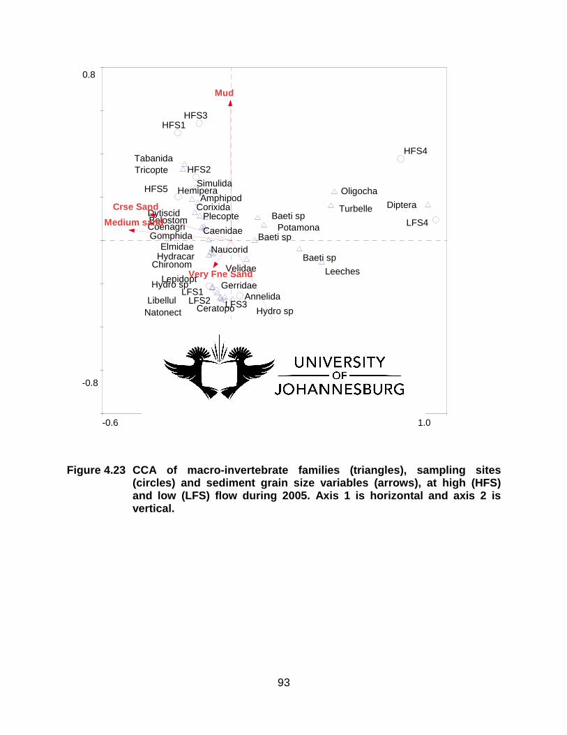
93

Figure 4.23 CCA of macro-invertebrate families (triangles), sampling sites

(circles) and sediment grain size variables (arrows), at high (HFS) and low (LFS) flow during 2005. Axis 1 is horizontal and axis 2 is vertical.

-0.6 1.0

-0.8

0.8

Amphipod

Annelida

Oligocha

Leeches

Elmidae

Dytiscid

Hydracar

Plecopte

Baeti sp

Baeti sp

Baeti sp

CaenidaeCoenagri Gomphida

Libellul

Lepidopt

Hemipera

Belostom Corixida

Gerridae

Naucorid

Natonect

Velidae

Tricopte

Hydro sp

Hydro sp

Ancylida

Turbelle Diptera

Ceratopo

Chironom

Simulida

Tabanida

Potamona

Crse Sand

Fne Sand

Medium sand

Very Fne Sand

Mud

HFS1

HFS2

HFS3

HFS4

HFS5

LFS1 LFS2 LFS3

LFS4

LFS5

94

Figure 4.24 CCA of macro-invertebrate families (triangles), sampling sites (circles) and sediment grain size variables (arrows), at high (HFS) and low (LFS) flow during 2006. Axis 1 is horizontal and axis 2 is vertical.

-0.6 1.0

-0.8

0.8

Amphipod

Annelida

Oligocha

Leeches

Elmidae

Dytiscid

Hydracar Plecopte

Baeti sp

Baeti sp

Baeti spCaenidae

Coenagri

Gomphida Libellul

Lepidopt

Hemipera

Belostom Corixida

GerridaeNaucorid

Natonect

Velidae

Hydro sp

Hydro sp

Turbelle

Diptera

Ceratopo

Chironom

Simulida

Tabanida

Potamona

Crse Sand

Fne Sand

Medium Sand

Vey Fne Sand

Mud

HFS1

HFS2

HFS3

HFS4

HFS5

LFS1

LFS2

LFS3LFS4

LFS5

95

Table 4.30 Summary of weightings of the first two axes of CCA for macro-invertebrate families and grain size variables, at both high and low flow. Variances explained by the two axes are given. Monte Carlo probability test of significance is shown for the first axis and all four axis. *p ≤≤≤≤0.05.

2005 Axes Weightings

CCA All Axes

Axes Ax1 Ax2 Eigenvalues 0.441 0.272

Sp-EnC 32 0.996 0.935

CPVS 33 36.9 59.7

CPVS-EN 34 50.5 81.6

F- ratio 1.757 1.363 P-Value 0.008 *0.017

2006 Axes Weightings

CCA All Axes

Axes Ax1 Ax2 Eigenvalues 0.312 0.199

Sp-EnC 35 0.942 0.944

CPVS 36 34.1 55.9

CPVS-EN 37 46.4 76.0

F- ratio 1.553 1391 P-Value 0.027 *0.016

32 Species–environmental variable correlation. 33 Cumulative percentage variance for species data. 34 Cumulative percentage variance of species–environmental variables’ relations. 35 Species–environmental variable correlation. 36 Cumulative percentage variance for species data. 37 Cumulative percentage variance of species–environmental variables’ relations.

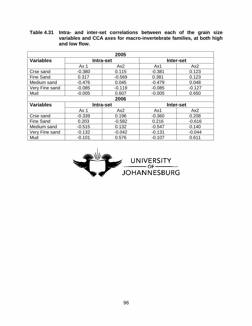
96

Table 4.31 Intra- and inter-set correlations between each of the grain size variables and CCA axes for macro-invertebrate families, at both high and low flow.

2005 Variables Intra -set Inter -set

Ax 1 Ax2 Ax1 Ax2 Crse sand -0.380 0.115 -0.381 0.123 Fine Sand 0.317 -0.569 0.381 0.123 Medium sand -0.476 0.045 -0.479 0.048 Very Fine sand -0.085 -0.119 -0.085 -0.127 Mud -0.005 0.607 -0.005 0.650

2006 Variables Intra -set Inter -set

Ax 1 Ax2 Ax1 Ax2 Crse sand -0.339 0.196 -0.360 0.208 Fine Sand 0.203 -0.582 0.216 -0.616 Medium sand -0.515 0.132 -0.547 0.140 Very Fine sand -0.132 -0.042 -0.131 -0.044 Mud -0.101 0.576 -0.107 0.611

97

Table 4.32 and 4.33 show water quality results for 2005 and 2006. Water pH was

generally lower during low flow as compared to high flow survey. Whereas, Oxygen

concentration levels were higher during high flow and lower during low flow.

Conductivity and COD concentration levels wre lower during flow and higher in high flow

surveys, whereas Kjeldahl nitrogen was higher in the low flow regime as compared to

high flow.

Table 4.32 Water quality results for low flow and high flow survey in 2005.

SITE pH Oxygen

mg/L

Temperature

° C

Kjeldahl N

(mg/L)

COD

(mg/L)

Conductivity

(µs/cm)

Oxygen

(%)

LFS1 7.84 10.51 17.1 5.5 237 262 99.2

LFS2 7.25 11.05 19.2 4.7 211 336 91.2

LFS3 7.15 11.06 19.8 6.8 219 244 75.3

LFS4 6.11 9.01 20.4 9.1 922 527 80.1

LFS5 7.3 9.81 22.3 6.4 222 227 93.2

HFS1 7.82 9.45 25.4 2.4 72.3 277 89.9

HFS2 7.11 9.65 25.3 3.2 83.5 319 94.3

HFS3 7.16 9.29 25.8 3.5 81 324 88.9

HFS4 6.15 8.28 27.4 7.9 720 884 95.3

HFS5 7.16 9.79 27.1 2.2 71.8 298 98.2

98

Table 4.33 Water quality results for low flow and high flow survey in 2006.

SITE pH Oxygen

mg/L

Temperature

° C

Kjeldahl N

(mg/L)

COD

(mg/L)

Conductivity

(µs/cm)

Oxygen

(%)

LFS1 7.23 10.7 17.3 4.9 189 268 82.3

LFS2 7.11 11.15 20.1 4.8 172 356 93.5

LFS3 7.14 10.92 19.7 6.6 201 236 76.5

LFS4 6.32 9.07 20.9 8.5 698 534 79.8

LFS5 7.34 9.71 22.8 3.92 174 236 94.2

HFS1 7.72 9.52 24.9 2.3 78.9 245 92.3

HFS2 7.66 8.95 25.9 3.5 89.3 299 95.6

HFS3 7.15 9.33 25.7 3.7 87 328 91.5

HFS4 6.18 7.78 27.3 8.1 529 752 94.2

HFS5 7.26 9.89 26.4 2.6 73.8 228 95.3

4.7 Metals concentration in fish liver and muscle tissue per sampling

site

Figure 4.25 shows cobalt (Co) concentration in fish liver and muscle, per sampling site.

The figure shows that station LFS2 has the highest Co concentration in fish liver and

muscle, whereas site LFS1 has the lowest concentration. Generally, more than 50% of

the sites have higher Co concentrations in the liver than in the muscle tissue.

99

Figure 4.25 Mean cobalt (Co) concentration (µg/g) in fish liver and muscle, per sampling site. n= 48 and 52 for 2005 and 2006, respectively.

Figure 4.26 shows that the highest concentration of aluminium (Al) in fish liver and

muscle was recorded in LFS3 while the least was recorded at stations HFS5 and LFS5.

Generally, five of the eight sites have higher Al concentrations in the muscle tissue than

in the liver. The upstream sites (LFS1 and HFS1) recorded relatively low concentrations

in both liver and muscle tissues.

Figure 4.26 Mean aluminium (Al) concentration (µg/g) in fish liver and muscle, per sampling site. n= 48 and 52 for 2005 and 2006, respectively.

Figure 4.27 shows that high concentrations of copper (Cu) were recorded in fish liver

and muscle sampled in LFS2 for muscle and LFS3 for liver, while low concentrations

0

100

200

300

400

500

600

700

800

HF

S1

HF

S2

HF

S3

HF

S4

HF

S5

LFS

1

LFS

2

LFS

3

LFS

4

LFS

5

HF

S1

HF

S2

HF

S3

HF

S4

HF

S5

LFS

1

LFS

2

LFS

3

LFS

4

LFS

5

Al in Liver

Al in Muscle

2005 2006

0

5

10

15

20

25

30

35

40

HF

S1

HF

S2

HF

S3

HF

S4

HF

S5

LFS

1LF

S2

LFS

3LF

S4

LFS

5

HF

S1

HF

S2

HF

S3

HF

S4

HF

S5

LFS

1LF

S2

LFS

3LF

S4

LFS

5

Co in Liver

Co in Muscle

2005 2006

100

were found in fish liver and muscle at HFS1, LFS1 and LFS5. The upstream sites (LFS1

and HFS1) recorded the lowest Cu concentrations in both liver and muscle tissues.

Figure 4.27 Mean copper (Cu) concentration (µg/g) in fish liver and muscle, per sampling site. n= 48 and 52 for 2005 and 2006, respectively.

Figure 4.28 shows that the highest concentration of zinc (Zn) was found in fish liver and

muscle from LFS3, and the lowest concentrations in fish liver and muscle from HFS5.

Most sites recorded high concentrations of Zn in muscle tissue. All high flow sites

recorded high concentrations in both liver and muscle tissues.

Figure 4.28 Mean zinc (Zn) concentration (µg/g) in fish liver and muscle per sampling site. n= 48 and 52 for 2005 and 2006, respectively.

Figure 4.29 shows that fish liver in LFS3 has the highest concentration of manganese

(Mn), whereas HFS3 has the lowest. The HFS1 site has the lowest concentration of Mn.

05

10152025303540

HF

S1

HF

S2

HF

S3

HF

S4

HF

S5

LFS

1LF

S2

LFS

3LF

S4

LFS

5

HF

S1

HF

S2

HF

S3

HF

S4

HF

S5

LFS

1LF

S2

LFS

3LF

S4

LFS

5

Cu in Liver

Cu in Muscle

2005 2006

0

20

40

60

80

100

HF

S1

HF

S2

HF

S3

HF

S4

HF

S5

LFS

1

LFS

2

LFS

3

LFS

4

LFS

5

HF

S1

HF

S2

HF

S3

HF

S4

HF

S5

LFS

1

LFS

2

LFS

3

LFS

4

LFS

5

Zn in Liver

Zn in Muscle

2005 2006

101

Generally, the concentration of Mn in all sampling sites was relatively low. The

upstream sites recorded relatively low concentrations of Mn in both liver and muscle

tissue.

Figure 4.29 Mean manganese (Mn) concentration (µg/g) in fish liver and muscle, per sampling site. n= 48 and 52 for 2005 and 2006, respectively.

Figure 4.30 shows the highest concentration of nickel (Ni) in liver was recorded in fish

sampled at site LFS2, and the highest concentration of Ni in muscle was recorded in

fish sampled at LFS2. Fish sampled at sites LFS1, HFS5 and LFS5 showed the lowest

concentration of Ni in both liver and muscle tissue.

Figure 4.30 Mean Nickel (Ni) concentration (µg/g) in fish liver and muscle, per sampling site. n= 48 and 52 for 2005 and 2006, respectively.

0

100

200

300

400

500

600

700

800

HF

S1

HF

S2

HF

S3

HF

S4

HF

S5

LFS

1

LFS

2

LFS

3

LFS

4

LFS

5

HF

S1

HF

S2

HF

S3

HF

S4

HF

S5

LFS

1

LFS

2

LFS

3

LFS

4

LFS

5

Mn in Liver

Mn in Muscle

2005 2006

0

0.2

0.4

0.6

0.8

1

1.2

HF

S1

HF

S2

HF

S3

HF

S4

HF

S5

LFS

1

LFS

2

LFS

3

LFS

4

LFS

5

HF

S1

HF

S2

HF

S3

HF

S4

HF

S5

LFS

1

LFS

2

LFS

3

LFS

4

LFS

5

Ni in Liver

Ni in Muscle

2005 2006

102

Figure 4.31 shows that the highest Cadmium (Cd) concentration in liver was recorded in

fish from site HFS1, while the highest Cd concentration in muscle was recorded in fish

from HFS3. The lowest concentration of Cd in both liver and muscle was recorded in

fish sampled at HFS2 and HFS5. The upstream sites (LFS1 and HFS1) recorded

significantly higher Cd concentrations in liver.

Figure 4.31 Mean cadmium (Cd) concentration (µg/g) in fish liver and muscle, per sampling site. n= 48 and 52 for 2005 and 2006, respectively.

Figure 4.32 shows that the highest concentration of lead (Pb) in liver was found at site

LFS3, and the highest concentration of Pb in muscle, was at site HFS5. The lowest

concentration of Pb in both liver and muscle was found at station HFS2. Most of the

sites recorded higher concentrations of Pb in liver, than in muscle tissue.

0

0.5

1

1.5

2

2.5

HF

S1

HF

S2

HF

S3

HF

S4

HF

S5

LFS

1LF

S2

LFS

3LF

S4

LFS

5

HF

S1

HF

S2

HF

S3

HF

S4

HF

S5

LFS

1LF

S2

LFS

3LF

S4

LFS

5

Cd in Liver

Cd in Muscle

2005 2006

0

1

2

3

4

5

6

HF

S1

HF

S2

HF

S3

HF

S4

HF

S5

LFS

1LF

S2

LFS

3LF

S4

LFS

5

HF

S1

HF

S2

HF

S3

HF

S4

HF

S5

LFS

1LF

S2

LFS

3LF

S4

LFS

5

Pb in Liver

Pb in Muscle

2005 2006

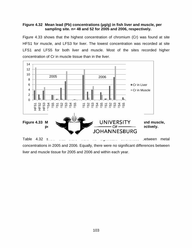
103

Figure 4.32 Mean lead (Pb) concentrations (µg/g) in fish liver and muscle, per sampling site. n= 48 and 52 for 2005 and 2006, respectively.

Figure 4.33 shows that the highest concentration of chromium (Cr) was found at site

HFS1 for muscle, and LFS3 for liver. The lowest concentration was recorded at site

LFS1 and LFS5 for both liver and muscle. Most of the sites recorded higher

concentration of Cr in muscle tissue than in the liver.

Figure 4.33 Mean chromium (Cr) concentrations (µg/g) in fish liver and muscle, per sampling site. n= 48 and 52 for 2005 and 2006, respectively.

Table 4.32 show that there were no significant differences between metal

concentrations in 2005 and 2006. Equally, there were no significant differences between

liver and muscle tissue for 2005 and 2006 and within each year.

0

2

4

6

8

10

12

14

HF

S1

HF

S2

HF

S3

HF

S4

HF

S5

LFS

1LF

S2

LFS

3LF

S4

LFS

5

HF

S1

HF

S2

HF

S3

HF

S4

HF

S5

LFS

1LF

S2

LFS

3LF

S4

LFS

5

Cr in Liver

Cr in Muscle

2005 2006

104

Table 4.34 Mean and Standard deviation in fish musle and liver for 2005 and 2006. Significance level between different tissues is shown.

2005 2006

Metal Mean in Liver

Mean in Muscle

SD in Liver

SD in Muscle

P Mean in Liver

Mean in Muscle

SD in Liver

SD in Muscle

P

Al 97.064 140.588 120.295 205.626 0.571 96.855 108.365 92.059 122.108 0.815

Ni 0.266 0.319 0.164 0.289 0.624 0.311 0.325 0.271 0.276 0.909

Cr 2.403 3.279 2.441 4.851 0.616 0.359 3.525 3.547 5.057 0.973

Pb 0.966 1.003 1.543 1.617 0.953 1.204 1.089 1.738 1.199 0.865

Co 6.949 8.012 9.745 10.423 0.816 7.859 8.963 11.277 11.357 0.829

Cu 4.953 3.760 9.853 4.698 0.733 5.097 3.788 9.822 4.693 0.708

Zn 31.397 29.863 25.708 26.372 0.897 31.995 30.249 26.035 26.462 0.883

Mn 6.199 4.646 9.947 7.425 0.697 6.711 5.06 9.979 7.602 0.682

Cd 0.273 0.229 0.658 0.433 0.863 0.281 0.339 0.655 0.732 0.856

Overall, the results clearly indicate that 2005 and 2006 surveys were not significantly

different in terms of water quality, sediment quality, fish and macro-invertebrate

commuty structures. It is clear in the results that there are significant differences

between mining and platinum processing areas in the RPM mine license area. There

are several “outliers” in the results, which are complemented by changes in biotic

community distribution. These results are discussed in detail in chapter five of this

study.

105

4.8 References

Clarke, K.R. and Gorley, R.N. 2006. Primer v6: User Manual/Totorial. PRIMER-E:

Plymouth.

Clarke, K.R., Somerfield, P.J. and Gorley, R.N. 2008. Exploratory null hypothesis testing

for community data: Similarity profiles and biota-environment linkage. J. Exp. Mar. Biol.

Ecol. 366: 56-69.

Field, J.G., Clarke, K.R. and Warwick, R.M. 1982. A practical strategy for analysing

multispecies distribution patterns. Mar. Ecol. Prog. Ser. 8: 37-52.

Warwick, R.M., Plat, H.M., Clarke, K.R., Agard, J. and Gobin, J. 1990. Analysis of

macrobenthic and meiobenthic community structure in relation to pollution and

disturbance in Hamilton Harbour, Bermuda. J. Exp. Mar. Biol. Ecol. 138: 119-142.

106

CHAPTER 5

DISCUSSION

5.1 Background

Macro-invertebrates and fish are useful bioindicators, providing a more accurate

understanding of changing aquatic conditions than chemical and microbiological

parameters (Ravera, 1998; Ravera, 2000; Ikomi et al., 2005). Various families of macro-

invertebrates differ in their sensitivity to habitat disturbance, and it is desirable that

measures of disturbance should in some way capture and utilize that information.

Methods of multivariate analysis have been widely used to identify pollution sources and

to apportion natural and anthropogenic contribution (Mico et al., 2006). It is for this

reason that these methods were chosen in the analysis of fish and macro-invertebrates

in the Hex River system. Several studies have shown that species dependent

(multivariate) methods are much more sensitive than species independent (univariate

and distributional) methods in discriminating between spatial and temporal trends

(Warwick et al., 1990) as such; the multivariate pattern of macro-invertebrates and fish

communities in the Hex River showed spatio-temporal trends. Multivariate methods

simply demonstrate change, indicating whether this can be regarded as deleterious.

Due to taxonomic constraints, the macro-invertebrate analysis of this study was

performed using class and family level, while fish communities were identified to

species level.

According to Kefford et al. (2010), when considering the impacts of contaminants on

lotic systems, it is important to differentiate between low flow and high flow regimes, as

each are likely to experience different modes of impacts. For example, studies have

shown that sedimentation has major impacts on invertebrates and fish during high flow

(Waters, 1995; Bilotta & Brazier, 2008). There are, however, less convincing examples

from during low flow, and the apparent associations that may be caused by confounding

factors. In this context, Dabrowski et al., (2005) showed that increased water velocity

decrease drift rate of the South African mayfly, Baetis harrisoni, while pyrethroid

107

insecticide increase drift rate. The findings of the current study provide information on

the effects of mining activities on water and sediment quality as well as the survival and

distribution of selected organisms in the area studied. These effects and possible

changes to macro-invertebrate and fish community structures, distribution and health

are discuused in this chapter.

5.2 Macro-invertebrate community patterns

The results of Cluster Analysis revealed three major macro-invetebrate groups that are

associated with the sampling regime. The abundance and diversity of organisms in the

low flow regime that was higher than the high flow, which indicates a clear seasonal

variation pattern of the community distribution, at all sampling sites. This supports

results of several studies (Nkwoji et al., 2010; Nelson & Roline, 1996; Dallas, 2004).

The results suggest that variations in river condition appear to have played a major role

in shaping the macro-invertebrate community structure. The trend was not evident in the

exposure sites (LFS4 and HFS4) for both high and low flow, as they constitute one

group. This sampling point is in the vicinity of a tailings dam and a discharge point from

platinum processing plants’ effluent. The results indicated major differences between

the low and high flow in situ measurements, pH, temperature, conductivity and

dissolved oxygen.

According to Onyema and Nkwankwo (2009), rainfall distributive patterns have a major

impacton on the water chemistry and resultant distribution of fauna. Rainfall may have

contributed to the observed macro-invertebrate distribution, as there was a 7% increase

in annual rainfall in the Rustenburg region between 2005 and 2006. There are other

physical factors that can affect the macro-invertebrate community structure, and the

species survival will depend on species tolerance levels. Apart from the seasonal

variation, it appears that there are no significant differences between the exposure and

the reference sites in terms of macro-invertebrate community distribution. Major

differences are observed in site 4.

108

5.2.1 Indicator species

The macro-invertebrate community patterns were described using two complementary

techniques. This section aims to determine which species are primarily responsible for

influencing the sample groupings, based on the cluster (dendrogram) and N-MDS. The

dendrogram and ordination plots for the abundance data divided the samples into three

different groups. The macro-invertebrate community indicated that there is seasonal

variation between the low and high flow samples. According to Corbet (1999), some

macro-invertebrate species can tolerate a broader range of environmental conditions,

whereas others are extremely sensitive to minor changes in the prevailing environment.

The presence of Gomphidae, Lepidoptera and Elmidae, all of which are sensitive to

pollution, suggest that there is an improvement in environmental conditions during high

flow regime for both 2005 and 2006 surveys. A closer look at species composition

indicated that macro-invertebrate communities found at the downstream sites had less

pollution-sensitive and more pollution-tolerant species than the upstream sites. The

presence of Corixidae, Simuliidae, and Tabanidae, all of which are pollution-tolerant,

suggests that there is a degree of pollution in the downstream sites, as compared to

Hydracarina, Elmidae and Lepidoptera, which are present in the upstream site.

Sampling site 4 did not show seasonal variation, and is characterised by the pollution-

tolerant taxa Baetidae, Oligochaeta and Tubellaria for both low and high flow regimes.

Several studies have shown that these groups normally increase in abundance where

there has been a physical disturbance (Palmer & O’Keeffee, 1990), and they survive

because they are filter feeders during the larval stage (McCafferty, 1999). The macro-

invertebrate community in this specific site suggests a highly disturbed environment.

This was confirmed by a very low Margalef’s species richness (d) and Shannon diversity

index (H’) (Figure 4.3). The downstream sites species composition and distribution

appears to be influenced by the increased platinum mining and processing activities.

109

5.2.2 Linking macro-invertebrate community patterns to measured

environmental variables

Mining activities are serious and important source of contamination within the natural

environment (Spellman & Drinan, 2000). The sensitivity and generality of multivariate

methods make them particularly valuable tools in the assessment of community change,

however it is important to relate this community changes to measured environmental

parameters (Warwick & Clarke 1991). Heavy metal concentrations in aquatic

ecosystems are usually monitored by measuring their concentration in water, sediment

and biota (Camusso et al., 1995; Binning & Bird, 2001). This suggests that most of the

metals involved come from the same source of pollution. According to Rosenberg and

Resh (1992), the decision to use macro-invertebrates as environmental indicators, is

mainly based on their ability to respond on different environmental variables such as

sediment quality, water quality, hydrology and other biological factors. This study

focused on water quality, sediment quality and physical characteristics of the sediment.

5.2.2.1 Water quality

Dallas and Day (1993) described water quality as a network of variables that are linked

or co-linked, and that changes in physical and chemical parameters may affect the way

biota respond. Figures 4.19 and 4.20 shows that the variables, temperature, Mn, Zn, Fe,

Cr, Cu pH and dissolved oxygen, indicated the variation in the distributive trends for

macro-invertebrate species within sampling sites. The high macro-invertebrate-

environment correlation coefficients and cumulative percentage variances for macro-

invertebrate and for macro-invertebrate-water quality relations, indicated that measured

water quality variables were therefore responsible for the main variations in macro-

invertebrate community patterns. Monte-Carlo probability test confirms that the relation

between macro-invertebrates and water quality were significant for axis one (F = 1.561 ,

p<0.037 and F= 1.196, p<0.022) and all axes (F= 1.435, p< 0.024 and F=2.217,

p<0.048) for 2005 and 2006, respectively (Table 4.24).

Ward (1992) confirmed that temperature influence the physiological process of species,

which leads to changes in the timing of life history events. The mean water temperature

110

during low flow was 19.8 0C, and during high flow was 26.2 0C. The increased mining

activities in summer appear to have contributed to the increase in temperature caused

by discharges into the system. The strong correlation of temperature and sampling

period, as seen in Figure 4.19 and 4.20, is indicative of seasonal influence on changes

in macro-invertebrate community patterns. This trend is in agreement with studies by

Nwankwo & Akisonji (1992), Rivers-Moore et al. (2004) and King et al. (2003). It

appears that the relatively low rainfall between 2005 and 2006 in the Rustenburg region,

resulting in a decrease in the amount and speed of water, and suspended materials in

the water column contributed to the water temperature and species distribution. The

results indicated that Amphipoda, Simuliidae and Hemiptera correlated strongly with

high temperatures, and these are taxa associated with mostly high flow sites with high

abundance and diversity.

Dissolved oxygen concentrations can vary spatially and temporally because of

respiration by organisms, photosynthesis by plants, atmospheric losses and gains,

changes in pressure and temperature, and groundwater inflow (Dodds, 2002; 2006).

Figure 4.19 and 4.20 indicated that dissolved oxygen plays a role in determining the

macro-invertebrate community structure. The results indicated that the upstream site’s

mean dissolved oxygen concentration during low (115%) and high (118%) flow was

within the proposed guideline of between 80 and 120% saturation (Dallas & Day, 2004).

The dissolved oxygen levels recorded at all low flow sites was below the guideline

recommended by Kempster et al. (1982). This appears to be caused by the organic

enrichment in the area, and the constant discharges into the system. The dissolved

oxygen concentration measured at sampling site 4 is a concern, as it remained at 2.09

mg/l on average for both sampling regimes in 2005 and 2006. This is below DWAF

guideline limits (DWAF, 1996). It should, however, be noted that this specific site

showed the lowest diversity of all sites, suggesting some lethal effects on macro-

invertebrates due to low oxygen saturation, which is in line with Dallas and Day’s (2004)

results. There was evidence of organic pollution (e.g. smell, algae and high abundance

of Baetidae) during sampling at this specific site. The increase in oxygen concentration

at site 5, which recorded 4.9 and 4.7 mg/l for both high and low flow samples,

respectively, created favourable conditions for fish survival. This is supported by an

111

improvement in the macro-invertebrate community distribution, in agreement with other

studies (Dallas & Day, 2004; Nkwoji et al., 2010)

Industrial activities generally cause acidification rather than alkalinization of rivers.

Acidification is normally the result of three different types of pollution, namely: low pH

point source effluents from industries, mine drainage (which is nearly always acidic),

and acid precipitation resulting largely from atmospheric pollution (DWAF, 1996).

According to Ward (1992), pH is also affected by temperature amongst other factors.

The pH values for both low and high flow regimes in the upstream sites were within the

normal range, but very low in the downstream sites. The association of pH decrease

with pollution-tolerant taxa in both low and high flow downstream sites suggests

increased levels of pollution. Except for site 4, the increase in diversity in most of the

downstream sites suggests that pH levels are within acceptable ranges for most macro-

invertebrate species’ survival, in line with the results of Rosenberg and Resh (1992),

and Ward (1992). The upstream site showed high pH levels that are considered to have

an insignificant impact on aquatic life, but may create favorable conditions for weed

growth.

Manganese is one of the most presented metals in the earth’s crust and is one of over

100 minerals (Post, 1999). Manganese is a functional component of nitrate assimilation

and an essential catalyst for numerous enzyme systems in animals, plants and bacteria

(DWAF, 1996). Manganese concentration levels (Tables 4.26 and 4.27) ranged from

0.019 mg/l for upstream site 1, to 0.369 mg/l for downstream site 4. Increased

manganese concentrations were found in the high flow surveys (compared to low flow

sites), as a result of the creation of favourable conditions for changes in redox potential,

dissolved oxygen and pH. This increase in manganese concentration was due to the

depletion in dissolved oxygen and a decrease in pH. These conditions were also

evident at site 4 for both high and low flow sampling regimes. The presence of pollution-

tolerant invertebrates at this site indicates that though manganese concentrations are

high, the acute and chronic toxicity effects for invertebrates have not been reached.

Manganese concentrations at site 5 were significantly reduced for both high and low

flow regimes, suggesting that there is a reduction in the dissolution of manganese-

112

containing minerals in the vicinity. This suggests that there is a degree of self-

purification from site 4 to site 5.

Iron (Fe) is the fourth most abundant element in the earth’s crust and may be present in

natural waters in varying quantities, depending on the geology of the area and other

chemical properties of the water body (DWAF, 1996). Iron is an important nutrient for

algae and other freshwater organisms, and is often found in higher concentrations in

water and sediments than other trace metals (Forstner & Wittman, 1979; Huu et. al.,

2010). The chemical behavior of iron in the aquatic environment is determined by

oxidation-reduction reactions, pH and the presence of coexisting inorganic and organic

complexing agents (DWAF, 1996). Iron is naturally released into the environment from

weathering of sulphide ores (pyrite, FeS2) and igneous, sedimentary and metamorphic

rocks (DWAF, 1996; Galvin, 1996).

Iron concentration levels (Tables 4.26 and 4.27) ranged from 1.45 mg/l for upstream site

1, to 5.17 mg/l for downstream site 4 for both 2005 and 2006, respectively. All the sites

exceeded the WHO limit of 0.3 mg/l. The presence of Iron trioxide in granite could be

the primary source of Iron in the water. The concentration levels of iron during low flow

at the upstream site 1 were higher, than at two of the downstream sites. This suggested

that there were other sources of iron at site 1 during low flow. This anomaly is not

evident in the high flow sites. Iron is most likely to have a detrimental environmental

impact because of reduction in pH DWAF (1996), and may be run-off from agricultural

and scrap metals’ dealers upstream of this site (Fatoki & Mathabatha, 2001). The high

concentration does not seem to have been influenced by the pH, conductivity and

temperature, as these parameters were at a normal level at this site. This suggests a

possibility of other sources of iron pollution near site 1. There is a strong association of

iron with the low flow site, and the presence of the somewhat pollution-tolerant species

like Elmidae suggests a relatively unpolluted environment. However, the fact that site 4

is not associated with the other four sites; suggests that high iron concentration

influences the macro-invertebrate community structure. Sampling site 5 has relatively

reduced concentration levels of iron, suggesting a possible self-cleaning of the Hex

River downstream of site 4. The high concentration of iron at site 4 appears to be

113

related to the low pH, leading to a toxic environment for macro-invertebrates; hence

only pollution-tolerant species are found here for both low and high flow regimes.

Zinc is an essential element for all organisms, as it forms the active site in various

metalloenzymes (DWAF, 1996). Zinc is one of the priority pollutants (Roy, 1997).

Soluble zinc salts (e.g. zinc carbonate, zinc chloride and zinc sulphate) or insoluble

precipitates of zinc salts (e.g. zinc carbonate, zinc oxide and zinc sulphide) occur readily

in industrial wastes (DWAF, 1996). According to Galvin (1996), chlorides and sulphides

of zinc in water react with dissolved carbon dioxide to produce hydroxides and

carbonates, which are absorbed into sediments. Copper increases zinc toxicity in soft,

but not in hard water, and zinc toxicity increases at lower oxygen concentrations

(DWAF, 1996). The results (Tables 4.26 and 4.27) indicate increased concentration of

zinc in water, of between 0.1 mg/l and 0.84 mg/l, which are below the TWQR of 2 mg/l.

The absence of pollution-sensitive species at all sampling sites appears not to be

because of zinc, since concentration levels are very low. The low concentration in the

water column does not mean that the water is not polluted with zinc, as metals tend to

bind in the bottom sediment (Davis et al., 1991) and dangers arise when there are

changes in the environmental conditions such as pH, salinity, temperature and redox

potential (van Vuren et al., 1994). The pH levels remain fairly highly alkaline,

suppressing the possibility of zinc to negatively affec the environment by becoming bio-

available. The pH levels were much higher at upstream site 1 for both low and high flow

sampling regimes, suggesting a low possibility of zinc pollution. The association of

higher zinc levels with site 4 suggests a nearby source of zinc pollution, other than

geology. There was a very strong evidence of organic pollution at this site, which

appears to have contributed to current zinc concentration levels. The low pH in this

specific site influences the bioavailability of zince in the prevailing environment.

Chromium is a relatively scarce metal and is usually found in very low concentrations in

the natural environment (DWAF, 1996). According to Jaagumagi (1990), chromium (VI)

is more readily accumulated than Cr (III), and is considered to be the most toxic form.

Concentrations of chromium ranged from 0.001 to 0.12 µg/l for both high and low flow

sites, with downstream sites having higher concentration levels for 2005 and 2006. Site

114

4 showed high chromium concentrations for high concentrations of Cr in 2005

compared to 2006. All other sites chromium (VI) concentrations are within the guideline

values set by DWAF (1996) of less than 7 µg/l. The presence of moderately tolerant

species of Elmidae and Hydrocarina, suggests a relatively healthy environment for

macro-invertebrates. It appears that naturally available chromium in the Rustenburg

region has not escaped into the aquatic environment. It can be deduced that, though the

ore body has some Cr and that it is one of the bi-products in the mining of platinum, it is

not yet bioavailable in and around the mining area.

The toxicity of Cu increases in water when water hardness and dissolved oxygen levels

are low. It is a common element in the rocks and minerals of the earth’s crust and is

commonly found as an impurity in the mineral ores (DWAF, 1996). The highest copper

concentrations recorded (0.32 µg/l) for 2005 and 2006 fell within the DWAF (1996)

guidelines of between 0.3 – 1.4µg/l for soft to very hard water. The presence of Diptera

at site 4 suggests that copper has not reached the stage of bioavailability due to high

recovery of copper in the processing plant.

5.2.2.2 Sediment quality

Mineral mining and processing are the most anthropogenic sources of metals affecting

the prevailing environment (Vanek et al., 2005). Sediments represent one of the final

sinks for heavy metals that are discharged to the receiving environment (Hollert et al.,

2003). According to Yusuf and Osibanjo (2006), the assessment and analysis of trace

metals found in sediments assist in further determination of pollutants that may not have

been detected in the water column. While Pettine (1994) explored the factors affecting

metals’ concentration in water, van Vuren et al. (1994) confirmed that metals bound in

sediments have no direct danger to the system, as long as they remain there. Changes

in environmental conditions such as pH, salinity, temperature or redox potential, allow

bound metals to be released back into the aquatic environment. The high macro-

inveterbrate-sediment correlation coefficients and cumulative percentage variances for

macro-invertebrate and for macro-invertebrate-sediment relations, indicated that

measured sediment quality variables were responsible for the main variations in macro-

115

inevertebrate patterns. The Monte-Carlo probability test confirms that the relationship

between macro-invertebrates and sediment quality was significant for axis one (F =

1.514 , p<0.014 and F=1.749, p<0.056 ) and all axes (F= 1.187, p< 0.026 and F= 1.985,

p<0.014) for 2005 and 2006, respectively (Table 4.18).

Table 5.1 Sediment Quality Guideline (SQG) concentration levels (mg/kg) of measured metals, as determined by the EPA (1999), OMEE (1998) and CCME (2002) expressed on a wet weight basis.

Metal SQG (mg/k g) (EPA, 1999)

SQG (mg/k g) (CCME, 2002)

SQG(mg/k g) OMEE (1998)

and Steyn et al. (1996) for

South Africa

Cobalt (Co) 3 50, 20

Chromium (Cr) 81-370

Copper (Cu) 34-270

Iron (Fe) 2-4%

Mercury (Hg) 0.17-0.486

Lead (Pb) 46.7-218

Zinc (Zn) 150-410

There is currently no South African Water Quality guideline for cobalt that can be used

to protect aquatic ecosystems. The results indicated that most of the available cobalt is

found in fractions 1 and 2 suggesting bioavailability of this metal for both 2005 and 2006

surveys. There were significant differences between fraction 1 and 4 and fraction 1 and

116

3 for both surveys. The cobalt concentrations of between 2.91 and 9.33 mg/kg (Tables

4.20 and 4.21) for both high and low flow sampling regimes, is significantly higher than

the recommended standard of the United State Environmental Protection Agency

guideline of 3 mg/kg (USEPA, 2000). It is also lower than recommendations made by

Steyn et al. (1996) for South Africa of 20 mg/kg (Table 5.1). These results concur with

Smith and Carson (1981) that cobalt concentrations in most freshwater sediments are

less than 20 mg/kg. The association of cobalt at the levels observed in the sediment

with high flow sites suggests no marked effect by favorable environmental conditions on

macro-invertebrates communities (Figure 4.15 and 4.16). This is confirmed by the

presence of predominantly somewhat pollution-tolerant macro-invertebrates at these

localities. The high pH levels at these sites suggest stable metals in sediment and a

reduced chance of cobalt escaping to the water column. This concurs with the results of

Awofolu et al. (2005) as well as, Ammal and Abdel-Satar (2005).

Zinc is a trace metal and an essential micronutrient in all organisms (DWAF, 1996).

According to Varkouhi (2007), zinc is very mobile during the weathering process like

lead and has a very high potential of combining with organic and inorganic groups to

adjust biological interactions and analysis of carbohydrates. Tables 4.20 and 4.21

indicated maximum Zn concentrations of 173.1 and 124.5 mg/kg for 2005 and 2006,

respectively. The results indicated that most of the available Zn is found in fractions 1

suggesting bioavailability if there are changes in pH. The highest concentration of Zn is

lower than the recommended South African Sediment Quality Guideline of 185 mg/kg,

as described by Steyn et al. (1996), and is higher than the United States Environmental

Protection Agency Sediment Quality Guideline of 120 mg/kg (USEPA, 2000). The

lowest concentration is far below both South African and USEPA guidelines for

sediment quality. Zinc concentration levels were generally the same for both high and

low flow sampling regimes. The high concentration levels of zinc suggest high risk

conditions, even though the source appears to be related to mining and other catchment

activities in the Rustenburg area. The presence of pollution-tolerant macro-

invertebrates, Baetidae suggests that sediments downstream of the active mining area

are polluted. This increase in concentration levels appears to be caused by the fine

material coming from the tailings dam, through storm water diversion channels. This is

117

possibly because of the condition of these channels and spillages from the top of the

tailings dam, caused by design and maintenance. The high concentration of zinc in

sediments of downstream sites is higher than concentrations in water, confirming the

results of Nguyena et al. (2005). There is a significant decline in zinc concentration in

the downstream site 5, due to increased dilution from tributaries, and because there are

no tailings dams or platinum processing activities in the vicinity.

Copper is a common element in the rocks and minerals of the earth’s crust and is

commonly found as an impurity in the mineral ores (DWAF, 1996). The Rustenburg

Platinum mine produces an average of 10.9 kt/a of copper in the Base Metals Refinery,

as a by-product of precious metals’ processing (Jones, 1999). The highest copper

concentrations recorded (39.64 mg/kg) at all sites fell within the Environmental

Protection Agency Sediment Quality Range of 34-270 mg/kg (EPA, 1999), and the

United States Environmental Protection Agency Sediment Quality Guideline of 32 mg/kg

(USEPA, 2000). This concentration was recorded in fraction 3. The results indicated

that there were no significant differences (p>0.05) in sediment copper concentrations,

between low and high flow regimes and 2005 and 2006 surveys. These results

indicated that the sediment is not polluted with copper for both high and low flow

sampling regimes. There was a reduction in copper production in BMR from 11.300 t in

2005 to 11.100 t in 2006 (U.S. Geological Survey, 2009). It appears that the source of

copper in the Hex River system is related to the discharges from the tailing dams in the

vicinity. This is in agreement with the results of Sekabira et al. (2010), who found that

there is a tendency of naturally available copper to be released to the aquatic

environment, depending on the structure of the ore body. The presence of Diptera at

site 4 suggests that copper has not affected the environment negatively as there is a

high recovery in the processing plant.

Iron is naturally released into the environment from weathering of sulphide ores and

igneous, sedimentary and metamorphic rocks (DWAF, 1996). It occurs as Fe (III) oxides

and hydroxides, with varying crystallinity in shallow and uncontaminated aquifers (Heron

& Christensen, 1995). The results show that high concentration was recorded in fraction

fraction 2 and 3 sugesting low bioavailability of Fe in the sediment. The results showed

118

no significant differences (p>0.05) in sediment iron concentrations between low and

high flow sites for 2005 and 2006, respectively. The highest iron concentration (187.85

mg/kg) was recorded at site 4, which is near the storm water drain diverting water away

from the tailing dam. This appears to be related to the geology of the area and to a

lesser extent storm water runoff and tailings dam discharges. These results concur with

those of Olubunmi and Olorunsola (2010) from a study at Agbabu Bitumen Deposit Area

in Nigeria on the accumulation of heavy metals in sediments. It appears that the lower

part of the Hex River system, within the mine lease area, is strongly affected by

releases from the nearby mine tailing dams.

Mercury is a very rare heavy metal geologically, and if present, its concentration is

normally very low in the environment (DWAF, 1996). Mercury has a very strong affinity

for sediments, and suspended solids and bacteria may transform inorganic mercury into

methyl mercury under anaerobic conditions (Jaagumagi, 1990a). The maximum

concentration recorded was in fraction 3 at site 5. There were no significant differences

between fraction 1 and 2, fraction, 1 and 3 and fraction 1 and 4. Tables 4.20 and 4.21

show concentrations of mercury ranging from 0.16 to 2.01 mg/kg for both high and low

flow sites, with downstream sites having higher concentrations levels. All other sites’

mercury concentrations are within the Canadian Freshwater Sediment Guideline of

between 0.17 and 0.486 mg/kg (CCME, 2002). The significant increase of mercury

concentrations during low flow, suggests that there are other potential sources of

pollution, other than mining and processing. Potential sources include air deposition

from the metal processing and smelting operations in the vicinity of Hex River. The

Watervaal Smelter is situated about 5 km to the Hex River and stack emissions

influenced by changes in wind direction appears to be impacting on both water and

sediment quality. There are several small stacks from RBMR and RPMR situated in the

same region as the smelting plant. This concur with the results of Papu-Zaxaka et al,

(2010) and Jaagumari (1990a), who found elevated levels of mercury in water and

sediments near smelting and processing plants. The presence of Elmidae at site 3,

suggests that mercury pollution downstream of site 1, has not affected the environment

negatively.

119

Lead is described as one of the most hazardous metals in most forms of life, and is

readily accessible to aquatic organisms (USEPA, 1986). Lead is contained in more than

200 minerals, though only sufficiently in galena, anglesite and cerrusite to justify

extraction (Spellman & Drinan, 2000). Lead has a tendency to remain tightly bound to

sediment under oxidizing conditions (Jaagumagi, 1990a), and is released into the

aquatic environment through the weathering of sulphide ores (DWAF, 1996). Tables

4.20 and 4.21 show concentrations of lead ranging from 3.19 to 99.42 mg/kg for both

high and low flow sites, with downstream sites having higher concentration levels. The

maximum concentration recorded was in fraction 2 and there were significant

differences between fractions. Site 4 showed high lead concentrations for high (98.3

mg/kg) and low (99.42 mg/kg) flow regimes. All other sites lead concentrations were

within the United States Environmental Protection Agency Sediment Quality Guideline

of 46.7-218 mg/kg (USEPA, 2000). Lead is highly associated with sites 1 and 2 of the

low flow samples. The presence of Elmidae and Hydrocarina that are somewhat

pollution-tolerant at these two sites, suggests that lead pollution has not affected the

macro-invertebrate communities. The significant increase of lead concentrations during

high flow, including at upstream sites, suggests that there is another source of pollution

other than mining and processing. It appears that upstream run-off and atmospheric

deposition are some of the sources of lead in the sediment, which is in agreement with

the findings of Papu-Zamxaka (2010) and Kumar et al. (2011).

Chromium is a relatively scarce metal and is usually found in very low concentrations in

the natural environment (DWAF, 1996). According to Jaagumagi (1990a), chromium

(VI) is more readily accumulated than Cr (III), and is considered the most toxic form.

Concentrations of chromium ranged from 1.98 to 7.45 mg/kg for both high and low flow

sites, with downstream sites having increased concentration levels. Fraction 2 and 3

showed highest concentration and there were no significant differences between

fractions. Site 4 showed high chromium concentrations for high concentrations of Cr in

2005 compared to 2006. All other sites chromium concentrations are within the United

States Environmental Protection Agency Sediment Quality Guideline of 81-370 mg/kg

(USEPA, 2000). As with lead, the association of Cr with site 1, site 2 and site 3,

together with the presence of Elmidae and Hydrocarina which are somewhat pollution-

120

tolerant, suggests a relatively favourable environmental conditions for macro-

invertebrates distribution. Research by Taylor et al. (1979), Papathanassiou and

Zenetos (1993), and Malik et al. (2010), has confirmed that the main sources of

chromium are emissions from ferrochromium, refractory production, cement

manufacturing, and the metal plating industries. Unlike most metals, the absence of

these industries in the Rustenburg region appears to have contributed to the low

chromium concentrations found during both sampling regimes. It appears that naturally

available chromium in the Rustenburg region has not escaped into the aquatic

environment.

5.2.2.3 Sediment grain size

Hogg and Norris (1991) found that sedimentation is one of the main causes of changes

in the ecological nature of streams and rivers. Sediments are considered to be the final

sink of pollutants in aquatic systems, and pose a risk to aquatic life, due to sediment

binding of metals and other pollutants (Wepener & Vermeulen, 2005). Wood and

Armitage (1997) confirmed that there are four ways in which sediment can affect macro-

invertebrates: (1) by changing the substrate composition and suitability of the substrate

for other species; (2) by increasing drift as a result of sediment deposition; (3) by

deposition on respiration structures affecting oxygen uptake; and (4) by affecting

feeding activities, by reducing the food value of periphyton. The high species-

environment correlation coefficients and cumulative percentage variances for macro-

invertebrate and for macro-invertebrate and sediment grain size relations, indicated that

measured sediment grain size variables were therefore responsible for the main

variations in species patterns. The Monte-Carlo probability test confirmed that the

relation between macro-inveterbrates and sediment grain size were significant for axis

one (F= 1.757, p< 0.008 and F= 1.553, p<0.027) and all axes (F= 1.363, p< 0.017 and

F=1.319, p<0.016) for 2005 and 2006, respectively (Table 4.30). The distribution of

sediment in localities downstream of mining areas was abnormally high. This was

accompanied by high metal concentrations in both water and sediments.

121

Rosenberg and Resh (1993) explored the impact of fine sediment input to rivers, and

how these affect aquatic organisms and Billota and Brazzier (2008) found that

sedimentation reduces the ability of drifting invertebrates to attach to the stream bed.

Kefford et. al. (2010) found that the beds of rivers during low flow are often dominated

by fine particles (sand, silt and clay), and the burial or in-filling of spaces by sediment is

thus unlikely to play an important role in any effects of sediment on the aquatic biota.

The current study confirmed that there is a clear seasonal variation in terms of macro-

invertebrate distribution. This appears to be related to the sediment type. This suggests

that changes in sediment grain size affect the community structure of macro-

invertebrates. The fine sediment (Mud) at site 4, coupled with the lowest diversity and

the presence of pollution-tolerant species like Turbellaria, Baetidae and Oligochateata,

suggests stressful environmental conditions at the site. This is similar to the results of

Harrison et al. (2007), who found that the presence of finer sediment can lead to the

reduction in macro-invertebrate abundance and diversity. The low Margalef’s species

richness (d) and Shannon diversity index (H) supports this observation.

Sediment grain size of most of the low flow sites are classified as very fine compared to

the high flow sites resulting in a low diversity ( Figures 4.23 and 4.24). This trend is

evident in both 2005 and 2006 surveys. This suggests a moderately polluted

environment, and hence the presence of a mixture of somewhat pollution-tolerant

species like Elmidae Chironomidae, Naucoridae and Hydracarina, and pollution-tolerant

species like Chironomidae, Veliidae and Baetidae. This agrees with the findings of

Wilkonson et al. (2006) that streams with low velocity are more likely to accumulate fine

sediments in response to increased sediment supply. While the low flow sites are

dominated by fine sediment, they also show strong associations with one another in

terms of settled COD and Kjeldahl Nitrogen though both these variables were excluded

on the ordination due to their high variance inflation factors (Table 4.32 and 33). The

elevated values of COD and Kjeldahl Nitrogen in muddy samples, were expected in

that, the patches of mud are naturally rich in organic matter and contain detritus, which

in turn requires large amounts of oxygen to oxidize organic material. Thus, high COD

provides potential for oxygen depletion in the Hex River system. This is in agreement

with studies by Josefson and Widbom (1988) and George et al. (2009).

122

The main potential for pollution of the environment comes from the a transportaion of

pollutants by run-off and possible seepage. It is therefore necessary to adopt a risk-

based approach when designing and constructing the tailings dam and it must be

ensured that maintainace plans are implemented (Witt, et. al., 2005). The accumulation

of metals and associated particle size in downstream sites, is attributed to the

observation that spillages from the tailing dams are not contained and are released

directly to the watercourse (Figure 5.1). Between 2006 and 2007 there were 30 tailing-

dam related incidents reported in RPM, due to pipe bursts or accidental discharges to

the watercourse. This combined with inadequate implementation of the tailing dam

maintenance plan, and the amount of slimes pumped to the tailings dam, contributed to

these incidents. A tailing dam is designed to carry a certain amount of slimes per day,

and this is based on the platinum ore processed in the RPM region (Figure 5.1).

Additional concentrations from other areas outside the RPM are also processed in the

Rustenburg region. This additional load has not catered for in the current capacity which

increases the likelihood of tailing incidents and discharges from RPM.

Figure 5.1. Schematic outlay of the hydrological cycle of a tailing disposal facility (Witt et. al., 2005).

123

The high flow sites are mostly characterised by a combination of coarse and medium

sediment grain size (Figures 4.23 and 4.24) for both 2005 and 2006. The macro-

invertebrate Margalef species richness (d), and the Shannon diversity index (H’) for high

flow sites, is generally low. These results concur with other findings, that reduced

species richness and diversity is indicative of high siltation in streams (Callisto &

Goulart, 2005).

5.3 Fish community patterns

The ordination confirmed the dendrogram showing that both high and low flow sites

have similar fish communities for both 2005 and 2006. The total number of fish was

much higher in the high flow sites, compared to the low flow ones. As observed in the

fish Margalef species richness (d) and Shannon diversity index (H’), this pattern

indicates that there is no seasonal variation of the fish community structure in all

sampling sites. These results suggest that natural variations in river condition and other

physico-chemical parameters appear to be responsible for the distribution of fish in the

Hex River. It appears that there is a difference between the reference and exposure

sites for both high and low flow sampling regimes, as shown by the fish community

structure. According to Kotze et al. (2004), fish communities and the individuals

themselves have various qualities that make them useful in biological monitoring. A

recent biomonitoring result in the Hex River tributaries in 2007 has indicated that there

is no significant change in the fish community distribution near RPM.

5.3.1 Indicator species

Two complementary techniques were used to describe fish community patterns. This

section aims to determine which species are primarily responsible for influencing the

sample groupings, based on the cluster and MDS groupings. Kleynhans (2002)

described the fish species intolerance, which is based on the specialization of

preference towards habitat, food, water quality and flow. The presence of B.

paludinosus, P. philander, L. cylindricus, B. trimaculatus, O. mossambicus, C.

gariepinus and B. unitaeniatus, Tilapia sparrmanii , all of which are tolerant to pollution,

suggests a highly stressed environment. A closer look at species composition indicated

124

that fish communities found at downstream sites had more pollution-tolerant species

than the upstream sites. The results shows that B. paludinosus is responsible for the

observed grouping, with average abundance of 2.22 and 1.63 after transformation log

(x+1) for 2005 and 2006, respectively. This species is tolerant to habitat changes, river

flow, and changes in water quality. Marked changes in these variables in the river

studied are indicative of a system that is highly modified from its natural condition.

5.3.2 Linking fish community patterns to measured environmental

variables

Mining activities threatens human and environmental health, because it is inherently

toxic and destructive (Boulanger & Gorman, 2004). Fish kills resulting from the

uncontrolled release of metals and acids from mining and processing activities into the

receiving waters, have been reported in the past (EPA, 1995). Clarke and Gorley (2006)

confirmed that it is important to relate community changes to measured environmental

parameters, as this may assist in pointing the source of impact for mitigation purposes.

According to Tonn et al. (1990) and Gordon et al. (1995), biological factors such as

resource availability, predator-prey relationships and inter-specific competition may play

a role in the distribution patterns of fish. As with macro-invertebrates, metal to metal

relationship were conducted for sediment and water concentration using the Pearson

correlation (r) coefficient, and in both cases there was a strong correlation. This

suggests that most of the metals involved come from the same source of pollution.

There are a number of activities in the downstream sites that appear to be impacting on

fish distribution in the vicinity; this includes bridges, human settlements, railway lines,

river diversions and the presence of slag and tailings dams. These human activities

appear to have altered the physical (stream size and sediment type) and chemical

(metals and water quality) properties, and impacts on the migration of most fish,

resulting in the reduced diversity in downstream sites. This concurs with several studies

(Jackson et al., 2001; Hinch et al., 1991; Malik et al., 2010). This section focuses on the

relationship between fish and water quality, sediment quality and metal

bioaccumulation, at four sampling sites.

125

5.3.2.1 Water quality

Dallas and Day (1993) and Phiri et al. (2005) described water quality as a network of

variables that are linked or co-linked and that changes in these physical and chemical

parameters may affect the way biota responds. According to Canli et al. (1998), in

aquatic systems heavy metal uptake occurs mainly from water, food uptake and

sediment. Pollution with heavy metals in aquatic ecosystems is growing at an alarming

rate, and has become a worldwide problem (Malik et. al., 2010). Figures 4.17 and 4.18

shows that the variables temperature, dissolved oxygen, Mn, Cr, Cu and pH

concentration explained the variation in the distributive trends for fish species. The high

species-water quality correlation coefficients and cumulative percentage variances for

fish and for fish-water quality relations, indicated that measured water quality variables

were responsible for the main variations in fish community patterns. The Monte-Carlo

probability test confirmed that the relation between fish and water quality was significant

for axis one (F = 0.615, p<0.039 and 0.488 and p<0.070 ) and all axes (F= 1.019, p<

0.048 and F=1.133, p<0.042) for both 2005 and 2006, respectively (Table 4.23). This

suggests that changes in water quality may be affecting fish distribution patterns.

Howell et al. (2010) found that when there are significant changes in temperature, fish

tend to move from areas of warmer water to colder water, to avoid thermal stress (table

4.32 and 4.33). Hellman et al. (2008) also confirmed that temperature influences the

physiological process of species, which leads to changes in the timing of life history

events. Equally, water temperature is influenced by the seasons, the amount of sunlight

reaching the water, the amount and speed of the water, the source of the water, and the

amount of material suspended in the water. The mean water temperature during low

flow was 19.8 0C, and during high flow it was 26.2 0C. The results indicated that T.

sparmanii, P. philander and B. paludinosus correlated strongly with high temperatures,

and these are all highly pollution-tolerant species. The fish community structure, as

indicated by the Margalef species richness (d), Pilou’s evenness (J’), and the Shannon

diversity index (H’), indicated a downstream decline from the upstream sites LFS1 and

HFS1. This suggests that mining activities with high water temperatures, combined with

low dissolved oxygen in the downstream sites, affect diversity of fish populations. At the

126

exposure sites, the COD values were higher considering the corresponding values of

Kjaldahl nitrogen. This can be attributed to the presence of oxides that consume oxygen

during oxidation. This concurs with the results of Aparicio et al. (2000) on the effect of

changes in water quality on fish.

According to Dodds (2002, 2006), dissolved oxygen concentrations can vary spatially

and temporally, because of respiration by organisms, photosynthesis by plants,

atmospheric losses and gains, changes in pressure and temperature, and groundwater

inflow. Figures 4.17 and 4.18 indicated that dissolved oxygen plays a role in determining

the fish community structure. The increase in temperature in downstream sites results in

a decrease in dissolved oxygen, since temperature changes have a direct relationship

with dissolved oxygen. The mean dissolved oxygen concentration in the exposure site 4

at both high (5.25 µg/l) and low (5.89 µg/l) flow regimes, was significantly lower

compared to the other sites with an average of 11.2 µg/l. Several studies have shown

that most fish do well in concentrations of 5µg/L, and are very stressed at levels lower

than these (Alabaster & Lloyd, 1980; Bain & Finn, 1988; Dallas & Day, 1993).

The results shows the association of manganese with site three (LFS3 and LFS2) for

both 2005 and 2006 (Figures 4.17 and 4.18). The presence of, L. molybdinus, a native

fish species, which is highly intolerant to pollution, is indicative of acceptable levels of

water quality at this site. According to Nussey et al. (2000), manganese is not lethal to

aquatic organisms, due to its low toxicity in water and sediments. The manganese

concentration level in all sites was within the DWAF Target Water Quality Range of 180

µg/l (Tables 4.27 and 28). The reduction in fish count during low flow can be attributed

to the seasonal variation of water levels in all sampling sites, and not due to manganese

concentration levels. This is in agreement with studies of Allert (2002) on the

assessment of the biological recovery of Upper Cedar Creek in Columbia.

According to Jaagumagi (1990a), chromium (VI) is more readily accumulated than Cr

(III), and is considered to be the most toxic form. Concentrations of chromium ranged

from 0.001 to 0.12 µg/l for both high and low flow sites, with downstream sites having

higher concentration levels for 2005 and 2006 (Tables 4.26 and 27). Site 4 showed high

127

chromium concentrations for high concentrations of Cr in 2005 compared to 2006. All

other sites chromium (VI) concentrations are within the guideline values set by DWAF

(1996) of less than 7 µg/l. The presence of the combination of tolerant and moderately

tolerant species of B. trimaculatus, L. cylindricus and C. gariepinus, suggests a

relatively healthy environment for fish populations. It can be concluded that, though the

ore body has Cr and that it is one of the bi-products in the mining of platinum, it is not

yet bioavailable in and around the mining area.

Copper is a common element in the rocks and minerals of the earth’s crust and is

commonly found as an impurity in the mineral ores (DWAF, 1996). Levels of copper in

the river varied between 0.02 mg/l to 0.32mg/l) for 2005 and 2006 fell within the DWAF

(1996) guidelines of between 0.3 – 1.4mg/l for soft to very hard water (Tables 4.27 and

28). These levels were also within the WHO guidelines for domestic water of supply of

1.0 mg/l. The presence of B. trimaculatus at exposure sites suggests that copper is not

bioavailable in areas where this species is found.

5.3.2.2 Sediment quality

Section 5.2.2.2 of the current study discusses sediment quality in relation to the macro-

invertebrate community patterns. Table 5.1 is a summary of Sediment Quality

Guidelines based on EPA (1999), CCMA (2002), OMME (1998) and Steyn et al. (1996).

The high fish species-sediment quality correlation coefficients and cumulative

percentage variances for fish species and for fish species-sediment quality relations,

indicated that measured sediment quality variables were therefore responsible for the

main variations in fish community patterns. The Monte-Carlo probability test confirmed

that the relation between species and sediment quality were significant for axis one (F=

0.614, p< 0.045 and F=2.018, p<0.015) and all axes (F= 0.532, p< 0.049 and F=1.737,

p<0.010) for 2005 and 2006, respectively (Table 4.16).

Zinc concentration levels were generally the same for both high and low flow sampling

regimes. Most of Zn available in the sediment is in fraction 2 and maximum

concentration levels range from 44.69 to 34.69 mg/kg for 2005 for 2005 and 2006,

respectively (Tables 4.21 and 4.22). These levels are lower than the sediment quality

128

guideline of between 150-410 mg/kg (EPA, 1999). The low concentration levels of zinc

at all sites, suggest that though Zn is bioavailable, the impact to fish is very minimal, if

any. The presence of the pollution-tolerant fish species, P. philander, T. sparmanii and

M. brevianalis, at site 2 and site 3, suggests that downstream sediment conditions are

polluted. Zinc concentrations levels were abnormally high at site 4 compared to the

other sites, suggesting the possibility of another source of zinc pollution, other than the

area geology. Alaa and Kloas (2010) confirmed that differences in habitat between

headwaters and floodplains contribute to the species migration and ability of the

sediment to accumulate metals. The significant reduction in zinc concentration at site 5,

suggests that the source of zinc is limited to site 4. Mogakabe and van Ginkel (2008) in

the Boospoort Dam near Rustenburg made a similar observation.

The lower concentration of copper in general, and the presence of pollution-tolerant fish

species, P. philander and T. sparmanii and S. intermedius and M. brevianalis at sites 2

and 3 in 2005 and 2006, suggests that downstream sediments are polluted. As

discussed in section 5.2.2.2, the increase in concentration levels of copper, though

below the Sediment Quality Guidelines appears to be related to increased activities of

processing and mining. The significant reduction in copper concentration at site 5 is

caused by the reduced platinum-processing activities. The total count of local fish

species is associated with seasonal variations of water levels, sediment movement and

contamination levels (Bain & Finn, 1988). This is confirmed by high Margalef species

richness, (d) in the downstream sites and highest at site 5 at both sampling regimes.

Nickel is one of the essential metals found in sediments, as it plays an important role in

biological systems (Fernandes et. al., 2008). The variation in nickel concentrations

ranged from 6.57 to 28.37 mg/kg for 2005 and 2006 at both high and low flow sites, with

the downstream sites having increased concentration levels. High concentration levels

were found at fraction 2. This proved the differences in contamination at sites with

specific kind of mining activity and or dilution effect during and outside the raining

season. Site 4 showed the highest nickel concentrations for high flow samples these

concentrations are within the NOAA (2009) Sediment Threshold Element Level (TEL) of

22.7 mg/g and Severe Effect Level (SEC) of 75 mg/g, respectively. There was a visible

129

blue trace of Ni in the sediment accumulated at this site during the low flow-sampling

regime. This suggests that the absence of fish during visual sampling may be related to

these concentration levels. All other sites have nickel concentrations within the NOAA

(2009) Lowest Element Level (LEL) of 16.0 mg/g and Severity Effect Level (SEC) of 75

mg/g. The association of upstream site 1 and the downstream site 5 with B. palidunosus

and B. trimaculatus, which are moderately tolerant to pollution, suggests that nickel

pollution does not affect the distribution of these fish species at these sites. The

downstream reduction of nickel concentration suggests that the Hex River conditions

improve downstream outside the mining area. This concurs with the results of several

studies on sediment metals in natural rivers (Ozturk et al., 2009; Fernandes et. al. 2008;

Ekeanyanwu et al., 2010).

Mercury has a very strong affinity for sediments and suspended solids, and dissolved

mercury salts are easily absorbed by fish (DWAF, 1996). High concentration levels of

Hg were found at fraction 2. The association of downstream site 3 with L. molybdinus

and L. marequensis, which are intolerant to pollution, suggests that mercury does not

have a negative impact at this site for both 2005 and 2006. The increase in organic

matter at site 4 appears to be stimulating bacterial activity, which causes mercury

reaction. This concurs with the results of Allen (1995). According to Schroeder and

Munthe (1998), about 95% of the mercury found in the atmosphere is in gaseous form,

making it a very stable metal. The air quality in the Rustenburg region is relatively

polluted, due to the presence of smelting and processing plants like RBMR and RPMR

situated about 5 km from the Hex River. The average dust emission concentration at the

main stack is (299 mg/dsm3) which is above the permitted value of 100 mg/dsm3

(Ecoserve, 2005). This appears to be contributing to the fallout of mercury in the water

and sediment, in and around the Hex River system. Annual isokinetic surveys have

revealed the presence of high concentration of mercury in the processing plant stacks in

the region. The concentration levels of mercury in sediments are discussed in section

5.2.2.2 of this study.

Concentration of iron in sediment is discussed in section 5.2.2.2. According to Dallas

and Day (2004), iron becomes very toxic at high concentration levels, and inhibits

130

various enzymes. The high concentration of Fe is found in fraction 1 for both 2005 and

2006 making it bioavailable. The lower part of the Hex River system within the mine

lease area, is strongly affected by releases from the mine tailing dams. As with mercury,

iron is associated with L. molybdinus and L. marequensis, two pollution intolerant

species at site 3. This suggests that though sediment is contaminated with iron, this is

within the acceptable toxicity levels to fish.

Concentration of Cr in sediment is discussed in section 5.2.2.2. As with lead, the

association of Cr with site 1, and site 3, together with the presence of C. gariepinus, L.

cylindricus, Amphilius uranoscopas, B. trimaculatus and B. palinodosus which are

somewhat pollution-tolerant, suggests a relatively healthy environment for fish survival.

Research by Taylor et al. (1979), Papathanassiou and Zenetos (1993), and Malik et al.

(2010), has confirmed that the main sources of chromium are emissions from

ferrochromium, refractory production, cement manufacturing, and the metal plating

industries. Unlike most metals, the absence of these industries in the Rustenburg region

appears to have contributed to the low chromium concentrations found during both

sampling regimes. It appears that naturally available chromium in the Rustenburg region

has not reached levels where it can be bioavailable.

5.3.2.3 Sediment grain size

Several experiments have demonstrated a clear relationship between fish size and

sediment grain size (Minami et al., 1994; Gibson & Robb, 1992; Keefe & Able, 1994).

The high species-sediment grain size correlation coefficients and cumulative

percentage variances for fish and for fish-sediment grain size relations, indicated that

measured sediment grain size variables were responsible for the main variations in fish

community patterns. The Monte-Carlo probability test confirmed that the relation

between fish and sediment grain size were significant for axis one (F = 0.659 , p<0.002

aand F=0.557, p<0.028) and all axes (F= 4.442, p< 0.016 and F= 1.836, p<0.013) for

2005 and 2006, respectively (Table 4.29). This suggests that changes in sediment

particle size affect the fish community structure. This concurs with the findings of

Kondolf (2000).

131

The sediment of all low flow sites is generally finer compared to the high flow sites,

resulting in a low abundance and diversity (Figures 4.21 and 4.22). The presence of

pollution-tolerant species like B. paludinosus, B. trimaculatus, C. gariepinus and L.

cylindricus, suggests moderately polluted environmental conditions. Wilkonson et al.

(2006) and Miller et al. (2011) found that streams with low velocity are more likely to

accumulate fine sediments in response to increased sediment supply, and that has an

influence on fish reproduction and survival. The increase in rainfall during the period

concerned appears to have influenced the sediment distribution.

The results show that high flow sites are characterized by a combination of coarse,

medium sand and mud sediment. High flow sites are much more diverse in terms of

fish, and comprise of mostly pollution-tolerant fish species, T. sparmanii, P. philander

and O. mossambicus (Kleynhans, 2002). According to Kondolf (2000), sedimentation

caused by erosion can disturb the spawning habitat for fish. During this study, there

were several modifications in the downstream sites, because of various human induced

impacts related to mining and people settlements. Generally, fish observed in the

downstream sites were mostly adults. Wilber and Clarke (2001) found that sediment

size and disposition may lead to burial of larvae and fish eggs, thereby affecting the

survival and stability of community structure. This trend was observed in the current

study, where a decrease in sediment grain size appeared to be correlated with

increased diversity in the downstream sites of the Hex River system. Equally, the size of

the river increases in the downstream sites in terms of the drainage area. This appears

to contribute to fish distribution patterns downstream of site 1. This concurs with findings

of Jackson et al. (2001).

5.3.2.4 Metal accumulation in fish

Fish living in polluted water tend to accumulate pollutants in their bodies through various

media. Several studies have confirmed that metals have a tendency to accumulate in

various organs of aquatic organisms (USEPA, 1991; Labonne et al., 2001; Van Aardt &

Erdman, 2004). According to Hayat et al. (2007) metal accumulation can adversely

affect the growth rate in fish, which in turn influences reproduction. There are several

132

factors e.g season, physical and chemical properties of water that can play a role in

metal accumulation in different fish tissues (Kargin, 1996). Naturally, metals are not

biodegradable, and once they enter the aquatic environment, bioaccumulation may

occur in fish tissue by means of metabolic and bioabsorption processes (Carpene et.

al., 1990).

Cobalt is an essential element in the body, and is always associated with nitrogen

assimilation and the synthesis of haemoglobin and muscle protein (Watanabe et al.,

1997). Figure 4.25 shows that for the upstream sites, the liver accumulated the highest

mean cobalt concentration of 26.9 µg/g and 2.1 µg/g in 2005 for the high and low flow

regimes, respectively. The 2006 survey revealed concentrations of 37.2 to 2.1 µg/g for

both high and low flow regimes. This suggests that there are other environmental

factors that appear to trigger cobalt bioavailability in the water column, during the rainy

season. The accumulation of cobalt in the downstream sites was significantly lower

(less than 7µg/g), except at sites 2 and 3 during the low flow sampling regime, where it

was more than 10 µg/g for both liver and muscle tissue. This trend can be attributed to

cobalt concentration levels in the water column and sediment was relatively high for

these two sites. The low concentrations of cobalt in fish muscle in other sites, suggest

that cobalt appears to be eliminated in the fish body through excretion. According to

Mansouri et al. (2011) the accumulation and elimination of cobalt in fish is dependent on

fish type, tissue type and exposure time. As discussed in section 5.3 of this study, fish

found in the downstream sites were generally adults. De Wet et. al. (1994) found that

there is an inverse relationship between body mass and metal concentration in fish. The

high water temperature (which promotes metabolism) in the high flow sites, appears to

have influenced the accumulation of cobalt in upstream fish liver and muscle tissue. The

accumulation of cobalt in fish muscles was generally higher than in the liver.

The high concentration of bio-available aluminium in water is toxic to a wide variety of

organisms (DWAF, 1996). According to Dallas and Day (2004), in aluminium-rich

aquatic systems, the toxicity in fish is caused by the acid, which results in aluminium

solubility. The concentrations of aluminium in 2005 were significantly high compared to

other metals analyzed, with sites 2 and 3 having the highest mean concentrations of

133

110 µg/g for liver and 680 µg/g for muscle during the high flow regime. The same trend

was observed for 2006 even though concentration levels decreased. Cleveland et al.

(1991) and Dallas and Day (1993) confirmed that bioaccumulation of metals and

lethality to fish, is pH dependent. The concentration of aluminium in both water column

and sediment was significantly higher when compared to other metals. The combination

of high aluminium concentration in both water and sediment, and low pH, appears to

have contributed to the low diversity and abundance at the downstream sites other than

site 5. This also suggests that native fish appear to have changed behavior, and have

move away to suitable environmental conditions. This concurs with the findings of Allin

and Wilson (2000) on the effects of aluminium on the physiology and swimming

behavior of junenile rainbow trout. The high concentration of aluminium in the muscle

tissue appears to be related to high liver excretion by adult fish.

Copper is an essential element and is needed for vital functions in living organisms, but

is very toxic to aquatic life at high concentrations (Hung et al., 1992). According to

Arnold et al. (2005) the most toxic copper species is the free cupric iron (Cu+), but other

forms like CuOH+ may be of concern when pH increases above 7.5. The mean copper

concentration increased from site 1 to site 3, and decreased at site 5 for all high flow

sites. The accumulation of copper in high flow fish muscle tissue is higher than in the

liver, for the first 3 sites. The same trend is observed at low flow sites, with sites 2 and 3

maximum concentrations being more than 32 µg/g and 35 µg/g for liver and muscle

tissue, respectively. The same trend was observed in the 2006 survey. This could be

caused by the inability of copper to bind to the liver membrane, due to the presence of

anions. This is in agreement with the findings of Di Toro et al. (2000). The combination

of discharges from the BMR pollution control dams and tailings dam incidents appears

to have influenced the creation of these anions. A slight improvement in the 2006

survey indicates successful rehabilitation methods of these incidents. Sites 2 and 3

were mostly dominated by adult fish in both low and high flow regimes, suggesting an

impact of copper pollution on the early life stages of fish. Studies by Mogakabe and Van

Ginkel (2008) in Bospoort Dam, downstream of RPM, revealed high concentrations of

metals in the fish muscle tissue.

134

Zinc is an essential micronutrient for all organisms, and is less toxic to human beings,

but highly toxic to fish (Alabaster & Lloyd, 1980). The lethal effect of zinc on fish is

thought to be because of the formation of insoluble compounds in the mucus covering

the gills (DWAF, 1996). The 2005 mean zinc concentration level in both liver and

muscle tissue was between 8.8 µg/g and 87 µg/g for both high and low flow sampling

regimes. Equally, the 2006 mean zinc concentration level in both liver and muscle tissue

was between 9.6 µg/g and 91 µg/g for both high and low flow sampling regimes (Figure

4.28). For high flow sites, the muscle tissue contained a higher concentration of zinc

than the liver tissue, except for site 2, which showed a significantly higher concentration

of zinc in the liver tissue. It appears that this anomaly is due to the time and duration of

exposure, and the adaptability of fish at this specific site. Karuppasamy (2004) found

that the differences in the level of heavy metal accumulation in the different organs can

be attributed to differences in the physiological role played by different organs. The fact

that the liver zinc concentration level is lower than in muscle tissue, suggests that the

concentration is largely influenced by the regulatory ability of the fish. The average zinc

concentration in muscle, of 42.2 µg/g, is lower than the international standards of

between 40-100 µg/g, as prescribed by Papagiannis et al. (2004).

Manganese is an essential micronutrient in plants and animals, which takes part, is the

formation of skeletons and photosynthetic productivity in plants (Dallas & Day, 2004).

Manganese is readily oxidizable and avails itself in water as MnO2 (DWAF, 1996). The

mean manganese concentration levels were significantly low at all sites, except for site

3, for both low and high flow sites (Figure 4.29). Manganese accumulation levels in

muscle and liver at other sites, were not significantly different (p>0.05) for 2005 and

2006 surveys (table 4.34). Most of the sites had relatively higher concentrations of

manganese in the fish liver than in muscle. Unlike other metals, it appears that

manganese regulation by the liver is slow resulting in accumulation as shown by high

concentration levels. This corroborates the findings of Nussey et al. (2000), which the

liver, in its role as a storage detoxification organ, can accumulate high levels of metals

compared to muscle. The low concentration of manganese in fish correlates with the

relatively low manganese concentration in water and sediment.

135

Nickel occurs as four basic ores, namely arsenide, laterite, silicate and sulphide (Galvin,

1996). Anthropogenic activities (mining, electroplating and steel plant operations) can

result in nickel discharge into the water and air (Galvin, 1996). The highest

accumulation of nickel was found in the liver at site 3 for 2005 (0.56 µg/g) and 2006 (0.9

µg/g), which is downstream of BMR where there is a nickel plant. As discussed in

section 5.3.2.2 in this study, there was a visible nickel accumulation in the sediment

during the low flow sampling regime at most downstream sites. This suggests that fish

in the vicinity were exposed to higher concentrations of nickel and consequently

accumulated more nickel in liver and muscle tissues. According to Baumann and May

(1984), nickel concentrations of more than 2.3 µg/g may cause reproductive impairment,

and lack of recruitment in fish. Nickel concentration levels in this survey; do not pose

any risk to humans when consumed (DWAF, 1996).

Cadmium occurs primarily in freshwater as divalent forms, including the free cadmium

(II) ion, cadmium chloride and cadmium carbonate, as well as variety of other inorganic

and organic compounds (DWAF, 1996). Cadmium is more toxic in acidic or neutral

waters (Kong et al., 1995). The 2005 mean cadmium concentration was between 0.1

and 2.3 µg/g for high flow sites, and between 0.1 and 2.4 µg/g for low flow sites (Figure

4.23). The highest accumulation of cadmium in liver was found at site 1 for both high

(2.3 µg/g) and low (1.7 µg/g) flow regimes. The 2006 concentration levels were slightly

high in both the liver and muscle tissues. The high concentration of cadmium in the

upstream site, which is outside the active platinum mining and processing area,

suggests that the agricultural use of sludges, fertilizers and pesticides in the vicinity, are

potential sources of cadmium. Jent et al. (1998) found that cadmium and copper

concentrations increased in fish liver, collected from water near the agricultural areas.

Active tobacco farming, west of site 1, may have contributed to higher cadmium

accumulation levels in fish liver due to siltation from the agricultural activities. The

concentrations of cadmium in fish muscle at site 3 of 1.3 µg/g and 2.3 µg/g for both low

and high flow regimes were below the consumption standard suggested by WHO

(2005).

136

Lead is a non-essential metal and is released into the aquatic environment by the

fertilizer industries, mining and the processing of ore (Handy, 1994), by the combustion

of fossil fuels (DWAF, 1996), and from domestic waste water (Ahmed & Bibi, 2010). The

current study found that lead concentration in fish was predominantly higher in the liver

than in muscle tissue (Figure 4.32). This was also found by Kock et al. (1996), Nussey

et al. (2000), and confirmed by Ahmed and Bibi. (2010). The highest accumulation of

lead was at site 3 during low flow regime, which also recorded the lowest pH levels.

This concurs with the findings of Jackson et al. (2005), that the toxicity of lead to fish

depends on the life stage and the water pH, the lower the pH, the more toxic lead

becomes to fish. Site 3 has the lowest Shannon diversity index, H’ (Figure 4.4). The

accumulation of lead in fish muscle at site 1 (2.2 and 2.7 µg/g) and site 3 (3.2 and

3.3µg/g), for 2005 and 2006, respectively were above the consumption standard

suggested by WHO (2005). The lead accumulation through the skin appears to be high

as a result of the duration of exposure of fish. This was confirmed by studies of Ahmed

and Bibi (2010) on the uptake and accumulation of waterborne lead in the freshwater

cyprinid

In natural waters, chromium exists in three oxidation states, of which Chromium (VI) is

the most toxic (DWAF, 1996). As with most heavy metals, the toxicity of chromium is

affected by the life stage, the water pH, hardness and temperature (Jackson et al.,

2005). Natural water may receive chromium from anthropogenic sources such as

industrial effluents (Galvin, 1996). The accumulation of Cr in fish liver and muscle tissue

showed no clear pattern, compared to other metals. This pattern was observed in both

2005 and 2006 surveys, suggesting uneven metal distribution in these localities. This

has also been found in several other studies (Seymore et al., 1994; Nussey et al.,

2000). There was no clear correlation of chromium concentration in water, with that in

fish liver and muscle tissue. It appears that changes in pH at these sites contributed to

the binding of chromium in the fish muscle tissue. This agrees with the findings of

Srinath et. al. (2002) on the Chromium (VI) biosorption and bioaccumulation in water.

It was observed that there was no significant difference in the 2005 and 2006

community structures. The macro-invertebrates and fish communities are affected

137

differently by different environmental variables. The impact of chemical charecteristics

(as depicted by sediment and water qualities) in these communities is much more

severe that the physical charecteristics (as depicted by the sediment grain size). The

release of process water, release from the active tailings dams, emissions and siltation

due to historical stockpiling of mining waste have contributed to the observed chemistry

of the Hex River River. It appears that the regional geology contributes to the release of

metals to surface water and river sediments but the majority of these metals are not

bioavailable.

138

5.4 References

Ahmed, M.S. and Bibi, S. 2010. Uptake and bioaccumulation of water borne lead (Pb) in

the fingerlings of a freshwater cyprinid, Catla catla. The Journal of Animal and Plant

Sciences 20 (3): 201-207.

Alaa, G.M. and Kloas, W. 2010. Water quality and heavy metal monitoring in water,

sediments, and tissues of the African Catfish Clarias gariepinus (Burchell, 1822) from

the River Nile, Egypt. Journal of Environmental Protection 1: 389-400.

Alabaster, J.S. and Lloyd, R. 1980. Water quality criteria for freshwater fish. Food and

Agriculture Organisation of the United Nations. Butterworths.

Allen, P. 1995, Long-term mercury accumulation in the presence of cadmium and lead

in Oreochromis aureus (Steindachner). J. Environ Sci. Health B 30(4): 549–567.

Allert, A. 2002. Assessment of the biological recovery of Upper Cedar Creek, Boone

Country, Missouri, following an abandoned mine land reclamation. U.S. Geological

Survey, Columbia Environmental Research Center. Columbia.

Allin, C.J. and Wilson, R.W. 2000. Effects of pre-acclimation to aluminium on the

physiology and swimming behavior of juvenile rainbow trout (Oncorhynchus mykiss)

during a pulsed exposure. Aquatic Toxicology 51: 213-224.

Amaal, M. and Abdel-Satar, A. 2005. Quality of River Nile sediment from Idfo to Cairo.

Egyptian Journal of Aquatic Research 31 (2): 182-199.

Aparicio, E., Varga, M.J., Olmo, J.M. and de Sostoa, A. 2000. Decline of native

freshwater fishes in a Mediterranean watershed on the Iberian Peninsula: A quantitative

assessment. Env. Biol. Fish. 59: 11-19.

Arellano, J.M., Ortiz, J.B., Captela Da Silva, D., Gonzales de Canales, M.L.,

Sarasquete, S. and Blasco, J. 1999. Levels of copper, zinc, manganese and iron in two

fish species from salt marshes of Cadiz Bay (southwest Iberian Peninsula). Biol. Inst.

Esp. Oceanogr. 15 (1-4): 485-488.

139

Arnold, W.R., Santore, R.C. and Costifas, J.S. 2005. Predicting copper toxicity in

estuarine and marine waters using the Biotic Ligand Model. Marine Pollution Bulletin 50:

1634-1640.

Awofolu, O.R., Mbolekwa, Z., Mtshemla, V. and Fatoki, O.S. 2005. Levels of trace

metals in water and sediments from Tyume River and its effects on an irrigated

farmland. Water SA., 31: 87-94.

Bain, B and Finn, T. 1988. Streamflow regulation and fish community structure.

Ecological Society of America. Ecology: 69 (2): 382-392.

Baumann, P.C. and May, T.W. 1984. Nickel residues in fish from inland waters of the

United States. In: Workshop Proceedings: The effects of trace elements on aquatic

ecosystems. Vol. 7. Electric Power Research Institute. Palo Alto. CA. pp. 1-16.

Bilotta, G.S. and Brazier, R.E. 2008. Understanding the influence of suspended solids

on water quality and aquatic biota. Water Research 42: 2849-2861.

Binning, K. and Baird, D. 2001. Survey of heavy metals in the sediments of Swartkops

River Estuary, Port Elizabeth, South Africa. Water SA 27: 461-466.

Boulanger, A and Gorman, A. 2004. Hard rock mining: Risk to community health.

Environmental Working Group. Washington DC. September.

Callisto, M. and Goulart, M. 2005. Invertebrate drift along the longitudinal gradient in a

neotropical stream in Serra do Cipo National Park, Brazil. Hydrobiologia 539: 47-56.

Camusso, M., Vigano, L. and Baistrini, R., 1995. Bioaccumulation of trace metals in

rainbow trout. Ecotox. Environ. Safe. 31: 133-141.

Canadian Council of Ministers of the Environment (CCME). 2002. Canadian Sediment

Quality Guideline for the Protection of Aquatic Life. Available online at:

www.ccme.za/asset/pdf/sedqg_summary.

140

Canli, M., Ay, O. and Kalay, M. 1998. Levels of heavy metals (Cd, Pb, Cu, Cr and Ni) in

tissues of Cyprinus carpio, Barbus capito and Chondrostoma regium from the Seyhan

River, Turkey. Turk. J. of Zool. 22: 149-157.

Carpene, E., Cattani, O., Serrazanetti, G.P., Fedrizzi, G. and Cortesi, P. 1990. Zinc and

copper in fish from natural waters and rearing ponds in Northern Italy. J. Fish. Biol. 37:

293-299.

Clarke, K.R. and Gorley, R.N. 2006. Primer v6: User Manual/Totorial. PRIMER-E:

Plymouth.

Cleveland, L., Little, E.E., Ingersoll, C.G., Wiedmeyer, R.H. and Hunn, J.B. 1991.

Sensitivity of brook trout to low pH, low calcium and elevated aluminium concentrations

during laboratory pulse exposures. Aquat. Toxicol. 19: 303-318.

Corbet, P.S. 1999. Dragonflies: Behaviour and ecology of Odonata. Cornell University

Press. New York.

Dabrowski, J.M., Bollen, A. and Schulz, R. 2005. Combined effects of discharge,

turbidity, and pesticides on mayfly behavior: Experimental evaluation of spray-drift and

runoff scenarios. Environmental Toxicology and Chemistry 24(6): 1395-1402.

Dallas, H.H. 2004. Seasonal variability of macroinvertebrates assemblage in two

regions of South Africa: Implications for aquatic bioassessment. African Journal of

Aquatic Science 29 (2): 173-184.

Dallas, H.F. and Day, J.A. 1993. The effect of water quality variables on riverine

ecosystems: A review. WRC report No TT 61/93. Water Research Commission.

Pretoria.

Davis, C.A., Tomlinson, K. and Stephenson, T. 1991. Heavy metals in River tee estuary

sediments. Environmental Technology. 12. 961- 972.

Dallas, H.F. and Day, J.A. 2004. The effects of water quality variables on aquatic

ecosystems. WRC Report No TT 224/04. Water Research Commission. Pretoria.

141

De Wet, L.M., Schoonbee, H.J., De Wet, L.P.D. and Wild, A.J.B., 1994.

Bioaccumulation of metals by the Southern Mouthbrooder, Psedocrenilabrus philander

(Weber 1897) from a mine-polluted impoundment. Water SA 20: 119-126.

Di Toro, D.M., Allen, H.E., Bergmann, H.L., Meyer, J.S., Santore, R.C. and Paquin, P.

2000. The Biotic Ligand Model: A computational approach for assessing the ecological

effects of copper and other metals in aquatic systems. International Copper Association,

Ltd. New York.

Dodds, W.K. 2002. Freshwater ecology: Concepts and environmental applications.

Academic Press. San Diego.

Dodds, W.K. 2006. Eutrophication and trophic state in rivers and streams. Limnol.

Oceanogr. 51 (1 part 2): 671-680.

DWAF (Department of Water Affairs and Forestry). 1996. South African Water Quality

Guidelines. Vol. 4: Agricultural Use for Irrigation. Department of Water Affairs and

Forestry. Pretoria.

Ecorserve. 2005. Emission Testing at Waterval Smelter. Anglo Platinum. Report No.

JE0223. Rustenbug.

Ekeanyanwu, C.R., Ogbuinyi, C.A. and Etienajirhevwe, O.F. 2010. Trace metal

distribution in fish tissues, bottom sediment and water from Okumeshi River in Delta

State, Nigeria. Ethiopian Journal of Environmental Studies and Management 3 (3): 12-

17.

EPA (1995). Human health and environmental damages from mining and mineral

processing wastes. Office of Solid Waste. Washington, D.C.

EPA (1999). Sediment Quality Guidelines developed for the national staus and trends

program. Report number 6/12/99.

Fatoki, O.S and Mathabatha, S. 2001. An assessment of heavy metal pollution in the

East London and Port Elizabeth harbours. Water SA 27 (2): 233-240.

142

Fernandes, C., Fontainhas-Fernandes, A., Cabral, D. and Salgado, M.A. 2008. Heavy

metals in water, sediment and tissues of Liza saliens from Esmoriz-Paramos lagoon,

Portugal. Environ. Monit. Assess. 136: 267-275.

Forstner, U. and Whitman, G.T. 1979. Metal pollution in aquatic environments (ed. E.D.

Goldberg). Springer Verlag. Berlin.

Freedman, B. 1995. Environmental ecology: The effects of pollution, disturbance and

other stresses. 2nd ed. Academic Press. London.

Galvin, R.M., 1996. Occurrence of metals in water. Water SA 22: 7-18.

George, A.D.I., Abowei, J.F.N. and Daka, E.R. 2009. Benthic macro invertebrate fauna

and physico-chemical parameters in Okpoka Creek sediments, Niger Delta, Nigeria.

International Journal of Animal and Veterinary Advances 1 (2): 59-65

Gibson, R.N. and Robb, L., 1992. The relationship between body size, sediment grain

size and the burying ability of juvenile plaice, Pleuronectes platessa. L. J. Fish Biol. 40:

771-778.

Gordon, J.M.D., Merret, N.R. and Haedrich, R.L. 1995. Environmental and biological

aspects of slope dwelling fishes of the North Atlantic. In: Hoper, A.G. (ed.), Deep water

fisheries of the North Atlantic Ocean slope. Kluwer Academic Publisher. Dordrecht.

Handy, R.D. 1994. Intermittent exposure to aquatic pollutants: Assessment, toxicity and

sub lethal responses in fish and invertebrates. Comp. Biochem. Physiol. 107c: 184.

Harrison, E.T., Norris, H.R. and Wilkonson, N.H. 2007. The impact of fine sediment on

benthic macroinvertebrates: Implications for river management. Proceedings of the 5th

Australian Stream Management Conference, Australian rivers: making a difference.

Charles Sturt University, Thurgoona, New South Wales.

143

Hayat, S., Javed, M. and Razzaq, S. 2007. Growth performance of metal stressed carps

viz. Catla catla, Labeao rohita and Cirrhina mrigala reared under semi-intensive culture

system. Pakistan Vet. J. 27 (1): 8-12.

Heron, S., and Christensen, T.H. 1995. Impact of sediment-bound iron on redox

buffering in a landfill leachate polluted aquifer (Vejen, Denmark). Environ. Sci. Technol.,

29, 187-192.

Hellmann, J.J., Byers, J.E., Bierwagen, B.G. and Dukes, J.S. 2008. Five potential

consequences of climate change for invasive species. Conservation Biology 22: 534-

543.

Hinch, S.C., Collins, N.C., and Harvey, H.H. 1991. Relative abundance of littoral zone

fishes: Biotic interactions, abiotic factors, and postglacial colonization. Ecology 72:

1314-1324.

Hogg, I.D. and Norris, R.H. 1991. Effects of runoff and land clearing and urban

development on the distribution and abundance of macroinvertebrates in pool areas of a

river. Australian Journal of Marine and Freshwater Research 42: 507-518.

Hollert, H., Keita, S., Koning, N, Rudolf, M., Ulrich, M. and Braubeck, T. 2003. A new

sediment contact assay to assess particle-bound pollutants using zebrafish (Danio

reriro) embryos. J. Soils Sediments 3 (3): 197-207.

Howell, P.J., Dunham, J.B. and Sankovich, P.M. 2010. Relationships between water

temperatures and upstream migration, cold water refuge use, and spawning of adult bull

trout from the Lostine River, Oregon, USA. Ecology of Freshwater Fish 19: 96-106.

Hung, T., Meng, P. and Wu, S.J. 1992. Species of copper and zinc in sediments

collected from the Antarctic Ocean and the Taiwan Erhjin Chi coastal area.

Environmental Pollution 80: 223-230.

Huu, H.H., Rudy, S. and An Van Damme 2010. Distribution and contamination status of

heavy metals in estuarine sediments near Cau Ong harbor, Ha Long Bay, Vietnam.

Geology Belgica 13 (1-2): 37-47.

144

Ikomi, R.B., Arimoro, F.O. and Odihirin, O.K. 2005. Composition, distribution and

abundance of macro-invertebrates of the upper reaches of River Ethiope, Delta State,

Nigeria. The Zoologist 3: 68-81.

Jaagumagi, R. 1990. Development of the Ontario provincial sediment quality guidelines

for arsenic, cadmium, chromium, copper, iron, lead, manganese, mercury, nickel and

zinc. Water Resources Branch, Watershed Management Section.

Jackson, D.A., Peres-Neto, P.R. and Olden, J.D. 2001. What controls who is where in

freshwater communities - the role of biotic, abiotic, and spatial factors. Canadian

Journal of Fisheries and Aquatic Science 58: 157-170.

Jackson, R.N., Baird, D. and Els, S. 2005. The effect of the heavy metals lead (Pb2+)

and Zinc (Zn2+) on the brood and larval development of the burrowing crustaceans,

Callianasa kraussi. Water SA 31 (1): 107-116.

Jent, S., Heing, J.S. and Ttate, C.M. 1998. Concentration distribution and composition

of selected trace metals in bed sediment and fish tissue in the South Platte River basin,

USA, 1992-1993. National Water Quality Assessment (NAWQA) program Report.

Jones, R.T. 1999. Platinum smelting in South Africa. South African Journal of Science

95: 525-534.

Josefson, A.B. and Widbom, B. 1988. Differential response of benthic macrofauna and

meiofauna to hypoxia in the Gullmar Fjord basin. J. Exp. Mar. Biol. Ecol. 100: 31-40.

Kargin, F., 1996. Seasonal changes in levels of heavy metals in tissue of Mullus

barbatus and Sparus aurata collected from Iskenderum Gulf (Turkey). Water, Air, Soil

Pollut. 90: 557-562.

Karuppasamy, R. 2004. Evaluation of Hg concentration in the tissue of fish Channa

punctatus (Bloch.) in relation to short and long-term exposure to phenyl mercuric

acetate. J. Plat. Jubilee A.U. 40: 197.

145

Keefe, M. and Able, K.W., 1994. Contributions of abiotic and biotic factors to settlement

in summer flunder, Paralichthys dentatus. Copeia: 458-465.

Kefford, B.J., Zalizniak, L., Dunlop, J.E., Nugegoda, D. and Choy, S.C. 2010. How are

macroinvertebrates of slow flowing lotic systems directly affected by suspended and

deposited sediments? Environmental Pollution 158: 543-550.

Kempster, P.L. Hattingh, W.H.J. and Van Vliet, H.R. 1982. Summarised water quality

criteria. Technical Report NR. Tr 108. Department of Environmental Affairs. Pretotia.

King, J.M., Scheepers, A.C.T., Fisher, R.C., Reinecke, M.K. and Smith, L.B. 2003. River

rehabilitation: Literature review studies and emerging principles. WRC Report No

1161/1/03. Water Research Commission. Pretoria.

Kleynhans, C.J. 2002. Fish intolerance ratings. Personal electronic communication of

Proceedings resulting from the National Fish Workshop, held at WRC during 2001.

Kock, G., Triendl, M. and Hofer, R. 1996. Seasonal patterns of metal accumulation in

Arctic char (Salvelinus alpines) from an oligotrophic Alpine lake related to temperature.

Can. J. Fish. Aquat. Sci. 53: 780-786.

Kondolf, G.M. 2000. Assessing salmonid spawning gravel quality. American Fisheries

Society 129: 262-281.

Kong, I.C., Bitton, G., Koopman, B. and Jung, K.E. 1995. Heavy metal toxicity testing in

environmental samples. Rev. Environ. Contam. Toxicol. 142: 119-147.

Kotze P.J, Steyn G.J, du Preez, H.H. and Kleynhans C.J. 2004. Development and

application of a fish based sensitivity-weighted index of biotic integrity for use in the

assessment of biotic integrity of the Klip River, Gauteng, South Africa. African Journal of

Aquatic Science 29 (2): 129-143.

Kumar, B., Kumar, S., Mishra, M., Prakash, D., Singh, S.K., Sharma, C.S. and

Mukherjee, D.P. 2011. An assessment of heavy metals in sediment from two tributaries

146

of lower stretch of Hugli estuary in West Bengal. Archives of Applied Science Research

3 (4): 139-146.

Labonne, M., Othman, D.B. and Luck, J.M. 2001. Lead isotopes in muscles as tracers

of metal sources and water movements in a lagoon (Thau Basin, S. France). Chem.

Geology 181: 181-191.

Malik, N., Biswas, A.K., Qureshi, T.A., Borana, K. and Virha, R. 2010. Bioaccumulation

of heavy metals in fish tissues of a freshwater lake of Bhopal. Environ. Monit. Assess.

160: 267-276.

Mansouri, B., Pourkhabbaz, A., Babaei, H., and Farhangfar, H. 2011. Experimental

studies on concentration and depuration of Cobalt in the selected organs of fresh water

fish Capoeta fusca. World Journal of Fish and Marine Sciences 3 (5): 387-392.

McCafferty, W.P. 1999. Aquatic entomology, the fishermen’s and ecologist’s illustrated

guide to insects and their relatives. Jones and Bartlett Publishers. Sudbury,

Massachusetts.

Mico, C., Recatala, L, Peris, M. and Sanchez, J. 2006. Assessing heavy metal sources

in agricultural soils of a European Mediterranean area by multivariate analysis. J.

Chemosphere 65: 863-872.

Miller, I.M., Warrick, J.A. and Morgan, C. 2011, Observations of coarse sediment

movements on the mixed beach of the Elwha Delta. Washington: Marine Geology, v.

282, pp. 201-214. DOI: 10.1016/ jmargeo.2011.02.012.

Minami, T., Sawano, K., Nakagawa, T. and Watanabe, K. 1994. Substrata preference

by juvenile flounder Verasper moseri. Bull. Hokkaido Natl. Fish. Res. Inst. 58: 53-60.

Mogakabe, D.E. and Van Ginkel, C.E. 2008. The water quality of the Boospoort Dam.

Internal Report No. N/0000/00/DEQ/0108 for the Department of Water Affairs and

Forestry, South Africa.

147

National Oceanic and Atmospheric Administration (NOAA). 2009. Screening quick

reference tables for in sediment. Available online at:

http://www.resposerestoration.noaa.gov/bookshelf/122 NEW-SQUIRTs.pdf (online

update: 23.03.2009).

Nelson, S.M and Roline, R.A. 1996. Recovery of a stream macro-invertebrate

community from mine drainage disturbance. Hydrobiologia 339: 73-84.

Nguyena, H., Leermakers, M., Osan, J. and Baeyens, W. 2005. Heavy metals in Lake

Balaton: Water column, suspended matter, sediment and biota. Science of the Total

Environment 340: 213-230

Nkwoji, J.A., Yakub, A., Ajani, G.E., Balogun, K.J., Renner, K.O., Igbo, J.K., Ariyo, A.A.

and Bello, B.O. 2010. Seasonal variation in the water chemistry and benthic macro-

invertebrates of a South Western Lagoon, Lagos, Nigeria. Journal of American Science

6 (3): 85-92.

Nussey, G., Van Vuren, J.H.J. and Du Preez, H.H. 2000. Bioaccumulation of chromium,

manganese, nickel and lead in the tissues of the moggel, Labeo umbratus (Cyprinidae),

from Witbank Dam, Mpumalanga, S Africa. Water SA 26 (2): 269-284.

Nwankwo, D.I. and Akisonji, A. 1992. Epiphyte community on water hyacinth Eichhornia

crassipes (Mart.) Solms. In coastal waters of southern Nigeria. Arch. Hydrobiol. 124 (4):

501-511.

Obasohan, E.E. 2008. Bioaccumulation of chromium, copper, manganese, nickel and

lead in a freshwater cichlid, Hemichromis fasciatus from Ogba River in Benin City,

Nigeria. African Journal of General Agriculture 4 (3): 141-152.

Olubunmi, E.F. and Olorunsola, E.O. 2010. Evaluation of the status of heavy metal

pollution of sediment of Agbabu Bitumen Deposit Area, Nigeria. European Journal of

Scientific Research. 41 (3): 373-382.

148

OMEE. 1998. Guideline for Use at Contaminated sites in Ontario. Appendix 2, Table E,

Sedimenta Quality Criteria, February 1997. Appendix revised September 1998.

Available online at: www.ene.gov.on.ca/envision/gp/3161e01_pdfH.

Onyema, I.C. and Nkwankwo, D.I. 2009. Chlorophyl a dynamics and environmental

factors in a tropical estuarine lagoon. Academia Arena 1 (1): 18-30.

Ozturk, M., Ozozen, G., Minareci., O and Minareci, E. 2009. Determination of heavy

metals in fish, water and sediment of Avsar Dam Lake in Turkey. Iran. J. Environ.

Health. Sci. Eng. 6 (2): 77-80.

Palmer, R.W. and O’Keeffe, J.H. 1990. Downstream effects of a small impoundment on

turbid river. Archiv. Fur. Hydrobiologie 119: 457-473.

Papagiannis, I., Kagalou, I., Leonardos, J., Petridis, D. and Kalfakaou, V. 2004. Copper

and zinc in four freshwater fish species from Lake Pamvotis (Greece). Environmental

International 30: 357.

Papathanassiou, E. and Zenetos, A. 1993. A case of recovery in benthic communities

following a reduction in chemical pollution in a Mediterranean ecosystem. Marine

Environ. Res. 36: 131-152.

Papu-Zamxaka, V., Mathee, A., Harpham, T., Barnes, B., Rollin, H., Lyons, M., Jordan,

W. and Clete, M. 2010. Elevated mercury exposure in communities living alongside the

Inanda Dam, South Africa. J. Environ. Monit. 12: 472-477.

Pettine, M. 1994. Soluble and particulate metals in the Po River: Factors affecting

concentration and partitioning. Sci. Total. Environ. 145 (3): 243-265.

Phiri, P., Mumba, O., Moyo, B.H.Z. and Kadewa, W. 2005. Assessment of the impact of

industrial effluents on water quality of receiving rivers in an urban area of Malawi.

Aquafield 3: 12-15.

Post, J.E. 1999. Manganese oxide minerals: Crystal structures and economic and

environmental significance. Proc. Natl. Acad. Sci. USA 96: 3447-3454.

149

Ravera, O. 1998. Utility and limits of biological and chemical monitoring of the aquatic

environment. Annali di Chimica 88: 909-913.

Ravera, O. 2000. The Lagoon of Venice: The results of both natural factors and human

influence. J. Limnol. 59 (1): 19-30.

Rivers-Moore, N.A., Jewitt, G.P.W., Weeks, D.C. and O’Keeffe, J.H. 2004. Water

temperature and fish distribution in the Sabie River system: Towards the development

of an adaptive tool. WRC Report No 1065/1/04. Water Research Commission. Pretoria.

Rosenberg, D.M. and Resh, VH. (Eds). 1992. Freshwater biomonitoring and benthic

macro-invertebrates. Springer-Verlag. New York.

Roy, J.I. 1997. Environmental Contaminants Encyclopaedia.National Park Service.

Water Resources Division. Colorado.

Schroeder, W.H. and Munthe, J. 1998. Atmospheric mercury - An overview. Atmos.

Environ. 32: 809-822.

Sekabira, K., Oryem Origa, H., Basamba, T.A., Mutumba, G. and Kakudidi, E. 2010.

Assessment of heavy metal pollution in the urban streams sediments and its tributaries.

Int. J. Environ. Sci. Tech 7 (3): 435-446.

Seymore, T., du Preez, H.H., van Vuren, J.H.J., Deacon, A. and Strydom, G. 1994.

Variations in selected water quality variables and metal concentrations in the sediment

of the lower Olifants and Selati Rivers, South Africa. Koedoe 37 (2): 1-18.

Smith, I.C. and Carson, B.L. 1981. Trace metals in the environment. Ann Arbor Science

Publishers. Ann Arbor, MI.

Spellman, F.R. and Drinan, J. 2000. The drinking water handbook. Technomic

Publishing. Basel.

Srinath, T., Verma, T., Ramteke, P.W. and Garg, S.K. 2002. Chromium (VI) biosorption

and bioaccumulation by a chromate resistant bacteria. Chemosphere 48: 427-435.

150

Steyn, C.E., van Der Watt, H.V.H. and Claassens, A.S. 1996. On the permissible

concentration for South African soils. South African Journal of Science 92: 359-363.

Taylor, M.C., Reeder, S.W. and Demayo, A., 1979. Guidelines for surface water quality.

Chromium. Environment Canada. Inland Water Directorate, Water Quality Branch.

Ottawa, Canada.

Tonn, W.M., Magnuson, J.J., Rask, M., and Toivonen, J. 1990. Intercontinental

comparisons of small-lake fish assemblages: The balance between local and regional

processes. Amer. Nat. 136: 345-375.

U.S. Geological Survey. 2009. Area Reports, international, Africa, Middle East. U.S.

Geological Survey Minerals Yearbook 2006, v.III, 290 pp.

United States Environmental Protection Agency (USEPA). 1986. Quality Criteria for

Water-1986. United States Environmental Protection Agency Office of Water Regulation

and Standards, Washington, DC. Report No. 440/5-86-001.

United States Environmental Protection Agency (USEPA). 1991. Assessment and

control of bioconcentratable contaminants in surface waters. Office of Health and

Environmental Assessment, USEPA. Cincinnati, Ohio.

United States Environmental Protection Agency (USEPA). 1999. National

recommended water quality criteria – Correction. U.S. Environmental Protection

Agency, EPA 822-Z-99-001.

United States Environmental Protection Agency (USEPA). 1999. Protocols for

developing sediment TMDLs. EPA 841-B-99-004. Office of Water (4503F). U.S. EPA,

Washington D.C.

United States Environmental Protection Agency (USEPA). 2000. Methods for measuring

the toxicity and bioaccumulation of sediment-associated contaminants with freshwater

invertebrates. 2nd ed. EPA, 600/R-99/064, Washington, D.C.

151

Van Aardt, W.J. and Erdmann, R. 2004. Heavy metals (Cd, Pb, Cu, Zn) in mudfish and

sediments from three hard-water dams of the Mooi River catchment, South Africa.

Water SA 30 (2): 211-218.

Vanek, A., Boruvka, L., Drabek, O., Mihaljevic, M. and Komarek, M. 2005. Mobility of

lead, zinc and cadmium in alluvial soils heavily polluted by smelting industry. Plant Soil

Environ. 51: 316-321.

Van Vuren, J.H.J., du Preez, H.H. and Deacon, A.R. 1994. Effects of pollutants on the

physiology of fish in the Olifants River (Eastern Transvaal). WRC Report No 350/1/94.

Water Research Commission. Pretoria.

Varkouhi, S. 2007. Geochemical evaluation of lead trace element in streambed

sediment. Proceedings of the WSEAS International Conference on Waste Management

and Water Pollution, Air Pollution, Indoor Climate. Archachon, France, October 14-16,

2007.

Ward, J.V. 1992. Aquatic insect ecology. Biology and habitat. Wiley. New York.

Warwick, R.M. and Clarke, K.R. (1991). A comparison of some methods for analyzing

changes in benthic community structure. J. Mar. Biol. Assoc. U.K., 71: 225-244.

Warwick, R.M., Plat, H.M., Clarke, K.R., Agard, J. and Gobin, J. 1990. Analysis of

macrobenthic and meiobenthic community structure in relation to pollution and

disturbance in Hamilton Harbour, Bermuda. J. Exp. Mar. Biol. Ecol. 138: 119-142.

Watanabe, T., Kiron, V. and Satoh, S. 1997. Trace minerals in fish nutrition.

Aquaculture 151: 185-207.

Waters, T.F. 1995. Sediments in streams, sources, biological effects and control.

American Fisheries Society Monograph 7. American Fisheries Society. Bethesda.

Maryland.

152

Wepener, V. and Vermeulen, L.A. 2005. A note on the concentration and bioavailability

of selected metals in sediments of Richards Bay Habour, South Africa. Water SA. 31

(4): 589-595.

Wepener, V. 1997. Metal ecotoxicology of the Olifants River in the Kruger National Park

and the effect thereof on fish haematology. Unpublished PhD thesis, Rand Afrikaans

University, South Africa.

Wilber, D.H. and Clarke, D.G. 2001. Biological effects of suspended sediments: A

review of suspended sediment impacts on fish and shellfish with relation to dredging

activities in estuaries. North American Journal of Fisheries Management 121: 855-875.

Wilkinson, S.N., Prosser, I.P. and Hughes, A.O. 2006. Predicting the distribution of bed

material accumulation using river network sediment budgets. Water Resources

Research 42: 1-17.

Witt, K.J., Wudtke, R.B. and Engels, J. 2005. Implementation and improvement of

design and authorisation procedures for proposed tailings facilities. Report of

Workpackage 4.1, of the RTD project Sustainable Improvement in Safety of Tailing

facilities (TAILSAFE), funded by European Commission, under contract No. EVG1-CT-

2002-00066.

Wood, P. J. and Armitage, P. D. (1997). Biological effects of fine sediment in the lotic environment. Environmental Management, 21, 203-217.

WHO (World Health Organization) 2005. Guidelines for drinking water. WHO. Geneva.

Yusuf, K.A. and Osibanjo, O. 2006. Trace metals in water and sediments from Ologe

Lagoon, Southwestern Nigeria. Pakistan. J. Scie. Ind. Res. 49: 88-96.

153

CHAPTER 6

THE MANAGEMENT PLAN

6.1 Introduction

Environmental impacts associated with mining are managed under section 15 of the

Mineral and Petroleum Resources Development Act (MPRDA) 28 of 2002. The Act

stipulates that each holder of a mining right must be in possession of an Environmental

Management Program Report (EMPR). As part of the EMPR, commitments are made to

ensure that all identified aspects are managed and performance assessment reports

submitted to the authorities. Although there are many stakeholders involved the

responsibility is given to the holder of the mining right to ensure that there is co-ordination

in the implementation of pollution control measures. Further to this, the National Water Act,

36 of 1998 stipulates an obligation to manage aquatic ecosystems sustainably as part of

the National Water Resource Strategy. The National River Health Program (RHP) has the

overall goal of expanding the ecological information on aquatic resources, in order to

support the national management of these systems (Roux, 2001).

Rustenburg Platinum Mines (RPM) was issued with a draft Integrated Water Use License

(IWUL) in terms of chapter four of the National Water Act which contains a number of

conditions. In 1996 the Department of Water Affairs and Forestry (DWAF) published the

Target Water Quality Ranges (TWQR) which serves as the primary guideline of

information for the protection and maintenance of the health of aquatic systems. The aim

is to ensure that the water quality variables are maintained within the ‘no effect’ range

(DWAF, 1996).

The Hex River is the largest river system in the Rustenburg region in terms of volume and

runoff. Rustenburg is a large town that is expanding due to mining activities in the

catchment. The Rustenburg Platinum Mines cover large area in the Hex River catchment

downstream of Olifantsnek Dam. There are number of land uses in the catchment,

including urban development, intensive mining activities and agricultural activities. A

154

number of discharges both planned and accidental occassionally take place from the

mining operations into the river system. Other catchment activities like agriculture and

grazing affect both the physical attributes and chemical constituents of the water body, and

ultimately affect the health of the aquatic system (Mokagabe & van Ginkel, 2008).

The Rustenburg Waste Water Treatment Works (WWTW) cannot keep up with the

expanding and increasing sewage loads received from the city and effluent from these

facilities pollutes the Hex River system, which eventually flows downstream to Bospoort

Dam (van der Walt et al., 2006). There is also effluent that discharges from the

Rustenburg Platinum mine into the Hex River.

Chapter five of this thesis confirmed the presence of metals in fish tissue, water and

sediment from the Hex River. The concentrations recorded pose a high risk to aquatic life

in the system. As the river is subject to high fishing effort, bioaccumulation of these toxic

metals has a potential to cause the fish to be unfit for human consumption. This study

revealed that platinum processing activities are the main source of these metals, although

there may be other sources such as runoff from agricultural activities.

Greenfield (2004) proposed a five-step framework that can be used to develop a river

management plan:

• Establishing monitoring objectives and performance criteria;

• Establishing a testable hypothesis and selecting statistical methods;

• Selecting analytical methods and alternative sampling designs;

• Evaluating expected monitoring program performance; and

• Designing and implementing a data management plan.

It is well known that variability of physical and biological components of an ecosystem

occurs at multiple spatial and temporal scales (McKenzie et al., 1992). Poor recognition of

these scales usually results in a weak fit between what is monitored and the management

questions being asked. In order to accommodate the variability inherent at different spatial

and temporal scales, it may be necessary to modify the sampling design, preferred

indicators, or sample sizes (Allan & Johnson., 1997). The implications of scale selection on

155

cost, level of effort, interpretation of the results, and relevance of information to decision

making, are obvious (Ringold et al., 1999).

The ecosystem components for this study were obtained from previous environmental

impact assessment (EIA) reports, concerns raised during public participation meetings

comments and concerns of authorities and the researchers professional judgment (Tables

6.1 and 6.2). Table 6.3 is the summary of current risk assessment, as covered in the

EMPR.

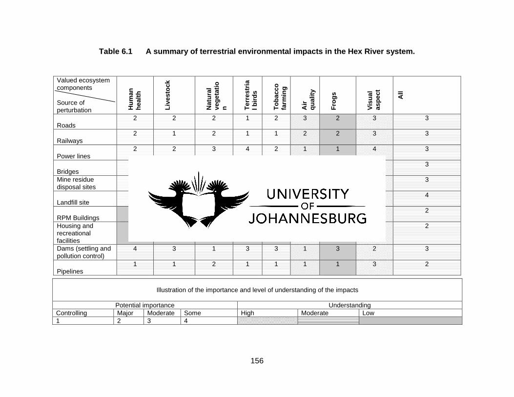
156

Table 6.1 A summary of terrestrial environmental impacts in the Hex River system.

Valued ecosystem components Source of perturbation H

uman

he

alth

Live

stoc

k

Nat

ural

ve

geta

tion T

erre

stria

l bird

s

Tob

acco

fa

rmin

g

Air

qual

ity

Fro

gs

Vis

ual

aspe

ct

All

Roads

2 2 2 1 2 3 2 3 3

Railways

2 1 2 1 1 2 2 3 3

Power lines

2 2 3 4 2 1 1 4 3

Bridges

2 2 3 2 2 2 3 3 3

Mine residue disposal sites

3 2 2 1 3 2 2 2 3

Landfill site

4 4 3 2 2 3 2 4 4

RPM Buildings

2 1 1 1 1 1 1 3 2

Housing and recreational facilities

2 1 1 1 1 1 1 2 2

Dams (settling and pollution control)

4 3 1 3 3 1 3 2 3

Pipelines

1 1 2 1 1 1 1 3 2

Illustration of the importance and level of understanding of the impacts

Potential importance Understanding

Controlling Major Moderate Some High Moderate Low 1 2 3 4

157

Table 6.2 A summary of aquatic environmental impacts in the Hex River system.

Valued ecosystem components Source of perturbation H

uman

he

alth

Aqu

atic

in

vert

ebra

tes

Aqu

atic

ve

geta

tion

Aqu

atic

bird

s

Fis

h

Fro

gs

Phy

to-

plan

kton

All

Sewage effluent discharges

3 3 1 4 3 3 2 3

Stormwater runoff

3 4 3 1 3 2 2 3

Chemical spillages

4 4 1 1 4 3 2 3

Recreation

2 1 2 3 3 2 3 3

Fishing

3 2 2 3 2 2 1 3

Sand mining

2 4 3 2 3 2 2 3

Tailing dam failure

3 4 3 1 3 2 2 3

Illustration of the importance and level of understanding of the impacts

Potential importance Understanding Controlling Major Moderate Some High Moderate Low 1 2 3 4

158

Table 6.3 RPM baseline risk assessment summary.

Ecosystem component

Source Identification Extent Severity Mitigation

Surface water 1. Spillage from mines 2. Rainfall runoff 3. Discharges 4. Floods 5. Pollution control

dams 6. Thickeners 7. Dewatering 8. Wash bays

• Discharge of polluted water into the Hex River system

regional Significant • ‘Green’ discharge assessments

• Immediate clean up or rehabilitation

• Recovery of local spillages and runoff report to existing pollution control dams

Ground water 1. Existing contamination of aquifers

2. Chemical storage tanks

• Spillages • Discharge into surface

water

regional Significant • Excavation of historical pollution and bioremediation.

• Bunded tanks and continuous testing

Natural vegetation and plant life

1. Surface infrastructure

2. Dust and stack fallout

• Decreased effect of grazing

• Diminishing of dominant grass and tree species.

RPM (local) Insignificant • Land management plans

Soils 1. Dust and stack fallout

2. Tailing dams

• Metals in soil and aquatic systems

RPM (local) Significant • Dust and gas control systems (e.g. ceramic filters, acid plant)

• Tailing dam maintenance plan Air quality 1. Sulphur and

nitrogen gas emissions.

2. Fine particulate fallout

• Damage to humans • Health risk to all life

forms

RPM (local) Significant • Acid plants • Pollution control dams • Ceramic filters • Dust suppressants

Noise 1. Mining equipment • Increased noise levels Local Insignificant

• Awareness • Provision of protective

equipment • Purchasing of low noise

equipment Visual aspect 1. Dumps

2. Tailings 3. Buildings 4. Stacks

• Visibility of dumps, tailing dams, plumes and structures

local Insignificant • Maintenance • Rehabilitation (concurrent)

159

The Hex River Management Plan will focus on aquatic systems while other terrestrial

impacts will be managed at business unit levels. General Managers of the seven

business units will take ownership of the implementation of the plan, and the Regional

Environmental Manager will monitor and report progress to the Regional Director of

Mining and Process Divisions (Figure 6.1).

Figure 6.1 Management structure of the Hex River Management system.

6.1.1 Objectives and performance criteria

The Hex River Management Plan aims to accomplish the following goals:

• To reduce RPM’s environmental footprint within their mining lease areas;

• To bring awareness to RPM’s senior management in order to ensure

sustainable environmental stewardship in the region;

• Strengthen relationships with all stakeholders through active participation in

the rehabilitation and restoration of impacted aquatic areas.

In order to meet the main goals of the management plan, the Hex River Management

committee should ensure that water quality issues affecting the River are addressed

and that changes in water quality are monitored as per schedule. It is also imperative

that all issued water use licenses be reviewed and that stringent internal conditions are

applied beyond provisions of legal requirements. The committee should ensure that

continuous engagement with the Department of Water Affairs (DWA) is maintained, so

that more enforcement from the authorities is observed. To realize these goals, each

Execution

Accountabilityand

Reporting

SponsorDirectors:

Mining and Process

General Managers

Mining Managers

Engineering Managers

Plant Managers

Regional Environmental

Manager

Environmental Coordinators

160

ecosystem component must be addressed and managed separately. Plans should be

developed to identify, correct and prevent potential impacts.

6.1.2 Water quality

The water license stipulates that the licensee must ensure that the water quality of the

water provided to downstream water users does not decrease because of mining-

related water use activities. Activities that lead to elevated levels of turbidity of any

watercourse should be minimized. Pollution of and disposal/spillages of any material

into the watercourse must be prevented, reduced, or otherwise remediated through

proper operation, maintenance and effective protective measures. The main objective is

to improve the water quality in the Hex River system towards attaining the reference

conditions of target water quality range (TWQR) prescribed by DWAF. This will be

achieved by ensuring that water quality changes are detected on time and that plans

are implemented to ensure that water quality is suitable for use.

6.1.3 Sediment quality

The main objective is to ensure early detection of changes in sediment’s physical and

chemical characteristics, and to assess its contribution to the health of the aquatic

system. It has been found from the literature that fish and macro-invertebrates respond

differently to changes in the physical and chemical characteristics of sediment. Biotic

changes associated with sediments need to be addressed at source, to ensure that

aquatic health is maintained and sustainable solutions are implemented.

6.1.4 Riparian Vegetation

The main objective is to ensure that changes in the riparian vegetation are detected in

time, and that corrective and preventative measures are put in place. RPM is obliged to

embark on a systematic long-term rehabilitation program, to restore the watercourse to

environmentally acceptable and sustainable conditions, during and after the completion

of the activities. This includes the rehabilitation of disturbed and degraded riparian

areas, to restore and upgrade the riparian habitat integrity in order to sustain a diverse

riparian ecosystem. This program must in particular address remedies for surface

161

cracks and settlement. All disturbed areas must be re-vegetated with indigenous

vegetation suitable to the area, in consultation with an indigenous plant expert, ensuring

that during rehabilitation only indigenous shrubs, trees and grasses are used is

restoring the biodiversity.

Since the beginning of the study these objectives have been communicated to all

internal stakeholders, and have been discussed intensively. Infrastructure has been

upgraded in most of the operations, to ensure that accidental discharges are minimized,

and that there are adequate resources to address these issues. A change management

procedure has been compiled and communicated to all stakeholders (e.g. exploration,

engineering, plant) to ensure that environmental coordinators are part of all planning

processes, and that no expansion or extension projects are approved by senior

management, without the approval of the Regional Environmental Manager (Figure 6.2).

6.1.5 Macro-invertebrates

The water usage license conditions stipulate that the licensee must take all reasonable

steps not to disturb the breeding, nesting and feeding habitats, and natural movement

patterns of aquatic biota. The main objective is to ensure early detection of short-term

changes in macro-invertebrate community structure in the Hex River and to identify

possible sources of pollution for immidiate rehabilitation.

6.1.6 Fish

The water use license stipulates that the licensee must take all reasonable steps to

allow the movement of fish. The main objective is to ensure early detection of long-term

changes of fish community structure and to assess levels of disturbance and the

possible impact on human health. It has been found from the literature that fish respond

differently to changes in environmental conditions. This change, at the end, will affect

the distribution of fish in the Hex River system.

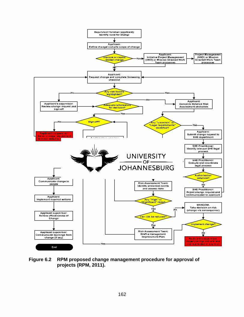
162

Figure 6.2 RPM proposed change management procedure for approval of

projects (RPM, 2011).

163

6.2 Statistical methods and hypotheses

6.2.1 Water quality

The main objective is to ensure that water quality changes are detected on time, and

that plans be put in place to ensure that water is suitable for domestic use and irrigation.

The hypotheses to be tested are:

1. Waste water treatment works (WWTW) strategies will result in increased

water quality;

2. Spillage reduction plans will result in improved water quality in the Hex River

system;

3. An improved pollution control system will result in decreased water pollution

in the River;

4. Reduced mining related terrestrial activities will result in decreased transfer

of polluted soil throughout the River system;

5. Tailing management plans will result in decreased heavy metal loading in

water, throughout the River system.

As with macro-invertebrates, sediment and fish, three additional Hex River tributaries

within the RPM lease area must be sampled for sediment quality bi-annually, or when

conditions similar to those for macro-invertebrates are triggered. Chapter three of this

thesis provides the materials and methods to be applied relating to field work, and

laboratory and data analysis. In addition, pollution control dams, thickener dams and

WWTW must be sampled as per legal requirements, and information should be entered

into the water management plan system for analysis and reporting. Water quality

analysis should be undertaken by an accredited laboratory in accordance with methods

prescribed by SABS.

6.2.2 Sediment quality

The main objective is to ensure early detection of changes in sediment’s physical and

chemical characteristics, and assess how these contribute to the health of the aquatic

system. The hypotheses to be tested are:

164

1. Water maintenance plans will result in the improved physical and chemical

quality of the Hex River sediments;

2. Pollution-control dams will result in decreased metal concentration in

sediment in the Hex River;

3. Tailing management plans will result in decreased heavy metal loading in

sediment, throughout the River system.

As with macro-invertebrates and fish, three additional Hex River tributaries within the

RPM lease area must be sampled for sediment quality bi-annually, or when conditions

similar to those for macro-invertebrates are triggered. Chapter three of this thesis

provides the materials and methods to be applied relating to fieldwork, and laboratory

and data analysis.

6.2.3 Riparian vegetation

The main objective is to ensure that changes in the riparian vegetation are detected on

time, and that corrective and preventative measures are put in place. The hypotheses to

be tested are:

1. Vegetation maintenance strategies will result in a healthy riparian zone;

2. Biodiversity action plans will result in early detection of exotic vegetation

species;

3. Concurrent rehabilitation (mine closure) plans will result in decreased

disturbances and flow modification of the Hex River system.

According to DWAF (1999), changes in riparian vegetation structure or function are

commonly associated with changes in river flow, exploitation for firewood, or changing

use of a riparian zone (for example grazing or ploughing). Riparian vegetation

monitoring should take place every three years, to detect the trend of improvement or

deterioration. To assess habitat integrity, the procedure to be used is the one prescribed

by Kleynhans (1996), Kleynhans et al (2007) and various field guides (Bromilov, 2001

and Henderson, 2001). The riparian indicator species should be used to determine the

riparian zone of RPM, as described by Hill (2005).

165

Additional surveys will be conducted, if there are major changes in the riparian

vegetation within the RPM, in order to determine severity, and to implement corrective

measures. These events include:

• Major veld fires in the riparian zone;

• Rezoning of a piece of land within the RPM license area;

• Settlement of people along the river banks within the floodline;

• Selling and acquisition of land within the current RPM lease area;

• Major exploration activities within the RPM license area.

6.2.4 Macro-invertebrates

The main objective is to ensure early detection of short-term changes in macro-

invertebrate community structure in the Hex River, and to identify possible sources of

pollution for urgent rehabilitation and restoration. The following hypotheses must be

tested:

1. Spillage reduction plans will result in an improved macro-invertebrate

community structure in the River system;

2. Improved pollution control dam capacity will result in decreased water and

sediment pollution in the River system;

3. Reduced mining-related terrestrial activities will result in decreased transfer

of polluted sediment throughout the River system;

4. Tailing management plans will result in decreased heavy metal and fine silt

impact, throughout the River system.

Three additional Hex River tributaries within the RPM lease area must be sampled. The

associated General Manager must take full accountability and ensure that reports are

submitted on time. This will include Klipfontein Spruit, Klipgat Spruit, and Paardekraal

Spruit. Two additional Hex River stations outside the RPM license area, will be sampled

for macro-invertebrates (Figure 6.3).

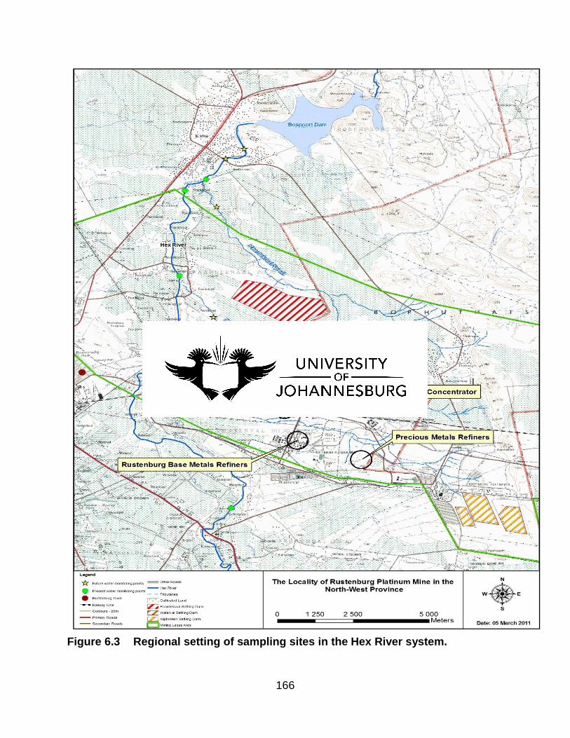
166

Figure 6.3 Regional setting of sampling sites in the Hex River system.

167

Biomonitoring must continue bi-annually (high and low flow regimes) to detect the trend

of improvement or deterioration. Invertebrate samples will be taken at all seven stations,

by following the SASS 5 protocol described by Dickens et. al. (2002). This will enable

the identification of possible impacts of the Rustenburg Platinum Mines (and other key

stakeholders) in the Hex River system (see Appendix 1). Early identification of effects

on the macro-invertebrates should prompt the water quality-monitoring program to

identify problematic variables to be mitigated, and to avoid further effects thereof on the

aquatic ecosystem. Additional surveys must be conducted if there are major

environmental incidents within the Rustenburg Platinum Mines license area, in order to

determine severity, and to implement corrective measures. These incidents will include:

1. Major chemical spillage in the vicinity of the Hex River;

2. Major accidental discharges from the pollution control systems;

3. Major floods influencing the River system;

4. Major exploration activities or any topography and soil disturbance that is not

rehabilitated on time;

5. Tailings dam failure, resulting in sediments entering the Hex River or its

tributaries.

Chapter three of this thesis provides the materials and methods to be applied relating to

fieldwork, and laboratory as well as data analysis.

6.2.5 Fish

The main objective is to ensure detection of long-term changes of fish community

structure, and to assess levels of disturbance and the possible impact on human health.

The following hypotheses must be tested:

1. Spillage reduction plans will result in an improved diversity of fish in the Hex

River;

2. Improved pollution-control dam capacity, will result in decreased

bioaccumulation in fish throughout the Hex River;

3. Reduced construction (barriers) related to RPM mining, will result in an

increased diversity of fish throughout the River system.

168

As with macro-invertebrates, three additional Hex River tributaries within the RPM lease

area must be sampled for fish bi-annually, or when conditions similar to those for

macro-invertebrates are triggered. Fish Response Assessment Index (FRAI) should be

in accordance with Kleynhans et al ( 2007).

6.3 Analytical methods and alternative designs

According to Baker and Huggins (2005), the ideal biomonitoring process for fish, macro-

invertebrates or the benthic algae sampling regime, would involve a large number of

whole samples from a known area, sampled from all of the important habitats, with

taxon identifications to species level. However, a protocol such as this is unachievable

for biological monitoring purposes, so compromises must be made to permit the

sampling of a large number of sites in a relatively short time, in order to obtain accurate

and relevant information at minimum cost. When deciding on the analytical method and

designs, it is imperative to ensure that data collected by different people participating in

the Hex River Management plan, are aligned and can be used collectively to make

future decisions.

6.3.1 Water quality

Chapter three provides the method and materials used for field work, and laboratory

and data analysis for water quality, and will not be discussed in this section. The

following physico-chemical water quality parameters must be analyzed in situ, by

making use of standard measurement techniques and apparatus:

• Dissolved Oxygen concentration (mg/l; Ecoscan D06);

• Conductivity (uS/cm; Cyberscan con 11);

• Oxygen Saturation (%; Ecoscan D06);

• Temperature (0C; Ecoscan D06);

• pH (Cyberscan pH 110).

Nutrient analysis must be conducted using a Merck cell test kit, for the following

parameters:

• Ammonium;

169

• Nitrates;

• Nitrites;

• Chlorides;

• Phosphates;

• Sulphates;

• Chemical Oxygen Demand.

• Biochemical Oxygen Demand

The following metals must be tested for in water, using standard methods:

• Cobalt (Co);

• Copper (Cu);

• Manganese (Mn);

• Cadmium (Cd);

• Mercury (Hg);

• Lead (Pb);

• Zinc (Zn).

• Nickel (Ni)

• Chromnium (Cr)

• Platinum (Pt)

6.3.2 Sediment

A standard protocol of the United States Environmental Protection Agency (USEPA,

2000) must be adopted for sediment assessment. Chapter three provides the method

and materials used for field work, and laboratory and data analysis for sediments, and

will not be discussed in this section. The following metals must be tested in sediment

samples:

• Cobalt (Co);

• Copper (Cu);

• Manganese (Mn);

• Cadmium (Cd);

• Mercury (Hg);

170

• Lead (Pb);

• Zinc (Zn).

• Nickel (Ni)

• Chromnium (Cr)

• Platinum (Pt)

6.3.3 Riparian vegetation

The immediate vegetation must be identified during high and low flow conditions in the

field, using a number of field guides (Kleynhans, 1999; Bromilov, 2001; Henderson,

2001). Data collected must include river channel, riparian zone (including invasion),

ground and vegetation cover, the main species present, and disturbances using the

Riparian Vegetation Index (RVI). The RVI is a site-specific approach, which places

particular emphasis on the ecological integrity of the riparian vegetation. The main

parameters to be considered when implementing the riparian vegetation management

objectives are:

• Exotic vegetation;

• Vegetation decrease;

• Bank erosion;

• Water abstraction;

• Flow modifications.

6.3.4 Macro-invertebrates

Chapter three discusses the method and materials used for field work, and laboratory

and data analysis, and will not be discussed in this section. Macro-invertebrates feed on

algae and leaf matter from the river, and in turn serve as food for larger aquatic

organisms such as fish, which are a major source of food for birds and humans. They

respond relatively quickly to localized conditions in a river, including water quality and

habitat changes. They are commonly found with a wide range of sensitivities, and have

suitable life-cycle duration for indicating short to medium term impacts on water quality.

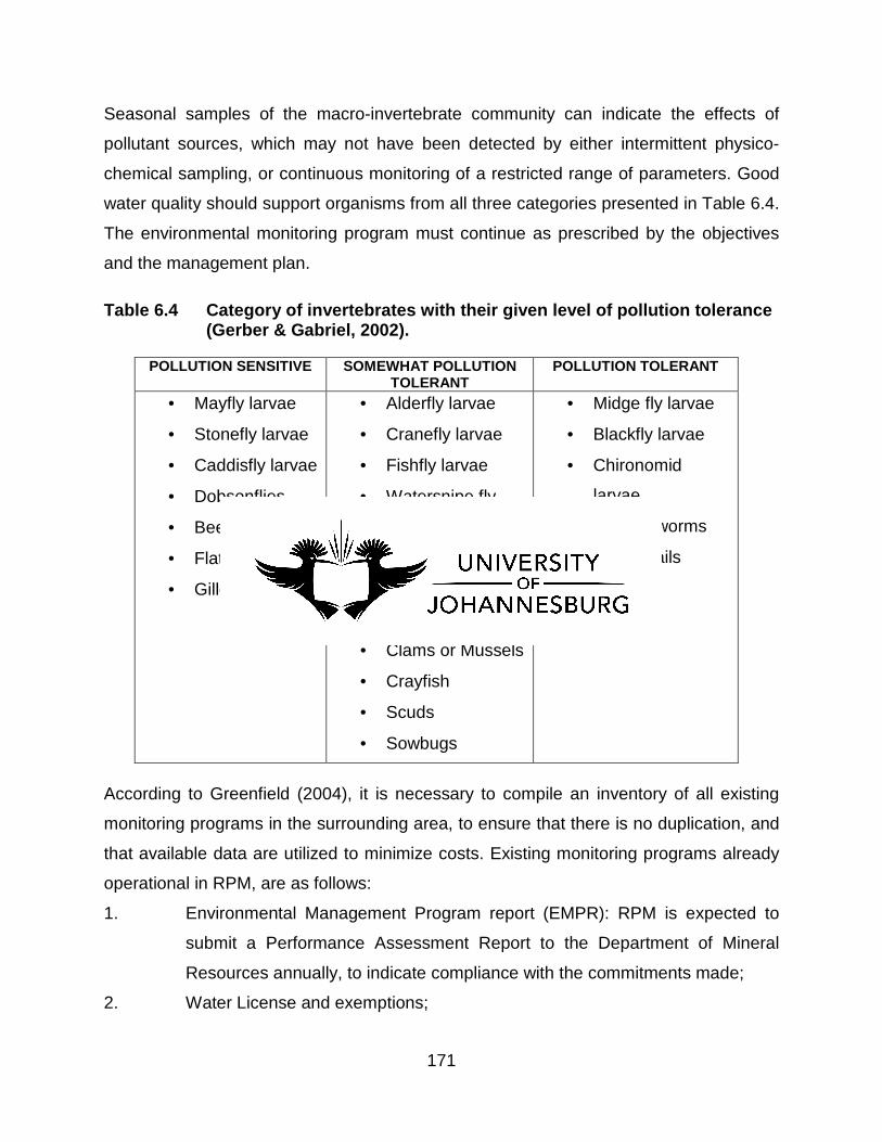
171

Seasonal samples of the macro-invertebrate community can indicate the effects of

pollutant sources, which may not have been detected by either intermittent physico-

chemical sampling, or continuous monitoring of a restricted range of parameters. Good

water quality should support organisms from all three categories presented in Table 6.4.

The environmental monitoring program must continue as prescribed by the objectives

and the management plan.

Table 6.4 Category of invertebrates with their given level of pollution tolerance (Gerber & Gabriel, 2002).

POLLUTION SENSITIVE SOMEWHAT POLLUTION TOLERANT

POLLUTION TOLERANT

• Mayfly larvae

• Stonefly larvae

• Caddisfly larvae

• Dobsonflies

• Beetles

• Flatworms

• Gilled snails

• Alderfly larvae

• Cranefly larvae

• Fishfly larvae

• Watersnipe fly

larvae

• Damselfly larvae

• Dragonfly larvae

• Beetle larvae

• Clams or Mussels

• Crayfish

• Scuds

• Sowbugs

• Midge fly larvae

• Blackfly larvae

• Chironomid

larvae

• Aquatic worms

• Lung snails

• Leeches

According to Greenfield (2004), it is necessary to compile an inventory of all existing

monitoring programs in the surrounding area, to ensure that there is no duplication, and

that available data are utilized to minimize costs. Existing monitoring programs already

operational in RPM, are as follows:

1. Environmental Management Program report (EMPR): RPM is expected to

submit a Performance Assessment Report to the Department of Mineral

Resources annually, to indicate compliance with the commitments made;

2. Water License and exemptions;

172

3. Prospecting Works Program: RPM is expected to demonstrate that all

exploration activities within the mine lease area are rehabilitated;

4. Mine Works Program: RPM is expected to demonstrate that all mining

activities within the mine license area are rehabilitated concurrently, and that

a mine closure certificate is received from the Department of Mineral

Resources (DMR);

5. Environmental Impact assessment (EIA): These are ongoing studies to

ensure that environmental impacts associated with expansion activities, are

mitigated;

6. Air Quality Management Program (AQMS): As part of the emission license,

RPM is obliged to monitor dust fall-out, fugitive emissions, and stack

emissions from PGM processing plants;

7. Legal compliance audits (permits, licenses, instructions and other

environmental authorizations);

8. RPM Waste Water Treatment Works monitoring;

9. Social and labour plans;

10. Tailing dam management plans;

11. Water maintenance plans.

6.3.5 Fish

Chapter three provides the method and materials used for field work, and laboratory

and data analysis, and will not be discussed in this section. In addition, descriptive

statistics must be computed using SPSS 13.0. The differences in metal concentration

will be tested using one-way analysis of variance (ANOVA), considering sites as

variables. Kolmogorov-Smirnoff and Lavene tests must be used to test normality and

homogeneity of variance, respectively.

173

6.4 Monitoring and evaluation

Monitoring involves the gathering of information, which may include observing or

measuring change, and is often the raw material/data used for evaluation. Evaluation is

the assessment of the effectiveness of a project against pre-defined objectives

(Rutherfurd et al., 2000).

The Hex River Management plan aims to accomplish the following goals:

1. Reduce RPM’s environmental footprint within their mining license areas;

2. Strengthen relationships with all stakeholders, through active participation in

the restoration of impacted areas;

3. To bring awareness to senior management, in order to ensure sustainable

environmental stewardship in the company.

The key objectives of this plan are derived from critical issues identified in chapters four

and five of this thesis as threatening the survival and sustainability of the Hex River

system. The key objectives supporting the overall goals are to:

1. Control all terrestrial activities leading to sediment transport into the aquatic

environment;

2. Control and monitor all discharges to the aquatic environment;

3. Understand the impact of the catchment processes on the quality of water;

4. Protect and enhance macro-invertebrates and their habitat;

5. Protect and enhance fish populations in the aquatic environment;

6. Improve community social responsibility;

7. Increase external stakeholder awareness on challenges and threats facing the

Hex River system;

8. Increase internal stakeholder awareness on challenges and threats facing the

Hex River system.

Key stakeholders in the implementation of the Hex river management plans are:

• Rustenburg Platinum Mine;

• Department of Water and Environment Affairs;

174

• Rustenburg Municipality;

• Rustenburg Community Forum;

• Kroondal Environmental Forum;

• Mfidikwe Environmental Forum;

• Various consultants (environmental, social and mining);

• Local Landowners.

At least two representatives from these key stakeholders must form part of the Hex

River Management Committee (HRMC).

Table 6.5 Objectives, output, actions and indicators to be used to test effectiveness of the management plan.

Objectives Output Actions Indicators

1. To control all terrestrial

activities leading to sediment

transport into the aquatic

systems.

Reduced/minimized erosion

events.

Implement erosion mitigation

where necessary

Number of erosion related

incidents.

Reduced incidents of tailing

dam/mine residue failures.

Increase buffer zones between

land use and the

Number of new developments.

Reduced development in the

license area.

Participate in the EIA public

participation.

Number of environmental

authorisations.

Reduced grazing.

Develop a grazing

management plan with

landowners.

Carrying capacity of the area

Improved fire management.

Compile a veld fire

management plan and

implement it.

Number of major veld fires.

Reduce total waste rock dump

area.

Compile a waste rock design

procedure.

Number of waste rock dumps.

Minimized waste dumping (legal

and illegal).

Review rehabilitation plan.

Land rehabilitated.

Proper topsoil handling.

Compile road design plan.

Number of new roads.

Minimized driving tracks.

Compile a flora and fauna

assessment.

Land rehabilitated.

Table 6.5 cont.

176

2. To control and monitor all

discharges to the aquatic

systems.

Decreased pollutants.

Minimize accidental discharges. Number of incidents.

Operational pollution-control

infrastructure.

Review adequacy of the current

pollution-control infrastructure.

Number of incidents and

improved water quality.

Compliant Waste Water

Treatment Works (WWTW).

Monitor compliance level.

Number of non-compliances.

No exceedance in water quality

standards

Develop trigger action response

plans.

Number of exceedances.

3. To understand the impact of

the catchment processes on

the quality of water.

Reduced water extractions.

Implement water recycling. Percent reduction of portable

water consumption and quality

improvement.

Clean and dirty water separation. Develop water maintenance

plan.

Number of non-compliances to

the plan.

Reduced non-primary activities’

consumption.

Identification of water saving

and quality improvement

projects

Number of non-primary water

uses

4. To protect and enhance

macro-invertebrates and

their habitat.

Improved community structure.

Conduct surface water

(biomonitoring) assessment.

Improved biotic integrity.

Table 6.5 cont.

177

Reduced sand-mining activities.

Register as an interested

affected party for all

development applications in the

vicinity (e.g. sand mining).

Number of authorities’ approval

(permits, licenses and record of

decisions).

Reduced sediment inflow.

Implement erosion mitigation

where necessary.

Number of erosion-related

incidents.

Increased riparian and catchment

vegetation.

Identify conditions to encourage

vegetation growth.

Improved Riparian Vegetation

Index.

5. To protect and enhance fish

populations in the aquatic

system.

Fish community structure.

Conduct surface water

(biomonitoring) assessment.

Habitat Quality Index.

Lack of barriers for fish in the

exposure areas.

Identify current and potential

barriers for fish passage, and

eliminate.

Number of new barriers.

Reduced fishing activities.

Compile an awareness plan

and educate fishermen,

Fishing incidents.

Reduced water-related recreation

activities.

Upgrade community

recreational activities.

Existing water recreational

activities.

Table 6.5 cont.

178

6. To improve community social

responsibility.

Implementation of Social and

Labour plan (SLP).

Adopt/commit to infrastructure

projects that may influence the

aquatic systems in the

Municipality’s Integrated

Development Plan (IDP).

Number of projects supported.

Avail resources for community

projects.

Enhance non-aquatic

recreational activities.

Number of recreational activities

improved, and participation.

Improved community health and

recreational projects.

Participate in health and

welfare projects to educate

communities about the

importance of aquatic health.

Number of health and welfare

projects participated, and role.

7. Increase stakeholder

awareness on challenges

and threats facing the Hex

River system.

Increased stakeholder awareness

of the aquatic system.

Enhance or establish

environmental forums to

include aquatic health.

Number of environmental forums

involved.

Reduced aquatic activities.

Identify alternative use for

aquatic use activities.

Number of alternative activities.

Improved collaboration in the

vicinity.

Attend stakeholder meetings. Number of meetings attended.

8. Increase internal awareness

on challenges and threats

facing the Hex River system.

Reduced development within RPM

lease area.

Identify all areas that are

currently impacting the aquatic

system.

Number of structures removed

or improved.

Table 6.5 cont.

179

Change management plan.

Develop change management

procedure.

Number of projects

(minor/major) approved.

Management accountability.

Define roles and responsibility. Number of employees trained.

Training plan. Develop a training manual for

environmental awareness.

Number of scheduled training

sessions conducted

180

6.5 Data and information management

A structured monitoring plan results in the collection of relevant data for management.

The data value arises not only because of the monetary and time investment to collect

the data, but also because the data is intended to satisfy high priority management

needs. For these reasons, it is imperative that data processing, storage and handling,

receive careful attention (Gustavo et al., 2001).

Section 4.5.1 of the EMS ISO 14001 standards (2004), of which all RPM operations are

accredited, requires the organization to establish and maintain records as necessary to

demonstrate conformity to the requirements of its environmental management system,

and the results achieved. It further stipulates that the organization must establish,

implement and maintain a procedure(s) for the identification, storage, protection,

retrieval, retention and disposal of records. Records must remain legible, identifiable

and traceable (BS EN ISO 14001: 2004).

According to Greenfield (2004), the development of a data management plan must

consider the following questions: (1) Where will the data go; (2) how will the data be

stored; (3) how will the data be maintained; (4) how will the data be checked; (5) how

accessible will the data be; (6) how will report be publihed; and (7) how much will the

plan cost?

6.5.1 Data quality assurance

Rustenburg Platinum Mines’ operations have a matured document control and record

management systems, supporting the study objectives. These systems must be

improved to support the current study and to ensure maximum utilization, and so that all

stakeholders realize the value. As an example, Enablon is the name of the system that

all Anglo American operations use to report on safety and sustainable development

data. It is hosted externally and maintained by consultants. All public reporting and

reporting to the corporate function has to be based on parameters entered in Enablon.

This is to ensure that Anglo American communicates the same information and that

errors are eliminated in advance

public.

The aim is to ensure that all data reported in the Enablon system is accurate, submitted

on time, approved and authorized appropriately

data use and communication is done. Data

reporting purposes and to ensure that deviations are reported, implemented and

communicated in time, to all relevant stakeholders. For this, clear roles and

responsibilities must be defined to ensure that the information is accurate and that the

right information is communicated to key stakeholders. Table 6.6 describes data

management roles and responsibility.

6.5.2 Quality control

Figure 6.4 summarizes the environmental data management process. Once

Administrator launches all campaigns

submitted”. This means that

collection, can capture new data

capturer is no longer able to edit the data for th

can review the data and submit for approval

be rejected and sent for recapturing.

Figure 6.4 Environmental data management process

Step 1. Data Capturer

Step 2. Data Expert

Step 3. Data Owner

181

errors are eliminated in advance, before information can be made available to the

The aim is to ensure that all data reported in the Enablon system is accurate, submitted

on time, approved and authorized appropriately, by the relevant persons

data use and communication is done. Data are used mainly for internal and publ

reporting purposes and to ensure that deviations are reported, implemented and

to all relevant stakeholders. For this, clear roles and

responsibilities must be defined to ensure that the information is accurate and that the

nformation is communicated to key stakeholders. Table 6.6 describes data

management roles and responsibility.

Figure 6.4 summarizes the environmental data management process. Once

Administrator launches all campaigns, they are reflected on the database as “to be

submitted”. This means that the data capturers, depending on the frequency of

collection, can capture new data. Once the data has been submitted for validation, the

capturer is no longer able to edit the data for that parameter. At this stage, the validator

can review the data and submit for approval, if satisfied with the inputs. If not, data can

be rejected and sent for recapturing.

Environmental data management process

Capture and Submit

Revise if not approved

Keep source data

Review submitted data

Validate and submit to data

owner

Review

Approve or reject

Provide assurance

before information can be made available to the

The aim is to ensure that all data reported in the Enablon system is accurate, submitted

by the relevant persons before any

used mainly for internal and public

reporting purposes and to ensure that deviations are reported, implemented and

to all relevant stakeholders. For this, clear roles and

responsibilities must be defined to ensure that the information is accurate and that the

nformation is communicated to key stakeholders. Table 6.6 describes data

Figure 6.4 summarizes the environmental data management process. Once the System

are reflected on the database as “to be

the data capturers, depending on the frequency of

been submitted for validation, the

at parameter. At this stage, the validator

if satisfied with the inputs. If not, data can

182

Once data is validated, the system will reflect “awaiting validation”. The data approver

will review the data and approve, if satisfied with the inputs. The approver may reject

the campaigns, if incorrect data is captured. Approval of data is required on a quarterly

basis, while capture and validation is done as data become available.

6.5.3 Information management

As part of the annual sustainability assurance process, an external auditor must be

appointed to review the integrity of the database, and to ensure accurate reporting for

key performance indicators. The assurance process must focus on the capturing,

validation and approval process. The assurance must also focus on the workflow, and

any instances of non-compliances must be raised for mitigation. All the campaigns for a

given period must be locked and annual reports drawn for internal stakeholders and for

reporting purposes (to society).

The main environmental parameters monitored on the Enablon database, are as

follows:

• Materials;

• Energy;

• Water;

• Land;

• Emissions;

• Discharges;

• Waste;

• Complaints and Incidents.

Depending on stakeholder requirements, further processing and refinement of Enablon

environmental data can be presented in tables, graphs, photographic records and digital

maps. The Enablon database is linked into the Pivot system, which has graphical and

report generating tools. The following reports are available:

• Environmental incidents;

• Non-compliances;

183

• Non-conformance;

• Community complaints;

• Observations;

• Training;

• Meeting/Engagement;

• Audits;

• Inspections;

• Legal instructions;

• Corrective and preventative measures status.

All employees and key stakeholders must have access to the report section on Pivot.

Key stakeholders must have a ‘read only’ access to Enablon, and data capturers and

system administrators must have a ‘read and write’ access to Enablon. The Regional

Environmental Manager (Approver), for later assurance purposes by the third party

auditor, must keep all supporting documentation and source documents. All operations’

data capturers must submit hard copies to the System administrator after capturing, and

these records should be forwarded to the Regional Environmental Manager for record

keeping purposes.

An information security system must be in place, to ensure data protection, and a back

up is carried out on a daily basis by the RPM IM department in Rustenburg. An IM

Specialist must be allocated to the Regional Environmental department, to ensure that

there is adequate IM support and that quality control systems are in place and adhered

to, by all data handling personnel.

184

Table 6.6 Data management roles and responsibilities

Data Management Stakeholders

Phases Data Management

Activities

Regional

Environmental

Manager

(Approver)

Task

Leader

Field

Team

Consultants System

Administrator

Communications

and

Data User

Auditor

(Third

Party)

PLA

N

1. Project scope x x

2. Historical data

gathering and

collection

planning

x x x x

EX

EC

UT

ION

3. Sampling plan x x x

4. Sampling

logistics

x x

5. Field data

collection

x x x

6. Field sampling x x

7. Laboratory

analysis

x x

RE

VIE

W

8. Data review x

9. Data verification

and validation

x x

185

Data Management Stakeholders

Phases Data Management

Activities

Regional

Environmental

Manager

(Approver)

Task

Leader

Field

Team

Consultants System

Administrator

Communications

and

Data User

Auditor

(Third

Party)

10. Consolidation

and record

keeping

x x

11. Data use &

analysis

x x x

186

6.5.4 Communicating program results

Mulder et al. (1999) viewed the inability of monitoring practitioners to communicate their

findings to a diverse audience, as a traditional weakness. Monitoring efforts should

conclude with the preparation of draft and final reports, to ensure the wide distribution of

collected information. An effective reporting process promotes a higher visibility and

accountability for monitoring activities, and supports the evaluation of objectives,

results, and future approaches to monitoring (Thom & Wellman, 1996).

In order to achieve optimal outcomes on the RPM objective of increasing stakeholder

(internal and external) awareness on challenges and threats facing the Hex River

system, an emphasis must be placed on providing information to key stakeholders (e.g.

RPM, DWEA and community forums).

The main function of the Regional Environmental Manager (Project manager) is to

ensure that there is sufficient information to fulfill the requirements for scientific,

decision-making and public evaluations for sustainable future management of the Hex

River. Existing stakeholder engagement forums should be utilised to provide

information, and to ensure that there is continuous buy-in and participation from existing

and new stakeholders.

6.5.4.1 Internal stakeholders

Monthly and quarterly reports should be produced, that outline the project status and

trends observed during the month. Possible sources of pollution must be discussed

briefly, and an incident reporting status summarized as shown in figure 6.5.

187

Figure 6.5 Example of a monthly report to stakeholders on incidents that may contribute to a decline in aquatic health in the Hex River.

These reports should be communicated to all General Managers for discussion with

their operational teams, so ensuring that corrective and preventive measures are taken.

Monthly environmental talk topics must be communicated to all operations for their

notice boards, to grow general environmental awareness on the leading indicators

(Figure 6.6).

188

Figure 6.6 Example of a monthly ‘one pager’ used for employee environmental awareness in the operations.

6.5.4.2 External stakeholders

A 24-hour environmental hotline must be introduced to ensure that all concerns and

complaints from the stakeholder are reported and addressed on time. All hotline

controllers must be trained to ensure that they understand the project, and that they can

access the database and have access to all project members.

All affected landowners must receive formal communications if there are changes in

water quality in their vicinities. Corrective and preventive measures must be

communicated to them, and a progress report given formally. Department of Water and

Environmental Affairs (or any applicable authority) must be notified of a deviation, if a

compliance point is infringed. Where necessary, other stakeholders should be notified

telephonically.

Bi-annual articles on the project status and results must be submitted to the local

newspaper (Rustenburg Herald) in three languages, Afrikaans, Setswana and English

to ensure that the information reaches all target groups. This information must be

placed on the Anglo American website (http://www.angloamericanplatinum.com), to

ensure transparency and the information should be used for scientific purposes. Bi-

11%1%

32%

1%3% 3%

6%2%

20%

21%

0%

43%

RPM monthly incidents

Air

Biodiversity

Hydrocarbons

Energy

Land

Tailings

Social

Systems

Waste

Water

189

annual Anglo Platinum ‘open days’ should be revised to include a presentation on the

project, and discuss successes and challenges of the Hex River management plan.

Flyers and digital communiqués should be issued to communities during these

engagements, to ensure that the information reaches the entire target group.

At least one public participation meeting should be held annually to ensure that there is

still alignment, and the audience should deliberate stakeholder concerns before

decisions are made. The Hex River Management Committee must continue to engage

with members of the public, to pursue the objective of taking active responsibility for

protecting and enhancing the status of the Hex River. One poster or paper presentation

should be made during a national conference (e.g. the Zoological Society of South

Africa) on the findings, and how impacts are managed, and about rehabilitation success

or challenges. The current report to society must be used to capture the progress and

success of the implementation of the Hex River management plan, as from 2012.

190

6.6 References

Allan, J.D. and Johnson, L.B. 1997. Catchment-scale analysis of aquatic ecosystems.

Freshwater Biol. 37: 107-111.

Baker, D.S. and Huggins, D.G. 2005. Sub-sampling techniques for macroinvertebrates,

fish and benthic algae sampled in biological monitoring of streams and rivers. Central

Plains Center for Bio-Assessment. Kansas. Report No. 132 of the Kansas Biological

Survey pp 1-25.

Bromilov, C. 2001. Problem plants of South Africa. Briza Publications. Pretoria.

Department of Water Affairs and Forestry (DWAF). 1996. South African Water Quality

Guidelines. Vol. 7: Aquatic Ecosystems. DWAF. Pretoria.

Department of Water Affairs and Forestry (DWAF). 1999. Resource directed measures

for protection of water resources. Vol. 3: River Ecosystems, Version 1.0. DWAF.

Pretoria.

Department of Water Affairs and Forestry (DWAF). 2006. Best practice guideline H3:

Water reuse and reclamation. Vol. 3: Aquatic Ecosystems. DWAF. Pretoria.

Dickens, C.W.S. and Graham, P.M. 2002. The South African Scoring System (SASS),

Version 5, Rapid bioassessment method for rivers. African Journal of Aquatic Science

27: 1-10.

Environmental Management Systems (EMS) EN ISO 14001. 2004. Environmental

management systems: Requirements with guidance for use. United Kingdom.

Gerber, A. and Gabriel, M.J.M. 2002. Aquatic macroinvertebrates of South African

Rivers: Illustration. Version 2. Institute for Water Quality Studies (IWQS). DWAF.

Pretoria.

Greenfield R. 2004. An assessment protocol for water quality integrity and management

of the Nyl Wetland system. PhD thesis, University of Johannesburg.

191

Gustavo, A., Bausch, W., Pautasso, A., Kahn, A. and Hallett, M. 2001. Dependable

Computing in Virtual Laboratories, icde, p. 0235, 17th International Conference on Data

Engineering (ICDE’01). Germany.

Henderson, L. 2001. Alien weeds and invasive plants. A complete guide to declared

weeds and invaders in South Africa. Agricultural Research Council. Pretoria.

Hill L 2005. Elands Catchment Comprehensive Reserve determination Study,

Mpumalanga Province. Ecological Classification and Ecological Water requirements

(quantity)

Jeffries M. and Mills D. 1990. Freshwater Ecology. Belhaven Press. London.

Kleynhans, C.J. 1996. A qualitative procedure for the assessment of the habitat integrity

status of the Luvuvhu River (Limpopo System, South Africa). Journal of Aquatic

Ecosystem Health 5: 1-4.

Kleynhans, C.J. 1999. The development of a fish index to assess the biological integrity

of South African Rivers. Water SA 25 (3): 265-278.

Kleynhans CJ, Mackenzie J and Louw MD. 2007. Module F: Riparian Vegetation

Response Assessment Index in River EcoClassification: Manual for EcoStatus

Determination (version 2). Joint Water Research Commission and Department of Water

Affairs and Forestry report, Pretoria, South Africa.

Kleynhans CJ, Louw MD, Moolman J. 2007. Reference frequency of occurrence of fish

species in South Africa. Report produced for the Department of Water Affairs and

Forestry (Resource Quality Services) and the Water Research Commission.

McKenzie, D.H., Hyatt, D.E. and McDonald, V.J. 1992. Ecological indicators. Vol. 1 and

2. Elsevier Applied Science. New York.

Mogakabe, D.E. and Van Ginkel, C.E. 2008. The water quality of the Bospoort Dam.

Internal Report No. N/0000/00/DEQ/0108 for the Department of Water Affairs and

Forestry, South Africa.

192

Mulder, B.S., Noon, B.R., Spies, T.A., Raphael, C.J., Palmer, A.R., Olsen, G.H.,

Reeves. G.H. and Welsh, H.H. 1999. The strategy and design of the effectiveness

monitoring program for the Northwest Forest Plan. General technical report PNW-GTR-

437. Department of Agriculture, Forest Service, Pacific Northwest Research Station,

Portland, Oregon, p. 138.

Republic of South Africa. 1998. National Water Act, Act 36 of 1998. Government

Gazette. No 19182. Pretoria.

Republic of South Africa. 2002. Mineral and Petroleum Resources Development Act,

Act 28 of 2002. Government Gazette. No23922. Pretoria.

Ringold, P.L., Mulder, B.S., Alegria, J., Czaplewski, R.L., Tolle, T. and Burnett, K. 1999.

Establishing a regional monitoring strategy: The Pacific Northwest Forest Plan.

Environmental Management 23: 179-192.

Roux, D.J. 2001. Development of the procedure for the implementation of the National

River Health Program in the Province of Mpumalanga. WRC Report No 850/1/01. Water

Research Commission. Pretoria.

Rustenburg Platinum Mines. 2011. Proposed change management procedure.

TZ.OPR.MW.010. Rustenburg.

Rutherfurd, I., Jerie, K. and Marsh, N. 2002. A rehabilitation manual for Astralian

streams. CRC for Catchment Hydrology and Land & Water Resources R&D

Corporation. Canbera. www.rivers.gov.au*

Thom, R.M. and Wellman, K.F. 1996. Planning aquatic ecosystem restoration

monitoring programs. IWR Report 96-R-23. US Army Corps of Engineers. Institute for

Water Resources. Alexandria, Virginia.

United States Environmental Protection Agency (USEPA). 2000. Methods for measuring

the toxicity and bioaccumulation of sediment-associated contaminants with freshwater

invertebrates. 2nd ed. EPA, 600/R-99/064, Washington, D.C.

193

Van der Walt, M., Marrx, C., Fouche, L., Pretorius, N. and St Arnaud, J. 2006. Turning

the sewage tide around: A good news case study about the Hex River Catchment.

WISA 2006 Biennial Conference & Exhibition, Durban.

194

CHAPTER 7

CONCLUSIONS AND RECOMMENDATIONS

Firstly, this chapter describes the background of the research and the conclusions

made, based on the results obtained. Secondly, suggestions are made for future

research that will ensure continual improvement towards sustainable management and

rehabilitation of the Hex River system. It was evident that the water quality, sediment

quality, fish and macro-invertebrate community structure in the Rustenburg region is

influenced differently by platinum mining activities.

7.1 Conclusions

Mining’s contribution to South Africa’s gross domestic product (GDP) is estimated at

about 19%, making it an extremely important sector, which requires very sound

management practices (Baxter, 2011). It has been recorded that South Africa is the

world’s biggest producer of platinum, and it still holds the world’s largest reserves of

platinum group metals (PGM). Rustenburg Platinum Mines (RPM) produce 15.8% of the

world total PGM’s and processes 34% of the total PGM produced in South Africa. The

increase in platinum mining and processing causes an increase in environmental stress

and associated costs. In this regard, there are also several social and environmental

aspects and impacts associated with mining of platinum that require attention, to

maintain sustainability in the Rustenburg region. The Hex River runs across mining

license area, with mining related activities on both sides, making it an immediate sink for

all potential unwanted events in the catchment area of the river. There have been a

number of historical major incidents, both social and environmental, which has led to

RPM being perceived as a non-compliant organization, by both communities and

authorities. The combination of stringent environmental legislation, enforcement and

improved leadership awareness in the past decade, has, however, allowed the

organization to prioritize on sustainability efforts, and to improve accountability at senior

management levels.

195

The purpose of the current study was to assess the impact of platinum mining on water

quality and selected aquatic organisms, and to develop a management plan for

sustainability purposes. The findings of the research have shown that there are areas

that have been impacted negatively by the platinum mining activities, in terms of water

quality and other selected aquatic organisms. The four objectives of the study are

discussed in the following paragraphs for both macro-invertebrates and fish.

This study has shown that the macro-invertebrate community structure, in terms of

abundance and diversity in this area, indicated a clear seasonal variation at all sampling

sites. Along with this trend, it has been confirmed that platinum production decreases in

early winter, due to annual maintenance shutdowns. The dissimilarity among the three

groups from the multivariate analysis was related back to the component species in

each group of samples, and the species responsible for the groupings identified. The

presence of invertebrates like Tabanidae, Gomphidae, Lepidoptera and Elmidae, all of

which are pollution-tolerant, suggests moderately polluted conditions. The mining of the

ore body appeared not to have a significant impact on the Hex River. The platinum

processing appears to be having a slight impact in the exposure sites. The findings

suggest that except for site 4 there were no significant differences between exposure

and reference sites, in terms of the representation of macro-invertebrates. Recent

studies in the area have also confirmed that there are no significant shifts in the macro-

invertebare community structure. The first objective of the study was met and this data

will be used as a comprehensive baseline to measure the success of RPM rehabilitation

activities.

The fish community structure indicated no clear-cut distinction between exposure and

reference sites. Unlike with the macro-invertebrates, there were no significant seasonal

variations in the fish communities. The multivariate analysis revealed one major group

at 40% Bray-Curtis similarity. It emerged that the pollution-tolerant species of Barbus

paludinosus is responsible for the observed group. Fish species richness is reduced at

the first two exposure sites, where active mining and processing takes place, and

improves at the most downstream site, situated at the border of the mine license area.

The domination of B. paludinosus, Pseudocrenilabrus philander and Barbus

196

trimacululatus at these sites is indicative of a highly polluted environment. The second

major finding was that, apart from direct mining and processing, it appears that there

are other possible activities influencing the fish community structure. The infrastructure

(e.g. bridges, human settlement, river diversions, tailing dams and railway lines) appear

to be influencing fish movement and reproduction. As in macro-invertebrates, the first

objective of the study was met and this data will be used as a comprehensive baseline

to measure the success of RPM rehabilitation activities, which aims to maintain the Hex

River sustainable.

Statistical testing concerning environmental variables, revealed inherent variability

among sites, and it was concluded that natural fluctuations and other unforeseen factors

act together to produce the observed community structure. The macro-invertebrate

component was more sensitive to changes in water temperature, dissolved oxygen, Iron

(Fe) and pH levels. The low pH level in downstream sites appears to be related to the

direct discharge of effluent, combined with the natural water chemistry in this region.

The high concentration levels of Fe appear to be related to the low pH levels at the

downstream sites. The macro-invertebrates were more sensitive to sediment quality as

measured by the concentration of heavy metals. Cobalt, zinc and lead exceeded the

recommended sediment quality guidelines, and thereby influenced the macro-

invertebrate community structure. The presence of these metals in all downstream sites

indicates that the river velocity is sufficient to transport these metals once they enter the

system. Strong measures must therefore be taken to prevent these metals from

entering the system. The macro-invertebrates were more sensitive to the type of

sediment as measured by percentage fine (mud) sediments. The presence of bridges,

human settlement, river diversions, tailings dams and railway lines, has influenced the

Hex River flow, and this has contributed to sediments and associated metals entering

the system. This ultimately appears to have resulted in changes in macro-invertebrate

community structure. As discussed above, various environmental factors affecting the

macro-invertebrate community distribution were identified meeting objective two of this

study.

197

The fish component was more sensitive to changes in water temperature, dissolved

oxygen, sediment, manganese (Mn), and zinc (Zn). The fish communities are sensitive

to changes in temperature hence the presence of the native highly pollution-tolerant fish

species, T. sparmanni, P. philander B. paludinosus at the downstream sites. Except for

site 4, the fish communities responded well in dissolved oxygen levels of 11.2 mg/l. The

high concentration of metals in the water column at downstream sites appears to have

no influence on the movement of fish. The high concentration of cobalt, zinc and lead,

which exceeded the recommended sediment quality guidelines, and thereby influenced

the fish community structure. As is the case with the macro-invertebrate communities,

physical barriers other than direct mining factors, appear to be affecting the fish

communities at the exposure sites. Fish communities appear to be affected by the

bioaccumulation of cobalt, aluminium, copper, manganese, lead and cadmium, in liver

and muscle tissue. The relatively high concentration of metals in muscle tissue appears

to be directly related to discharges from the platinum processing activities and because

physical barriers limit fish movement. An important finding to emerge from this study is

that non-core mining activities negatively affect the fish communities of the Hex River,

as a number of expected fish species were either absent or very low in abundance. The

agricultural activities west of site 1 appear to be the source of cadmium, which probably

leads to the relatively low diversity of fish upstream. Generally, the high concentration

levels of metals in the fish muscle tissue, makes them not suitable for consumption,

based on Word Health Organisation standards. As discussed above, various

environmental factors affecting the fish community distribution were identified meeting

objective two of the study.

The mining activities within the RPM mine license area appear to have an impact on the

ecology of the Hex River system. This includes accidental and emergency discharges,

chemical spillages from the pollution control dams, sewage effluent discharges, tailing

dams’ discharges, recreation, agriculture and small-scale mining. The highly impacted

areas are sites 2, 3 and 4, which are within the active mining and processing section of

RPM area. Associated activities and structures impacting these sites were identified and

likelihood and possible consequence identified meeting objective three of the current

study.

198

Finding sustainable solutions to manage mining challenges in South Africa as a whole

requires good research, committed executives, communities, authorities and non-

government organizations (NGO). The management plan should be developed to

ensure that all aspects are managed proactively, and that rehabilitation efforts resume

towards restoration of the current environmental damage. Overall accountability sits

with senior management in the Rustenburg region, and implementation should be

conducted by the operational managers, with Environmental managers responsible for

advising and reporting to all identified stakeholders. The management plan was

compiled for implementation and all key stakeholders notified meeting the fourth

objective of this study.

7.2 Recommendations

It is recommended that further research be undertaken, to ensure a broader

understanding of the study area, as follows:

1. Determination of the contribution of non-mining activities to the aquatic health

of the Hex River;

2. Determination of the impact of the riparian zone;

3. Comparing the macro-invertebrate lower taxonomic levels’ patterns with

those at family level;

4. Investigating and comparing the metal (water and sediment) uptake in

different organs of fish, including liver, gills, muscles and kidneys;

5. Determining the impact of stack emissions to water and sediment quality in

the Hex River;

6. Determining the impact of natural geology to fish and macro-invertebrate

community structure.

7. Determination of the impact of fish consumed in the reagion to human health.

199

7.3 References

Baxter, R. 2011. The vision towards competitive growth and meaningful transformation

of South African Mining sector. SAMID 2006. Chamber of Mines of South Africa,

Johannesburg.