Assemblage Stability in Stream Fishes: A Review

GARY D. GROSSMANJOHN F. DOWDMAURICE CRAWFORDSchool of Forest ResourcesUniversity of GeorgiaAthens, Georgia 30602, USA

ABSTRACT/We quantified the stability of nine stream fishassemblages by calculating coefficients of variation of popu-lation size for assemblage members. Coefficients of variationwere high and averaged over 96%; indicating that most as-semblages were quite variable. Coefficient of variation (CV)estimates were not significantly affected by: (1) years ofstudy, (2) mean abundance, (3) familial classification, or (4)mean interval between collections. We also detected minorregional differences in CVs. The high variability exhibited bymany stream fish assemblages suggests that it may be diffi-

cult to detect the effects of anthropogenic disturbances usingpopulation data alone. Consequently, we urge managers toexercise caution in the evaluation of the effects of these dis-turbances. More long-term studies of the ecological charac-teristics of undisturbed stream fish assemblages are neededto provide a benchmark against which disturbed systemscan be compared.

We suggest that CVs are a better estimator of population/as-semblage stability, than either Kendall's W or the standarddeviation of the logarithms of numerical censuses. This con-clusion is based on the following reasons. First, CVs scalepopulation variation by the mean and, hence, more accu-rately measure population variability. Second, this scalingpermits the comparison of populations with different meanabundances. Finally, the interpretation of CV values is lessambiguous than either of the aforementioned metrics.

Annual and season variations in flow regimes (i.e.,droughts and floods) can produce substantial fluctua-tions in the physical environment of many lotic eco-systems. Because droughts and floods occur with a rel-atively high frequency, especially when compared tomany other natural disturbances (e.g., El Nino, hurri-canes), lotic environments are excellent systems fortests of equilibrium and nonequilibrium ecologicaltheories. Implicit tests of such theories occurred asearly as 1951, when William Starrett (1951) observedlarge variations in species abundances in an Iowa riv-erine fish assemblage and attributed these variations tounpredictable hydrologic events. Similar results wereobtained by later researchers (Larimore 1954, Metcalf1959, Paloumupis 1958, Larimore and others 1959,

John 1964, Lowe and others 1967, Rinne 1975, Har-rell and others 1967, Harrell 1978, Mills and Mann1985, Moyle and Li 1979).

Prompted by the general ecological debate re-garding the importance of equilibrium and nonequili-brium processes to assemblage dynamics, Grossmanand others (1982) reviewed the literature on streamsystems. This review, coupled with a reanalysis of as-semblage structure data from an Indiana stream, ledthem to reiterate Starrett's hypothesis and suggest thathydrologic variability may facilitate coexistence in as-semblages of many stream organisms. The proposed

KEY WORDS: Community; Structure; Assemblage structure; Assem-blage stability; Community stability; Population vari-ability; Stream fishes

mechanism for coexistence is that mortality associatedwith the occurrence of floods and droughts acts toprevent resource limitation or competitive exclusionwithin lotic systems. Species residing in these environ-ments can utilize similar resources and coexist: a con-tradiction of several theoretical predictions (MacAr-thur 1972). If this mechanism is a general one for loticassemblages, ecological theory, especially equilibrium-based ecosystem stability and recovery models, mayhave little relevance to streams and rivers (but seeDeAngelis and Waterhouse 1987). Grossman andother's conclusions did not go unchallenged (Herbold1984, Rahel and others 1984, Yant and others 1984).Nonetheless, many investigators now agree that floodsand droughts can have a pervasive influence on bothstructural and functional characteristics of lotic eco-systems (Resh and others 1988).

The variability of lotic assemblages, coupled withthe potentially restricted applicability of many theoret-ical models, poses a special problem for agenciescharged with the detection and mitigation of anthro-pogenic disturbances in streams and rivers (e.g., toxi-cant spills, dams, channelization, etc.). Although somestream taxa apparently recover quickly from distur-bance (Yount and Niemi 1990), recovery rates arestrongly affected by factors such as: (1) persistence ofthe effects of disturbance, (2) species' differential abili-ties to survive disturbance and recovery (Kelly andHarwell 1990, Yount and Niemi 1990), (3) presence ofrefugia (Sedell and others 1990), and (4) hydrologicconditions (Cairns 1990, Yount and Niemi 1990). In

Environmental Management Vol. 14, No. 5, pp. 661-671 11990 Springer-Verlag New York Inc.

662 G. D. Grossman and others

addition, considerable disagreement exists over thedefinitions of disturbance and recovery (see Resh andothers 1988). Is recovery merely the reappearance ofspecies comprising the original assemblage, or the re-establishment of these species in their prior relativeabundances (i.e., previous assemblage structure)? Re-gardless of these problems, assessment of both distur-bance and recovery in lotic ecosystems is dependentupon characterization of the variability present in un-disturbed streams and rivers. With this goal in mind,we have quantified the variability of North Americanstream fish assemblages through an analysis of datafrom papers published since Grossman and others(1982). Our purpose here is threefold: first, to ascer-tain the progress made since 1982 with respect to thedebate over assemblage organization in lotic fishes,second, to suggest improvements in the methodologiescurrently used to assess assemblage stability in streamorganisms, and third, to relate this general topic to thedetection of disturbance and facilitation of recovery inlotic ecosystems.

Design of Stream Fish AssemblageOrganization Studies

At present, there are 10 published studies (Table 1)that test for mechanisms determining the organizationof lotic fish assemblages. The basic design of thesestudies is to delineate permanent station(s) along astream and then repeatedly sample the stations overmany years. Specific spatial and temporal require-ments are necessary to assure the validity of these re-sults (Grossman 1982, Grossman and others 1982,Connell and Sousa 1983). First, sampling should in-clude the minimum home-range sizes of the dominantspecies. This increases the probability that populationvariability is dominated by mortality and recruitment,rather than by movement in and out of the station.Secondly, sampling should comprise at least one meangeneration time of assemblage dominants to ensurethat stability is not an artifactual consequence of lowadult mortality coupled with great longevity and lowrecruitment (Frank 1968, Davis and van Blaricom1978). Although Connell and Sousa (1983) state thatthe minimum temporal requirement for an assem-blage stability study is one complete turnover of theassemblage, this is unnecessary for species with aquantifiable age structure (e.g., many fishes, trees,etc.). Because an investigator can age individuals ofsuch species, population stability caused by relativelyequal levels of recruitment and mortality (i.e., true sta-bility), can be differentiated from that due to great

longevity coupled with low adult mortality and recruit-ment (Grossman 1982, Warner and Chesson 1985).

After satisfying the spatial and temporal require-ments for assemblage organization studies, most inves-tigators tested for concordance of ranked abundancesof assemblage members (i.e., assemblage stability)using Kendall's W. Unfortunately, this test possessesmethodological limitations that affect its interpretation(Grossman and others 1985, Rahel and others 1984).Because W presently is being used for analyses of as-semblage stability, it seems worthwhile to describe theconsequences of these problems. First, confusion existsover W's null and alternative hypotheses. The null hy-pothesis for W is that concordance of ranks is not sig-nificantly different from 0 (i.e., random). Conversely,the alternative hypothesis merely states that concor-dance of ranks is significantly different from 0 (i.e.,nonrandom). Hence, when one rejects the null hy-pothesis, it does not necessarily mean that rankedabundances are stable, but that the relationship is sig-nificantly different from 0 or random. To determinethe level of stability present in an assemblage, it is nec-essary to examine the magnitude of W, which rangesfrom 0.0 to 1.0. If W is high (e.g., >0.75) and signifi-cant, one could conclude that ranked abundances arestable because the relationship is strong. Dependingon the number of rows and columns in the calculation,however, there are cases where the null hypothesis forW is rejected, yet the value of W is low (e.g., <0.50, seeRoss and others 1985, Matthews and others 1988). Inthese cases, investigators have concluded that rankedabundances were highly stable, a conclusion that maynot be warranted given W's low value.

Kendall's W possesses an additional problem; it isstrongly affected by the continued low abundances ofrare species (Grossman and others 1982, Rahel andothers 1984). Consequently, a statistically significantresult can be obtained if rare species remain rare whilecommon species fluctuate substantially. To control forthis possibility, it is necessary to sequentially delete therarest species from the analysis and recalculate W.Table 2 presents an example where an artifactual con-clusion of stability was reached as a result of thisproblem.

Given the interpretational difficulties of W, perhapsa different analytical tool is needed for the quantifica-tion of assemblage stability. We are currently using thecoefficient of variation (CV) of population size to as-sess assemblage stability patterns in Coweeta Creek,North Carolina (Freeman and others 1988). Thismetric has a variety of advantages over W: (1) it di-rectly measures the parameter of interest (i.e., popula-tion variability); (2) it standardizes variability (i.e., vari-

Stream Fish Assemblage Stability 663

Table 1. Review of stream fish assemblage organization studies published since 1982a

Study

Matthews and others(1988)

Matthews and others(1988)

Matthews and Others(1988)

Meffe and Berra(1988)

Card and Flittner(1974)

Moyle and Vondracek(1985)

Freeman and others(1988)

Grossman and others(1982)

Ross and others(1987)

Erman (1986)

Meffee and Minckley(1987)

Site

Piney Creek

Brier Creek

Kiamichi River

Cedar Fork

Sagehen Creekc

Martis Creek0

Coweeta Creek

Otter Creek

Black Creek

Sagehen Creek

Aravaipa Creek

Station

12593461571

89

10lOa2341231

1

Seasons(N)

11111111113

11111113333

3

d

Species(N)

151515159

131413131212

3444434653

9-22b

ll-19b

e

Studytime span

(yr)

15151515181818666

10

101146555554

9-13b

5-9b

Annualsamples

(N)

6666555333

5-7b

101146555554

4-12b

3-5b

Authors'conclusions

Ranks concordant,deterministicorganization

Ranks concordant,deterministicorganization

Ranks concordant,deterministicorganization

Ranks concordant,some equilibriumcharacteristics present

Not relevant

Ranks concordant,deterministicorganization

Ranks concordant,populations moderatelyfluctuating

Ranks not concordant,stochastic

Ranks concordant,populations stable

Ranks concordant,some populationfluctuation

Ranks concordant,population datanot given

aWe omitted some studies (e.g., Ross and others 1985, Matthews 1986) because later papers (e.g., Matthews and others 1988) included these data.bVaried by season.'Species subjected to substantial angling mortality (e.g., Salmo gairdneri) were excluded from calculations.dDue to changes in the stream fauna produced by an impoundment (Erman 1973), the data used in our reanalysis are the preimpoundment dataof Card and Flittner (1974)."Because population data were not presented we could not include data from this study in our analysis.

ance is expressed as a percentage of the mean), whichfacilitates comparison of species with different meanabundances; and (3) because population variation isexpressed as a percentage of the mean, its interpreta-tion is relatively unambiguous. Of course, we are leftwith the problem of classifying CV values, andFreeman and others (1988) have proposed the fol-lowing classification scheme: (1) CV =£ 25% = highlystable, (2) 25% < CV =£ 50% = moderately stable, (3)50% <CV ^ 75% = moderately fluctuating, (4) CV^ 76% = highly fluctuating. A determination of as-semblage stability then is made by examining CV

values for all assemblage members. We use this classifi-cation in our paper, but recognize its arbitrary nature.It is our hope that the classification system will be re-fined through dialectical exchanges and further com-parative study. Finally, for illustrative purposes, wepresent assemblage stability analyses based on W andCV values in Table 3.

Methods

To determine the variability present in stream fishassemblages, we calculated the CV of population size

664 G. D. Grossman and others

Table 2. Example of effects of rare species oncalculation of Wa

Year

Table 3. Comparison of Kendall's W and CV valuesfor three midwestern lotic fish assemblages3

Species

ABCDEF

1

16044811263240

11

2

24088280161

11

W

3

2791645939871771557239

Sig

4

7025313126439

11

Totalabundance

(%)

All speciesDelete rarest

species (F)Delete two rarest

species (E and F)

0.83

0.71

0.43

<0.01

<0.01

>0.20

100

99

97aData are from a North American stream and have been multipliedby a constant.

for assemblage members from nine drainages (Table1). These data sets comprise the assemblage organiza-tion studies previously discussed and should be con-sulted for habitat descriptions and collecting method-ologies. (For purposes herein, a site represents astream or river, whereas a station is the subsection of asite within which collections were made.) Rather thanreanalyze data from all stations in all sites, we selecteddata representing a longitudinal gradient along astream (e.g., Piney Creek stations 1, 2, 5, and 9), whichalso generally contained a majority of species present.An assemblage member was included in analyses if itoccurred in at least 50% of the annual censuses in asite and was not potentially subjected to substantial an-gling mortality (i.e., salmonids and Micropterus spp.).

Although five sites were sampled only duringsummer months, four additional sites were sampled inat least two seasons (Table 1). Because of possible sea-sonal differences in population variability, it was neces-sary to use two seasonal data sets, one based onsummer data only and a second including data fromall seasons. To calculate population CVs, we selectedone census from each set of collections made within agiven year. Because some data sets consisted of mul-tiple collections from multiple stations within a givenyear, it was necessary to further partition the data set.Consequently, we calculated CVs based on censusesfrom the station with the highest mean abundance fora species, as well as from the station with the lowestmean abundance. We used this partitioning to test forthe effects of habitat suitability (i.e., we assumed that

Site

Brier CreekStation 3Station 4Station 6

Piney CreekStation 1Station 2Station 5Station 9

Kiamichi RiverStation 1Station 5Station 7

X abundance(SD)

14(17)29 (50)30 (23)

58 (112)59 (70)42 (40)28 (17)

10(7)16(17)60 (105)

X C V(SD)

135 (38)112(33)133 (55)

91 (31)89 (36)99 (33)86 (57)

103 (44)70 (33)99 (47)

W

0.347b NS0.478C

0.434C

0.591d

0.502e

0.439=0.463e

0.317 NS0.542 NS0.671'

Presented are mean abundance values ± 1 SD, mean values for thecoefficient of variaion of population size (± 1 SD) for assemblagemembers, and W for each assemblage. We used the data and criteriaof Matthews and others (1988) for calculations of W. Conclusionsbased on CV values indicate that these assemblages are composed ofhighly fluctuating species whereas conclusions based on W valuesyield a different result (Matthews and others 1988).bSome of our values for W differ slightly from those of Matthews andothers (1988) due to minor computational errors in the aforemen-tioned paper. These small errors do not affect the conclusions ofMatthews and others (1988), however.CP < 0.05.dP < 0.001.°P < 0.01.

estimates from the station with the species' highestmean abundance represent its most favorable habitat,whereas the station with the lowest mean abundancerepresented its least favorable habitat). Thus, we con-ducted our analyses on four data sets: (1) CV estimatesbased on censuses from the station with the highestmean abundance during all seasons (set All-High), (2)CV estimates based on censuses from the station withthe lowest mean abundance during all seasons (set All-Low), (3) CV estimates based on censuses from thestation with the highest mean abundance duringsummer (set Summer-High), and (4) CV estimatesbased on censuses from the station with the lowestmean abundance during summer (set Summer-Low).These data sets are not independent, and as a conse-quence, we used the 0.01 level of significance to con-trol for experiment-wise error. Because all four datasets approximated a normal distribution (Figure 1),parametric statistics were used in most analyses. Weemployed distribution-free statistics, however, whendeviations from normality were large because of smallsample sizes.

Besides our interest in quantifying population vari-

Stream Fish Assemblage Stability 665

omOUJEC

2019-18-17-16-15-14-13-12-11 •10-

9-

.ll I...

COEFFICIENT OF VARIATIONFigure 1. The distribution of coefficient of variation of pop-ulation size estimates for the All-High data set. Distributionsfor the three remaining data sets were very similar.

ation within stream fish assemblages, we also exam-ined the effects of several methodological techniqueson CV estimates. First, it has been suggested thatstream fish populations fluctuate greatly because thedynamics of abundant, but variable, young-of-the-year(yoy) overwhelm stable adult populations (Yant andothers 1984). We tested this hypothesis in two ways.First, we calculated seasonal CVs for adults only andcompared these estimates to those based on all indi-viduals in the population, at three stations in CoweetaCreek. A t test for paired samples was used for hy-pothesis testing. Second, we compared CV estimatesbased on spring and autumn samples for four sites. Ifinclusion of yoy does significandy affect CV values,then there should be a significant difference betweenCV estimates made in seasons when yoy have thesmallest (i.e., spring) and the greatest (i.e., autumn) in-fluence on population size. We tested this hypothesisusing the signed ranks test. We also tested for theoverall effect of mean abundance on CV estimates bydividing species into 11 abundance classes (meanabundance classes: (1) 1-2 individuals, (2) 3-4, (3)5_6, (4) 7-8, (5) 9-10,.. . , (11) >20 individuals) andperforming an ANOVA on this data set. Abundanceclasses containing fewer than five estimates were de-leted from analyses.

To assess the effects of sampling regime on CVs, weclassified studies according to the number of annualcensuses in an estimate (classes = 3—5 years, 6—8years, and >8 years). In addition, we examinedwhether the mean number of years between censuses

significantly affected CV values (not all stations weresampled annually). For this analysis, treatment classeswere: 0-1 years, 1+-2 years, 2+—3 years, and >3years. We evaluated both effects statistically usingANOVA and Tukey-Kramer a posteriori tests.

We also determined whether within-site, regional,and taxonomic factors affected CV values. We testedfor seasonal differences in CV values within a stationusing either Friedman's test (more than two seasons)or the signed ranks test (two seasons), with species asblocks and season as the treatment (Sokal and Rohlf1981). A similar analysis was conducted to examineamong-station differences in CVs within a site. We ex-amined regional effects on CV estimates by assigningsites to geographical regions and using ANOVA andTukey-Kramer tests for significance testing. Regionalclassifications were as follows: (1) midwestern—BrierCreek, Kiamichi River, and Piney Creek; (2) northern—Cedar Fork Creek and Otter Creek; (3) south-eastern—Coweeta Drainage; (4) southern—BlackCreek; and (5) western—Martis Creek and SagehenCreek. Finally, we investigated the effect of taxonomicclassification on CVs by testing for significant differ-ences among six families (Cyprinidae, Cottidae, Per-cidae, Catostomidae, Centrarchidae, and Cyprinodon-tidae). In a secondary analysis, we tested for differ-ences between Notropis and non-Notropis cyprinidsusing a Mann-Whitney U test. Both regional and taxo-nomic hypotheses were evaluated using ANOVA andTukey-Kramer tests.

Hydrologic variation is a major cause of variation instream fish assemblages. To illustrate how hydrologicvariation may be compared within and amongdrainages, we constructed flow duration curves forseveral rivers in Georgia (Inman 1971). The total pe-riod of record for US Geological Survey gauging sta-tions was used to determine the cumulative frequencydistribution of the daily mean discharge (Searcy 1959).We scaled the discharge associated with each fre-quency class by the mean discharge for the samplingperiod to remove the effects of basin size and climaticvariation. Discharge then was plotted on a four-cyclelog scale (y axis); the frequency was plotted as the per-cent time the discharge was equaled or exceeded on anormal probability scale (x axis).

Results

Mean CV values were high for all data sets (All-High X ± SD = 99 ± 42, All-Low = 105 ± 40,Summer-High = 97 ± 41, Summer-Low = 102 ±42). In addition, neither mean CV values nor vari-ances differed significantly among data sets (X F =

666 G. D. Grossman and others

1.04, P > 0.05, Var F = 1.12, P > 0.05). Not surpris-ingly, mean abundances were significantly higher inAll-High and Summer-High data sets than in the re-maining two data sets (All-High, X ± SD = 38 ± 68,All-Low = 10 ± 19, Summer-High = 35 ± 67,Summer-Low = 16 ± 29, X F = 10.92, P < 0.001).Variances in mean abundance also differed signifi-cantly among data sets (Fmax = 12.29, P < 0.001). Re-dundancy among data sets ranged from a low of 21 %(All-High - All-Low) to a high of 69% (All-Low -Summer-Low) and averaged 54%. Redundancy oc-curred when an estimate fell into more than one classi-fication (e.g., when there was only one CV estimate fora species in a site, it occurred in both All-High andAll-Low data sets).

Inclusion of yoy did not significantly affect CVs atstation 1 in Coweeta Creek (Table 4). Because of in-sufficient sample sizes, tests were not possible for Co-weeta stations 2 and 3, but we observed an identicalpattern for these stations. Spring—autumn compar-isons for five stations at four sites also indicated a lackof significant differences between spring and autumnCV estimates (Table 5). These results suggest that in-clusion of yoy in CV estimates does not significantlyaffect CV values, at least in the sites examined.

Neither the number of samples in an estimate northe mean interval between samples significantly af-fected CV Values for any data set (Table 6). Coeffi-cient of variation estimates also did not differ signifi-cantly among mean abundance classes (Table 6).

Within a station, season only had a significant effecton CV values in one of six stations from four sites(Table 7). Within a site, among-station comparisons ofCVs did not yield significant results, regardless of thesite (Table 8). Regional analyses indicated thatsouthern and southeastern CV estimates were signifi-cantly lower then northern CVs in the All-High dataset (Table 6). Taxonomic effects were not apparent forany data set (Table 6). This was true even when theCyprinidae were separated into Notropis and non-TVo-tropis species:

All-LowSummer-HighSummer-LowAll-High

T =T =T =T =

-1.260.35

-0.370.19

P =P =P =P =

0.210.720.700.85

Flow duration curves represent the flow character-istics of a stream throughout the entire range of dis-charge (Searcy 1959). If coexistence in stream fish as-semblages is attributable to hydrologic variation(Grossman and others 1982), then flow durationcurves may enable us to identify the systems in whichthis mechanism is important. Flow duration curves areillustrated for several Georgia streams in Figures 2—4.

Plotting the flow duration curve on a probability axisexpands both ends of the curve. This enhances thedifferences between sites for both high flows and lowflows. Curves with steep slopes have flows that aremore highly variable, whereas a flat slope represents astream with regulated flows. Systems exhibiting steepflow duration curves may be more likely to contain as-semblages that are affected by disturbance. Stabiliza-tion of flows in such streams may have a greater effecton coexistence than it would have in less variablesystems.

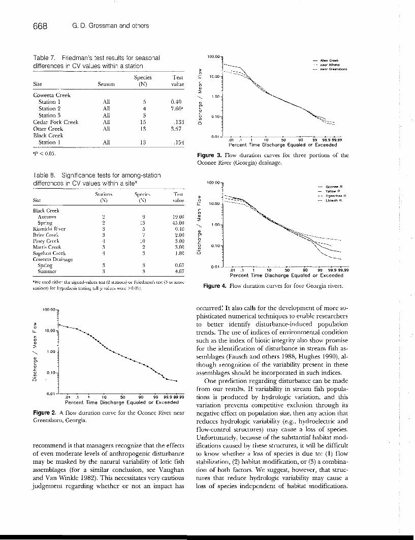
Flow duration curves varied both within and amongdrainage systems. The curves for three locations onthe Oconee River have similar slopes for the range offlows between 50% and 90% exceedence. However,extreme flows for the basins are different. AllenCreek, the smallest basin with a drainage area of 44.8km2, was most variable for high flows but less variablefor low flows. The middle-sized basin, the OconeeRiver near Athens, Georgia, had a drainage area of1030.8 km2. Its extreme flows fell between those ofAllen Creek and the 2823.1-km2 drainage area of theOconee River near Greensboro, Georgia. These flowdifferences are caused by differences in storage ca-pacity of the systems. Headwater streams tend to bemore variable, especially for high flow events, becausethey possess less channel storage. Downstream gaugesalso usually display less variability because they inte-grate different headwater subwatersheds.

Curves for four different rivers in Georgia illustratethe differences one can expect among systems. Allfour streams have drainage areas around 1036 km2.The Etowah River is in the Mountain province, theYellow River and Oconee River are in the Piedmontprovince, and the Ogeechee River is substantially inthe Coastal Plain province. Flow duration curves forthese streams do not have the same slope between the50% and 90% exceedence values. The Etowah Riverand Oconee River are flatter than the other two.Overall, there are more differences among rivers inlow flows than in high flows.

Discussion

Our findings suggest that many stream fish assem-blages are composed of species that vary substantiallyin population size (i.e., CV values for all four data setsaveraged over 96%). In addition, rare species did notfluctuate more than abundant species because: (1)mean CV values were virtually identical for low andhigh data sets, and (2) mean abundance did not signif-icandy affect CV values. Finally, sampling error prob-ably did not produce the high CV values observed, be-

Stream Fish Assemblage Stability 667

Table 4. Coefficient of variation of population size estimates for all population segments and for adults only, forstation 1, Coweeta Creek, North Carolina3

Spring

Species

Co. bairdiRh. cataractaeCl. funduloidesOn. mykissCa. oligolepis

All

236247

100117

Adultsonly

166747

148117

Summer

All

34816065

b

Adultsonly

338460

105b

Autumn

All

1737

1257768

Adultsonly

1749

125b68

"There were no significant differences in CV estimates for all versus adults only comparisons ((test for paired samples, on each set of seasonaldata).bAbsem.

Table 5. Estimates of coefficient of variation of population size for species present in a site duringmultiple seasons3

Site

Cowetea CreekStation 1

Cedar Fork CreekOtter CreekBlack Creek

Station 1Station 2

Seasons

Spring vs autumnSpring vs autumnSpring vs autumn

Spring vs autumnSpring vs autumn

Species(N)

61513

1310

T

8.065.044.0

38.021.5

aH0: CV estimates do not differ by season. None of the test values are significant at the 0.05 level (signed ranks test).

Table 6. Significance tests for the effects of numbers of samples, mean interval (years) between samples, meanabundance, region, and family, on CV estimates3

Data set

All-High

All-LowSummer-HighSummer-Low

Numberof samples

(F)

3.15

-0.16-0.25-0.83

Meaninterval

(F)

3.05

2.772.942.39

Meanabundance

(F)

1.21

1.662.40b

1.27

F

4.24C

1.931.223.04d

Region

Pairwisedifferences

south, southeast,< north

north, southwest, west> southeast

Family(F)

1.19

1.361.150.91

"Results are for F tests and Tukey-Kramer a posteriori tests. None of the hypothesis tests for differences in mean CV values between Notropis andNon-Notropis cyprinids were significant.b/> = 0.0244. Abundance classes: 11 < 7.CP < 0.005.dP = 0.0194.

cause studies in which different collecting methodswere used (i.e., seining, draining, and electrofishing)generally did not exhibit significant differences in CVvalues (i.e., midwestern, northern, and southernversus western and southwestern). These results sup-port the findings of Grossman and others (1982). Al-though we would not postulate that these systems areorganized solely by stochastic mechanisms (Grossman

and others 1982), the application of equilibrium-basedmodels to these assemblages may be inappropriate.

The high variability present in stream fish assem-blages poses a significant problem for resource man-agers. First, this variability may make the detection ofmany anthropogenic disturbance difficult. We are notsuggesting that managers take a passive role with re-spect to this problem; quite the contrary. What we do

668 G. D. Grossman and others

Table 7. Friedman's test results for seasonaldifferences in CV values within a station

Site

Coweeta CreekStation 1Station 2Station 3

Cedar Fork CreekOtter CreekBlack Creek

Station 1

Season

AllAllAllAllAll

All

Species(N)

543

1513

13

Testvalue

0.407.60a

.1333.57

.154

"P < 0.05.

Table 8. Significance tests for among-stationdifferences in CV values within a site3

Site

Black CreekAutumnSpring

Kiamichi RiverBrier CreekPiney CreekMartis CreekSagehen CreekCoweeta Drainage

SpringSummer

Stations(N)

2933434

33

Species(N)

91357

1023

33

Testvalue

19.0045.00

0.402.003.003.001.80

0.674.67

— Allen Creek- - near Athens

.01 .1 1 10 50 90 99 99.999.99Percent Time Discharge Equaled or Exceeded

Figure 3. Flow duration curves for three portions of theOconee River (Georgia) drainage.

1.00-;

Oconee R.— Yellow R.-- Oqeechee R.--- Etowoh R.

>0.05).

.01 .1 1 10 5O 90 99 99.9 99.99Percent Time Discharge Equaled or Exceeded

Figure 4. Flow duration curves for four Georgia rivers.

.01 .1 1 10 50 90 99 99.999.99Percent Time Discharge Equaled or Exceeded

Figure 2. A flow duration curve for the Oconee River nearGreensboro, Georgia.

recommend is that managers recognize that the effectsof even moderate levels of anthropogenic disturbancemay be masked by the natural variability of lotic fishassemblages (for a similar conclusion, see Vaughanand Van Winkle 1982). This necessitates very cautiousjudgement regarding whether or not an impact has

occurred! It also calls for the development of more so-phisticated numerical techniques to enable researchersto better identify disturbance-induced populationtrends. The use of indices of environmental conditionsuch as the index of biotic integrity also show promisefor the identification of disturbance in stream fish as-semblages (Fausch and others 1988, Hughes 1990), al-though recognition of the variability present in theseassemblages should be incorporated in such indices.

One prediction regarding disturbance can be madefrom our results. If variability in stream fish popula-tions is produced by hydrologic variation, and thisvariation prevents competitive exclusion through itsnegative effect on population size, then any action thatreduces hydrologic variability (e.g., hydroelectric andflow-control structures) may cause a loss of species.Unfortunately, because of the substantial habitat mod-ifications caused by these structures, it will be difficultto know whether a loss of species is due to: (1) flowstabilization, (2) habitat modification, or (3) a combina-tion of both factors. We suggest, however, that struc-tures that reduce hydrologic variability may cause aloss of species independent of habitat modifications.

Stream Fish Assemblage Stability 669

Although flow duration curves may aid us in identi-fying systems in which flow stabilization potentiallymay have strong physical or biological effects, the pre-cise relationship between these curves and populationvariability or species richness of fish assemblages is notwell known.

Connell and Sousa (1983) proposed that the stan-dard deviation of the logarithms (base 10) of sequen-tial censuses be used as an estimator of population sta-bility. They recognized that the CV of population sizecould be used for this purpose, but stated that it wassensitive to high values (Connell and Sousa 1983, p.800). Connell and Sousa (1983) noted that their indexwas sensitive to low values, but because they "weremore interested in population variation at lownumbers," they did not use the CV. Nevertheless, webelieve that CV values are a more relevant estimator ofpopulation stability for the following reasons. First,CVs express the standard deviation as a percentage ofthe mean: the type of variability most relative to a pop-ulation stability study. Connell and Sousa (1983) at-tempt to remove the effects of differential mean abun-dances by using logarithms as a scaling factor. Al-though this technique collapses the variabilityobserved, it does not scale variability by the originalmean abundance. This has important consequencesfor the measurement of population variability (Table9). Species of low abundance that also have standarddeviations greater than the mean may obtain lowvalues for Connell and Sousa's index (e.g., Table 9,Oncorhynchus mykiss). This cannot happen with CV esti-mates. Although a more complete analysis of the be-havior of these two estimators is in progress(Grossman, unpublished data), we suggest that exami-nation of assemblage members' CV values better rep-resent the parameter of interest in a population and/orassemblage stability study.

Second, because CV estimates are calculated by di-viding the standard deviation of population estimatesby mean abundance, their interpretation is simple andunambiguous. A CV value of 50% means that thestandard deviation is one-half the mean abundance. Incontrast, the interpretation of the standard deviationof the logarithms of sequential censuses is less clear. Infact, because of the use of logarithms, population vari-ability estimates are compressed, even though they arethe parameter of interest.

Although we prefer CV values over W for tests ofpopulation and/or assemblage stability, this techniqueis not without error. First, because CV values areratios, they may possess unusual distributional proper-ties, especially if the variance is correlated with themean. Neither of these problems influenced our dataset (e.g., Figure 1, Table 8), but they could affect

others. Second, by decomposing an assemblage into itscomponent populations, we are no longer examining"assemblage level" behavior. Third, the classificationsystem proposed for CV values does not have a stronga priori foundation. Fourth, CV values cannot distin-guish between sampling variability and actual popula-tion variability. Fifth, CV values cannot detect time-de-pendent trends in population variation (i.e., long-termincreases or decreases or cyclical fluctuations) or cor-related trends among assemblage members. Despitethese problems, most of which are shared by W (i.e., 3,4, and 5), we still believe that CV values are a valuabletool for quantifying assemblage stability. In addition,some of these limitations (i.e., 1 and 5) can be ad-dressed by examination of the abundance data uponwhich CV estimates are based. Finally, the use of simi-larity indices also shows promise for tests of assem-blage stability (see Matthews and others 1988); how-ever, their behavior must be investigated better beforewe can evaluate their efficacy.

We did not restrict our analyses to censuses taken atfrequencies representing at least one turnover of theassemblage, as suggested by Connell and Sousa (1983).We also did not heed our own criteria and directly ex-amine population age structures, because, with oneexception (Coweeta drainage), these data were notavailable. We did find, however, that increasing thetime interval between censuses did not significantly af-fect CV estimates.

Our analyses indicate that familial classification didnot have a strong effect on CVs. Centrarchid specieswere just as variable as cyprinids and percids. Al-though more data are needed to examine the gener-ality of this finding, our data base does include esti-mates from a variety of regions. Geographical analysesshowed that CV estimates varied significantly amongregions for All-High and Summer-Low data sets.These findings must be viewed as tentative, becausesome regions were represented by only one (i.e., southand southeast) or two (western and northern) streams.In fact, Coweeta Creek, the sole southeastern stream,is a southern Appalachian trout stream. It is certainlynot representative of the majority of lotic systems inthe region (i.e., Piedmont and Coastal Plain systems).

Although our data indicate that stream fish popula-tions are quite variable, we will not propose an organi-zational mechanism for these systems. Like Meffe andBerra (1988), we believe that more detailed environ-mental data are necessary for causal inferences re-garding the factors determining population levels andvariability. It is clear, however, that the assemblagesexamined here are probably not in equilibrium. In ad-dition, species within a given system may respond tobiological and physicochemical variation in a species-

670 G. D. Grossman and others

Table 9. Comparison of population variability estimtes made using CV of population size and standard deviationof the logarithms (base 10) of sequential censuses (Connell and Sousa 1983)a

Species

Calostomus tahoensisCoitus bairdiSalmo truttaRhinichthys osculusRhinichthys cataractaeOncorhynchus rnykissClinostomus funduloides

Abundance(X ± 1 SD)

245a ± 39354 ± 1124 ± 2922 ± 4217 ± 48 ± 97 ± 4

CV

16020

12319124

11149

Standard deviationof log (n + 1)

0.660.080.760.750.100.430.17

"Data rounded to the nearest individual, fractional values to ±0.1 were included in calculations.

specific manner (Mills and Mann 1985, Schlosser1985, Freeman and others 1988). The elucidation ofthese mechanistic responses should yield insights intothe maintenance of assemblage structure in streamfishes.

In conclusion, in contrast to other authors (Herbold1984, Yant and others 1984, Matthews 1986, Ross andothers 1987, Matthew and others 1988), we suggestthat populations comprising stream fish assemblagesvary substantially. Our purpose here is not to criticizethe conclusions of earlier investigators but to identifyhow different analytical techniques may yield differingconclusions. These conclusions also may strongly af-fect how resource professionals manage lotic systems.For example, we would urge resource managers to becautious with respect to the evaluation of anthropo-genic impacts on stream systems, because even sub-stantial impacts may be difficult to detect. A similarcaveat applies to the detection of recovery in damagedstreams. Mitigation effects should not be halted untilmean abundances and variability approximate predis-turbance levels. Of course this requires data on predis-turbance population dynamics, data which are lackingnot only for individual streams (but see Erman 1973,1986) but also for entire geographical regions. Conse-quendy, we would urge management agencies to un-dertake more long-term studies of stream fish assem-blages in undisturbed watersheds to provide a bench-mark against which disturbed systems can becompared.

Acknowledgments

We gratefully acknowledge T. Berra, D. Erman, W.Matthews, G. Meffe, P. Moyle, S. Ross, and J. Whi-taker, Jr., for providing access to their data sets onstream fishes, and R. Ratajczak for data analysis. Thismanuscript benefited from the comments of several ofthe aforementioned investigators as well as those of L.Barnthouse, J. Barrett, V. Boule, M. Freeman, P.Harper, J. Hill, H. Li, G. Niemi, D. Stouder, and D.

Yount. We also appreciate the patience and support ofB. Dowd and B. Mullen. Finally, we thank the Envi-ronmental Protection Agency and the Natural Re-sources Research Institute, University of Minnesota,for inviting us to participate in the Lode EcosystemsRecovery Workshop. Portions of this work were sup-ported by Mclntire-Stennis grant GEO-0035-MS tothe senior author.

Literature Cited

Cairns, J., Jr. 1990. Theoretical basis for predicting rate andpathways of recovery. Environmental Management 14:517-526.

Connell, J. H., and W. P. Sousa. 1983. On the evidenceneeded to judge ecological stability or persistence. AmericanNaturalist 121:789-824.

Davis, N., and G. R. van Blaricom. 1978. Spatial and tem-poral heterogeneity in a sand bottom epifaunal communityof invertebrates in shallow water. Limnology and Oceanog-raphy 23:417-427.

DeAngelis, D. L., and J. C. Waterhouse. 1987. Equilibriumand nonequilibrium concepts in ecological models. Ecolog-ical Monographs 57:1-21.

Erman, D. C. 1973. Upstream changes in fish populationsfollowing impoundment of Sagehen Creek, California.Transactions of the American Fisheries Society 102:626—629.

Erman, D. C. 1986. Long-term structure of fish populationsin Sagehen Creek, California. Transactions of the AmericanFisheries Society 115:682-692.

Fausch, K. D., J. R. Karr, and P. R. Yant. 1984. Regional ap-plication of an index of biotic integrity based on stream fishcommunities. Transactions of the American Fisheries Society113:39-55.

Frank, P. 1968. Life histories and community stability. Ecology49:355-357.

Freeman, M. C., M. K. Crawford, J. C. Barrett, D. E. Facey,M. G. Flood,]. Hill, D.J. Stouder, and G. D. Grossman.1988. Fish assemblage stability in a Southern Appalachianstream. Canadian Journal of Fisheries Aquatic Sciences45:1949-1958.

Card, R., and G. A. Flittner. 1974. Distribution and abun-dance of fishes in Sagehen Creek, California. Journal ofWildlife Management 38:347-358.

Stream Fish Assemblage Stability 671

Grossman, G. D. 1982. Dynamics and organization of a rockyintertidal fish assemblage: the persistence and resilience oftaxocene structure. American Naturalist 119:611-637.

Grossman, G. D., P. B. Moyle, and J. O. Whitaker, Jr. 1982.Stochasticity in structural and functional characteristics ofan Indiana stream fish assemblage: a test of communitytheory. American Naturalist 120:423-453.

Grossman, G. D., P. B. Moyle, and J. O. Whitaker, Jr. 1985.Stochasticity in structural and assemblage organization inan Indiana stream fish assemblage. American Naturalist126:275-285.

Harrell, H. L. 1978. Responses of the Devil's River (Texas)fish community to flooding. Copeia 1978:60—68.

Harrell, R. C., B.J. Davis, and T. C. Dorris. 1967. Streamorder and species diversity of fishes in an intermittentstream. American Midland Naturalist 78:428—436.

Herbold, B. 1984. Structure of an Indiana stream fish associ-ation: choosing an appropriate model. American Naturalist124:561-572.

Hughes, R. M. 1990. Use of ecoregions to develop biologicalcriteria for assessing recovery of aquatic ecosystems. Envi-ronmental Management.

Inman, E. 1971. Flow characteristic of Georgia streams.United States Geologic Survey Open File Report, Atlanta,Georgia. 262 pp.

John, K. R. 1964. Survival of fish in intermittent streams ofthe Chiricahua Mountains, Arizona. Ecology 45:112-119.

Kelly, J. R., and M. A. Harwell. 1990. Indicators of ecosystemrecovery. Environmenal Management 14:527—546.

Larimore, R. W. 1954. Minnow productivity in a small Illinoisstream. Transactions of the American Fisheries Society 84:110—116.

Larimore, R. W., W. F. Childers, and C. Heckrotte. 1959. De-struction and reestablishment of stream fish and inverte-brates affected by drought. Transactions of tlie American Fish-eries Society 88:261-285.

Lowe, C. H., D. S. Hinds, and E. A. Halpern. 1967. Experi-mental catastrophic selection and tolerances to low oxygenconcentration in native Arizona freshwater fishes. Ecology48:1013-1017.

MacArthur, R. 1972. Geographical ecology. Harper andRow, New York. 269 pp.

Matthews, W.J. 1986. Fish faunal structure in an Ozarkstream: stability persistence and a catastrophic flood. Co-peia 1986:388-397.

Matthews, W. J., R. C. Cashner, and F. P. Gelwick. 1988. Sta-bility and persistence of fish faunas and assemblages inthree mid-western streams. Copeia 1988:947-957.

Meffe, G. K., and W. L. Minckley. 1987. Persistence and sta-bility of fish and invertebrate assemblages in a repeatedlydisturbed Sonoran desert stream. American Midland Natu-ralist 117:177-191.

Meefe, G. K., and T. M. Berra. 1988. Temporal character-istics of fish assemblage structure in an Ohio stream. Copeia1988:684-690.

Metcalf, A. L. 1959. Fishes of Chautauqua, Cowley and Elkcounties, Kansas. University of Kansas Publications, Museum ofNatural History 11:345-400.

Mills, C. A., and R. H. Mann. 1985. Environmentally-in-

duced fluctuations in year-class strength and their implica-tions for management. Journal of Fish Biology 27(supplA):209-226.

Moyle, P. B., and H. W. Li. 1979. Community ecology andpredator-prey relations in warm water streams. Pages171-180 in H. Clepper; (ed.), Predator-prey systems infisheries management. Sport Fishing Institute, Wash-ington, DC.

Moyle, P. B., and B. Vondracek. 1985. Persistence and struc-ture of the fish assemblage in a small California stream.Ecology 66:1-13.

Paloumupis, A. A. 1958. Responses of some minnows toflood and drought conditions in an intermittent stream.Iowa State Journal of Science 32:547-561.

Rahel, F.J., J. D. Lyons, and P. A. Cochran. 1984. Stochasticor deterministic regulation of assemblage structure? It maydepend on how the assemblage is defined. American Natu-ralist 124:583-589.

Resh, V. H., A. V. Brown, A. P. Covich, M. E. Gurtz, H. W.Li, G. W. Minshall, S. R. Reice, A. L. Sheldon, J. B. Wal-lace, and R. Wissmar. 1988. The role of disturbance instream ecology. Journal of ttie North American BenthologicalSociety 7:433-455.

Rinne, J. N. 1975. Changes in minnow populations in a smalldesert stream resulting from naturally and artificially in-duced factors. Southwestern Naturalist 20:185—198.

Ross, S. T., W.J. Matthews, and A. A. Echelle. 1985. Persis-tence of stream fish assemblages: effects of environmentalchange. American Naturalist 126:24-40.

Ross, S. T., J. A. Baker, and K. E. Clark. 1987. Microhabitatpartitioning of Southeastern stream fishes: temporal andspatial predictability. Pages 42-51 in W.J. Matthews andD. C. Heins (eds.), Community and evolutionary ecology ofNorth American Stream fishes. University of Oklahoma,Norman, Oklahoma. 310 pp.

Schlosser, I.J. 1985. Flow regime, juvenile abundance, andthe assemblage structure of stream fishes. Ecology66:1484-1490.

Searcy, J. K. 1959. Flow duration curves. United States Geo-logic Survey Water Supply Paper 1542-A.

Sedell, J., R. Hauer, C. P. Hawkins, and J. Stamford. 1990.The role of refugia in recovery from disturbance: modernfragmented and disconnected river systems. EnvironmentalManagement 14:711-724.

Starrett, W. C. 1951. Some factors affecting the abundance ofminnows in the Des Moines River, Iowa. Ecology 32:13-27.

Vaughan, D. S., and W. Van Winkle. 1982. Corrected anal-ysis of the ability to detect reductions in year-class strengthof the Hudson River white perch (Morone americana) popu-lation. Canadian Journal of Fisheries and Aquatic Sciences39:782-785.

Warner, R. R., and P. L. Chesson. 1985. Coexistence me-diated by recruitment fluctuation a field guide to thestorage effect. American Naturalist 125:769-787.

Yant, P. R., J. A. Karr, and P. L. Angermeier. 1984. Stochas-ticity in stream fish communities: an alternative explana-tion. American Naturalist 124:573-582.

Yount, J. D., and G. J. Niemi. 1990. Recovery of lotic com-munities and ecosystems from disturbance—a narrativereview of case studies. Environmental Management 14:547—570.