Eco-efficiency and eco-productivity change over time in a multisectoral economic system
Upload
khangminh22Category
view
0download
0
UNIVERSITY OF GHANA
ECO-FUNCTIONAL BENTHIC BIODIVERSITY ASSEMBLAGE
PATTERNS IN THE GUINEA CURRENT LARGE MARINE
ECOSYSTEM
A THESIS SUBMITTED TO THE DEPARTMENT OF MARINE & FISHERIES SCIENCES FOR THE DEGREE OF DOCTOR OF PHILOSOPHY
BY
EMMANUEL LAMPTEY (10074462)
IN PARTIAL FULFILLMENT OF THE REQUIREMENTS FOR THE AWARD OF
A
PhD. OCEANOGRAPHY
DECEMBER, 2015
University of Ghana http://ugspace.ug.edu.gh
i
DECLARATION
This PhD thesis is original and independent research work conducted under
supervision of Dr. George Wiafe, Prof. Elvis Nyarko and Mr. A.K. Armah of the
Department of Marine and Fisheries Sciences. This research has not been included in
any thesis or dissertation submitted to other institution for a degree, or any other
qualifications. Authors whose works were used have been duly
referenced/recognised.
…………………………
Emmanuel Lamptey
(PhD Student)
……………………..……
Dr. G. Wiafe
(Principal Supervisor)
.....……………………… …………………………
Prof. Elvis Nyarko Mr. A.K. Armah
(Supervisor) (Supervisor)
University of Ghana http://ugspace.ug.edu.gh

ii
DEDICATION
I dedicate this piece of work to God Almighty and my family.
University of Ghana http://ugspace.ug.edu.gh

iii
ACKNOWLEDGMENT
I greatly would like to acknowledge my supervisors, Dr. George Wiafe, Prof. Elvis
Nyarko and Mr. A.K. Armah for their immense contribution and support towards the
thesis final milestone. I would like to acknowledge the support from my host
institution, University of Ghana for some financial support; the Department of
Marine & Fisheries Sciences, University of Ghana, for providing me with office and
laboratory space. My profound gratitude goes to the Guinea Current Large Marine
Ecosystem Programme for the opportunity to be onboard the RV Dr. Fritdjorf
Nansen to collect samples; and also to ESL consulting for the opportunity offered me
to on board the RV GeoExplorer to collect the epibenthic fauna samples during the
West Africa Gas Pipeline Project.
I owe a great deal of gratitude to my family for all manner of immeasurable support.
Further, to my friends, colleagues, former students, staff and students of Department
of Marine and Fisheries Sciences, I would like to express my heartfelt appreciation
for the diverse support and encouragements.
University of Ghana http://ugspace.ug.edu.gh
iv
TABLE OF CONTENTS
Page ABSTRACT…………………………………………………………………………1
CHAPTER ONE
1.0 GENERAL INTRODUCTION ........................................................................ 4
1.1 Study Objectives and Hypothesis ................................................................... 12
1.2 Study Justification .......................................................................................... 13
1.3 Datasets for the Thesis ................................................................................... 15 1.4 Organization of Thesis ................................................................................... 15
CHAPTER TWO
2.0 LITERATURE REVIEW ............................................................................... 17
2.1 Marine Benthic Biodiversity ......................................................................... 17
2.2 Functional Role of Benthic Communities ...................................................... 20
2.3 Biodiversity Indices and Measurements ........................................................ 23
2.3.1 Diversity Indices ................................................................................ 26
2.3.2 Functional Diversity ........................................................................... 28
2.3.3 Functional Diversity Indices .............................................................. 32
2.3.4 Functional Trait Analysis ................................................................... 37
2.4 Disturbance of Marine Biodiversity ............................................................... 40
2.5 Environmental Drivers of Marine Benthic Diversity ..................................... 46
2.5.1 Spatial and Temporal Patterns of Environmental Drivers ................. 50
2.5.2 Water Depth ....................................................................................... 53
2.5.3 Substrate Types .................................................................................. 54
University of Ghana http://ugspace.ug.edu.gh
v
2.5.4 Primary Productivity .......................................................................... 57
2.5.5 Organic Carbon .................................................................................. 58
2.5.6 General Oceanography ....................................................................... 63
2.5.7 The Guinea Current Ecosystem ......................................................... 64
CHAPTER THREE
3.0 MACROBENTHIC FUNCTIONAL TRAIT DIVERSITY AND
COMMUNITY STRUCTURE ALONG ENVIRONMENTAL GRADIENT .......... 70
3.1 Introduction ................................................................................................... 70
3.2 Materials and Methods .................................................................................. 76
3.2.1 Study Area ...................................................................................................... 76
3.2.2 Field Sampling ................................................................................... 76
3.2.3 Field Quality Control ......................................................................... 78
3.2.4 Laboratory Processing of Samples ..................................................... 79
3.2.4.1 Taxonomic Identification ........................................... 80
3.2.4.2 Laboratory Analysis of Abiotic Data ......................... 81
3.2.4.3 Analysis of Physical Parameters ................................ 81
3.2.4.4 Chemical Analysis ..................................................... 82
3.2.5 Functional Trait Analysis ................................................................... 84
3.2.5.1 Ecological and Biological Traits ................................ 87
3.2.5.2 Functional Trait Classification and Categorization .... 87
3.3 Statistical Analysis ........................................................................................ 89
3.4 Results ............................................................................................................ 94
3.4.1 Macrobenthic Fauna Community Structure ....................................... 94
3.4.2 Macrobenthic Faunistic Density ........................................................ 98
University of Ghana http://ugspace.ug.edu.gh
vi
3.4.3 Dominant Macrobenthic Taxa .......................................................... 100
3.4.4 Spatial Pattern of Sediment Abiotic Variables ................................. 103
3.4.5 Community Structural Analysis ....................................................... 107
3.4.5.1 Community Structure- Environmental Relation ...... 110
3.4.5.2 Functional Trait Richness and Distribution ............. 115
3.4.5.3 Distribution of Most Dominant Functional Traits ... 120
3.4.5.4 Multivariate Structural Analysis of Functional Trai 121
3.4.6 Functional Trait-Environment Interactions ...................................... 123
3.4.6.1 Functional Trait-Environment Model ...................... 126
3.6 Discussion .................................................................................................... 129
3.6.1 Species Composition and Abundance .............................................. 129
3.6.2 Functional Structure and Assemblage Patterns ................................ 131
3.6.3 Functional Trait-Environment Relationship .................................... 134
CHAPTER FOUR
4.0 ...... IMPACT OF DEMERSAL FISH TRAWLING ON THE STRUCTURE AND
FUNCTIONAL ASSEMBLAGES OF EPIBENTHIC FAUNA ALONG
BATHYMETRIC GRADIENT IN THE GUINEA CURRENT ............................. 140
4.1 Introduction .................................................................................................. 140
4.2 Study Objectives .......................................................................................... 144
4.3 Materials and Methods ................................................................................. 145
4.3.1 Study Area ........................................................................................ 145
4.3.2 Field Sampling ................................................................................. 145
4.3.3 Laboratory Processing of Samples ................................................... 147
4.3.4 Statistical Analysis ........................................................................... 151
University of Ghana http://ugspace.ug.edu.gh

vii
4.4 Results .......................................................................................................... 153
4.4.1 Epifauna Composition ...................................................................... 153
4.4.1.1 Comparison of Bathymetric Distribution of Epifauna
and Fish Assemblage Structure ...................................................... 156
4.4.2 Pattern of Major Epifaunal Taxa ...................................................... 159
4.4.3 Species Dominance and Pollution Status ......................................... 166
4.4.4 Epifauna Functional Composition .................................................... 177
4.4.4.1 Functional Group Diversity ...................................... 177
4.5 Discussion .................................................................................................... 181
4.5.1 Functional Group Classification ...................................................... 185
4.5.2 Ecosystem Health and Ecological Status ......................................... 188
CHAPTER FIVE
5.0 GENERAL CONCLUSION AND RECOMMENDATIONS ..................... 190
5.1 Conclusion .................................................................................................... 190
5.2 Recommendations ........................................................................................ 192
REFERENCES ......................................................................................................... 194
APPENDICES .......................................................................................................... 242
University of Ghana http://ugspace.ug.edu.gh

viii
LIST OF TABLES
Table 3.1 Biological traits category...........................................................................86
Table 3.2 Abundance and richness of major macrobenthic faunal groups .................. 95
Table 3.3 Densities (Ind./m2) of major macrobenthic faunal group in the continental
shelves of countries bordering the GCLME. ................................................................ 99
Table 3.4 Frequency of occurrence for 15 numerical dominant macrobenthic fauna.
For brevity only taxa contributing >20% were selected. P=Polychaete,
C=Crustacean, O=’Others’ ......................................................................................... 100
Table 3.5 Average water depths of the sampled GCLME countries.......................104
Table 3.6 Pairwise ANOSIM Analysis ..................................................................... 109
Table 3.7 BIO-ENV results for dominant ‘constant’ species with F>20 .................. 111
Table 3.8 Canonical Correspondence Analysis (CCA) results ................................. 112
Table 3.9 Summary of CCA results .......................................................................... 113
Table 3.10 Step-wise multiple regression model (using the Business Spreadsheet
Excel Software) for taxon assemblages and abiotic nitrates and calcium, p˂0.05 .... 115
University of Ghana http://ugspace.ug.edu.gh
ix
Table 3.11 Percentage Functional trait group richness using the F index described by
Guille 1970: F=pa/P × 100, where: pa, is the number of stations where the funtional
traits occurred and P is the total number of stations, thus classified as: constant
(F>50%), common (10% <F<49%) and rare traits (F<10%). .................................... 116
Table 3.12 Dominant traits with respective percent richness and frequency of
occurrence Dominant traits are highlighted based on trait category’s richness
contribution >4% and F>80% concurrently are highlighted ...................................... 117
Table 3.13 BIO-ENV results for ‘constant’ functional traits .................................... 123
Table 3.14 Results of Redundancy Analysis (RDA) ................................................. 125
Table 3.15 Summary of Redundancy Analysis Results (RDA) ................................ 125
Table 3.16 Step-wise multiple regression model (using the Business Spreadsheet
Excel Software) for dominant functional trait and abiotic variables ......................... 127
Table 3.17 Step-wise multiple regression model for dominant functional trait and
abiotic variables: TOC= total organic carbon ........................................................... 128
Table 4.1 Length of coastline and number of hauls made per sector. ..................... ..147
Table 4.2 Trawl station infromation and trawl distance covered during the West
Africa Pipeline Project baseline studies ..................................................................... 149
University of Ghana http://ugspace.ug.edu.gh

x
Table 4.3 Number of species, abundance and biomass of epibenthic fauna from 18
trawl hauls of the study area in March 2003. The percentage contribution of each
taxa is given in parenthesis ................................................................................... .....155
Table 4.4 Pairwise ANOSIM test of epifaunal abundance and biomass ................... 162
Table 4.5 SIMPER analysis results ..................................................................... ......164
Table 4.6 ABC Analysis result of bottom trawl epibenthic fauna data and pollution
status ..................................................................................................................... ......168
University of Ghana http://ugspace.ug.edu.gh
xi
LIST OF FIGURES
Figure 2.1 Human-induced processes of change from fish to jelly-fish domination
(after Richardson et al., 2009). ..................................................................................... 43
Figure 2.2 Conceptual map of the relationship between drivers of biodiversity in
marine systems and some potential surrogates (after McArthur et al., 2009) ............. 50
Figure 2.3 Guinea Current Ecosystem region (Google Earth Image) ......................... 68
Figure 2.4 Large-scale oceanic circulation in the Atlantic Ocean including the
Guinea Current Ecosystem region ............................................................................... 69
Figure 3.1 Map of the study area showing sampling points ........................................ 77
Figure 3.2 Spatial distribution of major macrobenthic fauna abundance on the
continental shelves of the GCLME countries .............................................................. 96
Figure 3.3 Spatial distribution of number of species (species richness) across
continental shelves of the GCLME countries .............................................................. 97
Figure 3.4 Distribution of abundance of dominant macrobenthic faunal species
across GCLME countries using F-index, F>20 ......................................................... 102
Figure 3.5a Mean Concentrations of nitrate, calcium, organic carbon, sand and clay
contents of the sediments across the GCLME countries ............................................ 105
University of Ghana http://ugspace.ug.edu.gh

xii
Figure 3.5b Mean concentrations of magnessium, sodium, potassium and phosphate
across the GCLME countries ..................................................................................... 106
Figure 3.6 Complete linkage of agglomerative dendrogram of Bray-Curtis similarity
of macrobenthic faunal abundance data for GCLME countries. ................................ 108
Figure 3.7 CCA ordination biplot for taxon-environment relationship .................... 113
Figure 3.8 Group average agglomerative dendrogram of Bray-Curtis similarity of
‘constant’ functional biological traits. ........................................................................ 119
Figure 3.9 Distribution of dominant functional trait richness across the GCLME
countries .................................................................................................................... 120
Figure 3.10 Complete-linkage of agglomerative dendrogram of Bray–Curtis
similarity of GCLME countries based on functional richness data of ‘constant’ trait. 122
Figure 3.11 Reducdancy Analysis (RDA) ordination of functional trait-environment
biplot .......................................................................................................................... 126
Figure 4.1 Map of routes along which bottom trawling was carried out .................. 150
Figure 4.2 Percent distribution of major epibenthic faunal richness (left) and
numerical abundance (right) ..................................................................................... 155
University of Ghana http://ugspace.ug.edu.gh
xiii
Figure 4.3 Bathymetric pattern of mean abundance (±SE) for epifauna and fish from
trawl catches ............................................................................................................... 157
Figure 4.4 Bathymetric pattern of mean biomass(±SE) for epifauna and fish from
trawl catches ............................................................................................................... 157
Figure 4.5 Distribution of Margalef’s species richness index along depth gradient
The error bars indicate 95% confidence interval ....................................................... 158
Figure 4.6 Distribution of Shannon-Wienner diversity index along depth gradient.
The error bars indicate 95% confidence interval ....................................................... 158
Figure 4.7 Mean biomass (±SE) of major epibenthic fauna along the bathymetric
gradient. ...................................................................................................................... 160
Figure 4.8 Mean Abundance (±SE) of major epibenthic fauna along the bathymetric
gradient ....................................................................................................................... 161
Figure 4.9 Non-parametric multidimensional scaling (MDS) of epibenthic faunal
abundance data ........................................................................................................... 163
Figure 4.10 ABC plots for stations T-04 and T-05 based on epibenthic fauna
abundance and biomass data ...................................................................................... 169
University of Ghana http://ugspace.ug.edu.gh
xiv
Figure 4.11 ABC plots for stations T-07 and T-08 based on epibenthic fauna
abundance and biomass data ...................................................................................... 170
Figure 4.12 ABC plots for stations T-10 and T-11 based on epibenthic fauna
abundance and biomass data ...................................................................................... 171
Figure 4.13 ABC plots for stations T-12 and T-13 based on epibenthic fauna
abundance and biomass data ...................................................................................... 172
Figure 4.14 ABC plots for stations T-14 and T-16 based on epibenthic fauna
abundance and biomass data ...................................................................................... 173
Figure 4.15 ABC plots for stations T-17 and T-19 based on epibenthic fauna
abundance and biomass data ...................................................................................... 174
Figure 4.16 ABC plots for stations T-20 and T-22 based on epibenthic fauna
abundance and biomass data ...................................................................................... 175
Figure 4.17 ABC plots for stations T-24 and T-25 based on epibenthic fauna
abundance and biomass data ..................................................................................... 176
Figure 4.18 ABC plots for stations T-26 based on epibenthic fauna abundance and
biomass data ............................................................................................................... 177
University of Ghana http://ugspace.ug.edu.gh
xv
Figure 4.19 Feeding Functional group categories for epibenthic fauna from 18 trawl
haul of Gulf of Guinea ............................................................................................... 178
Figure 4.20 Richness of functional feeding groups across bathymetric gradient ..... 179
Figure 4.21 The proportion of adult relative mobility of epibenthic fauna from 18
trawl hauls in the Gulf of Guinea. .............................................................................. 180
University of Ghana http://ugspace.ug.edu.gh

xvi
LIST OF PLATES
Plate 4.1 Beam trawl gear .......................................................................................... 146
Plate 4.2 Photographs of epibenthic fauna from bottom beam trawl samples. ......... 154
University of Ghana http://ugspace.ug.edu.gh

xvii
LIST OF ABBREVIATIONS AND ACRONYMS
ABC: Abundance-Biomass Comparison
ABC: Abundance Biomass Curve
ANOSIM: Analysis of Similarities
ANOVA: Analysis of Variance
BC: Benguela Current
B-EF: Biodiversity Ecosystem Function
BIO-ENV: Biological and Environment
BN: Benin
BTA: Biological Trait Analysis
CANOCO: Canonical Community Ordination
CBD: Convention on Biological Diversity
CC: Canary Current
CCA: Canonical Correspondence Analysis
CD: Cote D’ivoire
CI: Chlorine Index
CR: Cameroon
DBM: Dendrogram Based Measure
EA: Equatorial Anticyclonic
EAF: Ecosystem Approach to Fisheries
EAM: Ecosystem Approach to Management
EcoQO’s: Ecological Quality Objectives
FAD: Functional Attribute Diversity
FD: Functional Diversity
University of Ghana http://ugspace.ug.edu.gh

xviii
FE: Functional Evenness
FGR: Functional Group Richness
FR: Functional Richness
FS: Functional structure
FWHM: Full Width at Half Maximum
GA: Gabon
GB: Guinea Bissau
GC: Guinea Current
GCE: Guinea Current Ecosystem
GCLME: Guinea Current Large Marine Ecosystem
GH: Ghana
GNP: Gross National Product
GU: Guinea
HCL: Hydro Chloric Acid
HPGe: High Purity Germanium
INAA: Instrumental Neutron Activation Analysis
ITCZ: Intertropical Convergence Zone
KCl: Potassium Chloride
LI: Liberia
MCA: Multi Channel Analyzer
MDS: Multi-dimensional Scaling
MFAD: Modified Functional Attribute Diversity
MLRA: Multiple Linear Regression Analysis
MNSR: Miniature Neutron Source Reactor
NAS: North Atlantic Subtropical
University of Ghana http://ugspace.ug.edu.gh
xix
NEC: North Equatorial Cyclonic
NECC: North Equatorial Counter Current
NG: Nigeria
OC: Organic Carbon
OM: Organic Matter
POC: Particulate Organic Carbon
RDA: Redundancy Analysis
SEC: South Equatorial Cyclone
SECC: South Equatorial Counter Current
SIMPER: Similarity Percentages
SL: Sierra Leone
SOPs: Standard Operation Procedures
SR: Species Richness
STA: Species Trait Analysis
TG: Togo
TG-BN: Togo-Benin
TOC: Total Organic Carbon
TN: Total Nitrogen
University of Ghana http://ugspace.ug.edu.gh

1
ABSTRACT
Functional diversity, an important component of biodiversity, has in recent years
engaged global attention. This is in great part due to the mechanistic understanding
achieved from functional diversity studies in the face of accelerated global
biodiversity changes ascribed primarily to anthropogenic drivers. The exigency of
the situation has stimulated biodiversity-ecosystem functions (B-EF) studies to
elucidate ecosystem processes and services that are at threat notably in the marine
ecosystem. The marine benthos is the largest ecosystem on earth and supports the
highest phylogenetic diversity but has rather witnessed comparatively low attention
in the B-EF studies than the terrestrial counterpart. This thesis is aimed at i)
quantifying benthic functional diversity (using biological trait analysis) and
assemblages along abiotic gradients in the Guinea Current Large Marine Ecosystem
(GCLME); and ii) examining the impact of bottom trawling for demersal fishes on
the functional structure of epibenthic fauna along bathymetric gradients.
In achieving the above-mentioned objectives, epibenthic fauna of bottom trawl
samples were collected from Ghana to western Nigeria‘s continental shelf in 2003.
Further, macrobenthic infauna and abiotic samples were collected from coastal
waters of Guinea Bissau to Gabon in 2007. Each processed dataset was treated as a
stand-alone in the thesis. In decomposing the assemblage patterns, suites of
univariate and multivariate statistics were employed. The results indicated 381
macobenthic species comprising polychaetes (61.15% richness and 55.15%
abundance), crustaceans (18.64% richness and 28.02% abundance), molluscs (9.19%
richness and 2.23% abundance), echinoderms (2.63% richness and 1.84%
abundance) and ‗others‘ (8.39% richness and 12.76% abundance). Functional
diversity analysis indicated spatial differences in eco-functional traits namely small
University of Ghana http://ugspace.ug.edu.gh
2
body size, solitary lifestyle, burrowing and deposit-feeding, and these traits
dominated the assemblage especially from Ghana to Benin. The results suggest that
these areas are potential surrogates of allochthonous organic material possibly
driving pelagic productivity that is translated to the benthos. Significant (p<0.05)
relationship was found between functional traits (also species diversity) and
sediment parameters (i.e., nitrate, calcium, magnesium, organic carbon, silt & clay).
These abiotic variables largely implicate productivity and climate change models as
principal community drivers, and are likely to impact ecosystem functions directly
by altering B-EF relationship. Inferentially, the results indicated an unstable,
dynamic, productive and low biomass-supported ecosystem Guinea Current Large
Marine Ecosystem (GCLME), reflecting in the small body size solitary burrow-
dwelling deposit-feeding organisms, which potentially exert the strongest influence
on ecosystem processes (e.g., nutrient remineralization). These species used multiple
adaptative strategies including trophic, lifestyle, anatomical and morphological in the
prevailing environment.
Bottom trawled epibenthic sample analysis showed significant difference (p=0.002;
ANOSIM) of assemblages along bathymetric gradient, notably between shallow-
depth (11-30m) and deep-depth (51-70m). Functional analyses showed dominance of
carnivores (28% contribution), opportunistic/scavenging (9%) and herbivore (9%) in
shallow waters, while filter-feeders (18%) dominated deep waters suggesting
gradient in structuring forces. The high abundance of motile epibenthic fauna (64%)
is suggestive of an unstable substrate and turbulent system supporting motile
carnivores and filter-feeding organisms. The evidence of trophic interactions
between demersal fishes and epibenthic fauna occurred ideally in most tolerable and
favorable zone (i.e. mid-depth). Abundance-Biomass Comparison (ABC) analyses
University of Ghana http://ugspace.ug.edu.gh

3
indicated an ecosystem which is stressed (66.56%) with the degree of stress
inversely related to increasing water depth. The findings of this thesis have important
implications for marine biodiversity conservation and resource management
approach in the GCLME.
University of Ghana http://ugspace.ug.edu.gh
4
CHAPTER ONE
GENERAL INTRODUCTION
Biodiversity, from genes through species to ecosystems, play an important role in the
evaluation of the resilience of natural systems to environmental changes (Naeem et
al., 1999; Mant et al., 2014). Understanding the patterns and processes of
biodiversity at the primary, secondary and tertiary trophic levels is fundamental to
sustainable management of marine living resources (Sherman and Duda, 1999;
Costello, 2000; Hooper et al., 2005). Biodiversity loss is defined as a sudden change
to natural ecosystem setting due to human interventions. This is because natural
changes of biodiversity are a much slower and longer-term process (Kessler et al.,
2007), which may be reversible. Human activities have contributed to variability in
global climate, land cover and biodiversity at unprecedented rates (Steffen et al.,
2004). Human activities that affect biodiversity are referred to as critical
environmental issues (National Research Council, 1995). The world is facing
accelerated and apparently inevitable loss of species (Pimm et al., 1995) and
populations (Hughes et al., 1997) through anthropogenic impact on the world‘s
ecosystems.
The socioeconomic consequences of global biodiversity changes from critical
environmental issues will depend on how they translate into altered ecosystem
processes and services (Costanza et al., 1997; Balmford et al., 2002; Millennium
Ecosystem Assessment, 2003). Impact of biodiversity loss under economic terms
will mean that humankind will have to technically compensate for the services
ecosystems provide (e.g. CO2/O2 gas regulation, food production, raw material
University of Ghana http://ugspace.ug.edu.gh
5
production, prevention of soil erosion, genetic resources for pharmacy development,
regulation of hydrological flows) (Costanza, et al., 1998; Edwards and Abivardi,
1998). Nonetheless, the ecological impacts of biodiversity loss are poorly understood
(Solan et al., 2004).
Concerns of biodiversity loss are more amplified in the marine ecosystem due to the
uncertainties associated with the effects of the loss on the basic functioning of the
ecosystem and the oceans‘ capacity to withstand multiple human disturbances
(Snelgrove et al., 1997). Available information indicates that the oceans account for
approximately two-thirds of the value of global ecosystem services (Snelgrove,
1999), which is estimated to average $33 trillion US dollars/yr compared to the
Global GNP of $18 trillion/yr (Costanza et al., 1997). As a result, of the ecosystem
services , a large and increasing proportion of the world‘s population lives close to
the coast; thus the loss of services such as flood control and waste detoxification can
have disastrous consequences to coastal dwellers (Danielsen et al., 2005; Adger et
al., 2005). The marine seafloor is the largest ecosystem on earth (Snelgrove et al.,
1997) supporting high phylogenetic diversity (Snelgrove, 1999; Giller et al., 2004)
and key ecosystem services (Bremner, 2008) and as a consequence biodiversity
alterations/changes may have wider ecological and socio-economic implications.
Marine ecosystems provide a wide variety of goods and services, including food
resources for millions of people (Peterson and Lubchenco, 1997; Holmlund and
Hammer, 1999). The maritime domain has also been used by society for different
activities including fishing, aquaculture, shipping, tourism, renewable energies,
extraction of minerals etc. (Borja et al., 2013).
University of Ghana http://ugspace.ug.edu.gh
6
Marine biodiversity alterations at both local and global scales can disrupt the
ecological functions that species assemblages perform (Hughes et al., 2003). These
changes make differentiation between effects of species richness per se, and the
effects of functional group richness (i.e., functional diversity) on ecosystem function
a major issue in ecology (Solan et al., 2004). This is because, although biodiversity
generally enhances many process rates, such as resource use or biomass production,
across a wide spectrum of organisms and ecosystems, the evidence for positive
effects of biodiversity on ecosystem functioning (i.e., ecosystem processes,
properties and their maintenance, (Reiss et al., 2009) is neither ubiquitous nor
unequivocal (Thompson and Starzomski, 2007; Jiang et al., 2008).
Marine benthic faunal diversity, therefore, provides an ideal tool for exploring the
relationship between biodiversity and ecosystem functioning in the marine
environment (Snelgrove, 1999). Ecosystem functioning involves several processes,
which can be summarized as production, consumption and transfer of organic matter
to higher trophic levels, organic matter decomposition, and nutrient regeneration
(Danovaro et al., 2008). According to Jax (2005) ecosystem functioning refers to the
overall performance of ecosystem, and has been variously defined as incorporating,
individually or in combination, ecosystem processes (such as biogeochemical
cycles), properties (e.g. pools of organic matter), goods (food and medicines) and
services (e.g. regulating climate or cleansing air and water) as well as temporal
resistance or resilience of these factors over time in response to disturbance (Biles et
al., 2002; Hooper et al., 2005; Duffy and Stachowicz, 2006).
University of Ghana http://ugspace.ug.edu.gh
7
The assemblage patterns of the marine macrobenthos and associated functional
diversity, and their spatial and temporal variations as well as the drivers of functional
traits remain poorly understood. The importance of the marine macrobenthic
functional diversity includes roles in the structure and functioning of the systems,
particularly their productivity and resilience in the potential human-induced
disturbances/perturbations context (Solan et al., 2006). Essentially, the global
biodiversity concerns, exemplified by the predictions that species loss might impair
the functioning and sustainability of ecosystems (Naeem et al., 1994; Sala et al.,
2000; Loreau et al., 2001; Hooper et al., 2005; Worm et al., 2006;) have stimulated
ecosystem-based and experimental efforts to: i) understand the synergy between
biodiversity and ecosystem functioning, and ii) devise sustainable management
strategies (Levin, 2001).
The apparent failure of diversity conservation tactics (Soulé, 1991; Faith, 2011), and
the need to gain more profound understanding about the factors governing and/or
governed by biodiversity is urgent and crucial. Diversity indices are relevant tools on
which far-reaching decisions are based on in conservation science (Walker and Faith,
1994; Reid et al., 2004). Indices derived from phylogeny play an important role in
this area, where decisions frequently have to be taken on basis of a limited data about
the system in question. Previously, the tendency was to focus on species diversity in
one dimension using a single parameter (e.g., species richness) (Gaston, 2000).
However, current studies employ different descriptors, and example of two of such
descriptors that are improving description and understanding of diversity are
macrophysiology and trait approaches. Macrophysiology describes how
physiological traits are distributed in space (Chown et al., 2004); while
University of Ghana http://ugspace.ug.edu.gh
8
morphological traits enable exploration selection pressures between different species
assemblages (Vermeij, 1978; Ricklefs and Miles, 1994; Roy et al., 2004; McGill et
al., 2006). The functional trait approach is interested in explaining the abundances
and distributions of species (McGill et al., 2006). It advocates for the examination of
numerous functional traits and also species‘ abundance and trait distributions across
environmental gradients (McGill et al., 2006). The goal of the functional trait
approach is to explore how the fundamental niche is determined by physiological
and morphological traits and consequently how organismal traits and the
fundamental niche are related to the realized niche (McGill et al., 2006). A
functional trait is defined as an attribute of an organisms‘ morphology or physiology
that affects fitness indirectly via growth, reproduction and survival (Violle et al.,
2007). A trait-based approach in combination with an understanding of where
species occur in relation to environmental gradients may provide new perspectives to
species diversity; especially because most spatial and temporal patterns of diversity
are based solely on the unit of species richness (Roy et al., 2004).
Morphological traits are useful tools for detecting different selection pressures at
species-rich and species-poor systems (Vermeij, 1978). For example, gastropod shell
armour is more elaborate in species-rich tropical system than in species-poor
temperate rocky intertidal environments (Vermeij, 1978). This relationship infers a
gradient of protection against predation to tropical species (Vermeij, 1978).
Although most diversity measures are likely to correlate with species richness, e.g.
genetic diversity, in some cases the relationship between species richness and the
traits of species can be complex and non-linear (Foote, 1997; Roy and Foote, 1997).
Morphological diversity in most species-rich systems is not higher than in systems
University of Ghana http://ugspace.ug.edu.gh
9
with half the number of species, suggesting that species-poor systems can still harbor
a great variety of morphological trait diversity (Roy et al., 2001). Morphological
traits have also been used to examine differences between species-rich and species-
poor systems (Ricklefs and Miles, 1994). From basic principles, morphological traits
of species in species-rich systems, relative to species-poor systems, could be
expected to display either (a) increased morphological trait variety, i.e., a greater
occupied morphospace, and trait differences between species, (b) minimized trait
differences between species within a larger or similar occupied morphospace as
temperate species or (c) have similar traits, i.e. show morphological overlap, in an
occupied morphospace similar to temperate species (MacArthur, 1972; Ricklefs and
Miles, 1994).
Measures of ecological functioning emphasize the roles played by organisms and
include information on their interactions with their chemical and physical
environment (Bremner, 2005). Measuring changes in the rates of ecological
processes in the presence of anthropogenic impacts will, therefore, incorporate
information on the chemical and biological components of ecosystems (Bremner,
2005). Hence, investigation of ecological functioning focus on the types of taxa
present in marine communities and their responses to anthropogenic impacts. Taxa
interact in various ways with their physical and chemical environment depending on
the characteristics they express, and changes in the occurrence of these taxa have
implications for ecological processes (Bremner, 2005). Organisms sharing particular
characteristics are not always affected in the same way (Ramsay et al., 1996) and as
the methods also do not examine the responses of every taxon expressing a particular
characteristic; it is difficult to determine their general responses. This thus
University of Ghana http://ugspace.ug.edu.gh
10
compromises the ability of the methods to determine anthropogenic effects at the
ecosystem level (Bremner, 2005).
Nonetheless, a promising method for evaluating the ecological functioning of marine
benthic assemblages is the use of biological traits analysis (Bremner; 2005), which
originated from terrestrial and freshwater ecosystems studies (Olff et al., 1994;
Townsend and Hildrew, 1994; McIntyre et al., 1995). Many terrestrial ecosystem
studies have found positive effects of plant diversity on ecosystem processes, but this
pattern has been less general in marine systems, where many studies find weak or no
effects (Stachowicz et al., 2007). The biological trait analysis approach explicitly
incorporates information on the attributes of all members of the species assemblage,
and on a wide range of attributes connected to organisms‘ interactions with each
other and their physical and chemical environments, as well as their perceived
responses to anthropogenic stress (Bremner, 2005). It can also accommodate
intraspecific variation in trait expression (Chevenet et al., 1994); thereby overcoming
the problems encountered in trophic or functional group analyses where taxa fit into
more than one functional category. Characters such as reproduction type, larval type,
body size, movement, body form, growth rate, feeding type, attachment etc. are
substituted for species names and multivariate analyses are conducted (Fleddum,
2010). Ostensibly, several factors influence the number of traits selected for
inclusion in biological trait analysis, such as the length of the taxon list utilized, the
amount of information available on biological characteristics of these taxa and the
time required for gathering the information (Bremner, 2005). The use of the
biological trait analysis (BTA) makes it possible to compare assemblage patterns of
species and traits analyses, and also can reveal relationship of structure and
University of Ghana http://ugspace.ug.edu.gh

11
functional properties (Chevenet et al., 1994; Charvet et al., 2000; Bremner et al.,
2003b). The BTA can better discriminate environmental differences in comparison
with taxonomic composition. The traditional biodiversity data analysis methods tend
to underestimate the importance of rare species although it has provided useful
information of benthic community structure over the years (Bremner, 2005;
Fleddum, 2010). The use of BTA together with traditional biodiversity analysis is
helpful in identifying impact-driven alterations to ecological functioning as well as
providing information for ecosystem monitoring, management and conservation
(Fleddum, 2010). For example, Bremner et al. (2003b) compared traditional analysis
technique using relative taxa composition and trophic guilds with BTA in
investigating the functioning diversity of macrobenthic fauna in the southern North
Sea and eastern English Channel. They concluded that BTA can offer information on
assessing ecosystem functioning in benthic environments on both large and small
scales, and that there is a significant relationship between habitat and traits.
According to Usseglio-Polatera (2000b) the species trait approach has the potential
to evaluate the actual state of ecosystems, discriminate among different types of
human impact, and help to develop monitoring tools for ecological communities.
However, the use of the BTA in the marine benthic ecosystems has received little
attention (Bremner, 2005) and lags behind the freshwater and terrestrial counterparts
(Bremner, 2008). Of much concern is the lack of study in the Guinea Current Large
Marine Ecosystem (GCLME) focusing on functional species assemblages employing
the BTA approach. Where information on general benthic biodiversity in the region
has been carried out, the literature is widely dispersed and inadequate. The GCLME
is one of the productive large marine ecosystems in the world‘s ocean (Ukwe, 2003;
University of Ghana http://ugspace.ug.edu.gh
12
Ukwe et al., 2006). The fishery and the plankton have received some attention
(Bainbrige, 1972; Bakun, 1978; Mensah, 1995; Koranteng, 1998; Wiafe, 2002;
Wiafe 2008). However, very little is known about the dynamics of the macrobenthic
community, especially its functional diversity and community structure. Knowledge
of macrobenthic functional diversity and community structure will contribute
immensely to understanding the overall trophic dynamics, biodiversity and
ecosystem functioning of the GCLME.
1.1 Study Objectives and Hypothesis
The primary aim of this research is to investigate macrobenthic functional traits
diversity and community assemblages along spatial scales in the GCLME. The
research further explored whether environmental gradient, on spatial scale,
correlated with local species diversity and their functional attributes. The study
aimed at testing the hypothesis that the marine benthic functional biodiversity effects
on ecosysem processes/properties were the results of established environment
gradient in the ecosystem . Specifically, the following predictions were tested as part
of the overall hypothesis:
Dominant macrobenthic functional trait assemblages rather than species
richness exert the strongest control on ecosystem properties/process; and
abiotic stressors/drivers/factors select for differences in functional traits and
species assemblages.
In order to evaluate the central predictions of the study hypotheses, the following
objectives were formulated:
Identify and quantify dominant functional traits and elucidate their influence
on ecosystem functions;
University of Ghana http://ugspace.ug.edu.gh

13
Ascertain how macrobenthic faunal communities and eco-functional trait
assemblages are influenced by abiotic factors. This will assist in
understanding and predicting how benthic communities and ecosystem
properties might be affected by environmental variability and disturbance;
Identify dominant epibenthic functional traits across bathymetric gradients;
Investigate the effects of bottom trawling for demersal fishes on species
diversity and functional structure of epibenthic communities; and
Evaluate the ecological quality status of the GCLME using epibenthic
macrofauna species.
1.2 Study Justification
The past several decades have witnessed a soaring research interest on earth‘s
biodiversity across all environments, including studies that assessed trends in
biodiversity and the underlying mechanisms that produced and maintained such
trends. Escalating concerns over the loss of marine biodiversity and associated
consequences have increased the urgency for research for a better mechanistic
understanding.
Many of such studies/research have been carried out in short-term and on local scale
with findings (species diversity and the driven forces) which still limit our
understanding. Nonetheless, a growing body of research has addressed the functional
consequences of diversity for ecosystem processes (Stachowicz et al., 2008). The
primary goals of Biodiversity-Ecosystem functioning research have been to
investigate how biodiversity and ecosystem functioning are linked and to understand
the mechanisms that inform such relationships. In accordance, recent biodiversity
University of Ghana http://ugspace.ug.edu.gh
14
researches have principally focused on important links between number of species
and ecosystem functioning (Hooper et al., 2005; Worm et al., 2006; Solan et al.,
2008, 2009).
Earlier studies on biodiversity-ecosystem functioning tested whether ecosystem
functioning was enhanced in species-rich versus depauperated assemblages
(Srivastava and Vellend, 2005), but was demonstrated that biodiversity generally
enhances many process rates such as resources use or biomass production, across a
wide spectrum of organisms and ecosystems (Balvanera et al., 2006). However, the
evidence for positive effects of biodiversity of ecosystem functioning is neither
ubiquitous nor unequivocal (Thompson and Starzomski, 2007; Jiang et al., 2008),
stimulating conservable scientific debate (Loreau et al., 2002). Following from this,
four research themes namely: functional traits, environmental gradients, interactions
milieu and performance currencies have been suggested (McGill et al., 2006) as a
cornerstone of modern ecology in order to fully understand the biodiversity–
ecosystem functioning.
There have been many studies investigating the relationship between species
diversity, functional diversity and ecosystem function (Petchey and Gaston, 2002;
Petchey and Gaston, 2006; Bremner, 2008). In marine benthic ecosystems, however,
only a few studies have examined that relationship and most of them have shown a
strong correlation between species diversity and functional diversity (Bremner et al.,
2003b; Micheli and Halpern, 2005; Hewitt et al., 2008). Furthermore, there are
studies investigating how biotic and abiotic components affect the temporal and
spatial variability in functional diversity (Emmerson et al., 2001; Raffaelli et al.,
University of Ghana http://ugspace.ug.edu.gh
15
2003; Micheli and Halpern, 2005; Ieno et al., 2006; Bell, 2007; Norling et al., 2007),
but it seems that such processes affect species diversity and functional diversity in a
similar way (Bremner et al., 2003b; Micheli and Halpern, 2005; Hewitt et al., 2008).
1.3 Datasets for the Thesis
The datasets used for this thesis research included the following:
Epibenthic trawl samples collected along the continental shelves of Ghana,
Togo, Benin and western part of Nigeria in 2003 as part of the West Africa
Gas Pipeline Project (WAPCo, 2003). This data was used for the assessment
of the impacts of bottom trawling on epibenthic faunctional assemblage
patterns.
Macrobenthic fauna and sediment samples collected from Guinea Bissau to
Gabon in 2007 as part of the Guinea Current Large Marine Ecosystem
(GCLME) project comprising 16 countries (GCLME, 2006). This data was
used to investigate soft-bottom macrobenthic infauna functional assemblage
patterns and their response to environmental variability.
1.4 Organization of Thesis
The thesis comprises five chapters. Chapter 1 presents a general introduction to the
thesis, with a brief background information on marine biodiversity, functional
diversity, trait analysis, level of macrobenthic information in the GCLME, scientific
hypothesis and study objectives. The various data sets used in the analyses have also
been presented. Chapter 2 presents a detailed review of relevant literature on the
subject, biodiversity structure and functions of macrobenthic communities as well as
environemntal factors influencing benthic biodiversity assemblages. Chapter 3
University of Ghana http://ugspace.ug.edu.gh
16
describes the ‗macrobenthic functional traits diversity and community structure
along environmental gradient. Chapter 4 focuses on impact of demersal fish
trawling on the structure and functional assemblages of epibenthic fauna along
bathymetric gradient. Chapter 5 gives general conclusions and recommendations.
The species list and biological trait database are presented as Appendices I & II.
Appendix III shows the carbon:nitrate ratios and the sources of organic load, while
statistical descriptions are annotated in Appendix IV.
University of Ghana http://ugspace.ug.edu.gh

17
CHAPTER TWO
LITERATURE REVIEW
2.1 Marine Benthic Biodiversity
The idea of biodiversity has taken hold on science and society with its multifaceted
concepts (Zajac, 2008) and has also emerged as a major field within ecological
research. Biodiversity has been variously defined as the variety of life and
collectively referred to variation at all levels of biological organization (Sheppard,
2006). According to Harper and Hawksworth (1994), biodiversity refers to the extent
of genetic, taxonomic and ecological diversity over all spatial and temporal scales.
However, the Convention on Biological Diversity (CBD) gave the most important
and far-reaching definition in its Article 2 to mean ‗the variability among living
organisms from all sources including, inter alia, terrestrial, marine and other
aquatic ecosystems and the ecological complexes of which they are part; this include
diversity within species, between species and of ecosystem‘ (Convention on
Biological Diversity, 1992). In seeking to describe the "variety of life" or "nature,"
biodiversity includes three components of diversity, namely, "within species,"
"between species" and "of ecosystems" (Costello, 2000). The usage of the term is
value laden connoting that biodiversity is per se a good thing, that its loss is bad, and
that something should be done to maintain it.
Diversity is usually designed as being α-diversity (the diversity within a given
habitat), β-diversity (the degree to which communities show spatial variability in
species composition from place to place) and γ-diversity (the overall diversity in a
whole region; (Whittaker, 1975). At the species level in a given assemblage, α-
University of Ghana http://ugspace.ug.edu.gh
18
diversity can be regarded as either the number of species present (―species
richness‖), the proportional abundance or homogeneity of individual species
(―evenness‖ or ―equitability‖) or more commonly a combination of both (Terlizzi
and Schiel, 2009).
The marine benthic biodiversity comprise organisms that span a wide range of sizes,
including micro-, meio-, macro- and megafauna (Clarke and Warwick, 1994;
Dittmann, 1995; Zajac, 2008). These organisms are operationally classified as
microbenthos (< 63 µm), meiobenthos (from 63 µm to 500 µm) and macrobenthos
(> 500 µm or > 1000 µm) according to the sieve mesh size used for extracting them
from sediment cores or grabs. The macrofaunal forms are by far the better known
and are the main essential component of environmental impact studies (Clarke and
Warwick, 1994). Marine macrobenthos are a diverse group of organisms composed
mainly of molluscs (bivalves and snails), polychaetes (bristle worms), crustaceans
(amphipods, shrimps, and crabs) and echinoderms (sea cucumbers, brittle stars, sea
urchins) (Gray, 1981a). These organisms are central elements of marine ecosystems
and provide excellent indicators of environmental health. They also play multiple
ecological roles within the marine ecosystem and are a critical part of environmental
monitoring and evaluation programmes. Most macrobenthic animals are relatively
long lived (several years) and thus integrate changes and fluctuations in the
environment over a longer period of time. Changes in soft bottom zoobenthic
communities in response to the environmental impact have been successfully
implemented world-wide in pollution assessment studies and monitoring programs
(Pearson and Rosenberg, 1978).
University of Ghana http://ugspace.ug.edu.gh
19
Variations in species composition, abundance and biomass can be used to assess
environmental disturbance. Comparatively rich and diverse shallow-water benthic
communities are amenable for more sensitive analyses of eutrophication effects. The
potential benefits of using macro-invertebrates include quick detection of pollution
through differences between predicted and actual faunal assemblages (Ormerod and
Edwards, 1987). Of relative importance, benthic invertebrates are relatively sessile
(therefore allowing spatial patterns to imply causation), can be sampled
quantitatively without high cost, are well described taxonomically, and reveal
ecologically meaningful and important patterns, even at coarse levels of taxonomic
discrimination (Warwick, 1988c). Analysis of differences in macrobenthic
community structure is one of the mainstays of detecting and monitoring the
biological effects of marine pollution and habitat disturbance (Warwick and Clarke,
1993) as well as for ecological modeling (Tumbiolo and Downing, 1994; Josefson
and Rasmussen, 2000).
In most environmental studies of impacts, benthic invertebrates are the principal
targeted organisms (78 percent of all studies), reflecting their suitability as ecological
indicators (Clarke and Warwick, 1994; Peterson and Bishop, 2005). The
macrobenthic infaunal communities are especially suited for long-term comparative
investigations since many of the constituent species are of low mobility, relatively
long lived and integrate effects of environmental changes over time. Consequently,
macrobenthic fauna constitute good biological candidates for monitoring ecosystem
health and processes. Cury and Roy (2002) have stressed that studies that link the
different components of the trophic web or the spatial and temporal dynamics of the
University of Ghana http://ugspace.ug.edu.gh
20
interaction between the environment and marine resources are needed as they have
important implication for managing the resources.
Marine biodiversity is of direct benefit to society as a food source, potential
pharmacopoeia (Hunt and Vincent, 2006), stabilizer of inshore environments (Jie et
al., 2001) and regulator of atmospheric processes (Murphy and Duffus, 1996).
Marine biodiversity provides indirect benefits to society through ecological stability
(Menge et al., 1999) and benthic-pelagic coupling (Ponder et al., 2002) which
contribute to self-sustaining marine ecosystems. Marine biodiversity also has
recreational, aesthetic and intrinsic value (Wilson, 1994; Ponder et al., 2002).
2.2 Functional Role of Benthic Communities
Benthic communities perform numerous ecological functions to the systems they
inhabit. Benthic organisms continually process, transport, and modify marine
sediments. There are those that bind, protect and stabilize near-surface sediment and
those that loose and destabilize the sediment (Nichols and Boon, 1994). They also
play a vital role in organic matter processing and nutrient cycling at the
water/sediment interface (Aller and Yingst, 1985; Rosenberg, 2001) and
decomposition of dead matter or waste materials (Snelgrove et al., 1997). Sediment
organic matter is a causal factor of infaunal distribution (Snelgrove and Butman,
1994) being the dominant source of food for deposit-feeders (Pearson and
Rosenberg, 1978), and indirectly (e.g., through re-suspension) for suspension feeders
(Snelgrove and Butman, 1994). Benthic organisms also improve the conditions
within the sediment, such as oxygenation (Reise, 1985) and loosen subsurface
sediments and render them inhabitable by other macrofauna (Flint and Kalke, 1986).
University of Ghana http://ugspace.ug.edu.gh

21
Benthic invertebrate assemblages are heavily involved in the regulation of ecosystem
processes (Snelgrove, 1998), so provide a useful study unit. Functioning in these
assemblages will be dependent on the biological characteristics, or traits, exhibited
by constituent species, because these determine how the species contribute to
ecological processes.
Woodin and Jackson (1979) have proposed five functional groups of benthic
organisms in relation to their effects on the sediment: (i) mobile burrowers that
destabilize the sediment (including their feeding activity) such as crustaceans,
amphipods & tanaids, and Maldanid polychaetes; (ii) sedentary organisms that cause
the sediment to be more easily resuspended (e.g., infaunal holothurian, Molpadia
oolitica, Crustacean Callianassa ); (iii) sedentary organisms that do not inhabit tubes
that still straddle the sediment-water interface and modify the local hydrography
such as to reduce re-suspension and, by virtue of buried parts, bind the subsurface
particles together (e.g., seagrasses such Thalassia & Zostera, Sabelid polychaete
worms); (iv) tube builders that stabilize the sediment by incorporating it, often in
mucus-bound form into their tubes (e.g., mud snail Illyanasa obsolete, polychaete
Polydora); and (v) neutral species having no impact on sediment deposition or re-
suspension. The feeding type of the benthic community is considered as an
adaptation to the sediment characteristics (Rosenberg, 1995).
However, it has been suggested that animal and sediment correlation is a result of
hydrological and geological processes associated with sediment granulometry rather
than a function of organism in available space within sediment (Parry et al., 1999).
For macro-invertebrates, the requirements of life in unconsolidated sediments
University of Ghana http://ugspace.ug.edu.gh
22
inevitably involve the need to move particles around in some way, whether as a
consequence of locomotion through the sediments, or feeding upon the organic
material associated with them. This is known as bio-turbation (Hall, 1994). Bio-
turbation occurring in sediments regulates carbon degradation and bentho-pelagic
nitrogen cycling (Biles et al., 2002; Widdicombe et al., 2004).
Benthic species also affect the microbial processes in the sediments by modifying
particle distribution, sediment porosity, and solute transport (Krantzberg, 1985). Bio-
turbation of sediments by burrowing or deposit-feeders through processes such as
irrigation, pelletization and tube construction, usually increases sediment pore space
and thus, water content in the upper sediment layer (Rhoads, 1974; Rhoads and
Young, 1970). Bio-turbation lowers erosion resistance of the surface, and thus
destabilizes the bed sediment. Bio-turbation can be important in excluding particles
and pore water nutrients across the sediment-water interface as well as through
various vertical chemical gradients in the sediment (Nichols and Boon, 1994).
The impacts of invertebrates on biogeochemical processes are often due to biogenic
structure in marine sediments (Aller and Aller, 1986, Kristensen et al., 1991; Mayer
et al., 1995; François et al., 1997) and infaunal activity (Holst and Grunwald, 2001).
Biogenic structures can modify organic matter distribution and solute transport at the
water-sediment interface (Krantzberg 1985, de Vaugelas and Buscail, 1990). Solute
transport is enhanced by animal movement and burrow ventilation, which is a
process known as bio-irrigation (Riisgärd and Banta, 1998). Bioturbation (i.e.,
sediment biogenic activities) does not only play a crucial role in the stabilization of
marine benthic environments (Woodin and Jackson, 1979; Kristensen et al., 1985)
University of Ghana http://ugspace.ug.edu.gh
23
but, also in recycling of nutrients that enhance ocean productivity. Oceanic
productivity is related to abundance of commercially important species such as
fishes thereby depicting a coupling between benthic biodiversity (functional effects)
and fisheries (Hodson et al., 1981; Bell and Woodin, 1984; Josefson and Rasmussen,
2000) through primary production (Kjerve, 1994).
The health of marine ecosystems is often assessed in terms of the taxon composition
of faunal communities, or on the distribution of abundance/biomass between the
species present (e.g., Warwick and Clarke, 1991; Bonsdorff and Blomqvist, 1993).
Marine macrobenthic fauna are used in pollution and ecosystem health monitoring
studies to ascertain pollution effects on the ecosystem (Sherman and Anderson,
2002). Potential benefits of research on macro-invertebrates include quick
assessment of biological resources for conservation purposes and the detection of
pollution through differences between predicted and actual faunal assemblages
(Ormerod and Edwards, 1987). Macrobenthic communities have the capabilities to
integrate into their system both short-, and long-term environmental changes and
thus are excellent candidates for monitoring environmental impacts (Borja et al.,
2000). Snelgrove (1998) reported that the roles performed by benthic species are
important in regulating ecosystem processes and that these roles can be portrayed by
biological traits they exhibit.
2.3 Biodiversity Indices and Measurements
Measurements of biodiversity are often used as bases for making decisions on
planning and conservation actions. In conservation, diversity indices become mighty
tools on which far-reaching decisions are based on (Walker and Faith 1994; Reid et
University of Ghana http://ugspace.ug.edu.gh
24
al., 2004). It is evident from the biodiversity definition that there could be no clear
single all-embracing measure of biological diversity owing to its great complexity.
The breadth of ways in which differences can be expressed is infinite. The most
practical and relevant measures of biodiversity within species are the phenotypic or
visible attributes of populations. Nevertheless, measurements of biodiversity are
based on three assumptions (http://www.coastalwiki.org):
All species are equal in abundance: meaning that richness measurement makes
no distinctions amongst species and treats the species that are exceptionally
abundant in the same way as those that are extremely rare species. The relative
abundance of species in an assemblage is the only factor that determines its
importance in a diversity measure.
All individuals are equal in size: this means that there is no distinction between
the largest and the smallest individual; in practice however the smallest animals
can often escape for example by sampling with nets. Taxonomic and functional
diversity measures, however, do not necessarily treat all species and individuals
as equal.
Species abundance has been recorded in using appropriate and comparable
units. It is clearly unwise to use different types of abundance measure, such
as the number of individuals and the biomass, in the same investigation.
Diversity estimates based on different units are not directly comparable.
Biodiversity has many facets, yet three generally different concepts in its
quantification can be distinguished (Purvis and Hector, 2000):
(i) Richness: was probably the first measure used for assessing diversity.
Counting the number of taxa in the sample under consideration is always
University of Ghana http://ugspace.ug.edu.gh
25
the first step. Often richness or an estimate of it is the only measure
available for large unexplored regions;
(ii) Evenness- often the individuals are not evenly distributed among species.
A site containing dozens of species may not seem particularly diverse if
99.9% of the individuals belong to the same species. Evenness is defined
as the ratio of observed diversity to maximal possible diversity if all
species in a sample were equally abundant (Purvis and Hector, 2000); and
(iii) (iii) Phylogeny: difference between the observed organisms is another
facet of diversity. Phenotypic and genetic variability are reflected in
phylogeny. A community consisting of 30 species of polychaeta is
intuitively less diverse than one consisting of 30 benthic macrofaunal
species of 5 different classes. These three principal concepts can be
applied not only at the species level, the definition of the term species
being a problem of its own (Hey, 2001), but also on higher taxonomic
levels or arbitrary divisions like functional groups. Species is the unit of
diversity most easily conceptualized and is therefore most commonly
considered (Willig et al., 2003).
Many diversity indices combine two or even all three concepts into one number, in
order to summarize information for decisions and comparisons. However,
information is always lost in this process and none of the three concepts should be
held in low regard.
University of Ghana http://ugspace.ug.edu.gh
26
2.3.1 Diversity Indices
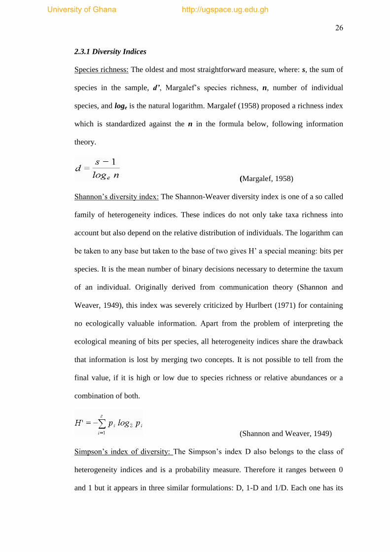
Species richness: The oldest and most straightforward measure, where: s, the sum of
species in the sample, d’, Margalef‘s species richness, n, number of individual
species, and loge is the natural logarithm. Margalef (1958) proposed a richness index
which is standardized against the n in the formula below, following information
theory.
(Margalef, 1958)
Shannon‘s diversity index: The Shannon-Weaver diversity index is one of a so called
family of heterogeneity indices. These indices do not only take taxa richness into
account but also depend on the relative distribution of individuals. The logarithm can
be taken to any base but taken to the base of two gives H‘ a special meaning: bits per
species. It is the mean number of binary decisions necessary to determine the taxum
of an individual. Originally derived from communication theory (Shannon and
Weaver, 1949), this index was severely criticized by Hurlbert (1971) for containing
no ecologically valuable information. Apart from the problem of interpreting the
ecological meaning of bits per species, all heterogeneity indices share the drawback
that information is lost by merging two concepts. It is not possible to tell from the
final value, if it is high or low due to species richness or relative abundances or a
combination of both.
(Shannon and Weaver, 1949)
Simpson‘s index of diversity: The Simpson‘s index D also belongs to the class of
heterogeneity indices and is a probability measure. Therefore it ranges between 0
and 1 but it appears in three similar formulations: D, 1-D and 1/D. Each one has its
University of Ghana http://ugspace.ug.edu.gh
27
own name but often they all use the symbol D and are simply called Simpson‘s
index, so attention is advisable at comparisons. In the formulation of 1-D, the
Simpson‘s index of diversity is the probability of encountering two different species
when randomly picking two individuals of a sample.
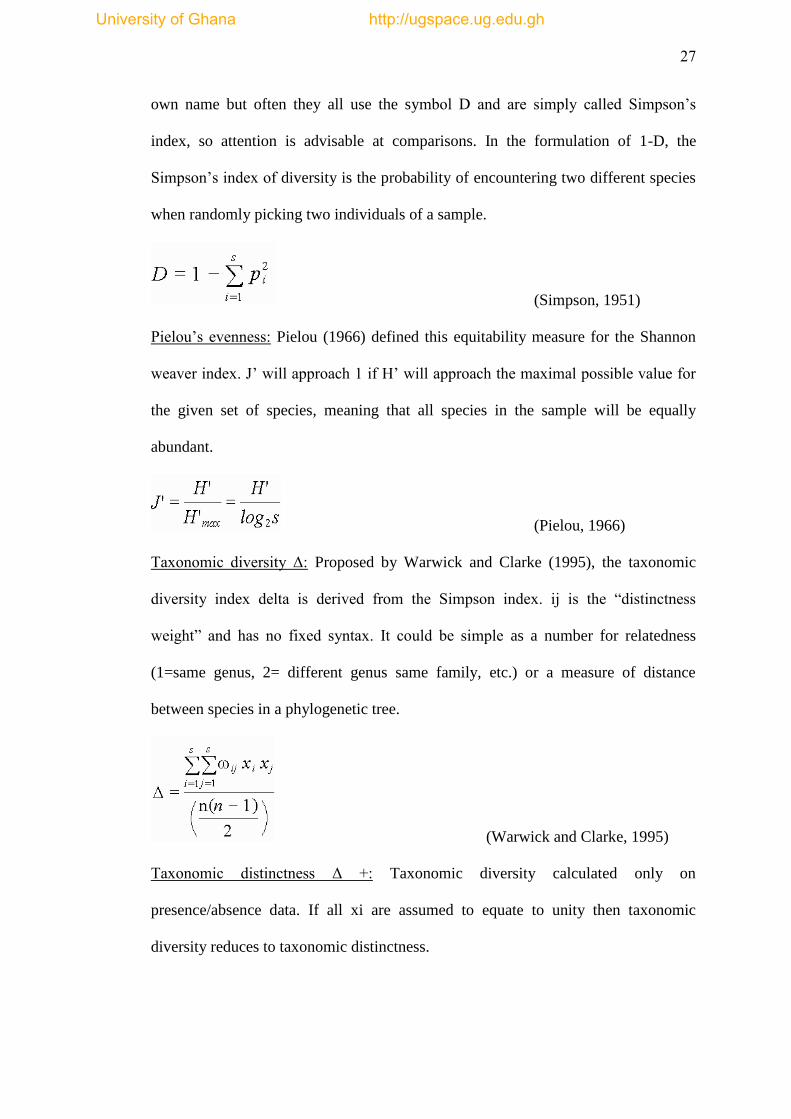
(Simpson, 1951)
Pielou‘s evenness: Pielou (1966) defined this equitability measure for the Shannon
weaver index. J‘ will approach 1 if H‘ will approach the maximal possible value for
the given set of species, meaning that all species in the sample will be equally
abundant.
(Pielou, 1966)
Taxonomic diversity Δ: Proposed by Warwick and Clarke (1995), the taxonomic
diversity index delta is derived from the Simpson index. ij is the ―distinctness
weight‖ and has no fixed syntax. It could be simple as a number for relatedness
(1=same genus, 2= different genus same family, etc.) or a measure of distance
between species in a phylogenetic tree.
(Warwick and Clarke, 1995)
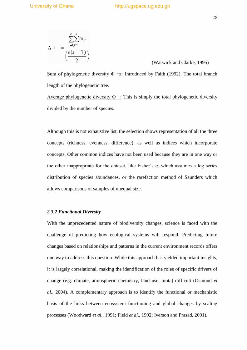
Taxonomic distinctness Δ +: Taxonomic diversity calculated only on
presence/absence data. If all xi are assumed to equate to unity then taxonomic
diversity reduces to taxonomic distinctness.
University of Ghana http://ugspace.ug.edu.gh
28
(Warwick and Clarke, 1995)
Sum of phylogenetic diversity Φ +z: Introduced by Faith (1992). The total branch
length of the phylogenetic tree.
Average phylogenetic diversity Φ +: This is simply the total phylogenetic diversity
divided by the number of species.
Although this is not exhaustive list, the selection shows representation of all the three
concepts (richness, evenness, difference), as well as indices which incorporate
concepts. Other common indices have not been used because they are in one way or
the other inappropriate for the dataset, like Fisher‘s α, which assumes a log series
distribution of species abundances, or the rarefaction method of Saunders which
allows comparisons of samples of unequal size.
2.3.2 Functional Diversity
With the unprecedented nature of biodiversity changes, science is faced with the
challenge of predicting how ecological systems will respond. Predicting future
changes based on relationships and patterns in the current environment records offers
one way to address this question. While this approach has yielded important insights,
it is largely correlational, making the identification of the roles of specific drivers of
change (e.g. climate, atmospheric chemistry, land use, biota) difficult (Osmond et
al., 2004). A complementary approach is to identify the functional or mechanistic
basis of the links between ecosystem functioning and global changes by scaling
processes (Woodward et al., 1991; Field et al., 1992; Iverson and Prasad, 2001).
University of Ghana http://ugspace.ug.edu.gh
29
Functional diversity can be quantified using a variety of indices that capture different
aspects of the distribution of trait values within a community (Bótta-Dukàt, 2005;
Ricotta, 2005; Petchey and Gaston, 2006). Functional groups describe organisms that
share a similar physiological or ecological function e.g. deposit-feeders, bioturbators,
predators (Bonsdorff and Pearson, 1999). The validity of using functional groups has
been questioned because analyses based on such divisions may be meaningless
without more comprehensive knowledge about life history and biology of marine
biota than is currently available for most species (Pearson, 2001). In addition, some
evidence points to species identity being closely linked to ecosystem services such as
bioturbation (Norling et al., 2007).
In a broad scale functional diversity research, Naeem and Wright (2003) proposed
four step-wise factors:
i. determination of species composition across sites through regional biotic
inventory of species pool and application of environmental filters (Woodward
and Diament, 1991; Keddy, 1992) (hierarchy of abiotic and biotic factors that
constrain the distribution and abundance of the species, see Diaz et al., 1999;
Lavorel and Garnier, 2002) to obtain local species composition.
ii. Species abundance determination through relative abundance or common and
rarity.
iii. Determination of functional traits by selecting driver of biodiversity impacts,
ecosystem process, screening the local biota for relevant functional traits,
establishing response traits relevant to the selected driver, and also establishing
effect traits relevant to selected ecosystem function.
iv. Determination of ecosystem functioning.
University of Ghana http://ugspace.ug.edu.gh
30
Nonetheless, functional diversity (utilizing functional/biological traits analysis) has
assumed increased prominence in biodiversity ecosystem function (e.g. Petchey and
Gaston, 2002; Bremner, 2006). According to Mason et al., (2005), functional
diversity is a measure (or group of measures) of the distribution of species and
abundance of a community in functional attribute space that represents the
following:
the amount of functional attribute space filled by species in the community
(functional richness),
the evenness of abundance distribution in filled niche space (functional
evenness), and
the degree to which abundance distribution in niche space maximizes
divergence in functional attributes within the community (functional
divergence).
In their perspective, Tilman, (2001) and Hooper et al. (2005) refer to functional
diversity to mean the range and value of organism traits that can influence ecosystem
properties. According to Hooper et al. (2005), functional diversity can be expressed
in a variety of ways including the number and relative abundance of functional
groups (Tilman et al., 1997, Hooper and Vitousek, 1998) and (Spehn et al., 2000),
the variety of interactions with ecological processes (Martinez, 1996), and the
average difference among species in functionally related traits (Walker et al., 1999).
Functional groups are defined as groups of taxa which share a range of similar
attributes and have analogous effects on major ecosystem processes (Bonsdorff and
Pearson, 1999).
University of Ghana http://ugspace.ug.edu.gh

31
Functional diversity results from the different ways by which different species
exhibit similar functional traits, or the number of different functional groups sharing
biological traits (Wright et al., 2006). Functional attributes of species are therefore
crucial to understanding the effects of marine biodiversity and its role in ecological
patterns and processes. Functional categorization of marine species is a useful
approach for comparing communities over large scales in a way that transcends
taxonomic boundaries, and for linking changes in structure to effects on ecological
function (e.g. Bellwood et al. 2003; Floeter et al. 2004; Micheli and Halpern, 2005).
An effective functional classification could be a cost-effective way of predicting
effects of loss (or restoration) of particular taxa on ecosystem functioning and could
have valuable implications for management and conservation (Micheli and Halpern,
2005). Functional classifications can enable meaningful comparison of the roles of
biodiversity in different ecosystems as they transcend taxonomic differences
(Micheli and Halpern, 2005; Bremner, 2006).
Functional classification of organisms can also improve mechanistic understanding
of community assembly (Micheli and Halpern, 2005). This is because diversity is
manifest in species identities (e.g., variations in form and functions) and therefore
variations in species traits is a key element in biological diversity (Crowe and
Russell, 2009). Reiss et al. (2009) emphasized that biodiversity-ecosystem
functioning (B-EF) experiments regarding traits, could hold species identity
constant, and alter traits and functional diversity to demonstrate whether species
provide unique contributions to ecosystem processes. Ecosystem functions (e.g.,
nutrient cycling, sediment stabilization etc.) are moderated by the functional
attributes of species in a community. To understand how an ecosystem will function
University of Ghana http://ugspace.ug.edu.gh
32
and its ability to provide crucial ecosystem services as well as its capacity to respond
to environmental changes, functional diversity of the assemblages are critical
fundamental steps.
Thus, there have been increased interests in examining ecosystem consequences of
biodiversity loss in marine systems (e.g., Emmerson and Raffaelli, 2000; Duffy et
al., 2001, Emmerson et al., 2001; Stachowicz et al., 2002; Solan et al., 2004; Hooper
et al., 2005; Worm et al. 2006; Bracken et al., 2008) especially in high latitude
locations. However, the biodiversity ecosystem function (B-EF) relationship can be
dependent on environmental conditions for specific ecosystem functions (Hiddink et
al., 2009), which differ in spatial scales. Functional diversity incorporates
interactions between organisms and their environment into a concept that can portray
ecosystem level structure in marine environments (Bremner et al., 2003a). The
functional traits of benthic species are modified on many temporal and spatial scales
(Solan et al., 2004) due to the effects of physical, chemical and biological
characteristics. Environmental gradients may form geographic patterns of diversity
by influencing local processes such as predation, resource partitioning, competitive
exclusion, and facilitations that determine species co-existence (Levin et al., 2001).
2.3.3 Functional Diversity Indices
Recently, several methods have been proposed and described on how to calculate
functional diversity (Mason et al., 2003, 2005; Botta-Dukát, 2005; Ricotta, 2005;
Petchey and Gaston, 2006; de Bello et al., 2006). Some consider species
presence/absence, whereas others are based on abundance data (e.g., Bady et al.,
2005; Botta-Dukát, 2005; Mason et al., 2005). However, incorporating species
University of Ghana http://ugspace.ug.edu.gh
33
abundances into a measure of functional diversity poses several questions on
weighing the relative contribution of richness and evenness components (Hurlbert,
1971), and on the relationship of trait dissimilarity (Walker et al., 1999) to the
ecological diversity of species (Magurran, 1988). It is therefore a more complex
problem than previously thought (Mouillot et al., 2005; Ricotta 2005; Petchey and
Gaston, 2006).
Petchey et al. (2004) compared four presence/absence measures of functional
diversity: (i) species richness (SR), (ii) functional group richness (FGR), (iii) a
dendrogram-based measure (DBM) and (iv) functional attribute diversity (FAD).
Although the simplest measure is SR, it assumes that all species are equally different
and the contribution of each species to functional diversity is independent of species
richness (Petchey et al., 2004). Functional group richness (FGR) is the number of
functional groups present in the community. FGR assumes that the species within the
same group are identical in function (Lawton and Brown, 1993) and assigning a
species into a category is unambiguous. However, many animal species use, for
instance, a variety of feeding strategies and show omnivory (Lancaster et al., 2005;
Woodward et al., 2005ab). Thus, measuring functional diversity based on FGR is not
always meaningful, even if its application can be fruitful when no taxonomical
information on the fauna of the study area is available (Cummins et al., 2005).
A further problem is that the number of functional groups is arbitrarily determined.
Petchey and Gaston (2002) applied cluster analysis from a matrix of functional traits,
and then used the sum of branch lengths of the dendrogram as a multivariate measure
of functional diversity (DBM). This function does not suffer from the problem of
University of Ghana http://ugspace.ug.edu.gh
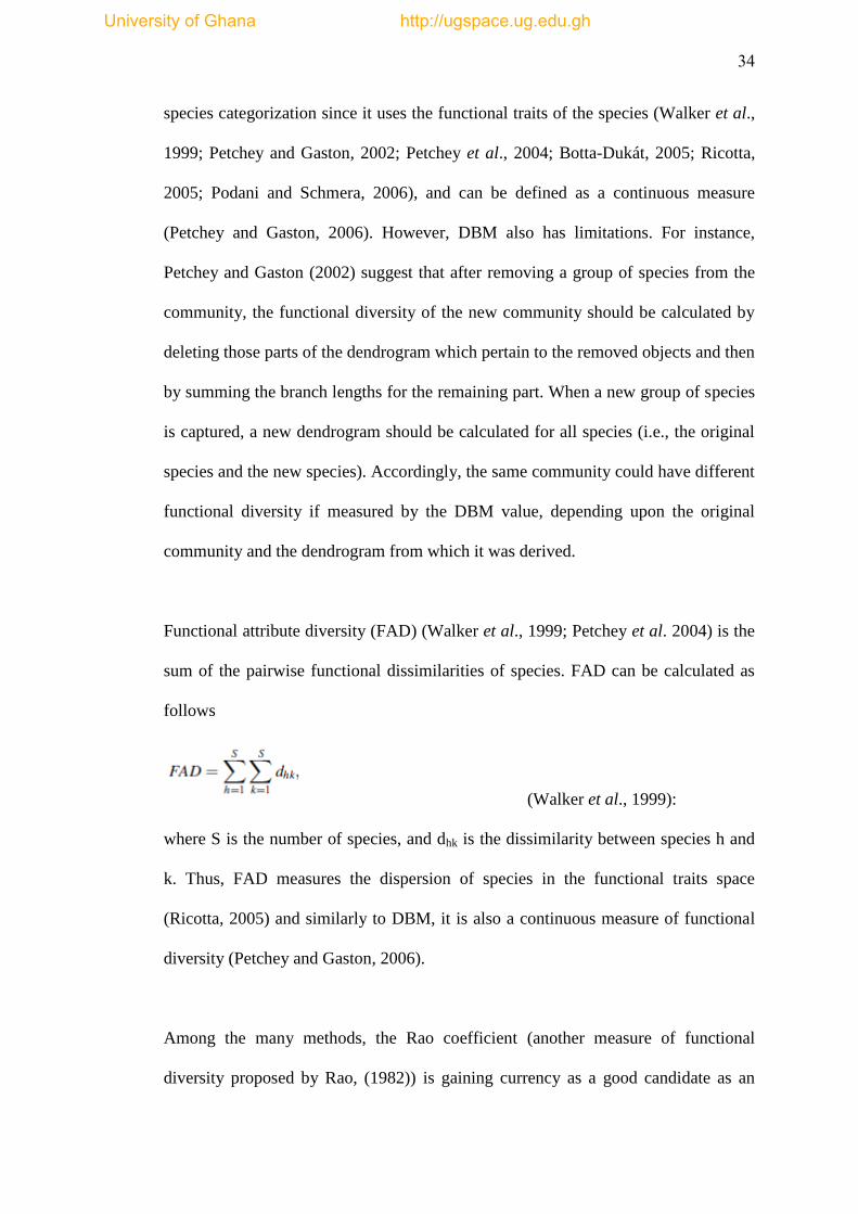
34
species categorization since it uses the functional traits of the species (Walker et al.,
1999; Petchey and Gaston, 2002; Petchey et al., 2004; Botta-Dukát, 2005; Ricotta,
2005; Podani and Schmera, 2006), and can be defined as a continuous measure
(Petchey and Gaston, 2006). However, DBM also has limitations. For instance,
Petchey and Gaston (2002) suggest that after removing a group of species from the
community, the functional diversity of the new community should be calculated by
deleting those parts of the dendrogram which pertain to the removed objects and then
by summing the branch lengths for the remaining part. When a new group of species
is captured, a new dendrogram should be calculated for all species (i.e., the original
species and the new species). Accordingly, the same community could have different
functional diversity if measured by the DBM value, depending upon the original
community and the dendrogram from which it was derived.
Functional attribute diversity (FAD) (Walker et al., 1999; Petchey et al. 2004) is the
sum of the pairwise functional dissimilarities of species. FAD can be calculated as
follows
(Walker et al., 1999):
where S is the number of species, and dhk is the dissimilarity between species h and
k. Thus, FAD measures the dispersion of species in the functional traits space
(Ricotta, 2005) and similarly to DBM, it is also a continuous measure of functional
diversity (Petchey and Gaston, 2006).
Among the many methods, the Rao coefficient (another measure of functional
diversity proposed by Rao, (1982)) is gaining currency as a good candidate as an
University of Ghana http://ugspace.ug.edu.gh
35
efficient functional diversity index, because it is a generalization of the Simpson‘s
index of diversity, it is easy intuitively understandable, and it can be used with
various measures of dissimilarity between species (both those based on a single trait,
and those based on many traits (Ricotta, 2005; Petchey and Gaston, 2006). However,
when intending to quantify the functional diversity, various methodological
decisions such as how many and which traits to use, how to weight them, how to
combine traits that are measured at different scales and how to quantify the species‘
relative abundances in a community have to be made.
The Rao index uses species traits to calculate dissimilarity among species (Botta-
Dukát, 2005; Lepš et al., 2006; Lavorel et al. 2008). The Rao index generally
reflects the probability that, picking randomly two individuals in a community (i.e., a
sample), they are different. For trait diversity, the Rao index represents the
probability that they are functionally different (e.g. for single traits, either they have
different trait values or different trait categories). The Rao coefficient is very
flexible, and can be used with various dissimilarity measures. For example,
Shimatani (2001) used it with taxonomic dissimilarity when exploring taxonomic
diversity and amino acid diversity; asymmetrical measures can be also used. The
main methodological decisions are mainly i) how to measure the species
dissimilarity, and ii) how to characterize the proportion of a species in the
community. These methodological decisions are also made even if other indices of
functional diversity other than Rao‘s coefficient are being used (Lepš et al., 2006).
The mechanistic models concerning the functional consequences of diversity have
been based on the fact that species differ from each other (and thus function
University of Ghana http://ugspace.ug.edu.gh

36
differently; MacArthur, 1955). Similarly, the importance of the differences among
species for maintaining species coexistence was explicitly expressed by the concept
of limiting similarity (MacArthur and Levins, 1967). Ecologists have thus
progressively realized that species differ from each other in terms of some traits
(Díaz and Cabido, 2001) and thus that the effect of ecological diversity might be
based on the ―extent of trait dissimilarity among species in a community‖ (or
functional diversity; Tilman, 2001; Petchey and Gaston, 2002). Traditionally, species
diversity has been considered a surrogate for functional diversity in most studies
linking biodiversity to ecosystem functioning (Díaz and Cabido, 2001; Loreau et al.,
2003). However, some pairs of species are very similar to each other, while some are
very different. Consequently, the relationship between species diversity and
functional diversity is expected to be positive (Petchey and Gaston, 2002) but not
necessarily very tight (Díaz and Cabido, 2001; Petchey and Gaston, 2006).
Other two widely used continuous measures of functional diversity are the
dendrogram-based measure (DBM) and the functional attribute diversity (FAD). In
contrast to DBM, FAD does not require the knowledge of the entire species pool
before the analysis, and hence FAD is a more ideal tool for measuring functional
diversity. However, the original form of FAD and its variants have several
undesirable properties (Schmera et al., 2009). A modified FAD (denoted by MFAD)
has therefore been suggested (Schmera et al., 2009). The MFAD allows for
calculating functional diversity without violating the twinning and monotonicity
criteria such that the number of species collected is compensated for (Schmera et al.,
2009). These requirements are met by replacing the original species by so-called
functional species and then by dividing FAD by the number of functional units.
University of Ghana http://ugspace.ug.edu.gh

37
Accordingly, MFAD measures the dispersion of species in the functional traits space
so that MFAD values for different communities can directly be compared if the same
set of functional trait is used.
2.3.4 Functional Trait Analysis
One of the most promising of the recently proposed approaches to measure
functional diversity is biological traits analysis (BTA) (Statzner et al., 1994). A
biological trait is a character of an organism that may be inherited or
environmentally determined. The character can be genotypic or phenotypic i.e., size,
body form, movement, feeding, larval type. These characteristics strongly influence
ecosystem properties. The contribution of a benthic species to ecosystem processes
may be determined by a suite of biological characteristics (Webb and Eyre, 2004a),
suggesting the involvement of a number of traits in ecological functioning.
Biological traits analysis uses a series of life history, morphological and behavioural
characteristics of species present in assemblages to indicate aspects of their
ecological functioning (here defined as the maintenance and regulation of ecosystem
processes (Naeem et al. 1999)). The roles performed by benthic species are
important for regulating ecosystem processes (Snelgrove, 1998) and these roles are
determined by the biological traits species exhibit (Bremner et al., 2006). Several
characteristics can be involved in organisms‘ responses to individual environmental
variables. For example, responses to benthic trawling have been linked to traits such
as feeding methods, body size, flexibility, mobility and burrowing activities (Kaiser
et al., 1998; Rumohr and Kujawski, 2000; Bradshaw et al., 2002; Thrush and
Dayton, 2002).
University of Ghana http://ugspace.ug.edu.gh
38
The approach aims to provide a description of multiple aspects of functioning based
on features of the biological ecosystem component. It does this by utilising specific
species traits as indicators of functioning (Diaz and Cabido, 2001) and examining the
occurrence of these traits over assemblages (Bremner, 2008). Biological Traits
Analysis (BTA) is based on habitat templet theory, which states that species‘
characteristics evolve in response to habitat constraint (Southwood, 1977).
Community structure is governed by habitat variability and the biological traits
exhibited by organisms will provide information about how they behave and respond
to stress (Lavorel et al., 1997), thereby indicating the state of the environment
(Usseglio-Polatera et al., 2000b). BTA uses multivariate ordination to describe
patterns of biological trait composition over entire assemblages (i.e., the types of
trait present in assemblages and the relative frequency with which they occur)
(Bremner et al., 2006).
Species trait analysis (STA) focuses on defining biological and ecological
characteristics of faunal assemblages. It incorporates information on species‘
distributions and the biological characteristics they exhibit, to produce a summary of
the biological trait composition of assemblages (Bremner et al., 2005). The approach
provides a link between species, environments and ecosystem processes, and is
potentially useful for the investigation of anthropogenic impacts on ecological
functioning (Bremner et al., 2005). Species diversity indices do not take into account
functional differences between species, though some authors pointed out the
necessity of including these differences between species to estimate a diversity
related to changes in environmental conditions or influencing ecosystem processes
(Diaz and Cabido, 2001; Mouillot et al., 2005). Alternative groups, functional
University of Ghana http://ugspace.ug.edu.gh
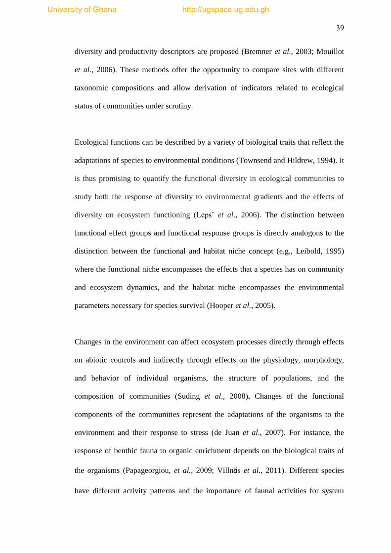
39
diversity and productivity descriptors are proposed (Bremner et al., 2003; Mouillot
et al., 2006). These methods offer the opportunity to compare sites with different
taxonomic compositions and allow derivation of indicators related to ecological
status of communities under scrutiny.
Ecological functions can be described by a variety of biological traits that reflect the
adaptations of species to environmental conditions (Townsend and Hildrew, 1994). It
is thus promising to quantify the functional diversity in ecological communities to
study both the response of diversity to environmental gradients and the effects of
diversity on ecosystem functioning (Lepsˇ et al., 2006). The distinction between
functional effect groups and functional response groups is directly analogous to the
distinction between the functional and habitat niche concept (e.g., Leibold, 1995)
where the functional niche encompasses the effects that a species has on community
and ecosystem dynamics, and the habitat niche encompasses the environmental
parameters necessary for species survival (Hooper et al., 2005).
Changes in the environment can affect ecosystem processes directly through effects
on abiotic controls and indirectly through effects on the physiology, morphology,
and behavior of individual organisms, the structure of populations, and the
composition of communities (Suding et al., 2008). Changes of the functional
components of the communities represent the adaptations of the organisms to the
environment and their response to stress (de Juan et al., 2007). For instance, the
response of benthic fauna to organic enrichment depends on the biological traits of
the organisms (Papageorgiou, et al., 2009; Villnäs et al., 2011). Different species
have different activity patterns and the importance of faunal activities for system
University of Ghana http://ugspace.ug.edu.gh

40
regulation is frequently associated with individual species traits (Norling et al.,
2007). For example, opportunistic species are less affected by sedimentation and
likely to respond positively to it (Tomassetti and Porrello, 2005).
2.4 Disturbance of Marine Biodiversity
Disturbance relates to the disruption of system‘s stability resulting from events
including natural and anthropogenic. It is often not possible to decide what has been
changed by anthropogenic stress and what is natural. This is because anthropogenic
stresses are superimposed on stresses caused by natural environmental factors
(Raffaelli and Hawkins, 1996). Anthropogenic stress is the response of a biological
entity (individual, population, community etc.) to an anthropogenic disturbance or
stressor. Stress can be any factor that negatively affects the physiology, growth,
reproduction and survival of an organism or that has consequences affecting
populations or communities (Shiel, 2009). Stress at one level of organization (e.g.
individual, population) may also have an impact on other levels, for example,
causing alterations in community structure. However, it is sometimes difficult to
detect the effects of anthropogenic stress at the level of individual organisms, and
impacts are more often investigated at a population or community level (Crowe et
al., 2000).
There is little doubt that anthropogenic disturbance have extensively altered the
global environment, leading to a decrease in biodiversity. Changes in marine
biodiversity are directly caused by exploitation, pollution and habitat destruction, or
indirectly through climate change and related perturbations of ocean
biogeochemistry (Jackson et al., 2001; Dulvy et al., 2003; Lötze et al., 2006).
University of Ghana http://ugspace.ug.edu.gh
41
Disturbance of the community by physical and biological factors may reduce the
number of organisms in the community to the point at which there is less
competition for resources, and hence less competitive exclusion and greater species
diversity (Dether, 1984).
Jackson and Chapman (2009) indicated a tendency to associate current biodiversity
changes with contemporary causes such as pollution, global warming and invading
species. In reality, impacts may be temporally disconnected from their causes; long-
term or historic activities may have precipitated chains of events, causing what we
see today. Anthropogenic influence and their consequences may also be
disconnected spatially (Jackson and Chapman, 2009).
Useful conclusions of Worm et al. (2006) indicate that high biodiversity in the
marine environment is associated with ecosystem stability and resilience, and with
the productivity and recovery potential of vital fisheries, although this was criticized
for two shortcomings (Hölker et al., 2007). In the marine environment, changes are
often assumed to be smaller, more localized or more easily reversed, although this
may not be the case-e.g., large fishing grounds take decades to recover (Thrush and
Dayton, 2002). Many impacts on ecosystem have now become global in scale (e.g.,
declines in major fisheries; Brander, 2007); others are limited to a local sphere of
influence. According to Worm et al. (2006) and Hölker, et al. (2007) the number of
overexploited or depleted fish stocks has been increasing over several decades and
the United Nations Food and Agriculture Organization (FAO) reports an increase
from about 10% in the mid-1970s to around 25% in the early 1990s (FAO, 2006).
The FAO data indicate, however, that the increasing trend has stabilized since the
University of Ghana http://ugspace.ug.edu.gh

42
early 1990s, whereas the Worm et al. (2006) data indicate that the increasing trend
continues.
Enhanced fisheries recovery occur at high diversity due to the fact fishers can switch
more readily among target species, potentially providing overfished taxa with a
chance to recover (Worm et al., 2006). Also taxonomically related species play
complementary functional roles in supporting fisheries productivity and recovery
(Worm et al., 2006). Another useful finding from Worm et al. (2006) indicated that
collapse of LME fisheries occurred at a higher rate in species-poor ecosystem
compared with species-rich ones, giving credence to the effects of biodiversity loss
on the ecosystem. Removal of mature fish affects the supply of juveniles elsewhere
in the system, with consequences for species richness and diversity, marine predator
populations, and food web functionality (Worm et al., 2006) that extend over a far
greater area and range of ecosystems than the fishing activity itself.
Recent evidence suggests that coastal and open-water systems can rapidly flip from
being dominated by fish (that keep jellyfish in check through competition or
predation) to a less desirable ‗gelatinous‘ state (Richardson et al., 2009). This new
ecosystem state is resistant to returning to its original state because jellyfish are
voracious predators of fish eggs and larvae, and effectively prevent fish from
returning. This flip to a jellyfish-dominated system once a critical threshold is
reached has been termed ‗the jellyfish joyride‘. Thus, natural ecosystems can be
slowly degraded by the combination of continued overfishing, eutrophication and
climate change to one where there are few fish, marine mammals and seabirds (Fig.
University of Ghana http://ugspace.ug.edu.gh
43
2.1). This change to jellyfish is consistent with the ‗rise of slime‘ (Pandolfi et al.,
2005).
Figure 2.1 Human-induced processes of change from fish to jelly-fish
domination (after Richardson et al., 2009).
These tipping points for ecosystems (illustrated in Fgiure 2.1) are generally unknown
and the new ecosystem state is resistant to returning to its original state (Richardson
et al., 2009). A pervasive and irreversible impact of human activity on natural
marine ecosystem is introduction of non-indigenous species. The opportunities for
species introduction have steadily increased over recent centuries (Hewitt and
Campbell, 2007). Non-indigenous species are now common inhabitants of most
geographic regions of the world. For example, up to 230 introduced species have
been documented for a single estuary (Loxahatchee River estuary in Florida, USA)
and about 400 are established in marine and estuarine habitats in the US alone (Ruiz
et al., 1997). Although the ecological effects of introduced species to the native
assemblage are not clearly fully understood, they pose a significant stress to marine
University of Ghana http://ugspace.ug.edu.gh
44
communities, particularly in areas already stressed by loss of habitat or high levels of
contamination (Clynick et al., 2009).
The degrading effects of fishing, habitat destruction, introduced species, and
eutrophication reinforce each other through positive feedbacks (Jackson, 2001;
Jackson et al., 2001; Lötze et al., 2006). For example, oysters were nearly eliminated
by overfishing, but their recovery is now hampered by hypoxia due to
eutrophication, by introduced species that compete for space and cause disease, and
by the explosive rise of formerly uncommon predators that were previously kept in
check by now overfished species in the Neuse River estuary, North Carolina, USA
(Lenihan and Peterson, 1998; Myers et al., 2007). Much of the overall decline of the
80 species reviewed by Lötze et al. (2006) was due to multiple suites of drivers: 45%
of depletions and 42% of extinctions involved multiple impacts. Nowhere have these
drivers been brought under effective regulation or control.
Trawling is the most important factor affecting the structure and function of soft-
bottom communities globally (Watling and Norse, 1998; Thrush and Dayton, 2002;
Gray et al., 2006). A number of studies have investigated the impacts of trawling on
different components of the marine ecosystem (e.g., Drabsch et al., 2001; Spark-
McConkey and Watling 2001; Thrush and Dayton, 2002; Nilsson and Rosenberg,
2003; Rosenberg et al., 2003). McConnaughey et al. (2000) further demonstrated
that there are chronic effects, which result in lower diversity in the sedentary
macrofauna in the heavily trawled areas of the eastern Bering Sea. Tillin et al. (2006)
found that chronic bottom trawling can lead to large-scale shifts in the functional
University of Ghana http://ugspace.ug.edu.gh

45
composition of benthic communities, with likely effects on the functioning of coastal
ecosystems.
Another important factor of disturbance to benthic communities is euthrophication.
Benthic eutrophication is defined as an increase in the rate of supply of organic
matter to benthic environment (Nixon, 1995). One of the most important effects of
eutrophication on aquatic organisms is the reduction in the concentration of
dissolved oxygen. Hypoxia or anoxia (low or nil oxygen content) can cause direct
mortality and reduced growth rates in organisms (Weston, 1990). Many studies have
documented changes in biodiversity of macrofaunal benthic communities under
hypoxia conditions (Nilsson and Rosenberg, 1994; Ritter and Montagna, 1999; Craig
et al., 2000; Meyers et al., 2000; Nilsson and Rosenberg, 2000; Rosenberg et al.,
2001) and into the behavioral or physiological responses of species to hypoxia
(Rosenberg et al., 1991; Holmes et al., 2002; Wu and Or, 2005). These studies
showed decreased biodiversity, alterations of species composition and reductions in
biological responses, when the benthic environment is subjected to short or long-
term hypoxia events. Although the effects of hypoxia on biodiversity, physiology
and behavioral responses have been extensively studied (Widdows et al., 1989;
Vaquel-Sunyer and Duarte, 2008; Hondorp et al., 2010), there has not been any
research into the combined effects of trawling and hypoxia on the biological traits of
benthic communities.
The intermediate disturbance hypothesis of Connell (1978) predicts maximum
biodiversity at a frequency of disturbance where recruitment is able to replace lost
individuals but inter-specific processes do not have time to exclude species. This
University of Ghana http://ugspace.ug.edu.gh

46
response has been recorded in many marine systems (Begon et al., 1996; Svensson et
al., 2007). Disturbance, both anthropogenic and natural, may act as a potential
abiotic drivers/surrogate for diversity at an appropriate spatial scale and temporal
scale (Harris et al., 2008). The stability of the seabed sediment surface exerts a major
control on benthic community structure (Newell et al., 1998). Species diversity tends
to be highest on stable rocky shores and on cohesive muddy shores, with the more
mobile sandy or fine gravel substrates typically showing much lower richness.
Sediment stability is dependent on slope, particle size and the degree of water motion
on the bed (Bagnold, 1963). The shape and roundness of sediment grains are
additional properties that determine the stability of a deposit (Lewis and McConchie,
1994) but grain shape is difficult to measure and is rarely recorded despite its likely
importance. Stability may also be influenced by the presence of biota through
biological armouring of the bed and binding of sediment by faunal mucus (Murray et
al., 2002). The stability of a sediment surface as a habitat is difficult to quantify,
particularly given that one of the key proxies, sediment grain size, is determined on
disaggregated samples which have been dislodged from their environment and may
have little physical resemblance to what an organism actually encounters (Snelgrove
and Butman, 1994).
2.5 Environmental Drivers of Marine Benthic Diversity
The goal of ecological research is to determine which easily measured characteristics
best describe the species assemblage of a particular space and time (Moore et al.,
1991). Models which have been suggested for understanding community dynamics
or species assemblages include ‗‗environmental stress models‘‘ and either
‗‗nutrient/productivity models‘‘ or the ‗‗food chain dynamics hypothesis‘‘ (Connell,
University of Ghana http://ugspace.ug.edu.gh
47
1975; Oksanen et al., 1981; Fretwell, 1987; Menge and Olson, 1990; Menge, 2000).
Environmental stress models assume that community structure results from species
interactions and disturbances, and how these are modified by underlying gradients of
environmental stress (where stress is a consequence of environmental conditions
such as temperature, moisture, salinity) (Menge et al., 2002). The two models
postulate that communities can be ordered along environmental gradient. McGill et
al. (2006) argued that general principle in community ecology may not be achieved
if research continues to focus on pair-wise species interactions independent of the
environment. Global species distributions are generally believed to be determined by
abiotic influences related to oceanographic and physiographic properties (Sanders,
1968; Ricklefs and Schluter, 1993). For instance, water motion affects biology by
acting as a transport mechanism for organisms and their propagules, as a dynamic
boundary between regimes, and as a force to which organisms must adapt or
respond, for example, in their feeding and locomotor activities (Nowell and Jumars,
1984; Denny, 1993).
The abiotic characteristics are expected to act as predictors of species assemblages in
unexplored areas (Franklin, 1995). Pitcher et al. (2007) identified grain size,
carbonate composition, available space, benthic irradiance, sheer stress, bathymetry,
bottom water physical properties, nutrient concentrations and turbidity as abiotic
surrogates of biotic distributions on the Great Barrier Reef; but these variables, while
useful predictors, may not be the forces driving the patterns they describe. The
influence of abiotic factors on species assemblages is due to the effect they exert on
fundamental niches. A species‘ fundamental niche was defined by Austin et al.
(1990) as ―that hypervolume defined by environmental dimensions within which a
species can survive and reproduce.‖ Fundamental niches are rarely fully realized by
University of Ghana http://ugspace.ug.edu.gh
48
species because interspecific competition, disease and disturbance events displace
individuals and populations, resulting in a reduced occupied hypervolume, often
referred to as the realized niche (Austin and Smith, 1989).
The environmental gradients that describe a species‘ fundamental niche can be
broadly grouped into resource gradients – e.g. chemicals or energy consumed by a
species; direct gradients – variables with a physiological influence on a species but
not consumed by it – e.g. sediment grain size or temperature; and indirect gradients –
variables correlated with direct and resource gradients but with no physiological
connection to the species – e.g. depth and latitude (Meynard and Quinn, 2007).
When niche theory was first proposed, species were expected to exhibit a Gaussian
distribution to environmental gradients but skewed distributions are more common in
ecological studies as the effects of additional variables express their influence
(Karadzic et al., 2003).
The abiotic variables which have been historically ascribed the greatest direct
influence over benthic organism distributions are temperature, salinity, oxygen
concentration, light availability and sediment composition (Snelgrove, 2001).
Environmental variables (such as sediment structure, organic matter content,
temperature, salinity, dissolved oxygen, nutrient concentrations, pH, turbidity, water
transparency and depth) have been found to correlate with abundance, density and
diversity of macrofauna and these variables may vary seasonally (Nicolaidou et al.,
1988; Arvanitidis et al., 1999; Hagberg and Tunberg, 2000; Mistri et al., 2000;
Mistri et al., 2001).
University of Ghana http://ugspace.ug.edu.gh
49
A model describing the influences of these factors and some of their potential
synergies is given in Figure 2.2. The figure depicts the influence of interdependency
of physical processes and potential surrogate abiotic drivers on biological
community structure. Olabarria (2006) found depth accounted for as much as a
quarter of the variance in benthic diversity in deep systems but, as benthic organisms
lack an apparent mechanism for measuring depth, some correlated water quality
parameter or seafloor characteristic most likely influences the settlement, recruitment
and survival processes that result in the observed depth related patterns. Lamptey et
al., (2010) identified nitrate-nitrogen, dissolved oxygen, salinity and water
temperature as suite of abiotic drivers of rocky intertidal biodiversity in Ghana. Gray
(2002) reduced Snelgrove‘s list of direct drivers (2001) to productivity, temperature
and sediment composition as the dominant variables in determining regional benthic
richness, noting that temperature and productivity are often correlated to depth and
latitude. Combinations of these driving influences occur with varying spatial and
temporal consistency, in turn producing semi-regular patterns of biodiversity. The
validity and origin of several identified general benthic biodiversity patterns are the
focus of much recent debate. For example, the latitudinal (spatial) richness gradient,
widely accepted as a rule for benthic fauna since the mid twentieth century (Thorson,
1957) has been shown to be weaker than previously thought (Snelgrove, 2001) or
entirely incorrect for some taxa or systems (Rex et al., 2005) due to the driving
influence of complex biotic and abiotic factors.
University of Ghana http://ugspace.ug.edu.gh
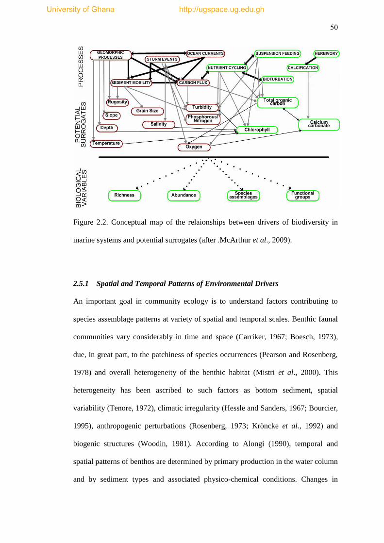
50
Figure 2.2. Conceptual map of the relaionships between drivers of biodiversity in
marine systems and potential surrogates (after .McArthur et al., 2009).
2.5.1 Spatial and Temporal Patterns of Environmental Drivers
An important goal in community ecology is to understand factors contributing to
species assemblage patterns at variety of spatial and temporal scales. Benthic faunal
communities vary considerably in time and space (Carriker, 1967; Boesch, 1973),
due, in great part, to the patchiness of species occurrences (Pearson and Rosenberg,
1978) and overall heterogeneity of the benthic habitat (Mistri et al., 2000). This
heterogeneity has been ascribed to such factors as bottom sediment, spatial
variability (Tenore, 1972), climatic irregularity (Hessle and Sanders, 1967; Bourcier,
1995), anthropogenic perturbations (Rosenberg, 1973; Kröncke et al., 1992) and
biogenic structures (Woodin, 1981). According to Alongi (1990), temporal and
spatial patterns of benthos are determined by primary production in the water column
and by sediment types and associated physico-chemical conditions. Changes in
University of Ghana http://ugspace.ug.edu.gh
51
environmental conditions promote changes in species assemblages at variety of
spatial scales (Lamptey et al., 2010). Many environmental factors affecting species
performance and interactions vary with spatial scale (Noda, 2009). There is,
however, no particular scales of change that are consistent among taxa (Burrows et
al., 2002), congruently demanding ambitious ecological models to decipher spatial
patterns. Physical or environmental factors, such as water depth and sediment type
and movement, are considered to determine large-scale patterns of distribution (e.g.
Thorson, 1957; Barry and Dayton, 1991). Within these patterns, however, spatial
heterogeneity exists at various scales, forming a mosaic of patches.
Spatial heterogeneity is often cited as a diversity driver, with high inshore species
richness being promoted by the variety of habitats available on a broad scale and
deep water benthic and planktonic richness occurring in spite of low biomass as a
result of small scale shifts in sediment or water composition in habitats which
otherwise appear homogenous (Snelgrove, 2001). Spatial pattern is difficult to
quantify and often refers to the spatial character and arrangement, position or
orientation of patches within a landscape (Li and Reynolds, 1993).
A greater understanding of the distribution and complexity of benthic habitats and a
common approach to measuring and describing this complexity will provide a spatial
framework within which to properly address spatially explicit research and
management goals (Kendall et al., 2005). The decline of many species has been
linked directly to habitat loss and fragmentation. Identifying what characteristics
make an area preferentially habitable for particular species has been examined by
many landscape ecologists and is being increasingly taken up by marine ecologists to
University of Ghana http://ugspace.ug.edu.gh
52
describe patterns of benthic diversity (Barrett et al., 2001). Recent advances in image
processing and GIS technologies have made it possible to link indices of landscape
pattern to ecological functions. However, the uncertainties in mapping the pattern
and extent of marine habitats have, until recently, been behind the rarity of habitat-
scale studies in marine ecology
Increasing species richness with increasing proximity to the equator is a long
recognized biogeographic pattern (Cox and Moore, 2005). While this pattern has
been documented in the marine environment (Attrill et al., 2001) it has recently been
found to be less general than previously thought (Gray, 2001). Hawkins et al. (2003)
and Willig et al. (2003) each cite thirty hypotheses to explain latitudinal richness
gradients. These were categorized by Mittelbach et al. (2007) into ecological,
historical and evolutionary groups. The ecological hypotheses concentrate on the
different adaptive challenges faced by organisms living in different climatic zones:
polar and temperate organisms must adapt to environmental conditions (Schemske,
2002) while tropical organisms, dealing with less harsh abiotic extremes, adapt to
biotic interactions (Crame, 2000). Historical explanations concentrate on the age and
stability of richness hotspots (Alongi, 1990).
Evolutionary models incorporate several possible drivers for high rates of speciation
including the wide variety of microhabitats available in tropical regions (Rex et al.,
2005) and higher rates of molecular evolution (Kerswell, 2006). Attempts to measure
and explain the extent of a latitudinal richness gradient in taxa other than molluscs
on broad geographic scales have found less evidence for a marine equivalent to the
terrestrial pattern (Gray, 2001) and brought into question the treatment of data in
University of Ghana http://ugspace.ug.edu.gh
53
describing such patterns. For example, Thorson‘s (1956) pattern of increasing
richness in benthic epifauna toward the equator was based only on the 140,000
marine taxa known at the time (Snelgrove, 2001). Diversity responses to pure spatial
gradients can vary depending on how assemblage data are treated. Ellingsen et al.
(2005) determined that latitude could account for variance in richness of molluscs
(11.8 % explained), annelids (9.6 %) and crustaceans (13.7 %) in Norwegian shelf
benthos.
2.5.2 Water Depth
Water depth has been a consistently powerful explanatory variable in benthic studies
(Nicolaidou and Papadopoulou, 1989; Gogina et al., 2010). When generalizing from
shallow to deep, intertidal and estuarine systems exhibit high biomass and low
species richness caused by high productivity and extreme environmental conditions
(Edgar, 2001), coastal shelves have moderate biomass and species richness
(Snelgrove, 2001), and the deep sea shows a decrease in biomass and increase in
richness (Levin et al., 2001). Peak benthic species richness values have been
recorded seaward of the continental rise, excluding the deep sea (Snelgrove, 2001).
The lower slope and abyssal plains become comparatively depauperate for some
groups, and species turnover tends to be high (Paterson et al., 1992). Levin et al.
(2001) stated that the deep sea houses greater diversity than coastal shelf systems,
although at far lower abundances. Areas with low abundance and high species
turnover require greater sampling effort to reliably account for diversity (Etter and
Mullineaux, 2001).
University of Ghana http://ugspace.ug.edu.gh
54
2.5.3 Substrate Types
Numerous studies have provided evidence to show significant differences in the
species composition between ‗hard‘ and ‗soft‘ substrata (Beaman et al., 2005;
Beaman and Harris, 2007; Williams and Bax 2001). For practical purposes, ‗soft
substrate‘ is usually defined as detrital mineral or biogenic sediment comprising
grains with a mean diameter less than 2 mm, although gravel size fractions are often
included (Lewis and McConchie, 1994). The term ‗hard substrate‘ is typically used
to represent rock outcrops but may include sediments with large grain size (e.g.
cobbles, boulders) since these materials can provide a surface that is functionally
comparable to bedrock. While the contrast between soft and hard substratum is
conceptually simple, defining the boundary between soft and hard substrates can be
complex in practice because some rock types are friable or semi consolidated and
may be partly covered by sediment (Ryan et al., 2007). In addition, because the
boundaries between adjacent soft-sediment environments are not always sharp as
those across hard and soft substrate features, the associated boundaries between
biological assemblages may be gradational and spatially complex (Beaman and
Harris, 2007).
Sediment particle size distribution and composition on the seabed express a strong
influence on the morphology and life history of species living in soft sediments
(Jones, 1950). These variables are determined by complex interactions between local
geology, rates of sediment production and supply, actions of bioeroders, current and
wave induced bed stress, and slope (Reineck and Singh, 1980). Generally, in high-
energy areas, coarse sediments (gravel) will predominate, whereas lower energy
(depositional) areas are muddy, although there are exceptions (Foster, 2001; Hart
University of Ghana http://ugspace.ug.edu.gh

55
and Kench, 2007) which have led to a highly complex and variable distribution of
seabed sediment types on the shelf and slope. Although several sediment surrogacy
relationships are well documented (Brown et al., 2001; Beaman and Harris, 2007;
Degraer et al., 2008), the nature and strength of sedimentary surrogates for species
composition within soft sediment environments remains a subject of debate (Dye
2006; Inoue et al., 2008; Stevens and Connolly, 2004). Soft substrates are home to
epifauna and infauna and plant life may include sea grasses (and their epiphytes) or
microphytic algae occurring at the sediment-water interface. Hard substrates can act
as habitat for epifauna and encrusting or macro-algae, but infauna are excluded.
The most basic way of characterizing any community is by the habitat type and for
benthic community habitat normally means sediment type (Hall, 1994). The
distribution of many of the benthic communities shows a clear correlation with
sediment type. Early studies suggested that macrobenthic communities could be
distinguished on the basis of sediment composition (Thorson, 1957; Buchanan et al.,
1978; van Dalfsen et al., 2000). Other studies, however, have shown little correlation
(Day et al., 1971; Sneiderer and Newell, 1999) and suggested that the distribution of
macrofuana in many sedimentary habitats is controlled by complex interaction
between physical and biological factors at the sediment–water interface, rather than
by the granulometric properties of the sediments themselves (Snelgrove and Butma,
1994). However, density-dependent variables play a minor role in structuring the
macrobenthic communities, which were probably affected more by other variables,
such as the kind of habitat and sediment structure (Mistri et al., 2000). Many
apparent relationships between sediment type and biota remain untested in an
University of Ghana http://ugspace.ug.edu.gh

56
experimental sense (Whitlatch, 1981) and have been challenged (Snelgrove and
Butman, 1994).
Storms and current eddies may contribute to primary space being made available in a
system in two fashions: increasing sheer stress at the benthos/water interface, which
can remove sediment, algal cover and motile fauna; and mechanical abrasion or
damage caused by moving sediment or projectiles (Sousa, 2001). Benthic organisms
continually process, transport, and modify seafloor bed sediments. There are those
that bind, protect and stabilize near-surface sediment and those that loose and
destabilize the sediment (Nichols and Boon, 1994).
Depending upon its life style, an organism may require a given size range of
sediment for tube building, burrowing or feeding (Wieser, 1959). The feeding type
of the benthic community is considered as an adaptation to the sediment
characteristics (Rosenberg, 1995). Certain mechanisms result in sediment-specific
distribution. One of these is the preferential ingestion or retention of specific grain
sizes during feeding. Adults of a variety of deposit-feeders have been shown to
ingest specific grain sizes of sediments (Whitlatch, 1977; 1980). For instance, newly
settled larvae may be restricted to feeding on the finest material within the bed or on
particular rich food items (Jumars et al., 1990) thus, optimal grain size may be
different for settling larvae and adults. Larger particles may be preferred by larger
organisms within a given species (Whitlatch and Weinberg, 1982 cited in Snelgrove
and Butman, 1994). Some species show little affinity with any one particular
sediment type, and the fauna within different sediment environments invariably
University of Ghana http://ugspace.ug.edu.gh
57
show some degree of overlap, which might be due to the grain size being a correlate
of the actual causative factor(s) (Snelgrove and Butman, 1994).
Much of the potential food for benthic organisms are located within the upper 2 cm
of the sediment (Whitlatch, 1977, 1980) and most of the organisms produce faecal
pellets that are deposited at or near the sediment surface. This process may result in
a change in the grain size of surface sediments (Hall, 1994). In mud, for instance,
this can result in a pelletised silt-clay matrix. It is therefore, evident that physical
processes impact upon biological features to structure the benthic organisms and its
habitat. Habitat selection based on the availability of a preferred grain size in feeding
is difficult to conceptualise in view of the ontogenic and hydrodynamic changes in
feeding behaviour and particle selectivity (Snelgrove and Butman, 1994). It has been
suggested that animal and sediment correlation is a result of hydrological and
geological processes associated with sediment granulometry rather than a function of
organism‗s available space within sediment (Parry et al., 1999). Benthic space can
also be made available in the wake of acute pollution events (Scanes et al., 1993),
fishing activity (Currie and Parry, 1996) and eutrophication (Tett et al., 2007), but
the effects tend to be locally focused.
2.5.4 Primary Productivity
Contrary to observed patterns in terrestrial systems (Currie et al., 2004), high
primary productivity in near shore waters tends to promote low species richness
(Snelgrove, 2001) and high evenness (Hillebrand et al., 2007). In these areas, the
role of producer tends to be dominated by a small number of species able to
monopolise resources under ambient conditions. Corresponding benthic communities
University of Ghana http://ugspace.ug.edu.gh
58
are dominated by the taxa best able to use the associated products (Lenihan and
Micheli, 2001) or withstand periods of anoxia imposed by excess organic input
(Dell'Anno et al., 2002). In contrast, oligotrophic waters are often home to low
biomass assemblages with high species richness, including a large proportion of
endemic taxa (Poore et al., 2008). Coral reefs, areas of high biomass and species
richness occurring in oligotrophic waters, are an exception. The symbiosis between
coral polyps and their resident zooxanthellae allows higher productivity than would
otherwise occur in the ambient conditions and the spatial complexity and diversity of
habitats provided by hard corals competing for space and light promotes a high
corresponding richness of invertebrate and fish life, in turn supporting a rich
community of predators (Cribb et al., 1994). Primary production can be estimated
from satellite or airborne spectral analysis of chlorophyll in surface waters (Parmar
et al., 2006). While productivity is directly linked to marine biodiversity, the
relationship has yet to be fully explored as a predictive surrogate over large scales.
2.5.5 Organic Carbon
Detrital matter derived from primary productivity and the wastes of secondary
production comprise a valuable resource in the photic zone and, excepting
chemosynthetic systems, almost the only energy input to the aphotic zone (Vetter,
1995; Carney, 2005). This material settles in particles of various sizes, among which
larger particles such as faecal pellets (Angel, 1984) and marine snow (Alldredge and
Silver, 1988) are particularly important. It is generally accepted that the flux of
particulate organic carbon (POC) from the euphotic zone controls the biomass and
abundance of deep-sea benthos. This notion was originally based on observations of
high benthic standing-crops beneath productive equatorial and near-shore waters,
University of Ghana http://ugspace.ug.edu.gh

59
and low standing-crops underlying oligotrophic gyres (Belyayev et al., 1973; Gage
and Tyler, 1991; Rowe et al., 1991; Blake and Hilbig, 1994). However, a direct
coupling between pulse-like sedimentation events and the activity of benthic fauna
has become clear (Aberle and Witte, 2003 and references therein). The detailed
nature of this coupling remains poorly understood because there have been few
studies which combine both types of measurements. One good example is a study by
Smith et al. (1997) in the equatorial Pacific, in which strong and significant
correlations (r2>0.9) were found between both megafaunal (phototransects) and
macrofaunal (enumerated from box core samples) abundances and annual POC
fluxes.
An interesting conclusion from this study was that macrofaunal abundance might
potentially serve as a proxy (i.e., surrogate) for POC flux in low energy abyssal
habitats, implying that the macrofauna themselves are either more widely or more
easily measured than POC fluxes (see also Rowe et al., 1991; Cosson et al., 1997).
The main technique to directly measure POC fluxes is using sediment traps. Seiter et
al. (2005) drew on particle-trap data from 61 locations, and produced a global map
of minimum POC flux to the seafloor which was based on global estimates of
diffusive oxygen uptake. This map, and the global map of total organic carbon
(TOC) concentrations that underpins it (Seiter et al., 2004), may prove useful in
making first order approximations of benthic productivity over broad scales,
assuming that benthic communities are not compromised by sediment de-
oxygenation. Indeed, the relationships between diversity and POC fluxes (or other
productivity proxies) are scale-dependent and may be complicated by other variables
University of Ghana http://ugspace.ug.edu.gh

60
that influence diversity including bottom-water oxygen concentration, hydrodynamic
regime and the stability of the physical environment (Levin et al., 2001).
Proxies of POC fluxes such as TOC, TOC:TN (total nitrogen) ratios, biochemical
markers and pigments in sediment have proven useful in explaining more localized
patterns of biodiversity. TOC is undoubtedly the most widely measured of these
parameters (Seiter et al., 2005), and, where a consistent and robust method (Galy et
al., 2007) has been applied to its measurement, TOC can be a useful surrogate for
biomass, deposit-feeding taxa, and community structure (Gogina et al., 2010).
However, its application is limited to interpolations from physical samples (Levin
and Gage, 1998) as no remote sensing proxy is available. Moreover, correlations
between TOC and diversity measures are not always found (Cartes et al., 2002)
because a large proportion of TOC in sediment may be refractory and thus resistant
to bacterial degradation. Sediment grain size can also affect the amount of
biologically available organic matter (OM) in shallow soft sediments (Taghon,
1982). Small particles have larger surface area per unit volume than large particles,
offering greater habitat for micro-organisms (Fauchald and Jumars, 1979; Petch,
1986; Neira and Hoepner, 1994) and associated organic matter. Some deposit-
feeding species use size-specific foraging mechanisms to select and ingest fine
sediments (Butman and Grassle, 1992; Sebesvari et al., 2006), but both selective and
non-selective deposit-feeders exhibit settlement preferences for sediments with high
concentrations of readily available organic carbon (Snelgrove and Butman, 1994;
Post et al., 2006).
The organic matter content of bottom sediments may be a more likely causal factor
than sediment grain size in determining infaunal distribution (Snelgrove and
University of Ghana http://ugspace.ug.edu.gh
61
Butman, 1994). This is because it is a dominant source of food for deposit-feeders
(Pearson and Rosenberg, 1978), indirectly (e.g., through resuspension) for
suspension feeders (Snelgrove and Butman, 1994). The sediment must be considered
as an indicator of the availability of food, and not as a first order factor directly
determining the distribution of feeding types (Snelgrove and Butman, 1994). Nichols
(1970) and Field (1971) have suggested that there is a strong relationship not only
between animal and grain-size distribution but also between animal and organic-
carbon distributions as well. However, a similarity between the type of sediment and
the percentage of organic matter, which have been ascribed to the hydrodynamic
conditions established during heavy rains, has been observed (Estacio et al., 1999).
Several deposit-feeding opportunistic species have been shown to colonize,
preferentially, organic-rich sediments over non-enriched sediments with comparable
grain size in shallow-water (Grassle et al., 1985; Tsutsumi et al., 1990) and in
associated slow water movements (Mistri et al., 2001). Organic matter was also
found to be correlated with annelid distribution (Arvanitidis et al., 1999). Seasonal
variations in particulate organic matter are greatly influenced by monsoonal rains.
Total organic matter levels decrease during the monsoon season as a result of
increase in river discharge and scouring of surface silt and clay and associated
organic matter (Alongi, 1990). The highest concentrations of organic matter in
sediments are in regions of upwelling and in proximity to rivers and more generally,
relate to the patterns of pelagic primary production (Alongi, 1990).
The availability, freshness or quality of organic matter (OM) pertains to the labile
fraction, which consists mainly of lipids, carbohydrates, proteins and nucleic acids
University of Ghana http://ugspace.ug.edu.gh
62
(Danavaro et al., 1993, 1995, 2001). Several useful biochemical parameters have
been derived to describe the lability of OM (Danavaro et al., 1995; Dauwe et al.,
1999), and some of these have proven useful for explaining different diversity
indices (Cartes et al., 2002). Such measures, however, often require a high degree of
discipline expertise (and advanced techniques), and as such are unlikely to be widely
employed in the capacity of surrogates. However, the Chlorin Index (CI) (Schubert
et al., 2005) is a simple analytic measurement of OM lability, whose reliability has
been demonstrated by comparison to more advanced techniques (e.g., Dauwe Index,
total hydrolysable amino acids, and % ß-alanine as non-protein amino-acid, and
sulfate reduction rates) (Schubert et al., 2005). The Chlorin Index (CI) is a measure
of the amount of chlorophyll (and its degradation products) that could be
transformed to phaeophytin, and is expressed as the ratio of the fluorescence
intensity of a sediment sample extracted in acetone and subject to HCl treatment to
that of the original sediment sample (Schubert et al., 2005). CIs have been found to
correlate well with an index of track richness developed from photographic stills of
seabed sediments, which conveyed differences in the diversity of tracks, faecal casts,
burrows and mounds of benthic biota in deep-sea sediments of the Lord Howe Rise
(Dundas and Przeslawski, 2009). Comparison with this index shows a greater
diversity of animal traces, and potentially more metazoan activity, in sediments of
apparently higher food quality. CIs thus show promise as an easily measured
geochemical surrogate of biodiversity for regions where organic loads are not
expected to give rise to significant sediment anoxia.
University of Ghana http://ugspace.ug.edu.gh
63
2.5.6 General Oceanography
Oceanographers measure and model variables that directly influence the physiology
and behavior of marine organisms (temperature, salinity, pH), variables affecting
productivity (nutrient concentrations, temperature and light intensity: see section
2.5.4 on productivity) and the currents that affect larval distributions. Some factors
such as pH and salinity vary sufficiently over regional and global scales to show
correspondence to biological patterns (Williams and Bax, 2001) but are sufficiently
uniform at a local scale (with the exception of estuarine systems) to preclude their
use in local surrogacy analyses (Bamber et al., 2008). Dissolved oxygen has been
identified as a key predictor of biodiversity in deep sea sediments (Levin and Gage,
1998).
In addition to determining local water properties and delivering food and oxygen,
ocean currents are important to the dispersal of many marine organisms which, in
turn, determines the potential distribution of many benthic taxa. Most larvae and
algal propagules spend their early development adrift and must attempt to settle
where the prevailing currents take them. With larval periods ranging from hours
(e.g., tropical ascidians in Cloney et al., 2006) to four and a half years (e.g.,
gastropod of the Tropical Atlantic Ocean in Strathmann and Strathmann, 2007), the
scope for currents to act as a surrogate for potential richness is substantial where
both life histories and water movements are well known. The relative rarity of long
larval life histories make local currents (~tens of kilometers) more important than
regional currents in determining benthic larval supply (Palumbi, 2001), but even
groups with well-known life histories have frustrated attempts to predict geographic
assemblies (Shulman and Bermingham, 1995). Stevens and Connolly (2004)
University of Ghana http://ugspace.ug.edu.gh

64
considered local scale current speed as an abiotic variable in their assessment of
surrogates in Moreton Bay, Australia, but found its predictive capacity negligible. In
addition to understanding larval supply patterns, the proximity of any given sample
to diversity hotspots must be taken into consideration (Bellwood et al., 2005).
Further information on biodiversity patterns as they relate to oceanographic variables
can be found in reviews by Hall (1994), Wolanski (2001), and Levin et al. (2001).
2.5.7 The Guinea Current Ecosystem
The oceanography of the Guinea Current Ecosystem (GCE) is dominated by the
Guinea Current (GC), but also the Benguela Current (South Equatorial), the Canary
(Counter Equitorial) play important roles in the regional oceanography that influence
coastal upwelling. The GCE and adjacent areas of the eastern tropical Atlantic,
bounded to the north by the Canary Current (CC) coastal upwelling region and to the
south by the Benguela Current (BC) coastal upwelling region, are affected by five
major basin-wide wind-driven cells of ocean circulation (Longhurst, 1962). These
are the North Atlantic Subtropical (NAS), North Equatorial Cyclonic (NEC),
Equatorial Anticyclonic (EA), and South Equatorial Cyclonic (SEC) gyres (Henin et
al., 1986). The circulation cells are formed due to latitudinal variations in the wind
stress that is due to the existence of the subtropical anticyclones and Intertropical
Convergence Zone (ITCZ), which separates the belts of the northeast and southwest
trade winds.
The major surface currents forming the peripheries of the gyres are the North
Equatorial Current (NEC), South Equatorial Current (SEC), North Equatorial
Counter Current (NECC), South Equatorial Counter Current (SECC), GC, and
University of Ghana http://ugspace.ug.edu.gh
65
Angola Current (Moroshkin et al., 1970; Stramma and Schott 1999). Other current
systems that may affect near surface circulation in the region are the equator-ward
CC feeding the NEC in the north and the BC feeding the SEC in the south (Arnault,
1987). The NEC, SEC, NECC, and SECC are the westward and eastward cross-basin
flows while the CC, GC, AC, and BC form the system of the tropical eastern
boundary currents (Richardson and Walsh, 1986).
Three narrow coastal sedimentary basins, with a few volcanic intrusions and
outcrops of hard rock forming the major capes, have developed on the edges of the
coastline along the GCE: from north to south, they include the Cote d‘Ivoire basin,
the Niger basin (Delta) and the coastal basins from Gabon to Angola (Allen and
Wells,1962, Quelennec,1984). The Volta, Niger and Congo basins dominate the
coastal geology of the GCE. The continental shelf widens towards the east reaching
its widest part of about 90 km off Cape Coast in Ghana. The shelf narrows again
further eastwards between Tema (Ghana) and Lagos (Nigeria). Off Nigeria, the
middle shelf configuration is modified by the Avon, Mahin and Calabar canyons, as
well as pockets of dead Holocene coral banks (Awosika and Ibe,1998). East of
Lagos, the shelf widens to about 85 km off the Niger Delta beyond which it narrows
to an average width of 30–40 km. The shelf generally breaks at depths of between
100 and 120m (Awosika and Ibe, 1998).
Generally, the northern subsystem of GCE is thermally unstable and is characterized
by intensive seasonal upwelling (around Cote d‘Ivoire—Ghana) while the southern
subsystem is mostly stable depending on nutrient input originating from land
drainage and river flood and oceanic turbulent diffusion, although periodic
University of Ghana http://ugspace.ug.edu.gh

66
upwellings have been reported (Bakun, 1978; Ukwe, 2003). The GC is a
geostrophically balanced current with isotherms sloping upwards towards the coast
and as the current intensifies, the slope becomes steeper bringing the thermocline
closer to the surface near the coast (Henin et al., 1986).The coastal upwelling and the
boreal summer intensification of the GC are thus related (Philander, 1979)
Although oceanography has been identified as a major driver of benthic biodiversity,
there are limited studies in the GC relating it to biodiversity distribution. Lœuff and
Cosel (1998) in their investigation of the benthic biodiversity pattern across
hydroclimatic conditions in the Tropical eastern Atlantic concluded the following:
i) five different hydroclimatic regions existed in the tropical eastern
Atlantic namely: the northern altemance region (Cape Blanc -Cape
Verga), the atypical tropical region (Cape Palmas - border
Benin/Nigeria), the southern altemance region (Cape Lopez - Cape Frio),
all with periodical upwelling of colder water, and two intercalated typical
tropical regions with warm water and reduced salinity.
ii) the fauna1 richness in the regions with upwelling is higher than in the
typical tropical regions because many benthic species avoid warm and
reduced salinity water;
iii) faunistic exchange and affinity are greater between the upwelling zones
and the areas bordering temperate zones;
iv) the cold regions are also more similar in fauna1 composition;
v) benthic communities in both tropical and temperate eastern Atlantic are
not fundamentally different;
University of Ghana http://ugspace.ug.edu.gh
67
vi) species diversity of benthic invertebrates in tropical West Africa is about
the same order of magnitude as in Europe and the Mediterranean; and
vii) hydro-climatic conditions do not favor the establishment of stenohaline
and stenotherm fauna in West Africa. Lœuff and Zabi (2002) also
demonstrated the existence of major types of faunal bionomic variations
at different spatial and temporal scales in benthic ecosystem of tropical
Atlantic coast of Africa.
University of Ghana http://ugspace.ug.edu.gh
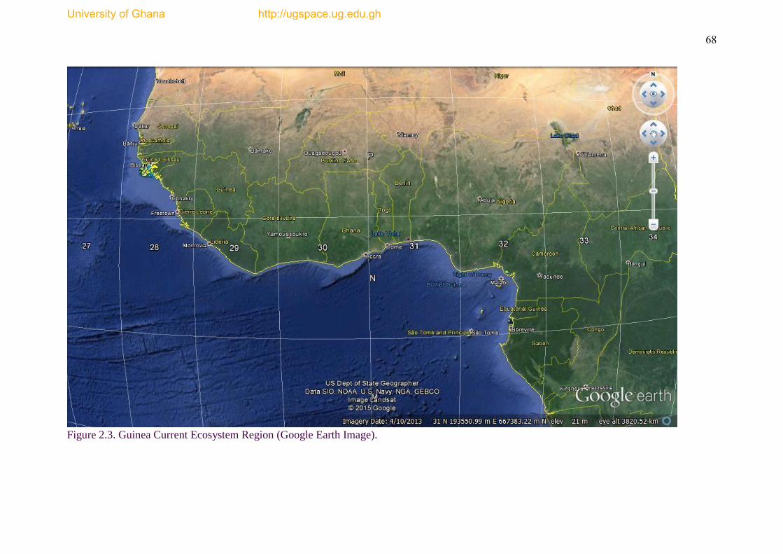
68
Figure 2.3. Guinea Current Ecosystem Region (Google Earth Image).
University of Ghana http://ugspace.ug.edu.gh

69
Figure 2.4. Large-scale oceanic circulation in the Atlantic Ocean including the
Guinea Current Ecosystem region. (Image Source: NASA)
University of Ghana http://ugspace.ug.edu.gh

70
CHAPTER THREE
MACROBENTHIC FUNCTIONAL TRAIT DIVERSITY AND COMMUNITY
STRUCTURE ALONG ENVIRONMENTAL GRADIENT
3.1 Introduction
The distribution of species and species‘ traits across environmental gradients can
provide an understanding of how assemblages that differ in diversity are composed
and their relative selection pressures (McGill et al., 2006). Comparing assemblages
at local scales can often yield more insights into processes that drive diversity
compared to global or regional scales (Gaston, 2000). However, a challenge to
understanding various local processes is the comparison of assemblages with
differing abundances in space and time, different histories (Underwood and Petraitis,
1993) and differing climatic and environmental settings. One approach for
comparing diversity is to compare the spatial distributions of species at different
geographic localities to look for generalities in community composition or habitat
use (MacArthur, 1972; Warwick and Ruswahyuni, 1987, Thrush et al., 2005). Many
of these approaches have been employed in most terrestrial ecosystems with the
marine counterparts lagging behind.
The marine ecosystems are composed of three units: (i) the physical environment
(e.g. seabed structure, sediment composition, waves, currents and water
temperature), (ii) the chemical environment (e.g. substances such as carbon, oxygen,
nitrogen and phosphorus and properties such as salinity and pH) and (iii) the biotic
environment (the assemblages of living organisms present in the system, ranging
University of Ghana http://ugspace.ug.edu.gh
71
from micro-organisms up to macroalgae, large marine mammals and humans)
(Bremner, 2005). Recent evidence suggests that environmental conditions are
intricately linked to biological traits, and hence ecological functioning (Bremner,
2006). Environmental conditions are all the things outside an organism that affect it
but, in contrast to resources, are not consumed by it (Begon et al., 1990). The
environment of an organism consists of all those phenomena outside an organism
that influence it, whether those factors are physical (abiotic) or are other organisms
(biotic) (Olff et al., 2009). Increasing moderation in environmental conditions leads
to increased abundances, more complex trophic structure, and increased influence of
species interactions on structure (Menge, 2000; Menge and Branch, 2001).
The main environmental gradients that have been associated with variation in species
diversity are energy-related variables (i.e., temperature), precipitation, productivity
and habitat heterogeneity (Currie, 1991; Rahbek and Graves, 2001; Hawkins et al.,
2003). Models which have been suggested for understanding community dynamics
include ‗‗environmental stress models‘‘ and either ‗‗nutrient/productivity models‘‘
or the ‗‗food chain dynamics hypothesis‘‘ (Connell, 1975; Oksanen et al., 1981;
Fretwell, 1987; Menge and Olson, 1990; Menge, 2000). Environmental stress models
assume that community structure results from species interactions and disturbances,
and how these are modified by underlying gradients of environmental stress (where
stress is a consequence of environmental conditions such as temperature, moisture,
salinity, etc.) (Menge et al., 2002).
The two models postulate that communities can be ordered along environmental
gradient. McGill et al. (2006) argued that general principle in community ecology
University of Ghana http://ugspace.ug.edu.gh
72
may not be achieved if research continues to focus on pair-wise species interactions
independent of the environment. They suggested four research themes: functional
traits, environmental gradients, interactions milieu and performance currencies, in
order to bring general patterns to community ecology. Relatively few studies have
explicitly incorporated structuring abiotic (environmental gradient) and biotic
(movement, dispersal) features that are key to species co-existence and vital for the
maintenance of species diversity (Loreau et al., 2003). The number of species in a
community are influenced by a variety of factors (e.g., physical stress, nutrient
availability, consumer pressure, habitat destruction), which result in non-random
diversity gradient in natural habitats (Zavaleta, 2004; Srivastava and Vellend, 2005).
From a theoretical point of view, functional diversity decreases with increasing
environmental constraints or stress (Mouillot et al., 2006). When environmental
constraints increase, coexisting species are more likely to be similar to one another
because environmental conditions (i.e., abiotic properties of the habitat) act as a
filter, allowing only a narrow spectrum of species to survive. The species that make
it through the environmental filters are likely to share many biological/ecological
characteristics through the niche filtering concept (Franzen, 2004; Statzner et al.,
2004). More precisely, environmental factors could limit the presence of certain
functional traits at certain sites and thus decrease functional diversity of local
communities in sites under environmental pressure such as confined parts in lagoons
(Mouillot et al., 2006).
Global species distributions are generally believed to be determined by abiotic
influences related to oceanographic and physiographic properties (Sanders, 1968;
University of Ghana http://ugspace.ug.edu.gh

73
Richlefs and Schluter, 1993). For instance, water motion affects biology by acting as
a transport mechanism for organisms and their propagules, as a dynamic boundary
between regimes, and as a force to which organisms must adapt or respond, for
example, in their feeding and locomotor activities (Nowell and Jumars, 1984; Denny,
1993). Thus mechanisms of species assemblages depend strongly on various
environmental conditions. However, the variability of species along major
environmental gradients in many components of biodiversity remains poorly
understood.
Nevertheless, environmental conditions and processes that occur at a variety of
spatial scales are critical elements to understand patterns of species assemblages.
Analysis of spatial patterns along environmental gradient at different scales is seen
as a logical requirement to deal with spatial and temporal confounding (Hurlbert,
1984), and provides tests for generality of models of species assemblages. There are
limited studies that have tested the consistency of patterns along sharp environmental
gradients at hierarchies of spatial scales (e.g., Benedetti-Cecchi, 2001). A better
understanding of the role played by abiotic factors is a key prerequisite for
forecasting the effects of shifts in environmental conditions on species diversity (or
species traits), as a result of human pressure, and for setting up adequate policies for
marine conservation and management (Terlizzi and Schiel, 2009).
The use of traits to predict functional response to environmental change has
developed rapidly over the last two decades (Grime et al., 1988; Woodward and
Diament, 1991; Chapin et al., 1993; McIntyre et al., 1995; Gitay and Noble, 1997;
Poff, 1997; Purvis et al., 2000), including studies on traits related to the probability
of extinction (e.g. Davies et al., 2000; Williams et al., 2005) and invasion (e.g.
University of Ghana http://ugspace.ug.edu.gh

74
Grotkopp et al., 2002; Hamilton et al., 2005; Olden et al., 2006). The community
assemblage that will affect ecosystem properties is the result of sorting processes
among individuals with appropriate response traits (Weiher et al., 1998; Grime,
2006). These response traits may encompass response to environmental change,
directly and response through compensatory dynamics due to consequent changes in
species interactions. The altered community will impact ecosystem processes via
changes in the representation of ecosystem-effect traits. Suites of effect on traits are
often reliable predictors of ecosystem function (Chapin et al., 1996; Diaz and
Cabido, 2001; Garnier et al., 2004) across a wide range of ecosystem types (Grime et
al., 1997; Reich et al., 2003; Diaz et al., 2004; Kremen, 2005), and understanding of
how traits affect various ecosystem properties is a currently growing area of research
(Suding et al., 2008).
The species trait diversity effects on ecosystem processes are the degree to which
abiotic conditions constrain the functional variations within communities that
influence the processes within the system (Hopper et al., 2002). Consequently,
merging our understanding of ecosystem level controls with our understanding of
community dynamics and assembly is an important focus of future study (Thompson
et al., 2001). Functional diversity is increasingly used to understand the biodiversity-
environment relation and biodiversity-ecosystem functioning and to decipher the
effect of anthropogenic activities on ecosystem (Dimitriadis and Koutsoubas, 2011).
Studies using functional traits to test the strength of different processes of
community assembly often find that habitat filtering plays a key role in the
communities‘ formation (Paine et al., 2011; Katabuchi et al., 2012; Shipley et al.,
University of Ghana http://ugspace.ug.edu.gh
75
2012). However, it is important to recognize that in many cases there is also
evidence that in varying degrees, other processes (e.g. limiting similarity, dispersal
limitation) play a role in the formation of the community structure (Cornwell and
Ackerly 2009; Katabuchi et al., 2012; Shipley et al., 2012).
There has been an overall lack of studies accounting for the fact that communities
assemble across environmental gradients (McGill et al., 2006). This chapter of the
thesis focuses on quantifying assemblage patterns of functional traits and assesseses
whether those patterns are the results of gradient in abiotic factors. The study
hypothesizes that multiple functional traits influence macrobenthic community
structure, and that traits relating to primary strategy or ‗ecological syndrome‘ (sets of
traits that are collectively associated with adaptation to particular environment
change (or gradient) (see Grime, 2001; Lavorel et al., 2007), will be similar among
species; and also, the dominant traits exert the strongest control on ecosystem
processes.
University of Ghana http://ugspace.ug.edu.gh
76
3.2 Materials and Methods
3.2.1 Study Area
The study locality is within the Guinea Current Large Marine Ecosystem (GCLME)
which borders 16 countries from Bissagos Island in Guinea Bissau to Angola in
Western Africa. It is number 28 of the 66 globally delineated large marine
ecosystems (LMEs) (IOC, 2013). The sampling extended from Bissagos Island to
Cape Lopex in Gabon and comprised of 11 countries (Figs. 2.3 and 3.1).
The GCLME is characterized by distinctive bathymetry, hydrography, chemistry and
trophodynamics. The Guinea Current System represents a Large Marine Ecosystem
(LME) ranked among the five most productive coastal and offshore waters in the
world with rich fishery resources, oil and gas reserves, precious minerals, a high
potential for tourism and serves as an important reservoir of marine biological
diversity of global significance (Sherman, 1993; Ukwe, 2003).
3.2.2 Field Sampling
Soft-bottom macrobenthic fauna samples were collected in replicate from the
Bissagos Island (Guinea Bissau) in the north to Cape Lopez (Gabon) in the south of
the GCLME onboard RV Fritdjorf Nansen as part of the GCLME fisheries resource
survey from May to July 2007. In all four stations were sampled for sediment in each
of the GCLME country, using a van Veen grab of surface area of 0.1m2
. At each
station, two replicate sediment samples were in order to ensure sample
representativeness due to the patchiness in the macrobenthic community.
The sediment samples were washed through a 0.5 mm mesh size sieve using filtered
seawater.
University of Ghana http://ugspace.ug.edu.gh
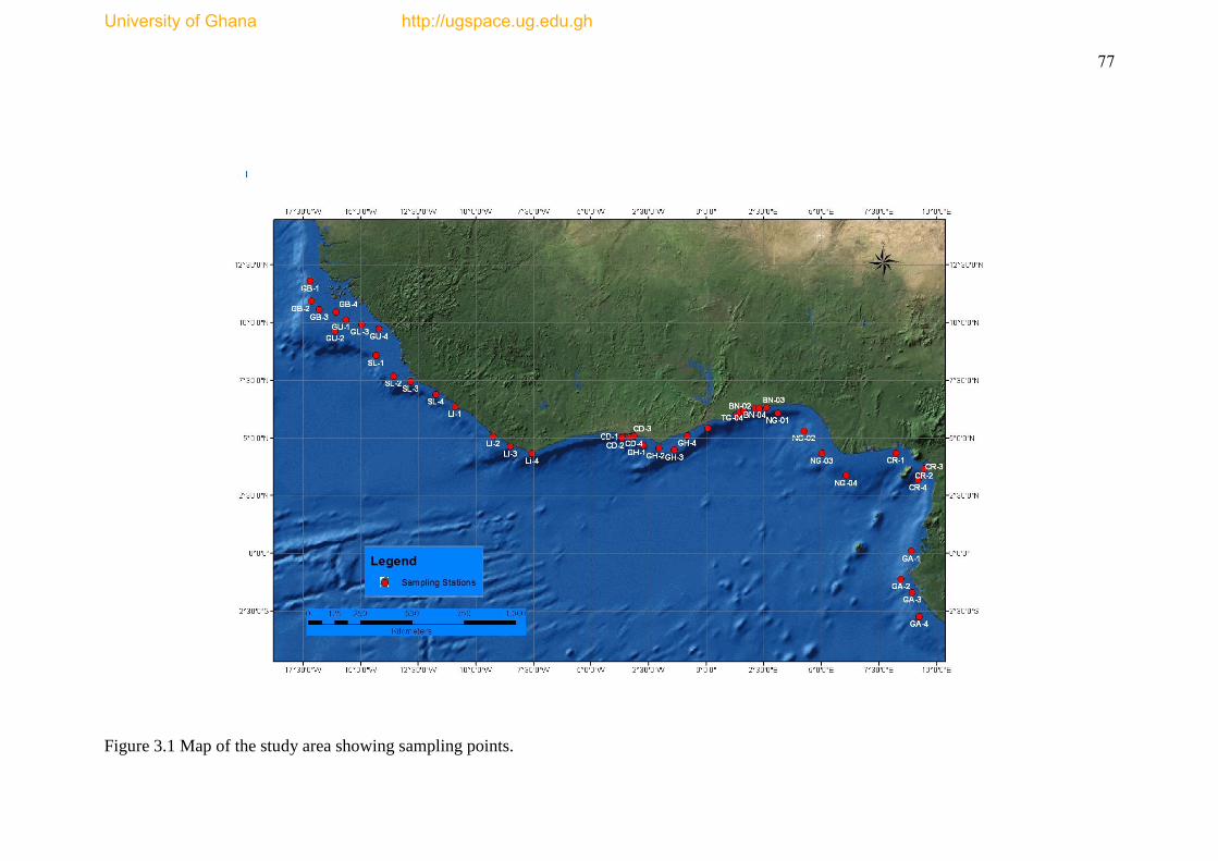
77
Figure 3.1 Map of the study area showing sampling points.
University of Ghana http://ugspace.ug.edu.gh
78
The retained samples on the sieve were transferred in turns into inner and outer-
labeled wide neck plastic sample holding containers and fixed with borax pre-
buffered with 10% formaldehyde solution for taxonomic identification in the
laboratory. The labeling followed a format of the station name and number (i.e.
country first 2 initial letters), date, replicate type, and fixative used (e.g. GB-03,
08/05/06, 1/3, Formalin). Each grab sample was evaluated on suitability of
acceptance as good grab sample. For instance, an acceptable grab sample has the top
layer of the sediment intact and not disturbed and also if +51% of the sample were
retrieved from the grab (Holme and McIntyre, 1971; Eleftheriou and Holme, 1984).
The top 2cm of each sediment sample was sub-sampled for physical and chemical
analyses. This was done using a 2 cm deep Kynar-coated scoop and placed into
separate jars as follows:
500 ml container for organic carbon content analysis (samples were frozen);
250 ml container for chemical analyses (samples were frozen);
ziplock bag for grain size analyses.
3.2.3 Field Quality Control
Basic quality control measures were followed for sediment macro-infauna sampling.
These measures were based on internationally accepted Standard Operation
Procedures (SOPs) in benthic sampling to ensure quality of the information gathered
(Holme and McIntyre, 1971; Eleftheriou and Holme, 1984; ASTM, 2006). Among
others, the following field quality control procedures and measures were observed:
Sediment samples collected at each station were ensured that they meet
international sample acceptance criteria. These include:
University of Ghana http://ugspace.ug.edu.gh
79
o Incomplete closure of grab
o Inadequate sediment samples
o Lack of surficial water
Only experienced persons assisted with the sediment sampling, sieving,
fixation and preservation.
Sediment was sieved with gentle flowing water hose to avoid squashing of
organisms.
All sieves were backwashed into storage containers after sieving to ensure
that organisms at the crevices of the sieve are removed.
Chemicals solutions such as formalin and ethanol for fixation and
preservation respectively were carefully and properly prepared.
Injurious and harmful chemicals were adequately labelled and stored in
appropriate cabinet.
3.2.4 Laboratory Processing of Samples
The processing and analyses of samples were performed in the Department of
Fisheries and Marine Science , University of Ghana laboratory for the sediment biota
and the activities included sorting of organisms (picking target organisms from the
sediment grains), preservation and taxonomic identification. For the abiotic
component both physical and chemical analyses were carried out on the sediment
samples and these are described in section 3.4.
The sample sorting involved emptying the contents of the fixed samples into 0.5 mm
mesh sieves and thoroughly washing with fresh water to get rid of all silt/clay
particles, as well as the formaldehyde fixative. The samples were then put into a tray
University of Ghana http://ugspace.ug.edu.gh
80
with a white background and macrobenthic faunal organisms sorted into preservation
vials containing 70% ethanol premixed with glycerol to prevent evaporation of the
ethanol.
3.2.4.1 Taxonomic Identification
The preserved organisms were put into petri dishes and identified to the lowest
taxonomic units as possible using Leica 2000 dissecting and compound microscopes.
Enumeration of individual species was carried out after the identification. Various
taxonomic guides were used in the species identification including Day, (1967ab);
LeLœuff and Intes, (1974); Fauchald, (1977); Edmunds, (1978); Intes and Lœuff
(1984); Kirkegaard, (1988); Cosel, (2006) and Rakel, (2007).
With regards to taxonomic identification, quality assurance measures were observed
in the laboratory to ensure that the quality and the integrity of the data from the
laboratory processes were not compromised. The following procedures were used.
Each sorted sample was crosschecked by other benthic expert to ensure that
all organisms had been picked before sample was discarded.
Species identification was verified independently by a colleague expert.
Unidentified species were assigned the genus name followed by 'sp.' (if only
one species, e.g. Glycera sp.) or 'spp.' (i.e. more than one species, e.g. Eunice
spp.) and put separately into vials for later identification.
Organisms preserved in vials were annotated with relevant information on
non-wettable sheets.
Data entering into computers were verified by another person to avoid wrong
entering.
University of Ghana http://ugspace.ug.edu.gh

81
3.2.4.2 Laboratory Analysis of Abiotic Data
The abiotic data collected were physical (grains size), and chemical (total organic
carbon, nutrients [i.e. nitrate, phosphate], calcium, sodium, potassium and
magnesium).
3.2.4.3 Analyses of Physical Parameters
Prior to the sediment grain size fraction analysis, the sediment samples were air-
dried, sieved through 200 mm mesh size sieve. The Bouyoucos Methods
(Bouyoucous, 1934) was used for the grain-size analysis. The method is based on the
principle that sediment particles were expected to settle in water at a speed directly
related to the square of their diameter and inversely related to the viscosity of the
water. As regards the Bouyoucous Method, forty grams (40 g) of the air-dried,
homogenized and sieved samples were transferred into polyethylene containers and
then 100 ml of calgon solution was added to disperse the particles. The solution was
stirred on a mechanical shaker for 90 minutes and then transferred into a
sedimentation cylinder after sieving through 45 µm.
The retained sand fraction was put in a moisturizing container and 5ml of hydrogen
peroxide was added to dissolve any organic matter present. The sample was oven
dried overnight at a temperature of 105o C, each sample was weighed afterwards.
The suspension was poured into a cylinder and made up to the 1 litre mark with
distilled water. The sediment particles were thoroughly stirred with a hand stirrer and
after five hours a hydrometer was carefully inserted into the suspensions and the
readings were taken. The hydrometer readings for a blank were also taken. This was
subtracted from the original hydrometer readings to give the actual weight of the
University of Ghana http://ugspace.ug.edu.gh
82
clay fractions. The weights of both the clay and sand fractions were calculated in
terms of percentages with respect to the initial weight taken, and the sum of their
combined weight was subtracted from 100 to give the percentage weight of the silt.
3.2.4.4 Chemical Analysis
Total Organic Carbon
The organic carbon content determination was carried out at the Ecological
Laboratory of the University of Ghana using the ELTRA 5500 C-S determinator.
The samples were pretreated with 10% hydrochloric acid to remove the inorganic
carbonates. The sediment samples were oven-dried at 60oC for 12 hours to get rid of
the moisture. The samples were then weighed individually and transferred into a
weighing boat of size 1.5 x 0.15 cm. The samples were then sent into an ELTRA
C5500 C-S determinator, with a furnace combustion temperature of about 1100oC.
After the combustion the percent organic carbon of the samples were determined and
recorded.
Sediment Nutrient Determination
Five grams (5 g) of each sediment sample was weighed into a beaker and 0.75M KCl
solution was added for extraction, after which the samples were shaken vigorously
for 1 hour. The resultant solution was filtered and 25ml of it taken for analysis of
nitrate and using the HACH DR/2010 Spectrophotometer following the methods in
A.P.H.A. et al., (1998). However, for phosphate analysis the EDTA method
(Golterman, 1996) was used for the P-extraction.
University of Ghana http://ugspace.ug.edu.gh

83
Elemental Analysis
The sediments were first dried to get rid of excess water and later oven-dried at a
temperature of 50oC to attain a constant mass. Sediments were then pounded into
powder form using a mortar and pestle. They were later passed through a 63µm sieve
(silt fraction) and later kept in labeled transparent polythene bags for analysis. One
hundred milligrams (100 mg) of each sample was enveloped via thermal sealing
inside 5×5 cm2
polyethylene thin film, which was heat-sealed in 8.9 cm3
rabbit
capsule for irradiation. Initially, the polyethylene film and rabbit capsules were
cleaned by soaking them into dilute nitric acid for three days and washed with de-
ionized water.
The sediment samples were analyzed by Instrumental Neutron Activation Analysis
(INAA). The neutron flux used for the irradiation was approximately 5.0.10
11 n
.cm
–
2.s
–1. The samples were sent into the Miniature Neutron Source Reactor (MNSR) by
means of a pneumatic transfer system operating at a pressure of 25 atmospheres. The
scheme of the irradiation was chosen so as to take into account the half-lives of the
radionuclides under investigation. In that regard, the following irradiation times were
selected: 10 seconds for the short-lived radionuclides; 3600 seconds for the
intermediate radionuclides; and 14400 seconds for long-lived elements.
After a short decay period the activity of the gamma-ray emitting radionuclides with
short and medium half-lives were measured. The measurements of the gamma-ray
spectral intensities were made using a spectroscopy system of high purity
germanium (HPGe) N-type coaxial detector Model GR 2518; high voltage power
supply Model 3105; and a spectroscopy amplifier Model 2020 (all manufactured by
Canberra Industries, Inc.). The detector system at fixed geometry was coupled to an
8k Ortec multichannel analyzer (MCA) emulation card and a 486 microcomputer.
University of Ghana http://ugspace.ug.edu.gh
84
The resolution of the detector system which operates at a bias voltage of –3000 V
full width at half maximum (FWHM) was 1.8 keV for 60
Co 1332 keV gamma-ray
with 25% relative efficiency.
The output spectral intensities of both the analytical samples and the standards were
processed and stored in the microcomputer software by means of the MCA card.
Qualitative analysis of the radioisotopes was achieved by means of identifying their
spectral intensities. The evaluations of the areas through integration under the photo
peaks of the identified elements were converted into their concentrations using the
comparator method (Dampare et al., 2005).
3.2.5 Functional Trait Analysis
The statistical analyses of the data was preceded by functional trait categorization as
described in the ensuing sections. The macrobenthic fauna species were categorized
using biological traits. The selection of biological traits and their categorization was
dictated by i) available information, ii) ecological functions and iii) perceived
sensitivities to environmental disturbance. The selected biological traits reflect
morphology (e.g. body size and form) and behaviour (adult mobility, sociability and
feeding habit). Some of these traits directly reflect ecological functions (e.g. food
and feeding habits), whereas others are indirect indicators. For example, body size
indicates the ratio of production/biomass and of production/respiration, beacuase for
invertebrate populations in most aquatic systems, the ratios of production/biomass
and of production/respiration are closely related to the maximum size achieved by
the different taxa (Statzner, 1987). Size also has implications for many other
ecological functions and considered to be an important trait of organisms because it
University of Ghana http://ugspace.ug.edu.gh

85
correlates with many aspects of its biology (e.g. metabolism, growth and
reproduction) (Calder, 1984). The selected biological traits were further divided into
categories as indicated in Table 3.1.
University of Ghana http://ugspace.ug.edu.gh

86
Table 3.1 Biological traits categorization
Numbers Adult Body
Size [BS]
Adult Mobility
[AM] Feeding Habit [FH]
Feeding
Structure [FS]
Sociability
[S]
Adult Body
Form [BF]
1 0.5-20mm Sessile Deposit-feeding Mandible Solitary Vermiform
2 20.5-40mm Crawl Filter/suspension Jaw Gregarious Cylindrical
3 40.5-60mm Burrow Opportunist/scavenger Proboscis Colonial Slender
4 60.5-80mm Swim Predator Palp Commensal Flattened
5 80.5-100mm Creep Herbivore Pharyngeal
Elongated
6 >120mm Glide Omnivore Tentacle
Tapered
University of Ghana http://ugspace.ug.edu.gh
87
3.2.5.1 Ecological and Biological Traits
Characteristics describing living modes of the organisms were classified in the
ecological traits. These traits have a strong effect on ecosystem functioning and
occur in most of the macrobenthic organisms. Mobility was described in the scale of
the capacity of the organisms to move in and outside of the sediment. Semi-mobile
organisms have the ability to move but they do so only if necessary and usually very
slowly. Mobility is an important ecological trait because it affects the capture
method of prey organisms or other food resources and defines the trophic
relationships of a benthic community.
The chosen morphological traits are important indicators of sediment condition
(sediment type and organic loading concentration). The average weight of an adult
individual was used to assign the organisms to the body size categories. The second
characteristic of the morphological traits was the body form. The attribute ―shell‖
describes all the organisms having external protecting structures while vermiform are
considered all the worm-like organisms with or without segmentation (length
width) (Papageorgiou et al., 2009).
3.2.5.2 Functional Trait Classification and Categorization
For every species, information was assigned in each trait catogory. The data on the
species traits was gathered from a variety of literature and internet sources. The
functional composition of the samples was determined using biological
(morphological) and ecological traits based on the fact that traits that affect resources
use (e.g., energy and nutrients), feeding interactions, habitats modification
University of Ghana http://ugspace.ug.edu.gh
88
(bioturbation and habitat providers) are recognized for their functional importance
(Pearson, 2001; Meysman et al., 2006; Hastings et al., 2007) and are wide ranging
(Bremner, 2008). As a result, six biological and ecological traits were used in the
functional classification analysis. These described the morphology and behaviour of
the macrobenthic invertebrates, reflecting their involvement in ecosystem processes
and perceived sensitivities to environmental disturbance (see Snelgrove et al., 1997;
Jennings and Kaiser, 1998; Bolam et al., 2002; Coleman and Williams, 2002; Thrush
and Dayton, 2002). Each of the six traits were sub-divided into categories, for
example the trait ‗feeding habit‘ contained the categories deposit-feeder,
filter/suspension feeder, opportunist/scavenger and predator (Table 3.1). As a result,
each species at each sampled station was assigned its biological and ecological traits
(see Appendices I & II), and the total traits were determined for each station under
each of the selected trait in Table 3.1. Further, statistical analyses of the traits and
their categorization were carried out as described in section 3.3.
The selected traits are likely to bring out the effect and response to environmental
drivers. For instance traits such as adult size is likely to change with severity of
disturbance (Pearson and Rosenberg, 1978), feeding type of the species determine its
ability to utilize/tolerate a new diet (Fauchald and Jumars, 1979). Mobility and and
sociability can be related to recovery patterns and resilience to disturbance (Thrush
and Whitlatch, 2001). Size and living habits indicate the ability to rework the
sdiment affecting sediment biogeochemistry (Michaud et al., 2006) providing a link
to ecosytem function.
University of Ghana http://ugspace.ug.edu.gh
89
3.3 Statistical Analysis
The data sets were analysed using suites of univariate and multivariate statistics.
Basic statistics of the species abundance were calculated as well as distributional
trends of the major macrobenthic taxa and dominant functional traits across the
sampled stations. Macrobenthic species abundance data were grouped into major
taxa namely polychaeta, mollusca, crustacea, echinodermata and ‗Others‘. Wet-
weight biomass of these major taxa were determined across the stations.
The frequency of occurrence of the data sets (taxonomic diversity and functional
richness) were calculated using the F index described by Guille (1970):
F=pa/P × 100 (1)
where: pa, is the number of stations where the species occurred and P is the total
number of stations. Using this formula the species (and also functional traits) data
were classified as: constant (F>50%), common (10%<F<49%) and rare species or
traits (F<10%). The data sets were refined and all the rare taxonomic species and
functional traits (F<10%) were eliminated from the data sets as they could
potentially introduce ‗noise‘ in the statistical analyses. In certain instances, only
data for constant taxonomic species and functional traits were used in the statistical
analyses. These have been indicated in the appropriate sections of the thesis.
For multivariate analysis, dendrograms of Bray-Curtis similarity index of the
composite station data for the GCLME countries were calculated for taxonomic
species abundance and fucntional trait richness using the PRIMER v6 package
(Clarke and Gorley, 2006). The data sets were first fourth-root transformed to
stabilize and normalize the variance (Clarke and Green, 1988). Using a complete
University of Ghana http://ugspace.ug.edu.gh

90
linkage, sample (country and biological traits) classifications were produced and
thereafter samples (i.e., countries and traits) related to each other identified based on
the resulting similarity matrix. The differences in the samples (i.e., GCLME
countries ) were assessed with one-way ANOSIM (Clarke and Warwick, 1994).
In order to demonstrate the most important abiotic variables related to assemblage
patterns of the taxonomic and functional traits, various statistical tools were
employed. Forward selection in a Canonical Correspondence Analysis (CCA) and
Redundancy Analysis (RDA) ordinations in the CANOCO package and rank
correlations between cluster matrix with the program BIO-ENV (Clarke and
Ainsworth, 1993) in the PRIMER package and Multiple Linear Regression Analysis
(MLRA) were utilized.
In the CCA and RDA analyses, the proportion of the total faunal variance (= sum of
all eigenvalues, called total inertia in CANOCO) which can be accounted for by the
environmental variables can be estimated as the ratio of eigenvalues of constrained
versus unconstrained axes. From this ratio, the percentage value which indicates the
percentage explanation of each separate environmental variable to the total fauna
and trait variance was calculated. Constrained axes are constructed to maximise the
fit with linear combinations of environmental variables, and remaining,
unconstrained axes represent a residual variation in data after extracting the
constrained axes.
For the functional trait data, the RDA was performed (Ter Braak, 1986) for only
identified dominant functional trait data (the identified dominant trait contributed
University of Ghana http://ugspace.ug.edu.gh
91
35.6% and their selection as dominant traits was based on the F index, i.e., F>85%)
(Guille, 1970) and trait richness >4%. This technique ensured that rare traits and/or
traits with low spatial occurrence and contribution were eliminated so that the
analysis was refined and ‗noisy‘ data were not included. It is the author‘s view
that functional traits (or taxonomic species) with the highest spatial coverage
(based on the F-index) possess valuable ecological information, having adapted
naturally possibly through ecological filtering to the varied environmental
gradient, are key in unearthing the main environmental drivers of community
assemblages.
The RDA was run using the package CANOCO 4.5 (Ter Braak and Smilauer,
2002), which combines both ordination and regression to ascertain relationships
between species (and also species traits) and environmental variables (Ter Braak,
1986). None of the environmental variables utilized reported inflation factor >20
(Ter Braak and Smilauer, 2002) and as a result none was eliminated from the
RDA and CCA analyses. All the environmental variables used for the analysis
were transformed (Log (x + 1)) to stabilize and normalize the variance. In the RDA
biplot, the first and second axes represent the most important environmental
gradient along which the macrobenthic functional traits are linearly distributed. The
direction of each environmental vector represents the maximum rate of change for
that particular environmental variable and its length indicates the relative
importance to the ordination.
The significance of all primary RDA axes was determined by a Monte Carlo
permutation test (199 permutations) of the eigenvalues (Ter Braak and Smilauer,
University of Ghana http://ugspace.ug.edu.gh
92
2002). A forward selection procedure ordered the environmental variables according
to the amount of variance they captured in the trait data (Ter Braak and Verdonschot,
1995). In the first step of this method, all environmental variables were ranked on the
basis of the fit for each separate variable. Each variable was treated as the sole
predictor variable and all other variables were ignored; hence, the variance explained
represents marginal effects. At the end of the first step of the forward selection, the
best variable was selected. Hereafter, all remaining environmental variables were
ranked on the basis of the fit (amount of variance explained) that each separate
variable gave in conjunction with the variable(s) (covariables) already selected
(conditional or unique effects). At each step, the statistical significance of the variable
added was tested using a Monte Carlo permutation test (199 unrestricted
permutations) (Ter Braak and Smilauer, 1998). This description of RDA is similar to
the CCA used for the taxonomic species and functional trait data sets except that the
RDA is a linear ordination whilst CCA is unimodal (weighted averaging).
Bio-Env analysis was the second method used for extracting important explanatory
variables from the taxonomic species and functional traits data. This harmonic
analysis uses a weighted Spearman's rank correlation between the resulting ranked
similarity matrices which underlie the MDS ordinations (or the dendrogram) of
species or traits and correlation-based. The variable or combinations of variables
which give the highest correlation coefficient is assumed to be the most important
explanatory vanable(s).
In order to confirm the explanatory variables and develop a simple model, the
taxonomic species and functional traits data were subjected to step-wise linear
multiple regression analysis. The analysis not only select the best explanatory
University of Ghana http://ugspace.ug.edu.gh

93
environmental variable to the dependent variable (ie., species diversity, functional
richness, and dominant functional traits) but also create a signifcant predictive model
of the dependent variables.
University of Ghana http://ugspace.ug.edu.gh
94
3.4 RESULTS
3.4.1 Macrobenthic Fauna Community Structure
The analysis of the taxa resulted in a numerical abundance of 3,048 individuals
(mean density = 693±579 indi/m2) comprising 381 species that belong to five major
taxonomic groups namely: Polychaeta, Crustacea, Mollusca, Echinodermata and
‗Others‘. Of the total numerical abundance, polychaetes contributed 55.15%,
crustaceans accounted for 28.02%; 12.76% was contributed by species placed in
―Others‖ category, while molluscs and echinoderms accounted for 2.23% and 1.84%
respectively (Table 3.2). Species placed in ‗Others‘ category included cnidarians,
sponges, sipunculids etc.
In terms of number of species, polychaetes comprised 233 species (61.32%),
crustaceans consisted 71 species (18.64%), 35 species (9.19%) were molluscs,
whereas echinoderms and ―others‖ category constituted 10 (2.63%) and 32 (8.39%)
species respectively. Polychaetes taxa contributed substantially and ranked highest in
terms of species richness and numerical abundance among the major macrobenthic
taxa in the study area. Crustaceans ranked second highest in terms of species
richness and numerical abundance. The dominant polychaete and crustacean species
could constitute important food resources for many commercially important
demersal fish species.
University of Ghana http://ugspace.ug.edu.gh

95
Table 3.2 Abundance and richness of major macrobenthic faunal groups.
Taxa
No. of Species
Abundance
(No. of indi.)
Abundance (%)
Polychaeta 233 1681 55.15
Crustacea 71 854 28.02
Mollusca 35 68 2.23
Echinodermata 10 56 1.84
Others 32 389 12.76
Total 380
3048
100
The distribution pattern of these macrobenthic fauna may therefore determine the
abundance of demersal fish stocks on the continental shelves of the GCLME as the
fish prey on these. The spatial pattern of all the major macrobenthic faunal taxa is
shown in Figures 3.2-3.13. The distribution pattern generally depicts two abundance
peaks especially for polychaetes, crustaceans and molluscs (Fig. 3.2). The lowest
abundances were noted from Guinea Bissau to Sierra Leone, with Guinea being
exception, while the highest abundances occurred in the central sections from Ghana
to Benin. Cameroon and Gabon recorded the lowest numerical abundance (Fig. 3.2).
The highest abundance of echinoderms occurred at Guinea Bissau (Fig. 3.2) but with
low species richness (Fig. 3.3) depicting dominance of few species, which could
suggest conditions tolerable to few species. The highest crustacean abundance and
richness was noted at Guinea (Figs. 3.2 and 3.3). Nonetheless, the composite
abundance and richness data indicated that Togo, Benin and Ghana, and Guinea
ranked highest. The composite data indicated considerable differences in species
abundances and richness in Togo, Benin, Ghana and Guinea with the other GCLME
countries (Figs. 3.2 and 3.3).
University of Ghana http://ugspace.ug.edu.gh

96
Figure 3.2 Spatial distribution of major macrobenthic fauna abundance on the continental shelves of the GCLME countries. See
Table 3.3 for the codes used on the x-axis.
0
50
100
150
200
250
300
350
400
450
500
GB GU SL LI CI GH TG BN NG CR GA
Ab
un
dan
ce (N
o.
of
ind
i.)
Country
POLYCHAETA
0
50
100
150
200
250
300
GB GU SL LI CI GH TG BN NG CR GA
Ab
un
dan
ce (N
o.
of
ind
i.)
Country
CRUSTACEA
0
2
4
6
8
10
12
14
16
18
20
GB GU SL LI CI GH TG BN NG CR GA
Ab
un
dan
ce (N
o.
of
ind
i.)
Country
MOLLUSCA
0
2
4
6
8
10
12
14
16
18
GB GU SL LI CI GH TG BN NG CR GA
Ab
un
dan
ce (N
o.
of
ind
i.)
Country
ECHINODERMATA
0
20
40
60
80
100
120
GB GU SL LI CI GH TG BN NG CR GA
Ab
un
dan
ce (N
o.
of
ind
i.)
Country
OTHERS
0
100
200
300
400
500
600
700
800
GB GU SL LI CI GH TG BN NG CR GA
Ab
un
dan
ce (N
o.
of
ind
i.)
Country
TOTAL
University of Ghana http://ugspace.ug.edu.gh
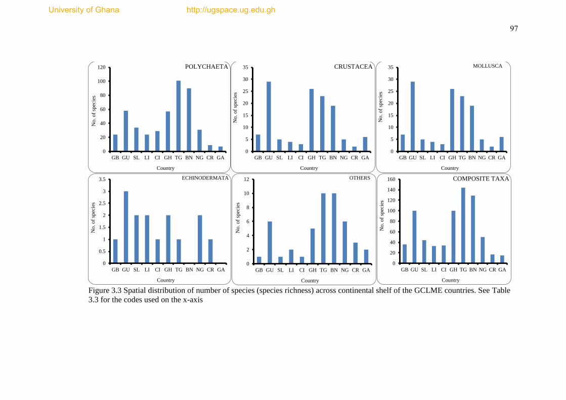
97
Figure 3.3 Spatial distribution of number of species (species richness) across continental shelf of the GCLME countries. See Table
3.3 for the codes used on the x-axis
0
20
40
60
80
100
120
GB GU SL LI CI GH TG BN NG CR GA
No.
of
spec
ies
Country
POLYCHAETA
0
5
10
15
20
25
30
35
GB GU SL LI CI GH TG BN NG CR GA
No.
of
spec
ies
Country
CRUSTACEA
0
5
10
15
20
25
30
35
GB GU SL LI CI GH TG BN NG CR GA
No.
of
spec
ies
Country
MOLLUSCA
0
0.5
1
1.5
2
2.5
3
3.5
GB GU SL LI CI GH TG BN NG CR GA
No.
of
spec
ies
Country
ECHINODERMATA
0
2
4
6
8
10
12
GB GU SL LI CI GH TG BN NG CR GA
No.
of
spec
ies
Country
OTHERS
0
20
40
60
80
100
120
140
160
GB GU SL LI CI GH TG BN NG CR GA
No.
of
spec
ies
Country
COMPOSITE TAXA
University of Ghana http://ugspace.ug.edu.gh
98
3.4.2 Macrobenthic Faunistic Density
The total densities for the respective countries are presented in Table 3.3. The overall
total density for the study area was 9,525 indi/m2 (mean density = 865.9±723.2
indi/m2). The highest densities were sequentially observed with polychaetes,
crustaceans, ‗other‘ taxa, molluscs and echinoderms, which are consistent with the
pattern of the species abundance data. The densities of polychaetes, crustaceans and
molluscs across the GCLME countries showed similar patterns to that of the species
abundance (Figure 3.2). The patterns indicated two peaks and troughs. The highest
densites occurred between Ghana and Benin, followed by Guinea Bissau to Sierra
Leone, whiles lowest densities were noted between Liberia-Cote d‘Ivoire, and
Cameroon-Gabon
University of Ghana http://ugspace.ug.edu.gh

99
Table 3.3 Densities (Ind./m2) of major macrobenthic faunal groups in the continental shelves of countries bordering the GCLME.
Country
Country
ID
Polychaeta Crustacea Mollusca Echinodermata ‗Others‘ Total
Guinea Bissau GB 647 138 13 50 3 850
Guinea GU 628 791 13 16 91 1538
Sierra Leone SL 481 194 6 22 16 719
Liberia LI 134 25 3 19 19 200
Cote d’Ivoire CD 241 25 0 9 31 306
Ghana GH 478 669 34 31 178 1391
Togo TG 1438 391 59 6 313 2206
Benin BN 959 325 50 0 303 1638
Nigeria NG 166 53 28 19 225 491
Cameroon CR 47 22 6 3 19 97
Gabon GA 34 38 0 0 19 91
University of Ghana http://ugspace.ug.edu.gh

100
3.4.3 Dominant Macrobenthic Taxa
The analysis of frequency of occurrence (F-index) of the 381 identified
macrobenthic faunal species across the 44 sampling locations, indicated that 15
species (contributed 35% to species abundance) occurred in >20% of the sampling
stations. They may constitute cosmopolitan species with greater geographical
coverage and could be excellent biological candidates for monitoring the health of
the GCLME. These species were predominantly polychaetes, however, the highest
occurrence species (59.0%) was noted for a crustacean, Ampelisca spp. The
polychaete with the highest frequency of occurrence was Glycera sp. and Eunice
vittata in that order with 41% and 39% respectively (Table 3.4).
Table 3.4 Frequency of Occurrence for 15 numerical dominant macrobenthic
fauna. For brevity only taxa contributing >20% were selected. P= Polychaete,
C=Crustacean, O= ‗Others‘ taxa .
Taxa Frequency of Occurrence (%)
Ampelisca spp. (C) 59.0
Glycera sp.(P) 41.0
Eunice vittata (P) 39.0
Sipunculid spp. (O) 39.0
Lumbrinereis aberrans (P) 32.0
Tanaid spp. (C) 30.0
Mysid sp. (C) 27.0
Armandia intermedia (P) 25.0
Prionospio pinnata (P) 25.0
Scoloplos madagascariensis (P) 25.0
Aricidea fauveli (P) 23.0
Lumbrinereis latrelli (P) 23.0
Lumbrinereis coccinea (P) 23.0
Nepthys lyrochaeta (P) 23.0
Prionospio sexoculata (P) 23.0
University of Ghana http://ugspace.ug.edu.gh

101
The spatial distribution of the abundance of the 15 most occurred species is
presented as Figure 3.4. A striking feature of the distribution was the high numbers
of Prionospio pinnata (Spionidae) at Guinea Bissau (Fig. 3.4), which also revealed
higher numerical abundance for echinoderm but low taxa richness (Figs. 3.2 and 3.3)
suggesting the existence microhabitats that support certain species. Eunice vittata
(Spionidae) was also highest at Togo followed by Guinea Bissau (Fig. 3.4).
There were numerical dominance of different species across the GCLME countries
suggesting the existence of abiotic gradients supporting organismal life. Ampelisca
spp. for instance ranked highest in Togo followed by Guinea. Ostensibly, the 3 most
occurred crustaceans (Ampelisca spp., Tanaid & mysid) were collectively dominant
numerically in Guinea, which thus rank the country highest in terms of crustacean
abundance. Sipunculid spp. was dominant in Ghana but was visibly absent in Guinea
Bissau, Togo, Benin and Nigeria (Fig. 3.4). The countries with the lowest
representation of these most occurred species were Nigeria, Gabon, Cameroon,
Liberia, Cote d‘ Ivoire and to some extent Sierra Leone.
University of Ghana http://ugspace.ug.edu.gh
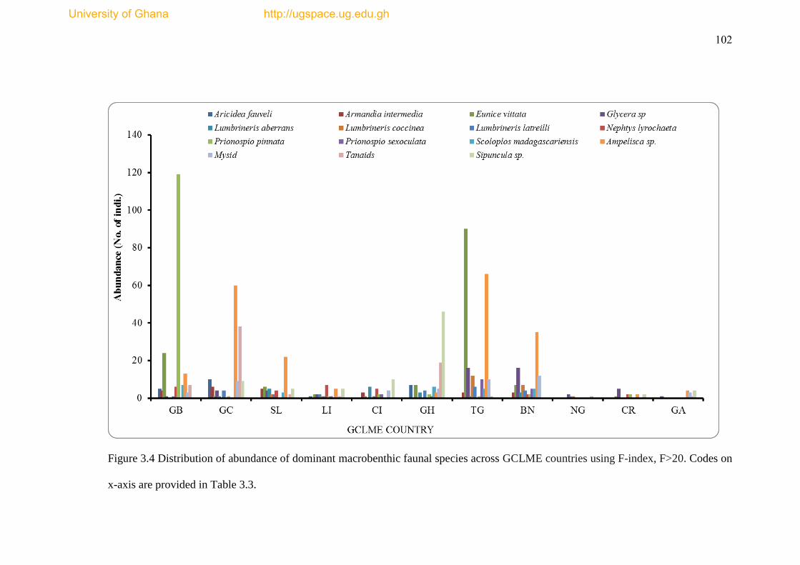
102
Figure 3.4 Distribution of abundance of dominant macrobenthic faunal species across GCLME countries using F-index, F>20. Codes on
x-axis are provided in Table 3.3.
University of Ghana http://ugspace.ug.edu.gh

103
3.4.4 Spatial Pattern of Sediment Abiotic Variables
The water depth the for the various sample stations ranged between 16 m and 153 m
(Appendix V) with the mean water depth of 54.7±33.7 m. However, 50% of the
stations had an average depth of 49 m.
The mean concentration levels and the distribution of the sediment abiotic variables
are presented in Figure 3.5. All the sediment parameters showed spatial differences
with peaking and troughing between the countries, but without discernible east-west
pattern. Average nitrate levels were higher at both west (Guinea Bissau, Guinea and
Sierra Leone) and east (Nigeria, Cameroon and Gabon) of GCLME than at the
central (Benin, Togo, Ghana, Cote d‘Ivoire and Liberia). There were considerable
within country spatial variations in the sediment parameters. Certain GCLME
countries, reported the highest mean concentrations namely phosphate in Benin,
sodium and organic carbon in Ghana, nitrate in Guinea Bissau, and silt in Cameroon
Calcium showed three spatial peaks at Sierra Leone, Gabon and Ghana in that
decreasing order. The lowest concentrations of calcium were noted at Togo, Benin
and Nigeria. However, the levels within Nigeria depicted the highest variations.
Total organic carbon and clay showed relatively similar pattern with Ghana
recording the highest mean concentrations.
Magnesium levels ranked highest at the western sections of the GCLME depicting a
similar pattern to ccalcium distribution. The lowest magnesium and calcium levels
occurred in Togo and Benin, which also depicted the highest species and dominant
University of Ghana http://ugspace.ug.edu.gh
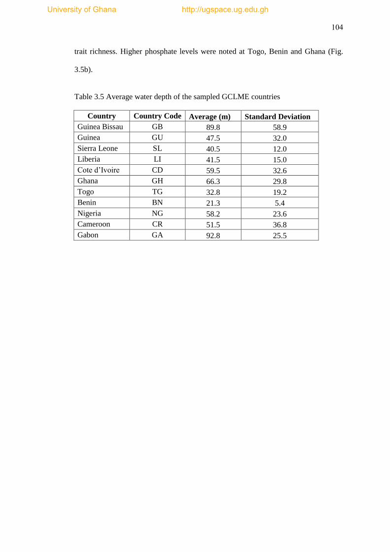
104
trait richness. Higher phosphate levels were noted at Togo, Benin and Ghana (Fig.
3.5b).
Table 3.5 Average water depth of the sampled GCLME countries
Country Country Code Average (m) Standard Deviation
Guinea Bissau GB 89.8 58.9
Guinea GU 47.5 32.0
Sierra Leone SL 40.5 12.0
Liberia LI 41.5 15.0
Cote d‘Ivoire CD 59.5 32.6
Ghana GH 66.3 29.8
Togo TG 32.8 19.2
Benin BN 21.3 5.4
Nigeria NG 58.2 23.6
Cameroon CR 51.5 36.8
Gabon GA 92.8 25.5
University of Ghana http://ugspace.ug.edu.gh
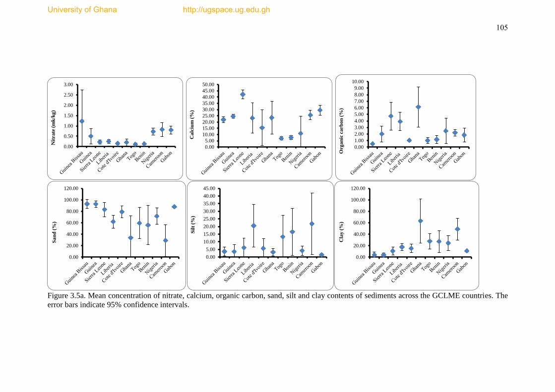
105
Figure 3.5a. Mean concentration of nitrate, calcium, organic carbon, sand, silt and clay contents of sediments across the GCLME countries. The
error bars indicate 95% confidence intervals.
0.00
0.50
1.00
1.50
2.00
2.50
3.00
Nit
ra
te (
mk
/kg
)
0.00
5.00
10.00
15.00
20.00
25.00
30.00
35.00
40.00
45.00
50.00
Ca
lciu
m (
%)
0.00
1.00
2.00
3.00
4.00
5.00
6.00
7.00
8.00
9.00
10.00
Org
an
ic c
arb
on
(%
)
0.00
20.00
40.00
60.00
80.00
100.00
120.00
Sa
nd
(%
)
0.00
5.00
10.00
15.00
20.00
25.00
30.00
35.00
40.00
45.00S
ilt
(%)
0.00
20.00
40.00
60.00
80.00
100.00
120.00
Cla
y (
%)
University of Ghana http://ugspace.ug.edu.gh

106
Figure 3.5b. Mean concentrations of magnesium, sodium, potassium and phosphate across the GCLME countries. The error bars indicate 95%
confidence intervals.
0.00
0.01
0.02
0.03
0.04
0.05
0.06
0.07
Ma
gn
esi
um
(m
g/k
g)
0.00
2.00
4.00
6.00
8.00
10.00
12.00
So
diu
m (
%)
0.00
1.00
2.00
3.00
4.00
5.00
6.00
7.00
8.00
9.00
Po
tass
ium
(%
)
0.00
1.00
2.00
3.00
4.00
5.00
6.00
7.00P
ho
sph
ate
(m
g/k
g)
University of Ghana http://ugspace.ug.edu.gh
107
3.4.5 Community Structural Analysis
An agglomerative Bray–Curtis similarity dendrogram of the pooled station species
abundance data to represent countries revealed three significant (p<0.05) groupings
based on the faunistic data (Fig. 3.6). Only Nigeria showed non-significant faunistic
structure with the other countries indicating either unique condition supporting
unique fauna or a stressful ecosystem. The first cluster ground (Group A) comprised
Cameroon, Liberia and Gabon. Cluster Group B is made up countries located at the
western part of the GCLME namely Guinea Bissau, Guinea, Sierra Leone, Cote d‘
Ivoire and Ghana. Ghana and Cote d‘Ivoire formed one sub-group under Group B
just as Guinea Bissau, Guinea and Sierra Leone. The last cluster Group C composed
of Benin and Togo, which showed the highest similarity index of 58%, followed by
Sierra Leone and Guinea at 54%, and together with Guinea Bissau at 47% (Fig. 3.6).
Liberia and Cameroon followed at 43% similarity before Ghana and Cote d‘ Ivoire
36%. The pattern shows high degree of spatial differences in the macrobenthic fauna
composition and abundance possibly due to prevailing gradients in environmental
conditions creating varied tolerable regimes for the organisms.
In order to test the level of similarity between the countries, the analysis of simlarity
(ANOSIM) test was run and the results indicated significant differences (p=0.001)
between the countries with the global R=51.2% (Table 3.6). However, the pairwise
test showed non-significant differences (p>0.05) between some countries notably
those bordering the western sections of the GCLME suggesting that the
macrobenthic fauna composition at those countries are relatively similar than the the
central and eastern sections of the GCLME.
University of Ghana http://ugspace.ug.edu.gh
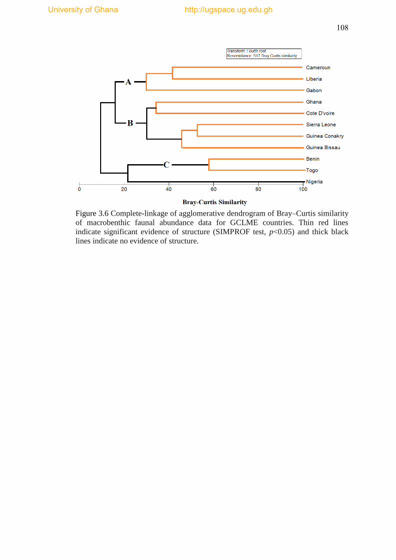
108
Figure 3.6 Complete-linkage of agglomerative dendrogram of Bray–Curtis similarity
of macrobenthic faunal abundance data for GCLME countries. Thin red lines
indicate significant evidence of structure (SIMPROF test, p<0.05) and thick black
lines indicate no evidence of structure.
University of Ghana http://ugspace.ug.edu.gh
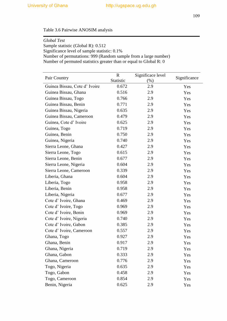
109
Table 3.6 Pairwise ANOSIM analysis
Global Test
Sample statistic (Global R): 0.512
Significance level of sample statistic: 0.1%
Number of permutations: 999 (Random sample from a large number)
Number of permuted statistics greater than or equal to Global R: 0
Pair Country R
Statistic
Significace level
(%) Significance
Guinea Bissau, Cote d‘ Ivoire 0.672 2.9 Yes
Guinea Bissau, Ghana 0.516 2.9 Yes
Guinea Bissau, Togo 0.766 2.9 Yes
Guinea Bissau, Benin 0.771 2.9 Yes
Guinea Bissau, Nigeria 0.635 2.9 Yes
Guinea Bissau, Cameroon 0.479 2.9 Yes
Guinea, Cote d‘ Ivoire 0.625 2.9 Yes
Guinea, Togo 0.719 2.9 Yes
Guinea, Benin 0.750 2.9 Yes
Guinea, Nigeria 0.740 2.9 Yes
Sierra Leone, Ghana 0.427 2.9 Yes
Sierra Leone, Togo 0.615 2.9 Yes
Sierra Leone, Benin 0.677 2.9 Yes
Sierra Leone, Nigeria 0.604 2.9 Yes
Sierra Leone, Cameroon 0.339 2.9 Yes
Liberia, Ghana 0.604 2.9 Yes
Liberia, Togo 0.958 2.9 Yes
Liberia, Benin 0.958 2.9 Yes
Liberia, Nigeria 0.677 2.9 Yes
Cote d‘ Ivoire, Ghana 0.469 2.9 Yes
Cote d‘ Ivoire, Togo 0.969 2.9 Yes
Cote d‘ Ivoire, Benin 0.969 2.9 Yes
Cote d‘ Ivoire, Nigeria 0.740 2.9 Yes
Cote d‘ Ivoire, Gabon 0.385 2.9 Yes
Cote d‘ Ivoire, Cameroon 0.557 2.9 Yes
Ghana, Togo 0.927 2.9 Yes
Ghana, Benin 0.917 2.9 Yes
Ghana, Nigeria 0.719 2.9 Yes
Ghana, Gabon 0.333 2.9 Yes
Ghana, Cameroon 0.776 2.9 Yes
Togo, Nigeria 0.635 2.9 Yes
Togo, Gabon 0.458 2.9 Yes
Togo, Cameroon 0.854 2.9 Yes
Benin, Nigeria 0.625 2.9 Yes
University of Ghana http://ugspace.ug.edu.gh
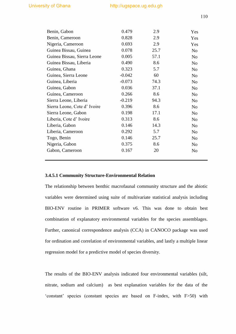
110
Benin, Gabon 0.479 2.9 Yes
Benin, Cameroon 0.828 2.9 Yes
Nigeria, Cameroon 0.693 2.9 Yes
Guinea Bissau, Guinea 0.078 25.7 No
Guinea Bissau, Sierra Leone 0.005 57.1 No
Guinea Bissau, Liberia 0.490 8.6 No
Guinea, Ghana 0.323 5.7 No
Guinea, Sierra Leone -0.042 60 No
Guinea, Liberia -0.073 74.3 No
Guinea, Gabon 0.036 37.1 No
Guinea, Cameroon 0.266 8.6 No
Sierra Leone, Liberia -0.219 94.3 No
Sierra Leone, Cote d‘ Ivoire 0.396 8.6 No
Sierra Leone, Gabon 0.198 17.1 No
Liberia, Cote d‘ Ivoire 0.313 8.6 No
Liberia, Gabon 0.146 14.3 No
Liberia, Cameroon 0.292 5.7 No
Togo, Benin 0.146 25.7 No
Nigeria, Gabon 0.375 8.6 No
Gabon, Cameroon 0.167 20 No
3.4.5.1 Community Structure-Environmental Relation
The relationship between benthic macrofaunal community structure and the abiotic
variables were determined using suite of multivariate statistical analysis including
BIO-ENV routine in PRIMER software v6. This was done to obtain best
combination of explanatory environmental variables for the species assemblages.
Further, canonical correspondence analysis (CCA) in CANOCO package was used
for ordination and correlation of environmental variables, and lastly a multiple linear
regression model for a predictive model of species diversity.
The results of the BIO-ENV analysis indicated four environmental variables (silt,
nitrate, sodium and calcium) as best explanation variables for the data of the
‗constant‘ species (constant species are based on F-index, with F>50) with
University of Ghana http://ugspace.ug.edu.gh

111
Spearman‘s correlation of 24.3% (Table 3.7). Silt and nitrate combination gave a
signifcant (p<0.05) correlation of 23.5%. However, when only the ten most occurred
species (i.e., species with the highest occurence) were used in the analysis, similar
abiotic variables (i.e., silt, nitrate, sodium and calcium) combined to give a
correlation of 28.6% although the overall analysis was not signficant (p=0.164).
Table 3.7 BIO-ENV results for dominant ‗constant‘ species with F>20.
No of variables Best variable Combination Correlation (pw)
‘Constant’ Species with F>20 (p=0.047; Rho=0.243)
4 Silt-Nitrate-Sodium-Calcium 0.243
3 Silt-Nitrate-Calcium 0.241
2 Silt-Nitrate 0.235
Ten Most Dominant ‘Constant’ Species with F>25 (p=0.164; Rho=0.204)
4 Silt-Nitrate-Sodium-Calcium 0.286
1 Nitrate 0.201
2 Silt-Nitrate 0.199
The forward selection of the CCA indicated that six environmental variables
namely magnesium, organic carbon, nitrate, sand, sodium and silt explained
significant variations in the species abundance data (‗constant‘ species). The highest
significantly (p=0.005) explained species variance was the effect of magnesium
(35%), total organic carbon (31% ) and nitrate (18%) (see Table 3.8). In the CCA
ordination the first two ordination axes showed 66.2% relationship between the
University of Ghana http://ugspace.ug.edu.gh
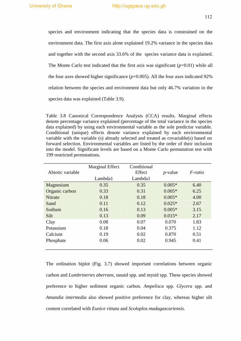
112
species and environment indicating that the species data is constrained on the
environment data. The first axis alone explained 19.2% variance in the species data
and together with the second axis 33.6% of the species variance data is explained.
The Monte Carlo test indicated that the first axis was significant (p=0.01) while all
the four axes showed higher significance (p=0.005). All the four axes indicated 92%
relation between the species and environment data but only 46.7% variation in the
species data was explained (Table 3.9).
Table 3.8 Canonical Correspondence Analysis (CCA) results. Marginal effects
denote percentage variance explained (percentage of the total variance in the species
data explained) by using each environmental variable as the sole predictor variable.
Conditional (unique) effects denote variance explained by each environmental
variable with the variable (s) already selected and treated as covariable(s) based on
forward selection. Environmental variables are listed by the order of their inclusion
into the model. Significant levels are based on a Monte Carlo permutation test with
199 restricted permutations.
Abiotic variable
Marginal Effect Conditional
Effect
p-value
F-ratio
Lambda1 Lambda1
Magnesium 0.35 0.35 0.005* 6.40
Organic carbon 0.33 0.31 0.005* 6.25
Nitrate 0.18 0.18 0.005* 4.00
Sand 0.11 0.12 0.025* 2.67
Sodium 0.16 0.13 0.005* 3.15
Silt 0.13 0.09 0.015* 2.17
Clay 0.08 0.07 0.070 1.83
Potassium 0.18 0.04 0.375 1.12
Calcium 0.19 0.02 0.870 0.51
Phosphate 0.06 0.02 0.945 0.41
The ordination biplot (Fig. 3.7) showed important correlations between organic
carbon and Lumbrineries aberrans, tanaid spp. and mysid spp. These species showed
preference to higher sediment organic carbon. Ampelisca spp. Glycera spp. and
Amandia intermedia also showed positive preference for clay, whereas higher silt
content correlated with Eunice vittata and Scoloplos madagascariensis.
University of Ghana http://ugspace.ug.edu.gh
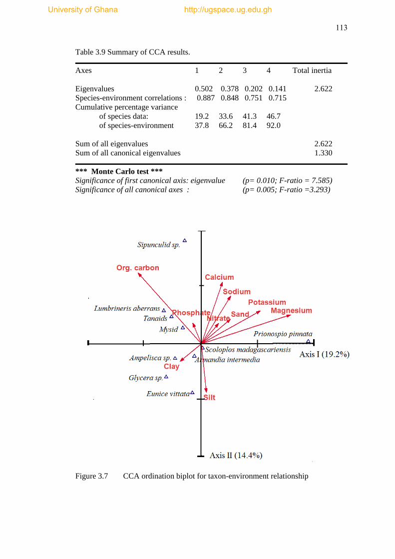
113
Table 3.9 Summary of CCA results.
Axes 1 2 3 4 Total inertia
Eigenvalues 0.502 0.378 0.202 0.141 2.622
Species-environment correlations : 0.887 0.848 0.751 0.715
Cumulative percentage variance
of species data: 19.2 33.6 41.3 46.7
of species-environment 37.8 66.2 81.4 92.0
Sum of all eigenvalues 2.622
Sum of all canonical eigenvalues 1.330
*** Monte Carlo test ***
Significance of first canonical axis: eigenvalue (p= 0.010; F-ratio = 7.585)
Significance of all canonical axes : (p= 0.005; F-ratio =3.293)
Figure 3.7 CCA ordination biplot for taxon-environment relationship
University of Ghana http://ugspace.ug.edu.gh
114
Predictive Linear Regression Model
To further test the interactions between diversity indices (species assemblages) and
abiotic variables, a multiple predictive regression model was run using the Business
Spreasheet Excel software. The result of this analysis showed that species
assemblages were significantly influenced by suite of abiotic variables (p<0.05).
Shannon-Wiener species diversity index was influenced by nitrate and calcium, and
these two variables explained 41.37% of the variance in the data (Table 3.10) and are
therefore important parameters predicting Shannon-Wiener‘s diversity in the
GCLME. The regression model depicted that the independent variables of nitrate and
calcium were correlated negatively with the dependent variable. This suggests that
low levels of the variables influence the species diversity but there could be a
threshold to these low levels. The variations in Margelef‘s species richness were also
explained by nitrate and calcium accounting for 41.71%. The model relationships
were indirect (negative) for nitrate and calcium and similar explanation as in the
Shannon-Wiener diversity could be adduced. Since none of the explained variances
(R squared) were 100%, the unexplained variances could constitute surrogate of
unmeasured environmental variables. This means that other factors such as
biological (competition and predation), physical (waves and tides), chemical
(pollutants), human disturbances, nature of the topography could all be critical in
seeking influence of environmental gradients to species community assemblages.
University of Ghana http://ugspace.ug.edu.gh
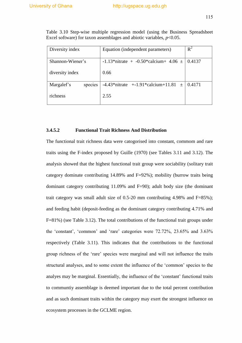
115
Table 3.10 Step-wise multiple regression model (using the Business Spreadsheet
Excel software) for taxon assemblages and abiotic variables, p<0.05.
Diversity index Equation (independent parameters) R2
Shannon-Wiener‘s
diversity index
-1.13*nitrate + -0.50*calcium+ 4.06 ±
0.66
0.4137
Margalef‘s species
richness
-4.43*nitrate +-1.91*calcium+11.81 ±
2.55
0.4171
3.4.5.2 Functional Trait Richness And Distribution
The functional trait richness data were catogorised into constant, commom and rare
traits using the F-index proposed by Guille (1970) (see Tables 3.11 and 3.12). The
analysis showed that the highest functional trait group were sociability (solitary trait
category dominate contributing 14.89% and F=92%); mobility (burrow traits being
dominant category contributing 11.09% and F=90); adult body size (the dominant
trait category was small adult size of 0.5-20 mm contributing 4.98% and F=85%);
and feeding habit (deposit-feeding as the dominant category contributing 4.71% and
F=81%) (see Table 3.12). The total contributions of the functional trait groups under
the ‗constant‘, ‗common‘ and ‗rare‘ categories were 72.72%, 23.65% and 3.63%
respectively (Table 3.11). This indicates that the contributions to the functional
group richness of the ‗rare‘ species were marginal and will not influence the traits
structural analyses, and to some extent the influence of the ‗common‘ species to the
analyes may be marginal. Essentially, the influence of the ‗constant‘ functional traits
to communtiy assemblage is deemed important due to the total percent contribution
and as such dominant traits within the category may exert the strongest influence on
ecosystem processes in the GCLME region.
University of Ghana http://ugspace.ug.edu.gh
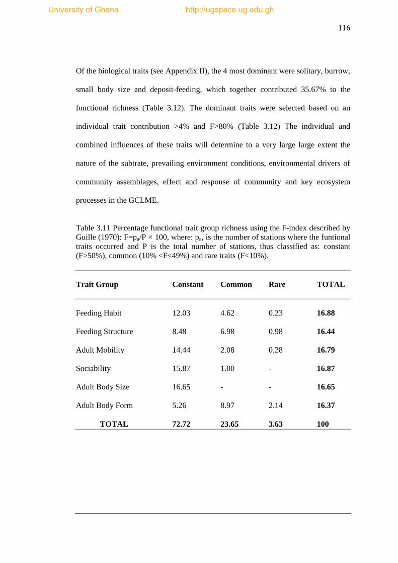
116
Of the biological traits (see Appendix II), the 4 most dominant were solitary, burrow,
small body size and deposit-feeding, which together contributed 35.67% to the
functional richness (Table 3.12). The dominant traits were selected based on an
individual trait contribution >4% and F>80% (Table 3.12) The individual and
combined influences of these traits will determine to a very large large extent the
nature of the subtrate, prevailing environment conditions, environmental drivers of
community assemblages, effect and response of community and key ecosystem
processes in the GCLME.
Table 3.11 Percentage functional trait group richness using the F-index described by
Guille (1970): F=pa/P × 100, where: pa, is the number of stations where the funtional
traits occurred and P is the total number of stations, thus classified as: constant
(F>50%), common (10% <F<49%) and rare traits (F<10%).
Trait Group Constant Common Rare TOTAL
Feeding Habit 12.03 4.62 0.23 16.88
Feeding Structure 8.48 6.98 0.98 16.44
Adult Mobility 14.44 2.08 0.28 16.79
Sociability 15.87 1.00 - 16.87
Adult Body Size 16.65 - - 16.65
Adult Body Form 5.26 8.97 2.14 16.37
TOTAL 72.72 23.65 3.63 100
University of Ghana http://ugspace.ug.edu.gh
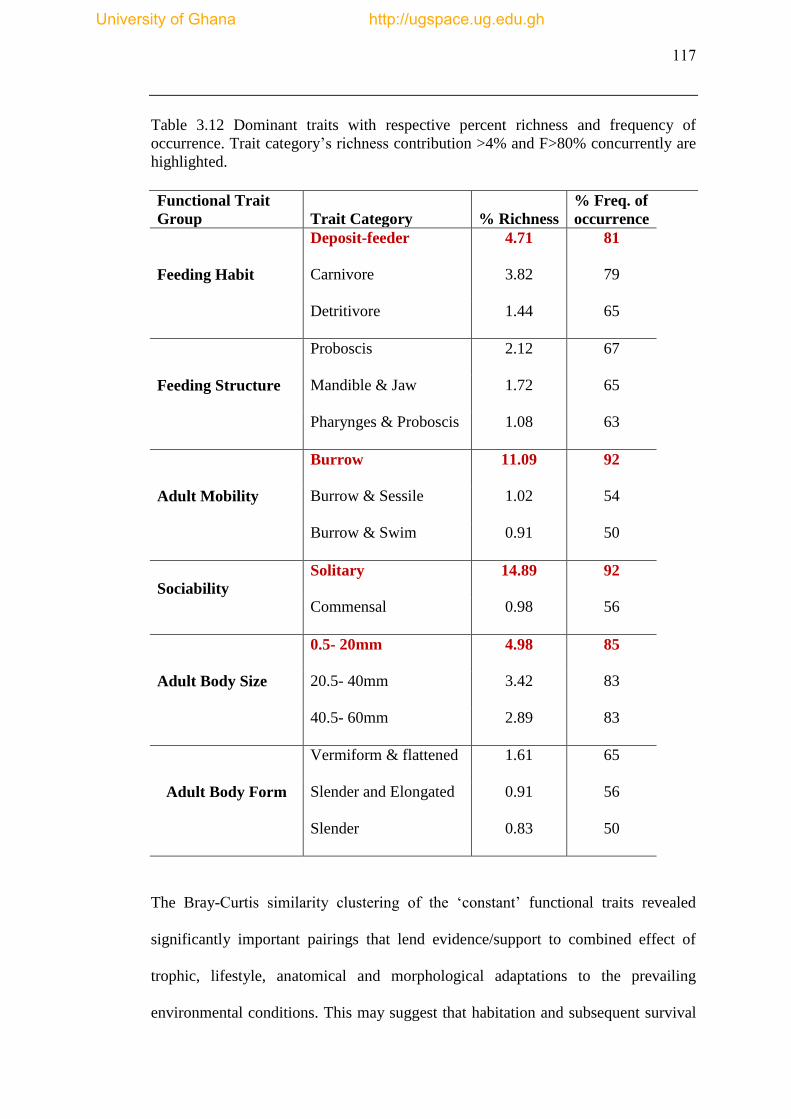
117
Table 3.12 Dominant traits with respective percent richness and frequency of
occurrence. Trait category‘s richness contribution >4% and F>80% concurrently are
highlighted.
Functional Trait
Group Trait Category % Richness
% Freq. of
occurrence
Feeding Habit
Deposit-feeder 4.71 81
Carnivore 3.82 79
Detritivore 1.44 65
Feeding Structure
Proboscis 2.12 67
Mandible & Jaw 1.72 65
Pharynges & Proboscis 1.08 63
Adult Mobility
Burrow 11.09 92
Burrow & Sessile 1.02 54
Burrow & Swim 0.91 50
Sociability
Solitary 14.89 92
Commensal 0.98 56
Adult Body Size
0.5- 20mm 4.98 85
20.5- 40mm 3.42 83
40.5- 60mm 2.89 83
Adult Body Form
Vermiform & flattened 1.61 65
Slender and Elongated 0.91 56
Slender 0.83 50
The Bray-Curtis similarity clustering of the ‗constant‘ functional traits revealed
significantly important pairings that lend evidence/support to combined effect of
trophic, lifestyle, anatomical and morphological adaptations to the prevailing
environmental conditions. This may suggest that habitation and subsequent survival
University of Ghana http://ugspace.ug.edu.gh
118
of macrobenthic organisms in their environment require multiple adaptive strategies
including biological and ecological, which may be determined by prevailing
environmental conditions. The dendrogram clustering depicted the highest cluster
pairs betwen madibular palps (feeding structure) and laterally-flattened (adult body
form) (Fig. 3.8) giving an indication of body form playing an important role in
organism‘s feeding strucutre as well as the feeding type.
Further, the results may suggest that species with elongated and tapered body form
are mainly carnivores or detritivores and that possibly facilitate their food acquision
mechanism. Slender and elongated species may also be commensal, which could
mean better attachment to host to ensure efficient feeding or optimal foraging. The
benthic solitary species and burrowing type (see Appendix I) indicated strong
signficant relationship (Fig. 3.8). The dendrogram also suggests that deposit-feeding
species range from different body sizes (Fig. 3.8) due possibly to the different
forms/types of organic carbon (refractory & labile) or sources (authotonous and
allochthonous) of organic carbon. The results also suggest that benthic carnivorous
species in the GCLME are of medium body size (i.e., 20.5-40.0mm) possibly to
facilitate quick movement for preys as well as adequate body size to handle the prey
items. Filter-feeders are species with maximum body size (i.e., 100.5- 120mm)
probably because they require greater amount of energy for active filter feeding in
possibly the high water current.
University of Ghana http://ugspace.ug.edu.gh
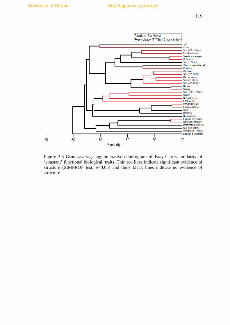
119
Figure 3.8 Group-average agglomerative dendrogram of Bray-Curtis similarity of
‗constant‘ functional biological traits. Thin red lines indicate significant evidence of
structure (SIMPROF test, p<0.05) and thick black lines indicate no evidence of
structure
University of Ghana http://ugspace.ug.edu.gh
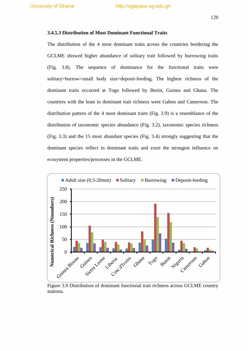
120
3.4.5.3 Distribution of Most Dominant Functional Traits
The distribution of the 4 most dominant traits across the countries bordering the
GCLME showed higher abundance of solitary trait followed by burrowing traits
(Fig. 3.8). The sequence of dominance for the functional traits were
solitary>burrow>small body size>deposit-feeding. The highest richness of the
dominant traits occurred at Togo followed by Benin, Guinea and Ghana. The
countires with the least in dominant trait richness were Gabon and Cameroon. The
distribution pattern of the 4 most dominant traits (Fig. 3.9) is a resemblance of the
distribution of taxonomic species abundance (Fig. 3.2), taxonomic species richness
(Fig. 3.3) and the 15 most abundant species (Fig. 3.4) strongly suggesting that the
dominant species reflect in dominant traits and exert the strongest influence on
ecosystem properties/processes in the GCLME.
Figure 3.9 Distribution of dominant functional trait richness across GCLME country
stations.
0
50
100
150
200
250
Nu
mer
ical
Ric
hn
ess
(Nn
um
ber
s)
Adult size (0.5-20mm) Solitary Burrowing Deposit-feeding
University of Ghana http://ugspace.ug.edu.gh
121
3.4.5.4 Multivariate Structural Analysis of Functional Traits
Bray-Curtis similarity analysis of the functional richness data for countries in the
GCLME indicated two major significant (p<0.05) cluster groups (Group A & B)
distinguished at 52% similarity level. Group A comprised Cameroon and Gabon,
located far east of the GCLME. Group B is made up of two subgroups namely B1
and B2, which is distinguished at 73% Bray-Curtis similarity level. Subgroup B1
comprised Liberia, Sierra Leone, Guinea Bissau, Nigeria and Cote d‘Ivoire in that
decreasing order of similarity, and these are mainly countries located west of the
GCLME except for Nigeria (Fig. 3.10). Group B2 comprised Ghana, Guinea
(subgroup B2i), Benin and Togo (subgroup B2ii), which with the exception of
Guinea, are countries located at the central part of the GCLME. In effect, the
analysis significantly categorized the countries bordering the GCLME into Eastern
Zone (i.e., Gabon & Cameroon), Central Zone (Benin, Togo & Ghana) and Western
(Guinea Bissau, Sierra Leone, Liberia & Cote d‘Ivoire). Guinea and Nigeria
presented macrobenthic functional structure that mimic the Central Zone and
Western Zone respectively. The similarity between the groups showed a sequential
declension from Central GCLME >Western GCLME>Eastern GCLME. The analysis
suggests that the eastern GCLME is low (poor) in benthic biodiversity, the western
GCLME moderately rich benthic biodiversity and the central GCLME rich benthic
biodiversity relatively.
Nonetheless, the highest Bray-Curtis similarity was noted between Togo and Benin
clustering at 97%. This was followed by the similarity of 96% between Liberia and
and Sierra Leone. Ghana and Guinea followed with 94% similarity (Fig. 3.10).
University of Ghana http://ugspace.ug.edu.gh
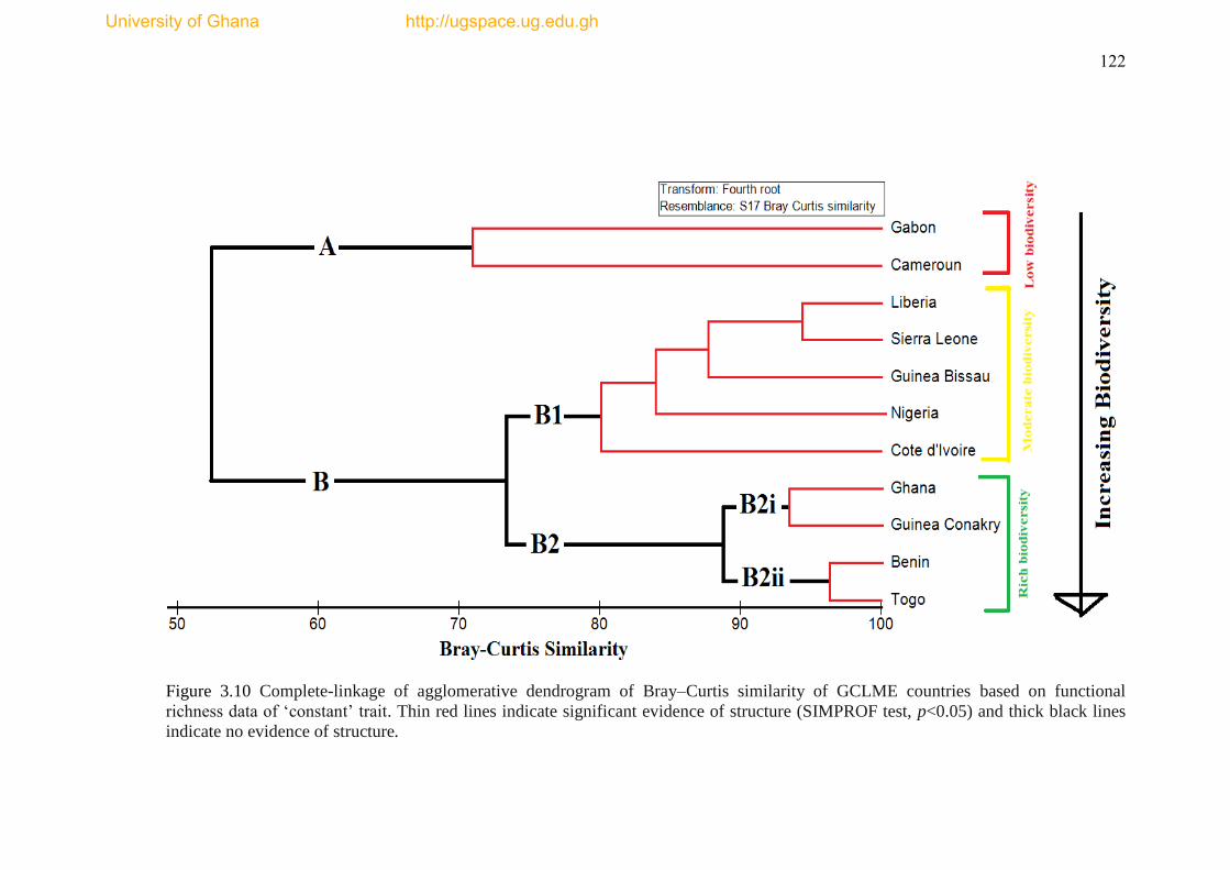
122
Figure 3.10 Complete-linkage of agglomerative dendrogram of Bray–Curtis similarity of GCLME countries based on functional
richness data of ‗constant‘ trait. Thin red lines indicate significant evidence of structure (SIMPROF test, p<0.05) and thick black lines
indicate no evidence of structure.
University of Ghana http://ugspace.ug.edu.gh

123
3.4.6 Functional Trait-Environment Interactions
The relationships between the functional trait and environment were examined using
the BIO-ENV procedures in the PRIMER v6 program (Clarke and Gorley, 2006).
The BIO-ENV procedure identified two variables as ‗best explaining‘ the dominant
benthic functional traits assemblages in the study area (Table 3.13). Nitrate and
magnesium produced the highest significant correlation (p=0.005) of 34.8%. Nitrate
alone showed 34.7% correlation with the dominant functional traits. However, for
the 4 dominant functional trait distribution, the ‗best match‘ was obtained with sand,
nitrate and potassium (ρw=0.286) (Table 3.13). Here also, nitrate alone indicated
good correlation (ρw=0.275).
Table 3.13 Bio-Env results for ‗constant‘ functional traits.
No of variables Best variable Combination Correlation (ρw)
‘Constant’ Traits (p=0.005; Rho=0.348)
2 Nitrate-Magnesium 0.348
1 Nitrate 0.347
4 Silt-Nitrate-Potassium-Magnesium 0.210
Four Most Dominant ‘Constant’ Traits (p=0.042; Rho=0.286)
3 Sand-Nitrate-Potassium 0.286
4 Sand-Nitrate-Potassium-Sodium 0.278
1 Nitrate 0.275
University of Ghana http://ugspace.ug.edu.gh
124
In the RDA, the environmental variables are shown as arrows, the lengths of
which indicate the relative importance and the directions of which are obtained
from the correlation of the variable to the axes. The orthogonal projection of a
trait l inear to an environmental arrow represents the approximate center of the
traits distribution along that particular environmental gradient.
In the RDA, the first four ordination axes accounted for 50.1% of explained total
variance in the dominant trait richness data. The first ordinantion axis accounted
for 49.5% of the trait variance, but the ordination axes showed 98.7% relationship
between the traits and environment indicating that the trait data is strongly
constrained on the environment data. The first ordination together with the second
axis accounted for 49.9% of the variance and 99.5% of the variance explained by
the environmental variables. This indicates that the first axis alone and the
environmental variables associated with it are important in explaining large
portion of the trait variance. The first ordination axis reflected environmental
samples with a gradient largely related to nitrate, calcium, organic carbon,
magnesium and sand at the positive end of the axis, which are linearly related to all
the dominant traits at the negative end of the axis (Fig. 3.11). The entire RDA
analysis resulted in a significant model as depicted by the Monte Carlo test (p ≤
0.005) (Table 3.15).
The results of forward selection environmental explanatory covarible(s) (marginal
effect) was significantly (p<0.05) noted for nitrate (21% explained variance), organic
carbon (11% explained variance) and clay (6% explained variance) (Table 3.14).
However, for the sole predictor environmental variables (marginal effect), the
University of Ghana http://ugspace.ug.edu.gh
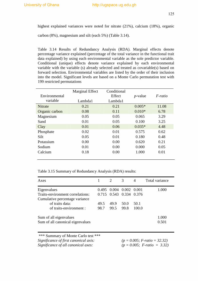
125
highest explained variances were noted for nitrate (21%), calcium (18%), organic
carbon (8%), magnesium and silt (each 5%) (Table 3.14).
Table 3.14 Results of Redundancy Analysis (RDA). Marginal effects denote
percentage variance explained (percentage of the total variance in the functional trait
data explained) by using each environmental variable as the sole predictor variable.
Conditional (unique) effects denote variance explained by each environmental
variable with the variable (s) already selected and treated as covariable(s) based on
forward selection. Environmental variables are listed by the order of their inclusion
into the model. Significant levels are based on a Monte Carlo permutation test with
199 restricted permutations
Environmental
variable
Marginal Effect Conditional
Effect
p-value
F-ratio
Lambda1 Lambda1
Nitrate 0.21 0.21 0.005* 11.08
Organic carbon 0.08 0.11 0.010* 6.78
Magnesium 0.05 0.05 0.065 3.29
Sand 0.01 0.05 0.100 3.25
Clay 0.01 0.06 0.035* 4.48
Phosphate 0.02 0.01 0.575 0.62
Silt 0.05 0.01 0.180 0.48
Potassium 0.00 0.00 0.620 0.21
Sodium 0.01 0.00 0.000 0.05
Calcium 0.18 0.00 1.000 0.01
Table 3.15 Summary of Redundancy Analysis (RDA) results:
Axes 1 2 3 4 Total variance
Eigenvalues 0.495 0.004 0.002 0.001 1.000
Traits-environment correlations: 0.715 0.543 0.334 0.376
Cumulative percentage variance
of traits data: 49.5 49.9 50.0 50.1
of traits-environment : 98.7 99.5 99.8 100.0
Sum of all eigenvalues 1.000
Sum of all canonical eigenvalues 0.501
*** Summary of Monte Carlo test ***
Significance of first canonical axis: (p = 0.005; F-ratio = 32.32)
Significance of all canonical axes: (p = 0.005; F-ratio = 3.32)
University of Ghana http://ugspace.ug.edu.gh
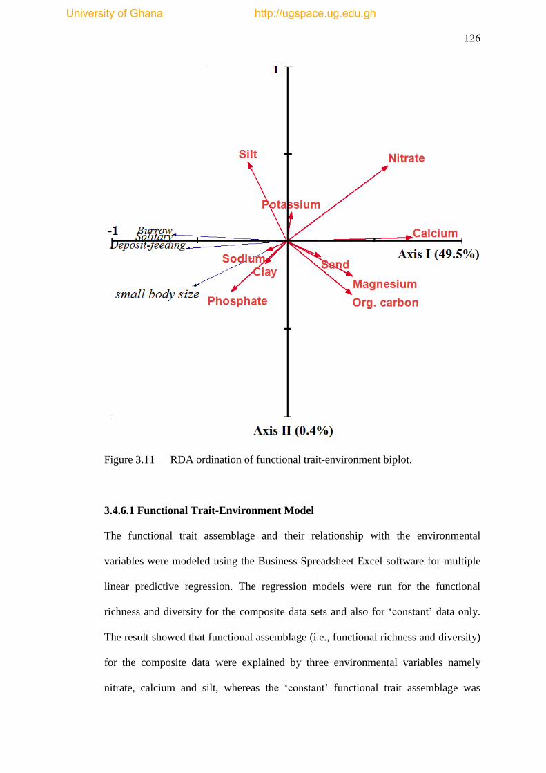
126
Figure 3.11 RDA ordination of functional trait-environment biplot.
3.4.6.1 Functional Trait-Environment Model
The functional trait assemblage and their relationship with the environmental
variables were modeled using the Business Spreadsheet Excel software for multiple
linear predictive regression. The regression models were run for the functional
richness and diversity for the composite data sets and also for ‗constant‘ data only.
The result showed that functional assemblage (i.e., functional richness and diversity)
for the composite data were explained by three environmental variables namely
nitrate, calcium and silt, whereas the ‗constant‘ functional trait assemblage was
University of Ghana http://ugspace.ug.edu.gh
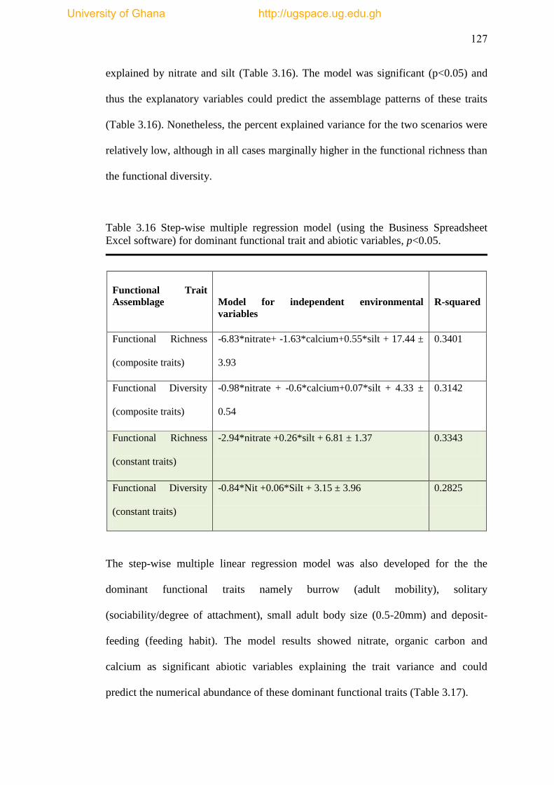
127
explained by nitrate and silt (Table 3.16). The model was significant (p<0.05) and
thus the explanatory variables could predict the assemblage patterns of these traits
(Table 3.16). Nonetheless, the percent explained variance for the two scenarios were
relatively low, although in all cases marginally higher in the functional richness than
the functional diversity.
Table 3.16 Step-wise multiple regression model (using the Business Spreadsheet
Excel software) for dominant functional trait and abiotic variables, p<0.05.
Functional Trait
Assemblage
Model for independent environmental
variables
R-squared
Functional Richness
(composite traits)
-6.83*nitrate+ -1.63*calcium+0.55*silt + 17.44 ±
3.93
0.3401
Functional Diversity
(composite traits)
-0.98*nitrate + -0.6*calcium+0.07*silt + 4.33 ±
0.54
0.3142
Functional Richness
(constant traits)
-2.94*nitrate +0.26*silt + 6.81 ± 1.37 0.3343
Functional Diversity
(constant traits)
-0.84*Nit +0.06*Silt + 3.15 ± 3.96 0.2825
The step-wise multiple linear regression model was also developed for the the
dominant functional traits namely burrow (adult mobility), solitary
(sociability/degree of attachment), small adult body size (0.5-20mm) and deposit-
feeding (feeding habit). The model results showed nitrate, organic carbon and
calcium as significant abiotic variables explaining the trait variance and could
predict the numerical abundance of these dominant functional traits (Table 3.17).
University of Ghana http://ugspace.ug.edu.gh

128
The model indicated that for burrowing trait, nitrate, total organic carbon and
calcium were the main environmental factors that could predict their richness (Table
3.17). All these variables depcited inverse relationship with the burrowing trait. The
results were also consistent with the other dominant traits, viz. deposit-feeding,
solitary, and small body size but with varying degrees of explained predictive
variances. The low R-sqaured values suggest the influence of other important
variables biological (competition and predation), physical (currents and
temperatures), chemical (organic and inorganic substances), and anthropogenic
disturbances as surrogates, which were probably not assessed in this study.
Table 3.17 Step-wise multiple regression model for dominant functional trait and
abiotic variables. TOC=total organic carbon
Dependent
Functional Trait
Model for independent environmental variables
R-squared
Burrow -17.48*nitrate + -5.24*TOC+-3.48*calcium +
34.92± 9.09
0.3796
Solitary -23.30*nitrate +-6.42*TOC+-4.72*calcium+
46.29± 12.55
0.3580
Small Body Size (0.5-
20mm)
-8.72*nitrate + -1.62*TOC+-1.09*calcium + 13.83
±3.96
0.3617
Deposit-feeding -8.68*nitrate + -3.19*TOC+-1.08*calcium + 15.18
± 5.04
0.3068
University of Ghana http://ugspace.ug.edu.gh
129
3.6 Discussion
3.6.1 Species Composition and Abundance
The species composition and dominance were noted for the polychaetes, crustaceans
and molluscs with numerical abundance, richness and density varying spatially
across the countries in the GCLME. Ecological variability is regarded as ubiquitous
patterns in marine benthos regardless of the habitats or taxa especially on the small-
scale level (Fraschetti et al., 2005). However, according to Benedetti-Cecchi (2009)
it is pertinent to address the issues of the variability of the processes driving the
change in the species assemblage (i.e., ecological drivers), and the variables that are
influenced by the forces (i.e., ecological response). The environmental changes
promoting fluctuations in species and assemblages are important ecological forces
(Benedetti-Cecchi, 2009), as spatial heterogeneity in species assemblage may
enhance productivity and increase resistance to disturbance (Hutchison et al., 2003).
The species assemblage (notably polychaete, crustaceans and molluscs) patterns
across sampled stations (countries) showed variations with higher taxa abundances,
richness and densities occuring in the central section of the GCLME (Benin, Togo
and Ghana) (see Figs. 3.2-3.3 and Table 3.2 and 3.3). These areas (country stations)
corresponded with moderate levels of sediment nitrate, calcium, magnesium and
higher total organic carbon at some areas. These areas showed surrogates of
allochthonous and autochthonous organic matter input (Appendix III). The
macrobenthic community structure was influenced by the abiotic variables namely:
nitrate, total organic carbon, silt, calcium and magnesium. These variables may be
influenced by the interactions with other environmental factors to create favourable
conditions for the organisms. For instance, the primary food source for benthos
University of Ghana http://ugspace.ug.edu.gh

130
originates, with a few localized exceptions, in euphotic surface waters. The
movement of water driven by currents, wind and other forces transports food
particles in the water mass and causes resuspension of bottom sediments (Pearson
and Rosenberg, 1987), which essentailly distribute food to benthic animals.
Essentially, benthic infaunal communities are organized structurally, numerically and
functionally in relation to gradients of resource availability, and are modified by
interactions with other environmental factors (Pearson and Rosenberg, 1987;
Wieking and Kröncke, 2005). Thus species distribution may be recognised as a
response to the varying effects of these modified environmental gradients in tandern
with other factors. According to Angel (1984) sedimentation of faecal pellets is
generally considered to be the major means of transporting phytogeneous primary
production to the benthos.
Nitrate is known to drive marine primary production (Camargo and Alonso, 2006),
thus the low levels of nitrate observed to influence species diversity, could be the
result of denitrification and nitrate uptake for pelagic primary production, with the
latter driving benthic diversity. In marine sediments, nitrate is often consumed within
the zone of denitrification (Lehmann et al., 2005) possibly as a result of organic
matter remineralization, which is also influenced by the conditions in the overlying
water. The observation and interactions between the organisms and the abiotic
variables suggest a more complex ecological driver-species assemblages relations in
the GCLME. This is because the assumed reason for high nitrate abstraction and
subsequent utilization reflecting in higher species abundance and diversity, could be
the result of complex interactions. The low correlation values realized in the BIO-
ENV matrix, CCA ordination and the predictive regression models (see Tables 3.7-
University of Ghana http://ugspace.ug.edu.gh
131
3.10, Fig. 3.6) support the assertion of a complex environmental stressors/drivers of
species and functional assemblage patterns in the GCLME.
3.6.2 Functional Structure and Assemblage Patterns
Functional biodiversity encompassed functional richness (FR– the number of
functional groups derived from a combination of functional feeding groups and habit
trait groups), functional diversity (FD – the number of functional groups and division
of individuals among these groups, and functional evenness (FE– the division of
individuals among functional groups). Furthermore, functional structure (FS)
comprised the composition and abundance of functional groups at each site. The
results of the functional biodiversity analysis revealed dominance of small size (0.5-
20 mm) burrow-dwelling solitary deposit-feeding organisms (dominated by
polychaetes), which potentially exert the strongest influence on the ecosystem
properties/processes in the GCLME region such as biogeochemical nutrient
remineralization of nitrate from organic matter. These traits further provide clear
indication/information about prevailing environmental conditions, nature of the
substrate, key ecosystem processes and possible response to ecological disturbances.
In the ecological processes, the interactions and feedback among species and their
respective environment are important elements in elucidating synergies.
The prevalence and dominance of small body size (0.5-20 mm) traits inferred habitat
instability (see Schwinghamer, 1983) and may result in high production relative to
total biomass (given the high turnover rates of member organisms (Bougdreau et al.,
1991). This suggests that the GCLME region is characterized by high productivity
but low total biomass as a result of small adult body size dominance. Essentially, the
University of Ghana http://ugspace.ug.edu.gh
132
size structure of marine macrobenthic communities is affected by anthropogenic
stressors such as organic enrichment (Pearson and Rosenberg, 1978; Gray, 1989;
Weston, 1990; Warwick and Clarke, 1994) and trawling (Jennings et al., 2001;
Duplisea et al., 2002), and thus size-dependent relationships provide objective basis
for understanding ecology and predicting conservation outcomes (Calder, 2001).
According to Calder (2001), adult body size exerts a quantitative dominance over
how an animal lives and for how long and on its rate of living and extraction of
resources from its environment, and consequently on how many of its kind can live
simultaneously on a unit of habitat.
The small body size organisms are closely related to the burrow-dwelling species,
and are well known to play key roles in ecosystem functioning of soft-bottom
temperate habitats (Austen and Widdicombe, 1998; Amaro et al., 2010).
Macrobenthic burrowers can affect recruitment, growth and survival of a variety of
organisms, and thus influence community biodiversity (Macdonald et al., 2012). The
profound effects of their burrowing and feeding activities can include the delivery of
food and solutes (e.g., oxygen) to subsurface sediments, alteration of sediment
geochemical and physical makeup (Braeckman et al., 2011), and increased potential
for grazing and subduction of smaller organisms (Needham et al., 2011). The
dominance of small body size burrow-dwelling species (e.g., Prionospio sexoculata
Prionospio cirrobranchiata, Paraonides lyra capensis) indicates characteristics of
short lifespans due possibly to habitat instability as large surface burrowers have
limitations on their ability to maintain an optimal burrow position in shifting
sediments (Bromley, 1990).
University of Ghana http://ugspace.ug.edu.gh
133
Small size organisms are mainly opportunistic species that respond to habitat
perturbations. According to Villnäs et al. (2011), such opportunistic species may
endure stress and take advantage of extra resources through processing the upper-
most layers of the sediments. Small body size burrow-dwelling traits are likely to
influence secondary production due to their short generations and may play essential
roles in sediment biogeochemistry (an important ecosystem process) due to their
bioturbatory activities. Further, burrowing deposit-feeding traits give lucid indication
of sediment characteristics including fine-grained soft substrate with potentially high
organic matter (i.e., silt or clay) supporting burrowing and deposit-feeding. The
retention for organic matter in sediment is influenced by the particle size (Milliman,
1994). Subsurface deposit-feeders tend to be common in muddier sediments
(Macdonald et. al., 2012b). Deposit-feeders play important role in bioturbation,
which is a critical process in biogeochemistry that ensures mineralization of nutrients
(e.g., nitrate) to drive primary production. This thus makes the GCLME a productive
ecosystem as acknowledged by Ukwe et al. (2006).
It has been demonstrated that macrobenthic fauna create burrow networks that
penetrate the sediment anoxic zone (Anderson and Meadows, 1978) and create
burrow ventilation (Webb and Eyre, 2004), which impact on the sediment (Rhoads,
1974) thus affecting sediment biogeochemistry (Aller and Aller, 1998; Wenzhöfer
and Glud, 2004). The importance of benthic macrofauna in nutrient dynamics and
benthic-pelagic coupling have been noted in several studies (Pilskaln et al., 1998;
Thrush and Dayton, 2002; Lohrer et al., 2004) suggesting that benthic bioturbators
have large-scale ecosystem implications (Bonsdoff and Rosenberg, 2007). The
University of Ghana http://ugspace.ug.edu.gh
134
results of this study lend potential evidence to benthic-pelagic coupling clearly
demonstrating the functional significance of marine macrobenthic species.
3.6.3 Functional Trait-Environment Relationship
Marine benthic biodiversity–environment relationships are well-understood in the
context of taxonomic species richness and species composition, whereas other
component of biodiversity, including functional richness (FR) and functional
diversity (FD) lag behind in scientific literature. Most studies to date have examined
either taxonomic assemblage patterns with few giving prominence to functional
diversity especially in the marine environment (Bremner et al., 2005 and 2008). The
relationships between functional diversity (and also taxonomic diversity) of marine
macrobenthic fauna and environmental factors showed synergistic association and
can give evidence of effect and response mechanisms. This present study established
strong association between functional diversity (also taxonomic diversity) and suites
of environmental parameters namely nitrate, calcium, organic carbon, mangesium,
silt and clay. These abiotic variables, which significantly influence the functional and
taxonomic species diversities, are largely related to primary productivity and climate
change factors. The spatial variations (or gradient) in these abiotic factors explained
and can predict the species abundance and functional stucture of macrobenthic
organisms in the GCLME. It is possible that the functional and community
assemblages of the macrobenthic fauna are tolerable to these abiotic variables, and
have as such emerged as dominant component through the habitat filteration process
(Mouillot et al., 2006).
University of Ghana http://ugspace.ug.edu.gh
135
It has been indicated that the adaptation of certain species to unpredictable
environments can be related in part to their life history (Grassle and Grassle, 1976)
and biological traits characteristics (Mouillot et al., 2006). Newell (1970) further
pointed out that where the tolerance limits for a particular environmental variable
have been determined for an organism, the organism‘s realized distribution is much
more restricted than its potential distribution. It is reasonable, therefore, to presume
that the gradients (spatial differences) in the environmental variables probably
ensured that only tolerant species or traits are selected and hence their distribution.
Among the many best matched environmental factors with species and functional
communities, sediment nitrate emerged as key abiotic driver. Nitrate is an important
nutrient in primary production (Camargo and Alonso, 2006) and thus productivity
models could be implicated here in influencing assemblage patterns. Nonetheless, the
possible reasons for the nitrate influence may include:
i) nitrogen is the most abundant chemical element on the earth atmosphere
(almost 80%) and essential components of many key biomolecules (e.g.,
amino acids, nucleotides) (Camargo and Alonso, 2006) and also ranked
fourth behind carbon, oxygen and hydrogen as the commonest chemical
element in living tissues (Campbell, 1990);
ii) most inorganic reactive nitrogen is in the form of nitrate and nitrate drives
aquatic productivity by increasing cyanobacteria (an important autotroph)
as they efficiently uptake nitrate for fast growth,, and
iii) less toxicity of nitrate in seawater animals probably because of the
ameliorating effect of water salinity (sodium, chloride, calcium and other
ions) on the tolerance of aquatic animals. Also nitrate has to be converted
University of Ghana http://ugspace.ug.edu.gh

136
into nitrite under internal body conditions for its toxicity to be realized
but owing to the low branchial permeability to nitrate ions by most
marine organisms (Cheng and Chen, 2002), the nitrate uptake in aquatic
animals is more limited than the nitrite uptake, thus contributing to the
relatively low toxicity of nitrate (Jensen, 1996; Cheng and Chen, 2002;
Alonso and Camargo, 2003; Camargo et al., 2005a).
Nitrate has been found to be a strong predictor of marine benthic assemblages
(Lamptey et al., 2010) due in part to their influence on primary productivity. Aquatic
animals are, in general, better adapted to relatively low levels of inorganic nitrogen
since natural (unpolluted) ecosystems often are not N saturated (Camargo et al.,
2005a), and that explains the low nitrogen correlation with benthic biodiversity (see
Tables 3.10 and 3.16).
Calcium and magnesium also emerged as important variables best explaining and
predicting functional biodiversity patterns in the GCLME. These parameters
implicate climate change effects on the benthic species and functional diversities.
The main climate change impact on the marine ecosystem is triggered by the
atmospheric CO2 dissolution in the ocean. Absoprtion of CO2 into the ocean leads to
low pH and decreased concentration of CO3-2
. The decreased concentration of CO3-2
means low CaCO3 saturation, which is important in calcification of benthic
organisms. According to Fabry et al. (2008), elevated partial pressure of CO2 (pCO2)
in seawater (also known as hypercapnia) impact on marine organisms both via
decreased CaCO3 saturation, which affects calcification rates, and via disturbance to
acid–base (metabolic) physiology. Some studies have indicated that the oceanic
uptake of anthropogenic CO2 and the concomitant changes in seawater chemistry
University of Ghana http://ugspace.ug.edu.gh

137
have adverse consequences for many calcifying organisms, and may result in
changes to biodiversity, trophic interactions, and other ecosystem processes (Kleypas
et al., 2006; Royal Society, 2005). Evidence from freshwater systems suggests
climate warming could also cause significant shifts in benthic community size
structure (Yvon-Durocher et al., 2011). Such shifts in size structure could have
significant impacts on marine ecosystems, affecting sediment production,
geochemistry, and the amount of food available to predators at higher trophic levels
(Jennings and Kaiser, 1998).
Further, during calcification, element such as magnesium is incorporated into
biogenic calcium carbonate (Dissard et al., 2010) and thus decalcification would lead
to the release of magnesium. Magnesium occurred in seawater to nearly constant
ratios to calcium (for the last 1Myrs, Broecker and Peng, 1982) and variations in
Mg/Ca in benthic shelly organisms (e.g., foraminiferans) on shorter timescale are
shown to be mainly related to changes in temperature (Anand et al., 2003; Reichart
et al., 2003; Barker et al., 2004), which is resultant effect of climate change. Other
environmental parameters such as pH or (CO32) may influence magnesium
incorporation into shelly organisms (Dissard et al., 2010). Higher temperature result
in higher amounts of magnesium incorporated into the shell matrix (Fergusson et al.,
2008; Dissard et al., 2010). Shells with higher Mg:Ca ratios are more soluble, so
even organisms with primarily calcite (less soluble than aragonite) skeletons may be
heavily impacted by future conditions.
The precipitation of CaCO3 in the upper ocean through the formation of calcareous
skeletons by marine organisms creates more acidic conditions which decrease the
University of Ghana http://ugspace.ug.edu.gh

138
capacity of the upper ocean to take up atmospheric CO2 (Kleypas et al., 2006).
Conversely, the dissolution of marine carbonates at depth, including biogenic
magnesium calcites (from coralline algae), aragonite (from corals and pteropods),
and calcite (from coccolithophorids and foraminifera), raises pH and increases the
capacity of the oceans to take up and store CO2 from the atmosphere (Feely et al.,
2004). The results of the analysis herein indicated that the selection of magnesium
and calcium as drivers of species and functional diversity supports the view of
carbonates dissolution at depth leading to the possible release of magnesium and
calcium.
In general, magnesium (Mg) calcite minerals with a significant mole percent (mol %)
MgCO3 are more soluble than aragonite and calcite, and it is therefore likely that
Mg-calcite, high latitude and cold-water calcifying organisms will be the first to be
affected by increasing ocean acidification (Andersson et al., 2008). The mole percent
of magnesium deposited by marine organisms varies from a few mol% to as much as
30 mol% between different species (Andersson et al., 2008), resulting in a significant
response variation among taxa to changing ambient conditions (Hoffmann et al.,
2008). In tropical and sub-tropical environments, the dependence of calcareous algae,
and other important reef calcifiers like echinoderms and benthic foraminifera, on
high-magnesium calcite, the most soluble of all calcium carbonate minerals, would
make these likely early casualties of climate change effect. The importance of
magnesium is seen on its influence on calcium carbonate precipitation. According to
Holmes-Farley, 2003), magnesium binds to the calcium carbonate crystals' growing
surface, when the latter begins to precipitate. The magnesium effectively clogs the
crystals' surface so that they no longer look like calcium carbonate, making them
University of Ghana http://ugspace.ug.edu.gh

139
unable to attract more calcium and carbonate, so the precipitation stops. Without the
magnesium, the abiotic (i.e. non-biological) precipitation of calcium carbonate would
likely increase enough to prohibit the maintenance of calcium and alkalinity at
natural levels.
Sea urchins and crustaceans, including lobsters and shrimp, exert higher biological
control by gradually accumulating intracellular stocks of ions; between moults
crustaceans are thought to harden their chitin and protein exoskeletons by continually
depositing calcite minerals (Convention on Biological Diversity, 2009). The shell
chemistry and mineralization of crustaceans suggest that they may withstand climate
change effect (e.g., ocean acidification) and saturation state decreases better than
molluscs, however the response of organisms is likely to be a function of individual
history and genetic variability (Cooley and Doney, 2009).
Organic carbon and sediment particles have been demonstrated as playing important
structuring role in marine species assemblages (Gray, 1989 and 2002; Lamptey and
Armah, 2008; Pearson and Rosenberg, 1978 and 1987; Snelgrove and Butman, 1994)
as they are associated with productivity and nutrition. It is therefore corroborating the
selection of these abiotic factors as key environmental drivers of taxonomic and the
functional assemblages in the GCLME. Organic matter is the main food source for
deposit-feeders (Pearson and Rosenberg, 1978), which were the dominant feeding
trait identified. The sediment type gives an indication of availability of food rather
and not as a first order factor determining species assemblages (Snelgrove and
Butman, 1994).
University of Ghana http://ugspace.ug.edu.gh

140
CHAPTER FOUR
IMPACT OF DEMERSAL FISH TRAWLING ON THE STRUCTURE AND
FUNCTIONAL ASSEMBLAGES OF EPIBENTHIC FAUNA ALONG
BATHYMETRIC GRADIENT IN THE GUINEA CURRENT LME
4.1 Introduction
The global biodiversity concerns (i.e., accelarated loss and decline) and the
predictions of impaired ecosystem functioning and sustainability (Naeem et al. 1994;
Sala et al., 2000; Loreau et al., 2001; Hughes et al., 2003; Hooper et al., 2005;
Worm et al., 2006; Hooper et al., 2012), have increased interests of investigating the
wider impacts of commercial fishing on non-target species (e.g. Alverson et al.,
1994; Dayton et al., 1995). The effects of mobile fishing gears on marine benthic
productivity and biodiversity are a global concern both for the fishing industry and
government regulators (Dayton et al., 1995; Auster and Langton, 1999;
McConnaught et al., 2000; Kaiser et al., 2002; Hiddink et al., 2007). The
socioeconomic consequences of the biodiversity changes depend on how they
translate into altered ecosystem processes and services (Costanza et al., 1997;
Balmford et al., 2002; Millennium Ecosystem Assessment, 2003).
The marine benthic ecosystems are increasingly affected by environmental stress and
degradation due to pollution (Halpern et al., 2008) and other anthropogenic factors
such as overfishing (Jackson, 2008), bottom trawling and dredging (Pauly et al.,
2005) and human-induced climate change (Bindoff et al., 2007). Many of the
expected responses to human activities in the marine environment may best be
University of Ghana http://ugspace.ug.edu.gh
141
monitored at the seafloor in the benthic communities (Jorgensen et al., 2011). This is
due to the fact that benthic organisms have limited locomotion; they are long-lived
and able to integrate into their system both short-term and long-term environmental
processes (Borja, 2000).
Increasing importance of marine biodiversity and fisheries in general have resulted in
integrated approach, such as Ecosystem Approach to Management (EAM), which
requires sustainable and ecosystem-based assessment. For instance, Ecosystem
Approach to Fisheries (EAF) requires that managers take account of the ecosystem
effects of fishing in management plans that are intended to achieve sustainable
exploitation of target species (Kaiser et al., 2002). Ecological Quality Objectives
(EcoQO‘s) is now used to assist in the movement toward an ecosystem approach to
management (Frid and Hall, 2001). Skjoldal et al. (1999) defined the EcoQ as an
overall expression of the structure and function of the aquatic systems. It is therefore
reasonable to assume that the development of ecosystem approaches to
environmental management is to define the ‗overall structure and function‘ desired
for the ecosystem being considered. It also calls for integration of commercial marine
resources (e.g., fish) and non-commercial communities (Brind'Amour et al., 2009)
such as epibenthic fauna.
Epifaunal component of the benthos includes organisms of high biomass and
potentially of high ecosystem importance as they provide habitat structure, and
potentially different functional components of the community (Jørgensen et al.,
2011). Larger fauna (e.g., epifauna) often represent long-lived and slowly
reproducing species that are more prone to decline if mortality is increased due to
University of Ghana http://ugspace.ug.edu.gh
142
fishing (Witbaard and Klein, 1994). For the marine benthos, the issues that need to
be considered include (i) aspects of the composition and structure of the benthic
community – species diversity, species abundance patterns (i.e., how individuals are
distributed between the species present), and biomass. Further, the functioning of this
assemblage; and (ii) functional attributes such as the productivity of the community
and the degree, rate and pathways of nutrient and carbon cycling. In coastal
ecosystem, indicators integrating both the structural (i.e., species composition) and
functional attributes of the communties are increasingly recognized as useful tools to
assess change in these ecosystems (Elliott and Quintino, 2007).
A huge body of knowledge exists on the evidence of fishing effects on the marine
macrobenthos (Jennings and Kaiser, 1998; Kaiser and De Groot, 2000; Trush and
Dayton, 2002), however a lack of comparable quantitative data of fish and epifauna
is still a concern and confounds our understanding of the extent of the fishing effects.
Given the growing appreciation of the value of marine biodiversity as critical to the
sustainability of commercially valuable ground fish stocks as well as for its own
unique heritage (Bengtsson et al., 1997; Costanza et al., 1997; Freckman et al., 1997;
Gray, 1997; Schlapfer and Schmidt, 1999), there is now an increasing need to
understand and sustain biodiversity as a part of any fisheries management plan.
Trawling is a common method for catching fish and bottom trawling is one kind of
fishing practice with heavy nets connected to large trawl doors. The nets drag along
the seafloor leaving deep visual marks on the sea bottom (Enticknap, 2002). The
design and mode of operation of the trawling gear influences how it interacts with
the seafloor and how many species are removed (Thrush and Dayton, 2002). The
University of Ghana http://ugspace.ug.edu.gh

143
otter trawl is an example of bottom trawl and is commonly used to catch fish and
invertebrate species. The otter trawl can penetrate the sea bed down to 20 cm
(Querios et al., 2006). The beam trawl is held open by a steel beam fitted with chains
and the penetration of the beam trawl and the amount of physical disturbance caused
by beam trawl, depend on the weight of the gear, towing speed and bottom type
(sediment), and varies between 3 mm and 6 cm (Lindeboom and de Groot, 1998a;
Duplisea et al., 2002).
Bottom trawling has been documented to cause extensive impacts on benthic
communities and habitats, leading to reduced biomass, production and diversity (e.g.
Kaiser and De Groot, 2000; Hiddink et al., 2006). When heavy trawling gear is
dragged along the seabed, some of the complex benthic structure that serves as
refugia are damaged (Stone et al., 2005). Bottom trawling is harmful to seafloor
habitats and this effect has been well studied in marine systems (Kaiser et al., 1998;
McConnaughey et al., 2000; Sparks-McConkey and Watling, 2001; Rosenberg et al.,
2003; Tillin et al., 2006). Modifications of the composition of benthic assemblages
may result in changes to the ecological functioning of the system (Bremner, 2006;
Tillins et al., 2006).
Relatively few studies have investigated the impact of bottom trawling on benthic
ecosystem integrating fisheries and epibenthic data/information along bathymetric
gradient. Nonetheless, most benthic biodiversity systems are stratified by water depth
(Zmarzly et al., 1994; Bergen, et al., 2001). Study of that nature will unearth the
influence of bathymetry on epibenthic fauna distribution and may obviate
confounding issues of impact of bottom trawling on the epibenthic bottom dwellers.
University of Ghana http://ugspace.ug.edu.gh

144
Integrated assessment of fisheries requires studies that focus on the whole ecosystem
and not only on single species, and that consider fishing activities as key pressures
affecting several ecosystem components (Gaertner et al., 2005; Massuti and
Reñones, 2005). Therefore, it is highly necessary to develop studies like these, which
identify the components, assemblage structure and functioning of ecosystems at a
regional scale.
4.2 Study Objectives
The present study is the first attempt in the Gulf of Guinea to compositely describe
the spatial distribution patterns of epibenthic fauna (treated as non-targeted species or
by-catch from bottom trawl). The main objectives were to characterise epibenthic
assemblages (i.e., composition and structure) caught by the beam trawl, establish the
bathymetric relationships between demersal fish and epibenthic fauna distribution
patterns in terms of abundance and biomass and ascertain the functional attributes
(i.e., feeding and mobility) of epibenthic fauna along bathymetric gradients.
The findings of this study will attempt to answer the questions: i) what are the
community structural differences in epifauna and fish in a bottom trawled samples?,
ii) how do the assemblage patterns of fish trawl samples and epibenthic by-catch
differ along bathymetric gradient? and iii) is the epifauna by-catch functionally
significant to influence ecosystem functions and processes?
University of Ghana http://ugspace.ug.edu.gh
145
4.3 Materials and Methods
4.3.1 Study Area
The study was conducted in the Gulf of Guinea of the Guinea Current Large Marine
Ecosystem along the continental shelves of Ghana, Togo, Benin and western part of
Nigeria. The GCLME extends from approximately latitude 120N south to about 16
0S
latitude, and varies from 200
west to about 120
east longitude (Fig. 2.3). It extends
from Bissagos Island (Guinea Bissau) to Republic of Congo with its boundary
extending in a north–south direction from the intense upwelling area of the Guinea
Current (GC) south to the northern seasonal limit of the Benguela Current (BC). In
an east–west sense, the GCLME includes the drainage basins of the major rivers
seaward to the GC front delimiting the GC from open ocean waters (a time- and
space-variable boundary).
4.3.2 Field Sampling
Epibenthic fauna samples were collected from beam trawl (Plate 4.1) catches carried
out from 3-14 March 2003 aboard the RV Geo-Explorer scientific vessel during the
West Africa Pipeline Project basleine studies from Ghana to Nigeria using a
randomized stratified survey design (Fig. 4.1 & Table 4.1). Beam trawls are very
effective in sampling vagile as well as epibenthic macrofauna and the latter may
represent a large proportion (density and biomass) of the catches (Kaiser et al., 1994;
Till et al., 2006). It should be noted that no trawl gear ever sample all the individuals
present in the path of the net (Jorgensen et al., 2011) and the beam trawl net based on
the mesh-size will select certain size classes of the same epibenthic faunal taxa. As
such, the actual epifauna abundance may have been grossly under-represented in the
University of Ghana http://ugspace.ug.edu.gh

146
sample collection and consequently the analysis likewise the fish data although fishes
are relatively larger than epifauna.
Therefore the impressions of the epibenthic community gained from the analysis of
the sample data is not that of the actual epifaunal community present at each sampled
location, but rather it is a view of the community biased by the differential selectivity
of the sampling gear for each species present at each location (Tillin et al., 2006).
Plate 4.1 Beam trawl gear. (Source: ilvo.vlaanderen & Grantontrawlers)
University of Ghana http://ugspace.ug.edu.gh
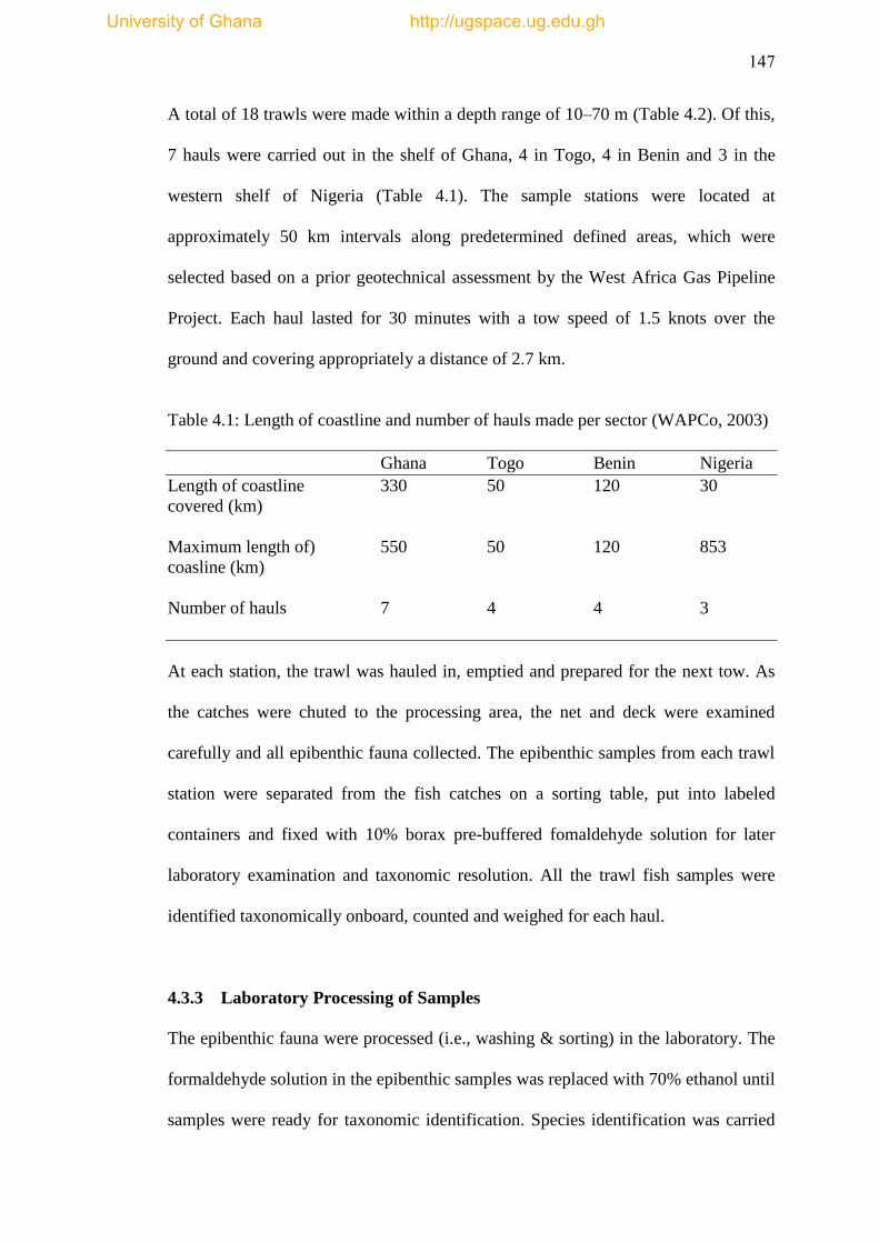
147
A total of 18 trawls were made within a depth range of 10–70 m (Table 4.2). Of this,
7 hauls were carried out in the shelf of Ghana, 4 in Togo, 4 in Benin and 3 in the
western shelf of Nigeria (Table 4.1). The sample stations were located at
approximately 50 km intervals along predetermined defined areas, which were
selected based on a prior geotechnical assessment by the West Africa Gas Pipeline
Project. Each haul lasted for 30 minutes with a tow speed of 1.5 knots over the
ground and covering appropriately a distance of 2.7 km.
Table 4.1: Length of coastline and number of hauls made per sector (WAPCo, 2003)
Ghana Togo Benin Nigeria
Length of coastline 330 50 120 30
covered (km)
Maximum length of) 550 50 120 853
coasline (km)
Number of hauls 7 4 4 3
At each station, the trawl was hauled in, emptied and prepared for the next tow. As
the catches were chuted to the processing area, the net and deck were examined
carefully and all epibenthic fauna collected. The epibenthic samples from each trawl
station were separated from the fish catches on a sorting table, put into labeled
containers and fixed with 10% borax pre-buffered fomaldehyde solution for later
laboratory examination and taxonomic resolution. All the trawl fish samples were
identified taxonomically onboard, counted and weighed for each haul.
4.3.3 Laboratory Processing of Samples
The epibenthic fauna were processed (i.e., washing & sorting) in the laboratory. The
formaldehyde solution in the epibenthic samples was replaced with 70% ethanol until
samples were ready for taxonomic identification. Species identification was carried
University of Ghana http://ugspace.ug.edu.gh

148
out to the lowest practicable taxonomic unit using various taxonomic manuals and
guides namely Day, (1967ab); LeLœuff and Intes, (1974); Fauchald, (1977);
Edmunds, (1978); Intes and Lœuff (1984); Kirkegaard, (1988); Cosel, (2006) and
Rakel, (2007). Each species was counted and weighed (blotted wet weight in grams)
to determine the biomass.
University of Ghana http://ugspace.ug.edu.gh
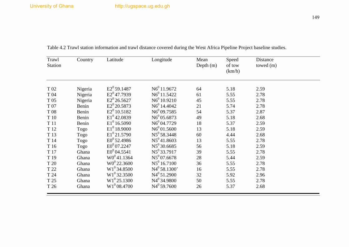
149
Table 4.2 Trawl station information and trawl distance covered during the West Africa Pipeline Project baseline studies.
Trawl Country Latitude Longitude Mean Speed Distance
Station Depth (m) of tow towed (m)
(km/h)
T 02 Nigeria E20
59.1487 N60
11.9672 64 5.18 2.59
T 04 Nigeria E20
47.7939 N60
11.5422 61 5.55 2.78
T 05 Nigeria E20
26.5627 N60
10.9210 45 5.55 2.78
T 07 Benin E20
20.5873 N60
14.4042 21 5.74 2.78
T 08 Benin E20
10.5182 N60
09.7585 54 5.37 2.87
T 10 Benin E10
42.0839 N60
05.6873 49 5.18 2.68
T 11 Benin E10
16.5090 N60
04.7729 18 5.37 2.59
T 12 Togo E10
18.9000 N60
01.5600 13 5.18 2.59
T 13 Togo E10
21.5790 N50
58.3448 60 4.44 2.68
T 14 Togo E00
52.4986 N50
41.8603 13 5.55 2.78
T 16 Togo E00
07.2247 N50
30.6685 56 5.18 2.59
T 17 Ghana E00
04.5541 N50
33.7917 39 5.55 2.78
T 19 Ghana W00 41.1364 N5
0 07.6678 28 5.44 2.59
T 20 Ghana W00 22.3600 N5
0 16.7100 36 5.55 2.78
T 22 Ghana W10 34.8500 N4
0 58.1300‘ 16 5.55 2.78
T 24 Ghana W10 32.3500 N4
0 51.2900 32 5.92 2.96
T 25 Ghana W10 25.1300 N4
0 34.9800 50 5.55 2.78
T 26 Ghana W10 08.4700 N4
0 59.7600 26 5.37 2.68
University of Ghana http://ugspace.ug.edu.gh
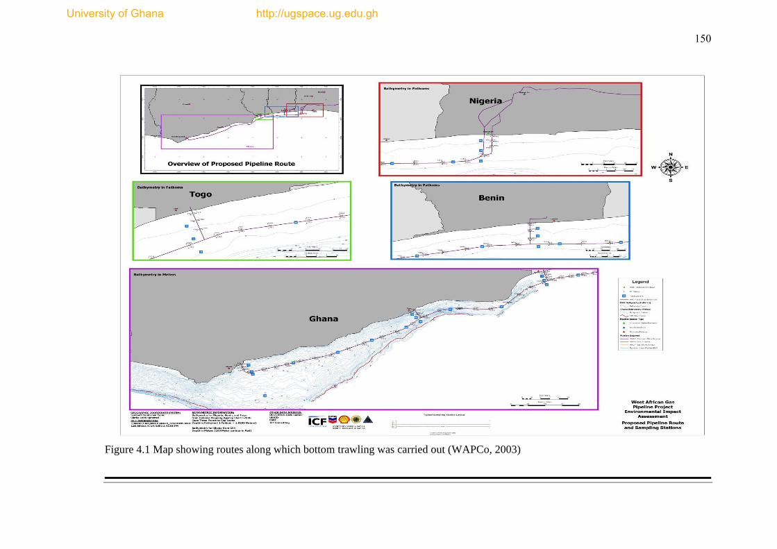
150
Figure 4.1 Map showing routes along which bottom trawling was carried out (WAPCo, 2003)
University of Ghana http://ugspace.ug.edu.gh
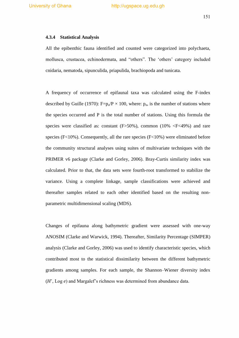
151
4.3.4 Statistical Analysis
All the epibenthic fauna identified and counted were categorized into polychaeta,
mollusca, crustacea, echinodermata, and ―others‖. The ‗others‘ category included
cnidaria, nematoda, sipunculida, priapulida, brachiopoda and tunicata.
A frequency of occurrence of epifaunal taxa was calculated using the F-index
described by Guille (1970): F=pa/P × 100, where: pa, is the number of stations where
the species occurred and P is the total number of stations. Using this formula the
species were classified as: constant (F>50%), common (10% <F<49%) and rare
species (F<10%). Consequently, all the rare species (F<10%) were eliminated before
the community structural analyses using suites of multivariate techniques with the
PRIMER v6 package (Clarke and Gorley, 2006). Bray-Curtis similarity index was
calculated. Prior to that, the data sets were fourth-root transformed to stabilize the
variance. Using a complete linkage, sample classifications were achieved and
thereafter samples related to each other identified based on the resulting non-
parametric multidimensional scaling (MDS).
Changes of epifauna along bathymetric gradient were assessed with one-way
ANOSIM (Clarke and Warwick, 1994). Thereafter, Similarity Percentage (SIMPER)
analysis (Clarke and Gorley, 2006) was used to identify characteristic species, which
contributed most to the statistical dissimilarity between the different bathymetric
gradients among samples. For each sample, the Shannon–Wiener diversity index
(H‘, Log e) and Margalef‘s richness was determined from abundance data.
University of Ghana http://ugspace.ug.edu.gh
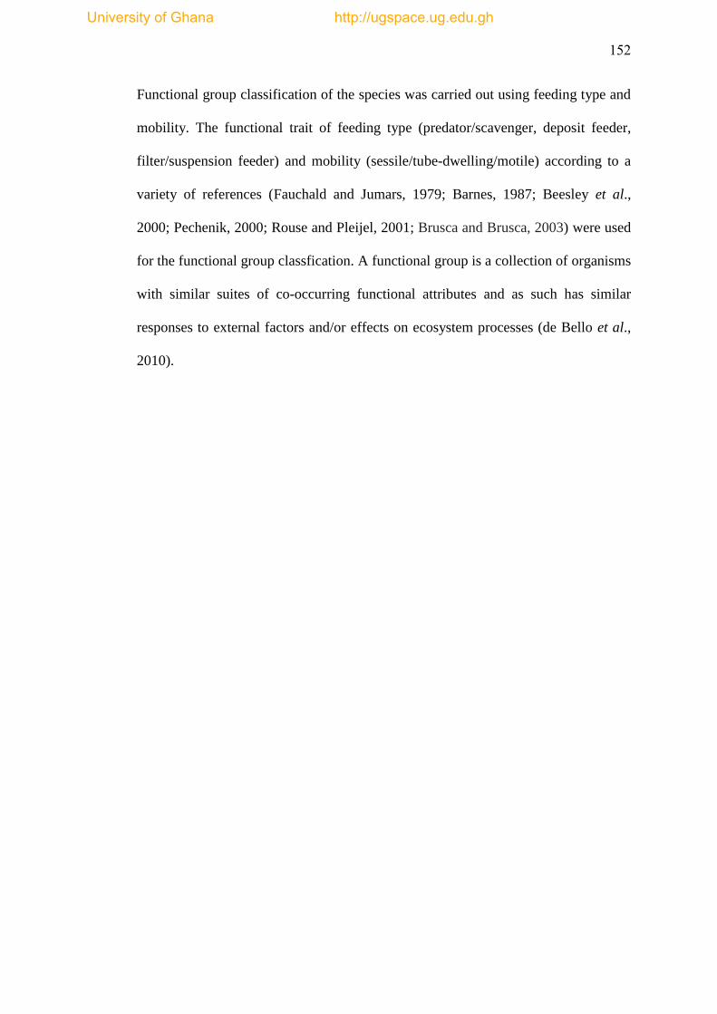
152
Functional group classification of the species was carried out using feeding type and
mobility. The functional trait of feeding type (predator/scavenger, deposit feeder,
filter/suspension feeder) and mobility (sessile/tube-dwelling/motile) according to a
variety of references (Fauchald and Jumars, 1979; Barnes, 1987; Beesley et al.,
2000; Pechenik, 2000; Rouse and Pleijel, 2001; Brusca and Brusca, 2003) were used
for the functional group classfication. A functional group is a collection of organisms
with similar suites of co-occurring functional attributes and as such has similar
responses to external factors and/or effects on ecosystem processes (de Bello et al.,
2010).
University of Ghana http://ugspace.ug.edu.gh
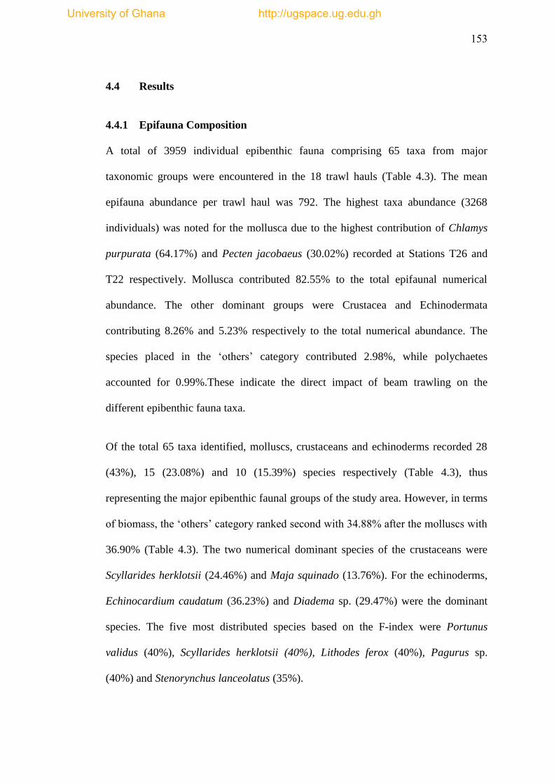
153
4.4 Results
4.4.1 Epifauna Composition
A total of 3959 individual epibenthic fauna comprising 65 taxa from major
taxonomic groups were encountered in the 18 trawl hauls (Table 4.3). The mean
epifauna abundance per trawl haul was 792. The highest taxa abundance (3268
individuals) was noted for the mollusca due to the highest contribution of Chlamys
purpurata (64.17%) and Pecten jacobaeus (30.02%) recorded at Stations T26 and
T22 respectively. Mollusca contributed 82.55% to the total epifaunal numerical
abundance. The other dominant groups were Crustacea and Echinodermata
contributing 8.26% and 5.23% respectively to the total numerical abundance. The
species placed in the ‗others‘ category contributed 2.98%, while polychaetes
accounted for 0.99%.These indicate the direct impact of beam trawling on the
different epibenthic fauna taxa.
Of the total 65 taxa identified, molluscs, crustaceans and echinoderms recorded 28
(43%), 15 (23.08%) and 10 (15.39%) species respectively (Table 4.3), thus
representing the major epibenthic faunal groups of the study area. However, in terms
of biomass, the ‗others‘ category ranked second with 34.88% after the molluscs with
36.90% (Table 4.3). The two numerical dominant species of the crustaceans were
Scyllarides herklotsii (24.46%) and Maja squinado (13.76%). For the echinoderms,
Echinocardium caudatum (36.23%) and Diadema sp. (29.47%) were the dominant
species. The five most distributed species based on the F-index were Portunus
validus (40%), Scyllarides herklotsii (40%), Lithodes ferox (40%), Pagurus sp.
(40%) and Stenorynchus lanceolatus (35%).
University of Ghana http://ugspace.ug.edu.gh
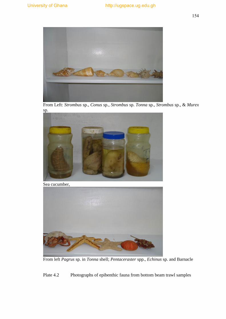
154
From Left: Strombus sp., Conus sp., Strombus sp. Tonna sp., Strombus sp., & Murex
sp.
Sea cucumber,
From left Pagrus sp. in Tonna shell; Pentaceraster spp., Echinus sp. and Barnacle
Plate 4.2 Photographs of epibenthic fauna from bottom beam trawl samples
University of Ghana http://ugspace.ug.edu.gh
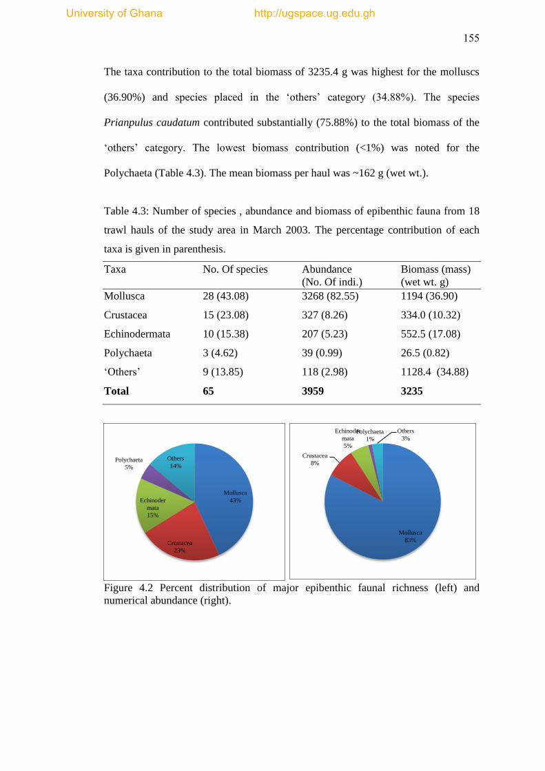
155
The taxa contribution to the total biomass of 3235.4 g was highest for the molluscs
(36.90%) and species placed in the ‗others‘ category (34.88%). The species
Prianpulus caudatum contributed substantially (75.88%) to the total biomass of the
‗others‘ category. The lowest biomass contribution (<1%) was noted for the
Polychaeta (Table 4.3). The mean biomass per haul was ~162 g (wet wt.).
Table 4.3: Number of species , abundance and biomass of epibenthic fauna from 18
trawl hauls of the study area in March 2003. The percentage contribution of each
taxa is given in parenthesis.
Taxa No. Of species Abundance Biomass (mass)
(No. Of indi.) (wet wt. g)
Mollusca 28 (43.08) 3268 (82.55) 1194 (36.90)
Crustacea 15 (23.08) 327 (8.26) 334.0 (10.32)
Echinodermata 10 (15.38) 207 (5.23) 552.5 (17.08)
Polychaeta 3 (4.62) 39 (0.99) 26.5 (0.82)
‗Others‘ 9 (13.85) 118 (2.98) 1128.4 (34.88)
Total 65 3959 3235
Figure 4.2 Percent distribution of major epibenthic faunal richness (left) and
numerical abundance (right).
Mollusca
43%
Crustacea
23%
Echinoder
mata
15%
Polychaeta
5%
Others
14%
Mollusca
83%
Crustacea
8%
Echinoder
mata
5%
Polychaeta
1%
Others
3%
University of Ghana http://ugspace.ug.edu.gh

156
4.4.1.1 Comparison of Bathymetric Distribution of Epifauna and Fish
Assemblage Structure
The distribution of taxa abundance across bathymetric gradient indicated a decrease
in numerical abundance of epibenthic fauna with increasing water depth (Fig. 4.3).
Abundance of fish on the other hand did not show any discernible bathymetric
pattern except that the highest abundance occurred at mid-depth water (i.e., 31-50m).
There were no significant differences (p>0.05) in abundance of epifauna and fish at
both mid-depth (31-50m) and deeper waters (51-70m), which suggests that for the
study area impact of bottom trawling epifauna abundance could be inferred from fish
catches, albeit comparatively fish abundances at these depths were relatively higher
than the epifauna. The significant difference (p<.05, ANOVA) between abundances
of fish and epibenthic fauna at shallow-dept (11-30m) suggests that trawling impact
at this depth would be significant on the epibenthic fauna, since numerically
epifauna ranked highest (Fig. 4.3).
For taxa biomass, the epifauna ranked highest across all the depth zones in
comparison with the fish abundance. The highest biomass (catch by weight) was
recorded at mid-depth (31-50m). The degree of variations in taxa biomass for both
epifauna and fish assemblage decreased with increasing water depth (Fig. 4.4). This
occurrence may suggest prevailing benign conditions at deeper depths or conversely
a higher degree of disturbances at shallow depths. This dichotomy may have been
due to the creation of different niches that have physiologically and ecologically
adapted to the respective zones.
University of Ghana http://ugspace.ug.edu.gh

157
Figure 4.3 Bathymetric pattern of mean abundance (±SE) for epifauna and fish from
trawl catches.
Figure 4.4 Bathymetric pattern of mean biomass (±SE) for epifauna and fish from
trawl catches.
0
200
400
600
800
1000
1200
1400
1600
11-30 m 31-50 m 51-70 m
Ab
un
dan
ce (
No.
of
ind
.)
Epifauna Fish
0
200
400
600
800
1000
1200
11-30 m 31-50 m 51-70 m
Mea
n B
iom
ass
(g)
Depth (m)
Epibenthic fauna Fish
University of Ghana http://ugspace.ug.edu.gh
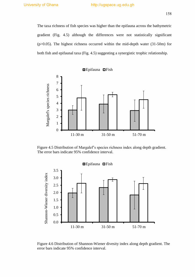
158
The taxa richness of fish species was higher than the epifauna across the bathymetric
gradient (Fig. 4.5) although the differences were not statistically significant
(p>0.05). The highest richness occurred within the mid-depth water (31-50m) for
both fish and epifaunal taxa (Fig. 4.5) suggesting a synergistic trophic relationship.
Figure 4.5 Distribution of Margalef‘s species richness index along depth gradient.
The error bars indicate 95% confidence interval.
Figure 4.6 Distribution of Shannon-Wiener divesity index along depth gradient. The
error bars indicate 95% confidence interval.
0
1
2
3
4
5
6
7
8
11-30 m 31-50 m 51-70 m
Mar
gal
ef's
sp
ecie
s ri
chnes
s
Epifauna Fish
0.0
0.5
1.0
1.5
2.0
2.5
3.0
3.5
11-30 m 31-50 m 51-70 m
Shan
non
-Wie
ner
div
ersi
ty i
ndex
Epifauna Fish
University of Ghana http://ugspace.ug.edu.gh
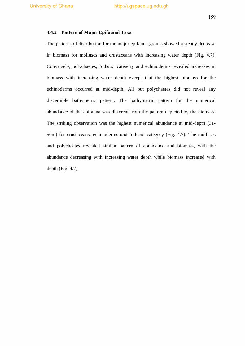
159
4.4.2 Pattern of Major Epifaunal Taxa
The patterns of distribution for the major epifauna groups showed a steady decrease
in biomass for molluscs and crustaceans with increasing water depth (Fig. 4.7).
Conversely, polychaetes, ‗others‘ category and echinoderms revealed increases in
biomass with increasing water depth except that the highest biomass for the
echinoderms occurred at mid-depth. All but polychaetes did not reveal any
discernible bathymetric pattern. The bathymetric pattern for the numerical
abundance of the epifauna was different from the pattern depicted by the biomass.
The striking observation was the highest numerical abundance at mid-depth (31-
50m) for crustaceans, echinoderms and ‗others‘ category (Fig. 4.7). The molluscs
and polychaetes revealed similar pattern of abundance and biomass, with the
abundance decreasing with increasing water depth while biomass increased with
depth (Fig. 4.7).
University of Ghana http://ugspace.ug.edu.gh

160
Figure 4.7 Mean biomass (±SE) of major epibenthic fauna along bathymetric gradient.
-50
0
50
100
150
200
250
300
11-30 m 31-50 m 51-70 m
Mollusca
-10
0
10
20
30
40
50
60
11-30 m 31-50 m 51-70 m
Crustacea
-30-20-10
01020304050607080
11-30 m 31-50 m 51-70 m
Echinodermata
-1
0
1
2
3
4
5
6
7
8
11-30 m 31-50 m 51-70 m
Polychaeta
-150
-100
-50
0
50
100
150
200
250
300
11-30 m 31-50 m 51-70 m
Others
University of Ghana http://ugspace.ug.edu.gh

161
Figure 4.8 Mean abundance (±SE) of major epibenthic fauna along bathymetric gradient.
-600
-400
-200
0
200
400
600
800
1000
1200
1400
1600
11-30 m 31-50 m 51-70 m
Mollusca
-10
0
10
20
30
40
50
11-30 m 31-50 m 51-70 m
Crustacea
-20
-10
0
10
20
30
40
50
60
70
11-30 m 31-50 m 51-70 m
Echinodermata
-2
0
2
4
6
8
10
12
11-30 m 31-50 m 51-70 m
Polychaeta
-10
-5
0
5
10
15
20
25
30
11-30 m 31-50 m 51-70 m
Others
University of Ghana http://ugspace.ug.edu.gh
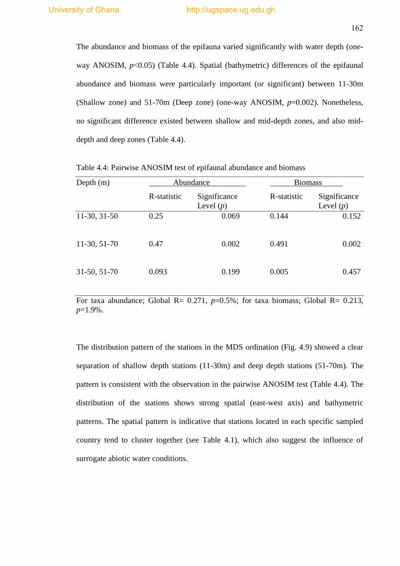
162
The abundance and biomass of the epifauna varied significantly with water depth (one-
way ANOSIM, p<0.05) (Table 4.4). Spatial (bathymetric) differences of the epifaunal
abundance and biomass were particularly important (or significant) between 11-30m
(Shallow zone) and 51-70m (Deep zone) (one-way ANOSIM, p=0.002). Nonetheless,
no significant difference existed between shallow and mid-depth zones, and also mid-
depth and deep zones (Table 4.4).
Table 4.4: Pairwise ANOSIM test of epifaunal abundance and biomass
Depth (m) Abundance Biomass
R-statistic Significance R-statistic Significance
Level (p) Level (p)
11-30, 31-50 0.25 0.069 0.144 0.152
11-30, 51-70 0.47 0.002 0.491 0.002
31-50, 51-70 0.093 0.199 0.005 0.457
For taxa abundance; Global R= 0.271, p=0.5%; for taxa biomass; Global R= 0.213,
p=1.9%.
The distribution pattern of the stations in the MDS ordination (Fig. 4.9) showed a clear
separation of shallow depth stations (11-30m) and deep depth stations (51-70m). The
pattern is consistent with the observation in the pairwise ANOSIM test (Table 4.4). The
distribution of the stations shows strong spatial (east-west axis) and bathymetric
patterns. The spatial pattern is indicative that stations located in each specific sampled
country tend to cluster together (see Table 4.1), which also suggest the influence of
surrogate abiotic water conditions.
University of Ghana http://ugspace.ug.edu.gh
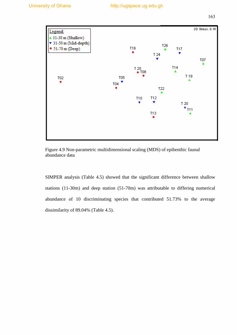
163
Figure 4.9 Non-parametric multidimensional scaling (MDS) of epibenthic faunal
abundance data
SIMPER analysis (Table 4.5) showed that the significant difference between shallow
stations (11-30m) and deep station (51-70m) was attributable to differing numerical
abundance of 10 discriminating species that contributed 51.73% to the average
dissimilarity of 89.04% (Table 4.5).
University of Ghana http://ugspace.ug.edu.gh
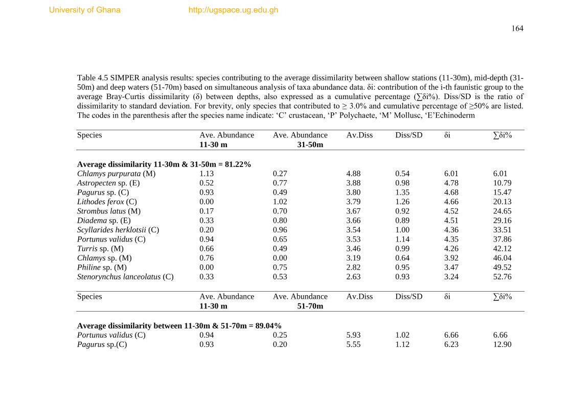
164
Table 4.5 SIMPER analysis results: species contributing to the average dissimilarity between shallow stations (11-30m), mid-depth (31-
50m) and deep waters (51-70m) based on simultaneous analysis of taxa abundance data. δi: contribution of the i-th faunistic group to the
average Bray-Curtis dissimilarity (δ) between depths, also expressed as a cumulative percentage (∑δi%). Diss/SD is the ratio of
dissimilarity to standard deviation. For brevity, only species that contributed to ≥ 3.0% and cumulative percentage of ≥50% are listed.
The codes in the parenthesis after the species name indicate: ‗C‘ crustacean, ‗P‘ Polychaete, ‗M‘ Mollusc, ‗E‘Echinoderm
Species Ave. Abundance Ave. Abundance Av.Diss Diss/SD δi ∑δi%
11-30 m 31-50m
Average dissimilarity 11-30m & 31-50m = 81.22%
Chlamys purpurata (M) 1.13 0.27 4.88 0.54 6.01 6.01
Astropecten sp. (E) 0.52 0.77 3.88 0.98 4.78 10.79
Pagurus sp. (C) 0.93 0.49 3.80 1.35 4.68 15.47
Lithodes ferox (C) 0.00 1.02 3.79 1.26 4.66 20.13
Strombus latus (M) 0.17 0.70 3.67 0.92 4.52 24.65
Diadema sp. (E) 0.33 0.80 3.66 0.89 4.51 29.16
Scyllarides herklotsii (C) 0.20 0.96 3.54 1.00 4.36 33.51
Portunus validus (C) 0.94 0.65 3.53 1.14 4.35 37.86
Turris sp. (M) 0.66 0.49 3.46 0.99 4.26 42.12
Chlamys sp. (M) 0.76 0.00 3.19 0.64 3.92 46.04
Philine sp. (M) 0.00 0.75 2.82 0.95 3.47 49.52
Stenorynchus lanceolatus (C) 0.33 0.53 2.63 0.93 3.24 52.76
Species Ave. Abundance Ave. Abundance Av.Diss Diss/SD δi ∑δi%
11-30 m 51-70m
Average dissimilarity between 11-30m & 51-70m = 89.04%
Portunus validus (C) 0.94 0.25 5.93 1.02 6.66 6.66
Pagurus sp.(C) 0.93 0.20 5.55 1.12 6.23 12.90
University of Ghana http://ugspace.ug.edu.gh
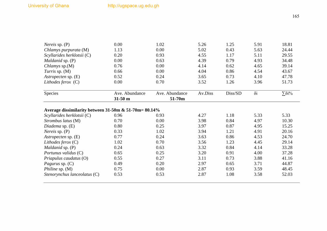
165
Nereis sp. (P) 0.00 1.02 5.26 1.25 5.91 18.81
Chlamys purpurata (M) 1.13 0.00 5.02 0.43 5.63 24.44
Scyllarides herklotsii (C) 0.20 0.93 4.55 1.17 5.11 29.55
Maldanid sp. (P) 0.00 0.63 4.39 0.79 4.93 34.48
Chlamys sp.(M) 0.76 0.00 4.14 0.62 4.65 39.14
Turris sp. (M) 0.66 0.00 4.04 0.86 4.54 43.67
Astropecten sp. (E) 0.52 0.24 3.65 0.73 4.10 47.78
Lithodes ferox (C) 0.00 0.70 3.52 1.26 3.96 51.73
Species Ave. Abundance Ave. Abundance Av.Diss Diss/SD δi ∑δi%
31-50 m 51-70m
Average dissimilarity between 31-50m & 51-70m= 80.14%
Scyllarides herklotsii (C) 0.96 0.93 4.27 1.18 5.33 5.33
Strombus latus (M) 0.70 0.00 3.98 0.84 4.97 10.30
Diadema sp. (E) 0.80 0.25 3.97 0.87 4.95 15.25
Nereis sp. (P) 0.33 1.02 3.94 1.21 4.91 20.16
Astropecten sp. (E) 0.77 0.24 3.63 0.86 4.53 24.70
Lithodes ferox (C) 1.02 0.70 3.56 1.23 4.45 29.14
Maldanid sp. (P) 0.24 0.63 3.32 0.84 4.14 33.28
Portunus validus (C) 0.65 0.25 3.20 0.91 4.00 37.28
Priapulus caudatus (O) 0.55 0.27 3.11 0.73 3.88 41.16
Pagurus sp. (C) 0.49 0.20 2.97 0.65 3.71 44.87
Philine sp. (M) 0.75 0.00 2.87 0.93 3.59 48.45
Stenorynchus lanceolatus (C) 0.53 0.53 2.87 1.08 3.58 52.03
University of Ghana http://ugspace.ug.edu.gh
166
4.4.3 Species Dominance and Pollution Status
In order to ascertain the impact and the level of habitat stress possibly from bottom
trawling or natural process, species abundance/biomass comparison (ABC) curves were
determined as proposed by Warwick (1986). Warwick suggested on theoretical
considerations that the distribution of the numbers of individuals among species should
differ from the distribution of biomass among species when influenced by pollution-
induced disturbance. This difference can be shown by K-dominance plots (Lambshead et
al., 1983; Shaw et al., 1983). The curves rank species in order of importance on the x-
axis and show the percentage of each species or the total numbers or biomass on a
cumulative scale (called percentage dominance) on the y-axis. There are three scenarios
of the ABC curves. These are:
i) when the community is approaching equilibrium, the biomass becomes
increasingly dominated by one or a few large species, each represented by few
individuals. The numerical dominants are generally smaller species. Hence, when
plotted as K-dominance curves, 'numerical diversity' is greater than 'biomass diversity',
so that the line for abundance lies well below the line for biomass, since one species
forms a much larger proportion of the total biomass than it does of the total numbers.
ii) Under stress (natural physical and biological or pollution-induced disturbances),
large competitive dominants are eliminated and biomass and abundance curves are close
together and crossing one or several times.
iii) Under severe disturbance, benthic communities become increasingly dominated
by one or a few very small species (usually annelids such as Capitella spp. or
oligochaetes) and few larger species are present. Hence 'numerical diversity' is lower
than 'biomass diversity'.
University of Ghana http://ugspace.ug.edu.gh
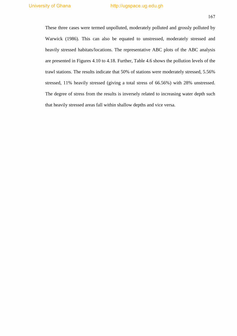
167
These three cases were termed unpolluted, moderately polluted and grossly polluted by
Warwick (1986). This can also be equated to unstressed, moderately stressed and
heavily stressed habitats/locations. The representative ABC plots of the ABC analysis
are presented in Figures 4.10 to 4.18. Further, Table 4.6 shows the pollution levels of the
trawl stations. The results indicate that 50% of stations were moderately stressed, 5.56%
stressed, 11% heavily stressed (giving a total stress of 66.56%) with 28% unstressed.
The degree of stress from the results is inversely related to increasing water depth such
that heavily stressed areas fall within shallow depths and vice versa.
University of Ghana http://ugspace.ug.edu.gh
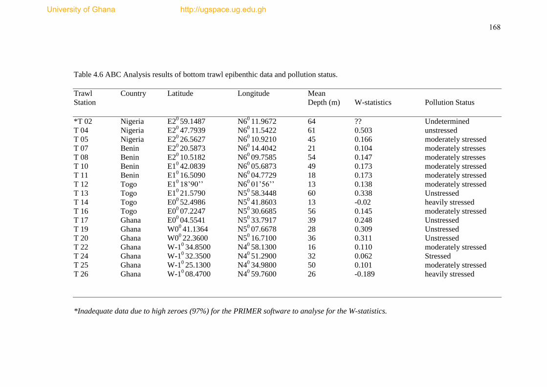
168
Table 4.6 ABC Analysis results of bottom trawl epibenthic data and pollution status.
Trawl Country Latitude Longitude Mean
Station Depth (m) W-statistics Pollution Status
*T 02 Nigeria E20
59.1487 N60
11.9672 64 ?? Undetermined
T 04 Nigeria E20
47.7939 N60
11.5422 61 0.503 unstressed
T 05 Nigeria E20
26.5627 N60
10.9210 45 0.166 moderately stressed
T 07 Benin E20
20.5873 N60
14.4042 21 0.104 moderately stresses
T 08 Benin E20
10.5182 N60
09.7585 54 0.147 moderately stresses
T 10 Benin E10
42.0839 N60
05.6873 49 0.173 moderately stressed
T 11 Benin E10
16.5090 N60
04.7729 18 0.173 moderately stressed
T 12 Togo E10
18‘90‘‘ N60
01‘56‘‘ 13 0.138 moderately stressed
T 13 Togo E10
21.5790 N50
58.3448 60 0.338 Unstressed
T 14 Togo E00
52.4986 N50
41.8603 13 -0.02 heavily stressed
T 16 Togo E00
07.2247 N50
30.6685 56 0.145 moderately stressed
T 17 Ghana E00
04.5541 N50
33.7917 39 0.248 Unstressed
T 19 Ghana W00 41.1364 N5
0 07.6678 28 0.309 Unstressed
T 20 Ghana W00 22.3600 N5
0 16.7100 36 0.311 Unstressed
T 22 Ghana W-10
34.8500 N40
58.1300 16 0.110 moderately stressed
T 24 Ghana W-10
32.3500 N40
51.2900 32 0.062 Stressed
T 25 Ghana W-10
25.1300 N40
34.9800 50 0.101 moderately stressed
T 26 Ghana W-10
08.4700 N40
59.7600 26 -0.189 heavily stressed
*Inadequate data due to high zeroes (97%) for the PRIMER software to analyse for the W-statistics.
University of Ghana http://ugspace.ug.edu.gh

169
Figure 4.10 ABC plots for stations T-04 (top) and T-05 (bottom) based on epibenthic
fauna abundance and biomass data.
University of Ghana http://ugspace.ug.edu.gh

170
Figure 4.11 ABC plots for stations T-07 (top) and T-08 (bottom) based on epibenthic
fauna abundance and biomass data.
University of Ghana http://ugspace.ug.edu.gh

171
Figure 4.12 ABC plots for stations T-10 (top) and T-11 (bottom) based on epibenthic
fauna abundance and biomass data.
University of Ghana http://ugspace.ug.edu.gh
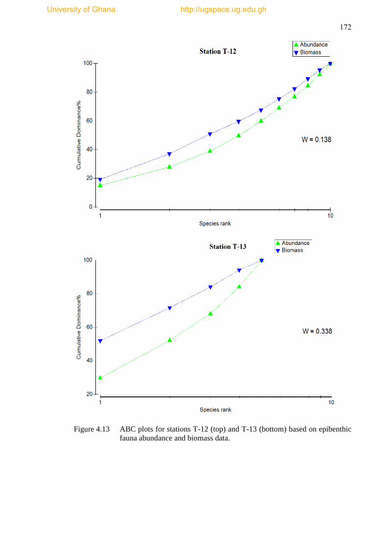
172
Figure 4.13 ABC plots for stations T-12 (top) and T-13 (bottom) based on epibenthic
fauna abundance and biomass data.
University of Ghana http://ugspace.ug.edu.gh
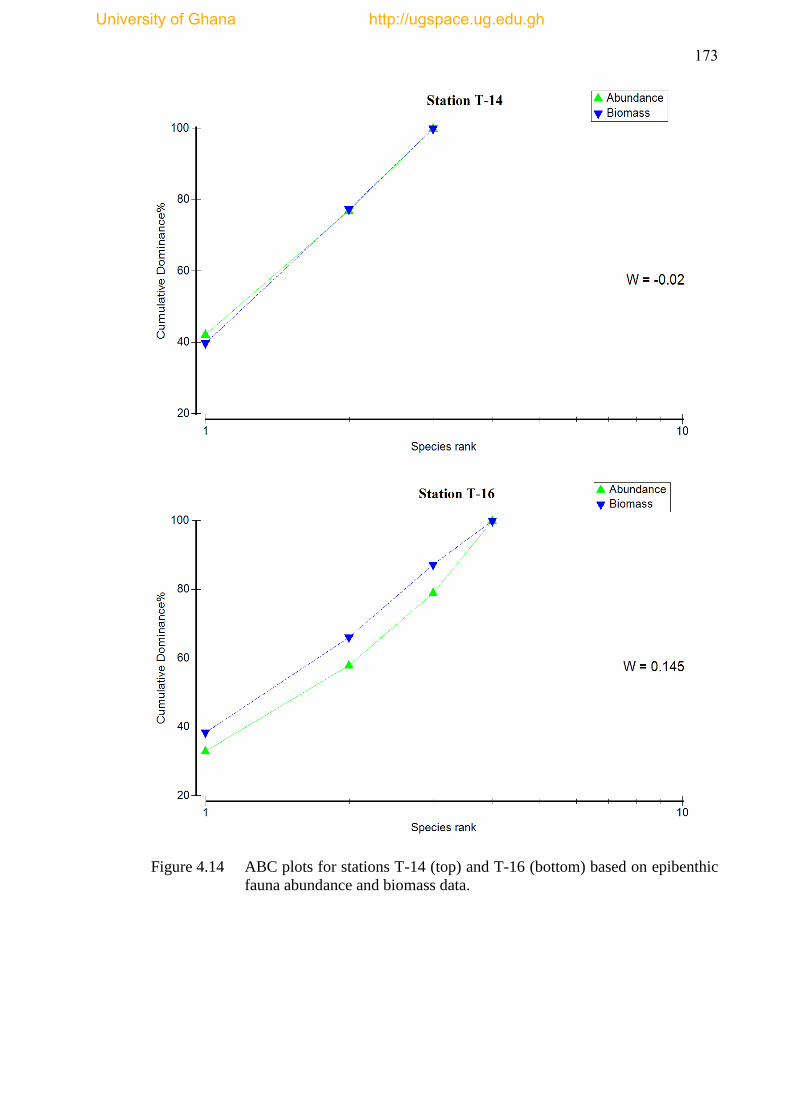
173
Figure 4.14 ABC plots for stations T-14 (top) and T-16 (bottom) based on epibenthic
fauna abundance and biomass data.
University of Ghana http://ugspace.ug.edu.gh
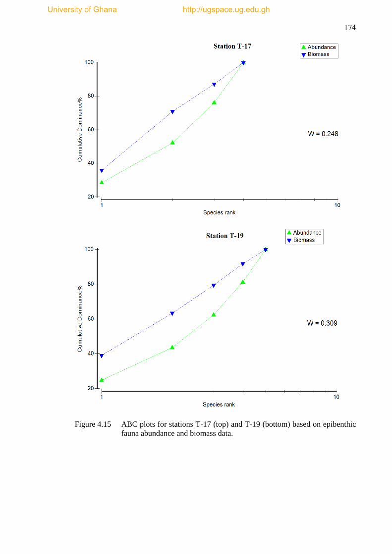
174
Figure 4.15 ABC plots for stations T-17 (top) and T-19 (bottom) based on epibenthic
fauna abundance and biomass data.
University of Ghana http://ugspace.ug.edu.gh

175
Figure 4.16 ABC plots for stations T-20 (top) and T-22 (bottom) based on epibenthic
fauna abundance and biomass data.
University of Ghana http://ugspace.ug.edu.gh

176
Figure 4.17 ABC plots for stations T-24 (top) and T-25 (bottom) based on epibenthic
fauna abundance and biomass data.
University of Ghana http://ugspace.ug.edu.gh

177
Figure 4.18 ABC plots for station T-26 based on epibenthic fauna abundance and
biomass data.
4.4.4 Epifauna Functional Composition
4.4.4.1 Functional Group Diversity
The main benthic feeding types can be divided in two ways: what they feed on and how
they feed. Category one can be divided into herbivores, carnivores, and detritivores, and
the second into suspension-feeders, filter-feeders, deposit-feeders, scavengers, and
predators (Fauchald and Jumars, 1979). Feeding strategy can offer ecologically relevant
information on if and how human activities may affect the ecosystem, from the scale of
an organism to the community. The Fauchald and Jumars (1979) feeding category was
used for the epibenthic functional categorization.
In all, a total of twelve benthic feeding group categories were identified with some
organisms sharing more than one feeding group. The result of feeding group
composition depicts that carnivores largely contributed to the feeding community with
University of Ghana http://ugspace.ug.edu.gh
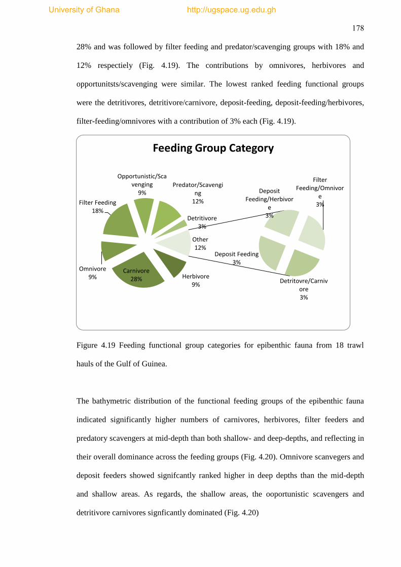
178
28% and was followed by filter feeding and predator/scavenging groups with 18% and
12% respectiely (Fig. 4.19). The contributions by omnivores, herbivores and
opportunitsts/scavenging were similar. The lowest ranked feeding functional groups
were the detritivores, detritivore/carnivore, deposit-feeding, deposit-feeding/herbivores,
filter-feeding/omnivores with a contribution of 3% each (Fig. 4.19).
Figure 4.19 Feeding functional group categories for epibenthic fauna from 18 trawl
hauls of the Gulf of Guinea.
The bathymetric distribution of the functional feeding groups of the epibenthic fauna
indicated significantly higher numbers of carnivores, herbivores, filter feeders and
predatory scavengers at mid-depth than both shallow- and deep-depths, and reflecting in
their overall dominance across the feeding groups (Fig. 4.20). Omnivore scanvegers and
deposit feeders showed signifcantly ranked higher in deep depths than the mid-depth
and shallow areas. As regards, the shallow areas, the ooportunistic scavengers and
detritivore carnivores signficantly dominated (Fig. 4.20)
Herbivore 9%
Carnivore 28%
Omnivore 9%
Filter Feeding 18%
Opportunistic/Scavenging
9% Predator/Scavengi
ng 12%
Detritivore 3%
Detritovre/Carnivore 3%
Deposit Feeding 3%
Deposit Feeding/Herbivor
e 3%
Filter Feeding/Omnivor
e 3%
Other 12%
Feeding Group Category
University of Ghana http://ugspace.ug.edu.gh

179
Figure 4.20 Richness of functional feeding groups across bathymetric gradient.
An important component of foraging strategy is motility and motility patterns may be
related to feeding. The structure of the feeding apparatus may force the animal to remain
sessile while feeding or the use of the feeding apparatus may be independent of, or
require locomotion for proper fuction. Further, the mobility pattern may indicate escape
response mechanisms of the organisms from disturbance (e.g., bottom trawling,
predation) and may influence the community pattern.
The results of the analysis revealed that approximatley 64% of the epibenthic fauna
encountered were motile and 12% were sessile with only 3% being sedentary (Fig.
4.21). This high mobility reflects in the dominance of carnivores, herbivores and filter
feeders functional groups. These feeding groups require mobility in their foraging
0
2
4
6
8
10
12
14
16
18
20
Num
ber
of
ind
ivid
ual
Feeding type
Shallow Middepth Deep
University of Ghana http://ugspace.ug.edu.gh
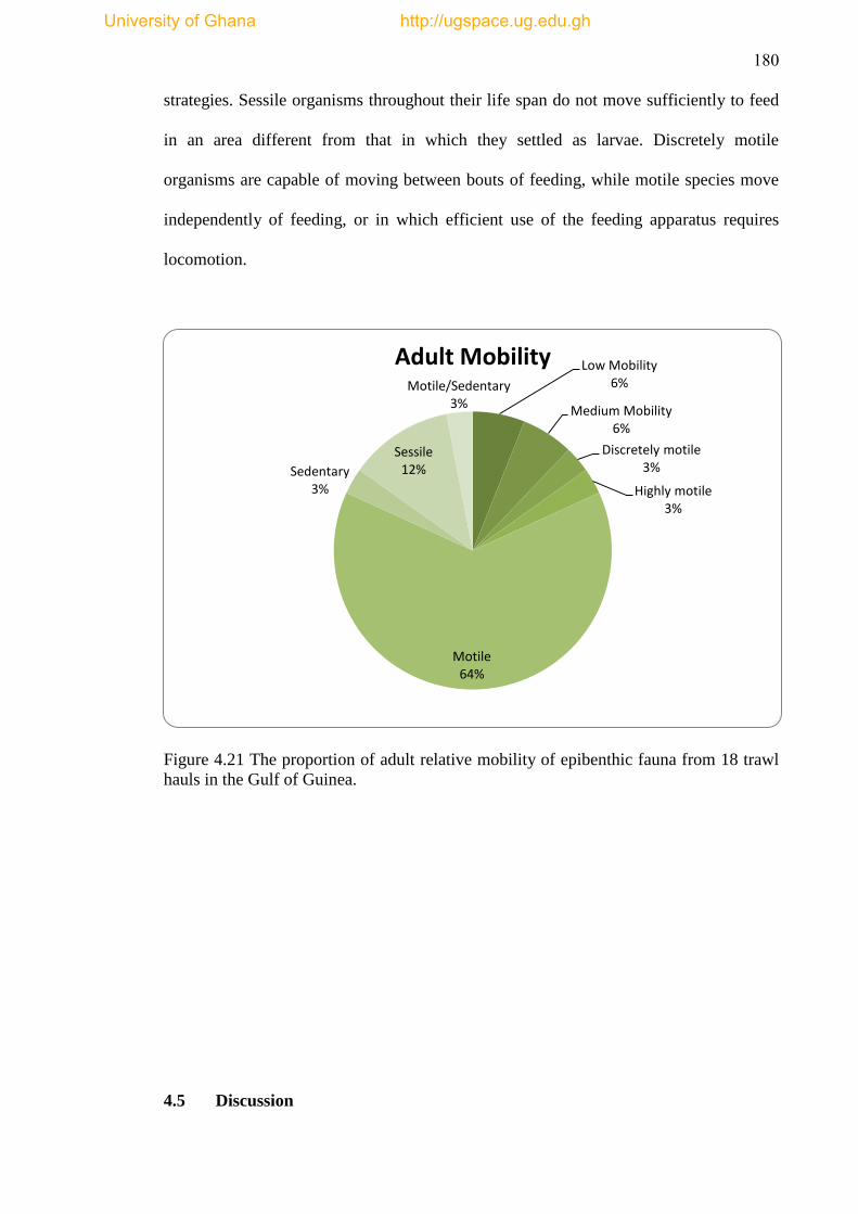
180
strategies. Sessile organisms throughout their life span do not move sufficiently to feed
in an area different from that in which they settled as larvae. Discretely motile
organisms are capable of moving between bouts of feeding, while motile species move
independently of feeding, or in which efficient use of the feeding apparatus requires
locomotion.
Figure 4.21 The proportion of adult relative mobility of epibenthic fauna from 18 trawl
hauls in the Gulf of Guinea.
4.5 Discussion
Low Mobility 6%
Medium Mobility 6%
Discretely motile 3%
Highly motile 3%
Motile 64%
Sedentary 3%
Sessile 12%
Motile/Sedentary 3%
Adult Mobility
University of Ghana http://ugspace.ug.edu.gh
181
Typical bottom beam trawling for demersal fishes are very efficient in catching
epibenthic invertebrates (Reiss et al., 2006). These epibenthic organisms though often
treated as by-catch are a dominant component of the trawl catches. According to Clarke
(2000), the direct effect of mortality caused by beam trawling varies from species to
species, with 10-40% mortality in gastropods, starfish, crustaceans and annelid worms,
from 10-50% for sea urchins to 30-80% for bivalves. However, this study showed that
epibenthic invertebrate by-catch was primarily made up of molluscs (82.6% richness
and 43.1% numerical abundance), crustaceans (23.1% richness) and echinoderms
(15.4% richness) (Table 4.3). These percentages are consistent and compared well with
estimated percentage of benthic production that is consumed by fish predators (~45%)
(Clarke, 2000).
At the community level, the mortality imposed by the trawl fishery will depend on the
level of direct mortality, the trawling frequency and the overlap in spatial distribution
between the fishery and the benthic organisms. Studies of the annual direct fishing
mortality rates on benthic invertebrates, for example, in the southern North Sea were
estimated at between 7 and 45% of the individuals (de Groot and Lindeboom, 1994).
The epibenthic faunal organisms often contribute considerably to total benthic biomass
(Lampitt et al., 1986) and carbon cycling (Piepenburg et al., 1995) and are supposed to
have a strong impact on the micro-scale environment with, for instance, bio-turbation
and bio-irrigation (Huettel and Gust, 1992). These important ecosystem services as a
result of their functional attributes is potentially eroded by bottom trawling activities,
which sweep the seafloor of epibenthic invertebrates that are treated as by-catch. Aside
the variation of the severity of impacts from species to species, the impact of the
trawling is also spatial dependent as trawling varies from location to location.
University of Ghana http://ugspace.ug.edu.gh
182
The current study revealed significant differences in epibenthic biomass across depth
scales. In particular, the biomasses of crustaceans and molluscs decreased with
increasing water depth (Fig. 4.8), which confirmed a generally recognized pattern (e.g.,
Rowe, 1983). Importantly, the epibenthic fauna community of the central sections of the
GCLME (Gulf of Guinea) presented a clear defined bathymetric pattern of distribution
both in terms of species abundance and functional richness and abundance. The
assemblage pattern depicted a significant difference (p<0.05) between shallow-depth
and deep-depth suggesting the existence of a unique abiotic factors or conditions
structuring the epibenthic species assemblages. At the mid-depth however, both the
species richness and diversity of fish and epibenthic fauna assemblages were
correlatively higher (Figs. 4.6 and 4.7), which i) suggested a trophic dependence or
interactions of fish and epibenthic fauna, and ii) the existence of conducive (or tolerable)
abiotic conditions supporting the higher diversity.
Dietary studies have confirmed that large fishes prey on decapods (Polunin et al., 2001)
and this was evident in this study with crustaceans numerically dominant at md-depth
(Fig. 4.9). The numerical dominance of echinoderms and species placed in ‗Others‘
category at mid-depth (Fig. 4.9) could further lend credence to the trophic interactions
or dependence of fishes on epibenthic fauna. It is reasonable to assume that these
epibenthic invertebrates are the dominant food items in the diet of the fishes. Stomach
content analyses by several authors have indicated dominance of benthic invertebrates in
demersal fishes. For instance, amphipods provide an important food resource to many
demersal and benthic fishes (e.g. Gon and Heemstra, 1990; Kock, 1992; Olaso et al.,
2000), as well as other benthic invertebrates (McClintock et al., 1994).
University of Ghana http://ugspace.ug.edu.gh
183
The observed higher Margalef‘s species richness and Shannon-Wiener diversity indices
at the mid-depth may have been driven by trophic and physiological adaptation of the
communities to the prevailing abiotic conditions. This may be as a result of the
existence of multiple micro-habitats serving as, i) refugia (the patchy, diverse and multi-
stratified sessile benthos offer a high diversity of potential microhabitats to small vagile
invertebrates) and ii) the refugia enhancing foraging strategy (hiding and striking at
preys). The assignment of a marine species to a given habitat will depend on the time it
spends in that habitat. In other words, it depends on the organism‘s depth distribution
and the resource segment that it feeds upon, as well as on where it has the best chance to
avoid being taken as prey in its turn or where it faces less competition for food and
space (Sarda et al., 2005).
Some species will likely prefer a certain habitat or move between habitats, as well as
gather or disperse, depending on other indirect factors such as vertical migrations under
the influence of the photoperiod, annual seasonality, hydrographic conditions of the
water masses, or inter and intraspecific relationships (e.g. resource competition,
recruitment, sexual maturity, mating, biochemical cues etc.) (Sarda et al, 2005). These
factors may have played considerable structuring role in the observed numerically
higher epibenthic fauna abundance and biomass as well as fish assemblages in the mid-
depth zone by this study. Understandably, the mid-depth zone represents transitional
waters of the turbulent shallow-water zone and benign deep-water zone, and probably
presented environmentally tolerable conditions that as a consequence supported rich and
diverse epibenthic fauna communities such as crustaceans, echinoderms and species in
the ‗Others‘ category (Fig. 4.9).
University of Ghana http://ugspace.ug.edu.gh
184
The selection of a given species to particular habitats is driven by the tolerance of the
species to the given environment (Lamptey and Armah, 2008). Newell (1970) pointed
out that where the tolerance limits for a particular environmental variable have been
determined for an organism, the organism‘s realized distribution is much more restricted
than its potential distribution. It is reasonable, therefore, to presume that the relatively
large significant bathymetric differences in the taxonomic species and functional
assemblages were probably the results of existence of extremes of environmental
variables restricting the realized distribution of the species across all bathymetric
gradients. In other words, the potential differing abiotic environmental factors (condition
and resources) in the shallow-depth and deep-depth ensured that species tolerable to
these extreme environmental conditions survived. The declension of species abundance
of molluscs with increasing water depth and increased polychaete abundance with
increasing water depth (Figs. 4.8 and 4.9) gave further support to the assertion of
differing abiotic structuring mechanism along bathymetric gradients.
The distribution pattern of polychaete taxa is indicative that the deep-depth is
characteristic of fine-grained soft substrate with potentially high organic matter, which
probably was influenced by pelagic productivity. This statement is supported by the
observation of dominance of deposit-feeding polychaetes in deep-depth (Fig. 4.20) with
low suspension/filter-feeding organisms (e.g. molluscs), emphasizing the theory of
trophic group ammensalism (Rhoads and Young, 1970). The theory suggested that the
physical instability of reworked environment may discourage the settling larvae of
suspension feeders, and if settling does occur, early growth stages may be inhibited or
killed by the unstable sediment conditions. The inhibitors (deposit-feeders) are
unaffected by this relationship, while the amensals (suspension-feeders and sessile
epifauna) are either discouraged from settling or are killed during early benthonic stage.
University of Ghana http://ugspace.ug.edu.gh
185
Ostensibly, deep-depth ecosystems have lower energetic turnover than shallow-water or
littoral systems and their carrying capacity is expected to be lower (Cartes et al., 2002).
Conversely, the high numerical abundance and the correspondingly high biomass of
molluscs in shallow-water could mean that there is high current energy, which has
trophically favored the molluscan assemblage (or have adapted trophically) due in great
part to their active and passive suspension-feeding mechanism. Most molluscs prefer to
attach to rock stones and shells (Jorcin, 1996) and thus their abundance in the shallow-
waters is a reflection of the nature of the substratum influenced possibly by the current
energy.
4.5.1 Functional Group Classification
According to Hamerlynck et al. (1993) it will make a great biological sense to base
functional and process studies on entities which be can distinguished clearly on the basis
of their species-abundance composition. Two methods traditional often used in
functional diversity in marine benthic ecosystems are: i) relative taxon composition
analysis, which interprets changes in the distribution of taxa in terms of the
characteristics they exhibit, and ii) trophic group analysis, which investigates differences
in feeding mechanisms between assemblages, although biological trait analysis have
been employed recently (Bremner et al., 2008). A more targeted approach proposed for
the study of functional diversity focuses specifically on feeding mechanisms, which are
generally thought to be one of the central processes structuring marine ecosystems
(Pearson and Rosenberg, 1978; 1987). Essentially, functional feeding strategies have
been used to explore the mechanims of the adaptations of communties to the
University of Ghana http://ugspace.ug.edu.gh

186
environment in different ecosystem including streams (see Principe et al., 2010),
estuaries and marine.
The bathymetric analysis of the functional feeding groups showed signficant (p=0.017).
bathymetric differences between shallow and deep zones, consistent with that of the
taxonomic species abundance. This suggests that functional feeding group
categorization may give comparable information about community assemblage patterns
and possibly the inherent environmental drivers. Bathymetric zonation is reflected in the
variations of environmental factors that ensure the selection of species with particular
functional trait in which this attribute consequently reflect in the ecosystem functioning
of the study locality.
The functional feeding groups contributed differently to the assemblage. For instance,
carnivores contributed 28%, filter feeders (18%) and predatory scavengers (12%) and
these were dominant at mid-depth. Functional feeding groups is necessary for
identification of functional groups partially independent of taxonomic determinations
(Cummins, 1974) in order to address important process oriented-ecosytems questions.
The concept concerns itself with how a resource or any other ecological component is
processed by different species to provide a specific ecosystem service or function
(Blondel, 2003). The carnivory was noted as the dominant functional feeding in the
epibenthic communities and is a reflection of the nature of the food resources in the
habitats level and the morphological and behavioural adaptation that have converged.
Feeding strategies are typical traits reflecting the adaptation of species (Statzner et al.,
2004). The dominance and distribution of the carnivores could be more closely related
to the abundance of their potential preys; the densities of these preys were higher in the
mid-depth. Predation can enhance coexistence between species of benthic organisms by
University of Ghana http://ugspace.ug.edu.gh
187
preventing monopolization of space (Parsons et al., 1995). The carnivorous species can
facilitate the transport of nutrients retained in the detritivores tissues back in to the
mobile pool (Ngai and Srivastava, 2006) and hence renew nutrients for primary
producers. The presence of carnivorous species further helped to transfer the nutrients
retained in deposit-feeders back into the mobile pool (Sivadas et al., 2013). Thus, the
functional diverse macrobenthic community rapidly consumed the organic matter and
converted it to benthic biomass which forms the food for organisms at the higher trophic
level such as the demersal fish.
The filter-feeders processed organic matter from the water column, while deposit-
feeders utilized the sedimented detritus. The numerical dominance of deposit-feeders at
the deep-depth is suggestive of the influence of the zone by pelagic resources.The
deposit-feeders as consumers of newly sedimented food is related to the production in
the water column (Gaston, 1987; Gaston et al., 1988; Josefson and Rasmussen, 2000).
Although the present study does not present information on the biological productivity
in the area, the Gulf of Guinea (GoG) region is characterized by a coastal upwelling that
increases the productivity in the water column (Wiafe, 2002), and part of this production
settles forming available food for the benthic community. Filter/suspension feeders need
high quality food arriving from surface waters and/or via bottom currents, which also
may make them some of the first organisms impacted by changes in pelagic production,
high sedimentation, or from pollution to the water column.
The potential food for filter/suspension feeders is mainly phytoplankton, which may be
produced in waters far away from their locations and transported to them by currents
(Pearson and Rosenberg, 1987). The trophic group mutual exclusion hypothesis
postulates that current speed controls community composition, through its effects on
University of Ghana http://ugspace.ug.edu.gh
188
food supply and sedimentary composition. Predators and scavengers on the other hand
need a rich community of potential prey in suitable size classes, and may respond
positively to enhanced biodiversity, but also to strong disturbances to the seafloor
resulting in mortality or exposure of benthic fauna (Kaiser and Spencer, 1996; Ramsay
et al., 1998). Food supply is therefore a key factor structuring marine benthic
communities (Pearson and Rosenberg, 1978, 1987; Wieking and Kröncke, 2005).
4.5.2 Ecosystem Health and Ecological Status
The ecological status of the marine environment has been assessed using different
tools/indices, and these have really focused on the benthos. One of the tools/indices
which has successfully been applied to assess the ecological status of the marine benthos
is the ABC (Abundance Biomass Curve) proposed by Warwick (1986). The ABC
analysis in this study revealed that 11% of the shelf in the Gulf of Guinea (19±9m
depth) is heavily stressed due possibly to anthropogenic activities such as fishing and
pollution. Five percent (5.56%) (32±8m) of the shelf area is stressed, while 50%
(36±18) of the locations were moderately stressed. Adding these areas of stress
amounted to a colossal 66.56% of the continental shelf area was stressed although 50%
of it is moderately stressed. Nonetheless, this finding presents a worrying picture of the
Gulf of Guinea that may exigently necessitate a regional pragmatic effort to arrest the
situation. Approximately, 28% (one-third) of the shelf area is unstressed and these areas
fall within the average water depth of 45±15m. It is thus evidently striking to note that
the degree of stress decrease with increasing water depth. This observation would mean
that shallow-depth areas experience intense disturbance possibly from fishing and
pollution from land drainages. Many bottom trawlers trawl within shallow-depth due to
less advanced technologies and possibly high cost of trawling in deep-depths within the
region.
University of Ghana http://ugspace.ug.edu.gh
189
The ecological health of marine ecosystem has been a concern and global efforts are
being made to ensure ‗good‘ ecological statuses in marine ecosystems. For example, the
Marine Strategy Directive Framework (European Commission, 2008), viewed the
ecological status as the integration of structure, function and processes of the marine
ecosystem with anthropogenic impacts. These require background scientific works to
fully understand the dynamics that will ensure that any intervention is not bereft with
adequate scientific information. The background works identified by the European
Commission to define the good ecological status has been grouped under various task
descriptors namely biodiversity (Cochrane et al., 2010); non-indigenous species (Olenin
et al., 2010); exploited fish (Piet et al., 2010); food-webs (Rogers et al., 2010); human-
induced eutrophication (Ferreira et al., 2010); seafloor integrity (Rice et al., 2010);
contaminants (Law et al., 2010); litter (Galgani et al., 2010); noise (Tasker et al., 2010)
and hydrographical conditions. This holistic initiative of the European Commission
could be harmonized within the Guinea Current Large Marine Ecosystem (GCLME)
Programme backed by sound management for implementing the tasks‘ findings in order
to stem the tide of the ecosystem deterioration, which if continued will lead to the
breakdown of its resilience with very devastating consequences.
University of Ghana http://ugspace.ug.edu.gh
190
CHAPTER FIVE
GENERAL CONCLUSION AND RECOMMENDATIONS
5.1 Conclusion
The study has demonstrated that functional traits of soft-bottom macrobenthic
assemblage patterns represented a direct and complex response to environmental factors
notably sedimentary nitrate, calcium, magnesium, organic carbon and sediment grain-
size fraction (silt & clay), which are in turn influenced by the their interactions with
other variables to drive functional and species diversity and assemblages. The study
revealed that the dominant functional traits (i.e., small adult size, solitary, burrow-
dwelling & deposit-feeding) potentially control the assemblage patterns and thus exert
the strongest influence on ecosytem processes such as biogeochemical function (nutrient
mineralization) contributing immensely to the productivity of the ecosystem. The
dominance and distribution of these key eco-fucntional traits are direct responses to
tolerance and trophic, morphological, behavioral adaptations to a highly dynamic and
unstable ecosystem.
The functional traits analysis, which is first its kind in the GCLME region, has
demonstrated that the BTA not only preserve taxonomic information, but also provide
important ecological information. These ecological information included the nature of
the ecosystem, the ecological status, potential ecosystem processes/functions, and
importantly discrimination between habitats/locations, with the latter creating
biodiversity zonation in the GCLME. These zones are i) central GCLME, (biodiversity
rich), ii) western GCLME (moderately rich biodiversity), and iii) eastern GCLME (poor
biodiversity). This habitat zonations may have significant implications not only for
University of Ghana http://ugspace.ug.edu.gh
191
resources management but monitoring of ecosystem health for conservation purposes in
the GCLME, which is experiencing some degree of ecological stress.
The empirically derived inferences of mechanistic effects of functional biodiversity on
ecosystem processes from this study provide important demonstration of relationship
between functional diversity and ecosystem functions in natural marine ecosystem. This
is against the backdrop of little effort in the scientific literature to demonstrate and
substantiate biodiversity-functional relations using data from the real world according to
Solan et al. (2008).
The key inferential findings of the study were:
The small body size dominant functional trait provided strongest evidence of
habitat instability, high productivity and low-biomass supported ecosystem
(i.e.,GCLME)
The habitat instability may be attributable to anthropogenic activities (i.e.,
fishing and pollution) creating a stressful condition that affect the ecological
health of the GCLME as evidenced by the inverse relations between habitat
stress and increasing water depth. Most marine fishing activities are concentrated
on shallow waters.
The ecological disturbances through fishing and/or pollution play interactive and
structuring roles in epibenthic fauna distribution patterns especially along
bathymetric gradient.
Benthic species adaptations to the unstable, dynamic, stressful and productive
GCLME environment are corroboratively through combined
mechanism/strategies notably feeding, lifestyle, anatomical and morphological.
University of Ghana http://ugspace.ug.edu.gh
192
The identified dominant traits provided an indication of a productive ecosystem
primarily influenced by ecosystem process/functions (i.e., nutrient mineralization
through biogeochemical functions by burrow dwelling deposit-feeders) and thus
providing the strongest empirical evidence of ecosystem function. This is further
corroborated by the identification of nitrate and organic carbon as key drivers of
functional and species richness.
The structuring effects of abiotic parameters (e.g., calcium, magnesium) on
functional and species diversities suggest climate change factors in the GCLME
and thus climate change factors are potential surrogates of abiotic drivers of
benthic community and functional structure.
Results indicated evidence of trophic/feeding dependence (or interactions) of
demersal fishes on (between) epibenthic fauna (notably crustaceans,
echinoderms and species in ‗others‘ category), but this occurred in the most
benign conditions or within environmental tolerable areas.
5.2 Recommendations
The use of functional traits notably adult body size, feeding habit, sociability and
mobility for environmental monitoring of the ecosystem health and to understand
ecosystem pocesses in the GCLME should be given a highest priority.
Concurrent investigations of marine benthos and demersal fisheries should be
important focus in any GCLME fisheries survey in order to understand the
effects of bottom trawling on the benthos with associated ecosystem services, as
well as trophic interactions.
University of Ghana http://ugspace.ug.edu.gh

193
Influence of Benguella and Canary currents on primary productivity or carbon
input in the GCLME should be investigated to elucidate the impact they have on
benthic community assemblages.
It is imperative for a long-term monitoring of rate of accumulation or
dissolution of CaCO3 and MgCO3 in marine organisms (benthic and planktoninc)
and also quantification of shifts in calcification rate in order to understand and
delineate the effects of climate change mechanisms in the GCLME.
University of Ghana http://ugspace.ug.edu.gh
194
REFERENCES
American Public Health Association (APHA), American Water Works Association
(AWWA), and Water Environment Federation (WEF). (1998). Standard methods for the
examination of water and wastewater, 20th
Edition. United Book Press, Inc., Baltimore,
Maryland. pp. 1325.
Aberle, A. and Witte, U. (2003). Deep-sea macrofauna exposed to a simulated
sedimentation event in the abyssal NE Atlantic: in situ pulse-chase experiments using 13
C-labelled phytodetritus. Marine Ecology Progress Series 251: 37-47.
Adger, W.N., Hughes, T.P., Folke, C., Carpenter, S.R. and Rockstrom, J. (2005). Social-
ecological resilience to coastal disasters. Science 309: 1036-1039.
Alldredge. A.L. and Silver, M.W. (1988). Characteristics, dynamics and significance of
marine snow. Progress in Oceanography 20: 41-82.
Aller, R.C. and Yingst, Y. (1985). Effects of the marine deposit-feeders Heteromastus
filiformis (polychaete), Macoma balthica (bivalve), and Tellina texana (bivalve) on
averaged sedimentary solute transport, reaction rates and microbial distributions.
Journal of Marine Research 43: 615-645.
Aller, J.Y. and Aller, R.C. (1986). Evidence for localized enhancement of biological
activity associated with tube and burrow structures in deep-sea sediments at the
HEBBLE site, western North Atlantic. Deep-Sea Research 33: 755-790.
Aller, R.C. and Aller, J.Y. (1998). The effect of biogenic irrigation intensity and solute
exchange on diagenetic reaction rates in marine sediments. Journal of Marine Research
56: 905–936.
Alongi, D.M. (1990). The ecology of tropical soft-bottom benthic ecosystems.
Oceanography Marine Biology Annual Review 28: 381-496.
Alonso, A. and Camargo, J.A. (2003). Short-term toxicity of ammonia , nitrite, and
nitrate to the aquatic snail Potamopyrgus antipodarum (Hydrobiidae, Mollusca). Bulletin
of Environmental Contamination and Toxicology 70: 1006-1012.
Alverson, D.L., Freeberg, M.H., Murawski, S.A. and Pope, J.G. (1994). A global
assessment of fisheries bycatch and discards. FAO Fisheries Technical Paper 339. FAO,
Rome. pp. 233.
Amaro T, Bianchelli S, Billett, DSM, Cunha MR, Pusceddu A. and Danovaro, R. (2010)
The trophic biology of the holothurian Molpadia musculus: implications for organic
matter cycling and ecosystem functioning in a deep submarine canyon. Biogeosciences
7: 2419–2432
Anand, P., Elderfield, H. and Conte, M.H. (2003). Calibration of Mg/Ca thermometry in
planktonic foraminifera from a sediment trap time series. Paleoceanography 18(15):
28.1–28.15.
University of Ghana http://ugspace.ug.edu.gh
195
Andersson, A.J., Mackenzie, F.T. and Bates, N.R. (2008). Life of the margin:
implications of ocean acidification on Mg-calcite, high latitude and cold-water marine
calcifiers. Marine Ecological Progress Series 373: 265-273.
Anderson, J.G. and Meadows, P.S. (1978). Microenvironments in marine sediments.
Proceedings of the Royal Society of Edinburgh Section B 76: 1-16.
Angel, M.V. (1984). Detrital organic fluxes through pelagic ecosystems: In: Fasham,
M.R.J. (ed.), Flows of energy and materials in marine ecosystems: theory and practice,
NATO Conference Series IV, Marine Science, Plenum Press, New York, pp. 475-516.
Arnault, S. (1987). Tropical Atlantic geostrophic currents and ships drifts. Journal of
Physical Oceanography 18: 1050-1060.
Arvanitidis, C., Koutsoubas, D., Dounas, C. and Eleftheriou. (1999). Annelid fauna of a
Mediterranean lagoon (Gialova lagoon, south- west Greece): community structure in a
severely fluctuating environment. Journal of Marine Biological Association, U.K 79:
849-856.
ASTM (2006). Standard guide for collection, storage, characterization and manipulation
of sediment for toxicological testing and for selection of samplers used used to collect
benthic invertebrates. E 1391-03. In: Annual book of standards. Vol, 11.05 biological
effects and environmental fate; biotechnology; pesticides. American Society for Testing
and Materials, West Conshohocken, PA.
Attril, M.J., Stafford, R. and Rowden, A.A. (2001). Latitudinal diversity patterns in
estuarine tidal flats: indications of a global cline. Ecography 24: 318-324.
Austen, M.C. and Widdicombe, S. (1998) Experimental evidence of effects of the heart
urchin Brissopsis lyrifera on associated subtidal meiobenthic nematode communities.
Journal of Experimental Marine Biology and Ecology 222: 219–238.
Auster, P.J. and Langton, R.W. (1999) The effects of fishing on fish habitat. In: Benaka,
L. (ed) Fish habitat essential fish habitat (EFH) and rehabilitation. American Fisheries
Society 22: 150-187
Austin, M.P. and Smith, T.M. (1989). A new model for the contin-uum concept.
Vegetation 83: 35–47.
Austin, M.P., Nicholls, A.O. and Margules, C.R. (1990). Measurement of the realized
qualitative niche: environmental niches of five Eucalyptus species. Ecological
Monographs 60: 161–177.
Awosika, L.F. and Ibe, A.C. (1998). Geomorphic features of the Gulf of Guinea shelf
and littoral drift dynamics. In: Ibe, A.C.. Awosika L.F and Aka, K. (Eds.), Nearshore
dynamics and sedimentology of the Gulf of Guinea, IOC/UNIDO, CEDA Press,
Cotonou, pp. 21–27.
Bady, P., Doledec, S., Fesl, C., Gayraud, S., Bacchi,M., Scholl, F. (2005). Use of
invertebrate traits for the biomonitoring of European large rivers: the effects of sampling
effort on genus richness and functional diversity. Freshwater Biology 50: 159–173.
University of Ghana http://ugspace.ug.edu.gh
196
Bagnold, R.A. (1963). Mechanics of marine sedimentation In: Hill, M.N. (ed.), The Sea.
The Earth Beneath the Sea, Interscience Publication, pp. 507-582.
Bainbridge, V. (1972). The zooplankton of the Gulf of Guinea. Bulletin of Marine
Ecology 8: 61–97
Bakun, A. (1978). Guinea current upwelling. Nature 27: 147-150.
Balmford, A., Bruner, A., Cooper, P., Costanza, R., Farber, S., Green, R.E., Jenkins, M.,
Jefferiss, P., Jessamy, V., Madden, J., Munro, K., Myers, N., Naeem, S., Paavola, J.,
Rayment, M., Rosendo, S., Roughgarden, J., Trumper, K. and Turner, R.K. (2002).
Ecology – economic reasons for conserving wild nature. Science 297: 950–953.
Balvanera, P., Pfisterer, A.B., Buchmann, N.,He, J.S., Nakashizuka, T., Raffaelli, D. and
Schmid, B. (2006). Quantifying the evidence for biodiversity effects on ecosystem
functioning and services. Annual Review of Ecology and Systematics 9: 1146–1156.
Bamber, R.N., Evans, N.J. and Robbins, R.S. (2008). The marine soft-sediment benthic
communities of Hong Kong: a comparison of submarine cave and open habitats. Journal
of Natural History 42(9-12): 953-965.
Barker, S., Kiefer, T., and Elderfield, H. (2004). Temporal changes in North Atlantic
circulation constrained by planktonic foraminiferal shell weights. Paleoceanography 19:
PA 3008.
Barnes, R. (1987). Invertebrate Zoology. Orlando, Florida: Dryden Press.
Barrett, N., Sanderson, J. C., Lawler, M., Halley, V. and Jordan, A. (2001). Mapping of
inshore marine habitats in south eastern Tasmania for marine protected area planning
and marine management. Technical Report. Tasmanian Aquaculture and Fisheries
Institute: Hobart.
Barry, J.P. and Dayton, P.K. (1991). Physical heterogeneity and the organization of
marine communities. In: Kolasa, J., Pickett, S.T.A. (Eds.), Ecological heterogeneity.
Springer- Verlag, New York, pp. 270-320.
Beaman R.J. and Harris P.T. (2005). Bioregionalization of the George V Shelf, East
Antarctica. Continental Shelf Research 25(14): 1657-1691.
Beaman, R.J. and Harris, P.T. (2007). Geophysical variables as predictors of
megabenthos assemblages from the northern Great Barrier Reef, Australia. In: Todd,
B.J. and Greene, H.G., Mapping the Seafloor for Habitat Characterization, Geological
Association of Canada. pp. 247-264.
Beesley, P.L., Ross, G.J. and Glasby, C.J. (2000). Polychaetes and Allies: The Southern
synthesis. Fauna of Australia. Vol 4A Polychaeta, Myzostomida, Pogonophora, Echiura,
Sipuncula. CSIRO Publishing. Melbourne. pp. 465
Begon, M., Harper, J.L., and Townsend, C.R. (1990). Ecology: individuals, populations,
and communities. Blackwell Scientific Publications, London. pp. 876.
University of Ghana http://ugspace.ug.edu.gh
197
Begon, M., Harper, J.L. and Townsend, C.R. (1996). Ecology, Indiviiduals, Populations
and Communities, Blackwell Science Ltd., Australia. pp. 958.
Bell, J.J. (2007). Contrasting patterns of species and functional composition of coral reef
sponge assemblages. Marine Ecology Progress Series 339: 73–81.
Bell, S.S and Woodin, S.A. (1984). Community unity: Experimental evidence for
meiofauna and macrofauna. Journal of Marine Research 42: 605-632.
Bellwood, D. R., Hughes, T. P., Connolly, S. R., and Tanner, J. (2005). Environmental
and geometric constraints on Indo-Pacific coral reef biodiversity. Ecology Letters 8(6):
643-651.
Bellwood, D.R., Hoey, A.S., Choat, H. (2003). Limited functional redundancy in high
diversity systems: resilience and ecosystem function on coral reefs. Ecology Letters 6:
281-285.
Belyayev, G.M., Vinogradova, N.G., Levenshteyn, R.Y., Pasternak, F.P., Sokolva,
M.N., Filtatova, Z.A., (1973). Distribution patterns of deep-water bottom fauna related
to the idea of the biological structure of the ocean. Oceanography 13: 114-121.
Benedetti-Cecchi, L. (2009). Environmental variability: analysis and ecological
implications. In: Wahl. M. (ed), Marine hard bottom communities; patterns, dynamics,
diversity and changes. Elsevier, Amsterdam. pp. 281-294.
Benedetti-Cecchi, L. (2001). Variability in abundance of algae and invertebrates at
different spatial scales on rocky sea shores. Marine Ecology Progress Series 215: 79–
92.
Bengtsson, J., Jones, H., Setala, H. (1997). The value of biodiversity. Trends in Ecology
and Evolution 12: 334-336.
Bergen, M., Weisberg, S., Smith, R., Cadien, D., Dalkey, A., Montagne, D., Stull, J.,
Velarde, R., Ranasinghe, J. (2001). Relationship between depth, sediment, latitude, and
the structure of benthic infaunal assemblages on the mainland shelf of southern
California. Marine Biology 138: 637–647.
Biles, C.L., Paterson, D.M., Ford, R.B., Solan, M. and Raffaelli, D.G. (2002).
Bioturbation, ecosystem functioning and community structure. Hydrology and Earth
System Sciences 6(6): 999-1005.
Bindoff, N., Willebrand, J., Artale, V., Cazenave, A., Gregory, J., Gulev, S., Hanawa,
K., Le Quéré, C., Levitus, S., Nojiri, Y., Shum, C., Talley, L. And Unnikrishnan, A.
(2007). Observations: Oceanic climate change and sea level. In: Solomon, S., Qin, D.,
Manning, M., Chen, Z.,Marquis, M., Averty, K.B., Tignor, M. and Miller, H.L. (eds.),
Climate Change 2007: The Physical Science Basis. Contribution of Working Group I to
the Fourth Assessment Report of the Intergovernmental Panel on Climate Change.
Cambridge, UK and New York, NY, USA; Cambridge University Press. pp. 385-431.
Blake, J.A. and Hilbig, B. (1994). Dense infaunal assemblages on the continental slope
off Cape Hatteras, North Carolina. Deep Sea Research II 41: 875-900.
University of Ghana http://ugspace.ug.edu.gh

198
Blondel, J. (2003). Guilds or functional groups: does it matter? Oikos 100: 223–231.
Boesch, D.F. (1973). Classification and community structure of macrobenthos in the
Hampton Roads area, Virginia. Marine Biology 21: 226-244.
Bolam S.G., Fernandes T.F. and Huxham M. (2002). Diversity, biomass, and ecosystem
processes in the marine benthos. Ecology Monograph 72: 599–615.
Bonsdorff, E. and Blomqvist, E.M. (1993). Biotic coupling on shallow water soft-
bottom-examples from the northern Baltic Sea. Journal of Oceanography and Marine
Biology 31: 153-176.
Bonsdorff, E. and Pearson, T.H. (1999). Variation in the sublittoral macrozoobenthos of
the Baltic Sea along environmental gradients: a functional-group approach. Australlia
Journal Ecology 24: 312–326.
Bonsdorff, E. and Rosenberg, R. (2007). The impact of benthic macrofauna for nutrient
fluxes from Baltic Sea sediment. Ambio 36(2): 161-167.
Bordowskiy, O.K. (1965a). Source of organic matter in marine basins. Marine Geology
3: 5-31.
Bordowskiy, O.K. (1965b). Accumulation of organic matter in bottom sediments.
Marine Geology 3: 33-82.
Borja, A., Franco, J., and Perez, V. (2000). A marine biotic index to establish the
ecological quality of soft-bottom benthos within European estuarine and coastal
environments. Marine Pollution Bulletin 40: 1100–1114.
Borja, A., Eliot, M., Andersen, J.H., Cardoso, A.C., Carstensen, J., Fereira, J.G.,
Heiskanen, A.-S., Marques, J.C., Neto, J.M., Teixeira, H., Uusitalo, L., Uyara, M.C. and
Zampoukas, N. (2013). Good Environmental Status of marine ecosystems: What is it
and how do we know when we have atained it? Marine Pollution Bulletin 76: 928 16-
27.
Botta-Dukát, Z. (2005). Rao‘s quadratic entropy as a measure of functional diversity
based on multiple traits. Journal of Vegetation Science 16: 533–540.
Bouncier, M. (1995). Long-term changes (1954 to 1982) in the benthic macrofauna
under the combined effects of anthropogenic and climate action (example of one
Mediterranean Bay). Oceanologia Acta 19(1): 67-78.
Boudreau, P.R., Dickie, L.M. and Kerr, S.R. (1991). Body-size spectra of production
and biomass as system-level indicators of ecological dynamics. Journal of Theoretical
Biology 152: 329–339.
Bouyoucos, G.J. (1934). The hydrometer method for making mechanical analysis of
soil. Soil Science 38: 335–343.
University of Ghana http://ugspace.ug.edu.gh
199
Bracken, M.E.S., Friberg, S.E., Gonzalez-Dorantes, C.A., and S.L. Williams. (2008).
Functional consequences of realistic biodiversity changes in a marine ecosystem. PNAS
105(3): 924-928.
Bradshaw, C., Veale, L.O. and Brand, A.R. (2002). The role of scallop-dredge
disturbance in long-term changes in Irish Sea benthic communities: a re-analysis of an
historical dataset. Journal of Sea Research 47: 161-184.
Braeckman, U., Provoost, P., Moens, T., Soetaert, K., Middelburg, J.J., Vincx, M., and
Vabaverbeke, J. (2011) Biological vs. Physical Mixing Effects on Benthic Food Web
Dynamics. PLoS ONE 6(3): e18078.
Brander, K.M. (2007). Global fish production and climate change. Proceedings of
National Academic Science USA 104: 19709-19714.
Bremner. J. (2005). Assessing ecological functioning in marine benthic communities.
PhD Thesis. Department of Marine Science and Coastal Management, University of
Newcastle upon Tyne. pp. 220.
Bremner J., Frid C.L.J., Rogers S.I. (2003a). Assessing marine ecosystem health: the
long-term effects of fishing on functional biodiversity in North Sea benthos. Aquatic
Ecosystem Health Management 6: 131–137.
Bremner J., Rogers S.I., Frid C.L.J. (2003b). Assessing functional diversity in marine
benthic ecosystems: a comparison of approaches. Marine Ecology Progress Series
254: 11–25.
Bremner, J., Frid, C. and Rogers, S.I. (2005). Biological traits of the North Sea benthos:
does fishing affect benthic ecosystem function? In: Barnes, P.T. and Thomas, J.P. (eds),
Benthic habitats and the effects of fishing. American Fisheries Society, Bethesda, MD,
pp. 477–489.
Bremner, J., Rogers, S.I., and Frid, C.L.J. (2006). Methods for describing ecological
functioning of marine benthic assemblages using biological traits analysis (BTA).
Ecological Indicators 6(3): 609-622.
Bremner, J. (2008). Species' traits and ecological functioning in marine conservation
and management. Journal of Experimental Marine Biology and Ecology 366: 37-47.
Brind'Amour, A., Rouyer, A. and Martin, J. (2009). Functional gains of including non-
commercial epibenthic taxa in coastal beam trawl surveys: a Note. Continental Shelf
Research 29: 1189-1194.
Broecker, W.S. and Peng, T.-H. (1982). Tracers in the Sea, Eldigio Press ed., Lamont
Doherty Geological observatory, Palisades NY, pp. 690.
Bromley, R. (1990). Trace fossils: Biology and Taphonomy. London, UK: Unwin
Hyman. pp. 280.
Brown, C.J., Hewer, A.J., Meadows, W.J., Limpenny, D.S., Cooper, K.M., Rees, H.L.,
and Vivian, C.M.G. (2001). Mapping of gravel biotopes and an examination of the
University of Ghana http://ugspace.ug.edu.gh
200
factors controlling the distribution, type and diversity of their biological communities.
Lowestoft, CEFAS.pp. 43.
Brusca, R. and Brusca, G. (2003). Invertebrates. Sunderland, Massachusetts: Sinauer
Association Inc.pp. 936.
Buchanan, J.B., Sheader, M., and Kingston, P.F. (1978). Sources of variability in the
benthic macrofauna off the South Northumberland coast, 1971-1976. Journal of the
Marine Biological Association of the UK 58: 191-209.
Burrows, M.T., Moore, J.J. and James, B. (2002). Spatial synchrony of population
changes in rocky shore communities in Shetland. Marine Ecology Progress Series 240:
39-48.
Butman, C.A. and Grassle, J.P. (1992). Active habitat selection by Capitella sp. I larvae.
Two-choice experiments in still water and flume flows. Journal of Marine Research
50(4): 669-715.
Calder, W.A. (1984). Size, Function and Life History. Harvard University Press,
Cambridge, Massachusetts. pp. 431.
Calder, W.A. (2001). Ecological consequences of body size. In: eLS. John Wiley and
Sons Ltd., Chichester. http://www.els.net (doi: 10.1038/npg.els.0003208).
Camargo, J.A., Alonso, A. and Salamanca, A. (2005). Nitrate toxicity to aquatic
animals: a review with new data for freshwater invertebrates. Chemosphere 58: 1255–
1267.
Camargo, J.A., Alonso, A. (2006). Ecological and toxicological effects of inorganic
nitrogen pollution in aquatic ecosystems: A global assessment. Environmental
International 32: 831–849.
Campbell, N.A. (1990). Biology (2nd edition). The Benjamin/Cummings Publishing
Company, Redwood City (CA). pp. 1101.
Carney, R. S. (2005). Zonation of deep biota on continental margins. Oceanography and
Marine Biology- an Annual. Review 43: 211–278.
Carriker, M.R. (1967). Ecology of estuarine benthic invertebrates: a perspective. In:
Lauff, G.H. (ed.), Estuarine. American Association for Advancement Science
Publication, Washington DC No.83. pp. 442-487.
Cartes, J.E., Abello, P., Lloris, D., Carbonell, P.T., Maynou, F., and De Sola, L.G.
(2002). Feeding guidles of western Mediterranean demersal fish and crustaceans: an
analysis based on spring survey. Scientia Marina 66(2): 209-220.
Convention on Biological Diversity (1992). Convention on Biological Diversity.
http://www.cbd.int/.
Convention on Biological Diversity (2009). Scienti- Synthesis of the impacts of ocean
acidification on marine biodiversity. Montreal, Technical Series No. 46. pp. 61.
University of Ghana http://ugspace.ug.edu.gh

201
Chapin, F.S., Autumn, K. and Pugnaire, F. (1993). Evolution of suites of traits in
response to environmental-stress. American Naturalist 142: S78–S92.
Chapin, F.S., Bret-Harte, M.S., Hobbie, S.E. and Zhong, H.L. (1996). Plant functional
types as predictors of transient responses of arctic vegetation to global change. Journal
of Vegetation Science 7: 347–358.
Charvet, S., Statzner B., Usseglio-Polatera, P. and Dumont, B. (2000). Traits of benthic
macroinvertebrates in semi-natural French streams: an initial application to
biomonitoring in Europe. Freshwater Biology 43: 277– 296.
Cheng, S-Y. and Chen, J-C.(2002). Study on the oxyhemocyanin, deoxymocyanin,
oxygen affinity and acid-base balance of Marsupenaeus japonicus following exposure
yo combined elevated nitrite and nitrate. Aquatic Toxicology 61: 181-193.
Chevenet, F., Doledec, S. and Chessel, D. (1994). A fuzzy coding approach for the
analysis of long-term ecological data, Freshwater Biology 31: 295–309.
Chıcharo, L., Chıcharo, M., Gaspar, M., Regala, J., Alves, F. (2002). Reburial time and
indirect mortality of Spisula solida clams caused by dredging. Fisheries Research 1379:
1–11.
Chown S.L, Gaston K.J. and Robinson D. (2004). Macrophysiology: large-scale patterns
in physiological traits and their ecological implications. Functional Ecology 18: 159–
167.
Clark, R.A. (2000). Long term changes in the North Sea ecosystem. Ph.D. Thesis.
Department of Marine Science and Coastal Management, University of Newcastle upon
Tyne. Newcastle upon Tyne. pp. 265.
Clarke, K.R. and Green, R.H (1988). Statistical design and analysis for ‗biological
effects‘ study. Marine Ecology Progress Series 46: 213-226.
Clarke, K.R. and Ainsworth, M.(1993). A method of linking multivariate community
structure to environmental variables. Marine Ecology Progress Series 92: 205-219.
Clarke, K.R. and Warwick, R.M. (1994). Change in marine communities: an approach
to statistical analysis and interpretation. Natural Environmental Research Council,
Plymouth Marine Laboratory, UK. pp. 144.
Clarke, K.R. and Gorley. R.N. (2006). PRIMER v6: User manual/tutorial. PRIMER-E,
Plymouth, UK.
Cloney, R.A., Young, C.M., and Svane, I. (2006). Phylum Chordata: Urochordata. In:
Young, C.M., Atlas of Marine Invertebrate Larvae. Elsevier, Barcelona. pp. 565-594.
Clynick, B.G., Blockley, D. and Chapman, M.G. (2009). Anthropogenic changes in
patterns of diversity on hard substrata: an overview. In: Wahl, M. (ed), Marine hard
bottom communities; patterns, dynamics, diversity and changes. Elsevier, Amsterdam.
pp. 247-256.
University of Ghana http://ugspace.ug.edu.gh

202
Cochrane, S.K.J., Connor, D.W., Nilsson, P., Mitchell, I., Reker, J., Franco, J.,
Valavanis, V., Moncheva, S., Ekebom, J., Nygaard, K., Serrao Santos, R., Naberhaus, I.,
Packeiser, T., van de Bund, W. and Cardoso, A.C (2010). Marine Strategy Framework
Directive – Task Group 1 Report Biological Diversity. EUR 24337EN – Joint Research
Centre, Luxembourg: Office for Official Publications of the European Communities: pp.
110.
Coleman, F.C. and Williams, S.L. (2002). Overexploiting marine ecosystem engineers:
potential consequences for biodiversity. Trends in Ecology and Evolution 17: 40-44.
Connell, J.H. (1975). Some mechanisms producing structure in natural communities: A
model and evidence from field experiments. In: Cody, M.L., and Diamond, J.M. (eds.),
Ecology and evolution of communities. Massachusetts Belknap Press. Cambridge, pp.
460–490.
Connell, J.H. (1978). Diversity in tropical rain forests and coral reefs. Science 199:
1302-1303.
Cooley, S.R. and Doney, S.C. (2009). "Anticipating ocean acidification's economic
consequences for commercial fisheries " Environmental Research Letters 4: 1-8.
Cornwell., W.K. and Ackerly, D.D. (2009). Community assembly and shifts in the
distribution of functional trait values across an environmental gradient in coastal
California. Ecological Monographs 79: 109-126.
Cosel, R.V. (2006). Taxonomy of tropical West Africa bivalves. VI. Remarks on
Lucinidae (Mollusc, Bivalvia), with description of six new genera and eight new
species. ZOOSYSTEMA 28(4): 805-851.
Cosson, N., Sibuet, M. and Galeron, J. (1997). Community structure and spatial
heterogeneity of the deep-sea macrofauna at three constrasing stations in the tropical
northeast Atlantic. Deep Sea Research 144: 247-269.
Costanza, R., d‘Arge, R., de Groot, R.S., Farber, S., Grasso, M., Hannon, B., Limburg,
K., Naeem, S., O‘Neill, R., Paruelo, J., Raskin, R., Sutton, P. and van den Belt, M.
(1997). The value of the world‘s ecosystem services and natural capital. Nature 387:
253-260.
Costanza, R., d‘Arge, R., de Groot, R., Farber, S., Grasso, M., Hannon, B., Limburg, K.,
Naeem, S., O‘Neill, R., Paruelo, J., Raskin, R., Sutton, P. and van den Belt, M. (1998).
The value of ecosystem services: putting the issues in perspective. Ecological
Economics 25(1): 67–72.
Costello, M.J. (2000). "The BioMar (Life) project: developing a system for the
collection, storage, and dissemination of marine data for coastal management." In:
Hiscock, K. and Peterborough,U.K, Classification of benthic marine biotopes of the
north-east Atlantic. Proceedings of a BioMar - Life workshop held in Cambridge 16-18
November 1994. Joint Nature Conservation Committee. pp. 9-17.
University of Ghana http://ugspace.ug.edu.gh
203
Costello, M.J. (2000). A framework for an action plan on marine biodiversity in
Ireland. Ecological Consultancy Services Ltd. (EcoServe). pp. 46.
Cox., C.B. and Moore., P.D. (2005). Biogeography: an ecological and evolutionary
approach. Blackwell Publishing. pp.428.
Craig, R.S., Austen, M.C., Boucher, G., Heip, C., Hutchings, P.A., King, G.M., Koike,
I., Lambshead, P.J.D. and Snelgrove, P. (2000). Global change and biodiversity linkages
across the sediment water interface: Biodiversity above and below the surface of soils
and sediments. BioScience 50(12): 1108-1120.
Crame, J.A. (2000). Evolution of taxonomic diversity gradients in the marine realm:
evidence from the composition of recent bivalve faunas. Paleobiology 26(2): 188-214.
Cribb, T.H., Bray, R.A., Barker, S.C., Adlard, R.D., and Anderson, G.R. (1994).
Ecology and diversity of digenean trematodes of reef and inshore fishes of Queensland.
International Journal for Parasitology 24(6): 851-860.
Crowe, T.P. and Russell, R. (2009). Functional and taxonomic perspectives of
marine biodiversity: relevance to ecosystem processes. In: Wahl, M. (ed.), Marine
hard bottom communities: patterns, dynamics, diversity, change. Elsevier,
Amsterdam, pp. 375-390.
Crowe, T.P., Thompson, R.C., Bray, S., Hawkins, S.J. (2000). Impacts of
anthropogenic stress on rocky intertidal communities. Journal of Aquatic Ecosystem
Stress and Recovery 7(4): 273-297.
Cummins, K.W. (1974). Structures and functions of stream ecosystems. BioScience 24:
631-641.
Cummins, K.W., Merritt, R.W. and Andeade, P.C.N. (2005). The use of invertebrate
functional groups to characterize ecosystem attributes in selected streams and rivers in
south Brazil. Studies on Neotropical Fauna and Environment 40(1): 69–89.
Currie, D.J. (1991). Energy and large scale patterns of animal- and plant-species
richness. American Naturalist 137: 27–49.
Currie, D.J., Mittelbach, G.G., Cornell, H.V., Field, R., Guegan, J.F., Hawkins, B.A.,
Kaufman, D.M., Kerr, J.T. Oberdorff, T., O‘Brien, E. and Turner, J.R.G. (2004).
Predictions and tests of climate-based hypotheses of broad-scale variation in taxonomic
richness. Ecological Letters 7: 1121–1134.
Currie, D.R., and Parry, G.D (1996). Effects of scallop dredging on a soft sediment
community: a large scale experimental study. Marine Ecology Progress Series 134:
131-150.
Cury, P. and Roy, C. (2002). Environmental forcing and fisheries resources in Cote
d‗Ivoire and Ghana: did something happen? In: MacGlade J.M., Cury, P., Koranteng,
K.A. and Hardman-Mountford, N.J. (eds.). The Gulf of Guinea large marine ecosystem:
environmental forcing and sustainable development of marine resources. Amsterdam:
Elsevier Science, pp. 241-260.
University of Ghana http://ugspace.ug.edu.gh
204
Dampare, S.B., Nyarko, B.J.B., Osae, S., Akaho, E.H.K., Asiedu, D.K., Serfor-Armah,
Y. and Nude, P. (2005). Simultaneous determination of tantalum, niobium, thorium and
uranium in placer columbite–tantalite deposits from the Akim Oda District of Ghana by
epithermal instrumental neutron activation analysis. Journal of Radioanalytical and
Nuclear Chemistry 265(1): 53-59.
Danielsen, F, Sorensen, M.K., Olwig, M.F., Selvam, V., Parish, F., Burgess, N.D.,
Hiralshi, T., Karunagaran, V.M., Rasmussen, M.S., Hansen, L.B., Quarto, A. and
Suryadiputra, N. (2005). The Asian Tsunami: a protective role for coastal vegetation.
Science 310: 643.
Danovaro, R., Fabiano, M., and Della Croce, N. 1993. Labile organic matter and
microbial biomasses in deep-sea sediments (Eastern Mediterranean Sea). Deep-sea
Research I, 40(5): 953- 965.
Danovaro, R., Della Croce, N., Eleftheriou, A., Fabiano, M., Papadopoulou, N., Smith,
C., Tselepides, A. (1995). Meiofauna of the deep Eastern Mediterranean Sea:
distribution and abundance in relation to bacterial biomass, organic matter composition
and other environmental factors. Progress in Oceanography 36: 329-341.
Danovaro, R., Dell‘Anno, A. and Fabiano, M. (2001). Bioavailability of organic matter
in the sediments of the Porcupine Abyssal Plain, northeasetrn Atlantic. Marine Ecology
Progress Series 220: 25-32.
Danovaro, R., Gambi, C., Dell‘Anno, A., Corinaldes, C., Fraschetti, S., Vanreusel, A.,
Vincx, M., and Gooday, A. (2008). Exponential decline of deep-sea ecosystem
functioning linked to benthic biodiversity loss. Current Biology 18: 1-8.
Dauwe, B.J., Middleburg, J.J., Herman, P.M.J. and Heip, C.H.R. (1999). Linking
diagenetic alteration of amino acids and bulk organic matter reactivity. Limnology and
Oceanography 44(7): 1809-1814.
Davies, K.F., Margules, C.R. and Lawrence, K.F. (2000). Which traits of species predict
population declines in experimental forest fragments? Ecology 81: 1450–1461.
Day, J.H. (1967a). A monograph on the Polychaeta of Southern Africa. Part 1 Errantia,
Trustees of the British Museum London. pp. 458.
Day, J.H. (1967b). A monograph on the Polychaeta of Southern Africa. Part II
Sedentaria, Trustees of the British Museum London. pp. 877.
Day., J.H., Field., J.G and Montgomery., M.P. (1971). The use of numerical methods to
determine the distribution of the benthic fauna across the continental shelf of North
Carolina. Journal of Animal Ecology 40: 93-126.
Dayton, P.K., Thrush, S.F., Agardy, M.T., Hofman, R.J (1995). Environmental effects
of marine fishing. Aquatic Conservation 5: 205–232.
de Bello, F., Lepsˇ, J. and Sebastia, M.T. (2006). Variations in species and functional
plant diversity along climatic and grazing gradients. Ecography 29: 801-810.
University of Ghana http://ugspace.ug.edu.gh

205
de Bello, F., Lavergne, S., Meynard, C.N., Lepsˇ, J. and Thuiller,W. (2010). The
partitioning of diversity: showing theseus a way out of the labyrinth. Journal of
Vegetation Science 21: 992–1000.
de Groot, S. and Lindeboom. H. (1994). Environmental impact of bottom gears on
benthic fauna in relation to natural resources management and protection of the
North Sea. Netherlands Institute for Sea Research, Den Burg, Texel, The
Netherlands: Netherlands Institute for Sea Research (NIOZ). pp. 257.
de Juan, Thrush, S.F. and Demestre, M. (2007). Functional changes as indicators of
trawling disturbance on a benthic community located in a fishing ground (NW
Mediterranean Sea), Marine Ecology Progress Series 334: 117–129.
de Vaugelas, J. and Buscail, R., (1990). Organic matter distribution in burrows of the
thalassinid crustacean Callichirus laurae, Gulf of Aqaba (Red Sea). Hydrobiologia 207:
269 – 277.
Degraer, S., Verfaillie, E., Willems, W., Adriaens, E., Vincx, M., & Van Lancker, V.
(2008). Habitat suitability modelling as a mapping tool for macrobenthic communities:
An example from the Belgian part of the North Sea. Continental Shelf Research 28(3):
369-379.
Dell‘Anno, A., Mei, M.E., Pusceddu, A. and Danovaro, R. (2002). Assessing the trophic
state and eutrophication of coastal marine systems: a new approach based on the
biochemical composition of sediment organic matter. Marine Pollution Bulletin 44:
611–622.
Denny, M.W. (1993). Air and water: the biology and physics of life’s media. Princeton
University Press, Princeton, N.J. pp. 341.
Derous, S., Agardy, T., Hillewaert, H., Hostens, K., Jamieson, G., Lieberknecht, L.,
Mees, J., Moulaert, I., Olenin, S., Paelinckx, D., Rabaut, M., Rachor, E., Roff, J.,
Stienen, E.W. M., van der Wal, J. T., Van Lancker, V., Verfaillie, E., Vincx,
M.,Weslawski, J. M., Degraer, S. (2007). A concept for biological valuation in the
marine environment, Oceanologia 49(1): 99–128.
Dether, M. N. (1984). ―Disturbance and recovery in intertidal pools: maintenance of
mosaic patterns‖ Ecological Monograph 54: 99-118.
Díaz, S., Cabido, M. and Casanoves, F. (1999). Functional implications of trait-
environment linkages in plant communities. In: Weiher, E. and Keddy, P. (eds.),
Ecological assembly rules, perspective, advances and retreats. Cambridge University
Press. UK. pp. 338-362.
Díaz, S. and Cabido, M. (2001). Vive la difference: plant functional diversity matters to
ecosystem processes. Trends in Ecology and Evolution 16: 646–655.
Díaz, S., Hodgson, J.G., Thompson, K., Cabido, M., Cornelissen, J.H.C., Jalili, A.,
Montserrat-Martí, G., Grime, J.P., Zarrinkamar, F., Asri, Y., Band, S.R., Basconcelo, S.,
University of Ghana http://ugspace.ug.edu.gh
206
Castro-Diez, P., Funes, G., Hamzehee, B., Khoshnevi, M., Pérez-Harguindeguy, N.,
Pérez-Rontomé, M.C., Shirvany, F.A.,Vendramini, F.,Yazdani, S., Abbas-Azimi, R.,
Bogaard, A., Boustani, S., Charles, M., Dehghan, M., De Torres-Espuny, L., Falczuk,
V., Guerrero-Campo, J., Hynd, A., Jones, G., Kowsary, E., Kazemi-Saeed, F., Maestro-
Martínez, M., Romo-Díez, A., Shaw, S., Siavash, B., Villar-Salvador, P. and Zak, M.R.
(2004). The plant traits that drive ecosystems: Evidence from three continents. Journal
of Vegetation Science 15: 295–304.
Dimitriadis, C. and Koutsoubas, D.(2011). ―Functional diversity and species turnover of
benthic invertebrates along a local environmental gradient induced by an aquaculture
unit: the contribution of species dispersal ability and rarity,‖ Hydrobiological 670: 307–
315.
Dissard, D., Nehrke, G., Reichart, G.J. and Bijma, J. (2010). Impact of seawater pCO2
on calcification and Mg/Ca and Sr/Ca ratios in benthic foraminifera calcite: results from
culturing experiments with Ammonia tepida. Biogeoscience 7: 81-93.
Dittmann, S. (1995). Benthos structure on tropical tidal flats of Australia. Helgoländer
Meeresunters 49: 539-551.
Drabsch, S.L., Tanner, J.E., and Comell, S.D. (2001). Limited infaunal response to
experimental trawling in previously untrawled areas. Journal of Marine Sciences 58:
1261-1271.
Duffy, J.E., McDonald, S.K., Rhode J.M. and Parker J.D. (2001). Grazer diversity,
functional redundancy, and productivity in seagress beds: an experimental test. Ecology
82: 2417–2434.
Duffy, J.E. and Stachowicz, J.J. (2006). Why biodiversity is important to oceanography:
potential roles of genetic, species, and trophic diversity in pelagic ecosystem processes.
Marine Ecology Progress Series 311: 179-189.
Dulvy, N.K., Sadovy, Y. and Reynolds, J.D. (2003). Extinction vulnerability in marine
populations. Fish and Fisheries 4: 25-64.
Dundas, K. and Przeslawski, R. (2009). Deep-sea Lebensspuren: Biological features on
the seafloor of the eastern and western Australian margin. Geoscience Australia Record
26. pp. 76.
Duplisea, D.E, Jennings, S., Warr, K.J., Dinmore, T.A. (2002). A size-based model of
the impacts of bottom trawling on benthic community structure. Canadian Journal of
Fisheries Aquatic Sciences 59: 1785–1795.
Dye, A.H. (2006). Is geomorphic zonation a useful predictor of patterns of benthic
infauna in intermittent estuaries in New South Wales, Australia? Estuaries and Coasts
29(3): 455-464.
Edgar, G.J. (2001). Australian Marine Habitats. Sydney: Reed New Holland Publishers
Australia Pty Ltd. pp. 624.
University of Ghana http://ugspace.ug.edu.gh
207
Edmunds, J. (1978). Sea shells and other molluscs found on West African shores and
estuaries. Ghana University Press. pp. 144.
Edwards P. and Abivardi, C. (1998). The value of Biodiversity: Where Ecology and
Economy Blend. Biological Conservation 83: 238-246.
Eleftheriou, A. and Holme, N.A. (1984). Macrofauna techniques. p. 140-216. In: Holm
N.A. and McIntyre, A.D. (eds.), Methods for the study of marine benthos. Blackwell
Scientific Publications, pp. 387.
Ellingsen, K.E., Clarke, K.R., Somerfield, P.J., and Warwick, R.M. (2005). Taxonomic
distinctness as a measure of diversity applied over a large scale: the benthos of the
Norwegian continental shelf. Journal of Animal Ecology 74(6): 1069-1079.
Elliott, M. and Quintino, V. (2007). The estuarine quality paradox: environmental
homeostasis and the difficulty of detecting anthropogenic stress in naturally stressed
areas. Marine Pollution Bulletin 54: 640–645.
Emmerson, M.C. and Raffaelli, D.G. (2000). Detecting the effects of diversity on
measures of ecosystem functioning: experimental design, null models and empirical
observations. Oikos 91:195–203.
Emmerson, M.C., Solan, M., Emes, C., Paterson, D.M., Raffaelli, D.G. (2001).
Consistent patterns and the idiosyncratic effects of biodiversity in marine ecosystems.
Nature 411: 73–77.
Enticknap,B. (2002). Understanding the effects of bottom trawl fisheries on Alaska‘s
living seafloor. Unpublished Report. Alaska Marine Conservation Council. pp. 22.
Estacio, F.J., Garcia-Adiego, E.M., Carballo, J.L., Sanchez-Noyano, J.E., Izquierdo, J.J.
and Garcia-Gomez, J.C. (1999). Interpreting temporal disturbances in an estuarine
benthic community under combined anthropogenic and climate effects. Journal of
Coastal Research 15(1): 155-167.
Etter, R.J. and Mullineaux, L.S. (2001). Deep sea communities. In: M. D. Bertness, S.
D. Gaines, & M. E. Hay, Marine Community Ecology. Sunderland MA: Sinauer. pp.
367-393.
European Commission (2008). Marine Strategy Framework Directive – TG. Directive
2008/56/EC of the European parliament and of the Council.
Fabry, V.J., Seibel, B.A., Freely, R.A. and Orr, J.C. (2008). Impacts of ocean
acidification on marine fauna and ecosystem processes, ICES Journal of Marine Science
65: 414-432.
Faith. D.P. (1992). Conservation evaluation and phylogenetic diversity. Biological
Conservation 61: 1-10.
Faith. D.P. (2011). Higher-level targets for ecosystem services and biodiversity should
focus on regional capacity for effective trade-offs. Diversity 3: 1-7.
University of Ghana http://ugspace.ug.edu.gh
208
FAO. (2006). The state of world highly migratory, straddling and other high seas
fishery resources and associated species, by Maguire, J.-J., Sissenwine, M., Csirke, J.,
Grainger, R. and Garcia, S. FAO Fisheries technical Paper No. 495. pp. 67.
Fauchald, K. 1977. The polychaete worms. Definitions and keys to the orders, families
and genera. Natural History Museum of Los Angeles County, Science Series 28: 1-188.
Fauchald, K. and Jumars, P. (1979). The diet of worms: a study of polychaete feeding
guilds. Oceanography Marine Biology Annual Review 17: 193-284.
Feely, R.A., Sabine, C.L., Lee, K., Berelson, W., Kleypas, J., Fabry, V.J., Millero, F.J.
(2004). Impact of anthropogenic CO2 on the CaCO3 system in the oceans. Science 305:
362-365.
Ferguson, J.E., Henderson, G.M., Kucera, M. and Rickaby, R.E.M. (2008). Systematic
change of foraminiferal Mg/Ca ratios across a strong salinity gradient. Earth and
Planetary Science Letters 265: 153–166.
Ferreira, J.G., Andersen, J.H., Borja, A., Bricker, S.B., Camp, J., Cardoso da Silva, M.,
Garcés, E., Heiskanen, A.S., Humborg, C., Ignatiades, L., Lancelot, C., Menesguen, A.,
Tett, P., Hoepffner, N. and Claussen, U. (2010). Marine Strategy Framework Directive-
Task Group 5 Report Eutrophication. EUR 24338 EN Joint Research Centre. Office for
Official Publications of the European Communities, Luxembourg. pp. 49.
Field, J.G. (1971). "A numerical analysis of changes in the soft-bottom fauna along a
transect across False Bay, South Africa," Journal of Experimental Marine Biology and
Ecology 7: 215-253.
Field, C.B., Chapin, F.S., Matson, P.A., Mooney, H.A., (1992). Responses of terrestrial
ecosystems to the changing atmosphere – a resource-based approach. Annual Review of
Ecology and Systematics 23: 201–235.
Fleddum, A.L. (2010). Effects of human disturbance on bilogical traits and structure of
macrobenthic communities. PhD Thesis, City University of Hong Kong. pp.451.
Flint, R.W. and Kalke, R.D. (1986). Biological enhancement of estuarine benthic
community structure. Marine Ecology Progress Series 31: 23-33.
Floeter, S.R, Ferreira, C.E.L., Dominici-Arosemena, A., Zalmon, I.R. (2004).
Latitudinal gradients in Atlantic reef fish communities: trophic structure and spatial use
patterns. Journal Fish Biology 64: 1680–1699.
Foote, M. (1997). Sampling, taxonomic description, and our evolving knowledge of
morphological diversity. Paleobiology 23: 181–206.
Fortin, M. J., Keitt, T. H., Maurer, B. A., Taper, M. L., Kaufman, D. M., & Blackburn,
T. M. (2005). Species' geographic ranges and distributional limits: pattern analysis and
statistical issues. Oikos 108(1): 7-17.
Foster, M.S. (2001). Rhodoliths: Between rocks and soft places. Journal of Phycology
37(5): 659-667.
University of Ghana http://ugspace.ug.edu.gh

209
François, F., Poggiale, J-C., Durbec, J-P. and Stora, G. (1997). A new approach for the
modelling of sediment reworking induced by a macrobenthic community. Acta
Biotheoritica 45: 295-319.
Franklin, J. (1995). Predictive vegetation mapping:Geographic modelling of biospatial
patterns in relation to environmental gradients. Progress in Physical Geography 19(4):
474- 499.
Franzen, D. 2004. Plant species coexistence and dispersion of seed traits in a grassland.
Ecography 27: 218–224.
Fraschetti, S., Terlizzi, A. and Benedetti-Cecchi, L. (2005). Patterns of distribution of
marine assemblages from rocky shores: eveidence of relevant scales of variation.
Marine Ecological Progress Series 296: 13-29.
Freckman, D.W., Blackburn, T.H., Bussaard, L., Hutchings, P., Palmer, M.A.,
Snelgrove, P.V.R., (1997). Linking biodiversity and ecosystem functioning of soils and
sediments. Ambio 26: 556-562.
Fretwell, S.D. (1987). Food chain dynamics: The central theory of ecology. Oikos 50:
291–301.
Frid, C. and Hall, S. (2001). Ecological quality objectives for benthic communities: If
we protect the habitat do we need to do more? CM 2001/T:06. Theme session: Use
and information content of ecosystem metrics and reference points. pp. 15.
Gaertner, J.C., Bertrand, J.A., Gil de Sola, L., Durbec, J.P., Ferrandis, E. and Souplet. A.
(2005). Large spatial scale variation of demersal fish assemblage structure on the
continental shelf of the NW Mediterranean Sea. Marine Ecology Progress Series 297:
245-257.
Gage, J.D. and Tyler, P.A. (1991). Deep-sea Biology: A Natural History of Organisms
at the Deep-Sea Floor. Cambridge University Press, Cambridge. pp. 504.
Galgani, F., Fleet, D., van Franeker J., Katsanevakis, S., Maes, T., Mouat, J.,
Oosterbaan, L., Poitou, I., Hanke, G., Thompson, R., Amato, E., Birkun, A., Janssen, C.
(2010). Marine Strategy Framework Directive–Task Group Report Marine litter. EUR
24340 EN –Joint Research Centre, Luxembourg: Office for Official Publications of the
European Communities. pp. 48.
Galy, V., Bouchez, J. and France-Lanord, C. (2007). Determination of total organic
carbon content and delta C-13 in carbonate-rich detrital sediments. Geostandards and
Geoanalytical Research 31(3): 199-207.
Garnier, E., Cortez, J., Billès, G., Navas, M-L., Roumet, C., Debussche, M., Laurent, G.,
Blanchard, A., Aubry, D., Bellmann, A., Neill, C., Toussaint, J-P. (2004). Plant
functional markers capture ecosystem properties during secondary succession. Ecology
85(9): 2630–2637.
University of Ghana http://ugspace.ug.edu.gh
210
Gaston, G.R. (1987). Benthic polychaete of the middle Atlantic Bight: feeding and
distribution. Marine Ecology Progress Series 36: 251-262.
Gaston, G., Lee, D.A. and Nasci, J.C. (1988). Estuarine macrobenthos in Calcasieu
Lake, Louisiana: community and trophic structure. Estuaries 11: 192-200.
Gaston, K.J. (2000). Global patterns in biodiversity. Nature 405: 220-227.
GCLME (2006). Transbounday Diagonistic Analysis: a programme of the goverments
of the GCLME countries. GCLME regional coordinating unit, Accra, Ghana. pp. 175.
Gerino, M., Stora, G., François-Carcaillet, F., Gilbert, F., Poggiale, J.C., Mermillod-
Blondin, F., Desrosiers, G. and Vervier, P. (2003). Macro-invertebrate functional groups
in freshwater and marine sediments: a common mechanistic classification. Vie et Milieu
53(4): 221–231.
Giller, P.S., Hillebrand, H., Berninger, UG., Gessner, M.O., Hawkins, S., Inchausti, P.,
Inglis, C., Leslie, H., Malmqvist, B., Monaghan, M.T., Morin, P.J., and O‘Mullan, G.
(2004). Biodiversity effects on ecosystem functioning: emerging issues and their
experimenter test in aquatic environments. Oikos 104: 423-436.
Gitay, H. and Noble, I.R. (1997). What are functional types and how should we seek
them? In: Smith, T.M., Shugart, H.H. and Woodward, F.I. (eds.), Plant Functional
Types: Their Relevance to Ecosystem Properties and Global Change, Cambridge
University Press, UK. pp. 3–19.
Gogina, M., Glockzin, M., Zettler, M.L. (2010). Distribution of benchi macrofaunal
communities in the western Galtic Sea with regard to near-bottom environmental
parameters. Causal analysis. Journal of Marine Systems 79: 112-123.
Golterman, H.L. (1996). Fractionation of sediment phosphate with chelating
compounds: a simplification, and comparison with other methods. Hydrobiologia 335:
87-95.
Gon, O. and Heemstra, P.C. (Eds). (1990). Fishes of the Southern Ocean. Smith, J.L.B.
Institute of Ichthyology, Graham. pp. 462.
Grassle, J.P and Grassle, J.F., (1976). Sibling species in the marine pollution indicator
Capitella (Polychaeta). Science 192: 567-569.
Grassle, J.F., Grassle, J.P., Brown-Leger, L.S., Petrecca, R.F. and Copley, N.J. (1985).
Subtidal macrobenthos of Narragansett bay. Field and mesocosm stuides of the effects
of eutrophication and arganic input on benthic populations. In: Gray, J.S. and
Christiansen, M.E. (eds.), Marine biology of Polar Regions and effects of stress on
marine organisms. Proceedings of the 18th European Marine Biology Symposium,
Chichester, England, John Wiley, pp. 421-434.
Gray, J.S. (1981). The ecology of marine sediments: an introduction to the structure and
function of benthic communities. Cambridge University Press, Cambridge. pp. 185.
University of Ghana http://ugspace.ug.edu.gh

211
Gray, J.S (1989). Effects of environmental stress on species-rich assemblages.
Biological Journal of Linnaeus Society 37: 19–32.
Gray, J.S. (1997). Marine biodiversity: patterns, threats, and conservation needs.
Biodiversity Conservation 6: 153-175.
Gray, J.S. (2001). Marine diversity: the paradigms in patterns of species richness
examined. Scientia Marina 65: 41-56.
Gray, J.S. (2002). Species richness of marine soft sediments. Marine Ecology Progress
Series 244: 285-297.
Gray, J.S., Dayton, P.K., Thrush, S.F. and Kaiser, M.H. (2006). On effects of trawling
benthos and sampling design. Marine Pollution Bulletin 52: 840-843.
Grime J.P., Hodgson, J.G. and Hunt, R. (1988). Comparative plant ecology: a functional
approach to common British species. Unwin Hyman, London.
Grime, J.P., Thompson, K., Hunt, R., Hodgson, J.G., Cornelissen, J.H.C., Rorison, I.H.,
Hendry, G.A.F. Ashenden, T.W., Askew, A.P., Band, S.R., Booth, R.E., Bossard, C.C.,
Campbel, B.D., Cooper, J.E.L., Davison, A.W., Gupta, P.L., Hall, W., Hands, D.W.,
Hannahs, M.A., Hillier, S.H., Hodkinson, D.J., Jalili, A., Liu, Z., Mackey, J.M.L.,
Matthews, N., Mowforth, M.A., Neal, A.M., Reader, R.J., Reiling, K., Ross-Fraser, W.,
Spencer, R.E., Sutton, F., Tasker, D.E., Thorpe, P.C., Whitehouse. J. (1997). Integrated
screening validates primary axes of specialisation in plants. Oikos 79: 259-281.
Grime, J.P. (2001). Plant strategies, vegetation processes and ecosystem properties.
John Wiley and Sons, Chichester. pp. 417.
Grime J.P. (2006). Trait convergence and trait divergence in herbaceous plant
communities: mechanisms and consequences. Journal of Vegetation Science 17: 255–
260.
Grotkopp, E., Rejmanek, M, and Rost, T.L. (2002). Toward a causal explanation of
plant invasiveness: seedling growth and lifehistory strategies of 29 pine (Pinus) species.
American Naturalist 159: 396–419.
Guille, A. (1970). Benthic bionomy of continental shelf of the French Catalane Coast.II.
Benthic communities of the macrofauna. Vie et Milieu 218: 149–280.
Hagberg, J. and Tunberg, B.G. (2000). Studies on the co-variation between physical
factors and the long-term variation of the marine soft-bottom macrofauna in Western
Sweden. Estuarine, Coastal and Shelf Science 50: 373-385.
Hall, S.L. (1994). Physical disturbance and marine benthic communities: Life in
unconsolidated sediments. Oceanography and Marine Biology, Annual Reviews 32:
179-239.
Halpern, B.S., Walbridge, S., Selkoe, K.A., Kappel, C.V., Micheli, F., D'Argosa, C.,
Bruno, J.F., Casey, K.S., Ebert, C., Fox, H.E., Fuijita, R., Heinemann, D., Lenihan, H.
University of Ghana http://ugspace.ug.edu.gh

212
S., Madin, E.M.P., Perry, M.T., Selig, E.R., Spalding, M., Steneck, R. and Watson, R.
(2008). A global map of human impact on marine ecosystems. Science 319: 948-952.
Hamerlynck, O., Hostens, K., Arellano, R.V., Mees, J. and Van Damme, P.A. (1993).
The mobile epibenthic fauna of soft bottoms in the Dutch Delta (south-west
Netherlands); spatial structure. Netherlands Journal of Aquatic Ecology 27: 343–358.
Hamilton, M.A., Murray, BR, Cadotte, M.W, Hose, G.C., Baker, A.C., Harris, C.J.,
Licari, D. (2005). Life-history correlates of plant invasiveness at regional and
continental scales. Ecology Letters 8: 1066–1074.
Harper, J.L. and Hawksworth D.L. (1994). Biodiversity: measurement and estimation.
Preface. Philosophical Transactions of the Royal Society, London 345: 5–12.
Harris, P.T., Heap, A.D., Whiteway, T. and Post, A. (2008). Application of biophysical
information to support Australia's representative marine protected area program. Ocean
and Coastal Management 51: 701-711.
Hart, D.E. and Kench, P.S. (2007). Carbonate production of an emergent reef platform,
Warraber Island, Torres Strait, Australia. Coral Reefs 26: 53-68.
Hastings, A., Byers, J.E., Crooks, J.A., Cuddington,K., Jones, C.G., Lambrinos,J.G.,
Tally, T.S., Wilson W.G. (2007). Ecosystem engineering in space and time. Ecology
Letters 10: 153-164.
Hawkins, B.A., Field, R., Cornell, H.V., Currie, D.J., Guégan, J.F., Kaufman, D.M.,
Kerr, J.T., Mittelbach, G.G., Oberdorff, T., O‘Brien, E.M., Porter, E.E and Turner,
J.R.G. (2003a). Energy, water, and broad-scale geographic patterns of species richness.
Ecology 84: 3105–3117.
Henin, C., Hisard, P. and Piton, B. (1986). Observations hydrologiques dans I‘ Ocean
Atlantique Equitorial. ORSTOM FOCAL 1: 1-191.
Hessle, R.R. and Sanders, H.L. (1967). Faunal diversity in the deep sea. Deep Sea
Research 14: 65-78.
Hewitt, J.E., Thrush, S.F. and Dayton, P.D. (2008). Habitat variation, species diversity
and ecological functioning in a marine system, Journal of Experimental Marine Biology
and Ecology 366: 116–122.
Hewitt, C.L. and Campbell, M.L (2007). Mechaisms for the prevention of marine bio-
invasions for better biosecurity. Marine Pollution Bulletin 55: 395-401.
Hey, J. (2001). The mind of the species problem. Trends in Ecology and Evolution
16(7): 326-329.
Hiddink, J.G., Jennings, S., Kaiser, M.J., Queirós, A.M., Duplisea, D.E. and Piet, G.J.
(2006). Cumulative impacts of seabed trawl disturbance on benthic biomass, production
and species richness in different habitats. Canadian Journal of Fisheries and Aquatic
Sciences 63: 721–736.
University of Ghana http://ugspace.ug.edu.gh

213
Hiddink, J.G., Jennings, S., Kaiser, M.J. (2007). Assessing and predicting the relative
ecological impacts of disturbance on habitats with different sensitivities. Journal of
Applied Ecology 44: 405-413.
Hiddink, J.G., Davies, T.W., Perkins, M., Machairopoulou, M. and Neill. S.P. (2009).
Context dependency of relationships between biodiversity and ecosystem functioning is
different for multiple ecosystem functions. Oikos 118: 1892–1900.
Hillebrand, H., Gruner, D.S., Borer, E.T., Bracken, M.E.S., Cleland, E.E., Elser, J.J.,
Harpole, W.S., Ngai, J.T., Seabloom, E.W. Shurin, J.B. and Smith, J.E. (2007).
Consumer versus resource control of producer diversity depends on ecosystem type and
producer community structure. Proceedings of the National Academy of Sciences of the
USA 104: 10904–10909.
Hodson, R.G., Hackman, J.O. and Bennett, C.R. (1981). Food habits of young spots in
nursery areas of the Cape Fear River Estuary, North Carolina. Transactions of the
American Fishery Society 110: 495-501.
Hofmann, G.E., O‘Donnell, M.J. and Todgham, A.E. (2008). Using functional genomics
to explore the effects of ocean acidificiation on calcifying marine organisms. Marine
Ecological Progress Series 373: 219-225.
Hölker, F., Dörner, H., Schulze, T., Haertel-Borer, S.S., Peacor, S.D. and Mehner, T.
(2007). Species-specific responses of planktivorous fish to the introduction of a new
piscivore: implications for prey fitness. Freshwater Biology 52: 1793–1806.
Holme, N.A. and A.D. McIntyre (1971). Methods for the study of marine benthos. IBP
Handbook No. 16 Blackwell, Oxford, U.K. pp. 334.
Holmes-Farley, R. (2003). Aquarium chemistry: magnesium in reef aquaria. Advanced
Aquarist Online Article. http://www.advancedaquarist.com/2003/10/chemistry.
Holmes, S.P., Miller, N. and Weber, A. (2002). The respiration and hypoxic tolerance of
Nucula nitidosa and N. nucleus: factors responsible for determining their distribution.
Journal of the Marine Biological Association of the United Kingdom 82: 971-981.
Holmlund, C.M. and Hammer, M. (1999). Ecosystem services generated by fish
populations. Ecological Economics 29: 253-268.
Holst, G. and Grunwald, B. (2001). Luminescence lifetime imaging with transparent
oxygen optodes. Sensors Actuators B 74: 78–90.
Hondorp, W., Breitburg, D.L. and Davias, L.A. (2010). Eutrophication and Fisheries:
separating the effects of nitrogen loads and hypoxia on the pelagic-to-demersal ratio and
other measures of landing composition. Marine and Coastal Fisheries: Dynamics,
Management and Ecosystem Science 2: 339-361.
Hooper, D.U. and Vitousek, P.M. (1998). Effects of plant composition and diversity on
nutrient cycling. Ecological Monographs 68: 121–149.
University of Ghana http://ugspace.ug.edu.gh
214
Hooper, D.U., Solan, M., Symstad, A., Diaz, S., Gessner, M.O., Buchman, N.,
Degrange, V., Grime, P., Hulot, F., Mermillod-Blondin, F., Roy, J., Spehn, E., and van
Peer, L. (2002). Species diversity, functional diversity, and ecosystem functioning. In:
Loreau, M., Naeem, S.and Inchausti, P. (eds.), Biodiversity and Ecosystem Functioning.
Synthesis and Perspectives, Oxford University Press. pp. 95–208.
Hooper, D.U., Chapin, F.S. III, Ewel, J.J., Hector, A., Inchausti, P., Lavorel, S., Lawton,
J.H., Lodge, D.M., Loreau, M., Naeem, S., Schmid, B., Setala, H., Symstad, A.J.,
Vandermeer, J. and Wardle, D.A. (2005). Effects of biodiversity on ecosystem
functioning: a consensus of current knowledge. Ecological Monographs 75: 3-35.
Hooper, D.U., Adair, E.C., Cardinale, B.J., Byrnes, J.E.K., Hungate, B.A., Matulik,
K.L., Gonzalez, A., Duffy, J.E., Gamfeldt, L., and. Connor. M.I. (2012). A global
synthesis reveals biodiversity loss as a major driver of ecosystem change. Nature 486:
105–108.
Huettel, M. and Gust, G. (1992). Impact of bioroughness on interfacial solute exchange
in permeable sediments. Marine Ecology Progress Series 89: 253–267.
Hughes, J.B., Daily, G.C. and Ehrlich, P.R. (1997). Population diversity: its extent and
extinction. Science 278: 689–692.
Hughes, T.P., Baird, A.H., Bellwood, D.R., Card, M., Connolly, S.R., Folke, C.,
Grosberg, R., Hoegh-Guldberg, O., Jackson, J.B.C., Kleypas, J., Lough, J.M., Marshall,
P., Nyström, M., Palumbi, S.R., Pandolfi, J.M., Rosen, B. and Roughgarden. J. (2003).
Climate change, human impacts, and the resilience of coral reefs. Science 301: 929-
933.
Hunt, B. and Vincent, A.C.J (2006). Scale and sustainability of marine bioprospecting
for pharmaceuticals. Ambio 35: 57-64.
Hurlbert, S.H. (1971). The non-concept of species diversity: a critique and alternative
parameters. Ecology 52: 577–586.
Hurlbert, S.H. (1984). Pseudoreplication and the design of ecological field experiments.
Ecological Monograph 54: 187-211.
Hutchison, M.J., John, E.A and Wijesinghe, D.K. (2003). Towards understanding the
consequences of soil heterogeneity for plant populations and communities. Ecology 84:
2322-2334.
Ieno, E.N., Solan, M., Batty, P. and Pierce. G.J. (2006). How biodiversity affects
ecosystem functioning: roles of infaunal species richness, identity and density in the
marine benthos. Marine Ecology Progress Series 311: 263–271.
IOC (2013). IOC-IUCN-NOAA consultative committee meeting on Large Marine
Ecosystems (LMEs). Intergovernmental Oceanographic Commission report on meetings
of experts and equivalent bodies, 15th
Annual Session, Paris France. pp. 36.
University of Ghana http://ugspace.ug.edu.gh
215
Inoue, T., Suda, Y., and Sano, M. (2008). Surf zone fishes in an exposed sandy beach at
Sanrimatsubara, Japan: does fish assemblage structure differ among microhabitats?
Estuarine and Coastal Shelf Science 77: 1-11.
Intes, A. and Lœuff, P. (1984). Polychaeta of Ivory Coast III. Faunstic/Climatic
relationship, regional units in the Gulf of Guinea. Journal of Tropical Oceanography
19(1): 3-24.
Iverson, L.R. and Prasad, A.M. (2001). Potential changes in tree species richness and
forest community types following climate change. Ecosystems 4: 186–199.
Jackson, A.C. and Chapman, M.G. (2009). Changing biodiversity: introduction. In:
Wahl. M. (ed), Marine hard bottom communities; patterns, dynamics, diversity and
changes, Ecological Studies 206. pp. 241-245.
Jackson, J.B.C. (2001) .What was natural in the coastal oceans? Proc Natl Acad Sci.,
USA 98: 5411–5418.
Jackson, J.B.C., Kirby, M.X., Berger, W.H., Bjorndal, K.A., Botsford, L.W.,Bourque,
B.J., Bradbury, R.H., Cooke, R., Erlandson, J., Estes, J.A., Hughes, T.P., Kidwell, S.,
Lange, C.B., Lenihan, H.S., PandoLfi, J.M., Peterson, C.H., Steneck, R.S., Tegner, M.J.
and Warner, R.R. (2001). Historical overfishing and the recent collapse of coastal
ecosystems. Science 293: 629–637.
Jackson J.B.C. (2008). Shifting baselines, local impacts and global change on coral
reefs.PLos Biology, 6(2): e54.
Jax, K. (2005), ―Function and ‗functioning‘ in ecology: what does it mean?‖ Oikos
111(3): 641–648.
Jennings, S. and Kaiser, M.J. (1998) .The effects of fishing on marine ecosystems.
Advances in Marine Biology 34: 201–352.
Jennings, S., Pinnegar, J.K., Polunin, N.V.C., Warr, K.J. (2001). Impacts of trawling
disturbance on the trophic structure of benthic invertebrate communities. Marine
Ecology Progress Series 213: 127–142.
Jensen, F.B. (1996). Uptake, elimination and effects of nitrite and nitrate in freshwater
crayfish (Astacus astacus). Aquatic Toxicology 34: 95-104
Jiang, L., Zhichao, P.U. and Diana, R. (2008). On the importance of the negative
selection effects for the relationship between biodiversity and ecosystem functioning.
Oikos 117(4): 488-493.
Jie, H., Zhinan, Z, Zishan, Y. and Widdows, J. (2001). Differences in the benthic-
pelagic particle flux (biodeposition and sediment erosion) at intertidal sites with and
without clam cultivation in eastern China. Journal of Experimental Marine Biology and
Ecology. pp. 245-261.
Jones, N.S. (1950). Marine bottom communities. Biological Reviews of the Cambridge
Philosophical Society 25(3): 283-313.
University of Ghana http://ugspace.ug.edu.gh

216
Jorcin, A. (1996). Distribucion, abundancia y biomasa de Erodona mactroides DAUDIN
(Mollusca, Bivalvia), en la Laguna de Rocha (Dpto. De Rocha, Uruguay). Revista
Brasileiro de Biologia 56: 155-162.
Jørgensen, L.L, Renaud, P.E., Sabine K.J. and Cochrane, S.K.J. (2011). Improving
benthic monitoring by combining trawl and grab surveys. Marine Pollution Bulletin
62(6): 1183-1190.
Josefson, A.B. and Rasmussen, B. (2000). Nutrient retention by benthic macrofaunal
biomass of Danish estuaries: importance of nutrient load and residence time. Estuaries
Coastal Shelf Science 50: 205-216.
Jumars, P.A., Mayer, L.M., Deming, J.W., Baross, J.A and Wheatcroft, R.A. (1990).
Deep-sea deposit-feeding strategies suggested by environmental and feeding constraints.
Philosophical Transactions of the Royal Society of London. Series A 331: 85-101.
Kaiser, M.J., Rogers, S. I. and McCandless, D.T. (1994). Improving quantitative surveys
of epibenthic communities using a modified 2 m beam trawl. Marine Ecology Progress
Series 106: 131-138.
Kaiser, M.J. and Spencer. B.E. (1996).The effects of beam-trawl disturbance on infaunal
comunities in different habitats. Journal of Animal Ecology 65: 348-358.
Kaiser, M.J., Edwards, D.B., Armstrong, P., Radford, K., Lough, N.E.L., Flatt, R.P. and
Jones, H.D. (1998). Changes in megafaunal benthic communities in different habitats
after trawling disturbance. ICES Journal of Marine Science 55: 353-361.
Kaiser M.J. and de Groot, S.J. (2000). The effects of fishing on non-target species and
habitats: biological, conservation and socio-economic issues. Blackwell Science,
Oxford. pp. 399.
Kaiser, M.J., Collie, J.S., Hall, S.J., Jennings, S. and Poiner, I.R (2002). Modification of
marine habitats by trawling activities: prognosis and solutions. Fish Fish 3: 114–136.
Karadzic, B., Marinkovic, S. and Katarinovski, D. (2003). Use of the beta-function to
estimate the skewness of species responses. Journal of Vegetation Science 14(6): 799-
805.
Katabuchi, M., Kurokawa, H., Davies, S.J., Tan, S. and Nakashizuka, T. (2012). Soil
resource availability shapes community trait structure in a species-rich dipterocarp
forest. Journal of Ecology 100: 643–651.
Keddy, P.A. (1992). Assembly and response rules: two goals for predictive community
ecology. Journal Vegetation Science 3: 157-164.
Kendall, M., Jensen, O., Alexander, C., Field, D., McFall, G., Bohne, R. and Monaco,
M. (2005). Benthic mapping using sonar, video transects and an innovative approach to
accuracy assessment: a characterization of bottom features in the Georgia Bights.
Journal of Coastal Research 21: 1154-1165.
University of Ghana http://ugspace.ug.edu.gh

217
Kerswell, A.P. (2006). Global biodiversity patterns of benthic marine algae. Ecology
87(10): 2479-2488.
Kessler, J.J., Rood, T., Tekelenburg, T. and Bakkenesm M. (2007). Biodiversity and
socio-economic impacts of selected agro-commodity production systems. The Journal of
Environment and Development 16(2): 131-160.
Kirkegaard, J. B. (1988). The polychaeta of West Africa part II, Errant species,
Nephtyidae to Dorvilleidae. Zoological Museum, University of Copenhagen, Denmark.
pp. 89.
Kjerve, B. (1994). Coastal Lagoons. In: Coastal lagoon processes, Kjerve, B. (ed.).
Elsevier Oceanographic Series. Amsterdam. pp. 1-8.
Kleypas, J.A., Feely, R.A., Fabry, V.J., Langdon, C., Sabine, C.L. and Robbins, L.L.
(2006). Impacts of ocean acidification on coral reefs and other marine calcifiers: a guide
for future research. Report of a workshop held 18–20 April 2005, St Petersburg, FL,
sponsored by NSF, NOAA and the US Geological Survey. pp. 88.
Kock, K.H. (1992). Antarctic fish and fisheries. Cambridge Univerity Press, pp. 359.
Koranteng, K.A. (1998). The impacts of environmental forcing on the dynamics of
demersal fishery resources of Ghana. PhD Thesis, University of Warwick (U.K.). pp.
376.
Krantzberg, G. (1985). The influence of bioturbation on physical, chemical and
biological parameters in aquatic environments: a review. Environmental Pollution 39:
99–122.
Kremen, C. (2005). Managing ecosystem services: what do we need to know about their
ecology? Ecology Letters 8: 468–479.
Kristensen, E., Jensen, M.H and Andersen, T.K (1985). The impact of polychaete
(Nereis virens Sars) burrows on nitrification and nitrate reduction in estuarine sediment.
Journal of Experimental Marine Biology and Ecology 85: 75-91.
Kristensen, E., Aller, R.C. and Aller, J.Y. (1991). Oxic and anoxic decomposition of
tubes from the burrowing sea anemone Ceriantheopsis americanus: Implications for
bulk sediment carbon and nitrogen balance. Journal of Marine Research 49: 589-617.
Kröncke, I., Duineveld, G.C.A., Raak, S., Rachor, E. and Daan, R. (1992). Effects of a
former discharge of drill cuttings on the macrofauna community. Marine Ecology
Progress Series 91: 277-287.
Lambshead, P.J.D., Platt, H.M. and Shaw, K.M. (1983). The detection of differences
among assemblages of marine benthic species based on an assessment of dominance and
diversity. Journal of Natural History 17: 859-874.
University of Ghana http://ugspace.ug.edu.gh
218
Lampitt, R.., Billett, D.S.M.. and Rice, A. L.(1986): Biomass of invertebrate
megabenthos from 500 to 4100 m in the northeast Atlantic Ocean, Marine Biology 93:
69–81.
Lamptey, E. and Armah, A.K. (2008). Factors Affecting Macrobenthic fauna in a
Tropical Hypersaline Coastal Lagoon in Ghana, West Africa. Journal of Estuaries and
Coasts 31: 1006-1019.
Lamptey, E., Armah, A.K. and Allotey, L.C. (2010). Spatial assemblages of tropical
intertidal rocky shore communities in Ghana, West Africa. Nova Science Publisher Inc.,
New York. pp.52.
Lancaster, J., Bradley D.C.; Hogan, A. and Waldron, S. (2005). Intraguild omnivory in
predatory stream insects. Journal of Animal Ecology 74(4): 619-629.
Lavorel, S., McIntyre, S., Landsberg, J. and Forbes, D. (1997). Plant functional
classifications: from general groups to specific groups based on response to disturbance.
Trends in Ecology and Evolution 12: 474-478.
Lavorel, S. and Garnier, E. (2002). Predicting changes in plant community composition
and ecosystem functioning from plant traits: revisiting the Holy Grail. Functional
Ecology 16: 545-556.
Lavorel, S., Diaz, S., Dornelissen, H.C., Garnier, E., Harrison, S.P., McIntyre, S.,
Pausas, J.G., Pérez-Harguindeguy, N., Roumet, C. and Urcelay, C. (2007). Plant
functional types: are we getting any closer to the Holy Grail? In: Canadell, J.G., Pataki,
D.E. and. Pitelka, L.F. (eds.). Terrestrial ecosystems in a changing world. The IGBP
Series. Springer-Verlag, Berlin-Heidelberg. pp. 103-113.
Lavorel, S., Grigulis, K., McIntyre, S., Williams, N.S.G., Garden, D., Dorrough, J.,
Berman, S., Quetier, F., Thebault, A. and Bonis, A. (2008). Assessing functional
diversity in the field methodology matters! Functional Ecology 22: 134-147.
Law, R., Hanke, G., Angelidis, M., Batty, J., Bignert, A., Dachs, J., Davies, I., Denga,
Y., Duffek, A., Herut, B., Hylland, K., Lepom, P., Leonards, P., Mehtonen, J., Piha,
H., Roose, P., Tronczynski, J., Velikova, V., Vethaak D. (2010). Marine Strategy
Framework Directive, Task Group 8 Report, Contaminants and pollution effects. Piha
H. (ed). EUR 24335– Scientific and Technical Research series, JRC and ICES. pp. 171.
Lawton, J.H. and Brown. V.K. (1993). Redundancy in ecosystems. In Schulze, E. and
Mooney, H. (eds.). Biodiversity and Ecosystem Function. Springer-Verlag, Berlin,
Germany. pp 255–270.
Lehmann, M.F., Sigman, D.M., McCorkle, D.C., Brunelle, B.G., Hoffmann, S., Kienast,
M., Cane, G. and Clement, J. (2005). Origin of the deep bering Sea nitrate deficit:
constraints from the nitrogen and oxygen isotopic composition of water column nitrate
and benthic nitrate fluxes. Global Biogeochemical Cycles 19: 1-15.
Leibold, M.A. (1995). The niche concept revisited: mechanistic models and community
context. Ecology 76: 1371–1382.
University of Ghana http://ugspace.ug.edu.gh

219
Le Lœuff, P. and Intes, A. (1974). Les thalassinidea (Crustacea, Decapoda) Du Golfe de
Guinée systématique-Écologiè. Vol. XII, No. 1. pp 17-69.
Le Loeuff, P, and von Cosel, R. (1998). Biodiversity patterns of the marine benthic
fauna on the Atlantic coast of tropical Africa in relation to hydroclimatic conditions and
paleogeographic events. Acta Oecol 19: 309-321.
Lœuff, P and Zabi, G.S.F. (2002). Spatial and temporal variations in benthic fauna and
communities of the Tropical Atlantic coast of Africa. In: McGlade, J.M., Cury, P.
Koranteng, K.A. and Hardman-Mountford N.J.,. The Gulf of Guinea Large Marine
Ecosystem Environmental Forcing and Sustainable Development of Marine Resources.
pp 147-160.
Lenihan, H.L. and Peterson, C.H. (1998). How habitat degradation through fishery
disturbance enhances impacts of hypoxia on oyster reefs. Ecological Applications 8:
128-140.
Lenihan, H. and Micheli, F. (2001). Soft-Sediment Communities. In: Bertness, M.D.,
Gaines, S.D. and Hay, M.E. Marine Community Ecology, Sunderland MA: Sinauer. pp.
550.
Lepš J., de Bello, F., Lavorel, S. and Berman, S. (2006). Quantifying and interpreting
functional diversity of natural communities: practical considerations matter. – Preslia
78: 481–501.
Levin, L.A. and Gage, J.D. (1998). Relationships between oxygen, organic matter and
the diversity of bathyal macrofauna. Deep Sea Research 45: 129-163.
Levin, L.A., Etter, R..J., Rex, M.A., Smith, A.J., Pineda, C.R., Stuart, J., Hessler, R.R.
and Pawson, D. (2001). Environmental influences on regional deep sea species
diversity. Annual Reviews of Ecology and Systematics 32: 51-93.
Lewis, D.W. and McConchie, D. (1994). Analytical Sedimentology. New York:
Chapman and Hall. pp. 197.
Li, H. and Reynolds, J.F. (1993). A new contagion index to quantify spatial patterns in
landscape. Landscape Ecology 8: 155-162.
Lindeboon, H.J. and de Groot, S.J. (1998a). The effects of different types of fisheries on
the North Sea and Irish Sea benthic ecosystems. RIVO-DLO Report C003/98. pp. 404.
Lohrer, A.M., Thrush, S.F. and Gibbs, M.M. (2004). Bioturbators enhance ecosystem
function through complex biogeochemical interactions. Nature 431: 1092–1095.
Longhurst, A.R. (1962). A review of the oceanography of the Gulf of Guinea, Bull Inst
Fr Afr Noire 14A(3): 633–663.
University of Ghana http://ugspace.ug.edu.gh
220
Loreau, M., Naeem, S., Inchausti, P., Bengtsson, J., Grime, J.P., Hector, A., Hooper,
D.U., Huston, M.A., Raffaelli, D., Schmid, B., Tilman, D. and Wardle, D.A. (2001).
Biodiversity and ecosystem functioning: Current knowledge and future challenges.
Science 294: 804-808.
Loreau, M., Naeem, S. and Inchausti, P. (2002). Biodiversity and ecosystem functioning.
Synthesis and perspectives. Oxford University Press, Oxford, UK. pp. 368.
Loreau, M., Mouquet, N. and Gonzalez, A. (2003). Biodiversity as spatial insurance in
heterogeneous landscapes. Proceedings of the National Academy of Sciences of the USA
100: 12765-12770.
Lötze, H.K., Lenihan, H.S., Bourque, B.J., Bradbury, R.H., Cooke, R.G., Kay, M.C.,
Kidwell, S.M., Kirby, M.X, Peterson, C.H., Jackson, J.B. (2006). Depletion,
degradation, and recovery potential of estuaries and coastal seas worldwide. Science
312: 1806–1809.
MacArthur, R.H. (1955). Fluctuations of animal populations, and a measure of
community stability. Ecology 36: 533-536.
MacArthur, R.H., and Levins. R. (1967). The limiting similarity convergence and
divergence of coexisting species. American Naturalist 101: 377–385.
MacArthur, R.H. (1972). Geographical ecology: patterns in the distribution of species.
Harper and Row, New York, U.S.A. pp. 269.
Macdonald, T., Burd, B., van Roodselaar, A. (2012a). Size structure of marine soft-
bottom macrobenthic communities across natural habitat gradients: implications for
productivity and ecosystem functions. PloS ONE 7(7): e40071.
Macdonald, T., Burd, B., van Roodselaar, A. (2012b). Facultative feeding and
consistency of trophic structure in marine soft-bottom macrobenthic communities.
Marine Ecology Progress Series 445: 129–140.
Magurran, A.E. (1988). Ecological Diversity and its Measurement. Princeton University
Press, Princeton, U.S.A. pp. 179.
Mant, R., Perry, E., Heath, M., Munroe, R., Väänänen, E., Großheim, C., Kümper-
Schlake, L. (2014). Addressing climate change – why biodiversity matters. UNEP-
WCMC, Cambridge, UK. available online at: http://unep-wcmc.org/resources-and-
data/biodiversity-criteria-in-iki. pp 1535.
Margalef, R. (1958). Information theory in ecology. General Systems 3: 36–71.
Martinez, N.D. (1996). Defining and measuring functional aspects of biodiversity. In:
Gaston, K.J. (ed.), Biodiversity: a biology of numbers and difference, Blackwell
Scientific Publications, Oxford, pp. 115–148.
Mason, N.W.H., MacGillivray, K., Steel, J.B. and Wilson. J.B. (2003). An index of
functional diversity. Journal of Vegetation Science 14: 571-578.
University of Ghana http://ugspace.ug.edu.gh
221
Mason, N.W.H., Mouillot, D., Lee, W.G. and Wilson. J.B. (2005). Functional richness,
functional evenness and functional divergence: the primary components of functional
diversity. Oikos 111: 112-118.
Massutí, E. and Reñones, O. (2005). Demersal resource assemblages in the trawl fishing
grounds off the Balearic Islands (western Mediterranean). Science Marine 69: 167-181.
Mayer, M.S., Schaffner, L. and. Kemp, W.M. (1995). Nitrification potentials of benthic
macrofaunal tubes and burrow walls: effects of sediment NH4+ and animal irrigation
behavior. Marine Ecology Progress Series 121: 157-169.
McArthur, M.A., Brooke, B., Przeslawski, R., Ryan, D.A., Lucieer, V. L., Nichol, S.,
McCallum, A.W., Mellin, C., Cresswell, I.D. and Radke, L.C. (2009). A review of
abiotic surrogates for marine benthic biodiversity. Geoscience Australia Record
2009/42. pp. 61.
McClintock, J.B., Baker, B., Slattery, M,, Hamann, M., Kopitzke, R., Heine, J. (1994).
Chemotactic tube-foot responses of the spongivorous sea star Perknaster fuscus to
organic extracts from antarctic sponges. Journal chemical Ecology 20: 859- 870.
McConnaughey, R.A, Mier, K.L and Dew, C.B. (2000). An examination of chronic
trawling effects on soft-bottom benthos of the eastern Bering Sea. Journal of Marine
Science 57: 1377-1388.
McGill, B.J., Enquist B.J., Weiher E., and Westoby, M. (2006). Rebuilding community
ecology from functional traits. Trends in Ecological Evolution 21: 178–185.
McIntyre, S., Lavorel, S, Tremont, R.M. (1995). Plant life-history attributes – their
relationship to disturbance responses in herbaceous vegetation. Journal of Ecology 83:
31–44.
Menge, B.A. and Olson, A.M. (1990). Role of scale and environmental factors in
regulation of community structure. Trends in Ecology and Evolution 5: 52–57.
Menge, B.A., Daley, B.A., Lubchenco, J., Sanford, E., Dahlhoff, E., Halpin, P.M.,
Hudson, G. and Burnaford, J.L. (1999). Top-down and bottom-up regulation of New
Zealand rocky intertidal communities. Ecological Monographs 69(3): 297-330.
Menge, B.A. (2000). Top-down and bottom-up community regulation in marine rocky
intertidal habitats. Journal of Experimental Marine Biology Ecology 250: 257–289.
Menge, B.A. and Branch, G.M. (2001). Rocky intertidal communities. In: Bertness, M.
D., Gaines, S.D. Hay, M.E. (Eds.) Marine community ecology, Sinauer Associates,
Sunderland, pp. 221–252.
University of Ghana http://ugspace.ug.edu.gh
222
Menge, B.A., Olson, A.M. and Dahlhoff, E.P. (2002). Environmental stress, bottom-up
effects, and community dynamics: integrating molecular-physiological and ecological
approaches. Integrative and Comparative Biology 42: 892-908.
Mensah, M.A. (1995). The occurrence of zooplankton off Tema during the period 1969
– 1992. In: Bard, F. X. and. Koranteng K. A (eds.), Dynamics and Use of Sardinella
Resources from Upwelling off Ghana and Ivory Coast., ORSTOM Editions, Paris. pp.
279–289.
Meyers, M.B. Di Toto, D.M. and Lowe, S.A. (2000). Coupling suspension feeders to the
Chesapeake Bay eutrophication model: water quality ecosystem modelling 1: 123-140.
Meynard, C. N., and Quinn, J.F. (2007). Predicting species distributions: a critical
comparison of the most common statistical models using artificial species. Journal of
Biogeography 34(8): 1455-1469.
Meysman, F.J., Middelburg, J.J. and Heip, C.H. (2006). Bioturbation: a fresh look at
Darwin‘s last idea. Trends in Ecology and Evolution 21: 688–695.
Michaud, E., Desrosiers, G., Mermillod-Blondin, F., Sundby, B., Stora, G., (2006). The
functional group approach to bioturbation: II. The effects of the Macoma balthica
community on fluxes of nutrients and dissolved organic carbon across the sediment-
water interface. Journal of Experimental Marine Biology and Ecology 337: 178–189.
Micheli, F. and Halpern. B.S. (2005). Low functional redundancy in coastal marine
assemblages. Ecological Letters 8(4): 391-400.
Millennium Ecosystem Assessment, (2003). Ecosystem Studies: Ecosystem Science and
Management. Island Press, Washington, DC. pp. 137.
Milliman, J.D. (1994).―Organic matter content in U.S.Atlantic continental slope
sediments: decoupling the grain-size factor. Deep Sea Research 41: 797-808.
Mistri, M., Fano, E.A., Rossi, G., Caselli, K. and Rossi, R.(2000). Variability in
macrobenthos communiies in the Vali di Comacchio, northern Italy, an
hypereutrophized lagoonal ecosystem. Estuarine, Coastal Shelf Science 51: 599-611.
Mistri, M., Rossi, R. and Fano, E.A. (2001). Structure and secondary production of a
soft bottom macrobenthic community in a brackish lagoon (Saccadi Goro, North-eastern
Italy). Estuarine, Coastal and Shelf Science 52: 605-616.
Mittelbach, G.G., Schemske, D.W., Cornell, H.V., Allen, A.P., Brown, J.M., Bush,
M.B., Harrison, S.P., Hurlbert, A.H., Knowlton, N., Lessios, H. A., McCain, C.M.,
McCune, A. R., McDade, L. A., McPeek, M.A., Near, T.J., Price, T.D., Ricklefs, R.E.,
Roy, K., Sax, D. F., Schluter, D., Sobel, J.M. and Turelli, M. (2007). Evolution and the
latitudinal diversity gradient: speciation, extinction and biogeography. Ecology Letters
10(4): 315-331.
Moore, D.M., Lees, B.G., and Davey, S.M. (1991). A new method for predicting
vegetation distributions using decision tree analysis in a geographic information system.
Environmental Management 15(1): 59-71.
University of Ghana http://ugspace.ug.edu.gh
223
Moroshkin, K.V., Bubnov, V.A. and Bulatov R.P. (1970).Water circulation in the
eastern South Atlantic Ocean. Oceanology 10: 27-34. Translated from Okeanologiya
10: 38-47.
Mouillot, D., Mason, W. H. N., Dumay, O. and Wilson, J. B. (2005). Functional
regularity: a neglected aspect of functional diversity. Oecologia 142: 353-359.
Mouillot, D., Spathari S., Reizopoulou, S., Laugier, T., Sabetta, L., Basset, A., and Do
Chi, T. (2006). Alternatives to taxonomic-based approaches to assess changes in
transitional water communities. Aquatic Conservation: Marine and Freshwater
Ecosystems 16: 468-482.
Murphy D.D. and Duffus A.D. (1996). Conservation biology and marine biodiversity,
Conservation Biology 88: 155-163.
Murray, J.M.H., Meadows, A. and Meadows, P.S. (2002). Biogeomorphological
implications of microscale interractions between sediment geotechnics and marine
benthos: a review. Geomorphology 47: 15-30.
Myers, R.A., Baum, J.K., Shepherd, T.D., Powers, S.P., Peterson, C.H. (2007).
Cascading effects of the loss of apex predatory sharks from a coastal ocean. Science
315: 1846–1850.
Naeem, S., Thompson, L.J., Lawler, S.P., Lawton, J.H. and Woodfin, R.M. (1994).
Declining biodiversity can alter the performance of ecosystems. Nature 368: 734–737
Naeem, S., Chapin, F.S., Costanza, R., Ehrlich, P.R., Golley, F.B., Hooper, D.U.,
Lawton, J. H., O'Neill, R.V., Mooney, H.A., Sala, O.E., Symstad, A.J. and Tilman, D.
(1999). Biodiversity and Ecosystem Functioning: Maintaining Natural Life Support
Processes. Issues in Ecology. Ecological Society of America, Washington. pp. 4-11.
Naeem, S. and Wright J.P. (2003). Disentangling biodiversity effects on ecosystem
functioning: deriving solutions to a seemingly insurmountable problem. Ecology Letters
6: 567–579.
National Research Council (1995). Understanding marine biodiversity. National
Academy Press, Washington, D.C. pp. 128.
Needham, H.R, Pilditch, C.A, Lohrer A, Thrush, S.F (2011). Context-specific
bioturbation mediates changes to ecosystem functioning. Ecosystems 14: 1096– 1109.
Neira, C., and Hoepner, T. (1994). The role of Heteromastus filiformis (Capitellidae,
Polychaeta) in organic carbon cycling. Ophelia 39(1): 55-73.
Newell, R.C. (1970). Biology of intertidal animals. New York: Elsevier. pp. 555
Newell, R.C., Sneiderer, L.J. and Hitchcock, D.R. (1998). The impact of dredging works
in coastal waters: a review of the sensitivity to disturbance and subsequent recovery of
biological resources on the sea bed. Oceanography and Marine Biology: an Annual
Review 36: 127-178.
University of Ghana http://ugspace.ug.edu.gh
224
Ngai, J.T. and Srivastava, D.S. (2006). ―Predators accelerate nutrient cycling in a
bromeliad ecosystem,‖ Science 314 (5801): 963-963.
Nichols, F.H. (1970). Benthic polychaetes assemblages and their relationship to the
sediment in Port Madison, Washington. Marine Biology 6: 48-57.
Nichols, M.M. and Boon III, J.D. (1994). Sediment transport processes in coastal
lagoons. In: Kjerfve, B. (ed.), Coastal lagoon processes. Elsevier Oceanography Series
60. Amsterdam. pp. 577.
Nicolaidou, A., Bourgoutzani, F., Zenetos, A., Guelorget, O. and Perthuisot, J.P. (1988).
Distribution of molluscs and polychaetes in coastal lagoons in Greece. Estuarine,
Coastal and Shelf Science 26: 337-350.
Nicolaidou, A. and Papadopoulou, K. N. (1989). Factors affecting the distribution and
diversity of polychaetes in Amvrakikos Bay, Greece. Marine Ecology (Pubblicazioni
Della Stazione Zoologica Di Napoli I) 10(3): 193-204.
Nilsson, H.C. and Rosenberg, R. (1994). Hypoxic response of two marine benthic
communities. Marine Ecology Progress Series 115: 209-217.
Nilsson, H.C. and Rosenberg, R. (2000). Succession in marine benthic habitats and
fauna in response to oxygen deficiency: analysed by sediment profile-imaging and by
grab samples. Marine Ecology Progress Series 197: 139-149.
Nilsson, H.C. and Rosenberg, R. (2003). Effects on a marine sedimentary habitats of
experimental trawling analysed by sediment profile imagery (SPI). Journal of
Experimental Marine Biology and Ecology 285: 453-463.
Nixon, S.W. (1995). Coastal marine eutrophication: a definition, social causes and
future concerns. Ophelia 41: 199-219.
Noda, T. (2009). Metacommunity-level coexistence mechanisms in rocky intertidal
sessile assemblages based on a new empirical synthesis. Population Ecology 51: 41-55.
Norling, K. Rosenberg, R. Hulth, S. Gremare A. and Bonsdorff, E. (2007). Importance
of functional biodiversity and species-specific traits of benthic fauna for ecosystem
functions in marine sediments, Marine Ecology Progress Series 332: 11–23.
Nowell, A.R.M. and Jumars, P.A. (1984). Flow environments of aquatic benthos.
Annual Reviews of Ecological Systematics 15: 303-328.
Oksanen, L. Fretwell, S.D., Arruda, J. and Niemela, P. (1981). Exploitation ecosystems
in gradients of primary productivity. American Naturalist 118: 240–261.
Olabarria, C. (2006). Faunal change and bathymetric diversity gradient in deep-sea
prosobranchs from Northeastern Atlantic. Biodiversity and Conservation 15(11): 3685-
3702.
University of Ghana http://ugspace.ug.edu.gh
225
Olaso, I., Rauschert, M. and De Broyer, C. (2000). Impact of the family
Artetidraconidae (Pisces) on the eastern Weddell Sea benthic communities. Marine
Ecology Progress Series 194: 143-158.
Olden, J.D, Poff, N.L, Bestgen, K.R (2006). Life-history strategies predict fish invasions
and extirpations in the Colorado River Basin. Ecological Monographs 76: 25–40.
Olenin, S., F. Alemany, A.C. Cardoso, S. Gollasch, P. Goulletquer, M. Lehtiniemi, T.
McCollin, D. Minchin, L. Miossec, A. Occhipinti-Ambrogi, H. Ojaveer, K. Rose.,
Jensen, M. Stankiewicz, I. Wallentinus, B. Aleksandrov, (2010). Marine Strategy
Framework Directive–Task Group Report Non -indigenous species. EUR 24342 EN–
Joint Research Centre, Luxembourg: Office for Official Publications of the European
Communities: pp. 44.
Olff, H., Pegtel, D.M., Van Groenendanel, J.M. and Bakker, J.P. (1994). Germination
strategies during grassland germination. Journal of Ecology 82(1): 69-77.
Olff, H., Alonso, D., Berg, M.P., Eriksson, B.K. Loreau, M., Piersma, T., & Rooney, N.
(2009). Parallel ecological networks in ecosystems. Philosophical Transactions of Royal
Society B 364: 1755–1779.
Ormerod, S.J. and Edwards, R.W. (1987). The ordination and classification of macro
invertebrate assemblages in the catchments of the River Wye in relation to
environmental factors. Freshwater Biology 17: 533-546.
Osmond, B., Ananyev, G., Berry, J., Langdon, C., Kolber, Z., Lin, G., Monson, R.,
Nichol, C., Rascher, U., Schurr, U., Smith, S., Yakir, D., 2004. Changing the way we
think about global climate change research: scaling up in ecosystem experimental
science. Global Change Biology 10: 393-407.
Paine, C.E.T., Baraloto, C., Chave, J. and Herault, B. (2011). Functional traits of
individual trees reveal ecological constraints on community assembly in tropical rain
forests. Oikos 120: 720– 727.
Palumbi, S.R. (2001). The Ecology of Marine Protected Areas. In: Bertness, M.D.
Gaines, S.D. and. Hay, M.E. (eds.), Marine Community Ecology, Sunderland MA:
Sinauer Associates, Inc. pp. 509-532.
Pandolfi, J.M., Jackson, J.B.C., Baron, N., Bradbury, R.H., Guzman, H.M., Hughes,
T.P., Kappel, C.V., Micheli, F., Ogden, J.C., Possingham, H.P. and Sala, E. (2005). Are
U.S. Coral Reefs on the Slippery Slope to Slime? Science 307: 1725–1726.
Papageorgiou, N., Sigala, K. And Karakassi, I. (2009). Changes of macrofaunal
functional composition at sedimentary habitats in the vicinity of fish farms. Estuarine,
Coastal and Shelf Science 83: 561-568.
Parmar, R.M., Arora, R.K., Rao, M.V. and Thyagarajan, K. (2006). OCEANSAT-2
mission and its applications - art. no. 64070C. In: Conference on GEOSS and Next-
Generation Sensors and Missions. Goa, INDIA: Spie-Int Soc Optical Engineering. pp.
C4070-C4070.
University of Ghana http://ugspace.ug.edu.gh

226
Parry, D.M., Kendall, M.A., Rowden, A.A and Widdicombe, S. (1999). Species body
size distribution patterns of marine benthic macrofauna assemblages from contrasting
sediment types. Journal Marine Biological Association U.K. 79: 793-801.
Parsons, T.R., Takahashi, M. and Hargrave, B. (1995). Biological Oceanographic
processes. Butterworth Heinemann Ltd. Oxford. pp. 330.
Paterson, G.L.J., Lambshead, P.J.D. and Gage, J.D. (1992). Down the slippery slope: A
study of polychaete assemblages from bathymetric transects in the Rockall Trough.
Polychaete Research Newsletter No. 14, Vol 2.
Pauly, D., Watson, R.. and Alder, J. (2005). Global trends in world fisheries: impacts on
marine ecosystems and food security. Philosophical Transactions of the Royal Society
B-Biological Sciences 360: 5-12.
Pearson, T.H. and Rosenberg. R. (1978). Macrobenthic succession in relation to organic
enrichment and pollution of the marine environment. Oceanography and Marine
Biology: an Annual Review 16: 229-311.
Pearson, T.H. and Rosenberg. R. (1987). Feast and fanime: structuring factors in marine
benthic communities. In: Gee J. and P. Giller (eds), Organization of communities: past
and present. Oxford. The 27th Symposium of the British Ecological Society
Aberystwyth. Blackwell Scientific Publications 373-395.
Pearson, T.H. (2001). Functional group ecology in soft-sediment marine benthos: the
role of bioturbation. Oceanography and Marine Biology: an Annual Review 39: 233-
267.
Pechenik, J.A. (2000). Biology of the invertebrates, 2nd
ed., New York: McGraw-Hill.
Pp. 73.
Petch, D.A. (1986). Selective deposit-feeding by Lumbrineris cf. latreilli (Polychaeta:
Lumbrinereidae), with a new method for assessing selectivity by deposit-feeding
organisms. Marine Biology 93: 443-448.
Petchey, O.L. and Gaston, K.J. (2002). Functional diversity (FD), species richness and
community composition, Ecology Letters 5: 402–411.
Petchey, O.L, Hector, A., Gaston, K.J. (2004). How do different measures of functional
diversity perform? Ecology 85: 847–857.
Petchey, O.L. and Gaston, K.J. (2006). Functional diversity: back to basics and looking
forward. Ecology Letters 9: 741-758.
Peterson, C.H. and Lubchenco J. (1997). Marine ecosystem services. In: Daily, G.C
(ed.) Nature's Services: Societal Dependence on Natural Ecosystems, Island Press,
Washington, DC. pp. 177–194.
Peterson, C.H. and Bishop, M.J. (2005). Assessing the environmental impacts of beach
nourishment. BioScience 55: 887-896.
University of Ghana http://ugspace.ug.edu.gh

227
Philander, S.G.H. (1979). Upwelling in the Gulf of Guinea. Journal of Marine Research
37: 23-33.
Pielou, E.C. (1996). The measurement of diversity in different types of biological
collections. Journal of Theoritical Biology 13: 131-144.
Piepenburg, D.. Blackburn, T.H., von Dorien, C.F., Gutt, J., Hall, P.O.J., Hulth, A.,
Kendall, M.A., Opaliński, K.W., Rachor, E. and Schmid. M.K (1995). Partitioning of
benthic communities respiration in the Arctic NW Barents Sea. Marine Ecology
Progress Series 118: 199–213.
Piet, G.J., Albella, A.J., Aro, E., Farrugio, H., Lleonart, J., Lordan, C., Mesnil, B.,
Petrakis, G., Pusch, C., Radu, G. and Ratz, H.J. (2010). Marine Strategy Framework
Directive – Task Group 3 Report Commercially exploited fish and shellfish. EUR 24316
EN – Joint Research Centre, Luxembourg: Office for Official Publications of the
European Communities: pp. 82.
Pilskaln, C.H., Churchill, J.H. and Mayer, L.M. (1998). Resuspension of sediment by
bottom trawling in the Gulf of Maine and potential geochemical consequences.
Conservation Biology 12: 1223–1229.
Pimm, S.L., Russell, G.J., Gittleman, J.H. and Broks, T.M. (1995). The future of
biodiversity. Science 269: 347-350.
Pitcher, C. R., Doherty, P., Arnold, P., Hooper, J., Gribble, N., Bartlett, C., Browne, M.,
Campbell, N., Cannard, T., Cappo, M., Carini, G., Chalmers, S., Cheers, S., Chetwynd,
D., Colefax, A., Coles, R., Cook, S., Davie, P., De'ath, G., Devereux, D., Done, B.,
Donovan, T., Ehrke, B., Ellis, N., Ericson, G., Jacobsen, I., Johnson, J., Jones, M.,
Kinninmoth, S., Kistle, S., Last, P., Leite, A., Marks, S., McLeod, I., Oczkowicz, S.,
Robinson, M., Rose, C., Seabright, D., Sheils, J., Sherlock, M., Skelton, P., Smith, D.,
Smith, G., Speare, P., Stowar, M., Strickland, C., Van der Geest, C., Venables, W.,
Walsh, C., Wasssenberg, T., Welna, A., & Yearsley, G. (2007). Seabed Biodiversity on
the Continental Shelf of the Great Barrier Reef World Heritage Area.,
AIMS/CSIRO/QM/QDPI CRC Reef Research Task Final Report. pp. 320.
Podani, J. and Schmera, D. (2006). On dendrogram-based measures of functional
diversity. Oikos 115: 179–185.
Poff, N.L. (1997). Landscape filters and species traits: towards mechanistic
understanding and prediction in stream ecology. Journal of the North American
Benthological Society 16: 391–409.
Polunin, N.V.C., Morales-Nin, B., Pawsey, W.E, Cartes, J.E., Pinnegar, J.K. and
Moranta, J. (2001). Feeding relationships in Mediterranean bathyal assemblages
elucidated by stable nitrogen and carbon isotope data. Marine Ecology Progress Series
220: 13–23.
Ponder, W., Hutchings, P. and Champman, R. (2002). Overview of the conservation of
Australian Marine Invertebrates: A Report for Environment Australia. Sydney,
Australian Museum. pp. 588.
University of Ghana http://ugspace.ug.edu.gh

228
Poore, G.C.B., McCallum, A.W. and Taylor, J. (2008). Decapod Crustacea of the
continental margin of southwestern Australia and central Western Australia: preliminary
identifications of species from FRV Southern Surveyor voyage SS10-2005. Melbourne,
Museum Victoria. Reports 11: 1-106.
Post, A.L., Wassenberg, T.J., and Passlow, V. (2006). Physical surrogates for
macrofaunal distributions and abundance in a tropical gulf. Marine and Freshwater
Research 57(5): 469-483.
Principe, R.E., Gualdoni, C.M., Oberto, A.M., Raffaini, G.B. and Corigliano, M.C.
(2010). Spatial-temporal patterns of functional feeding groups in mountain streams of
Córdoba, Argentina. Ecología Australia 20: 257–268.
Purvis, A., Gittleman, J.L., Cowlishaw, G. and Mace, G.M. (2000). Predicting extinction
risk in declining species. Proceedings of the Royal Society of London Series B-
Biological Sciences 267: 1947–1952.
Purvis, A. and Hector, A. (2000). Getting the measure of biodiversity. Nature 405: 212-
219.
Quelennec, R.E. (1984). Identification des problemes d‘erosion sur le littoral sableux
deCote d‘Ivoire. Propositions d‘actions prioritaires. Rapport du BRGM. pp. 46.
Queirós, A.M., Hiddink, J.G., Hinz, H., Kaiser, M.J. (2006). The effects of chronic
bottom trawling disturbance on biomass, production and size spectra of invertebrate
infauna communities from different habitats. Journal of Experimental Marine Biology
and Ecology 335: 91–103.
Raffaelli, D. and Hawkins, S. (1996). Intertidal Ecology. Kluwer Academic Publishers,
London. pp. 356.
Raffaelli, D., Emmerson, M., Solan, M., Biles, C., Paterson, D. (2003).Biodiversity and
ecosystem functioning in shallow coastal waters: an experimental approach. Journal of
Sea Research 49: 133–141.
Rahbek, C. and Graves, G.R. (2001). Multiscale assessment of patterns of avian species
richness. Proceedings of National Academy of Science USA 98: 4534–4539.
Rakel, H. O. (2007). A study of West African brittle stars (Ophiuroidea) as a base for
further benthic investigations in the Gulf of Guinea. MS. Thesis, University of Bergen,
Institute of Biology. pp. 96.
Ramsay, K., Kaiser, M.J. and Hughes R.N. (1996). Changes in hermit crab feeding
patterns in response to trawling disturbance. Marine Ecological Progress Series 144(1-
3): 63–72.
Ramsay, K., Kaiser, M.J. and Hughes, R.N (1998). Responses of ben- thic scavengers to
fishing disturbance by towed gears in different habitats. Journal Experimental Marine
Biology and Ecology 224: 73–89.
University of Ghana http://ugspace.ug.edu.gh
229
Rao, C.R. (1982). Diversity and dissimilarity coefficients: a unified approach.
Theoretical Population Biology 21: 24-43.
Reich, P.B., Wright, I.J., Cavender-Bares, J., Craine, J.M., Oleksyn, J., Westoby, M.,
Walters, M.B. (2003). The evolution of plant functional variation: traits, spectra, and
strategies. International Journal of Plant Sciences 164: S143–S164.
Reichart, G.J., Jorissen, F., Anschutz, P. And Mason, P.R.D. (2003). Single
foraminiferal test chemistry records the marine environment. Geology 31: 355-358.
Reid, R.S., Gachimbi, L.N., Worden, J., Wangui, E.E., Mathai, S., Mugatha, S.M.,
Campbell, D.J., Maitima, J.M., Butt, B., Gichohoi, H., Ogol, E. (2004). Linkages
between changes in land use, biodiversity and land degradation in the Loitokitok area of
Kenya. LUCID Working Paper 49, Int. Livestock Res. Institute and United Nations
Environ. Programme/Division of Global Environ. Facility Coordination, Nairobi,
Kenya.
Reineck, H.E. and Singh, I.B. (1980). Depositional Sedimentary Environments: with
Reference to Terrigenous Clastics. Berlin: Springer - Verlag. pp. 549.
Reise, K. (1985). Tidal flat ecology: An experimental approach to species interactions.
Ecological studies. Berlin: Springer. pp. 191.
Reiss, H., Kröncke, I. and Ehrich, S. (2006). Estimating the catching efficiency of a 2-m
beam trawl for sampling epifauna by removal experiments. ICES Journal of Marine
Science 63: 1453-1464.
Reiss, J., Bridle, J.R., Montoya, J.M. and Woodward, G. (2009). Emerging horizons in
biodiversity and ecosystem functioning research. Trends in Ecology and Evolution
24(9): 505-515.
Rex, M.A., Crame, J.A., Stuart, C.T. and Clarke, A. (2005). Large-scale biogeographic
patterns in marine molluscs: A confluence of history and productivity? Ecology 86(9):
2288-2297.
Rhoads, D.C. and Young, D.K. (1970). The influences of deposit- feeding organisms on
sediment stability and community trophic structure. Journal of Marine Research 28:
156-178.
Rhoads, D.C (1974). Organism-sediment relations on the muddy seafloor.
Oceanography and Marine Biology Annual Review 12: 263-300.
Rice, J., Arvanitidis, C. Borja, A. Frid C., Hiddink, J. Krause, J. Lorance, P. Ragnarsson,
S.A. Skold, M. Trabucco, B. (2010). Marine Strategy Framework Directive –Task
Group Report Seafloor integrity. EUR 24334 EN– Joint Research Centre, Luxembourg:
Office for Official Publications of the European Communities: pp. 73.
University of Ghana http://ugspace.ug.edu.gh
230
Richardson, A.J., Bakun, A. Hays, G.C. and Gibbons, M.J. (2009). The jellyfish joyride:
casuses, consequences and mangement response to a more gelatinous future. Trends in
Ecology and Evolution 24(6): 312-322.
Richardson, P.L. and Walsh, D. (1986). Mapping climatological seasonal variations of
surface currents in the tropical Atlantic using ship drifts. Journal of Geophysical
Research 19: 10537-10550.
Ricklefs, R.E. and Schluter. D. (1993). Species diversity: regional and historical
influences. In: Ricklefs, R.E. and Schluter, D. (eds.). Species diversity in ecological
communities. Historical and geographical perspectives. University of Chicago Press,
Chicago, Illinois, USA. pp. 350–363.
Ricklefs, R.E. and Miles. D.B. (1994). Ecological and evolutionary inferences from
morphology: an ecological perspective. In: Wainwright, P.C. and Reilly, S.M. (eds),
Ecological morphology: integrative organismal biology. University of Chicago Press,
Chicago, Illinois, USA. pp. 13–41.
Ricotta, C. (2005). Through the jungle of biological diversity. Acta Biotheoretica 53:
29-38.
Riisgärd, H.U. and Banta, G.T. (1998). Irrigation and deposit feeding by the lugwoim
Arenicola marina, characteristics and secondary effects on the environment. A review of
current knowledge. Vie Milieu 48: 243-257.
Ritter, C. and Montagna, P.A. (1999). Seasonal hypoxia and models of benthic response
in a Texas Bay. Estuaries 22(1): 7-20.
Rogers, S., M. Casini, P. Cury, M. Heath, X. Irigoien, H. Kuosa, M. Scheidat, H. Skov,
K.I. Stergiou, V.M. Trenkel, J. Wikner, O. Yunev, (2010). Marine Strategy Framework
Directive– Task Group 4 Report Food Webs. EUR 24343 EN – Joint Research Centre,
Luxembourg: Office for Official Publications of the European Communities. pp. 55
Rosenberg, R. (1973). Succession in benthic macrofauna in a Swedish fjord subsequent
to the closure of a sulphite pulp mill. Oikos 24: 244-258.
Rosenberg, R. Hellman, B., Johansson, B.(1991). Hypoxia tolerance of marine benthic
fauna. Marine Ecology Progress Series 79: 127-131.
Rosenberg, R. (1995). Benthic marine fauna structured by hydrodynamic processes and
food availability. Netherlands Journal of Sea Research 34: 303-317.
Rosenberg, R., Nilsson, H.C. and Diaz, R.J. (2001). Response of benthic fauna and
changing sediment redox profiles over a hypoxic gradient. Estuaries, Coastal and Shelf
Science 53: 343-350.
Rosenberg, R, Nilsson, H.C., Gremare, A. and Amouroux, J.M. (2003). Effects of
demersal trawling on marine sedimentary habitats analysed by sediment profile imagery.
Journal of Experimental Marine Biology and Ecology 285: 465-477.
Rouse, G.W. and Pleijel, F. (2001). Polychaetes. Oxford University Press. N.Y. pp. 354.
University of Ghana http://ugspace.ug.edu.gh
231
Rowe, G.T. (1983). Biomass and production of the deep-sea macrobenthos. In: Rowe,
G.T. (ed.), The sea, vol. 8. Wiley-Interscience, New York. pp. 97-121.
Rowe, G.T., Sibuet, M.S., Deming, J., Kripounoff, A., Tietjen, J., Macko, S., Theroux,
R. (1991). ―Total sediment biomass and preliminary estimates of organic carbon in
deep-sea sediments. Journal of Marine Research 43: 925-950.
Roy, K. and Foote, M. (1997). Morphological approaches to measuring biodiversity.
Trends in Ecology and Evolution 12: 277-281.
Roy, K., Blalch, D.P. and Helberg, M.E. (2001). Spatial patterns of morphological traits
across the Indo-pacific: analyses using strombid gastropod. Proceedings of the Royal
Society B 268: 2503-2508.
Roy, K., Jablonski, D. and Valentine. J.W. (2004). Beyond species richness:
biogeographic patterns and biodiversity dynamics using other metrics of diversity. in M.
V. Lomolino and L. R. Heaney, (eds.). Frontiers of biogeography: new directions in the
geography of nature. Sinauer, Sunderland, USA. pp. 151–170.
Royal Society. (2005). Ocean acidification due to increasing atmospheric carbon
dioxide. Policy Document 12/05, The Royal Society, London. pp. 60.
Ruiz, G.M., Carlton, J.T., Grosholz, E.D. and Hines, A.H. (1997). Global invasion of
marine and estuarine habitats by indigenous species: mechanisms, extent and
consequences. American Zoology 37: 621-632.
Rumohr, H. and Kujawski, T. (2000). The impact of trawl fishery on the epifauna of the
southern North Sea. ICES Journal of Marine Science 57(5): 1389-1394.
Ryan, D.A., Brooke, B. P., Collins, L.B., Kendrick, G.A., Baxter, K.J., Bickers, A.N.,
Siwabessy, P.J.W. and Pattiaratchi, C.B. (2007). The influence of geomorphology and
sedimentary processes on shallow water benthic habitat distribution: Esperance Bay,
Western Australia. Estuarine and Coastal Shelf Science 72: 379-386.
Schmera, D., Eros, T. and Podani, J. (2009). A measure for assessing functional
diversity in ecological communities. Aquatic Ecology 43: 157–167.
Shannon, C.E. and Weaver, W. (1949). The Mathematical Theory of Communication.
University of Illinois Press, Urbana. pp. 144.
Sivadas, S.K., Ingole, B.S. and Fernandes, C.E.G. (2013). Environmental gradient
favours functionally diverse macrobenthic communities in a placer rich tropical bay. The
Scientific World Journal, ID 750580: 1-12.
Sala, O.E., Chapin, F.S., Armesto, J.J., Berlow, E., Bloomfield, J., Dirzo, R., Huber-
Sanwald, E., Huenneke, L.F., Jackson, R.B., Kinzig, A., Leemans, R., Lodge, D.M.,
Mooney, H.A.,Oesterheld, M., Poff, N.L., Sykes, M.T., Walker, B.H.,Walker, M. And
Wall, D.H. (2000). Global biodiversity scenarios for the year 2100. Science 287: 1770-
1774.
University of Ghana http://ugspace.ug.edu.gh
232
Sanders, H.L. (1968). Marine benthic diversity: a comparative study. American
Naturalist 102: 243-282.
Sarda, F., Company, J.B. and Costa, C. (2005). A morphologicalapproach for
relating decapod crustacean cephalothorax shape with distribution in the water column.
Marine Biology 147: 611-618.
Scanes, P.R., Mann, R.A., Manning, T.M., and Chapman, J.C. (1993). Observations on
the biota of an estuarine beach at Hardys Bay (NSW, Australia) following a spillage of
aldrin. Marine Pollution Bulletin 26(12): 687-691.
Schemske, D. (2002). Tropical diversity: patterns and processes. In: Chazdon, R. and
Whitmore, T. (eds.), Ecological and Evolutionary Perspectives on the Origins of
Tropical Diversity: Key Papers and Commentaries. Chicago IL: University of Chicago
Press. pp. 163-173.
Schlapfer, F. and Schmid, B., (1999). Ecosystem effects of biodiversity: a classification
of hypotheses and exploration of empirical results. Ecological Applications 9: 893- 912.
Schubert, C.J., Niggerman, J., Klockgether, G., and Ferdelman, G., (2005). Chlorin
Index: A new parameter for organic matter freshness in sediment. Geochemistry
Geophysics and Geosystems 6(3): 1-12.
Schwinghamer, P. (1983). Influence of pollution along a natural gradient and in a
mesocosm experiment on biomass-size spectra of benthic communities. Marine Ecology
Progress Series 46: 199-206.
Sebesvari, Z., Esser, F. and Harder, T. (2006). Sediment-associated cues for larval
settlement of the infaunal spionid polychaetes Polydora cornuta and Streblospio
benedicti. Journal of Experimental Marine Biology and Ecology 337: 109–120.
Sneiderer, L.J. and Newell, R.C. (1999). Analysis of the relationship between sediment
composition and benthic community structure in coastal deposits: Implications for
marine aggregate dredging. ICES Journal of Marine Series 56: 757-765.
Seiter, K., Hensen, C., Schroter, J. and Zabel, M. (2004). Organic carbon content in
surface sediments – defining regional provinces. Deep-Sea Research 51: 2001-2026.
Seiter, K., Hensen, C. and Zabel, M. (2005). Benthic carbon mineralisation on a global
scale. Global Biogeochemical Cycles 19: 1-26.
Shaw, K.M., Lambshead, P.J.D. and Platt, H.M. (1983). Detection of pollution-induced
disturbance in marine benthic assemblageswith special reference to nematodes. Marine
Ecology Progress Series 11: 195-202.
Sheppard, C. (2006). The muddle of ‗biodiversity‘. Marine Pollution Bulletin 52(2):
123–124.
Sherman, K. (1993). ―Large Marine Ecosystems as Global Units for Marine Resources
Management- an Ecological Perspective,‖ Sherman, K.A., Alexander, L.M. and Gold,
University of Ghana http://ugspace.ug.edu.gh
233
B.D. (eds.), Large Marine Ecosystems-Stress, Mitigation, and Sustainability. AAAS
Selected Symposium, Westview Press Inc., Boulder, CO. pp 3-14.
Sherman, K. And Duda, A.M. (1999). An ecosystem approach to global assessment and
management of coastal waters. Marine Ecology and Progress Series 190: 271-287.
Sherman, K. and Anderson, E.D. (2002). A modular approach to monitoring, assessing
and managing large marine ecosystems. In: McGlade J.M., Cary, P. Koranteng, K.A.
and Hardman-Mountford, N. J. (eds.). The Gulf of Guinea Large Marine Ecosystem.
Elsevier, Amsterdam. pp. 9–26.
Shiel, D.R. (2009). Multiple stressors and disturbance: when changes is not in the nature
of thing. In: Wahl, M. (ed.), Marine hard bottom communities; patterns, dynamics,
diversity and changes. Ecological Studies 206. pp. 281-294.
Shimatani, K. (2001). On the measurement of species diversity incorporating species
differences. Oikos 93: 135-147.
Shipley, B., Paine, C.E.T. and Baraloto, C. (2012). Quantifying the importance of local
niche-based and stochastic processes to tropical tree community assembly. Ecology 93:
760-769.
Shulman, M. J., and Bermingham, E. (1995). Early-life histories, ocean currents, and the
population-genetics of Caribbean reef fishes. Evolution 49(5): 897-910.
Simpson, E.H. (1951). "The Interpretation of Interaction in Contingency Tables".
Journal of the Royal Statistical Society, Series B 13: 238–241
Skjoldal, H.R., Gool, SV., Offringa, H., Dam, C.V., Water, J., Degré, E., Bastinck, J.,
Pawlak, J., Lassen, H., Svelle, M., Nilsen, H.-G. and Lorentzen, H. (1999). Workshop on
Ecological Quality Objectives (EcoQOs) for The North Sea. Scheveningen- the
Netherlands. 1-3 September 1999, Tema Nord, The Hague. pp 591.
Smith, C.R., Berelson, W., DeMaster, D.J., Dobbs, F.C., Hammond, D., Hoover, D.J.,
Popoe, R.H. and Stephen (1997). Latitudinal variation in benthic processes in the
abyssal equatorial Pacific: control by biogenic particle flux. Deep-Sea Research II 44(9-
10): 2295-2317.
Snelgrove, P.V.R and Butma, C.A., (1994). Animal-sediment relationships revised:
cause versus effect. Oceanography and Marine Biology. Annual Review 32: 111-177.
Snelgrove, P.V.R., T.H. Blackburn, F.A. Hutchings, D.M. Alongi, J.F. Grassle, H.
Hummel, G. King, I. Koike, P.J.D. Lambshead, N.B. Ramsing, and V. Soliweiss.
(1997). The importance of marine sediment biodiversity in ecosystem processes. Ambio
26(8): 578-583.
Snelgrove, P.V.R. (1998). The biodiversity of macrofaunal organisms in marine
sediments: Biodiversity and Conservation 7: 1123-1132.
University of Ghana http://ugspace.ug.edu.gh

234
Snelgrove, P.V.R. (1999). Getting to the bottom of marine biodiversity: Sedimentary
habitats. ocean bottoms are the most widespread habitat on Earth and support high
biodiversity and key ecosystem services. Bioscience 49: 129–138.
Snelgrove, P.V.R. (2001). Diversity of Marine Species. Encyclopedia of Ocean
Sciences. Oxford: Academic Press. pp. 748-757.
Solan, M., Cardinale, B.J., Downing, A.L., Engelhardt, K.A.M., Ruesink, J.L. and
Srivastava, D.S (2004). Extinction and ecosystem function in the marine benthos.
Science 306: 1177–1180.
Solan, M., Raffaelli, D.G., Paterson, D.M., White, P.C.L. and Pierce, G.J. (2006).
Marine biodiversity and ecosystem function: empirical approaches and future research
needs. Marine Ecology Progress Series 311: 175-178.
Solan, M., Batty, P., Bulling, M.T., Godbold, J.A. (2008). How biodiversity affects
ecosystem process: implications for ecological revolutions and benthic ecosystem
function. Aquatic Biology 2: 289-301.
Solan, M., Godbold, J.A., Symstad, A.,Flynn, D.F.B., Bunker, D. (2009). Biodiversity
ecosystem function research and biodiversity futures: early bird catches the worm or a
day late and a dollar short?. In: Naeem, S., Bunker, D.E., Hector, A., Loreau, M.,
Perrings, C. (eds.). Biodiversity and human impacts. Ecological and societal
implications. Oxford University Press. pp.30-45.
Soulé, M.E. (1991). Land use planning and wildlife maintenance, guidelines for
conserving wildlife in an urban landscape. Journal of the American Planning
Association 57(3): 313-323.
Sousa, W.P. (2001). Natural disturbance and the dynamics of marine benthic
communities. In: Bertness, M.D., Gaines, S.D and Hay, M.E. Marine Community
Ecology, Sunderland MA: Sinauer Associates, Inc. pp. 85-132.
Southwood, T.R.E. (1977). Habitat, the templet for ecological strategies? Journal of
Animal Ecology 46: 337–365.
Sparks-McConkey, P.J. and Watling, L. (2001). Effects on the ecological integrity of a
soft-bottom habitat from trawling disturbance. Hydrobiologia 456: 73-85.
Spehn, E.M., Joshi, J., Schmid, B., Diemer, M. and Koerner, C. (2000). Aboveground
resource use increases with plant species richness in experimental grassland ecosystems.
Functional Ecology 14: 326–337.
Srivastava, D.S. and Vellend, M. (2005). Biodiervsity-ecosystem function research: is it
relevant to conservation? Annual review of Ecology, Evolution and Systematics 36: 267-
294.
Stachowicz J.J., H. Fried, R.W. Osman, R.B. Whitllatch. (2002). Biodiversity, invasion
resistance, and marine ecosystem function. Reconciling pattern and process. Ecology
83: 2575-2590.
University of Ghana http://ugspace.ug.edu.gh

235
Stachowicz, J.J., Bruno, J.F. and Duffy, J.E. (2007). Understanding the effects of marine
biodiversity on communities and ecosystems. Annual Review of Ecology, Evolution and
Systematics 38: 739-766.
Stachowicz, J.J., Best, R.J., Bracken, M.E.S. and Graham, M.H. (2008).
Complementarity in marine biodiversity manipulations: Reconciling divergent evidence
from field and mesocosm experiments. Proceedings of the National Acadamy of
Sciences USA 105: 18842-18847.
Statzner, B. (1987). Characteristics of lotic ecosystems and consequences for future
research directions. In: Schulze E-D. Ans Zwölfer, H. (eds.), Potentials and limitations
of ecosystem analysis. Springer Verlag, Berlin. pp. 365-390.
Statzner, B., Resh, V.H. and Roux, A.L. (1994). The synthesis of long-term ecological
research in the context of concurrently developed ecological theory: design of a research
strategy for the Upper Rhoˆne River and its floodplain. Freshwater Biology 31: 253–
263.
Statzner, B., Doledec, S., and Hugueny, B. (2004). Biological trait composition of
European stream invertebrate communities: assessing the effects of various trait filter
types. Ecography 27: 470–488.
Steffen, W., Sanderson, A., Tyson, P.D., Jäger, J., Matson, P.A., Moore III, B., Oldfield,
F., Richardson, K., Schellnhuber, H.J., Turner II, B.L. and Wasson, R.J. (2004). Global
Change and the Earth System: A Planet Under Pressure. Springer-Verlag, Berlin. pp.
336.
Stevens, T. and Connolly, R.M. (2004). Testing the utility of abiotic surrogates for
marine habitat mapping at scales relevant to management. Biological Conservation
119(3): 351-362.
Stone, R.P., Masuda, M.M. and Malecha, P.W. (2005). Effects of bottom trawling on
soft-sediment epibenthic communities in the Gulf of Alaska. Americam Fisheries
Society Symposium 41: 461–475.
Stramma, L. and Schott, F. (1999). The mean flow field of the tropical Atlantic Ocean,
Deep-Sea Research 46: 279–303.
Strathmann, M.F. and Strathmann, R.R. (2007). An extraordinarily long larval duration
of 4.5 years from hatching to metamorphosis for teleplanic veligers of Fusitriton
oregonensis. Biological Bulletin 213(2): 152-159.
Suding, K.N., Lavorel, S., Chapin, F.S., Cornelissen, J.H.C., Dı´az S., Garnier, E.,
Golberg, D., Hooper, D.U., Jackson, S. and Navasm, M-L (2008). Scaling
environmental change through the community-level: a trait-based response-and-effect
framework for plant. Global Change Biology 14: 1125-1140.
Svensson, J.R., Lindegarth, M., Siccha, M., Lenz, M., Molis, M., Wahl, M. and Pavia,
H. (2007). Maximum species richness at intermediate frequencies of disturbance:
Consistency among levels of productivity. Ecology 88(4): 830-838.
University of Ghana http://ugspace.ug.edu.gh
236
Taghon, G.L.(1982). Optimal foraging by deposit feeding invertebrates: roles of particle
size and organic coating. Oecologia 52: 295-304.
Tasker, M.L., Amundin, M., Andre, M., Hawkins, A., Lang, W., Merck, T., Scholik-
Schlomer, A., Teilmann, J., Thomsen, F., Werner, S. and Zakharia, M. (2010). Marine
Strategy Framework Directive Task Group 11 Report - Underwater noise and other
forms of energy. Available from http://www.ices.dk/projects/MSFD/TG11final.pdf. pp.
54.
Tenore, K.R. (1972). Macrobenthos of the Pamlico River estuary, North Carolina.
Ecological Monographs 42: 51-69.
Ter Braak, C.J.F. (1986). Canonical correspondence analysis: A new eigenvector
technique for multivariate direct gradient analysis. Ecology 67: 1167-1179.
Ter Braak, C.J.F. and Verdonschot, P.F.M. (1995). Canonical correspondence analysis
and related multivariate methods in aquatic ecology. Aquatic Science 57: 255-289.
Ter Braak, C.J.F and Smilauer, P. (1998). CANOCO Reference Manual and user‘s guide
to Canoco for windows: Software for Canoconical Community Ordination (version 4).
Ithaca, NY: Microcomputer Power. pp. 500.
Ter Braak, C.J. and Smilauer, P. (2002). Canoco reference manual and Canoco Draw for
Windows User's guide: Software for Canonical Community Ordination (version 4.5).
Microcomputer Power (Ithaca, NY, USA). pp. 500.
Terlizzi, A. and Schiel, D.R. (2009). Patterns along environmental gradient. In: Wahl, L.
(ed.), Marine hard bottom communities: patterns, dynamics, diversity and change.
Springer. pp. 101-109.
Tett, P., Gowen, R., Mills, D., Fernandes, T., Gilpin, L., Huxham, M., Kennington, K.,
Read, P., Service, M., Wilkinson, M. and Malcolm, S. (2007). Defining and detecting
undesirable disturbance in the context of marine eutrophication. Marine Pollution
Bulletin 55: 282-297.
Thompson, J.N., Reichman, O. J., Morin, P.J., Polis, G.A., Power, M.E., Sterner, R.W.,
Couch, C.A., Gough, L., Holt, R., Hooper, D.U., Keesing, F., Lovell, C.R., Milne, B.T.,
Molles, M.C., Roberts, D.W. and Strauss, S.Y. (2001). Frontiers of ecology. BioScience
51: 15–24.
Thompson, R. and Starzomski, B.M. ( 2007). What does biodiversity actually do? A
review for managers and policy makers. Biodiversity Conservation 16: 1359–1378.
Thorson, G. (1956). Marine level-bottom animal communities of recent seas. Journal of
Paleontology 30(4): 1001-1002.
Thorson, G. (1957). Bottom communities (sublittoral or shallow shelf). In: Hedgpeth, G.
(ed.). Treatise on Marine Ecology and paleoecology. Memoir of Geological Society of
America 67: 461-534.
University of Ghana http://ugspace.ug.edu.gh
237
Thrush, S.F. and Dayton, P.K (2002). Disturbance to marine benthic habitats by trawling
and dredging: implications for marine biodiversity. Annual Review of Ecology and
Systematics 33: 449–473.
Thrush, S.F. and Whitlatch, R.B. (2001). Recovery dynamics in benthic communities:
balancing detail with simplification. Ecological Studies 151: 297–316.
Thrush, S.F., Hewitt, J.E., Herman, P.M.J. and Ysebaert, T. (2005). Multi-scale analysis
of species environment relationships. Marine Ecology Progress Series 302: 13-26
Tillin, H.M., Hiddink, J.G., Jennings, S., Kaiser, M.J. (2006). Chronic bottom trawling
alters the functional composition of benthic invertebrate communities on a sea-basin
scale. Marine Ecology Progress Series 318: 31-45.
Tilman, D., Knops, J., Wedin, D., Reich, P., Ritchie, M. and Siemann, E. (1997). The
influence of functional diversity and composition on ecosystem processes. Science 277:
1300–1302.
Tilman, D. (2001). Functional diversity. In: Encyclopedia of Biodiversity, Vol. 3 (ed.
S.A. Levin), Academic Press, San Diego. pp. 109–120
Tomassetti, P. and Porrello, S. (2005). Polychaetes as indicators of marine fish farm
organic enrichment. Aquaculture International 13: 109–128.
Townsend C.R. and Hildrew A.G. (1994). Species traits in relation to a habitat templet
for river systems. Freshwater Biology 31: 265–275.
Tsutsumi, H., Fukunga, S., Fujita, N. and Sumida, M., (1990). Relationship between
growth of Capitella sp. and organic enrichment of the sediment. Marine Ecology
Progress Series 63: 157-162.
Tumbiolo, M.L. and Downing, J.A. (1994). An empirical model for the prediction of
secondary production in marine benthic invertebrate populations. Marine Ecology
Progress Series 114: 165-174.
Ukwe, C.N. (2003). Implementing innovative best environmental practices and policy
approaches for the reduction of nutrient pollution in transboundary waterbodies in
Western Africa: contributions of UNIDO technical assistance programmes. In: Ibe, A.C.
Ukwe C.N. and Nwilo, P.C. (eds.), Proceedings of an expert group meeting on pollution
and sediment sources in the Nigerian Inland waterways and strategies for their
management, Lokoja, Nigeria, pp. 198–224.
Ukwe, C.N., Ibe, C.A., Nwilo, P.C. and Huidobro, P.A. (2006). Contributing to the
WSSD Targets on Oceans and Coasts in west and central Africa: The Guinea Current
Large Marine Ecosystem Project. International Journal of Oceans and Oceanography
1: 21-44.
Underwood, A.J. and Petraitis, P.S. (1993). Structure of intertidal assemblages in
different locations: how can local processes be compared? In: Ricklefs, R.E. and
Schluter, D. (eds) Species Diversity in Ecological Communities: Historical and
Geographical Perspectives. The University of Chicago Press, London. pp. 39-51.
University of Ghana http://ugspace.ug.edu.gh
238
Usseglio-Polatera P., Bournaud M., Richoux P. and Tachet H. (2000b). Biological and
ecological traits of benthic freshwater macroinvertebrates: relationships and definition
of groups with similar traits. Freshwater Biology 43: 175–205.
Van Dalfsen, J.A., Essink, K., Toxvig Madsen, H., Birklund, J., Romero, J. and
Manzanera, M. (2000). Differential response of macrozoobenthos to marine sand
extraction in the North Sea and Western Mediterranean. ICES Journal of Marine
Science 57: 1439-1445.
Vaquer-Sunyer , R. and Duarte, C.M. (2008). Threshold of hypoxia for marine
biodiversity. PNAS 105(40): 15452-15457
Vermeij,G.J.(1978). Biogeography and adaptation. Harvard University Press,
Cambridge, Massachusetts. pp. 332.
Vetter, E. W. (1995). Detritus-based patches of high secondary production in the
nearshore benthos. Marine Ecology Progress Series 120: 251-262.
Villnäs, A., Perus, J. and Bonsdorff, E. (2011). Structure and functional shifts in
zoobenthos induced by organic enrichment- implications for community recovery
potential. Journal of Sea Research 65: 8-18.
Violle, C., Navas, M.L., Vile, D., Kazakou, E., Fortunel, C., Hummel, I. and Garnier, E.
(2007). Let the concept of trait be functional!. Oikos 116: 882–892.
Walker, P.A and Faith, D.P. (1994). Diversity: Procedures for conservation evaluation
based on phylogenetic diversity. Biodiversity. Letters 2: 132–139.
Walker, B., Kinzig, A. and Langridge, J. (1999). Plant attribute diversity, resilience, and
ecosystem function: the nature and significance of dominant and minor species,
Ecosystems 2: 95–113.
WAPCo. (2003). Environmental impact assessment for the West Africa Gas Pipeline.,
West Africa Power Company.
Warwick, R.M. (1986). A new method for detecting pollution effects on marine
macrobenthic communities. Marine Biology 92: 557-562.
Warwick, R.M and Ruswahyuni (1987). Comparative study of the structure of some
tropical and temperate marine soft-bottom macrobenthic communities. Marine Biology
95: 641-649.
Warwick, R.M. (1988). The level of taxonomic discrimination required to detect
pollution effects on marine benthic communities. Marine Pollution Bulletin 19: 259-
268.
Warwick, R.M. and Clarke, K.R. (1991). A comparison of some methods for analysing
changes in benthic community structure. Journal of the Marine Biological Association
of the UK 71: 225–244.
University of Ghana http://ugspace.ug.edu.gh
239
Warwick, R.M. and Clarke, K.R. (1993). ―Increased variability as a sympton of stress in
marine communities‖. Journal of Experimental Marine Biology and Ecology 172: 215–
226.
Warwick, R.M. and Clarke, K.R. (1994). Relearning the ABC - Taxonomic changes and
abundance biomass relationships in disturbed benthic communities. Marine Biology
118: 739–744.
Warwick, R.M. and Clarke, K.R. (1995). New ‗biodiversity‘ measures reveal a decrease
in taxonomic distinctness with increasing stress. Marine Ecology Progress Series 129:
301–305.
Watling, L and Norse, E.A. (1998). Disturbance of the seabed by mobile fishing gear: a
comparison to forest clearcutting. Conservation Biology 12: 1180-1197.
Webb, A.P. and Eyre. B.D. (2004). Effect of natural populations of burrowing
Thalassinidean shrimp on sediment irrigation, benthic metabolism, nutrient fluxes and
denitrification. Marine Ecology Progress Series 268: 205–220
Weiher E., Clarke, G.D.P. and Keddy, P.A (1998). Community assembly rules,
morphological dispersion, and the coexistence of plant species. Oikos 81: 309–322.
Wenzhöfer, F. and Glud, R.N. (2004). Small-scale spatial and temporal variability in
coastal benthic O2 dynamics: Effects of faunal activity. Limnology and Oceanography
49: 1471–1481.
Weston, D.P. (1990). Quantitative examination of Macrobenthic community change
along an organic enrichment gradient. Marine Ecology Progress Series 61: 233-244.
Whitlatch, R.B. (1977). Seasonal changes in the community structure of the
macrobenthos inhabiting the intertidal sand and mud flats of Barn stable Harbour,
Massachusetts. Biological Bulletin 152: 275-295.
Whitlatch, R.B. (1980). Pattern of resource utilization and coexistence in marine
intertidal deposit-feeding communities. Journal of Marine Research 38: 743-765.
Whitlatch, R.B. (1981). Animal-sediment relationships in intertidal marine benthic
habitats: some determinants of deposit-feeding species diversity. Journal of
Experimental Marine Biology and Ecology 53: 31-45.
Whitlatch, R.B. and Weinberg, J.R. (1982). Factors influencing particle selection and
feeding rate in the polychaete Cistenides (Pectinaria) gouldii. Marine Biology 71:
33-40.
Whittaker, R.H. (1975). Communities and ecosystems. 2nd Edition. Macmillan, New
York. pp. 352.
Wiafe, G. (2002). Spatial and temporal dynamics of plankton communities in the Gulf of
Guinea ecosystem. PhD Thesis., University of Ghana, Legon. pp.188.
University of Ghana http://ugspace.ug.edu.gh
240
Wiafe, G., Yaqub, H. B., Mensah, M. A., and Frid, C. L. J. (2008). Impact of climate
change on long-term zooplankton biomass in the upwelling region of the Gulf of
Guinea. ICES Journal of Marine Science 65: 318–324.
Widdicombe, S., Austen, M. C., Kendall, M. A., Olsgard, F., Schaanning, M. T.,
Dashfield, S. L. and Needham, H. R. (2004). Importance of bioturbators for biodiversity
maintenance: indirect effects of fishing disturbance. Marine Ecology Progress Series
275: 1-10.
Widdows, J., Newell, R.I.E. and Mann, R. (1989). Effects of hypoxia and anoxia on
survival, energy metabolism, and feeding of Oyster Larvae (Crassostrea virginica,
Gmelin). Biological Bulletin 177: 154-166.
Wieking, G. and I. Kröncke. (2005). Is benthic trophic structure affected by food
quality? The Dogger Bank example. Marine Biology 146: 387-400.
Wieser. W. (1959). The effect of grain size on the distribution of small invertebrates
inhabiting the beaches of Puget Sound. Limnology and Oceanography 4: 181-194.
Williams N.S.G, Morgan J.W, McDonnell M.J, McCarthy M.A (2005). Plant traits and
local extinctions in natural grasslands along an urban-rural gradient. Journal of Ecology
93: 1203–1213.
Williams, A. and Bax, N. J. (2001). Delineating fish-habitat associations for spatially
based management: an example from the south-eastern Australian continental shelf.
Marine and Freshwater Research 52(4): 513-536.
Willig, M.R., Kaufman, D.M., and Stevens, R.D. (2003). Latitudinal gradients of
biodiversity: pattern, process, scale and synthesis. Annual Review of Ecology and
Systematics 34: 273-309.
Wilson, E.O. (1994). The Diversity of Life. London: Penguin. pp. 243.
Witbaard, R. and Klein, R. (1994). Long-term trends on the effects of the southern
North Sea beamtrawl fishery on the bivalve mollusc Arctica islandical. (Mollusca,
bivalvia). ICES Journal Marine Science 51: 99-105.
Wolanski, E. (2001). Oceanographic Processes of Coral Reefs: Physical and Biological
Links in the Great Barrier Reef. Boca Raton: CRC Press.
Woodin, S.A. and Jackson, J.B.C (1979). Interphyletic competition among marine
benthos. American Zoologist 19: 1029-1043.
Woodin, S.A. (1981). Disturbance and community structure in shallow water sand flat.
Ecology 62: 1052-1066.
Woodward, G., Speirs, D.C. and Hildrew, A.G. (2005a). Quantification and resolution
of a complex, size-structured food web. Advances in Ecological Research 36: 85–135.
Woodward, G., Thompson, R., Townsend, C.R. and Hildrew, A.G. (2005b). Pattern and
process in food webs: evidence from running waters. In: Belgrano, A. Scharler, U.M.
University of Ghana http://ugspace.ug.edu.gh
241
Dunne, J. and Ulanowicz, R.E. (eds.), Aquatic Food Webs: an ecosystem approach,.
Oxford University Press, Oxford, U.K. pp. 51–66.
Woodward, F.I., Thompson, G.B. and McKee, I.F. (1991). The effects of elevated
concentrations of carbon-dioxide on individual plants, populations, communities and
ecosystems. Annals of Botany 67: 23–38.
Woodward, F.I. and Diament, A.D. (1991). Functional approaches to predicting the
ecological effects of global change. Functional Ecology 5: 202-212.
Worm, B., Barbier, E.B., Beaumont, N., Duffy, J.E., Folke, C., Halpern, B.S., Jackson,
J.B.C., Lötze, H.K., Micheli, F., Palumbi, S.R., Sala, E., Selkoe, K.A., Stachowicz, J.J.
and Watson, R. (2006). Impacts of biodiversity loss on ocean ecosystem services.
Science 314: 787-790.
Wright, J.P., Naeem, S., Hector, A., Lehman, C., Reich, P.B., Schmid, B. and Tilman,
D. (2006). Conventional functional classification schemes underestimate the relationship
with ecosystem functioning. Ecology Letters 9: 111–120.
Wu, R.S.S and Or, Y.Y. (2005). Bioenergetics, growth and reproduction of amphipods
are affected by moderately low oxygen regimes. Marine Ecological Progress Series
297: 215-223.
www.coastalwiki.org/wiki/Measurements_of_biodiversity.
Yvon-Durocher, G., Montoya, J.M., Trimmer, M. and Woodward, G. (2011). Warming
alters the size spectrum and shifts the distribution of biomass in freshwater ecosystems.
Global Change Biology 17: 1681–1694.
Zajac, R.N. (2008). Macrobenthic biodiversity and sea floor landscape structure.
Journal of Experimental Marine Biology and Ecology 366: 198-203.
Zavaleta, E.S. and Hulvey, K.B. (2004). Realistic species losses disproportionately
reduce grassland resistance to biological invasions. Science 306: 1175–1177.
Zmarzly, D.L., Stebbins, T.D., Pasko, D., Duggan, R.M. and Barwick, K.L. (1994).
Spatial patterns and temporal succession in soft-bottom macroinvertebrate assemblages
surrounding an ocean outfall on the southern San Diego shelf: relation to anthropogenic
and natural events. Marine Biology 118: 293-307.
University of Ghana http://ugspace.ug.edu.gh
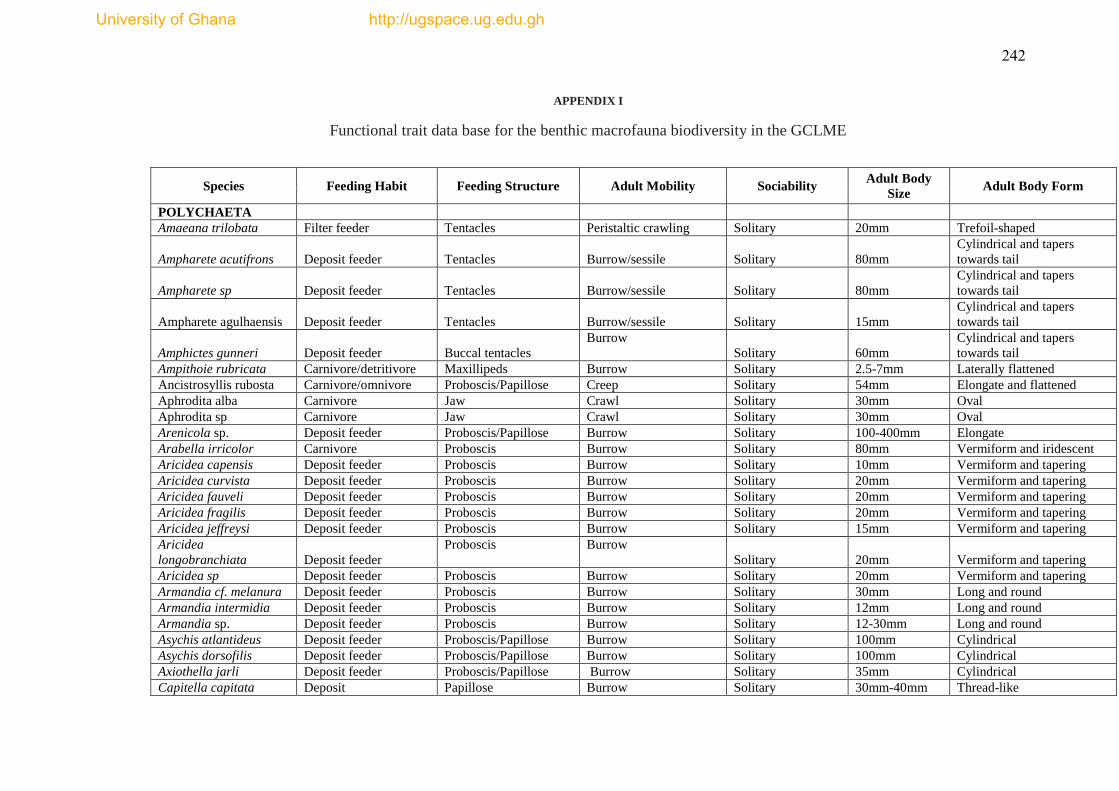
242
APPENDIX I
Functional trait data base for the benthic macrofauna biodiversity in the GCLME
Species Feeding Habit Feeding Structure Adult Mobility Sociability Adult Body
Size Adult Body Form
POLYCHAETA
Amaeana trilobata Filter feeder Tentacles Peristaltic crawling Solitary 20mm Trefoil-shaped
Ampharete acutifrons Deposit feeder Tentacles Burrow/sessile Solitary 80mm
Cylindrical and tapers
towards tail
Ampharete sp Deposit feeder Tentacles Burrow/sessile Solitary 80mm
Cylindrical and tapers
towards tail
Ampharete agulhaensis Deposit feeder Tentacles Burrow/sessile Solitary 15mm
Cylindrical and tapers
towards tail
Amphictes gunneri Deposit feeder Buccal tentacles
Burrow Solitary 60mm
Cylindrical and tapers
towards tail
Ampithoie rubricata Carnivore/detritivore Maxillipeds Burrow Solitary 2.5-7mm Laterally flattened
Ancistrosyllis rubosta Carnivore/omnivore Proboscis/Papillose Creep Solitary 54mm Elongate and flattened
Aphrodita alba Carnivore Jaw Crawl Solitary 30mm Oval
Aphrodita sp Carnivore Jaw Crawl Solitary 30mm Oval
Arenicola sp. Deposit feeder Proboscis/Papillose Burrow Solitary 100-400mm Elongate
Arabella irricolor Carnivore Proboscis Burrow Solitary 80mm Vermiform and iridescent
Aricidea capensis Deposit feeder Proboscis Burrow Solitary 10mm Vermiform and tapering
Aricidea curvista Deposit feeder Proboscis Burrow Solitary 20mm Vermiform and tapering
Aricidea fauveli Deposit feeder Proboscis Burrow Solitary 20mm Vermiform and tapering
Aricidea fragilis Deposit feeder Proboscis Burrow Solitary 20mm Vermiform and tapering
Aricidea jeffreysi Deposit feeder Proboscis Burrow Solitary 15mm Vermiform and tapering
Aricidea
longobranchiata Deposit feeder
Proboscis Burrow Solitary 20mm Vermiform and tapering
Aricidea sp Deposit feeder Proboscis Burrow Solitary 20mm Vermiform and tapering
Armandia cf. melanura Deposit feeder Proboscis Burrow Solitary 30mm Long and round
Armandia intermidia Deposit feeder Proboscis Burrow Solitary 12mm Long and round
Armandia sp. Deposit feeder Proboscis Burrow Solitary 12-30mm Long and round
Asychis atlantideus Deposit feeder Proboscis/Papillose Burrow Solitary 100mm Cylindrical
Asychis dorsofilis Deposit feeder Proboscis/Papillose Burrow Solitary 100mm Cylindrical
Axiothella jarli Deposit feeder Proboscis/Papillose Burrow Solitary 35mm Cylindrical
Capitella capitata Deposit Papillose Burrow Solitary 30mm-40mm Thread-like
University of Ghana http://ugspace.ug.edu.gh
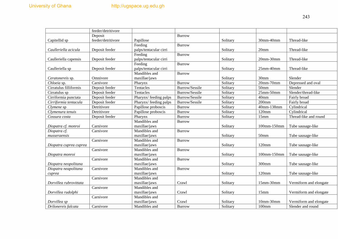
243
feeder/detritivore
Capitellid sp
Deposit
feeder/detritivore Papillose
Burrow Solitary 30mm-40mm Thread-like
Caulleriella acicula Deposit feeder
Feeding
palps/tentacular cirri
Burrow Solitary 20mm Thread-like
Caulleriella capensis Deposit feeder
Feeding
palps/tentacular cirri
Burrow Solitary 20mm-30mm Thread-like
Caulleriella sp Deposit feeder
Feeding
palps/tentacular cirri
Burrow Solitary 25mm-40mm Thread-like
Ceratonereis sp. Omnivore
Mandibles and
maxillae/jaws
Burrow Solitary 30mm Slender
Chloeia sp. Carnivore Pharynx Burrow Solitary 20mm-70mm Depressed and oval
Cirratulus filliformis Deposit feeder Tentacles Burrow/Sessile Solitary 50mm Slender
Cirratulus sp Deposit feeder Tentacles Burrow/Sessile Solitary 25mm-50mm Slender/thread-like
Cirriformia punctata Deposit feeder Pharynx/ feeding palps Burrow/Sessile Solitary 40mm Fairly broad
Cirriformia tentacula Deposit feeder Pharynx/ feeding palps Burrow/Sessile Solitary 200mm Fairly broad
Clymene sp Detritivore Papillose proboscis Burrow Solitary 40mm-138mm Cylindrical
Clymenura tenuis Detritivore Papillose proboscis Burrow Solitary 120mm Cylindrical
Cossura costa Deposit feeder Pharynx Burrow Solitary 15mm Thread-like and round
Diopatra cf. monroi Carnivore
Mandibles and
maxillae/jaws
Burrow Solitary 100mm-150mm Tube sausage-like
Diopatra cf.
musseraensis
Carnivore Mandibles and
maxillae/jaws
Burrow Solitary 50mm Tube sausage-like
Diopatra cuprea cuprea
Carnivore Mandibles and
maxillae/jaws
Burrow Solitary 120mm Tube sausage-like
Diopatra monroi
Carnivore Mandibles and
maxillae/jaws
Burrow Solitary 100mm-150mm Tube sausage-like
Diopatra neopolitana
Carnivore Mandibles and
maxillae/jaws
Burrow Solitary 300mm Tube sausage-like
Diopatra neapolitana
cuprea
Carnivore Mandibles and
maxillae/jaws
Burrow Solitary 120mm Tube sausage-like
Dorvillea rubrovittata
Carnivore Mandibles and
maxillae/jaws Crawl Solitary 15mm-30mm Vermiform and elongate
Dorvillea rudolphi
Carnivore Mandibles and
maxillae/jaws Crawl Solitary 15mm Vermiform and elongate
Dorvillea sp
Carnivore Mandibles and
maxillae/jaws Crawl Solitary 10mm-30mm Vermiform and elongate
Drilonereis falcata Carnivore Mandibles and Burrow Solitary 100mm Slender and round
University of Ghana http://ugspace.ug.edu.gh
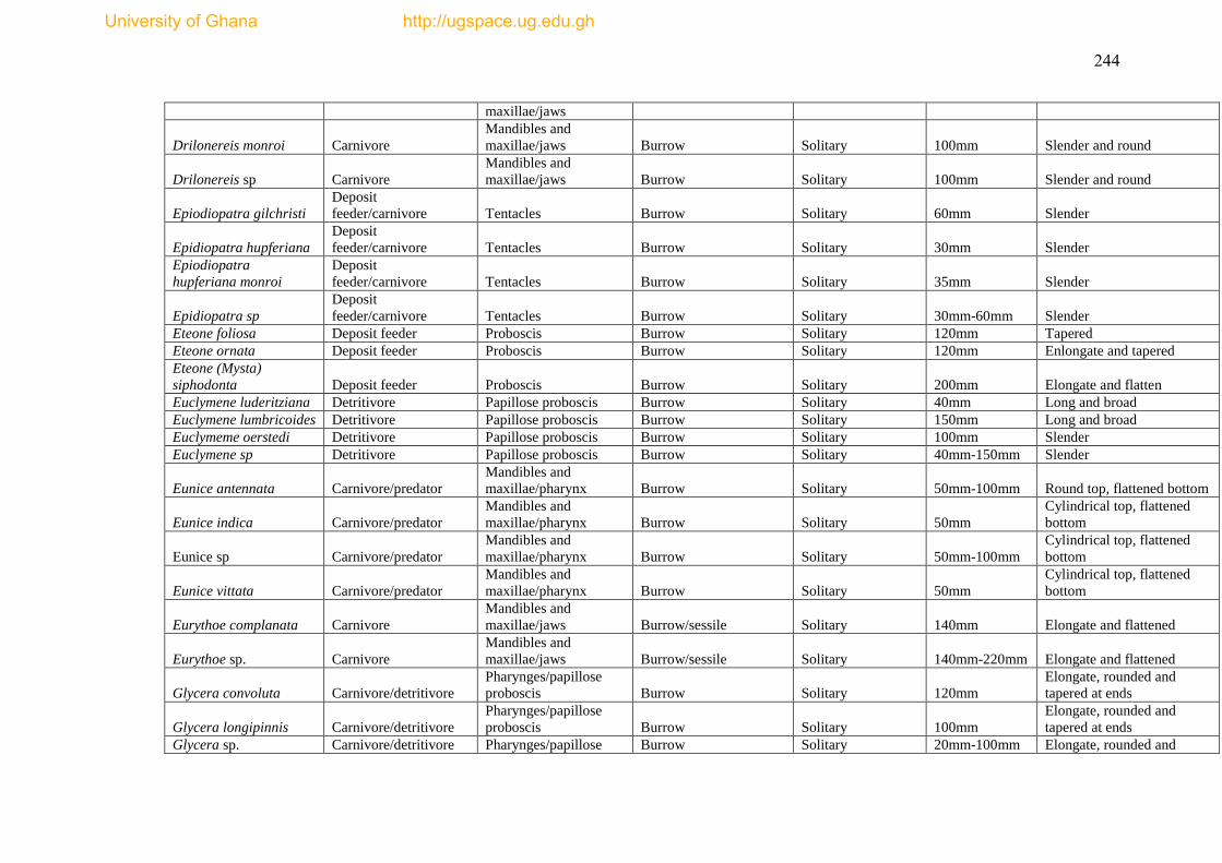
244
maxillae/jaws
Drilonereis monroi Carnivore
Mandibles and
maxillae/jaws Burrow Solitary 100mm Slender and round
Drilonereis sp Carnivore
Mandibles and
maxillae/jaws Burrow Solitary 100mm Slender and round
Epiodiopatra gilchristi
Deposit
feeder/carnivore Tentacles Burrow Solitary 60mm Slender
Epidiopatra hupferiana
Deposit
feeder/carnivore Tentacles Burrow Solitary 30mm Slender
Epiodiopatra
hupferiana monroi
Deposit
feeder/carnivore Tentacles Burrow Solitary 35mm Slender
Epidiopatra sp
Deposit
feeder/carnivore Tentacles Burrow Solitary 30mm-60mm Slender
Eteone foliosa Deposit feeder Proboscis Burrow Solitary 120mm Tapered
Eteone ornata Deposit feeder Proboscis Burrow Solitary 120mm Enlongate and tapered
Eteone (Mysta)
siphodonta Deposit feeder Proboscis Burrow Solitary 200mm Elongate and flatten
Euclymene luderitziana Detritivore Papillose proboscis Burrow Solitary 40mm Long and broad
Euclymene lumbricoides Detritivore Papillose proboscis Burrow Solitary 150mm Long and broad
Euclymeme oerstedi Detritivore Papillose proboscis Burrow Solitary 100mm Slender
Euclymene sp Detritivore Papillose proboscis Burrow Solitary 40mm-150mm Slender
Eunice antennata Carnivore/predator
Mandibles and
maxillae/pharynx Burrow Solitary 50mm-100mm Round top, flattened bottom
Eunice indica Carnivore/predator
Mandibles and
maxillae/pharynx Burrow Solitary 50mm
Cylindrical top, flattened
bottom
Eunice sp Carnivore/predator
Mandibles and
maxillae/pharynx Burrow Solitary 50mm-100mm
Cylindrical top, flattened
bottom
Eunice vittata Carnivore/predator
Mandibles and
maxillae/pharynx Burrow Solitary 50mm
Cylindrical top, flattened
bottom
Eurythoe complanata Carnivore
Mandibles and
maxillae/jaws Burrow/sessile Solitary 140mm Elongate and flattened
Eurythoe sp. Carnivore
Mandibles and
maxillae/jaws Burrow/sessile Solitary 140mm-220mm Elongate and flattened
Glycera convoluta Carnivore/detritivore
Pharynges/papillose
proboscis Burrow Solitary 120mm
Elongate, rounded and
tapered at ends
Glycera longipinnis Carnivore/detritivore
Pharynges/papillose
proboscis Burrow Solitary 100mm
Elongate, rounded and
tapered at ends
Glycera sp. Carnivore/detritivore Pharynges/papillose Burrow Solitary 20mm-100mm Elongate, rounded and
University of Ghana http://ugspace.ug.edu.gh
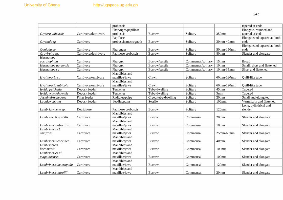
245
proboscis tapered at ends
Glycera unicornis Carnivore/detritivore
Pharynges/papillose
proboscis Burrow Solitary 350mm
Elongate, rounded and
tapered at ends
Glycinde sp Carnivore
Papillose
proboscis/macrognath Burrow Solitary 30mm-40mm
Elongateand tapered at both
ends
Goniada sp Carnivore Pharynges Burrow Solitary 50mm-150mm
Elongateand tapered at both
ends
Gravirella sp. Carnivore/detritivore Papillose proboscis Burrow Solitary 80mm Slender and elongate
Harmothoe
corralophilla Carnivore Pharynx Burrow/sessile Commensal/solitary 15mm Broad
Harmothoe goreensis Carnivore Pharynx Burrow/sessile Commensal/solitary 10mm Small, short and flattened
Harmothoe sp Carnivore Pharynx Burrow/sessile Commensal/solitary 10mm-35mm Short and flattened
Hyalinoecia sp Carnivore/omnivore
Mandibles and
maxillae/jaws Crawl Solitary 60mm-120mm Quill-like tube
Hyalinoecia tubicola Carnivore/omnivore
Mandibles and
maxillae/jaws Crawl Solitary 60mm-120mm Quill-like tube
Isolda pulchella Deposit feeder Tentacles Tube-dwelling Solitary 45mm Tapered
Isolda whydahaensis Deposit feeder Tentacles Tube-dwelling Solitary 5mm Tapered
Jasmineira elegans Filter feeder Radioles/palps Creep/tube-dwelling Solitary 20mm Small and elongated
Laonice cirrata Deposit feeder feedingpalps Sessile Solitary 100mm Vermiform and flattened
Lumbriclymene sp. Detritivore Papillose proboscis Burrow Solitary 120mm
Long, cylindrical and
slender
Lumbreneris gracilis Carnivore
Mandibles and
maxillae/jaws Burrow Commensal 20mm Slender and elongate
Lumbrineris aberrans Carnivore
Mandibles and
maxillae/jaws Burrow Commensal 10mm Slender and elongate
Lumbrineris cf.
cavifrons Carnivore
Mandibles and
maxillae/jaws Burrow Commensal 25mm-65mm Slender and elongate
Lumbrineris coccinea Carnivore
Mandibles and
maxillae/jaws Burrow Commensal 40mm Slender and elongate
Lumbrinereis
hartimanis Carnivore
Mandibles and
maxillae/jaws Burrow Commensal 100mm Slender and elongate
Lumbrineries cf.
magalhaensis Carnivore
Mandibles and
maxillae/jaws Burrow Commensal 100mm Slender and elongate
Lumbrineris heteropoda Carnivore
Mandibles and
maxillae/jaws Burrow Commensal 120mm Slender and elongate
Lumbrineris latreilli Carnivore
Mandibles and
maxillae/jaws Burrow Commensal 20mm Slender and elongate
University of Ghana http://ugspace.ug.edu.gh

246
Lumbrinereis paradoxa Carnivore
Mandibles and
maxillae/jaws Burrow Commensal 20mm Slender and elongate
Magelona cincta Deposit feeder
Feeding
palaps/proboscis Burrow Solitary 30mm Slender
Magelona papillicornis Deposit feeder
Feeding
palaps/proboscis Burrow Solitary 170mm Slender
Magelona capensis Deposit feeder
Feeding
palaps/proboscis Burrow Solitary 35mm Slender
Malacoceros indica Deposit feeder Tentacles/feeding palps Burrow Solitary 60mm Vermiform and flattened
Malacoceros sp Deposit feeder Tentacles/feeding palps Burrow Solitary 60mm Vermiform and flattened
Magelona sp Deposit feeder Feeding palps Burrow Solitary 20mm-170mm Slender
Maldane decorata Detritivore Pharynx Burrow Solitary 100mm Sausage-like mud tube
Maldane sarsi Detritivore Pharynx Burrow Solitary 100mm Sausage-like mud tube
Maldanella sp Detritivore Pharynx Burrow Solitary 45mm-70mm Cylindrical and elongate
Marphysa adenensis Omnivore/detritivore
Mandibles and
maxillae/pharynx Burrow Solitary 70mm Slender and rounded
Marphysa cf.
mossambica Omnivore/detritivore
Mandibles and
maxillae/pharynx Burrow Solitary 350mm Slender and flattened
Marphysa sanguinea Omnivore/detritivore
Mandibles and
maxillae/pharynx Burrow Solitary 250mm Long and oval
Marphysa sp. Omnivore/detritivore
Mandibles and
maxillae/pharynx Burrow Solitary 30mm-250mm Slender, rounded /flattened
Magelomma
vesiculosum Filter feeder Tentacular crown Sessile Solitary 100mm Slightly tapered
Megalomma sp Filter feeder Tentacular crown Sessile Solitary 20mm-100mm Slightly tapered
Mesochaetopterus
minutes Detritivore Grooved palps Burrow Solitary 15mm Elongate
Naineris laevigata Detritivore/carnivore Proboscis Burrow Solitary 40mm Vermiform and flattened
Nematonereis unicornis Detritivore/carnivore Mandibles and maxillae Burrow Solitary 150mm-200mm Slender
Nephtys capensis Carnivore
Pharynges/papillose
proboscis Burrow Solitary 60mm Elongate and depressed
Nephtys (aglaophamus)
dibranchis Carnivore
Pharynges/papillose
proboscis Burrow Solitary 25mm Elongate and depressed
Nephtys (aglaophamus)
lyrochaeta Carnivore
Pharynges/papillose
proboscis Burrow Solitary 30mm Elongate and depressed
Nephtys hombergi Carnivore
Pharynges/papillose
proboscis Burrow Solitary 200mm Elongate and depressed
Nephtys macrousa Carnivore Pharynges/papillose Burrow Solitary 150mm Elongate and depressed
University of Ghana http://ugspace.ug.edu.gh

247
proboscis
Nephtys sp Carnivore
Pharynges/papillose
proboscis Burrow Solitary 6.5mm-200mm Elongate and depressed
Nephtys sphaerocirrata Carnivore
Pharynges/papillose
proboscis Burrow Solitary 25mm Elongate and depressed
Neries sp.
Omnivore/filter
feeder/deposit feeder Papillose proboscis Burrow/creep Solitary/commensal 15mm-120mm Elongate
Neridines gilchristi Deposit feeder Tentacles/palps Burrow Solitary 25mm Vermiform and flattened
Nicolea sp. Deposit feeder Buccal tentacles Sessile Solitary 50mm-100mm Elongate and tapered
Nicomache sp. Deposit feeder Jaws/keel Burrow/sessile Solitary 160mm-240mm Cylindrical
Notomastus aberrans Deposit feeder Jaws Burrow Solitary 60mm Elongate and round
Notomastus fauvelli Deposit feeder Jaws Burrow Solitary 90mm Elongate and round
Notomastus latriceus Deposit feeder Jaws Burrow Solitary 300mm Elongate and round
Notomastus sp Deposit feeder Jaws Burrow Solitary 60mm-300mm Elongate and round
Onuphis (Nothria)
conchylega Omnivore Jaws Sessile Solitary 40mm-150mm Elongate and vermiform
Onuphis eremita Omnivore Jaws Sessile Solitary 80mm-120mm Elongate and vermiform
Onuphis geophiliformis Omnivore Jaws Sessile Solitary 30mm Elongate and vermiform
Onuphis holobranchiata Omnivore Jaws Sessile Solitary 60mm depreesed
Onuphis sp. Omnivore Jaws Sessile Solitary 40mm-350mm Elongate and vermiform
Ophelina sp Deposit feeder Proboscis Burrow Solitary 50mm Vermiform
Ophiodromus cf.
berrisfordi Carnivore Proboscis Burrow Solitary 28mm Flattened and tapered
Ophiodromus sp Carnivore Proboscis Burrow Solitary 8mm-28mm Flattened and tapered
Orbinia curvieri Deposit feeder Pharynges Burrow Solitary 300mm Vermiform
Oriopsis neglecta Suspension feeder
Branchial
crown/radioles/palps Creep Solitary 3mm-4mm Fairly stout
Paralacydonia
paradoxa Omnivore/carnivore Pharynx/papillose Burrow/swim Solitary 20mm-30mm Elongate and rectangular
Paraonides sp.
Deposit feeder/surface
feeder Pharynges Burrow Solitary 10mm-20mm Thread-like
Paraonides lyra
capensis
Deposit feeder/surface
feeder Pharynges Burrow Solitary 10mm Thread-like
Pareulepis sp
Deposit
feeder/carnivore Jaws Burrow Solitary/commensal 35mm Oblong
Paronuphis antartica Carnivore
Mandibles and
maxillae/pharynx Burrow Solitary 20mm-30mm Vermiform and elongate
Paronuphis sp. Carnivore Mandibles and Burrow Solitary 20mm-30mm Vermiform and elongate
University of Ghana http://ugspace.ug.edu.gh
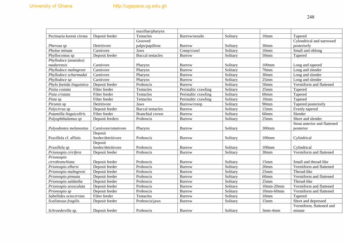
248
maxillae/pharynx
Pectinaria koreni cirrata Deposit feeder Tentacles Burrow/sessile Solitary 10mm Tapered
Pherusa sp Detritivore
Grooved
palps/papillose Burrow Solitary 30mm
Cylondrical and narrowed
posteriorly
Pholoe minuta Carnivore Jaws Creep/crawl Solitary 10mm Small and oblong
Phyllocomus sp Deposit feeder Buccal tentacles Burrow Solitary 50mm Tapered
Phyllodoce (anatides)
madarensis Carnivore Pharynx Burrow Solitary 100mm Long and tapered
Phyllodoce malmgreni Carnivore Pharynx Burrow Solitary 70mm Long and slender
Phyllodoce scharmadai Carnivore Pharynx Burrow Solitary 30mm Long and slender
Phyllodoce sp Carnivore Pharynx Burrow Solitary 25mm Long and slender
Phylo foetida linguistica Deposit feeder Proboscis Burrow Solitary 50mm Vermiform and flattened
Pistia costata Filter feeder Tentacles Peristaltic crawling Solitary 25mm Tapered
Pista cristata Filter feeder Tentacles Peristaltic crawling Solitary 60mm Tapered
Pista sp Filter feeder Tentacles Peristaltic crawling Solitary 10mm Tapered
Piromis sp Detritivore Jaws Burrow/creep Solitary 90mm Tapered posteriorly
Polycirrus sp Deposit feeder Buccal tentacles Burrow Solitary 15mm Evenly tapered
Potamilla linguicollris Filter feeder Branchial crown Burrow Solitary 60mm Slender
Polyophthalamus sp Deposit feeders Proboscis Burrow Solitary 25mm Short and slender
Polyodontes melanontus Carnivore/omnivore Pharynx Burrow Solitary 300mm
Stout anterior and flattened
posterior
Praxillela cf. affinis
Deposit
feeder/detritivore Proboscis Burrow Solitary 100mm Cylindrical
Praxillela sp
Deposit
feeder/detritivore Proboscis Burrow Solitary 100mm Cylindrical
Prionospio cirrifera Deposit feeder Proboscis Burrow Solitary 30mm Vermiform and flattened
Prionospio
cirrobranchiata Deposit feeder Proboscis Burrow Solitary 15mm Small and thread-like
Prionospio elhersi Deposit feeder Proboscis Burrow Solitary 20mm Vermiform and flattened
Prionospio malmgreni Deposit feeder Proboscis Burrow Solitary 25mm Thread-like
Prionospio pinnata Deposit feeder Proboscis Burrow Solitary 60mm Vermiform and flattened
Prionospio saldanha Deposit feeder Proboscis Burrow Solitary 25mm Thread-like
Prionospio sexoculata Deposit feeder Proboscis Burrow Solitary 10mm-20mm Vermiform and flattened
Prionospio sp Deposit feeder Proboscis Burrow Solitary 10mm-60mm Vermiform and flattened
Sabellides octocirrata Filter feeder Tentacles Burrow Solitary 10mm Tapered
Scalistosus fragilis Deposit feeder Proboscis/jaws Burrow Solitary 15mm Short and depressed
Schroederella sp. Deposit feeder Proboscis Burrow Solitary 3mm-4mm
Vermiform, flattened and
minute
University of Ghana http://ugspace.ug.edu.gh
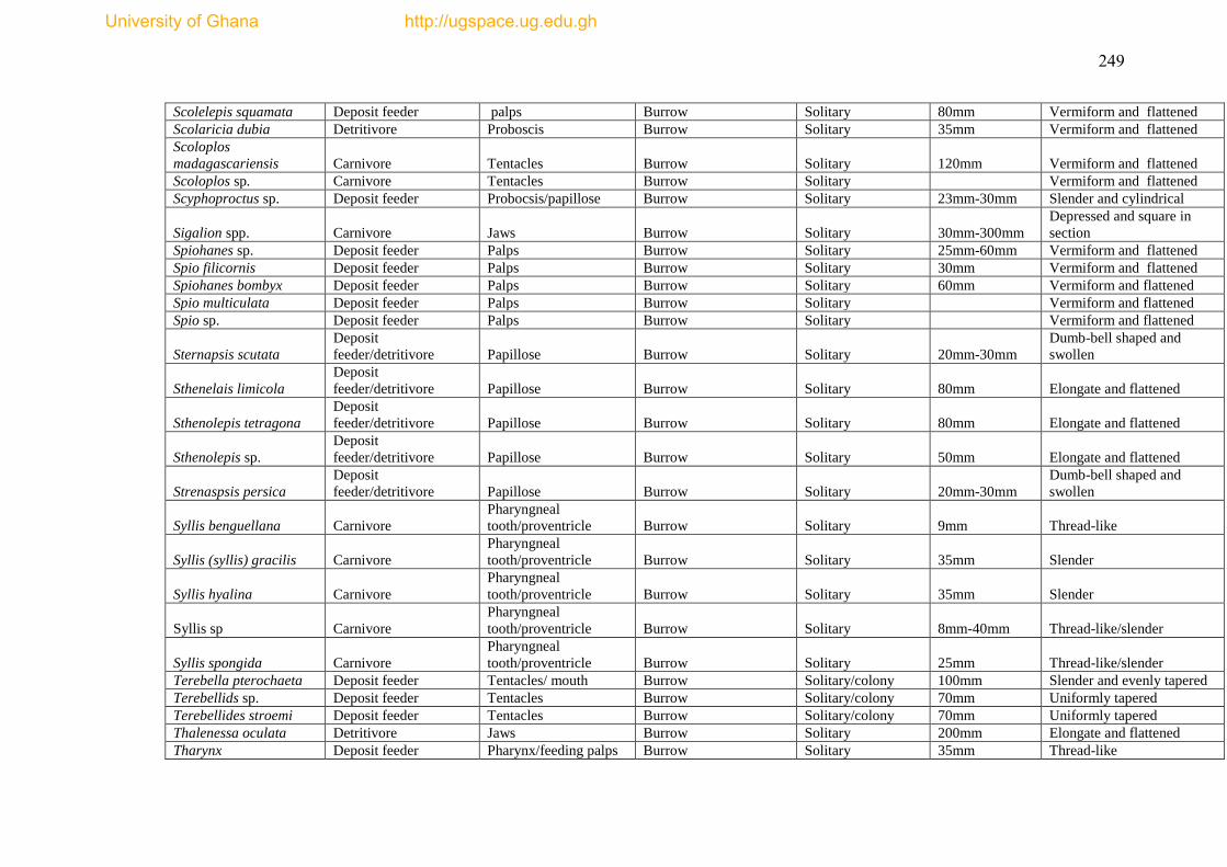
249
Scolelepis squamata Deposit feeder palps Burrow Solitary 80mm Vermiform and flattened
Scolaricia dubia Detritivore Proboscis Burrow Solitary 35mm Vermiform and flattened
Scoloplos
madagascariensis Carnivore Tentacles Burrow Solitary 120mm Vermiform and flattened
Scoloplos sp. Carnivore Tentacles Burrow Solitary Vermiform and flattened
Scyphoproctus sp. Deposit feeder Probocsis/papillose Burrow Solitary 23mm-30mm Slender and cylindrical
Sigalion spp. Carnivore Jaws Burrow Solitary 30mm-300mm
Depressed and square in
section
Spiohanes sp. Deposit feeder Palps Burrow Solitary 25mm-60mm Vermiform and flattened
Spio filicornis Deposit feeder Palps Burrow Solitary 30mm Vermiform and flattened
Spiohanes bombyx Deposit feeder Palps Burrow Solitary 60mm Vermiform and flattened
Spio multiculata Deposit feeder Palps Burrow Solitary Vermiform and flattened
Spio sp. Deposit feeder Palps Burrow Solitary Vermiform and flattened
Sternapsis scutata
Deposit
feeder/detritivore Papillose Burrow Solitary 20mm-30mm
Dumb-bell shaped and
swollen
Sthenelais limicola
Deposit
feeder/detritivore Papillose Burrow Solitary 80mm Elongate and flattened
Sthenolepis tetragona
Deposit
feeder/detritivore Papillose Burrow Solitary 80mm Elongate and flattened
Sthenolepis sp.
Deposit
feeder/detritivore Papillose Burrow Solitary 50mm Elongate and flattened
Strenaspsis persica
Deposit
feeder/detritivore Papillose Burrow Solitary 20mm-30mm
Dumb-bell shaped and
swollen
Syllis benguellana Carnivore
Pharyngneal
tooth/proventricle Burrow Solitary 9mm Thread-like
Syllis (syllis) gracilis Carnivore
Pharyngneal
tooth/proventricle Burrow Solitary 35mm Slender
Syllis hyalina Carnivore
Pharyngneal
tooth/proventricle Burrow Solitary 35mm Slender
Syllis sp Carnivore
Pharyngneal
tooth/proventricle Burrow Solitary 8mm-40mm Thread-like/slender
Syllis spongida Carnivore
Pharyngneal
tooth/proventricle Burrow Solitary 25mm Thread-like/slender
Terebella pterochaeta Deposit feeder Tentacles/ mouth Burrow Solitary/colony 100mm Slender and evenly tapered
Terebellids sp. Deposit feeder Tentacles Burrow Solitary/colony 70mm Uniformly tapered
Terebellides stroemi Deposit feeder Tentacles Burrow Solitary/colony 70mm Uniformly tapered
Thalenessa oculata Detritivore Jaws Burrow Solitary 200mm Elongate and flattened
Tharynx Deposit feeder Pharynx/feeding palps Burrow Solitary 35mm Thread-like
University of Ghana http://ugspace.ug.edu.gh
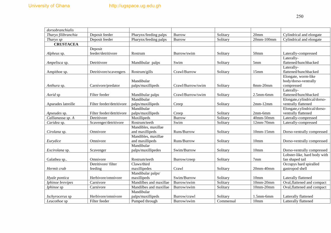
250
dorsobranchialis
Tharyx filibranchia Deposit feeder Pharynx/feeding palps Burrow Solitary 20mm Cylindrical and elongate
Tharyx sp Deposit feeder Pharynx/feeding palps Burrow Solitary 20mm-100mm Cylindrical and elongate
CRUSTACEA
Alpheus sp.
Deposit
feeder/detritivore Rostrum Burrow/swim Solitary 50mm Laterally-compressed
Ampelisca sp. Detritivore Mandibular palps Swim Solitary 5mm
Laterally-
flattened/hunchbacked
Ampithoe sp. Detritivore/scavengers Rostrum/gills Crawl/Burrow Solitary 15mm
Laterally-
flattened/hunchbacked
Anthura sp. Carnivore/predator
Mandibular
palps/maxillipeds Crawl/Burrow/swim Solitary 8mm-20mm
Elongate, worm-like
body/dorso-ventrally
compressed
Aorid sp Filter feeder Mandibular palps Crawl/Burrow/swim Solitary 2.5mm-6mm
Laterally-
flattened/hunchbacked
Apseudes latreille Filter feeder/detritivore
Mandibular
palps/maxillipeds Creep Solitary 2mm-12mm
Elongate,cylindrical/dorso-
ventrally flattened
Apseudes sp. Filter feeder/detritivore
Mandibular
palps/maxillipeds Creep Solitary 2mm-6mm
Elongate,cylindrical/dorso-
ventrally flattened
Callianassa sp. A Detritivore Maxillipeds Burrow Solitary 40mm-50mm Laterally-compressed
Caridea sp. Scavenger/detritivore Rostrum/teeth Swim Solitary 12mm-70mm Laterally-compressed
Cirolana sp. Omnivore
Mandibles, maxillae
and maxillipeds Runs/Burrow Solitary 10mm-15mm Dorso-ventrally compressed
Eurydice Omnivore
Mandibles, maxillae
and maxillipeds Runs/Burrow Solitary 10mm Dorso-ventrally compressed
Excirolana sp. Scavenger
Mandibular
palps/maxillipedes Swim/Burrow Solitary 10mm Dorso-ventrally compressed
Galathea sp.. Omnivore Rostrum/teeth Burrow/creep Solitary 7mm
Lobster-like, hard body with
fan shaped tail
Hermit crab
Detritivore/ filter
feeding
Claws/third
maxillipedes Crawl Solitary 20mm-40mm
Occupys hard spiralled
gastropod shell
Hyale pontica Herbivore/omnivore
Mandibular palps/
maxillipeds Swim/Burrow Solitary 10mm Laterally flattened
Iphinoe brevipes Carnivore Mandilbes and maxillae Burrow/swim Solitary 10mm-20mm Oval,flattened and compact
Iphinoe sp Carnivore Mandilbes and maxillae Burrow/swim Solitary 10mm-20mm Oval,flattened and compact
Ischyrocerus sp Herbivore/omnivore
Mandibular
palps/maxillipeds Burrow/crawl Solitary 1.5mm-6mm Latterally flattened
Leucothoe sp Filter feeder Pumped through Burrow/swim Commensal 10mm Latterally flattened
University of Ghana http://ugspace.ug.edu.gh

251
sponge
Ligia olfersi Scavengers
Mandibles,maxillae and
maxillipeds Runs/Burrow Solitary 15mm-25mm Broad, flattened and smooth
Liljeborgia sp. Carnivore
Mandibular
palp/maxillipeds Burrow Commensal/solitary 1.5mm-5mm Latterally flattened
Mysid Omnivore/herbivore
Mandibles, maxillae
and maxillipeds Swim/Burrow Solitary 40mm-50mm Latterally compressed
Palinurus sp Omnivore Rostrum/teeth Burrow Solitary 250mm
Elongate, semi-circular with
fan-like telson
Penaeid shrimp Scavenger/detritivore Rostrum/teeth Swim Solitary 60mm
Cylindrical and latterally
compressed
Perioculodes sp. Omnivore Rostrum/teeth Burrow/swim Solitary 2mm-5mm Larrerally flattened
Portumnus sp. Carnivores /detritivore
Maxilliped,
mandibular, cheliped Swim Solitary
33-170mm
width, 23-
76mm length Dorso-ventrally flattened
Tanaids Filter feeder
Mandibles, maxillipeds
and chela Burrow Solitary 2mm-6mm
Elongate body,
cylindrical/dorsoventrally
flattened
Uca tangerii Detritivore buccal frame,chelae Burrow Solitary
14-30mm
width, 8-17mm
length Dorso-ventrally flattened
Upogebia sp. Filter feeder
Maxillipeds/mandibular
palps Burrow Solitary 40mm
Elongate,semi-circular
withfan-like telson
Urothoe sp. Detritivore Maxillipeds/mandibles Burrow Solitary 2mm-5mm Laterally flattened
Xanthid crab Detritivore Buccal frame, chelae Burrow Solitary/commensal 15mm-25mm
Dorso-ventrally flattened
with broad carapace
MOLLUSCS
Arca subglobosa Filter feeder Siphon/gills Burrow/sessile Solitary 12mm-25mm
Almost square,rounded
anterior, pointed posterior
Asterina sp. Carnivore Tube feet/ stomach Burrow/sessile Solitary 20mm
Flattened body with short
rounded arms
Cardium sp Filter feeder Siphon/gills Burrow/sessile Solitary 15-100mm Circular
Corbula sp Filter feeder Siphon/gills Burrow Solitary 200mm Oval to triangular
Chiton canariensis Omnivore Radula Creep/sessile Colony 20mm-35mm Oval and flattened
Diplodonta sp. Filter feeder Siphon/gills Burrow/ creep Solitary 15mm-25mm Circular
Donax oweni Filter feeder Siphon/gills Burrow/sessile Colony 10mm-20mm Triangular
Dosinia sp. Filter feeder Siphon/gills Burrow Colony 15mm-30mm Circular /triangular
Glycemeris seripta Filter feeder Siphon/gills Burrow Solitary 50mm Slightly rounded
University of Ghana http://ugspace.ug.edu.gh
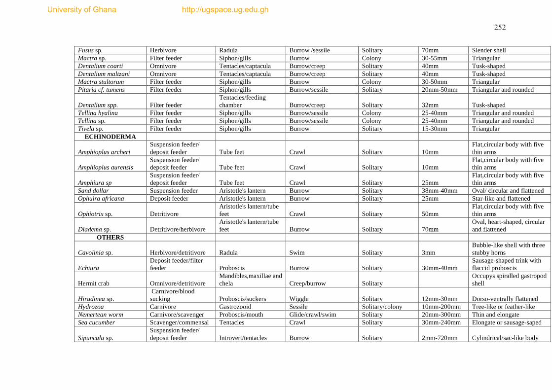
252
Fusus sp. Herbivore Radula Burrow /sessile Solitary 70mm Slender shell
Mactra sp. Filter feeder Siphon/gills Burrow Colony 30-55mm Triangular
Dentalium coarti Omnivore Tentacles/captacula Burrow/creep Solitary 40mm Tusk-shaped
Dentalium maltzani Omnivore Tentacles/captacula Burrow/creep Solitary 40mm Tusk-shaped
Mactra stultorum Filter feeder Siphon/gills Burrow Colony 30-50mm Triangular
Pitaria cf. tumens Filter feeder Siphon/gills Burrow/sessile Solitary 20mm-50mm Triangular and rounded
Dentalium spp. Filter feeder
Tentacles/feeding
chamber Burrow/creep Solitary 32mm Tusk-shaped
Tellina hyalina Filter feeder Siphon/gills Burrow/sessile Colony 25-40mm Triangular and rounded
Tellina sp. Filter feeder Siphon/gills Burrow/sessile Colony 25-40mm Triangular and rounded
Tivela sp. Filter feeder Siphon/gills Burrow Solitary 15-30mm Triangular
ECHINODERMA
Amphioplus archeri
Suspension feeder/
deposit feeder Tube feet Crawl Solitary 10mm
Flat,circular body with five
thin arms
Amphioplus aurensis
Suspension feeder/
deposit feeder Tube feet Crawl Solitary 10mm
Flat,circular body with five
thin arms
Amphiura sp
Suspension feeder/
deposit feeder Tube feet Crawl Solitary 25mm
Flat,circular body with five
thin arms
Sand dollar Suspension feeder Aristotle's lantern Burrow Solitary 38mm-40mm Oval/ circular and flattened
Ophuira africana Deposit feeder Aristotle's lantern Burrow Solitary 25mm Star-like and flattened
Ophiotrix sp. Detritivore
Aristotle's lantern/tube
feet Crawl Solitary 50mm
Flat,circular body with five
thin arms
Diadema sp. Detritivore/herbivore
Aristotle's lantern/tube
feet Burrow Solitary 70mm
Oval, heart-shaped, circular
and flattened
OTHERS
Cavolinia sp. Herbivore/detritivore Radula Swim Solitary 3mm
Bubble-like shell with three
stubby horns
Echiura
Deposit feeder/filter
feeder Proboscis Burrow Solitary 30mm-40mm
Sausage-shaped trink with
flaccid proboscis
Hermit crab Omnivore/detritivore
Mandibles,maxillae and
chela Creep/burrow Solitary
Occupys spiralled gastropod
shell
Hirudinea sp.
Carnivore/blood
sucking Proboscis/suckers Wiggle Solitary 12mm-30mm Dorso-ventrally flattened
Hydrozoa Carnivore Gastrozooid Sessile Solitary/colony 10mm-200mm Tree-like or feather-like
Nemertean worm Carnivore/scavenger Proboscis/mouth Glide/crawl/swim Solitary 20mm-300mm Thin and elongate
Sea cucumber Scavenger/commensal Tentacles Crawl Solitary 30mm-240mm Elongate or sausage-saped
Sipuncula sp.
Suspension feeder/
deposit feeder Introvert/tentacles Burrow Solitary 2mm-720mm Cylindrical/sac-like body
University of Ghana http://ugspace.ug.edu.gh
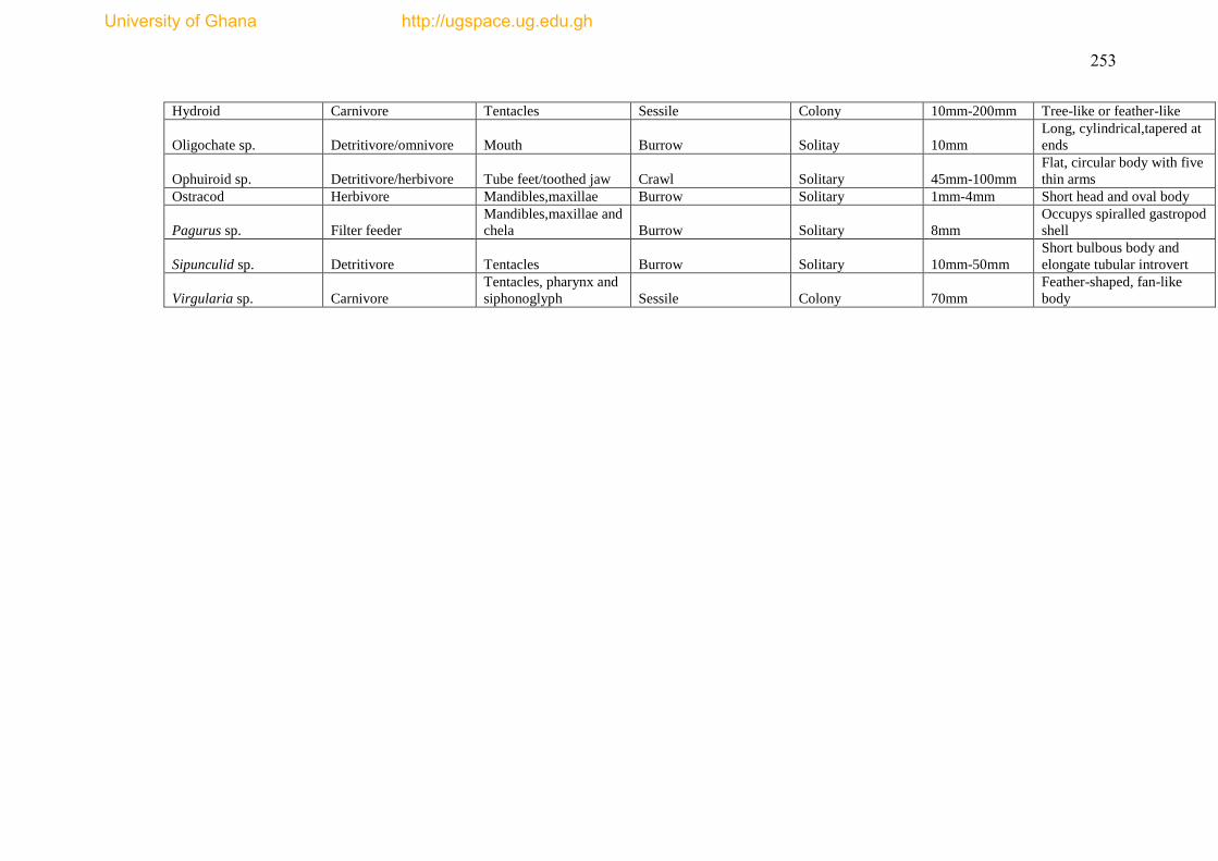
253
Hydroid Carnivore Tentacles Sessile Colony 10mm-200mm Tree-like or feather-like
Oligochate sp. Detritivore/omnivore Mouth Burrow Solitay 10mm
Long, cylindrical,tapered at
ends
Ophuiroid sp. Detritivore/herbivore Tube feet/toothed jaw Crawl Solitary 45mm-100mm
Flat, circular body with five
thin arms
Ostracod Herbivore Mandibles,maxillae Burrow Solitary 1mm-4mm Short head and oval body
Pagurus sp. Filter feeder
Mandibles,maxillae and
chela Burrow Solitary 8mm
Occupys spiralled gastropod
shell
Sipunculid sp. Detritivore Tentacles Burrow Solitary 10mm-50mm
Short bulbous body and
elongate tubular introvert
Virgularia sp. Carnivore
Tentacles, pharynx and
siphonoglyph Sessile Colony 70mm
Feather-shaped, fan-like
body
University of Ghana http://ugspace.ug.edu.gh
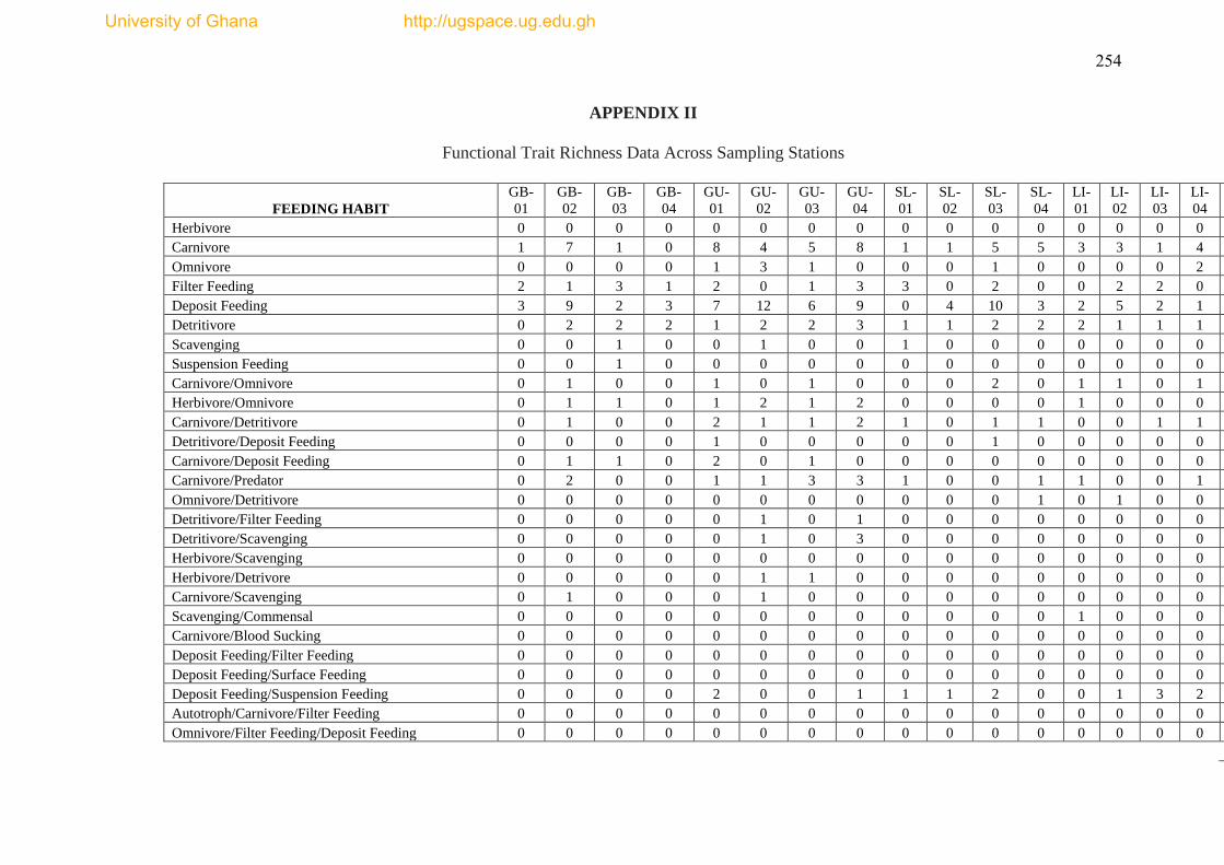
254
APPENDIX II
Functional Trait Richness Data Across Sampling Stations
FEEDING HABIT
GB-
01
GB-
02
GB-
03
GB-
04
GU-
01
GU-
02
GU-
03
GU-
04
SL-
01
SL-
02
SL-
03
SL-
04
LI-
01
LI-
02
LI-
03
LI-
04
Herbivore 0 0 0 0 0 0 0 0 0 0 0 0 0 0 0 0
Carnivore 1 7 1 0 8 4 5 8 1 1 5 5 3 3 1 4
Omnivore 0 0 0 0 1 3 1 0 0 0 1 0 0 0 0 2
Filter Feeding 2 1 3 1 2 0 1 3 3 0 2 0 0 2 2 0
Deposit Feeding 3 9 2 3 7 12 6 9 0 4 10 3 2 5 2 1
Detritivore 0 2 2 2 1 2 2 3 1 1 2 2 2 1 1 1
Scavenging 0 0 1 0 0 1 0 0 1 0 0 0 0 0 0 0
Suspension Feeding 0 0 1 0 0 0 0 0 0 0 0 0 0 0 0 0
Carnivore/Omnivore 0 1 0 0 1 0 1 0 0 0 2 0 1 1 0 1
Herbivore/Omnivore 0 1 1 0 1 2 1 2 0 0 0 0 1 0 0 0
Carnivore/Detritivore 0 1 0 0 2 1 1 2 1 0 1 1 0 0 1 1
Detritivore/Deposit Feeding 0 0 0 0 1 0 0 0 0 0 1 0 0 0 0 0
Carnivore/Deposit Feeding 0 1 1 0 2 0 1 0 0 0 0 0 0 0 0 0
Carnivore/Predator 0 2 0 0 1 1 3 3 1 0 0 1 1 0 0 1
Omnivore/Detritivore 0 0 0 0 0 0 0 0 0 0 0 1 0 1 0 0
Detritivore/Filter Feeding 0 0 0 0 0 1 0 1 0 0 0 0 0 0 0 0
Detritivore/Scavenging 0 0 0 0 0 1 0 3 0 0 0 0 0 0 0 0
Herbivore/Scavenging 0 0 0 0 0 0 0 0 0 0 0 0 0 0 0 0
Herbivore/Detrivore 0 0 0 0 0 1 1 0 0 0 0 0 0 0 0 0
Carnivore/Scavenging 0 1 0 0 0 1 0 0 0 0 0 0 0 0 0 0
Scavenging/Commensal 0 0 0 0 0 0 0 0 0 0 0 0 1 0 0 0
Carnivore/Blood Sucking 0 0 0 0 0 0 0 0 0 0 0 0 0 0 0 0
Deposit Feeding/Filter Feeding 0 0 0 0 0 0 0 0 0 0 0 0 0 0 0 0
Deposit Feeding/Surface Feeding 0 0 0 0 0 0 0 0 0 0 0 0 0 0 0 0
Deposit Feeding/Suspension Feeding 0 0 0 0 2 0 0 1 1 1 2 0 0 1 3 2
Autotroph/Carnivore/Filter Feeding 0 0 0 0 0 0 0 0 0 0 0 0 0 0 0 0
Omnivore/Filter Feeding/Deposit Feeding 0 0 0 0 0 0 0 0 0 0 0 0 0 0 0 0
University of Ghana http://ugspace.ug.edu.gh
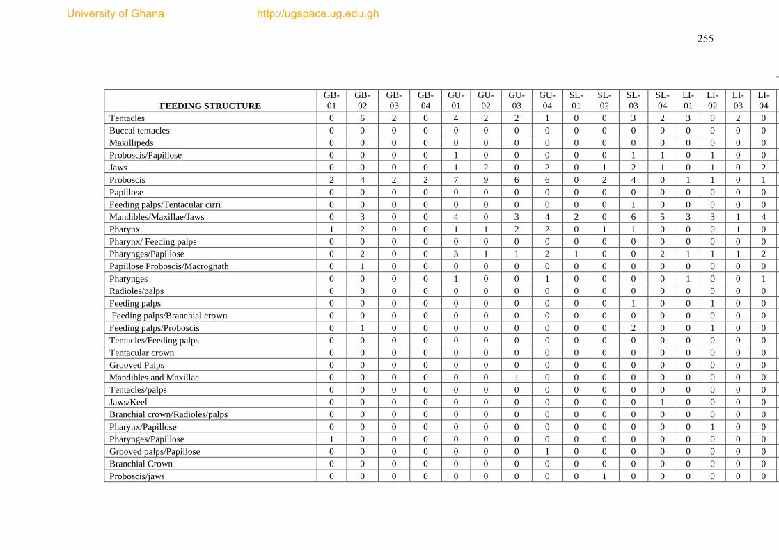
255
FEEDING STRUCTURE
GB-
01
GB-
02
GB-
03
GB-
04
GU-
01
GU-
02
GU-
03
GU-
04
SL-
01
SL-
02
SL-
03
SL-
04
LI-
01
LI-
02
LI-
03
LI-
04
Tentacles 0 6 2 0 4 2 2 1 0 0 3 2 3 0 2 0
Buccal tentacles 0 0 0 0 0 0 0 0 0 0 0 0 0 0 0 0
Maxillipeds 0 0 0 0 0 0 0 0 0 0 0 0 0 0 0 0
Proboscis/Papillose 0 0 0 0 1 0 0 0 0 0 1 1 0 1 0 0
Jaws 0 0 0 0 1 2 0 2 0 1 2 1 0 1 0 2
Proboscis 2 4 2 2 7 9 6 6 0 2 4 0 1 1 0 1
Papillose 0 0 0 0 0 0 0 0 0 0 0 0 0 0 0 0
Feeding palps/Tentacular cirri 0 0 0 0 0 0 0 0 0 0 1 0 0 0 0 0
Mandibles/Maxillae/Jaws 0 3 0 0 4 0 3 4 2 0 6 5 3 3 1 4
Pharynx 1 2 0 0 1 1 2 2 0 1 1 0 0 0 1 0
Pharynx/ Feeding palps 0 0 0 0 0 0 0 0 0 0 0 0 0 0 0 0
Pharynges/Papillose 0 2 0 0 3 1 1 2 1 0 0 2 1 1 1 2
Papillose Proboscis/Macrognath 0 1 0 0 0 0 0 0 0 0 0 0 0 0 0 0
Pharynges 0 0 0 0 1 0 0 1 0 0 0 0 1 0 0 1
Radioles/palps 0 0 0 0 0 0 0 0 0 0 0 0 0 0 0 0
Feeding palps 0 0 0 0 0 0 0 0 0 0 1 0 0 1 0 0
Feeding palps/Branchial crown 0 0 0 0 0 0 0 0 0 0 0 0 0 0 0 0
Feeding palps/Proboscis 0 1 0 0 0 0 0 0 0 0 2 0 0 1 0 0
Tentacles/Feeding palps 0 0 0 0 0 0 0 0 0 0 0 0 0 0 0 0
Tentacular crown 0 0 0 0 0 0 0 0 0 0 0 0 0 0 0 0
Grooved Palps 0 0 0 0 0 0 0 0 0 0 0 0 0 0 0 0
Mandibles and Maxillae 0 0 0 0 0 0 1 0 0 0 0 0 0 0 0 0
Tentacles/palps 0 0 0 0 0 0 0 0 0 0 0 0 0 0 0 0
Jaws/Keel 0 0 0 0 0 0 0 0 0 0 0 1 0 0 0 0
Branchial crown/Radioles/palps 0 0 0 0 0 0 0 0 0 0 0 0 0 0 0 0
Pharynx/Papillose 0 0 0 0 0 0 0 0 0 0 0 0 0 1 0 0
Pharynges/Papillose 1 0 0 0 0 0 0 0 0 0 0 0 0 0 0 0
Grooved palps/Papillose 0 0 0 0 0 0 0 1 0 0 0 0 0 0 0 0
Branchial Crown 0 0 0 0 0 0 0 0 0 0 0 0 0 0 0 0
Proboscis/jaws 0 0 0 0 0 0 0 0 0 1 0 0 0 0 0 0
University of Ghana http://ugspace.ug.edu.gh
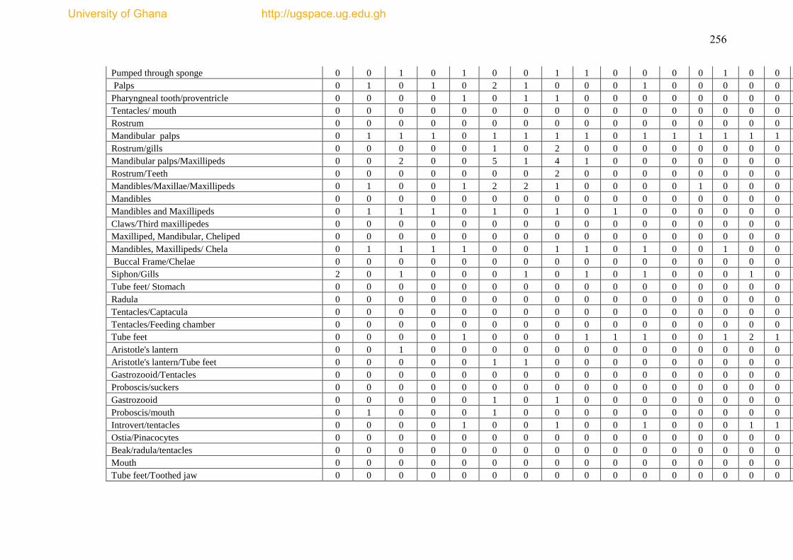
256
Pumped through sponge 0 0 1 0 1 0 0 1 1 0 0 0 0 1 0 0
Palps 0 1 0 1 0 2 1 0 0 0 1 0 0 0 0 0
Pharyngneal tooth/proventricle 0 0 0 0 1 0 1 1 0 0 0 0 0 0 0 0
Tentacles/ mouth 0 0 0 0 0 0 0 0 0 0 0 0 0 0 0 0
Rostrum 0 0 0 0 0 0 0 0 0 0 0 0 0 0 0 0
Mandibular palps 0 1 1 1 0 1 1 1 1 0 1 1 1 1 1 1
Rostrum/gills 0 0 0 0 0 1 0 2 0 0 0 0 0 0 0 0
Mandibular palps/Maxillipeds 0 0 2 0 0 5 1 4 1 0 0 0 0 0 0 0
Rostrum/Teeth 0 0 0 0 0 0 0 2 0 0 0 0 0 0 0 0
Mandibles/Maxillae/Maxillipeds 0 1 0 0 1 2 2 1 0 0 0 0 1 0 0 0
Mandibles 0 0 0 0 0 0 0 0 0 0 0 0 0 0 0 0
Mandibles and Maxillipeds 0 1 1 1 0 1 0 1 0 1 0 0 0 0 0 0
Claws/Third maxillipedes 0 0 0 0 0 0 0 0 0 0 0 0 0 0 0 0
Maxilliped, Mandibular, Cheliped 0 0 0 0 0 0 0 0 0 0 0 0 0 0 0 0
Mandibles, Maxillipeds/ Chela 0 1 1 1 1 0 0 1 1 0 1 0 0 1 0 0
Buccal Frame/Chelae 0 0 0 0 0 0 0 0 0 0 0 0 0 0 0 0
Siphon/Gills 2 0 1 0 0 0 1 0 1 0 1 0 0 0 1 0
Tube feet/ Stomach 0 0 0 0 0 0 0 0 0 0 0 0 0 0 0 0
Radula 0 0 0 0 0 0 0 0 0 0 0 0 0 0 0 0
Tentacles/Captacula 0 0 0 0 0 0 0 0 0 0 0 0 0 0 0 0
Tentacles/Feeding chamber 0 0 0 0 0 0 0 0 0 0 0 0 0 0 0 0
Tube feet 0 0 0 0 1 0 0 0 1 1 1 0 0 1 2 1
Aristotle's lantern 0 0 1 0 0 0 0 0 0 0 0 0 0 0 0 0
Aristotle's lantern/Tube feet 0 0 0 0 0 1 1 0 0 0 0 0 0 0 0 0
Gastrozooid/Tentacles 0 0 0 0 0 0 0 0 0 0 0 0 0 0 0 0
Proboscis/suckers 0 0 0 0 0 0 0 0 0 0 0 0 0 0 0 0
Gastrozooid 0 0 0 0 0 1 0 1 0 0 0 0 0 0 0 0
Proboscis/mouth 0 1 0 0 0 1 0 0 0 0 0 0 0 0 0 0
Introvert/tentacles 0 0 0 0 1 0 0 1 0 0 1 0 0 0 1 1
Ostia/Pinacocytes 0 0 0 0 0 0 0 0 0 0 0 0 0 0 0 0
Beak/radula/tentacles 0 0 0 0 0 0 0 0 0 0 0 0 0 0 0 0
Mouth 0 0 0 0 0 0 0 0 0 0 0 0 0 0 0 0
Tube feet/Toothed jaw 0 0 0 0 0 0 0 0 0 0 0 0 0 0 0 0
University of Ghana http://ugspace.ug.edu.gh
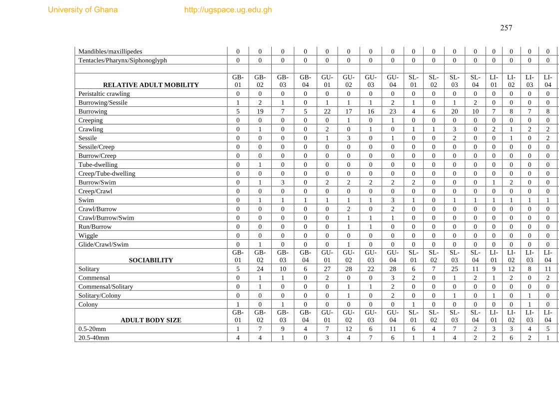
257
Mandibles/maxillipedes 0 0 0 0 0 0 0 0 0 0 0 0 0 0 0 0
Tentacles/Pharynx/Siphonoglyph 0 0 0 0 0 0 0 0 0 0 0 0 0 0 0 0
RELATIVE ADULT MOBILITY
GB-
01
GB-
02
GB-
03
GB-
04
GU-
01
GU-
02
GU-
03
GU-
04
SL-
01
SL-
02
SL-
03
SL-
04
LI-
01
LI-
02
LI-
03
LI-
04
Peristaltic crawling 0 0 0 0 0 0 0 0 0 0 0 0 0 0 0 0
Burrowing/Sessile 1 2 1 0 1 1 1 2 1 0 1 2 0 0 0 0
Burrowing 5 19 7 5 22 17 16 23 4 6 20 10 7 8 7 8
Creeping 0 0 0 0 0 1 0 1 0 0 0 0 0 0 0 0
Crawling 0 1 0 0 2 0 1 0 1 1 3 0 2 1 2 2
Sessile 0 0 0 0 1 3 0 1 0 0 2 0 0 1 0 2
Sessile/Creep 0 0 0 0 0 0 0 0 0 0 0 0 0 0 0 0
Burrow/Creep 0 0 0 0 0 0 0 0 0 0 0 0 0 0 0 0
Tube-dwelling 0 1 0 0 0 0 0 0 0 0 0 0 0 0 0 0
Creep/Tube-dwelling 0 0 0 0 0 0 0 0 0 0 0 0 0 0 0 0
Burrow/Swim 0 1 3 0 2 2 2 2 2 0 0 0 1 2 0 0
Creep/Crawl 0 0 0 0 0 0 0 0 0 0 0 0 0 0 0 0
Swim 0 1 1 1 1 1 1 3 1 0 1 1 1 1 1 1
Crawl/Burrow 0 0 0 0 0 2 0 2 0 0 0 0 0 0 0 0
Crawl/Burrow/Swim 0 0 0 0 0 1 1 1 0 0 0 0 0 0 0 0
Run/Burrow 0 0 0 0 0 1 1 0 0 0 0 0 0 0 0 0
Wiggle 0 0 0 0 0 0 0 0 0 0 0 0 0 0 0 0
Glide/Crawl/Swim 0 1 0 0 0 1 0 0 0 0 0 0 0 0 0 0
SOCIABILITY
GB-
01
GB-
02
GB-
03
GB-
04
GU-
01
GU-
02
GU-
03
GU-
04
SL-
01
SL-
02
SL-
03
SL-
04
LI-
01
LI-
02
LI-
03
LI-
04
Solitary 5 24 10 6 27 28 22 28 6 7 25 11 9 12 8 11
Commensal 0 1 1 0 2 0 0 3 2 0 1 2 1 2 0 2
Commensal/Solitary 0 1 0 0 0 1 1 2 0 0 0 0 0 0 0 0
Solitary/Colony 0 0 0 0 0 1 0 2 0 0 1 0 1 0 1 0
Colony 1 0 1 0 0 0 0 0 1 0 0 0 0 0 1 0
ADULT BODY SIZE
GB-
01
GB-
02
GB-
03
GB-
04
GU-
01
GU-
02
GU-
03
GU-
04
SL-
01
SL-
02
SL-
03
SL-
04
LI-
01
LI-
02
LI-
03
LI-
04
0.5-20mm 1 7 9 4 7 12 6 11 6 4 7 2 3 3 4 5
20.5-40mm 4 4 1 0 3 4 7 6 1 1 4 2 2 6 2 1
University of Ghana http://ugspace.ug.edu.gh
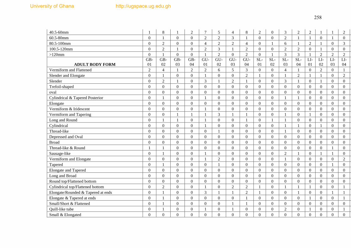
258
40.5-60mm 1 8 1 2 7 5 4 8 2 0 3 2 2 1 1 2
60.5-80mm 0 1 0 0 2 2 3 1 0 0 2 1 1 0 1 0
80.5-100mm 0 2 0 0 4 2 2 4 0 1 6 1 2 1 0 3
100.5-120mm 0 2 1 0 2 3 1 2 0 0 2 2 0 1 0 0
>120mm 0 1 0 0 1 2 0 2 0 1 3 3 1 2 2 2
ADULT BODY FORM
GB-
01
GB-
02
GB-
03
GB-
04
GU-
01
GU-
02
GU-
03
GU-
04
SL-
01
SL-
02
SL-
03
SL-
04
LI-
01
LI-
02
LI-
03
LI-
04
Vermiform and Flattened 2 4 1 2 2 6 5 3 0 0 4 1 0 2 0 1
Slender and Elongate 0 1 0 0 1 0 0 2 1 0 1 2 1 1 0 2
Slender 0 2 1 0 3 1 2 1 0 0 3 1 0 1 0 0
Trefoil-shaped 0 0 0 0 0 0 0 0 0 0 0 0 0 0 0 0
oval 0 0 0 0 0 0 0 0 0 0 0 0 0 0 0 0
Cylindrical & Tapered Posterior 0 1 0 0 1 0 0 0 0 0 1 1 0 0 0 0
Elongate 0 0 0 0 0 0 0 0 0 0 0 0 0 0 0 0
Vermiform & Iridescent 0 0 0 0 1 0 0 0 0 0 0 0 0 0 0 0
Vermiform and Tapering 0 0 1 1 1 3 1 1 0 0 1 0 1 0 0 0
Long and Round 0 1 1 0 1 0 0 1 0 1 1 0 0 0 0 0
Cylindrical 0 0 0 0 1 0 0 0 0 0 1 1 0 1 0 0
Thread-like 0 0 0 0 0 1 0 0 0 0 1 0 0 0 0 0
Depressed and Oval 0 0 0 0 0 0 0 0 0 0 0 0 0 0 0 0
Broad 0 0 0 0 0 0 0 0 0 0 0 0 0 0 0 0
Thread-like & Round 1 1 0 0 0 0 0 0 0 0 0 0 0 0 1 0
Sausage-like 0 1 0 0 1 0 0 0 0 0 2 1 0 1 1 0
Vermiform and Elongate 0 0 0 0 1 2 0 0 0 0 1 0 0 0 0 2
Tapered 0 1 0 0 0 1 0 0 0 0 0 0 0 0 1 0
Elongate and Tapered 0 0 0 0 0 0 0 0 0 0 0 0 0 0 0 0
Long and Broad 0 0 0 0 0 0 0 0 0 0 0 0 0 0 0 0
Round top/Flattened bottom 0 0 0 0 0 0 0 0 0 0 0 0 0 0 0 0
Cylindrical top/Flattened bottom 0 2 0 0 1 0 2 2 1 0 1 1 1 0 0 1
Elongate/Rounded & Tapered at ends 0 1 0 0 3 1 1 2 1 0 0 1 0 0 1 1
Elongate & Tapered at ends 0 1 0 0 0 0 0 1 0 0 0 0 1 0 0 1
Small/Short & Flattened 0 1 0 0 0 0 1 1 0 0 0 0 0 0 0 0
Quill-like tube 0 1 0 0 1 0 1 0 0 0 2 0 1 0 0 1
Small & Elongated 0 0 0 0 0 0 0 0 0 0 0 0 0 0 0 0
University of Ghana http://ugspace.ug.edu.gh
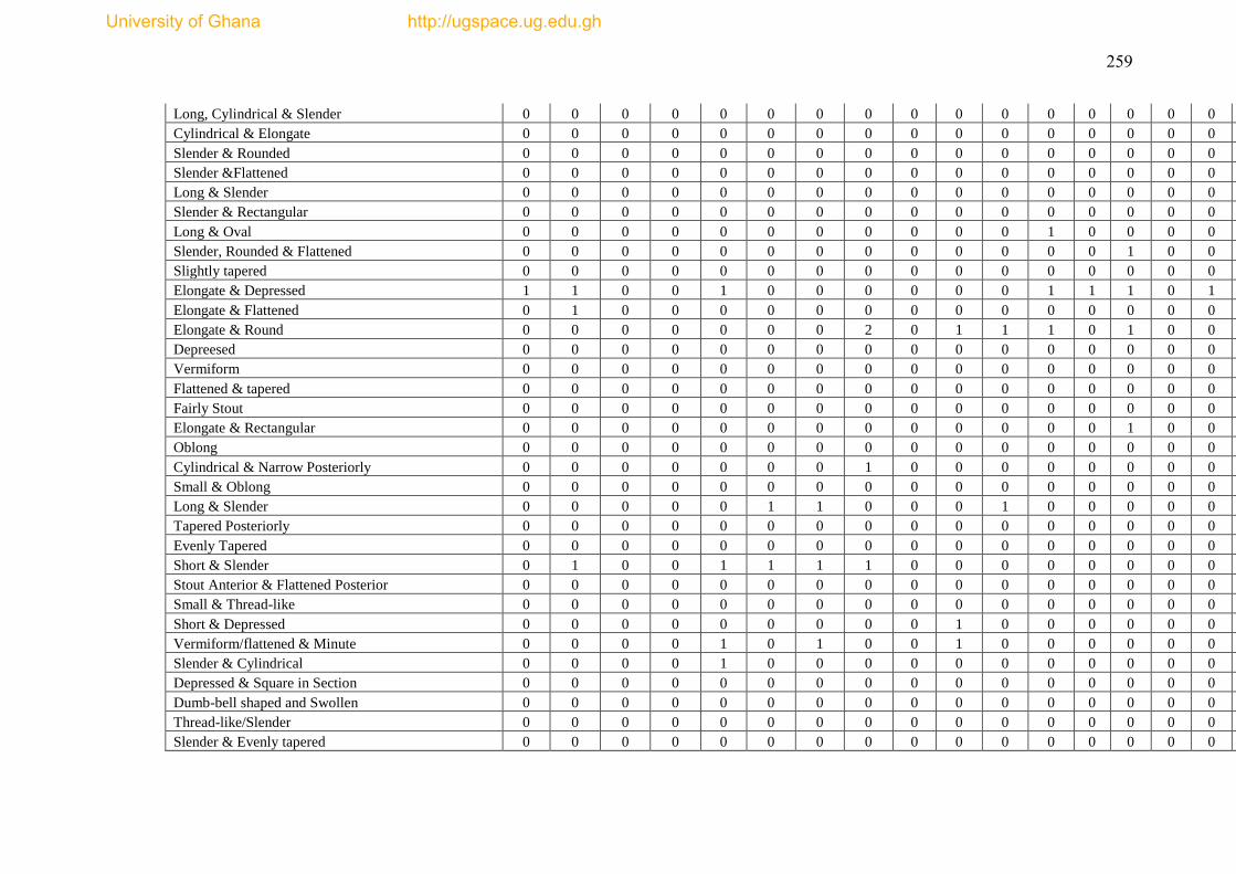
259
Long, Cylindrical & Slender 0 0 0 0 0 0 0 0 0 0 0 0 0 0 0 0
Cylindrical & Elongate 0 0 0 0 0 0 0 0 0 0 0 0 0 0 0 0
Slender & Rounded 0 0 0 0 0 0 0 0 0 0 0 0 0 0 0 0
Slender &Flattened 0 0 0 0 0 0 0 0 0 0 0 0 0 0 0 0
Long & Slender 0 0 0 0 0 0 0 0 0 0 0 0 0 0 0 0
Slender & Rectangular 0 0 0 0 0 0 0 0 0 0 0 0 0 0 0 0
Long & Oval 0 0 0 0 0 0 0 0 0 0 0 1 0 0 0 0
Slender, Rounded & Flattened 0 0 0 0 0 0 0 0 0 0 0 0 0 1 0 0
Slightly tapered 0 0 0 0 0 0 0 0 0 0 0 0 0 0 0 0
Elongate & Depressed 1 1 0 0 1 0 0 0 0 0 0 1 1 1 0 1
Elongate & Flattened 0 1 0 0 0 0 0 0 0 0 0 0 0 0 0 0
Elongate & Round 0 0 0 0 0 0 0 2 0 1 1 1 0 1 0 0
Depreesed 0 0 0 0 0 0 0 0 0 0 0 0 0 0 0 0
Vermiform 0 0 0 0 0 0 0 0 0 0 0 0 0 0 0 0
Flattened & tapered 0 0 0 0 0 0 0 0 0 0 0 0 0 0 0 0
Fairly Stout 0 0 0 0 0 0 0 0 0 0 0 0 0 0 0 0
Elongate & Rectangular 0 0 0 0 0 0 0 0 0 0 0 0 0 1 0 0
Oblong 0 0 0 0 0 0 0 0 0 0 0 0 0 0 0 0
Cylindrical & Narrow Posteriorly 0 0 0 0 0 0 0 1 0 0 0 0 0 0 0 0
Small & Oblong 0 0 0 0 0 0 0 0 0 0 0 0 0 0 0 0
Long & Slender 0 0 0 0 0 1 1 0 0 0 1 0 0 0 0 0
Tapered Posteriorly 0 0 0 0 0 0 0 0 0 0 0 0 0 0 0 0
Evenly Tapered 0 0 0 0 0 0 0 0 0 0 0 0 0 0 0 0
Short & Slender 0 1 0 0 1 1 1 1 0 0 0 0 0 0 0 0
Stout Anterior & Flattened Posterior 0 0 0 0 0 0 0 0 0 0 0 0 0 0 0 0
Small & Thread-like 0 0 0 0 0 0 0 0 0 0 0 0 0 0 0 0
Short & Depressed 0 0 0 0 0 0 0 0 0 1 0 0 0 0 0 0
Vermiform/flattened & Minute 0 0 0 0 1 0 1 0 0 1 0 0 0 0 0 0
Slender & Cylindrical 0 0 0 0 1 0 0 0 0 0 0 0 0 0 0 0
Depressed & Square in Section 0 0 0 0 0 0 0 0 0 0 0 0 0 0 0 0
Dumb-bell shaped and Swollen 0 0 0 0 0 0 0 0 0 0 0 0 0 0 0 0
Thread-like/Slender 0 0 0 0 0 0 0 0 0 0 0 0 0 0 0 0
Slender & Evenly tapered 0 0 0 0 0 0 0 0 0 0 0 0 0 0 0 0
University of Ghana http://ugspace.ug.edu.gh
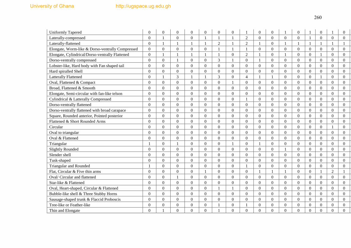
260
Uniformly Tapered 0 0 0 0 0 0 0 1 0 0 1 0 1 0 1 0
Laterally-compressed 0 1 0 0 1 1 1 2 0 0 0 0 1 0 0 0
Laterally-flattened 0 1 1 1 1 2 1 2 1 0 1 1 1 1 1 1
Elongate, Worm-like & Dorso-ventrally Compressed 0 0 0 0 0 1 1 1 0 0 0 0 0 0 0 0
Elongate, Cylindrical/Dorso-ventrally Flattened 0 1 1 1 1 1 0 2 1 0 1 0 0 1 0 0
Dorso-ventrally compressed 0 0 1 0 0 3 1 0 1 0 0 0 0 0 0 0
Lobster-like, Hard body with Fan shaped tail 0 0 0 0 0 0 0 0 0 0 0 0 0 0 0 0
Hard spiralled Shell 0 0 0 0 0 0 0 0 0 0 0 0 0 0 0 0
Latterally Flattened 0 1 3 1 1 3 0 4 1 1 0 0 0 1 0 0
Oval, Flattened & Compact 0 0 0 0 0 0 1 0 0 0 0 0 0 0 0 0
Broad, Flattened & Smooth 0 0 0 0 0 0 0 0 0 0 0 0 0 0 0 0
Elongate, Semi-circular with fan-like telson 0 0 0 0 0 0 0 0 0 0 0 0 0 0 0 0
Cylindrical & Latterally Compressed 0 0 0 0 0 0 0 1 0 0 0 0 0 0 0 0
Dorso-ventrally flattened 0 0 0 0 0 0 0 0 0 0 0 0 0 0 0 0
Dorso-ventrally flattened with broad carapace 0 0 0 0 0 0 0 0 0 0 0 0 0 0 0 0
Square, Rounded anterior, Pointed posterior 0 0 0 0 0 0 0 0 0 0 0 0 0 0 0 0
Flattened & Short Rounded Arms 0 0 0 0 0 0 0 0 0 0 0 0 0 0 0 0
Circular 0 0 0 0 0 0 0 0 0 0 0 0 0 0 1 0
Oval to triangular 0 0 0 0 0 0 0 0 0 0 0 0 0 0 0 0
Oval & Flattened 0 0 0 0 0 0 0 0 0 0 0 0 0 0 0 0
Triangular 1 0 1 0 0 0 1 0 1 0 0 0 0 0 0 0
Slightly Rounded 0 0 0 0 0 0 0 0 0 0 1 0 0 0 0 0
Slender shell 0 0 0 0 0 0 0 0 0 0 0 0 0 0 0 0
Tusk-shaped 0 0 0 0 0 0 0 0 0 0 0 0 0 0 0 0
Triangular and Rounded 1 0 0 0 0 0 0 1 0 0 0 0 0 0 0 0
Flat, Circular & Five thin arms 0 0 0 0 1 0 0 0 1 1 1 0 0 1 2 1
Oval/ Circular and flattened 0 0 1 0 0 0 0 0 0 0 0 0 0 0 0 0
Star-like & Flattened 0 0 0 0 0 0 0 0 0 0 0 0 0 0 0 0
Oval, Heart-shaped, Circular & Flattened 0 0 0 0 0 1 1 0 0 0 0 0 0 0 0 0
Bubble-like shell & Three Stubby Horns 0 0 0 0 0 0 0 0 0 0 0 0 0 0 0 0
Sausage-shaped trunk & Flaccid Proboscis 0 0 0 0 0 0 0 0 0 0 0 0 0 0 0 0
Tree-like or Feather-like 0 0 0 0 0 1 0 1 0 0 0 0 0 0 0 0
Thin and Elongate 0 1 0 0 0 1 0 0 0 0 0 0 0 0 0 0
University of Ghana http://ugspace.ug.edu.gh
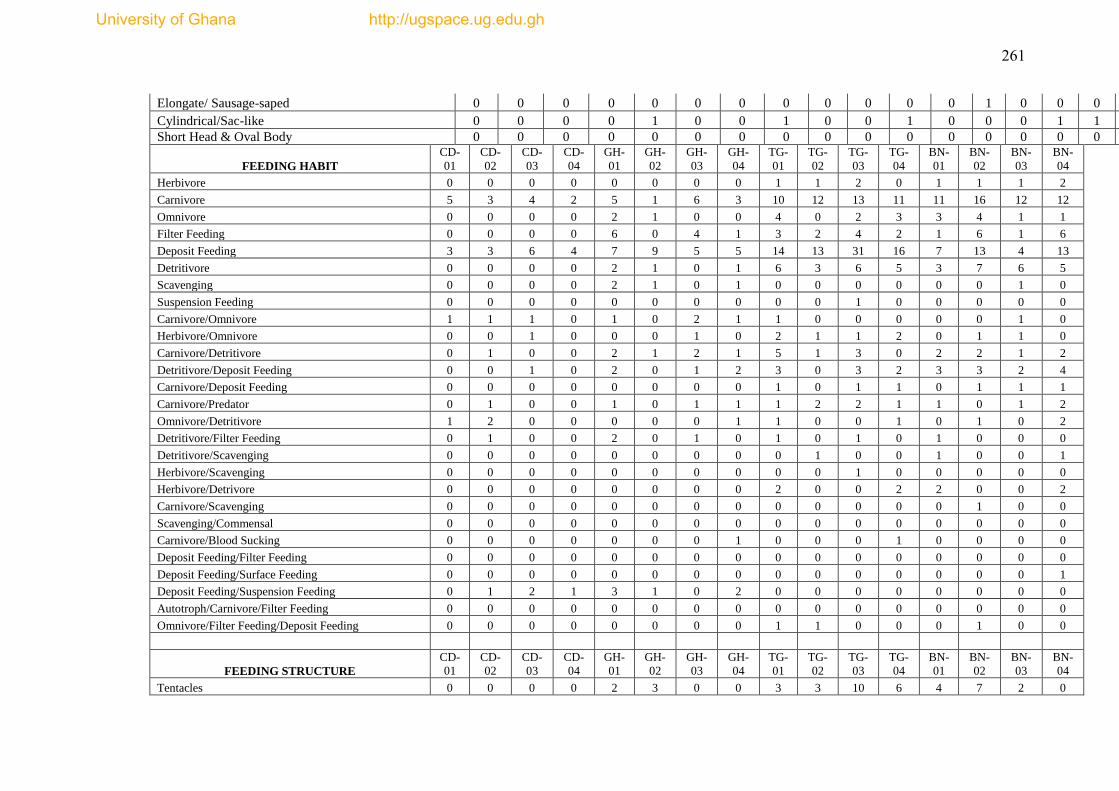
261
Elongate/ Sausage-saped 0 0 0 0 0 0 0 0 0 0 0 0 1 0 0 0
Cylindrical/Sac-like 0 0 0 0 1 0 0 1 0 0 1 0 0 0 1 1
Short Head & Oval Body 0 0 0 0 0 0 0 0 0 0 0 0 0 0 0 0
FEEDING HABIT
CD-
01
CD-
02
CD-
03
CD-
04
GH-
01
GH-
02
GH-
03
GH-
04
TG-
01
TG-
02
TG-
03
TG-
04
BN-
01
BN-
02
BN-
03
BN-
04
Herbivore 0 0 0 0 0 0 0 0 1 1 2 0 1 1 1 2
Carnivore 5 3 4 2 5 1 6 3 10 12 13 11 11 16 12 12
Omnivore 0 0 0 0 2 1 0 0 4 0 2 3 3 4 1 1
Filter Feeding 0 0 0 0 6 0 4 1 3 2 4 2 1 6 1 6
Deposit Feeding 3 3 6 4 7 9 5 5 14 13 31 16 7 13 4 13
Detritivore 0 0 0 0 2 1 0 1 6 3 6 5 3 7 6 5
Scavenging 0 0 0 0 2 1 0 1 0 0 0 0 0 0 1 0
Suspension Feeding 0 0 0 0 0 0 0 0 0 0 1 0 0 0 0 0
Carnivore/Omnivore 1 1 1 0 1 0 2 1 1 0 0 0 0 0 1 0
Herbivore/Omnivore 0 0 1 0 0 0 1 0 2 1 1 2 0 1 1 0
Carnivore/Detritivore 0 1 0 0 2 1 2 1 5 1 3 0 2 2 1 2
Detritivore/Deposit Feeding 0 0 1 0 2 0 1 2 3 0 3 2 3 3 2 4
Carnivore/Deposit Feeding 0 0 0 0 0 0 0 0 1 0 1 1 0 1 1 1
Carnivore/Predator 0 1 0 0 1 0 1 1 1 2 2 1 1 0 1 2
Omnivore/Detritivore 1 2 0 0 0 0 0 1 1 0 0 1 0 1 0 2
Detritivore/Filter Feeding 0 1 0 0 2 0 1 0 1 0 1 0 1 0 0 0
Detritivore/Scavenging 0 0 0 0 0 0 0 0 0 1 0 0 1 0 0 1
Herbivore/Scavenging 0 0 0 0 0 0 0 0 0 0 1 0 0 0 0 0
Herbivore/Detrivore 0 0 0 0 0 0 0 0 2 0 0 2 2 0 0 2
Carnivore/Scavenging 0 0 0 0 0 0 0 0 0 0 0 0 0 1 0 0
Scavenging/Commensal 0 0 0 0 0 0 0 0 0 0 0 0 0 0 0 0
Carnivore/Blood Sucking 0 0 0 0 0 0 0 1 0 0 0 1 0 0 0 0
Deposit Feeding/Filter Feeding 0 0 0 0 0 0 0 0 0 0 0 0 0 0 0 0
Deposit Feeding/Surface Feeding 0 0 0 0 0 0 0 0 0 0 0 0 0 0 0 1
Deposit Feeding/Suspension Feeding 0 1 2 1 3 1 0 2 0 0 0 0 0 0 0 0
Autotroph/Carnivore/Filter Feeding 0 0 0 0 0 0 0 0 0 0 0 0 0 0 0 0
Omnivore/Filter Feeding/Deposit Feeding 0 0 0 0 0 0 0 0 1 1 0 0 0 1 0 0
FEEDING STRUCTURE
CD-
01
CD-
02
CD-
03
CD-
04
GH-
01
GH-
02
GH-
03
GH-
04
TG-
01
TG-
02
TG-
03
TG-
04
BN-
01
BN-
02
BN-
03
BN-
04
Tentacles 0 0 0 0 2 3 0 0 3 3 10 6 4 7 2 0
University of Ghana http://ugspace.ug.edu.gh
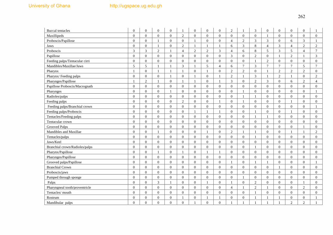
262
Buccal tentacles 0 0 0 0 1 0 0 0 2 1 3 0 0 0 0 1
Maxillipeds 0 0 0 0 2 0 0 0 0 0 0 1 0 0 0 0
Proboscis/Papillose 0 0 1 0 0 1 0 0 4 2 3 3 0 6 3 1
Jaws 0 0 1 0 2 1 1 1 6 3 8 4 3 4 2 2
Proboscis 3 3 2 1 4 2 2 3 4 6 8 5 3 5 4 7
Papillose 0 0 0 0 0 0 0 0 3 0 2 0 1 2 1 3
Feeding palps/Tentacular cirri 0 0 0 0 0 0 0 0 0 0 1 2 0 0 0 0
Mandibles/Maxillae/Jaws 5 5 1 1 3 1 5 4 6 7 3 7 7 7 5 7
Pharynx 1 0 1 1 1 0 1 0 2 2 0 1 2 2 2 0
Pharynx/ Feeding palps 0 0 0 1 0 1 0 1 2 1 3 1 2 1 0 2
Pharynges/Papillose 1 2 1 0 1 1 0 1 3 0 2 3 0 6 2 4
Papillose Proboscis/Macrognath 0 0 0 0 0 0 0 0 0 0 0 0 0 0 0 0
Pharynges 0 0 0 1 0 0 0 0 0 1 0 0 0 0 0 1
Radioles/palps 0 0 0 0 0 0 0 0 0 1 1 0 0 0 0 0
Feeding palps 0 0 0 0 2 0 0 1 0 1 0 0 0 1 0 0
Feeding palps/Branchial crown 0 0 0 0 0 0 0 0 0 0 0 0 0 0 0 1
Feeding palps/Proboscis 0 0 0 0 0 1 1 1 0 0 1 0 0 1 0 0
Tentacles/Feeding palps 0 0 0 0 0 0 0 0 0 0 1 1 0 0 0 0
Tentacular crown 0 0 0 0 0 0 0 0 0 0 0 0 0 0 0 0
Grooved Palps 0 0 0 0 0 0 0 0 0 0 0 0 0 0 1 0
Mandibles and Maxillae 0 0 1 0 0 0 1 0 2 1 1 0 0 1 1 2
Tentacles/palps 0 0 0 0 0 0 0 0 0 0 1 0 0 0 0 0
Jaws/Keel 0 0 0 0 0 0 0 0 0 0 0 0 0 0 0 0
Branchial crown/Radioles/palps 0 0 0 0 0 0 0 0 0 0 1 0 0 0 0 0
Pharynx/Papillose 0 0 1 0 1 0 1 1 0 0 0 0 0 0 0 0
Pharynges/Papillose 0 0 0 0 0 0 0 0 0 0 0 0 0 0 0 0
Grooved palps/Papillose 0 0 0 0 0 0 0 0 1 0 1 1 0 0 0 1
Branchial Crown 0 0 0 0 0 0 0 0 0 0 0 0 1 0 0 0
Proboscis/jaws 0 0 0 0 0 0 0 0 0 0 0 0 0 0 0 0
Pumped through sponge 0 0 0 0 0 0 0 0 0 1 0 0 0 0 0 0
Palps 0 0 3 1 0 0 1 0 1 0 2 0 0 0 1 0
Pharyngneal tooth/proventricle 0 0 0 0 0 0 0 0 4 1 2 1 0 0 2 0
Tentacles/ mouth 0 0 0 0 0 0 0 0 0 0 1 0 0 0 0 0
Rostrum 0 0 0 0 1 0 1 1 0 0 1 1 1 0 0 1
Mandibular palps 0 0 0 0 0 1 0 0 1 1 1 1 1 2 2 1
University of Ghana http://ugspace.ug.edu.gh
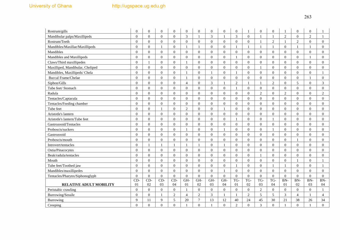
263
Rostrum/gills 0 0 0 0 0 0 0 0 0 1 0 0 1 0 0 1
Mandibular palps/Maxillipeds 0 0 0 0 3 1 3 1 3 0 1 1 2 0 2 1
Rostrum/Teeth 0 0 0 0 0 0 0 0 0 0 1 2 1 2 0 0
Mandibles/Maxillae/Maxillipeds 0 0 1 0 1 1 0 0 1 1 1 1 0 1 1 0
Mandibles 0 0 0 0 0 0 0 0 0 0 0 0 0 0 0 0
Mandibles and Maxillipeds 0 0 0 0 0 0 0 0 1 0 0 0 0 0 1 0
Claws/Third maxillipedes 0 1 0 0 1 0 0 0 0 0 0 0 0 0 0 0
Maxilliped, Mandibular, Cheliped 0 0 0 0 0 0 0 0 0 0 1 0 0 0 0 0
Mandibles, Maxillipeds/ Chela 0 0 0 0 1 0 1 0 1 0 0 0 0 0 0 1
Buccal Frame/Chelae 0 0 0 0 1 0 0 0 0 0 0 0 0 0 1 0
Siphon/Gills 0 0 0 0 4 0 3 1 2 1 1 2 0 5 0 3
Tube feet/ Stomach 0 0 0 0 0 0 0 0 1 0 0 0 0 0 0 0
Radula 0 0 0 0 0 0 0 0 0 0 2 0 2 0 0 2
Tentacles/Captacula 0 0 0 0 0 0 0 0 0 0 0 0 0 0 0 0
Tentacles/Feeding chamber 0 0 0 0 0 0 0 0 0 0 0 0 0 0 0 0
Tube feet 0 0 1 0 2 0 0 1 0 0 0 0 0 0 0 0
Aristotle's lantern 0 0 0 0 0 0 0 0 0 0 0 0 0 0 0 0
Aristotle's lantern/Tube feet 0 0 0 0 0 0 0 0 1 0 0 1 0 0 0 0
Gastrozooid/Tentacles 0 0 0 0 0 0 0 0 0 0 0 0 0 0 0 0
Proboscis/suckers 0 0 0 0 1 0 0 1 0 0 0 1 0 0 0 0
Gastrozooid 0 0 0 0 0 0 0 0 0 0 0 0 0 0 0 0
Proboscis/mouth 0 0 0 0 0 0 0 0 0 0 0 0 0 1 0 0
Introvert/tentacles 0 1 1 1 1 1 0 1 0 0 0 0 0 0 0 0
Ostia/Pinacocytes 0 0 0 0 0 0 0 0 0 0 0 0 0 0 0 0
Beak/radula/tentacles 0 0 0 0 0 0 0 0 0 0 1 0 0 0 0 0
Mouth 0 0 0 0 0 0 0 0 0 0 0 0 0 1 0 1
Tube feet/Toothed jaw 0 0 0 0 0 0 0 0 1 0 0 1 1 0 0 1
Mandibles/maxillipedes 0 0 0 0 0 0 0 1 0 0 0 0 0 0 0 0
Tentacles/Pharynx/Siphonoglyph 0 0 0 0 0 0 0 0 0 0 0 0 0 0 0 0
RELATIVE ADULT MOBILITY
CD-
01
CD-
02
CD-
03
CD-
04
GH-
01
GH-
02
GH-
03
GH-
04
TG-
01
TG-
02
TG-
03
TG-
04
BN-
01
BN-
02
BN-
03
BN-
04
Peristaltic crawling 0 0 0 0 1 0 0 0 0 0 2 0 0 0 0 1
Burrowing/Sessile 0 0 1 2 4 2 3 1 1 2 5 5 3 4 1 4
Burrowing 9 11 9 5 20 7 13 12 40 24 45 30 21 38 26 34
Creeping 0 0 0 0 1 0 1 0 2 0 3 0 1 0 1 0
University of Ghana http://ugspace.ug.edu.gh
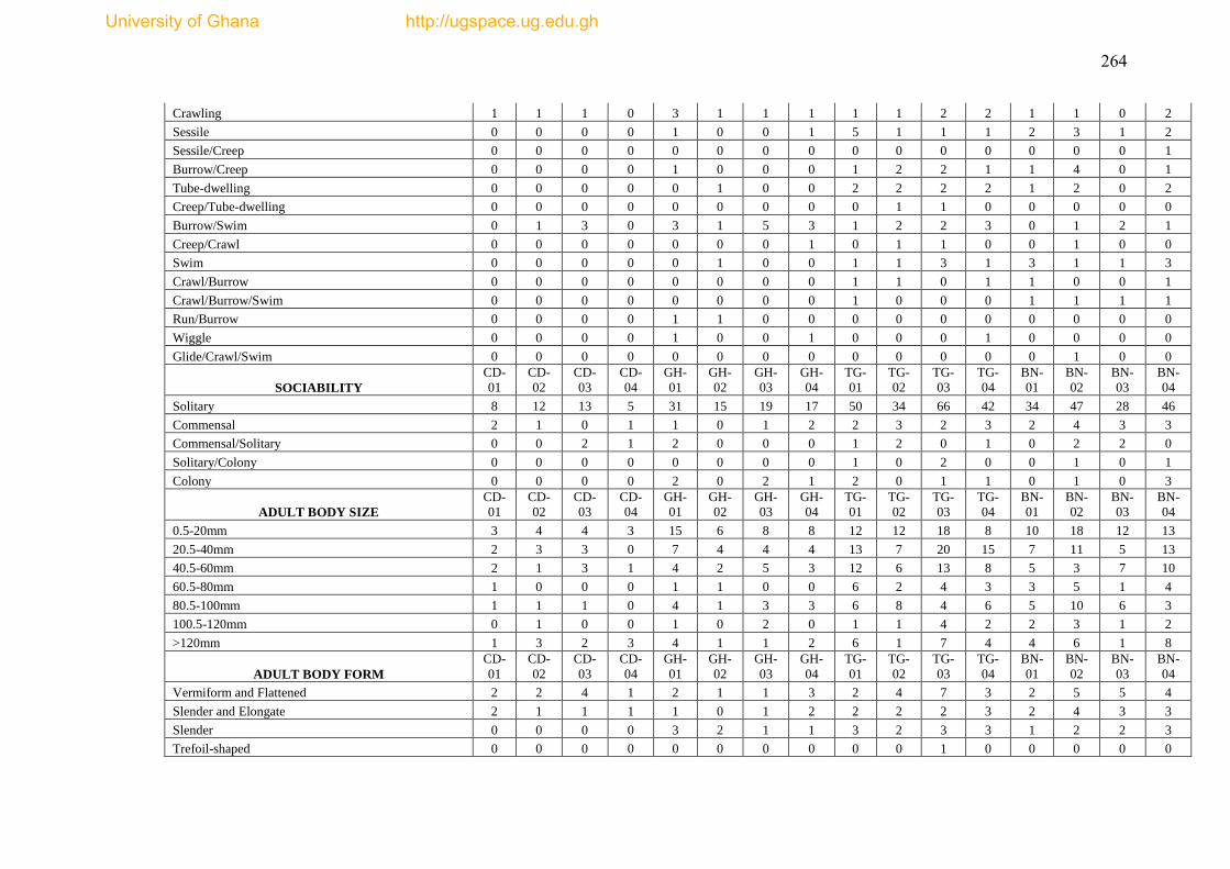
264
Crawling 1 1 1 0 3 1 1 1 1 1 2 2 1 1 0 2
Sessile 0 0 0 0 1 0 0 1 5 1 1 1 2 3 1 2
Sessile/Creep 0 0 0 0 0 0 0 0 0 0 0 0 0 0 0 1
Burrow/Creep 0 0 0 0 1 0 0 0 1 2 2 1 1 4 0 1
Tube-dwelling 0 0 0 0 0 1 0 0 2 2 2 2 1 2 0 2
Creep/Tube-dwelling 0 0 0 0 0 0 0 0 0 1 1 0 0 0 0 0
Burrow/Swim 0 1 3 0 3 1 5 3 1 2 2 3 0 1 2 1
Creep/Crawl 0 0 0 0 0 0 0 1 0 1 1 0 0 1 0 0
Swim 0 0 0 0 0 1 0 0 1 1 3 1 3 1 1 3
Crawl/Burrow 0 0 0 0 0 0 0 0 1 1 0 1 1 0 0 1
Crawl/Burrow/Swim 0 0 0 0 0 0 0 0 1 0 0 0 1 1 1 1
Run/Burrow 0 0 0 0 1 1 0 0 0 0 0 0 0 0 0 0
Wiggle 0 0 0 0 1 0 0 1 0 0 0 1 0 0 0 0
Glide/Crawl/Swim 0 0 0 0 0 0 0 0 0 0 0 0 0 1 0 0
SOCIABILITY
CD-
01
CD-
02
CD-
03
CD-
04
GH-
01
GH-
02
GH-
03
GH-
04
TG-
01
TG-
02
TG-
03
TG-
04
BN-
01
BN-
02
BN-
03
BN-
04
Solitary 8 12 13 5 31 15 19 17 50 34 66 42 34 47 28 46
Commensal 2 1 0 1 1 0 1 2 2 3 2 3 2 4 3 3
Commensal/Solitary 0 0 2 1 2 0 0 0 1 2 0 1 0 2 2 0
Solitary/Colony 0 0 0 0 0 0 0 0 1 0 2 0 0 1 0 1
Colony 0 0 0 0 2 0 2 1 2 0 1 1 0 1 0 3
ADULT BODY SIZE
CD-
01
CD-
02
CD-
03
CD-
04
GH-
01
GH-
02
GH-
03
GH-
04
TG-
01
TG-
02
TG-
03
TG-
04
BN-
01
BN-
02
BN-
03
BN-
04
0.5-20mm 3 4 4 3 15 6 8 8 12 12 18 8 10 18 12 13
20.5-40mm 2 3 3 0 7 4 4 4 13 7 20 15 7 11 5 13
40.5-60mm 2 1 3 1 4 2 5 3 12 6 13 8 5 3 7 10
60.5-80mm 1 0 0 0 1 1 0 0 6 2 4 3 3 5 1 4
80.5-100mm 1 1 1 0 4 1 3 3 6 8 4 6 5 10 6 3
100.5-120mm 0 1 0 0 1 0 2 0 1 1 4 2 2 3 1 2
>120mm 1 3 2 3 4 1 1 2 6 1 7 4 4 6 1 8
ADULT BODY FORM
CD-
01
CD-
02
CD-
03
CD-
04
GH-
01
GH-
02
GH-
03
GH-
04
TG-
01
TG-
02
TG-
03
TG-
04
BN-
01
BN-
02
BN-
03
BN-
04
Vermiform and Flattened 2 2 4 1 2 1 1 3 2 4 7 3 2 5 5 4
Slender and Elongate 2 1 1 1 1 0 1 2 2 2 2 3 2 4 3 3
Slender 0 0 0 0 3 2 1 1 3 2 3 3 1 2 2 3
Trefoil-shaped 0 0 0 0 0 0 0 0 0 0 1 0 0 0 0 0
University of Ghana http://ugspace.ug.edu.gh

265
oval 0 0 0 0 0 0 0 0 0 1 1 1 0 0 0 0
Cylindrical & Tapered Posterior 0 0 0 0 1 1 0 0 1 2 3 2 2 1 0 1
Elongate 0 0 0 0 0 0 0 0 1 1 1 0 0 1 1 0
Vermiform & Iridescent 0 0 0 0 0 0 0 0 0 0 0 0 0 1 0 0
Vermiform and Tapering 0 0 0 0 2 1 2 0 0 0 2 0 0 0 0 0
Long and Round 0 0 0 0 0 0 0 0 1 1 1 0 0 0 0 1
Cylindrical 0 0 2 0 1 1 0 1 1 0 1 2 1 5 3 0
Thread-like 1 0 0 0 0 1 0 1 3 2 3 4 0 1 1 4
Depressed and Oval 0 0 0 0 0 0 0 0 0 0 0 0 0 0 0 0
Broad 0 0 0 1 0 0 0 0 0 1 1 0 0 0 0 1
Thread-like & Round 0 0 0 0 0 0 0 0 0 0 0 0 0 0 0 0
Sausage-like 1 1 0 0 1 0 1 0 1 1 2 2 2 1 1 1
Vermiform and Elongate 0 0 0 0 1 0 0 0 4 0 2 1 3 2 0 2
Tapered 0 0 0 0 1 1 0 0 2 2 5 3 1 2 0 3
Elongate and Tapered 0 0 0 0 0 0 0 0 2 1 1 1 1 0 0 1
Long and Broad 0 0 0 0 0 0 0 0 1 0 0 0 0 2 0 1
Round top/Flattened bottom 0 0 0 0 1 0 0 0 0 0 0 0 0 0 0 0
Cylindrical top/Flattened bottom 0 1 0 0 0 0 1 1 1 2 2 1 0 0 1 1
Elongate/Rounded & Tapered at ends 0 1 0 0 1 1 1 1 2 1 2 0 2 2 1 1
Elongate & Tapered at ends 0 0 0 0 0 0 0 0 0 1 0 0 0 0 0 0
Small/Short & Flattened 0 0 1 1 1 0 0 0 0 0 0 1 0 0 1 0
Quill-like tube 1 0 0 0 0 0 1 0 0 0 0 0 0 0 0 0
Small & Elongated 0 0 0 0 0 0 0 0 0 1 1 0 0 0 0 0
Long, Cylindrical & Slender 0 0 0 0 0 0 0 0 0 0 0 0 0 0 0 0
Cylindrical & Elongate 0 0 0 0 0 0 0 0 2 0 1 0 2 1 0 0
Slender & Rounded 0 0 0 0 1 0 0 0 1 3 0 0 1 1 1 1
Slender &Flattened 0 1 0 0 0 0 0 0 0 0 0 0 0 0 0 0
Long & Slender 0 0 0 0 0 0 0 0 0 0 0 0 0 0 0 0
Slender & Rectangular 0 0 0 0 0 0 0 0 0 0 0 0 0 0 0 0
Long & Oval 1 1 0 0 0 0 0 1 1 0 0 1 0 0 0 0
Slender, Rounded & Flattened 0 0 0 0 0 0 0 0 0 0 0 0 0 0 0 1
Slightly tapered 0 0 0 0 0 0 0 0 0 0 0 0 0 0 0 0
Elongate & Depressed 1 1 1 0 0 0 1 0 1 2 0 3 2 4 1 3
Elongate & Flattened 0 0 0 0 0 0 1 0 3 0 0 0 3 0 1 3
Elongate & Round 0 0 1 0 0 1 1 0 1 1 3 2 0 1 0 0
University of Ghana http://ugspace.ug.edu.gh

266
Depreesed 0 0 0 0 0 0 0 0 1 0 1 0 1 0 1 1
Vermiform 0 0 0 1 0 0 0 0 0 0 0 0 0 0 0 0
Flattened & tapered 0 0 0 0 0 0 0 0 0 0 0 0 0 0 0 0
Fairly Stout 0 0 0 0 0 0 0 0 0 0 0 0 0 0 0 0
Elongate & Rectangular 0 1 1 0 1 0 1 1 0 0 0 0 0 0 0 0
Oblong 0 0 0 0 0 0 0 0 0 0 0 0 0 1 0 0
Cylindrical & Narrow Posteriorly 0 0 0 0 0 0 0 0 1 0 1 1 0 0 0 1
Small & Oblong 0 0 0 0 0 0 0 1 0 1 1 0 0 1 0 0
Long & Slender 1 0 0 0 0 0 0 0 0 0 0 0 0 0 0 0
Tapered Posteriorly 0 0 0 0 0 0 0 0 0 0 1 0 0 0 0 1
Evenly Tapered 0 0 0 0 0 0 0 0 0 0 1 0 0 0 0 0
Short & Slender 0 0 0 0 0 0 0 0 0 0 0 0 0 0 0 0
Stout Anterior & Flattened Posterior 0 0 0 0 0 0 0 0 0 0 0 0 0 0 0 0
Small & Thread-like 0 1 0 1 0 0 0 0 1 0 0 0 0 0 0 1
Short & Depressed 0 0 0 0 0 0 0 0 0 0 0 0 0 0 0 0
Vermiform/flattened & Minute 0 0 0 0 0 0 0 0 0 0 0 0 0 0 0 0
Slender & Cylindrical 0 0 0 0 0 0 0 0 0 0 0 0 0 0 0 0
Depressed & Square in Section 0 0 0 0 0 0 0 0 0 0 1 0 0 0 1 0
Dumb-bell shaped and Swollen 0 0 0 0 0 0 0 0 0 0 2 0 0 1 1 0
Thread-like/Slender 0 0 0 0 0 0 0 0 2 0 2 1 0 0 0 0
Slender & Evenly tapered 0 0 0 0 0 0 0 0 0 0 1 0 0 0 0 0
Uniformly Tapered 0 0 0 0 0 0 0 0 1 0 1 0 0 1 0 1
Laterally-compressed 0 0 1 0 2 0 1 1 1 1 2 3 1 1 1 1
Laterally-flattened 0 0 0 0 0 1 0 0 1 2 1 1 2 2 2 2
Elongate, Worm-like & Dorso-ventrally Compressed 0 0 0 0 0 0 0 0 1 0 0 0 1 0 0 1
Elongate, Cylindrical/Dorso-ventrally Flattened 0 0 0 0 2 0 2 0 2 0 1 0 1 0 0 0
Dorso-ventrally compressed 0 0 0 0 1 2 0 1 0 0 0 0 0 0 1 0
Lobster-like, Hard body with Fan shaped tail 0 0 0 0 0 0 0 0 0 0 1 0 1 1 0 0
Hard spiralled Shell 0 1 0 0 1 0 0 0 0 0 0 0 0 0 0 0
Latterally Flattened 0 0 0 0 2 0 1 1 1 1 0 2 0 0 0 0
Oval, Flattened & Compact 0 0 1 0 0 0 1 0 0 0 0 0 0 0 0 0
Broad, Flattened & Smooth 0 0 0 0 1 0 0 0 0 0 0 0 0 0 0 0
Elongate, Semi-circular with fan-like telson 0 0 0 0 0 0 0 0 0 0 0 1 0 1 0 0
Cylindrical & Latterally Compressed 0 0 0 0 0 0 0 0 0 0 0 0 0 0 0 0
Dorso-ventrally flattened 0 0 0 0 2 0 0 1 0 0 1 1 0 0 0 0
University of Ghana http://ugspace.ug.edu.gh
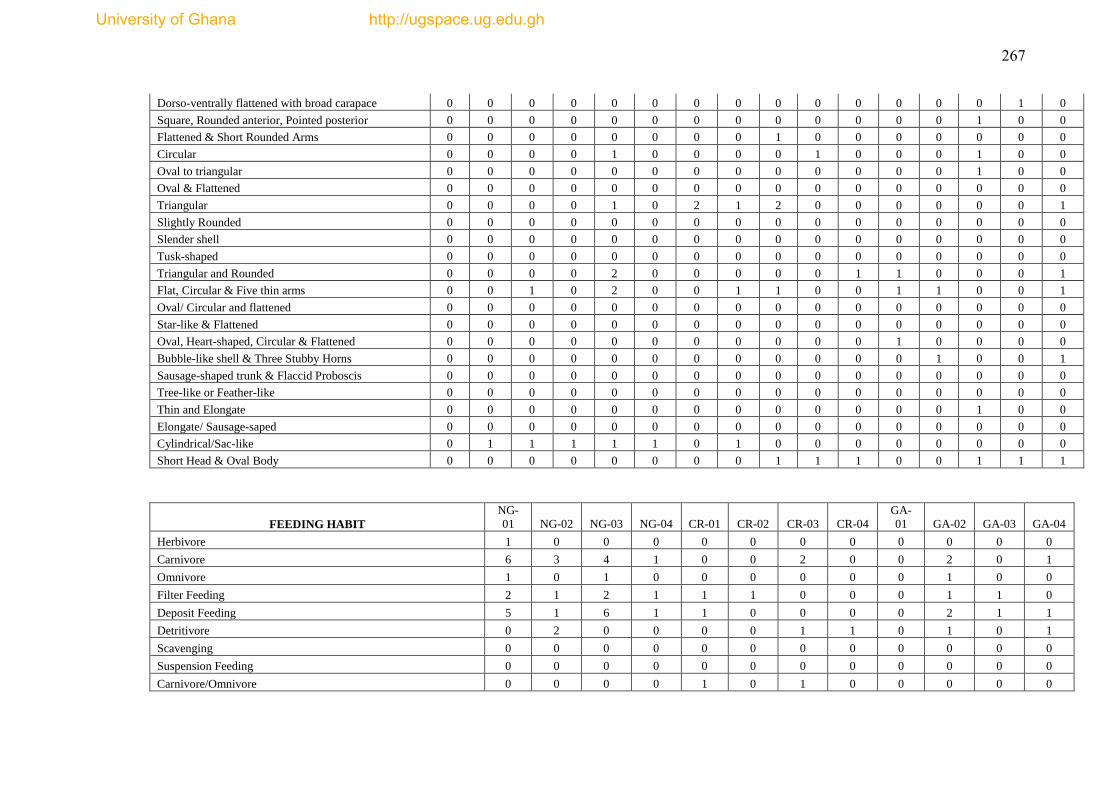
267
Dorso-ventrally flattened with broad carapace 0 0 0 0 0 0 0 0 0 0 0 0 0 0 1 0
Square, Rounded anterior, Pointed posterior 0 0 0 0 0 0 0 0 0 0 0 0 0 1 0 0
Flattened & Short Rounded Arms 0 0 0 0 0 0 0 0 1 0 0 0 0 0 0 0
Circular 0 0 0 0 1 0 0 0 0 1 0 0 0 1 0 0
Oval to triangular 0 0 0 0 0 0 0 0 0 0 0 0 0 1 0 0
Oval & Flattened 0 0 0 0 0 0 0 0 0 0 0 0 0 0 0 0
Triangular 0 0 0 0 1 0 2 1 2 0 0 0 0 0 0 1
Slightly Rounded 0 0 0 0 0 0 0 0 0 0 0 0 0 0 0 0
Slender shell 0 0 0 0 0 0 0 0 0 0 0 0 0 0 0 0
Tusk-shaped 0 0 0 0 0 0 0 0 0 0 0 0 0 0 0 0
Triangular and Rounded 0 0 0 0 2 0 0 0 0 0 1 1 0 0 0 1
Flat, Circular & Five thin arms 0 0 1 0 2 0 0 1 1 0 0 1 1 0 0 1
Oval/ Circular and flattened 0 0 0 0 0 0 0 0 0 0 0 0 0 0 0 0
Star-like & Flattened 0 0 0 0 0 0 0 0 0 0 0 0 0 0 0 0
Oval, Heart-shaped, Circular & Flattened 0 0 0 0 0 0 0 0 0 0 0 1 0 0 0 0
Bubble-like shell & Three Stubby Horns 0 0 0 0 0 0 0 0 0 0 0 0 1 0 0 1
Sausage-shaped trunk & Flaccid Proboscis 0 0 0 0 0 0 0 0 0 0 0 0 0 0 0 0
Tree-like or Feather-like 0 0 0 0 0 0 0 0 0 0 0 0 0 0 0 0
Thin and Elongate 0 0 0 0 0 0 0 0 0 0 0 0 0 1 0 0
Elongate/ Sausage-saped 0 0 0 0 0 0 0 0 0 0 0 0 0 0 0 0
Cylindrical/Sac-like 0 1 1 1 1 1 0 1 0 0 0 0 0 0 0 0
Short Head & Oval Body 0 0 0 0 0 0 0 0 1 1 1 0 0 1 1 1
FEEDING HABIT
NG-
01 NG-02 NG-03 NG-04 CR-01 CR-02 CR-03 CR-04
GA-
01 GA-02 GA-03 GA-04
Herbivore 1 0 0 0 0 0 0 0 0 0 0 0
Carnivore 6 3 4 1 0 0 2 0 0 2 0 1
Omnivore 1 0 1 0 0 0 0 0 0 1 0 0
Filter Feeding 2 1 2 1 1 1 0 0 0 1 1 0
Deposit Feeding 5 1 6 1 1 0 0 0 0 2 1 1
Detritivore 0 2 0 0 0 0 1 1 0 1 0 1
Scavenging 0 0 0 0 0 0 0 0 0 0 0 0
Suspension Feeding 0 0 0 0 0 0 0 0 0 0 0 0
Carnivore/Omnivore 0 0 0 0 1 0 1 0 0 0 0 0
University of Ghana http://ugspace.ug.edu.gh

268
Herbivore/Omnivore 0 0 0 0 0 0 0 0 0 1 0 0
Carnivore/Detritivore 2 1 0 0 1 0 1 1 0 0 0 0
Detritivore/Deposit Feeding 0 1 1 0 0 0 0 0 0 0 0 1
Carnivore/Deposit Feeding 0 0 0 0 0 0 0 1 0 0 0 0
Carnivore/Predator 0 0 0 0 0 0 0 1 0 0 0 0
Omnivore/Detritivore 1 1 1 0 1 0 0 0 0 0 0 0
Detritivore/Filter Feeding 1 1 1 0 0 0 0 0 0 0 0 0
Detritivore/Scavenging 0 0 0 0 0 1 1 0 0 0 0 0
Herbivore/Scavenging 0 0 0 0 0 0 0 0 0 0 0 0
Herbivore/Detrivore 2 1 1 0 0 0 0 0 0 0 0 0
Carnivore/Scavenging 0 0 0 0 0 0 1 0 0 1 0 0
Scavenging/Commensal 0 0 0 0 0 0 0 0 0 0 0 0
Carnivore/Blood Sucking 0 0 0 0 0 0 0 0 0 0 0 0
Deposit Feeding/Filter Feeding 0 0 0 0 0 0 0 0 0 0 0 0
Deposit Feeding/Surface Feeding 0 0 0 0 0 0 0 0 0 0 0 0
Deposit Feeding/Suspension Feeding 0 0 0 0 0 1 1 1 1 1 0 0
Autotroph/Carnivore/Filter Feeding 1 0 0 0 0 0 0 0 0 0 0 0
Omnivore/Filter Feeding/Deposit Feeding 1 0 0 0 0 0 0 0 0 0 0 0
FEEDING STRUCTURE
NG-
01 NG-02 NG-03 NG-04 CR-01 CR-02 CR-03 CR-04
GA-
01 GA-02 GA-03 GA-04
Tentacles 1 1 4 0 0 0 0 0 0 0 0 0
Buccal tentacles 0 0 1 0 0 0 0 0 0 0 0 0
Maxillipeds 0 0 0 0 0 0 0 0 0 0 0 0
Proboscis/Papillose 2 1 0 0 0 0 1 0 0 0 0 0
Jaws 0 0 0 0 0 0 0 1 0 0 0 0
Proboscis 0 0 0 0 1 0 0 0 0 1 0 1
Papillose 0 1 1 0 0 0 0 0 0 0 0 1
Feeding palps/Tentacular cirri 0 0 0 0 0 0 0 0 0 0 0 0
Mandibles/Maxillae/Jaws 4 2 2 0 1 0 0 1 0 1 0 0
Pharynx 0 0 0 0 0 0 1 0 0 0 0 0
Pharynx/ Feeding palps 2 0 0 0 0 0 0 0 0 0 1 0
Pharynges/Papillose 4 2 2 1 1 0 2 1 0 0 0 0
Papillose Proboscis/Macrognath 0 0 0 0 0 0 0 0 0 0 0 0
University of Ghana http://ugspace.ug.edu.gh
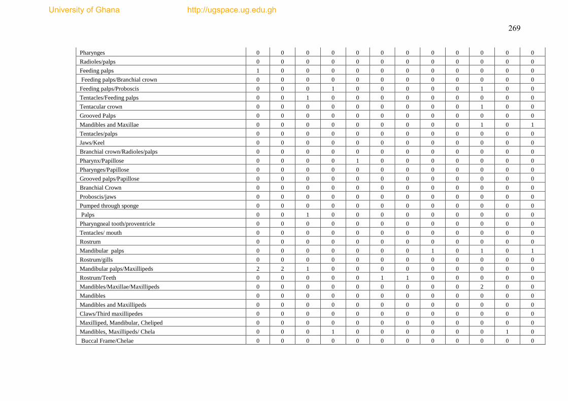
269
Pharynges 0 0 0 0 0 0 0 0 0 0 0 0
Radioles/palps 0 0 0 0 0 0 0 0 0 0 0 0
Feeding palps 1 0 0 0 0 0 0 0 0 0 0 0
Feeding palps/Branchial crown 0 0 0 0 0 0 0 0 0 0 0 0
Feeding palps/Proboscis 0 0 0 1 0 0 0 0 0 1 0 0
Tentacles/Feeding palps 0 0 1 0 0 0 0 0 0 0 0 0
Tentacular crown 0 0 0 0 0 0 0 0 0 1 0 0
Grooved Palps 0 0 0 0 0 0 0 0 0 0 0 0
Mandibles and Maxillae 0 0 0 0 0 0 0 0 0 1 0 1
Tentacles/palps 0 0 0 0 0 0 0 0 0 0 0 0
Jaws/Keel 0 0 0 0 0 0 0 0 0 0 0 0
Branchial crown/Radioles/palps 0 0 0 0 0 0 0 0 0 0 0 0
Pharynx/Papillose 0 0 0 0 1 0 0 0 0 0 0 0
Pharynges/Papillose 0 0 0 0 0 0 0 0 0 0 0 0
Grooved palps/Papillose 0 0 0 0 0 0 0 0 0 0 0 0
Branchial Crown 0 0 0 0 0 0 0 0 0 0 0 0
Proboscis/jaws 0 0 0 0 0 0 0 0 0 0 0 0
Pumped through sponge 0 0 0 0 0 0 0 0 0 0 0 0
Palps 0 0 1 0 0 0 0 0 0 0 0 0
Pharyngneal tooth/proventricle 0 0 0 0 0 0 0 0 0 0 0 0
Tentacles/ mouth 0 0 0 0 0 0 0 0 0 0 0 0
Rostrum 0 0 0 0 0 0 0 0 0 0 0 0
Mandibular palps 0 0 0 0 0 0 0 1 0 1 0 1
Rostrum/gills 0 0 0 0 0 0 0 0 0 0 0 0
Mandibular palps/Maxillipeds 2 2 1 0 0 0 0 0 0 0 0 0
Rostrum/Teeth 0 0 0 0 0 1 1 0 0 0 0 0
Mandibles/Maxillae/Maxillipeds 0 0 0 0 0 0 0 0 0 2 0 0
Mandibles 0 0 0 0 0 0 0 0 0 0 0 0
Mandibles and Maxillipeds 0 0 0 0 0 0 0 0 0 0 0 0
Claws/Third maxillipedes 0 0 0 0 0 0 0 0 0 0 0 0
Maxilliped, Mandibular, Cheliped 0 0 0 0 0 0 0 0 0 0 0 0
Mandibles, Maxillipeds/ Chela 0 0 0 1 0 0 0 0 0 0 1 0
Buccal Frame/Chelae 0 0 0 0 0 0 0 0 0 0 0 0
University of Ghana http://ugspace.ug.edu.gh

270
Siphon/Gills 1 0 1 0 1 0 0 0 0 0 0 0
Tube feet/ Stomach 0 0 0 0 0 0 0 0 0 0 0 0
Radula 2 1 0 0 0 0 0 0 0 0 0 0
Tentacles/Captacula 1 0 1 0 0 0 0 0 0 0 0 0
Tentacles/Feeding chamber 0 0 0 0 0 1 0 0 0 0 0 0
Tube feet 0 0 0 0 0 0 1 0 0 0 0 0
Aristotle's lantern 0 0 0 0 0 0 0 0 0 0 0 0
Aristotle's lantern/Tube feet 1 0 1 0 0 0 0 0 0 0 0 0
Gastrozooid/Tentacles 0 0 0 0 0 0 0 0 0 0 0 0
Proboscis/suckers 0 0 0 0 0 0 0 0 0 0 0 0
Gastrozooid 0 0 0 0 0 0 1 0 0 0 0 0
Proboscis/mouth 0 0 0 0 0 0 1 0 0 1 0 0
Introvert/tentacles 0 0 0 0 0 1 0 1 1 1 0 0
Ostia/Pinacocytes 1 0 0 0 0 0 0 0 0 0 0 0
Beak/radula/tentacles 0 0 1 0 0 0 0 0 0 0 0 0
Mouth 0 0 0 0 0 0 0 0 0 0 0 0
Tube feet/Toothed jaw 0 0 0 0 0 0 0 0 0 0 0 0
Mandibles/maxillipedes 0 0 0 0 0 0 0 0 0 0 0 0
Tentacles/Pharynx/Siphonoglyph 0 1 0 0 0 0 0 0 0 0 0 0
RELATIVE ADULT MOBILITY
NG-
01 NG-02 NG-03 NG-04 CR-01 CR-02 CR-03 CR-04
GA-
01 GA-02 GA-03 GA-04
Peristaltic crawling 0 0 1 0 0 0 0 0 0 0 0 0
Burrowing/Sessile 2 0 1 0 0 0 0 0 0 0 0 0
Burrowing 14 8 10 3 5 1 4 4 1 4 2 2
Creeping 1 1 2 0 0 0 0 0 0 0 0 0
Crawling 0 1 0 0 0 0 1 0 0 0 0 0
Sessile 2 1 0 0 0 0 1 0 0 1 0 0
Sessile/Creep 0 0 0 0 0 0 0 0 0 0 0 0
Burrow/Creep 3 0 2 0 0 1 0 0 0 0 0 0
Tube-dwelling 0 0 1 0 0 0 0 0 0 0 0 0
Creep/Tube-dwelling 0 0 0 0 0 0 0 0 0 0 0 0
Burrow/Swim 0 0 0 0 0 0 0 0 0 2 0 1
Creep/Crawl 0 0 0 0 0 0 0 0 0 0 0 0
University of Ghana http://ugspace.ug.edu.gh

271
Swim 1 1 0 0 0 1 1 1 0 1 0 1
Crawl/Burrow 0 0 0 0 0 0 0 0 0 0 0 0
Crawl/Burrow/Swim 0 0 0 0 0 0 0 0 0 0 0 0
Run/Burrow 0 0 0 0 0 0 0 0 0 1 0 0
Wiggle 0 0 0 0 0 0 0 0 0 0 0 0
Glide/Crawl/Swim 0 0 0 0 0 0 1 0 0 1 0 0
SOCIABILITY
NG-
01 NG-02 NG-03 NG-04 CR-01 CR-02 CR-03 CR-04
GA-
01 GA-02 GA-03 GA-04
Solitary 18 9 15 3 5 3 7 4 1 10 2 4
Commensal 3 1 1 0 0 0 0 0 0 0 0 0
Commensal/Solitary 1 0 0 0 0 0 0 1 0 0 0 0
Solitary/Colony 0 1 1 0 0 0 1 0 0 0 0 0
Colony 1 1 0 0 0 0 0 0 0 0 0 0
ADULT BODY SIZE
NG-
01 NG-02 NG-03 NG-04 CR-01 CR-02 CR-03 CR-04
GA-
01 GA-02 GA-03 GA-04
0.5-20mm 2 3 3 1 0 0 1 1 0 3 1 3
20.5-40mm 5 1 1 1 1 1 1 1 0 2 0 1
40.5-60mm 2 2 5 0 2 1 2 2 0 2 1 0
60.5-80mm 6 3 3 0 1 0 0 0 0 0 0 0
80.5-100mm 3 1 1 0 0 0 1 0 0 0 0 0
100.5-120mm 1 1 0 1 0 0 1 0 0 1 0 0
>120mm 2 1 3 0 1 1 2 1 1 2 0 0
ADULT BODY FORM
NG-
01 NG-02 NG-03 NG-04 CR-01 CR-02 CR-03 CR-04
GA-
01 GA-02 GA-03 GA-04
Vermiform and Flattened 1 0 2 0 1 0 0 0 0 0 0 0
Slender and Elongate 4 1 1 0 0 0 0 0 0 0 0 0
Slender 0 0 0 1 0 0 1 0 0 1 0 0
Trefoil-shaped 0 0 0 0 0 0 0 0 0 0 0 0
oval 0 0 0 0 0 0 0 0 0 0 0 0
Cylindrical & Tapered Posterior 1 0 2 0 0 0 0 0 0 0 0 0
Elongate 2 0 0 0 0 0 0 0 0 0 0 0
Vermiform & Iridescent 0 0 0 0 0 0 0 0 0 0 0 0
Vermiform and Tapering 0 0 0 0 0 0 0 0 0 0 0 1
Long and Round 0 0 0 0 0 0 0 0 0 0 0 0
Cylindrical 0 0 0 0 0 0 0 0 0 0 0 0
University of Ghana http://ugspace.ug.edu.gh
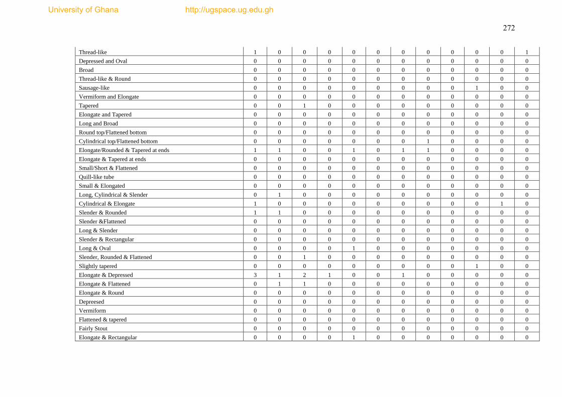
272
Thread-like 1 0 0 0 0 0 0 0 0 0 0 1
Depressed and Oval 0 0 0 0 0 0 0 0 0 0 0 0
Broad 0 0 0 0 0 0 0 0 0 0 0 0
Thread-like & Round 0 0 0 0 0 0 0 0 0 0 0 0
Sausage-like 0 0 0 0 0 0 0 0 0 1 0 0
Vermiform and Elongate 0 0 0 0 0 0 0 0 0 0 0 0
Tapered 0 0 1 0 0 0 0 0 0 0 0 0
Elongate and Tapered 0 0 0 0 0 0 0 0 0 0 0 0
Long and Broad 0 0 0 0 0 0 0 0 0 0 0 0
Round top/Flattened bottom 0 0 0 0 0 0 0 0 0 0 0 0
Cylindrical top/Flattened bottom 0 0 0 0 0 0 0 1 0 0 0 0
Elongate/Rounded & Tapered at ends 1 1 0 0 1 0 1 1 0 0 0 0
Elongate & Tapered at ends 0 0 0 0 0 0 0 0 0 0 0 0
Small/Short & Flattened 0 0 0 0 0 0 0 0 0 0 0 0
Quill-like tube 0 0 0 0 0 0 0 0 0 0 0 0
Small & Elongated 0 0 0 0 0 0 0 0 0 0 0 0
Long, Cylindrical & Slender 0 1 0 0 0 0 0 0 0 0 0 0
Cylindrical & Elongate 1 0 0 0 0 0 0 0 0 0 1 0
Slender & Rounded 1 1 0 0 0 0 0 0 0 0 0 0
Slender &Flattened 0 0 0 0 0 0 0 0 0 0 0 0
Long & Slender 0 0 0 0 0 0 0 0 0 0 0 0
Slender & Rectangular 0 0 0 0 0 0 0 0 0 0 0 0
Long & Oval 0 0 0 0 1 0 0 0 0 0 0 0
Slender, Rounded & Flattened 0 0 1 0 0 0 0 0 0 0 0 0
Slightly tapered 0 0 0 0 0 0 0 0 0 1 0 0
Elongate & Depressed 3 1 2 1 0 0 1 0 0 0 0 0
Elongate & Flattened 0 1 1 0 0 0 0 0 0 0 0 0
Elongate & Round 0 0 0 0 0 0 0 0 0 0 0 0
Depreesed 0 0 0 0 0 0 0 0 0 0 0 0
Vermiform 0 0 0 0 0 0 0 0 0 0 0 0
Flattened & tapered 0 0 0 0 0 0 0 0 0 0 0 0
Fairly Stout 0 0 0 0 0 0 0 0 0 0 0 0
Elongate & Rectangular 0 0 0 0 1 0 0 0 0 0 0 0
University of Ghana http://ugspace.ug.edu.gh
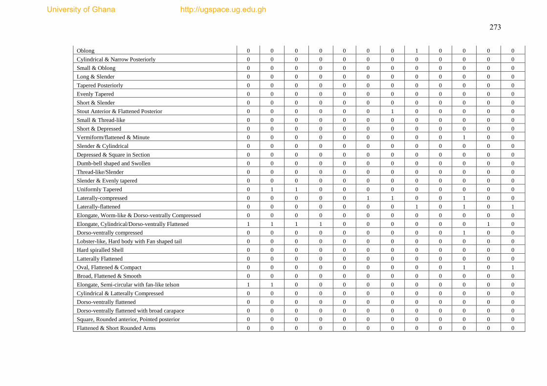
273
Oblong 0 0 0 0 0 0 0 1 0 0 0 0
Cylindrical & Narrow Posteriorly 0 0 0 0 0 0 0 0 0 0 0 0
Small & Oblong 0 0 0 0 0 0 0 0 0 0 0 0
Long & Slender 0 0 0 0 0 0 0 0 0 0 0 0
Tapered Posteriorly 0 0 0 0 0 0 0 0 0 0 0 0
Evenly Tapered 0 0 0 0 0 0 0 0 0 0 0 0
Short & Slender 0 0 0 0 0 0 0 0 0 0 0 0
Stout Anterior & Flattened Posterior 0 0 0 0 0 0 1 0 0 0 0 0
Small & Thread-like 0 0 0 0 0 0 0 0 0 0 0 0
Short & Depressed 0 0 0 0 0 0 0 0 0 0 0 0
Vermiform/flattened & Minute 0 0 0 0 0 0 0 0 0 1 0 0
Slender & Cylindrical 0 0 0 0 0 0 0 0 0 0 0 0
Depressed & Square in Section 0 0 0 0 0 0 0 0 0 0 0 0
Dumb-bell shaped and Swollen 0 0 0 0 0 0 0 0 0 0 0 0
Thread-like/Slender 0 0 0 0 0 0 0 0 0 0 0 0
Slender & Evenly tapered 0 0 0 0 0 0 0 0 0 0 0 0
Uniformly Tapered 0 1 1 0 0 0 0 0 0 0 0 0
Laterally-compressed 0 0 0 0 0 1 1 0 0 1 0 0
Laterally-flattened 0 0 0 0 0 0 0 1 0 1 0 1
Elongate, Worm-like & Dorso-ventrally Compressed 0 0 0 0 0 0 0 0 0 0 0 0
Elongate, Cylindrical/Dorso-ventrally Flattened 1 1 1 1 0 0 0 0 0 0 1 0
Dorso-ventrally compressed 0 0 0 0 0 0 0 0 0 1 0 0
Lobster-like, Hard body with Fan shaped tail 0 0 0 0 0 0 0 0 0 0 0 0
Hard spiralled Shell 0 0 0 0 0 0 0 0 0 0 0 0
Latterally Flattened 0 0 0 0 0 0 0 0 0 0 0 0
Oval, Flattened & Compact 0 0 0 0 0 0 0 0 0 1 0 1
Broad, Flattened & Smooth 0 0 0 0 0 0 0 0 0 0 0 0
Elongate, Semi-circular with fan-like telson 1 1 0 0 0 0 0 0 0 0 0 0
Cylindrical & Latterally Compressed 0 0 0 0 0 0 0 0 0 0 0 0
Dorso-ventrally flattened 0 0 0 0 0 0 0 0 0 0 0 0
Dorso-ventrally flattened with broad carapace 0 0 0 0 0 0 0 0 0 0 0 0
Square, Rounded anterior, Pointed posterior 0 0 0 0 0 0 0 0 0 0 0 0
Flattened & Short Rounded Arms 0 0 0 0 0 0 0 0 0 0 0 0
University of Ghana http://ugspace.ug.edu.gh
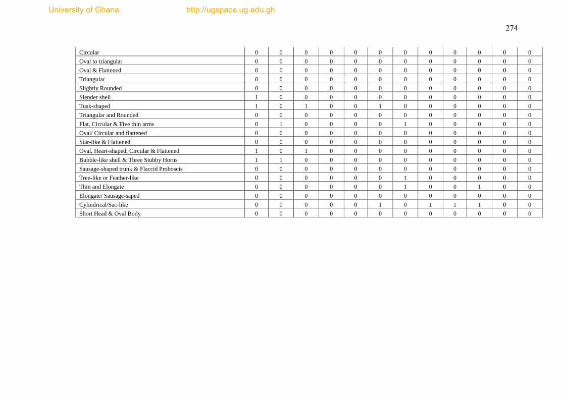
274
Circular 0 0 0 0 0 0 0 0 0 0 0 0
Oval to triangular 0 0 0 0 0 0 0 0 0 0 0 0
Oval & Flattened 0 0 0 0 0 0 0 0 0 0 0 0
Triangular 0 0 0 0 0 0 0 0 0 0 0 0
Slightly Rounded 0 0 0 0 0 0 0 0 0 0 0 0
Slender shell 1 0 0 0 0 0 0 0 0 0 0 0
Tusk-shaped 1 0 1 0 0 1 0 0 0 0 0 0
Triangular and Rounded 0 0 0 0 0 0 0 0 0 0 0 0
Flat, Circular & Five thin arms 0 1 0 0 0 0 1 0 0 0 0 0
Oval/ Circular and flattened 0 0 0 0 0 0 0 0 0 0 0 0
Star-like & Flattened 0 0 0 0 0 0 0 0 0 0 0 0
Oval, Heart-shaped, Circular & Flattened 1 0 1 0 0 0 0 0 0 0 0 0
Bubble-like shell & Three Stubby Horns 1 1 0 0 0 0 0 0 0 0 0 0
Sausage-shaped trunk & Flaccid Proboscis 0 0 0 0 0 0 0 0 0 0 0 0
Tree-like or Feather-like 0 0 0 0 0 0 1 0 0 0 0 0
Thin and Elongate 0 0 0 0 0 0 1 0 0 1 0 0
Elongate/ Sausage-saped 0 0 0 0 0 0 0 0 0 0 0 0
Cylindrical/Sac-like 0 0 0 0 0 1 0 1 1 1 0 0
Short Head & Oval Body 0 0 0 0 0 0 0 0 0 0 0 0
University of Ghana http://ugspace.ug.edu.gh
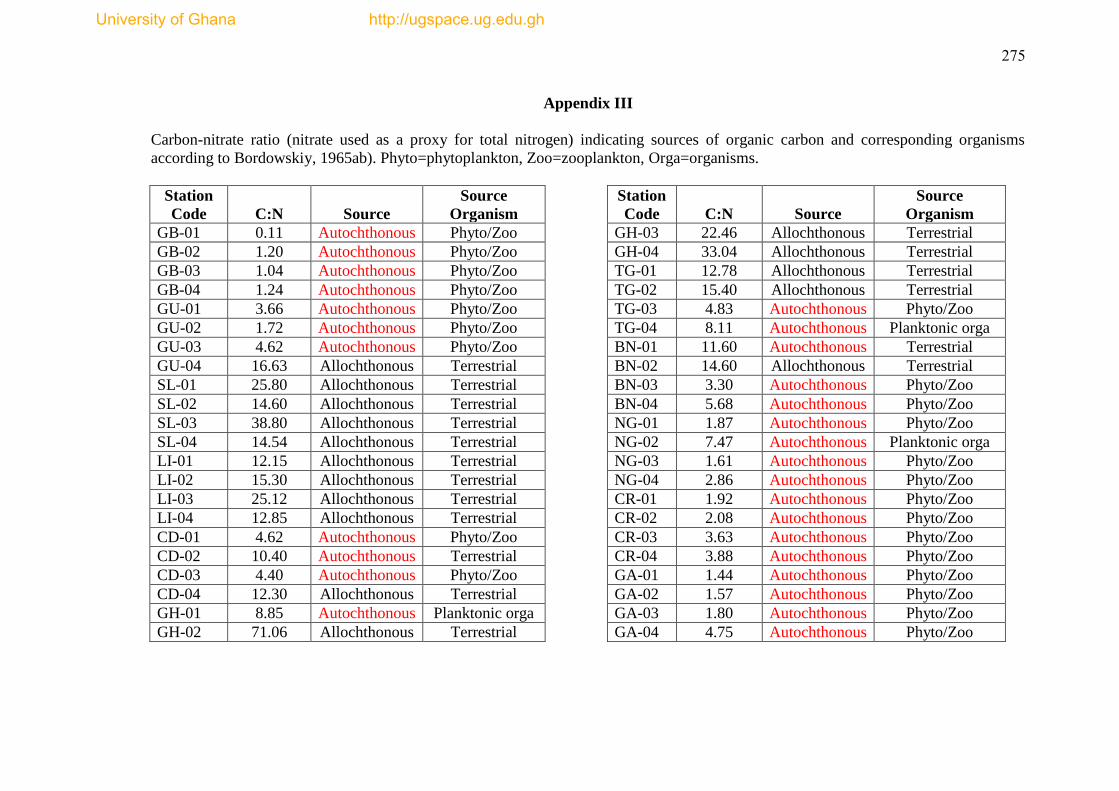
275
Appendix III
Carbon-nitrate ratio (nitrate used as a proxy for total nitrogen) indicating sources of organic carbon and corresponding organisms
according to Bordowskiy, 1965ab). Phyto=phytoplankton, Zoo=zooplankton, Orga=organisms.
Station
Code C:N Source
Source
Organism
Station
Code C:N Source
Source
Organism
GB-01 0.11 Autochthonous Phyto/Zoo
GH-03 22.46 Allochthonous Terrestrial
GB-02 1.20 Autochthonous Phyto/Zoo
GH-04 33.04 Allochthonous Terrestrial
GB-03 1.04 Autochthonous Phyto/Zoo
TG-01 12.78 Allochthonous Terrestrial
GB-04 1.24 Autochthonous Phyto/Zoo
TG-02 15.40 Allochthonous Terrestrial
GU-01 3.66 Autochthonous Phyto/Zoo
TG-03 4.83 Autochthonous Phyto/Zoo
GU-02 1.72 Autochthonous Phyto/Zoo
TG-04 8.11 Autochthonous Planktonic orga
GU-03 4.62 Autochthonous Phyto/Zoo
BN-01 11.60 Autochthonous Terrestrial
GU-04 16.63 Allochthonous Terrestrial
BN-02 14.60 Allochthonous Terrestrial
SL-01 25.80 Allochthonous Terrestrial
BN-03 3.30 Autochthonous Phyto/Zoo
SL-02 14.60 Allochthonous Terrestrial
BN-04 5.68 Autochthonous Phyto/Zoo
SL-03 38.80 Allochthonous Terrestrial
NG-01 1.87 Autochthonous Phyto/Zoo
SL-04 14.54 Allochthonous Terrestrial
NG-02 7.47 Autochthonous Planktonic orga
LI-01 12.15 Allochthonous Terrestrial
NG-03 1.61 Autochthonous Phyto/Zoo
LI-02 15.30 Allochthonous Terrestrial
NG-04 2.86 Autochthonous Phyto/Zoo
LI-03 25.12 Allochthonous Terrestrial
CR-01 1.92 Autochthonous Phyto/Zoo
LI-04 12.85 Allochthonous Terrestrial
CR-02 2.08 Autochthonous Phyto/Zoo
CD-01 4.62 Autochthonous Phyto/Zoo
CR-03 3.63 Autochthonous Phyto/Zoo
CD-02 10.40 Autochthonous Terrestrial
CR-04 3.88 Autochthonous Phyto/Zoo
CD-03 4.40 Autochthonous Phyto/Zoo
GA-01 1.44 Autochthonous Phyto/Zoo
CD-04 12.30 Allochthonous Terrestrial
GA-02 1.57 Autochthonous Phyto/Zoo
GH-01 8.85 Autochthonous Planktonic orga
GA-03 1.80 Autochthonous Phyto/Zoo
GH-02 71.06 Allochthonous Terrestrial
GA-04 4.75 Autochthonous Phyto/Zoo
University of Ghana http://ugspace.ug.edu.gh
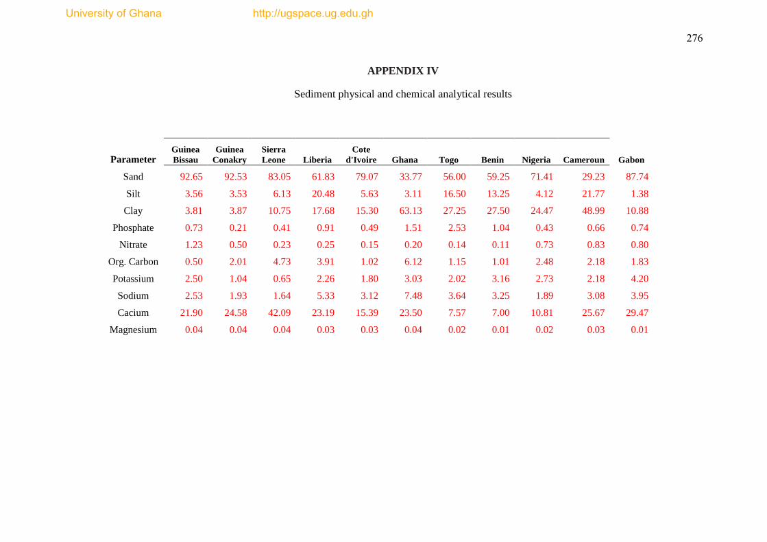
276
APPENDIX IV
Sediment physical and chemical analytical results
Parameter Guinea
Bissau
Guinea
Conakry
Sierra
Leone Liberia
Cote
d'Ivoire Ghana Togo Benin Nigeria Cameroun Gabon
Sand 92.65 92.53 83.05 61.83 79.07 33.77 56.00 59.25 71.41 29.23 87.74
Silt 3.56 3.53 6.13 20.48 5.63 3.11 16.50 13.25 4.12 21.77 1.38
Clay 3.81 3.87 10.75 17.68 15.30 63.13 27.25 27.50 24.47 48.99 10.88
Phosphate 0.73 0.21 0.41 0.91 0.49 1.51 2.53 1.04 0.43 0.66 0.74
Nitrate 1.23 0.50 0.23 0.25 0.15 0.20 0.14 0.11 0.73 0.83 0.80
Org. Carbon 0.50 2.01 4.73 3.91 1.02 6.12 1.15 1.01 2.48 2.18 1.83
Potassium 2.50 1.04 0.65 2.26 1.80 3.03 2.02 3.16 2.73 2.18 4.20
Sodium 2.53 1.93 1.64 5.33 3.12 7.48 3.64 3.25 1.89 3.08 3.95
Cacium 21.90 24.58 42.09 23.19 15.39 23.50 7.57 7.00 10.81 25.67 29.47
Magnesium 0.04 0.04 0.04 0.03 0.03 0.04 0.02 0.01 0.02 0.03 0.01
University of Ghana http://ugspace.ug.edu.gh

277
APPENDIX V
Water depth of sampling locations
Station Code Country Depth (m)
GB-01 Guinea Bissau 53.0
GB-02 Guinea Bissau 125.0
GB-03 Guinea Bissau 153.0
GB-04 Guinea Bissau 28.0
GU-01 Guinea 26.0
GU-02 Guinea 94.0
GU-03 Guinea 43.0
GU-04 Guinea 27.0
SL-01 Sierra Leone 52.0
SL-02 Sierra Leone 34.0
SL-03 Sierra Leone 27.0
SL-04 Sierra Leone 49.0
LI-01 Liberia 34.0
LI-02 Liberia 54.0
LI-03 Liberia 54.0
LI-04 Liberia 24.0
CD-01 Cote d‘Ivoire 63.0
CD-02 Cote d‘Ivoire 102.0
CD-03 Cote d‘Ivoire 49.0
CD-04 Cote d‘Ivoire 24.0
GH-01 Ghana 100.0
GH-02 Ghana 76.0
GH-03 Ghana 60.0
GH04 Ghana 29.0
TG-01 Togo 59.0
TG-02 Togo 20.0
TG-03 Togo 35.0
TG-04 Togo 17.0
BN-01 Benin 28.0
BN-02 Benin 18.0
BN-03 Benin 16.0
BN-04 Benin 23.0
NG-01 Nigeria 87.0
NG-02 Nigeria 37.0
NG-03 Nigeria 67.9
NG-04 Nigeria 41.0
University of Ghana http://ugspace.ug.edu.gh

278
CR-01 Cameroon 64.0
CR-02 Cameroon 22.0
CR-03 Cameroon 98.0
CR-04 Cameroon 22.0
GA-01 Gabon 101.0
GA-02 Gabon 111.0
GA-03 Gabon 55.0
GA-04 Gabon 104.0
University of Ghana http://ugspace.ug.edu.gh
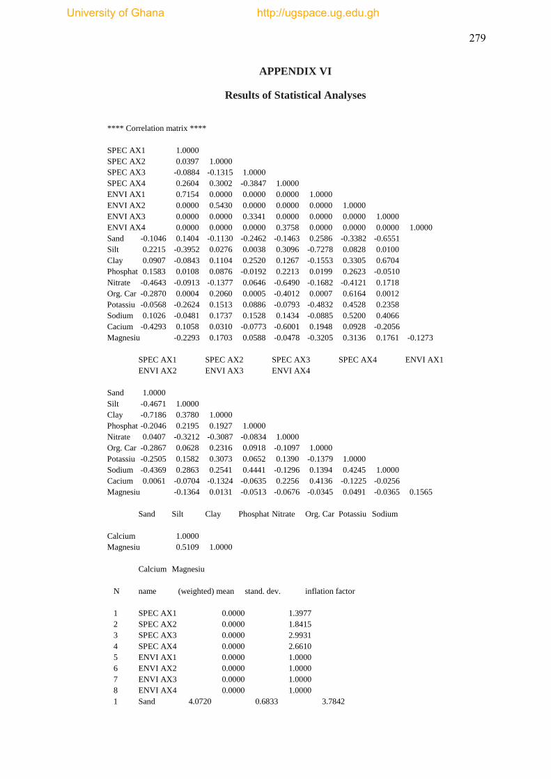
279
APPENDIX VI
Results of Statistical Analyses
**** Correlation matrix ****
SPEC AX1 1.0000
SPEC AX2 0.0397 1.0000
SPEC AX3 -0.0884 -0.1315 1.0000
SPEC AX4 0.2604 0.3002 -0.3847 1.0000
ENVI AX1 0.7154 0.0000 0.0000 0.0000 1.0000
ENVI AX2 0.0000 0.5430 0.0000 0.0000 0.0000 1.0000
ENVI AX3 0.0000 0.0000 0.3341 0.0000 0.0000 0.0000 1.0000
ENVI AX4 0.0000 0.0000 0.0000 0.3758 0.0000 0.0000 0.0000 1.0000
Sand -0.1046 0.1404 -0.1130 -0.2462 -0.1463 0.2586 -0.3382 -0.6551
Silt 0.2215 -0.3952 0.0276 0.0038 0.3096 -0.7278 0.0828 0.0100
Clay 0.0907 -0.0843 0.1104 0.2520 0.1267 -0.1553 0.3305 0.6704
Phosphat 0.1583 0.0108 0.0876 -0.0192 0.2213 0.0199 0.2623 -0.0510
Nitrate -0.4643 -0.0913 -0.1377 0.0646 -0.6490 -0.1682 -0.4121 0.1718
Org. Car -0.2870 0.0004 0.2060 0.0005 -0.4012 0.0007 0.6164 0.0012
Potassiu -0.0568 -0.2624 0.1513 0.0886 -0.0793 -0.4832 0.4528 0.2358
Sodium 0.1026 -0.0481 0.1737 0.1528 0.1434 -0.0885 0.5200 0.4066
Cacium -0.4293 0.1058 0.0310 -0.0773 -0.6001 0.1948 0.0928 -0.2056
Magnesiu -0.2293 0.1703 0.0588 -0.0478 -0.3205 0.3136 0.1761 -0.1273
SPEC AX1 SPEC AX2 SPEC AX3 SPEC AX4 ENVI AX1
ENVI AX2 ENVI AX3 ENVI AX4
Sand 1.0000
Silt -0.4671 1.0000
Clay -0.7186 0.3780 1.0000
Phosphat -0.2046 0.2195 0.1927 1.0000
Nitrate 0.0407 -0.3212 -0.3087 -0.0834 1.0000
Org. Car -0.2867 0.0628 0.2316 0.0918 -0.1097 1.0000
Potassiu -0.2505 0.1582 0.3073 0.0652 0.1390 -0.1379 1.0000
Sodium -0.4369 0.2863 0.2541 0.4441 -0.1296 0.1394 0.4245 1.0000
Cacium 0.0061 -0.0704 -0.1324 -0.0635 0.2256 0.4136 -0.1225 -0.0256
Magnesiu -0.1364 0.0131 -0.0513 -0.0676 -0.0345 0.0491 -0.0365 0.1565
Sand Silt Clay Phosphat Nitrate Org. Car Potassiu Sodium
Calcium 1.0000
Magnesiu 0.5109 1.0000
Calcium Magnesiu
N name (weighted) mean stand. dev. inflation factor
1 SPEC AX1 0.0000 1.3977
2 SPEC AX2 0.0000 1.8415
3 SPEC AX3 0.0000 2.9931
4 SPEC AX4 0.0000 2.6610
5 ENVI AX1 0.0000 1.0000
6 ENVI AX2 0.0000 1.0000
7 ENVI AX3 0.0000 1.0000
8 ENVI AX4 0.0000 1.0000
1 Sand 4.0720 0.6833 3.7842
University of Ghana http://ugspace.ug.edu.gh
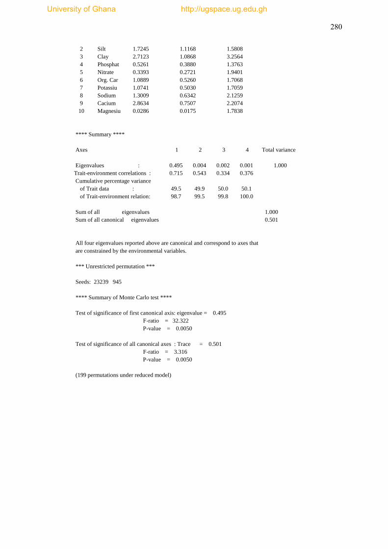
280
2 Silt 1.7245 1.1168 1.5808
3 Clay 2.7123 1.0868 3.2564
4 Phosphat 0.5261 0.3880 1.3763
5 Nitrate 0.3393 0.2721 1.9401
6 Org. Car 1.0889 0.5260 1.7068
7 Potassiu 1.0741 0.5030 1.7059
8 Sodium 1.3009 0.6342 2.1259
9 Cacium 2.8634 0.7507 2.2074
10 Magnesiu 0.0286 0.0175 1.7838
**** Summary ****
Axes 1 2 3 4 Total variance
Eigenvalues : 0.495 0.004 0.002 0.001 1.000
Trait-environment correlations : 0.715 0.543 0.334 0.376
Cumulative percentage variance
of Trait data : 49.5 49.9 50.0 50.1
of Trait-environment relation: 98.7 99.5 99.8 100.0
Sum of all eigenvalues 1.000
Sum of all canonical eigenvalues 0.501
All four eigenvalues reported above are canonical and correspond to axes that
are constrained by the environmental variables.
*** Unrestricted permutation ***
Seeds: 23239 945
**** Summary of Monte Carlo test ****
Test of significance of first canonical axis: eigenvalue = 0.495
F-ratio = 32.322
P-value = 0.0050
Test of significance of all canonical axes : Trace = 0.501
F-ratio = 3.316
P-value = 0.0050
(199 permutations under reduced model)
University of Ghana http://ugspace.ug.edu.gh

281
Canonical Correspondence Analysis
Program CANOCO Version 4.54 October 2005 - written by Cajo J.F. Ter Braak
(C) 1988-2005 Biometris - quantitative methods in the life and earth sciences
Plant Research International, Wageningen University and Research Centre
Box 100, 6700 AC Wageningen, the Netherlands
CANOCO performs (partial) (detrended) (canonical) correspondence analysis,
principal components analysis and redundancy analysis.
CANOCO is an extension of Cornell Ecology program DECORANA (Hill,1979)
For explanation of the input/output see the manual or
Ter Braak, C.J.F. (1995) Ordination. Chapter 5 in:
Data Analysis in Community and Landscape Ecology
(Jongman, R.H.G., Ter Braak, C.J.F. and Van Tongeren, O.F.R., Eds)
Cambridge University Press, Cambridge, UK, 91-173 pp.
*** Type of analysis ***
Model Gradient analysis
indirect direct hybrid
linear 1=PCA 2= RDA 3
unimodal 4= CA 5= CCA 6
,, 7=DCA 8=DCCA 9
10=non-standard analysis
Type analysis number
Answer = 5
*** Data files ***
Species data : C:\Users\user 1\Desktop\Functional Traits_Infauna\BioAbunDOm
Covariable data :
Environmental data : C:\Users\user 1\Desktop\Functional Traits_Infauna\EnvDataTrasformed
Initialization file:
Forward selection of envi. variables = 1
Scaling of ordination scores = 2
Diagnostics = 3
File : C:\Users\user 1\Desktop\Functional Traits_Infauna\BioAbunDOm
Title : WCanoImp produced data file
Format : (I5,1X,10F4.0)
No. of couplets of species number and abundance per line : 0
No samples omitted
Number of samples 44
Number of species 10
Number of occurrences 150
File : C:\Users\user 1\Desktop\Functional Traits_Infauna\EnvDataTrasformed
Title : WCanoImp produced data file
Format : (I5,1X,10F6.2)
No. of environmental variables : 10
No interaction terms defined
University of Ghana http://ugspace.ug.edu.gh
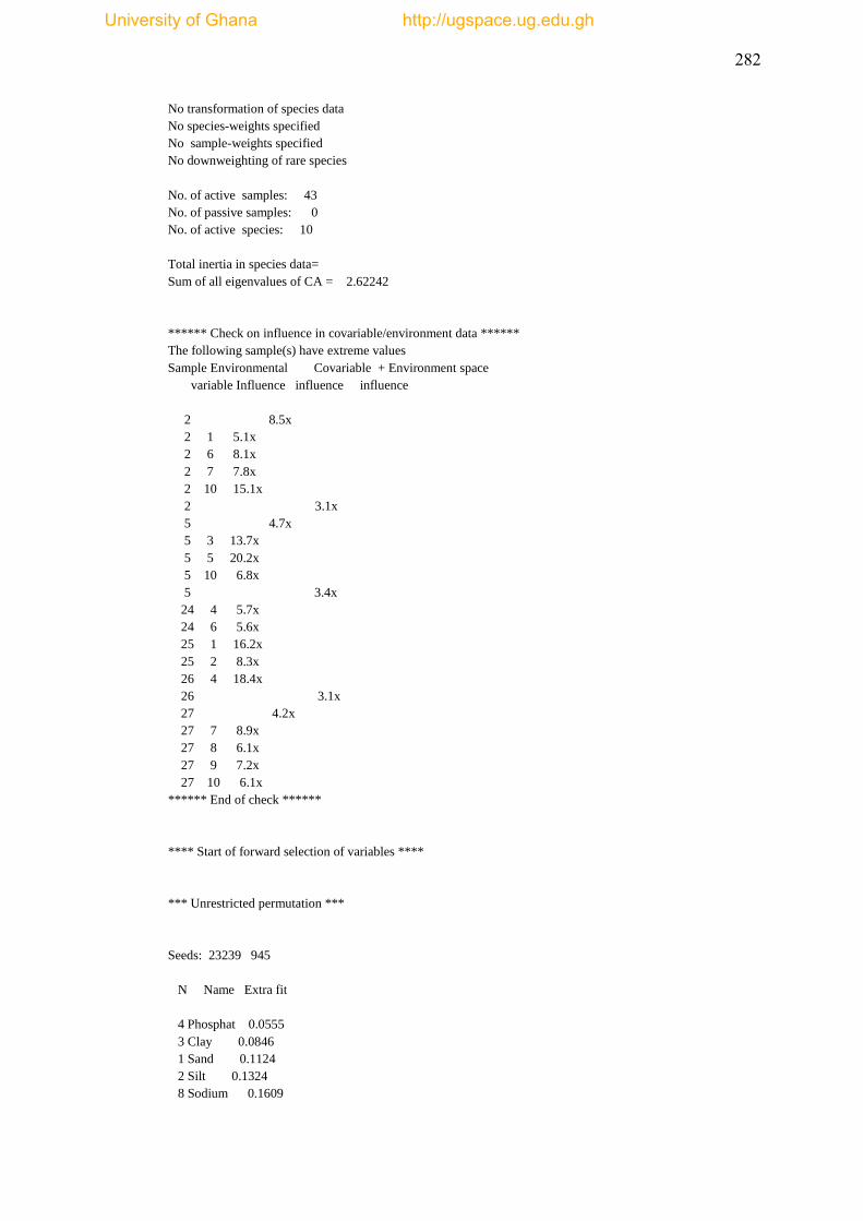
282
No transformation of species data
No species-weights specified
No sample-weights specified
No downweighting of rare species
No. of active samples: 43
No. of passive samples: 0
No. of active species: 10
Total inertia in species data=
Sum of all eigenvalues of CA = 2.62242
****** Check on influence in covariable/environment data ******
The following sample(s) have extreme values
Sample Environmental Covariable + Environment space
variable Influence influence influence
2 8.5x
2 1 5.1x
2 6 8.1x
2 7 7.8x
2 10 15.1x
2 3.1x
5 4.7x
5 3 13.7x
5 5 20.2x
5 10 6.8x
5 3.4x
24 4 5.7x
24 6 5.6x
25 1 16.2x
25 2 8.3x
26 4 18.4x
26 3.1x
27 4.2x
27 7 8.9x
27 8 6.1x
27 9 7.2x
27 10 6.1x
****** End of check ******
**** Start of forward selection of variables ****
*** Unrestricted permutation ***
Seeds: 23239 945
N Name Extra fit
4 Phosphat 0.0555
3 Clay 0.0846
1 Sand 0.1124
2 Silt 0.1324
8 Sodium 0.1609
University of Ghana http://ugspace.ug.edu.gh
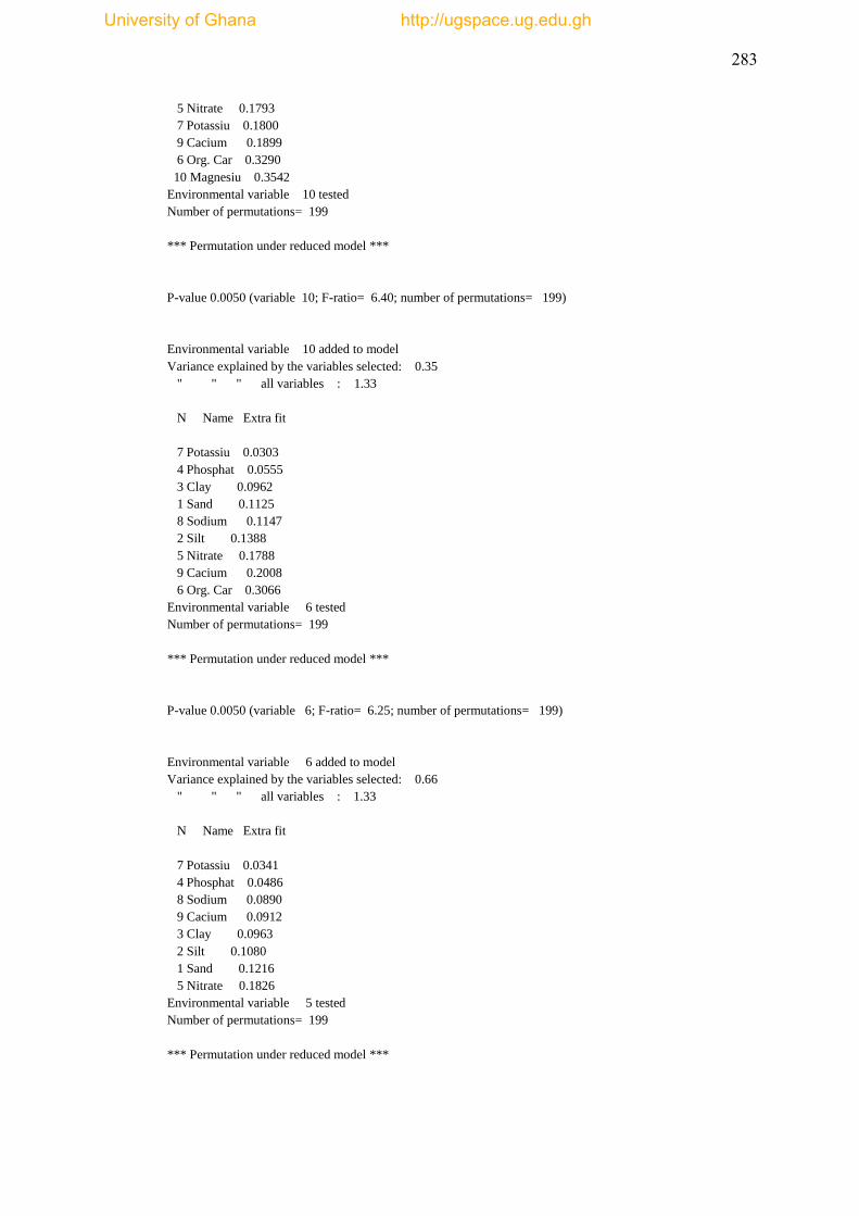
283
5 Nitrate 0.1793
7 Potassiu 0.1800
9 Cacium 0.1899
6 Org. Car 0.3290
10 Magnesiu 0.3542
Environmental variable 10 tested
Number of permutations= 199
*** Permutation under reduced model ***
P-value 0.0050 (variable 10; F-ratio= 6.40; number of permutations= 199)
Environmental variable 10 added to model
Variance explained by the variables selected: 0.35
" " " all variables : 1.33
N Name Extra fit
7 Potassiu 0.0303
4 Phosphat 0.0555
3 Clay 0.0962
1 Sand 0.1125
8 Sodium 0.1147
2 Silt 0.1388
5 Nitrate 0.1788
9 Cacium 0.2008
6 Org. Car 0.3066
Environmental variable 6 tested
Number of permutations= 199
*** Permutation under reduced model ***
P-value 0.0050 (variable 6; F-ratio= 6.25; number of permutations= 199)
Environmental variable 6 added to model
Variance explained by the variables selected: 0.66
" " " all variables : 1.33
N Name Extra fit
7 Potassiu 0.0341
4 Phosphat 0.0486
8 Sodium 0.0890
9 Cacium 0.0912
3 Clay 0.0963
2 Silt 0.1080
1 Sand 0.1216
5 Nitrate 0.1826
Environmental variable 5 tested
Number of permutations= 199
*** Permutation under reduced model ***
University of Ghana http://ugspace.ug.edu.gh
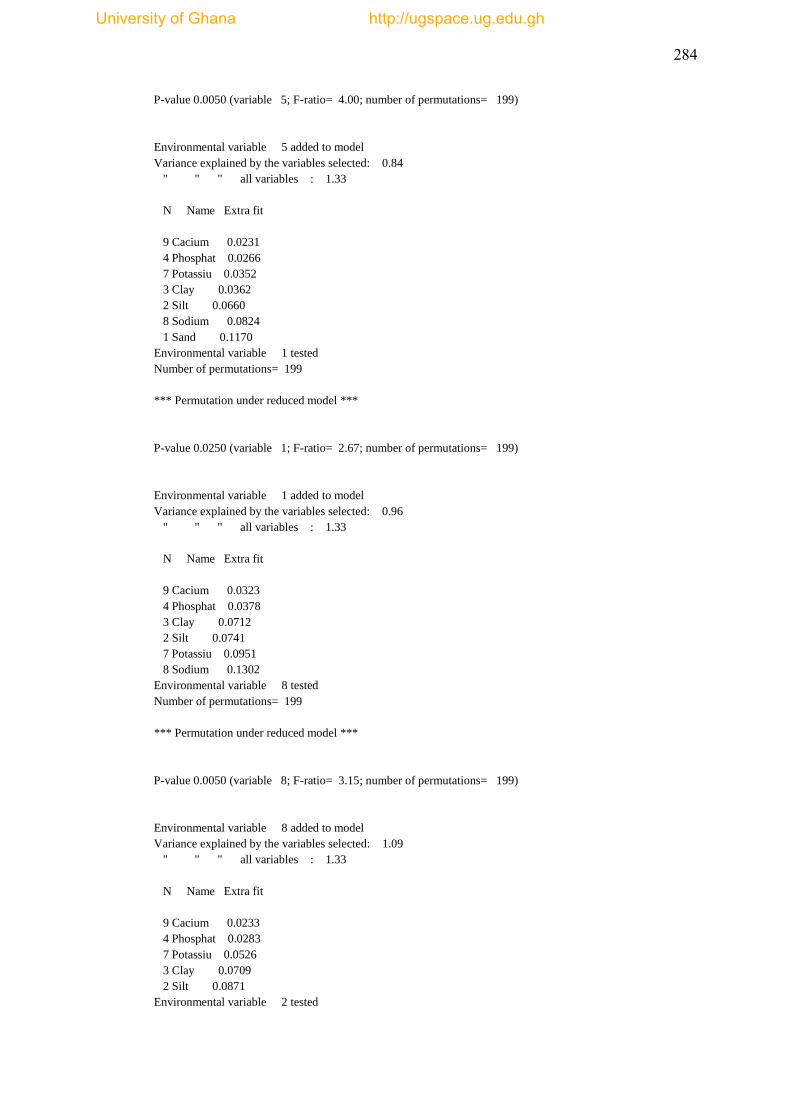
284
P-value 0.0050 (variable 5; F-ratio= 4.00; number of permutations= 199)
Environmental variable 5 added to model
Variance explained by the variables selected: 0.84
" " " all variables : 1.33
N Name Extra fit
9 Cacium 0.0231
4 Phosphat 0.0266
7 Potassiu 0.0352
3 Clay 0.0362
2 Silt 0.0660
8 Sodium 0.0824
1 Sand 0.1170
Environmental variable 1 tested
Number of permutations= 199
*** Permutation under reduced model ***
P-value 0.0250 (variable 1; F-ratio= 2.67; number of permutations= 199)
Environmental variable 1 added to model
Variance explained by the variables selected: 0.96
" " " all variables : 1.33
N Name Extra fit
9 Cacium 0.0323
4 Phosphat 0.0378
3 Clay 0.0712
2 Silt 0.0741
7 Potassiu 0.0951
8 Sodium 0.1302
Environmental variable 8 tested
Number of permutations= 199
*** Permutation under reduced model ***
P-value 0.0050 (variable 8; F-ratio= 3.15; number of permutations= 199)
Environmental variable 8 added to model
Variance explained by the variables selected: 1.09
" " " all variables : 1.33
N Name Extra fit
9 Cacium 0.0233
4 Phosphat 0.0283
7 Potassiu 0.0526
3 Clay 0.0709
2 Silt 0.0871
Environmental variable 2 tested
University of Ghana http://ugspace.ug.edu.gh

285
Number of permutations= 199
*** Permutation under reduced model ***
P-value 0.0150 (variable 2; F-ratio= 2.17; number of permutations= 199)
Environmental variable 2 added to model
Variance explained by the variables selected: 1.18
" " " all variables : 1.33
N Name Extra fit
4 Phosphat 0.0127
9 Cacium 0.0233
7 Potassiu 0.0533
3 Clay 0.0718
Environmental variable 3 tested
Number of permutations= 199
*** Permutation under reduced model ***
P-value 0.0700 (variable 3; F-ratio= 1.83; number of permutations= 199)
Environmental variable 3 added to model
Variance explained by the variables selected: 1.25
" " " all variables : 1.33
N Name Extra fit
4 Phosphat 0.0189
9 Cacium 0.0252
7 Potassiu 0.0439
Environmental variable 7 tested
Number of permutations= 199
*** Permutation under reduced model ***
P-value 0.3750 (variable 7; F-ratio= 1.12; number of permutations= 199)
Environmental variable 7 added to model
Variance explained by the variables selected: 1.29
" " " all variables : 1.33
N Name Extra fit
4 Phosphat 0.0148
9 Cacium 0.0201
Environmental variable 9 tested
Number of permutations= 199
*** Permutation under reduced model ***
University of Ghana http://ugspace.ug.edu.gh
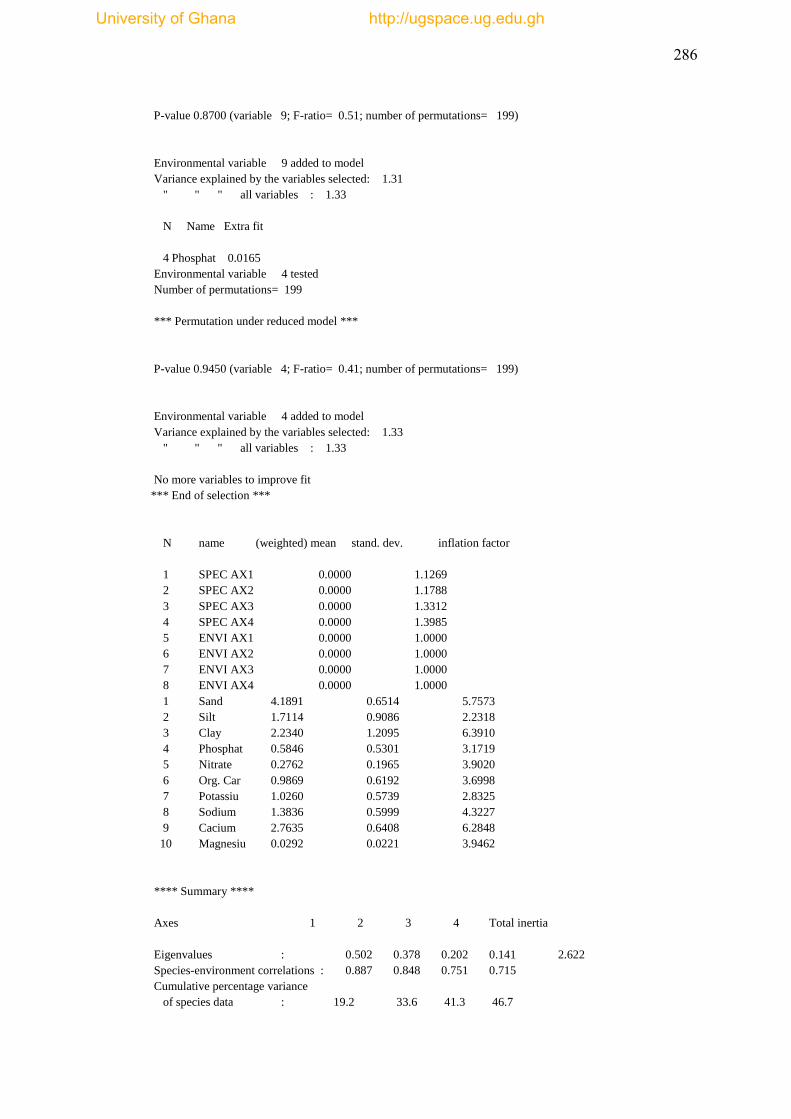
286
P-value 0.8700 (variable 9; F-ratio= 0.51; number of permutations= 199)
Environmental variable 9 added to model
Variance explained by the variables selected: 1.31
" " " all variables : 1.33
N Name Extra fit
4 Phosphat 0.0165
Environmental variable 4 tested
Number of permutations= 199
*** Permutation under reduced model ***
P-value 0.9450 (variable 4; F-ratio= 0.41; number of permutations= 199)
Environmental variable 4 added to model
Variance explained by the variables selected: 1.33
" " " all variables : 1.33
No more variables to improve fit
*** End of selection ***
N name (weighted) mean stand. dev. inflation factor
1 SPEC AX1 0.0000 1.1269
2 SPEC AX2 0.0000 1.1788
3 SPEC AX3 0.0000 1.3312
4 SPEC AX4 0.0000 1.3985
5 ENVI AX1 0.0000 1.0000
6 ENVI AX2 0.0000 1.0000
7 ENVI AX3 0.0000 1.0000
8 ENVI AX4 0.0000 1.0000
1 Sand 4.1891 0.6514 5.7573
2 Silt 1.7114 0.9086 2.2318
3 Clay 2.2340 1.2095 6.3910
4 Phosphat 0.5846 0.5301 3.1719
5 Nitrate 0.2762 0.1965 3.9020
6 Org. Car 0.9869 0.6192 3.6998
7 Potassiu 1.0260 0.5739 2.8325
8 Sodium 1.3836 0.5999 4.3227
9 Cacium 2.7635 0.6408 6.2848
10 Magnesiu 0.0292 0.0221 3.9462
**** Summary ****
Axes 1 2 3 4 Total inertia
Eigenvalues : 0.502 0.378 0.202 0.141 2.622
Species-environment correlations : 0.887 0.848 0.751 0.715
Cumulative percentage variance
of species data : 19.2 33.6 41.3 46.7
University of Ghana http://ugspace.ug.edu.gh
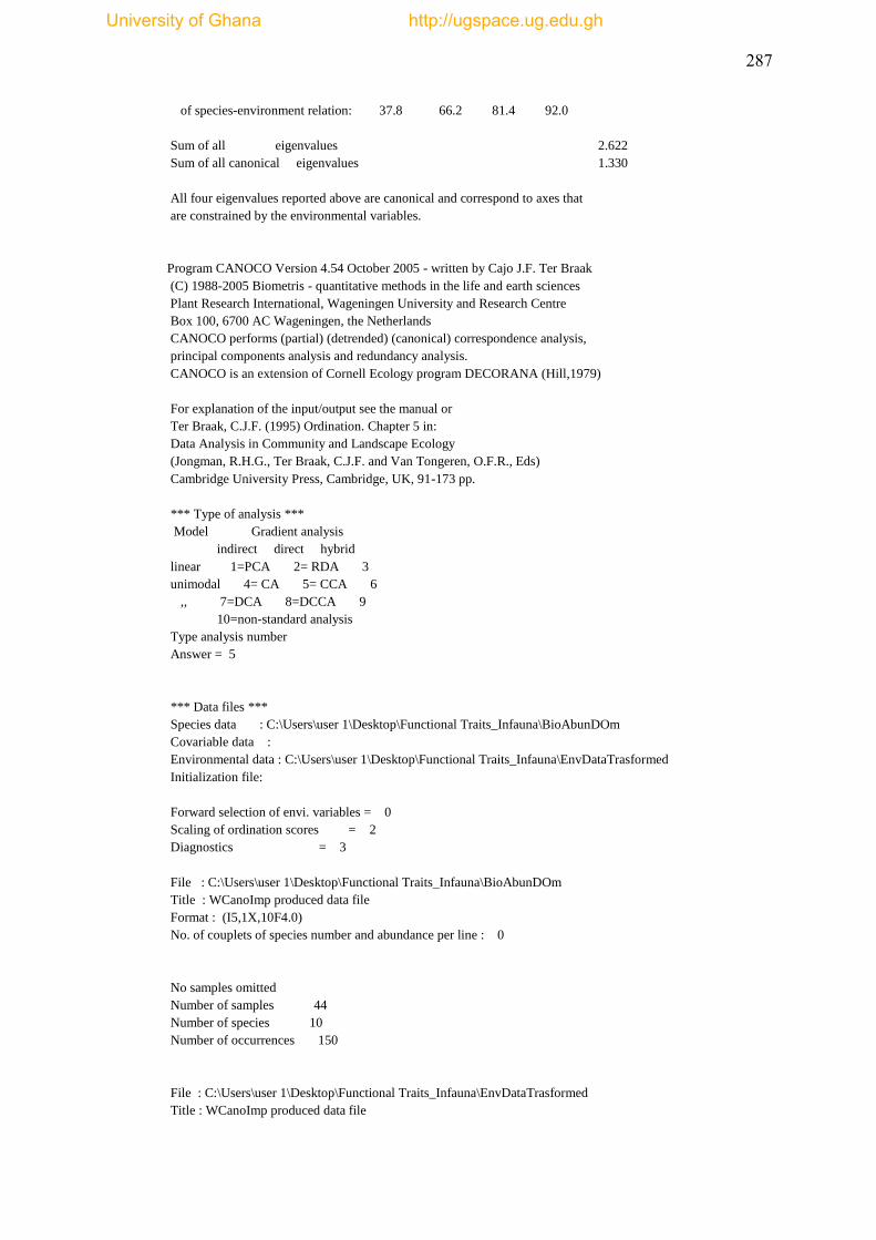
287
of species-environment relation: 37.8 66.2 81.4 92.0
Sum of all eigenvalues 2.622
Sum of all canonical eigenvalues 1.330
All four eigenvalues reported above are canonical and correspond to axes that
are constrained by the environmental variables.
Program CANOCO Version 4.54 October 2005 - written by Cajo J.F. Ter Braak
(C) 1988-2005 Biometris - quantitative methods in the life and earth sciences
Plant Research International, Wageningen University and Research Centre
Box 100, 6700 AC Wageningen, the Netherlands
CANOCO performs (partial) (detrended) (canonical) correspondence analysis,
principal components analysis and redundancy analysis.
CANOCO is an extension of Cornell Ecology program DECORANA (Hill,1979)
For explanation of the input/output see the manual or
Ter Braak, C.J.F. (1995) Ordination. Chapter 5 in:
Data Analysis in Community and Landscape Ecology
(Jongman, R.H.G., Ter Braak, C.J.F. and Van Tongeren, O.F.R., Eds)
Cambridge University Press, Cambridge, UK, 91-173 pp.
*** Type of analysis ***
Model Gradient analysis
indirect direct hybrid
linear 1=PCA 2= RDA 3
unimodal 4= CA 5= CCA 6
,, 7=DCA 8=DCCA 9
10=non-standard analysis
Type analysis number
Answer = 5
*** Data files ***
Species data : C:\Users\user 1\Desktop\Functional Traits_Infauna\BioAbunDOm
Covariable data :
Environmental data : C:\Users\user 1\Desktop\Functional Traits_Infauna\EnvDataTrasformed
Initialization file:
Forward selection of envi. variables = 0
Scaling of ordination scores = 2
Diagnostics = 3
File : C:\Users\user 1\Desktop\Functional Traits_Infauna\BioAbunDOm
Title : WCanoImp produced data file
Format : (I5,1X,10F4.0)
No. of couplets of species number and abundance per line : 0
No samples omitted
Number of samples 44
Number of species 10
Number of occurrences 150
File : C:\Users\user 1\Desktop\Functional Traits_Infauna\EnvDataTrasformed
Title : WCanoImp produced data file
University of Ghana http://ugspace.ug.edu.gh
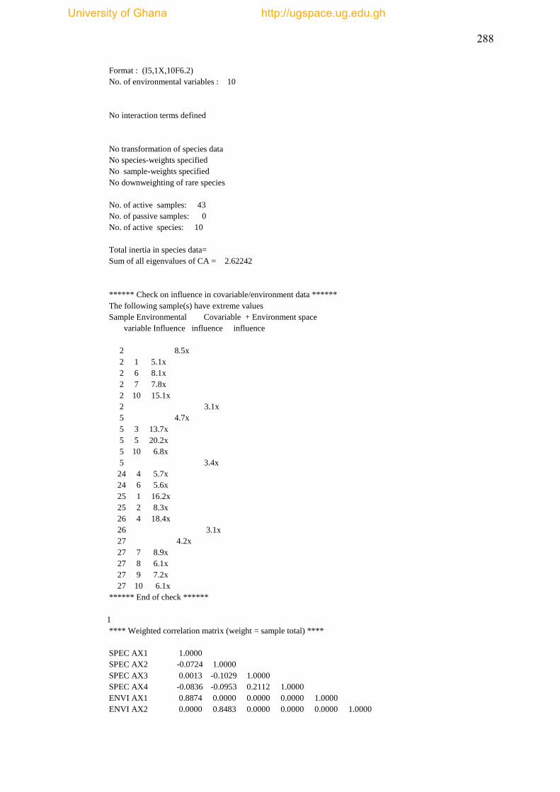
288
Format : (I5,1X,10F6.2)
No. of environmental variables : 10
No interaction terms defined
No transformation of species data
No species-weights specified
No sample-weights specified
No downweighting of rare species
No. of active samples: 43
No. of passive samples: 0
No. of active species: 10
Total inertia in species data=
Sum of all eigenvalues of CA = 2.62242
****** Check on influence in covariable/environment data ******
The following sample(s) have extreme values
Sample Environmental Covariable + Environment space
variable Influence influence influence
2 8.5x
2 1 5.1x
2 6 8.1x
2 7 7.8x
2 10 15.1x
2 3.1x
5 4.7x
5 3 13.7x
5 5 20.2x
5 10 6.8x
5 3.4x
24 4 5.7x
24 6 5.6x
25 1 16.2x
25 2 8.3x
26 4 18.4x
26 3.1x
27 4.2x
27 7 8.9x
27 8 6.1x
27 9 7.2x
27 10 6.1x
****** End of check ******
1
**** Weighted correlation matrix (weight = sample total) ****
SPEC AX1 1.0000
SPEC AX2 -0.0724 1.0000
SPEC AX3 0.0013 -0.1029 1.0000
SPEC AX4 -0.0836 -0.0953 0.2112 1.0000
ENVI AX1 0.8874 0.0000 0.0000 0.0000 1.0000
ENVI AX2 0.0000 0.8483 0.0000 0.0000 0.0000 1.0000
University of Ghana http://ugspace.ug.edu.gh

289
ENVI AX3 0.0000 0.0000 0.7512 0.0000 0.0000 0.0000 1.0000
ENVI AX4 0.0000 0.0000 0.0000 0.7151 0.0000 0.0000 0.0000 1.0000
Sand 0.2289 0.1846 -0.0941 0.4429 0.2580 0.2176 -0.1253 0.6194
Silt 0.0386 -0.3665 -0.3735 -0.1228 0.0435 -0.4321 -0.4972 -0.1718
Clay -0.1690 -0.1322 -0.2686 -0.2799 -0.1905 -0.1559 -0.3576 -0.3914
Phosphat -0.0687 0.1560 -0.2377 -0.2141 -0.0774 0.1839 -0.3164 -0.2994
Nitrate 0.1353 0.1526 0.5922 0.3063 0.1525 0.1799 0.7883 0.4284
Org. Car -0.5006 0.5331 0.1823 -0.0446 -0.5641 0.6284 0.2427 -0.0624
Potassiu 0.4647 0.2475 -0.0949 -0.1157 0.5237 0.2918 -0.1263 -0.1618
Sodium 0.2304 0.3594 -0.0471 -0.4534 0.2597 0.4236 -0.0627 -0.6341
Cacium 0.1658 0.4644 0.3263 0.1389 0.1869 0.5474 0.4343 0.1942
Magnesiu 0.7038 0.2184 -0.0174 -0.0654 0.7931 0.2575 -0.0231 -0.0915
SPEC AX1 SPEC AX2 SPEC AX3 SPEC AX4 ENVI AX1
ENVI AX2 ENVI AX3 ENVI AX4
Sand 1.0000
Silt -0.5015 1.0000
Clay -0.7623 0.5064 1.0000
Phosphat -0.3234 0.4245 0.4265 1.0000
Nitrate 0.2746 -0.4072 -0.6518 -0.3158 1.0000
Org. Car -0.2197 -0.1818 -0.0173 0.2024 0.1984 1.0000
Potassiu -0.2797 0.3311 0.2699 0.0966 0.0202 -0.1134 1.0000
Sodium -0.4988 0.3289 0.3958 0.6086 -0.1137 0.2253 0.5769 1.0000
Calcium 0.1433 -0.2895 -0.3131 -0.1014 0.5123 0.5523 0.1636 0.2041
Magnesium -0.0005 0.0846 0.0622 -0.0003 0.0038 -0.0879 0.5539 0.4005
Sand Silt Clay Phosphat Nitrate Org. Car Potassiu Sodium
Cacium 1.0000
Magnesiu 0.5281 1.0000
Calcium Magnesiu
N name (weighted) mean stand. dev. inflation factor
1 SPEC AX1 0.0000 1.1269
2 SPEC AX2 0.0000 1.1788
3 SPEC AX3 0.0000 1.3312
4 SPEC AX4 0.0000 1.3985
5 ENVI AX1 0.0000 1.0000
6 ENVI AX2 0.0000 1.0000
7 ENVI AX3 0.0000 1.0000
8 ENVI AX4 0.0000 1.0000
1 Sand 4.1891 0.6514 5.7573
2 Silt 1.7114 0.9086 2.2318
3 Clay 2.2340 1.2095 6.3910
4 Phosphat 0.5846 0.5301 3.1719
5 Nitrate 0.2762 0.1965 3.9020
6 Org. Car 0.9869 0.6192 3.6998
7 Potassiu 1.0260 0.5739 2.8325
8 Sodium 1.3836 0.5999 4.3227
9 Calcium 2.7635 0.6408 6.2848
10 Magnesiu 0.0292 0.0221 3.9462
University of Ghana http://ugspace.ug.edu.gh
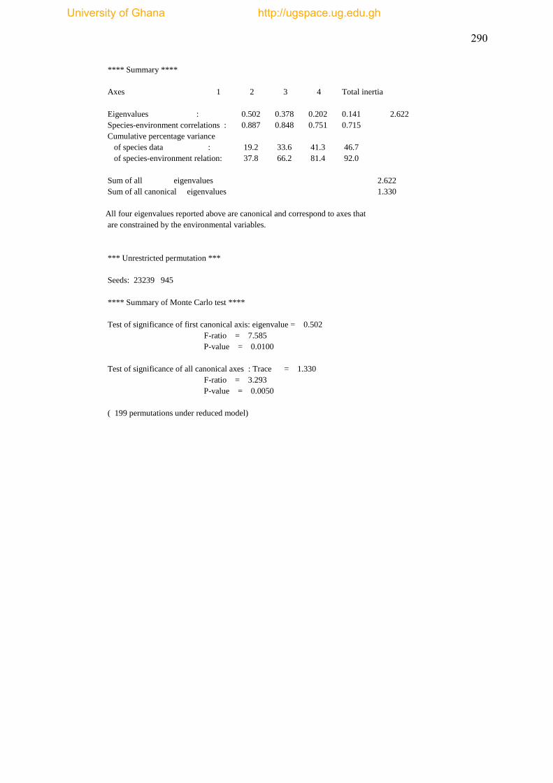
290
**** Summary ****
Axes 1 2 3 4 Total inertia
Eigenvalues : 0.502 0.378 0.202 0.141 2.622
Species-environment correlations : 0.887 0.848 0.751 0.715
Cumulative percentage variance
of species data : 19.2 33.6 41.3 46.7
of species-environment relation: 37.8 66.2 81.4 92.0
Sum of all eigenvalues 2.622
Sum of all canonical eigenvalues 1.330
All four eigenvalues reported above are canonical and correspond to axes that
are constrained by the environmental variables.
*** Unrestricted permutation ***
Seeds: 23239 945
**** Summary of Monte Carlo test ****
Test of significance of first canonical axis: eigenvalue = 0.502
F-ratio = 7.585
P-value = 0.0100
Test of significance of all canonical axes : Trace = 1.330
F-ratio = 3.293
P-value = 0.0050
( 199 permutations under reduced model)
University of Ghana http://ugspace.ug.edu.gh

291
Ampipod Capitellid sp.
Tanaid sp. Nepthys sp.
Tellina sp. Sipuncula sp. (Sipunculidae)
University of Ghana http://ugspace.ug.edu.gh

292
Glycera spp. (Glyceridae)
University of Ghana http://ugspace.ug.edu.gh

293
Marphysa sp. (Eunicidae)
University of Ghana http://ugspace.ug.edu.gh

294
Nepthys sp. (Nepthyidae)
Maldane sp.(Maldanidae)
University of Ghana http://ugspace.ug.edu.gh
Copyright © 2022 FDOKUMEN