aspects of modelling - The University of Brighton

ASPECTS OF MODELLING PERFORMANCE IN COMPETITIVE

CYCLING

PATRICK CANGLEY

A thesis submitted in partial fulfilment of the requirements of the University of Brighton for

the degree of Doctor of Philosophy

May 2012

The University of Brighton

2

ABSTRACT

The aim of this thesis was to design, construct and validate a model to be used for

enhancing the performance of competitive cyclists in road time trials. Modelling can be an

effective tool for identifying methods to enhance performance in sports with a high

mechanical component such as cycling. The thesis questioned whether an effective road

cycling model could be built. Existing models were analysed and found to have insufficient

predictive accuracy to make them effective under general time trial conditions. It was

hypothesised that an effective and generalised model could be developed.

A computer simulation model was constructed that extended the functionality of existing

models. The three-dimensional model combined the bicycle, rider and environment in a

single parameterised system which simulated road cycling at high frequency. Three model

components were validated against published benchmark studies. Firstly, a pedalling

model was compared to an experimental benchmark study. Modelled vertical pedal force

normalised root mean squared error (NRMSE) was 9.5% and horizontal pedal force

NRMSE was 8.8% when compared to the benchmark. Both these values were below the

10% error level which a literature analysis indicated as the limit for validity. Modelled

crank torque NRMSE was 4.9% and the modelled crank torque profile matched the

benchmark profile with an R2 value of 0.974. A literature analysis indicated R2>0.95 was

required for validity. Secondly, bicycle self-stability was evaluated against a benchmark

model by comparing the eigenvalues for weave and capsize mode. Weave mode error level

of 9.3% was less than the 10% error considered the upper limit for validity. Capsize mode

error could not be evaluated as the modelled profile did not cross zero. Thirdly, modelled

rear tyre cornering stiffness was qualitatively compared with the results of an experimental

study. The experimental study reported mean cornering stiffness of 60N/deg at 3 degrees

slip angle, 10 degrees camber and 330N vertical load. This compared well with a model

simulation which generated mean cornering stiffness of 62N/deg at 3 degrees slip angle, 4

degrees camber and 338N load.

Experimental validation comprised a field case study and a controlled field time trial using

14 experienced cyclists. In the former study, modelled completion time was 1% less than

actual time. In the latter study, model prediction over a 4 km time trial course was found to

be within 1.4±1.5 % of the actual time (p=0.008).

The validated model was used to test potential performance enhancement strategies. A

strategy of power variation in response to gradient changes had been previously proposed,

3

but never experimentally confirmed. The thesis model predicted a 4% time advantage for a

variable power strategy compared to a constant power strategy. This was confirmed

experimentally in field trials when 20 cyclists obtained a significant (p<0.001) time

advantage of 2.9±1.9 %. The model also predicted a 1.2% time advantage if power was

varied in head/tail wind conditions on an out-and-back time trial course. A 2% time

advantage was obtained in field trials but was not statistically significant (p=0.06).

A final investigation examined the sensitivity of model prediction to variances in

assumptions and initial conditions. An important sensitivity was the aerodynamic

coefficient which could cause time differences of up to 6%. Tyre forces were also found to

be a critical factor in the accuracy of model prediction.

The thesis investigation confirmed the hypothesis that an effective and generalised model

could be built and used to predict performance in road time trials.

4

CONTENTS

Abstract ..................................................................................... 2

List of Figures............................................................................ 7

List of Tables ............................................................................. 10

Preface, Acknowledgements and Declaration .......................... 12

Chapter 1 Rationale and Literature Review

1.1 Introduction................................................................................. 13

1.2 Rationale ..................................................................................... 14

1.3 Literature Review........................................................................ 23

1.4 Conclusions................................................................................. 44

Chapter 2 Model Design

2.1 Introduction................................................................................. 45

2.2 Modelling Software..................................................................... 46

2.3 Bicycle Model ............................................................................. 52

2.4 Rider Model ................................................................................ 58

2.5 Environment Modelling............................................................... 64

2.6 Summary..................................................................................... 68

Chapter 3 Pedalling Validation

3.1 Introduction................................................................................. 69

3.2 Validity Definition ...................................................................... 70

3.3 Methods ...................................................................................... 73

3.4 Results ........................................................................................ 76

3.5 Discussion................................................................................... 80

Chapter 4 Bicycle Stability Validation

4.1 Introduction................................................................................. 87

4.2 Methods ...................................................................................... 88

4.3 Results ........................................................................................ 90

4.4 Discussion................................................................................... 94

5

Chapter 5 The Tyre Model

5.1 Introduction................................................................................. 97

5.2 Methods ...................................................................................... 100

5.3 Results ........................................................................................ 103

5.4 Discussion................................................................................... 108

Chapter 6 Field Validation - Case Study

6.1 Introduction................................................................................. 112

6.2 Methods ...................................................................................... 112

6.3 Results ........................................................................................ 116

6.4 Discussion................................................................................... 118

Chapter 7 Field Validation – Controlled Trials

7.1 Introduction................................................................................. 122

7.2 Methods ...................................................................................... 122

7.3 Results ........................................................................................ 125

7.4 Discussion................................................................................... 126

Chapter 8 Performance Enhancement - Gradient

8.1 Introduction................................................................................. 128

8.2 Methods ...................................................................................... 129

8.3 Results ........................................................................................ 133

8.4 Discussion................................................................................... 135

Chapter 9 Performance Enhancement - Wind

9.1 Introduction................................................................................. 140

9.2 Methods ...................................................................................... 141

9.3 Results ........................................................................................ 145

9.4 Discussion................................................................................... 147

Chapter 10 Sensitivity Analysis

10.1 Introduction................................................................................. 150

10.2 Methods ...................................................................................... 150

10.3 Results ........................................................................................ 152

10.4 Discussion................................................................................... 156

Chapter 11 Summary, Limitations, Future Research and Conclusion

11.1 Summary..................................................................................... 160

11.2 Limitations .................................................................................. 162

11.3 Future Research........................................................................... 163

11.4 Conclusion .................................................................................. 164

6

References.................................................................................. 166

Appendices

1. Technical documentation on CD.............................................. 183

2. Simulation settings .................................................................. 184

3. Tyre dynamics theory .............................................................. 186

4. Simulation of tyre performance ............................................... 189

5. Briefing for participants in Chapter 8 field trials ...................... 190

6. Results for Chapter 9 wind experiment .................................... 193

7

LIST OF FIGURES


1.1 Literature structure of bicycle/rider modelling………………….. 23

1.2 Bicycle angles/positions/forces…………………………………. 34

1.3 Rider originated positions/forces………………………………… 34

1.4 Environmental originated angles/positions……………………… 34


2.1 Conceptual design of the thesis model …....................................... 49

2.2 Example of a Simulink/SimMechanics model …………………... 50

2.3 Parameters for a single SimMechanics block…………………….. 51

2.4 Model 3D 'stick man' visualisation……………………………… 51

2.5 Model visualisation with ellipsoids representing inertia………… 52

2.6 Bicycle axes direction and orientation…………………………… 53

2.7 Bicycle structure…………………………………………………. 55

2.8 Rider body segments…………………………………………….. 59

2.9 Foot/pedal angle relative to the right horizontal…………………. 61

2.10 Chainring change logic…………………………………………… 63


3.1 Forward dynamics methodology applied to pedalling…………… 69

3.2 Visualisation of pedalling model ……………………………... 73

3.3 Horizontal pedal force against crank angle reported by the model and the literature …………………………………………………

78

3.4 Vertical pedal force against crank angle reported by the model and the literature …………………………………………………

78

3.5 Crank torque against crank angle reported by the model and the literature. (Inset: model two-leg crank torque) ………………….

79

3.6 Regression analysis of REF and model crank torque……………. 79

3.7 Crank two-leg pedalling torque profile at 350W and 90 rpm (Broker, 2003)……………………………………………………

81

3.8 Horizontal pedal force against crank angle. Comparison of modelled and experimental data in the REF study ……………...

83

3.9 Vertical pedal force against crank angle. Comparison of modelled and experimental data in the REF study………………………….

83

3.10 Comparison of model and experimental data for horizontal and vertical pedal force in Neptune and Hull (1998)………………..

84

8


4.1 Eigenvalues showing stability modes obtained from the linearised V2 model…………………………………………………………

91

4.2 Eigenvalues reported by the JBike6 emulation of the V2 model… 91

4.3 Capsize mode zero crossing speed dependency on head angle and trail (based on a design by Dressel, 2007)………………………..

92

4.4 Roll and steer response to perturbation at a velocity of 5 m/s…… 93

4.5 Roll and steer response to perturbation at a velocity of 3 m/s…… 93

4.6 Change in velocity due to conservation of energy after a perturbation……………………………………………………….

94


5.1 Front tyre slip angle and resulting lateral force………………….. 105

5.2 Front tyre camber angle and resulting lateral force……………… 106

5.3 Front wheel yaw and rear wheel roll rates (in local reference frame)…………………………………………………………….

106

5.4 Total power from both wheels generated by slip and camber lateral force……………………………………………………….

107

5.5 Front tyre aligning and overturning moments…………………… 108

Chapter 6 Field Validation – Case Study

6.1 The time trial course……………………………………………… 114

6.2 Course gradient profile…………………………………………… 115

6.3 Modelled optimum power against distance for the time trial (height profile is also shown)…………………………………….

117

6.4 Modelled optimum speed and actual speed against distance for the time trial……………………………………………………..

118


7.1 Time trial course (run from north to south)……………………… 123

7.2 Gradient profile of trial course…………………………………… 124

7.3 Relationship between predicted and actual completion time for the time trial….……………………………………………………

126

Chapter 8 Performance Enhancement - Gradient

8.1 Optimum power profile against distance (height profile is also shown)………………………………………………….…………

130

8.2 Speed resulting from the constant and variable power strategies (related to gradient profile)………………………………………

134

8.3 Effect of speed RMSE on completion time. Change % is measured between the mean value for constant power and the mean value for variable power……………………………………

136

9

Chapter 9 Performance Enhancement – Wind

9.1 Course path (from north to south and return)……………………. 142

9.2 Course profile (from left to right and return)……………………... 142

9.3 Anemometer and wind direction vane…………………………… 144

9.4 Helmet camera…………………………………………………… 144

9.5 Individual completion times for constant and variable power strategies………………………………………………………….

146


10.1 Effect of key parameter variation on completion time…………… 154

10.2 Mean power, torque and cadence reductions in response to leg mass changes……………………………………………………...

154

10.3 Effect of peak power level on completion time …………………. 155

10.4 Effect of parameter variation on completion time in Olds et al., (1995)…………………………………………………………….

157

10.5 Effect of parameter variation on completion time in Martin et al., (1998)…………………………………………………………….

157

10

LIST OF TABLES


1.1 Model error level for track cycling …………………………… 18

1.2 Differences between anthropometric or physiologically based prediction of T/T performance and actual field T/T time……..

20

1.3 Differences between ergometer predictions of T/T performance and actual field T/T time………………………………………

21

1.4 Differences between First Principle model prediction of T/T performance and actual field T/T time…………………………

21


2.1 Model software versions utilised in each experiment…………. 46

2.2 Model structure outline………………………………………… 47

2.3 Bicycle parameters…………………………………………….. 55

2.4 Wheel rim deflection under 115 N load……………………….. 56

2.5 Generic rider body parameters…………………………………. 59


3.1 Summary of pedalling models in the literature that reported forces and torques ……………………………………………

74

3.2 Model pedal force and crank torque compared to the REF study……………………………………………………………

77



5.1 Differences in motorcycle and bicycle characteristics………… 99

5.2 Bicycle tyre parameters………………………………………… 100

5.3 Tyre outputs from a 4° steering step-input…………………….. 104

Chapter 6 Field Validation – Case Study

6.1 Rider parameters………………………………………………. 113

6.2 Experimental and model results……………………………….. 116


7.1 Results of field trial …………………………………………… 125

11

Chapter 8 Performance Enhancement – Gradient

8.1 Results for constant power and variable power strategies over the time trial……………….. …………………………………

133

Chapter 9 Performance Enhancement – Wind

9.1 Results of constant power and constant speed strategies……… 146

9.2 Differences between wind data measured at a static position on the T/T course and measured dynamically by an anemometer on the bicycle………………………………………………….

147


10.1 Effect of key parameter variation on completion time………… 153

10.2 Forces and moments generated by pedalling………………….. 155

12

PREFACE

Thesis Outline

This thesis presents the design, construction and validation of a computer

simulation model to be used for identifying performance enhancement strategies for

competitive cyclists in road time trials.

Thesis Structure

• Review the development and current state of modelling in cycling.

• Construct an effective and generalised cycling simulation model that combines

bicycle, rider and environment.

• Validate the model against the literature in respect of pedalling, bicycle stability

and tyre performance.

• Validate the model against time trial experiments conducted in the field.

• Utilise the validated model to predict performance enhancements and confirm

predictions experimentally.

• Analyse the sensitivity of model predictions to initial assumptions and

parameter variation.

Acknowledgements

The advice, support and encouragement of my supervisors has been invaluable in

completing this thesis. Many thanks to Martin Bailey, Louis Passfield and Helen Carter.

Also, a big thank you to my wife who has been a wise and perceptive 'sounding board' for

many of the concepts presented in the thesis.

Declaration

I declare that the research contained in this thesis, unless otherwise formally indicated

within the text, is the original work of the author. The thesis has not been previously

submitted to this or any other university for a degree, and does not incorporate any material

already submitted for a degree.

Signed:

Date:

13

CHAPTER ONE

RATIONALE AND LITERATURE REVIEW

1.1 Introduction

This thesis was undertaken because the author was a competitive cyclist and wished to

identify mechanisms and strategies for improving the performance of cyclists in road time

trials. Existing studies have tended to approach performance enhancement from a

physiological perspective (Hagberg et al., 1981; Buchanan and Weltman, 1985; Lucia et al,

1999; Stepto et al., 2001) or from a mechanical perspective (Kyle and Burke, 1984; Kautz

and Hull, 1993; di Prampero et al., 1979; Martin and Spirduso, 2001). Some mechanically-

based studies have used modelling to identify performance enhancements since mechanical

parameters and relationships can usually be quantified with greater precision than

physiological factors (Olds et al., 1995; Martin et al., 1998). A modelling approach enables

iterative simulations to reduce optimal parameter combinations to a small subset prior to

field testing, thus reducing both time and cost (Olds, 2001). However, a limited number of

models have been identified that simulated field conditions and there has been some doubt

as to the effectiveness of such models in predicting performance for general time trial

conditions (Atkinson et al., 2003). If these limitations were confirmed, the aim of the thesis

was to develop an effective and generalised model for the purpose of enhancing the

performance of competitive cyclists in road time trials. Definitions for 'effectiveness' and

'generalised' are presented in section 1.2.3. Performance enhancement was defined as a

reduction in completion time over a road time trial course. A model in this context meant a

computer simulation that reproduced the features of a bicycle, rider and environment that

substantially affected performance.

The structure of the thesis departs somewhat from convention in that it presents an

extended rationale before reviewing the literature. This approach was adopted because the

aim of the thesis and the associated research question were determined at the outset and did

not evolve from the literature review. The aim of improving time trial performance of road

cyclists through modelling first required the following question to be answered: 'Can an

effective and generalised model of road cycling be constructed?'. The rationale therefore

conducted an analysis of existing models to see if the question had already been answered.

If no qualifying models were found, it was hypothesised that an effective and generalised

model could be built. The main content of the thesis then became the design, construction

14

and validation of such a model. The literature review constituted the first stage in the

design process by analysing existing models to identify their technology, functionality,

strengths and omissions in order to guide the development of a new model. The next stage

(Chapter 2) was to source a suitable multi-body modelling software package and build the

model components and functionality identified from the literature review. Chapters 3 to 7

validated that model and Chapters 8 to 10 used the validated model to identify and test

some performance enhancement strategies. However, the bulk of such work is planned to

be conducted as post-doctoral research.

1.2 Rationale

1.2.1 Cycling Model Justification

A large number of mechanical variables influence the performance of a competitive

cyclist, potentially requiring extensive field testing to identify optimal combinations. The

extended time scale inherent in this approach is often unfeasible suggesting that alternative

methods would be of considerable assistance in developing performance enhancements.

Computer simulation provides such an alternative if a comprehensive and valid model can

be built. Potential mechanical performance enhancements can then be relatively quickly

identified and evaluated using the model. Only those that show potential are then

progressed to field trials (Olds, 2001; Atkinson et al., 2003; Popov et al., 2010).

1.2.2 Study Delimitation

Cycling models were excluded from consideration if they fell into the following categories:

(1) Mass-start or team races where the effects of tactics and drafting make mechanical

performance enhancement difficult to quantify. (2) Time trial (T/T) models that did not

validate their predictions against field experiment or race results. Time trial models

validated against laboratory trials have reduced ecological validity (Jobson et al., 2007;

Jobson et al., 2008). (3) Models based on metabolic energy expenditure in cycling

(Hettinga et al., 2009) or the mechanical energy balance (Broker and Gregor, 1994).

Consideration of physiological factors associated with energy models or the power level

input by the rider would have required a separate investigation from that conducted to

investigate mechanical factors. It was fully acknowledged that the ability of competitive

cyclists to achieve and maintain high power levels was a key factor in time trial

performance. However, inclusion of physiological modelling and field trials measuring

energy expenditure would have greatly exceeded the limit on thesis size. Rider power

levels were therefore taken as a 'known variable' while being kept within the range of

commonly reported values.

15

1.2.3 Definitions

A model can take many forms in scientific investigations; in this work it refers to any

system that predicts performance in cycling. A key aspect of a model is defining its

validity. From a philosophical perspective, models are similar to hypothesis in that they

can never be proved true but only false (Kuhn, 1970; Popper, 1959). In the scientific

context, models can be seen as representations that guide further study, but are not

amenable to proof or unequivocal validity (Murray-Smith, 1995). At best, therefore, a valid

model can be defined (Oreskes et al., 1994) as one that has an acceptable probability of: (1)

confirming experimental data, (2) confirming the results of other similar models, (3)

confirming preconceptions based on experience. This thesis utilises all three criteria and

also uses the term 'effectiveness'' which has similar connotations and might be thought

synonymous. However, validity is evaluated for each of the sub-components of the model

while effectiveness is only applied to the complete model results. Effectiveness without

validity could conceivably be due to a fortunate combination of invalid model sub-

components.

Effectiveness in this thesis has been defined as the percentage error between actual time

trial completion time and model predicted completion time. No widely accepted

effectiveness threshold could be identified from the literature and, therefore, one had to be

established by examining relevant data. An initial approach was to identify the within-

subject coefficient of variation (CV) (CV% = (standard deviation/mean)x100) from

experimental cycling studies. The only identified field study (Paton and Hopkins, 2006)

analysed completion time CV in a small number of international road time trials. They

found within-subject CV ranged 1.8% to 2.0% over five races with course lengths that

varied from 17 to 75 km. This error can principally be divided into biological variation and

environmental variation (wind, hills, road surface, corners) with some equipment

measurement error. Biological variation can generally be ascertained from laboratory

ergometer time trials. Studies have reported ergometer 20 km and 40 km time trial CV's as

follows: 1.1% and 0.1% (Palmer et al., 1996), 0.7% (Smith et al., 2001), 0.9% (Lindsay et

al., 1996), 0.9% (Laursen et al., 2003), 1.9% and 2.1% (Sporer and McKenzie, 2007),

1.0% and 0.1% (Hickey et al., 1992), 1.2% and 0.6% (Zavorsky et al., 2007). The 1.1%

average of these CV's was considered to be largely attributable to biological variation since

environmental conditions were likely to be largely constant in a laboratory. Some part of

these CV's must also have been due to measurement error which, for an SRM ergometer, is

quoted by the manufacturer at ~2%. It can be concluded that measurement error largely

16

cancelled out in the above studies where durations were greater than 20 minutes and is

therefore ignored in this analysis. The ~0.9% balance of error in the study of Paton and

Hopkins (2006) can therefore be attributed to environmental error.

Another approach to calculating environmental error was to analyse the percentage

variation in the mean completion time for the top 50 finishers in the UK National 10 mile

time trial over the last 10 years. A 1.7% variation in time, thought to be primarily due to

changes in environmental conditions, was calculated from the National 10 mile time trial

results posted by Cycling Time Trials UK (http://www.cyclingtimetrials.org.uk) [Accessed

17 August 2011]. Support for this figure was provided by informal questioning of the

experienced competitive cyclists who participated in the field trials presented later in this

thesis. The cyclists considered a 1.7% variance in time due to environmental conditions as

being typical when posed as a 23 s variation on a 23 minute time for a 10 mile time trial.

Additional evidence as to the typical variations in performance intrinsic to cycling on the

road comes from the times of the 2006 UK 25 mile time trial champion. Nine completion

times for 25 mile competitions over 2006 were recorded (www.beninstone.com/page2.htm)

[Accessed 3 September 2008] and ranged from 49.55 min to 52.65 min. This range of ~6%

over a single distance is considered typical for elite time trialists and it seems unlikely that

such variation could be attributed to physiological 'off-days' or equipment factors, leaving

the environment as the likely determinant. Anecdotal evidence suggests that gradient, wind

and corners are the main factors (Schmidt, 1994).

Therefore, the 'effective' percentage error level of model predicted time against actual time

is set at ≤2.8% comprising the 1.1% biological error for repeated measurements described

above and a 1.7% environmental error. This is somewhat higher than the ~2% reported by

Paton and Hopkins (2006). Their figure may have been lower due to only examining

world-class professional cyclists. It should be noted that the analysis conducted in the

above paragraphs is largely guided by informed judgement. Therefore, the final level set

for effectiveness is not 'true' in any absolute sense but is considered to be 'empirically

adequate' (van Fraassen, 1980).

A 'generalised' model is defined as one that is not hard-coded to any particular set of

parameters and conditions. Model parameters and coefficients can often be specified to

generate acceptable results for a given set of conditions. The model must be virtually re-

written if those conditions change appreciably (Yeardon et al., 2006). In the context of a

road cycling time trial, a generalised model allows parameters for environment, bicycle

17

and rider to be loaded prior to a simulation and a completion time generated without any

changes to the model's structure or logic.

1.2.4 Existing Model Evaluation

Cycling models that predicted performance on the track or in road time trials were

analysed to establish their accuracy and generality of application. Although the research

question only applied to road modelling, track studies were included in this analysis to

provide a wider context in which to evaluate the road model findings. An opportunity for a

new model would be identified if existing models were found to fail the effectiveness

criteria specified above. It is important to note that not all the values presented in the

following analyses were reported directly by the studies examined. Where required data

was missing, values were deduced and approximated only where sufficient and relevant

source data was provided.

1.2.4.1 Track Cycling Models

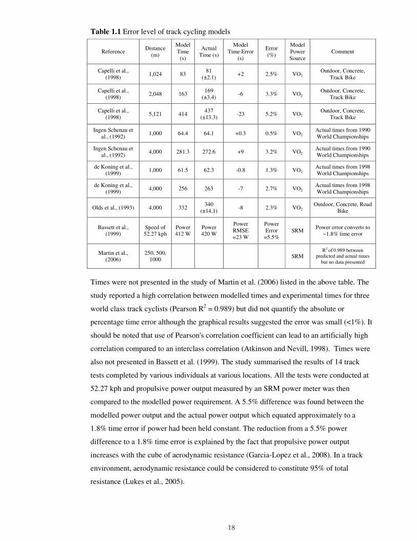
Studies that experimentally validated a track cycling model are listed in Table 1.1. The

mean error level of the models was 2.6%. The modelled results presented in the table were

mean values calculated over a number of participants which was considered acceptable.

More accurate predictions could be expected from a model parameterised to a specific

individual (i.e. a model initialised with generalised parameters is likely to have less

predictive accuracy than one initialised with a rider's individual characteristics). It should

be noted that in track cycling, finishing position is more sensitive to percentage error than

in road events due to the smaller spread of finishing times. For example, in the 2008 World

Championships the top 10 competitors in the 1000 m were separated by 1.5 s. The

predicted finishing position varied by five places if the prediction error increased by <1%.

18

Table 1.1 Error level of track cycling models

Times were not presented in the study of Martin et al. (2006) listed in the above table. The

study reported a high correlation between modelled times and experimental times for three

world class track cyclists (Pearson R2 = 0.989) but did not quantify the absolute or

percentage time error although the graphical results suggested the error was small (<1%). It

should be noted that use of Pearson's correlation coefficient can lead to an artificially high

correlation compared to an interclass correlation (Atkinson and Nevill, 1998). Times were

also not presented in Bassett et al. (1999). The study summarised the results of 14 track

tests completed by various individuals at various locations. All the tests were conducted at

52.27 kph and propulsive power output measured by an SRM power meter was then

compared to the modelled power requirement. A 5.5% difference was found between the

modelled power output and the actual power output which equated approximately to a

1.8% time error if power had been held constant. The reduction from a 5.5% power

difference to a 1.8% time error is explained by the fact that propulsive power output

increases with the cube of aerodynamic resistance (Garcia-Lopez et al., 2008). In a track

environment, aerodynamic resistance could be considered to constitute 95% of total

resistance (Lukes et al., 2005).

Reference Distance

(m)

Model Time

(s)

Actual Time (s)

Model Time Error

(s)

Error (%)

Model Power Source

Comment

Capelli et al., (1998)

1,024 83 81

(±2.1) +2 2.5% VO2

Outdoor, Concrete, Track Bike


2,048 163 169

(±3.4) -6 3.3% VO2



5,121 414 437

(±13.3) -23 5.2% VO2


Ingen Schenau et al., (1992)

1,000 64.4 64.1 +0.3 0.5% VO2 Actual times from 1990 World Championships

Ingen Schenau et al., (1992)

4,000 281.3 272.6 +9 3.2% VO2 Actual times from 1990 World Championships

de Koning et al., (1999)

1,000 61.5 62.3 -0.8 1.3% VO2 Actual times from 1998 World Championships

de Koning et al., (1999)

4,000 256 263 -7 2.7% VO2 Actual times from 1998 World Championships

Olds et al., (1993) 4,000 332 340

(±14.1) -8 2.3% VO2

Outdoor, Concrete, Road Bike

Bassett et al., (1999)

Speed of 52.27 kph

Power 412 W

Power 420 W

Power RMSE =23 W

Power Error

=5.5% SRM

Power error converts to ~1.8% time error

Martin et al., (2006)

250, 500, 1000

SRM R2 of 0.989 between

predicted and actual times but no data presented

19

1.2.4.2 Road Time Trial Models

Three modelling methodologies predicting road time trial performance have been reported

in the literature: (1) Correlation methods have predicted completion times from

anthropometric or physiological variables (Table 1.2). (2) Completion times have been

predicted from laboratory ergometer trials (Table 1.3). (3) 'First Principles' models have

been developed that predict completion times (Table 1.4).

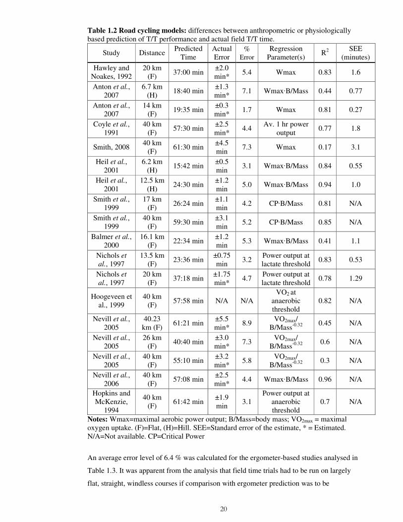
An average error level of 5.1 % was calculated for the correlation-based studies analysed

in Table 1.2. It was considered important in this analysis to extract values that would be

meaningful to an athlete or coach rather than to conduct a purely statistical analysis.

Anecdotal evidence suggested that prediction error in absolute time was more meaningful

to competitors than relative percentage errors. Coefficient of determination value (R2) was

usually reported by the studies but would possibly be of less relevance to an individual

athlete than the standard error of the estimate (SEE) indicating scatter or variability in the

prediction. The time error at two SEE was considered a meaningful measure of the extent

of the prediction error that could occur for a non-outlier individual. The Actual Error

column in Table 1.2 therefore presents this value.

20

Table 1.2 Road cycling models: differences between anthropometric or physiologically based prediction of T/T performance and actual field T/T time.

Study Distance Predicted Time

Actual Error

% Error

Regression Parameter(s)

R2 SEE (minutes)

Hawley and Noakes, 1992

20 km (F) 37:00 min

±2.0 min* 5.4 Wmax 0.83 1.6

Anton et al., 2007

6.7 km (H)

18:40 min ±1.3 min*

7.1 Wmax·B/Mass 0.44 0.77

Anton et al., 2007

14 km (F)

19:35 min ±0.3 min*

1.7 Wmax 0.81 0.27

Coyle et al., 1991

40 km (F)

57:30 min ±2.5 min*

4.4 Av. 1 hr power output

0.77 1.8

Smith, 2008 40 km (F)

61:30 min ±4.5 min

7.3 Wmax 0.17 3.1

Heil et al., 2001

6.2 km (H)

15:42 min ±0.5 min

3.1 Wmax·B/Mass 0.84 0.55

Heil et al., 2001

12.5 km (H)

24:30 min ±1.2 min

5.0 Wmax·B/Mass 0.94 1.0

Smith et al., 1999

17 km (F)

26:24 min ±1.1 min

4.2 CP·B/Mass 0.81 N/A

Smith et al., 1999

40 km (F)

59:30 min ±3.1 min

5.2 CP·B/Mass 0.85 N/A

Balmer et al., 2000

16.1 km (F)

22:34 min ±1.2 min

5.3 Wmax·B/Mass 0.41 1.1

Nichols et

al., 1997 13.5 km

(F) 23:36 min

±0.75 min

3.2 Power output at lactate threshold

0.83 0.53

Nichols et

al., 1997 20 km

(F) 37:18 min ±1.75

min* 4.7 Power output at

lactate threshold 0.78 1.29

Hoogeveen et al., 1999

40 km (F)

57:58 min N/A N/A VO2 at

anaerobic threshold

0.82 N/A

Nevill et al., 2005

40.23 km (F)

61:21 min ±5.5 min*

8.9 VO2max/ B/Mass-0.32 0.45 N/A

Nevill et al., 2005

26 km (F)

40:40 min ±3.0 min*

7.3 VO2max/ B/Mass-0.32

0.6 N/A

Nevill et al., 2005

40 km (F)

55:10 min ±3.2 min*

5.8 VO2max/ B/Mass-0.32

0.3 N/A

Nevill et al., 2006

40 km (F)

57:08 min ±2.5 min*

4.4 Wmax·B/Mass 0.96 N/A

Hopkins and McKenzie,

1994

40 km (F)

61:42 min ±1.9 min

3.1 Power output at

anaerobic threshold

0.7 N/A

Notes: Wmax=maximal aerobic power output; B/Mass=body mass; VO2max = maximal oxygen uptake. (F)=Flat, (H)=Hill. SEE=Standard error of the estimate, * = Estimated. N/A=Not available. CP=Critical Power

An average error level of 6.4 % was calculated for the ergometer-based studies analysed in

Table 1.3. It was apparent from the analysis that field time trials had to be run on largely

flat, straight, windless courses if comparison with ergometer prediction was to be

21

successful. This was due to the difficulty of reproducing environmental conditions on an

ergometer.

Table 1.3 Road cycling models: Differences between ergometer predictions of T/T performance and actual field T/T time.

Study Distance Predicted

Time Actual Error

% Error

R2 SEE

(minutes) Jobson et al.,

2007 40.23 km (F)

60:12 min +2.5 min 4.2 0.69 2.4

Jobson et al., 2008

40.23 km (U)

57:06 min +3.7 min 6.5 0.79 1.5

Smith et al., 2001

40 km (F)

54:21 min +3.1 min 5.7 N/A N/A

Palmer et al., 1996

40 km (F)

56:24 min +5.0 min 8.9 0.96 N/A

Palmer et al., 1996

40 km (F)

56:24 min +3.8 min 6.7 0.96 N/A

Notes: (F)=Flat, (U)=Undulating, * = Estimated. N/A=Not available

First Principles models have predicted performance from bicycle/rider equations of motion

and environmental forces (Table 1.4). These have been relatively successful compared to

the previous two categories as might be expected from modelling based on a firm

relationship to real-world physical laws. However, the models analysed were not forward

integration models and, therefore, specified fixed parameter values for the duration of a

simulation which restricted their effectiveness when applied to variable courses and

conditions.

Table 1.4 Road cycling models: differences between First Principle model prediction of T/T performance and actual field T/T time.

Study Distance Predicted

Value Actual Error % Error R2

SEE (W)

Martin et

al., 1998 0.47 km

(F) 172±15.2

W +0.8±14.7 W 0.5 0.97 2.7

Olds et al., 1995

26 km (F)

42:38 min +1.65 min 3.87 0.79 N/A

Notes: (F)=Flat, N/A=Not available

1.2.4.3 Comparison of Track and Road Models

The error level in road time trial models of between 3.9% and 6.4% was consistently

higher than the 1% to 2.6% found in track models and also higher than the 2.8% specified

as acceptable for this study. It is suggested that the higher error levels for road models can

largely be explained by a failure to adequately account for the variations in environmental

resistive forces such as gradient and wind velocity/direction that may occur frequently in

road cycling. The largest of these effects is considered to be gradient variation. The critical

22

effect of gradient can be seen in a field study conducted on an effectively windless airfield

taxiway with a gradient of only 0.5% (Martin et al., 1998). Despite the apparently flat

course, gravity accounted for up to 20% of the total resistive force when travelling at a

steady-state speed of 7 m/s. The contribution to resistance from environmental wind has

also been modelled as a constant. However, this is rarely the case due to variations in

strength and direction arising from the effects of topography and changes in route

direction. Rolling resistance as a constant will have a lesser distorting effect, but road

surface friction is variable (Kyle, 1994) and steering to follow a path which will always

generate tyre slip resistance (Kyle, 1984; Sharp, 2008).

Track models validated on an indoor track require no adjustment for gradient, wind or

surface although some adjustment is required for changes in forces and velocities induced

by the track banking (e.g. normal force on the tyres, Craig and Norton (2001)). Studies

conducted on outdoor tracks have predominantly reported wind <1 m/s and smooth

concrete surfaces. The studies presented in Table 1.1 have not made adjustment for these

factors despite identifying them as possible sources of error. Bassett et al. (1999) suggested

that the higher model error level sometimes reported for outdoor track testing is a

consequence of these omitted factors

Finally, many road models assume a steady-state condition as time to accelerate at the start

is a negligible proportion of overall time (Martin et al., 2006; Olds, 2001). However,

acceleration/deceleration is an inherent consequence of the environmental resistance

variations that occur constantly in road cycling on even the flattest courses. Failure to

adequately account for the rate of resistance changes increases the error level in road

cycling models. This can only be satisfactorily addressed with a high frequency of model

simulation that senses the changes and immediately generates an appropriate response.

1.2.5 Rationale Summary

Error level in models developed for individual events on the track was found to be

typically 2.6% while the error level for equivalent road time trial models was typically

5.3%. While track error levels met model effectiveness criteria, those for road cycling did

not and were, therefore, considered too high to guide mechanical performance

enhancement adequately. It is considered that the latter was due to incomplete modelling of

the combined rider, bicycle and environment and insufficient frequency of model

simulation. If mechanical performance is to be effectively enhanced, a need exists for a

new comprehensive and integrated road time trial model that is simulated at a high

23

frequency. The hypothesis of this thesis is that an effective and generalised road cycling

model can be built and subsequently used to predict performance enhancements.

1.3 Literature Review

The analysis above provides the rationale for this thesis and identifies a requirement for a

new road cycling model. The remainder of this chapter examines studies that provide

evidence on the features and functions that should be incorporated in the new model if it is

to fulfil its purpose.

The published research is analysed under the headings of sports science literature and

mechanical engineering literature. A combination of research from both disciplines

provides a broad base of expertise which will assist the new model to meet its design

objectives. It is, however, interesting to note the absence of cross-citations between the two

disciplines. The sports science literature has been primarily concerned with human systems

and therefore contributed mostly to rider biomechanics while the engineering literature has

been primarily concerned with machines and contributed mostly to bicycle dynamics. The

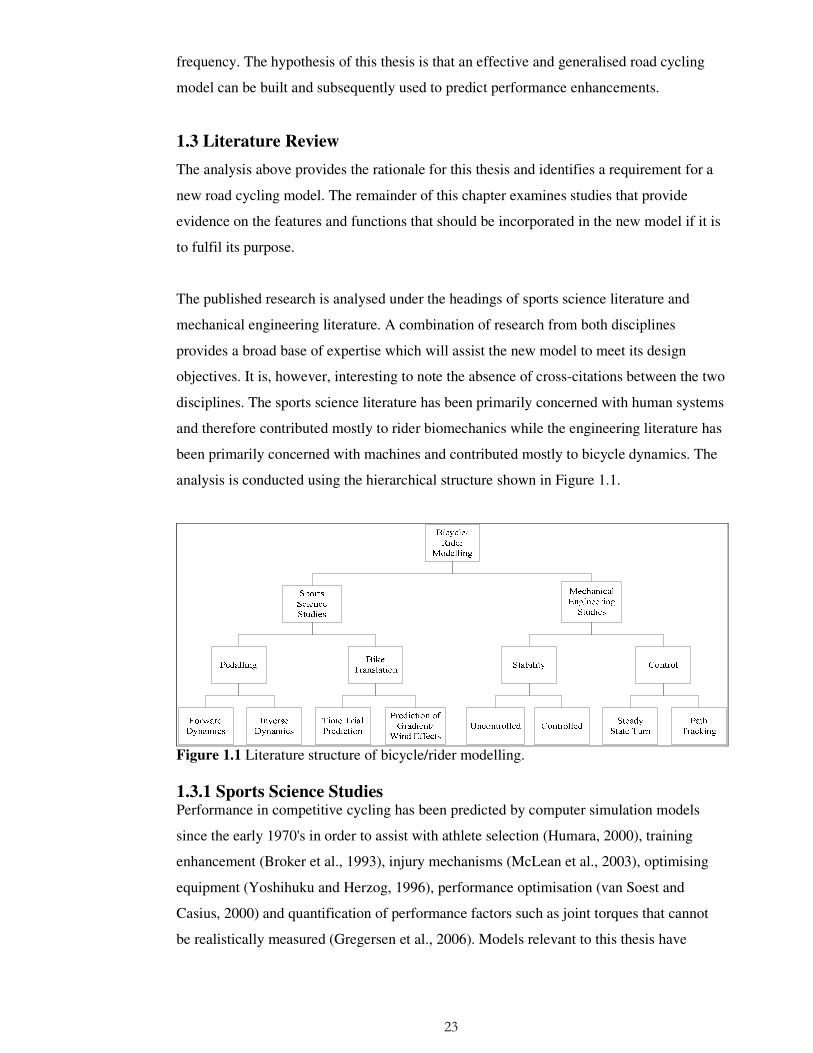
analysis is conducted using the hierarchical structure shown in Figure 1.1.

Figure 1.1 Literature structure of bicycle/rider modelling. 1.3.1 Sports Science Studies Performance in competitive cycling has been predicted by computer simulation models

since the early 1970's in order to assist with athlete selection (Humara, 2000), training

enhancement (Broker et al., 1993), injury mechanisms (McLean et al., 2003), optimising

equipment (Yoshihuku and Herzog, 1996), performance optimisation (van Soest and

Casius, 2000) and quantification of performance factors such as joint torques that cannot

be realistically measured (Gregersen et al., 2006). Models relevant to this thesis have

24

predominantly simulated the biomechanics of the pedalling action or the translational

dynamics of the bicycle/rider and these are analysed below.

1.3.1.1 Pedalling Models

The objective of most pedalling research has been to either optimise performance or

elucidate motor control mechanisms in human movement (based on neural strategies to

coordinate muscle activation) (Raasch and Zajac, 1999; Zajac et al., 2003). A common

model aim has been to optimise input parameters such as: saddle position (Gonzalez and

Hull, 1989), crank length (Martin and Spirduso, 2001), cadence (Redfield and Hull,

1986b), ankle angle profile (Chapman et al., 2007; Price and Donne, 1997), pedal/foot

position (Gregersen et al., 2006) or chainring shape (Kautz and Hull, 1995). Other models

have sought to minimise an objective function such as internal work (Neptune and van den

Bogert, 1998), joint torques (Marsh et al., 2000), muscle stress (Hull et al., 1988), effective

pedal force (Redfield and Hull, 1986a) and muscular work (Neptune and Hull, 1998).

Models have also sought to maximise metabolic efficiency (Smith et al., 2005) and

maximise power output (Yoshihuku and Herzog, 1996).

The main determinant of pedalling performance is the torque generated by leg muscle

contraction but an experimental analysis of pedalling is constrained by the difficulty of

directly measuring leg joint torques without invasive surgery. One solution to this problem

has been to use a forward dynamics model which generates neural commands to activate

individual leg muscles (Otten, 2003; Erdemir et al., 2007). The resulting joint torques

could then be derived as a function of muscle parameters such as length, cross sectional

area, moment arm, force/length/velocity relationship, tendon slack length, pennation and

actuation timing (Lloyd and Besier, 2003). Hip, knee and ankle torques have been input to

models that output total force applied to the pedal in cycling (Neptune and Hull, 1998;

Buchanan et al., 2005; Hakansson and Hull, 2007; Neptune and Hull, 1999; van Soest and

Casius, 2000). The kinematiclly constrained nature of pedalling also enabled less

sophisticated forward dynamics models to generate realistic pedal forces and motion when

only net joint torques were input to the model rather than individual muscle excitations

(Runge et al., 1995; Kautz and Hull, 1995). A weakness of forward dynamics models can

be their dependency on approximations of muscle activation magnitude/timing obtained

from EMG analysis. A further weakness can be their reliance on estimated joint torques

obtained from inverse dynamics studies (Neptune and Kautz, 2001). Their strength is an

ability to make prediction of outcomes for novel conditions that is not possible with

inverse dynamics models.

25

Inverse dynamics models provide an alternative method for examining pedalling, utilising

a technique where leg joint torques are calculated 'backwards' from measured pedal forces

and limb motion. While avoiding the complexity and uncertainty of muscle modelling,

these models generally calculate a 'net' joint torque which does not account for

agonist/antagonist co-activations, passive energy storage and the contribution of bi-

articular muscles (Van Ingen Schenau et al., 1992). Nevertheless, the bulk of pedalling

models fall into this category with computed joint torques being used to actuate closed-

loop five bar linkages comprising three leg segments, the crank and seat post (Hull and

Jorge, 1985; Fregly et al., 1996; Smak et al., 1999; Kautz et al., 1991). Inverse dynamics

analysis tends to be descriptive of a specific condition whereas a forward dynamics model

has the capability to make predictions for conditions that are not specified a priori. In

consequence, a forward dynamics model is likely to be required if a generalised model for

predicting road time trial performance is to be developed.

Hull et al. (1991) investigated the concept of internal work by developing a pedalling

model that demonstrated a key advantage of modelling when optimising performance.

Internal work was defined as work done by muscles to accelerate/decelerate the leg

segments during the reciprocating motion of pedalling, but which was not transferred to

bicycle propulsion. Internal work reduction would therefore increase efficiency. A number

of theoretical eccentric chainring profiles were modelled and 'pedalled', each one

differently minimising changes in segment velocity which was assumed to be the main

source of internal work. A maximum 48% reduction of internal work was obtained but the

excess of metabolic work over external work was found to be less than 9 W on 200 W

suggesting that segment velocity (internal work) was not a major factor in efficiency.

Modelling therefore provided a method of investigation that enabled the study to be

conducted without the manufacture of a large number of differently profiled chainrings.

It should be noted that none of the pedalling optimisations reported in the above studies

have been confirmed in field cycling trials. The model outputs have generally been

validated against data obtained from subjects pedalling on a static ergometer but the

optimisations have not been confirmed in road cycling where they might be confounded by

bicycle translation and rotation in three dimensions.

26

1.3.1.2 Bicycle Translation Models

Translation is defined as the motion of the bicycle/rider in a longitudinal, lateral or vertical

direction. The key literature relating to bicycle translation has been summarised in section

1.2 (Rationale) but a more extensive analysis is included here. Three types of study that

predict bicycle translation have been identified. Firstly, 'goodness-of-fit' models correlate

one or more anthropometric or physiological parameters (e.g. subject mass or maximal

oxygen consumption) to time trial performance and derive equations that use the

parameter(s) as a performance predictor (Coyle et al., 1991; Balmer et al., 2000; Anton et

al., 2007; Laursen et al., 2003). This approach does not include terms that account for the

variations in resistive forces that occur in field cycling (e.g. gradient, wind, and corners)

and, therefore, implicitly assumes field conditions are identical to a laboratory ergometer.

However, studies have shown that forces resulting from pedalling, steering, balancing and

path tracking have a significant effect on the dynamics of bicycle translation which casts

doubt on approaches that ignore them (Roland and Lynch, 1972; Cole and Khoo, 2001;

Meijaard et al., 2007; Sharp, 2008). In the second method, experimental time trials have

been completed on a laboratory ergometer configured with a resistive force that emulated

environmental resistances and field performance predicted from the result. To be

mechanically valid in the field, this approach requires the ergometer to be programmed

with the interaction of bicycle dynamics and environmental factors at each time instant

over a course. For example, Ordinance Survey maps show gradient changes at 10 m

intervals over a typical undulating time trial course (i.e. approximately every 10 s) whereas

many ergometers can only be programmed to change resistive force at ≥1 minute intervals.

This would mean that actual changes of gradient (and associated cyclist work) that

occurred within a one minute time period would not be implemented by the ergometer until

the start of the next time period. The ergometer's resistance due to gradient would therefore

not accurately reflect an actual course. In the worst case, nearly a minute of severe actual

climbing could be implemented in the ergometer resistance setting as a flat road .

The third method can be characterised as 'first principles' models (Olds, 2001) which use

physical laws to build power demand/supply relationships which are then parameterised

from experimental observations. Such models allow 'what if' questions to be answered by

changing parameters and predicting the response of output variables without the necessity

for experimental measurement (variables may be un-measurable in some instances). First

principles models can broadly be divided into models where the parameters and

relationships remain constant over the duration of a simulation and those where parameters

are changed systematically throughout the simulation (defined for the purpose of this thesis

27

as pacing models). The constant parameter models calculate propulsive forces (i.e. power

output the cyclist generates at the crank) less forces resisting forward motion

(gravitational, aerodynamic, rolling, frictional, inertial) in order to arrive at a predicted

steady state velocity for a given power output. A power supply/demand model (Olds,

2001) will, in some cases, include physiological factors in arriving at the available power

supply (Olds, 1998). Acceleration/deceleration may also be modelled, most notably in

track cycling where standing starts and banked turns introduce clear speed variations (de

Koning et al., 1999).

An early study (di Prampero et al., 1979) attempted to quantify resistive forces (primarily

aerodynamic) by towing a cyclist at various constant speeds behind a car for 100 m on a

straight, smooth, flat, windless car racing circuit and measuring the tension in the tow rope.

Expressions were presented for aerodynamic, rolling, and gravitational resistive forces.

Although the total resistive forces were known from the experiment, there was no means to

verify the proportionate allocation proposed by the authors. A significant advance in

bicycle translation modelling was reported in a study by Olds et al. (1995) which was one

of the first to validate a model against field time trials. The model applied weightings and

relationships to a large number of parameters that either contributed to bicycle propulsion

(mainly athlete physiological capacity) or resisted motion (mainly aerodynamic, gradient

and rolling forces). Results from 41 field trials over a 26 km course were compared to

model predictions with errors ranging from +6 min to -3 min on a mean time of ~43 min.

Unfortunately the field trials were not controlled, precluding separation of errors into those

due to the accuracy of the propulsive/resistive force equations and those due to one or

more subjects performing below their laboratory-measured capability. The course profile

was also not representative of a typical time trial since a 6.5 km straight, flat (mean

gradient <0.5%), windless (0.77 m/s) course was used four times in opposite directions

with the clock stopped for each turn.

Bicycle translation modelling took a major step forward when Martin et al. (1998)

eliminated the physiological performance predictions that were not accounted for in the

Olds et al., (1995) model. This highlighted the effects on performance of forces resisting

motion. An SRM power meter (Schoberer Rad Messtechnik GmbH, Julich, DE) was

validated and aerodynamic resistance forces quantified in a wind tunnel before a model

was developed and validated in controlled field trials over a 472 m course. (The SRM is a

device that measures power applied by the rider to the crank by sensing crank torque and

angular velocity). Reversing the usual approach, speed was controlled over the course

28

(runs at 7, 9 and 11 m/s) and then power output measured by the SRM power meter was

compared with power output predicted by the model. A mean power output of 172.8 W

was found for the field trial versus 178 W predicted by the model with a standard error of

measurement of 2.7 W and R2 > 0.99. However, the course on an airport perimeter track

was untypical of road cycling being short (~56 s), flat (0.3% gradient) and straight with a

wind speed of ~2.4 m/s at ~90° (implying almost nil environmental wind effect (Kyle,

1994)). Furthermore, acceleration effects were largely ignored as subjects crossed the start

line at the target speed and largely maintained that speed throughout. Any model

developed in this thesis should simulate the effects of environmental wind and gradient

that occurs in a typical road time trial.

1.3.1.3 The Effect of Pedalling on Translation

Pedalling is the engine of bicycle translation which makes it surprising that no pedalling

model has been identified that activates a bicycle translation model. Logically, this

activation is required if a cycling model is to emulate real-world cycling correctly.

Numerous bicycle translation models have been presented with propulsion provided by an

idealised power output rather than from pedal forces or joint torques (Swain, 1997;

Jeukendrup et al., 2000). The ability of these models to reproduce field bicycle translation

might be questioned, particularly as variable resistive forces in road cycling would make it

surprising for a pedalling cyclist to constantly produce an unvarying power output. Any

model developed in this thesis should be able to generate bicycle propulsion from the

cyclist's pedalling and simulate that propulsion at a frequency that reflects the changes in

forces over a pedal cycle.

1.3.1.4 The Effect of Gradient and Wind on Translation

Pacing models developed for time trials have predicted the effect of different gradients and

wind speed or direction on performance usually with the objective of optimising rider race

strategy to changes in the environment (Maronski, 1994; Swain, 1997; Atkinson and

Brunskill, 2000; Gordon, 2005; Atkinson et al., 2007a; Atkinson et al., 2007b). A strategy

of systematically varying power output in response to changes in gradient and wind is

typically calculated such that a rider's overall race time is minimised. Foster et al. (1993)

investigated the effects of varying speed over a simulated 2 km course on an ergometer

while resistive forces were held constant and found that completion time was minimised

with a constant speed. This basic concept underlies all mechanical pacing strategies as it

can be proved mathematically that constant speed over a course (with or without resistance

variations) will always be fastest (Maronski, 1994; Gordon, 2005). Variation in power

29

output then becomes the mechanism to reduce variation in speed during a race although

this is constrained by the rider's physiological capacity (Liedl et al., 1999). The earliest

pacing studies utilised the general cycling model of di Prampero (1979) to investigate

strategies that minimised race time in response to changes in course wind speed or

direction and gradient (Swain, 1997). Swain's findings confirmed that any variation in

propulsion that served to reduce speed variance would reduce course time regardless of the

responsible resistive force or its characteristics (assuming the same work done). The extent

of power output variance applied by the rider was the single most important controllable

variable when attempting to minimise completion time. Power variance has usually been

presented as a ± percentage variance against a constant power output strategy. Values

implemented in studies have ranged from ±5% on 224 W (Atkinson et al., 2007a) through

±10% on 289 W (Atkinson et al., 2007b) to ±20% on 435 W (Gordon, 2005). The average

climbing/descending gradient is also a critical parameter with the above three studies

applying variances of ±5%, ±10% and ±2.5% respectively. Lastly, climbing distance as a

proportion of total distance influences completion time. The above studies all applied

idealised profiles of 50% (i.e. equal constant gradient climbing and descending). The study

of Atkinson et al. (2007a) implemented a 5% power output and 5% gradient variance with

a resulting 2.3% time saving. The study of Gordon (2005) implemented only a 2.5%

gradient variance but a 20% power output variance and reported a time saving of 1.6%.

Atkinson et al. (2007b) reported a 7.9% time saving for a 10% gradient variance,

demonstrating that gradient is a major variable in deciding how much time can be saved

with a constant versus variable power output strategy. In essence, a variable power output

strategy will only be effective on hilly time trial courses. The time saving occurs because

more time is spent on the ascent than on the descent and therefore the speed on the ascent

has a greater effect on the overall time.

As an additional observation, it has been shown mathematically (Gordon, 2005) that a

variable power output strategy can generate a greater time saving over a steep climb and

gradual descent compared to an equivalent balanced climb/descent (e.g. a 10% ascent and

2% descent versus a 6% ascent/descent over the same distance with mean power output the

same). Gordon (2005) also demonstrate the non-linear increase in time saving with

gradient by increasing gradient from 3.5% to 5.25% on a balanced idealised climb with

the associated potential time saving increasing from 100 s to 200 s (physiological

limitations were ignored).

30

It is interesting to note that studies which vary wind resistance (out and back course with

head/tail wind) show much less time saving in response to power variation than changes in

gradient. Swain (1997) reported a normalised 0.8% saving for ±4.4 m/s wind, Atkinson

and Brunskill (2000) reported a 0.1% saving for a ±2.2 m/s wind and Atkinson et al.

(2007b) reported a 0.7% saving for a ±2 m/s wind. These results are to be expected as

power requirement increases with the cube of air velocity while the power response to

gradient increase is nearly linear.

The models of Swain (1997) and di Prampero (1979) were not validated in laboratory or

field trials. One concern was the aerodynamic equations of di Prampero which could be

questioned on the grounds that they were derived from data obtained whilst towing a

cyclist behind a vehicle. The above models were possibly not validated in the field because

their theoretical construct was based on a simplified representation of gradient and wind

forces which was not realisable in the real world. In particular, symmetrical

increase/decrease in resistive forces were applied at arbitrary intervals and the models were

constrained to planar motion which excluded the effects of three dimensional translation

and rotation required for a bicycle/rider to stay upright and follow a path.

In summary, whilst most pacing models provide important contributions to theory, they

have not been validated in the field and their application in field cycling should therefore

be treated with caution. Logically a complete road cycling model requires input of path

tracking and gradient data at a rate that adequately reproduces a real course consistent with

measurement accuracy. Without the facility to include and examine these effects, a model

is at risk of oversimplifying the problem. Wind and gradient generally change continuously

in the field rather than in the fixed and balanced fashion at a few time points assumed in

most pacing models. Any model developed in this thesis must have the capability to

numerically integrate a solution to the equations of motion at sufficiently small time steps

to account for frequent changes in environmental conditions.

1.3.1.5 Translation Model Limitations

It has been suggested (Olds, 2001; Martin et al., 2006) that bicycle translation models often

require extension if they are to predict field performance effectively. Most models from the

sports science literature treat the bicycle/rider as a single machine with one longitudinal

degree of freedom (but no lateral or vertical translation) and no rotational degrees of

freedom (i.e. no yaw, roll or pitch). In addition, most existing models have no steering

torque, no tyre forces, no rider body lean, no steering geometry effects (trail or steering

31

axis inclination), no pedalling torque profile, no pedalling/roll interaction, no gear changes

and acceleration effects only associated with standing start races (deKoning et al., 1999).

One consequence of these limitations is that propulsive and resistive forces are often

measured and modelled at frequencies specified in many seconds or even minutes. In

reality, many input variables change on a second-by-second basis. A study that reports a

good model/experimental fit from a single measurement taken at the end of a trial may

conceal wide divergences at intermediate time points.

The above omissions suggest that a general limitation of existing models is the small

number of parameters and relationships included in the equations of motion and the low

simulation frequency. Models that predict optimum power output over a course can

therefore be questioned when conditions are not tightly controlled. Real-world field

cycling consists of continuously changing resistive forces changes generated from a wide

range of parameters with periods measured in seconds (Euler et al., 1999). It is likely that

some of the bicycle/rider mechanisms included in a comprehensive model will have

limited effect on performance and there is little evidence enabling these factors to be

identified a priori. Hatze (2005) considered it essential that a model should be developed

with the most complete set of functions possible, which could then be reduced once

validated outputs were available to control the process. Other limitations of sports science

translation models when predicting real-world cycling performance include: (1)

Translation models are not constructed from multiple bodies that comprise a bicycle/rider

and cannot therefore model the effects of such a structure on performance (e.g. frame twist,

wheel flex and rider body lean). (2) Pedalling model optimisation predictions have not

usually been validated by a translating bicycle/rider system in a field context. (3) Where

models have been validated by field trials, they have often been run over straight, flat,

windless courses which tend to confirm model predictions but are not typical of most road

cycling.

1.3.2 Mechanical Engineering Studies

The dynamics of single track vehicles is an established discipline within mechanical

engineering that includes the bicycle, motorcycle and scooter. The bicycle/rider as a

machine is subject to the well established mechanical laws that define the dynamics of

rigid bodies. In classical mechanics, Newton (1686) and Euler (1775) identified the

essential components of rigid body translation and rotation (point mass, constraints, joints,

forces) and established the free body principal based on applied forces and reaction forces,

encapsulated in the characteristic Newton-Euler equations of motion. A re-formulation of

32

Newtonian mechanics in terms of kinetic and potential energy by Lagrange in 1788,

contributed a major advance in simplifying equation derivation. The resulting differential-

algebraic equations (DAE) and ordinary differential equations (ODE) have become the

predominant method used to the present day. Early applications of rigid body dynamics

were often directed at investigating biomechanical problems with a particular emphasis on

human locomotion. Research areas included human walking (Fischer, 1906), total body

motion (Chaffin, 1969), bipedal stability (Vukobratovic et al., 1970) and a complete

representation of the human body (Huston and Passerello, 1971).

Building rigid body models was computationally constrained until the late 1960's as the

numerical methods required for solving non-linear differential equations were often

impractical by hand. Computer developments removed this constraint and led to the

publication of numerical formalisms (Hooker and Margulies, 1965; Roberson and

Wittenberg, 1967) that created a new branch of mechanics entitled Multibody System

Dynamics. Continuing growth in computer power also facilitated symbolic manipulation of

the equations of motion, enabling simplified and more efficient expressions to be obtained

(Levinson, 1977; Schiehlen and Kreuzer, 1977). In the 1970's, finite element analysis was

also applied to creating bicycle models with an emphasis on investigating bicycle stability.

Notably, the software package SPACAR was released by the University of Delft and is still

in widespread use (van Soest et al., 1992). Finally, the current state-of-the-art comprises

unified modelling, simulation and animation software packages which include previously

unavailable facilities to model friction, impact and closed kinematic chains together with

links to computer aided design (CAD) input and hardware programming output. Multibody

system dynamics is now a major branch of mechanics in its own right (Schiehlen, 1997),

utilising software modelling to solve engineering problems in industries such as rail and

road vehicle design (ADAMS (www.mscsoftware.com)), aerospace (Vortex (www.cm-

labs.com)), civil engineering (FEDEM (www.fedem.com)) and robotics (Dymola

(www.dynasim.se)). An important development in mechanical modelling was the release

in 2002 of SimMechanics (www.mathworks.com) which, for the first time, made

modelling of mechanical systems (such as a bicycle/rider) accessible to non-

mathematicians since the equations of motion were automatically derived by the software.

Similar integrated packages since released include BikeSim (www.carsim.com), 20-Sim

(www.20sim.com) and Simpack (www.simpack.com).

33

1.3.2.1 Single Track Vehicle Dynamics

In engineering, single track vehicles pose the 'inverted pendulum' stability problem (i.e.

they do not remain upright when at rest). The bicycle has been extensively modelled since

the invention of the safety bicycle by John Starley in 1885, usually with the objective of

identifying the mechanics that keep a moving uncontrolled bicycle upright and deriving

governing equations of motion. Bicycle dynamics studies have generally only considered

the mechanics of the uncontrolled vehicle (i.e. no rider although the rider body has

sometimes been included as an inert mass). Models developed over the last 100 years can

generally be divided into three groups: Firstly, qualitative discussions of bicycle dynamics,

too reduced to capture a bicycle's self-balancing capacity (Maunsell, 1946; Jones, 1970;

Den Hartog, 1948; Le Henaff, 1987; Olsen and Papadopoulos, 1988). Secondly, models

with insufficient mass and geometry to allow self-stability or with control inputs that

overrode uncontrolled steer dynamics (Timoshenko and Young, 1948; Lowell and McKell,

1982; Getz and Marsden, 1995; Fajans, 2000; Astrom et al., 2005; Limebeer and Sharp,

2006). Thirdly, some thirty rigid body dynamics models have been identified that include

bicycle mass, geometry and steering characteristics sufficient to enable self-stability

together with their governing equations of motion (Wipple, 1899; Carvallo, 1900; Dohring,

1955; Weir, 1972; Eaton, 1973; Psiaki, 1979; Sharp, 1971; Van Zytveld, 1975; Collins,

1963; Singh, 1964; Rice and Rowland, 1970; Roland and Massing, 1971; Roland and

Lynch, 1972; Roland, 1973; Koenen, 1983; Franke et al., 1990; Meijaard et al., 2007).

More recently, the research emphasis has moved from stability to control with studies

investigating the control logic necessary for a bicycle to track a defined path (Yavin, 1999;

Getz and Hedrick, 1995; Getz, 1995; Frezza and Beghi, 2006).

. A typical bicycle model contains a limited number of dynamic variables that can be

adjusted to achieve either stability or control objectives. These are presented in

diagrammatic form below to provide an overview. The mechanics of cycling are analysed

under three categories: Firstly, the bicycle is analysed in respect of the main variables

which specify its motion (Figure 1.2). Principally these are translation in forward, lateral

and vertical directions and rotation about these axes, defined respectively as roll, pitch and

yaw. Additionally, steering is initiated about an inclined steering axis and propulsion is

generated by rotation of the rear wheel. Secondly, the rider is analysed in respect of both

motion and forces that contribute to bicycle stability and translation (Figure 1.3).

Principally these are upper body lean/weight transfer together with steering torque and

crank torque from pedalling. It should be noted that the Figures are intended as a

simplifying conceptual representation and therefore omit the interactions between

components. Thirdly, the main environmental factors are considered comprising gradient,

34

path tracking and aerodynamic resistance (Figure 1.4). In each diagram, input to the system

is shown on row 2 and the resulting effect on row 3.

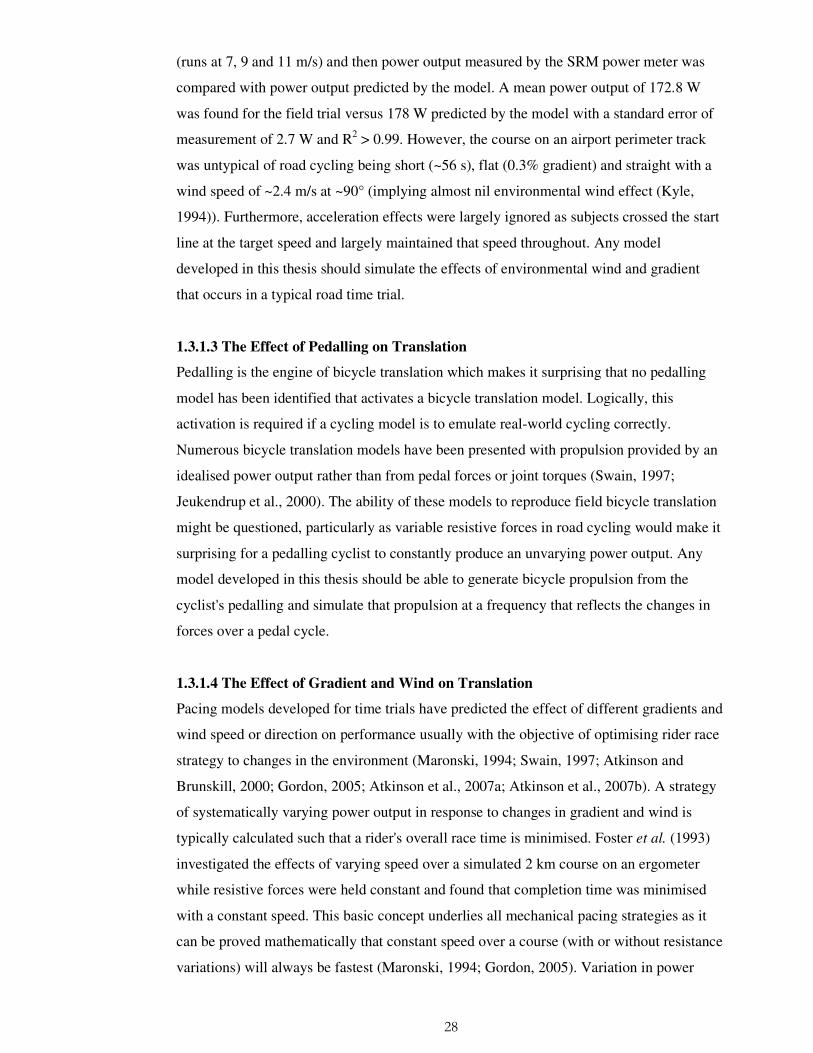
Figure 1.2 Bicycle modelling. Angles/positions/forces (derivatives computed as required).

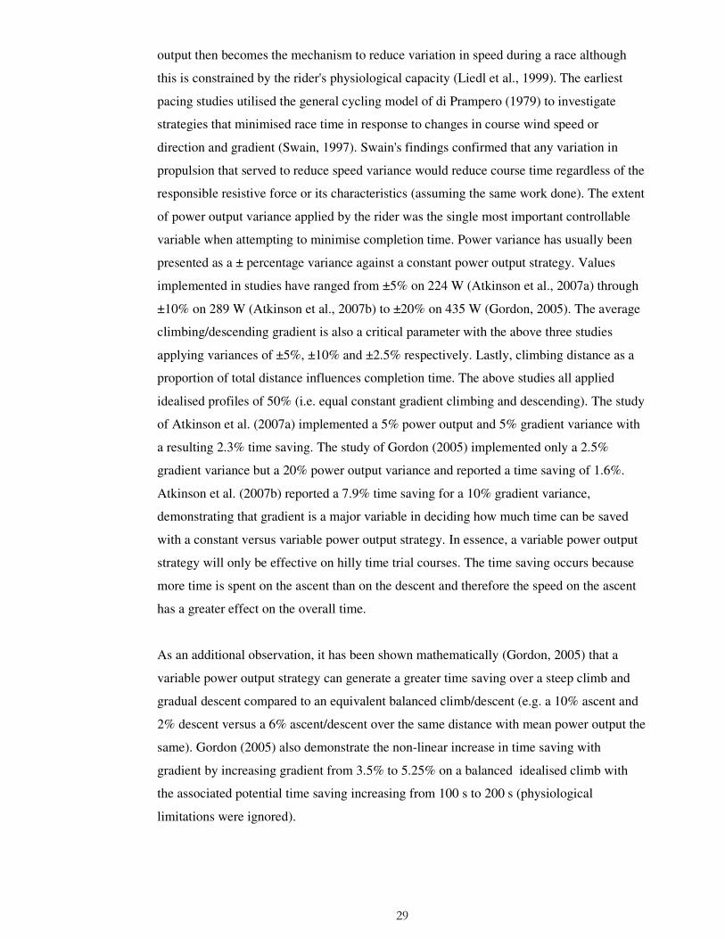
Figure 1.3 Rider modelling. Positions/forces (derivatives computed as required).

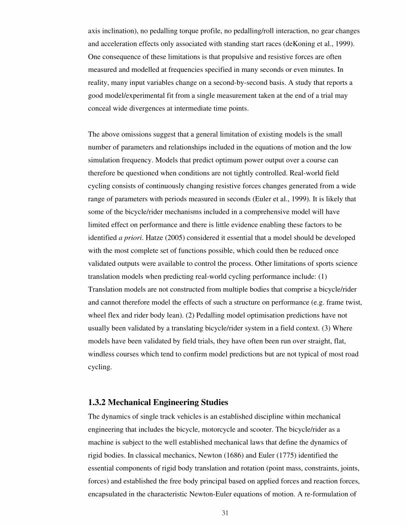
Figure 1.4 Environmental modelling. Angles/positions (derivatives computed as required).

1.3.2.2 Vehicle Stability

Translational stability was the first problem to attract the attention of the scientific

community once the design of the 'three triangle' Rover safety bicycle was stabilised

towards the end of the 19th century. It is interesting to realise that bicycle development in

the 1890's was a leading edge technology for the time and therefore drew considerable

35

scientific attention. In mechanical engineering terms, a bicycle was similar to the well

known problem of balancing an inverted pendulum on a moving cart. Longitudinal cart

translation to overcome the pendulum's natural tendency to capsize mirrored a bicycle's

inherent tendency to capsize at slow speeds, presenting an interesting challenge when

formulating the equations of motion that kept a bicycle upright. Research into bicycle

stability has generally proceeded on the basis of 'no rider control' even when a rider mass

was included as an inert addition to the bicycle rear frame. This seemingly somewhat

unworldly method of analysis was (and is) based on the assumption that bicycle designers

were seeking to achieve some combination of stability and manoeuvrability independently

of a rider. Since there would always be some delay between environmental changes and

rider compensatory inputs, an optimal design would be achieved if the instantaneous

response of the bicycle (i.e. uncontrolled) conformed to the design objectives. It also

proved surprisingly difficult to describe a bicycle mathematically, a challenge which was

first seriously addressed by a Cambridge undergraduate, Francis Whipple, in 1899.

Whipple formally derived generalised linear (upright, straight-running) and non-linear

(steering, rolling) equations of motion for the bicycle (Wipple, 1899) although it took

nearly 100 years before both were confirmed as essentially correct (Hand, 1988; Meijaard

and Schwab, 2006). It is perhaps a measure of Whipple’s original achievement that the

complexity of his non-linear equations precluded their being solved until sufficient

computer power was available to solve them numerically.

Over the period 1900 to the 1950's, numerous authors developed governing equations of

motion for the bicycle and also investigated the factors which influenced the self-stability

(i.e. no rider control) of a straight-ahead moving bicycle in response to small lateral

perturbations. Studies reported on the dynamics of steering response (Timoshenko and

Young, 1948), bicycle roll (with and without a fixed rider) (Rice and Rowland, 1970; Van

Zytveld, 1975), geometry (e.g. steering axis inclination and trail) (Papadopoulos, 1987)

and wheel gyroscopic effects (Den Hartog, 1948). However, few of the published

equations were validated by reference to other work and subsequent analysis (Hand, 1988)

has shown that errors and/or omissions were not uncommon (Bower, 1915; Pearsall, 1922).

A recent study examined the majority of previous work and having corrected all

identifiable errors, created a unified product claimed as the definitive benchmark equations

of motion for an uncontrolled bicycle (Meijaard et al., 2007). An experimental study was

generally supportive of the model predictions although the confirmation was not supported

with statistical data (Kooijman et al., 2008).

36

The dynamics of a motorcycle has many similarities to the bicycle particularly when

examining stability with no rider input. Due to the involvement of motorcycle

manufacturers from the mid 1950's onwards, an increasing contribution to the single track

vehicle literature was provided from motorcycle and scooter studies (Dohring, 1955; Sing

and Goel, 1971; Sharp, 1971). These added to the growing accumulation of generalised

equations of motion although few were checked for validity against other derivations. The

stability orientation of single track vehicle research also started to migrate towards a wider

consideration of the real-world factors affecting a single track vehicle being ridden on the

road. Most notably, motorcycle researchers started to include tyre forces in their equations

since they were clearly critical to performance at higher vehicles speed and vehicle weight

(Sing, 1964; Sharp, 1971; Weir 1972; Eaton, 1973). Beneficially, tyre force analysis then

'trickled-down' to improve the accuracy of bicycle research (Rice and Roland, 1970;

Roland and Massing, 1971; Roland and Lynch, 1972). Other factors were introduced that

made studies more realistic including propulsion and drag forces (Collins, 1963), an active

rider (Van Zytveld, 1975) and vehicle acceleration (Lobas, 1978; Limebeer et al., 2001). A

shift in research emphasis from vehicle stability to control resulted from developments in

control engineering and from the formal quantification by Sharp (1971) of the weave,

wobble and capsize modes. These modes clarified the previously known fact (Whipple,

1899) that self-stability only occurred within a narrow speed band while stability at other

speeds required varying degrees of explicit control.

Despite some question marks over the real-world relevance of single track vehicle stability

studies, they will be discussed at length as the model to be constructed for this thesis will

be validated against uncontrolled bicycle stability models from the literature. It is

important therefore to specify the assumptions which underlie such models and which

should be emulated if the thesis model is to be compared. The main features are as follows:

• The single track bicycle is composed of four rigid bodies comprising two wheels, a

rear frame (possibly including rigid inert rider) and a front frame hinged to the rear

frame along an inclined steering axis.

• Wheels are rigid, non-slipping, knife-edge discs with a single ground contact point.

• Wheels are holonomically constrained in the normal (vertical) direction (i.e. they

must remain on the ground). They exhibit no slip and are therefore non-

holonomically constrained in the longitudinal and lateral directions. A non-

holonomic constraint has the characteristic that the bicycle position at any instant is

37

unknown unless the time history of the wheel path is also known. In mathematical

terms, the bicycle’s position cannot be found by integration of its velocity.

• The effects of propulsive and resistive forces are ignored.

• Responses are measured over a range of speeds with speed held constant for each

measurement run.

• There are no control ( steering, roll) inputs

• Finally a linearised model must be extracted from what is likely to be a model with

many non-linear features (e.g. steering/roll inputs, path tracking, and acceleration).

Essentially this represents the bicycle as a system that is in upright equilibrium and

moving straight ahead at a constant velocity.

1.3.2.3 Weave, Wobble and Capsize Modes

These modes describe the stability response of an uncontrolled single track vehicle running

straight-ahead at various speeds when perturbed by a small lateral force. It is initially

surprising to find a considerable proportion of the vehicle dynamics literature measuring

these responses given that they ignore any control applied by a rider. In the early years of

bicycle research, this probably reflected interest in how a bicycle remained upright. In

more recent times, matching the uncontrolled stability results of previous models has

primarily been used to confirm a new model’s validity (Weir, 1972; Franke et al., 1990). It

is also important to note that theoretical stability studies are more important in motorcycle

research where the higher speeds can make instability on the road life-threatening

(Evangelou et al., 2006; Limebeer et al., 2002).

The capsize mode is specified as the upper speed where uncontrolled roll and steering

responses to a small perturbation are unable to prevent the bicycle falling due to gravity

(Sharp, 1971). Capsize mode is normally associated with a slow, non-oscillatory toppling

of the bicycle at speeds above approximately 6 m/s. In reality this instability is so slight

that it is likely to be easily and unconsciously corrected by a rider. Weave mode describes

a slow oscillation between left leaning/left steering and vice-versa when the upright

uncontrolled bicycle is perturbed at speeds from approximately 0.5 to 4.3 m/s (Limebeer

and Sharp, 2006). Again a rider perceives little difficulty in controlling weave mode except

perhaps at very low speeds (i.e. close to performing a track stand). Wobble mode is more

significant to a cyclist as it describes the rapid oscillation (4- 10 Hz) of the steering

assembly (bars, forks, front wheel) that can occur at speeds above 10 m/s, often on a fast

descent (Sharp, 1985). Vehicle models that reflect this phenomenon usually include a tyre

model and thus have been largely confined to motorcycle research where higher speed,

38

performance and safety requirements have justified the development of sophisticated tyre

models. However, the phenomenon is experienced by cyclists and therefore, with the

addition of recently available tyre parameters (Seffen et al., 2001; Limebeer and Sharp,

2006), should be observable in a complete bicycle model. The instability starts with an

imbalance in the front assembly that oscillates the steering from side to side. The problem

is exacerbated when rider corrective action coincides with the oscillation rather than

opposing it. Stability is usually restored through some combination of speed change, riding

position and reduced handlebar grip although an increase in steering damping may be

required to cure the problem at source (Sharp, 2001).

It has proved difficult to experimentally validate the stability responses obtained from

models particularly at the higher speeds required for motorcycles. Instrumented

motorcycles have been developed by a number of researchers (Dohring, 1955; Eaton,

1973; Koenen, 1983) but all require a rider to input sufficient perturbation to initiate a

weave, wobble or capsize response. Such input is difficult to measure with accuracy. The

low resolution of instrumentation can also conceal experimental capsize, weave, wobble

responses suggesting that the subtlety of stability modes measured on a model have limited

application to a vehicle on the road where a controller (the rider) is likely to be correcting

stability issues instinctively. In the case of the bicycle, studies with various degrees of

implementation rigour have attempted to construct a machine that is uncontrollable. They

have generally found that major changes to the vehicles geometry are required before the

vehicle becomes uncontrollable to an experienced rider (Jones, 1970; Astrom et al., 2005).

One study attempted to experimentally validate the stability modes of an uncontrolled

bicycle using an indoor sports hall and later repeated the tests on a large treadmill

(Kooijman et al., 2008). A rider-less bicycle instrumented for steering angle, speed, yaw

and roll was accelerated to a desired speed by being pushed by the researcher who then

applied a perturbation by striking the saddle laterally. A good fit with the modelled

stability responses was reported such that the three stability modes could be identified and

they occurred over the speed ranges predicted. However, it should be noted that while the

results clearly supported the theoretical predictions, this was not confirmed in a statistical

sense as no attempt was made to quantify the variations in response that would occur by

chance.

1.3.2.4 Bicycle Controllers

This review of bicycle models has so far considered uncontrolled single track vehicles

where a bicycle or motorcycle is 'launched' at a defined speed without a rider or controller

39

and the resulting stability response measured. This establishes the basic dynamic

characteristics of a bicycle which must be incorporated into a bicycle/rider model if it is to

accurately represent real world cycling. It also enables the thesis model to be validated

against established models that have been built on similar principles.

The uncontrolled bicycle is only the first stage in the progression to a comprehensive

bicycle/rider model that can accurately emulate the performance of a competitive cyclist in

the field. The next stage adds a controller to the model (either human or programmatic) in

order to generate inputs additional to those which are an intrinsic result of the bicycle

geometry (Astrom et al., 2005). Bicycle controllers have become increasingly complex

over the last 25 years in parallel with the development of control theory and the emergence

of control engineering as a discrete discipline (Vaculin et al., 2004). While the main impact

of new control techniques has been in industries such as aerospace, automotive and

robotics, they have also been applied to single track vehicles which provide a surprisingly

challenging control problem (Seffen et al., 2001). In particular, bicycle and motorcycle

uncontrolled stability models that had previously identified a narrow self-stability speed

range have been extended to include a controller that maintains the vehicle in an

equilibrium upright orientation over a wider range of speeds (Chen and Dao, 2010). This

was followed by the development of steady state cornering controllers and finally to full

path-tracking controllers that emulate the control inputs of a rider following a typical

horizontal road profile (Popov et al., 2010; Rowell et al., 2010; Sharp, 2007).

1.3.2.5 Bicycle Control Theory

Before examining the literature relating to bicycle control, it is important to summarise the

underlying dynamics of bicycle steering. Essentially roll and steering interact to achieve

both stability and path tracking, although the sequence of bicycle response will be different

depending on an initial steering or roll input. A roll input will cause the steering of a static

or moving bicycle to turn in the direction of the lean due to varying combinations of the

trail, steering axis angle (castor), fork centre-of-mass offset and gyroscopic forces (Fajans,

2000). Trail is defined as the longitudinal distance between the front tyre contact point and

the steering axis intersection with the ground (Astrom et al., 2005). Most studies that

model uncontrolled bicycle stability commence a stability trial by applying a lateral

perturbation, say from the left side (Schwab et al., 2005). This generates bicycle lean to the

right which thus causes the steering to turn right. However, the momentum of the

bicycle/rider mass continues straight ahead resulting in the bicycle/rider rolling leftwards.

The steering response again follows the bicycle lean so now switches to steer left and, in

40

an uncontrolled bicycle, the whole cycle is repeated until the oscillations subside or the

bicycle falls. Similarly, a right turn steering input causes the bicycle to roll left followed by

the steering also turning left which then causes the bicycle to roll right and so on until the

oscillation again subsides or the bicycle capsizes. In control theory terminology, the

bicycle can be described as a non-minimum phase system or more colloquially as requiring

counter-steer to initiate a turn (Sharp and Limebeer, 2001).

Numerous studies have identified the origins of the forces that are responsible for the

linked roll/steer responses (Jackson and Dragovan, 2000; Le Henaff, 1987; Fajans, 2000;

Cox, 1997). Three steering torques are generated, the most important of which originates

from the moment arm created by the front tyre contact point displacement from the

steering axis (the mechanical trail). During a turn, the road exerts a lateral tyre force at the

contact point which applies a moment about the steering axis and thus acts to reduce the

steering angle (i.e. straightens out the turn). This straightening effect increases with the

square of the bicycle velocity and thus directional stability increases with speed. A second

steering torque originates from a gyroscopic effect that seeks to maintain the front wheel

angular momentum by increasing the steering angle in the direction of a lean. This torque

increases in proportion to bicycle velocity (but note that if there is no lean, gyroscopic

forces act to keep the steering pointing straight ahead). Finally the gravitational force

acting in the normal direction on the front tyre increases a turn due to the trail/centre of

mass location and is independent of speed.

Three roll torques are also generated by a moving bicycle which can be combined to

achieve a steady state turn. Steering input initiates a turn which generates centripetal

acceleration into the turn. Gravity applies a roll torque dropping the bicycle/rider towards

the inside of the turn, while inertial force acting in the direction of original travel tries to

keep the bicycle/rider upright. Additionally there is a small torque rotating the bicycle

upright due to the effect of yaw acceleration. Clearly, all the steering and roll torques must

be coordinated and balanced to achieve any desired turn and it is perhaps surprising that

the human controller can achieve this without control inputs from the handlebars during

riding 'hands-off'. However, hands-off riding is controlled by small lateral rider centre-of-

mass shifts (Fajans, 2000) which rolls the bicycle in the opposite direction and initiates

steering in that direction (often incorrectly attributed solely to body lean) (Kirshner, 1979).

This process is further complicated by the out-of-plane pedalling forces that introduce

bicycle roll together with matched upper body lean (Jackson and Dragovan, 2000). It is

41

important to note that no previous models have been identified that include all these forces

necessary for a model to fully replicate road cycling.

1.3.2.6 Theoretical Compared to Field Cycling

The above description of bicycle dynamics emphasises some fundamental differences

between uncontrolled stability studies and a model that must accurately represent the

forces that control a bicycle and rider in the field. In the field, a turn cannot usually be

initiated by roll input unless some transient external force (e.g. road camber or side wind)

is applied to the bicycle/rider ensemble (Fajans, 2000). A rider can of course lean their

upper body laterally while maintaining steering direction (an intrinsic feature of pedalling)

but this is achieved by moving the bicycle in the opposite direction such that total mass

remains over the two support points represented by the tyre contact patches. A turn is

almost invariably initiated by a steering input which must be a counter-steer in order to

generate a roll in the desired direction of turn (Limebeer and Sharp, 2006). Almost all turns

are therefore generated by counter-steering although the cyclist is usually unaware of the

process. A valid field cycling model should primarily initiate path tracking through

steering input rather than upper body movement with roll angle being a resultant dependant

on bicycle geometry, inertias and speed (unless side winds are also being modelled).

1.3.2.7 Straight Running Control

The first application of control theory to bicycle modelling introduced a control scheme

that maintained upright straight-ahead equilibrium over a wider range of speeds than was

achievable in uncontrolled self-stability (Suryanarayanan et al., 2002; Getz and Marsden,

1995). However, these controllers were primarily concerned with maintaining the bicycle

upright and did not attempt to control the bicycle to track a specified heading. For

example, a change of bicycle heading would be expected as a result of the lateral

perturbation commonly introduced during stability analysis but any such response has

generally been neither measured nor controlled. More complete applications of control

theory have therefore sought to constrain the bicycle to follow a straight path following a

lateral perturbation (Beznos et al., 1998). However such a task is not representative of most

real-world cycling as an external force creates the control problem, a condition which

would only occasionally occur (usually due to environmental wind and/or lateral road

camber). Never-the-less, these studies established the central concept of a relationship

between roll angle and steering angle although the most common sequence is likely to be a

steering input initiating a roll response. Models in this category (as with most bicycle

models) lack an active rider which would greatly increases the complexity of the control

42

problem by introducing factors such as upper body lean, rider weight transfer, handle-bar

couple and out-of-plane pedalling moments. As with all uncontrolled stability modelling,

an idealised bicycle is assumed which runs at constant speed with no propulsive forces to

create rear wheel torque and the associated chain tension, gearing and crank angular

velocity.

1.3.2.8 Steady-State Turning

Maintaining a bicycle in a constant radius turn can be considered a control problem of

intermediate complexity between that of straight running and complex path tracking. The

underlying principle of balancing roll and steer remains unchanged. Centripetal force

combined with bicycle inertia will tend to lean the bicycle away from the centre of the

turn. This motion can be opposed by gravitational force due to leaning the bicycle into the

turn such that a steady state turn radius can be achieved (Sharp, 2001). Numerous studies

have presented the equations of motion that maintain this balance, with steer angle and

bicycle velocity being the main control inputs (Cossalter and Lot, 2002; Tanaka and

Murakami, 2004). Chen and Dao (2006) noted that maintaining a stable turn was relatively

trivial for a human but demanding for an unmanned bicycle controller. They addressed the

problem by developing a 'fuzzy' controller which essentially mimicked human logic using

a decision tree of the type 'If roll angle and change in roll angle are negative and large, then

steering angle should be negative and large'. Their controller was also of particular interest

being one of the few implemented in the Matlab/Simulink environment used in this

research.

A study from the leading bicycle/motorcycle research group at Imperial College, London

(Limebeer and Sharma, 2008) considered the effects of acceleration/braking in a turn and

noted that wobble-mode damping improves under acceleration and degrades under

braking. The latter finding would appear to reinforce the anecdotal perception of road

cyclists that the bicycle can become unstable when braking hard for a corner at the bottom

of a steep hill. However, this study did emphasise the theoretical mathematics at the

expense of the effective application required for the development of a realistic road time

trial model. The modelled acceleration of 1 ms-2 would have required considerable force

application by the cyclist on the handlebars and pedals (with associated roll, yaw and steer

effects) but the model assumed smooth 'invisible hand' propulsion. Clearly investigations

must isolate conditions and declare assumptions, but the results remain theoretical until

they are extended to include the missing real-world factors.

43

1.3.2.9 Path Tracking

Following a complex path which changes continuously in unpredictable ways is one of the

most challenging tasks facing a bicycle model that seeks to emulate field cycling. The first

problem is to define the path at an acceptable resolution and then to structure the data in a

format that provides input to the bicycle tracking controller. A path is often defined by

lateral deviations from a longitudinal vector which may be specified in the local or global

coordinate system (Getz, 1995; Frezza and Beghi, 2006). Additionally, the radius of turns

may be specified (Getz and Hendrick, 1995), sometimes by a sine function (Yavin, 1999).

A controller then faces the two essentially separate tasks of tracking the defined path and

preventing the bicycle from falling. Assuming a human rider, the principal control inputs

are steer torque and bicycle velocity although the latter is largely pre-determined in a

competitive situation where minimising course time is the objective function. As steer

torque affects both path tracking and bicycle stability, a conflict can result in neither

objective being met. The approach adopted by most models is to implement separate

controllers for stability and tracking with the former meeting its objectives first and then

providing input to the latter (Frezza et al., 2004; Miyagishi et al., 2003).

Considering the tracking controller, two methodologies are commonly utilised to maintain

the bicycle on the required path. The first can be described as 'preview' (Sharp, 2007)

where a look-ahead controller maintains a constantly updated register of the locations of a

defined number of forward track points. This data then generates the required steering

torque to follow the path and keep the bicycle upright while taking account of velocity,

roll, and centripetal/gravitational forces. A second and less exact approach can be

described as compensatory tracking (Chen and Dao, 2006) where a controller examines the

tracking time history and sets the steering torque to bring the bicycle to the next predicted

track location. Such a controller is relatively simple to implement by setting the derivative

gain in a proportional integral derivative (PID) controller, but noticeably lags the change of

direction that occurs in a pronounced turn. However, the effect can be minimised in a

model with a variable time step solver where the time step interval reduces when states are

changing rapidly such that results are usually satisfactory for a course with <45° changes

in direction.

1.3.2.10 Limitations of Vehicle Dynamics Studies

The limitations of existing vehicle dynamics models when simulating real-world cycling

can be summarised as follows: (1) Studies often develop powerful models but do not apply

44

them to real-world cycling by limiting investigations to vehicle stability and control under

restricted conditions. (2) There is an emphasis on developing models to satisfy theoretical

objectives with limited progression of the theoretical underpinnings into practical

application in models that replicate road cycling. (3) Relatively simple linear models tend

to be developed as they are more amenable to mathematical manipulation whereas realistic

cycling models are inherently non-linear. For example, the quadratic relationship between

forward speed and air resistance. (4) Most existing models make assumptions that preclude

the prediction of performance outcomes. For example, an initially fixed vehicle speed is

usually specified and maintained for the duration of a trial. (5) The bicycle tends to be

represented in a model by four rigid bodies (two wheels and front/rear frames). A

geometry that excludes handlebars, saddle and cranks largely precludes the modelling of

pedalling and upper body forces that originate from the rider

1.4 Conclusion

A valid cycling model is potentially an important tool for sports scientists who seek to

identify mechanical performance enhancements prior to incurring the time and cost of field

testing. However, existing road cycling models exhibit poor performance prediction when

applied to generalised time trial courses. This lack of an effective cycling model is partly

attributable to the division in previous research between the mechanics of the bicycle and

the biomechanics of the rider. A model for road time trial courses is therefore required

which improves on the predictive capability of existing models. A review of the literature

has identified the limited capacity of existing models to combine bicycle, rider and

environmental factors in a single unified system simulated at a frequency that reflects the

changes in resistive forces in the field. A new model that incorporates these features could

enable more accurate predictions to be made, add to understanding and lead to new

questions for resolution. The model to be developed in this thesis is intended to meet these

requirements and enable cyclists and their coaches to identify mechanisms for enhancing

competitive performance.

45

CHAPTER TWO

MODEL DESIGN

2.1 Introduction

The model design objective was to simulate all aspects of a cyclist riding over a road time

trial course. A numerical model of the bicycle, rider and environment was required which

could simulate road cycling and thus allow experimental analysis of the modelled system.

The model was intended to represent the main features observed during cycling. The

design philosophy followed Hatze (2005) in that only by including all possible features and

functions could those that were important be identified.

The system was developed in SimMechanics and Simulink which are toolboxes of Matlab

(version 7.5) (The Mathworks, Natick, MA, USA) and have similar functionality to the

multibody dynamics software packages discussed in section 1.3.2. A mechanical machine

was built by linking rigid bodies with joints and applying initial conditions including

inertial properties, degrees of freedom, coordinate systems, constraints and applied forces.

Equations of motion based on Newton's second law were automatically derived by the

system and then solved by forward numerical integration (Wood and Kennedy, 2003;

Schlotter, 2003). The machine could be viewed as an animation which allowed visual trial-

and-error tuning where parameter data was not available. For example, rider upper body

roll angle could be set from empirical experience. This feature was also useful to identify

errors. For example, some errors in 'ankling' profiles were identified by visual inspection.

The model developed with SimMechanics progressed through a number of versions over a

period of four years. Each version developed and validated some component or function of

the system before the final validation of the complete unified model. Model enhancements

were subsequently incorporated without further validation of the enhancement in isolation,

where this was considered to not impact on overall system validity. Examples included

changes in rider elbow angle, bicycle drive shaft position and reduction of model

maximum time-step size to 0.2 s. Development proceeded as an iterative cycle of testing,

feedback and modification.

This chapter presents a broad description of the model design and functionality. The

detailed technical documentation enabling other researchers to reproduce the model is

46

presented on an attached CD-ROM with an index in Appendix 1. Different versions of the

model were current at the time of each experiment described in Chapters 3 to 9 (Table 2.1).

Although the results reported in each chapter are dependent on the level of model

development at that time, it is considered that this was always sufficient for the issue

investigated. In general, progressively more demanding experiments were matched by a

progressively more comprehensive model.

Table 2.1 Model software versions utilised in each experiment

Version Released Chapter Applied Main Features Comment

V1 Nov 2007 3

(Pedalling) Pedalling rider, static

bike

V2 Sept 2008 4

(Self-Stability) Dynamic bike, inert

rider

V3 May 2009 5

(Tyres) Bike+rider with rear

hub propulsion Full gear system.

Upper body motion

V3 " 6

(Case Study) " "

V4 Apr 2010 7 (Controlled Trials)

Bike+rider with pedal force propulsion

Gears removed.

Enhanced upper body

V4 " 8

(Gradient) " "

V5 Jan 2011 9

(Wind) Bike+rider with joint

torque propulsion Wind data updated

continuously

.

Model functionality was implemented both physically and analytically. For example,

power generation at the crank could activate the rear wheel analytically (i.e. by torque,

angular velocity and power equations) or physically when the two were connected by gears

and drive shafts.

2.2 Modelling Software

The model structure was divided into three linked areas comprising the bicycle, the rider

and the environment. Each area contained sub-models that represented functions such as

aerodynamics, transmission, steering, and tyre forces (Appendix 1) (Table 2.2).

47

Table 2.2 Model structure outline

Bicycle Rider Environment

16 rigid bodies with dimension/mass/inertia

14 body segments Course track (from digital map)

3D translation and rotation freedom

Symmetrical two legged pedalling Course gradient

Holonomic + non-holonomic wheel constraints

Cyclic vertical/horizontal pedal force (phased 180°)

Bicycle/rider aerodynamics

Tyres (slip/camber forces, aligning/overturning moments)

Synchronised bicycle-rider roll Environmental wind speed/direction

Geometry (COM, steer axis, trail, wheelbase)

Balance, counter-steering and path following

Transmission Torso and arm rotation

Frame + wheel flex

SimMechanics models rigid-body machines as blocks linked by lines which specify the

geometric and kinematic relationship between bodies. Each body has a locally attached

reference frame which enables body locations to be specified in any combination of global

and local coordinates systems including implicit references to adjoining bodies. Joints add

degrees-of-freedom (DOF) between bodies. Joints can be activated with forces or torques

and initial conditions can be set. Forces can also be applied to rigid bodies with gravity

being inbuilt but definable. Constraint and driver blocks allow limits to be placed on

degrees-of-freedom as well as providing functions such as gears and rolling wheels. Bodies

are linked with lines that essentially represent 2-way 'action-reaction' physical connections

providing implicit inertial effects throughout the system. The machine's motion is

simulated by numerically integrating its dynamics using a variable-step ordinary

differential equation (ODE) solver (ode45 Dormand-Prince) operating to defined

tolerances. This eliminates the requirement to explicitly state or solve equations of motion.

The thesis model operated in forward dynamics mode such that force applied to the model

resulted in motion subject to specified constraints (e.g. non-slipping wheels, leg hyper-

extension prevention, limited upper body lean, and non-backlash transmission). A 3D

visualisation tool assisted development by providing real-time graphical feedback when the

model was simulated, enabling the results of design decisions to be evaluated interactively.

Simulink is an environment for building dynamic simulation systems. It provides an

interactive graphical environment and a customizable set of block libraries that allow the

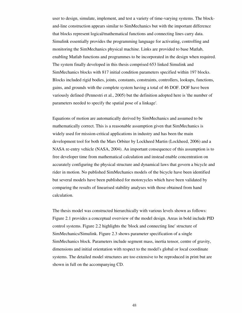
48

user to design, simulate, implement, and test a variety of time-varying systems. The block-

and-line construction appears similar to SimMechanics but with the important difference

that blocks represent logical/mathematical functions and connecting lines carry data.

Simulink essentially provides the programming language for activating, controlling and

monitoring the SimMechanics physical machine. Links are provided to base Matlab,

enabling Matlab functions and programmes to be incorporated in the design when required.

The system finally developed in this thesis comprised 653 linked Simulink and

SimMechanics blocks with 817 initial condition parameters specified within 197 blocks.

Blocks included rigid bodies, joints, constants, constraints, controllers, lookups, functions,

gains, and grounds with the complete system having a total of 46 DOF. DOF have been

variously defined (Pennestri et al., 2005) but the definition adopted here is 'the number of

parameters needed to specify the spatial pose of a linkage'.

Equations of motion are automatically derived by SimMechanics and assumed to be

mathematically correct. This is a reasonable assumption given that SimMechanics is

widely used for mission-critical applications in industry and has been the main

development tool for both the Mars Orbiter by Lockheed Martin (Lockheed, 2006) and a

NASA re-entry vehicle (NASA, 2004). An important consequence of this assumption is to

free developer time from mathematical calculation and instead enable concentration on

accurately configuring the physical structure and dynamical laws that govern a bicycle and

rider in motion. No published SimMechanics models of the bicycle have been identified

but several models have been published for motorcycles which have been validated by

comparing the results of linearised stability analyses with those obtained from hand

calculation.

The thesis model was constructed hierarchically with various levels shown as follows:

Figure 2.1 provides a conceptual overview of the model design. Areas in bold include PID

control systems. Figure 2.2 highlights the 'block and connecting line' structure of

SimMechanics/Simulink. Figure 2.3 shows parameter specification of a single

SimMechanics block. Parameters include segment mass, inertia tensor, centre of gravity,

dimensions and initial orientation with respect to the model's global or local coordinate

systems. The detailed model structures are too extensive to be reproduced in print but are

shown in full on the accompanying CD.

49

Figure 2.1 Conceptual design of the thesis model.

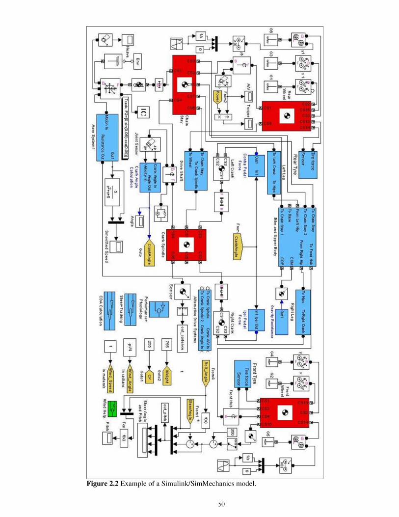
50

Figure 2.2 Example of a Simulink/SimMechanics model.

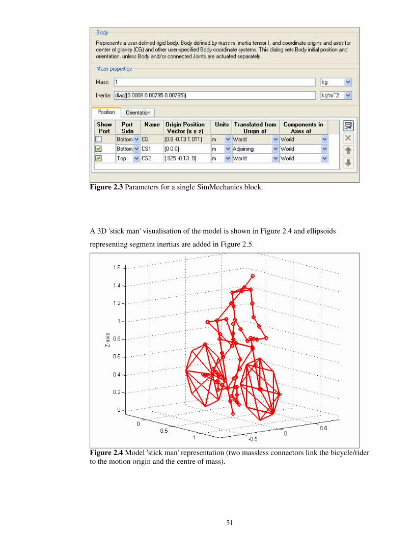
51

Figure 2.3 Parameters for a single SimMechanics block. A 3D 'stick man' visualisation of the model is shown in Figure 2.4 and ellipsoids

representing segment inertias are added in Figure 2.5.

Figure 2.4 Model 'stick man' representation (two massless connectors link the bicycle/rider to the motion origin and the centre of mass).

52

Figure 2.5 Model visualisation with ellipsoids representing segment inertias.

2.3 Bicycle Model

2.3.1 Configuration

The bicycle and rider were laterally symmetrical about the x-z plane with the left side

being defined as contra-lateral and the right side as ipsi-lateral. The bicycle reference

configuration was defined as stationary, upright, straight-ahead equilibrium with no

steering angle and the ipsi lateral crank arm pointing vertically upwards. The model was

configured with a globally-fixed right handed orthogonal coordinate system comprising

longitudinal x axis, lateral y axis and vertical z axis (Figure 2.6). The system viewed from

the rear in the reference configuration gave positive axis orientations of x = forward, y =

left and z = up.

53

Figure 2.6 Bicycle axes direction and orientation

A right handed steering axis was orientated positively upwards. A global coordinate

system was generally used to specify body locations although a local coordinate system

was used where it simplified the construction. The global origin was located at the rear

wheel/ground contact point for the convenience of making all system dimensions positive.

Gravity acted downwards at 9.81 ms-2. The bicycle had DOF for longitudinal, lateral and

vertical translation together with roll, yaw and pitch rotation. A 'motion origin' was defined

as the ensemble centre of mass (COM) in the reference configuration projected vertically

to the ground plane (x-y plane). Additional DOF were enabled for rotation of the steer axis,

chainring/cranks and both wheels (see Appendix 2 for axis orientations).

The ipsi lateral crank arm pointing vertically upwards was specified as zero degrees and

named 'top dead centre' (TDC). The ipsi lateral crank arm rotated clockwise through 360

degrees in a cycle with its position when pointing vertically downwards defined as 'bottom

dead centre' (BDC). A single COM was specified for the complete bicycle/rider and

located by application of a force balance. The longitudinal COM was found by balancing

the system about the z-axis. Gravity was then changed to act longitudinally and the system

re-balanced about the x-axis followed by iterative z-axis and x-axis balancing to arrive at a

54

stable COM. The centre of pressure (COP) was calculated using the SimMechanics

visualisation tool which displayed bicycle/rider frontal area. The frontal area was divided

into rider head, rider torso+arms and rider legs+bicycle. Each area was measured and input

to the following algorithm:

L L U U W W

L U W

A d A d A dCOP

A A A

+ +=

+ +

where COP was centre of pressure relative to COM, A was surface area, d was centre of

surface area vertical distance to COM and subscripts L, U and W represented the three

surface areas (http://www.grc.nasa.gov/WWW/K-12/airplane/bga.html) [Accessed 14

February 2009]. The COP, COM and motion origin were located in inertial space by means

of massless connectors linked to the bicycle frame.

2.3.2 Frame

The dimensions and mass of the bicycle were taken from measured values for a

commercially available bicycle which measured 59 cm vertically from the crank spindle to

the top tube (Figure 2.7). Pilot trials suggested that the choice of frame size had a small

effect on performance which was subsequently largely confirmed by the sensitivity

analysis conducted in Chapter 10. A larger than average frame size was selected in order to

emphasise any effects due to frame flex. A front and rear frame were specified separately

with the rear frame comprised of six rigid bodies modelled as tubes plus the rear wheel.

The front frame comprised handle bars, stem, fork and front wheel and was connected to

the rear frame by a steering joint with its axis inclined upwards at 72 degrees to the left

horizontal. Only one seat stay, chain stay and fork arm were modelled and placed on the

bicycle longitudinal centre line since SimMechanics allowed separate rigid bodies to

occupy the same physical space without penalty. The mass of each body was obtained by

weighing or by reference to the manufacturer's specifications. The inertia tensor of each

body was derived from its dimensions, mass and density using algorithms provided by

SimMechanics. Flexibility was built into the frame by enabling the steering joint to

additionally rotate about the longitudinal axis (x-axis). A spring/damper was placed on this

rotation axis to control the level of flex. The main bicycle parameters are listed in Table

2.3.

55

Figure 2.7 Bicycle structure Table 2.3 Bicycle parameters

Parameter Front Frame

Rear Frame

Complete Bicycle

Comment

No. of Bodies 5 11 16

Mass (kg) 2.8 5.9 8.7 includes accessories

Trail (m) 0.065

Steer Axis (°) 72

Wheel Radius (m) 0.35 0.35

Wheelbase (m) 1.01

COM (x,y,z) (m) (0.52, 0, 1.01) includes rider

COP (x,y,z) (m) (0.53, 0, 0.9) includes rider

2.3.3 Wheels

Both wheels were modelled as symmetrical knife-edge rigid discs rotating about a lateral

hub axis. The inertial mass of each wheel was distributed evenly between the hub and the

rim utilising SimMechanics algorithms for a rotating disc. Wheel rotation and translation

were related by a non-holonomic constraint which enforced pure rolling without slip.

Holonomic constraints controlled each wheel's relationship to the ground. In version V4

and V5, a sine function controlled wheel (and frame) vertical oscillation simulating road

surface and tyre vertical compliance. The tyres were not modelled in a physical sense but

56

the forces and torques generated by the front and rear tyre were derived analytically and

applied to the wheel hub (see Tyre Model, Chapter 5).

2.3.4 Wheel Stiffness

Wheel lateral flexibility was modelled by enabling additional hub rotation about the x-axis

with the level of flex being controlled by a spring/damper. Correctly modelling this feature

was important for bicycle performance as narrow rims and long spokes make bicycle

wheels particularly susceptible to lateral flex. This is evidenced by the front wheel rim

rubbing the brake blocks when pedalling out of the saddle (Tew and Sayers, 1999). Both

the vertical (z axis) and lateral (y axis) stiffness of bicycle wheels can affect performance

but anecdotal evidence from competitive cyclists suggests the latter is critical for fast

stable cornering (Roues Artisanales, 2008). Vertical compliance has been studied in detail

(Hull et al., 1996; Minguez and Vogwell, 2008; Redfield, 2005) but largely applied to the

rough surfaces encountered in mountain-bike cycling. The front and rear wheels lateral

stiffness was modelled separately to obtain the correct oversteer/understeer attitude when

cornering during the path-following task. A comprehensive analysis of lateral stiffness for

67 pairs of wheels (front and rear) covering most of the major wheel types/manufacturers

was conducted by Damon Rinard (www.sheldonbrown.com/rinard/wheel/index.htm)

[Accessed 5 April 2009]. Each wheel was held horizontally by the hub in a jig and

deflection at the unconstrained rim was measured when a weight representing typical

lateral force was applied vertically at four separate locations around the circumference.

Rear wheels were tested from both sides as stiffness was affected by the rear hub offset

that accommodated the cassette. Results from three widely used racing wheels that covered

a range of stiffness values are shown in Table 2.4. In addition, the linearity of rim

deflection was assessed using the default load of 115N and loads of ±10%. Deflection was

found to be predominantly linear within that force range (R2 = 0.98).

Table 2.4 Wheel rim deflection under 115 N load.

Bontrager

RaceLite

Campagnolo

Neucleon

Mavic

Kysirium

Mean

Deflection

Front Wheel Deflection (mm)

1.35 (24) 1.98 (22) 2.11 (18) 1.81

Rear Wheel Deflection (mm) 1.61 (28) 1.96 (24) 2.84 (20) 2.14

Notes. Number of wheel spokes shown in brackets. All rear values are mean of left side/right side deflection. Measurement error (SD) of ±0.05 mm.

57

The above values have been largely confirmed by a separate study which found a 1 mm

rim deflection in response to a 60 N lateral force for a wheel with 1.6 mm spokes, a '4x'

lacing pattern and a 795 mm4 lateral moment of inertia (Gavin, 1996).

Once wheel flexibility values had been obtained from the literature, the bicycle model was

modified to incorporate lateral wheel flex. It was implemented by the addition of an x axis

rotation to the wheel hub joint where previously only y axis rotation provided forward

rolling. A spring/damper was connected to the x axis rotation in order to implement the

required degree of wheel flex. A wheel model was fixed in a jig and spring/damper gains

obtained by applying a 155 N lateral force to the rim until the mean deflection from Table

2.4 was obtained. Damping values were set to give a force rise rate which reached steady

state in ~100 ms (Verma et al., 1980). A spring constant of 136 N/m and a damping

constant of 3 deg/s were obtained for the front wheel with the equivalent values for the rear

wheel being 116 N/m and 2.6 deg/s respectively. These values are considered to be

realistic as it has been shown in the tyre model (Chapter 5) that lateral force on a cornering

bicycle wheel is in the region of 60 N per degree of slip angle which is consistent with the

115 N applied in the above analysis.

2.3.5 Transmission

A laterally orientated crank spindle was located at the junction of the bicycle frame seat

tube and down tube (Figure 2.7) rotating about a lateral axis (y-axis). Crank arms were

welded at 90 degrees to each end of the crank spindle and orientated in 180 degrees

opposition. Conceptual pedals were positioned at the end of each crank arm but

incorporated in the foot. The drive transmission from the crank to the rear wheel was

physically modelled in versions V4 and V5 as follows: Gear wheels fitted to the crank

spindle and rear axle connected a rotating drive shaft running longitudinally from the crank

spindle to the rear axle. The drive shaft transmitted propulsive torque from the crank to the

rear wheel. The final drive ratio was defaulted to 2.86:1 although the numbers of teeth on

the gear wheels were adjustable to change the ratio. Frictional losses in the drive train were

not modelled. All model versions calculated power at the rear wheel in order to match the

great majority of field trials which measured power at the rear wheel. If transmission

friction loss is modelled in the future, it can be noted that a power loss of ~2.5% has been

proposed by Kyle (1988) while Martin et al. (2006) calculated a loss of 6 W at a mean

power output of 255 W.

58

2.3.6 Balance

The model included gravitational forces and therefore the bicycle had to be actively

controlled to remain upright (e.g. as for an inverted pendulum). Balance was maintained

with a proportional-integral-derivative (PID) controller that countered roll by applying a

steering torque in the direction of any fall. The resulting steering torque was then modified

by a second PID that ensured the bicycle tracked a defined path (see Path Tracking below).

2.3.7 Steering

Steering was modelled as a joint torque applied at the steering axis linking the front and

rear frames. The effects of the steering function were dependent on the front frame

geometry that primarily comprised the steering axis inclination (72 degrees), wheelbase

(1.01 m) and trail (0.065 m) and are shown in Figure 2.7. Trail was a critical parameter as

it regulated the roll and steer necessary to keep the bicycle upright due to its influence on

the degree of front-end pitch that occurred with steering (Roland,1973). Bicycle pitch due

to roll and steering was calculated in the model to check correct functioning of the steering

mechanism meeting the requirement for such analysis presented by Roland (1973).

2.4 Rider model

2.4.1 Structure

The rider was constructed from 14 rigid bodies as listed in Table 2.5 and graphically

presented in Figure 2.8. Generic body segment parameters were obtained from Slaughter

and Lohman (1976) with the exception of leg segments and inertias which were obtained

from a reference study (Redfield and Hull, 1986a). Simulations used these generic

parameters unless rider weight was varied to analytically calculate gravitational and tyre

resistance force. The pelvis was fixed to the top of the bicycle seat tube, the forearms to the

handle bars and the feet to the pedals. Segments were symmetrically distributed about the

sagittal plane. The leg and arm segments were linked by frictionless revolute joints

enabling rotation about the y-axis while the shoulders and hips which were modelled by

spherical joints. The rider torso had a rotational DOF about the pelvis (x axis rotation)

which was defined as 'lean' in contrast to 'roll' for the bicycle about the same axis. The foot

was assumed to be fixed to the pedal (via a cleat) and therefore the two bodies were

represented by a single segment linking the ankle joint to the crank arm.

59

Table 2.5 Generic rider body parameters

Segment Mass (kg) Length (m) Moment of Inertia (kg·m2)

(x y z axes) Foot + Pedal (2) 2.1 0.203 (0.0003 0.002 0.002)

Shank (2) 6.54 0.433 (0.0024 0.05413 0.05413)

Thigh (2) 14.72 0.393 (0.009 0.10183 0.10183)

Pelvis 0.5 0.26 (0.0012 0.0034 0.0034)

Torso 36.7 0.49 (0.16 1.02293 1.02293)

Shoulders 0.5 0.42 (0.0004 0.003 0.003)

Head 4.9 0.24 (0.02814 0.03282 0.03282)

Upper Arm (2) 4.1 0.28 (0.0008 0.00811 0.00811)

Lower Arm + Hand (2) 3.2 0.33 (0.0008 0.00795 0.00795) Trochanteric Length* 0.89 Hip to Crank (vertical) 0.693 Hip to Crank (horizontal) 0.212

Note: Total mass is shown for (2) segments while inertia is shown for a single segment. * distance from proximal aspect of greater trochanter to bottom of foot with leg straight.

Figure 2.8 Rider body segments.

60

2.4.2 Reference study

The dimensions and mass of each leg segment were important for pedalling simulation so

values were taken from a 'reference' study (Redfield and Hull, 1986a) and used in

simulations. Redfield and Hull (1986a) was defined as 'REF' since its data had been widely

used in bicycle pedalling studies (Hull and Jorge, 1985; Jorge and Hull, 1986; Redfield and

Hull 1986b). The REF study reported kinematic and kinetic pedalling data collected from

three experienced male cyclists who rode their own bicycles on rollers at a workrate of 200

W (two-legs) and a seated cadence of 80 rpm. Segment inertial data were determined

according to procedures outlined by Drillis and Contini (1966) while subject mass and

anthropometric data were taken from a representative subject in the study of Jorge and Hull

(1986). The REF study measured normal and tangential pedal forces in the sagittal plane

for one leg using an instrumented pedal and averaged the data over two trials. Associated

crank and pedal angles were simultaneously recorded by rotary potentiometers. Foot/pedal

angle was approximated to a sine wave by fitting the measured foot/pedal angle data to a

Fourier series. Segment acceleration was derived analytically from the crank motion, pedal

motion and leg geometry and then combined with pedal force and inertial data in an

inverse dynamics analysis to obtain ankle, knee and hip joint torques over a cycle. All the

above data was variously used in different model versions as reported below.

Body segment moments of inertia were reported about the lateral axis (y axis) by the

studies above. However, the 3D thesis model required an inertia tensor specified as a 3x3

matrix requiring a minimum of the three diagonal values (representing rotation about the

three principal axes). Diagonal values were therefore approximated geometrically using

ellipsoid algorithms available within SimMechanics and segment shape/volume/density

data from Hanavan (1964). These generic values were applied in all simulations.

2.4.3 Pedalling

Each leg together with the seat tube and crank arm was modelled as a closed-loop 5-bar

linkage with one DOF at the ankle and a common DOF at the crank spindle. The crank

angle in model versions V3 and V4 was a consequence of the propulsion method (rear hub

torque or pedal forces). The ankle angle ('ankling') in those versions was specified by an

interpolated lookup file that monitored foot/pedal orientation relative to the right horizontal

at each degree of crank rotation. Experimentally measured foot/pedal angle over a cycle

was digitised from the REF study to create the lookup file (Figure 2.9). The lookup file

defined the right foot/pedal angle at each crank angle with a mirrored left foot/pedal

lookup file offset by 180 degrees. A constraint placed across the ankle then obtained the

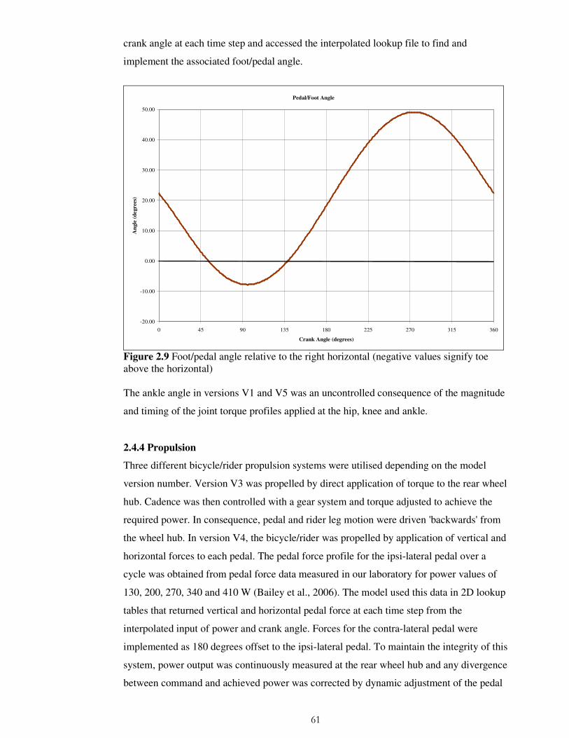
61

crank angle at each time step and accessed the interpolated lookup file to find and

implement the associated foot/pedal angle.

Pedal/Foot Angle

-20.00

-10.00

0.00

10.00

20.00

30.00

40.00

50.00

0 45 90 135 180 225 270 315 360

Crank Angle (degrees)

An

gle

(d

egree

s)

Figure 2.9 Foot/pedal angle relative to the right horizontal (negative values signify toe above the horizontal) The ankle angle in versions V1 and V5 was an uncontrolled consequence of the magnitude

and timing of the joint torque profiles applied at the hip, knee and ankle.

2.4.4 Propulsion

Three different bicycle/rider propulsion systems were utilised depending on the model

version number. Version V3 was propelled by direct application of torque to the rear wheel

hub. Cadence was then controlled with a gear system and torque adjusted to achieve the

required power. In consequence, pedal and rider leg motion were driven 'backwards' from

the wheel hub. In version V4, the bicycle/rider was propelled by application of vertical and

horizontal forces to each pedal. The pedal force profile for the ipsi-lateral pedal over a

cycle was obtained from pedal force data measured in our laboratory for power values of

130, 200, 270, 340 and 410 W (Bailey et al., 2006). The model used this data in 2D lookup

tables that returned vertical and horizontal pedal force at each time step from the

interpolated input of power and crank angle. Forces for the contra-lateral pedal were

implemented as 180 degrees offset to the ipsi-lateral pedal. To maintain the integrity of this

system, power output was continuously measured at the rear wheel hub and any divergence

between command and achieved power was corrected by dynamic adjustment of the pedal

62

forces. Thus while pedalling forces are normally a result of leg joint torques, in this model

the leg pedalling motion was driven by pedal forces. Finally, in version V5 bicycle/rider

propulsion was driven by leg joint torques as described for the static pedalling study in

Chapter 3.

2.4.5 Upper Body

A PID controlled upper body lean about the x-axis, synchronised in opposition to the

bicycle roll generated by pedalling. This maintained the ensemble COM above the

wheelbase (corrected for the effects of centripetal force). The extent of the lean was

estimated from a video filmed from behind a cyclist competing in a time trial. Upper body

rotations about the y-axis and z-axis and were not considered to be of sufficient magnitude

to require inclusion in the current model. The rider's arms were passively fixed to the

handlebars such that initial arm bend combined with spherical joints provided enough

tolerance to accommodate the lean and the steering.

2.4.6 Cadence

An analytical gear system was developed for version V3 which automatically maintained

cadence within a range of 80-100 rpm by varying the chainwheel/cassette sprocket ratio.

The system selected combinations from a 53/39 chainring and a 10-speed 12-27 sprocket

cassette that implemented a valid cadence in response to the balance of resistive and

propulsive forces at each time step (the gears were typical of those used by competitive

cyclists). The system started from rest in the small chainring (39) and the lowest sprocket

(27) and changed up/down through the sprockets and chainrings sequentially. The

chainring change logic is in Figure 2.10.

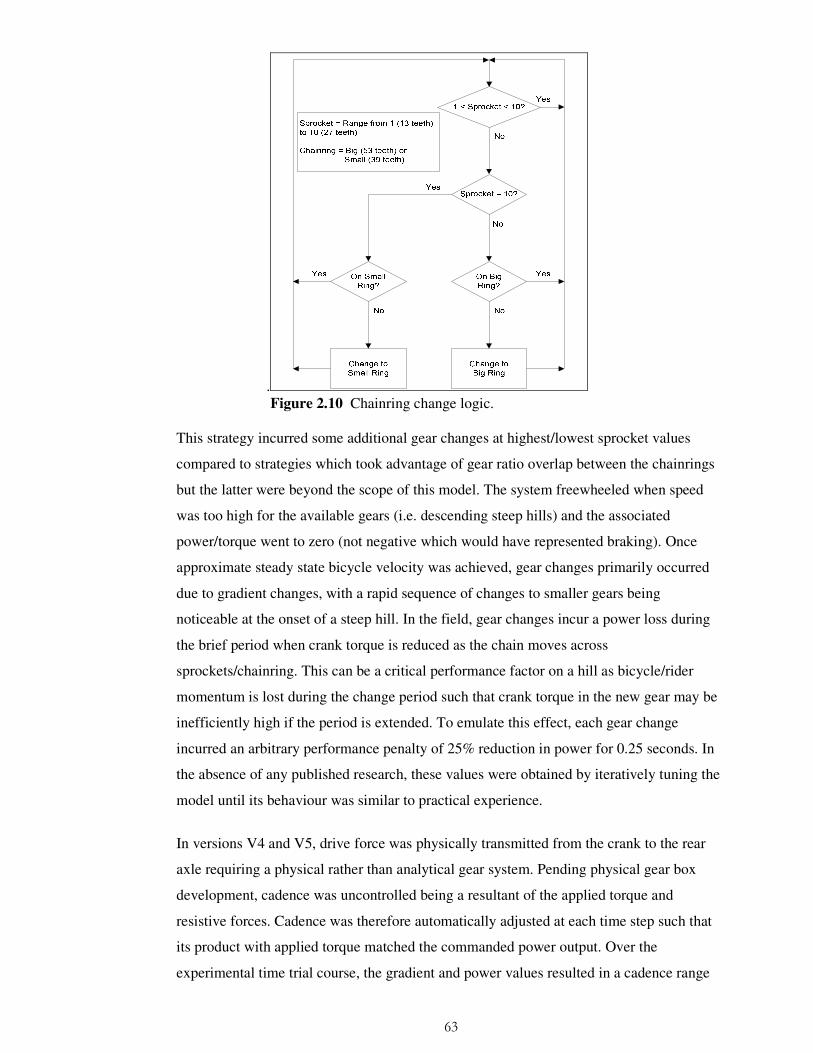
63

. Figure 2.10 Chainring change logic.

This strategy incurred some additional gear changes at highest/lowest sprocket values

compared to strategies which took advantage of gear ratio overlap between the chainrings

but the latter were beyond the scope of this model. The system freewheeled when speed

was too high for the available gears (i.e. descending steep hills) and the associated

power/torque went to zero (not negative which would have represented braking). Once

approximate steady state bicycle velocity was achieved, gear changes primarily occurred

due to gradient changes, with a rapid sequence of changes to smaller gears being

noticeable at the onset of a steep hill. In the field, gear changes incur a power loss during

the brief period when crank torque is reduced as the chain moves across

sprockets/chainring. This can be a critical performance factor on a hill as bicycle/rider

momentum is lost during the change period such that crank torque in the new gear may be

inefficiently high if the period is extended. To emulate this effect, each gear change

incurred an arbitrary performance penalty of 25% reduction in power for 0.25 seconds. In

the absence of any published research, these values were obtained by iteratively tuning the

model until its behaviour was similar to practical experience.

In versions V4 and V5, drive force was physically transmitted from the crank to the rear

axle requiring a physical rather than analytical gear system. Pending physical gear box

development, cadence was uncontrolled being a resultant of the applied torque and

resistive forces. Cadence was therefore automatically adjusted at each time step such that

its product with applied torque matched the commanded power output. Over the

experimental time trial course, the gradient and power values resulted in a cadence range

64

of 70 to 115 rpm. These values that were considered acceptable for a competitive cyclist.

An initial-condition velocity of 10 m/s was implemented in field trials to simulate a rolling

start.

2.5 Environment Modelling

2.5.1 Path tracking

Single track vehicle path tracking has been extensively studied in the literature (Popov et

al., 2010; Rowell et al., 2010; Sharp, 2007) and can be broadly divided into schemes that

apply 'compensatory tracking' or 'preview tracking'. The latter anticipates future road

direction and applies steering inputs in advance to minimise tracking error. The technique

is more complex but more accurate (Sharp, 2007) than compensatory tracking which

applies a corrective steering input only at the time a tracking error is identified. A simple

compensatory tracking scheme was used in the present model as low bicycle speed and fast

steering response resulted in minimal tracking error.

The control scheme for following the path track was as follows: A desired path was

marked on a digital map and converted to grid reference comprising easting and northing

coordinates at defined intervals along the path. These co-ordinates were then loaded into a

two column lookup file with longitudinal displacement from the start in column 1 and

associated lateral displacement in column 2. The compass heading (north, east, south or

west) closest to the intended bicycle start direction was defined as the map longitudinal (x)

axis and the orthogonal co-ordinate direction defined as the map lateral (y) axis.

SimMechanics initial conditions required that the bicycle pointed along the positive

bicycle longitudinal (x) axis (effectively due east). The map longitudinal axis was therefore

aligned with the bicycle longitudinal axis to minimise steering correction at simulation

start. At each time step, the model checked the bicycle longitudinal displacement and

found the interpolated longitudinal displacement in the lookup file. The bicycle lateral

displacement was then compared with the interpolated map lateral displacement and the

error generated corrective steering action.

Additionally, the height of easting/northing co-ordinates was required at each time step in

order to calculate the resistive force due to gravity. Initially these were obtained from

Ordinance Survey (Memory-Map Ltd, Aldermaston, UK) but it was found that this data

was insufficiently accurate. The resolution was 50 m horizontally and 10 m vertically with

intervening gradient estimated by linear interpolation. Height data obtained by laser aerial

65

mapping was therefore purchased (www.centremapslive.com) [Accessed 28 November

2009] with 5 m horizontal and 1 m vertical resolution.

The thesis model required a control scheme that responded to both tracking error and

bicycle roll in order to maintain the bicycle upright and follow the path. Studies have

specified rider lean as an important control variable for implementing a tracking task in

bicycle and motorcycle models (Weir, 1972; Peterson and Hubbard, 2008). However,

existing models have not included a pedalling cyclist and have therefore neglected the

bicycle roll and steer that occurs within a pedal cycle as a result of the offset pedal force

applied during the down-stroke. In road cycling, this roll is countered by rider lean and

steer with the resulting forces/motions generating an oscillatory path over a pedal cycle.

Additionally, side winds generate roll independent of rider action which must be countered

by steering input. It can be noted that small rider lateral weight shift on the saddle can steer

the bicycle in 'hands-off' riding (VanZytveld, 1975) but this was considered too specialised

for a general purpose model.

In the thesis model, steering input controlled roll to keep the bicycle upright by

maintaining the COM gravitational vector (as modified by centripetal force) above the

support line linking the front and rear tyre contact patches. Simultaneously, steering input

responded to path tracking error in order to implement path-following. This was

implemented via a PID controller that monitored the combined roll and tracking error and

calculated the necessary steering response. Identifying appropriate PID gain values was

critical in this process. Proportional gain was generally set low as only small steering angle

changes were required for quite large direction changes. Derivative gain was set high since

direction changes incurred considerable bicycle/rider oscillation unless strongly damped.

In model versions V2 and V3, the PID output activated steering angle. Steering angle

rather than steer torque was used in these versions as it resulted in lower tracking error

with no apparent unrealistic mechanical effects (the small kinematic effect of steering

torque on the rider's arms was ignored). Rider body lean was required to simply oppose the

bicycle roll generated by steering and thus maintain the ensemble COM above the wheel

base (allowing for centripetal effects). In model versions V4 and V5, PID output activated

steering torque. This method modelled bicycle velocity and turn radius more accurately

when following a circular path although its slower response generated a greater path-

following error. However, the numerical solver reduced the integration time step when the

66

error variance increased (primarily during cornering) and thus achieved a root mean

squared error (RMSE) between the actual and desired path that averaged less than 1 m.

2.5.2 General Resistive Forces

Aerodynamic and gradient resistances were modelled analytically (i.e. by Simulink

equations) and applied in the x-axis and y-axis of the global coordinate system at the

bicycle/rider COP (aerodynamic) and COM (gravitational). Rolling resistance was

incorporated in the tyre model, while inertial resistance due to acceleration required no

explicit modelling as it was applied implicitly by SimMechanics.

2.5.3 Aerodynamic resistance

The induced air flow due to bicycle motion was modified by both the speed and direction

of the environmental wind in order to calculate the apparent air flow. Apparent air flow

was resolved into x and y components before calculating the resistive forces applied to the

bicycle/rider COP with the following expression

2

2

0.5

0.5Ax x

Ay y

F p CDA V

F p CDA V

= ⋅ ⋅ ⋅

= ⋅ ⋅ ⋅ (1)

where the x and y subscripts denote the longitudinal and lateral axes respectively, FA was

the aerodynamic resistive force, V was the apparent air velocity, p was the air density and

CDA was the coefficient of drag area (drag multiplied by frontal area). Initial values were

set at p=1.22 kg.m3 (typical sea level) and CDA=0.3 which was typical for an average sized

cyclist on a road racing bicycle without tribars (Martin et al., 1998; Kyle, 1994).

CDA was estimated for individual participants in Chapters 7, 8 and 9. Frontal area was

calculated from regression equations based on height and weight (Heil, 2001; Heil, 2002).

Form drag was estimated from bike type defined as full T/T bike, road bike with tribars or

standard road bike (Bassett et al., 1999). It was assumed that bike type defined riding

position and that a full T/T bike included a rider with aerodynamic helmet and overshoes.

Any changes in surface drag were ignored as they have been shown to be a small

component of total drag (Brownlie et al., 2010; Gibertini et al., 2010). CDA was the

product of frontal area and form drag although the two were interdependent so no absolute

value for form drag was defined (Bassett et al., 1999). In all cases, the estimated CDA was

compared against experimental data present in Kyle (1994) to ensure that values were

realistic.

67

The CDA value was modified dynamically throughout a simulation due to changes in the

road/bicycle heading relative to the apparent air flow. Adjustments were those presented in

Martin et al. (1998). The air density was held constant as trials were conducted in similar

environmental conditions with respect to temperature, pressure and humidity (Olds et al.,

1995). The yaw angle of the bicycle from the right horizontal was monitored to ensure the

resistive forces were applied as values opposing motion.

2.5.4 Enviromental Wind

Environmental wind strength and direction were specified with initial values although

both could be varied during a trial if dynamically measured profiles were available. The

wind vector was resolved into x and y axis components with the following expressions

cos

sinW x W

W y W

V V W

V V W

θ

θ

= ⋅

= ⋅ (2)

where VW was the wind velocity and Wθ was the wind angle from the right horizontal. The

resolved components were then subtracted from the induced air velocities measured on the

x-axis and y-axis to arrive at the apparent air velocities for each axis. The model re-

calculated the effect of wind on apparent air velocity at each time step because the

bicycle/road direction changed continuously.

2.5.5 Gravitational Forces

SimMechanics allowed the road to be inclined such that the appropriate gravitational

forces were automatically applied physically. However, the gradient could not be changed

during a simulation making the method unrepresentative of a real road course. The gradient

changed frequently in the field trials so the component of the gravitational force which

aligned with the velocity vector of the cyclist/cycle ensemble was calculated analytically

and applied at each time step to determine the propulsive or retarding effect of gravity at

that instant. The following expression was used for the calculation:

sin(arctan( ))G RF M g G= ⋅ ⋅ (3)

where FG was the applied gravitational force, M was the ensemble mass, g was the

environmental gravitational force and GR the gradient as a decimal. The effect of gradient

on rolling resistance was considered negligible over the utilised courses and therefore

ignored. The bicycle/rider was not rotated about the y axis to reflect the slope of the

ground as the effect on pedalling has been found to be minimal (Caldwell et al., 1998). The

resistive force was resolved into x-axis and y-axis values and then applied in opposition to

the ensemble direction of travel at each time step.

68

2.5.6 Acceleration/Deceleration

Inertial resistance acts when the bicycle/rider accelerates or decelerates. It is measured as

the change in kinetic energy (KE) separated into a component arising from the

wheels/chainwheel rotation (KER) and a component arising from the translation of the

ensemble (KET) as follows:

2 2

2 2

1( )

21

( )2

T f i

R f i

KE m v v

KE I ω ω

∆ = −

∆ = −

(4)

where f subscript indicates final velocity, i subscript indicates initial velocity, I moment of

inertia and ω angular velocity. Under acceleration, additional power must be supplied by

the rider to increase KE which remains elevated until reduced by subsequent deceleration.

It can be noted that KE changes should be accounted-for in so-called 'steady-state' cycling

as power variations over a crank cycle continuously accelerate/decelerate the bicycle

(Hanson et al., 2002; Fregly et al., 1996). In addition, acceleration/deceleration is an

intrinsic feature of all cycling on the road due to the constant change (however small) in

one or more of the resistive forces (Atkinson et al., 2007c). All inertial forces were

internally computed and applied by SimMechanics from rigid body mass/velocity data

requiring no explicit programming.

2.6 Summary

This chapter describes the construction of a model that meets the requirements specified in

Chapter 1. The model combined a bicycle, rider and the environment in a single unified

structure in order to effectively represent road time trial cycling. The model was a

generalised tool built from first principles such that it could represent a wide range of

competitive riders and conditions. Simulations were implemented in forward dynamics

mode which reproduces real world conditions where input forces result in output motion.

Equations of motion were solved at <1 s intervals enabling the model to predict

performance at a frequency which closely simulated the constant change of conditions

occurring in field road cycling. The following chapters will validate this model against the

literature and field trials.

69

CHAPTER THREE

PEDALLING VALIDATION

3.1 Introduction

The purpose of this chapter is to asses the validity of the V1 version of the thesis model

(see Table 2.1). This version simulated a rider pedalling on a static bicycle which was

functionally equivalent to an ergometer. Redfield and Hull (1986a) (previously defined as

'REF') was used as the benchmark against which to assess the validity of the pedalling

component of the full thesis model. REF used pedal forces and crank torque obtained

experimentally as inputs to an inverse dynamics model that calculated leg joint torques.

The forward dynamics V1 model reversed this process by inputting these joint torques and

outputting the resulting pedal forces and crank torque. Model validity was quantified by

tracking the error between the V1 model outputs and the REF inputs over a pedal cycle.

The concept of validating a forward dynamics human movement model by tracking its

outputs against equivalent values obtained from an experimental inverse dynamics analysis

is well established (Neptune and Hull, 1998; Pandy, 2001; Otten, 2003; Zajac et al., 2003;

Erdemir et al., 2007; Buchanan et al., 2004). The outputs of other studies that measured

pedal forces and crank torque generated by pedalling were also examined to confirm that

the REF study was representative.

Most pedalling model validity studies have utilised one of two approaches: either 1) a

forward dynamics model where the activation of muscles (or joint torques) is propagated

forward to yield pedal forces which are compared with empirical data; or 2) the alternative

inverse dynamics methodology where pedal force and limb motion are measured

experimentally and propagated 'backwards' to obtain net joint torques. A forward dynamics

model has the advantage of being able to predict outcomes for novel conditions whereas an

inverse dynamics analysis is essentially descriptive of a specific condition (Olds, 2001).

The typical structure of a forward dynamics model is shown in Figure 3.1 and that model

was employed here, but without the muscle activation phase since muscle physiology and

mechanics was outside the scope of this investigation.

Figure 3.1 Forward dynamics methodology applied to pedalling

70

3.2 Validity Definition

Pedalling validation studies are rare in the literature, making it necessary also to consider

studies examining motor control mechanisms in human movement where the underlying

principles are similar (primarily neural strategies to coordinate muscle activation). The

utility of a model depends on its validity but no 'gold standard' has been identified for the

validation of musculo-skeletal models and there is little agreement on either the model

outputs that should be compared with experimental data or the level of convergence

between the two data sets that confers validity. Studies have utilised root mean squared

error (RMSE), coefficients of determination (linear regression) and standard deviations

(SD) to compare model and experimental data. Subjective judgment based on visual

examination of graphs is sometimes used as a validation method. For example, a vertical

jump study (Seth and Pandy, 2004) used joint torques obtained from an experimental

inverse dynamics analysis as the input to two different types of forward dynamics model to

compare their respective ground reaction forces (GRF). Results were not quantified, but

presented qualitatively with comments such as "the tracking results reproduced the desired

GRF's with good accuracy" (Seth and Pandy, 2004, page 3) combined with reference to

descriptive graphs rather than to specific numerical data.

Even where quantitative results were presented, the imprecision of 'validity' remained due

to the lack of an established criterion. For example, a study examining elbow flexion

compared a three-muscle forward dynamics model prediction of elbow joint torque with an

experimental inverse dynamics computation (Challis and Kerwin, 1994). The model was

considered valid when an apparent 5.5% RMSE was obtained. A visual examination of the

presented graphs suggested an error nearer 10% using an RMSE normalised to the data

range (NRMSE) (Cahouet et al., 2002). In a subsequent study (Challis, 1997), the previous

model was claimed as valid because the RMSE percentage was smaller than the inherent

error of an inverse dynamics analysis. However, no evidence was presented of inverse

dynamics error levels or why a lower error level should confer validity. A similar lack of

validity 'standards' was apparent in a study by Seth and Pandy (2007) who examined joint

torques in a vertical jump computed by various methodologies. These authors decided that

the criterion values (described as 'actual') should be those predicted by a forward dynamics

parameter optimisation model. Declaring model derived data to be a criterion is unusual,

certainly in respect of joint torques where the baseline is usually derived from inverse

dynamics analysis of experimental data. However, as noted by Seth and Pandy (2007), the

inherent error of inverse dynamics (Runge et al., 1995; Risher et al., 1997; Kuo, 1998;

71

Silva and Ambrosio, 2004)) does not necessarily confer any greater validity than a forward

dynamics parameter optimisation approach.

Standard deviation has also been used as a validity measure. For example, a recumbent

pedalling study compared pedal forces, joint moments and crank torque predicted by a

forward dynamics model with data computed by inverse dynamics analysis of

experimental data for sixteen subjects (Hakansson and Hull, 2007). A tracking method was

employed where the model muscle activation was optimised to minimise the RMSE

between the model and experimental results. The model was considered valid if one or less

standard deviations separated the model data from the mean experimental values but no

RMSE values were reported. Thelen et al. (2003) validated a forward dynamics model

against experimental data by reporting both standard deviation and RMSE in a pedalling

study that examined tangential and radial pedal forces. They considered their model to be

valid when model values were within 1 SD of experimental data and also reported absolute

RMSE values of 17 N and 37 N respectively for the two pedal force vectors. However

RMSE values in isolation give little indication of validity and NRMSE values were not

presented. Calculating NRMSE by estimation from the presented graphs suggests values of

approximately 4% and 9% respectively which could therefore be taken to indicate a valid

model in the view of Thelen et al. (2003).

Validation based on linear regression analysis between experimental data and model

results has been utilised in a number of modelling studies. Lloyd and Besier (2003)

investigated knee torque in a running study where experimental values calculated from

inverse dynamics were compared to the predictions of an EMG based forward dynamics

model. A coefficient of determination (R2) of ~0.95 was reported for a representative

subject with a slope of ~0.93 and a y intercept of ~3.1 N.m. A 'mean residual error' was

also calculated to indicate the magnitude of the residual error about the least squares

regression line although the term was not defined and would likely be zero if interpreted

literally. Reported error values for knee torque were 4.9 - 7.8 N.m suggesting that RMSE

was actually being measured. Residual scatter should perhaps be termed 'standard error of

the estimate' (SEE) rather than RSME although the two are functionally equivalent here.

Calculating NRMSE from the presented graphs in order to enable comparison with other

studies suggests values of approximately 4% to 5%, adding to the evidence that values near

this level are required for support of validity.

72

A gait study also used regression analysis to quantify validity by comparing joint torques

computed by an EMG-driven forward dynamics model with values derived from an

experimental inverse dynamics approach (White and Winter, 1992). Coefficients of

determination ranged from 0.72 to 0.97 for the ankle, knee and hip joints. The authors

showed a more comprehensive approach to model validation by reporting RMSE values of

10 to 20 N.m and NRMSE values of 23% to 72%. The authors speculated that the

divergence could result from erroneous inverse dynamics calculations and/or inaccurate

equations contained in the model but despite the high error levels they still declared "the

closeness with which the joint moment curves matched in the present study supports using

the modelling approach" (White and Winter, 1992, page 1). The low coefficients and the

high NRMSE values make this assertion questionable.

Another gait study (Buchanan et al., 2005) presented what they characterised as a 'hybrid'

approach where joint moments from an inverse dynamics analysis were compared with the

predictions of a forward dynamics model. Muscle parameters in the forward dynamics

model were adjusted until convergence was achieved with the inverse dynamics calculated

values. If the parameters in this calibration process remained physiologically reasonable,

the forward dynamics model could then be used to predict joint torques when completely

novel tasks were undertaken (although only for individuals with similar characteristics).

This was confirmed when the model predicted ankle moments against experimental data

with an RMSE of 7.1 N.m and an R2 value of 0.94. The two data sets closely tracked a

presented graph and the NRMSE could be estimated from the graph at 9%.

Forward dynamics models of conventional bicycle pedalling are rare and only one has

been identified that quantified model validation. Neptune and Hull (1998) developed a

pedalling model driven by 15 muscle actuators per leg at a cadence of 90 rpm and a

workrate of 225 W. Muscle activation was optimised to minimise a composite of the

tracking error for horizontal/vertical pedal forces, crank torque and net leg joint torques.

Experimental data for the comparison was obtained from 6 experienced cyclists riding their

own bicycles on an ergometer. Tracking error (referred to as RMS in the study) was

calculated as a composite value, being the sum of the squared residuals for each tracked

quantity normalised by the inter-subject variability for that quantity. The reported results

relevant to validation showed that model force and torque data were 'almost always' within

1 SD of experimental data. Digitisation of presented graphs should have enabled RMSE

and NRMSE to be calculated, but unfortunately only tracking error quantities were shown

which could not be re-processed.

73

In summary, the consensus of human movement modelling studies would suggest that a

forward dynamics model can be considered valid if it tracks experimental data with

standard deviation ≤1SD, coefficient of determination R2 >0.95 or NRMSE <10%. Those

values were therefore adopted as the validity benchmarks for this chapter. The aim of the

chapter was to establish if the pedal forces/crank torque predicted by the V1 model met

one or more of the validity measures when compared to the REF values.

3.3 Methods

3.3.1 Model Specification

A 3D model comprising rider pelvis, leg segments, bicycle seat tube and cranks was

constructed utilising the geometry and parameters specified in sections 2.3 and 2.4 which

were considered typical for a competitive cyclist (Redfield and Hull, 1986a). A single body

fixed in the global reference frame represented the bicycle seat tube. Lateral bodies at the

lower and upper ends of the seat tube represented the crank spindle and rider hips

respectively. The left and right legs were represented by four segments (thigh, shank,

combined foot/pedal and crank arm) linked to the common seat tube by the crank spindle

and rider pelvis. Viewed from the side, each leg therefore operated as a closed loop five-

bar planar linkage constrained to move in the sagittal plane (Figure 3.2). Frictionless

revolute joints linked the segments of each leg at the hip, knee, ankle, pedal spindle and

crank spindle. The right and left crank arms were fixed to the crank spindle with 'weld'

joints but with 180 degree opposed orientation. The seat tube length was set to

geometrically prevent knee hyperextension when the pedal was at the lowest point in its

trajectory while allowing for an 'ankling' motion.

Figure 3.2 Visualisation of pedalling model at TDC.

74

This system had three DOF: one for each ankle angle and one being a common crank

angle. Simulations started from the reference configuration. The model was activated by

hip, knee and ankle torque profiles obtained from the REF study and a resistive torque and

gear ratio was applied to achieve performance consistent with the REF study (200 W and

80 rpm). In emulation of the REF, all inputs and outputs in this evaluation related to the

ipsi-lateral leg unless otherwise specified. Control strategy for the contra-lateral leg was

applied symmetrically but 180 degrees out-of-phase. To confirm the REF study as

representative, similar inverse dynamics pedalling studies were identified (Table 3.1) and

their kinematic and kinetic profiles compared with the REF. Tracked quantities for

validation were:

• Pedal force (horizontal and vertical) over a cycle

• Crank torque over a cycle.

Table 3.1 Summary of pedalling models in the literature that reported forces and torques.

ID Study Power (W) Cadence

(rpm) Comment

REF Redfield and Hull (1986a) 200 80 REF study

Hull Hull and Jorge (1985) 200 80 **

Redfield Redfield and Hull (1986b) 196 100 No ankle data

Fregly Fregly et al. (1996) 225 75 Hip and ankle signs reversed

Smak Smak et al. (1999) 250 120 Hip and ankle signs reversed

Coyle Kautz et al. (1991) 250 90 Pedal forces only

Stone Stone and Hull (1995) 300 84 Pedal forces only

Kautz Kautz and Hull (1993) 250 90 Pedal forces only

Neptune Neptune and Hull (1998) 225 90

** Ankle, knee and hip positive and negative directions of rotation are reversed from the published data to provide a consistent presentation in this study

3.3.2 Assumptions and Approximations

The REF study assumed the pelvis was fixed immovably to the seat tube and the model

reproduced this assumption to enable the comparison. In reality, at medium to high

intensities, some 3% of total power can be transferred from the upper body to the legs

through pelvis rotation (Van Ingen Schenau et al., 1990). It was considered that the

resulting error in joint torque calculation was a reasonable approximation given the likely

minimal effect on speed over a time trial course which was the relevant objective of the

thesis model. The same conclusion was reached by Neptune and Hull (1995) in their

similar study.

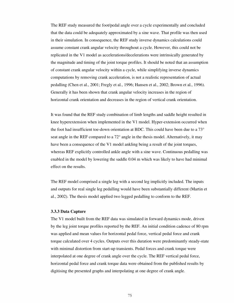
75

The REF study measured the foot/pedal angle over a cycle experimentally and concluded

that the data could be adequately approximated by a sine wave. That profile was then used

in their simulation. In consequence, the REF study inverse dynamics calculations could

assume constant crank angular velocity throughout a cycle. However, this could not be

replicated in the V1 model as accelerations/decelerations were intrinsically generated by

the magnitude and timing of the joint torque profiles. It should be noted that an assumption

of constant crank angular velocity within a cycle, while simplifying inverse dynamics

computations by removing crank acceleration, is not a realistic representation of actual

pedalling (Chen et al., 2001; Fregly et al., 1996; Hansen et al., 2002; Brown et al., 1996).

Generally it has been shown that crank angular velocity increases in the region of

horizontal crank orientation and decreases in the region of vertical crank orientation.

It was found that the REF study combination of limb lengths and saddle height resulted in

knee hyperextension when implemented in the V1 model. Hyper-extension occurred when

the foot had insufficient toe-down orientation at BDC. This could have been due to a 73°

seat angle in the REF compared to a 72° angle in the thesis model. Alternatively, it may

have been a consequence of the V1 model ankling being a result of the joint torques,

whereas REF explicitly controlled ankle angle with a sine wave. Continuous pedalling was

enabled in the model by lowering the saddle 0.04 m which was likely to have had minimal

effect on the results.

The REF model comprised a single leg with a second leg implicitly included. The inputs

and outputs for real single leg pedalling would have been substantially different (Martin et

al., 2002). The thesis model applied two legged pedalling to conform to the REF.

3.3.3 Data Capture

The V1 model built from the REF data was simulated in forward dynamics mode, driven

by the leg joint torque profiles reported by the REF. An initial condition cadence of 80 rpm

was applied and mean values for horizontal pedal force, vertical pedal force and crank

torque calculated over 4 cycles. Outputs over this duration were predominantly steady-state

with minimal distortion from start-up transients. Pedal forces and crank torque were

interpolated at one degree of crank angle over the cycle. The REF vertical pedal force,

horizontal pedal force and crank torque data were obtained from the published results by

digitising the presented graphs and interpolating at one degree of crank angle.

76

3.3.4 Data Analysis

A tracking problem was defined to compare the pedal forces and crank torque output by

the model against the equivalent experimental data that formed the input to the REF study.

The model and REF data were examined to establish their difference at each one degree of

crank angle and a quantity computed that represented that difference over the cycle.

Differences were expressed as absolute RMSE, normalised NRMSE, area under the curve

(AUC) and simple arithmetic mean (Mean). AUC values represented the impulse over the

duration of the simulation. For AUC and Mean, horizontal pedal forces were treated as

absolute (eliminating a zero sum) and percentage variance quantified the V1 model relative

to the REF. The use of AUC and Mean data enables insights that are concealed by the

'directionless' nature of RMSE and NRMSE values. RMSE was computed from the

following expression:

21 20

1( ( ) ( ))

T

RMSE M t M t dtT

= −∫

where 1M is the REF data, 2M is the model data, t is the time step and T is the total

simulation time. NRMSE was calculated by normalising RMSE with respect to the mean

of the range of values for each contributing data set as follows:

( )

21 20

2

0 01

1( ( ) ( ))

100%1

( ( ( )) ( ( )))2

T

i ii

M t M t dtT

NRMSE

Max t T M t Min t T M t=

−

= ×

< < − < <

∫

∑

where Max0 and Min0 are functions that identify the maximum and minimum values in a

data set.

A linear regression analysis compared the REF and model crank torque as an additional

method of quantifying the tracking error. Coefficient of determination (R2), regression

slope and y intercept were calculated to quantify the level of convergence.

3.4 Results

A model simulation over 4 cycles was driven by the REF joint torques and resulted in

mean power of 207 W and mean cadence of 78 rpm. The results of the comparison

between the model and the REF relating to pedal forces and crank torque are shown in

Table 3.2.

77

Table 3.2. Model pedal force and crank torque compared to the REF study.

Error AUC Mean

RMSE NRMSE REF Model ∆ REF. Model ∆

Horizontal Pedal (N)

All 15.4 8.8% |20,982| |23,982| +14.3% |52.6| |64.7| +23%

Fwd. 17.8 10.1% 11,106 12,952 +16.7% 64.5 81.1 +26%

Back 12.1 6.9% -9,874 -11,026 +13.5% -40.7 -48.3 +9%

Vertical Pedal (N)

Down 25.5 9.5% -43,156 -45,051 +4.4% -119.7 -125 +4%

Crank Torque (N.m)

Net Propulsion

2.6 4.9% 5,426 5,312 -2.1% 15 14.7 -2%

Positive 2.8 5.2% 5,731 5,699 -0.6% 19.7 19.6 -0.5%

Negative 1.8 3.4% -305 -382 +25.3% -4.4 -5.5 +25%

Note. ∆ = difference of the model relative to the REF. Absolute values indicate that negative values have been summed as positive.

3.4.1 Pedal Forces

The total horizontal pedal force NRMSE was 8.8%, which the AUC and Mean positive

differences showed was due to greater positive force production by the model than the

REF. The graph in Figure 3.3 shows a divergence in the rearwards pedal force of the model

shortly after BDC which was not present in the REF. The vertical pedal force NRMSE of

9.5% was entirely in the downwards direction with the AUC and Mean positive differences

showing a greater force from the model than the REF. A similar divergence just before

BDC can be seen in the graph at Figure 3.4.

3.4.2 Crank Torque

The crank torque NRMSE was 4.9% of net propulsion which the AUC and Mean negative

differences (-2.1% and -2% respectively) showed was primarily due to the model torque

being less than the REF. The negative torque (i.e. counter-rotational torque) of both model

and REF during part of the recovery showed that the ascending leg did not ascend fast

enough or rested on the crank or resisted crank rotation (Figure 3.5). The peak torque

during the down-stroke (Figure 3.5) was also somewhat less in the model than the REF

which is consistent with the model positive AUC being slightly below the reference (Table

3.2). The model two-leg crank torque (inset to Figure 3.5) showed two peaks similar in

78

magnitude to the single-leg profile and demonstrated that two legs eliminated the

occurrence of negative torque at the crank.

Horizontal Pedal Force

-100.00

-50.00

0.00

50.00

100.00

150.00

0.00 45.00 90.00 135.00 180.00 225.00 270.00 315.00 360.00


Fo

rce

(N)

Kautz

Reference

Coyle

Smak

Stone

Model

Neptune

Figure 3.3 Horizontal pedal force against crank angle reported by the model and the literature.

Vertical Pedal Force

-500.00

-400.00

-300.00

-200.00

-100.00

0.00

100.00

0.00 45.00 90.00 135.00 180.00 225.00 270.00 315.00 360.00


Fo

rce

(N)

Kautz

Reference

Coyle

Smak

Stone

Model

Neptune

Figure 3.4 Vertical pedal force against crank angle reported by the model and the literature.

79

-20.00

-10.00

0.00

10.00

20.00

30.00

40.00

50.00

60.00

0.00 45.00 90.00 135.00 180.00 225.00 270.00 315.00 360.00


To

rqu

e (

N.m

) Reference

Redfield

Hull

Smak

Coyle

Neptune

Model

0

5

10

15

20

25

30

35

40

45

0 45 90 135 180 225 270 315 360


Torq

ue

(N.m

)

Figure 3.5 Crank torque against crank angle reported by the model and the literature. (Inset: model two-leg crank torque)

A crank torque regression analysis between the REF and the model produced a coefficient

of determination (R2) of 0.974 (Figure 3.6). The slope of 0.972 and the y intercept of 0.1

indicated close equivalence between the two data sets.

y = 0.972x + 0.1043

R2 = 0.9739

-10.00

0.00

10.00

20.00

30.00

40.00

50.00

-10.00 0.00 10.00 20.00 30.00 40.00 50.00

Reference Torque (N.m)

Mod

el

Torq

ue

(N.m

)

Figure 3.6 Regression analysis of REF and model crank torque.

80

3.5 Discussion

The purpose of this chapter was to validate version V1 of the forward dynamics thesis

model by comparing its output data with experimentally derived input data presented in an

inverse dynamics REF study. Validating the output data of a forward dynamics human

movement model against input data from an experimental inverse dynamics analysis is

well established in the literature (Neptune and Hull, 1998; Pandy, 2001; Otten, 2003; Zajac

et al., 2003; Erdemir et al., 2007; Buchanan et al., 2004). The aim was achieved with the

error levels between the thesis and REF models being within the ranges widely accepted in

the literature. The model simulation generated power output of 207 W and cadence of 78

rpm which were similar to the REF values of 200 W and 80 rpm. The model pedal force

and crank torque profiles were qualitatively similar to the REF and related studies in

respect of profile phasing and amplitude. In particular, the horizontal pedal force exhibited

the characteristic positive values required for the foot to rotate the crank forward through

TDC and negative values to rotate the crank rearwards through BDC. The vertical pedal

force showed a negative peak at ~100 degrees of crank rotation which was consistent with

the peak effective force of the other studies shown in Figure 3.4. However, the model

predicted a second and larger negative peak at ~155 degrees which may be an artefact of

the variance in crank angular velocity discussed below. A similar uncharacteristic

deviation was seen in the horizontal pedal force at ~200 degrees which may be attributable

to the same cause. Both these artefacts were however attenuated in the resulting crank

torque profile. Error levels could be partly attributable to the imprecision inherent to the

inverse dynamic method employed by the REF. Further error factors are discussed below.

The model predicted no positive vertical force during recovery indicating minimal 'pulling-

up'. This finding was in agreement with the REF and the majority of experimental studies,

although positive crank torques throughout the pedal cycle have been found experimentally

at high workrates (Coyle et al, 1991), or predicted by single-leg models configured to

optimise performance (Redfield and Hull, 1986a; Kautz and Hull, 1995). Pedal forces and

crank torques from the other similar studies listed in Table 3.1 are plotted in Figures 3.3 -

3.5 and show that the REF model was generally representative.

Crank torque was derived from pedal forces and was, therefore, arguably the best

representation of the effect of varying leg joint torques in pedalling. Crank torque NRMSE

was lower than that of the pedal forces, which may reflect more effective pedal force

orientation by the model. The model crank torque profile (Figure 3.5) showed good

81

equivalence to the REF study in respect of the key values of peak torque (~42 N.m) and the

crank angle at which it occurred (~90 degrees). The model crank torque profile was also

consistent with the other experimental studies (Table 3.2) which were conducted at similar

intensities of 200-250 W and 80-90 rpm. Interestingly, all the graphs of torque profiles

showed between 6 N.m and 17 N.m of negative torque during recovery indicating counter-

rotational crank torque during that period. Detailed analysis of single leg crank torque is

perhaps unnecessary as two leg pedalling eliminates negative crank torque (Bertucci et al.,

2005; Caldwell et al., 1998; Hansen et al., 2002) such that the positive/negative inertial,

gravitational and muscular contributions attributable to either leg are difficult to

distinguish. To confirm the elimination of negative crank torque, the combined crank

torque was predicted by the model (insert to Figure 3.5) and the resulting

amplitude/phasing was found to be similar to the profiles reported by Hull et al.(1992),

Kautz and Neptune (2002) and Broker (2003) (Figure 3.7).

Figure 3.7 Crank two-leg pedalling torque profile at 350W and 90 rpm (Broker, 2003).

A central issue for quantitative model validation was identification of the appropriate

quantities to be measured and the level that indicated acceptable validity. There is rarely an

absolute answer to these questions and therefore a judgement on validity largely depends

on comparison between present error levels and error levels considered acceptable in

previous work. A literature review suggested that to achieve validity, the model should

meet one or more of the following criteria: (1) model predictions within 1 SD of

experimental results, (2) a coefficient of determination between model and experiment

>0.95, (3) an NRMSE <10%. AUC was also introduced as a relevant validity measure.

Comparing model results against the REF, a regression analysis of crank torque indicated

82

validity with an R2 value of 0.97 while the slope of 0.972 plus the y intercept of 0.1 also

indicated almost complete equivalence between the two data sets. Considering NRMSE,

the vertical and horizontal pedal forces can be considered valid at 8-9% while the crank

torque showed excellent validity with an NRMSE of 4%. The AUC results reinforce the

NRMSE results in respect of the amplitude and direction of variances between the model

and REF. No standard deviation comparison was made as the REF study only reported on a

single subject. This might be seen as a limitation although it has been suggested that a

single subject is appropriate in validation studies when the objective is to compare outputs

between two methods using identical inputs rather than to establish a general pattern of

pedalling forces and torques (Heintz and Gutierrez-Farewik, 2007).

It should be noted that extensive parameter manipulation was not required to achieve the

convergence presented above. This contrasts with some forward dynamics muscle models

where up to 59 parameters had been extensively tuned (Heine et al., 2003). The only

parameters adjusted to minimise tracking error were the crank resistance force and gear

ratio in order to achieve the target performance of 200 W and 80 rpm from the given joint

torque inputs. During cycling in the field, this resistance would result from the wind,

rolling and gradient resistances acting against the bicycle/rider.

When examining the V1 model error level presented above, it is of value to consider the

'acceptable' error level reported by other pedalling studies that constructed a model and

compared results with experimental data. The REF study itself developed a joint moment

optimisation model and compared the resulting pedal forces with their experimental data.

The difference between the model predicted and actual forces was termed the 'error'. The

REF did not itself conduct an NRMSE analysis, but NRMSE was calculated by digitising a

REF graph which resulted in an approximate 19% error for horizontal forces and

approximate 16% error for vertical forces (compared to values of 10.1% and 9.5%

respectively in the thesis model) (Figures 3.8 and 3.9). The REF pedal force comparison

was not specifically intended for validation purposes, but the error levels of 19% and 16%

were clearly considered to be acceptable with the first characterised as "a good comparison

of actual and computed pedal force profiles" (Redfield and Hull, 1986a, page 10) and the

second presented as "the vertical profiles give excellent agreement" (Redfield and Hull,

1986a, page 10). Causes of inverse dynamics modelling errors are discussed below.

83

0 90 180 270 360-100

-50

0

50

100

150


Fo

rce

(N

)

Experimental Data Set

Modelled Data Set

Figure 3.8 Horizontal pedal force against crank angle. Comparison of modelled and experimental data in the REF study (for graph clarity, the model forces shown in Figure 3.3 are not reproduced here).

0 90 180 270 360-350

-300

-250

-200

-150

-100

-50

0

50

100

150


Fo

rce

(N

)

Experimental Data Set

Modelled Data Set

Figure 3.9 Vertical pedal force against crank angle. Comparison of modelled and experimental data in the REF study (for graph clarity, the model forces shown in Figure 3.4 are not reproduced here). .

A similar pattern was seen in the forward dynamics pedalling model of Neptune and Hull

(1998) which was close to the design of the V1 model. The study measured six subjects

and found model force/torque outputs matched the experimental results ±1 SD. To relate

these findings to the current study, the pedal force graphs were digitised (Figure 3.10) and

the NRMSE calculated giving an approximate horizontal error of 6% and an approximate

84

vertical error of 7%. The authors presented this error level as "a pedalling simulation in

close agreement with the experimental data" (Neptune and Hull, 1998, page 6) and

"success of the model in reproducing the experimental pedalling mechanics" (Neptune and

Hull, 1998, page 6). This suggests a similar validity for the V1 model as the equivalent

NRMSE errors were 8.8% and 9.5%. The most likely explanation for differences in the

results is the measurement error of the instrumented pedals used in the experimental trials

(Challis and Kerwin, 1996).

Figure 3.10 Comparison of model and experimental data for horizontal and vertical pedal force in Neptune and Hull (1998).

A final assessment of the V1 model validity can be made by comparing the seven crank

torque profiles included in Figure 3.5 even though they are not all exact equivalents for

workrate/cadence. If it is assumed that the peak torque value is representative of the

complete torque profile, the mean ±SD value for all seven profiles in Figure 3.5 is 49±8

N.m. This level of standard deviation in pedalling torque is similar to that seen in other

studies reporting a similar mean torque (Neptune and Hull, 1998 = 47±12; Neptune and

Hull, 1999 = 50±6; Bertucci et al., 2005 = 49±8). The spread of torque profiles in Figure

3.5 are therefore predominantly within the range of variability expected from normal

experimental sampling error, suggesting that the 'oscillations' in the model torque profile

are not significant.

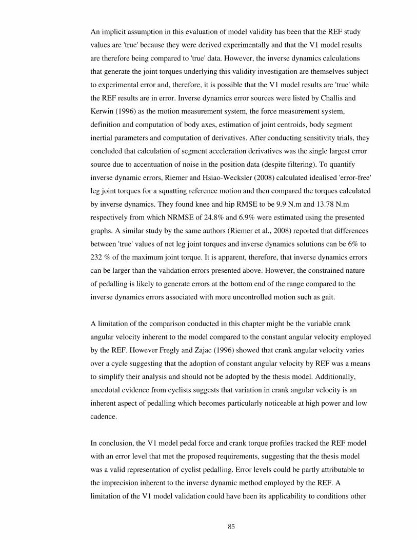
85

An implicit assumption in this evaluation of model validity has been that the REF study

values are 'true' because they were derived experimentally and that the V1 model results

are therefore being compared to 'true' data. However, the inverse dynamics calculations

that generate the joint torques underlying this validity investigation are themselves subject

to experimental error and, therefore, it is possible that the V1 model results are 'true' while

the REF results are in error. Inverse dynamics error sources were listed by Challis and

Kerwin (1996) as the motion measurement system, the force measurement system,

definition and computation of body axes, estimation of joint centroids, body segment

inertial parameters and computation of derivatives. After conducting sensitivity trials, they

concluded that calculation of segment acceleration derivatives was the single largest error

source due to accentuation of noise in the position data (despite filtering). To quantify

inverse dynamic errors, Riemer and Hsiao-Wecksler (2008) calculated idealised 'error-free'

leg joint torques for a squatting reference motion and then compared the torques calculated

by inverse dynamics. They found knee and hip RMSE to be 9.9 N.m and 13.78 N.m

respectively from which NRMSE of 24.8% and 6.9% were estimated using the presented

graphs. A similar study by the same authors (Riemer et al., 2008) reported that differences

between 'true' values of net leg joint torques and inverse dynamics solutions can be 6% to

232 % of the maximum joint torque. It is apparent, therefore, that inverse dynamics errors

can be larger than the validation errors presented above. However, the constrained nature

of pedalling is likely to generate errors at the bottom end of the range compared to the

inverse dynamics errors associated with more uncontrolled motion such as gait.

A limitation of the comparison conducted in this chapter might be the variable crank

angular velocity inherent to the model compared to the constant angular velocity employed

by the REF. However Fregly and Zajac (1996) showed that crank angular velocity varies

over a cycle suggesting that the adoption of constant angular velocity by REF was a means

to simplify their analysis and should not be adopted by the thesis model. Additionally,

anecdotal evidence from cyclists suggests that variation in crank angular velocity is an

inherent aspect of pedalling which becomes particularly noticeable at high power and low

cadence.

In conclusion, the V1 model pedal force and crank torque profiles tracked the REF model

with an error level that met the proposed requirements, suggesting that the thesis model

was a valid representation of cyclist pedalling. Error levels could be partly attributable to

the imprecision inherent to the inverse dynamic method employed by the REF. A

limitation of the V1 model validation could have been its applicability to conditions other

86

than those examined here. The sensitivity of model output to changes in key parameters

required evaluation before the model could be considered a generalised tool for optimising

pedalling performance. To continue the thesis model validation, the bicycle dynamics had

to be validated so that the pedalling rider and bicycle could be combined into a complete

system.

87

CHAPTER FOUR

BICYCLE STABILITY VALIDATION

4.1 Introduction

The purpose of this chapter was to validate a model of the bicycle without environmental

forces or rider control (version V2). Validation compared model 'uncontrolled stability'

with a benchmark study from the literature (Meijaard et al., 2007) by extracting

eigenvalues for the characteristic stability modes. To match the benchmark, the rider was

included only as a non-pedalling, non-steering inert mass. It must be emphasised that the

software used for the comparison did not allow complete equivalence between the V2

model and the benchmark. The term 'validity' in this chapter is therefore approximate with

'functional similarity' being more accurate. Bicycle self-stability was an important factor in

model development because an unstable bicycle would have required a complex rider

control scheme to remain upright and accurately follow a time trial course (Jones, 1970).

Bicycle models have been built to investigate self-stability in order to highlight the

intrinsic dynamics of a bicycle and quantify the effects of design parameters on handling

(Meijaard et al., 2007; Sharp, 2008; Dohring, 1955). In particular, handling is likely to be

improved if a bicycle is self-stable before the addition of a human controller. Despite the

large number of bicycle models, few have been subject to rigorous validation. One

approach to model validation has been to compare model equations of motion to previous

studies both to confirm mathematical correctness and to identify errors or omissions.

Surprisingly, this process was largely ignored until a comprehensive review of bicycle and

motorcycle models by Hand in 1988. This work was further developed by a number of

associated researchers leading to the publication of a 'benchmark' bicycle model by

Meijaard et al. (2007) which claimed to be complete and free of errors. The benchmark

model was made available on the internet as 'JBike6'

(http://ruina.tam.cornell.edu/research/topics/bicycle_mechanics/JBike6_web_folder/index.

htm). This provided an online version of the benchmark model which could be used for

validation of other bicycle models. However, as noted above, the thesis model could not be

completely replicated in JBike6 and therefore the stability validation was not

mathematically precise (other validations matched eigenvalues to ten decimal places).

88

Eigenvalues are a model-independent measure of bicycle stability being the roots of the

characteristic equations and independent of variations in coordinate systems, initial

conditions or of any particular equation derivation. As discussed in section 1.3.2.3, a

bicycle system has four eigenmodes commonly characterised as weave, capsize, castering

and wobble with the oscillatory weave eigenmodes having a real and imaginary part. The

eigenvalues for these modes indicate bicycle instability if the real part is positive or

stability if it is negative. Weave mode and capsize mode values are the main determinants

of stability. The former typically represents the lower velocity boundary of self-stability

while the latter represents the upper boundary. The bicycle is therefore self-stable at speeds

when both quantities are negative. Capsize mode is dominated by lean with the bicycle

usually falling over slowly at higher speeds. Weave mode is oscillatory such that the

bicycle sways about its headed direction at lower speeds usually leading to the bicycle

falling to the x-y plane. Eigenvalues representing bicycle stability are therefore a valid

comparative measure when examining the outcomes from hand-derived equations of

motion (as in the benchmark) and those automatically calculated by SimMechanics.

The objectives of this chapter were threefold:

• Validate a linearised version of the V2 model by comparing its stability-mode

eigenvalues to those reported by the benchmark bicycle model of Meijaard et al.

(2007). Additionally, eigenvalue sensitivity to bicycle geometry was evaluated.

• Validate the roll/steer response of the non-linear V2 model by comparing it to the

previously reported response of uncontrolled bicycles.

• Test whether the non-linear V2 model conformed to conservation of energy

principles by measuring its increase in velocity after a perturbation.

4.2 Methods

4.2.1 General Methodology

The V2 model used in this chapter was a sub-set of the full bicycle/rider model described

in Chapter 2. The full model was modified by reducing the rider to a rigid inert mass fixed

to the rear frame. Rider upper body lean capability was removed as were rider originated

forces delivered to the pedals and handle-bars. The rider's arms were decoupled from the

handle bars to prevent inadvertent steer damping. The arms remained in place to maintain

inertia but the spherical/revolute joints at the shoulders and elbows were replaced with

weld joints to make the arms rigid. The investigation required upright straight-running at a

constant speed on a flat road so aerodynamic and gravitational resistive forces were

removed. A velocity actuator was connected to the rear frame COM that launched and

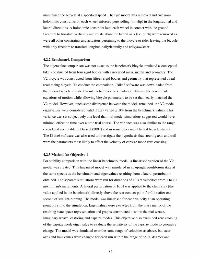
89

maintained the bicycle at a specified speed. The tyre model was removed and two non-

holonomic constraints on each wheel enforced pure rolling (no-slip) in the longitudinal and

lateral directions. A holonomic constraint kept each wheel in contact with the ground.

Freedom to translate vertically and rotate about the lateral axis (i.e. pitch) were removed as

were all other constraints and actuators pertaining to the bicycle or rider leaving the bicycle

with only freedom to translate longitudinally/laterally and roll/yaw/steer.

4.2.2 Benchmark Comparison

The eigenvalue comparison was not exact as the benchmark bicycle emulated a 'conceptual

bike' constructed from four rigid bodies with associated mass, inertia and geometry. The

V2 bicycle was constructed from fifteen rigid bodies and geometry that represented a real

road racing bicycle. To conduct the comparison, JBike6 software was downloaded from

the internet which provided an interactive bicycle simulation utilising the benchmark

equations of motion while allowing bicycle parameters to be set that nearly matched the

V2 model. However, since some divergence between the models remained, the V2 model

eigenvalues were considered valid if they varied ±10% from the benchmark values. This

variance was set subjectively at a level that trial model simulations suggested would have

minimal effect on time over a time trial course. The variance was also similar to the range

considered acceptable in Dressel (2007) and in some other unpublished bicycle studies.

The JBike6 software was also used to investigate the hypothesis that steering axis and trail

were the parameters most likely to affect the velocity of capsize mode zero crossing.

4.2.3 Method for Objective 1

For stability comparison with the linear benchmark model, a linearised version of the V2

model was created. This linearised model was simulated in an upright equilibrium state at

the same speeds as the benchmark and eigenvalues resulting from a lateral perturbation

obtained. Ten separate simulations were run for durations of 10 s at velocities from 1 to 10

m/s in 1 m/s increments. A lateral perturbation of 10 N was applied to the chain stay (the

value applied in the benchmark) directly above the rear contact point for 0.1 s after one

second of straight-running. The model was linearised for each velocity at an operating

point 0.5 s into the simulation. Eigenvalues were extracted from the mass matrix of the

resulting state-space representation and graphs constructed to show the real weave,

imaginary weave, castoring and capsize modes. This objective also examined zero crossing

of the capsize mode eigenvalue to evaluate the sensitivity of the capsize mode to geometry

change. The model was simulated over the same range of velocities as above, but steer

axes and trail values were changed for each run within the range of 65-80 degrees and

90

0.05–0.065 m respectively. The capsize mode zero crossing point was recorded for each

run and a graph produced to show the zero crossing sensitivity to changes in the two design

parameters.


The non-linear V2 model was simulated at velocities of 5 m/s and 3 m/s. Steer and roll

angle response to the lateral perturbation applied for Objective 1 were recorded and

presented as graphs.


A non-linear version of the benchmark model (Meijaard et al., 2007) enabled bicycle

energy conservation to be compared with the non-linear V2 model. This benchmark model

was energetically conservative, which required the sum of the gravitational, kinetic and

potential energies to remain constant regardless of system motion. In consequence, there

was no energy dissipating forces such as friction at the steering joint or wheel hub.

Additionally, the wheel/road contact points were modelled with no-slip (non-holonomic)

constraints which did not dissipate energy in contrast to the forces generated by a tyre

model. The non-linear V2 model was required to demonstrate the behaviour of the

energetically conservative benchmark model by transferring energy to forward velocity as

steer and roll oscillations from a lateral perturbation subsided. This necessitated the

removal from the thesis model of all energy dissipating functions such as tyres and

aerodynamics. The model was simulated at a constant velocity of 5 m/s and perturbed with

10 N after 1 s. Steady state velocity before and after the perturbation was recorded to

identify any change in velocity attributable to conservation of energy.

4.3 Results

In respect of Objective 1 (stability comparison), the model was found to be self-stable from

a velocity of 3.8 m/s up to the limit of testing at 10 m/s (Figure 4.1). The model achieved

low speed self-stability when the real weave mode eigenvalue changed from positive to

negative at 3.8 m/s. However, no upper self-stability limit was apparent from the capsize

mode eigenvalue which remained negative over the tested speed range.

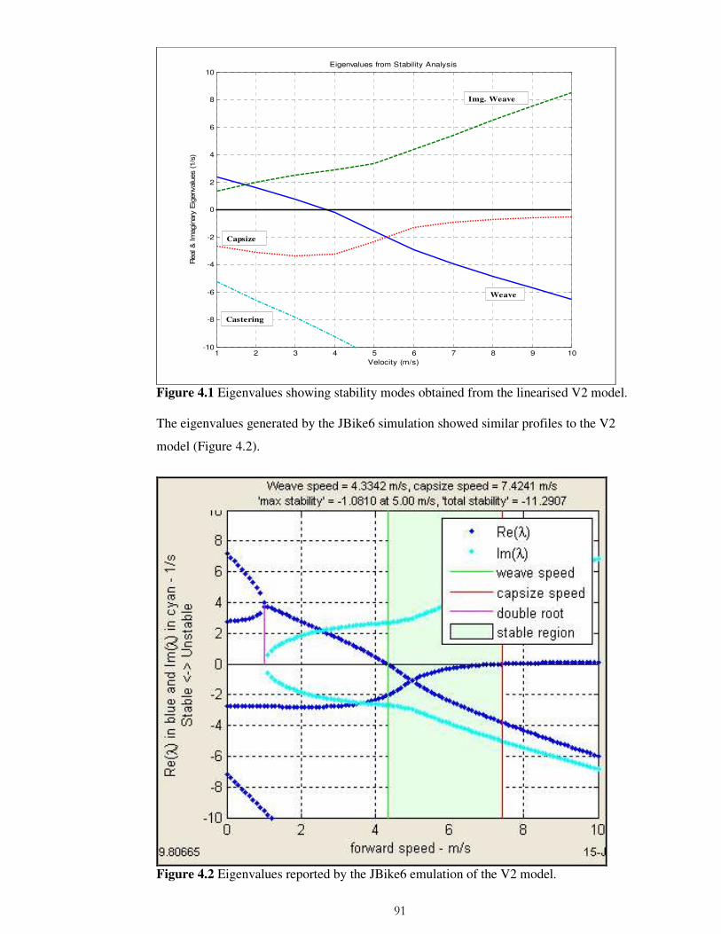
91

1 2 3 4 5 6 7 8 9 10-10

-8

-6

-4

-2

0

2

4

6

8

10

Velocity (m/s)

Real &

Im

agin

ary

Eig

envalu

es (1/s

)

Eigenvalues from Stability Analysis

Img. Weave

Weave

Capsize

Castering

Figure 4.1 Eigenvalues showing stability modes obtained from the linearised V2 model. The eigenvalues generated by the JBike6 simulation showed similar profiles to the V2

model (Figure 4.2).

Figure 4.2 Eigenvalues reported by the JBike6 emulation of the V2 model.

92

The initial self-stability velocity was 4.3 m/s for the JBike6 model and 3.9 m/s for the V2

model giving the latter a 9.3% better initial stability. The upper self-stability velocity was

7.4 m/s for the JBike6 model but the V2 model remained stable up to the limit of testing at

10 m/s. Running the JBike6 model with systematic changes in steering angle and trail

(Dressel, 2007) generated an upper self-stability (capsize mode zero crossing) at a velocity

of 10.4 m/s with trail having the main effect (Figure 4.3).

55.2

5.45.6

5.86

6.2

6870

7274

7678

809.2

9.4

9.6

9.8

10

10.2

10.4

10.6

10.8

Trail (mm)Head Angle (degrees)

Sp

eed

(m

/s)

Figure 4.3 Capsize mode zero crossing speed dependency on head angle and trail (based on a design by Dressel, 2007).

In respect of Objective 2 (roll and steer response to a perturbation), at 5 m/s the bicycle

exhibited oscillations that gradually decayed until upright equilibrium was restored (Figure

4.4). It was noted that the rate of roll and steer oscillation decay increased approximately

linearly with velocity. In contrast, at 3 m/s (i.e. below the self-stability threshold) the

system exhibited increasing roll and steer oscillation leading to over-turning within eight

seconds (Figure 4.5). The roll/steer oscillation period was 2.5 seconds at 3 m/s with slower

velocities increasing this period and thus advancing the onset of capsize.

93

0 0.5 1 1.5 2 2.5 3 3.5 4 4.5 5-0.05

-0.04

-0.03

-0.02

-0.01

0

0.01

0.02

0.03

0.04

0.05

Time(s)

Angle

(degre

es)

Roll and Steer Angles at 5 m/s

Steer

Roll

Figure 4.4 Roll and steer response to perturbation at a velocity of 5 m/s

0 1 2 3 4 5 6 7-5

-4

-3

-2

-1

0

1

2

3

4

5Roll and Steer Angles at 3 m/s

Time (s)

Angle

(degre

es)

Roll

Steer

Figure 4.5 Roll and steer response to perturbation at a velocity of 3 m/s.

The positive roll angle and negative steer angle in Figures 4.4 and 4.5 shows that the

steering turned in the same direction as the roll. The steering response lagged the roll by

94

about 0.25 s at 3 m/s while the steering response was almost coincident with roll at 5 m/s.

There was a notable reduction in the peak roll/steer angle response to perturbation from 5

degrees at 3 m/s to 0.05 degrees at 5 m/s.

In respect of Objective 3, a small permanent velocity increase of 8e-6 m/s was observed

after a 10 N perturbation was applied 1 s into a 5 m/s run (Figure 4.6).

0 0.5 1 1.5 2 2.5 3 3.5 4 4.5 54.999998

5

5.000002

5.000004

5.000006

5.000008

5.00001

5.000012

5.000014

5.000016

Time (s)

Velo

city (m

/s)

Velocity Change after Perturbation

Figure 4.6 Change in velocity due to conservation of energy after a perturbation.

4.4 Discussion

The first objective was to show that the V2 model generated uncontrolled stability

responses consistent with the benchmark of Meijaard et al. (2007) as represented by

JBike6. The model eigenvalue profiles for real weave, imaginary weave and castering

modes (Figure 4.1) generally showed good equivalence to those generated by JBike6

(Figure 4.2). Real weave mode became negative (indicating the transition from oscillatory

instability to bicycle self-stability) at 4.3 m/s for the JBike6 model and 3.9 m/s for the

thesis model. The difference of 9.3% was within the 10% variation considered acceptable

given the variations in design (Dressel, 2007).

The castering mode eigenvalue (which reflects the front wheel tendency to steer in the

direction of travel) was similar between the two models. As expected, the eigenvalues

showed this tendency increased with velocity in both models. The capsize mode was the

only eigenvalue clearly different between the two models. The JBike6 model showed

95

capsize mode becoming positive at 7.4 m/s which indicated the uncontrolled bicycle would

slowly start to lean to one side at that speed extending into a spiral to the ground over time.

The thesis model showed no such tendency with the bicycle remaining stable up to the 10

m/s test limit. Examination of eigenvalue graphs for similar bicycle configurations showed

that capsize mode was reported to become positive over a particularly wide range of

values. The experimental study of Kooijman et al. (2008) reported a zero crossing at 7.9

m/s and also exhibited the curvilinear capsize plot below 3 m/s seen in the thesis model.

Dressel (2007) with benchmark-equivalent equations of motion reported a zero crossing at

8 m/s while a separate study produced by a benchmark co-author (Schwab et al., 2007)

reported zero crossing at ~7.896 m/s. This latter study also suggested that the positive

capsize eigenvalue would again approach zero from above (i.e. become negative) as the

speed increased further. In the same study, a hypothetical bicycle was modelled with zero

trail and zero gyroscopic forces which showed the capsize mode remaining permanently

negative.

It seemed likely that the capsize mode zero crossing had a dependency on bike geometry.

Trail appeared to be the critical parameter as demonstrated by the change in capsize speed

due to systematic variation in steer axis and trail (Figure 4.3). Notably, at a head angle of

80 degrees, a trail increase from 5.1 cm to 5.9 cm increased the capsize mode zero crossing

from 9.5 m/s to 10.4 m/s. This suggested that the V2 model zero crossing would have

occurred in the region of 11 m/s if testing had continued to that level. Future analyses

involving other parameters such as the wheelbase could be expected to generate further

changes to self-stability velocity (Roland, 1973).

A limitation of the study was the difference between the benchmark bicycle and the thesis

bicycle due to the design constraints in JBike6. It is possible that the validity of the

eigenvalue similarity obtained in the current comparison was compromised by the thesis

model approximation in JBike6. However it is suggested that the stability differences were

too small to substantially undermine the results

Considering Objective 2 (roll and steer response), the graphs plotting roll and steer

conformed to a typical transition from instability to self-stability at a velocity in the region

of 4 m/s (Schwab et al., 2005; Limebeer and Sharp, 2006). The steer response was in the

same direction as the perturbation-induced roll to prevent a fall, which is largely a

consequence of the steering geometry and especially the trail (Jackson and Dragovan,

2000; Fajans, 2000). The steering phase lag observed at lower velocities has been noted by

96

other studies (Meijaard et al., 2007; Dressel, 2007). As the bicycle rolls, the slow steering

response tends to generate an excess steer input which consequently generates roll in the

reverse direction (due to centripetal force) followed by escalating oscillations until the

bicycle over-turns. However, as velocity increases, the steering lag reduces and the

steering input therefore increasingly matches that required to only correct the initial roll.

The steer/roll oscillations are thus rapidly damped. Oscillation period of 1.6 seconds and

phase lag of 0.1 seconds at 4.6 m/s were reported by Meijaard et al. (2007) which are

consistent with the values of 2.5 seconds and 0.25 seconds at this study's lower speed of 3

m/s (oscillation period and lag increase at lower velocities). Steer/roll oscillation period

and steer phase lag for a given velocity can be precisely calculated from the complex

weave mode eigenvalues and eigenvectors (Dressel, 2007) but that was beyond the scope

of this study.

Considering Objective 3 (energy conservation), an increase in steady state velocity after a

perturbation was observed, although the effect was small as was expected for an applied

force of only 10 N. Given the observed roll angle of 0.05 degrees at 5 m/s (Figure 4.4) and

a 10 N force applied at chain-stay height (0.35 m), approximately 0.0031 J was added to

total system energy of approximately 1100 J (0.000002818 % increase). This is consistent

with the velocity increase of 0.000012 m/s on 5 m/s (0.0000024 % increase) seen in Figure

4.6. However, it should be noted that a considerably higher additional velocity of 0.022

m/s on 4.6 m/s was reported by Meijaard et al. (2007) using a model built with the

SPACAR non-linear equation generator and solver. The difference in post-perturbation

speed may have been due to the magnitude of the perturbation which was not reported by

Meijaard et al. (2007). Never-the-less, the thesis model velocity increase demonstrated that

the model generally conformed to the conservation of energy principle that required

perturbation energy to be conserved in additional bicycle/rider momentum.

In conclusion, the evidence presented in this chapter indicated that the stability and

dynamics of the thesis model were functionally equivalent to a benchmark model with both

exhibiting self stability above ~4 m/s. The main divergence between the model and the

benchmark was in upper self-stability velocity which may have been due to geometry

differences between the two models. It is therefore proposed that the bicycle dynamics

component of the full thesis model can be considered valid, laying a sound foundation for

the next stage of experimental validation.

97

CHAPTER FIVE

THE TYRE MODEL

5.1 Introduction

The handling and path-following of a bicycle are substantially influenced by the behaviour

of two small contact patches linking the tyres to the road, making an accurate tyre model

critical to performance prediction. If a bicycle is to turn, the two tyres must provide equal

and opposite inwards forces opposing the centripetal force acting inwards. The centripetal

acceleration into a turn is driven by the magnitude of the lateral tyre force provided by tyre

slip and wheel camber. Tyre forces are a critical component in the accuracy of model

prediction as they are not only generated by path-following but also by the continuous steer

and roll resulting from the pedalling action. The objective of this chapter was to show that

tyre forces were realistic and similar to other studies. To achieve this, tyre forces were

examined in isolation from the forces that would result once the tyres were incorporated

into the full model simulated over a time trial. Familiarity with tyre dynamics theory is

assumed for this chapter and a summary is provided in Appendix 3.

Few studies have experimentally investigated bicycle tyres and only two have been

identified that conducted on-road investigations. Cole and Khoo (2001) constructed a

towed rig that calculated cornering stiffness for non-standard bicycle tyres that were 0.25

m diameter (0.35 m standard), 0.054 m width (0.02 m standard) and inflated to 35 psi (80-

100 psi standard). Never-the-less, a cornering stiffness of 3,553 N/rad (equivalent to 62 N

per degree of slip) at zero camber and 329 N vertical load was found which was in good

agreement with the only other identified road experimental tests conducted by Roland and

Lynch (1972).

Roland and Lynch (1972) constructed a tyre testing machine towed behind a vehicle that

mounted a bicycle wheel to roll at various normal forces, slip angles and camber angles

with the resulting forces and moments being measured. Eleven varied tyre types were

evaluated with radii of 0.31-0.35 m and inflation pressures of 60-110 psi. A non-linear

expression was derived which related normalised lateral force to a number of input

parameters and coefficients. The trials obtained a mean cornering stiffness (less one radial

carcass construction tyre not considered relevant to competitive cycling as they are

virtually never used) of 3,680 N/rad at zero camber and 338 N vertical load (equivalent to

98

64 N per degree of slip). Surprisingly, no relationship was found between cornering

stiffness and tyre inflation pressure although theory would suggest this might explain some

of the difference between studies.

A summary of the Roland and Lynch (1972) findings was contained in Roland (1973)

reporting cornering coefficient values (cornering stiffness normalised to vertical load)

ranging from 0.15 to 0.35. However, the original data graphs showed the mean cornering

coefficient to be 0.19 when the slip angle/lateral force slope was measured at the origin

with zero camber and 338 N load (again excluding one experimental radial tyre). Sharp

(2008) assumed cornering stiffness to be the mid-point of the range reported by Roland

(1973) and therefore used a coefficient of 0.25 which over-estimated the parameter. Sharp

(2008) also reported rear tyre cornering stiffness to be ~100% greater than the front

presumably due to an assumed front/rear load split of 309/613 N (taken from the reported

camber stiffness). This 34/66% front/rear split suggested an exceptionally upright riding

position possibly due to the handlebars extending backwards as in a so-called 'shopping

bike'. For competitive bicycles, a front/rear split of 45/55% is recommended

(www.calfeedesign.com) [Accessed 4 April 2009] while the geometry used in building the

V3 model gave a 47/53% split which equated to 338/383 N. Additionally, the

experimental work of Roland and Lynch (1972) demonstrated that a 100% increase in rear

vertical load relative to the front would only generate a ~50% increase in slip lateral force,

which finding was supported in concept by Cole and Khoo (2001).

Only one study of those shown in Table 5.2 reports a rolling resistance coefficient, which

is surprising given that rolling resistance (R/R) can generate significant resistance to

motion particularly at the lower speeds incurred during hill climbing. A study by Kyle

(2003) contains the most comprehensive experimental tyre testing that can be identified in

respect of tyre type, surface and inflation pressure (the latter two factors in particular being

key components of the R/R coefficient). The study reported a coefficient of 0.004 for a 23

mm clincher tyre at 95 psi rolling on smooth tarmac and this value has been adopted in the

thesis model.

Other studies have reported bicycle tyre cornering and camber coefficients but without

specifying the origin of the reported values or the methods employed to obtain them

(Sharp, 2008; Limebeer and Sharp, 2006). A modelling study by Meijaard and Schwab

(2006) utilised a 38/62% front/rear load split while the assigned cornering stiffness values

of 1500/2500 were estimates based on previous experience and were acknowledged to be

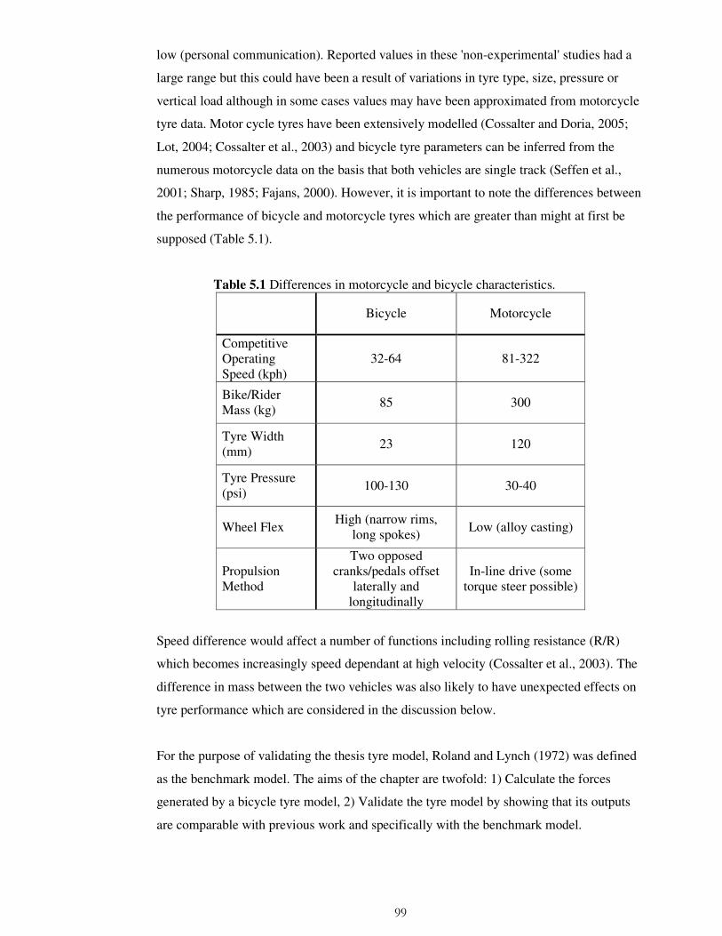
99

low (personal communication). Reported values in these 'non-experimental' studies had a

large range but this could have been a result of variations in tyre type, size, pressure or

vertical load although in some cases values may have been approximated from motorcycle

tyre data. Motor cycle tyres have been extensively modelled (Cossalter and Doria, 2005;

Lot, 2004; Cossalter et al., 2003) and bicycle tyre parameters can be inferred from the

numerous motorcycle data on the basis that both vehicles are single track (Seffen et al.,

2001; Sharp, 1985; Fajans, 2000). However, it is important to note the differences between

the performance of bicycle and motorcycle tyres which are greater than might at first be

supposed (Table 5.1).

Table 5.1 Differences in motorcycle and bicycle characteristics.

Bicycle Motorcycle

Competitive Operating Speed (kph)

32-64 81-322

Bike/Rider Mass (kg) 85 300

Tyre Width (mm)

23 120

Tyre Pressure (psi) 100-130 30-40

Wheel Flex High (narrow rims,

long spokes) Low (alloy casting)

Propulsion Method

Two opposed cranks/pedals offset

laterally and longitudinally

In-line drive (some torque steer possible)

Speed difference would affect a number of functions including rolling resistance (R/R)

which becomes increasingly speed dependant at high velocity (Cossalter et al., 2003). The

difference in mass between the two vehicles was also likely to have unexpected effects on

tyre performance which are considered in the discussion below.

For the purpose of validating the thesis tyre model, Roland and Lynch (1972) was defined

as the benchmark model. The aims of the chapter are twofold: 1) Calculate the forces

generated by a bicycle tyre model, 2) Validate the tyre model by showing that its outputs

are comparable with previous work and specifically with the benchmark model.

100

5.2 Methods

5.2.1 General Outline

Each wheel was constrained to roll with no-slip by two non-holonomic constraints

controlling longitudinal and lateral motion respectively. Tyre forces and moments in all

three axes were then calculated analytically at each time step from wheel longitudinal slip,

lateral slip, camber angle and vertical force. To enable this calculation, the tyre parameters

listed in Table 5.2 were obtained from the published data shown.

5.2.2 Tyre Parameters

The identification of tyre parameters is critical to model fidelity and appropriate values

should be found from experimental testing. However, no tyre testing facilities were

available for this study and therefore tyre parameters were estimated from experimental

measurement of bicycle tyres as reported in the literature. These are summarised in Table

5.2.

Table 5.2 Bicycle tyre parameters (* = parameter utilised in the thesis model)

Meijaard &

Schwab (2006)

Limebeer & Sharp (2006)

Cole & Khoo (2001)

Roland & Lynch (1972)

Sharp (2008)

Cornering Stiffness (N/rad)

Front=1,500 Rear=2,500

4842 3,553 3,680* Front=4,430 Rear=8,778

Camber Stiffness (N/rad)

338 49 Front=309* Rear=613*

Aligning Moment (Nm/rad)

Front=71* Rear=176*

Overturning Moment (Nm/rad)

-0.31 at 5° camber*

Vertical Stiffness (N/m)

150,000 125,787- 178,165

Vertical Load (N) 338 329 338 Front=309 Rear=613

Rolling Resistance Coefficient

0.0068

Relaxation Length (m)

0.1* Front=0.021* Rear=0.028*

Contact Patch Length (m)

0.1 Front=0.12 Rear=0.13

Pneumatic Trail (m)

Front=0.012 Rear=0.018

0.003 Front=0.016* Rear=0.02*

Crown Radius (m) Front=0.015 Rear=0.02

0.02 0.01

Cornering stiffness has been shown to be the single most important tyre parameter (Roland

and Lynch, 1972) but variances were considerable in the values reported above which

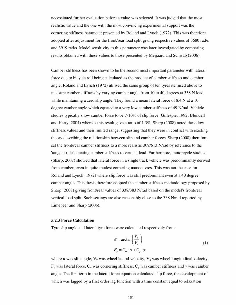
101

necessitated further evaluation before a value was selected. It was judged that the most

realistic value and the one with the most convincing experimental support was the

cornering stiffness parameter presented by Roland and Lynch (1972). This was therefore

adopted after adjustment for the front/rear load split giving respective values of 3680 rad/s

and 3919 rad/s. Model sensitivity to this parameter was later investigated by comparing

results obtained with these values to those presented by Meijaard and Schwab (2006).

Camber stiffness has been shown to be the second most important parameter with lateral

force due to bicycle roll being calculated as the product of camber stiffness and camber

angle. Roland and Lynch (1972) utilised the same group of ten tyres itemised above to

measure camber stiffness by varying camber angle from 10 to 40 degrees at 338 N load

while maintaining a zero slip angle. They found a mean lateral force of 8.4 N at a 10

degree camber angle which equated to a very low camber stiffness of 49 N/rad. Vehicle

studies typically show camber force to be 7-10% of slip force (Gillespie, 1992; Blundell

and Harty, 2004) whereas this result gave a ratio of 1.3%. Sharp (2008) noted these low

stiffness values and their limited range, suggesting that they were in conflict with existing

theory describing the relationship between slip and camber forces. Sharp (2008) therefore

set the front/rear camber stiffness to a more realistic 309/613 N/rad by reference to the

'tangent rule' equating camber stiffness to vertical load. Furthermore, motorcycle studies

(Sharp, 2007) showed that lateral force in a single track vehicle was predominantly derived

from camber, even in quite modest cornering manoeuvres. This was not the case for

Roland and Lynch (1972) where slip force was still predominant even at a 40 degree

camber angle. This thesis therefore adopted the camber stiffness methodology proposed by

Sharp (2008) giving front/rear values of 338/383 N/rad based on the model's front/rear

vertical load split. Such settings are also reasonably close to the 338 N/rad reported by

Limebeer and Sharp (2006).

5.2.3 Force Calculation

Tyre slip angle and lateral tyre force were calculated respectively from:

arctan y

x

y

V

V

F C Cα γ

α

α γ

=

= ⋅ + ⋅

(1)

where α was slip angle, Vy was wheel lateral velocity, Vx was wheel longitudinal velocity,

Fy was lateral force, Cα was cornering stiffness, Cγ was camber stiffness and γ was camber

angle. The first term in the lateral force equation calculated slip force, the development of

which was lagged by a first order lag function with a time constant equal to relaxation

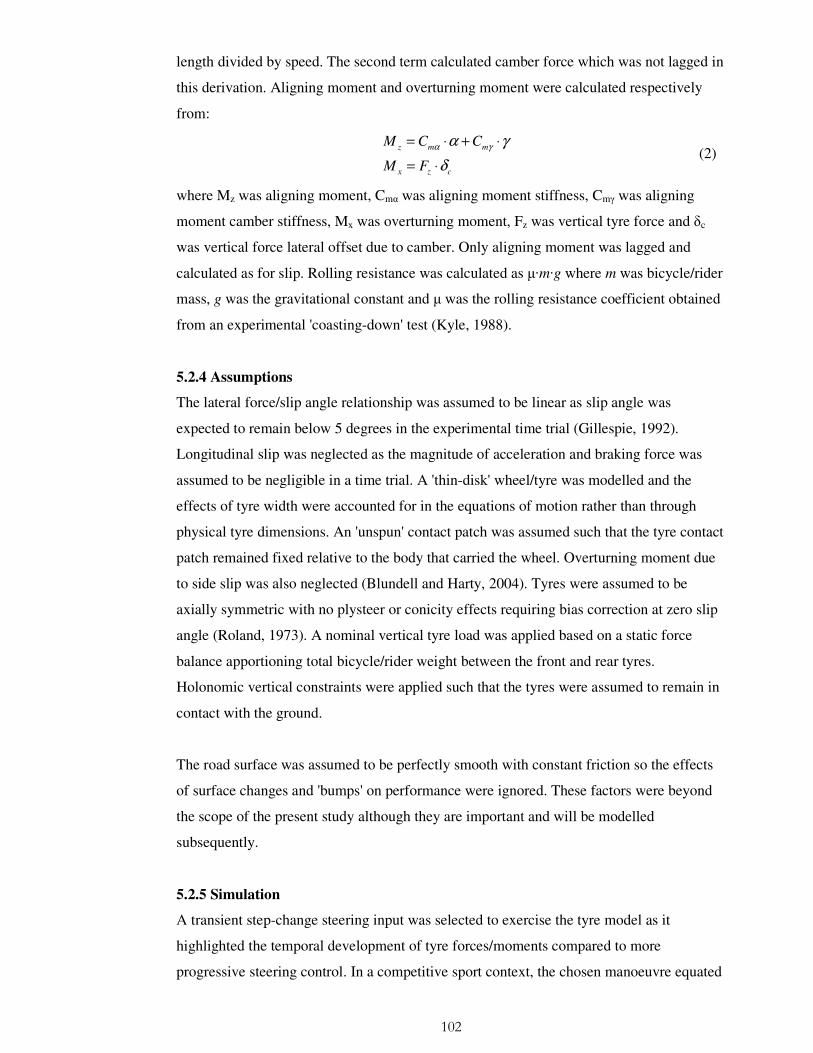
102

length divided by speed. The second term calculated camber force which was not lagged in

this derivation. Aligning moment and overturning moment were calculated respectively

from:

z m m

x z c

M C C

M F

α γα γ

δ

= ⋅ + ⋅

= ⋅ (2)

where Mz was aligning moment, Cmα was aligning moment stiffness, Cmγ was aligning

moment camber stiffness, Mx was overturning moment, Fz was vertical tyre force and δc

was vertical force lateral offset due to camber. Only aligning moment was lagged and

calculated as for slip. Rolling resistance was calculated as µ·m·g where m was bicycle/rider

mass, g was the gravitational constant and µ was the rolling resistance coefficient obtained

from an experimental 'coasting-down' test (Kyle, 1988).

5.2.4 Assumptions

The lateral force/slip angle relationship was assumed to be linear as slip angle was

expected to remain below 5 degrees in the experimental time trial (Gillespie, 1992).

Longitudinal slip was neglected as the magnitude of acceleration and braking force was

assumed to be negligible in a time trial. A 'thin-disk' wheel/tyre was modelled and the

effects of tyre width were accounted for in the equations of motion rather than through

physical tyre dimensions. An 'unspun' contact patch was assumed such that the tyre contact

patch remained fixed relative to the body that carried the wheel. Overturning moment due

to side slip was also neglected (Blundell and Harty, 2004). Tyres were assumed to be

axially symmetric with no plysteer or conicity effects requiring bias correction at zero slip

angle (Roland, 1973). A nominal vertical tyre load was applied based on a static force

balance apportioning total bicycle/rider weight between the front and rear tyres.

Holonomic vertical constraints were applied such that the tyres were assumed to remain in

contact with the ground.

The road surface was assumed to be perfectly smooth with constant friction so the effects

of surface changes and 'bumps' on performance were ignored. These factors were beyond

the scope of the present study although they are important and will be modelled

subsequently.

5.2.5 Simulation

A transient step-change steering input was selected to exercise the tyre model as it

highlighted the temporal development of tyre forces/moments compared to more

progressive steering control. In a competitive sport context, the chosen manoeuvre equated

103

to a cyclist changing direction to exploit a gap during the final sprint of a road race (similar

to the initial action of the 'lane change' manoeuvre used in vehicle testing).

The V3 bicycle/rider model was simulated from rest and accelerated upright and straight-

ahead to reach a steady-state speed of 11.1 m/s after ~7.5 s. A transient steering input was

applied after ~7.9 s comprising a step-input of 4 degrees to the right generating a bicycle

yaw rate of 40 degrees/s with subsequent steer/roll inputs returning the bicycle to upright

equilibrium on a new track after 9 s when the simulation was terminated. Forces, moments

and motions for front and rear tyres were recorded at the simulation time-step frequency

(~0.1 s) enabling results to be presented as graphs and analysed. All results are presented

as absolute values since force generation consumes energy regardless of tyre orientation

with respect to any particular axis.

5.3 Results

Tyre output data measured by the simulation and resulting derived values are shown in

Table 5.3. Only the period containing pronounced steering motion from ~7.9 s to 9.0 s

contributed significantly to the results.

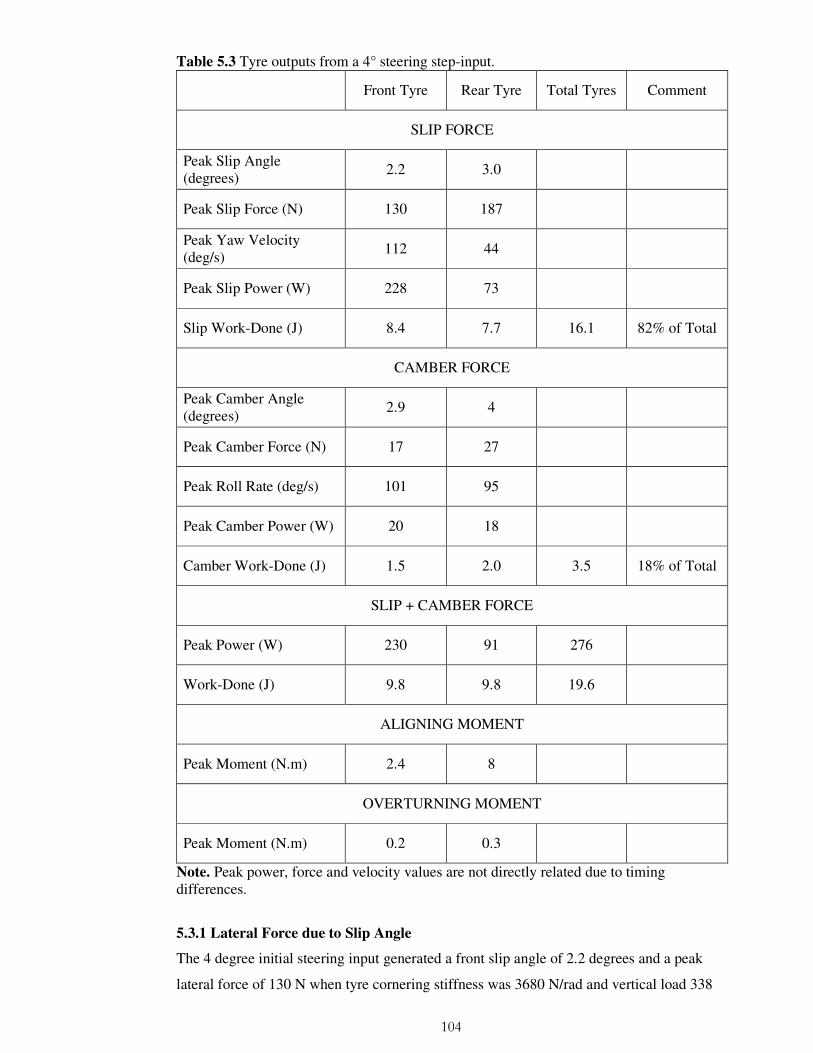
104

Table 5.3 Tyre outputs from a 4° steering step-input.

Front Tyre Rear Tyre Total Tyres Comment

SLIP FORCE

Peak Slip Angle (degrees)

2.2 3.0

Peak Slip Force (N) 130 187

Peak Yaw Velocity (deg/s)

112 44

Peak Slip Power (W) 228 73

Slip Work-Done (J) 8.4 7.7 16.1 82% of Total

CAMBER FORCE

Peak Camber Angle (degrees)

2.9 4

Peak Camber Force (N) 17 27

Peak Roll Rate (deg/s) 101 95

Peak Camber Power (W) 20 18

Camber Work-Done (J) 1.5 2.0 3.5 18% of Total

SLIP + CAMBER FORCE

Peak Power (W) 230 91 276

Work-Done (J) 9.8 9.8 19.6

ALIGNING MOMENT

Peak Moment (N.m) 2.4 8

OVERTURNING MOMENT

Peak Moment (N.m) 0.2 0.3

Note. Peak power, force and velocity values are not directly related due to timing differences.

5.3.1 Lateral Force due to Slip Angle

The 4 degree initial steering input generated a front slip angle of 2.2 degrees and a peak

lateral force of 130 N when tyre cornering stiffness was 3680 N/rad and vertical load 338

105

N (Figure 5.1). When combined with a front wheel yaw velocity that peaked at 112 deg/s,

a peak power of 228 W was transferred from forward propulsion to lateral propulsion.

Integrating the power profile over the simulation showed that the power transfer

represented 8.4 J of work.

7.8 7.9 8 8.1 8.2 8.3 8.4-200

-100

0

100

Time (s)

Lat

eral

For

ce (

N)

Force

Angle

-2

0

2

4

Slip

Ang

le (

degr

ees)

Figure 5.1 Front tyre slip angle and resulting lateral force.

A peak lateral force of 187 N was measured at the rear tyre (higher than the front tyre due

to the greater vertical load of 383 N) together with a rear frame yaw velocity of 44 deg/s

giving a peak power transfer from forward to lateral propulsion of 73 W. The lower rear

wheel power (despite greater lateral force generation) was due to both lower frame yaw

velocity compared to front wheel yaw velocity and to peak yaw velocity occurring later in

the cycle and thus not coinciding with peak force. Integrating rear wheel lateral power over

the period gave work-done of 7.7 J which was closer to the front tyre value since

integration eliminated the effect of the peak timing difference. Total forward-to-lateral

work-done as a consequence of steering input was 16.1 J, all of which would have been

applied to bicycle propulsion if straight-running had been maintained.

5.3.2 Lateral Force due to Camber Angle

A peak front wheel camber angle of 2.9 degrees resulted from the steering input which

generated 17 N of lateral force (Figure 5.2). This was treated as additive to the slip induced

lateral force as the angle-force relationships remained linear at the small angles of this

simulation. Rear wheel camber angle of 4 degrees (Table 5.3) was greater than front wheel

camber as it was not reduced by steering geometry effects. Additionally, a larger rear

camber force of 27 N was found due to both the increased camber angle and the higher rear

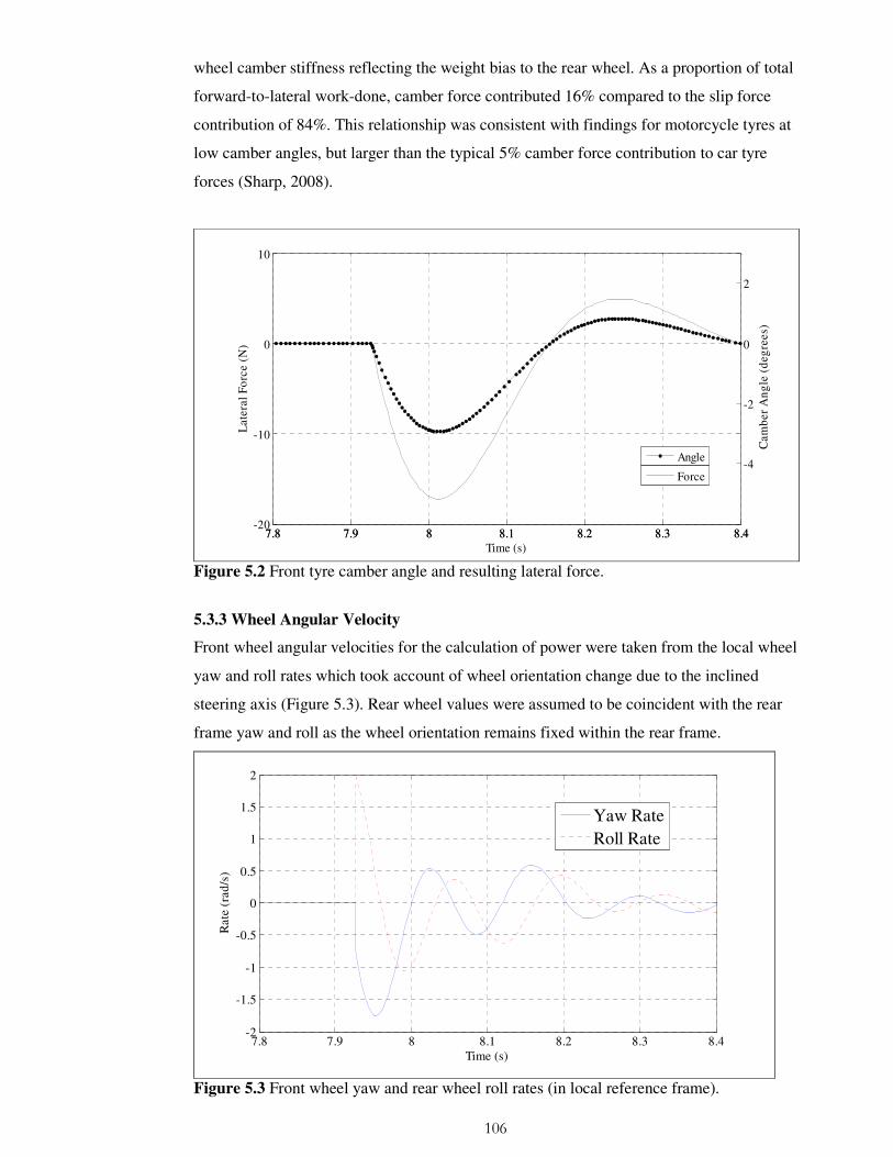
106

wheel camber stiffness reflecting the weight bias to the rear wheel. As a proportion of total

forward-to-lateral work-done, camber force contributed 16% compared to the slip force

contribution of 84%. This relationship was consistent with findings for motorcycle tyres at

low camber angles, but larger than the typical 5% camber force contribution to car tyre

forces (Sharp, 2008).

7.8 7.9 8 8.1 8.2 8.3 8.4-20

-10

0

10

Time (s)

Lat

eral

For

ce (

N)

7.8 7.9 8 8.1 8.2 8.3 8.4

-4

-2

0

2

Cam

ber

Ang

le (

degr

ees)

Force

Angle

Figure 5.2 Front tyre camber angle and resulting lateral force.

5.3.3 Wheel Angular Velocity

Front wheel angular velocities for the calculation of power were taken from the local wheel

yaw and roll rates which took account of wheel orientation change due to the inclined

steering axis (Figure 5.3). Rear wheel values were assumed to be coincident with the rear

frame yaw and roll as the wheel orientation remains fixed within the rear frame.

7.8 7.9 8 8.1 8.2 8.3 8.4-2

-1.5

-1

-0.5

0

0.5

1

1.5

2

Time (s)

Rat

e (r

ad/s

)

Yaw RateRoll Rate

Figure 5.3 Front wheel yaw and rear wheel roll rates (in local reference frame).

107

5.3.4 Combined Slip and Camber Force

It should be noted that peak power values are not additive as the peak of two power

profiles can occur at different time points in the simulation. The joint peak is at the time

point where the combination of the two profiles gives the highest value.

Peak lateral power generated by the 'lane change' manoeuvre (including both wheels and

slip/camber force) was 276 W with total work-done over the period amounting to 19.6 J.

Work-done was divided equally between the two wheels suggesting a neutral cornering

balance for the bicycle. The power profile in Figure 5.4 showed a distribution similar to

most of the measured quantities with an initial peak followed by reducing peaks as the

bicycle lateral oscillations subsided. To investigate the effect of cornering stiffness values

presented by Meijaard and Schwab (2006), front cornering stiffness was reduced to 1500

rad/s (-58%) and rear cornering stiffness to 2500 rad/s (-36%). The resulting total power

profile is shown in Figure 5.4. Total peak power reduced from 276 W to 124 W and work-

done dropped from 19.6 J to 11.7 J (reduction percentages were distorted by timing

differences). The percentage peak power and work-done reductions at both wheels were

almost identical to the cornering stiffness reductions. It is apparent from this result that

peak force generation and work-done was approximately proportional to cornering

stiffness. This was consistent with the model assumption of a linear relationship between

slip angle and lateral force at the low slip angles generated in the current simulation. A

graph of the data suggests, however, that the rate of force reduction was proportionately

less at lower force levels (the velocity component of power calculation remained largely

constant across both simulations).

7.8 7.9 8 8.1 8.2 8.3 8.4-50

0

50

100

150

200

250

300

Time (s)

Pow

er (

W)

Model Cornering StiffnessMeijaard and Schwab (2006) Cornering Stiffness

Figure 5.4 Total power from both wheels generated by slip and camber lateral force.

108

5.3.5 Tyre Moments

The front tyre aligning and overturning moments are shown in Figure 5.5. The aligning

moment at 2.4 N.m was likely to be of sufficient magnitude for its self-centering effect to

be sensed by the rider through the steering. The larger rear aligning moment of 8 N.m

reflected the greater rear lateral slip force and the greater rear pneumatic trail. This

potentially under-steering characteristic may have only applied to the simulated manoeuvre

because an initial counter-steer was missing (initial roll and steer were not in opposite

directions). A peak overturning moment of 0.2 N.m is shown in Figure 5.5 which was

unlikely to have been of sufficient magnitude to influence rider control.

7.8 7.9 8 8.1 8.2 8.3 8.4-2

0

2

Time (s)

Ali

gnin

g M

omen

t (N

.m)

7.8 7.9 8 8.1 8.2 8.3 8.4-0.2

0

0.2

Ove

rtur

ning

Mom

ent (

N.m

)

Aligning

Overturning

Figure 5.5 Front tyre aligning and overturning moments.

5.4 Discussion

The first aim of this chapter was to develop a bicycle tyre model that generated forces and

moments in response to steering input. Lateral tyre force from side-slip and camber thrust

consequent on a partial lane change manoeuvre were generated that met this requirement.

Force vectors offset from the contact patch centre also generated aligning, overturning and

rolling resistance moments. The first aim was therefore achieved successfully. The second

aim was to compare the model results with values from the single track vehicle literature

and confirm that the model results were realistic. This comparison was largely qualitative

as gold standard bicycle tyre studies were not available for a quantitative analysis. The

study of Roland and Lynch (1972) was the only study where actual values could be

compared and the match was found to be good. Other studies have incorporated tyre

models into bicycle handling simulations but have reported eigenvalues relating to bicycle

109

self-stability rather than calculating tyre forces (Limebeer and Sharp, 2006; Sharp, 2008).

Field studies have been limited to measuring force and motion associated with the bicycle

frame (e.g. steering angles and torques) as tyre forces can only be calculated indirectly

from other instrumentation. Testing tyres separately from the bicycle usually requires

expensive machinery only available to tyre/vehicle manufacturers and some universities.

Roland and Lynch (1972) reported a mean cornering stiffness of 60 N/degree at 3 degrees

slip angle, 10 degrees camber angle and 330 N vertical load. Although not necessarily

reproducing the response of a steered bicycle, the similarity of this result to the rear tyre

force obtained in the current simulation (62N/deg at 3 degrees slip, 4 degrees camber and

338 N load) provides support for the validity of the thesis tyre model, but with unresolved

questions remaining on the contribution of camber to lateral force generation. Surprisingly,

Roland and Lynch (1972) showed that camber thrust only contributed between zero and

33% of total lateral force when a 40 degree camber angle was applied. Further research is

clearly needed to establish whether the approximately equal lateral force generated by 40°

of camber and 3° of side-slip in motorcycles (Cossalter et al., 2003; Cossalter and Doria,

2005) is applicable to the bicycle. However, it should be noted that there is some

ambiguity in this area as Sharp (2007) reports an estimated 80+% of lateral force at 50

degrees camber angle is attributable to camber thrust in a motorcycle simulation. These

differences may be due variations in bicycle and motorcycle tyre hysteresis. Motorcycle

tyre compression at rest is small whereas bicycle tyre depth can reduce by up to one third

with a seated rider (unpublished observations). Centrifugal force from the different tyre

rotation velocities would be expected to further emphasise this difference when moving.

Proportionately greater hysteresis would therefore be expected in the bicycle tyre with

hysteresis being the main energy absorbing mechanism in tyres (Hewson, 2005).

Indirect support for the results of this simulation comes from a study that simulated a lane

change manoeuvre and reported the resulting bicycle displacement and steer/roll angles

(Sharp, 2008). The study simulated an initial 14 degree change of heading completed in

approximately two seconds at a speed of 6 m/s. This was twice the angle at half the rate of

this study and therefore proportionately similar. The comparison is somewhat confounded

by the inclusion of counter-steer in the Sharp (2008) simulation (although surprisingly it

produced no initial path deviation away from the turn). The roll angle was almost identical

between the two studies at 7.5 and 8 degrees while the Sharp (2008) peak steer angle of

~2.5 degrees was similar to the 4 degrees found here leading to the conclusion that overall,

the studies showed a similar response.

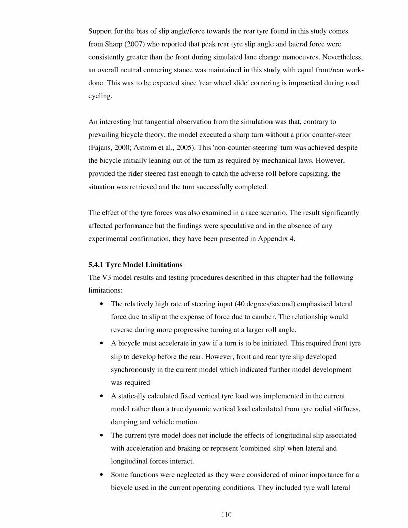
110

Support for the bias of slip angle/force towards the rear tyre found in this study comes

from Sharp (2007) who reported that peak rear tyre slip angle and lateral force were

consistently greater than the front during simulated lane change manoeuvres. Nevertheless,

an overall neutral cornering stance was maintained in this study with equal front/rear work-

done. This was to be expected since 'rear wheel slide' cornering is impractical during road

cycling.

An interesting but tangential observation from the simulation was that, contrary to

prevailing bicycle theory, the model executed a sharp turn without a prior counter-steer

(Fajans, 2000; Astrom et al., 2005). This 'non-counter-steering' turn was achieved despite

the bicycle initially leaning out of the turn as required by mechanical laws. However,

provided the rider steered fast enough to catch the adverse roll before capsizing, the

situation was retrieved and the turn successfully completed.

The effect of the tyre forces was also examined in a race scenario. The result significantly

affected performance but the findings were speculative and in the absence of any

experimental confirmation, they have been presented in Appendix 4.

5.4.1 Tyre Model Limitations

The V3 model results and testing procedures described in this chapter had the following

limitations:

• The relatively high rate of steering input (40 degrees/second) emphasised lateral

force due to slip at the expense of force due to camber. The relationship would

reverse during more progressive turning at a larger roll angle.

• A bicycle must accelerate in yaw if a turn is to be initiated. This required front tyre

slip to develop before the rear. However, front and rear tyre slip developed

synchronously in the current model which indicated further model development

was required

• A statically calculated fixed vertical tyre load was implemented in the current

model rather than a true dynamic vertical load calculated from tyre radial stiffness,

damping and vehicle motion.

• The current tyre model does not include the effects of longitudinal slip associated

with acceleration and braking or represent 'combined slip' when lateral and

longitudinal forces interact.

• Some functions were neglected as they were considered of minor importance for a

bicycle used in the current operating conditions. They included tyre wall lateral

111

distortion due to side forces, contact patch longitudinal/lateral migration, delayed

camber force lag, camber steering and turn slip.

5.4.2 Conclusion

A tyre model was developed which generated force profiles consistent with the literature

and output values similar to those reported by a benchmark model. The tyre model

contributed to overall model validity although further development will be required if all

aspects of tyre performance are to be accurately modelled.

112

CHAPTER SIX

FIELD VALIDATION - CASE STUDY

6.1 Introduction

It has been proposed that maintaining constant speed is the optimum strategy to employ in

a cycling time trial in contrast to the more usual constant power strategy (Swain, 1997;

Gordon, 2006; Atkinson et al., 2007a). The logic behind this strategy in relation to an

undulating course is that more time is spent on the ascents than the descents. Lower speed

on an ascent therefore has a disproportionate affect on total time. Attempting to maintain

speed on the ascent minimises this loss of time but requires a variable power strategy with

power increased on ascents and decreased on descents while maintaining the same overall

work-done. It can be stated that constant speed over any course is always fastest and the

nearer a rider can approach constant speed, the faster they will go. However, it must be

noted that the amount by which a rider can vary power to maintain constant speed will be

limited by a rider's physiological capacity. To model this performance enhancement

strategy requires the simulation of gradient variation and, therefore, emphasises

environment modelling.

In this chapter, environment modelling is combined with the previously validated model

components in respect of rider pedalling, bicycle dynamics and tyres to give a first

assessment of full model validity. The validation was conducted as a case study by

comparing the completion time for a single cyclist adopting a variable power strategy over

the 2008 Women's National time trial course with a comparable model simulation. It was

hypothesised that a close match would be obtained and thus support the thesis model

validity while at the same time giving an initial indication as to the efficacy of a variable

power strategy.

6.2 Methods

6.2.1 Introduction

The V3 bicycle/rider model described in Chapter 2 was utilised in this case study. The

rider characteristics and the course track/gradient were obtained as described below and

entered into the model.

113

6.2.2 The Subject

An experienced competitive cyclist agreed to participate in the study. The participant was

female, aged 35, rode a full time trial bike, was in regular training and had previously

finished in the top ten in UK national time trials. Other parameters (Table 6.1) were

obtained as follows: mean power was estimated from previous laboratory tests and time

trial history, peak power was estimated from time trial history, drag coefficient (CDA) was

calculated as described in section 2.5.3, rolling resistance was as specified in section 5.2.3

and preferred cadence was taken from time trial history. Critical speed was defined as the

speed that would result if the rider maintained constant mean power over a completely

straight, flat, smooth and windless course (Swain, 1997; Gordon, 2005). Critical speed

therefore represented the fastest possible 'aerobic' time and was estimated from a model

simulation. Default body segment mass values were proportionately adjusted to the

subject's total mass. Segment dimensions and inertias were not modified as they were

considered to describe the subject adequately and pilot simulations showed little sensitivity

to those parameters. The bicycle dimensions/geometry/inertia remained at the default

values as pilot simulations also showed little sensitivity.

Table 6.1 Rider parameters

Description Value

Mass (bicycle+rider) (kg) 73.5

Mean Power (W) 250

Mean Peak Power over 30 s (W) 325

Drag Coefficient 0.30

Coefficient of Rolling Resistance 0.004

Critical Speed (m/s) 11.05

Preferred Cadence (rpm) 95

The participant did not normally employ a variable power race strategy. The model,

therefore, calculated a personalised optimum power output profile that minimised speed

variance over the course within the constraints of the subject's mean and peak power. The

participant committed this profile to memory as far as possible and agreed to attempt to

apply that variable power strategy in the forthcoming women's national time trial.

6.2.3 The Course

The field trial was conducted on the Road Time Trial Council course P883 on the A3 main

road near Petersfield in Hampshire (UK) which was used for the 2008 UK women's 10

mile time trial championship. The course was a relatively straight dual carriageway out-

114

and-back course with a roundabout at half distance which made it typical of many UK time

trials (Figure 6.1). Direction of travel was from south west to north east and had multi-

roundabout layouts at the start and turn. The gradient profile is shown in Figure 6.2

comprising an average uphill gradient of 3.3%, a maximum gradient of 10% and a total of

80 m climbed.

Only the outward leg of 8,000 m was modelled thus avoiding the roundabout sections

which V3 of the thesis model was unable to represent accurately. The course coordinates

were plotted every 10 m (northings and eastings) utilising digital mapping software

(Memory-Map Ltd, Aldermaston, UK). The distance and direction between each

coordinate was obtained from trigonometric calculation and the resulting data transposed

to the model's global coordinate system. At each time step, the model compared bicycle

distance travelled and yaw angle with the map data and made the necessary steering

correction to maintain the bicycle on the desired track. The root mean squared error

(RMSE) between the desired and actual track was computed to quantify the tracking error.

Figure 6.1 The time trial course (run from south to north).

115

Figure 6.2 Course gradient profile 6.2.4 Enviromental Wind

The aerodynamic resistance was modified by both the speed and direction of the

environmental wind. A constant wind from the west-north-west at 2 m/s was specified

from Meteorological Office data for the trial day (www.metoffice.gov.uk) [Accessed 1

June 2010]. The course track was predominantly towards the north-east resulting in a wind

direction that was predominantly at 90° to the track. However, wind angle to the bicycle

varied continuously with the heading and, consequently, so did the aerodynamic resistance

as described in section 2.5.3.

6.2.5 Gear Selector

The V3 model included a gear selection sub-system that automatically maintained cadence

within a range set at 80-100 rpm. The system selected combinations from a 53/39

chainring and 12-27 cassette that minimised cadence change in response to speed

variations resulting from resistive force changes. The system freewheeled when speed was

too high for the available gears (i.e. down steep hills) and the associated power/torque went

to zero (but not negative which would have represented braking). Each gear change

incurred a performance penalty of 25% reduction in power for 0.25 seconds. No research

could be identified to guide these parameter values and they were therefore set by running

model simulations over a range of values until the time delay and power loss subjectively

approximated to the cycling experience of the author when changing gear.

6.2.6 Model Simulation

The simulation accelerated the bicycle/rider from rest over a 'neutralised' zone to bring it

up to near critical speed before measurement started. Subsequently at each time point,

actual speed was compared with critical speed and power output increased/decreased

within physiological limits to eliminate the error. At the same time, an algorithm having

forward knowledge of road gradient, adjusted the power output such that mean power

output over the course equalled the desired mean power. In model version V3, propulsive

power was applied at the crank spindle and transmitted to the rear wheel hub as variable

torque. At each time step, torque delivered to the rear wheel was modified by gear changes

116

to keep the crank cadence within range while meeting the power output demand. The

rider's legs were 'inversely' driven by the crank motion which was therefore unrealistic in

this version of the model. The steering maintained the bicycle/rider on the desired track,

while steer and roll angles were inversely linked to ensure the bicycle remained upright as

described in Chapter 2.

6.2.8 Field Data Collection

The subject's bicycle was fitted with an SRM power meter (Schoberer Rad Messtechnik

GmbH, Julich, DE) which recorded power, speed, time and cadence at 1 s intervals over

the race duration. The power meter was calibrated in accordance with the manufacturer's

instructions prior to the start of the race. Owing to roundabouts at the start, the SRM data

was only processed after approximately 200 m when a near steady-state speed was

reached. Similarly, data capture ceased before appreciable deceleration occurred prior to

the turn roundabout.

6.2.9 Data Processing

Time, distance, power, speed and cadence were recorded from the simulation and the field

trial and loaded into Excel. Additionally, path tracking root mean squared error (RMSE),

gradient profile, gear change history and work-done were obtained from the model.

6.3 Results

Experimental and simulation results are shown in Table 6.2. The model predicted the

participant would take 736 s to complete the course while the actual time was 8 s slower at

744 s (-1.1%). The power, speed and work-done values differed by less than 1.2% between

the two conditions suggesting that environmental and rider parameters were correctly

chosen.

Table 6.2 Experimental and model results

Actual Model Model

Error

Error

Percentage

Time (s) 744 736 -8 -1.1%

Mean Power (W) 250 251 +1 +0.4%

Mean Speed (m/s) 10.81 10.94 +0.13 +1.2%

Work done (J) 186,000 184,736 -1264 -0.7%

Peak 30 s Power (W) 327 337 +10 +3.1%

Mean Cadence (rpm) 98 91 -7 -7.1%

117

The simulation power output profile matched to gradient is shown in Figure 6.3. It was

notable that power usually peaked before the summit of a hill reflecting the model response

to a reducing gradient at that time with the reverse pattern on a descent. The periodic drops

in power reflected the cost of gear changes as implemented by the gear selection module

although in the interests of clarity, most gear changes are not shown. The simulated mean

power of 251 W, peak power of 337 W and cadence of 92 rpm showed variances of 0.4%,

3.1% and 7.1% respectively from the measured values.

150

200

250

300

350

400

0 1000 2000 3000 4000 5000 6000 7000 8000

Distance (km)

Pow

er (

W)

60.00

65.00

70.00

75.00

80.00

85.00

90.00

95.00

Heig

ht

(m)

Power

Height

Figure 6.3 Modelled optimum power against distance for the time trial (height profile is also shown).

The simulation speed resulting from the optimum power output exhibited a visually similar

profile to the actual speed achieved by the subject although not all the minor variations

were followed (Figure 6.4). Deviations were to be expected given that the subject had

committed the power profile to memory. Nevertheless, the mean speed from the simulation

of 10.94 m/s and the actual speed of 10.81 m/s were separated by 1.2% .

118

6

7

8

9

10

11

12

13

14

15

16

0 1 2 3 4 5 6 7 8

Distance (km)

Sp

eed

(m

/s)

Optimum Speed

Actual Speed

Figure 6.4 Modelled optimum speed and actual speed against distance for the time trial. Simulated work-done varied by 0.7% from the measured value indicating that overall, the

subject had followed the target power output profile. The mean model tracking error of 2

cm was excellent, but perhaps misleading, as the bicycle followed the path to <0.5 cm

when the road was straight (the predominant condition) but deviated to a peak RMSE of 52

cm on the bends. The model showed little sensitivity to gear changes which incurred a total

time cost of 3 s. The 2 m/s environmental wind from the north-north-west increased

completion time by 3.2 s. This was consistent with the effect that would be expected from

a predominantly side wind.

6.4 Discussion

The aims of this chapter were to model environmental parameters and incorporate them

into a unified thesis model for validation against experimental data. This was achieved

with the simulation predicting a time 1.1% lower than the actual time which was well

within the 2.8% target set in this thesis for an effective model. Model prediction of work-

done, mean power, peak power and mean speed reported values within 3% of the

experimental case study indicating an overall pattern of model validity.

The only previous study that predicted field performance from a first principles model was

Olds (1995) who reported a 3.8% error over a 26 km course. The higher error could have

been due to the static nature of the model which did not include iterative modelling of

gradient during the simulation. Variations in gradient are a critical factor in time trial

performance (Martin et al., 1998).

119

This simulation incorporated actual course track/gradient profiles and realistic wind

conditions, demonstrating the ability of the thesis model to replicate a real-world time trial

course where environmental conditions change constantly. This compares with the fixed or

semi-fixed environmental parameters used to model approximate courses in all the time

trial simulations examined by this thesis. A limitation of the thesis model was the fixed

value for both environmental wind strength and direction which did not replicate the

performance effect of constant changes in both parameters that occur in the real world

(Atkinson et al., 2003). However, the variation in apparent wind was modelled as the

course changed direction relative to the environmental wind. Accurate modelling of wind

data will require a bicycle fitted with a portable anemometer to capture wind strength and

direction in real time. This approach is investigated in Chapter 9.

It should be noted that the model predictions were not obtained by extensive parameter

manipulation which can be used to obtain post hoc matches with experimental data

(Yeadon and King, 2002; Mills et al., 2009). All parameter values were set a priori except

the environmental wind conditions which were subsequently obtained from the

Meteorological Office.

It was interesting to note that the variable power profile calculated by the model coincided

with the subject achieving a place in the top ten, beating her previous best result in several

attempts at the same competition. The subject was only partially able to follow the power

output profile, but it was possible that the strategy made at least some contribution to her

success. This evidence suggested that a more extensive evaluation of variable power

strategies in a time trial was warranted.

The measured results listed in Figure 6.2 were all obtained from the SRM power meter

which recorded power, speed, cadence, distance and time. The accuracy of the power

meter was therefore important in determining the accuracy of the results. The reliability of

the power value is specified by the manufacturer as ±2% but the reliability of speed and

cadence measurement is not specified. Paton and Hopkins (2006) evaluated the reliability

of the SRM using data recorded by eleven racing cyclists who each completed three 5 min

maximum effort trials on an ergometer. The error attributable to the SRM was found to be

1.1% which was an improvement on the manufacturer's specification. Gardner et al. (2004)

used a certified calibration rig to evaluate the accuracy of 15 SRM's over 11 months and

found an error level of -0.8±1.7%. Cadence error was found to be -0.9±0.7% at 100 rpm.

Mean percent difference in power output between standard laboratory and cool outdoor

120

conditions was found to be 5.2% demonstrating that device calibration must be conducted

under trial conditions. In summary, the SRM error level can be expected to be in the range

1-2%.

The ±2% reliability of the power meter might be expected to cancel out over an 8 km

course but in a worst case scenario might result in a 1% mean power value error. This

would equate to a ~0.4% speed error (see section 1.2.4.1) which would change the

measured time over the course to 744±3 s. The model experimental error would therefore

be 1.1±0.4% which would not be a substantial change to the result of the trial.

The model error levels for time, mean power, mean speed and work-done were all within

the error range of the SRM suggesting that the model adequately represented the

experimental conditions. However, the model peak power was 3.1% higher than the

experimental peak power which was likely to have been the main contributor to the faster

time recorded by the model. A 7.1% lower mean cadence was also recorded by the model

but this would be expected to generate a physiological rather than performance effect

(Lucia et al., 2001).

A potential study limitation was the validity of the gear change system included in the

model version V3 used in this simulation. It was surprising that some 90 gear changes only

cost 3 s of time over the trial. This may have been due to the assumption of a 25% power

reduction over 0.25 s for each change. With gradients of up to 9 %, the time cost of gear

changing should perhaps have been modelled dynamically as they would be expected to

increase during low cadence climbing when high chainring/chain contact forces would be

present. However, no data on this issue could be identified to guide dynamic parameter

adjustment. It may be that cadence and the associated gear system has little effect on

performance in a purely mechanical context. The specification of 80-100 rpm may also

have been simplistic as studies have shown that mean cadence varies with power and

gradient (Marsh and Martin, 1997). Professional cyclists typically drop their preferred

cadence from 90-100 rpm on the flat to 70-75 rpm in high mountains (Lucia et al., 2001).

A limitation of the investigation in respect of validating a generalised model was the

relatively straight course. A more circuitous course (>45 degree bends) would be required

if the bicycle dynamics, balance, steering, tyre forces and path tracking were to be

comprehensively tested.

In conclusion, the close match between the model's predicted time and the participant's

actual time gave confidence that the thesis model was valid when simulating the

121

combination of rider, bicycle and environment in a field time trial. However, this case

study was not validation and therefore a similar field trial had to be conducted, but under

controlled conditions and with a representative sample of cyclists. The mean difference

between predicted and actual time should be within the criterion set for model

effectiveness.

122

CHAPTER SEVEN

FIELD VALIDATION – CONTROLLED TRIALS

7.1 Introduction

This chapter completes the model validation process by comparing model prediction

against the results of a controlled field trial using a sample of competitive cyclists.

Predicted and actual results were evaluated with a statistical analysis. Ecological validity

was maintained by conducting the validation over an actual field time trial course.

Over one hundred bicycle/cycling models of various types have been considered in this

thesis, but only the model of Olds et al. (2005) explicitly predicts performance over a real

road time trial course. The model of Martin et al. (1998) has the functionality to progress

into a generalised road time trial model, but has primarily been used to make theoretical

predictions on the performance effects of gradient and wind. Other models predict field

performance by regression from physiological variables or laboratory tests and could

potentially be developed into generalised road time trial models, but this has not yet been

done. The model of Olds et al. (2005) predicted completion time of 46:38 min over a flat

'out-and-back' 6.5 km time trial course completed four times. Forty-one cyclists of various

experience levels completed the trial in a mean time of 44:17 min, which represented a

model prediction error of 3.87%. This error level is the only finding in the literature against

which the prediction of the current model can be directly compared.

The aim of this chapter was to validate the full thesis model by comparing predicted and

actual times for cyclists riding over a field time trial course.

7.2 Methods

7.2.1 Model Development

Model version V4 was developed for this investigation. The main enhancement was

propulsion generation from pedal forces transmitted to the rear wheel hub rather than direct

torque application to the hub. Horizontal and vertical pedal force profiles were obtained

from previous investigations in this laboratory as described in section 2.4.4. An important

consequence of this change was that the bicycle rolled and steered over a 360° crank cycle

due to the pedal force offset to the bicycle centre line. This development also resulted in

bicycle velocity pulsation over a crank cycle. A penalty was the necessity to remove the

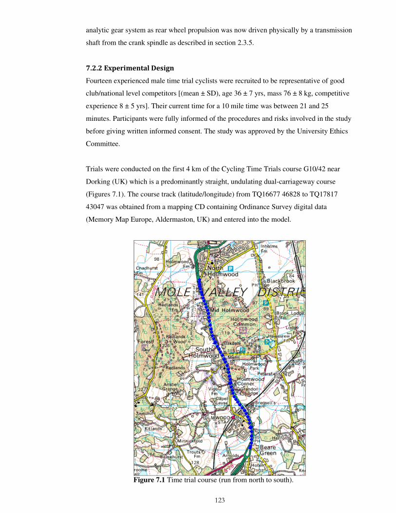
123

analytic gear system as rear wheel propulsion was now driven physically by a transmission

shaft from the crank spindle as described in section 2.3.5.

7.2.2 Experimental Design

Fourteen experienced male time trial cyclists were recruited to be representative of good

club/national level competitors [(mean ± SD), age 36 ± 7 yrs, mass 76 ± 8 kg, competitive

experience 8 ± 5 yrs]. Their current time for a 10 mile time was between 21 and 25

minutes. Participants were fully informed of the procedures and risks involved in the study

before giving written informed consent. The study was approved by the University Ethics

Committee.

Trials were conducted on the first 4 km of the Cycling Time Trials course G10/42 near

Dorking (UK) which is a predominantly straight, undulating dual-carriageway course

(Figures 7.1). The course track (latitude/longitude) from TQ16677 46828 to TQ17817

43047 was obtained from a mapping CD containing Ordinance Survey digital data

(Memory Map Europe, Aldermaston, UK) and entered into the model.

Figure 7.1 Time trial course (run from north to south).

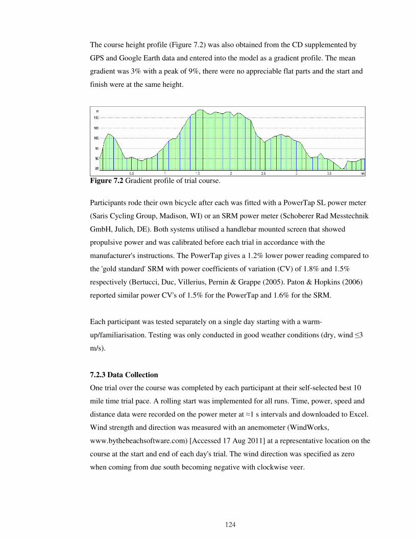
124

The course height profile (Figure 7.2) was also obtained from the CD supplemented by

GPS and Google Earth data and entered into the model as a gradient profile. The mean

gradient was 3% with a peak of 9%, there were no appreciable flat parts and the start and

finish were at the same height.

Figure 7.2 Gradient profile of trial course.

Participants rode their own bicycle after each was fitted with a PowerTap SL power meter

(Saris Cycling Group, Madison, WI) or an SRM power meter (Schoberer Rad Messtechnik

GmbH, Julich, DE). Both systems utilised a handlebar mounted screen that showed

propulsive power and was calibrated before each trial in accordance with the

manufacturer's instructions. The PowerTap gives a 1.2% lower power reading compared to

the 'gold standard' SRM with power coefficients of variation (CV) of 1.8% and 1.5%

respectively (Bertucci, Duc, Villerius, Pernin & Grappe (2005). Paton & Hopkins (2006)

reported similar power CV's of 1.5% for the PowerTap and 1.6% for the SRM.

Each participant was tested separately on a single day starting with a warm-

up/familiarisation. Testing was only conducted in good weather conditions (dry, wind ≤3

m/s).

7.2.3 Data Collection

One trial over the course was completed by each participant at their self-selected best 10

mile time trial pace. A rolling start was implemented for all runs. Time, power, speed and

distance data were recorded on the power meter at ≈1 s intervals and downloaded to Excel.

Wind strength and direction was measured with an anemometer (WindWorks,

www.bythebeachsoftware.com) [Accessed 17 Aug 2011] at a representative location on the

course at the start and end of each day's trial. The wind direction was specified as zero

when coming from due south becoming negative with clockwise veer.

125

7.2.4 Model Simulation

A separate simulation was run for each individual after the model was parameterised with

their mass, CDA and the wind conditions in their trial (Figure 7.3). Default values were

used for the bicycle and body segments as pilot testing showed little model sensitivity to

variations in either set of values (sections 2.3 and 2.4). Height and weight data were

provided by the participant and used to calculate body surface area (BSA) and frontal area

(Heil et al., 2001). Individual CDA was calculated from frontal area, riding position and

bicycle type as specified in section 2.5.3. The participant's recorded power profile was used

as input to drive the simulation and the predicted time over the course was obtained as the

output.

7.2.5 Statistical Analysis

Data sets were checked for normality with a Shapiro-Wilks test and for equal/unequal

residual variance with an F-Test. Data were analysed with a paired t-test to identify any

significant difference between predicted and actual completion time and with linear

regression to identify any relationship between predicted and actual completion time. All

data were analysed with SPSS (SPSS Inc, Chicago, IL) with significance set at p≤0.05.

7.3 Results

The required assumptions for the statistical analysis were confirmed with data sets

normally distributed (p>0.248) and an F-Test showing unequal variances between data sets

(F>1.194, p>0.288). The results are shown in Table 7.1.

Table 7.1 Results of field trial (see section 2.5.3 for explanation of bicycle type).

Mean predicted and actual times for the 14 participants were 371 (±35) s and 366 (±32) s

respectively. The predicted time was 5 (±6) s greater than the actual time which was a

significant difference (t = -3.104, p = 0.008). The 95% confidence interval difference was

126

1.5 s to 8.4 s. The mean model prediction error was 1.4%. Actual and predicted times were

closely related (R2 = 0.973) with an SEE of 5.5 s (Figure 7.3).

Figure 7.3 Relationship between predicted and actual completion time for the time trial.

7.4 Discussion

The aim of this chapter was to validate the full thesis model by comparing the predicted

and actual times for a sample of 14 competitive cyclists in a controlled field time trial. The

predicted time was 5 s greater than the actual time which represented a 1.4% model error

level. This compared well with the error level of 3.87% reported for the model of Olds et

al. (1995). The model prediction error was also less than the 2.8% error specified as the

upper limit for an effective model in this thesis. A regression analysis of predicted and

actual times also showed a strong relationship with an R2 value of 0.973 and a low data

scatter represented by an SEE of 5.5 s. The bias towards a higher predicted than actual time

may have reflected unmeasured assistance from wind and traffic within a trial.

It was not clear if the statistically significant difference (p=0.008) between the predicted

and actual time had any real-world implications. The mean actual and percentage size of

the error (5 s and 1.4% respectively) were similar to the variance that would be considered

typical by competitive cyclists (see section 1.2.3). It is suggested therefore that the

significant difference in times does not undermine the model's value as a predictive tool.

127

Comparison with Martin et al. (1998) must be indirect as their measured dependant

variable was power rather than completion time. However, it can be calculated from the

presented data (for the 11 m/s trials which were equivalent to this study) that the average

model predicted time over the equivalent distance was 3.3 s faster than the actual time of

365 s giving a 0.9% error. This compares well with a 366 s completion time and 1.4% error

in the present study. However, it must be noted that this agreement was likely to be

coincidental as the course of Martin et al. (1998) was flat (0.3% gradient) and completely

straight. Martin et al. (1998) also found that model predicted time was less than actual time

which was the reverse of this study. In part, this may reflect the absence of a traffic

'towing' effect on their closed airfield course.

Olds et al. (1995) compared model predicted and actual times for 41 cyclists over a 26 km

flat (<0.5% gradient) course. The mean model predicted time was 0.74 min greater than the

actual time of 42.8 min giving an error level of 1.73%, similar to the 1.4% found in this

study. However, Olds et al. (1995) reported a large error SD of ±2.07 min and range of

+5.56 to -3.15 min which they attributed to less accurate modelling of the sixteen non-

competitive cyclists included in their study.

Model version V4 used in this experiment had the limitation that cadence was uncontrolled

due to the removal of the gear system utilised in V3. This was a consequence of design

limitations in SimMechanics precipitated by the change to propulsion from pedal forces.

Physiological factors were not considered in this thesis, but it can be noted that cadence

remained within physiologically acceptable limits of 73-121 rpm. There was no theoretical

reason or experimental evidence to indicate that cadence would have any mechanical effect

on bicycle translation. Model simulations also showed no effect of cadence on bicycle

speed.

In conclusion, this chapter successfully completed the sequence of investigations to

establish the validity of the thesis model. Validity was found in previous chapters for

pedalling, bicycle dynamics, tyres and a case study with this chapter combining those

components into a single unified model and confirming that model's validity. The weight

of evidence accumulated in all these investigations suggests that the thesis model was an

adequate representation of road time trials and could be safely used to identify

performance enhancements for competitive cyclists. The next phase of the thesis

development was therefore to use the model to identify performance enhancement

strategies and to then experimentally confirm the efficacy of such strategies.

128

CHAPTER EIGHT

PERFORMANCE ENHANCEMENT - GRADIENT

8.1 Introduction

This chapter used the validated model to confirm the results of a previous investigation and

then modelled a performance enhancement strategy over a real road course and confirmed

the model predictions with experimental trials.

Changes in human and environmental variables are known to influence cycling speed

(Atkinson et al., 2003). In races where the environmental conditions are variable, it has

been calculated that a pacing strategy that attempts to maintain a constant speed, rather

than a constant effort or power output strategy should prove fastest (Atkinson and

Brunskill, 2000; Atkinson et al., 2007a; Atkinson et al., 2007b; Swain, 1997). The time

advantage of a variable power output strategy has been proposed to be proportional to the

magnitude and rate of changes in environmental resistive forces (Atkinson et al., 2003).

Gordon (2005) proposed that change in gradient was the single most important factor

influencing the performance benefit of a variable power output strategy.

Considering the effect of gradient, a constant speed pacing strategy is implemented by

varying power output in response to changes in the course gradient (Gordon, 2005; Swain,

1997). On an undulating time-trial course, more time is spent on the ascents and therefore

the power and speed during this phase has a greater impact on the final time than the power

and speed on the descents (see section 6.1). Whilst physiological and technical constraints

may prevent a constant speed being maintained on the ascents, an advantage can still be

gained if the variance from a constant speed is minimised (Atkinson et al., 2007b).

Swain (1997) was one of the first investigators to draw attention to the mechanical

performance advantage that could be obtained by varying power output (expressed as VO2)

in response to variances in wind and gradient. Over a theoretical 10 km course with 10

symmetrical climbs and descents of 5–15 % gradient, Swain (1997) calculated time

savings of 4–8 % were possible. Subsequently, Atkinson et al. (2007a) re-calculated the

results of Swain (1997) using a more complete model of cycling power output demands

(Martin et al., 1998). These researchers calculated that a variable power output strategy

could reduce race time by 5-9%. Gordon (2005) modelled a 40 km course with 20

symmetrical climb/descents of 2.5 % and obtained a time saving of 1.6 % compared to an

equivalent constant power output strategy. The lesser time saving of Gordon (2005)

129

reflects the reduced gradient profile and emphasises the importance of a large gradient

variance if the advantage of a variable power output strategy is to be realised.

The modelled predictions of previous studies that a performance advantage would result

from adopting a variable power output strategy over an undulating course have never been

experimentally validated in the field. The omission may have been due the inability of

previous models to replicate the gradient variations of a real time trial course and thus

precluded calculation of the continuously varying power output required to drive a field

experiment. An opportunity therefore existed for the thesis model to demonstrate both its

ability to model the environment and to dynamically solve equations of motion at a

frequency that reflected a continuously changing environment.

The objectives of this chapter were threefold:

(1) Simulate the thesis model over the course modelled by Atkinson et al. (2007a) and

establish equivalence between the two models.

(2) Use the thesis model to predict the time advantage of a variable power output strategy

over a real undulating road time trial course.

(3) Experimentally test the thesis model prediction over the same course. It was

hypothesised that a variable power output strategy would reduce speed variation and result

in a time saving compared to a constant power output strategy.

8.2 Methods

Model version V4 was used throughout this chapter. It should be noted that over an

undulating course, constant speed is synonymous with variable power while constant

power is synonymous with variable speed. The terms 'constant' and 'variable' refer to the

speed of the bicycle or the power of the rider and not the pedalling style. There was no

requirement in the trials described below for the rider to maintain or vary the angular

velocity of the cranks within a pedal cycle.

8.2.1 Method for Objective 1 - Model Equivalence

The parameters specified by Atkinson et al. (2007a) in their variable-v-constant power

simulation 'Course 1' were entered into the thesis model. A 10 km straight course was

composed of alternating 1 km segments of ±5% gradient. A mean power of 289 W was

varied by 10% giving a power output range of 260–318 W. Bicycle/rider mass was 80 kg

and CDA was 0.258 with no environmental wind.

130

8.2.2 Method for Objective 2 - Model Performance Prediction

Thesis model simulations compared the time taken to cover a 4 km undulating time-trial

course utilising either a constant or a variable power output strategy. The course described

in Chapter 7 was used for the simulation. CDA was estimated for each participant from

their height, weight, bicycle type and riding position as specified in section 2.5.3. Default

parameters for the bicycle and rider were utilised (Appendix 2) except for the following

which were calculated from mean values for the participants: bike/rider mass=793 N,

CDA=0.29. The constant power output simulation was run at 255 W. The variable power

output profile was derived as follows: The model initially calculated a 'critical' speed for

the default bicycle/rider on a completely flat, straight, smooth, windless course at 255 W.

The course track and gradients were then introduced resulting in changes in speed. Power

output was recalculated to minimise the speed changes relative to critical speed but

constrained to a peak power output of 325 W (+27%) for a maximum of 30 s (this value

was based on the time trial histories of the participants). Power output during the descents

was adjusted to both maintain constant speed and achieve the overall mean of 255 W.

Power was always ≥0 as negative values would represent braking which was not modelled

in this version. Changes in aerodynamic resistance with speed were included in the

calculations. Environmental wind and rolling resistance were modelled as constant. The

resulting power profile together with the related course height profile is shown in Figure

8.1.

Figure 8.1 Optimum power profile against distance (height profile is also shown).

131

8.2.3 Method for Objective 3 - Experimental Confirmation

8.2.3.1 Participants

21 competitive male time trial cyclists gave informed consent to take part in this study

[(mean ± SD), age 34 ± 8 yrs, mass 72 ± 6 kg, competitive experience 8 ± 4 yrs]. Selected

participants were representative of club level competitors with a current time of 21–25 min

for a 10 mile time-trial (2010 UK national championship times ranged from 18:37 to 23:27

min). Participants were briefed on the aims and organisation of the trials (Appendix 5). The

study was approved by the University Ethics Committee and performed in accordance with

the university ethical standards.

8.2.3.2 Time-Trial Course

Trials were conducted on the same time trial course described in Chapter 7. The gradient of

the selected course was considered representative of the ‘sporting’ time trial that was

necessary if a mechanical advantage from power variance was to be identified. Limiting

the distance to 4 km minimised physiological fatigue which could also have confounded

identification of a mechanical advantage which was the objective of this experiment.

8.2.3.3 Variable Power Profile

The variable power output profile described above was applied to control a participant's

power output. The mean power level of 255 W was based on pilot work which suggested

that all participants would be able to complete all trials at that intensity. The modelled peak

power for four elite participants was increased to 400 W in order to obtain data on the

effect of that parameter on performance. The model calculated variable power output

profile was downloaded as sound files to a small personal digital assistant combined with a

global positioning system (PDA/GPS, Mio P560, Mio Technology Ltd, Gatwick, UK). The

PDA was secured to the participant’s arm and the required power output was conveyed via

an earpiece at ~80 m intervals as they progressed down the course. During pilot testing,

intervals of any greater period were found to be impractical for participant implementation.

8.2.3.4 Equipment

Participants rode their own bicycles, the characteristics of which, along with clothing,

accessories and tyre pressures, were not specified, but were required to remain constant for

each participant. The performance of 16 participants was measured utilising a power

measuring rear hub (PowerTap SL, Saris Cycling Group, Madison, WI). The performance

of the remaining 5 participants was measured from a power measuring crank system

(Schoberer Rad Messtechnik GmbH, Julich, DE). Both systems were calibrated before

each trial in accordance with the manufacturer’s instructions.

132

8.2.3.5 Experimental Trials

All the experimental field trials were conducted over a 5 h period which started with a

warm-up and equipment familiarisation. Participants completed 4 separate trials, two using

a constant power output and two using the variable power output strategy. Rolling starts

were implemented so that participants crossed the starting line at the target power output.

Testing was conducted in dry weather with winds ≤3 m/s. The wind strength and direction

was measured with an anemometer (WindWorks, USA, www.bythebeachsoftware.com). If

the wind speed changed by more than 1 m/s or by 20 degrees in direction, a trial was

rejected and repeated after a delay. This occurred on 4 occasions.

Trials 1 and 2 (‘constant power output’) required a constant power of 255 W to be

maintained over the course. Trial 3 and 4 (‘variable power output’) required participants to

vary power output as directed through their earpiece with the objective of minimising

speed variation over the course while maintaining a 255 W average. Participants were

instructed to maintain the same riding position within and between trials to minimise

variance due to aerodynamics. The results for one participant were excluded as a constant

aerodynamic position was not maintained within trials.

8.2.3.6 Data Collection

Time, power, speed and distance data for each trial were recorded using the power meter at

≈1 s intervals. The root mean squared error (RMSE) between targeted and actual values for

both power and speed were calculated for each trial. Where mean power output differed

from the 255 W target power, completion time was normalised to the estimated speed that

would have resulted if the target power had been maintained. The data for this

normalisation was derived by running multiple simulations of the model over the complete

course using a range of power values and obtaining an exponential power-to-speed

relationship. The relationship was essentially linear within the range of experimentally

observed power variances.

8.2.3.7 Statistical Analysis

Data sets were checked for normality with a Shapiro-Wilkes test and for equal/unequal

residual variance with an F-Test. Data were analysed with an SPSS linear mixed model

(Version 15.1, SPSS Inc, Chicago, IL) to identify any significant difference between

completion time at constant and variable power (Landau and Everitt, 2004). Trial order

was not randomised since any learning or fatigue effects would be apparent in power

output profile deviation from the commanded profile. A pilot study had shown that the

selected sequence generated a learning effect which acted to improve accuracy in

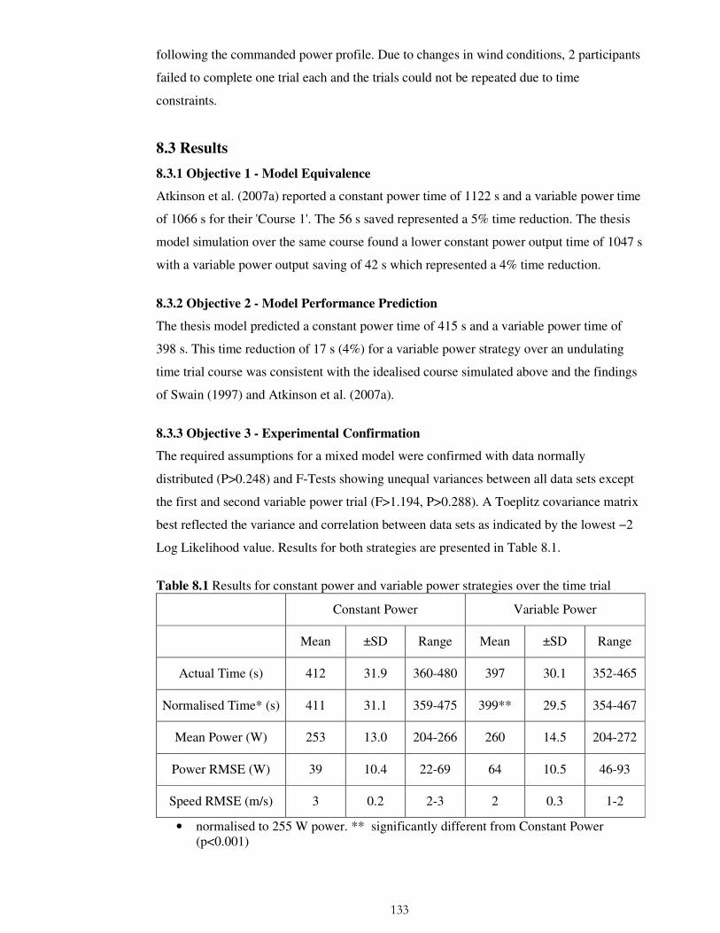
133

following the commanded power profile. Due to changes in wind conditions, 2 participants

failed to complete one trial each and the trials could not be repeated due to time

constraints.

8.3 Results

8.3.1 Objective 1 - Model Equivalence

Atkinson et al. (2007a) reported a constant power time of 1122 s and a variable power time

of 1066 s for their 'Course 1'. The 56 s saved represented a 5% time reduction. The thesis

model simulation over the same course found a lower constant power output time of 1047 s

with a variable power output saving of 42 s which represented a 4% time reduction.

8.3.2 Objective 2 - Model Performance Prediction

The thesis model predicted a constant power time of 415 s and a variable power time of

398 s. This time reduction of 17 s (4%) for a variable power strategy over an undulating

time trial course was consistent with the idealised course simulated above and the findings

of Swain (1997) and Atkinson et al. (2007a).

8.3.3 Objective 3 - Experimental Confirmation

The required assumptions for a mixed model were confirmed with data normally

distributed (P>0.248) and F-Tests showing unequal variances between all data sets except

the first and second variable power trial (F>1.194, P>0.288). A Toeplitz covariance matrix

best reflected the variance and correlation between data sets as indicated by the lowest −2

Log Likelihood value. Results for both strategies are presented in Table 8.1.

Table 8.1 Results for constant power and variable power strategies over the time trial

Constant Power Variable Power

Mean ±SD Range Mean ±SD Range

Actual Time (s) 412 31.9 360-480 397 30.1 352-465

Normalised Time* (s) 411 31.1 359-475 399** 29.5 354-467

Mean Power (W) 253 13.0 204-266 260 14.5 204-272

Power RMSE (W) 39 10.4 22-69 64 10.5 46-93

Speed RMSE (m/s) 3 0.2 2-3 2 0.3 1-2

• normalised to 255 W power. ** significantly different from Constant Power (p<0.001)

134

The achieved mean power for the constant strategy was 253 W and 260 W for the variable

strategy. The mean time normalised to 255 W for the constant power output trials was

411±31.1 s and 399±29.5 s for the variable power output trials. The difference of 12±8 s

was significant (P <0.001) and represented a 2.9±1.9% advantage for the variable power

strategy. The 95 % confidence interval (CI) time for the variable power output trial was

391–413 s versus 401–428 s for the constant power output trial. An example of the

constant and variable power output strategies is shown in Figure 8.2. The underlying

concept of the constant -v- variable power strategy is apparent from Figure 8.2. As the

cyclist negotiates the steepest gradient changes, the speed variance increases more for the

constant power strategy than for the variable power strategy.

Figure 8.2 Speed resulting from the constant and variable power strategies (related to gradient profile).

RMSE for the constant power strategy was 39 ± 10 W. This 15% variance exceeded the

≤5% variance that was considered to adequately represent a constant power strategy. The

increased variance indicated that participants had difficulty following the constant power

output strategy. As expected, the variable power output strategy RMSE was higher at

64±11 W indicating that participants implemented the increase in power phasing required

by this strategy. Speed RMSE exhibited the reverse pattern with the constant strategy at

3±0.2 m/s and the variable strategy at 2±0.3 m/s. This confirmed that the variable power

output strategy more closely approximated to a constant speed as required by mechanical

pacing theory. No difference in time saved with the variable power output strategy was

found for the four elite participants with a 400 W peak power constraint.

135

8.4 Discussion

This chapter investigated the advantage of a variable power output strategy compared to a

constant power output strategy over an undulating time trial course. Atkinson et al. (2007a)

had modelled the comparison over an idealised course and running the thesis model over

the same course produced similar results. However, the thesis model time was 7% lower

than the time of Atkinson et al. (2007a) and the time saving of 4% was less than the 5%

time saving found by Atkinson et al. (2007a). There are a number of possible reasons for

these divergences. The two models were very different in structure but the completely

straight course might be expected to nullify most of the difference due to steering. The tyre

forces generated by the pedalling action in the thesis model should have reduced speed

compared to Atkinson et al. (2007a), but speed was in fact higher. One clear difference in

the thesis model was its progressive change in bicycle speed as gradient changed whilst

speed change was instantaneous in the Atkinson et al. (2007a) model. However, the time

effect of this difference might be expected to balance out over a simulation. It is interesting

to note that a comparable study by Swain (1997) obtained a 4% time advantage (the same

as the thesis model) which Atkinson et al. (2007a) attributed to differences in CDA. This

would have been unlikely to affect completion time in the present comparison as CDA in

the thesis model was set at the value used by the Atkinson et al. (2007a). Nevertheless,

aerodynamics were likely to have been the main source of variance because they were the

predominant resistive forces.

The advantage of a variable power strategy was modelled over a real time trial course and

the simulation found a 4% time saving which was in general agreement with the results

from previous simulations over idealised courses. The model simulation was broadly

confirmed by the experimental results which found that a variable power output strategy

saved 12 s (2.9%) over a 4 km undulating time-trial course. This saving was worthwhile as

it would equate to 40-50 s over a full 10 mile time trial. Such a saving would have

promoted the 10th placed rider to 3rd in the 2008 UK National 10 time trial championship

(http://www.cyclingtimetrials.org.uk/Competition/NationalChampionships/MensResults/1

0m/tabid/379/Default.aspx) [Accessed 10 March 2010]. The lesser experimental time

saving of 2.9% compared to the simulated 4% saving can be partly explained by the

inability of participants to perfectly follow either the constant or variable power strategies

but particularly the former. This was highlighted in the constant power output strategy

where the RMSE should have been 0 W but was actually 39 W (Table 8.1). This error

acted to reduce the time saving. The practical difficulty of following a defined power

output profile is at least partly a consequence of instantaneous changes in gradient

136

requiring rapid changes in power output. The result was a tendency for the rider to oscillate

around the target power output.

Additionally, the observed time gain might have been influenced by the accuracy with

which a participant adhered to the variable power output strategy. However, no

relationship between speed variance (RMSE) and time over the course was found (Figure

8.3). This finding suggests that if a systematic learning effect caused the variable power

trials to be more accurately followed (variable trials were always run after constant trials)

then this made no contribution to the increased time saving observed for the variable trials.

It can be noted that a paired samples t-test did find a significant difference (p <0.001,

t=8.1) between the 2.6 (±0.24) m/s mean speed RMSE at constant power and 2.2 (±0.31)

m/s mean speed RMSE at variable power.

R2 = 0.0196

-7

-5

-3

-1

1

-31 -29 -27 -25 -23 -21 -19 -17 -15 -13 -11 -9 -7 -5 -3 -1

Change in Speed RMSE (%)

Ch

an

ge

in T

ime

(%)

Figure 8.3 Effect of speed RMSE on completion time. Change % is measured between the mean value for constant power and the mean value for variable power.

Comparison with the theoretical predictions of previous studies was difficult as there was

no exactly comparable power output variance which was a key factor in determining the

effectiveness of a variable power strategy. For example, variable power output levels have

been fixed at ±5 % of 224 W (Atkinson et al., 2007b) and ±20 % of 435 W (Gordon, 2005)

while mean power output variance in the present study approximated to ±27 % of 255 W.

The average climbing/descending gradient is also a key parameter affecting the time saved.

Fixed gradients have been specified in previous studies with Atkinson et al. (2007a)

applying ±5 % and Gordon (2005) ±2.5 %. In contrast, the mean gradient change in the

137

present study was ±3 %, but varied continuously and peaked at 9 %. It should be noted that

in time-trials on the road, constant gradient is extremely unlikely, even over short distances

(Atkinson et al., 2003). Despite the above limitations, comparisons with previous studies

show comparable time savings. Atkinson et al. (2007b) calculated a 2.3 % time saving

while Gordon (2005) calculated a 1.6 % time saving compared to the 2.9% saving in the

present study. Interestingly, this highlights that the larger the gradient variance, the greater

the potential time saving. This was consistent with theory as (all other things being equal)

constant power would cause larger speed loss on steep climbs and thus a larger contrast

with variable power. This would be similar to the effect of mean power variance when

gradient was held constant. A low power level would cause constant power speed

variations to be large and result in a large contrast with variable power. Increasing the

extent of power variation should always be beneficial on 'balanced' courses whatever the

gradient or mean power level until the variation reaches the point where constant speed can

be maintained. In summary, there is a 'trade-off' between mean power level and gradient.

High power cyclists on small climbs will gain little benefit from a variable power strategy

in contrast to a constant power strategy while low power cyclists on steep climbs will gain

the most. Ability to vary power is beneficial at almost all times. Note that all of the above

refer to relative gains and not absolute performance.

Apparently refuting the above, the higher peak power (400 W versus 325 W) set for four

riders did not result in an increase in the time saved when using a variable power strategy.

The model predicted an increase in time reduction of ~4 s but the random variances

introduced by wind and traffic may have acted to obscure such a small saving measured

across only four riders (see Chapter 10 for further detail on sensitivity to peak power

level).

This study sought to test the concept of mechanical pacing by eliminating physiological

factors. Results were not affected by a participant's physiological state at trial completion

provided the commanded power profile had been achieved. The only consideration in

setting the mean and peak power levels was that they could be accurately followed by all

participants. Physiological pacing is, of course, important in road time-trials and studies

have found reduced performance when power change is greater than ±5 % at near

threshold intensity for approximately one hour (Chaffin et al., 2008; Lander et al., 2009;

Liedl et al., 1999; Palmer et al., 1997). The 27 % power increase employed in the present

study could therefore confound the mechanical pacing findings if an athlete was unable to

maintain that level of variation over the whole course while also maintaining the necessary

138

mean power. Investigation of physiological pacing clearly necessitates different

instrumentation and protocols which if deployed simultaneously with mechanical pacing

analysis would be likely to confuse cause and effect. The reductionist approach adopted in

the present study prevented the confounding influence of physiological factors over

mechanical in the attribution of any time saving.

An implied assumption of this study was that a common mean power between conditions

represented equal metabolic energy expenditure. However, this was an approximation as

anaerobic resources expended when applying a variable power strategy would be

replenished at a slower rate than depletion (Tanaka et al., 1993; Green et al., 1996).

Anaerobic stress responses also increases exponentially above threshold and reduce at a

more linear rate (Lucia et al., 1999). No adjustments were made for these factors as

published anaerobic recovery data could not be modelled with the accuracy and reliability

of the mechanical data utilised in the present model (Bogdanis et al., 1995; Arsac et al.,

2004; Ferguson et al., 2010).

It could be argued that work-done should be the same in the constant and variable power

output trials as implemented by others (Atkinson et al., 2007b). In the present study, power

output and distance were held constant while work-done was allowed to vary in order to

calculate elapsed time. The alternative protocol of keeping work-done constant would

result in the variable power output strategy covering a different distance, but time-trials are

not generally decided in this manner.

Potential limitations of the study were the validity and reliability of the power meters

employed. The PowerTap has been shown to give a 1.2 % lower power reading compared

to the ‘gold standard’ SRM. This would not have affected the within-subject comparisons

that were the objective of this investigation as all participants used the same power meter

between trials. Considering reliability, power coefficients of variation (CV) of 1.8 % and

1.5 % have been reported for the Power Tap and SRM respectively (Bertucci et al., 2005).

Paton & Hopkins (2006) reported similar power CVs of 1.5 % for the PowerTap and 1.6 %

for the SRM but more importantly for this study, identified the component of the CVs due

to mechanical error as 0.9 % and 1.1 % respectively (equivalent to a ~ 0.4 % speed error).

Speed error is the quantity of interest when evaluating the within-subject measurement

error of the power meter which is applicable to this study. The effect of power meter

measurement error on the observed time difference of 2.9% would therefore have been

small. Additionally, any systematic error in the power meter would not have been relevant

139

as the time difference between the variable and constant power trials were measured

within-subject.

The modelled course length was 4043 m, but distances of up to 4053 m were recorded by

the power meter attached to the bicycle. This variance included some level of random

measurement error but was considered to be primarily due to excess steering input by some

participants. A steering effect occurs when demanded power is at the upper end of an

individual's capability requiring increased pedal down-force which incurs bicycle roll,

upper body counter-roll and resultant steering. The tyre diameter entered into the power

meter was not a factor as the same equipment and settings were used for all within-subject

repeated trials. As variable distance was most often observed during variable power trials,

a variable power simulation was run over a distance of 4053 m and the time compared with

the variable power time predicted for the 4043 m course. The gradient and direction of the

additional length were extrapolated from the existing course. The variable power output

time for the 4043 m course was 352 s while the time for the 4053 m course was 353 s. This

increase of 1 s (0.5%) was close to the expected value given the mean speed of ~11 m/s for

all participants. The variation in mean power and work-done arising from variation in

distance travelled would therefore have had a small effect on the findings of this

investigation.

Environmental wind changes and aerodynamic effects from passing vehicles were not

measured within a trial. However, it is unlikely that these factors contributed substantially

to the identified time difference considering that measured wind speed varied by ≤1 m/s at

the start of successive trials for a participant. Although not measured, traffic volume did

not change noticeably over the duration of any trials. Nevertheless, an important objective

for a future study is to quantify the aerodynamic effects of changes in wind and traffic

during a trial.

In conclusion, the thesis model was used to identify a potential performance enhancement

and the predicted advantage was experimentally supported by field trials. The validated

thesis model demonstrated that it could perform the function for which it was designed to

the specified accuracy level. Competitive cyclists can use the findings of this chapter to

enhance their performance by adopting a variable power output strategy over an undulating

time-trial course. However, competitors will need to explore their physiological capacity to

vary power output if they are to realise the full potential of the strategy.

140

CHAPTER NINE

PERFORMANCE ENHANCEMENT - WIND

9.1 Introduction

Cycling models have predicted a reduction in time to complete a road time trial when

power application was varied in response to head and tail winds (Swain, 1997; Atkinson

and Brunskill, 2000; Gordon 2005; Atkinson et al., 2007a). However, these predictions

have never been confirmed in the field. The objective of a variable power strategy is to

maintain constant speed as was discussed in the gradient investigation presented in Chapter

8. Power must be increased as resistance increases, whether that is due to a hill or a head

wind. Conversely, power is reduced as resistance reduces due to either a descent or a tail

wind. A variable power strategy should minimise completion time provided power is

appropriately increased into the head wind and reduced with the tail wind.

Previous investigations in this thesis have suggested that accuracy of wind measurement

may have been a factor in the prediction error for field time trials. In particular, static

measurement of wind speed and direction at one time and place on the course would not

reflect the constant change in both quantities that was likely to occur over the duration of a

time trial. A method was therefore required to dynamically measure wind at a participant's

instantaneous position as they progressed over the course. No previous studies have been

identified that examined this problem.

A further possible error factor identified in previous chapters was the drafting effect of

passing traffic. A field experiment by Kyle (1994) found that speed increased in a time trial

by 0.5-5.0 kph when vehicles passed with 1-2 m side clearance. Speed was increased on

average by 1 kph for cars, 2 kph for vans and ≥3 kph for trucks. An interesting finding was

that the drafting effect reduced to zero as the wind changed to a 90° side wind. No other

studies investigating traffic effects have been identified.

The aims of this study were to:

• Model an 'out-and-back' time trial course with a head wind on the outward leg and

a tail wind on the return leg. Use the model to compare completion times for a

constant power strategy over the course with a variable power strategy which

would be implemented as a constant speed strategy.

141

• Investigate completion times for competitive cyclists experimentally using the

same course and strategies. It was hypothesised that the constant speed strategy

would be fastest and that the experimental time gain would be similar to the

modelled time gain.

• Investigate the effect of accurate wind measurement and drafting from passing

traffic on completion times.

9.2 Methods

9.2.1 Simulation

Model version V5 (propulsion from rider leg joint torques) was used in this chapter. An

'out-and back' time trial course was modelled as described below. CDA was estimated for

each rider from weight, height, bicycle type (road bike) and riding position (on 'hoods') as

specified in section 2.5.3. Default rider and bicycle values were utilised (Appendix 2)

except for the following values which were set at the mean of the participants (Appendix

6): bike/rider mass=802 N, wind direction=0.7 rad backing from due south, wind

speed=4.4 m/s, CDA=0.33. The rider was simulated over the course from north to south

and return with the 'turn' roundabout period ignored. One simulation was run at constant

power of 200 W and a second simulation at the constant speed measured in the first

simulation. Completion times for the two simulations were recorded and compared.

9.2.2 Experiment Participants

Six competitive male time trial cyclists gave informed consent to take part in this study

[(mean ± SD), age 53 ± 7 yrs, mass 73 ± 5 kg, competitive experience 12 ± 8 yrs].

Participants were representative of club level competitors with a current best time of 23–25

min for a 10 mile time-trial. The study was approved by the university Ethics Committee

and performed in accordance with the university ethical standards.

9.2.3 Equipment

Participants rode their own bicycles which were required to be road bikes with

conventional handlebars and not specialised time trial bikes. They were required to ride on

the 'hoods' for all trials. To record performance in the trials, the bicycle rear wheel was

replaced by a wheel containing a power measuring rear hub (PowerTap SL, Saris Cycling

Group, Madison, WI). The system was calibrated before each trial in accordance with the

manufacturer’s instructions. Clothing and accessories were not restricted but were required

to remain constant between trials.

142

9.2.4 Time Trial Course

This study utilised the second half of the G10/42 course (Figure 9.1) which was presented

in Chapter 7. The G10/42 is a predominantly straight dual-carriageway course with the

latter part being relatively flat (mean 1.3% gradient) and unobstructed by trees or

buildings, making it suitable for tests that investigated the effect of wind rather than

gradient (Figure 9.2). It is also a busy main road dual carriageway enabling investigation of

the drafting effect of passing vehicles. The course track (latitude/longitude) from TQ17662

42718 to TQ17162 39888 and return was obtained from a mapping CD containing

Ordinance Survey digital data (Memory Map Europe, Aldermaston, UK).

Figure 9.1 Course path (from north to south and return)

Figure 9.2 Course profile (run from left to right and return)

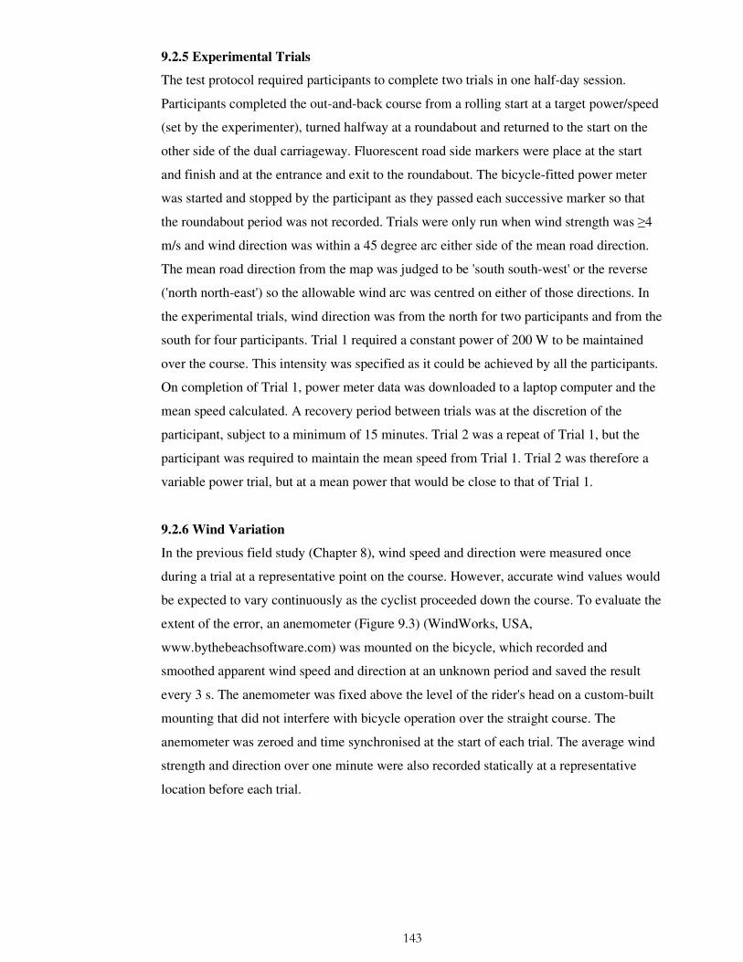
143

9.2.5 Experimental Trials

The test protocol required participants to complete two trials in one half-day session.

Participants completed the out-and-back course from a rolling start at a target power/speed

(set by the experimenter), turned halfway at a roundabout and returned to the start on the

other side of the dual carriageway. Fluorescent road side markers were place at the start

and finish and at the entrance and exit to the roundabout. The bicycle-fitted power meter

was started and stopped by the participant as they passed each successive marker so that

the roundabout period was not recorded. Trials were only run when wind strength was ≥4

m/s and wind direction was within a 45 degree arc either side of the mean road direction.

The mean road direction from the map was judged to be 'south south-west' or the reverse

('north north-east') so the allowable wind arc was centred on either of those directions. In

the experimental trials, wind direction was from the north for two participants and from the

south for four participants. Trial 1 required a constant power of 200 W to be maintained

over the course. This intensity was specified as it could be achieved by all the participants.

On completion of Trial 1, power meter data was downloaded to a laptop computer and the

mean speed calculated. A recovery period between trials was at the discretion of the

participant, subject to a minimum of 15 minutes. Trial 2 was a repeat of Trial 1, but the

participant was required to maintain the mean speed from Trial 1. Trial 2 was therefore a

variable power trial, but at a mean power that would be close to that of Trial 1.

9.2.6 Wind Variation

In the previous field study (Chapter 8), wind speed and direction were measured once

during a trial at a representative point on the course. However, accurate wind values would

be expected to vary continuously as the cyclist proceeded down the course. To evaluate the

extent of the error, an anemometer (Figure 9.3) (WindWorks, USA,

www.bythebeachsoftware.com) was mounted on the bicycle, which recorded and

smoothed apparent wind speed and direction at an unknown period and saved the result

every 3 s. The anemometer was fixed above the level of the rider's head on a custom-built

mounting that did not interfere with bicycle operation over the straight course. The

anemometer was zeroed and time synchronised at the start of each trial. The average wind

strength and direction over one minute were also recorded statically at a representative

location before each trial.

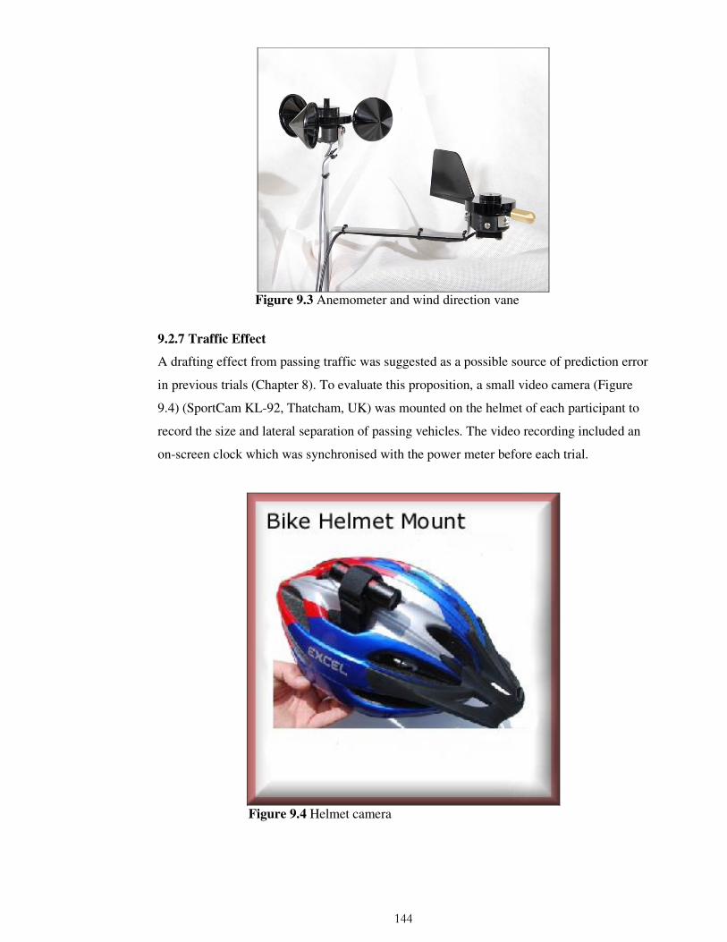
144

Figure 9.3 Anemometer and wind direction vane

9.2.7 Traffic Effect

A drafting effect from passing traffic was suggested as a possible source of prediction error

in previous trials (Chapter 8). To evaluate this proposition, a small video camera (Figure

9.4) (SportCam KL-92, Thatcham, UK) was mounted on the helmet of each participant to

record the size and lateral separation of passing vehicles. The video recording included an

on-screen clock which was synchronised with the power meter before each trial.

Figure 9.4 Helmet camera

145

9.2.8 Data Collection and Analysis

Time, power, speed and distance data for each trial were recorded using the power meter at

≈1 s intervals. If mean power output in Trial 2 differed from Trial 1, completion time in

Trial 2 was normalised to the power output level of Trial 1. The relationship between speed

and power was obtained by running multiple simulations over the complete course using a

representative subject.

Environmental wind strength and direction were calculated at 3 s intervals from the

dynamically collected apparent wind data using vector algebra. At each time point, bicycle

distance travelled and speed were taken from power meter data and bicycle direction from

the course map. Calculated values were averaged over the trial duration and compared to

the statically measured values. Dynamic and static values were averaged over all

participants to give a single measure of wind speed and wind direction error.

Analysis of the video recording sought to identify any correlation between passing traffic

and bicycle speed recorded by the power meter.

9.2.9 Statistical Analysis

Data sets were checked for normality with a Shapiro-Wilkes test and analysed with a pair-

matched t-test (Version 15.1, SPSS Inc, Chicago, IL) to identify any significant difference

between completion time at constant and variable power. Trial order was not randomised

since the mean speed from the constant power trial was required as an input to the variable

power trial. Static and dynamic wind values were compared with t-tests for repeated

measures to identify significant differences.

9.3 Results

The model predicted completion time for the mean of all riders at constant power of 200 W

was 834 s which reduced to 823 s at constant speed. The model therefore predicted that a

constant speed strategy was 1.3% faster than a constant power strategy.

Experimental results are listed in Table 9.1 with a more detailed breakdown in Appendix 6.

Data were normally distributed (p=0.876). The individual times for the variable and

constant power strategies are shown in Figure 9.5. The constant power trial was completed

in 813±64.5 s at a mean power of 204 W while the constant speed trial was completed in

793±50.9 s at a mean power of 209 W. The constant speed completion time increased to

797±52.4 s when power was normalised to 204 W. The actual difference in time between

146

the trials of 20±16.6 s (2.5%) was significant (p<0.001), but after normalisation, the time

difference was 16±15.5 s (2.0%) which was non-significant (p=0.056). The 95%

confidence interval difference was -1 s to 32 s. Statistical power was 0.7 for the normalised

result. Mean peak power in Trial 2 was 367 W and mean within-subject power standard

deviation was 75.5 W.

Table 9.1 Results of constant power and constant speed strategies.

Constant Power Trial (target of 200 W)

Constant Speed Trial (speed from Constant Power)

Power (W)

Speed (m/s)

Time (s) Power (W)

Speed (m/s)

Time (s)

Actual 204±1.8 8.73±0.7 813±64.5 209±2.7 8.95±0.6 793±50.9

Normalised - - - 204±2.1 8.90±0.6 797±52.4

Modelled 200 8.51 834 200 8.62 823

700

750

800

850

900

950

1 2 3 4 5 6

Participant

Tim

e (s

)

Constant Power

Variable Power

Figure 9.5 Individual completion times for constant and variable power strategies.

Wind data is shown in Table 9.2. The statically measured wind speed was 4.7±1.4 m/s and

the dynamically measured wind speed was 4.8±2.1 m/s. The difference of 3% was not

significant (p=0.809). The static wind direction was 0.7±1.6 radians and the dynamic wind

direction was 0.6±1.9 radians (zero radians = due south and <0 indicated veer). The

difference (18% veer) was not significant (p=0.672).

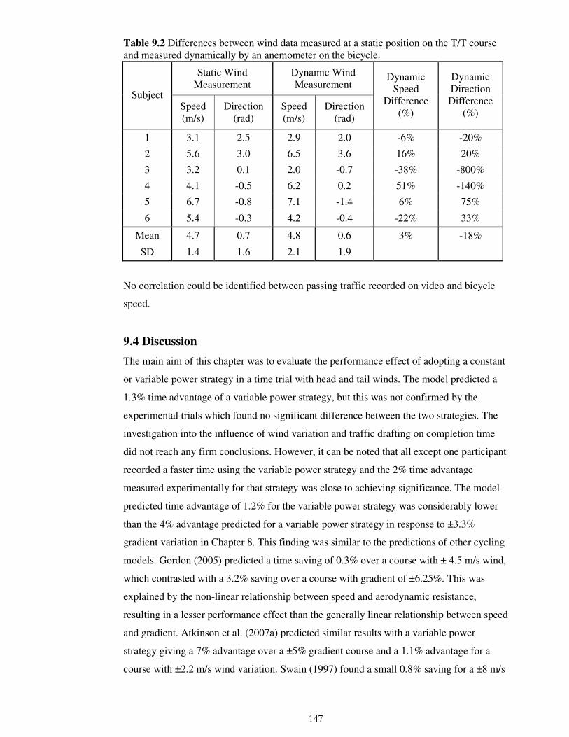
147

Table 9.2 Differences between wind data measured at a static position on the T/T course and measured dynamically by an anemometer on the bicycle.

Static Wind Measurement

Dynamic Wind Measurement

Subject Speed (m/s)

Direction (rad)

Speed (m/s)

Direction (rad)

Dynamic Speed

Difference (%)

Dynamic Direction Difference

(%)

1 3.1 2.5 2.9 2.0 -6% -20%

2 5.6 3.0 6.5 3.6 16% 20%

3 3.2 0.1 2.0 -0.7 -38% -800%

4 4.1 -0.5 6.2 0.2 51% -140%

5 6.7 -0.8 7.1 -1.4 6% 75%

6 5.4 -0.3 4.2 -0.4 -22% 33%

Mean 4.7 0.7 4.8 0.6 3% -18%

SD 1.4 1.6 2.1 1.9

No correlation could be identified between passing traffic recorded on video and bicycle

speed.

9.4 Discussion

The main aim of this chapter was to evaluate the performance effect of adopting a constant

or variable power strategy in a time trial with head and tail winds. The model predicted a

1.3% time advantage of a variable power strategy, but this was not confirmed by the

experimental trials which found no significant difference between the two strategies. The

investigation into the influence of wind variation and traffic drafting on completion time

did not reach any firm conclusions. However, it can be noted that all except one participant

recorded a faster time using the variable power strategy and the 2% time advantage

measured experimentally for that strategy was close to achieving significance. The model

predicted time advantage of 1.2% for the variable power strategy was considerably lower

than the 4% advantage predicted for a variable power strategy in response to ±3.3%

gradient variation in Chapter 8. This finding was similar to the predictions of other cycling

models. Gordon (2005) predicted a time saving of 0.3% over a course with ± 4.5 m/s wind,

which contrasted with a 3.2% saving over a course with gradient of ±6.25%. This was

explained by the non-linear relationship between speed and aerodynamic resistance,

resulting in a lesser performance effect than the generally linear relationship between speed

and gradient. Atkinson et al. (2007a) predicted similar results with a variable power

strategy giving a 7% advantage over a ±5% gradient course and a 1.1% advantage for a

course with ±2.2 m/s wind variation. Swain (1997) found a small 0.8% saving for a ±8 m/s

148

wind, but the power variation allowed in the variable power strategy in that study was

restricted to 10%.

The negative findings of this study could be related to a number of limitations. The number

of participants was low and it was possible that an increased number would have resulted

in a statistically significant finding. However, the requirement for wind conditions that

combined the required direction and speed together with dry weather limited the number of

completed trials. The time difference may also have been reduced due to the difficulty

some participants experienced in maintaining a constant speed. Constant speed required

high and varying power levels for extended periods in some wind conditions. Wind gusts

caused almost instantaneous speed changes making it more difficult for a rider to maintain

constant speed than was the case for the gradient variation studied in Chapter 8. It is

important to remember that any variation from constant speed increases completion time

and reduces the advantage relative to constant power.

The comparison of static and dynamic wind values showed no statistical difference which

suggested that the accuracy of wind data was not a factor in model prediction error.

However, this finding was subject to a number of limitations. The wind gauge was not

designed for scientific accuracy under field conditions and, therefore, the measurement

noise in the trials might have obscured real changes. A pedalled bicycle experiences

continual direction changes independently of path-following. The accuracy of the

directional data obtained from the map and the anemometer may therefore have been low,

possibly further reduced by the smoothing applied by the wind meter. Unfortunately, no

'gold standard' could be identified which might have supported the quality of the collected

data. A GPS approach to measuring position and direction may be more effective in future

research. It can also be argued that mean values for wind speed and direction over multiple

cyclists and trials have limited relevance to model predictive accuracy. Further research

will be required to address this issue.

The failure to identify a traffic drafting effect was almost certainly due to the sensitivity of

the power meter. The power meter averaged speed over several wheel revolutions which

when combined with the speed fluctuations inherent in pedalling, obscured small

variations. Additionally, most trials in this study were conducted at the weekend when

commercial traffic with the greatest drafting effect was scarce. The traffic drafting effect

for a single vehicle was expected to be small and, therefore, difficult to measure but

anecdotal evidence suggested that the cumulative effect could be substantial. Any

149

reduction in drafting effect due to side winds was likely to have been small as trial

conditions required predominant head and tail winds. A more sensitive measurement

method will be required for further research.

The trials attempted to eliminate the effect of any physiological factors in the results by

setting a relatively low power output target and limiting the course length. It seems likely

that this was successful given that actual mean power levels were generally above target

and had to be normalised downwards. The peak power level required to maintain constant

speed in Trial 2 was within the capacity of the participants. However, it can be noted that

the variations in wind required constant and substantial power adjustments as shown by the

high within-subject power standard deviation. This supports the finding from Chapter 8

that implementing an effective variable power strategy requires considerable physiological

capacity.

In conclusion, this section investigated the proposition that performance would be

enhanced if power was varied to most nearly maintain constant speed over an out-and-back

time trial course with alternating head and tail winds. The thesis model predicted a 1.3%

time advantage when power was varied to maintain constant speed. This was not

confirmed by experimental trials, but the 2% time advantage obtained with the variable

power strategy did approach significance. A study with more subjects might be expected to

achieve significance. The present research was constrained by participant availability

coinciding with suitable wind conditions. Wind is a considerably less controllable variable

than gradient which made it difficult to experimentally confirm the model prediction. No

significant differences were found between static and dynamic wind measurements,

although the research method had limitations. Traffic drafting as a factor in model

prediction error will require a new research design if the effect is to be quantified.

150

CHAPTER TEN

SENSITIVITY ANALYSIS

10.1 Introduction

A variety of methods have been applied to evaluating the sensitivity of a model's output to

variations in its input parameters (Cheng and Holland, 1998; Benke et al., 2008; Jang and

Han, 1997). Some studies, such as Law and Kelton (1991), have taken a statistical

approach to parameter variation using a Monte Carlo simulation, but such methods were

considered to be excessive for a parameter set predominantly known from experimental

work. Other studies have applied numerical optimisation of an objective function (Perl,

2004) which, although related to parameter variation, required development of complex

techniques that would be excessive for the purpose of this thesis. A method appropriate to

the present study would be a relatively simple analysis of a computational model response

to variation in input parameters' (Scovil and Ronsky, 2006; Xiao and Higginson, 2010).

The aim of this study was to evaluate the effect on model results of variation in parameter

values. Parameters were only investigated if there was evidence from published studies or

anecdotally from competitive cyclists that variation would have an important effect. The

findings will indicate whether the level of uncertainty resulting from the pooled uncertainty

of the evaluated parameters gives confidence in overall model validity.

10.2 Methods

The method adopted in this chapter was to analyse the response of a computational model

to variation in input parameters' (Scovil and Ronsky, 2006; Xiao and Higginson, 2010).

10.2.1 Key Parameters

The thesis model contained 817 initial condition parameters requiring selection of a subset

that were likely to substantially influence simulation results. Of necessity, parameters were

selected by judgment based on relevant literature, model experience and practical cycling

experience. Two 'first principles' models were identified which both simulated field

cycling and conducted a sensitivity analysis (Olds et al., 2005; Martin et al., 1998). The

studies reported model sensitivity to environmental wind speed, ensemble mass, CDA and

rolling resistance, which experience supported as key parameters. These parameters were

examined in the present analysis together with tyre effects and power variation which were

151

also thought likely to be important. The range of parameter variation was based on the

variation that was likely to occur for a given parameter and was also influenced by the

extent of variation necessary to generate an output effect. The measured output for each

analysis was completion time.

10.2.2 Mass and Inertia Tensor

The effect of variation in leg segment mass and inertia tensor values was examined as they

were thought to influence performance in pedalling (Hull and Gonzalez, 1988; Gonzalez

and Hull, 1989). Model version V1 (ergometer equivalent model) was used to conduct the

sensitivity analysis in order to maintain comparison with the reference studies and

eliminate any effects of bicycle motion. Baseline outputs for mean power, torque and

cadence were measured at the crank spindle using the default segment mass values. Three

V1 simulations of 4 s duration with baseline initial condition power (255 W) were then

completed with all leg segment masses reduced successively by 50%, 75% and ~100%

(zero mass is not permitted in SimMechanics). Mean power, torque and cadence were

measured for each simulation and presented as graphs. A further simulation was completed

with default mass values but inertia tensor values reduced to zero.

10.2.3 Peak Power Variation

The evaluation of a variable versus constant power strategy in Chapter 8 imposed a peak

power output of 325 W on participants. This raised the possibility that the time saving

found for the variable power strategy might have been greater if a higher peak power had

been adopted. The issue had already been partly investigated in Chapter 8 when the peak

power limit for four participants was increased to 400 W. This should have helped to

maintain speed on climbs and thus maintain a more constant speed, which would have

enhanced performance compared to the constant power output strategy. However, although

the gradient was sufficient for a reduced speed variance, no performance advantage was

found. This unexpected result indicated that further research was needed if any time

advantage from a high peak power was to be identified. Consequently, multiple

simulations were run to plot the variable power output strategy completion time when peak

power was systematically increased from 250 W to 1000 W.

10.2.4 Tyre Model

Tyre models have not previously been included in field cycling models and it was therefore

important to investigate model sensitivity to a tyre model. Trial simulations indicated that

the tyre model might generate a greater performance effect than expected, given its

152

omission from previous research. An initial investigation re-ran the simulation for

participant number three in Chapter 7 (a representative participant), but with the tyre model

removed. The difference in completion time with and without tyre forces was compared. It

was hypothesised that any time difference would be related to tyre hysteresis generated by

the continuous roll and steer resulting from pedalling at high power output. Some

hysteresis should appear as lateral force generation so two new simulations were conducted

to isolate the lateral force contribution due to pedalling. A straight, flat course of 4043 m at

a constant power of 255 W was simulated. In the first simulation, the bicycle was propelled

with pedal forces resulting in roll and steer as in model version V4. The same course was

then simulated with rider pedalling disabled and the bicycle propelled by rear wheel torque

as in model version V3. Total front and rear lateral tyre forces and moments were recorded

together with completion time.

10.3 Results

10.3.1 Main Parameters

The effects of parameter variation for CDA, wind speed, wind direction and ensemble

mass are shown in Table 10.1. The table also shows the range of values that are considered

reasonable for each parameter, derived by relating model "trial and error" simulations to

practical experience. Selected ranges are also consistent with similar field studies (Martin

et al., 1998; Olds et al., 1995). The data is presented as a graph in Figure 10.1 in a form

that indicates the relative importance of each parameter. Starting from 12 o'clock, the plots

become more important as they advance towards 3 o'clock. The most important parameter

was CDA which generated a ~6% change in completion time when the parameter was

varied by 20% (well within the range achievable by a cyclist (Bassett et al., 1999)).

Conversely, rolling resistance was the least important parameter with a 2% change in

completion time resulting from a 50% change in parameter value. The effect of parameter

variation was often symmetrical about the system default value resulting in nearly linear

variable plots.

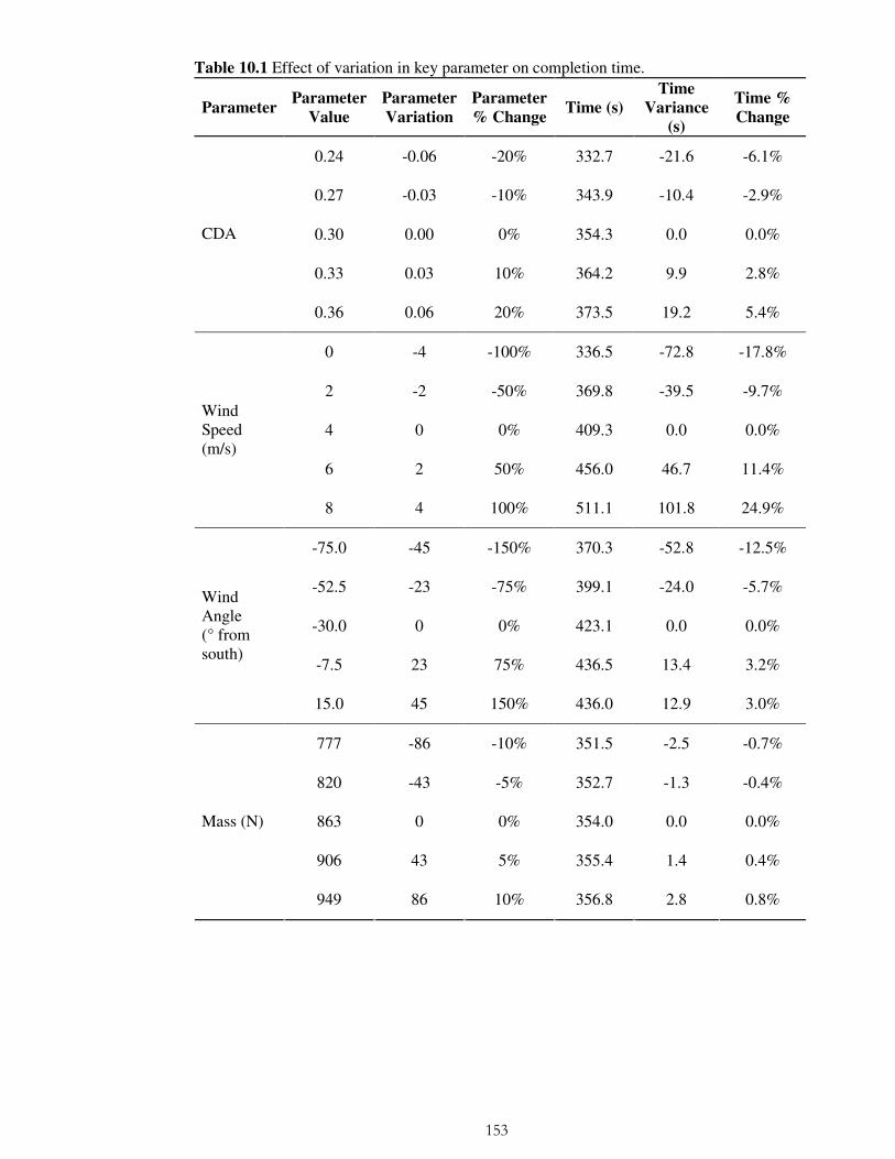
153

Table 10.1 Effect of variation in key parameter on completion time.

Parameter Parameter

Value

Parameter

Variation

Parameter

% Change Time (s)

Time

Variance

(s)

Time %

Change

0.24 -0.06 -20% 332.7 -21.6 -6.1%

0.27 -0.03 -10% 343.9 -10.4 -2.9%

0.30 0.00 0% 354.3 0.0 0.0%

0.33 0.03 10% 364.2 9.9 2.8%

CDA

0.36 0.06 20% 373.5 19.2 5.4%

0 -4 -100% 336.5 -72.8 -17.8%

2 -2 -50% 369.8 -39.5 -9.7%

4 0 0% 409.3 0.0 0.0%

6 2 50% 456.0 46.7 11.4%

Wind Speed (m/s)

8 4 100% 511.1 101.8 24.9%

-75.0 -45 -150% 370.3 -52.8 -12.5%

-52.5 -23 -75% 399.1 -24.0 -5.7%

-30.0 0 0% 423.1 0.0 0.0%

-7.5 23 75% 436.5 13.4 3.2%

Wind Angle (° from south)

15.0 45 150% 436.0 12.9 3.0%

777 -86 -10% 351.5 -2.5 -0.7%

820 -43 -5% 352.7 -1.3 -0.4%

863 0 0% 354.0 0.0 0.0%

906 43 5% 355.4 1.4 0.4%

Mass (N)

949 86 10% 356.8 2.8 0.8%

154

-100

-50

0

50

100

-20 -10 0 10 20

Time Change (%)

Pa

ram

eter

Ch

an

ge

(%)

Wind Speed

Wind Angle

Mass

CDA

Figure 10.1 Effect of key parameter variation on completion time. 10.3.2 Mass and Inertia Tensor

The effect of leg mass reduction is shown in Figure 10.2. All mean output values reduced

substantially after 50% mass reduction. The effect of inertia tensor reduction was

negligible with mean power, torque and cadence reducing respectively by 0.04%, 0.07%

and 0.1%.

150.00

180.00

210.00

240.00

270.00

0 25 50 75 100

% Leg Mass Reduction

Po

wer

(W

)

To

rqu

e*1

0 (

Nm

)

55.00

65.00

75.00

Ca

den

ce (

rpm

)

Mean PowerMean TorqueMean Cadence

Figure 10.2 Mean power, torque and cadence reductions in response to leg mass changes.

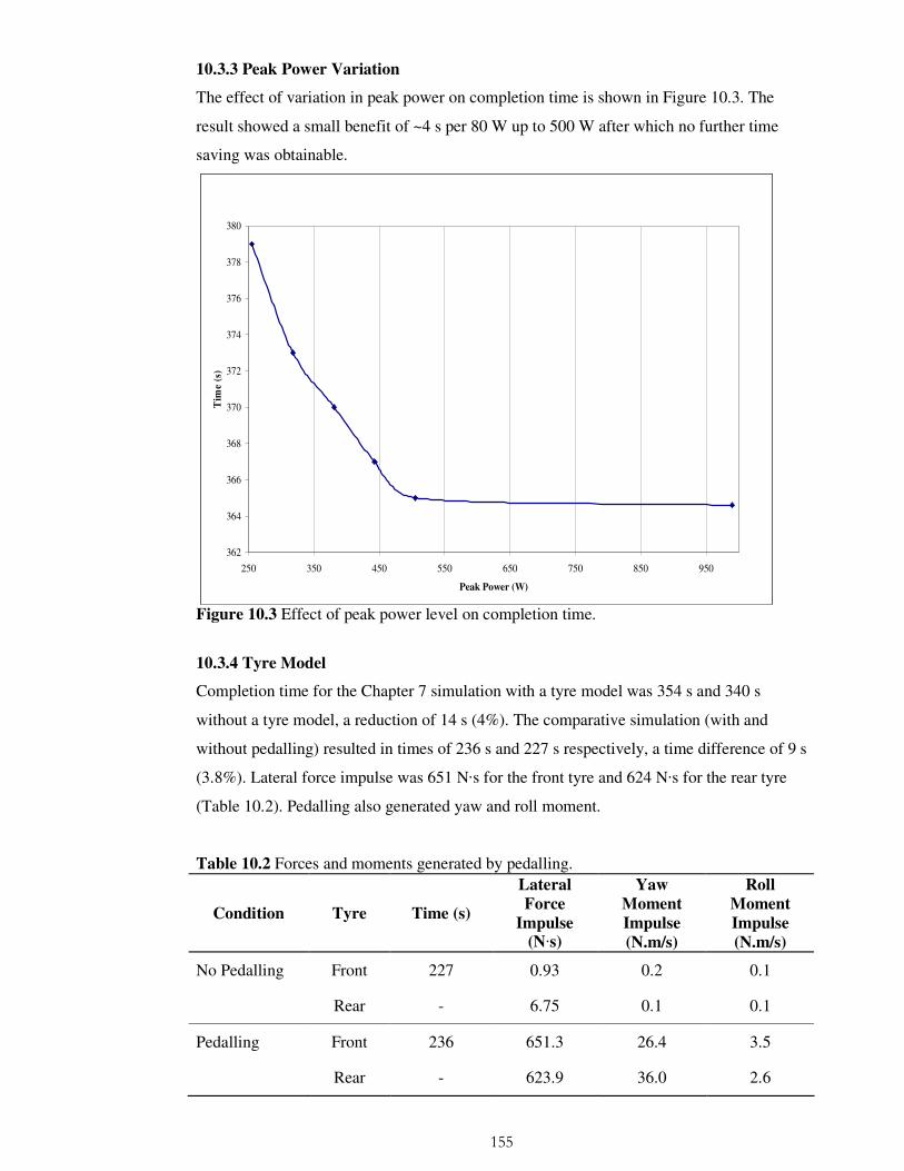
155

10.3.3 Peak Power Variation

The effect of variation in peak power on completion time is shown in Figure 10.3. The

result showed a small benefit of ~4 s per 80 W up to 500 W after which no further time

saving was obtainable.

362

364

366

368

370

372

374

376

378

380

250 350 450 550 650 750 850 950

Peak Power (W)

Tim

e (s

)

Figure 10.3 Effect of peak power level on completion time.

10.3.4 Tyre Model

Completion time for the Chapter 7 simulation with a tyre model was 354 s and 340 s

without a tyre model, a reduction of 14 s (4%). The comparative simulation (with and

without pedalling) resulted in times of 236 s and 227 s respectively, a time difference of 9 s

(3.8%). Lateral force impulse was 651 N·s for the front tyre and 624 N·s for the rear tyre

(Table 10.2). Pedalling also generated yaw and roll moment.

Table 10.2 Forces and moments generated by pedalling.

Condition Tyre Time (s)

Lateral

Force

Impulse (N·s)

Yaw

Moment

Impulse

(N.m/s)

Roll

Moment

Impulse

(N.m/s)

No Pedalling Front 227 0.93 0.2 0.1

Rear - 6.75 0.1 0.1

Pedalling Front 236 651.3 26.4 3.5

Rear - 623.9 36.0 2.6

156

10.4 Discussion

The thesis model was evaluated in respect of its sensitivity to initial parameter variation.

The aerodynamic parameters of CDA and wind speed had the greatest effect on completion

time (Table 10.1). A CDA error of 10 % generated a time difference of 2.8% which would

have invalidated the findings in Chapters 7 and 8. As individual CDA was estimated from

relationships presented in the literature, some degree of error was likely to be present.

However, there was no evidence of a systematic bias in the parameter so the ± errors might

be expected to balance out. The relationship between percentage wind speed change and

percentage time change exhibited a curvilinear track which might be expected given the

exponential nature of aerodynamic resistance, but the wind angle parameter was notably

non-linear. This was likely to result from complex changes in aerodynamic force as the

wind struck the bicycle and rider from an increasingly oblique angle. Wind tunnel trials

would be required to further quantify this effect. Variation in mass values affected

completion time by <1% suggesting that the accuracy of total bicycle and rider mass was

not critical.

The sensitivity of key parameter values was similar to those reported by Olds et al., (1995)

(Figure 10.4) and Martin et al., (1998) (Figure 10.5). The exception was the wind speed

profile in the former study which may be in error as it was not reported directly in the

study and had to be calculated by regression.

157

-100

-50

0

50

100

-20 -10 0 10 20

Time Change (%)

Param

ete

r C

han

ge (

%)

Wind Speed

Mass

CDA

Figure 10.4 Effect of parameter variation on completion time in Olds et al., (1995).

-100

-50

0

50

100

-20 -10 0 10 20

Time Change (%)

Pa

ram

ete

r C

han

ge (

%)

Wind Speed

Rolling Resistance

CDA

Figure 10.5 Effect of parameter variation on completion time in Martin et al., (1998).

158

Considering the variable power strategy sensitivity to peak power, the model prediction of

a 4 s saving for each 80 W increase in peak power up to 500 W did not reflect the

experimental finding from the field trial in Chapter 8. In that trial, peak power for four

participants was increased from 325 W to 400 W but their time saving remained within

two SD of the mean for all participants. It was possible that any additional time saved was

lost in the random time fluctuations due to environmental wind and traffic. The model of

Atkinson et al., (2007a) predicted a similar time saving of ~7 s per 80 W increase in mean

power when peak power was +10% of mean. That study noted that as power increased,

there would be less loss of speed during climbs thus reducing the difference in time spent

between climbing and descending. The almost zero increase in time saving above 500 W

predicted by the present model suggests that this was the power output level at which the

modelled course effectively became 'flat' in a speed variation context.

The sensitivity of pedalling to variation in leg segment mass was surprising and not known

to have been previously reported in the literature. A model error is possible but it is not

apparent why such an error should only occur at ≤50% reduction in leg mass. A possible

source of error might have been the method chosen to assess the sensitivity to mass

changes. The joint torque profiles which drove the model remained the same as those

required to produce a crank power of 255W with the ‘normal’ leg mass , as leg mass was

reduced. With lighter joint segments it may be that the joint torque profiles were

inappropriate for the greater segment accelerations experienced with reduced segment

masses. This could have lead to a less coordinated and efficient pedalling action, although

this was not obviously apparent from viewing the animation of the model. With hindsight,

it may have been more helpful to reverse engineer the model and assess the effect of

segment mass change by examining the changes in joint torques required to achieve a

power output of 255W at the crank.

As a precursor to a future investigation, it was noted that keeping limb mass constant but

varying gravity by ±100% resulted in an inverse ±1% variance in power at the crank.

Furthermore, when leg mass and gravity were simultaneously varied, the result was

considerably greater than the sum of the individual effects.

The effect of a tyre model on cycling performance was found to be considerably more

important than previously identified in the literature. This may have been a consequence of

transferring motorcycle tyre concepts to cycling models (Meijaard and Schwab, 2006;

Limebeer and Sharp, 2006; Cossalter, 2003). Motorcycle models have assumed that lateral

159

tyre forces are primarily a consequence of path following, while it is likely that pedalling is

the predominant influence on tyre force in a bicycle. Although the forces are small for each

cycle, the accumulated forces are significant over a complete time trial. It should be noted

that lateral tyre forces are likely to vary with power level as greater down-stroke pedal

force will usually generate more bicycle roll and steer. In the broader modelling context, it

is interesting to consider the similarity between lateral tyre force measurement and

measurement of human joint torques in that, for all practical purposes, both data can only

be obtained from modelling.

Intuitively, lateral forces generated by steering and roll tyre hysteresis should impede

forward motion, but it is not immediately apparent how these forces are applied

mechanically. It is possible that conservation of energy principles dictate that lateral tyre

force diminishes longitudinal propulsive force (Schwab et al., 2007). It is also possible for

yaw, roll and steer accelerations to affect the maintenance of system momentum (Limebeer

and Sharma, 2010). Further research into both of these possibilities is beyond the scope of

this thesis.

In conclusion, this chapter has investigated the effect of parameter variation on model

outputs. Variations in aerodynamic parameters were found to have the greatest effect on

completion time and were sufficient to negate the experimental model validation

conducted in Chapter 7. They could also throw doubt on the finding in Chapter 8 that a

variable power output strategy is faster than equivalent constant power over an undulating

course. However, it seems unlikely that random or modelling errors combined in a

particular direction throughout twenty participants and across eighty trials. It was

considered reasonable, therefore, to assume that the relationship between the modelled and

experimental result reflected reality. A further finding from the sensitivity analysis was the

importance of including a tyre model if a rider/bicycle model is adequately to represent

road cycling. Overall, model sensitivity to parameter variation seemed unlikely to negate

the validity found in the experiments conducted for this thesis.

160

CHAPTER ELEVEN

SUMMARY, LIMITATIONS, FUTURE RESEARCH

AND CONCLUSION

11.1 Summary

This thesis was undertaken with the objective of identifying ways to enhance the

performance of cyclists competing in road time trials. It was apparent that a purely

experimental approach would be inefficient given the large number of variables that could

be involved and the difficulty of accurately measuring outcomes in the field. Modelling

provided an alternative whereby, once a model was developed, simulations could rapidly

identify a short-list of promising enhancements that could then be evaluated in field

experiments. The ability to quantify mechanical parameters accurately suggested that

modelling mechanically based enhancements would yield more useable insights than could

be obtained from physiological modelling.

The research question was posed as 'Can a generalised and effective model of road cycling

be constructed?' Effectiveness was defined as model prediction of completion time over a

time trial course to an acceptable level of accuracy. Acceptable accuracy was set by

estimating the error level that was likely to make model derived performance

enhancements credible to competitive cyclists. A generalised model was one that could

respond to parameterised and continuously changing rider and environmental variables

during a simulation. Existing cycling models were analysed in Chapter 1 to establish their

accuracy and generalisation in predicting time trial performance. It became apparent from

examining some eighty cycling models developed over the last hundred years that they

divided into: 1) those developed in an engineering environment (section 1.3.2) and 2) those

developed in a sport science context (section 1.3.1). Sport science modelling studies had

extensively investigated the rider contribution to performance, but largely ignored the

contribution from bicycle dynamics. Mechanical engineering based studies had taken the

opposite approach. Both disciplines had largely ignored the environmental impact on

performance or had approximated environmental factors by setting predominantly static

values which did not reflect 'real-world' cycling. Existing models could also be

characterised as 'conceptual models' versus 'predictive models', the former describing

performance trends and the latter predicting specific outcomes for given conditions. Only

two models were identified that made specific time predictions over a time trial course, but

161

they were constrained by limited or unrepresentative course characteristics (Martin et al.,

1998; Olds et al., 1995). Neither could be described as generalised tools.

A model was developed in Chapter 2 with the intention of drawing on the strengths of

existing models, addressing their weaknesses and adding new features not previously

implemented in a single system. These included gears, tyres, transmission, pedalling and

steering. A key initial requirement was to identify an appropriate multi-body modelling

software package. After evaluation of possible packages including ADAMS, Dymola,

AutoSim and 20-Sim, SimMechanics was selected as the most suitable product. The

resulting model was developed in stages with model components completed and validated

within each stage prior to full validation of the completed model.

Validation commenced in Chapter 3 when model forces generated by pedalling were

compared with a published benchmark study. Model crank torque was similar to the

benchmark (R2=0.97, NRMSE=4%) as were pedal forces (NRMSE=8-9%). Chapter 4

validated bicycle self-stability by comparing model eigenvalues to a published benchmark.

Model eigenvalues were found to exhibit <10% variance from the benchmark values. Tyre

characteristics were evaluated in Chapter 5 with forces and moments generated by the tyres

being similar to the only relevant study that could be identified. Field validation

commenced in Chapter 6 with a case study that found model predicted time varied by 1%

from actual time over a time trial course. Chapter 7 conducted a similar field experiment

with a sample of competitive cyclists and found a 1.4% error between predicted and actual

time. The error levels from both studies were well within the target error level of 2.8%

specified for the model. The validated model was then used to predict performance

enhancement strategies in road time trials. Firstly, Chapter 8 investigated the advantage of

adopting a variable power strategy over an undulating course. The model predicted a 4 %

time saving which was close to the experimental time saving of 2.9%. Chapter 9 applied

the same strategy to a course with a head and tail wind and although a 2% advantage was

obtained, this was not statistically significant. Finally the model sensitivity to input

parameters was evaluated. CDA was found to be the most important parameter with a

variance of 20% generating a ~6% change in completion time. Wind was also an important

parameter with a 50% change in wind speed generating a ~10% change in completion time.

In summary, a model was designed, developed and validated successfully and then utilised

to predict a performance enhancement strategy that was confirmed experimentally.

162

11.2 Limitations

Although a comprehensive model was developed, there were areas where the model was

incomplete. Most notably, modelling of the rider's upper body did not include forces

applied to the handlebars which can be considerable particularly during climbing

(Bolourchi and Hull, 1985; Soden and Adeyefa, 1979). Model development requires

modelling of the three dimensional forces applied by each hand and their synchronisation

with pedalling and body roll. Steering should also be implemented by applying forces to

the handlebars rather than by application of torque direct to the steering joint. The absence

of a gear system and therefore the ability to control rider cadence is also a significant

limitation of the current model. Resolving this issue is largely dependant on finding a way

to arrange the SimMechanics blocks in a manner that avoids a system error. A number of

minor model enhancements might improve prediction accuracy but are not priority

developments as their treatment in other models suggests they would have minimal impact.

There has to be a question over whether the 'benchmark' studies used for model validation

were adequately definitive and/or adequately tested model functions. They were not

established 'gold standards' and would require more extensive critique in the literature

before they could be considered as such. However, in the absence of established gold

standards, the studies selected to validate the main model components of rider pedalling

and bicycle stability had been extensively cited in the literature while the study of bicycle

tyres was the most comprehensive available from a very limited number of sources. The

approach was therefore adopted of building on previous work by conducting experimental

validation of bicycle/rider components through comparison to the most complete of

existing studies. Experimental validation was conducted for the field time trials as no

appropriate benchmark studies could be identified from the literature. Nevertheless, further

validation may be necessary, particularly if model predictions for new conditions are found

to be significantly less accurate than present values.

Accurate simulation results were not dependant on parameter tuning due to the 'first

principles' model design. However, sensitivity analysis identified three parameters that

substantially affected outcomes. Firstly, CDA generally ranged from 0.25 to 0.35 for a

competitive road cyclist, but the chosen value influenced completion time by up to 6%.

Individual CDA values had to be estimated from body size and regression equations (Heil,

2001; Heil, 2002) as wind tunnel facilities were not available to obtain values with greater

accuracy. Sensitivity analysis also showed that wind strength and wind direction parameter

values could also substantially affect completion time suggesting they should be measured

163

dynamically at the position of the moving cyclist. However, dynamic wind measurement

on the bicycle found no statistical difference from statically measured values.

Nevertheless, until further data is available, predicting field trial results should be treated

with caution if strong wind conditions are present.

A limitation of the model was the type of courses over which the model was validated.

Courses were predominantly straight with medium gradient variation. The validity may not

be maintained for courses with large and frequent changes of direction and/or severe

gradients such as the Alpe d'Huez course used in the Tour de France. Another limitation

was the use of completion time as the only measure of model validity. Studies with

measuring devices fitted to the bicycle would be needed if model validity were to be based

on agreement between specific modelled and actual quantities (such as steer torque or roll

angle) rather than at the overall completion time level. A further thesis limitation which

could affect the application of performance enhancements in real-world cycling was the

exclusion of physiological factors. For example, the mechanical benefits of a variable

power strategy could be negated by an increase in physiological cost. Future investigation

using the model will need to consider methods for including some quantification of

physiological factors.

11.3 Future Research

The emphasis in this thesis was on building a cycling model rather than using it for its

intended purpose of identifying performance enhancement mechanisms and strategies.

Nevertheless, the efficacy of pacing strategies in response to variations in gradient and

wind were investigated with the validated model. However, the main benefit of the model

to the research community should be realised over the coming months and years as

investigations into mechanical performance enhancement in cycling can be undertaken at

considerably less time and cost and possibly greater accuracy. Planned investigations will

seek to quantify the effect of parameter variation in the following areas: 1) Bicycle related

factors such as weight, saddle position, Q factor, crank length, tyre characteristics,

eccentric chainrings and cornering optimisation. 2) Rider related factors such as inertial

and gravitational additions to muscular work at higher cadences, mechanical advantages of

'ankling' styles and riding style to minimise loss of power due to tyre lateral forces. 3)

Environmental factors such as road surface effects, cumulative effect of path variance

about the most direct line, maintenance of momentum in climbing and further analysis of

drafting effects of traffic.

164

Perhaps more importantly, the model and the model concepts will be introduced to the

research community through publication and collaborative projects. Activity to this end has

already commenced with articles in three journals (two in progress), five conference

presentations and model development and application work with the Australian Institute of

Sport (AIS) and UK Sport (Paralympic Cycling). Further agreements to develop and apply

the model will be actively sought with a joint venture to develop a track version being a

particular priority. A key objective of such a partnership would be to obtain access to laser

mapping of a velodrome. The mechanical factors that affect speed on the banking are an

area where research is required and for which the thesis model is well suited. Another

investigation would seek to model the trajectory and power that minimises work-done

when transitioning from the front to the back in the team pursuit. Selection of gear ratio for

sprint events could also be modelled effectively. It is intended that future model

development will include links to computational fluid dynamics (CFD) research which is

being developed to provide a more complete aerodynamic environment in track cycling.

11.4 Conclusion

The aim of this thesis was to develop an effective and generalised model for the purpose of

enhancing the performance of competitive cyclists in road time trials. It was questioned

whether such a model already existed and if not; it was hypothesised that such a model

could be developed. An existing model meeting the requirements could not be identified

creating an opportunity to build a new model that would satisfy the aim. A model was

constructed using rigid body modelling software and key components of the model were

validated against selected benchmarks. Modelled crank torque profile was similar to a

benchmark (R2=0.974). Bicycle self-stability matched a benchmark with <10% error.

Modelled tyre cornering stiffness deviated from a benchmark by <4%. The validated

model was then utilised to model performance enhancement strategies over actual road

courses. This experimental validation comprised a field case study and a controlled field

time trial. In the former study, modelled completion time was 1% less than actual time. In

the latter study, model prediction over a 4 km time trial course was found to be within

1.4±1.5 % of the actual time (p=0.008).

The combined modelling of rider, bicycle and environment in a system simulated at high

frequency has extended the capability of existing road cycling models. In particular, the

new model predicted the effect of changes in mechanical parameters and strategies on field

performance with accuracy acceptable to competitive cyclists. Additionally, the new model

165

emulated the changes in environmental factors necessary for realistic modelling of an

actual time trial course. An effective and generalised modelling system is, therefore, now

available to researchers investigating performance in competitive cycling. This should

enable advances in improving sport performance that were not possible with the tools

previously available.

The thesis conducted research across a wide rage of literature. Its findings exploited the

synergy obtainable when concepts were combined from disciplines that had previously

developed separately. It also distilled the essential technical information on rider, bicycle

and environment from the diverse literature pool to enable the design of an effective

model. This led to a comprehensive cycling model being specified followed by

identification of multi-body modelling software which enabled the model to be built.

Building and validating the model drew on diverse disciplines including computer

programming, engineering design, mathematics, modelling, cycling expertise, hardware

assembly and field experiment design.

The resulting model of road cycling is an important addition to the tools available to sports

scientists for researching and enhancing the performance of competitive cyclists. The lack

of modelling studies in the literature suggests that sports scientists are not fully aware of

the increased research opportunities provided by the recent development of user-friendly

modelling packages. Traditionally, modelling has been the preserve of mathematicians and

engineers, but this has changed with the availability of software packages that automate the

writing of model equations. This thesis has shown what can now be achieved by

'generalists', surpassing what previously would only have been attempted by 'experts'. It

can be hoped that this work will increase awareness amongst sports scientists of the

opportunities to extend their research capability with modelling. This could be based on

developing the current model or by using the current model as a guide to developing new

models in other software. The universality of the concepts that define three dimensional

rigid body machines means that relatively small adaptations are required to move models

between sports. The flexibility of the thesis model software has already enabled the cycling

model to be 'migrated' to model rowing, archery and the pole vault. The most suitable

sports are those where the athlete operates a 'machine' of some sort, preferably with a

significant environmental component. Ski jumping and canoeing are currently being

investigated. In summary therefore, this thesis not only provides a unique cycling model to

researchers, but lays a foundation for the much wider use of modelling throughout the

sports science community.

166

REFERENCES

Anton, M. M., Izquierdo, M., Ibanez, J., Asiain, X., Mendiguchia, J. and Gorostiaga, E. M. (2007). Flat and uphill climb time trial performance prediction in elite amateur cyclists. International Journal of Sports Medicine, 28(4), 306-313. Arsac, L. M., Thiaudiere, E., Diolez, P. and Gerville-Reache, L. (2004). Parameter estimation in modeling phosphocreatine recovery in human skeletal muscle. European

Journal of Applied Physiology, 91(4), 419-424. Åström, K.J., Klein, R.E. and Lennartsson, A. (2005). Bicycle dynamics and control: Adapted bicycles for education and research. IEEE Control Systems Magazine, 25(4), 26-47. Atkinson, G. and Nevill, A. (2000). Typical error versus limits of agreement. Sports

Medicine, 30(5), 375-381. Atkinson, G. and Brunskill, A. (2000). Pacing strategies during a cycling time trial with simulated headwinds and tailwinds. Ergonomics, 43(10), 1449-1460. Atkinson, G., Peacock, O. and Law, M. (2007a). Acceptability of power variation during a simulated hilly time trial. International Journal of Sports Medicine, 28(2), 157-163. Atkinson, G., Peacock, O. and Passfield, L. (2007b). Variable versus constant power strategies during cycling time-trials: prediction of time savings using an up-to-date mathematical model. Journal of Sports Sciences, 25(9), 1001-1009. Atkinson, G., Davison, R., Jeukendrup, A. and Passfield, L. (2003). Science and cycling: current knowledge and future directions for research. Journal of Sports Sciences, 21(9), 767-87. Atkinson, G., Peacock, O., St Clair Gibson, A. and Tucker, R. (2007c). Distribution of power output during cycling: impact and mechanisms. Sports Medicine, 37(8), 647-667. Bailey, M., Nesi, X., Passfield, L. and Carter, H. (2006). Comparison of cycle crank torque computed from forces applied to the pedals and measured with an SRM ergometer. Proceedings of the European College of Sport Science Congress, July 5th - 8th, Lausanne, Switzerland. Balmer, J., Davison, R. C., Coleman, D. A. and Bird, S. R. (2000). The validity of power output recorded during exercise performance tests using a Kingcycle air-braked cycle ergometer when compared with an SRM powermeter. International Journal of Sports

Medicine, 21(3), 195-199. Bassett, D. R., Jr., Kyle, C. R., Passfield, L., Broker, J. P. and Burke, E. R. (1999). Comparing cycling world hour records, 1967-1996: modeling with empirical data. Medicine and Science in Sports and Exercise, 31(11), 1665-1676. Benke, K. K., Lowell, K. E. and Hamilton, A. J. (2008). Parameter Uncertainty, Sensitivity Analysis and Prediction Error in a Water-Balance Hydrological Model. Mathematical and

Computer Modelling, 47, 1134-1149.

167

Bertucci, W., Duc, S., Villerius, V. and Grappe, F. (2005a). Validity and reliability of the Axiom PowerTrain cycle ergometer when compared with an SRM powermeter. International Journal of Sports Medicine, 26(1), 59-65. Bertucci, W., Duc, S., Villerius, V., Pernin, J. N. and Grappe, F. (2005b). Validity and reliability of the PowerTap mobile cycling powermeter when compared with the SRM Device. International Journal of Sports Medicine, 26(10), 868-873. Beznos, A. V., Formal'sky, A. M., Gurfinkel, E. V., Jicharev, D. N., Lensky, A. V., Savitsky, K. V. and Tchesalin, L. S. (1998). Control of autonomous motion of two-wheel bicycle with gyroscopic stabilisation. IEEE International Conference on Robotics and

Automation, 3, 2670-2675. Blundell, M. and Harty, D. (2004). The Multibody Systems Approach to Vehicle Dynamics. Oxford, UK: Butterworth-Heinemann. Bogdanis, G. C., Nevill, M. E., Boobis, L. H., Lakomy, H. K. and Nevill, A. M. (1995). Recovery of power output and muscle metabolites following 30 s of maximal sprint cycling in man. Journal of Physiology, 482 ( Pt 2), 467-480. Bolourchi, F. and Hull, M. L. (1985). Induced loads during simulated bicycling. International Journal of Sports Biomechanics, 1, 308-329. Bower, G. S. (1915). Steering and stability of single-track vehicles. The Automobile

Engineer, V, 280-283. Broker, J. P. (2003). Cycling Power. Champaign, IL: Human Kinetics. Broker, J. P. and Gregor, R. J. (1994). Mechanical energy management in cycling: source relations and energy expenditure. Medicine and Science in Sports and Exercise, 26(1), 64-74. Broker, J.P., Gregor, R.J. and Schmidt, R.A. (1993). Extrinsic feedback and the learning of kinetic patterns in cycling. Journal of Applied Biomechanics, 9(2), 111-123. Brown, D. A., Kautz, S. A. and Dairaghi, C. A. (1996). Muscle activity patterns altered during pedaling at different body orientations. Journal of Biomechanics, 29(10), 1349-1356. Brownlie, L., Ostafichuk, P., Tews, E., Muller, H., Briggs, E. and Franks, K. (2010). The wind-averaged aerodynamic drag of competitive time trial cycling helmets. Procedia

Engineering, 2(2), 2419-2424. Buchanan, M. and Weltman, A. (1985). Effects of pedal frequency on VO2 and work output at lactate threshold (LT), fixed blood lactate concentrations of 2 mM and 4 mM, and max in competitive cyclists. International Journal of Sports Medicine, 6(3), 163-168. Buchanan, T. S., Lloyd, D. G., Manal, K. and Besier, T. F. (2004). Neuromusculoskeletal modeling: estimation of muscle forces and joint moments and movements from measurements of neural command. Journal of Applied Biomechanics, 20(4), 367-395.

168

Buchanan, T. S., Lloyd, D. G., Manal, K. and Besier, T. F. (2005). Estimation of muscle forces and joint moments using a forward-inverse dynamics model. Medicine and Science

in Sports and Exercise, 37(11), 1911-1916. Cahouet, V., Luc, M. and David, A. (2002). Static optimal estimation of joint accelerations for inverse dynamics problem solution. Journal of Biomechanics, 35(11), 1507-1513. Caldwell, G. E., Li, L., McCole, S. D. and Hagberg, J. M. (1998). Pedal and Crank Kinetics in Uphill Cycling. Journal of Applied Biomechanics, 14(3), 245-259. Capelli, C., Schena, F., Zamparo, P., Monte, A. D., Faina, M. and di Prampero, P. E. (1998). Energetics of best performances in track cycling. Medicine and Science in Sports

and Exercise, 30(4), 614-624. Carvallo, M. E. (1900). Théorie du mouvement du Monocycle et de la Bicyclette. Journal

de L'Ecole Polytechnique, 5(2), 119-188. Chaffin, D. B. (1969). A computerized biomechanical model-development for the use in studying gross body actions. Journal of Biomechanics, 2, 429-441. Challis, J. H. (1997). Producing physiologically realistic individual muscle force estimations by imposing constraints when using optimization techniques. Medical

Engineering and Physics, 19(3), 253-261. Challis, J. H. and Kerwin, D. G. (1994). Determining individual muscle forces during maximal activity: Model development, parameter determination, and validation. Human

Movement Science, 13(1), 29-61. Challis, J. H. and Kerwin, D. G. (1996). Quantification of the uncertainties in resultant joint moments computed in a dynamic activity. Journal of Sports Sciences, 14(3), 219-231. Chapman, A., Vicenzino, B., Blanch, P. and Hodges, P. (2007). Do differences in muscle recruitment between novice and elite cyclists reflect different movement patterns or less skilled muscle recruitment? Journal of Science and Medicine in Sport, 12(1), 31-34. Chen, C. and Dao, T. (2006). Fuzzy Control for Equilibrium and Roll-Angle Tracking of an Unmanned Bicycle. Multibody System Dynamics, 15(4), 321-346. Chen, C. and Dao, T. (2010). Speed-adaptive roll-angle-tracking control of an unmanned bicycle using fuzzy logic. Vehicle System Dynamics, 48(1), 133 - 147. Chen, G., Kautz, S. A. and Zajac, F. E. (2001). Simulation analysis of muscle activity changes with altered body orientations during pedaling. Journal of Biomechanics, 34(6), 749-756. Cheng, R. C. H. and Holland, W. (1998). Two-point methods for assessing variability in simulation output. Journal of Statistical Computation and Simulation, 60, 183-205. Cole, D. J. and Khoo, Y. H. (2001). Prediction of vehicle stability using a 'back to back' tyre test method. International Journal of Vehicle Design, 26(5), 573-582. Collins, R. N. (1963). A mathematical analysis of the stability of two-wheeled vehicles. Dept. of Mechanical Engineering, University of Wisconsin, Ph.D. Thesis.

169

Cossalter, V. and Lot, R. (2002). A Motorcycle Multi-Body Model for Real Time Simulations Based on the Natural Coordinates Approach. Vehicle System Dynamics, 37(6), 423-447. Cossalter, V. and Doria, A. (2005). The relation between contact patch geometry and the mechanical properties of motorcycle tyres. Vehicle System Dynamics, 43(1), 156-164. Cossalter, V., Doria, A., Lot, R., Ruffo, N. and Salvador, M. (2003). Dynamic Properties of Motorcycle and Scooter Tires: Measurement and Comparison. Vehicle System

Dynamics, 39(5), 329-352. Cox, A. J. (1997). Angular momentum and motorcycle counter-steering. American Journal

of Physics, 66(11), 1018-1020. Coyle, E. F., Feltner, M. E., Kautz, S. A., Hamilton, M. T., Montain, S. J., Baylor, A. M., Abraham, L. D. and Petrek, G. W. (1991). Physiological and biomechanical factors associated with elite endurance cycling performance. Medicine and Science in Sports and

Exercise, 23(1), 93-107. Craig, N. P. and Norton, K. I. (2001). Characteristics of track cycling. Sports Medicine, 31(7), 457-468. de Koning, J. J., Bobbert, M. F. and Foster, C. (1999). Determination of optimal pacing strategy in track cycling with an energy flow model. Journal of Science and Medicine in

Sport, 2(3), 266-277. Den Hartog, J. P. (1948). Mechanics. New York and London: McGraw-Hill. di Prampero, P. E., Cortili, G., Mognoni, P. and Saibene, F. (1979). Equation of motion of a cyclist. Journal of Applied Physiology, 47(1), 201-206. Döhring, E. (1955). Stability of single-track vehicles. Die Stabilität von

Einspurfahrzeugen. Forschung Ing.-Wes, 21(2), 50-62. Dressel, A. (2007). The Benchmarked Linearized Equations of Motion for an Idealized Bicycle. http://ecommons.library.cornell.edu/handle/1813/3615?mode=full, Ph.D. Thesis. Drillis, R. and Contini, R. (1966). Body Segment Parameters. New York: Office of Vocational Rehabilitation. Eaton, D. J. (1973). Man-machine dynamics in the stabilization of single-track vehicles. University of Michigan, Ph.D. Thesis. Erdemir, A., McLean, S., Herzog, W. and van den Bogert, A. J. (2007). Model-based estimation of muscle forces exerted during movements. Clinical Biomechanics, 22(2), 131-154. Euler, L. (1776). Nova methods motum corporum rigidarum determinandi. Novi

Commentarii Academiae Scientiarum Petropolitanae, 20, 208-283. Euler, M., Braune, G., Schaal, S. and Zollman, D. (1999). Using Audiotape to Collect Data Outside the Lab: Kinematics of the Bicycle. http://www.science.uva.nl/research/amstel/bicycle/.

170

Evangelou, S., Limebeer, D. J. N., Sharp, R. S. and Smith, M. C. (2006). Control of motorcycle steering instabilities. IEEE Control Systems Magazine, 26, 78-88. Fajans, J. (2000). Steering in bicycles and motorcycles. American Journal of Physics, 68(7), 654-659. Ferguson, C., Rossiter, H. B., Whipp, B. J., Cathcart, A. J., Murgatroyd, S. R. and Ward, S. A. (2010). Effect of recovery duration from prior exhaustive exercise on the parameters of the power-duration relationship. Journal of Applied Physiology, 108(4), 866-874. Fischer, O. (1906). Einfuhrung in die Mechanik lebender Mechanismen. Leipzig, Foster, C., Green, M. A., Snyder, A. C. and Thompson, N. N. (1993). Physiological responses during simulated competition. Medicine and Science in Sports and Exercise, 25(7), 877-882. Franke, G., Suhr, W. and Riess, F. (1990). An advanced model of bicycle dynamics. European Journal of Physics, 11(2), 116-121. Fregly, B. J. and Zajac, F. E. (1996). A state-space analysis of mechanical energy generation, absorption, and transfer during pedaling. Journal of Biomechanics, 29(1), 81-90. Frezza, R., Saccon, A. and Beghi, A. (2004). Model Predictive and Hierarchical Control for Path Following with Motorcycles: Application to the Development of the Pilot Model for Virtual Prototyping. CDC Conference, Atlantis, Bahamas. Frezza, R. and Beghi, A. (2006). A virtual motorcycle driver for closed-loop simulation. IEEE Control Systems Magazine, 5, 62-77. Garcia-Lopez, J., Rodriguez-Marroyo, J. A., Juneau, C. E., Peleteiro, J., Martinez, A. C. and Villa, J. G. (2008). Reference values and improvement of aerodynamic drag in professional cyclists. Journal of Sports Sciences, 26(3), 277-286. Gardner, A. S., Stephens, S., Martin, D. T., Lawton, E., Lee, H. and Jenkins, D. (2004). Accuracy of SRM and power tap power monitoring systems for bicycling. Medicine and

Science in Sports and Exercise, 36(7), 1252-1258. Gavin, H. P. (1996). Bicycle Wheel Spoke Patterns and Spoke Fatigue. Journal of

Engineering Mechanics, 122(8), 736-742. Getz, N. H. (1995). Internal equilibrium control of a bicycle. Proceedings of the 34th IEEE

Conference on Decision and Control, 4, 4285-4287. Getz, N. H. and Marsden, J. E. (1995). Control for an autonomous bicycle. IEEE

International Conference on Robotics and Automation, 2, 1397-1402. Getz, N. H. and Hedrick, J. K. (1995). An Internal Equilibrium Manifold Method of Tracking for Nonlinear Nonminimum Phase Systems. American Control Conference,

Seattle, 1-5. Gibertini, G., Grassi, D., Macchi, C. and De Bortoli, G. (2010). Cycling shoe aerodynamics. Sports Engineering, 12(3), 155-161.

171

Gillespie, T. D. (1992). Fundamentals of Vehicle Dynamics. Warrendale, PA: SAE. Gonzalez, H. and Hull, M. L. (1989). Multivariable optimization of cycling biomechanics. Journal of Biomechanics, 22(11-12), 1151-1161. Gordon, S. (2005). Optimising distribution of power during a cycling time trial. Sports

Engineering, 8(2), 81-90. Green, S., Dawson, B. T., Goodman, C. and Carey, M. F. (1996). Anaerobic ATP production and accumulated O2 deficit in cyclists. Medicine and Science in Sports and

Exercise, 28(3), 315-321. Gregersen, C. S., Hull, M. L. and Hakansson, N. A. (2006). How changing the inversion/eversion foot angle affects the nondriving intersegmental knee moments and the relative activation of the vastii muscles in cycling. Journal of Biomechanical Engineering, 128(3), 391-398. Hagberg, J. M., Mullin, J. P., Giese, M. D. and Spitznagel, E. (1981). Effect of pedaling rate on submaximal exercise responses of competitive cyclists. Journal of Applied

Physiology, 51(2), 447-451. Hakansson, N. A. and Hull, M. L. (2007). Influence of pedaling rate on muscle mechanical energy in low power recumbent pedaling using forward dynamic simulations. IEEE

Transactions on Neural Systems and Rehabilitation Engineering, 15(4), 509-516. Hanavan, E. P. (1964). A mathematical model of the human body. Aerospace Medical

Research Laboratories, Wright-Patterson Air Force Base, Ohio, AMRL-TR-64-102, AD-608-463. Hand, R. S. (1988). Comparisons and stability analysis of linearized equations of motion for a basic bicycle model. M.Sc. thesis, Cornell University., Hansen, E. A., Andersen, J. L., Nielsen, J. S. and Sjogaard, G. (2002). Muscle fibre type, efficiency, and mechanical optima affect freely chosen pedal rate during cycling. Acta

Physiologica Scandinavica, 176(3), 185-194. Hatze, H. (2005). Towards a comprehensive large-scale computer model of the human neuromusculoskeletal system. Theoretical Issues in Ergonomics Science, 6(3-4), 239-250. Hawley, J. A. and Noakes, T. D. (1992). Peak power output predicts maximal oxygen uptake and performance time in trained cyclists. Europen Journal of Applied Physiology

and Occupational Physiology, 65(1), 79-83. Heil, D. P., Murphy, O. F., Mattingly, A. R. and Higginson, B. K. (2001). Prediction of uphill time-trial bicycling performance in humans with a scaling-derived protocol. European Journal of Applied Physiology, 85(3-4), 374-382. Heil, D. P. (2002). Body mass scaling of frontal area in competitive cyclists not using aero-handlebars. European Journal of Applied Physiology, 87(6), 520-528. Heil, D. P. (2005). Body size as a determinant of the 1-h cycling record at sea level and altitude. European Journal of Applied Physiology, 93(5-6), 547-554.

172

Heine, R., Manal, K. and Buchanan, T. S. (2003). Using Hill-Type Muscle Models and EMG Data in a Forward Dynamic Analysis of Joint Moment: Evaluation of Critical Parameters. Journal of Mechanics in Medicine & Biology, 3(2), 169-186. Heintz, S. and Gutierrez-Farewik, E. M. (2007). Static optimization of muscle forces during gait in comparison to EMG-to-force processing approach. Gait and Posture, 26(2), 279-288. Hettinga, F. J., De Koning, J. J., Hulleman, M. and Foster, C. (2009). Relative importance of pacing strategy and mean power output in 1500-m self-paced cycling. British Journal of

Sports Medicine, Hewson, P. (2005). Method for estimating tyre cornering stiffness from basic tyre information. Journal Proceedings of the Institution of Mechanical Engineers, Part D, 219(12), 1407-1412. Hickey, M. S., Costill, D. L., McConell, G. K., Widrick, J. J. and Tanaka, H. (1992). Day to day variation in time trial cycling performance. International Journal of Sports

Medicine, 13(6), 467-470. Hoogeveen, A. R., Schep, G. and Hoogsteen, G. S. (1999). The ventilatory threshold, heart rate, and endurance performance: relationships in elite cyclists. International Journal of

Sports Medicine, 20(2), 114-117. Hooker, W. W. and Margulies, G. (1965). The dynamical attitude equations for n-body satellite. Journal on Astronomical Science, 12, 123-128. Hopkins, S. R. and McKenzie, D. C. (1994). The laboratory assessment of endurance performance in cyclists. Canadian Journal of Applied Physiology, 19(3), 266-274. Hull, M. L. and Jorge, M. (1985). A method for biomechanical analysis of bicycle pedalling. Journal of Biomechanics, 18(9), 631-644. Hull, M. L. and Gonzalez, H. (1988). Bivariate optimization of pedalling rate and crank arm length in cycling. Journal of Biomechanics, 21(10), 839-49. Hull, M. L., Gonzalez, H. K. and Redfield, R. (1988). Optimization of Pedaling Rate in Cycling Using a Muscle Stress-Based Objective Function. Journal of Applied

Biomechanics, 4(1), 33-41. Hull, M. L., Kautz, S. and Beard, A. (1991). An angular velocity profile in cycling derived from mechanical energy analysis. Journal of Biomechanics, 24(7), 577-86. Hull, M. L., Wang, E. L. and Moore, D. F. (1996). An empirical model for determining the radial force-deflection behavior of off-road bicycle tires. Cycling Science, 8(1), 6-12. Humara, M. (2000). Personnel Selection in Athletic Programs. Athletic Insight, 2(2), 1-7. Huston, R. L. and Passerello, C. E. (1971). On the dynamics of a human body model. Journal of Biomechanics, 4, 369-378. Jackson, A. W. and Dragovan, M. (2000). An experimental investigation of bicycle dynamics. American Journal of Physics, 68(10), 973-978.

173

Jang, J. H. and Han, C. S. (1997). The state sensitivity analysis of the front wheel steering vehicle: In the time domain. Journal of Mechanical Science and Technology, 11(6), 595-604. Jeukendrup, A. E., Craig, N. P. and Hawley, J. A. (2000). The bioenergetics of World Class Cycling. Journal of Science and Medicine in Sport, 3(4), 414-433. Jobson, S. A., Nevill, A. M., George, S. R., Jeukendrup, A. E. and Passfield, L. (2008). Influence of body position when considering the ecological validity of laboratory time-trial cycling performance. Journal of Sports Sciences, 26(12), 1269-1278. Jobson, S. A., Nevill, A. M., Palmer, G. S., Jeukendrup, A. E., Doherty, M. and Atkinson, G. (2007). The ecological validity of laboratory cycling: Does body size explain the difference between laboratory- and field-based cycling performance? Journal of Sports

Sciences, 25(1), 3-9. Jones, D. E. H. (1970). The Stability of the bicycle. Physics Today, 23(3), 34-40. Jorge, M. and Hull, M. L. (1986). Analysis of EMG measurements during bicycle pedalling. Journal of Biomechanics, 19(9), 683-694. Kautz, S. A. and Hull, M. L. (1993). A theoretical basis for interpreting the force applied to the pedal in cycling. Journal of Biomechanics, 26(2), 155-65. Kautz, S. A. and Hull, M. L. (1995). Dynamic optimization analysis for equipment setup problems in endurance cycling. Journal of Biomechanics, 28(11), 1391-1401. Kautz, S. A. and Neptune, R. R. (2002). Biomechanical determinants of pedaling energetics: internal and external work are not independent. Exercise and Sport Sciences

Reviews, 30(4), 159-165. Kautz, S. A., Feltner, M. E., Coyle, E. F. and Baylor, A. M. (1991). The Pedaling Technique of Elite Cyclists. International Journal of Sport Biomechanics, 7, 29-53. Kirshner, D. (1979). Some nonexplanations of bicycle stability. American Journal of

Physics, 48(1), 36-38. Koenen, C. (1983). The dynamics behaviour of a motorcycle when running straight ahead and when cornering. Delft University of Technology, Ph.D. Thesis. Kooijman, J. D. G., Schwab, A. L. and Meijaard, J. P. (2008). Experimental validation of a model of an uncontrolled bicycle. Multibody System Dynamics, 19(1-2), 115-132. Kuhn, T. S. (1970). The Structure of Scientific Revolution. Chicago: University of Chicago Press. Kuo, A. D. (1998). A least-squares estimation approach to improving the precision of inverse dynamics computations. Journal of Biomechanical Engineering, 120(1), 148-159. Kyle, C. R. (1988). The Mechanics and Aerodynamics of Cycling. Champaign, IL: Human Kinetics Press. Kyle, C. R. (1994). Energy and aerodynamics in bicycling. Clinics in Sports Medicine, 13(1), 39-73.

174

Kyle, C. R. (2003). Selecting Cycling Equipment. (2nd Edition). Champaign, IL: Human Kinetics. Kyle, C. R. and Burke, E. R. (1984). Improving the racing bicycle. Mechanical

Engineering, 106(9), 34 - 45. Landau, S. and Everitt, B. (2004). A handbook of statistical analysis using SPSS. London: Chapman & Hall. Lander, P. J., Butterly, R. J. and Edwards, A. M. (2009). Self-paced exercise is less physically challenging than enforced constant pace exercise of the same intensity: influence of complex central metabolic control. British Journal of Sports Medicine, 43(10), 789-795. Laursen, P. B., Shing, C. M. and Jenkins, D. G. (2003). Reproducibility of the cycling time to exhaustion at .VO2peak in highly trained cyclists. Canadian Journal of Applied

Physiology, 28(4), 605-615. Law, A. M. and Kelton, W. D. (1991). Simulation Modeling and Analysis. (3rd). Boston, USA: McGraw Hill. Le Henaff, Y. (1987). Dynamical stability of the bicycle. European Journal of Physics, 8, 207-210. Levinson, D. A. (1977). Equations of motion for multi-rigid-body systems via symbolic manipulation. Journal of Spacecraft and Rockets, 14, 479-487. Liedl, M. A., Swain, D. P. and Branch, J. D. (1999). Physiological effects of constant versus variable power during endurance cycling. Medicine and Science in Sports and

Exercise, 31(10), 1472-1477. Limebeer, D. J. N. and Sharp, R. S. (2006). Bicycles, motorcycles and models. IEEE

Control Systems Magazine, 36, 34-61. Limebeer, D. J. N. and Sharma, A. (2008). The Dynamics of the Accelerating Bicycle. 3rd

International Symposium on Communications, Control and Signal Processing, Limebeer, D. J. N. and Sharma, A. (2010). Burst Oscillations in the Accelerating Bicycle. Journal of Applied Mechanics, 77, 34-41. Limebeer, D. J. N., Sharp, R. S. and Evangelou, S. (2001). The stability of motorcycles under acceleration and braking. Journal of Mechanical Engineering Science, 215(C9), 1095-1109. Limebeer, D. J. N., Sharp, R. S. and Evangelou, S. (2002). Motorcycle steering oscillations due to road profiling. Journal of Applied Mechanics, 69(6), 724-739. Lindsay, F. H., Hawley, J. A., Myburgh, K. H., Schomer, H. H., Noakes, T. D. and Dennis, S. C. (1996). Improved athletic performance in highly trained cyclists after interval training. Medicine and Science in Sports and Exercise, 28(11), 1427-1434. Lloyd, D. G. and Besier, T. F. (2003). An EMG-driven musculoskeletal model to estimate muscle forces and knee joint moments in vivo. Journal of Biomechanics, 36(6), 765-776.

175

Lobas, L. G. (1978). Controlled and programmed motion of a bicycle on a plane. Mechanics of Solids, 13(6), 18-23. Lockheed (2006). Lockheed Martin Space Systems Uses SimMechanics. http://www.mathworks.com/company/user_stories/Lockheed-Martin-Space-Systems-Uses-

SimMechanics-with-a-Real-Time-Simulator-to-Automate-Mars-Reconnaissance-Orbiter-

Development.html, Lot, R. (2004). A Motorcycle Tire Model for Dynamic Simulations: Theoretical and Experimental Aspects. Meccanica, 39, 207-220. Lowell, J. and McKell, H. D. (1982). The Stability of Bicycles. American Journal of

Physics, 50, 1106. Lucia, A., Hoyos, J. and Chicharro, J. L. (2001). Preferred pedalling cadence in professional cycling. Medicine and Science in Sports and Exercise, 33(8), 1361-1366. Lucia, A., Sanchez, O., Carvajal, A. and Chicharro, J. L. (1999). Analysis of the aerobic-anaerobic transition in elite cyclists during incremental exercise with the use of electromyography. British Journal of Sports Medicine, 33(3), 178-85. Lukes, R. A., Chin, S. B. and Haake, S. J. (2005). The understanding and development of cycling aerodynamics. Sports Engineering, 8, 59-74. Maronski, R. (1994). On optimal velocity during cycling. Journal of Biomechanics, 27(2), 205-213. Marsh, A. P. and Martin, P. E. (1997). Effect of cycling experience, aerobic power, and power output on preferred and most economical cycling cadences. Medicine and Science in

Sports and Exercise, 29(9), 1225-1232. Marsh, A. P., Martin, P. E. and Sanderson, D. J. (2000). Is a joint moment-based cost function associated with preferred cycling cadence? Journal of Biomechanics, 33(2), 173-180. Martin, J. C. and Spirduso, W. W. (2001). Determinants of maximal cycling power: crank length, pedaling rate and pedal speed. European Journal of Applied Physiology, 84(5), 413-418. Martin, J. C., Lamb, S. M. and Brown, N. A. (2002). Pedal trajectory alters maximal single-leg cycling power. Medicine and Science in Sports and Exercise, 34(8), 1332-1336. Martin, J. C., Gardner, A. S., Barras, M. and Martin, D. T. (2006). Modeling sprint cycling using field-derived parameters and forward integration. Medicine and Science in Sports

and Exercise, 38(3), 592-597. Martin, J. C., Milliken, D. L., Cobb, J. E., McFadden, K. L. and Coggan, A. R. (1998). Validation of a Mathematical Model for Road Cycling Power. Journal of Applied

Biomechanics, 14(3), 276-291. Maunsell, F. G. (1946). Why does a bicycle keep upright? The Mathematical Gazette, 30, 195-199.

176

McLean, S. G., Su, A. and van den Bogert, A. J. (2003). Development and validation of a 3-D model to predict knee joint loading during dynamic movement. Journal of

Biomechanical Engineering, 125(6), 864-874. Meijaard, J. P., Papadopoulos, J. M., Ruina, A. and Schwab, A. L. (2007). Linearized dynamics equations for the balance and steer of a bicycle: a benchmark and review. Proceedings of the Royal Society of London, A463, 1955-1982. Meijaard, J. P. and Schwab, A. L. (2006). Linearized equations for an extended bicycle model. European Conference on Computational Mechanics, 1-18. Mills, C., Pain, M. and Yeardon, M. (2009). Reducing ground reaction forces in gymnastics’ landings may increase internal loading. Journal of Biomechanics, 42(6), 671-678. Minguez, J. M. and Vogwell, J. (2008). An analytical model to study the radial stiffness and spoke load distribution in a modern racing bicycle wheel. Proceedings of the

Institution of Mechanical Engineers, Part C, 222(4), 563-576. Miyagishi, S., Kageyama, I., Takama, K., Baba, M. and Uchiyama, H. (2003). Study on construction of a rider robot for two-wheeled vehicle. JSAE Review, 24(3), 321-326. Murray-Smith, D. J. (1995). Enhanced environments for the development and validation of dynamic system models. Mathematics and Computers in Simulation, 39(5-6), 459-464. NASA (2004). NASA's X-43A Scramjet. http://www.mathworks.com/company/user_stories/NASAs-X-43A-Scramjet-Achieves-

Record-Breaking-Mach-10-Speed-Using-MathWorks-Tools-for-Model-Based-

Design.html?by=company, Neptune, R. R. and Hull, M. L. (1995). Accuracy assessment of methods for determining hip movement in seated cycling. Journal of Biomechanics, 28(4), 423-437. Neptune, R. R. and van den Bogert, A. J. (1998). Standard mechanical energy analyses do not correlate with muscle work in cycling. Journal of Biomechanics, 31(3), 239-245. Neptune, R. R. and Hull, M. L. (1998). Evaluation of performance criteria for simulation of submaximal steady-state cycling using a forward dynamic model. Journal of

Biomechanical Engineering, 120(3), 334-341. Neptune, R. R. and Hull, M. L. (1999). A theoretical analysis of preferred pedaling rate selection in endurance cycling. Journal of Biomechanics, 32(4), 409-415. Neptune, R. R. and Herzog, W. (1999). The association between negative muscle work and pedaling rate. Journal of Biomechanics, 32(10), 1021-1026. Neptune, R. R. and Kautz, S. A. (2001). Muscle activation and deactivation dynamics: the governing properties in fast cyclical human movement performance? Exercise and Sport

Sciences Reviews, 29(2), 76-80. Nevill, A. M., Jobson, S. A., Palmer, G. S. and Olds, T. S. (2005). Scaling maximal oxygen uptake to predict cycling time-trial performance in the field: a non-linear approach. European Journal of Applied Physiology, 94(5-6), 705-710.

177

Nevill, A. M., Jobson, S. A., Davison, R. C. and Jeukendrup, A. E. (2006). Optimal power-to-mass ratios when predicting flat and hill-climbing time-trial cycling. European Journal

of Applied Physiology, 97(4), 424-431. Newton, I. (1687). Philosophiae Naturalis Principia Mathematica. Royal Society, London, Nichols, J. F., Phares, S. L. and Buono, M. J. (1997). Relationship between blood lactate response to exercise and endurance performance in competitive female master cyclists. International Journal of Sports Medicine, 18(6), 458-463. Olds, T. (1998). The mathematics of breaking away and chasing in cycling. Europen

Journal of Applied Physiology and Occupational Physiology, 77(6), 492-497. Olds, T. (2001). Modelling human locomotion: applications to cycling. Sports Medicine, 31(7), 497-509. Olds, T. S., Norton, K. I. and Craig, N. P. (1993). Mathematical model of cycling performance. Journal of Applied Physiology, 75(2), 730-737. Olds, T. S., Norton, K. I., Lowe, E. L., Olive, S., Reay, F. and Ly, S. (1995). Modeling road-cycling performance. Journal of Applied Physiology, 78(4), 1596-1611. Olsen, J. and Papadopoulos, J. M. (1988). Bicycle Dynamics - The Meaning Behind the Math. Bike Tech, 7(6), 13-15. Oreskes, N., Shrader-Frechette, K. and Belitz, K. (1994). Verification, validation, and confirmation of numerical models in the earth sciences. Science, 263, 641-646. Otten, E. (2003). Inverse and forward dynamics: models of multi-body systems. Philosophical Transactions of the Royal Society of London. Series B: Biological Sciences, 358(1437), 1493-1500. Palmer, G. S., Noakes, T. D. and Hawley, J. A. (1997). Effects of steady-state versus stochastic exercise on subsequent cycling performance. Medicine and Science in Sports

and Exercise, 29(5), 684-687. Palmer, G. S., Dennis, S. C., Noakes, T. D. and Hawley, J. A. (1996). Assessment of the reproducibility of performance testing on an air-braked cycle ergometer. International

Journal of Sports Medicine, 17(4), 293-298. Pandy, M. G. (2001). Computer modeling and simulation of human movement. Annual

Review of Biomedical Engineering, 3, 245-273. Papadopoulos, J. M. (1987). Bicycle steering dynamics and self-stability: A summary report on work in progress. Cornell Bicycle Research Project, Cornell University, pp 1-23. Paton, C. D. and Hopkins, W. G. (2006). Ergometer error and biological variation in power output in a performance test with three cycle ergometers. International Journal of Sports

Medicine, 27(6), 444-447. Pearsall, R. H. (1922). The stability of a bicycle. The Institution of Automobile Engineers,

Proceeding Session, XVII(1), 395-404.

178

Pennestri, E., Cavacece, M. and Vita, L. (2005). On the computation of degrees-of-freedom: a didactic perspective. ASME International Design Engineering Conference,

Long Beach, California, Perl, J. (2004). PerPot - a meta-model and software tool for analysis and optimisation of load-performance-interaction. International Journal of Performance Analysis in Sport, 4(2), 61-73. Peterson, D. L. and Hubbard, M. (2008). Yaw rate and velocity tracking control of a hands-free bicycle. International Mechanical Engineering Congress and Exposition,

Boston., Popov, A. A., Rowell, S. and Meijaard, J. P. (2010). A Review on Motorcycle and Rider Modelling for Steering Control. Vehicle System Dynamics, 48(6), 775-792. Popper, K. R. (1959). The Logic of Scientific Discovery. New York: Basic Books. Price, D. and Donne, B. (1997). Effect of variation in seat tube angle at different seat heights on submaximal cycling performance in man. Journal of Sports Sciences, 15(4), 395-402. Psiaki, M. L. (1979). Bicycle stability: A mathematical and numerical analysis. Undergradute thesis, Princeton University, NJ., Raasch, C. C. and Zajac, F. E. (1999). Locomotor strategy for pedaling: muscle groups and biomechanical functions. Journal of Neurophysiology, 82(2), 515-525. Redfield, R. (2005). Large motion mountain biking dynamics. Vehicle System Dynamics, 43(12), 845-865. Redfield, R. and Hull, M. L. (1986a). On the relation between joint moments and pedalling rates at constant power in bicycling. Journal of Biomechanics, 19(4), 317-29. Redfield, R. and Hull, M. L. (1986b). Prediction of pedal forces in bicycling using optimization methods. Journal of Biomechanics, 19(7), 523-540. Rice, R. S. and Roland, R. D. (1970). An evaluation of the performance and handling qualities of bicycles. Cornell Aeronautical Laboratory, Report no. VJ-2888-K. Riemer, R. and Hsiao-Wecksler, E. T. (2008). Improving joint torque calculations: optimization-based inverse dynamics to reduce the effect of motion errors. Journal of

Biomechanics, 41(7), 1503-1509. Riemer, R., Hsiao-Wecksler, E. T. and Zhang, X. (2008). Uncertainties in inverse dynamics solutions: a comprehensive analysis and an application to gait. Gait and Posture, 27(4), 578-588. Risher, D. W., Schutte, L. M. and Runge, C. F. (1997). The use of inverse dynamics solutions in direct dynamics simulations. Journal of Biomechanical Engineering, 119(4), 417-422. Roberson, R. E. and Wittenburg, J. (1967). A dynamical formalism for an arbitrary number of interconnected rigid bodies, with reference to the problem of satellite attitude control. 3rd Congr. Int. Fed. Autom. Control, Butterworth, 1(3), Paper 46.

179

Roland, R. D. (1973). Computer simulation of bicycle dynamics. Proceedings of the ASME

Symposium Mechanics and Sport, 35-83. Roland, R. D. and Massing, D. E. (1971). A digital computer simulation of bicycle dynamics. Cornell Aeronautical Laboratory, Report no. YA-3063-K-1. Roland, R. D. and Lynch, J. P. (1972). Bicycle dynamics tire characteristics and rider modeling. Cornell Aeronautical Laboratory, Report no. YA-3063-K-2. Roue (2008). Wheel Stiffness. http://www.rouesartisanales.com/article-23159755.html, Rowell, S., Popov, A. and Meijaard, J. P. (2010). Predictive control to modelling motorcycle rider steering. International Journal of Vehicle Systems Modelling and Testing, 5(2-3), 124-160. Runge, C. F., Zajac, F. E., 3rd, Allum, J. H., Risher, D. W., Bryson, A. E., Jr. and Honegger, F. (1995). Estimating net joint torques from kinesiological data using optimal linear system theory. IEEE Transactions on Biomedical Engineering, 42(12), 1158-1164. Schiehlen, W. (1997). Multibody System Dynamics: Roots and Perspectives. Multibody

System Dynamics, 1(2), 149-188. Schiehlen, W. and Kreuzer, E. (1977). Rechnergestutzes Aufstellen der Bewegungsgleichungen gewohnlicher Mehrkorpersysteme. Ingenieur-Archiv, 46, 185-194. Schmidt, A. (1994). Handbook of Competitive Cycling. Aachen: Meyer and Meyer Verlag. Schwab, A. L., Meijaard, J. P. and Papadopoulos, J. M. (2005). Benchmark Results on the Linearized Equations of Motion of an Uncontrolled Bicycle. International Journal of

Mechanical Science and Technology, 19(1), 292-304. Schwab, A. L., Meijaard, J. P. and Kooijman, J. D. G. (2007). Some recent developments in bicycle dynamics. Proceedings of the 12th World Congress in Mechanism and Machine

Science, Scovil, C. Y. and Ronsky, J. L. (2006). Sensitivity of a Hill-based muscle model to perturbations in model parameters. Journal of Biomechanics, 39(11), 2055-2063. Seffen, K. A., Parks, G. T. and Clarkson, P.J. (2001). Observations on the controllability of motion of two-wheelers. Proceedings of the Institute of Mechanical Engineers, 215(1), 143-156. Seth, A. and Pandy, M. G. (2004). A nonlinear tracking method of computing net joint torques for human movement. Conference Proceedings IEEE Engineering, Medical and

Biology Society, 6, 4633-4636. Seth, A. and Pandy, M. G. (2007). A neuromusculoskeletal tracking method for estimating individual muscle forces in human movement. Journal of Biomechanics, 40(2), 356-366. Sharp, R. S. (1971). The stability and control of motorcycles. Journal of Mechanical

Engineering Science, 13(5), 316-329.

180

Sharp, R. S. (1985). The lateral dynamics of motorcycles and bicycles. Vehicle System

Dynamics, 14(4-6), 265-283. Sharp, R. S. (2001). Stability, control and steering responses of motorcycles. Vehicle

System Dynamics, 35(4-5), 291-318. Sharp, R. S. (2008). On the stability and control of the bicycle. Applied Mechanics

Reviews, 61, 1-24. Sharp, R.S. (2007). Optimal stabilization and path-following controls for a bicycle. Journal

Proceedings of the Institution of Mechanical Engineers, Part C: Journal of Mechanical

Engineering Science, 221(4), 415-427. Sharp, Robin S. and Limebeer, David J. N. (2001). A Motorcycle Model for Stability and Control Analysis. Multibody System Dynamics, (2), 123-142. Silva, M. P. and Ambrosio, J. A. (2004). Sensitivity of the results produced by the inverse dynamic analysis of a human stride to perturbed input data. Gait and Posture, 19(1), 35-49. Singh, D. V. (1964). Advanced concepts of the stability of two-wheeled vehicle-application of mathematical analysis to actual vehicles. Dept. of Mechanical Engineering,

University of Wisconsin, Ph.D. Thesis. Singh, D. V. and Goel, V. K. (1971). Stability of Rajdoot Scooter. SAE Paper no. 710273., Slaughter, M. H. and Lohman, T. G. (1980). An objective method for measurement of musculo-skeletal size to characterize body physique with application to athletic population. Medicine and Science in Sports and Exercise, 12, 170-174. Smak, W., Neptune, R. R. and Hull, M. L. (1999). The influence of pedaling rate on bilateral asymmetry in cycling. Journal of Biomechanics, 32(9), 899-906. Smith, J. C., Dangelmaier, B. S. and Hill, D. W. (1999). Critical power is related to cycling time trial performance. International Journal of Sports Medicine, 20(6), 374-378. Smith, M. F. (2008). Assessment Influence on Peak Power Output and Road Cycling Performance Prediction. International Journal of Sports Science & Coaching, 3(2), 211-226. Smith, M. F., Davison, R. C., Balmer, J. and Bird, S. R. (2001). Reliability of mean power recorded during indoor and outdoor self-paced 40 km cycling time-trials. International

Journal of Sports Medicine, 22(4), 270-274. Smith, N. P., Barclay, C. J. and Loiselle, D. S. (2005). The efficiency of muscle contraction. Progress in Biophysics and Molecular Biology, 88(1), 1-58. Soden, P. D. and Adeyefa, B. A. (1979). Forces applied to a bicycle during normal cycling. Journal of Biomechanics, 12(7), 527-41. Sporer, B. C. and McKenzie, D. C. (2007). Reproducibility of a laboratory based 20-km time trial evaluation in competitive cyclists using the Velotron Pro ergometer. International Journal of Sports Medicine, 28(11), 940-944.

181

Stepto, N. K., Martin, D. T., Fallon, K. E. and Hawley, J. A. (2001). Metabolic demands of intense aerobic interval training in competitive cyclists. Medicine and Science in Sports

and Exercise, 33(2), 303-310. Stone, C. and Hull, M. L. (1995). The effect of rider weight on rider-induced loads during common cycling situations. Journal of Biomechanics, 28(4), 365-375. Swain, D. P. (1997). A model for optimizing cycling performance by varying power on hills and in wind. Medicine and Science in Sports and Exercise, 29(8), 1104-1108. Tanaka, H., Bassett, D. R., Jr., Swensen, T. C. and Sampedro, R. M. (1993). Aerobic and anaerobic power characteristics of competitive cyclists in the United States Cycling Federation. International Journal of Sports Medicine, 14(6), 334-338. Tanaka, Y. and Murakami, T. (2004). Self sustaining bicycle robot with steering controller. IEEE International Workshop on Advanced Motion Control, 193-197. Tew, G. S. and Sayers, A. T. (1999). Aerodynamics of yawed racing cycle wheels. Journal

of Wind Engineering & Industrial Aerodynamics, 82, 209-222. Thelen, D. G., Anderson, F. C. and Delp, S. L. (2003). Generating dynamic simulations of movement using computed muscle control. Journal of Biomechanics, 36(3), 321-328. Timoshenko, S. and Young, D. H. (1948). Advanced Dynamics. New York: McGraw-Hill. Vaculin, O, Kruger, W. R. and Valasek, M. (2004). Overview of Coupling of Multibody and Control Engineering Tools. Vehicle System Dynamics, 41(5), 415 - 429. van Fraassen, B. (1980). The Scientific Image. New York: Oxford University Press. Van Ingen Schenau, G. J., van Woensel, W. W., Boots, P. J., Snackers, R. W. and de Groot, G. (1990). Determination and interpretation of mechanical power in human movement: application to ergometer cycling. European Journal of Applied Physiology and

Occupational Physiology, 61(1-2), 11-19. van Ingen Schenau, G. J., Boots, P. J., de Groot, G., Snackers, R. J. and van Woensel, W. W. (1992). The constrained control of force and position in multi-joint movements. Neuroscience, 46(1), 197-207. van Soest, A. J., Schwab, A. L., Bobbert, M. F. and van Ingen Schenau, G. J. (1992). SPACAR: a software subroutine package for simulation of the behavior of biomechanical systems. Journal of Biomechanics, 25(10), 1219-1226. van Soest, O. and Casius, L. J. (2000). Which factors determine the optimal pedaling rate in sprint cycling? Medicine and Science in Sports and Exercise, 32(11), 1927-1934. Van Zytveld, P. J. (1975). A method for the automatic stabilization of an unmannned bicycle. Dept. of Aeronautics and Astronautics, Stanford University, M.Sc. Thesis. Verma, M. K., Scott, R. A. and Segel, L. (1980). Effect of Frame Compliance on the Lateral Dynamics of Motorcycles. Vehicle System Dynamics, 9(4), 181-206. Vukobratovic, M., Frank, A. A. and Juricic, D. (1970). On the stability of biped locomotion. IEEE Transactions on Biomedical Engineering, BME-17, 25-36.

182

Weir, D. H. (1972). Motorcycle handling dynamics and rider control and the effect of design configuration on response and performance. University of California, Ph.D. Thesis. Whipple, F. J. W. (1899). The Stability of the Motion of a Bicycle. Quarterly Journal of

Pure and Applied Mathematics, 30, 312-348. White, S. C. and Winter, D. A. (1992). Predicting muscle forces in gait from EMG signals and musculotendon kinematics. Journal of Electromyography and Kinesiology, 2(4), 217-231. Wood, G. D. and Kennedy, D. C. (2003). Simulating Mechanical Systems in Simulink with SimMechanics. http://www.mathworks.com/matlabcentral/fx_files/2871/1/SimMechanics.pdf, Xiao, M. and Higginson, J. S. (2008). Muscle function may depend on model selection in forward simulation of normal walking. Journal of Biomechanics, 41, 3236-3242. Yavin, Y. (1999). Stabilization and control of the motion of an autonomous bicycle by using a rotor for the tilting moment. Computer Methods in Applied Mechanics and

Engineering, 178(3-4), 233-243. Yeadon, M. R. and King, M. A. (2002). Evaluation of a torque driven simulation model of tumbling. Journal of Applied Biomechanics, 18, 195-206. Yeadon, M. R., Kong, P. W. and King, M. A. (2006). Parameter determination for computer simulation model of a diver and a springboard. Journal of Applied Biomechanics, 22, 167-176. Yoshihuku, Y. and Herzog, W. (1996). Maximal muscle power output in cycling: a modelling approach. Journal of Sports Sciences, 14(2), 139-157. Zajac, F. E., Neptune, R. R. and Kautz, S. A. (2003). Biomechanics and muscle coordination of human walking: part II: lessons from dynamical simulations and clinical implications. Gait and Posture, 17(1), 1-17. Zavorsky, G. S., Murias, J. M., Gow, J., Kim, D. J., Poulin-Harnois, C., Kubow, S. and Lands, L. C. (2007). Laboratory 20-km cycle time trial reproducibility. International

Journal of Sports Medicine, 28(9), 743-748.

183

APPENDICIES

APPENDIX 1

Technical Documentation Files on Accompanying CD

Animation of Running Simulation

Bicycle Structure

Rider Structure

Pedalling

Transmission Structure

Propulsion

Steering, Balance, Path-Following

Tyre Model

Aerodynamics

Gradient

Upper Body Motion

Wheel Motion

Gear System

Performance Monitor

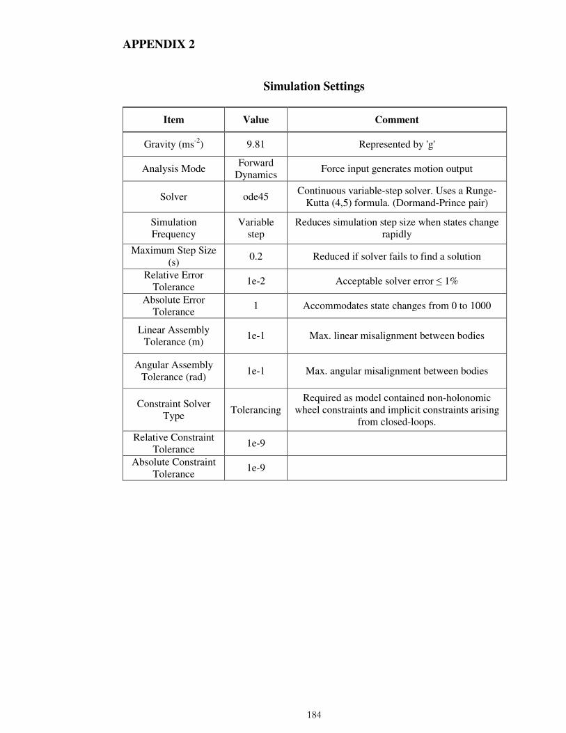
184

APPENDIX 2

Simulation Settings

Item Value Comment

Gravity (ms-2) 9.81 Represented by 'g'

Analysis Mode Forward Dynamics

Force input generates motion output

Solver ode45 Continuous variable-step solver. Uses a Runge-

Kutta (4,5) formula. (Dormand-Prince pair)

Simulation Frequency

Variable step

Reduces simulation step size when states change rapidly

Maximum Step Size (s)

0.2 Reduced if solver fails to find a solution

Relative Error Tolerance

1e-2 Acceptable solver error ≤ 1%

Absolute Error Tolerance

1 Accommodates state changes from 0 to 1000

Linear Assembly Tolerance (m)

1e-1 Max. linear misalignment between bodies

Angular Assembly Tolerance (rad)

1e-1 Max. angular misalignment between bodies

Constraint Solver Type

Tolerancing Required as model contained non-holonomic

wheel constraints and implicit constraints arising from closed-loops.

Relative Constraint Tolerance

1e-9

Absolute Constraint Tolerance

1e-9

185

Main Default Parameters

Item (Version) Location Description Default Value

Weight System Total weight of rider/bicycle 804 N Constant

Power " Define a constant power run 255 W

Mean Power " Rider mean power for a variable power run.

255 W

Wind Direction Environment Wind angle relative to south

(clockwise is negative) -45°

Wind Velocity " Wind velocity 2 m/s

IC System Initial bicycle longitudinal velocity at start of simulation

10 m/s

Big Ring (V3) Gear Selector Multiplier converting small ring (39

teeth) to big ring (53 teeth) 1.3584

Cassette Gears (V3)

" Switch Block containing 10 Gain

blocks defining 10 gear ratios 1/4.08 to

1/1.96

Bias (V3) " In 'u + 0.25', second term defines

number of seconds power is reduced at each gear change

0.25 s

Power Decrement

(V3) "

Multiplier reducing power at each gear change

0.75

Stop Distance Environment Course distance after which

simulation terminates 4043 m

Critical Velocity

Performance Rider velocity at mean power against

aero resistance only 11.05 m/s

Frame Flex Rear Frame Lateral flex modelled by a spring damper on x axis of steering joint

Spring=1,000, Damp=51

Wheel Flex " Lateral flex modelled by a spring

damper on x axis of hub joint (spring stiffness in N/m, damping in N·s/m)

Front: Spring=136 Damp=3 Rear: Spring=116 Damp=2.6

2*Joint Spring Damper

Transmission Left and right pedal spindle damping 1 rad/s

Crank Length " Length of crank arms 0.170 m

wbase Bicycle Distance from front to rear wheel

contact points (adjusted to set trail) 1.01 m

Trail " Distance front wheel contact to steer

axis/ground plane intersection 0.065 m

CDA Rider Coefficient of drag x frontal area 0.3

MaxAV (V3) Gear Selector Maximum crank angular velocity (cadence)

-10.5 rad/s

MinAV (V3) " Minimum crank angular velocity (cadence)

-8.5 rad/s

p Aerodynamics Air density (pressure/(humidity

constant*temp) 1.2234 kg/m3

Transmission Ratio

Transmission Rotational ratio of crank spindle to rear wheel hub

2.86:1

Wheels Wheels Front and rear wheel radius 0.35 m

Steer Axis Front Frame Steer axis angle relative to left horizontal 72°

COM Bicycle/Rider x and z coordinates of COM x=0.5027 m z=1.0091 m

186

APPENDIX 3

Tyre Dynamics Theory

A summary of tyre theory relating to the bicycle is presented here in order to clarify

concepts discussed in Chapter 5. It is abstracted from a number of established text books

which emphasise single track vehicles (Gillespie, 1992; Blundell and Harty, 2004;

Cossalter, 2006). A tyre develops lateral force to enable steering control of bicycle

heading, oppose centripetal acceleration in cornering and resist external side forces such as

wind and road camber. Lateral force is developed in proportion to tyre 'slip' angle and

wheel camber angle. The term 'slip' is a misnomer as it refers to the angle between a wheel

heading and its direction of travel which are misaligned in a turn or under the influence of

side wind/road camber. In reality, the tread rubber does not slip relative to the road surface

but is deflected sideways with respect to the tyre circumference. Lateral tension builds in

the tread as it moves rearwards in the contact patch, the distortion generating an increasing

side force until the tread looses adhesion in the rear part of the contact patch and 'slides' in

that area. A 'slide' is defined as complete loss of adhesion resulting in zero force

generation. The total lateral force is obtained by integrating the force generated across the

contact patch which initially increases with slip angle before reducing as the rear sliding

area extends forward. The centroid of the lateral force is offset behind the geometrical

centre of the contact patch resulting in a moment arm about the wheel's vertical z axis

known as the 'pneumatic trail'. Lateral force therefore has the secondary effect of

generating a torque defined as the 'aligning moment' which opposes steering and thus

creates an automatic self-centering mechanism. Lateral force does not develop

instantaneously in a turn leading to a 'relaxation length' which defines the force lag in

terms of distance travelled (actual lag timing therefore being speed dependant). It is

important to note that the front and/or back tyre will always have a slip angle in any

small/medium radius turn due to geometry as the wheels track around the turn pivot point.

This is true even for a steady-state turn with no steering angle as a so-called 'steady-state'

requires continuous centripetal acceleration towards the turn centre. The force for such

acceleration is supplied by the lateral force from the two tyres (with some gravitational

contribution if the road is banked).

Wheel camber is the second source of lateral force generation although at small camber

angles (<5°), camber force is typically 10% of side slip force. However, at large camber

angles (>20°), camber force is reported to become predominant in single track vehicles

which includes bicycles and motorcycles (Gillespie, 1992). Camber lateral force (or

187

'camber thrust') is a geometric consequence of tyre tread deformation when a loaded wheel

leans relative to the road creating an outwards lateral force component of the vertical load.

The resultant force from the road acts to create a lateral force in the direction of the lean

which assists in driving the centripetal acceleration required for a turn. Slip and camber

effects interact and are not always additive but at low angles they can be accounted for

separately and summed. The increase in both forces remains largely linear over the range

of corners commonly found in competitive cycling.

A further force generated by both slip and camber is the 'overturning moment' which

attempts to roll the bicycle out of a turn although the effect is generally not apparent to the

rider. In the case of a cambered tyre, the road contact point migrates laterally around the

tread radius creating a lateral moment arm between the vertical load and the intersection of

the wheel plane/road plane. Side slip generates a similar moment arm when the contact

patch migrates sideways relative to the wheel plane during cornering. These effects are

geometrically accounted for if tyre width is explicitly modelled and the contact patch is

allowed to migrate but otherwise must be implemented analytically by the addition of

terms to the model equations.

The principal manufactured characteristics of a tyre are the lateral force per angle of slip

(N/rad) defined as 'cornering stiffness', lateral force per angle of camber (N/rad) defined as

'camber stiffness' and extent of radial deflection under load defined as 'vertical stiffness'.

These parameters will vary with vertical load on the tyre and are therefore often expressed

as 'coefficients' where the stiffness value is normalised (i.e. divided by the vertical load).

All stiffness values increase with increased tyre inflation pressure leading to potentially

greater lateral force generation and thus greater cornering capability. The model requires

tyre stiffness values to be entered as parameters and these must therefore have been

previously determined from experimental work on a tyre testing machine or obtained from

the literature.

Rolling resistance (R/R) calculated by the tyre model can be compared to values

commonly used in cycling studies that consider resistive forces (Candau et al., 1999; de

Groot et al., 1995; Grappe et al., 1999). Such studies usually calculate R/R as the product

of rider/bicycle weight and an R/R 'coefficient', arriving at typical values of 2.5 – 4.5 N

which is equivalent to the aerodynamic resistance at 7-8 mph. However, the R/R

coefficient is not of itself a resistance value but simply normalises a previously measured

(and often unspecified) R/R force to the current bicycle vertical load. The implied R/R

188

force value will usually have originated from a bicycle towing or 'coasting-down' field

experiment but will in consequence be dependant on the other variables pertaining to that

test. Principally these are tyre vertical/radial stiffness, tread rubber properties, inflation

pressure and road surface. To evaluate the potential effect of these variables, it is important

to understand the mechanical process of R/R generation. The principal force-generating

mechanism is 'hysteresis' whereby the energy required to compress tyre tread rubber and

side walls is greater than the energy released during their rebound. Tyre tread approaches

the contact patch in an uncompressed state, becomes compressed/uncompressed to varying

extent as it moves through the contact patch before returning to its uncompressed state on

exit. Integrating force generation over the contact patch gives a net positive force in the

tyre tread which acts vertically upwards against the wheel. However, the centroid of this

force is offset longitudinally in front of the geometric centre of the contact patch, creating a

moment arm which exerts an anti-clockwise torque about the wheel centre (a vertical

analogue of the lateral aligning moment). To maintain an equilibrium wheel state, a couple

about the wheel centre transfers the torque to a longitudinal resistive force. The magnitude

of the hysteresis force and its centroid location will vary with tyre dimensions, rubber

modulus of elasticity, tyre stiffness (primarily inflation) and the roughness of the road

surface (ignoring any 'bump' force from vertical wheel centre displacement). Weight

increases hysteresis by increasing the size of the contact patch and thus the volume of tread

rubber being 'worked'. However, the limited importance of weight on R/R is apparent from

the results of a coasting-down test by Candau et al. (1999). They reported a R/R increase of

29% when 15 kg was added to a 76 kg bicycle/rider but an increase of 53% when, instead,

tyre pressure (23 mm Vittoria clinchers) was reduced from 145 to 85 psi and surface was

changed from tiles to linoleum. The effect of surface is emphasised by Kyle (2003) who

found the R/R coefficient increased from 0.003 on linoleum to 0.0054 on rough tarmac

(+80%). In contrast, Roland and Rice (1973) reported a mean R/R coefficient of 0.0068 in

their evaluation of nine different tyres. Clearly therefore, the R/R force reported by most

studies is a general approximation which could be expected to vary from moment-to-

moment and day-to-day quite independently of the commonly modelled weight variable.

189

APPENDIX 4

A Simulation of Tyre Performance in a Race

The 'lane-change' scenario modelled in Chapter 5 was used to investigate the possible

effect of tyre forces on performance in a cycle race. Flat stages in events such as the Tour

de France often end with a mass sprint over the last few hundred meters with the winner

determined by very small margins. A sprinter will typically remain in the slipstream of the

leader until the last possible moment before pulling out to power past. The steering input

for this manoeuvre is functionally equivalent to a 'lane change'. An important performance

issue is therefore the loss of longitudinal propulsive power to lateral 'steering' power during

this lane change. Such a power transfer could translate into loss of longitudinal position

relative to 'non-steering' competitors and might loose the race for the instigator. The

simulation found 19.6 J of tyre propulsive work transferred to lateral work which was

incurred between 7.92 s and 9 s when steady-state velocity was 11.1 m/s. During this

period, total bicycle/rider work-done was 257 J and a distance of 11.9 m was covered

suggesting that the propulsive loss of 7.63% (19.6/257*100) would equate to 0.9 m loss of

longitudinal position. A typical bicycle wheelbase of 1 m makes this a loss of almost a bike

length which would often equate to several places in a professional road race. The main

conclusion from this analysis is not the exactitude of the position loss but rather that all the

disparate force measurements by an 'un-tuned' bicycle model sum to a result that is

believable in the context of real-world cycling.

190

APPENDIX 5

Briefing for Participants in Chapter 8 Field Trials

The research objective is to investigate the effect of power phasing on time trial

performance. A mathematical model is utilised to calculate the required power increase on

hills and decrease on descents that will improve overall time compared to a constant effort

strategy. Total physiological work-done is kept constant between the two conditions to

enable the comparison. A participant will complete five runs over the first 2.5 miles of the

RTTC course G10/42 on the A24 dual carriageway south of Dorking. For those familiar

with the course, a run will terminate prior to the first roundabout and participants and their

bicycles will be ferried back to the start by car. Each run will be followed by a rest period

and the complete session is expected to last a maximum of four hours. Run 1 and 2 will be

completed at a constant power of 255 W. Run 3 and 4 will be conducted at the optimum

variable power predicted by the model with the power requirement at ~80 m intervals

being conveyed by a sound file to the participant through an ear piece connected to a small

GPS and PDA computer carried on the arm. Higher calibre riders will be presented with a

more demanding variable power profile which should increase their time saving. Run 5

will be completed at a 'best effort' 10 mile intensity with no imposed controls to establish

the participant's baseline capability.

A participant's bicycle will be fitted with a PowerTap rear wheel and handlebar monitor

enabling them to view their power level and adjust effort to meet the power value

requested from the earpiece (already fitted power meters can be used). The PowerTap

monitor shows 'smoothed' 10 s moving average power to minimise fluctuations and power

requests via the earpiece will be delivered approximately 10 m prior to the requested power

being required. It takes practice to maintain the requested power and two runs at each

protocol are included in order to improve accuracy in meeting the power profile. Cadence

and gear changes are unrestricted. All course completion times will be recorded both by

the participant operating the PowerTap controls and by the investigator with a stop watch.

It is important that all runs are competed successively in order to eliminate any effect of

environmental wind (i.e. by making it common to all runs). It is the change in run time for

different strategies that is being measured and not the absolute times (which would be

related to wind conditions, aerodynamics etc). Participants however must maintain the

same posture on the bike both within and between runs which should be seated and on the

drops or tribars.

191

The investigation requires cycling at time trial intensity on the public road with an earpiece

and therefore participants must be fully aware of the collision risk from other traffic. They

should exercise their normal road cycling judgement at all times and should abort a run if

there is any danger of a collision from continuing to cycle at a competitive speed.

Participants will get up to speed on the starting slip road before joining the main

carriageway and the investigator will be positioned at this junction to indicate if it is safe to

join the main road. The investigator will then drive to the finish to record the finishing time

and to ferry the participant back to the start. No testing will be conduct in conditions of

rain, strong winds, poor visibility and morning/evening rush-hours.

Within a week prior to the above field session, a 1-2 hour meeting will be held in Ashtead

with the following objectives:

• Explain and discuss the field trial protocol and complete informed consent form.

• Participant provides data on recent 10 mile time trial performances for relatively

flat, windless courses where a good result was obtained (from power meter files if

available). This enables the predictive model to be parameterised with the

participant's physiological capacity and aerodynamic characteristics.

• The participant's bicycle will be temporarily be fitted with the PowerTap rear wheel

and run on a turbo-trainer to ensure correct operation. It is not necessary to use a

time trial bike. A road bike is suitable because it is the change in time between runs

that is being measured and not the absolute speed for any run.

• Issues such as chain compatibility, Shimano/Campag hub, 9/10 speed etc will be

resolved at this stage so that the bicycle can subsequently be quickly re-configured

at the field venue.

• The participant will be familiarised with the course profile and the approximate

power levels that will be requested through the earpiece during each ascent/descent.

Within two weeks of completing their field trial, a participant will be provided with details

of their personal results. On completion of the study, each participant will be provided with

a copy of the full study results and findings in which personal data will not be identified.

All personal data is kept secure and confidential and not disclosed to any third parties.

192

Results from pilot testing have shown a 4% time improvement for the variable power

strategy (i.e. potential 60 second improvement for a 25 minute 10). Two factors increase

the time saved:

1. More and steeper course undulations. The strategy has zero effect on a completely

flat course.

2. The extent to which a rider can exceed their mean power on the ascents and recover

on the descents sufficient for the next climb and to complete the course. i.e. very

personal to each rider but those who practice short maximum effort interval training

will do well.

193

APPENDIX 6

Results for Wind Experiment (Chapter 9)

aspects of modelling - The University of Brighton

Documents

Transcript of aspects of modelling - The University of Brighton