www.elsevier.com/locate/patrec

Pattern Recognition Letters 27 (2006) 709–714

Artifacts of Markov blanket filtering based on discretized featuresin small sample size applications

Theo A. Knijnenburg a,*, Marcel J.T. Reinders a, Lodewyk F.A. Wessels a,b

a Information and Communication Theory Group, Faculty of Electrical Engineering, Mathematics and Computer Science,

Delft University of Technology, Mekelweg 4, 2628 CD Delft, The Netherlandsb Department of Pathology, The Netherlands Cancer Institute, Plesmanlaan 121, 1066 CX Amsterdam, The Netherlands

Received 1 April 2005; received in revised form 16 September 2005Available online 10 January 2006

Communicated by K. Tumer

Abstract

Markov blanket filtering based on discretized features (MBF) has been proposed as a feature selection strategy. Critical evaluation ofMBF has demonstrated its contradictory and counterintuitive nature, which results in undesirable properties for small sample size appli-cations such as classification based on microarray gene expression data.� 2005 Elsevier B.V. All rights reserved.

Keywords: Pattern recognition; Feature evaluation and selection

1. Introduction

The context of classification based on microarray data,i.e. having a large number of genes (features) and a smallnumber of samples, makes feature selection a very impor-tant step in the construction of a classifier. The task of fea-ture selection is to remove features that are unnecessary forclassification. Two types of features are generally perceivedas being unnecessary: features that are irrelevant to the out-come classes and features that are redundant given otherfeatures (Koller and Sahami, 1996). Removal of irrelevantand redundant features decreases the complexity of theclassifier without losing essential information; generallyleading to a better classification performance. One way tofind this relevant non-redundant feature subset is by usingMarkov blankets (Pearl, 1988) as for example done in(Mamitsuka, 2002; Xie et al., 2003) and in the field ofmicroarray data by Xing et al. (2001).

0167-8655/$ - see front matter � 2005 Elsevier B.V. All rights reserved.

doi:10.1016/j.patrec.2005.10.019

* Corresponding author. Tel.: +31 (0) 152783418; fax: +31 (0)152781843.

E-mail address: t.a.knijnenburg@ewi.tudelft.nl (T.A. Knijnenburg).

Employing artificial datasets, we demonstrate contradic-tory and counterintuitive properties of MBF under smallsample size conditions. More specifically, we show thatthe features scored as being the most redundant by MBFcritically dependent on the parameter settings. We investi-gate these artifacts both analytically and empirically, onartificial and real datasets. This paper is divided into threesections. In Section 2 the Markov blanket filtering algo-rithm based on binary discretized features is revisited andillustrated. In Section 3 we describe the artificial data andmicroarray datasets that were used in the experiments. Sec-tion 4 reports on these experiments, thereby explaining theproperties of the coverage score and identifying the result-ing artifacts. Finally, conclusions are presented.

2. Markov blanket filtering based on discretized features

2.1. Overview of the MBF algorithm

Markov blanket filtering is a backward feature selectionalgorithm. Initially, for each feature in feature subset V aMarkov blanket is defined. The Markov blanket Mi for

710 T.A. Knijnenburg et al. / Pattern Recognition Letters 27 (2006) 709–714

feature fi is defined as the S features that have the highestPearson correlation with feature fi, where S is the size ofthe Markov blanket. For each feature, the coverage ofits blanket (i.e. how well the information in a feature iscovered by its blanket) is computed. This operation isdescribed in more detail below. The feature that has thelowest score (i.e. the highest coverage) is considered to bethe most redundant and is removed from the dataset. Thisprocess is iterated until the feature subset contains S fea-tures. This is a logical stopping criterion as at this pointit is no longer possible to create blankets of size S.

More formally, this algorithm is summarized as follows:

Iterate

• For each feature fi 2 V, let Mi be the set of S fea-tures fi 2 V � {fi} for which the correlationsbetween fi and fj are the highest.

• Compute the coverage score for each feature fi:DG(fijMi).

• Define V = V � {fk} wherek ¼ arg min

iðDGðf ijM iÞÞ

Until jVj = S

2.2. Computing the coverage of a blanket

The coverage by blanket Mi for feature fi is defined as(adapted from (Koller and Sahami, 1996; Xing et al., 2001)):

DGðf ijM iÞ ¼XN

t¼1

P tðMDi; fDiÞ �XK

k¼1

�P tðckjMDi; fDiÞ

� logP tðckjMDi; fDiÞ

P tðckjMDiÞ

� ��ð1Þ

where N is the number of samples, ck denotes the class la-bels and K is the number of classes. Here, MDi and fDi arethe binary discretized versions of Mi and fi respectively, i.e.MDi, fDi 2 {0,1}. In words, DG is the summation of thecross-entropies of each sample weighted by the probabilityof occurrence (of the feature vector) of that sample. Thisscore will be zero if a feature is perfectly covered by itsblanket. Theoretically, such a feature is then conditionallyindependent of the class labels c given the Markov blanketof this feature. That is, feature fi provides us with no infor-mation about the class labels c beyond what is already con-tained in Mi. In this case Pt(ckjMDi,FDi) = Pt(ckjMDi),"t,k. A higher score implies a worse blanket.

2.3. The blanket score explained using the notion of order

In this section we aim to clarify the coverage scorethrough an analogy with the (re)binning of samples from dif-ferent classes. A totally disordered state is defined as a statein which all the samples are in one single bin. Given that westart off with an equal number of samples from each class, a

randomly selected sample is equally likely to come fromeither class. (There is minimal separability on the basis ofthis bin.) A totally ordered state is defined as a state in whicheach (non-empty) bin holds samples from one class only. It isstraightforward to show that changes in the conditionalprobabilities P(ckjbin), which result from rebinning the sam-ples, i.e. sub-dividing a bin, can only increase the order.

To put this in the context of Markov blanket filtering:Initially, blanket MDi of size S divides the samples into2S bins and thereby creates some state of order in the data.(In the case that a Markov blanket consists of two features(S = 2), these bins are 00, 01 10 and 11.) It should be notedthat the degree of order depends on the amount of infor-mation the features in MDi contain about the class labels.That is, when the features contained in MDi are highly cor-related with the class labels, MDi will induce a high state oforder. On the other hand, if the features contained in MDi

have a low correlation with the class labels, MDi will inducea low state of order. Adding a new feature fDi to the Mar-kov blanket MDi will result in a subdivision of the existingbins in MDi, and, by doing so, possibly change one or moreconditional probabilities and thus increase the state oforder. The amount of change is represented by DG. (A con-ditional probability is simply the ratio between the numberof samples from one class in a bin and the total number ofsamples in that bin.)

In the case that fDi contains information about the classlabels that was not previously contained in MDi, thisincreases the order resulting in a positive value for DG.Hence, large values of DG imply that fDi is not well coveredby MDi, and, consequently feature fDi cannot be removedfrom the feature subset. When fDi does not contribute addi-tional information (with respect to the information alreadycontained in the blanket), there will not be an increase inthe order, and DG will equal zero. In such a case, fDi is wellcovered and can therefore safely be removed.

3. Datasets

In this section we briefly describe the artificial data,which was used to illustrate the properties of MBF, andreal microarray datasets that were used to show the effectsof MBF in practical small-sample-size cases.

3.1. Artificial dataset

The artificial data model is used to create homogeneousgroups of features. A group is created by generating K cop-ies of a binary prototype feature and apply bit errors. Aprototype is a binary vector with a given degree of correla-tion with the class labels. A bit error causes the value of asample in a feature to flip from 1 to 0 or vice versa. Theartificial data model is specified by the following variables:

1. The correlation of the prototype with the class labelsbefore applying bit errors q.

2. The bit error probability p.

2 4 6 8 10 12 14

0

0.1

0.2

0.3

0.4

0.5

0.6

0.7

0.8

0.9

1

The feature that is removed (having the lowest coverage score/ranking)

Pro

babi

lity

that

the

rem

oved

feat

ure

is fr

om g

roup

B

S = 2 dataset DB

S = 5 A = 1.00 B = 0.00FRS = 2 dataset D

SS = 5 A = 0.75 B = 0.25FRS = 2 dataset D

NS = 5

A = 0.50 B = 0.50

FR

ρ

ρ

ρ ρ

ρ

ρ

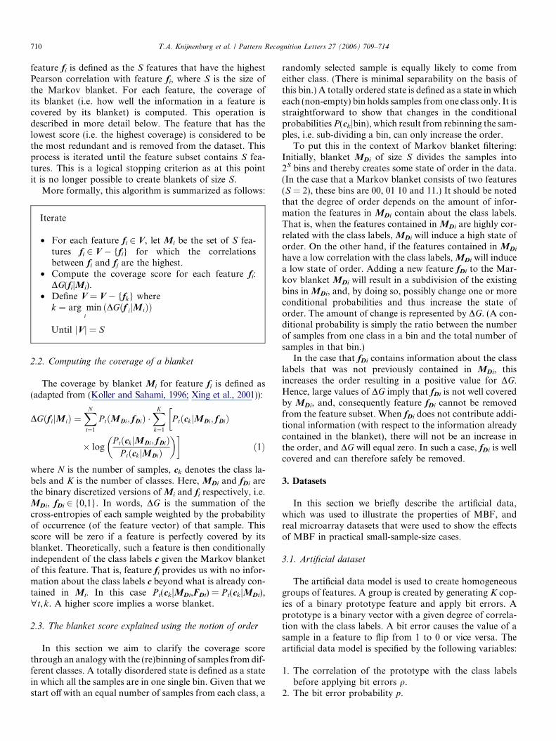
Fig. 1. Removing features using Markov blanket filtering (and ascomparison feature ranking) from three different datasets.

T.A. Knijnenburg et al. / Pattern Recognition Letters 27 (2006) 709–714 711

3. The number of samples N.4. The size of the group K.

3.2. Microarray datasets

In our experiments, we employed three publicly avail-able small-sample-size microarray gene expression data-sets, all consisting of two classes:

1. Leukemia dataset (LD), consisting of 72 samples and3571 genes (Golub et al., 1999).

2. Breast cancer metastases dataset (BCMD), consisting of78 samples and 4919 genes (Van ‘t Veer et al., 2002).

3. Colon tumor dataset (CTD), consisting of 62 samplesand 1908 genes (Alon et al., 1999).

4. Experiments and results

In this section we describe the experiments and interprettheir results in order to illustrate and understand the prop-erties of MBF.

4.1. Erroneous feature removal

Given two groups of features with identical mutualcorrelations within each group, such that one group hasa larger degree of correlation with the class labels thanthe other, one expects MBF to initially remove the featuresleast correlated with the class labels, since in general thesefeatures only slightly increase the order and have a smallvalue of DG, when compared to features that are highlycorrelated to the outcome classes. This experiment wasdesigned to investigate the degree to which MBF satisfiesthis hypothesis.

The datasets employed in this experiment are generatedwith the artificial data model and consist of two groups;Group A and Group B; each group consists of 10 features(K = 10). The bit error probability for both groups is 0.2(p = 0.2) and the number of samples is 80 (N = 80). Thisnumber is a realistic (small sample) dataset size for geneexpression datasets. Half of these samples (40) are assignedto Class 1; the other half to Class 2.

Three different datasets are created. Each dataset ischaracterized by a different degree of correlation of thegroup prototypes, PA and PB with the class labels:

1. Dataset 1 (DB): A big difference between correlations ofthe class prototypes, i.e. qA = 1.00 and qB = 0.00.

2. Dataset 2 (DS): A small difference between correlationsof the class prototypes, i.e. qA = 0.75 and qB = 0.25.

3. Dataset 3 (DN): No difference between correlations ofthe class prototypes, i.e. qA = 0.50 and qB = 0.50.

MBF is applied to remove features from the three differ-ent datasets. We performed the experiments for blanket

sizes of two and five, i.e. S = 2.5. As a comparison, theremoval of features using correlation based feature ranking(FR) was also performed. In feature ranking, features areremoved in reversed ranking order, i.e. the feature with thelowest correlation with the class labels is the first featureto be removed. This experiment is repeated 10,000 timesfor each dataset and each feature removal strategy (in eachrepetition a new dataset is generated). Fig. 1 depicts theprobability that the ith removed feature is from Group Bfor the different datasets and different strategies. (Note thatthe curves stop at 15 since Markov blanket filtering is ter-minated when the number of features left equals S.)

We now focus our attention on how MBF removes fea-tures from these datasets. Especially the first few featuresthat are removed provide insight into the algorithm, sinceinitially all the features will have blankets consisting offeatures from their own group. In DB (data points markedwith circles in Fig. 1), where Group A is perfectly corre-lated with the class labels (before applying bit errors) andGroup B is uncorrelated, we see some striking behavior.When Markov blanket filtering is applied using a blanketsize of two (S = 2, solid line) the algorithm prefers toremove features from Group B, the group, which is uncor-related with the class labels. However, with a blanket sizeof five (S = 5, dashed line) the behavior turns around.Now, features from Group A are far more likely to beremoved from the dataset in the initial stages. This effectis also noticeable if the class correlations of both groupsare not chosen not to differ so extremely. See the resultfor dataset DS (depicted by squares in Fig. 1). Of course,if the class correlation of Groups A and B are the same,features from both groups are equally probable to beremoved. (See results for DN, represented by triangles.)

The results of this experiment are not confined toartificial datasets. The same phenomenon is encounteredwith the real data. Here, we applied MBF to the threemicroarray gene expression datasets, using the same

0 5 10 15 20

0

0.05

0.1

0.15

0.2

S

N = 16

0 5 10 15 20

0

0.05

0.1

0.15 N = 80

ρ = 0.75ρ = 0

ρ = 1

ρ = 0.75

ρ = 0

ρ = 1

ΔGΔG

712 T.A. Knijnenburg et al. / Pattern Recognition Letters 27 (2006) 709–714

preprocessing as in (Xing et al., 2001): A two-componentGaussian unconditional mixture model was employed todiscretize all the measurements, followed by an entropybased ranking strategy to select the 360 most informativegenes (features) from each dataset.

After that, MBF employing the binary values wasapplied on the three groups of 360 features with blanketsizes two and five. To compare the different blanket sizes,the overlap between the first ten removed genes using ablanket size of two and five was computed. The samewas done for the first 50 and 100 removed genes for bothblanket sizes. Results are presented in Table 1. This tablealso lists the average absolute Pearson correlation withthe class labels of the entire feature subset of 360 genes,that passed the ranking filter, denoted by q360, and theaverage absolute Pearson correlation with the class labelsof the first ten removed features using MBF, denoted byq10. (For the sake of brevity the first ten features that areremoved using MBF are from here on denoted by R10.)

From Table 1 we can see that filtering with differentblanket sizes results in the removal of different features:The R10 features removed with S = 2 have a significantlylower correlation with the class labels than the R10 featuresremoved with S = 5. It is important to notice this is inaccordance with the results found in the previous experi-ment using the artificial data. This scheme holds for theLeukemia and the colon tumor dataset, but not for thebreast cancer metastasis dataset. An explanation for thiscan be found in the fact that the overall correlation ofthe 360 features that passed the ranking filter is quite lowand the variation in this correlation is small, especiallywhen compared to the other two datasets. That is whythe influence of the class correlation is much less significantin this case.

4.2. Behavior of the coverage score

To further investigate the contradictory and counterin-tuitive properties of MBF we set up a second experiment.In this experiment we analyzed the influence of the blanketsize S, the number of samples N and the class-correlationq on the coverage score. The artificial data model wasemployed to generate features and their accompanyingblankets by creating groups of size S + 1. The first feature

Table 1Overlap between removed feature sets using MBF with different blanketsizes

Dataset Overlapin first10

Overlapin first50

Overlapin first100

S q10 q360

LD 0 14 43 2 0.50 ± 0.13 0.50 ± 0.115 0.75 ± 0.08

BCMD 5 17 39 2 0.27 ± 0.06 0.27 ± 0.085 0.27 ± 0.07

CTD 1 15 43 2 0.37 ± 0.09 0.37 ± 0.115 0.50 ± 0.13

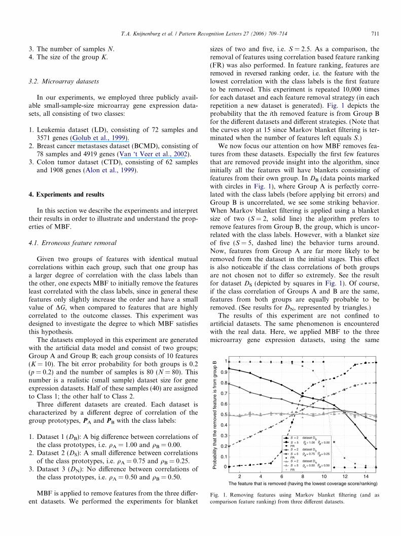
of a group will fulfill the role of fDi, while the other S fea-tures of the group represent MDi. The blanket score, DG,was computed for N = [16, 80,512], p = 0.2, q = [0, 0.75,1]and S = 1,2, . . . , 20. Each experiment was repeated 3000times. The results are depicted in Fig. 2. Here, DG on thevertical axis represents the average DG across the 3000experiments.

The results in Fig. 2 illustrate that the behavior of DG isinfluenced by three effects: True-order, Pseudo-order andBig-blanket-order.

4.2.1. True-order

When a feature truly contains information about theclass labels (jqj > 0) and its addition to an existing blanketincreases the state of order, DG will be positive. The ordercreated by the addition of such a feature is defined as‘True-order’. For example, for the triangle-marked curvesin Fig. 2 (q = 1) the coverage scores represent True-ordercreated by the addition of informative features.

4.2.2. Pseudo-order

From the results, we observe that for features uncorre-lated with the class labels (q = 0), DG initially increases.This behavior (increase in DG with increasing blanket size)is a result of ‘Pseudo-order’.

S

0 5 10 15 20

0

0.05

0.1

S

N = 512

ρ = 0.75ρ = 0

ρ = 1

ΔG

Fig. 2. Behavior of DG under different initial class correlations, differentnumbers of samples and different blanket sizes.

0 10 20 30 40 500.3

0.35

0.4

0.45

0.5

W

e

BCMD

FRS = 2S = 5

0 10 20 30 40 500.1

0.15

0.2

0.25

0.3

W

e

CTD

FRS = 2S = 5

0 10 20 30 40 500

0.05

0.1

0.15

0.2

W

e

LD

FRS = 2S = 5

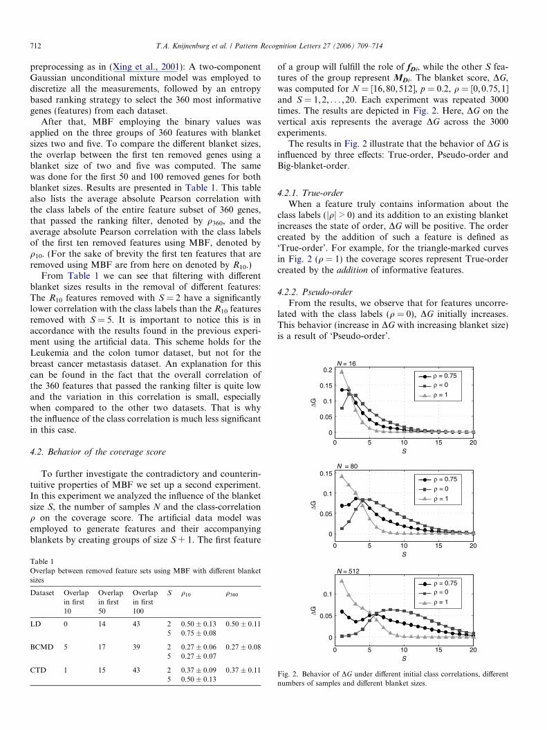
Fig. 3. Estimated prediction error (e) for feature ranking (FR) and MBF(with S = 2 and 5) on three gene expression datasets using the NMC.

T.A. Knijnenburg et al. / Pattern Recognition Letters 27 (2006) 709–714 713

Theoretically, a feature fDi that is uncorrelated withthe class labels should have a coverage score DG of zero(independent of blanket MDi), because such a feature pos-sesses no information about the class labels and thereforecannot increase the order. However, depending on theblanket size and the number of samples, the average num-ber of samples per bin (N/2S) can become really small. Inthat case, rebinning of the bins induced by blanket MDi

due to the addition of feature fDi results in substantialchanges in the conditional probabilities, even for uninfor-mative features. Consequently, DG will be larger than zero.The resulting increase in order is of course not genuine, wecan say that in this case DG represents an increase inPseudo-order, which one could compare to a form ofovertraining.

4.2.3. Big-blanket-order

A third effect visible in Fig. 2, is that, regardless of thevalue of q, DG may sometimes initially increase, but even-tually always decreases towards zero. We refer to this lattereffect as ‘Big-blanket-order’.

This decrease in the coverage score is caused by the stateof order already induced by a large blanket MDi. The blan-ket MDi with size S divides N samples across 2S bins. Sinceeach bin division can only increase the order (or keep it thesame), a larger blanket size results in a higher state of orderfor a fixed sample size. Consequently, an increase in orderdue to the addition of fDi becomes less likely, which causesthe coverage score of a feature to decrease with increasingS. An extreme case occurs when performing MBF withan infinite blanket size and a finite number of samples.The infinite number of bin divisions will place every sampleinto a separate bin. Now, blanket MDi provides a totallyordered state. There is no feature fDi that can increasethe order, consequently DG will be zero.

From the results (Fig. 2) it is clear that the value of S

where Big-blanket-order sets in is a function of q. The cov-erage score of feature/blanket combinations that have ahigh class correlation will start converging to zero at asmaller blanket size, because their initial state of orderinduced by the blanket is high. On the other hand, the cov-erage score of feature/blanket combinations that have asmall class correlation will start converging to zero at a lar-ger blanket size, because their initial state of order is low,followed by a phase where Pseudo-order is introduced,after which Big-blanket-order sets in. Obviously, the num-ber of samples, N, also plays a role. With only a few sam-ples it will be quite easy to arrive at a totally ordered statewith a relatively small blanket size, while a larger numberof samples requires a lot more bin divisions until eachnon-empty bin holds samples from one class only.

We conclude this section by noting that the reversal ofremoval behavior as observed in the previous experimentcan be explained by the behavior of the coverage score asanalyzed with this experiment. See the middle plot inFig. 2 (N = 80) and compare the behavior of DG at sizesS = 2 and S = 5.

4.3. Classification performance

In the final experiment, we compared the classificationperformance of MBF with FR based on discretized fea-tures on the three microarray datasets. The size of theselected feature subsets, W, ranged from 1 to 50 features.Testing and training was done using sixteen repeats of a10-fold cross-validation process, encapsulating the featureselection process in the cross validation loop, thereby pre-venting selection bias (Ambroise and McLachlan, 2002).As classifier we used the nearest mean classifier (NMC),since the NMC was found to perform reliable on micro-array gene expression datasets (Dudoit et al., 2002; Van‘t Veer et al., 2002). The results are depicted in Fig. 3.

From Fig. 3 it is evident that MBF performs better withS = 2 than with S = 5. This poorer performance for S = 5can most probably be attributed to the ‘Pseudo-order’effect, which was discussed in the previous experiment.(Since the dataset sizes for the three datasets are all aroundN = 80, the middle figure in Fig. 2 is related.) The result ofthis effect is that for S = 5, DG for uninformative features islarger than for informative features. Consequently thelatter are discarded, while the less informative, or noisyfeatures are retained. For S = 2, this is the other way

714 T.A. Knijnenburg et al. / Pattern Recognition Letters 27 (2006) 709–714

around. Preferring less informative features over informa-tive features obviously has an undesirable effect on the clas-sification performance, as is evident from the results. The‘Pseudo-order’ effect, which exists due to the fragmentationof the data, can be countered by the application of smooth-ing in the form of employing the Bayes estimator for theconditional probabilities in Eq. (1). Although this regular-ization strategy can lead to an improved classification per-formance for S = 2, MBF is still not successful for largerblankets. (Results not shown.) This shows that the trade-off between artifact-suppression and information loss byemploying regularization is not at all straightforward.Estimation of log-likelihood measures like the coveragescore under small sample size conditions thus remains achallenge.

In addition, it is evident from these figures that simplefeature ranking always outperforms MBF in terms of min-imal error rate achieved (also when smoothing is applied).Explanations for this cannot only be found in the artifactsof the coverage score, but also in blanket definition andfeature removal strategy, which are obviously both notoptimal. Search strategies like a beam search in combina-tion with an objective function (e.g. the minimization ofthe sum of DG’s or the minimization of the classificationerror) to search through trees of possible feature elimina-tions across a sequence of removal steps could be used toimprove upon the greedy removal strategy. These are, how-ever, a topic of further research. Furthermore, the numberof genes where this minimal performance of FR is reachedis also smaller than the number of genes where MBFreaches its minimal value. Given that MBF is supposedto retain only informative (relevant, yet non-redundant)features, and thereby (1) reducing the size of the final fea-ture set considerably, and, (2) consequently improving theclassification performance, one expects MBF to performbetter than FR at a smaller number of features. The resultson both artificial and real datasets illustrate, however, theopposite.

5. Conclusion

The study of Markov blanket filtering based on discret-ized features (MBF) as outlined in this paper has indicated

its contradictory and counterintuitive nature. Using artifi-cial data we were able to identify three effects of whichtwo can be labeled as artifacts that ultimately find their ori-gin in the small sample size. Empirical studies on threemicroarray gene expression datasets revealed that theseartifacts prevent MBF from outperforming simple featureranking. All this leads us to question the usability of thistechnique in small sample size applications and hints at afundamental rethinking of gene selection strategies underthese small sample size conditions.

References

Alon, U., Barkai, N., et al., 1999. Broad patterns of gene expressionrevealed by clustering analysis of tumour and normal colon cancertissues probed by oligonucleotide arrays. Proc. Nat. Acad. Sci. USA96, 6745–6750.

Ambroise, C., McLachlan, G.J., 2002. Selection bias in gene extraction onbasis of microarray gene-expression data. Proc. Nat. Acad. Sci. USA99, 6562–6566.

Dudoit, S., Fridlyand, J., Speed, T., 2002. Comparison of discriminationmethods for the classification of tumors using gene expression data. J.Amer. Stat. Assoc. 97, 77–87.

Golub, T.R., Slonim, D.K., et al., 1999. Molecular classification ofcancer: Class discovery and class prediction by gene expressionmonitoring. Science 286, 531–537.

Koller, D., Sahami, M., 1996. Toward optimal feature selection. In: Saitta,L. (Ed.), Machine Learning, Proceedings of the Thirteenth Interna-tional Conference (ICML1996). Morgan Kaufmann Publishers, SanFrancisco, pp. 284–292.

Mamitsuka, H., 2002. Iteratively selecting feature subsets for mining fromhigh-dimensional databases. In: The Sixth European Conference onPrinciples and Practice of Knowledge Discovery in Databases (PKDD2002). Helsinki, Finland, pp. 361–372.

Pearl, J., 1988. Probabilistic Reasoning in Intelligent Systems. MorganKaufmann Publishers, San Mateo, California.

Van ‘t Veer, L.J., Dai, H., Van de Vijver, M.J., et al., 2002. Geneexpression profiling predicts clinical outcome of breast cancer. Nature415, 530–536.

Xie, L., Chang, S.F., et al., 2003. Feature selection for unsuperviseddiscovery of statistical temporal structures in video. In: IEEEInternational Conference on Image Processing (ICIP2003). Barcelona,Spain, vol. 1, pp. 29–32.

Xing, E.P., Jordan, M.I., Karp, R.M., 2001. Feature Selection for high-dimensional genomic microarray data. In: Brodley, C.E., Danyluk,A.P. (Eds.), The Eighteenth International Conference on MachineLearning (ICML2001). Morgan Kaufmann Publishers, San Francisco,pp. 601–608.