Are the 41 kyr glacial oscillations a linear response to Milankovitch forcing?
12
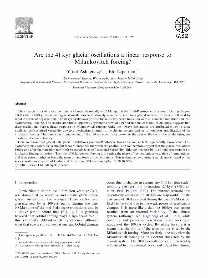
Quaternary Science Reviews 23 (2004) 1879–1890 Are the 41 kyr glacial oscillations a linear response to Milankovitch forcing? Yosef Ashkenazy a, , Eli Tziperman b a Environmental Sciences, Weizmann Institute, Rehovot 76100, Israel b Department of Earth and Planetary Sciences and Division of Engineering and Applied Sciences, Harvard University, Cambridge, MA, USA Received 7 January 2004; accepted 20 April 2004 Abstract The characteristics of glacial oscillations changed drastically 0:8 Ma ago, at the ‘‘mid-Pleistocene transition’’. During the past 0.8 Ma the 100 kyr glacial–interglacial oscillations were strongly asymmetric (i.e., long glacial intervals of growth followed by rapid intervals of deglaciation). The 40 kyr oscillations prior to the mid-Pleistocene transition were of a smaller amplitude and less- asymmetrical looking. The smaller amplitude, apparently symmetric form and period that matches that of obliquity, suggests that these oscillations were a linear response to Milankovitch forcing, while the 100 kyr oscillations are attributed either to some nonlinear self-sustained variability due to a mechanism internal to the climate system itself or to nonlinear amplification of the insolation forcing. The significant strengthening of the 100 kyr eccentricity power in the past 800 kyr is one of the intriguing questions of climate history. Here we show that glacial–interglacial oscillations pre-mid-Pleistocene transition are, in fact, significantly asymmetric. This asymmetry may contradict a straight forward linear Milankovitch explanation, and we therefore suggest that the glacial oscillations before and after the transition may both be explained as self-sustained variability (although the possibility of nonlinear response to insolation forcing still exists). The role of Milankovitch forcing is in setting the phase of the oscillations (e.g. time of terminations) and their period, rather in being the main driving force of the oscillations. This is demonstrated using a simple model based on the sea ice switch mechanism of Gildor and Tziperman (Paleoceanography 15 (2000) 605). r 2004 Elsevier Ltd. All rights reserved. 1. Introduction Earth climate of the last 2.7 million years (2.7 Ma) was dominated by repetitive and drastic glacial–inter- glacial oscillations, the ice-ages. These cycles were characterized by a 100 kyr period during the past 0.8 Ma (time of the mid-Pleistocene transition), and by a 40 kyr period before that (Fig. 1). It is generally believed that orbital forcing plays a significant role in this variability (Milankovitch hypothesis), although what that role is still somewhat unclear. Orbital changes occur due to changes in eccentricity (100 kyr time scale), obliquity (40 kyr), and precession (20 kyr) (Milanko- vitch, 1941; Paillard, 2001). The extreme scenario that eccentricity variations on 100 kyr are responsible for the existence of 100 kyr signal during the past 0.8 Ma is not likely to be valid due to the weak power of eccentricity changes. It is more likely that the 100 kyr oscillations resulted from an internal variability of the climate system (although see Hagelberg et al., 1991) while obliquity and precession variations phase lock (and modulate) the 100 kyr cycles. By phase locking it is meant that the timing of the terminations is set by the Milankovitch forcing. More precisely, one may view the Milankovitch forcing as an external clock felt by the climate system. The 100 kyr oscillations are then weakly influenced by this external clock, and adjust their timing ARTICLE IN PRESS 0277-3791/$ - see front matter r 2004 Elsevier Ltd. All rights reserved. doi:10.1016/j.quascirev.2004.04.008 Corresponding author. Tel.: +972-8-934-4924; fax: +972-8-934- 4124. E-mail addresses: [email protected] (Y. Ashkenazy), [email protected] (E. Tziperman).
Transcript of Are the 41 kyr glacial oscillations a linear response to Milankovitch forcing?
ARTICLE IN PRESS
0277-3791/$ - se
doi:10.1016/j.qu
�Correspond4124.
E-mail addr
(Y. Ashkenazy)
Quaternary Science Reviews 23 (2004) 1879–1890
Are the 41 kyr glacial oscillations a linear response toMilankovitch forcing?
Yosef Ashkenazya,�, Eli Tzipermanb
aEnvironmental Sciences, Weizmann Institute, Rehovot 76100, IsraelbDepartment of Earth and Planetary Sciences and Division of Engineering and Applied Sciences, Harvard University, Cambridge, MA, USA
Received 7 January 2004; accepted 20 April 2004
Abstract
The characteristics of glacial oscillations changed drastically � 0:8Ma ago, at the ‘‘mid-Pleistocene transition’’. During the past
0.8Ma the � 100kyr glacial–interglacial oscillations were strongly asymmetric (i.e., long glacial intervals of growth followed by
rapid intervals of deglaciation). The 40 kyr oscillations prior to the mid-Pleistocene transition were of a smaller amplitude and less-
asymmetrical looking. The smaller amplitude, apparently symmetric form and period that matches that of obliquity, suggests that
these oscillations were a linear response to Milankovitch forcing, while the 100 kyr oscillations are attributed either to some
nonlinear self-sustained variability due to a mechanism internal to the climate system itself or to nonlinear amplification of the
insolation forcing. The significant strengthening of the 100 kyr eccentricity power in the past � 800 kyr is one of the intriguing
questions of climate history.
Here we show that glacial–interglacial oscillations pre-mid-Pleistocene transition are, in fact, significantly asymmetric. This
asymmetry may contradict a straight forward linear Milankovitch explanation, and we therefore suggest that the glacial oscillations
before and after the transition may both be explained as self-sustained variability (although the possibility of nonlinear response to
insolation forcing still exists). The role of Milankovitch forcing is in setting the phase of the oscillations (e.g. time of terminations)
and their period, rather in being the main driving force of the oscillations. This is demonstrated using a simple model based on the
sea ice switch mechanism of Gildor and Tziperman (Paleoceanography 15 (2000) 605).
r 2004 Elsevier Ltd. All rights reserved.
1. Introduction
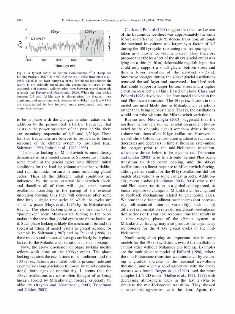
Earth climate of the last 2.7 million years (2.7Ma)was dominated by repetitive and drastic glacial–inter-glacial oscillations, the ice-ages. These cycles werecharacterized by a 100 kyr period during the past0.8Ma (time of the mid-Pleistocene transition), and bya 40 kyr period before that (Fig. 1). It is generallybelieved that orbital forcing plays a significant role inthis variability (Milankovitch hypothesis), althoughwhat that role is still somewhat unclear. Orbital changes
e front matter r 2004 Elsevier Ltd. All rights reserved.
ascirev.2004.04.008
ing author. Tel.: +972-8-934-4924; fax: +972-8-934-
esses: [email protected]
, [email protected] (E. Tziperman).
occur due to changes in eccentricity (100 kyr time scale),obliquity (40 kyr), and precession (20 kyr) (Milanko-vitch, 1941; Paillard, 2001). The extreme scenario thateccentricity variations on 100 kyr are responsible for theexistence of 100 kyr signal during the past 0.8Ma is notlikely to be valid due to the weak power of eccentricitychanges. It is more likely that the 100 kyr oscillationsresulted from an internal variability of the climatesystem (although see Hagelberg et al., 1991) whileobliquity and precession variations phase lock (andmodulate) the 100 kyr cycles. By phase locking it ismeant that the timing of the terminations is set by theMilankovitch forcing. More precisely, one may view theMilankovitch forcing as an external clock felt by theclimate system. The 100 kyr oscillations are then weaklyinfluenced by this external clock, and adjust their timing
ARTICLE IN PRESS
2500 2000 1500 1000 500 0
Time [kyr BP]
2
3
4
5
δ18O
IceV
olu
me
DSDP607
40kyr 100kyr
Fig. 1. A typical record of benthic Foraminifera d18O (Deep Sea
Drilling Project (DSDP) Site 607, Raymo et al., 1989; Ruddiman et al.,
1989) which is (at least partly) a proxy for global ice-volume; the
record is not orbitally tuned and the chronology is based on the
assumption of constant sedimentation rates between several magnetic
reversals (see Raymo and Nisancioglu, 2003). While the time period
between 2.5 and 0.8Ma ago is characterized by frequent, less
dominant, and more symmetric ice-ages of � 40 kyr, the last 0.8Ma
are characterized by less frequent, more pronounced, and more
asymmetric ice-ages.
Y. Ashkenazy, E. Tziperman / Quaternary Science Reviews 23 (2004) 1879–18901880
to be in phase with the changes in solar radiation. Inaddition to the pronounced 1/100 kyr frequency thatexists in the power spectrum of the past 0.8Ma, thereare secondary frequencies of 1/40 and 1/20 kyr. Theselast two frequencies are believed to result due to linearresponse of the climate system to insolation (e.g.,Saltzman, 1990; Imbrie et al., 1992, 1993).The phase locking to Milankovitch is more clearly
demonstrated in a model scenario: Suppose we initializesome model of the glacial cycles with different initialconditions for the land ice volume and other variables,and run the model forward in time, simulating glacialcycles. Then all the different initial conditions areinfluenced by the same external Milankovitch clock,and therefore all of them will adjust their internaloscillation according to the pacing of the externalinsolation forcing; thus they will converge after sometime into a single time series in which the cycles aresomehow paced (Hays et al., 1976) by the Milankovitchforcing. This phase locking gives a new meaning to the‘‘pacemaker’’ idea: Milankovitch forcing is the pace-maker in the sense that glacial cycles are phase-locked toit. Such phase locking is likely the mechanism behind thesuccessful fitting of model results to glacial records, forexample by Saltzman (1987) and by Paillard (1998), asthese models and the actual ice ages are likely both phaselocked to the Milankovitch variations in solar forcing.Now, the above discussion of phase locking mostly
reflects work done on the 100 kyr cycles. The phaselocking requires the oscillations to be nonlinear, and the100 kyr oscillations are indeed both large-amplitude andasymmetric (long glaciation followed by rapid deglacia-tions), both signs of nonlinearity. It seems that the40 kyr oscillations are more often thought of as beinglinearly forced by Milankovitch forcing, especially byobliquity (Raymo and Nisancioglu, 2003; Tzipermanand Gildor, 2003).
Clark and Pollard (1998) suggest that the areal extentof the Laurentide ice-sheet was approximately the samebefore and after the mid-Pleistocene transition, althoughthe maximal ice-volume was larger by a factor of 3/2during the 100 kyr cycles (assuming the isotopic signal istaken as a mostly ice volume proxy). They thereforepropose that the ice-sheet of the 40 kyr glacial cycles waslying on a thin (� 30m) deformable regolith layer thatcould only support a small glacier bottom stress andthus a lower elevation of the ice-sheet (� 2 km).Successive ice-ages during the 40 kyr glacial oscillationsremoved the soft layer and uncovered a hard bed-rockthat could support a larger bottom stress and a higherelevation ice-sheet (� 3 km). Based on above Clark andPollard (1998) developed a ice-flow model to explain themid-Pleistocene transition. The 40 kyr oscillations in thismodel are most likely due to Milankovitch variationsrather than being self-sustained. That is, the oscillationswould not exist without the Milankovitch variations.Raymo and Nisancioglu (2003) suggested that the
northern hemisphere summer insolation gradient (domi-nated by the obliquity signal) somehow drives the ice-volume variations of the 40 kyr oscillations. However, aswe will show below, the insolation gradient is symmetric(increases and decreases in time at the same rate) unlikethe ice-ages prior to the mid-Pleistocene transition,which are shown below to be asymmetric. Tzipermanand Gildor (2003) tried to attribute the mid-Pleistocenetransition to deep ocean cooling, and the 40 kyroscillations as a linear response to Milankovitch forcing,although their results for the 40 kyr oscillations did notmatch observations in some critical aspects. Addition-ally, recent studies (Ruddiman, 2003, 2004) related themid-Pleistocene transition to a global cooling trend, tolinear response to changes in Milankovitch forcing, andto feedback mechanisms related to greenhouse gases.We note that other nonlinear mechanisms (not necessa-rily self-sustained internal variability) such as (i)different sedimentation rates during glaciation/deglacia-tion periods or (ii) variable response time that results ina time varying phase of the climate system toMilankovitch forcing, may also produce the asymmetrywe observe for the 41 kyr glacial cycles of the mid-Pleistocene.Nonlinearity does play an important role in some
models for the 40 kyr oscillations, even if the oscillationscannot exist without Milankovitch forcing. Examplesare the multiple-state model of Paillard (1998), wherethe mid-Pleistocene transition was simulated by assum-ing a gradual increase in the maximal ice-volumethreshold, and where a good agreement with the proxyrecords was found. Berger et al. (1999) used the morecomplex LLN-2D model (Gallee et al., 1991, 1992) withdecreasing atmospheric CO2 in the last 2.7Ma tosimulate the mid-Pleistocene transition. They showeda reasonable agreement with the data. Again, the
ARTICLE IN PRESS
2 2.5 3 3.5 4δ18
O
0
300
Co
un
t
Histogram
DataRand. data
2
3
4
δ18O
40kyr (DSDP 607)
0 0.02 0.04 0.06Freq., f [1/kyr]
0
0.2
S(f)
Power Spec.
2500 2000 1500 1000Time [kyr BP]
2
3
δ18O
(a) Data
(b) Phase randomized data
IceV
olu
me
41kyr(c) (d)
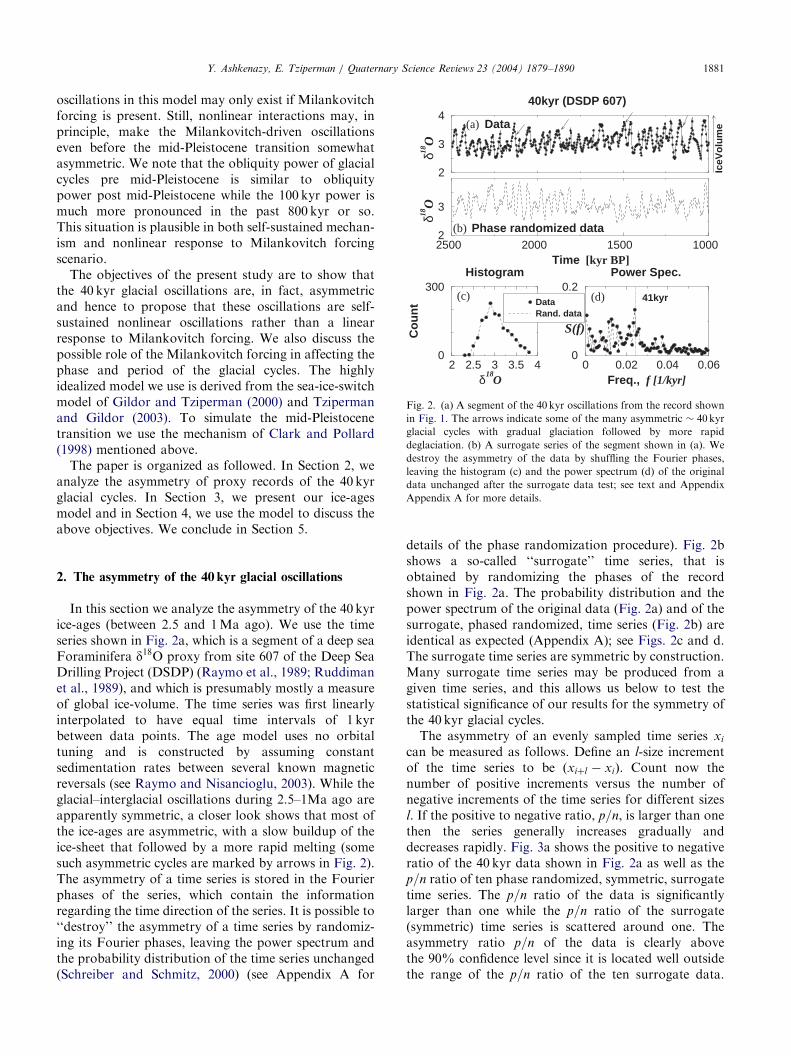
Fig. 2. (a) A segment of the 40 kyr oscillations from the record shown
in Fig. 1. The arrows indicate some of the many asymmetric � 40kyr
glacial cycles with gradual glaciation followed by more rapid
deglaciation. (b) A surrogate series of the segment shown in (a). We
destroy the asymmetry of the data by shuffling the Fourier phases,
leaving the histogram (c) and the power spectrum (d) of the original
data unchanged after the surrogate data test; see text and Appendix
Appendix A for more details.
Y. Ashkenazy, E. Tziperman / Quaternary Science Reviews 23 (2004) 1879–1890 1881
oscillations in this model may only exist if Milankovitchforcing is present. Still, nonlinear interactions may, inprinciple, make the Milankovitch-driven oscillationseven before the mid-Pleistocene transition somewhatasymmetric. We note that the obliquity power of glacialcycles pre mid-Pleistocene is similar to obliquitypower post mid-Pleistocene while the 100 kyr power ismuch more pronounced in the past 800 kyr or so.This situation is plausible in both self-sustained mechan-ism and nonlinear response to Milankovitch forcingscenario.The objectives of the present study are to show that
the 40 kyr glacial oscillations are, in fact, asymmetricand hence to propose that these oscillations are self-sustained nonlinear oscillations rather than a linearresponse to Milankovitch forcing. We also discuss thepossible role of the Milankovitch forcing in affecting thephase and period of the glacial cycles. The highlyidealized model we use is derived from the sea-ice-switchmodel of Gildor and Tziperman (2000) and Tzipermanand Gildor (2003). To simulate the mid-Pleistocenetransition we use the mechanism of Clark and Pollard(1998) mentioned above.The paper is organized as followed. In Section 2, we
analyze the asymmetry of proxy records of the 40 kyrglacial cycles. In Section 3, we present our ice-agesmodel and in Section 4, we use the model to discuss theabove objectives. We conclude in Section 5.
2. The asymmetry of the 40 kyr glacial oscillations
In this section we analyze the asymmetry of the 40 kyrice-ages (between 2.5 and 1Ma ago). We use the timeseries shown in Fig. 2a, which is a segment of a deep seaForaminifera d18O proxy from site 607 of the Deep SeaDrilling Project (DSDP) (Raymo et al., 1989; Ruddimanet al., 1989), and which is presumably mostly a measureof global ice-volume. The time series was first linearlyinterpolated to have equal time intervals of 1 kyrbetween data points. The age model uses no orbitaltuning and is constructed by assuming constantsedimentation rates between several known magneticreversals (see Raymo and Nisancioglu, 2003). While theglacial–interglacial oscillations during 2.5–1Ma ago areapparently symmetric, a closer look shows that most ofthe ice-ages are asymmetric, with a slow buildup of theice-sheet that followed by a more rapid melting (somesuch asymmetric cycles are marked by arrows in Fig. 2).The asymmetry of a time series is stored in the Fourierphases of the series, which contain the informationregarding the time direction of the series. It is possible to‘‘destroy’’ the asymmetry of a time series by randomiz-ing its Fourier phases, leaving the power spectrum andthe probability distribution of the time series unchanged(Schreiber and Schmitz, 2000) (see Appendix A for
details of the phase randomization procedure). Fig. 2bshows a so-called ‘‘surrogate’’ time series, that isobtained by randomizing the phases of the recordshown in Fig. 2a. The probability distribution and thepower spectrum of the original data (Fig. 2a) and of thesurrogate, phased randomized, time series (Fig. 2b) areidentical as expected (Appendix A); see Figs. 2c and d.The surrogate time series are symmetric by construction.Many surrogate time series may be produced from agiven time series, and this allows us below to test thestatistical significance of our results for the symmetry ofthe 40 kyr glacial cycles.The asymmetry of an evenly sampled time series xi
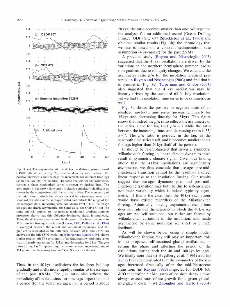
can be measured as follows. Define an l-size incrementof the time series to be ðxiþl � xiÞ. Count now thenumber of positive increments versus the number ofnegative increments of the time series for different sizesl. If the positive to negative ratio, p=n, is larger than onethen the series generally increases gradually anddecreases rapidly. Fig. 3a shows the positive to negativeratio of the 40 kyr data shown in Fig. 2a as well as thep=n ratio of ten phase randomized, symmetric, surrogatetime series. The p=n ratio of the data is significantlylarger than one while the p=n ratio of the surrogate(symmetric) time series is scattered around one. Theasymmetry ratio p=n of the data is clearly abovethe 90% confidence level since it is located well outsidethe range of the p=n ratio of the ten surrogate data.
ARTICLE IN PRESS
0.8
1
1.2
1.4
0.8
1
1.2
1.4
0.8
1
1.2
1.4
0 10 20 30 40 50 60
Lag, l
1
3
5
7
Asy
mm
etry
, p/n
(d) Artificial data
(b) ODP 677
(a) DSDP 607
(c) Summer insolation 7025N
Fig. 3. (a) The asymmetry of the 40 kyr oscillations proxy record
(DSDP 607 shown in Fig. 2a), calculated as the ratio between the
positive increments and the negative increments for different time lags
(solid line, see text for details). The same analysis for ten symmetric,
surrogate phase randomized series is shown by dashed lines. The
asymmetry in the proxy time series is clearly statistically significant as
shown by the comparison with the surrogate data. The asymmetry of
the data is well outside the shown vertical bars (marking mean � 1
standard deviation of the surrogate data) and outside the range of the
10 surrogate data, indicating 90% confidence level. Thus, the 40 kyr
ice-ages are clearly asymmetric. (b) Same as (c) for ODP 677. (c) The
same analysis applied to the average meridional gradient summer
insolation shows that this obliquity-dominated signal is symmetric.
Thus, the 40 kyr ice ages cannot be the result of a linear response to
Milankovitch forcing. (Insolation (Laskar, 1990; Paillard et al., 1996)
is averaged between the vernal and autumnal equinoxes, and the
gradient is calculated as the difference between 70�N and 25�N. An
analysis of the July 65�N insolation of Berger and Loutre (1991) shows
similar results.) (d) The asymmetry of an idealized sawtooth time series
that is linearly increasing for 35 kyr and decreasing for 5 kyr. The p=n
ratio for lag 1 is 7, representing the ration between increasing time of
35 kyr and the decreasing time of 5 kyr. See text for details.
Y. Ashkenazy, E. Tziperman / Quaternary Science Reviews 23 (2004) 1879–18901882
Thus, in the 40 kyr oscillations the ice-sheet buildupgradually and melts more rapidly, similar to the ice-agesof the past 0.8Ma. The p=n ratio also reflects theperiodicity of the data since for time lags larger than halfa period (for the 40 kyr ice ages, half a period is about
20 kyr) the ratio becomes smaller than one. We repeatedthe analysis for an additional record [Ocean DrillingProject (ODP) Site 677 (Shackleton et al., 1990)] andobtained similar results (Fig. 3b); the chronology thatwe use is based on a constant sedimentation rateassumption (4.24 cm/kyr) for the past 2.5Ma.A previous study (Raymo and Nisancioglu, 2003)
suggested that the 41 kyr oscillations are driven by thevariations in the northern hemisphere summer insola-tion gradient due to obliquity changes. We calculate theasymmetry ratio p=n for the insolation gradient pre-sented in Raymo and Nisancioglu (2003) and find that itis symmetric (Fig. 3c). Tziperman and Gildor (2003)also suggested that the 41 kyr oscillations may belinearly driven by the standard 65�N July insolation,yet we find this insolation time series to be symmetric aswell.Fig. 3d shows the positive to negative ratio of an
idealized sawtooth time series (increasing linearly for35 kyr and decreasing linearly for 5 kyr). This figureshows that indeed the p=n ratio reflects the asymmetry ofthe series, since for lag 1=1 p=n ¼ 7 while the ratiobetween the increasing times and decreasing times is 35/5=7. The p=n ratio is periodic in the lag, as thesawtooth time series itself, and it becomes smaller than 1for lags higher than 20 kyr (half of the period).It should be re-emphasized that given a symmetric
Milankovitch forcing, a linear climate dynamics mustresult in symmetric climate signal. Given our findingabove that the 41 kyr oscillations are significantlyasymmetric, we thus conclude that ice-ages pre-mid-Pleistocene transition cannot be the result of a directlinear response to the insolation forcing. Our resultssuggest that ice-ages dynamics pre- and post-mid-Pleistocene transition may both be due to self-sustainednonlinear variability which is indeed typically asym-metric. If this is the case, then the 40 kyr oscillationswould have existed regardless of the Milankovitchforcing. Admittedly, having asymmetric oscillationsdoes not rule out the scenario in which the 40 kyr iceages are not self sustained, but rather are forced byMilankovitch variations in the insolation, and madeasymmetric by some nonlinear ice sheet or climatefeedbacks.As will be shown below using a simple model,
Milankovitch forcing may still play an important rolein our proposed self-sustained glacial oscillations, insetting the phase and affecting the period of theoscillations during both the 40 and 100 kyr ice ages.We finally note that (i) Hagelberg et al. (1991) and (ii)King (1996) demonstrated that the asymmetry of the ice-ages increased drastically after the mid-Pleistocenetransition. (iii) Raymo (1992) inspected for DSDP 607d18O that ‘‘after 2.2Ma, rates of ice sheet decay almostalways exceed rates of ice growth for a given glacial-interglacial cycle.’’ (iv) Zhonghui and Herbert (2004)
ARTICLE IN PRESSY. Ashkenazy, E. Tziperman / Quaternary Science Reviews 23 (2004) 1879–1890 1883
reconstructed the SST of eastern equatorial Pacific andpointed out the asymmetry of the temperature signalduring the glacial cycles even before the mid-Pleistocenetransition.
400 300 200 100 0
Time [kyr BP]
0
10
20
30
40
50
V(t
) [1
06
km3 ]
Vmin
Vmax
glac
iatio
n
deg
laciation
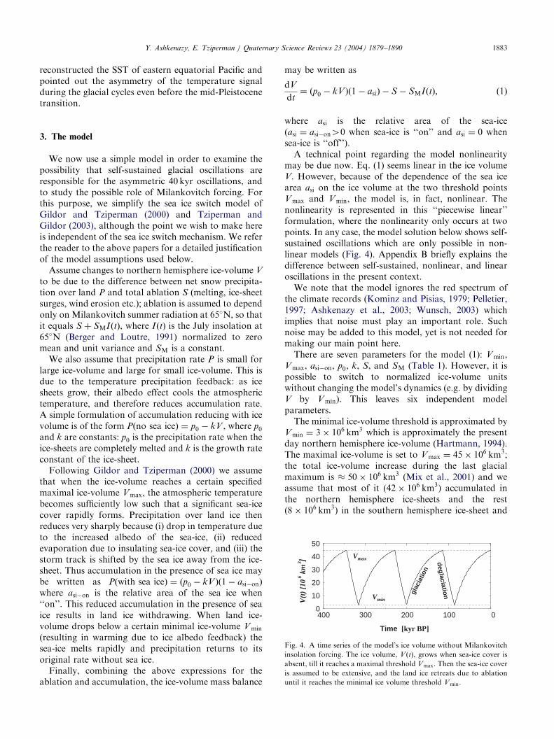
Fig. 4. A time series of the model’s ice volume without Milankovitch
insolation forcing. The ice volume, V ðtÞ, grows when sea-ice cover is
absent, till it reaches a maximal threshold Vmax. Then the sea-ice cover
is assumed to be extensive, and the land ice retreats due to ablation
until it reaches the minimal ice volume threshold Vmin.
3. The model
We now use a simple model in order to examine thepossibility that self-sustained glacial oscillations areresponsible for the asymmetric 40 kyr oscillations, andto study the possible role of Milankovitch forcing. Forthis purpose, we simplify the sea ice switch model ofGildor and Tziperman (2000) and Tziperman andGildor (2003), although the point we wish to make hereis independent of the sea ice switch mechanism. We referthe reader to the above papers for a detailed justificationof the model assumptions used below.Assume changes to northern hemisphere ice-volume V
to be due to the difference between net snow precipita-tion over land P and total ablation S (melting, ice-sheetsurges, wind erosion etc.); ablation is assumed to dependonly on Milankovitch summer radiation at 65�N, so thatit equals S þ SMIðtÞ, where IðtÞ is the July insolation at65�N (Berger and Loutre, 1991) normalized to zeromean and unit variance and SM is a constant.We also assume that precipitation rate P is small for
large ice-volume and large for small ice-volume. This isdue to the temperature precipitation feedback: as icesheets grow, their albedo effect cools the atmospherictemperature, and therefore reduces accumulation rate.A simple formulation of accumulation reducing with icevolume is of the form Pðno sea iceÞ ¼ p0 � kV , where p0and k are constants: p0 is the precipitation rate when theice-sheets are completely melted and k is the growth rateconstant of the ice-sheet.Following Gildor and Tziperman (2000) we assume
that when the ice-volume reaches a certain specifiedmaximal ice-volume Vmax, the atmospheric temperaturebecomes sufficiently low such that a significant sea-icecover rapidly forms. Precipitation over land ice thenreduces very sharply because (i) drop in temperature dueto the increased albedo of the sea-ice, (ii) reducedevaporation due to insulating sea-ice cover, and (iii) thestorm track is shifted by the sea ice away from the ice-sheet. Thus accumulation in the presence of sea ice maybe written as Pðwith sea iceÞ ¼ ðp0 � kV Þð1� asi�onÞ
where asi�on is the relative area of the sea ice when‘‘on’’. This reduced accumulation in the presence of seaice results in land ice withdrawing. When land ice-volume drops below a certain minimal ice-volume Vmin
(resulting in warming due to ice albedo feedback) thesea-ice melts rapidly and precipitation returns to itsoriginal rate without sea ice.Finally, combining the above expressions for the
ablation and accumulation, the ice-volume mass balance
may be written as
dV
dt¼ ðp0 � kV Þð1� asiÞ � S � SMIðtÞ; ð1Þ
where asi is the relative area of the sea-ice(asi ¼ asi�on40 when sea-ice is ‘‘on’’ and asi ¼ 0 whensea-ice is ‘‘off’’).A technical point regarding the model nonlinearity
may be due now. Eq. (1) seems linear in the ice volumeV. However, because of the dependence of the sea icearea asi on the ice volume at the two threshold pointsVmax and Vmin, the model is, in fact, nonlinear. Thenonlinearity is represented in this ‘‘piecewise linear’’formulation, where the nonlinearity only occurs at twopoints. In any case, the model solution below shows self-sustained oscillations which are only possible in non-linear models (Fig. 4). Appendix B briefly explains thedifference between self-sustained, nonlinear, and linearoscillations in the present context.We note that the model ignores the red spectrum of
the climate records (Kominz and Pisias, 1979; Pelletier,1997; Ashkenazy et al., 2003; Wunsch, 2003) whichimplies that noise must play an important role. Suchnoise may be added to this model, yet is not needed formaking our main point here.There are seven parameters for the model (1): Vmin,
Vmax, asi�on, p0, k, S, and SM (Table 1). However, it ispossible to switch to normalized ice-volume unitswithout changing the model’s dynamics (e.g. by dividingV by Vmin). This leaves six independent modelparameters.The minimal ice-volume threshold is approximated by
Vmin ¼ 3 106 km3 which is approximately the presentday northern hemisphere ice-volume (Hartmann, 1994).The maximal ice-volume is set to Vmax ¼ 45 106 km3;the total ice-volume increase during the last glacialmaximum is 50 106 km3 (Mix et al., 2001) and weassume that most of it (42 106 km3) accumulated inthe northern hemisphere ice-sheets and the rest(8 106 km3) in the southern hemisphere ice-sheet and
ARTICLE IN PRESS
Table 1
Model’s parameters
Parameter Short description Value
Vmin Minimum ice-volume threshold 3 106 km3
Vmax Maximum ice-volume threshold
for last 0.81Ma45 106 km3
Maximum ice-volume threshold
for 3–1Ma ago28 106 km3
k Ice-sheet constant growth rate 1=40kyrp0 Precipitation rate 0:25 SvS Constant ablation rate 0:21 SvSM Milankovitch ablation constant 0:023Svasi�on Relative sea-ice area 0.3
Y. Ashkenazy, E. Tziperman / Quaternary Science Reviews 23 (2004) 1879–18901884
in mountain glaciers. Following Gildor and Tziperman(2000) and Tziperman and Gildor (2003) we choose therelative sea-ice area to be asi�on ¼ 0:3. FollowingPelletier (1997) and Imbrie and Imbrie (1980) we choosea ice-volume growth rate constant to be 1=k ¼ 40 kyr.We choose p0 ¼ 0:25 Sv, S ¼ 0:21 Sv, and SM ¼
0:023 Sv, values which are close to the values ofTziperman and Gildor (2003).
4. The mid-Pleistocene transition and role of
Milankovitch forcing
Using the simple model presented in the previoussection, we wish to now make two main points. First, wewill try to show that the 41 kyr oscillations of the mid-Pleistocene may be described as self-sustained oscilla-tions, consistent with their asymmetry discussed inSection 2. Second, we would like to demonstrate thatMilankovitch forcing can set the phase of the oscilla-tions, as well as strongly affect and even stabilize theperiod of the glacial cycles with respect to changes invarious external parameters. Our mechanism for themid-Pleistocene transition itself is based on the ‘‘pan-cake ice sheet’’ theory of Clark and Pollard (1998).
4.1. Self-sustained 40 kyr glacial oscillations
Clark and Pollard (1998) suggested that prior to themid-Pleistocene transition, the north American con-tinent was covered by a few tens of meters of regolithwhich was eliminated by repeated 40 kyr glaciations.The regolith layer can support a smaller horizontalstress by the ice sheet and therefore resulted in a thinnerice sheet. It is fairly simple to incorporate the Clark andPollard (1998) idea into our model. The maximal ice-volume Vmax specified as one of the parameters in ourmodel is, in fact, a function of the maximum stress thatmay be supported at the bottom of the ice sheet. Underthe assumption of perfect plasticity, the ice sheet heighthðyÞ is characterized by the so-called parabolic profile
(Weertman, 1976; Ghil, 1994) whose height and hencevolume depends on the maximum allowed bottomstress.Note that the maximal area of the ice sheet is
determined in our model by its impact on climate viathe albedo effect. The land ice area grows until its areaand therefore albedo are such that climate coolssufficiently to form sea ice. Thus, according to thisscenario (and hence, according to the scenario of Clarkand Pollard, 1998) the oscillations in temperature beforethe mid-Pleistocene transition are expected to beroughly of the same magnitude as those of the 100 kyroscillations. In fact, a recent study (Zhonghui andHerbert, 2004) presented data that indicates thatEquatorial temperature oscillations (Eastern Pacific)pre- and post-mid-Pleistocene transition have roughlythe same amplitude variation.Recent indications are that about half of the benthic
d18O signal during the 100 kyr cycles is due totemperature and half due to ice volume effects (Schraget al., 1996). If the 40 kyr ice volume oscillations are 2/3of those during the 100 kyr ice ages, yet the temperaturevariations are the same, this requires the ratio of icevolume to temperature effects to be different during the40 kyr ice ages. This raises some interesting questions:did the fraction of the isotopic signal related totemperature change vary during the mid-Pleistocenetransition? Why and in what way? It is not clear how toaddress these questions given present uncertainty inproxy records from the early Pleistocene.We wish to emphasize that the main point of this
work is not that the sea ice switch mechanism applies tothe 40 kyr glacial cycles, but rather that these cycles arewell described as a self-sustained variability of theclimate system (although we cannot rule out thealternative possibility of nonlinear response to Milan-kovitch forcing). Other model equations that result inself-sustained variability are likely to fit the record aswell. The role of Milankovitch forcing discussed lateragain does not depend on the details of the model usedhere, and should work equally well for other modelswith self-sustained oscillations.Now, we assume that the change in the regolith layer
resulted in a change to the maximum supportablebottom stress. This implies that the maximal possibleland ice-volume therefore changed linearly from Vmax ¼
28 106 km3 at 1Ma ago, to Vmax ¼ 45 106 km3
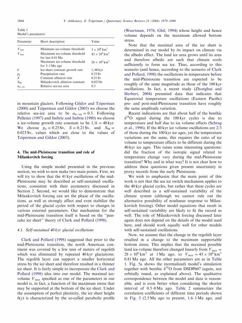
0.81Ma ago. All the other parameters are as in Table1. Fig. 5a shows the (normalized) model’s simulationtogether with benthic d18O from DSDP607 (again, notorbitally tuned, as explained above). The qualitativecorrespondence between the model and data is reason-able, and is even better when considering the shorterinterval of 0.5–0Ma ago. Table 2 summarizes thecorrelation coefficients of different time periods shownin Fig. 5 (2.5Ma ago to present, 1.6–1Ma ago, and
ARTICLE IN PRESS
2500 1500 500
2500 1500 500
2
3
4
5
δ18O
No orbital tuning
DSDP607Model
(a)
400 01600 1200
Time [kyr BP]
2
3
4
5
δ18O
2
3
4
5
δ18O
With orbital tuning
DSDP607Model
(b)
(c) (d)
Fig. 5. (a) A simulation of the mid-Pleistocene transition. The model is
run with Milankovitch forcing (65�N July insolation) for the past
3Ma. Motivated by proxy observations, the maximal ice volume
threshold before 1Ma ago is set to � 2=3 of the maximal ice volume ofthe last 0.8Ma; i.e., Vmax ¼ 28 106 km3 before 1Ma ago, increases
linearly to Vmax ¼ 45 106 km3 at 0.81Ma ago and remain constant
later on. A proxy record that is not orbitally tuned (DSDP 607, black
curve) is shown with the normalized model data (gray curve). (b) Same
as (a) but for orbitally tuned chronology (Raymo et al., 1989;
Ruddiman et al., 1989). Here the agreement between the data and the
model is better than for the non-orbitally tuned data, most probably
due to the calibration of the data with Milankovitch forcing. (c)
Enlargement of a segment (1.6–1Ma ago) from the 40 kyr oscillation
era shown in (b). (d) Enlargement of a segment from the 100 kyr
oscillations (the last 0.5Ma) shown in (b). The correlation coefficients
between the data and the model are summarized in Table 2.
Table 2
A summary of the correlation coefficients between the data (DSDP 607
and ODP 677) and the model as shown in Fig. 5a
2.5–0Ma ago 1.6–1Ma ago 0.5–0Ma ago
DSDP607 vs. Model 0.26 (0.39) 0.11 (0.47) 0.62 (0.64)
ODP677 vs. Model 0.23 (0.53) 0.12 (0.57) 0.33 (0.73)
DSDP607 vs. ODP677 0.36 (0.67) �0.1 (0.73) 0.51 (0.73)
The value in brackets are the correlation coefficients for the orbitally
tuned records ODP 677 (Shackleton et al., 1990) and DSDP 607
(Ruddiman et al., 1989; Raymo et al., 1989) (shown in Figs. 5b–d);
these values indicate better correspondence between the data and the
model, most probably due to phase-locking to Milankovitch.
0 10 20 30 40Lag,l
0.70.80.9
11.11.21.31.4
Asy
mm
etry
, p/n
DataPhase rand. data
(a)
0 0.02 0.04 0.06f [1/kyr]
0
0.2
0.4
0.6
0.8
S(f)
0 0.02 0.04 0.06f [1/kyr]
12.5Ma 00.8Ma
100kyr41kyr
Spectral Analysis
23ky
r
19ky
r
23ky
r
41kyr
19ky
r
(b) (c)
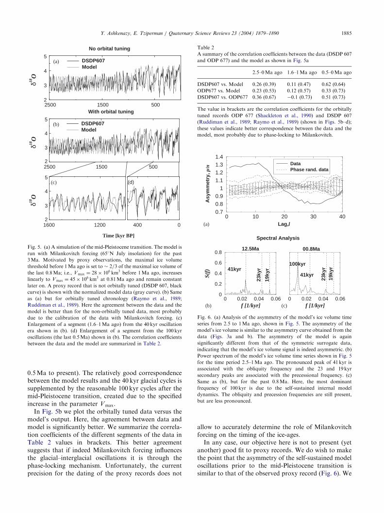
Fig. 6. (a) Analysis of the asymmetry of the model’s ice volume time
series from 2.5 to 1Ma ago, shown in Fig. 5. The asymmetry of the
model’s ice volume is similar to the asymmetry curve obtained from the
data (Figs. 3a and b). The asymmetry of the model is again
significantly different from that of the symmetric surrogate data,
indicating that the model’s ice volume signal is indeed asymmetric. (b)
Power spectrum of the model’s ice volume time series shown in Fig. 5
for the time period 2.5–1Ma ago. The pronounced peak of 41 kyr is
associated with the obliquity frequency and the 23 and 19 kyr
secondary peaks are associated with the precessional frequency. (c)
Same as (b), but for the past 0.8Ma. Here, the most dominant
frequency of 100 kyr is due to the self-sustained internal model
dynamics. The obliquity and precession frequencies are still present,
but are less pronounced.
Y. Ashkenazy, E. Tziperman / Quaternary Science Reviews 23 (2004) 1879–1890 1885
0.5Ma to present). The relatively good correspondencebetween the model results and the 40 kyr glacial cycles issupplemented by the reasonable 100 kyr cycles after themid-Pleistocene transition, created due to the specifiedincrease in the parameter Vmax.In Fig. 5b we plot the orbitally tuned data versus the
model’s output. Here, the agreement between data andmodel is significantly better. We summarize the correla-tion coefficients of the different segments of the data inTable 2 values in brackets. This better agreementsuggests that if indeed Milankovitch forcing influencesthe glacial–interglacial oscillations it is through thephase-locking mechanism. Unfortunately, the currentprecision for the dating of the proxy records does not
allow to accurately determine the role of Milankovitchforcing on the timing of the ice-ages.In any case, our objective here is not to present (yet
another) good fit to proxy records. We do wish to makethe point that the asymmetry of the self-sustained modeloscillations prior to the mid-Pleistocene transition issimilar to that of the observed proxy record (Fig. 6). We
ARTICLE IN PRESSY. Ashkenazy, E. Tziperman / Quaternary Science Reviews 23 (2004) 1879–18901886
wish to use this similarity to motivate our suggestionthat the 40 kyr oscillations may have been self-sustainedoscillations rather than a linear response to Milanko-vitch forcing. In Fig. 6a we show the asymmetry analysis(previously performed on the observations in Section 2,Fig. 3). Similarly, the spectrum for the 40 kyr oscilla-tions is similar for the model and observations (Figs. 6band c). Specifically, the ratio of the orbital frequencies ofobliquity and precession are similar. Next, we discussthe role of Milankovitch forcing in these self-sustainedoscillations.
4.2. Milankovitch forcing: phase locking and possible
stabilization of glacial period
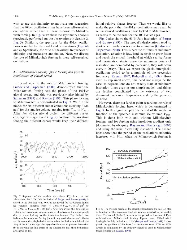
Proceed now to the role of Milankovitch forcing.Gildor and Tziperman (2000) demonstrated that theMilankovitch forcing sets the phase of the 100 kyrglacial cycles, and this was previously also hinted bySaltzman (1987) and Raymo (1997). This phase lockingto Milankovitch is demonstrated in Fig. 7. We run themodel for six different initial conditions (starting 3Maago) for the land ice volume, ranging from Vmin to Vmax.After few 40 kyr glacial cycles, the different curvesconverge to single curve (Fig. 7). Without the isolationforcing the different curves would keep their different
400 300 200 100 00
10
20
30
40
50
V(t
) [1
06km
3]
3000 2900 2800 2700 26000
10
20
30
40
50(a)
(b)
Time [kyr BP]
Fig. 7. Segments of the model’s ice volume V ðtÞ from the last
3Ma when the 65�N July insolation of Berger and Loutre (1991) is
added to the ablation term. We run the model for six different initial
ice volumes [ranging from V ð�3MaÞ ¼ Vmin ¼ 3 106 km3 to
V ð�3MaÞ ¼ Vmax ¼ 28 106 km3]. After few cycles the different ice
volume curves collapse to a single curve (displayed in the upper panel)
due to phase locking to the insolation forcing. The dashed line
indicates the insolation forcing (in arbitrary vertical scales and offsets)
and it seems that deglaciation starts when insolation is minimal. (a)
V ðtÞ of the 3–2.6Ma ago. (b) V ðtÞ of 0.4Ma ago to present. Note that
(b) is showing the final parts of the simulations that their beginnings
are shown in (a).
initial relative phases forever. Thus we would like tomake the point that the 40 kyr oscillations may again beself-sustained oscillations phase locked to Milankovitch,as seems to be the case for the 100 kyr ice ages.Fig. 7 also shows the 65�N July insolation of Berger
and Loutre (1991). The model’s deglaciations tend tostart when insolation is close to minimum (Gildor andTziperman, 2000). This is because at times of minimuminsolation, ablation is low, land ice tends to grow fasterand reach the critical threshold at which sea ice formsand termination starts. Since the minimum points ofinsolation are dominated by precession, they will occurevery � 20 kyr. Thus, we expect the glacial-interglacialoscillation period to be a multiple of the precessionfrequency (Raymo, 1997; Ridgwell et al., 1999). How-ever, as explained above, this need not always be thecase, as deglaciations do not exactly start at minimuminsolation times even in our simple model, and thingsare further complicated by the existence of twodominant precession frequencies, and by the presenceof noise.However, there is a further point regarding the role of
Milankovitch forcing here, which is demonstrated inFig. 8. In this figure we plot the period of the model asfunction of the specified maximum ice volume Vmax.This is done both with and without Milankovitchforcing, and for forcing using insolation gradient only(dominated by obliquity, Raymo and Nisancioglu, 2003)and using the usual 65�N July insolation. The dashedlines show that the period of the oscillations smoothlyincreases with Vmax when no Milankovitch forcing is
25 35 45Vmax [10
6km
3]
40
80
120
160
Per
iod
[kyr
]
With MilankovitchWithout Milankovitch
40
80
120
160(a) 65N July insolation
(b) Insolation gradient
Fig. 8. The average period of the glacial cycles during the past 0.8Myr
as function of the maximum land ice volume specified in the model,
Vmax. The dotted (dashed) lines show the period as function of Vmax
with (without) Milankovitch forcing. Upper panel: Milankovitch
forcing is the July radiation at 65�N (Berger and Loutre, 1991). Lower
panel: the gradient of the June 21st insolation from 70�N to 25�N
(which is dominated by the obliquity signal) is used as Milankovitch
forcing (based on Laskar, 1990).
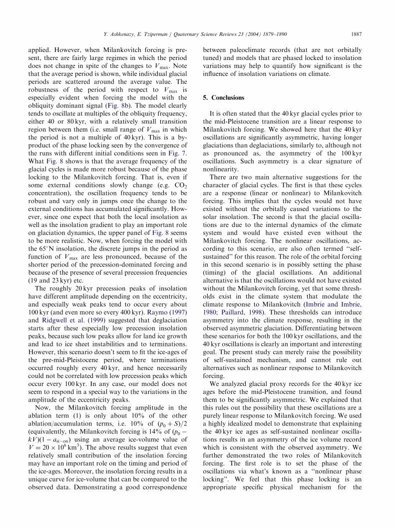
ARTICLE IN PRESSY. Ashkenazy, E. Tziperman / Quaternary Science Reviews 23 (2004) 1879–1890 1887
applied. However, when Milankovitch forcing is pre-sent, there are fairly large regimes in which the perioddoes not change in spite of the changes to Vmax. Notethat the average period is shown, while individual glacialperiods are scattered around the average value. Therobustness of the period with respect to Vmax isespecially evident when forcing the model with theobliquity dominant signal (Fig. 8b). The model clearlytends to oscillate at multiples of the obliquity frequency,either 40 or 80 kyr, with a relatively small transitionregion between them (i.e. small range of Vmax in whichthe period is not a multiple of 40 kyr). This is a by-product of the phase locking seen by the convergence ofthe runs with different initial conditions seen in Fig. 7.What Fig. 8 shows is that the average frequency of theglacial cycles is made more robust because of the phaselocking to the Milankovitch forcing. That is, even ifsome external conditions slowly change (e.g. CO2
concentration), the oscillation frequency tends to berobust and vary only in jumps once the change to theexternal conditions has accumulated significantly. How-ever, since one expect that both the local insolation aswell as the insolation gradient to play an important roleon glaciation dynamics, the upper panel of Fig. 8 seemsto be more realistic. Now, when forcing the model withthe 65�N insolation, the discrete jumps in the period asfunction of Vmax are less pronounced, because of theshorter period of the precession-dominated forcing andbecause of the presence of several precession frequencies(19 and 23 kyr) etc.The roughly 20 kyr precession peaks of insolation
have different amplitude depending on the eccentricity,and especially weak peaks tend to occur every about100 kyr (and even more so every 400 kyr). Raymo (1997)and Ridgwell et al. (1999) suggested that deglaciationstarts after these especially low precession insolationpeaks, because such low peaks allow for land ice growthand lead to ice sheet instabilities and to terminations.However, this scenario doesn’t seem to fit the ice-ages ofthe pre-mid-Pleistocene period, where terminationsoccurred roughly every 40 kyr, and hence necessarilycould not be correlated with low precession peaks whichoccur every 100 kyr. In any case, our model does notseem to respond in a special way to the variations in theamplitude of the eccentricity peaks.Now, the Milankovitch forcing amplitude in the
ablation term (1) is only about 10% of the otherablation/accumulation terms, i.e. 10% of ðp0 þ SÞ=2(equivalently, the Milankovitch forcing is 14% of ðp0 �kV Þð1� asi�onÞ using an average ice-volume value ofV ¼ 20 106 km3). The above results suggest that evenrelatively small contribution of the insolation forcingmay have an important role on the timing and period ofthe ice-ages. Moreover, the insolation forcing results in aunique curve for ice-volume that can be compared to theobserved data. Demonstrating a good correspondence
between paleoclimate records (that are not orbitallytuned) and models that are phased locked to insolationvariations may help to quantify how significant is theinfluence of insolation variations on climate.
5. Conclusions
It is often stated that the 40 kyr glacial cycles prior tothe mid-Pleistocene transition are a linear response toMilankovitch forcing. We showed here that the 40 kyroscillations are significantly asymmetric, having longerglaciations than deglaciations, similarly to, although notas pronounced as, the asymmetry of the 100 kyroscillations. Such asymmetry is a clear signature ofnonlinearity.There are two main alternative suggestions for the
character of glacial cycles. The first is that these cyclesare a response (linear or nonlinear) to Milankovitchforcing. This implies that the cycles would not haveexisted without the orbitally caused variations to thesolar insolation. The second is that the glacial oscilla-tions are due to the internal dynamics of the climatesystem and would have existed even without theMilankovitch forcing. The nonlinear oscillations, ac-cording to this scenario, are also often termed ‘‘self-sustained’’ for this reason. The role of the orbital forcingin this second scenario is in possibly setting the phase(timing) of the glacial oscillations. An additionalalternative is that the oscillations would not have existedwithout the Milankovitch forcing, yet that some thresh-olds exist in the climate system that modulate theclimate response to Milankovitch (Imbrie and Imbrie,1980; Paillard, 1998). These thresholds can introduceasymmetry into the climate response, resulting in theobserved asymmetric glaciation. Differentiating betweenthese scenarios for both the 100 kyr oscillations, and the40 kyr oscillations is clearly an important and interestinggoal. The present study can merely raise the possibilityof self-sustained mechanism, and cannot rule outalternatives such as nonlinear response to Milankovitchforcing.We analyzed glacial proxy records for the 40 kyr ice
ages before the mid-Pleistocene transition, and foundthem to be significantly asymmetric. We explained thatthis rules out the possibility that these oscillations are apurely linear response to Milankovitch forcing. We useda highly idealized model to demonstrate that explainingthe 40 kyr ice ages as self-sustained nonlinear oscilla-tions results in an asymmetry of the ice volume recordwhich is consistent with the observed asymmetry. Wefurther demonstrated the two roles of Milankovitchforcing. The first role is to set the phase of theoscillations via what’s known as a ‘‘nonlinear phaselocking’’. We feel that this phase locking is anappropriate specific physical mechanism for the
ARTICLE IN PRESSY. Ashkenazy, E. Tziperman / Quaternary Science Reviews 23 (2004) 1879–18901888
common and somewhat more vague suggestion thatMilankovitch forcing is the pacemaker of glacial cycles(Hays et al., 1976). The second role of the Milankovitchforcing demonstrated here is in the stabilization of theglacial period to slow changes (such as changes to thebedrock or atmospheric CO2). The model used heredisplays nonlinear self-sustained oscillations, that arealso forced (externally) by Milankovitch forcing. Thisoscillations may exist even without the Milankovitchvariations, yet these variations ‘‘pace’’ (via nonlinearphase locking) the self sustained oscillations due to theinternal climate variability.Raymo and Nisancioglu (2003) proposed that the
insolation gradient has a dominant effect on ice-ages ofthe 40 kyr oscillations, because the insolation gradient isdominated by the obliquity signal. We cannot rule out adominant role for the insolation gradient, although ourresults imply that the 40 kyr cycles are not a linearresponse to obliquity forcing. It is possible that theinsolation gradient somehow phase locks a nonlinearoscillation during the 40 kyr ice ages.The model presented in this paper is clearly highly
simplified and excludes many important physical pro-cesses; clearly it would be desirable to use a morecomplex model to look into these issues. However, themain point of this work does not depend on the detailsof the specific simple model we have used. The robustmessage of this paper is that we have demonstrated thatthe 40 kyr oscillations are significantly asymmetric andmay not be explained as a linear response to Milanko-vitch forcing. These cycles may therefore be self-sustained oscillations, as the 100 kyr oscillations arecommonly believed to be.
Acknowledgements
ET is supported by the McDonnell Foundation. Wethank Hezi Gildor and Peter Stone for helpful discus-sions, and to two anonymous reviewers for their helpfulcomments.
Appendix A. Phase randomization
Given a time series hk with a sampling rate D, it ispossible to perform a Fourier transform in order to findthe frequency spectrum of the series. The Fouriertransform results in a complex Fourier series Hn �
An exp½ijn where An is the Fourier amplitude and jn isthe phase. The relation between the original series hk
and Fourier series Hn is
Hn � DXN�1
k¼0
hke2pikn=N
and
hk �1
ND
XN�1
n¼0
Hne�2pikn=N ;
where N is the number of data points of the time serieshk.Now, the information regarding the ‘‘time direction’’
of the time series hk if stored in the Fourier phasesjn—when, e.g., one inverts the direction of the timeseries hk by changing D to �D just the phase jn changesto jn þ p while the Fourier amplitude An remainsunaffected. The asymmetry of hk is an indication forthe time direction of the series and is reflected in theFourier phases jn. Thus, if one would like to ‘‘destroy’’the asymmetry of the time series hk he shouldfirst perform a Fourier transform, then replace thephases jn by uniformly distributed random phases andthen perform an inverse Fourier transform. The result-ing series should not contain any information regardingthe time direction of the original series. It is knownhowever that this procedure may alter the originalprobability distribution of hk; one would prefer to keepthe original distribution of the time series unchangedafter randomizing the Fourier phases in order topreserve as much knowledge as possible of the originaltime series.Schreiber and Schmitz (2000) suggested an algorithm
which preserves both the original probability distribu-tion of the time series as well as its Fourier ampli-tudes but randomizes the Fourier phases. The algorithmis an iterative algorithm and consists of the followingsteps:
(i)
Store a sorted list of the original data fhkg and thepower spectrum fSng of fhkg.(ii)
Begin (l ¼ 0) with a random shuffle fhðl¼0Þk g of thedata.
(iii) Replace the power spectrum fSðlÞn g of fhðlÞk g by fSng
(keeping the Fourier phases of fSðlÞk g) and then
transform back.
(iv) Sort the series obtained from (iii). (v) Replace the sorted series from (iv) by the sorted fhkgand then return to the pre-sorting order [i.e., theorder of the series obtained from (iii)]; the resultingseries is fh
ðlþ1Þk g.
Repeat steps (iii)–(v) until convergence (i.e., untilseries from consecutive iterations will be almost thesame)In order to check if a time series is symmetric or
asymmetric it is possible to generate many surrogatesymmetric time series out of the original time series andthen to check how significant is the asymmetry of theoriginal time series compare to the asymmetry of thesurrogate (symmetric) time series.
ARTICLE IN PRESSY. Ashkenazy, E. Tziperman / Quaternary Science Reviews 23 (2004) 1879–1890 1889
Appendix B. Linear, nonlinear and self-sustained glacial
oscillations
B.1. Linear oscillations
A basic equation for linear oscillations is theharmonic oscillator d2x=dt2 þ x ¼ 0. The amplitude ofthe oscillations of a harmonic oscillator depend on theinitial conditions; i.e., different initial conditions willlead to oscillations with different amplitudes propor-tional to the amplitude of the initial conditions. Whenforced by an external periodic forcing (e.g. Milankovitchforcing), with a frequency different from the naturalfrequency and damped by friction, the oscillationamplitude will be proportional to the amplitude of theexternal forcing.
B.2. Nonlinear self-sustained oscillations
Suppose now that we add a nonlinear term to theharmonic oscillator to get the van Der Pol oscillator,d2x=dt2 � eð1� x2Þdx=dt þ x ¼ 0. When e � 1 one ob-tains a periodic solution (for t � 0) which is independent
of the initial conditions and results in a single uniquecurve in the phase space. I.e., xðtÞ ¼ 2 cos t anddx=dt ¼ �2 sin t. These are self-sustained oscillations(although only weakly nonlinear), and this is what isreferred to in the text of this paper as self-sustainedoscillations, requiring no external forcing to be sus-tained. When e � 1 the oscillations are also periodic andself-sustained but strongly nonlinear with sharp transi-tions (fast and slow phases); these are relaxation
oscillations (Strogatz, 1994), which are the class of self-sustained oscillations perhaps the most relevant toglacial cycles. The power spectrum of such oscillationsshows the basic frequency of the system with severalstrong harmonics.
References
Ashkenazy, Y., Baker, D.R., Gildor, H., Havlin, S., 2003. Nonlinearity
and multifractality of climate change in the past 420,000 years.
Geophysical Research Letters 30 (22), 2146 (10.1029/
2003GL018099).
Berger, A., Loutre, M.F., 1991. Insolation values for the climate of the
last 10 million years. Quaternary Science Review 10, 297–317.
Berger, A., Li, X., Loutre, M., 1999. Modelling northern hemisphere
ice volume over the last 3Ma. Quaternary Science Review 18, 1–11.
Clark, P.U., Pollard, D., 1998. Origin of the middle Pleistocene
transition by ice sheet erosion of regolith. Paleoceanography 13 (1),
1–9.
Gallee, H., vanYpersele, J., Fichefet, T., Tricot, C., Berger, A., 1991.
Simulation of the last glacial cycle by a coupled sectorially
averaged climate-ice sheet model. 1. The climate model. Journal
of Geophysical Research 96, 13,139–13,161.
Gallee, H., vanYpersele, J., Fichefet, T., Marsiat, I., Tricot, C., Berger,
A., 1992. Simulation of the last glacial cycle by a coupled
sectorially averaged climate-ice sheet model. 2. Response to
insolation and CO2 variations. Journal of Geophysical Research
97, 15,713–15,740.
Ghil, M., 1994. Cryothermodynamics: the chaotic dynamics of
paleoclimate. Physica D 77, 130–159.
Gildor, H., Tziperman, E., 2000. Sea ice as the glacial cycles climate
switch: role of seasonal and orbital forcing. Paleoceanography 15,
605–615.
Hagelberg, T., Pisias, N., Elgar, S., 1991. Linear and nonlinear
couplings between orbital forcing and the marine d18O record
during the late Neogene. Paleoceanography 6 (4), 729–746.
Hartmann, D., 1994. Global Physical Climatology. Academic Press,
San Diego.
Hays, J.D., Imbrie, J., Shackleton, N.J., 1976. Variations in the earth’s
orbit: pacemakers of the ice ages. Science 194, 1121–1132.
Imbrie, J., Imbrie, J.Z., 1980. modelling the climatic response to
orbital variations. Science 207, 943–953.
Imbrie, J., Boyle, E.A., Clemens, S.C., Duffy, A., Howard, W.R.,
Kukla, G., Kutzbach, J., Martinson, D.G., McIntyre, A., Mix,
A.C., Molfino, B., Morely, J., Peterson, L.C., Pisias, N., Prell,
W.L., Raymo, M.E., Shackleton, N.J., Toggweiler, J.R., 1992.
On the structure and origin of major glaciation cycles. 1.
Linear responses to Milankovitch forcing. Paleoceanography 7,
701–738.
Imbrie, J., Berger, A., Boyle, E.A., Clemens, S.C., Duffy, A., Howard,
W.R., Kukla, G., Kutzbach, J., Martinson, D.G., McIntyre, A.,
Mix, A.C., Molfino, B., Morley, J.J., Peterson, L.C., Pisias, N.G.,
Prell, W.L., Raymo, M.E., Shackleton, N.J., Toggweiler, J.R.,
1993. On the structure and origin of major glaciation cycles. 2. The
100,000–year cycle. Paleoceanography 8, 699–735.
King, T., 1996. Quantifying nonlinearity and geometry in time series of
climate. Quaternary Science Review 15, 247–266.
Kominz, M., Pisias, N., 1979. Pleistocene climate—deterministic or
stochastic. Science 204, 171–173.
Laskar, J., 1990. The chaotic motion of the solar system: a numerical
estimate of the chaotic zones. Icarus 88, 266–291.
Milankovitch, M., 1941. Canon of insolation and the ice-age problem.
Royal Serbian Academy, Special Publication No. 132, translated
from German by Israel Program for Scientific Translations,
Jerusalem, 1969.
Mix, A.C., Bard, E., Schneider, R., 2001. Environmental processes of
the ice age: land oceans glaciers (EPILOG). Quaternary Science
Reviews 20, 627–657.
Paillard, D., 1998. The timing of Pleistocene glaciations from a simple
multiple-state climate model. Nature 391, 378–381.
Paillard, D., 2001. Glacial cycles: toward a new paradigm. Reviews of
Geophysics 39, 325–346.
Paillard, D., Labeyrie, L., Yiou, P., 1996. Macintosh program
performs time-series analysis. Eos Transactions AGU 77, 379.
Pelletier, J., 1997. Analysis and modeling of the natural variability of
climate. Journal of Climate 10, 1331–1342.
Raymo, M.E., 1992. Global climate change: a three million year
perspective. In: Kukla, G., Went, E. (Eds.), Start of a Glacial,
NATO ASI Series I, Vol. 3. Proceedings of the Mallorca NATO
ARW. Springer, Heidelberg, pp. 207–223.
Raymo, M.E., 1997. The timing of major terminations. Paleoceano-
graphy 12, 577–585.
Raymo, M.E., Nisancioglu, K., 2003. The 41 kyr world: Milanko-
vitch’s other unsolved mystery. Paleoceanography 18 (1), 1011
(doi:10.1029/2002PA000791).
Raymo, M.E., Ruddiman, W.F., Backman, J., Clement, B.M.,
Martinson, D.G., 1989. Late pliocene variation in northern
hemisphere ice sheets and north atlantic deep circulation.
Paleoceanography 4, 413–446.
Ridgwell, A.J., Watson, A.J., Raymo, M.E., 1999. Is the spectral
signature of the 100 kyr glacial cycle consistent with a Milankovitch
origin? Paleoceanography 14, 437–440.
ARTICLE IN PRESSY. Ashkenazy, E. Tziperman / Quaternary Science Reviews 23 (2004) 1879–18901890
Ruddiman, W.F., 2003. Orbital forcing ice volume and greenhouse
gases. Quaternary Science Reviews 22, 1597–1629.
Ruddiman, W.F., 2004. The role of greenhouse gases in orbital-scale
climatic changes. EOS 85 (1), 1.
Ruddiman, W.F., Raymo, M.E., Martinson, D.G., Clement, B.M.,
Backman, J., 1989. Pleistocene evolution: Northern hemisphere
ice sheets and North Atlantic Ocean. Paleoceanography 4,
353–412.
Saltzman, B., 1987. Carbon dioxide and the d18O record of late-
Quaternary climatic change: a global model. Climate Dynamics 1,
77–85.
Saltzman, B., 1990. Three basic problems of paleoclimatic modeling: a
personal perspective and review. Climate Dynamics 5, 67–78.
Schrag, D., Hampt, G., Murray, D., 1996. Pore fluid constraints on the
temperature and oxygen isotopic composition of the glacial ocean.
Science 272, 1930–1932.
Schreiber, T., Schmitz, A., 2000. Surrogate time series. Physica D 142,
346–382.
Shackleton, N.J., Berger, A., Peltier, W.R., 1990. An alternative
astronomical calibration of the lower pleistocene time scale based
on ODP site 677. Transactions of the Royal Society of Edinburgh:
Earth Sciences 81, 251–261.
Strogatz, S., 1994. Nonlinear Dynamics and Chaos. Westview Press,
Boulder, CO, USA.
Tziperman, E., Gildor, H., 2003. The mid-Pleistocene climate
transition and the source of asymmetry between glaciation and
deglaciation times. Paleoceanography 18 (1) (10.1029/
2001PA000627).
Weertman, J., 1976. Milankovitch solar radiation variations and ice
age ice sheet sizes. Nature 261, 17–20.
Wunsch, C., 2003. The spectral description of climate change including
the ky energy. Climate Dynamics 20, 353–363 (doi:10.1007/s00382-
002-0279-z).
Zhonghui, L., Herbert, T.W., 2004. High-latitude influence on the
eastern equatorial pacific climate in the early Pleistocene epoch.
Nature 427, 720–723 (doi:10.1038/nature02338).