Earth and Planetary Science Letters 392 (2014) 217–229

Contents lists available at ScienceDirect

Earth and Planetary Science Letters

www.elsevier.com/locate/epsl

Geomagnetic intensity variations for the past 8 kyr: Newarchaeointensity results from Eastern China

Shuhui Cai a,b,∗, Lisa Tauxe c, Chenglong Deng a, Yongxin Pan b, Guiyun Jin d,Jianming Zheng e, Fei Xie f, Huafeng Qin b, Rixiang Zhu a

a State Key Laboratory of Lithospheric Evolution, Institute of Geology and Geophysics, Chinese Academy of Sciences, Beijing 100029, Chinab Key Laboratory of the Earth’s Deep Interior, Institute of Geology and Geophysics, Chinese Academy of Sciences, Beijing 100029, Chinac Scripps Institution of Oceanography, University of California, San Diego, La Jolla, CA 92093-0220, USAd School of History and Culture, Shandong University, Jinan 250100, Chinae Zhejiang Provincial Institute of Cultural Relics and Archaeology, Hangzhou 310014, Chinaf Hebei Province Institute of Cultural Relics, Shijiazhuang 050000, China

a r t i c l e i n f o a b s t r a c t

Article history:Received 3 August 2013Received in revised form 9 February 2014Accepted 12 February 2014Available online 6 March 2014Editor: L. Stixrude

Keywords:archaeointensityChinaregional model of Eastern Asianon-dipolar moment

In this study, we have carried out paleointensity experiments on 918 specimens spanning the last ∼7 kyr,including pottery fragments, baked clay and slag, collected from Shandong, Liaoning, Zhejiang and HebeiProvinces in China. Approximately half of the specimens yielded results that passed strict data selectioncriteria and give high-fidelity paleointensities. The virtual axial dipole moments (VADMs) of our sitesrange from ∼2 × 1022 to ∼13 × 1022 Am2. At ∼2250 BCE our results suggest a paleointensity low of∼2 × 1022 Am2, which increases to a high of ∼13 × 1022 Am2 by ∼1300 BCE. This rapid (less than1000 yrs) six-fold change in the paleointensity may have important implications for the dynamics ofcore flow at this time. Our data from the last ∼3 kyr are generally in good agreement with the ARCH3k.1model, but deviate significantly at certain time periods from the CALS3k.4 and CALS10k.1b model, whichis likely due to differences in the data used to constrain these models. At ages older than ∼3 ka, whereonly the CALS10k.1b model is available for comparison, our data deviate significantly from the model.Combining our new results with the published data from China and Japan, we provide greatly improvedconstraints for the regional model of Eastern Asia. When comparing the variations of geomagnetic field inthree global representative areas of Eastern Asia, the Middle East and Southern Europe, a common generaltrend of sinusoidal variations since ∼8 ka is shown, likely dominated by the dipole component. However,significant disparities are revealed as well, which we attribute to non-dipolar components caused bymovement of magnetic flux patches at the core-mantle boundary.

© 2014 Elsevier B.V. All rights reserved.

1. Introduction

The geomagnetic field is generated by the motion of the Earth’sfluid outer core and its variation is driven by the Earth’s deepinternal dynamics. Therefore, the behavior of geomagnetic fieldhas significant potential to yield insight into Earth’s geodynam-ics, such as the influence of core-mantle interactions (Biggin etal., 2012; Bloxham, 2000), changes in outer-core flow and geo-magnetic jerks (Bloxham et al., 2002; Dumberry and Finlay, 2007;Mandea et al., 2010; Olsen and Mandea, 2008). Besides the geo-dynamic significance, connections between the geomagnetic field

* Corresponding author at: Institute of Geology and Geophysics, Chinese Academyof Sciences, 19 Bei-Tu-Cheng-Xi-Lu, Beijing 100029, China. Tel.: +86 (10) 8299 8418;fax: +86 (10) 6201 0846.

E-mail address: shuhui.cai08@gmail.com (S. Cai).

http://dx.doi.org/10.1016/j.epsl.2014.02.0300012-821X/© 2014 Elsevier B.V. All rights reserved.

and global climate have been suggested (Courtillot et al., 2007;Gallet et al., 2005; Kent, 1982), but these claims remain contro-versial (Bard and Delaygue, 2008). Furthermore, archaeomagneticstudies focusing on the detailed evolution of the geomagnetic fieldover the past ∼8 kyr have a potential application on archaeomag-netic dating (Ben-Yosef et al., 2008b, 2010; Pavón-Carrasco et al.,2009, 2011).

The geomagnetic field varies over a broad range of timescales.To understand the variation over periods of thousands of yearswe rely entirely on measurements of remanent magnetizationfrom geological and archaeological materials. Archaeomagneticdata from Eastern Asia, however, are sparse, particularly those thatwould be widely regarded as reliable (Yu, 2012). The main ar-chaeomagnetic work in China was carried out in the 1980s and1990s (Huang et al., 1998; Shaw et al., 1995, 1999; Tang et al.,1991; Wei et al., 1982, 1986, 1987) and published data are rather

218 S. Cai et al. / Earth and Planetary Science Letters 392 (2014) 217–229

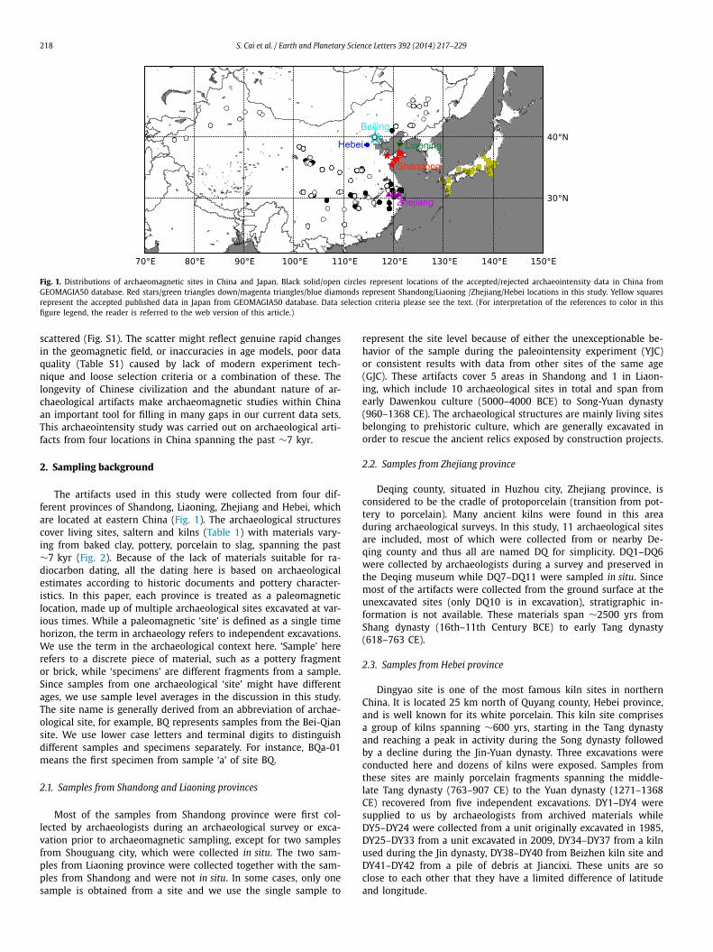
Fig. 1. Distributions of archaeomagnetic sites in China and Japan. Black solid/open circles represent locations of the accepted/rejected archaeointensity data in China fromGEOMAGIA50 database. Red stars/green triangles down/magenta triangles/blue diamonds represent Shandong/Liaoning /Zhejiang/Hebei locations in this study. Yellow squaresrepresent the accepted published data in Japan from GEOMAGIA50 database. Data selection criteria please see the text. (For interpretation of the references to color in thisfigure legend, the reader is referred to the web version of this article.)

scattered (Fig. S1). The scatter might reflect genuine rapid changesin the geomagnetic field, or inaccuracies in age models, poor dataquality (Table S1) caused by lack of modern experiment tech-nique and loose selection criteria or a combination of these. Thelongevity of Chinese civilization and the abundant nature of ar-chaeological artifacts make archaeomagnetic studies within Chinaan important tool for filling in many gaps in our current data sets.This archaeointensity study was carried out on archaeological arti-facts from four locations in China spanning the past ∼7 kyr.

2. Sampling background

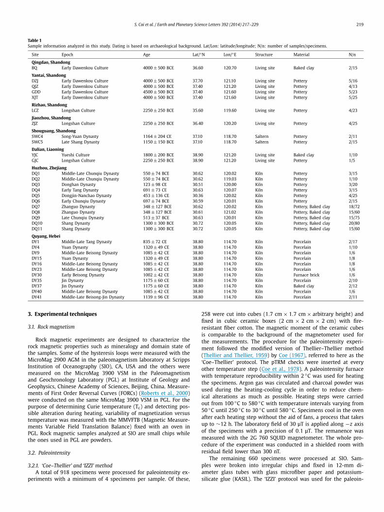
The artifacts used in this study were collected from four dif-ferent provinces of Shandong, Liaoning, Zhejiang and Hebei, whichare located at eastern China (Fig. 1). The archaeological structurescover living sites, saltern and kilns (Table 1) with materials vary-ing from baked clay, pottery, porcelain to slag, spanning the past∼7 kyr (Fig. 2). Because of the lack of materials suitable for ra-diocarbon dating, all the dating here is based on archaeologicalestimates according to historic documents and pottery character-istics. In this paper, each province is treated as a paleomagneticlocation, made up of multiple archaeological sites excavated at var-ious times. While a paleomagnetic ‘site’ is defined as a single timehorizon, the term in archaeology refers to independent excavations.We use the term in the archaeological context here. ‘Sample’ hererefers to a discrete piece of material, such as a pottery fragmentor brick, while ‘specimens’ are different fragments from a sample.Since samples from one archaeological ‘site’ might have differentages, we use sample level averages in the discussion in this study.The site name is generally derived from an abbreviation of archae-ological site, for example, BQ represents samples from the Bei-Qiansite. We use lower case letters and terminal digits to distinguishdifferent samples and specimens separately. For instance, BQa-01means the first specimen from sample ‘a’ of site BQ.

2.1. Samples from Shandong and Liaoning provinces

Most of the samples from Shandong province were first col-lected by archaeologists during an archaeological survey or exca-vation prior to archaeomagnetic sampling, except for two samplesfrom Shouguang city, which were collected in situ. The two sam-ples from Liaoning province were collected together with the sam-ples from Shandong and were not in situ. In some cases, only onesample is obtained from a site and we use the single sample to

represent the site level because of either the unexceptionable be-havior of the sample during the paleointensity experiment (YJC)or consistent results with data from other sites of the same age(GJC). These artifacts cover 5 areas in Shandong and 1 in Liaon-ing, which include 10 archaeological sites in total and span fromearly Dawenkou culture (5000–4000 BCE) to Song-Yuan dynasty(960–1368 CE). The archaeological structures are mainly living sitesbelonging to prehistoric culture, which are generally excavated inorder to rescue the ancient relics exposed by construction projects.

2.2. Samples from Zhejiang province

Deqing county, situated in Huzhou city, Zhejiang province, isconsidered to be the cradle of protoporcelain (transition from pot-tery to porcelain). Many ancient kilns were found in this areaduring archaeological surveys. In this study, 11 archaeological sitesare included, most of which were collected from or nearby De-qing county and thus all are named DQ for simplicity. DQ1–DQ6were collected by archaeologists during a survey and preserved inthe Deqing museum while DQ7–DQ11 were sampled in situ. Sincemost of the artifacts were collected from the ground surface at theunexcavated sites (only DQ10 is in excavation), stratigraphic in-formation is not available. These materials span ∼2500 yrs fromShang dynasty (16th–11th Century BCE) to early Tang dynasty(618–763 CE).

2.3. Samples from Hebei province

Dingyao site is one of the most famous kiln sites in northernChina. It is located 25 km north of Quyang county, Hebei province,and is well known for its white porcelain. This kiln site comprisesa group of kilns spanning ∼600 yrs, starting in the Tang dynastyand reaching a peak in activity during the Song dynasty followedby a decline during the Jin-Yuan dynasty. Three excavations wereconducted here and dozens of kilns were exposed. Samples fromthese sites are mainly porcelain fragments spanning the middle-late Tang dynasty (763–907 CE) to the Yuan dynasty (1271–1368CE) recovered from five independent excavations. DY1–DY4 weresupplied to us by archaeologists from archived materials whileDY5–DY24 were collected from a unit originally excavated in 1985,DY25–DY33 from a unit excavated in 2009, DY34–DY37 from a kilnused during the Jin dynasty, DY38–DY40 from Beizhen kiln site andDY41–DY42 from a pile of debris at Jiancixi. These units are soclose to each other that they have a limited difference of latitudeand longitude.

S. Cai et al. / Earth and Planetary Science Letters 392 (2014) 217–229 219

Table 1Sample information analyzed in this study. Dating is based on archaeological background. Lat/Lon: latitude/longitude; N/n: number of samples/specimens.

Site Epoch Age Lat/◦N Lon/◦E Structure Material N/n

Qingdao, ShandongBQ Early Dawenkou Culture 4000 ± 500 BCE 36.60 120.70 Living site Baked clay 2/15

Yantai, ShandongDZJ Early Dawenkou Culture 4000 ± 500 BCE 37.70 121.10 Living site Pottery 5/16QJZ Early Dawenkou Culture 4000 ± 500 BCE 37.40 121.20 Living site Pottery 4/13GDD Early Dawenkou Culture 4500 ± 500 BCE 37.40 121.60 Living site Pottery 5/23XJT Early Dawenkou Culture 4000 ± 500 BCE 37.40 121.60 Living site Pottery 5/25

Rizhao, ShandongLCZ Longshan Culture 2250 ± 250 BCE 35.60 119.60 Living site Pottery 4/23

Jiaozhou, ShandongZJZ Longshan Culture 2250 ± 250 BCE 36.40 120.20 Living site Pottery 4/25

Shouguang, ShandongSWC4 Song-Yuan Dynasty 1164 ± 204 CE 37.10 118.70 Saltern Pottery 2/11SWC5 Late Shang Dynasty 1150 ± 150 BCE 37.10 118.70 Saltern Pottery 2/15

Dalian, LiaoningYJC Yueshi Culture 1800 ± 200 BCE 38.90 121.20 Living site Baked clay 1/10GJC Longshan Culture 2250 ± 250 BCE 38.90 121.20 Living site Pottery 1/5

Huzhou, ZhejiangDQ1 Middle-Late Chunqiu Dynasty 550 ± 74 BCE 30.62 120.02 Kiln Pottery 3/15DQ2 Middle-Late Chunqiu Dynasty 550 ± 74 BCE 30.62 119.03 Kiln Pottery 1/10DQ3 Donghan Dynasty 123 ± 98 CE 30.51 120.00 Kiln Pottery 3/20DQ4 Early Tang Dynasty 691 ± 73 CE 30.63 120.07 Kiln Pottery 3/15DQ5 Dongjin-Nanchao Dynasty 453 ± 136 CE 30.36 120.02 Kiln Pottery 4/25DQ6 Early Chunqiu Dynasty 697 ± 74 BCE 30.59 120.01 Kiln Pottery 2/15DQ7 Zhanguo Dynasty 348 ± 127 BCE 30.62 120.02 Kiln Pottery, Baked clay 18/72DQ8 Zhanguo Dynasty 348 ± 127 BCE 30.61 121.02 Kiln Pottery, Baked clay 15/60DQ9 Late Chunqiu Dynasty 513 ± 37 BCE 30.63 120.01 Kiln Pottery, Baked clay 15/75DQ10 Shang Dynasty 1300 ± 300 BCE 30.72 120.05 Kiln Pottery, Baked clay 20/80DQ11 Shang Dynasty 1300 ± 300 BCE 30.72 120.05 Kiln Pottery, Baked clay 15/60

Quyang, HebeiDY1 Middle-Late Tang Dynasty 835 ± 72 CE 38.80 114.70 Kiln Porcelain 2/17DY4 Yuan Dynasty 1320 ± 49 CE 38.80 114.70 Kiln Porcelain 1/10DY9 Middle-Late Beisong Dynasty 1085 ± 42 CE 38.80 114.70 Kiln Porcelain 1/6DY15 Yuan Dynasty 1320 ± 49 CE 38.80 114.70 Kiln Porcelain 1/8DY16 Middle-Late Beisong Dynasty 1085 ± 42 CE 38.80 114.70 Kiln Porcelain 1/8DY23 Middle-Late Beisong Dynasty 1085 ± 42 CE 38.80 114.70 Kiln Porcelain 1/6DY30 Early Beisong Dynasty 1002 ± 42 CE 38.80 114.70 Kiln Furnace brick 1/6DY35 Jin Dynasty 1175 ± 60 CE 38.80 114.70 Kiln Porcelain 2/10DY37 Jin Dynasty 1175 ± 60 CE 38.80 114.70 Kiln Baked clay 2/12DY40 Middle-Late Beisong Dynasty 1085 ± 42 CE 38.80 114.70 Kiln Porcelain 1/6DY41 Middle-Late Beisong-Jin Dynasty 1139 ± 96 CE 38.80 114.70 Kiln Porcelain 2/11

3. Experimental techniques

3.1. Rock magnetism

Rock magnetic experiments are designed to characterize therock magnetic properties such as mineralogy and domain state ofthe samples. Some of the hysteresis loops were measured with theMicroMag 2900 AGM in the paleomagnetism laboratory at ScrippsInstitution of Oceanography (SIO), CA, USA and the others weremeasured on the MicroMag 3900 VSM in the Paleomagnetismand Geochronology Laboratory (PGL) at Institute of Geology andGeophysics, Chinese Academy of Sciences, Beijing, China. Measure-ments of First Order Reversal Curves (FORCs) (Roberts et al., 2000)were conducted on the same MicroMag 3900 VSM in PGL. For thepurpose of determining Curie temperature (Tc) and detecting pos-sible alteration during heating, variability of magnetization versustemperature was measured with the MMVFTB (Magnetic Measure-ments Variable Field Translation Balance) fixed with an oven inPGL. Rock magnetic samples analyzed at SIO are small chips whilethe ones used in PGL are powders.

3.2. Paleointensity

3.2.1. ‘Coe–Thellier’ and ‘IZZI’ methodA total of 918 specimens were processed for paleointensity ex-

periments with a minimum of 4 specimens per sample. Of these,

258 were cut into cubes (1.7 cm × 1.7 cm × arbitrary height) andfixed in cubic ceramic boxes (2 cm × 2 cm × 2 cm) with fire-resistant fiber cotton. The magnetic moment of the ceramic cubesis comparable to the background of the magnetometer used forthe measurements. The procedure for the paleointensity experi-ment followed the modified version of Thellier–Thellier method(Thellier and Thellier, 1959) by Coe (1967), referred to here as the‘Coe–Thellier’ protocol. The pTRM checks were inserted at everyother temperature step (Coe et al., 1978). A paleointensity furnacewith temperature reproducibility within 2 ◦C was used for heatingthe specimens. Argon gas was circulated and charcoal powder wasused during the heating-cooling cycle in order to reduce chem-ical alterations as much as possible. Heating steps were carriedout from 100 ◦C to 580 ◦C with temperature intervals varying from50 ◦C until 250 ◦C to 30 ◦C until 580 ◦C. Specimens cool in the ovenafter each heating step without the aid of fans, a process that takesup to ∼12 h. The laboratory field of 30 μT is applied along −z axisof the specimens with a precision of 0.1 μT. The remanence wasmeasured with the 2G 760 SQUID magnetometer. The whole pro-cedure of the experiment was conducted in a shielded room withresidual field lower than 300 nT.

The remaining 660 specimens were processed at SIO. Sam-ples were broken into irregular chips and fixed in 12-mm di-ameter glass tubes with glass microfiber paper and potassium-silicate glue (KASIL). The ‘IZZI’ protocol was used for the paleoin-

220 S. Cai et al. / Earth and Planetary Science Letters 392 (2014) 217–229

Fig. 2. Various samples analyzed in this study: (a) baked clay from Shandong, (b) slag from Zhejiang, (c) porcelain fragment from Hebei, (d–h) pottery fragments withdifferent shapes and decorations from Zhejiang.

tensity experiment (Tauxe and Staudigel, 2004), which is believedto be better than the traditional protocols (Aitken et al., 1988;Coe, 1967) because it can easily detect the effect of high tem-perature pTRM tails (Yu and Tauxe, 2005; Yu et al., 2004). ThepTRM checks were also included at every other step. Specimenswere heated in one of two ovens, which have residual fields lessthan 10 nT during zero-field steps, in the paleomagnetic shieldedroom at SIO. Measurements were made on a 2G cryogenic mag-netometer. Heating steps were carried out from 100 ◦C to 580 ◦C(with a few up to 600 ◦C) with temperature intervals varying from100 ◦C to 15 ◦C, generally larger for low temperatures and smallerfor high temperatures. Specimens were cooled in the oven aftereach heating step with a fan and cooling times are 30–45 min-utes. A laboratory field is applied along −z axis of the specimensand field value of 30 μT or 50 μT was chosen depending on theexpected ancient field of samples.

3.2.2. Anisotropy correctionThe effect of anisotropy of TRM (ATRM) on paleointensity es-

timation has long been recognized (Aitken et al., 1981, 1988;Rogers et al., 1979). TRM anisotropy is sometimes observed ingeological samples, but occurs frequently in archaeological ar-tifacts because of manufacturing procedures, which makes theanisotropy correction in archaeological study non-trivial. The biasin paleointensity caused by ATRM can be corrected by determin-ing the anisotropy tensor of each specimen (Selkin et al., 2000;Veitch et al., 1984). This can be determined by anisotropy ofmagnetic susceptibility (AMS) or anisotropy of anhysteretic rema-nent magnetization (AARM) or ATRM. While it is generally agreedthat AMS is a poor approximation for ATRM, the preference forAARM and ATRM remains controversial. Some authors prefer the

ATRM correction because in theory AARM is different from ATRM(Chauvin et al., 2000). Others argue that AARM is preferable be-cause the corrections are usually similar (Ben-Yosef et al., 2008a;Mitra et al., 2013), it is faster to determine the AARM tensor thanthe ATRM one, and there is no further laboratory alteration withthe AARM tensor. Some studies use a partial TRM (pTRM) to de-termine the ATRM tensor in order to avoid bias introduced by al-teration when heating to high temperatures (Chauvin et al., 2000;Genevey and Gallet, 2002; Hill et al., 2008), while total TRMs areused in other studies based on the assumption that total TRMcorrection avoids the complications of pTRM tails that may affectpTRMs. The use of pTRM checks insures that the ATRM tensor hasnot been affected by alteration (Shaar et al., 2010, 2011).

Here we impart a total TRM along the six axes of each spec-imen (±x, ±y, ±z) following the method of Veitch et al. (1984).For some specimens we used an initial demagnetization step todetermine a baseline. When calculating the ATRM tensor, we pre-fer the original method proposed by Veitch et al. (1984) to themodified version by Selkin et al. (2000) because the latter mightchange paleointensity parameters which are critical to data selec-tion (Paterson, 2013). Following the six ATRM measurements, weinclude an additional step, which is a repeat of the first measure-ment position to test for possible alteration during the heatingsrequired to measure the tensor.

3.2.3. Cooling rate correctionDodson and McClelland-Brown (1980) showed that blocking

temperatures of single domain grains are related to the coolingrate and the TRM acquired at different cooling rates in the samefield might differ significantly. This will bias the estimation of pa-leointensity (Halgedahl et al., 1980). In order to obtain the most

S. Cai et al. / Earth and Planetary Science Letters 392 (2014) 217–229 221

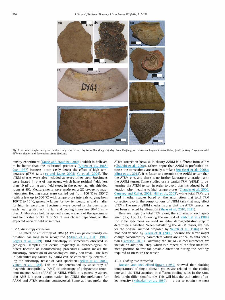
Fig. 3. (a) and (c) Hysteresis loops of representative samples. Red (blue) loop is before (after) paramagnetic correction. The hysteretic parameters, Bc: coercivity, Bcr: remanencecoercivity, Mr: remanent magnetization and Ms: saturated magnetization, are listed on the plots. Data are analyzed with the software of Pmagpy-2.184 by Lisa Tauxe. (b) Dayplot after Dunlop (2002a, 2002b). Red dots are projections of hysteretic parameters. Samples of DQ5b and STZb are marked as blue and green dots separately. (d) and (e)FORC plots after Roberts et al. (2000). Data are analyzed with the software of FORCinel_1.17. (For interpretation of the references to color in this figure legend, the reader isreferred to the web version of this article.)

accurate results, we applied a cooling rate correction for each spec-imen after the paleointensity experiment. We followed the proce-dure suggested by Genevey and Gallet (2002) and used the sametemperature as for the ATRM correction (the total TRM). We useda three-step protocol (4 in some cases including the baseline step).First, specimens were cooled ‘fast’, in about 30 minutes, to acquireTRM1. Then they were cooled in a ‘slow’ step (without a fan) whichtakes ∼12 h to cool to 40 ◦C from 580 ◦C for TRM2. Finally, theywere subjected to a second ‘fast’ step similar to the first for TRM3.The third step is for monitoring of alterations. The correction fac-tor was calculated from the ratio of the average of TRM1 and TRM3to TRM2. For consistency, the same specimens were used for allprocedures during the paleointensity experiment, ATRM correctionand cooling rate correction.

The cooling rate correction was only applied for specimens pro-cessed at SIO because ovens there were cooled with a fan. Thefurnace used in PGL does not have a fan and specimens are coolednaturally, taking ∼12 h cooling to room temperature from 600 ◦C.Therefore a cooling rate correction is not necessary for specimensprocessed in PGL, assuming that the original cooling also took ofthe order of 12 h.

4. Results

4.1. Rock magnetic results

For the purpose of detecting the magnetic phases, representa-tive sister specimens were selected for the hysteresis loops andFORC measurements. Most of the specimens show similar hys-teresis behavior (Figs. 3a, c) with slightly wasp-waisted or goose-

necked shapes indicating either SP/SD mixtures or mixtures ofdifferent magnetic phases (Tauxe et al., 1996). Samples are gener-ally saturated before 300 mT and the coercivity (Bc) ranges from∼10 mT to ∼35 mT, which show the dominance of soft mag-netic minerals. The hysteresis parameters are calculated followingTauxe et al. (2010) and projected on the Day plot (Day et al., 1977)extended by Dunlop (2002a, 2002b). Most of the specimens fallinto the pseudo-single domain (PSD) area and close to single do-main (SD) region (Fig. 3b), which allows us to infer that SD parti-cles mixed with superparamagnetic (SP) grains are dominant. Thisis supported by the FORC plots (Figs. 3d, e), which show weak-interaction SD particles mixed with SP grains (Roberts et al., 2000).The fine-grained composition of samples assures their possibilityfor achieving accurate paleointensity values.

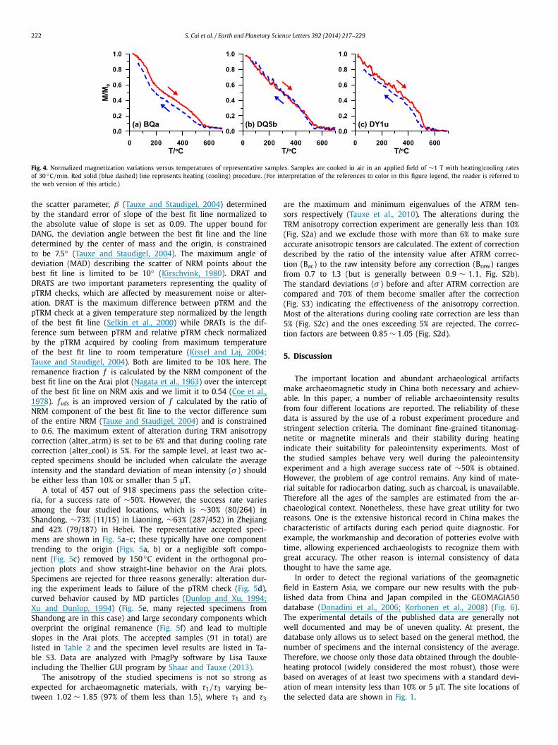
The variations of magnetization versus temperature (M–T) aremeasured for determination of Curie temperature (Tc) and detec-tion of possible alteration during heating. Tcs estimated from M–Tcurves range from ∼550 ◦C to ∼580 ◦C, indicating Ti-poor titano-magnetite or magnetite as the main magnetic mineral. This is inagreement with the hysteresis analysis, which shows a dominantlow coercivity component (Dunlop and Özdemir, 1997). Represen-tative curves (Fig. 4) are reasonably reversible indicating slight orno alteration during heating, a prerequisite for successful paleoin-tensity experiments.

4.2. Paleointensity results

The selection parameters during paleointensity data analysis arecrucial to the reliability of intensity estimation. Selection criteriaused in this study are listed in Table S2. The upper bound for

222 S. Cai et al. / Earth and Planetary Science Letters 392 (2014) 217–229

Fig. 4. Normalized magnetization variations versus temperatures of representative samples. Samples are cooked in air in an applied field of ∼1 T with heating/cooling ratesof 30 ◦C/min. Red solid (blue dashed) line represents heating (cooling) procedure. (For interpretation of the references to color in this figure legend, the reader is referred tothe web version of this article.)

the scatter parameter, β (Tauxe and Staudigel, 2004) determinedby the standard error of slope of the best fit line normalized tothe absolute value of slope is set as 0.09. The upper bound forDANG, the deviation angle between the best fit line and the linedetermined by the center of mass and the origin, is constrainedto be 7.5◦ (Tauxe and Staudigel, 2004). The maximum angle ofdeviation (MAD) describing the scatter of NRM points about thebest fit line is limited to be 10◦ (Kirschvink, 1980). DRAT andDRATS are two important parameters representing the quality ofpTRM checks, which are affected by measurement noise or alter-ation. DRAT is the maximum difference between pTRM and thepTRM check at a given temperature step normalized by the lengthof the best fit line (Selkin et al., 2000) while DRATs is the dif-ference sum between pTRM and relative pTRM check normalizedby the pTRM acquired by cooling from maximum temperatureof the best fit line to room temperature (Kissel and Laj, 2004;Tauxe and Staudigel, 2004). Both are limited to be 10% here. Theremanence fraction f is calculated by the NRM component of thebest fit line on the Arai plot (Nagata et al., 1963) over the interceptof the best fit line on NRM axis and we limit it to 0.54 (Coe et al.,1978). fvds is an improved version of f calculated by the ratio ofNRM component of the best fit line to the vector difference sumof the entire NRM (Tauxe and Staudigel, 2004) and is constrainedto 0.6. The maximum extent of alteration during TRM anisotropycorrection (alter_atrm) is set to be 6% and that during cooling ratecorrection (alter_cool) is 5%. For the sample level, at least two ac-cepted specimens should be included when calculate the averageintensity and the standard deviation of mean intensity (σ ) shouldbe either less than 10% or smaller than 5 μT.

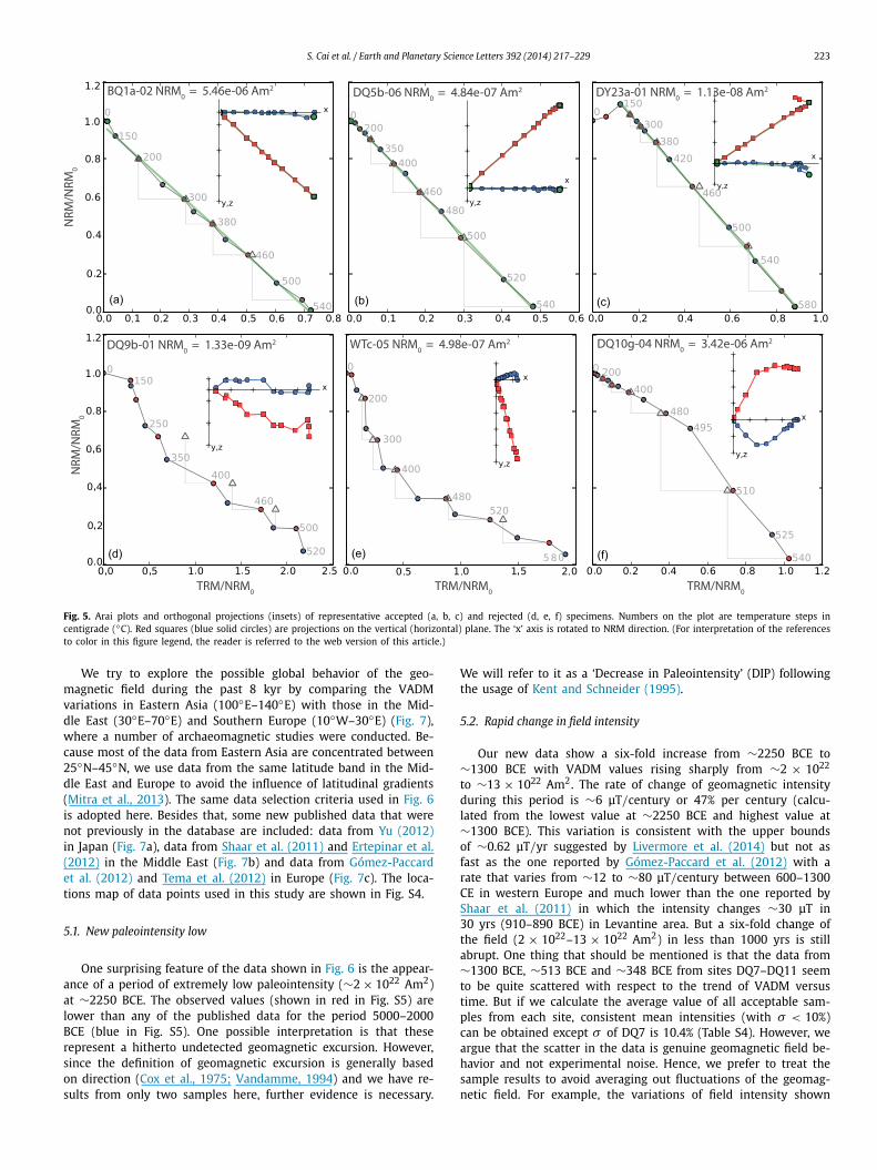
A total of 457 out of 918 specimens pass the selection crite-ria, for a success rate of ∼50%. However, the success rate variesamong the four studied locations, which is ∼30% (80/264) inShandong, ∼73% (11/15) in Liaoning, ∼63% (287/452) in Zhejiangand 42% (79/187) in Hebei. The representative accepted speci-mens are shown in Fig. 5a–c; these typically have one componenttrending to the origin (Figs. 5a, b) or a negligible soft compo-nent (Fig. 5c) removed by 150 ◦C evident in the orthogonal pro-jection plots and show straight-line behavior on the Arai plots.Specimens are rejected for three reasons generally: alteration dur-ing the experiment leads to failure of the pTRM check (Fig. 5d),curved behavior caused by MD particles (Dunlop and Xu, 1994;Xu and Dunlop, 1994) (Fig. 5e, many rejected specimens fromShandong are in this case) and large secondary components whichoverprint the original remanence (Fig. 5f) and lead to multipleslopes in the Arai plots. The accepted samples (91 in total) arelisted in Table 2 and the specimen level results are listed in Ta-ble S3. Data are analyzed with PmagPy software by Lisa Tauxeincluding the Thellier GUI program by Shaar and Tauxe (2013).

The anisotropy of the studied specimens is not so strong asexpected for archaeomagnetic materials, with τ1/τ3 varying be-tween 1.02 ∼ 1.85 (97% of them less than 1.5), where τ1 and τ3

are the maximum and minimum eigenvalues of the ATRM ten-sors respectively (Tauxe et al., 2010). The alterations during theTRM anisotropy correction experiment are generally less than 10%(Fig. S2a) and we exclude those with more than 6% to make sureaccurate anisotropic tensors are calculated. The extent of correctiondescribed by the ratio of the intensity value after ATRM correc-tion (Bac) to the raw intensity before any correction (Braw) rangesfrom 0.7 to 1.3 (but is generally between 0.9 ∼ 1.1, Fig. S2b).The standard deviations (σ ) before and after ATRM correction arecompared and 70% of them become smaller after the correction(Fig. S3) indicating the effectiveness of the anisotropy correction.Most of the alterations during cooling rate correction are less than5% (Fig. S2c) and the ones exceeding 5% are rejected. The correc-tion factors are between 0.85 ∼ 1.05 (Fig. S2d).

5. Discussion

The important location and abundant archaeological artifactsmake archaeomagnetic study in China both necessary and achiev-able. In this paper, a number of reliable archaeointensity resultsfrom four different locations are reported. The reliability of thesedata is assured by the use of a robust experiment procedure andstringent selection criteria. The dominant fine-grained titanomag-netite or magnetite minerals and their stability during heatingindicate their suitability for paleointensity experiments. Most ofthe studied samples behave very well during the paleointensityexperiment and a high average success rate of ∼50% is obtained.However, the problem of age control remains. Any kind of mate-rial suitable for radiocarbon dating, such as charcoal, is unavailable.Therefore all the ages of the samples are estimated from the ar-chaeological context. Nonetheless, these have great utility for tworeasons. One is the extensive historical record in China makes thecharacteristic of artifacts during each period quite diagnostic. Forexample, the workmanship and decoration of potteries evolve withtime, allowing experienced archaeologists to recognize them withgreat accuracy. The other reason is internal consistency of datathought to have the same age.

In order to detect the regional variations of the geomagneticfield in Eastern Asia, we compare our new results with the pub-lished data from China and Japan compiled in the GEOMAGIA50database (Donadini et al., 2006; Korhonen et al., 2008) (Fig. 6).The experimental details of the published data are generally notwell documented and may be of uneven quality. At present, thedatabase only allows us to select based on the general method, thenumber of specimens and the internal consistency of the average.Therefore, we choose only those data obtained through the double-heating protocol (widely considered the most robust), those werebased on averages of at least two specimens with a standard devi-ation of mean intensity less than 10% or 5 μT. The site locations ofthe selected data are shown in Fig. 1.

S. Cai et al. / Earth and Planetary Science Letters 392 (2014) 217–229 223

Fig. 5. Arai plots and orthogonal projections (insets) of representative accepted (a, b, c) and rejected (d, e, f) specimens. Numbers on the plot are temperature steps incentigrade (◦C). Red squares (blue solid circles) are projections on the vertical (horizontal) plane. The ‘x’ axis is rotated to NRM direction. (For interpretation of the referencesto color in this figure legend, the reader is referred to the web version of this article.)

We try to explore the possible global behavior of the geo-magnetic field during the past 8 kyr by comparing the VADMvariations in Eastern Asia (100◦E–140◦E) with those in the Mid-dle East (30◦E–70◦E) and Southern Europe (10◦W–30◦E) (Fig. 7),where a number of archaeomagnetic studies were conducted. Be-cause most of the data from Eastern Asia are concentrated between25◦N–45◦N, we use data from the same latitude band in the Mid-dle East and Europe to avoid the influence of latitudinal gradients(Mitra et al., 2013). The same data selection criteria used in Fig. 6is adopted here. Besides that, some new published data that werenot previously in the database are included: data from Yu (2012)in Japan (Fig. 7a), data from Shaar et al. (2011) and Ertepinar et al.(2012) in the Middle East (Fig. 7b) and data from Gómez-Paccardet al. (2012) and Tema et al. (2012) in Europe (Fig. 7c). The loca-tions map of data points used in this study are shown in Fig. S4.

5.1. New paleointensity low

One surprising feature of the data shown in Fig. 6 is the appear-ance of a period of extremely low paleointensity (∼2 × 1022 Am2)at ∼2250 BCE. The observed values (shown in red in Fig. S5) arelower than any of the published data for the period 5000–2000BCE (blue in Fig. S5). One possible interpretation is that theserepresent a hitherto undetected geomagnetic excursion. However,since the definition of geomagnetic excursion is generally basedon direction (Cox et al., 1975; Vandamme, 1994) and we have re-sults from only two samples here, further evidence is necessary.

We will refer to it as a ‘Decrease in Paleointensity’ (DIP) followingthe usage of Kent and Schneider (1995).

5.2. Rapid change in field intensity

Our new data show a six-fold increase from ∼2250 BCE to∼1300 BCE with VADM values rising sharply from ∼2 × 1022

to ∼13 × 1022 Am2. The rate of change of geomagnetic intensityduring this period is ∼6 μT/century or 47% per century (calcu-lated from the lowest value at ∼2250 BCE and highest value at∼1300 BCE). This variation is consistent with the upper boundsof ∼0.62 μT/yr suggested by Livermore et al. (2014) but not asfast as the one reported by Gómez-Paccard et al. (2012) with arate that varies from ∼12 to ∼80 μT/century between 600–1300CE in western Europe and much lower than the one reported byShaar et al. (2011) in which the intensity changes ∼30 μT in30 yrs (910–890 BCE) in Levantine area. But a six-fold change ofthe field (2 × 1022–13 × 1022 Am2) in less than 1000 yrs is stillabrupt. One thing that should be mentioned is that the data from∼1300 BCE, ∼513 BCE and ∼348 BCE from sites DQ7–DQ11 seemto be quite scattered with respect to the trend of VADM versustime. But if we calculate the average value of all acceptable sam-ples from each site, consistent mean intensities (with σ < 10%)can be obtained except σ of DQ7 is 10.4% (Table S4). However, weargue that the scatter in the data is genuine geomagnetic field be-havior and not experimental noise. Hence, we prefer to treat thesample results to avoid averaging out fluctuations of the geomag-netic field. For example, the variations of field intensity shown

224 S. Cai et al. / Earth and Planetary Science Letters 392 (2014) 217–229

Table 2The list of accepted results on sample level. Blab: applied field in the lab; Bacc: average paleointensity of a sample after anisotropy and cooling rate correction (those withoutcooling rate correction are marked with ‘∗ ’); σB: standard deviation of Bacc; σVADM: standard deviation of VADM; na: number of specimens accepted.

Sample Blab(μT)

Bacc

(μT)σB

(μT)σB

(%)VADM(×1022 Am2)

σVADM

(×1022 Am2)

na Method

BQa 30 35.7 2.0 5.6 6.41 0.36 5 IZZIBQb 30 33.0∗ 1.1 3.3 5.93 0.2 8 Coe–ThellierDZJa 30 30.8∗ 2.3 7.3 5.46 0.4 6 Coe–ThellierDZJe 30 34.7 2.0 5.7 6.17 0.35 3 IZZIGDDc 30 26.1 4.5 17.3 4.66 0.8 3 IZZIGDDd 30 31.1 2.1 6.7 5.55 0.37 3 IZZIGJCa 30 25.4 2.8 10.9 4.45 0.49 5 IZZILCZa 30 16.8∗ 2.0 12.1 3.06 0.37 2 Coe–ThellierLCZc 30 24.7 1.8 7.2 4.5 0.32 6 IZZIQJZa 30 36.5∗ 1.9 5.1 6.5 0.33 3 Coe–ThellierQJZd 30 36.4 2.3 6.3 6.49 0.41 5 IZZISWC4a 30 46.9∗ 2.6 5.4 8.38 0.46 6 Coe–ThellierSWC4b 30 44.0∗ 1.5 3.4 7.86 0.27 3 Coe–ThellierSWC5b 30 58.0∗ 3.3 5.6 10.37 0.58 7 Coe–ThellierXJTc 30 29.9 1.6 5.5 5.33 0.29 4 IZZIYJC1a 30 51.5 2.1 4 9.01 0.36 6 IZZIZJZa 30 12.8∗ 1.4 10.9 2.3 0.25 8 Coe–ThellierZJZd 30 29.2 0.9 2.9 5.21 0.15 4 IZZIZJZf 30 25.9 3.8 14.8 4.63 0.68 4 IZZIDQ1a 30 47.7 1.4 2.9 9.24 0.26 4 IZZIDQ1c 30 41.1 1.5 3.6 7.98 0.29 4 IZZIDQ2a 30 52.2 3.1 6 10.13 0.61 3 IZZIDQ3a 30 58.8 5.8 9.8 11.41 1.12 6 IZZIDQ4a 30 41.7 0.8 1.9 8.09 0.15 5 IZZIDQ4c 30 41.6 0.7 1.8 8.07 0.14 4 IZZIDQ5a 30 59.9 1.9 3.1 11.66 0.36 5 IZZIDQ5b 30 61.1 3.2 5.2 11.89 0.62 8 IZZIDQ6b 30 60.1 3.9 6.5 11.7 0.76 4 IZZIDQ7a 50 35.0 0.7 2 6.79 0.14 4 IZZIDQ7e 50 37.4 0.4 1 7.25 0.07 3 IZZIDQ7f 50 42.7 1.7 4 8.28 0.33 4 IZZIDQ7g 50 44.3 1.2 2.6 8.59 0.22 4 IZZIDQ7h 50 40.3 2.4 6 7.82 0.47 4 IZZIDQ7j 50 49.6 2.9 5.8 9.61 0.56 3 IZZIDQ7k 50 48.1 3.6 7.5 9.32 0.7 4 IZZIDQ7l 50 41.7 2.0 4.8 8.09 0.39 4 IZZIDQ7o 50 46.7 1.7 3.6 9.05 0.33 4 IZZIDQ7p 50 45.8 0.7 1.5 8.88 0.14 4 IZZIDQ7q 50 48.0 0.5 0.9 9.32 0.09 3 IZZIDQ7r 50 40.8 0.5 1.3 7.9 0.1 4 IZZIDQ8a 50 51.9 1.1 2.2 10.07 0.22 3 IZZIDQ8b 50 49.5 3.4 6.9 9.6 0.67 3 IZZIDQ8d 50 45.7 1.6 3.6 8.86 0.32 3 IZZIDQ8f 50 39.0 0.2 0.6 7.57 0.05 4 IZZIDQ8g 50 48.4 1.5 3 9.39 0.28 4 IZZIDQ8h 50 50.9 1.6 3.2 9.88 0.31 3 IZZIDQ8i 50 53.6 1.1 2 10.39 0.2 4 IZZIDQ8j 50 50.1 2.8 5.5 9.72 0.54 4 IZZIDQ8k 50 49.7 2.4 4.9 9.65 0.47 4 IZZIDQ8m 50 45.3 1.3 2.9 8.78 0.25 4 IZZIDQ8p 50 46.8 2.0 4.4 9.07 0.39 3 IZZIDQ9a 30 47.7 1.4 3 9.24 0.27 5 IZZIDQ9d 30 50.8 2.9 5.6 9.84 0.56 5 IZZIDQ9e 30 48.0 1.8 3.7 9.31 0.35 4 IZZIDQ9f 30 45.3 1.5 3.4 8.78 0.3 5 IZZIDQ9h 30 47.5 2.8 6 9.22 0.55 5 IZZIDQ9i 30 43.9 3.2 7.3 8.51 0.62 4 IZZIDQ9l 30 46.2 0.7 1.5 8.96 0.14 3 IZZIDQ9m 30 50.4 1.6 3.2 9.77 0.32 5 IZZIDQ9o 30 55.5 4.9 8.9 10.76 0.96 4 IZZIDQ9p 30 57.6 1.5 2.5 11.16 0.28 3 IZZIDQ10b 50 60.3 1.6 2.6 11.68 0.3 4 IZZIDQ10e 50 66.8 4.8 7.1 12.94 0.92 4 IZZIDQ10f 50 56.9 4.0 7 11.01 0.77 3 IZZIDQ10h 50 66.6 4.3 6.5 12.9 0.84 4 IZZIDQ10j 50 53.2 1.6 3 10.31 0.31 4 IZZIDQ10q 50 63.4 3.0 4.7 12.28 0.58 4 IZZIDQ10r 50 60.7 3.8 6.2 11.75 0.73 4 IZZIDQ10s 50 65.1 4.9 7.5 12.62 0.95 4 IZZIDQ11a 50 54.7 2.1 3.8 10.59 0.41 3 IZZIDQ11c 50 57.3 4.8 8.3 11.09 0.92 4 IZZIDQ11d 50 50.5 2.9 5.7 9.79 0.56 4 IZZIDQ11e 50 64.3 1.8 2.9 12.45 0.36 4 IZZI

S. Cai et al. / Earth and Planetary Science Letters 392 (2014) 217–229 225

Table 2 (continued)

Sample Blab(μT)

Bacc

(μT)σB

(μT)σB

(%)VADM(×1022 Am2)

σVADM

(×1022 Am2)

na Method

DQ11f 50 52.8 3.2 6 10.23 0.62 4 IZZIDQ11g 50 61.6 6.1 9.9 11.93 1.18 5 IZZIDQ11l 50 54.1 1.8 3.3 10.48 0.34 4 IZZIDQ11m 50 54.2 4.1 7.5 10.49 0.79 3 IZZIDQ11n 50 59.3 0.9 1.5 11.48 0.18 3 IZZIDQ11p 50 59.6 3.4 5.6 11.55 0.65 3 IZZIDY15 30 55.6∗ 2.1 3.8 9.75 0.37 8 Coe–ThellierDY16 30 58.9∗ 2.1 3.5 10.32 0.36 4 Coe–ThellierDY1a 30 58.0∗ 2.6 4.4 10.16 0.45 9 Coe–ThellierDY1u 30 64.6 3.1 4.8 11.33 0.54 5 IZZIDY23a 30 43.4 1.4 3.3 7.6 0.25 5 IZZIDY30a 30 57.2 1.4 2.5 10.02 0.25 6 IZZIDY35a 30 51.9∗ 0.5 0.9 9.1 0.08 5 Coe–ThellierDY35u 30 52.6 1.8 3.4 9.21 0.31 4 IZZIDY37a 30 49.3 0.7 1.5 8.63 0.13 4 Coe–ThellierDY37u 30 46.7 2.5 5.4 8.18 0.44 6 IZZIDY40a 30 55.1 1.7 3 9.65 0.29 4 IZZIDY41c 30 52.9 1.4 2.6 9.28 0.24 5 Coe–ThellierDY4a 30 46.7 3.7 8 8.18 0.65 8 Coe–ThellierDY9a 30 51.6 1.4 2.8 9.04 0.25 6 IZZI

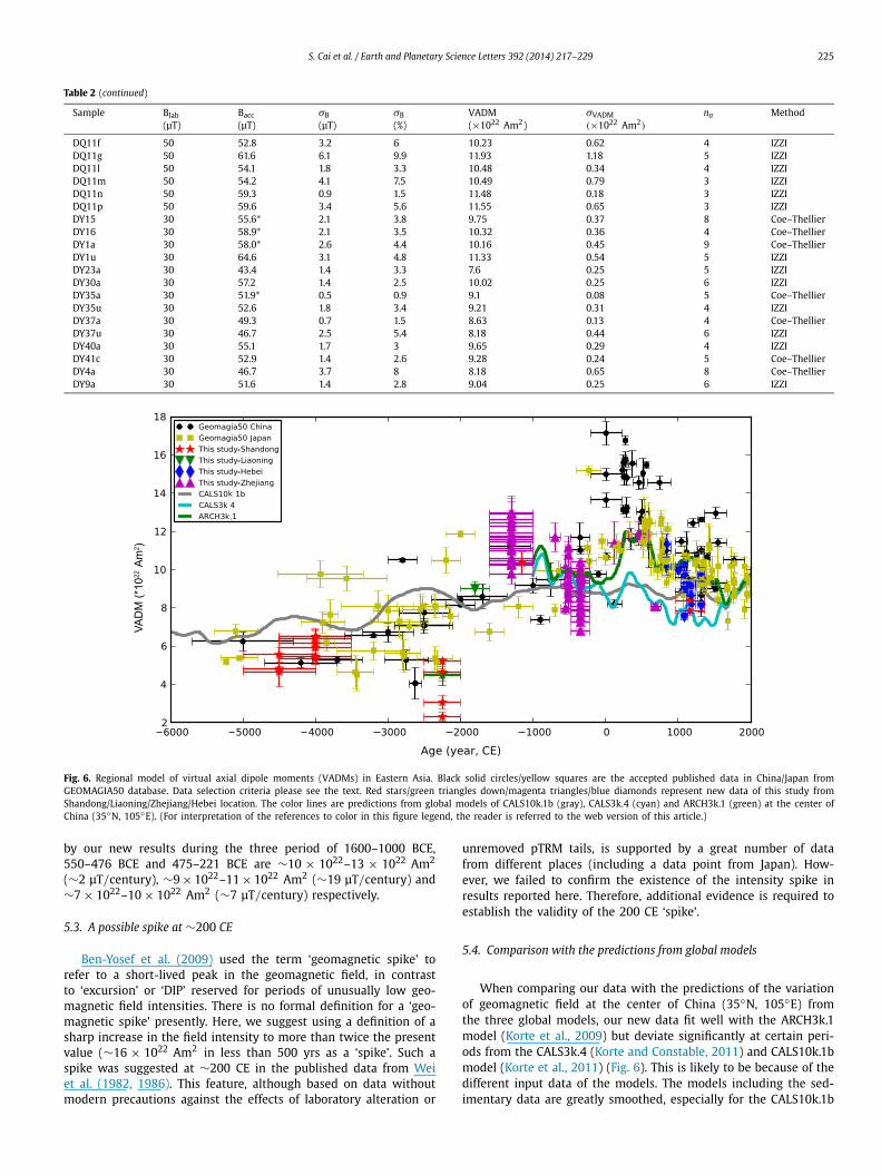
Fig. 6. Regional model of virtual axial dipole moments (VADMs) in Eastern Asia. Black solid circles/yellow squares are the accepted published data in China/Japan fromGEOMAGIA50 database. Data selection criteria please see the text. Red stars/green triangles down/magenta triangles/blue diamonds represent new data of this study fromShandong/Liaoning/Zhejiang/Hebei location. The color lines are predictions from global models of CALS10k.1b (gray), CALS3k.4 (cyan) and ARCH3k.1 (green) at the center ofChina (35◦N, 105◦E). (For interpretation of the references to color in this figure legend, the reader is referred to the web version of this article.)

by our new results during the three period of 1600–1000 BCE,550–476 BCE and 475–221 BCE are ∼10 × 1022–13 × 1022 Am2

(∼2 μT/century), ∼9 × 1022–11 × 1022 Am2 (∼19 μT/century) and∼7 × 1022–10 × 1022 Am2 (∼7 μT/century) respectively.

5.3. A possible spike at ∼200 CE

Ben-Yosef et al. (2009) used the term ‘geomagnetic spike’ torefer to a short-lived peak in the geomagnetic field, in contrastto ‘excursion’ or ‘DIP’ reserved for periods of unusually low geo-magnetic field intensities. There is no formal definition for a ‘geo-magnetic spike’ presently. Here, we suggest using a definition of asharp increase in the field intensity to more than twice the presentvalue (∼16 × 1022 Am2 in less than 500 yrs as a ‘spike’. Such aspike was suggested at ∼200 CE in the published data from Weiet al. (1982, 1986). This feature, although based on data withoutmodern precautions against the effects of laboratory alteration or

unremoved pTRM tails, is supported by a great number of datafrom different places (including a data point from Japan). How-ever, we failed to confirm the existence of the intensity spike inresults reported here. Therefore, additional evidence is required toestablish the validity of the 200 CE ‘spike’.

5.4. Comparison with the predictions from global models

When comparing our data with the predictions of the variationof geomagnetic field at the center of China (35◦N, 105◦E) fromthe three global models, our new data fit well with the ARCH3k.1model (Korte et al., 2009) but deviate significantly at certain peri-ods from the CALS3k.4 (Korte and Constable, 2011) and CALS10k.1bmodel (Korte et al., 2011) (Fig. 6). This is likely to be because of thedifferent input data of the models. The models including the sed-imentary data are greatly smoothed, especially for the CALS10k.1b

226 S. Cai et al. / Earth and Planetary Science Letters 392 (2014) 217–229

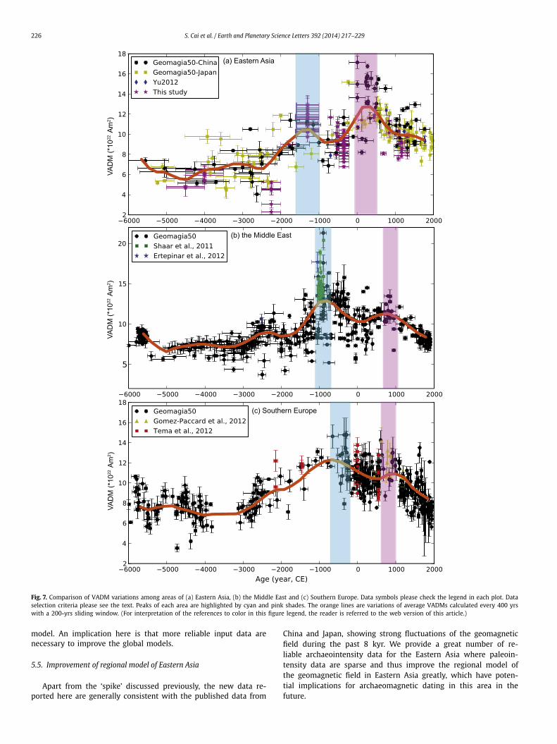
Fig. 7. Comparison of VADM variations among areas of (a) Eastern Asia, (b) the Middle East and (c) Southern Europe. Data symbols please check the legend in each plot. Dataselection criteria please see the text. Peaks of each area are highlighted by cyan and pink shades. The orange lines are variations of average VADMs calculated every 400 yrswith a 200-yrs sliding window. (For interpretation of the references to color in this figure legend, the reader is referred to the web version of this article.)

model. An implication here is that more reliable input data arenecessary to improve the global models.

5.5. Improvement of regional model of Eastern Asia

Apart from the ‘spike’ discussed previously, the new data re-ported here are generally consistent with the published data from

China and Japan, showing strong fluctuations of the geomagneticfield during the past 8 kyr. We provide a great number of re-liable archaeointensity data for the Eastern Asia where paleoin-tensity data are sparse and thus improve the regional model ofthe geomagnetic field in Eastern Asia greatly, which have poten-tial implications for archaeomagnetic dating in this area in thefuture.

S. Cai et al. / Earth and Planetary Science Letters 392 (2014) 217–229 227

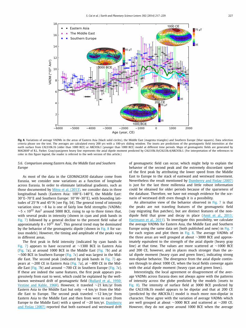
Fig. 8. Variations of average VADMs in the areas of Eastern Asia (black solid circles), the Middle East (magenta triangles) and Southern Europe (blue squares). Data selectioncriteria please see the text. The averages are calculated every 200 yrs with a 100-yrs sliding window. The insets are predictions of the geomagnetic field intensities at theearth surface from CALS10k.1b (older than 1000 BCE) or ARCH3k.1 (younger than 1000 BCE) model at different time periods. Maps of geomagnetic fields are generated byMAGMAP of R.L. Parker. Gray/cyan/green heavy line represents the axial dipole moment predicted by CALS10k.1b/CALS3k.4/ARCH3k.1. (For interpretation of the references tocolor in this figure legend, the reader is referred to the web version of this article.)

5.6. Comparison among Eastern Asia, the Middle East and SouthernEurope

As most of the data in the GEOMAGIA50 database come fromEurasia, we consider now variations as a function of longitudeacross Eurasia. In order to eliminate latitudinal gradients, such asthose documented by Mitra et al. (2013), we consider data in threelongitudinal bands (Eastern Asia: 100◦E–140◦E, the Middle East:30◦E–70◦E and Southern Europe: 10◦W–30◦E), with bounding lati-tudes of 25◦N and 45◦N (see Fig. S4). The general trend of intensityvariation since ∼8 ka is one of fairly low field strengths (VADMs:∼5 × 1022 Am2 around 5000 BCE, rising to up to three times that,with several peaks in intensity (shown in cyan and pink bands inFig. 7) followed by a general decline to the present field value ofapproximately 8×1022 Am2. This general trend may be dominatedby the behavior of the geomagnetic dipole (shown in Fig. 8 for var-ious models). However, the timing and amplitude of the peaks varyin different areas.

The first peak in field intensity (indicated by cyan bands inFig. 7) appears to have occurred at ∼1300 BCE in Eastern Asia(Fig. 7a), at around 1000 BCE in the Middle East (Fig. 7b) and at∼500 BCE in Southern Europe (Fig. 7c) and was largest in the Mid-dle East. The second peak (indicated by pink bands in Fig. 7) ap-pears at ∼200 CE in Eastern Asia (Fig. 7a), at ∼800 CE in the Mid-dle East (Fig. 7b) and around ∼700 CE in Southern Europe (Fig. 7c).If these are indeed the same features, the first peak appears pro-gressively from east to west, which could be explained by the well-known westward drift of geomagnetic field (Bullard et al., 1950;Vestine and Kahle, 1968). However, it traveled ∼21 km/yr fromEastern Asia to the Middle East but only ∼4 km/yr from the Mid-dle East to Europe. The second peak traveled ∼12 km/yr fromEastern Asia to the Middle East and then from west to east (fromEurope to the Middle East) with a speed of ∼20 km/yr. Dumberryand Finlay (2007) reported that both eastward and westward drift

of geomagnetic field can occur, which might help to explain thebehavior of the second peak and the extremely discordant speedof the first peak by attributing the lower speed from the MiddleEast to Europe to the stack of eastward and westward movement.Nevertheless the result mentioned by Dumberry and Finlay (2007)is just for the last three millennia and little robust informationcould be obtained for older periods because of the sparseness ofthe database. Therefore, we have not enough evidence for the sce-nario of westward drift even though it is a possibility.

An alternative view of the behavior observed in Fig. 7 is thatthe peaks are not traveling features of the geomagnetic field(say migrating flux patches), but are distinct features of the non-dipole field that grow and decay in place (Amit et al., 2011;Hartmann et al., 2011). To investigate this possibility, we calculatethe average VADMs for Eastern Asia, the Middle East and SouthernEurope using the same data set (both published and new) in Fig. 7for each region and plot them in Fig. 8. The average VADMs ofthe three areas are well grouped at about ∼3000 BCE and approx-imately equivalent to the strength of the axial dipole (heavy grayline) at that time. The values are more scattered at ∼1000 BCEand 200 CE, however, and in places much stronger than the ax-ial dipole moment (heavy cyan and green lines), indicating strongnon-dipolar behavior. The divergence from the axial dipole contin-ues through to about 1000 CE, when the local fields converge againwith the axial dipole moment (heavy cyan and green lines).

Interestingly, the local agreement or disagreement of the aver-age VADMs across Eurasia does not always agree with the patternsof intensity across the globe predicted by the models (insets toFig. 8). The intensity of surface field at 3000 BCE predicted bythe CALS10k.1b model appears to be dipolar and that at 200 CE(predicted by the ARCK3k.1) model is much more non-dipolar incharacter. These agree with the variation of average VADMs whichare well grouped at about ∼3000 BCE and scattered at ∼200 CE.However, they do not agree around 1000 BCE when the average

228 S. Cai et al. / Earth and Planetary Science Letters 392 (2014) 217–229

VADMs are scattered but the surface field is predicted to be moredipolar and vice versa at 1000 CE. As shown in Fig. 6, there israther poor agreement between the data from China and Japan andthe behavior predicted from the global field models, especially theCALS series. One reason for this might be that the predictions fromthe models are only based on the published data in the databaseand the new data are not included. Therefore, we suggest that theglobal models need to be updated with the new data.

6. Conclusions

In this study, new, reliable, archaeointensity results covering thelast 7 kyr are obtained from four locations in eastern China. Thesefill the gap of archaeomagnetic study in China ever since the sys-tematic work carried out by Wei et al. (1982, 1986, 1987) duringthe 1980s. Several conclusions can be drawn from our new dataset.

1. A newly detected period of paleointensity as low as ∼2 ×1022 Am2 (a DIP) at ∼2250 BCE, even though based on onlytwo samples, is revealed by our results.

2. A sharp, up to six-fold increase in paleointensity from the DIPat ∼2250 BCE to a high field strength at ∼1300 BCE withVADM ranging from ∼2×1022 to ∼13×1022 Am2 is detected.The rate of change of geomagnetic intensity during this periodis ∼6 μT/century or 47% per century.

3. A possible intensity spike of ∼17 × 1022 Am2 at ∼200 CE issuggested by the published data from Wei et al. (1982, 1986),which needs further investigation as the data were obtainedby methods lacking modern checks.

4. The new data generally agree with the ARCH3k.1 model butdeviate significantly from the CALS3k.4 and CALS10k.1b modelat certain periods because of the different input data of themodels, suggesting that more reliable inputs are necessary toimprove the global models.

5. Combining the published data in China and Japan, we providegreatly improved constraints for the regional model of East-ern Asia, which has implications for archaeomagnetic datingin this area in the future.

6. When comparing the Eastern Asian curve with that of two rep-resentative areas in the world, the Middle East and SouthernEurope, we conclude that the spike in intensity observed inthe Middle East around ∼1000 BCE may not be global. Weprefer to explain the peaks in the three areas as distinct fea-tures of the non-dipole field that grow and decay in place asopposed to traveling features of the geomagnetic field causedby migrating flux patches.

Acknowledgements

We thank Limin Wang, Jinghao Yang, Xinmin Xu, Sheng Huangand Shihu Li for sample collection. We thank Jason Steindorf forhis help in the laboratory. We thank Ron Shaar for the fruitful andinsightful discussions. We thank Greig A. Paterson for the usefuldiscussions during the revision of the manuscript. This study wassupported by NSFC1 grants 90814000 and 41274073 awarded toRZ, NSF grant EAR1141840 awarded to LT, CAS Strategic PriorityResearch Program grant XDA05130603-B awarded to GJ, and theNational Key Basic Research Program of China grant 2012CB821900and NSFC grant 40925012 awarded to CD. The visit of SC to UCSDfrom September 2011 to August 2012 was supported by the KeyLaboratory of the Earth’s Deep Interior of CAS. We thank Carlo Lajand two anonymous reviewers for their helpful comments that im-proved this paper.

Appendix A. Supplementary material

Supplementary material related to this article can be found on-line at http://dx.doi.org/10.1016/j.epsl.2014.02.030.

References

Aitken, M.J., Alcock, P., Bussell, G.D., Shaw, C., 1981. Archaeomagnetic determina-tion of the past geomagnetic intensity using ancient ceramics: Allowance foranisotropy. Archaeometry 23, 53–64.

Aitken, M.J., Allsop, A.L., Bussell, G.D., Winter, M.B., 1988. Determination of the in-tensity of the Earth’s magnetic field during archeological times: Reliability ofthe Thellier technique. Rev. Geophys. 26, 3–12.

Amit, H., Korte, M., Aubert, J., Constable, C., Hulot, G., 2011. The time-dependenceof intense archeomagnetic flux patches. J. Geophys. Res. 116. http://dx.doi.org/10.1029/2011JB008538.

Bard, E., Delaygue, G., 2008. Comment on “Are there connections between theEarth’s magnetic field and climate?” by V. Courtillot, Y. Gallet, J.-L. Le Mouël, F.Fluteau, A. Genevey EPSL 253 (2007) 328. Earth Planet. Sci. Lett. 265, 302–307.

Ben-Yosef, E., Ron, H., Tauxe, L., Agnon, A., Genevey, A., Levy, T.E., Avner, U.,Najjar, M., 2008a. Application of copper slag in geomagnetic archaeointen-sity research. J. Geophys. Res., Solid Earth 113, B08101. http://dx.doi.org/10.1029/2007jb005235.

Ben-Yosef, E., Tauxe, L., Ron, H., Agnon, A., Avner, U., Najjar, M., Levy, T.E., 2008b.A new approach for geomagnetic archaeointensity research: insights on an-cient metallurgy in the Southern Levant. J. Archaeol. Sci. 35, 2863–2879.http://dx.doi.org/10.1016/j.jas.2008.05.016.

Ben-Yosef, E., Tauxe, L., Levy, T.E., Shaar, R., Ron, H., Najjar, M., 2009. Geomagnetic in-tensity spike recorded in high resolution slag deposit in Southern Jordan. EarthPlanet. Sci. Lett. 287, 529–539.

Ben-Yosef, E., Tauxe, L., Levy, T.E., 2010. Archaeomagnetic dating of copper smeltingsite F2 in the Timna Valley (Israel) and its implications for the modelling ofancient technological developments. Archaeometry 52, 1110–1121.

Biggin, A., Steinberger, B., Aubert, J., Suttie, N., Holme, R., Torsvik, T., van der Meer,D., van Hinsbergen, D., 2012. Possible links between long-term geomagneticvariations and whole-mantle convection processes. Nat. Geosci. 5, 526–533.

Bloxham, J., 2000. Sensitivity of the geomagnetic axial dipole to thermal core-mantleinteractions. Nature 405, 63–65.

Bloxham, J., Zatman, S., Dumberry, M., 2002. The origin of geomagnetic jerks. Na-ture 420, 65–68.

Bullard, E.C., Freedman, C., Gellman, H., Nixon, J., 1950. The westward drift of theEarth’s magnetic field. Philos. Trans. R. Soc. Lond. A 243, 67–92.

Chauvin, A., Garcia, Y., Lanos, P., Laubenheimer, F., 2000. Paleointensity of the ge-omagnetic field recovered on archaeomagnetic sites from France. Phys. EarthPlanet. Inter. 120, 111–136.

Coe, R.S., 1967. Paleo-intensities of the Earth’s magnetic field determined from Ter-tiary and Quaternary rocks. J. Geophys. Res. 72, 3247–3262.

Coe, R.S., Grommé, S., Mankinen, E.A., 1978. Geomagnetic paleointensities fromradiocarbon-dated lava flows on Hawaii and the question of the Pacificnondipole low. J. Geophys. Res., Solid Earth 83, 1740–1756.

Courtillot, V., Gallet, Y., Mouël, J.L., Fluteau, F., Genevey, A., 2007. Are there con-nections between the Earth’s magnetic field and climate?. Earth Planet. Sci.Lett. 253, 328–339.

Cox, A., Hillhouse, J., Fuller, M., 1975. Paleomagnetic records of polarity transitions,excursions, and secular variation. Rev. Geophys. 13, 185–189.

Day, R., Fuller, M., Schmidt, V.A., 1977. Hysteresis properties of titanomagnetites:Grain-size and compositional dependence. Phys. Earth Planet. Inter. 13, 260–267.

Dodson, M.H., McClelland-Brown, E., 1980. Magnetic blocking temperatures ofsingle-domain grains during slow cooling. J. Geophys. Res. 85, 2625–2637.

Donadini, F., Korhonen, K., Riisager, P., Pesonen, L.J., 2006. Database for Holocenegeomagnetic intensity information. Eos 87, 137–143.

Dumberry, M., Finlay, C.C., 2007. Eastward and westward drift of the Earth’s mag-netic field for the last three millennia. Earth Planet. Sci. Lett. 254, 146–157.

Dunlop, D.J., 2002a. Theory and application of the Day plot (Mrs/Ms versus Hcr/Hc)1. Theoretical curves and tests using titanomagnetite data. J. Geophys. Res. 107.http://dx.doi.org/10.1029/2001JB000486.

Dunlop, D.J., 2002b. Theory and application of the Day plot (Mrs/Ms versus Hcr/Hc)2. Application to data for rocks, sediments, and soils. J. Geophys. Res. 107.http://dx.doi.org/10.1029/2001JB000487.

Dunlop, D.J., Özdemir, Ö., 1997. Rock Magnetism: Fundamentals and Frontiers. Cam-bridge University Press, pp. 61–66.

Dunlop, D.J., Xu, S., 1994. Theory of partial thermoremanent magnetization in mul-tidomain grains: I. Repeated identical barriers to wall motion (single microcoer-civity). J. Geophys. Res. 99, 9005–9023.

Ertepinar, P., Langereis, C.G., Biggin, A.J., Frangipane, M., Matney, T., Ökse, T., En-gin, A., 2012. Archaeomagnetic study of five mounds from Upper Mesopotamiabetween 2500 and 700 BCE: Further evidence for an extremely strong geomag-netic field ca. 3000 years ago. Earth Planet. Sci. Lett. 357–358, 84–98.

S. Cai et al. / Earth and Planetary Science Letters 392 (2014) 217–229 229

Gallet, Y., Genevey, A., Fluteau, F., 2005. Does Earth’s magnetic field secular variationcontrol centennial climate change?. Earth Planet. Sci. Lett. 236, 339–347.

Genevey, A., Gallet, Y., 2002. Intensity of the geomagnetic field in Western Europeover the past 2000 years: new data from French ancient pottery. J. Geophys.Res. 107. http://dx.doi.org/10.1029/2001JB000701.

Gómez-Paccard, M., Chauvin, A., Lanos, P., Dufresne, P., Kovacheva, M., Hill, M.J., Bea-mud, E., Blain, S., Bouvier, A., Guibert, P., 2012. Improving our knowledge ofrapid geomagnetic field intensity changes observed in Europe between 200 and1400 AD. Earth Planet. Sci. Lett. 355–356, 131–143.

Halgedahl, S.L., Day, R., Fuller, M.D., 1980. The effect of cooling rate on the intensityof weak-field TRM in single-domain magnetite. J. Geophys. Res. 85, 3690–3698.

Hartmann, G.A., Genevey, A., Gallet, Y., Trindade, R.I.F., Le Goff, M., Najjar, R.,Etchevarne, C., Afonso, M.C., 2011. New historical archeointensity data fromBrazil: Evidence for a large regional non-dipole field contribution over the pastfew centuries. Earth Planet. Sci. Lett. 306, 66–76.

Hill, M.J., Lanos, P., Denti, M., Dufresne, P., 2008. Archaeomagnetic investigationof bricks from the VIIIth-VIIth century BC Greek-indigenous site of Incoronata(Metaponto, Italy). Phys. Chem. Earth 33, 523–533.

Huang, X.G., Li, D.J., Wei, Q.Y., 1998. Secular Variation of Geomagnetic Intensity forthe Last 5000 Years in China-Comparison between the southwest and OtherParts of China. Chin. J. Geophys. 41, 385–396.

Kent, D.V., 1982. Apparent correlation of palaeomagnetic intensity and climaticrecords in deep-sea sediments. Nature 299, 538–539.

Kent, D.V., Schneider, D.A., 1995. Correlation of paleointensity variation records inthe Brunhes/Matuyama polarity transition interval. Earth Planet. Sci. Lett. 129,135–144.

Kirschvink, J.L., 1980. The least-squares line and plane and the analysis of palaeo-magnetic data. Geophys. J. R. Astron. Soc. 62, 699–718.

Kissel, C., Laj, C., 2004. Improvements in procedure and paleointensity selection cri-teria (PICRIT-03) for Thellier and Thellier determinations: application to Hawai-ian basaltic long cores. Phys. Earth Planet. Inter. 147, 155–169.

Korhonen, K., Donadini, F., Riisager, P., Pesonen, L.J., 2008. GEOMAGIA50: Anarcheointensity database with PHP and MySQL. Geochem. Geophys. Geosyst. 9,Q04029. http://dx.doi.org/10.1029/2007gc001893.

Korte, M., Constable, C., 2011. Improving geomagnetic field reconstructions for0–3 ka. Phys. Earth Planet. Inter. 188, 247–259.

Korte, M., Donadini, F., Constable, C.G., 2009. Geomagnetic field for 0–3 ka: 2. A newseries of time-varying global models. Geochem. Geophys. Geosyst. 10, Q06008.http://dx.doi.org/10.1029/2008gc002297.

Korte, M., Constable, C., Donadini, F., Holme, R., 2011. Reconstructing the Holocenegeomagnetic field. Earth Planet. Sci. Lett. 312, 497–505.

Livermore, P.W., Fournier, A., Gallet, Y., 2014. Core-flow constraints on extremearcheomagnetic intensity changes. Earth Planet. Sci. Lett. 387, 145–156.

Mandea, M., Holme, R., Pais, A., Pinheiro, K., Jackson, A., Verbanac, G., 2010. Ge-omagnetic jerks: rapid core field variations and core dynamics. Space Sci.Rev. 155, 147–175.

Mitra, R., Tauxe, L., McIntosh, S.K., 2013. Two thousand years of archeointensity fromWest Africa. Earth Planet. Sci. Lett. 364, 123–133.

Nagata, T., Arai, Y., Momose, K., 1963. Secular variation of the geomagnetic totalforce during the last 5000 years. J. Geophys. Res. 68, 5277–5281.

Olsen, N., Mandea, M., 2008. Rapidly changing flows in the Earth’s core. Nat.Geosci. 1, 390–394.

Paterson, G.A., 2013. The effects of anisotropic and non-linear thermorema-nent magnetizations on Thellier-type paleointensity data. Geophys. J. Int. 193.http://dx.doi.org/10.1093/gji/ggt1033.

Pavón-Carrasco, F.J., Osete, M.L., Torta, J.M., Gaya-Piqué, L.R., 2009. A regionalarcheomagnetic model for Europe for the last 3000 years, SCHA.DIF.3K: Ap-plications to archeomagnetic dating. Geochem. Geophys. Geosyst. 10, Q03013.http://dx.doi.org/10.1029/2008gc002244.

Pavón-Carrasco, F.J., Rodríguez-González, J., Osete, M.L., Torta, J.M., 2011. A Matlabtool for archaeomagnetic dating. J. Archaeol. Sci. 38, 408–419.

Roberts, A.P., Pike, C.R., Verosub, K.L., 2000. First-order reversal curve diagrams: Anew tool for characterizing the magnetic properties of natural samples. J. Geo-phys. Res., Solid Earth 105, 28461–28475.

Rogers, J., Fox, J.M.W., Aitken, M.J., 1979. Magnetic anisotropy in ancient pottery.Nature 277, 644–646.

Selkin, P.A., Meurer, W.P., Newell, A.J., Gee, J.S., Tauxe, L., 2000. The effect of rema-nence anisotropy on paleointensity estimates: A case study from the ArcheanStillwater Complex. Earth Planet. Sci. Lett. 183, 403–416.

Shaar, R., Tauxe, L., 2013. Thellier GUI: An integrated tool for analyzing paleoin-tensity data from Thellier-type experiments. Geochem. Geophys. Geosyst. 14,677–692.

Shaar, R., Ron, H., Tauxe, L., Kessel, R., Agnon, A., Ben-Yosef, E., Feinberg, J.M., 2010.Testing the accuracy of absolute intensity estimates of the ancient geomagneticfield using copper slag material. Earth Planet. Sci. Lett. 290, 201–213.

Shaar, R., Ben-Yosef, E., Ron, H., Tauxe, L., Agnon, A., Kessel, R., 2011. Geomagneticfield intensity: How high can it get? How fast can it change? Constraints fromIron Age copper slag. Earth Planet. Sci. Lett. 301, 297–306.

Shaw, J., Yang, S., Wei, Q.Y., 1995. Archaeointensity variations for the past 7500 yearsevaluated from ancient Chinese ceramics. J. Geomagn. Geoelectr. 47, 59–70.

Shaw, J., Yang, S., Rolph, T.C., Sun, F.Y., 1999. A comparison of archaeointensity re-sults from Chinese ceramics using microwave and conventional Thellier’s andShaw’s methods. Geophys. J. Int. 136, 714–718.

Tang, C., Zheng, J.Y., Li, D.J., Wei, S.F., Wei, Q.Y., 1991. Paleointensity determinationsfor the Xinjiang Region, NW China. J. Geomagn. Geoelectr. 43, 363–368.

Tauxe, L., Staudigel, H., 2004. Strength of the geomagnetic field in the Creta-ceous Normal Superchron: New data from submarine basaltic glass of theTroodos Ophiolite. Geochem. Geophys. Geosyst. 5, Q02H06. http://dx.doi.org/10.1029/2003GC000635.

Tauxe, L., Mullender, T.A.T., Pick, T., 1996. Potbellies, wasp-waists, and superparam-agnetism in magnetic hysteresis. J. Geophys. Res., Solid Earth 101, 571–583.

Tauxe, L., Butler, R., Banerjee, S.K., van der Voo, R., 2010. Essentials of Paleomag-netism. University of California Press, Berkeley, pp. 69–72.

Tema, E., Gomez-Paccard, M., Kondopoulou, D., Almar, Y., 2012. Intensity of theEarth’s magnetic field in Greece during the last five millennia: New data fromGreek pottery. Phys. Earth Planet. Inter. 202–203, 14–26.

Thellier, E., Thellier, O., 1959. Sur I’intensité du champ magnétique terrestre dans lepassé historique et géologique. Ann. Geophys. 15, 285–378.

Vandamme, D., 1994. A new method to determine paleosecular variation. Phys.Earth Planet. Inter. 85, 131–142.

Veitch, R.J., Hedley, I.G., Wagner, J.J., 1984. An investigation of the intensity of thegeomagnetic field during Roman times using magnetically anisotropic bricksand tiles. Arch. Sci. (Geneva) 37, 359–373.

Vestine, E.H., Kahle, A.B., 1968. The westward drift and geomagnetic secular change.Geophys. J. R. Astron. Soc. 15, 29–37.

Wei, Q.Y., Li, D.J., Cao, G.Y., Zhang, W.S., Wang, S.P., 1982. Intensity of the geo-magnetic field near Loyang, China between 500 BC and AD 1900. Nature 296,728–729.

Wei, Q.Y., Li, D.J., Cao, G.Y., Zhang, W.X., Wei, S.F., 1986. The total intensity of geo-magnetic field in southern China for the period from 4500 B.C. to A.D. 1500. J.Geomagn. Geoelectr. 38, 1311–1322.

Wei, Q.Y., Zhang, W.X., Li, D.J., Aitken, M.J., Busseil, G.D., Winter, M., 1987. Geomag-netic intensity as evaluated from ancient Chinese pottery. Nature 328, 330–333.

Xu, S., Dunlop, D.J., 1994. Theory of partial thermoremanent magnetization in mul-tidomain grains: II. Effect of microcoercivity distribution and comparison withexperiment. J. Geophys. Res. 99, 9025–9033.

Yu, Y.J., 2012. High-fidelity paleointensity determination from historic volca-noes in Japan. J. Geophys. Res., Solid Earth 117, B08101. http://dx.doi.org/10.1029/2012jb009368.

Yu, Y.J., Tauxe, L., 2005. Testing the IZZI protocol of geomagnetic field inten-sity determination. Geochem. Geophys. Geosyst. 6, Q06H11. http://dx.doi.org/10.1029/2004GC000840.

Yu, Y.J., Tauxe, L., Genevey, A., 2004. Toward an optimal geomagnetic fieldintensity determination technique. Geochem. Geophys. Geosyst. 5, Q02H07.http://dx.doi.org/10.1029/2003GC000630.