Aquifer Response to Sinusoidal or Arbitrary Stage of Semipervious Stream

ow, to atical aquiferderived. Fords, a “rampus stream,l method istegral. Ind using botho the stream

Aquifer Response to Sinusoidal or Arbitrary Stageof Semipervious Stream

Sushil K. Singh1

Abstract: Analytical expressions for the aquifer responses, viz., groundwater head, rate of flow and cumulative volume of flgeneralized sinusoidal stage of semipervious streams considering the stream boundary resistance, are derived. The analyresponses to a linear stream stage and to a typical analytical flood wave that was used by Cooper and Rorabaugh, are alsoa zero-stream resistance, the aquifer responses converge to those for a fully penetrating stream. Also, two analytical methokernel method” and a “Fourier series method,” for obtaining the aquifer responses to an arbitrary temporal stage of sempervioare developed. The analytical expressions of the ramp kernels for different aquifer responses are developed. The ramp kernefound superior to the conventional convolution that uses numerical integration or pulse kernels for obtaining the convolution inthe Fourier series method, the aquifer responses to sinusoidal stage are used along with Fourier series. The results obtainemethods are in close agreement. The new methods are also applicable to fully penetrating streams by assigning a zero value tresistance.

DOI: 10.1061/(ASCE)0733-9429(2004)130:11(1108)

CE Database subject headings: Aquifers; Ground-water flow; Streams; Flocculation; Floods.

anddwa-be-

tage

theund-tions

stics,specdock

rtantforanddel.om-ion ofessedivesn thetheyspect

l

idale not

re-vol-

e re-Them theund-fer is

s used

stre-than

hethe

nte-reamis be-emi-

un-stage

been;

eri-

247

mustoneitor.sibleper is,118/

Introduction

The stream aquifer interaction takes place when the streamaquifer are hydraulically connected. The subsurface or grounter hydraulics of the stream aquifer interaction is importantcause:(1) The aquifer is recharged during a rising stream sand the recharged water remains in a temporary storage(bankstorage); (2) during the falling stream stage or a lean period,aquifer feeds water to the stream. The initial gradient of growater head may affect the net flow to the stream. The interacplay important roles in the study of bank storage characteriexchange of water and solutes, and legal aspects. A judicial aof the interaction has been discussed by Bouwer and Mad(1997).

The analytical solutions to interaction problems are impobecause apart from their application being straightforwardsimplified cases, they also provide a means of calibratingvalidating the mathematics of a numerical solution or a moAlthough the validation of a numerical model is generally accplished using observed data, the appropriateness or validatdiscretization and numerical technique can be better assusing an analytical solution. An analytical solution also ggood insight into the dependence of the solution variable ostate variables. The limitation of the analytical model is thatare applicable to simplified or idealized cases. A theoretical a

1Scientist, National Institute of Hydrology Roorkee, Roorkee-667, Uttar Anchal, India. E-mail: [email protected]

Note. Discussion open until April 1, 2005. Separate discussionsbe submitted for individual papers. To extend the closing date bymonth, a written request must be filed with the ASCE Managing EdThe manuscript for this paper was submitted for review and pospublication on August 20, 2002; approved on June 12, 2004. This papart of the Journal of Hydraulic Engineering, Vol. 130, No. 11November 1, 2004. ©ASCE, ISSN 0733-9429/2004/11-1108–1
$18.00.
1108 / JOURNAL OF HYDRAULIC ENGINEERING © ASCE / NOVEMBER 20

t

of seepage was provided by Bouwer(1965). Analytical solutionsfor simplified cases are available, e.g., a constant stage(i.e., a stepchange in the stream stage) of semipervious stream(Hall andMoench 1972; Marino 1973; Halek and Svec 1979), or a typicaanalytical flood wave in a fully penetrating stream(Cooper andRorabaugh 1963). The analytical aquifer responses to a sinusoor a typical analytical flood wave in a semipervious stream aravailable. The hydraulic solution variables or the aquifersponses, i.e., groundwater head, rate of flow, and cumulativeume of flow at a certain distance away from the stream arquired for understanding the stream aquifer interaction.aquifer responses are observed up to a certain distance frostream aquifer interface. The steady periodic solution for growater head in case of interaction between tides and aquiavailable (Nielsen 1990). Zlotnik and Huang(1999) used thesame analytical step response for groundwater head as waby Hall and Moench(1972) and Halek and Svec(1979); there-fore, the claim that shallow penetration and semiperviousambed have been considered separately, in a different waythat of Hall and Moench(1972), needs rethinking. They gave texpressions for groundwater head for other conditions inLaplace domain. Prior numerical solutions of convolution igral, for obtaining groundwater head due to changing ststage, remains untested against an analytical solution; thiscause of no such analytical solution being available for the spervious stream. Also, Barlow et al.(2000), while verifying theirnumerical model observe that the analytical solutions for thesteady responses to a periodic stage or a temporally varyingof a semipervious stream are not available.

The treatment for an arbitrary temporal stream stage hasattempted mostly using the convolution(Hall and Moench 1972Singh 1994; Zlotnik and Huang 1999; Barlow et al. 2000). Inthese studies, convolution or Duhamel’s integral is solved numcally or using pulse kernels(conventional convolution). Singh
(1994) used convolution and pulse kernels to obtain the aquifer
04

eamsgiveflow,

m,ker-vede use

othercounand

reinte-givenses

ors andere isaqui-vious

gen-rived.urieritrary

tion

i---

of itsquiferional.en-atertropic,ence

alizedl

ion,

tream

g

n ofe

ss

responses to a temporally varying stage of semipervious strThe use of the conventional method of convolution does notaccurate results near the peak, particularly for the rate ofeven with a sufficiently small time step size(Singh 1994; Barlowet al. 2000). Singh et al.(2002), in case of a semipervious streaprovided a solution of the convolution equation using rampnels(new kernels), but only for groundwater head. They obserthat the use of the ramp kernels gives superior results than thof the pulse kernels; expressions for the pulse kernels foraquifer responses are not available. Other methods that acfor temporal variation in stream stage are by GovindarajuKoelliker (1994), and Workman et al.(1997). These methods aapplicable for fully penetrating streams and use numericalgration or numerical solution technique; also, these studiesthe solution for only groundwater head, other aquifer respoare not dealt with. Marino(1975) gave a numerical solution fgroundwater head considering the stream as semiperviouaccounting for the temporal variation in the stream stage. Tha need to develop analytical methods that can give accuratefer responses to an arbitrary temporal stage of a semiperstream.

In this article, analytical unsteady aquifer responses to aeralized sinusoidal stage of a semipervious stream are deAlso, two analytical methods, a ramp kernel method and a Foseries method, for obtaining aquifer responses to an arbstage of semipervious stream, are developed.

Governing Differential Equation

The partial differential equation governing the water interacbetween an aquifer and a semipervious stream(see Fig. 1) with atemporally varying stage, is written as

] 2h2 −

1 ] h= 0 s1d

Fig. 1. (a) Illustration of the problem and(b) idealized stream crosection

] x b ] t

JOURNAL

.

t

hs0,td = Hstd s2d

−] h

] x=

Hstd − h

Rwhen x = 0 s3d

hsx,0d = hs`,td = 0 s4d

whereh5groundwater head at a distancex from the stream aqufer interface at timet fLg; b=T/S5hydraulic diffusivity of aquifer fL2T−1g; T5transmissivity of aquiferfL2T−1g; S5storage coefficient of aquifer [dimensionless]; H5stream stagefLg; andR5resistance to the flow imparted by the stream becausesemipervious bed and banks and partial penetration of the afLg; this resistance may alternatively be viewed as an addithypothetical length of aquifer with no storage within it(see, Fig1). Eqs.(1)–(4) assume one-dimensional horizontal flow perpdicular to the stream length and a horizontal initial groundwhead. The aquifer is considered confined, homogeneous, isoand infinite(i.e., groundwater head is not affected by the presof aquifer boundary).

Aquifer Responses to Continuous Generalized SineWave

Let the excitation in the stream stage be a continuous genersine wave,Hstd=a sinsvt+«d, wherea5amplitude of sinusoidastream stagefLg; v5angular frequency of sinusoidal excitatfT−1g; and«5phase shift[dimensionless]. Prior to the excitationthe stream and aquifer are assumed in equilibrium, i.e., sstage coincides with the groundwater head.

Groundwater Head

Substituting f=h−R]h/]x in Eq. (1), one has the followinequation, to determinef:

]2f

] x2 −1

b

] f

] t= 0 s5d

with the initial and boundary conditions as

fs0,td = Hstd s6d

fsx,0d = 0; fs`,td = 0 s7d

Solution of Eq.(5) satisfying Eqs.(6) and (7) is given by

f =2

ÎpE

x/2Îbt

`

HSt −x2

4bu2De−u2du s8d

For a sinusoidal excitation in the stream stage, the solutioEq. (8), and then the solution of Eq.(1) is obtained from thsolution of an analogous problem of heat conduction(Carslaw
and Jaeger 1959), and is written in the present context as
OF HYDRAULIC ENGINEERING © ASCE / NOVEMBER 2004 / 1109

ng

of

f

ace. The

hsx,tda

=e−v8x sinsvt + « − v8x − dd

Îs1 + v8Rd2 + sv8Rd2+

1

pE

0

` sv cos« − u sin«dHRÎu

bcosSxÎu

bD + sinSxÎu

bDJ

su2 + v2dS1 +uR2

bD e−ut du s9d

wherev8 and« are given by

v8 =Î v

2bs10d

d = tan−1S v8R

1 + v8RD s11d

For the steady periodic solution, the second term of the right-hand side of Eq.(9) is zero, which is observed after a sufficiently lotime.

Rate of Flow

The rate of flow through a unit width, along the stream, of the aquifer at sectionx at time t, i.e., qsx,td, is given by

qsx,td = − T] h

] xs12d

whereqsx,td5rate of flow from unit width, along the stream, of aquiferfL2T−1g. If qsx,td is positive, the flow is in the directionincreasingx. Substitutingh from Eq. (9) into Eq. (12) and integrating:

qsx,td

aÎvTS=

e−v8x sinsvt + « − v8x − d + p/4dÎs1 + v8Rd2 + sv8Rd2

−1

pÎvE

0

` sv cos« − u sin«dÎuHcosSxÎu

bD − RÎu

bsinSxÎu

bDJ

su2 + v2dS1 +uR2

bD e−ut du s13d

The rate of flow to the aquifer at the stream aquifer interface is obtained by puttingx=0 in Eq. (13):

qs0,td

aÎvTS=

sinsvt + « − d + p/4dÎs1 + v8Rd2 + sv8Rd2

−1

pÎvE

0

` sv cos« − u sin«dÎu

su2 + v2dS1 +uR2

bD e−ut du s14d

whereqs0,td5rate of flow per unit length of the stream to the aquifer through the stream aquifer interface.

Cumulative Volume of Flow

The cumulative volume of flow crossing the sectionx, through a unit width of the aquifer, up to timet , Vsx,td is given by

Vsx,td =E0

t

qsx,tddt s15d

whereVsx,td5cumulative volume of flow from unit width of aquifer, at sectionx, up to timet fL2g. If Vsx,td is positive, the volume oflow is in the direction of increasingx. Substituting Eq.(13) into Eq. (15) and integrating, one obtains

Vsx,tda

Î v

TS=

e−v8xscoss« − v8x − d + p/4d − cossvt + « − v8x − d + p/4ddÎs1 + v8Rd2 + sv8Rd2

+Îv

pE

0

` sv cos« − u sin«dHcosSxÎu

bD − RsinSxÎu

bDJ

Îusu2 + v2dS1 +uR2

bD se−ut − 1ddu s16d

Cumulative volume of flow through the stream aquifer interfacesx=0d can be obtained from Eq.(16) by substitutingx=0:

Vs0,tda

Î v

TS=

scoss« − d + p/4d − cossvt + « − d + p/4ddÎs1 + v8Rd2 + sv8Rd2

+Îv

pE

0

` sv cos« − u sin«d

Îusu2 + v2dS1 +uR2

bD se−ut − 1ddu s17d

whereVs0,td5cumulative volume of flow from a unit length of the stream, transferred to the aquifer, at the stream aquifer interf
aquifer responses to a sine wave in the stream can be obtained by taking«=0 and that for a cosine wave can be obtained by

onstion

age isof

eadof

d by:

fromuifer” Forligiblerhe

is-eamponse

,

ones toessionob-

taking «=p /2. Satisfying the assumptions by the field conditiup to a possible extent is the limiting condition for the applicaof the solutions.

Aquifer Responses to a Unit Step Rise in StreamStage

The groundwater head due to a unit step rise in the stream stavailable(Carslaw and Jaeger 1959) for an analogous problemheat conduction. In the present context, it is expressed as

Uhsx,td = erfcS x

2ÎbtD − efsx/Rd+sbt/R2dgerfcS x

2Îbt+

Îbt

RD

s18d

whereUh5unit step response function for the groundwater h[dimensionless]. The unit step response function for the rateflow is obtained by substitutingUh from Eq. (18) for h into Eq.(12) and differentiating:

Uqsx,td =T

Refsx/Rd+sbt/R2dgerfcS x

2Îbt+

Îbt

RD s19d

where Uq5unit step response function for rate of flowfLT−1g.The unit step response function for volume of flow is obtainesubstitutingUq from Eq.(19) for q, into Eq.(15) and integrating

Uvsx,td = SsR+ xdH− erfcS x

2ÎbtD +

2Îp

Îbt

sR+ xde−x2/4bt

+R

R+ xefsx/Rd+sbt/R2dgerfcS x

2Îbt+

Îbt

RDJ s20d

whereUv5unit step response function for volume of flowfLg.

Response Distance

The aquifer responses are observed within a certain distancethe stream aquifer interface. The distance up to which the aqresponses are observed may be termed “response distance.generalized sinusoidal wave, the aquifer responses are negif v8x.4.6, even withR=0. Thus, if x.6.5Îb /v, the aquiferesponses are negligible forR=0. In case of a step rise in tstream stage, the aquifer responses are negligible ifx.4Îbt forR=0. The greater the value ofR, the shorter the response dtance. Therefore, the aquifer hydraulic diffusivity and the strresistance are two important parameters governing the res
distance.
wheret8= t− td. The expression for the rate of flow is obtained from

JOURNAL

a

Aquifer Responses to a Linear Stream Stage

The aquifer responses to a linear stream stage[Hstd=ct, wherec5constant] are obtained as

hsx,td = ctFS1 −sx + Rd2 + R2

2btDerfcS x

2ÎbtD −

x + 2RÎpbt

e−x2/4bt

−R2

btefsx/Rd+sbt/R2dgerfcS x

2Îbt+

Îbt

RDG s21d

qsx,td = cSsR+ xdF− erfcS x

2ÎbtD +

2Îp

Îbt

sR+ xde−x2/4bt

+R

R+ xefsx/Rd+sbt/R2dgerfcS x

2Îbt+

Îbt

RDG s22d

Vsx,td = cSsR+ xdtF− S1 +x2s3R+ xd + 6R2sR+ xd

6btsR+ xd DerfcS x

2ÎbtD

+1

3ÎpS6R2 + 3Rx+ x2

sR+ xdÎbt+

4Îbt

R+ xDe−x2/4bt

+R3

sR+ xdbtefsx/Rd+sbtR2dgerfcS x

2Îbt+

Îbt

RDG s23d

Aquifer Responses to a Typical Analytical FloodWave

A typical analytical and symmetrical flood wave is written(Coo-per and Rorabaugh 1963) as

Hstd =h0

2s1 − cosvtd for t ø td

= 0 for t . td s24d

where v=2p / td fT−1g; td5duration of the flood wavefTg; andh05peak stream stagefLg. Aquifer responses to the excitatigiven by Eq.(24) can be obtained by superposing the responsa step rise and a cosine wave in the stream stage. The exprfor the groundwater head due to this typical flood wave is
tained using Eqs.(9) and (18) as
2hsx,tdh0

= Uhsx,td −e−v8x cossvt − v8x − ddÎs1 + v8Rd2 + sv8Rd2

+1

pE

0

` uHRÎu

bcosSxÎu

bD + sinSxÎu

bDJ

su2 + v2dS1 +uR2

bD e−ut du for t ø td s25ad

2hsx,tdh0

= Uhsx,td − Uhsx,t8d +1

pE

0

` uHRÎu

bcosSxÎu

bD + sinSxÎu

bDJ

su2 + v2dS1 +uR2

bD se−ut − e−ut8ddu for t . td s25bd

Eqs.(13) and (19) as


2qsx,td

h0ÎvTS

=Uqsx,tdÎvTS

−e−v8x cossvt − v8x − d + p/4d

Îs1 + v8Rd2 + sv8Rd2−

1

pÎvE

0

` u3/2HcosSxÎu

bD − RÎu

bsinSxÎu

bDJ

su2 + v2dS1 +uR2

bD e−ut du for t ø td s26ad

2qsx,td

h0ÎvTS

=Uqsx,td − Uqsx,t8d

ÎvTS−

1

pÎvE

0

` u3/2HcosSxÎu

bD − RÎu

bsinSxÎu

bDJ

su2 + v2dS1 +uR2


The expression for cumulative volume of flow is obtained using Eqs.(16) and (20), as

2Vsx,tdh0

Î v

TS=Î v

TSUvsx,td −

e−v8xssinsv8x + d − p/4d + sinsvt − v8x − d + p/4ddÎs1 + v8Rd2 + sv8Rd2

−Îv

pE

0

` u1/2HcosSxÎu

bD − RÎu

bsinSxÎu

bDJ

su2 + v2dS1 +uR2

bD se−ut − 1ddu for t ø td s27ad

2Vsx,tdh0

Î v

TS=Î v

TSsUvsx,td − Uvsx,t8dd −

Îv

pE

0

` u1/2HcosSxÎu

bD − RÎu

bsinSxÎu

bDJ

su2 + v2dS1 +uR2


eam.atinglicable-

m.esf

xpres-ingh

op-d ands areo in

ary-tion

;

grals

ta-

ad is

The stream resistance is zero for a fully penetrating strTherefore, the aquifer responses in case of a fully penetrstream can be obtained using the relevant expressions appfor a semipervious stream withR=0. Even atx=0, stream resistance is there, which can account for the curved streamlines(nearthe stream aquifer interface) and partial penetration of the streaCooper and Rorabaugh(1963) has given the aquifer respons(groundwater head at any value ofx, but rate and volume ostream depletion atx=0, i.e., stream aquifer interface) for fullypenetrating streams; under these conditions, ifR=0 is put in therespective expressions for aquifer responses, one gets the esions given by Cooper and Rorabaugh(1963). A first approximation of R can be obtained using the approach given by S(2003); however, its accurate value can be obtained throughtimization of the integral squared errors between the observecomputed groundwater heads. The steady periodic solutionobtained when the term containing the infinite integral is zerthe proposed solutions.

Treatment for Arbitrary Stream Stage

Ramp Kernel Method

The response of an initially relaxed linear system, to a time ving excitation, can be expressed by the following convoluintegrals:

Ysx,td =Et

XstduYsx,t − tddt s28d
0

-

Ysx,td =E0

t ] Xstd] t

UYsx,t − tddt s29d

where X5excitation; Y5response; x5spatial variableuYsx,td5instantaneous unit response function forY; andUYsx,td5unit step response function forY. If the excitation ismeasured at discrete intervals of time, the convolution inteneed to be expressed in a discretized time domain. Eqs.(28) and(29) in discretized forms are obtained as

Ysx,nDtd = oi=1

n

XiaYfx,sn − i + 1dDtg s30d

Ysx,nDtd = oi=1

nDXi

DtdYfx,sn − i + 1dDtg s31d

where a5pulse kernel;d5ramp kernel;Dt5uniform time stepsize; DXi =Xi −Xi−1; and i ,n5indices for time steps. The excition, i.e., X, in the present context, is the stream stageH. Thepulse and ramp kernels are given by

aYsx,mDtd =E0

Dt

uYsx,mDt − tddt

= UYsx,mDtd − UYfx,sm− 1dDtg s32d

dYsx,mDtd =E0

Dt

UYsx,mDt − tddt s33d

The expression for the ramp kernel for the groundwater he
obtained from Eq.(33) fY=hg using the expression ofUh:
04

l.Eq.

uifer

is

l-s

tive

ralurier

uch antform

ndribednearrestage

is ex-

m-gdx-

-la-

-r re-

dhsx,mDtd = Dtf1 − F1sm− 1dg − SmDt +sx + Rd2 + R2

2bDDF1smd

− sx + 2RdÎ Dt

pbDF2smd −

R2

bex/RDF3smd s34d

F1smd = erfS x

2ÎbmDtD s35d

F2smd = Îme−x2/4bmDt s36d

F3smd = ebmDt/R2erfcS x

2ÎbmDt+

ÎbmDt

RD s37d

where DF1smd=F1smd−F1sm−1d ;DF2smd=F2smd−F2sm−1d;andDF3smd=F3smd−F3sm−1d. Eq. (34) was used by Singh et a(2002). The ramp kernel for the rate of flow is obtained from(33) fY=qg as

dqsx,mDtd = SSsR+ xdDF1smd + 2ÎbDt

pDF2smd + ex/RRDF3smdD

s38d

and the ramp kernel for the rate of flow at the stream aqinterfacesx=0d is

dqs0,mDtd = SS2ÎbDt

psÎm− Îsm− 1dd + RDF4smdD s39d

F4smd = ebmDt/R2erfcSÎbmDt

RD s40d

whereDF4smd=F4smd−F4sm−1d. The ramp kernel in this caseobtained from Eq.(33) fY=Vg as

dvsx,mDtd = SF− DtsR+ xds1 − F1sm− 1ddSsR+ xdmDt

+x2s3R+ xd + 6R2sR+ xd

6bDDF1smd

+ S6R2 + 3Rx+ x2

3DÎ Dt

pbDF2smd +

R3

bex/RDF3smd

+4

3ÎbsDtd3

pDF5smdG s41d

F5smd = m3/2e−x2/4bmDt s42d

whereDF5smd=F5smd−F5sm−1d. The ramp kernels for the voume of flow at the stream aquifer interfacesx=0d are obtained a

dvs0,mDtd = SF− RDt + 2R2Î Dt

pbsÎm− Îsm− 1dd +

R3

bDF4smd

+4

3ÎbsDtd3

psm3/2 − sm− 1d3/2dG s43d

SubstitutingR=0 in the expressions of kernels, the respec
kernels for a fully penetrating stream can be obtained.
JOURNAL

Fourier Series Method

Although it is difficult to represent an arbitrarily varying tempostage of semipervious stream by an algebraic function, a Foseries is best suited to describe an arbitrary stream stage. Sattempt was made by Swamee and Singh(2003), however, iwould be appropriate to give some details here. The generalof Fourier series representing an arbitrary stream stage is:

Hstd =a0

2+ o

k=1

` Sak coskpt

td+ bk sin

kpt

tdD s44d

ak =2

tdE

0

td

Hstdcoskpt

tddt s45d

bk =2

tdE

0

td

Hstdsinkpt

tddt s46d

where td5duration of stream stage variation; aak. ,bk5constants of Fourier series. The Fourier series descby Eq.(44) converges slowly and results in a poor matchingthe discontinuity att= td, even if infinite number of terms aconsidered. In order to avoid this, the end points of streamwere made to yield zero height using the transformation:

jstd = Hstd −t

tdHstdd s47d

wherej5transformed stream stagefLg. Eq. (47) yields jstdd=0.Then, the transformed stream stage with zero end pointspressed by a Fourier series:

jstd = ok=1

`

bk sinkpt

tds48d

where

bk =2

tdE

0

td

jstdsinkpt

tddt s49d

The Fourier series[Eq. (48)] has one-half of the terms in coparison to the original Fourier series[Eq. (46)] and has a stronconvergence. The integral appearing in Eq.(49) was evaluatenumerically. From Eqs.(47) and (48), the stream stage was epressed as

Hstd = Hstddt

td+ o

k=1

`

bk sinkpt

tds50d

Truncating the summation in Eq.(50) by taking a finite number of termssk=kdd, which also avoids high-frequency osciltions in the stream stage, Eq.(50) was modified to

Hstd = Hstddt

td+ o

k=1

kd

bk sinkpt

tds51d

It was observed that 5–10 coefficientsskd=5–10d satisfactorily represent a typical variation in stream stage. The aquifesponses toHstd are obtained using:

Ystd = YL + YS s52d

whereYL5aquifer response on account of linear term of Eq.(51);
andYS5aquifer response to sinusoidal term of Eq.(51).

ionalblesn-byithnal

a-rease

theahanondi-

Application

Response to Sinusoidal Stream Stage

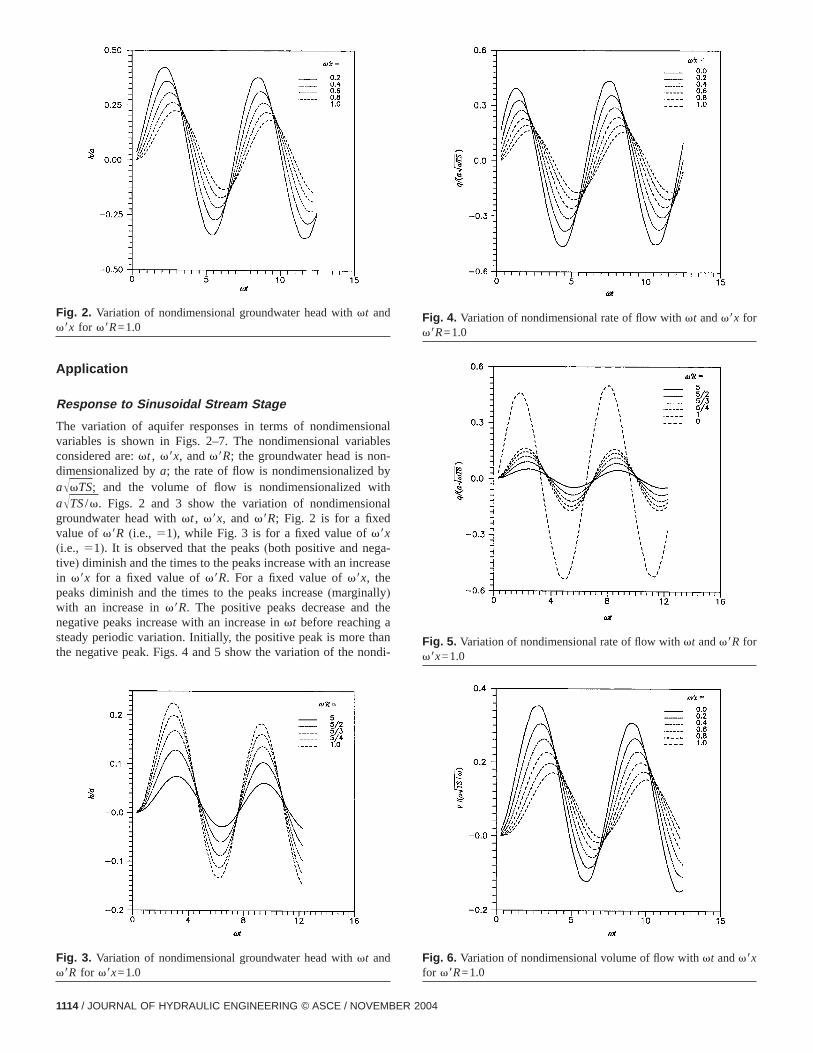
The variation of aquifer responses in terms of nondimensvariables is shown in Figs. 2–7. The nondimensional variaconsidered are:vt , v8x, andv8R; the groundwater head is nodimensionalized bya; the rate of flow is nondimensionalizedaÎvTS; and the volume of flow is nondimensionalized waÎTS/v. Figs. 2 and 3 show the variation of nondimensiogroundwater head withvt , v8x, and v8R; Fig. 2 is for a fixedvalue of v8R (i.e., 51), while Fig. 3 is for a fixed value ofv8x(i.e., 51). It is observed that the peaks(both positive and negtive) diminish and the times to the peaks increase with an incin v8x for a fixed value ofv8R. For a fixed value ofv8x, thepeaks diminish and the times to the peaks increase(marginally)with an increase inv8R. The positive peaks decrease andnegative peaks increase with an increase invt before reachingsteady periodic variation. Initially, the positive peak is more tthe negative peak. Figs. 4 and 5 show the variation of the n

Fig. 2. Variation of nondimensional groundwater head withvt andv8x for v8R=1.0

Fig. 3. Variation of nondimensional groundwater head withvt andv8R for v8x=1.0


Fig. 4. Variation of nondimensional rate of flow withvt andv8x forv8R=1.0

Fig. 5. Variation of nondimensional rate of flow withvt andv8R forv8x=1.0

Fig. 6. Variation of nondimensional volume of flow withvt andv8xfor v8R=1.0

04

the

e

e witga-ionale

s tofto

n in-thesing

se of

sis-

e

nce

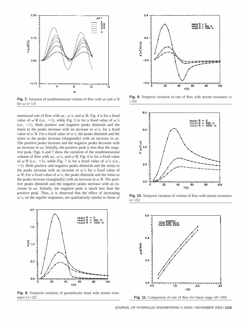
mensional rate of flow withvt , v8x, andv8R; Fig. 4 is for a fixedvalue of v8R (i.e., 51), while Fig. 5 is for a fixed value ofv8x(i.e., 51). Both positive and negative peaks diminish andtimes to the peaks increase with an increase inv8x, for a fixedvalue ofv8R. For a fixed value ofv8x, the peaks diminish and thtimes to the peaks increase(marginally) with an increase invt.The positive peaks increase and the negative peaks decreasan increase invt. Initially, the positive peak is less than the netive peak. Figs. 6 and 7 show the variation of the nondimensvolume of flow withvt , v8x, andv8R; Fig. 6 is for a fixed valuof v8R (i.e., 51), while Fig. 7 is for a fixed value ofv8x (i.e.,51). Both positive and negative peaks diminish and the timethe peaks increase with an increase inv8x for a fixed value ov8R. For a fixed value ofv8x, the peaks diminish and the timesthe peaks increase(marginally) with an increase inv8R. The posi-tive peaks diminish and the negative peaks increase with acrease invt. Initially, the negative peak is much less thanpositive peak. Thus, it is observed that the effect of increav8x, on the aquifer responses, are qualitatively similar to tho

Fig. 7. Variation of nondimensional volume of flow withvt andv8Rfor v8x=1.0

Fig. 8. Temporal variation of groundwater head with stream retancesx=25d

JOURNAL

Fig. 9. Temporal variation of rate of flow with stream resistancsx=25d

h

Fig. 10. Temporal variation of volume of flow with stream resistasx=25d

Fig. 11. Comparison of rate of flow for linear stagesR=100d


for a

ream

re-rSimil

timewegativet di-ge of

ge areard in

d

tained

s atob-d hastime

utionf

es asampegra-ulse

nting

thedwaterhe

p

1 63

1 63

1 63

1 63

increasingv8R. Besides these variations(Figs. 2–7), it is feltappropriate to present the results in terms of state variablestypical flood wave that lasts only for a certain time.

The aquifer responses to the typical flood wave in the st(Eq. (24)), were obtained forh0=2, td=50, T=50, and b=5,000 with different values ofR (250, 500, 750, and 1,000). Thetemporal variations of the aquifer responses with the streamsistance are shown in Figs. 8–10 forx=25 m. The groundwatehead at a section increases, attains a peak, then decreases.variations were observed withx (instead ofR) when R is fixed(instead ofx). The peak is diminished and flattened and theto the peak increases, whenx or R is increased. The rate of float a section increases, attains a peak, then decreases to a npeak before increasing. Both negative and positive peaks gminished with an increase inx or R. Thus, the effect of increasinR, on the aquifer responses, is qualitatively similar to thosincreasingx.

Superiority of Ramp Kernels

Two cases, i.e., linear stream stage and sinusoidal stream staconsidered. Rowe(1960) observed that some rivers show linvariation in their stage. The exact analytical solutions derivethis paper were used for the comparison.

Linear Stream StageAn example of linearly varying stream stage(H=0 at t=0 andH=2 at t=2) was taken withR=100, 500, and 1,000;T=50; andb=5,000. The rate of flow were obtained atx=10 for differentvalues ofR using both kernels. The rate flow forR=100, obtaine

Table 1. Aquifer Responses Using Pulse and Ramp Kernels

Dt hs0,2d

0.123 37a

Pulse Ramp

2.00 0.094 82 0.123 37 0

1.00 0.113 55 0.123 37 0

0.50 0.120 25 0.123 37 0

0.25 0.122 49 0.123 37 0aAnalytical results.

Fig. 12. Comparison of rate of flow for sinusoidal stagesR=100d


ar

e

e

using the pulse and ramp kernels are compared to that obusing the analytical solution, in Fig. 11(for pulse kernels,Dt=0.25 and for ramp kernelsDt=2, were taken). A similar differ-ence was observed forR=500 and 1,000. The aquifer responset=2 for different time step sizes are given in Table 1. It isserved that the use of ramp kernels give superior results anthe advantage of yielding accurate results even with a longerstep size.

Sinusoidal Stream StageAquifer responses to a sinusoidal stagesa=2,v=0.1pd of semi-pervious streams(R=100, 500, and 1,000) were obtained atx=10. The parameters considered are:b=5,000;T=50; andDt=1. The rate of flow obtained using both kernels forR=100is compared to that obtained using the exact analytical solin Fig. 12. Similar difference was observed for other values oR.Thus, the use of the ramp kernels yields aquifer responsgood as obtained using the analytical solution. Also, the rkernels are found superior to the pulse kernel. Numerical inttion of the convolution integral is inferior even to the use of pkernels.

Response to Arbitrary Stream Stage

The high-frequency oscillations are removed while represethe stream stage by a Fourier series. A field example(river in aglacial outwash valley aquifer near Cartland, New York) fromReynolds(1986) was taken to illustrate the application ofproposed methods. The measured stream stage and grounhead(at 161.4 m from the stream) were used. The value of t

qs0,2d Vs0,2d

0.083 04a 0.081 63a

Ramp Pulse Ram

4 0.083 04 0.083 04 0.08

3 0.083 04 0.081 93 0.08

5 0.083 04 0.081 42 0.08

8 0.083 04 0.081 21 0.08

Fig. 13. Rate of flow for arbitrary stagesR=544.1,x=161.4d

Pulse

.042 4

.063 9

.074 3

.079 2

04

,sing

s areow,

e twoe ac-

seriesiate

ry toesis-fully

i.e.,w atream

uousineartypicalthose

urierto an

Ana-re-

eam,m re-e, onose

.ov-

onses

paredac-and

timece infully

ge isd. Itf theedi-

gree-

and

ony-ward

parameters were taken asR=544.1,T=74.08 andb=13,625(seeSingh et al. 2002). The aquifer responses were obtained uboth ramp kernel and Fourier series methods withDt=5 h andk=9, respectively. Results obtained using the two methodcompared in Figs. 13 and 14 for the rate and volume of flrespectively. It is observed that the results obtained using thmethods are in close agreement. In ramp kernel method, thtual stream stage variation can be accounted for. In Fouriermethod, it is not necessary to obtain solution for intermedtime steps; while in the ramp kernel method, it is necessaobtain the kernels for intermediate time steps. If the stream rtance is set to zero, the aquifer responses applicable forpenetrating streams can be obtained.

Conclusions

Analytical expressions for obtaining the aquifer responses,groundwater head, rate of flow, and cumulative volume of floan aquifer section, to a sinusoidal stage in a semipervious st

Fig. 14. Volume of flow for arbitrary stagesR=544.1,x=161.4d

have been derived. These expressions are generalized and ca

0 0 0 0

JOURNAL

,

yield aquifer responses to a continuous sine or a contincosine flood wave. The analytical aquifer responses to a lstream stage have been derived. The aquifer responses to aanalytical flood wave have been derived, which converge togiven by Cooper and Rorabaugh for particular conditions.

Two analytical methods, the ramp kernel method and Foseries method, are developed for obtaining aquifer responsesarbitrary temporal stream stage of a semipervious stream.lytical expressions for the ramp kernels for different aquifersponses are derived.

The conclusions are as follows.1. The aquifer responses, in case of a fully penetrating str

can be obtained by assigning a zero value to the streasistance. The effect of increasing the stream resistancthe aquifer responses, is found qualitatively similar to thof increasing the distance from stream aquifer interface

2. Aquifer hydraulic diffusivity and the stream resistance gern the response distance up to which the aquifer respare practically observed.

3. The ramp kernel method yields superior results as comto using the conventional convolution. It can take intocount any observed temporal variation of stream stagerequires the computation of kernels for intermediatesteps. Substituting a zero value for the stream resistanthe expressions of kernels, the respective kernels for apenetrating stream can be obtained.

4. In the Fourier series method, the observed stream stasmoothed, i.e., high-frequency oscillations are removecan take into account any observed temporal variation ostream stage and does not require the solution for intermate time steps.

5. The results obtained using both methods are in close ament. The methods are able to closely(almost exactly) re-produce the exact analytical solutions in case of linearsinusoidal stream stage.

Acknowledgments

The writer is grateful to two anonymous reviewers and the anmous associate editor for the suggestions and criticisms to
nthe improvement of the manuscript.
Appendix. Hints on Derivations of Aquifer Responses

1 .d

dxfe−v8x sinsvt + « − v8x − ddg = − v8e−v8x cossvt + « − v8x − dd − v8e−v8x sinsvt + « − v8x − dd

= −Îv

be−v8xS 1

Î2cossvt + « − v8x − dd −

1Î2

sinsvt + « − v8x − ddD= −Îv

be−v8x sinsvt + « − v8x − d + p/4d

2 .d

dxE

0

`

ffsx,ude−utgdu=E0

` d

dxffsx,ude−utgdu

3 . Et E`

ffsx,ude−utgdu dt=E`

fsx,udduEt

e−ut dt


lution

nel.”

srs and

s

nt

y

.,

ertain

,

—

to

e

o-.

.

to

ge.”

tion.”

duations

Notation

The following symbols are used in this paper:a 5 amplitude of sinusoidal flood wavefLg;

ak,bk 5 coefficients of Fourier series[dimensionless];Fj , j =1,2, . . ,5

5 functions;H 5 stream stagefLg;h 5 groundwater headfLg;i 5 index for time steps[dimensionless]

kd 5 number of coefficient in Fourier sine series[dimensionless];

m,n 5 indices for time steps[dimensionless];q 5 rate of flow through unit width of aquifer

section,fL2T−1gR 5 stream resistancefLg;S 5 storage coefficient of aquifer[dimensionless];T 5 transmissivity of aquiferfL2T−1g;t 5 time fTg;

td 5 duration of flood wave or time period for acontinuous wavefTg;

UY 5 unit step response function;uY 5 instantaneous unit response function forY;V 5 cumulative volume of flow through unit width

of aquifer sectionfL2g;X 5 system excitation;x 5 distance measured from stream aquifer

interfacefLg;Y 5 system response;a 5 pulse kernel;b 5 hydraulic diffusivity of aquiferfL2T−1g;

Dt 5 computational time step sizefTg;d 5 ramp kernel;v 5 angular frequency of sinusoidal flood wave

fTg; andj 5 transformed stagefLg.

Units

fLg 5 meterfTg 5 hour

References

Barlow, P. M., DeSimone, L. A., and Moench, A. F.(2000). “Aquiferresponse to stream-stage and recharge variations. II: Convo


method and application.”J. Hydrol., 230(3–4), 211–229.Bouwer, H.(1965). “Theoretical aspect of seepage from open chan

J. Hydraul. Div., Am. Soc. Civ. Eng., 91(3), 601–608.Bouwer, H., and Maddock, III, I.(1997). “Making sense of interaction

between groundwater and stream flow: Lessons for water masteadjudicators.”River, 6(1), 19–31.

Carslaw, H. S., and Jaeger, J. C.(1959). Conduction of heat in solid,

Oxford, New Delhi.Cooper, H. H., and Rorabaugh, M. I.(1963). “Ground-water moveme

and storage due to flood stages in surface stream.”Geological Surve

Water Supply Paper 1536-J, U.S. Dept. of Interior, Washington, D.C340–365.

Govindaraju, R. S., and Koelliker, J. K.(1994). “Applicability of linear-ized Boussinesq equation for modeling bank storage under uncaquifer parameters.”J. Hydrol., 157(1–4), 349–366.

Halek, V., and Svec, J.(1979). Groundwater hydraulics, Elsevier Science

Amsterdam, The Netherlands, 539–544.Hall, F. R., and Moench, A. F.(1972). “Application of the convolution

equation to stream aquifer relationships.”Water Resour. Res., 8(2),487–493.

Marino, M. A. (1973). “Water table fluctuation in semipervious streamUnconfined aquifer systems.”J. Hydrol., 19, 43–52.

Marino, M. A. (1975). “Digital simulation model of aquifer responsestream stage fluctuation.”J. Hydrol., 25, 51–57.

Reynolds, R. J.(1987). “Diffusivity of a glacial-outwash aquifer by thflood wave-response technique.Ground Water, 25(3), 290–299.

Rowe, P. P.(1960). “An equation for estimating transmissibility and cefficient of storage from river level fluctuations.”J. Geophys. Res,65(10), 3419–3424.

Nielsen, P.(1990). “Tidal dynamics of water table in beaches.”WaterResour. Res., 26(9), 2127–2134.

Singh, S. K.(1994). “Semi-pervious stream and aquifer interaction.”RepNo. TR(BR)-110, National Institute of Hydrology, Roorkee, India.

Singh, S. K. (2003). “Flow depletion of semipervious streams duepumping.”J. Irrig. Drain. Eng., 129(6), 449–453.

Singh, S. K., Mishra, G. C., Swamee, P. K., and Ojha, C. S. P.(2002).“Aquifer diffusivity and stream resistance from varying stream staJ. Irrig. Drain. Eng., 128(1), 57–61.

Swamee, P. K., and Singh, S. K.(2003). “Estimation of aquifer diffusivityfrom stream stage variation.”J. Hydrologic Eng., 8(1), 20–24.

Workman, S. R., Serrano, S. E., and Liberty, K.(1997). “Developmenand application of an analytical model of stream/aquifer interactJ. Hydrol., 200(1–4), 149–164.

Zlotnik, V., and Huang, H.(1999). “Effect of shallow penetration anstreambed sediments on aquifer response to stream stage fluct(analytical model).” Ground Water, 37(4), 599–605.

04

Aquifer Response to Sinusoidal or Arbitrary Stage of Semipervious Stream

Documents

Transcript of Aquifer Response to Sinusoidal or Arbitrary Stage of Semipervious Stream