Expressing Arbitrary Reward Functions as Potential-Based Advice

Anna HarutyunyanVrije Universiteit Brussel

aharutyu@vub.ac.be

Sam DevlinUniversity of York

sam.devlin@york.ac.uk

Peter VrancxVrije Universiteit Brussel

pvrancx@vub.ac.be

Ann NoweVrije Universiteit Brussel

anowe@vub.ac.be

Abstract

Effectively incorporating external advice is an importantproblem in reinforcement learning, especially as it movesinto the real world. Potential-based reward shaping is a wayto provide the agent with a specific form of additional re-ward, with the guarantee of policy invariance. In this work wegive a novel way to incorporate an arbitrary reward functionwith the same guarantee, by implicitly translating it into thespecific form of dynamic advice potentials, which are main-tained as an auxiliary value function learnt at the same time.We show that advice provided in this way captures the inputreward function in expectation, and demonstrate its efficacyempirically.

IntroductionThe term shaping in experimental psychology (dating atleast as far back as (Skinner 1938)) refers to the idea ofrewarding all behavior leading to the desired behavior, in-stead of waiting for the subject to exhibit it autonomously(which, for complex tasks, may take prohibitively long). Forexample, Skinner discovered that, in order to train a rat topush a lever, any movement in the direction of the leverhad to be rewarded. Reinforcement learning (RL) is a frame-work, where an agent learns from interaction with the en-vironment, typically in a tabula rasa manner, guaranteed tolearn the desired behavior eventually. As with Skinner’s rat,the RL agent may take a very long time to stumble uponthe target lever, if the only reinforcement (or reward) it re-ceives is after that fact, and shaping is used to speed up thelearning process by providing additional rewards. Shapingin RL has been linked to reward functions from very earlyon; Mataric (1994) interpreted shaping as designing a morecomplex reward function, Dorigo and Colombetti (1997)used shaping on a real robot to translate expert instructionsinto reward for the agent, as it executed a task, and Randløvand Alstrøm (1998) proposed learning a hierarchy of RL sig-nals in an attempt to separate the extra reinforcement func-tion from the base task. It is in the same paper that they un-cover the issue of modifying the reward signals in an uncon-strained way: when teaching an agent to ride a bicycle, andencouraging progress towards the goal, the agent would get

Copyright c� 2015, Association for the Advancement of ArtificialIntelligence (www.aaai.org). All rights reserved.

“distracted”, and instead learn to ride in a loop and collectthe positive reward forever. This issue of positive reward cy-cles is addressed by Ng, Harada, and Russell (1999), wherethey devise their potential-based reward shaping (PBRS)framework, which constrains the shaping reward to have theform of a difference of a potential function of the transition-ing states. In fact, they prove a stronger claim that such aform is necessary1 for leaving the original task unchanged.This elegant and implementable framework led to an ex-plosion of reward shaping research and proved to be ex-tremely effective (Asmuth, Littman, and Zinkov 2008), (De-vlin, Kudenko, and Grzes 2011), (Brys et al. 2014), (Sneland Whiteson 2014). Wiewiora, Cottrell, and Elkan (2003)extended PBRS to state-action advice potentials, and Devlinand Kudenko (2012) recently generalized PBRS to handledynamic potentials, allowing potential functions to changeonline whilst the agent is learning.

Additive reward functions from early RS research, whiledangerous to policy preservation, were able to convey be-havioral knowledge (e.g. expert instructions) directly. Po-tential functions require an additional abstraction, and re-strict the form of the additional effective reward, but providecrucial theoretical guarantees. We seek to bridge this gap be-tween the available behavioral knowledge and the effectivepotential-based rewards.

This paper gives a novel way to specify the effectiveshaping rewards, directly through an arbitrary reward func-tion, while implicitly maintaining the grounding in poten-tials, necessary for policy invariance. For this, we first ex-tend Wiewiora’s advice framework to dynamic advice po-tentials. We then propose to in parallel learn a secondaryvalue function w.r.t. a variant of our arbitrary reward func-tion, and use its successive estimates as our dynamic ad-vice potentials. We show that the effective shaping rewardsthen reflect the input reward function in expectation. Em-pirically, we first demonstrate our method to avoid the issueof positive reward cycles on a grid-world task, when giventhe same behavior knowledge that trapped the bicyclist from(Randløv and Alstrøm 1998). We then show an application,where our dynamic (PB) value-function advice outperformsother reward-shaping methods that encode the same knowl-edge, as well as a shaping w.r.t. a different popular heuristic.

1Given no knowledge of the MDP dynamics.

BackgroundWe assume the usual reinforcement learning frame-work (Sutton and Barto 1998), in which the agent interactswith its Markovian environment at discrete time steps t =

1, 2, . . .. Formally, a Markov decision process (MDP) (Put-erman 1994) is a tuple M = hS,A, �, T ,Ri, where: S is aset of states, A is a set of actions, � 2 [0, 1] is the discount-ing factor, T = {Psa(·)|s 2 S, a 2 A} are the next statetransition probabilities with Psa(s

0) specifying the proba-

bility of state s

0 occuring upon taking action a from states, R : S ⇥ A ! R is the expected reward function withR(s, a) giving the expected (w.r.t. T ) value of the rewardthat will be received when a is taken in state s. R(s, a, s

0)

2

and rt+1 denote the components of R at transition (s, a, s

0)

and at time t, respectively.A (stochastic) Markovian policy ⇡ : S⇥A ! R is a prob-

ability distribution over actions at each state, so that ⇡(s, a)gives the probability of action a being taken from state s

under policy ⇡. We will use ⇡(s, a) = 1 and ⇡(s) = a inter-changeably. Value-based methods encode policies throughvalue functions (VF), which denote expected cumulative re-ward obtained, while following the policy. We focus onstate-action value functions. In a discounted setting:

Q

⇡(s, a) = ET ,⇡

h 1X

t=0

�

trt+1|s0 = s, a0 = a

i(1)

We will omit the subscripts on E from now on, and implyall expectations to be w.r.t. T ,⇡. A (deterministic) greedypolicy is obtained by picking the action of maximum valueat each state:

⇡(s) = argmax

aQ(s, a) (2)

A policy ⇡

⇤ is optimal if its value is largest:

Q

⇤(s, a) = sup

⇡Q

⇡(s, a), 8s, a

When the Q-values are accurate for a given policy ⇡, theysatisfy the following recursive relation (Bellman 1957):

Q

⇡(s, a) = R(s, a) + �E[Q⇡

(s

0, a

0)] (3)

The values can be learned incrementally by the followingupdate:

Qt+1(st, at) = Qt(st, at) + ↵t�t (4)where Qt denotes an estimate of Q⇡ at time t, ↵t 2 (0, 1)

is the learning rate at time t, and

�t = rt+1 + �Qt(st+1, at+1)�Qt(st, at) (5)is the temporal-difference (TD) error of the transition, in

which at and at+1 are both chosen according to ⇡. This pro-cess is shown to converge to the correct value estimates (theTD-fixpoint) in the limit under standard approximation con-ditions (Jaakkola, Jordan, and Singh 1994).

2R is a convention from MDP literature. In reinforcementlearning it is more common to stick with R(s, a, s0) for specifi-cation, but we will refer to the general form in our derivations.

Reward ShapingThe most general form of reward shaping in RL can be givenas modifying the reward function of the underlying MDP:

R

0= R+ F

where R is the (transition) reward function of the baseproblem, and F is the shaping reward function, withF (s, a, s

0) giving the additional reward on the transition

(s, a, s

0), and ft defined analogously to rt. We will always

refer to the framework as reward shaping, and to the auxil-iary reward itself as shaping reward.

PBRS (Ng, Harada, and Russell 1999) maintains a poten-tial function � : S ! R, and constrains the shaping rewardfunction F to the following form:

F (s, s

0) = ��(s

0)� �(s) (6)

where � is the discounting factor of the MDP. Ng etal (1999) show that this form is both necessary and suffi-cient for policy invariance.

Wiewiora et al (2003) extend PBRS to advice potentialfunctions defined over the joint state-action space. Note thatthis extension adds a dependency of F on the policy be-ing followed (in addition to the executed transition). Theauthors consider two types of advice: look-ahead and look-back, providing the theoretical framework for the former:

F (s, a, s

0, a

0) = ��(s

0, a

0)� �(s, a) (7)

Devlin and Kudenko (2012) generalize the form in Eq. (6)to dynamic potentials, by including a time parameter, andshow that all theoretical properties of PBRS hold.

F (s, t, s

0, t

0) = ��(s

0, t

0)� �(s, t) (8)

From Reward Functions to DynamicPotentials

There are two (inter-related) problems in PBRS: efficacyand specification. The former has to do with designing thebest potential functions, i.e. those that offer the quickest andsmoothest guidance. The latter refers to capturing the avail-able domain knowledge into a potential form, in the easiestand most effective way. This work primarily deals with thatlatter question.

Locking knowledge in the form of potentials is a conve-nient theoretical paradigm, but may be restrictive, when con-sidering all types of domain knowledge, in particular behav-ioral knowledge, which is likely to be specified in terms ofactions. Say, for example, an expert wishes to encourage anaction a in a state s. If following the advice framework, shesets �(s, a) = 1, with � zero-valued elsewhere, the shap-ing reward associated with the transition (s, a, s

0) will be

F (s, a, s

0, a

0) = �(s

0, a

0) � �(s, a) = 0 � 1 = �1, so

long as the pair (s0, a0) is different from (s, a).3 The favor-able behavior (s, a) will then factually be discouraged. Shecould avoid this by further specifying � for state-actionsreachable from s via a, but that would require knowledge

3Assume the example is undiscounted for clarity.

of the MDP. What she would thus like to do is to be ableto specify the desired effective shaping reward F directly,but without sacrificing optimality provided by the potential-based framework.

This work formulates a framework to do just that. Givenan arbitrary reward function R

†, we wish to achieve F ⇡R

†, while maintaining policy invariance. This question isequivalent to seeking a potential function �, based on R

†,s.t. F� ⇡ R

†, where (and in the future) we take F� to meana potential-based shaping reward w.r.t. �.

The core idea of our approach is to introduce a secondary(state-action) value function �, which, concurrently with themain process, learns on the negation of the expert-providedR

†, and use the consecutively updated values of �t as a dy-namic potential function, thus making the translation intopotentials implicit. Formally:

R

�= �R

† (9)

�t+1(s, a) = �t(s, a) + �t��t (10)

�

�t = r

�t+1 + ��t(st+1, at+1)� �t(st, at) (11)

where �t is the learning rate at time t, and at+1 is chosenaccording to the policy ⇡ w.r.t. the value function Q of themain task. The shaping reward is then of the form:

ft+1 = ��t+1(st+1, at+1)� �t(st, at) (12)The intuition of the correspondence between R

† and F

lies in the relation between the Bellman equation (for �):

�

⇡(s, a) = �R

†(s, a) + ��

⇡(s

0, a

0) (13)

and shaping rewards from an advice potential function:

F (s, a) = ��(s

0, a

0)� �(s, a) = R

†(s, a) (14)

This intuition will be made more precise later.

TheoryThis section is organized at follows. First, we extend thepotential-based advice framework to dynamic potential-based advice, and ensure that the desired guarantees hold.(Our dynamic (potential-based) value-function advice isthen an instance of dynamic potential-based advice.) Wethen turn to the question of correspondence between R

† andF , showing that F captures R

† in expectation. Finally, weensure that these expectations are meaningful, by arguingconvergence.

Dynamic Potential-Based AdviceAnalogously to (Devlin and Kudenko 2012), we augmentWiewiora’s look-ahead advice function (Eq. (7)) with a timeparameter to obtain our dynamic potential-based advice:F (s, a, t, s

0, a

0, t

0) = ��(s

0, a

0, t

0) � �(s, a, t), where t/t0

is the time of the agent visiting state s/s0 and taking actiona/a0. For notational compactness we rewrite the form as:

F (s, a, s

0, a

0) = ��t0(s

0, a

0)� �t(s, a) (15)

where we implicitly associate s with st, s0 with st0 , andF (s, a, s

0, a

0) with F (s, a, t, s

0, a

0, t

0). As with Wiewiora’s

framework, F is now not only a function of the transition(s, a, s

0), but also the following action a

0, which adds a de-pendence on the policy the agent is currently evaluating.

We examine the change in the optimal Q-values of theoriginal MDP, resulting from adding F to the base rewardfunction R.

Q

⇤(s, a) = E

h 1Pt=0

�

t(rt+1 + ft+1)|s0 = s

i

(12)= E

h 1Pt=0

�

t(rt+1 + ��t+1(st+1, at+1)

��t(st, at))

i

= Eh 1Pt=0

�

trt+1

i+ E

h 1Pt=1

�

t�t(st, at)

i

�Eh 1Pt=0

�

t�t(st, at)

i

= Eh 1Pt=0

�

trt+1

i� �0(s, a)

(16)Thus, once the optimal policy w.r.t. R + F is learnt, to

uncover the optimal policy w.r.t. R, one may use the bi-ased greedy action-selection (Wiewiora, Cottrell, and Elkan2003) w.r.t. the initial values of the dynamic advice function.

⇡(s) = argmax

a

�Q(s, a) + �0(s, a)

�(17)

Notice that when the advice function is initialized to 0,the biased greedy action-selection above reduces to the basicgreedy policy (Eq. (2)), allowing one to use dynamic adviceequally seamlessly to simple state potentials.

Shaping in ExpectationLet R† be an arbitrary reward function, and let � be thestate-action value function that learns on R

�= �R

†,while following some fixed policy ⇡. The shaping rewardat timestep t w.r.t. � as a dynamic advice function is givenby:

ft+1 = ��t+1(st+1, at+1)� �t(st, at)

= ��t(st+1, at+1)� �t(st, at)

+��t+1(st+1, at+1)� ��t(st+1, at+1)(11)= �

�t � r

�t+1 + ���(st+1, at+1)

= r

†t+1 + �

�t + ���(st+1, at+1)

(18)Now assume the process has converged to the TD-fixpoint

�

⇡ . Then:

F (s, a, s

0, a

0) = ��

⇡(s

0, a

0)� �

⇡(s, a)

(3)= ��

⇡(s

0, a

0)

�R�(s, a)� �E[�⇡

(s

0, a

0)]

(9)= R†

(s, a)

+�(�

⇡(s

0, a

0)� E[�⇡

(s

0, a

0)])

(19)

Thus, we obtain that the shaping reward F w.r.t. theconverged values �⇡ , reflects the expected designer rewardR†

(s, a) plus a bias term, which measures how different thesampled next state-action value is from the expected nextstate-action value. This bias will at each transition furtherencourage transitions that are “better than expected” (andvice versa), similarly, e.g., to ”better-than-average” (and viceversa) rewards in R-learning (Schwartz 1993).

To obtain the expected shaping reward F(s, a), we takethe expectation w.r.t. the transition matrix T , and the policy⇡ with which a

0 is chosen.

F(s, a) = E[F (s, a, s

0, a

0)]

= R†(s, a) + �E[�⇡

(s

0, a

0)� E[�⇡

(s

0, a

0)]]

= R†(s, a)

(20)Thus, Eq. (18) gives the shaping reward while �’s are not

yet converged, (19) gives the component of the shaping re-ward on a transition after �⇡ are correct, and (20) establishesthe equivalence of F and R† in expectation.4

Convergence of �If the policy ⇡ is fixed, and the Q

⇡ estimates are cor-rect, the expectations in the previous section are well-defined, and � converges to the TD-fixpoint. However,� is learnt at the same time as Q. This process can beshown to converge by formulating the framework on twotimescales (Borkar 1997), and using the ODE method ofBorkar and Meyn (2000). We thus require5 the step sizeschedules {↵t} and {�t} satisfy the following:

lim

t!1

↵t

�t= 0 (21)

Q and � correspond to the slower and faster timescales,respectively. Given that step-size schedule difference, wecan rewrite the iterations (for Q and �) as one iteration, witha combined parameter vector, and show that the assump-tions (A1)-(A2) from Borkar and Meyn (2000) are satisfied,which allows to apply their Theorem 2.2. This analysis isanalogous to that of convergence of TD with Gradient Cor-rection (Theorem 2 in (Sutton et al. 2009)), and is left outfor clarity of exposition.

Note that this convergence is needed to assure that � in-deed captures the expert reward function R

†. The form ofgeneral dynamic advice from Eq. (15) itself does not poseany requirements on the convergence properties of � toguarantee policy invariance.

ExperimentsWe first demonstrate our method correctly solving a grid-world task, as a simplified instance of the bicycle problem.We then assess the practical utility of our framework on alarger cart-pole benchmark, and show that our dynamic (PB)

4Note that function approximation will introduce an (unavoid-able) approximation-error term in these equations.

5In addition to the standard stochastic approximation assump-tions, common to all TD algorithms.

VF advice approach beats other methods that use the samedomain knowledge, as well as a popular static shaping w.r.t.a different heuristic.

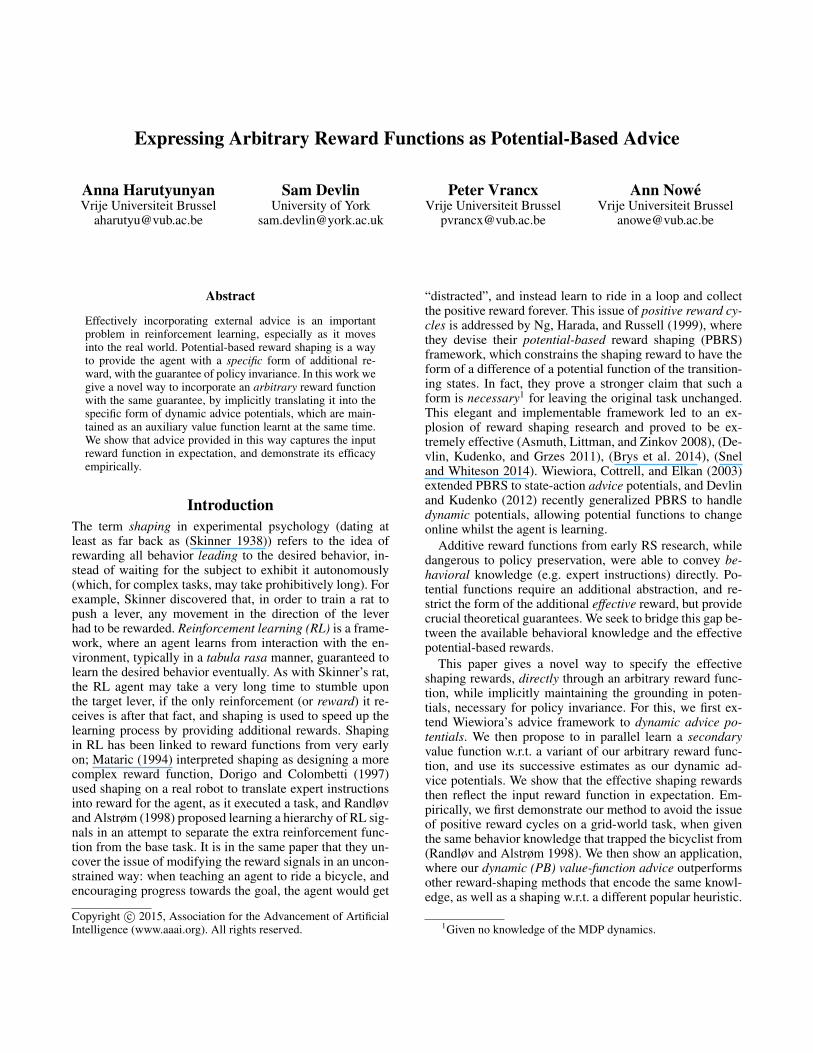
Grid-WorldThe problem described is a minimal working example of thebicycle problem (Randløv and Alstrøm 1998), illustratingthe issue of positive reward cycles.

Given a 20 ⇥ 20 grid, the goal is located at the bottomright corner (20, 20). The agent must reach it from its ini-tial position (0, 0) at the top left corner, upon which eventit will receive a positive reward. The reward on the rest ofthe transitions is 0. The actions correspond to the 4 cardinaldirections, and the state is the agent’s position coordinates(x, y) in the grid. The episode terminates when the goal wasfound, or when 10000 steps have elapsed.

Given approximate knowledge of the problem, a naturalheuristic to encourage is transitions that move the agent tothe right, or down, as they are to advance the agent closer tothe goal. A reward function R

† encoding this heuristic canbe defined as

R

†(s, right) = R

†(s, down) = c, c 2 R+

, 8s

When provided naıvely (i.e. with F = R

†), the agentis at a risk of getting “distracted”: getting stuck in a pos-itive reward cycle, and never reaching the goal. We ap-ply our framework, and learn the corresponding � w.r.t.R

�= �R

†,setting F accordingly (Eq. (12)). We comparethat setting with the base learner and with the non-potential-based naıve learner.6

Learning was done via Sarsa with ✏-greedy action selec-tion, ✏ = 0.1. The learning parameters were tuned to thefollowing values: � = 0.99, c = 1, ↵t+1 = ⌧↵t decay-ing exponentially (so as to satisfy the condition in Eq. (21)),with ↵0 = 0.05, ⌧ = 0.999 and �t = 0.1.

We performed 50 independent runs, 100 episodes each(Fig. 1(a)). Observe that the performance of the (non-PB)agent learning with F = R

† actually got worse with time, asit discovered a positive reward cycle, and got more and moredisinterested in finding the goal. Our agent, armed with thesame knowledge, used it properly (in a true potential-basedmanner) and the learning was accelerated significantly, com-pared to the base agent.

Cart-PoleWe now evaluate our approach on a more difficult cart-polebenchmark (Michie and Chambers 1968). The task is to bal-ance a pole on top a moving cart for as long as possible. The(continuous) state contains the angle ⇠ and angular velocity˙

⇠ of the pole, and the position x and velocity x of the cart.

6To illustrate our point more clearly in the limited space, weomit the static PB variant with (state-only) potentials �(x, y) =x+y. It depends on a different type of knowledge (about the state),while this experiment compares two ways to utilize the behavioralreward function R

†. The static variant does not require learning,and hence performs better in the beginning.

10 20 30 40 50 60 70 80 90 1000

1000

2000

3000

4000

5000

6000

7000

8000

Episodes

Step

s

BaseNon−PB adviceDynamic advice

(a) Grid-world

10 20 30 40 50 60 70 80 90 1000

1000

2000

3000

4000

5000

6000

7000

8000

9000

10000

Episodes

Step

s

BaseNon−PB adviceMyopic PB adviceStatic PB (angle)Dynamic (PB) VF advice

(b) Cart-pole

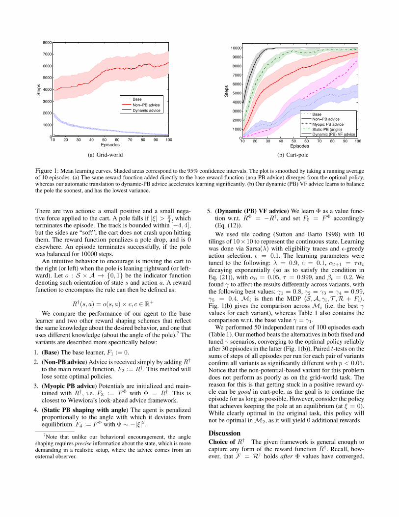
Figure 1: Mean learning curves. Shaded areas correspond to the 95% confidence intervals. The plot is smoothed by taking a running averageof 10 episodes. (a) The same reward function added directly to the base reward function (non-PB advice) diverges from the optimal policy,whereas our automatic translation to dynamic-PB advice accelerates learning significantly. (b) Our dynamic (PB) VF advice learns to balancethe pole the soonest, and has the lowest variance.

There are two actions: a small positive and a small nega-tive force applied to the cart. A pole falls if |⇠| > ⇡

4 , whichterminates the episode. The track is bounded within [�4, 4],but the sides are “soft”; the cart does not crash upon hittingthem. The reward function penalizes a pole drop, and is 0elsewhere. An episode terminates successfully, if the polewas balanced for 10000 steps.

An intuitive behavior to encourage is moving the cart tothe right (or left) when the pole is leaning rightward (or left-ward). Let o : S ⇥ A ! {0, 1} be the indicator functiondenoting such orientation of state s and action a. A rewardfunction to encompass the rule can then be defined as:

R

†(s, a) = o(s, a)⇥ c, c 2 R+

We compare the performance of our agent to the baselearner and two other reward shaping schemes that reflectthe same knowledge about the desired behavior, and one thatuses different knowledge (about the angle of the pole).7 Thevariants are described more specifically below:

1. (Base) The base learner, F1 := 0.2. (Non-PB advice) Advice is received simply by adding R

†

to the main reward function, F2 := R

†. This method willlose some optimal policies.

3. (Myopic PB advice) Potentials are initialized and main-tained with R

†, i.e. F3 := F

� with � = R

†. This isclosest to Wiewiora’s look-ahead advice framework.

4. (Static PB shaping with angle) The agent is penalizedproportionally to the angle with which it deviates fromequilibrium. F4 := F

� with � ⇠ �|⇠|2.7Note that unlike our behavioral encouragement, the angle

shaping requires precise information about the state, which is moredemanding in a realistic setup, where the advice comes from anexternal observer.

5. (Dynamic (PB) VF advice) We learn � as a value func-tion w.r.t. R�

= �R

†, and set F5 = F

� accordingly(Eq. (12)).We used tile coding (Sutton and Barto 1998) with 10

tilings of 10⇥10 to represent the continuous state. Learningwas done via Sarsa(�) with eligibility traces and ✏-greedyaction selection, ✏ = 0.1. The learning parameters weretuned to the following: � = 0.9, c = 0.1, ↵t+1 = ⌧↵t

decaying exponentially (so as to satisfy the condition inEq. (21)), with ↵0 = 0.05, ⌧ = 0.999, and �t = 0.2. Wefound � to affect the results differently across variants, withthe following best values: �1 = 0.8, �2 = �3 = �4 = 0.99,�5 = 0.4. Mi is then the MDP hS,A, �i, T ,R + Fii.Fig. 1(b) gives the comparison across Mi (i.e. the best �values for each variant), whereas Table 1 also contains thecomparison w.r.t. the base value � = �1.

We performed 50 independent runs of 100 episodes each(Table 1). Our method beats the alternatives in both fixed andtuned � scenarios, converging to the optimal policy reliablyafter 30 episodes in the latter (Fig. 1(b)). Paired t-tests on thesums of steps of all episodes per run for each pair of variantsconfirm all variants as significantly different with p < 0.05.Notice that the non-potential-based variant for this problemdoes not perform as poorly as on the grid-world task. Thereason for this is that getting stuck in a positive reward cy-cle can be good in cart-pole, as the goal is to continue theepisode for as long as possible. However, consider the policythat achieves keeping the pole at an equilibrium (at ⇠ = 0).While clearly optimal in the original task, this policy willnot be optimal in M2, as it will yield 0 additional rewards.

DiscussionChoice of R† The given framework is general enough tocapture any form of the reward function R

†. Recall, how-ever, that F = R† holds after � values have converged.

Table 1: Cart-pole results. Performance is indicated with standard error. The final performance refers to the last 10% of the run. Dynamic(PB) VF advice has the highest mean, and lowest variance both in tuned and fixed � scenarios, and is the most robust, whereas myopic shapingproved to be especially sensitive to the choice of �.

Best � values Base � = 0.8Variant Final Overall Final OverallBase 5114.7±188.7 3121.8±173.6 5114.7±165.4 3121.8±481.3Non-PB advice 9511.0±37.2 6820.6±265.3 6357.1±89.1 3405.2±245.2Myopic PB shaping 8618.4±107.3 3962.5±287.2 80.1±0.3 65.8±0.9Static PB 9860.0±56.1 8292.3±261.6 3744.6±136.2 2117.5±102.0Dynamic (PB) VF advice 9982.4±18.4 9180.5±209.8 8662.2±60.9 5228.0±274.0

Thus, the simpler the provided reward function R

†, thesooner will the effective shaping reward capture it. In thiswork, we have considered reward functions R† of the formR

†(B) = c, c > 0, where B is the set of encouraged be-

havior transitions. This follows the convention of shaping inpsychology, where punishment is implicit as absence of pos-itive encouragement. Due to the expectation terms in F , weexpect such form (of all-positive, or all-negative R

†) to bemore robust. Another assumption is that all encouraged be-haviors are encouraged equally; one may easily extend thisto varying preferences c1 < . . . < ck, and consider a choicebetween expressing them within a single reward function, orlearning a separate value function for each signal ci.

Role of discounting Discounting factors � in RL deter-mine how heavily the future rewards are discounted, i.e. thereward horizon. Smaller �’s (i.e. heavier discounting) yieldquicker convergence, but may be insufficient to convey long-term goals. In our framework, the value of � plays two sep-arate roles in the learning process, as it is shared between �

and Q. Firstly, it determines how quickly � values converge.Since we are only interested in the difference of consecu-tive �-values, smaller �’s provide a more stable estimate,without losses. On the other hand, if the value is too small,Q will lose sight of the long-term rewards, which is detri-mental to performance, if the rewards are for the base taskalone. We, however, are considering the shaped rewards.Since shaped rewards provide informative immediate feed-back, it becomes less important to look far ahead into thefuture. This notion is formalized by Ng (2003), who proves(in Theorem 3) that a “good” potential function shortens thereward horizon of the original problem. Thus �, in a sense,balances the stability of learning � with the length of theshaped reward horizon of Q.

Related WorkThe correspondence between value and potential functionshas been known since the conceivement of the latter. Ng etal (1999) point out that the optimal potential function is thetrue value function itself (as in that case the problem reducesto learning the trivial zero value function). With this insight,there have been attempts to simultaneously learn the basevalue function at coarser and finer granularities (of functionapproximation), and use the (quicker-to-converge) former asa potential function for the latter (Grzes and Kudenko 2008).Our approach is different in that our value functions learn on

different rewards with the same state representation, and ittackles the question of specification rather than efficacy.

On the other hand, there has been a lot of researchin human-provided advice (Thomaz and Breazeal 2006),(Knox et al. 2012). This line of research (interactive shap-ing) typically uses the human advice component heuristi-cally as a (sometimes annealed) additive component in thereward function, which does not follow the potential-basedframework (and thus does not preserve policies). Knox andStone (2012) do consider PBRS as one of their methods, but(a) stay strictly myopic (similar to the third variant in thecart-pole experiment), and (b) limit to state potentials. Ourapproach is different in that it incorporates the external ad-vice through a value function, and stays entirely sound in thePBRS framework.

Conclusions and Outlook

In this work, we formulated a framework which allows tospecify the effective shaping reward directly. Given an arbi-trary reward function, we learned a secondary value func-tion, w.r.t. a variant of that reward function, concurrentlyto the main task, and used the consecutive estimates of thatvalue function as dynamic advice potentials. We showed thatthe shaping reward resulting from this process captures theinput reward function in expectation. We presented empir-ical evidence that the method behaves in a true potential-based manner, and that such encoding of the behavioraldomain knowledge speeds up learning significantly more,compared to its alternatives. The framework induces littleadded complexity: the maintenance of the auxiliary valuefunction is linear in time and space (Modayil et al. 2012),and, when initialized to 0, the optimal base value function isunaffected.

We intend to further consider inconsistent reward func-tions, with an application to humans directly providing ad-vice. The challenges are then to analyze the expected effec-tive rewards, as the convergence of a TD-process w.r.t. in-consistent rewards is less straightforward. In this work weidentified the secondary discounting factor �� with the pri-mary �. This need not be the case, in general: ��

= ⌫�.Such modification adds an extra term �-term into Eq. (20),potentially offering gradient guidance, which is useful if theexpert reward is sparse.

AcknowledgmentsAnna Harutyunyan is supported by the IWT-SBO projectMIRAD (grant nr. 120057).

ReferencesAsmuth, J.; Littman, M. L.; and Zinkov, R. 2008. Potential-based shaping in model-based reinforcement learning. InProceedings of 23rd AAAI Conference on Artificial Intelli-gence (AAAI-08), 604–609. AAAI Press.Bellman, R. 1957. Dynamic Programming. Princeton, NJ,USA: Princeton University Press, 1st edition.Borkar, V. S., and Meyn, S. P. 2000. The ODE methodfor convergence of stochastic approximation and reinforce-ment learning. SIAM Journal on Control and Optimization38(2):447–469.Borkar, V. S. 1997. Stochastic approximation with two timescales. Systems and Control Letters 29(5):291 – 294.Brys, T.; Nowe, A.; Kudenko, D.; and Taylor, M. E. 2014.Combining multiple correlated reward and shaping signalsby measuring confidence. In Proceedings of 28th AAAI Con-ference on Artificial Intelligence (AAAI-14), 1687–1693.AAAI Press.Devlin, S., and Kudenko, D. 2012. Dynamic potential-basedreward shaping. In Proceedings of the 11th InternationalConference on Autonomous Agents and Multiagent Systems(AAMAS-12), 433–440. International Foundation for Au-tonomous Agents and Multiagent Systems.Devlin, S.; Kudenko, D.; and Grzes, M. 2011. An empiricalstudy of potential-based reward shaping and advice in com-plex, multi-agent systems. Advances in Complex Systems(ACS) 14(02):251–278.Dorigo, M., and Colombetti, M. 1997. Robot Shaping: Ex-periment In Behavior Engineering. MIT Press, 1st edition.Grzes, M., and Kudenko, D. 2008. Multigrid reinforce-ment learning with reward shaping. In Krkov, V.; Neruda,R.; and Koutnk, J., eds., Artificial Neural Networks - ICANN2008, volume 5163 of Lecture Notes in Computer Science.Springer Berlin Heidelberg. 357–366.Jaakkola, T.; Jordan, M. I.; and Singh, S. P. 1994. On theconvergence of stochastic iterative dynamic programmingalgorithms. Neural computation 6(6):1185–1201.Knox, W. B., and Stone, P. 2012. Reinforcement learningfrom simultaneous human and MDP reward. In Proceed-ings of the 11th International Conference on AutonomousAgents and Multiagent Systems (AAMAS-12), 475–482. In-ternational Foundation for Autonomous Agents and Multia-gent Systems.Knox, W. B.; Glass, B. D.; Love, B. C.; Maddox, W. T.; andStone, P. 2012. How humans teach agents: A new experi-mental perspective. International Journal of Social Robotics4:409–421.Mataric, M. J. 1994. Reward functions for accelerated learn-ing. In In Proceedings of the Eleventh International Confer-ence on Machine Learning (ICML-94), 181–189. MorganKaufmann.

Michie, D., and Chambers, R. A. 1968. Boxes: An experi-ment in adaptive control. In Dale, E., and Michie, D., eds.,Machine Intelligence. Edinburgh, UK: Oliver and Boyd.Modayil, J.; White, A.; Pilarski, P. M.; and Sutton, R. S.2012. Acquiring a broad range of empirical knowledge inreal time by temporal-difference learning. In Systems, Man,and Cybernetics (SMC), 2012 IEEE International Confer-ence on, 1903–1910. IEEE.Ng, A. Y.; Harada, D.; and Russell, S. 1999. Policy in-variance under reward transformations: Theory and applica-tion to reward shaping. In In Proceedings of the SixteenthInternational Conference on Machine Learning (ICML-99),278–287. Morgan Kaufmann.Ng, A. Y. 2003. Shaping and policy search in reinforce-ment learning. Ph.D. Dissertation, University of California,Berkeley.Puterman, M. 1994. Markov Decision Processes: DiscreteStochastic Dynamic Programming. New York, NY, USA:John Wiley & Sons, Inc., 1st edition.Randløv, J., and Alstrøm, P. 1998. Learning to drive abicycle using reinforcement learning and shaping. In Pro-ceedings of the Fifteenth International Conference on Ma-chine Learning, 463–471. San Francisco, CA, USA: MorganKauffman.Schwartz, A. 1993. A reinforcement learning methodfor maximizing undiscounted rewards. In ICML, 298–305.Morgan Kaufmann.Skinner, B. F. 1938. The behavior of organisms: An experi-mental analysis. Appleton-Century.Snel, M., and Whiteson, S. 2014. Learning potentialfunctions and their representations for multi-task reinforce-ment learning. Autonomous Agents and Multi-Agent Systems28(4):637–681.Sutton, R., and Barto, A. 1998. Reinforcement learning: Anintroduction, volume 116. Cambridge Univ Press.Sutton, R. S.; Maei, H. R.; Precup, D.; Bhatnagar, S.; Silver,D.; Szepesvari, C.; and Wiewiora, E. 2009. Fast gradient-descent methods for temporal-difference learning with lin-ear function approximation. In Proceedings of the 26th An-nual International Conference on Machine Learning, ICML’09, 993–1000. New York, NY, USA: ACM.Thomaz, A. L., and Breazeal, C. 2006. Reinforcement learn-ing with human teachers: Evidence of feedback and guid-ance with implications for learning performance. In Pro-ceedings of the 21st AAAI Conference on Artificial Intelli-gence (AAAI-06), 1000–1005. AAAI Press.Wiewiora, E.; Cottrell, G. W.; and Elkan, C. 2003. Prin-cipled methods for advising reinforcement learning agents.In Machine Learning, Proceedings of the Twentieth Interna-tional Conference (ICML-03), 792–799.