Appendix A - Springer LINK

Appendix A

Special functions and mathematical operations

The purpose of this appendix is to define the special functions and mathematicaloperations used in the main text, and to describe their most important properties. Thematerial draws heavily from two valuable resources: the Handbook of MathematicalFunctions edited by Abramowitz and Stegun (1965) and Weisstein’s MathWorld(Weisstein, www). Unless stated otherwise, the symbols x and z denote real andcomplex variables, respectively.

A.1 DEFINITIONS AND BASIC PROPERTIES OF SPECIAL FUNCTIONS

A.1.1 Heaviside step function, sign function, and rectangle function

Three closely related functions are the Heaviside step function

HðxÞ �0 x < 0

1=2 x ¼ 0

1 x > 0,

8<: ðA:1Þ

the sign function

sgnðxÞ ��1 x < 0

0 x ¼ 0

þ1 x > 0

8<: ðA:2Þ

and the rectangle function

PðxÞ �1 jxj < 1=2

1=2 jxj ¼ 1=2

0 jxj > 1=2.

8><>: ðA:3Þ

It follows from these definitions that

sgnðxÞ ¼ 2½HðxÞ � 12 ðA:4Þ

andPðxÞ ¼ Hðx þ 1

2Þ � Hðx � 1

2Þ: ðA:5Þ

A.1.2 Sine cardinal and sinh cardinal functions

The sine cardinal, or ‘‘sinc’’, function is

sincðxÞ � sin x

x; ðA:6Þ

some integrals of which are included in Table A.1.Similarly, the sinh cardinal function is (Weisstein,2003a)

sinhcðxÞ � sinh x

x: ðA:7Þ

A.1.3 Dirac delta function

Dirac’s delta function has zero magnitude everywhere except the origin, and unitarea. It can be defined in terms of a limiting form of, for example, the rectanglefunction

�ðxÞ ¼ lim"!0

Pðx="Þ"

; ðA:8Þor the Gaussian

�ðxÞ ¼ lim"!0

exp½�ðx="Þ2ffiffiffi�

p"

: ðA:9Þ

A.1.4 Fresnel integrals

The Fresnel integrals are

CðxÞ �ðx

0

cos�

2u2

� �du ðA:10Þ

and

SðxÞ �ðx

0

sin�

2u2

� �du: ðA:11Þ

Asymptotic properties are

limx!1

CðxÞ ¼ð10

cos�

2u2

� �du ¼ 1

2ðA:12Þ

and

limx!1

SðxÞ ¼ð10

sin�

2u2

� �du ¼ 1

2: ðA:13Þ

636 Appendix A

Table A.1. Integrals of integer

powers of the sine cardinal

function (Weisstein, 2006).

N

ð10

dx sincN x

1 �=2

2 �=2

3 3�=8

4 �=3

5 115�=384

A.1.5 Error function, complementary error function, and right-tail probability

function

The error function is

erfðxÞ � 2ffiffiffi�

pðx

0

e�t2 dt: ðA:14Þ

Its limiting value for large x is

limx!1

erfðxÞ ¼ 1: ðA:15Þ

The complementary error function, plotted in Figure A.1 (cyan line of upper graph), is

erfcðxÞ � 1� erfðxÞ ¼ 2ffiffiffi�

pð1

x

e�t2 dt: ðA:16Þ

A simple approximation to erfcðxÞ, shown as ‘‘approx 1’’ in Figure A.1 and valid forlarge x, is

erfcðxÞ e�x2ffiffiffi�

px: ðA:17Þ

A slightly more accurate version (‘‘approx 2’’) is (Abramowitz and Stegun, 1965)

erfcðxÞ 2ffiffiffi�

p e�x2

x þffiffiffiffiffiffiffiffiffiffiffiffiffiffix2 þ 2

p : ðA:18Þ

At the expense of a little more complication, a very accurate value can be obtainedusing the approximation

erfcðxÞ 2ffiffiffi�

p e�x2

x þffiffiffiffiffiffiffiffiffiffiffiffiffiffiffiffiffiffiffiffiffiffiffiffiffiffiffiffiffiffiffiffiffiffiffiffiffiffiffiffiffiffiffiffiffiffiffiffiffiffiffiffiffiffiffiffiffix2 þ 2� ð1� 2=�Þ21�1:2117x

p ; ðA:19Þ

shown as ‘‘approx 3’’. The fractional errors for all three approximations are alsoplotted (lower graph). For Equation (A.19), the fractional error is less than 0.1% forall x � 0. For negative arguments, the following symmetry property can be used

erfcðxÞ ¼ 2� erfcð�xÞ: ðA:20Þ

The erfc function is closely related to the right-tail probability function (Kay, 1998,p. 21), defined as

FðxÞ � 1ffiffiffiffiffiffi2�

pð1

x

exp � u2

2

!du: ðA:21Þ

The precise relationships between these two functions and their inverses are

FðxÞ ¼ 1

2erfc

xffiffiffi2

p�

ðA:22Þ

and

F�1ðxÞ ¼ffiffiffi2

perfc�1ð2xÞ: ðA:23Þ

Appendix A 637

638 Appendix A

Figure A.1. The complementary error function erfcðxÞ and approximations 1 to 3 (upper graph)

and fractional error (lower). The approximations are indicated by ‘‘approx 1’’ (Equation A.17),

‘‘approx 2’’ (Equation A.18), and ‘‘approx 3’’ (Equation A.19).

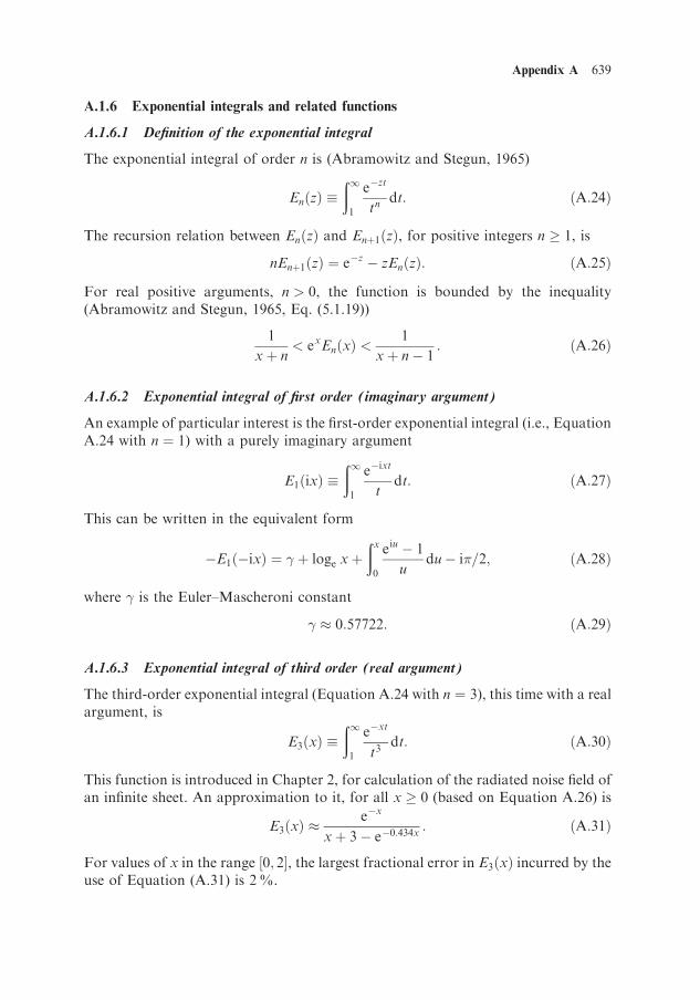
A.1.6 Exponential integrals and related functions

A.1.6.1 Definition of the exponential integral

The exponential integral of order n is (Abramowitz and Stegun, 1965)

EnðzÞ �ð11

e�zt

tn dt: ðA:24Þ

The recursion relation between EnðzÞ and Enþ1ðzÞ, for positive integers n � 1, is

nEnþ1ðzÞ ¼ e�z � zEnðzÞ: ðA:25Þ

For real positive arguments, n > 0, the function is bounded by the inequality(Abramowitz and Stegun, 1965, Eq. (5.1.19))

1

x þ n< exEnðxÞ <

1

x þ n � 1: ðA:26Þ

A.1.6.2 Exponential integral of first order (imaginary argument)

An example of particular interest is the first-order exponential integral (i.e., EquationA.24 with n ¼ 1) with a purely imaginary argument

E1ðixÞ �ð11

e�ixt

tdt: ðA:27Þ

This can be written in the equivalent form

�E1ð�ixÞ ¼ þ loge x þðx

0

eiu � 1

udu � i�=2; ðA:28Þ

where is the Euler–Mascheroni constant

0:57722: ðA:29Þ

A.1.6.3 Exponential integral of third order (real argument)

The third-order exponential integral (Equation A.24 with n ¼ 3), this time with a realargument, is

E3ðxÞ �ð11

e�xt

t3dt: ðA:30Þ

This function is introduced in Chapter 2, for calculation of the radiated noise field ofan infinite sheet. An approximation to it, for all x � 0 (based on Equation A.26) is

E3ðxÞ e�x

x þ 3� e�0:434x: ðA:31Þ

For values of x in the range ½0; 2, the largest fractional error in E3ðxÞ incurred by theuse of Equation (A.31) is 2%.

Appendix A 639

A.1.6.4 Sine and cosine integral functions

The sine integral and cosine integral functions are, respectively,

SiðxÞ �ðx

0

sin u

udu ðA:32Þ

and

CiðxÞ � þ loge x þðx

0

cos u � 1

udu: ðA:33Þ

These two functions are related to the exponential integral via (Abramowitz andStegun, 1965, p. 232)

SiðxÞ ¼ �

2þ 1

2i½E1ðixÞ � E1ð�ixÞ ðA:34Þ

and

CiðxÞ ¼ � 1

2½E1ðixÞ þ E1ð�ixÞ: ðA:35Þ

It follows thatE1ð�ixÞ ¼ �CiðxÞ � i½SiðxÞ � �=2: ðA:36Þ

Asymptotic values are

limx!1

SiðxÞ ¼ð10

sin u

udu ¼ �

2ðA:37Þ

andlim

x!1CiðxÞ ¼ 0: ðA:38Þ

A.1.7 Gamma function and incomplete

gamma functions

A.1.7.1 Gamma function

A.1.7.1.1 Definition and importantvalues

The gamma function is

GðzÞ �ð10

tz�1 e�t dt; ðA:39Þ

which for real arguments satisfies theproperty

Gðx þ 1Þ ¼ xGðxÞ ðx > 0Þ: ðA:40ÞImportant values of GðxÞ are listed inTable A.2. It follows from Equation(A.39) and the result Gð1Þ ¼ 1 that,for integer n

Gðn þ 1Þ ¼ n! ðn � 1Þ: ðA:41Þ

640 Appendix A

Table A.2. Selected values of the gamma

function GðxÞ for 0 < x � 1. Values outside

this range can be calculated using

Gðx þ 1Þ ¼ xGðxÞ. All GðxÞ values in the

table are approximate except Gð1Þ. The exactvalue of Gð1=2Þ is �1=2.

x GðxÞ

1/5 4.5908

1/4 3.6256

1/3 2.6789

2/5 2.2182

1/2 1.7725

3/5 1.4892

2/3 1.3541

3/4 1.2254

4/5 1.1642

1 1

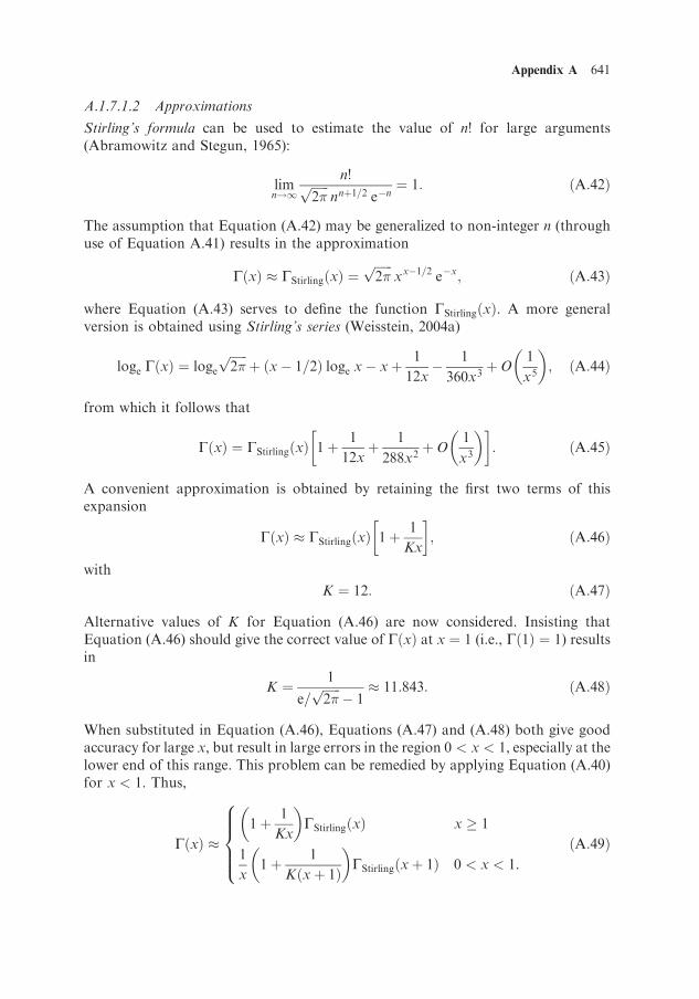
A.1.7.1.2 Approximations

Stirling’s formula can be used to estimate the value of n! for large arguments(Abramowitz and Stegun, 1965):

limn!1

n!ffiffiffiffiffiffi2�

pnnþ1=2 e�n

¼ 1: ðA:42Þ

The assumption that Equation (A.42) may be generalized to non-integer n (throughuse of Equation A.41) results in the approximation

GðxÞ GStirlingðxÞ ¼ffiffiffiffiffiffi2�

pxx�1=2 e�x; ðA:43Þ

where Equation (A.43) serves to define the function GStirlingðxÞ. A more generalversion is obtained using Stirling’s series (Weisstein, 2004a)

loge GðxÞ ¼ logeffiffiffiffiffiffi2�

pþ ðx � 1=2Þ loge x � x þ 1

12x� 1

360x3þ O

1

x5

� ; ðA:44Þ

from which it follows that

GðxÞ ¼ GStirlingðxÞ 1þ 1

12xþ 1

288x2þ O

1

x3

� � �: ðA:45Þ

A convenient approximation is obtained by retaining the first two terms of thisexpansion

GðxÞ GStirlingðxÞ 1þ 1

Kx

� �; ðA:46Þ

with

K ¼ 12: ðA:47Þ

Alternative values of K for Equation (A.46) are now considered. Insisting thatEquation (A.46) should give the correct value of GðxÞ at x ¼ 1 (i.e., Gð1Þ ¼ 1) resultsin

K ¼ 1

e=ffiffiffiffiffiffi2�

p� 1

11:843: ðA:48Þ

When substituted in Equation (A.46), Equations (A.47) and (A.48) both give goodaccuracy for large x, but result in large errors in the region 0 < x < 1, especially at thelower end of this range. This problem can be remedied by applying Equation (A.40)for x < 1. Thus,

GðxÞ 1þ 1

Kx

� GStirlingðxÞ x � 1

1

x1þ 1

Kðx þ 1Þ

� GStirlingðx þ 1Þ 0 < x < 1.

8>>><>>>:

ðA:49Þ

Appendix A 641

In general, there is a small discontinuity through x ¼ 1, which can be removed bychoosing

K ¼ e�ffiffiffi2

pffiffiffi8

p� e

11:840: ðA:50Þ

Figure A.2 shows the gamma function with various approximations (upper graph)and the fractional error incurred by these (lower). The approximation obtained usingEquation (A.49) (with Equation A.50 for K) is not shown in the upper graph becauseit cannot be distinguished from the exact function GðxÞ on this scale. The largestfractional error incurred by use of this approximation (shown as a cyan curve in thelower graph) is about 0.01%, and occurs when x 3:5.

A.1.7.1.3 Use of the gamma function

Integrals of the form ð10

xp expð�BxqÞ dx ðA:51Þ

appear in several chapters of this book. It follows from the definition of the gammafunction (Equation A.39) that this integral can be writtenð1

0

xp expð�BxqÞ dx ¼ B�ðpþ1Þ=q

qG

p þ 1

q

� : ðA:52Þ

A.1.7.2 Incomplete gamma functions

Two incomplete gamma functions are of interest here. The first, known as the lowerincomplete gamma function, is defined as (Abramowitz and Stegun, 1965, p. 260)

ða; xÞ �ðx

0

e�t ta�1 dt: ðA:53Þ

The second is the upper incomplete gamma function (Abramowitz and Stegun, 1965;Weisstein, 2002)

Gða; xÞ �ð1

x

e�t ta�1 dt: ðA:54Þ

These two functions are complementary in the sense that their sum gives an ordinary(i.e., complete) gamma function

ða; xÞ þ Gða; xÞ ¼ GðaÞ: ðA:55ÞImportant properties include

Gða; 0Þ ¼ limx!1

ða; xÞ ¼ GðaÞ ðA:56Þ

and (Weisstein, 2002)

Gð0; xÞ ¼E1ðxÞ � i� x < 0

�E1ð�xÞ x > 0.

�ðA:57Þ

642 Appendix A

Appendix A 643

Figure A.2. Upper graph: the gamma function GðxÞ defined by Equation (A.39) and

approximations ‘‘Stirling1’’ (Equation A.43), ‘‘Stirling3’’ (Equation A.45), ‘‘K¼ 12’’ (Equa-

tion A.49þEquation A.47); lower graph: fractional error incurred by the three approximations

from the upper graph, plus a fourth approximation, labeled ‘‘K¼ 11.840’’ (Equation

A.49þEquation A.50).

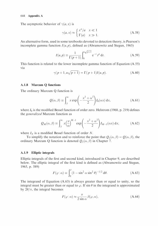
The asymptotic behavior of ða; xÞ is

ða; xÞ xa=a x � 1

GðaÞ x � 1.

�ðA:58Þ

An alternative form, used in some textbooks devoted to detection theory, is Pearson’sincomplete gamma function Iðu; pÞ, defined as (Abramowitz and Stegun, 1965)

Iðu; pÞ � 1

Gðp þ 1Þ

ðuffiffiffiffiffiffipþ1

p

0

e�t tp dt: ðA:59Þ

This function is related to the lower incomplete gamma function of Equation (A.55)via

ð p þ 1; uffiffiffiffiffiffiffiffiffiffiffip þ 1

pÞ ¼ Gð p þ 1ÞIðu; pÞ: ðA:60Þ

A.1.8 Marcum Q functions

The ordinary Marcum Q function is

Qð; �Þ �ð1�

x exp � x2 þ 2

2

!I0ðxÞ dx; ðA:61Þ

where I0 is the modified Bessel function of order zero. Helstrom (1968, p. 219) definesthe generalized Marcum function as

QMð; �Þ �ð1�

xx

� �M�1

exp � x2 þ 2

2

!IM�1ðxÞ dx; ðA:62Þ

where IN is a modified Bessel function of order N.To simplify the notation and to reinforce the point that Q1ð; �Þ ¼ Qð; �Þ, the

ordinary Marcum Q function is denoted Q1ð; �Þ in Chapter 7.

A.1.9 Elliptic integrals

Elliptic integrals of the first and second kind, introduced in Chapter 9, are describedbelow. The elliptic integral of the first kind is defined as (Abramowitz and Stegun,1965, p. 589)

Fð’ IÞ �ð’0

ð1� sin2 sin2 Þ�1=2 d : ðA:63Þ

The integrand of Equation (A.63) is always greater than or equal to unity, so theintegral must be greater than or equal to ’. If sin in the integrand is approximatedby 2 =�, the integral becomes

Fð’ IÞ �

2 sin �ð’; Þ; ðA:64Þ

644 Appendix A

where

�ð’; Þ � arcsin2’

�sin

� : ðA:65Þ

The right-hand side of Equation (A.64) satisfies the inequality

’ � �

2 sin �ð’; Þ � Fð’ IÞ: ðA:66Þ

The function Fð’ IÞ has a singularity at � ¼ ¼ �=2. Use of Equation (A.64)avoids this singularity, while still providing a useful approximation away from it.

The elliptic integral of the second kind is

Eð’ IÞ �ð’0

ð1� sin2 sin2 Þþ1=2 d : ðA:67Þ

A similar approximation to that leading to Equation (A.64) gives

Eð’ IÞ �

4 sin ð� þ sin � cos �Þ; ðA:68Þ

where � ¼ �ð’; Þ is given by Equation (A.65). This approximation satisfies theinequality

’ � �

4 sin ð� þ sin � cos �Þ � Eð’ IÞ: ðA:69Þ

A.1.10 Bessel and related functions

A.1.10.1 Bessel function of the first kind

Bessel functions of the first kind are solutions to the ordinary differential equation(Abramowitz and Stegun, 1965, p. 358)

z2d2w

dz2þ z

dw

dzþ ðz2 � �2Þw ¼ 0: ðA:70Þ

The solutions to this equation, denoted J��ðzÞ, are Bessel functions (of the first kind)of order ��. The normalization (for positive integer n) is (Weisstein, 2004b)ð1

0

½JnðxÞ2 dx ¼ 1: ðA:71Þ

Related integrals are (Wolfram, www)ð10

1

xJ�ðxÞ2 dx ¼ 1

2�ðRe � > 0Þ ðA:72Þ

and (Weisstein, 2004b) ð10

J1ðxÞx

� �2

dx ¼ 4

3�: ðA:73Þ

Appendix A 645

A series expansion is (Abramowitz and Stegun, 1965, p. 360)

J�ðxÞ ¼x

2

� ��X1n¼0

ð�x2=4Þn

n! Gð� þ n þ 1Þ : ðA:74Þ

The asymptotic behavior of J�ðxÞ for small and large x is given by (Abramowitz andStegun, 1965)

J�ðxÞ

1

Gð� þ 1Þx

2

� ��x � 1ffiffiffiffiffiffi

2

�x

rcos x � ��

2� �

4

� �x � 1,

8>><>>: ðA:75Þ

valid for x > 0 and real, non-negative �.

A.1.10.2 Modified Bessel function

Modified Bessel functions of the first kind, denoted I��ðzÞ, are solutions to theordinary differential equation (Abramowitz and Stegun, 1965)

z2d2w

dz2þ z

dw

dz� ðz2 þ �2Þw ¼ 0: ðA:76Þ

They are related to J�ðzÞ according to (Abramowitz and Stegun, 1965, p. 375):

I�ðzÞ ¼expð��i=2ÞJ�ðizÞ �� < arg z � �=2

expð3��i=2ÞJ�ð�izÞ �=2 < arg z � �.

�ðA:77Þ

Other important properties include

I�nðzÞ ¼ InðzÞ; ðA:78Þ

I�ðzÞ ¼z

2

� ��X1k¼0

ðz2=4Þk

k! Gð� þ k þ 1Þ ; ðA:79Þ

and

I�ðzÞ �ezffiffiffiffiffiffiffiffi2�z

p 1� 4�2 � 1

8zþ Oðz�2Þ

" #jarg zj < �=2: ðA:80Þ

Levanon (1988) suggests the approximation

I0ðxÞ 1

6ð1þ cosh xÞ þ 1

3cosh

x

2þ cosh

ffiffiffi3

px

2

!: ðA:81Þ

The modified Bessel function is plotted in Figure A.3 (upper graph), together with theapproximation of Equation (A.81). The fractional error increases with increasingargument (lower graph). For the range 0 < x < 15 the error is less than 2%.

646 Appendix A

Appendix A 647

Figure A.3. Upper graph: the modified Bessel function I0ðxÞ and Levanon’s approximation

(Equation A.81); lower graph: fractional error incurred by use of Levanon’s approximation.

A.1.10.3 Airy functions

The second-order differential equation

d2w

dz2� z

dw

dz¼ 0 ðA:82Þ

has two independent solutions, known as Airy functions, one of which, denotedAiðzÞ, vanishes for large real values of its argument, while the other, BiðzÞ, isunbounded in this limit. They are related to the Bessel functions J�1=3 and I�1=3

via (Abramowitz and Stegun, 1965, p. 446)

AiðzÞ ¼ffiffiffiz

p

3½I�1=3ð�Þ � Iþ1=3ð�Þ ðA:83Þ

and

BiðzÞ ¼ffiffiffiz

3

r½I�1=3ð�Þ þ Iþ1=3ð�Þ ðA:84Þ

where

� ¼ 23z3=2: ðA:85Þ

Alternative expressions that are more convenient to use for negative arguments are

Aið�zÞ ¼ffiffiffiz

p

3½Jþ1=3ð�Þ þ J�1=3ð�Þ; ðA:86Þ

and

Bið�zÞ ¼ffiffiffiz

3

r½J�1=3ð�Þ � Jþ1=3ð�Þ: ðA:87Þ

The value and gradient of the Airy functions at the origin are given by

Aið0Þ ¼ Bið0Þffiffiffi3

p ¼ 3�2=3

Gð2=3Þ 0:35503 ðA:88Þ

and

�Ai0ð0Þ ¼ Bi 0ð0Þffiffiffi3

p ¼ 3�1=3

Gð1=3Þ 0:25882: ðA:89Þ

A.1.11 Hypergeometric functions

A.1.11.1 Gauss’s hypergeometric function

Gauss’s hypergeometric function (sometimes abbreviated as the ‘‘hypergeometricfunction’’) is (Weisstein, 2004c)

2F1ða; b; c; zÞ ¼GðcÞ

GðbÞGðc � bÞ

ð10

tb�1ð1� tÞc�b�1

ð1� tzÞa dt: ðA:90Þ

This function is a solution of the differential equation

zð1� zÞ d2u

dz2þ ½c � ða þ b þ 1Þz du

dz� abu ¼ 0 ðA:91Þ

648 Appendix A

that is regular at the origin, and normalized such that

2F1ða; b; c; 0Þ ¼ 1: ðA:92ÞIf jxj < 1, Equation (A.90) may be expanded as a power series:

2F1ða; b; c; xÞ ¼GðcÞ

GðaÞGðbÞX1n¼0

Gða þ nÞGðb þ nÞGðc þ nÞ xn: ðA:93Þ

Of particular interest (for Chapter 5, in connection with the bulk modulus of bubblywater) is the special case for b ¼ c � 1 ¼ a

2F1ða; a; a þ 1; zÞ ¼ a

ð10

ta�1

ð1� tzÞa dt: ðA:94Þ

A.1.11.2 Confluent hypergeometric function of the first kind

The confluent hypergeometric function of the first kind, denoted 1F1ða; b; zÞ, is(Weisstein, 2003b)

1F1ða; b; zÞ ¼GðbÞ

Gðb � aÞGðaÞ

ð10

ezt ta�1

ð1� tÞ1þa�bdt: ðA:95Þ

Of particular interest (for Chapter 7, in connection with the third and highermoments of the Rician probability distribution function) is the special case b ¼ 1

1F1ða; 1; zÞ ¼1

GðaÞGð1� aÞ

ð10

ezt ta�1

ð1� tÞa dt: ðA:96Þ

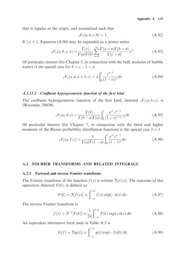
A.2 FOURIER TRANSFORMS AND RELATED INTEGRALS

A.2.1 Forward and inverse Fourier transforms

The Fourier transform of the function f ðxÞ is written I½ f ðxÞ. The outcome of thisoperation, denoted FðkÞ, is defined as:

FðkÞ ¼ I½ f ðxÞ �ðþ1

�1f ðxÞ expð�ikxÞ dx: ðA:97Þ

The inverse Fourier transform is

f ðxÞ ¼ I�1½FðkÞ � 1

2�

ðþ1

�1FðkÞ expðþikxÞ dk: ðA:98Þ

An equivalent alternative form used in Table A.3 is

Gð f Þ ¼ I½gðtÞ �ðþ1

�1gðtÞ expð�2�iftÞ dt; ðA:99Þ

Appendix A 649

with

gðtÞ ¼ I�1½Gð f Þ ¼

ðþ1

�1Gð f Þ expðþ2�iftÞ df : ðA:100Þ

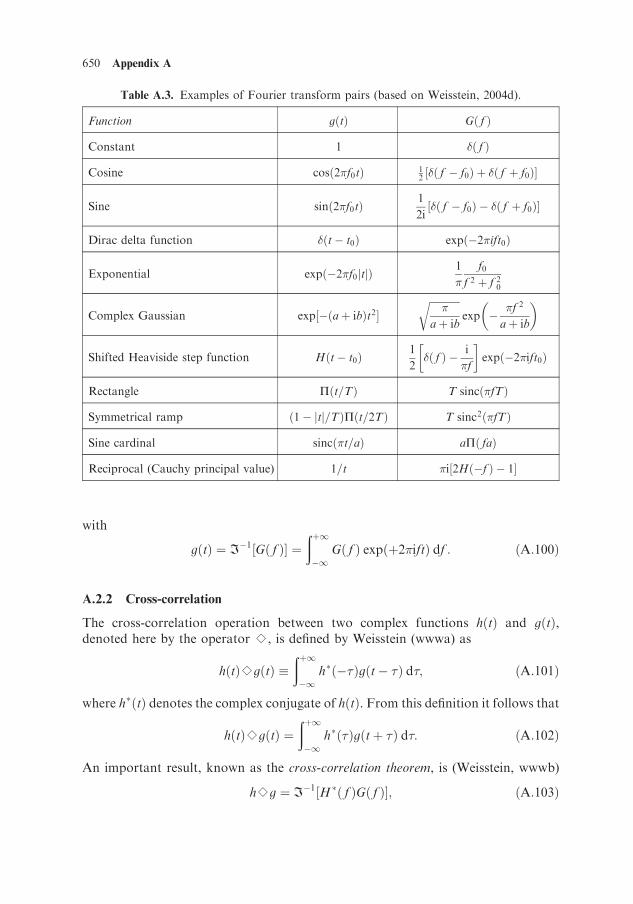
A.2.2 Cross-correlation

The cross-correlation operation between two complex functions hðtÞ and gðtÞ,denoted here by the operator s, is defined by Weisstein (wwwa) as

hðtÞsgðtÞ �ðþ1

�1h�ð��Þgðt � �Þ d�; ðA:101Þ

where h�ðtÞ denotes the complex conjugate of hðtÞ. From this definition it follows that

hðtÞsgðtÞ ¼ðþ1

�1h�ð�Þgðt þ �Þ d�: ðA:102Þ

An important result, known as the cross-correlation theorem, is (Weisstein, wwwb)

hsg ¼ I�1½H �ð f ÞGð f Þ; ðA:103Þ

650 Appendix A

Table A.3. Examples of Fourier transform pairs (based on Weisstein, 2004d).

Function gðtÞ Gð f Þ

Constant 1 �ð f Þ

Cosine cosð2�f0tÞ 12½�ð f � f0Þ þ �ð f þ f0Þ

Sine sinð2�f0tÞ1

2i½�ð f � f0Þ � �ð f þ f0Þ

Dirac delta function �ðt � t0Þ expð�2�ift0Þ

Exponential expð�2�f0jtjÞ1

�

f0

f 2 þ f 20

Complex Gaussian exp½�ða þ ibÞt2ffiffiffiffiffiffiffiffiffiffiffiffi�

a þ ib

rexp � �f 2

a þ ib

�

Shifted Heaviside step function Hðt � t0Þ1

2�ð f Þ � i

�f

� �expð�2�ift0Þ

Rectangle Pðt=TÞ T sincð�fTÞ

Symmetrical ramp ð1� jtj=TÞPðt=2TÞ T sinc2ð�fTÞ

Sine cardinal sincð�t=aÞ aPð faÞ

Reciprocal (Cauchy principal value) 1=t �i½2Hð�f Þ � 1

whereHð f Þ ¼ I½hðtÞ ðA:104Þ

andGð f Þ ¼ I½gðtÞ: ðA:105Þ

The special case with h ¼ g, known as the Wiener–Khinchin theorem, relates theautocorrelation function hsh to the Fourier transform of the power spectrum:

hsh ¼ I�1½jHð f Þj2: ðA:106Þ

An alternative definition, used in Chapter 6 (following Burdic, 1984; McDonoughand Whalen, 1995), is

ChgðtÞ �ðþ1

�1hð�Þg�ð� � tÞ d�: ðA:107Þ

The two definitions are related according to

hðtÞsgðtÞ ¼ C�hgð�tÞ: ðA:108Þ

A.2.3 Convolution

The convolution operation between functions hðtÞ and gðtÞ is denoted here by theoperator � and defined as (Weisstein, 2003c)

hðtÞ � gðtÞ �ðþ1

�1hð�Þgðt � �Þ d�: ðA:109Þ

It follows from Equations (A.101) and (A.109) that

hðtÞsgðtÞ ¼ h�ð�tÞ � gðtÞ: ðA:110ÞThe Fourier transform of the product hðtÞgðtÞ is equal to the convolution of theindividual transforms Hð f Þ and Gð f Þ (i.e., Weisstein, 2003c)

I½hðtÞgðtÞ ¼ Hð f Þ � Gð f Þ: ðA:111ÞEquation (A.111) is known as the convolution theorem. Alternative forms of thetheorem are (Weisstein, wwwc)

I½h � g ¼ FG; ðA:112Þ

I�1½HG ¼ h � g; ðA:113Þ

and

I�1½H � G ¼ hg: ðA:114Þ

A.2.4 Discrete Fourier transform

The discrete Fourier transform (DFT) of the function xðnÞ is

XðmÞ �XN�1

n¼0

xðnÞ exp �i2�m

Nn

� ; ðA:115Þ

Appendix A 651

the inverse transform of which is (Oppenheim and Schafer, 1989)

xðnÞ ¼ 1

N

XN�1

m¼0

XðmÞ exp þi2�mn

N

� ; n ¼ 0; 1; 2; . . . ;N � 1: ðA:116Þ

A common application of the DFT is for a continuous function of time, say FðtÞ, thathas been sampled at discrete time intervals

tn ¼ t0 þ n �t: ðA:117ÞIn the analysis of signals of this form, it is common to evaluate expressions of theform

Gð!Þ �XN�1

n¼0

FðtnÞ expð�i!tnÞ; tn ¼ t0 þ n �t: ðA:118Þ

The inverse transform that follows from Equation (A.116) is

FðtnÞ ¼1

N

XN�1

m¼0

Gð!mÞ expðþi!mtnÞ; n ¼ 0; 1; 2; . . . ;N � 1; ðA:119Þ

where

!m ¼ 2�

N �tm: ðA:120Þ

A.2.5 Plancherel’s theorem

The Fourier transform pair gðtÞ and Gð f Þ are related according to Plancherel’stheorem (Weisstein, wwwd)ðþ1

�1jgðtÞj2 dt ¼

ðþ1

�1jGð f Þj2 df : ðA:121Þ

Thus, jGð f Þj2 is the energy spectral density of the time series gðtÞ. The correspondingrelationship for the discrete transform pair is

XN�1

n¼0

jxðnÞj2 ¼ �f �tXN�1

n¼0

jXðmÞj2: ðA:122Þ

A.3 STATIONARY PHASE METHOD FOR EVALUATION

OF INTEGRALS

A.3.1 Stationary phase approximation

The stationary phase method is a way of approximating integrals of the form

Iða; bÞ ¼ðb

a

f ðxÞ exp½i�ðxÞ dx; ðA:123Þ

where f ðxÞ is a slowly varying function; and �ðxÞ is a phase term. It is one of a more

652 Appendix A

general class of approximations known as saddle point methods (Skudrzyk, 1971;Chapman, 2004). The basic requirement is for f ðxÞ to vary slowly compared with �,in such a way that the amplitude f does not change significantly during a period ofei�. There is also a requirement that the phase approaches a maximum or minimumeither within or close to the integration interval. If there is only one such point ofstationary phase, the integral is

Iða; bÞ ffiffiffiffiffiffiffiffiffiffiffiffiffiffiffiffiffi

2�

j�00ðx0Þj

sf ðx0ÞEsð; �Þ ei�ðx0Þ; ðA:124Þ

where x0 is the point of stationary phase such that

�0ðx0Þ ¼ 0 ðA:125Þand

s ¼ sgn½�00ðx0Þ: ðA:126ÞThe variables and � are related to a and b according to

¼ gðaÞ; ðA:127Þand

� ¼ gðbÞ ðA:128Þwhere

gðxÞ �ffiffiffiffiffiffiffiffiffiffiffiffiffiffiffiffiffij� 00ðx0Þj

�

rðx � x0Þ: ðA:129Þ

Finally, the function Esð; �Þ is defined as

Esð; �Þ �1ffiffiffi2

pð�

exp si�

2x2

� �dx; ðA:130Þ

which in terms of Fresnel integrals becomes

Esð; �Þ ¼Cð�Þ � CðÞ þ si½Sð�Þ � SðÞffiffiffi

2p : ðA:131Þ

If there is more than one stationary phase point, and if these are not too closetogether, their individual contributions may be added.

A.3.2 Derivation

The derivation of Equation (A.124) follows. It is convenient to write the integrationlimits as x� such that

I ¼ðxþ

x�

f ðxÞ exp½i�ðxÞ dx ðA:132Þ

and expand �ðxÞ around some point x0 (to be specified)

�ðxÞ ¼ �ðx0Þ þ �0ðx0Þðx�x0Þ þ 12� 00ðx0Þðx�x0Þ2 þ 1

6�000ðx0Þðx�x0Þ3 þ � � � ðA:133Þ

If �ðxÞ is a rapidly varying function, the exponential is oscillatory and the netcontribution to the integral averaged over many cycles is small. However, if the

Appendix A 653

phase slows down, the contributions can build up quickly. For this reason it is usefulto expand about points at which the first derivative vanishes (known as points of‘‘stationary phase’’). Thus, the value of x0 is chosen to ensure that �0ðx0Þ ¼ 0, andtherefore

�ðxÞ ¼ �ðx0Þ þ 12�00ðx0Þðx � x0Þ2 þ 1

6�000ðx0Þðx � x0Þ3 þ � � � ðA:134Þ

and

I ¼ ei�ðx0Þðxþ

x�

f ðxÞ expfi½12�00ðx0Þðx � x0Þ2 þ 1

6� 000ðx0Þðx � x0Þ3 þ � � �g dx: ðA:135Þ

So far no approximation has been made, other than the assumptions that a point ofstationary phase exists and the function �ðxÞ may be replaced by a Taylor expansionabout that point. To proceed further, the third and higher order derivatives areassumed to make a negligible contribution to the phase in the vicinity of x0, suchthat the phase of Equation (A.135) is approximated by its first term only

I ei�ðx0Þðxþ

x�

f ðxÞ expfi½12�00ðx0Þðx � x0Þ2g dx: ðA:136Þ

If the variation in the amplitude term is assumed to be negligible in the region ofinterest, f ðx0Þ may then be factored out of the integral

I f ðx0Þ ei�ðx0Þðxþ

x�

expfi½12�00ðx0Þðx � x0Þ2g dx: ðA:137Þ

Changing the integration variable to

u ¼ffiffiffiffiffiffiffiffiffiffiffiffiffiffiffiffiffij�00ðx0Þj

�

rðx � x0Þ; ðA:138Þ

Equation (A.137) can be written (without further approximation)

I ffiffiffiffiffiffiffiffiffiffiffiffiffiffiffiffiffi

2�

j� 00ðx0Þj

sf ðx0Þ ei�ðx0ÞEsðu�; uþÞ; ðA:139Þ

where

u� ¼ffiffiffiffiffiffiffiffiffiffiffiffiffiffiffiffiffij�00ðx0Þj

�

rðx� � x0Þ ðA:140Þ

and

s ¼ sgn½� 00ðx0Þ: ðA:141ÞThus,


2�

j� 00ðx0Þj

sf ðx0ÞEsðu�; uþÞ ei�ðx0Þ; ðA:142Þ

which is equivalent to Equation (A.124).The function Esðu�; uþÞ is a linear combination of Fresnel integrals (see Equation

A.131). If the limits of integration in Equation (A.137) are extended to infinity it

654 Appendix A

becomes

limju�j!þ1

Esðu�; uþÞ ¼ eis�=4: ðA:143Þ

Therefore (in this limit)


2�

j�00ðx0Þj

sf ðx0Þ ei½�ðx0Þþs�=4; ðA:144Þ

which is the standard stationary phase result quoted in many textbooks and is validwhen the point of stationary phase is well within the range of integration. Equation(A.142) is a generalization that retains its accuracy for situations with a stationaryphase point close to the integration limits.

A.4 SOLUTION TO QUADRATIC, CUBIC, AND QUARTIC EQUATIONS

A.4.1 Quadratic equation

Readers will be familiar with the quadratic equation

Ax2 þ Bx þ C ¼ 0 ðA:145Þand its solution in the form

x ¼ �B �ffiffiffiffiffiffiffiffiffiffiffiffiffiffiffiffiffiffiffiffiffiB2 � 4AC

p

2A: ðA:146Þ

A.4.2 Cubic equation

There are times when the solution to a third-order polynomial (a cubic equation) isneeded and this is given below. Any cubic equation can be written in the form

x3 þ Ax2 þ Bx þ C ¼ 0: ðA:147ÞThere are three solutions to Equation (A.147), given by (Archbold, 1964; Weisstein,2004e)

xn ¼ yn ¼ A

3; ðA:148Þ

where

yn ¼ bn �Q

3bn

; ðA:149Þ

bn ¼ e2�in=3 �R

2�

ffiffiffiffiffiffiffiffiffiffiffiffiffiffiffiffiffiffiffiffiffiffiffiffiffiffiffiffiffiffiR

2

� 2

� Q

3

� 3

s !1=3

; ðA:150Þ

Q ¼ �A2

3þ B; ðA:151Þ

Appendix A 655

and

R ¼ 2A3

27� AB

3þ C: ðA:152Þ

The three solutions to Equation (A.147) are obtained using n ¼ 0, 1, and 2 (or anythree consecutive integers) in Equation (A.150). The choice of sign in Equation(A.150) is arbitrary,1 but once made it must remain the same for all three valuesof n.

A.4.3 Quartic and higher order equations

Sometimes a fourth-order polynomial (quartic equation) is encountered. The solutionto such an equation is described by Archbold (1964) and Weisstein (2004f ).

The visionary 19th-century mathematician Evariste Galois proved that nogeneral purpose formula, comparable with the algorithm given above for the solutionto the cubic equation, exists for polynomials of order 5 or higher. In doing so he alsolaid the foundations of modern group theory, all before a tragic death at the age ofjust 20. Livio (2005) gives a fascinating historical account of the events leading up tothis proof.

A.5 REFERENCES

Abramowitz, M. and Stegun, I. A. (1965) Handbook of Mathematical Functions, U.S. Govern-

ment Printing Office, Washington, D.C., available at http://www.math.sfu.ca/�cbm/aands/

(last accessed March 23, 2009).

Archbold, J. W. (1964) Algebra (Third Edition), Pitman, London.

Burdic, W. S. (1984) Underwater Acoustic Systems Analysis, Prentice Hall, Englewood Cliffs,

NJ.

Chapman, C. H. (2004) Fundamentals of Seismic Wave Propagation (Appendix D: Saddle-point

Methods), Cambridge University Press, Cambridge, U.K.

Helstrom, C. W. (1998) Statistical Theory of Signal Detection, Pergamon Press, Oxford, U.K.

Kay, S. M. (1998) Fundamentals of Statistical Signal Processing: Detection Theory, Prentice

Hall, Upper Saddle River, NJ.

Levanon, N. (1988) Radar Principles, Wiley, New York.

Livio, M. (2005) The Equation that Couldn’t Be Solved: How Mathematical Genius Discovered

the Language of Symmetry, Simon & Schuster, New York.

McDonough, R. N. and Whalen, A. D. (1995) Detection of Signals in Noise (Second Edition),

Academic Press, San Diego, CA.

Oppenheim, A. V. and Schafer, R. W. (1989) Discrete-Time Signal Processing, Prentice Hall,

Englewood Cliffs, NJ.

Skudrzyk, E. (1971) The Foundations of Acoustics: Basic Mathematics and Basic Acoustics,

Springer Verlag, Vienna.

656 Appendix A

1 Although in theory the two roots give identical answers, any practical implementation is

subject to rounding errors. These can be reduced by choosing the larger of the two roots in

magnitude.

Weisstein, E. W. (2002) Incomplete gamma function, available at http://mathworld.wolfram.

com/IncompleteGammaFunction.html (last accessed August 28, 2008).

Weisstein, E. W. (2003a) Sinhc function, available at http://mathworld.wolfram.com/Sinhc

Function.html (last accessed August 28, 2008).

Weisstein, E. W. (2003b) Confluent hypergeometric function of the first kind, available at

http://mathworld.wolfram.com/ConfluentHypergeometricFunctionoftheFirstKind.html (last

accessed August 28, 2008).

Weisstein, E. W. (2003c) Convolution, available at http://mathworld.wolfram.com/

Convolution.html (last accessed August 28, 2008).

Weisstein, E. W. (2004a) Stirling’s series, available at http://mathworld.wolfram.com/Stirlings

Series.html (last accessed August 28, 2008).

Weisstein, E. W. (2004b) Bessel function of the first kind, available at http://mathworld.

wolfram.com/BesselFunctionoftheFirstKind.html (last accessed August 28, 2008).

Weisstein, E. W. (2004c) Hypergeometric function, available at http://mathworld.wolfram.com/

HypergeometricFunction.html (last accessed August 28, 2008).

Weisstein, E. W. (2004d) Fourier transform, available at http://mathworld.wolfram.com/

FourierTransform.html (last accessed August 28, 2008).

Weisstein, E. W. (2004e) Cubic formula, available at http://mathworld.wolfram.com/Cubic

Formula.html (last accessed August 28, 2008).

Weisstein, E. W. (2004f) Quartic equation, available at http://mathworld.wolfram.com/Quartic

Equation.html (last accessed August 28, 2008).

Weisstein, E. W. (2006) Sinc function, available at http://mathworld.wolfram.com/Sinc

Function.html (last accessed August 28, 2008).

Weisstein, E. W. (www) Wolfram MathWorld, available at http://mathworld.wolfram.com/

(last accessed April 12, 2007).

Weisstein, E. W. (wwwa) Cross-correlation, available at http://mathworld.wolfram.com/Cross-

Correlation.html (last accessed July 10, 2007).

Weisstein, E. W. (wwwb) Cross-correlation theorem, available at http://mathworld.wolfram.

com/Cross-CorrelationTheorem.html (last accessed July 10, 2007).

Weisstein, E. W. (wwwc) Convolution theorem, available at http://mathworld.wolfram.com/

ConvolutionTheorem.html (last accessed July 10, 2007).

Weisstein, E. W. (wwwd) Plancherel’s theorem, available at http://mathworld.wolfram.com/

PlancherelsTheorem.html (last accessed November 28, 2008).

Wolfram (www) Wolfram functions, available at http://functions.wolfram.com/BesselAiry

StruveFunctions/BesselJ/21/02/02/] (last accessed April 11, 2007).

Appendix A 657

Appendix B

Units and nomenclature

B.1 UNITS

B.1.1 SI units

The International System of Units (abbreviated SI, from the French Systeme Inter-nationale d’Unites) is used throughout this book (bipm, www; Taylor and Thompson,2008; Anon., 2008). For example, energy is expressed in joules (symbol J), pressure inpascals (symbol Pa), and intensity in watts per square meter (W/m2). Further,standard SI prefixes are used to denote multiples of integer powers of 1000, suchas ‘‘mega’’ for one million and ‘‘milli’’ for one thousandth, as indicated by Table B.1.Also in use are prefixes for integer powers of 10 between 10�2 and 10þ2, the mostcommon being centi for 10�2 (as in centimeter). These are listed in Table B.2.

B.1.2 Non-SI units

For mainly historical reasons, units that are not part of SI are sometimes encounteredin underwater acoustics, especially for units of distance or pressure. Some commonnon-SI units are listed in Table B.3, together with a conversion to their SI equivalents.For the definition of many other units see Rowlett (www).

B.1.3 Logarithmic units

Logarithmic units form a special category of (non-SI) units that are typically used toquantify ratios of parameters that might vary by many orders of magnitude. Specialnames are typically given to such logarithmic units to help remind us of the physicalquantity they represent. Common examples are the octave (a base-2 logarithmic unitused to quantify frequency ratios), the decibel (a base-10 logarithmic unit used to

quantify power ratios) and the neper (a base-e logarithmic unit used to quantifyamplitude ratios). These and other relevant logarithmic units are described below.

B.1.3.1 Base-10 logarithmic units

B.1.3.1.1 Bel and decibel

Relative levels. The bel is a logarithmic unit of power or energy ratio. A physicalparameter that is proportional to power or energy is referred to in the following as a

660 Appendix B

Table B.1. SI prefixes for indices equal to an integer

multiple of 3. One terajoule (1012 J) is written 1TJ.

The range of prefixes most likely to be encountered is

in the white (unshaded) region. Those least likely to be

encountered are shaded dark gray.

Prefix name Symbol Index Example

yotta- Y 24 1YJ¼ 1024 J

zetta- Z 21 1ZJ¼ 1021 J

exa- E 18 1EJ¼ 1018 J

peta- P 15 1PJ¼ 1015 J

tera- T 12 1TJ¼ 1012 J

giga- G 9 1GJ¼ 109 J

mega- M 6 1MJ¼ 106 J

kilo- k 3 1 kJ¼ 103 J

— — 0 1 J¼ 100 J

milli- m �3 1mJ¼ 10�3 J

micro- m �6 1 mJ¼ 10�6 J

nano- n �9 1 nJ¼ 10�9 J

pico- p �12 1 pJ¼ 10�12 J

femto- f �15 1 fJ¼ 10�15 J

atto- a �18 1 aJ¼ 10�18 J

zepto- z �21 1 zJ¼ 10�21 J

yocto- y �24 1 yJ¼ 10�24 J

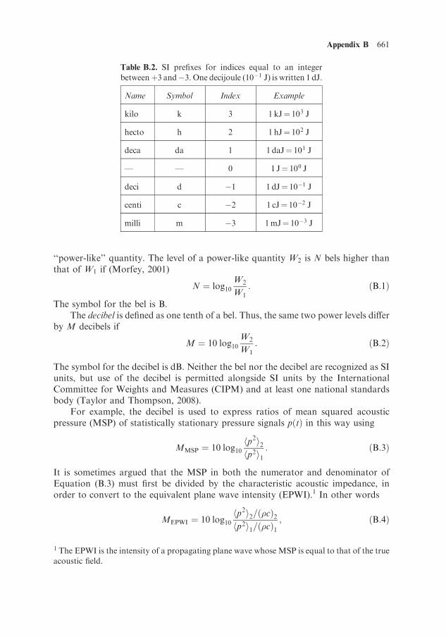
‘‘power-like’’ quantity. The level of a power-like quantity W2 is N bels higher thanthat of W1 if (Morfey, 2001)

N ¼ log10W2

W1

: ðB:1Þ

The symbol for the bel is B.The decibel is defined as one tenth of a bel. Thus, the same two power levels differ

by M decibels if

M ¼ 10 log10W2

W1

: ðB:2Þ

The symbol for the decibel is dB. Neither the bel nor the decibel are recognized as SIunits, but use of the decibel is permitted alongside SI units by the InternationalCommittee for Weights and Measures (CIPM) and at least one national standardsbody (Taylor and Thompson, 2008).

For example, the decibel is used to express ratios of mean squared acousticpressure (MSP) of statistically stationary pressure signals pðtÞ in this way using

MMSP ¼ 10 log10hp2i2hp2i1

: ðB:3Þ

It is sometimes argued that the MSP in both the numerator and denominator ofEquation (B.3) must first be divided by the characteristic acoustic impedance, inorder to convert to the equivalent plane wave intensity (EPWI).1 In other words

MEPWI ¼ 10 log10hp2i2=ð�cÞ2hp2i1=ð�cÞ1

; ðB:4Þ

Appendix B 661

Table B.2. SI prefixes for indices equal to an integer

betweenþ3 and�3. One decijoule (10�1 J) is written 1 dJ.

Name Symbol Index Example

kilo k 3 1 kJ¼ 103 J

hecto h 2 1 hJ¼ 102 J

deca da 1 1 daJ¼ 101 J

— — 0 1 J¼ 100 J

deci d �1 1 dJ¼ 10�1 J

centi c �2 1 cJ¼ 10�2 J

milli m �3 1mJ¼ 10�3 J

1 The EPWI is the intensity of a propagating plane wave whose MSP is equal to that of the true

acoustic field.

Table B.3. Frequently encountered non-SI units (in alphabetical order).

Unit Symbol SI equivalent Notes

atmosphere See standard atmosphere

bar bar 100 kPa 1Pa¼ 1N/m2

dyne dyn 10 mN 1dyn¼ 1 g cm/s2; 1N¼ 1 kg m/s2

dyne per square centimeter dyn/cm2 0.1 Pa

erg erg 0.1 mJ 1 erg¼ 1 dyn cm; 1 J¼ 1Nm

erg per square centimeter erg/cm2 1mJ/m2

fathom 1.8288m 1 fathom¼ 6 ft (international fathom)

foot ft 304.8mm

hour h 3600 s

inch in 25.4mm 1 ft¼ 12 in. The capacity of air guns (see Chapter

10) is sometimes expressed in cubic inches

(1 in3 � 16:39 cm3)

international nautical mile nmi 1.852 km There is no internationally recognized symbol or

abbreviation for this unit. The abbreviation

‘‘nmi’’ is adopted (preferred over ‘‘nm’’ to avoid

a conflict with the SI symbol for a nanometer)

knot kn (1852/3600)m/s The knot is defined as one nautical mile per hour

� 0.5144m/s (1 nmi/h), such that 9 kn¼ 4.63m/s, exactly

liter L 1000 cm3 The uppercase ‘‘L’’ is preferred to the alternative

(lowercase) letter ‘‘l’’ to avoid possible confusion

with the number ‘‘1’’

microbar mbar 0.1 Pa 1 mbar¼ 10�6 bar

millimeter per hour mm/h 1mm/(3600 s) Used as a unit of rainfall rate

�0.2778 mm/s

MKS rayl See rayl

nautical mile See international nautical mile

poise 0.1 Pa s 1 poise¼ 1 dyn s/cm2

pound-force per square inch psi �6.895 kPa

rayl dyn s/cm2 10 Pa s/m One pascal second per meter (1 Pa s/m) is

sometimes known as an ‘‘MKS rayl’’. The rayl is

not an SI unit.

standard atmosphere 101.325 kPa Pressure under standard conditions of

temperature and pressure, denoted PSTP (see

Section 14.2.2)

yard yd 0.9144m 1 yd¼ 3 ft

where ð�cÞn is the characteristic impedance at the measurement location indicated bythe value of the subscript n. Often the impedance is the same at locations 1 and 2, inwhich case Equations (B.3) and (B.4) are equivalent. In all other cases it is importantto state which of the two is being used. Throughout this book the convention ofEquation (B.3) (MSP ratio) is adopted, partly to conform to the de facto definition ofpropagation loss used in underwater acoustics, which since 1980 omits the impedanceratio (Ainslie and Morfey, 2005) and partly to avoid the ambiguities associated withthe EPWI definition in the absence of an agreed standard reference value for theimpedance (Ainslie, 2004, 2008).

Absolute levels. It is common practice to specify absolute power levels by re-placing the denominator W1 in Equation (B.2) with an agreed standard referencevalue. Thus, a power W may be expressed as an absolute level by defining the powerlevel LW in decibels, relative to a reference value Wref , as

LW 10 log10W

Wref

: ðB:5Þ

When the decibel is used in this way, to avoid ambiguity both the reference value andthe nature of the quantity W (in this case power) must be stated. Internationallyaccepted reference values for power and energy levels are 1 pW and 1 pJ, respectively.For example, a sound source of acoustic power (one watt) has a power level of10 log10ð1=10�12Þ ¼ 120 dB re pW.2

The sound pressure level Lp is defined in terms of the MSP (Morfey, 2001)

Lp 10 log10hp2ip2ref

; ðB:6Þ

where the reference pressure pref is equal to 1 mPa, making the MSP reference valueequal to 1 mPa2. Thus, the sound pressure level of an acoustic field whose RMSpressure is one pascal (MSP¼ 1 Pa2) is 10 log10ð1=10�12Þ ¼ 120 dB re mPa2. The samequantity is often written 120 dB re mPa. The squared unit is adopted here to avoidinconsistencies that otherwise arise when this quantity is combined with other ratiosin decibels.3 For example, it seems more natural to express the spectral density level indB re mPa2/Hz than in dB re mPa/

ffiffiffiffiffiffiffiHz

p.

Other physical parameters relevant to acoustics are energy density and intensity.When expressed as levels, their standard reference values are, respectively, 1 pJ/m2

and 1 pW/m2 (Morfey, 2001). When used in a spectral density, the reference unit forfrequency is one hertz. For example, the power spectral density level has the unitdB reW/Hz.

Appendix B 663

2 Or, equivalently, 120 dB re 1 pW.3 It is p2ref and not pref that appears in the denominator of Equation (B.6).

B.1.3.1.2 pH (acidity measure)

The pH of a solution is a logarithmic measure of the reciprocal concentration ofhydrogen ions dissolved in the solution.

pH ¼ �log10½Hþ�; ðB:7Þ

where ½Hþ� denotes the molar concentration of hydrogen (Hþ) ions. The precisedefinition depends on convention. For example, it might include only the concentra-tion of free protons (the free proton scale) or might also include that of protonsassociated with other ions.

Chapter 4 mentions four different pH scales: the U.S. National Bureau ofStandards4 scale ( pHNBS), the ‘‘seawater scale’’ ( pNSWS), the ‘‘total proton scale’’( pHT), and the ‘‘free proton scale’’ ( pHF). As there is no single universally adoptedconvention, a choice is necessary between these. The NBS scale is considered un-suitable for modern use in seawater (Brewer et al., 1995; Millero, 2006). The otherthree are defined below (following Millero, 2006).

The free proton scale is given by

pHF �log10½Hþ�F; ðB:8Þ

where the notation ½X� indicates the concentration of ion X, defined as the number ofmoles of that ion per kilogram of solution. Thus, ½Hþ�F is the concentration of freehydrogen ions in units of moles per kilogram (Brewer et al., 1995).

The total proton scale is given by

pHT �log10½Hþ�T; ðB:9Þ

where ½Hþ�T includes hydrogen sulfate ions

½Hþ�T ¼ ½Hþ�F þ ½HSO�4 �: ðB:10Þ

Finally, the SWS scale, recommended by UNESCO for use in seawater (Dickson andMillero, 1987), also includes the concentration of hydrogen associated with fluorideions. Thus

pHSWS �log10½Hþ�SWS; ðB:11Þwhere

½Hþ�SWS ¼ ½Hþ�T þ ½HF�: ðB:12Þ

B.1.3.1.3 Decade

The decade is a logarithmic unit of frequency ratio. The frequency f2 is N decadeshigher than f1 if (Pierce, 1989)

N ¼ log10f2f1: ðB:13Þ

IfN is negative then it is more conventional to say that f2 is jNj decades lower than f1.

664 Appendix B

4 Now the National Institute of Standards and Technology (NIST).

B.1.3.2 Base-e logarithmic unit (neper)

The neper is a logarithmic unit of amplitude ratio. Consider a sinusoidal oscillation ofamplitude A2. The amplitude level of this oscillation is N nepers higher than that ofanother of amplitude A1 if (Morfey, 2001)

N ¼ logeA2

A1

: ðB:14Þ

The symbol for the neper is Np.A change in amplitude level of 1Np is associated with a change in power level of

20 log10 e decibels. However, it is not correct to say that 1Np is equal to 20 log10 edecibels unless the neper is redefined in terms of (the square root of ) a power ratio(Mills and Morfey, 2005).

B.1.3.3 Base-2 logarithmic units

B.1.3.3.1 Octave

The octave is a logarithmic unit of frequency ratio. The frequency f2 is N octaveshigher than f1 if (Pierce, 1989)

N ¼ log2f2f1: ðB:15Þ

If N is negative then it is more conventional to say that f2 is jNj octaves lower than f1.

B.1.3.3.2 Phi

The phi unit is a logarithmic unit of reciprocal grain diameter. A spherical sedimentgrain of diameter5 d has a grain size of N phi units if (Krumbein and Sloss, 1963)

N ¼ �log2d

dref; ðB:16Þ

where the reference diameter is

dref 1 mm: ðB:17ÞThe symbol for the phi unit is �. For example, if d ¼ 0.25mm, the grain sizeexpressed in phi units is written 2�.

B.2 NOMENCLATURE

B.2.1 Notation

A concerted effort has been made to employ a consistent notation throughout thisbook. While there is no separate list of symbols, the notation used is defined as and

Appendix B 665

5 The ‘‘diameter’’ of non-spherical grains is defined implicitly in terms of the mesh sizes of

sieves able to separate them.

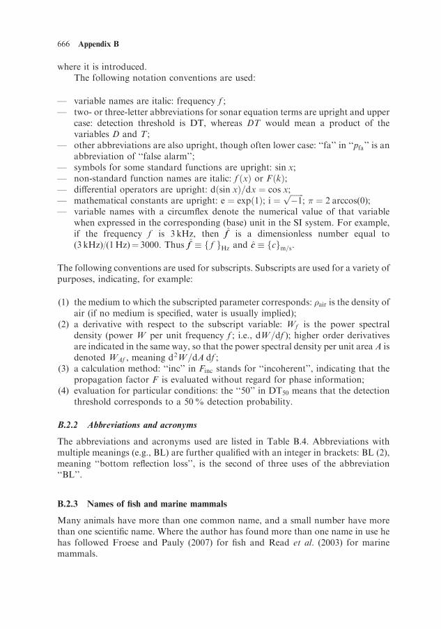
where it is introduced.The following notation conventions are used:

— variable names are italic: frequency f ;— two- or three-letter abbreviations for sonar equation terms are upright and upper

case: detection threshold is DT, whereas DT would mean a product of thevariables D and T ;

— other abbreviations are also upright, though often lower case: ‘‘fa’’ in ‘‘pfa’’ is anabbreviation of ‘‘false alarm’’;

— symbols for some standard functions are upright: sin x;— non-standard function names are italic: f ðxÞ or FðkÞ;— differential operators are upright: dðsin xÞ=dx ¼ cos x;— mathematical constants are upright: e ¼ expð1Þ; i ¼

ffiffiffiffiffiffiffi�1

p; � ¼ 2 arccos(0);

— variable names with a circumflex denote the numerical value of that variablewhen expressed in the corresponding (base) unit in the SI system. For example,if the frequency f is 3 kHz, then ff is a dimensionless number equal to(3 kHz)/(1Hz)¼ 3000. Thus ff f f gHz and cc fcgm=s.

The following conventions are used for subscripts. Subscripts are used for a variety ofpurposes, indicating, for example:

(1) the medium to which the subscripted parameter corresponds: �air is the density ofair (if no medium is specified, water is usually implied);

(2) a derivative with respect to the subscript variable: Wf is the power spectraldensity (power W per unit frequency f ; i.e., dW=df ); higher order derivativesare indicated in the same way, so that the power spectral density per unit area A isdenoted WAf , meaning d2W=dA df ;

(3) a calculation method: ‘‘inc’’ in Finc stands for ‘‘incoherent’’, indicating that thepropagation factor F is evaluated without regard for phase information;

(4) evaluation for particular conditions: the ‘‘50’’ in DT50 means that the detectionthreshold corresponds to a 50% detection probability.

B.2.2 Abbreviations and acronyms

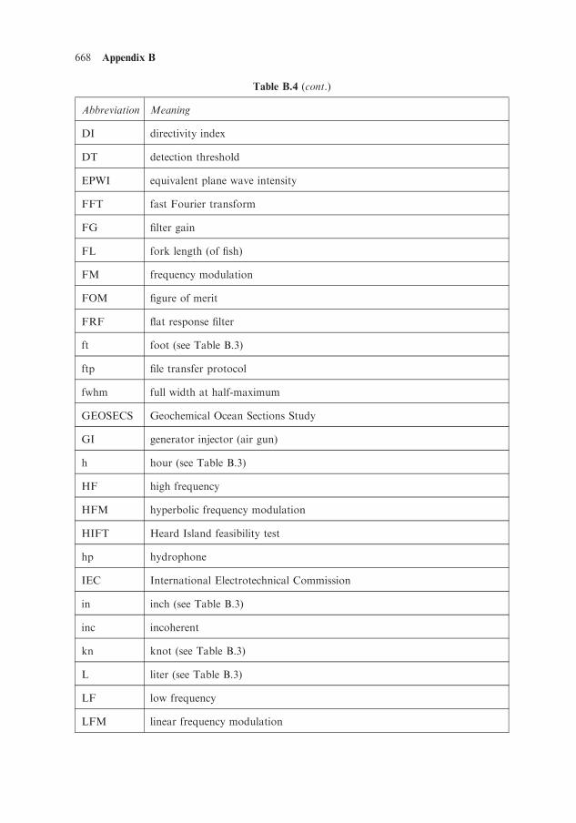
The abbreviations and acronyms used are listed in Table B.4. Abbreviations withmultiple meanings (e.g., BL) are further qualified with an integer in brackets: BL (2),meaning ‘‘bottom reflection loss’’, is the second of three uses of the abbreviation‘‘BL’’.

B.2.3 Names of fish and marine mammals

Many animals have more than one common name, and a small number have morethan one scientific name. Where the author has found more than one name in use hehas followed Froese and Pauly (2007) for fish and Read et al. (2003) for marinemammals.

666 Appendix B

Appendix B 667

Table B.4. List of abbreviations and acronyms, and their meanings.

Abbreviation Meaning

AG array gain

ANSI American National Standards Institute

APL Applied Physics Laboratory (University of Washington)

arr array

atm atmospheric

ATOC acoustic thermometry of ocean climate

BB broadband

BBS bottom backscattering strength

BIPM Bureau International des Poids et Mesures (International Bureau of

Weights and Measures)

BL (1) background level

BL (2) bottom reflection loss

BL (3) bottom reflected (path)

BR bottom refracted (path)

BSS bottom scattering strength

BSX backscattering cross-section

BW the quantity BW ¼ 10 log10 BB, where BB is the numerical value of the

bandwidth in hertz

CIPM Comite International des Poids et Mesures (International Committee for

Weights and Measures)

coh coherent

CS column strength

CW continuous wave

dB decibel (see Section B.1.3)

deg degree (angle)

DFT discrete Fourier transform

(continued)

668 Appendix B

Table B.4 (cont.)


DI directivity index

DT detection threshold

EPWI equivalent plane wave intensity

FFT fast Fourier transform

FG filter gain

FL fork length (of fish)

FM frequency modulation

FOM figure of merit

FRF flat response filter

ft foot (see Table B.3)

ftp file transfer protocol

fwhm full width at half-maximum

GEOSECS Geochemical Ocean Sections Study

GI generator injector (air gun)

h hour (see Table B.3)

HF high frequency

HFM hyperbolic frequency modulation

HIFT Heard Island feasibility test

hp hydrophone

IEC International Electrotechnical Commission

in inch (see Table B.3)

inc incoherent

kn knot (see Table B.3)

L liter (see Table B.3)

LF low frequency

LFM linear frequency modulation

Appendix B 669


LPM linear period modulation

MKS meter kilogram second system of units (predecessor to SI)

MSP mean square (acoustic) pressure

NB narrowband

NBS National Bureau of Standards (now NIST)

NIST National Institute of Standards and Technology

NL noise level

nmi international nautical mile (see Table B.3)

Np neper (see Section B.1.3)

pdf (1) probability density function

pdf (2) portable document format

peRMS peak equivalent RMS

PG processing gain

pH logarithmic measure of acidity (see Section B.1.3)

PL propagation loss

p-p peak to peak

psi pound-force per square inch (see Table B.3)

RAFOS ‘‘SOFAR’’ spelt backwards

RL reverberation level

RMS root mean square

ROC receiver operating characteristic

Rx receiver

SBR signal to background ratio

SBS surface backscattering strength

SE signal excess

(continued)

670 Appendix B

Table B.4 (cont.)


SI Systeme Internationale d’Unites (International System of Units)

SL (1) source level

SL (2) surface reflection loss

SL (3) standard length (of fish)

SNR signal to noise ratio

SOFAR sound fixing and ranging

SPL sound pressure level

SRR signal to reverberation ratio

SSS surface scattering strength

stat static

STP standard temperature and pressure; note: at STP the temperature and

pressure are YSTP ¼ 273:15 K and PSTP ¼ 101:325 kPa (one standard

atmosphere), respectively

SWS seawater scale (of pH)

tgt target

tot total

TL total length (of fish)

TPL total path loss

TS target strength, the quantity TS ¼ 10 log10��back

4�, where ��back is the

backscattering cross-section in square meters

Tx transmitter

UNESCO United Nations Educational, Scientific and Cultural Organization

VBS volume backscattering strength

vs. versus

WMO World Meteorological Organization

WS wake strength

B.3 REFERENCES

Ainslie, M. A. (2004) The sonar equation and the definitions of propagation loss, J. Acoust.

Soc. Am., 115, 131–134.

Ainslie, M. A. (2008) The sonar equations: Definitions and units of individual terms, Acoustics

’08, Paris, June 29–July 4, 2008, pp. 119–124. This article is missing from the search index

of the CD version of the Acoustics ’08 Proceedings. The paper can be located on the CD

by means of its identification number (475), at /data/articles/2008/000475.pdf It is also

available at http://intellagence.eu.com/acoustics2008/acoustics2008/cd1 (last accessed

April 12, 2010).

Ainslie, M. A. and Morfey, C. L. (2005) ‘‘Transmission loss’’ and ‘‘propagation loss’’ in

undersea acoustics, J. Acoust. Soc. Am., 118, 603–604.

Anon. (2008) The Little Big Book of Metrology, National Physical Laboratory, Teddington,

U.K.

bipm (www) The International System of Units (SI), Bureau International des Poids et Mesures,

available at http://www.bipm.org/en/si (last accessed September 21, 2008).

Brewer, P. G., Glover, D. M., Goyet, C., and Shafer, D. K. (1995) The pH of the North

Atlantic Ocean: Improvements to the global model of sound absorption, J. Geophysical

Res., 100(C5), 8761–8776.

Crocker, M. J. (Ed.) (1997) Encyclopedia of Acoustics, Wiley, New York.

Dickson, A. G. and Millero, F. J. (1987) A comparison of the equilibrium constants for the

dissociation of carbonic acid in sea water media, Annex 3 of Thermodynamics of the

Carbon Dioxide System in Seawater (report by the Carbon Dioxide Sub-panel of the Joint

Panel on Oceanographic Tables and Standards, Unesco Technical Papers in Marine

Science 51, Unesco, Paris.

Froese, R. and Pauly D. (Eds.), FishBase, version (01/2007), available at http://www.fishba-

se.org/search.php (last accessed March 23, 2009).

Jensen, F. B., Kuperman, W. A., Porter, M. B., and Schmidt, H. (1994) Computational Ocean

Acoustics, AIP Press, New York.

Krumbein, W. C. and Sloss, L. L. (1963) Stratigraphy and Sedimentation (Second Edition),

Freeman, San Francisco.

Kuperman, W. A. and Roux, P. (2007) Underwater Acoustics, in T. D. Rossing (Ed.), Springer

Handbook of Acoustics (pp. 149–204), Springer Verlag, New York.

Appendix B 671


WW1 First World War

WW2 Second World War

yd yard (see Table B.3)

z-p zero to peak

Kuperman, W. A. (1997) Propagation of sound in the ocean, in M. J. Crocker (Ed.), Ency-

clopedia of Acoustics (pp. 391–408), Wiley, New York.

Millero, F. J. (2006) Chemical Oceanography (Third Edition), CRC/Taylor & Francis.

Mills, I. and Morfey, C. L. (2005). On logarithmic ratio quantities and their units, Metrologia,

42, 246–252.

Morfey, C. L. (2001) Dictionary of Acoustics, Academic Press, San Diego, CA.

Pierce, A. D. (1989) Acoustics: An Introduction to its Physical Principles and Applications,

American Institute of Physics, New York.

Read, A. J., Halpin, P. N., Crowder, L. B., Hyrenbach, K. D., Best, B. D., and Freeman S. A.

(Eds.) (2003) OBIS-SEAMAP: Mapping Marine Mammals, Birds and Turtles, World

Wide Web electronic publication, available at http://seamap.env.duke.edu/species (last

accessed October 22, 2009).

Rossing, T. D. (Ed.) (2007) Springer Handbook of Acoustics, Springer Verlag, New York.

Rowlett (www) R. Rowlett, A Dictionary of Units, available at http://www.unc.edu/�rowlett/

units/ (last accessed April 2, 2007).

Taylor, B. N. and Thompson, A. (2008) The International System of Units (SI) (NIST Special

Publication 330, 2008 Edition), U.S. Department of Commerce, National Institute of

Standards & Technology.

672 Appendix B

Appendix C

Fish and their swimbladders

C.1 TABLES OF FISH AND BLADDER TYPES

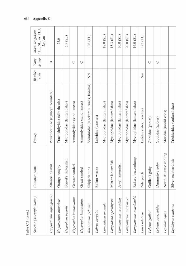
The scattering properties of fish generally are sensitive to the presence or absence of agas enclosure, or ‘‘swimbladder’’. The main purpose of this appendix is to enable thereader to assess the likelihood that a particular order, family, or species of fish isequipped with such a bladder, and where a bladder is present to provide furtherinformation about its relevant properties. General rules are described in Table C.3(by order) and Table C.4 (by family). Where known to the author, information aboutfish length is also provided.

Table C.7 presents a long list of information by individual species, but despite itslength it is not a complete list. In fact it is not even close to complete. Rather, itcomprises relevant information collected by the author over a number of years.Regardless of its shortcomings, its existence at all owes itself partly to David Weston,who impressed upon the author the importance of bladdered fish in underwateracoustics, and partly to FishBase (Froese and Pauly, 2007), from which much ofthe information is gleaned.

Table C.1 describes abbreviations used to describe types of fish in terms ofwhether or not a bladder is present, and if so whether a duct is present connectingit to the gut of the fish (in which case the fish is known as a physostome) or not (aphysoclist). The shape of the bladder varies between different species.

Each time the bladder code is used, it is accompanied by a lower case suffixindicating the source of the information, and these suffixes are listed in Table C.2. Forexample, ‘‘Sw’’ means that the fish is a physostome according to Whitehead andBaxter (1989), whereas ‘‘Nb’’ means that it has no swimbladder according to Froeseand Pauly (2007).

Two more keys are presented below to aid the interpretation of the main list ofspecies in Table C.7. The first (Table C.5) describes a list of categories, referred tohere as ‘‘Yang groups’’, which describe the likely behavior of the fish. The groups are

used by Yang (1982) to describe the relative ‘‘catchability’’ of the different species forhis population estimates. The reason they are useful here is that catchability isinfluenced by the fish’s behavior which in turn affects its likely acoustical properties,its environment, or both. For example, groups B and C are demersal fish, whichmeans that their properties are easily confused with (and might be affected by) theproperties of the seabed. The other groups are pelagic. For Yang’s group C, the terms‘‘sandeels’’ and ‘‘gobies’’ are interpreted here, respectively, as Ammodytidae andGobidae.

The second key (Table C.6) defines the abbreviations used to describe the fishlength information (last column of Table C.7).

674 Appendix C

Table C.1. Bladder presence and type key used in Tables C.3, C.4, and C.7.

Bladder code Means

J Bladder missing in adults ( juveniles physoclist or physostome)

L Physoclist

M With bladder (bladder sometimes partly or completely filled with fat;

uncertain air fraction)a

N No bladder

P With bladder (physoclist or physostome)

S Physostome

a The ‘‘M’’ stands for ‘‘Myctophidae’’, a family representative of this category.

Table C.2. Reference key.

Reference code Means

b Froese and Pauly (2007)

e Egloff (2006)

f Foote (1997)

i Iversen (1967)

k Kitajima et al. (1985)

m Simmonds and MacLennan (2005)

r Bertrand et al. (1999)

w Whitehead and Baxter (1989)

Table C.3. Bladder type by order for ray-finned fishes (Actinopterygii). See Tables C.1 and C.2 for bladder and

reference codes used in the last column.

Order Families Bladder Relevant extract

present

(bladder

code)

Anguilliformes Anguillidae, Chlopsidae, Colocongridae, Yes (Sb) ‘‘Swim bladder present, duct

Congridae, Derichthyidae, usually present’’

Heterenchelyidae, Moringuidae,

Muraenesocidae, Muraenidae,

Myrocongridae, Nemichthyidae,

Nettastomatidae, Ophichthidae,

Serrivomeridae, Synaphobranchidae

Clupeiformes Chirocentridae, Clupeidae, Denticipitidae, Yes (Sw) ‘‘Clupeoids . . . are physostomesEngraulidae, Pristigasteridae with one, or often two, ducts

between the swimbladder and

the exterior: a pneumatic duct

from the stomach, and an anal

duct to the ‘cloaca’,’’ p. 300.

‘‘[Pneumatic duct] is invariably

present,’’ p. 346

Gadiformes Bregmacerotidae, Euclichthyidae, Yes (Lb) ‘‘Swim bladder without

Gadidae, Lotidae, Merluccidae, Moridae, pneumatic duct’’

Muranolepididae, Phycidae

Gadiformes Macrouridae, genus Squalogadus No (Nb) ‘‘The swim bladder is absent in

Melanomus and Squalogadus’’

Gadiformes Melanonidae No (Nb ) ‘‘The swim bladder is absent in

Melanomus and Squalogadus’’

Myctophiformes Myctophidae Yes (Mb) ‘‘Swim bladder usually present’’

Myctophiformes Neoscopelidae, genus Scopelengys No (Nb) ‘‘Swim bladder present in all

but Scopelengys’’

Myctophiformes Neoscopelidae, except Scopelengys Yes (Mb) ‘‘Swim bladder present in all

but Scopelengys’’

Notacanthiformes Halosauridae, Notacanthidae Yes (Pb) ‘‘Swim bladder present’’

Perciformes Sciaenidae Yes (Pb) ‘‘Swim bladder usually having

many branches and used as a

resonating chamber’’

Perciformes Ammodytidae No (Nb) ‘‘No swim bladder’’

Pleuronectiformes Achiridae, Achiropsettidae, Bothidae, Only in ‘‘Adults almost always without

Citharidae, Cynoglossidae, juveniles swim bladder’’

Paralichthyidae, Pleuronectidae, (Jb)

Psettodidae, Samaridae, Scophthalmidae,

Soleidae

Table C.4. Bladder type by family; see Table C.3 for details.

Family Order Bladder code

Achiridae Pleuronectiformes Jb

Achiropsettidae Pleuronectiformes Jb

Ammodytidae Perciformes Nb

Anguillidae Anguilliformes Sb

Bothidae Pleuronectiformes Jb

Bregmacerotidae Gadiformes Lb

Chirocentridae Clupeiformes Sw

Chlopsidae Anguilliformes Sb

Citharidae Pleuronectiformes Jb

Clupeidae Clupeiformes Sw

Colocongridae Anguilliformes Sb

Congridae Anguilliformes Sb

Cynoglossidae Pleuronectiformes Jb

Denticipitidae Clupeiformes Sw

Derichthyidae Anguilliformes Sb

Engraulidae Clupeiformes Sw

Euclichthyidae Gadiformes Lb

Gadidae Gadiformes Lb

Halosauridae Notacanthiformes Pb

Heterenchelyidae Anguilliformes Sb

Lotidae Gadiformes Lb

Macrouridae, genus Squalogadus Gadiformes Nb

Melanonidae Gadiformes Nb

Merluccidae Gadiformes Lb

Moridae Gadiformes Lb

Moringuidae Anguilliformes Sb

Muraenesocidae Anguilliformes Sb

Muraenidae Anguilliformes Sb

Muranolepididae Gadiformes Lb

Myctophidae Myctophiformes Mb

Myrocongridae Anguilliformes Sb

Nemichthyidae Anguilliformes Sb

Neoscopelidae, except Scopelengys Myctophiformes Mb

Neoscopelidae, genus Scopelengys Myctophiformes Nb

Nettastomatidae Anguilliformes Sb

Notacanthidae Notacanthiformes Pb

Table C.5. ‘‘Catchability’’ key

(Yang groups) used in Table

C.7.

Yang group Means

A Cod-like

B Flatfish

C Eels

D Herring-like

E Mackerel-like

Table C.6. Length key used in Table C.7.

Length code Name Description

FL Fork length Distance from tip of snout to end of middle caudal rays

(Froese and Pauly, 2007)

SL Standard length Distance from tip of snout to end of vertebral column

(roughly the start of the caudal fin) (Froese and Pauly,

2007)

TL Total length Distance from tip of snout to end of caudal fin (Froese

and Pauly, 2007)

L50 — The length at which 50% of females have reached sexual

maturity (Knijn et al., 1993)

Table C.4. (cont.)

Family Order Bladder code

Ophichthidae Anguilliformes Sb

Paralychthyidae Pleuronectiformes Jb

Pleuronectidae Pleuronectiformes Jb

Phycidae Gadiformes Lb

Pristigasteridae Clupeiformes Sw

Psettodidae Pleuronectiformes Jb

Samaridae Pleuronectiformes Jb

Sciaenidae Perciformes Pb

Scophthalmidae Pleuronectiformes Jb

Serrivomeridae Anguilliformes Sb

Soleidae Pleuronectiformes Jb

Synaphobranchidae Anguilliformes Sb

678 Appendix C

TableC.7.Fishandtheirbladders,sortedbyscientificname.Keys:forbladdercodeseeTablesC.1andC.2;forYanggroupseeTableC.5.

MaximumlengthisfromFroeseandPauly(2007)(seeTableC.6);L50isfromKnijnet

al.(1993).

Species(scientificname)

Commonname

Family

Bladder

Yang

Max.length/cm

code

group

(TL,SL,orFL);

L50/cm

Acantholabruspalloni

Scale-rayedwrasse

Labridae(wrasses)

25.0(TL)

Acipensersturio

Sturgeon

Acipenseridae(sturgeons)

500(TL)

Agonuscataphractus

Hooknose

Agonidae(poachers)

B21.0(TL)

Alosa

pseudoharengus

Alewife

Clupeidae(herrings,shads,sardines,

Sm

40.0(SL)

menhadens)

Ammodytesmarinus

Lessersand-eel

Ammodytidae(sandlances)

C25.0(TL)

Ammodytestobianus

Smallsand-eel


C20.0(SL)

Anarhichasdenticulatus

Northernwolffish

Anarhichadidae(wolf-fishes)

180(TL)

Anarhichaslupus

Wolf-fish


A150(TL)

Anarhichasminor

spottedwolffish


180(TL)

Anguilla

anguilla

Europeaneel

Anguillidae(freshwatereels)

133(TL)

Anisarchusmedius

Stouteelblenny

Stichaeidae(pricklebacks)

30.0(TL)

Anoplogaster

cornuta

Commonfangtooth

Anoplogastridae

15.2(SL)

Antimora

rostrata

Bluehake

Moridae(moridcods)

Aphanopuscarbo

Blackscabbardfish

Trichiuridae(cutlassfishes)

110(SL)

Aphia

minuta

Transparentgoby

Gobiidae(gobies)

C7.9(TL)

Arctogadusglacialis

Arcticcod

Gadidae(codsandhaddocks)

32.5(TL)

Appendix C 679Argentinasilus

Greaterargentine

Argentinidae(argentinesorherring

Lm

D70.0

smelts)

Argentinasphyraena

Argentine

Argentinidae(argentinesorherring

D

smelts)

Argyropelecushem

igymnus

Half-nakedhatchetfish

Sternoptychidae

3.9(SL)

Argyropelecusolfersii

Hatchet-fish

Sternoptychidae

ArgyrosomushololepidotusMadagascarmeagre

Sciaenidae(drumsorcroakers)

Le

200(TL)

Argyrosomusregius

Meagre


Arnoglossuslaterna

Scaldfish

Bothidae(lefteyeflounders)

B25.0(SL)

Artediellusatlanticus

Atlantichookearsculpin

Cottidae(sculpins)

15.0(SL)

Aspitrigla

cuculus

EastAtlanticredgurnard

Triglidae(sea-robins)

B50.0(TL)

Astronesthes

gem

mifer

Snaggletooth

Stomiidae(barbeleddragonfishes)

17.0(SL)

Belonebelone

Garpike

Belonidae(needlefishes)

Benthodesmuselongatus

Elongatefrostfish


100.0(TL)

Benthosemafibulatum

Spinycheeklanternfish

Myctophidae(lanternfishes)

10.0

Benthosemaglaciale

Glacierlanternfish


10.3(SL)

Benthosemapanamense

Lampfish


5.5

Benthosemapterotum

Skinnycheeklanternfish


7.0

Benthosemasuborbitale

Smallfinlanternfish


3.9(SL)

Beryxdecadactylus

Alfonsino

Berycidae(alfonsinos)

(continued)

680 Appendix C

TableC.7(cont.)


Commonname

Family

Bladder

Yang

Max.length/cm

code

group

(TL,SL,orFL);

L50/cm

Bolinichthysdistofax


9.0(SL)

Bolinichthysindicus

Lanternfish


4.5(SL)

Bolinichthyslongipes


5.0(SL)

Bolinichthysphotothorax


7.3(SL)

Bolinichthyssupralateralis


11.7(SL)

Boreogadussaida

Polarcod


Le

40.0(TL)

Bramabrama

Atlanticpomfret

Bramidae(breams)

D

Brevoortia

tyrannus

Atlanticmenhaden


50.0(TL)

menhadens)

Brosm

ebrosm

eTusk

Lotidae(hakesandburbots)

Buenia

jeffreysii

Jeffrey’sgoby

Gobiidae(gobies)

C

Buglossidium

luteum

Solenette

B

Caelorhinchuscaelorhinchus

Hollowsnoutgrenadier

Macrouridae(grenadiersorrattails)

Callionymuslyra

Dragonet

Callionymidae(dragonets)

B

Callionymusmaculatus

Spotteddragonet

Callionymidae(dragonets)

Centrolabrusexoletus

Rockcook

Labridae(wrasses)

Centrolophusniger

Blackfish

Centrolophidae

Appendix C 681Chelonlabrosus

Thicklipgreymullet

Mugilidae(mullets)

Chim

aeramonstrosa

Rabbitfish

Chimaeridae(shortnosechimaeras

A

orratfishes)

Chirolophisascanii

Yarrel’sblenny


Ciliata

mustela

Fivebeardrockling


Ciliata

septentrionalis

Northernrockling


Clupea

harengusharengus

Atlanticherring


Sfm

D45.0(SL);24(L50)

menhadens)

Clupea

harengusmem

bras

Balticherring


24.2(TL)

menhadens)

Clupea

pallasiipallasii

Pacificherring


46.0(TL)

menhadens)

Conger

conger

Europeanconger

Congridae(congerandgardeneels)

A300(TL)

Coregonusartedi

Cisco

Salmonidae(salmonids)

Sm

57.0(TL)

Coryphaenoides

arm

atus

Abyssalgrenadier


102(TL)

Coryphaenoides

rupestris

Roundnosegrenadier


110(TL)

Cottunculusmicrops

Polarsculpin

Psychrolutidae(fatheads)

30.0(SL)

Cottunculusthomsonii

Pallidsculpin

Psychrolutidae(fatheads)

35.0(SL)

Crystallogobiuslinearis

Crystalgoby

Gobiidae(gobies)

C

Ctenolabrusrupestris

Goldsinny-wrasse

Labridae(wrasses)

Cyclopteruslumpus

Lumpsucker

Cyclopteridae(lumpfishes)

A

(continued)

682 Appendix C

TableC.7(cont.)


Commonname

Family

Bladder

Yang

Max.length/cm

code

group

(TL,SL,orFL);

L50/cm

Cyclothonebraueri

Garrick

Gonostomatidae(bristlemouths)

3.8(SL)

Diaphustheta

Californianheadlightfish


11.4(TL)

Dicentrarchuslabrax

Europeanseabass

Moronidae(temperatebasses)

Le

103(TL)

Echiichthysvipera

Lesserweever

Trachinidae(weeverfishes)

B

Echiodondrummondii

Pearlfish

Carapidae(pearlfishes)

A

Enchelyopuscimbrius

Fourbeardrockling


A

Engraulisanchoita

Argentineanchoita

Engraulidae(anchovies)

17.0(SL)

Engraulisaustralis

Australiananchovy


15.0(SL)

Engraulisencrasicolus

Europeananchovy


20.0(SL)

Engrauliseurystole

Silveranchovy


15.5(TL)

Engraulisjaponicus

Japaneseanchovy


18.0(TL)

Engraulismordax

Californiananchovy


24.8(SL)

Engraulisringens

Anchoveta


Sm

20.0(SL)

Entelurusaequoreus

Snakepipefish

Sygnathidae(pipefishesandseahorses)

Etm

opterusspinax

Velvetbellylanternshark

Dalatiidae(sleepersharks)

A

Euthynnusaffinis

Kawaka

Scombridae(mackerels,tunas,bonitos)

Nbi

100.0(FL)

Euthynnusalleteratus

Littletunny


Nb

122(TL)

Appendix C 683Euthynnuslyneatus

Blackskipjack


Nb

84.0(FL)

Eutrigla

gurnardus

Greygurnard

Triglidae(sea-robins)

B60.0(TL);19L50

Gadiculusargenteus

Silverycod


15.0(TL)

argenteus

Gadiculusargenteusthori

Silverypout


D15.0(TL)

Gadusmorhua

cod


Lfm

A200(TL);70L50

Gaidropsarusvulgaris

Three-beardedrockling


A

Galeorhinusgaleus

Topeshark

Triakidae(houndsharks)

A

Gasterosteusaculeatus

Three-spinedstickleback

Gasterosteidae(sticklebacksand

Le

aculeatus

tubesnouts)

Glyptocephaluscynoglossus

Witch

Pleuronectidae(righteyeflounders)

B

Gobiusniger

Blackgoby

Gobiidae(gobies)

C

Gobiusculusflavescens

Two-spottedgoby

Gobiidae(gobies)

C

Gymnammodytes

Smoothsand-eel


C

semisquamatus

Gymnelusretrodorsalis

Auroraunernak

Zoarcidae(eelpouts)

14.0(TL)

Halargyreusjohnsonii

Slendercodling

Moridae(moridcods)

56.0(TL)

Helicolenusdactylopterus

Blackbellyrosefish

Sebastidae(rockfishes,rockcods,and

47.0(TL)

dactylopterus

thornyheads)

Hippocampusguttulatus

Long-snoutedseahorse

Syngnathidae(pipefishesandseahorses)

Le

16.0(TL)

Hippoglossoides

platessoides

Americanplaice


B82.0(TL);17L50

(continued)

684 Appendix C

TableC.7(cont.)


Commonname

Family

Bladder

Yang

Max.length/cm

code

group

(TL,SL,orFL);

L50/cm

Hippoglossushippoglossus

Atlantichalibut


B

Hoplostethusatlanticus

Orangeroughy

Trachichthyidae(slimeheads)

75.0

Hygophum

benoiti

Benoit’slanternfish


5.5(SL)

Hyperoplusim

maculatus

Greatersandeel


C

Hyperopluslanceolatus

Greatsandeel


C

Katsuwonuspelamis

Skipjacktuna


Nbi

108(FL)

Labrusbergylta

Ballanwrasse

Labridae(wrasses)

Lampadenaanomala


18.0(SL)

Lampadenaspeculigera

Mirrorlanternfish


15.3(SL)

Lampanyctuscrocodilus

Jewellanternfish


30.0(SL)

Lampanyctusintricarius


20.0(SL)

Lampanyctusmacdonaldi

Rakerybeaconlamp


16.0(SL)

Latesniloticus

Nileperch

Latidae(lates,perches)

Sm

193(TL)

Lebetusguilleti

Guillet’sgoby

Gobiidae(gobies)

C

Lebetusscorpioides

Diminutivegoby

Gobiidae(gobies)

C

Lepidioneques

NorthAtlanticcodling

Moridae(moridcods)

Lepidopuscaudatus

Silverscabbardfish


Appendix C 685Lepidorhombusboscii

Fourspottedmegrim

Scopthalmidae(turbots)

40.0(SL)

Lepidorhombuswhiffi

agonis

Megrim

Scopthalmidae(turbots)

B

Lesuerigobiusfriesii

Fries’sgoby

Gobiidae(gobies)

C

Lim

andalimanda

Dab


40.0(SL);12L50

Lophiuspiscatorius

Angler

Lophiidae(goosefishes)

A

Lumpenuslampretaeform

isSnakeblenny


A50.0(TL)

Lycenchelysalba

Zoarcidae(eelpouts)

26.7(SL)

Lycenchelysmuraena

Zoarcidae(eelpouts)

22.6(SL)

Lycenchelyssarsi

Sars’swolfeel

Zoarcidae(eelpouts)

Lycodes

esmarkii

Greatereelpout

Zoarcidae(eelpouts)

Lycodes

eudipleurostictus

Doublelineeelpout

Zoarcidae(eelpouts)

Lycodes

frigidus

Zoarcidae(eelpouts)

69.0(TL)

Lycodes

pallidus

Paleeelpout

Zoarcidae(eelpouts)

Lycodes

reticulatus

Arcticeelpout

Zoarcidae(eelpouts)

36.0(TL)

Lycodes

seminudus

Longeareelpout

Zoarcidae(eelpouts)

51.7(TL)

Lycodes

squamiventer

Scalebellyeelpout

Zoarcidae(eelpouts)

26.0(TL)

Lycodes

vahlii

Vahl’seelpout

Zoarcidae(eelpouts)

A

Lycodonusflagellicauda

Zoarcidae(eelpouts)

19.9(SL)

Macquarianovemaculeata

Australianbass

Percichthyidae(temperateperches)

Le

60.0(TL)

(continued)

686 Appendix C

TableC.7(cont.)


Commonname

Family

Bladder

Yang

Max.length/cm

code

group

(TL,SL,orFL);

L50/cm

Macrourusberglax

Onion-eyedgrenadier


Macruronusnovaezelandiae

Bluegrenadier

Merlucciidae(merluccidhakes)

120(TL)

Mallotusvillosus

Capelin

Osmeridae(smelts)

Lm

Maurolicusmuelleri

Pearlsides

Sternoptychidae

Melanogrammusaeglefinus

Haddock


Lem

A100.0(TL);30L50

Melanonusgracilis

Pelagiccod


18.7(SL)

Melanonuszugmayeri

Arrowtail


28(TL)

Merlangiusmerlangus

Whiting


A70.0(TL);20L50

Merlucciusalbidus

Offshorehake


40.0(TL)

Merlucciusaustralis

Southernhake


Lm

126(TL)

Merlucciusgayigayi

SouthPacifichake


Lm

87.0(TL)

Merlucciusgayiperuanus

Peruvianhake


68.0(TL)

Merlucciusmerluccius

Europeanhake


A

Merlucciusproductus

NorthPacifichake


Lm

91.0(TL)

Microchirusvariegatus

Thickbacksole

B

Microgadustomcod

Atlantictomcod


Le

38.0(TL)

Micromesistiusaustralis

Southernbluewhiting


Lm

90.0(TL)

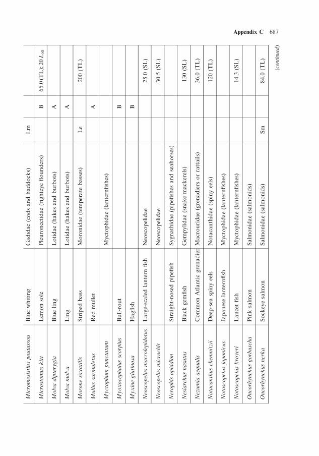
Appendix C 687Micromesistiuspoutassou

Bluewhiting


Lm

Microstomuskitt

Lemonsole


B65.0(TL);20L50

Molvadipterygia

Blueling


A

Molvamolva

Ling


A

Moronesaxatilis

Stripedbass

Moronidae(temperatebasses)

Le

200(TL)

Mullussurm

uletus

Redmullet

A

Myctophum

punctatum


Myoxocephalusscorpius

Bull-rout

B

Myxineglutinosa

Hagfish

B

Neoscopelusmacrolepidotus

Large-scaledlanternfish

Neoscopelidae

25.0(SL)

Neoscopelusmicrochir

Neoscopelidae

30.5(SL)

Nerophisophidion

Straight-nosedpipefish


Nesiarchusnasutus

Blackgemfish

Gempylidae(snakemackerels)

130(SL)

Nezumia

aequalis

CommonAtlanticgrenadierMacrouridae(grenadiersorrattails)

36.0(TL)

Notacanthuschem

nitzii

Deep-seaspinyeels

Notacanthidae(spinyeels)

120(TL)

Notoscopelusjaponicus

Japaneselanternfish


Notoscopeluskroyeri

Lancetfish


14.3(SL)

Oncorhynchusgorbuscha

Pinksalmon


Oncorhynchusnerka

Sockeyesalmon


Sm

84.0(TL)

(continued)

688 Appendix C

TableC.7(cont.)


Commonname

Family

Bladder

Yang

Max.length/cm

code

group

(TL,SL,orFL);

L50/cm

Onogadusargentatus

Arcticrockling


Onogadusensis


Orcynopsisunicolor

Plainbonito


Nb

130(FL)

Oryziaslatipes

Japanesericefish

Adrianichthyidae(ricefishes)

Le

4.0(TL)

Osm

erusmordaxdentus

Arcticrainbowsmelt

Osmeridae(smelts)

32.4(TL)

Osm

erusmordaxmordax

Atlanticrainbowsmelt

Osmeridae(smelts)

Sm

35.6(TL)

Pagrusmajor

Redseabream

Sparidae(porgies)

Pk

100.0(SL)

Perca

fluviatilis

Europeanperch

Percidae(perches)

Le

51.0(TL)

Pholisgunnellus

Rockgunnel

Pholidae

A25.0(SL)

Pholislaeta

Crescentgunnel

Pholidae

25.0(TL)

Phrynorhombusnorvegicus

Norwegian(topknot)

B

Phycisblennoides

Forkbeard


Pleuronectesplatessa

Europeanplaice


B100.0(SL);33L50

Pollachiuspollachius

Pollack


A

Pollachiusvirens

Pollock


Lm

A130(TL)

Pomatoschistusmicrops

Commongoby

Gobiidae(gobies)

C

Pomatoschistusminutus

Sandgoby

Gobiidae(gobies)

C

Appendix C 689Pomatoschistusnorvegicus

Norwaygoby

Gobiidae(gobies)

C

Pomatoschistuspictus

Paintedgoby

Gobiidae(gobies)

C

Protomyctophum

arcticum


Pterycombusbrama

Silverpomfret

Bramidae(breams)

40.0

Raja

batis

Skate

B

Raja

circularis

Sandyray

B

Raja

clavata

Roker

B

Raja

fullonica

Shagreenray

B

Raja

montagui

Spottedray

Rajidae(skates)

B80.0(TL)

Raja

naevus

Cuckooray

B

Raja

radiata

Starryray

B47L50

Ranicepsraninus

Tadpolefish


Pc

Rastrineobola

argentea

Silvercyprinid

Cyprinidae(minnowsorcarps)

Sm

9.0(SL)

Rhinonem

uscimbrius


Salm

osalar

Atlanticsalmon

Salmonidae(salmons,trouts)

150(TL)

Salm

otruttatrutta

Seatrout


140(SL)

Salvelinusalpinus

Charr


Sardaaustralis

Australianbonito


Nb

180(FL)

Sardachiliensischiliensis

EasternPacificbonito


Nb

102(TL)

(continued)

690 Appendix C

TableC.7(cont.)


Commonname

Family

Bladder

Yang

Max.length/cm

code

group

(TL,SL,orFL);

L50/cm

Sardachiliensislineolata

Pacificbonito


102(FL)

Sardaorientalis

Stripedbonito


Nb

102(FL)

Sardasarda

Atlanticbonito


Nb

91.4(FL)

Sardinapilchardus

Europeanpilchard


25.0(SL)

menhadens)

Sardinopssagax

SouthAmericanpilchard


Sm

39.5(SL)

menhadens)

Sciaenopsocellatus

Reddrum


155(TL)

Scomber

japonicus

Chubmackerel


64.0(TL)

Scomber

scombrus

Atlanticmackerel


Nf

E60.0(FL);30L50

Scomberesoxsaurus

Skipper

Scomberesicidae(sauries)

Scopelengystristis

Pacificblackchin

Neoscopelidae

Nb

20.0(SL)

Scopthalm

usmaxim

us

Turbot

B

Scopthalm

usrhombus

Brill

B

Sebastes

fasciatus

Acadianredfish


30.0(TL)

thornyheads)

Sebastes

marinus

Oceanperch


Lm

A100.0(TL)

thornyheads)

Appendix C 691

Sebastes

mentella

Deepwaterredfish


55.0(TL)

thornyheads)

Sebastes

schlegelii


Sm

65.0(TL)

thornyheads)

Sebastes

viviparus

Norwayhaddock


A

thornyheads)

Sillagociliata

Sandsillago

Sillaginidae(smelt-whitings)

Le

51.0(TL)

Soleasolea

Commonsole

Soleidae(soles)

B70.0;27L50

Sparusaurata

Giltheadseabream

Sparidae(porgies)

Le

70.0(TL)

Spinachia

spinachia

Fifteen-spinedstickleback

Gasterosteidae(sticklebacksand

tubesnouts)

Sprattussprattusbalticus

Balticsprat


16.0(TL)

menhadens)

Sprattussprattussprattus

Europeansprat


Sm

D16.0(SL);10L50

menhadens)

Squalusacanthias

Spurdog

A

SymbolophoruscaliforniensisBigfinlanternfish


11.0(SL)

Symphodusmelops

Labridae(wrasses)

Synaphobranchuskaupii

Kaup’sarrowtootheel

Synaphobranchidae(cut-throateels)

100.0(TL)

Syngnathusacus

Greaterpipefish


Taractes

asper

Roughpomfret

Bramidae(breams)

Theragra

chalcogramma

Walleyepollock

Lfm

(continued)

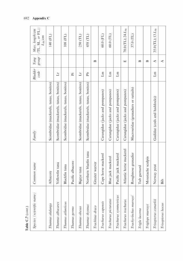
692 Appendix C

TableC.7(cont.)


Commonname

Family

Bladder

Yang

Max.length/cm

code

group

(TL,SL,orFL);

L50/cm

Thunnusalalunga

Albacore


140(FL)

Thunnusalbacares

Yellowfintuna


Lr

Thunnusatlanticus

Blackfintuna


108(FL)

Thunnusgermo

Pacificalbacore

Pi

Thunnusobesus

Bigeyetuna


Lr

250(TL)

Thunnusthynnus

Northernbluefintuna


Pb

458(TL)

Trachinusdraco

Greaterweever

B

Trachuruscapensis

Capehorsemackerel

Carangidae(jacksandpompanos)

Lm

60.0(FL)

Trachuruspicturatus

Bluejackmackerel


Lm

60.0(TL)

Trachurussymmetricus

Pacificjackmackerel


Lm

Trachurustrachurus

Atlantichorsemackerel


E70.0(TL);24L50

Trachyrinchusmurrayi

Roughnosegrenadier


37.0(TL)

Trigla

lucerna

Tubgurnard

B

Triglopsmurrayi

Moustachesculpin

B

Trisopterusesmarkii

Norwaypout


Lm

A35.0(TL);13L50

Trisopterusluscus

Bib

A

Appendix C 693

Trisopterusminutus

Poorcod


A

Urophycistenuis

Whitehake


Valenciennellus

Constellationfish

Sternoptychidae

3.1(SL)

tripunctulatus

Xiphiasgladius

Swordfish

Xyphiidae

Zeusfaber

Dory

A

C.2 REFERENCES

Bertrand, A., Josse, E., and Masse, J. (1999) In situ acoustic target-strength measurement of

bigeye (Thunnus obesus) and yellowfin tuna (Thunnus albacares) by coupling split-beam

echosounder observations and sonic tracking, ICES J. Marine Science, 56, 51–60.

Crocker, M. J. (Ed.) (1997) Encyclopedia of Acoustics, Wiley, New York.

Egloff, M. (2006) Failure of swim bladder inflation of perch, Perca fluviatilis L. found in

natural populations, Aquatic Sciences, 58(1), 15–23.

Foote, K. G. (1997) Target strength of fish, in M. J. Crocker (Ed.), Encyclopedia of Acoustics

(pp. 493–500), Wiley, New York.

Froese, R. and Pauly, D. (Eds.), FishBase, version (01/2007), available at http://www.

fishbase.org/search.php (last accessed March 23, 2009).

Iversen, R. T. B. (1967) Response of yellowfin tuna (Thunnus albacares) to underwater sound,

in W. N. Tavolga (Ed.), Marine Bio-acoustics (Vol. 2, pp. 105–121), Proceedings Second

Symposium on Marine Bio-Acoustics, American Museum of Natural History, New York,

Pergamon Press, Oxford, U.K.

Kitajima, C., Tsukashima, Y., and Tanaka, M. (1985) The voluminal changes of swim bladder

of larval red sea bream Pagrus major, Bull. Japanese Soc. Scientific Fisheries, 51, 759–764.

Knijn, R. J., Boon, T. W., Heessen, H. J. L., and Hislop, J. R. G. (1993) Atlas of North Sea

Fishes: Based on Bottom-trawl Survey Data for the Years 1985–1987 (ICES Cooperative

Research Report No. 194), International Council for the Exploration of the Sea,

Copenhagen, 1993.

Simmonds, E. J. andMacLennan D. N. (2005) Fisheries Acoustics (Second Edition), Blackwell,

Oxford, U.K.

Tavolga, W. N. (Ed.) (1967)Marine Bio-acoustics (Vol. 2), Proceedings Second Symposium on

Marine Bio-Acoustics, American Museum of Natural History, New York, Pergamon Press,

Oxford, U.K.

Whitehead, P. J. P. and Baxter, J. H. S. (1989) Swimbladder form in clupeoid fishes, Zoological

Journal of the Linnean Society, 97, 299–372.

Yang, J. (1982) An estimate of the fish biomass in the North Sea, J. Cons. int. Explor. Mer, 40,

161–172.

694 Appendix C

Index(bold indicates main entry)

absorption cross-section 245

see also extinction cross-section; scattering

cross-section

acidity see pH

acoustic deterrents 523, 524, 525, 632

acoustic intensity 32 ff, 56 ff, 95 ff, 209, 245,

417, 550, 663

acoustic power 31 ff, 37 ff, 56 ff, 80 ff, 97,

209, 245

acoustic pressure 31ff, 41, 58, 96 ff, 192 ff,

233ff, 430, 492, 525ff, 548 ff, 563ff,

661

see also pressure (RMS)

acoustic sensors

communications equipment 88 ff, 523,

526, 575, 599 ff, 632

echo sounder see echo sounder

fisheries sonar 5, 22, 519, 520, 575

minesweeping sonar 520, 522, 575

navigation sonar 22, 528, 575

oceanographic sensors 5, 22, 528, 575

search sonar 519, 522, 575

seismic survey sensors 534 ff, 575

sidescan sonar 515 ff, 575

acoustic waveguide 462

bottom duct 478, 483, 508

channel axis 21, 138, 462 ff, 496ff

convergence zone 474

cut-off frequency 449, 458, 472, 490

deep sound channel 148, 462

multipath propagation 308, 452, 525

SOFAR channel 20�21, 23surface duct 459ff, 462 ff, 471 ff, 478ff, 502

adiabatic pulsations (of air bubble) 230 ff,

240, 367

see also isothermal pulsations; polytropic

index

Airy functions 204, 448, 648

Albersheim’s approximation 315�316,330ff, 597 ff

ambiguity

ellipse 301, 304

function 300�301, 304 ffsurface 301ff

volume 300

amplitude threshold 51, 63, 312, 313, 326 ff,

346, 531ff

see also detection threshold (DT); energy

threshold

analogue to digital converter (ADC) 251

analytic signal 281�282see also envelope function; Hilbert

transform

APL-UW High-Frequency Ocean

Environmental Acoustic Models

Handbook 175, 364ff, 372 ff, 392 ff,

411, 424ff, 622

array gain (AG) 62 ff, 69 ff, 76, 85 ff, 90, 98 ff,

102ff, 107, 114 ff, 122, 252, 271 ff,

308, 580ff, 594 ff, 611ff, 622 ff, 629

asdics 12, 16, 17

asdivite 12

ATOC 528

attenuation coefficient of compressional

wave 197, 199

see also attenuation coefficient of shear

wave; volume attenuation coefficient

in pure seawater see attenuation of sound

in seawater

in rocks 183

in sediments 172ff, 377 ff, 604

in whale tissue 156

attenuation coefficient of shear wave 197,

199

see also attenuation coefficient of

compressional wave

in rocks 183

in sediments 180

attenuation of sound in seawater 18, 28 ff,

146�148, 471audibility of sound in seawater 29, 615ff

see also attenuation of sound in seawater;

visibility of light in seawater

audiogram 550

see also hearing threshold

of cetaceans 551ff, 619 ff

of fish 555ff

of human divers 554 ff

of pinnipeds 551 ff

of sirenians 554

autocorrelation function 296 ff, 651

narrowband approximation 299

autospectral density 287, 296

background energy level 97, 98, 113

background level (BL) 610, 625ff

backscattering cross-section (BSX) 41, 106,

209, 400, 491, 493, 607

see also scattering cross-section; target

strength (TS)

of fish 219, 223, 246

of fluid objects 214�215of gas bubble 216, 246

of metal spheres 211

of rigid objects 210 ff

backscattering strength

bottom 391 ff

Chapman�Harris model 372

Ellis�Crowe model 224, 396, 398

Ogden�Erskine model 371�372surface 371ff, 502

Bacon, Francis 3

Ballard, Robert see historical vessels

(Titanic)

Balls, R. (Captain) see historical sonar

equipment (fish finder)

bandwidth 42, 61 ff, 68, 73, 76, 80 ff, 104,

112 ff, 279, 283ff, 306, 345, 346, 577,

579, 587, 604, 612 ff

see also critical bandwidth; critical ratio;

effective bandwidth

Batchelder, L. 17 see also historical

institutions (Submarine Signal

Company); sound speed profile

(thermocline)

bathymetry 126ff, 142

bathythermograph see also

conductivity�temperature�depth(CTD) probe

expendable (XBT) 129 ff

Spilhaus 17

beamformer 44 ff, 252 ff

array response 45, 61 ff, 84 ff, 98, 114

array shading see shading function

beam pattern 45 ff, 61, 252 ff, 272 ff, 576ff,

602, 607ff, 625

beamwidth 46, 69 ff, 261, 264, 265, 496,

513, 626

broadside beam 46, 71 ff, 87 ff, 102ff,

115 ff, 253ff, 267 ff

endfire beam 47, 114, 253ff, 267 ff, 580

sidelobe 257 ff, 264, 265, 627

steering angle 46, 252ff

Beaufort wind force 159ff

da Silva et al. 160, 162, 165

Lindau 160

WMO CMM�IV 165

WMO code 1100 159, 164, 165

Beauvais, G. A. see historical sonar

equipment (Brillouin�Beauvaisamplifier)

Behm, Alexander 16

Bessel function 261, 316, 645�646, 648see also modified Bessel function

696 Index

Beudant, Francois see historical events

(speed of sound in water, first

measurement of )

binary integration see M out of N

detection

bistatic sonar 96, 493 ff, 508, 587

Blake, L. I. 14

Boltzmann constant 126, 549

bottom reflected path 443 ff, 462

bottom refracted path 444 ff

Boyle, Robert William 10 ff

see also historical institutions (Applied

Research Laboratory); historical

institutions (Board of Invention and

Research)

Bragg scattering vector 206, 224

Bragg, W. H. (Professor) see historical


Research)

Brillouin, Leon see historical sonar

equipment (Brillouin�Beauvaisamplifier)

bubble pulse 537 ff

bulk modulus 193, 194 ff

adiabatic 367

see also polytropic index

of air 367

of dilute suspension 225

of gas bubble 229, 230 ff

isothermal 367

see also polytropic index

of saturated sediment 227

of water 8, 32, 192, 225, 228, 649

carrier wave 280

caustic 445 ff, 468ff, 504 ff

characteristic impedance 58, 429, 552, 576,

663

see also impedance

of air 37, 417

of seabed 172

of water 417, 550

chemical relaxation 18, 146

boric acid 18, 147

magnesium carbonate 18, 147

magnesium sulfate 18

Chilowski, Constantin 10 ff

see also Langevin, Paul

chi-squared distribution 51, 328

coherent addition 35ff

coherent processing 51, 64 ff, 99 ff, 279,

312ff, 346, 574 ff, 606ff

Colladon, Daniel see historical events

(speed of sound in water, first

measurement of)

column strength (CS) 410, 412�413complementary error function (erfc) 49 ff,

85 ff, 339 ff, 482, 597, 637�638compressibility see bulk modulus

compressional wave 179, 193ff, 379


compressional wave

speed of compressional wave

Conan Doyle, Arthur 311

conductivity�temperature�depth (CTD)

probe 129, 134

see also bathythermograph

convergence zone (CZ) 474

see also acoustic waveguide

convolution 281, 344, 651

theorem 651

correlation

function 206

length 205, 206, 362, 370

radius 207, 224

cosine integral function (Ci) 640

Cox�Munk surface roughness slope see

roughness slope (surface)

critical angle see reflection coefficient

critical bandwidth 557 ff

critical ratio 557 ff

cross-correlation function 297, 298

cross-correlation theorem 650

CTD see conductivity�temperature�depth(CTD) probe

cubic equation, roots of 240, 476, 655

Curie, Jacques and Pierre see historical

events (piezoelectricity, discovery of )

cusp 468

da Vinci, Leonardo 18, 53

damping coefficient 216, 229, 237, 243 ff,

373

see also damping factor

damping factor 229ff

see also damping coefficient

Index 697

decibel (dB) 29, 58, 175, 525�526, 661�663see also logarithmic units

deep scattering layer 402, 412

density 192 ff, 492 ff

of air 30, 151, 237

of fish flesh 153, 155, 222

of metals 210, 212

of rocks 180ff

of seawater 8, 28, 127 ff, 233

of sediments 172 ff, 176, 178, 203, 227,

377ff, 393, 441, 449, 500, 604

of whale tissue 156

of zooplankton 156, 157

detection area 590

detection probability 47 ff, 71 ff, 85 ff, 92 ff,

103ff, 107 ff, 115 ff, 313ff, 329 ff

cumulative 354

detection range 77 ff, 90 ff, 107 ff, 117ff,

585ff, 605, 614 ff

detection theory 21, 47 ff, 311

detection threshold (DT) 63ff, 74 ff, 85 ff,

89 ff, 103 ff, 107 ff, 115ff, 279, 315 ff,

326ff, 347 ff, 355 ff, 581ff, 597 ff,

612ff

detection volume 587 ff

DFT see discrete Fourier transform (DFT)

dilatation 193 ff

dilatational viscosity see viscosity (bulk)

dipole source 38, 69, 419ff, 424 ff, 485,

535ff, 621

see also monopole source

Dirac delta function 62, 222, 314ff, 412,

591, 636, 650

Dirac distribution 314 ff

directivity factor 115, 266 ff, 580ff, 611 ff,

622

see also directivity index (DI)

directivity index (DI) 62, 69, 266, 580 ff,

594ff, 611

see also directivity factor

Dirichlet window see shading function

(rectangular window)

discrete Fourier transform (DFT) 43ff,

651ff

Doppler autocorrelation function (DACF)

299ff

Doppler effect 99, 298

Doppler resolution 294, 295, 301ff

see also frequency resolution; range

resolution

dose�response relationship 563

duct axis see acoustic waveguide (channel

axis)

echo energy level 606

echo level (EL) 400, 493, 508, 607 ff

echo sounder 5, 16, 22, 516, 575

see also acoustic sensors

multi-beam 516, 518, 519, 575

single beam 515, 516

effective angle 457

effective bandwidth 283ff

effective pulse duration 282 ff

effective water depth 457 ff

electromagnetic wave

radar 17, 21, 311 ff, 476

visibility of light 10, 29, 163

ellipsoid 212

surface area 155

volume 155

elliptic integrals 155, 467 ff, 644

energy density 32, 663

kinetic energy density 32

potential energy density 32

energy threshold 51, 63, 328

see also amplitude threshold; detection

threshold (DT)

envelope function 282 ff, 298

see also analytic signal; Hilbert transform

equivalent plane wave intensity (EPWI) 58,

493, 552ff, 661ff

equivalent target strength 607 ff

see also target strength (TS)

error function (erf ) 453, 481, 494, 508,

533 ff, 637

Ewing, Maurice see historical events

(SOFAR channel, discovery of )

explosives 431, 538ff

scaled charge distance 539ff

shock front 539 ff

similarity theory of Kirkwood and Bethe

539

exponential integrals 39, 66, 100, 297, 639

extinction cross-section

see also absorption cross-section;

scattering cross-section

698 Index

of fish 246

of gas bubble 246

facet strength 399

false alarm 7, 48, 54

false alarm probability 50 ff, 72, 87, 103,

115, 312, 328, 345, 350 ff, 582, 597ff,

613

false alarm rate 104, 115, 582, 613

far field 209, 400, 418, 431, 514ff, 576, 608

Fay, H. J. W. 13

Fessenden, Reginald 9 ff, 516

see also historical sonar equipment

(fathometer); historical sonar

equipment (Fessenden oscillator)

figure of merit (FOM) 69, 75 ff, 85, 91 ff,

101, 113, 121, 585, 619 ff

filter

anti-alias 42, 251, 594

band-pass 80

Doppler 99, 297

see also discrete Fourier transform

(DFT); Fourier transform

flat response 62, 84, 594 ff, 610

high-pass 42

low-pass 42, 251, 289

matched 280, 296ff, 345, 508, 606, 612

passband 42, 43, 62, 80, 264, 474, 558

pre-whitening 595

spatial see beamformer

temporal 42, 594

filter gain (FG) 593 ff

FishBase 152, 673

Fisheries Hydroacoustic Working Group

(FHWG) 560, 563

form function 210

see also scattering cross-section

Fourier transform 206, 281, 286, 289, 296,

649, 651, 652

Franklin, Benjamin 13, 18, 573

frequency modulation (FM) 22

hyperbolic (HFM) 283 ff, 305

linear (LFM) 283ff, 304 ff

frequency resolution 44, 90

see also Doppler resolution

frequency spread 285 ff

Fresnel integrals 288, 293, 636, 653

full width at half-maximum (f.w.h.m.) 44 ff,

256ff, 287

fusion gain 350 ff

gamma function 498, 640

incomplete 291, 328, 342, 497, 628, 642

Stirling’s formula 641

Gaussian distribution 47ff, 71, 208, 312,

316, 322

Gerrard, Harold 10, 14

see also historical institutions (Board of

Invention and Research)

grain size 172 ff, 180, 377, 392 ff, 454, 583,

599, 665

Gray, Elisha 14

see also historical institutions (Submarine

Signal Company)

grazing angle 38, 114, 116, 198ff, 205 ff,

224, 362ff, 376 ff, 428, 448ff, 464 ff,

495ff, 607, 626

Hall�Novarini bubble population density

model 169, 231 ff, 367

Hamming, Richard 259

see also shading function (Hamming

window)

Hayes, Harvey 13 ff

see also historical institutions (Naval

Experimental Station); historical

institutions (Naval Research

Laboratory)

Heard Island Feasibility Test (HIFT) 22,

528

hearing threshold 418, 550 ff, 619

see also audiogram; permanent threshold

shift; temporary threshold shift

Heaviside step function 281, 452, 635, 650

HFM see frequency modulation (FM)

HIFT see Heard Island Feasibility Test

(HIFT)

Hilbert transform 281

historical events

1918 Armistice 12

Cold War 4, 21

echolocation, first demonstration of 12

echo ranging, conception of 8, 13

First World War (WW1) 4, 7, 10 ff

piezoelectricity, discovery of 10, 13

Roswell incident 21

Index 699

Second World War (WW2) 4, 12 ff, 408 ff,

418

SOFAR channel, discovery of 20

‘‘sonar’’, coining of 17

speed of sound in water, first

measurement of 8

historical institutions

Anti-Submarine Division 12

see also asdics

Applied Research Laboratory (ARL) 16

Board of Invention and Research (BIR)

10, 14

British Admiralty 12, 13

California, University of 17

Columbia, University of 17

Lighthouse Board, U.S. 14

Manchester, University of 10

Marine Studios, Florida 23

National Defense Research Committee

(NDRC) 17

Naval Experimental Station, New

London 14

Naval Research Laboratory (NRL) 16, 17

Oxford University Press 12

Public Instruction and Inventions,

Ministry of 13

Submarine Signal Company 14, 16, 17

Woods Hole Oceanographic Institution

(WHOI) 17

historical sonar equipment

Brillouin�Beauvais amplifier 12, 13

‘‘eel’’ 15

fathometer 15

Fessenden oscillator 10, 11, 516

fish finder 15

gruppenhorchgerat (GHG) 17

JK projector 16

M�B tube 14, 15

M�V tube 15

QB 16

recording echo sounder 16

rho-c rubber 16

Rochelle salt 10, 16

sound fixing and ranging (SOFAR) 21

see also RAFOS

sound surveillance system (SOSUS) 21

towed fish 14

U-3 tube 15

underwater bell 8, 10, 14

historical vessels

Glen Kidston 16

Nautilus, USS 22

Prinz Eugen 17

Titanic, RMS 4, 10, 22

Hooke’s law 193

Hunt, F. V. 5, 7, 17, 515

see also historical events (‘‘sonar’’, coining

of )

Huxley, Thomas Henry 251

hydrophone

sensitivity 54, 514, 545, 594

hydrophone array

horizontal line array 55, 69 ff, 87 ff, 102ff,

116, 253, 267ff

line array 44, 114, 252ff, 267 ff, 580

planar array 261, 266ff

vertical line array 602

hypergeometric functions 232, 320, 648

in-beam noise level 74 ff, 92, 107, 584ff,

601 ff

in-beam noise spectrum level 92, 105

in-beam signal level 584 ff, 601 ff

incoherent addition 51, 80, 335, 341, 343,

578

incoherent processing 51, 80, 112, 327, 591

instantaneous frequency 283, 285 ff, 291ff

integration time 72, 89, 316, 345, 346, 597,

599, 602

Iselin, Columbus see historical institutions

(Woods Hole Oceanographic

Institution)

isothermal pulsations (of air bubble) 229 ff,

367

see also adiabatic pulsations; polytropic

index

K distribution 348

Kirchhoff approximation 208, 212

Lame parameters 195

Langevin, Paul 10 ff

see also historical events (echo location,

first demonstration of)

LFM see frequency modulation (FM)

700 Index

historical events (cont.)

Lichte, H. 19, 20, 439

see also historical events (SOFAR

channel, discovery of)

Liebermann, L. 18, 139

Lippmann, Gabriel see historical events

(piezoelectricity, discovery of)

Lloyd mirror 36, 64, 443, 474, 592

logarithmic units

see also pH

bel 660

see also decibel (dB)

decade 664

neper (Np) 29, 30, 660, 665

octave 264, 420, 558, 562, 595, 596, 665

phi unit (�) 173, 665

see also grain size

third octave 420 ff

longitudinal wave see compressional wave

M out of N detection 356

Marcum function 21

generalized Marcum function 330, 644

Marcum Q function 314 ff, 644

Marcum, J. 21

Marley, Bob 513

Marti, P. see historical sonar equipment

(recording echo sounder)

matched filter gain (MG) 306 ff, 612

mean square pressure (MSP) see pressure

(mean square)

see also pressure (RMS)

Mersenne see historical events (echo

ranging, conception of)

Michel, Jean Louis see historical vessels

(Titanic)

Minnaert, Marcel 191

modified Bessel function 314, 320, 326, 329,

644, 646�647see also Bessel function

monopole source 31ff, 418ff, 428, 491ff,

576

see also dipole source

Mundy, A. J. 14

see also historical institutions (Submarine

Signal Company)

M-weighting 559

Nash, G. H. see historical sonar equipment

(towed fish)

natural frequency 215, 216

see also resonance frequency

near field see far field

Neptunian waters 146

noise

ambient 55, 66, 73, 309, 415 ff

background 37 ff, 55, 61, 67, 427, 485, 557,

578, 614, 629

colored 596

dredger 490

flow 545, 549

foreground 578, 579

gain (NG) see array gain (AG)

isotropic 61 ff, 269 ff

level (NL) 61, 483, 585, 593, 605, 621, 624

non-acoustic 549, 578, 579

platform 579

precipitation 414, 415, 426, 489, 578, 596

self 55, 545, 550, 579

shipping 425, 427, 484, 485, 599

spectrum level 75

thermal 415, 484, 485, 488, 489, 545, 549,

578, 579

wind 115, 424�426, 484, 560, 614, 621,624

non-SI units 659, 662

see also logarithmic units; SI units

Nyquist frequency 42

Nyquist interval 87, 345, 346

Nyquist rate 306, 345

Ockham, William of 27

one-dominant-plus-Rayleigh distribution

313, 318, 322, 342

Painleve, Paul 13

see also historical institutions (Public

Instruction and Inventions, Ministry

of)

particle velocity 32, 192, 209, 550, 557, 630

permanent threshold shift (PTS) 558 ff

pH 664

free proton scale 664

National Bureau of Standards (NBS) scale

138, 147, 664

of seawater 28, 138, 147

Index 701

seawater scale 138, 664

total proton scale 138, 664

Physics of Sound in the Sea 17

physoclist 152, 158, 220, 401, 402, 619, 673,

674

physostome 152, 157, 158, 220, 401, 402,

673ff

Pichon, Paul 12

Pierce, G. W. 13

Plancherel’s theorem 652

Planck, Max 361

plane propagating wave 58, 552

Poisson’s ratio 195, 196

polytropic index 230, 234 ff

pressure

acoustic 31 ff, 58, 96, 97, 192, 198, 233,

243, 430, 492, 529, 531, 540, 550, 661

atmospheric 31, 60, 126, 127, 139, 151,

177, 216ff

complex 32, 35, 96

gauge 31

hydrostatic 30, 127, 151, 220, 230, 231

peak 431, 539, 540, 560, 565

peak to peak 525

peak-equivalent RMS (peRMS) 431, 531,

533, 534, 548, 617

RMS 32, 59, 415, 417, 431, 515, 529, 531,

533, 534, 549, 550, 576, 663

static 30, 31, 127, 231, 239, 367

zero to peak 525, 537

Principles of Underwater Sound 5, 18, 514,

576

prior knowledge 357, 583, 589, 591

probability of detection see detection

probability

probability of false alarm see false alarm

probability

processing gain (PG) 308, 593, 602, 610,

628

propagation factor 33, 59, 80, 608

see also propagation loss (PL)

coherent 64, 577

cylindrical spreading 452, 454, 481, 483,

494, 498

differential 452, 478, 496, 500, 576, 607,

608

incoherent 36, 82, 593

Lloyd mirror 443, 476

mode stripping 453, 494, 498

multipath propagation 443ff, 452ff, 478ff,

one-way 101, 106, 107, 116, 491, 494, 616,

619, 625, 627

single mode 457

spherical spreading 452

two-way 96, 100, 104, 113

Weston’s flux method 464 ff, 478ff

propagation loss (PL) 58, 60, 66 ff, 83 ff,

96, 101ff, 113 ff, 307, 365, 418ff,

440, 483, 493, 504, 506, 544, 576,

583 ff, 592ff, 607 ff, 663

see also propagation factor

PTS see permanent threshold shift (PTS)

pulse duration 96 ff, 115, 285, 287, 291,

294, 295, 302, 303, 305, 306, 345,

346, 495, 497, 531, 539, 565

see also effective pulse duration

p-wave see compressional wave

Q-factor 216ff, 244ff

quadratic equation, roots of 655

quartic equation, roots of 656

radiant intensity 33, 34, 60, 428, 429, 576,

592, 608

scattered 40, 99, 209, 396, 397, 400, 608

radiation damping 242, 243, 244, 373

see also damping coefficient; damping

factor

radius of curvature 466, 472, 476, 480, 504,

505

RAFOS 528

see also SOFAR

raised cosine spectrum see shading function

(Tukey window)

range resolution 115, 301 ff, 613

see also doppler resolution

Rayleigh distribution 51, 71, 317, 323, 340,

345, 347, 352, 355, 612

Rayleigh fading 317, 319, 582

Rayleigh parameter 205, 208, 373

Rayleigh�Plesset equation 232, 242

receiver operating characteristic (ROC)

curve 71, 85, 103, 115, 315 ff, 344ff,

581

reciprocity principle 492

702 Index

pH (cont.)

rectangle function 70, 253, 280, 285ff, 635,

636

reduced target strength 402, 406

see also target strength (TS)

reference distance 59, 60, 420, 431, 514, 544

reference pressure 59, 415, 554, 556, 663

reflection coefficient 408

see also reflection loss

amplitude 198, 201, 221, 222

angle of intromission 378

bottom 172, 177, 202ff, 375 ff, 447 ff,

452ff, 480

coherent 205, 207, 209

critical angle 378

cumulative 480

energy 200

Rayleigh 199, 375, 455

surface 30, 35, 37, 362 ff, 466

total internal reflection 377

reflection loss

see also reflection coefficient

bottom 375 ff, 445, 454ff, 508

surface 364 ff, 467ff

relaxation frequency 29, 147

resonance frequency 152, 216, 219 ff, 232 ff,

238, 239, 246, 409, 412, 413

see also resonant bubble radius

adiabatic 234

isothermal 235

Minnaert frequency 216, 232, 234, 236,

237, 238, 239

resonant bubble radius 232ff, 241

see also resonance frequency

reverberation level (RL) 495, 508

Reverberation Modeling Workshop 498,

503

Rice, Stephen 21

see also Rician distribution

Richardson, Lewis 10

see also historical vessels (Titanic)

Rician distribution 21, 317, 318, 319, 322

Rician fading 318, 319, 321

right-tail probability function 329, 637

rigidity modulus see shear modulus

RMS pressure see pressure (RMS)

see also acoustic pressure

ROC curve see receiver operating

characteristic (ROC) curve

rock 180

igneous 179, 180, 182, 183

metamorphic 180, 182

sedimentary 179, 180, 181, 182, 183, 184

roughness slope

bottom 225

surface 374

roughness spectrum 206, 224, 369, 392, 398

see also wave height spectrum

Gaussian 207, 224

Rutherford, Ernest (Lord) 10, 11, 14, 125

see also historical institutions

(Manchester, University of )

Ryan, C. P. (Captain) 14

see also historical institutions (Board of

Invention and Research)

salinity 20, 128, 129, 133, 139, 146,

absolute 129

practical 129

profile 134, 136, 439, 461

surface 135

scattering coefficient 41, 223, 224

see also scattering strength

backscattering coefficient 224, 225, 371

bottom 391ff, 496, 497

surface 42, 116, 369 ff, 625ff

scattering cross-section

see also absorption cross-section;

backscattering cross-section (BSX);

extinction cross-section

differential 40, 41, 209, 210, 214, 494, 607

of gas bubble 216, 243

total 209, 245

scattering strength

see also scattering coefficient

backscattering strength 371, 391

bottom 391ff

Ellis�Crowe model 398

Lambert’s rule 396

McKinney�Anderson model 399

surface 371ff

sea state 165ff

search sonar


coastguard sonar 522

helicopter dipping sonar 521, 575

hull-mounted sonar 15, 521, 575

sonobuoy 522, 575

towed array sonar 15, 522, 575, 579

Index 703

sediment

biogenic 172

chemical 172

clastic 172

consolidated 180, 385

unconsolidated 172 ff, 375ff, 583

seismic survey sources


air gun 535 ff, 560, 562, 575, 662

boomer 537, 538, 575

sleeve exploder 537, 538

sparker 537, 538, 575

sub-bottom profiler 514, 516, 520, 575

water gun 537, 538, 575

shading degradation 264, 269, 270

shading function 252, 259

cosine window 257, 264

Hamming window 259, 202, 264

Hann window 254, 258, 270, 583, 585

raised cosine window 258, 260

rectangular window 253, 254, 264

Taylor window 261, 264

triangular window 264

Tukey window 259, 264

shadow zone 459, 462

shear modulus 153, 192 ff, 219, 227

see also bulk modulus

shear speed see speed of shear wave

shear viscosity see viscosity (shear)

shear wave 172, 179ff, 194ff, 227, 379ff,

457

see also attenuation coefficient of shear

wave; speed of shear wave

SI units 39, 128, 141, 164, 659, 661

see also logarithmic units; non-SI units

sign function 635

signal energy level 97, 105

signal excess (SE) 63, 67, 84, 100, 112, 121,

322, 346, 357, 583 ff, 602ff, 621 ff

see also detection threshold (DT); figure of

merit (FOM)

signal gain (SG) 63, 69, 273, 584, 602

see also array gain (AG)

signal level 74 ff, 92 ff, 95, 109ff, 117, 414,

491, 585, 629

signal to background ratio (SBR) 55, 98,

100, 112, 116

signal to noise ratio (SNR) 5, 41, 51, 62,

67, 84, 104, 271, 272, 314, 324 ff,

332, 340ff, 345ff, 400, 545, 595, 598,

599

signal to reverberation ratio (SRR) 508

sine cardinal function (sinc) 43 ff, 253 ff,

296 ff, 636, 650

sine integral function (Si) 267, 640

sinh cardinal function (sinhc) 82, 91, 203,

383, 636

Smith, B. S. see historical institutions

(Applied Research Laboratory)

snapping shrimp 429

Snell’s law 19, 171, 199, 366, 377, 449, 459,

471, 480, 481, 505

SOFAR see acoustic waveguide (SOFAR

channel); historical sonar equipment

(SOFAR); see also historical sonar

equipment (SOSUS)

sonar equation 5, 6, 53, 573, 666

active (Doppler filter) 100

active (energy detector) 112

active (matched filter) 606

broadband passive (incoherent) 84, 279,

591

narrowband passive (coherent) 67, 279,

574

use of (worked examples) 74, 88, 105, 117,

583, 599, 613

sonar oceanography 27, 125

sound exposure level 559 ff

sound pressure level (SPL) 58, 417, 418,

663

sound speed see speed of compressional

wave; speed of sound in seawater

sound speed profile 145, 383, 459 ff, 474ff,

490

afternoon effect 16, 17

downward refracting 459, 462, 474 ff,

478 ff, 500, 502

isothermal layer 599

solar heating 459, 474

sound speed gradient 20, 28, 177ff, 389,

440, 445ff, 459, 471 ff, 478, 494, 506

summer 20, 459ff, 474

thermocline 129, 474, 479

see also Batchelder, L.;

bathythermograph

upward refracting 20, 462 ff, 478 ff, 500

wind mixing 365, 459, 462

winter 459 ff, 583

704 Index

source factor 60, 65, 74, 80, 81, 89, 100,

106, 419 ff, 424, 426, 429, 485, 491,

492, 496, 528, 548, 575, 576, 592,

607, 615

source level (SL) 60, 68, 85, 96, 97, 101,

113, 417, 493, 514, 525, 529, 531,

575, 592, 608

of acoustic cameras 523, 527

of acoustic communications systems 523,

526

of acoustic deterrent devices 523, 524, 525

of acoustic transponders 523, 527

dipole 419ff, 424 ff, 535ff

of echo sounders 515, 516, 518, 519

energy 96, 430, 525, 540, 544

of explosives 541

of fisheries sonar 519, 520

of marine mammals 542 ff, 616ff

of military search sonar 519, 521, 522

of minesweeping sonar 520

monopole 419ff, 428

of oceanographic research sonar 523, 528

peak to peak 430, 431, 540ff, 616

peak-equivalent RMS (peRMS) 431, 533,

548, 617

of seismic survey sources 534 ff

of sidescan sonars 515, 517, 519

of sub-bottom profilers 516, 520

zero to peak 431, 540

source spectrum level 88 ff, 417, 424 ff, 483,

599, 604

spatial filter see beamformer

specific heat ratio of air 150, 217, 230, 234,

235

spectral density

level 57, 61, 65, 67, 68, 81, 84, 488, 602,

663

power 66, 75, 89, 287, 424, 428, 595

speed of compressional wave 193

see also speed of shear wave; Wood’s

equation

in air 30, 148

in bubbly water 228, 365

see also Wood’s equation

in dilute suspension 226

see also Wood’s equation

in fish flesh 153, 155, 221

in metals 212

in rocks 181�183

in seawater see speed of sound in seawater

in sediments 172ff, 176, 177, 178, 196,

203, 227, 377 ff, 389, 393, 445 ff, 455,

500

in whale tissue 156

in zooplankton 156, 157

speed of shear wave see also speed of

compressional wave

in metals 212

in rocks 181�183in sediments 179, 379

speed of sound in seawater 8, 13, 19, 28,

126, 139, 145, 379

Leroy et al. formula 144

Mackenzie’s formula 140, 459

spherical wave 31�34spheroid

oblate 155

prolate 153, 154, 155, 215, 405, 407

Spilhaus, Athelstan 17

see also bathythermograph; historical

institutions (Woods Hole

Oceanographic Institution)

Spitzer Jr., Lyman see Physics of Sound in

the Sea

SPL see sound pressure level (SPL)

standard atmosphere 126, 220, 662

see also standard temperature and

pressure (STP)

standard gravity 126

standard temperature and pressure (STP)

126, 128, 151, 216, 219, 220, 662,

670

stationary phase approximation 284, 289,

290, 291�295, 296, 447, 448, 652statistical detection theory 21, 47, 311

Stirling’s formula see gamma function

Stokes, G. 18

STP see standard temperature and pressure

(STP)

Sturm, Charles-Francois see historical

events (speed of sound in water, first

measurement of)

surface area

of ellipsoid 155, 405

of fish 153, 405

of fish bladder 153, 401, 409

surface decoupling 459, 471, 474

surface tension 151, 230 ff

Index 705

surface wave spectrum 362

Neumann�Pierson 166, 167, 363

Pierson�Moskowitz 166, 168, 362, 364,

369, 370

SURTASS 519, 522

s-wave see shear wave

Swerling distributions 21

Swerling I 328

Swerling II 327, 340, 341, 344, 357

Swerling III 328

Swerling IV 327, 342, 343, 344, 347, 357

swim bladder 675, 676, 678

taper function see shading function

target strength (TS) 99, 101, 105, 113, 400,

493, 607, 610

of cetaceans 402, 403

of euphausiids 404

of fish 222, 401, 404, 619, 620, 624

of fish shoal 400

of gastropods 406

of human diver 402

of jellyfish 407

of marine mammals 402, 403

of mine 408

of siphonophore 407

of squid 406

of submarine 408

of surface ship 408

of torpedo 408

temperature

profile 127, 129, 131, 134, 135

see also sound speed profile

(thermocline)

potential 133

surface 20, 128, 129, 130, 459

temporary threshold shift (TTS) 558ff

Texas at Austin, University of see

Reverberation Modeling Workshop

thermal conductivity of air 151, 237, 244

thermal damping 243


factor

thermal diffusion frequency 236, 239

thermal diffusion length 235

thermal diffusivity 151

of air 151, 217, 235, 237

thermohaline circulation 128

third octave see logarithmic units

total internal reflection see reflection

coefficient

total path loss (TPL) 96, 97, 100, 101, 113

transmission coefficient

amplitude 199, 202

energy 200

transmission loss 60

transverse wave see shear wave

triangulation 15, 21

TTS see temporary threshold shift (TTS)

tunneling 472, 474

Udden�Wentworth sediment classification

scheme 173, 174

see also grain size

underwater acoustics 30, 191

Urick, R. J. 13, 19

see also Principles of Underwater Sound

viscosity 18, 146

see also attenuation of sound in seawater;

viscous damping

bulk 139, 155, 217, 244

shear 139, 155, 217, 232, 242, 244

viscous damping 242, 246


factor

visibility of light in seawater 29

see also audibility of sound in seawater

volume

see also surface area

of arthropods 152

of euphausiids 152

of fish 153

of fish bladder 153

volume attenuation coefficient


compressional wave; attenuation of

sound in seawater

of bubbly water 411

of dispersed fish 411

volume backscattering strength 399, 409 ff

volume viscosity see viscosity (bulk)

von Hann, Julius 257

see also shading function (Hann window)

wake strength 413

Washington, University of see APL�UWHigh-Frequency Ocean

706 Index

Environmental Acoustic Models

Handbook

wave equation 192, 193, 194, 200, 491

wave height 37

spectrum 166, 367

see also roughness spectrum

mean peak-to-trough 167

RMS 167, 168, 169

significant 166, 167, 168

waveguide see acoustic waveguide

Weibull distribution 348

Wells, A. F. 16

Weston, David E. 245, 439, 464, 468

see also propagation factor (Weston’s flux

method)

whispering gallery 468

Wiener�Kinchin theorem 651

wind speed 40, 159, 162�165, 166 ff, 367ff,424ff, 471 ff, 478, 484ff, 585, 621,

623, 624

window function see shading function

WMO see World Meteorological

Organization (WMO)

WOA see World Ocean Atlas (WOA)

Wood, Albert Beaumont 10, 11, 13, 14, 16

see also historical institutions (Applied

Research Laboratory); historical


Research); historical sonar

equipment (recording echo sounder);

Wood’s equation

Wood’s equation 226, 228, 366

World Meteorological Organization

(WMO) 159, 160, 162, 163, 164,

165, 166, 168

World Ocean Atlas (WOA) 129, 130, 131,

133, 135, 136, 137, 145

XBT see bathythermograph (expendable)

Young’s modulus 196

Zacharias, J. (Professor) see historical sonar

equipment (SOSUS)

Index 707

Appendix A - Springer LINK

Documents

Transcript of Appendix A - Springer LINK