Appendix - Springer

Appendix

1 Matrix Algebra

1.1 MATRICES

Matrix

A matrix of order (n x p) is a rectangular array of elements consisting of n rows and p columns. A matrix is denoted by a boldface letter, say A, where

an al2 alp

a2l a22 a2p

A=

The elements are denoted by aij, i = 1,2, ... , n, j = 1,2, ... , p, where the first subscript i refers to the row location, and the second subscript j refers to the column location of the element. The matrix is also sometimes denoted by (( aij ) ).

Example 0/ a Matrix

The matrix B = [! ~ -~] has 2 rows and 3 columns and is a (2 x 3)

matrix, whereas the matrix C = [-~ -~ 1 has 3 rows and 2 columns -3 8

and is a (3 x 2) matrix.

Transpose 0/ a Matrix

The tmnspose of the matrix A (n x p) is the matrix B (p x n) obtained by interchanging rows and columns so that

bij=aji, i=I,2, ... ,p; j=I,2, ... ,n.

618 Appendix

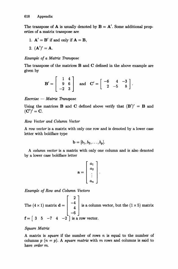
The transpose of A is usually denoted by B = A'. Some additional properties of a matrix transpose are

1. A' = B' if and only if A = B,

2. (A')' = A.

Example 0/ a Matrix 'Iranspose

The transpose of the matrices B and C defined in the above example are given by

Exercise - Matrix 'Iranspose

Using the matrices B and C defined above verify that (B')' = B and (C')' = C.

Row Vector and Column Vector

A row vector is a matrix with only one row and is denoted by a lower case letter with boldface type

A column vector is a matrix with only one column and is also denoted by a lower case boldface letter

a~ [I ]. Example 0/ Row and Column Vectors

Tb. (4 xl) matrix d ~ [ ~~ 1 is a column vector, bul lhe (1 x 5) matrix

f= [3 5 -7 4 -2] is a row vector.

Square Matrix

A matrix is square if the number of rows n is equal to the number of columns p (n = p). A square matrix with m rows and columns is said to have order m.

1 Matrix Algebra 619

Symmetrie Matrix

A square matrix A of order m is symmetrie, if the transpose of A is equal toA.

A = A' if Asymmetrie.

Diagonal Elements

The elements aii, i = 1,2, ... , m, are ealled the diagonal elements of the square matrix A with elements aij, i = 1,2, ... ,m, j = 1,2, ... , m.

TInce 01 a Matrix

The sum of the diagonal elements of A is ealled the tmce of A and is denoted by tr(A). The trace of the (m x m) matrix is given by tr(A) = L:'l aii.

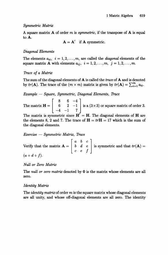
Example - Square, Symmetrie, Diagonal Elements, TInee

The matrix H = 6 2 -1 is a (3 x 3) or square matrix of order 3. [ 8 6 -4] -4 -1 7

The matrix is symmetrie sinee H' = H. The diagonal elements of H are the elements 8, 2 and 7. The trace of H = tr H = 17 which is the sum of the diagonal elements.

Exercise - Symmetrie Matrix, TInee

Verify that the matrix A = [ a~:bjC] is symmetrie and that tr(A) =

(a+d+ I).

Null or Zero Matrix

The null or zero matrix denoted by 0 is the matrix whose elements are all zero.

Identity Matrix

The identity matrix of order m is the square matrix whose diagonal elements are all unity, and whose off-diagonal elements are all zero. The identity

620 Appendix

matrix of order m is usually denoted by Im and is given by

1 0 0 1

I m = 0 0

0 0

Diagonal Matrix

0 0

1

o o

o o 1

A diagonal matrix is a matrix whose off-diagonal elements are all zero. The identity matrix is a special case of a diagonal matrix.

Submatrix

A submatrix of a matrix A is a matrix obtained from A by deleting some rows and columns of A.

Example 0/ Submatrix

The (2 x 2) matrix C* = [~ -i] is a submatrix of the matrix C =

[ ~ =: ! ]. C· is obtained from C by deleting the first row and the 2 1-5

third column.

1.2 MATRIX OPERATIONS

Equality 0/ Matrices

Two matrices A and B are equal, if and only if each element of A is equal to the corresponding element of B: aij = bij , i = 1,2, ... ,n, j = 1,2, ... ,p.

Addition 0/ Matrices

The addition of two matrices A and B is carried out by adding together corresponding elements. The two matrices must have the same order. The sum is given by C where

C=A+B

and where Cij = aij + bij , i = 1,2, ... ,n, j = 1,2, ... ,po


Additive Inverse

A matrix B is the additive inverse of a matrix A, if the matrices sum to the null matrix 0

B+A=O,

where bij + aij = 0 or bij = -Bij, i = 1,2, ... , n, j = 1,2, ... ,po This additive inverse is denoted by B = - A. H C = A + B then C' = A' + B'.

Ezample

The sum of the matrices A and B given below is denoted by C.

A = [-: ~ ] 2 -4

[ 2 -5] B = -~ -~

[ 4 + 2 3 -5] [6 -2] -6 - 2 9 - 2 = -8 7 .

2+4 -4+6 6 2 C =

The matrix D = [-: =~] is the additive inverse of the matrix A -2 4

mnreA+D= [~ n Ezercise

Verify that C' = A' + B' using the matriees A, B and C in the previous example.

Scalar Multiplication 0/ a Matrix

The scalar multiplication of a matrix A by a sealar k is earried out by multiplying each element of A by k. This scalar produet is denoted by k A and the elements by kaij, i = 1,2, ... , n, j = 1,2, ... ,po

Product 0/ Two Matrices

The product of two matriees A (n x p) = (aij)and B (p x m) = (bjk ) is denoted by C = AB, if the number of eolumns (P) of Ais equal to the number of rows (P) of B, and if the elements of C = (Cij) are given by

P

Cik = Laijbjk. j=1

The order of the produet matrix C is (n x m).

622 Appendix

Example

The matrix A = [-: ~ ] when multiplied by the sealar 3 yields the 2 -4

matrix 3A = [-~~ 2~ ]. 6 -12

The produet of the two matrices A and B, where A is given above and

B [ 0 62] .. b = 1 -2 3 ,IS glven y

C=AB [ (4)(0) + (3)(1)

(-6)(0) + (9)(1) (2)(0) + (-4)(1)

= [ ~ -~~ ~;]. -4 20-8

Some additional properties are:

1. A+B=B+A.

2. (A + B) + C = A + (B + C).

3. a(A+B) = aA +aB.

4. (a + b)A = aA + bA.

5. (AB)C = A(BC).

6. (A + B)C = AC + BC.

(4)(6) + (3)(-2) (4)(2) + (3)(3) ] (-6)(6) + (9)( -2) (-6)(2) + (9)(3) (2)(6) + (-4)(-2) (2)(2) + (-4)(3)

7. In general AB i- BA even if the dimensions eonform for multiplication.

8. For square matrices A and B

tr(A + B) = trA + trB and tr(AB) = tr(BA).

Exercise

Given A = [~ - ~ ], B = [~ _ ~ ] and C = [ - ~ ~] verify the

properties 1 through 8 given above.


Multiplicative Inverse

The multiplicative inverse of the square matrix A (m x m) is the matrix B (m x m) satisfying the equation AB = BA = Im, where Im is the identity matrix of order m. The multiplieative inverse of A is usually denoted by B = A -1. If A has an inverse it is unique.

Some additional properties are:

1. If C = AB then C-1 = B-1 A-1

2. (A')-l = (A -1)'

3. IfC = AB then C' = B'A'.

4. (kA)-1 = (l/k)A -1.

Example

The inverse of the matrix A = [_~ -~] is given by A -1 = [ t i ] sinee AA -1 = [ _~ -2 ] [! !] = [1 0] 2 j 1 0 1 .

2

A Useful Result

Given asymmetrie nonsingular matrix A (p x p) and matrices B and C of order (p x q), the inverse of the matrix [A + BC'] is given by

[A + BC'tl = A -1 - A -IB[I + c' A -IBt1C' A -1.

An important special ease of this result is when B and C are (p xl) vectors, say b and c. The inverse of the matrix [A + bc'] is given by

[A+ bC']-1 = A-1 _ A -lbc'A -1.

1 + b'A -IC

Exercise

(a) Verify the above two results by using matrix multiplieation.

(b) The equieorrelation matrix has the form B = (1 - p)1 + pii', where p is a eonstant eorrelation eoefficient and i (n xl) is a vector of unities. Show by using the above result that the matrix B-1 is given by

B-1 = _1_ 1- pii' . (1 - p) (1 - p)2 + p(1 - p)n

Idempotent Matrix

An idempotent matrix A is a matrix that has the property AA = A. If A is idempotent and has full rank then A is an identity matrix.

624 Appendix

Example

The matrix B = [ ~ -1 ] [1 -1] [1 -1] o is idempotent since 0 0 0 0 =

[1 -1] o O·

Exercise

Show that the mean centering matrix [I - kii'] is idempotent, where 1 is an (n x n) identity matrix and i (n xl) is a vector of unities.

Kronecker Product or Direct Product

If A(n x m) and B(p x q), the Kronecker product of A and B is denoted by A ® B and is given by the matrix

allB a12B al m B a21B a22B a2mB

an1B an2B ... anmB

Example

Given A = [ ~ -! ] B = [ ~ ] then

2 [ ~ ] -1

[n I ~ [ 1~ -3] -5 A®B = 12 and

3 [ ~ ] 4 [ ~ ] 15 20

3 [~ -!] [ 6 -3] = 1~ ~; . B®A =

5 [~ -!] 15 20

Some properties of Kronecker products are as follows:

1. (A ® B) ® C = A ® (B ® C).

2. (A + B) ® C = (A ® C) + (B ® C).

3. (A®B)(C®D)=AC®BD.

4. (A®B)'=A'®B'.


5. tr(A ® B) = tr(A)tr(B).

6. For vectors a and b

a'®b=b®a'=ba'.

7. In general A ® B :f:. B ® A as demonstrated in the above example.

Exercise

(a) Use the matriees A and B defined in the example above to show that (A ® B)' = (A' ® B').

(b) Use the matriees A = [! -~] and B = [-! ~] to verify that

tr(A ® B) = tr(A)tr(B).

1.3 DETERMINANTS AND RANK

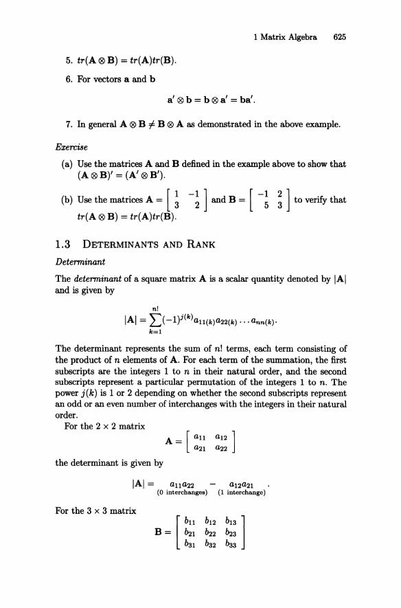
Determinant

The determinant of a square matrix Ais a sealar quantity denoted by lAI and is given by

n!

lAI = ~)-1)j(k)an(k)a22(k) ... ann(k)· k=l

The determinant represents the sum of n! terms, each term eonsisting of the product of n elements of A. For each term of the summation, the first subscripts are the integers 1 to n in their natural order, and the second subseripts represent a partieular permutation of the integers 1 to n. The power j (k) is 1 or 2 depending on whether the second subscripts represent an odd or an even number of interehanges with the integers in their natural order.

For the 2 x 2 matrix

A = [an a12 ] a21 a22

the determinant is given by

lAI = ana22 a12a21

For the 3 x 3 matrix

(0 interchanges ) (1 interchange )

[ bn b12 b13 ]

B = ~1 ~2 ~3 b31 b32 b33

626 Appendix

the determinant is given by

IBI = bll~2ba3 - bll~3b32 + b12~3b31 (0 interchanges) (1 interchange) (2 interchanges)

- b12~lb33 + b13~lb32 - b13~2b31 (1 interchange) (2 interchanges) (1 interchange)

NOTE: n! = 3! = 6 terms.

Nonsingular

If lAI '# 0 then A is said to be nonsingular. The determinant of the matrix A (n x n) can be evaluated in terms

of the determinants of submatrices of A. The determinant of the submatrix of A obtained after deleting the jth row and kth column of A is called the minor of ajk and is denoted by IAjkl. The cofactor of ajk is the quantity (-l)j+kIAjkl. The determinant of A can be expressed by lAI = L;=l ajk( -l)j+kIAjkl for any k and is called the cofactor expansion ofA.

Example

The determinant of the matrix B = 4 5 1 can be determined [ 1 3 -2] -3 -4 7

by expanding about the first row obtaining

Equivalently expanding about the third column

Exercise

Verify the value of the determinant in the example by expanding about the second row.

Some useful properties of the determinant are:

1. lAI = lAI'·

2. If each element of a row (or column) of Ais multiplied by the scalar k then the determinant of the new matrix is klAI.

3. IkAI = IAlkP if A is (p x p).

4. If each element of a row (or column) of Ais zero then lAI = o.


5. If two rows (or columns) of Aare identical then lAI = O.

6. The determinant of a matrix remains unchanged if the elements of one row (or column) are multipled by a scalar k and the results added to a second row (or column).

7. The determinant of the product AB of the square matrices A and B is given by IABI = lAI/BI.

8. If A -1 exists then lA-li = IAI-1.

9. A -1 exists if and only if lAI =I- o. 10. IA ® BI = IAlnlBlm where A(n x n) and B(m x m).

11. (A ® B)-l = A -1 X B-1.

12. If A(p x p) is non-singular, B(p x m) and C(m x p) then IA + BC/ = IAI-1IIp + A -lBC/ = lA-lI/Im + CA -lBI where Ip(p x p) and Im (m x m) are identity matrices.

Relation Between Inverse and Determinant

The inverse of the matrix A is given by A -1 = l*r A *, where A * is the

transpose of the matrix of cofactors of A. The matrix A * is called the adjoint of A.

Example

For the (2 x 2) matrix A = [_~ -~] the determinant is given by

54 - 8 = 46. The matrix of cofactors is given by [~ ~] and hence the

adjoint matrix is A * = [~ ~]. The inverse of A is therefore given by

A-1 _ 1 [6 2] -46 4 9 .

Exercise

(a) Verify that lA-li = IAI-1 using the matrix A in the previous exampIe.

(b) Verify the inverse of the matrix A in the example above using the adjoint and determinant of A -1 to get A.

( c) U se the properties above to show that the determinant of the equicorrelation matrix is given by IpI+(I-p)ii'l = (l-p)n-1[1+p(n-l)], where i (n xl) is a vector of unities.

628 Appendix

Rank 0/ a Matrix

The rank of a matrix A, rank (A), is the order of the !argest nonsingular submatrix of A. HAis nonsingular then A is said to have juli rank.

Example

Given the matrix B = [ ~ ~] the rank is the order of the largest -1 4

nonsingular submatrix of B. Since B is (3 x 2) the rank cannot exceed 2 since a (2 x 2) matrix is the largest square submatrix of B. The three possible submatrices are

The first of these submatrices has determinant zero and hence is singular. The remaining two submatrices are nonsingular. The rank of the matrix B is therefore 2.

Exercise

(al Verify that th. rank of th. matrix A given by A ~ [ ! is 2 and determine all (2 x 2) matrices that have rank 2.

3 -4] 4 2

11 0

(b) Using the matrix B in the above example and A in (a) verify that rank (BA) = 2.

The following properties are useful.

1. HA and B are nonsingu!ar matrices with the appropriate dimensions and if C is arbitrary of appropriate dimension, then

(a) rank (AB) ~ min[rank (A), rank (B)J

(b) rank (AC) = rank (C)

(c) rank (CA) = rank (C)

(d) rank (ACB) = rank (C).

2. The rank of an idempotent matrix is equal to its trace.


1.4 QUADRATIC FORMS AND POSITIVE DEFINITE

MATRICES

Quadratic Form

Given a symmetrie matrix A (n x n) and an (n xl) vector x, a quadratic form is the scalar obtained from the product

n n

x'Ax = L LaijXiXj. i=l j=l

The matrix A must be square, but need not be symmetrie, since for any square matrix B the quadratie form x'Bx ean be written equivalently in terms of a symmetrie matrix A. Thus

x'Ax= x'Bx.

There is no 1088 of generality therefore, in assuming the matrix A in a quadratie form is symmetrie.

Exercise

Given x = [ -2: 1 and A = [! ~ -~ 1 determine the value of -a 0 -1 4

x' Ax and solve for a in the equation x' Ax = 10.

Congruent Matrix

A square matrix B is congruent to a square matrix A if there exists a nonsingular matrix P sueh that A = P'BP. By defining the linear transformation y = Px the quadratie form y'By is equivalent to x' Ax. If A is of rank r, there exists a nonsingular matrix P such that the congruent matrix B is diagonal. In this ease B has r nonzero diagonal elements and the remaining (n-r) diagonal elements are zero, therefore y'By = E;=l biiy;.

Positive Definite

A real symmetrie matrix A (n x n) is positive definite if the quadratie form x' Ax is positive for all (n x 1) vectors x. If A is positive definite and nonsingular, then A is eongruent to an identity matrix in that there exists a nonsingular matrix P sueh that

x'Ax = y'y, where y = Px.

Positive Semidefinite, Negative Definite, Nonnegative Definite

The matrix A is positive semidefinite if x' Ax ~ 0 for all x, and x' Ax = 0 for at least one x. It is negative definite if x' Ax < 0 for all x, and negative

630 Appendix

semidefinite if x' Ax ~ 0 for all x and x' Ax = 0 for at least one x. The matrix Aisnonnegative definite if it is not negative definite.

Exercise

Suppose that A = aa' where a(p xl) and show that x' Ax is positive definite if a 1= o.

Some additional results are:

1. The determinant of a positive definite matrix lAI is positive.

2. If A is positive definite (semidefinite) then for any nonsingular matrix P, p' AP is positive definite (semidefinite).

3. A is positive definite if and only if there exists a nonsingular matrix V such that A = V'V.

4. If A is (n x p) of rank p then A' Aispositive definite and AA' is positive semidefinite.

5. If Ais positive definite then A -1 is positive definite.

1.5 PARTITIONED MATRICES

A matrix A can be parlitioned into submatrices by drawing horizontal and verticallines between rows and columns of the matrix. Each element of the original matrix is contained in one and only one submatrix. A parlitioned matrix is usually called a block matrix.

[an a12 a13 a14

A = a21 a22 a23 a24 a31 a32 a33 a34 a41 a42 a43 a44

Product 0/ Parlitioned Matrices

The product of two block matrices can be determined if the column partitions of the first matrix correspond to the row partitions of the second matrix. As usual, the total number of columns of the first matrix must be equal to the total number of rows of the second,

and using A above

[ AuBu + A12B21 + A13B31

AB= A21 Bu + A22 B21 + A23 B31

Inverse 0/ a Partitioned Matrix


Au B12 + A12B22 + A13B32].

A21 B12 + A22B22 + A23B32

Let the (n xp) matrix A be partitioned into four submatrices A U(n1 xpd, A 12 [n1 x (p - pdl, A 21 [(n - nd x P1l and A 22 [(n - nd x (p - pdl and

hence A = [!~~ !~:]. If B = A -1 exists, then B = [:~~ :~:] can be related to A by the following

1. B u = [Au - A 12Ai21 A 21l-1 = [Ail + Al} A12B22A21Aill·

2. B 12 = -All A 12 [A22 - A 21A l l A 12J-1 = -All A 12B 22 .

3. B 21 = -Ai21 A2dAu - A 12Ail A2d-1 = -Ai21 A 21B u .

4. B 22 = [A22 - A21Al11 A 12J-1 = [Ai21 + Ai21 A21BuA12Aill.

Exercise

1. (a) Verify the above expressions for B = A -1 by multiplication to show that AB = I.

(b) Verify the above expressions for B = A -1 by solving for the four submatrices in B in the equation AB = I.

2. :: ~::~:~[ Im! th: i~Tle :: ::::::::: i::: -7 1 8

[ 5 -3] 1 8'

Determinant 0/ a Partitioned Matrix

The determinant of lAI can be expressed as follows:

1. lAI = IA22 11Au - A 12Ail A 22 1 = IAu llA22 - A 21A ll A 12 1·

2. lAI = IA22 1/IBu l = IAu l/IB22 1, where B u and B 22 are defined above with the inverse of a partitioned matrix.

If A 21 = A 12 = 0 then

1 A -1 = [Al} 0] . 0 A-1 . 22

632 Appendix

Exercise

(a) Use the expression for lAI in (1) above to determine lAI in the previous exercise.

(b) Show that lAI = lAu IIA22 I using the matrix A in the previous exercise.

1.6 EXPECTATIONS OF RANDOM MATRICES

An (n xp) random matrix Xis a matrix whose elements Xij i = 1,2, ... , n, j = 1,2, ... ,p, are random variables. The expected value of the random matrix X denoted by E[X] is the matrix of constants E[Xij] i = 1,2, ... , n, j = 1,2, ... ,p, if these expectations exist.

Let Y (n x p) and X (n x p) denote random matrices whose expectations E[YJ and E[X] exist. Let A (m x n) and B (p x k) be matrices of constants. The following properties hold:

1. E[AXB] = AE[X]B.

2. E[X + Y] = E[X] + E[YJ.

Let z (n xl) be a random vector and let A (n x n) be a matrix of constants. The expected value of the quadratic lorm z' Az is given by E[z'Az] = E7=1 Ej=laijE[ZiZj] where A has elements ~j and z has elements Zi.

Exercise

(a) Show that E[(X+A)'(X+A)] = L'+A'IT+IT'A+A'A, where X is a random matrix E[X] = IT and E[X'X] = L'.

(b) Show that E[x' Ax] = Ef=l E;=laijO'ij + Ef=l E;=laijJ.tiJ.tj, where E[(Xi - J.ti)(Xj - J.tj)] = O'ij, i,j = 1,2, ... ,po

1.7 DERIVATIVES OF MATRIX EXPRESSIONS

If the elements of the matrix A are functions of a random variable x, then the derivative of A with respect to x is the matrix whose elements are the derivatives of the elements of A. For A = (~j), dAldx = (daijldx).

If x is a (p x 1) vector, the derivative of any function of x, say I(x), is the (p xl) vector of elements (8118xj), j = 1,2, ... ,po

Given a vector x (p xl) and a vector a (p xl), the vector derivative of the scalar x'a with respect to the vector x is denoted by 8(x'a)/8x = a,

which is equivalent to the vector

8~x'a) Xp


Given a vector x (p xl) and a matrix A (p x p), the vector derivative of Ax is given by 8AI ax = A' or 8AI ax' = A.

Given a vector x (p x 1) and a matrix A (p x p), the vector derivative of the quadratic form x' Ax with respect to the vector x is denoted by 8(x' Ax)/ax = 2Ax, which is equivalent to the vector

8(~Ax) xp

Given a matrix X (nxm) then the derivative of a function ofX, say I(X), with respect to the elements of X is the (n x m) matrix of partial derivatives (81 I 8Xij). Some useful properties of the matrix derivative involving the tra.ce operator are:

1. &tr(X) = I.

2. &tr(AX) = A'.

3. &tr(X' AX) = (A + A')X.

The derivative of adeterminant lXI of a matrix X, with respect to the elements of the matrix, is given by 81XI/8X = (X')* = adjoint of X'.

Exercise

(a) Show that if 1= (a - Bx)'(a - Bx) where a (n xl), B (n x p), and x (p x 1) then 81 lax = [2B'Bx - 2B'a].

(b) Show that if f= tr(A - BX)'(A - BX) where A (n x p), B (n x r) and X (r x p) then 8118X = [2B'BX - 2B' Al.

634 Appendix

~-----------------------X2

FIGURE A.1. Addition of Two Vectors

2 Linear Algebra

2.1 GEOMETRIC REPRESENTATION FOR VECTORS

A veetor x' = (Xl, X2, ••• ,Xn ) ean be represented geometrieally in an n-dimensional space, as a directed line segment from the origin to the point with coordinates (Xl, X2, . •. ,xn ). The n-dimensional vector space is formed by n mutually perpendieular axes Xl. X 2 , ••• ,Xn . The coordinates (Xl, X2, ••• , x n ) are values of Xl. X 2 , ••• , X n respectively. Figure A.l shows the vectors xi = (Xll, X21, Xat) and x~ = (X12, X22, Xa2) in a threedimensional space. The addition 0/ the two vectors xi + x~ = (Xll + X12, X21 + X22, Xa1 + Xa2) is also shown in Figure A.1. Figure A.2 shows scalar multiplication by a sealar k for a two-dimensional vector x' = (Xll, X2t), where kx' = (kxl1, kX2t).

The length 0/ the vector x' = (Xl, X2, ••• ,Xn ) is given by the Euclidean distance between the origin and the point (Xl. X2, ••• ,xn ) and is denoted by

n 1/2 IIxll = ..j(X1 - 0)2 + (X2 - 0)2 + ... + (Xn - 0)2 = [I>~] .

i=l

The angle (J between the vector Xl = (Xl1, X21o ••• , xnt) and the veetor x2 = (X12, X22, ••• ,Xn2) is given by

n n 1/2 n 1/2 eos (J = I>i1Xi2/ [I>~l ] [I>~2] .

i=l i=l i=l

kx

x

2 Linear Algebra 635

(kxll • kxZI )

I I I I I I I I

~----------~--------~--- Xl

FIGURE A.2. Sealar Multiplieation

The matrix produet of the (n x 1) veetors Xl and X2 is given by

and henee eosB = X~X2/(X~XI)I/2(X;X2)1/2.

In Figure A.3, the angle B between xi = (Xll' X21) and x~ = (XI2, X22) is given by eos (J = [XllXI2 +X2IX22J/[X~1 +X~IJI/2[x~2 +X~2P/2. If eos(J = ±1 the veetors Xl and X2 are said to be orthogonal.

The distanee from the vector point xi = (Xll, X2b ... , xnt) to the veetor point x~ = (XI2' X22, . .. ,Xn 2) is the Euclidean distanee between the two points

The projection of the veetor X2 on the veetor Xl is a veetor that is a sealar multiple of Xl given by

where B is the angle between X2 and Xl, and k is the sealar given by Ilx211/llxIIi eosB.

636 Appendix

X22 --

1 1

Xl 1

1 (X12 • X22) ---1------

1 1 1 1 1 1 1 1

"""-___ ---' ____ --1. _____ Xl

FIGURE A.3. Angle Between Two Vectors

Exercise

(a) Given Xl = [ ~ ] and X2 = [ ! ] plot the veetors Xl and X2 in the

two-dimensional space formed by the axes Xl and X 2 •

(b) Plot the vector (Xl + X2) and the veetor 2XI in the two-dimensional space in (a).

(e) Determine the length of the veetors XI. X2 and (Xl + X2).

(d) Determine the angle () between the veetors Xl and X2.

(e) Determine the distanee between the tips of the vectors Xl and X2'

(f) Determine the projeetion X2 of the veetor X2 on Xl and determine the veetor X; = X2 - X2. Show that X2 and x; are orthogonal.

2.2 LINEAR DEPENDENCE AND LINEAR

TRANSFORMATIONS

Linearly Dependent Vectors

If one vector X in n-dimensional space ean be written as a linear eombination of other veetors in n-dimensional space, then X is said to be linearly dependent on the other veetors. If


then x is linearly dependent on V!, ... , vp-

The set of (p + 1) vectors (x, Vi, ... , vp ) is also a linearly dependent set, if any one of the vectors can be written as a linear combination of the remaining vectors in the set.

Linearly Independent Vectors

A set of vectors is linearly independent, if it is not possible to express one vector as a linear combination of the remaining vectors in the set. In an n-dimensional space the maximum number of linearly independent vectors is n. Thus given any set of n linearly independent vectors, all other vectors in the n-dimensional space can be expressed as a linear combination of the linearly independent set.

Basis for an n-Dimensional Space

The set of n linearly independent vectors is said to generate a basis for the n-dimensional space.

In two-dimensional space linearly dependent vectors are colinear or lie along the same line. In three-dimensional space linearly dependent vectors are in the same two-dimensional plane and may be colinear. If the set of linearly independent vectors are mutually orthogonal then the basis is said to be orthogonal.

Generation of a Vector Space and Rank of a Matrix

If the matrix A (n x p) has rank r, then the vectors formed by the p columns of A generate an r-dimensional vector space. Similarly the rows of A generate an r-dimensional vector space. In other words, the rank of a matrix is the maximum number of linearly independent columns, and equivalently the maximum number of linearly independent rows.

Exercise

(al Given Ihe vecOOrn x, ~ [ -n x, ~ [ ! 1 and x, ~ [ n show

that they are linearly independent by showing that each cannot be written as a linear combination of the remaining two.

(b) Let A = [Xi,X2,X3] and determine lAI for the values of x!, X2,X3

given in (a).

Linear Transformation

Given a p-dimensional vector x, a linear transformation of x, is given by the matrix product

y=Ax,

638 Appendix

where A (n x p) is called a transformation matrix. The matrix A maps the n-dimensional vector x into a Jrdimensional vector y. If A is a square nonsingular matrix, the transformation is one to one, in that x = A -ly and hence each point in x corresponds to exactly one and only one point iny.

Orthogonal1'ransformation, Rotation, Orthogonal Matrix

If A is a square matrix and A has the property that A' = A -1, then the equation y = Ax is an orthogonal tro.nsformation or rotation. The matrix A in this case is called an orthogonal matrix. If A is orthogonal, A also has the property that lAI = ±1. The transformation is orthogonal because it can be viewed as a rotation of the coordinate axes through some angle (J. The angle (J between any pair of vectors remains the same after the transformation.

Example

In Figure A.4, the point M has coordinates (Xl, X2) with respect to the Xl - X 2 axes and has coordinates (Zl, Z2) with respect to the ZI - Z2 axes. The angle rP between Xl and Zl is the angle of rotation required to rotate the Xl - X2 axes into the ZI - Z2 axes. The coordinates (Zl, Z2) of the point M in Zl - Z2 space can be described in terms of the coordinates (Xi! X2) of M in Xl - X 2 space using the equations

Zl = Xl COSrP + X2 sinrP Z2 = -Xl sin rP + X2 COS rP.

In matrix notation the linear transformation to [ ;~ ] from [ :~ ] can

be expressed as [ Zl ] = [ c~ ~ sin ~ ] [ Xl ]. The transformation Z2 - SIn'f' COS'f' X2

. [cos rP sin rP ] matrIX A = . A. A. has the property that -SIn'f' COS'f'

A-1 - 1 [COS rP -sinrP]_[COs rP -sinrP]=AI

- cos2 rP + sin2 rP sin rP cos rP - sin rP cos rP '

and hence the transformation is orthogonal as required.

Exercise

(a) Let A = [~~~ -~~~] denote a transformation matrix. Show

that A -1 = A' and hence that A is an orthogonal transformation matrix.

X2

/ /

M -----7\

// 1\ // I \

./ I \ ./ I

I Zl


--~~~----L--------------Xl

FIGURE A.4. Rotation ofAxes

(b) Use the results of the above example to show that the angle of rotation in (a) is 45°.

(c) Give the transformation matrix corresponding to 4J = 60°.

2.3 SYSTEMS OF EQUATIONS

Let Xl, X2, X3 denote the unknowns in a system of three equations

a11 X I + al2 X 2 + al3x 3 bl

a2lXI + a22X2 + a23X3 = b2

a3l X I + a32 X 2 + a33X 3 b3 ·

The system of equations can be represented by a matrix equation

Ax=b,

where

Solution Vector for a System of Equations

The solution vector x is given by

x= A-Ib.

640 Appendix

Exercise

1. Given 'he three linearly independent vectors X, ~ [ -i l' X, ~

[ -!] and ~ ~ U l Ify ~ U 1 m con'Wned in 'he 'p=

generated by Xl, X2 and X3 then there exist coefficients a, b and c such that y = aXI + bX2 + CX3' Show that the equation for y can be

wri'ten os y ~ Af, where f ~ [ : landSOl" for f.

2. Solve the system of equations

3XI +X2 - 4X3

2XI + 5X2 +X3

Xl - 4X2 + 3X3

= = =

3

10

-6

for XI, X2 and X3 using the expression X = A -ly.

Homogeneous Equations - Trivial and Nontrivial Solutions

If the vector b in the system Ax = b is the null vector 0, the system is said to be a system of homogeneous equations. The obvious solution X = 0 is said to be a trivial solution. If A is (n x p) ofrank r, where x and b are (p xl), then the system of n homogeneous equations in p unknowns given by Ax = b has (p - r) linearly independent solutions in addition to the trivial solution x = O. In other words, a nontrivial solution exists if and only if the rank of A is less than p. If A is a square matrix a nontrivial solution exists if and only if lAI = o.

2.4 COLUMN SPACES, PROJECTION OPERATORS AND

LEAST SQUARES

Column Space

Given an (n x p) matrix X, the columns of X denoted by the p vectors xI, X2, ... ,xp span a vector space called the column space of X. The set of all vectors y (n xl), defined by y = Xb for all vectors b (p xl), b =I 0, is the vector space generated by the columns of X.

Orthogonal Complement

The set of all vectors z (p xl) such that Xz = 0 generates the orthogonal complement to the column space of X.


Projection

Given a vector y (n xl) and a p-dimensional column space defined by the matrix X (n x p), p::; n, the vector y (n x 1) is a projection of y onto the column space of X, if there exists a (p xl) vector b such that y = Xb, and a vector e (n xl) such that e is in the orthogonal complement to the column space of X. If Y is the projection of y, then y = y + e, and the vector e is the part of y that is orthogonal to the column space of X.

Ordinary Least Squares Solution Vector

Given an (n x p) matrix X of rank p, and a vector y (n xl), n ~ p, the projection of y onto the column space of X is given by the ordinary least squares solution vector

y = X(X'X)-lX'y, where b = (X'X)-lX'y.

Idempotent Matrix - Projection Operator

The matrix X(X'X)-lX' is an idempotent matrix and is called the projection operator for the column space of X. The vector e = (y - y) = [I - X(X'X)-l X']y is orthogonal to the column space of X. The idempotent matrix [I - X(X'X)-l X'] is called the projection operator for the vector space orthogonal to the column space of X.

Exercise

1. Given X (n x p) and y (n x 1) demonstrate the following:

(a) X(X'X)-lX' is idempotent.

(b) [I - X(X'X)-lX'] is idempotent.

(c) [I - X(X'X)-lX'][X(X'X)-lX'] = O.

(d) y'(y - y) = 0, where y = X(X'X)-lX'y.

2. Given X =

1 1 1 2 1 3 1 4 y = [~ 1 5 6

Y = X(X'X)-l X'y and (y - y).

d t . bA (X'X)-lX'y, e ermlne =

642 Appendix

3 Eigenvalue Structure and Singular Value Decomposition

3.1 EIGENVALUE STRUCTURE FOR SQUARE MATRICES

Eigenvalues and Eigenvectors

Given a square matrix A of order n, tbe values of tbe scalars A and (n x 1) vectors v, vi- 0, tbat satisfy tbe equation

Av= AV, (A.1)

are called tbe eigenvalues and eigenvectors of tbe matrix A. Tbe problem of finding A and v in (A.1) is commonly referred to as tbe eigenvalue problem. From (A.1) it can be seen tbat if visa solution tben kv is also a solution wbere k is an arbitrary scalar. Tbe eigenvectors are tberefore unique up to a multiplicative constant. It is common to impose tbe additional constraint tbat v'v = 1, and bence tbat tbe eigenvector be normalized to bave a lengtb of 1.

Chamcteristic Polynomial, Chamcteristic Roots, Latent Roots, Eigenvalues

Rewriting (A.1) as (A - AI)v = 0,

we obtain a system of homogeneous equations. A nontrivial solution v =f 0 requires that

lA-All =0.

This equation yields a polynomial in A of degree n and is commonly called tbe chamcteristic polynomial. Tbe solutions of the equation are tbe roots of the polynomial, and are sometimes referred to as chamcteristic roots or latent roots, altbougb tbe most common term used in statistics is eigenvalues.

Tbe characteristic polynomial bas n roots or eigenvalues some of wbich may be equal. For each eigenvalue A tbere is a corresponding eigenvector v satisfying (A.1). Tbe matrix A is singular if and only if at least one eigenvalue is zero.

Some additional properties of eigenvalues and eigenvectors are:

1. Tbe eigenvalues of a diagonal matrix are tbe diagonal elements.

2. Tbe matrices A and A' bave tbe same eigenvalues but not necessarily tbe same eigenvectors.

3. If A is an eigenvalue of A tben 1/ A is an eigenvalue of A -1.

3 Eigenvalue Structure and Singular Value Decomposition 643

4. H>. is an eigenvalue of A and v the corresponding eigenvector, then for the matrix A k, >.k is an eigenvalue with corresponding eigenvector V.

5. H the eigenvalues of A are denoted by >'t, >'2, ... ,>'n, then

n n

trA = L>'j and lAI = 11 >'j. ;=1 ;=1

Eigenvalues and Eigenvectors for Real Symmetrie Matrices and Some Properties

In statistics the matrix A will usually have real elements and be symmetrie. In this case the eigenvalues and eigenvectors have additional properties:

1. H the rank of A is r then (n - r) of the eigenvalues are zero;

2. H k of the eigenvalues are equal the eigenvalue is said to have multiplicity k. In this ease there will be k orthogonal eigenvectors corresponding to the common eigenvalue;

3. H two eigenvalues are distinct then the eorresponding eigenvectors are orthogonal;

4. An nth order symmetrie matrix produees a set of n orthogonal eigenvectors.

5. For idempotent matriees the eigenvalues are zero or one.

6. The maximum value of the quadratie form v' A v subject to v'v = 1 is given by >'1 = ~ A VI, where >'1 is the largest eigenvalue of A and VI is the eorresponding eigenvector.

Similarly the second largest eigenvalue >'2 = v~A v2 of A is the maximum value of v' Av subject to ~Vl = 0 and V~V2 = 1, where V2 is the eigenvector corresponding to >'2. The kth largest eigenvalue >'k = v'kAvk of A is the maximum value of v' Av subject to vkVI = v'kV2 = ... = VkV(k-l} = 0 and vkVk = 1, where Vk is the eigenvector eorresponding to >'k. The above properties are essentially summarized by the following statement. HAis real symmetrie of order n, there exists an orthogonal matrix V such that

V'AV = A or A = VAV',

where A is a diagonal matrix of eigenvalues of A with diagonal elements >'1, >'2, ... , >'n; and V is the matrix whose columns are the eorresponding eigenvectors Vt, V2, ... , Vn . The orthogonal matrix V diagonalizes the matrix A.

644 Appendix

7. If A is nonsingular and symmetrie then A" = VA "V', where A = VAV'.

8. If A = V AV' then the quadratic form x' Ax can be written as y' Ay where y = Vx.

Example

Given the matrix

6 fl 0

A= fl 4 j! 0 j! 2

the eigenvalues are obtained by solving the determinantal equation IA -,XII = 0, which in this case is given by

(6 -'x) fl

o

flO (4-,X) j! j! (2 -'x)

=0.

The resulting characteristic polynomial is given by

3 15 (6 - ,X) (4 - 'x)(2 -'x) - 2(6 -'x) - 2(2 -'x) = O.

The characteristic roots or eigenvalues determined from this polynomial are ,X = 1, 3 and 8.

The corresponding eigenvectors are obtained by solving the equation (A - 'xI)v = 0 for each of the eigenvalues ,X determined above. Corresponding to ,X = 3 the equation becomes

3fl fll Oj!

o j! -1

Adding the condition that vf + v~ + v~ = 1 yields the eigenvector

v' = [-~ {fd a], the remaining two eigenvectors are given by

[-VI ~ -Vi] and [~ JH //0]


corresponding to >. = 1 and >. = 8 respectively. The complete matrix of eigenvectors is given by

V=

corresponding to >. = 1,3 and 8 respectively. The reader should verify that V'V=I.

Ezercise

(a) Show that the eigenvalues of the matrix A - [ :

by 1, 1 and 4.

1 1 1 2 1 are given 1 2

(b) Show that v' = (7a' ta, ta) is an eigenvector corresponding to

>. = 4.

(c) Show that the remaining two eigenvectors corresponding to the double root >. = 1 are

( 1 1) (2 1 1) 0, y'2' - y'2 and - y'6' y'6' y'6 .

(d) Show that the 3 x 3 matrix of eigenvectors

1 0 2 va -y'6 1 1

V= v'3 y'2 76 1 1 1

Va -y'2 y'6

satisfies V'V = I.

Spectral Decomposition

The equation A = V AV' can be written

where >'1, >'2"", >'n are the eigenvalues of A and VI, V2, ••• , Vn are the corresponding eigenvectors. This equation gives the spectral decomposition ofA.

646 Appendix

Matrix Approximation

Let Z (n x p) be a matrix such that A = Z'Z and let A(l) denote the first l terms of the spectral decomposition A(l) = E;=I"\jVjvj, l< n. This expression minimizes tr(Z - X)(Z - X)' = E~l E~=l(aij - Xij)2 among an (n x p) matrices X of rank l. Thus the first few terms of the spectral decomposition of A = Z'Z can be used to provide a matrix approximation toA.

Example

For the matrix A of the previous example the matrix of eigenvalues can be approximated in decimal form by

[ -0.327 -0.500 0.802]

V = 0.598 0.547 0.586 . -0.732 0.671 0.120

The spectral decomp08ition for A is given by

[ (0.327)2 -(0.327)(0.598) (0.327)(0.732)]

A = 1 -(0.327)(0.598) (0.598)2 -(0.598)(0.732) (0.327)(0.732) -(0.598)(0.732) (0.732)2

[ (0.500)2 -(0.500)(0.547) -(0.500)(0.671)]

+3 -(0.500)(0.547) (0.547)2 (0.547)(0.671) -(0.500)(0.671) (0.547)(0.671) (0.671)2

[ (0.802)2 (0.802)(0.586) (0.802)(0.120) 1

+8 (0.802)(0.586) (0.586)2 (0.586)(0.120). (0.802)(0.120) (0.586)(0.120) (0.120)2

This simplifies to

[ 0.107 -0.196 0.239] [ 0.750

A = -0.196 0.358 -0.438 + -0.821 0.239 -0.438 0.536 -1.007

[ 5.146 3.760 0.770]

+ 3.760 2.747 0.563 . 0.770 0.563 0.115

-0.821 -1.007] 0.898 1.101 1.101 1.351

Except for inaccuracies due to rounding this matrix should be equivalent to the decimal form of

[ 6.000 2.739 0.000]

A = 2.739 4.000 1.225 . 0.000 1.225 1.000

As a matrix approximation the term of the spectral decomp08ition corresponding to ..\ = 8, say Al, can be viewed as a first approximation to A.


The differenee between the two matriees A - Al is given by

[ 0.857 1.017 -0.768] 1.017 1.256 0.663 .

-0.768 0.663 1.887

If two terms (.x = 8 and .x = 3) are used, we obtain A2 with the differenee given by (A - A2), whieh is approximately the matrix term eorresponding to .x = 1 in the spectral deeomposition. It would appear that the variation in the magnitudes of the errors is quite small eompared to the variation in the magnitudes in the original matrix. In other words the speetral decomposition approximation seems to be weighted toward the larger elements ofA.

Exercise

Determine the spectral decomposition for the matrix given in the eigenvalue exercise above and eomment on the quality of the approximation based on the largest eigenvalue.

Eigenvalues tor Nonnegative Definite Matrices

If the real symmetrie matrix A is positive definite then the eigenvalues are all positive. If the matrix is positive semidefinite then the eigenvalues are nonnegative with the number of positive eigenvalues equal to the rank of A.

3.2 SINGULAR VALUE DECOMPOSITION

Areal (n x p) matrix A of rank k ean be expressed as the produet of three matrices that have a useful interpretation. This decomposition of A is referred to as a singular value decomposition and is given by

A=UDV',

where

1. D (k x k) is a diagonal matrix with positive diagonal elements ab a2, ... ,ak, which are ealled the singular values of A, (without loss of generality we ~sume that the aj, j = 1,2, ... , k, are arranged in deseending order).

2. The k columns ofU (n x k), UI, U2,"" Uk are called the left singular vectors of A and the k eolumns ofV (p x k), Vb V2,"" Vk are ealled the right singular vectors of A.

3. The matrix A can be written as the sum of k matriees, each with rank 1, A = E7=1 ajujvj. The subtraction of any one of these terms from the sum results in a singular matrix for the remainder of the sumo

648 Appendix

4. The matrices U (n x k) and V (p x k) have the property that U'U = V'V = Ij hence the columns of U form an orthonormal basis for the columns of A in n-dimensional spare and the columns of V form an orthonormal basis for the rows of A in p-dimensional spare.

5. Let A(.e) denote the first .e terms of the singular value decomposition for Aj hence A(.e) = ~;=1 QjUjvj. This expression minimizes tr[(AX)(A - X)'] = ~~=1 ~~=l(aij - Xij)2 among all (n x p) matrices X of rank .e. Thus the singular value decomposition can be used to provide a matrix approximation to A.

Complete Singular Value Decomposition

A complete singular value decomposition can be obtained for A by adding (n-k) orthonormal vectors Uk+b' •. , t1n to the existing set Ub"" Uk. Similarly the orthonormal vectors Vk+b"" vp are added to the set Vb V2, ••. ,

vp ' Denoting the n column vectors Uj, j = 1,2, ... , n by U* and the p column vectors by V* then U*'U = I and V*'V* = I and A = U*D*V*

is the complete singular value decomposition where D* = [~ ~] .

Generalized Singular Value Decomposition

A generalized singular value decomposition permits the left and right singular vectors to be orthonormalized with respect to given positive definite matrices n (n x n) and ~ (p x p) where

N'nN = M/~M = I. The generalized singular value decomposition of A (n x p) is given by

k

A = NDM' = LQjDjmj, j=1

where Qj, j = 1,2, ... , k, are the diagonal elements ofD, Dj, j = 1,2, ... , n, are the columns of N and mj, j = 1,2, ... ,p, are the columns of M. The columns of N and M are referred to as the generalized left and right singular vectors of A respectively. The diagonal elements of D are called the generalized singular values.

Let A(.e) denote the first .e terms of the generalized singular value decomposition for A, hence A(.e) = ~~=1 QjDjmj. This expression for A(.e) mjnimizes ~~=1 ~:=1(aij - Xij)2~jWi among all matrices X of rank at most .e where the ~j and Wi are the elements of ~ and n respectively. The generalized singular value decomposition can be used to provide a matrix approximation to A.

The generalized singular value decomposition of A given by NDM' where N'nN = I and M'~M = I can be related to the singular value

3 Eigenvalue Strueture and Singular Value Decomp08ition 649

decomposition by writing

n1/ 2 A.1/2 = n1/2NDM' .1/2 = UDV

where U = n1/ 2N and V = .1/2M and U'U = V'V = I.

Relationship to Spectral Decomposition and Eigenvalues

If the matrix Aissymmetrie, the singular value decomposition is equivalent to the spectral decomposition

A=UDV' =VAV'.

In this ease, the left and right singular vectors are equal to the eigenvectors and the singular values are equal to the eigenvalues.

The singular value decomposition of the (n x p) matrix A ean also be related to the spectral decomposition for the symmetrie matrices AA' and A' A. For the singular value decomposition

A=UDV',

the eigenvalues of AA' and A' A are the squares of the singular values of A. The eigenvectors of AA' are the eolumns of U and the eigenvectors of A' A are the columns of V. Since covarianee matrices and correlation matrices ean be written in the form A' A, the eigenvalues and eigenvectors are often determined using the singular value decomposition.

Data Appendix for Volume 11

Introduction

This data appendix contains twenty-two data tables that are used in the chapter exercises throughout Volume 11. Outlines to the data sets are given below. In some cases the data tables represent additional observations or variables derived from the data sets used in this text or in Volume I. A listing of the data tables follow the outlines.

Data Set Vl Bus Data

This data set consists of observations on additional variables in the study of bus driver absenteeism used in Chapter 6. The data set is divided into the three contingency tables listed below.

Part I - Day by Sex by Attendance Part 11 - Day by Garage by Attendance Part 111 - Garage by Sex by Attendance

Data Set V2 Accident Data

This data set consists of observations on some additional variables for the accident data introduced in Chapter 6. The observations are based on the same 86,769 accidents employed in Chapter 6. A four-dimensional contingency table relating INJURY LEVEL, SEATBELT USAGE, POINT OF IMPACT and DRIVER CONDITION is given below. The variable POINT OF IMPACT indicates where on the vehicle the collision occurred. The remaining three variables were used in Chapter 6.

Data Set V9 Accident Data

This data set consists of observations on some additional variables for the accident data introduced in Chapter 6 and in data set V2. The observations are based on the same 86,769 accidents employed in Chapter 6. A four dimensional contingency table relating INJURY LEVEL, SEATBELT USAGE, SPEED LIMIT and DRIVER CONDITION is given below. The variable SPEED LIMIT refers to the posted speed limit for the road on which the accident occurred. The remaining variables were used in Chapter 6.

652 Data Appendix

Data Set V4 Real Estate Data

This data set consists of 116 observations on three bedroom bungalows listed and sold through areal estate multiple listing service in a given year in a particular area of a large city. The variables are LISTP (list price), SELLP (selling price), SQF (square feet), ROOMS (total number of rooms), BEDR (total number of bedrooms), GARAGE (no garage = 0, single garage = 1, double garage = 2), EXTRAS (numerical code 1, 2, or 3 denoting number of extras that come with the house), CHATTELS (numerical code 0, 1, 2, 3 indieating the number of additional items included in the price), AGE (age of the house), BATHR (no. of bathroom pieces Le. a fuU bath usuaUy has three pieces while a half bath usuaUy has two pieces), and SELLDAYS (number of days the house was listed before it was sold). Some of the variables from this data set were used in Volume I.

Data Set V5 Automobile Data Part I

This data set contains observations on a sampie of 97 automobiles selected from the Fuel Consumption Guide 1985 published by Transport Canada. The table contains observations on ENGSIZE, WEIGHT, AUTOMAT (0 = standard, 1 = automatie transmission), FOR (0 = domestic, 1 = foreign), URBRATE (urban fuel consumption rate), HWRATE (highway fuel consumption rate) and slope shiftersj FWFIGHT = FOR * WEIGHT, FENGSIZE = FOR * ENGSIZE, AENGSIZE = AUTOMAT * ENGSIZE, AWEIGHT = AUTOMAT * WEIGHT. An additional sampie of observations from this data set was introduced in Volume I.

Data Set V6 Financial Accounting Data

This data set consists of 80 observations collected from the Data Stream data base for a sampie of UK companies for the year 1983. An additional sampie of observations from this data base was used in Volume I. The variables are RETCAP (return on capital), WCFTDT (ratio ofworking capital flow to total debt), LOGSALE (log to base 10 of total sales), LOGASST (log to base 10 oftotal assets), CURRAT (current ratio), QUIKRAT (quick ratio), NFATAST (ratio ofnet fixed assets to total assets), PAYOUT (payout ratio), WCFTCL (ratio of working capital flow to current liabilities), GEARRAT (gearing ratio or debt-equity ratio), CAPINT (capital intensity or ratio of total sales to total assets), INVTAST (ratio of total inventories to total assets), and FATTOT (gross fixed assets to total assets).

Data Set V7 Air Pollution Data Part I

This data consists of observations on 80 U.S. cities for the year 1960 obtained from Gibbons, Dianne Ij Gary C. McDonald and Richard F. Gunst, "The Complementary Use of Regression Diagnostics and Robust Estimators," Naval Research Logistics 34, 1, February, 1987. Other cities from this

Data Appendix 653

data set were also used in Chapter 9 and 10 and in Volume I, Chapter 4. The variables are defined below.

TMR SMIN SMEAN

SMAX PMIN

PMEAN

PMAX

PM2 GE65 PERWH NONPOOR

LPOP

- total mortality rate - smallest biweekly sulfate reading (p,g/m3 x 10) - arithmetic mean of biweekly sulfate readings

(p,g/m3 x 10) -largest biweekly sulfate reading (p,g/m3 x 10) - smallest biweekly suspended particulate reading

(p,g/m3 x 10) - arithmetic mean of biweekly suspended particu

late reading (p,g/m3 x 10) - largest biweekly suspended particulate reading

(p,g/m3 x 10) - population density per square mile xO.1 - percent of population at least 65 x 10 - percent of whites in population - percent of families with income above poverty

level - logarithm (base 10) of population x 10

Data Set V8 Shopping Attitude Data

This data set consists of 200 observations obtained from a mail survey designed to obtain attitudes of females pertaining to shopping for clothing. Seven of the items designed to measure shopping orientation are given by

Al: I like sales people to leave me alone until I find clothes that I want to buy.

A2: I like to pay cash for clothing purchases. A3: Price is a good indicator of the quality of clothes. A4: I usually spend more than I planned when shopping for

clothes. A5: I do not think clothing shops provide enough customer service

these days. A6: When clothing is sold at a reduced price there is often some

thing wrong with it. A7: I like to shop where my friends shop for clothes.

The responses were coded from 1 (strongly agree) to 5 (strongly disagree). In addition to the seven shopping orientation variables two additional variables included in the data set are WORK and AGE. These variables are coded as follows:

654 Data Appendix

WORK Code

o 1

respondent works outside home respondent does not work outside home

AGE Code

1 2 3

Age 240r less 25-34 35-44

Code 4 5 6

Data Set V9 R.C.M.P. OjJicer Data

Age 45-54 55-64 65 and over

This data set contains observations from Royal Canadian Mounted Police (R.C.M.P.) ofticers regarding their satisfaction with various aspects of their jobs. The responses were combined into four factors labeled SATF1, SATF2, SATF3 and SATF4. The four factors can be characterized respectively as satisfaction with job characteristics, salary and benefits, commanding ofticer and co-workers. The observations were obtained from ten different municipal detachments in Alberta, Canada. Observations from this data set were used for examples in Chapters 9 and 10 and also in Volume I.

Data Set Vl0 Mystery Data

This data set consists of observations on five of the ten variables from the mystery data given in Table 8.11. The five variables are Cl, C3, C8, C9 and C10 defined below:

Cl: Importance of more than one murder or crime. C3: Importance of powerful opponents. C8: Importance of many possible suspects. C9: Importance of puzzle being "fair play" by giving clues. C1O: Importance of suspects appearing as average people.

Data Set Vll and V12 Bank Employee Data

These two data sets represent two different sampies of 100 observations each selected from a larger data set. This bank employee data has been used by SPSSX to provide examples for the SPSSX User's Guide. Table Vll is an expansion of Table 7.9. Table Vll indudes all the variables in Table 7.9 plus the additional variables SEX, RACE and JOBCAT. Table V12 is identical to Table D3 of Volume I. The variables in these two data sets are listed below:

LCURRENT LSTART SEX JOBCAT

RACE SENIOR AGE EXPER

Data Set V13

Data Appendix 655

- In (current salary) - In (starting salary) - male = 0, female = 1 - 1 = clerical, 2 = office trainee, 3 = security officer, - 4 = college trainee, 5 = MBA trainee - white = 0, nonwhite = 1 - seniority with the bank in months - age in years - relevant job experience in years

Panel Data

This data set is derived from the U niversity of Michigan Panel Study of Income Dynamics and is an expansion of the data summarized in Table 8.25. The purpose of the data in this application is to study the factors that influence married female participation in the labor force. Table V13 contains 200 observations. The last 100 observations in the table are arepetition of the observations in Table 8.25. The variables are defined below.

THISYR

LASTYR

BLACK

EDUC AGE CHILDI

CHILD2

HUBINC

- indicator variable for whether the wife worked outside the horne in the year of the survey (l=yes, O=no)

- indicator variable for whether the wife worked outside the horne in the previous year (l=yes, O=no)

- indicator variable for black race (l=black, O=not black)

- education level (years) of the respondent - age level of the respondent (years) - indicator variable for whether there are children in

the horne under the age of 2 (l=yes, O=no) - indicator variable for whether there are children in

the horne between the ages of 2 and 6 (l=yes, O=no) - income of husband in 1000 dollars.

Data Sets V14 and V15 U.S. Divorce Data

Data set V14 provides a summary of the available grounds for divorce in the United States by state (including District of Columbia) in 1982. The data was obtained from The World Almanac and Book 0/ Facts 1983 published for the Boston Herald American by Newspaper Enterprise Association, Inc., New York. The nine available grounds for divorce are listed below. States that have the ground available are coded 1, if they do not they are coded O.

656 Data Appendix

BREAK CRUEL DESERT NOSUPPOR ALCOHOL FELONY IMPOTENT INSANE SEPARATE

- marriage breakdown/incompatibility - cruelty - desertion - nonsupport - alcohol and/or drug addiction - felony - impotency - insanity - living separate and apart for a specified period.

Data set V15 is a subset of V14 consisting of the observations for 20 states.

Data Sets V16 and V17 U.S. Crime Data

Data set V16 summarizes the crime rates by state (per 100,000 population) for nine categories for the United States in 1980. The data set was obtained from The World Almanac and Book 0/ Facts 1983published for the Boston Herald American by Newspaper Enterprise Association, !nc. New York. The nine types of crime are violent, property, murder, rape, robbery, assault, burglary, larceny and auto theft.

Data set V17 is a subset of V16 consisting of the observations for 15 states.

Data Set V18 Automobile Data Part II

This data set comes from the same database as V5. This sampie consists of observations on 20 different automobiles with respect to COMBRATE (rate of fuel consumption), CYLIND (no. of cylinders), WEIGHT, ENGSIZE and FOR (l=foreign manufacturer, O=North American manufacturer). The observations on all but FOR are ranks as defined below.

CYLIND ENGSIZE COMBRATE WEIGHT

Data Set V19

- 4, 6, 8 becomes 1, 2 and 3 respectively - 15-18 = 1, 20-24 = 2, 28-30 = 3, 38-41 = 4, 50 = 5 - 64-71 = 1, 74-84 = 2, 93-97 = 3,104-110 = 4 - (2000,2250) = 1, (2500,2750) = 2, 3000 = 3,

3500 = 4, 4000 = 5

Cola Similarity Data

This data set consists of a dissimilarity matrix relating ten different brands of cola soft drinks [0 = same, 100 = completely different]. The dissimilarity matrix was derived from an experiment involving ten university students aged 18-21 years. Subjects were blindfolded and then asked to taste ten different colas without swallowing. Subjects rinsed their mouths with distilled water between tastes. Subjects were asked to judge the similarity between all possible pairs (45) of the ten colas over a five-day period. The

Data Appendix 657

dissimilarity matrix is an average of the ten dissimilarity matrices of the ten subjects. The data was obtained from Schiffman, Susan S., Lance M. Reynolds and Forest W. Young (1981) Introduction to Multidimensional Scaling: Theory, Methods and Applications, New York: Academic Press.

Data Set V20 Gar Similarity Data

A number of subjects were asked to compare 11 automobiles with respect to overall similarity. The rank order of the 55 dissimilarities are given in a dissimilarity matrix (1 = most similar pair, 55 = least similar pair). This matrix was obtained from Green, Paul E., Frank J. Carmone and Scott M. Smith (1989) Multidimensional Scaling: Concepts and Applications, Boston: AHyn and Bacon.

Data Set V21 Air Pollution Data Part II

This data set consists of a subset of observations from Data Set V7.

Data Set V22 Shopping Attitude Data Part II

This data set consists of 200 observations from a mail survey designed to obtain attitudes of females pertaining to shopping for clothing. Eighteen items designed to measure shopping orientation are contained in the data set. The first seven items were included in Data Set V8 along with variables measuring WORK and AGE. Table V22 contains these items plus the additional 11 items summarized below.

A8: I always buy my clothes at the same shops. A9: I visit several shops before buying clothes for myself. AlO: I think shops that carry weH known makes of clothing are

overpriced. All: I like to have someone with me when I shop for clothes. A12: I like to make my own buying decisions rat her than get advice

from others. A13: To me, shopping for clothes is fun. A14: I feel creative when I go shopping for clothes. A15: Buying new clothes gives me a lift. A16: I only go shopping for clothes when I really need something. A17: Shopping for clothes gives me no satisfaction. A18: I like browsing in clothing shops without buying anything.

658 Data Appendix

TABLE Vl. Bus Data Part I

Day Sex Attend Frequency

Sun Male Present 1676 Mon Male Present 4931 Tues Male Present 4850 Wed Male Present 4835 Thurs Male Present 4832 Fri Male Present 4857 Sat Male Present 2702 Sun Female Present 162 Mon Female Present 361 Tues Female Present 392 Wed Female Present 398 Thurs Female Present 396 Fri Female Present 413 Sat Female Present 297 Sun Male Absent 132 Mon Male Absent 461 Tues Male Absent 494 Wed Male Absent 501 Thurs Male Absent 512 Fri Male Absent 479 Sat Male Absent 242 Sun Female Absent 30 Mon Female Absent 79 Tues Female Absent 96 Wed Female Absent 98 Thurs Female Absent 92 Fri Female Absent 83 Sat Female Absent 63

TABLE Vl. Bus Data Part III

Garage Sex Attend Frequency

1 Male Present 15422 2 Male Present 10811 3 Male Present 10023 1 Female Present 1086 2 Female Present 801 3 Female Preeent 697 1 Male Absent 1658 2 Male Absent 1069 3 Male Absent 977 1 Female Absent 274 2 Female Absent 319 3 Female Absent 223

Data Appendix 659

TABLE VI. Bus Data Part 11

Day Garage Attend Frequency

Sun 1 Present 855 Mon 1 Present 2170 Tues 1 Present 2123 Wed Present 2113 Thurs Present 2129 Fri Present 2157 Sat 1 Present 1308 Sun 2 Present 514 Mon 2 Present 1634 Tues 2 Present 1619 Wed 2 Present 1625 Thurs 2 Present 1636 Fri 2 Present 1644 Sat 2 Present 857 Sun 3 Present 460 Mon 3 Present 1475 Tues 3 Present 1482 Wed 3 Present 1469 Thurs 3 Present 1437 Fri 3 Present 1450 Sat 3 Present 813 Sun Absent 81 Mon Absent 222 Tues Absent 269 Wed Absent 279 Thurs Absent 263 Fri Absent 235 Sat Absent 148 Sun 2 Absent 46 Mon 2 Absent 182 Tues 2 Absent 197 Wed 2 Absent 191 Thurs 2 Absent 180 Fri 2 Absent 172 Sat 2 Absent 95 Sun 3 Absent 44 Mon 3 Absent 149 Tues 3 Absent 142 Wed 3 Absent 155 Thurs 3 Absent 187 Fri 3 Absent 174 Sat 3 Absent 83

660 Data Appendix

TABLE V2. Accident Data

Seatbelt Point of Injury Driver Frequency Impact Level Condition

Yes Front None Normal 7389 Yes Front None Bdrink 199 Yes Front Minimal Normal 308 Yes Front Minimal Bdrink 30 Yes Front Minor Normal 169 Yes Front Minor Bdrink 13 Yes Front Majfat Normal 18 Yes Front Majfat Bdrink 2 Yes Rear None Normal 3509 Yes Rear None Bdrink 79 Yes Rear Minimal Normal 207 Yes Rear Minimal Bdrink 5 Yes Rear Minor Normal 106 Yes Rear Minor Bdrink 1 Yes Rear Majfat Normal 5 Yes Rear Majfat Bdrink Yes Rside None Normal 827 Yes Rside None Bdrink 21 Yes Rside Minimal Normal 36 Yes Rside Minimal Bdrink 5 Yes Rside Minor Normal 27 Yes Rside Minor Bdrink 1 Yes Rside Majfat Normal 8 Yes Lside None Normal 775 Yes Lside None Bdrink 14 Yes Lside Minimal Normal 53 Yes Lside Minimal Bdrink 3 Yes Lside Minor Normal 42 Yes Lside Majfat Normal 7 Yes Lside Majfat Bdrink

Data Appendix 661

TABLE V2. Accident Data (continued)

Seatbelt Point of Injury Driver Frequency Impact Level Condition

No Front None Normal 37492 No Front None Bdrink 2833 No Front Minimal Normal 2025 No Front Minimal Bdrink 384 No Front Minor Normal 1337 No Front Minor Bdrink 278 No Front Majfat Normal 135 No Front Majfat Bdrink 48 No Rear None Normal 16280 No Rear None Bdrink 768 No Rear Minimal Normal 913 No Rear Minimal Bdrink 50 No Rear Minor Normal 491 No Rear Minor Bdrink 42 No Rear Majfat Normal 28 No Rear Majfat Bdrink 6 No Rside None Normal 4165 No Rside None Bdrink 218 No Rside Minimal Normal 397 No Rside Minimal Bdrink 27 No Rside Minor Normal 207 No Rside Minor Bdrink 26 No Rside Majfat Normal 28 No Rside Majfat Bdrink 4 No Lside None Normal 4034 No Lside None Bdrink 173 No Lside Minimal Normal 184 No Lside Minimal Bdrink 20 No Lside Minor Normal 237 No Lside Minor Bdrink 24 No Lside Majfat Normal 46 No Lside Majfat Bdrink 8

662 Data Appendix

TABLE V3. Accident Data

Seatbelt Speed Injury Driver Frequency Limit Level Condition

Yes Lt60kph None Normal 9838 Yes Lt60kph None Bdrink 234 Yes Lt60kph Minimal Normal 401 Yes Lt60kph Minimal Bdrink 31 Yes Lt60kph Minor Normal 219 Yes Lt60kph Minor Bdrink 10

Yes Lt60kph Majfat Normal 11

Yes Lt60kph Majfat Bdrink 1 Yes 60-89kph None Normal 2021 Yes 60-89kph None Bdrink 60 Yes 60-89kph Minimal Normal 144 Yes 60-89kph Minimal Bdrink 11 Yes 60-89kph Minor Normal 68 Yes 60-89kph Minor Bdrink 2 Yes 60-89kph Majfat Normal 6 Yes 60-89kph Majfat Bdrink 1 Yes Gt89kph None Normal 641 Yes Gt89kph None Bdrink 19 Yes Gt89kph Minimal Normal 59 Yes Gt89kph Minimal Bdrink 1 Yes Gt89kph Minor Normal 57 Yes Gt89kph Minor Bdrink 3 Yes Gt89kph Majfat Normal 21 Yes Gt89kph Majfat Bdrink 2 No Lt60kph None Normal 52269 No Lt60kph None Bdrink 3242 No Lt60kph Minimal Normal 2531 No Lt60kph Minimal Bdrink 350 No Lt60kph Minor Normal 1609 No Lt60kph Minor Bdrink 228 No Lt60kph Majfat Normal 91 No Lt60kph Majfat Bdrink 26 No 60-89kph None Normal 7993 No 60-89kph None Bdrink 571 No 60-89kph Minimal Normal 790 No 60-89kph Minimal Bdrink 87 No 60-89kph Minor Normal 452 No 60-89kph Minor Bdrink 87 No 60-89kph Majfat Normal 58 No 60-89kph Majfat Bdrink 16 No Gt89kph None Normal 1709 No Gt89kph None Bdrink 179 No Gt89kph Minimal Normal 198 No Gt89kph Minimal Bdrink 44 No Gt89kph Minor Normal 211 No Gt89kph Minor Bdrink 55 No Gt89kph Majfat Normal 88 No Gt89kph Majfat Bdrink 24

TA

BL

E V

4,

Rea

l E

state

Data

LIS

TP

S

EL

LP

S

QF

R

OO

MS

B

ED

R

GA

RA

GE

E

XT

RA

S

CH

AT

TE

LS

A

GE

S

EL

LD

AY

S

BA

TH

R

7900

0 75

400

1365

7

4 2

3 2

8 31

6

8500

0 79

800

1170

6

3 2

2 1

7 48

4

9100

0 82

000

1160

6

4 2

2 2

6 15

6

1078

00

9850

0 13

06

6 3

1 3

3 6

18

5 83

000

8000

0 11

20

5 3

2 1

2 5

28

6 85

000

8500

0 10

40

6 3

2 2

3 7

35

4 85

800

8400

0 11

30

6 3

2 2

1 7

57

4 89

800

8400

0 12

32

6 3

1 3

2 7

30

6 97

600

9680

0 13

64

7 4

2 3

0 7

1 6

9940

0 95

800

1260

6

3 0

2 0

7 30

6

1038

00

1015

00

1302

6

3 0

2 3

5 30

6

7780

0 74

000

1040

6

3 0

1 1

8 28

4

1038

00

1010

00

1278

6

3 2

1 1

7 33

6

1070

00

1020

00

1408

7

3 2

3 3

8 24

6

1098

00

1070

00

1225

6

3 2

1 0

6 2

6 93

800

9000

0 11

60

6 3

2 3

2 6

44

6 95

600

8800

0 10

40

6 3

1 2

1 7

41

4 10

2000

98

000

1424

7

3 2

1 0

6 54

6

1118

00

1044

00

1232

6

3 2

3 0

7 36

6

9580

0 89

800

1270

6

3 0

2 0

7 51

6

tJ

1058

00

1020

00

1298

6

3 2

2 0

7 57

6

I" ....

1350

00

1280

00

1340

6

3 2

3 0

7 38

6

I" :>

1398

00

1240

00

1380

6

3 2

3 2

9 21

6

"0

9980

0 91

600

1200

6

3 2

3 1

10

35

6 "0

~

1094

00

1060

00

1180

6

3 2

3 0

7 63

6

ä. 10

9800

91

600

1200

6

3 2

3 1

10

37

6 ><'

11

0800

10

2000

12

60

6 3

2 3

3 7

45

6 97

200

9400

0 12

19

6 3

2 1

2 7

43

6 10

1000

98

000

1154

6

3 2

1 0

7 30

6

CI)

C

I)

~

TA

BL

E V

4. R

eal

Est

ate

Dat

a (c

onti

nued

) ~

LIS

TP

SEL

LP

SQF

RO

OM

S B

ED

R

GA

RA

GE

E

XT

RA

S C

HA

TT

EL

S A

GE

SE

LLD

AY

S B

AT

HR

1058

00

9860

0 12

21

6 3

2 3

0 7

62

Cl

6 ~

1118

00

1000

00

1205

6

3 2

2 1

7 11

2 6

CD

9180

0 85

000

1170

6

3 0

2 3

8 25

4

f 10

7800

98

000

1200

6

3 2

2 1

7 6

4

6 95

600

9350

0 11

20

6 3

2 1

1 7

16

6 97

800

9300

0 11

30

6 3

2 2

0 9

37

4

~ 99

800

92

00

0

1270

5

3 0

1 0

5 5

8

6 10

3800

98

000

1120

6

3 2

2 0

6 6

7

6 10

3800

10

1000

10

72

6 3

2 3

1 7

15

7 10

5000

98

000

1130

6

3 2

3 2

7 43

6

8600

0 84

000

1080

6

3 0

1 0

10

59

4

9500

0 88

000

1060

6

3 1

1 1

11

39

4

1098

00

1010

00

1232

6

3 2

3 0

8 43

9

1236

00

1140

00

1200

6

3 1

3 1

10

26

6 95

800

9200

0 10

80

6 3

0 2

0 11

3

2

4 13

0000

12

2000

14

60

6 3

2 3

1 7

17

7 91

200

8780

0 11

00

6 3

2 3

2 10

61

7

9380

0 89

000

1140

6

3 0

1 1

11

12

4 11

9600

10

8000

12

48

6 3

2 2

0 12

4

3

6 89

800

8740

0 10

50

6 3

2 1

0 11

26

4

1070

00

1030

00

1286

6

3 2

2 0

12

15

6

1118

00

1060

00

1250

6

3 2

3 0

9 70

7

7780

0 77

000

1056

5

3 1

3 0

12

8 4

9180

0 85

800

1135

6

3 2

2 0

12

60

4 97

800

96

00

0

1280

6

3 2

3 4

10

24

4

1006

00

9600

0 11

00

5 3

2 2

0 1

0

73

4 81

000

8100

0 10

60

6 3

1 1

0 11

4

3 91

800

8400

0 10

80

6 3

0 3

1 10

25

4

9500

0 90

000

1080

6

3 2

1 2

11

20

4

TA

BL

E V

4. R

eal

Est

ate

Dat

a (c

onti

nued

)

LIS

TP

SEL

LP

SQF

RO

OM

S B

ED

R

GA

RA

GE

E

XT

RA

S C

HA

TT

EL

S A

GE

SE

LLD

AY

S B

AT

HR

9580

0 90

000

1140

5

3 1

1 1

11

24

8 10

3800

10

3000

11

60

6 3

2 3

1 9

18

7 10

5000

10

1800

10

89

6 3

2 2

0 6

24

4 93

000

8600

0 10

40

6 3

0 3

1 10

17

4

9980

0 96

000

1200

6

3 2

2 1

9 12

6

1075

00

1040

00

1257

6

3 2

2 0

9 7

6 95

800

9400

0 12

60

5 3

1 2

0 8

47

6

7700

0 76

000

1106

6

3 2

2 1

5 64

4

7780

0 76

000

1120

6

3 0

1 1

1 1

0

6 79

000

7400

0 11

90

6 3

2 1

0 1

48

6 85

000

8300

0 12

64

6 3

1 1

1 3

50

6 87

000

8300

0 12

32

6 3

0 1

0 1

36

6

8780

0 83

800

1160

6

3 2

1 0

1 9

6 89

800

8800

0 11

90

6 3

2 1

5 1

20

6 93

800

9102

8 13

92

6 3

0 2

0 1

44

7 97

600

9600

0 12

20

6 3

2 2

3 6

15

6 12

8400

12

3000

14

50

6 3

2 2

0 1

13

5 87

200

8720

0 12

06

6 3

0 1

0 1

11

6 87

800

8200

0 11

50

6 3

0 1

1 2

35

4 89

800

8780

0 12

04

6 3

0 1

1 1

22

6 95

800

9200

0 13

40

6 3

0 1

1 1

12

6 0

8300

0 76

000

1160

6

3 0

1 2

1 48

6

~

8980

0 86

000

1200

5

3 0

2 1

1 40

6

'" 91

800

8900

0 12

02

6 3

2 1

0 1

57

4

>

9780

0 95

200

1278

6

3 2

1 0

1 12

6

~ 10

6150

99

000

1260

6

3 1

3 2

6 53

6

B. 11

9600

11

0000

12

84

6 3

0 3

1 3

2 6

$<.

8700

0 83

500

1237

6

3 0

1 2

2 17

4

9180

0 88

000

1050

5

3 0

2 0

7 12

4

g C/1

TA

BL

E V

4. R

eal

Est

ate

Data

(co

nti

nu

ed)

~ L

IST

P

SE

LL

P

SQ

F

RO

OM

S

BE

DR

G

AR

AG

E

EX

TR

AS

C

HA

TT

EL

S

AG

E

SE

LL

DA

YS

B

AT

HR

0

1018

00

9900

0 13

20

6 3

2 2

5 2

14

6 ~

1150

00

1040

00

1490

7

3 2

1 2

2 3

5

6 ID

1384

00

1300

00

1491

7

3 2

2 3

1 33

6

>-89

000

8300

0 11

54

6 3

0 1

0 6

38

6 ~

9380

0 89

000

1224

6

3 0

2 0

1 43

6

I:S

9780

0 96

000

1220

6

3 2

1 0

6 28

4

~ 10

3000

99

000

1152

6

3 2

1 0

2 13

4

1058

00

1010

00

1392

8

4 0

1 2

2 3

5

6 12

9800

12

4000

14

80

7 3

2 1

1 0

2 7

9580

0 92

000

1042

5

3 2

3 1

7 20

3

9660

0 95

000

1167

6

3 0

1 0

1 6

6 11

2000

10

6000

12

46

6 3

2 2

0 1

62

4 11

4000

10

0000

14

40

6 3

0 2

2 1

34

7 13

5000

12

2400

15

64

7 3

1 2

3 1

32

7

1110

00

1050

00

1224

6

3 2

2 1

7 55

6

1150

00

1140

00

1325

6

3 2

2 0

1 63

6

1270

00

1210

00

1270

5

3 2

3 1

6 21

7

9180

0 88

000

1340

8

4 0

1 1

2 21

6

1058

00

1040

00

1270

6

3 1

1 0

1 48

6

1198

00

1150

00

1460

7

3 0

1 0

3 3

4

6 87

800

8500

0 10

01

6 3

2 3

2 7

82

4

1018

00

9700

0 12

27

6 3

2 1

1 1

67

6 77

800

7780

0 11

24

6 3

2 2

0 8

21

4 78

000

7800

0 10

70

6 3

1 3

0 12

19

4

7800

0 73

000

1120

5

3 2

2 0

5 21

4

9580

0 85

400

1200

6

3 2

3 0

9 52

6

1058

00

1010

00

1308

6

3 0

3 2

7 2

9 97

400

9600

0 11

13

6 3

0 1

0 8

37

4

1050

00

9800

0 13

45

6 3

2 1

1 7

16

6

TA

BL

E V

5. A

utom

obil

e D

ata

Par

t I

EN

GS

IZE

W

EIG

HT

F

OR

A

UT

OM

AT

F

WE

IGH

T

FE

NG

SIZ

E

AE

NG

SIZ

E

AW

EIG

HT

U

RB

RA

TE

H

WR

AT

E

16

2500

0

0 0

0 0

0 73

48

18

25

00

1 1

2500

18

18

25

00

103

73

50

4000

0

1 0

0 50

40

00

148

84

23

3000

1

0 30

00

23

0 0

121

69

38

4000

0

1 0

0 38

40

00

133

78

20

2500

1

0 25

00

20

0 0

86

55

18

2500

0

0 0

0 0

0 97

52

12

17

50

1 1

1750

12

12

17

50

75

50

20

2750

1

1 27

50

20

20

2750

87

53

50

40

00

0 1

0 0

50

4000

14

9 86

25

27

50

0 1

0 0

25

2750

10

1 57

34

35

00

1 0

3500

3

4

0 0

145

83

23

3000

1

1 30

00

23

23

3000

10

7 70

28

30

00

0 1

0 0

28

3000

12

0 63

18

25

00

1 0

2500

18

0

0 86

56

50

40

00

0 1

0 0

50

4000

14

7 79

18

27

50

0 1

0 0

18

2750

11

7 73

16

25

00

0 1

0 0

16

2500

97

63

22

27

50

0 0

0 0

0 0

110

59

18

2750

1

1 27

50

18

18

2750

10

1 74

50

35

00

0 1

0 0

50

3500

14

7 8

0

50

4000

0

1 0

0 50

40

00

169

96

20

2500

0

0 0

0 0

0 97

57

t::

l 23

30

00

1 1

3000

23

23

30

00

125

83

Q>

16

2500

1

0 25

00

16

0 0

96

63

.... Q>

23

2750

0

0 0

0 0

0 10

4 59

>

22

30

00

0 1

0 0

22

3000

11

7 75

'ö

'ö

20

27

50

0 1

0 0

20

2750

10

2 60

(!

)

16

2250

0

0 0

0 0

0 79

51

8-

20

2750

0

0 0

0 0

0 97

57

x·

50

4000

0

1 0

0 50

40

00

152

87

50

3500

0

1 0

0 50

35

00

149

86

15

2000

1

0 20

00

15

0 0

85

55

Q)

Q)

-'I

TA

BL

E V

5. A

utom

obil

e D

ata

Par

t I

(con

tinu

ed)

0)

0)

00

EN

GS

IZE

W

EIG

HT

F

OR

A

UT

OM

AT

F

WE

IGH

T

FE

NG

SIZ

E

AE

NG

SIZ

E

AW

EIG

HT

U

RB

RA

TE

H

WR

AT

E

22

2500

0

0 0

0 0

0 8

7

55

Ö ~

38

3500

0

1 0

0 38

35

00

132

81

~

38

3000

0

1 0

0 38

30

00

14

0

75

~ 50

35

00

0 1

0 0

50

3500

1

47

80

16

25

00

0 0

0 0

0 0

74

46

I! 23

35

00

0 1

0 0

23

3500

1

30

86

~

50

4000

1

1 40

00

50

50

40

00

172

116

50

3500

0

0 0

0 0

0 17

2 8

2

38

3000

0

1 0

0 38

30

00

120

81

18

2750

1

1 27

50

18

18

2750

10

4 68

50

35

00

0 0

0 0

0 0

141

75

22

3000

0

1 0

0 22

30

00

110

72

38

4000

0

1 0

0 38

40

00

13

2

77

34

35

00

1 1

3500

34

3

4

3500

13

3 77

25

27

50

0 0

0 0

0 0

102

54

16

27

50

0 1

0 0

16

2750

9

6

60

16

25

00

0 0

0 0

0 0

73

48

32

30

00

1 0

3000

32

0

0 13

4 72

5

0

3500

0

0 0

0 0

0 1

57

77

50

40

00

0 1

0 0

50

4000

14

7 80

50

35

00

0 1

0 0

50

35

00

14

7

80

25

3000

0

0 0

0 0

0 1

07

55

58

40

00

0 1

0 0

58

40

00

17

8 9

5

18

2500

1

0 25

00

18

0 0

90

58

28

30

00

0 1

0 0

28

3000

11

8 69

22

27

50

0 0

0 0

0 0

93

5

3

38

3500

0

1 0

0 38

35

00

145

77

22

3000

0

1 0

0 22

30

00

119

79

28

3500

0

0 0

0 0

0 13

4 6

7

18

2500

1

1 25

00

18

18

2500

9

7

66

20

2500

0

0 0

0 0

0 9

7

57

25

30

00

0 0

0 0

0 0

99

5

9

23

3000

1

0 30

00

23

0 0

103

64

TA

BL

E V

5. A

utom

obil

e D

ata

Par

t I

(con

tinu

ed)

EN

GS

IZE

W

EIG

HT

F

OR

A

UT

OM

AT

F

WE

IGH

T

FE

NG

SIZ

E

AE

NG

SIZ

E

AW

EIG

HT

U

RB

RA

TE

H

WR

AT

E

28

3000

0

1 0

0 28

30

00

122

71

18

2750

0

1 0

0 18

27

50

101

63

28

3000

0

1 0

0 28

30

00

118

69

22

2750

0

0 0

0 0

0 11

2 62

22

30

00

0 1

0 0

22

3000

98

64

15

22

50

1 0

2250

15

0

0 80

59

20

30

00

1 0

3000

20

0

0 11

3 66

16

22

50

0 0

0 0

0 0

88

54

16

2250

1

1 22

50

16

16

2250

92

60

15

20

00

1 1

2000

15

15

20

00

87

59

20

3000

1

1 30

00

20

20

3000

13

0 88

38

35

00

0 1

0 0

38

3500

13

2 81

33

30

00

1 0

3000

33

0

0 18

1 10

1 20

27

00

1 1

2700

20

20

27

00

98

67

50

3500

0

0 0

0 0

0 15

7 77

18

25

00

1 0

2500

18

0

0 92

61

16

25

00

1 1

2500

16

16

25

00

102

62

16

2500

1

1 25

00

16

16

2500

91

60

20

27

50

0 1

0 0

20

2750

10

9 70

20

30

00

1 1

3000

20

20

30

00

98

57

25

3000

0

1 0

0 25

30

00

104

58

16

25

00

1 0

2500

16

0

0 90

63

0

30

3000

0

1 0

0 30

30

00

118

69

~

24

2750

1

1 27

50

24

24

2750

96

63

ID

25

3000

0

1 0

0 25

30

00

92

59

~ 25

27

50

0 1

0 0

25

2750

10

1 57

18

25

00

1 0

2500

18

0

0 95

57

(D

16

2250

0

0 0

0 0

0 97

60

~

41

3500

0

1 0

0 41

35

00

134

77

25

3000

1

0 30

00

25

0 0

118

67

38

3500

0

1 0

0 38

35

00

126

76

~

co

670 Data Appendix

TABLE V6. Financial Accounting Data

RETCAP WCFTCL WCFTDT GEARRAT LOGSALE LOGASST

0.19 0.16 0.16 0.15 5.2291 4.8315 0.22 0.26 0.16 0.54 4.1495 4.3402 0.11 0.26 0.20 0.49 5.3831 4.8811 0.12 0.08 0.08 0.39 4.1225 3.9333 0.21 0.34 0.34 0.11 4.1195 4.5811 0.12 0.25 0.25 0.19 4.1503 3.9086 0.15 0.25 0.16 0.35 5.6998 5.5511 0.10 0.12 0.09 0.39 4.4162 4.2128 0.08 0.04 0.04 0.50 4.1108 4.5126 0.31 0.12 0.11 0.41 4.4618 4.1928 0.21 0.36 0.33 0.08 4.3899 4.2336 0.22 0.31 0.31 0.16 4.0253 3.8344 0.20 0.48 0.48 0.13 3.8513 3.8164 0.11 0.18 0.15 0.23 3.9068 3.8685 0.38 0.25 0.20 0.21 5.1631 4.6669 0.23 0.24 0.24 0.00 5.1130 4.9712 0.32 0.09 0.09 0.11 4.7114 4.3123 0.13 0.06 0.05 0.55 4.6763 4.4912 0.29 0.60 0.60 0.00 4.5233 4.8709 0.09 0.10 0.09 0.28 4.9876 4.4058

-2.22 -1.28 -1.28 1.78 4.0554 3.5485

0.17 0.12 0.11 0.28 4.2831 3.9619 -0.04 -0.04 -0.04 0.46 4.7616 4.3153 0.26 0.23 0.23 0.00 4.2468 3.8779 0.21 0.40 0.30 0.20 4.4106 4.3829 0.15 0.30 0.21 0.66 4.3984 4.3634 0.23 0.07 0.01 0.11 4.8314 4.4399 0.20 0.33 0.28 0.33 4.2050 4.0364 0.19 0.16 0.14 0.30 4.3139 4.1727 0.08 0.18 0.10 0.35 4.9510 4.8675 0.19 0.15 0.14 0.19 5.5754 5.4405

0.20 0.63 0.35 0.21 4.7722 4.8638

0.14 0.21 0.20 0.30 4.9993 4.8282 0.04 0.01 0.07 0.18 4.1786 3.9151 0.10 0.15 0.12 0.13 5.1613 5.780l

-0.09 -0.46 -0.22 0.68 3.9671 4.0802 0.10 0.18 0.14 0.23 5.6884 5.6334

0.20 0.13 0.12 0.05 4.1908 4.4200 0.13 0.17 0.13 0.22 5.4876 5.3501 0.08 0.14 0.14 0.19 4.0891 3.8731

Data Appendix 671

TABLE V6. Financial Accounting Data (continued)

NFATAST CAPINT FATTOT INVTAST PAYOUT QUIKRAT CURRAT

0.28 2.47 0.36 0.42 0.31 0.54 1.33 0.13 0.64 0.16 0.04 0.45 0.83 0.93 0.43 3.18 0.74 0.13 0.50 0.84 1.09 0.23 1.55 0.50 0.37 0.65 0.50 1.09 0.30 1.56 0.50 0.20 0.25 1.10 1.74 0.34 1.74 0.38 0.31 0.80 1.00 1.89 0.48 1.39 0.62 0.22 0.46 0.73 1.38 0.26 1.60 0.42 0.30 1.03 0.94 1.57

0.25 1.58 0.33 0.31 0.00 0.74 1.28

0.17 1.88 0.25 0.31 0.25 0.66 1.10

0.40 1.43 0.71 0.17 0.61 1.06 1.49

0.42 1.55 0.62 0.17 0.25 0.97 1.38

0.68 0.96 0.97 0.13 0.60 0.61 1.00 0.40 1.09 0.64 0.15 0.80 0.92 1.23 0.21 3.13 0.32 0.38 0.39 0.33 1.39 0.27 5.44 0.38 0.50 0.36 0.24 1.29 0.09 2.51 0.13 0.31 0.53 0.86 1.34

0.24 1.51 0.40 0.42 0.00 0.44 1.14 0.57 0.45 0.58 0.01 0.21 1.18 1.21 0.34 3.82 0.50 0.46 1.52 0.34 1.28 0.16 3.21 0.30 0.37 0.00 0.50 1.06 0.26 2.07 0.32 0.37 0.22 0.67 1.36 0.19 2.79 0.32 0.28 0.00 0.72 1.11 0.21 2.34 0.26 0.27 0.53 1.20 1.83 0.24 1.07 0.36 0.24 0.42 1.77 2.72 0.70 1.08 1.07 0.15 0.00 0.29 0.58 0.17 2.46 0.22 0.00 0.67 0.88 0.88 0.53 1.47 1.16 0.07 0.21 0.77 0.91 0.25 1.38 0.33 0.42 0.52 0.49 1.28 0.31 1.21 0.51 0.27 1.08 1.44 2.36 0.22 1.36 0.36 0.22 0.40 0.96 1.35 0.21 0.81 0.34 0.26 0.51 2.63 3.98 0.72 1.48 0.74 0.09 0.53 0.26 0.54 0.28 1.83 0.54 0.23 4.21 1.08 1.57 0.12 0.96 0.21 0.28 0.43 0.57 1.40 0.62 0.77 0.71 0.19 0.00 0.60 1.45 0.33 1.14 0.52 0.23 0.12 0.83 1.56 0.04 2.35 0.07 0.37 0.33 0.80 1.42 0.26 1.37 0.52 0.41 0.53 0.75 1.73 0.17 1.64 0.27 0.34 0.91 0.74 1.57

672 Data Appendix


RETCAP WCFTCL WCFTDT GEARRAT LOGSALE LOGASST

0.14 0.41 0.37 0.21 4.3516 4.3615 0.12 0.30 0.25 0.29 4.2835 4.1800 0.17 0.20 0.20 0.33 4.4271 4.0467 0.27 0.38 0.38 0.00 3.6470 3.9209 0.22 0.45 0.44 0.18 3.8183 3.5728 0.13 0.35 0.35 0.00 4.4159 4.4739

-0.10 -0.70 -0.70 0.00 2.7973 3.8199 0.13 0.18 0.16 0.30 3.7923 3.6307 0.14 0.09 0.07 0.63 6.6360 6.1332 0.07 0.03 0.03 0.49 4.5339 4.5888 0.31 1.57 0.27 0.54 2.0212 3.7313 0.18 0.48 0.41 0.08 4.0326 4.0720 0.26 0.16 0.16 0.72 3.9202 3.8331 0.08 0.13 0.10 0.47 4.5782 4.4681 0.16 0.14 0.14 0.15 4.3202 4.2248 0.09 0.10 0.08 0.45 4.2578 4.2315 0.29 0.12 0.12 0.29 4.6570 4.9039 0.22 0.21 0.19 0.45 3.5813 3.5751 0.12 0.12 0.12 0.39 4.2843 4.0931 0.26 0.78 0.78 0.01 3.7270 3.6617 0.10 2.12 2.12 0.01 0.0000 5.0505 0.15 0.16 0.15 0.44 4.2181 3.9019 0.16 0.20 0.13 0.34 4.2322 4.2077 0.12 0.11 0.11 0.48 4.7735 4.4443 0.16 0.25 0.22 0.11 4.3490 3.9451 0.23 5.46 5.46 0.00 3.7897 4.2260 0.11 0.26 0.20 0.24 3.8366 3.6951 0.15 0.17 0.14 0.28 3.9725 3.8831

-0.02 -0.11 -0.08 0.89 4.3601 4.1623 0.10 0.06 0.05 0.41 4.6635 4.5154 0.08 0.09 0.08 0.05 4.6209 4.4724 0.08 0.08 0.06 0.45 4.0991 3.9227 0.11 0.12 0.11 0.44 4.9139 4.6044 0.10 0.04 0.04 0.47 4.2430 3.8602 0.08 0.04 0.04 0.42 4.8882 5.1535 0.20 0.57 0.57 0.01 3.8650 3.7666

-0.16 -0.54 -0.15 0.54 4.1210 4.8298 0.10 0.37 0.15 0.49 3.5941 4.0571 0.06 0.07 0.06 0.64 4.7757 4.2350 0.26 0.25 0.25 0.46 4.1162 4.3087

Data Appendix 673


NFATAST CAPINT FATTOT INVTAST PAYOUT QUIKRAT CURRAT

0.72 0.98 0.93 0.07 0.47 0.57 0.74 0.31 1.27 0.56 0.33 0.63 0.97 1.91 0.14 2.40 0.23 0.43 0.33 1.00 1.97 0.57 0.53 0.70 0.13 0.57 0.69 0.97 0.13 1.76 0.38 0.45 0.00 1.18 2.43 0.08 0.88 0.41 0.22 0.46 0.58 1.29 0.46 0.09 0.75 0.00 0.00 8.82 8.82 0.24 1.45 0.33 0.52 0.43 0.56 1.82 0.31 3.18 0.37 0.28 0.66 0.60 1.05 0.20 0.88 0.29 0.44 0.81 0.75 1.63 0.06 0.02 0.07 0.00 0.74 2.55 2.55 0.35 0.91 0.53 0.07 0.45 1.91 2.22 0.22 1.22 0.43 0.17 0.00 0.78 1.01 0.51 1.29 0.78 0.18 0.21 0.65 1.03 0.34 1.25 0.58 0.24 0.73 0.72 1.23 0.34 1.06 0.45 0.27 0.83 0.62 1.12 0.27 0.57 0.34 0.02 0.40 1.03 1.06 0.21 1.01 0.29 0.40 0.37 0.63 1.29 0.31 1.55 0.52 0.24 0.64 0.69 1.08 0.45 1.16 0.79 0.07 0.07 1.93 2.23 0.00 0.00 0.00 0.00 0.61 1.97 1.97 0.21 2.07 0.23 0.44 1.40 0.52 1.05 0.45 1.06 0.68 0.16 0.71 0.68 1.09 0.27 2.13 0.43 0.36 0.87 0.65 1.27 0.22 2.53 0.31 0.40 0.20 0.97 1.99 0.26 0.37 0.43 0.00 0.22 6.22 6.22 0.31 1.38 0.59 0.23 0.27 0.99 1.62 0.22 1.23 0.33 0.34 0.54 0.94 1.89 0.47 1.58 0.64 0.22 0.00 0.50 0.85 0.27 1.41 0.55 0.46 0.00 0.52 1.41 0.16 1.41 0.23 0.38 0.65 0.57 1.25 0.40 1.50 0.51 0.34 2.13 0.54 1.25 0.15 2.04 0.25 0.54 0.46 0.49 1.37 0.19 2.41 0.31 0.46 0.00 0.54 1.25 0.22 0.54 0.33 0.00 0.79 1.09 1.09 0.09 1.25 0.18 0.21 0.23 2.10 3.09 0.72 0.20 1.01 0.00 0.00 1.56 1.56 0.27 0.34 0.45 0.59 0.49 0.62 3.33 0.44 3.47 0.54 0.30 0.00 0.46 1.00 0.10 0.64 0.12 0.74 0.07 0.18 1.53

674 Data Appendix

TABLE V7. Air Pollution Data

CITY TMR SMIN SMEAN SMAX PMIN PMEAN PMAX

Providence 1096 30 163 349 56 119 223 Jackson 789 29 70 161 27 74 124 Johnstown 1072 88 123 245 70 166 452 Jersey City 1199 155 229 340 63 147 253 Huntington 967 60 70 137 56 122 219 Des Moines 950 31 88 188 61 183 329 Denver 841 2 61 188 54 126 229 Reading 1113 50 94 186 34 120 242 Toledo 1031 67 86 309 52 104 193 Fresno 845 18 34 198 45 119 304 Memphis 873 35 48 69 46 102 201 York 957 120 162 488 28 147 408 Milwaukee 921 65 134 236 49 150 299 Savannah 990 49 71 120 46 82 192 Omaha 922 20 74 148 39 107 198 Topeka 904 19 37 91 52 101 158 Columbus 877 94 161 276 74 119 190 Beaumont 728 27 71 144 32 76 190 Winston 802 28 58 128 72 147 306 Detroit 817 52 128 260 59 146 235 EI Paso 618 47 87 207 49 150 373 Macon 869 18 27 128 22 122 754 Rockford 842 33 66 210 36 86 143 Jackson 928 41 52 138 39 77 124 Fall River 1157 62 79 136 18 102 254 Boston 1112 42 163 337 55 141 252 Dayton 847 18 106 241 50 132 327 Charlotte 791 43 81 147 62 124 234 Miami 897 44 57 68 33 54 124 Bridgeport 938 137 205 308 32 91 182 Sioux Falls 795 18 55 121 25 108 358 Chicago 1000 75 166 328 88 182 296 South Bend 888 73 77 261 28 90 164 Norfolk 803 49 112 198 39 89 242 Cleveland 969 69 160 282 86 174 336 Austin 689 40 46 58 10 78 157 Knoxville 825 56 77 157 28 135 302 Indianapolis 969 50 139 269 92 178 275 Nashville 919 54 160 362 45 130 310 Seattle 938 47 179 32 69 141

Data Appendix 675

TABLE V7. Air Pollution Data (continued)

CITY PM2 PERWH NONPOOR GE65 LPOP

Providemce 116.1 97.9 83.9 109 58.5645

Jackson 21.3 60.0 69.1 64 52.7195

Johnstown 15.8 98.7 73.3 103 54.4829

Jersey City 1357.2 93.1 87.3 103 57.8585

Huntington 18.1 97.0 73.2 93 54.0617 Des Moines 44.8 95.9 87.1 97 54.2540 Denver 25.4 95.8 86.9 82 59.6819 Reading 31.9 98.2 86.1 112 54.3999 Toledo 133.2 90.5 86.1 98 56.5985 F'resno 6.1 92.5 78.5 81 55.6342 Memphis 83.5 63.6 72.5 73 57.9728 York 26.2 97.7 84.8 97 53.7719 Milwaukee 150.2 94.4 90.4 88 60.7711 Savannah 42.7 65.9 72.0 65 52.7485 Omaha 29.9 94.0 86.4 90 56.6075

Topeka 25.9 92.7 84.1 99 51.5010

Columbus 127.2 88.1 86.3 79 58.3440

Beaumont 23.5 79.3 79.9 58 54.8574

Winston 44.7 75.8 79.9 62 52.7744 Detroit 191.5 84.9 86.5 72 65.7546

EI Paso 29.8 96.7 77.9 45 54.9703

Macon 28.6 69.0 73.7 62 52.5624 Rockford 40.3 95.8 88.2 85 53.2173 Jackson 18.7 94.3 86.5 90 51.2055 Fall River 71.7 98.7 82.9 116 56.0042

Boston 174.5 97.3 88.5 109 64.9275 Dayton 53.9 89.8 87.1 74 58.4175 Charlotte 50.2 75.4 79.5 57 54.3475 Miami 45.5 85.1 77.2 100 59.7083 Bridgeport 103.3 94.7 90.7 94 58.1530 Sioux Falls 10.6 99.3 82.4 92 49.3739 Chicago 167.5 85.2 89.4 86 67.9385 South Bend 51.1 94.0 88.4 84 53.7770 Norfolk 86.7 73.6 73.1 53 57.6231 Cleveland 261.1 85.5 88.6 89 62.5445 Austin 20.9 87.2 75.2 76 53.2661 Knoxville 25.8 92.5 72.5 74 55.6594

Indianapolis 173.5 85.6 87.2 85 58.4359 Nashville 75.1 80.8 76.5 79 56.0178

Seattle 26.2 95.2 88.8 96 60.4423

676 Data Appendix


CITY TMR SMIN SMEAN SMAX PMIN PMEAN PMAX

Dallas 757 31 69 148 22 96 230 Mobile 823 47 67 248 29 129 284 Phoenix 758 15 86 266 98 247 573 Augusta 823 31 46 158 28 66 142 Youngstown 915 75 145 263 58 148 371 Chattanooga 940 10 105 191 69 186 361 Galveston 873 62 72 86 23 55 125 Fort Worth 789 9 32 73 28 79 152 Flint 747 64 80 229 49 124 468 Charleston 780 15 283 940 55 225 958 New Haven 983 39 124 288 42 88 248 Portland 1146 42 140 287 50 82 147 St. Louis 1004 60 182 299 63 168 295 Atlantic City 1338 54 75 110 25 71 118 New Orleans 1027 49 96 187 62 87 117 Las Vegas 727 31 79 201 50 145 389 Little River 910 19 61 175 29 72 147 San Francisco 925 16 62 202 32 70 183 Raleigh 801 34 49 97 39 80 132 Oklahoma City 812 18 26 63 42 84 173 Worcester 1082 71 90 204 32 99 229 Gary 796 113 190 290 56 170 420 Pittsburgh 1031 55 150 345 43 166 475 Waco 914 20 28 88 10 76 156 Manchester 1102 35 76 129 32 66 156 Terre Haute 1294 63 135 214 53 118 203 Allentown 1059 129 146 305 60 135 261 Richmond 974 49 115 214 26 82 206 Houston 716 18 65 171 26 117 385 Newark 1017 54 131 297 42 113 232 Birmingham 943 55 145 341 38 146 400 Shreveport 891 84 88 272 47 104 197 Columbia 727 11 84 167 55 112 274 Brockton 1139 46 142 332 30 79 165 Tampa 1259 60 105 197 48 94 233 Lansing 799 46 57 226 34 76 160 Kansas City 969 38 141 350 70 142 343 Buffalo 1012 59 114 193 23 131 978 San Bernadino 901 18 131 282 39 140 255 Spokane 1045 14 36 66 19 101 409

Data Appendix 677


CITY PM2 PERWH NONPOOR GE65 LPOP

Oallas 29.7 85.4 81.4 71 60.3487 Mobile 25.3 67.7 74.6 57 54.9735 Phoenix 7.2 94.5 80.9 72 58.2185 Augusta 15.2 70.2 67.8 60 53.3574 Youngstown 49.0 90.8 87.1 89 57.0672 Chattanooga 27.7 82.4 74.0 77 54.5205 Galveston 32.7 78.6 76.8 64 51.4726 Fort Worth 35.8 89.3 80.7 73 57.5832 Flint 58.2 90.1 87.8 62 55.7323 Charleston 27.9 94.2 78.6 70 54.0299 New Haven 108.3 94.7 89.9 99 58.1975 Portland 21.4 99.5 83.1 114 52.6186 St. Louis 64.6 85.5 84.9 93 63.1389 Atlantic City 28.0 82.3 77.0 140 52.0650 New Orleans 77.7 69.0 75.7 73 59.3876 Las Vegas 1.6 90.5 88.7 45 51.0386 Little River 31.7 78.5 74.0 86 53.8557 San Francisco 84.0 87.5 88.1 90 64.4457 Raleigh 19.6 73.9 70.9 65 52.2810 Oklahoma City 24.0 90.6 81.4 79 57.0913 Worcester 38.5 99.3 87.2 116 57.6584 Gary 61.1 84.7 89.1 62 57.5857 Pittsburgh 78.8 93.2 85.3 95 63.8119 Waco 14.5 83.9 70.2 98 51.7635 Manchester 20.0 99.7 86.8 109 52.5081 Terre Haute 26.1 95.5 78.1 123 50.3526 Allentown 45.5 99.2 86.4 104 56.9211 Richmond 56.3 73.6 83.2 82 56.1119 Houston 72.7 79.9 81.9 54 60.9453 Newark 242.0 86.6 89.6 94 62.2774 Birmingham 56.8 65.4 74.2 77 58.0268 Shreveport 16.3 65.9 69.6 74 54.4945 Columbia 17.9 71.0 69.2 59 54.1635 Brockton 37.4 98.0 87.7 113 53.9524 Tampa 59.2 88.5 70.0 171 58.8787 Lansing 17.6 97.2 85.6 78 54.7560 Kansas City 63.3 88.6 85.9 92 60.1682 Buffalo 84.6 91.5 93.2 99 61.2872 San Bernadino 4.0 94.3 89.7 109 60.4525 Spokane 16.3 97.7 91.4 111 54.5723

678 Data Appendix

TABLE V8. Shopping Attitude Data Part I

WORK AGE Al

1 2 2 1 4 3 o 1 1 o 1 I 1 5 2 1 2 3 o 3 1 1 5 4 1 5 2

1 6 5 o 1 1 1 4 3

o 1 1 o 5 1 1 5 2 1 5 3 o 3 1

2 3 1 2 2 o 4 2 o 2 1

o 1 2 o 1 1 o 3 2

o I 1 o 2 1 1 5 3

1 1 1

1 3 3 o 2 1 1 3 3 1 5 4 o 1 1

o 2 1

o 3 2

6 2 1 4 3 o 5 1

5 2 1 6 3 1 2 1 1 6 4 1 3 3 o 3 2 o 2 1 o 2 1 o 2 1 o 1 1

5 5 o 5 1

A2 A3 A4 A5 A6 A7

5 2 2 4 4 4 2 1 5 1 3 333 5 5 4 3 5 2 544 1 1 5 1 3 3 1 2 3 4 3 5 144 3 4 4 1 153 3 3 1 153 1 4 2 3 5 3 3 3 3 4 I 535 1 3 5 2 3 3 241 545 135 1 4 5 1 1 5 3 2 4 133 3 3 4 I 2 3 332 2 3 2 3 3 4

44432 2 I 545 4 4 4 5 3 3 3 5 2 4 3 4 5 5 3 3 1 535 1 2 2 2 3 4 4 5 3 4 5 5 551 535 135 1 3 3 4 2 2 3 4 5 1 133 1 1 5 4 3 5 5 5 113 133 2 4 2 2 3 4 4 1 5 5 5 3 5 3 4 5 5 2 4 2 3 3 4

123 1 2 2 1 233 2 2 2 223 3 4 1 131 3 1 453 1 3 3 243 2 4 224 2 2 3 135 3 1 1 445 2 2 4 3 5 1 455 3 5 3 3 5 5 553 5 5 5 4 3 1 555 135 1 3 3 3 4 2 3 4 4

Data Appendix 679

TABLE V8. Shopping Attitude Data Part I (continued)

WORK AGE Al

1 3 2

o 3

5 5

1 2 3

o 3 2

o 2 1

4 4 4 3

1 6 2

Oll o 4 2

6 2 o 2 1

o 2 1 o 1

1 2 o 4 1 6 4

o 2 3

2 2 o 2 1

o 2 1

o 2 o 2 1 6 3

o 3 2 o 5 2

5 2 4 3

o 1 1

4 2

5 3

6 3 5 3

1 2

o 2 1

2 2 3 2

o 2 1

6 3

1 2

o 3 4

1 2 5 5

1 2 2 o 3 3

5 3 1 6 3 o 2

A2 A3 A4 A5 A6 AT

3 5 3 3 1 3 2 244 4 1 5 2 1 3 1 2 3 344 3 2 4 2 4 4 543 535

433 2 4 3 2 3

4 4 123 5 5 1 345 22224 33413 3 5 3 3 5 4 2 3 2 335 4 5 244 5 353 543 4 5 4 443 23313 5 3 1 545 2 4 244 4 2 3 2 4 5 4

2 3 3 545 3 2 122 5 521 245 1 153 1 3 2 2 2 334 2 2 4 4 4 4

3 5 3 3 21513 4 3 2 5 5 5

1 1 3 1 3 3 1 5 1 3 133 2

334 1 2 2 4 434 3 3 435 4 3 1 444 3 242 2 4 1 1 5 1 2 3 4 5 1 445 13443 232 243 242 244 2 4 4 2 4 2 1 132 3 3 2 3 3 3 3 4 4 4 4 3 3 4 1 133 2 2 333 133 532 3 3 4

680 Data Appendix

TABLE V8. Shopping Attitude Data Part I (continued)

WORK AGE Al

I 2 3 I I I

I 4 3 o 2 I

6 3 o 5 2 o 3 I o 2 1

1

1

o 1

1

1

1

o 1

1

o 1

I o 1

o o

1

1

1

1

1

o o o o 1

1

1

1

1

o o o o

I

o

2

2 6 6

5

3

4

2

3 6

5

1

4 1

2 4 3

4 1

6 5 6

5

5

4 5 5

3 1

5

6 3 2

5

2

4

3 5

2

3

3

I

2 3 5

4 2

3

2

2 2 2

2

2

I

1

I

2 1

1 3 2

4

3 3

3 1

2 2

2

2

2

2

3

3 1

2

2

A2 A3 A4 A5

3 3 2 3 5 4 4 4 1 153 3 5 I 3 2 4 I 525 3

2 343 555 3

2 1

1

1

1

1

4

1 2 2

3

4

4

4

2 2 1

5 5 1

1

3

1

2

3 1

1

2 2

1

5

3 3 2

2

1

1

1

4

1

2

2

3

2

1

1

3 2

2

2 4

3 2 1

3

3 4 1

1

3 2

3

5

2

5 3

1

1 2

2

4 1

5

2

3

4

1

1

4 3 3

3 5 3 4 2 5 2

2 2 2

2

4 2 5 2

1

5

4

3 5 3

5

5 4

2

5

4 5

3

5

1

1

2 2 2 3

1

5 4 1 3 2 3 3 4 3 1

2

3

4

2

3 4 4 3

3 5

2

1

3 3

1

4

4

5

2

1

2

3

3 5 4

2 3

4 4

4

A6 A7

4 5 3 3

3 I 2 5 2 5 4 4 4 5 5 3 4 I

I

3

2

I

3

1

2

4

2

3 4

4

3 4 3

3 5

3 2

I

3 2

3 I 4

2 5

I

3 3 4 2

3 4

2

2

4

3

1

4 4 3 3

3

3

2 3

3 3 5

5

4 4

4 4 4 3

5

5 4 4

2

3 3 3

5 4

4

5

3

3

3 2

3

5 I

4

4 4

4

4

Data Appendix 681

TABLE VB. Shopping Attitude Data Part I (continued)

WORK AGE Al

I 5 3 I I I

o 3 I o 4 2 o I I

o 6 2 o 1 1

o 4 3

I 6 5 o 1 I I 6 5 o I 2 I o o o o I 1

o o o 1

I o

I o o o o I

1

o o o 1

o o o I

I o o o 1 o 1

o

6

2 2 2

5 6 I 5 4

2

6 6 4 6 2

2

I 2

5

2

6

2

2

1

3 1

5 2

6

4 5 I 2 5 4 6

2

6

3 1

1

1 1

4 2 3 2 1

2 5 1

2

1 1

I 1

2

1

3 1

1

1

2

1

1

2 3 3 2

1

1

3 2

3 1

2

A2 A3 A4 A5 A6 A7

I 3 5 3 1 3 2 3 2 2 2 4

3 I 2 3 3 4 242 145 5 5 355 2 2 2 4 4 4 5 5 1 555 2 3 3 4 3 4 3 131 1 4

5 5 355 1 153 I 3 5 3 I 555 1

2

3

3 1

1

3 1

2 3 1

1 1

1

3 5

3 3 5 2

1

5 3

3 2

3 1

5 1

1

2

4 5 3 2 1

5

1

3 4

3

4 1

1 4 4 2 5 3 1 4 2 3 3 4 3

2 4 1

3

5

5 3 4 4 3 1

3 4 5 3 2

5 2

4 1

4 3 2

1

2

3 2 3

2 3 3 5 5

5 2 1

I 1

4 4 3 3 3

1

5 1

3 2 5 5 2

2 1

3 4 3 1

5

4 4 3 3 2 4 2

2 4

2

3

2

5 4 4

2 3 2

5 3

5

3 5 4 3 1

3 3 5 5 1

2 2

4

1

1

2

3 4 1

1 3 4 2

4 3 1

4 3 4 5 5 3

3 4 1

5

5

5 2 5 2 3 1

3 3 4 5 1

4 1

4 3

3 5 3

5 4 2 2 5

4 5 1

3 4 3 2 5

5 5 4 5 3 5 5

5

3 5 5

4 3

3 4 4 5 3 4 3 4 4

682 Data Appendix

TABLE V9. R.C.M.P. Officer Data

DET SATFl SATF2 SATF3 SATF4

1 3.8 4.0 4.0 4.0 1 3.0 3.5 5.0 4.0 1 3.6 4.5 3.0 3.0 1 3.2 2.5 4.0 5.0 1 3.8 3.0 5.0 3.0 1 4.4 4.5 5.0 5.0 2 3.8 4.5 5.0 4.0 2 3.2 2.5 4.0 4.0 2 3.8 3.5 5.0 5.0 2 3.8 4.0 4.0 4.0

2 4.4 3.5 4.0 4.0 2 4.2 2.5 5.0 5.0 2 3.6 3.5 4.0 5.0 2 4.4 4.0 5.0 4.0 2 4.6 4.0 5.0 5.0 2 4.2 3.5 5.0 5.0 2 4.0 4.0 5.0 5.0 2 3.6 4.0 4.0 4.0 2 4.2 4.0 5.0 5.0 3 3.2 3.0 4.0 4.0 3 3.6 4.5 5.0 5.0 3 3.6 4.5 5.0 4.0 3 3.8 4.0 5.0 4.0 3 3.8 4.0 5.0 5.0

3 3.4 4.0 4.0 5.0 3 2.8 3.5 5.0 4.0 3 3.6 3.5 5.0 4.0 4 3.0 4.5 5.0 2.0 4 2.8 3.0 4.0 3.0 4 2.8 4.0 3.0 5.0 4 4.0 3.0 5.0 4.0 4 2.4 2.0 5.0 4.0 4 4.4 3.0 5.0 4.0 4 3.2 5.0 5.0 5.0 4 3.4 4.0 3.0 5.0 4 4.6 2.0 3.0 4.0 4 4.0 2.5 4.0 4.0 4 4.6 3.5 5.0 3.0 4 4.6 4.0 4.0 5.0 4 2.4 4.0 3.0 4.0 4 4.0 4.0 5.0 4.0

4 3.2 2.0 3.0 5.0 4 4.4 4.0 4.0 4.0 4 3.6 4.0 5.0 5.0 4 4.2 3.5 4.0 4.0 4 4.0 3.0 5.0 4.0 5 3.8 3.0 4.0 3.0 5 2.8 3.0 1.0 4.0 5 3.6 5.0 4.0 4.0 5 4.0 3.5 2.0 5.0

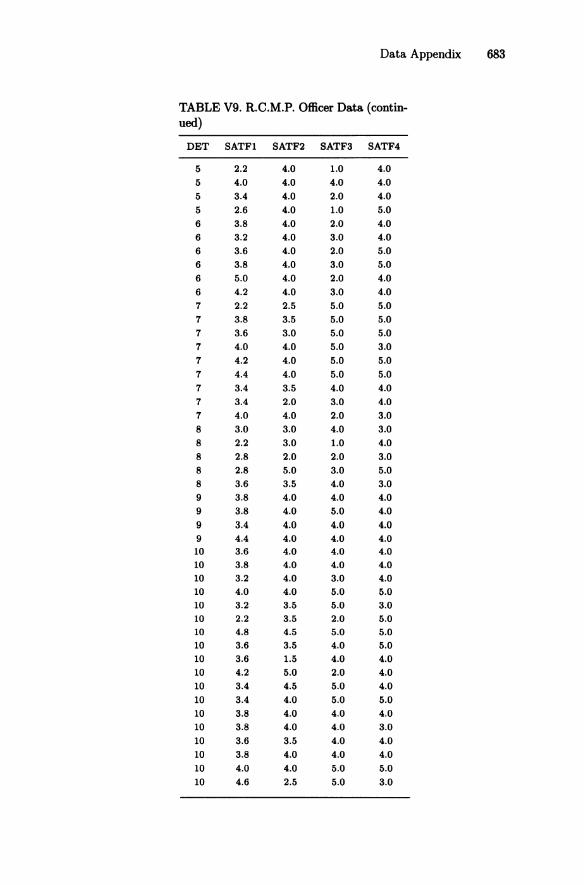
Data Appendix 683

TABLE V9. R.C.M.P. Officer Data (contin-ued)

DET SATFI SATF2 SATF3 SATF4

5 2.2 4.0 1.0 4.0 5 4.0 4.0 4.0 4.0 5 3.4 4.0 2.0 4.0 5 2.6 4.0 1.0 5.0 6 3.8 4.0 2.0 4.0 6 3.2 4.0 3.0 4.0 6 3.6 4.0 2.0 5.0 6 3.8 4.0 3.0 5.0 6 5.0 4.0 2.0 4.0 6 4.2 4.0 3.0 4.0 7 2.2 2.5 5.0 5.0 7 3.8 3.5 5.0 5.0 7 3.6 3.0 5.0 5.0 7 4.0 4.0 5.0 3.0 7 4.2 4.0 5.0 5.0 7 4.4 4.0 5.0 5.0 7 3.4 3.5 4.0 4.0 7 3.4 2.0 3.0 4.0 7 4.0 4.0 2.0 3.0 8 3.0 3.0 4.0 3.0 8 2.2 3.0 1.0 4.0 8 2.8 2.0 2.0 3.0 8 2.8 5.0 3.0 5.0 8 3.6 3.5 4.0 3.0 9 3.8 4.0 4.0 4.0 9 3.8 4.0 5.0 4.0

9 3.4 4.0 4.0 4.0 9 4.4 4.0 4.0 4.0 10 3.6 4.0 4.0 4.0 10 3.8 4.0 4.0 4.0 10 3.2 4.0 3.0 4.0 10 4.0 4.0 5.0 5.0 10 3.2 3.5 5.0 3.0 10 2.2 3.5 2.0 5.0 10 4.8 4.5 5.0 5.0 10 3.6 3.5 4.0 5.0 10 3.6 1.5 4.0 4.0 10 4.2 5.0 2.0 4.0 10 3.4 4.5 5.0 4.0 10 3.4 4.0 5.0 5.0 10 3.8 4.0 4.0 4.0 10 3.8 4.0 4.0 3.0 10 3.6 3.5 4.0 4.0 10 3.8 4.0 4.0 4.0 10 4.0 4.0 5.0 5.0 10 4.6 2.5 5.0 3.0

684 Data Appendix

TABLE VIO. Mystery Data

SEXED Cl C3 C8 C9 ClO

7 12 11 16 20 17 5 19 10 11 4 11 3 15 15 11 12 13 8 14 11 20 20 9 4 12 12 12 12 1 7 12 12 11 15 13 6 12 18 18 11 19 8 12 19 14 19 12 8 16 18 15 20 2 1 13 19 18 17 14 8 11 3 16 19 15 8 11 10 10 18 10 7 12 9 17 16 16 5 12 11 11 11 11 6 11 17 17 18 17 7 11 11 11 11 11 8 12 13 20 12 13 6 12 18 18 18 17 7 11 20 20 17 8 8 11 14 13 14 11

6 16 15 17 17 14 6 11 18 20 18 13 4 11 17 14 18 11 8 11 17 17 14 11

5 11 18 18 11 3 6 12 12 12 12 20 6 4 20 11 1 20 5 12 13 12 13 13 8 11 10 17 17 9 7 12 19 19 11 19 8 8 12 18 18 15 7 14 3 18 13 10 6 4 8 15 20 11 8 12 12 13 13 13 7 11 11 11 11 14 3 11 11 8 18 8 7 7 20 12 20 12 4 12 19 17 14 10 8 12 12 14 15 11

7 12 13 17 20 11

7 18 6 19 19 19 8 9 4 8 14 11

8 11 16 18 14 10 3 16 15 16 17 16 3 17 16 11 15 12 6 11 12 14 15 15 1 11 17 10 14 10

5 10 9 13 11 11

4 13 17 15 15 8 5 19 19 4 4 19

Data Appendix 685

TABLE VlO. Mystery Data (contin-ued)

SEXED Cl C3 C8 C9 ClO

7 19 12 20 20 20 7 12 15 14 14 14 7 19 12 11 11 11 7 12 15 14 15 9 8 10 11 13 17 10 2 11 20 20 17 1 7 12 19 19 11 11

11 7 13 7 11 4 14 18 19 14 6 8 11 15 15 17 16 5 16 15 7 9 5 2 19 11 18 5 12 2 11 18 17 11 10

5 12 10 15 7 10 7 12 14 18 16 14 8 11 7 3 1 3 7 12 17 15 16 18 7 16 11 13 19 16 7 11 17 16 11 18 6 11 12 12 12 12 6 11 19 19 11 11 7 11 20 18 20 20 7 11 19 18 18 19 5 13 8 14 16 14 4 11 18 8 17 8 8 11 11 10 10 10 7 12 15 15 15 12 3 18 16 15 15 10 8 12 11 20 19 11

4 17 16 18 12 13 3 12 19 12 12 13 8 5 0 11 19 18 8 12 11 19 19 10 3 15 16 17 20 16 7 17 16 12 11 15 7 12 19 13 13 13 8 11 3 10 10 15 6 11 17 20 11 17 8 12 17 18 19 10 3 12 19 20 20 8 8 11 16 15 3 7 7 11 20 20 20 10 6 11 16 14 18 10 2 11 10 18 18 20 3 12 9 13 14 15 8 11 15 19 15 18 8 11 13 14 15 13 5 11 6 15 10 11 3 11 15 10 17 12 3 9 17 7 17 16

686 Data Appendix

TABLE Vll. Bank Employee Data Part I

LCURRENT LSTART SEX JOBCAT RACE EDUC SENIOR AGE EXPER

9.6853

10.2524

10.0345

9.4174

9.9282 10.2128

9.1050

9.3038

9.6816 9.9965

10.0858

9.6473

9.5359

10.3735

9.3927

9.5042

9.4556

10.0962

9.1378

10.2921

10.1659

9.3414

9.9035

9.4556 9.3927 9.5539 9.8119

10.1166

10.1266 10.5133

9.4174 10.6334

9.4174

10.2400

10.0266

9.5750

10.1166

9.0359

9.7642

9.2873

8.6376 9.3049

9.4575

8.7948

8.6793 9.2301

9.3049

9.1582

9.1582

9.3147

8.7483

8.7483

8.7483

8.6995

9.1049

8.6482

9.2591

9.6158

8.7483 9.4724

8.7483 8.7483 8.7483 9.1377 9.5956 9.5462

9.6800 8.5941

9.3060 8.6995

9.5479

9.2103

8.9226

9.3497

9.0572 8.4763

9.0711

9.0848

9.3927

9.1442

9.4415

9.3673

9.1757 9.3147 8.7578

9.2183 9.0642

10.0301

8.4118

8.4763 8.7948

8.5941

8.9226

8.4381

8.5370 8.9618 8.3138

8.6586 8.5941 9.3926

o o o o o o o o o o o o o o o o o o o o o o o o o o o o o o o o o o o o o

1

1

1

1

1

1

4

5 5 3

5

4

2

2 5 4

4

5

1 2

3 2 3

4

2

4

5 3 5

3 3

3 4

5 5

5

3 5

3 5

5

1

5 1

2

1

2

2

2

1

2

1

1

1

5

o o o o o o o o o o o o o o o o o o o o o o o o o o o o o o o o o o o o o o o o o o o o o o o o o o

16

19

15

12 16

19

12

12

15 16

16

15

16

15

12

12

8 16

12

18

21

8 16

8 12 12

16 19 18 19

12 16

8 19 16

15

19

12

12

12

12

12

12 15

8 15

8 12

8 16

81

83

98

94

83

78

70

70

78

90

94

78

82

82

69

66

85

91

95

94

88 69

77

74 79 78

86 80 75

96

95 97 87

67

93

98

65

98

65

76

95

64

90 93

66 82 74 91

66 73

28.50

41.92

41.17

46.25

35.17

30.08 44.50

27.83

35.42 34.33

34.00

38.92

44.42

29.50

63.58

27.42

58.08

33.75 29.33

39.67

56.67

59.42 48.33

63.50 54.17 59.83

32.25 42.58 35.42 44.92

56.00 37.08

64.25

36.92 33.42

37.17

28.42

64.50

23.00

40.17

55.25

45.50

61.67 26.83

46.17

58.75 55.25 33.50 64.25

31.92

0.25

13.00

12.00

20.00

5.75 2.92

18.00

3.42

11.08

5.67 4.92

14.67

12.42

2.83

29.00

3.92

36.50

3.67

3.83

4.67

22.00

14.50 22.00

34.00 25.67 32.25

5.00 16.58 6.17

14.58

25.58 5.83

37.58

6.25 2.83

9.50

2.17

31.75 0.00

0.50

19.00

16.50

17.08 0.92

8.00

22.08 3.58 6.92

19.00 1.25

Data Appendix 687

TABLE Vll. Bank Employee Data Part I (continued)


9.1050 8.3848 9.0070 8.4118 9.2591 8.4381 9.3622 8.5370 9.7527 9.6238 9.0780 8.9847 8.8901 9.5298

9.8389 9.0216

10.0123 9.4970

8.9771

8.8530 8.7483

8.2687 8.3138 8.2687 8.9618

8.8392 8.6482

8.9862 8.6995

8.3138 9.0288 8.5941 9.7642 8.9618 8.8217 9.3361 9.2301

9.5324 9.4174

9.4026 9.3775

9.4076 10.0758 9.4319 9.2301

8.3138 8.4763 8.6586 8.7483

8.6995 8.7483 8.7483

8.6995 9.5104

8.7483 8.4250

10.3546 9.3497 9.4222 8.6995 9.4174 8.1886

10.5966 9.7779 9.3927 8.7483 9.1569 8.5941 9.3201 8.6995 9.1819 8.6995 9.3927 8.6995

9.4174 8.6995 9.1050 8.2687 9.2418 8.5941 9.1881 8.6482 8.8217 8.1886

8.8305 8.3138 9.1313 8.4763 9.3876 8.6995 9.0848 8.3848

9.0143 8.4118 8.9464 8.1886 9.3038 8.3138 9.1881 8.3848

1

1

1

1

o o o o o o o o o o o o o o o o o o o o o

1

1

1

2

2

2

4

4

1

1

4

4

1

4

2

1

2

4

1

2

2 3

3 3

3

5

3 2 4 2

3 5

3 1

2

3

3

3 2

2

2

1

1

2

o o o o o o o o o o o o o o o o o o

1

1

1

1

1

1

1

1

1

1

1

1

8 12 12 17 16 16 12 12

12 16 16 15

16 12

8

12 16

8

8

12

8 8 8 8

12 12

12 12 17 12 12 16 8

15 14 15

8 8 8

15 12 12

8 16

15 12 12 15 12 12

81 69 97

73 79 90 86 72

86 65

86 65

64 90 83 67 68 72

98 86 79

92 68 76 91 74

73 81 70 94 91 66 67 88 79 90 92

83 94 78 74 97 81 84

86 92

73 96 85 75

24.33 23.42 53.92 55.58 28.42 29.92 52.00 52.17 62.00 30.75

32.00 59.50 29.00 44.50 59.08 51.50 27.58 56.92

27.83 28.67 48.50

60.67 32.92 35.25 30.33 48.25

38.67 24.75 32.08 34.58 53.50 35.33 47.25 57.50 30.33 42.17 37.83

48.83 29.17 48.67 45.17 60.67

51.50 47.58 40.50 25.50

47.92 60.50 54.17 27.58

0.42 0.00 4.00

31.25 1.67 0.58

13.00 4.67

6.00 6.58

1.58 20.08

3.00 0.25 6.25

15.08 0.92

26.58 2.17

3.08 20.50 36.00

12.92 12.00 4.08

22.67

12.92 0.75 5.58 8.50

26.17 10.67 25.42 29.92

3.92 15.92 12.00

25.17 3.00 4.25 9.75

10.33

0.00 17.83

6.58 0.42

12.83 1.92 8.42 2.67

688 Data Appendix

TABLE V12. Bank Employee Data Part II

LCURRENT LSTARr SEX JOBCAT RACE EDUC SENIOR AGE EXPER

10.6310 9.9970 9.8627

10.2128 9.4174 9.9988 9.8532

10.0078 10.2219 10.2400 9.9988

10.2036 10.3514 9.9988

10.2887 9.4174 9.9641 9.4174

10.1064 10.1811 10.3498 10.0753 10.0648 10.1659 9.4125 9.8782 9.8201

10.1659 9.9451 9.9321

10.5662 9.5104 9.5324 9.5411 9.0288 9.1695 9.1942 9.3308 9.0711 9.3725 9.1695 9.3725 9.1942 9.6512 9.2648 9.1881 8.9227 9.6037 9.6198 9.1881

10.0858 9.2301 9.0711 9.4724 8.7483 9.2591 9.4880 9.5104 9.3060 9.0711 9.5462 9.5462 9.3049 9.4724 9.4880 8.7483 9.0360 8.6995 9.4880 9.8520 9.3927 9.3927 9.0711 9.4174 8.7483 9.0821 9.0474 9.4566 9.3049 9.5816 9.5471 8.6995 8.4888 8.6691 8.4764 8.5942 8.2990 8.5370 8.5132 8.7193 8.4118 8.6482 8.5942 8.6995 8.5942 8.5717 8.3428 8.8818 8.7483 8.4764

o o o o o o o o o o o o o o o o o o o o o o o o o o o o o o o o 1 1

1

1

1

1

1

1

1 1 1

1

1

1

1

1 1

5 5 4 4

3

4 5 4 4

4 5

5

4 5 4 3 4 3

5 5 4 5 4

4 3

4 4 4

5 5 5 3

2 1

1

1

1

2 1

2 2

2 2 1

2

1

1

2

1

2

o o o o o o o o o o o o o o o o o o o o o o o o o o o o o o o o o o o o o o o o o o o o o o o o o o

16 15 16 18 12 17 19 19 17 16 19 17 18 18 19

8

16 8

19 16 19 20 16 17 12 16 16 19 19 18 19 12 12 16

8

12 12 15

8

12 12 12 12 16 15 12 15 15 12 12

73 83 93 80 77 93 64 81 89 65 65 83 91 75 78 78 93 84 68 86 93 89 84 78 80 76 93 69 80 78 91 83 77 93 79 98 92 81 74 72 83 63 78 97 94 88 90 75 73 79

40.33 31.08 31.17 29.50 52.92 32.33 31.92 30.75 34.17 28.00 39.75 30.17 30.17 41.17 32.92 63.75 30.67 63.42 29.50 42.42 31.67 35.58 30.25 29.75 61.67 32.67 29.75 28.83 45.67 39.42 34.33 50.25 24.33 31.50 50.17 47.33 44.00 27.17 59.83 25.75 25.83 25.08 27.17 30.58 29.50 54.42 58.00 28.75 54.08 24.33

12.50 4.08 1.83 2.42

26.42 2.67 2.25 5.17 3.17 1.58

10.75 0.75 3.92

10.42 3.75

35.75 4.00

31.67 0.75

12.50 0.58 0.50 1.08 2.17

38.33 5.08 2.92 6.17

18.42 12.42 5.67

23.67 0.33 0.67 5.83

20.33 3.67 1.58

26.50 2.50 1.33 0.75 3.92 1.42 0.25 8.92 4.50 0.42

11.00 0.67

Data Appendix 689

TABLE V12. Bank Employee Data Part 11 (continued)


9.3414

9.2003

9.4742

9.9233

9.1182

9.6434

9.1632

9.0288

8.8901

8.7948

9.4026

9.5148

9.2360

9.3200

9.1819

9.3518

9.2591

9.1182

8.8038

9.0216

9.2183

9.0431

8.8392

9.1313

9.2761

9.3622

9.4970

8.9695

9.2591 9.3254

9.0710

9.1049

9.2873

9.2704

9.3038

9.0982

9.4556

9.2761

9.4366

9.4173

9.5539

9.3147

9.4173

8.8479

9.2928

8.7856

8.8217

9.2534

8.9695

8.9065

8.3428

8.3848

8.5942

8.8818

8.4118

8.7948

8.5370

8.4763

8.3848

8.3138

8.7948

8.4763

1

1

1

8.6482 1

8.5941 1

8.3848 1

8.6269

8.3848 1

8.4118 1

8.2687

8.4118

8.6269

8.4763

8.3138

8.4118 1

8.5941 0

8.5941 0

8.8530 0

8.5370 0

8.7671 0 8.7948 0

8.5370 0

8.6995 8.8818

o o

8.6995 0

8.6995 0

8.6995 0

8.7483 0

8.7483 0

8.6995 0

8.6995 0

8.7483 0

8.6482 0

8.6995 0

8.3138

8.7483

8.3138

8.3138

8.5941

8.6269

8.3138

2

2 2

2

2

2

1

2

2

2

1

2

1

2

2

2

2

1

2

1

1

1

1

2

2

1

2

2

2

3

3

2

3

1

1

1

1

1 1

1

o o o o o o o o o o o o o o o o o o o o o o o o 1

1

1

1

1

1

1

1

1

1

1

1

1

1

1

1

12

12

15

16

12

16

12

12

12

12

16

12

15

12

12

12

12

12

8 12

15

8 12

12

12

12

16

12

8 15

12 15

17

16

12

12

15

12

15

12

12

15

12

12

15

12

12

12

12

12

92

79

90

93

68

90

69 87

80

84

98

82

82

73

93

72

89

69

88

69

64

73

82

81

88 96

67

84

67 66

97 82

70

78

90

80

67

76

96

91

78

98

90

72

84

66

72

72

69

85

25.50

24.67

28.75

32.50

23.42

30.42

24.42

53.92

25.00

62.42

43.92

28.17

30.17

27.33

25.25

27.33

25.83

23.67

62.50

23.67

29.08

60.50

53.92

24.08

29.92

39.50

41.67

44.58

51.42 30.75

53.08 59.75

47.33

33.83

37.50

57.17

29.33

28.33

31.92

45.50

55.33

33.67

43.67

46.50

55.17

60.50

51.50

50.33

50.00

51.00

0.50

0.42

1.83

1.83

0.17

0.00

1.67

13.58

0.00

24.00

11.92

0.92

4.25

2.67

0.42

1.50

0.00

0.00

34.33

0.17

4.75

13.25

29.83

1.08

3.17

9.42

10.00

15.00

8.08 7.00

26.25 30.92

16.00

8.75

14.42

22.67

4.83

1.50

4.08

20.00

23.42

2.83

17.42

9.67

19.25

13.58

22.58

14.08

11.08 19.00

690 Data Appendix

TABLE V13. Panel Data

THISYR LASTYR HUBINC AGE EDUC BLACK CHILDl CHILD2

o 1 7.352 27 10 1 0 0 o 6.784 35 12 0 0 0

1 1 6.059 40 12 0 0 0 1 1 6.438 35 12 1 0 0 1 0 4.739 28 10 0 0 1 1 1 6.617 30 10 0 0 1 1 1 6.041 35 10 0 0 1 1 1 4.343 46 7 0 0 0 1 0 9.724 32 10 0 0 0

1 1.855 30 10 1 0 0 1 1 11.267 45 12 0 0 1 1 1 15.430 33 16 0 0 0

1 8.123 39 12 0 0 0 1 1 5.813 22 12 0 0 1 1 0 6.167 27 12 0 0 0 o 0 4.093 23 10 1 0 1 o 1 2.920 25 12 1 0 1 o 0 8.111 43 12 0 0 1 1 1 11.502 38 12 0 0 0 o 0 11.311 40 12 0 0 1 1 0 6.093 44 12 1 0 0 o 0 7.718 31 12 0 0 1 1 1 9.919 42 12 0 0 0 o 0 0.222 24 12 0 0 0 1 1 7.452 42 12 0 0 0 1 1 6.382 31 12 1 0 0 1 1 7.689 38 12 1 0 0 o 0 6.609 43 12 0 0 0 o 7.721 24 12 0 0 1 o 0 36.357 29 12 0 0 0 o 0 3.668 31 12 0 0 0 1 0 8.257 37 12 0 0 0 1 1 11.283 42 12 0 0 0 1 1 5.714 34 12 0 0 0 o 1 9.967 25 10 0 0 1 o 0 7.629 25 10 1 1 0 1 1 10.154 31 12 0 0 0 o 0 10.370 35 12 0 1 0 o 0 15.365 40 12 0 0 1 o 0 11.917 26 12 0 0 1

1 11.023 34 12 0 0 0 1 17.598 39 12 0 0 0 1 7.424 43 12 0 0 0

o 0 8.812 23 12 0 0 1 1 1 4.841 40 12 0 0 0 o 0 10.848 36 12 0 0 0

o 9.810 25 12 0 0 1 1 15.138 30 12 0 0 1 1 9.966 27 12 0 0 0

1 1 8.328 32 12 0 0 1

THISYR

1

1 o o o 1

1

o o o 1 1

1 1

o 1

o 1 o 1 1 o

1

o 1 1

o o o 1

1

1

o o 1

o 1

1

1

1

1

1 1 1 o 1

1

o 1

LASTYR

1

1 o 1 o 1

1

o o o 1 1

1 1

o 1 o 1 o 1 1 o 1 1

o 1

1

o 1 o o 1

1

o o 1

o 1 1

1

1

1

1 1 1 1

o o o 1

Data Appendix 691

TABLE V13. Panel Data (continued)

HUBINC AGE

8.856 37 7.443 37

14.264 27 0.000 35 3.401 39 0.000 33 9.136 46 4.839 32

14.168 28 7.671 33 1.599 38 3.853 40 5.366 40 7.041 46

12.187 46 12.408 40

5.693 26 3.869 21 3.069 26 7.588 27 7.786 44

12.581 36 5.962 39 4.406 45 6.341 31 7.517 35 7.984 40 7.823 43 6.852 24 8.807 34 9.923 25 9.148 30 4.511 43

15.248 30 7.651 45

20.515 39 8.375 41 7.514 27 9.474 32

10.149 33 4.782 31

10.472 35 6.762 23 9.467 29

10.342 32 1.240 44

13.820 34 9.727 40 8.853 46 8.061 36

EDUC BLACK

12 0 10 0 12 0

10 0 12 0

16 0

12 0 7 0

12 0 12 0 12 0 12 0

12 0 12 0 12 0 12 0 12 0

12 0 12 1

16 0

12 0 12 0 10 1

10 1

12 0 12 0 12 0 12 0

12 0 12 0

12 0 12 0

7 1 12 0 12 0

12 0 12 0

12 0 12 0 18 0 12 1 12 1

12 0 12 0 12 0

12 0

12 0 12 0 12 0 12

CHILD1

o o o o o o o o o o o o o o o o o o o o o o o o o o o o 1 o o o o o o o o o o o o o 1

o o o o o o o

CHILD2

o o 1

1

1

o o o 1

1

o o 1 1

o o 1

o 1

o o o o o o 1

o o o 1

1

1

1

1

o o o 1

o o o 1

o 1 1

o o o o o

692 Data Appendix

TABLE VI3. Panel Data (continued)

THISYR

o o 1

1 1

1

1

o o 1 1

1

1 1

1

1

1 1

o o 1

1 1 1 o 1

o 1 o o 1

1

1

o 1 1

1

o 1

1 1 o 1 o 1

1 1

1

1

o

LASTYR

o o 1

o o o 1

o 1

1

1

o 1

1

1

1 1 1

o 1

1

1 o 1

o 1

o o o o 1

1

1

1

1 1

1

o 1

1 1 o o o 1

1 1

1

o o

HUBINC

4.340 13.648

4.973 8.427

18.320 7.680 5.612

13.554 5.329

10.511 10.486 14.071 9.024

14.329 5.118 3.044 2.640 2.050 6.750 3.383 6.630 7.000 8.815 3.450

12.031 6.144

11.513 12.167 9.968 5.888

10.232 8.017

11.686 28.363

4.343 10.554

2.484 5.672

13.319 7.678 7.162 7.804

13.648 9.311

27.938 6.704 7.711 8.576 7.223

11.259

AGE EDUC BLACK

42 12 0 31 12 0 38 10 1 46 12 0 46 18 0 29 10 25 12 0 32 12 0 26 12 0 29 12 0 34 12 0 38 16 0 32 12 0 36 12 0

28 18 0 37 12 1 38 7 1 43 7 1 23 12 1 24 12 0 40 12 0 46 12 0 42 12 0 46 12 0 42 12 0 31 12 1 39 12 0

46 12 0 28 16 0 23 12 0 32 12 0 40 12 0 45 12 0 31 12 0 46 7 1 38 12 0

29 10 0

44 12 0 31 18 1 35 18 1 24 12 0 34 12 0 28 16 0 27 12 0 46 12 0

27 12 0 32 12 0 38 16 0 26 16 0 31 16 0

CHILDI

o o o o o o o o o o o o o o 1

o o o o o o o o o o o o o

1 o o o o o o o o o o o o o o o o o o o 1

CHILD2

o 1 1

o o 1

1

1 o o o o o 1

o o o o 1

o o o o o o o 1

1

o o o o o 1

o o 1

o o o o o

1 o 1

o o 1 o

Data Appendix 693

TABLE V13. Panel Data (continued)

THISYR LASTYR HUBINC AGE EDUC BLACK CHILDI CHILD2

o 0 26.063 30 12 0 0 1

1 11.776 42 12 0 0 0 1 12.793 46 18 0 0 0

1 11.080 44 12 0 0 0

1 1 7.074 31 12 0 0 0

1 1 6.679 36 12 0 0 1

o

1

1

1

o

1

o o

o o

1

1

1

o 1

o 1

o 1

1

o o o

o 15.868 45 12 0 0 0

1

o

1

1

1

o o

1

1

o o

1

o 1

o o 1

o o o o 1

o 1

1

7.972

0.000

3.030

2.970

9.305

8.125 13.033

0.000 2.781

3.010

26.056

5.795

0.000

2.639

9.087

12.312

7.325

3.517

17.140 24.054

6.144 13.211 9.309

3.135 2.935

9.067 10.629

8.207

9.772 8.955

6.204 9.378

54.281

7.525

11.504

5.763

5.683

10.937

9.361

6.342

7.160

7.788 2.402

42

29

43

27

40

30

29

39

30

35

40

46

36 28

24 34

33

26 35

40

42 34 45

40 45

41 44 24

42 46

46 32

45

31

32

42

32

40

45

35 31

31 25

16

12

10

16

12

12

10

12

12 12

12

12

12

12

12

12 12

10 12

12

12

12 12

10 10 12

12 12

12 12

10 12

12 12

12

12 12

12

12

12

10 12

10

o

o o o o 1

o o o o o o o o o o

1 o o o o o o o o o 1

o o o o o o o o o o

o 1

o o o o o o o o o o o o o o o o o o o o o o o o o o o o o o o o 1

o o o o o o o o

o o o o o o 1

o 1

o o o 1

1

o o o o o o o o o o o o o o o o o o o 1

o o 1

o o 1

o 1

o

CD

:f

TA

BL

E V

14

. U

.S.

Div

orc

e D

ata

ST

AT

E

BR

EA

K

CR

UE

L

DE

SE

RT

N

OS

UP

PO

R

AL

CO

HO

L

FE

LO

NY

IM

PO

TE

NT

IN

SA

NE

S

EP

ER

AT

E

t=' ~ '"

Ala

bam

a 1

1 1

1 1

1 1

1 1

>

Ala

ska

1 1

1 0

1 1

1 1

0 ~

Ari

zone

1

0 0

0 0

0 0

0 0

Arl

amsa

s 0

1 1

1 1

1 1

1 1

Q.

Cal

ifom

ia

1 0

0 0

0 0

0 1

0 ~.

Col

orad

o 1

0 0

0 0

0 0

0 0

Con

nect

icut

1

1 1

1 1

1 0

1 1

Del

awar

e 1

0 0

0 0

0 0

0 1

Dis

t of

Col

umbi

a 0

0 0

0 0

0 0

0 1

Flo

rida

1

0 0

0 0

0 0

1 0

Geo

rgia

1

1 1

0 1

1 1

1 0

Haw

aii

1 0

0 0

0 0

0 0

1 Id

aho

1 1

1 1

1 1

0 1

1 Il

lino

is

0 1

1 0

1 1

1 0

0 In

dian

a 1

0 0

0 0

1 1

1 0

Iow

a 1

0 0

0 0

0 0

0 0

Kan

sas

1 0

0 0

0 0

0 0

0 K

entu

cky

1 0

0 0

0 0

0 0

1 L

ouis

iana

0

1 1

1 1

1 0

0 1

Mai

ne

1 1

1 1

1 0

1 1

0 M

aryl

and

0 1

1 0

0 1

1 1

1 M

assa

chus

etts

1

1 1

1 1

1 1

0 1

Mic

higa

n 1

0 0

0 0

0 0

0 0

Min

neso

ta

1 0

0 0

0 0

0 0

0 M

issi

ssip

pi

1 1

1 0

1 1

1 1

0 M

isso

uri

1 0

0 0

0 0

0 0

0

TA

BL

E V

14

. U

.S.

Div

orce

Dat

a (c

onti

nued

)

ST

AT

E

BR

EA

K

CR

UE

L

DE

SE

RT

N

OS

UP

PO

R

AL

CO

HO

L

FE

LO

NY

IM

PO

TE

NT

IN

SA

NE

S

EP

ER

AT

E

Mo

nta

na

1 0

0 0

0 0

0 0

0 N

ebra

ska

1 0

0 0

0 0

0 0

0 N

evad

a 1

0 0

0 0

0 0

1 1

New

Ham

pshi

re

1 1

1 1

1 1

1 0

1 N

ew J

erse

y 0

1 1

0 1

1 0

1 1

New

Mex

ico

1 1

1 0

0 0

0 0

0 N

ewY

ork

0

1 1

0 0

1 0

0 1

No

rth

Car

olin

a 0

0 0

0 0

0 1

1 1

No

rth

Dak

ota

1

1 1

1 1

1 1

1 0

Ohi

o 1

1 1

0 1

1 1

1 1

Okl

ahom

a 1

1 1

1 1

1 1

1 0

Ore

gon

1 0

0 0

0 0

0 0

0 P

enns

ylva

nia

1 1

1 0

0 1

1 1

1 R

hode

Isl

and

1 1

1 1

1 1

1 0

1 S

ou

th C

arol

ina

0 1

1 0

1 0

0 0

1 S

ou

th D

ako

ta

0 1

1 1

1 1

0 0

0 'T

hnne

ssee

1

1 1

1 1

1 1

0 0

Tex

as

1 1

1 0

0 1

0 1

1 0

Uta

h

0 1

1 1

1 1

1 1

0 ~

Ver

mon

t 0

1 1

1 0

1 0

1 1

CI'

Vir

gini

a 0

1 1

0 0

1 0

0 1

>

Was

hing

ton

1 0

0 0

0 0

0 0

0 ~

Wes

t V

irgi

nia

1 1

1 0

1 1

0 1

1 5-

Wis

cons

in

1 0

0 0

0 0

0 0

1 S<

. W

yom

ing

1 0

0 0

0 0

0 1

1

8

8

TA

BL

E V

15.

u.s.

Div

orce

Dat

a S

ubse

t t:::

I ~

CD

ST

AT

E

BR

EA

K

CR

UE

L

DE

SE

RT

N

OS

UP

PO

R

AL

CO

HO

L

FE

LO

NY

IM

PO

TE

NT

IN

SA

NE

S

EP

ER

AT

E

>

Ala

bam

a 1

1 1

1 1

1 1

1 1

~ A

lask

a 1

1 1

0 1

1 1

1 0

~ A

rizo

Da

1 0

0 0

0 0

0 0

0 A

rkan

sas

0 1

1 1

1 1

1 1

1 C

alif

orni

a 1

0 0

0 0

0 0

1 0

Col

orad

o 1

0 0

0 0

0 0

0 0

Con

nect

icut

1

1 1

1 1

1 0

1 1

Flo

rid

a 1

0 0

0 0

0 0

1 0

Geo

rgia

1

1 1

0 1

1 1

1 0

Haw

aii

1 0

0 0

0 0

0 0

1 In

dia

na

1 0

0 0

0 1

1 1

0 Io

wa

1 0

0 0

0 0

0 0

0 K

ansa

s 1

0 0

0 0

0 0

0 0

Mas

sach

uset

ts

1 1

1 1

1 1

1 0

1 M

inne

sota

1

0 0

0 0

0 0

0 0

Mis

siss

ippi

1

1 1

0 1

1 1

1 0

Neb

rask

a 1

0 0

0 0

0 0

0 0

So

uth

Car

olin

a 0

1 1

0 1

0 0

0 1

So

uth

Dak

ota

0

1 1

1 1

1 0

0 0

Ten

ness

ee

1 1

1 1

1 1

1 0

0

TA

BL

E V

16.

U.S

. C

rim

e D

ata

STA

TE

VIO

LE

NT

P

RO

PE

RrY

M

UR

DE

R

RA

PE

RO

BB

ER

Y

ASS

AU

LT

BU

RG

LA

RY

L

AR

CE

NY

C

AR

TH

EFT

Ala

bam

a 44

8 44

85

13

30

132

273

1526

26

42

316

A1a

ska

479

5730

9

62

90

317

1385

37

27

617

Ari

zon

a 65

0 75

19

10

45

193

401

2155

48

91

473

Ark

ansa

s 33

5 34

75

9 26

80

21

8 11

19

2169

18

7 C

alif

om

ia

893

6939

14

58

38

4 43

6 23

16

3880

74

2 C

olo

rad

o

528

6804

6

52

160

309

2030

43

25

448

Co

nn

ecti

cut

412

5469

4

21

218

168

1700

30

89

678

Del

awar

e 47

4 63

01

6 24

13

7 30

6 16

30

4216

45

5 F

lori

da

983

7418

14

56

35

5 55

6 25

06

44

34

47

7 G

eorg

ia

555

5048

13

44

19

7 29

9 16

99

2976

37

2 H

awai

i 29

9 71

82

8 34

19

0 65

18

47

4732

61

2 ld

aho

31

3 44

68

3 22

46

24

1 12

38

2993

23

6 Il

lino

is

494

4781

10

26

21

7 23

9 12

42

3039

49

8 In

dia

na

377

4552

8

33

141

194

1313

28

07

432

low

a 20

0 45

46

2 14

54

12

9 10

79

3219

24

7 K

ansa

s 38

9 49

89

6 31

11

3 23

7 15

21

3196

27

1 0

Ken

tuck

y

266

3167

8

19

95

143

1040

18

75

250

~

I'>

Lou

isia

na

665

4788

15

44

19

7 40

7 15

23

2888

37

6 ~

Mai

ne

193

4174

2

12

30

146

1182

27

72

219

"0

Mar

yla

nd

85

2 57

77

9 40

39

3 41

0 16

98

3629

45

0 (1

)

Mas

sach

use

tts

601

5477

4

27

235

334

1740

26

85

1051

8-

Mic

higa

n 63

9 60

36

10

46

244

338

1741

37

10

584

)<'

Min

nes

ota

22

7 45

71

2 23

99

10

2 12

46

3029

29

5 M

issi

ssip

pi

341

3075

14

24

81

22

1 11

79

1717

17

8 M

isso

uri

554

4878

11

32

22

3 28

7 16

68

2795

41

4 0

)

co ~

0)

~

TA

BL

E V

16.

U .S

. C

rim

e D

ata

(con

tinu

ed)

Ö

ST

AT

E

VIO

LE

NT

P

RO

PE

RT

Y

MU

RD

ER

R

AP

E

RO

BB

ER

Y

AS

SA

UL

T

BU

RG

LA

RY

L

AR

CE

NY

C

AR

l'H

EF

T

~

CD

Mo

nta

na

222

4801

4

21

34

163

950

3529

32

1 ~

Neb

rask

a 22

4 40

80

4 23

82

11

4 91

5 29

21

243

CD

Nev

ada

912

7941

20

67

46

0 36

4 29

06

4356

67

8 ~

New

Ham

pshi

re

179

4499

2

17

42

118

1312

28

77

309

New

Jer

sey

604

5797

6

30

303

263

1878

31

89

729

New

Mex

ico

615

5364

13

43

12

7 43

0 14

92

3521

35

0 N

ewY

ork

10

29

5882

12

30

64

1 34

4 20

61

3064

75

9 N

ort

h C

aro

lin

a 45

5 41

85

10

22

82

33

9 14

22

2546

21

6 N

ort

h D

ako

ta

54

2909

1

9 7

35

488

2242

17

9 O

hio

498

4933

8

34

223

232

1466

30

40

426

Old

aho

ma

419

4633

5

41

104

291

1748

40

87

420

Ore

gon

490

6196

5

41

152

291

1748

40

87

360

Pen

nsyl

vani

a 36

3 33

72

6 23

17

7 15

6 10

38

1915

41

8 R

ho

de

Isla

nd

408

5524

4

17

118

493

1716

29

64

843

So

uth

Car

oli

na

660

4779

11

37

11

8 49

3 16

70

2803

30

6 S

ou

th D

ako

ta

126

3116

1

12

20

93

692

2255

16

8 T

hnne

ssee

45

8 40

39

10

37

180

229

1501

21

75

363

Tex

as

550

5592

16

47

20

8 27

7 18

53

3181

55

8 U

tah

30

3 55

77

3 27

80

19

1 13

21

3931

32

3 V

erm

ont

178

4809

2

29

38

108

1526

29

88

294

Vir

gini

a 30

7 43

12

8 27

12

0 15

1 12

02

2882

22

7 W

ashi

ngto

n 46

4 64

50

5 52

13

5 27

1 18

62

4192

39

5 W

est

Vir

gini

a 18

3 23

67

7 15

48

11

2 73

8 14

29

199

Wis

cons

in

182

4616

2

14

70

94

1079

32

91

245

Wyo

min

g 39

2 45

93

6 28

44

31

3 90

3 33

44

345

TA

BL

E V

17.

V.S

. C

rim

e D

ata

Su

bse

t

ST

AT

E

VIO

LE

NT

P

RO

PE

RT

Y

MU

RD

ER

R

AP

E

RO

BB

ER

Y

AS

SA

UL

T

BU

RG

LA

RY

L

AR

CE

NY

C

AR

TH

EF

T

Ala

bam

a 44

8 44

85

13

30

132

273

1526

26

42

316

Cal

ifor

nia

893

6939

14

58

38

4 43

6 23

16

3880

74

2 F

lori

da

983

7418

14

56

35

5 55

6 25

06

4434

47

7 M

assa

chus

etts

60

1 54

77

4 27

23

5 33

4 17

40

2685

10

51

New

Ham

sph

ire

179

4499

2

17

42

118

1312

28

77

309

New

Jer

sey

6

04

57

97

6 30

30

3 26

3 18

78

3189

72

9 N

ew M

exic

o 61

5 53

64

13

43

127

430

1492

35

21

350

New

Yo

rk

1029

58

82

12

30

641

344

2061

30

64

759

No

rth

Dak

ota

54

29

09

1 9

7 35

48

8 22

42

179

Ore

gon

490

6196

5

41

152

291

1748

40

87

360

Ten

ness

ee

458

4039

10

37

18

0 22

9 15

01

2175

36

3 T

exa

s 55

0 55

92

16

47

208

277

1853

31

81

558

Ver

mon

t 17

8 48

09

2 29

38

10

8 15

26

2988

29

4 t:I

W

ash

ing

ton

46

4 64

50

5 52

13

5 27

1 18

62

4192

39

5 P>

.... W

est

Vir

gini

a 18

3 23

67

7 15

48

11

2 73

8 14

29

199

P> i a> 8. >:;l.

0)

co

co

700 Data Appendix

TABLE V18. Automobile Data Part 11

TYPE ENGSIZE CYLIND COMBRATE WEIGHT FOR

Pontiac Paris 5 3 4 5 0 Honda Civic 1 1 1 1 Buick Century 4 2 4 3 0 Subaru GL 1 2 1 Volvo 740GLE 2 2 3 1 Plymouth Caravel 2 2 3 0 Honda Accord 1 2 2 1 Chev Camaro 3 2 3 4 0 Plymouth Horizon 2 2 2 0 Chrysler Daytona 2 1 2 3 0 Cadillac Fleetw 4 3 4 5 0 Ford Mustang 5 3 4 4 0 Toyota Celica 2 2 2 1 Ford Escort 1 2 2 0 Toyota Tercel 1 1 1 Toyota Camry 2 2 1 Mercury Capri 5 3 4 4 0 Toyota Cressida 3 2 3 4 1 Nissan 300ZX 3 2 4 4 1 Nissan Maxima 3 2 4 4 1

TABLE V19. Cola Similarity Data

00 Diet Pepsi

34 00 RC Cola

79 54 00 Yukon

86 56 70 00 Dr. Pepper

76 30 51 66 00 Shasta

63 40 37 90 35 00 Coca-Cola

57 86 77 50 76 77 00 Diet Dr. Pepper

62 80 71 88 67 54 66 00 Tab

65 23 69 66 22 35 76 71 00 Pepsi-Cola

26 60 70 89 63 67 59 33 59 00 Diet-Rite

Data Appendix 701

TABLE V20. Car Similarity Data

00 Mustang SVO 27 00 Cadillac Seville 26 01 00 Lincoln Continental 17 38 39 00 Ford Eecort 13 28 29 36 00 Corvette 25 41 42 10 35 00 Chevrolet Corvette 15 32 30 45 09 48 00 NisBan 300ZX 24 40 02 12 43 11 34 00 Renault Alliance 16 33 31 46 08 49 14 44 00 Porshe 944 37 07 05 50 18 52 19 51 21 00 Jaguar XJ6 47 06 04 53 23 55 22 54 20 03 00 Mercedes 500SEL

CJ

tw

0 po .... po >

:g ~

TA

BL

E V

21.

Air

Pol

luti

on D

ata

Sub

set

5- ><.

CIT

Y

TM

R

SM

IN

SM

EA

N

SM

AX

P

MIN

P

ME

AN

P

MA

X

PM

2

PE

RW

H

NO

NP

OO

R

Jers

ey C

ity

11

99

155

229

340

63

147

253

1357

.2

93.1

87

.3

Den

ver

84

1 2

61 .

18

8 54

12

6 22

9 25

.4

95.8

86

.9

Mil

wau

kee

921

65

134

236

49

150

299

150.

2 94

.4

90.4

M

aco

n

869

18

27

128

22

122

754

28.6

69

.0

73.7

B

ost

on

11

12

42

163

337

55

141

252

174.

5 97

.3

88.5

B

rid

gep

ort

93

8 13

7 20

5 30

8 32

91

18

2 10

3.3

94.7

90

.7

Ch

icag

o

1000

75

16

6 32

8 88

18

2 29

6 16

7.5

85.2

89

.4

Au

stin

68

9 40

46

58

10

78

15

7 20

.9

87.2

75

.2

Sea

ttle

93

8 1

47

17

9 32

6

9

141

26.2

95

.2

88.8

M

obil

e 8

23

47

67

24

8 29

12

9 28

4 25

.3

67.7

74

.6

Au

gu

sta

823

31

46

158

28

66

142

15.2

70

.2

67.8

C

har

lest

on

78

0 15

28

3 94

0 55

22

5 95

8 27

.9

94.2

78

.6

TA

BL

E V

22.

Sho

ppin

g A

ttit

ud

e D

ata

Par

t 11

Al

A2

A

3 A

4

A5

A6

A7

AB

A

9

AIO

A

ll

Al2

A

l3

Al4

A

l5

Al6

A

l7

AlB

W

OR

K

AG

E

2 5

2 2

4 4

4 4

2 2

2 4

4 4

2 2

4 4

2 2

3 2

I 5

I I

3 4

2 3

2 3

3 4

2 2

4 2

2 4

I 3

3 3

5 5

4 4

2 2

2 4

4 4

4 2

4 2

I I

I 3

5 2

5 4

4 2

3 2

5 2

2 3

2 4

4 2

1 1

2 I

I 5

1 3

3 4

2 2

4 2

2 4

2 1

4 4

2 5

3 I

2 3

4 3

5 5

3 4

3 2

1 1

1 5

5 4

2 2

I I

4 4

3 4

4 2

4 2

2 4

4 4

2 2

4 5

1 3

4 I

I 5

3 3

3 2

4 5

4 4

2 2

2 4

5 4

2 5

2 I

I 5

3 1

4 4

2 1

5 I

2 5

2 I

4 4

2 5

5 2

3 5

3 3

3 2

4 4

4 4

4 4

4 I

3 5

2 6

I 3

4 I

5 3

5 4

2 1

5 2

2 3

1 4

5 1

1 1

3 I

3 5

2 3

3 2

4 3

4 2

5 4

2 2

4 5

2 4

I 2

4 I

5 4

5 4

2 I

3 2

4 4

4 1

2 4

1 1

I I

3 5

1 4

5 4

2 1

4 2

4 5

5 1

4 2

1 5

2 I

I 5

3 2

4 1

4 3

1 4

5 5

2 1

2 5

2 5

3 I

3 3

3 3

4 4

2 4

2 2

5 5

5 I

4 2

2 5

I I

2 3

3 3

2 4

2 3

4 2

I 1

1 4

5 1

1 3

3 2

3 2

3 3

4 2

4 3

2 4

4 4

2 4

3 4

2 2

0 2

4 4

4 3

2 2

4 2

3 2

2 3

4 I

I 3

4 2

2 ~

2 I

5 4

5 4

4 4

2 3

4 I

5 3

3 I

2 5

1 4

'" I

4 5

3 3

3 5

2 4

2 2

4 5

5 5

2 2

5 1

2 >

2

2 4

3 4

5 5

5 2

2 1

4 1

4 1

5 5

4 1

I ~

I 3

3 I

5 3

5 4

2 2

4 2

2 2

1 4

5 2

1 I

~ 2

I 2

2 2

3 4

2 2

2 4

I 2

2 I

4 4

4 1

3 I

4 5

3 4

5 5

4 3

3 3

2 2

3 2

2 4

3 I

1

~

~

~ T

AB

LE

V22

. S

hopp

ing

Add

itud

e D

ata

Par

t 11

(co

ntin

ued)

0

Al

A2

A

3

A4

A

5

A6

A

7

A8

A9

A

IO

All

A

I2

AI3

A

14

A

I5

AI6

A

17

AI8

W

OR

K

AG

E

Q> .... Q>

I 5

5 I

5 3

5 5

I 2

3 I

2 1

2 1

5 2

I 2

>- 't:I

3 1

3 5

I 3

3 4

3 2

4 1

4 4

2 2

4 4

2 5

't:I

I 4

2 2

3 4

5 5

2 3

5 I

2 2

2 I

5 I

2 I

~ 8-

3 I

I 3

3 I

1 4

2 2

4 2

2 2

2 2

2 2

2 3

5<.

I 5

4 3

5 5

5 5

I 1

5 I

4 4

2 4

5 2

1 2

3 I

I 3

I 3

3 4

2 3

4 2

2 2

2 4

4 2

2 3

4 2

I 4

2 2

3 5

2 4

5 2

4 4

3 2

3 3

2 5

I 4

4 1

5 5

5 4

2 2

3 3

3 4

2 2

4 2

1 1

1 3

5 3

4 5

5 2

1 4

4 2

2 4

4 2

4 4

1 2

2 2

4 2

3 3

4 4

2 2

4 1

2 2

2 4

5 2

1 3

2 I

2 3

1 2

2 4

2 2

1 3

4 4

2 2

4 1

2 6

3 1

2 3

3 2

2 4

2 3

2 3

2 4

2 2

4 2

2 4

1 2

2 2

3 3

4 4

2 2

2 2

3 4

4 2

4 4

1 5

2 1

1 3

1 1

3 2

2 2

4 2

2 2

2 4

4 2

2 5

3 1

4 5

3 1

3 5

2 2

2 2

4 4

2 2

2 4

2 6

1 3

2 4

3 2

4 3

2 3

2 2

4 4

2 3

4 2

2 2

4 2

2 4

2 2

3 2

4 3

3 2

5 4

4 2

1 5

2 6

3 1

3 5

3 1

1 4

4 2

2 4

2 2

2 4

4 2

2 3

2 4

4 5

2 2

4 4

2 2

2 4

2 4

1 4

4 2

1 3

1 3

5 1

4 5

5 4

2 2

2 2

2 3

2 4

4 2

1 2

1 3

5 3

3 5

5 4

2 2

4 2

4 4

4 2

2 2

1 2

1 5

5 3

5 5

5 5

4 2

4 2

4 4

1 2

4 5

1 2

1 4

3 1

5 5

5 4

2 2

1 3

4 4

5 1

2 4

1 1

5 1

3 5

1 3

3 5

4 3

1 1

3 5

2 2

4 5

2 5

1 3

4 2

3 4

4 4

2 1

4 2

3 4

2 2

5 2

1 5

TA

BL

E V

22.

Sho

ppin

g A

ttit

ud

e D

ata

Par

t 11

(co

ntin

ued)

Al

A2

A3

A4

A

5 A

6

A7

A8

Ag

AIO

A

ll

AI2

A

I3

AI4

A

I5

AI6

A

I7

AI8

W

OR

K

AG

E

2 I

3 5

I 3

3 4

2 1

4 1

1 4

1 3

4 4

2 3

I I

3 2

2 4

4 3

2 3

4 2

4 4

4 2

4 4

1 3

5 4

1 5

2 I

3 4

2 3

3 I

3 3

2 2

4 2

2 5

3 1

2 3

3 4

4 5

2 3

1 5

5 5

5 1

1 5

2 2

2 3

2 4

2 4

4 4

2 4

2 3

4 4

2 2

2 2

1 3

I 5

4 3

5 3

5 2

2 3

4 2

2 2

2 4

5 4

I 2

4 I

I 4

3 I

3 3

2 2

2 4

3 4

2 3

4 2

2 4

3 I

2 4

3 2

3 4

2 3

4 2

5 5

2 3

3 2

2 4

2 4

I 4

1 2

3 4

3 3

5 1

2 2

2 2

5 I

2 6

I 5

5 I

3 4

5 4

2 2

4 2

4 4

2 4

4 2

I I

2 2

2 2

1 2

4 4

2 I

4 I

2 2

2 4

4 4

I 4

2 3

3 4

I I

3 4

2 2

4 I

2 4

2 4

4 2

2 6

I 3

5 3

3 5

4 4

2 4

5 3

4 3

2 3

2 2

I 2

I 2

3 2

3 3

5 3

2 2

3 I

4 4

4 2

3 3

I 2

I 4

5 2

4 4

5 4

I 2

2 4

4 4

2 2

4 5

I 1

2 3

5 3

5 4

3 4

4 I

5 2

2 2

2 2

4 2

2 I

1 4

5 4

4 4

3 4

2 3

4 3

3 3

2 2

4 2

1 4

4 2

3 3

I I

3 2

4 2

2 3

3 3

2 4

4 2

2 6

0 3

5 3

I 5

4 5

4 2

I 4

I 2

4 2

I 5

2 1

2 ~

2 2

4 2

4 4

4 2

4 2

I 4

4 4

2 2

4 4

2 2

tI>

I 2

3 2

4 5

4 2

4 2

3 2

4 3

2 2

4 3

I 2

>

I 2

3 3

5 4

5 5

4 2

5 I

2 5

5 4

4 5

I 2

~ 1

3 2

I 2

2 5

3 4

4 I

I I

3 3

I 4

4 1

2 =

I

5 2

I 2

4 5

2 I

I 2

4 2

4 2

3 4

I 1

2 ~

3 1

1 5

3 1

3 2

2 2

2 2

2 4

2 2

4 4

2 6

~

c.n

~

TA

BL

E V

22.

Sho

ppin

g A

ttit

ud

e D

ata

Par

t II

(co

ntin

ued)

tJ

A

l A

2 A

3

A4

A

5 A

6

A7

A8

A9

AlO

A

ll

Al2

A

I3

Al4

A

I5

Al6

A

l7

AI8

W

OR

K

AG

E

~

po

2 2

2 2

3 3

4 4

2 3

2 4

4 1

3 2

4 4

1 3

>

2 2

2 4

4 4

4 4

2 2

4 2

2 3

2 2

4 2

1 5

~ 2

1 3

5 1

3 3

4 4

2 5

5 4

2 2

2 5

2 2

5 8-

3 2

I 5

1 1

3 2

4 2

2 2

2 2

2 4

4 4

2 4

><.

I 4

3 2

5 5

5 2

4 2

4 3

3 4

I 4

5 4

1 1

2 I

I 3

1 3

3 4

2 2

4 2

2 2

2 2

5 2

2 4

3 1

I 5

1 1

3 4

4 4

4 4

2 4

2 4

4 2

2 5

3 I

I 3

3 1

2 4

2 3

5 2

4 2

2 2

4 2

2 6

3 I

I 3

3 4

1 3

2 5

2 4

4 2

2 2

5 2

2 5

2 2

2 4

4 3

4 4

2 3

2 3

4 3

2 3

4 3

2 1

I 3

3 I

4 3

5 2

4 3

4 2

2 3

2 4

5 4

1 2

I 4

3 I

4 4

4 5

2 3

2 2

5 3

4 2

4 4

2 1

2 3

2 4

2 2

4 4

2 3

2 3

3 4

2 2

4 2

2 2

2 I

I 5

1 2

3 4

2 3

5 1

2 3

2 2

4 2

2 3

1 4

5 1

4 4

5 4

1 2

2 3

4 3

2 2

4 4

1 2

3 1

3 4

1 4

3 4

2 2

4 2

2 3

2 3

4 2

2 6

2 2

3 2

2 4

3 4

2 2

1 4

2 2

2 3

4 2

2 1

4 2

4 2

2 4

4 4

1 2

4 4

2 2

1 5

5 2

1 3

1 2

4 4

2 4

2 2

2 2

4 2

2 4

2 4

4 2

2 2

5 1

1 3

2 3

3 4

1 2

4 2

4 2

2 4

4 2

2 5

2 2

3 3

3 3

4 3

2 3

2 2

3 3

I 3

4 4

2 2

3 4

4 4

3 3

4 3

4 3

3 2

4 5

3 1

2 4

1 3

3 I

1 3

3 2

2 4

2 1

5 1

1 1

1 4

4 2

2 5

3 3

3 3

I 3

3 4

2 4

2 2

5 4

2 2

4 4

2 6

I 5

3 2

3 3

4 4

2 3

I 2

3 3

2 2

3 4

1 2

TA

BL

E V

22.

Sho

ppin

g A

ttit

ud

e D

ata

Par

t 11

(co

ntin

ued)

Al

A2

A

3

A4

A

5

A6

A

7

AB

Ag

AlO

A

ll

AI2

A

I3

A1

4

AI5

A

I6

AI7

A

lB

WO

RK

A

GE

3 3

3 2

3 4

5 4

2 3

4 3

4 4

I 2

4 4

2 2

I 5

4 4

4 3

3 4

2 3

4 2

3 4

2 2

4 4

2 I

3 I

I 5

3 3

1 5

2 2

2 4

3 4

I 4

4 2

2 4

I 3

5 I

3 2

5 2

4 4

4 4

I 2

2 4

5 2

1 2

3 2

1 4

I 2

I 4

2 2

2 2

4 5

2 2

4 2

2 6

2 5

2 5

3 5

4 5

5 2

5 5

4 5

I 5

5 1

1 5

I 2

3 4

3 4

4 4

4 2

4 2

4 4

4 2

2 4

1 3

I 5

5 I

5 5

5 3

3 2

4 4

4 4

2 2

3 4

1 2

1 3

1 1

5 3

4 2

2 3

5 1

1 1

1 3

5 1

2 2

2 2

4 4

4 4

4 4

4 2

4 2

4 4

4 2

2 4

2 2

3 1

I 3

I 1

3 4

2 4

4 2

4 4

2 2

4 2

2 6

5 1

I 3

3 1

3 4

1 2

1 3

1 1

I 1

5 3

2 6

4 1

2 3

2 3

3 2

4 4

5 2

2 2

2 4

5 3

1 5

2 1

2 5

3 2

3 4

2 4

4 2

5 5

5 1

2 5

2 3

3 1

3 3

3 1

2 4

2 1

3 4

2 4

2 4

4 2

2 4

2 4

2 4

4 3

3 4

2 4

4 2

2 2

2 2

4 2

2 2

2 1

1 2

3 1

3 4

1 3

4 1

1 1

I 4

4 2

2 3

2 2

1 5

1 2

3 4

1 2

4 2

1 2

1 4

5 1

2 6

2 2

3 2

2 4

5 5

2 1

2 2

4 2

3 2

4 4

1 5

0 '" 2

3 2

2 3

2 5

4 2

3 2

1 2

1 1

5 2

1 2

1 .... '"

2 4

2 2

4 3

4 4

2 3

2 4

2 2

2 4

5 1

2 1

:>

1 4

2 2

2 4

4 2

4 5

4 2

2 2

2 4

4 2

1 4

'ö

'ö

1 4

4 2

3 4

4 4

2 2

2 4

2 2

2 4

4 5

2 1

~

1 2

3 4

4 3

4 2

4 3

1 4

2 4

2 2

5 4

2 2

5-1

2 2

2 4

4 4

4 2

2 4

2 2

2 1

2 5

1 I

4 x· -t

0 -t

~

00

TA

BL

E V

22.

Sho

ppin

g A

ttit

ud

e D

ata

Par

t 11

(co

ntin

ued)

0

Al

A2

A3

~

A4

A

5

A6

A

7

AB

A

9 A

IO

All

A

I2

AI3

A

I4

AI5

A

I6

A1

7

AlB

W

OR

K

AG

E

.. ~ 2

I I

5 3

3 3

2 4

4 I

4 2

3 I

4 4

2 2

3 ;>

'"

0 I

5 3

2 3

3 5

5 5

2 2

3 2

3 2

2 4

4 I

4 '"

0 (l)

I 5

3 I

5 5

5 2

I 2

4 4

4 4

2 4

4 2

I 1

8-3

I 4

5 2

3 4

5 2

2 4

2 4

4 4

I 4

4 2

6 x·

2 I

I 4

I 2

4 5

2 4

5 I

2 1

I 4

4 2

2 5

4 I

I 3

I I

2 2

2 2

2 4

5 5

3 2

3 5

2 6

3 I

3 5

3 3

3 4

I 2

4 2

I 2

I 4

5 1

2 5

3 3

2 3

3 2

3 4

2 2

2 3

2 3

2 4

5 2

2 5

3 I

3 5

I 3

3 5

2 2

4 2

3 4

2 2

4 2

2 4

I I

5 5

1 1

5 I

5 5

5 I

5 5

5 I

I 5

I 5

2 I

2 4

4 4

4 4

2 2

2 2

4 4

4 2

2 4

I 5

2 2

5 2

4 2

4 4

4 I

5 2

5 4

4 2

2 4

I 3

I 3

3 I

5 5

5 4

2 2

4 2

2 2

2 2

4 4

I 1

2 I

I 5

2 I

3 5

2 3

1 2

4 5

4 I

2 4

2 5

2 I

1 4

1 3

3 3

3 2

4 4

3 3

2 2

5 2

2 6

2 2

I 5

2 3

3 4

1 1

I 2

5 4

5 I

3 4

2 3

2 2

2 3

3 4

2 4

1 2

2 2

2 2

1 3

4 1

2 2

3 I

2 5

3 2

3 2

3 4

4 2

3 3

2 3

3 2

2 5

I 5

4 1

5 3

5 4

2 2

3 2

3 2

3 2

4 2

1 2

I 3

I I

4 4

I I

I 2

5 I

I I

I 4

5 I

I 4

3 3

5 2

2 2

4 4

4 2

4 3

2 2

I 4

5 3

1 3

I 2

2 2

3 2

4 2

2 2

3 2

4 4

2 2

3 2

1 5

2 2

3 2

4 4

4 4

2 4

2 4

2 2

2 4

4 2

2 2

2 I

4 3

4 3

4 5

I 1

2 1

2 3

2 I

5 I

2 3

1 I

1 1

4 I

4 4

1 1

4 1

4 4

1 1

4 4

1 3

TA

BL

E V

22.

Sho

ppin

g A

ttit

ud

e D

ata

Par

t II

(co

ntin

ued)

Al

A2

A3

A4

A

5 A

6 A

7 A

B

A9

AIO

A

ll

Al2

A

l3

Al4

A

l5

Al6

A

l7

AlB

W

OR

K

AG

E

3 I

3 5

3 1

3 2

2 4

5 4

5 3

2 4

2 3

2 5

I 2

3 2

2 2

4 2

2 I

4 2

3 3

2 3

4 2

2 I

I 3

1 2

3 3

4 5

2 2

3 2

2 3

2 4

4 2

1 3

2 2

4 2

1 4

5 2

2 4

2 4

1 2

2 4

5 1

I 4

1 5

5 1

3 5

5 2

1 2

4 2

2 3

2 5

5 2

1 1

2 2

2 2

4 4

4 4

2 2

2 4

4 4

2 2

2 4

1 6

1 5

5 1

5 5

5 4

2 2

5 2

4 5

3 2

4 5

1 1

3 2

3 3

4 3

4 2

4 3

2 4

4 4

4 2

3 4

1 4

5 3

1 3

1 1

4 4

4 3

4 2

5 5

5 1

2 5

2 6

I 5

5 I

3 5

5 4

2 2

3 3

I I

1 4

5 2

1 1

5 1

1 5

3 1

3 2

4 4

4 2

4 4

3 2

4 4

2 6

2 5

3 1

5 5

5 4

4 2

2 3

2 3

3 4

5 2

1 1

3 I

3 4

1 1

3 4

2 2

2 2

2 4

2 1

4 2

2 6

1 2

4 3

4 2

5 2

1 1

5 1

2 5

1 3

4 1

1 2

1 3

3 2

4 3

3 4

2 2

2 2

2 3

1 4

4 1

1 2

1 3

4 1

3 4

5 4

2 3

4 2

2 2

1 4

2 2

1 2

1 1

1 2

3 1

4 2

2 1

4 1

4 4

2 1

4 4

1 5

4 1

1 3

2 1

2 4

4 3

2 2

4 4

2 2

2 4

2 6

2 3

4 2

4 3

2 4

2 3

1 5

2 2

1 1

5 2

2 1

t::l

po

3 1

4 3

2 4

5 2

4 4

1 3

4 4

4 2

4 5

1 5

.. SI>

2 2

2 2

2 2

4 2

2 2

4 2

2 2

2 2

2 2

1 4

>

1 3

5 3

4 4

5 4

2 2

4 2

3 4

2 2

4 2

1 2

"0

"0

2 1

3 3

2 3

1 4

2 3

1 4

2 4

1 1

5 4

2 6

(1)

5 1

1 5

1 1

3 4

2 2

4 2

4 4

2 2

4 2

2 6

ä. 1

1 4

5 3

4 4

5 2

2 5

2 4

4 4

2 2

4 1

4 sr ~

co

~

.....

0

TA

BL

E V

22.

Sho

ppin

g A

ttit

ud

e D

ata

Par

t 11

(co

ntin

ued)

0 ~

Al

A2

A3

A

4

A5

A

6

A7

AB

A

9

AlO

A

ll

AI2

A

I3

AI4

A

I5

AI6

A

I7

AlB

W

OR

K

AG

E

... ~ 2

I 2

5 I

3 3

4 2

2 4

I 3

2 2

4 5

2 2

6 :>

"0

I

3 3

2 2

4 2

4 2

2 I

4 I

4 4

3 5

2 2

2 "0

~

I 5

3 I

5 5

5 4

2 2

2 2

2 5

I 2

4 2

1 2

8-I

3 4

I 4

5 5

2 2

4 3

2 2

4 2

4 4

2 I

1 x·

I 3

3 I

4 3

5 3

2 2

4 2

4 2

I 4

5 2

I 2

2 5

2 4

2 3

4 4

2 3

2 2

5 3

2 2

4 3

1 5

I 2

4 4

3 4

5 5

2 4

3 2

2 2

2 5

5 2

2 2

3 I

I 3

2 I

3 4

2 3

2 2

4 4

2 2

2 2

2 6

I 5

3 3

5 5

5 4

4 2

4 3

2 2

2 4

4 2

I 2

I 3

5 3

3 5

5 4

2 2

5 2

2 4

4 2

4 2

I 2

I 3

5 I

5 5

5 5

4 1

4 I

3 4

I 5

4 I

I I

2 2

3 5

3 2

3 2

3 3

4 2

2 3

I 2

5 2

2 3

I 3

4 I

5 5

5 4

I 3

2 4

I 2

I 4

5 2

I I

I I

4 3

4 2

5 5

4 I

I 4

5 5

4 I

4 5

I 5

2 5

3 2

3 3

4 4

2 2

2 3

3 3

I 4

4 2

I 2

3 I

I 5

I I

3 4

2 2

2 2

4 4

2 2

4 2

2 6

3 I

3 5

3 3

3 2

4 2

4 2

4 4

2 2

4 4

2 4

2 2

4 2

3 3

4 4

3 2

4 2

2 2

2 3

4 4

I 5

I 4

5 2

5 4

4 4

2 1

3 2

2 1

2 4

4 3

I I

I 5

3 I

5 5

5 4

2 2

4 2

2 2

2 4

5 2

I 2

3 3

2 3

I I

3 4

2 4

2 2

2 4

2 2

4 2

2 5

2 2

5 4

2 4

4 4

4 4

2 2

2 2

2 4

5 I

I 4

3 I

2 3

2 I

3 4

2 2

2 4

I 4

2 2

4 4

2 6

I 5

4 I

4 4

4 2

4 3

4 3

5 3

2 2

4 5

I 2

2 I

I 5

I 3

4 5

5 3

2 I

2 2

I 4

5 2

2 6

Index

Author Index

A Agresti, Alan 87, 116 Amemiya, Takeshi 327 Anderberg, M.R 568, 603 Andersen, Erling B. 46, 87, 116,

306, 327, 453, 465, 467 Anderson, T.W. 169, 190, 191, 241,

327 Arabie, P. 567, 584, 603

B Ben-Akiva, Moshe 322,327 Bernstein, Ira H. 467 Bibby, J.M. 144, 157, 169, 190,

191, 327, 468, 568, 604 Bishop, Yvonne M.M. 46, 58, 87,

116

C Cailliez, Francis 583, 603 Carmone, Frank J. 585, 601, 602,

603 Carroll, J.D. 584, 603 Cattell, R.B. 417, 467 Christensen, Ronald 87, 116 Conway, Delores A. 417, 467 Cooper, Martha C. 564, 565, 566,

567, 604 Coxon, A.P.M. 585, 591, 602, 603

D Davidson, M.L. 591, 602, 603 de Leeuw, J. 595, 605 Devlin, S.J. 156, 191 Dubes, R.C. 564, 568, 603 Duffy, Dianne E. 87, 116,306,328

E Edelbrock, Craig 567, 603

Everitt, B.S. 46, 116, 467, 568, 603

F Feldt, L.S. 163, 191 Fienberg, Stephen E. 46, 58, 82,

87, 116, 306, 321, 327 Fomby, Thomas B. 306, 327 ForthofIer, Ron N. 115, 116 Fox, John 306, 327 Freeman, Daniel H. Jr. 46, 115,

116 Freeman, J.L. 115, 116

G Geisser S. 163, 191 Gibbons, Dianne 347,467 Giffi, A. 467, 603 Gnanadesikan, R 157, 191 Gordon, A.D. 568,603 Gorsuch, RL. 406, 426, 467 Graef, Jed 592, 605 Green, Paul E. 585, 601, 602, 603 Greenacre, M.J. 453, 457, 461, 462,

468 Greenhouse, S.W. 163, 191 Griffiths, W.E. 286, 306, 327 Grizzle, James E. 115, 116 Gunst, R.F. 347, 467

H Hakistan, A.R. 417, 467 Harman, H.H. 406, 467 Hartigan, J.A. 603 Hawkins, D.M. 157, 191, 467 Hill, R Carter 286, 306, 327 Holland, Paul W. 46, 58, 87, 116 Hosmer, David W. 290,306,327 Hubert, L. 567, 603 Huynh, H. 163, 191

712 Author Index

J Jackson, J. Edward 388, 431, 467 Jain, A.K. 564, 568, 603 Jambu, Michel 467, 603 Jobson, J.D. 164, 191, 417, 420,

467, 600, 603 Johnson, llichard A. 144, 169, 191,

241, 327, 468, 479 Johnson, Stanley R. 306, 327 JollifIe, LT. 388, 396, 426, 468 Judge, George C. 286, 306, 327

K Kent, J.T. 144, 157, 169, 190, 191,

327, 468, 568, 604 Kettering, J.R. 156, 191 Klett, C. James 562, 604 Koch, Gary G. 115, 116 Korkie, R. 164, 191 Kryzanowski, W.J. 144, 191, 327 Kruskal, J .B. 602, 603

L Lachenbruch, Peter A. 278, 327 Landis, J.R. 115, 116 Lawley, D.N. 426, 468 Lebart, L. 453, 465, 468 Lee, Tsoung-Chao 286, 306, 327 Lehnen, R.G. 115, 116 Lemeshow, Stanley 290,306,327 Lerman, Steven, R. 322, 327 Lewandowsky, Stephan 594, 604 Lewyckyj, R. 595, 605 Lorr, Mauriee 568, 604 Lütkepohl, Helmut 286, 306, 327

M MeCullagh, P. 306, 327 MeDonald, G.C. 347, 467 MacDonnell, W.R. 346, 468 Maddala, G.S. 308, 322, 327 Mardia, K.V. 144, 149, 157, 169,

190, 191, 327, 468, 568, 604

Maxwell, A.E. 346, 426, 468

Milligan, GIen W. 563, 564, 565, 566, 567, 604

Mojena, R. 546, 604 Morineau, A. 453, 465, 468 Morrison, Donald F. 169, 191, 241,

328,468 Mulaik, Stanley A. 426, 468,480

N NeIder, J.A. 306, 327 Nerlove, S.B. 601, 604 Nishisato, S. 457, 462, 468

o Ogilvie, John 594, 604 Overall, John E. 562, 604

p Padmos, P. 592, 605 Press, S. James 190, 191, 241, 328

R Reinganum, Mare R. 417, 467 Reynolds, H.T. 46, 87, 115, 116 Reynolds, M.L. 591, 595, 601, 602,

604 Rogers, W.T. 417, 467 Romney, A.K. 601, 604

S Santner, Thomas J. 87, 116,306,

328 ScnüDnan,S.S.591,595,601,602,

604 Schneck, Rodney 420, 467, 600,

603 Seber, G.A.F. 169, 190, 192, 241,

278, 328, 388, 431, 468, 568, 604

Shepard, R.N. 601, 604 Spenee, lan 592, 594, 604, 605 Smith, Seott M. 585,601,602,603 Starmer, C. 115, 116 Stevens,JamesI69,192,241,328,

468

T Takane, )'. 595, 605 Tatsuoka, Maurice 218,328 Theil, Henri 468

U Upton, Graham, J.G. 46, 116

W Waganaar, W.A. 592,605 Warwick, K.M. 453, 465, 468

Author Index 713

Wiehern, Dean W. 144, 169, 191, 241, 327, 468, 479

Wish, M. 602, 603 Wishart, David 546, 605

y )'oung, F.W. 584, 591, 592, 595,

601, 602, 604, 605

Z ZeHner, A. 180, 192

714 Subject Index

Subject Index

A addition of matrices 620 addition of vectors 634 additive constant problem 582 additive inverse 621 additive model, cell densities 42 adjusted R2 68 agglomeration schedule 535 agglomerative clustering 520 Akaike's criterion 68, 417 ALSCAL 595 among sum of squares matrix 215,

547 analysis ofvariance (ANOVA) 209,

210, 513, 554 angle between two vectors 635 arithmetie mean of eigenvalues 143 asymmetrie association 25 average column profile 437 average eigenvalue criterion 376 average effect 28, 30 average generalized variance 376 average linkage 510, 522, 527 average profile 437 averaging response functions 100 average row profile 437

B backward stepwise model selection

70 balanced two-way MANOVA 234-

238 Bartlett's chi-square 173, 184, 218,

248 basis for an n-dimensional space

637 Bayes theorem criterion 261 Beale's F-ratio 547 between sum of squares 513 between sum of squares matrix 516,

526,547 binary data in clustering 541 binary similarity coefficients 505

binomial distribution 19 biplots 429-431 bipolar component 360 biquartimax rotation 404 bivariate correlation in dual scal-

ing 458 bivariate distributions for categor-

ical data column profiles 14 column proportions 14 column total proportions 14 conditional density 12 independence 12 joint density or cell density

12 joint distribution 12 marginal density 12 odds ratio 16 row profiles 14 row proportions 14 row total proportions 14

block diagonal covariance matrix 94

block matrix 630 blocks of violators 587 Bonferroni approximation 220 broken stick model 395 Burt matrices 462

C canonical correlation

Bartlett's chi-square 184 canonieal loadings 186 canonieal variables 183 canonieal weights 183 derivation 181 eigenvalue problem 182 inference 184 interpretation 184 Rao's F-statistic 184 redundancy analysis 187 relation to correspondence anal-

ysis 459 structure correlations 186 Wilk's lambda 184

canonical discriminant analysis 244-257

canonical discriminant functions 248

canonicalloadings 186 canonical variables 183 canonical variate scores 183 canonical weights 183 categorical data and variables 10,

12, 291, 433, 502 cell density, cell probability 12, 27,

434 cell frequency models 27 cell parameter coding 226 census 9 centering matrix 571 centroid clustering 491, 512, 514,

522 chain-like clusters 523 change in within sum of squares

512 characteristic polynomial 642 characteristic roots 642 chi-statistic 297, 306 chi-square statistic

canonical correlation inference 184

correspondence analysis 440 discriminant analysis inference

248 ellipsoid test for normality 149 equal correlation structure 167 equal variance-equal covari-

ance 166 equality of covariance matri

ces 221 equality of eigenvalues 377 goodness of fit in contingency

tables 41, 48, 49 goodness of fit in factor anal

ysis 414 goodness of fit in logistic re

gression 290 Hyunh-Feldt pattern test 166

Subject Index 715

independence in contingency tables 21, 48, 49

independent blocks 168 logistic regression model in-

ference 287 loglinear model inference 57 MANOVA inference 218,236 mean vector inference 157 minimum logit chi-square 306 multivariate regression infer-

ence 173 multivariate skewness test 149 profile analysis 229-234 sphericity test 165 Wald statistic, weighted least

squares 96 zero correlation structure 165

city block metric 491 classification typologies 562 clumping method of clustering 563 cluster analysis

agglomerative hierarchical approach 520-559

choosing the number of clusters 537-550

clumping techniques, fuzzy clustering 563

cluster validity 535, 564, 567 combined with other meth

ods 553-559 comparison of group proxim-

ity measures 523-527 cophenetic correlation 535 dendograms 534 density method 562 derived proximities 534-537 external validity 567 hierarchical methods 519-559 internal validity 535, 564, 566 k-means algorithm 560 Monte Carlo studies of method

ology 563-566 measures of cluster quality 550,

551

716 Subject Index

multivariate approaches 526, 527

outlie~524, 525, 527-534 partitioning methods 560-562 Q-sort methods 562 test statistics for number of

cluste~ 543, 546-549 variable standardization 558,

566 cluster quality 550 cluster sampling 9 coefficient of concordance 551 collapsing contingency tables 44,

77 column effect 28, 30 column marginal densities 436 column marginal vecto~ 434 column marginals 20 column masses 435 column profile 14, 435 column profile coordinates 444 column profile deviations 437 column proportions 14, 23 column sampie sizes 20 column space 640 column total proportion 14 common factor analysis model 389 common factors 389 communality 374, 390 compact clusters 523 complete linkage 509, 522, 541 complete singular value decomposi-

ton 648 concordant pai~ 551 conditional covariance matrix 147 conditional density 12, 135, 146 conditional distribution 135, 146 conditional independence model 51,

55 conditional likelihood chi-square

57 conditional logit model 321 conditional mean vector 146 confidence ellipsoids 158, 159 confimatory analysis 9

confusion matrix 263, 264, 274, 294-296, 303

congruency coefficient 494 congruent matrix 629 consumer choice logit model 321 constant column density model 28 constant probability density con-

tour 145 constant row density model 28 contingency tables

cell frequencies 17 collapsibility 77-81 comparison of nested models

57 conditional independence model

51,55 correspondence analysis 24, 431-

466 expected cell frequencies 21-

24, 47-53 four-dimensional tables 70-77 Goodman-Kruskallambda 25-

27 goodness of fit 21, 48-53, 51,

68, 96-98 hierarchical models 56 hypergeometrie distribution 19 independence 21, 48 inference for loglinear mod-

els 35-42 inference for weighted least

squares 96-98 interaction 29, 31, 37, 52, 60-

68, 76, 93-95, 103-109, 113

interative proportional fitting 52

joint densities 12, 17 joint frequency distribution 12,

17 likelihood ratio chi-square 21,

41, 49 logit models 82-87, 102-104 loglinear models 30-42, 47-

77

marginal frequencies 12, 17 maximum likelihood estima

tion 36,51 measures of association 24--

27 models for row proportions

87-114 models for three-dimensional

tables 47-56 multidimensional tables 46-

114 multinomial distribution 18 n~three-way interaction model

52,56 observed cell frequencies 17 partial independence model

51,55 Pearson chi-square 21, 41, 48 Poisson distribution 19, 23 product multinomial distribu-

tion 20, 23, 88, 89 repeated measurement designs

109-114 response functions 104 response variables 87 row and column profiles 14 row and column proportions

14 sampling models 18-24 saturated model 29, 53, 56 simple models 27-30 Simpson's paradox 44-46 standardized residuals 58 stepwise model selection 70 structural and random zeroes

81-82 three-dimensional tables 47-

69 three-way interaction 52,63-

66,76 tw~dimensional tables 17-43 two-way interaction 29, 31,

37, 60-68 Wald statistic 96

Subject Index 717

weighted least squares esti-mation 87-114

continuation differences 100 continuation ratios 87, 103, 315 continuous scale 7 Cook's D 298 coordinates 634 coordinates for row and column

profiles 444 cophenetic correlation 535 correlation between profiles 499 correlation matrix 136 correlation ratio in MANOVA 218 correlation structure 255 correlation with principal comp~

nents 374 correlation-type proximity 486 correlation-type similarity 494 correspondence analysis

average profiles 437 bivariate plots 444-448 Burt matrices 462-466 cell proportions or densities

433 coordinates for principal axes

444 correspondence matrix 433 dual scaling 454-457 frequency response tables 453-

461 generalized least squares ap

proximation 450 generalized singular value de

composition 443 multiple correspondence anal

ysis 462-466 partial contributions to total

inertia 448 Pearson chi-square 440 principal axes 444 profile deviations 437 profiles for rows and columns

435 relation to canonical correla

tion 459

718 Subject Index

relation to eigenvalues, eigen-vectors 451

row and column masses 434 squared eosines 449 total inertia 442

covariance matrix 94, 135, 434 eosine coefficient 494 covariance biplot 502, 581 cross validation 10, 171, 189, 377,

415,600

D data analysis 10 data collection, sampling 8 data matrix 2, 131 data reduction 9 dendogram 534 density 12 density methods of clustering 562 derivatives of matrix expressions

632 derived dimensions 591 derived dissimilarities 584 derived distances 584 derived proximities 534 derived proximity matrix 535 deviance statistic 298, 306 design matrix 92 determinant of a matrix 625 determinant of a partitioned ma-

trix 631 DFBETA 298 diagonal elements 619 diagonal matrix 620 dichotomous logistic regression 285 dichotomous response model 279 dichotomous response variable 82 dimension reduction 256 director product or Kronecker prod-

uct 179,624 directed line segment 634 discordant pairs 551 discrepancy function 415, 417 discrete 7 discriminant analysis

Bayes theorem criterion 261 Bartlett's chi-square 248 classification criteria 258-263 classification in practice 263 classification prediction eval-

uation 263, 264 classification using discrimi

nant analysis 258-278 dimension reduction 256 discrimination without nor

mality 277,278 eigenvalue problem 247,248 Fisher's discriminant criterion

247, 259 interpretation 249-255 Mahalanobis distance 257, 258,

273, 274 maximum likelihood criterion

261 minimax criterion 261 minimum cost criterion 262 minimum total probability of

misclassification 261 multiple group classification

268 nearest neighbor method 278 quadratic discriminant func

tion 262 Rao's F-statistic 249 relation to canonical correla

tion 255 relation to MANOVA 242,247 unequal covariance matrices

262 variable selection 274-277

discriminant function coefficients 249,250

discriminant function means 252-254

discrimination using ranks 277 discrimination without normality

277 dissection in clustering 518 dissimilarity 486 dissimilarity matrix 570

distance between centroids 512 distance-type proximity 486 distribution of probability density

contour 146 divisive clustering 520 double-mean-centered matrix 498 dual scaling 454-457 dummy variables 222-228, 294, 502

E eifect coding 92,224 eigenvalue 143, 165, 166, 248, 352,

451, 456, 572, 642 eigenvalue problem 182, 247, 352,

642 eigenvalue one criterion 376, 394 eigenvalues for nonnegative defi

nite matrices 647 eigenvector 143, 182, 183, 248, 352,

451, 456, 572, 642 ellipsoid 141, 359 elliptical shaped clusters 527 equal cell probability model 27 equal correlation structure 167, 397 equal profiles 232 equal variance-equal covariance struc

ture 162, 166 equality of covariance matrices 215,

216,221 equality of eigenvalues 377 equality of matrices 620 equality of mean vectors 215, 216 equamax: rotation 404 error covariance matrix 172 error perturbation 565 Euclidean distance 487, 634 Euclidean distance between cen-

troids 512 Euclidean distance matrix 571 evaluation phase in MDS 591 examples, Chapter 6

contingency table for admission status by sex by faculty 45,46

Subject Index 719

contingency table for bus driver attendance by type of shift by day of week 66-69, 84-86

contingency table for bus driver attendance by type of shift by sex 78-81

contingency table for crime opinion by age 12-17, 28, 29,32,33

contingency table for crime rating by education level 110-114

contingency table for driver injury level by seatbelt usage 18, 22, 26, 27, 36-43

contingency table for driver injury level by seatbelt usage by driver condition 47-50,60-66,71-77,89-109

contingency table for heart disease by age by smoking habit 44, 45

examples, Chapter 7 bank employee salary data 175-

178, 184-189 police officer stress data 134,

139, 158-161, 166-168 portfolio returns 133, 138, 143,

144, 149-151 examples, Chapter 8

bank employee salary data 240-244

bond rating data 269-278, 309-320

married female work data 279-281,287-291,293-303,323-326

mystery novel data 245-247, 250-254, 257, 258

public safety data 210-212, 216-218, 221-234, 236-239

720 Subject Index

yield curve data 264-267, 303, 304

examples, Chapter 9 air pollution data 347-387,392-

418,430 contingency table for convic

tion status by sex by type of charge 434-450, 461, 464,465

contingency table for driver injury level by seatbelt usage by driver condition 453-459, 463, 464

police officer stress data 419-427

examples, Chapter 10 air pollution data 484, 485,

488-492,495-497,500,501, 510-516, 521-523, 536-541, 549-562, 572-580

grounds for divorce data 505-508, 541-545

police officer stress data 595-601

world data 527-534 expected frequencies 21 expected value of a matrix 632 expected value of a quadratie form

632 experimental design 8 experimentwise error rate 159 explanatory or factor variables 87 exploratory factor analysis 388-

426 external cohesion 519 external clustering criteria 564

F F-test statistie

canonical correlation inference 184

discriminant analysis inference 249

equality of covariance matrices 221

financial portfolio inference 164 Hotelling's T2 test, mean vec

tor 158 Hotelling's T 2 test, two groups

219 MANOVA inference 216,236 multiple correlation 169 multivariate regression infer-

ence 173 profile analysis 229-234 T2 max test for outliers 152

factor analysis common factor analysis model

389-398 communalities and unique vari

ance 390 cross validation 415 determining the number of fac-

tors 394-397 estimation 391-398 factor scores 410, 411 geometrie interpretation 406-

409 goodness of fit 414-417 maximum likelihood estima-

tion 413-415 multivariate normality 413 rotation 398-409 scree test for number of fac

tors 395 simulation study of factor cri

teria 417-419 used with multiple regression

412 used with principal compo-

nents 391 factor loadings 389 factor pattern matrix 389 factor rotation 398-406 factor score coefficient matrix 410 factor scores 410 factor structure matrix 390 factor variables 87 feasible generalized least squares

181

financial portfolio inference 164 finite population 19 first order partial eorrelation 148 Fisher discriminant eriterion 244,

247, 259 Fisher Z-transformation 156 forward stepwise model selection

70 Freeman-Thkey deviations 24 frequeney response table 453 fundamental theorem of MDS 571 furthest neighbor proximity 509 fuzzy c1ustering 563

G G(+) measure 551 gamma coefficient 551 Geisser-Greenhouse proeedure 163 generalized least squares 179, 450 generalized singular value decom-

position 443, 648 generalized varianee measure 141,

143,376 geometrie interpretation of data

matrix 140 geometrie mean 30, 376 geometrie mean of eigenvalues 143 geometry of factor analysis 406 geometry of principal components

357 Goodman and Kruskal's lambda

25 goodness of fit 10, 59, 68, 289, 414 grand mean vector 213 graphical interpretation, diserim-

inant functions 252-254 group effect parameters 215 group effects 215 group effects design matrix 226 group profiles 229-234 group proximities 508-518 Guttman lower bounds 394 Guttman rank image approach 588

Subject Index 721

H haphazard sampie 9 Hamann coefficient 504 Helment matrix 166 Heywood eases 414 hierarchieal c1ustering 519 hierarchleal system 56 hierarchy principle 56 higher-order partial correlations 148 homogeneity of covarianee matri-

ees 215, 216, 221 homogeneous equations 182, 640 horizontal profiles 233 Hosmer-Lemeshow test 289 Hotelling's T2 test 152, 158, 219 Hyunh-Feldt strueture 163, 166 hypergeometrie distribution 18, 19

I ineomplete eontingency table 82 ineremental sum of squares 512,

514 idempotent matrix 623 independence 12, 24, 48,135,165,

440 independenee model 27, 48, 55 independence of irrelevant alter-

natives 308, 322 independent bloeks 168 identity matrix 619 indeterminancy, factor analysis 390 index variable 347 indicator variables 222-228 indivisible seale 7 infinitely divisible scale 7 inHuence measurement 171, 189,

298, 387 image diagram 587 inerease in within sum of squares

513 ineremental sum of squares 512 individual difference models 601 initial phase in MDS 585 interaction 29, 31, 93, 99 interaction response variable 113

722 Subject Index

intercept vector 147 internal cohesion 519 internal clustering criteria 564 interval scale 7 inverse of a matrix 621,623 inverse of a partitioned matrix 631 isolated point 524 iterative proportional fitting 52

J Jaccard's coefficient 504, 541 jackknife procedure 264, 295 joint density table 12 joint distribution 12, 132

K k-means algorithm 560 Kendall's coefficient of concordance

551 Kronecker product or direct prod

uct 624 kurtosis 149

L latent roots 642 Lawley-Hotelling test 173 left singular vector 428 level of a profile 499 leverage 298 linear functions, row proportions

90 linear probability model 282 linear transformations 145, 638 linearly dependent vectors 637 logistic distribution 284 logistic model 283 logistic regression model

categorical explanatory vari-ables 291, 292

chi-statistic 296 deviance statistic 297 goodness of fit 289 Hosmer-Lemeshow test 289 inference 286-291 influence diagnostics 296-299

leverage 296 maximum likelihood estima

tion 285, 286 minimum logit chi-square 306 Newton-Raphson procedure

286 prediction and classification

294-296 residuals 297 role of the intercept 293 stepwise variable selection 296

logistic transformation 284 logit function 83 loglinear models

conditional independence model 51,55

four-dimensional tables 70-77 goodness of fit 21, 48-53, 57,

68 hierarchical models 56 interaction 37, 63 iterative proportional fitting

52 logit models 82-87 maximum likelihood estima-

tion 36,51 model selection 57, 70 multiplicative form 36, 56 no-three-way interaction mdoel

52,56 partial independence model

51, 55 quasi-Ioglinear model 82 saturated model 29, 53, 56 standardized estimates 39, 58 standardized residuals 39,58 stepwise model selection 70 three-dimensional tables 47-

69 two-dimensional tables 30-42 uniform order models 70

lower bound for number of factors 394

M Mahalanobis distance 141, 148, 150,

156, 163, 251, 259, 268, 214, 382, 491, 518, 521

Manhattan metric 491 marginal analysis 98 marginal association 13 marginal density 12 marginal distribution 146 marginal homogeneity 110 marginal symmetry 110 matching coefficients 503 matrix 611 matrix approximation 346-353, 426-

431,646 maximally correlated 181 maximum likelihood factor anal

ysis 413 maximum R2 estimation 394 maximum row and column densi-

ties 25 mean-centered data matrix 131 mean-centered profile 500 mean-centered variables 481 mean-corrected data matrix 131 mean-corrected variables 481 mean shift model 152 mean square among 210 mean square within 210 mean vector profile 161 mean vectors 135, 213 measurement seales 7, 8 measures of association 25 metric MDS 510 metric phase in MDS 590, 595 minimax criterion 261 minimum cost criterion 262 minimum logit chi-square 306 minimum total probability of mis-

classification 261 Minkowski metric 493 mode analysis 562 monotone regression 581 monotonicity 588

Subject Index 723

Monte Carlo studies in clustering 564

Monte Carlo studies in MDS 592 Monte Carlo study in factor anal-

ysis 411 moving average rule 546 MSA 210 MSW210 multidimensional sealing (MDS)

additive constant problem 582 ALSCAL algorithm 595 derived dissimilarities 585 disparities 586 dissimilarities 510, 585 dissimilarity matrix 510 double-mean-centering 511 Euclidean distance matrix 511 evaluation phase 591 fundamental theorem 511 Guttman rank image approach

588 metric scaling 510-584 metric phase 590 monotone regression 581 Monte Carlo studies of stress

592-594 nonmetric sealing 584-601 ordinal scaling 585 other scaling models 601 pool-adjacent-violators algo-

rithm 587 principal coordinates analy

sis 581 proximity matrix 510 relation to cluster analysis 519,

591 relation to principal compo-

nents 581 Shepard-Kruskal algorithm 585 stress measure 590, 591 ties 588-590 types of monotonicity 588, 589

multinomial distribution 18, 21 multinomiallogit 306-326 multiphase sampling 9

724 Subject Index

multiple comparison procedures 220 multiple correlation 147, 168 multiple correspondence analysis

462-465 multiple group classification 268 multiple linear regression 172, 188 multiple observations in logistic

regression 304 multiple regression with factors 412 multiple regression with principal

components 378 multiplicative form of loglinear model

36,56 multiplicative inverse of a matrix

623 multivariate analysis of covariance

228 multivariate analysis of variance

(MANOVA) among group sum of squares

matrix 215 Bartlett's chi-square statistic

218 block sum of squares matrix

235 correlation ratio 218 equality of covariance matri

ces 216, 221 Hotelling's T 2 for two group

case 219 indicator variables, coding and

multivariate regression 222-228

MANOVA with a covariate 228,239-242

multiple comparison procedures 220

one-way MANOVA 209-234 Rao's F-statistic 216 relation to one-way ANOVA

209,210 repeated measures design and

profile analysis 229-234 total sum of squares matrix

215

two-way MANOVA 234-242 Wilk's lambda 216 within group sum of squares

matrix 215 used with cluster analysis 555

multivariate centrallimit theorem 140

multivariate distance - see Mahalanobis distance

multivariate distributions and sampIes

canonical correlation 181-189 conditional distributions, in-

dependence 135 correlation matrix 136, 137 covariance matrix 135, 137 discriminant analysis 242-278 eigenvalues and eigenvectors

143 generalized variance 141 geometrie interpretation 140 joint distribution 132 mean-centering, mean-correcting

137 mean vector 135, 136 Mahalanobis distance 141 multivariate analysis of vari-

ance (MANOVA) 209-242 multivariate centrallimit the

orem 140 multivariate kurtosis 149 multivariate normal distribu

tion 144-169 multivariate regression 169-

181 multivariate skewness

multivariate kurtosis 149 multivariate measures of proxim

ity 517 multivariate normal distribution

canonical correlation 181-189 conditional distributions 146 constant probability density

contour 145, 146 covariance matrix 165-169

density 145 discriminant analysis 242-278 equal correlation structure 167 equal variance-equal covari-

ance structure 166 financial port folio inference 164 goodness of fit 148 Hotelling's T 2 152, 158 Hyunh-Feldt pattern 166 independence 165 inference for covariance ma

trix 165-169 inference for mean vector 157-

164 kurtosis 149 likelihood function 157 linear transformations 145 Mahalanobis distance 149, 163 marginal distributions 146 multivariate analysis of vari-

ance (MANOVA) 209-242 multivariate regression 169-

181 outliers 150-155 partial correlation 147, 148 partitioning the normal 146 regression function 147 repeated measurements 160,

161 profiles, profile comparisons

160, 161 robust estimation 156 Scheffe's multiple comparison

procedure 159 skewness 149 sphericity test 165 transformations 150 T 2 max 152 Wishart distribution 165 zero correlation test 165

multivariate paired comparison test 237

multivariate qualitative response models 322

multivariate random variables 132

Subject Index 725

multivariate regression Bartlett's chi-square test 173 estimation 170, 171 inference 173, 174 model 170-174 other asymptotic tests 173 Rao's F test 173 relationship to generalized least

squares 179 relationship to multiple regres

sion 172 relationship to ordinary least

squares 171 Wilk's lambda 173, 174 ZeHner's seemingly unrelated

regression 180 multivariate regression coefficients

147, 170 multivariate regression function 147,

170 multivariate regression residuals

172 multivariate sampies 131, 136 multivariate skewness 149 multivariate trimming 156

N n-dimensional space 140, 634 natural clusters 562, 519 nearest neighbor proximity 278,

509 negative definite matrix 394, 629 negative semidefinite 629 nested models 286 nested sequence of partitions 312 Newton-Raphson procedure 286,

302,591 no-three-way interaction model 52,

56 nominal scale 7 non-fuH rank design matrix 226 non-hierarchical model 57 nonmetric multidimensional unfold-

ing 602 nonmetric phase in MDS 586

726 Subject Index

nonnegative definite matrix 629 nonprobability sampIe 9 nonsingular matrix 626 nontrivial solution of a system of

equations 640 normal goodness of fit 148, 149 normalized varimax rotation 400 numerical taxonomy 504,518 null matrix 619

o objective function 520 oblique rotation 406 observed frequencies 17, 290 Ocheae coefficient 505 odds ratio 16 optimality criterion 521 ordinal responses 10 1 ordinal scale 7 ordinal scaling 585 ordinary least squares 171, 283 ordinary least squares solution vec-

tor 641 original dissimilarities 586 orthogonal complement 640 orthogonal matrix 359,390,570 orthogonal transformation 638 orthogonal vectors 635 orthogonality 143 orthomax rotation 403 outliers 146, 150, 152, 171, 189,

381, 524, 527

p Jrdimensional ellipsoid 141, 359 Jrdimensional space 140 paired comparisons 584 parallel profiles 230-233 parallelepiped 142 parameter 10 parameter matrix 147 partial association 73 partial contributions to total in

ertia 448 partial correlation 147, 168

partial correlation matrix 148 partial dendogram 534 partial independence model 51, 55 partition rank 535 partitioned matrix 630 partitioning method 559 partitioning the multivariate nor-

mal 146 partitioning a multivariate random

variable 134 partitions 584 pattern recognition 518 Pearson chi-square 21, 48, 440 phi coefficient 505 Pillai test 173 plots for principal components 365,

368 plots of profiles 438, 439 plots ofprofile deviations 441,442 point binomial 279 point biserial correlation 550 Poisson distribution 18, 19, 23 polychotomous response variable

86,306-326 pool adjacent violators algorithm

587 population 9 positive definite matrix 394, 629 positive semidefinite matrix 571,

629 predicted frequencies 290 prediction success matrix or table

294-296, 303 preference models 601 primary approach to ties 590 principal axes 359, 444 principal coordinates analysis 581 principal components analysis

bipolar component 360 communality and variance ex

plained 374 criteria for number of com

ponents to retain 376 cross validation 377 dimension reduction 346-350

eigenvalue problem 352 equality of eigenvalues test 377 geometry 359,360 matrix approximation 347-359 outlier detection using prin-

cipal components 365--367 plotting principal components

365-367 plotting principal component

scores 365-367 principal component scores 365 spectral decomposition 356 supplementary points and di-

mensions 380 standardized principal com

ponents 371 used with multiple regression

378--381 used with cluster analysis 557 used with multidimensional

scaling 581 principal components biplot 429 principal component scores 365 principal factor method 394, 397 principle of distributional equiva-

lence 450 probability density contour 146 probability sampie 9 probit analysis 282, 299 probit transformation 283 Procrustes rotation 406 product multinomial distribution

18, 20, 23, 88 product multinomial sample 59,

453 product of partitioned matrices 630 product of two matrices 621 profile analysis in repeated mea-

sures 229--234 profile characterization 161 profile comparisons 229--234 profile correlation 499 profile deviations 437 profile level 499

Subject Index 727

profiles and profile plots 14-16, 47, 48, 161, 499

profile scatter 499 profile shape 499 profile variation 499 projection 641 projection of a vector on a vector

635 projection operator 641 proportion of variance explained

187 proportional reduction in error 25 proximity between groups proximity matrix 570 proximity measurement

average linkage 510 binary data 502, 503 categorical variables 502 centroid method 512 complete linkage, furthest neigh-

bor 509 correlation 494 dissimilarity 486 Euclidean distance 487 group proximities 508--518 incremental sum of squares

512 Mahalanobis distance 491 multivariate measures of prox-

imity 516--518 profile similarity 498-500 similarity 486 similarity matrices 495--498 single linkage, nearest neigh-

bor 509 sums of squares matrices 516 ultrametric inequality 515 updating group proximities 510,

511,514 Ward's method 514

pseudo-F statistic 547 pseudo-R2 289 pseudo-t2 statistic 547

728 Subject Index

Q Q-sort method 562 qth order partial correlation 148 Q-type factor analysis 428 Q-type matrix 562 Q-type proximity measure 486, 494 quadratic discriminant function 262 quadratic form 629 qualitative response regression mod

els conditionallogit and consumer

choice 321, 322 dichotomous response 279-284 linear probability model 282 logistic regression 284-299 multinomiallogit 306-317 multivariate qualitative response

322-326 probit 299-304

qualitative scales and variables 7,8 quantitative scales and variables

7 quartimax rotation 403 quasi-Ioglinear model 82 quota sampie 9

R R-type factor analysis 428 R-type matrix 562 R2 68, 289 R2g 549 Rand index 567 Rand index - adjusted 567 random matrix 632 random sampie 9 random zeroes 81 rank correlation 387 rank of a matrix 628 Rao's F-statistic 173, 184, 216,

249 ratio scale 7 raw SUlD of squares and cross prod

ucts matrix 139 reduced model 173 redundancy analysis 187

redundancy measure 187, 188 relative clustering criteria 564 reliability 8 relocate clustering method 561 repeated measurement designs 105,

109, 166 repeated measurements in MANOVA

229-234 repeated measurements on a sin

gle variable 160 repeated measures comparisons 160 repeated measures in a random-

ized block 162 replicability in clustering 564 representative sampie 9 residual SUlD of squares matrix 172,

173 residuals in multivariate regresson

171, 189 response functions 282 response levels 88 response variables 82, 87, 102, 104 restricted least squares estimator

174 right singular vector 428 rigid rotation 390, 398 robust estimation 156 robust principal components 387 rotation of a vector 638 rotation ofaxes 638 row effects 28, 30 row marginal densities 435 row marginal vectors 434 row marginals 20 row masses 435 row profile 14, 435 row profile coordinates 444 row profile deviations 437 row proportion 14, 23, 89 row sampie sizes 20 row total proportion 14 Roy's test 173 RSQ 572

S sampie correlation matrix 137 sampie covariance matrix 136, 214 sampie grand mean vector 214 sampie joint densities 17 sampie joint frequency distribu

tion 17 sampie marginal frequency distri-

bution 17 sampie mean vector 136, 214 sampling 9 sampling model assumptions 18-

24 sampling models 18 saturated loglinear model 29, 32,

53,56 scalar multiplication of a matrix

621 scalar multiplication of a vector

634 scale shift in outlier analysis 152 scaling response eategories 456 seatter in profiles 499 scatterplot 382 Scheffe's multiple eomparison pro-

cedure 159, 219 Schwartz eriterion 417 scree plot 395 seree test 395 seeondary approach to ties 590 seed points 560 seemingly unrelated regression model

180 seleetion and interpretation phase

591 semipartial R 2 549 shape of a profile 499 Shepard diagram 587 Shepard-Kruskal algorithm 585 shrinking off-diagonal elements 156 similarities from dissimilarities similarity in clustering 486 similarity matrix 495 simple matching coefficient 504,

541

Subject Index 729

simple random sampie 9 simple structure 398 Simpson's paradox 44, 77 simultaneous confidence intervals

219 simultaneous confidence region for

I' 159 simultaneous linear regression 458 single linkage 541, 509, 521 singular value decomposition 24,

426-431, 647 singular values 427, 444, 648 singular vector, left and right 428,

647 single equation methods 312 skewness 149 solution of systems of equations

640 space conserving 524 space diluting 524 spatial plots 597, 599 specifie varianee 390 spectral deeomposition 356, 645 spherieal multivariate distribution

165 spherieal eovarianee matrix 547 spherieal shaped clusters 526 sphericity test 165, 414 split sampie 264 square matrix 618 squared eosines 449 squared Euelidean distanee 487 squared Euelidean distanee ma-

trix 490 squared multiple eorrelation esti-

mate 394 squared profile deviations 440 SSA 210 SSTRESS 590 SSW 210 standardization proeedures 566 standardized discriminant function

eoefficients 250 standardized estimates 39, 58

730 Subject Index

standardized Euclidean distance 490

standardized logistie density 284 standardized observations 138 standardized principal components

371,374 standardized profiles 500 standardized residuals 24, 58 standardized scoring coefficients 374 standardized scores 371,374 steepest descent procedure 591 stepwise logistie regression 296 stepwise model selection 70 stratified sampling 9 STRESS 590 stress in clustering 535 STRESSR 591 strong monotonicity 588 structural zeroes 81 structure correlation matrix 187 structure correlations 186 submatrix 621 subpopulation 20, 88 sum of squares and cross prod-

ucts matrix 138 sum of squares for blocks 235 sum of squares for groups 235 summing response functions 100 supplementary dimensions 380 supplementary points 381 surrogate variable 8 survey sampling 8 symmetrie biplot 431 symmetrie matrix 619, 643 symmetrie measure of association

25 system of equations 639 systematie sampling 9

T T2_max 152 tax map method 563 tetrads 585 three-way interaction 63, 76 ties in MDS 588-590

total inertia 442 total redundancy 188 total symmetry hypothesis 110 total sum of squares 210, 513 total sum of squares matrix 215,

516, 547 total within group sum of squares

513 trace of a matrix 617 trace measure of overall variance

142 transforming to normality 150 transpose of a matrix 617 trapezoid 142 tree diagram 519 triadie comparisons 584 trivial solution, systems of equa

tions 640 Thkey's multiple comparison pro

cedure 220 two-group classification 258-267 two-group comparison of mean vec-

tors 219 two-way MANOVA 234-238

U uniform order loglinear model 70 ultrametrie inequality 515, 535 unbalanced MANOVA 239-241 unequal covariance matrices 262 unfolding models in MDS 602 unique factors 389 unique variance 390 univariate analysis of variance, ANOVA

209,210 UPGMA 510 UPGMC 514 upper tail rule 546 updating group proximities 510

V variable selection 274, 296 variance explained in principal com

ponents 374 variance ratio criterion 547

variation around the centroid 491 variation between profiles 491 variation within groups 491 varimax rotation in factor analy-

sis 400 vector, row and column 618 vector random variable in multi

variate distributions 131 vector space 634

W Wald statistic 96 Ward's method 514, 522, 527 weak monotonicity 588 weighted Euclidean distance 490 weighted least squares 87,283,306 weighted least squares modelling

for contingency tables continuation differences 100 continuation ratios 87, 103,

315 design matrices 106, 112 estimation using weighted least

squares 87-95 explanatory variables 87 factor variables 87 goodness of fit 96 inference procedures 96 logit models 102 marginal analysis 98 ordinal response categories 101

Subject Index 731

product multinomial distribution 88

repeated measurement designs 109-114

response levels 88 response variables 87 subpopulations 88 summing response functions

100 tests for symmetry with re

peated measures 110 two or more response vari

ables 104-114 Wald statistic 96

weighted sums of ordinal responses 101

Wilk's lambda 173,174,184,216, 235, 248, 249, 275

Wishart distribution 165 within group sampie covariance ma

trix 214 within group sum of squares 513 within group sum of squares ma

trix 215, 526, 547

Z Zellner's seemingly unrelated re

gression model 180 zero correlation in a multivariate

distribution 165 zero matrix 619

Springer Texts in Statistics (continued [rom p. ii)

Keyfitz

Kiefer

Kokoska and Nevison

Lindman

Madansky

McPherson

Nguyen and Rogers

Nguyen and Rogers

Noether

Peters

Pfeiffer

Santner and Duffy

Saville and Wood

Sen and Srivastava

Whittle

Zacks

Applied Mathematical Demography Second Edition

Introduction to Statistical Inference

Statistical Tables and Formulae

Analysis of Variance in Experimental Design

Prescriptions for Working Statisticians

Statistics in Scientific Investigation: Its Basis, Application, and Interpretation

Fundamentals of Mathematical Statistics: Volume I: Probability for Statistics

Fundamentals of Mathematical Statistics: Volume II: Statistical Inference

Introduction to Statistics: The Nonparametrie Way

Counting for Something: Statistical Principles and Personalities

Probability for Applications

The Statistical Analysis of Discrete Data

Statistical Methods: The Geometric Approach

Regression Analysis: Theory, Methods, and Applications

Probability via Expectation, Third Edition

Introduction to Reliability Analysis: Probability Models and Statistical Methods

Appendix - Springer

Documents

Transcript of Appendix - Springer