Appendix: outline answers to selected problems - Springer Link
72
Appendix: outline answers to selected problems CHAPTER 1 Outline 1.2: The area of one fibre end is A. = nD;/4; the cylindrical area is Ae = nDfL f . We seek 2A. = O.OIAe: Lf/D f = 50. Outline 1.3: We may assume that the surface of the ends of the glass fibres is negligible compared with the cylindrical area along the length. A mass of glass M occupies a volume V = M/ p, and the length of the fibres is V = nD2L/4. The area of the cylindrical surface of the fibres is A = nDL. Combining these expression, we find the surface area per unit mass is A/M = 4/ pD = 157 m 2 /kg, and hence the surface area of 20 g is about 3.14 m 2 • The volume of the glass fibres is a mere V = M/p = 0.02 kgf(2540 kg/m3) = 7.874 x 1O-6 m3 = 7.874ml. Outline 1.4: For hexagonal packing V f = n.J3/6 = 90.7%. For square packing, V f = n/4 = 78.5%. Outline 1.5: It is common in production to express quantities in terms of weight fractions Wi' whereas in analysis and design the term volume fraction Vi is used. For the composite as a whole, or for any individual constituent, the two quantities are related by density: for a weight of material Wi of density Pi in a composite mass We' the weight fraction ofi is Wi = W;/We' If the volume ofi is Vi' then Wi = P;Yi and the volume fraction is defined as Vi = V;/Ve' Thus we have w f = WffWe = Wf/(W f + Wb + Wee)' and hence V, = (w ,lp,)/(w ,Ip, + wplpp + wee/Pee) = 0.139 Outline 1.6: (a) regular balanced non-symmetric; (b) regular symmetric unbal- anced; (c) no terms apply; (d) symmetric for purposes of analysis; (e) no terms apply. Outline 1.7: Resin-rich interstices in cloth; bending of rovings as they interlace each other reduces strength because of the off-axis loading effect.
-
Upload
khangminh22 -
Category
Documents
-
view
0 -
download
0
Transcript of Appendix: outline answers to selected problems - Springer Link

Appendix: outline answers to selected problems
CHAPTER 1
Outline 1.2: The area of one fibre end is A. = nD;/4; the cylindrical area is Ae = nDfLf . We seek 2A. = O.OIAe: Lf/Df = 50.
Outline 1.3: We may assume that the surface of the ends of the glass fibres is negligible compared with the cylindrical area along the length. A mass of glass M occupies a volume V = M/ p, and the length of the fibres is V = nD2L/4. The area of the cylindrical surface of the fibres is A = nDL. Combining these expression, we find the surface area per unit mass is A/M = 4/ pD = 157 m 2/kg, and hence the surface area of 20 g is about 3.14 m2• The volume of the glass fibres is a mere V = M/p = 0.02 kgf(2540 kg/m3) = 7.874 x 1O-6 m3 = 7.874ml.
Outline 1.4: For hexagonal packing V f = n.J3/6 = 90.7%. For square packing, V f = n/4 = 78.5%.
Outline 1.5: It is common in production to express quantities in terms of weight fractions Wi' whereas in analysis and design the term volume fraction Vi is used. For the composite as a whole, or for any individual constituent, the two quantities are related by density: for a weight of material Wi of density Pi in a composite mass We' the weight fraction ofi is Wi = W;/We' If the volume ofi is Vi' then Wi = P;Yi and the volume fraction is defined as Vi = V;/Ve'
Thus we have wf = WffWe = Wf/(Wf + Wb + Wee)' and hence
V, = (w ,lp,)/(w ,Ip, + wplpp + wee/Pee) = 0.139
Outline 1.6: (a) regular balanced non-symmetric; (b) regular symmetric unbalanced; (c) no terms apply; (d) symmetric for purposes of analysis; (e) no terms apply.
Outline 1.7: Resin-rich interstices in cloth; bending of rovings as they interlace each other reduces strength because of the off-axis loading effect.
OUTLINES TO PROBLEMS I I 371 L-__________________________________________________
Outline 1.8: (a) The precise answer depends on the number of fibres through the thickness of the prepreg tape. Where this is large, typically to-12, laying prepreg crossply or parallel will sensibly give the same volume fraction of fibres in the laminate as in the prepreg. Where fibres are crossed in single layers, VI = 3n/16 = 58.9%.
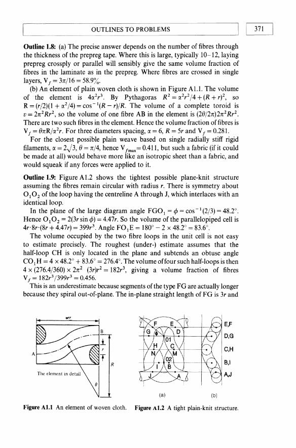
(b) An element of plain woven cloth is shown in Figure ALl. The volume of the element is 40(2r3. By Pythagoras R2 = 0(2r2/4 + (R + r)2, so R = (r/2)(1 + 0(2/4) = cos -l(R - r)/R. The volume of a complete toroid is v = 2n2 Rr2, so the volume of one fibre AB in the element is (20/2n)2n2 Rr2. There are two such fibres in the element. Hence the volume fraction of fibres is VI = OnR/0(2r . For three diameters spacing, 0( = 6, R = 5r and VI = 0.281.
For the closest possible plain weave based on single radially stiff rigid filaments, 0( = 2J3, 0 = n/4, hence V Imax= 0.411, but such a fabric (if it could be made at all) would behave more like an isotropic sheet than a fabric, and would squeak if any forces were applied to it.
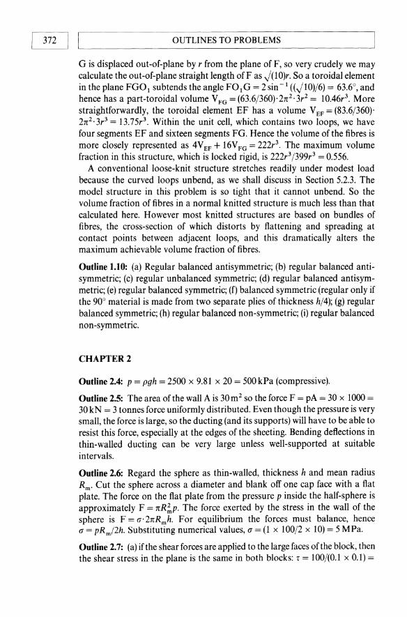
Outline 1.9: Figure A1.2 shows the tightest possible plane-knit structure assuming the fibres remain circular with radius r. There is symmetry about 0 10 2 of the loop having the centreline A through J, which interlaces with an identical loop.
In the plane of the large diagram angle FGO 1 = ¢ = cos - 1 (2/3) = 48.2°. Hence 0 10 2 = 2(3r sin ¢) = 4.47r. So the volume of the parallelopiped cell is 4r·8r·(8r + 4.47r) = 399r3. Angle F01E = 180° - 2 x 48.2° = 83.6°.
The volume occupied by the two fibre loops in the unit cell is not easy to estimate precisely. The roughest (under-) estimate assumes that the half-loop CH is only located in the plane and sub tends an obtuse angle COl H = 4 x 48.2° + 83.6° = 276.4°. The volume offour such half-loops is then 4 x (276.4/360) X 2n2 (3r)r2 = 182r3, giving a volume fraction of fibres VI = 182r3 /399r 3 = 0.456.
This is an underestimate because segments of the type FG are actually longer because they spiral out-of-plane. The in-plane straight length of FG is 3r and
"-!t-,,<~~=----\;l-.l----t~p..-'l E,F
(a) (b)
D,G
C,H
B,I
A,J
Figure ALl An element of woven cloth. Figure A1.2 A tight plain-knit structure.
I 372 I I'----~ OUTLINES TO PROBLEMS
G is displaced out-of-plane by r from the plane of F, so very crudely we may calculate the out-of-plane straight length ofF as ,)(lO)r. So a toroidal element in the plane FG0 1 subtends the angle F0 1 G = 2 sin -1 ((,)10)/6) = 63.6°, and hence has a part-toroidal volume V FG = (63.6/360)·2n 2 • 3r2 = 10.46r3• More straightforwardly, the toroidal element EF has a volume V EF = (83.6/360)· 2n2 ·3r3 = 13.75r3. Within the unit cell, which contains two loops, we have four segments EF and sixteen segments FG. Hence the volume of the fibres is more closely represented as 4V EF + 16V FG = 222r3. The maximum volume fraction in this structure, which is locked rigid, is 222r3/399r 3 = 0.556.
A conventional loose-knit structure stretches readily under modest load because the curved loops unbend, as we shall discuss in Section 5.2.3. The model structure in this problem is so tight that it cannot unbend. So the volume fraction of fibres in a normal knitted structure is much less than that calculated here. However most knitted structures are based on bundles of fibres, the cross-section of which distorts by flattening and spreading at contact points between adjacent loops, and this dramatically alters the maximum achievable volume fraction of fibres.
Outline 1.10: (a) Regular balanced antisymmetric; (b) regular balanced antisymmetric; (c) regular unbalanced symmetric; (d) regular balanced antisymmetric; (e) regular balanced symmetric; (f) balanced symmetric (regular only if the 90° material is made from two separate plies of thickness h/4); (g) regular balanced symmetric; (h) regular balanced non-symmetric; (i) regular balanced non-symmetric.
CHAPTER 2
Outline 2.4: p = pgh = 2500 x 9.81 x 20 = 500 kPa (compressive).
Outline 2.5: The area of the wall A is 30 m 2 so the force F = pA = 30 x 1000 = 30 kN = 3 tonnes force uniformly distributed. Even though the pressure is very small, the force is large, so the ducting (and its supports) will have to be able to resist this force, especially at the edges of the sheeting. Bending deflections in thin-walled ducting can be very large unless well-supported at suitable intervals.
Outline 2.6: Regard the sphere as thin-walled, thickness h and mean radius Rm. Cut the sphere across a diameter and blank off one cap face with a flat plate. The force on the flat plate from the pressure p inside the half-sphere is approximately F = nR!p. The force exerted by the stress in the wall of the sphere is F = a·2nRm h. For equilibrium the forces must balance, hence a = pRm /2h. Substituting numerical values, a = (1 x 100/2 x 10) = 5 MPa.
Outline 2.7: (a) if the shear forces are applied to the large faces of the block, then the shear stress in the plane is the same in both blocks: '[ = 100/(0.1 x 0.1) =
OUTLINES TO PROBLEMS _-----------ll I 373
10000 N 1m 2 • (b) if the shear forces are applied to narrow opposite faces, then "1 = 100/(0.1 x 0.01) = 100000N/m2 and r 2 = 1001 (0.1 x 0.02) = 50000 N/m2 .
Outline 2.8: No. The analysis in Section 2.3.4 shows that the forces are related to the length of the edge of the element over which they are applied, and hence Fyldy = Fzldz.
Outline 2.9: Faces ABFE and DCGH carry stresses due to the torque. AEHD and BFGC carry complementary shear stresses. ABCD and EFGH are stressfree.
Outline 2.10: Shear stresses on ABC and DEF are caused by the applied torque. ACFD and ABED carry complementary shear stresses. CBEF is stress free.
Outline 2.11: Those faces which carry stress do not (in principle) distort, and those faces which do distort are stress free.
Outline 2.12: CBEF is an unloaded face and distorts when the rod is twisted about its longitudinal axis. ABED, ACFD, ABC and DEF carry stress and are notionally unstrained.
Outline 2.13: 90° = 1.571 c. Ymax= ± ROIL = 0.01 x ± 1.571/0.4 = ±0.0393, i.e. Ymax= ± 3.93%. We assume that the neck does not buckle during this large twist, and the shear strains are small so that tan Y = y.
Outline 2.14: (a) Fx = 50kN, hence ax = 50 x 103 /(1 x 8 x 10- 3) = 6.25 MPa
ex = O"x/E = 6.25 x 10⁶ 13 X 109 = 2.08 x 10- 3 = 0.208%
ey = - vex = - 0.0729%
Lx = Lo(1 + ex) = 1(1 + 0.(0208) = 1002.08 mm
Ly = Lo(1 + ey) = 1(1 - 0.000729) = 999.27 mm
(b) FXY = 30kN, hence 'xy = 30000/(1 x 8 x 10- 3) = 3.75 MPa
Yxy = 'txylG = 3.75 x 10⁶/1.11 x 109 = 0.00338 = 0.338%
Lo remains unchanged at 1000mm Change of angle is 0.00338 radians, i.e. about 0.194°.
(c) Fx = Fy = 50 kN. ax = ay = 6.25 MPa
ex = O"x/E - vO"ylE = 0.65 x 6.25 x 106/3 x 109 = 0.001354 = 0.1354%
Lx = Lo(l + ex) = 1001.354mm = Ly
Outline 2.15: The shear stress is independent of the direction of loading: ,,=F/A=6000/(0.1 x0.15)=4x 10⁵ N/m 2 • y=r/G=0.1333. The in-plane displacement u ~ yh = 0.1333 x 0.01 = 1.333 mm.
Outline 2.16: (a) False. The hoop strain describes fractional increase in diam-
OUTLINES TO PROBLEMS 374 I I L-__________________________ _
eter. Using Hooke's law we find CH = O"H/E - VO"A/E = (pR/Eh)(l-v/2), from which we can see that doubling the pressure doubles the hoop strain but not the diameter, because the new diameter is 2R(1 + cH). (b) True, because O"H = pR/h. (c) True, see (a). (d) False. The original enclosed volume is approximately Vo = nR2L.
The new volume V is V = nR2(1 + cH)2L(1 + CA). Assuming small strains so we can neglect products of small quantities, the fractional increase in volume of the vessel is Cv = CA + 2cH" From Hooke's law we find CA = (pR/Eh)(! - v), hence Cv = (pR/2Eh)(5 - 4v). (e) False for almost all materials. CH/CA = (2 - v)/(1 - 2v). This expression only has the same value as O"H/O" A when v = 0, which is true for some low density flexible foams.
Outline 2.17: (a) Assume here that the polymer behaves elastically. The mean diameter is Dm = 0.775 m. The cross-sectional area A = nDmh = n x 0.775 x 0.025=6.09xl0- 2 m 2. The tensile stress is 0"=F/A=4xl05/6.09x 10- 2 = 6.57 X 10⁶ Pa. The tensile strain is C = O"/E = 6.57 x 10⁶/7 x 108 = 9.386 x 10 - 3. The change in length is ~L = cLo = 9.386 x 10 - 3 X 1 X 103 = 9.386m.
(b) The hoop stress O"H = pD/2h = 0.32 x 106 x 0.775/0.05 = 4.96 x 10⁶ Pa. 0" A = 2.48 X 10⁶ Pa. The strains may be calculated from
( :: ) = (~(~E ~;'E ~ )(::) = (_15~tx 1~0-:10 -1~~732 XX 1~0_-910 ~ )(::)
YAH 0 0 1/G 'AH 0 0 4x 10⁻⁹ 'AH
8H = 1.43 X 10- 9 X 4.96 X 106 - 5.72 X 10- 10 x 2.48 X 106 = 5.674 X 10- 3
8Dm = SHDm = 5.674 X 10- 3 X 0.775 = 4.4 X 10- 3 = 4.4mm
8A = - 5.72 X 10- 10 X 4.96 X 106 + 1.43 X 10- 9 x 2.48 X 106 = 7.094 X 10- 4
8L = SA = 7.094 X 10- 4 x 1 X 103 = 0.709 m.
In practice polyethylene will creep under load, the strain will increase with time under load. This book does not discuss this pattern of behaviour, which is very important for polymers; there is a full discussion of this in the author's Engineering with Polymers.
Outline2.18: From the outline to Problem 2.16 we have .i1V/Vo = (pR/2Eh) (5 - 4v) = (5 X 105 x 62.5/2 x 3 x 109 x 5)(5 - 1.4) = 0.00375. We assume the pipe is thin-walled and that the restraint on radial expansion at each end of the tube can be neglected.
Outline 2.19: (a) In a thin-walled pipe the hoop stress O"H is twice the axial stress, 0" Ao so the strain response is given by
OUTLINES TO PROBLEMS n_n~ I _ti£] In the hoop direction the strain is (v/2) less than if the pipe were only under hoop stress. In the axial direction there will be no axial strain at all under internal pressure if v = 0.5. This is exploited in the rubber inner tubes for pneumatic bicycle tyres, for which v = 0.5. The closed tube does change its diameter on inflation, which is desirable to achieve a snug fit under the tyre carcase, but does not change its length, which is desirable to avoid creasing and damage within the tyre which is relatively undeformable in the 'length' direction.
(b) In a thin-walled sphere under internal pressure, the hoop stress in any direction is the same. So in any two perpendicular directions we have identical hoop stresses, (1, giving
( ex) (liE -viE ey = -viE liE
Yxy 0 0
This means that the restraining effect is the same as that described in the text above.
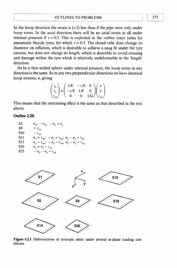
Outline 2.20:
S2 O"y; -O"x; -O"x + O"y
S9 + 'xy
SlO -'xy
Sll O"x + 'xy; -O"y + 'xy; O"x-O"Y+'Xy
S12 O"x-'xy; -O"y-'xy; O"x-O"y-'xy
S20 O"x + O"y-'xy
S25 - O"x - O"y + 'xy
Figure A2.1 Deformations of isotropic sheet under several in-plane loading conditions.
OUTLINES TO PROBLEMS 376 I I ~-------------------------
Missing (Figure A 2.1) are the following:
Sl O"x; -O"y; o"x - O"y
S5 O"x + O"y
S8 -O"x - O"y
S13 O"y + Txy; - O"x + Txy; - O"x +O"y + Txy
S14 O"y - Txy; -O"x - Txy; - O"x + O"y - Txy
S19 O"x+O"y+Txy
S26 -O"x - O"y - Txy
Outline2.21: We know T=(GO/L)'(nR4/2), hence o =2LT/(GnR4) =2 x 4000 x 45000/(80 x 109 x 3.14 X (0.0625)4) = 94.29 radians, i.e. about 15 complete revolutions. The shear stress at the surface of the shaft is 'xy = GOR/L = 80 x 109 x 94.29 x 0.0625/4000 = 11.79 MPa, which is well within the capability of the material, which would typically be able to withstand some 80 MPa.
Outline 2.22: 0 = 4° = 4/57.29 = 0.0698c
T = 2nR3hG8/L = 2n·(0.05)3 x 6 x 10- 3 x 1.4 X 109 x 0.0698/1.1 = 418.6 Nm
T = G8R/L = 1.4 x 109 x 0.0698 x 0.05/1.1 = 4.44 MPa
Y = T/G =4.44 x 10⁶/1.4 x 109 = 3.17 X 10- 3 = 0.317%
Outline 2.23: (a) Using the x' x' base in Figure 2.37, the first moment of an elemental strip distant z from x' x' ofthickness dz and constant width b is bz dz. Hence we confirm formally that the centroid is at the co-ordinate
z* = (b J~ z dz)/bh = (bh 2/2)/bh = h/2
Taking the second moment of the same elemental strip about the centroid axis xx we have
f +hl 2
I =b z2dz = (b/3)[( + h/2)3 -( -h/2)3] = bh3/12 -h12
(b) First we must locate the centroid. Taking first moments of the flange and web elements separately we have [bh l + bl (h - hl)Jz* = bh l (h - hd2) + bl (h - hl )2/2, which leads to z* = [bh l (2h - hi) + bl (h - hl )2J/[2{bh l + bl (h - hi))]' We can now calculate the second moment of area of the complete Tee section by calculating the second moment of area of the flange and web elements about their own centroids and achieving the second moment ofthese elements about z* using the parallel axis theorem:
Ix' x' = bh~/12 + b1h(h - hl)3/12 + bh l (h - hl/2 - z*f + bl (h - hl)(z* - (h - hl)/2)2
Both stress and strain profiles are linear with depth.
Outline 2.24: Let the total depth of the section be hi' total breadth b, and wall thickness h2 • We can calculate the second moment of area of the complete beam, lx, in terms of the second moments of the flanges (Irx) and the web (Iwx),

~~~~~~~~O_U_T_L_IN_E_S_T_O~PR_O_B_L_E_M_S~~~~~~~~~ I 377
all terms about the centroid of the complete beam.
Iwx = h2(hl - 2h2)3 /12 and Ifx = 2(bh~/12 + bh2(h 1 - h2)2/4)
hence
Iwx/lx = [h2(h 1 - 2h2)3J/[b l h~ - (b 1 - hJ(hl - 2h2n Putting b = hd2 and assuming hz «hi' we find Iwx/lx ~ (hi - 6hz)/4h1, and if hz = O.1h p Iwxllx ~ 0.1.
Outline 2.25: 1= bh3 /12 = 12 x 125 x 1O- 1Z 112 = 1.25 x 1O- 10m4
Kx = M/EI = 0.1/1 x 109 x 1.25 X 10- 10 = 0.8/m
Rx = l/Kx = 1.25 m
At the top surface of the beam Z = - 2.5 mm
cx=ZKx= -2.5 x 10- 3 xO.8= -2 x 10- 3 = -0.2%
(Jx = Ecx = - 2 X 10- 3 X 9 X 109 = -18 MPa
Outline 2.26: For circular corrugations the periodic width is We = 4Rm, with wall thickness h and depth he (Figure 2.36). The second moment of area about the centroid of the corrugations is the same as that of a circle, i.e. Ic1 ~ nR!h. Along the length, the second moment of area for a length We is ILl = W eh3 112 = Rmh3/3. The anisotropy ratio for bending stiffness is R 1 = 1c1/ILl = 1O(Rm/W. If Rm = 5h, then Rl ~ 250.
F or square corrugations, (ignoring the taper needed in practice, which has a small effect on the essence of these calculations), the second moment of area along the sheet about its centroid is ILl = weh3 /12. Across the width of the sheet we have, per unit corrugation, IeZ = [(wel2 + h)h~ - (we/2 - h) (he - 2h)3]/12. (It is sensible to check extremes. If we = 2h, we have a solid sheet of width We = 2h and depth he confirmed by Ie = hh~ 16. If we» h and he» h, and noting that (he - 2W "'" h~ - 6h~h if products of small quantities are neglected, Ie ~ weh~hI4.)
So for a real sheet the ratio of stiffnesses for equal lengths is given by the ratio Rz = Iez/lLl ~ 3(he/W. If he ~ 10h, Rz ~ 300.
The bending stiffness per unit weight along the corrugations may be represented by II A. Hence the ratio oflongitudinal bending stiffnesses per unit weight is given by
(1/ A),q/(I/ A)circ = (h~ /8)/(h~/8) = 1
Outline 2.27: (a) Dll = D22 = D = Eh3/[12(1- VZ)] = 3 X 109 X 8 x 10- 9 /[12(0.8775)] = 2.279Nm
D12 = - vD = - 0.7979 Nm
Kx = MxI[D(l - v2)] = 1/[2.279 x 0.8775J = 0.500/m
Ky = -VKx = -0.175/m
I 378 I LI _______________ O_U_T_L_IN_E_S_T_O __ PR_O __ BL_E_M_S ______________ ~
To suppress anticlastic curvature we have to ensure that Ky = 0, so that Ky = (- vMx + My)/[D(1 - v2 )], i.e. My = + vMx = 0.35 N, and hence
K" = [M" - vMy]/[D(1 - v2)] = M,,/D = 1/2.279 = 0.4388 /m.
(b) Kx = (Mx - vM)/[D(1 - v2)] = 0.65 x 1/[2.279 x 0.8775] = 0.325/m = Ky The application of equal moments Mx and My reduces the curvature Kx from 0.5/m (from Mx acting alone) and results in synclastic rather than anticlastic curvature.
(a) u" = [Ez/(1 - V2)](K" + VKy)
=[(3 X 10⁹ x -1 x 10³)/0.8775](0.5+0.35 x -0.175)= -1.5MPa f." = (h/2)K" = -10- 3 x 0.5 = -5 x 10- 4 = -0.05%
I'.y = (h/2)Ky = 0.0175%
The strain profiles are shown in Figure 2.42.
Outline 2.28:
M1 M,,; -My; M,,-My M5 M,,+My M8 -M,,-My M9 M"y MlO -M"y M13 My + M"y; - M,,+ M"y; - M,,+ My+ M"y M14 My-M"y; -M"-M,,y; -M"+My-M,,y M19 M"+My+M,,y M26 -M"-My-M,,y
Missing (Figure A2.2) are M2 (My; - Mx; - Mx + My). MIl (M" + MXY; - My + Mxy; Mx - My + Mx,)' Ml2 (Mx - MXY; - My - MXY; Mx - My - Mx,)' M20 (Mx + My - MXY )' M25 ( - Mx - My + MXY)'
Outline 2.29: To sketch the deformed sheet we need to calculate the midplane strains and curvatures. We can use expressions such as ex = ZKx, and e~ =
(e~ + e~)j2:
f.: = (0.3121 + 0.3046)/2 = 0.30835%
I'.~ = (-0.2848 - 0.2335)/2 = -0.25415%
Y:y = ( - 0.3266 - 0.1239)/2 = - 0.22525%
From e~ = ( - h/2)K" and e~ = ( + h/2)K", we have K" = - (e~ - e~)jh
K" = - (0.3046 - 0.3121) x 0.01/4 x 10- 3 = 0.01875/m
Ky = - ( - 0.2748 + 0.2335) x 0.01/4 x 10- 3 = 0.10325/m
K"y = - (-0.3266 + 0.1239) x 0.01/4 x 10- 3 = 0.5068/m

[
, J ' -'- -- 'I "", //M ---' . xy
M2
OUTLINES TO PROBLEMS
M11
M20 M25
M --r-~-
M12
-~ I 379
Figure A2.2 Deformations of flat sheet under different bending moments.
The midplane stresses are related to the midplane strains by
(ax) (E/{l- v2) vE/{l- v2) 0)( E:) ay = vE/{l - v2) E/{l - v2) 0 E; Txy 0 0 G Yxy
from which we find that ax/ay = (e~ + Ve;)/Ve~ + e;), i.e. only v is needed to calculate the required stress ratios.
Outline 2.30: See Figure A2.3.
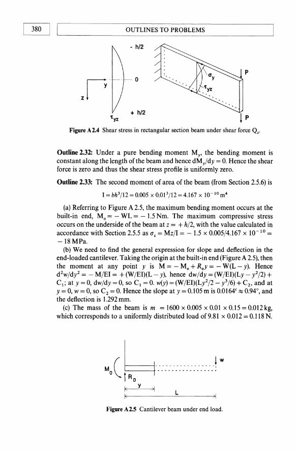
Outline 2.31: The profiles are shown in Figure A 2.4. The bending stress is zero at the neutral axis, and has maximum values at upper and lower surface. The shear stress is greatest at the neutral axis and zero at top and bottom surfaces.
Figure A2.3 Shear in paperback book in three-point bending.
OUTLINES TO PROBLEMS I 380 I I ~------------------------------------------------~
- h/2
o
+ h/2
Figure A 2.4 Shear stress in rectangular section beam under shear force Q •.
Outline 2.32: Under a pure bending moment My, the bending moment is constant along the length of the beam and hence dMy/dy = O. Hence the shear force is zero and thus the shear stress profile is uniformly zero.
Outline 2.33: The second moment of area of the beam (from Section 2.5.6) is
1= bh3/12 = 0.005 x 0.01 3/12 = 4.167 x 10- 10 m4
(a) Referring to Figure A 2.5, the maximum bending moment occurs at the built-in end, Mo = - WL = - 1.5 Nm. The maximum compressive stress occurs on the underside of the beam at z = + h/2, with the value calculated in accordance with Section 2.5.5 as (1c = Mz/I = -1.5 x 0.005/4.167 x to- 10 = -18MPa.
(b) We need to find the general expression for slope and deflection in the end-loaded cantilever. Taking the origin at the built-in end (Figure A 2.5), then the moment at any point y is M = - Mo + RoY = - W(L - y). Hence d2w/dy2 = - M/EI = + (W/EI)(L - y), hence dw/dy = (W/EI)(Ly - y2/2) + C 1; at Y = 0, dw/dy = 0, so C 1 = O. w(y) = (W/EI)(Ly2/2 - y3/6) + C2, and at y = 0, w = 0, so C2 = O. Hence the slope at y = 0.105 m is 0.0164c ~ 0.94°, and the deflection is 1.292 mm.
(c) The mass of the beam is m = 1600 x 0.005 x 0.01 x 0.15 = 0.012 kg, which corresponds to a uniformly distributed load of 9.81 x 0.012 = 0.118 N.
(1_ _ ___ __ _ _ __ J w
"0 ~----------------: 1<
y L
Figure A2.5 Cantilever beam under end load.
OUTLINES TO PROBLEMS _-----'I 1 381
The load per unit length is therefore WI = 0.118N/0.15m = 0.787N/m. From Figure 2.62, and using the principle of superposition, the deflection at the free end, taking self-weight loading into account, is W max= (L 3 lEI) (W 13 + WI L/8) = 1.8 + 0.008 = 1.808 mm. In this example the effect of the self-weight loading is small.
Outline 2.34: (Jc = PjA = n2EI/AL 2 = n2(Jcl/ccAL 2, hence Cc = (n21/AL 2)
Outline 2.35: The Euler buckling condition is Pc (J. EI/L 2 (J. EnR 4 IL 2. The load exerted by the mass of the tree is Pc (J. pgnR 2L, so pg R 2 L (J. ER 4/U, and hence for same material L (J. R 2j3, which is a statement of Kleiber's law. We can refine the analysis to take account of the non-uniform cross-sectional area of the tree trunk, and that the load is acting non-uniformly axially along the trunk rather than concentrated at the ends, but the basic shape of the result still stands, although the constant of proportionality is slightly different.
Outline 2.36: We need to find the radius of gyration for each section. (a) For the thin-walled tube r ~ ,j {nR!hI4)/(2nRmh)} = Rm/2. Hence L = 60r = 30Rm, so a tube behaves as if it were more slender than it really is. (b) The minimum second moment of area is I = h4 /4, so II A = 3h2/4, leading to L = 30h,j3.
Outline 2.37: (a) Ignoring any restraint exerted by surrounding fibres, the second moment of area of one fibre is If = nRi 14 = 4.91 x 10- 22 m4 , so for the complete bundle P ca ~ 1000n2 Elr/L 2 = 3.44 mN. (b) If the fibres are closepacked and bonded together with no voids, then as a rough approximation the radius of the circular bundle is about Rb = 1.66 x 1O- 4 m2, with a crosssectional area Ab=8.631x10- s m2 and Ib=5.93xlO- 16 m4 . Hence PCb ~ n2EIb/L 2 = 4.15 N, and the slenderness ratio of the bundle is (L/r)b ~ 120. The ratio of the buckling loads is therefore Pcb/Pca = 1207.
Outline 2.38: (a) Crossover occurs when Sc = kh/D = n2/(L/r)2, and hence (b) (L/r) (J. ,j(D/h).
Outline 2.39: A = 4.9R,j (Rlh) = 2 m. The critical buckling pressure is predicted as Pc = E(h/R)3/[4(1- v2 )] = 10 x 109 (6/100)3/[4 x 0.91] = 0.6 MPa. This is substantially below the value suggested for failure under internal pressure. The calculation assumes no value of safety factor, and it would be wise to down-rate the external applied pressure by a factor of perhaps 2 in a practical design.
CHAPTER 3
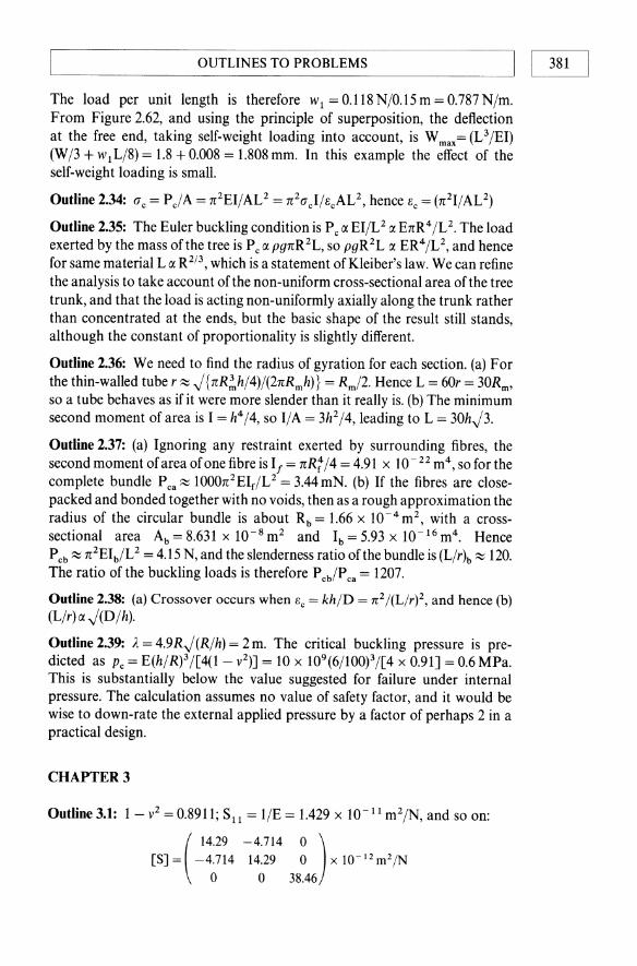
Outline 3.1: 1 - v2 = 0.8911; Sll = liE = 1.429 x 10- 11 m2 IN, and so on:
( 14.29 -4.714 0 )
[S]= -40.714 14.29 0 xlO- 12 m2 /N
o 38.46
[~8iJ ,---I ________ O_U_T_L_I_N_E_S_T_O_P_R_O_B_L_E_M_S _______ ----'
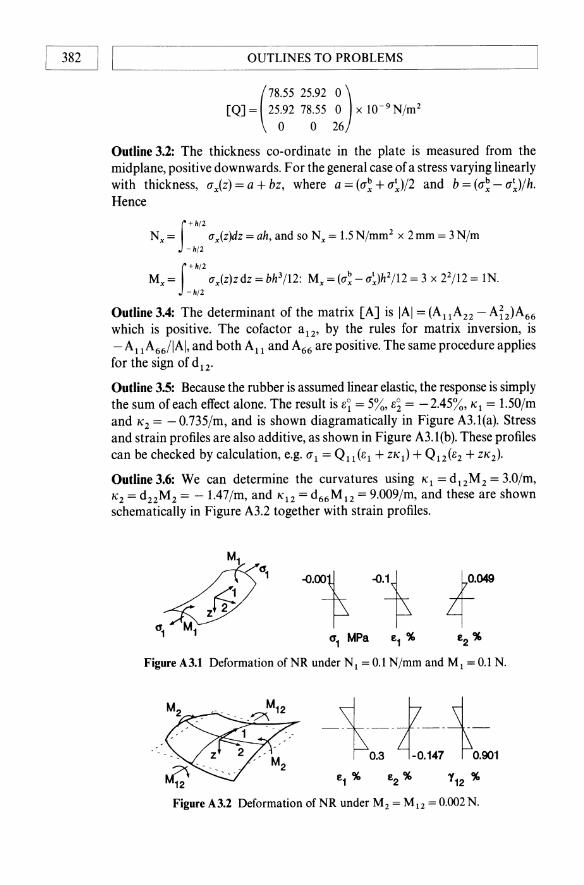
(78.55 25.92 0)
[Q] = 25.92 78.55 0 x 1O- 9 N/m2
o 0 26
Outline 3.2: The thickness co-ordinate in the plate is measured from the midplane, positive downwards. For the general case of a stress varying linearly with thickness, (Tx(z) = a + bz, where a = ((T~ + (T~)/2 and b = ((T~ - (T~)/h. Hence
Nx = ax(z)dz = ah, and so Nx = 1.5N/mm2 x 2mm = 3 N/m f+hl 2
-h12
Mx = ax(z)zdz = bh3/12: Mx = (a~ - a~)h2/12 = 3 x 22/12 = IN. f +hl 2
-h12
Outline 3.4: The determinant of the matrix [A] is IAI = (All A22 - Ai2)A66 which is positive. The cofactor a12' by the rules for matrix inversion, is - All A66/IAI, and both All and A66 are positive. The same procedure applies for the sign of d12.
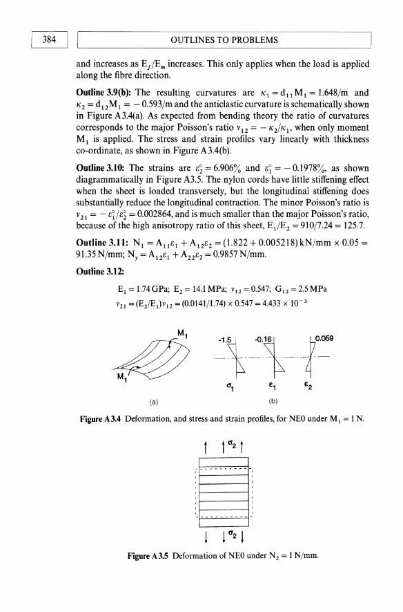
Outline 3.5: Because the rubber is assumed linear elastic, the response is simply the sum of each effect alone. The result is E~ = 5%, E~ = - 2.45%, 1<1 = 1.50/m and 1<2 = - O.735/m, and is shown diagramatically in Figure A3.1(a). Stress and strain profiles are also additive, as shown in Figure A3.1(b). These profiles can be checked by calculation, e.g. (T 1 = Q ll (El + Zl<l) + Q12 (E2 + ZI(2)·
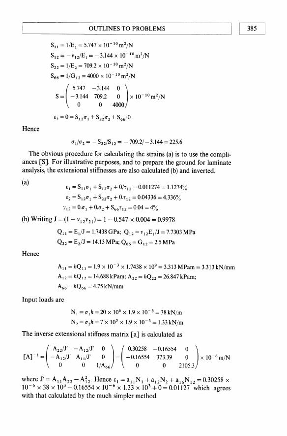
Outline 3.6: We can determine the curvatures using 1<1 = d12M2 = 3.0/m, 1<2 = d22M2 = -1.47/m, and 1<12 = d66 M12 = 9.009/m, and these are shown schematically in Figure A3.2 together with strain profiles.
0'1 MPa £1 % £2 %
Figure A3.1 Deformation of NR under N 1 = 0.1 N/mm and M 1 = 0.1 N.
Figure A3.2 Deformation of NR under M2 = M12 = 0.002 N.

~ _______ O_UT_L_I_N_E_S_T_O_P_R_O_B_L_E_M_S ________ ---"I 1 383
ax MPa ay MPa
Figure A3.3 Stress profiles in NR under Kl = lOO/m.
Outline 3.7: Assuming K1 = 0 we have M1 = D12K2 = (0.0004299 kNmm) x 1.00/m = 0.0004299 N. M2 = D22K2 = 0.0008773 N. Stress profiles are given in Figure A3.3.
Outline 3.8:
Sll = l/El = 7.463 X lO-12 Pa -1; S12 = Vl2SII = -2.090 X lO-12 Pa- l
S22 = 1/E2 = 112 X lO-12 Pa- l; S66 = 1/012 = 196.1 X lO-12 Pa- l
V2l = v12E2/El = 0.28 x 8.9/134 = 0.0186; J = (1 - V12 v21 ) = 0.995
Ql1 = EdJ = 134.70Pa; Q12 = VI2E2/J = 2.504 OPa
Q22 = E2/J = 8.9450Pa; Q66 = 0 12 = 5.1 OPa
All = Ql1h = 134 x 109 x 1.25 X 10- 4 = 16.84 x 10⁶N/m = 16.84kN/mm
A12 = 0.313 kN/mm; Azz = 1.118 kN/mm; A66 = 0.6375 kN/mm
Dll = Ql1h3/12 = 21.92 x lO-3 Nm
D12 = 407.6 X 10⁻⁶ Nm
D22 = 1.456 x 1O- 3kNmm; D66 = 8.301 x 1O- 4 kNmm
To calculate the compliance coefficients, we must invert the [A] and [DJ matrices.
IAI = (A12A22 - Ai2)A66 = 11.94
a" = A22A66/IAI = 1.118 x 0.6375/11.94 = 0.05969 mm/kN
al2 = - A12A66/IAI = -0.01672mm/kN
a22 = A1IA66/IAI = 0.8989mmkN
a66 = (All A22 - Ai2)!1AI = 1.569 mm/kN
Similarly d ll = 45.85/mmkN; d 12 = - 12.84/mmkN; d22 = 690.3/mmkN; d66 = 1205/mmkN.
Outline 3.9(a): From Section 1.3.1 we noted that E1 = V fEf + V mEmo Because [,f = [,1' we can write (J f = Ef '['l' so the load taken by the fibres, Pf can be expressed as Pf = Af(Jf = AfEf(J1/E1 = AfEfP1/A1E1 = V f Ef P1/E 1 and hence P f/P 1 = 1/(1 + V mEm/V fE f)' Substituting numerical values for V f (say, 0.3,0.5,0.7) and Em/Ef (say 0.1 and 0.01) leads to the following conclusions: Fibre load-bearing efficiency increases as the proportion of fibres increases
OUTLINES TO PROBLEMS 384 I I ~--------------------------------------------------~
and increases as Ef/Em increases. This only applies when the load is applied along the fibre direction.
Outline 3.9(b): The resulting curvatures are "1 = d u M1 = 1.648/m and "2 = d12M1 = - 0.593/m and the anticlastic curvature is schematically shown in Figure A3.4(a). As expected from bending theory the ratio of curvatures corresponds to the major Poisson's ratio V12 = - "2/"1' when only moment M1 is applied. The stress and strain profiles vary linearly with thickness co-ordinate, as shown in Figure A3.4(b).
Outline 3.10: The strains are 8~ = 6.906% and 8~ = - 0.1978%, as shown diagrammatically in Figure A3.5. The nylon cords have little stiffening effect when the sheet is loaded transversely, but the longitudinal stiffening does substantially reduce the longitudinal contraction. The minor Poisson's ratio is V21 = - 8~/8~ = 0.002864, and is much smaller than the major Poisson's ratio, because of the high anisotropy ratio of this sheet, EdE2 = 910/7.24 = 125.7.
Outline 3.11: N1 = AU81 + A1282 = (1.822 + 0.005218)kN/mm x 0.05 = 91.35 N/mm; Ny = A1281 + A2282 = 0.9857 N/mm.
Outline 3.12:
El = 1.74 GPa; E2 = 14.1 MPa; V12 = 0.547; G 12 = 2.5 MPa
V21 = (E2/E1)V12 = (0.0141/1.74) x 0.547 = 4.433 x 10- 3
(a) (b)
Figure A3.4 Deformation, and stress and strain profiles, for NEO under Ml = 1 N .
. -----------, 1----------1
Figure A 3.5 Deformation ofNEO under N2 = 1 N/mm.
L--_______ O_U_T_L_IN_E_S_T_O_P_R_O_B_LE_M_S _______ ~ I 385
Hence
SII = 1/EI = 5.747 x 1O- lo m2/N
S12 = -v 12/E I = -3.144 x 1O-lo m2/N
S22 = 1/Ez = 709.2 x 10- 10 m2/N
S66 = 1/G12 = 4000 x lO- lo mz/N
( 5.747 -3.144 0)
S= -3.144 709.2 0 x 1O- lo m2/N
o 0 4000
(J II(J Z = - S22/S12 = - 709.21 - 3.144 = 225.6
The obvious procedure for calculating the strains (a) is to use the compliances [S]. For illustrative purposes, and to prepare the ground for laminate analysis, the extensional stiffnesses are also calculated (b) and inverted.
(a) 61 = Sll(J I + S12(J 2 + O/! 12 = 0.011274 = 1.1274%
6z = S12(J I + SZ2(J 2 + 0·!12 = 0.04336 = 4.336%
Y12 = O.(J I + O.(J Z + S66! 12 = 0.04 = 4%
(b) Writing J = (1- V 12V 21 ) = 1 - 0.547 x 0.004 = 0.9978
Hence
Qll = EI/J = 1.7438 GPa; QI2 = v12EdJ = 7.7303 MPa
Q22 = EzIJ = 14.13 MPa; Q66 = G 12 = 2.5 MPa
All = hQII = 1.9 x 10- 3 x 1.7438 X 109 = 3.313 MPam = 3.313 kN/mm
A12 = hQ12 = 14.688 kPam; A22 = hQZ2 = 26.847 kPam;
A66 = hQ66 = 4.75 kN/mm
Input loads are
NI = (Jlh = 20 x 106 x 1.9 X 10- 3 = 38kN/m
N2 = (J2h = 7 x 105 x 1.9 X 10- 3 = 1.33 kN/m
The inverse extensional stiffness matrix [a] is calculated as
( A22II' -AdI' 0 ) (0.30258 -0.16554 0 )
[Ar l = -A12/I' AliiI' 0 = -0.16554 373.39 0 xlO- 6m/N
o 0 1/A66 0 0 2105.3
where l' = AllA22 - Ai2· Hence el = all N 1 + a 12N 2 + a 16N 12 = 0.30258 X
10- 6 x 38 X 103 - 0.16554 X 10- 6 x 1.33 X 103 + 0 = 0.01127 which agrees with that calculated by the much simpler method.
OUTLINES TO PROBLEMS 386 I I L-________________________________ __
Outline 3.13:
[SC] = [sc]T =
(-vd( -v1tl
E1E1G 12
+ V11 ----EZG12 E2G 12
v12 1 ----E 1G12 E 1G 12
o o
E1
1-V12V21
[sc]T v12E z [Q] = [Sr 1 =-=
1 - V12V21 lSI
0
(1 - V12 v1tl
E1E1G12
o
o
V21 E l
1- V12V21
E2
1- V12V21
0
0
0
G12
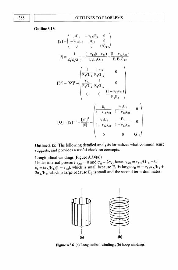
Outline 3.15: The following detailed analysis formalizes what common sense suggests, and provides a useful check on concepts.
Longitudinal windings (Figure A3.6(a)) Under internal pressure r AH = 0 and a H = 2a A' hence YAH = r AH/G 11 = o. SA = (a A/E 1)(1 - v12), which is small because E1 is large. SH = - v11a AIEl + 2a AIEl' which is large because El is small and the second term dominates.
IITll
-- - -
(a) (b)
Figure A3.6 (a) Longitudinal windings; (b) hoop windings.

~ ______________ O_U_T_LI_N_E_S_T_O_P_R_O_B_L_E_M_S ______________ ~I I 387
Under opposing torques, shear strain is the result of applied shear stress; eH=eA =0.
Under axial tensile load, (J A is defined by PIA, and (J H = 'AH = O. e A = (J AlE 1 , and eH = -V12 (J AIEl' both direct strains being small because E1 is large.
Hoop windings (Figure A3.6(b» Under internal pressure, YAH = 0; eA = (J AlE 2 - 2V12(J AIEl' large because E2 is small; eH = - V12(J AIEl + 2(J AIEl' small because E1 is large.
Under opposing torques YAH = 'AuiG 12> the same as for fibres along the aXIS.
Under axial load, "I AU = O. eA = (J A/E2' large because E2 is small; eH = (J AIEl' small because E1 is large.
Outline 3.16: Using the [T] matrix Equation (3.43) we have, for a lamina of thickness h :
h't12 = huX< - sin Ocos 0) + hu,(sin o cosO)
If (Jx = (Jy, then '12 = 0 for any value of e, and it does not matter whether applied force resultants are tensile or compressive. Indeed this is true for any material, not just unidirectional composites.
Outline3.17: By inspection (Jx=Nxlh=(Jy=2.5N/mm2, and 'xy=0.5NI mm2. Using Equation (3.34) we have
(u8 ) (ux) (0.25 0.75 0.866)(UX )
U b = [T(600)] uy = 0.75 0.25 -0.866 uy 'tab 'txy -0.433 +0.433 -0.5 'txy
Hence (Ja = 0.25 x 2.5 + 0.75 x 2.5 + 0.866 x 0.5 = 2.933 N/mm2. (Jb = 2.067N/mm2, 'Xy = - 0.25N/mm2.
Outline 3.18:
(Ill ) ( IlX) ( 0.75 0.25 0.866)(0.005) (0.006366) 112 = [T(300)] Ily = 0.25 0.75 -0.866 0.007 = 0.005634
"112/2 . Yxyl2 -0.433 0.433 0.5 0.001 0.001366
Hence (e 1, e2, "112) = (0.006366, 0.005634, 0.002732).
Outline 3.19: We have (Jx = - 3.5 MPa, (Jy = + 7 MPa and 't'xy = -1.4 MPa. From Equation (3.10).
(u1 ) ( 0.250.75 0.866)(UX )
U 2 = 0.25 0.75 -0.866 uy 't 12 -0.433 0.433 0.5 'txy
Hence (J 1 = 0.25 x - 3.5 + 0.75 x 7 + 0.866 x - 1.4 = 3.1626 MPa
U 2 = 0.3374 MPa, 't12 = 5.2465 MPa

OUTLINES TO PROBLEMS I 388 I I ~------------------------------------------------~
Using Equation (3.33), Sll = 7.4128 X to- 11 m2 (N, S12 = - 2.857 X
to- 11 m2(N, S22 = 28.57 X to- 11 m2(N, and S66 = 23.81 X to- 11 m2 IN. SO from Equation (3.63):
SI1 = (7.1428 x 0.625 + 28.57 x 0.5625 + 18.096 x 0.1875) x 10- 11
= 199.1 x 1O- 12 m2jN
and hence the coefficients of the transformed compliance matrix are:
( 199.1 4.464 -130.9 )
[S] = 4.464 91.96 -54.64 x 1O- 12 m2jN -130.9 - 54.64 370.2
The required strains are
ex = [199.1 x - 3.5 X 10⁶ + 4.464 x 7 x 106 + (- 130.9) x (- 1.4 X 10⁶)] x 10- 12
= -4.823 X 10- 4 = -0.04823%, ey = 0.07046%, Yxy = - 0.04426%
Outline 3.20: We can recast the expression for l/Ex in Equation (3.64) in terms of cos (), using sin2 () = 1 - cos2 (), to give a quadratic in cosz ():
(l/El + I/E2 + 2V12/Gdcos4 8 + (l/G12 - 2vdEl - 2/E2)cos28 + (1/E2 -l/Ex) = 0
We seek the values of ()1 for Ex = 0.99E1 and ()z for Ex = 0.95E1. Substituting numerical values and solving the quadratic in cos2 () gives ()1 = 1°, and ()2 = 2.275°. To obtain accurate values oflongitudinal modulus it is necessary to align the fibres precisely in the direction of test. A 2° misalignment produces nearly 5% error.
Outline 3.21: We can recast the expression for I/GXY in Equation (3.64) as a quadratic in cosz (), and substitute GXY = 0.95 G 12 to give 2.667 cos4 () + 133.3cos2 () - 10.526 = 0, from which () = 79°, i.e. 11° misalignment.
Outline 3.22: We can combine VXy and Ex in Equation (3.64) as VXy = [A (sin4 () + cos4 () + B(sin2 () cos2()]/[Ccos4 () + Dsin4 () + Esin2 () cos2 ()], and then express this equation in terms of sin (), which has the form: vxy=[A+ Msin2() + Nsin4()]/[C + Psin2() + Qsin4()]. We can now find the maximum value ofvxy by setting dVxy/d() = 0. Using s = sin () and c = cos () gives dVxyld() = sc[(C + Psz + Qs4)(2M + 4Ns2) - (A + MS2 + Ns4)(2P + 4QS2)]/[C + PS2 + QS4]. SO provided C + PS2 + QS4 #- 0, the problem reduces to sin () = 0, or cos () = 0, (which are both legitimate solutions, but neither is a maximum), or, after some rearrangement, we obtain sin2 () = -(CM - AP)/[2(CN - AQ)]. Going back over all the changes of symbol, we can now substitute values of elastic constants: A = v1z/E l , B = - (1/E1 + l/E2 -1/G1z), C=1/E1, D=I/Ez, E=(1/G12 -2v12/E1), M=B-2A, N = - M, P = E - 2C, and Q = C + D - E.
For a high modulus carbon fibre epoxy ply having El = 208 GPa, E2 = 7.6 GPa, G 12 = 4.8 GPa and V12 = 0.3, we find VXy has its maximum value when sinz () = 0.239, i.e. () = ± 29.25°.
L-_____________ O_U_T_L_IN_E_S_T_O __ PR_O_B_L_E_M_S ______________ ~I I 389
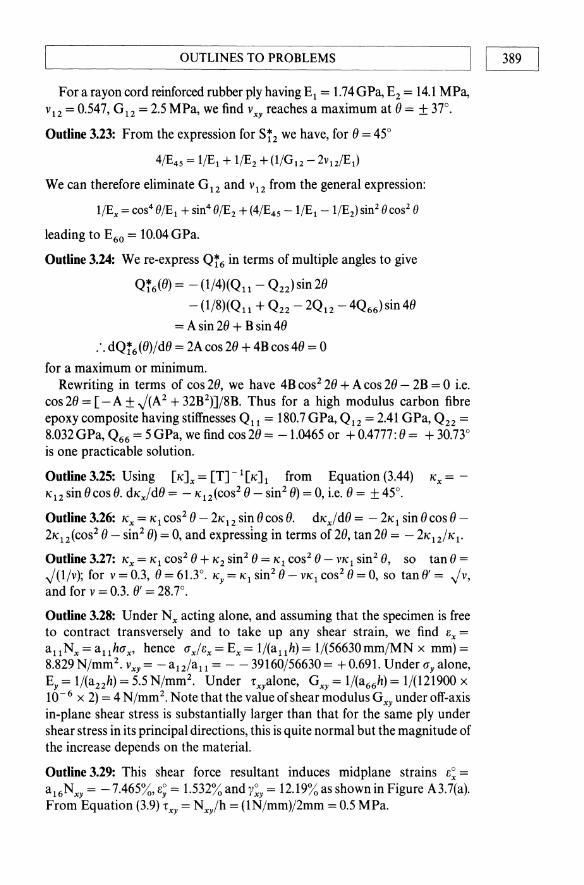
For a rayon cord reinforced rubber ply having El = 1.74GPa, E2 = 14.1 MPa, v12 = 0.547, G12 = 2.5 MPa, we find VXy reaches a maximum at 8 = ± 37°.
Outline 3.23: From the expression for ST2 we have, for 8 = 45°
4/E45 = llEl + llE2 + (l/G12 - 2v12IEI)
We can therefore eliminate G12 and V12 from the general expression:
l/Ex = cos4 OIEI + sin4 O/E2 + (4/E45 - llEl - l/E2) sin2 0 cos2 0
leading to E60 = 10.04 GPa.
Outline 3.24: We re-express QT6 in terms of multiple angles to give
QT6(8) = - (1/4)(Q u - Q22) sin 28
-(1/8)(Qu + Q22 -2Q12 -4Q66)sin48
= A sin 28 + B sin 48
:. dQT6(8)/d8 = 2Acos 28 + 4B cos 48 = 0
for a maximum or minimum. Rewriting in terms of cos 28, we have 4B cos2 28 + A cos 28 - 2B = 0 i.e.
cos 28 = [ - A ± .j(A 2 + 32B2)]/8B. Thus for a high modulus carbon fibre epoxy composite having stiffnesses Qll = 180.7 GPa, Q12 = 2.41 GPa, Q22 =
8.032 GPa, Q66 = 5 GPa, we find cos 28 = -1.0465 or + 0.4777: 8 = + 30.73° is one practicable solution.
Outline 3.25: Using [,,]x = [Tr 1[,,] 1 from Equation (3.44) "x = -"12 sin 8 cos 8. d"x/d8 = - "12 (cos2 8 - sin2 8) = 0, i.e. 8 = ± 45°.
Outline 3.26: "x = "1 cos2 8 - 2"12 sin 8 cos 8. d"x/d8 = - 2"1 sin 8 cos 8-2"12(COS2 8 - sin2 8) = 0, and expressing in terms of 28, tan 28 = - 2"12/"1'
Outline 3.27: "x = "1 cos2 (J + "2 sin2 (J = "1 cos2 (J - V"l sin2 (J, so tan (J = .j(I/v); for v = 0.3, 8 = 61.3°. "y = "1 sin2 8 - V"l cos2 8 = 0, so tan (J' = .jv, and for v = 0.3. 8' = 28.7°.
Outline 3.28: Under Nx acting alone, and assuming that the specimen is free to contract transversely and to take up any shear strain, we find ex = allNx = allhax' hence ax/ex = Ex = l/(auh) = 1/(56630mm/MN x mm) = 8.829 N/mm2. v xy = - a12/aU = - - 39160/56630 = + 0.691. Under a y alone, Ey = 1/(a22h) = 5.5 N/mm2. Under 'xyalone, GXY = 1/(a66h) = 1/(121900 x 10-6 x 2) = 4 N/mm2. Note that the value of shear modulus GXY under off-axis in-plane shear stress is substantially larger than that for the same ply under shear stress in its principal directions, this is quite normal but the magnitude of the increase depends on the material.
Outline 3.29: This shear force resultant induces midplane strains e~ = a16NXY = - 7.465%, e; = 1.532% and ')'~y = 12.19% as shown in Figure A3.7(a). From Equation (3.9) 'xy = Nxy/h = (IN/mm}/2mm = 0.5 MPa.

390 I LI ______________ O_U_T_L_I_N_ES_T_O __ P_RO __ BL_E_M_S ______________ ~
(a) (b)
Figure A3.7 Deformation ofNE30 under N xy = 1 N/mm.
The stresses and strains in the principal directions are
(J 1 = 0.433 MPa; (J 2 = - 0.433 MPa and t 12 = 0.25 MPa; and 81 = 0.06471%; 82 = - 5.998%; and Y12 = 13.89%
The strains in the principal directions are shown in Figure A3.7(b).
Outline 3.30: The boundary conditions are Bx = 0.05, Ny = N XY = O. We find N x = Bx/all = (0.05/56.63) kN/mm = 0.8829 N/mm, so that By = a12Nx = - 3.457%, YXY = a66Nx = - 6.591%.
Outline 3.31: Boundary conditions YXy = 0.05. Bx = By = 0 give N x =A16yxy =
0.5874kN/mm x 0.05 = 29.37N/mm (O"x = 14.68 MPa), Ny = A 26yxy =
9.76 N/mm (O"y = 4.88 MPa), N XY = A 66 yxy = 17.16 N/mm (tXY = 8.582 MPa). By use of the stress transformation matrix [T] we find 0"1= 19.67 MPa, 0"2= -0.1004MPa,t12 = +0.045 MPa.
Outline3.32: The resulting curvatures are Kx=d12My=-11.75/m, Ky=
d22My = 27.27/m and Kxy = d26My = 4.595/m, as shown schematically in Figure A3.8. The minor Poisson's ratio is vyX = - "x/"y = 11.75/27.27 = 0.4309 (as expected from the response to the transverse load Ny).
Outline 3.33: (a)B~ = 5.663%,B; = - 3.916%, Y~y = -7.465%, "x = -8.934/m, "y = 26.69/m, Kxy = O. To achieve suppression of twisting, MXY = - 0.01256 N. (b) B~ = 5.663%, B; = - 3.916%, Y~y = -7.465%, "x = 0, "y = 2.368/m, Kxy = O. To suppress the curvatures we need to apply Mx = 0.2723 N and Mxy = 0.1541 N.
Outline 3.34: The free development of twisting curvature implies that Mxy = 0, hence "Xy = - (016/066)"x = -17.11/m, leading to Mx =
(011 - 0i6/0 66)"x = 0.0838 N and My = (012 - 016026/D66)"x = 0.0361 N .
. -
Figure A3.8 Deformation of NE30 under My = 0.1 N.
OUTLINES TO PROBLEMS I I 391 ----'
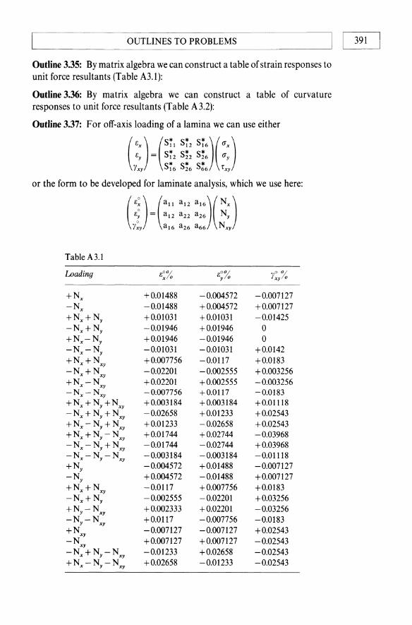
Outline 3.35: By matrix algebra we can construct a table of strain responses to unit force resultants (Table All):
Outline 3.36: By matrix algebra we can construct a table of curvature responses to unit force resultants (Table A 3.2):
Outline 3.37: For off-axis loading of a lamina we can use either
or the form to be developed for laminate analysis, which we use here:
(':) (a" a" a" f' ) e; = a12 a22 a26 Ny Y~y a16 a26 a66 Nxy
Table A3.1
Loading £~% e;% Y~y%
+Nx +0.01488 -0.004572 -0.007127 -Nx -0.01488 +0.004572 +0.007127 +Nx+Ny +0.01031 +0.01031 -0.01425 -Nx+Ny -0.01946 +0.01946 0 +Nx-Ny +0.01946 -0.01946 0 -NX-Ny -0.01031 -0.01031 +0.0142 +Nx+NXY +0.007756 -0.0117 +0.0183 -Nx+NXY -0.02201 -0.002555 +0.003256 +N -N x xy +0.02201 +0.002555 -0.003256 -Nx-Nxy -0.007756 +0.0117 -0.0183 +Nx + Ny +NXY +0.003184 +0.003184 +0.01118 -Nx+Ny+NXY -0.02658 +0.01233 +0.02543 +Nx - Ny + NXY +0.01233 -0.02658 +0.02543 +Nx + Ny - N XY +0.01744 +0.02744 -0.03968 -Nx-Ny+NXY -0.01744 -0.02744 +0.03968 -N -N -N x y xy -0.003184 -0.003184 -0.01118 +Ny -0.004572 +0.01488 -0.007127 -Ny +0.004572 -0.01488 +0.007127 +Nx + NXY -0.0117 +0.007756 +0.0183 -Nx+Ny -0.002555 -0.02201 +0.03256 +N -N y xy +0.002333 +0.02201 -0.03256 -N -N y xy +0.0117 -0.007756 -0.0183 +NXY -0.007127 -0.007127 +0.02543 -N +0.007127 +0.007127 -0.02543 xy -Nx+Ny-NXY -0.01233 +0.02658 -0.02543 +N -N-N x y xy +0.02658 -0.01233 -0.02543

392 I I OUTLINES TO PROBLEMS
Table A3.2
Loading Kx/m Ky/m Kx/m
+Mx + 7.144 -2.195 -3.421 -Mx -7.144 +2.195 +3.421 +Mx+My +4.949 +4.949 -6.842 -Mx+My -9.339 +9.339 0 +Mx-My +9.339 -9.339 0 -Mx-My -4.949 -4.949 +6.842 +Mx+MXY +3.723 -5.615 +8.785 -Mx+Mxy -10.56 -1.226 + 15.63 +M -M x xy + 10.56 + 1.226 -15.63 -Mx-My -3.723 5.615 -8.785 +Mx+My+MXY + 1.528 + 1.528 5.364 -Mx+My+MXY -12.76 +5.918 + 12.21 +Mx-My+MXY +5.918 -12.76 + 12.21 +Mx+My-MXY +8.37 +8.37 -19.05 -Mx-My+ MXY +8.37 -8.37 + 19.05 +M -M -M x y xy -1.528 -1.528 -5.364 +My -2.195 + 7.144 -3.421 -My +2.195 -7.144 +3.421 +Mx+MXY -5.615 +3.723 +8.785 -My+MXY -1.226 -10.56 + 15.63 +M -M y xy + 1.226 10.56 -15.63 -M -M y xy +5.615 -3.723 -8.785
+MXY -3.421 -3.421 + 12.21 -M +3.421 xy + 3.421 -12.21 +Mx+ My-Mxy -5.918 + 12.76 -12.21 +M -M -M x y xy + 12.76 -5.918 -12.21
(a) Let x be the hoop direction and y the axial direction in the tube. Under axial tension, Ny, we have
B~ = - 3.92 Ny hoop contraction
B; = + 9.09 Ny axial extension
Yxy = 1.53 Ny small positive shear (positive twist)
(b) Under internal pressure, p, we know that N x = 2 Ny, and hence
B~ = (2a ll + a12)Ny = 9.4 Ny
B; = (2a12 + au) Ny = 1.25 Ny
Y:y = (2a16 + a26) = - 13.41 Ny
We see that the tube increases in length and diameter, and develops large negative shear.
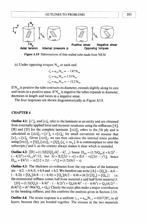
OUTLINES TO PROBLEMS I I 393 ----~
Ny Axial tension
Positive shear Negative shear Internal pressure p Opposing torques
Figure A3.9 Deformations of thin-walled tube made from NE30.
(c) Under opposing torques N XY at each end:
£: = a16 N xy = - 7.47 Nxy
£; = a26 Nxy = 1.53 N xy
Y:y = a66 N xy = -12.2 N xy
If N xy is positive the tube contracts its diameter, extends slightly along its axis and twists in a positive sense. If N xy is negative the tubes expands in diameter, decreases in length and twists in a negative sense.
The four responses are shown diagrammatically in Figure A3.9.
CHAPTER 4
Outline 4.1: [£oJL and [KJL refer to the laminate as an entity and are obtained from externally applied force and moment resultants using the stiffnesses [AJ, [BJ and [DJ for the complete laminate. [8(Z)J f refers to the fth ply and is calculated as [8(Z)J f = [8°JL + Z[KJL; for small curvatures we assume that [K]f = [K]L· Given [£(z)]f' we can then calculate the internal stress profiles using [a(z)]f = [QJf [8(Z)J f = [QJf[£~ + ZKd· It is commonplace to omit the subscriptsf and L as the context always makes it clear which is intended.
Outline 4.2: [DJ = (1/3)L[QJf(h} - h}-I) hence D66 = (1/3)Q66(( +h/2)3-(- h/2)3) = G 12 h3 /12, but G = E/[2(1 + v)] = E(1 - v)/[2(1 - v2)J, hence D66 = Eh3(1 - v)/[12 x 2(1 - v2 )J = (1/2)D(1 - v).
Outline 4.3: The thickness co-ordinates from the top surface of the laminate are -h/2, -h/4, 0, +h/4and +h/2. We therefore can write: [A] = [QJ( -h/4-( - h/2)) + [QbJ (h/4 - ( - h/4)) + [QaJ(h/2 - h/4) = (h/2){[QaJ + [QbJ} i.e. the extensional stiffness comes half from material a and half from material b.
[DJ = (1/3)[Qa(( - h/4)3 - ( - h/2)3) + Qb((h/4)3 - ( - h/4)3) + Qa((h/2)3 -(h/4)3) ] = (h3/96)(7Qa + Qb). Clearly the outer plies make a major contribution to the bending stiffness, and this confirms the analysis given in Section 2.5.6.
Outline 4.4: The strain response is a uniform Y12 = a66N12 = 0.03728% in all layers, because they are bonded together. The stresses in the two materials

I 394 I t~ _______________ O_U_T_L_IN_E_S_T_O_P_R_O_B_L_E_M_S ______________ ~
are different because of the different moduli. Thus we have 't'12(AI) = Q66(AI)Y~2 = 26GPa x 0.0003728 = 9.692 MPa, and 't'12(S) = Q66(S)Y~2 = 81.3 GPa x 0.0003728 = 30.31 MPa, as shown in Figure A4.1.
Outline 4.5: El = (f del = 1/(all hd = 1/(7.19 x 10-6 x 1) = 139.1 GPa (= E2 because a22 = all)' Using the formal definition v12 = -e2/e 1 under a single uniform stress (fl' e1=allN1, and e2=a12N1, so v12 =-a12/all = - (- 2.106)/7.19 = + 0.293. As the plies are isotropic, V 21 = V 12 • G12 = 1/ a66hd = 1/(18.64 x 10-6 x 1) = 53.65 GPa.
Outline 4.6: It is helpful to distinguish two situations: (a) e~ = 0; and (b) e~ free to contract.
(a) Applying e~ = 0, e; = 0.1 % induces N x = A12 e; = 44.56 N/mm and Ny = A22e; = 152.1 N/mm, with the stress profiles shown in Figure A4.2(a).
(b) Applying e; = 0.1% with e~ free to contract induces Nx = 0 =Alle~ + A12e;, so e~ = - A 12e;/All = - 0.0293%, and Ny = A12e~ + A22e; = 139.1 N/mm, with the stress profiles (e.g. (fxs = Q12Sey) shown in Figure A4.2(b).
Outline 4.7: For Rm = 0.02m, h = 0.OO1m,p = 2.5 MPa, T = 100Nm we have (fH = pRm/h = 50 MPa, NH=N/mm, NA=25N/mm, 't'AH=T/(2nR!h)= 39.8 MPa, N AH = 39.8 N/mm. Let the axis of the tube correspond to the x direction in laminate analysis. eA = all NA + a12NH = 0.007445%, eH =
a12NA + a22NH = 0.03069%, and YAH = a66NAH = 0.07418%. The change in enclosed volume is nRrL[1 - (1 + eH)2(1 + eA)] ~ nRrL(2eH + eA) = 0.54 x 10⁻⁶ m3. The stress profiles are shown in Figure A4.3.
Outline 4.8: The resulting twisting curvature is given by
K12 = d66M12 = (161.3/mmMN) x 2N =0.3226/m
~~=-[1-Mm8 "12 MPa 112 "
Figure A4.1 Response of SAL4S to N 12 = 20 N/mm.
--t ~ ~ ~ S 63.19 225.7 -2.914 '2D7.2
~ _~: _ _78~______ ?-91:)___ _70.96
Figure A4.2 Response of SAL4S to: (a) ex = 0, ey = 0.1%; (b) ey = 0.1%.

OUTLINES TO PROBLEMS I I 395 L-________________________________________________ ~
~ -t~~~=t~;: GA MPa GH MPa 'tAH MPa
Figure A4.3 Response of SAL4S tube to p = 2.5 MPa. T= 100 Nm.
s ~_~~~ ~0'01613 AI -2.f1d7 ----- -------- -----AI S
't12 MPa 112 "
Figure A4.4 Response of SAL4S to M12 = 2 N.
The strain profile varies linearly with thickness co-ordinate, Y12(Z) = ZK 12• and the stress profile shows a discontinuity at the interface between steel and aluminium because of the change of modulus (Figure A4.4). At the interface above the midplane, h = - 0.25 mm, and we find
ru(S) = Q66(S) x -0.25 X 10- 3 x 0.3226 = - 6.558 MPa
r u(AI) = Q66(AI) x - 0.25 x 10 - 3 x 0.3226 = - 2.097 MPa
Outline 4.9: Allowing no transverse curvature to develop (Kx = 0), and applying Ky = O.1/m induces My = Ky/(d22 - di2/dll) = 1.728 Nand Mx = - d12My/dll = 0.4875 N with stress profiles shown in Figure A4.5(a).
Allowing transverse curvature Kx to develop we find Mx = 0, My = (D22 - Di2/Dll)Ky = 1.59N and Kx = - D12Ky/Dll = - 0.02824/m, with stress profiles in Figure A4.5(b).
Outline 4.10: The shear strain response, Y~2 = a66 N12 = 0.06147%, is uniform through the thickness, leading to stresses of (J 1 (S) = Q11 (S)Y~2 = 49.98 MPa and (J 1 (F) = 0.01482 MPa.
S -1.58 -5.642 0.01336 -5.196 __ ~-3.16 ~-11'28 i10'02673~-10'39 ~ --- .g~a) - .~.964______ .~ - -.~.~--
Figure A4.5 Stress profiles in SAL4S: (a) "2 = 0.1/m, "1 = 0; (b) "2 = OJ/m.

OUTLINES TO PROBLEMS I 396 I I ~---------------------------------
Outline 4.11: The curvatures are Kl = dl1 Ml = 0.1472/m and K2 = d12M I = -0.04121/m, as shown diagrammatically in Figure A4.6(a). The stress and strain profiles are shown in Figure A4.6(b), and show clearly that the foam acts merely as a separator: its role in bending is to prevent shear between the inside surfaces of the steel plies.
Outline 4.12: All = A22 = 90.4 kN/mm, A12 = 25.33 kN/mm, A66 = 32.64 kN/ mm. Dll = D22 = 610.8 kNmm, D12 = 171.1 kNmm, D66 = 220.2 kNmm. In-plane stiffnesses are not affected because increasing the foam from 0.6 to 5 mm contributes negligible in-plane stiffness. The bending stiffnesses are dramatically increased because the steel is now much further from the midplane of the laminate.
Outline 4.13: Taking steel as the top ply, Bl1 = (1/2) [Ql1S(O - (- h/2)2) + QllA«h/2f - 0)] = (Ql1A - Ql1s)(h 2 /8) = (78.55 - 225.7) x 103 x 1/8 = - 18.394 kN. Other values of Bij are given in Table 4.6. If the top layer were aluminium, then Bl1 = + 18.394 kN.
Outline 4.14: Consider a laminate of thickness h, made from two materials a and b (Figure A4.7), having thicknesses ha = (h/2)(1 - IX) and hb = (h/2)(1 + IX). [B] = (1/2) [[Q]a (( -lXh/2)2 - ( - h/2)2) + [Q]b( (h/2f - ( -lXh/2)2)] =
(h2/8)[[Q]a(1X2 - 1) + ([Q]a/[Q]b)(1-1X2)]. By differentiation [B] has its maximum value when IX = 0 (i.e. plies have the same thickness) and when [Q]b» [Q]a'
Outline 4.15: For two plies of materials a and b (Figure A4.8) [B] = (1/2)([Q]a(0 - (- h/2)2 + [Q]b«h/2)2 - 0)) = (h 2/8)( - [Q]a + [Q]b)' So if [Q]a> [Q]b then [B] will be negative. Note that although Bij may be positive
M -15.3 0.3025 .~
f. ~ r~~~~~st·OO7358 r"~ O'x MPa CJy kPa tx % ty %
Figure A4.6 Curvatures and profiles for MSF232S under M, = 2 N.
- -h/2 a --ah/2
------0 h
b
- h/2
Figure A4.7 Thickness co-ordinates for non-regular non-symmetric laminate.

OUTLINES TO PROBLEMS _~I I 397
----0
- -h/2
jh b
- h/2
a
Figure A4.8 Thickness co-ordinates for regular nonsymmetric laminate.
or negative, [b] and [h] may contain terms of either sign when the full ABD matrix is inverted.
Outline 4.16: The deformation responses are B~ = 0.00263%, B~ = - 0.000915%, K1 = 0.212/m and K2 = - 0.0656/m. The midplane strains are small, and the transverse curvature is negligible in this example. The strain profiles are linear through the thickness as expected, and are shown in Figure A4.9. The longitudinal stress profile is linear through the thickness of each ply, but there is a discontinuity at the interface between the aluminium and the steel caused by the different values of modulus. The transverse stress profile is calculated from
(A4.1)
using appropriate materials constants for each ply.
Outline 4.17: For two plies the surface co-ordinates from the top are - h/2(a), 0, (b) + h/2. 2[B] = [Q.](O - (- h/2f) + [Qb] (h/2f - 0), hence[B] = (h2/8) ([Q.] - [Qb])'
For four plies alb/alb, the reader will find [B] = (h2/16)([Qb] - [Q.]); and in general for n plies alternating in pairs alb, [B] = (h 2/4n)([Qb] - [Q.]). As the number of alternating plies increases, the laminate behaves increasingly as if it were more symmetric.
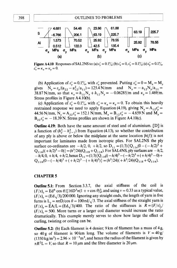
Outline 4.18: We shall discuss three different responses. (a) Application of B~ = 0.1%, with no imposed restraints. We realize that
N x = Mx = My = 0 so from Equation (4.22) we find N y = B~/a22 = 113.3 N/mm, B~ = a12N y = - 0.031%, Kx = h12 N y = - 0.5183/m and Ky = 1.489/m. The stress profiles are in Figure A4.10(a).
:'k:3 zf.:::7 ~·~~--f:§7 £1 % £2 % <11 MPa <12 MPa
Figure A 4.9 Response of SAL2NS to M 1 = 2 N.
I 398 I '---I ________ O_U_T_L_IN_E_S_T_O_PROBLEMS
2f4.681 tr:54.48 ~'86~1.88 -~ r s -6.766 206.1 63.19 2215.7 63.19 22E.7
AI 1.573 70.52 25.92 78.55 25.92 78.55 _ 0.512 122.3 42.5 135.4
O'x MPa O'y MPa O'x MPa O'y MPa O'x MPa O'y MPa
(a) (b) (e)
Figure A4.10 Responses ofSAL2NS to: (a) 1:; = 0.1%; (b) I:~ = 0, f.; = 0.1%; (c) 1:; = 0.1%, e~ = Kx = Ky = O.
(b) Application of B~ = 0.1%, with B~ prevented. Putting B~ = 0 = Mx = My gives Ny = By/(a22 - ai2/all) = 125.4 N/mm and N x = - a 12Ny/all = 38.87N/mm, so that Kx=hllNx+h12Ny= -0.06285/m and Ky= 1.469/m. Stress profiles in Figure A4.10(b).
(c) Application of e; = 0.1%, with B~ = Kx = Ky = O. To obtain this heavily restrained response we need to apply Equation (4.19), giving N x = A12B~ = 44.56N/mm, Ny = A22B~ = 152.1 N/mm, Mx = B12B~ = -4.659N and My = B22B; = -18.39N. Stress profiles are shown in Figure A4.1O(c).
Outline 4.19: Both have the same amount of steel and of aluminium. [DJ is a function of (h} - h}-l) from Equation (4.13), so whether the contribution of any ply is above or below the midplane at the same location Ih(j)1 is not important for laminates made from isotropic plies. For SAL2NS the ply surface co-ordinates are - h/2, 0, + h/2, so Dll = (l/3){Q11 s(O - (- h/2)3 + QllA(( + h/2)3 -O)} = (h3/24)(QllS + QllA)' For SAL4NS, ply surfaces are -h/2, -h/4, 0, +h/4, +h/2, hence D11 = (1/3){Qlls(( -h/4)3 -( -h/2)3 +( +h/4)3 -0)+ QllA(O-( -h/4)3 +( + h/2)3 -( + h/4)3)} = (h 3/24)( + h3/24)(QllS + QllA)'
CHAPTER 5
Outline 5.1: From Section 3.3.7, the axial stiffness of the coil is (F/x)c = Ed4 cos e/[16D3n(1 + v cos e)], and using v = 0.33 as a typical value, (F/x)c = (Ed~3)/2000oo. Ignoring any straight ends, the length of yarn in five furns is Ly = nnD/cos e = loond/~3. The axial stiffness of the straight yarn is (F/x)y = EA/L= (Ed~3)/400. The ratio of the stiffnesses is R = (F/x)y/ (F/x)c = 500. More turns or a larger coil diameter would increase the ratio dramatically. This example merely serves to show how large the effect of curling, twisting or coiling can be.
Outline 5.2: (b) Each filament is 4 denier; 9 km of filament has a mass of 4 g, so 40 g of filament is 90 km long. The volume of filaments is V = 40 g/ (1350 kg/m3) = 2.96 x 10- 5m3, and hence the radius ofthe filament is given by nR2L = V, so that R = to 11m and the fibre diameter is 20 11m.

OUTLINES TO PROBLEMS I I 399 ------------------------------------------~
Outline 5.3: For a symmetric four-ply stack (0°/90°), we find Dll/D22 =
(7Qll + Q22)f(Qll + 7Qd· For an eight-ply stack (0°/90% °/90°), of the same total thickness, Dll/D22 = (llQll + 5Qll)/(5Qll + llQd. Clearly convergence to Dll ~ D22 is rapid as the number of plies increases.
Outline 5.4: All = 2Qll(0)hf + 2Qll(90)hf = 2 x 0.125(180.7 + 8.032) = 47.19 kN/mm. For calculation of D12 it is better to use the formal ply co-ordinates.
D12 = (~){QdO)(( - hd4)3 - (- hd2)3 + (hd2)3 - (hd4)3)
+ Q'2(90)(( + hd4)3 - (- hL/4)3)}
= (h~/12)Q'2 = (0.53/12) x 2.41 = 0.0251 kNmm
Outline 5.5: (a) Under N x alone the longitudinal strain profile is uniform. If the plies were unbonded, the 0° plies would contract laterally much more (V12 = OJ) than the 90° plies (V21 = 0.3 x 8/180 = 0.0133). To achieve uniform contraction, an internal tension is applied to the 0° plies and an internal compression to the 90° plies.
(b) The discontinuity in bending stress (jy(z) at the interface arises from a difference in modulus in the plies either side of the interface, using the same kind of argument based on v 12 and v 21'
Outline 5.6: Under a single load N x and using the data in Table 5.2, we find Ex = 1/(all hL ) = 1/(21.21 x 10- 6 x 0.5) = 9403 GPa; V12 = - a 12/a ll = - (- 0.5414)/21.21 = + 0.0255. For this crossply laminate V21 = V12. Note that v 12 for the laminate is substantially less than the major ratio for the single ply but greater than the minor ratio. GXY = 1/(a66 hd = 1/(400 x 10-6 x 0.5) = 5 GPa. The result for the shear modulus is expected because both the 0° and the 90° plies are under the same shear stress and achieve the same shear strain.
Outline 5.7: The strain response is Yxy = 0.4% under a uniform shear stress !xy = 20 MPa. !Xy(z) is uniform because the transformed reduced shear stiffness Q66 is the same in plies oriented at 0° and 90° to the reference x direction. The values of Q11 (0°) and Q 11 (90°) are different, hence the discontinuity at the interfaces between differently oriented plies.
Outline 5.8: The resulting curvatures are Kx = d 11 Mx = 0.604/m and Ky =
d 12 Mx = - 0.0491/m. These curvatures correspond to the stress and strain profiles in Figure A5.1.
(J MPa x (J MPa y
Figure AS.1 Response of C + 4S to Mx = 1 N.
OUTLINES TO PROBLEMS I 400 I I ~--------------------------------------------------~
Outline 5.9: (a) Assuming e~ is free to contract we find e~ = - V12e~ = -0.0255 x 0.02 = - 0.00051%. Hence N x = Au e~ + A12e~ = 9.432N/mm. Ny = A12 e~ + A22 e~ = O. The stress in the top 0° ply is ax = Q u (OO)e~ + Q12(00)e~ = 36.13 MPa. In the 90° ply care must be taken to identify the appropriate coefficients of [Q]. We calculate the stress ax in the 90° ply as ax = Ql1(900)e~ + Q12(900)e~ = 1.594 MPa.
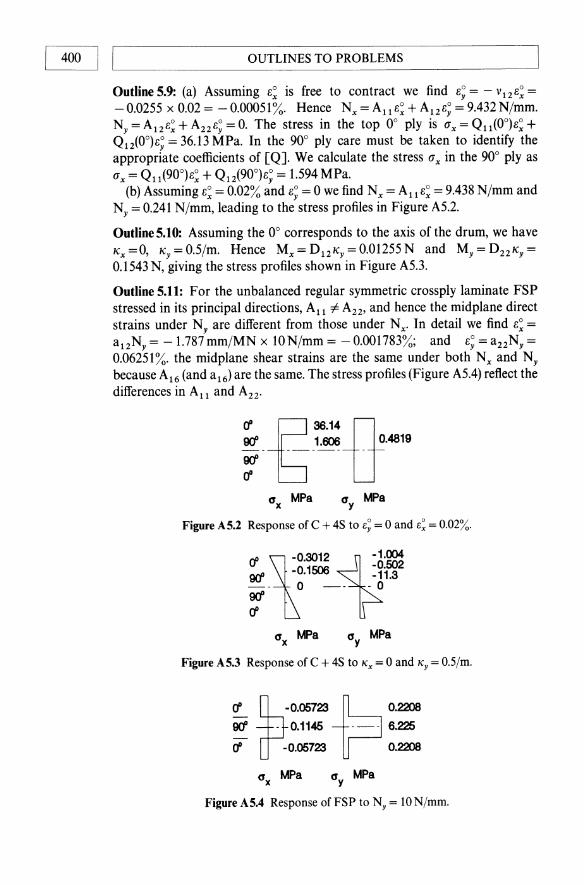
(b) Assuming e~ = 0.02% and e; = 0 we find N x = Au e~ = 9.438 N/mm and Ny = 0.241 N/mm, leading to the stress profiles in Figure A5.2.
Outline 5.10: Assuming the 0° corresponds to the axis of the drum, we have Kx =0, Ky = 0.5/m. Hence Mx = D12Ky = 0.01255 N and My = D22Ky = 0.1543 N, giving the stress profiles shown in Figure A5.3.
Outline 5.11: For the unbalanced regular symmetric crossply laminate FSP stressed in its principal directions, All -# A22, and hence the midplane direct strains under Ny are different from those under N x . In detail we find e~ = a12Ny = - 1.787 mm/MN x 10 N/mm = - 0.001783%; and 8; = a22Ny = 0.06251 %. the midplane shear strains are the same under both N x and Ny because A16 (and a16) are the same. The stress profiles (Figure A5.4) reflect the differences in All and A22.
rf E 36.14ll ~b-t606U""'·
c:r MPa x
c:r MPa y
Figure AS.2 Response of C + 4S to e; = 0 and e: = 0.02%.
rf \0.3012 iJ-6:~ oct -0.1506 -11.3 -- ° -- -° oct rf
c:r MPa x
c:r MPa y
Figure AS.3 Response of C + 4S to Kx = 0 and Ky = O.S/m.
rf ~0'05723 ~ 0.2208 oct - 0.1145 --- 6.225
rf -0.05723 0.2208
c:r MPa x
c:r MPa y
Figure AS.4 Response of FSP to Ny = 10 N/mm.

OUTLINES TO PROBLEMS
Outline 5.12: "x = d ll Mx = 13. 78 /mmMN x 1 N = 0.01378/m; "y = d 12Mx = - 0.OO3729/m.
Outline 5.13: Under Nx = 10N/mm, vxy = 0.001787/0.0329 = 0.05419. Under Ny = 10 N/mm, Vyx = 0.001787/0.06251 = 0.02859.
Ex= l/(all hd= 1/(32.91 x 10- 6 x 4.5) = 6.752 GPa. Ey = l/(a22 hd= 3.555 GPa. GXY = 1/(a66 hd = o. 364 GPa.
Outline 5.14: If we designate in the two-ply laminate the top ply as a and the bottom ply as b, we find from B = (t)l:Qf(h; - h;-t) that
B11 = (!)[Q11.(OO)(O - (- hj2)2 + Q11b(900)((hj2)2 - O)J
but plies a and b have the same properties but orientated differently, so we can write Qlla(OO) = Q11' and Qllb(900) = Q22' hence
B11 = (!)[Q11 (- h2j4) + Qd + h2j4)] = (h2j8) [Q22 - Q11J
Similarly
B22 = (!)[Q22(0 - (- hj2)2) + Q11 ((hj2)2 - 0)] = (h2j8) [Q11 - Q22J = - B11
For a non-symmetric arrangement (oo/90o/0o/90oh of total thickness h:
B11 = (!) [Q11 (( - hj4)2 - (- hj2)2 + Q22(0 - ( - hj4)2) + Q11 ((hj4)2 - 0)
+ Q22 (( hj2)2 - (hj4)2)]
from which Bll = (h 2/16) [Q22 - Qll]' and hence as the number of plies increases, the size of B decreases at constant thickness of laminate, and hence the non-symmetric character of the laminate diminishes.
Outline 5.15: By symmetry Q12 =Q21> and hence B12 = (!)[Qd( -h/2f-0)+ QdO - (h/2)2)] = 0, and so the corresponding inverse coefficient b t2 = o. K y =b12 N x =O. Nx=O.
Outline 5.16: It would seem essential to apply only a moment Mx to eliminate the curvature "x' but further thought will confirm that this will also induce an anticlastic curvature "y. To suppress both curvatures it is necessary to apply moments Mx and My via edge clamps, which may be calculated from the simultaneous equations Gx = all Nx + b ll Mx + b12 My; "x = b ll Nx + d ll Mx + d12My; "y = b t2Nx + d12Mx + d22 M y• Noting that "x = 0 = "y = b t2, we find My = - (d12/ddMx = - bllNxI(d ll - di2!dd. Substituting numerical values, Mx = - 1.144 N, My = - 0.02922 N, leading to Gx = 0.02121% and Gy = -0.0005414%.
OutiineS.17: Taking Nx=Ny = 10N/mm, we can calculate Gx=Gy = 0.05558%, "x = 3.131/m and "y = - 3. 131jm. For Nxy = 10N/mm we obtain Yxy = 0.4%.
Outline 5.18: G~ = 0 = 6; = Y~y = "x = "y. "xy = d66 Mxy = 19 200/MNmm x 1 N= 19.2/m.
L§J
I 402 I IL--_______ O_U_T_L_IN_E_S_T_O_P_R_O_B_L_E_M_S _______ -'
Outline 5.19: The simultaneous equations to be solved are Kx = d11 Mx + d12MyandKy = d12Mx + d22My, where Mx = 1 N andKy = O. KxandMyareas yet unknown. We see My = - (d12/dzz}Mx' and hence Kx = (dll -di2/dzz}Mx. This leads to My = + 0.02553 N; Kx = 2.736/m.
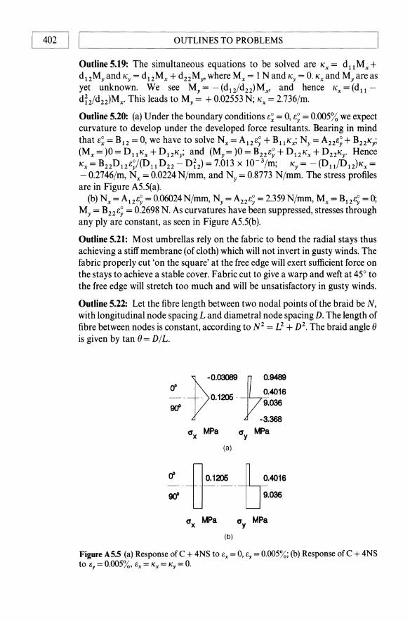
Outline 5.20: (a) Under the boundary conditions e~ = 0, e~ = 0.005% we expect curvature to develop under the developed force resultants. Bearing in mind that e~ = B12 = 0, we have to solve Nx = A12 e~ + B11 Kx; Ny = A22e~ + B22Ky; (Mx = )0= DllKx + D12Ky; and (My=)O = B22e~ + D12Kx+ D22Ky. Hence Kx= B22D12e;/(D11D22-Di2) = 7.013 X to- 3/m; Ky= -(Dll/DdKx= - 0.2746/m, N x = 0.0224 N/mm, and Ny = 0.8773 N/mm. The stress profiles are in Figure A5.5(a).
(b) Nx=A12 e; =0.06024N/mm, Ny =A22 e; =2.359N/mm, Mx= B12e; =0; My = B22 e; = 0.2698 N. As curvatures have been suppressed, stresses through any ply are constant, as seen in Figure A5.5(b).
Outline 5.21: Most umbrellas rely on the fabric to bend the radial stays thus achieving a stiff membrane (of cloth) which will not invert in gusty winds. The fabric properly cut 'on the square' at the free edge will exert sufficient force on the stays to achieve a stable cover. Fabric cut to give a warp and weft at 45° to the free edge will stretch too much and will be unsatisfactory in gusty winds.
Outline 5.22: Let the fibre length between two nodal points of the braid be N, with longitudinal node spacing Land diametral node spacing D. The length of fibre between nodes is constant, according to N 2 = L2 + D2. The braid angle () is given by tan ()= D/L.
PO.03OB9 _~~.9489 ~_ _ 0.1206 _ 0.4016 9fI 9.036
-3.368
(J MPa y
(a)
~_Ib~_L·4016 9(f U 09.036
Figure AS.5 (a) Response of C + 4NS to ex = 0, ey = 0.005%; (b) Response of C + 4NS to ey = 0.005%, Ex = Kx = Ky = O.
OUTLINES TO PROBLEMS I I 403 L-________________________________________________ ~
Using the diameter as a subscript, for the given undeformed braid, tan ()25 = 1, so L25 = D 45' and n = D25,,)2. For the 20 mm former we have N2 = qo + D~o = 2D~5' so L~o = 2 x 625 - 400 = 850, hence L20 = 29.15 mm, and ()20=tan-1(D20/L20)=tan-1 (20/29.15)= 34.45°. Similarly for the 30mm former: N2 = qo + D~o = 2D~5: L30 = 18.7mm, ()30 = 58°.
Outline 5.23: Maximum shear stiffness obtains when () = ± 45°. For an inextensible braid of negligible thickness compared with the diameter we have for a 25 mm tube: tan ()25 = D25/L 25, where ()25 = 30°, hence L 25 = 25/tan 30 = 43.33 mm, and the distance between nodes is N 2 = 25 2 + 43.332 •
For () = 45°, L = D, so N 2 = 2D2: D2 = N 2/2 = (625 + 1877)/2, so D = 35.37mm.
Outline 5.24: For a unidirectional lamina stressed at () to its principal direction, or for a symmetrical angleply laminate stressed at () to its principal directions, we can write
g = l/Gxy = Acos2 (J sin2 (J + B(sin4 (J + cos4 (J)
= B + (A - 2B)sin2 (J - (A - 2B) sin4 (J
i.e. dg/d() = 2(A - 2B) sin () cos () (1 - 2 sin 2()) = 0 for a minimum, so one root is sin () = 1/")2.
Outline 5.25: Using the data for aij in Table 5.6 we find Ex = 1/(all hd = 1/(3225 x 10- 6 x 4) = 77.52 MPa. v12 = - a12/all = -( - 8817)/3225 = 2.734. This is an exceptionally high value, even for composite materials. Ey = 1/ (a22 hd =9.56 MPa. GXY = 1/(a66 hd = 327.4 MPa. Note that although G 12 = 2.5 MPa when stressed in the principal directions, the application of r xy in global co-ordinates gives a much larger value of GXY ( + 30°).
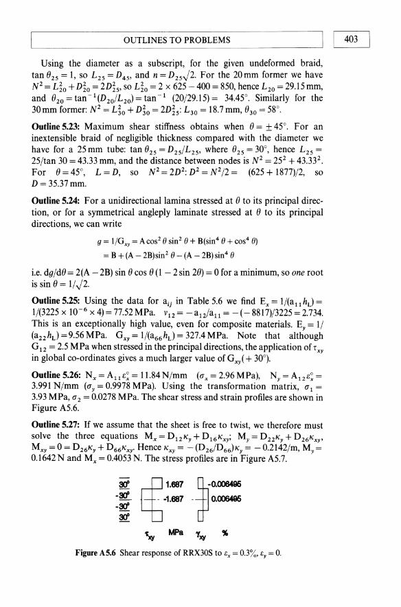
Outline 5.26: Nx=Alle~=11.84N/mm (lTx = 2.96 MPa), Ny=A12e~= 3.991 N/mm (lTy = 0.9978 MPa). Using the transformation matrix, IT 1 = 3.93 MPa, IT 2 = 0.0278 MPa. The shear stress and strain profiles are shown in Figure A5.6.
Outline 5.27: If we assume that the sheet is free to twist, we therefore must solve the three equations Mx = D 12 "y + D 16"xy; My = D 22"y + D 26"xy, MXY = 0 = D 26"y + D66"xy· Hence "xy = - (D26/D66)"y = - 0.2142/m, My = 0.1642 Nand Mx = 0.4053 N. The stress profiles are in Figure A5.7.
3{/ (lSU )---3{/ - -1.687 - 0.006496 -3{/ 3{/
"xv t.1Pa Txy " Figure A5.6 Shear response of RRX30S to ex = 0.3%, Ily = O.
404 I LI _______________ O_U_T_L_IN_E_S_T_O __ PR_O_B_L_E_M_S ______________ ~
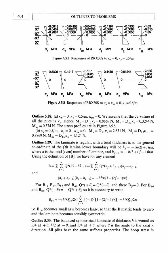
- ,0.0918 ~0.04166{0.04676l0.1197 ~0.0138 {1063 W -0.0459 -0.02078 -0.02338 -0.0698 -0.0068 -0.816 W -0.2867 -0.1009 0.1636 -0.382 -0.0066 1.86 --- 0 --- 0 --- - 0 ---- 0 ---- 0 --- 0 -W W
ax MPa ay MPa '\y MPa a1 MPa a2 MPa "12 kPa
Figure AS.7 Responses of RRX30S to Kx = 0, Ky = O.5jm.
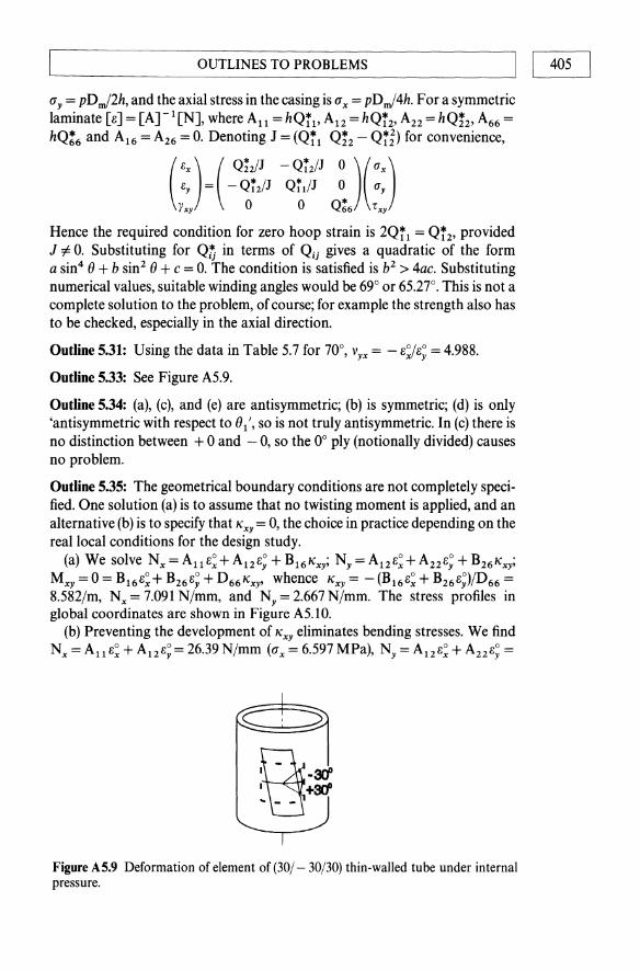
W to.332610.1217l-g:~ to.4418 \0.01244 ~-f.~ W 0.0936 1.083 --- 0 - -0 -- -0 --- 0 --- 0 ---- 0 -W W
Figure AS.8 Responses of RRX30S to Kx = Kxy = 0, Ky = 0.5jm.
Outline 5.28: (a) Kx = 0, Ky = O.5/m, Kxy = O. We assume that the curvature of all the plies is Ky. Hence Mx = D12Ky = 0.8869 N, My = D22Ky = 0.3244 N, MXY = 0.374 N. The stress profiles are in Figure AS.8.
(b) Kx = O.S/m, Ky = 0, Kxy = O. Mx = Dl1 Kx = 2.631 N, My = D12Kx = 0.8869 N, MXY = D 16 Kx = 1.124 N.
Outline 5.29: The laminate is regular, with a total thickness h, so the general co-ordinate of the fth lamina lower boundary will be hf = - (hI2) + fhjn, where n is the total (even) number oflaminae, and hf - 1 = - hj2 + (f - l)hln. Using the definition of [B], we have for any element . .
B=(!) L Q*(h;-h;_l)=@ L Q*(h,+h'_l)(h,-h'_l) ,=1 ,=1
and (h, + h'-l)(h, - h'-l) = - h2jn{1 - (2J - 1)/n}
For BWB12,B22 and B66,Q*(+e)=Q*(-e), and these Bij=O. For B16
and B26, Q*( - e) = - Q*( + e), so it is necessary to write
• B16 = - WQT6j2n) L {( - 1)'[1-(2J- l)jn]} = h2 QT6j2n
,=1
i.e. B16 becomes small as n becomes large, so that the B matrix tends to zero and the laminate becomes sensibly symmetric.
Outline 5.30: The balanced symmetrical laminate of thickness h is wound as hj4 at + e, hj2 at - e, and hj4 at + e, where e is the angle to the axial x direction. All plies have the same stiffness properties. The hoop stress is
~ _____________ O_U_T_L_IN_E_S_T_O __ PR_O_B_L_E_M_S ______________ ~I I 405
(Jy = pD,J2h, and the axial stress in the casing is (Jx = pD,J4h. For a symmetric laminate [e] = [A] -lEN], where Au = hQ1't, A12 = hQT2' A22 = hQ!2' A66 = hQ:6 and A16 = A26 = O. Denoting J = (Qil Qi2 - QiD for convenience,
( ex) (Q!1J -~T2/J 0)( ax) ey = - Q12/J Q11/J 0 ay
')Ixy 0 0 Q:6 't'xy
Hence the required condition for zero hoop strain is 2QTl = Q!2' provided J # O. Substituting for Qt in terms of Qij gives a quadratic of the form a sin4 0 + b sin2 0 + c = O. The condition is satisfied is b2 > 4ac. Substituting numerical values, suitable winding angles would be 69° or 65.27°. This is not a complete solution to the problem, of course; for example the strength also has to be checked, especially in the axial direction.
Outline 5.31: Using the data in Table 5.7 for 70°, Vyx = - e~/e~ = 4.988.
Outline 5.33: See Figure A5.9.
Outline 5.34: (a), (c), and (e) are antisymmetric; (b) is symmetric; (d) is only 'antisymmetric with respect to 01' , so is not truly antisymmetric. In (c) there is no distinction between + 0 and - 0, so the 0° ply (notionally divided) causes no problem.
Outline 5.35: The geometrical boundary conditions are not completely specified. One solution (a) is to assume that no twisting moment is applied, and an alternative (b) is to specify that "xy = 0, the choice in practice depending on the real local conditions for the design study.
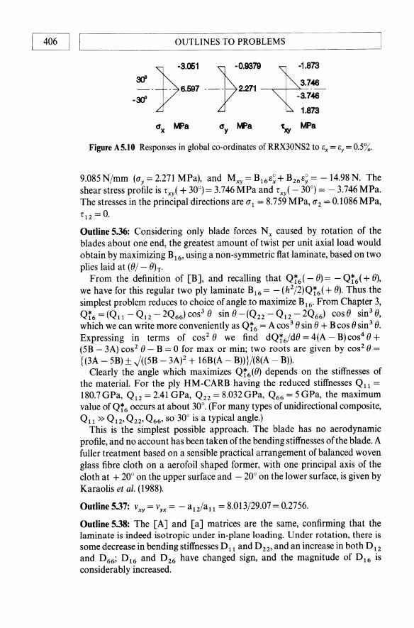
(a) We solve Nx=Aue~+A12e~+B16"XY; Ny=A12e~+A22e~+B26"xy; Mxy = 0 = B16e~ + B26e~ + 0 66 "Xy, whence "Xy = - (B16e~ + B26e~)fD66 = 8.582/m, Nx = 7.091 Nlmm, and Ny = 2.667 N/mm. The stress profiles in global coordinates are shown in Figure A5.10.
(b) Preventing the development of "xy eliminates bending stresses. We find Nx = All e~ + A12e~= 26.39N/mm «(Jx = 6.597 MPa), Ny = A12e~ + A22e~ =
Figure A5.9 Deformation of element of (301 - 30130) thin-walled tube under internal pressure.
OUTLINES TO PROBLEMS I 406 I I L-____________________________________ ___
?J:f _pO::: ._)-::~:::: -?J:f -3.746
1.873
Gx MPa Gy MPa ~ MPa
Figure AS.tO Responses in global co-ordinates of RRX30NS2 to ex = ey = 0.5%.
9.085 N/mm (O'y = 2.271 MPa), and Mxy = B16e~ + B26 e; = - 14.98 N. The shear stress profile is 'Xy( + 30°) = 3.746 MPa and 'Xy( - 30°) = - 3.746 MPa. The stresses in the principal directions are 0' 1 = 8.759 MPa, 0'2 = 0.1086 MPa, '12 = O.
Outline 5.36: Considering only blade forces Nx caused by rotation of the blades about one end, the greatest amount of twist per unit axial load would obtain by maximizing B16, using a non-symmetric flat laminate, based on two plies laid at (e/ - eh.
From the definition of [B], and recalling that Q1'6(-e)= -Q1'6(+e), we have for this regular two ply laminate B16 = - (h 2/2)Q1'6( + e). Thus the simplest problem reduces to choice of angle to maximize B16. From Chapter 3, Q1'6 = (Qll - Q 12 - 2Q66) cos3 e sin e -(Q22 - Q 12 - 2Q66) cos e sin3 e, which we can write more conveniently as Q1'6 = A cos3 e sin e + B cos e sin3 e. Expressing in terms of cos2 e we find dQ1'6/de = 4(A - B)cos4 e + (5B - 3A) cos2 e - B = 0 for max or min; two roots are given by cos2 () =
{(3A - 5B) ± J((5B - 3A)2 + 16B(A - B)) }/(8(A - B)). Clearly the angle which maximizes Q1'6(()) depends on the stiffnesses of
the material. For the ply HM-CARB having the reduced stiffnesses Qll =
180.7 GPa, Q12 = 2.41 GPa, Q 22 = 8.032 GPa, Q66 = 5 GPa, the maximum value ofQ1'6 occurs at about 30°. (For many types of unidirectional composite, Qll »Q12' Q22' Q66' so 30° is a typical angle.)
This is the simplest possible approach. The blade has no aerodynamic profile, and no account has been taken of the bending stiffnesses of the blade. A fuller treatment based on a sensible practical arrangement of balanced woven glass fibre cloth on a aerofoil shaped former, with one principal axis of the cloth at + 20° on the upper surface and - 20° on the lower surface, is given by Karaolis et al. (1988).
Outline 5.37: vxy = Vyx = - a12/a ll = 8.013/29.07 = 0.2756.
Outline 5.38: The [A] and [a] matrices are the same, confirming that the laminate is indeed isotropic under in-plane loading. Under rotation, there is some decrease in bending stiffnesses D 11 and D 22' and an increase in both D 12 and D 66; D 16 and D 26 have changed sign, and the magnitude of D 16 is considerably increased.
OUTLINES TO PROBLEMS I I 407 ~--------------------------------------------------~
:~[~~Jf=~=: [:~~W~1:~ ax MPa ay ~a \y ~a a, t"I)a a2 MPa ~'2 MPa
Figure AS.ll Responses of QI60S to Nx = 10 N/mm.
Outline 5.39: QI60S responds with a curvature "xy = - 4.519 X 10- 3 x 20 = - 0.09038/m. QI60Sa shows much larger curvature of opposite sign lexy = 52.25 X 10- 3 x 20 = + 1.045/m. The isotropic sheet does not twist because d16 =0.
Outline 5.40: The strains are e~ = all Nx = 29.07 X 10-6 x 10 = 2.907 X 10- 4
e; = a12 Nx = - 8.013 X 10- 5• The stresses in thefth ply are calculated using [O"]J = [Q*]J [eO], using the appropriate value of angle for the fth ply, and this leads to the profiles in Figure A5.11.
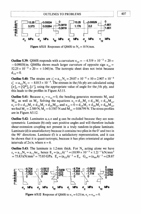
Outline 5.41: Because "y = "xy = 0, the bending generates moments My and Mxy as well as Mx. Solving the equations lex = d11 Mx + d12 My + d16Mxy, "y = 0 = d12Mx + d22My + d26Mxy, and "Xy = 0 = d16Mx + d26My + d66Mxy, we find Mx = 2.589 N, My = 0.3307 Nand Mxy = 0.06799 N. The stress profiles are in Figure A5.12.
Outline 5.42: Laminates a, c, e and g can be excluded because they are nonsymmetric. Laminate (b) only uses positive angles and will therefore include shear-extension coupling not present in a truly random-in-plane laminate. Laminate (d) is unsatisfactory because it contains two plies in the 0° and two in the 90° directions. Laminate (f) is a satisfactory representation, and it can be shown that it is quasi-isotropic, because it has plies orientated at angular intervals of 2n/n, where n = 6.
Outline5.43: The laminate is 1.2mm thick. For Nx acting alone we have ex = allNx = all hO"x, hence Ex =(a ll h)-l = (10.99 x 10- 3 x 1.2)-1 kN/mm2 = 75.83 kN/mm2 = 75.83 GPa. Ey = (a22 h)-l = Ex. GXY = (a66 h)-1 =(28.87
-: ~i ~:m:~ ~~ ~~&~:~ t-i!i -eo- 0 --- o· -0 -- 0 - - 0 --- - 0 80 !L
ax UPa ay MPa \y MPa a, UPa a2 UPa 'C12 UPa
Figure AS.12 Response of QI60S to "x = O.25/m, "y = "xy = O.
OUTLINES TO PROBLEMS 408 I I ~--------------------------------------------------~
X 10- 3 X 1.2)-1 = 28.86 GPa. For N" acting alone By= a12 N", and B" =
all N", hence V"y = - By/B" = - a12/a ll = + 3.444/10.99 = 0.3134. Note that for an isotropic material G = E/(2(1 + v)) = 75.83/(2 x 1.3134) = 28.87 GPa. Thus under in-plane loading the laminate CRNDM7 is a good representation of an isotropic-in-the-plane random laminate. But in bending the representation is less convincing. D 16 =F D26 =F 0, so there is twist-bend coupling, and V"y
taken as - d 12/d11 = 0.34, which is a little higher than the value of V"y for inplane loading. Bending behaviour is discussed further in Section 5.8.3.
Outline 5.44: Consider a unidirectional lamina stressed uniaxially in the x direction at 0 to its principal direction: (1" = Q! 1 (O)B". For three identical laminae a,b, and c, inclined at O.,Ob'Oc' the total stress will be (1,,= m [Q!1 (OJ + Q!1 (Ob) + Q!1 (Oc)]B". For a very large number of micro laminae randomly oriented in the plane, the total stress is given by
Substituting gives
where
Er= a"/e,, = [3Q11 + 2(Q12 + Q66) + 3Q22]/8
= 3E l /8J + 3E2/8J + v12 E2/4J + G12/2,
J = 1- V12 V2l
Using V 12 ~ 0.3 and assuming E f» Ep' it follows that J ~ 1; micromechanics relations 1/E2 = Vf/Ef + Vp/Ep, and 1/G12 = Vf/Gf + V JGp lead to G 12 ~ E2/2.6 and v12E2/ = 0.075. Thus the terms in E2 amount to 0.267E2, i.e. about E2/4.
Outline 5.45: To avoid in-plane direct shear coupling, use a balanced crossply or angleply laminate (Sections 5.3,5.4, 5.6).
To eliminate all direct-bending coupling in flat plates use a symmetric laminate (Sections 5.3.2,5.3.3,5.5.1,5.5.2,5.5.5,5.6.1).
To avoid bending-twisting use any crossply laminate (Section 5.3), or an anti symmetric laminate (5.5.3, also Table 5.19).
To avoid extension-bending, use any symmetric laminate, or an antisymmetric angleply laminate.
To eliminate extension-twisting use any crossply laminate or any symmetric angleply laminate.
Outline 5.46: To achieve balance (A16 = A26 = 0) we must have the same number of plies in the + 0 and - 0 directions. Two plies ( + 0/ - Oh gives [B] =F O. Four plies as ( + 0/ - 0). retains D16 = D26 =F 0 and ( + 0/ - 0/ + 0/ - 0) ensures [B] =F O. Six plies can achieve balance but not symmetry. Eight plies laid up as ( + 0/ - 0/ - 0/ + 0/ - 0/ + 0/ + 0/ - Oh satisfies the requirements.
OUTLINES TO PROBLEMS I I 409 L-________________________________________________ ~
Outline 5.47: SLl has a thickness hd3, with its ply co-ordinates (in units of hL /12) - 2, -1,0, + 1, + 2. From the definition of [B] we have [B] = (ht/288){[Q(B1)] 1(( _1)2 - (- 2)2 + ( + 2)2 - (+ 1)2 + [Q(B2)]2(02 - (_1)2 + (+ 1)2 - 02} = O.The approach for SL2 has the same format. For the laminateas-a-whole the ply co-ordinates (in multiples of hd12) are - 6, - 5, - 4, - 3, -2,0, +2, +4, +6; so [B] = (ht/288){[Q(B1)] 1(( _5)2 -( - 6f +( _2)2_ ( - 3)2 + (2)2 - 0 + ( + 4)2 - ( + 2)2) + [Q(B 2)]2 (( - 4)2 - (- 5)2 + ( - 3)2 -(_4)2 + 0 - (- 2)2 + (+ 6)2 - (+4)2} = O.
Outline 5.48: Consider the sublaminate (BdB2h having co-ordinates from the top - h/2, 0 and + h/2. We find terms such as
All = Qll (°1), (h/2) + QIl (°2)' (+ h/2) = (h/2) [Ql1 (01) + QIl (02)]
Dll = (t)[Ql1 (01)(03 - ( - h/2)3) + Ql1 (02)(( + h/2)3 - 03)]
Hence
CHAPTER 6
Outline 6.1: Applying the stresses gives the individual results:
Uniaxial tensile stress Uniaxial compressive stress Uniaxial tensile stress Uniaxial compressive stress Shear stress
0"1 = +20MPa 0"1 = -20MPa 0"2 = +20MPa 0"2 = -20MPa
'12 = 20MPa
F=62 F=11.5 F= 1.5 F=7 F=3
As expected, it can be seen that the values of load factor vary widely with the character and direction of the applied stress.
Outline 6.2: Applying the Tsai-Hill criterion to the Kevlar-epoxy lamina we obtain the results shown in Table A6.1.
The values of Tsai-Hill load factors are mainly as expected. Note in particular the values of F for the stresses (0"1 = 0"2 = '12 = + 20 MPa) is the same as that for (0" 1 = 0,0"2' = '12 = + 20 MPa) because of the negative term in the Tsai-Hill equation. Indications ofthe most likely mode offailure under the loading conditions shown can, with due experimental care, be gauged from the stress/strength ratios, with the dominant term in bold type. For 0" 1 = 0"2 = - 20 MPa the two ratios are similar in value.
Outline 6.3: Calculating the limiting ratios using data for ply EG leads to the load factors shown in Table A6.2 using the maximum stress and strain criteria.
In each loading situation but one, the value ofload factor obtained from the maximum stress or maximum strain criterion is less than that using the Tsai-Hill failure criterion, because interactions are ignored. For

410 I I OUTLINES TO PROBLEMS
Table A6.1 Failure data for 1 mm thick Kelvar/epoxy (see also data of Problem 6.l)
111 112 t12 F 111/111max 112/112max t 12/t 12max
+20 +20 1.5 0.016 0.667 -20 +20 1.475 0.087 0.667 +20 -20 6.912 0.016 0.143 -20 -20 7 0.087 0.143 +20 20 2.996 0.016 0.333 -20 20 2.903 0.087 0.333 +20 +20 20 1.342 0.016 0.667 0.333 -20 +20 20 1.323 0.087 0.667 0.333 +20 -20 20 2.752 0.016 0.143 0.333 -20 -20 20 2.757 0.087 0.143 0.333
+20 20 1.342 0.667 0.333 -20 20 2.757 0.143 0.333
Table A6.2 Load factors for lamina 30 G
Load,N 111max/111 112max/112 t 12max/t12 e1max/e1 e2max/e2 "'hmaxl"'l12
Nx lO 267 80 37 295 99 37 Ny 10 800 27 37 4490 27 37 Nxy 10 231 62 32 180 52 32
Nx l0} 200 20 275 21 Ny 10
Nxl0 } Ny 10 107 149 32 109 1460 32 Nxy lO
N x = Ny = 10 Nlmm, the first two terms in the full Tsai-Hill criterion cancel out so the result of that calculation degenerates to the maximum stress criterion.
Outline 6.4: Referring to Section 3.3.2 and substituting u 1 = 2txy sin 9 cos 9, u 2 = - 2txy sin 9 cos 9, t 12 = tXy(cos2 9 - sin2 9) into the modified Tsai-Hill criterion gives
t xy = [4 sin2 fJ cos2 fJ/(11 1max)2 + 4 sin2 fJ cos2 fJ/(11 2maxf + (cos2 fJ - sin2 fJf/(t 12max)2rO,S
Note that whereas I1xmax(9) varies widely (from 111max to 0"2max), tXymaxvaries but little over the range 0° < 9 < 90°.
Outline 6.5: The hoop stress uH( = 0" x) = 20" A' Transforming into stresses in the principal directions we find 0" 1 = U A (1 + cos 2 9), 0"2 = U A (1 + sin 2 9) and

OUTLINES TO PROBLEMS I I 411 L-__________________________________________________ ~
't'12 = - 0" A sin 0 cos O. Using 0" A = pR/2h. the shortened Tsai-Hill criterion gives:
Pmax = (20" Ah/R)[(1 + cos2 W/(O" lmax)2 + (1 + sin2 W/(u2maxf
+ sin2 Ocos2 0/('t"12max)2rO.5
from which it can be seen that the failure pressure varies by a factor of about 2 over the range 0° < 0 < 90°.
Outline 6.6: The responses of lamina OK to the compressive load N x = - 10 N/mm may be inferred from Table 6.11 by changing the sign of stresses and strains. Using appropriate values of compressive strength, the values shown in Table A6.3 of load factor are obtained.
The first conclusion must be that the load factors under compressive load are much more uniform (over this range of angle) than under tensile load, and that there is a minimum in the region of 45°, caused not least by a change in the likely dominant mode of failure. Using stress/strength ratios, we infer compressive longitudinal (yielding) failure at 0 = 0°, shear for 0 = 30° and 45°, and transverse compressive failure for 0 = 75° and 90°. There are competing claims for 0 = 15° (shear, longitudinal compression) and 0 = 45° (mainly shear but with growing influence from transverse compression).
Outline 6.7: The shear strength will depend on whether the applied shear stress is positive or negative, which is important for composites, because the resolved stresses in the principal directions are limited by differing tensile and compressive strengths, which need to be taken into account when applying the Tsai-Hill criterion.
Values of stresses in the principal directions and the factor F by which the applied force has to be multiplied to cause failure are given in Table A6.4.
These data confirm that for a single ply a negative shear stress is more damaging than a positive shear stress, because the transverse stresses in the principal direction are tensile, thus providing a splitting force in a weak direction, and hence a lower load factor to failure.
On the basis of stress/strength ratios, at small and large values of 0 the failure of Lamina OG is dominated by shear. Around 0 = 45° the failure is transverse dominated (zero shear stress at 45°), but the influence of transverse tensile failure is broader (and more damaging - below 30° and above 60° - for Nxy = -1 N/mm, than for N XY = + 1 N/mm where the transverse stress is compressive.
Table A6.3 Tsai-Hillload factor for Lamina OK under Nx =
-10N/mm
Angle 0° Factor
o 15 30 45 60 75 90 23 12.84 11.29 11.03 11.29 12.4 14

412 I I OUTLINES TO PROBLEMS
Table A6.4 Load factors for shear stress applied to lamina (}G
N xy (}O
(11 MPa (12 MPa '12 MPa F N/mm
+1 0 0 0 1 80 +1 15 0.5 -0.5 0.866 90.87 +1 30 0.866 -0.866 0.5 140.2 +1 45 1 -1 0 252.2 +1 60 0.866 -0.866 -0.5 140.2 +1 75 0.5 -0.5 -0.866 90.87 +1 90 0 0 -1 80 -1 0 0 0 -1 80 -1 15 -0.5 0.5 -0.866 83.81 -1 30 -0.866 0.866 -0.5 93.39 -1 45 -1 1 0 99.61 -1 60 -0.866 0.866 0.5 93.39 -1 75 -0.5 0.5 0.866 83.81 -1 90 0 0 1 80
Table A6.5 Most likely modes of failure for lamina (}G
0 shear 15 shear 30 transverse tension 45 transverse tension 60 shear 75 shear 90 shear
transverse tension transverse tension transverse tension transverse t/shear shear/transverse t shear/transverse t transverse tension
transverse tension transverse tension transverse t/shear shear shear shear transverse tension
Outline 6.8: Using the stress/strength ratios as a rough guide, the dominant failure mechanisms are likely to be as shown in Table A6.5; where two modes are given, the one likely to be most influential is quoted first, even though this situation is difficult to interpret.
Comments: Table 6.20: ai and a~ have the same sign through the range of (), whereas ,i2 changes sign part way through the range. The location of first failure is on the bottom surface.
Table 6.21: Curvature Kx changes sign but all stresses in principal directions maintain their signs over a range of (); all first failures occur on the bottom surface.
Table 6.22: Curvature Kxy and the direct stresses in the principal directions change their signs over the range of (); the location of first failure varies with e.
Outline 6.9: Lamina ()K has a low value of compressive strength (in practice it is a yield stress for this material), and the first obvious conclusion is that for
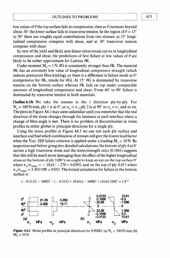
OUTLINES TO PROBLEMS I I 413 ~--------------------------------------------------~
low values of 0 the top surface fails in compression, then as 0 increases beyond about 30° the lower surface fails in transverse tension. In the region of 0 = 15° to 30° there are roughly equal contributions from two stresses: at 15° longitudinal compression competes with shear, and at 30° transverse tension competes with shear.
In view of the yield and likely non-linear stress/strain curves in longitudinal compression and shear, the predictions of first failure at low values of 0 are likely to be rather approximate for Lamina OK.
Under moment Mx = 1 N, OG is consistently stronger than OK. The material OK has an extremely low value of longitudinal compressive strength (which induces premature fibre kinking), so there is a difference in failure mode at 0° (compressive for OK, tensile for OG). At 15° OG is dominated by transverse tension on the bottom surface whereas OK fails on top under comparable amounts of longitudinal compression and shear. From 60° to 90° failure is dominated by transverse tension in both materials.
Outline 6.10: We take the stresses in the 1 direction ply-by-ply. For Nx = 100N/mm, ply 1 is at 0°, so (1x = (11; ply 2 is at 90° so (1y = 111 and so on. The plots in Figure A6.1 may seem unfamiliar until you remember that the real direction of the stress changes through the laminate at each interface where a change of fibre angle is met. There is no problem of discontinuities in stress profiles in either global or principal directions for a single ply.
Using the stress profiles in Figure A6.1 we can test each ply surface and interface and find which combination of stresses will give the lowest load factor when the Tsai-Hill failure criterion is applied under a loading My = 10 N. By inspection and before going into detailed calculations, the bottom of ply 4 at 0° carries a high transverse stress and the stress/strength ratio (0.1061) suggests that this will be much more damaging than the effect of the higher longitudinal stress at the bottom of ply 3 (90°); we ought to keep an eye on the top surface 0° where (12/112max = -10.61/ - 270 = 0.0393, and on the top of ply 4 (0°) where 112/112max = 5.303/100 = 0.053. The formal calculation for failure at the bottom surface is
( - 0.3133/ -16(0)2 - ( - 0.3133 x 10.61)/( - 1600f + (10.61/100f = l/p2
~~_~~_~ ~8~ ____ ~_-~ _\:!t ad 22.88 1.096 rf -0.1566 5.3
00 00 -~~ 1~ 0'1 MPa 0'2 MPa 0'1 MPa 0'2 MPa
Figure A6.1 Stress profiles in principal directions for 0/90SG: (a) Nx = 100 N/mm; (b) M y = ION.
I 414
I I OUTLINES TO PROBLEMS
Table A6.6 Failure sequence for 0/90 SG under My = 10 N
Moment Kx Ky Kxy Tsai-Hill Place Angle (N) (1m) (1m) (1m) factor degrees
My 10 -0.0706 0.9903 0 9.428 4b 0 18.86 4t 0 25.43 1t 0
Thus we arrive at the sequence for the first three failure events (Table A6.6): Comparing these results with those for Mx = ION in Table A6.6, we see
that, as expected, the midplane curvatures and failure sequences are quite different when bending moments are applied in the two different principal directions.
Outline 6.11: For Nxy = + 100N/mm the stress profiles are (Table A6.7(a)): First ply failure occurs in plies 2 and 3 at - 45° with F = 1.517 (and the + 45° plies fail at F = 2.309).
For N XY = lOON/mm we find the following stress profiles (uniform in each ply) (Table A6.7(b)): Applying the Tsai-Hill criterion we incur first ply failure (in shear) in the 0° and 90° plies at F = 1.4 (then - 45° at F = 2.125, and + 45° at F = 3.233). But modes for later failures are not easy to determine from these combinations of direct stresses.
The conclusion is that the thicker tube (b) fails at a rather lower torque than the thinner tube (a); if for other reasons it is necessary to use tube (b) then it would be desirable to protect the 0° and 90° plies by putting them inside the 45° plies in an arrangement such as ( + 45°/ - 4SO /0° /90°),.
Table A6.7 Stress profiles (a) in (+45°/ -4SO)s, N xy = 100N/mm
Ply No. Angle 1T1 1T2 '12 ° (MPa) (MPa) (MPa)
1 +45 338.2 -61.76 0 2 -45 -338.2 61.76 0
(b) in (0°/90°/+ 45°/-45°)s, N xy = 100N/mm
Ply No. Angle 'xy '12 1T1 1T2
° (MPa) (MPa) (MPa) (MPa)
1 0 57.18 57.18 0 0 2 90 57.18 - 57.18 0 0 3 +45 142.8 0 241.5 -44.11 4 midplane -45 142.8 0 -241.5 44.11

OUTLINES TO PROBLEMS I
Table A6.8 Tsai-Hill factors for (8/ - 8) SG under N x = -10N/mm
8° 0 15 30 45 60 75 90 Factor 320 149 57.01 31.66 30.42 41.96 54
Outline 6.12: 8 = 0° longitudinal tension, 8 = 15° shear with substantial transverse tension, 8 = 30°, 45° shear, 8 = 60° almost equal shear and transverse tension, 8 = 75° - 90° transverse tension.
Outline 6.13: See Table A6.8. The conclusion for this laminate is that the load factor in uniaxial compression in the x direction is always greater than that for uniaxial tension.
Outline 6.14: The reference direction x in the angle ply laminate is taken as the hoop direction. The response for (8/ - 8)SG under Nx = 10N/mm, Ny = 5 N/mm are as shown in Table A6.9. From the tabulated data we can see the following:
• The maximum value of Tsai-Hillioad factor occurs at about 33°. • The shear stress, 12 is zero at about 26.5°. • The transverse stress (J 2 has a minimum value at about 35°. • The longitudinal stress (J 1 has a maximum value at about 35°. • The global transverse strain 8y is zero at about 45° and 75°.
Working on the basis of (J d(J Imax' (J 2/(J 2max' , 12/' 12max' we deduce the following as the most likely modes of failure: 8 = 0° transverse tension, 8 = 15° - 20° shear but much transverse tension, f) = 30° - 40° transverse tension, 8 = 45° - 55° transverse tension but much shear, 8 = 60° - 90° transverse tension.
Table A6.9 Load factors for laminates{O/ - O)SG underNx = lON/mm, Ny = 5 N/mm
0 ex ey t t t Tsai-Hill Place Yxy 0'1 0'2 '12
(%) (%) (%) (MPa) (MPa) (MPa) factor
0 0.009463 0.02029 0 5 2.5 0 39.6 all 15 0.0098 0.01774 0 5.311 2.189 0.204 44.62 all 20 0.01032 0.01566 0 5.53 1.97 0.1766 49.23 all 25 0.01133 0.01294 0 5.77 1.73 0.06354 55.63 all 30 0.01307 0.009654 0 5.986 1.514 -0.1522 62.08 all 35 0.01577 0.006046 0 6.114 1.386 -0.4699 62.55 all 40 0.01949 0.002545 0 6.083 1.417 -0.8578 53.91 all 45 0.024 -0.000317 0 5.852 1.648 -1.25 43.02 all 55 0.03333 -0.002734 0 4.822 2.618 -1.742 29.23 all 60 0.03715 -0.002382 0 4.298 3.202 -1.759 25.7 all 65 0.04008 -0.001435 0 3.753 3.747 -1.635 23.43 all 75 0.04359 0.000847 0 2.941 4.559 -1.098 21.02 all 90 0.0451 0.002478 0 2.5 5 0 20.03 all
I 415
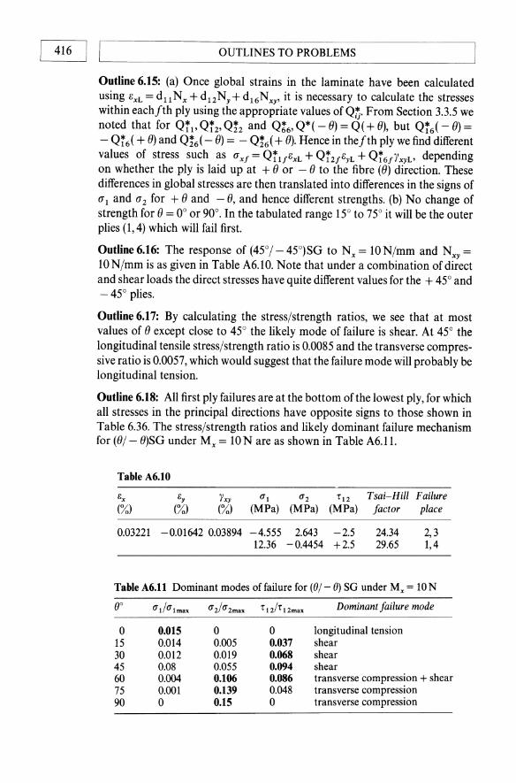
416 I LI ______________ O_U_T_L_IN __ ES_T_O __ P_RO __ BL_E_M_S ______________ ~ Outline 6.15: (a) Once global strains in the laminate have been calculated using BxL = duNx + d12Ny+ d16Nxy, it is necessary to calculate the stresses within each fth ply using the appropriate values of QU' From Section 3.3.5 we noted that for Q1\, Qi2' Qi2 and Q~6' Q*( - 0) = Q( + 0), but Qi6( - 0) = - Qi6( + 0) and Qi6( - 0) = - Qi6( + 0). Hence in thefth ply we find different values of stress such as (1x! = Qil/BXL + Qi2!BYL + Qi6!YXYL> depending on whether the ply is laid up at + 0 or - 0 to the fibre (0) direction. These differences in global stresses are then translated into differences in the signs of (11 and (12 for + 0 and - 0, and hence different strengths. (b) No change of strength for 0 = 0° or 90°. In the tabulated range 15° to 75° it will be the outer plies (1,4) which will fail first.
Outline 6.16: The response of (45°/- 45°)SG to Nx = 10 N/mm and NXY = 10 N/mm is as given in Table A6.10. Note that under a combination of direct and shear loads the direct stresses have quite different values for the + 45° and - 45° plies.
Outline 6.17: By calculating the stress/strength ratios, we see that at most values of 0 except close to 45° the likely mode of failure is shear. At 45° the longitudinal tensile stress/strength ratio is 0.0085 and the transverse compressive ratio is 0.0057, which would suggest that the failure mode will probably be longitudinal tension.
Outline 6.18: All first ply failures are at the bottom of the lowest ply, for which all stresses in the principal directions have opposite signs to those shown in Table 6.36. The stress/strength ratios and likely dominant failure mechanism for (0/ - O)SG under Mx = 10 N are as shown in Table A6.11.
Table A6.10
Bx By "/xy 0'1 0'2 t12 Tsai-Hill Failure (%) (%) (%) (MPa) (MPa) (MPa) factor place
0.03221 -0.01642 0.03894 -4.555 2.643 -2.5 24.34 2,3 12.36 -0.4454 +2.5 29.65 1,4
Table A6.11 Dominant modes of failure for «()/ - ()) sa under Mx = 10 N
()O u l/U Imax U 2/U 2max t12/t 12max Dominant failure mode
0 0.015 0 0 longitudinal tension 15 0.014 0.005 0.037 shear 30 0.012 0.019 0.068 shear 45 0.08 0.055 0.094 shear 60 0.004 0.106 0.086 transverse compression + shear 75 0.001 0.139 0.048 transverse compression 90 0 0.15 0 transverse compression
OUTLINES TO PROBLEMS I I 417 ~------------------------------------------------~
Outline 6.19: Using the concept of stress/strength ratios as a rough guide, shear failure is dominant in the range () = 0° to 25° and 65° to 90°. In the region 30° to 60° transverse tensile failure is dominant; at 45° no shear stress is present in the principal directions.
Outline 6.20: The directions of transverse stresses in the laminate (90% °). are reversed compare with those in (0°/90°)., and so the free edges between 90° and 0° plies are in compression and therefore not prone to splitting. This is therefore an advantageous arrangement where narrow laminates, or wide laminates with holes, are to be used.
CHAPTER 7
Outline 7.1: At To the block has dimensions L1 L2L3, and at T 1 the new dimensions are L1(1 + IXAT) x L2(1 + IXAT) x L3(1 + IXAT). The fractional increase in volume of the block, i.e. the volume strain, is given by Ev = A V /V 0 = (V - Vo)/V = (1 + IXAT)3 - 1. Neglecting second order terms of small quantities, (1 + IXAT)3 ~ 1 + 3IXAT, hence Ev ~ 3IXAT.
Outline 7.2: The new major axes in the principal directions are D1 = Do(1 + 1X1AT) =40(1 +6 x 10- 6(60-15))=40.011 mm. D2 = Do(1 + 1X2AT) = 40.063 mm. The circular hole at 15°C has become slightly elliptical at 60°C.
Outline 7.3: Let the co-ordinate of the midplane of the sheet be z = 0, so that fluid x is in contact with the surface z = - h/2 and y in contact with z = + h/2. The midplane strain in the sheet is given by EO = (If + E')/2 = (IX(T 1 - To)IX(T 2 - T 0))/2 = (1X/2) (T 1 + T 2 - 2T 0)' The midplane curvature can be found from Equation (3.11), [E] = [EO] + Z[K], hence EX = EO + ( - h/2)K and E' = eO + (h/2)K, giving K = IX(T 2 - T l)/h.
Outline 7.4: K = 0.4438 m, O'~ = 42.33 MPa, O'~ = - 19.38 MPa, Ei = 6.435 X
10-4 • (For interest Fa = 57.85 N.)
Outline 7.5: The analysis must now be reworked for different thicknesses of the component strips. Let the thickness of a be ha' and of b be hb . The force equilibrium Fa = - Fa still holds, but the moment equilibrium is (Figure A7.1)
(A7.1)
Figure A 7.1 Non-symmetrical two-ply laminate.
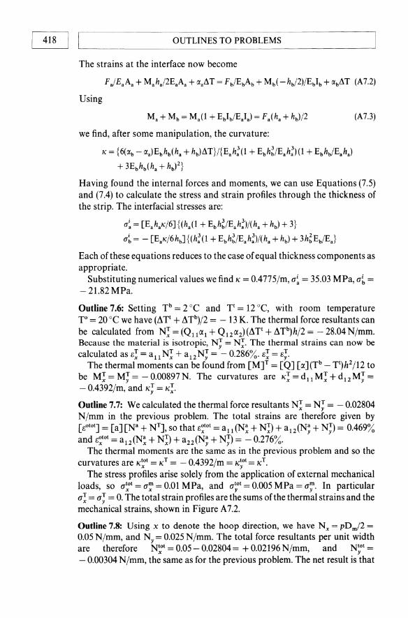
OUTLINES TO PROBLEMS 418 I I ~--------------------------------------------------~
The strains at the interface now become
Using
Ma + Mb = Ma(1 + Eb1b/Ea1a) = Fa(ha + hb)/2
we find, after some manipulation, the curvature:
K = {6(lXb -lXa)Ebhb(ha + hb)dT}/{Eah; (1 + Ebh~/Eah;)(1 + Ebhb/Eaha)
+ 3Ebhb(ha + hb)2}
(A7.3)
Having found the internal forces and moments, we can use Equations (7.S) and (7.4) to calculate the stress and strain profiles through the thickness of the strip. The interfacial stresses are:
a~ = [EahaK/6]{(ha(1 + Ebh~/Eah;)/(ha + hb ) + 3}
a~ = - [EaK/6 hb ] {( h; (1 + Eb h~lEa h;)/( ha + hb ) + 3 h~ EblE.}
Each of these equations reduces to the case of equal thickness components as appropriate.
Substituting numerical values we find" = 0.477S/m, a~ = 3S.03 MPa, lT~ = - 21.82 MPa.
Outline 7.6: Setting Tb = 2°C and TI = 12°C, with room temperature P = 20°C we have (L\TI + L\Tb)/2 = -13 K. The thermal force resultants can be calculated from N~ = (Q1lal + Q12az)(L\TI + L\Tb)h/2 = - 28.04 N/mm. Because the material is isotropic, N~ =~. The thermal strains can now be calculated as e~ = all N~ + alzNJ = - 0.286%. e~ = eJ.
The thermal moments can be found from [M]T = [Q] [a](Tb - TI)hz/12 to be M~ = MJ = - 0.00897N. The curvatures are ,,~= dllM~ + dlzMJ = - 0.4392/m, and "J = ,,~. Outline 7.7: We calculated the thermal force resultants N~ = NJ = - 0.02804 N/mm in the previous problem. The total strains are therefore given by [eOIOI] = [a] [N" + NT], so that e~lol = all (N~ + ~) + alz(N~ + N;) = 0.469% and e~lol = adN~ + N~ + a2z(N~ + NJ) = - 0.276%.
The thermal moments are the same as in the previous problem and so the curvatures are ,,~I = "T = - 0.4392/m = ,,~Ol = "T.
The stress profiles arise solely from the application of external mechanical loads, so lT~1 = lT~ = 0.Q1 MPa, and a~ol = O.OOS MPa = a~. In particular a~ = a; = O. The total strain profiles are the sums of the thermal strains and the mechanical strains, shown in Figure A 7.2.
Outline 7.8: Using x to denote the hoop direction, we have N x = pDml2 = O.OSN/mm, and Ny =0.02SN/mm. The total force resultants per unit width are therefore N~I = O.OS - 0.02804 = + 0.02196 N/mm, and N~ol = - 0.00304 N/mm, the same as for the previous problem. The net result is that
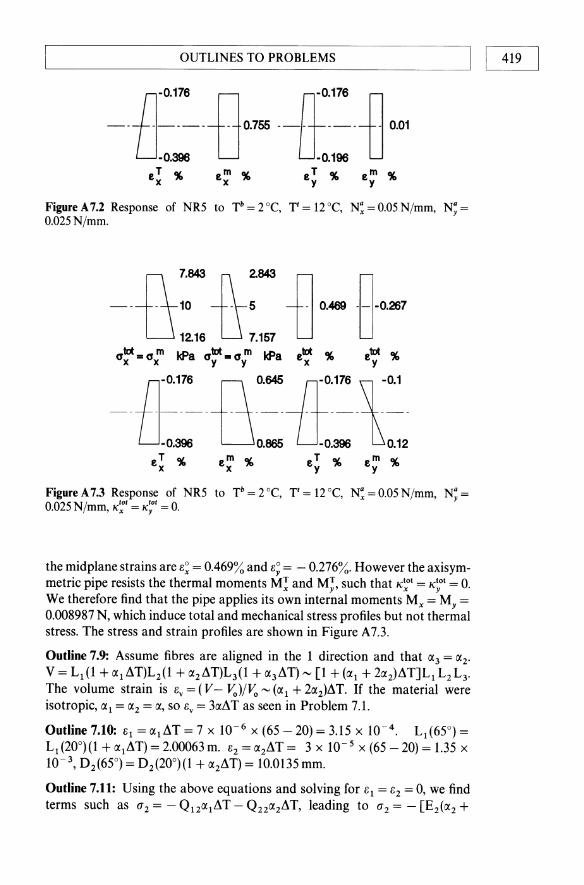
OUTLINES TO PROBLEMS ____ 11 419
Figure A 7.2 Response of NR5 to Tb = 2 ce, Tt = 12°C, N: = 0.05 N/mm, N; = 0.025N/mm.
_. n :~ ~:843 n OM9 Hn281
U12.16U7.157 U 0 atot .. a m kPa a tot .. a m kPa .. tot % .. trA % x x y y x y
Figure A 7.3 Response of NR5 to Tb = 2°C, r = 12°C, N: = 0.05 N/mm, N; = 0.025 N/mm, K~t = K~ot = O.
the midplane strains are e~ = 0.469% and 1'; = - 0.276%. However the axisymmetric pipe resists the thermal moments M! and M;, such that <ot = K~ot = O. We therefore find that the pipe applies its own internal moments Mx = My = 0.008987N, which induce total and mechanical stress profiles but not thermal stress. The stress and strain profiles are shown in Figure A 7.3.
Outline 7.9: Assume fibres are aligned in the 1 direction and that a3 = a2•
V = L1 (1 + a1 dT)L2(1 + a2dT)L3 (1 + a3 dT) "" [1 + (a 1 + 2(2)d T]L1 L2 L3 •
The volume strain is ey = (V - ~)j~ "" (a 1 + 2(2 )dT. If the material were isotropic, a1 = a2 = a, so ey = 3adT as seen in Problem 7.1.
Outline 7.10: 1'1 = a1dT = 7 x 10- 6 x (65 - 20) = 3.15 X 10- 4 . L1(65°) = L1 (20°)(1 + a1dT) = 2.00063 m. 1'2 = a2dT = 3 x 10- 5 x (65 - 20) = 1.35 X
10- 3 , D2(65°) = O2(20°)(1 + a2dT) = 10.0135 mm.
Outline 7.11: Using the above equations and solving for 1'1 = 1'2 = 0, we find terms such as 0'2 = - Q12a1dT - Q22a2AT, leading to 0'2 = - [E2(a Z +

420 I LI ______________ O_U_r_L_IN __ ES_r_O __ p_RO __ BL_E_M_S ______________ ~
v12(Xl)AT]/(l + V12 v21). The negative sign confirms that a compressive stress had to be applied to counter the free therma,l strain caused by an increase in temperature.
Outline 7.12: We assume that ex = 0, and that the rod is free to change its transverse dimensions, hence
( e1) (Sl1 S12 0 )(111) (1X1) e2 = S12 S22 0 0 + 1X2 ~r
')'12 0 0 S66 0 0
Thus we have 61 = ° = (J dEl + (XIAT, i.e. (J 1 = - El(XlAT = - El(Xl (T - To) = - 45.6 X 109 x 7 X 10- 6 X ( - 25 - 20) = + 14.364 MPa. 62 = 111( - v12IEl) + (X2AT= 14.364 x 10⁶ x (-0.274/45.6 x 109)+3 x 10- 5 x -45= -0.1436%.
It is worth studying the more formal approach, using the thermal force resultants. We have Ni = AT'h(Qll(Xl + Q12(X2)' N1 = AT· h(Q12 (Xl + Q22(X2)' The problem states that el = 0 = all [NT + ND + a12 NJ, Recalling that a12/a ll = - v12' we find after some manipulation that NT = - AThEl (Xl'
Outline 7.13: The inverse strain transformation matrix for 30° is
(0.75 0.25 -0.866)
[rr 1 = 0.25 0.75 0.866 0.433 -0.433 0.5
IXx = 0.75 x 1 x 10- 5 + 0.25 x 2 x 10- 4 = 5.75 x 1O- 5/K
lXy = 0.25 x 1 x 10- 5 + 0.75 x 2 x 10- 4 = 1.525 x 1O- 4/K
IXxy/2 = 0.433 x 1 x 10- 5 - 0.433 x 2 x 10-4 = - 8.227 x 10- 5 = IXxy/2 hence (Xxy= -1.6454 x 1O- 4/K. The sheet dimensions become
Lx = 350(1 + 5.75 x 10- 5 x 35) = 350.70mm
Ly = 230(1 + 1.525 x 10-4 x 35)= 231.23mm
')'xy = IXXy~T = -1.6454 x 10- 4 x 35 = - 5.759 x 10- 3 = - 0.5759%
Outline 7.14: Because the sheet is orientated at 30° to the principal directions, we must now use the transformed reduced stiffnesses [Q*] to find the stresses from the strains. The thermal force resultant is given by
( N!) (Q~l Q~2 Q~6)( IXX) N; = Q!2 Q!2 Q!6 lXy ~r'h Nxy Q16 Q26 Q66 IXxy
Using data from Table 3.7, we calculate N! = 0.531 N/mm, N~ = 0.246 N/mm, and N!'y = ( + )0.248 N/mm. It must be emphasized that these forces are only needed when all three constraints to thermal change are imposed.
Outline 7.15: (a) We have already found the expansion coefficients to be «(Xx, (Xy' (Xx) = (0.575, 1.525, -1.6453) x 10- 4/K. Hence (N!, N~, N!y) = [Q*] [(X] AT·

I I 421 L-__________________________________________________ ~ OUTLINES TO PROBLEMS
h = (0.4555,0.2109, 0.2119)N/mm. Using the [a] matrix in Table 3.8 the thermal strains are [eDT] = [a] [NT]: (e~T, e~T, y~;)= (0.1725, 0.4575,- 0.4936)%.
(b) The thermal force resultants given by [NT] = [Q*] [IX] (L\Tb + L\Tt)h/2 are (N~, N~, N~y) = ( - 0.2809, - 0.1299, - 0.1307) N/mm and hence (e~T, e~T, y~;) = [a] [NT] = (- 0.1064%, - 0.2821%, + 0.3044%).
The thermal moment resultants given by [MT] = [Q*] [IX] (Tb - Tt)h2/12 are (M~, M~, M~,) = ( - 0.05821, - 0.02693, - 0.02708) N. Using the Ed] matrix from Table 3.8 we can now calculate the curvatures for three situations: (i) for a flat plate where all curvatures are free to develop; (ii) for the thin-walled tube where "x and "yare prevented but the tube is free to twist; and (iii) for a thinwalled tube where all three curvatures are prevented.
(i) ["T] = Ed] [MT]: ("x, ICy, "Xy) = ( - 0.6612, - 1.754, + 1.892)/m. (ii) This tube problem is rather more tricky. The tube form prevents the
development of curvatures in the hoop and longitudinal directions. We therefore need to solve simultaneously the equations ,,~ = 0 = d 11 Mx + d 12 My + d16 M~y; ,,~= 0 = d 12 Mx + d22My + d26M~y; "~y = d16 Mx + d26My + d66M!y, where Mx and My include the internal mechanical moment needed to suppress the development of thermal curvatures ,,! and ,,~. Hence Mx = (d12d26 -d16d22)M!/(dlld22 - di2) = 1.712 M!y, and My = (dlld26 - d 12d 16)M!y/ (di2 - d11dnl = 0.5692 M~y' Hence ,,! =,,~ = 0 as required, and "!y = -0.2366/m.
It is worth looking more carefully at the values of Mx and My: they each consist of the thermal moment MT (which here is negative), and the additional internal mechanical moment M:" (here positive) which counterbalances the thermally-induced curvature, i.e. Mx = M~ + M~. The thermal moments do not induce stress in a single ply, but the internal mechanical moments do induce stresses which are shown in Figure A 7.4.
(iii) To achieve "x = ICy = "Xy in this problem we can take the commonsense approach of applying internal mechanical moments to overcome the thermal moments: Mi = - Mf, so that (M~, M~, M~ = ( + 0.05821, + 0.02694, + 0.02707) N. These internal mechanical moments induce the total and mechanical stress profiles shown in Figure A 7.5.
(c) N~ = pdm/2= 0.04 x 30/2 = 0.6N/mm, and N~ = OJ N/mm. The midplane strains now correspond to the effective force resultant Ne = N8 + NT.
_ \Mlre1 \-0,01732 .:: 01o,01769\n~7« l~a t m. 0
otd..om MPa otat.om '1!f otd.=om otd.=om "tat=" m x x Y Y 1 1 2 2 12 12
Figure A 7.4 Response of NE30 tube to Kx = Ky = 0, free to develop Kxy. Stresses in MPa.

OUTLINES TO PROBLEMS I 422 I I L-__________________________________________________ ~
a'ld. • a m MPa atat • am., tat =., m a'ld. = a m atat = a m x x y y x¥ X¥ 1 1 2 2
Figure A 7.5 Response of NE30 tube to Kx = Ky = Kxy = O. Stresses in MPa.
Thus N~ = 0.6 - 0.2809 = 0.3191 N/mm, N; = 0.3 - 0.1299 = 0.1701 N/mm, and N~y=N!,y= -0.1307N/mm. Hence e~t=allN~+a12N;+a16N~y = 2.117%, e~ot = 0.09528% and y~; = - 3.715%.
Stresses are calculated from the mechanical strains and curvatures. Thus from [eom] = [a] [Na] and ["m] = Ed] [Mm], [O'~z)] = [Q*] [eom + z"m].
For the midplane we have e~m= allN~+ a12N~= 0.02223, e~m= a12N~ + a22N~ = 0.003771, and y~~ = a16N~ + a26N~ = - 0.040194. Hence O'~ = Q!le~m+ Q!2e~m+ Q!6Y~~ = 0.298 MPa. Alternatively because the in-plane load is uniform across the wall thickness, we simply find O'~ = N~/h = 0.6/2 = 0.3 MPa, with a minor difference attributable to rounding off error between computed and manual calculations.
For stresses away from the midplane we first need to calculate the curvatures induced by the mechanical internal moments. ,,~= d11 M~ + d12M~ + d16M~y = 0.6612/m, ,,~= + 1.754/m, and "xy = - 1.892/m. Hence at z = - 0.001 m we obtain e~m + z,,~ = 0.02157, e~m + z,,~ = 0.002017, and Y~~ + z~ = - 0.0383, leading to ~( - 0.001 m) = 0.2127 MPa, ~( - 0.001 m) = 0.1096 MPa, and r~y( - 0.001 m) = - 0.04061 MPa. We then obtain the
--B :]:::":\~::n:::-H~ 0.3873 0.1904 0.04061 0.3733 0.2045
atat • am MPa a'ld.. am 'r lilt. 'r m alllt ... am alllt III am 'r lilt • 'r m x x y y X¥ X¥ 1 1 2 2 12 12
Figure A 7.6 Response ofNE30 tube to Kx = Ky = Kxy = O. P = 40 kPa. Stresses in MPa.
~ ~::: n:: ~~::: [\ :::4 ~ :::- n~:::9 TI -0.172£1 U 2.29 TI-O.4575 0 0.5228 UO•4936 U-4.209
e T " em" e T "e m " 1, T " 1,m" x x y y 'X:J 'X:J
Figure A 7.7 Strain response of NE30 tube to internal pressure and temperature gradient.
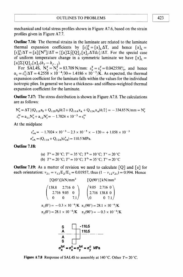
L-______________ O_u_T_L_IN_E_S_T_O __ PR_O_B_L_E_M_S ______________ ~1 I 423
mechanical and total stress profiles shown in Figure A7.6, based on the strain profiles given in Figure A7.7.
Outline 7.16: The thermal strains in the laminate are related to the laminate thermal expansion coefficients by [e]r = [a]L~T, and hence [a]L = [e]V~T = [a][NT]/~T = {[a]I:HQ]J[a]J~Tdz}/~T. For the special case of uniform temperature change in a symmetric laminate we have [a]L = [a] I: [Q]J[a]J{hJ - h J-1)'
For SAL4S, N~ = N; = 83.709 N/mm: e~ = e; = 0.042558%, and hence a 1 = eI/~T = 4.2558 x 10⁻⁴/30= 1.4186 x lO- s/K. As expected, the thermal expansion coefficient for the laminate falls within the values for the individual isotropic plies. In general we have a thickness- and stiffness-weighted thermal expansion coefficient for the laminate.
Outline 7.17: The stress distribution is shown in Figure A7.8. The calculations are as follows:
N~ = L\T {(QllslXs + Q12SlXs)h/2+ (QllAIXA + Q12AIXA)h/2} = - 334.85 N/mm = N;
e~c= allN~+ a12N;= -1.7024 x 10- 3 = e;c
At the midplane
e~A= -1.7024 x 10- 3 -203 X 10- 5 x -120= + 1.058 x 10- 3
U~A = (QIIA + Q12A)(e~A) = 110.5 MPa.
Outline 7.18:
(a) TO = 20°C; Tt = 35°C; Tb = 10 °C; rc = 20°C (b) TO = 20 °C; Tt = 10 °C; Tb = 35°C; T C = 20°C
Outline 7.19: As a matter of revision we need to calculate [Q] and [a] for each orientation: V21 = v12 E2/E l = 0.01957, thus (1- V12V21) = 0.994. Hence
[Q(OO)] kN/mm2
(138.8 2.716 0 )
2.716 9.05 0 o 0 7.1
[Q(900)] kN/mm2
(9.05 2.716 0) 2.716 138.8 0 o 0 7.1
1X1(00) = -OJ x 1O- 6jK 1X1(900) = 28.1 X 1O- 6jK
1X2(00) = 28.1 X 1O- 6jK 1X2(900) = -OJ x 1O- 6/K
~.--)::~-----atot _ aC _ atot .. aC MPa
x x y y
Figure A 7.8 Response of SAL4S to assembly at 140°C. Other T= 20°C.
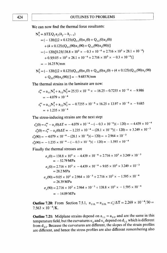
OUTLINES TO PROBLEMS I 424 I I ~------------------------------------------------~
We can now find the thermal force resultants:
N~ =il.T!.QfcxAhf-hf-d
= ( - 120) [(2 x 0.125)(Qll (0) cx 1 (0) + Q dO) CX 2 (0))
+ (4 X 0.125)(Qll (90)cxl (90)+ Qd90)cx2(90))]
= (-120)[0.25(138.8 X 10³ x - 0.3 X 10- 6 + 2.716 X 103 x 28.1 x 10- 6)
+ 0.5(9.05 x 103 x 28.1 X 10- 6 + 2.716 X 10³ x - OJ x 10- 6)]
= -16.25N/mm
Ni = (-120) [(2 x 0.125)(Q12(0)CX1(0) + Q22(0)CX2(0) + (4 x 0.125)(Ql 2 (90) cx l (90)
+ Q22(90)cx2(90))] = - 9.685 N/mm
The thermal strains in the laminate are now:
e~c =allN~ +a12Ni= 25.53 x 10- 6 x -16.25 -0.7255 x 10- 6 x -9.986
= -4.079 x 10- 4
e;C = a12N~ + a22Ni = - 0.7255 X 10- 6 x 16.25 + 13.97 x 10- 6 x - 9.685
= + 1.235 X 10- 4
The stress-inducing strains are the next step:
e:(O) = e~c - CX l (O)il.T = - 4.079 X 10- 4 - (- OJ x 10- 6)( -120) = - 4.439 X 10⁻⁴
e;(O) =e;c-cx2(0)il.T = -1.235 x 10- 4 -(28.1 x 10- 6)(-120)= +3.249 x 10- 3
e:(90) = - 4.079 X 10- 4 - (28.1 x 10- 6)( -120) = + 2.964 X 10- 3
e;(90) = -1.235 x 10- 4 _( -0.3 x 10- 6)( -120)= -1.595 x 10⁻⁴
Finally the thermal stresses are
ux(O) = 138.8 x 10³ x - 4.439 X 10⁻⁴ + 2.716 X 103 x 3.249 X 10- 3
= -52.79MPa
uy(O) = 2.716 x 10³ x - 4.439 X 10- 4 + 9.05 X 103 x 3.249 x 10- 3
= 28.2MPa
uX<90) =9.05 x 103 x 2.964 X 10- 3 + 2.716 X 10³ x -1.595 X 10- 4
= 26.39MPa
uy(90) = 2.716 x 103 x 2.964 X 10- 3 + 138.8 X 10³ x - 1.595 X 10- 4
= -14.09MPa
Outline 7.20: From Section 7.5.1, (J(llL = (J(22L = e~/AT = 2.269 x 10⁻⁴/30 = 7.563 x 1O-6/K.
Outline 7.21: Midplane strains depend on all = a 22, and are the same in this temperature field, but the curvatures "x and ICy depend on d ll which is different from d 22• Because the curvatures are different, the slopes of the strain profiles are different, and hence the stress profiles are also different remembering also

L-______________ O_U_T_L_IN_E_S_T_O_P_R_O_B_L_E_M_S ______________ ~I I 425
that terms in 11 and 22 in [Q(OO)] and [Q(900)] are different:
O"x(OO) = Ql1 (O°){e~ + ZKx} + QdOO) {B; + ZKy}
O"A900) = Ql1 (90°){e~ + ZKx} + Q12(900) {B; + ZKy}
O"y(OO) = Q12(O°){e~ + ZKx} + Q22(OO) {B; + ZKy}
O"y(900) = Q12(90°){e~ + ZKx} + Qd900) {B; + ZKy}
Outline 7.22: To suppress "2 we need to apply a moment M; which alone gives "T = - "1, where ,,1 is the thermally-induced curvature from example 1.3, i.e. "T = - 0.6569/m. Hence M; = - "1fd22 = - 0.6569/3.245 = - 0.2024 N. "T = d12M; = - 41.94 x 10- 3 X - 0.2024 = 0.OO8489/m. The total curvatures are now "2 = "1 + "T = 0.6569 + ( - 0.6569) = 0, as required. The total midplane strains are the same as for Examples 3 and 4. The total stress profiles are given in Figure 7.20.
Outline 7.23: The temperature gradient through the thickness induces a bending strain linear through the thickness. The discontinuity in stress (T~ot(z) arises from the change of expansion coefficient at the interface between dissimilar plies and from the change of stiffness. At the upper interface the 0° ply if unbonded would expand in the y direction by (X2 ATi and the 90° ply if unbonded would expand freely by the smaller amount 1X1 ATi. To achieve the same strain e; at the interface, we have to apply an internal compressive force to the 0° ply and a tensile force to the 90° ply, as shown in Figure 7.20.
Outline 7.24: In order to suppress the bending caused by the temperature gradient, it is necessary to apply moments M~ = 0.5518 Nand M; = 0.2108 N. The midplane strains arising from the temperature gradient are e~ = e; = 0.005673%. The total and thermal stress profiles are shown in Figure A 7.9, and the mechanical and thermal strains are shown in Figure A 7.10.
Outline 7.25: By inspection the total stresses profile is that given in Figure A7.11. The mechanical strain profile can be constructed graphically from the thermal strain profile B~(Z) in the figure, and hence the mechanical stress (T~(z) calculated from (T~(OO) = Q11 e~(z) + Q12 e;(z).
rf 1J:~:~ ,~:m (~~1~ ~:~:m 9f! 19.27 -2.95 -28.42 9.258 --- - 21.12- - - -1.624- - -21.12 - -- 1.624 9f! 22.97 -0.2992 -13.81 -6.009 rf -13.81 1.438 22..97 -0.534
-6.51 1.246 24.81 0.5566 a tot MPa aT MPa atot MPa aT MPa x x y y
Figure A 7.9 Stress response of C + 4S to TO = 20°C. Tt = 40°C, Tb = 15°C, T C = 125°C.
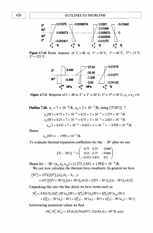
I 426 I IL-______________ O_U_T_L_IN_E_S_T_O_P_R_O_B_L_E_M_S ______________ ~
~ fO.01375 ~0'0008074 y~:~~ \0.01642 -- - - 0.005673 -- -- -- 0.005673 - ° 9ft -0.002539 (j -0.002401 -0.01075
eT '" em '" eT '" em '" x x y y
Figure A 7.10 Strain response of C + 4S to TO = 20°C, Tt = 40°C, Tb = 15°C, TC = 125°C.
~~.~~-;:: -zr_::::: 9ft -6.498 -1.328
-2.93 -0.04122
CJ~ MPa CJ~ MPa e ~ '"
Figure A 7.11 Response of C + 4S to TO = T C = 20°C, Tt = Tb = 50°C, "I = "2 = O.
Outline7.26: IXI = 7 x 10- 6/K, 1X2= 3 x lO-s/K; using [T(300)]-I:
Hence
IXA300) = 0.75 x 7 x 10- 6 + 0.25 x 3 x 10- 5 = 1.275 x 1O- 5/K
lXi300) = 0.25 x 7 x 10-6 +0.75 x 3 x 10- 5 =2.425 x 1O- 5jK
IXx/2 = 0.433 x 7 x 10- 6 - 0.433 x 3 x 10- 5 = - 9.959 x 1O-6jK
IXxPOO) = - 1.992 x 10 - 5/K
To evaluate thermal expansion coefficients for the - 30° plies we use:
( 0.75 0.25 0.866)
[T( - 30°)] -I = 0.25 0.75 -0.866 -0.433 0.433 0.5
Hence for - 30°: (lXx, ocY' OCXY) = (1.275,2.425, + 1.992) x 10- S/K. We can now calculate the thermal force resultants. In general we have
[NT] = ~T~[Q*]f[lX]f(hf - hf-I)
= ~T {[Q*( + 300 )]f[lX( + 300 )]f(h/2) + [Q*( - 300 )]f[lX( - 300 )]f(h/2)}
Unpacking this into the fine detail we have terms such as
N! = AT(h/2) {(Q11 (300)lXx(300) + Q12(300)lXy(300) + Q16(300)lXxy (300))
+ Q!I (- 300)lXx( - 30°) + Q!2( - 300 )lXy( - 30°) + Q!6( - 300 )lXxy( - 30°)}
Substituting numerical values we find
(N!, N~, N!y) = ~ T(h/2)(79.62977, 73.0185, 0) x 104 SI units
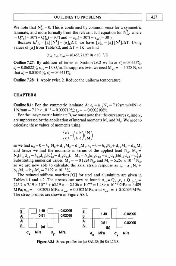
OUTLINES TO PROBLEMS I I 427 L-________________________________________________ ~
We note that N;y = O. This is confirmed by common sense for a symmetric laminate, and more formally from the relevant full equation for N;y, where - Q!6( + 30°)= Q!6( - 30°) and - (XXy( + 30°) = (XXy( - 30°).
Because (e1)L = [a] [NT] = [(X]LLlT, we have [(X]L = [a][NT]jLlT. Using values of [a] from Table 7.2, and LlT = 1K, we find
(lXxL' lXyL' IXxyL) = (6.463,21.99,0) x 10- 6 jK
Outline 7.27: By addition of terms in Section 7.6.2 we have e~ = 0.0555%, e; = 0.06022%, KXY = 1.083jm. To suppress twist we need MXY = - 5.728 N, so that e~ = 0.03841 %, e; = 0.05411 %.
Outline 7.28: 1. Apply twist. 2. Reduce the uniform temperature.
CHAPTER 8
Outline8.1: For the symmetric laminate A: ex= allNx= 7.19 (mmjMN) x 1 Njmm = 7.19 x 10-6 = 0.000719%; ey = - 0.0002106%.
For the unsymmetric laminate B, we must note that the curvatures Kx and Ky are suppressed by the application of internal moments Mx and My. We need to calculate these values of moments using
so we find Kx = 0 = hll Nx + du Mx + dl2My; Ky = 0 = h12Nx + d12Mx + d22My and hence we find the moments in terms of the applied load Nx: Mx = N~hlld22 - h12d12)f(di2 - dlld22); My = Nx(hu d12 - h12du)f(dud22 - d~2)' Substituting numerical values, Mx = - 0.1224 Nx, and My = 5.263 X 10- 3 Nx, so we are now able to calculate the axial strain response as ex = all N x + bll Mx + b12My = 7.192 x 10⁻⁴ %.
The reduced stiffness matrices [Q] for steel and aluminium are given in Tables 4.1 and 4.2. The stresses can now be found: (lxs = Qusex + Q12sey = 225.7 x 7.19 x 10-6 + 63.19 x - 2.106 X 10-6 = 1.489 X 10- 3 GPa = 1.489 MPa; (lys = - 0.02095 MPa; (lxAl = 0.5102 MPa, and (lyAl = + 0.02095 MPa. The stress profiles are shown in Figure A8.1.
!P.,~ctJ°:02095 - 0.51 0.02095 ~ (b)
Figure AU Stress profiles in: (a) SAL4S; (b) SAL2NS.
OUTLINES TO PROBLEMS 428 I I ~--------------------------------------------~
Outline 8.2: Webs in a channel section are not wide, so edge effects need to be assessed. Using (00/900)s will put the interface between 90° and 0° plies in compression, which is safer.
Outline 8.3: The cross-sectional area A = 8 x lO - 6 m 2 and I = 4 X 23 X lO - 12/
12 = 2.666 x lO-12 m4. The radius of gyration is r = y'(I/A)= 0.577mm, so the slenderness ratio is L/r = 87, so Euler buckling is likely. Ex = (all h)-1 = (10.96 x 2mm2/MN)-1 = 45.6 GPa, and hence the critical buckling load is Pc=4n2x45.6xlO9x2.666x10-12/0.01=478N. The stress 240MPa corresponds to a strain 0.526%. Note that the compressive strength of this material is much higher than the buckling strength.
Outline 8.4: Under axial tension we can see from Table 6.32 that failure would occur at N x = 556.6 N. For a mean circumference 2nRm = 471 mm, the failure load in tension is expected to be 262.2 kN.
Under axial compression we saw from Problem 6.13 that failure would occur at N x = - 570.1 N provided buckling did not occur, i.e. a compressive load of - 268.5 kN.
For this thin-walled tube the radius of gyration is r = y'(I/A) =y'(R2 m/4) = 37.5 mm, and hence the slenderness ratio is L/r = 0.1/0.375 = 2.7, so Euler buckling is not expected.
For local buckling, we estimate from Section 2.8.5 the critical buckling stress as O'c ~ 0.5Exh/Dm. From Table 6.31, all = 19.02mm/MN, so Ex = (all h)-l = 26GPa,and hence O'c= -0.5 x 26 x 109 x 2/50= -173MPa,or Pc= -163kN. The local buckling stress formula is for an isotropic material. We should note that a22 = 43.09 mm/MN, so there is more 'give' round the circumference which is likely to reduce the buckling load a little. The conclusion remains however that under axial compression the tube would fail by buckling rather than by reaching its axial compressive strength.
Outline 8.5: For 0/90SG all = 21.21 mm/MN and for 45/- 45SG all = 110.3 mm/MN. Buckling load is proportional to modulus, so the + 45/ - 45SG buckles at only about one-fifth the load for O/90SG. Men's neckties are normally cut from woven cloth cut 'on the bias', because the low modulus Ex helps to make a neat knot with a neat gather (a buckling effect). It is much more difficult to tie an elegant knot in a necktie cut 'on the square' from woven cloth.
Outline 8.6: The [AJ matrix (but not its inverse) is the same for both laminates (a) and (b), as expected. The non-symmetric laminate (b) has a non-zero [BJ matrix, also as expected. The compliance matrices for laminate (a) and (b) are clearly quite different, and hence the superficial (but incorrect) conclusion must be that the strains in the two tubes under the same pressure are quite different.
For a flat element, the strain responses in the symmetric laminate can be calculated from such general equations as Bx = allNx + a 12Ny; By = a12Nx + a22Ny• Setting NA = N x = 5N/mm and NH = N y = 10N/mm for the tube
L-______________ O_U_T_L_IN_E_S_T_O __ PR_O_B_L_E_M_S ______________ ~I I 429
we find 6x = (38.04 x 5 - 23.78 x 10) x 10-6 = - 47.6 X 10⁻⁶, and 6y =
+ 742.9 X 10⁻⁶. For a thin-walled tube these strains also apply. For the flat non-symmetric laminate we have the response kxy = b16Nx +
b26Ny. But when the non-symmetric laminate takes the form of a tube, the wall is not free to take up twisting curvature caused by internal pressure. It therefore follows that this curvature must be suppressed by applying an internal twisting moment Mxy, which with the direct force resultants makes kxy = O. Thus for the non-symmetric laminate the simultaneous equations to be solved are 6x = a11Nx + a12Ny + b16Mxy; 6y = a12Nx + a22Ny + b26Mxy; "xy = 0 = b16Nx+ b26Ny + d66 Mxy· Hence Mxy = - (b16Nx + b26Ny)/d66' Letting N x = 5 N/mm, and Ny = lON/mm, we have Mxy = - (119.3 x 5 + 42.69 x 10)/ 1512 = - 0.677 N. The hoop strain 6x is found to be 6x = (47.45 x 5 - 20.41 x 10 + 119.3 x (- 0.677)) X 10-6 = - 47.62 X 10⁻⁶. Similarly 6y = 742.95 X 10⁻⁶.
Thus we see that the strain responses to tubes made from both laminates (a) and (b) are identical (within rounding errors), provided the boundary conditions are correctly identified.
Outline 8.7: Note that the angle has been specified with reference to the circumferential direction, so the natural co-ordinate system to use to solve the problem is x for the hoop direction and y for the axial direction. This is not the normal convention, but provides a good opportunity to adapt the theory to this circumstance.
The wall thickness h = 3 mm, diameter D = 120 mm, pressure p = 0.4 MPa = 0.4 N/mm2. The hoop stresses may be expressed in terms of forces per unit width: NH = (JHh= pD/2 = 24 N/mm, NA = 12 N/mm.
We may now calculate the strains using [6°] = [a] [N]:
e~ = all NH + a12NA = (7.383 x 24 - 19.87 x 12) x 10- 3 = - 0.0612
e: = a12NH + a22NA = (-19.87 x 24 + 59.31 x 12) x 10- 3 = + 0.2348
')':H = a16NH + a26NA = (- 0.444 x 24 + 0.091 x 12) x 10- 3 = - 0.00956
Hence under air pressure (and ignoring localized end effects) the new diameter is D(1 + 6H) = 112.66 mm, new length = L(1 + 6A) = 12.348 m, and there is a radial twist (J = LYAHiR = 10 x - 0.00956/0.06 = - 1.59c = - 91.29°, as shown in Figure A5.9.
The mass of water is not negligible. At the top end of the hose the axial force per unit width is NAw = DpgL/4 = 0.12 x 1000 x 9.81 x 10/4 = 0.03 x 10⁵ N/m = 3 N/mm. Under an internal water pressure of 0.4 MPa we have the hoop force NH = 24 N/mm as before, but the axial force is now increased to NA = 15N/mm. This leads to 6H = -0.121, 6A = + 0.4128 and YAH = -0.0093. Compared with air pressure using water in this test nearly doubles the hoop strain, gives over half as much axial strain but hardly changes the twist at all. At the lower end of the pipe the response to air and water are the same.
The change in length of the pipe under water alone can be found by establishing the force acting on the underside of an element of tube of cross-

I 430 I IL-______________ O_U_T_L_IN_E_S_T_O_P_R_O_B_L_E_M_S ______________ ~
section A solely due to the weight of water underneath it. At a distance z from the lower end, the force on the lower side of an element of length dz is F(z)= Apgz. The extension of the element, dA= (F/AE)dz. The increase in length A of the pipe is the sum of all the elements, i.e.:
,i = f (A pg/AE)zdz = ApgL2/2AE = WL/2AE
where W is the weight ofthe water in the pipe, and E is the effective modulus of the material. It can therefore be seen that the total change in length of the pipe under the water is the same as half the total weight of water acting at the lower end.
Outline 8.8: Although a flat sheet made from C + 4NS would develop curvature under a direct stress, this tube cannot bend when direct stresses are applied to it, so where appropriate, it is necessary to include the boundary conditions "x = "y = 0, in addition to the applied force resultant(s).
(a) and (b): Noting that b12 = 0, we must solve the four simultaneous equations: ex = allNx+ a12Ny+ bllMx; ey = a12Nx + a22Ny+ b22My; "x = 0 = bllNx+dllMx+d12M,; "y=O=b22Ny+d12Mx+d22My. The moments Mx and My can be re-expressed in terms ofNx, Ny, and the various coefficients: Mx=(d12b22Ny-d22bllNx)/(dlld22 -dI2) and My=(dllb22Ny-d12bllNx)/ (dI2 - dlld22)· These values of moments may now be used in the expressions above to calculate ex and ey under externally applied Nx and Ny.
(c) When the tube is subject to a couple, the external load applied, Nxy, induces a shear strain Yxy = a66Nxy' There is no shear-bending coupling, so no moments need to be applied to suppress curvature.
Outline 8.9: For the symmetric laminate, the shear stress is given by 't'xy = T/(2nR2h) = 30/(2n(0.025)2 x 5 x 10- 4 = 15.28 MPa. The force resultant per unit width is N xy = 't'xyh = 7639N/m = 7.639N/mm. This leads to Yxy = a66Nxy = 43.49 x 10- 6 x 7.639 = 3.322 x 10⁻⁴ • The angle of twist is (J = yL/R = 0.0106c = 0.607°.
In tube form the bending curvatures are suppressed by applying internal moments Mx and My which can be related to the force N xy using "x = 0 = b16N xy + dllMx+ d12My; "y = 0 = b26Nxy + d12Mx + d22My. This gives Mx = My = Nx,(b26dll - b16dd/(dI2 - d lld22). Substituting numerical values we find Mx = 0.8923 N, and hence Yxy = a66Nxy + b16 Mx + b26My = 331.6 x 10⁻⁶, which agrees within rounding errors.
The stress profiles are shown in Figure A8.2.
Outline 8.10: dll = 32.89 x 1O- 3jNm, hence Wmax = Fz L3dll/3b= 1 x 0.001 x 32.89 x 10- 3/3 x 0.01 = 1.1 mm.
Outline 8.11: Let the thickness of the composite beam be hc. Its stiffness is proportional to E1 h~, and E1 = V fEf + V pEp. The mass of beam per unit cross-sectional area is
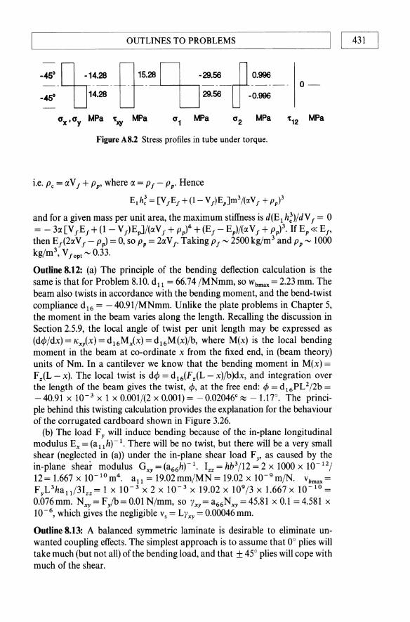
OUTLINES TO PROBLEMS I I 431
-450_~14.28 _ n 15:28 D_-29.~_~ _O.~ __ 0-
_450 LJ4.28 IT ---029.56 U-O.996
MPa MPa
Figure AS.2 Stress profiles in tube under torque.
i.e. Pc = aV J + PP' where a = PJ - pp. Hence
El h~ = [VfEf + (1- V f) Ep ]m3/(IXV f + pp)3
and for a given mass per unit area, the maximum stiffness is d(El h~)/dV J = 0 = - 3a [V JEJ + (1 - VJ)Ep]/(aVJ + pp)4 + (EJ - Ep)/(aV J + pp)3. If Ep« EJ, then EJ (2aVJ - pp) = 0, so Pp = 2aVJ. Taking PJ ~ 2500kg/m3 and Pp ~ 1000 kg/m3, V JoP! ~ 0.33.
Outline 8.12: (a) The principle of the bending deflection calculation is the same is that for Problem 8.10. d ll = 66.74 /MNmm, so Wbmax = 2.23 mm. The beam also twists in accordance with the bending moment, and the bend-twist compliance d 16 = - 40.91/MNmm. Unlike the plate problems in Chapter 5, the moment in the beam varies along the length. Recalling the discussion in Section 2.5.9, the local angle of twist per unit length may be expressed as (d</>/dx) = Kxix) = d16Mx(x) = d16M(x)/b, where M(x) is the local bending moment in the beam at co-ordinate x from the fixed end, in (beam theory) units of Nm. In a cantilever we know that the bending moment in M(x) = Fz(L - x). The local twist is d</> = d16(Fz(L - x)/b)dx, and integration over the length of the beam gives the twist, </>, at the free end: </> = d 16PU/2b = -40.91 x 10- 3 x 1 x 0.001/(2 x 0.001) = -0.02046c ~ -1.17°. The principle behind this twisting calculation provides the explanation for the behaviour of the corrugated cardboard shown in Figure 3.26.
(b) The load Fy will induce bending because of the in-plane longitudinal modulus Ex = (all h)-I. There will be no twist, but there will be a very small shear (neglected in (a)) under the in-plane shear load Fy, as caused by the in-plane shear modulus G XY = (a66h)-1. Izz = hb3/12 = 2 x 1000 x 10- 12/
12= 1.667 x 10- 10 m4 . all = 19.02mm/MN = 19.02 x 10- 9 mjN. Vbmax = FyL3hall/3Izz= 1 x 10- 3 X 2 X 10- 3 x 19.02 x 109/3 x 1.667 x 10- 1°= 0.076mm. N xy = Fy/b= O.OlN/mm, so Yxy=a 66N Xy =45.81 x 0.1 =4.581 x 10⁻⁶, which gives the negligible Vs = LyXY = 0.00046mm.
Outline 8.13: A balanced symmetric laminate is desirable to eliminate unwanted coupling effects. The simplest approach is to assume that 0° plies will take much (but not all) ofthe bending load, and that ± 45° plies will cope with much of the shear.
432 1 ,---I _________ OUTLINES TO PROBLEMS
For simplicity we assume that a tube of the same mean diameter may be used. Thus we seek a composite tube in which Gsls = Gele and EsIs = Eele, where subscripts sand c denote steel and composite. From Chapter 2 we know that for a thin-walled tube 1= nR!h and J = 21, so the stiffness criteria reduce to a pair of simultaneous equations: Goho + G45h45 = Gshs' and Eoho + E45h45 = EA, in which 0 refers to properties in the principal directions and 45 to the 45° directions. he = ho + h45.
The values of E45 and G 45 must relate to a balanced symmetric angleply laminate (45°/- 45°)s' and not just to a single ply, in order to include the constraint of suppressing shear coupling. Values of density derive from El and Ef using the rule of mixtures, Pc = P f V f + Pm V m·
The data in the tables lead to the following:
Property Steel EG HM-CARB
EoGPa 208 45.6 180 GoGPa 81.3 5.14 5 E45 GPa 15.5 22.7 G45 GPa 12.84 15.1 Pc kg/m3 7830 2070 1522
We have two stiffness equations which can be solved simultaneously to obtain the total thickness needed of each ply orientation, and hence the total number of plies n needed. The results of these calculations, with an estimate ofthe ratio of the mass of the composite pipe to the steel pipe, are as follows:
Material Relative
mass
EG 2.79 22 5.2 42 2.1 HM-CARB 0.918 8 5.08 40 1.17
* Half the 45° plies will be set at + 45' and the other half at _45'.
Outline 8.14: The ratio Ex/GXY is particularly large for unidirectional plies having a large anisotropy ratio, and is sensitive to changes in angle of the applied stress to the principal directions. See ply NE for 8 = 0° and 30° in Chapter 3. The use of crossply structures may retain high anisotropy ratios (if the basic ply has a high anisotropy ratio), but the ratio Ex/Gxy will fall dramatically as the crossply laminate is rotated with respect to the stress direction; at 45° the peak in Gxy (8) may give a fractional ratio of Ex/GXY. See the sequence of laminates C + 4S, C + 4S/ - 15, C + 4S/ - 30, and C + 4S/ - 45 in Section 5.5.6.

Index
[A] matrix (extensional stiffness) 128, 141
[ABO] matrix 128 carbon-epoxy C + 4S 207, 236 carbon-epoxy C + 4NS 212 carbon-epoxy -45/45S 359 carbon-epoxy -45/ -45/45/45T
360 carbon-PEEK APC44/ -4 233 CRNOM7245 epoxy-glass 45G 172 epoxy-glass OOG 260 epoxy-glass 30G 266 epoxy-glass 8G 270, 272 epoxy-glass 0/90SG 276 epoxy-glass 0/90NSG 280 epoxy-glass 30/ - 30SG 282 epoxy-glass 30/ - 30NSG 292, 337 epoxy-glass 30/-30S 335 epoxy-glass 8/-8SG 287 epoxy-glass 60/0/ -6OSG 294 epoxy-glass 60/0/ -60NS 297 flat-sawn spruce FSP 210 flat-sawn spruce 3PL Y30 228 flat-sawn spruce 3PLY45 227 glass-epoxy QI60S 237, 238 glass-epoxy QI60NS 239,240 Kevlar-epoxy OK 256 Kevlar-epoxy 8K 268, 274 natural rubber NR 131 natural rubber NR5 314 nylon-elastomer NEO 142 nylon-elastomer NE30 166 rayon-rubber RRX30S 221 rayon-rubber RRX30NS2 229 steel/aluminium SAL4S 180 steel/aluminium SAL2NS 189
steel/aluminium SAL4NS 191 steel/foam MSF23S 184
[a] matrix (extensional compliance) 129
[abhd] matrix, for data see [ABO] matrix
Accelerator 13 Adhesion 19 Aluminium 179 Aluminium trihydrate 41 Angle, helix 224 Angleply ratio 234 Anisotropic material, definition of 17,
121 Anisotropy ratio 10, 139, 155, 241 Anticlastic curvature 24, 92 Antisymmetric laminates, definition of
32,230 Aorta 218 APC2233 Area
properties of 50, 85-9 second moment of 50, 86-8
Artery 37, 218 Aspect ratio 19 Axes, transformation of 148-53
B matrix (coupling) 128, 186, 212, 227-33, 239-40, 246-8
Balanced laminates, definition of 32, 227
Balloon (rubber toy) 61, 67, 242-3 Banana 27-9, 253-4 Beam 52,56, 82-5, 105-8, 361-8 Belting 10, 14, 31, 36, 137 Bending 24, 30, 55
beams 81-108, 361-8
INDEX 434 I I L-____________________________________________________ ~
Bending cont'd isotropic plate 128-30
Bending moment diagram 56-7 Bias, on the 195, 203, 215, 428 Bimetallic strip 46, 186, 308-10 Binder 197 Binder yam 198 Blade
helicopter rotor 36, 38 wind turbine 46, 227-8, 232, 406
Boat hull 242 inflatable 36, 205
Bond, interfacial 8, 18-19, 25 Bottle 194, 244 Bracing plies 14, 228-9 Braiding 38-9, 195,216-17,224,
348,402 Braid angle 216 Bubble 243 Buckling 71-2, 109-19, 160, 199,
206, 215, 219, 243, 347, 381 causes 110 cylinders 116-18 Euler 111, 355, 381, 428 flat plates 113-16 local 113, 117, 118,351,355,
428 prevention 118-19
Building, inflatable 36, 205 Bulges 113 Bundles 12, 18, 196, 199, 372, 381
C + 4S carbon-epoxy ply 207 Cable 52 Calendar 13-14, 36 Canoe 40, 242 Cantilever 52,56-7, 362 Carbon fibre-epoxy 207-8, 212-14 Carpet plot 234, 235 Casing 38, 219, 226, 404 Celery 27, 31, 252 Cellulose 139, 173, 241, 253 Centroid 85-6, 363, 376 Chair shell 41 Chipboard 242 Chitin 138 Chopped strand mat 40, 242 Cladding panels 41 Cloth, see Fabric Collagen 138, 218 Column 111
Comb 93-4 Compatibility 48-307 Complementary shear force 63, 69,
101, 102 Compliance coefficient 76, 123
see also labhdl matrix Compliance matrix 76, 129, 141
transformed 153 Composites 4-9
see also Lamina; Laminate Compression moulding 41 Concurrent engineering 3 Constraint 353
see also Restraint Contact moulding 40 Co-ordinates 23, 34, 122, 176, 177,
349-50 Cork 77 Corrugation 88-9, 148, 377 Cotton 159, 196, 214 Couple 53, 55 Coupling 46, 125, 156, 186-8, 246-8,
352 bend-extension 186, 206, 212, 233,
239, 247-8, 359, 408 bend-twist 46, 202, 217, 220, 227,
247,408 direct-twist 46, 220, 227, 230,
247,408 shear-bend 220 shear-extension 202, 206, 220, 223
227, 247, 359, 408 Cracking 25, 258 Crease 241 Crimp 197-8 Crumpling 109 Crosslinking 12, 13, 33, 139, 311,
320, 321 Cure temperature 320-1 Curing, see Crosslinking Curvature
anticlastic 24, 92, 79, 163, 164, 332
beam 84-5, 309 bending 92-3 midplane 90, 127-30, 313, 316
sketching 98-9 plate 90-9 radius of 84 sign convention 85 synclastic 164, 186, 314, 325,
326

INDEX I I 435 L-____________________________________________________ ~
transfonnation of axes 164 twisting 24, 93-8, 163
Cylinder, thin-walled 61, 116-18
D matrix 128, 141, 178 d matrix (bending compliance) 129 Dandelion 31, 119, 254 Deflection 67
beams 105-7, 361-8 Deformation 55, 67
beams 83 Delamination 298-302, 355 Denier 201 Density 10, 21 Design 2, 11, 255 Diameter, fibre 21 Dinghy, inflatable 36, 205 Discontinuity 179, 182, 213, 222,
231, 362 Displacement 21, 55, 67, 105 Distortion 67 Dough moulding compound (DMC)
41,42 Drape 36, 109, 198, 216 Dress 215 Driveshaft 234
Earthworm 205-6 Eccentricity 112, 118, 356 Edge, free 113-18, 351-6, 402 Edge effects 44, 298-302 EG glass fibre-epoxy lamina 172,
237,259-60 EG45172 Elastic constants 140, 141, 158
apparent 154, 171 Elastin 218 Energy 26, 79, 80 Epoxy resin 21 Equilibrium 53, 60, 89,91, 110,307,
309, 344 Expansion coefficient 21 Extrusion 203, 204, 348
Fabric 4, 8, 12, 197-9 braided 216-17 flexible 199 knitted 22, 36, 371-2 mechanics 199 off-axis loading 214 triangular weave 42, 43 unidirectional 12
woven 22, 35, 194, 197-9, 214-16, 371
Failure, transverse 26 Failure criterion 255-9
interactive 258 maximum strain 257-8, 260, 265 maximum stress 257, 264-5 non-interactive 257-8 Tsai-Hill 258, 261
Failure location 275-7 Failure mode 259, 272 Failure sequence 274, 284 Felt 241 Fibres 11
bulked 199 bundles 12, 18 carbon 21 glass 21 kinking 29 length 19-21
critical 19-20 effective 19-20
Kevlar 29 properties 21 pull-out 25-7 textured 199 wool 73
Filaments 196 Filament winding 38, 195, 217-18,
224-6,234, 348 Film, plastics 203 First ply failure 274-5 Fish 160-1 Flange 88, 350, 351, 356, 376 Flexibility 74, 81-2 Flexure, see Bending Foam 183, 242-4 Folding 109 Force 53
resultant 53, 55 resultant per unit width 126-9,
176-8 thermal 311, 313, 317-18
shear 21, 62-3 complementary shear 63
Free body diagrams 54, 58, 61, 63, 309
Friction 197, 198
Garment 119, 196, 199, 200, 215 Gathering 109, 428 Gelcoat 13, 40

436 I I INDEX L-____________________________________________ ~
Geotextiles 204 Glass fibre-expoxy lamina EG 172,
237,259-60 Glass transition temperature 321 Glider wing 37, 202, 234 Global directions 122, 147, 167, 224 Gluten 205 Golfclub 234 Grain 174 Grass 32, 139, 253 Grips 125, 171, 214 Gyration, radius of 112
[hl matrix 187, 239 Hand lay-up 12, 34 Handkerchief 214-15 Hardboard 241 Helicopter rotor blades 38 Hemicellulose 173 Hemp 139 Heterogeneous material 17 Homogeneity 16 Homogeneous material 16-17, 136,
306 Hooke's law 74-5, 123-4, 139, 146,
153 generalized 153
Hose 38, 216, 218, 353 Hygroscopic effects 343-4 Hygroscopic expansion coefficient 344
Impregnation 197 Inhomogeneous material 16 Instability 110, 332 Interactive failure criterion 258, 264, 265 Interface 18
fibre-matrix 18 between plies 176, 180, 182, 190
Interlacing 39, 196, 198, 218 Interlaminar failure 45, 298-302 Interstices 197 Isotropy 16, 121, 175
J = (1 - v2 ) or (1 - v12v21) 141 Joint 50, 53-4
Kevlar fibres 10, 29, 256 Kevlar-epoxy ply 256 Kleiber's law 381
Lamina 9, 17 carbon-PEEK APC2 141
NEO 141-2 NE30 165 natural rubber NR5 314 OOG 259-60 carbon-epoxy 207,212,329 co-ordinates 9, 122, 136, 146 flat-sawn spruce FSP 210 Kevlar-epoxy 256 Kevlar-epoxy 8K 268 rayon-rubber (RR) 220 epoxy-glass 30G 266 epoxy-glass 8G 270 unidirectional 365 see also Ply
Laminate 17 angleply 22,36-9, 174, 194, 195
anti symmetric 247 beam 366 carbon-PEEK APC44/ -4 233 carbon-epoxy -45/45S 359 carbon-epoxy -45/ -45/45/45T
359 edge stresses 301-2 epoxy-glass 30/ - 30SG 282,
334-7 epoxy-glass 30/ - 30S 357 epoxy-glass 30/30/ - 30/ - 30T
357 epoxy-glass 30/ - 30NSG 292-3,
337-40 epoxy-glass 8/-8SG 287,342 stiffness 36-7, 217-36 strength 280-94 symmetric 217 non-symmetric 227 rayon-rubber RRX30S 220-4 rayon-rubber RRX30NS2
228-32 temperature change 334-43 manufacture 38-9
co-ordinates 176-7 crossply 22, 34, 194, 195, 202-14
beam 366 carbon-epoxy C + 4S 207-10,
328-32 carbon-epoxy C + 4NS 212-14,
332-4, 359-60 edge stresses 299-301 epoxy-glass Ol90SG 276-9, 343 epoxy-glass 0/90NSG 279-80 flat-swan spruce FSP 210 manufacture 34
'---_________ IN_D_E_x ________ ----'1 I 437
Laminate crossply cont'd
stiffness 34, 206-14, 235-6 strength 44, 27~-80, 341 temperature change 328-34, 341
isotropic plies 175-93 steel/aluminium SAL4S 179-83,
318-24, 355 steel/aluminium SAL2NS
188-91, 326-8, 355 steel/aluminium SAL4NS 191-2 steel/foam MSF23S 183-6
macromechanics 32 non-symmetric 186, 248
isotropic plies 188-92 SAL2NS 188-91 SAL4NS 191-2
quasi-homogeneous 249 quasi-isotropic 42, 236-41
epoxy-glass 60/0/ -60SG 294-6 epoxy-glass 60/0/ -60NS 297-8 glass-epoxy QI60S 237-8 glass-epoxy QI60NS 238-41 stiffness 237-41 strength 294-8
random 39-42, 174,241-6 CRNDM7245 stiffness 39, 241-6 manufacture 40-2
special 234-49 stacking code 195-6 symmetric 33
SAL4S 179 temperature change 317-43 thin-walled structures 353-68 unidirectional 33
manufacture 33 stiffness 33 see also Angleply; Crossply
vocabulary 32 Laminate analysis programme xvi Lateral contraction 68, 158 Lateral contraction ratio 21, 68, 92,
124 see also Poisson's ratio
Lay-up 12-13 Lazy tongs 217, 282 Lignin 173 Linear elastic behaviour 73-119
see also Ply; Lamina; Laminate Load factor 258 Lobe 117
Longitudinal modulus 23, 140 Longitudinal direction 136 Lung 61
Macromechanics 17 laminate 32 unidirectional ply 23, 136
Magnesium hydroxide 41 Mandrel 38, 225 Manufacture 12-15, 33-42, 348 Mat 22,40 Material
composite 4-7 unidirectional 9-31, 136-74,
251-73, 314-17 uniform 2-4
Matrix 5, 10, 18 Maximum strain failure criteria 257,
265 Maxwell reciprocal relationship 140 Melamine-formaldehyde 32 Metridium senile 206 Microfibrils 173 Micromechanics 17
unidirectional ply 17, 18,256,315 Midplane 90, 126, 176 Midplane curvature 90 Misalignment 157, 197,388 Mixture 5 Modulus 21
compressive 74 elastic 74 longitudinal 23, 140, 352
off-axis 35, 154 normalized 155 rigidity 74 shear 21, 24, 74, 140
off-axis 154 tensile 21 transverse 23, 140 Young's 21,74
Moisture 343-5 Molecular orientation 7, 138, 203-5,
242-4, 254, 286 Moment 53, 83-5, 105-7 Moment of area, second 85-9, 102 Moment of inertia, see Second
moment of area Moment resultant per unit width 90-7,
108, 126-30, 177-8 thermal 312-14, 317-18
Moment, twisting 94-7

438 I LI _____________________ I_N_D_E_X ____________________ ~ Mould 12-13,41-2 Moulding
compression 20 contact 12-13, 40, 348 injection 20
Moulding compound 20,41-2 MSF23S mild steel/foam laminate
183-6 Muscle 37, 160,205-6,218
Natural materials 8 Necktie 428 Netting 203-4, 243 Neutral axis 84-6, 89 Neutral plane 83 Node 198, 217, 282 Non-interactive failure criterion 257,
260 Normalized weighting factor 248 Notation
contracted 136 double suffix 62, 69
Nylon 138 Nylon cord elastomer
NEO 141-4 NE30165-72
Off-axis loading stiffness 29-30, 145-73,214-41 strength 30-1,264-74,280-302 thermal expansion 315-17, 334-42
Orthotropic material 17, 18, 35, 121
Panel 42, 88, 242 Paper 241 Papier mach6 241 Papyrus 194 Parallel axes theorem 86, 364 Pastry 32, 205 Pipes 145, 173,201,217,386
see also Tubes Pipes, pressure 36, 38, 60-1, 78,
373 Plane, neutral 83 Plastics
crosslinkable 12, 14 thermoplastics 14
Plate 5 bending 90-9 examples 51 deflections 108
Plate theory 90-9, 108
Ply 7 bracing 14 isotropic 122-34 unidirectional 9, 23-31, 136-74,
255-72, 365 Plywood 11, 35, 194,210,344
3PLY45227 3PLY30 227
Poisson's ratio 21, 44, 68, 124, 139, 140,244
crossply laminates 44, 214 major 140-4, 166 minor 140-2, 167 off-axis 154-6, 166, 167
Polymers 7, 137-8 thermoplastics 138
Polyamide (nylon) 196, 214 aromatic 267
Polyester 21, 214 Polyethylene 13~, 194, 203 Polypeptide 138 Polypropylene 138 Polysaccharide 138, 173 Polystyrene 254 Polyurethane 199, 242 Prepreg 14, 33, 35, 38, 348 Press 12-13 Pressure 59-62, 117-18 Pressure vessel 200, 203, 242, 286 Pre-tension 119, 206 Primer 18 Principal directions 23, 121, 136, 146,
202,222,255,261,264,314 Principal stress 255 Profile (cross-sections) 348-55 Properties 21
see also [ABD1; Matrix; Lamina; Ply; Laminate
Protein rubber 138 Pultrusion 14, 34, 186 PVC 138
Radius of curvature 83-5, 90-3 Radius of gyration 112, 381, 428 Rayon-rubber (RR) 220-4, 227-32 Reaction 54-7 Reduced stiffness matrix 77, 124 Reference direction 122, 202, 217 Regular 32, 178, 196 Resin 13, 14 Resin injection 42 Restraint 181, 215, 304-7
L-________ I_N_DE_X ________ ----.JI I 439
Resultant force 55 force per unit width 126-8, 176-7
Reuter's matrix [Rl 152-4, 157 Rigidity, modulus of 74 Rod 5,9, 18
examples 51 shear stress 64-5 shear strain 72-3
Rods in matrix model 9-11 Rovings 34, 35, 196 Rubber
band 138 latex 159 natural rubber 130-5 protein 138 rayon-rubber (RR) 220-32 reinforced 6, 216, 220, 358 styrene-butadiene 138
Rule of mixtures 23
Saddle-shape 118 see also Anticlastic curvature
S2 (wood structure) 174 Sail 35 Sailplane 37, 202, 234 Sandwich 14, 32, 88, 184, 243, 344,
366 Sausage 286 Scale of dimensions 4, 9, 50 Sea anemone 206 Seam 215, 216 Second moment of area 85, 110, 358,
376 Shaft 52 Shape, cross-sectional 52 Shark 218 Shear force diagram 57 Shear, interlaminar 45 Sheet 6 Sheet moulding compound (SMC) 20,
41,42 Shell 6
examples of shells 51, 59-62 Shoe 38, 58, 117 Shorthand stacking code 195-6 Shrinkage 21, 305 Shrink-wrapping 203, 243 Sign convention 55-6 Silk 138, 196 Size 18 Size effects 332, 339
Sketching deformations 98-9 Skirt 35, 216 Slenderness 109-12, 119, 347, 381,
428 Spraying 41 Spring 31, 42, 76, 159-60, 199, 218,
353 Spruce 210, 227, 228 Square, on the 428 Stability 110, 118 Stack of plies 17, 33, 176, 194 Stacking code 195-6 Stacking sequence 194, 298 Staples 196 Statical determinacy 54, 59 Statical indeterminacy 54 Statics 53-5 Steel 179, 183 Steel/aluminium laminates 179-83,
188-93, 318-28 Stiffness 23, 33, 36, 73, 81
bending stiffness 81-120, 128-30, 169, 178, 206, 362, 366-8
data, see [ABDl matrix examples 74, 81 matrix, extensional 128, 141, 147,
159, 177,206,220,227,232 matrix, in-plane 128 isotropic materials 81-120 unidirectional laminate 33 unidirectional ply 121-74 thin-walled structures 346-69 matrix, reduced 77, 124-5, 141,
158 aluminium 179 natural rubber (NR) 131 nylon-elastomer (NE) 142 steel 179
torsion 216 transformed reduced stiffness 146,
158, 162 nylon-elastomer NE30 165
Strain 20-1, 67-8 biaxial 68 break 21 effective stress-inducing 312, 319 energy 79 examples 66-7 lateral 67 midplane 98
sketching 98 profile 127, 132-3, 144
INDEX 440 I I L-____________________________________________ __
Strain conl'd shear 21, 69-73 tensile 20, 66 thermal 68, 306 transformation of axes 151-3 volumetric 68
Strength 25-31,251-302,340-3 angleply 280-94, 342 compressive 28, 261 crossply 275-80, 341 data 21
glass-epoxy OOG 259 Kevlar-epoxy 256
interfacial 18-20, 45 interlaminar shear 45, 255 laminates (wide) 44, 274-98 longitudinal strength 25, 255 shear (in-plane) 29, 255 temperature change 340-3 tensile 21 transverse 26, 255 unidirectional ply 25, 255-74
Stress 20-21, 58-65 axial 61 bending 84, 90-1 biaxial 77, 308 compressive 58 curing 305, 320 direct 58 hoop 61 plane 77, 124 profile 127, 132, 134, 135, 170,
182, 184 residual 304, 320-1, 326 shear 20, 62-6
bending 84, 101-4, 368 rods and tubes 64-6
tensile 20, 58-9 thermal 306, 312, 318 transformation 148-50 transformation matrix [T) 149
Stress-strain curve 74-6 Stress-strength ratios 259 Stretch-fit garments 119, 200, 215 String 31, 138, 159 Structural shapes 49-51 Structures 3, 49-52
woven 4 laminates 11, 32-46 thin-walled 59-62, 70-2, 77,
346-69 Strut 52, 111-12, 350
Superposition 107, 112 Support 53, 350-1
built-in 53-4, 106, 351 fixed (encastred) 53-4, 57, 106,
351 free edge 114-15, 351 pin 53-4 roller 53-4 simply-supported 54, 56, 105, 106,
351 Suppression of curvature 170, 355,
359 Sweater 71, 72, 200 Symmetric laminates 32, 196, 307
stress transformation matrix 149
[T) transformation matrix 148-58, 316, 344
Temperature cure 321 stress-free 321
Temperature change 310-43 Temperature gradient 305, 313,
323-5, 330, 336 Tendons 17 Test, tensile 125 Thermal conductivity 31 Thermal expansion 15, 31, 68, 304-10 Thermal expansion coefficient 21, 31,
68, 314-16, 330, 337 apparent shear 316
Thermal force resultant per unit width 311,317-18
Thermal moment resultant per unit width 312, 317-18
Thermal stress 312 Thermoplastics, short fibre reinforced
19-20 Thin-walled 60
cylinders 60-2, 70 spheres 62 structures 70-2, 77, 346-68 tubes (pipes) 70-2, 307
Tie bar 52, 59, 353 Tights 200-1 Torque 65, 79-81 Torsion 65, 73, 358-60 Tracheid 174 Transverse modulus 23, 140 Tree 112, 173, 381 Tsai-Hill failure criteria 258-61,
343

~ _______________ I_N_DE_X ________________ ~I I ~1 Tubes 159, 215, 353, 355
examples 51,61, 174 filament wound 224-6 internal pressure 60-2, 357 shear stresses 64-5 thin-walled 60, 70-2, 81, 134, 174,
429 temperature change 307, 317 torque 285-6 twist 81, 358-60 see also Pipes
Twisting curvature 93-8 Twisting moment 94-8 Twisting of yarns 196, 199 Tyre (pneumatic) 14, 36, 228, 375
Umbrella 35, 216, 402 Unbalanced laminates 227 Unidirectional ply 23-31, 130-74,
255-74, 314-17
Vein 37 Vocabulary
unidirectional ply 17 laminate 32
Voids 13,40 Volume fraction 10, 14, 22-5, 139,
173-4, 370-1 typical 22
Wagner tension field 72 Warp yarns 197 Warping 35, 45-6, 73, 303, 347, 353 Weave 4, 34, 42-3, 197 Web 376 Weft yarns 197 Weight fraction 10, 22, 370 Wet-out 198
see also Impregnation Whale 218 Wing
airplane 217, 234 sailplane 37, 234
Wood 27, 31, 173-4,253, 334 Wool 73, 196, 214 Wrinkling 70, 109, 118
Yarns 12, 73, 196 Young's modulus 74
see also Modulus