Ancestral Reconstruction and Investigations of Genomics ...
150
Thèse de Doctorat école doctorale sciences pour l’ingénieur et microtechniques UNIVERSITÉ DE FRANCHE-COMTÉ n Ancestral Reconstruction and Investigations of Genomics Recombination on Chloroplasts Genomes B ASHAR T ALIB A L -N UAIMI
-
Upload
khangminh22 -
Category
Documents
-
view
6 -
download
0
Transcript of Ancestral Reconstruction and Investigations of Genomics ...

Thèse de Doctorat
é c o l e d o c t o r a l e s c i e n c e s p o u r l ’ i n g é n i e u r e t m i c r o t e c h n i q u e s
U N I V E R S I T É D E F R A N C H E - C O M T É
n
Ancestral Reconstruction andInvestigations of GenomicsRecombination on ChloroplastsGenomes
BASHAR TALIB AL-NUAIMI


Thèse de Doctorat
é c o l e d o c t o r a l e s c i e n c e s p o u r l ’ i n g é n i e u r e t m i c r o t e c h n i q u e s
U N I V E R S I T É D E F R A N C H E - C O M T É
THESE DE DOCTORAT DE L’ETABLISSEMENT UNIVERSITE BOURGOGNE FRANCHE-COMTE
PREPAREE A Université de Franche-Comté
École doctorale n°37Sciences Physiques pour l'Ingénieur et Micro techniques
Doctorat de spécialité: Informatique
Ancestral Reconstruction and Investigations of Genomics Recombination on Chloroplasts Genomes
ByBashar Talib Hameed Al-Nuaimi
PR. ARNAUD LE ROUZIC RapporteurPR. FRÉDÉRIC MAGOULÉS
Université de Paris-Sud Université de Paris-Saclay Rapporteur
PR. CHRISTOPHE GUYEUX Université deFranche-Comté ExaminateurPR. SYLVAIN CONTASSOT-VIVIER Université deLorraine ExaminateurrASST PROF JEAN-FANÇOIS COUCHOT Université deFranche-Comté Directeur
N◦ 2 1 4 1 1 3 4 5
Thèse présentée et soutenue à Besançon le 13 octobre 2017Composition du Jury :

DEDICATION
Throughout my life, one person has always been there during those difficult and tryingtimes. I would like to dedicate this thesis and everything I do to my wife. In addition to myfamily, I have always been surrounded by strong supportive friends. I would not be who Iam today without the support of my supervisor Jean-François COUCHOT
I also dedicate this work to my friends ; Bassam Alkindy and Abbas Abdul Azeez, who hasencouraged me all the way and whose encouragement has made sure that I give it all ittakes to finish that which I have started.
1


ACKNOWLEDGEMENTS
Firstly, I would like to express my sincere gratitude to my adviser Dr. Jean-FrançoisCOUCHOT for the continuous support of my Ph.D. study and related research, for hispatience, motivation, and immense knowledge. His guidance helped me in all the time ofresearch and writing of this thesis. I could not have imagined having a better adviser andmentor for my Ph.D. study.
Besides my adviser, I would like to thank the rest of my thesis committee : Prof. ChristopheGuyeux, Prof. Frédéric Magoulès, Prof. Arnaud Le Rouzic, and Prof. Sylvain Contassot-Vivier for their insightful comments and encouragement, but also for the hard questionwhich incented me to widen my research from various perspectives.
My sincere thanks also goes to Prof. Raphaël Couturier, Dr. Michel Salomon, who providedme an opportunity to join their team as intern, and who gave access to the laboratory andresearch facilities. Without they precious support it would not be possible to conduct thisresearch.
My gratitude and my thanks go to the crew members of DISC for the friendly and warmatmosphere in which it supported me to work. Therefore, Thanks Julien Bourgeois, directorof DISC (Informatique des systèmes complexes) department in Besançon, DominiqueMenetrier, Jean-Michel Caricand, Laurent Steck, Stéphanie Pardo and to all other peopleif I forget his name. For their unwavering support and encouragement.
I would also like to express my strongly thanks to the crew of supercomputer facili-ties (Mesocentre) for their generous advices and help in launching the calculations usingsupercomputer capabilities by installing the modules, creation the site Internet that makesdreams come true. Therefore, thanks to Laurent Philippe, Kamel Mazouzi, GuillaumeLaville, and Cédric Clerget.
I thank my fellow labmates in for the stimulating discussions, for the sleepless nights wewere working together before deadlines, and for all the fun we have had in the last fouryears. Also, I thank my friends in the following institution Panisa Treepong, Serge Moulin.In particular, I am grateful to Dr. Bassam Alkindy for enlightening me the first glance ofresearch.
Last but not the least, I would like to thank my wife : my parents and to my family forsupporting me spiritually throughout writing this thesis and my life in general.
3


ABSTRACT
Ancestral reconstruction and investigations of genomicsrecombination on chloroplasts genomes
Bashar Talib Hameed Al-NuaimiUniversité de Bourgogne Franche-Comté, 2017
Supervisor : Jean-François Couchot
The evolution theory underpins on modern Biology. All new species emerge from anexisting species. This results in different species are sharing a common ancestry, asrepresented in phylogenetic classification. The common ancestry can explain the similari-ties between all living organisms, such as general chemistry, cell structure, DNA as thegenetic material and genetic code. The individuals of a species share the same genesbut (ordinarily) different sequence of alleles of these genes. An individual inherits allelesfrom their ancestry or parents. The purpose of phylogenetic studies is to analyze thechanges that occur in different organisms during the evolution by identifying the relation-ships between genomic sequences and determining the ancestral sequences and theirdescendants. A phylogeny study can also estimate time of divergence between groupsof organisms that share a common ancestor. Phylogenetic trees are useful in fields ofbiology, such as bioinformatics, for a systematic and comparative phylogenetic. Evolutio-nary tree or phylogenetic tree is a branching exhibit the evolutionary relationships amongvarious biological organisms or other existence based upon differences and similaritiesin their genetic characteristics. Phylogenetic trees are built from molecular data like DNAsequences and protein sequences. In a phylogenetic tree, nodes represent genomicsequences and are called taxonomic units. Each branch connects any two adjacent nodes.Every similar sequence will be a neighbor on the outer branches, and a common internalbranch will connect them to a common ancestor. Internal branches are called hypotheticaltaxonomic units. Thus the taxonomic units joined together in the tree are implied to havedescended from a common ancestor. Our research performed in this dissertation focuseson improving appropriate evolutionary prototypes and robust algorithms for solving thephylogenetic and ancestral inference problems applying on gene order and DNA dataunder the whole-genome evolution, along with their applications.
Ancestral genome reconstruction can be described as a phylogenetic study of speciesof interest to extra details than what is provided by a standard phylogenetic tree. It mayinclude information on ancestor species such as their gene content, the configuration of
5

6 Abstract
these genes in the genome, the nucleotide sequence itself. Such information can help tounderstand the history of evolutionary a set of organisms better and through shed light onthe genomic basis of phenotypes.
In this thesis, we are interested in both theoretical and practical problems in phylogenetictree reconstruction and genome rearrangements. We propose a heuristic approach toancestral genome reconstruction, and we implement one of the practical tools applicableto the analysis of real datasets spanning a complex phylogeny and accommodatinga variety of genome architectures. We demonstrate the efficiency of our approach onthe well-studied data set of chloroplast genomes and apply it to the reconstruction ofrearrangement histories of complete, and really accurate reconstruction of some specificbacteria lineages such as Mycobacterium Genus. The reconstructing ancestral genomesproblem of in a given phylogenetic tree stands in different comparative genomics domains.In this work, we focus on reconstructing ancestral genomes by the gene order, accessibilityto reconstruction a whole genome DNA sequences. Ancestral genome reconstruction inthis sense and for chloroplastic genomes and specific bacteria strains is the topic of thisthesis.
KEY WORDS : Ancestral reconstruction, nucleotide sequence, taxonomic units,phylogenetic tree, Mycobacterium Genus, Chloroplastic genomes

CONTENT
Dedication 1
Acknowledgements 3
Abstract 5
Table of Contents 10
List of Figures 13
List of Tables 16
List of Abbreviations 17
I General introduction 19
1 General Presentation 21
1.1 Introduction . . . . . . . . . . . . . . . . . . . . . . . . . . . . . . . . . . . . 21
1.2 Presentation of the Problems . . . . . . . . . . . . . . . . . . . . . . . . . . 22
1.3 State of the art : a general overview . . . . . . . . . . . . . . . . . . . . . . 23
1.4 Organization of the thesis manuscript . . . . . . . . . . . . . . . . . . . . . 24
1.5 Publications . . . . . . . . . . . . . . . . . . . . . . . . . . . . . . . . . . . . 25
1.5.1 Publications in international conferences and journals . . . . . . . . 25
1.5.2 Publications in national seminars and workshops . . . . . . . . . . . 26
II SCIENTIFIC BACKGROUND 27
2 Scientific Background 29
2.1 Chromosomes and genomes . . . . . . . . . . . . . . . . . . . . . . . . . . 29
2.1.1 A short overview . . . . . . . . . . . . . . . . . . . . . . . . . . . . . 29
2.1.2 Genome and DNA mutations . . . . . . . . . . . . . . . . . . . . . . 30
2.1.3 Model of Nucleotide Substitution . . . . . . . . . . . . . . . . . . . . 31
7

8 CONTENT
2.2 Sequence alignment . . . . . . . . . . . . . . . . . . . . . . . . . . . . . . . 32
2.2.1 BLAST . . . . . . . . . . . . . . . . . . . . . . . . . . . . . . . . . . 33
2.2.2 Local Sequence Alignment : Smith–Waterman algorithm . . . . . . . 33
2.2.3 Global Sequence Alignment : the Needleman Wunsch example . . . 34
2.2.4 Multiple Sequence Alignment (MSA) . . . . . . . . . . . . . . . . . . 35
2.3 About phylogenetic trees . . . . . . . . . . . . . . . . . . . . . . . . . . . . . 36
2.4 Phylogeny construction methods . . . . . . . . . . . . . . . . . . . . . . . . 37
2.4.1 Neighbor-Joining Algorithm . . . . . . . . . . . . . . . . . . . . . . . 37
2.4.2 Maximum Parsimony . . . . . . . . . . . . . . . . . . . . . . . . . . . 38
2.4.3 Bayesian methods . . . . . . . . . . . . . . . . . . . . . . . . . . . . 39
2.4.4 Maximum Likelihood . . . . . . . . . . . . . . . . . . . . . . . . . . . 39
2.4.5 Ancestral genome reconstruction . . . . . . . . . . . . . . . . . . . . 39
III Contributions 41
3 Comparison of Metaheuristics to Measure Gene Effects on PhylogeneticSupports and Topologies 43
3.1 Introduction . . . . . . . . . . . . . . . . . . . . . . . . . . . . . . . . . . . . 43
3.2 Presentation of the problem . . . . . . . . . . . . . . . . . . . . . . . . . . . 45
3.3 Phylogenetic predictions using metaheuristics . . . . . . . . . . . . . . . . . 47
3.3.1 Binary Particle Swarm Optimization . . . . . . . . . . . . . . . . . . 47
3.3.1.1 BPSO applied to phylogeny . . . . . . . . . . . . . . . . . . 47
3.3.1.2 Distributed BPSO with MPI . . . . . . . . . . . . . . . . . . 49
3.3.1.3 Distributed BPSO Algorithm : Version I . . . . . . . . . . . 50
3.3.1.4 Distributed BPSO Algorithm : Version II . . . . . . . . . . . 50
3.4 Genetic algorithm . . . . . . . . . . . . . . . . . . . . . . . . . . . . . . . . . 50
3.4.1 Genotype and fitness value . . . . . . . . . . . . . . . . . . . . . . . 50
3.4.2 Genetic process . . . . . . . . . . . . . . . . . . . . . . . . . . . . . 51
3.4.3 Crossover step . . . . . . . . . . . . . . . . . . . . . . . . . . . . . . 52
3.4.4 Mutation step . . . . . . . . . . . . . . . . . . . . . . . . . . . . . . . 52
3.4.5 Random step . . . . . . . . . . . . . . . . . . . . . . . . . . . . . . . 53
3.4.6 Genetic algorithm evaluation on a large group of plant species . . . 53
3.4.7 First experiments on Rosales order . . . . . . . . . . . . . . . . . . 54
3.5 A simulated annealing approach . . . . . . . . . . . . . . . . . . . . . . . . 57
3.5.1 General presentation . . . . . . . . . . . . . . . . . . . . . . . . . . . 57

CONTENT 9
3.5.2 Designing SA for phylogenetic studies . . . . . . . . . . . . . . . . . 58
3.6 Comparison of the metaheuristics . . . . . . . . . . . . . . . . . . . . . . . 61
3.6.1 Data generation . . . . . . . . . . . . . . . . . . . . . . . . . . . . . 61
3.6.1.1 Genomes recovery and annotations . . . . . . . . . . . . . 61
3.6.1.2 Extracting subsets of genomes for simulations . . . . . . . 62
3.6.1.3 A simple comparison in small dimensions . . . . . . . . . . 62
3.6.2 Experimenting the heuristics on small collections of genomes . . . . 64
3.6.2.1 A first family of algae . . . . . . . . . . . . . . . . . . . . . 64
3.6.2.2 A second family with two problematic bootstraps . . . . . . 66
3.6.3 Early analysis on SA computed problem : an illustration . . . . . . . 67
3.6.4 A further comparison of the distributed versions of GA and BPSOperformance . . . . . . . . . . . . . . . . . . . . . . . . . . . . . . . 70
3.7 Conclusion . . . . . . . . . . . . . . . . . . . . . . . . . . . . . . . . . . . . 73
4 Relation between Gene Content and Taxonomy in Chloroplasts 75
4.1 Materials and methods . . . . . . . . . . . . . . . . . . . . . . . . . . . . . . 76
4.1.1 Data acquisition . . . . . . . . . . . . . . . . . . . . . . . . . . . . . 76
4.1.2 Core and pan genome . . . . . . . . . . . . . . . . . . . . . . . . . . 76
4.2 Obtained results . . . . . . . . . . . . . . . . . . . . . . . . . . . . . . . . . 79
4.2.1 Gene content . . . . . . . . . . . . . . . . . . . . . . . . . . . . . . . 79
4.2.2 Relations between gene content and taxonomy . . . . . . . . . . . . 80
4.3 Through a well supported tree of chloroplasts . . . . . . . . . . . . . . . . . 83
4.3.1 How we computed our phylogenetic tree, and why . . . . . . . . . . 83
4.3.2 Phylogenetic investigations . . . . . . . . . . . . . . . . . . . . . . . 83
4.4 Conclusion . . . . . . . . . . . . . . . . . . . . . . . . . . . . . . . . . . . . 84
5 Ancestral Reconstruction and Investigations of Genomic Recombination onCampanulides Chloroplasts 85
5.1 Introduction . . . . . . . . . . . . . . . . . . . . . . . . . . . . . . . . . . . . 85
5.2 Presentation of the problem . . . . . . . . . . . . . . . . . . . . . . . . . . . 86
5.3 Ancestral analysis methods . . . . . . . . . . . . . . . . . . . . . . . . . . . 87
5.3.1 Method I : Naked eye investigation . . . . . . . . . . . . . . . . . . . 87
5.3.2 Method II : Ancestor Prediction based on Gene Contents . . . . . . 88
5.4 Discussion . . . . . . . . . . . . . . . . . . . . . . . . . . . . . . . . . . . . 90
5.4.1 The Apiales order . . . . . . . . . . . . . . . . . . . . . . . . . . . . 90
5.4.2 The Asterales order . . . . . . . . . . . . . . . . . . . . . . . . . . . 92

10 CONTENT
5.4.3 The Fabids order . . . . . . . . . . . . . . . . . . . . . . . . . . . . . 94
5.4.4 Comparison with MLGO . . . . . . . . . . . . . . . . . . . . . . . . . 95
5.5 Conclusion . . . . . . . . . . . . . . . . . . . . . . . . . . . . . . . . . . . . 99
6 On the Ability to Reconstruct Ancestral Genomes from Mycobacterium Ge-nus 101
6.1 Introduction . . . . . . . . . . . . . . . . . . . . . . . . . . . . . . . . . . . . 101
6.2 A concrete semi-automatic ancestral reconstruction . . . . . . . . . . . . . 103
6.2.1 Multiple sequence alignment . . . . . . . . . . . . . . . . . . . . . . 104
6.2.2 Phylogenetic study . . . . . . . . . . . . . . . . . . . . . . . . . . . . 105
6.2.3 Ancestral reconstruction : mononucleotidic variants . . . . . . . . . . 105
6.2.4 Ancestral reconstruction of larger variants . . . . . . . . . . . . . . . 106
6.3 Discussion . . . . . . . . . . . . . . . . . . . . . . . . . . . . . . . . . . . . 118
6.4 Conclusion . . . . . . . . . . . . . . . . . . . . . . . . . . . . . . . . . . . . 118
IV Conclusion 119
7 Conclusion and Perspectives 121
7.1 Conclusion . . . . . . . . . . . . . . . . . . . . . . . . . . . . . . . . . . . . 121
7.2 Future work . . . . . . . . . . . . . . . . . . . . . . . . . . . . . . . . . . . . 122
V Appendix 125
8 Appendix 127
BIBLIOGRAPHY 136

LIST OF FIGURES
2.1 DNA has a double-helix shape. Bases are found in pairs inside the doublehelix. The bases in DNA are named A, T, G, and C. Pyrimidine T ( resp. C)forms pairs with purine A (resp. G), and vice versa, https://www.slideshare.net/AmyHollingsworth/lab5dnaextractionfromstrawberriesandliverfall2014. . 31
2.2 A mutation occurs when a DNA sequence is damaged or changed, whichmay for instance alter the genetic message carried by a gene. . . . . . . . . 31
2.3 Single Nucleotide Polymorphism (SNP). . . . . . . . . . . . . . . . . . . . . 32
2.4 Global alignments are applied for comparing homologous genes whereaslocal alignment can be used to locate homologous regions in otherwisenon-homologous genes. . . . . . . . . . . . . . . . . . . . . . . . . . . . . . 33
2.5 Multiple sequence alignment of various sequences of Apiales order. . . . . 36
2.6 Example of a phylogenetic tree structure. . . . . . . . . . . . . . . . . . . . 37
3.1 Overview of the proposed pipeline. . . . . . . . . . . . . . . . . . . . . . . . 46
3.2 The distributed structure of BPSO algorithm. . . . . . . . . . . . . . . . . . 49
3.3 Random pair selections from given population. . . . . . . . . . . . . . . . . 51
3.4 Outline of the genetic algorithm. . . . . . . . . . . . . . . . . . . . . . . . . 52
3.5 (a) Two individuals were selected from given population. The first portionfrom determined crossover position in the first individual is switched withthe first portion of the second individual. The number of crossover positionsis determined by Ncrossover. (b) Random mutations are applied depending onthe value of Nmutation, changing randomly gene state from 1 to 0 or vice versa. 53
3.6 Average fitness of Rosales order . . . . . . . . . . . . . . . . . . . . . . . . 55
3.7 The best obtained topologies for Rosales order,Topology0 . . . . . . . . . 56
3.8 The best obtained topologies for Rosales order,Topology0 . . . . . . . . . 56
3.9 The best obtained topologies for Rosales order,Topology0 . . . . . . . . . 56
3.10 Simulated annealing as a threshold class algorithm. . . . . . . . . . . . . . 58
3.11 Successive positions given by the three metaheuristics : circles, points, andtriangles are respectively for SA, GA, and PSO. . . . . . . . . . . . . . . . 63
3.12 Illustration of output provided by simulated annealing approach : three-humpcamel function, one instance of parallelled SA with final greedy local descent. 63
3.13 Phylogeny of family Number 1 with the whole core genome. . . . . . . . . . 65
3.14 Obtained topologies with the first family. . . . . . . . . . . . . . . . . . . . . 68
11
12 LIST OF FIGURES
3.15 Obtained topologies with the second family. . . . . . . . . . . . . . . . . . . 68
3.16 Illustration of clade analysis with a 3-parallelized SA. . . . . . . . . . . . . . 69
3.17 Illustration of convergence on 3-parallelized SA. . . . . . . . . . . . . . . . 71
3.18 BPSO with 10 and 15 particles vs. GA. . . . . . . . . . . . . . . . . . . . . . 71
4.1 Taxonomy backbone tree . . . . . . . . . . . . . . . . . . . . . . . . . . . . 78
4.2 The distributions of chloroplast genomes depending on the genomes size. . 79
4.3 Classification of chloroplast genomes according to numbers of pan genes. . 81
4.4 ACCA gene loss in various branches of the tree . . . . . . . . . . . . . . . . 82
5.1 Most supported phylogenetic tree obtained from Apiales order. . . . . . . . 87
5.2 Simulation of ancestral reconstruction process between two genomes . . . 88
5.3 Apiales and Asterales species tree. The numbers shown at each branch arebootstrap values computed by RAxML [1]. A letter has also been associatedto each internal node as defined in Step 1. . . . . . . . . . . . . . . . . . . . 89
5.4 Simulation of gene investigation step between two genomes. . . . . . . . . 90
5.5 Graphical presentation of genes alignment between pairs of genomes(Bras_hainla, Kalo_septemlobus) and (Bras_hainla, Meta_delavayi) . . . . 92
5.6 Graphical presentation of genes alignment between genomes Kalo_sep-temlobus and Meta_delavayi . . . . . . . . . . . . . . . . . . . . . . . . . . 93
5.7 (A) : Example of gene correspondances in sister genomes D. carota and A.cerefolium. For instance YCF68 is found in position 111 in A. cerefoliumwhile it is missing from D. carota. Additionally, ORF56 is in 2 copies, posi-tions 114 and 115, in D. carota, while this gene is only represented once atposition 115 in its sister. (B) Comparison between two sisters. The resultis the ancestor genome (C). We can reasonably deduce that two copies ofORF56 have been deleted from genome A. cerefolium. The ancestor, forthis part, contains too the gene YCF68, which has been deleted from thegenome D. carota . . . . . . . . . . . . . . . . . . . . . . . . . . . . . . . . 93
5.8 Insertion and deletion events found during ancestor reconstructionon Apiales order. Letters in red refer to ancestor genomes (their lengths areprovided too). . . . . . . . . . . . . . . . . . . . . . . . . . . . . . . . . . . . 94
5.9 Summary of the complete ancestral genomes reconstruction of the Aste-rales order. Insertion and deletion events are provided, with names andlength of each internal node. . . . . . . . . . . . . . . . . . . . . . . . . . . 95
5.10 A phylogenetic tree in the reconstruction of the Fabids ancestor and theunambiguous reconstruction accuracy of our algorithms on this tree. Al-phabetic characters represent the ancestors. L stands for the length ofeach node (number of genes), [D, I] describes the number of deletions andinsertion, while inversions are indicated too. . . . . . . . . . . . . . . . . . . 96

LIST OF FIGURES 13
5.11 Example of comparison with MLGO on Apiales order. We show similarity ingene contents between our results, ancestor node (C), and ancestor node(A1) from MLGO. . . . . . . . . . . . . . . . . . . . . . . . . . . . . . . . . . 98
5.12 Apiales order tree produced by MLGO. . . . . . . . . . . . . . . . . . . . . 98
6.1 Various genome rearrangement events. . . . . . . . . . . . . . . . . . . . . 103
6.2 Representation of a multiple sequence alignment. . . . . . . . . . . . . . . 103
6.3 A synteny representation of all available Mycobacterium strains . . . . . . . 108
6.4 Well-supported phylogenies on M. canettii species using a M. tuberculosisas outgroup . . . . . . . . . . . . . . . . . . . . . . . . . . . . . . . . . . . . 108
6.5 Well-supported phylogenies of M. tuberculosis species with M. africanum asoutgroup. Phylogenetic trees have been calculated on the entire genomeswith RAxML and GTR Gamma model . . . . . . . . . . . . . . . . . . . . . 109
6.6 SNPs location of mononucleotidic variants of M. canettii. . . . . . . . . . . . 110
6.7 SNPs location of mononucleotidic variants of M. turberculosis. . . . . . . . 110
6.8 A representation of M. tuberculosis genomes species tends to show morethan 95% nucleotide similarity with little recombination events. . . . . . . . . 111
6.9 Synteny blocks in M. canettii. Each genome is colored according to theposition of the corresponding region in the first genome (gray if a region isunshared). . . . . . . . . . . . . . . . . . . . . . . . . . . . . . . . . . . . . 111
6.10 Dot plots provide an alternative representation of the synteny map of M.canettii. Black diagonal lines show syntenic regions sharing the same orien-tation, whereas red anti-diagonal ones represent blocks of synteny betweenopposite strands. The description of all of these species tends to show ahigh sequence similarity with little recombination events. . . . . . . . . . . . 112
6.11 The insertions and deletions of nucleotides (indels) on the internal node ofthe tree (a) represent the nucleotides contain the ancestor nodes and theirchildren on M. canettii species . . . . . . . . . . . . . . . . . . . . . . . . . 113
6.12 Example of an ancestral reconstruction of one problematic column in thealignment . . . . . . . . . . . . . . . . . . . . . . . . . . . . . . . . . . . . . 114
6.13 Ancestral reconstruction examples on M. canettii species . . . . . . . . . . 115
6.14 Ancestral reconstruction examples on M. tuberculosis species . . . . . . . 116
6.15 Flowchart of the proposed approach. . . . . . . . . . . . . . . . . . . . . . . 117


LIST OF TABLES
2.1 Some examples of genome varieties . . . . . . . . . . . . . . . . . . . . . . 30
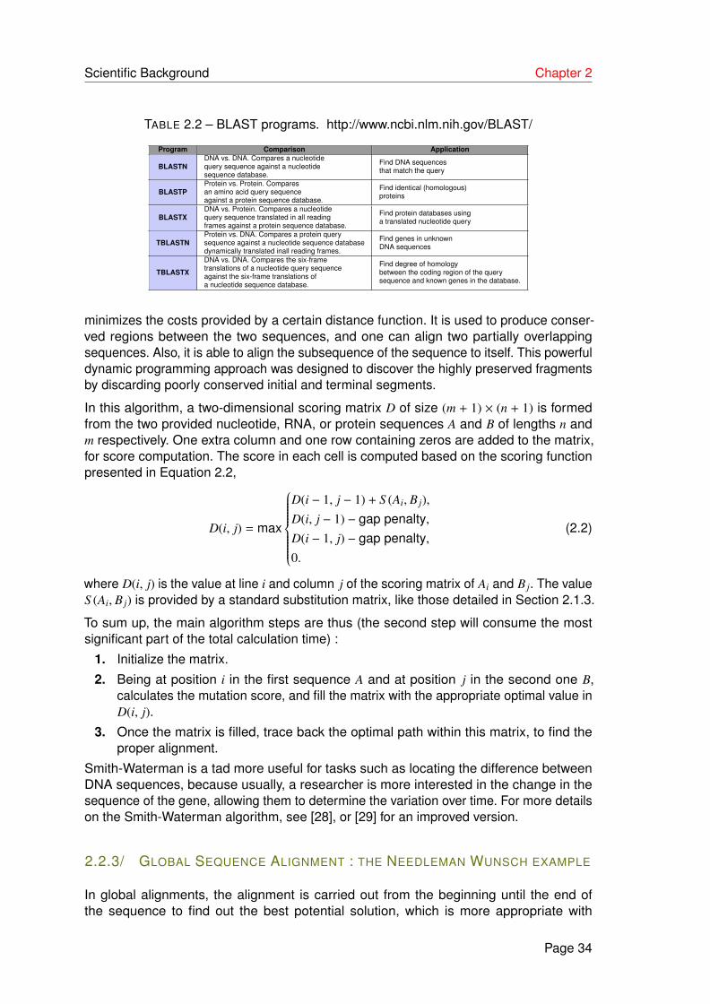
2.2 BLAST programs. http://www.ncbi.nlm.nih.gov/BLAST/ . . . . . . . . . . . 34
3.1 Results of genetic algorithm approach on various families. . . . . . . . . . . 46
3.2 Genomes information of Rosales species under consideration . . . . . . . . 48
3.3 Best tree in each swarm . . . . . . . . . . . . . . . . . . . . . . . . . . . . . 55
3.4 Best topologies obtained from the generated trees, b is the lowest bootstrapof the best tree having this topology, p is the number of considered genesto obtain this tree. . . . . . . . . . . . . . . . . . . . . . . . . . . . . . . . . 55
3.5 The CONSEL results regarding best trees . . . . . . . . . . . . . . . . . . . 57
3.6 Family number 1 (Pelargonium cotyledonis as outgroup). . . . . . . . . . . 64
3.7 Family number 2 (Chromera velia as outgroup). . . . . . . . . . . . . . . . . 66
3.8 Groups from BPSO version I. . . . . . . . . . . . . . . . . . . . . . . . . . . 72
3.9 Groups from PSO version II. . . . . . . . . . . . . . . . . . . . . . . . . . . . 72
3.10 PSO vs GA. . . . . . . . . . . . . . . . . . . . . . . . . . . . . . . . . . . . . 72
4.1 Information on chloroplast sizes at highest taxonomic level . . . . . . . . . 75
4.2 Example of genomes information of Streptophyta clade . . . . . . . . . . . 76
4.3 Summarized properties of the pan genomes at the highest taxonomic level. 77
4.4 Taxonomy in the second level . . . . . . . . . . . . . . . . . . . . . . . . . . 80
4.5 Example of comparison between pairwise genomes from various species,to investigate the changes that occurred within branches of the tree. . . . . 81
5.1 Genomes information of Apiales order. . . . . . . . . . . . . . . . . . . . . . 86
5.2 Gene duplicate for each genome in Apiales order. . . . . . . . . . . . . . . 91
5.3 Gene duplicate for each genome in Asterales order. . . . . . . . . . . . . . 97
5.4 The variation in comparison results of ancestral genomes nodes on Aste-rales order with MLGO. . . . . . . . . . . . . . . . . . . . . . . . . . . . . . 97
5.5 The variation in ancestral genomes nodes which were achieved by compa-ring our method results with MLGO tool on Fabids order. . . . . . . . . . . . 98
6.1 Information about some Mycobacterium genomes. . . . . . . . . . . . . . . 104
15

16 LIST OF TABLES
6.2 Number of alignment columns with polymorphism, by pair of strains, on M.canettii genomes. Note that, when a large string is deleted at some locationin the tree, all the characters of this deletion are counted here. . . . . . . . 107
6.3 Variations in the alignment of M. tuberculosis . . . . . . . . . . . . . . . . . 107
6.4 Number of SNPs in the considered species (100.X refers to an ancestralnode, as in the tree) . . . . . . . . . . . . . . . . . . . . . . . . . . . . . . . 107

ABBREVIATIONS
AlignSeqs Align a Set of Unaligned Sequences.
BLAST . . . Basic Local Alignment Search Tool.
BPSO . . . . Binary Particle Swarm Optimization.
BP . . . . . . . . Bootstrap Probability.
DOGMA . . Dual Organellar GenoMe Annotator.
DPSO . . . . distributed Particle Swarm Optimization.
DNA . . . . . . Deoxyribonucleic Acid.
EMBL . . . . European Molecular Biology Laboratory.
GA . . . . . . . Genetic Algorithm.
Gap . . . . . . Absence of a homologous character in either sequence could be a reason ofdeletion in the comparing sequence or an insertion in the sequence to which it iscompared to. In either case a gap is added and a value of -1 is added to the score.Gap indicated an arbitrary number of null characters (represented by dashes).
GSA . . . . . . Global Sequence Alignment.
GTR . . . . . . GTRGAMMA : GTR model of nucleotide substitution with the Γ model of rateheterogeneity. All model parameters are estimated by RAxML.
Indel . . . . . An insertion/deletion polymorphism, commonly abbreviated “indel,” is a typeof genetic variation in which a specific nucleotide sequence is present (insertion) orabsent (deletion).
JModelTest jModelTest is a tool to carry out statistical selection of best-fit models ofnucleotide substitution.
LSA . . . . . . Local Sequence Alignment.
LUCA . . . . Last Universal Common Ancestor.
MUSCLE . MUltiple Sequence Comparison by Log- Expectation.
MSA . . . . . . Multiple Sequence Alignment.
ML . . . . . . . Maximum Likelihood.
MP . . . . . . . Maximum Parsimony.
MTBC . . . . Mycobacterium tuberculosis complex.
MLGO . . . . Maximum Likelihood for Gene-Order analysis.
MLWD . . . . Maximum Likelihood on Whole-genome Data.
NCBI . . . . . National Center of Biotechnology Information.
NW . . . . . . . Needle-man Wunsch Alignment.
PHAST . . . Phylogenetic Analysis with Space/Time Models.
PSA . . . . . . Pairwise Sequence Alignment.
17

18 abbreviations
PSO . . . . . . Particle Swarm Optimization.
RAxML . . . Randomized Axelerated Maximum Likelihood.
RNA . . . . . . Ribonucleic acid.
rRNA . . . . . ribosomal RNA.
SW . . . . . . . Smith-Waterman Alignment.
T-COFFEE multiple sequence alignment that provides a dramatic improvement in ac-curacy with a modest sacrifice in speed as compared to the most commonly usedalternatives.
Topo . . . . . Topology.
TU . . . . . . . . Taxonomy Unit
tRNA . . . . . Transfer RNA.

IGENERAL INTRODUCTION
19

1GENERAL PRESENTATION
1.1/ INTRODUCTION
Why to reconstruct ancestral genomes ? From a fundamental point of view, studies ofcontemporary biological systems using, for example, approaches related to anatomy,biochemistry, physiology, and molecular biology are seriously limited by the absence of amechanism of evolution description that would explain their establishment, organization,and functioning. The long-term aim of possessing ancestral genomes is thus to establish abroad framework for studying evolution despite the cruel lack of historical data. To achievethis goal, many algorithmic developments are necessary to efficiently and systematicallyprocess the large volumes of available data following a rigorous methodology.
Genomics studies are a typical case of very large volume data investigations : they are ofvery high resolution (until nucleotide level) and very reliable (many genome sequencescontain less than one error every 10,000 bases), very abundant (100 sequenced euka-ryotic genomes for instance, and more than 1,000 prokaryotes), and centralized in publicdatabases. Genomes also provide fundamental entry points to the functional propertiesof organisms, such as the presence or absence of genes, the expansion or regressionof gene families, the topology of the cis-regulatory elements. In other words, it informsabout the likelihood of certain metabolic or developmental pathways that may exist inan organism, and the importance of functions specific to each species. Genomes thusrepresent the foundation on which many advances can be achieved, and accessing suchinformation in an ancestral genome provides a broad spectrum of these properties.
From a more practical point of view, given the astronomical amount of genomic datasupplied to the community, the pace of which is likely to accelerate further in the comingyears, it is critical to maintain a substantial degree of organization for distribution andpresentation of data. Ancestral genome reconstructions will allow the sequences andannotations of modern species to be linked naturally with those of ancestral species inthe direction of Evolution, following the phylogeny of species. The ancestral genomes willserve as single reference points for comparing descending genomes, which will greatlyfacilitate the identification of ancestral genomics properties, and therefore specific lineagegains or losses. Conversely, the results that will continue to be obtained with differentorganization models will enrich them in return. To sum up, ancestral genomes are part ofthe foundations that will help us decipher the different molecular components contributingto the evolution of species, and that have led to such a variety of species and biologicalsystems we can currently observe.
21

General Introduction Chapter 1
The aim of this thesis is to participate to the development of tools able to reconstructthe successive ancestors in several given lineages, thus providing a dynamic view of theevolution of genomes
1.2/ PRESENTATION OF THE PROBLEMS
Recently, many approaches have been developed to solve the ancestral reconstructionproblem [2, 3, 4, 5, 6], but either they are limited to the evolution of one given character(for instance, a particular nucleotide), or conversely they theoretically focus on large-scalenuclear genomes (several billions of nucleotides) facing multiple recombination events.Large-scale genomic evolution problem can’t be tackled with same approaches thanone-character methods : when considering the set of all possible recombinations onlarge genomes, the problem is indeed NP-hard. As far as we know, there is no directlyapplicable solution solving the evolution of large DNA sequences. Conversely, in this thesis,we focus on genomes that have a reasonable size and who faced a rational number ofrecombination like in the chloroplast case. Even if the problem becomes a priori tractablefor such cases, it however requires the design of ad hoc solutions, and various difficultiesremain to circumvent when dealing with such a specificity. For illustration purpose, thesolutions will be applied on mid-scale genomes of chloroplasts first, and then of bacteria,growing so bit by bit the complexity of the problem we consider.
Let us recall the importance of understanding well the evolution of such mid-scale genomes.Chloroplasts are one of the main organelles in the plant cell. They are considered to haveoriginated from cyanobacteria through endosymbiosis when an eukaryotic cell engulfeda photosynthesizing cyanobacterium, which further remained and became a permanentresident in the cell 1. The term of chloroplast comes from the combination of chloro andplastid : it is an organelle (found in plant cells) that contain the chlorophyll. Chloroplast hasindeed the ability to convert water, light energy, and carbon dioxide in chemical energy byusing carbon-fixation cycle [7]. As this conversion releases oxygen, chloroplasts originatedthe breathable air and represent a mid to long-term carbon storage medium. Consequently,exploring the evolutionary history of chloroplasts is thus of great interest and we proposeto investigate it by the mean of ancestral genomes reconstruction.
This reconstruction will be realized with the desire to explain how molecules have evolvedover time, and to validate (or not) that this way can present evidence of their cyanobacteriaorigin. This long-term objective necessitates numerous intermediate advanced methods.For instance, it requires the ability to apply the ancestral reconstruction on a well-supportedphylogenetic tree of a representative collection of chloroplastic genomes. Moreover, itnecessitates the ability to detect content evolution (modification of genomes like geneloss and gain) along this accurate tree. These two prerequisites (gene content evolution,accurate phylogeny inference) have already been investigated in the literature, as reportedbriefly in the next section.
1. cf. Wikipedia
Page 22
General Introduction Chapter 1
1.3/ STATE OF THE ART : A GENERAL OVERVIEW
There exist two main computational methods to handle gene order and to propose an-cestral genome architectures : rearrangement-based and homology-based methods. Therearrangement-based methods typically search for the set of ancestral gene orders that mi-nimizes the sum of rearrangement distances over all branches of the given phylogeny [3, 4].Homology-based methods are used to solve the small phylogeny problem that consistsof the ancestral gene orders reconstruction of a species tree at the internal nodes fromextant genomes. This process takes gene adjacency into account and handles them asbinary characters with present and absence states. In this way, by observing the geneorder as a set of adjacency genes, the aim is to discover which adjacency is contained inthe ancestral genomes [2, 8]. These methods offer a better understanding of the genomeevolution history and can further improve our knowledge of the mechanisms linking organicsequences to their functions. Despite this, ancestral genetic sequence reconstructionsuffers from several limits such as those involved in the regulation of genes (insertion,deletion, duplication). Along with the examination of molecular evolution, it relies on thevalidity of models and their fundamental hypothesis [9].
Accordingly, a critical component of ancestral reconstruction of genomes is the unders-tanding of the phylogenetic tree relations between the species being examined [10]. It iscrucial to identify the most suitable tree topology by using for instance bootstrap estima-tions in a maximum likelihood approach [11, 12]. Moreover, calculating the lengths of itsbranches is essential for a perfect reconstruction, as well as for evaluating the exactnessof that reconstruction through simulations [13]. The lengths are related to the number ofrecombination and mutations that are likely to occur between an ancestor and its childnodes. This is why any error in the inferred phylogenetic relation will have obvious dramaticeffects on the reconstructed ancestors.
So ancestral genome reconstruction (AGRC) can be described as an extension of phylo-genetic study of species of interest : it provides extra details than what is usually obtainedby a classical phylogenetic tree [11]. It may include information about ancestor speciessuch as their gene content, the organized of these genes in the genome, the nucleotidesequence itself, and so on [14]. Such information can help to understand better the evo-lutionary history of a set of organisms and through shed light on the genomic basis ofphenotypes [15]. The observation of species is described by the peak or last nodes of thetree (leaves) that are gradually correlated by branches to their common ancestor [16], whilenodes are represented by the branching points of the tree, which are usually designatedto as inner nodes or the ancestors [17].
The ancestral reconstruction problem is as old as the field of molecular evolution. Forinstance, over past decades, many methods were proposed to reconstruct phylogeniesfrom gene-order data. The prior algorithm has been established by Fitch [18] : Fitch’sparsimony algorithm first assumes a binary alphabet and is based on maximum parsimony(MP) patterns : it finds the labels to the internal nodes of a tree that reduce the numberof changes or modification along tree edges. The most modern methods for phylogenyreconstruction from genome rearrangements include GRAPPA [3] and MGR [4]. However,these approaches are limited to cases where gene content are similar or when only a fewdeletions are expected [5]. Among the most recent methods which are based on geneadjacency, InferCARsPro is comparatively faster, but often produces an excessive numberof chromosomes [2]. This problem is tackled by newer methods such as GapAdj [8], but it
Page 23

General Introduction Chapter 1
is achieved by sacrificing a significant part of accuracy. Recently was proposed a fasterand more accurate method called PMAG [5], which is a probabilistic framework method toinfer ancestral gene order, and which involves gene insertions and deletions in addition torearrangements. PMAG not only accurately infers ancestral genomes but also does anexcellent job in assembling adjacencies into logical gene order [6]. All the aforementionedapproaches, if we except PMAC, only deal with gene permutations, and they discard forinstance the possibility of gene duplication or deletion. There is so an obvious lack of toolsthat concretely deal with ancestral reconstruction of mid-scale genomes, which considerall possible recombination – and we propose to fill this gap.
1.4/ ORGANIZATION OF THE THESIS MANUSCRIPT
This current chapter is devoted to a general introduction of the thesis, providing theproblematics and a brief description of both thesis subject and objectives. The introductionaims to place the work presented here in a more general context and provides essentialdata necessary for nonspecialists to understand the scope and development of the analysispresented here. The second part proposes a brief state-of-the-art about phylogeneticreconstruction, with existing methods that are related to this work.
Chapter 2 introduces some notions of biology that are essential for understanding thevarious problems addressed during this thesis. It gives a brief overview on how a phyloge-netic tree can be generated from a set of DNA sequences, and some concepts regardingphylogenetic analysis and algorithms used for phylogenetic reconstruction. The conceptsof local and global alignments and the most common implementations are detailed in thischapter too. Multiple alignment algorithms are additionally given. It is moreover explainedwhy small divergences in given sequences may lead to a hard alignment problem. Toanalyze aligned sequences, we describe various phylogenetic concepts and terminologies.Methods for constructing phylogenetic trees are finally summarized (such as distance andcharacter based methods), together with bootstrap analysis.
Chapter 3 illustrates essential resources jointly introduced in an artificial intelligencealgorithm for phylogenetic tree reconstruction. In this chapter, we study first the relevanceof the Simulated Annealing (SA) algorithm to fulfill the optimization task. Then, variousmetaheuristics have been executed in a distributed manner using supercomputing facilities.Our proposal is based on genetic algorithm and a particle swarm optimization approachthat are developed in both linear and parallel fashions, in order to reconstruct a wellsupported phylogenetic tree while removing genes that blur the phylogenetic signal. Animproved simulated annealing method is finally added, and a comparison of 3 givenmetaheuristics on a large number of new groups of species is proposed.
Chapter 4 discusses other methods that are used in our ad-hoc algorithm to generateancestral genomes. Investigations of genomic recombination on campanulides chloro-plasts are further detailed, depending on all provided information obtained with previouslypresented tools in Chapter 3. Then, in Chapter 5, we describe the relations that canbe found between the phylogeny of a large set of 845 complete chloroplast genomes,and the evolution of gene content inside these sequences. Core and pan genomes havebeen computed on de novo annotations of these genomes, the former being used forproducing well-supported phylogenetic trees while the latter provides information regardingthe evolution of gene contents over time, and illustrates the specificity of some branches
Page 24

General Introduction Chapter 1
of the trees.
In Chapter 6, we propose to reconstruct all ancestors of all complete available genomesof Mycobacterium tuberculosis and M. canettii. Doing so allows us to consider completegenomes that are more complex than the chloroplasts. The study starts by investigatingthe single nucleotide polymorphism level, while insertions-deletions (indels) and largescale recombinations are regarded in a second stage. By mixing automatic reconstructionof obvious situations with human interventions on signaled problematic cases, we provethat it is possible to achieve a concrete, complete, and really accurate reconstruction oflineages of the Mycobacterium tuberculosis complex.
Finally, the conclusion of the manuscript provides a summary of researches that havebeen realized during this thesis. A discussion about possible future work in this area isproposed too, to open the debate and introduce putative further investigations.
1.5/ PUBLICATIONS
All the objectives of this thesis have been investigated, even though a lot of work still remainto be realized. These investigations have been validated by the following publications.
1.5.1/ PUBLICATIONS IN INTERNATIONAL CONFERENCES AND JOURNALS
1. CIBB 2015 Bassam Alkindy, Bashar Al-Nuaimi, Christophe Guyeux, Jean-FrançoisCouchot, Michel Salomon, Reem Alsrraj, and Laurent Philippe. "Binary ParticleSwarm Optimization Versus Hybrid Genetic Algorithm for Inferring Well SupportedPhylogenetic Trees". In Computational Intelligence Methods for Bioinformatics andBiostatistics : 12th International Meeting, CIBB 2015, Naples, Italy, September 10-12,2015, pp. 165-179, Springer International Publishing, 2015.
2. IJBBB 2017 Al-Nuaimi Bashar, Christophe Guyeux, Bassam AlKindy, Jean-FrançoisCouchot, and Michel Salomon. "Relation between Gene Content and Taxonomy inChloroplasts". in International Journal of Bioscience, Biochemistry and Bioinformatics(IJBBB) 2017 Vol.7(1) : 41-50 ISSN : 2010-3638.
3. IWBBIO 2017 Christophe Guyeux, Bashar Al-Nuaimi, Bassam Alkindy, Jean-François Couchot and Michel Salomon. "On the Ability to Reconstruct AncestralGenomes from Mycobacterium Genus”. In International Conference on Bioinforma-tics and Biomedical Engineering (IWBBIO 2017) pp. 642-658. Springer InternationalPublishing, Granada, Spain, April 26-28,2017.
4. JIB 2017 Bashar Al-Nuaimi, Roxane Mallouhi, Bassam AlKindy, Christophe Guyeux,Michel Salomon, and Jean-François Couchot. "Ancestral reconstruction and in-vestigations of genomic recombination on Campanulids chloroplasts". IntegrativeBioinformatics (JIB). Date of submission : 7th of November, 2016.
5. BMC 2017 Régis Garnier, Christophe Guyeux, Jean-François Couchot, Michel Sa-lomon, Bashar Al-Nuaimi and Bassam AlKindy. "Comparison of Metaheuristics toMeasure Gene Effects on Phylogenetic Supports and Topologies". Submitted toSpecial Issue on BMC Bioinformatics Supplement. Date of submission : 23th of May,2017.
Page 25

General Introduction Chapter 1
6. BMC 2017 Christophe Guyeux, Bashar Al-Nuaimi, Bassam Alkindy, Jean-FrançoisCouchot and Michel Salomon. "Investigating the ancestral reconstruction of bacterialgenomes”. Submitted to Special Issue on BMC Bioinformatics Supplement. Date ofsubmission : 22th of July, 2017.
1.5.2/ PUBLICATIONS IN NATIONAL SEMINARS AND WORKSHOPS
1. SeqBio’2015 Bashar Al-Nuaimi, Roxane Mallouhi, Bassam AlKindy, ChristopheGuyeux, Michel Salomon, and Jean-François Couchot. "Ancestral reconstruction andinvestigations of genomic recombination on Campanulides chloroplasts". Workshopof SeqBio 2015, Orsay, November 2015.
2. Femto-st’2015 Bassam Alkindy, Bashar Al-Nuaimi, Huda Al’Nayyef, Panisa Tree-pong, Christophe Guyeux, Jean-François Couchot, Michel Salomon, and JacquesBahi. "Bioinformatics Approaches on Genomic Evolution in Femto-ST (Core Genome,Phylogenetic Analysis, Transposable Elements, and Ancestral Reconstruction)".Workshop of Femto-ST, June 2015, Besancon, France. Note : Poster.
3. Femto-st’2016 Bashar Al-Nuaimi, Bassam Alkindy, Christophe Guyeux, Jean-François Couchot, and Michel Salomon. "Ancestral reconstruction and investigationsof genomic recombination on Campanulids chloroplasts and Mycobacterium Genus".Workshop of Femto-ST, August 2016, Besancon, France.
Page 26

IISCIENTIFIC BACKGROUND
27


2SCIENTIFIC BACKGROUND
In this chapter, we introduce some notions of biology which are sufficient for the unders-tanding of problems addressed in this thesis. Indeed, the challenges of reconstructing
chromosomal rearrangements and ancestral genomes requires to know the structure ofgenomes. Obviously, phylogenetic tree reconstruction is a first step in the understanding ofthe ancestral relationship among a set of biological sequences. It includes the constructionof a tree, where the nodes indicate separate evolutionary paths, and the branch lengthsgive an approximation of how distant the sequences represented by those branches are.Additionally, in this chapter, we will present various sequence alignment algorithms, whichare a fundamental step in molecular phylogenetics to explain the evolution of speciation,quantification of substitution patterns and gene duplication events, but also a useful tool foridentifying mutations leading to genetic diseases. This chapter covers the pairwise globaland local alignments by dynamic programming with various scoring schemes, multiplesequence alignments that are reduced to pair-wise alignment, and profile alignment byusing a guide tree. This chapter presents also a brief information on how a phylogenetictree can be constructed from a set of DNA sequences, and how to evaluate the generatedtree. Finally, some concepts concerning phylogenetic analysis and algorithms used forphylogenetic reconstruction will be reported. Note that the state-of-the-art part related tomultiple sequence alignment and their use for phylogenetic analysis has been studied incommon with my colleague Panisa Treepong, and written "four hands" as our investigationsin this field have been performed together, in team.
2.1/ CHROMOSOMES AND GENOMES
2.1.1/ A SHORT OVERVIEW
Genomes contain the complete genetic material of an individual or a species, encoded inits DNA, except certain viruses whose genome is carried by RNA molecules. From oneorganism to another, the genome organization may differ. It can be composed of one ormore DNA molecules, which will have a significant impact on the complexity of the problemof reconstructing chromosomal rearrangements and ancestral genomes. In prokaryotes(bacteria and archaea), the genome is located in the cytoplasm of the cells, which isusually contained in a circular DNA molecule. However, there are many exceptions : somespecies may have several circular chromosomes, or a single linear chromosome, or alinear chromosome and a circular one [19]. There may also be an extra-chromosomalcomponent contained in plasmids and episomes.
29

Scientific Background Chapter 2
In eukaryotes, we can distinguish the following :
1. Nuclear DNA composed of several linear chromosomes, contained in the nucleus ofthe cells (an element which indeed characterizes eukaryotic cells).
2. Non-nuclear DNA, contained in organelles, i.e., the chloroplastic chromosome contai-ned in the chloroplasts of photosynthetic organisms (algae and plants), or themitochondrial chromosome contained in mitochondria of all the other eukaryotes.
In eukaryotes, linear chromosomes are characterized by a centromere and two telomeresin most organisms. The centromere shares the chromosome in two arms (left and right)and is essential for the smooth unfolding of the cell divisions. The telomeres are the twoends of a chromosome [20]. The number of chromosomes contained in the cell of anorganism varies according to the considered species 1. The size of the genome is mainlymeasured according to its number of nucleotides, or bases (in bp for base pair, sincethe majority of the genomes is made up of double strands of DNA). Multiples are alsoused, like kb for kilobase or Mb (megabase), which are respectively equal to 1,000 and1,000,000 bases. Note that the size of a genome may vary from a few kb in viruses toseveral hundreds of thousands of Mb in some eukaryotes, as shown in Table 2.1.
The quantity of DNA is not proportional to the complexity of an organism. Some ferns, forexample, have genomes more than ten times larger than the human one [21, 7, 22].
TABLE 2.1 – Some examples of genome varieties
Species Kingdom Genomes size Number of genesMycobacterium tuberculosis Bacteria 4.41Mb 4,008
Brucella abortus(chromosome 2)Brucella abortus(chromosome 1) Bacteria
2,12 Mb1,16 Mb
22001156
Actinidia chinensis Plantae 616.1 Mb 39,040Takifugu rubripes Animalia 390 Mb 22–29,000
Plasmodium falciparum Alveolata 22.9 Mb 5,268Drosophila melanogaster Animalia 122.6 Mb 17,000
Homo sapiens Animalia 3.2 Gb 18,826
2.1.2/ GENOME AND DNA MUTATIONS
The cell is the ‘building block’ of life. It mainly performs functions for maintaining daily lifeand passing the genetic instructions to the next generation. The former function is particu-larly facilitated by proteins whereas the latter is mainly achieved through Deoxyribonucleicacids (DNA).
DNA is a polymer, where its monomer units are nucleotides. Each nucleotide in a DNAhas three parts : a pentose sugar (desoxyribose), a phosphate, and one “base”. Indeed,nucleotides can be classified into four types corresponding to their distinct bases : Adenine(A), Cytosine (C), Guanine (G), and Thymine (T). A and G are called purines, havinga two-ring structure, while C and T are called pyrimidines and they conversely have a
1. For example, man has 23 pairs of linear chromosomes whereas Escherichia coli, an intestinal bacterium,has only one circular chromosome.
Page 30

Scientific Background Chapter 2
one-ring structure (see Figure 2.1). For the sake of concision, DNA is simply representedas a sequence over the alphabet (A, C, G, T).
During organism evolution, its DNA is replicated and passed on to its offspring. And throughDNA replication, changes can occur in the sequence, which is referred as mutation. Thesevariations in the DNA sequences occur at the base level, as depicted in Figure 2.2. Thesemodifications change the characteristics of the generations and eventually, may leadto the production of new species. This evolutionary manner of DNA mutations can berepresented, in a certain way, by a phylogenetic tree, introduced later in this chapter.
DNA Double Helix
Fig. 2.1 – DNA has a double-helix shape. Bases are found in pairs inside the doublehelix. The bases in DNA are named A, T, G, and C. Pyrimidine T ( resp. C) forms pairswith purine A (resp. G), and vice versa, https://www.slideshare.net/AmyHollingsworth/lab5dnaextractionfromstrawberriesandliverfall2014.
Fig. 2.2 – A mutation occurs when a DNA sequence is damaged or changed, which mayfor instance alter the genetic message carried by a gene.
These genomic mutations are now easily accessible via modern sequencing technologies,making it possible to discover single nucleotide polymorphisms 2, short insertions anddeletions (INDELs) as well as other genomic mutations like duplication and inversions.
2.1.3/ MODEL OF NUCLEOTIDE SUBSTITUTION
As previously stated, over time, nucleotide sequences can “evolve” through substitution.This process can cause a nucleotide (A, C, T or G) to change into another nucleotide,and this is one of the most central driving force behind evolution. This modification in aDNA sequence may lead to an inactivation of a gene or to a mutation in the protein that
2. Let us recall that a single nucleotide polymorphism, usually abbreviated to SNP, is a mutation in asingle nucleotide (A, T, C, or G) that occurs at a particular position in the genome, as shown in Figure 2.3.Each mutation is present to some appreciable degree within a population. Each organism has several singlenucleotide polymorphisms that together create a unique DNA pattern for that.
Page 31

Scientific Background Chapter 2
Fig. 2.3 – Single Nucleotide Polymorphism (SNP).
the sequence codes. As proteins are the building blocks of organic life, this may causesignificant variations in an organism’s characteristics. Alternatively, this modification mayhave no effect at all, being silent.
Commonly, this type of mutation can take place once or twice each million years on agiven sequence location. Estimating the evolution of organisms over hundreds of millionsof years, models of nucleotide evolution are helpful in speculating how one sequenceof nucleotides may have evolved from another. These models can be inferred by eitherassuming that two given sequences had shared a common DNA ancestor or by assumingthat one sequence evolved into the other.
At the simplest level, the proportion can be used for defining such a matrix P of nucleotidesubstitution :
Pd =nd
n(2.1)
where n indicates the total number of nucleotides in the sequence, and nd is the numberof base d, d = {A,C,G,T }. Other richer probabilistic models have been proposed in theliterature, to provide a more accurate estimation of the mutation matrix P, like Jukes andCantor [23], Kimura [24], and Tamura and Nei [25].
2.2/ SEQUENCE ALIGNMENT
One of the principal problems in computational molecular biology is sequence alignment.A sequence alignment is a process of aligning blocks of provided sequences (of DNA,RNA, or protein) to recognize similar regions – that may be a consequence of functionalor evolutionary relationships between the sequences. Aligned sequences of amino acidsor nucleotides are reproduced as rows within a matrix. Gaps are inserted between thedeposits so that residues with identical or similar sequences are arranged in successivecolumns.
Let us for instance consider two sequences which are homogeneous except that thefirst sequence contains one other residue (e.g., a given nucleotide). When we view thealignment of these two sequences, the other residue will be matched to a gap. Thiscorresponds to an insertion event in the first sequence or a deletion event in the second.On the other hand, if we note that an insertion event has occurred in the first sequence(concerning the second) then we know how to match that residue to a gap in the second.
Page 32

Scientific Background Chapter 2
Thus one way to build a sequence alignment is to find a series of insertions, deletions,or replacements collectively called mutation events, which will transform one sequenceinto the other. The number of mutation events needed to transform one sequence into theother is called the edit distance.
Indeed, in sequence alignment, there are two broad categories, namely the local and theglobal one. A local alignment returns the best matching subsequence, while in a globalalignment, we obtain the best match of both sequences in their totality. Local sequencealignments intend to reveal similar regions in a given pair of sequences. In other words,they find an optimal local alignment by searching for two segments with maximum similarityscore by discarding weak initial and terminal fragments, see. Figure 2.4 for an illustrativeexample.
Many algorithms have been developed for these two kinds of alignments, some of the mostpopular ones being summarized in the next subsections.
Fig. 2.4 – Global alignments are applied for comparing homologous genes whereas localalignment can be used to locate homologous regions in otherwise non-homologous genes.
2.2.1/ BLAST
Basic Local Alignment Search Tool (BLAST) is a database sequence search engine pro-posed by the National Center for Biotechnology Information (NCBI). The first version ofBLAST was published in 1990 and it supported only ungapped searches. The secondversion, releazed in 1997 [26], has been designed to determine high-scoring local ali-gnments between sequences, without discrediting the speed of such searches. BLASTaddresses thus an essential problem in bioinformatics research. It uses a heuristic processthat attempts local as crossed to global alignments and, therefore, it is suitable to identifyrelationships between sequences (amino-acid sequences of proteins or the nucleotides ofDNA sequences) which share only isolated regions of similarity [27].
Table 2.2 displays the different BLAST programs available on the NCBI web server.
2.2.2/ LOCAL SEQUENCE ALIGNMENT : SMITH–WATERMAN ALGORITHM
The Smith-Waterman algorithm was developed by Temple F. Smith and Michael S. Wa-terman in 1981 [28]. Using a dynamic programming approach, it is able to provide theoptimal local alignment between two strings. The algorithm estimates the alignment that
Page 33
Scientific Background Chapter 2
TABLE 2.2 – BLAST programs. http://www.ncbi.nlm.nih.gov/BLAST/
Program Comparison Application
BLASTNDNA vs. DNA. Compares a nucleotidequery sequence against a nucleotidesequence database.
Find DNA sequencesthat match the query
BLASTPProtein vs. Protein. Comparesan amino acid query sequenceagainst a protein sequence database.
Find identical (homologous)proteins
BLASTXDNA vs. Protein. Compares a nucleotidequery sequence translated in all readingframes against a protein sequence database.
Find protein databases usinga translated nucleotide query
TBLASTNProtein vs. DNA. Compares a protein querysequence against a nucleotide sequence databasedynamically translated inall reading frames.
Find genes in unknownDNA sequences
TBLASTX
DNA vs. DNA. Compares the six-frametranslations of a nucleotide query sequenceagainst the six-frame translations ofa nucleotide sequence database.
Find degree of homologybetween the coding region of the querysequence and known genes in the database.
minimizes the costs provided by a certain distance function. It is used to produce conser-ved regions between the two sequences, and one can align two partially overlappingsequences. Also, it is able to align the subsequence of the sequence to itself. This powerfuldynamic programming approach was designed to discover the highly preserved fragmentsby discarding poorly conserved initial and terminal segments.
In this algorithm, a two-dimensional scoring matrix D of size (m + 1) × (n + 1) is formedfrom the two provided nucleotide, RNA, or protein sequences A and B of lengths n andm respectively. One extra column and one row containing zeros are added to the matrix,for score computation. The score in each cell is computed based on the scoring functionpresented in Equation 2.2,
D(i, j) = max
D(i − 1, j − 1) + S (Ai, B j),D(i, j − 1) − gap penalty,D(i − 1, j) − gap penalty,0.
(2.2)
where D(i, j) is the value at line i and column j of the scoring matrix of Ai and B j. The valueS (Ai, B j) is provided by a standard substitution matrix, like those detailed in Section 2.1.3.
To sum up, the main algorithm steps are thus (the second step will consume the mostsignificant part of the total calculation time) :
1. Initialize the matrix.
2. Being at position i in the first sequence A and at position j in the second one B,calculates the mutation score, and fill the matrix with the appropriate optimal value inD(i, j).
3. Once the matrix is filled, trace back the optimal path within this matrix, to find theproper alignment.
Smith-Waterman is a tad more useful for tasks such as locating the difference betweenDNA sequences, because usually, a researcher is more interested in the change in thesequence of the gene, allowing them to determine the variation over time. For more detailson the Smith-Waterman algorithm, see [28], or [29] for an improved version.
2.2.3/ GLOBAL SEQUENCE ALIGNMENT : THE NEEDLEMAN WUNSCH EXAMPLE
In global alignments, the alignment is carried out from the beginning until the end ofthe sequence to find out the best potential solution, which is more appropriate with
Page 34

Scientific Background Chapter 2
closely related sequences that have approximately the same length. S.A.Needleman andC.D.Wunsch [30] have developed the first method of this category, naturally called theNeedleman-Wunsch algorithm. The objective of this latter is to maximize the number ofmatches between the sequences along the entire length of the sequences. The originalNeedleman-Wunsch algorithm computes the minimal edit distance of two sequences undera very general scoring scheme, taking O(n3) time and O(n2) space.
This algorithm is constituted by the following steps, similar to the Smith-Waterman ones :
— Initialization : A two-dimensional matrix D must be firstly initialized. The row vectorrepresents the first sequence A, while the column one corresponds to the secondsequence B.
— Matrix scoring : We fill the matrix D in the same manner than in Smith-Waterman.D(i, j) is computed recursively according to a dynamic programming approach. IfS (i, j) is the substitution score for residues Ai and B j and g is the gap penalty, thenwe have :
D(i, j) = max
D(i − 1, j − 1) + S (Ai, B j) match Ai with B j
D(i − 1, j) − g(insertion in A)D(i, j − 1) − g(insertion in B)
(2.3)
— Traceback and alignment : Tracing back process starts from the lowest rightposition in the scoring matrix. We then follow the maximum scores until reaching theupper left position. The path drawn in this matrix is considered to correspond to themost optimal global alignment for the two given sequences.
The main differences between Needleman-Wunsch and Smith-Waterman algorithms are :
— The zero condition : in Smith-Waterman, we insert a 0 in the cell i, j if Di, j is negative,which is not the case in the Needleman-Wunsch case.
— Sequences in scoring matrix are ordered in an opposite direction.
2.2.4/ MULTIPLE SEQUENCE ALIGNMENT (MSA)
Multiple sequence alignment is an expansion of pairwise alignment to combine more thantwo sequences at a time. They are implemented to identify conserved regions among aset of sequences, evaluating by doing so if they are evolutionarily related. Alignments arealso used to help in building evolutionary relationships on phylogenetic trees construction,as described in the next section.
The goal of MSA is to align all of the sequences in a given set if possible. A MSA is thus acollection of three or more nucleotide or amino acid sequences that are aligned partiallyor entirely. Identical residues are aligned in columns across the length of the sequences.These aligned residues are homologous in a fundamental sense or even in an evolutionarysense : they are probably derived from a common ancestor.
Figure 2.5 is an example of the result of MSA applied on Apiales order. However, as soonas the sequences exhibit some divergence, the problem of multiple alignments becomesextraordinarily difficult to solve. And if exact approaches produce optimal alignments, theyare not feasible in time or space for more than a few sequences. Let us finally notice that
Page 35

Scientific Background Chapter 2
the alignment accuracy can be hard to estimate and their actual biological significancecan be ambiguous.
In practice, a very popular progressive sequence alignment tool is the Clustal family [31],in particular the weighted variant ClustalW that is incorporated in many web tools likeGenomeNet 3 or EBI 4. Another important progressive alignment approach is called T-Coffee [32], which operates as a post processing on various MSAs of the same set ofsequences that are provided by other existing methods like Clustal. Due to its principleof conception, T-Coffee is slower than Clustal and its derivatives but, in general, it yieldsmore accurate alignments for distantly related sequence sets.
Fig. 2.5 – Multiple sequence alignment of various sequences of Apiales order.
2.3/ ABOUT PHYLOGENETIC TREES
An evolutionary or phylogenetic tree is an acyclic graph (or branching diagram, seeFigure 2.6) that is used to emphasize evolutionary relationships among groups of biologicalspecies, that is, their phylogeny based upon similarities and variations in their geneticor physical characteristics. The nodes are connected in the tree by branches. The latterhighlight the relationship between taxonomic units (TU) at the leaves of the tree andtheir ancestors, corresponding to the internal nodes of the graph. Each branch has alength that represents, for example, the number of expected mutations per site (in amino-acids or nucleotide sequences) that have probably happened in these branches, in asequence based phylogeny. Thus, branch lengths provide the time of variation betweentwo organisms and their common ancestor. There are basically two kinds of phylogenetictrees :
— The unrooted Phylogenetic Trees : evaluate the relationships between all thegiven TUs. However, they usually do not provide sufficient information to deduce theevolution from the last common ancestors.
— The rooted Phylogenetic Trees : embed a root node that represents the lastcommon ancestor of all TUs in the tree. The main way to root a tree is to specify anoutgroup, which is a TU known to be outside the group of TUs under consideration.This latter can be a species known to have diverged before the divergence of theconsidered TUs.It can be noticed that the time of evolution of a rooted species represented bya rooted phylogenetic tree can be computed from each sub-ancestor to the lastcommon one when either the date of divergence or the divergence rate are known.Until now, however, this question is still an intensive subject of research.
3. http://align.genome.jp/4. http://www.ebi.ac.uk/clustalw
Page 36

Scientific Background Chapter 2
Fig. 2.6 – Example of a phylogenetic tree structure.
2.4/ PHYLOGENY CONSTRUCTION METHODS
The most known and commonly used methods of tree construction can be classified intotwo central divisions : distance-based and character-based methods.
Distance-based methods begin by transforming the original data into a matrix of pairwisedistance values. The next stage is to infer a tree either by sequential joining approaches,or by estimating a set of candidate trees and applying a type of optimality criteriontechnique to select the best one. Under the minimum evolution criterion, the tree thathas a minimum sum of branch lengths is selected as the best estimate. Distance-basedalgorithms encompass UPGMA and Neighbor-Joining, this latter being explained in thenext subsection.
Character-based methods can depend on a divergence of phylogenetic characters suchas genetic and molecular attributes to construct phylogenetic trees. As long as that thereis divergence among taxa in the characteristic and that the characteristic is heritable,it could probably be accepted as a phylogenetic character. In this context, molecularphylogenetics, attempt to estimate the modification rates and patterns occurring in thesequences (protein, DNA, or RNA) and to reconstruct the evolutionary history of organismsusing such characters.
Algorithms used to create phylogenetic trees using characters are more complicated thandistance-based methods [33]. The algorithms are based on an optimization criterion suchas Maximum Likelihood, Maximum Parsimony, or Bayesian methods in order to find thebest tree according to the considered characters. For the sake of illustrations, we will detailsuch methods at the end of this chapter.
2.4.1/ NEIGHBOR-JOINING ALGORITHM
As previously said, the neighbor-joining algorithm constructs unrooted phylogenetic treesusing distance methods. Both topology and branch lengths are computed by iterativelyspecifying (based on a distance matrix) a neighbor as a pair of TUs that are joined in asingle internal node X in an unrooted tree, depending on the previously computed distance
Page 37

Scientific Background Chapter 2
matrix. An iteration of the neighbor-joining algorithm consists of the following steps :
1. Construct an unresolved tree with all TUs in a starlike structure with no hierarchy.
2. Construct a distance matrix by pairwise comparison and calculate the value of branchlengths, to identify the two most related sequences (TUs) : NJ seeks to build a treewhich minimizes the sum of all branch lengths.
3. Determine which TUs are connected to an internal node X. They are treated now asone TU.
4. Join the closest neighbors (TUs with similar characters), the base pair that has thesmallest sum-of-branch-lengths.
5. The algorithm is repeated until the topology of the tree is obtained.
The neighbor-joining method produces an unrooted tree. The sum of the branch lengthsof N TUs in the tree is calculated as follows. Let us define Di j and LAB as the distancebetween TUs i and j and the branch length between nodes a and b respectively. The sumof branch lengths of the tree is defined based on the following formula :
S =
N∑i=1
LiX =1
N − 1
∑i< j
Di j/
The distance between nodes X and Y is calculated as follows :
LXY =1
2(N − 2)
N∑k=3
(D1k + D2k) − (N − 2)(L1X + L2X) − 2N∑
i=3
LiY
The term inside the brackets is the sum of all distances including LXY , and the outer term
12(N−2) is to eliminate unrelated branch lengths.
Neighbor-joining [34] is a method which is especially suited for datasets comprisinglineages with broadly varying rates of evolution. It can be used in combination withtechniques that allow correction for superimposed substitutions.
2.4.2/ MAXIMUM PARSIMONY
The Maximum parsimony method [35] aims at minimizing branch lengths by reducingthe number of mutations. This approach predicts the evolutionary tree that minimizesthe number of actions needed to generate the marked variation in the sequences fromcommon ancestral sequences. In a maximum parsimony phylogenetic study, the besttree is specified as the tree with the lowest branch lengths. More precisely, for givensequences, a MSA algorithm is used to align the sequences, and to identify the informativepositions, that is, columns in the multiple sequence alignment with no gap and at least twocharacters.
The next step is to count the number of changes and assign this cost to each generatedphylogenetic tree. The method then computes the total length L for each tree, which iscalculated according to the following formula :
L =
C∑j=1
w jl j
Page 38
Scientific Background Chapter 2
where l j is the cost for character j, C is the total number of characters, and wi is theassigned weight for each character, which is set to 1 in most cases. The tree that maximizesthis L value is finally selected.
2.4.3/ BAYESIAN METHODS
For the sake of completeness, we evoke here the well-known and frequently used Bayesianmethods [36], which estimate the phylogeny by calculating the conditional probability giventhe model, based on the following formula :
Pr[Tree|Data] =Pr[Data|Tree] × Pr[Tree]
Pr[Data]
where Pr[Tree|Data] is called a posterior probability distribution 5.
Bayesian methods can thus apply a model of sequence evolution and are ideal for buildinga phylogeny using sequence data.
2.4.4/ MAXIMUM LIKELIHOOD
The Maximum Likelihood (ML) criteria requires a probabilistic model for the evolutionaryprocess and finds the most likely tree, given the probabilistic model and the knownsequences at the leaves. In other words, ML techniques are used to determine thetopology and branch lengths that have the largest likelihood to produce the aligned data,providing the substitution model and the tree. The likelihood value is computed after thealignment stage and by considering some DNA or amino acids substitution models.
In ML method, the searching space is fulfill using a quartet program. This latter finds allpossible sequence combinations for tree reconstruction, while the Maximum Parsimonycriteria prefers solutions that minimize the number of mutations along the tree edges [37].Bayesian methods and Maximum likelihood can apply a model of sequence evolution andare ideal to construct a phylogeny using data sequences. The main drawback of thesemethods is that they are computationally expensive. However, with today’s computers, thisis not too much a problem.
One of the most common tests used to evaluate the reliability of a deduced tree is the so-called Felsenstein’s bootstrap test [38], which is usually estimated using Efron’s bootstrapresampling technique [39]. It is accomplished in practice by sampling the input data [40]and measuring the proportion of deduced trees that support each branch of the best treepreviously obtained. As a global rule, if the bootstrap value for a given internal branch is95% or higher, the topology will be considered "valid" at that branch 6.
2.4.5/ ANCESTRAL GENOME RECONSTRUCTION
Ancestral reconstruction may focus at sequence level or at gene order level, the formerbeing quite resolved [41, 8, 42, 43, 6, 13, 10, 44, 45], at least if we do not consider
5. A posterior probability is the probability that the tree is considered to be correct, if it has the maximumprobability.
6. In Bayesian approaches, this is the posterior probability itself that gives an evaluation of robustness :the support of a branch increases with its probability.
Page 39
Scientific Background Chapter 2
indels and mutation neighborhood, while the latter is more difficult in general, due to itscombinatorial complexity. More precisely, given an alignment of DNA sequences and atree, ancestral nucleotides of extant species can be obtained by modeling the evolutionof a trait through time as a stochastic process (Markov chain). Using it as the basis forstatistical inference, both maximum likelihood or Bayesian inference approaches can beapplied to estimate ancestral configuration.
Well known software like RAxML [46], BEAST2 [47], or PAML [48] can be used for suchreconstructions. However, most of the time, like in the R package [49], indels are notconsidered in such ancestral state reconstruction, even if researches have recently beenrealized via the so-called “Poisson Indel Process” [50]. Such process is a significantimprovement, if we compare it with the parsimony approach that can be found in PHASTsoftware, or with the Thorne-Kishino-Felsenstein model of indel evolution. Large scalemodifications, for its part, is most of the time regarded in a combinatorial frameworkby modeling genomes as permutations of genes or homologous regions. Indeed, thisgenome rearrangement problem [51] is usually formulated as follows : “given two genomes(permutations) and a set of allowable operations (like inversion, deletion, or transposition),what is the shortest sequence of operations that will transform one genome into the other ?”.As stated previously, even in the case of three genomes, such a problem is NP-hard [52],although it has received much attention in mathematics and computer science [53].
Page 40

IIICONTRIBUTIONS
41


3COMPARISON OF METAHEURISTICS TO
MEASURE GENE EFFECTS ONPHYLOGENETIC SUPPORTS AND
TOPOLOGIES
A huge and continuous increase in the number of completely sequenced chloroplastgenomes, available for evolutionary and functional studies in plants, has been observed
during the past years. Consequently, it appears possible to build large-scale phylogenetictrees of plant species. However, building such a tree that is well-supported can be adifficult task, even when a subset of close plant species is considered. Usually, the difficultyraises from a few core genes disturbing the phylogenetic information, due for example tohomoplasy problems. Fortunately, a reliable phylogenetic tree can be obtained once theseproblematic genes are identified and removed from the analysis. Therefore, in this chapterwe address the problem of finding the largest subset of core genomes which allows tobuild the best supported tree. As an exhaustive study of all core genes combination isredhibitory, since the combinatorics of the situation made it computationally infeasible,we investigate three well-known metaheuristics to solve this optimization problem. Moreprecisely, we design and compare distributed approaches using genetic algorithm, particleswarm optimization, and simulated annealing. The last approach is a new contribution andtherefore described in details, whereas the two former ones have been already studiedin a previous PhD/thesis. They have been designed de novo in a new platform, and newexperiments have been achieved on a larger set of chloroplasts, to compare togetherthese three metaheuristics. Finally, the ways genes affect both tree topology and supportsare assessed using statistical tools like Lasso or dummy logistic regression, in an hybridapproach of the genetic algorithm. This chapter is the concatenation of a previous workpublished in 2015 [54] with Bassam Al Kindy, a former PhD student at the University ofFranche-Comté.
3.1/ INTRODUCTION
These last years, the investigation of the evolutionary relationship between different plantshas benefited from the multiplication of newly available chloroplast sequences. Indeed,thanks to the tools presented in the previous chapter of this thesis, it is possible to process
43

Comparison of Metaheuristics to Measure Gene Effects on Phylogenetic Supports andTopologies Chapter 3
these sequences in order to build a phylogenetic tree that accurately characterizes theevolutionary lineages among the chloroplasts. Efficient coding sequence prediction andannotation tools have been developed to deal specifically with chloroplasts, for exampleDOGMA [55], and as can already been explained, there is also a great choice for thealignment of sequences. Moreover, given a set of sequences or characters, many well-established bioinformatics programs based on Bayesian inference or maximum likelihood,like BEAST or RAxML [46], can be used to reconstruct a phylogenetic tree. The objective isto obtain the most reliable and robust phylogeny, for instance in order to perform ancestralanalysis with a high confidence level. As stated previously, several methods can be usedto estimate the robustness of the produced tree, the most widely used are the bootstrapand the decay (or Bremer) analyses.
Obviously, a first condition to be able to build a phylogenetic tree for a given set of closeplant species is to identify as precisely as possible the corresponding core genome (theset of genes in common). However, even if the core genome is large and accurate, theresulting phylogeny is not necessarily well-supported. In fact, the core genome genesare not constrained through evolution in a similar way. On the one hand some evolveunder strong evolutionary constraints and thus reflect the story of the species while, onthe other hand, other genes evolve more freely due to a lower role in the survival andadaptability of a species. The latter tell their own history and thus disturb the phylogeneticinformation. Furthermore, the way the robustness and accuracy of the obtained phyloge-netic tree are altered by the amount of used data for the reconstruction process is notcompleted understood. Nevertheless, if we consider a set of species reduced to lists ofgene sequences, an obvious dependence between the chosen subset of sequences andthe obtained tree (topology, branch length, and/or robustness) can be observed. Thisdependence is usually regarded by the mean of gene trees merged in a phylogeneticnetwork. In fact, phylogenetic networks are necessary to represent events like horizontalgene transfers, but statistical methods to infer such networks are still limited and underdevelopment.
In this chapter, we consider the situation from a dual point of view, that consists instarting with the complete core genome and then to remove the genes responsible forinconsistent phylogenetic signal. In other words, the objective is to find the largest part ofthe core genome that produces a phylogenetic tree as supported as possible, and whichtherefore gives the fairest view of the relationships between most of the sequences underconsideration. Searching the problematic genes by exhaustively testing the combinationsof core genome genes is nonsense due their huge number. Therefore, to speed up thefinding of a satisfactory combination we rather consider metaheuristics. The first one,introduced in a previous work [1], is an ad hoc Genetic Algorithm (GA) which in somecases is not able to converge towards a suitable solution. Next, a Binary Particle SwarmOptimization (PSO) approach has been published in the the CIBB proceedings book [56].Finally, in this chapter, which extends and improves the two former ones, we study therelevance of the Simulated Annealing (SA) algorithm to fulfill the optimization task. Alsonotice that the different metaheuristics have been executed in a distributed manner usingsupercomputing facilities. To sum up, the contribution of this chapter is threefold : first, itproposes a new simulated annealing approach, second a new version of the PSO, andthird a comparison of the three metaheuristics on a large number of new groups of species.
Page 44

Comparison of Metaheuristics to Measure Gene Effects on Phylogenetic Supports andTopologies Chapter 3
3.2/ PRESENTATION OF THE PROBLEM
Let us introduce the problem of determining a phylogeny (evolution tree) for a given setof species by considering a set of chloroplast genomes that have been annotated usingDOGMA [55] (the approach we applied is detailed in Section 3.6). To start we need topick one or several genes on which the phylogeny will be based. Therefore we use therestricted core genome [57, 58], which consists of conserved genes present everywhere,whose size is larger than one hundred genes when the species are close enough. Thenmultiple sequence alignments are performed using muscle [59] and finally a phylogenetictree is inferred thanks to the maximum-likelihood tree builder RAxML [46].
The relevance of the obtained tree is then assessed by its bootstrap values : if these onesare all above 95 the tree is well-supported. In this case we can reasonably estimate thatthe phylogeny of these species is solved. Bootstrapping is a random sampling techniquecommonly used to estimate the significance of branches of a phylogenetic tree. It consiststo randomly select columns in the aligned DNA core sequences to be neglected duringthe tree building process and to check whether the same nodes are recovered. A largenumber of bootstrap repetitions, usually between 50 and 1000, are used to assess thetree reliability. As an illustration, a node which appears 95 times out of 100 by dropping acolumn means that the node is well-supported. Conversely, a low support value claimsthat a reduced part of the alignment supports the node, since by removing columns thenode is reconstructed in different ways.
When such a well-supported tree is not built, but rather a tree having some branchesexhibiting low supports, some genes of the core genome can be responsible of this lack ofsupport. The objective is then to identify the most supported tree using the largest subsetof core genes, a typical optimization problem. Obviously, the optimization problem we facecannot be solved by a brute force approach checking all possible combination of genes,due to the resulting combinatorial explosion. Indeed, for a core genome of n genes therewould be 2n trees to infer and that is clearly intractable in practice. To overcome such acombinatorial situation, a typical choice is to use a metaheuristic method.
In [1], we have first investigated the mixing of a genetic algorithm with Lasso tests to findproblematic genes. Unfortunately, thorough and careful experimental investigations haveled to results, recalled in Table 3.1, showing that this proposal is not able to predict thephylogeny of some particular plant orders. As can be seen, the lowest bootstrap value (orbootstrap score) obtained for 15 group of species is below 95 (column b in the table). Therelevance of binary particle swarm optimization to find the largest subset of core genes hasbeen studied in [56], producing slightly better bootstrap scores than GA with Lasso tests.In this chapter we introduce a third well-known metaheuristic method, namely simulatedannealing, and we compare the three approaches considering new sets of species. Likethe two former ones, the computations with SA algorithm will be done in a distributedmanner. Multiple algorithm instances will be launched using a same cooling schedule andat the end of each Markov chain, for a same temperature, a centralized communicationscheme will take place.
To sum up, Figure 3.1 gives an overview of the proposed pipeline to obtain the ancestralhistory of a set of species.
Page 45

Comparison of Metaheuristics to Measure Gene Effects on Phylogenetic Supports andTopologies Chapter 3
GA SABPSO
Fig. 3.1 – Overview of the proposed pipeline.
TABLE 3.1 – Results of genetic algorithm approach on various families.
Group occ c # taxa b Terminus Likelihood Outgroup
Gossypium_group_0 85 84 12 26 1 -84187.03 Theo_cacaoEricales 674 84 9 67 3 -86819.86 Dauc_carotaEucalyptus_group_1 83 82 12 48 1 -62898.18 Cory_gummiferaCaryophyllales 75 74 10 52 1 -145296.95 Goss_capitis-viridisBrassicaceae_group_0 78 77 13 64 1 -101056.76 Cari_papayaOrobanchaceae 26 25 7 69 1 -19365.69 Olea_maroccanaEucalyptus_group_2 87 86 11 71 1 -72840.23 Stoc_quadrifidaMalpighiales 422 78 10 96 3 -91014.86 Mill_pinnataPinaceae_group_0 76 75 6 80 1 -76813.22 Juni_virginianaPinus 80 79 11 80 1 -69688.94 Pice_sitchensisBambusoideae 83 81 11 80 3 -60431.89 Oryz_nivaraChlorophyta_group_0 231 24 8 81 3 -22983.83 Olea_europaeaMarchantiophyta 65 64 5 82 1 -117881.12 Pice_abiesLamiales_group_0 78 77 8 83 1 -109528.47 Caps_annuumRosales 81 80 10 88 1 -108449.4 Glyc_sojaEucalyptus_group_0 2254 85 11 90 3 -57607.06 Allo_ternataPrasinophyceae 39 43 4 97 1 -66458.26 Oltm_viridisAsparagales 32 73 11 98 1 -88067.37 Acor_americanusMagnoliidae_group_0 326 79 4 98 3 -85319.31 Sacc_SP80-3280Gossypium_group_1 66 83 11 98 1 -81027.85 Theo_cacaoTriticeae 40 80 10 98 1 -72822.71 Loli_perenneCorymbia 90 85 5 98 2 -65712.51 Euca_salmonophloiaMoniliformopses 60 59 13 100 1 -187044.23 Prax_clematideaMagnoliophyta_group_0 31 81 7 100 1 -136306.99 Taxu_maireiLiliopsida_group_0 31 73 7 100 1 -119953.04 Drim_granadensisbasal_Magnoliophyta 31 83 5 100 1 -117094.87 Ascl_niveaAraucariales 31 89 5 100 1 -112285.58 Taxu_maireiAraceae 31 75 6 100 1 -110245.74 Arun_giganteaEmbryophyta_group_0 31 77 4 100 1 -106803.89 Stau_punctulatumCupressales 87 78 11 100 2 -101871.03 Podo_totaraRanunculales 31 71 5 100 1 -100882.34 Cruc_wallichiiSaxifragales 31 84 4 100 1 -100376.12 Aral_undulataSpermatophyta_group_0 31 79 4 100 1 -94718.95 Mars_crenataProteales 31 85 4 100 1 -92357.77 Trig_doichangensisPoaceae_group_0 31 74 5 100 1 -89665.65 Typh_latifoliaOleaceae 36 82 6 100 1 -84357.82 Boea_hygrometricaArecaceae 31 79 4 100 1 -81649.52 Aegi_geniculataPACMAD_clade 31 79 9 100 1 -80549.79 Bamb_emeiensiseudicotyledons_group_0 31 73 4 100 1 -80237.7 Eryc_pusillaPoeae 31 80 4 100 1 -78164.34 Trit_aestivumTrebouxiophyceae 31 41 7 100 1 -77826.4 Ostr_tauriMyrtaceae_group_0 31 80 5 100 1 -76080.59 Oeno_glaziovianaOnagraceae 31 81 5 100 1 -75131.08 Euca_cloezianaGeraniales 31 33 6 100 1 -73472.77 Ango_floribundaEhrhartoideae 31 81 5 100 1 -72192.88 Phyl_henonisPicea 31 85 4 100 1 -68947.4 Pinu_massonianaStreptophyta_group_0 31 35 7 100 1 -68373.57 Oedo_cardiacumGnetidae 31 53 5 100 1 -61403.83 Cusc_exaltataEuglenozoa 29 26 4 100 3 -8889.56 Lath_sativus
Page 46

Comparison of Metaheuristics to Measure Gene Effects on Phylogenetic Supports andTopologies Chapter 3
3.3/ PHYLOGENETIC PREDICTIONS USING METAHEURISTICS
3.3.1/ BINARY PARTICLE SWARM OPTIMIZATION
Particle Swarm Optimization (PSO) [60] is a stochastic optimization technique whichhas been successfully applied on various problems like function optimization, artificialneural network training,. . . . In this method, each particle has to learn from the successof neighboring individuals. An emergent behavior enables individual swarm members,particles, to learn from the discoveries, or from previous experiences, of the other particlesthat have obtained the most accurate solutions.
In the case of the standard binary PSO model [61], the particle position is a vector of Nbinary parameters. Next, a score (real number) is associated to each vector according tothe optimization problem. The approach defines then how to move the particles in the Ndimensional binary search space so that the produced optimal binary vector with respectto the highest score.
In more details, each particle i is represented by a binary vector Xi whose length N isthe dimension of the search space. A 1 in coordinate j of this vector means that theassociated j-th parameter is selected. A swarm of n particles is then a list of n vectors ofpositions (X1, X2, . . . , Xn) together with their associated velocities V = (V1,V2, ...,Vn), whichare N-dimensional vectors of values in [0, 1] and which are initially randomly set. At eachiteration, the velocity vector is updated as follows :
Vi(t + 1) = wVi(t) + φ1(Pbest
i − Xi)
+ φ2(Pbest
g − Xi)
(3.1)
where w, φ1, and φ2 are weighted parameters setting the level of each three trends for theparticle, which are respectively to continue in its adventurous direction, to move in thedirection of its own best position Pbest
i , or to follow the gregarious instinct to the global bestknown solution Pbest
g . Both Pbesti and Pbest
g are computed according to the scoring function.
The position of the particle is then updated as follows :
Xi j(t + 1) =
1 if ri j ≤ Sig(Vi j(t + 1)),0 otherwise,
(3.2)
where ri j is a threshold that depends on both the particle i and the parameter j, while theSig function is the sigmoid one [61], that is :
Sig(Vi j(t + 1)) =1
1 + e−Vi j(t+1) (3.3)
Let us now recall how the BPSO approach has been used to solve our optimization problemrelated to phylogeny [56].
3.3.1.1/ BPSO APPLIED TO PHYLOGENY
The Rosales order, which has already been analyzed in [1] using a hybrid genetic algorithmand Lasso test approach has been retained here also. The Rosales order is constituted by9 ingroup species and 1 outgroup (Mollissima), as described in Table 3.2. They have beenannotated using DOGMA and their core genome has been computed according to the
Page 47

Comparison of Metaheuristics to Measure Gene Effects on Phylogenetic Supports andTopologies Chapter 3
method described in [57, 58]. Its size is equal to 82 genes. Unfortunately, the phylogenycannot be resolved directly neither by considering all these core genes nor by consideringany of the 82 combinations of 81 core genes.
TABLE 3.2 – Genomes information of Rosales species under consideration
Species Accession Seq.length Family GenusChiloensis NC_019601 155603 bp Rosaceae FragariaBracteata NC_018766 129788 bp Rosaceae FragariaVesca NC_015206 155691 bp Rosaceae FragariaVirginiana NC_019602 155621 bp Rosaceae FragariaKansuensis NC_023956 157736 bp Rosaceae PrunusPersica NC_014697 157790 bp Rosaceae PrunusPyrifolia NC_015996 159922 bp Rosaceae PyrusRupicola NC_016921 156612 bp Rosaceae PentactinaIndica NC_008359 158484 bp Moraceae MorusMollissima NC_014674 160799 bp Fagaceae Castanea
As some branches are not well supported, we can wonder whether a few genes canbe incriminated in this lack of support, for a large variety of reasons encompassinghomoplasy, stochastic errors, undetected paralogy, incomplete lineage sorting, horizontalgene transfers, or even hybridization. If so, we face the optimization problem presentedpreviously : find the most supported tree using the largest subset of core genes.
Genes of the core genome are now supposed to be lexicographically ordered. Each subsetS of the core genome is thus associated with a unique binary word w of length n : foreach i, 1 ≤ i ≤ n, wi is 1 if the i-th core gene is in S and 0 otherwise. Any n-length binaryword w can be associated with its percentage p of 1’s and the lowest bootstrap b of thephylogenetic tree we obtain when considering the subset of genes associated to w. Eachword w is thus associated with a fitness score value F =
b+p2 .
In the BPSO context the search space is then {0, 1}N , where N = 82 in Rosales. Each nodeof this N-cube is associated with the set of following data : its subset of core genes, thededuced phylogenetic tree, its lowest bootstrap b and the percentage p of considered coregenes, and, finally, the score b+p
2 . Notice that two close nodes of the N-cube have two closepercentages of core genes. We thus have to construct two phylogenies based on closesequences, leading with a high probability to the same topology with close bootstraps. Inother words, the score remains essentially unchanged when moving from a node to one ofits neighbors. It allows to find optimal solutions using approaches like BPSO.
During swarm initialization, the L particles (set to 10 in our experiments) of a swarm arerandomly distributed among all the vertices (binary words) of the N-cube that have a largepercentage of 1’s. The objective is then to move these particles in the cube so that theywill converge to an optimal node.
At each iteration, the particle velocity is updated by taking into account its own best positionand the best one considering the whole particle swarm (both identified according to thefitness value). It is influenced by constant weight factors as expressed in Equation (3.1). Inthis one, we have set φ1 = c1 · r1 and φ2 = c2 · r2 where c1 = 1 and c2 = 1, while r1, r2 arerandom numbers belonging to [0.1,0.5], and w is the inertia weight that is computed basedon the following formula :
w = wmax −wmax − wmin
Imax× I′cur (3.4)
Page 48

Comparison of Metaheuristics to Measure Gene Effects on Phylogenetic Supports andTopologies Chapter 3
Fig. 3.2 – The distributed structure of BPSO algorithm.
where Imax represents the maximum number of iterations (or time step) and I′cur is thecurrent iteration. This equation determines the contribution rate of a particle’s previousvelocity and is determined as in [62].
To increase the number of included components in a particle, we reduce the interval ofEquation (3.1) to [0.1, 0.5]. For instance, if the velocity Vi j of an element is equal to 0.51and ri j = 0.83, then Sig(0.51) = 0.62. So ri j > Sig(Vi j) and this leads to 0 in the vectorelement j of the particle i. By minimizing the interval, we increase the probability of havingri j < Sig(Vi j) and consequently the number of 1s, which means more included elements inthe particle (a larger number of core genes).
Note that a large inertia weight facilitates a global search, while a small inertia weighttends more to a local investigation [63]. In other words, a larger value of w facilitates acomplete exploration, whereas small values promote exploitation of areas. This is whyEberhart and Shi [64] suggested to decrease w over time, typically from 0.9 to 0.4, therebygradually changing from exploration to exploitation. Finally, each particle position is updatedaccording to Equation (3.2).
3.3.1.2/ DISTRIBUTED BPSO WITH MPI
Traditional PSO algorithms are time consuming in sequential mode. The distributed versionshown in Figure 3.2 has thus been proposed to minimize the execution time as muchas possible. The general idea of the proposed algorithm is simple : a processor core isemployed for each particle in order to compute its fitness value, while a last core called themaster centralizes the obtained results. In other words, if we have a swarm of ten particles,we use ten cores as workers and one core as master (or supervisor).
More precisely, the master initializes the particles of the swarm and distributes them to theworkers. When one worker finishes its job, it sends a “terminate” signal with the fitness
Page 49

Comparison of Metaheuristics to Measure Gene Effects on Phylogenetic Supports andTopologies Chapter 3
value to the master. This latter waits until all the workers have finished their jobs. Then, itdetermines the position of the particle that has the best fitness value as the global bestposition and sends this information to the workers that update their respective particlevelocity and position. This mechanism is repeated until a particle achieves a fitness valuelarger than or equal to 95 with a large set of included genes. In the following, two distributedversions of the BPSO described previously are considered : in version I the equation usedto update the velocity is slightly changed as shown below, and in version II we use theequations of Section 3.3.1.
3.3.1.3/ DISTRIBUTED BPSO ALGORITHM : VERSION I
In this version Equation (3.1), which is used to update the velocity vector, is replaced by :
Vi(t + 1) = x · [Vi(t) + C1(Pbesti − Xi) + C2(Pbest
g − Xi)] (3.5)
where x, C1, and C2 are weighted parameters setting the level of each three trendsfor the particle.The default values of these parameters are C1 = c1 · r1 = 2.05, C2 =
c2 · r2 = 2.05, while x which represents the constriction coefficient is computed accordingto formula [65, 66] :
x =2 × k
|2 −C − (√
C × (C − 4))|, (3.6)
where k is a random value between [0,1] and C = C1 + C2, where C ≥ 4. According toClerc [66], using a constriction coefficient results in particle convergence over time.
3.3.1.4/ DISTRIBUTED BPSO ALGORITHM : VERSION II
This version is a distributed approach of the sequential PSO algorithm presented previouslyin Section 3.3.1.
3.4/ GENETIC ALGORITHM
A genetic algorithm (GA) is a well-known metaheuristic algorithm which has been describedby a rich body of literature since its introduction [67, 68]. In the following, we will onlydiscuss the choices we made regarding operators and parameters. For further informationand applications regarding the genetic algorithm, see for example [69, 70, 71, 72].
3.4.1/ GENOTYPE AND FITNESS VALUE
Genes of the core genome are supposed again to be lexicographically ordered. At eachsubset s′ of the core genome corresponds thus a unique binary word w of length n : foreach i lower or equal to n (i ∈ {1, . . . , n}), wi is 1 if the i-th core gene is in s′, else wi isequal to 0. At each binary word w of length n, we can associate its percentage p of 1’s andthe lowest bootstrap b of the phylogenetic tree we obtain when considering the subset of
Page 50

Comparison of Metaheuristics to Measure Gene Effects on Phylogenetic Supports andTopologies Chapter 3
genes associated to w. At each word w we can thus associate the score b + p as fitnessvalue, which must be as large as possible.
3.4.2/ GENETIC PROCESS
Until now, binary words (genotypes) of length n that have been investigated are :
1. the word having only 1’s (systematic mode) ;
2. all words having exactly one 0 (systematic mode) ;
3. at least 200 1 words having between 2 and 10 (ten) 0’s randomly located (randommode).
To each of these words is attached its score b + p. This latter is used to select the 50 bestwords, or fittest individuals, in order to build the initial population (see the upper part ofFigure 3.3). After that, the genetic algorithm loops during 200 iterations or until discoveringa word such that its score is larger than 190 (corresponding approximately to a case whereat least 95% of core genes are used, which produces a tree whose bootstraps are largerthan 95).
During an iteration the algorithm applies the following steps to produce a new populationP′ given a population P (see Figure 3.4) :
Fig. 3.3 – Random pair selections from given population.
— Repeat five times a random pickup of a couple of words and mix them using acrossover approach. The obtained words are added to the population P, as describedin Section 3.4.3, resulting in population Pc.
— Mutate 5 words of the population Pc, the mutated words being added too to Pc, asdetailed in Section 3.4.4, leading to population Pm.
— Add 5 new random binary words having less than 10% of 0’s (see Section 3.4.5) toPm producing population Pr.
— Select the 50 best words in population Pr to form the new population P′.
Let us now explain with more details each step of this genetic algorithm.
1. 200 is a parameter that has been specified according to our experiments : it seems to offer the besttrade-off between computation time and quality of the initial population.
Page 51
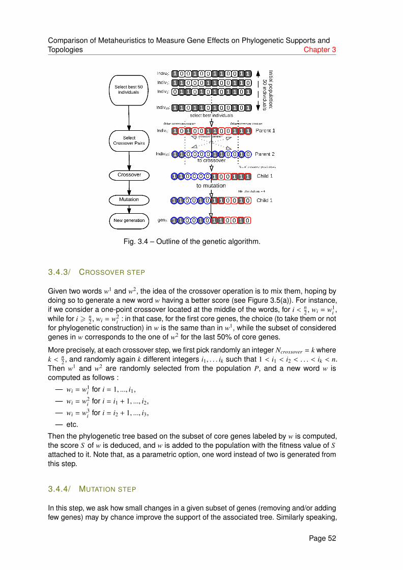
Comparison of Metaheuristics to Measure Gene Effects on Phylogenetic Supports andTopologies Chapter 3
Fig. 3.4 – Outline of the genetic algorithm.
3.4.3/ CROSSOVER STEP
Given two words w1 and w2, the idea of the crossover operation is to mix them, hoping bydoing so to generate a new word w having a better score (see Figure 3.5(a)). For instance,if we consider a one-point crossover located at the middle of the words, for i < n
2 , wi = w1i ,
while for i > n2 , wi = w2
i : in that case, for the first core genes, the choice (to take them or notfor phylogenetic construction) in w is the same than in w1, while the subset of consideredgenes in w corresponds to the one of w2 for the last 50% of core genes.
More precisely, at each crossover step, we first pick randomly an integer Ncrossover = k wherek < n
2 , and randomly again k different integers i1, . . . ik such that 1 < i1 < i2 < . . . < ik < n.Then w1 and w2 are randomly selected from the population P, and a new word w iscomputed as follows :
— wi = w1i for i = 1, ..., i1,
— wi = w2i for i = i1 + 1, ..., i2,
— wi = w3i for i = i2 + 1, ..., i3,
— etc.
Then the phylogenetic tree based on the subset of core genes labeled by w is computed,the score S of w is deduced, and w is added to the population with the fitness value of Sattached to it. Note that, as a parametric option, one word instead of two is generated fromthis step.
3.4.4/ MUTATION STEP
In this step, we ask how small changes in a given subset of genes (removing and/or addingfew genes) may by chance improve the support of the associated tree. Similarly speaking,
Page 52
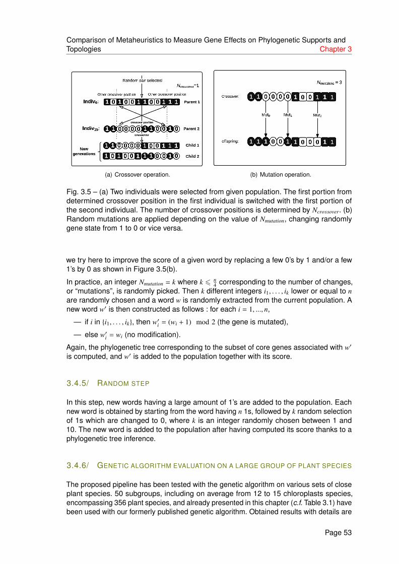
Comparison of Metaheuristics to Measure Gene Effects on Phylogenetic Supports andTopologies Chapter 3
(a) Crossover operation. (b) Mutation operation.
Fig. 3.5 – (a) Two individuals were selected from given population. The first portion fromdetermined crossover position in the first individual is switched with the first portion ofthe second individual. The number of crossover positions is determined by Ncrossover. (b)Random mutations are applied depending on the value of Nmutation, changing randomlygene state from 1 to 0 or vice versa.
we try here to improve the score of a given word by replacing a few 0’s by 1 and/or a few1’s by 0 as shown in Figure 3.5(b).
In practice, an integer Nmutation = k where k 6 n4 corresponding to the number of changes,
or “mutations”, is randomly picked. Then k different integers i1, . . . , ik lower or equal to nare randomly chosen and a word w is randomly extracted from the current population. Anew word w′ is then constructed as follows : for each i = 1, ..., n,
— if i in {i1, . . . , ik}, then w′i = (wi + 1) mod 2 (the gene is mutated),
— else w′i = wi (no modification).
Again, the phylogenetic tree corresponding to the subset of core genes associated with w′
is computed, and w′ is added to the population together with its score.
3.4.5/ RANDOM STEP
In this step, new words having a large amount of 1’s are added to the population. Eachnew word is obtained by starting from the word having n 1s, followed by k random selectionof 1s which are changed to 0, where k is an integer randomly chosen between 1 and10. The new word is added to the population after having computed its score thanks to aphylogenetic tree inference.
3.4.6/ GENETIC ALGORITHM EVALUATION ON A LARGE GROUP OF PLANT SPECIES
The proposed pipeline has been tested with the genetic algorithm on various sets of closeplant species. 50 subgroups, including on average from 12 to 15 chloroplasts species,encompassing 356 plant species, and already presented in this chapter (c.f. Table 3.1) havebeen used with our formerly published genetic algorithm. Obtained results with details are
Page 53

Comparison of Metaheuristics to Measure Gene Effects on Phylogenetic Supports andTopologies Chapter 3
contained too in Table 3.1. Column Occ represents the amount of generated phylogenetictrees from the corresponding search space for each group. The column c representsthe number of core genes included within each group. The # taxa column is the amountof species corresponding to the considered group. b is the lowest value from bootstrapanalysis. The Terminus column contains the termination stage for each subgroup, namely :the systematic (1), random (2), or optimization (3) stage using genetic algorithm and/orLasso test. These stages, which have been proposed in [1], correspond to the systematicdeletion of 0 or 1 gene (N + 1 computations for N core genes), random suppression of coregenes (ranging from 2 to 5 genes), and the so-called genetic algorithm on binary wordpopulations improved by the use of a statistical test. Finally, the Likelihood column storesthe likelihood value of the best phylogenetic tree (i.e., according to the lowest bootstrapvalue b). A large occurrence value in this table means that the associated p-value and/orsubgroup has its computation terminated in either penultimate or last pipeline stage. Anoccurrence of 31 is frequent due to the fact that 32 MPI threads (one master plus 31slaves) have been launched on our supercomputing facility.
Notice that the groups in Table 3.1 can be divided in four parts :
— Groups of species stopped in systematic stage with weak bootstrap values. This isdue to the fact that an upper time limit has been set for each group and/or subgroups,while each computed tree in these remarkable groups needed a lot of times forcomputations.
— Subgroups terminated during systematic stage with desired bootstrap value.
— Groups or subgroups terminated in random stage with desired bootstrap value.
— Finally, groups or subgroups terminated with optimization stages.
A majority of subgroups has its phylogeny satisfactorily resolved, as can be seen onall obtained trees which can be downloadable at http://meso.univ-fcomte.fr/peg/phylo.However, some problematic subgroups still remain to be investigated, which explains whythe distributed BPSO is considered in the next section.
3.4.7/ FIRST EXPERIMENTS ON Rosales ORDER
In a first collection of experiments, we have implemented the proposed BPSO algorithm ona supercomputing facility. Investigated species are the ones listed in Table 3.2. 10 swarmshaving a variable number of particles have been launched 10 times, with c1 = 1, c2 = 1,and w linearly decreasing from 0.9 to 0.4. Obtained results are summarized in Table 3.3that contains, for each 10 runs of each 10 swarms : the number of removed genes andthe minimum bootstrap of the best tree. Remark that some bootstraps are not so far fromthe intended ones (larger than 95), whereas the number of removed genes are in averagelarger than what is desired.
Seven topologies have been obtained after either convergence or maxIter iterations. Only3 of them have occurred a representative number of times, namely the Topologies 0, 2,and 4, which are depicted in Figures 3.7, 3.8 and 3.9 (see details in Table 3.4).
These three topologies are almost well supported, except in a few branches. We can noticethat the differences in these topologies are based on the sister relationship of two speciesnamed Fragaria vesca and Fragaria bracteata, and of the relation between Pentactinarupicola and Pyrus pyrifolia. Due to its larger score and number of occurrences, we tend toselect Topology 0 as the best representative of the Rosale phylogeny.
Page 54

Comparison of Metaheuristics to Measure Gene Effects on Phylogenetic Supports andTopologies Chapter 3
Fig. 3.6 – Average fitness of Rosales order
TABLE 3.3 – Best tree in each swarm
RemovedSwarm genes F b
1 4 75.5 732 6 75.5 763 20 75 884 52 59.5 895 3 75.5 726 19 77.5 927 47 63.5 928 9 73.5 749 10 72.5 7310 13 76.5 84
TABLE 3.4 – Best topologies obtained from the generated trees, b is the lowest bootstrap ofthe best tree having this topology, p is the number of considered genes to obtain this tree.
Topology Swarms b p F Occurrences0 1, 2, 3, 4, 5, 6, 7, 8, 9, 10 92 63 77.5 5681 1, 2, 3, 4, 5, 6, 10 63 45 54 112 1, 2, 3, 4, 5, 6, 7, 8, 9, 10 76 67 71.5 553 8, 1, 2, 3, 4 56 41 48.5 54 1, 2, 3, 4, 5, 6, 7, 8, 9, 10 89 30 59.5 655 1, 3, 4, 5, 6, 9 71 33 52 96 5, 6 25 45 35 2
To further validate this choice, CONSEL [73] software has been used on per site likelihoodsof each best tree obtained using the RAxML [46]. The CONSEL computes the p-values ofvarious well-known statistical tests, like the so-called approximately unbiased (au), Kishino-Hasegawa (kh), Shimodaira-Hasegawa (sh), and Weighted Shimodaira-Hasegawa (wsh)tests. Obtained results are provided in Table 3.5, they confirm the selection of Topology 0as the tree reflecting the best the Rosales phylogeny.
After having verified that BPSO can be used to resolve phylogenetic issues thanks to the
Page 55

Comparison of Metaheuristics to Measure Gene Effects on Phylogenetic Supports andTopologies Chapter 3
Fig. 3.7 – The best obtained topologies for Rosales order,Topology0
Fig. 3.8 – The best obtained topologies for Rosales order,Topology0
Fig. 3.9 – The best obtained topologies for Rosales order,Topology0
Rosales order, we now intend to deeply compare the genetic algorithm versus the swarmparticle optimization. In order to do so, a large collection of group of plant species havebeen selected, on which we have successively launched the genetic algorithm and theBPSO one in distributed mode.
Page 56

Comparison of Metaheuristics to Measure Gene Effects on Phylogenetic Supports andTopologies Chapter 3
TABLE 3.5 – The CONSEL results regarding best trees
Rank item obs au np bp pp kh sh wkh wsh1 0 -1.4 0.774 0.436 0.433 0.768 0.728 0.89 0.672 0.9072 4 1.4 0.267 0.255 0.249 0.194 0.272 0.525 0.272 0.4393 2 3 0.364 0.312 0.317 0.037 0.328 0.389 0.328 0.383
3.5/ A SIMULATED ANNEALING APPROACH
3.5.1/ GENERAL PRESENTATION
The original Simulated Annealing (SA) method is a local search based threshold classalgorithm. Basically, a threshold algorithm is a loop in which a move is either done ornot, according to a given criterion and until reaching a freeze [74]. Specifically, after aninitialization step, this loop is composed by (a) a move in the neighborhood of the currentsolution, (b) an evaluation of this new position by a real-valued scoring function, then (c)a test, given a well chosen criterion, to store this position as the new best one. Variouscriteria can be considered. For instance, if a position is evaluated as a better solutionthan the best existing one, it becomes the reference solution for next iterations whenthe acceptation criterion is “only if best cost (score)” algorithm, which is a variant of aclassical greedy local search [75]. The “all is accepted” algorithm produces, for its part,a random walk. Finally, between these two extremal situations, an acceptation criterionallows to store sometimes too positions with poorer scores than the best solution, whichis an upward move via a stochastic component to avoid local minima. Such a stochasticapproach facilitates theoretical analysis of asymptotic convergence. As such algorithmscan be successfully used for a broad range of optimization problems, SA has been largelycovered in the literature during the last decades [76, 75], for both empirical [77, 78] –typically on NP-hard problems – and theoretical perspectives [79, 75].
In simulated annealing, the criterion is inspired by the Metropolis-Hastings statistical(Markov chain Monte Carlo) thermodynamics algorithm [75]. SA simulates the coolingof a material in a heat bath until a steady (frozen or thermodynamic equilibrium) state.When the solid material is heated over its melting point, its solidification rate inducesits structural properties. Two major antagonistic strategies are commonly used. On theone hand, after a fast cooling (quenching), the steady state is constituted by differentthermodynamic free level areas. This corresponds to a local minimum for a local search,when considering energy as a score. On the other hand, after a slow cooling (annealing),almost one sole thermostatic level is expected, which corresponds to a global minimum.As feasible solutions of SA are system states, the structural proximity of the latter leads tothe concept of solution neighborhood.
Thermodynamic laws show that at temperature t, the probability to increase in energy ofthe value δE is given by p(δE) = exp(−δE/kt) with k equal to the Boltzmann’s constant. Me-tropolis simulations [80] consist in the generation of a state perturbation, in the evaluationof energy modification, and finally in the decision to reject or not the new state accordingto the probability p(δE). That is, the probability to keep a better (lower) level of energy is 1,while the one to keep an infinitely worst level of energy is equal to 0. Or, in other words,the likelihood to save a given state decreases as the energy level increases. A best globalsolution is reached by searching series of equilibria. Each equilibrium is obtained by seriesof Metropolis thresholds. The stop condition is typically an arbitrary duration or a number
Page 57
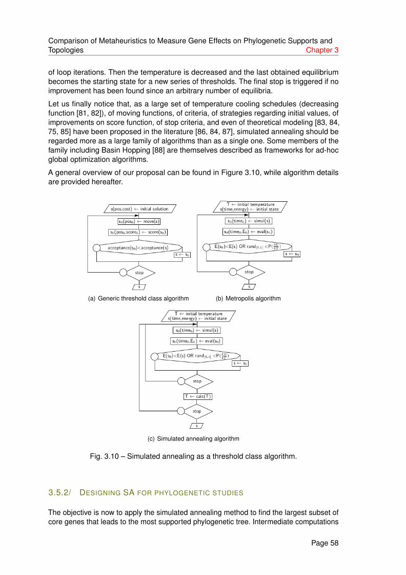
Comparison of Metaheuristics to Measure Gene Effects on Phylogenetic Supports andTopologies Chapter 3
of loop iterations. Then the temperature is decreased and the last obtained equilibriumbecomes the starting state for a new series of thresholds. The final stop is triggered if noimprovement has been found since an arbitrary number of equilibria.
Let us finally notice that, as a large set of temperature cooling schedules (decreasingfunction [81, 82]), of moving functions, of criteria, of strategies regarding initial values, ofimprovements on score function, of stop criteria, and even of theoretical modeling [83, 84,75, 85] have been proposed in the literature [86, 84, 87], simulated annealing should beregarded more as a large family of algorithms than as a single one. Some members of thefamily including Basin Hopping [88] are themselves described as frameworks for ad-hocglobal optimization algorithms.
A general overview of our proposal can be found in Figure 3.10, while algorithm detailsare provided hereafter.
(a) Generic threshold class algorithm (b) Metropolis algorithm
(c) Simulated annealing algorithm
Fig. 3.10 – Simulated annealing as a threshold class algorithm.
3.5.2/ DESIGNING SA FOR PHYLOGENETIC STUDIES
The objective is now to apply the simulated annealing method to find the largest subset ofcore genes that leads to the most supported phylogenetic tree. Intermediate computations
Page 58

Comparison of Metaheuristics to Measure Gene Effects on Phylogenetic Supports andTopologies Chapter 3
of subsets will help to understand, using regressions, the effects of given genes on both to-pology and supports. However, SA is complex to set up in practice, and finding new optimain finite time cannot be guaranteed, as related by Aarts, Korst, and van Laarhoven [74].To enlarge the probability of success, we targeted the following requirements during ourexperiments :
— a concise representation for the problem under consideration ;
— a cooling schedule fitting with complexity, time, convergence, and precision conside-rations ;
— a moving function adapted to the state (solution) space ;
— and, similarly, an acceptation function adapted to the state space.
These four requirements are discussed hereafter.
Temperature scheduling. A criterion to increase the probability to reach convergenceis the so-called logarithmic fading of control parameter (i.e., temperature). The most simplechoice is tn+1 = C · tn, where C ∈ [0, 1] is a constant. However, according to our experiments,such a solution is not able to produce relevant results in the phylogenetic problem underconsideration. This is why the control parameter has been updated following a tieredapproach, leading to an inhomogeneous Markov model : the temperature decreases onlyafter the end of its associated Markov chain. Additionally, near an equilibrium, the Markovchain length must increase when the control parameter decreases. But, as above, at lowtemperature the computation time may become prohibitive without any synchronisationbetween the control parameter and the Markov chain characteristics. To solve such anissue, various schedule solutions proposed in the literature link these two parameters. Afterhaving tested classical benchmarking functions like the well known three-hump camel,Levi [89], and Booth, we finally have chosen :
tn+1 =
t f
t1
nm−1i
× tn
where t is the control parameter, ti and t f are respectively the maximum (initial) andminimum (final) of allowed control parameter values for the SA computation, while nm isthe maximal number of Markov chains (equal to the temperature steps) allowed duringcomputation.
About a relevant configuration of SA according to the state space. As in the othermethods, the state space is constituted by Boolean vectors Xi of the form (Xi1, . . . , Xin),where n is the number of core genes. Xi j is equal to 1 if and only if gene number j inalphabetic order is in the alignment provided to the phylogenetic tool. We thus navigateagain on the n-cube on which each node (that is, each state) corresponds to a subset ofcore genes and has additionally a labeled value provided by the subset scoring function– which is again the average between the lowest bootstrap and the number of selectedcore genes. We can easily define a distance between two points inside this cube, like anHamming distance between Boolean vectors, and the node score can be considered asthe altitude of the current position.
To sum up, there is a topology on the state space, with neighborhood notion betweentwo states, while the altitude (the score of a subset of genes, which is related to the SA
Page 59

Comparison of Metaheuristics to Measure Gene Effects on Phylogenetic Supports andTopologies Chapter 3
energy) is varying between two locations. Both the density and the form of energy peaksare varying through the landscape. Neighborhoods and moves, acceptation probability,temperature scheduling functions, and their related initial values are dependant on thecharacteristics, or the topology, of this state space. Obviously, there is no general way toset up the parameters of the simulated annealing in this situation, as usually with suchheuristics. Even choosing close configurations of closely related problems like similarchloroplasts is not a guarantee of success.
Having these considerations in mind, we have stated some hypotheses at the basis of theneighboring notion. First of all, we assume that a solution is better if it is closer to the wholecore genome, so improving the number of 1’s in the Boolean vector is a desired trend.Secondly, we assume no correlation between genes, and so removing (or adding) onegene cannot modify so much the scoring function. As a consequence, the next investigatedstate should be near the previous one, in terms of Hamming distance, and most likely witha similar or larger number of active genes. In particular, moves in the state space cannotbe randomized as what occurs in the original SA algorithm. Furthermore, the starting statemust be the Boolean vector constituted by 1’s (that is, the whole core genome), while thescoring function must preferably tend to add genes in the considered subset (if possible).With such requirements, the neighborhood function has been designed as follows :
— A number between 1 and move_distancemax (a parameter to set) is randomly chosen,following a Gaussian law. It corresponds to the number of coordinates that maypossibly change.
— A subset of distinct coordinates are chosen accordingly, defining this move.
— For each Boolean coordinate, if the associated gene is inactive (0), it is activated (1).Otherwise, the gene is inactivated with a probability equal to nz
nc × α, where nz is thenumber of inactivated genes in the best current solution, nc is the total number ofcore genes in the problem, and α is a user-defined parameter.
Proposed SA optimization. Scores in this proposal are obtained using RAxML [90].As an inference of a bootstrapped and rooted phylogenetic tree may take times, and aswe need to compute several trees, each calculated state is tagged so that it is neverrecomputed without an explicit user demand. Associated and detailed results are bufferedon disk. Then a simple, reliable, and not really space-characteristics dependent solutionis the synchronization of some SAs after the end of a Markov chain [91]. In order to doso, a batch of SAs is launched with the same configuration. After a chain, each runningSA shares its own best known solution to a server. Then, it demands to this server if abetter state has been found before starting the next chain. Finally, each SA halts after nlocal non optimizing chains. So a stopped SA is not restarted, even if a better solution isfound elsewhere (i.e., the proposed SA stops as soon as possible).
Acceptance function is also selected to take advantage of previous moves, to allowsome (not too large) jumps. This is an adaptation of the so-called Tsallis acceptanceprobabilities [86] with a control parameter normalization :(
1 −(1 − q) ∗ ∆
∆ ∗ t
) 11−q
,
where ∆ is the score difference between the previous and current states, ∆ their mean, t isa control parameter, and q is a user-defined factor.
Page 60

Comparison of Metaheuristics to Measure Gene Effects on Phylogenetic Supports andTopologies Chapter 3
How to stop the SA. To fix a predefined control (temperature) value needs to knowsome state space characteristics, so we choose an end criterion related to the absence ofprogression in scores. In other words, the proposed simulated annealing algorithm stopsafter t consecutive Markov chains without any score improvement. As SA is very slow onlow temperatures, the choice has been to choose a small value for t. Then, a greedy localsearch can be launched on SA best states.
3.6/ COMPARISON OF THE METAHEURISTICS
3.6.1/ DATA GENERATION
3.6.1.1/ GENOMES RECOVERY AND ANNOTATIONS
At this stage, 780 complete genomes of chloroplasts have been downloaded from theNCBI, constituting the set of all available complete chloroplastic genomes at the date of thebeginning of our study [56]. Various gene prediction methods have been previously tested,in order to translate these complete genomes in lists of annotated coding sequences.These methods encompass the single use of NCBI annotated genomes, the use ofautomatic annotation tools specific to organelles like DOGMA [55], and the mix of both.
Indeed, annotations from NCBI website are of very variable quality : humanly well-curatedgenomes go together with genomes having a lot of annotation errors, concerning either thegene names (classification or spelling errors) or DNA sequences (start and stop position,length). As the number of well annotated genomes was not enough to constitute a testingset for our experiments, we are then left to find an acceptable way to annotate the whole780 complete genomes. As stated above, we tested various ways to annotate the genomes,and we evaluated them by checking their ability to recover the annotations (sequencepositions and gene names) of the subset of humanly, well-curated genomes.
According to our experiments, there was no way to improve enough the quality of NCBIannotations [57]. Neither by cross-validating them using automatic annotation tools, nor bytrying to correct errors in gene names and positions with these tools and some edit dis-tances [58, 12]. Furthermore, to cluster the whole NCBI DNA sequences fail in separatingwell annotated genes in well separated clusters, due to junk DNA in the NCBI sequences.The large number of obvious errors in the NCBI annotated complete chloroplastic genomescan be explained by the large variety of annotation tools used during sequence submission,most of them being not specific to this kind of genomes (unlike DOGMA), to a misuseof these tools, or due to errors in manual annotations. The absence of a clear norm inthe gene naming process adds difficulties, so that the sole method to provide accurateannotations to these 780 complete genomes was to constitute a basis of knowledge, witha subset of well curated genomes that represent well the plant diversity. And, to blast eachgenome against the basis, which is indeed what is done by DOGMA.
We finally have written a script that automatically send requests to the DOGMA webservice, and recovers the annotated genomes. Due to this automatic process, the genename spelling issue is resolved, and we can recover the clusters of homologous codingsequences by simply considering gene names. By applying the same tool for coding se-quence prediction and naming process, we have resolved the problem of quality variabilityin annotations. And as DOGMA has been specifically designed for chloroplasts, errors in
Page 61

Comparison of Metaheuristics to Measure Gene Effects on Phylogenetic Supports andTopologies Chapter 3
sequence positions have been reduced as possible. At this stage, and using our scripton DOGMA web service, we have then a collection of 780 complete and “well” annotatedchloroplastic genomes, from which gene names can be used to recover core and pangenomes of any subset of genomes.
3.6.1.2/ EXTRACTING SUBSETS OF GENOMES FOR SIMULATIONS
To test the ability, for the three proposed metaheuristics methods, to find the largest subsetof core genes that leads to the most supported trees, we needed to extract, from the set ofannotated genomes, various distinct subsets that are such that :
— Using the whole core genome in the alignment, we cannot obtain a well supportedtree.
— The time to compute this tree is reasonable, as we want to compute a lot of treesusing a lot of subsets of core genes. For a given subset of core genes, this computa-tion time encompasses :
1. the multi-alignment of each core gene using Muscle [59],
2. the concatenation of each aligned sequence to reconstruct the “sub” genome ofeach considered species (i.e., the part corresponding to the considered subsetof core genes),
3. the computation of the best phylogenetic tree corresponding to this alignment(with RAxML [90]),
4. the addition of bootstrap supports to this best tree using RAxML again,
5. and finally the verification that one of these supports is lower than 95 at least. Ifso, this tree is considered as not well supported.
Given a subset of genomes, the multi-alignment of each core gene can be computed onlyonce, prior to the research of the best subset of core genes leading to the most supportedtree. So we do not have to consider the alignment stage when searching subsets ofgenomes with : (a) problematic phylogenies and (b) a time to infer their tree as low aspossible. We stopped the process above before Stage 4 and we randomly pick anothersubset of species if the time to find their best phylogenetic trees using their whole coregenome (i.e., Stage 3) exceeds 10 seconds. If this computation time is below this threshold,we then compute 50 bootstraps and we check if the best bootstrapped tree has a problemof supports. If so, we have found a convenient subset of annotated genomes, on which wecan test the three metaheuristics.
3.6.1.3/ A SIMPLE COMPARISON IN SMALL DIMENSIONS
After having executed the three metaheuristics previously described, we have validatedthem on test examples. We have first performed a 1D/2D comparison of the three propo-sals, to obtain an easy-to-understand representation of the convergence of the optimizationalgorithms. Obtained results are depicted in Figure 3.11, circles denote successive po-sitions given by SA, points are for GA, while PSO corresponds to triangles. Figure 3.12represents the output evolution of the simulated annealing, with the consecutive endsof the Markov chains and the evolution of acceptation density. From the results, we candeduce that the desired convergence behavior is well obtained, and that the comparison
Page 62

Comparison of Metaheuristics to Measure Gene Effects on Phylogenetic Supports andTopologies Chapter 3
seems fair : no algorithm seems to underperform the other ones, and the general evolutionof the energy seems to be comparable for the three algorithms. Such results allow us tofurther investigate simulated annealing, particle swarm optimization, and genetic algorithmfor their ability to find the largest subset of core genes that leads to the most supportedtree.
Fig. 3.11 – Successive positions given by the three metaheuristics : circles, points, andtriangles are respectively for SA, GA, and PSO.
Fig. 3.12 – Illustration of output provided by simulated annealing approach : three-humpcamel function, one instance of parallelled SA with final greedy local descent.
Page 63

Comparison of Metaheuristics to Measure Gene Effects on Phylogenetic Supports andTopologies Chapter 3
TABLE 3.6 – Family number 1 (Pelargonium cotyledonis as outgroup).
Accession Nb Name Nb. of genes Length (nuc.)NC_024082.1 Cylindrotheca closterium 257 165,809NC_014808.1 Thalassiosira oceanica CCMP1005 138 141,790NC_025313.1 Cerataulina daemon 195 120,144NC_028052.1 Pelargonium cotyledonis 271 166,111NC_015403.1 Fistulifera solaris 192 134,918NC_024084.1 Leptocylindrus danicus 155 125,213
3.6.2/ EXPERIMENTING THE HEURISTICS ON SMALL COLLECTIONS OF GENOMES
We first focus on small sets of species with unresolved phylogenies, for computationalreasons and because small trees are easier to compare. Even in such small sets, as thecore genome contains more than 100 genes, the number of combinations to test is farfrom what is tractable using a brute force approach. We will see that it is easy to obtainvarious opposed but very well supported trees using large subsets of core genes, leadingto the necessity to optimize both parameters.
3.6.2.1/ A FIRST FAMILY OF ALGAE
We have first considered the family listed in Table 3.6. The detailed taxonomy informationis provided hereafter.
— Cylindrotheca closterium. Stramenopiles ; Bacillariophyta ; Bacillariophyceae ; Ba-cillariophycidae ; Bacillariales ; Bacillariaceae.
— Thalassiosira oceanica CCMP1005. Stramenopiles ; Bacillariophyta ; Coscinodis-cophyceae ; Thalassiosirophycidae ; Thalassiosirales ; Thalassiosiraceae.
— Cerataulina daemon. Stramenopiles ; Bacillariophyta ; Mediophyceae ; Biddulphio-phycidae ; Hemiaulales ; Hemiaulaceae.
— Pelargonium cotyledonis. Viridiplantae ; Streptophyta ; Embryophyta ; Tracheo-phyta ; Spermatophyta ; Magnoliophyta ; Eudicotyledons ; Gunneridae ; Pentapetalae ;Rosids ; Malvids ; Geraniales ; Geraniaceae.
— Fistulifera solaris. Stramenopiles ; Bacillariophyta ; Bacillariophyceae ; Bacillario-phycidae ; Naviculales ; Naviculaceae.
— Leptocylindrus danicus. Stramenopiles ; Bacillariophyta ; Coscinodiscophyceae ;Chaetocerotophycidae ; Leptocylindrales ; Leptocylindraceae.
This family is constituted by 6 genomes, of length ranging from 120,144 to 166,111nucleotides. The number of detected genes, for its part, ranges from 138 to 271, with acore genome of 122. The phylogeny with the alignment of these core genes leads to asmall weakness in one branch (bootstrap of 94), as depicted in Figure 3.13. Indeed, insidethis bacillariophyta phylum (eukaryotic algae), C.closterium, and F.solaris are naturally inthe same clade, being both in the same class of bacillariophyceae, while the three otherspecies are in three different classes inside this phylum.
To wonder whether some genes may be responsible of such weak uncertainty, we havefirstly launched the genetic algorithm : its systematic mode (in population initialization
Page 64
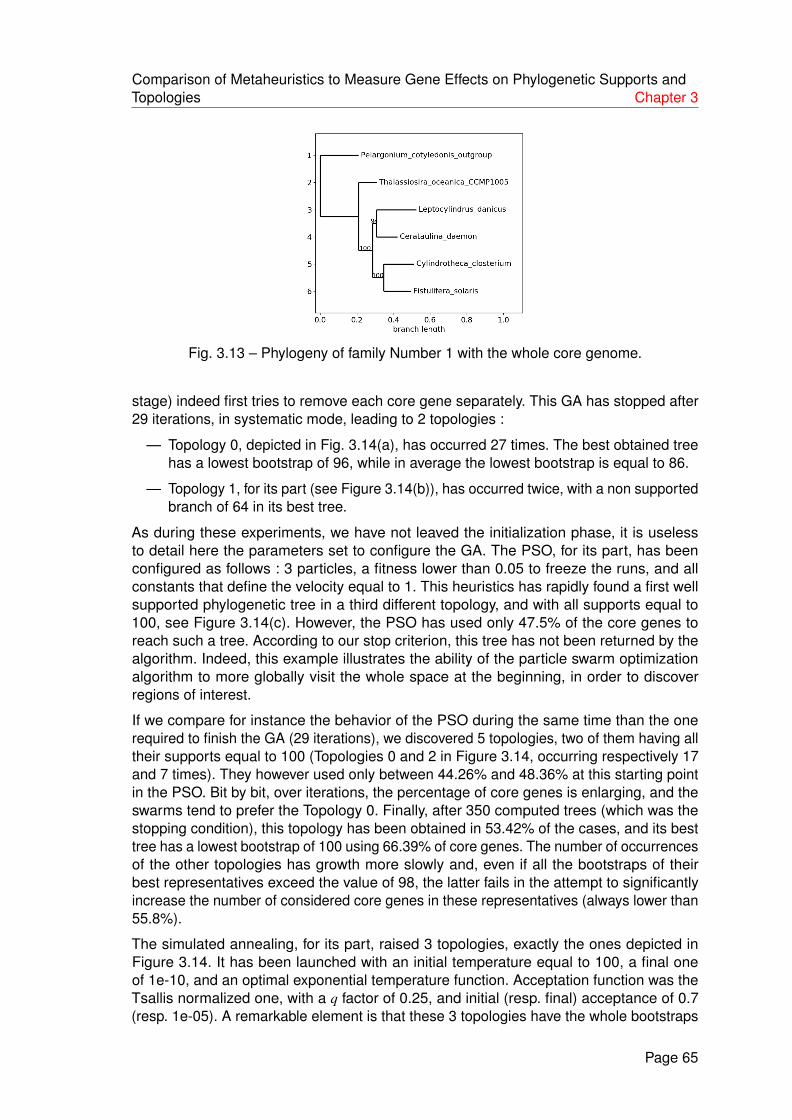
Comparison of Metaheuristics to Measure Gene Effects on Phylogenetic Supports andTopologies Chapter 3
Fig. 3.13 – Phylogeny of family Number 1 with the whole core genome.
stage) indeed first tries to remove each core gene separately. This GA has stopped after29 iterations, in systematic mode, leading to 2 topologies :
— Topology 0, depicted in Fig. 3.14(a), has occurred 27 times. The best obtained treehas a lowest bootstrap of 96, while in average the lowest bootstrap is equal to 86.
— Topology 1, for its part (see Figure 3.14(b)), has occurred twice, with a non supportedbranch of 64 in its best tree.
As during these experiments, we have not leaved the initialization phase, it is uselessto detail here the parameters set to configure the GA. The PSO, for its part, has beenconfigured as follows : 3 particles, a fitness lower than 0.05 to freeze the runs, and allconstants that define the velocity equal to 1. This heuristics has rapidly found a first wellsupported phylogenetic tree in a third different topology, and with all supports equal to100, see Figure 3.14(c). However, the PSO has used only 47.5% of the core genes toreach such a tree. According to our stop criterion, this tree has not been returned by thealgorithm. Indeed, this example illustrates the ability of the particle swarm optimizationalgorithm to more globally visit the whole space at the beginning, in order to discoverregions of interest.
If we compare for instance the behavior of the PSO during the same time than the onerequired to finish the GA (29 iterations), we discovered 5 topologies, two of them having alltheir supports equal to 100 (Topologies 0 and 2 in Figure 3.14, occurring respectively 17and 7 times). They however used only between 44.26% and 48.36% at this starting pointin the PSO. Bit by bit, over iterations, the percentage of core genes is enlarging, and theswarms tend to prefer the Topology 0. Finally, after 350 computed trees (which was thestopping condition), this topology has been obtained in 53.42% of the cases, and its besttree has a lowest bootstrap of 100 using 66.39% of core genes. The number of occurrencesof the other topologies has growth more slowly and, even if all the bootstraps of theirbest representatives exceed the value of 98, the latter fails in the attempt to significantlyincrease the number of considered core genes in these representatives (always lower than55.8%).
The simulated annealing, for its part, raised 3 topologies, exactly the ones depicted inFigure 3.14. It has been launched with an initial temperature equal to 100, a final oneof 1e-10, and an optimal exponential temperature function. Acceptation function was theTsallis normalized one, with a q factor of 0.25, and initial (resp. final) acceptance of 0.7(resp. 1e-05). A remarkable element is that these 3 topologies have the whole bootstraps
Page 65

Comparison of Metaheuristics to Measure Gene Effects on Phylogenetic Supports andTopologies Chapter 3
TABLE 3.7 – Family number 2 (Chromera velia as outgroup).
Accession Nb Name Nb. of genes Length (nuc.)NC_024082.1 Cylindrotheca closterium 257 165,809NC_014808.1 Thalassiosira oceanica CCMP1005 138 141,790NC_027721.1 Pseudo-nitzschia multiseries 267 111,539NC_024084.1 Leptocylindrus danicus 155 125,213NC_014340.2 Chromera velia 265 120,426
equal to 100. Furthermore, Topology 2 appears as the best one according to the producedresult (it was Topology 0 according to the GA, while PSO has not succeeded in separatingthese two topologies). With details, the SA has stopped after 364 computed trees, with6 occurrences of Topology 0, 43 of Topo. 1, and 315 for the Topology 2. Similarly, thepercentage of core genes leading to the best representative in each topology is respectivelyof 56.56% (Topo. 0), 74.59% (Topo. 1), and 94.98% (Topo. 2), which thus outperforms theother ones according to these simulations.
Obviously, both PSO and SA have converged to local minima that are not global ones if weconsider that both minimum bootstraps and proportion of core genes must be maximized.Launching them again with other initial values and parameters may select other optimalpositions in the cube. The genetic algorithm with this family is emblematic, as duringits initial population generation it has returned Topology 0 that is totally supported with99.18% of the core genome. This topology seems to be an acceptable representation ofthe phylogenetic relationship between these chloroplasts. But it is remarkable that, usingthe same large proportion of core gene, we can break in the sister relationship betweenL.danicus and C.daemon. Indeed, this behavior has been obtained frequently with variouscollections of data, which will be illustrated below.
Up to now, we only have considered one problematic bootstrap, which may be easy toresolve when removing genes. New difficulties are added when there are at least twoproblems in the list of bootstraps, as improving the first one may lead to a decrease in thesecond value. We have investigated this point in the second tested family.
3.6.2.2/ A SECOND FAMILY WITH TWO PROBLEMATIC BOOTSTRAPS
The second small set of genomes is constituted by 4 Bacillariophyta plus an Alveolataas outgroup, as listed in Table 3.7. Taxonomic details are provided hereafter, while thephylogenetic tree based on the alignment of the core genome is provided in Figure 3.15(a).
— Cylindrotheca closterium. Stramenopiles ; Bacillariophyta ; Bacillariophyceae ; Ba-cillariophycidae ; Bacillariales ; Bacillariaceae.
— Thalassiosira oceanica CCMP1005. Stramenopiles ; Bacillariophyta ; Coscinodis-cophyceae ; Thalassiosirophycidae ; Thalassiosirales ; Thalassiosiraceae.
— Pseudo-nitzschia multiseries. Stramenopiles ; Bacillariophyta ; Bacillariophyceae ;Bacillariophycidae ; Bacillariales ; Bacillariaceae.
— Leptocylindrus danicus. Stramenopiles ; Bacillariophyta ; Coscinodiscophyceae ;Chaetocerotophycidae ; Leptocylindrales ; Leptocylindraceae.
— Chromera velia. Alveolata ; Chromerida
Page 66

Comparison of Metaheuristics to Measure Gene Effects on Phylogenetic Supports andTopologies Chapter 3
The phylogenetic tree is not well-supported, having two bootstrap values of 86. Further-more, T.oceanica and L.danicus are not sisters in this tree, while they belong in theCoscinodiscophyceae class of diatom. More seriously, the two other species belong tothe Bacillariaceae family, which is in contradiction with this tree. It is not a necessity torecover exactly the known taxonomy, as we focus on chloroplasts, but this tree is at leastsuspicious if we consider both supports and taxonomy. This example illustrates the factthat to use the largest common subset of sequences is not sufficient enough to guaranteea well conducted phylogenetic study. Conversely, and obviously, to have good supportsis not enough, as all best trees in the different topologies of the previous family are wellsupported in the SA case : the largest number of core genes must be thus coupled withthe research of the best supports.
Once again, the genetic algorithm has stopped rapidly, in the systematic mode. The 22first genes have been tested (i.e., removed) before finding Topology 0 of Figure 3.15(a)with a lowest bootstrap equal to 96 (and 99.18% of the genes), thus stopping the GA, whilea new topology (Topology 1, see Fig. 3.15(b)) has occurred three times (best tree havingtwice 94 as bootstraps). Compared with the first family, the genetic algorithm stops herebefore succeeding to reinforce the confidence put in Topology 0, which justifies to test thetwo other approaches.
PSO heuristics produces the same two topologies after 1,165 computed trees, with allsupports equal to 100, and approximately the same number of trees (632 for Topo. 0 and533 for Topo. 2) and of genes (70.49% versus 74.59%). We stopped the swarm manually,as these two scores have not been improved during the last 500 iterations. Obviously,the 3 particles have been blocked in two local extrema, and the way we configured theirvelocity (0.9 and 0.8 for φ1 and φ2) does not allow them to leave these optima. So we stillcannot choose definitively the topology number 0.
Finally, the simulated annealing has produced 400 trees before convergence. They allbelong to the two topologies detailed above. However, produced results show that Topologynumber 1 must be preferred, according to the SA, and this latter is neither the one obtainedwith the whole core genome, nor the best one according to GA. Indeed, after convergence,all bootstraps here are equal to 100 in the best tree found inside each topology. Buttopology of Figure 3.15(b) has been obtained in 88.5% of the cases. More significantly,best tree in Topology 1 is obtained using 96.72% of the core genome, while for Topology 0,the best tree uses 90.98% of it. Remark that using the nine-tenths of the core genome,you can obtain a first topology with all supports equal to 100, while using more than 96%you can find a different topology with again all supports equal to 100. And, if we considerthe average between the lowest bootstrap and the proportion of core genes as a score, thebest topology according to GA has a score of 97.59/100, while it is of 98.36 for Topology 1found by the SA.
We will now further investigate the simulated annealing convergence process, beforestudying more deeply the two other algorithms in a next section.
3.6.3/ EARLY ANALYSIS ON SA COMPUTED PROBLEM : AN ILLUSTRATION
An example of a SA batch run (three clients on the first family described previously) isdepicted in Figure 3.16. For easy understanding, only some outputs have been reported inthe figure.
Page 67

Comparison of Metaheuristics to Measure Gene Effects on Phylogenetic Supports andTopologies Chapter 3
(a) Topology 0 (b) Topology 1
(c) Topology 2
Fig. 3.14 – Obtained topologies with the first family.
(a) Topology 0 with the whole core genome (b) Topology 1 obtained by GA
Fig. 3.15 – Obtained topologies with the second family.
Page 68

Comparison of Metaheuristics to Measure Gene Effects on Phylogenetic Supports andTopologies Chapter 3
Fig. 3.16 – Illustration of clade analysis with a 3-parallelized SA.
Page 69

Comparison of Metaheuristics to Measure Gene Effects on Phylogenetic Supports andTopologies Chapter 3
On the lower part, all moves of the simulated annealing are reported with their nature :synchronized move in yellow (i.e., copy, from a shared memory, of the best known solutionfound in the three SAs), move with an accepted status in orange, and rejected moves inblack. Active genes are filled squares and not selected ones are white squares. Otherimportant data for analysis are reported, such as : temperature, accepted score of otherSAs (green and purple), and Hamming distance between two consecutive positions(moving behavior indicator).
On the upper part, a graph of accepted scores from the three SAs is provided, with thetemperature variations due to move iterations (a lower score is a better one). As werepresented the first run on a new collection of genomes, no previous configurations wereavailable to set up the parameters. Consequently, a broad range of temperatures has beenconsidered. The Markov chains are short, in order to reduce the computation time. Fromthis beginning of an experiment, it can be deduced that :
— the temperature ranges well, allowing further experiments on the same set of data ;
— even with a poor configuration, SAs have found a score “not so bad”, which isassociated to a topology that other heuristics have considered as a good one.
Another SA evolution is provided in Figure 3.17, in which the three main curves do notrepresent moves, but “moves of locally selected moves”, which are stabilized over time.
3.6.4/ A FURTHER COMPARISON OF THE DISTRIBUTED VERSIONS OF GA ANDBPSO PERFORMANCE
During the experiments of the previous section, it was impossible to evaluate in practice thebehavior of the genetic algorithm, as this latter found an optimum during the initializationstage. Similarly, BPSO has underperformed the two other algorithms, while SA alwaysproduced interesting results. This is why we decided, after having studied the SA evolutionon the first family, to further investigate both BPSO (with its two velocity versions) andGA in large collections of experiments, distributed in a supercomputer facilities. To do so,12 groups of plant genomes have been extracted from our set of annotated genomes.They have been applied on our two swarm versions, and results have been compared tothe genetic algorithm ones.
Comparisons are provided in Tables 3.8 and 3.9. In these tables, Topo. column stands forthe number of topologies, NbTrees is the total number of obtained trees using 10 swarms,b is the minimum bootstrap value of selected w, 100 − p is the number of missing genes inw and Occ. is the number of occurrences of the best obtained topology from 10 swarms.As can be seen in these tables, the two versions of BPSO did not provide the same kind ofresults :
— In the case of Chlorophyta, Pinus, and Bambusoideae, the second version of theBPSO has outperformed the first one, as the minimum bootstrap b of the best tree isfinally larger for at least one swarm.
— In the Ericales case, the first version has produced the best result.
We can also remark that Malpighiales has better b in GA than the two versions of BPSO.Pinus data set has got maximum bootstrap b larger than what has been obtained usingthe genetic algorithm, while Picea and Trebouxiophyceae have got the same values of bthan with genetic algorithm. Further comparison results between GA and both versions ofBPSOs are provided in Figure 3.18.
Page 70
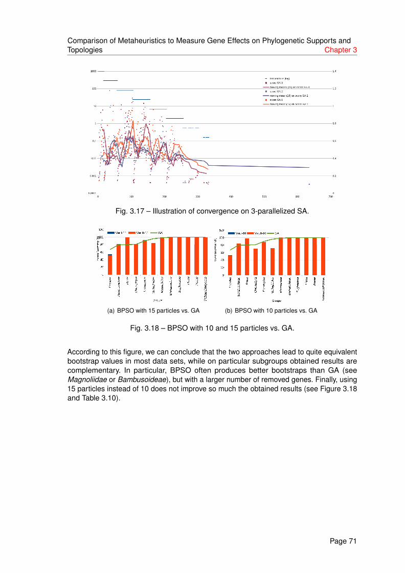
Comparison of Metaheuristics to Measure Gene Effects on Phylogenetic Supports andTopologies Chapter 3
Fig. 3.17 – Illustration of convergence on 3-parallelized SA.
(a) BPSO with 15 particles vs. GA (b) BPSO with 10 particles vs. GA
Fig. 3.18 – BPSO with 10 and 15 particles vs. GA.
According to this figure, we can conclude that the two approaches lead to quite equivalentbootstrap values in most data sets, while on particular subgroups obtained results arecomplementary. In particular, BPSO often produces better bootstraps than GA (seeMagnoliidae or Bambusoideae), but with a larger number of removed genes. Finally, using15 particles instead of 10 does not improve so much the obtained results (see Figure 3.18and Table 3.10).
Page 71

Comparison of Metaheuristics to Measure Gene Effects on Phylogenetic Supports andTopologies Chapter 3
TABLE 3.8 – Groups from BPSO version I.
Group Topo. NbTrees b |c| 100 − p′ Occ. Swarms ParticlesPinus 3 508 98 79 32 462 1,2,3,4,5,6,7,8,9,10 10Pinus 3 530 94 79 11 129 1,2,3,4,5,6,7,8,9,10 15Picea 1 100 100 85 42 100 1,2,3,4,5,6,7,8,9,10 10Picea 1 428 100 85 13 428 1,2,3,4,5,6,7,8,9,10 15
Magnoliidae 3 750 100 79 20 613 1,2,3,4,5,6,7,8,9,10 10Magnoliidae 3 845 100 79 19 707 1,2,3,4,5,6,7,8,9,10 15
Ericales 30 344 53 84 26 185 1,2,3,4,5,6,7,8,9,10 10Ericales 34 555 54 84 5 363 1,2,3,4,5,6,7,8,9,10 15
Bambusoideae 8 496 72 94 37 456 1,2,3,4,5,6,7,8,9,10 10Bambusoideae 11 694 69 94 18 621 1,2,3,4,5,6,7,8,9,10 15
Eucalyptus 16 828 86 83 7 632 1,2,3,4,5,6,7,8,9,10 10Eucalyptus 20 1073 86 80 4 845 1,2,3,4,5,6,7,8,9,10 15
Malpighiales 34 327 65 78 35 233 1,2,3,4,5,6,7,8,9,10 10Malpighiales 38 483 69 78 40 326 1,2,3,4,5,6,7,8,9,10 15Chlorophyta 25 191 70 24 11 109 1,2,3,4,5,6,7,8,9,10 10Chlorophyta 29 94 68 24 11 1 1,2,3,4,5,6,7,8,9,10 15Euglenozoa 3 450 100 26 7 292 1,2,3,4,5,6,7,8,9,10 10Euglenozoa 3 520 100 26 4 491 1,2,3,4,5,6,7,8,9,10 15
Ehrhartoideae 2 23 100 81 0 23 1,2,3,4,5,6,7,8,9,10 10Ehrhartoideae 3 455 100 81 0 451 1,2,3,4,5,6,7,8,9,10 15
Trebouxiophyceae 3 409 100 41 2 405 1,2,3,4,5,6,7,8,9,10 10Trebouxiophyceae 3 415 100 41 8 354 1,2,3,4,5,6,7,8,9,10 15
Poeae 1 971 100 80 9 971 1,2,3,4,5,6,7,8,9,10 10Poeae 1 1399 100 80 20 1399 1,2,3,4,5,6,7,8,9,10 15
TABLE 3.9 – Groups from PSO version II.
Group Topo. NbTrees b |c| 100 − p′ Occ. Swarms ParticlesPinus 3 615 98 79 14 275 1,2,3,4,5,6,7,8,9,10 10Pinus 3 628 100 79 12 558 1,2,3,4,5,6,7,8,9,10 15Picea 1 635 100 85 14 635 1,2,3,4,5,6,7,8,9,10 10Picea 1 821 100 85 15 821 1,2,3,4,5,6,7,8,9,10 15
Magnoliidae 3 494 100 79 16 73 1,2,3,4,5,6,7,8,9,10 10Magnoliidae 3 535 100 79 42 384 1,2,3,4,5,6,7,8,9,10 10
Bambusoideae 6 952 84 81 23 94 1,2,3,4,5,6,7,8,9,10 10Bambusoideae 9 1450 82 81 18 113 1,2,3,4,5,6,7,8,9,10 15
Eucalyptus 17 972 88 80 18 618 1,2,3,4,5,6,7,8,9,10 10Eucalyptus 23 1439 92 80 10 843 1,2,3,4,5,6,7,8,9,10 15Chlorophyta 25 529 71 24 6 397 1,2,3,4,5,6,7,8,9,10 10Chlorophyta 46 1500 82 24 11 397 1,2,3,4,5,6,7,8,9,10 10
Ericales 30 97 51 84 11 56 1,2,3,4,5,6,7,8,9,10 10Ericales 34 1257 52 84 7 800 1,2,3,4,5,6,7,8,9,10 15
Malpighiales 35 725 72 79 25 445 1,2,3,4,5,6,7,8,9,10 10Malpighiales 86 1464 84 79 45 359 1,2,3,4,5,6,7,8,9,10 15Euglenozoa 3 197 100 26 1 165 1,2,3,4,5,6,7,8,9,10 10Euglenozoa 3 450 100 26 10 393 1,2,3,4,5,6,7,8,9,10 15
Ehrhartoideae 1 24 100 81 10 24 1,2,3,4,5,6,7,8,9,10 10Ehrhartoideae 1 20 100 81 9 20 1,2,3,4,5,6,7,8,9,10 15
Trebouxiophyceae 3 319 100 41 1 313 1,2,3,4,5,6,7,8,9,10 10Trebouxiophyceae 3 818 100 41 2 81 1,2,3,4,5,6,7,8,9,10 15
Poeae 1 991 100 80 22 991 1,2,3,4,5,6,7,8,9,10 15Poeae 1 1490 100 80 26 1490 1,2,3,4,5,6,7,8,9,10 15
TABLE 3.10 – PSO vs GA.
BPSO ver.I BPSO ver.IIGroup 10 15 10 15 GAEricales 53 54 51 52 67Bambusoideae 72 69 84 82 80Pinus 98 94 98 100 80Chlorophyta 70 68 71 82 81Eucalyptus 86 86 88 92 90Malpighiales 65 69 72 84 96Magnoliidae 100 100 100 100 98Ehrhartoideae 100 100 100 100 100Euglenozoa 100 100 100 100 100Picea 94 100 100 100 100Poeae 80 80 100 100 100Trebouxiophyceae 100 100 100 100 100
Page 72

Comparison of Metaheuristics to Measure Gene Effects on Phylogenetic Supports andTopologies Chapter 3
3.7/ CONCLUSION
This chapter has presented three metaheuristics to produce a well supported phylogenetictree based on the largest possible subset of core genes. These methods are, namely,genetic algorithm, binary particle swarm optimization, and simulated annealing. They havebeen evaluated on various sets of chloroplast species and deployed on a supercomputerfacilities. At this level, two main issues can be signaled when considering the objective toreconstruct the ancestral genomes of all existing chloroplasts.
On the one hand, given the average between the percentage of core genes and the lowestbootstrap as scoring function, we have shown on simple examples that, given a set ofspecies, various global optima with contradictory topologies can be reached. These firstexperiments emphasize that sometimes the phylogeny of chloroplasts cannot perfectly beresolved using a tree : a phylogenetic network may be more close to the reality, brancheswithin this network being as strong as the associated tree topology is frequent. In thefirst instance, this difficulty has not been considered : our current objective is to designalgorithms making it possible to reconstruct ancestors through a tree. In case of success,we will then try to improve our pipeline, to become compatible with network topologies.
On the other hand, given a set of annotated genomes, we have proposed some methodsto find the most supported tree based on the largest subset of core genes. In casewhere the considered species are close enough, their core genome is close to eachgenome alone : the intersection of sets that share a large amount of genes is large. In thissituation, and in case of convergence of our method, the obtained well supported tree isbased on a large part of each genome, and it can be considered as well representative :ancestral reconstruction can be reasonably applied on it. Conversely, when consideringthe chloroplasts of all possible plants, there is concern about the representativeness of thecore genome, as the latter may be very small. This concerns passes from the phylogenetictree to the ancestors reconstructed on it. To investigate this risk and the means to removeit, the evolution of core genome within the chloroplast taxonomy will be investigated in thenext chapter.
Page 73


4RELATION BETWEEN GENE CONTENT
AND TAXONOMY IN CHLOROPLASTS
The aim of this chapter is to investigate the evolution of the core genome of chloroplastswhen enlarging the set of considered species. Core and pan genomes have been
computed here on de novo annotation of the 845 genomes available at the time of thisstudy. We take the opportunity to investigate the specificity of some branches of thetree, when specificity is obtained on accessory genes. After having detailed the materialand methods, we emphasize some remarkable relation between well-known events ofthe chloroplast history, like endosymbiosis, and the evolution of gene contents over thephylogenetic tree.
This study shows that taking simply the core genome of the whole 845 chloroplasts at thebeginning of the pipeline presented in the previous chapter is not satisfactory, as this coregenome is too small and not really representative. Enriching our method is thus a necessityto automatically obtain a well supported phylogenetic tree of the whole chloroplasts, onwhich the ancestral reconstruction process can operate. The content of this chapter hasbeen presented in the ICBSB 2016 [92] conference and published in IJBBB journal [93].
TABLE 4.1 – Information on chloroplast sizes at highest taxonomic level
Taxonomy nb. of min length max average standartgenomes length length deviation
Alveolata 4 85535 140426 115714.2 19648.3Cryptophyta 2 121524 135854 128689.0 7165.0Euglenozoa 7 80147 143171 98548.7 19784.5Haptophyceae 3 95281 107461 102683.6 5307.6Rhodophyta 9 149987 217694 183755.5 18092.2Stramenopiles 35 89599 165809 124895.1 15138.0Viridiplantae 775 80211 289394 150194.9 20376.8
75

Relation between Gene Content and Taxonomy in Chloroplasts Chapter 4
4.1/ MATERIALS AND METHODS
4.1.1/ DATA ACQUISITION
A set of 845 chloroplastic genomes (green algae, red algae, gymnosperms, and so on)has been downloaded from the NCBI website, representing all the available completegenomes at the date of March, 2016 (see Table 4.1). An example of such sequences,taken from the Streptophyta clade (a Viridiplantae), is provided in Table 4.2. Note thatthis set does not really constitute a very balanced representation of the diversity of plants,as plants of particular and immediate interest to us like Viridiplantae are first sequenced.We must however deal with such bias, as genomic data acquisition is most of the timehuman-centred. This set of sequences presents too a certain variability in terms of length,as detailed in Table 4.1.
Each genome has been annotated with DOGMA [55], an online automatic and accurateannotation tool of organellar genomes, following a same approach than in [57]. To applyit on our large scale database, a script that automatic send requests to the website hasbeen used. By doing such annotations, the same gene prediction and naming processhas been applied with the same average quality of annotation. In particular, when a geneappears twice in the considered set of genomes, it receives twice the same name (nospelling error). At this level, each genome is then described by an ordered list of genenames, with possible duplicates (other approaches for the annotation stage are possible,as explained in the previous chapter [57]). This description will allow us to investigate, laterin this chapter, the evolution of gene content among the species tree, leading to the studyof core and pan genomes described below.
4.1.2/ CORE AND PAN GENOME
Given a collection of genomes, it is possible to define their core genes as the commongenes that are shared among all the species, while the pan genome is the union of all thegenes that are in at least one genome (all the species have each core gene, while a pangene is in at least one genome). Shared genes are evidences of evolution from a commonancestor and of the relatedness of chloroplast organisms.
TABLE 4.2 – Example of genomes information of Streptophyta clade
Organism name Accession Sequence Nb ofnumber length CDS
Epimedium sagittatum NC_029428.1 158273 85Berberis bealei NC_022457.1 164792 267Torreya fargesii NC_029398.1 137075 100Lepidozamia peroffskyana NC_027513.1 165939 93Actinidia chinensis NC_026690.1 156346 271Quercus aliena NC_026790.1 160921 259Quercus aquifolioides NC_026913.1 160415 176Sedum sarmentosum NC_023085.1 150448 99
Page 76

Relation between Gene Content and Taxonomy in Chloroplasts Chapter 4
TABLE 4.3 – Summarized properties of the pan genomes at the highest taxonomic level.
Taxonomy Nb. Min N.b Max N.b Average Nb.genomes of pan genes of pan genes of pan genes
Alveolata 4 253 266 262.25Cryptophyta 2 258 259 258.5Euglenozoa 7 193 267 253.428
Haptophyceae 3 251 266 258.333Rhodophyta 9 156 267 246.222
Stramenopiles 35 73 271 238.971Viridiplantae 775 85 271 229.827
To distinguish and determine the core genes may be of importance either to identifythe specificity and the shared functionality of a given set of species, or to evaluate theirphylogeny using the largest set of shared coding sequences (see the previous chapter).In the case of chloroplasts, an important category of genome modification is indeed theloss of functional genes, either because they become ineffective or due to transfer to thenucleus. Thereby, a small number of gene loss among species may indicate that thesespecies are close to each other and belong to a similar lineage, while a significant lossmeans distant lineages. So core genome is obviously of importance when inferring thephylogenetic relationship, while accessory genes of pan genome explain in some extendeach species specificity.
Three approaches have formerly been proposed (by members of the DISC department,FEMTO-ST) for eliciting core genomes. The first one uses correlations computed onpredicted coding sequences [57], while the second one uses gene names providedduring an annotation stage (e.g., names found in NCBI database or automatically set byDOGMA [58]). The third method tries to take the advantages from the first two approaches,by considering gene information and DNA sequences, in order to find the targeted coregenome [12]. Indeed, the naming process of genes is not standardized, and spellingerrors may occur, while conversely start and stop positions of coding sequences aresometimes erroneous, which handicaps the two first approaches. This explains the reasonto be of the last approach, that tries to take the best of the two other noisy approachesdealing with sequences or names. At this stage, we have definitively chosen the secondapproach described above, on names provided by DOGMA. Indeed, when checking all thepossibilities on a few set of accurately annotated genomes, we have recovered at best theannotations on complete sequences by using this approach. Obtained results regardinggene content are discussed in the next section.
Page 77

Relation between Gene Content and Taxonomy in Chloroplasts Chapter 4
Fig. 4.1 – Taxonomy backbone tree
Page 78

Relation between Gene Content and Taxonomy in Chloroplasts Chapter 4
4.2/ OBTAINED RESULTS
4.2.1/ GENE CONTENT
Genes are rearranged in the genome by evolutionary events like insertion, deletion, transpo-sition, and inversion, which are called genome rearrangements [94]. Such rearrangementscan be studied by putting sets of genes at the leaves of the taxonomy tree downloaded onthe NCBI website, which is partially reproduced in Figure 4.1.
It is true that this taxonomy tree is not fully accurate, as it is a general overview of plantspecies relationship based on dated information related to their geography, morphology,and so on. Nucleus DNA phylogeny has been used partially to recently update the taxo-nomy, but we have no information of support. And the nucleus evolution is not necessarilythe same than the chloroplast one. However, such a taxonomic tree can be consideredto have a rough, general overview of gene content evolution through various families ofplants.
Fig. 4.2 – The distributions of chloroplast genomes depending on the genomes size.
A summary of obtained results, in terms of contents evolution at the top taxonomy level, isprovided in Table 4.3. It is further detailed for the next taxonomic levels in Table 4.4. Thecore genome is constituted by 36 coding sequences, namely : ATPA, ATPB, ATPH, ATPI,PETB, PETG, PSAA, PSAB, PSAC, PSAJ, PSBA, PSBC, PSBD, PSBE, PSBF, PSBH,PSBI, PSBJ, PSBL, PSBN, PSBT, PSI_PSBT, RBCL, RPL14, RPL16, RPL2, RPL20,RPL36, RPS11, RPS12, RPS12_3END, RPS14, RPS19, RPS2, RPS7, and RRN16. Thepan genome of the whole considered species, for its part, contains 268 genes. The coregenome has thus 36 of the whole chloroplast genes, and it is too small to hope to infer arepresentative chloroplast phylogeny by using a subset of these 36 core genes.
To raise this issue, we decided to consider that :
1. The taxonomy tree can be considered as trustworthy at the uppers classificationlevels (e.g., class and order) as for instance brown algae are obviously separatedfrom land plants.
2. Errors may appear when going deeper in the taxonomy tree, for instance whenconsidering family or genus levels. But, at this stage, the core genome is large enoughto accurately apply the method of the previous chapter for inferring a supported tree.
Page 79
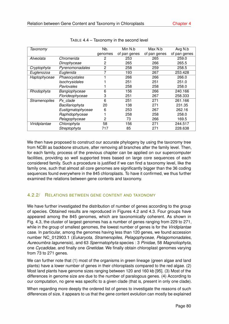
Relation between Gene Content and Taxonomy in Chloroplasts Chapter 4
TABLE 4.4 – Taxonomy in the second level
Taxonomy Nb. Min N.b Max N.b Avg N.bgenomes of pan genes of pan genes of pan genes
Alveolata Chromerida 2 253 265 259.0Dinophyceae 2 265 266 265.5
Cryptophyta Pyrenomonadales 2 258 259 258.5Euglenozoa Euglenida 7 193 267 253.428Haptophyceae Phaeocystales 1 266 266 266.0
Isochrysidales 1 251 251 251.0Pavlovales 1 258 258 258.0
Rhodophyta Bangiophyceae 6 156 266 240.166Florideophyceae 3 251 267 258.333
Stramenopiles Px_clade 6 251 271 261.166Bacillariophyta 20 138 271 231.35Eustigmatophyceae 6 253 267 262.16Raphidophyceae 1 258 258 258.0Pelagophyceae 2 73 266 169.5
Viridiplantae Chlorophyta 58 156 271 244.517Streptophyta 717 85 271 228.638
We then have proposed to construct our accurate phylogeny by using the taxonomy treefrom NCBI as backbone structure, after removing all branches after the family level. Then,for each family, process of the previous chapter can be applied on our supercomputerfacilities, providing so well supported trees based on large core sequences of eachconsidered family. Such a procedure is justified if we can find a taxonomy level, like thefamily one, such that almost all core genomes are significantly bigger than the 36 codingsequences found everywhere in the 845 chloroplasts. To have it confirmed, we thus furtherexamined the relations between gene contents and taxonomy.
4.2.2/ RELATIONS BETWEEN GENE CONTENT AND TAXONOMY
We have further investigated the distribution of number of genes according to the groupof species. Obtained results are reproduced in Figures 4.2 and 4.3. Four groups haveappeared among the 845 genomes, which are taxonomically coherent. As shown inFig. 4.3, the cluster of largest genomes has a number of genes ranging from 229 to 271,while in the group of smallest genomes, the lowest number of genes is for the Viridiplantaecase. In particular, among the genomes having less than 120 genes, we found accessionnumber NC_012903.1 (Eukaryota, Stramenopiles, Pelagophyceae, Pelagomonadales,Aureoumbra lagunensis), and 63 Spermatophyta species : 3 Pinidae, 58 Magnoliophyta,one Cycadidae, and finally one Gnetidae. We finally obtain chloroplast genomes varyingfrom 73 to 271 genes.
We can further note that (1) most of the organisms in green lineage (green algae and landplants) have a lower number of genes in their chloroplasts compared to the red algae. (2)Most land plants have genome sizes ranging between 120 and 160 kb [95]. (3) Most of thedifferences in genome size are due to the number of paralogous genes. (4) According toour computation, no gene was specific to a given clade (that is, present in only one clade).
When regarding more deeply the ordered list of genes to investigate the reasons of suchdifferences of size, it appears to us that the gene content evolution can mostly be explained
Page 80
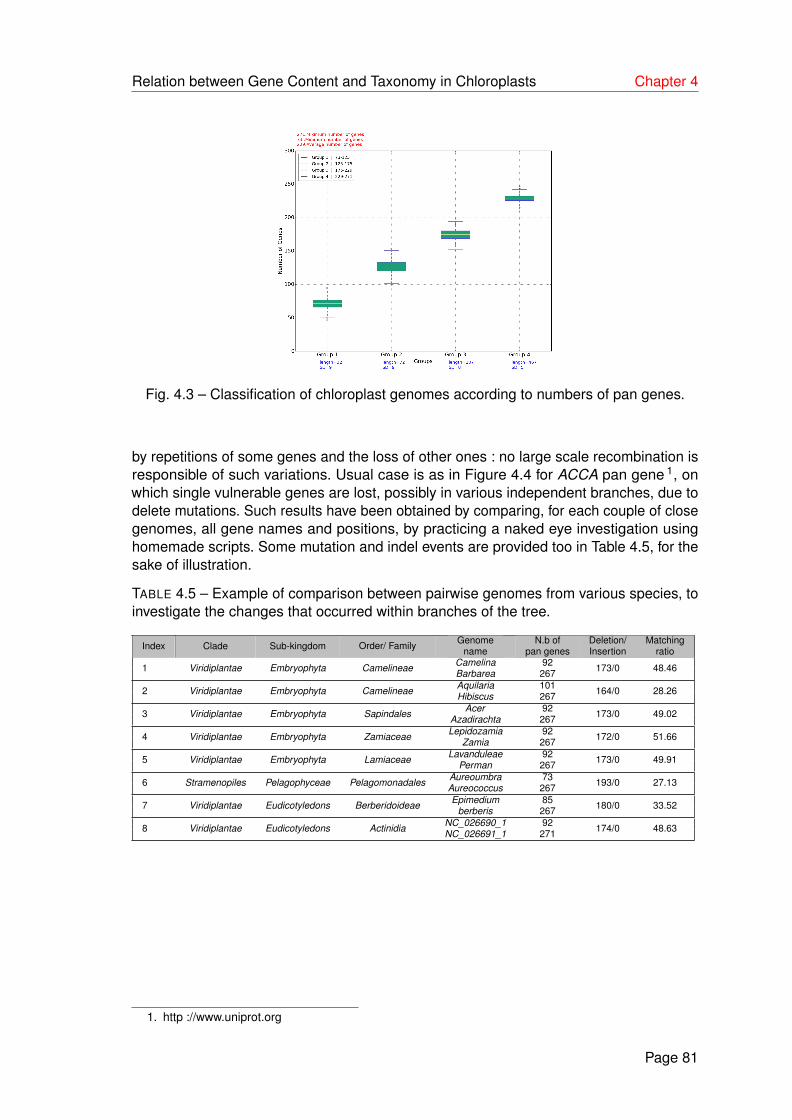
Relation between Gene Content and Taxonomy in Chloroplasts Chapter 4
Fig. 4.3 – Classification of chloroplast genomes according to numbers of pan genes.
by repetitions of some genes and the loss of other ones : no large scale recombination isresponsible of such variations. Usual case is as in Figure 4.4 for ACCA pan gene 1, onwhich single vulnerable genes are lost, possibly in various independent branches, due todelete mutations. Such results have been obtained by comparing, for each couple of closegenomes, all gene names and positions, by practicing a naked eye investigation usinghomemade scripts. Some mutation and indel events are provided too in Table 4.5, for thesake of illustration.
TABLE 4.5 – Example of comparison between pairwise genomes from various species, toinvestigate the changes that occurred within branches of the tree.
Index Clade Sub-kingdom Order/ Family Genomename
N.b ofpan genes
Deletion/Insertion
Matchingratio
Camelina 921 Viridiplantae Embryophyta Camelineae Barbarea 267 173/0 48.46
Aquilaria 1012 Viridiplantae Embryophyta Camelineae Hibiscus 267 164/0 28.26
Acer 923 Viridiplantae Embryophyta Sapindales Azadirachta 267 173/0 49.02
Lepidozamia 924 Viridiplantae Embryophyta Zamiaceae Zamia 267 172/0 51.66
Lavanduleae 925 Viridiplantae Embryophyta Lamiaceae Perman 267 173/0 49.91
Aureoumbra 736 Stramenopiles Pelagophyceae Pelagomonadales Aureococcus 267 193/0 27.13
Epimedium 857 Viridiplantae Eudicotyledons Berberidoideae berberis 267 180/0 33.52
NC_026690_1 928 Viridiplantae Eudicotyledons Actinidia NC_026691_1 271 174/0 48.63
1. http ://www.uniprot.org
Page 81

Relation between Gene Content and Taxonomy in Chloroplasts Chapter 4
Fig. 4.4 – ACCA gene loss in various branches of the tree
Page 82

Relation between Gene Content and Taxonomy in Chloroplasts Chapter 4
4.3/ THROUGH A WELL SUPPORTED TREE OF CHLOROPLASTS
4.3.1/ HOW WE COMPUTED OUR PHYLOGENETIC TREE, AND WHY
The next step to realize when trying to reconstruct the evolution of gene content overtime is to deeply investigate the phylogeny of these chloroplasts, in order to obtain a treeas supported as possible. As stated previously, a branching error in the tree may leadto an erroneous transmission of an ancestral state, which is dramatically perpetuateduntil reaching the last universal common ancestor. However, as we considered all existingplant taxa, we faced chloroplastic sequences that have diverged a lot since two billion ofyears, so the core genome of these 845 sequences is very small when compared withsequence length of each representative, and inferring a tree on such a partial informationwill probably lead to numerous errors.
After investigations of the previous section, the approach finally chosen has been to groupplant families per close packets (same family in the taxonomy). Such a grouping enlargesthe number of shared gene sequences (core genes of the considered family) on which amore representative phylogeny can be computed [1]. After having aligned the core genesof each family using MUSCLE [59] on our supercomputer facilities, we then have inferreda phylogenetic tree per family. To obtain such a tree, the RAxML [46, 96] program hasbeen employed to compute the phylogenetic maximum-likelihood (ML) function with thesetup described hereafter. General Time Reversible model of nucleotide substitution, withΓ model of rate heterogeneity and hill-climbing optimization method. The outgroup, for itspart, has been randomly picked from a close but different family of chloroplasts.
After such a computing, if all bootstrap values are larger than 95%, then we have conside-red that the phylogeny is resolved, as the largest possible number of genes has led to avery well supported tree. In case where some branches are not supported, we can wonderwhether a few genes can be incriminated. Such problem has been resolved by finding thelargest subset of core genes leading to the most supported tree, by the heuristic approachdetailed in the previous chapter and published in [56, 1]. Obtained trees are then mergedon a well-supported and representative supertree.
4.3.2/ PHYLOGENETIC INVESTIGATIONS
The approach detailed in the previous section has led to a well supported phylogenetictree of the whole available chloroplasts, with the ordered list of genes at each leaf of thetree. An overview of the latter is provided in Figure 4.1. Obtained tree, available on ourwebsite, is in general coherent with the NCBI taxonomy, except in some specific locations.
By going into the details of the obtained tree, it is well known that the first plants en-dosymbiosis ended in a great diversification of lineages comprising Red Algae, GreenAlgae, and Land Plants (terrestrial). The interesting point in the production of our resultsis that the organisms resulting from the first endosymbiosis are distributed in each of thelineages found in the chloroplast genome structure evolution as outlined in Figure 4.1. Moreprecisely, all Red Algae chloroplasts are grouped together in one lineage, while GreenAlgae and Land Plant chloroplasts are all in a second lineage. Furthermore, organismsresulting from the secondary endosymbioses, as listed in Table 4.4, are well localized inthe tree : both the chloroplasts of Brown Algae and Dinoflagellates representatives arefound exclusively in the lineage also comprising the Red Algae chloroplasts from which
Page 83

Relation between Gene Content and Taxonomy in Chloroplasts Chapter 4
they evolved, while the Euglens is related to Green Algae from which they evolved. Thislatter makes sense regarding biology, history of lineages, and theories of chloroplastsorigins (and so photosynthetic ability) in different Eucaryotic lineages [97].
4.4/ CONCLUSION
In this chapter, we made significant progress in the study of chloroplastic sequence evolu-tion, by providing material and methods required in the quest of the ancestral genome ofthe chloroplasts. A large set of complete chloroplast genomes has been studied de novoregarding both core and pan genomes, phylogenetic relationship, and gene content modifi-cations. We then started to study the produced data, by emphasizing some remarkablerelations between well-known events of the chloroplast history and the evolution of genecontents over the phylogenetic tree.
Our intention is now to investigate more systematically such relations between remarkableancestral nodes in the tree, endosymbiosis events, and evolution of gene content. We willwonder whether some branches of the trees are statistically remarkable when consideringgene content (for instance, do we have a correlation between the presence or absence of asubset of genes, and a particular taxonomy). To do so, we must investigate, in the followingchapters, how gene ordering and content of each ancestral node can be computed usingad hoc algorithms, how ancestral DNA sequences can be inferred, and finally how ancestralintergenic regions can be deduced. By producing such ancestral genomes, it will thenbe possible to investigate hypotheses formulated by biologists, regarding the origin ofchloroplasts, their recombination events, and the transfer of some material to the nucleus.
Page 84

5ANCESTRAL RECONSTRUCTION AND
INVESTIGATIONS OF GENOMICRECOMBINATION ON CAMPANULIDES
CHLOROPLASTS
In this chapter, we propose a semi-automated method to rebuild genome ancestors ofchloroplasts by taking into account gene duplicate. Two methods have been used in orderto achieve this work : a naked eye investigation using homemade scripts, whose resultsare considered as a basis of knowledge, and a dynamic programming based approachsimilar to Needleman-Wunsch. The latter fundamentally uses the gestalt pattern matchingmethod of sequence matcher to evaluate the occurrences probability of each gene in thelast common ancestor of two given genomes.
The two approaches have been applied on sets of sequences of reasonable sizes, makingit possible to apply a manual inspection for cross validation. The chosen chloroplasticgenomes are from Apiales, Asterales, and Fabids orders, the latter having inversions too.These closely related group of families have been chosen because Apiales species donot undergo insertions or deletions, while they slightly occur in the Asterales and Fabidsorders. We then carried out a series of experiments to extensively verify and comparethe obtained ancestral reconstruction results with the latest released approach calledMLGO (Maximum Likelihood for Gene-Order analysis). The first part of this chapter hasbeen presented in the 2015 SeqBio workshop [98] and is currently submitted to Journal ofIntegrative Bioinformatics (JIB).
5.1/ INTRODUCTION
This chapter starts with proposing a way to reconstruct the Last Universal Common Ances-tor (LUCA) of the whole set of all available chloroplastic genomes. It aims at investigatingscientific and technical obstacles that may appear when trying to answer this difficultquestion. The proposed ancestral reconstruction is twofold. Firstly, a few number of fami-lies is selected as running example, from the large collection of complete chloroplasticgenomes presented in the previous chapter. Their coding sequences have been furtherextracted and automatically annotated them following the approach detailed in the previouschapter, and in [56, 57, 58]. Using the commonly genes by these species, a well-supported
85

Ancestral Reconstruction and Investigations of Genomic Recombination on CampanulidesChloroplasts Chapter 5
phylogenetic tree has been obtained. However, as signaled previously, the core genome ofthe whole specie is too small to produce an accurate tree. We then have decided to applythe strategy of the two previous chapters to obtain a well supported tree of the chloroplastswe considered here, that are composed by combinations of a few number of close families.
This first step being achieved, the second stage is now to design algorithms that study theevolution of gene content and ordering among the tree, and the latter must be validatedwith naked eye on these small combinations of plant families. Our proposal in this chapterfocuses on this second stage, and illustrates which kind of results can be obtained on threesmall groups of Campanulides species. It will be completed in further work, by obtainingancestral nucleotide sequence of each gene, and by filling intergenic regions using eitherstate-of-the-art or novel algorithms.
As previously stated, ancestral genome reconstruction has already been investigatedin the literature [13, 10]. Usually, state of the art algorithms deal with permutations ofintegers. Our problem applied to chloroplasts may appear as more difficult, as we relaxthe permutation hypothesis. However, in the classical Multiple Genome RearrangementProblem [45], targeted genomes are bacterial or nucleus ones, which have much moregenes than a chloroplast. Furthermore, gene order and content do not evolve so muchwhen considering related plant species. Such observations explain why state-of-the-artalgorithms cannot be applied to our particular problem even if this latter should be solvable.
5.2/ PRESENTATION OF THE PROBLEM
Let us consider a set of complete chloroplastic genomes for close plant species, likethe Apiales order as shown in Table 5.1.
Taken into consideration results from the previous chapter, we assume first that :
1. Each genome has been annotated with Dogma [55]. By doing so, the same geneprediction and naming process has been thus applied with the same quality ofannotation. At this level, each genome is described by an ordered list of gene names,with possible duplicates.
2. The sequences inside the core genome have been multialigned, and a well supportedphylogenetic tree has been obtained based on this alignment as shown in Figure 5.1for Apiales order. This stage may necessitate to remove a few core genes in eachfamily, by using methods detailed in the previous chapters and in [56, 1, 99].
Our objective is then to reconstruct ancestral genomes at each node of the phylogenetictree until the root node.Such a reconstruction is threefold : it requires first to find the
TABLE 5.1 – Genomes information of Apiales order.
Organism name Accession Genome Id Sequence length Number of genes Lineage
Daucus carota NC_008325.1 114107112 155,911 bp 138 ApiaceaeAnthriscus cerefolium NC_015113.1 323149061 154,719 bp 132 ApiaceaePanax ginseng NC_006290.1 52220789 156,318 bp 132 AraliaceaeEleutherococcus senticosus NC_016430.1 359422122 156,768 bp 134 AraliaceaeAralia undulata NC_022810.1 563940258 156,333 bp 135 AraliaceaeBrassaiopsis hainla NC_022811.1 558602891 156,459 bp 134 AraliaceaeMetapanax delavayi NC_022812.1 558602979 156,343 bp 134 AraliaceaeSchefflera delavayi NC_022813.1 558603067 156,341 bp 134 AraliaceaeKalopanax septemlobus NC_022814.1 563940364 156,413 bp 134 Araliaceae
Page 86

Ancestral Reconstruction and Investigations of Genomic Recombination on CampanulidesChloroplasts Chapter 5
Fig. 5.1 – Most supported phylogenetic tree obtained from Apiales order.
ordered list of genes of each ancestor, then the DNA sequence of each ancestral gene,and finally to fill in intergenic regions.
For all three steps of reconstruction, the authorized operations are :
• insertion, deletion, duplicate, or inversion of one or a block of genes, at gene listslevel ;
• operations which are commonly considered in the Needleman-Wunsch edit dis-tance [30] (insertion, modification, or deletion of a nucleotide, together with openingand enlarging a gap), at DNA sequence levels.
The operations listed above allow to reduce the number of leaf nodes. Notice that the globaloptimum over the whole tree may be obtained with a few local solutions (one ancestor oftwo genomes) that are not optimal.
5.3/ ANCESTRAL ANALYSIS METHODS
Two methods have been applied on our set of data : an automatic gestalt pattern basedgene features matching process and a naked eye manual cross-validation. Let us begin byintroducing the manual approach. This was completed first to determine which ancestorgenomes our automatic algorithm should produce.
5.3.1/ METHOD I : NAKED EYE INVESTIGATION
As stated above, this method was not an algorithm that automatically builds the ancestorsof the provided genomes, but it was a method applied by hand, as follows. We haveproduced ad hoc software to represent each triplet constituted by two sister speciesand their closest cousin as three parallel lines, as described in Figure 5.2. On each lineare located numerous equidistant vertices, one per coding sequence in the associated
Page 87

Ancestral Reconstruction and Investigations of Genomic Recombination on CampanulidesChloroplasts Chapter 5
genome, and all sequences having the same gene name according to Dogma are linkedby an edge.
Fig. 5.2 – Simulation of ancestral reconstruction process between two genomes
We then have manually deduced the ancestral genome of each couple of sister speciesby a consensus approach. Each part shared in common in their genomes is put in theancestor. In case of a difference, the two sister genomes are compared locally with theirclosest cousin. If the latter agrees with one of the two sisters, the agreement (sequenceof genes) is put on the ancestor and this part of the lines is considered as resolved. Ifthe closest cousin cannot help to resolve the situation, because it locally presents a thirdpattern different from the two sisters, then one or more new close cousins are considered,and the solution that minimizes the number of rearrangement operations is finally chosen,leading to the local ancestor gene list (parsimonious approach).
By doing so and verifying our results three times (by matching the gene contents ofeach genome with three cousin genomes in the same clade), we obtained a trustworthyancestral list of genes at each internal node. Our next objective was then to automaticallyrecover these ancestors.
5.3.2/ METHOD II : ANCESTOR PREDICTION BASED ON GENE CONTENTS
This method is fivefold :
— Step 1. In this stage, all the nodes are named following an alphabetical order. Eachletter in an internal node represents an ancestor genome.
An example of the result of this stage can be seen in Figure 5.3 when applied on aApiales and Asterales species tree.
Page 88

Ancestral Reconstruction and Investigations of Genomic Recombination on CampanulidesChloroplasts Chapter 5
Fig. 5.3 – Apiales and Asterales species tree. The numbers shown at each branch arebootstrap values computed by RAxML [1]. A letter has also been associated to eachinternal node as defined in Step 1.
— Step 2. This stage automatically selects the two closest sister species according tothe Needleman-Wunsch distance applied to lists of genes. The other species arethen ordered according to their distance in the tree (number of nodes between it andone of the two sister species, and Needleman-Wunsch distance to solve ex-aequocases), yielding to what is further denoted as an ordered list of cousins.
— Step 3 In the simplest situation, all the gene couples between the two sister speciescompletely match. In this case, the ancestor is directly deduced as being the sameas its children. In any other situation (i.e., there is at least one deleted, duplicated, orinserted gene. . . ), then a deeper investigation is initiated using one or more cousingenome(s).In this case, we iterate all genes in the two sister genomes U1 and U2. If gene gi inU1 matches properly in name, position, and orientation with g′i in U2, then we addit in the ancestor genome γ at position i. Otherwise, consider the gene g′′i at thesame location in the first cousin genome : if gi or g′i is equal to g′′i then add the mostfrequent gene to the ancestor genome γ in position i, else this gene is considered asan insertion.Figure 5.4 gives a simulation example of the considered procedure. We suppose thatthe leaves A, B, C, D, and E are genes, and the objective is to predict the ancestor α1.Note that genes A, B, and D match in positions. Concerning the problematic C gene
Page 89

Ancestral Reconstruction and Investigations of Genomic Recombination on CampanulidesChloroplasts Chapter 5
between these two genomes, we need a cousin to determine whether it is present inthe α1 ancestor genome or not. One or both genomes in α2 subtree are consideredto be cousin(s) to treat the problem of gene C. The two cousin genomes have onecopy of gene C in their gene lists. According to our voting system, gene C will bein α1 ancestor and one delete operation is recorded (AB_D). An insert state is alsomarked in α2 subtree, where gene E did not appear in either cousin genomes of α1tree, nor in its sister. Such a deletion is illustrated in Figures 5.5.
Fig. 5.4 – Simulation of gene investigation step between two genomes.
The conflict resolution presented above has been refined by considering the gestaltpattern matching method [100] based on dynamic programming like in Needleman-Wunsch.
— Step 4. After applying the previous step to all genes of the sister species, theirancestor is then reconstructed. The subtree of the two sister genomes is thenreplaced by the list of genes of their ancestor.
— Step 5. Repeat from Step 2 until the final root ancestor is constructed.
5.4/ DISCUSSION
We performed the whole process of ancestral gene order reconstruction on two datasets, namely : Apiales and Asterales. The starting point is the phylogenetic tree alreadypresented in Figure 5.3.
5.4.1/ THE Apiales ORDER
Let us first consider the Apiales order. We then apply the manual and the automaticapproaches to infer ancestral states at each internal node of the tree. The results wereconvergent and they lead to the following conclusions regarding the evolution of genecontent among the tree.
Page 90
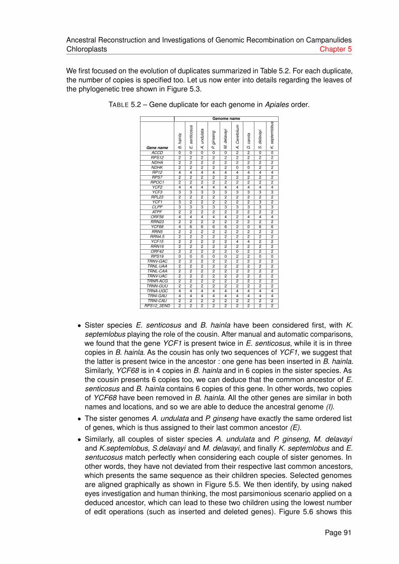
Ancestral Reconstruction and Investigations of Genomic Recombination on CampanulidesChloroplasts Chapter 5
We first focused on the evolution of duplicates summarized in Table 5.2. For each duplicate,the number of copies is specified too. Let us now enter into details regarding the leaves ofthe phylogenetic tree shown in Figure 5.3.
TABLE 5.2 – Gene duplicate for each genome in Apiales order.
Genome name
Gene name B.h
ainl
a
E.s
entic
osus
A.u
ndul
ata
P.gi
nsen
g
M.d
elav
ayi
A.C
eref
oliu
m
D.c
arot
a
S.d
elav
ayi
K.s
epte
mlo
bus
ACCD 0 0 0 0 0 2 2 0 0RPS12 2 2 2 2 2 2 2 2 2NDHA 2 2 2 2 2 2 2 2 2NDHK 2 2 2 2 2 0 0 2 2RP12 4 4 4 4 4 4 4 4 4RPS7 2 2 2 2 2 2 2 2 2
RPOC1 2 2 2 2 2 2 2 2 2YCF2 4 4 4 4 4 4 4 4 4YCF3 3 3 3 3 3 3 3 3 3RPL23 2 2 2 2 2 2 2 2 2YCF1 3 2 2 2 2 2 2 3 2CLPP 3 3 3 3 3 3 3 3 3ATPF 2 2 2 2 2 2 2 2 2
ORF56 4 4 4 4 4 2 4 4 4RRN23 2 2 2 2 2 2 2 2 2YCF68 4 6 6 6 6 2 0 6 6RRN5 2 2 2 2 2 2 2 2 2
RRN4.5 2 2 2 2 2 2 2 2 2YCF15 2 2 2 2 2 4 4 2 2RRN16 2 2 2 2 2 2 2 2 2ORF42 2 2 2 2 2 0 2 2 2RPS19 0 0 0 0 0 2 2 0 0
TRNV-GAC 2 2 2 2 2 2 2 2 2TRNL-UAA 2 2 2 2 2 2 2 2 2TRNL-CAA 2 2 2 2 2 2 2 2 2TRNV-UAC 2 2 2 2 2 2 2 2 2TRNR-ACG 2 2 2 2 2 2 2 2 2TRNN-GUU 2 2 2 2 2 2 2 2 2TRNA-UGC 4 4 4 4 4 4 4 4 4TRNI-GAU 4 4 4 4 4 4 4 4 4TRNI-CAU 2 2 2 2 2 2 2 2 2
RPS12_3END 2 2 2 2 2 2 2 2 2
• Sister species E. senticosus and B. hainla have been considered first, with K.septemlobus playing the role of the cousin. After manual and automatic comparisons,we found that the gene YCF1 is present twice in E. senticosus, while it is in threecopies in B. hainla. As the cousin has only two sequences of YCF1, we suggest thatthe latter is present twice in the ancestor : one gene has been inserted in B. hainla.Similarly, YCF68 is in 4 copies in B. hainla and in 6 copies in the sister species. Asthe cousin presents 6 copies too, we can deduce that the common ancestor of E.senticosus and B. hainla contains 6 copies of this gene. In other words, two copiesof YCF68 have been removed in B. hainla. All the other genes are similar in bothnames and locations, and so we are able to deduce the ancestral genome (I).
• The sister genomes A. undulata and P. ginseng have exactly the same ordered listof genes, which is thus assigned to their last common ancestor (E).
• Similarly, all couples of sister species A. undulata and P. ginseng, M. delavayiand K.septemlobus, S.delavayi and M. delavayi, and finally K. septemlobus and E.sentucosus match perfectly when considering each couple of sister genomes. Inother words, they have not deviated from their respective last common ancestors,which presents the same sequence as their children species. Selected genomesare aligned graphically as shown in Figure 5.5. We then identify, by using nakedeyes investigation and human thinking, the most parsimonious scenario applied on adeduced ancestor, which can lead to these two children using the lowest numberof edit operations (such as inserted and deleted genes). Figure 5.6 shows this
Page 91

Ancestral Reconstruction and Investigations of Genomic Recombination on CampanulidesChloroplasts Chapter 5
matching process applied on Meta_Delavayi and kalo_septemlobus, which have acore genome of 169 genes (only the 23 first genes are depicted). Note that, in thisexample, Meta_Delavayi (L) and kalo_septemlobus (M) match completely, so theancestor H is very easy to obtain (H = L ∩ M has 169 genes).
Fig. 5.5 – Graphical presentation of genes alignment between pairs of genomes (Bras_-hainla, Kalo_septemlobus) and (Bras_hainla, Meta_delavayi)
• Let us finally compare A. cerefolium and D. carota. YCF68 gene exists in 2 copies inA. cerefolium while it is missing in D. carota, as shown in Figure 5.7. The cousin, forits part, also contains the gene YCF68 (in 6 copies), and so our algorithm concludesto the presence of this gene (in 2 copies) in the ancestor of A. cerefolium and D.carota. Additionally, D. carota contains 4 copies of ORF56, while this gene is onlyrepresented twice in its sister. As the cousin genome has 4 representatives of ORF56,we can reasonably deduce that this is the case too in the ancestor of these two sisterspecies : two copies of the gene ORF56 have been deleted from the genome A.cerefolium. Such decisions are depicted in Figure 5.7 (B), which shows a specificregion of the ancestor genome (C). This region has been generated by our algorithm,which has been applied on A. cerefolium and D. carota, and it has been crossmanually validated.
The process detailed above continues with the obtained ancestors and is repeated untilreaching the root of the tree : the Last Universal Common Ancestor (LUCA) of Apiales.By operating this reconstruction stage, we found that chloroplasts of this order have notfaced so much deletion or insertion in their genomes. Indeed, in most of the cases, thedisparity comes from the variation in numbers of gene copies. The obtained results aresummarized in Figure 5.8.
5.4.2/ THE Asterales ORDER
We have then examined the Asterales order, which is close to the Apiales one. Table 5.3contains what has been deduced from our experiments on this order. As can be seen, As-
Page 92

Ancestral Reconstruction and Investigations of Genomic Recombination on CampanulidesChloroplasts Chapter 5
Fig. 5.6 – Graphical presentation of genes alignment between genomes Kalo_septemlobusand Meta_delavayi
Fig. 5.7 – (A) : Example of gene correspondances in sister genomes D. carota and A.cerefolium. For instance YCF68 is found in position 111 in A. cerefolium while it is missingfrom D. carota. Additionally, ORF56 is in 2 copies, positions 114 and 115, in D. carota,while this gene is only represented once at position 115 in its sister. (B) Comparisonbetween two sisters. The result is the ancestor genome (C). We can reasonably deducethat two copies of ORF56 have been deleted from genome A. cerefolium. The ancestor,for this part, contains too the gene YCF68, which has been deleted from the genome D.carota
terales genomes have faced much more modifications compared to the Apiales ones. Thisdifference between the two orders lead to a larger variation in the lengths of Asteralesgenomes.
For the sake of illustration, let us consider for instance the chloroplast of H. annuus.It only contains 161 coding sequences while its sister species, namely P. argentatum,has 183 genes. The matching process previously described has led in this case to anancestor of size 162. More precisely, 23 genes have been inserted and two other oneshave been deleted in P. argentatum, while only one gene has been removed in H. annuus,as described in Figure 5.9.
In this second order and in most cases, genes are comparable in both names and locations,
Page 93

Ancestral Reconstruction and Investigations of Genomic Recombination on CampanulidesChloroplasts Chapter 5
Fig. 5.8 – Insertion and deletion events found during ancestor reconstruction on Apialesorder. Letters in red refer to ancestor genomes (their lengths are provided too).
having the same positions if we do not consider duplicates. Indeed, almost all differences inthis set of chloroplastic genomes come from a variation in the number of copies, which hasbeen inferred well by our automatic tool. Let us now investigate a third order, to compare itwith Apiales (only a few variations of genomes) and Asterales (large variety in duplicates).
5.4.3/ THE Fabids ORDER
It was easy to deal with Apiales order, while Asterales improved the complexity of theancestral reconstruction, due to duplicates. However, in both cases the proposed algorithmwas able to recover results that have been inferred manually (naked eye investigation). Wenow consider a larger and more complicated order, namely the Fabids, to evaluate theperformances of our proposal when facing a complex collection of genomes.
Indeed, the main problem with this new order is that it contains large scale inversions insome branches, while it was not the case with the two other orders previously studied.In this case, a single inversion detection algorithm has been able to highlight helpfulinformation regarding such regions, like the beginning and the end (insertion or deletion)of reversals. However, the most difficult case where insertions or deletions are inside theinversion zone is difficult to handle.
In this situation, we proposed to select one of the two sisters to operate as a reference. Wethen search for the best cousin within the same clade, and we compare the status of eachgene in this region (matching, or need insertion or deletion). Most of the reversal regionswe considered match at the genes names level, but with reverse positions. Figure 5.10presents our finding on Fabids order, with information about the length of each node. Weprovide also various rearrangement information like the number of insertion, deletion, andinversion.
Page 94

Ancestral Reconstruction and Investigations of Genomic Recombination on CampanulidesChloroplasts Chapter 5
Fig. 5.9 – Summary of the complete ancestral genomes reconstruction of the Asteralesorder. Insertion and deletion events are provided, with names and length of each internalnode.
5.4.4/ COMPARISON WITH MLGO
For the sake of comparison, we have examined the ancestral genome contents ofboth Apiales and Asterales species with MLGO tool, which stands for Maximum Like-lihood for Gene Order Analysis 1. This latter is, to the best of our knowledge, the firstweb tool for phylogeny and ancestral genomes reconstruction compatible with genomerearrangements [6].
On the one hand, the ancestors in the Apiales order, provided either by our approach orwith MLGO, are very similar in terms of gene contents. However our method outperformsMLGO when investigating the specific location of genes and their number of duplicates.On the other hand, results are very different for some nodes in the Asterales case, assummarized in Table 5.4. For instance, when gene YCF1 in internal node d has 2 copies inboth of its two children and their closest cousin has 2 occurrences of this gene too. In thiscase, our algorithm proposes to set the number of YCF1 in d to 2, while MLGO producedonly one copy. Similar consequences can be outlined in the most difficult case, namelythe Fabids order, as highlighted by Table 5.5. At each time, our algorithm outperformsthe MLGO results by producing what is the most likely ancestral state (numbers of genesand their positions) in each situation. For instance, considering the ancestral node M, wefound that gene INFA is missing in the first child while it is present in the second one. Wealso found it in the two closest cousins, with one copy at each time. The most reasonablescenario is to consider that the ancestral node under consideration also has a single copyof INFA. This result is produced by our algorithm, while MLGO considers that M mustnot have INFA in its genome. Other divergent results can be reported, as in the ordinarycase of node E : gene ATPF is present once in each of the two children. So our algorithmconsiders that it is present once in E, while with MLGO, we found that this node mustcontain two copies of ATPF. Other nodes are problematic in the MLGO case, for example,
1. http://www.geneorder.org
Page 95

Ancestral Reconstruction and Investigations of Genomic Recombination on CampanulidesChloroplasts Chapter 5
Fig. 5.10 – A phylogenetic tree in the reconstruction of the Fabids ancestor and theunambiguous reconstruction accuracy of our algorithms on this tree. Alphabetic charactersrepresent the ancestors. L stands for the length of each node (number of genes), [D, I]describes the number of deletions and insertion, while inversions are indicated too.
{a, b, c, d} as can be seen in Table 5.5. Each time, our algorithm produces results inagreement with the one that have been deduced manually, while in some cases MLGOhas yielded surprising results.
Page 96

Ancestral Reconstruction and Investigations of Genomic Recombination on CampanulidesChloroplasts Chapter 5
TABLE 5.3 – Gene duplicate for each genome in Asterales order.
Genome name
Gene name G.a
byss
inic
a
J.vu
lgar
is
L.sa
tiva
A.f
rigid
a
C.i
ndic
um
C.m
orifo
lium
P.cl
emat
idea
A.a
deno
phor
a
H.a
nnuu
s
P.ar
gent
atum
ACCD 0 0 0 0 0 0 2 0 0 0NDHB 4 4 4 4 4 4 4 4 4 4RPS12 2 2 2 2 2 2 3 3 3 2NDHA 0 0 2 2 0 0 0 0 0 0NDHK 2 2 2 2 2 2 2 2 2 0NDHF 0 0 0 0 0 0 0 0 0 2RPL2 4 4 4 2 2 2 2 2 4 6RPS7 2 2 2 2 3 3 3 3 2 4YCF2 2 2 2 2 2 2 7 2 2 6YCF3 3 3 3 3 3 3 3 3 3 3RPL23 2 2 2 2 2 2 4 4 2 2YCF1 0 0 0 0 2 2 4 3 0 4CLPP 3 3 3 3 3 3 3 3 3 3ATPF 2 2 2 2 2 2 3 2 2 2
ORF56 4 4 4 4 4 4 4 4 4 4RRN23 2 2 2 2 2 2 2 2 2 2YCF68 2 6 2 2 4 4 5 4 2 2RRN5 2 0 2 2 2 2 2 2 2 0
RRN4.5 2 2 2 2 2 2 2 2 2 0YCF15 2 4 2 2 2 2 2 2 2 0RRN16 2 2 2 2 2 2 2 2 2 0ORF42 2 2 2 2 2 2 0 2 2 0RPS19 2 0 0 0 0 0 3 3 2 2RPL14 0 0 0 0 0 0 2 2 0 0RPS3 0 0 0 0 0 0 0 0 0 2
ORF188 0 0 0 0 0 0 0 0 0 0CCSA 0 0 0 0 0 0 0 0 0 0RPOB 0 0 0 0 0 0 0 0 0 3RPOA 0 0 0 0 0 0 0 0 0 2PSBD 0 0 0 0 0 0 0 0 0 3
TRNA-UGC 4 4 4 5 5 5 4 4 4 2TRNI-GAU 4 4 4 4 4 4 4 4 4 4TRNI-CAU 0 2 0 0 0 0 0 0 2 2TRNI-ACG 2 0 2 2 2 2 2 2 0 0TRNR-ACG 2 2 2 2 2 2 2 2 2 2TRNN-GUU 2 2 2 2 2 2 2 2 2 2TRNV-GAC 2 2 2 2 2 2 2 2 2 0TRNL-UAA 2 2 2 2 2 2 2 2 2 0TRNL-CAA 2 2 2 2 2 2 4 4 2 0TRNV-UAC 2 0 2 2 2 2 2 2 2 0TRNF-GAA 2 0 0 0 0 0 2 2 0 0TRNT-GGU 0 0 0 2 2 2 0 0 0 0TRAN-GCA 0 0 0 0 0 0 2 2 0 0TRNS-GCU 0 0 0 0 0 0 2 3 2 2TRNR-UCU 0 0 0 0 0 0 0 0 0 2
RPS12_3END 2 2 2 2 2 2 2 2 2 2
TABLE 5.4 – The variation in comparison results of ancestral genomes nodes on Asteralesorder with MLGO.
Species genome Ancestor resultsAncestor
nodeGenename
Genome 1(Nb of genes)
Genome 2(Nb of genes)
Cousin genome 1(Nb of genes)
Cousin genome 2(Nb of genes) Ancestor MLGO
j RPOA 1 2 3 2 2 1g RPOA 2 2 1 1 2 1g TRNF-GGA 2 1 2 2 2 1e TRNF-GGA 2 2 1 1 2 1d YCF1 2 2 2 1 2 1
Page 97

Ancestral Reconstruction and Investigations of Genomic Recombination on CampanulidesChloroplasts Chapter 5
TABLE 5.5 – The variation in ancestral genomes nodes which were achieved by comparingour method results with MLGO tool on Fabids order.
Species genome Ancestor resultsAncestor
nodeGenename
Genome 1(Nb of genes)
Genome 2(Nb of genes)
Cousin genome 1(Nb of genes)
Cousin genome 2(Nb of genes) Ancestor MLGO
M INFA — 1 1 1 1 —N ACCD 2 2 2 1 2 1T ACCD 1 2 2 2 2 1Q YCF1 1 2 1 1 1 2E NDHK 2 2 1 1 2 1E INFA 2 1 — — 1 —E ATPF 1 1 2 2 1 2d RPS16 2 — 1 1 1 2c RPS19 2 1 2 2 2 1b RPS19 2 2 1 2 2 1a PSBG 1 — — — — 1a TRNK-UUU 2 1 2 — 2 1a NDHK 1 2 2 — 2 1
Fig. 5.11 – Example of comparison with MLGO on Apiales order. We show similarityin gene contents between our results, ancestor node (C), and ancestor node (A1) fromMLGO.
Heli_annuus
Pana_ginseng
Aral_undulata
Sche_delavayi
Bras_hainla
Eleu_senticosus
Kalo_septemlobus
Meta_delavayi
Dauc_carota
Anth_cerefolium
A9
A8
A1A1
A8
A7
A5
A4
A2A2
A4
A3A3A5
A7
A6A6
A9
Fig. 5.12 – Apiales order tree produced by MLGO.
Page 98

Ancestral Reconstruction and Investigations of Genomic Recombination on CampanulidesChloroplasts Chapter 5
5.5/ CONCLUSION
This chapter has presented a first ancestral reconstruction of gene content and order andits application to Apiales, Astrales, and Fabids orders. The approach can be considered asa recursive tree reduction. Experiments have shown that this approach is more accuratethan MLGO which is considered as the state of the art tool for genomes reconstruction.
Page 99


6ON THE ABILITY TO RECONSTRUCT
ANCESTRAL GENOMES FROMMycobacterium GENUS
In this thesis, we state that, even if the ancestral reconstruction problem is NP-hard intheory, its exact resolution is feasible in various situations. The previous chapter focused
on organelles that contain various genomic changes caused by rearrangements, like geneduplication and loss. However, we claimed that the small size of these genomes make itpossible to deal in practice with the ancestral reconstruction problem. In this chapter, weenlarge the size of genomes by considering particular bacteria, namely some clonal ones.In the latter, the increase of the genome size is balanced by the decrease of recombinationevents, when compared with chloroplasts. This is the reason why we claim that theancestral reconstruction problem is tractable too for such genomes, even if tools andalgorithms introduced in the previous chapter must be adapted to the bacterial reign. Suchaccurate reconstruction, which identifies too some highly homoplasic mutations will beapplied in this chapter, to two Mycobacterium pathogenetic bacterias. By mixing automaticreconstruction of obvious situations with human interventions on signaled problematiccases, we will indicate that it should be possible again to achieve a concrete, complete,and really accurate reconstruction of lineages of the Mycobacterium tuberculosis complex.Thus, it is possible to investigate how these genomes have evolved from their last commonancestors. Let us finally note that the content of this chapter has been presented in theIWBBIO conference, 2017 edition [101].
6.1/ INTRODUCTION
Mycobacterium tuberculosis is presently still one of the principal causes of death world-wide. Approximately one-third of the world population is infected by the Mycobacteriumtuberculosis complex (MTBC), with about 9 million event cases annually, leading to es-timated a million deaths each year. Due to their different host tropism and phenotypes,members of MTB complex display various pathogenicities ranging from particularly human(M. tuberculosis, M. africanum, and M. canetti) or rodent pathogens (M. microti) to Myco-bacteria with a broad host spectrum (like M. bovis, see [102, 103, 104]). Mycobacteriumtuberculosis has been in the human population for thousands of years, as fragments of thespinal column of Egyptian mummies from 2300 BCE show definite pathological signs of
101
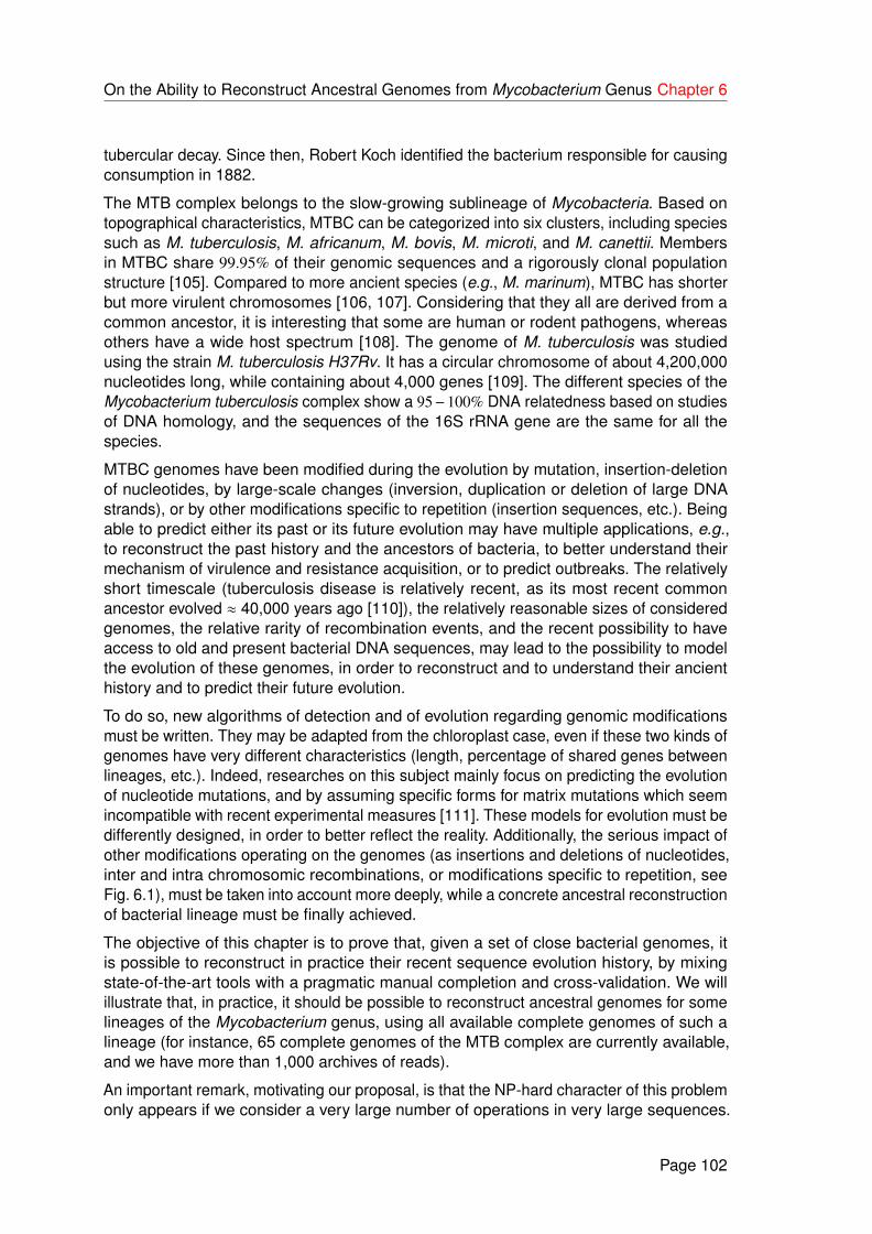
On the Ability to Reconstruct Ancestral Genomes from Mycobacterium Genus Chapter 6
tubercular decay. Since then, Robert Koch identified the bacterium responsible for causingconsumption in 1882.
The MTB complex belongs to the slow-growing sublineage of Mycobacteria. Based ontopographical characteristics, MTBC can be categorized into six clusters, including speciessuch as M. tuberculosis, M. africanum, M. bovis, M. microti, and M. canettii. Membersin MTBC share 99.95% of their genomic sequences and a rigorously clonal populationstructure [105]. Compared to more ancient species (e.g., M. marinum), MTBC has shorterbut more virulent chromosomes [106, 107]. Considering that they all are derived from acommon ancestor, it is interesting that some are human or rodent pathogens, whereasothers have a wide host spectrum [108]. The genome of M. tuberculosis was studiedusing the strain M. tuberculosis H37Rv. It has a circular chromosome of about 4,200,000nucleotides long, while containing about 4,000 genes [109]. The different species of theMycobacterium tuberculosis complex show a 95−100% DNA relatedness based on studiesof DNA homology, and the sequences of the 16S rRNA gene are the same for all thespecies.
MTBC genomes have been modified during the evolution by mutation, insertion-deletionof nucleotides, by large-scale changes (inversion, duplication or deletion of large DNAstrands), or by other modifications specific to repetition (insertion sequences, etc.). Beingable to predict either its past or its future evolution may have multiple applications, e.g.,to reconstruct the past history and the ancestors of bacteria, to better understand theirmechanism of virulence and resistance acquisition, or to predict outbreaks. The relativelyshort timescale (tuberculosis disease is relatively recent, as its most recent commonancestor evolved ≈ 40,000 years ago [110]), the relatively reasonable sizes of consideredgenomes, the relative rarity of recombination events, and the recent possibility to haveaccess to old and present bacterial DNA sequences, may lead to the possibility to modelthe evolution of these genomes, in order to reconstruct and to understand their ancienthistory and to predict their future evolution.
To do so, new algorithms of detection and of evolution regarding genomic modificationsmust be written. They may be adapted from the chloroplast case, even if these two kinds ofgenomes have very different characteristics (length, percentage of shared genes betweenlineages, etc.). Indeed, researches on this subject mainly focus on predicting the evolutionof nucleotide mutations, and by assuming specific forms for matrix mutations which seemincompatible with recent experimental measures [111]. These models for evolution must bedifferently designed, in order to better reflect the reality. Additionally, the serious impact ofother modifications operating on the genomes (as insertions and deletions of nucleotides,inter and intra chromosomic recombinations, or modifications specific to repetition, seeFig. 6.1), must be taken into account more deeply, while a concrete ancestral reconstructionof bacterial lineage must be finally achieved.
The objective of this chapter is to prove that, given a set of close bacterial genomes, itis possible to reconstruct in practice their recent sequence evolution history, by mixingstate-of-the-art tools with a pragmatic manual completion and cross-validation. We willillustrate that, in practice, it should be possible to reconstruct ancestral genomes for somelineages of the Mycobacterium genus, using all available complete genomes of such alineage (for instance, 65 complete genomes of the MTB complex are currently available,and we have more than 1,000 archives of reads).
An important remark, motivating our proposal, is that the NP-hard character of this problemonly appears if we consider a very large number of operations in very large sequences.
Page 102

On the Ability to Reconstruct Ancestral Genomes from Mycobacterium Genus Chapter 6
Fig. 6.1 – Various genome rearrangement events.
On our side and with the chosen bacteria, we will consider quite small sequences and arelatively small number of large scale recombinations. So we face tractable problems invarious real situations, on which simple and pragmatic approaches may work.
6.2/ A CONCRETE SEMI-AUTOMATIC ANCESTRAL RECONSTRUC-TION
Fig. 6.2 – Representation of a multiple sequence alignment.
The complete sequences of the 65 Mycobacterium genomes available on the NCBI 1 havebeen downloaded. Listed according to their species, 42 genomes of tuberculosis, 15 bovis,2 africanum, 5 canettii, and 1 microti have been recovered. Table 6.1 shows informationabout some of these Mycobacterium genomes. Among this MTBC, we particularly focusedon tuberculosis and on canettii because the virulent tuberculosis species is supposedto have emerged from canettii forty thousand years ago. To verify such an evolutionaryhypothesis, the first task of our approach, proposed to achieve an ancestral reconstructionof close genomes, is to perform a multiple sequence alignment of the sequences. Thistask is described in the next section.
1. ftp ://ftp.ncbi.nih.gov/genomes
Page 103

On the Ability to Reconstruct Ancestral Genomes from Mycobacterium Genus Chapter 6
TABLE 6.1 – Information about some Mycobacterium genomes.
Organism name Accession Sequence length Number of genesMycobacterium tuberculosis W-148 NZ_CP012090.1 4,418,548 bp 4,133Mycobacterium tuberculosis H37Rv NC_018143.2 4,411,709 bp 4,132Mycobacterium africanum GM041182 NC_015758.1 4,389,314 bp 4,089Mycobacterium africanum strain 25 CP010334.1 4,386,422 bp 4,798Mycobacterium microti strain 12 CP010333.1 4,370,115 bp 4,321Mycobacterium canettii CIPT 140010059 NC_015848.1 4,482,059 bp 4,137Mycobacterium canettii CIPT 140070008 NC_019965.1 4,420,197 bp 4,103Mycobacterium bovis strain ATCC BAA-935 NZ_CP009449.1 4,358,088 bp 4,095Mycobacterium bovis BCG str. Tokyo 172 NZ_CP014566.1 4,371,707 bp 4,076
6.2.1/ MULTIPLE SEQUENCE ALIGNMENT
The first problem of this alignment stage, is to identify a common starting point in thesecomplete circular genomes. In order to do so, we searched for a reference sequence of200 nucleotides from M. tuberculosis H37Rv, and we found it or its transconjugate in eachgenome using a local blast. Then, a circular rotation (together with a transconjugate opera-tion if needed) has been performed on each complete genome, so that each sequencestarts with the same 200 nucleotides, if we except SNPs. Once these sequences havebeen operated to share the same orientation and starting location, the overall alignment ofeach chromosome has been performed.
Alignment of large sets of sequences is a common task during biological investigationsand has a wide variety of applications incorporating homology detection [112], findingevolutionarily relevant sites, and phylogenetics. A multiple sequence alignment, as depictedin Figure 6.2, may explain many aspects about a gene : which regions are constrained,which sites undergo positive selection [113], and potentially the structure of its geneproduct [114]. Furthermore, aligning sequences can help to detect events of mutations orrecombination in couples of close genomes.
To achieve such an alignment, we thus have considered the AlignSeqs function fromDecipher R package [115]. Indeed, after various tests on well known alignment tools thatcan perform a large MSA on several to tens of thousands of sequences, like MAFFT [116],we found that package was the only one that achieved to align complete bacterial genomeswith a good accuracy. AlignSeqs performs group-to-group alignment [117, 118], and alignsa sequence established by merging groups along a guide tree until all the input sequencesare aligned, as shown in Figure 6.2.
This AlignSeqs function takes as input two aligned sets of DNA sequences and returns amerged alignment. It can be used to achieve multiple sequence alignment on sequences ofthe same kind. Indeed, multiple alignments are accomplished by aligning two sequences,merging with another sequence, combining with another set of sequences, and so onuntil all the sequences are aligned [119, 117]. We thus obtained a first representation ofsynteny of the whole 65 Mycobacterium genomes, which is depicted in Figure 6.3. It can beobserved that these 65 genomes have a high sequence similarity with low recombinationevents.
Page 104

On the Ability to Reconstruct Ancestral Genomes from Mycobacterium Genus Chapter 6
6.2.2/ PHYLOGENETIC STUDY
This first representation of synteny blocks, obtained thanks to the multiple sequencealignment of the whole Mycobacterium genus, has allowed us to detect the location ofa few large scale inversions. We thus have been able to manually invert again theseinversions, so that the multiple alignment became quite perfect, if we except small indelsand SNPs. It is then possible to use all the 65 complete genomes in the next stage, namelythe phylogenetic study.
Indeed, the evolutionary history of our population of genomes can be represented asa phylogenetic tree using the multiple sequence alignment combined with manual localinversions previously obtained. As previously recalled, various methods are well establi-shed in the literature to investigate the best phylogenetic tree for a given set of alignedsequences. On our side, we decided to consider the use of RAxML as a default phyloge-netic tree reconstruction toolkit, a well known and reputed software based on maximumlikelihood [1, 46].
As we reversed the inversions, our phylogenetic investigations are based on the wholegenome. This leads to well supported and trustworthy trees of strains, on which we canreliably consider to reconstruct ancestral states. As an illustrative example, we representthe phylogenetic trees of M. canettii species with the M. tuberculosis outgroup in Figure 6.4.This very well supported tree has been obtained using RAxML with GTR Gamma model asadvised by JModelTest 2.0. The M. tuberculosis phylogeny, for its part, leads to bootstrapsupports larger than 98%, as shown in Figure 6.5.
Note that, with these bacteria, we have not to find the largest subset of core sequencesthat leads to the most supported tree, as aligning the whole complete genomes leads toa well supported tree : it is not possible to improve the results, which is nice as the coregenome is many times greater than in the chloroplast case. Indeed, let us recall that M.tuberculosis species have 42 genomes with size 4Mb and 4000 genes, while in the casestudy on the chloroplasts, the genome has around 271 pan genes in maximum. So, itis not sure that the heuristic approach to find the core gene of the previous chapter cansucceed to find the well-supported phylogenies).
Having an accurate representation of the general evolution of MTBC strains due to thisphylogenetic study, we are then left to reconstruct the ancestral states of the alignmentat each internal node of the tree. This final ancestral reconstruction will be applied in twostages, considering first the variants of length 1 in the alignment (namely, single nucleotidepolymorphism and indels of 1 nucleotide), and then larger variants that mainly consist ofinsertion or deletion of a subsequence at a location in the tree.
6.2.3/ ANCESTRAL RECONSTRUCTION : MONONUCLEOTIDIC VARIANTS
Focusing on mononucleotidic variants, we separated the treatment of single nucleotidepolymorphisms (SNPs) versus insertion-deletions (indels). For the former, the situationseems quite simple, the only problem being to prevent confusion between a “true” SNPand a SNP induced by a recombination of the indel kind. For the latter, future challengesencompass to determine which indels are related to tandem repeats, which are associatedwith mobile elements, or which are due to repeated sequences. Let us detail each casehereafter.
Page 105

On the Ability to Reconstruct Ancestral Genomes from Mycobacterium Genus Chapter 6
Regarding SNPs, the ancestral reconstruction is achieved as follows. The marginal proba-bility distributions for bases at ancestral nodes in the phylogenetic tree are first calculated.These distributions are obtained using the sum-product message passing algorithm [120],assuming independence of sites. The ancestral reconstruction is done by using PHASTsoftware [121], which reconstructs indels too by parsimony, also assuming site indepen-dence. Obtained results on mononucleotidic variants are then carefully visually checked,as the number of such variants is not excessive, see Tables 6.2 and 6.3.
At the end, 2,956 SNPs and 166 indels have been found in the alignment of the cladeconstituted by the 5 strains of M. canettii, as shown in Figure 6.6. The Figure 6.7, for itspart, represents the location of the 394 SNPs and of the 25 indels that have been found inthe alignment of the clade constituted by 8 genomes of M. tuberculosis.
6.2.4/ ANCESTRAL RECONSTRUCTION OF LARGER VARIANTS
Mycobacterium species considered in this chapter are highly conserved, with really similarregions and without rearrangement. As previously evoked, we found only a few signifi-cant inversions, like the one at the last common ancestor of strains CIPT 140010059,140070010, 140060008, 140070017, and 140070008, as shown in Figure 6.9. The Fi-gure 6.10, for its part, is a dotplot representing these homologous regions, as identifiedby the FindSynteny function in R. All the Synteny blocks of the 42 M. tuberculosis arefinally depicted in Figure 6.8, where we have obtained 99% of DNA sequence identity. Tosum up, if we except a large scale inversion, we can only report some small indels at thisrecombination level.
Ad hoc algorithms have then been designed to deal with mid size variants. More specifically,we have written first a string algorithm that detects small and noisy inversions, but thelatter, distributed on our supercomputer facilities, was only able to detect artifacts. Soeither the MTBC genomes have not faced inversion events during its recent history, orthis recombination case still needs further investigations. Authors tend to prefer the firstpossibility, as Mycobacterium genomes evolve in a clonal manner (which is not the case,for instance, with Yersinia genus, in which a large amount of mobile elements has led toa large number of reported inversions [122]). Duplication, for its part, has not yet beeninvestigated but, as for inversions, the analysis of synteny blocks tends to show that suchevents are rare, at least if we consider the large scale ones.
Both indels of midsize and SNPs have been deeply studied, using PHAST software asdetection tool. From obtained results, we can conclude the following points. (1) Suchevents are quite rare in some lineages of the MTB complex like tuberculosis, as describedin Table 6.4. (2) Most of the times, the situation is very easy to manually understand,leading either to an insertion or to a deletion at an obvious internal node of the tree,as illustrated in Figure 6.11 and 6.12. (3) Most of the times, the inserted motif has notfaced mutations during evolution : leaves that contain the motif have no mutation in it,thereby contributing to an easy to resolve situation. (4) Surprisingly, ancestral statesrecovered by PHAST and its parsimony approach leads to disappointing results. Similarly,obviously wrong results have been obtained with state-of-the-art competitor software. Tosum up, a manual reconstruction of mid size indels is possible, due to the low number ofthese recombinations that are mainly very easy to resolve, while automatic tools from theliterature are not currently able to do it.
All these steps are summarized in Figure 6.15. In this one, gray boxes correspond to
Page 106

On the Ability to Reconstruct Ancestral Genomes from Mycobacterium Genus Chapter 6
TABLE 6.2 – Number of alignment columns with polymorphism, by pair of strains, on M.canettii genomes. Note that, when a large string is deleted at some location in the tree, allthe characters of this deletion are counted here.
canettii0 canettii1 canettii2 canettii3 canettii4 tuberculosis1canettii0 0 3524 27256 60957 4833 3354canettii1 3524 0 27260 61233 7971 1150canettii2 27256 27260 0 62717 27468 27437canettii3 60957 61233 62717 0 60987 61346canettii4 4833 7971 27468 60987 0 7510
tuberculosis1 3354 1150 27437 61346 7510 0
TABLE 6.3 – Variations in the alignment of M. tuberculosis
tuberculosis4 tuberculosis19 tuberculosis17 tuberculosis16 tuberculosis27 tuberculosis28 tuberculosis24 tuberculosis10tuberculosis4 0 199770 214401 219205 216387 217235 216919 217186
tuberculosis19 199770 0 212403 219039 216908 216672 216726 216953tuberculosis17 214401 212403 0 216808 216534 217011 216786 216882tuberculosis16 219205 219039 216808 0 216669 216916 216251 216678tuberculosis27 216387 216908 216534 216669 0 142974 189148 199505tuberculosis28 217235 216672 217011 216916 142974 0 189460 199412tuberculosis24 216919 216726 216786 216251 189148 189460 0 194315tuberculosis10 217186 216953 216882 216678 199505 199412 194315 0
M. canettii SNPsFathers Children No. of SNPs
100.2 canettii2 1041canettii3 12398
100 canettii0 1canettii1 9
100.3 100 28100.2 735
100.X 100.3 111canettii4 438
M. tuberculosis SNPsFathers Children No. of SNPs
100 tuberculosis19 5tuberculosis17 14
100.2 tuberculosis24 1tuberculosis10 0
100.3 tuberculosis27 0tuberculosis28 0
98 100.2 1100.3 0
100.4 98 0tuberculosis16 1
100.X 100 5100.4 1
TABLE 6.4 – Number of SNPs in the considered species (100.X refers to an ancestral node,as in the tree)
manual steps whereas all the other ones are automatically executed. Indeed, obtainedresults on mononucleotidic variants have been carefully checked by naked eye, as thenumber of such variants is not excessive, while ad hoc algorithms were designed to dealwith variants of larger size, see Figures 6.13 and 6.14.
Page 107

On the Ability to Reconstruct Ancestral Genomes from Mycobacterium Genus Chapter 6
Fig. 6.3 – A synteny representation of all available Mycobacterium strains
canettii3
canettii2
canettii4
canettii0
canettii1
tuberculosis1
100
100
100
0
0.0222492341505057
1.13350463263489
0.0028540642378931
0.000822467770649221
0.0420622817927064
0.011128511153227
0.0000251084644880016
0.00015886107370991
0.00138470441710612
0.00138470441710612
Fig. 6.4 – Well-supported phylogenies on M. canettii species using a M. tuberculosis asoutgroup
Page 108

On the Ability to Reconstruct Ancestral Genomes from Mycobacterium Genus Chapter 6
tuberculosis3
tuberculosis27
tuberculosis21
africanum0
tuberculosis11
tuberculosis16
tuberculosis2
tuberculosis12
tuberculosis10
tuberculosis5
tuberculosis28
tuberculosis17
tuberculosis24
tuberculosis8
tuberculosis20
tuberculosis4
tuberculosis19
tuberculosis6
tuberculosis14
98
100
100
100
100
100
100
100
100
100
98
100
100
100
100
100
0.0000197020502557342
0.000110031487841622
0.0000262697916791557
0.0000445672479343333
0.000470208864616972
0.0000328560867679076
0.0000572775641172595
0.0000825812274753868
0.0000348426039531669
0.0000657198304253068
0.000040813411144852
0
0.000440969058963007
0.0000334339625761579
0.0000848608674630182
0.0000764940408430897
0.000214940772553843
0.00000985577022640209
0.0000295627107053678
0.000292343251339158
0.000019782816389073
0.000138990850469072
0.0000136922898245743
0.000373290242880245
0.0000399151178664264
0.000019715364200289
0.000271655696976591
0.00000328557392262749
0.0000471848635404516
0.000040677226965614
0.0000459819967599828
0.000152378355803515
0.000080766982286315
0.000148542094443374
0.00016050594824306
0.0000290924035100542
0.000470208864616972
Fig. 6.5 – Well-supported phylogenies of M. tuberculosis species with M. africanum asoutgroup. Phylogenetic trees have been calculated on the entire genomes with RAxMLand GTR Gamma model
Page 109

On the Ability to Reconstruct Ancestral Genomes from Mycobacterium Genus Chapter 6
Fig. 6.6 – SNPs location of mononucleotidic variants of M. canettii.
Fig. 6.7 – SNPs location of mononucleotidic variants of M. turberculosis.
Page 110
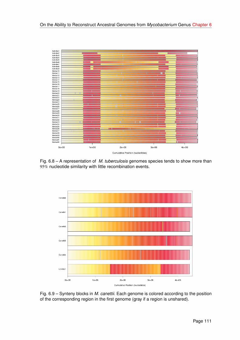
On the Ability to Reconstruct Ancestral Genomes from Mycobacterium Genus Chapter 6
Fig. 6.8 – A representation of M. tuberculosis genomes species tends to show more than95% nucleotide similarity with little recombination events.
Fig. 6.9 – Synteny blocks in M. canettii. Each genome is colored according to the positionof the corresponding region in the first genome (gray if a region is unshared).
Page 111

On the Ability to Reconstruct Ancestral Genomes from Mycobacterium Genus Chapter 6
Fig. 6.10 – Dot plots provide an alternative representation of the synteny map of M. canettii.Black diagonal lines show syntenic regions sharing the same orientation, whereas redanti-diagonal ones represent blocks of synteny between opposite strands. The descriptionof all of these species tends to show a high sequence similarity with little recombinationevents.
Page 112

On the Ability to Reconstruct Ancestral Genomes from Mycobacterium Genus Chapter 6
Fig. 6.11 – The insertions and deletions of nucleotides (indels) on the internal node ofthe tree (a) represent the nucleotides contain the ancestor nodes and their children on M.canettii species
Page 113

On the Ability to Reconstruct Ancestral Genomes from Mycobacterium Genus Chapter 6
Fig. 6.12 – Example of an ancestral reconstruction of one problematic column in thealignment
Page 114

On the Ability to Reconstruct Ancestral Genomes from Mycobacterium Genus Chapter 6
Fig. 6.13 – Ancestral reconstruction examples on M. canettii species
Page 115

On the Ability to Reconstruct Ancestral Genomes from Mycobacterium Genus Chapter 6
Fig. 6.14 – Ancestral reconstruction examples on M. tuberculosis species
Page 116

On the Ability to Reconstruct Ancestral Genomes from Mycobacterium Genus Chapter 6
Fig. 6.15 – Flowchart of the proposed approach.
Page 117

On the Ability to Reconstruct Ancestral Genomes from Mycobacterium Genus Chapter 6
6.3/ DISCUSSION
The obtained ancestors have not yet been studied in this chapter. They will be investigatedwith updated and improved algorithms, encompassing mobile elements and gene contentevolution analyzes. In order to do so, we will consider the phylogenetic tree whose leaveswill contain sets of genes, and we will compute core and pan genomes at each internalnode of the tree. Having this core and pan tree, we will design an algorithm to investigatemore deeply the evolution of these pan and core genomes over the tree, to see if somebranches can be related to hot spots of evolution. We thus intend to determine at whichrate such loss or gain occurs, and which kinds of functionality are concerned. We willfinally compute how much mutations fall inside a coding sequence, by studying whichkind of genes has evolved on the phylogenetic tree, by wondering if the mutation ratehas changed over time, and if such mutability can be related to environmental events. Inother words, we will wonder which variations have been potentially significant among thenumerous events that have been found when aligning these sequences.
With such a pipeline, we intend to investigate the following questions. Are some recombina-tions at the origin of severe tuberculosis epidemics ? Are transposases responsible of suchrecombinations like inversions [123, 124] ? Are transposases in general more present inM. tuberculosis (affecting humans) than in M. africanum, M. bovis, or M. bovis BCG ? Arethey related to the virulence of the strain ? How core and pan genomes have evolved overtime in this complex ? Finally, we will compare the last common ancestor of this complexto a M. canettii, to see if the canettii ancestor hypothesis can be verified by the ancestralreconstruction way.
At this point, our partial conclusion is that the reconstruction of ancestral sequences ispossible, at least in the case of close and clonal bacterias. Furthermore, elements beingpart of this reconstruction have already been designed, at least in their first revision (forinstance to detect and deal with mononucleotidic variants). However, the MTB complexseems to be a little too complicated for a first deep investigation of semi-automatic recons-truction of ancestral sequences of bacteria, and a genus like Brucella may be more easyto deal with in a first concrete investigation of this problem.
6.4/ CONCLUSION
In this chapter, we have firstly emphasized that, even if various algorithms and software al-ready exist to face the NP-hard character of the ancestral genome reconstruction problem,they do not work perfectly, in particular when SNPs or indels fall into repeated sequences.We have then argued that, when regarding the relatively low number of mutation andrecombination events in such Mycobacterium, a pragmatic approach is possible. We haveproposed to reconstruct all ancestors of all complete available genomes of Mycobacteriumtuberculosis and of M. canettii. The study has started by investigating single nucleotidepolymorphism level, while indels and large scale recombination are regarded in a secondstage. Our conclusion is that, by mixing automatic reconstruction of obvious situationswith human interventions on signaled problematic cases, it may be possible to achievea concrete, complete, and really accurate reconstruction of some specific bacteria li-neages. We can thus investigate how these genomes have evolved from their last commonancestors.
Page 118

IVCONCLUSION
119

7CONCLUSION AND PERSPECTIVES
7.1/ CONCLUSION
In this thesis work, we made significant progress in the quest of the ancestral genome ofchloroplasts and of MTBC. A large set of complete chloroplast genomes has first beenstudied de novo regarding both core and pan genomes, phylogenetic relationship, andgene content modifications. We then started to explore the produced data, by emphasizingsome remarkable relations between well-known events of chloroplast history and theevolution of gene contents over the phylogenetic tree.
Three metaheuristics have then been used (genetic algorithm, binary particle swarmoptimization, and simulated annealing) to produce a well supported phylogenetic treebased on the largest possible subset of core genes. They have been evaluated on varioussets of chloroplast species and deployed on a supercomputer facilities. Given the averagebetween the percentage of core genes and the lowest bootstrap as scoring function,we have shown on simple examples that, given a set of species, various global optimawith contradictory topologies can be reached. These first experiments emphasize thatsometimes the phylogeny of chloroplasts cannot perfectly be resolved using a tree : aphylogenetic network may be more close to the reality, branches within this network beingas strong as the associated tree topology is frequent.
We have first investigated the gene order problem and DNA ancestral coding sequencereconstruction in the case of organelles. We applied our designed methods to the case ofchloroplasts, which is more complex than mitochondria due to the size of the genomes,gene prediction issues, and because two chloroplasts do not share the same genes. Ateach time, we have considered all currently available complete genomes, and we haveapplied ancestral state reconstruction algorithms coupled with careful human curation.
After having investigated our ability to reconstruct all ancestors of all complete availablegenomes of Campanulids chloroplasts, we then considered larger genomes by focusingon the ancestral reconstruction of Mycobacterium pathogenetic bacterias. The studystarted by investigating manually large scale recombination and then focusing on bothsingle nucleotide polymorphism and indels using PHAST and human operations. Indeed,by mixing automatic reconstruction of obvious situations with human interventions onsignaled problematic cases, we have shown that a concrete, complete, and really accuratereconstruction of the lineage ancestors can be achieved.
121

Conclusion and Perspectives
7.2/ FUTURE WORK
Genomes of chloroplasts have notably lost functional genes, either because they becomeineffective or due to transfer to the nucleus. We thus first plan to determine more preciselythe rate of such loss, whether this is indeed related to a nucleus transfer, and which kindof functionality is practically concerned. Indeed, this thesis is an ongoing work regardinginvestigating more systematically such relations between remarkable ancestral nodes inthe tree, endosymbiosis events, and evolution of gene content. We will wonder whethersome branches of the trees are statistically remarkable when considering gene content(for instance, do we have a correlation between the presence or absence of a subset ofgenes, and a particular taxonomy). Then, the gene ordering and content of each ancestralnode will be computed using ad hoc algorithms. Ancestral DNA sequence reconstruction,which has been initiated here, will be totally inferred, and ancestral intergenic regionswill be deduced, in order to have all ancestral genomes with confidence indications likeprobabilities.
We will then wonder if evidence of the Cyanobacteria origin of chloroplasts can be statedusing our approach. In particular, the last universal common ancestor of all chloroplastswill be compared to available cyanobacterial genomes, regarding gene contents and DNAsequences, to see if a cyanobacterial origin of chloroplasts can be assessed by the meanof ancestral reconstruction. At this stage, it may be interesting to compare both ancestors(of chloroplasts on the one hand, and of Cyanobacteria on the other hand).
Concerning our heuristic approaches for detecting blurring genes in phylogenetic studies,we note that networks can be obtained by merging gene trees. In future work, we willpropose a way to obtain such networks with large subsets of random core genes, and willshow that such ways reinforce the stability and the confidence of the network. We intendto provide too criteria for deciding if either a tree or a network is preferable for a givenset of DNA sequences. We will measure the impact of this choice and of the coexistenceof different well-supported topologies on works like ancestral genome reconstruction.Finally, the various ways to set up the metaheuristics proposed here will be systematicallyinvestigated, to find the best manner to configure these ones when targeting the largestsubset of core genes leading to the most supported tree or network.
Practically speaking, we intend to reconstruct all ancestors of all complete availablegenomes of specific bacteria strains. We plan to start to reconstruct the ancestors of theBrucella abortus lineage, in which the low number of indels, mutations, and inversionsallow a human validation of the complete reconstruction. This first study will be enlargedto the whole Brucella genus, using all available complete genomes. More complex but stillclonal genomes will then be investigated, to go deeper in the study and understandingof genomic recombinations. Targeted bacterias will be the Yersinia pestis on the onehand, and Pseudomonas aeruginosa on the other hand. Moreover, we intend to comparethem with ancient DNA when available (like for Y. pestis). In parallel, original mathematicaldescription of some recombination mechanisms will be proposed, encompassing branchingprocess and partial differential equation approaches for modeling mobile elements. We willthen study which kinds of genes (in terms of functionality) have mutated over time, if themutation rate has evolved among branches of the phylogenetic tree, and if such mutabilitycan be related to environmental events.
We want to correlate the evolutionary history of microorganisms to epidemiological data :events of genomic recombination may be related to epidemic outbreaks. Moreover, such
Page 122

Conclusion and Perspectives
putative correlations may be learned by deep learning algorithms, leading to a new wayto predict epidemic risks. Finally, we intend to develop and test new bioinformatic tools :Dummy logit regression and LASSO test to evaluate effects of genes on phylogeny ;automated core and pan genomes extraction ; Laplacian eigenmaps with Gaussian mixturemodel for sequence clustering ; deep learning algorithms to detect insertion sequences,virulent factors, and other sequences of interest... Finally, all the knowledge gained andtools developed regarding the evolution of genomes will be applied to cancer diseases, bycomparing the evolution of genomes between healthy and tumorous cells.
Page 123


VAPPENDIX
125

8APPENDIX
Listing 8.1 – This code is to download genbank or unannotated fasta files.
from Bio import Entrez,SeqIOfrom tabulate import tabulatefrom sys import argvfrom numpy import array,savetxtimport osimport xlsxwriter
Entrez.email = ’[email protected]’gbk=’Genomes_gb/’ # the folder to store gbk filesfasta=’Genomes_fasta/’ # the folder to store fasta filesdef saveGenome(genomeName ,typ): # fetch the files from genbank
if typ==’gb’:if not os.path.exists(gbk):
os.mkdir(gbk)handle=Entrez.efetch(db=’nucleotide’,id=genomeName ,rettype=typ) # Accession id works, returns genbank format, looks in the ’nucleotide’ database#store locallylocal_file=open(gbk+genomeName ,’w’)local_file.write(handle.read())handle.close()local_file.close()
else:if not os.path.exists(’Genomes_fasta’):
os.mkdir(’Genomes_fasta’)handle=Entrez.efetch(db=’nucleotide’,id=genomeName ,rettype=typ) # Accession id works, returns genbank format, looks in the ’nucleotide’ database#store locallylocal_file=open(fasta+genomeName ,’w’)local_file.write(handle.read())handle.close()local_file.close()
def getGenomes(listName,typ): # input: give the list of genomes names to fetch them from genbank. typ: gb or fasta.id_list=open(listName).read().split(’\n’)if not os.path.exists(’Genomes_gb’):
os.mkdir(’Genomes_gb’)act_Gen=os.listdir(gbk)if not os.path.exists(’Genomes_fasta’):
os.mkdir(’Genomes_fasta’)fasta_Gen=os.listdir(fasta)for i in range(len(id_list)-1):
print ’Try to fetch %s from genBank...’%id_list[i],act_Gen=os.listdir(gbk)fasta_Gen=os.listdir(fasta)if id_list[i] not in act_Gen and typ==’gb’:
#print ’Try to fetch %s from genBank...’%id_list[i],saveGenome(id_list[i],typ)print ’done!’
elif id_list[i] not in fasta_Gen and typ==’fasta’:#print ’Try to fetch %s from genBank...’%id_list[i],saveGenome(id_list[i],typ)print ’done!’
else: print ’Exist!’
def GeneCount(typ,mapp=[1,1,1,1,1,1,1,1,1,1,1,1,1]):# extract information from each genome in the folder.
if typ==’gb’:i=1Data=[]v=os.listdir(gbk)print v
127

Appendix
for GID in os.listdir(gbk):gb_file=gbk+GIDgene=0trna=0rrna=0orf=0print ’working with: ’,gb_file,’...’,gb_record=SeqIO.read(open(gb_file,"r"), "genbank")for v in gb_record.features:
if v.type==’gene’: # count the number of genesgene+=1
elif v.type==’tRNA’: # count the number of tRNAtrna+=1
elif v.type==’rRNA’: # count the number of rRNArrna+=1
elif ’orf’ in v.type.lower():orf+=1
Organism=gb_record.features[0].qualifiers[’organism’][0]try:
if ’plastid:’ in gb_record.features[0].qualifiers[’organelle’][0]:Plastid=gb_record.features[0].qualifiers[’organelle’][0].split(’plastid:’)[1]
else: Plastid=gb_record.features[0].qualifiers[’organelle’][0]except IOError, KeyError:
print ’Error with plast ID..Passed’pass
Accession=gb_record.idGenomeID=gb_record.annotations[’gi’]Seq_Version=gb_record.annotations[’sequence_version’]SeqLength=str(len(gb_record.seq))+’ bp’Date=gb_record.annotations[’date’]Taxonomy=’ <-- ’.join(x for x in gb_record.annotations[’taxonomy’])Data.append([str(i),Organism,Plastid,Accession ,GenomeID,Seq_Version ,SeqLength ,str(gene),str(trna),str(rrna),str(orf),Date,Taxonomy])print ’done!’i+=1
f=open(’genomes_info_test.dat’,’w’) # store the data in list format, each row for one genome.f.write(str(Data))f.close()head=[’No’,’Name’,’Plastid’,’Accession’,’GenomeId’,’Seq.Ver.’,’Seq. length’,’Nb.Genes’,’Nb.tRNA’,’Nb.rRNA’,’Nb.ORF’,’Last Update’,’Taxonomy’]head1=[head[idx] for idx in range(len(mapp)) if mapp[idx]==1]
#print tabulate(Data,head1,tablefmt="grid") # print tableData.insert(0,head)# Create a workbook and add a worksheet.workbook = xlsxwriter.Workbook(argv[1].split(’.’)[0]+’_info.xlsx’)worksheet = workbook.add_worksheet()# Start from the first cell. Rows and columns are zero indexed.row = 0col = 0# Iterate over the data and write it out row by row.#f1=open(’text_genomes.txt’,’w’)for rec in Data:
col=0for item in rec:
if mapp[rec.index(item)]==1:if rec.index(item)==len(rec)-1:
if ’<--’ in item[-1]:fam=item.split(’ <-- ’)worksheet.write(row, col, fam[fam.index(argv[1].split(’.’)[0])+1])
else: worksheet.write(row, col,item)else: worksheet.write(row, col,item)col+=1
row+=1#f1.write(’%s\t%s\t%s\t%s\t%s\t%s\t%s\t%s\t%s\t%s\t%s\t%s\t%s\n’%(no,name,pid,access,gid,sv,sl,ng,ntrna,nrrna,norf,lupd,tax)) #store as text file.#f1.close()print head1
if argv[2].lower()==’gb’ or argv[2].lower()==’gbk’:getGenomes(argv[1],argv[2])
# argv[1]: list of genomes names, argv[2]: retreive format [gb or fasta]GeneCount(argv[2],mapp=eval(argv[3]))
# extract information from each genome.elif argv[2].lower()==’fasta’:
getGenomes(argv[1],argv[2])GeneCount(argv[2],mapp=eval(argv[3]))
# argv[2]: retreive format [gb or fasta], argv[3]: save info. Map formatelse: print ’Syntax:\npython S1_fetchgenome.py <list of genomes accessions > <fasta or gb>’
’’’retreive all genomes in a list of genomes names.syntax:
getGenomes(<list of genomes names>,<retreiving format: ’gb’ or ’fasta’>)’’’
Page 128

Appendix
Listing 8.2 – PSO implementation.#-*-coding:utf8-*-from __future__ import divisionfrom os import system, listdir,mkdirfrom os.path import existsfrom sys import argvfrom commands import getstatusoutputfrom cogent import LoadTreefrom random import random, randintfrom numpy import arrayfrom numpy import *#import matplotlib.pyplot as pltimport timeimport numpy as np
GENOMES = listdir(’Genomes’)
GENES = sorted([k.split(’]’)[0] for k in open(’Genomes/’+GENOMES[0]).read().split(’gene=’)[1:]])##GENES.remove(’RRN4.5’)
GENES_OU = {’noyau’:[’elp’,’ef1a’,’rpb2’,’pepck’,’pold’], ’ARN’:[’rrnL’,’rrnS’],’Myto’:GENES}
dst=argv[1]
if not exists(dst):mkdir(dst)
def bootstraps(arbre):X = [k.split(’:’)[0] for k in arbre.split(’)’)[1:] if ’:’ in k]return [eval(x) for x in X if x != ’’]
def faite(texte):if texte in listdir(dst) and ’arbre’ in listdir(dst+texte):
boots = bootstraps(open(dst+texte+’/arbre’).read())return (texte, boots)
else:print texte+’--> not exists’fait([],[GENES[k] for k in range(len(GENES)) if particule[’position’][k]==0],[k for k in listdir(’Genomes’) if ’outgroup’ in k][0])
def fait(sans_genome = [], sans_gene = [], outgroup = ’E.vogeli’):if dst not in listdir(’.’):
system(’mkdir %s’%dst)if ’alignements’ not in listdir(’.’):
system(’mkdir alignements’)for k in sans_genome:
assert k in GENOMESfor k in sans_gene:
assert k in GENESassert outgroup not in sans_genomeassert outgroup in GENOMESsansGenome = sorted(sans_genome)sansGene = sorted(sans_gene)texte = ’’for gene in GENES:
if gene in sansGene:texte += ’0’
else:texte += ’1’
if texte in listdir(dst) and ’arbre’ in listdir(dst+texte):print " => deja fait"boots = bootstraps(open(dst+texte+’/arbre’).read())return (texte, boots)
else:try:
system(r’\rm -fr %s’%dst+texte)except:
passsystem(’mkdir %s’%dst+texte)
#############################################dd = [k for k in listdir(’Genomes’) if ’~’ not in k]dico = {}for k in dd:
dico[k.split(’.dogma’)[0]]={}fic = open(’Genomes/’+k).read().split(’>’)[1:]for l in fic:
if l.split(’\n’)[0].split(’]’)[0].split(’=’)[1] not in sansGene and l.split(’\n’)[0].split(’]’)[0].split(’=’)[1] in GENES:dico[k.split(’.dogma’)[0]][l.split(’\n’)[0].split(’]’)[0].split(’=’)[1]]=’’.join(l.split(’\n’)[1:])
for k in dico[dico.keys()[0]].keys():dd=open(dst+texte+’/gene_’+k+’.fasta’,’w’)for l in dico.keys():
Page 129

Appendix
dd.write(’>’+l+’\n’)dd.write(dico[l][k]+’\n’)
dd.close()#print "Alignements"################### ALIGNEMENTS ##########################for k in GENES:
if k not in sans_gene:if ’gene_’+k+’.fasta_aln’ not in listdir(’alignements/’):
print " * Alignements avec t_coffee de :",k#print ’t_coffee %s’%dst+texte+’/’+k+’ -mode mcoffee -multi_core 1 -n_core 6 -max_n_proc 6 -output fasta’#getstatusoutput(’t_coffee %s’%dst+texte+’/gene_’+k+’.fasta -mode mcoffee -multi_core 1 -n_core 6 -max_n_proc 6 -output fasta’)#getstatusoutput(’t_coffee %s’%dst+texte+’/gene_’+k+’.fasta -mode mcoffee -multi_core 0 -output fasta’)#getstatusoutput(’mv gene_* alignements/’)system(’t_coffee %s’%dst+texte+’/gene_’+k+’.fasta -mode mcoffee -multi_core 0 -output fasta’)system(’mv gene_* alignements/’)
#for k in listdir(texte):# print " - alignement de",k.split(’gene_ ’)[1].split(’.fasta ’)[0]# #getstatusoutput(’muscle -in ’+texte+’/’+k+’ -out ’+texte+’/’+k+’_aln’)for k in GENES:
if k not in sans_gene:system(’cp alignements/gene_’+k+’.fasta_aln %s’%dst+texte+’/’)
#############################################dico = {}
dd = [k for k in listdir(’Genomes’) if ’~’ not in k]
for k in dd:dico[k.split(’.dogma’)[0]]=’’
for cle in GENES_OU.keys():for k in GENES_OU[cle]:
if ’gene_’+k+’.fasta_aln’ in listdir(dst+texte):fic = open(dst+texte+’/’+’gene_’+k+’.fasta_aln’).read().split(’>’)[1:]for fi in fic:
if fi.split(’\n’)[0] in dd:dico[fi.split(’\n’)[0]]+=’’.join(fi.split(’\n’)[1:])
s=’’for k in dico.keys():
s += ’>’+k+’\n’s += dico[k]+’\n’
fic = open(dst+texte+’/alignements.fasta’,’w’)fic.write(s)fic.close()
#############################################ddd=open(dst+texte+’/alignements.fasta’).read()
ss=str(len(dd)-len(sans_genome))+’ ’ss += str(len(’’.join(ddd.split(’>’)[1].split(’\n’)[1:])))+’\n’for k in ddd.split(’>’)[1:]:
ss += k.split(’\n’)[0].rstrip(’ ’)+’ ’ss += ’’.join(k.split(’\n’)[1:])+’\n’
ee=open(dst+texte+’/alignementsRAxML.fasta’,’w’)ee.write(ss)ee.close()
#############################################subs={}for k in listdir(’alignements’):
if k.endswith(’fasta_aln’):ee=open(’alignements/’+k).read().split(’>’)[1]ee=’’.join(ee.split(’\n’)[1:])subs[k.split(’gene_’)[1].split(’.fasta_aln’)[0]]=len(ee)
modele = open(dst+texte+’/modele.txt’,’w’)debut,fin = 1,0for cle in GENES_OU.keys():
for k in GENES_OU[cle]:if ’gene_’+k+’.fasta_aln’ in listdir(dst+texte):
fin += subs[k]if fin>debut:
modele.write(’DNA, ’+cle+’ = ’+str(debut)+’-’+str(fin)+’\n’)debut = fin + 1
modele.close()
#############################################
Page 130

Appendix
# -f D: fast Hill-clambing with RELL Bootstraps from http://www.ncbi.nlm.nih.gov/pubmed/23418397# -f d: default fast hill... from http://link.springer.com/article/10.1007/s11265 -007-0067-4#page-1getstatusoutput(’raxmlHPC-SSE3 -d -f o -p 12345 -m GTRGAMMA -q %s’%dst+texte+’/modele.txt -n ’+texte+’1 -o ’+outgroup+’ -s %s’%dst+texte+’/alignementsRAxML.fasta’)
getstatusoutput(’raxmlHPC-SSE3 -d -f o -p 12345 -m GTRGAMMA -q %s’%dst+texte+’/modele.txt -n ’+texte+’2 -o ’+outgroup+r’ -b 0123 -N autoMRE -s %s’%dst+texte+’/alignementsRAxML.fasta’)
getstatusoutput(’raxmlHPC-SSE3 -f o -m GTRGAMMA -q %s’%dst+texte+’/modele.txt -n ’+texte+’3 -o ’+outgroup+’ -f b -t RAxML_bestTree.’+texte+’1 -z RAxML_bootstrap.’+texte+’2’)’’’getstatusoutput(’raxmlHPC-PTHREADS-SSE3 -d -T 6 -f o -p 12345 -m GTRGAMMA -q %s’%dst+texte+’/modele.txt -n ’+texte+’1 -o ’+outgroup+’ -s %s’%dst+texte+’/alignementsRAxML.fasta’)
getstatusoutput(’raxmlHPC-PTHREADS-SSE3 -d -T 6 -f o -p 12345 -m GTRGAMMA -q %s’%dst+texte+’/modele.txt -n ’+texte+’2 -o ’+outgroup+r’ -b 0123 -N autoMRE -s %s’%dst+texte+’/alignementsRAxML.fasta’)
getstatusoutput(’raxmlHPC-PTHREADS-SSE3 -f o -T 6 -m GTRGAMMA -q %s’%dst+texte+’/modele.txt -n ’+texte+’3 -o ’+outgroup+’ -f b -t RAxML_bestTree.’+texte+’1 -z RAxML_bootstrap.’+texte+’2’)#sleep(5)’’’system(’mv RAxML_bestTree.’+texte+’1 %s’%dst+texte)system(’mv RAxML_info.’+texte+’1 %s’%dst+texte)system(’mv RAxML_log.’+texte+’1 %s’%dst+texte)system(’mv RAxML_randomTree.’+texte+’1 %s’%dst+texte)system(’mv RAxML_result.’+texte+’1 %s’%dst+texte)system(’mv RAxML_bipartitionsBranchLabels.’+texte+’3 %s’%dst+texte)system(’mv RAxML_info.’+texte+’3 %s’%dst+texte)system(’cp RAxML_bipartitions.’+texte+’3 %s’%dst+texte)system(’mv RAxML_bipartitions.’+texte+’3 %s’%dst+texte+’/arbre’)system(’mv RAxML_bootstrap.’+texte+’2 %s’%dst+texte)system(’mv RAxML_info.’+texte+’2 %s’%dst+texte)
#system(’rm %s’%dst+texte+’/*fasta’)system(’rm %s’%dst+texte+’/*_aln’)
boots = bootstraps(open(dst+texte+’/arbre’).read())return (texte, boots)
def addition(mot1, mot2):return ’’.join([str((int(mot1[k])+int(mot2[k]))%2) for k in range(len(mot1))])
’’’def plotxy(x,y):
print "X",xprint "Y",ycoefficients = polyfit(x,y,0.05)poly = poly1d(coefficients)xs = arange(min(x)-1, max(x)+1,0.05)ys = poly(xs)#plot(xs, ys)plt.plot(x, y, ’o’)plt.ylabel(’Iteration’)plt.xlabel(’Fitness’)plt.draw()time.sleep(0.05)
’’’POPULATION = 10#[k for k in listdir(dst) if ’arbre’ in listdir(dst+k)]POP = []fitness = 0Thresh=95mx_iter=10C1 = 2.05C2 = 2.05C = C1+C2# Constriction Coefficientk1 = random.random()x1 = 2*k1/abs(2-C-(C*(C-4))**0.5)print x1i =0x=[]cur_iter=1minor_results=[]oldfit=0oldgbest=[]# Initiallisation de la populationy=[k for k in listdir(dst) if ’arbre’ in listdir(dst+k)]dead=[]y2 = []x2=[]start_time= time.time()y=[k for k in listdir(dst) if ’arbre’ in listdir(dst+k)]dead=[]start_time= time.time()for k in range(POPULATION):
position = array([randint(0,1) for k in range(len(GENES))])vitesse = array([random.random() for k in range(len(GENES))])POP.append({’position’:position ,
Page 131

Appendix
’vitesse’:vitesse,’score’:0,’best’:position})
while cur_iter <=mx_iter:Population=[k for k in listdir(dst) if ’arbre’ in listdir(dst+k)]print "\n* New round %d"%(cur_iter)#For each particle# Calculate fitness value# If the fitness value is better than the best fitness value (pBest) in history# set current value as the new pBest#Endfor item, particule in enumerate(POP):
particle_starttime=time.time()print " - particule %d: %s "%(item,’’.join(str(a) for a in particule[’position’]))#print " - Vitesse %d: %s "%(item,’, ’.join(str(a) for a in particule[’vitesse ’]))if ’’.join(str(a) for a in particule[’position’]) not in Population:
Population.append(’’.join(str(a) for a in particule[’position’]))resultat = fait([],[GENES[k] for k in range(len(GENES)) if particule[’position’][k]==0],[k for k in listdir(’Genomes’) if ’outgroup’ in k][0])
else: resultat =(’’.join(str(a) for a in particule[’position’]),bootstraps(open(dst+’’.join(str(a) for a in particule[’position’])+’/arbre’).read()))print resultat[1]Min=min(resultat[1])if Min>particule[’score’]:
particule[’score’] = Minparticule[’best’] = particule[’position’]particle_endtime=time.time()-particle_starttimeprint"particle_endtime",particle_endtimeprint "...... position:%s, score:%d\n"%(’’.join([str(u) for u in particule[’position’]]), particule[’score’])
else: print "...... position:%s, score:%d\n"%(’’.join([str(u) for u in particule[’position’]]), particule[’score’])#x1.append(particule[’score’])#y1.append(i)#plotxy(x1,y1)
#print particule[’score’]#Choose the particle with the best fitness value of all the particles as the gBestfitness = max([k[’score’] for k in POP])gBest = array([k[’position’] for k in POP if k[’score’] == fitness][0])i= i+1x2.append(fitness)y2.append(i)if cur_iter <=mx_iter:
print ’End Round:%d\n...... Best position: %s\tFitness:%d\n’%(cur_iter ,’’.join(str(a) for a in gBest),fitness)for particule in POP:
r1=random.uniform(0.1,0.5)r2=random.uniform(0.1,0.5)particule[’vitesse’]= x1*particule[’vitesse’]particule[’vitesse’]+= C*r1*(particule[’best’]-particule[’position’])particule[’vitesse’]+= C*r2*(gBest-particule[’position’])# Update particle position according equation (b)l=[]for u in particule[’vitesse’]:
#print"U:",ur=random.uniform(0.1,0.5)#print "r",rv=1/(1+math.exp(-u))#print"expo:",vif r<v:
l.append(1)else: l.append(0)
particule[’position’]=array(l)#particule[’position ’]+= [int(round(u)) for u in list(particule[’vitesse ’])]#particule[’position ’]%= 2
cur_iter+=1else:
print ’Iteration:%d\tBest position: %s\tFitness:%d...Done!’%(cur_iter ,’’.join(str(a) for a in gBest),fitness)
f=open(dst+dst.replace(’/’,’’),’w’)print "--- %s seconds ---",time.time() - start_timeprint"x2",x2print"y2",y2f.write(’x2=’+str(x2)+’\n’)f.write(’y2=’+str(y2)+’\n’)f.close()
Listing 8.3 – Graphical presentation of genes alignment between genomes.from pickle import loadimport PIL.Image as Imageimport PIL.ImageDraw as ImageDrawimport PIL.ImageFont as ImageFontfrom ALL_ANCESTORS import *dico = load(open(’Apiales_GenesList.pkl’))# Tree 1r=3d=40
Page 132

Appendix
dec=10for (genome1,genome2,genome3) in [(’Bras_hainla’,’K’,’Eleu_senticosus’),(’Kalo_septemlobus’,’I’,’Meta_delavayi’),(’I’,’G’,’K’),(’G’,’D’,’Sche_delavayi’),(’Pana_ginseng’,’E’,’Aral_undulata’),(’D’,’F’,’E’),(’Dauc_carota’,’C’,’Anth_cerefolium’),(’C’,’B’,’F’)]:
print (genome1,genome2,genome3)Genome1 = dico[genome1]Genome2 = dico[genome2]Genome3 = dico[genome3]nb_genes=max(len(Genome1),len(Genome2),len(Genome3))
im = Image.new(’RGB’,(d*nb_genes+2*dec, 600),(255,255,255))draw = ImageDraw.Draw(im)font = ImageFont.truetype("/usr/share/fonts/truetype/dejavu/DejaVuSans.ttf",30)
draw.text((10,30),genome1 ,(0,0,0),font=font)draw.text((10,345),genome2 ,(0,0,0),font=font)draw.text((10,545),genome3 ,(0,0,0),font=font)
font = ImageFont.truetype("/usr/share/fonts/truetype/dejavu/DejaVuSans.ttf",8)for item1, k1 in enumerate(Genome1):
for item2, k2 in enumerate(Genome2):if k1 == k2:
draw.line((d*item1+dec,100,d*item2+dec,300),(0,255,0))
for item1, k1 in enumerate(Genome2):for item2, k2 in enumerate(Genome3):
if k1 == k2:draw.line((d*item1+dec,300,d*item2+dec,500),(0,255,0))
for item1, k1 in enumerate(Genome1):for item2, k2 in enumerate(Genome1):
if k1 == k2 and item1 != item2:draw.arc((d*item1+dec,50,d*item2+dec,150),180,0,(255,0,0))
for item1, k1 in enumerate(Genome2):for item2, k2 in enumerate(Genome2):
if k1 == k2 and item1 != item2:draw.arc((d*item1+dec,250,d*item2+dec,350),0,180,(255,0,0))
for item1, k1 in enumerate(Genome3):for item2, k2 in enumerate(Genome3):
if k1 == k2 and item1 != item2:draw.arc((d*item1+dec,450,d*item2+dec,550),0,180,(255,0,0))
for item, k in enumerate(Genome1):if Genome1.count(k)>1:
draw.ellipse((d*item-r+dec,100-r,d*item+r+dec,100+r),(255,0,0))else:
draw.ellipse((d*item-r+dec,100-r,d*item+r+dec,100+r),(0,0,0))if item%2==0:
draw.text((d*item+dec-10,85),str(item)+’ ’+k,(0,0,255),font=font)else:
draw.text((d*item+dec-10,115),str(item)+’ ’+k,(0,0,255),font=font)
for item, k in enumerate(Genome2):if Genome2.count(k)>1:
draw.ellipse((d*item-r+dec,300-r,d*item+r+dec,300+r),(255,0,0))else:
draw.ellipse((d*item-r+dec,300-r,d*item+r+dec,300+r),(0,0,0))if item%2==0:
draw.text((d*item+dec-10,285),str(item)+’ ’+k,(0,0,255),font=font)else:
draw.text((d*item+dec-10,315),str(item)+’ ’+k,(0,0,255),font=font)
for item, k in enumerate(Genome3):if Genome3.count(k)>1:
draw.ellipse((d*item-r+dec,500-r,d*item+r+dec,500+r),(255,0,0))else:
draw.ellipse((d*item-r+dec,500-r,d*item+r+dec,500+r),(0,0,0))if item%2==0:
draw.text((d*item+dec-10,485),str(item)+’ ’+k,(0,0,255),font=font)else:
draw.text((d*item+dec-10,515),str(item)+’ ’+k,(0,0,255),font=font)
im.save(’drawGenomes/’+genome1+’_’+genome2+’_’+genome3+’.png’)
Listing 8.4 – Python code to alignment and construction the phylogenetic tree for specificspecies.
Page 133

Appendix
from os import systemfrom rpy2.robjects.packages import importrfrom cogent import LoadTree#from pyfaidx import Fastafrom Bio import SeqIOimport osimport sysfrom optparse import OptionParserfrom Bio.Seq import Seqfrom Bio.SeqRecord import SeqRecord
esp = [(’africanum’,0)]for k in [0,11,2,12,1,3,13,14,10]:
#for k in range(13):esp.append((’tuberculosis’,k))
dd=eval(open(’dicoGenomes7.txt’).read())
chaine = ""
for es in esp:acces = [i for i in dd.keys() if dd[i][’espece’]==es[0]and dd[i][’number’]==es[1]][0]print acceschaine += ">"+es[0]+str(es[1])+"\n"#chaine += open(’Genomes/’+acces+’.fasta’).read().split(’\n’)[1]+’\n’
def chunks(l, n):"""Yield successive n-sized chunks from l."""#for i in xrange(1, len(l), n):
yield l[10000:n]#print len(l)
if __name__ == ’__main__’:handle = open(’Genomes/’+acces+’.fasta’, ’r’)records = list(SeqIO.parse(handle, "fasta"))record = records[0]
for pos, chunk in enumerate(chunks(record.seq.tostring(),3100000)):chunk_record = SeqRecord(Seq(
chunk, record.seq.alphabet),id=record.id, name=record.name,description=record.description)
outfile = ’my_data/’+acces+’.fasta’# % pos
SeqIO.write(chunk_record , open(outfile, ’w’), "fasta")chaine += ’’.join(open(’my_data/’+acces+’.fasta’).read().split(’\n’)[1:])+’\n’
fic = open(’Data/aligne.fasta’,’w’)fic.write(chaine)fic.close()
bio=importr(’Biostrings’)seqs=bio.readDNAStringSet("Data/aligne.fasta")dec=importr(’DECIPHER’)aligned = dec.AlignSeqs(seqs)bio.writeXStringSet(aligned,file="Data/result.fasta")exit()
raw_input("C’est bon ?")
system("raxmlHPC-PTHREADS-SSE3 -T 8 -s Data/result.fasta -m GTRGAMMA -n tuberculosis1 -f o -p 123 -o africanum0")system("raxmlHPC-PTHREADS-SSE3 -T 8 -s Data/result.fasta -m GTRGAMMA -n tuberculosis2 -f o -p 123 -b 0123 -N autoMRE -o africanum0")system("raxmlHPC-PTHREADS-SSE3 -T 8 -m GTRGAMMA -n tuberculosis3 -f b -t RAxML_bestTree.tuberculosis1 -z RAxML_bootstrap.tuberculosis2 -o africanum0")
# On affiche l’arbrearbre = LoadTree(treestring=open("RAxML_bipartitions.tuberculosis3").read())print arbre.asciiArt()
Listing 8.5 – Python code to reconstruct Ancestral Clade by using PHAST
from os import system, listdirfrom cogent import LoadTreearbre = str(LoadTree(treestring=open(’DataAncestor/RAxML_bipartitions.canettii3’).read()))arbre = arbre.replace(’):’,’)100.X:’)output = open(’DataAncestor/arbreClade.newick’,’w’)output.write(arbre)output.close()
Page 134
Appendix
seq = "DataAncestor/result_canettii.fasta"system(’rm DataAncestor/*.fa’)system(’rm DataAncestor/*.probs’)system("phyloFit --gaps-as-bases --tree DataAncestor/arbreClade.newick --out-root DataAncestor/mytree "+seq)system("prequel --keep-gaps --no-probs "+seq+" DataAncestor/mytree.mod DataAncestor/anc")system("prequel --keep-gaps "+seq+" DataAncestor/mytree.mod DataAncestor/anc")
s=open(seq).read()for k in listdir(’DataAncestor’):
if k.endswith(’.fa’):s+=’\n’+open(’DataAncestor/’+k).read()
fic = open(’DataAncestor/aligneAvecAncetres.fasta’,’w’)fic.write(s)fic.close()
system(’seaview DataAncestor/aligneAvecAncetres.fasta’)
Page 135


BIBLIOGRAPHY
[1] Bassam AlKindy, Christophe Guyeux, Jean-François Couchot, Michel Salomon,Christian Parisod, and Jacques M. Bahi. Hybrid genetic algorithm and lasso testapproach for inferring well supported phylogenetic trees based on subsets of chloro-plastic core genes. CoRR, abs/1504.05095, 2015.
[2] Jian Ma. A probabilistic framework for inferring ancestral genomic orders. InBioinformatics and Biomedicine (BIBM), 2010 IEEE International Conference On,pages 179–184. IEEE, 2010.
[3] Guillaume Bourque and Pavel A Pevzner. Genome-scale evolution : reconstructinggene orders in the ancestral species. Genome research, 12(1) :26–36, 2002.
[4] Max Alekseyev and Pavel A Pevzner. Breakpoint graphs and ancestral genomereconstructions. Genome research, pages gr–082784, 2009.
[5] Fei Hu, Lingxi Zhou, and Jijun Tang. Reconstructing ancestral genomic ordersusing binary encoding and probabilistic models. In Bioinformatics Research andApplications, pages 17–27. Springer, 2013.
[6] Fei Hu, Jun Zhou, Lingxi Zhou, and Jijun Tang. Probabilistic reconstruction ofancestral gene orders with insertions and deletions. Computational Biology andBioinformatics, IEEE/ACM Transactions on, 11(4) :667–672, 2014.
[7] Nigel Chaffey. Alberts, b., johnson, a., lewis, j., raff, m., roberts, k. and walter, p.molecular biology of the cell. Annals of Botany, 91(3) :401–401, 2003.
[8] Yves Gagnon, Mathieu Blanchette, and Nadia El-Mabrouk. A flexible ancestralgenome reconstruction method based on gapped adjacencies. BMC bioinformatics,13(Suppl 19) :S4, 2012.
[9] Lior Pachter. An introduction to reconstructing ancestral genomes. In Proceedingsof Symposia in Applied Mathematics, volume 64, page 1, 2007.
[10] Virginie Lopez Rascol, Pierre Pontarotti, and Anthony Levasseur. Ancestral animalgenomes reconstruction. Current opinion in immunology, 19(5) :542–546, 2007.
[11] Mark Pagel. The maximum likelihood approach to reconstructing ancestral characterstates of discrete characters on phylogenies. Systematic biology, pages 612–622,1999.
[12] Bassam AlKindy, Huda Al-Nayyef, Christophe Guyeux, Jean-François Couchot,Michel Salomon, and Jacques M. Bahi. Improved core genes prediction for construc-ting well-supported phylogenetic trees in large sets of plant species. CoRR,abs/1504.06110, 2015.
[13] Mathieu Blanchette, Abdoulaye Baniré Diallo, Eric D Green, Webb Miller, and DavidHaussler. Computational reconstruction of ancestral dna sequences. In Phylogeno-mics, pages 171–184. Springer, 2008.
[14] Jakub Kovác, Brona Brejová, and Tomáš Vinar. A practical algorithm for ancestralrearrangement reconstruction. In Algorithms in Bioinformatics, pages 163–174.Springer, 2011.
137

Bibliography
[15] Jian Ma, Aakrosh Ratan, Louxin Zhang, Webb Miller, and David Haussler. A heuristicalgorithm for reconstructing ancestral gene orders with duplications. In ComparativeGenomics, pages 122–135. Springer, 2007.
[16] Kuan Yang. Ancestral Genome Reconstruction in Bacteria. PhD thesis, VirginiaPolytechnic Institute and State University, 2012.
[17] Cedric Chauve, Haris Gavranovic, Aida Ouangraoua, and Eric Tannier. Yeastancestral genome reconstructions : The possibilities of computational methods ii.Journal of Computational Biology, 17(9) :1097–1112, September 2010.
[18] Walter M Fitch. Toward defining the course of evolution : minimum change for aspecific tree topology. Systematic zoology, pages 406–416, 1971.
[19] Joe Hinnebusch and Kit Tilly. Linear plasmids and chromosomes in bacteria. Mole-cular microbiology, 10(5) :917–922, 1993.
[20] Tibor Vellai and Gabor Vida. The origin of eukaryotes : the difference betweenprokaryotic and eukaryotic cells. Proceedings of the Royal Society of London B :Biological Sciences, 266(1428) :1571–1577, 1999.
[21] Jaume Pellicer, Michael F Fay, and Ilia J Leitch. The largest eukaryotic genome ofthem all ? Botanical Journal of the Linnean Society, 164(1) :10–15, 2010.
[22] Jeremy B Searle. Speciation, chromosomes, and genomes. Genome research,8(1) :1–3, 1998.
[23] Allan C Wilson and Vincent M Sarich. A molecular time scale for human evolution.Proceedings of the National Academy of Sciences, 63(4) :1088–1093, 1969.
[24] Motoo Kimura. A simple method for estimating evolutionary rates of base substitu-tions through comparative studies of nucleotide sequences. Journal of molecularevolution, 16(2) :111–120, 1980.
[25] Koichiro Tamura and Masatoshi Nei. Estimation of the number of nucleotide sub-stitutions in the control region of mitochondrial dna in humans and chimpanzees.Molecular biology and evolution, 10(3) :512–526, 1993.
[26] Stephen F Altschul and Warren Gish. [27] local alignment statistics. Methods inenzymology, 266 :460–480, 1996.
[27] Stephen F Altschul, Warren Gish, Webb Miller, Eugene W Myers, and David J Lipman.Basic local alignment search tool. Journal of molecular biology, 215(3) :403–410,1990.
[28] Temple F Smith and Michael S Waterman. Identification of common molecularsubsequences. Journal of molecular biology, 147(1) :195–197, 1981.
[29] Osamu Gotoh. An improved algorithm for matching biological sequences. Journalof molecular biology, 162(3) :705–708, 1982.
[30] Saul B Needleman and Christian D Wunsch. A general method applicable to thesearch for similarities in the amino acid sequence of two proteins. Journal ofmolecular biology, 48(3) :443–453, 1970.
[31] Desmond G Higgins and Paul M Sharp. Clustal : a package for performing multiplesequence alignment on a microcomputer. Gene, 73(1) :237–244, 1988.
[32] Cédric Notredame, Desmond G Higgins, and Jaap Heringa. T-coffee : A novelmethod for fast and accurate multiple sequence alignment. Journal of molecularbiology, 302(1) :205–217, 2000.
Page 138

Bibliography
[33] Joseph Felsenstein. Phylogenies from molecular sequences : inference and reliability.Annual review of genetics, 22(1) :521–565, 1988.
[34] Naruya Saitou and Masatoshi Nei. The neighbor-joining method : a new method forreconstructing phylogenetic trees. Molecular biology and evolution, 4(4) :406–425,1987.
[35] Y Tateno, N Takezaki, and M Nei. Relative efficiencies of the maximum-likelihood,neighbor-joining, and maximum-parsimony methods when substitution rate varieswith site. Molecular Biology and Evolution, 11(2) :261–277, 1994.
[36] John P Huelsenbeck, Fredrik Ronquist, Rasmus Nielsen, and Jonathan P Bollback.Bayesian inference of phylogeny and its impact on evolutionary biology. science,294(5550) :2310–2314, 2001.
[37] Louigi Addario-Berry, Benny Chor, Mike Hallett, Jens Lagergren, Alessandro Pan-conesi, and Todd Wareham. Ancestral maximum likelihood of evolutionary trees ishard. Journal of Bioinformatics and Computational Biology, 2(02) :257–271, 2004.
[38] J Felsenstein. Estimation of confidence in phylogeny : the complete-and-partialbootstrap technique. Mol. Phylogenet. Evol, 39 :783–791, 1985.
[39] Bradley Efron, Elizabeth Halloran, and Susan Holmes. Bootstrap confidence le-vels for phylogenetic trees. Proceedings of the National Academy of Sciences,93(23) :13429–13429, 1996.
[40] Pamela S Soltis, Douglas E Soltis, et al. Applying the bootstrap in phylogenyreconstruction. Statistical Science, 18(2) :256–267, 2003.
[41] Jian Ma, Aakrosh Ratan, Brian J Raney, Bernard B Suh, Louxin Zhang, Webb Miller,and David Haussler. Dupcar : reconstructing contiguous ancestral regions withduplications. Journal of computational biology, 15(8) :1007–1027, 2008.
[42] Bradley R Jones, Ashok Rajaraman, Eric Tannier, and Cedric Chauve. Anges :reconstructing ancestral genomes maps. Bioinformatics, 28(18) :2388–2390, 2012.
[43] Jian Ma, Louxin Zhang, Bernard B Suh, Brian J Raney, Richard C Burhans, W JamesKent, Mathieu Blanchette, David Haussler, and Webb Miller. Reconstructing conti-guous regions of an ancestral genome. Genome research, 16(12) :1557–1565,2006.
[44] Bret Larget, Donald L Simon, Joseph B Kadane, and Deborah Sweet. A bayesiananalysis of metazoan mitochondrial genome arrangements. Molecular Biology andEvolution, 22(3) :486–495, 2005.
[45] Sridhar Hannenhalli, Colombe Chappey, Eugene V Koonin, and Pavel A Pevzner.Genome sequence comparison and scenarios for gene rearrangements : A testcase. Genomics, 30(2) :299–311, 1995.
[46] Alexandros Stamatakis. Raxml version 8 : a tool for phylogenetic analysis andpost-analysis of large phylogenies. Bioinformatics, 30(9) :1312–1313, 2014.
[47] Remco Bouckaert, Joseph Heled, Denise Kühnert, Tim Vaughan, Chieh-Hsi Wu,Dong Xie, Marc A Suchard, Andrew Rambaut, and Alexei J Drummond. Beast2 : a software platform for bayesian evolutionary analysis. PLoS Comput Biol,10(4) :e1003537, 2014.
[48] Ziheng Yang. Phylogenetic analysis by maximum likelihood (paml), 2000.
[49] Emmanuel Paradis, Julien Claude, and Korbinian Strimmer. Ape : analyses ofphylogenetics and evolution in r language. Bioinformatics, 20(2) :289–290, 2004.
Page 139

Bibliography
[50] Alexandre Bouchard-Côté and Michael I Jordan. Evolutionary inference via the pois-son indel process. Proceedings of the National Academy of Sciences, 110(4) :1160–1166, 2013.
[51] GA Watterson, Warren J Ewens, Thomas Eric Hall, and A Morgan. The chromosomeinversion problem. Journal of Theoretical Biology, 99(1) :1–7, 1982.
[52] Shimon Even and Oded Goldreich. The minimum-length generator sequence pro-blem is np-hard. Journal of Algorithms, 2(3) :311–313, 1981.
[53] Guillaume Fertin. Combinatorics of genome rearrangements. MIT press, 2009.
[54] Bassam Alkindy, Bashar Al-Nuaimi, Christophe Guyeux, Jean-François Couchot,Michel Salomon, Reem Alsrraj, and Laurent Philippe. Binary particle swarm optimi-zation versus hybrid genetic algorithm for inferring well supported phylogenetic trees.In International Meeting on Computational Intelligence Methods for Bioinformaticsand Biostatistics, pages 165–179. Springer, 2015.
[55] Stacia K. Wyman, Robert K. Jansen, and Jeffrey L. Boore. Automatic annotation of or-ganellar genomes with dogma. BIOINFORMATICS, Oxford Press, 20(172004) :3252–3255, 2004.
[56] Reem Alsrraj, Bassam AlKindy, Christophe Guyeux, Laurent Philippe, and Jean-François Couchot. Well-supported phylogenies using largest subsets of core-genesby discrete particle swarm optimization. Proceedings of CIBB, 2 :1, 2015.
[57] Bassam Alkindy, Jean-François Couchot, Christophe Guyeux, Arnaud Mouly, MichelSalomon, and Jacques M. Bahi. Finding the core-genes of chloroplasts. Journal ofBioscience, Biochemistery, and Bioinformatics, 4(5) :357–364, 2014.
[58] Bassam Alkindy, Christophe Guyeux, Jean-François Couchot, Michel Salomon, andJacques Bahi. Gene similarity-based approaches for determining core-genes ofchloroplasts. In BIBM14, IEEE Int. Conf. on Bioinformatics and Biomedicine, Belfast,United Kingdom, November 2014. Short paper.
[59] Robert C Edgar. Muscle : multiple sequence alignment with high accuracy and highthroughput. Nucleic acids research, 32(5) :1792–1797, 2004.
[60] J. Kennedy and R.C. Eberhart. Particle swarm optimization. In Proceedings of IEEEInt. Conf. on Neural Networks, volume 4, pages 1942–1948, 1995.
[61] M. A. Khanesar, H. Tavakoli, M. Teshnehlab, and M. A. Shoorehdeli. Novel binaryparticle swarm optimization. www.intechopen.com, (978-953-7619-48-0) :11, 2009.
[62] K Premalatha and AM Natarajan. Hybrid pso and ga for global maximization. Int. J.Open Problems Compt. Math, 2(4) :597–608, 2009.
[63] R. Poli, J. Kennedy, and T. Blackwell. Particle swarm optimization. Springer Science+ Business Media, 1(10.1007/s11721-007-0002-0) :33–57, 2007.
[64] R. C Eberhart and Y. Shi. Particle swarm optimization : developments, applica-tions and resources. In Evolutionary Computation, 2001. Proceedings of the 2001Congress on, volume 1, pages 81–86. IEEE, 2001.
[65] D. Sedighizadeh and E. Masehian. Particle swarm optimization methods, taxo-nomy and applications. International Journal of Computer Theory and Engineering,1(5) :486–502, 2009.
[66] M. Clerc. The swarm and the queen : towards a deterministic and adaptive particleswarm optimization. In Evolutionary Computation, 1999. CEC 99. Proceedings ofthe 1999 Congress on, volume 3. IEEE, 1999.
Page 140

Bibliography
[67] John H. Holland. Adaptation in Natural and Artificial Systems. The University ofMichigan Press, 1975.
[68] John H. Holland. Adaptation in Natural and Artificial Systems - Second edition. MITPress, Cambridge, MA, USA, 1992.
[69] Dinabandhu Bhandari, CA Murthy, and Sankar K Pal. Genetic algorithm with elitistmodel and its convergence. International Journal of Pattern Recognition and ArtificialIntelligence, 10(06) :731–747, 1996.
[70] Lashon B. Booker, David E. Goldberg, and John H. Holland. Classifier systems andgenetic algorithms. Artificial intelligence, 40(1) :235–282, 1989.
[71] Eric Krevice Prebys. The genetic algorithm in computer science. MIT Undergrad. J.Math, 2007 :165–170, 2007.
[72] David E Goldberg. Genetic algorithms in search, optimization and machine learning.Reading : Addison-Wesley, 1993.
[73] H. Shimodaira and M. Hasegawa. Consel : for assessing the confidence of phyloge-netic tree selection. Bioinformatics, 17(12) :1246–1247, 2001.
[74] Emile Aarts and Jan K. Lenstra, editors. Local Search in Combinatorial Optimization.John Wiley & Sons, Inc., New York, NY, USA, 1st edition, 1997.
[75] Colin R. Reeves. Simulated Annealing. John Wiley & Sons, Inc., New York, NY,USA, 1993.
[76] NE Collins, RW Eglese, and BL Golden. Simulated annealing–an annotated bibliogra-phy. American Journal of Mathematical and Management Sciences, 8(3-4) :209–307,1988.
[77] D. S. Johnson, C. R. Aragon, L. A. McGeoch, and C. Schevon. Optimization by simu-lated annealing : an experimental evaluation ; part i, graph partitioning. Operationsresearch, 37(6) :865–892, 1989.
[78] D. S. Johnson, C. R. Aragon, L. A. McGeoch, and C. Schevon. Optimization bysimulated annealing : an experimental evaluation ; part ii, graph coloring and numberpartitioning. Operations research, 39(3) :378–406, 1991.
[79] F. Romeo and A. Sangiovanni-Vincentelli. A theoretical framework for simulatedannealing. Algorithmica, 6(1-6) :302–345, 1991.
[80] N. Metropolis, A. W. Rosenbluth, M. N. Rosenbluth, A. H. Teller, and E. Teller.Equation of state calculations by fast computing machines. The journal of chemicalphysics, 21(6) :1087–1092, 1953.
[81] B. Hajek. Cooling schedules for optimal annealing. Mathematics of operationsresearch, 13(2) :311–329, 1988.
[82] Harry Cohn and Mark Fielding. Simulated annealing : searching for an optimaltemperature schedule. SIAM Journal on Optimization, 9(3) :779–802, 1999.
[83] V. Granville, M. Krivanek, and J.-P. Rasson. Simulated annealing : a proof ofconvergence. Pattern Analysis and Machine Intelligence, IEEE Transactions on,16(6) :652–656, Jun 1994.
[84] D. Mitra, F. Romeo, and A. Sangiovanni-Vincentelli. Convergence and finite-time be-havior of simulated annealing. In Decision and Control, 1985 24th IEEE Conferenceon, pages 761–767. IEEE, 1985.
Page 141

Bibliography
[85] Miranda Lundy and Alistair Mees. Convergence of an annealing algorithm. Mathe-matical programming, 34(1) :111–124, 1986.
[86] P. Salamon, P. Sibani, and R. Frost. Facts, Conjectures, and Improvements forSimulated Annealing. SIAM e-books. Society for Industrial and Applied Mathematics,2002.
[87] P. Siarry, editor. Métaheuristiques. Algorithmes. Eyrolles, 1 edition, 2014.[88] B. Olson, I. Hashmi, K. Molloy, and A. Shehu. Basin hopping as a general and ver-
satile optimization framework for the characterization of biological macromolecules.Advances in Artificial Intelligence, 2012, 2012.
[89] Sudhanshu K Mishra. Some new test functions for global optimization and perfor-mance of repulsive particle swarm method. 2006.
[90] Alexandros Stamatakis, Thomas Ludwig, and Harald Meier. Raxml-iii : a fast programfor maximum likelihood-based inference of large phylogenetic trees. Bioinformatics,21(4) :456–463, 2005.
[91] R. Azencott, editor. Simulated Annealing Parallelization Techniques. Wiley & Sons,Inc, 1992.
[92] Internaitonal Conference on Biomedical Signal and Bioinformatics (ICBSB 2016)),volume 1, AUT University, Auckland, New Zealand, November 21-24, 2016.
[93] Bashar Al-Nuaimi, Christophe Guyeux, Bassam AlKindy, Jean-Franccois Couchot,and Michel Salomon. Relation between gene content and taxonomy in chloroplasts.IJBBB, 7 :41–50, 2017.
[94] Mikita Suyama and Peer Bork. Evolution of prokaryotic gene order : genomerearrangements in closely related species. Trends in Genetics, 17(1) :10–13, 2001.
[95] Beverley R Green. Chloroplast genomes of photosynthetic eukaryotes. The plantjournal, 66(1) :34–44, 2011.
[96] Jeffrey Rizzo and Eric C Rouchka. Review of phylogenetic tree construction. Uni-versity of Louisville Bioinformatics Laboratory Technical Report Series, pages 2–7,2007.
[97] Xi Li, Ti-Cao Zhang, Qin Qiao, Zhumei Ren, Jiayuan Zhao, Takahiro Yonezawa, Ma-sami Hasegawa, M James C Crabbe, Jianqiang Li, and Yang Zhong. Complete chlo-roplast genome sequence of holoparasite cistanche deserticola (orobanchaceae)reveals gene loss and horizontal gene transfer from its host haloxylon ammodendron(chenopodiaceae). PloS one, 8(3) :e58747, 2013.
[98] Alain Denise, Olivier Lespinet, and Mireille Régnier, editors. Proceedings of the Se-qBio 2015 workshop : String algorithms for bioinformatics, Orsay, France, November2015.
[99] Bassam Alkindy, Christophe Guyeux, Jean-François Couchot, Michel Salomon, andJacques Bahi. Using genetic algorithm for optimizing phylogenetic tree inference inplant species. In MCEB15, Mathematical and Computational Evolutionary Biology,Porquerolles Island, France, June 2015. poster.
[100] John W Ratcliff and David E Metzener. Pattern-matching-the gestalt approach. DrDobbs Journal, 13(7) :46, 1988.
[101] Christophe Guyeux, Bashar Al-Nuaimi, Bassam AlKindy, Jean-François Couchot,and Michel Salomon. On the ability to reconstruct ancestral genomes from my-cobacterium genus. In IWBBIO 2017, 5th Int. Work-Conf. on Bioinformatics andBiomedical Engineering, pages ***–***, Granada, Spain, apr 2017. Springer.
Page 142

Bibliography
[102] Noel H Smith, Stephen V Gordon, Ricardo de la Rua-Domenech, Richard S Clifton-Hadley, and R Glyn Hewinson. Bottlenecks and broomsticks : the molecular evolutionof mycobacterium bovis. Nature Reviews Microbiology, 4(9) :670–681, 2006.
[103] IC Shamputa, Cho SangNae, J Lebron, LE Via, H Mukundan, MA Chambers, WR Wa-ters, MH Larsen, et al. Introduction and epidemiology of mycobacterium tuberculosiscomplex in humans. Tuberculosis, leprosy and mycobacterial diseases of man andanimals : the many hosts of mycobacteria, pages 1–16, 2015.
[104] Roland Brosch, Stephen V Gordon, M Marmiesse, P Brodin, C Buchrieser, K Eigl-meier, T Garnier, C Gutierrez, G Hewinson, K Kremer, et al. A new evolutionaryscenario for the mycobacterium tuberculosis complex. Proceedings of the nationalacademy of Sciences, 99(6) :3684–3689, 2002.
[105] Michaela M Gutacker, James C Smoot, Cristi A Lux Migliaccio, Stacy M Ricklefs,Su Hua, Debby V Cousins, Edward A Graviss, Elena Shashkina, Barry N Kreiswirth,and James M Musser. Genome-wide analysis of synonymous single nucleotidepolymorphisms in mycobacterium tuberculosis complex organisms : resolution ofgenetic relationships among closely related microbial strains. Genetics, 162(4) :1533–1543, 2002.
[106] Serge Mostowy, Debby Cousins, Jacqui Brinkman, Alicia Aranaz, and Marcel ABehr. Genomic deletions suggest a phylogeny for the mycobacterium tuberculosiscomplex. Journal of infectious Diseases, 186(1) :74–80, 2002.
[107] Makiko Yamada-Noda, Kiyofumi Ohkusu, Hiroyuki Hata, Mohammad Monir Shah,Pham Hong Nhung, Xiao Song Sun, Masahiro Hayashi, and Takayuki Ezaki. Myco-bacterium species identification–a new approach via dnaj gene sequencing. Syste-matic and applied microbiology, 30(6) :453–462, 2007.
[108] Michel Fabre, Yolande Hauck, Charles Soler, Jean-Louis Koeck, Jakko Van Ingen,Dick Van Soolingen, Gilles Vergnaud, and Christine Pourcel. Molecular characte-ristics of “mycobacterium canettii” the smooth mycobacterium tuberculosis bacilli.Infection, Genetics and Evolution, 10(8) :1165–1173, 2010.
[109] RD Fleischmann, D Alland, Jonathan A Eisen, L Carpenter, O White, J Peterson,R DeBoy, R Dodson, M Gwinn, D Haft, et al. Whole-genome comparison of my-cobacterium tuberculosis clinical and laboratory strains. Journal of bacteriology,184(19) :5479–5490, 2002.
[110] Thierry Wirth, Falk Hildebrand, Caroline Allix-Béguec, Florian Wölbeling, Tanja Ku-bica, Kristin Kremer, Dick van Soolingen, Sabine Rüsch-Gerdes, Camille Locht,Sylvain Brisse, et al. Origin, spread and demography of the mycobacterium tubercu-losis complex. PLoS Pathog, 4(9) :e1000160, 2008.
[111] Gregory I Lang and Andrew W Murray. Estimating the per-base-pair mutation rate inthe yeast saccharomyces cerevisiae. Genetics, 178(1) :67–82, 2008.
[112] Yong Wang, Ruslan I Sadreyev, and Nick V Grishin. Procain server for remoteprotein sequence similarity search. Bioinformatics, 25(16) :2076–2077, 2009.
[113] Carsten Kemena and Cedric Notredame. Upcoming challenges for multiple sequencealignment methods in the high-throughput era. Bioinformatics, 25(19) :2455–2465,2009.
[114] Tandy Warnow. Large-scale multiple sequence alignment and phylogeny estimation.In Models and Algorithms for Genome Evolution, pages 85–146. Springer, 2013.
Page 143

Bibliography
[115] R Core Team. R : A Language and Environment for Statistical Computing. RFoundation for Statistical Computing, Vienna, Austria, 2014.
[116] Kazunori D Yamada, Kentaro Tomii, and Kazutaka Katoh. Application of the mafftsequence alignment program to large data—reexamination of the usefulness ofchained guide trees. Bioinformatics, 32(21) :3246–3251, 2016.
[117] Erik S Wright. The art of multiple sequence alignment in r. 2014.
[118] Erik S Wright. Decipher : harnessing local sequence context to improve proteinmultiple sequence alignment. BMC bioinformatics, 16(1) :322, 2015.
[119] Robert C Gentleman, Vincent J Carey, Douglas M Bates, Ben Bolstad, MarcelDettling, Sandrine Dudoit, Byron Ellis, Laurent Gautier, Yongchao Ge, Jeff Gentry,et al. Bioconductor : open software development for computational biology andbioinformatics. Genome biology, 5(10) :1, 2004.
[120] Judea Pearl. Reverend bayes on inference engines : A distributed hierarchicalapproach. In AAAI, pages 133–136, 1982.
[121] Melissa J Hubisz, Katherine S Pollard, and Adam Siepel. Phast and rphast :phylogenetic analysis with space/time models. Briefings in bioinformatics, 12(1) :41–51, 2011.
[122] Marcel A Behr. Evolution of mycobacterium tuberculosis. In The New Paradigm ofImmunity to Tuberculosis, pages 81–91. Springer, 2013.
[123] Patricia Siguier, Jonathan Filée, and Michael Chandler. Insertion sequences inprokaryotic genomes. Current opinion in microbiology, 9(5) :526–531, 2006.
[124] Casey M Bergman and Hadi Quesneville. Discovering and detecting transposableelements in genome sequences. Briefings in bioinformatics, 8(6) :382–392, 2007.
Page 144

Document réalisé avec LATEX et :le style LATEX pour Thèse de Doctorat créé par S. Galland — http://www.multiagent.fr/ThesisStyle
la collection de paquets tex-upmethodology — http://www.arakhne.org/tex-upmethodology/

Résumé :
La théorie de l’évolution repose sur la biologie moderne. Toutes les nouvelles espèces émergentd’une espèce existante. Il en résulte que différentes espèces partagent une ascendance commune,telle que représentée dans la classification phylogénétique. L’ascendance commune peut expliquerles similitudes entre tous les organismes vivants, tels que la chimie générale, la structure cellulaire,l’ADN comme matériau génétique et le code génétique. Les individus d’une espèce partagent lesmêmes gènes mais (d’ordinaire) différentes séquences d’allèles de ces gènes. Un individu hérite desallèles de leur ascendance ou de leurs parents. Le but des études phylogénétiques est d’analyserles changements qui se produisent dans différents organismes pendant l’évolution en identifiant lesrelations entre les séquences génomiques et en déterminant les séquences ancestrales et leursdescendants. Une étude de phylogénie peut également estimer le temps de divergence entre lesgroupes d’organismes qui partagent un ancêtre commun. Les arbres phylogénétiques sont utilesdans les domaines de la biologie, comme la bioinformatique, pour une phylogénétique systématiqueet comparative. L’arbre évolutif ou l’arbre phylogénétique est une exposition ramifiée les relationsévolutives entre divers organismes biologiques ou autre existence en fonction des différences etdes similitudes dans leurs caractéristiques génétiques. Les arbres phylogénétiques sont construits àpartir de données moléculaires comme les séquences d’ADN et les séquences de protéines. Dansun arbre phylogénétique, les noeuds représentent des séquences génomiques et s’appellent desunités taxonomiques. Chaque branche relie deux noeuds adjacents. Chaque séquence similairesera un voisin sur les branches extérieures, et une branche interne commune les reliera à unancêtre commun. Les branches internes sont appelées unités taxonomiques hypothétiques. Ainsi, lesunités taxonomiques réunies dans l’arbre impliquent d’être descendues d’un ancêtre commun. Notrerecherche réalisée dans cette dissertation met l’accent sur l’amélioration des prototypes évolutifsappropriés et des algorithmes robustes pour résoudre les problèmes d’inférence phylogénétiques etancestrales sur l’ordre des gènes et les données ADN dans l’évolution du génome complet, ainsi queleurs applications.La reconstruction du génome ancestral peut être décrite comme une étude phylogénétique d’espècesd’intérêt pour des détails supplémentaires que ce qui est fourni par un arbre phylogénétique standard.Il peut s’agir d’informations sur les espèces ancêtres telles que leur contenu génétique, la configurationde ces gènes dans le génome, la séquence nucléotidique elle-même. Ces informations peuvent aiderà mieux comprendre l’évolution de l’évolution d’un ensemble d’organismes et à travers la lumièregénérique sur les bases génomiques des phénotypes.Dans cette thèse, nous sommes intéressés par des problèmes théoriques et pratiques dans lareconstruction des arbres phylogénétiques et les réarrangements du génome. Nous proposons uneapproche heuristique de la reconstruction ancestrale du génome et nous mettons en œuvre un desoutils pratiques applicables à l’analyse des ensembles de données réels couvrant une phylogéniecomplexe et accueillant une variété d’architectures génomiques. Nous démontrons l’efficacité de notreapproche sur l’ensemble de données bien étudié des génomes de chloroplastes et nous l’appliquonsà la reconstruction des histoires de réarrangement de la reconstruction complète et très précisede certaines lignées de bactéries spécifiques telles que le genre Mycobacterium. Le problème dereconstruction des génomes ancestrales dans un arbre phylogénétique donné se situe dans différentsdomaines génomiques comparatifs. Dans ce travail, nous nous concentrons sur la reconstructiondes génomes ancestrales par l’ordre des gènes, l’accessibilité à la reconstruction des séquencesd’ADN d’un génome complet. La reconstruction du génome ancestral en ce sens et pour les génomeschloroplaciques et les souches de bactéries spécifiques est le sujet de cette thèse.
Mots-clés : Reconstruction ancestrale, séquence nucléotidique, unités taxonomiques, arbre phylogénétique,Mycobacterium Genre, Chloroplastic génomes