omics based methods for health claims of dietary antioxidants
Upload
khangminh22Category
view
0download
0
PhD Thesis – Statistical Genetics
STATISTICAL METHODS FOR THE INTEGRATION ANALYSIS OF
–OMICS DATA (GENOMICS, EPIGENOMICS AND TRANSCRIPTOMICS):
AN APPLICATION TO BLADDER CANCER
Author
Silvia Pineda Sanjuán
Supervisors
Núria Malats
Spanish National Cancer Research Centre
Genetic and Molecular Epidemiology
Madrid, Spain
Kristel Van Steen
Systems and Modeling Unit
Montefiore Institute
Liége, Belgium
Madrid, Spain, September 15th, 2015
Universidad Autónoma de Madrid
FACULTAD DE MEDICINA
Departamento de Medicina Preventiva y
Salud Pública
Université de Liège
SCIENCES APPLIQUÉES
Département d’Electricité, Electronique et
Informatique

Panel Defense
Fernando Rodríguez Artalejo, Ph.D. (Department of Preventive Medicine and Public Health, UAM, Spain)
Alfonso Valencia, Ph.D. (Structural Biology and Biocomputing programme, CNIO, Spain)
Douglas Easton, Ph.D. (Centre for Cancer Genetic Epidemiology, Department of Public Health, Cambridge, UK) Monika Stoll, Ph.D. (Department of Genetic Epidemiology, University of Munster, Germany) Mario F. Fraga, Ph.D. (Asturias Central University Hospital, CSIC, Spain) Fátima Al-Shahrour, Ph.D. (Substitute) (Translational Bioinformatics unit, CNIO, Spain) Stephan Ossowski, Ph.D. (Substitute) (Genomic and Epigenomic Variation Disease, CRG, Spain)

To my sister María,
To my parents,
To Mikel,


i
Acknowledgements
In the first place, I would like to thank to my supervisors, Núria Malats and Kristel Van Steen, for
their support during my entire PhD study, for her patience, motivation, enthusiasm, the
immense scientific knowledge and also personal advice that will be all very important in the
development of my career. I thank Núria for giving me the opportunity to work with her and her
group. She trusted me from the beginning and she always encouraged me with new challenges
to make me think and go deeper into each scientific issue. I thank Kristel to agree on this
collaboration and received me in her group for an entire year. I am very happy to have met and
work with both of them and I am very grateful for the opportunity of this joint PhD opportunity.
I also want to give a special thanks to Roger Milne. He guided me the first year I was in the CNIO
when I was completely lost in this new thing it was for me “research”. I learnt many things from
him scientific and personally.
I also want to thank the members of my CNIO committee thesis, Alfonso Valencia, Manuel
Hidalgo and Peter Van Der Spek for their comments and suggestions during my PhD that made
me progress on my research.
I also want to thank Fernando Rodríguez Artalejo, the director of my doctoral program in the
UAM, for all the general talks we have had about science that I really enjoyed. Also to him and
to Axelle Lambotte, from the administrative office in the ULg, for all their help with the
administrative issues from both universities that have been sometimes very complicated and
frustrated.
I also want to thank all the funding support that have made possible this thesis, la Obra Social
Fundación La Caixa, the Short-Term Scientific Mission (STSM) from COST Action BM1204, and
the ULg fellowship for foreign students.
I would like to thank to all the members of the Molecular and Genetic Epidemiology group in
CNIO, to Roger, Toni, Gäelle, Salman, Mat, Raquel, Jesús, André, Alexandra, Marien, Marina that
have already left the group, to Evangelina and Mirari that are here since I started. To Paulina,
Marta, Esther and Veronica that have been the last incorporations to the group. I really want to
thank to all of them for all the discussions we have had in the group, the talks during the lunch,
the Friday beers and also the life outside the CNIO doors. I would like to give a special thanks to
Toni for his friendship and all the geeks talks that I miss them since he left, to Paulina for all her
help during my writing, for reading my thesis and for her valuable comments, and mainly for her

ii
patience in the most critical moments during this process and her friendship inside and outside
the CNIO. I do not want to forget Ángel from the bioinformatics unit in CNIO who has helped me
every time I was lost in this Linux world (I still owe him some beers) and Guille from CEGEN unit
in CNIO, who has helped me in understanding and solving many of the genetic issues.
I also thank to the members of the Systems and Modeling Unit from the Montefiore Institute in
the ULg, Kiril, Ramouna, Elena, Françoise and Kris for welcome me in the group and explained
and shared with me their projects. I would like to give a special thanks to Kiril, Ramouna and Kris
for all the time we have passed together during the entire year I was in Liège. I really had a good
time going to all the restaurants to taste the food from all of our countries and all the interesting
talks we had trying to explain our different cultures to each other.
Because having fun is also an important part of doing a PhD, I would like to give a special thanks
to all my friends, for all the good times we have passed together.
Especialmente, quiero agradecer a mis padres que me han enseñado los valores importantes de
la vida, a mi hermana de la que admiro la disciplina que tiene en el deporte y que intento
aprender cada día. Son las personas más importantes en mi vida, nunca dudaron que este era el
camino que debía escoger y me apoyaron en cada decisión que fui tomando confiando en mí y
simplemente estando en cada momento para cualquier cosa. También quiero agradecer
tremendamente a Mikel, mi compañero, ya que me ha apoyado y acompañado durante todo
este proceso y en la parte más emocional de estudiar un doctorado, especialmente estos últimos
meses que han sido los más complicados. Siempre me convencía de que yo podía hacerlo y no
solo me ha apoyado en esta etapa, sino que juntos empezamos la próxima etapa de la que
seguro aprenderemos, nos reiremos, tendremos buenos momentos y los malos momentos
quedarán para las historietas.
At last, to all the people that has crossed in my way during these last four years because have
contributed in somehow to this thesis.

iii
Summary
An increase amount of –omics data are being generated and single –omics analysis have been
performed to analyze them in the last decades. They have revealed significant findings to better
understand the biology of complex disease, such as cancer, but combining more than two –
omics data may reveal important biological insights that are not found otherwise. For this
reason, in the last five years the idea of integrating data has appeared on the context of system
biology. However, the integration of –omics data requires of appropriate statistical techniques
to address the main challenges that high-throughput data impose. In this thesis, we propose
different statistical approaches to integrate –omics data (genomics, epigenomics and
transcriptomics from tumor tissue and genomics from blood samples) in individuals with bladder
cancer. In the first approach, a framework based on a multi-staged strategy is proposed. Pairwise
combinations using the three –omics measured in tumor were analyzed (transcriptomics-
epigenomics, eQTL and methQTL) to end with the combination of all of them in triples
relationships. They showed a whole spectrum of the associations between them and sound
biological trans associations identifying new possible molecular targets. In the second approach,
a multi-dimensional analysis is applied where the three –omics are considered together in the
same model. Penalized regression methods (LASSO and ENET) were applied since they can
combine the data in a large input matrix dealing with many of the –omics integrative challenges.
Besides, a permutation–based MaxT method was proposed to assess goodness of fit while
correcting by multiple testing which are the main drawbacks of the penalized regression
methods. We obtained and externally validated in an independent data set a list of genes
associated with genotypes and DNA methylation in cis relationship. Finally, this approach is
applied to integrate the three –omics in tumor with the genomics in blood samples in an
integrative eQTL analysis. This approach was compared with the 2 stage regression (2SR)
approach previously used for eQTL integrative analysis. Our approach highlighted relevant
eQTLs including also the ones found by the 2SR approach generating a list of genes and eQTLs
that may be considered in future analysis. Overall, we have shown that –omics integrative
analysis are needed to find missing, hidden or unreliable information and the application of the
appropriate statistical approaches help in the integration of all the information available
showing interesting biological relationships.

iv
Resumen
En las últimas décadas, la cantidad de datos -ómicos generados ha incrementado
considerablemente y con ellos, se han realizado múltiples análisis considerando cada dato –
ómico por separado. Este tipo de análisis ha revelado hallazgos significativos para entender
mejor las enfermedades complejas, como el cáncer, pero la combinación de más de dos
conjuntos de datos –ómicos puede revelar nuevos conocimientos biológicos que no se podrían
encontrar de otra forma. Así, en los últimos cinco años, ha aparecido el concepto de integración
de datos en el contexto de la biología de sistemas. No obstante, la integración de datos –ómicos
requiere de técnicas estadísticas apropiadas para hacer frente a los principales retos que los
datos de alto rendimiento (-ómicos) imponen. En esta tesis, proponemos diferentes
aproximaciones estadísticas para integrar datos –ómicos (genómica, transcriptómica y
epigenómica del tejido tumoral y la genómica de muestras en sangre) en individuos con cáncer
de vejiga. Como primer enfoque, se propone un marco basado en una estrategia de etapas
múltiples donde se analizan todas las posibles combinaciones por parejas utilizando los tres
datos -ómicos medidos en el tejido tumoral (transcriptómica-epigenómica, eQTL y methQTL)
para finalmente, combinar los resultados significativos en relaciones triples. Estas relaciones
sugieren patrones y asociaciones biológicas trans muy interesantes. Como segundo enfoque, se
propone un análisis multi-dimensional, donde los tres datos -ómicos se consideran
conjuntamente en el mismo modelo. Para ello, se han aplicado métodos de regresión penalizada
(LASSO y ENET), ya que pueden combinar los datos en una misma matriz de entrada haciendo
frente a muchos de los retos que la integración de datos –ómicos impone. Además se propone
un método basado en permutaciones MaxT para evaluar la bondad de ajuste a la vez que se
corrige por test múltiples ya que precisamente estos son los inconvenientes principales de los
métodos de regresión penalizada. Como resultado, hemos obtenido y validado en una base de
datos externa, una lista de genes asociados con genotipos y metilación del ADN en relaciones
cis. Por último, este mismo enfoque se ha implementado para integrar los tres datos -ómicos en
tumor con la genómica en las muestras de sangre en un análisis de integración de eQTLs y se ha
comparado con una regresión en 2 etapas ya que es un método previamente utilizado para el
análisis de integración de eQTLs. Nuestro enfoque muestra relevantes eQTLs además de las ya
propuestas por la regresión en 2 etapas generando una lista de genes y eQTLs que pueden ser
consideradas en análisis futuros. En general, esta tesis muestra lo necesarios que son los análisis
de integración de datos –ómicos para encontrar información que todavía no conocemos.
Además demostramos que la implementación de los métodos estadísticos más apropiados, nos

v
proporciona la posibilidad de integrar toda la información disponible mostrando relaciones
biológicas interesantes.

vi
Résumé
Ces dernières décennies, la quantité de données -omiques générées a considérablement
augmenté résultant en de multiples analyses des données de -omiques considérés séparément.
Ce type d'analyse a permis des avancées significatives dans la comprehension des maladies
complexes comme le cancer, et la combinaison de plusieurs ensembles de données –omiques
entre elles pourrait permettre d’approfondir encore les connaissances biologiques. Ainsi, ces
cinq dernières années, est apparu le concept d'intégration des données dans le contexte de la
biologie des systèmes. Cependant, l'intégration des données -omiques exige l’application de
méthodes statistiques appropriées pour relever les défis majeurs imposés par les données de
haute performance (-omiques). Dans cette thèse, nous proposons différentes approches
statistiques pour intégrer données -omiques (génomique, transcriptomique et epigenomique
au sein de tissu tumoral et génomique des échantillons de sang) chez des personnes atteintes
d'un cancer de la vessie. Une première approche est fondée sur une stratégie en plusieurs
étapes. Toutes les combinaisons possibles de paires sont analysées en utilisant les trois données
-omiques mesurées dans le tissu tumoral (transcriptomique-épigénomique, eQTL et methQTL)
pour terminer avec la combinaison de chacun d'eux dans les triples relations. Nous avons montré
un large spectre d’associations entre elles et les associations trans biologiques sonores qui ont
permis d’identifier de nouvelles cibles moléculaires potentielles. Une deuxième approche
consiste en une analyse multi-dimensionnelle, où les trois données -omiques sont considérées
ensemble dans le même modèle. À cette fin, des méthodes de régressions pénalisées ont été
appliquées (LASSO et ENET), permettant de relever les defis de l’integration de données -
omiques en les entrant dans de larges matrices. Les permutations MaxT ont permis d’évaluer la
qualité de l'ajustement tout en corrigeant pour les tests multiples qui sont les principaux
inconvénients des méthodes de régressions pénalisées. Nous avons identifié et validé dans une
base de données externe une liste de gènes associés aux génotypes et à la méthylation de l'ADN
dans les relations cis. Enfin, cette même approche a été appliquée pour intégrer les trois -
omiques tumorales et les données génomiques des échantillons de sang en une analyse
d'intégration des eQTL. Cette méthode a été comparée avec la régression en 2 étapes déjà
utilisée pour l'intégration des eQTLs. Notre approche a mis en lumière des eQTLs d’intérêt
comprenant ceux déjà proposés par la régression en 2 étapes et permettant de générer une liste
de gènes et d’eQTLs qui pourront être pris en compte dans les analyses futures. Au total, cette
thèse a montré que l'intégration des données -omiques est nécessaire pour l’identification
d’informations manquantes, cachées ou fausses. L’application de méthodes statistiques

vii
appropriées permet l’intégration des informations disponibles pointant des relations
biologiques intéressantes.

viii

ix
Contents
Acknowledgments ................................................................................................................ i
Summary ............................................................................................................................ iii
Resumen ............................................................................................................................ iv
Résumé .............................................................................................................................. vi
List of Figures ..................................................................................................................... xi
List of Tables .................................................................................................................... xiii
Abbreviations .................................................................................................................... xv
PART 1: INTRODUCTION AND AIMS ...................................................................................... 1
Chapter 1. Introduction to –omics data ............................................................................. 3
1.1. Genomics ..................................................................................................................... 3
1.2. Epigenomics ................................................................................................................. 5
1.3. Transcriptomics ............................................................................................................ 6
Chapter 2. From one –omics analysis to pairwise –omics analysis ...................................... 7
2.1. Epienomics - Transcriptomics ...................................................................................... 7
2.2. Genomics - Transcriptomics ......................................................................................... 8
2.3. Genomics - Epigenomics .............................................................................................. 9
2.4. Statistical methods for pairwise analysis ................................................................... 10
Chapter 3. Integrative –omics analysis ............................................................................ 13
3.1. Introduction to data integration .................................................................................. 13
3.2. Challenges of –omics integrative analysis ................................................................... 14
3.3. Statistical methods for –omics integrative analysis .................................................... 15
Chapter 4. From standard regression methods to penalized regression methods ............ 18
Chapter 5. Introduction to bladder cancer and data types ............................................... 24
5.1. Cancer epidemiology ................................................................................................... 24
5.2. Bladder cancer epidemiology ...................................................................................... 25
5.3. Bladder cancer tumorigenesis ..................................................................................... 26
5.4. Bladder cancer etiology ............................................................................................... 26
5.5. Bladder cancer data and –omics assessment used in this thesis ................................ 27

x
Chapter 6. Hypothesis, objectives and thesis organization .............................................. 29
6.1. Hypothesis ................................................................................................................... 29
6.2. Objectives .................................................................................................................... 29
6.3. Thesis Organization ..................................................................................................... 29
PART 2: PRE-PROCESSING ANALYSIS AND QUALITY
CONTROL ........................................................................................................... 31
Chapter 1. Genomics from blood and tumor tissue ......................................................... 33
1.1. SNP genotype data from blood samples .................................................................... 33
1.2. SNP genotype data from tumor tissue samples ........................................................ 34
Chapter 2. Epigenomics from tumor tissue ...................................................................... 40
Chapter 3. Transcriptomics from tumor tissue ................................................................ 44
PART 3: NOVEL STATISTICAL APPROACHES FOR MULTI–OMICS
INTEGRATIVE ANALYSIS ........................................................................................ 49
Chapter 1. Framework for the integration of genomics, epigenomics and transcriptomics in complex diseases .......................................................................................................... 51
Chapter 2. Integration analysis of three –omics data using penalized regression methods: An application to bladder cancer ................................................................................... 77
Chapter 3. Integrative eQTL –omics analysis considering tumor tissue and blood samples in individuals with bladder cancer ................................................................................... 115
PART 4: GENERAL DISCUSSION ......................................................................................... 125
PART 5: CONCLUSIONS..................................................................................................... 135
BIBLIOGRAPHY ................................................................................................................ 141
SUPPLEMENTARY MATERIAL ............................................................................................ 155
APPENDIX........................................................................................................................ 189

xi
List of Figures
PART 1 – Chapter 1
Figure 1.1.1. Location and structure of the DNA molecule in the human genome
Figure 1.1.2. Representation of DNA methylation with the addition of a methyl group (-CH3) to the 5’ position of the cytosine
Figure 1.1.3. Synthesis of mRNA copied from the DNA base sequences by RNA polymerase
PART 1 – Chapter 2
Figure 1.2.1. Inactivation of a gene by DNA methylation
Figure 1.2.2. SNP regulating in cis (a) and trans (b) the expression of a gene
PART 1 – Chapter 4
Figure 1.4.1. Graphical representation of the relationship between the shrinkage factor and MSE.
Figure 1.4.2. Graphic representation of the different penalty functions.
Figure 1.4.3 Values of MSE with the confident interval for the different values of lambda (𝜆𝑙𝑎𝑠𝑠𝑜).
Figure 1.4.4 Representation of the shrunk coefficients of the regression model for the different values of lambda.
PART 1 – Chapter 5
Figure 1.5.1. Incidence and mortality rates for all cancers separated between males and females in different regions worldwide.
Figure 1.5.2. Incidences and Mortality ASR per 100,000 for the 20th highest in Europe for both sexes, males and females.
PART 2 – Chapter 2
Figure 2.1.1 Kappa coefficient by chromosomes
Figure 2.1.2. Percentage of disagreement by chromosome considering the number of pair SNPs with kappa ≤ 0.8 divided by the total pair SNPs in the chromosome.
PART 2 – Chapter 2
Figure 2.2.1. Infinium assay for methylation.
Figure 2.2.2. Distribution of the DNA methylation data. β-values for autosomal chromosomes (A) and X-chromosome (B) only females. M-values for autosomal chromosomes (C) and X-chromosome (D) only females.

xii
PART 2 – Chapter 3
Figure 2.3.1. Distance between arrays.
Figure 2.3.2. Boxplot representing the distribution corresponding to each array.
Figure 2.3.3 MA plot representing the mass of the distribution of M and A.
Figure 2.3.4. Distribution of gene expression data after preprocessing and QC.
PART 3 – Chapter 1
Figure 3.1.1. Framework for data integration showing the steps to integrate genetic variants, DNA methylation levels, and gene expression levels.
Figure 3.1.2. GWAS-reported SNPs significantly associated with gene expression levels and/or DNA methylation levels in UBC.
Figure 3.1.3. Circular representation of the “hotspots” found for SNPs (A), CpGs (B) and gene expression probes (C) extracted from the relationships on the triplets.
Figure 3.1.4. Example of one triple relationship where integrated common genetic variants with DNA methylation and gene expression in one of the main possible scenarios for regulation.
PART 3 – Chapter 2
Figure 3.2.1. Scenario and workflow of the overall analysis implemented.
Figure 3.2.2. Deviance across the genome when applying LASSO and ENET to select SNPs, CpGs or both (Global model).
Figure 3.2.3. Venn diagrams showing the overlap between the significant genes compared by the two methods (LASSO and ENET) and models (SNPs, CpGs and Global)
Figure 3.2.4. Example of a correlation plot for MMP7 detected by the Global model using ENET but not using LASSO.
PART 3 – Chapter 3
Figure 3.3.1. Percentage of disagreement per chromosome for the genotypes measured in tumor and blood.
Figure 3.3.2. Overlapping of the number of genes (A) and germline SNPs (B) after MT correction using permutation – based MaxT method for model 1 and 3 and BY for model 2.

xiii
List of Tables
PART 1 – Chapter 5
Table 1.5.1. Characteristics of the studied patients
PART 2 – Chapter 1
Table 2.1.1: Summary of SNPs in blood and tumor
PART 2 – Chapter 2
Table 2.2.1. Distribution of β-values by autosomal chromosomes both sexes and X-chromosome in females classified by low, medium or high methylation.
Table 2.2.2. Distribution of M-values by autosomal chromosomes both sexes and X-chromosome in females classified by low, medium or high methylation.
PART 3 – Chapter 1
Table 3.1.1. Characteristics of the studied patients
Table 3.1.2. Summary of SNPs genotyped
Table 3.1.3. Strength of correlations between gene expression and DNA methylation
Table 3.1.4. Strong correlation for cis-acting and trans-relationships between CpG methylation and gene expression
Table 3.1.5: Significant (FDR<0.05) cis-eQTLs and trans-eQTLs by MAF and sign of the association
Table 3.1.6: Significant (FDR<0.05) cis-methQTLs and trans-methQTLs by MAF and sign of the association
Table 3.1.7: Distribution of the 1,946 triple relationships directions per pairwise analysis
PART 3 – Chapter 2
Table 3.2.1. Statistically significant genes associated with SNPs and/or CpGs selected by LASSO&Permuted based maxT algorithm
Table 3.2.2. Statistically significant genes associated with SNPs and/or CpGs selected by ENET&Permuted based maxT algorithm.
Table 3.2.3. Significant genes obtained by LASSO&Permuted based maxT algorithm for the three models (SNP, CPG, and Global) in the original dataset (EPICURO Study) and the replication dataset (TCGA).
Table 3.2.4. Significant genes obtained by ENET&Permuted based maxT algorithm for the three models (SNP, CPG, and Global) in the original dataset (EPICURO Study) and the replication dataset (TCGA).

xiv
PART 3 – Chapter 3
Table 3.3.1.Genes and germline SNPs selected by the three models in the original data (TCGA data) and the simulated dataset.

xv
Abbreviations
SBC/EPICURO Spanish Bladder Cancer/EPICURO
TCGA The Cancer Genome Atlas study
DNA deoxyribonucleic acid
SNP Single Nucleotide Polymorphisms
CpG Cytosine-phosphate-Guanine
mRNA messenger RNA
GWAS Genome Wide Association Studies
eQTL expression Quantitative Trait Loci
methQTL methylation Quantitative Trait Loci
OLS ordinary least square
PCA Principal Component Analysis
FA Factor Analysis
LD Linkage Disequilibrium
PCs Principal Components
CCA Canonical Correlation Analysis
MFA Multiple Factor Analysis
SCCA Sparse Canonical Correlation Analysis
PLS Partial Least Squares
MSE Mean Squared Error
LASSO Least Absolute Shrinkage and Selection Operator
ENET Elastic Net
CV Cross Validation
ASR Age Standardize Rate
UBC Urothelial Bladder cell Carcinoma
NMI Non-muscle Invasive
MI Muscle Invasive
TCGA The Cancer Genome Atlas
QC Quality Control
MAF Minor Allele Frequency

xvi
RMA Robust Multi-Array Average
LOI Loss Of Imprinting
2SR 2-Stage Regression
MLR Multiple Linear Regression

PART 1.
INTRODUCTION AND AIMS

2
PART 1. Introduction and Aims
One important goal in human genetics and molecular epidemiology is to elucidate the genetic
architecture of complex diseases. Important technological advances are crucial to better
characterize the different layers of the biological processes that are involved in a complex
disease. However, the vast amount of molecular –omics data that are generated (genomics,
epigenomics, transcriptomics, proteomics, metabolomics, among others) needs from optimal
modelling to extract the most information possible that has been hidden or missing until now.
Data integration is the technique to process the different types of –omics data as combinations
of predictor variables to allow comprehensive modelling of complex diseases or phenotypes.
The frame of the work presented here is under the umbrella of data integration focusing on the
methodological aspects of the process to perform an integrative –omics analysis.
In the introduction of this thesis a description of the –omics data that are used for this work is
discussed from the simplest to the most complex relationships in terms of molecular description,
bioinformatics and statistical methods providing biological information and examples of studies
that have been performed in the context of data integration. In Chapter 1, the three types of
data we are using in the thesis (genomics, epigenomics and transcriptomics) are described. In
chapter 2, the biological combinations of these three types of data and the main statistical
methods used to analyze the associations are described. In chapter 3, the overview and
challenges of integrative –omics analysis and the main statistical methods that have been used
for data integration is described and in chapter 4 the penalized regression methods, which are
advanced statistical methods we are using in this thesis to perform the data integration are
described with a detailed description. Finally, chapter 5 is intended to explain the epidemiology,
tumorigenesis and etiology of bladder cancer and the data used on this thesis (the Spanish
Bladder Cancer (SBC)/EPICURO study and The Cancer Genome Atlas study (TCGA)) and chapter
6 provides the hypothesis, objectives and organization of the thesis.

3
PART 1. Introduction and Aims
Chapter 1: Introduction to –omics data
This chapter introduces the three –omics data (genomics, epigenomics and transcriptomics)
used in this thesis. A short description of the concept of each dataset and their functions in the
human biological system is provided.
1.1. Genomics
Genomics is considered as the study of the genomic DNA (deoxyribonucleic acid) data that is
available in many species. The human genome is the complete sequence of the genetic
information of humans and is stored in each cell. Within cells, DNA is packed in the nucleus and
in the mitochondrias. Here I will only refer to the first DNA. Genetic information is organized
into structures called chromosomes and is encoded as the DNA molecule. The DNA consists of
two strands containing millions of nucleotides. The nucleotides are organic molecules that
serves as a subunits and are composed of a nitrogen nucleobase (guanine (G), adenine (A),
thymine (T) and cytosine (C)), a five-carbon sugar and at least one phosphate group. This
information includes protein-coding genes and non-coding sequences (Figure 1.1.1).
Figure 1.1.1 Location and structure of the DNA molecule in the human genome. (Copied from National Human Genome Research Institute (https://www.genome.gov/))

4
PART 1. Introduction and Aims
The Human Genome Project produced the first complete DNA sequence of individual human
genomes in 2001 (Venter et al. 2001) with a consensus of approximately three billion nucleotide
positions. DNA sequencing is the process to determine the order of all the nucleotides within
the DNA molecule. It is now possible to collect the whole genetic information from each
individual in a study using whole genome sequencing and this will be a very important
achievement in the future of the personalized medicine. Most of the studies until now, including
this thesis, have determined a subset of genetic markers to capture as much of the complete
genome information as possible. The markers used are Single Nucleotide Polymorphisms (SNPs)
that are changes of one nucleotide base pair that occurs in at least 1% of the population. In
humans, the majority of the SNPs are bi-allelic, indicating the two possible bases at the
corresponding position within a gene. If we define A as the common allele and B as the variant
allele, three combinations are possible: AA (the common homozygous), AB (the heterozygous)
and BB (the variant homozygous). These combinations are known as the genotypes and they are
assessed with SNP genotyping platforms.
1.2. Epigenomics
Epigenomics is the study of all the epigenetic modifications that occur on the genetic material
in a cell without alterations in the DNA sequence. These changes mainly include DNA
methylation and histones modifications. DNA methylation is associated with a number of very
important processes (genomic imprinting, X-chromosome inactivation, suppression of repetitive
elements, and regulation of cell specific gene expression) (Bird 2002), being the most studied
epigenetic marker. In humans, DNA methylation involves the addition of a methyl group to the
5’ position of the cytosine at a Cytosine-phosphate-Guanine (CpG) dinucleotide by DNA
methyltransferase (DNMT) enzymes (Figure 1.1.2).

5
PART 1. Introduction and Aims
Figure 1.1.2. Representation of DNA methylation with the addition of a methyl group (-CH3) to the 5’ position of the cytosine. (Copied from Samir Zakhari. The NIAAA journal 2013;35 (1):6-16) They are distributed over the human genome with the exception of some regions with high
density of CpG dinucleotides that are denominated CpG islands. These specific regions are often
located in gene promoters (the region that facilitates transcription of a particular gene) and they
are usually unmethylated in normal cells. When methylated, often are associated with gene
silencing. The CpG shores, located at 2kb from the island’s boundaries are also important in gene
regulation. Alterations in DNA methylation may affect phenotypic transmission and may be part
of the etiology of human disease (Robertson & Wolffe 2000; Portela & Esteller 2010) and are
very well implicated in carcinogenesis (Esteller 2008). To assess information of the CpG sites in
the genome the methylation beadchip platforms are used.
1.3. Transcriptomics
Transcriptomics is the study of the complete set of RNA transcripts that are produced by the
genome. This process is called transcription and it is the first step of gene expression in which a
particular segment of DNA is copied into RNA by the enzyme RNA polymerase. In the process of
transcription the two DNA may be labeled as antisense strand that serves for the production of
the RNA transcript and the sense strand which includes the DNA version of the transcript
sequence. The antisense strand is identical to the sense strand with the exception that thymines
(T) are replaced with uraciles (U) in the RNA (Figure 1.1.3).

6
PART 1. Introduction and Aims
Figure 1.1.3. Synthesis of mRNA copied from the DNA base sequences by RNA polymerase. (Copied from Bioknowledgy webpage)
The RNA molecule encodes at least one gene that will be transcribed as messenger RNA (mRNA)
if the gene transcribed encodes a protein, or non-coding RNA (microRNA), ribosomal RNA
(rRNA), transfer RNA (tRNA), or other enzymatic RNA molecules if not. mRNA abundance can be
used as an indirect measure of gene expression. The expression of different genes allows cells
to differentiate and perform different functions. There are an estimated 20,000-25,000 human
protein-coding genes (Human Genome Sequencing Consortium International 2004; Pennisi
2012) whose mRNA transcript levels can be measured using high-throughput data with
microarray platforms.

7
PART 1. Introduction and Aims
Chapter 2. From one –omics analysis to pairwise –omics analysis
The –omics data shown in Chapter 1 have been extensively studied to better understand and
characterize complex diseases, such as cancer. The individual analysis of each –omics data has
provided an interesting amount of new findings in the last decades. Genomics have been mainly
studied through SNPs in Genome Wide Association Studies (GWAS). Transcriptomics have been
also extensively studied with differential gene expression analysis, and epigenomics, a less
studied –omics data type, has been also assessed through Epigenomics Wide Association Studies
(EWAS) (Rakyan et al. 2011) following the success of GWAS. In this chapter, I give an overview
of the analysis of the pairwise combinations between these three types of data and the main
statistical methods to analyze them.
2.1. Epigenomics – Transcriptomics
In 1975, it was first suggested that DNA methylation was involved in gene regulation (Riggs 1975)
showing the X chromosome inactivation process. Since then, the study of the relationship
between the CpG sites and the gene silencing became very important. Also, the position of the
CpG sites in the genome, and especially with respect to the gene, influences this relationship.
For example, methylated CpG islands and shores located in promoter regions of the gene may
act blocking the expression of the gene while if they are located within the gene body, it might
stimulate transcription (Jones 2012) (Figure 1.2.1).
Figure 1.2.1. Inactivation of a gene by DNA methylation

8
PART 1. Introduction and Aims
The relationship between DNA methylation and gene expression is very important to better
understand the complexity of the traits. In this regard, hypermethylation of CpG islands and
shores in the promoter region of a tumor-suppressor gene is a major event in many cancers
(Portela & Esteller 2010). Many studies have been performed looking at relationships between
these two –omics data types.
2.2. Genomics – Transcriptomics
The expression levels of many genes shows abundant natural variation and this variation of
many genes has a heritable component in humans (Morley et al. 2004). Studies usually assess
whether gene expression levels, measured as a quantitative phenotype, are significantly
associated with genetic variation (SNP genotyped). This association is known as expression
Quantitative Trait Loci (eQTL) and it has been extensively studied (Stranger et al. 2007;
Zhernakova et al. 2013; Cheung & Spielman 2009; Bryois et al. 2014), also linked with diseases
(Nica et al. 2010; Nicolae et al. 2010; Westra et al. 2013; Shpak et al. 2014). Normally, they are
categorized according to the distance between the SNP and the target gene. The last agreement
for this definition refers to cis-acting eQTL if the distance is within 1MB window of the gene (the
SNP is located within 1MB upstream and 1MB downstream the gene) and trans-acting,
otherwise (Figure 1.2.2).

9
PART 1. Introduction and Aims
Figure 1.2.2. SNP regulating in cis (a) and trans (b) the expression of a gene. Cis-acting is close to the target gene while trans-acting is located far from the target gene. Both variants have different influence on the levels of expression. Individuals with the G variant of the cis relationship have a higher expression and the same with individuals with the T variant in the trans relationship. (Copied from Vivian G. Cheung and Richard S. Spielman doi:10.1038/nrg2630)
2.3. Genomics – Epigenomics
DNA methylation regulates gene expression and genetic variants are associated with gene
expression too, therefore it is plausible that genetic variants may be related with DNA
methylation levels. Less studied than the others pairwise combinations is the study of
methylation Quantitative Trait Loci (methQTL) where the genetic variants are associated with
the methylation levels. The studies performed in the last years (Bell et al. 2010; Banovich et al.
2014; Heyn et al. 2014) have demonstrated that a genetic-epigenetic association exists pointing
to new molecular mechanism behind complex diseases. As in the eQTL analyses, they can be
classified as cis-acting (1MB distance between the CpG site and the SNP involved in the relation)
and trans-acting, although the last ones have still not be very extensive studied.

10
PART 1. Introduction and Aims
To analyze these relationships, the models are constructed using only two different scales at a
time, for instances, gene expression or SNPs that have either continuous values for the level of
expression or categorical variables in the case of the SNPs indicating overexpressed or
underexpressed genes depending on the allele. Same idea when the input variables are the CpGs
with the difference that CpGs can also be measured in a continuous scale indicating an
overexpressed or underexpressed genes with higher or lower levels of methylation. Normally,
the aim of these analyses is to determine genes using SNPs or CpGs that may act as risk factors,
mediators, confounders or effect modifiers. But at present, studies considering CpGs as the
entities in a continuous scale and SNPs in a categorical scale indicating higher or lower levels of
methylation depending on the SNP allele are also established. Different statistical methods to
implement these pairwise combinations can be used, including linear regression or correlation.
2.4. Statistical methods for pairwise analysis
To assess correlations between two continuous variables such as in the study of epigenomics –
transcriptomics pairwise, the typical method used is Pearson correlation coefficient. It was
developed by Karl Pearson from a related idea introduced by Francis Galton in 1880s (Stigler
1989). This measure checks the linear correlation between two continuous variables.
Definition of Pearson correlation:
𝜌𝑋,𝑌 =𝑐𝑜𝑣 (𝑋, 𝑌)
𝜎𝑋, 𝜎𝑌
where, 𝑐𝑜𝑣 is the covariance and 𝜎𝑋, 𝜎𝑌 are the standard deviation of X and Y respectively.
The correlation coefficient can take values from -1 to 1. A value of 1 implies a perfect positive
correlation between X and Y while -1 implies a perfect negative correlation. A value of 0 means
that there is no correlation. This coefficient belongs to a parametric test, requiring that the
distribution of the variables follows a normal distribution. When it is not possible to assess the
normality assumption, for example in the case of DNA methylation, Spearman’s rank correlation
coefficient (non-parametric test) can be used. It was developed by Charles Spearman (Spearman
1904) and measure the statistical dependence between two variables.

11
PART 1. Introduction and Aims
Definition of Spearman correlation:
Considering a sample of size n and being the n raw scores 𝑥𝑖, 𝑦𝑖
𝜌𝑋,𝑌 = 1 −6 ∑ 𝑑𝑖
2
𝑁(𝑁2 − 1)
where 𝑑𝑖 = 𝑥𝑖 − 𝑦𝑖 is the differences between ranks. The values of the coefficient are
interpreted as in the Pearson correlation.
For the analysis of eQTLS and methQTLs, the most popular method to identify them is through
linear regression models. The linear regression modeling is an approach to assess the
relationship between a dependent continuous variable Y (response variable) and one or more
independent variables denoted as X (predictors). When only one predictor variable is used, we
name it as simple linear regression model and multiple when more than one is used.
Definition of linear regression model:
Consider a data set where 𝑦 = (𝑦1, … 𝑦𝑛)𝑡 is the response variable and 𝑥 = (𝑥1𝑗, … 𝑥𝑛𝑗)𝑡 𝑗 =
1, … 𝑝 are the predictors, the model takes the form:
𝑦𝑖 = 𝛼 + 𝛽1𝑥𝑖1 + 𝛽2𝑥𝑖2 + ⋯ + 𝛽𝑝𝑥𝑖𝑝 + 𝜀𝑖, 𝑖 = 1 … 𝑛
where n is the sample size, p the number of predictors and εi the error variable (residuals).
To estimate the parameters, it is normally used the ordinary least square (OLS) estimator that
minimizes the sum of squared errors with the assumption that the sum of errors (∑ 𝜀𝑖) is equal
to 0. An example of how to obtain the regression model for a simple linear regression is shown:
𝑚𝑖𝑛 (∑ 𝜀𝑖2 = ∑(𝑦𝑖 − (
𝑛
𝑖=1
𝑛
𝑖=1
𝛼 + 𝛽1𝑥𝑖1))2)
To estimate α and β, we obtain the solution of the derivative conditioned to each parameter:
𝜕
𝜕𝛼(∑ 𝜀𝑖
2 = ∑ (𝑦𝑖 − (𝑛𝑖=1
𝑛𝑖=1 𝛼 + 𝛽1𝑥𝑖1))2)=−2 ∑ (𝑦𝑖 − (𝑛
𝑖=1 𝛼 + 𝛽1𝑥𝑖1))2 (1)
𝜕
𝜕𝛽1(∑ 𝜀𝑖
2 = ∑ (𝑦𝑖 − (𝑛𝑖=1
𝑛𝑖=1 𝛼 + 𝛽1𝑥𝑖1))2)=−2 ∑ (𝑦𝑖 − (𝑛
𝑖=1 𝛼 + 𝛽1𝑥𝑖1))2 (2)
To obtain the minimizing point, (1) and (2) are derivate and set to 0:
∑ 𝑦𝑖 − 𝑛𝛼 − 𝛽1 ∑ 𝑥𝑖 = 0
𝑛
𝑖=1
𝑛
𝑖=1
(3)

12
PART 1. Introduction and Aims
∑ 𝑥𝑖𝑦𝑖 − 𝛼 ∑ 𝑥𝑖
𝑛
𝑖=1
− 𝛽1 ∑ 𝑥𝑖2 = 0
𝑛
𝑖=1
𝑛
𝑖=1
(4)
Solving (3) and (4), the parameters are obtained as:
𝛼 =1
𝑛(∑ 𝑦𝑖 − 𝛽1 ∑ 𝑥𝑖
𝑛
𝑖=1
𝑛
𝑖=1
) = �̅� − 𝛽1�̅�
𝛽1 =∑ 𝑥𝑖𝑦𝑖 −
1𝑛
(∑ 𝑦𝑖 ∑ 𝑥𝑖𝑛𝑖=1
𝑛𝑖=1 )𝑛
𝑖=1
∑ 𝑥𝑖2 −
1𝑛 (∑ 𝑥𝑖
𝑛𝑖=1 )
2𝑛𝑖=1
=∑ (𝑥𝑖 − �̅�)(𝑦𝑖 − �̅�)𝑛
𝑖=1
∑ (𝑥𝑖 − �̅�)2𝑛𝑖=1
=𝑆𝑥𝑦
𝑆𝑥𝑥
where �̅� and �̅� are the mean of x and y, 𝑆𝑥𝑦 is the covariance between x and y, and 𝑆𝑥𝑥 is the
variance of x.
To apply linear regression models, the following assumptions need to be verified: linearity (the
mean of the response variables is a linear combination of the parameters (regression
coefficients) and the predictor variables), homoscedasticity (same variance in the errors of the
response variables), independence of errors (the errors are uncorrelated), and lack of
multicollinearity in the predictors (the predictors cannot be correlated between them).
It is important to mention than when the response variable is binary or time-dependent, special
cases from linear regression models are used: logistic regression and cox regression,
respectively. Linear regression models are normally applied when the independent variables are
the SNPs (categorical) and the response variable is continuous such as the gene expression levels
(eQTLs) or the DNA methylation levels (methQTLs). Usually, one SNP at a time is analyzed to
assume the lack of multicollinearity.

13
PART 1. Introduction and Aims
Chapter 3. Integrative –omics analysis
In Chapter 2, pairwise combination considering three –omics data has been covered. These may
provide some of the pieces of the puzzle of complex diseases showing new mechanism of the
whole human genome, but the processes that happen in our body are much complex. Going one
step further in integrative analysis to consider all the –omics data type together is a must. An
overview of the statistical methods applied in –omics data integration analysis and its main
challenges are described is this chapter.
3.1. Introduction to data integration
The concept of data integration can have numerous meanings: Lu et al. (2005)defined data
integration in the context of functional genomics as the process of statistically combining diverse
sources of information from functional genomics experiments to make large-scale predictions.
Hamid et al. (2009) explained the data integration in a much broader context where it includes
the fusion with biological domain knowledge using a variety of bioinformatics and
computational tools and lastly Kristensen et al. (2014) and Ritchie et al. (2015) introduced the
concept of data integration as a system biology approach. Kristensen et al. remarks that the
principles of integrative genomics are based on the study of molecular events at different levels
on the attempt to integrate their effects in a functional or causal framework. Ritchie et al.
remarks that the complete biological model is only likely to be discovered if the different levels
of genetic, genomic and proteomic regulation are considered in an analysis.
Based on these ideas, statistical methods are emerging specifically for –omics integrative
analysis. Some examples in the literature have lastly explored the combination and integration
of –omics data. Gibbs et al. (2010) combined both eQTLs and methQTLs in human brain. Bell et
al. (2011) combined DNA methylation patterns with genetic and gene expression in HapMap cell
lines or Wagner et al. (2014) combined also three data sets, DNA methylation, genetic, and
expression in untransformed human fibroblasts. However, any of these analyses have combined
more than 2 –omics data in the same model at the same time, mainly because of a lack of
methodology to deal with the challenges arising with the implementation of integrative –omics
analysis.

14
PART 1. Introduction and Aims
3.2. Challenges of -omics integrative analysis
While integrative –omics analysis will allow us to explore new questions and discover new
findings, numerous challenges arise such as heterogeneity of the data, huge dimensionality, n
<< p problem, high correlation. At the individual data sets level, an exhaustive quality control,
descriptive studies, and an estimation of missing values need to be conducted with a special
attention since the whole analysis will depend on how good is done this process. When dealing
with the huge heterogeneity between –omics data sets (SNPs are measured as categorical
variables where 0, 1, and 2 are representing the number of variants while CpGs are measured in
a continuous scale which is different from the gene expression continuous scale) numerous
difficulties are attached. Thus, to be able to model them appropriately it is crucial to know in
detail the scale structure of the data together with the biological meaning of each –omics and
their relationships. Another main challenge is due to the high dimensionality of the data as
millions of data per each data set are determined in the same individuals. Therefore, the
necessity of performing data reduction in order to obtain the most relevant results appears. But
even with data reduction, the huge amount of independent variables will be always smaller than
the number of individuals (n << p) and it is also a problem to deal with. Consequently from the
dimensionality and (n << p), statistical power becomes an issue and correction by multiple
testing increase dramatically. To fix these issues, filtering is performing before analysis that may
facilitate the integration in a smaller subset. This filtering can be done in a biological way, such
as the one carry out by Biofilter (Bush et al. 2009) that uses public information from GWAS; or
in a statistical way, through different statistical methods such as Principal Component Analysis
(PCA) or Factor Analysis (FA) which are explained later. Another possibility of filtering is for
example reducing the number of SNPs by Linkage Disequilibrium (LD) or CpGs that belong to the
same CpG islands. These last approaches are also used to avoid high correlated data which is
also a challenge to deal with. The problem with filtering is that it can exclude functional markers
and lose important information. Nevertheless, the majority of statistical methods cannot be
applied because of multi-collinearity (high correlation). So, it will be necessary or filtering before
analysis assuming that some information may be lost or finding the proper statistical method to
select the most relevant information.
Apart of the methodological challenges presented before, interpretation, replication and
validation of this complexity are also important challenges. After integrating the –omics data,
normally a huge amount of results are generated and ways for interpretation are needed. Also,
a way of controlling the possible identification of false positives association behind is needed.
At the end, the results have to be trustable and understandable and the replication becomes an

15
PART 1. Introduction and Aims
issue. If the findings derived from a single –omics analysis are difficult to replicate in an
independent data set, the idea of replicating the combination of more than two –omics becomes
almost impossible. So, new ideas for replicating and validating are needed.
3.3. Statistical methods for –omics integrative analysis
To perform integrative analysis, different strategies can be applied, one aims to divide data
analysis into multiple steps, and signals are enriched with each step of the analysis. Another is
to combine more than two –omics data sets simultaneously in the same model. Consequently,
multivariable approaches need to be taken into account to face the challenges mentioned
before.
To reduce data dimensionality, PCA is a method that converts a set of observations into a set of
values of linearly uncorrelated variables called principal components (PCs). The new values
generated retain most of the observable information based on the correlation between the
original variables.
Definition of PCs
Considering a sample of n observations on a vector of p variables 𝑥 = (𝑥1, 𝑥2, … , 𝑥𝑝) the first PC
of the sample is defined by the linear transformation:
𝑧1 = 𝒂𝟏𝑻𝒙 = ∑ 𝑎𝑖1𝑥𝑖
𝑝
𝑖=1
where the vector 𝒂𝟏 = (𝑎11, 𝑎21, … , 𝑎𝑝1) is chosen such that 𝑣𝑎𝑟[𝑧1] is maximum.
Likewise, the kth PC is defined equally subject to
𝑐𝑜𝑣[𝑧𝑘 , 𝑧𝑙] = 0 𝑓𝑜𝑟 𝑘 > 𝑙 ≥ 1
𝒂𝒌𝑇𝒂𝒌 = 1
FA is related to PCA in that it is used to describe the variability among observed, correlated
variables. This variability is recovered in what is called factor where multiple observed variables
have similar patterns of responses because they are all associated with a latent variable.

16
PART 1. Introduction and Aims
Definition of FA
Considering the same vector of p variables 𝑥 = (𝑥1, 𝑥2, … , 𝑥𝑝) as in the PCA, they can be
expressed as linear functions and an error term, that is
𝑥1 = 𝜆11𝑓1 + 𝜆12𝑓2 + ⋯ + 𝜆1𝑚𝑓𝑚 + 𝜀1k
𝑥2 = 𝜆21𝑓1 + 𝜆22𝑓2 + ⋯ + 𝜆2𝑚𝑓𝑚 + 𝜀2 . . .
𝑥𝑝 = 𝜆𝑝1𝑓1 + 𝜆𝑝2𝑓2 + ⋯ + 𝜆𝑝𝑚𝑓𝑚 + 𝜀𝑝
Where 𝜆𝑗𝑘 are constants called factor loadings, 𝜀𝑗 are the errors and 𝑓1, 𝑓2, … , 𝑓𝑚 are the factors.
FA attempts to achieve a reduction from p to m, while the number of PCs are the same as the p
variables. Both FA and PCA are used in single data sets to reduce dimensionality.
Also related with PCA, canonical correlation analysis (CCA) is important. In this case the
application is in a two vector of variables X and Y, and it investigates the overall correlation
finding linear combinations of the two sets of variables.
Definition of CCA
Considering 𝑥 = (𝑥1, 𝑥2, … , 𝑥𝑛) and 𝑦 = (𝑦1, 𝑦2, … , 𝑦𝑚) two vectors of random variables, it is
defined the cross-covariance ∑ = 𝑐𝑜𝑣 (𝑥, 𝑦)𝑿𝒀 as a matrix where 𝑐𝑜𝑣 (𝑥𝑖, 𝑦𝑖) is the covariance
for (𝑥𝑖, 𝑦𝑖). CCA look for vectors 𝑎 and 𝑏 that maximize
𝜌 =𝑎′ ∑ 𝑏′
𝑋𝑌
√𝑎′ ∑ 𝑎𝑋𝑋 √𝑏′ ∑ 𝑏𝑌𝑌
The optimal linear combination of variables from the sets X and Y are called canonical vectors
and are given by:
𝑎 = Σ𝑥𝑥−1/2
𝑢 𝑏 = Σ𝑦𝑦−1/2
𝑣
From which the new variables 𝜂 = 𝑎′𝑥 and 𝜃 = 𝑏′𝑦 are obtained. They are called canonical
variables or latent variables.
All these methods are more exploratory than hypothesis-testing, the PCA and FA work in linear
combinations with one set of variables at a time and the CCA works in the linear combination of
two sets of data. Moreover all of them generate thousands of variables without selection. They
are useful in the context of filtering but not in the performance of –omics integrative modeling.

17
PART 1. Introduction and Aims
For more details look at Jollife (2002) book. Therefore, some statistical applications have been
proposed for –omics integrative analysis.
Multiple factor analysis (MFA) is an extension of PCA where more than one variable can be
studied. The idea is to find whether a group of individuals is described by a set of variables
structured in groups. It was proposed by Brigitte Escofier and Jérôme Pagès in 1980s (Escofier &
Pagès 1994). It is based on the computation of a PCA in each data set and then look for common
factors. An example of an application in the contexts of –omics integration is shown in (de Tayrac
et al. 2009). They focus on a study combining the genome and the transcriptome of gliomas.
This method is a way of integrating data, but do not provide specific relationships between each
data set. Another extension from the approach showed before is the sparse canonical
correlation analysis (SCCA) that is an extension of CCA. SCCA allows the analysis of two sets of
variables in order to establish the relationship between them. The idea behind is to add
parameters λu and λv for variable selection to the vectors u and v. The entire algorithm is
explained in detail in (Parkhomenko et al. 2009) with an example of application in genomic data
integration. Another example of new implementations is the multivariate partial least squares
(PLS) regression (Wold et al. 1984) that is a statistical method that support a relation to PC
regression which is based on PCA. PLS is used to find relationships between two matrices (X and
Y). The algorithm proceeds iteratively, extracting the linear combination of predictor variables
that best describe the response variables. An example applied to microarray data is shown in
(Palermo et al. 2009). These methods are based on frequentist statistics techniques, but there
are others based on machine learning approach or Bayesian statistics that are not introduced is
this thesis.
Even though, these methods have good properties, one goal of integrative analysis adopted in
this thesis is to determine entities (i.e. genes) using at least two –omics integrated in the same
model. For that, penalized regression methods have very good properties that overpass all the
challenges aforementioned.

18
PART 1. Introduction and Aims
Chapter 4. From standard regression methods to penalized regression
methods
In Chapter 2, I comment about the application of linear regression models to relate a variable
response Y with p variables predictors X1, X2 ,… , Xp . In this model, the estimates of the
coefficients are based in minimizing the sum of the squared error producing unbiased
estimators. The bias of an estimator is defined as the difference of the expected value and the
true value of the parameter. When unbiased, this difference is zero. Therefore, the mean
squared error (MSE) measure how well the estimate is. It is defined as:
𝑀𝑆𝐸 =∑ (𝑦𝑖 − 𝑓𝑖)2
𝑖
𝑛 − 𝑝 − 1
Where 𝑓𝑖 is the estimated model of 𝑦𝑖.
For a given solution 𝑥0,
𝑀𝑆𝐸 = 𝐸[(𝑌 − 𝑓(𝑥0)]2 = 𝐸𝜀2 − 𝐸[[𝑓(𝑥0)]2
+ [𝑓(𝑥0) − 𝐸[[𝑓(𝑥0) − 𝐸[𝑓(𝑥0)]]2
]
= 𝑛𝑜𝑖𝑠𝑒 + 𝑏𝑖𝑎𝑠2 + 𝑣𝑎𝑟𝑖𝑎𝑛𝑐𝑒
Where ε is the residual error from the adjusted model.
So, among unbiased estimators, minimizing the MSE is equivalent to minimizing the variance.
Consequently, penalized regression methods sacrifice a little bias to reduce the variance of the
predicted values through a shrinkage factor improving predictions overall as is represented in
Figure 1.4.1.

19
PART 1. Introduction and Aims
Figure 1.4.1. Graphical representation of the relationship between the shrinkage factor and the bias, variance and MSE. The bias estimator is increasing while the variance is decreasing when the amount of shrinkage increase. The optimal result have to maintain the minimum MSE as possible. (Copied from Stanford university webpage, Jonathan Taylor presentation on penalized models)
Penalized regression methods have very good properties for high throughput –omics integrative
analysis. They can deal with the majority of the challenges listed in Chapter 3: they can be
applied when the number of parameters is much higher than the number of samples, they
produce sparse models to be interpretable, they allow for the use of different scale variables in
the same model, so more than two –omics can be analyzed at the same time in the same model,
and one of the most important properties in analyzing high-throughput data, they can deal with
highly correlated variables.
The principle penalty functions that have been proposed are the l1 norm solved by the Least
Absolute Shrinkage and Selection Operator (LASSO) proposed by Tibshirani (1996), the l2 norm
solved by ridge regression proposed by Hoerl & Kennard (1970), and the combination of the l1
and l2 norm solve by Elastic Net (ENET) proposed by Zou (2005).

20
PART 1. Introduction and Aims
Definition of the methods
Considering a multiple linear regression model:
𝑦𝑖 = 𝛼 + 𝛽1𝑥𝑖1 + 𝛽2𝑥𝑖2 + ⋯ + 𝛽𝑝𝑥𝑖𝑝 + 𝜀𝑖, 𝑖 = 1 … 𝑛
The estimators for LASSO, ridge and ENET are defined as:
�̂�𝑙𝑎𝑠𝑠𝑜 = 𝑎𝑟𝑔𝑚𝑖𝑛 {1
𝑁∑(𝑦𝑖 − 𝑥𝑖𝛽)2 + 𝜆𝑙𝑎𝑠𝑠𝑜 ∑|𝛽𝑗|
𝑝
𝑗=1
𝑁
𝑖=1
}
�̂�𝑟𝑖𝑑𝑔𝑒 = 𝑎𝑟𝑔𝑚𝑖𝑛 {1
𝑁∑(𝑦𝑖 − 𝑥𝑖𝛽)2 + 𝜆𝑟𝑖𝑑𝑔𝑒 ∑ 𝛽𝑗
2
𝑝
𝑗=1
𝑁
𝑖=1
}
�̂�𝑒𝑛𝑒𝑡 = 𝑎𝑟𝑔𝑚𝑖𝑛 {1
𝑁∑(𝑦𝑖 − 𝑥𝑖𝛽)2 + 𝜆1 ∑|𝛽𝑗|
𝑝
𝑗=1
𝑁
𝑖=1
+ 𝜆2 ∑ 𝛽𝑗2
𝑝
𝑗=1
}
The amount of shrinkage is determined by the parameters: 𝜆𝑙𝑎𝑠𝑠𝑜, 𝜆𝑟𝑖𝑑𝑔𝑒, 𝜆1 and 𝜆2 In the case
of the LASSO and ENET, the values will cause shrinkage of the estimates of the regression
towards 0. In the case of the ridge, the estimates of the regression will never be 0. This is the
reason why in this thesis LASSO and ENET are the only penalized regression methods applied
since, we are interesting in variable selection methods to obtain sparse results. Regarding the
behavior of these three penalty functions, a graphical representation is shown in Figure 1.4.2 in
a two-parameter case β1 and β2. The shapes in the figure belongs to the constraints: ∑ |𝛽𝑗|𝑝𝑗=1 ≤
𝑡 for LASSO, ∑ 𝛽𝑗2𝑝
𝑗=1 ≤ 𝑡 for ridge and the combination of both for ENET. As a consequence of
the shapes LASSO and ENET are likely to perform variables selection β1=0 and/or β2=0.

21
PART 1. Introduction and Aims
Figure 1.4.2. Graphic representation of the different penalty functions. The rhombus, circle and oval shapes represent the LASSO, Ridge and ENET constraint, respectively. The eclipses
represents the penalized likelihood contours from the OLS solution (�̂�) and the dots are the penalized likelihood solution tangent to the constraints. If the likelihood contour first touch the constraint at point zero, the estimate is zero and the variable is not selected. In case of ridge, the eclipses can never touch the point zero due to the circle shape.
To select the optimal penalization parameter, k-fold cross validation (CV) (Trevor Hastie, Rob
Tibshirani and Jerome Friedman 2001) is used. The measure used in the CV normally is the MSE,
but others can be used such as deviance, area under the curve, etc…In Figure 1.4.3 and Figure
1.4.4 an example is shown when applying LASSO to a multiple linear regression model for
explaining gene expression levels by several SNPs. Figure 1.4.3 shows the selection of 𝜆𝑙𝑎𝑠𝑠𝑜 by
CV. Each red dot represents the value of the MSE per each value of 𝜆𝑙𝑎𝑠𝑠𝑜. The optimal value is
when the MSE is minimum and correspond to a 𝜆𝑙𝑎𝑠𝑠𝑜 = 0.89 selecting 5 variables different
from 0.

22
PART 1. Introduction and Aims
Figure 1.4.3 Values of MSE with the confidence interval for the different values of lambda (𝝀𝒍𝒂𝒔𝒔𝒐). The y-axis represents the values of MSE, the down x-axis represents the values of lambda (𝜆𝑙𝑎𝑠𝑠𝑜) and the up x-axis represents the number of variables different from 0.
Figure 1.4.4 shows the shrunken values of the coefficients of the regression model when 𝜆𝑙𝑎𝑠𝑠𝑜
vary and it is observable that when 𝜆𝑙𝑎𝑠𝑠𝑜 = 0.89, only 5 color lines are different from 0, that
are the values selected from the LASSO with the optimal lambda.

23
PART 1. Introduction and Aims
Figure 1.4.4 Representation of the shrunken coefficients of the regression el for the different values of lambda. The y-axis represents the value of the coefficients, the down x-axis represents the values of lambda (𝜆𝑙𝑎𝑠𝑠𝑜) and the up x-axis represents the number of variables different from 0.
Penalized regression methods have been applied in GWAS studies context (Wu et al. 2009; Ayers
& Cordell 2010; Van Eijk et al. 2012; Chen et al. 2010; Zhou et al. 2010) where penalized logistic
regression was applied. Also, a recent evaluation of the LASSO and ENET in GWAS studies has
been published (Waldmann et al. 2013), and we also have previously used penalized regression
methods in a candidate pathway analysis where we assess genetic variation in the TP53 pathway
and Urothelial Bladder Cancer (UBC) risk (Pineda et al. 2014) [Appendix 1]. This work was
developed as part of my Master thesis performed during the first year of my PhD fellowship.
Briefly, we investigated a total number of 184 tagSNPs in a case/control study where we applied
first a classical statistical analysis using logistic regression to assess individual SNPs association
and second the LASSO penalized logistic regression analysis to assess all the SNPs
simultaneously. Finally, penalized regression methods have been applied in integrative analysis
(Mankoo et al. 2011), where penalized cox regression was used.

24
PART 1. Introduction and Aims
Chapter 5. Introduction to bladder cancer and data types
5.1. Cancer Epidemiology
Cancer is the leading cause of death worldwide (Ferlay et al. 2013). There were 14.1 million new
cancer cases, 8.2 million cancer deaths, and 32.6 million people living with cancer in the last
estimation from Globocan (http://globocan.iarc.fr/) for the period of 2012. Notable are the
differences observed between sex: the overall age standardize rate (ASR) cancer incidence is
around 25% higher in men than in women (205 vs. 165 per 100,000); and also among regions:
from Western Africa (95.3 per 100,000) with the lowest incidence rate to Australia (318.5 per
100,000) with the highest rate (Figure 1.5.1).
Figure 1.5.1. Incidence and mortality rates for all cancers separated between males and females in different regions worldwide. (Extracted from Globocan 2012)

25
PART 1. Introduction and Aims
5.2. Bladder cancer epidemiology
The present work uses a –omics dataset from bladder cancer patients. This represents one of
the major types of cancer with 429,793 new cases and 165,084 deaths according to the
estimation from Globocan (2012). The ASR varies across regions, with a higher rate in Europe
with approximately 12 per 100,000. The highest incidence rate in Europe is shown by Belgium,
Spain being in the 7th position. In terms of gender, bladder cancer also affects more men than
women (9 vs. 2.2 per 100,000 the ASR respectively) (Figure 1.5.2).
Figure 1.5.2. Incidences and Mortality ASR per 100,000 for the 20th highest in Europe for both sexes. (Extracted from Globocan 2012)
Bladder cancer is an important public health problem in Spain, mainly among men being the 5th
most frequent cancer (ASR= 13.9 per 100,000) but with a huge difference between the
incidences rates for men (ASR= 26.0) and women (ASR = 3.7) with a gender man:woman ratio of
7:1, in contrast with the ratio 3:1 in the westernized world.

26
PART 1. Introduction and Aims
5.3. Bladder cancer tumorigenesis
Bladder cancer encompasses various types of cancer according to their morphology, urothelial
bladder cell carcinoma (UBC) being the most common occurring in up to 90% of all bladder
cancer patients. UBC is further subtype in three groups according to their grade of
differentiation (G) and stage (T): 1) low-risk, papillary, non-muscle invasive (NMI) tumors (60-
65% of all UBC), 2) high-risk NMI (15-20% of all UCB), and 3) muscle invasive (MI) (20-30% of all
UCB). Supporting these morphological subtypes, differential genetic pathways were identified.
While deletion of both arms of the chromosome 9 is an initial step in bladder carcinogenesis as
similarly frequent in both subtypes, somatic mutation in FGFR3 are more frequent in low-risk
NMI tumors, while mutations in TP53 and RB pathways are mainly involved in high-risk NMI and
MI (Wu 2009). Mutations in PIK3CA are a common event that can occur early in NMI supporting
the hypothesis of different molecular pathways (López-Knowles et al. 2006).
5.4. Bladder cancer etiology
Bladder cancer is a complex disease that involves environmental exposures and genetic factors
for its development. Cigarette smoking, occupational exposures, arsenic, Schistosoma
haematobium infection, some medications, and genetic variation are the major risk factors
associated with the disease as reviewed recently in (Malats & Real 2015). Tobacco consumption
is the best established environmental risk factor and also occupational exposure to aromic
amines, polycyclic aromatic hydrocarbons, and dyes have been associated with bladder cancer
risk (Samanic et al. 2006; Samanic et al. 2008). For genetic factors, one study conducted in
Scandinavian twins population-based estimated that 31% of the total variance of bladder cancer
is explained by genetic factors while non-shared environmental factors would explain the 67%
(Lichtenstein et al. 2000). Even though there is no high-penetrance allele/gene, low penetrance
genetic variants have been found associated with bladder cancer risk. NAT2 slow acetylation and
GSTM1 null genotypes increase UBC risk and in addition, the interaction between tobacco and
NAT2 is also well established (García-Closas et al. 2006). In addition, polymorphism in these
genes (MYC, TP63, PSCA, TERT-CLPTM1L, TACC3-FGFR3, CBX6, CCNE1) have been identified
associated with bladder cancer risk thorough GWAS (Nathaniel Rothman et al. 2010).

27
PART 1. Introduction and Aims
5.5. Bladder cancer data and –omics assessment
The data used in this thesis in Chapters 1 and 2 of Part 3 come from the pilot phase of the
SBC/EPICURO. This is a multicenter hospital-based case-control study conducted in Spain
between 1998 and 2001. The pilot phase was implemented recruiting individuals in 2 hospitals
in Spain (Hospital del Mar,Barcelona, and Hospital General de Elche) during 1997-1998 and
included total of 70 patients newly diagnosed of a histologically confirmed UBC with available
fresh tumor tissue from which tumor DNA and RNA were successfully extracted and used. Table
1.5.1 displays the characteristics of the individuals included in the pilot study. The majority were
males (93%) and current (50%) or former (36%) smokers. Based on the disease subtypes, 45% of
individuals had low-grade- NMIBC, 22% had high-grade NMIBC, and 29% had MIBC.
Table 1.5.1. Characteristics of the studied patients
Characteristics N (%)
Total 72
Gender
Male
Female
67 (93)
5 (7)
Age
Mean (SD)
Min-max
65.6 (9.5)
41-80
Region
Barcelona
Elche
31 (43)
41 (57)
Smoking status
Non-smoker
Current
Former
Unknown
8 (11)
36 (50)
26 (36)
2 (3)
Tumor-stage*
Low-grade-NMI
High-grade-NMI
MI
Unknown
32 (45%)
16 (22%)
21 (29%)
3 (4%)
* Risk group was defined according to the grade (G) and stage (T)
characteristics.

28
PART 1. Introduction and Aims
Genomics and epigenomics data were available for 46 individuals and transcriptomics data for
43. The overlapping between the three –omics data was 27. Genomic data was assessed with
SNP genotyping with the IlluminaHap 1M array, epigenomics with bisulphite Infinium Human
Methylation 27 Bead chip Kit detecting CpG sites and transcriptomics with the measurements
of the levels of gene expression with the Affymetrix DNA microarray Human Gene 1.0 ST Array.
We dedicate the next part of the thesis (PART 2) to describe in detail each –omics data set and
the preprocessing and quality control analysis we applied.
For the replication purposes, UBC tumor and blood data from the TCGA
consortium (https://tcga-data.nci.nih.gov/tcga/) was used. Already preprocessed data (level 3)
was downloaded with TCGA-Assembler (Zhu et al. 2014). The data was profiled for 905,422 SNPs
with the Genome wide 6.0 Affymetrix array for tumor tissue and blood samples, 20,502 gene
expression probes with the RNASeqV2 platform for tumor tissue, and 350,271 CpGs with the
HumanMethylation450K Illumina array for tumor tissue. 238 individuals with overlapping data
from the 3–omics measured in tumor tissue and 181 with overlapping data also from genomic
blood samples contributed to replicate results from Chapter 2 - Part 3 and in the discovery phase
of Chapter 3 - Part 3.

29
PART 1. Introduction and Aims
Chapter 6. Hypothesis, Objectives and Thesis organization
6.1. Hypotheses
This is mainly a methodological development endeavor based on the needs voluminous
agnostic/exploratory studies require. While there is no a specific scientific hypothesis behind
the –omics exploration, my thesis pretend to support the concepts that 1) integrative –omics
studies is a tool to find new mechanisms to better characterize the complex genetic architecture
of complex diseases and 2) the amount of –omics data generated needs from the development
of appropriate methodological approaches to analyze them and overcoming the
abovementioned challenges this field imposes.
6.2. Objectives
The general objective of this work was to dissect and fix the methodological challenges of –omics
data integration by combining different –omics data sets (genomics, epigenomics, and
transcriptomics) under the umbrella of systems biology to identify relationships between and
within the different types of molecular structures.
The specific objectives:
1. To perform the integration of three –omics data measured in tumor tissue in a multi-
step process where all possible pairwise combinations are considering.
2. To perform the integration in a multi-dimensional approach where three –omics are
analyzed in the same model at the same time.
3. To perform the integration of four –omics considering different levels of source material
(tumor and blood samples) by adapting the previous developed tool to a 2 Stage
Regression approach.
6.3. Thesis organization
The thesis is organized in 5 parts. PART 1 already presented an introduction to the –omics data
integrative field and the resources upon which this thesis has been conducted. PART 2 describes
in detail the pre-processing of the data and the quality control applied to each of the 3 –omics
data used in this thesis. PART 3, structured as 3 scientific manuscripts, addresses the specific
scientific and methodological objectives of this thesis. Within this part, Chapter 1 proposes a
framework analysis for the integration of three –omics data based on a multi-step process
integrating all the possible pairwise combinations. Chapter 2 proposes an integrative model to
jointly analysis 3 –omics data using penalized regression methods. Chapter 3 proposes an

30
PART 1. Introduction and Aims
integrative eQTL –omics multi-material level analysis considering tumor tissue and blood
samples. Finally, the last two parts are a general discussion (PART 4) and the conclusions of the
thesis (PART 5).
PART 2.
PRE-PROCESSING AND QUALITY CONTROL

32
PART 2. Preprocessing and quality control
The -omics data measures are subject to different noises and errors and a number of critical
steps are required to preprocess the raw data. This part of preprocessing following of the
appropriate Quality Control (QC) probably is the main and most important part of the entire
integrative analysis. The different approaches to implement the preprocessing and QC are data
type-depending and will differ over the –omics data types and the high-throughput technologies
used. This is the initial stage of all the data integration process that will be follow of a basic
analysis to visualize graphically and statistically the different data types. The integration process,
and therefore the statistical approach to perform the integration analysis will be based on what
it is identified in this stage. Also, in this stage any problem or anomaly of the data can be
detected.
In this part, the preprocessing, QC and basic analysis is described from the three types of –omics
data from the SBC/EPICURO project that are used in this thesis. Chapter 1 describes the
genomics from blood and tumor tissue and a comparison between both measures. Chapter 2
describes the epigenomics data (DNA methylation) from tumor tissue and chapter 3 describes
the transcriptomics data (gene expression) from tumor tissue.

33
PART 2. Preprocessing and quality control
Chapter 1: Genomics from blood and tumor tissue
This chapter describes the preprocessing and QC of the genomic data from the SBC/EPICURO
project used in this thesis as well as its basic analysis. A comparison between the genomic data
measured in blood and tumor tissue are also assessed in this chapter.
1.1. SNP genotype data from blood samples
SNPs were genotyped in blood samples using two different platforms, the Illumina HapMap 1M
array and the Illumina HumanHap Omni Express array. A total of 1,046,990 SNPs were
genotyped in 39 individuals with the first platform and 703,525 SNPs were genotyped in 16
individuals with the second array. The data generated by both Illumina array platforms were
visualized and analyzed with BeadStudio software separately. For the first platform, since the
number of individuals was quite small, we decided to obtain the genotype calling using the
cluster file obtained when the same array was applied to germline DNA from 2,424 subjects
included in the main SBC/EPICURO study. This cluster file was imported to the BeadStudio
project and the cluster analysis was processed for all the SNPs generating a SNP matrix with the
genotypes per individual and the information of each SNP (dbSNP name, variant, position and
chromosome). For the second platform as the array was different from that applied previously
in the SBC/EPICURO study and the sample size was very small, we used the cluster file from
Illumina. In both cases, from Beadstudio the genotypes (AA, Aa, aa) were obtained in forward
strand for those samples having a call rate higher than 90% and introduced to R software to
perform the pre-processing and QC. First, the genotypes were transformed in numerical
categories being 0 (the common homozygous), 1 (the heterozygous) and 2 (the variant
homozygous). Second, the number of missing and the Minor Allele Frequency (MAF) was
calculated. The categories are represented in Table 2.1.1 In the first column are represented the
SNPs obtained from the first platform and in the second column the SNPs that are common for
both platforms (547,068). For both array, the annotation was done using the UCSC hg19, NCBI
build 37 to make them comparable and homogenize their position in the genome.

34
PART 2. Preprocessing and quality control
1.2. SNP genotype data from tumor tissue samples
SNPs were genotyped using also the Illumina HumanHap 1M array in tumor samples. A total of
1,047,101 SNPs were genotyped in 46 individuals. As in the genotyping in blood the genotype
calling was performed using the cluster file from the same array applied to germline DNA from
2,424 subjects included in the main SBC/EPICURO study. The same pre-processing and QC was
applied and the SNPs by MAF and missingness categories are represented in the third column of
Table 2.1.1. The annotation was also done using the UCSC hg19, NCBI build 37 to make the array
comparable and homogenize its position in the genome.
Table 2.1.1: Summary of SNPs in blood and tumor
The overlap between SNPs in blood and tumor was 543,244 for 29 individuals. For all the
analysis, SNPs that have a MAF > 0.05, < 20% of missingness, a LD ≠ 1 and less that two individuals
with the variant allele to avoid an increase number of false positives were considered.
Based on the idea that tumors acquire frequent somatic alterations, a concordance analysis was
performed to see whether the differences are enough significant to consider these two
measurements as different –omics data sets. To perform this analysis, kappa weighted
measurement was applied to obtain the disagreement between two SNPs (tumor vs. blood).
Each pair is represented in a weighted matrix where cells located on the diagonal represent
SNP blood
Illumina Hap 1M
(n=39)
SNP blood
Illumina Hap 1M +
Illumina HumanHap Omni
(n=39+16)
SNP tumor
Illumina Hap 1M
(n=46)
Nº SNPs 1,046,990 547,068 1,047,101
maf
= 0.0
(0.01 – 0.2]
(0.2 – 0.4]
> 0.4
151,075
399,767
344,976
151,172
47,860
221,748
189,286
88,174
150,548
420,716
327,762
148,075
Nº missing
No missing
5% missing
20% missing
> 20% missing
982,017
44,545
11,318
9,110
510,884
28,551
3,809
3,824
488,288
400,918
147,732
10,163

35
PART 2. Preprocessing and quality control
complete agreement, while cells one off the diagonal are weighted 1, and cells two off the
diagonal are weighted 2. Kappa takes values from 0 to 1, being 0 total disagreement and 1 total
agreement. An example for one pair is shown in Box 1 where the disagreement between the
SNP measures in blood and tumor was kappa = 0.35.
Box 1. Example of the application of weighted kappa in a SNP pair
Blood
Tumor
0 (AA) 1 (Aa) 2 (aa) Total
0 (AA) 17 3 0 20
1 (Aa) 1 1 1 3
2 (aa) 0 0 0 0
Total 18 4 1 23
𝑘𝑎𝑝𝑝𝑎 = 1 −∑ ∑ 𝑤𝑖𝑗𝑥𝑖𝑗
𝑘𝑗=1
𝑘𝑖=1
∑ ∑ 𝑤𝑖𝑗𝑚𝑖𝑗𝑘𝑗=1
𝑘𝑖=1
, 𝑤ℎ𝑒𝑟𝑒
𝑘 = 𝑛𝑢𝑚𝑏𝑒𝑟 𝑜𝑓 𝑐𝑜𝑑𝑒𝑠 𝑎𝑛𝑑
𝑤𝑖𝑗, 𝑥𝑖𝑗 𝑎𝑛𝑑 𝑚𝑖𝑗 𝑎𝑟𝑒 𝑡ℎ𝑒 𝑤𝑒𝑖𝑔ℎ𝑡, 𝑜𝑏𝑠𝑒𝑟𝑣𝑒𝑑 𝑎𝑛𝑑 𝑒𝑥𝑝𝑒𝑐𝑡𝑒𝑑 𝑣𝑎𝑙𝑢𝑒𝑠 𝑟𝑒𝑠𝑝𝑒𝑐𝑡𝑖𝑣𝑒𝑙𝑦.
The expected values are: The weighted matrix is:
0 (AA) 1 (Aa) 2 (aa) Total 0 (AA) 1 (Aa) 2 (aa)
0 (AA) 15.65 3.48 0.87 20 0 (AA) 0.0 1.0 2.0
1 (Aa) 2.35 0.52 0.13 3 1 (Aa) 1.0 0.0 1.0
2 (aa) 0 0 0 0 2 (aa) 2.0 1.0 0.0
Total 18 4 1 23
𝒌𝒂𝒑𝒑𝒂 = 1 −∑ ∑ 𝑤𝑖𝑗𝑥𝑖𝑗
𝑘𝑗=1
𝑘𝑖=1
∑ ∑ 𝑤𝑖𝑗𝑚𝑖𝑗𝑘𝑗=1
𝑘𝑖=1
= 1
−(17 ∗ 0 + 3 ∗ 1 + 0 ∗ 2 + 1 ∗ 1 + 1 ∗ 0 + 1 ∗ 1 + 0 ∗ 2 + 0 ∗ 1 + 0 ∗ 0)
(15.65 ∗ 0 + 3.48 ∗ 1 + 0.87 ∗ 2 + 2.35 ∗ 1 + 0.52 ∗ 0 + 0.13 ∗ 1 + 0 ∗ 2 + 0 ∗ 1 + 0 ∗ 0)
= 1 −5
7.7= 𝟎. 𝟑𝟓

36
PART 2. Preprocessing and quality control
After applying this measure to the whole set of overlapping SNPs (543,244), we found that there
were disagreement in all the chromosomes. This result is expected due to the somatic mutations
produced in the tumor. Figure 2.1.1 represents the kappa coefficient by chromosome in a
reverse Manhattan plot and Figure 2.1.2 represents the percentage of disagreement by
chromosome considering the number of SNP pairs with kappa ≤ 0.8 divided by the total number
of SNP pairs in the chromosome.

37
PART 2. Preprocessing and quality control
Figure 2.1.1 Kappa coefficient by chromosomes

38
PART 2. Preprocessing and quality control
Figure 2.1.2. Percentage of disagreement by chromosome considering the number of pair SNPs with kappa ≤ 0.8 divided by the total pair SNPs in the chromosome.

39
PART 2. Preprocessing and quality control
Chromosome 9 was the chromosome with the highest percentage of disagreement (25%)
which can be explained with the early deletion of both arms of chromosome 9 in many UBC
cases (Wu 2005). Chromosomes Y (13%), 17 (7%), 8 (5%) and 11 (5%) showed larger
disagreement in comparison to the others. Deletions in the short arms of chromosomes 8 and
11 were associated with bladder tumor progression (Wu 2005). These results supported to
consider the two measurements (tumoral genotypes and germline genotypes) as two different
–omics data sets.
For chapters 1 and 2 in part 3 of this thesis, genomic measure in tumor was used. In chapter 1
univariable analyses was applied and a sample without missing was not required, but in
chapter 2, multivariable models were applied requiring no missing values to avoid problems
with a very small sample size. For this reason, we performed an imputation analysis using
BEAGLE 3.3.2. with the method for inferring haplotype phase and sporadic missing data in
unrelated individuals (Browning & Browning 2007).

40
PART 2. Preprocessing and quality control
Chapter 2: Epigenomics from tumor tissue
This chapter contains the preprocessing, QC, and exploratory single analysis of the epigenomic
data from the EPICURO project.
DNA methylation was assessed in 46 tumor samples with the Infinium Human Methylation 27
BeadChip platform that quantitatively generate 27,578 CpG dinucleotides spanning 14,495
genes. To generate the CpGs, first an initial bisulfite conversion step is performed before the
automated Infinium assay. Unmethylated cytosines are chemically deaminated to uracil in the
presence of bisulfite, while methylated cytosines are refractory to the effects of bisulfite and
remain cytosine. After bisulfite conversion, each sample is purified and applied to the
BeadChips. To estimate the methylation status, two bead types are used that correspond to
each CpG locus –one to the methylated (M) and the other to the unmethylated (U) state. Both
bead types for the same CpG locus will incorporate the same type of labeled nucleotide,
determined by the base preceding “C” in the CpG locus (Figure 2.2.1).
Figure 2.2.1. Infinium assay for methylation. (Copied from Illumina: http://www.illumina.com/documents/products/appnotes/appnote_dna_methylation_analysis_infinium.pdf)
Then, the array is fluorescently stained and the intensities of the methylated and
unmethylated bead type are measured with the β-values that are recorded for each locus in
each sample via BeadStudio software. The β-value is defined as:
𝛽 =max(𝑀, 0)
max(𝑈, 0) + max(𝑀, 0) + 100

41
PART 2. Preprocessing and quality control
The maximum between signal intensity and 0 is used for β calculation to avoid the negative
numbers caused by background subtractions, consequently, β-values rank between 0
(unmethylated) and 1 (methylated). The constant 100 was used to regularize the β-values
when they were very small. β-value has a direct biological interpretation that corresponds to
the percentage of methylated sites, but for analytical and statistical purpose, the β-value has
severe heterocedasticity which impose a challenge in applying many statistical methods (Du
et al. 2010); consequently M-value has been proposed as a logarithm transformation that is
more statistically valid even though it does not have an intuitive biological meaning. The M-
value is calculated as follows:
𝑀 = 𝑙𝑜𝑔2 (max(𝑀, 0) + 1
max(𝑈, 0) + 1)
M-value ranges between -∞ (unmethylated) and +∞ (methylated). In our study, M-values
were used when applying linear regression models, while β-values were used in the rest of the
analyses.
For the 46 tumor samples in EPICURO, we obtained the β-value from BeadStudio software
with the detection p-values for the total number of 27,578 sites. CpGs with a detection p-value
> 0.05 as Illumina recommended were rejected leaving 27,164 sites. Then, the CpGs with β-
values < 0 or > 1 were also excluded yielding 26,634 sites. The Infinium HumanMethylation27
array detects some CpGs that are non-specific and map to genomic sequences and also some
CpGs that cross-react with other sequences. (Chen et al. 2011) published a list of CpGs that
are SNPs or cross reactive probes for this specific array that we used to filter CpGs in our
analysis. A total number of 908 CpGs were SNPs and 2,985 were cross-reactive probes. Finally
a total number of 23,034 CpGs were kept and used in chapter 1 and 2 in PART 3 of this thesis.
The annotation was done using the UCSC hg19, NCBI build 37 to make the array comparable
and homogenize its position in the genome.
An exploratory analysis was performed to inspect the patterns of DNA methylation according
to β-value and M-value. In the Figure 2.2.2 the distribution of β-values and M-values is
represented according to CpGs located in the autosomal chromosomes for both sexes and the
X-chromosome in females. Table 2.2.1 and Table 2.2.2 shows the distribution of the β-values
and M-values respectively according to three categories of methylation levels (low, medium
and high).

42
PART 2. Preprocessing and quality control
Figure 2.2.2. Distribution of the DNA methylation data. β-values for autosomal chromosomes (A) and X-chromosome (B) only females. M-values for autosomal chromosomes (C) and X-chromosome (D) only females.
The differences observed in our data for autosomal chromosome and X-chromosome in
females are concordant to the already known patterns due to the X-chromosome inactivation.
This is a mechanism that silences the majority of the genes on one X chromosome in each
female cell (Carrel & Willard 2005) to equalize the expression of sex-linked genes between
males (XY) and females (XX) (Lyon 1961). DNA methylation plays an important role in these
processes maintaining one of the X active (Xa) and the other inactive (Xi). Some studies have
shown that CpG islands have a tendency to be methylated on the Xi and unmethylated on the
Xa (Tribioli et al. 1992; Hellman & Chess 2007; Ibragimova et al. 2014; Sharp et al. 2011). In
the figures, it is also observed that β-values follow a beta distribution in the autosomal
chromosomes while the M-values follow a bimodal distribution that accomplishes the

43
PART 2. Preprocessing and quality control
homoscedastic characteristic. In both cases the majority of the values are in the low category
as shown in the tables 2.2.1 and 2.2.2. Low values of methylation were observed in 73% of the
β-values and the 68% of the M-values. In the case of the X-chromosomes the distribution is
approximated to a normal distribution having medium values of methylation. For this thesis,
the M-values are used as the measured of DNA methylation.
Table 2.2.1. Distribution of β-values by autosomal chromosomes both sexes and X-chromosome in females classified by low, medium or high methylation.
Low
(β < 0.3)
Medium
(β ∈ 0.3-0.7)
High
(β > 0.7)
Autosomal Chromosomes
N 969,888 180,240 181,632
Freq. (%) 73% 13% 14%
X – Chromosome in females
N 616 1,479 419
Freq. (%) 24% 59% 17%
Table 2.2.2. Distribution of M-values by autosomal chromosomes both sexes and X-chromosome in females classified by low, medium or high methylation.
Low
(M < -2)
Medium
(M ∈ -2,2)
High
(M > 2)
Autosomal Chromosomes
N 907,730 289,295 134,735
Freq. (%) 68% 22% 10%
X – Chromosome in females
N 393 1,847 274
Freq. (%) 16% 73% 11%

44
PART 2. Preprocessing and quality control
Chapter 3: Transcriptomics from tumor tissue
This chapter contains the preprocessing, QC and exploratory single analysis of the
transcriptomics data from the EPICURO project.
Gene expression data was obtained from 43 tumor samples with the Affymetrix DNA
microarray Human Gene 1.0 ST platform with 32,321 probes. The DNA microarray is a
collection of microscopic DNA spots attached to a solid surface. Each spot contains a specific
DNA sequence known as probes. These are a short section of a gene or other DNA elements
that are used to hybridize cDNA sample. Then, probe-target hybridization is usually detected
and quantified by fluorescence that determines relative abundance of nucleic acid sequences
in the target. Once the raw intensity levels are generated and stored in .CEL files, they are
preprocessed using bioconductor affy package in R (Gautier et al. 2004) using the Robust
Multi-Array Average (RMA) algorithm (Irizarry et al. 2003). This algorithm consist in three
steps: (1) Background correction to remove local artifacts and background noise, (2) log2
transformation to make variation similar across orders of magnitude and (3) quantile
normalization to adjust data for technical variation. Finally, a linear model fits to the
normalized data to obtain expression measure for each probe set.
After preprocess the data, the QC was performed using Bioconductor arrayQualityMetrics
package in R (Kauffmann et al. 2009). This package generates a report with several figures that
detects if there are problems in the arrays. Figure 2.3.1 shows the distance between two
arrays. This was computed as the mean absolute difference between the data of the array.
Outlier detection was performed by looking for arrays for which the sum of the distance to all
other arrays was exceptionally large. The array 22, 11, 19, 34, 32, 20 and 21 cluster differ from
the rest of the arrays showing exceptionally large distance from the others and therefore likely
outliers.

45
PART 2. Preprocessing and quality control
Figure 2.3.1. Distance between arrays. The color scale is chosen to cover the range of distances encountered in the dataset. Patterns in this plot can indicate clustering of the arrays either because of intended biological or unintended experimental factors (batch effects).
Figure 2.3.2 shows the distribution per sample where one expects the boxes to have similar
positions and widths. When the distribution is very different from the other, this may indicate
experimental problems. The detection of outliers was performed by computing the
Kolmogorov-Smirnov statistic between each array’s distribution and the pooled distribution.
This test is applied to compare distributions and inspect whether they come from the same
distribution or another. In this case, 20, 21, 22, 32 and 34 arrays were considered as outliers.

46
PART 2. Preprocessing and quality control
Figure 2.3.2. Boxplot representing the distribution corresponding to each array. Finally, Figure 2.3.3 shows the mass of the distribution of M and A defined as:
M = log2 (I1) - log2 (I2) and A = 1/2 (log2 (I1) + log2 (I2)), where I1 is the intensity of the array
studied, and I2 is the intensity of a "pseudo" array that consists of the median across arrays.
The detection of outliers was performed by computing Hoeffding's statistic Da on the joint
distribution of A and M for each array. The figure below shows the 4 arrays with the highest
value of Da (top row) and 4 with the lowest (bottom row). This test defined an outlier when
the statistic Da > 0.15 and no outliers were marked in our data.

47
PART 2. Preprocessing and quality control
Figure 2.3.3 MA plot representing the mass of the distribution of M and A. Typically, we expect the mass of the distribution in an MA plot to be concentrated along the M = 0 axis, and there should be no trend in M as a function of A.
After the inspection of these graphs, we considered to delete the arrays marked as outlier in
the Figure 2.3.1 and Figure 2.3.2 to avoid any problem in further analysis. The RMA algorithm
was re-run again with the final sample set of 37 and the QC was also re-run to ensure that no
outlier was detected.
After annotating the probes, we deleted the ones that were not assigned to any gene using
the affymterix hugene 10 annotation data from Bioconductor in R (MacDonald JW). 20,899
probes were annotated to genes for 37 individuals and these were used in chapter 1 and 2 in
PART 3 of this thesis. They were annotated using the UCSC hg19, NCBI build 37 to make them
comparable and homogenize their position in the genome.
Figure 2.3.4 represents graphically the distribution of the final number of probes and samples
after applying the RMA algorithm. It follows a normal distribution and therefore parametric
statistics were applied to analyze these data.

48
PART 2. Preprocessing and quality control
Figure 2.3.4. Distribution of gene expression data after preprocessing and QC.

PART 3.
NOVEL STATISTICAL APPROACHES FOR INTEGRATIVE –OMICS ANALYSIS

The general objective of this thesis was to dissect and fix the methodological challenges of –
omics data integration where data from tumoral tissue (genomics, epigenomcis and
transcriptomics) and data from blood samples (genomics) are combined. To this end, we
planned three specific objectives: (1) to perform the integration in a multi-step process
considering all possible pairwise combinations from tumoral samples, (2) to perform the
integration in a multi-dimensional approach where all the –omics are combined together from
tumoral samples and (3) to perform the integration at multi-material level using data from the
different source material (tumor and blood).
In this part, we address these three specific objectives structured in three scientific papers
where first, a framework to integrate the three –omics data from tumoral tissue based on
pairwise combinations is proposed (published: Pineda et al. 2015 Human Heredity). Second,
penalized regression methods with a permutation-based MaxT method are performed to
integrate the three –omics data from tumoral tissue in the same model at the same time
(accepted with minor revision: Pineda et al. 2015 PlosGenetics) and, third, an integrative eQTL
–omics multi-material level is proposed using the previous approach developed (submitted:
Pineda et al. 2015 AJHG).

51
PART 3. Novel statistical approaches for integrative –omics analysis
Chapter 1. Framework for the integration of genomics, epigenomics
and transcriptomics in complex diseases
Silvia Pineda(1,2), Paulina Gomez-Rubio(1), Antoni Picornell(1), Kirylo Bessonov(2), Mirai
Márquez(1), Manolis Kogevinas(3), Francisco X Real (4,5), Kristel Van Steen (2,6), Núria
Malats(1)
(1) Genetic and Molecular Epidemiology Group, Spanish National Cancer Research Centre
(CNIO), Madrid, Spain.
(2) Systems and Modeling Unit, Montefiore Institute, University of Liége, Liége, Belgium
(3) Centre for Research in Environmental Epidemiology (CREAL), Barcelona, Spain; Institut
Municipal d'Investigació Mèdica - Hospital del Mar, Barcelona, Spain.
(4) Epithelial Carcinogenesis group, Spanish National Cancer Research Centre (CNIO), Madrid,
Spain.
(5) Departament de Ciències Experimentals i de la Salut, Universitat Pompeu Fabra, Barcelona,
Spain.
(6) Bioinformatics and Modeling, GIGA-R, University of Liege, Avenue de l’Hôpital 1, Liége,
Belgium
Hum Hered 2015;79:124-136 (DOI:10.1159/000381184)

52
PART 3. Novel statistical approaches for integrative –omics analysis
Abstract
Objectives: Different types of ‘omics’ data are becoming available in the post genome era; still
a single ‘omics’ assessment provides limited insights to understand the biological mechanism
of complex diseases. Genomics, epigenomics and transcriptomics data provide insight into the
molecular dysregulation of neoplastic diseases, among them urothelial bladder cancer (UBC).
Here we propose a detailed analytical framework necessary to achieve an adequate
integration of the three sets of ‘omics’ data to ultimate identify previously hidden genetic
mechanisms in UBC. Methods: We build a multi-staged framework to study possible pairwise
combinations and integrate data in three-way relationships. SNP genotypes, CpG methylation
levels, and gene expression levels were determined for a total of 70 individuals with UBC and
with available fresh tumor tissue. Results: We suggest two main hypothesis-based scenarios
for gene regulation based on the “omics” integration analysis where DNA methylation affects
gene expression and genetic variants co-regulate gene expression and DNA methylation. We
identified several three-way trans-association “hotspots” that are found at the molecular level
and that deserve further studies. Conclusions: The proposed integrative framework allowed
us to identify relationships at the whole genome level providing some new biological insights
and highlighting the importance of integrating ‘omics’ data.

53
PART 3. Novel statistical approaches for integrative –omics analysis
Introduction
Big data at the molecular field (‘omics’ data) is being generated at an unprecedented pace,
this including genome, methylome, transcriptome, and microbiome, among others. There is a
growing interest in combining the different types of ‘omics’ datasets that are becoming
available since a single ‘omics’ assessment provides limited insights into the understanding of
the underlying biological mechanisms of a physiological/pathological condition. For example,
even when many genome-wide association studies (GWAS) have identified several Single
Nucleotide Polymorphisms (SNP) involved in complex diseases, the functional implications of
the susceptibility loci are still poorly understood and they only partially account for the
phenotype variability. Combining different ‘omics’ data types seems to be a more suitable
approach, as it will likely reveal previously hidden information.
The simplest form of data integration involves the combination of two different data types,
common examples being genetic variants and gene expression or, more recently, genetic
variants and DNA methylation. DNA methylation involves the addition of a methyl group to
the 5’ position of the cytosine at a Cytosine-phosphate-Guanine (CpG) site. Genomic regions
with high density of CpG dinucleotides are denominated CpG islands; they are often located
in gene promoters and have important roles in gene regulation. CpG sites located up to 2kb
from the island’s boundaries are called CpG shores and it has been demonstrated that they
are also very important for gene regulation and that they are implicated in cancer (Irizarry et
al. 2009). Both CpG islands and shores, when hypermethylated and located in the promoter
region of a gene, negatively regulate gene repression (Jones 2012). Therefore, it is important
to take into account the relationship between DNA methylation and gene regulation in order
to better understand complex diseases (Portela & Esteller 2010). For example, it has been
shown that hypermethylation of CpGs located in the promoter region of some tumor
suppressor genes (INK4A, Rb, VHL, hMLH1, BRCA1, etc) contribute to cancer development
(Esteller 2008). Therefore, analyzing gene expression data without considering epigenetics
provides an incomplete genomic explanation of the transcriptome. Moreover, as DNA
methylation regulates gene expression, genetic variants affecting CpG sites might, in turn,
affect gene expression too. It is well known that genetic variants can alter gene expression
levels and hence the importance of connecting the DNA sequence to the RNA level. The
identification of these expression quantitative trait loci (eQTL) relationships may help to
identify regulators of gene expression (Cheung & Spielman 2009). These eQTLs have been
extensively studied to find associations between common genetic variants and gene
expression levels (Nica et al. 2010; Nicolae et al. 2010; Pickrell et al. 2010; Westra et al. 2013;

54
PART 3. Novel statistical approaches for integrative –omics analysis
Zhernakova et al. 2013). By contrast, the study of potential associations between common
variants, DNA methylation levels (methylation QTLs, methQTLs), and gene expression has
generated less interest, so far (Heyn et al. 2014; Gibbs et al. 2010; Zhang et al. 2010; Bell et al.
2011; Drong et al. 2013).
Genome, transcriptome, and methylome data offer unique opportunities when combined in
the same analyses. This strategy has been applied to HapMap cell lines (Bell et al. 2011), whole
blood from healthy human subjects (Van Eijk et al. 2012), and human monocytes (Liu et al.
2013). Furthermore, some studies have combined these types of data to better understand
complex diseases, such as breast cancer (Li et al. 2013) or type 2 diabetes (Greenawalt et al.
2012). As DNA methylation is tissue-specific, these analyses have also been applied to different
types of tissues, such as human brain (Gibbs et al. 2010) or adipose tissue (Drong et al.
2013)(Drong et al. 2013). It is worth noting that the majority of these studies have only
assessed cis- relationships, but trans- effects deserve further study within the ‘omics’ context,
especially as the complex organization of chromatin in the nucleus is better understood.
In the present study we built and propose a multi-staged analytical framework to integrate
‘omics’ data. We tested it in an urothelial bladder cancer (UBC) model using common genetic
variants, DNA methylation, and gene expression transcripts data from 70 cancer patients. We
proved the ability of the framework to identify some “multi-omics” relationships that provided
further knowledge to better understand the biological mechanisms underlying the disease.

55
PART 3. Novel statistical approaches for integrative –omics analysis
Material and Methods
Study Subjects: SNP genotypes, CpG methylation levels, and gene expression levels were
measured for a total of 70 individuals with available fresh tumor tissue that were recruited as
part of the pilot phase of the EPICURO study. All of them were histologically confirmed UBC
cases recruited in 2 hospitals in Spain during 1997-1998. Tumor DNA and RNA were extracted
and used for ‘omics’ assessment. SNP data was available for 46 patients, CpG methylation for
46 patients and gene expression for 43. The overlapping of patients between the three ‘omics’
was 31 for the expression-methylation relationship, 27 for the eQTL, and 46 for the methQTL
studies.
SNP genotype data: Genotyping was performed using Illumina HumanHap 1M array in tumor
samples. A total of 1,047,101 SNPs were genotyped in 46 individuals. For genotype calling, we
used the cluster file obtained when the same array was applied to germline DNA from 2,424
subjects included in the main EPICURO study. We considered SNPs with <5% of missing values
and with a minor allele frequency (MAF) ≥ 0.01. Standard Quality Control (QC) was performed
using BeadStudio and R. From BeadStudio, the genotypes (AA, Aa, aa) were obtained in
forward strand for those samples having a call rate higher than 90%.
DNA methylation data: After bisulphite modification of 46 tumor DNA samples using EZ-96
DNA METHYLATIONGOLD KIT (Zymo Research, Irvin, CA, USA), CpG methylation data was
generated using the Infinum Human Methylation 27 BeadChip Kit that detected the CpG sites
with two probes, one designed against the unmethylated site (signal U) and the other against
the methylated site (signal M). The level of methylation was determined at each locus by the
intensity of the two possible fluorescent signals (Bibikova et al. 2009). At each CpG site, the
methylation levels were measured with the β-value, defined as:
𝛽 =max(𝑀, 0)
max(𝑈, 0) + max(𝑀, 0) + 100
The maximum between signal intensity and 0 is used for β calculation to avoid the negative
numbers caused by background subtractions, consequently, β-values rank between 0
(unmethylated) and 1 (methylated). The constant 100 was used to regularize the β-values
when they were very small. Although β-values are useful under some circumstances, it has
been demonstrated that M-values are more statistically valid than β-values due to a better
approximation of the homocedasticity (Du et al. 2010). This property is important when
applying regression models that require this assumption. The M-value is calculated as follows:

56
PART 3. Novel statistical approaches for integrative –omics analysis
𝑀 = 𝑙𝑜𝑔2 (max(𝑀, 0) + 1
max(𝑈, 0) + 1)
It ranges between -∞ (unmethylated) and +∞ (methylated). In our study, M-values were used
when applying linear regression models, while β-values were used in the rest of the analyses.
The initial number of CpGs in the studied array was 27,578. We then applied BeadStudio
software and R to preprocess the data. Background normalization was performed minimizing
the amount of variation in background signals between arrays and, as recommended by
Illumina, CpGs were rejected when detection p-value was > 0.05. The β-values < 0 or > 1 were
also excluded. CpGs with SNPs (N=908) or cross reactive probes (N=2,985) were deleted based
on earlier reports for the 27K array (Chen et al. 2011). After QC, a total number of 23,034 CpGs
were kept for analysis. These were classified in 3 categories for subsequent analyses: CpG
islands (located in the promoter region of a gene), CpG island shores (in a sequence up to 2Kb
from an island) and CpGs outside of an island or a shore.
Gene expression data: Gene expression data were obtained from 43 tumor samples using the
Affymetrix DNA Microarray Human Gene 1.0 ST Array with 32,321 probes. This array was
based on 2006 (UCSC hg19, NCBI build 37) human genome sequence with coverage of RefSeq,
Ensembl and putative complete CDS GenBank transcripts (www.affymetrix.com). QC was
performed using Bioconductor libraries in R (www.bioconductor.org/). The
arrayQualityMetrics package (Kauffmann et al. 2009) was used to implement a background
correction and to carry out normalization of expression levels across arrays. Application of QC
steps resulted in 20,899 probes and 37 individuals. The affy library in R (Gautier et al. 2004)
was used to annotate the probes.
Statistical Analysis
First, tumoral DNA methylation levels in CpG sites and gene expression levels were compared
using Spearman’s rank correlation for non-normally distributed variables. Second, we assessed
eQTLs and methQTLs, via linear regression modeling for those expression-methylation pair
probes that were strongly associated in the previous step. To perform these analyses, we
obtained a linear regression model for each SNP as:
𝐺𝑒𝑛𝑒 𝐸𝑥𝑝𝑟𝑒𝑠𝑠𝑖𝑜𝑛𝑖 = 𝛼 + 𝛽 ∗ 𝑆𝑁𝑃𝑖
𝑀𝑒𝑡ℎ𝑦𝑙𝑎𝑡𝑖𝑜𝑛 𝐶𝑝𝐺 𝑖 = 𝛼 + 𝛾 ∗ 𝑆𝑁𝑃î

57
PART 3. Novel statistical approaches for integrative –omics analysis
Prior to analysis, we excluded those SNPs that had less than two individuals per genotype due
to the imbalance that may produce a highly differential gene expression values, i.e: an
individual with rare homozygous genotype and with an extreme gene expression value that
could produce an artificial high significant p-value.
Expression-methylation probe pairs and eQTLs and methQTLs were classified in three
categories according to possible genomic distance effects: cis-acting, if probes were located
within 1Mb; trans-acting, if probes were on the same chromosome but located more than
1Mb apart; and trans-acting-outside, if they were on different chromosomes. To control the
analyses for multiple testing we applied the Benjamini & Yekutieli (Benjamini & Yekutieli 2001)
FDR method that allows for panel dependencies between tests. We applied this correction
taking into account the number of tests performed in the eQTL and the methQTL study
independently. Finally, we checked the regions of the trait-associated SNPs already published
for UBC.
Third, in line with the study, we integrated the results obtained from pairwise analyses on
genome, epigenome and trascriptome data. We checked the SNPs that were common in the
eQTL and methQTL analysis based on those probes-CpGs that were previously correlated in
order to have a complete view of the genome in individuals with UBC. We obtained the
distribution of the triplets (SNP-CpG-Gene expression) that were significantly associated in the
same relationship.
Statistical analyses were performed with R and results were visualized with Circos software
(Krzywinski et al. 2009).

58
PART 3. Novel statistical approaches for integrative –omics analysis
Results
The majority of the individuals included in our study were male (93%) and current (50%) or
former (36%) smokers. According to established criteria based on tumor stage (T) and grade
(G) for UBC, individuals were classified as having low-risk non-muscle invasive tumors (45%),
high-risk non-muscle invasive tumors (22%) or muscle-invasive tumors (29%) (Table 3.1.1).
Table 3.1.1. Characteristics of the studied patients
Characteristics N (%)
Total 72
Gender Male Female
67 (93) 5 (7)
Age Mean (SD) Min-max
65.6 (9.5)
41-80
Region Barcelona Elche
31 (43) 41 (57)
Smoking status Non-smoker Current Former Unknown
8 (11)
36 (50) 26 (36) 2 (3)
Tumor-stage Low-grade-NMIBC High-grade-NMIBC MIBC Unknown
32 (45%) 16 (22%) 21 (29%) 3 (4%)

59
PART 3. Novel statistical approaches for integrative –omics analysis
The description of the study results is organized in four sections following the framework steps
proposed (Figure 3.1.1): (1) Description of the patterns of individual ‘omics’ data, globally and
according to epidemiological data, (2) Correlation analysis between methylation and
expression probes, (3) Identification of cis- and trans- eQTLs and methQTLs, and (4) Integration
of results derived from the previous pairwise analysis.

60
PART 3. Novel statistical approaches for integrative –omics analysis
Figure 3.1.1. Framework for data integration showing the steps to integrate genetic variants, DNA methylation levels, and gene expression levels. Step 1 corresponds to the preprocessed data, quality control and global patterns individually per data set. Steps 2, 3 and 4 are represented for purple boxes corresponding to the analysis performed and the input data, and green oval boxes correspond to the results and the input of the next step.

61
PART 3. Novel statistical approaches for integrative –omics analysis
1. Patterns of individual ‘omics’ data. Table 3.1.2 shows the distribution of the genotypes
according to their MAF; 14% had a MAF of 0 and were excluded from the analysis, 11% ranged
between (0.01-0.05], 30% between (0.05-0.2] and 31% between (0.2-0.4]. Missingness <5%
was observed in 84% of the SNPs.
Table 3.1.2. Summary of SNPs genotyped
SNPs N (%)
Total number 1,047,101
MAF [0.0] (0.0 – 0.01] (0.01 – 0.05] (0.05 – 0.2]
(0.2 – 0.4] (0.4 – 1.0]
150,548 (14)
0 ( 0) 108,496 (11) 312,220 (30) 327,762 (31) 148,075 (14)
Missingness No missing 5% missing 20% missing > 20% missing
488,288 (47) 400,918 (38) 147,732 (14)
10,163 (1)
MAF = 0.0 means that all individuals are common homozygous for the measured SNP.
The patterns for DNA methylation according to the β- and M-values were different for
autosomal chromosomes and X-chromosomes in females due to the X-chromosome
inactivation in females. The majority (71%) of CpGs in autosomal chromosomes were
unmethylated (β < 0.3) while, as expected, the majority of the CpGs (66%) in the X-
chromosomes showed β-values in the range (0.3 ≤ β < 0.7). While the M-values for autosomal
chromosomes displayed a bimodal distribution, X-chromosomes approximated a normal
distribution (Figure 2.2.2). No significant different methylation patterns were found according
to the clinical/epidemiological data considered, i.e. smoking status, tumor stage, age, and sex
(Pearson’s χ2-test, data not shown).
The expression of the gene probes after background correction and normalization followed a
normal distribution (Figure 2.3.4). We did not find any significant difference according to the
clinical/epidemiological data by applying student’s t-test (data not shown).

62
PART 3. Novel statistical approaches for integrative –omics analysis
2. Correlation between gene expression and DNA methylation. While it is well established
that DNA methylation may affect the expression of a gene, mainly when the relationship is in
cis-, little is known when it is in trans-. We investigated a total of 481,387,566 possible
correlations between gene expression and methylation both in cis- and in trans-. The number
of comparisons performed was based on data derived from 31 individuals (Table 3.1.3). We
obtained 19,335 strong-negative (ρ < -0.7) and 88,503 strong-positive (ρ > 0.7) associations
between gene expression and methylation corresponding to 7,359 expression traits and 9,537
CpG sites. The distribution of the stronger relationships according to the CpG location and
direction is shown in Table 3.1.4: 5,414 (28%) were located in CpG islands, 1,690 (59%) in CpG
shores and 2,433 (57%) outside of CpG islands/shores. There were 263 (0.03%) cis-acting
correlations, 6,177 (0.02%) trans-acting correlations within the same chromosome, and
101,398 (0.02%) trans-acting outside the chromosome (trans-out correlations). A whole list of
CpGs with significant cis- association with a gene can be found in Table S3.1.1.
Table 3.1.3. Strength of correlations between gene expression and DNA methylation
Spearman’s rho Strength of correlation Nº of combinations
(-0.9 : -1.0] Very Strong-negative 0
(-0.7 : -0.9] Strong-negative 19,335
(-0.4 : -0.7] Moderate-negative 9,266,544
(-0.0 : -0.4] Weak-negative 238,601,864
[0.0] No correlation 380,834
(0.0 : 0.4] Weak-positive 223,165,638
(0.4 : 0.7] Moderate-positive 9,864,848
(0.7 : 0.9] Strong-positive 88,503
(0.9 : 1.0] Very Strong-positive 0

63
PART 3. Novel statistical approaches for integrative –omics analysis
Table 3.1.4. Strong correlation for cis-acting and trans-relationships between CpG methylation and gene expression
Negative
correlation N (%)
Positive correlation
N (%)
Cis-acting (same gene)
CpG island/shore 37 (80) 9 (20)
CpG outside 3 (37) 5 (63)
Cis-acting (dif. gene)
CpG island/shore 41 (26) 116 (74)
CpG outside 11 (21) 41 (79)
Trans-acting CpG island/shoe 757 (17) 3,736 (83)
CpG outside 412(24) 1,272 (76)
Trans-acting-outside
chromosome
CpG island/shore 11,860 (16) 63,054 (84)
CpG outside 6,214 (23) 20,270 (76)
3. Identification of cis- and trans- eQTLs and methQTLs. In order to detect genetic variants
affecting gene expression or DNA methylation, we investigated a total of 7,359 expression
traits and 9,537 CpG sites that were strongly correlated in the previous step. The number of
SNPs considered here after QC was 429,892 for the eQTL and 492,189 for the methQTL
analyses, resulting in a total of 3,163,575,228 eQTLs in 27 individuals and 4,694,006,493
methQTLs explored in 46 individuals. After correction for multiple testing (FDR<0.05), we
obtained 471,818 significant eQTLs involving 154,203 SNPs, and 643,095 methQTLs involving
148,528 SNPs. These results pointed to the fact that multiple expression probes and CpGs were
significantly associated with more than one SNP. We refer to this phenomenon as “hotspots”
(Figure S3.1.1). We show the distribution of QTLs classified by genomic distance and MAF of
the relationship for eQTLs in Table 3.1.5 and methQTLs in Table 3.1.6. When classifying the
QTLs by genomic distance we observed 441 cis-eQTLs (0.02%), 23,685 trans-eQTLs (0.01%) and
447,692 trans-out-eQTLs (0.01%); and 538 cis-methQTLs (0.01%), 29,938 trans-methQTLs
(0.01%), and 612,619 trans-out-methQTLs (0.01%). When classifying the QTLs in terms of MAF
the majority had a MAF ≤ 0.2 (0.006%), while 0.003% and 0.002% had MAFs of (0.2-0.4] and ≥
0.4, respectively. Detailed information regarding the cis- relationship is provided in Tables
S3.1.2 and S3.1.3. When we checked how the significant findings are distributed in terms of
the direction of the relationship, there were more QTLs positively than negatively (60% vs.
40% eQTL, 63% vs. 37% methQTLs) associated implying that having more copies of the rare
allele increases the levels of the gene expression or the levels of methylation. Lastly, we
investigated, for QTL associations in our study, how many of the SNPs involved have been

64
PART 3. Novel statistical approaches for integrative –omics analysis
previously reported as a trait associated SNPs for UBC. We found that the SNP rs401681-
TERT/CLPTM1L on chromosome 5 was associated with the expression of FRMD6 located on
chromosome 14 (p-value = 3.7*10-5), and with the cg18368125-TMED6 on chromosome 16 (p-
value = 4.8*10-5). Also, the SNP rs1495741-NAT2 on chromosome 8 was associated with the
expression of C19orf73 located in chromosome 19 (Figure 3.1.2).
Table 3.1.5: Significant (FDR<0.05) cis-eQTLs and trans-eQTLs by MAF and sign of the association
MAF Sign cis-eQTL N (%)
trans-eQTL N (%)
Trans-out-eQTL N (%)
(0.01-0.2]
Positive 106
(0.005) 7,026
(0.005) 127,177 (0.004)
Negative 56
(0.002) 2,857
(0.002) 61,134 (0.002)
(0.2-0.4]
Positive 95
(0.003) 4,759
(0.003) 88,213 (0.003)
Negative 66
(0.002) 3,220
(0.002) 65,457 (0.002)
> 0.4
Positive 57
(0.003) 2,930
(0.002) 54,087 (0.002)
Negative 61
(0.003) 2,893
(0.002) 51,624 (0.002)
%: Percentage of significant eQTLs after multiple testing correction over the total number of cis- (2,331,808), trans- (151,738,928) and trans-out (3,009,504,492) eQTL

65
PART 3. Novel statistical approaches for integrative –omics analysis
Table 3.1.6: Significant (FDR<0.05) cis-methQTLs and trans-methQTLs by MAF and sign
MAF Sign cis-methQTL
N (%) trans-methQTL
N (%)
trans-methQTL-out
N (%)
(0.01-0.2]
Positive 137
(0.004) 8,576
(0.004) 190,221 (0.004)
Negative 61
(0.002) 3,554
(0.002) 72,611 (0.002)
(0.2-0.4]
Positive 118
(0.003) 6,864
(0.003) 139,830 (0.003)
Negative 139
(0.004) 5,230
(0.002) 98,068 (0.002)
> 0.4
Positive 39
(0.001) 3,090
(0.001) 57,476 (0.001)
Negative 44
(0.001) 2,624
(0.001) 54,413 (0.001)
%: Percentage of significant methQTLs after multiple testing correction over the total number of cis- (3,499,636), trans- (224,328,090) and trans-out (4,466,178,767) methQTL.

66
PART 3. Novel statistical approaches for integrative –omics analysis
Figure 3.1.2. GWAS-reported SNPs significantly associated with gene expression levels and/or DNA methylation levels in UBC.
4. Integration of results derived from the pairwise analysis. From the final subset of eQTLs
and methQTLs, we obtained 49,708 common SNPs (50% from the total SNPs for eQTLs and
methQTLs), affecting a total of 227,572 eQTLs (207 cis-acting) and 298,869 methQTLs (247 cis-
acting). Multiple expression probes and CpGs were significantly associated with more than one
SNP and vice versa. We found that 1,469 QTLs belonged to a triple relationship (SNP-CpG-Gene
expression) (Table S3.1.4). Regarding the association patterns, majority (29%) of these 1,469
triplets show a positive association pattern, that is, the higher the methylation the higher the
expression, where the rare allele is classified with higher expression and methylation levels. A
second pattern (19%) regarded to “the higher the methylation the lower the expression”,
where the rare allele is associated with high expression levels and low methylation levels.
When restricted to cis-relationship, no triplets were found but there were 19 pairs (1 eQTL, 1
methQTL and 17 CpG-Gene expression pairs) that were in cis. The distribution of these triplets

67
PART 3. Novel statistical approaches for integrative –omics analysis
was completely different than that of the rest of the triplets. The most frequent pattern (32%)
show a positive association between the SNP and methylation and negative for the association
of both (SNPs and CpGs) with the expression. All the possible patterns with their percentages
are shown in Table 3.1.7. Lastly, we checked for the “hotspots” in these triplets and we found
some of them for SNPs, CpGs and Gene Expression probes (Figure 3.1.3).
Table 3.1.7: Distribution of the 1,946 triple relationships directions per pairwise analysis
eQTL methQTL Expr-methy N1 (%) N2 (%)
+ + + 419 (29) 1 (5)
- - - 58 (4) 3 (16)
+ - - 276 (19) 4 (21)
- + + 78 (5) 1 (5)
- + - 262 (18) 6 (32)
+ - + 62 (4) 3 (16)
- - + 250 (17) 1 (5)
+ + - 64 (4) 0 (0)
1 The total distribution for the 1,469 triplets 2 The distribution only for the ones that had one pair in cis-effect

68
PART 3. Novel statistical approaches for integrative –omics analysis
Figure 3.1.3. Circular representation of the “hotspots” found for SNPs (A), CpGs (B) and gene expression probes (C) extracted from the relationships on the triplets. Each chromosome is represented with a different color and the color of the lines corresponds to the SNPs, CpGs or gene expression probes that are located in the chromosome that share the color with. The name of the genes is located in the gene with the “hotspot”.

69
PART 3. Novel statistical approaches for integrative –omics analysis
Discussion
The post genome era delivers a wealth of ‘omics’ data allowing to explore the relationships
between genetics, epigenetics and gene expression being of great importance to better
understand the biological mechanism underlying a disease. In the cancer field, this integrative
approach becomes particularly crucial on the basis of the knowledge indicating that SNPs,
CpGs, and gene expression play an important role in the development of these complex
diseases (You & Jones 2012; Kanwal & Gupta 2012).
In this work, we propose an ’omics’ integrative analytical framework based on a multi-staged
strategy and we apply it to explore the relationships between three sets of data measured at
a genome-wide level in UBC tumor samples. We provide further evidences on how common
genetic variation and DNA methylation are statistically associated with the regulation of gene
expression. Based on the knowledge that DNA is looped, allowing the interaction between two
DNA regions located far away from each other, we not only studied cis- but also trans-
relationships (Bickmore & van Steensel 2013). Here, we show that some SNPs are associated
with DNA methylation, that the latter is associated with gene expression, and that some SNPs
associate with both DNA methylation and gene expression.
Individual and pairwise analysis:
The global pattern for methylation observed in our study (Figure 2.2.2) parallels that reported
previously for germline (blood) (Bell et al. 2011). Consistently with previous studies performed
in blood (Bell et al. 2011; Van Eijk et al. 2012) and human brain samples (Zhang et al. 2010),
we found that - when located in an island/shore - the correlations between DNA methylation
and gene expression from the same gene are predominantly negative, supporting the known
biological mechanisms of gene regulation (80%). DNA methylation occurs near the
Transcription Start Site (TSS) of a gene, blocking the initiation of gene expression (Review in
(Jones 2012)). To highlight relevant results, four different CpGs (cg01354473, cg07778029,
cg25047280, cg26521404) located in a CpG island of HOXA9 gene on chromosome 8 were
negatively correlated with the expression of the gene. It was reported that HOXA9 acts as a
tumor suppressor gene in oral cancer (Uchida et al. 2014) while methylation of this gene has
been associated with the regulation of its expression in UBC (Reinert et al. 2011) and with risk
of different cancers such as breast (Gilbert et al. 2010), oral cavity (Guerrero-Preston et al.
2011), and ovarian (Wu et al. 2007), as well as with risk of recurrence in UBC (Reinert et al.
2012). The observed negative association between four CpGs and HOXA9 expression in our

70
PART 3. Novel statistical approaches for integrative –omics analysis
study suggests that the inhibition of HOXA9 expression may affect the development of UBC
and supports the approach applied in this study.
On the other hand, the ENCODE Project provided some clues in the understanding of the
biological behavior of trans- relationships and of the CpGs belonging to cis-relationships when
located in a different gene (Encode Project Consortium 2004). In our study, we mainly
observed positive correlations (79%) in all of these scenarios, meaning that increasing levels
of methylation correlates with increasing levels of gene expression or the other way around,
suggesting either a direct mechanism or an indirect mechanism where methylation affects
expression of a gene repressor, thus leading to apparent association with increased gene
levels. These results warrant further mechanistic studies explaining the complex association
between DNA methylation and gene expression.
Little is known about the relationship between genetic variants and DNA methylation. Heyn et
al. (2014) recently published a methQTL analysis using the cancer genome atlas data but only
with SNPs detected in GWAS studies and cis-acting methQTLs. They detected one methQTL in
UBC where the SNP rs401681 in TERT_CLPTM1L was associated with cg06550200 located in
CLPTM1L; unfortunately we have not been able to replicate this association as this CpG is not
present in the 27K methylation array. Nonetheless, for the first time we have performed cis-
and trans- acting methQTL analysis in UBC tumor tissue samples using CpGs that were
previously correlated with gene expression. From this assessment, we found 538 cis-
relationships listed in the Table S3.1.3 with all necessary information for further studies and
validation. More frequently, cis- relationships between genetic variants and gene expression
levels have been assessed. We also performed eQTL association studies in cis- and trans- in
the same conditions that for methQTLs and found 441 cis-eQTLs (Table S3.1.2). We performed
these analyses on significant expression-methylation correlated probes identified in the first
step upon the assumption that epigenetics interferes with the gene expression levels.
The proportion of eQTLs (0.01%, 471,818) and methQTLs (0.01%, 643,477) was similar,
although more SNPs were involved in eQTLs (32.6%, 154,203) than in methQTLs (22.7%,
148,528), possibly because of the smaller sample size of the former. Similarly, we found no
major differences in the percentages of QTL associations classified as cis-, trans- and trans-out
according to the genomic distance defined before. Nevertheless, when considering the MAF
distribution, a higher number of QTLs were observed for SNPs with MAF ≤ 0.2. While these
results should be interpreted cautiously, due to the possibility of false positives, it is worth
highlighting that we found a greater number of positive than negative QTLs relationships,

71
PART 3. Novel statistical approaches for integrative –omics analysis
meaning that having the rare allele is associated with increased gene expression or
methylation levels.
Some studies have related SNPs associated with complex diseases at genome-wide
significance level to gene expression or methylation levels (Heyn et al. 2014; Westra et al.
2013; Fu et al. 2012). Out of the 14 GWAS UBC SNPs (N Rothman et al. 2010), two showed to
be associated with gene expression and methylation in trans-relationships (Figure 3.1.2).
Interestingly, rs401681-TERT/CPTL1M, a variant strongly associated with low grade and low
risk UBC (N Rothman et al. 2010), was found associated with a lower expression of FRMD6 in
our study, a gene that was reported to be involved in the inhibition of proliferation in human
cells (Visser-Grieve et al. 2012).
Integrative analysis:
We observed an enrichment of significant associations of genetic variants with methylation
and gene expression with 49,708 SNP related to 227,572 eQTLs and 298,869 methQTLs (207
eQTLs and 247 methQTL in cis-) suggesting a co-regulated expression and methylation. The
percentage of enrichment associated with eQTLs (11.5%) and methQTLs (10.0%) was similar
to that found by Wagner et al. (2014) who detected an enrichment of 9.5% in fibroblasts. Bell
et al. (2011) also found an enrichment in lymphoblastoid cell lines. By contrast, Gibbs et al.
(2010) found only a modest overlap between both data in brain tissues, while Drong et al.
(2013) found no enrichment in adipose tissue. This highlights the fact that a specific genetic
variants may show tissue-specific effects and that little is known about them at a genome wide
level. We also found a total of 1,469 QTLs where the same SNP was significantly associated
with both eQTL and methQTL in previously identified gene expression-CpG significant pairs.
This three-way type relationship between SNP-CpG-Gene expression supports the notion that
the three data sets implemented in this study are closely related in regulating part of the
genome, an observation that may provide new insight into the genetics of this complex
disease. Furthermore, we observed that the most frequent pattern (29%) in these three way
relationships is a positive association pattern, suggesting that hypermethylation may act
through a direct mechanisms or affect a repressor gene associated with an over-expression of
gene levels. In addition, having the rare allele is associated with hypermethylation and over-
expression pattern. This finding together with the fact that, in our study, we have
demonstrated that 82% of the CpGs that are related with gene expression in trans-effect are
positively correlated suggest that if one SNP is co-regulating both, this relation should be
positive. Thus, we could hypothesize that the rare allele of the SNP associates with

72
PART 3. Novel statistical approaches for integrative –omics analysis
hypermethylation that, at the same time, associates with over-expression, as a possible
regulation scenario in trans-effect. When inspecting the cis-relationships, no triplets were
found, but there were 19 pairs (1 eQT, 1 methQTL and 17 CpG-gene expression pairs) that
were in cis. In this scenario, the most frequent pattern (32%) suggests that having the rare
allele is associated with hypermethylation and under-expression where the expression and
methylation are associated inversely. This fact suggests another possible regulation scenario
based on previous findings. We demonstrated that the 79% of the CpGs located in the
promoter region of the gene are negatively correlated in cis with the gene expression levels;
meaning that higher methylation levels may affect to a decrease in the gene expression levels.
An example of this scenario is shown in Figure 3.1.4 where the SNP rs289516 located in gene
DLC1 is negatively associated in trans with the expression of HOXA9 (β = -1.1; p-value = 3.7*10-
5) and positively with the cg01354473 located in the island of the HOXA9 gene (β = 1.8; p-value
= 9.9*10-5). The relationship between the expression and the methylation levels in HOXA9
gene was already reported as negatively correlated (r2 = -0.7; p-value = 1.4*10-5). It has been
already published that the methylation of HOXA9 is negatively correlated with the gene
expression in UBC (Reinert et al. 2011) as we observed in our study. We added a new step on
this complex scenario, since the SNP rs289516 is also involved in this triple relationship. This
SNP belongs to the DLC1 gene considered as a tumor suppressor gene and the particular SNP
has been picked up in two GWAS, one for asthma (Moffatt et al. 2010) and one for breast
cancer (Hunter et al. 2007), but any of them passed the GWAS significant threshold. Other
examples with biological support are the triplet composed by the SNP rs29658399 located in
gene DNAH11, the gene expression of HSPA1A, and the cg00929855 located in gene HSPA1A.
It has been published that the HSPA1A promoter methylation underlies the defect in gene
expression reduction observed in UBC cell lines (Qi et al. 2013). In addition we found some
“hotspots” in these triplets regarding SNPs, CpGs and gene expressions probes. In the circos
plot (Figure 3.1.3 A) we observed a predominant relation for one SNP (rs10569 located in the
gene PGM2) in chromosome 4. PGM2 is a protein-coding gene and is associated with diseases
such as pneumonia and hypoxia. While alterations in this gene have not yet been directly
associated with cancer, hypoxia is a known relevant process for tumor survival. This SNP was
positively associated with the expression of SETBP1, coding for an important cancer gene
located in chromosome 18 that is observed also as a predominant “hotspot” in Figure 3.1.3 C.
Somatic mutations in SETBP1 (Piazza et al. 2013), as well as its expression patterns (Makishima
et al. 2013), are related with myeloid leukemia disease. Moreover in Figure 3.1.3 B we
observed a very predominant “hotspot” regarding three CpGs belonging to three different
genes but close located in chromosome 6; Two of them (cg02622316 located in the gene

73
PART 3. Novel statistical approaches for integrative –omics analysis
ZNF96 and cg02599464 located in the gene HIST1H41) were already published as
hypermethylated in individuals with muscle invasive bladder cancer (Ibragimova et al. 2014).
The first one is associated positively with many SNPs and gene expression probes and the
second is associated positive and negative with some SNPs and positively with some gene
expression probes. A more detailed discussion of the potential biological findings than
involved the triple relationships is beyond this particularly study and detailed results about all
the combinations are provided in Table S3.1.4.
Figure 3.1.4. Example of one triple relationship where integrated common genetic variants with DNA methylation and gene expression in one of the main possible scenarios for regulation.

74
PART 3. Novel statistical approaches for integrative –omics analysis
The integrative framework:
We built and propose a multi-staged ‘omics’ integration framework that its application does
not require a strong methodological knowledge, being easy and effective to use. The multi-
staged framework we applied has the advantage of analyzing data of all subjects that overlap
among pairs of data and has not to restrict only to the few individuals with a complete overlap
among all the data types. Thus, we take advantage of more samples using this framework than
integrating the data in a multi-dimensional model. Therefore, we show here the application
for the first time of multi-staged framework that allowed us to (1) integrate more than two
‘omics’ data for the same set of individuals, (2) dissect the biological relationships that may
point to new mechanisms involved in the development/progression of UBC through a
hypothesis-based models built step by step, and (3) to envision the complexities of the general
scenario of genomic regulation.
Conclusions:
While these results are exciting, we acknowledge the following limitations. First, in this study
we use the 27K methylation array that only covers a selection of CpG sites making infeasible
to replicate previous reported findings using the 450k array. Second, statistical power is a
commonplace in any QTL analysis given the extensive amount of data analyzed and the small
sample size. While this limitation needs to be considered in the interpretation of the results,
it is worth mentioning that a large enough size will unlikely be available to meet the standard
criteria of statistical power; therefore, our study represents a proof of concept in the
integrative ’omics’ field. In addition, while we might not be able to address for unmeasured
confounding factors, no differences were found between demographic factors and
methylation and gene expression in our series. Validation of these results to discard false
positive findings is not trivial due to the multiple genomic factors, the models considered, and
the characteristics of the series. Despite these limitations, this study has several strengths. We
have performed the study in tumor samples what gave us the opportunity to study in detail
the regulation of three types of ‘omics’ data in UBC providing some evidences on the genomics
regulation of the tumor. We have applied an easy, reproducible, and detailed framework to
perform an integrative study of the relationships between genetic variations, DNA methylation
and gene expression, showing a whole spectrum of the associations between them. We have
shown that ‘omics’ data integration helps unraveling biological mechanisms involved in UBC.
All these relations may help in the identification of new molecular targets to be further
explored in detail, mainly regarding trans- relationships.

75
PART 3. Novel statistical approaches for integrative –omics analysis
In conclusion, this study provides the scientific community with a pipeline to integrate more
than two sets of ‘omics’ data that can be applied in future analyses seeking to better
understand the biology behind the complex diseases. In addition, we highlight the importance
of integrating ‘omics’ data to identify new genetic mechanisms in UBC. While several pieces
of evidences support these findings, they still require of experimental validation to be
considered conclusive.


77
PART 3. Novel statistical approaches for integrative –omics analysis
Chapter 2. Integration analysis of three –omics data using penalized
regression methods: An application to bladder cancer
Silvia Pineda (1,2), Francisco X Real (3), Manolis Kogevinas (4), Alfredo Carrato A (5), Stephen J.
Chanock (6), Núria Malats* (1), Kristel Van Steen* (2,7)
(1) Genetic and Molecular Epidemiology Group, Spanish National Cancer Research Centre
(CNIO), Madrid, Spain.
(2) Systems and Modeling Unit – BIO3, Montefiore Institute, Liège, Belgium.
(3) Epithelial Carcinogenesis Group, Spanish National Cancer Research Centre (CNIO), Madrid,
and Departament de Ciències Experimentals i de la Salut, Universitat Pompeu Fabra, Barcelona,
Spain.
(4) Centre for Research in Environmental Epidemiology (CREAL) and Parc de Salut Mar,
Barcelona, Spain.
(5) Servicio de Oncología, Hospital Universitario Ramon y Cajal, Madrid, and Servicio de
Oncología, Hospital Universitario de Elche, Spain
(6) Division of Cancer Epidemiology and Genetics, National Cancer Institute, Department of
Health and Human Services, Bethesda, Maryland, USA.
(7) Systems Biology and Chemical Biology, GIGA-R, Liège Belgium.
* Equal contributions
Plos Genetics 2015 – (minor revision)

78
PART 3. Novel statistical approaches for integrative –omics analysis
Abstract
Omics data integration is becoming necessary to investigate the still unknown genomic
mechanisms of complex diseases. During the integration process, many challenges arise such as
data heterogeneity, the smaller number of individuals in comparison to the number of
parameters, multicollinearity, and interpretation and validation of results due to their
complexity and lack of knowledge about biological mechanisms. To overcome some of these
issues, innovative statistical approaches are being developed. In this work, we propose a
permutation-based method to concomitantly assess significance and correct by multiple testing
with the MaxT algorithm to be applied in penalized regression methods (LASSO and ENET) when
exploring relationships between common genetic variants, DNA methylation and gene
expression measured in bladder tumor samples. The overall analysis flow consisted of three
steps: (1) SNPs/CpGs were selected per each gene probe within 1Mb window upstream and
downstream the gene; (2) LASSO and ENET were applied to assess the association between each
expression probe and the selected SNPs/CpGs in three multivariable models (SNP, CPG, and
Global models, the latter integrating SNPs and CPGs); and (3) the significance of each model was
assessed using the permutation-based MaxT method. 48 genes whose expression levels were
significantly associated with both SNPs and CPGs were identified. Importantly, 36 (75%) of them
were replicated in an independent data set (TCGA). The performance of the proposed method
was checked with a simulation study and further supported our results with a biological
interpretation based on an enrichment analysis. The approach we propose allows reducing
computational time and is flexible and easy to implement when analyzing several omics data.
Our results highlight the importance of integrating omics data by applying appropriate statistical
strategies to discover new insights into the complexity of disease genetic mechanisms.

79
PART 3. Novel statistical approaches for integrative –omics analysis
Author summary
At present, it is already possible to generate different type of omics – high throughput – data in
the same individuals. However, we still lack of appropriate methodology to combine them. Many
challenges arise while the amount of data increases and we need to find the way to identify and
understand the complex relationships when integrating data. In this regard, new statistical
approaches are needed as the ones we proposed and apply here to integrate three types of
omics data (genomics, epigenomics, and transcriptomics) generated in bladder cancer tumor
samples. Using these innovative approaches (LASSO and ENET combined with a permutation-
based MaxT method) we found 48 genes whose expression levels were significantly associated
with genomics and epigenomics markers. We supported the adequacy of the approaches by
replicating 75% of our results in an independent data set from The Cancer Genome Atlas
Consortium, by assessing its performance in a simulation study, and with sound biological
evidences of the results obtained.

80
PART 3. Novel statistical approaches for integrative –omics analysis
Introduction
Integrating different omics data types, such as genomics, epigenomics and transcriptomics, may
provide a new strategy to discover unknown genomic mechanisms involved in complex diseases
(Greenawalt et al. 2012; Li et al. 2013; Serizawa et al. 2011). In the cancer field, these biological
processes are the consequence of alterations in multiple pathways including gene mutations,
epigenetic changes, modifications in gene regulation, and environmental influences. In the
process to integrate all of this information, many challenges arise, among them the high
dimensionality of data since >2 omics data sets with millions of measurements are available from
the same set of individuals, and he huge heterogeneity between omics data due to the different
measurement scales (Hamid et al. 2009). Besides that, the data might be highly correlated, i.e.,
Single Nucleotide Polymorphisms (SNPs) that are in high linkage disequilibrium (LD) block or
DNA CpG sites that belong to the same CpG island, contributing to multicollinearity in the
analysis. Another challange in omics data integration regards to the very small number of
individuals in comparison to the number of parameters (“n << p”). In addition, interpretation
and validation of new results requires of available information and resources that are still
unknown and lacking, respectively. In this rapidly evolving scenario, advanced methodological
techniques are continuously emerging, demanding the development of improved data analysis
tools (Chadeau-Hyam et al. 2013; Kristensen et al. 2014; Ritchie et al. 2015).
Integrative omics analysis refers to the combination of at least two different types of omics data.
Relationships between two sets of omics parameters such as the expression quantitative trait
loci (eQTL) (Shpak et al. 2014; Bryois et al. 2014; Li et al. 2013) or the methylation-QTL (methQTL)
(Serizawa et al. 2011; Drong et al. 2013; Heyn et al. 2014), have been recently reported. The
most commonly approach used for this type of pairwise analysis has been univariable models
(i.e., Spearman/Pearson correlation or linear regression models) assuming that the changes in
gene expression levels are only affected by one parameter. Until present, the combination of >2
omics data has been less explored. Towards this end, the previously mentioned challenges are
magnified and there is a lack of advanced methodologies to deal with them. Recently, we
published an integrative framework as a first approach to integrate genomics, epigenomics, and
transcriptomics in individuals with urothelial bladder cancer (UBC) (Pineda et al. 2015). In this
work, we found that gene expression was affected by both DNA methylation and genetic
variants, both co-regulating different genome spaces and we interpreted that the regulation of
expression of a given gene results from the combination of genetic variants that, at the same
time, could be influenced by the levels of DNA methylation in specific, mostly trans-, CpGs.
Therefore, the integration of multiple types of omics data by applying multivariable approaches

81
PART 3. Novel statistical approaches for integrative –omics analysis
becomes essential to understand the intricacy of the genomic mechanisms behind complex
diseases and to overcome the above mentioned challenges.
In this regard, previous developments are Principal Component Analysis (PCA), to reduce data
dimensionality, or Canonical Correlation Analysis (CCA) to investigate the overall correlation
between two sets of variables. However, these methods are descriptive or exploratory
techniques rather than hypothesis-testing procedures. While some statistical applications have
been developed in an omics integrative framework (sparse canonical correlation analysis
(Parkhomenko et al. 2009), multiple factor analysis (de Tayrac et al. 2009), or multivariate partial
least square regression (Palermo et al. 2009)), none of them offers the possibility to combine >2
omics data together in the same model.
In this scenario, the Least Absolute Shrinkage and Selection Operator (LASSO) proposed by
Tibshirani in 1996 (Tibshirani 1996) and the Elastic Net (ENET) proposed by Hui Zou and Trevor
Hastie in 2005 (Hui Zou 2005) as penalized regression methods can model more than one type
of omics data, after appropriate standardization, face multicollinearity issues, and the “n << p”
problem. More importantly, both methods simultaneously execute variable selection and
parameter estimation reducing the computation time while the traditional methods work on
the two problems separately, first selecting the relevant parameters and then computing the
estimates. LASSO and ENET have already been applied to GWAS studies (Pineda et al. 2014; Cho
et al. 2010; Zhou et al. 2010) as well as in the context of integrative studies (Mankoo et al. 2011).
One limitation of penalized regression techniques is that the penalty produces biased
estimators; consequently, standard errors are not meaningful and cannot provide p-values to
assess significance. Here, we propose a permutation-based approach to assess significance and
we combined it with a correction of Multiple Testing (MT) using the MaxT algorithm (Peter H.
Westfall & Young 1993). We apply this permutation-based MaxT method with LASSO and ENET
to identify relationships between common genetic variation, DNA methylation, and gene
expression, all determined in UBC tumor samples. In particular, we first built a two omics
integrative models associating SNPs or CpGs with gene expression levels and, then, we
integrated the three omics data to assess whether changes in gene expression levels could be
confounded/modified by genetic variants and/or DNA methylation.
Material and Methods
Penalized Regression Methods
LASSO and ENET penalized regression methods are applied to high-dimensional problems with
a large number of parameters. The penalization produces a shrinkage of the regression
coefficients towards zero given a sparse model reducing the irrelevant parameters. Both

82
PART 3. Novel statistical approaches for integrative –omics analysis
methods deal with highly correlated variables though in a different way. LASSO tends to select
one variable from a group of correlated features whereas ENET selects the whole group of
variables, when evidence for their relevance exists. The shrunk estimators introduce a bias while
reducing the variance resulting in a better precision and accuracy model and, therefore,
increasing its statistical power.
Definition of the methods
Consider the standard linear regression model where 𝑦 = (𝑦1, … 𝑦𝑛)𝑡 is the response variable
and 𝑥 = (𝑥1𝑗, … 𝑥𝑛𝑗)𝑡 𝑗 = 1, … 𝑝 are the standardized predictors, the LASSO solves the l1
penalized regression problem, the Ridge regression (Hoerl & Kennard 1970) solves the l2
penalized regression problem and the ENET is the combination between the l1 and l2 penalized
regression problem.
For the LASSO and ENET estimates 𝛽0 ,̂ �̂� = (�̂�1, … , �̂�𝑝)𝑡; ( 𝛽0 ,̂ �̂�) are defined by
( 𝛽0 ,̂ �̂�) = arg 𝑚𝑖𝑛 {∑ (𝑦𝑖 − 𝛽0 − ∑ 𝛽𝑗𝑥𝑖𝑗
𝑝
𝑗=1
)
2𝑛
𝑖=1
}
𝑤𝑖𝑡ℎ 𝑡ℎ𝑒 𝑟𝑒𝑠𝑡𝑟𝑖𝑐𝑡𝑖𝑜𝑛𝑠:
∑|𝛽𝑗|
𝑝
𝑗=1
≤ 𝑡 (𝐿𝐴𝑆𝑆𝑂), (1)
∑|𝛽𝑗|
𝑝
𝑗=1
≤ 𝑡 , ∑ 𝛽𝑗2
𝑝
𝑗=1
≤ 𝑡 (𝐸𝑁𝐸𝑇). (2)
Here, 𝑡 ≥ 0 is the tuning parameter that controls the amount of shrinkage that is applied to the
estimates. For �̂�𝑗0 the un-penalized least squares estimate, 𝑡0 = ∑|�̂�𝑗
0|. Values of 𝑡 < 𝑡0 will lead
to shrinkage towards 0; some coefficients may be exactly equal to 0.
Using the Lagrangian form, this optimization problem is equivalent to
(LASSO):
�̂�𝑙𝑎𝑠𝑠𝑜 = 𝑎𝑟𝑔𝑚𝑖𝑛 {1
𝑁∑(𝑦𝑖 − 𝑥𝑖𝛽)2 + 𝜆 ∑|𝛽𝑗|
𝑝
𝑗=1
𝑁
𝑖=1
} (3)
where λ is the penalty parameter related to t. To obtain the optimal penalty, k-fold cross
validation (CV) (Trevor Hastie; Rob Tibshirani; Jerome Friedman 2001) was applied maximizing
the penalized log-likelihood function.
(ENET):

83
PART 3. Novel statistical approaches for integrative –omics analysis
�̂�𝑒𝑛𝑒𝑡 = 𝑎𝑟𝑔𝑚𝑖𝑛 {1
𝑁∑(𝑦𝑖 − 𝑥𝑖𝛽)2 + 𝜆1 ∑|𝛽𝑗|
𝑝
𝑗=1
𝑁
𝑖=1
+ 𝜆2 ∑ 𝛽𝑗2
𝑝
𝑗=1
} , (4)
where λ1, λ2 are the penalty parameters related to t. In this sense, ENET can be viewed as a
penalized least squares method. With 𝛼 = 𝜆2/(𝜆1 + 𝜆2), solving �̂�𝑒𝑛𝑒𝑡 in equation (4) is
equivalent to the following optimization problem:
�̂�𝑒𝑛𝑒𝑡 = 𝑎𝑟𝑔𝑚𝑖𝑛 {1
𝑁∑(𝑦𝑖 − 𝑥𝑖𝛽)2 + (1 − 𝛼) ∑|𝛽𝑗|
𝑝
𝑗=1
𝑁
𝑖=1
+ 𝛼 ∑ 𝛽𝑗2
𝑝
𝑗=1
} (5)
This expression involves a convex combination of the LASSO and ridge penalty. When 𝛼 = 1 the
ENET becomes ridge regression and when 𝛼 = 0 the ENET becomes LASSO. To obtain the
optimal penalty (λ), k-fold CV selecting the best 𝛼 was applied. This value was obtained using a
vector of 𝛼𝜖(0.01, 0.99) 𝑏𝑦 0.01.
The LASSO and ENET methods described above were applied to our data with the R package
glmnet, that relies on cyclical coordinate descent, computed along a regularization path (Jerome
Firedman; Trevor Hastie; Rob Tibshirani 2010). To avoid sample size problems in variable
selection while not introducing an important bias k = 5 was used in the k-fold CV.
These methods are promising in the context of high-throughput data but one of their drawbacks
is that they do not provide p-values to assess statistical significance of relationships, nor give a
formal assessment of the overall goodness-of-fit. Therefore, a permutation based strategy was
adopted to assess significance of discovered relationships combined with a MT correction
approach (MaxT algorithm (Peter H. Westfall & Young 1993)) building upon the statistical
concept of deviance. The deviance is used to compare two models and in this case we defined
it as:
𝐷𝑒𝑣𝑖𝑎𝑛𝑐𝑒 = 2[𝑙𝑜𝑔𝑙𝑖𝑘(𝑓𝑢𝑙𝑙𝑚𝑜𝑑𝑒𝑙) − 𝑙𝑜𝑔𝑙𝑖𝑘(𝑛𝑢𝑙𝑙𝑚𝑜𝑑𝑒𝑙)].
Here 𝑙𝑜𝑔𝑙𝑖𝑘 is the loglikelihood function, 𝑓𝑢𝑙𝑙𝑚𝑜𝑑𝑒𝑙 refers to the model with the parameters
selected by LASSO or ENET, and 𝑛𝑢𝑙𝑙𝑚𝑜𝑑𝑒𝑙 is the model with only the intercept estimated. Thus,
the interpretation would be, the higher the deviance the better the model.
Permutation-based MaxT method
MaxT algorithm of Westfall & Young (Peter H. Westfall & Young 1993) is a step-down FWER-
controlling MT procedure. The method uses the raw p-values or directly the statistics as
explained in (Ge et al. 2003). Using this aproach, the permutation needed to obtain the p-values
was combined with the one needed to apply the MaxT algorithm saving computational time. In

84
PART 3. Novel statistical approaches for integrative –omics analysis
this work, the deviance obtained per each of the permuted LASSO/ENET model is used to
compute the MaxT algorithm and individuals within gene expression measure are permuted,
that is the dependent variable in the models. The algorithm is explained in Box 1.
Discovery phase: The Spanish Bladder Cancer/EPICURO Study
Here 70 patients with a histologically confirmed UBC recruited in 2 hospitals during 1997-1998
are considered as part of the pilot phase of the Spanish Bladder Cancer/EPICURO Study.
According to established criteria based on tumor stage and grade for UBC, the individuals were
classified as low-grade non-muscle invasive tumors, high-grade non-muscle invasive tumors and
muscle-invasive tumors. Three sets of omics data were determined in fresh tumor tissue
including common genetic variation (GSE51641), DNA methylation (GSE71666), and gene
expression (GSE71576). The three omics data overlapped in 27 individuals from which the 44%
were low-grade non-muscle invasive tumors, 30% high-grade non-muscle invasive tumors and
26% muscle-invasive tumors. Table S3.2.1 shows the correspondent IDs for the 27 samples used
in the following analysis. The study was approved by the local ethics committee of the
Box 2. Permutation-based MaxT method
From the original data, order the deviance obtained per each observed statistics:
|𝐷𝑠1| ≥ |𝐷𝑠2| ≥ |𝐷𝑠3| ≥ ⋯ ≥ |𝐷𝑠𝑚|.
For the bth permutation, b=1…B
1. Permute the n individuals of each of the vectors 𝑌𝑚 = (𝑦1, … 𝑦𝑛)𝑚
2. Compute the statistics 𝐷1𝑏,…𝐷𝑚𝑏
3. Compute the 𝑈𝑖,𝑏 = max𝑙=𝑖…𝑚|D𝑠𝑙,𝑏| , the successive step-down
procedure is: 𝑈𝑚,𝑏 = |D𝑠𝑚,𝑏|
…
𝑈2,𝑏 = max|D𝑠2,𝑏 , D𝑠3,𝑏, … , D𝑠𝑚,𝑏|
𝑈1,𝑏 = max|D𝑠1,𝑏 , D𝑠2,𝑏, D𝑠3,𝑏 , … , D𝑠𝑚,𝑏|
4. The steps are repeated B times and the adjusted p-values are estimated
by:
𝑃𝑎𝑑𝑗,𝑖 =#{𝑏; 𝑈𝑖𝑏 ≥ |𝐷𝑠𝑖|}
𝐵 𝑓𝑜𝑟 𝑖 = 1 … 𝑚

85
PART 3. Novel statistical approaches for integrative –omics analysis
participating centers and written informed consent was obtained from all participants at the
time of recruitment.
Genotyping was performed using Illumina HumanHap 1M array in tumor samples. A total of
1,047,101 SNPs were genotyped in 46 individuals and after the standard quality control and filter
the SNPs that were is perfect LD (r2=1), they resulted in 567,513 SNPs. The application of
multivariable models required no missing values, so genotypes were imputed with BEAGLE 3.0
method (Browning & Browning 2007). CpG methylation data was generated using the Infinium
Human Methylation 27 BeadChip Kit. At each CpG site, the methylation levels were measured
with M-values using the log2 transformation of the β-values since they are more statistically
valid due to a better approximation of the homoscedasticity. The initial number of CpGs in the
studied array was 27,578 and after background normalization and QC, a total number of 23,034
CpGs were left for analysis. Gene expression data were obtained from 44 tumor samples using
the Affymetrix DNA Microarray Human Gene 1.0 ST Array with 32,321 probes. After the
application of QC it resulted in 20,899 probes and 37 individuals. Further details about the
preprocessing of the data and the quality control applied can be found elsewhere (Pineda et al.
2015). The three measures were annotated using the UCSC hg19, NCBI build 37 to make them
comparable and homogenize their position in the genome.
Simulation Study
To generate a simulation sample where the association between SNPs and/or CpGs with gene
expression is broken and therefore no significant results should be observed, 10 gene
expression probes from our discovery sample were randomly selected. From those genes there
was no correlation structure between the probes and they followed a multivariate normal
distribution. Then, the mean (µ= 8.4) and variance (σ2= 0.4) of all the probes together were
obtained and applied to the same sample size of the discovery phase (p= 20,899 probes and N=
27 individuals).
Replication phase: The Cancer Genome Atlas (TCGA)
UBC tumor data were obtained from The Cancer Genome Atlas (TCGA) consortium (https://tcga-
data.nci.nih.gov/tcga/) to replicate our findings. Data was downloaded and processed with the
TCGA-Assembler (Zhu et al. 2014). Individuals were only muscle invasive UBC and the tumors
were profiled with Genome wide 6.0 Affymetrix, RNASeqV2, and the HumanMethylation450K
Illumina array obtaining with available data for 905,422 SNPs, 20,502 gene expression probes,
and 350,271 CpGs. The total number of individuals with overlapping data from the three

86
PART 3. Novel statistical approaches for integrative –omics analysis
platforms was 238. TableS3.2.2 shows the correspondent IDs for the 238 samples used in the
following analysis.
Overall analysis flow
Penalized regression methods LASSO and ENET were applied to the discovery data in
combination with the proposed permutation-based MaxT method to select the SNPs and/or
CpGs associated with gene expression levels in the following multivariable models:
SNP model:
𝐺𝑒𝑛𝑒 𝐸𝑥𝑝𝑟𝑒𝑠𝑠𝑖𝑜𝑛 𝑙𝑒𝑣𝑒𝑙𝑠𝑖 = 𝛼1𝑆𝑁𝑃1 + 𝛼2𝑆𝑁𝑃2 + ⋯ + 𝛼𝑝𝑆𝑁𝑃𝑝; 𝑖 = 1 … 𝑚
CPG model:
𝐺𝑒𝑛𝑒 𝐸𝑥𝑝𝑟𝑒𝑠𝑠𝑖𝑜𝑛 𝑙𝑒𝑣𝑒𝑙𝑠𝑖 = 𝛾1𝐶𝑃𝐺1 + 𝛾2𝐶𝑃𝐺2 + ⋯ + 𝛾𝑝𝐶𝑃𝐺𝑝; 𝑖 = 1 … 𝑚
Global model = SNP + CPG model:
𝐺𝑒𝑛𝑒 𝐸𝑥𝑝𝑟𝑒𝑠𝑠𝑖𝑜𝑛 𝑙𝑒𝑣𝑒𝑙𝑠𝑖 = 𝛼1𝑆𝑁𝑃1 + ⋯ + 𝛼𝑝𝑆𝑁𝑃𝑝 + 𝛾1𝐶𝑃𝐺1 + ⋯ + 𝛾𝑝𝐶𝑃𝐺𝑝; 𝑖 = 1 … 𝑚
To apply this integrative idea to our set of data the next steps were performed: (1) SNPs and
CpGs that were in 1MB window upstream and downstream were selected from each probe in
the gene expression array; (2) LASSO and ENET were applied to each probe and model (SNP,
CpG, and Global models) obtaining the deviance per model; And (3), the permutation-based
MaxT method was applied to obtain the adjusted p-values (B= 100 permutations and significant
adjusted p-value < 0.1). The scenario and workflow is represented in Figure 3.2.1.

87
PART 3. Novel statistical approaches for integrative –omics analysis
Figure 3.2.1. Scenario and workflow of the overall analysis implemented. The proposed integrative framework is based on three steps. Step 1 corresponds to the selection of SNPs and CpGs in 1MB window upstream and downstream from each probe in the gene expression array. Step 2 corresponds to the application of the LASSO and ENET to each probe obtaining the deviance per probe. Step 3 corresponds to the permutation-based MaxT method application where individuals are permuted B=100 times obtaining the deviance per probe.

88
PART 3. Novel statistical approaches for integrative –omics analysis
Subsequently this analysis flow was applied to the simulated data set using the same criteria. In
the replication scenario, we wanted to find whether the genes that were significant in the
discovery phase were also significant in the replication dataset. Therefore, the analysis was
restricted to the genes that showed to be significant in the discovery phase considering the
models (SNP, CPG and/or Global) and methods (LASSO and/or ENET) from which they were
significant. Follow the scenario show in Fig. 1: First, for the genes restricted, SNPs and CpGs were
selected in 1MB window from the TCGA database, even if they were not the same as in those
analyzed in the discovery phase and, second LASSO and/or ENET were applied to SNP, CPG
and/or Global model. Finally, the permutation-based MaxT method was applied to obtain
significance and correct by multiple testing. The replication analysis was performed with the
same software and criteria as in the discovery analysis.
Gene enrichment analysis
The entire list of the significant genes identified by both LASSO and ENET and by the three
models in the discovery phase was considered to perform a gene enrichment analysis with the
bioinformatics tool DAVID (Dennis et al. 2003; Huang et al. 2009) to provide a biological
interpretation to the results. The functional annotation clustering analysis module that offers
DAVID was used. The gene term annotation is based of 14 annotation categories (Gene Ontology
(GO), Biological process, GO Molecular Function, GO Cellular Component, KEGG Pathways,
BioCarta Pathways, Swiss-Prot Keywords, BBID Pathways, SMART Domains, NIH Genetics
Association DB, UniProt Sequence Features, COG/KOG Ontology, NCBI OMIM, InterPro Domains,
and PIR Super-Family Names) collected in the DAVID knowledgebase
(https://david.ncifcrf.gov/knowledgebase/DAVID_knowledgebase.html).The method identifies
related genes by measuring the similarity of their global annotation profiles. So, the “grouping
term” is based on the idea that two genes that have similar annotation profiles, are functionally
related. Each group term provides an enrichment score (ES) that indicates biological significance
when ≥1.3 (equivalent to non-log scale 0.05). DAVID also provides a p-value to examine the
significance of gene-term enrichment, which is corrected by Benjamini MT (Benjamini &
Hochberg 1995).

89
PART 3. Novel statistical approaches for integrative –omics analysis
Results
Discovery Phase
LASSO and ENET were applied to 20,899 gene expression probes in each of the three models.
Under the conditions mentioned above, LASSO yielded 9 genes with a significant signal in the
SNP models, 19 in the CpG models, and 23 in the Global models. In Table 3.2.1, the significant
genes mapped to each probe are listed with its deviance and p-value. Figures 3.2.2A, 3.2.2B, and
3.2.2C display all the probes analyzed with their deviances represented across the genome.
Detailed information about the SNPs and/or CpGs mapped to these genes is provided as
Supplementary Material (S3.2.1 – S3.2.6 Excel). ENET identified a lower number of significant
genes: 11 in the SNP model, 6 in the CpG model, and 4 in the Global model. These results are
shown in Table 3.2.2 and Figures 3.2.2D, 3.2.2E, and 3.2.2F. When the MT correction threshold
was relaxed, ENET provided additional significant genes.
Some genes overlapped between methods and models: CLIC6 was identified by the three LASSO
models; AIM2 and SCNN1A came out in the SNP and CpG models; four genes PTN, CRTAC1,
SERPINB3 and SERPINB4 were identified in the SNP and Global models; and five genes (S100A9,
IGJ, FREM2, C15orf48 and KRT20) emerged in the CpG and Global models. Interestingly, 15 genes
showed significance in the Global model when combining 3 omics data while they were not
detected when analyzing only 2 types of omics data. The overlap of genes identified by the ENET
model was lower: MSMB and IGF2 were identified by the SNP and CpG models, and PTN and
SERPINB3 were selected by the SNP and the Global model. When comparing the methods
overlap between LASSO and ENET was found in four (PTN, SERPINB3, SERPINB4 and CEACAM6),
one (MSMB), and three (SERPINB3, PTN and IGHD) significant genes in the SNP, CpG, and Global
models, respectively. These results are displayed in Figure 3.2.3 using Venn diagrams. In the
simulation study, as expected, no gene was significantly associated with any of the two methods
and the three models. An example of the deviances of each gene for the SNP model and LASSO
method is shown in Figure S3.2.1.

90
PART 3. Novel statistical approaches for integrative –omics analysis
Table 3.2.1. Statistically significant genes associated with SNPs and/or CpGs selected by LASSO&Permuted based maxT algorithm
Gene Name Chromosome Model Deviance p-value1
AIM2 1 SNPs
CpGs
55.8
61.5
0.1
0.06
PLA2G2A 1 CpGs 71.4 0.01
S100A9 1 CpGs
SNPs + CpGs
53.7
52.4
0.03
0.08
HMGCS2 1 CpGs 53.3 0.02
PIGR 1 CpGs 75.8 < 0.01
CTSE 1 CpGs 60.7 0.06
S100A2 1 SNPs + CpGs 58.7 0.04
CP 3 CpGs 51.1 0.02
TMEM45A 3 SNPs + CpGs 57.3 0.08
IGJ 4 CpGs
SNPs + CpGs
58.4
59.0
0.03
0.09
UBD 6 SNPs + CpGs 75.0 0.07
TRIM31 6 SNPs + CpGs 47.1 0.1
PTN 7 SNPs
SNPs + CpGs
67.0
92.0
0.08
< 0.01
ARHGEF35 7 SNPs + CpGs 49.6 0.09
CRH 8 SNPs + CpGs 56.7 0.1
CRTAC1 10 SNPs 66.2 0.03
MSMB 10 CpGs 67.3 0.06
CRTAC1 10 SNPs
SNPs + CpGs 60.9 0.1
TNNT3 11 CpGs 44.9 0.09
SAA1 11 SNPs + CpGs 127.8 0.04
SCCN1A 12 SNPs
CpGs
57.9
58.8
0.08
0.03
KRT5 12 CpGs 58.2 0.03
TSPAN8 12 SNPs + CpGs 67.2 0.05
MYBPC1 12 SNPs + CpGs 74.5 0.08
SLC38A4 12 SNPs + CpGs 51.7 0.08
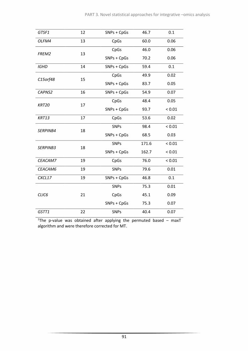
91
PART 3. Novel statistical approaches for integrative –omics analysis
GTSF1 12 SNPs + CpGs 46.7 0.1
OLFM4 13 CpGs 60.0 0.06
FREM2 13 CpGs
SNPs + CpGs
46.0
70.2
0.06
0.06
IGHD 14 SNPs + CpGs 59.4 0.1
C15orf48 15 CpGs
SNPs + CpGs
49.9
83.7
0.02
0.05
CAPNS2 16 SNPs + CpGs 54.9 0.07
KRT20 17 CpGs
SNPs + CpGs
48.4
93.7
0.05
< 0.01
KRT13 17 CpGs 53.6 0.02
SERPINB4 18 SNPs
SNPs + CpGs
98.4
68.5
< 0.01
0.03
SERPINB3 18 SNPs
SNPs + CpGs
171.6
162.7
< 0.01
< 0.01
CEACAM7 19 CpGs 76.0 < 0.01
CEACAM6 19 SNPs 79.6 0.01
CXCL17 19 SNPs + CpGs 46.8 0.1
CLIC6 21
SNPs
CpGs
SNPs + CpGs
75.3
45.1
75.3
0.01
0.09
0.07
GSTT1 22 SNPs 40.4 0.07
1The p-value was obtained after applying the permuted based – maxT algorithm and were therefore corrected for MT.

92
PART 3. Novel statistical approaches for integrative –omics analysis
Table 3.2.2. Statistically significant genes associated with SNPs and/or CpGs selected by ENET&Permuted based maxT algorithm.
Gene Name Chromosome Model Deviance p-value1
REN 1 CPG 84.3 0.03
CRABP2 1 CPG 65.2 0.09
ANXA10 4 SNP 137.0 0.01
PTN 7 SNP
SNP + CPG
97.2
102.5
0.07
0.09
MSMB 10 SNP
CPG
91.8
78.9
0.07
0.06
MMP7 11 SNP 94.8 0.06
TCN1 11 SNP 88.9 0.07
IGF2 11 SNP
CPG
101.6
92.1
0.05
0.04
MMP7 11 SNP + CPG 99.4 0.08
GTSF1 12 SNP 109.6 0.05
IGHD 14 SNP + CPG 97.5 0.1
SERPINB4 18 SNP 105.2 0.04
SERPINB3 18 SNP
SNP + CPG
171.6
171.3
0.02
0.01
CEACAM6 19 SNP 108.4 0.03
NRLP2 19 CPG 84.2 0.04
CEACAM5 19 CPG 92.1 0.06
IGLJ3 22 SNP 97.7 0.05
1The p-value was obtained after applying the permuted based – maxT algorithm and corrected by MT.

93
PART 3. Novel statistical approaches for integrative –omics analysis

94
PART 3. Novel statistical approaches for integrative –omics analysis
Figure 3.2.2. Deviance across the genome when applying LASSO and ENET to select SNPs, CpGs
or both (Global model). The dots in the figure indicate the deviance of each gene located in the
corresponding position in the genome. There are a total of 20,899 gene expression probes
measured. Significant genes after applying the permutation-based MaxT method are tagged.
The figures represent the deviance per gene expression probe using LASSO for the SNP model
(A), the CpG model (B) and the Global model (C) and using ENET for the SNP model (D), the CpG
model (E) and the Global model (F).

95
PART 3. Novel statistical approaches for integrative –omics analysis
Figure 3.2.3. Venn diagrams showing the overlap between the significant genes compared by the two methods (LASSO and ENET) and models (SNPs, CpGs and Global). (A) Number of significant genes using the LASSO method for the three models (SNP, CPG, and Global); (B) number of significant genes using the ENET method for the three models (SNP, CPG and Global); and (C) number of significant genes per model comparing the two methods (LASSO and ENET).
Replication Phase
The replication study was done by restricting the analysis to those genes that showed significant
results in the Discovery Phase (48 genes) considering the same model and method and by
applying the same criteria of analysis to the TCGA data. Overall, we were able to replicate 75%
of the results: from the 48 genes, a total of 36 genes provided a significant association at least
in one of the models considered. Regarding the LASSO models, the replication resulted in 3/9
genes from the SNP models, 17/19 genes from the CPG models, and 19/23 genes from the Global
models (Table 3.2.3). Regarding ENET, the replication resulted in 3/10 genes from the SNP
model, 3/6 genes from the CPG model, and 3/3 genes from the Global model (Table 3.2.4).

96
PART 3. Novel statistical approaches for integrative –omics analysis
Table 3.2.3. Significant genes obtained by LASSO&Permuted based maxT algorithm for the three models (SNP, CPG, and Global) in the original dataset
(EPICURO Study) and the replication dataset (TCGA).
Original Data (EPICURO) Validation Data (TCGA)
Gene probeset Chr Start end Dev
p-
value
SNPs
(N)
CpGs
(N) Dev p-value1
SNPs
(N)
CpGs
(N)
SNPs
(overlap)
SNPs
(rep)
CpGs
(overlap)
CpGs
(rep)
SNP
mo
del
SERPINB3 8023696 18 61322433 61329197 171.6 <0.01 29 0 1 0 3 0
SERPINB4 8023688 18 61304495 61311502 98.4 <0.01 15 0 1 0 2 0
CEACAM6 8029098 19 42259398 42276113 79.6 0.01 10 0 1 0 0 0
CLIC6 8068383 21 36041688 36090519 75.3 0.01 30 3.5E-08 0.9 1 14 0
CRTAC1 7935535 10 99624758 99790585 66.2 0.03 18 2.4E+09 0.001 12 4 1 (LD)
GSTT1 8074980 22 24376141 24384284 40.4 0.07 16 8.3E+07 <0.001 34 4 1 (LD)
PTN 8143144 7 136912092 137028546 67.0 0.08 9 0 1 0 1 0
SCNN1A 7960529 12 6456011 6486523 57.9 0.08 26 0 1 0 8 0
AIM2 7921434 1 159032275 159046647 55.8 0.1 6 5.7E+05 0.03 1 2 0
CEACAM7 8037053 19 42177235 42192096 76.0 < 0.01 19 1.5E+07 < 0.001 2 17 0

97
PART 3. Novel statistical approaches for integrative –omics analysis
PIGR 7923929 1 207101869 207119811 75.8 < 0.01 21 6.4E+08 0.001 19 18 1
PLA2G2A 7913216 1 20301925 20306932 71.4 0.01 10 5.2E+09 < 0.001 57 9 0
CP 8091385 3 148890292 148939832 51.1 0.02 3 1.6E+09 < 0.001 24 1 0
HMGCS2 7919055 1 120290620 120311555 53.3 0.02 8 0 1 0 8 -
CP
G m
od
el
KRT5 7963427 12 52908361 52914243 58.2 0.02 25 3.6E+12 < 0.001 112 24 5
C15orf48 7983478 15 45722763 45725645 49.9 0.02 7 1.5E+08 < 0.001 23 5 0
KRT13 8015323 17 39657233 39661865 53.6 0.02 8 8.2E+11 < 0.001 5 6 0
IGJ 8100827 4 71521259 71532348 58.4 0.03 2 4.2E+08 < 0.001 19 2 0
SCNN1A 7960529 12 6456011 6486523 58.8 0.03 29 2.1E+09 < 0.001 12 27 0
S100A9 7905571 1 153330330 153333502 53.7 0.04 11 5.0E+11 < 0.001 33 9 1
KRT20 8015124 17 39032141 39041495 48.4 0.05 3 5.9E+09 < 0.001 45 3 0
CTSE 7909164 1 206317459 206332103 60.7 0.06 12 3.4E+09 < 0.001 36 12 1
AIM2 7921434 1 159032275 159046647 61.5 0.06 8 4.7E+07 0.002 27 4 0
OLFM4 7969288 13 53602972 53626186 60.0 0.06 10 1.6E+10 < 0.001 47 9 6
MSMB 7927529 10 51549553 51562590 67.3 0.06 7 0 1 0 6 0

98
PART 3. Novel statistical approaches for integrative –omics analysis
FREM2 7968678 13 39261173 39461265 46.0 0.08 2 4.4E+07 < 0.001 13 1 0
CLIC6 8068383 21 36041688 36090519 45.1 0.09 4 1.2E+08 < 0.001 19 4 0
TNNT3 7937749 11 1940799 1959935 44.9 0.09 26 5.2E+08 < 0.001 72 22 0
SERPINB3 7920285 18 61322433 61329197 162.7 <0.01 15 0 3.0E+09 <0.001 6 4 1 0 0 0
KRT20 7905571 17 39032141 39041495 93.7 <0.01 19 7 5.7E+09 <0.001 8 38 0 0 0 0
PTN 7935535 7 136912092 137028546 92.0 <0.01 12 0 2.6E+08 <0.001 0 1 0 0 0 0
SERPINB4 7938758 18 61304495 61311502 68.6 0.03 4 0 7.9E+08 <0.001 27 11 0 0 0 0
Glo
bal
mo
del
SAA1 7962559 11 18287808 18291521 127.8 0.04 20 1 7.9E+08 0.6 0 1 5 1 0 0
S100A2 7957966 1 153533587 153538306 58.7 0.04 20 7 1.0E+11 <0.001 1 5 5 0 3 0
C15orf48 7964927 15 45722763 45725645 83.7 0.05 19 6 1.7E-07 <0.001 1 6 0 0 0 0
TSPAN8 7963817 12 71518877 71551779 67.2 0.05 8 1 9.9E+05 0.02 1 0 3 0 1 0
FREM2 7968678 13 39261173 39461265 70.2 0.06 14 2 2.9E+07 <0.001 3 10 3 0 1 0
CLIC6 7983478 21 36041688 36090519 75.3 0.07 25 2 1.4E+08 <0.001 21 15 0 1 (LD) 0 0
UBD 7995712 6 29523390 29527702 75.0 0.07 6 5 8.8E+08 <0.001 0 25 0 0 0 0
CAPNS2 7981724 16 55600584 55601592 54.9 0.07 8 1 5.8E+07 <0.001 10 12 0 0 0 0

99
PART 3. Novel statistical approaches for integrative –omics analysis
MYBPC1 8023688 12 101988747 102079657 74.5 0.08 23 3 9.9E-08 1 0 1 2 0 2 0
TMEM45
A 8037197 3 100211463 100296285 57.3 0.08 12 0 1.6E+08 0.001 11 19 0 1 (LD) 0 0
S100A9 8015124 1 153330330 153333502 52.5 0.08 6 4 4.9E+11 <0.001 15 24 0 1 (LD) 4 1
SLC38A4 8023696 12 47158544 47219780 51.7 0.08 15 1 1.6E+08 0.001 8 15 6 0 1 0
IGJ 8068383 4 71521259 71532348 59.0 0.09 3 2 3.3E+08 0.003 1 3 0 0 0 0
ARHGEF5 8081288 7 143883177 143892791 49.6 0.09 8 0 1.2E+07 <0.001 11 8 0 1 (LD) 0 0
CRTAC1 8100827 10 99624758 99790585 60.9 0.1 7 5 3.8E+09 <0.001 7 9 1 0 3 1
IGHD 8136981 14 106303102 106312014 59.4 0.1 7 1 - - - - - - - -
CRH 8151092 8 67088612 67090846 56.7 0.1 3 0 9.4E+08 <0.001 7 10 0 0 0 0
TRIM31 8178330 6 30070674 30080867 47.1 0.1 23 4 5.8E+08 <0.001 0 43 0 0 0 0
CXCL17 8143144 19 42932696 42947136 46.8 0.1 3 5 7.4E+08 <0.001 8 11 0 0 0 0
GTSF1 8124650 12 54849737 54867386 46.7 0.1 2 1 2.1E+07 <0.001 18 46 2 0 1 1
1Bonferroni correction for the p-value were: 0.005 (SNP model), 0.003 (CPG model) and 0.002 (Global model); SNPs (N) and CpGs (N) are the number of SNPs and CpGs that were selected by LASSO per each gene expression probe in EPICURO data with the Illumina HumanHap 1M array and the Methylation 27k array; SNPs (overlap) and CpGs (overlap) are the number of SNPs and CpGs that were present in the TCGA data with the Genome wide 6.0 Affymetrix and the Methylation 450k array; and the SNPs (rep) and CpGs (rep) are the ones selected by LASSO in the TCGA data in common with the EPICURO data. The gene with “no p-value” is a gene that was not present in the RNASeqV2 in TCGA data.

100
PART 3. Novel statistical approaches for integrative –omics analysis
Table 3.2.4. Significant genes obtained by ENET&Permuted based maxT algorithm for the three models (SNP, CPG, and Global) in the original dataset (EPICURO Study) and the replication dataset (TCGA).
Original Data (EPICURO) Validation Data (TCGA)
Gene probeset Chr Start end Dev
p-
value
SNPs
(N)
CpGs
(N) Dev p-value1
SNPs
(N)
CpGs
(N)
SNPs
(overlap)
SNPs
(rep)
CpGs
(overlap)
CpGs
(rep)
SNP
mo
del
ANXA10 8098246 4 169013707 169108891 137.0 0.01 17 1.4E+08 <0.001 13 7 1
SERPINB3 8023696 18 61322433 61329197 171.6 0.02 30 1.4E+09 0.08 32 3 0
CEACAM6 8029098 19 42259398 42276113 108.4 0.03 28 1.4E+09 0.04 4 5 0
SERPINB4 8023688 18 61304495 61311502 105.2 0.04 31 1.1E+08 0.07 10 8 1 (LD)
GTSF1 7963817 12 54849737 54867386 109.6 0.05 19 1.6E+06 0.08 7 9 2 (LD)
IGF2 7937772 11 2150348 2170833 101.6 0.05 56 3.9E+12 0.002 31 12 0
IGLJ3 7981730 22 23247030 23247205 97.7 0.05 183 - - - - -
MMP7 7951217 11 102391240 102401478 94.8 0.06 19 2.8E+08 0.004 10 6 1 (LD)
PTN 8143144 7 136912092 137028546 97.2 0.07 24 0 1 0 10 0
MSMB 7927529 10 51549553 51562590 91.8 0.07 78 0 1 0 0 0
TCN1 7948444 11 59620281 59634041 88.9 0.07 122 0 1 0 0 0

101
PART 3. Novel statistical approaches for integrative –omics analysis
CP
G m
od
el
CP
G m
od
el
CP
G m
od
el
REN 7923608 1 204123944 204135465 84.3 0.03 22 0 1 1 22 0
IGF2 7937772 11 2150348 2170833 92.1 0.04 15 8.1E+12 <0.001 609 12 7
NLRP2 8031398 19 55476652 55512508 84.2 0.04 34 8.0E+08 < 0.001 10 28 2
CEACAM5 8029086 19 42212530 42234436 92.1 0.06 26 9.3E+08 0.009 1 23 0
MSMB 7927529 10 51549553 51562590 78.9 0.06 9 6.2E+07 0.3 36 7 1
CRABP2 7921099 1 156669410 156675375 65.2 0.09 39 1.1E+10 <0.001 132 35 11
Glo
bal
mo
del
SERPINB3 7920285 18 61322433 61329197 171.3 0.01 27 1 5.3E+09 <0.001 37 15 0 0 1 1
MMP7 7951217 11 102391240 102401478 99.4 0.08 62 18 2.3E+08 0.003 5 2 0 0 0 0
PTN 8143144 7 136912092 137028546 102.5 0.09 20 0 6.1E+08 <0.001 16 15 0 0 0 0
IGHD 7981724 14 106303102 106312014 97.5 0.1 35 6 - - - - - - - -
1Bonferroni correction for the p-values is: 0.008 (CPG model) and 0.01 (Global model); SNPs (N) and CpGs (N) are the number of SNPs and CpGs that were selected by ENET per each gene expression probe in EPICURO data with the Illumina HumanHap 1M array and the Methylation 27k array; SNPs (overlap) and CpGs (overlap) are the number of SNPs and CpGs that were present in the TCGA data with the Genome wide 6.0 Affymetrix and the Methylation 450k array and the SNPs (rep) and CpGs (rep) are the ones selected by ENET in the TCGA data in common with the EPICURO data. The gene with no p-value is a gene that was not present in the RNASeqV2 in TCGA data.

102
PART 3. Novel statistical approaches for integrative –omics analysis
Gene enrichment study
Using DAVID, 46 genes out of 48 genes were annotated from 14 public annotation categories
showing significant signals in the discovery phase. After enrichment analysis, 7 clusters with
an ES ≥1.3 were found (Table S3.2.3). The cluster with the highest ES (3.5) regarded to the
terms “extracellular region, secreted, and signal peptide” grouping the genes OLFM4, CRTAC1,
MSMB, IGJ, MMP7, IGF2, PIGR, TCN1, CXCL17, S100A9, SAA1, IGHD, CRH, CTSE, FREM2,
PLA2G2A, CEACAM7, CEACAM6, CEACAM5, REN, PTN, CP. The rest of the clusters found with
an ES ≥1.3 were not significant after MT correction. However, we highlight the cluster “EF hand
and calcium ion binding” (ES= 1.3) grouping the genes S100A9, S100A2, CAPNS2, ANXA10,
CRTAC1, FREM2, MMP7, PLA2G2A.

103
PART 3. Novel statistical approaches for integrative –omics analysis
Discussion
Integration analysis in the field of omics data is emerging to find new biological insights in
complex traits (Knowles & Hurst 2014). In this regard, our pathophysiological understanding
of UBC could be improved by using innovative approaches based on its omics data to identify
hidden mechanisms in which multiple factors are involved. We previously analyzed the same
set of omics data used here following a multi-stage approach by proposing an omics
integration analysis framework. The results from this previous work highlighted relevant omics
trans-acting relationships in UBC [12]. Here, we propose an omics integrative analysis pipeline
using LASSO and ENET, and restrict attention to cis-acting relationships. The three omics data
are combined in a large input matrix and then a permutation-based MaxT method is adapted
to assess the significant models while correcting for MT.
The assets of our approach, in comparison with classical approaches (Kristensen et al. 2014;
Ritchie et al. 2015), are the possibility to work with a large number of parameters, even if the
sample size is small, dealing with more than one set of heterogeneous data with high-
correlated variables, and providing MT corrected p-values to assess the models’ goodness of
fit. Furthermore, the results are easily interpretable due to the dimensionality reduction
during the variable selection process.
The expression of 48 genes was found to be significantly associated with SNPs and CpGs in
UBC, pointing to new mechanisms in an intricate scenario where common genetic variants and
DNA methylation regulate gene expression in cis-acting (1MB) relationships. Some of the
genes were identified by the three models and by the two methods, likely underscoring the
existence of true relationships.
The LASSO and ENET applications as part of the aforementioned integrative analysis
framework led to different results. This is not surprising, mainly for two reasons: (1) the α
parameter (equation 5) that uses LASSO is always equal to 1 while ENET uses α < 1. This gives
a smaller penalization and therefore more variables with β ≠ 0 were foreseen using ENET; and
(2) the fact that SNPs and CpGs may be correlated, mainly when they are closely positioned in
the genome, makes that LASSO selects one from the set of parameters that are highly
correlated while ENET forms groups of nets with these variables. In our analysis only 4/24 (SNP
model), 1/25 (CpG model) and 3/28 (Global model) genes were found common in both
methods. The genes detected only by LASSO showed large deviances and borderline p-values
with ENET. Waldmann et al (Waldmann et al. 2013) stated that ENET usually detects more true
and false positives associations. In our case, this fact may result in an increased probability of
having a significant association by chance. This, on its turn, can provoke a decrease in power.

104
PART 3. Novel statistical approaches for integrative –omics analysis
On the other hand, ENET selected some genes that were not selected by LASSO, mainly due to
the correlated structure of the parameters. An example of this is shown in Figure 3.2.4,
showing that MMP7 has three correlation nets that probably are responsible for the gene
selection with ENET and not with LASSO. All these comparisons are shown in Table S3.2.4.
Figure 3.2.4. Example of a correlation plot for MMP7 detected by the Global model using ENET but not using LASSO. The bar color represented the levels of correlation from 0 (no correlation) to 1 (perfect correlation) between SNPs and CpGs that were selected for the MMP7 models. Three nets of correlated variables are the ones responsible that the gene is only selected by ENET and not by LASSO. Regarding the differences between the models, 13/25 significant genes in the CpG model and
6/20 significant genes in the SNP model were not significant in the Global model. It is reported
in the literature that 10% of SNPs are associated with gene expression and DNA methylation
(Wagner et al. 2014; Bell et al. 2011), so DNA methylation may confound or modify the
association between SNP and gene expression. Even though this is the potential explanation,
a discordant due to sample size cannot be discard since the penalty function is selected by CV.

105
PART 3. Novel statistical approaches for integrative –omics analysis
However, k = 5 was used to apply the k-fold CV to decrease the problem of small sample size
while not increasing the bias. In the reverse scenario, 16 genes were selected exclusively in
the Global model. Some of the genes identified had high deviances and borderline p-values,
probably because the Global models increase the deviance due to the addition of more
information when integrating data. For the non-significant genes, the explanation could be
due to the existence of an interaction effect between SNPs and CpGs (Table S3.2.5). This fact
supports the importance of integrating omics data to discover hidden information.
The validity of the strategy that we have developed and of the results is supported by the fact
that the 75% (36/48) of the genes identified in the Discovery Phase were replicated using TCGA
data by applying the same strategy, this representing 64% of all gene models found since some
of the genes overlap between models and approaches. Also, the null results from the
simulation study indicate that the significant associations observed in our data are not by
chance.
Importantly, several of the genes that emerged from our analyses have been previously shown
to be important in bladder cancer biology, including KRT20, IGF2, CTSE, ANXA10 and CRH.
These 5 genes have already been proposed for a panel of molecular markers to improve the
diagnosis and follow up of UBC as part of a 12-gene expression urine signature to identify
patients suffering from UBC and predict tumor aggressiveness (Mengual et al. 2010). The five
genes aforementioned were also replicated in the TCGA data. Furthermore, KRT20, IGF2, and
CTSE have also been previously associated with UBC. KRT20 expression was observed as
abnormal pattern in a 65% of the papillary noninvasive UBC. The authors suggest that the
correlation between FGFR3 mutations with normal KRT20 pattern may indicate that the
mutation probably occurs earlier (van Oers et al. 2007). A loss of imprinting (LOI) of IGF2 gene
has been associated with an increased risk of cancer. LOI is a common epigenetic event in
cancer and a LOI of IGF2 has been reported in UBC (Byun et al. 2007). In our analysis, IGF2 was
detected in the SNP and CPG models suggesting that both (SNPs and CpGs) may be involved
in regulating the expression levels of this gene. CTSE expression was significantly associated
with progression-free survival in pTa tumors in a study of gene expression profiles in UBC (Wild
et al. 2005).
We also performed a gene enrichment analysis to assess whether the significant genes
reported had similar biological function. The cluster with the highest ES was ”Extracellular
region, secreted, and signal peptide”. Secreted proteins are known to play a crucial role in cell
signaling and the cellular secretome has a major impact on multiple aspects of tumor cell
biology (cell growth, migration, invasion, and angiogenesis) (Karagiannis et al. 2010). In

106
PART 3. Novel statistical approaches for integrative –omics analysis
addition, some genes, among them S100A9 and S100A2, were grouped under the “EF hand
and calcium ion binding” term. The S100 family is composed of, at least, 24 members carrying
the Ca2+ binding EF-hand motif. Expression of members of the S100 protein family is regulated
during inflammation and carcinogenesis and has been associated with poor prognosis in
patients with UBC (Yao et al. 2007). Other studies reported an overexpression of S100A9 in
UBC tissue (Dokun et al. 2008; Minami et al. 2010).
Limitations of this work are the small sample size of the Discovery Phase study due to the lack
of enough fresh tumor tissue in the same set of individuals and the lack of a comparable and
independent UBC patient series with the 3-omics data available to replicate our results. The
TCGA project focused on muscle invasive UBC while EPICURO has both, muscle invasive and
non-muscle invasive and both datasets applied different high-throughput
technologies/platforms. The SNP arrays were different in EPICURO and TCGA data genotyping
different SNPs with the consequence of different coverage for genomic measure. DNA
methylation arrays were also different, being the 27k the one in EPICURO and the 450k in
TCGA. Although the 450k contains almost the 90% of the CpGs, the number of match was not
enough as show in Table 3.2.3 and Table 3.2.4. Finally, the different technologies to measure
transcriptomics becomes in an extensive heterogeneity problem. In EPICURO, gene expression
levels were measured with microarray technology which gives relative values at probe set
level, that is, for one gene different expression levels can be obtained from each mapped
probe, while in TCGA, gene expression was measured with RNA-seq which gives absolute
values of the gene expression levels. These differences between data sets introduce a massive
heterogeneity that makes the replication even more difficult. In spite of that, we replicated
75% of the identified genes (64% of the models) with TCGA data, providing strong support to
the appropriateness of our approach and the relevance of the results obtained. Another
potential limitation regards to the possibility that tumor samples were contaminated by
stroma cells. Consequently, we checked whether the expression of all the genes reported as
significant here were or not expressed in UBC cell lines (Earl et al. 2015). The only gene found
not expressed in UBC cell lines was IGJ, this confirming the value of our results.
Strengths of the approach we have used here are the no need of filtering by LD in SNPs or
grouping CpGs within CpG islands when dealing with a huge number of heterogeneous and
correlated parameters delivered by different arrays. The reason is because LASSO and ENET
can deal with high correlated variables at the same time that act as variable selection method.
By performing data reduction/filtering before applying the statistical methods, there is a
chance to filter out the functional SNPs and/or CpGs and thereby lose their association with

107
PART 3. Novel statistical approaches for integrative –omics analysis
gene expression. The adaptation of a strategy that performs a permutation and the maxT
algorithm to assess p-values and to correct by MT avoiding a double permutation and
therefore reducing computational time, is worthwhile emphasizing. Worthy to mention in this
regard is that the permutation-based method consider the permutation of individuals within
each gene which allows to control for the possible dependence structure between genes. In
addition, the MaxT algorithm is a permutation-based FWER controlling procedure which is
adapted to the correlation structure found in the data and has been shown to be
asymptotically optimal under dependence (Meinshausen et al. 2011).
We have demonstrated that the integration of multiple omics data types allows the
identification of hidden mechanisms that were missed when analyzing single omics data types,
one at a time. There is an urgent need to develop statistical methods to fill the gap between
the huge amount of data generated and the mechanistic understanding of complex diseases.
Here, we present two penalized regression methods (LASSO and ENET) in combination with a
permutation – based strategy (permutation-based MaxT method) to deal with common
problems found in integrative analysis: heterogeneity between data types, number of
individuals much smaller than the parameters to assess, multicollinearity, and sparseness to
facilitate the interpretation of the results. This approach is flexible and easy to implement in
different omics data and diseases as well as when considering interaction terms in the model.
We contribute to the field with a methodological development and with several significant
and sound molecular associations conforming part of the genetic architecture of UBC. By using
this cancer as an example, we conclude that modeling the intricacy of omics data variation
with appropriate statistical strategies will certainly improve our knowledge of the mechanisms
involved in complex diseases.

108
PART 3. Novel statistical approaches for integrative –omics analysis
This manuscript has been reviewed by two noted experts in the field. While both found
significant value in it, each identified a number of minor issues that need to be addressed.
Down below are the responses to the Reviewer’s comments:
Reviewer #1
Reviewer #1: Pineda et al use Lasso and elastic net with correct for multiple testing with
MaxT to integrate several genomics platforms. 27 patients from the Spanish Bladder Cancer
EPICURO study had SNP data, DNA methylation and gene expression data for testing the
method. This is an interesting approach that could also be used to model subtypes and
outcomes.
(1) For lasso and elastic net, you can adjust the parameters of alpha and lambda. Is there a
big difference in the parameters between the individual SNP and individual CpG analysis vs
the combined analysis?
It would be good to add to the supplement the parameters used. Is your elastic net model
leaning towards lasso or ridge regression?
For each model applied, the parameters are re-estimated using cross validation. In the case of
LASSO, to obtain the lambda penalty 5-fold cross validation is applied maximizing the
penalized log-likelihood function. For ENET, the optimal penalty for lambda is obtained using
the same strategy (5-fold cross validation maximizing the penalized log-likelihood) but in this
case selecting the best alpha using an alpha vector of 𝛼𝜖(0.01, 0.99) 𝑏𝑦 0.01, as explained in
material and methods line 127. So, we obtained one estimation per model and method that
makes: 125,394 lambdas and 62,697 alphas. Therefore, we cannot study one by one but to
answer the reviewer questions, we checked globally if there were any pattern of the
parameters lambda and alpha we needed to pay attention to. Regarding the differences
between models, for LASSO the mean(lambda) = 0.135, 0.08 and 0.129 for SNP, CPG and
Global model respectively. For ENET, we cannot assume any pattern or leaning towards lasso
or ridge regression between the three models. The mean(alpha)=0.46 and sd(alpha)=0.31 with
minimum value=0.01 and maximum value=0.99 for all of them (SNP, CPG and Global model).
If the tuning parameters for SNP were drastically different from what was seen for CpG, could
you bias feature selection in the combined model if a suboptimal alpha and lambda was picked
for one or both of the data platforms. In tables 3 and 4 it looks like there is a preferential pick
of SNPs over CpGs in the combined model.
The tuning parameters between SNP model and CPG model are different because this is the
way that penalized regression methods control by different scales. SNPs are categorical and
CpGs are continuous in our analysis, thus it is normal to have different tuning parameters. In
our previous answer we showed that Global model had a tuning parameter in the middle but
closer to the SNP model at global numbers. The tuning parameter is not the responsible of
selected more SNPs, but the tuning parameter is closer to the SNP model because more SNPs
are selected. In any case, the numbers showed are global and we cannot extract any

109
PART 3. Novel statistical approaches for integrative –omics analysis
conclusion without studying individually one by one, which becomes impossible because of
the amount of lambdas and alphas estimated. This question of big numbers is one of the
challenges we try to answer in this paper when analyzing high-throughput data.
Potential explanation to answer the question of why Global model select more SNPs than CpGs
are state in the manuscript. In the introduction we hypothesized that the biological idea
behind the integration is based in previous finding where gene expression was affected by
both DNA methylation and genetic variants, both co-regulating different genome spaces
interpreting that the regulation of expression of a given gene results from the combination of
genetic variants that, at the same time, could be influenced by the levels of DNA methylation
in specific CpGs. In the results we showed that when integrating different results are found
and in the discussion we commented on the differences due to correlation, confusion and/or
modifier factors. We do not detail each specific example due to a question of extension of the
manuscript, but we provide in supplementary material, the entire list of genes, SNPs and CpGs
per model and method to see in detail if interesting.
(2) I highly recommend a supplemental table that lists the samples used for analysis from both
the EPICURO and the TCGA study so that people could have the exact data set if they want to
implement and test your method. It would be useful since your performed your analysis on 27
of the 70 patients in EPICURO and 238 of the over 400 TCGA samples.
Following the reviewer’s recommendation we have added Table S3.2.1 with information on
the 27 samples from EPICURO data and Table S3.2.2 with information on the 238 samples
from the TCGA data used in the analysis. With this change, the previous Tables S3.2.1-S3.2.3
are now S3.2.3-S3.2.5 Tables.
(3) Gene expression was modeled by your methods with SNP data alone, CpG data alone,
and SNP and CpG data combined. Did you limit to the same 27 EPICURO patients for all
analyses?
Although the overlap considering pairwise is higher than considering the three –omics, in this
study we wanted to check whether combining the three –omics new information was found
and to do that we needed to restrict the three models to the same individuals since allow us
to compare in same conditions. So yes, we used the same sample for the three models to make
them comparable. That is, the overlapping of individuals with the three types of –omics data
from EPICURO, that was 27, was used to perform the three models (SNP alone, CpG alone and
the combination). We added a supplementary table specifying the samples to specify the ones
we have used.
(4) The Discovery phase was performed on a probe level for the gene expression data vs the
replication phase which was performed on a gene-level. In your final 48 genes selected from
your model, where there probes for the same gene (from the microarray) that were
discordant? If there were, could these be some that didn't replicate in the TCGA data.

110
PART 3. Novel statistical approaches for integrative –omics analysis
We performed the analysis for the Discovery phase at probe level and the reason is because
different probes map to the same gene and can give different levels of expression. It is very
well noted that the discordant in the replication phase could be explain by differences
between probes in the discovery phase.
We comment on the discussion in line 466 that one of the limitations of this type of analysis is
the lack of comparable dataset. Consequently a massive heterogeneity is introduced in the
study.
As the reviewer point, we observed that from the set of the 48 genes significantly associated
in the EPICURO data (microarray technology), four were mapped for more than one probe
from which only one gene (SAA1) was not replicated in the TCGA data (RNAseq). One possible
reason could be that microarray technology map the probes to the genes for different
transcripts given relative values of gene expression while RNAseq gives the absolute value of
gene expression. Consequently the different expression observed by one technology cannot
be observed by the other and effectively the gene that had more than one probe and was not
replicated in our study had a Pearson coefficient = 0.58 between probes while the other three
had Pearson coefficients = 0.94, 0.90 and 0.98. This is an illustrative example of the problems
we find to replicate when massive heterogeneity is introduced but not the only one, so we
decided not to give specific examples, but as we think that the reviewer comment is very well
pointed we have specified in the discussion the differences between microarray and RNAseq.
(5) There were a few genes that made the SNP only and the CpG only models but not the
combined model. Any thoughts as to why?
In line 421 we discussed that in the literature 10% of SNPs are associated with gene expression
and DNA methylation, so DNA methylation may confound or modify the association between
SNP and gene expression. Although, we believe this is one possible explanation, we cannot
discard some discordant due to a small sample size since we estimate the optimal parameters
using k-fold cross-validation. In any case we used the smallest k possible (k=5) to apply cross
validation to avoid sample size problems in variable selection while not introducing big bias.
We added a line to clarify the k used because was not clear in line 143 and a line to add a
limitation due to sample size when using cross validation in the discussion in line 423.
(6) It would also be useful to know if these are muscle invasive or non-muscle invasive or
histology designations such as papillary and squamous. The fact that only 75% of your genes
were replicated in TCGA could be because of a different patient population in addition to the
difference in data platforms.
In line 469 we discuss about this issue since the TCGA samples are only muscle invasive UBC
while in EPICURO are both, muscle-invasive and non-muscle invasive. Consequently this
could be one of the reasons why the replication is only 75% of the genes. To clarify these
differences we have added in material and methods two lines with the information from
both EPICURO data and TCGA data.

111
PART 3. Novel statistical approaches for integrative –omics analysis
Reviewer #2
Reviewer #2: In this manuscript, the authors describe a permutation-based algorithm for
assessing the significance of relationships uncovered by penalized regression methods
(LASSO and ENET) in “multi-omic” databases, concomitantly using the MaxT algorithm to
correct for multiple hypothesis testing. The method is applied to combined mutation, DNA
copy number, and gene expression data from the authors’ own urothelial bladder cancer
(UBC) studies and “replicated” by analysis of the TCGA UBC data. They then follow up with
simulation studies and a Gene Ontology enrichment analysis. As stated in the cover letter,
the principal contribution is methodological. It follows up on a more biologically-focused
version of the analysis by the authors (Pineda, et al., Human Heredity, in press).
None of the individual ingredients of the method are novel, but they are combined (and
customized for the particular types of omic data) in an interesting way. Penalized regression
methods should probably be used in omic analysis even more often than they are -- because
of the typical mismatch between number of variables and number of cases. And careful
attention to multiple hypothesis testing is vital to proper control of Type I statistical error.
(1) I don't THINK that lack of independence of the vectors over genes or unequal variances
are issues that would compromise the validity of the permutation test in this algorithm. But,
since the authors have presumably thought deeply about those questions, they should
address them briefly but directly -- at a place of their choosing in the manuscript.
The permutation test was done permuting individuals within the genes with the intention of
avoiding any problem of dependence structure between genes. When we consider to apply a
permutation-based approach to assess significance, we thought in two possibilities, one
permuting individuals within each gene and two, permuting genes. The results from the
second approach was more restrictive due to the correlation structure of the genes since we
did not consider that the genes may be correlated between them. For that reason, we decided
to use the permutation-based approach permuting individuals. In addition to this, the MaxT
algorithm is a permutation-based FWER controlling procedure which is adapted to the
correlation structure found in the data and has been shown to be asymptotically optimal
under dependence. Following the reviewer’s recommendation we briefly and directly
comment on this in the discussion line 498 adding also a new reference [46].
(2) The level of writing is uneven. I suggest careful copy-editing of the text prior to publication.
We have checked carefully the writing of the manuscript detecting a discordant between using
active and passive voice that we have already corrected.
(3) Relatively minor comments/questions:
1. Line 244: I assume that the gene enrichment analysis using David was based on the Gene
Ontology. If so, that should be stated directly, along with specification of the database type
and evidence parameters used for the analysis.

112
PART 3. Novel statistical approaches for integrative –omics analysis
The gene enrichment analysis is based on 14 annotation categories (Gene Ontology (GO),
Biological process, GO Molecular Function, GO Cellular Component, KEGG Pathways,
BioCarta Pathways, Swiss-Prot Keywords, BBID Pathways, SMART Domains, NIH Genetics
Association DB, UniProt Sequence Features, COG/KOG Ontology, NCBI OMIM, InterPro
Domains, and PIR Super-Family Names) collected in the DAVID knowledgebase
(https://david.ncifcrf.gov/knowledgebase/DAVID_knowledgebase.html). Even though this
information can be found in the reference we provide in the manuscript, we specify now in
the manuscript line 265.
2. Line 312 – 320. “Importantly, we replicated results for 36 (75%) of them in an independent
data set (TCGA).” Does “restricting the analysis to those genes …” mean that the calculation
was done over the entire set but that only the results for the 48 genes (i.e., 75% replication)
are being reported here? The figures given would seem to relate to the sensitivity of
replication but not its specificity. What about the numbers related to specificity? Overall, I
think the replication study needs further description and (no pun intended) specificity.
The replication phase is done with restrictions to the genes detected in the discovery phase
(48 genes) considering the models (SNP, CPG and/or Global) and methods (LASSO and/or
ENET) from which they were significant. That is, we took only the genes significantly associated
in the discovery phase and apply the same strategy but only in those genes to see if they were
significantly associated also in the TCGA. We have modified the paragraph in material and
methods line 244 to better explain and clarify the replication study following the reviewer’s
suggestion.
Regarding sensitivity and specificity, we do not consider the 75% of replicated genes as a
sensitivity estimation rate because we cannot consider our results as the “real true” and
therefore, the estimation of specificity is behind the same consideration. In spite of this, to be
sure we were doing the replication properly, we performed the same replication study with a
set of genes randomly selected from the TCGA data. We observed that the percentages of
significant genes was much lower than when considering the genes significant in our discovery
phase, but we need to think that the sample size is much higher, so we cannot differentiate
between a true positive due to power issues, a true positive due to a threshold selection or a
false positive in the replication dataset.
It’s appropriate that the authors list the major differences in the two studies (platform, etc.)
and that the level of concordance is perhaps surprising.
We were conscious of the limitation that the differences between platforms in the two studies
was a limitation in our study and we believe that this is one of the reason why we do not
replicate the 100% of the genes. For these reason we comment in line 471 this limitation, but
as suggested by the reviewer, we have added in this part of the discussion more details about
the different platforms in both studies to point out this limitation. Regarding the level of
concordance, we need to think that the sample size in the discovery phase is the biggest
limitation and those genes significant are probably the ones with the highest signal.

113
PART 3. Novel statistical approaches for integrative –omics analysis
3. Lines 337 – 346: This manuscript is focused on methodology, not biology, but, nonetheless,
the reader will wonder whether there’s any biological significance to the categories that
showed up in the gene ontology analysis. Do the authors think there’s any meaning to the
categories or are they just ones that happened to show up despite the multiple hypothesis-
testing correction?
We introduce in our manuscript that one of the big challenges –omics data integration impose
is the interpretation of the final results. To assess this challenge we search for biological
meaning of our final results. In one way, we searched directly in the literature whether
previous publications found already some of our genes and many interesting results came out
that are discuss in the discussion part. In other way, we performed an enrichment analysis to
find if some of our genes had similar biological functions. We found interesting results with
two main clusters with implications in UBC that we also discuss.
4. Lines 371 – 381: Could another reason for the lack of concordance between LASSO and ENET
be the sheer statistical arbitrariness of selecting just a handful of top genes out of many
thousands -- especially given the occurrence of high correlations among the vectors for
different genes?
The necessity of giving a threshold to correct my multiple testing is always problematic. The
equilibrium between type I error and type II error is one of the more important issues in
statistical genetics. Which is the threshold of false positives we are able to assume while no
detecting false negatives? One of the differences we observed that can be seen in Table S3.2.4
and we comment in the discussion line 400 is that some of the genes selected by LASSO are
borderline with ENET. So the arbitrariness of the statistical selection is an important issue. In
the reference we provide, Waldmann et al. demonstrated that ENET usually detects more true
and false positives associations and can provoke a decrease in power.


115
PART 3. Novel statistical approaches for integrative –omics analysis
Chapter 3. Integrative eQTL –omics analysis considering tumor tissue and blood samples in individuals with bladder cancer
Silvia Pineda (1,2), Kristel Van Steen* (2,3), Núria Malats* (1),
(1) Genetic and Molecular Epidemiology Group, Spanish National Cancer Research Centre
(CNIO), Madrid, Spain.
(2) Systems and Modeling Unit – BIO3, Montefiore Institute, Liège, Belgium.
(3) Systems Biology and Chemical Biology, GIGA-R, Liège Belgium.
* Equal contributions
American Journal of Human Genetics 2015 – Submitted

116
PART 3. Novel statistical approaches for integrative –omics analysis
Abstract
Integrative –omics analysis approaches to combine different data are emerging. These data
are mainly determined in the same source material (i.e., tumor sample). However, the
integration of data from different material levels (i.e., blood and tumor) may also reveal
important knowledge on the human genetic architecture. To model this multi material-level
structure, integrative-eQTL analysis applying 2-Stage Regression (2SR) has been proposed. This
approach consists on two stages, (1) gene expression levels are regressed with markers at
somatic level and (2), the residuals-adjusted are regressed with the germline genotypes. Such
an approach relies on several assumptions needed to overcome challenges high-throughput -
omics data impose. Previously, we have shown that penalized regression methods in
combination with a permutation–based MaxT method are promising to this regard. In this
report, we assess whether our previously developed strategy can also be considered when
integrating different data source material and we compared it with two different ways of
parameter estimation in the 2SR-approach, one using multiple linear regression (MLR) and
other using LASSO to control for correlated data. We applied the three strategies to integrate
genomic, epigenomic and transcriptomic data from tumor tissue with germline genotypes
from 181 individuals with bladder cancer from the TCGA Consortium. Our study showed no
significant results when the 2SR-MLR was applied supporting, as previously showed, the
underestimation of this approach when variables are correlated, in contrast of the other two
approaches. Furthermore, our approach propose a list of relevant eQTLs including and
extending the ones found by the 2SR-LASSO approach to be considered in future analysis.
117
PART 3. Novel statistical approaches for integrative –omics analysis
Integrative –omics data analysis (IODA) are starting to emerge for the combination of different
high-throughput platform biological derived information to better understand the complexity
of biological systems. IODA are mainly focused in the combination of –omics data from the
same source material, such as tumor samples (Mankoo et al. 2011), human brain (Zhang et al.
2010; Gibbs et al. 2010) or blood samples (Van Eijk et al. 2012). However, the integration of
data from different material levels (i.e., blood and tumor) may also reveal important
knowledge about the hierarchy of the human genetic architecture. For instance, the influences
of germline variants in gene expression are normally studied in cell lines and normal tissue but
not in tumor tissue due to the complexity of the transcript regulation caused by the somatic
changes produced in the tumor (Fredriksson et al. 2014). To approach this further level of
complexity, Li et al. (Li et al. 2013; Li et al. 2014) performed cis-eQTL analysis in breast cancer
by applying a 2-stage regression (2SR) approach. In stage one, the gene expression level was
regressed with all somatic changes (copy number variation and DNA methylation) in cis-
relationship. In stage two, the residual-adjusted outcome was regressed with the germline
genotypes also in cis-relationship. While this approach presents computational and data
management advantages, its validity relies on assumptions that are not met in the majority of
large scale genomic studies, namely the risk factor of interest should not to be correlated with
the rest of the covariates and the tumor SNPs and/or CpGs may be highly correlated between
them. When this occurs, the 2SR approach may introduce a bias resulting in a loss of power as
demonstrated by Demissie et al.(Demissie & Cupples 2011) and Che et al.(Che et al. 2012) in
comparison with a multiple linear regression (MLR) approach. Similarly, an application of the
2SR approach for detection of QTLs has shown a loss of power when covariates are correlated
(Zeegers et al. 2004). Another limitation of the method proposed by Li et al. is that they applied
MLR, a method that cannot be applied when the number of parameters to be estimated in the
model is larger than the sample size (n<<p problem), a prevalent scenario in large genomics
studies. Demissie et al(Demissie & Cupples 2011) and Che et al.(Che et al. 2012) also
mentioned on the critical issue when applying 2SR and MLR because when a study involves
correlated independent variables, the two approaches produced incongruent results. This is a
fact in the majority of the genomic analyses, since variables such as SNPs and CpGs may be
highly correlated between them and therefore the eQTLs may suffer of harmful
multicollinearity, thus, none of the two approaches are valid.
To overcome these limitations, we propose to adapt an integrative method we previously
developed and which is based on penalized regression (LASSO and ENET) in combination with
permutation-based maxT method(Peter H. Westfall & Young 1993) to obtain p-values and
correct them for multiple testing (Pineda, et al. 2015). This approach can deal with the

118
PART 3. Novel statistical approaches for integrative –omics analysis
challenges that large genomic studies impose and it is well suited to perform eQTL assessment
when –omics multi material-level data need to be integrated. Here, we apply our method by
performing an eQTL- IODA analysis and compare our strategy with the 2SR approach and with
a 2SR using LASSO to deal with the n<<p problem and correlated variables.
Urothelial bladder cancer (UBC) tumor data and blood sample from the same patients were
obtained from The Cancer Genome Atlas (TCGA) consortium (https://tcga-
data.nci.nih.gov/tcga/) by downloading and processing them with the TCGA-Assembler(Zhu et
al. 2014). The data was profiled with Genome wide 6.0 Affymetrix, RNASeqV2, and the
HumanMethylation450K Illumina array. A total number of 905,422 SNPs, 20,502 gene
expression probes, and 350,271 CpGs were obtaining from tumor samples and 905,422 SNPs
from blood samples for 181 individuals. SNPs were measured with the same platform in blood
and tumor samples expecting to have some differences due to somatic mutations within the
tumor. Consequently, we performed an agreement study by pairs of SNPs to check the rate of
disagreement between tumor and blood using the weighted Kappa Index (wKI). Each pair was
represented in a weighted matrix where cells located on the diagonal represent agreement,
while cells one off the diagonal are weighted 1, and cells two of the diagonal are weighted 2.
Figure 3.3.1 displays the percentage of disagreement (wKI) per chromosome. The highest
disagreement is observed in chromosome 9 (29%) supporting the deletion of both arms of the
chromosome 9 frequent in bladder cancer patients (Wu 2005).

119
PART 3. Novel statistical approaches for integrative –omics analysis
Figure 3.3.1. Percentage of disagreement per chromosome for the genotypes measured in tumor and blood. Each percentage is calculated with the number of genotypes within the chromosome with kappa < 0.8 divided by the total number of genotypes within the chromosome.

120
PART 3. Novel statistical approaches for integrative –omics analysis
Tumors acquire frequent somatic alterations as observed with the non-concordance between
tumor and germline polymorphism, which can directly impact in tumor gene expression. Thus,
to integrate genomic data from both DNA sources, we excluded those tumor genotypes in
agreement (wKI >0.8) between the 2 sources. As chromosome 9 was the one with the highest
rate of disagreement, we restricted the study to this chromosome. The fact that we selected
the chromosome 9 which is the one with the highest disagreement should be not affect the
study, since we deleted those SNPs in tumor that has a wKI > 0.8 since that information was
already account with the blood SNPs. The analysis was hence performed in a total number of
33,735 germline SNPs with minor allele frequency (MAF) >0.05, 8,845 tumor SNPs with MAF
>0.05, 6,617 tumor CpGs located in the chromosome 9 filtered by the cross reactive probes
and the polymorphic CpGs, and 717 gene expression probes with at least 20% of the
individuals with expression levels >0. Three different models were applied to find the
association between germline SNPs located in 1MB window (cis-relationship) with gene
expression levels [Box 3].
Model 1 (Global-LASSO) is an extension from our previous approach where germline
genotypes are introduced in a linear LASSO model with the 3 tumor –omics datasets. Model 2
Box 3. Models applied to the subset of chromosome 9 for the integration of 3
tumor –omics and 1 blood -omic datasets
Model 1: Global – LASSO (4-omics)
𝐺𝑒𝑛𝑒 𝐸𝑥𝑝𝑟𝑒𝑠𝑠𝑖𝑜𝑛 𝑙𝑒𝑣𝑒𝑙𝑠 𝑡𝑢𝑚𝑜𝑟𝑖 = 𝛼1𝑆𝑁𝑃𝑡𝑢𝑚𝑜𝑟1 + 𝛼2𝑆𝑁𝑃𝑡𝑢𝑚𝑜𝑟2 + ⋯ +
𝛼𝑝𝑆𝑁𝑃𝑡𝑢𝑚𝑜𝑟𝑝 + 𝛾1𝐶𝑝𝐺1 + 𝛾2𝐶𝑝𝐺2 + ⋯ + 𝛾𝑝𝐶𝑝𝐺𝑝 + 𝛼1𝑆𝑁𝑃𝑏𝑙𝑜𝑜𝑑1 +
𝛼2𝑆𝑁𝑃𝑏𝑙𝑜𝑜𝑑2 + ⋯ + 𝛼𝑝𝑆𝑁𝑃𝑏𝑙𝑜𝑜𝑑𝑝; 𝑖 = 1 … 𝑚
Model 2 (2SR-MLR) & Model 3 (2SR-LASSO):
𝐺𝑒𝑛𝑒 𝐸𝑥𝑝𝑟𝑒𝑠𝑠𝑖𝑜𝑛 𝑙𝑒𝑣𝑒𝑙𝑠 𝑡𝑢𝑚𝑜𝑟𝑖
= 𝛼1𝑆𝑁𝑃𝑡𝑢𝑚𝑜𝑟1 + 𝛼2𝑆𝑁𝑃𝑡𝑢𝑚𝑜𝑟2 + ⋯ + 𝛼𝑝𝑆𝑁𝑃𝑡𝑢𝑚𝑜𝑟𝑝
+ 𝛾1𝐶𝑝𝐺𝑡𝑢𝑚𝑜𝑟1 + 𝛾2𝐶𝑝𝐺𝑡𝑢𝑚𝑜𝑟2 + ⋯ + 𝛾𝑝𝐶𝑝𝐺𝑡𝑢𝑚𝑜𝑟𝑝; 𝑖 = 1 … 𝑚
𝑅𝑒𝑠𝑖𝑑𝑢𝑎𝑙𝑠 𝑡𝑢𝑚𝑜𝑟𝑖 = 𝐺𝑒𝑛𝑒 𝐸𝑥𝑝𝑟𝑒𝑠𝑠𝑖𝑜𝑛 𝑡𝑢𝑚𝑜𝑟 − 𝐺𝑒𝑛𝑒 𝐸𝑥𝑝𝑟𝑒𝑠𝑠𝑖𝑜𝑛̂ 𝑡𝑢𝑚𝑜𝑟
𝑅𝑒𝑠𝑖𝑑𝑢𝑎𝑙𝑠 𝑡𝑢𝑚𝑜𝑟𝑖
= 𝛼1𝑆𝑁𝑃𝑏𝑙𝑜𝑜𝑑1 + 𝛼2𝑆𝑁𝑃𝑏𝑙𝑜𝑜𝑑2 + ⋯ + 𝛼𝑝𝑆𝑁𝑃𝑏𝑙𝑜𝑜𝑑𝑝; 𝑖
= 1 … 𝑚
Residuals in model 2 are obtained from MLR and for model 3 from LASSO

121
PART 3. Novel statistical approaches for integrative –omics analysis
follows the 2SR approach applying MLR (2SR-MLR) and model 3 also follows the 2SR method
but applying LASSO (2SR-LASSO) to overcome with the correlated structure between markers
that cannot be made when using 2SR-MLR. Large genomic studies need to deal also with a
higher number of parameters than individuals (p > n) what represents a limitation for 2SR-
MLR since MLR requires n < p. To fix this issue, we used the markers selected by LASSO in 2SR-
LASSO to run 2SR-MLR. The same strategy with the permutation – based MaxT method
developed in (Pineda, et al. 2015) to obtain p-values and assess for Multiple Testing (MT) was
applied in both Global-LASSO and 2SR-LASSO, and extended to 2SR-MLR to make the results
comparable. Finally, we performed a simulation study with synthetic-data where the
association between markers (SNPs tumor and blood and CpGs tumor) and gene expression
levels was broken. We generated a gene expression sample with the same number of genes
and individuals than in the observed data (p= 717, N= 181) considering all the genes following
a normal distribution with mean (µ= 6.9) and standard deviation (σ= 0.61) extracted for the
total mean and total variance from the TCGA sample.
Table 3.3.1 shows the results of the three models. After MT correction, 2SR-MLR did not
selected any significant eQTL when permutation-based MaxT method is applied. In contrast,
Global-LASSO selected 4,896 eQTLs involving 491 genes and 2SR-LASSO selected 266 eQTLs
involving 13 genes. 2SR-MLR selected one eQTL (rs16917078-TSTD2) after applying Benjamini
& Yekutieli (BY) (Benjamini & Yekutieli 2001) FDR correction to the single p-values obtained in
stage 2 from the MLR model. This eQTL was also detected by Global-LASSO but not by 2SR-
LASSO. As expected, Global-LASSO selected the eQTLs identified in 2SR-LASSO. The
overlapping between genes and germline SNPs is represented in Figure 3.3.2 For the
simulation study, 2SR-MLR did not detect any significant results with any of the MT correction
methods; models Global-LASSO and 2SR-LASSO detected significant genes (6% and 3%,
respectively) and germline SNPs (2% and 1%, respectively) pointing to lower proportion of
false positive results yielded by 2SR-LASSO.

122
PART 3. Novel statistical approaches for integrative –omics analysis
Table 3.3.1.Genes and germline SNPs selected by the three models in the original data (TCGA data) and the simulated dataset.
1After applying Benjamini and Hochberg for multiple testing correction
Figure 3.3.2. Overlapping of the number of genes (A) and germline SNPs (B) after MT correction using permutation – based MaxT method for model 1 and 3 and BY for model 2.
Model 1
(Total)
Model 2
(2SR- MLR)
Model 3
(2SR-LASSO)
Original data
(TCGA)
Nº genes 491 0 (1-BY)1 13
Nº SNPs Germline 4,896 0 (1-BY)1 266
Simulation
N(µ = 6,σ = 0.6)
Nº genes 43 (6%) 0 20 (3%)
Nº SNPs Germline 800 (2%) 0 566 (1%)

123
PART 3. Novel statistical approaches for integrative –omics analysis
Most of the eQTLs studies addressing tumor expression have been performed without
consideration of genetic and epigenetic changes in tumors (Kristensen et al. 2006; Loo et al.
2012; Chen et al. 2014). However, advances in high-throughput technologies have enabled the
exploration of somatic alterations in cancer genomes(Watson et al. 2013). To perform such
studies, integrative analysis are needed and consequently appropriate statistical approaches
to implement them. In this study, we have shown that the multi-level integration of different
source material to perform integrative eQTL assessment can be easily assess with the
implementation of our approach previously proposed.
Our results confirm that the 2SR method considering MLR residuals (model 2) underestimates
the associations and fail to detect eQTLs as showed in (Demissie & Cupples 2011; Che et al.
2012). This method did not produce any significant results when the permutation based MaxT
method was applied to correct for MT. Moreover, when FDR was used to correct by MT only
one eQTL remains significant demonstrating that the absence of significant results is not
attributable to the MT method applied. In contrast, the extension of this strategy using the
residuals from LASSO (model 3) produced interesting results showing an increase in power
detection when using the penalized residuals, likely explained because the correlation
problem between variables may be controlled by using LASSO(Tibshirani 1996). More
important are the results that our strategy (model 1) provides including all the genes detected
by 2SR–LASSO and the one detected with 2SR–MLR when FDR for MT correction is applied.
One of the most important aspects in statistical genetics is the control for false positives, this
requiring of not being too restrictive to lose valuable information (false negatives). The optimal
method would provide a satisfactory balance between false positives and false
negatives(Goeman & Solari 2014). In this study, to control the amount of false positives we
performed a simulation study estimating that the proportion of eQTLs detected when the
signal between gene expression and markers is broken was 2% (Global-LASSO) and 1% (2SR-
LASSO). These percentages suggest a small proportion of signals detected that may be
assumed as a rough estimation of false positives. Nonetheless, our approach detects a higher
number of eQTLs than the other two approaches, thus, to be sure that the significant results
were not due to an artifact of the strategy applied we run 100 times the Global-LASSO with
the observed data and we applied the MaxT algorithm to assign p-values and correct for MT.
With this validation, we should expect no significant results and indeed no significant results
were obtained. Consequently, our approach allows to decrease the false negative rate and
serve as a prioritization of interesting genes producing list of candidate genes and candidate
loci to be explored in detail in future analysis. Importantly, it is that even knowing that some
results may be false positives, the ones detected by the 2SR models are found also with ours

124
PART 3. Novel statistical approaches for integrative –omics analysis
and from the list of genes generated with our approach many of them have been already
associated with UBC. Further details on these findings are out of the purpose of this report.
The entire list of genes and associated eQTLs is provided as supplementary material (Excel S1).
Furthermore, our approach used in the Global-LASSO model is easily applicable and can
accommodate any type of –omics data regardless of heterogeneity, collinearity, or number of
factors in the study. Another important advantages is the reduction of computational time
since the 2SR approach needs to adjust two models per gene analyzed while in our approach
just one model is needed. This is a very important property when the study is extended at the
genome wide level.
To conclude, eQTL IODA using different sources material may improve our knowledge in
cancer risk but proper statistical methods are needed to consider the large amount of –omics
data generated. We demonstrate that our approach provides a list of eQTLs that can serve for
future analysis or as a prioritization to perform functional analysis. The approach is easy to
apply and adaptable to any type of data being an important contribution for integrative
analysis.

PART 4.
GENERAL DISCUSSON


127
PART 4. Discussion
Single –omics data analysis has revealed significant findings that contributed to better
characterize both the inherited and somatic genetic architecture of UBC, among other cancers.
These studies involved genetic susceptibility factors detected trough GWAS (Nathaniel Rothman
et al. 2010) and EWAS (Marsit et al. 2011), somatic DNA alterations (The Cancer Genome Atlas
Research Network 2014) or gene expression signatures to predict disease progression (Kim et
al. 2014). However, the integration of two or more –omics considering a multi –omics data
approach will decipher further interrogations not covered by a single –omics data type analysis.
Nonetheless, dealing with such amount of data, coming frequently from high-throughput
technologies, impose many challenges that need to be addressed appropriately (Hamid et al.
2009; Chadeau-Hyam et al. 2013; Kristensen et al. 2014; Ritchie et al. 2015). Having this scenario
in mind, our objective was to dissect and fix some of the methodological challenges posed by –
omics data integration. The work described in PART 3 of this thesis shows that applying
appropriate –omics data integrative statistical strategies, sound biological insights in the
complexity of UBC are discovered.
The first step in any integrative –omics approach implementation is to conduct data quality
control and to assess data scale and dimensionality for each dataset component. A detailed
single analysis of each –omics component was described in PART 2. Regarding genomics, we
highlighted the differences found when measuring them in blood and tumor (Figure 2.1.2) due
to the somatic mutations acquire during carcinogenesis. While it is known that tumor DNA is
affected by somatic mutations, to our knowledge, no articles were published assessing it at SNP
level. Only few studies showed that variants on pharmacogenetic genes belonging to drug
metabolic pathways are not affected by differences between germline and tumoral SNPs
(McWhinney & McLeod 2009; Weiss et al. 2007; Marsh et al. 2005). We found that in UBC, the
blood-tumor genotypes differences are frequent in terms of disagreement percentages,
especially for chromosome 9 (25%), Y (13%), 17 (7%), 8 (5%) and 11 (5%). The differences in
chromosome 9 are explained due to the deletion of both arms of this chromosome that occurs
early during the urothelial tumorigenesis (Wu 2005). Also deletions in the short arms of
chromosome 8 and 11 are associated with bladder tumor progression (Wu 2005). We also
confirmed these findings using TCGA Consortium data (Figure 3.3.1) that provided blood-tumor
genotypes differences in chromosome 9 (29%), Y (25%) and 17 (19%) in MIBC, and differences
in chromosome Y and 17 were even larger. The important disagreement between both genomics
measurements support to consider these data as two different –omics data sets. In the
epigenomics single analysis, we highlighted the differences found between autosomal
chromosomes and X-chromosome (Figure 2.2.2) supporting previous evidences (Bell et al. 2011).

128
PART 4. Discussion
This finding is explained by the fact that one of the X-chromosome inactivation in females is
done through methylation mechanisms. It is also important to consider the differences observed
between the distributions of the β- and the M-values. While the former follows a beta
distribution in the autosomal chromosomes taking values from 0 to 1, the later follows a bimodal
distribution taking values from -∞ to +∞. This last transformation achieves the homocedastic
characteristic which is an assumption n most of the statistical methods including the ones used
in this thesis. Gene expression data follow a normal distribution as showed in Figure 2.3.4
facilitating the use of parametric statistical methods for its analysis.
This thesis represents an important advancement in –omics data integration not only because
of the number of –omics data sets that have been combined (3 –omics data in tumor plus 1 –
omics data measured in blood) but mainly because of the innovative analytical methods we
propose and apply in their integration. First, a framework build upon a multi-staged strategy
analyzing all the possible pairwise relationships between genomics, epigenomics, and
trasncriptomics was proposed and applied using tumor data from individuals with UBC included
in the EPICURO pilot phase. The framework (Figure 3.1.1) proposes 4 consecutive steps starting
with the preprocessing and QC of each –omics dataset aforementioned (Step 1) followed by the
pairwise analysis between genomics and transcriptomics that showed interesting correlations
between DNA methylation and gene expression (Step 2), the eQTL and metQTL analysis
performed with the correlated expression-methylation pairs (ρ ≥ |0.7|) obtained in the previous
step (Step 3), and the combination of the pairwise analysis in an integrative way that also
showed interesting results (Step 4). Among these results, we highlight a 10% of enrichment of
common genetic variants (49,708 SNPs) associated with both gene expression (eQTLs) and
methylation (methQTLs), a total of 1,469 trans-acting triple relationships (SNP – CpG –
Expression), 19 of the pairs being involved in a cis-acting relationship, and regions with hotspots
(Figure 3.1.3) showing some important multiple biological relationships.
In comparison with other integrative analysis using the same three –omics data types, our
framework integrates step by step the pairwise relationships resulting in a final combination
showing triples relationships that are lastly explored in more detail. For example, in comparison
with the analysis showed by Gibbs et al. (2010) and Bell et al. (2011), they both perform first
the eQTL and methQTL analysis and then check for the overlapping SNPs between both analyses.
However, they do not show a combination between the three types of data as we do, although
they do not restrict the eQTLs and methQTLs to the correlated expression-methylation pairs as
we do. Another example is the study by Wagner et al. (2014) that first analyze eQTLs and
methQTLs and then look at the correlation between gene expression and DNA methylation to

129
PART 4. Discussion
find the overlapping between the three data types. They used genes rather than CpGs or SNPs
as the primary unit of interest for the overlapping, while we used the specific SNPs and CpGs for
the overlapping. In addition, they only considered cis-relationships while we considered both,
cis and trans. It is well established that gene expression levels are controlled by a combination
of cis and trans-acting regulators (Cheung & Spielman 2009). Therefore, the study of trans
relationships is also crucial when considering the biological complexity of cancer. The studies by
Zhang et al. (2010), Drong et al. (2013), and Olsson et al. (2014) focus the analysis in the methQTL
assessment and then, with the SNPs that were significant, they perform subsequent eQTLs
analysis. This approach limits the study to differentially methylated regions of interest and does
not perform an exploration at genome wide level. Similar to our strategy, Van Eijk et al. (2012)
first obtained the correlation between DNA methylation and gene expression levels and then
performed eQTL and methQTLs analyses. They performed an accurate multi-staged analysis
where they assessed with the final subset of significant relationships a causal relationships study
between the three types of data while we assessed specific triples relationships to find patterns
of relationships and interesting regions (hotspots). In conclusion, our framework does not only
accomplish pairwise analysis but also provides the integration of the three –omics data
combining the significant results from the pairwise analysis as showed in Step 4.
While the previous approach allows to advance in the integration process by dissecting the
pairwise relationships between the three –omics data step by step, it does not permit the
assessment of all potential associations and adjustments among the whole set of markers. To
advance in this more comprehensive regard, all –omics data were combined in a large input
matrix using penalized regression methods and we adapted a permutation –based MaxT method
to correct for multiple testing and provide p-values. In the introduction, we commented about
the challenges –omics integrative analysis imposes (heterogeneity, dimensionality, n << p,
correlation, interpretation, replication and validation). Most of them are addressed in this work
by using two types of penalized regression methods, LASSO and ENET. We also commented that
among the pitfalls of these two methods are the non-assessment of statistical significance and
consequently to correct by MT. With our contribution, we are able to deal with these
methodological challenges. LASSO and ENET are flexible strategies and can be applied even if
the variables have different scale. They are variable selection methods and consequently they
can deal with high dimensionality. They can be applied when the sample size is smaller than the
number of parameters and also when the variables are correlated. Besides, with the
permutation –based MaxT method, we are able to obtain p-values and correct by MT capturing
only the significant models that have passed the threshold for MT, thus they encourage sparsity

130
PART 4. Discussion
and therefore the models are interpretable. After applying the workflow proposed in
Material&Methods (Figure 3.2.1), the expression of 48 genes was found significantly associated
with several SNPs and CpGs in cis-acting effect. Interesting are the differences found by applying
the two methods LASSO and ENET to the three models, SNP model, CPG model, and Global
model (SNP+CPG). The reason is due to the selection process of both methods. ENET tends to
select nets of variables that are highly correlated while LASSO selects just one representative
variable of the net. Also differences were found when applying the three models. The main
difference between models regards to the genes identified only when combining together SNPs
and CpGs likely explained because of the addition of more information when integrating, a fact
that further supports the importance of integrating –omics data to discover hidden information.
As we highlighted in the introduction, the validation of these complexities represents a big
challenge and new ideas and approaches for replicating are needed. Typically, replication
studies have been based in reproducing the same relationship between the marker and the trait
in the study, but this is very difficult in the –omics field due to the lack of a similar population
with same –omics data sets measured in the same platforms. The TCGA has generated data for
individuals with UBC though they are MIBC and all the –omics platforms used are different from
the ones generated data in the EPICURO samples. Because of this important heterogeneity, a
replication study at gene level was considered in this work. We assessed whether the genes
selected in our study considering 1Mb window up- and downstream were also selected in the
TCGA series using the same analytical strategy. Importantly, we found that the 75% of the
identified genes (64% of the models) were replicated and therefore, it supported our approach.
In addition, to validate our approach, we checked the literature and found that several genes
were previously reported as important in UBC (KRT20, IGF2, CTSE, ANXA10 and CRH) (Mengual
et al. 2010). Furthermore, an enrichment analysis was also performed for biological validation
and two clusters were found. The “EF hand and calcium ion binding” cluster includes two
important genes (S100A9 and S100A2) that were previously associated with UBC (Yao et al.
2007; Dokun et al. 2008; Minami et al. 2010). This approach demonstrates that the integration
of multiple –omics data allows the identification of hidden genomics information not identified
when only one –omics data set is considered. Previously, some advantages have already been
done to combine data matrices for each sample into one large input matrix to perform
integrative analysis (Fridley et al. 2012; Mankoo et al. 2011; Kim et al. 2013). They all applied
different and valid approaches to integrate -omics data, but they all predict one phenotype, such
as survival risk or drug cytotoxicity. Thus, they all have the limitation to integrate –omics data
considering more than one output variable to be estimated as we do considering all the probes

131
PART 4. Discussion
in the gene expression array as independent output variables. Our approach is flexible and easy
to implement in different –omics data and disease models as well as adaptable to consider
interaction terms in the model.
The developed approach abovementioned was also applied to perform an integrative eQTL
analysis considering two levels of information: genomics measured in blood and in tumor. This
approach was compared with the 2SR strategy using MLR for eQTL integrative analysis
conducted in other studies (Li et al. 2014; Li et al. 2013). Our results showed no significant eQTLs
when using 2SR approach according to the evaluation performed of this method by Demissie &
Cupples (2011) and Che et al. (2012) confirming the underestimation and loss of power of the
results. We proposed extending this method applying LASSO and using its residuals to avoid the
problem MLR has with correlated variables. By doing this, we found significant results pointing
to an increase of power of the method. Interesting are the results from our approach that
increase remarkably the number of significant results including the ones from the other
approaches. We are aware that false positives may be an issue but one of the most important
aspects in statistical genetics with difficult solution until now, is how to control by MT while not
being too restrictive (Goeman & Solari 2014). Assuming that a proportion of false positives may
occur, our approach can serve to select top results producing a list of candidate genes and loci
to be explored in detail in future analyses. It has the advantages that it can be easily
accommodated to different –omics data, it deals with heterogeneity and collinearity or the
number of factors, and it reduces computational time.
Overall, this work has strengths and limitations that should be mentioned. The sample size is a
limitation in –omics integrative studies and certainly in this thesis. Nevertheless, one of the
strengths for the multi-staged approach responds to the fact that the overlap for the samples
available between pairs (epigenomics – transcriptomics = 31, genomics-epigenomics = 46,
genomics – transcriptomics = 27) is higher than the overlap between triplets (genomics-
epigenomics-transcriptomics = 27). In the multi-staged approach, pairwise combinations are
applied to obtain the integrative results using the specific sample in each step increasing them
the size. Despite this issue, the problem of the n << p obligates to perform a one marker analysis
per model which always is a limitation when correcting by MT. LASSO and ENET deal with this
issue although EPICURO sample size is very small to yield strong biological conclusions. This work
needs to be seen as a methodological contribution that adds different –omics data integrative
approaches to be applied in bigger sample sizes. In this regard, when applying LASSO &
permutation –based MaxT method to perform the integrative eQTL analysis with a bigger
sample size (181 individuals) as showed in chapter 3 of PART3, the number of eQTLs detected

132
PART 4. Discussion
increase remarkably. One potential explanation could be the increase in power due to the
increase of sample size, although we need to be cautious when comparing these two studies
because in the first one applied to EPICURO data, the gene expression levels are measured with
microarray technology, while in the second one applied to TCGA data, the expression levels are
measured with RNA sequencing. Microarray data follows a normal distribution and does not
contain zeros giving a relative value of gene expression levels while RNA sequencing gives the
absolute values of gene expression levels with zero value when the gene is not expressed that,
in fact, makes the genes not being normally distributed.
For this thesis, no filter by LD in SNPs or grouping CpGs in a CpG island was considered. The
reason is that by performing data reduction the causal markers may be excluded and thereby
the true association may be lost. Also, some of the statistical methods that perform data
reduction, such as PC or FA, convert the markers into linear combinations of the original ones
making difficult the understanding of the original values. In the first approach from our work, as
no filter was performed, to avoid the problem of the possible correlation between p-values due
to the correlation between variables, Benjamini and Yekuteili FDR (Benjamini & Yekutieli 2001)
MT approach was applied. This method can be used under general dependence between tests
through the null distribution resampling. In the second approach, LASSO and ENET can deal
directly with collinearity and high dimensionality and hence no filtering was needed.
It is very important to take into consideration in which type of data the integrative analysis is
performed. Tissue selection is an important factor to consider for eQTL analysis and
consequently for any genomics integrative analysis. For instance, the effect of a SNP on a
transcript may only be revealed in a tissue-specific manner. Studies performed in individuals
with breast cancer showed an association between a specific locus and FGFR2 in tumor tissue
(Meyer et al. 2008), but the association was not showed in normal tissue (Seo et al. 2013). For
this reason, in this thesis we have been cautious with the type of data considered in each
analysis. For the two first approaches we used tumor tissue which gave us the opportunity to
study in detail the regulation in the tumor setting, and in the last contribution, tumor tissue was
considered to estimate the somatic alterations before assessing the risk of loci in blood samples
associated with tumor gene expression. On the other hand, the contamination of tumor samples
by stroma cells may represent a potential limitation derived from their use. In this regard, one
of the genes found significant in the second approach (IGJ) was not expressed in UBC cell lines
(Earl et al. 2015).

133
PART 4. Discussion
An important consideration in all –omics studies is how to validate results both at the biological
functional level and at the replication level to determine whether the results are more likely to
be true positives than false positives. In this thesis, a biological validation-like was performed
looking for the existence of published evidences that would help in the interpretation of our
results. In addition, an enrichment analysis was performed with DAVID bioinformatics tool to
find clusters within our final results showing interesting biological information that further
supported our analytic approaches. Nevertheless the biological interpretation is still a challenge
because of the lack of biological information at present. Regarding the replication, the ideal
scenario would be to replicate the results in a highly similar but independent data set. However,
the lack of a comparable and independent UBC patient series with the three –omics data
available made this difficult. As pointing in the introduction, new ideas of validating, replicating
and interpreting this type of results are needed.
The generation of high-throughput –omics data in very large sample sizes will be soon possible
due to the decrease in cost and the amount of public data/samples available. Playing with these
voluminous datasets, we will be able to improve our statistical strategies to integrate them.
Consequently, and issue we will need to consider is the computational storage and the
computational time. To deal with this issue, we will need the best computational strategies to
work with big data. This is a dynamic field where statistics, biology, and informatics met
requiring of multidisciplinary teams and collaborative work to fix the challenges it poses and to
advance in the knowledge of the complexities of the traits. But in this equation, the role of the
epidemiology is still lacking. Epidemiologists aim to integrate this massive amount of –omics
data generated with the non–omics information coming from other sources, such as
questionnaires, registries, and candidate markers. Adding this information to the integrative
type of analysis applied in this thesis will lead to the building of better predictive risk models.
However, the integration of these non-omics type of data poses other methodological
challenges need to face. As an attempt to approach the –omics and non-omics data integration
López de Maturana et al. (2015) have submitted a review where I also contribute.
Another future endeavor is to model the causal relationships between the -omics data to link
them to the phenotype outcome. Among the proposals is the one used by Olsson et al. (2014)
where they used a causal inference test (CIT) (Millstein et al. 2009) to model the causal
relationship between genotype, DNA methylation and phenotypic outcome, or the one used by
Van Eijk et al. (2012) where they inferred the directionality in the relationship between genetic
variants, methylation, and expression with the local edge oriented (LEO) scores based on
structural equation models (Aten et al. 2008).

134
PART 4. Discussion
To finish, integrative –omics analysis are needed to find hidden mechanistic information.
Evolving statistical procedures that operate in the integration of more than one single -omics
data set will be critical to extract information related to complex diseases mimicking their
multifactorial nature. The preliminary successes of the approaches described in this thesis make
of them potential tools to be applied extensively in the exploration of the genetic architecture
of other complex diseases.

PART 5.
CONCLUSIONS


137
Conclusions in English
1. By applying the approaches showed in this thesis:(1) a multi-stage approach proposing a framework to integrate >2 –omics data using pairwise combinations, (2) a multidimensional approach using penalized regression methods with a permutation-based MaxT approach to integrate >2 –omics data in the same model and (3) an extension to integrate >2 –omics data from different sources material (tumor and blood), we have demonstrated that
integrative –omics analysis are possible with the implementation of the appropriate statistical modelling and they allow the identification of hidden mechanism not observed when analyzing a single –omics data type.
2. The framework we propose not only accomplish pairwise analysis, but also provides the
integration of the three –omics data combining the significant results from the pairwise
analysis. Applying the integrative framework to the SBC/EPICURO data, relevant integrative
results were found: a 10% of enrichment of 49,708 genetic variants commonly associated with both, eQTLs and methQTLs, a total of 1,469 trans triple significant relationships (SNP – CpG – Expression), being 19 of the pairs involved in a cis relationship and genetic regions “hotspots” suggesting predominant relationships in some regions of the genome.
3. With the multidimensional approach using penalized regression methods (LASSO and ENET) we were able to deal with some of the main challenges –omics data impose (heterogeneity, dimensionality, n << p and multicolinearity). And in combination with a permutation –based
MaxT method, we were able to assess significance and provide a multiple testing corrected p-value for each association which were the pitfalls of the penalized regression methods.
4. Applying the penalized regression & permutation –based MaxT strategy to the SBC/EPICURO
data, we found a list of 48 genes differently expressed according to several SNP genotypes and CpGs levels in cis relationship. Besides, we replicated the 75% of the genes in an
independents data set (TCGA data) despite of the massive heterogeneity. In addition, we have given a biological interpretation of the results with an enrichment analysis highlighting the “EF hand and calcium ion binding” cluster involving two genes (S100A9 and S100A2)
previously associated with UBC.
5. Applying the penalized regression & permutation –based MaxT strategy to integrate 4-omics
from different source material (3-omics tumor, 1-omics blood) to the TCGA data, we were able to perform an integrative eQTL analysis. The models were adjusted for the possible
alterations in tumor to find the germline SNPs associated with gene expression. We demonstrated that our strategy found not only the same results than the 2SR-LASSO
approach (an extension of the 2SR-MLR), but also increase the number of significant eQTLs suggesting an increase in power.

138
Conclusiones en Español
1. A través de los diferentes planteamientos que mostramos en esta tesis: (1)una estrategia de etapas múltiples donde se propone un marco para integrar >2 datos –ómicos utilizando combinaciones por parejas, (2) un enfoque multidimensional con métodos de regresión penalizada junto con un método basado en permutaciones MaxT para integrar >2 datos –ómicos en el mismo modelo y (3) una extensión de este último para integrar >2 datos –
ómicos de diferente material (tumor y sangre), hemos sido capaces de demostrar que, con los métodos estadísticos adecuados, los análisis de integración de datos -ómicos son posibles y permiten identificar mecanismos que no se han observado al analizar solo un tipo de dato –ómico.
2. El marco propuesto, no sólo analiza las combinaciones por pares, sino que también
proporciona la integración de los tres datos -ómicos combinando los resultados
significativos del análisis por pares. Aplicando este marco a los datos del estudio SBC/EPICURO, se encontraron resultados relevantes: un enriquecimiento del 10% en 49,708 variantes genéticas comúnmente asociadas con ambos, eQTLs y methQTLs, un total de 1,469 triples relaciones trans (SNP - CpG - Expresión), donde 19 de las parejas participan en una relación cis y algunas regiones genéticas "puntos calientes" que sugieren relaciones
predominantes en algunas regiones del genoma.
3. Utilizando métodos de regresión penalizada (LASSO y ENET) en un enfoque
multidimensional, hemos sido capaces de hacer frente a algunos de los principales retos que los datos -ómicos imponen (heterogeneidad, dimensionalidad, n << p y multicolinealidad). Además, en combinación con un método basado en permutaciones MaxT, hemos sido
capaces de evaluar la bondad de ajuste de los modelos y proporcionar un p-valor corregido
por comparaciones múltiples, siendo estas las dificultades de los métodos de regresión penalizada.
4. Aplicando métodos de regresión penalizada junto con un método basado en permutaciones
MaxT a los datos del estudio SBC/EPICURO, hemos encontrado una lista de 48 genes
asociados a varios polimorfismos y niveles de metilación del ADN en relación cis. Además, replicamos el 75% de los genes en una base de datos independiente (datos del TCGA) a pesar
de la gran heterogeneidad entre estas dos bases de datos. Además, proporcionamos una
interpretación biológica de los resultados mediante un análisis de enriquecimiento destacando el "mano EF y sitio de unión de iones de calcio" grupo que involucra a dos genes
(S100A9 y S100A2) previamente asociados con cáncer de vejiga.
5. Aplicando métodos de regresión penalizada junto con un método basado en permutaciones MaxT para integrar 4-ómicas de material de origen diferente (3-ómicas tumor, 1-ómica sangre) a los datos del estudio TCGA, hemos sido capaces de realizar un análisis de
integración de eQTLs ajustando primero las posibles alteraciones en el tumor y analizando después los SNPs en línea germinal asociados a los niveles de expresión del gen en estudio. Hemos demostrado que usando nuestra estrategia, no sólo encontramos los mismos
resultados que con la regresión en 2 etapas aplicando LASSO (una extensión de la regresión en 2 etapas aplicando regresión múltiple), sino que también aumentamos el número de eQTLs significativas sugiriendo un aumento de poder estadístico.

139
Conclusions en Française
1. Par les différentes approches que nous utilisons dans cette thèse : (1) une stratégie multi-étapes qui propose un cadre pour intégrer >2 données -omiques en utilisant les combinaisons de paires, (2) une stratégie multidimensionnelle, utilisant une des méthodes de régressions pénalisées avec des permutations MaxT pour intégrer >2 données -omiques dans le même modèle et (3) une extension de celui-ci pour intégrer >2 données -omiques issues de
matériaux différent (tumeur et sang), nous avons montré que l’intégration de données -omiques est possible avec l’implémentation des modèles statistiques appropriés et permet d'identifier des mécanismes cachés qui n’ont pas été observé lors de l'analyse d’un seul type de données -omiques.
2. Le cadre proposé permet non seulement l’analyse des combinaisons de paires, mais fournit
également l'intégration des trois données -omiques en combinant les résultats d'analyse des
paires significatives. L'application de ce cadre aux données de l'étude SBC/EPICURO, a
conduit à des résultats significatifs: un enrichissement de 10% des 49,708 variantes
génétiques communément associés conjointement aux eQTLs et methQTLs, un total de
1,469 relations trans triples (SNP - CPG - expression), où 19 couples participent à une relation
cis et certaines régions génétiques "points chauds" qui suggèrent des relations qui prévalent
dans certaines régions du génome.
3. À l'aide d’une approche multidimensionnelle utilisant des méthodes de régression pénalisés
(LASSO et ENET), nous avons pu relever certains défis majeurs imposés par les données -
omiques (hétérogénéité, dimensionnalité, n << p multicolinéarité). En outre, en combinaison
avec une méthode basée sur des permutations MaxT, nous avons été en mesure d'évaluer la
qualité de l'ajustement des modèles et de fournir une valeur de p corrigée pour les
comparaisons multiples pour chaque association, qui sont les principaux inconvénients des
méthodes de régressions pénalisées.
4. En appliquant des méthodes de régressions pénalisées et une méthode basée sur des
permutations MaxT aux données de l’étude SBC/EPICURO, nous avons trouvé une liste de 48
gènes exprimés différentiellement en fonction des polymorphismes et des différents niveaux
de méthylation de l'ADN dans une relation cis. De plus nous reproduisons 75% des gènes
dans une base de données distincte (données TCGA) malgré la grande hétérogénéité entre
ces deux bases de données. Nous fournissons également une interprétation biologique des
résultats dans une analyse d’enrichissement pointant le groupe "main EF et le site de liaison
des ions calcium" impliquant deux gènes (S100A9 et S100A2) précédemment associés avec
le cancer de la vessie.
5. L'application des méthodes de régression pénalisée et d’une méthode basée sur des
permutations MaxT pour intégrer quatre -omiques issus de différents matériaux biologiques
(3-omiques tumeur, 1-omique sang) sur les données d'étude TCGA, a permis d’effectuer une
analyse d'intégration des eQTLs. Les modèles ont été ajustés aux possibles altérations dans
la tumeur permettant d’identifier des variants germinaux associés aux niveaux d'expression
des gènes à l'étude. Nous avons démontré que l'utilisation de notre stratégie permettait non
seulement d’identifier les mêmes résultats qu'avec la régression en deux étapes utilisant le
LASSO (une extension de la régression en deux étapes à l'aide de la régression multiple), mais
aussi d'augmenter le nombre des eQTLs significatifs suggérant une puissance statistique
accrue.


BIBLIOGRAPHY


143
Bibliography
Aten, J.E. et al., 2008. Using genetic markers to orient the edges in quantitative trait networks: the NEO software. BMC systems biology, 2, p.34.
Ayers, K.L. & Cordell, H.J., 2010. SNP selection in genome-wide and candidate gene studies via penalized logistic regression. Genetic epidemiology, 34(8), pp.879–91.
Banovich, N.E. et al., 2014. Methylation QTLs are associated with coordinated changes in transcription factor binding, histone modifications, and gene expression levels. PLoS genetics, 10(9), p.e1004663.
Bell, C.G. et al., 2010. Integrated genetic and epigenetic analysis identifies haplotype-specific methylation in the FTO type 2 diabetes and obesity susceptibility locus. PLoS One, 5(11), p.e14040.
Bell, J.T. et al., 2011. DNA methylation patterns associate with genetic and gene expression variation in HapMap cell lines. Genome biology, 12(1), p.R10.
Benjamini, Y. & Hochberg, Y., 1995. Controlling the False Discovery Rate: A Practical and Powerful Approach to Multiple Testing. Journal of the Royal Statistical Society. Series b (Methodological), 57(1), p.11.
Benjamini, Y. & Yekutieli, D., 2001. The control of the false discovery rate in multiple testing under dependency. The Annals of Statistics, 29(4), pp.1165–1188.
Bibikova, M. et al., 2009. Genome-wide DNA methylation profiling using Infinium(R) assay. Epigenomics, 1(1), pp.177–200.
Bickmore, W.A. & van Steensel, B., 2013. Genome architecture: domain organization of interphase chromosomes. Cell, 152(6), pp.1270–84.
Bird, A., 2002. DNA methylation patterns and epigenetic memory. Genes & development, 16(1), pp.6–21.
Browning, S.R. & Browning, B.L., 2007. Rapid and accurate haplotype phasing and missing-data inference for whole-genome association studies by use of localized haplotype clustering. American journal of human genetics, 81(5), pp.1084–97.
Bryois, J. et al., 2014. Cis and trans effects of human genomic variants on gene expression. C. D. Brown, ed. PLoS genetics, 10(7), p.e1004461.
Bush, W.S., Dudek, S.M. & Ritchie, M.D., 2009. Biofilter: a knowledge-integration system for the multi-locus analysis of genome-wide association studies. Pacific Symposium on Biocomputing. Pacific Symposium on Biocomputing, pp.368–79.
Byun, H.-M. et al., 2007. Examination of IGF2 and H19 loss of imprinting in bladder cancer. Cancer research, 67(22), pp.10753–8.
Carrel, L. & Willard, H.F., 2005. X-inactivation profile reveals extensive variability in X-linked gene expression in females. Nature, 434(7031), pp.400–4.

144
Bibliography
Chadeau-Hyam, M. et al., 2013. Deciphering the complex: methodological overview of statistical models to derive OMICS-based biomarkers. Environ Mol Mutagen, 54(7), pp.542–557.
Che, R., Motsinger-Reif, A.A. & Brown, C.C., 2012. Loss of power in two-stage residual-outcome regression analysis in genetic association studies. Genetic epidemiology, 36(8), pp.890–4.
Chen, L.S. et al., 2010. Insights into colon cancer etiology via a regularized approach to gene set analysis of GWAS data. American journal of human genetics, 86(6), pp.860–71.
Chen, Q.-R. et al., 2014. Systematic genetic analysis identifies Cis-eQTL target genes associated with glioblastoma patient survival. PloS one, 9(8), p.e105393.
Chen, Y. et al., 2011. Sequence overlap between autosomal and sex-linked probes on the Illumina HumanMethylation27 microarray. Genomics, 97(4), pp.214–22.
Cheung, V.G. & Spielman, R.S., 2009. Genetics of human gene expression: mapping DNA variants that influence gene expression. Nature reviews. Genetics, 10(9), pp.595–604.
Cho, S. et al., 2010. Joint identification of multiple genetic variants via elastic-net variable selection in a genome-wide association analysis. Annals of human genetics, 74(5), pp.416–28.
Demissie, S. & Cupples, L.A., 2011. Bias due to two-stage residual-outcome regression analysis in genetic association studies. Genetic epidemiology, 35(7), pp.592–6.
Dennis, G. et al., 2003. DAVID: Database for Annotation, Visualization, and Integrated Discovery. Genome biology, 4(5), p.P3.
Dokun, O.Y. et al., 2008. Relationship of SNCG, S100A4, S100A9 and LCN2 gene expression and DNA methylation in bladder cancer. International journal of cancer. Journal international du cancer, 123(12), pp.2798–807.
Drong, A.W. et al., 2013. The presence of methylation quantitative trait loci indicates a direct genetic influence on the level of DNA methylation in adipose tissue. PLoS One, 8(2), p.e55923.
Du, P. et al., 2010. Comparison of Beta-value and M-value methods for quantifying methylation levels by microarray analysis. BMC Bioinformatics, 11, p.587.
Earl, J. et al., 2015. The UBC-40 Urothelial Bladder Cancer cell line index: a genomic resource for functional studies. BMC genomics, 16(1), p.403.
Van Eijk, K.R. et al., 2012. Genetic analysis of DNA methylation and gene expression levels in whole blood of healthy human subjects. BMC Genomics, 13, p.636.
Encode Project Consortium, 2004. The ENCODE (ENCyclopedia Of DNA Elements) Project. Science (New York, N.Y.), 306(5696), pp.636–40.
Escofier, B. & Pagès, J., 1994. Multiple factor analysis (AFMULT package). Computational Statistics & Data Analysis, 18(1), pp.121–140.
145
Bibliography
Esteller, M., 2008. Epigenetics in cancer. N Engl J Med, 358(11), pp.1148–1159.
Ferlay, J. et al., 2013. GLOBOCAN 2012 v1.0, Cancer Incidence and Mortality Worldwide: IARC CancerBase No. 11, Lyon, France: International Agency for Research on Cancer.
Fredriksson, N.J. et al., 2014. Systematic analysis of noncoding somatic mutations and gene expression alterations across 14 tumor types. Nature Genetics, 46(12), pp.1258–63.
Fridley, B.L. et al., 2012. A Bayesian integrative genomic model for pathway analysis of complex traits. Genetic epidemiology, 36(4), pp.352–9.
Fu, Y.-P. et al., 2012. Common genetic variants in the PSCA gene influence gene expression and bladder cancer risk. Proceedings of the National Academy of Sciences of the United States of America, 109(13), pp.4974–9.
García-Closas, M. et al., 2006. NAT2 slow acetylation, GSTM1 null genotype, and risk of bladder cancer: results from the Spanish Bladder Cancer Study and meta-analyses. Lancet, 366(9486), pp.649–59.
Gautier, L. et al., 2004. affy--analysis of Affymetrix GeneChip data at the probe level. Bioinformatics, 20(3), pp.307–315.
Ge, Y., Dudoit, S. & Speed, T.P., 2003. Resampling-based multiple testing for microarray data analysis. Test, 12(1), pp.1–77.
Gibbs, J.R. et al., 2010. Abundant quantitative trait loci exist for DNA methylation and gene expression in human brain. PLoS Genet, 6(5), p.e1000952.
Gilbert, P.M. et al., 2010. HOXA9 regulates BRCA1 expression to modulate human breast tumor phenotype. The Journal of clinical investigation, 120(5), pp.1535–50.
Goeman, J.J. & Solari, A., 2014. Multiple hypothesis testing in genomics. Statistics in medicine, 33(11), pp.1946–78.
Greenawalt, D.M. et al., 2012. Integrating genetic association, genetics of gene expression, and single nucleotide polymorphism set analysis to identify susceptibility Loci for type 2 diabetes mellitus. Am J Epidemiol, 176(5), pp.423–430.
Guerrero-Preston, R. et al., 2011. NID2 and HOXA9 promoter hypermethylation as biomarkers for prevention and early detection in oral cavity squamous cell carcinoma tissues and saliva. Cancer prevention research (Philadelphia, Pa.), 4(7), pp.1061–72.
Hamid, J.S. et al., 2009. Data integration in genetics and genomics: methods and challenges. Hum Genomics Proteomics, 2009.
Hellman, A. & Chess, A., 2007. Gene body-specific methylation on the active X chromosome. Science (New York, N.Y.), 315(5815), pp.1141–3.
Heyn, H. et al., 2014. Linkage of DNA methylation quantitative trait Loci to human cancer risk. Cell Rep, 7(2), pp.331–338.

146
Bibliography
Hoerl, A.E. & Kennard, R.W., 1970. Ridge Regression: Biased Estimation for Nonorthogonal Problems. Technometrics, 12(1), pp.55–67.
Huang, D.W., Sherman, B.T. & Lempicki, R.A., 2009. Systematic and integrative analysis of large gene lists using DAVID bioinformatics resources. Nature protocols, 4(1), pp.44–57.
Hui Zou, T.H., 2005. Regularization and variable selection via the Elastic Net. Journal of the Royal Statistical Society, Series B, 67, pp.301–320.
Human Genome Sequencing ConsortiumInternational, 2004. Finishing the euchromatic sequence of the human genome. Nature, 431(7011), pp.931–45.
Hunter, D.J. et al., 2007. A genome-wide association study identifies alleles in FGFR2 associated with risk of sporadic postmenopausal breast cancer. Nature genetics, 39(7), pp.870–4.
Ibragimova, I. et al., 2014. A global profile of gene promoter methylation in treatment-naïve urothelial cancer. Epigenetics : official journal of the DNA Methylation Society, 9(5), pp.760–73.
Irizarry, R.A. et al., 2003. Exploration, normalization, and summaries of high density oligonucleotide array probe level data. Biostatistics (Oxford, England), 4(2), pp.249–64.
Irizarry, R.A. et al., 2009. The human colon cancer methylome shows similar hypo- and hypermethylation at conserved tissue-specific CpG island shores. Nature genetics, 41(2), pp.178–86.
Jerome Firedman; Trevor Hastie; Rob Tibshirani, 2010. Regularization Paths for Generalized Linear Models via Coordinate Descent. Journal of Statistical Software, 33(1).
Jollife, I.I., 2002. Principal Component Analysis, Springer Series in Statistics.
Jones, P.A., 2012. Functions of DNA methylation: islands, start sites, gene bodies and beyond. Nature reviews. Genetics, 13(7), pp.484–92.
Kanwal, R. & Gupta, S., 2012. Epigenetic modifications in cancer. Clinical genetics, 81(4), pp.303–11.
Karagiannis, G.S., Pavlou, M.P. & Diamandis, E.P., 2010. Cancer secretomics reveal pathophysiological pathways in cancer molecular oncology. Molecular oncology, 4(6), pp.496–510.
Kauffmann, A., Gentleman, R. & Huber, W., 2009. arrayQualityMetrics--a bioconductor package for quality assessment of microarray data. Bioinformatics, 25(3), pp.415–416.
Kim, D. et al., 2013. ATHENA: Identifying interactions between different levels of genomic data associated with cancer clinical outcomes using grammatical evolution neural network. BioData mining, 6(1), p.23.

147
Bibliography
Kim, W.T. et al., 2014. S100A9 and EGFR gene signatures predict disease progression in muscle invasive bladder cancer patients after chemotherapy. Annals of oncology : official journal of the European Society for Medical Oncology / ESMO, 25(5), pp.974–9.
Knowles, M.A. & Hurst, C.D., 2014. Molecular biology of bladder cancer: new insights into pathogenesis and clinical diversity. Nature Reviews Cancer, 15(1), pp.25–41.
Kristensen, V.N. et al., 2006. Genetic variation in putative regulatory loci controlling gene expression in breast cancer. Proceedings of the National Academy of Sciences of the United States of America, 103(20), pp.7735–40.
Kristensen, V.N. et al., 2014. Principles and methods of integrative genomic analyses in cancer. Nat Rev Cancer, 14(5), pp.299–313.
Krzywinski, M. et al., 2009. Circos: an information aesthetic for comparative genomics. Genome research, 19(9), pp.1639–45.
Li, Q. et al., 2014. Expression QTL-based analyses reveal candidate causal genes and loci across five tumor types. Human molecular genetics, 23(19), pp.5294–302.
Li, Q. et al., 2013. Integrative eQTL-based analyses reveal the biology of breast cancer risk loci. Cell, 152(3), pp.633–641.
Lichtenstein, P. et al., 2000. Environmental and heritable factors in the causation of cancer--analyses of cohorts of twins from Sweden, Denmark, and Finland. The New England journal of medicine, 343(2), pp.78–85.
Liu, Y. et al., 2013. Methylomics of gene expression in human monocytes. Hum Mol Genet, 22(24), pp.5065–5074.
Loo, L.W.M. et al., 2012. cis-Expression QTL analysis of established colorectal cancer risk variants in colon tumors and adjacent normal tissue. PloS one, 7(2), p.e30477.
López de Maturana, E. et al., 2015. Towards the integration of omics data in epidemiological studies: still a “long and winding road.” Genetic epidemiology.
López-Knowles, E. et al., 2006. PIK3CA mutations are an early genetic alteration associated with FGFR3 mutations in superficial papillary bladder tumors. Cancer research, 66(15), pp.7401–4.
Lu, L.J. et al., 2005. Assessing the limits of genomic data integration for predicting protein networks. Genome research, 15(7), pp.945–53.
Lyon, M.F., 1961. Gene action in the X-chromosome of the mouse (Mus musculus L.). Nature, 190, pp.372–3.
MacDonald JW, hugene10sttranscriptcluster.db: Affymetrix hugene10 annotation data (chip hugene10sttranscriptcluster). R package version 8.3.1.
Makishima, H. et al., 2013. Somatic SETBP1 mutations in myeloid malignancies. Nature genetics, 45(8), pp.942–6.

148
Bibliography
Malats, N. & Real, F.X., 2015. Epidemiology of bladder cancer. Hematology/oncology clinics of North America, 29(2), pp.177–89, vii.
Mankoo, P.K. et al., 2011. Time to recurrence and survival in serous ovarian tumors predicted from integrated genomic profiles. S. Deb, ed. PloS one, 6(11), p.e24709.
Marsh, S. et al., 2005. Concordance of pharmacogenetic markers in germline and colorectal tumor DNA. Pharmacogenomics, 6(8), pp.873–7.
Marsit, C.J. et al., 2011. DNA Methylation Array Analysis Identifies Profiles of Blood-Derived DNA Methylation Associated With Bladder Cancer. Journal of Clinical Oncology, 29(9), pp.1133–1139.
McWhinney, S.R. & McLeod, H.L., 2009. Using germline genotype in cancer pharmacogenetic studies. Pharmacogenomics, 10(3), pp.489–93.
Meinshausen, N., Maathuis, M.H. & Bühlmann, P., 2011. Asymptotic optimality of the Westfall–Young permutation procedure for multiple testing under dependence. The Annals of Statistics, 39(6), pp.3369–3391.
Mengual, L. et al., 2010. Gene expression signature in urine for diagnosing and assessing aggressiveness of bladder urothelial carcinoma. Clinical cancer research : an official journal of the American Association for Cancer Research, 16(9), pp.2624–33.
Meyer, K.B. et al., 2008. Allele-specific up-regulation of FGFR2 increases susceptibility to breast cancer. PLoS biology, 6(5), p.e108.
Millstein, J. et al., 2009. Disentangling molecular relationships with a causal inference test. BMC genetics, 10(1), p.23.
Minami, S. et al., 2010. Proteomic study of sera from patients with bladder cancer: usefulness of S100A8 and S100A9 proteins. Cancer genomics & proteomics, 7(4), pp.181–9.
Moffatt, M.F. et al., 2010. A large-scale, consortium-based genomewide association study of asthma. The New England journal of medicine, 363(13), pp.1211–21.
Morley, M. et al., 2004. Genetic analysis of genome-wide variation in human gene expression. Nature, 430(7001), pp.743–7.
Nica, A.C. et al., 2010. Candidate causal regulatory effects by integration of expression QTLs with complex trait genetic associations. G. Gibson, ed. PLoS genetics, 6(4).
Nicolae, D.L. et al., 2010. Trait-associated SNPs are more likely to be eQTLs: annotation to enhance discovery from GWAS. PLoS Genet, 6(4), p.e1000888.
Van Oers, J.M.M. et al., 2007. FGFR3 mutations and a normal CK20 staining pattern define low-grade noninvasive urothelial bladder tumours. European urology, 52(3), pp.760–8.
Olsson, A.H. et al., 2014. Genome-wide associations between genetic and epigenetic variation influence mRNA expression and insulin secretion in human pancreatic islets. PLoS genetics, 10(11), p.e1004735.

149
Bibliography
Palermo, G., Piraino, P. & Zucht, H.D., 2009. Performance of PLS regression coefficients in selecting variables for each response of a multivariate PLS for omics-type data. Adv Appl Bioinform Chem, 2, pp.57–70.
Parkhomenko, E., Tritchler, D. & Beyene, J., 2009. Sparse canonical correlation analysis with application to genomic data integration. Stat Appl Genet Mol Biol, 8, p.Article 1.
Pennisi, E., 2012. Genomics. ENCODE project writes eulogy for junk DNA. Science (New York, N.Y.), 337(6099), pp.1159, 1161.
Peter H. Westfall & Young, S.S., 1993. Resampling-based multiple testing: Examples and methods for p-value adjustment, Wiley-Interscience: New York.
Piazza, R. et al., 2013. Recurrent SETBP1 mutations in atypical chronic myeloid leukemia. Nature genetics, 45(1), pp.18–24.
Pickrell, J.K. et al., 2010. Understanding mechanisms underlying human gene expression variation with RNA sequencing. Nature, 464(7289), pp.768–72.
Pineda, S., Gomez-Rubio, P., et al., 2015. Framework for the Integration of Genomics, Epigenomics and Transcriptomics in Complex Diseases. Human heredity, 79(3-4), pp.124–36.
Pineda, S. et al., 2014. Genetic variation in the TP53 pathway and bladder cancer risk. a comprehensive analysis. M. Katoh, ed. PloS one, 9(5), p.e89952.
Pineda, S., Real, F.X., et al., 2015. Integration analysis of three omics data using penalized regression methods: An application to bladder cancer. PLoS Genet.
Portela, A. & Esteller, M., 2010. Epigenetic modifications and human disease. Nat Biotechnol, 28(10), pp.1057–1068.
Qi, W. et al., 2013. Inhibition of inducible heat shock protein-70 (hsp72) enhances bortezomib-induced cell death in human bladder cancer cells. PloS one, 8(7), p.e69509.
Rakyan, V.K. et al., 2011. Epigenome-wide association studies for common human diseases. Nature reviews. Genetics, 12(8), pp.529–41.
Reinert, T. et al., 2011. Comprehensive genome methylation analysis in bladder cancer: identification and validation of novel methylated genes and application of these as urinary tumor markers. Clinical cancer research : an official journal of the American Association for Cancer Research, 17(17), pp.5582–92.
Reinert, T. et al., 2012. Diagnosis of bladder cancer recurrence based on urinary levels of EOMES, HOXA9, POU4F2, TWIST1, VIM, and ZNF154 hypermethylation. B. C. Christensen, ed. PloS one, 7(10), p.e46297.
Riggs, A.D., 1975. X inactivation, differentiation, and DNA methylation. Cytogenetics and cell genetics, 14(1), pp.9–25.

150
Bibliography
Ritchie, M.D. et al., 2015. Methods of integrating data to uncover genotype–phenotype interactions. Nature Reviews Genetics, 16(2), pp.85–97.
Robertson, K.D. & Wolffe, A.P., 2000. DNA methylation in health and disease. Nature reviews. Genetics, 1(1), pp.11–9.
Rothman, N. et al., 2010. A multi-stage genome-wide association study of bladder cancer identifies multiple susceptibility loci. Nat Genet, 42(11), pp.978–984.
Rothman, N. et al., 2010. A multi-stage genome-wide association study of bladder cancer identifies multiple susceptibility loci. Nature genetics, 42(11), pp.978–84.
Samanic, C. et al., 2006. Smoking and bladder cancer in Spain: effects of tobacco type, timing, environmental tobacco smoke, and gender. Cancer epidemiology, biomarkers & prevention : a publication of the American Association for Cancer Research, cosponsored by the American Society of Preventive Oncology, 15(7), pp.1348–54.
Samanic, C.M. et al., 2008. Occupation and bladder cancer in a hospital-based case-control study in Spain. Occupational and environmental medicine, 65(5), pp.347–53.
Seo, J.-H. et al., 2013. Deconvoluting complex tissues for expression quantitative trait locus-based analyses. Philosophical transactions of the Royal Society of London. Series B, Biological sciences, 368(1620), p.20120363.
Serizawa, R.R. et al., 2011. Integrated genetic and epigenetic analysis of bladder cancer reveals an additive diagnostic value of FGFR3 mutations and hypermethylation events. Int J Cancer, 129(1), pp.78–87.
Sharp, A.J. et al., 2011. DNA methylation profiles of human active and inactive X chromosomes. Genome research, 21(10), pp.1592–600. Available at: http://www.pubmedcentral.nih.gov/articlerender.fcgi?artid=3202277&tool=pmcentrez&rendertype=abstract [Accessed April 30, 2015].
Shpak, M. et al., 2014. An eQTL analysis of the human glioblastoma multiforme genome. Genomics, 103(4), pp.252–63.
Spearman, C., 1904. The Proof and Measurement of Association between Two Things. The American Journal of Psychology, 15(1), pp.72–101.
Stigler, S.M., 1989. Francis Galton’s Account of the Invention of Correlation. Statistical Science, 4(2), pp.73–79.
Stranger, B.E. et al., 2007. Population genomics of human gene expression. Nat Genet, 39(10), pp.1217–1224.
De Tayrac, M. et al., 2009. Simultaneous analysis of distinct Omics data sets with integration of biological knowledge: Multiple Factor Analysis approach. BMC Genomics, 10, p.32.
The Cancer Genome Atlas Research Network, 2014. Comprehensive molecular characterization of urothelial bladder carcinoma. Nature, 507(7492), pp.315–22.

151
Bibliography
Tibshirani, R., 1996. Regression Shrinkage and Selection via the Lasso. Journal of the Royal Statistical Society. Series b (Methodological), 58(1), pp.267–288.
Trevor Hastie; Rob Tibshirani; Jerome Friedman, 2001. The Elements of Statistical Learning, Springer Series in Statistics.
Tribioli, C. et al., 1992. Methylation and sequence analysis around EagI sites: identification of 28 new CpG islands in XQ24-XQ28. Nucleic acids research, 20(4), pp.727–33.
Uchida, K. et al., 2014. Investigation of HOXA9 promoter methylation as a biomarker to distinguish oral cancer patients at low risk of neck metastasis. BMC cancer, 14(1), p.353.
Venter, J.C. et al., 2001. The sequence of the human genome. Science (New York, N.Y.), 291(5507), pp.1304–51.
Visser-Grieve, S., Hao, Y. & Yang, X., 2012. Human homolog of Drosophila expanded, hEx, functions as a putative tumor suppressor in human cancer cell lines independently of the Hippo pathway. Oncogene, 31(9), pp.1189–95.
Wagner, J.R. et al., 2014. The relationship between DNA methylation, genetic and expression inter-individual variation in untransformed human fibroblasts. Genome biology, 15(2), p.R37.
Waldmann, P. et al., 2013. Evaluation of the lasso and the elastic net in genome-wide association studies. Frontiers in genetics, 4, p.270.
Watson, I.R. et al., 2013. Emerging patterns of somatic mutations in cancer. Nature reviews. Genetics, 14(10), pp.703–18.
Weiss, J.R. et al., 2007. Concordance of pharmacogenetic polymorphisms in tumor and germ line DNA in adult patients with acute myeloid leukemia. Cancer epidemiology, biomarkers & prevention : a publication of the American Association for Cancer Research, cosponsored by the American Society of Preventive Oncology, 16(5), pp.1038–41.
Westra, H.J. et al., 2013. Systematic identification of trans eQTLs as putative drivers of known disease associations. Nat Genet, 45(10), pp.1238–1243.
Wild, P.J. et al., 2005. Gene expression profiling of progressive papillary noninvasive carcinomas of the urinary bladder. Clinical cancer research : an official journal of the American Association for Cancer Research, 11(12), pp.4415–29.
Wold, S. et al., 1984. The Collinearity Problem in Linear Regression. The Partial Least Squares (PLS) Approach to Generalized Inverses. SIAM Journal on Scientific and Statistical Computing, 5(3), pp.735–743.
Wu, Q. et al., 2007. DNA methylation profiling of ovarian carcinomas and their in vitro models identifies HOXA9, HOXB5, SCGB3A1, and CRABP1 as novel targets. Molecular cancer, 6, p.45.
Wu, T.T. et al., 2009. Genome-wide association analysis by lasso penalized logistic regression. Bioinformatics (Oxford, England), 25(6), pp.714–21.

152
Bibliography
Wu, X.-R., 2009. Biology of urothelial tumorigenesis: insights from genetically engineered mice. Cancer metastasis reviews, 28(3-4), pp.281–90.
Wu, X.-R., 2005. Urothelial tumorigenesis: a tale of divergent pathways. Nature reviews. Cancer, 5(9), pp.713–25.
Yao, R. et al., 2007. The S100 proteins for screening and prognostic grading of bladder cancer. Histology and histopathology, 22(9), pp.1025–32.
You, J.S. & Jones, P.A., 2012. Cancer genetics and epigenetics: two sides of the same coin? Cancer Cell, 22(1), pp.9–20.
Zeegers, M., Rijsdijk, F. & Sham, P., 2004. Adjusting for covariates in variance components QTL linkage analysis. Behavior genetics, 34(2), pp.127–33.
Zhang, D. et al., 2010. Genetic control of individual differences in gene-specific methylation in human brain. Am J Hum Genet, 86(3), pp.411–419.
Zhernakova, D. V et al., 2013. DeepSAGE reveals genetic variants associated with alternative polyadenylation and expression of coding and non-coding transcripts. V. G. Cheung, ed. PLoS genetics, 9(6), p.e1003594.
Zhou, H. et al., 2010. Association screening of common and rare genetic variants by penalized regression. Bioinformatics (Oxford, England), 26(19), pp.2375–82.
Zhu, Y., Qiu, P. & Ji, Y., 2014. TCGA-assembler: open-source software for retrieving and processing TCGA data. Nature methods, 11(6), pp.599–600.

SUPPLEMENTARY MATERIAL

a
Supplementary Material
Supplementary Material: PART 3 - Chapter 1
Table S3.1.1: Strong correlations between gene expression and methylation located in the same gene.
Table S3.1.2: cis-eQTLs significant (FDR < 5%)
Table S3.1.3: cis-mQTLs significant (FDR < 5%)
Table S3.1.4: Triple relationship (SNP-CpG-Expression)
Tables S3.1.1-S3.1.4 refer to the accompanying CD
Figure S3.1.1: Distribution of significant multiple QTLs per expression probes (A) and per CpGs (B). Distribution of significant multiple eQTLs (C) and methQTLs (D) per SNPs

b
Supplementary Material
Supplementary Material: PART 3 - Chapter 2
S3.2.1 Excel: SNP-LASSO model. Information about SNPs associated with gene expression using LASSO with SNP model for the discovery and replication phase. S3.2.2 Excel: CPG-LASSO model. Information about CpGs associated with gene expression using LASSO with CPG model for the discovery and replication phase. S3.2.3 Excel: Global-LASSO model. Information about SNPs and CpGs associated with gene expression using LASSO with Global model for the discovery and replication phase. S3.2.4 Excel: SNP-ENET model. Information about SNPs associated with gene expression using ENET with SNP model for the discovery and replication phase. S3.2.5 Excel: CPG-ENET model. Information about CpGs associated with gene expression using ENET with CPG model for the discovery and replication phase. S3.2.6 Excel: Global-ENET model. Information about SNPs and CpGs associated with gene expression using ENET with Global model for the discovery and replication phase.
S3.2.1-S3.2.6 Excel refer to the accompanying CD

c
Supplementary Material
Figure S3.2.1: Deviance across the genome when applying LASSO for the SNP model for the simulated data. The number of genes simulated
are 20,899 for 27 individuals using a multivariate normal distribution (µ = 8.4, σ2 = 0.4). No gene was significantly associated after the
permutation-based MaxT algorithm.

d
Supplementary Material
Table S3.2.1: IDs corresponding to the 27 samples from EPICURO data used in this analysis
GSE71666 GSE71576 GSE51641
10090510 10090510 4118698416
10090910 10090910 4235966055
10091310 10091310 4235966030
10091710 10091710 4235966045
10091910 10091910 4118698575
10092810 10092810 4235966022
10093010 10093010 4239166109
10093110 10093110 4235966295
10093210 10093210 4118698560
10093310 10093310 4235966250
10093410 10093410 4118698403
10093510 10093510 4239166219
10093710 10093710 4118698451
10094010 10094010 4235966024
10094310 10094310 4239166062
10094410 10094410 4239166175
30105412 30105412 4118698428
30105711 30105711 4118698441
30106516 30106516 4235966298
30106619 30106619 4118698433
30107012 30107012 4235966076
30107610 30107610 4235966233
30107713 30107713 4235966253
30107919 30107919 4118698426
30108817 30108817 4235966029
30109911 30109911 4118698434
30110214 30110214 4118698427

e
Supplementary Material
Table S3.2.2: IDs corresponding to the 238 samples from the TCGA data used in this analysis
A0S7 A0YX A0F0 A0F6 A0YN A0YR A0YO A1HR
A1A3 A20J A20N A20O A20P A20Q A20T A20U
A0C8 A13J A1A5 A1A6 A1A7 A1AA A1AB A1AC
A1AG A1AF A20R A20X A2LA A2LB A27C A2HX
A2I6 A2PC A3B3 A3B4 A3EE A2EC A2EF A2EJ
A2EO A2ES A2C5 A2HO A2HQ A2OE A3JX A3JW
A2LD A3B6 A3IT A3IL A3IN A3B8 A3MF A3MI
A3B7 A3MH A3IB A3IU A3IS A3IM A2I4 A3IV
A3B5 A3JM A3JZ A3N6 A3KJ A3PH A3PJ A3PK
A3OQ A3OS A3JV A3QG A3QH A3QI A3QU A3YL
A3X1 A3X2 A3X6 A3Y1 A3SJ A3SL A3SM A3SN
A3SQ A3SR A3SS A3VY A3BM A3OO A3RC A3RD
A3WS A3WV A0F1 A0F7 A0EZ A42C A3WW A3ZE
A42R A40E A40G A3Z7 A42F A42E A47T A47S
A47X A47Y A43N A43P A43S A43U A43X A42P
A5UA A5W6 A5KE A5KF A5BY A5BZ A5C0 A5C1
A5RJ A5Z6 A4IJ A4XJ A541 A43Y A5BR A5BS
A5BV A5BX A3Z9 A4ZW A2OF A5ND A4AC A54R
A6AV A6AW A6B0 A6B1 A6B2 A6B5 A6B6 A4TZ
A677 A678 A62N A62O A62P A62S A61P A6I1
A5RH A6FZ A6MB A66R A6FI A6FN A69X A6DX
A6MF A7DU A6TF A6TG A6TH A6TI A76B A763
A72E A7DV A6TA A6TB A6TC A6TD A6TE A6TK
A41N A41P A41Q A41S A78K A78L A78N A78O
A20V A1AE A2I2 A2EL A3MG A3NA A3N5 A3OP
A3SP A3QF A3YS A47W A5U8 A5RI A5BU A5ZZ
A6C6 A6ME A767 A6ZA A13I A20W A1AD A2I1
A2EK A3I6 A3IE A3IK A3RB A3WX A3SO A3WC
A3ZF A47V A42Q A5NE A5BT A51V A4U1 A6I3
A3IQ A766 A762 A1HS A3WY A519

f
Supplementary Material
Table S3.2.3: Functional Annotation Clustering from DAVID tool (Enrichment score ≥ 1.3)
Cluster 1 Enrichment Score: 3.5
Category Term Count PValue Genes Benjamini
GOTERM_CC_FAT GO:0005576~extracellular
region 17 1.05E-05
OLFM4, CRTAC1, MSMB, IGJ, MMP7, IGF2, PIGR, TCN1, CXCL17, FREM2, SAA1, REN, IGHD, CRH, PLA2G2A, PTN, CP
7.79E-04
SP_PIR_KEYWORDS Secreted 15 1.41E-05 OLFM4, CRTAC1, MSMB, S100A9, MMP7, IGF2, PIGR, TCN1, CXCL17, SAA1, REN, IGHD, CRH, PTN, CP
2.02E-03
SP_PIR_KEYWORDS signal 20 3.81E-05
OLFM4, CRTAC1, MSMB, IGJ, MMP7, IGF2, PIGR, TCN1, CXCL17, SAA1, FREM2, REN, CRH, CTSE, CEACAM7, PLA2G2A, PTN, CEACAM6, CEACAM5, CP
2.72E-03
UP_SEQ_FEATURE signal peptide 20 4.17E-05
OLFM4, CRTAC1, MSMB, IGJ, MMP7, IGF2, PIGR, TCN1, CXCL17, SAA1, FREM2, REN, CRH, CTSE, CEACAM7, PLA2G2A, PTN, CEACAM6, CEACAM5, CP
8.55E-03
GOTERM_CC_FAT GO:0044421~extracellular
region part 11 1.02E-04 OLFM4, CRTAC1, SAA1, FREM2, MSMB,
REN, MMP7, PLA2G2A, PTN, IGF2, CP 3.78E-03
GOTERM_CC_FAT GO:0005615~extracellular
space 9 2.74E-04 OLFM4, SAA1, MSMB, REN, MMP7,
PLA2G2A, PTN, IGF2, CP 6.74E-03
UP_SEQ_FEATURE disulfide bond 16 1.08E-03 OLFM4, CRTAC1, MSMB, IGJ, IGF2, PIGR, TCN1, CXCL17, REN, IGHD, CTSE, CEACAM7, PLA2G2A, PTN, CEACAM6, CP
1.05E-01

g
Supplementary Material
SP_PIR_KEYWORDS disulfide bond 16 1.48E-03 OLFM4, CRTAC1, MSMB, IGJ, IGF2, PIGR, TCN1, CXCL17, REN, IGHD, CTSE, CEACAM7, PLA2G2A, PTN, CEACAM6, CP
6.81E-02
SP_PIR_KEYWORDS glycoprotein 19 4.63E-03
SLC38A4, OLFM4, CRTAC1, IGJ, KRT13, IGF2, TSPAN8, PIGR, TCN1, FREM2, REN, IGHD, CTSE, CEACAM7, CEACAM6, CEACAM5, SERPINB4, SERPINB3, CP
1.24E-01
UP_SEQ_FEATURE glycosylation site:N-linked
(GlcNAc...) 14 1.37E-01
SLC38A4, OLFM4, IGJ, TSPAN8, PIGR, TCN1, FREM2, REN, IGHD, CTSE, CEACAM7, CEACAM6, CEACAM5, CP
9.20E-01
Cluster 2 Enrichment Score: 1.8
Category Term Count PValue Genes Benjamini
GOTERM_BP_FAT
GO:0032101~regulation of
response to external stimulus 4 5.63E-03 SAA1, PLA2G2A, TSPAN8, IGF2
7.77E-01
GOTERM_BP_FAT
GO:0050727~regulation of
inflammatory response 3 1.30E-02 SAA1, PLA2G2A, IGF2
7.52E-01
GOTERM_BP_FAT
GO:0006952~defense
response 5 5.03E-02 SAA1, S100A9, CRH, PLA2G2A, IGF2
8.40E-01
Cluster 3 Enrichment Score: 1.7
Category Term Count PValue Genes Benjamini
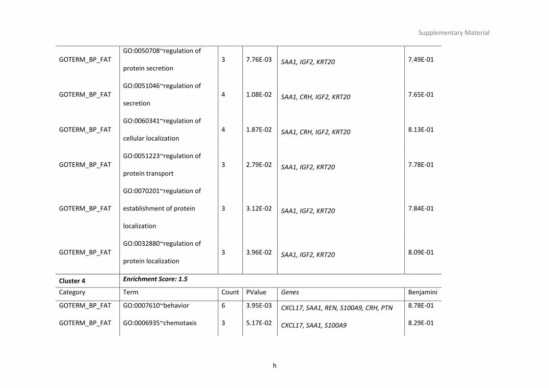
h
Supplementary Material
GOTERM_BP_FAT GO:0050708~regulation of
protein secretion 3 7.76E-03 SAA1, IGF2, KRT20 7.49E-01
GOTERM_BP_FAT GO:0051046~regulation of
secretion 4 1.08E-02 SAA1, CRH, IGF2, KRT20 7.65E-01
GOTERM_BP_FAT GO:0060341~regulation of
cellular localization 4 1.87E-02 SAA1, CRH, IGF2, KRT20 8.13E-01
GOTERM_BP_FAT GO:0051223~regulation of
protein transport 3 2.79E-02 SAA1, IGF2, KRT20 7.78E-01
GOTERM_BP_FAT
GO:0070201~regulation of
establishment of protein
localization
3 3.12E-02 SAA1, IGF2, KRT20 7.84E-01
GOTERM_BP_FAT GO:0032880~regulation of
protein localization 3 3.96E-02 SAA1, IGF2, KRT20 8.09E-01
Cluster 4 Enrichment Score: 1.5
Category Term Count PValue Genes Benjamini
GOTERM_BP_FAT GO:0007610~behavior 6 3.95E-03 CXCL17, SAA1, REN, S100A9, CRH, PTN 8.78E-01
GOTERM_BP_FAT GO:0006935~chemotaxis 3 5.17E-02 CXCL17, SAA1, S100A9 8.29E-01

i
Supplementary Material
GOTERM_BP_FAT GO:0042330~taxis 3 5.17E-02 CXCL17, SAA1, S100A9 8.29E-01
GOTERM_BP_FAT GO:0007626~locomotory
behavior 3 1.30E-01 CXCL17, SAA1, S100A9 9.48E-01
Cluster 5 Enrichment Score: 1.4
Category Term Count PValue Genes Benjamini
UP_SEQ_FEATURE region of interest:Coil 2 3 9.54E-03 KRT5, KRT13, KRT20 4.82E-01
UP_SEQ_FEATURE region of interest:Linker 12 3 9.54E-03 KRT5, KRT13, KRT20 4.82E-01
UP_SEQ_FEATURE region of interest:Coil 1B 3 1.13E-02 KRT5, KRT13, KRT20 4.44E-01
UP_SEQ_FEATURE region of interest:Coil 1A 3 1.13E-02 KRT5, KRT13, KRT20 4.44E-01
UP_SEQ_FEATURE region of interest:Linker 1 3 1.13E-02 KRT5, KRT13, KRT20 4.44E-01
UP_SEQ_FEATURE region of interest:Rod 3 1.16E-02 KRT5, KRT13, KRT20 3.83E-01
UP_SEQ_FEATURE region of interest:Head 3 1.23E-02 KRT5, KRT13, KRT20 3.46E-01
UP_SEQ_FEATURE region of interest:Tail 3 1.29E-02 KRT5, KRT13, KRT20 3.18E-01
SP_PIR_KEYWORDS Intermediate filament 3 1.38E-02 KRT5, KRT13, KRT20 2.46E-01
INTERPRO
IPR018039:Intermediate
filament protein, conserved
site
3 1.42E-02 KRT5, KRT13, KRT20 2.85E-01

j
Supplementary Material
INTERPRO IPR016044:Filament 3 1.42E-02 KRT5, KRT13, KRT20 2.85E-01
INTERPRO IPR001664:Intermediate
filament protein 3 1.46E-02 KRT5, KRT13, KRT20 2.41E-01
PIR_SUPERFAMILY PIRSF002282:cytoskeletal
keratin 3 1.78E-02 KRT5, KRT13, KRT20 3.84E-01
SP_PIR_KEYWORDS keratin 3 4.29E-02 KRT5, KRT13, KRT20 4.66E-01
GOTERM_CC_FAT GO:0005882~intermediate
filament 3 8.06E-02 KRT5, KRT13, KRT20 7.12E-01
GOTERM_CC_FAT GO:0045111~intermediate
filament cytoskeleton 3 8.37E-02 KRT5, KRT13, KRT20 6.60E-01
GOTERM_MF_FAT GO:0005198~structural
molecule activity 4 1.79E-01 KRT5, MYBPC1, KRT13, KRT20 9.94E-01
GOTERM_CC_FAT GO:0044430~cytoskeletal part 5 2.29E-01 TNNT3, KRT5, MYBPC1, KRT13, KRT20 8.82E-01
GOTERM_CC_FAT GO:0005856~cytoskeleton 5 4.84E-01 TNNT3, KRT5, MYBPC1, KRT13, KRT20 9.93E-01
SP_PIR_KEYWORDS coiled coil 5 6.92E-01 OLFM4, KRT5, TRIM31, KRT13, KRT20 9.99E-01

k
Supplementary Material
GOTERM_CC_FAT GO:0043232~intracellular non-
membrane-bounded organelle 6 8.29E-01 TNNT3, KRT5, MYBPC1, S100A9, KRT13,
KRT20 1.00E+00
GOTERM_CC_FAT GO:0043228~non-membrane-
bounded organelle 6 8.29E-01 TNNT3, KRT5, MYBPC1, S100A9, KRT13,
KRT20 1.00E+00
Cluster 6 Enrichment Score: 1.3
Category Term Count PValue Genes Benjamini
GOTERM_BP_FAT GO:0051046~regulation of
secretion 4 1.08E-02 SAA1, CRH, IGF2, KRT20 7.65E-01
GOTERM_BP_FAT GO:0060341~regulation of
cellular localization 4 1.87E-02 SAA1, CRH, IGF2, KRT20 8.13E-01
GOTERM_BP_FAT
GO:0048585~negative
regulation of response to
stimulus
3 2.19E-02 SAA1, CRH, IGF2 8.14E-01
GOTERM_BP_FAT GO:0051047~positive
regulation of secretion 3 2.57E-02 SAA1, CRH, IGF2 7.85E-01
GOTERM_BP_FAT GO:0006954~inflammatory
response 4 3.76E-02 SAA1, S100A9, CRH, IGF2 8.17E-01

l
Supplementary Material
GOTERM_BP_FAT GO:0006952~defense
response 5 5.03E-02 SAA1, S100A9, CRH, PLA2G2A, IGF2 8.40E-01
GOTERM_BP_FAT GO:0051050~positive
regulation of transport 3 9.21E-02 SAA1, CRH, IGF2 9.24E-01
GOTERM_BP_FAT
GO:0051240~positive
regulation of multicellular
organismal process
3 1.07E-01 SAA1, CRH, IGF2 9.27E-01
GOTERM_BP_FAT GO:0009611~response to
wounding 4 1.20E-01 SAA1, S100A9, CRH, IGF2 9.41E-01
GOTERM_BP_FAT GO:0007267~cell-cell signaling 4 1.57E-01 S100A9, CRH, CEACAM6, IGF2 9.61E-01
Cluster 7 Enrichment Score: 1.3
Category Term Count PValue Genes Benjamini
GOTERM_MF_FAT GO:0005509~calcium ion
binding 8 4.19E-03 CAPNS2, ANXA10, CRTAC1, FREM2,
S100A9, MMP7, PLA2G2A, S100A2 3.57E-01
SP_PIR_KEYWORDS calcium 6 3.55E-02 CAPNS2, FREM2, S100A9, MMP7, PLA2G2A, S100A2
4.37E-01
UP_SEQ_FEATURE domain:EF-hand 1 3 6.58E-02 CAPNS2, S100A9, S100A2 7.89E-01
UP_SEQ_FEATURE domain:EF-hand 2 3 6.58E-02 CAPNS2, S100A9, S100A2 7.89E-01

m
Supplementary Material
INTERPRO IPR018249:EF-HAND 2 3 1.02E-01 CAPNS2, S100A9, S100A2 6.75E-01
INTERPRO IPR018247:EF-HAND 1 3 1.04E-01 CAPNS2, S100A9, S100A2 6.43E-01
INTERPRO IPR011992:EF-Hand type 3 1.19E-01 CAPNS2, S100A9, S100A2 6.62E-01

n
Supplementary Material
Table S3.2.4: Comparison of the deviance, p-value and SNPs and/or CpGs detected by each model between LASSO and ENET methods
LASSO ENET
GENE Dev. p.value
markers detected
Dev. P.value markers detected
SNP
mo
del
AIM2 55.8 0.1 6 91.8 0.13 18
CRTAC1 66.2 0.03 18 72.8 0.24 23
SCNN1A 57.9 0.08 26 54.1 0.55 47
CLIC6 75.3 0.01 30 75.3 0.17 104
GSTT1 40.4 0.07 16 43.8 0.9 24
ANXA10 0 - - 137.0 0.01 17
MSMB 4.0 1 3 91.8 0.07 78
MMP7 0 - - 94.8 0.06 19
TCN1 16.3 0.88 1 88.9 0.07 122
IGF2 10.5 0.98 1 101.6 0.05 55
GTSF1 50.4 0.23 2 109.6 0.05 19
IGLJ3 0 - - 97.7 0.05 182
CP
G m
od
el
S100A9 52.5 0.08 10 74.6 0.53 42
S100A2 58.7 0.04 27 58.7 0.66 56
CRTAC1 60.9 0.1 12 62.3 0.55 12
SAA1 127.
8 0.04 21 102.7 0.31 35
MYBPC1 74.5 0.08 26 74.5 0.55 34
SLC38A4 51.7 0.08 16 56.0 0.74 21
GTSF1 46.7 0.1 3 82.2 0.28 9
TSPAN8 67.2 0.05 9 69.3 0.55 9

o
Supplementary Material
FREM2 70.2 0.06 16 76.0 0.52 27
C15orf48 83.7 0.05 25 42.7 0.23 9
CAPNS2 54.9 0.07 9 66.5 0.48 21
KRT20 93.7 <0.01 26 93.7 0.11 53
SERPINB4 68.5 0.03 4 94.0 0.12 18
CXCL17 46.8 0.1 8 45.5 0.24 7
CLIC6 75.3 0.07 27 75.3 0.51 31
TMEM45A 57.3 0.08 13 66.2 0.48 61
IGJ 59.0 0.09 5 174.6 1 32
UBD 75.0 0.07 11 75.5 0.51 11
ARHGEF35 49.6 0.09 9 51.9 0.8 14
CRH 56.7 0.1 4 60.1 0.59 5
TRIM31 47.1 0.1 27 40.6 0.32 55
MMP7 0 - - 99.4 0.08 64
Glo
bal
mo
del
S100A9 53.6
6 0.03 11 46.06 0.59 8
CTSE 60.7 0.06 12 70.12 0.23 17
PLA2G2A 71.4 0.01 10 66.78 0.26 32
HMGCS2 53.3 0.02 8 58.21 0.18 10
AIM2 61.5 0.06 8 104.8
8 0.12 24
PIGR 75.8 <0.01 21 75.48 0.12 21
TNNT3 44.9 0.09 26 36.19 0.82 59
SCNN1A 58.8 0.03 29 58.76 0.18 31
KRT5 58.2 0.02 25 58.14 0.18 31

p
Supplementary Material
FREM2 46.0 0.08 2 48.24 0.45 2
OLFM4 60.0 0.06 10 61.90 0.16 11
C15orf48 49.9 0.02 7 48.80 0.41 6
KRT20 48.4 0.05 3 39.50 0.74 1
KRT13 53.6 0.02 8 54.01 0.25 8
CEACAM7 76.0 <0.01 19 77.40 0.16 32
CLIC6 45.1 0.09 4 47.35 0.50 6
CP 51.1 0.02 3 47.98 0.47 3
IGJ 58.4 0.03 2 94.72 0.17 16
CRABP2 9.78 0.99 2 65.2 0.09 26
REN 0 - 0 84.3 0.03 22
IGF2 89.0
1 0.17 11 92.1 0.04 15
CEACAM5 90.8
5 0.19 22 92.1 0.06 26
NLRP2 14.2
6 0.93 2 84.2 0.04 34

q
Supplementary Material
Table S3.2.5: Comparison of genes selected by each model (SNP, CpG and Global model) using LASSO
Global model SNP model CPG model
GENE Dev P SNPs CPGs Dev P SNPs
(common) Dev P
CPGs (common)
GSTM1 79.9 0.03 12 5 0.0 - 0 0.0 - 0
TMEM45A 57.3 0.01 12 1 53.1 0.23 14 (11) 1.2 1.0 1 (1)
ANXA10 153.3 0.01 22 0 0.0 - 0 0.0 - 0
ALDH7A1 41.1 0.05 6 0 41.1 0.36 6 (6) 6.2 1.0 1 (0)
UBD 53.7 0.04 2 4 3.1 1.0 1 (1) 91.0 0.22 13 (4)
PTN 81.6 0.04 14 0 79.3 0.04 12 (12) 0.0 - 0
IGF2 77.95 0.02 8 2 31.3 0.21 4 (3) 92.3 0.23 13 (2)
SLC38A4 57.8 0.01 18 2 0.0 - 0 13.3 0.94 3 (2)
SERPINB4 78.0 0.02 6 0 91.7 <0.01 13 (6) 17.0 0.90 1 (0)
SERPINB3 142.3 0 1 0 171.6 0.80 29 (11) 25.2 0.46 1 (0)
CEACAM5 88.9 0.02 13 5 0.0 - 0 (0) 77.6 0.05 16 (5)
AIM2 10.7 0.95 1 (1) 0 107.5 0.02 24
FCGR3A 54.5 0.55 23 (14) 4 45.1 0.04 24
AGMO 51.4 0.06 18 (18) 0 45.2 0.04 13

r
Supplementary Material
PTN 81.6 0.04 14 (11) 0 79.3 0.04 12
ARHGEF35 48.4 0.10 7 (5) 1 40.5 0.05 5
SAA2 16.8 0.72 5 (3) 1 69.3 0.04 13
IGHD 66.9 0.11 9 (9) 2 71.7 0.01 10
SERPINB4 78.0 0.02 6 (6) 0 91.7 0 13
CEACAM6 14.7 1.0 0 1 70.4 0.02 9
CLIC6 75.3 0.09 25 (14) 2 73.0 0.02 21
PLA2G2A 88.6 0.77 24 6 (6) 72.9 0.04 12
HMGCS2 0.0 - 0 0 58.7 0.04 10
S100A8 63.1 0.10 3 4 (3) 55.1 0.04 4
AIM2 10.7 0.95 1 0 70.3 0.04 10
PIGR 0.0 - 0 0 65.0 0.04 9
IGJ 59.0 0.16 3 2 (2) 70.8 0.05 4
BHMT 0 - 0 0 49.4 0.05 9
LCN2 70.7 0.08 11 6 (5) 49.7 0.05 6
MSMB 0.0 - 0 0 77.3 0.02 8

s
Supplementary Material
TCN1 21.7 0.87 1 1 (1) 55.1 0.04 8
KRT5 12.3 0.98 0 1 (1) 58.2 0.04 25
CAPNS2 62.7 0.08 15 1 (1) 50.7 0.04 7
KRT13 63.3 0.09 8 4 (4) 52.3 0.04 7
C3 42.1 0.19 10 4 (3) 629 0.04 21
CEACAM7 44.7 0.28 2 3 (2) 77.5 0.02 25
CEACAM5 88.9 0.02 13 5 (5) 77.6 0.05 16
NLRP2 0.0 - 0 0 73.1 0.05 16

t
Supplementary Material
Supplementary Material: PART 3 - Chapter 3
S3.3.1 Excel: Genes and associated eQTLs from model 1, 2 and 3. S3.3.1 Excel refer to the accompanying CD

u
Supplementary Material
R code used in this thesis
Silvia Pineda Sanjuán
Gene Expression preprocessing #Download the Bioconductor program to preprocess the Affy data source("http://bioconductor.org/biocLite.R") biocLite("affy") biocLite("arrayQualityMetrcis") #Read the data library("affy") mydta.affy=ReadAffy() #To read all the .CEL files featureNames(mydta.affy) #To see all the .CEL files we already read geneNames(mydta.affy) #To see all the probes that are in the file affy.data<-exprs(mydta.affy) #To see tha matrix wioth the data ######################### ## Preprocessing the data ######################### ###### # rma algortihm ####### mydta.rma<-rma(mydta.affy) dim(mydta.rma) library("arrayQualityMetrics") arrayQualityMetrics(expressionset=mydta.rma,outdir="QAnorm",force=FALSE,do.logtransform=TRUE) ########## ###After the QC we have decided to remove 7 samples ############## mydta.rma.qc<-rma(mydta.affy) ##The data without the 7 samples dim(mydta.rma.qc) library("arrayQualityMetrics") arrayQualityMetrics(expressionset=mydta.rma.qc,outdir="QAnormQC",force=FALSE,do.logtransform=TRUE)

v
Supplementary Material
############# #To obtain the symbol genes associated to the probesetID using the affymetrix library ############# biocLite("annotate") library("annotate") biocLite("hugene10sttranscriptcluster.db") library("hugene10sttranscriptcluster.db") genenames<-as.character(colnames(expr.rma.data)) HUGO_GeneSymbol<-getSYMBOL(genenames,"hugene10sttranscriptcluster.db") HUGO_ChrSymbol<-lookUp(genenames, "hugene10sttranscriptcluster.db" , "CHR") HUGO_StartSymbol<-lookUp(genenames, "hugene10sttranscriptcluster.db" , "CHRLOC") HUGO_EndSymbol<-lookUp(genenames,"hugene10sttranscriptcluster.db","CHRLOCEND") Correlation between Gene expression and DNA methylation ########### ## Spearman Correlation ############# CorrelationSpearman<-function(i,x,idx,y,idy){ i<-as.numeric(i) print(i) result<-NULL expr<-NULL methy<-NULL d=1 for(z in i:(i+500)){ for(k in 1:ncol(x){ print(d) result[d]<-cor(x[idx,k],y[idy,z],use="pairwise",method="spearman") methy[d]<-colnames(x)[k] expr[d]<-colnames(y)[z] d=d+1 } } results<-list(result,methy,expr) return(results) } spear.expr.methy<-CorrelationSpearman (parameterToPararelize,methylationData,id.methylation, expressionData,id.expression)

w
Supplementary Material
eQTL analysis
######################### ##Regression model non-adjusted ######################### library("parallel") Csnp<-as.numeric(Csnp) results <- rep( list(list()), ncol(expressionData) ) for(j in 1:ncol(expr. expressionData)){ print(paste("j=",j)) eQTL<-function(i){ i<-as.numeric(i) coef.snp<-NULL p.snp<-NULL SNP<-NULL expr<-NULL fit<-lm(expressionData [id.expr,j]~snpsData[id.snps,i]) if(summary(fit)$coefficients[2,4]<=0.05){ expr<-colnames(expressionData)[j] SNP<-colnames(snpsData)[i] coef.snp<-coefficients(fit)[2] p.snp<-summary(fit)$coefficients[2,4] results<-list(expr,SNP,coef.snp,p.snp) return(c(results)) } } out<-mclapply((Csnp+1):(Csnp+10000),eQTL,mc.cores=20) results[[j]]<-do.call(rbind,out) } eqtl.results<-do.call(rbind,results) colnames(eqtl.results)<-c("probeset","SNP","coefficient","p.value")

x
Supplementary Material
Running LASSO with the Global model (SNP+CPG) ##An example file used in this analysis is showed at the end #df.expr.annotate.qc = data frame with the info of the gene array order by row #expr.rma.data.qc=matrix with the gene expression values per individual #df.snps.tumor.qc = data frame with the info for SNPs order by row #snps.data.tumor.qc = matrix with the genotypes per individual and SNP #df.cg.qc = data frame with the info of the CpGs order by row #M.data.qc = matrix with the M-value per individual and CpG for (i in 1:nrow(df.expr.annotate.qc){ print(i) gene.list[i]<-as.vector(df.expr.annotate.qc$gene[i]) gene.probe[i]<-as.vector(df.expr.annotate.qc$probeset[i]) df.expr.gene<-df.expr.annotate.qc[i,] expr.rma.gene<-expr.rma.data.qc[id.expr,i] ##Cis SNPs df.snps.tumor.qc$Categ<-ifelse(df.snps.tumor.qc$Chr==df.expr.gene$chr & (abs(df.snps.tumor.qc$Position- as.numeric(as.character(df.expr.gene$start)))<=1000000 | abs(df.snps.tumor.qc$Position-as.numeric(as.character(df.expr.gene$end)))<=1000000), "cis-acting",ifelse (df.snps.tumor.qc$Chr!=df.expr.gene$chr,"trans-acting ",NA)) df.snps.tumor.cis<-df.snps.tumor.qc[which(df.snps.tumor.qc$Categ=="cis-acting"),] id.snps.cis<-match(df.snps.tumor.cis$NameSNP, colnames(snps.data.tumor.qc)) snps.data.tumor.cis<-snps.data.tumor.qc[id.tumor,id.snps.cis] if(length(id.snps.cis)>1){ snps.data.tumor.cis.qc<-unique(snps.data.tumor.cis,MARGIN=2) } else { snps.data.tumor.cis.qc<-snps.data.tumor.cis } #Cis CpGs df.cg.qc$Categ<-ifelse(df.cg.qc$Chr==df.expr.gene$chr & (abs(df.cg.qc$MapInfo-as.numeric(as.character(df.expr.gene$start)))<=1000000 | abs(df.cg.qc$MapInfo-as.numeric(as.character(df.expr.gene$end)))<=1000000),"cis-acting", ifelse(df.cg.qc$Chr!=df.expr.gene$chr,"trans-acting",NA)) df.methy.cis<-df.cg.qc[which(df.cg.qc$Categ=="cis-acting"),] id.methy.cis<-match(df.methy.cis$Name, colnames(M.data.qc)) M.data.cis<-M.data.qc[id.methy,id.methy.cis]

y
Supplementary Material
if(length(id.methy.cis)>1){ if(dim(snps.data.tumor.cis.qc)[2]>0){ if(dim(snps.data.tumor.cis.qc)[1]>1){ gene.data<-cbind(expr.rma.gene,snps.data.tumor.cis.qc,M.data.cis) ############### #Aplying LASSO # ############### ##GENES gene.lasso.cv<-cv.glmnet(gene.data[,2:ncol(gene.data)],gene.data[,1], standardize=TRUE,alpha=1,nfolds=5) gene.lasso<-glmnet(gene.data[,2:ncol(gene.data)],gene.data[,1], standardize=TRUE,alpha=1,lambda=gene.lasso.cv$lambda.min) GENE.lasso.probe[[i]]<-rownames(gene.lasso$beta)[which(gene.lasso$beta!=0)] GENE.lasso.coef[[i]]<-gene.lasso$beta[which(gene.lasso$beta!=0)] GENE.lasso.id[[i]]<-match(rownames(gene.lasso$beta)[which(gene.lasso$beta!=0)], colnames(gene.data)) GENE.lasso.lambda[i]<-gene.lasso.cv$lambda.min #Deviance GENE.lasso.dev.ratio[i]<-gene.lasso$dev GENE.lasso.dev.null[i]<-gene.lasso$nulldev #same than with glm GENE.lasso.dev[i]<-deviance(gene.lasso) #different from the one produced by glm GENE.lasso.dev[i]<-gene.lasso$nulldev*gene.lasso$dev } } } } save(gene.probe,gene.list,GENE.lasso.probe,GENE.lasso.coef,GENE.lasso.id,GENE.lasso.lambda,GENE.lasso.dev,GENE.lasso.dev.null,file="ResultsGENElasso.Dev.RData")

z
Supplementary Material
Running ENET with the Global model (SNP+CPG) ##An example file used in this analysis is showed at the end #df.expr.annotate.qc = data frame with the info of the gene array order by row #expr.rma.data.qc=matrix with the gene expression values per individual #df.snps.tumor.qc = data frame with the info for SNPs order by row #snps.data.tumor.qc = matrix with the genotypes per individual and SNP #df.cg.qc = data frame with the info of the CpGs order by row #M.data.qc = matrix with the M-value per individual and CpG for (i in 1:nrow(df.expr.annotate.qc){ print(i) gene.list[i]<-as.vector(df.expr.annotate.qc$gene[i]) gene.probe[i]<-as.vector(df.expr.annotate.qc$probeset[i]) df.expr.gene<-df.expr.annotate.qc[i,] expr.rma.gene<-expr.rma.data.qc[id.expr,i] ##Cis SNPs df.snps.tumor.qc$Categ<-ifelse(df.snps.tumor.qc$Chr==df.expr.gene$chr & (abs(df.snps.tumor.qc$Position-as.numeric(as.character(df.expr.gene$start)))<=1000000 | abs(df.snps.tumor.qc$Position-as.numeric(as.character(df.expr.gene$end)))<=1000000),"cis-acting", ifelse (df.snps.tumor.qc$Chr!=df.expr.gene$chr,"trans-acting ",NA)) df.snps.tumor.cis<-df.snps.tumor.qc[which(df.snps.tumor.qc$Categ=="cis-acting"),] id.snps.cis<-match(df.snps.tumor.cis$NameSNP, colnames(snps.data.tumor.qc)) snps.data.tumor.cis<-snps.data.tumor.qc[id.tumor,id.snps.cis] if(length(id.snps.cis)>1){ snps.data.tumor.cis.qc<-unique(snps.data.tumor.cis,MARGIN=2) } else { snps.data.tumor.cis.qc<-snps.data.tumor.cis } #Cis CpGs df.cg.qc$Categ<-ifelse(df.cg.qc$Chr==df.expr.gene$chr & (abs(df.cg.qc$MapInfo-as.numeric(as.character(df.expr.gene$start)))<=1000000 | abs(df.cg.qc$MapInfo-as.numeric(as.character(df.expr.gene$end)))<=1000000),"cis-acting", ifelse(df.cg.qc$Chr!=df.expr.gene$chr,"trans-acting",NA)) df.methy.cis<-df.cg.qc[which(df.cg.qc$Categ=="cis-acting"),] id.methy.cis<-match(df.methy.cis$Name, colnames(M.data.qc)) M.data.cis<-M.data.qc[id.methy,id.methy.cis]

aa
Supplementary Material
# if(length(id.methy.cis)>1){ if(dim(snps.data.tumor.cis.qc)[2]>0){ if(dim(snps.data.tumor.cis.qc)[1]>1){ gene.data<-cbind(expr.rma.gene,snps.data.tumor.cis.qc,M.data.cis) ################## #Aplying enet ENET ################## ##GENES alphalist<-seq(0.01,0.99,by=0.01) elasticnet<-lapply(alphalist, function(a){try(cv.glmnet(gene.data[,2:ncol(gene.data)], gene.data[,1],standardize=TRUE,alpha=a ,nfolds=5))}) xx<-rep(NA,length(alphalist)) yy<-rep(NA,length(alphalist)) for (j in 1:length(alphalist)) { if(class(elasticnet[[j]]) != "try-error"){ xx[j]<-elasticnet[[j]]$lambda.min id.cv.opt<-grep(elasticnet[[j]]$lambda.min,elasticnet[[j]]$lambda,fixed=TRUE) yy[j]<-elasticnet[[j]]$cvm[id.cv.opt] } } id.min<-which(yy==min(yy,na.rm=TRUE)) lambda<-xx[id.min] alpha<-alphalist[id.min] gene.enet<-glmnet(gene.data[,2:ncol(gene.data)],gene.data[,1],standardize=TRUE, alpha=alpha,lambda=lambda) ## alpha.enet[i]<-alpha GENE.enet.probe[[i]]<-rownames(gene.enet$beta)[which(gene.enet$beta!=0)] GENE.enet.coef[[i]]<-gene.enet$beta[which(gene.enet$beta!=0)] GENE.enet.id[[i]]<-match(rownames(gene.enet$beta)[which(gene.enet$beta!=0)], colnames(gene.data[,2:ncol(gene.data)])) GENE.enet.lambda[i]<-gene.enet$lambda #Deviance GENE.enet.dev.ratio[i]<-gene.enet$dev GENE.enet.dev.null[i]<-gene.enet$nulldev #same than with glm GENE.enet.dev[i]<-gene.enet$nulldev*gene.enet$dev }

bb
Supplementary Material
} } } save(gene.list,gene.probe,GENE.enet.probe,GENE.enet.coef,GENE.enet.id,GENE.enet.lambda, GENE.enet.dev,alpha.enet,GENE.enet.dev.null,R2,R2_adj,SSres,MSE,file="ResultsGENEenet.Dev.RData") Permutation based-MaxT: LASSO with Global model (SNP+CPG) ##An example file used in this analysis is showed at the end #df.expr.annotate.qc = data frame with the info of the gene array order by row #expr.rma.data.qc=matrix with the gene expression values per individual #df.snps.tumor.qc = data frame with the info for SNPs order by row #snps.data.tumor.qc = matrix with the genotypes per individual and SNP #df.cg.qc = data frame with the info of the CpGs order by row #M.data.qc = matrix with the M-value per individual and CpG library("glmnet") library("parallel") set.seed(2) m<-length(gene.list) B<-100 p<-27 GENE.lasso.dev.b.results<-matrix(NA,B,m) for(b in 1:B){ print(paste("b=",b)) b.sample<-sample(p) lasso.b<-function(i){ gene.lasso.b.cv<-NULL gene.lasso.b<-NULL GENE.lasso.dev.b<-NULL print(paste("i=",i)) id.gene<-grep(gene.probe[i],df.expr.annotate.qc$probeset) df.expr.gene<-df.expr.annotate.qc[id.gene,] expr.rma.gene<-expr.rma.data.qc[id.expr,id.gene] expr.rma.gene.b<-expr.rma.gene[b.sample] ##Cis SNPs df.snps.tumor.qc$Categ<-ifelse(df.snps.tumor.qc$Chr==df.expr.gene$chr & (abs(df.snps.tumor.qc$Position-as.numeric(as.character(df.expr.gene$start)))<=1000000 | abs(df.snps.tumor.qc$Position-as.numeric(as.character(df.expr.gene$end)))<=1000000),"cis-actin

cc
Supplementary Material
g", ifelse(df.snps.tumor.qc$Chr!=df.expr.gene$chr,"trans-acting ",NA)) df.snps.tumor.cis<-df.snps.tumor.qc[which(df.snps.tumor.qc$Categ=="cis-acting"),] id.snps.cis<-match(df.snps.tumor.cis$NameSNP, colnames(snps.data.tumor.qc)) snps.data.tumor.cis<-snps.data.tumor.qc[id.tumor,id.snps.cis] if(length(id.snps.cis)>1){ snps.data.tumor.cis.qc<-unique(snps.data.tumor.cis,MARGIN=2) } else { snps.data.tumor.cis.qc<-snps.data.tumor.cis } #Cis CpGs df.cg.qc$Categ<-ifelse(df.cg.qc$Chr==df.expr.gene$chr & (abs(df.cg.qc$MapInfo-as.numeric(as.character(df.expr.gene$start)))<=1000000 | abs(df.cg.qc$MapInfo-as.numeric(as.character(df.expr.gene$end)))<=1000000),"cis-acting", ifelse(df.cg.qc$Chr!=df.expr.gene$chr,"trans-acting",NA)) df.methy.cis<-df.cg.qc[which(df.cg.qc$Categ=="cis-acting"),] id.methy.cis<-match(df.methy.cis$Name, colnames(M.data.qc)) M.data.cis<-M.data.qc[id.methy,id.methy.cis] gene.data<-cbind(snps.data.tumor.cis.qc,M.data.cis) ###LASSO### id.exclude<-match(colnames(gene.data),GENE.lasso.probe[[i]]) id.exclude<-which(is.na(id.exclude)==TRUE) gene.lasso.b.cv<-try(cv.glmnet(gene.data[,1:ncol(gene.data)],expr.rma.gene.b, exclude=id.exclude,standardize=TRUE,alpha=1,nfolds=5)) if(class(gene.lasso.b.cv) == "try-error"){ GENE.lasso.dev.b<-NA } else { id.lasso.b<-which(length(GENE.lasso.id[[i]])==gene.lasso.b.cv$nzero) if(length(id.lasso.b)==0){ lambdalist<-seq(0,min(gene.lasso.b.cv$lambda),by=0.00001) if(length(lambdalist)>1){ gene.lasso.b.cv<-cv.glmnet(gene.data[,1:ncol(gene.data)], expr.rma.gene.b, exclude=id.exclude,standardize=TRUE,alpha=1,nfolds=5,lambda=lambdalist) id.lasso.b<-which(length(GENE.lasso.id[[i]])==gene.lasso.b.cv$nzero) } else { GENE.lasso.dev.b<-NA }

dd
Supplementary Material
} cvm<-which(gene.lasso.b.cv$cvm==min(gene.lasso.b.cv$cvm[id.lasso.b])) lambda<-gene.lasso.b.cv$lambda[cvm] gene.lasso.b<-glmnet(gene.data[,1:ncol(gene.data)], expr.rma.gene.b,exclude=id.exclude, standardize=TRUE,alpha=1,lambda=lambda) id.lasso.b.df<-which(length(GENE.lasso.id[[i]])==gene.lasso.b$df) if(length(id.lasso.b.df)!=0 & gene.lasso.b$lambda!=0){ GENE.lasso.dev.b<-GENE.lasso.dev.null[[i]]*gene.lasso.b$dev } else { GENE.lasso.dev.b<-NA } } return(c(GENE.lasso.dev.b)) } out<-mclapply(1:m,lasso.b,mc.cores=30) GENE.lasso.dev.b.results[b,]<-do.call(rbind,out) teststats<-rbind(GENE.lasso.dev,GENE.lasso.dev.b.results) #First row are the original values and the rest are the permuted values rownames(teststats)<-c("Obs.Dev",paste("est.b",c(1:100),sep = "")) colnames(teststats)<-gene.probe ## # # ordering original data test statistics # # teststats[is.na(teststats)] <- 0 #the NA becomes 0 to be able to order the matrix s = order(teststats[1,],decreasing=TRUE) # # # # # non-monotonized p-values B=100 m=dim(teststats)[2] uvals = rep(0,B) pvals = rep(NA,m) for (i in m:1){ print(i) uvals = apply(cbind(uvals,teststats[2:(B+1),s[i]]),1,max) pvals[s[i]] = mean(uvals>=teststats[1,s[i]]) } maxmaxt <- as.data.frame(cbind(colnames(GENE.lasso.dev.b.results)[s],pvals[s]))

ee
Supplementary Material
Permutation based-MaxT: ENET with Global model (SNP+CPG) ##An example file used in this analysis is showed at the end #df.expr.annotate.qc = data frame with the info of the gene array order by row #expr.rma.data.qc=matrix with the gene expression values per individual #df.snps.tumor.qc = data frame with the info for SNPs order by row #snps.data.tumor.qc = matrix with the genotypes per individual and SNP #df.cg.qc = data frame with the info of the CpGs order by row #M.data.qc = matrix with the M-value per individual and CpG
library("glmnet") library("parallel") set.seed(2) m<-length(gene.list) B<-100 p<-27 GENE.enet.dev.b.results<-matrix(NA,B,m) for(b in 1:B){ print(paste("b=",b)) b.sample<-sample(p) enet.b<-function(i){ gene.enet.b.cv<-NULL gene.enet.b<-NULL GENE.enet.dev.b<-NULL print(paste("i=",i)) id.gene<-grep(gene.probe[i],df.expr.annotate.qc$probeset) df.expr.gene<-df.expr.annotate.qc[id.gene,] expr.rma.gene<-expr.rma.data.qc[id.expr,id.gene] expr.rma.gene.b<-expr.rma.gene[b.sample] ##Cis SNPs df.snps.tumor.qc$Categ<-ifelse(df.snps.tumor.qc$Chr==df.expr.gene$chr & (abs(df.snps.tumor.qc$Position-as.numeric(as.character(df.expr.gene$start)))<=1000000 | abs(df.snps.tumor.qc$Position-as.numeric(as.character(df.expr.gene$end)))<=1000000),"cis-acting", ifelse(df.snps.tumor.qc$Chr!=df.expr.gene$chr,"trans-acting ",NA)) df.snps.tumor.cis<-df.snps.tumor.qc[which(df.snps.tumor.qc$Categ=="cis-acting"),] id.snps.cis<-match(df.snps.tumor.cis$NameSNP, colnames(snps.data.tumor.qc)) snps.data.tumor.cis<-snps.data.tumor.qc[id.tumor,id.snps.cis]

ff
Supplementary Material
if(length(id.snps.cis)>1){ snps.data.tumor.cis.qc<-unique(snps.data.tumor.cis,MARGIN=2) } else { snps.data.tumor.cis.qc<-snps.data.tumor.cis } #Cis CpGs df.cg.qc$Categ<-ifelse(df.cg.qc$Chr==df.expr.gene$chr & (abs(df.cg.qc$MapInfo-as.numeric(as.character(df.expr.gene$start)))<=1000000 | abs(df.cg.qc$MapInfo-as.numeric(as.character(df.expr.gene$end)))<=1000000),"cis-acting", ifelse(df.cg.qc$Chr!=df.expr.gene$chr,"trans-acting",NA)) df.methy.cis<-df.cg.qc[which(df.cg.qc$Categ=="cis-acting"),] id.methy.cis<-match(df.methy.cis$Name, colnames(M.data.qc)) M.data.cis<-M.data.qc[id.methy,id.methy.cis] gene.data<-cbind(snps.data.tumor.cis.qc,M.data.cis) ###ENET### id.exclude<-match(colnames(gene.data),GENE.enet.probe[[s[i]]]) id.exclude<-which(is.na(id.exclude)==TRUE) alphalist<-seq(0.01,0.99,by=0.01) elasticnet.b.cv<-lapply(alphalist, function(a){try(cv.glmnet(gene.data[,1:ncol(gene.data)], expr.rma.gene.b,exclude=id.exclude,standardize=TRUE,alpha=a,nfolds=5))}) cvm<-rep(NA,length(alphalist)) lambda<-rep(NA,length(alphalist)) cvm.min<-rep(NA,length(alphalist)) lambda.min<-rep(NA,length(alphalist)) cvm.null<-rep(NA,length(alphalist)) for (j in 1:length(alphalist)) { if(class(elasticnet.b.cv[[j]]) != "try-error"){ id.enet.b<-which(length(GENE.enet.id[[s[i]]])==elasticnet.b.cv[[j]]$nzero) if(length(id.enet.b)!=0){ cvm[j]<-which(elasticnet.b.cv[[j]]$cvm==min(elasticnet.b.cv[[j]]$cvm[id.enet.b])) cvm.min[j]<-min(elasticnet.b.cv[[j]]$cvm[id.enet.b]) lambda[j]<-elasticnet.b.cv[[j]]$lambda[cvm[j]] } } } if(length(na.omit(lambda))!=0){ id.min<-which(cvm.min==min(cvm.min,na.rm=TRUE))
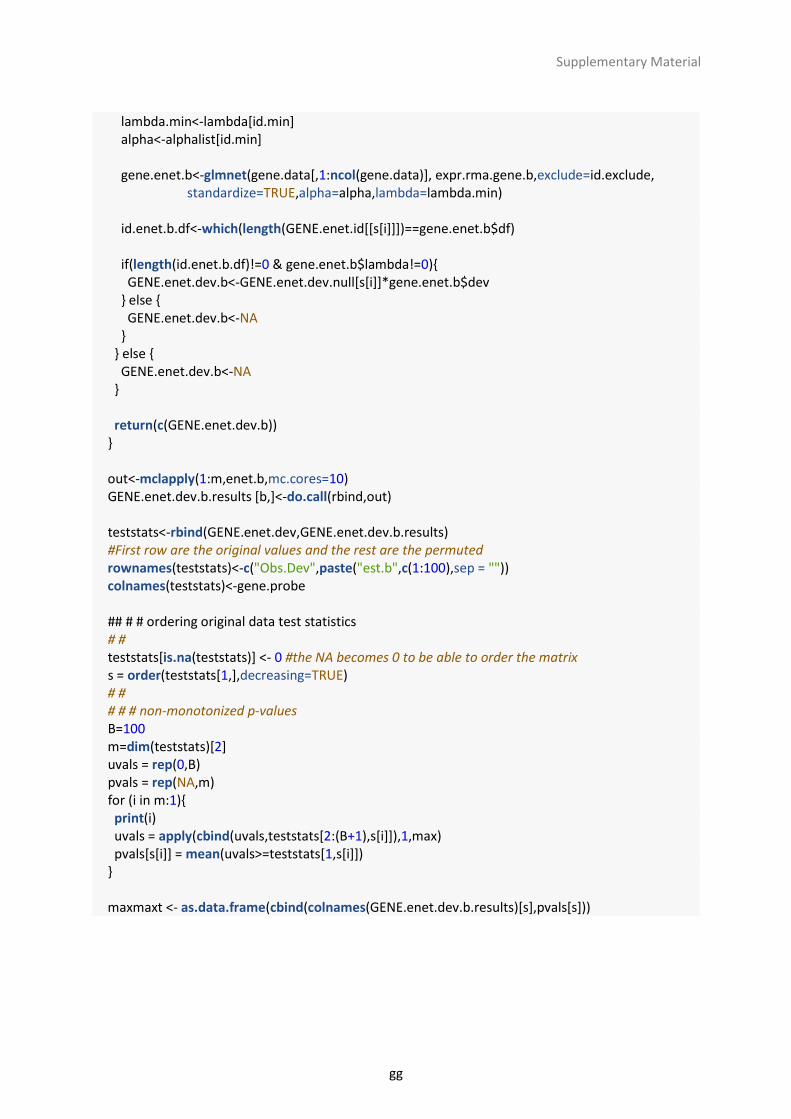
gg
Supplementary Material
lambda.min<-lambda[id.min] alpha<-alphalist[id.min] gene.enet.b<-glmnet(gene.data[,1:ncol(gene.data)], expr.rma.gene.b,exclude=id.exclude, standardize=TRUE,alpha=alpha,lambda=lambda.min) id.enet.b.df<-which(length(GENE.enet.id[[s[i]]])==gene.enet.b$df) if(length(id.enet.b.df)!=0 & gene.enet.b$lambda!=0){ GENE.enet.dev.b<-GENE.enet.dev.null[s[i]]*gene.enet.b$dev } else { GENE.enet.dev.b<-NA } } else { GENE.enet.dev.b<-NA } return(c(GENE.enet.dev.b)) } out<-mclapply(1:m,enet.b,mc.cores=10) GENE.enet.dev.b.results [b,]<-do.call(rbind,out) teststats<-rbind(GENE.enet.dev,GENE.enet.dev.b.results) #First row are the original values and the rest are the permuted rownames(teststats)<-c("Obs.Dev",paste("est.b",c(1:100),sep = "")) colnames(teststats)<-gene.probe ## # # ordering original data test statistics # # teststats[is.na(teststats)] <- 0 #the NA becomes 0 to be able to order the matrix s = order(teststats[1,],decreasing=TRUE) # # # # # non-monotonized p-values B=100 m=dim(teststats)[2] uvals = rep(0,B) pvals = rep(NA,m) for (i in m:1){ print(i) uvals = apply(cbind(uvals,teststats[2:(B+1),s[i]]),1,max) pvals[s[i]] = mean(uvals>=teststats[1,s[i]]) } maxmaxt <- as.data.frame(cbind(colnames(GENE.enet.dev.b.results)[s],pvals[s]))

hh
Supplementary Material
Example files used in the R code
Correlation between Gene expression and DNA methylation
eQTL analysis
MethylationData
CpGs
Individuals cg00000292 cg00002426 cg00005847 cg00006414 cg00007981 cg00008493
10090110 0.147817 -4.0826683 2.685858 -4.90956 -5.851988 6.163102
10090210 2.4470796 -2.2438665 1.318464 -3.112244 -5.249451 6.02881
10090510 0.1218647 -4.0959792 2.184173 -4.235395 -5.024319 5.427359
10090910 -0.3459959 -2.7344368 1.777525 -3.867592 -5.125091 5.700051
10091210 1.5235213 -5.1090725 2.819315 -4.822256 -7.35714 5.535791
ExpressionData
Probeset
Individuals 7892501 7892502 7892503 7892504 7892505 7892506
10090510 9.168303 4.934505 6.282962 11.03266 4.790657 4.899811
10090910 7.492617 4.932734 5.464684 11.35226 4.239772 4.886739
10091310 9.468703 5.093432 6.004068 11.06449 4.958094 4.458435
10091710 7.825073 5.273232 4.466145 11.15985 5.678544 4.702994
10091810 9.588365 5.018018 5.092825 10.6012 4.135782 4.600051
SnpsData
snps
Individuals rs3131972 rs3115860 rs3131969 rs1048488 rs3115850 rs2905046
10090110 0 0 0 1 1 0
10090210 1 0 0 0 1 0
10090510 0 2 1 0 0 1
10090910 2 0 1 0 1 0
10091210 0 0 0 0 1 0

ii
Supplementary Material
Running LASSO with the Global model (SNP+CPG) Running ENET with the Global model (SNP+CPG) Permutation based-MaxT: LASSO with Global model (SNP+CPG) Permutation based-MaxT: ENET with Global model (SNP+CPG) #df.expr.annotate.qc = data frame with the info of the gene array order by row
probeset gene chr start end
7896756 FAM87A 8 325931 333174
7896759 LOC643837 1 763064 789740
7896761 SAMD11 1 861121 879961
7896779 KLHL17 1 895967 901095
7896798 PLEKHN1 1 901877 910482
7896817 ISG15 1 948847 949915
#expr.rma.data.qc = matrix with the gene expression probes values per individual
Probeset
Individuals 7892501 7892502 7892503 7892504 7892505 7892506
10090510 9.168303 4.934505 6.282962 11.03266 4.790657 4.899811
10090910 7.492617 4.932734 5.464684 11.35226 4.239772 4.886739
10091310 9.468703 5.093432 6.004068 11.06449 4.958094 4.458435
10091710 7.825073 5.273232 4.466145 11.15985 5.678544 4.702994
10091810 9.588365 5.018018 5.092825 10.6012 4.135782 4.600051
#df.snps.tumor.qc = data frame with the info for SNPs order by row
NameSNP Chr Position
rs3094315 1 752566
rs3115860 1 753405
rs3115850 1 761147
rs12562034 1 768448
rs12124819 1 776546
rs4040617 1 779322
#snps.data.tumor.qc = matrix with the genotypes per individual and SNP
snps
Individuals rs3131972 rs3115860 rs3131969 rs1048488 rs3115850 rs2905046
10090110 0 0 0 1 1 0
10090210 1 0 0 0 1 0
10090510 0 2 1 0 0 1
10090910 2 0 1 0 1 0

jj
Supplementary Material
#df.cg.qc = data frame with the info of the CpGs order by row
Name Chr MapInfo
cg00000292 16 28890100
cg00002426 3 57743543
cg00005847 2 177029073
cg00007981 11 93862594
cg00008493 14 93813777
cg00008713 18 11980953
#M.data.qc = matrix with the M-value per individual and CpG
CpGs
Individuals cg00000292 cg00002426 cg00005847 cg00006414 cg00007981 cg00008493
10090110 0.147817 -4.0826683 2.685858 -4.90956 -5.851988 6.163102
10090210 2.4470796 -2.2438665 1.318464 -3.112244 -5.249451 6.02881
10090510 0.1218647 -4.0959792 2.184173 -4.235395 -5.024319 5.427359
10090910 -0.3459959 -2.7344368 1.777525 -3.867592 -5.125091 5.700051
10091210 1.5235213 -5.1090725 2.819315 -4.822256 -7.35714 5.535791


APPENDIX


Published papers during my PhD
Silvia Pineda, Paulina Gomez-Rubio, Antoni Picornell, Kyrilo Bessonov, Mirari Márquez, Manolis
Kogevinas, Francisco X Real, Kristel Van Steen, Núria Malats. “Framework for the integration of
genomics, epigenomics, and transcriptomics for complex diseases” Hum Hered 2015;79:124-
136. DOI:10.1159/000381184
Silvia Pineda, Roger L. Milne, M. Luz Calle, Nathaniel Rothman, Evangelina López de Maturana, Jesús Herranz, Manolis Kogevinas, Stephen J. Chanock, Adonina Tardón, Mirari Márquez, Lin T. Guey, Montserrat García-Closas, Josep Lloreta, Erin Baum, Anna González-Neira, Alfredo Carrato, Arcadi Navarro, Debra T. Silverman, Francisco X. Real Núria Malats. “Genetic variation in the TP53 pathway and bladder cancer risk. A comprehensive analysis” PLoS One. 2014 May 12; 9(5):e89952. DOI:10.1371/journal.pone.0089952
Divyansh Agarwal, Silvia Pineda, et al. “FGF receptor genes and breast cancer susceptibility: results from the Breast Cancer Association Consortium”, British Journal of Cancer (February 2014), 1–13 | DOI: 10.1038/bjc.2013.769
Submitted papers
Silvia Pineda, Francisxo X Real, Manolis Kogevinas, Alfredo Carrato, Stephen J. Chanock, Núria Malats, Kristel Van Steen. “Integration analysis of three omics data using penalized regression methods: An application to bladder cancer” PlosGenetics, 2015
Evangelina López de Maturana, Silvia Pineda, Angela Brand, and Núria Malats. Towards the integration of omics data in epidemiological studies: still a “long and winding road.” Genetic Epidemiology, (2015)
Silvia Pineda, Kristel Van Steen, Núria Malats. “Integrative eQTL –omics analysis considering tumor
tissue and blood samples in individuals with bladder cancer” AJHG, 2015

Participation in conference during my PhD
Capita Selecta in Complex Disease Analysis
Liège, Belgium
Oral Presentation: Integration analysis of ‘omics’ data with penalized regression: An application in bladder cancer
Nov. 24-26, 2014
SEE: XXXII Scientific Meeting of the Spanish Epidemiology Society
Alicante, Spain
Oral Presentation: Integration analysis of ‘omics’ data with penalized regression: An application in bladder cancer
Sept. 3-5, 2014
EMGM: European Mathematical Genetics Meeting
Köln, Germany
Poster: Integration analysis of ‘OMICS’ data using penalized regression methods: An application to bladder cancer
April 1-2, 2014
XIV Scientific Meeting of the Spanish Biometrics Society
Ciudad Real, Spain
Oral presentation: Statistical approaches for the integration of ‘omics’ and epidemiological data: an application to bladder cancer.
May 22-24, 2013
SEE: XXX Scientific Meeting of the Spanish Epidemiology Society
Santander, Spain
Oral presentation: The application of penalized regression (LASSO) for genetic association studies
Oct. 17-19, 2012
5TH International Consortium of Bladder Cancer Meeting
Spanish National Cancer Research Centre (CNIO), Madrid, Spain
Poster: Eped+omics, statistical approaches for the integration of ‘omics’ data: An application in bladder cancer
Oct. 8-9, 2012

Invited talks & seminars during my PhD
Cancer Genomics and Personalized Medicine Workshop
Barcelona, Spain
Invited Speaker: Adapting innovative statistical modelling for integrative –omics analysis towards the identification of cancer molecular insights
July 1, 2015
Statistical Modeling of Cancer Genetic Predisposition
Vienna, Austria
Invited Speaker: Approaching the complexity of bladder cancer genetic predisposition by applying innovative statistical modelling
Mar. 19-20, 2015
Teaching during my PhD
Master Degree in Molecular Oncology
Bio-health studies center, Madrid, Spain.
Course: Survival Analysis
April 25, 2015
Mentor of students from medical degree in the preventive medicine and public health course
Autónoma University, Madrid, Spain.
April, 2015
Master in Bioinformatics and computational biology
Institute of Health Carlos III (ISCIII), Madrid, Spain
Course: Genomic Variation
Feb. 3-4, 2015

Copyright © 2022 FDOKUMEN