Chapter 7. Functional Genomics

Contents

7. Structural Genomics 7.1. Annotating Protein Function

7.1.1. The BLAST Search Tool at NCBI 7.1.2. Functional Annotation Using Yeast Knockout Mutations 7.1.3. Functional Annotation Using Mouse Knockout Mutations 7.1.4. Gene Knockdown Using RNAi 7.1.5. Gene Editing Using CRISPR-CAS 7.1.6. 7.1.7. Protein Localization Using GFP Tags 7.1.8. Protein-Protein Interactions by Yeast 2-hybrid

7.2. Proteomics 7.2.1. What is Proteomics 7.2.2. Protein Modifications 7.2.3. Technology for Proteomic Analysis 7.2.4. Structural Analysis of Proteins

7.3. Transcriptome and Gene Expression 7.3.1. Single Transcript Abundance Estimation 7.3.2. Genome-wide Transcript Abundance Estimation

CONCEPTS OF GENOMIC BIOLOGY Page 7- 1

The Central Dogma of molecular biology simply stated is that DNA is coded into RNA and RNA is coded into pro-tein. Further, we know that the phenotype of a gene is determined by the proteins made inside the cell. Thus, it is because of the function of the protein that the gene is expressed as a phenotype. In this chapter will examine how we go about understanding protein function so that the annotation of proteins found at NCBI is determined. The tools that are required to do this will also be consid-ered. Today we extend this functional analysis to include a sophisticated analysis of gene expression that involves both all transcripts made by a genome, the transcrip-tome, and all proteins made from a genome, the prote-ome.

Previously in Chapter 6 Structural Genomics, we ex-

amined how genes were identified in sequenced ge-nomes. Once the coding sequences are identified, the lo-cation of introns and exons, the promoter region and the 3’-UTR have been identified, the next step is to annotate the structure and function of the protein products of pro-tein coding ORFs. The general approach and some of the tools available for this task are outlined here.

7.1.1. The BLAST Search Tool at NCBI (RETURN)

The Basic Local Alignment Search Tool (BLAST) at NCBI provides the ability to search a sequence database with a given sequence called a query sequence. Those se-quences most similar to the query are reported back with a sequence alignment shown, a computed score indicat-ing similarity of the query to the sequences found in the database, and any corresponding annotation for the sim-ilar hit sequences to the query. Thus, we can learn how the proteins function that are most closely related to the query sequence we are using.

There are several types of BLAST sequencing that can be used. These include:

I. Nucleotide BLAST – using a nucleotide query to search a nucleotide database for the most simi-lar sequences.

CHAPTER 7. FUNCTIONAL GENOMICS (RETURN)

7.1. ANNOTATING PROTEIN FUNCTION (RETURN)

CONCEPTS OF GENOMIC BIOLOGY Page 7- 2

II. Protein BLAST – using a protein query to search a protein database for the most similar se-quences.

III. Translated BLAST searches including a. BLASTX – using a translated nucleotide

query in all 3 reading frames to search a protein database for protein databases for sequences most similar to the translated query.

b. TBLASTN – using a protein sequence to search a nucleotide database translated in all 3 reading frames.

Note that we do a laboratory covering the BLAST tool at NCBI, and examples of these searches are executed and examined. The utility of BLAST can be further ex-tended by linking BLAST Search Results to a gene ontol-ogy (GO). The Gene Ontology Consortium attempts pro-vides a framework for relating functional information about genes to the function of the whole organism, e.g. determining when, where, and how a gene functions (in-cluding metabolic and developmental pathways). The ex-tension of BLAST described above can be executed at sev-eral different web pages including the BLAST2GO page. Such analyses have been conducted on virtually every ge-nome sequenced, to provide at least a minimal functional analysis of the genome sequence. An example of the GO analysis of the Yeast Genome is given in Figure 7.1. The

number of genes in various categories organized in two different ways is shown in the figure.

7.1.2. Functional Annotation Using Yeast Knockout Mutations (RETURN)

The purpose of making a knockout mutation is to re-place the open reading frame of an endogenous gene in

Figure 7.1. Yeast GO analysis, indicating the number of genes in each category. Each of the roughly 6200 genes identified in the yeast genome have been placed in one or more GO categories, and a graphic summary of the analysis is presented above. Note that the categories can be al-tered so that critical points of interest can be investigated in more de-tail.

CONCEPTS OF GENOMIC BIOLOGY Page 7- 3

the yeast genome with a replacement sequence that makes the endogenous gene nonfunctional. Typically, the replacement sequence is a selectable marker gene that allows the easy detection of the insertion. The most commonly used selectable marker is a gene for resistance to the antibiotic kanamycin. The KanR (kanamycin re-sistance) cassette including a promoter for the gene is in-serted between a sequence of approximate 50 base-pairs near the start site at the 5’-end of the gene to a sequence about 50 base-pairs long near the 3’-end of the gene. As a result, the middle portion of the gene is removed (de-leted) and the cassette is inserted. The insertion is accom-plished by a process referred to as homologous recombi-nation (Figure 7.2a)

This recombinant construct is made in a shuttle vector (refer to Chapter 4, The Genomic Biologists Toolkit, sec-tion 4.2.3.) so that it can be transferred into yeast cells, and selection performed for cells that are stably resistant to kanamycin. This indicates that the knockout construct has been successfully recombined into the chromosomal DNA.

Successful knockouts are further verified using PCR. A

forward primer (A) outside the gene on the 5’-end and a reverse primer (B) inside the endogenous gene are used in one PCR reaction, while a forward primer (C) also inside the endogenous gene and a reverse primer (D) outside the 3’-end of the gene are used in a second reaction. If

Figure 7.2. a) Yeast Knockout mutations are constructed using a KanR cassette by homologous recombination (see text for details). B) verifica-tion of the knockout by PCR using 4 primer sets A-B, C-D, A-KanB, and KanC-D.

CONCEPTS OF GENOMIC BIOLOGY Page 7- 4

the knockout was unsuccessful, these two sets of primers will each amplify endogenous gene sequences. However, if the knockout was successfully made these primers will not amplify sequences but using the same (A) and (D) pri-mers with a reverse primer that lands inside the KanR cas-sette (KanB), and a forward primer also landing inside the cassette (KanC) in Figure 7.2b will amplify sequences in the knockout, while they will not amplify endogenous gene sequences.

When you want to determine the phenotype of a gene in any Eukaryote, knockout mutations of the yeast ortholog are a valuable tool for doing this. However, the technique only works when an ortholog of the gene of in-terest can be found in yeast. This is particularly useful for genes with simple metabolic phenotypes.

The steps involved would be as follows:

I. Identify the putative protein of interest using a BLAST search.

II. Determine whether there is a yeast ortholog of your gene of interest.

III. Construct a knockout of that gene and deter-mine the phenotype of the knockout.

IV. Obtain a cDNA clone of the gene of interest from the appropriate Eukaryotic organism.

V. Construct a yeast expression shuttle vector that expresses the gene of interest.

VI. Move that construct into the yeast knockout and determine whether the normal phenotype is re-stored or if knockout phenotype remains.

The limitation of this analysis is that your gene of in-terest must have a yeast ortholog. However, yeast has a genome that contains approximately 6,300 genes, and most Eukaryotes contain several-fold more genes. Yeast cells are essentially unicellular, while most Eukaryotes of interest are multicellular, and have many genes associ-ated with the developmentally appropriate expression of genes. In order to use the knockout approach on complex multicellular organisms, mouse knockouts have proven more useful for many genes.

7.1.3. Functional Annotation Using Mouse Knockout Mutations (RETURN)

A mouse knockout is made using homologous recom-bination just as in yeast. The mouse knockout cassette contains the ends of the target gene just as with yeast, but it contains two selectable markers, one inside the gene of interest, and the other outside the gene of inter-est. These two markers make it possible to distinguish between a true homologous recombination knockout, and integration of the foreign DNA vector into a random site in the genome which would not produce a mouse knockout (Figure 7.3).

CONCEPTS OF GENOMIC BIOLOGY Page 7- 5

The deletion module is introduced into embryonic mouse stem cells (ES) from an agouti mouse, and the ES cells are incubated on “selective” media such that the cells with the internal deletion marker (neoR in the case shown in Figure 7.3) and lacking the marker outside the deletion site (tk in Figure 7.3) are allowed to grow. This enriches the growing cells that have the deletion module inserted into the target gene via homologous recombina-tion and minimizes cells that had the full DNA vector ran-domly integrated into the genome which is the other pos-sible outcome. Note that it is still possible that only the inside marker randomly integrates randomly, and the outside marker is lost without homologous recombina-tion taking place, but this is less likely event than homol-ogous recombination.

Once cells expressing the inside marker are have been grown and selected, they are injected into a developing embryo of a black mouse (Figure 7.4). The animals that results from these injected embryos will be chimeric,

meaning that they contain a mixture of agouti injected cells and the original black mouse embryonic cells. These chimeric mice are then mated, and agouti mice and black

Figure 7.3. A mouse knockout is made using homologous recombination just as in yeast. The knockout cassette contains the ends of the target gene just as with yeast, but it contains two selectable markers, one in-side he gene of interest, and the other outside the gene of interest. Here neoR is the maker inside the gene, and thymidine kinase (tk) is the maker outside. Embryonic mouse stem cells are incubated with deletion mod-ule with two possible outcomes. Either the neoR maker homologously recombines into the gene of interest (left), or the deletion module ran-domly integrates in which case the cells will express both the neoR and the tk genes.

CONCEPTS OF GENOMIC BIOLOGY Page 7- 6

mice result from this cross. Note that agouti is dominant to black, and agouti mice are also likely heterozygous

for the knockout mutation. This can be verified using PCR, and then a line of knockout mice can be created.

Once the knockout mice have been obtained. The next task is to determine the biochemical, physiological, morphological, regulatory, and/or behavioral functional phenotype of the knocked-out gene. Not only do such gene knockouts provide valuable information about the expected phenotype of the gene, but they also can yield valuable experimental material for investigation of the function of the gene.

One difficulty in using knockout mutations to investi-gate gene function can be that the knockout may be le-thal. Complete absence of the gene/protein may lead a non-viable mouse that cannot survive and a line that can-not be propagated for further study. Under such circum-stances, a possible solution is to create a gene knock-down rather than a gene knockout.

7.1.4. Gene Knockdown Using RNAi (RETURN) We have previously discussed the role of natural RNAi

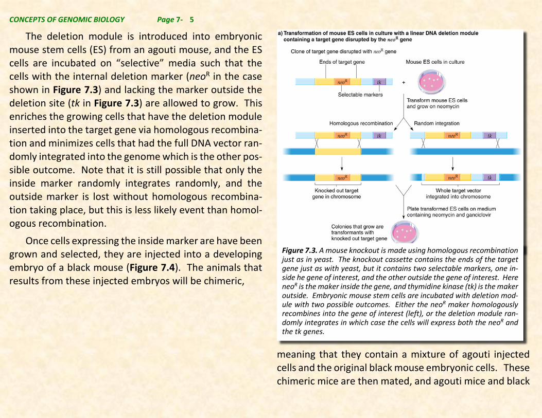
in gene regulation by miRNAs and siRNAs, but it is also possible to construct a gene that can be used for syn-thetic RNAi (Figure 7.5). The engineered synthetic gene places the sequence to be knocked down in the

An I

Figure 7.4. Once the agouti mouse ES cells containing the knockout con-struct are selected, they are injected into the embro of a black mouse where they become part of a chimeric embryo that produces a chimeric mouse. If any of the agouti, knockout-bearing cells become germline cells, agouti mice will result from the cross of two chimeri agouti mice. These resulting agouti mice should be homozygous for the knockout (de-letion) of the gene of interest, and a line of these mice can be propa-gated for future study.

CONCEPTS OF GENOMIC BIOLOGY Page 7- 7

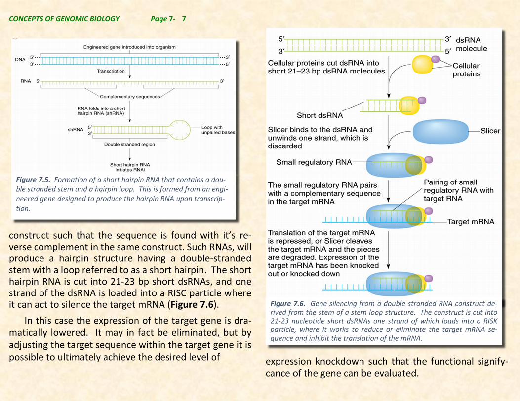
construct such that the sequence is found with it’s re-verse complement in the same construct. Such RNAs, will produce a hairpin structure having a double-stranded stem with a loop referred to as a short hairpin. The short hairpin RNA is cut into 21-23 bp short dsRNAs, and one strand of the dsRNA is loaded into a RISC particle where it can act to silence the target mRNA (Figure 7.6).

In this case the expression of the target gene is dra-matically lowered. It may in fact be eliminated, but by adjusting the target sequence within the target gene it is possible to ultimately achieve the desired level of

expression knockdown such that the functional signify-cance of the gene can be evaluated.

Figure 7.5. Formation of a short hairpin RNA that contains a dou-ble stranded stem and a hairpin loop. This is formed from an engi-neered gene designed to produce the hairpin RNA upon transcrip-tion.

Figure 7.6. Gene silencing from a double stranded RNA construct de-rived from the stem of a stem loop structure. The construct is cut into 21-23 nucleotide short dsRNAs one strand of which loads into a RISK particle, where it works to reduce or eliminate the target mRNA se-quence and inhibit the translation of the mRNA.

CONCEPTS OF GENOMIC BIOLOGY Page 7- 8

7.1.5. Gene Editing Using Crispr-CAS (RETURN) One of the newest technologies for editing genes is

the CRISPR-CAS9 technique. Link out at the How CRISPR Works link given or watch this brief NOVA video on how CRISPR works. Note that this technology is just now emerging, and it is clear that it has many uses related to those technologies we have talked about above for gene functional analysis. It is very powerful and can be used to delete an entire gene or to edit only a single nucleotide or a few nucleotides to determine the role that specific parts of proteins play.

The ethical consequences of using CRISPR for gene therapy on humans has been subject to debate, and an interesting presentation is given in a TED Talk by Ellen Jorgensen.

7.1.6. Protein Localization using GFP Tags (RETURN) An important type of annotation for proteins involves

determining where inside the cell the protein is normally localized. This can be accomplished using a protein from the jellyfish that naturally fluoresces green called Green Fluorescent Protein (GFP). This protein can be added to the 3’- or 5’-end of the protein and this modified chimeric gene inserted into the organism of choice using one of the techniques above.

It is preferable to examine the localization of a protein in the organism from which the protein comes, but some-times this is not really possible. Since most of the protein localization signals within protein sequences are univer-sal, it is possible to make the construct in yeast and ex-amine localization in the yeast system rather than in the system of origin.

7.1.7. Protein-Protein Interactions by Yeast 2-hybrid

(RETURN) Many proteins interact with one or more other pro-

teins, and the interacting partners of a protein are a crit-ical part of understanding the function of the protein. For example, protein kinases or methylases that phos-phory-late or methylate other proteins must of necessity inter-act with the proteins they modify. Subunits of multisub-unit proteins must interact, and the proteins of larger complexes such as spliceosomes and ribosomes are all examples of protein-protein interactions.

The goal of a yeast two hybrid experiment is to deter-mine if two or more proteins interact with each other. Review the role of the Gal4p protein in regulating the GAL-regulon genes that we discussed earlier. Recall that Gal4p has a DNA binding domain (BD) and an activation domain (AD) that is responsible for activating RNA poly-merase to transcribe the gene associated with the UAS promoter. To conduct a yeast two-hybrid experiment a chimeric gene is first constructed in the yest genome that

CONCEPTS OF GENOMIC BIOLOGY Page 7- 9

has a UAS enhancer sequence ahead of a reporter gene such as the lacZ gene from the lac operon in E. coli. Then two plasmid constructs are made. The first has the BD fused with an interacting protein that we will call the bait. The second plasmid has the AD fused with a second pro-tein that we call the prey. Figure 7.7 describes the results obtained when the bait interacts with the prey. If they do not interact then no transcription of the reporter oc-curs. By testing a series of proteins as preys, multiple in-teracting partners with the bait can be tested.

Figure 7.7. Overview of Yeast two-hybrid assay, checking for interac-tions between two proteins, called here Bait and Prey. (A) Gal4 tran-scription factor gene produces a two domain protein (BD and AD) which is essential for transcription of the reporter gene (LacZ); (B,C) Two fusion proteins are prepared: Gal4BD+Bait and Gal4AD+Prey. Neither of them is sufficient to initiate the transcription (of the reporter gene) alone; (D) When both fusion proteins are produced and Bait part of the first inter-acts with Prey part of the second, transcription of the reporter gene oc-curs.

CONCEPTS OF GENOMIC BIOLOGY Page 7- 10

The study of genes and DNA sequences could be de-

scribed as Genomics. A subdivision of genomics dealing with all the RNAs found in cells is referred to as Tran-scriptomics. Proteomics refers to all of the proteins ex-pressed in organisms, their structure, and when and where they function in the organism and in cells. The

study of the metabolites produced in cells can also be characterized as Metabolomics. Understanding the inte-gration of these types if information is referred to as sys-tems biology.

7.2.1. What is Proteomics (RETURN)

Proteomics could be considered: a) A catalog of all proteins expressed throughout the life

cycle of the organism. b) A catalog of all proteins expressed in each cell or tis-

sues of an organism. c) A catalog of all proteins expressed under all condi-

tions in an organism. d) A catalog of all proteins expressed in all tissues of an

organism. e) Understanding the structural properties of proteins. f) Analyze the function of all proteins in an organism

• To understand how proteins of an organism inter-act with each other.

• To understand how proteins of an organism are modified & regulated

While genomics has greatly facilitated proteomics projects, characterizing a proteome is considerably more complex than sequencing a genome. At the most basic level, there are far more proteins than genes in a eukary-otic organism. For example, humans possess approxi-mately 25,000 genes, but are estimated to have between 200,000 and 2 million unique proteins. Many of these

7.2. PROTEOMICS (RETURN)

Genomics DNA

Proteins

Metabolites

RNA

The Central Dogma

Proteomics

Metabolomics

Transcriptomics

Transcription

Systems Biology

Translation

Cellular Catalysis

Phenotype Phenomics

The Omics

Figure 7.8. The subdivisions of genomic biology and their relationship to the central dogma.

CONCEPTS OF GENOMIC BIOLOGY Page 7- 11

proteins are produced by alternative splicing. These splice variants are likely to have non overlapping func-tions. In addition, the exact proteins that are expressed at any given moment depend on a person’s age, health, and environmental stimuli. To complicate matters fur-ther, the diverse chemical properties of proteins make it difficult to develop a “one size fits all” approach to char-acterizing the proteome. Instead, a wide variety of tech-nologies is necessary.

7.2.2. Protein Modifications (RETURN)

There are numerous ways that lead to one gene pro-ducing multiple amino acid sequences, and numerous mechanisms of posttranslational control of protein func-tion including covalent modification, or by other mecha-nisms.

Review Chapter 3, section 3.7.2. on mRNA splicing. Recall that in Figure 3.57. an example of transcript splic-ing that generates calcitonin in thyroid tissue while the same transcript generates CGRP in neuronal cells. This is an example of two unique proteins being created from a single gene transcript. This phenomenon is not uncom-mon. Often related proteins are made for the same pri-mary transcript under different circumstances.

Protein function may be altered by posttranslational modifications as well. Posttranslational modifications are defined as any changes to the covalent bonds of a protein after it has been fully translated. There are numerous

types of posttranslational modifications, a subset of which is shown in Table 7.1. Many of these such as phos-phorylation, acetylation, and methylation have already been discussed. A detailed description of the chemistry involved in each of these posttranslational modifications is beyond the scope of this chapter. The list given here is meant to show the functional diversity of posttransla-tional modification and its importance.

Another type of posttranslational protein modification is proteolytic cleavage, i.e., fragmenting the protein

Table 7.1. Chemical Modification of Proteins that Affect Functionality

1) Phosphorylation: activation and inactivation of enzymes 2) Acetylation: protein stability, used in histones 3) Methylation: regulation of gene expression 4) Acylation: membrane tethering, targeting 5) Glycosylation: cell–cell recognition, signaling 6) Hydroxyproline: protein stability, ligand interactions 7) Ubiquitination: destruction signal 8) Others

a. Sulfation: protein–protein and ligand interactions b. Disulfide-bond formation: protein stability c. Deamidation: protein–protein and ligand interactions d. Pyroglutamic acid: protein stability e. GPI anchor: membrane tethering f. Nitration of tyrosine: inflammation

CONCEPTS OF GENOMIC BIOLOGY Page 7- 12

caused by a specific protease degrading the protein. Be-side the Calcitonin and CRGP examples that we have al-ready discussed (see Figure 3.57, Chapter 3, Section 3.7.2), many peptide hormones such as Insulin are pro-duced by proteolytic cleavage of a primary product. The digestive proteases trypsin and chymo-trypsin are also examples of protein activation by cleavage of a pep-tide fragment from the protein.

7.2.3. Technology for Proteomic Analysis (RETURN) The advent of proteomics required the development

of technologies for studying multiple proteins simul-tane-ously. A few of the most important of these are listed below.

2-D Gel Electrophoresis 2-D gel electrophoresis is one of the oldest prote-

omics technologies. In this approach, proteins are usually first separated by their charge in a tube of polyacrylamide with a pH gradient going from end to end. When a protein encounters a pH level where its charge is neutralized (iso-electric point), it no longer moves along an applied elec-tric field. Once proteins have been separated on the basis of charge, the tube is transferred onto a second gel slab with constant pH. Applying an electric field across the second gel will separate the

proteins on the basis of their molecular weight. The end result is that each protein will have a unique x–y position

Basic Acidic

High M

W

Low M

W

Figure 7.9. 2-D Gel electrophoresis separation of proteins in the X-axis direction takes place from acid to basic, while sep-aration in the Y-axis direction takes place from low to high molecular weight. Usually one can identify over 2500 spots (unique proteins) in a 2-D protein gel.

CONCEPTS OF GENOMIC BIOLOGY Page 7- 13

on the 2-D gel. Samples of proteins identified by their po-sition on the gel can be removed for further experimental analysis.

Differential in gel electrophoresis is a recent develop-ment that has allowed researchers to compare proteomic profiles in two different samples more accurately. To un-derstand this technology, consider two populations of E. coli, one grown in the presence of benzoic acid and the other grown in its absence. The proteins in one sample are labeled with one fluorescent dye (Cy3 in this case, blue in Figure 7.10), and the proteins in the second sam-ple are labeled with another dye (Cy5, red in Figure 7.10.). The two dyes are matched for charge and mass so that they will affect proteins migrating in a gel in the same way. Protein samples derived under the two conditions are then mixed together and loaded onto a single 2-D gel. After the gel has been run, it is exposed to light of one wavelength in order to excite the Cy3 dye and light of an-other wavelength in order to excite the Cy5 dye. Exam-ples of the results are shown in Figure 7.10. Images cap-tured in this way can be further processed by software to estimate differences in protein expression between indi-vidual proteins expressed under the two conditions. On the aggregate level, the images can be subtracted or overlaid to compare overall patterns of protein expres-sion, and consequently learn the effect of the treatment on the proteome.

Figure 7.10. Differential 2-Gel electrophoresis. Two protein samples are stained with either Cy3 or Cy5 fluorescent dyes. The samples are mixed and separated as in Figure 7.8. Subsequently the gels can be analyzed by looking at each sample using an appropriate color of UV light.

with benzoic

acid

Cy3

without benzoic

acid

Cy5

CONCEPTS OF GENOMIC BIOLOGY Page 7- 14

Despite the long history of 2-D gel electrophoresis, there are several caveats associated with this technique. First, it does not work well with very large or very small proteins, and low-abundance proteins are difficult to de-tect with this technique. Also, membrane-bound proteins cannot be characterized using 2-D gels. Unfortunately, the most promising drug targets belong to this class of proteins, and they may not be abundantly expressed. However it remain a viable approach to identifying differ-ential protein expression one of the main goals of prote-omic analysis.

Mass Spectrometry The 2-D gel technique requires a way to identify the

protein in each spot on the gel. What has emerged is the use of mass spectrometry to identify the spots once they have been removed from the gel.

Mass spectrometers are devices that measure the mass-to-charge ratios of ions. These ions might be very simple or as complex as peptides. Four components make up every mass spectrometer: an ion source, a mass ana-lyzer, an ion detector, and a data acquisition unit. Be-cause mass spectrometers are only able to analyze ions, a sample must be ionized first to create an ion source. The mass analyzer typically consists of some combination of magnetic or electric fields that can be manipulated by the experimenter to determine the mass-to-charge ratio of an ion of interest. The ion detector measures the pres-

ence of ions, and the data acquisition unit allows experi-mental measurements to be analyzed by computer. The picture in the slide shows a researcher using a mass spec-trometer.

A mass-spectrometry experiment can begin with ex-

traction of a protein of interest from a 2-D gel. Typically, proteins are too large to be analyzed directly by mass spectrometers, so they must first be broken down into smaller, more manageable peptides. This is done by di-gesting the protein with a protease, such as trypsin, that cleaves the protein between specific amino acids. The mass spectrum generated is processed by a computer that attempts to identify the protein likely to be repre-

Figure 7.10. A typical mass spectrum of a protein. The peaks repre-sent the mass position of the various molecular ions made and ana-lyzed.

CONCEPTS OF GENOMIC BIOLOGY Page 7- 15

sented by the spectrum. Theoretical peptide mass finger-prints (i.e., mass spectra) are calculated for all proteins in a database. This is done by first identifying the trypsin cleavage sites in all proteins in the database and then cal-culating the mass of the peptides that would result from cleavage with trypsin. These calculated fragments are then compared with the fragments obtained from the mass-spectrometry experiment. A close match allows re-searchers to identify the protein represented by the ex-perimental mass spectrum. In this way a library of previ-ously determined protein mass signatures can be used to identify an unknown protein derived from a gel.

Protein Chips Protein chips are able to simultaneously detect and

quantitate thousands of different protein molecules. This involves fastening some method for detection of each specific protein to a matrix such as a nitrocellulose mem-brane. The diverse chemistry of proteins requires varied methods for detecting proteins and measuring their ac-tivity.

To date, protein chips have been designed to detect the presence of proteins by using antibodies; to detect protein–protein, protein–nucleic acid, protein–small molecule, and protein–lipid interactions; and to measure enzyme–substrate reactions. The image in Figure 7.11. comes from a protein-chip experiment that uses antibod-ies to detect yeast proteins. Each dot in the array repre-sents a different protein. Note that the terms “protein”

and “peptide microarray” are sometimes used in place of “protein chip.”

7.2.4. Structural Analysis of proteins (RETURN) One of the most valuable aspects of proteome and

protein is examination of protein 3-dimentional structure (tertiary structure). Structural analysis of proteins is typ-ically done by X-ray crystallography. This is a costly and time-consuming process that requires purification and crystallization of the protein, and lengthy data collection

Figure 7.11. Protein chip showing various spots on a pro-tein array. This figure came from a yeast experiment where the level of expression of yeast proteins was measured by the size and intensity of each spot on the gel.

CONCEPTS OF GENOMIC BIOLOGY Page 7- 16

and calculation to generate a 3-D structure related to the amino acid primary structure of the given protein.

There are tools at NCBI and at other sources that are available to examine the structural properties of pro-teins, compare protein structures, and to search the structure database for proteins with similar structures. Because of the time and expense of determing a struc-ture, these bioinformatic techniques can be very useful in comparing proteins. Structural investigation of proteins allows pharmaceuti-cal designers to investigate protein surfaces and deter-mine binding sites for potential drugs once a protein is identified as a potential site for a therapeutic drug. They are also useful for investigation of protein-protein inter-actions by identifying specific amino acids on the protein surface that favor stronger or weaker interactions. In so doing the ability to investigate the properties of proteins is an important tool in the design of new drugs.

We will examine this site more in the laboratory por-tion of the course.

CONCEPTS OF GENOMIC BIOLOGY Page 7- 17

The transcriptome of an organism is defined as:

a) All the mRNAs and other RNAs expressed throughout the life cycle of the organism.

b) All mRNAs and other RNAs expressed in each cell or tissues of an organism.

c) All mRNAs and other RNAs expressed under all condi-tions in an organism.

d) All mRNAs and other RNAs expressed in all tissues of an organism. Transcriptomics or transcriptome Analysis the is the

investigation of all RNA sequences made by an organism defining when and where in an organism each one is made. As such, quantitatively measuring the level of every mRNA the organism makes in every tissue, and in response to various environmental signals are major goals of transcriptomics.

As previously discussed in Chapter 3, section 3.7. (see Figure 3.54) the expression of genes is controlled at vari-ous levels, including transcriptional regulation, pro-cessing regulation, several posttranscriptional steps, mRNA degradation regulation, translational regulation, and several posttranslational steps. The sum effect of

these regulatory steps establishes the level of a given mRNA inside a cell.

Note that the level of any molecule inside a cell re-sults from the rate at which the molecule is made and the rate at which the molecule is degraded. Thus, if you in-crease the rate at which a translatable mRNA molecule is produced, but do not change the rate at which it is de-graded the mRNA will accumulate to a higher level inside a cell. We call the level of mRNA that results from bal-ancing synthesis and degradation, the steady-state level, i.e. level that exists when the rate of production/synthe-sis is equal to the rate of degradation.

Two additional caveats are critical. First, the regula-tory steps that we discussed in Chapter 3, are able to modulate the steady state level of an mRNA. And second, the number of protein molecules made from an mRNA is directly proportional to the steady-state level of the mRNA.

We also know that combinatorial gene regulation (Chapter 3, section 3.5.6., Figure 3.33) is a significant part of the reason groups of genes are controlled differently in different tissues and in response to different signals. This means that transcriptional regulation controls an or-ganism’s transcriptome, i.e. the ultimate level expression of all genes, under all circumstances, in all tissues of the organism.

7.3. TRANSCRIPTOME AND GENE EXPRESSION (RETURN)

CONCEPTS OF GENOMIC BIOLOGY Page 7- 18

Assessing this complex pattern of gene regulation, can be done by targeting specific individual mRNAs that have been implicated in specific processes is one way that such changes in the expression of a gene can be deter-mined. This was in fact the initial way in which the tran-scriptome was analyzed, and it remains a valuable for val-idating the newer multi-transcript approaches that allow assessment of nearly all RNAs made by an organism sim-ultaneously.

7.3.1. Single Transcript Abundance Estimation (RE-

TURN) There are three approaches to estimating steady-

state levels of single transcript abundance that have been developed. These approaches can be either semi-quanti-tative, e.g. Northern Blotting and RT-PCR, or quantitative, e.g. Real-time PCR. Note that although these approaches were originally developed to analyze the expression of mRNA one sequence at a time, they remain useful as tools DNA for validating the expression of individual genes in more complex genome-wide approaches.

Northern Blot Analysis of RNA Northern blotting analyzes RNA in much the same

way that Southern blotting does DNA (see Figure 7.12). RNA is extracted from the cell, and size-separated by gel electrophoresis. Multiple samples can be run on the same gel, but the limit is basically the width of the gel and the number of lanes available to load samples into. Once

the sample is separated, the RNAs are directly eluted from the gel, and are bound to a membrane filter, mak-ing a copy of the gel blotted onto the filter. All mRNAs are then bound to the filter, so a means of identifying each mRNA you wish to analyze is required.

Individual RNAs bound to the membrane are identi-fied by hybridization between the bound cellular RNAs and a labeled (usually DNA) probe that is complementary to the mRNA to be identified. Hybridization of the probe leads to the production of a spot on the blot correspond-ing to the location of the RNA being detected. Based on the size and intensity of the spot, the amount of RNA de-tected by the probe can be identified, and based on the position on the blot the sizes of the RNA can be deter-mined (if size standards were included.

In addition to size, Northern blot analysis is used to determine whether a specific mRNA is present in a cell type, and if so, at what levels (size and intensity of the spot). The steady-state level of the mRNA is estimated from the size of the spot, and gene expression is meas-ured in this way.

CONCEPTS OF GENOMIC BIOLOGY Page 7- 19

To be able to accurately determine the relative amounts of RNA, a number of conditions must be met when performing a Northern blot. First it is essential to verify the integrity of the RNA. If the RNA is partially de-graded, the hybridization intensity will not accurately reflect the amount of RNA in the original sample. Second, there must be more labeled probe than there is RNA com-plementary to it. If not, then the amount bound will be a reflection of the amount put into the hybridization mix, and there will be competition among the comple- mentary RNAs in different positions on the blot. Third, sufficient time needs to be allowed for the probe to find its complementary RNA. Finally, there should be an inde-pendent means of showing that approximately equal amounts of RNA were loaded in each lane of the gel. This

task is usually done by using a second probe comple-men-tary to an RNA that is found in equal amounts in the var-ious RNAs. This loading control can also be used to nor-malize the hybridization intensities by adjusting for dis-crepancies in RNA amounts in each lane.

RNA sampling is widely used to study changes in the expression of individual genes in development, tissue specialization, or the response of cells to various physio-logical stimuli. Note that the technique requires a se-quence specific probe in order to be useful. If the se-quence of the gene of interest is unknow, it may not be possible to generate a sequence specific probe. Thus, Northern blotting requires sequence information con-cerning the gene to be studied.

Figure 7.12. Northern blot analysis of RNA. Extracted RNA is placed in the wells of an agarose gel, and the RNAs are separated on the basis of size. The size-separated are blotted onto a nitrocellulose membrane. The membrane is removed from the gel, and probed with a labeled probe that allows detection of a specific mRNA species. The labeled probe is then detected, and an image is produced showing the position of the labeled probe in the original gel. Note that the example shown here uses radioactively labeled probes, and detection by audoradiography. However, newer techniques employ chemiluminescent probes and detect light using a very sensitive camera.

CONCEPTS OF GENOMIC BIOLOGY Page 7- 20

RT-PCR

RT-PCR (Reverse Transcriptase – Polymerase Chain Reaction) is a technique that uses reverse transcriptase

to make a DNA copy of each mRNA strand called a first-strand cDNA (Figure 7.14). First strand complementary

DNAs (cDNA) are generated from each individual mRNA using an oligo(dT) primer that anneals to the poly(A) tails of mRNAs. The specific mRNA of interest is subsequently

Figure 7.13. Examples of Northern Blot showing typical results. [A] Sec-tion of a Northern Blot showing the expression of the AIM1 gene in root (R), leaf (L). stem (S), cotyledon (C), silique (Si), and flower (F) tissues. Size and intensity of the spot corresponds to the relative steady state level of mRNA in each cell type. [B] A comparison of the expression of AIM1 and AtMFP2 genes in tissues showing low expression (R & L) with tissues showing high expression (Si & F). [C] Comparison of AIM1 expes-sion in root with expression at varying times in either total darkness (eti-olated) or times in the continuous light. Note the rRNA loading control shown in (C), showing that equivalent amonts of RNA were added to each lane of the gel.

A A A T T T

Figure 7.14. Reverse transcription of an mRNA fol-lowed by PCR to amplify the DNA strand. An Oligo-dT primer is used to prime the synthesis of a first strand cDNA. This is then amplified by PCR using a forward (light Green) and a reverse (yellow) primer.

CONCEPTS OF GENOMIC BIOLOGY Page 7- 21

analyzed using sequence-specific PCR primers to amplify a part or all of the given mRNA.

Following PCR, the products are separated by agarose gel electrophoresis and visualize using a double srand-DNA-specific DNA dye (Figure 7.15).

One of the difficulties with RT-PCR is knowing when to stop the PCR. If the enough cycles of PCR are run to use up all of the dNTP in the reaction, then the amount of product formed will be an underestimation of mRNA in the sample, and if too few PCR cycles are run, a

measurable amount of product may not be formed. This means that estimation of the true amount of mRNA in the sample must be done using several different number of cycles of PCR, and even then it may not be possible to find a way to make a valid comparison.

Real-time PCR

Real time PCR or quantitative PCR (qPCR) is a more quantitative way to measure changes in mRNA levels than either Northern Blots or RT-PCR. Reverse transcrip-tase is utilized with an mRNA template to generate first-strand cDNA as in RT-PCR, but the PCR amplification step is done in the presence of a dye such as SYBR green, a dye that stains only dsDNA as it is being made. The thermocy-cler used for quantitative PCR is equipped with a laser de-tector that detects SYBR green fluorescence in real-time as the dsDNA is being made.

Analysis of the fluorescence output allows the deter-mination of the number of cycles of PCR required to reach a level of dsDNA that is about half way to the maximum that can be achieved, and this is used to estimate the number of mRNA molecules in the original sample.

Figure 7.15. RT-PCR Technology. PCR amplified first-strand cDNA is sep-arated on agarose gel electrophoresis. The PCR products are visualized using a ds-DNA stain, and the image generated is photographically rec-orded.

CONCEPTS OF GENOMIC BIOLOGY Page 7- 22

By subsequently running a reference RNA, one can as-

sure that each sample is compared based on the same amount of cellular RNA, and by doing replicated samples from different treatments the level of mRNA expression can be compared. Since the amount of dsDNA doubles each PCR cycle, the number of cycle of PCR to reach a given amount of signal corresponds to the relative num-ber of mRNA molecules in each sample. Because the amount of product made is estimated in real time, the limitations of simple RT-PCR are largely overcome by Quantitative PCR. Additionally, one calculates a real com-parison and is able to correct for sample loading differ-ences. This makes qPCR the standard for estimating gene expression differences, and it is the most commonly used

Figure7.16. Quantitative or Real-time PCR monitors is a form of RT-PCR, but a thermocycler is used that measures the amount of dsDNA formed in real time, i.e. with each cycle of PCR. As a consequence it is not necessary to run electrophoresis and separate products of PCR.

Figure 7.17. Quantitative PCR. Analysis of the fluorescent output re-veals how many cycles of PCR are required to get to a given level of flu-orescence. This allows comparison of samples for the number of copies of the mRNA detected by the PCR primers.

CONCEPTS OF GENOMIC BIOLOGY Page 7- 23

tool for validating individual mRNAs in the genome-wide studies to be described below.

7.3.2. Genome-wide Transcript Abundance Estima-

tion (RETURN)

Because of the single gene techniques above, we learned a great deal about eukaryotic gene expression but the advent of high throughput DNA sequencing tech-niques requires the ability to survey the expression of the entire transcriptome simultaneously. Such techniques are referred to as Genome-wideTranscription Abundance estimation techniques (GWTA). We will discuss the mi-croarray as a tool for GWTA estimation, and the transcrip-tome sequencing techniques such as Massively Parallel Signature Sequencing (MPSS) techniques that are now the standard. We will also briefly mention Serial Analysis of Gene Expression (SAGE) techniques.

Microarrays Microarrays permit the simultaneous analysis of the

RNA expression of thousands of genes. For fully se-quenced genomes, microarrays can be used to analyze the expression of every gene. Northern blots, on the other hand, are limited by the number of lanes on the gel and by the number of probes that can be used on the same blot. Northern blots normally have 20–40 lanes,

and no more than three probes can be used simultane-ously. Thus, microarrays increase the throughput by sev-eral orders of magnitude.

Another difference between microarrays and North-ern blots is that microarrays have DNA sequences that represent the labeled “probes” in a Northern blot at-tached to a solid support that can be glass, plastic, or a nylon membrane, while the mRNAs, which are separated by size and immobilized in a Northern Blot, are labeled either directly or through a cDNA intermediary. Thus, on the microarray, the bound DNA probe must be in excess just as is the fee DNA probe in a Northern Blot. To be con-sistent with the terminology of Northern blots, for micro-arrays the bound DNA is referred to as the “probe,” and the labeled RNA or cDNA is called the “target”.

Most microarray experiments compare the RNA pop-ulations found in two different samples. The samples can be tumor tissue and normal tissue, cells that have re-ceived a drug treatment and cells that have not, or cells at two different points in the cell cycle (see Figure 7.18.), etc.

CONCEPTS OF GENOMIC BIOLOGY Page 7- 24

Labeling of the target RNA is usually performed by generating a single-stranded cDNA, using the enzyme re-verse transcriptase. One method of labeling uses fluores-cently labeled nucleotides that are incorporated into the cDNA during the reverse-transcription reaction. This is generally the way the nucleotides labeled with the dyes Cy3 and Cy5 are incorporated into targets used in com-petitive hybridization. Many different labels can be incor-porated depending on the type of microarray experiment that is being performed. For experiments in which two different RNA populations are analyzed on the same mi-croarray (competitive hybridization), two dyes are used that fluoresce at different wavelengths, most commonly Cy3 and Cy5. Labeling can also use biotin-conjugated RNA bases. Fluorescently labeled avidin is then bound to the biotin.

Additionally, several different solid supports for the arrayed probes can be used including membrane sup-ports such as nitrocellulose, glass (microscope slides), and computer chips (video on microarray technology). Spotted microarrays are usually produced on glass micro-scope slides while a process called photolithography is used to produce computer chips. Photolithography that leads to the synthesis of the probe directly on the com-puter chip. You may want to link out to this video on mi-croarray construction.

Once fluorescent labeled samples from each treat-ment, they can be mixed and hybridized to the sequence

Preparation of RNA

Preparation and la-beling of cDNAs

Biological Treatment to generate samples

Hybridization of la-beled cDNAs with

fixed probe set

Image analysis of hy-bridization pattern

Cy3 Cy5

Figure 7.18. A yeast microarray experiment to compare the effect of two treatments such as budding cells ver-sus sporulating cells on the expression of all genes in the yeast genome. Samples were labeled with Cy3 and Cy5, and a comparative analysis of the amount of each label in each sample.

CONCEPTS OF GENOMIC BIOLOGY Page 7- 25

array. Each labeled RNA sequence will find an appropri-ate location in the array where it can hybridize with the probe located at that position.

Confocal laser scanning microscopy is used to deter-

mine the amount of fluorescently labeled target that has hybridized to the DNA on the microarray (Figure 7.19).

If the specific RNA is expressed in both treatments, both Cy3- and Cy5-labeled cDNAs will hybridize at that spot. At another spot perhaps on y Cy3-labeled cDNA hy-bridizes, while at still other locations only Cy5-labeled cDNA will hybridize. Thus, by measuring the amount of each dye detected at each position in the array, one can determine the level or expression of that specific mRNA. All of the conditions for quantitative mRNA hybridization

discussed for Northern Blots will also apply to microar-rays, and it may not be possible to establish optimal con-ditions for all of the probes in the gel. This can lead to misestimation of some of the RNAs in the samples.

Figure 7.19. Confocal laser scanning microscopy to de-tect positional fluorescence in a microarray. a laser beam is aimed at each spot on the microarray. The fluorescent light that is emitted upon excitation of the dye passes through a pinhole that effectively eliminates all sur-rounding light. This condition permits a precise determi-nation of the level of fluorescence coming from the hy-bridized target at a single spot on the microarray. For competitive hybridization, the microarray is scanned twice, using different wavelengths for each of the fluo-rescent dyes Cy3 and Cy5.

Figure 7.20. A microarray image showing spots with predominantly Cy3-expressing sequences (), predominantly Cy5-expressiong se-quences (), and equally expressed sequences ().

CDKNIA

MYC

CONCEPTS OF GENOMIC BIOLOGY Page 7- 26

SAGE – Serial Analysis of Gene Expression

There are several other means of obtaining genome-wide expression profiles including SAGE (Serial Analysis of Gene Expression). SAGE differs from microarray tech-niques because it requires a DNA sequencing step. The basic concept behind SAGE is that the abundance of dif-ferent RNAs in a sample can be determined by sequenc-ing each cDNA made from the RNA. In SAGE, instead of sequencing the entire cDNA, only a short DNA sequence tag is sequenced, but this is enough sequence to unam-biguously identify the transcript uniquely. The number of occurrences of the tag is then determined for the sample, and these are compared between treatments.

A “tag” sequence is cut from each cDNA using re-striction enzymes. The tags are then ligated together in a specific way to form a concatemer. Concatamers are then further ligated together, and sequenced. The bor-ders of each tag are identified using software that recog-nizes the four-base restriction site and the tag length. The sequences of the individual tags are then compared with the known sequences of 3’ untranslated regions of the genes for the organism under analysis. The relative abun-dance of each tag is calculated and is taken as a measure of the level of expression of the associated gene.

The details for setting up SAGE are time consuming and laborious to set up. Thus, SAGE is not widely used, although it was the first sequence-based method for RNA abundance estimation.

Transcriptome Sequencing Approaches to Gene Expression Analysis

The advent of high throughput DNA sequencing tech-niques has created a number of cDNA-sequencing ap-proaches to evaluating gene expression. These expand on SAGE but are much less laborious and costly. One of the early methods called MPSS or Massively Parallel Sig-nature Sequencing.

MPSS is used to analyse the level of gene expression in a sample by counting the number of individual mRNA molecules that each gene in the organism produces. By analyzing the tag counts in RNA samples prepared from different treatments, the expression of genes can be compared across the treatments. Basically, “tagged” products from cDNA are amplified by PCR so that each mRNA molecule produces circa 100,000 PCR products with a unique tag. The tags are used to attach the PCR products to microbeads used for DNA sequencing using a next generation sequencer. A sequence signature of ~16-20 bp of high quality sequence is obtained. This is per-formed in parallel. This is the signature sequencing part of the analysis. Since at least a million sequence signa-tures are obtained per experiment (from millions of

CONCEPTS OF GENOMIC BIOLOGY Page 7- 27

beads) in parallel, the procedure is referred to as Mas-sively parallel signature sequencing.

Computer analysis is then used to count and analyze each signature sequence (MPSS tag) in an MPSS dataset, and the level of expression of any single gene is calculated by dividing the number of signatures from that gene by the total number of signatures for all mRNAs present in the dataset.

MPSS has routine sensitivity at a level of a few mole-

cules of mRNA per cell, and the datasets are in a digital format that simplifies the management and analysis of the data.

Today, another, more popular, approach involves ob-taining a cDNA library from the tissue and/or treatment given. Then using high-throughput cDNA sequencing, random fragments (usually 50 or 100 bp in length) from the library are sequenced using an approach like whole genome shotgun sequencing. These fragments are then assembled to create full length transcripts for all genes represented in the dataset. The number of short reads contributing to each full-length sequence is then com-puted, and provides a basis for gene expression compari-sons for all genes in the transcriptome. This analysis can be performed in tandem for as many treatments/tissues as you wish to compare, and it becomes a valid basis for expression analysis that requires a minimum of preexist-ing knowledge of the transcriptome. Thus, this technique is useful both for organisms with fully sequenced ge-nomes, but also allows the investigation of organisms that do not have available sequenced genomes.

Figure 7.21. A sample MPSS data set showing the counts (on right) for seven different transcripts. Note the 4 base sequence ligated to each tag used to identify the start of the sequence tag (to the right).