Analyzing Forced Unfolding of Protein Tandems by Ordered Variates, 2: Dependent Unfolding Times

Analyzing Forced Unfolding of Protein Tandems by OrderedVariates, 1: Independent Unfolding Times

E. Bura,* D. K. Klimov,y and V. Barsegovz

*Department of Statistics, George Washington University, Washington, DC; yDepartment of Bioinformatics & Computational Biology,George Mason University, Manassas, Virginia; and zDepartment of Chemistry, University of Massachusetts, Lowell, Massachusetts

ABSTRACT Most of the mechanically active proteins are organized into tandems of identical repeats, (D)N, or heterogeneoustandems, D1–D2–. . .–DN. In current atomic force microscopy experiments, conformational transitions of protein tandems can beaccessed by employing constant stretching force f (force-clamp) and by analyzing the recorded unfolding times of individualdomains. Analysis of unfolding data for homogeneous tandems relies on the assumption that unfolding times are independent andidentically distributed, and involves inference of the (parent) probability density of unfolding times from the histogram of thecombined unfolding times. This procedure cannot be used to describe tandems characterized by interdomain interactions, orheteregoneous tandems. In this article, we introduce an alternative approach that is based on recognizing that the observeddata are ordered, i.e., first, second, third, etc., unfolding times. The approach is exemplified through the analysis of unfolding timesfor a computer model of the homogeneous and heterogeneous tandems, subjected to constant force. We show that, in the ex-perimentally accessible range of stretching forces, the independent and identically distributed assumption may not hold. Spe-cifically, the uncorrelated unfolding transitions of individual domains at lower force may become correlated (dependent) at elevatedforce levels. The proposed formalism can be used in atomic force microscopy experiments to infer the unfolding time distributionsof individual domains from experimental histograms of ordered unfolding times, and it can be extended to analyzing proteintandems that exhibit interdomain interactions.

INTRODUCTION

Many modular proteins perform their biological function in

linear tandems of identical or nonidentical repeats. There are

numerous examples of polyproteins that consist of ‘‘head-to-

tail’’ (C-terminal-to-N-terminal) connected homogeneous

domains (D)N ¼ D–D–. . .–D, as well as heterogeneous do-

mains D1–D2–. . .–DN. Titin is a giant polyprotein that con-

tains tandem arrays of immunoglobulins (Ig) domains,

separated by short linker sequences (1,2). The 27th and

28th domains of human cardiac titin (I27 and I28) have been

extensively studied (3,4). Actin cross-linking filamins play

an important role in cellular locomotion (5,6). The mechan-

ical stability of filamin domains provide the necessary flex-

ibility to actin cross-links (7,8). The most studied filamins

are ddFLN, a dimeric filamin from Dictyostelium discoideum,

and human filamin A protein. Both proteins have two sub-

units, one of which contains an actin-binding domain, whereas

the other is a rodlike tandem of several Ig (ddFLN) or Ig-like

domains (filamin A) (9). The extracellular matrix (ECM), which

determines the elasticity and tensile strength of tissues, con-

tains fibronectin (Fn) tandems. Fibronectin type III (FnIII)

contains binding sites for the components of the ECM as-

sembly triggered by mechanical stretching (10). Ubiquitin

(Ub), a naturally occurring multimeric protein (Ub)N of N ¼9 identical Ub repeats (11,12), is involved in protein degra-

dation and several signaling pathways.

It has become possible to unfold individual domains in pro-

tein tandems by applying either relatively constant pulling

force f (force-clamp), or time-dependent force (force-ramp)

(4,13–15). Recently, the constant force-clamp technique was

used to study the unfolding kinetics of single polyubiquitin

and titin molecules (16–19). The forced unraveling of a poly-

protein is identified by a series of stepwise increases of its

end-to-end distance X, observed at times ft1, t2, . . ., tmg,which mark the unfolding of individual modules. For ex-

ample, at f � 120 pN, the polyubiquitin chain elongates in

steps of DX � 20 nm, marking the unfolding of individual

modules, or integer multiples of DX, which corresponds to

the simultaneous unfolding of several modules (16,17).

Two approaches are currently used to analyze forced

unfolding times of homogeneous protein tandems. The first

is based on first-order kinetics of step-by-step unraveling of

identical domains,

fng/fn� 1g/ . . ./f1g/f0g;

with equal rates for each step, kn, n�1 ¼ . . . ¼ k1,0 (20,21). In

the second approach, the average relative extension of the

chain x [ ÆX/Læ (x # 1), where L is the total contour length of

the tandem, is identified with the unfolding probability P(t).The global unfolding rate, K, is then obtained from the fit of

the theoretical probability P(t) ¼ 1 � exp [ � Kt] to x (17–

19,22), assuming single-step exponential unfolding kinetics

for each domain.

Both approaches are applicable when the unfolding times

are 1), independent, 2), exponentially distributed, and 3), are

realizations of the same probability density function (pdf). In

Submitted February 5, 2007, and accepted for publication April 10, 2007.

Address reprint requests to V. Barsegov, Tel.: 978-934-3661; Fax: 978-934-

3013; E-mail: [email protected].

Editor: Feng Gai.

� 2007 by the Biophysical Society

0006-3495/07/08/1100/16 $2.00 doi: 10.1529/biophysj.107.105866

1100 Biophysical Journal Volume 93 August 2007 1100–1115

statistical terms, these approaches are applicable to protein

tandems characterized by independent identically distributed

(iid) unfolding times with exponential parent pdf. The ‘‘ex-

ponentiality condition’’ holds when the forced unraveling of

the individual proteins is described by a single-step transition

F / U, from the folded state (F) to the unfolded state (U).

However, when unfolding involves the formation of inter-

mediate species, the kinetics becomes nonexponential. The

‘‘independence hypothesis’’ is satisfied when the proteins

are connected by long linkers that smooth out the effect of

sudden chain elongation resulting from the unfolding of a

particular domain, say Dm, on the immediate neighbor pro-

teins (Dm11 and Dm�1), or when the cantilever tip picks up

tandems of short length, i.e., N ¼ 2–5, so that the unfolding

transitions are separated by long waiting periods that ‘‘decor-

relate’’ the consecutive unfolding times. However, the

unfolding ‘‘staircase’’ X(t) may involve a variable number

of steps ranging from few to few tens, as well as simulta-

neous unraveling of more than one protein, resulting in cor-

related unfolding events (17). Whether the condition that

unfolding times are identically distributed is satisfied depends

on the tandem composition and the magnitude of applied

force. The terminal proteins that are close to the point of force

application could be subjected to stretching force for longer

times as compared with domains in the interior of the tandem.

This could make the unfolding times of otherwise identical

repeats sample nonidentical distributions.

An alternative approach to forced unfolding data analysis

can be based on analyzing ordered variates, i.e., first, second,

third, etc., unfolding times. This approach has been used in

the past in lifetime testing (23,24) and system reliability

studies (25,26). In the context of forced rupture of hormone-

receptor complexes, order statistics has been recently used

by Tees et al. to describe the lifetimes of parallel bonds (27).

In this article, we use order-statistics-based methodology to

analyze forced unfolding that is characterized by indepen-

dent (uncorrelated) unfolding times. This is the simplest case

and computational formulas are straightforward. It also serves

as the basic paradigm for understanding the ideas underly-

ing order statistics and to further guide the extension of the

methodology to dependent (correlated) unfolding times.

First, we present the order statistics formalism for inde-

pendent identically distributed and independent nonidenti-

cally distributed (inid) unfolding times, which can be used to

analyze forced unfolding data for homogeneous and heter-

ogeneous tandems, respectively. To illustrate the use of the

proposed approach, we simulate the force-induced unravel-

ing of the homogeneous tandem S2–S2–S2, and the heter-

ogeneous tandem S2–S1–S2 formed by model b-barrels S2

and S1. These protein models were used in the past to study

the basic principles of protein folding (28). Next, we use

order statistics to infer the (parent) unfolding time pdfs for

the individual S2 and S1 domains. To validate the use of the

order statistics formalism, we compare the parameters of the

pdfs for domains S2 and S1, inferred from the order statistics

analysis of unfolding data for the tandems, with the cor-

responding parameters obtained for single domains S2 and

S1. We conclude in a discussion of our results and of future

directions.

METHODS

Order statistics for independent random variables

Motivation

In a typical force-clamp atomic force microscopy (AFM) experiment, a

protein tandem (D)N is subjected to the external constant stretching force f.

The cantilever tip randomly picks up a tandem of any length n, 1 # n # N.

The unfolding trajectories of the tandem end-to-end distance X show

characteristic stepwise increases fDX(t1), DX(t2), . . ., DX(tn)g recorded at

times ft1, t2, . . ., tng (16–19), which mark the unfolding transition of in-

dividual domains. The main goal of unfolding time data analysis is to obtain

the unfolding time distributions of individual proteins. However, since any

number of n proteins can unfold at any given time, it is not possible to deter-

mine which specific domain unfolded at time ti, ti 2 ft1, t2, . . ., tng.An alternative approach is based on recognizing that, by the very method

of instrumentation used in force-clamp AFM, the recorded unfolding times

of individual proteins are ordered, i.e., t1 , t2 , . . . , tn. That is, the ob-

served unfolding times comprise a set of ordered time variates or order sta-

tistics characterized by cumulative distribution functions (cdfs) Fr:n(t), and

probability density functions (pdfs) fr:n(t) of the r-th unfolding time, r ¼ 1,

2, . . ., n, in a tandem of length n # N. The r-th order statistic cdf Fr:n(t) is

defined to be the probability that the r-th unfolding time tr does not exceed t,

i.e., Fr(t) ¼ Prob(tr # t), and the r-th order statistic pdf is given by fr:n(t) ¼dFr:n(t)/dt. Both Fr:n(t) and fr:n(t) depend on the parent cdf C(t) and pdf

c(t), which represent the distributions of the individual proteins in the tan-

dem. Hence, theory based on order statistics can be employed to infer the

parent cdf C(t) and parent pdf c(t), from the cdf Fr:n(t) and pdf fr:n(t) of the

r-th order statistic, respectively.

The order statistical measures can be obtained by grouping the unfolding

times into sets,

ðft1:n1g; ft2:n1

g; . . . ; ftn1 :n1gÞ; . . . ; ðft1:Ng; ft2:Ng; . . . ; ftN:NgÞ;

(1)

of ordered times, for each tandem length ni with n1 , n2 , . . . , N. The

notation tr:n denotes the r-th smallest unfolding time (from below) among ntimes, and will be used in the rest of the article to identify ordered variates.

Simply indexed variables, such as ti, will indicate unordered variates. The

sets in Eq. 1 can then be binned into histograms of ordered unfolding times,

which can be subsequently used to estimate the order statistics pdfs,

ðf1:n1;f2:n1

; . . . ;fn1 :n1Þ; . . . ; ðf1:N;f2:N; . . . ;fN:NÞ: (2)

In the pdfs in Eq. 2, the r-th and r9-th unfolding times (r9 6¼ r) in a tandem

of length n have different distributions, i.e., fr, n(t) 6¼ fr9, n(t), and the r-th

unfolding times in samples of size n1 and n2 6¼ n1 do not belong to the same

distribution, i.e., fr;n1ðtÞ 6¼ fr;n2

ðtÞ: By construction, c(t) ¼ f1:1, i.e., the

pdf for the first order statistic in a tandem of unit size (n ¼ 1) is the parent

density when all individual parent pdfs are identical.

Iid unfolding times

The definition of order statistics does not require the random variables be

iid. In this article, we focus on order statistics of iid random variables. The

formalism for iid unfolding times can be used to analyze uncorrelated

Analysis of Ordered Unfolding Times 1101

Biophysical Journal 93(4) 1100–1115

unfolding times of homogeneous tandems (D)N. The r-th unfolding time tr:nfor a tandem of length n is such that r � 1 values are below it, and n � r

values are above it. By taking into account the number of all possible per-

mutations, we obtain (23,24)

Fr:nðtÞ ¼ +n

m¼r

n

m

� �CðtÞmð1�CðtÞÞn�m

fr:nðtÞ ¼ nn� 1

r � 1

� �CðtÞr�1ð1�CðtÞÞn�r

cðtÞ; (3)

where C(t) (c(t)) are the parent cdf (pdf) and�

nm

�¼ n!=m!ðn� mÞ!

(Appendix I). Special cases are the extreme order statistics, i.e., the

minimum t1:n with pdf f1:n(t) ¼ n(1 � C(t))n�1c(t), and the maximum tn:n

with pdf fn:n(t) ¼ nC(t)n�1c(t) (24,29).

The forced unfolding times of the r-th order can also be described by the

average time, mr:n, and its higher moments, mðkÞr:n : The k-th moment of the r-th

order statistic of iid unfolding times in a sample (tandem) of size (length) n is

computed by evaluating the integral,

mðkÞr:n ¼

Z N

0

dtfr:nðtÞtk

¼ 1

Bðr; n� r 1 1Þ

Z N

0

dtCðtÞr�1ð1�CðtÞÞn�rcðtÞtk

;

(4)

where B(r, n� r 1 1)¼ (r� 1)!(n� r)!/n! is the b-function (30), and mr:n is

obtained by setting k ¼ 1 in Eq. 4.

The cdf and pdf of the r-th and (r 1 1)-st order statistics in a sample of

size (tandem length) n are related to the cdf and pdf of the r-th order statistic

in a sample of reduced size n � 1 via the recurrence relations

nFr:n�1ðtÞ ¼ ðn� rÞFr:nðtÞ1rFr11:nðtÞ;nfr:n�1ðtÞ ¼ ðn� rÞfr:nðtÞ1rfr11:nðtÞ: (5)

Equation 5 can be used in unfolding time data analysis to relate unfolding

time distributions for tandems of different length (n1 6¼ n2). Applying the

second Eq. 5 recursively, we obtain the parent pdf c(t):

ncðtÞ[ nf1:1ðtÞ ¼ +n

r¼1

fr:nðtÞ: (6)

This property provides a means to infer the parent distribution for a single

domain D as c(t) [ f1:1(t) from the r-th order statistics pdfs fr:n (1 # r # n),

when the unfolding times are iid. The case of exponential iid unfolding times

is reviewed in Appendix I.

The moments of order statistics also satisfy similar recurrence relations.

By multiplying both sides of the second Eq. 5 by t taken to the k-th power

and evaluating the integral from zero to infinity (as in Eq. 4), we obtain

nmðkÞr:n�1 ¼ ðn� rÞmðkÞr:n 1 rm

ðkÞr11:n; (7)

for 1 # r # n � 1. By using Eq. 7 recursively, we obtain:

mðkÞ

[ mðkÞ1:1 ¼

1

n+n

i¼1

mðkÞi:n : (8)

In Eq. 8, m(k) is the k-th moment of the unfolding time for a single domain.

By performing integration by parts and using the definition of the k-th moment

of the r-th order statistic (Eq. 4) we obtain another useful formula,

mðkÞr11:n ¼ m

ðkÞr:n 1 k

n!

r!ðn� rÞ!

Z N

0

dtCðtÞrð1�CðtÞÞn�rcðtÞ;

(9)

which allows computation of the k-th moment of the unfolding times of

order r 1 1 from the k-th moments of lower orders.

Inid unfolding times

Order statistics for independent nonidentically distributed (inid) random

variables can be used to analyze uncorrelated unfolding times for hetero-

geneous tandems. The cdfs and pdfs are expressed in terms of the permanent

of a matrix A, per[A] (31). The permanent is defined as the determinant

except that all signs are positive (32,33) (see also Appendix II). More

specifically,

Fr:nðtÞ ¼ +n

m¼r

1

m!ðn� mÞ! per

C1ðtÞ 1�C1ðtÞC2ðtÞ 1�C2ðtÞ

..

. ...

CnðtÞ 1�CnðtÞ

266664

377775

m m� r

fr:nðtÞ ¼1

ðr � 1Þ!ðn� rÞ! per

C1ðtÞ 1�C1ðtÞ c1ðtÞC2ðtÞ 1�C2ðtÞ c2ðtÞ

..

. ... ..

.

CnðtÞ 1�CnðtÞ cnðtÞ

266664

377775

r � 1 n� r 1 :

(10)

The numbers under the columns indicate number of copies of each

column. Recurrence relations for inid variables read (34)

+n

i¼1

F½i�r:n�1ðtÞ ¼ rFr11:nðtÞ1 ðn� rÞFr:nðtÞ

+n

i¼1

f½i�r:n�1ðtÞ ¼ rfr11:nðtÞ1 ðn� rÞfr:nðtÞ; (11)

where r ¼ 1, . . . , n � 1. In Eqs. 11, F½i�r:n�1ðxÞ and f

½i�r:n�1ðxÞ denote, respec-

tively, the cdf and pdf of the r-th order statistic in the reduced sample of size

n � 1, which is obtained from the original sample by dropping the i-th variate

ti, i ¼ 1, . . . , n.

Langevin simulations of tandems S2–S2–S2and S2–S1–S2

To test the use of ordered variates in analyzing forced unfolding of protein

tandems, we performed Langevin simulations of forced unfolding using a

coarse-grained model of the homogeneous protein tandem S2–S2–S2, and

heterogeneous tandem S2–S1–S2 of linearly connected domains S2 and S1.

The off-lattice Ca-based coarse grained models (CGM) (35–37) of protein

tandems serve as conceptual representations of the wild-type multidomain

proteins. The tandem length n ¼ 3 allows us to analyze the first (r ¼ 1),

second (r ¼ 2), and third (r ¼ 3) order statistics of unfolding times.

Tandem construction

Tandem S2–S2–S2 is constructed by ‘‘head-to-tail’’ linking three b-barrel

domains S2. Tandem S2–S1–S2 is constructed by linking two S2 domains

and one b-sheet domain S1. Domains S2 and S1 are connected through

1102 Bura et al.


flexible linkers of five neutral residues (Fig. 1). Both S1 and S2 consist of 46

hydrophobic (B), hydrophilic (L), and neutral (N) residues. Each bead is

represented by a united atom at the position of the Ca-atom (Fig. 1). The

distance between Ca-carbons is a ¼ 3.8 A. The contour length of single S1

and S2 is equal to L ¼ 46a. The potential energy of the tandem con-

formations,

V ¼ VBL 1 VBA 1 VDIH 1 VNB; (12)

includes the bond length (VBL) and bond angle (VBA) potentials, the dihedral

angle potential (VDIH), and nonbonded potential (VNB) introduced elsewhere

(28,37). The nonbonded distance (R) dependent interaction between a pair

of B residues is given by VBBNBðRÞ ¼ 4leh ða=RÞ12 � ða=RÞ6

h i; where l ac-

counts for variation in the strength of hydrophobic interactions and eh¼ 1.25

kcal/mol is the average strength of hydrophobic contacts. The interaction

between all other residues is repulsive (28,37). The energy function includes

attractive interactions but does not distinguish chiral states. The native struc-

tures of both S1 and S2 have Q0 ¼ 106 native contacts (with 6.8 A cutoff)

and potential energies of �85.5 kcal/mol and �88.0 kcal/mol, respectively.

Forced unfolding simulations

The forced unfolding kinetics are obtained by integrating the Langevin

equations,

hdxj

dt¼ �@Vtot

@xj

1 gjðtÞ; (13)

for each residue coordinate xj, subject to the total potential Vtot ¼ V � fX.

The stretching force f¼ fn of magnitude f¼ 66 pN, is applied to both C- and

N-terminals of the tandems in the fixed direction n (Fig. 1). In Eq. 13, h is

the friction coefficient and gj is Gaussian white noise. Equation 13 was

numerically integrated with step size dt ¼ 0.05tL, where tL ¼ (ma2/eh)1/2 ¼3 ps is the unit of time, and m � 3 3 10�22g is the residue mass, at tem-

perature Ts ¼ 0.69eh/kB. Ts is below the equilibrium folding temperature

TF � 0.79eh/kB for S1 and S2, and is the temperature at which the average

fraction of native contacts ÆQ(Ts)æ/Q0 � 0.7. Before generating the forced

unfolding transitions, the initially folded structures of S2–S2–S2 and S2–S1–

S2 were equilibrated for 100 ns at T ¼ Ts. The unfolding time of an in-

dividual domain S2 or S1 in the tandem was defined as the time at which all

contacts (native and nonnative) were disrupted for the first time. Throughout

the article the unfolding rates and times are expressed in terms of the number

of integration steps Ntot. The transformation from Ntot to time t is given by

t ¼ Ntotdt.

RESULTS

Preliminary analysis of unfolding times fortandems S2–S2–S2 and S2–S1–S2

To prepare the stage for the use of order statistics, in this

section we: a), analyze the unfolding times of single domains

S2 and S1 and estimate their parent distributions c(t)S2 and

c(t)S1, and b), test the unordered unfolding times for

domains S1 and S2 in tandems S2–S2–S2 and S2–S1–S2

for independence and (in)equality of their (parent) distribu-

tions. We show that at f ¼ 66 pN, the unfolding times for the

S2–S2–S2 tandem are iid random variables, whereas the

unfolding times for the S2–S1–S2 tandem form a set of inid

variables.

Single domains S2 and S1

We generated 477 unfolding trajectories for single domain

S2, and 300 for single domain S1, by stretching the protein at

constant force f ¼ 66 pN. The histograms of the unfolding

times for S2 and S1 and the nonparametric density estimates

are presented in Fig. 2. A density estimate, which provides

a visual assessment of the distribution, attempts to estimate

the density by locally weighting the observations (38–40).

Kernel density estimates, such as those shown in Fig. 2, are a

generalization of histograms (Appendix III). Both histo-

grams and density estimates indicate that the unfolding times

of S2 and S1 are nonidentically distributed. Quantile-quantile

(Q � Q) plots of the unfolding times for S2 and S1 versus

quantiles of the exponential distribution, k exp [ �kt], with

rate k ¼ kS1 for S1 and k ¼ kS2 for S2, and the Gamma

distribution (Eq. 14) are given in Fig. 3. The parameters of

both the Gamma and the exponential distribution were

computed using the maximum likelihood estimation (MLE)

method (Appendix IV).

A Q-Q plot is a graphical technique for determining

whether two data sets come from populations with a

common distribution (41). For example, if the first sample

has nine data points, say 2, 3, 0, 1, 6, 10, 7, 5, 20, the 0.1, 0.2,

. . . , 0.9 quantiles are calculated and placed on the x axis. The

quantiles of the second sample, say 1.5, 3, 2, 6, 13, 8, 10, 5,

FIGURE 1 (a) (left) Model protein S2 (three-letter code B9N3(LB)3

NBLN2B9N3(LB)5L) formed by the hydrophobic residues (B, blue spheres),

hydrophilic residues (L, red), and neutral residues (N, gray); (a, right) The

heterogeneous tandem S2–S2–S2 of S2 domains ‘‘head-to-tail’’ connected

by the flexible linkers of five neutral residues (green). (b, left) Model protein

S1 (three-letter code B9N3(LB)3NBLN2LBN(BL)4N2LB9); (b, right) the

heterogeneous tandem S2–S1–S2 of S2 domains, separated by S1 domain,

connected by the linkers as in tandem S2–S2–S2. The direction of constant

force f is shown by the arrow.



11, are placed on the y axis. A quantile is a number xp such

that 100 3 p% of the data values are #xp. For example, the

0.25 quantile (25-th percentile) of a variable is a value x0.25

such that 25% of the data are less than or equal to that value.

For the two data sets in this example, the quantiles of the first

set are x0.1¼ 0, x0.2¼ 1, x0.3¼ 2, x0.4¼ 3, x0.5¼ 5, x0.6¼ 6,

x0.7¼ 7, x0.8 ¼ 10, x0.9 ¼ 20, and the quantiles of the second

set are y0.1¼ 1.5, y0.2¼ 2, y0.3¼ 3, y0.4¼ 5, y0.5¼ 6, y0.6¼ 8,

y0.7¼ 10, y0.8¼ 11, y0.9¼ 13. The Q-Q plot is the scatterplot

of the corresponding quantiles (fxp, ypg) of the two data sets.

The 45� line (with slope 1) serves as the reference line. If the

two sets come from a population with the same distribution,

the points fall along the reference line. The greater the de-

parture from the line, the greater the evidence that the two

data sets come from populations with different distributions.

The Q-Q plots for single domains S2 and S1 show smaller

deviations from the reference line for Gamma quantiles com-

pared with the Q-Q plots with exponential quantiles (Fig. 3).

This is particularly evident for the S2 unfolding times. We

used the Gamma ansatz to parametrize the parent pdfs for S2

and S1,

cgammaðtÞ ¼k

a

GðaÞ ta�1

e�kt; (14)

where a is the shape parameter and k is the unfolding rate.

The Gamma ansatz is a generalization of the exponential

distribution and can be used to model lifetime data (when

a ¼ 1, cgamma(t) is the exponential pdf with rate k). We pa-

rametrized the unfolding times for single S2 and S1 domains

using Eq. 16 and ML estimation. The ML estimates of a and

k for single domains S2 and S1 are given in Table 1.

Forced unfolding of S2–S2–S2 and S2–S1–S2

We generated 500 unfolding trajectories for S2–S2–S2 and

S2–S1–S2. Fig. 4 displays the tandem end-to-end distance

X as a function of the number of integration steps Ntot for a

few runs. We extracted the unfolding times for the first (S2)

domain t1, second (S2 or S1) domain t2, and the third (S2)

domain t3. The obtained data sets (ft1g, ft2g, and ft3g) were

tested for independence and equality of distributions.

Test for independence

The most widely used measure of dependence between ran-

dom variables T1 and T2 is the (Pearson) correlation coef-

ficient (42), which is an appropriate measure of dependence

when the random variables have a multivariate normal or an

elliptical distribution. However, protein unfolding times are

not normally distributed (Fig. 2). More appropriate are non-

parametric and scale-invariant measures (43), such as the

Spearman’s rank correlation coefficient defined by

R ¼12 +

n

i¼1

RiSi

nðn2 � 1Þ� 3ðn 1 1Þ

n� 1; (15)

where Ri ¼ rank(T1i), Si ¼ rank(T2i), i ¼ 1, . . ., n. R lies be-

tween �1 and 1 and is zero when T1 and T2 are independent

FIGURE 2 The distributions of forced unfolding times (in units of inte-

gration steps) for single S2 domain (a) and single S1 domain (b) obtained

at f ¼ 66 pN. The histograms of unfolding times are based on number

of bins, nb, computed using Sturge’s formula nb ¼ 1 1 log 2np, where np is

the number of data points (39). The overlaid curve is the nonparametric

density estimate (the bandwidth bw ¼ 0:9 3 minðSD; IQR=1:34Þn�1=5p is

the default value used in the R software (40), where SD is the standard

deviation, and IQR is the interquantile range (38)). The number of bins nb

and the bandwidth bw in Figs. 6–8, 10, and 12 are estimated as described

above.

1104 Bura et al.


(42). If the sample size is large, the random variable Z ¼Rffiffiffiffiffiffiffiffiffiffiffin� 1p

is approximately standard normal, when T1 and T2

are independent.

Results for S2–S2–S2. The values of R(ti, tj) (i, j ¼ 1, 2, 3)

for the unfolding times (ft1g, ft2g, ft3g) of S2–S2–S2 are

given in Table 2. We see that R(t1, t2) ¼ 0, R(t1, t3)¼ �0.11,

and R(t2, t3) ¼ �0.08. The p-values for testing that R(ti, tj) ¼0 (i.e., ti and tj are independent) were 0.94, 0.02, and 0.06,

respectively. The p-values were computed using the

Z ¼ Rffiffiffiffiffiffiffiffiffiffiffin� 1p

test statistic since the sample size is large

enough (500) to use the standard normal approximation. The

p-value of 0.02 means that there is a 2% chance of observing

a Spearman rank correlation coefficient as large (in absolute

value) as the observed even if the two unfolding times t1 and

t3 are independent. The threshold p-value, which represents

the level of tolerance for rejecting the independence

hypothesis, was set to 0.01. In statistical hypothesis testing,

the null hypothesis is rejected if the p-value is smaller than

the threshold. At level 0.01, all pairs (ftig, ftjg) are

uncorrelated, implying that the S2 domains in the tandem

S2–S2–S2 unfold independently. We also examined whether

the unfolding times of the first S2 (S21), second S2 (S22), and

third S2 domain (S23) are identically distributed. The Q-Qplots in Fig. 5 show the S2i unfolding time quantiles against

FIGURE 3 Q-Q plots of the forced unfolding times

(in units of integration steps) for single S2 domain (a,

b) and single S1 domain (c, d) for the data displayed in

Fig. 2. (a and c) Quantiles (open circles) of unfolding

times for single S2 and S1 domains versus exponential

quantiles. (b and d) Quantiles of unfolding times for

single S2 and S1 domains versus Gamma quantiles.

The dashed line is the 45� reference line.

TABLE 1 The maximum likelihood estimates of a and k

(in units of integration steps) with 95% confidence intervals

for single domains S2 and S1 obtained at f ¼ 66 pN

Single domain Shape parameter a Unfolding rate k

S1 4.92 6 0.71 (1.66 6 0.3) 3 10�5

S2 0.96 6 0.14 (2.22 6 0.5) 3 10�7

FIGURE 4 Trajectories of the tandem end-to-end distance, X/a, as a func-

tion of time (in units of integration steps, Ntot) for tandem S2–S2–S2 (a) and

S2–S1–S2 (b) obtained at f ¼ 66 pN. The progress of unfolding is witnessed

as a series of stepwise increases in X/a.



the corresponding S2j quantiles (i, j ¼ 1, 2, 3, i 6¼ j). For S2–

S2–S2, almost all data points fall on the reference line,

indicating approximate equality of the parent distributions,

i.e., cS21ðtÞ � cS22

ðtÞ � cS23ðtÞ: The histograms of the

unfolding times for S21, S22, and S23 are displayed in Fig.

6 along with kernel density estimates. Both histograms and

density estimates agree with the Q-Q plots that the unfolding

times of the three identical proteins S21, S22, and S23 are

identically distributed.

Results for S2–S1–S2. The values of R(ti, tj) for the

unfolding times of S2–S1–S2 are given in Table 2. We see that

R(t1, t2) ¼ �0.09, R(t1, t3) ¼ �0.07, and R(t2, t3) ¼ �0.03

with p-values 0.04, 0.13, and 0.43, respectively. At level 0.01,

none of the unfolding time pairs are correlated and we

conclude that the S2 and S1 domains in the tandem S2–S1–S2unfold independently. The Q-Q plots (Fig. 5) indicate

approximate equality of the distributions for terminal S2

domains, i.e., cS21ðtÞ � cS23

ðtÞ: Large deviations from the

reference line in the Q–Q plots for S21 vs. S12, and S12 vs. S23

(Fig. 5) indicate that the unfolding times of S2 and S1 have

different distributions (cS21ðtÞ 6¼ cS12

ðtÞ; cS23ðtÞ 6¼ cS12

ðtÞ).The histograms of unfolding times and density estimates (Fig.

7) agree with the findings from the Q-Q plots.

Order statistics: from ordered variatesto parent densities

To generate ordered time variates as observed in force-clamp

experiments, the unfolding time triplets ft1g, ft2g, ft3g for

domains S21 (t1), S22 (t2), and S23 (t3) in S2–S2–S2, and

domains S21 (t1), S12 (t2), and S23 (t3) in S2–S1–S2, were

rearranged in increasing time order. That is, tmin , tmed , tmax,

where tmin¼min(t1, t2, t3), tmed¼min f(t1, t2, t3)� tming, and

tmax¼max(t1, t2, t3) are the minimum, median, and maximum

unfolding time, respectively. The ordered variates from 500

runs were grouped into ordered sets of the first ftming¼ft1:3g,second ftmedg ¼ ft2:3g, and third ftmaxg ¼ ft3:3g unfolding

times.

Iid unfolding times for S2–S2–S2. The forced unfolding

times for S2–S2–S2 form a set of iid random variables. The

histograms and density estimates for the three order statistics

ft1:3g, ft2:3g, and ft3:3g are displayed in Fig. 8. The parent

pdf c(t) can be obtained by ‘‘summing over’’ the order statis-

tics pdfs (see Eq. 6), i.e., cðtÞ[ f1:1ðtÞ ¼ 1=n +n

r¼1fr:nðtÞ:

This procedure is equivalent to binning all three variates tr:3,

r ¼ 1, 2, 3, into a single histogram, i.e., all unfolding time

data are combined into a single sample (of size 3 3 500 ¼1500). This is common practice in statistical analyses of

forced unfolding times obtained in force-clamp measurements

on homogeneous tandems, such as S2–S2–S2. However, it is

justified only when unfolding times are iid variables. The

unfolding time histogram and density estimates for the sin-

gle S2 domain (Fig. 2) and combined sample are superposed

in Fig. 9.

The agreement between the corresponding histograms and

between the density estimates is excellent, pointing to the

fact that the two distributions (cS2) for single S2 domain, and

cðtÞ ¼ 1=n +n

r¼1fr:nðtÞ; constructed from the order statistics

pdfs, are identical. This finding provides an empirical proof

of Eq. 6 when it is applied to describing iid unfolding times.

Using maximum likelihood estimation on the combined data,

the shape was estimated to be a S2 ¼ 1:18 and the rate was

estimated to be kS2 ¼ 2:24310�7; with 95% confidence

intervals (1.09, 1.27) and (2.03, 2.49) 3 10�7, respectively.

Comparing these estimates with the corresponding ML

estimates for the single S2 domain, aS2 ¼ 0:96 and

kS2 ¼ 2:22310�7 with respective 95% confidence intervals

(0.83, 1.10) and (1.87, 2.72) 3 10�7, we see that the

estimates for single S2 and the combined sample, obtained

by using the order statistics pdfs, are fairly similar.

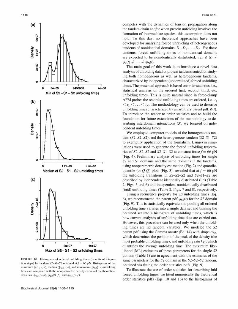
Inid unfolding times for S2–S1–S2. The unfolding times

for the heterogeneous tandem S2–S1–S2 form a set of inid

random variables. The histograms and density estimates for

the three order statistics ft1:3g, ft2:3g, and ft3:3g are dis-

played in Fig. 10. The pdf f1:3(t) of the first order statistic

shows a bimodal profile with the peak at shorter (longer)

times corresponding to unfolding of less (more) stable do-

main S1 (S2). We used the Gamma distribution (Eq. 14) to

model the parent pdfs for domains S2 and S1. Thus, we set

cS2ðtÞ¼kaS2

S2 taS2�1exp½�kS2t�=GðaS2Þ and cS1ðtÞ¼kaS1

S1 taS1�1

exp½�kS1t�=GðaS1Þ; where aS2, aS1, and kS2, kS1, are the

shape and unfolding rates for S2 and S1, respectively, and

gða;yÞ[R y

0xa�1�x

dx: The cdfs for S2 and S1 are CS2(t) ¼g(aS2, kS2t)/G(aS2) and CS1(t) ¼ g(aS1, kS1t)/G(aS1),

respectively. The expressions for the pdfs of the first

(f1:3), second (f2:3), and third (f3:3) order statistics for the

S2–S1–S2 tandem are obtained by inserting cS2, cS1, CS2,

and CS1 into the following equations (see Eq. 10),

TABLE 2 Spearman rank correlation coefficients for unfolding times for domains S21 (t1), S22 (t2), and S23 (t3) in tandem S2–S2–S2,

and for domains S21 (t1), S12 (t2), and S23 (t3) in tandem S2–S1–S2, obtained at f ¼ 66 pN

S2-S2-S2 S2-S1-S2

Time t1 t2 t3 Time t1 t2 t3

t1 1 0.0 (0.94) �.11 (0.02) t1 1 �0.09 (0.04) �.07 (0.13)

t2 0 1 �.08 (0.06) t2 �0.09 (0.04) 1 �0.03 (0.44)

t3 �0.11 (0.02) �0.08 (0.06) 1 t3 �0.07 (0.13) �0.03 (0.44) 1

The p-values for testing R ¼ 0 are in parentheses.

1106 Bura et al.


f1:3ðtÞ ¼1

2per

1�C1ðtÞ 1�C1ðtÞ c1ðtÞ1�C2ðtÞ 1�C2ðtÞ c2ðtÞ1�C3ðtÞ 1�C3ðtÞ c3ðtÞ

264

375

f2:3ðtÞ ¼ per

C1ðtÞ 1�C1ðtÞ c1ðtÞC2ðtÞ 1�C2ðtÞ c2ðtÞC3ðtÞ 1�C3ðtÞ c3ðtÞ

264

375

f3:3ðtÞ ¼1

2per

C1ðtÞ C1ðtÞ c1ðtÞC2ðtÞ C2ðtÞ c2ðtÞC3ðtÞ C3ðtÞ c3ðtÞ

264

375: (16)

Order statistics pdfs, given by Eq. 16, were used to fit the

histograms of the ordered first (ft1:3g), second (ft2:3g), and

third (ft2:3g) unfolding times (Fig. 10). The results, dis-

played in Fig. 11, show good agreement between the histo-

grams of ordered variates and theoretical order statistics pdfs.

The values of the fitting parameters are given in Table 3. The

shape parameters aS2 and aS1, and unfolding rates kS2 and

kS1, for S2 and S1 domains in the tandem S2–S1–S2, compare

well with the ML estimates of the same quantities for the

single S2 and S1 domains. However, the values for aS2 and

aS1 for tandem S2–S1–S2 obtained from the numerical fit are

FIGURE 5 Q-Q plots of forced unfolding times

(t1, t2) (a), (t1, t3) (c), and (t2, t3) (e) for domains S21

(t1), S22 (t2), and S23 (t3) in tandem S2–S2–S2

obtained at f ¼ 66 pN. Q-Q plots of forced

unfolding times (t1, t2) (b), (t1, t3) (d), and (t2, t3) (f)

for domains S21 (t1), S12 (t2), and S23 (t3) in tandem

S2–S1–S2 obtained at f ¼ 66 pN.



FIGURE 7 The distributions of forced unfolding times (in units of integra-

tion steps) for domains S21 (a), S12 (b), and S23 (c) in tandem S2–S1–S2

obtained at f ¼ 66 pN. Histograms of the unfolding times are overlaid with

corresponding nonparametric density estimates.

FIGURE 6 The distributions of forced unfolding times (in units of integra-

tion steps) for domains S21 (a), S22 (b), and S23 (c) in tandem S2–S2–S2

obtained at f ¼ 66 pN. Histograms of the unfolding times are overlaid with

corresponding nonparametric density estimates.

1108 Bura et al.


larger than the corresponding ML estimates of the same

quantities for single S2 and S1 domains.

DISCUSSION

Summary of main results

Conformational transitions in wild-type protein tandems and

engineered polyproteins can be studied in force-clamp AFM

experiments by employing constant stretching force and re-

cording the unfolding times of individual domains (16–19).

Up to now statistical analyses of forced unfolding times for

homogeneous tandems ((D)N) relied on the assumption that

the recorded unfolding times form a set of independent iden-

tically distributed (iid) random variables with identical exponen-

tial parent pdfs for each domain D, i.e., c1(t) ¼ c2(t) ¼ . . .cN(t) ¼ c(t). However, when the forced unfolding kinetics

FIGURE 9 (a) Comparison of the histograms of forced unfolding times

(in units of integration steps) for single S2 domain (white bars) and for

combined data set for tandem S2–S2–S2 (gray bars), obtained by using Eq.

6. (b) Nonparametric density estimates of the theoretical probability density

for single S2 domain (solid curve) and for combined data set (dashed curve).

FIGURE 8 Histograms of ordered unfolding times (in units of integration

steps) for tandem S2–S2–S2 obtained at f ¼ 66 pN. Histograms of the

minimum (ft1:3g, a), median (ft2:3g, b), and maximum (ft3:3g, c) unfolding

times are compared with the nonparametric density curves of the theoretical

densities, f1:3(t) (a), f2:3(t) (b), and f3:3(t) (c).



competes with the dynamics of tension propagation along

the tandem chain and/or when protein unfolding involves the

formation of intermediate species, this assumption does not

hold. To this day, no theoretical approaches have been

developed for analyzing forced unraveling of heterogeneous

tandems of nonidentical domains, D1–D2–. . .–DN. For these

tandems, forced unfolding times of nonidentical domains

are expected to be nonidentically distributed, i.e., c1(t) 6¼c2(t) 6¼ . . . 6¼ cN(t).

The main goal of this work is to introduce a novel data

analysis of unfolding data for protein tandems suited for study-

ing both homogeneous as well as heterogeneous tandems,

characterized by independent (uncorrelated) forced unfolding

times. The presented approach is based on order statistics, i.e.,

statistical analysis of the ordered first, second, third, etc.

unfolding times. This is quite natural since in force-clamp

AFM probes the recorded unfolding times are ordered, i.e., t1, t2 , . . . , tN. The methodology can be used to describe

unfolding times characterized by an arbitrary parent pdf, c(t).To introduce the reader to order statistics and to build the

foundation for future extensions of the methodology to de-

scribing interdomain interactions (3), we focused on inde-

pendent unfolding times.

We employed computer models of the homogeneous tan-

dem (S2–S2–S2), and the heterogeneous tandem (S2–S1–S2)

to exemplify application of the formalism. Langevin simu-

lations were used to generate the forced unfolding trajecto-

ries of S2–S2–S2 and S2–S1–S2 at constant force f ¼ 66 pN

(Fig. 4). Preliminary analysis of unfolding times for single

S2 and S1 domains and the same domains in the tandems,

using nonparametric density estimation (Fig. 2) and quantile-

quantile (or Q-Q) plots (Fig. 3), revealed that at f ¼ 66 pN

the unfolding transitions in S2–S2–S2 and S2–S1–S2 are

described by independent identically distributed (iid) (Table

2; Figs. 5 and 6) and independent nonidentically distributed

(inid) unfolding times (Table 2, Figs. 7 and 8), respectively.

Using a recurrence property for iid unfolding times (Eq.

6), we reconstructed the parent pdf cS2(t) for the S2 domain

(Fig. 9). This is statistically equivalent to pooling all ordered

unfolding time variates into a single data set and binning the

obtained set into a histogram of unfolding times, which is

how current analyses of unfolding time data are carried out.

However, this procedure can be used only when the unfold-

ing times are iid random variables. We modeled the S2

parent pdf using the Gamma ansatz (Eq. 14) with shape aS2,

which determines the position of the peak of the density (the

most probable unfolding time), and unfolding rate kS2, which

quantifies the average unfolding time. The maximum like-

lihood (ML) estimates of these parameters for the single S2

domain (Table 1) are in agreement with the estimates of the

same parameters for the S2 domain in the S2–S2–S2 tandem,

obtained via fitting the order statistics pdfs (Fig. 9).

To illustrate the use of order statistics for describing inid

forced unfolding times, we fitted numerically the theoretical

order statistics pdfs (Eqs. 10 and 16) to the histograms of

FIGURE 10 Histograms of ordered unfolding times (in units of integra-

tion steps) for tandem S2–S1–S2 obtained at f ¼ 66 pN. Histograms of the

minimum (ft1:3g, a), median (ft2:3g, b), and maximum (ft3:3g, c) unfolding

times are compared with the nonparametric density curves of the theoretical

densities, f1:3(t) (a), f2:3(t) (b), and f3:3(t) (c).

1110 Bura et al.


ordered unfolding times (Fig. 10) for the S2–S1–S2 tandem

assuming the Gamma ansatz for the parent pdfs for domains

S2 and S1 (Eq. 14). The results are presented in Fig. 11. The

obtained shape parameters, aS2 and aS1, and unfolding rates,

kS2 and kS1 (Table 3), agree well with the ML estimates of

these quantities for the single S2 and S1 domains (Table 1).

However, due to flexible linkers, the values of aS2 (1.55,

2.05, and 1.75, Table 3) and aS1 (7.45, 4.95, Table 3),

obtained for the S2–S1–S2 tandem, are slightly larger than

the corresponding ML estimates of these quantities for single

domains (0.96 for S2 and 4.92 for S1, Table 1). These find-

ings imply that statistical analyses and theoretical modeling

of unfolding data on wild-type protein tandems and polypro-

teins must take into account the effect of flexible linkers as

their presence results in prolonged forced unfolding times.

Dependent forced unfolding times

In a separate set of Langevin simulations of forced unfold-

ing for tandems S2–S2–S2 and S2–S1–S2, we increased the

applied constant force from f ¼ 66 pN to f ¼ 88 pN to

explore the effect of stretching force on the distribution and

the dependence structure of the unfolding times. For each

tandem, 500 unfolding trajectories were generated. The

histograms of forced unfolding times for the first (S21),

second (S22), and third (S23) S2 domain of tandem S2–S2–

S2, obtained at f¼ 88 pN, are displayed in Fig. 12. These can

be directly compared with the corresponding histograms and

density estimates obtained for the same tandem at f ¼ 66 pN

(Fig. 6). As evidenced by both histograms and kernel density

estimates as well as Q-Q plots, the nonidentical unfolding

time distributions (Fig. 12) for individual S2 domains

obtained at higher force f ¼ 88 pN, are starkly different

from the corresponding identical distributions for the same

domains obtained at f ¼ 66 pN (Figs. 5 and 6).

Aside from the overall shift toward shorter unfolding

times, due to Df¼ 22 pN force increase, we witness a drastic

change in the unfolding pattern. Specifically, at f¼ 88 pN the

unfolding time distribution for the first S2 domain (S21) is

bimodal with the first peak at shorter times (�0.4 3 106) and

the second peak at longer times (�1.3 3 106). The unfolding

time distributions for the second (S22) and third domain (S23)

are peaked around 2.0 3 106 and 1.3 3 106, respectively

(Fig. 12). These results imply that at f ¼ 88 pN, on average,

the forced unfolding of tandem S2–S2–S2 proceeds through

initial unraveling of the terminal S2 domains (S21 first and

S23 second), followed by the unfolding of the middle domain

(S22). In contrast, the identical unfolding time distributions

for all three S2 domains, obtained at f¼ 66 pN, are peaked at

about the same time point t � 4.0 3 106 (Fig. 6), which

implies that at lower force any of the three S2 domains in the

tandem can unfold first, second, or last.

We also observed that increased force induces dependence

between the unfolding transitions in S2 domains. Whereas at

f ¼ 66 pN the individual unfolding times for all three

domains in the S2–S2–S2 and S2–S1–S2 tandems were found

FIGURE 11 The fit of the histograms for the

minimum ft1:3g (a), median ft2:3g (b), and

maximum ft3:3g (c) unfolding times (in units of

integration steps) for tandem S2–S1–S2 (bars).

Theoretical order statistics pdfs fr:3(t) (r ¼ 1, 2,

3, (see Eq. 16) are overlaid.

TABLE 3 Numerical values of a and k (in units of integration

steps) for domains S2 and S1 in tandem S2–S1–S2, obtained

from the fit of the order statistics pdfs fr:3, r ¼ 1, 2, 3, to the

histograms of the ordered forced unfolding times ft1:3g, ft2:3g,and ft3:3g

Order statistics pdf aS2 aS1 kS2 kS1

f1:3 1.55 7.45 3.04 3 10�7 0.92 3 10�5

f2:3 2.05 4.95 3.82 3 10�7 1.92 3 10�5

f3:3 1.75 4.85 2.85 3 10�7 1.56 3 10�5



to be pairwise independent (Table 2), this is no longer the

case at f ¼ 88 pN. Table 4 reports the Spearman rank

correlation coefficients for three pairs of unfolding times (t2,

t1), (t3, t1), and (t3, t2), in tandems S2–S2–S2 and S2–S1–S2

recorded at f¼ 88 pN. For the homogeneous tandem S2–S2–

S2, unfolding times for domains S21 (t1) and S23 (t3) have a

Spearman rank correlation of �0.17 indicating statistically

significant dependence (correlation) with a p-value of 0;

similarly, unfolding times for domains S22 (t2) and S23 (t3)

have a Spearman rank correlation of �0.19 that is highly

statistically significant with a p-value of 0 (Table 4). Yet,

unfolding times for domains S21 (t1) and S22 (t2) have zero

Spearman rank correlation coefficient with a high p-value of

0.95, which indicates statistically significant independence

of the forced unfolding times between domains S21 and S22

(Table 4). These findings are particularly striking given that

the domains S21 and S23 are spacially separated by the

middle domain S22, whereas S21 and S22 domains are nearest

neighbors. Similar analysis for the heterogeneous tandem

S2–S1–S2 revealed statistically significant dependence be-

tween the forced unfolding times for the first S21 and the

second domain S12 (R ¼ �0.16 and associated 0 p-value,

Table 4), and the second S12 and the third S23 domain

(R ¼ �0.23 and associated 0 p-value, Table 4).

The observed pairwise dependence of unfolding events is

not unexpected. Indeed, when the timescale of tension

FIGURE 12 (a, c, and e) Histograms of forced

unfolding times (bars) and nonparametric density

estimates of the theoretical probability densities

(curve) for domains S21 (a), S22 (c), and S23 (e) for

tandem S2–S2–S2 at f ¼ 88 pN. (b, d, and f) Q-Qplots of forced unfolding times (t1, t2) (b), (t1, t3)

(d), and (t2, t3) (f) for domains S21 (t1), S22 (t2), and

S23 (t3).

1112 Bura et al.


propagation along the tandem chain is comparable with the

average forced unfolding time of domains S2 and S1, the

recorded forced unfolding times ftig and ftjg (i 6¼ j¼ 1, 2, 3)

are separated by ‘‘waiting periods,’’ fDtijg (Dtij ¼ ti � tj),that are not long enough to decorrelate the consecutive

unfolding transitions. Uncorrelated at lower force unfolding

transitions of individual domains in the tandem may thus

become correlated (dependent) at elevated force levels. Even

for homogeneous tandems, such as S2–S2–S2, whether the

unfolding times of identical repeats are identically distri-

buted depends on the magnitude of applied force. By

comparing the unfolding time pdfs for S2 domains obtained

at f ¼ 88 pN (Fig. 12) with the corresponding pdfs obtained

at f ¼ 66 pN (Figs. 5 and 6), we see that at higher force un-

raveling of the domains closer to the point of force appli-

cation (terminal domains S21 and S23) is characterized by

shorter unfolding times compared with those for the more

remote middle S22 domain.

It is likely that forced unfolding times of wild-type protein

tandems, analyzed in force-clamp AFM experiments, also in-

volve a complicated force-induced dependence structure.

Yet, current approaches to statistical analysis of unfolding

times rely on the simplifying assumption that the recorded

unfolding times form a set of iid random variables. Because

applied stretching force may couple the unfolding transitions

of the individual tandem domains, novel theory and new

approaches to statistical data analysis of correlated forced

unfolding times that do not use the iid assumption are much

needed.

CONCLUSIONS

In this article we introduced and tested an order statistics

based methodology for analyzing the forced unfolding times

of protein tandems. We used this approach to analyze com-

puter simulated unfolding transitions, characterized by in-

dependent identically distributed (iid) and independent

nonidentically distributed (inid) unfolding times. The order

statistics based methodology presented here can now be used

in force-clamp AFM experiments to study force-induced

unfolding in both homogeneous and heterogeneous protein

tandems.

An intriguing finding of this work is that the iid assump-

tion, currently used in statistical analyses of forced unfolding

data, that the unfolding transitions in the protein tandems of

identical repeats can be characterized by independent iden-

tically distributed unfolding times may not hold at elevated

piconewton levels of applied force. We showed that a mod-

erate increase in the magnitude of applied force may result in

correlated unfolding transitions, characterized by dependent

unfolding times. In the case of tandems S2–S2–S2 and S2–

S1–S2 formed by noninteracting domains S2 and/or S1,

correlated unfolding events are due to competition between

the unfolding kinetics and the dynamics of force propagation

along the tandem chain, which couples consecutive unfold-

ing transitions. The dependence among unfolding times may

also be mediated by the interdomain interactions. For ex-

ample, heterogeneous tandems of I27–I28 repeats show en-

hanced domain stabilization against applied force, which

results in the increase of the average unfolding force from f�260 pN (for the tandem of repeated Ig domains I27 of titin) to

f � 300 pN (for I27–I28 repeats) (3). Similar domain sta-

bilization effect has been observed in heterogeneous tandems

of Fn3 domains (44).

These experimental findings, in unison with our theoret-

ical results, necessitate extending the statistical tools for

independent forced unfolding times, presented in this article,

to accommodate correlated unfolding transitions. Depending

on the tandem composition, correlated unfolding transitions

are described by dependent identically distributed (did) un-

folding times (homogeneous tandems) and dependent non-

identically distributed (dnid) unfolding times (heterogeneous

tandems). For the convenience of the reader, the possible

types of unfolding transitions are classified in Table 5. The

development of order statistics based methodology for de-

scribing correlated unfolding data will enable researchers to

accurately probe protein-protein interactions. Order statistics

type methodology can also be formulated for analyzing

forced unfolding data available from force-ramp AFM

measurements.

To take full advantage of the presented methodology, one

needs to be able to determine: a), (in)dependence of forced un-

folding times, and b), (in)equality of the (parent) unfolding

time distributions of individual proteins in a tandem under

study. Both simple empirical tools and rigorous statistical

tests for assessing the (in)dependence of unfolding times and

(in)equality of the (parent) distributions are needed. Because

in force-clamp AFM experiments, ordered unfolding times

are the only observable quantities, tests for deducing the

dependence structure among the original but otherwise

TABLE 4 Spearman rank correlation coefficients for the unfolding times for domains S21 (t1), S22 (t2), and S23 (t3) in tandem

S2–S2–S2, and for domains S21 (t1), S12 (t2), and S23 (t3) in tandem S2–S1–S2 obtained at f ¼ 88 pN

S2-S2-S2 S2-S1-S2

Time t1 t2 t3 Time t1 t2 t3

t1 1 0.0 (0.95) �.17 (0.00) t1 1 �.16 (0.00) 0.01 (0.83)

t2 0.00 (0.95) 1 �0.19 (0.00) t2 �0.16 (0.00) 1 �0.23 (0.00)

t3 �0.17 (0.00) �0.19 (0.00) 1 t3 0.01 (0.83) �0.23 (0.00) 1

The p-values for testing R ¼ 0 are in parentheses.



unobservable unfolding times and (in)equality of the unfold-

ing time distributions have to be based on the observed

ordered data. Development of such statistical tests along with

methodology for analyzing correlated forced unfolding data is

in progress (45).

APPENDIX I: ORDER STATISTICS FOR IIDUNFOLDING TIMES

Suppose fT1, T2, . . ., Tng are n random variables with distribution function,

C(t1, . . ., tn) ¼ Prob[T1 # t1, . . ., Tn # tn] (uppercase letters represent ran-

dom variables whereas lowercase letters represent their values). If they are

arranged in increasing order, T1:n # T2:n # . . . # Tn:n, then Tr:n—the r-th

order statistic—is equal to the r-th smallest value. When the random var-

iables Ti, i¼ 1, . . ., n, are independent with common cumulative distribution

function (cdf), C(t)¼ Prob[Tr # t], their joint cdf is the product of their com-

mon marginals, Cðt1; . . . ; tnÞ ¼Qn

i¼1 Prob½Ti # ti� ¼Qn

i¼1 CðtiÞ: Let

Fr:n(t) denote the cdf of the r-th order statistic Tr:n, r ¼ 1, 2, . . ., n. Then,

Fr:nðtÞ ¼ Probðat least r of the T9s are #tÞ

¼ +n

i¼r

n

i

� �Prob½T1 # t�ið1� Prob½T1 # t�Þn�i

¼ +n

i¼r

n

i

� �CðtÞið1�CðtÞÞn�i

: (A1)

The pdf of Tr:n, fr:n(t), is obtained by differentiating Eq. A1,

fr:nðtÞ[dFr:nðtÞ

dt¼ ncðtÞ n� 1

r � 1

� �CðtÞr�1ð1�CðtÞÞn�r

:

(A2)

Equations A1 and A2 are the same as Eq. 3 for the r-th order statistic given in

the main text.

In many applications, unfolding times of proteins are modeled as iid ex-

ponential random variables, and the unfolding times are characterized by the

rate of unfolding K. Then, Cexp(t)¼ 1� exp [�Kt], cexp(t)¼ K exp [�Kt],

and

Fexp

r:n ðtÞ ¼ +n

m¼r

n

m

� �ð1� e

�KtÞme�ðn�mÞKt

fexp

r:n ðtÞ ¼ nn� 1

r � 1

� �ð1� e

�KtÞr�1e�ðn�rÞKt

Ke�Kt: (A3)

The minimum and maximum order statistics pdfs are given by f1:nexp(t) ¼ n

exp [ �Kt(n � 1)]K exp [ �Kt] and fexpn:n ðtÞ ¼ n(1 � exp [ �Kt])n–1K exp

[ �Kt]. The minimum unfolding times with exponential parent pdf are also

exponentially distributed, i.e. f1:nexp(t) ¼ nK exp [ �nKt], with the average

unfolding time, m1:n ¼ 1/nK. This implies that the average first unfolding

time in the tandem of length n, m1:n, is exactly n times shorter than the

average first unfolding time in the tandem of unit length (n ¼ 1), m1:1, i.e.

m1:n ¼ m1:1/n.

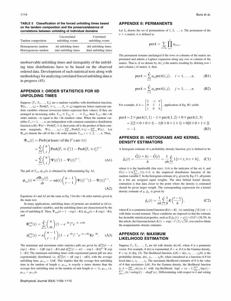
APPENDIX II: PERMANENTS

Let Sn denote the set of permutations of 1, 2, . . ., n. The permanent of the

n 3 n matrix A is defined as

perA ¼ +s2Sn

Yn

i¼1

aisðiÞ:

The permanent remains unchanged if the rows or columns of the matrix are

permuted and admits a Laplace expansion along any row or column of the

matrix. That is, if we denote by A(i, j) the matrix resulting by deleting row i

and column j of matrix A, then

perA ¼ +n

j¼1

aij perAði; jÞ; i ¼ 1; . . . ; n; (B1)

perA ¼ +n

i¼1

aij perAði; jÞ; j ¼ 1; . . . ; n: (B2)

For example, if A ¼2 �1 0

0 2 1

1 0 0

24

35; application of Eq. B1 yields

perA¼ 23perAð1;1Þ�13perAð1;2Þ103perAð1;3Þ¼ 2ð2301031Þ�1ð0301131Þ10ð0301132Þ¼�1: (B3)

APPENDIX III: HISTOGRAMS AND KERNELDENSITY ESTIMATORS

A histogram estimate of a probability density function g(t) is defined to be

ghðtÞ ¼Gðt 1 hÞ � GðtÞ

h¼ 1

nh+n

i¼1

1ft , ti # t 1 hg; (C1)

where h is the bandwidth (bin size), 1(A) is the indicator of the set A, and

GðtÞ ¼ 1=n +n

i¼11fti # tg is the empirical distribution function of the

random variable T. In the histogram estimate of g, given by Eq. C1, all points

in a bin are assigned equal weights. The idea behind kernel density

estimation is that data closer to the point where the density is estimated

should be given larger weight. The corresponding expression for a kernel

density estimate of g, gk; is given by

gkðtÞ ¼1

nh+n

i¼1

1

hK

t � ti

h

� �; (C2)

where K is a symmetric kernel function (K(t)¼K(�t)), satisfyingR

KðtÞdt ¼ 1

with finite second moment. These conditions are imposed so that the estimate

has desirable statistical properties, such as EðgkðtÞÞ ¼ gðtÞ1Oðh2Þ (38,39). In

this article, the Gaussian kernel, KðtÞ ¼ expð�t2=2Þ=ffiffiffiffiffiffi2pp

;was used to obtain

the nonparametric density estimates.

APPENDIX IV: MAXIMUMLIKELIHOOD ESTIMATION

Suppose T1, T2, . . . , Tn are iid with density c(x;u), where u is a parameter

vector. For example, if c(t) is exponential, u ¼ k; if it is the Gamma density,

u ¼ (a, k) (Eq. 14). The likelihood function, L(u) ¼ c(t1, t2, . . . , tnju), is the

probability density, c(t1, t2, . . . , tnju), when considered as a function of u for

fixed data t1, t2, . . . , tn. The maximum likelihood estimator of u is the value

of u that maximizes L(u). For the Gamma density, the likelihood function

is L ¼Qn

i¼1 cðtija; kÞ with log-likelihood, logL ¼ ða� 1Þ+n

i¼1logðtiÞ�

+n

i¼1kti1nalogðkÞ � nlogGðaÞ: Differentiating with respect to k and setting

TABLE 5 Classification of the forced unfolding times based

on the tandem composition and the presence/absence of

correlations between unfolding of individual domains

Tandem composition

Uncorrelated

unfolding events

Correlated

unfolding events

Homogeneous tandem iid unfolding times did unfolding times

Heterogeneous tandem inid unfolding times dnid unfolding times

1114 Bura et al.


it equal to zero yields k ¼ 1=+tian: There is no closed-form solution for a,

but a numerical solution can be obtained. We used the optimization algorithm

in R (40) to find the ML estimates of a and k.

We thank two anonymous referees for valuable suggestions, which improved

this article significantly.

This work was supported by National Science Foundation grant DMS-

0204563 (E. Bura), and a start-up fund from the University of Massachu-

setts Lowell (V. Barsegov).

REFERENCES

1. Labeit, S., M. Gautel, A. Lakey, and J. Trinick. 1992. Towards a molec-ular understanding of titin. EMBO J. 11:1711–1716.

2. Trinick, J., P. Knight, and A. Whiting. 1984. Purification and prop-erties of native titin. J. Mol. Biol. 180:331–356.

3. Li, H. B., A. F. Oberhauser, S. B. Fowler, J. Clarke, and J. M.Fernandez. 2000. Atomic force microscopy reveals the mechanicaldesign of a modular protein. Proc. Natl. Acad. Sci. USA. 97:6527–6531.

4. Carrion-Vazquez, M., A. F. Oberhauser, S. B. Fowler, P. E. Marszalek,S. E. Proedel, J. Clarke, and J. M. Fernandez. 1999. Mechanical andchemical unfolding of a single protein: a comparison. Proc. Natl. Acad.Sci. USA. 96:3694–3699.

5. Stossel, T. P., J. Condeelis, L. Cooley, J. H. Hartwig, A. Noegel, M.Schleicher, and S. S. Shapiro. 2001. Filamins as integrators of cellmechanics and signalling. Nat. Rev. Mol. Cell Biol. 2:138–145.

6. Feng, Y., and C. A. Walsh. 2004. The many faces of filamin: a versatilemolecular scaffold for cell motility and signalling. Nat. Cell Biol. 6:1034–1038.

7. Schwaiger, I., A. Kardinal, M. Schleicher, A. A. Niegel, and M. Rief.2004. A mechanical unfolding intermediate in an actin-crosslinking pro-tein. Nat. Struct. Biol. 11:81–85.

8. Schwaiger, I., M. Schleicher, A. A. Niegel, and M. Rief. 2005. Thefolding pathway of a fast-folding immunoglobulin domain revealed bysingle-molecule mechanical experiments. EMBO Rep. 6:46–51.

9. Popowicz, G. M., R. Muller, A. A. Noegel, M. Schleicher, R. Huber,and T. A. Holak. 2004. Molecular structure of the rod domain ofDictyostelium filamin. J. Mol. Biol. 342:1637–1646.

10. Schwarzbauer, J. E., and J. L. Sechler. 1999. Fibronectin fibrillogen-esis: a paradigm for extracellular matrix assembly. Curr. Opin. Struct.Biol. 11:622–627.

11. Pickard, C. M. 2001. Mechanisms underlying ubiquitination. Annu.Rev. Biochem. 70:503–533.

12. Weissman, A. M. 2001. Themes and variations on ubiquitylation. Nat.Rev. Mol. Cell Biol. 2:169–178.

13. Rief, M., M. Gautel, F. Oesterhelt, J. M. Fernandez, and H. E. Gaub.1997. Reversible unfolding of individual titin immunoglobulin do-mains by AFM. Science. 276:1109–1112.

14. Zinober, R. C., D. J. Brockwell, G. S. Beddard, A. W. Blake, P. D.Olmsted, S. E. Radford, and D. A. Smith. 2002. Mechanically unfold-ing proteins: the effect of unfolding history and the supramolecularscaffold. Protein Sci. 11:2759–2765.

15. Steward, A., J. L. Toca-Herrera, and J. Clarke. 2002. Versatile cloningsystem for construction of multimeric proteins for use in atomic forcemicroscopy. Protein Sci. 11:2179–2183.

16. Brujic, J., R. I. Z. Hermans, K. A. Walther and. J. M. Fernandez.2006. Single-molecule force spectroscopy reveals signatures of glassydynamics in the energy landscape of ubiquitin. Nature Physics. 2:282–286.

17. Oberhauser, A. F., P. K. Hansma, M. Carrion-Vazquez, and J. M.Fernandez. 2001. Stepwise unfolding of titin under force-clamp atomicforce microscopy. Proc. Natl. Acad. Sci. USA. 98:468–472.

18. Schlierf, M., H. Li, and J. M. Fernandez. 2004. The unfolding kineticsof ubiquitin captured with single-molecule force-clamp techniques.Proc. Natl. Acad. Sci. USA. 101:7299–7304.

19. Fernandez, J. M., and H. Li. 2004. Force-clamp spectroscopy monitorsthe folding trajectory of a single protein. Science. 303:1674–1678.

20. Zhang, B., G. Xu, and J. S. Evans. 1999. A kinetic molecular model ofthe reversible unfolding and refolding of titin under force extension.Biophys. J. 77:1306–1315.

21. Hummer, G., and A. Szabo. 2003. Kinetics from nonequilibriumsingle-molecule pulling experiments. Biophys. J. 85:5–15.

22. Brujic, J., R. I. Z. Hermans, S. Garcia-Manyes, K. A. Walther, andJ. M. Fernandez. 2007. Dwell-time distribution analysis of poly-protein unfolding using force-clamp spectroscopy. Biophys. J. 92:2896–2903.

23. David, H. A., and H. N. Nagaraja. 2003. Order Statistics. WileyInterscience, New York.

24. Gumbel, E. J. 2004. Statistics of Extremes. Dover Publications, New York.

25. Beckmann, P. 1967. Probability in Communication Engineering.Harcourt, Brace & World, New York.

26. Singpurwalla, N. D., and S. P. Wilson. 1999. Statistical Methods inSoftware Engineering: Reliability and Risk. Springer Verlag, New York.

27. Tees, D. F. J., J. T. Woodward, and D. A. Hammer. 2001. Reliabilitytheory for receptor-ligand bond dissociation. J. Chem. Phys. 114:7483–7496.

28. Klimov, D. K., and D. Thirumalai. 2000. Native topology determinesforce-induced unfolding pathways in globular proteins. Proc. Natl.Acad. Sci. USA. 97:7254–7259.

29. Arnold, B. C., and N. Balakrishnan. 1989. Relations, bounds andapproximations for order statistics. In Lecture Notes in Statistics. 53.Springer-Verlag, New York.

30. Abramowitz, M., and I. A. Stegun. 1972. Handbook of MathematicalFunctions. Dover Publications, New York.

31. Vaughan, R. J., and W. N. Venables. 1972. Permanent expressions fororder statistics densities. J. R. Statist. Soc. B. 34:308–310.

32. Minc, H. 1983. Theory of permanents 1978–1981. Lin. Mult. Algebra.12:227–263.

33. Minc, H. 1983. Theory of permanents 1982–1985. Lin. Mult. Algebra.21:109–148.

34. Sathe, Y. S., and U. J. Dixit. 1990. On a recurrence relation for orderstatistics. Stat. Probab. Lett. 9:1–4.

35. Onuchic, J. N., and P. G. Wolynes. 2004. Theory of protein folding.Curr. Opin. Struct. Biol. 14:70–75.

36. Dill, K. A., S. Bromberg, K. Yue, K. M. Fiebig, D. P. Yee, P. D.Thomas, and H. S. Chan. 1995. Principles of protein folding: a perspec-tive from simple exact models. Protein Sci. 4:561–602.

37. Veitshans, T., D. K. Klimov, and D. Thirumalai. 1997. Protein foldingkinetics: time scales, pathways, and energy landscapes in terms ofsequence dependent properties. Fold. Des. 2:1–22.

38. Silverman, B. W. 1986. Density Estimation. Chapman and Hall, London,UK.

39. Scott, D. W. 1992. Multivariate Density Estimation: Theory, Practice,and Visualization. Wiley, New York.

40. R Development Core Team. 2006. R: A Language and Environmentfor Statistical Computing. R Foundation for Statistical Computing,Vienna, Austria. (http://www.R-project.org).

41. Davison, A. C. 2003. Statistical Models. Cambridge University Press,Cambridge, UK.

42. Gibbons, J. D., and S. Chakraborti. 2003. Nonparametric StatisticalInference, 4th Ed. Marcel Dekker, New York.

43. Kendall, M. G., and J. D. Gibbons. 1990. Rank Correlation Methods,5th Ed. Edward Arnold, London, UK.

44. Oberhauser, A. F., C. Badilla-Fernandez, M. Carrion-Vazquez,and J. M. Fernandez. 2002. The mechanical hierarchies of fibronectinobserved with single-molecule AFM. J. Mol. Biol. 319:433–447.

45. Bura, E., D. K. Klimov, and V. Barsegov. Analyzing forced unfoldingof protein tandems by ordered variates. 2. Dependent unfolding times.In press.



Analyzing Forced Unfolding of Protein Tandems by Ordered Variates, 2: Dependent Unfolding Times

Documents

Transcript of Analyzing Forced Unfolding of Protein Tandems by Ordered Variates, 2: Dependent Unfolding Times