Analyzing Flexibility in Design of Waste-to-Energy Systems

Proceedings of the 2014 Industrial and Systems Engineering Research Conference

Y. Guan and H. Liao, eds.

Analyzing Flexibility in Design of Waste-to-Energy Systems

Qihui Xie, Michel-Alexandre Cardin, Tsan Sheng Ng, Shuming Wang, Junfei Hu

Department of Industrial and Systems Engineering

National University of Singapore

Block E1A #06-25, 1 Engineering Drive, Singapore, 117576

Abstract

Flexibility in design of waste-to-energy (WTE) systems provides ways to achieve environmental and economic

sustainability under uncertainty. However, when and how to exercise the flexibility remains challenging in the face

of growing uncertainty. This paper considers flexibility as a mechanism to ensure better sustainability for WTE

systems with long-term lifecycles. Specifically, the flexibility of capacity expansion is considered. A multistage

stochastic programming model is proposed to design a stochastically optimal decision rule to guide decision making

on capacity expansion. An algorithm based on Lagrangian decomposition is developed to solve the model.

Experiments show that the expected net present value (ENPV) of the flexible design provides significant

improvement over the fixed rigid design in terms of economic lifecycle performance. Furthermore, by being able to

make decisions in any time period based on available information as uncertainties are resolved, the proposed

multistage model can achieve a higher value of flexibility than the two-stage model, which has been used in the

design of flexible urban infrastructure systems.

Keywords Flexibility in engineering design, real options analysis, multistage stochastic programming, waste-to-energy system,

risk management

1. Introduction Municipal waste management has become a critical issue for the sustainable development of megacities due to their

high population density and limited land area. Taking Singapore as an example, the total amount of municipal waste

has increased from 4.7 million to 6.9 million tons per year during the last decade [1]. At the same time, energy

supply has also become a challenging problem for the sustainable development of megacities. Therefore, waste-to-

energy (WTE) technologies, such as anaerobic digestion (AD), are enjoying high favor due to their capability for

recovering energy while efficiently disposing of waste. This paper addresses the problem of how to design manage a

sustainable WTE system with a long lifespan.

When one thinks about the design of large scale engineering systems like WTE systems, the traditional way is to

search for optimal system configurations based on observed requirements and forecasted demands. However,

because of the complexity of the environment, the future is always full of uncertainty. In traditional optimization

design approaches, uncertainty is not fully recognized. Flexibility in engineering design, however, is a novel concept

that provides a promising way to handle uncertainty. In general, flexibility can improve the performance of a system

by reducing the risk in downside scenarios and capturing the upside opportunities. In this paper, flexibility is

considered as a mechanism to improve the lifecycle performance of WTE systems.

The main contribution of this paper is a multistage stochastic programming model to develop a decision rule to

guide the exercise of flexibility. When a system is designed with flexibility, it is important to tell the managers when

and how to exercise it to gain the added value. In this paper, the specified flexibility is capacity expansion. In the

literature, the strategies of planning capacity expansion are either simply predefined without comprehensive

investigation or not practical from a management perspective. The proposed model provides a way to develop

stochastically optimal decision rules to guide dynamic decision making based on past information or uncertainty

estimations. This dynamic planning strategy will not only improve the lifecycle performance of the system, but also

make the management process more efficient and convenient.

Xie, Cardin, Ng, Wang, Hu

2. Background and Related Work

2.1. Flexibility and Real Options

Flexibility is an important system attribute that enables engineering systems to change easily in the face of

uncertainty [2]. It is associated with the concept of real options, which provide the “right, but not the obligation, to

change a system as uncertainty unfolds” [3]. It has been shown that flexibility can improve expected performance by

10% to 30% compared to standard design and evaluation approaches [4].

Designing engineering systems for flexibility can be organized into five phases: initial/standard design generation,

uncertainty recognition, concept generation and enabler identification, design space exploration, and process

management [5]. This paper proposes a methodology for exploring the design space. In literature, there are two

categories of methodologies for the design space exploration procedure. The first one is to build analytic models,

such as decision analysis [6, 7], binomial lattice [8], and stochastic programming [9, 10]. The other category is

simulation models, which explicitly model the stochastic scenarios and decisions enabled by flexible designs [11,

12] . However, both of the two types of methodologies have some limitations. In the analytic approach, all of the

decisions of flexibility exercise are determined as outcomes of the model; there are no generic decision rules to

guide managers as uncertainty is resolved throughout the lifecycle of the project. Although the simulation approach

explicitly employs generic decision rules, it lacks a systematic way to choose the most preferable decision rules.

This paper addresses the importance of decision rules for their advantages of lifecycle performance and management

practicability. A systematic method is proposed to develop stochastically optimal decision rules that will guide

dynamic decision making based on available information as uncertainties are resolved.

2.2. Capacity Expansion under Uncertainty

In traditional engineering approaches of engineering systems design, designers intend to build big systems to take

advantage of economies of scale [13]. However, these approaches ignore the stochastic nature of the demand

process, relying on the forecasting of the uncertain future. If the real demands fail to grow as anticipated, the system

will suffer a lot of loss because a large amount of initial investments will be wasted. The flexibility of capacity

expansion, however, enables systems to keep good performance in face of the uncertainties. The main idea of this

strategy is to start with a small system and expand when the time is ripe. It can benefit the system reducing the

negative effects in downside scenarios and better capturing upside opportunities.

Once a system has been embedded with the flexibility to expand, the key problems are to decide the initial capacity,

the time periods to expand, and the amount of capacity to be expanded at each time. In the literature, there are

typically two categories of approaches to address the capacity expansion problem: stochastic programming and

simulation.

Of the studies that have applied stochastic programming to flexibility design problems [9, 10, 14], the models

applied to multi-period capacity expansion problems are generally static planning models which consist of only two

stages. The first stage includes the decisions on capacity expansion for each time period, which have to be made

without knowing the outcome of the uncertainties. The second stage is the realization of some other variables that

occur after the uncertainties have been revealed. It is easy to see that the formulation does not fully follow a rational

process because it forces the decision maker to plan the capacities for all time periods before realizing any of the

uncertainties. A more realistic formulation would be a multistage problem in which the capacity in each time period

is decided over time as the uncertainties are resolved, as a way to flexibly adapt to changing conditions.

Simulation, which models stochastic scenarios and decision making, is another technology used to study flexible

design in engineering systems. De Neufville, Scholtes [12] built a simulation model based on a spreadsheet to

quantify the value of flexibility in the public parking garage capacity expansion problem. In that model, a decision

rule was exploited to capture the management’s decision making process in response to the observed demand

scenario. Decision rules are used to determine when and how to exercise the flexibility in operations, in light of

some observation regarding the main uncertainty sources. They are crucial to the lifecycle value assessment of

flexible design alternatives [15]. However, since simulation cannot naturally be used to find an optimal solution, it is

unable to systematically develop the most preferable decision rule.

In this paper, a multistage stochastic programming model is proposed to systematically develop decision rules that

will guide the decision making process of capacity expansion exploiting ideas of flexibility. In this model, the


sequential decisions are made based on past information about uncertainties in every time period. By being able to

take advantage of information over time, the system can achieve a better lifecycle performance. In particular, the

outcome of the model consists of a simple strategic decision rule under which managers can easily make

sophisticated decisions based on available information. This characteristic improves practicability in the

management process.

2.3. Waste-to-Energy Systems

Municipal solid waste management is becoming a major issue in the sustainable development of megacities. In the

face of increasing waste and limited landfill sites, WTE technologies, which generate energy in the form of

electricity and/or heat from waste, are enjoying high favor due to their capability of recovering energy while

efficiently disposing of waste. Various WTE technologies are promising in terms of offering electricity, heat, and

transport fuels [16]. To support decision making in the design and choice of WTE technologies, the existing

literature related to WTE systems has mainly focused on system optimization and evaluation [17-19]. Little research

has been done to analyze WTE systems from the perspective of flexibility, specifically as a mechanism to ensure

better sustainability. This paper targets at the issues of considering flexibility for WTE systems and managing the

decision making process during the implementation of such flexible systems. A multistage stochastic programming

model is developed to guide decision making when the system is implemented in an uncertain future. It is argued

that explicitly considering uncertainty and flexibility will result in the better use of resources by planning for careful

adaption to changing environments. Overall, this should contribute to a more resilient and sustainable system.

3. Methodology This paper aims to address the problem of when and how to exercise the flexibility. The steps below describe the

process in generic terms to analyze WTE systems for flexibility.

Step 1: Initial Analysis

The first step analyzes the design problem. The lifecycle performance of the system is measured using an economic

model which is built based on some assumptions on the cost and revenue drivers. The initial analysis is developed

by assuming deterministic values of the uncertainties and fixed design variables.

Step 2: Uncertainty Analysis

In the second step, the lifecycle performance of the design is evaluated under uncertainties. After investigating the

historical data, the main uncertainties drivers are modelled using stochastic functions like Geometric Brownian

Motion (GBM), S-curve function, etc. Monte Carlo simulation is then applied to generate a number of possible

scenarios of uncertainties. By substituting different scenarios into the economic model developed in step 1, the

performance of the design under uncertainties can be evaluated based on expected net present value (ENPV).

Step 3: Flexibility Analysis

This step will focus on flexible concepts to handle the uncertainties. The WTE system is assumed to be embedded

with the flexibility to be expanded modularly as needed. Stochastic programming models are built to decide the

optimal system design configurations and decision rules. First, a two-stage stochastic programming model is

introduced as a representative of the static planning models used in many existing studies. Then, a multistage

stochastic programming model is proposed to develop a stochastically optimal decision rule to guide dynamic

decision making on capacity expansion. Due to the large scale of the proposed multistage model, an algorithm based

on Lagrangian decomposition is developed to solve it. The performances of the models are then compared through

an out-of-sample test. Finally, a sensitivity analysis is conducted to test the influence of uncertainties on the

performance of the models.

4. Application

4.1. Initial Analysis

Due to the increasing waste generation and decreasing landfill space, Singapore is facing more and more pressure on

the issue of municipal waste management. Anaerobic digestion (AD), which has high efficiency in the energy

recovery process and has been widely used in European countries, is one of the potential solutions to remedy the

situation. This study aims to investigate how to embed and manage flexibility in an upcoming AD plant that treats

organic waste – wood, paper, horticultural, and organic waste – in Singapore. First, a deterministic case is studied,


i.e. assuming the amount of waste processed in each year, 𝑤𝑡 , is accurately forecasted. The problem of optimizing

the capacity 𝑐 to achieve the maximum net present value can be formulated as below:

Problem DA: 𝑧𝐷𝐴 = max ∑ 𝜎𝑡(𝑅𝑡(𝑤𝑡) − 𝐶𝑡(𝑐, 𝑤𝑡) − 𝑃𝑡(𝑓𝑡))𝑇𝑡=0 (1)

s.t. 𝑐 + 𝑓𝑡 ≥ 𝑤𝑡 , ∀𝑡 (2)

𝑐 ≥ 0, 𝑓𝑡 ≥ 0, ∀𝑡 (3)

where 𝜎 is the discount rate factor, 𝑅𝑡(𝑤𝑡) is the revenue function in year t, 𝐶𝑡(𝑐, 𝑤𝑡) is the cost function in year 𝑡,

𝑓𝑡 is the capacity shortage in year 𝑡 and 𝑃𝑡(𝑓𝑡) is the corresponding penalty of capacity shortage.

The AD plant makes revenue, 𝑅𝑡(𝑤𝑡), by selling electricity and compost, as well as the tipping fee from the

customers. The cost of the plant, 𝐶𝑡(𝑐, 𝑤𝑡) , mainly includes transportation, capacity installation, land rental,

maintenance, labor and waste disposal cost. It is important to point out that, once the actual amount of waste

collected is larger than the current capacity, a capacity shortage, 𝑓𝑡, will occur and trigger a penalty 𝑃𝑡(𝑓𝑡). The

rationale is that the plant has to pay extra fees to dispose the unprocessed waste in landfill.

4.2. Uncertainty Analysis

The deterministic model relies on the forecasting of the amount of waste collected. However, the forecasting is

always not accurate. In this step, two main sources of uncertainty are considered: the amount of organic waste and

the recycling rate. The amount of organic waste generated in year t, 𝑤𝑔𝑡, is modeled using GBM. The recycling rate

of organic waste in year t, 𝑟𝑡, is modeled by a stochastic S-curve function. The amount of waste that can be collected

by the AD plant, 𝑤𝑡 , can be represented by the product of 𝑤𝑔𝑡 and 𝑟𝑡, i.e.

𝑤𝑡 = 𝑤𝑔𝑡𝑟𝑡 (4)

Based on the assumption of the uncertainty factors, K scenarios of uncertainties data are generated using Monte

Carlo simulation. Assume each scenario has a probability of 𝑃𝑘 . Let 𝑤𝑡𝑘 represent the amount of organic waste

collected by the AD plant in year t in scenario 𝑘, the baseline inflexible problem can be reformulated as below:

Problem BSI: 𝑍𝐵𝑆𝐼 = max ∑ 𝑃𝑘 (∑ 𝜎𝑡 (𝑅𝑡𝑘(𝑤𝑡

𝑘) − 𝐶𝑡𝑘(𝑐, 𝑤𝑡

𝑘) − 𝑃𝑡𝑘(𝑓𝑡

𝑘))𝑇𝑡=0 )𝐾

𝑘=1 (5)

s.t. 𝑐 + 𝑓𝑡𝑘 ≥ 𝑤𝑡

𝑘 , ∀𝑡 (6) 𝑐 ≥ 0, 𝑓𝑡

𝑘 ≥ 0, ∀𝑘, 𝑡 (7)

Here 𝑍𝐵𝑆𝐼 represents the ENPV of the system under uncertainties. By using the data of AD plant operation

described in [20] and solving problem BSI under 𝐾 = 100 scenarios of uncertainty and, the resulted ENPV of the

system is 𝑍𝐵𝑆𝐼 = $27.3 million for T = 10 years. The problem DA can be solved to optimal with 𝑧𝐷𝐴 =$32.9 million. The comparison of the results shows that the deterministic model overestimates the value of the

system by ignoring the uncertainty. This finding can be explained by “Flaw of Averages”, which means that relying

on the most likely or average scenario may lead to incorrect design selection and investment decisions [21]. It is

because that the response of the designs under different scenarios is nonlinear, i.e., the output from an upside

scenario does not necessarily balance the output from a downside scenario.

4.3. Flexibility Analysis

4.3.1. Model Formulation

Since the uncertainties have been shown to have crucial influence on the performance of the system in Section 4.2,

they must be explicitly considered in the design process. By assuming the system with the flexibility of capacity

expansion, the design space must be explored for the most valuable design configurations and decision rules to

expand. Different stochastic models are built under the assumption that the AD plant is modularly designed, i.e., it

can expand the capacity by units of modules.

Two-stage Model

In the two-stage model, an initial capacity 휀c𝑈 is installed and a plan for capacities in every year is decided in the

initial phase. Once the system is deployed, the capacities plan does not change no matter what the actual realizations

of the uncertainties are. Let 𝑐𝑡 be the decision variable representing the number of modules installed in year 𝑡 and c𝑀

be the maximum number of modules allowed to be installed. The two-stage model can then be formulated as below:

Problem TSF: max ∑ 𝑃𝑘 (∑ 𝜎𝑡 (𝑅𝑡𝑘(𝑤𝑡

𝑘) − 𝐶𝑡𝑘(𝑐𝑡 , 𝑤𝑡



𝑘=1 (8)

s.t. 𝑐𝑡c𝑈 + 𝑓𝑡𝑘 ≥ 𝑤𝑡

𝑘, 𝑡 = 1,2, … , 𝑇, ∀k (9)


𝑐0 = 휀 (10)

𝑐𝑡 ≤ c𝑀, ∀t, k (11) 𝑐𝑡 ≥ 𝑐𝑡−1, 𝑡 = 1,2, … , 𝑇, ∀k (12)

c𝑀, 휀 ∈ 𝑁 (13)

𝑐𝑡 ∈ 𝑁, 𝑓𝑡𝑘 ≥ 0 , ∀t, k (14)

In the above formulation, the constraint (10) defines the initial capacity, constraint (11) forces the capacity installed

to be less than the maximum capacity c𝑀 , and constraint (12) indicates that the capacity installed will not be

abandoned. It is important to point out that there is not any decision rule in the two-stage model since the capacity in

every time period is planned before the implementation of the system.

Multistage Model

In the multistage setting, the uncertain data is revealed gradually over time in 𝑇 periods and the decisions can be

adapted to this process [22]. The values of capacity 𝑐𝑡𝑘, chosen at stage t in scenario 𝑘, depends on information about

the uncertainties, 𝜃𝑡𝑘 , available up to time 𝑡. 𝜃𝑡

𝑘 contains the realization of uncertainties up to time t, i.e. 𝜃𝑡𝑘 =

(𝑤1𝑘 , … 𝑤𝑡−1

𝑘 ). The decision making process has the following form:

𝑑𝑒𝑐𝑖𝑠𝑖𝑜𝑛(𝑐1𝑘) → 𝑜𝑏𝑠𝑒𝑟𝑣𝑎𝑡𝑖𝑜𝑛(𝜃2

𝑘) → 𝑑𝑒𝑐𝑖𝑠𝑖𝑜𝑛(𝑐2𝑘) … → 𝑜𝑏𝑠𝑒𝑟𝑣𝑎𝑡𝑖𝑜𝑛(𝜃𝑇

𝑘) → 𝑑𝑒𝑐𝑖𝑠𝑖𝑜𝑛(𝑐𝑇𝑘)

The main advantage of the proposed multistage stochastic programming model is that it provides an explicit

decision rule. A decision rule 𝛿 is a mapping from the set of uncertainty realizations up to time 𝑡 to the decision

space. It can be described as a function of the current capacity and realization of uncertainties in past years, i.e.:

𝑐𝑡𝑘 = 𝛿(𝑐𝑡−1

𝑘 , 𝜃𝑡𝑘) (15)

The objective of this method is to explore different types of decision rules and find the most preferable 𝛿, as well as

its corresponding parameters. For demonstration purposes, a simple decision rule is considered in this paper: in time

period 𝑡, if the observed amount of waste collected in the last year is more than a certain threshold (i.e.( 𝑐𝑡−1𝑘 −

𝛼)𝑐𝑈), then expand the capacity by 𝛽𝑐𝑈. The decision rule variables are 𝛼 and 𝛽. Here, α represents the severity

level of the current capacity, a higher α means the decision maker is keener to expand capacity to prevent capacity

shortage; and β represents the scale of each expansion. The rule can be realized through the following constraints:

𝑤𝑡−1𝑘 − (c𝑡−1

𝑘 − 𝛼)c𝑈 ≥ 𝑀(𝑒𝑡𝑘 − 1), t=1,2…T,∀ k (16)

𝑤𝑡−1𝑘 − (c𝑡−1

𝑘 − 𝛼)c𝑈 ≤ 𝑀𝑒𝑡𝑘, 𝑡 = 1,2 … 𝑇, ∀ 𝑘 (17)

ℎ𝑡𝑘 ≤ 𝛽𝑐𝑈, 𝑡 = 1,2 … 𝑇, ∀ 𝑘 (18)

ℎ𝑡𝑘 ≥ (𝑒𝑡

𝑘 − 1)𝑀 + 𝛽𝑐𝑈, 𝑡 = 1,2 … 𝑇, ∀ 𝑘 (19)

ℎ𝑡𝑘 ≤ 𝑒𝑡

𝑘𝑀, 𝑡 = 1,2 … 𝑇, ∀ 𝑘 (20)

c𝑡𝑘𝑐𝑈 = c𝑡−1

𝑘 𝑐𝑈 + ℎ𝑡𝑘 , 𝑡 = 1,2 … 𝑇, ∀ 𝑘 (21)

where 𝑀 is a large enough number, 𝑒𝑡𝑘 is a binary variable indicating whether to expand in year 𝑡 in scenario 𝑘, and

ℎ𝑡𝑘 is the amount of capacity added. When the waste amount in year 𝑡 − 1 reaches a certain threshold, i.e. (𝑐𝑡−1

𝑘 −𝛼)𝑐𝑈 , (16) and (17) will force 𝑒𝑡

𝑘 =1, which means the flexibility of expanding capacity should be exercised.

Meanwhile, (18), (19), and (20) will force ℎ𝑡𝑘 to be equal to c𝑈𝛽𝑘, the amount of capacity to be added. Finally, (21)

ensures that the capacity is expanded. Conversely, when the waste amount in the previous year is less than the

threshold, 𝑒𝑡𝑘 will be equal to 0 and the capacity will not be expanded.

By explicitly expressing the decision rule, the model can be formulated as problem MSF:

Problem MSF: 𝑍MSF = 𝑚𝑎𝑥 ∑ 𝑃𝑘 (∑ 𝜎𝑡 (𝑅𝑡𝑘(𝑤𝑡

𝑘) − 𝐶𝑡𝑘(𝑐𝑡 , 𝑤𝑡



𝑘=1 (22)

s.t. (16) - (21) and −c𝑡

𝑘 + c𝑀 ≥ 0, ∀𝑡, 𝑘 (23)

c0𝑘 − 휀 = 0, ∀𝑘 (24)

c𝑈c𝑡𝑘+𝑓𝑡

𝑘 ≥ 𝑤𝑡𝑘, 𝑡 = 1,2, … , 𝑇, ∀𝑘 (25)

ℎ𝑡𝑘 ≥ 0, 𝑓𝑡

𝑘 ≥ 0, 𝑒𝑡𝑘 ∈ {0, 1} , ∀t, k (26)

c𝑀, 휀 ∈ 𝑁; 𝛼, 𝛽 ∈ 𝑍 (27)

The outcome of this model consists of two parts. The first part is the initial system design variables, 휀 and 𝑐𝑀, which

determine the initial capacity and the maximum capacity. The second part is the decision rule variables, α and β,

which guide managers to decide when and how to expand the capacity.


4.3.2. Solution Procedure and Computational Experiments

Lagrangian Decomposition

It can be seen that the problem MSF is a mixed integer linear program (MILP). The number of constraints and

decision variables increase exponentially as the number of scenarios considered increases. An MILP of such a large

scale is not solvable in modest time. Therefore, the solution method calls for a decomposition technique. The

structure of the model suggests the Lagrangian decomposition where each scenario is solved independently, as the

decisions are made only based on the past information in that scenario. It is to see that the different scenarios are

linked by the variables 𝐶𝑚, 휀, 𝛼, 𝑎𝑛𝑑 𝛽, which are decided at the very beginning of the project to ensure that the

initial designs and decision rules are constant in every scenario. Identical copies of these linking decision variables,

𝐶𝑚𝑘, 휀𝑘, 𝛼𝑘, 𝑎𝑛𝑑 𝛽𝑘, are created and one of these copies is used in one subproblem. At the same time, the following

linking constraints are added as conditions that the copies of the linking decision variables are identical.

𝛽1 − 𝛽𝑘 = 0 , 𝑘 ≠ 1 (28)

𝛼1 − 𝛼𝑘 = 0, 𝑘 ≠ 1 (29)

c𝑀1 − c𝑀

𝑘 = 0, 𝑘 ≠ 1 (30)

휀1 − 휀𝑘 = 0, 𝑘 ≠ 1 (31)

These constraints are further dualized by introducing a vector of Lagrange multipliers, 𝜆𝑘 , 𝜇𝑘 , 𝜈𝑘 , 𝑎𝑛𝑑 𝜉𝑘, so the

model can be decomposed into subproblems that can be solved independently. This will result in the following

decomposable problems (LR):

Problem LR: 𝑍LR = 𝑚𝑎𝑥 ∑ 𝑃𝑘 (∑ 𝜎𝑡 (𝑅𝑡𝑘(𝑤𝑡

𝑘) − 𝐶𝑡𝑘(𝑐𝑡

𝑘 , 𝑤𝑡𝑘) − 𝑃𝑡

𝑘(𝑓𝑡𝑘))𝑇

𝑡=0 )𝐾𝑘=1 + ∑ (𝜆𝑘(𝛽1 − 𝛽𝑘+1) +𝐾−1

𝑘=1

𝜇𝑘(𝛼1 − 𝛼𝑘+1) + 𝜈𝑘(c𝑀1 − c𝑀

𝑘+1) + 𝜉𝑘(ε1 − ε𝑘+1)) (32) s.t. (20), (21), (25) and

𝑤𝑡−1𝑘 − (c𝑡−1

𝑘 − 𝛼𝑘)c𝑈 ≥ 𝑀(𝑒𝑡𝑘 − 1), t=1,2…T,∀ k (33)

𝑤𝑡−1𝑘 − (c𝑡−1

𝑘 − 𝛼𝑘)c𝑈 ≤ 𝑀𝑒𝑡𝑘, 𝑡 = 1,2 … 𝑇, ∀ 𝑘 (34)

ℎ𝑡𝑘 ≤ 𝛽𝑘𝑐𝑈, 𝑡 = 1,2 … 𝑇, ∀ 𝑘 (35)

ℎ𝑡𝑘 ≥ (𝑒𝑡

𝑘 − 1)𝑀 + 𝛽𝑘𝑐𝑈, 𝑡 = 1,2 … 𝑇, ∀ 𝑘 (36)

−c𝑡𝑘 + c𝑀

𝑘 ≥ 0, ∀𝑡, 𝑘 (37)

c0𝑘 − 휀𝑘 = 0, ∀𝑘 (38)

ℎ𝑡𝑘 , 𝑓𝑡

𝑘 ≥ 0, 𝑒𝑡𝑘 ∈ {0, 1} , ∀t, k (39)

c𝑀𝑘 ≥ 0, 휀𝑘 ∈ 𝑁, 𝛼𝑘 ∈ 𝑍, 𝛽𝑘 ∈ 𝑍, ∀k (40)

Problem LR can be further decomposed into 𝐾 scenario subproblems 𝐿𝑅𝑘 which can be solved very efficiently.:

Problem 𝐿𝑅𝑘: 𝑍LR𝑘 = max (∑ 𝜎𝑡 (𝑅𝑡𝑘(𝑤𝑡

𝑘) − 𝐶𝑡𝑘(𝑐𝑡

𝑘 , 𝑤𝑡𝑘) − 𝑃𝑡

𝑘(𝑓𝑡𝑘))𝑇

𝑡=0 + 𝐻𝜇𝑘𝛼𝑘 + 𝐻𝜆

𝑘𝛽𝑘 + 𝐻𝜈𝑘𝑐𝑀

𝑘 +

𝐻𝜉𝑘휀𝑘) (41)

where 𝐻𝜇𝑘 , 𝐻𝜆

𝑘 , 𝐻𝜈𝑘 , 𝑎𝑛𝑑 𝐻𝜉

𝑘are suitable coefficients consisting of the Lagrange multipliers corresponding to

𝛼𝑘, 𝛽𝑘, 𝑐𝑀𝑘, 𝑎𝑛𝑑 휀𝑘 respectively.

It is clear that 𝑍LR = ∑ 𝑍LR𝑘𝐾𝑘=1 constitutes an upper bound to 𝑍MSF for any 𝜆𝑘 , 𝜇𝑘, 𝜈𝑘 , 𝜉𝑘 [23]. Therefore,

approaching the optimum of problem MSF from above is equivalent to solving the following dual problem:

Problem LD: 𝑍𝐿𝐷 = min𝜆,𝜇,𝜈,𝜉

𝑍LR (42)

Theoretically, if all the constraints are convex and all the variables are continuous, the optimum of 𝐿𝐷 will be equal

to the optimum of 𝑀𝑆𝐹. However, a duality gap may exist due to the existence of the integer decision variables.

This means that the optimum of 𝐿𝐷 will be strictly larger than the optimum of 𝑀𝑆𝐹. Therefore, the aim of this

section is to obtain a good upper bound of 𝑀𝑆𝐹 by solving 𝐿𝐷 with a subgradient method. A heuristic method can

then be used to generate feasible solutions to 𝑀𝑆𝐹, which are lower bounds.

A subgradient method is used to search for 𝑍𝐿𝐷 because it has an empirically good performance [24]. In this method,

given initial values, a sequence of multiplier values {𝜆𝑖 , 𝜇𝑖, 𝜈𝑖 , 𝜉𝑖} is generated by the following rule (in the example

of 𝜆, the other multipliers are the same way):

𝜆𝑘𝑖+1 = 𝜆𝑘

𝑖 + 𝑡𝑖(𝛽1𝑖

− 𝛽𝑘𝑖) (43)


where 𝛽1𝑖 and 𝛽𝑘

𝑖 are the optimal solution to LR with the multipliers set to 𝜆𝑘

𝑖 and 𝑡𝑖 is a scalar step size in the 𝑖𝑡ℎ

iteration. For the choice of step size 𝑡𝑖, the most commonly used strategy is adopted [23]:

𝑡𝑖 =𝜌𝑖(𝑍𝐿𝑅(𝜆𝑖,𝜇𝑖,𝜈𝑖,𝜉𝑖)−𝑍∗)

∑((𝛽1𝑖−𝛽𝑘

𝑖)2

+(𝛼1𝑖−𝛼𝑘

𝑖)2

+(c𝑀1

𝑖−c𝑀𝑘

𝑖)2

+(𝜀1𝑖−𝜀𝑘

𝑖)2

) (44)

where 𝑍∗ is the value of the best known feasible solution to model 𝑀𝑆𝐹, which is obtained using a heuristic method;

𝑍𝐿𝑅(𝜆𝑖 , 𝜇𝑖, 𝜈𝑖 , 𝜉𝑖) is the optimal solution to the problem 𝐿𝑅 with multipliers set to 𝜆𝑖 , 𝜇𝑖 , 𝜈𝑖 , 𝜉𝑖 , and the scalar 𝜌𝑖 is

chosen between 0 and 2 and halved whenever 𝑍𝐿𝑅(𝜆𝑖 , 𝜇𝑖, 𝜈𝑖 , 𝜉𝑖) fails to decrease in a fixed number of iterations.

The solution procedure mainly consists of two components: obtaining a good upper bound using a subgradient

method and postulating a feasible solution as a best lower bound from the solutions of 𝐿𝑅. The algorithm can be

summarized as the following steps:

Initialize the multipliers by setting 𝜆𝑘0 = 𝜇𝑘

0= 𝜈𝑘

0 = 𝜉𝑘0

= 0. Denote RMSF as the problem with the

integer requirement on the binary variables problem MSF be relaxed. Solve RMSF and let 𝑍∗ = 𝑍RMSF.

Solve the subproblems LR𝑘. Obtain an upper bound 𝑍𝐿𝑅(𝜆𝑖 , 𝜇𝑖, 𝜈𝑖 , 𝜉𝑖) = ∑ 𝑍LR𝑘𝐾𝑘=1 . Retain the best upper

bound found so far.

Postulate a feasible set of decision variables, (𝛼, 𝛽, 𝑐𝑀, 휀), based on the solutions to the subproblems.

Substitute them into the original problem MSF to get a feasible solution, which yields a lower bound 𝑍∗.

Update the multipliers using the solutions obtained in step 2 and the lower bound obtained in step 3, by (43)

and (44). Then go to step 2.

Because solving the dual to optimality is not guaranteed, the search is terminated after a predetermined number of

iterations. In the present work, the limit is 20 iterations because experiments have shown this allows one to obtain a

good solution in modest computational time.

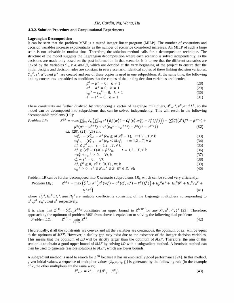
The algorithm is implemented in C++ by calling CPLEX to solve problems LR𝑘 and 𝑅𝑀𝑆𝐹. After running it on a

DELL workstation to solve the problem with a size of 100 scenarios and 10 year periods, it turns out that the

algorithm is able to get feasible solutions with a duality gap of 9%. Furthermore, Table 1 shows that the algorithm is

capable of efficiently solving large size problems that are not solvable using the CPLEX MIP solver.

Table 1: Comparison of the results for 10 years

No. of scenarios

CPLEX proposed algorithm

NPV

($, million)

solution time

(s)

NPV

($, million)

solution time

(s)

10 23.7 2 23.6 46

50 N/A* N/A 26.5 212

100 N/A N/A 25.2 481

*N/A means the problem is not solvable within considerable computational time

Computational Experiments

An out-of-sample test is conducted to compare the results of the two stochastic programming models for the flexible

design, as well as the model for the baseline inflexible design. Three simulation models are built to represent the

operation process of the AD plant under capacity plans resulting from the three optimization models. The outcomes

of the optimization models, i.e. the value of the initial design variables, the capacity plan, and the decision rule

variables, are then input to the simulation models. In each experiment, 10,000 scenarios of uncertainty data are

generated using the same technique as in the optimization models. After running 20 replications, the average ENPV

and the value of flexibility, which suggests the discounted profit of the flexible designs compared to the baseline

inflexible design, are measured to see whether the proposed multistage model MSF can improve the lifecycle

performance of the system. The values of flexibility are defined below:

𝑉𝑎𝑙𝑢𝑒 𝑜𝑓 𝐹𝑙𝑒𝑥𝑖𝑏𝑖𝑙𝑖𝑡𝑦𝑇𝑆𝐹 = 𝐸𝑁𝑃𝑉𝑇𝑆𝐹 − 𝐸𝑁𝑃𝑉𝐵𝑆𝐼 (45)

𝑉𝑎𝑙𝑢𝑒 𝑜𝑓 𝐹𝑙𝑒𝑥𝑖𝑏𝑖𝑙𝑖𝑡𝑦𝑀𝑆𝐹 = 𝐸𝑁𝑃𝑉𝑀𝑆𝐹 − 𝐸𝑁𝑃𝑉𝐵𝑆𝐼 (46)

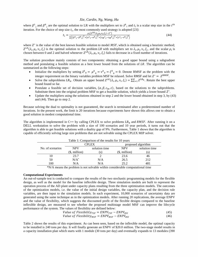
Table 2 shows the results of this experiment. As can been seen, based on the inflexible model, the optimal capacity

to be installed is 240 tons per day. It will finally generate an ENPV of $20.0 million. The two-stage model results in

a capacity installation plan which starts with 1 module (30 tons per day) and eventually expands to 13 modules (390


tons per day). The ENPV of this static capacity plan is $28.0 million, thus $8.0 million of value of flexibility is

achieved comparing to the inflexible design. As for the proposed multistage stochastic model, the initial capacity

and a decision rule are obtained for the managers to make decisions: install a capacity of 3 modules in the initial

phase, then expand the capacity by 2 modules once the amount of waste collected in last year is higher than the

current capacity. By following this decision rule, the ENPV can be as high as $31.2 million, with value of flexibility

of $11.2 million.

Table 2: Results of out of sample simulation (10,000 scenarios, 20 replications)

Models Capacity Plan / Decision rule ENPV ($ million) Value of flexibility ($ million)

Inflexible c = 240 20.0 -

Two-stage c = (1, 6, 8, 9, 10, 11, 13, 13, 13, 13, 13) 28.0 8.0

Multistage 휀 = 5, c𝑀 = 25, α = 0, β = 2 31.2 11.2

It is easy to conclude from the results that by enabling flexibility in the WTE system, the ENPV improves

significantly. In addition, by making dynamic decisions based on the decision rules from the multistage model, the

value of flexibility improves by 40.0% (from $8.0 million to $11.2 million) compared to the static capacity plan

from the two-stage model. The results show that the improvement in the value of flexibility from the multistage

model is significant and reliable.

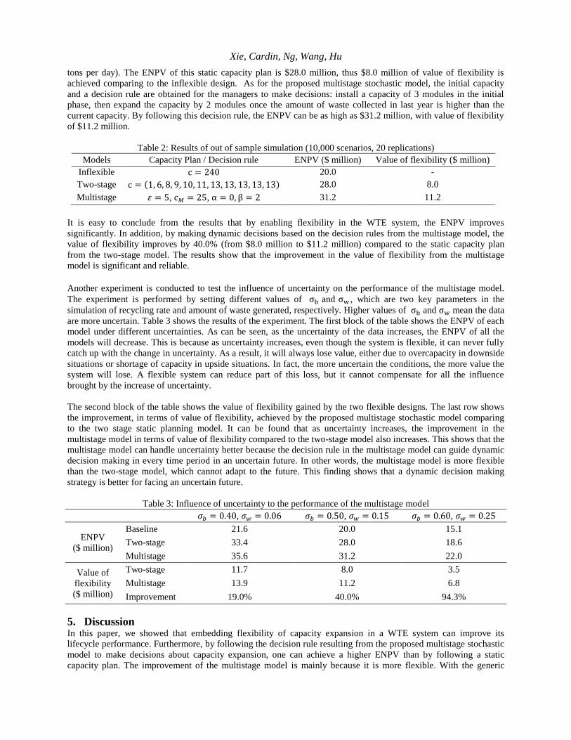
Another experiment is conducted to test the influence of uncertainty on the performance of the multistage model.

The experiment is performed by setting different values of σb and σw , which are two key parameters in the

simulation of recycling rate and amount of waste generated, respectively. Higher values of σb and σw mean the data

are more uncertain. Table 3 shows the results of the experiment. The first block of the table shows the ENPV of each

model under different uncertainties. As can be seen, as the uncertainty of the data increases, the ENPV of all the

models will decrease. This is because as uncertainty increases, even though the system is flexible, it can never fully

catch up with the change in uncertainty. As a result, it will always lose value, either due to overcapacity in downside

situations or shortage of capacity in upside situations. In fact, the more uncertain the conditions, the more value the

system will lose. A flexible system can reduce part of this loss, but it cannot compensate for all the influence

brought by the increase of uncertainty.

The second block of the table shows the value of flexibility gained by the two flexible designs. The last row shows

the improvement, in terms of value of flexibility, achieved by the proposed multistage stochastic model comparing

to the two stage static planning model. It can be found that as uncertainty increases, the improvement in the

multistage model in terms of value of flexibility compared to the two-stage model also increases. This shows that the

multistage model can handle uncertainty better because the decision rule in the multistage model can guide dynamic

decision making in every time period in an uncertain future. In other words, the multistage model is more flexible

than the two-stage model, which cannot adapt to the future. This finding shows that a dynamic decision making

strategy is better for facing an uncertain future.

Table 3: Influence of uncertainty to the performance of the multistage model

𝜎𝑏 = 0.40, 𝜎𝑤 = 0.06 𝜎𝑏 = 0.50, 𝜎𝑤 = 0.15 𝜎𝑏 = 0.60, 𝜎𝑤 = 0.25

ENPV

($ million)

Baseline 21.6 20.0 15.1

Two-stage 33.4 28.0 18.6

Multistage 35.6 31.2 22.0

Value of

flexibility

($ million)

Two-stage 11.7 8.0 3.5

Multistage 13.9 11.2 6.8

Improvement 19.0% 40.0% 94.3%

5. Discussion In this paper, we showed that embedding flexibility of capacity expansion in a WTE system can improve its

lifecycle performance. Furthermore, by following the decision rule resulting from the proposed multistage stochastic

model to make decisions about capacity expansion, one can achieve a higher ENPV than by following a static

capacity plan. The improvement of the multistage model is mainly because it is more flexible. With the generic


decision rule, the model enables managers to easily decide the capacity until the uncertainties of previous years are

known. In contrast, the static capacity plan tells managers how to deploy the capacity throughout the system’s

lifespan before knowing any of the uncertainties realization. Since the plan is designed to achieve the highest

average performance among all possible scenarios in the future, it may perform poorly in some extreme scenarios.

Therefore, the multistage model can improve the overall performance of the system.

Although we have shown that the proposed capacity expansion strategy can achieve significant performance

improvements, there are some limitations to this paper. First, the problem MSF is solved by using a Lagrangian

decomposition algorithm to find an upper bound and a lower bound. Since the duality gap obtained is about 9%, this

means that taking the lower bound as the solution cannot guarantee optimality. Therefore, a heuristic method is

needed to polish a better solution between the bounds. One possible way is to use Bender’s decomposition with the

current best solution to solve to optimum. However, this procedure may be very time consuming. In this paper, we

do not include this procedure. Since a solution with a duality gap of 9% has already shown that the proposed model

can significantly improve the lifecycle performance of the system, the optimal solution would, of course, provide an

even better performance. Therefore, such a suboptimal solution is sufficient for the purposes of this paper.

Another limitation of this paper is that it only makes comparison between the proposed model and a two-stage static

planning model. A further comparison could be made with the classic multistage stochastic model. In the classic

multistage stochastic models, uncertainty is modeled as a scenario tree in which each path represents a scenario. The

outcome of the model includes individual capacity expansion plans for each scenario. It is worth mentioning that the

proposed model is a special case of the classic multistage stochastic model: if the constraints of the decision rule are

relaxed, and so is the equality of the initial design variables, then the model will become a classic multistage model.

It is easy to see that the optimal objective value, the ENPV, of the multistage stochastic model will be larger than in

the proposed model, which means that it can provide a better theoretical performance.

However, the decision rule from the proposed model has advantage in management practice. To follow the results of

the classic multistage stochastic models, it requires the managers to approximate the realization of uncertainties to a

sample path in the modelling. This procedure is not an easy task in management practice. In contrast, in the

proposed multistage model things are much easier for managers: they do not need to identify the path, they only

need to follow the simple decision rule, i.e. expand the capacity by a certain amount if the observed uncertainty

realization in last year reaches a certain threshold. In other words, the decision making is independent from any time

period or uncertainty scenario. Simplicity of the decision making process is important in management practice as a

complicated process may be opposed by managers. Thus, the proposed model has an advantage when the system is

implemented in reality. This argument can be verified by a simulation game in which experiments are conducted by

having people simulate the decision making process, similar to the methodology of Cardin, Yue [25]. Therefore, a

future work can be to compare the performance of the proposed multistage stochastic model and a classic multistage

stochastic model, both in theory and in practice.

6. Conclusion In this paper, flexibility is considered as a mechanism to improve the lifecycle performance of WTE systems. The

problem of managing the exercise of the embedded flexibility was addressed, i.e. when and how to expand the

capacity. A multistage stochastic programming model was proposed to develop stochastically optimal decision rules

to guide decision making on capacity expansion. The model was solved using an algorithm based on Lagrangian

decomposition. The experimental results showed that, by embedding flexibility of capacity expansion, the lifecycle

performance of the WTE system could be improved significantly. Furthermore, the proposed multistage stochastic

model outperformed other models in providing a more sophisticated strategy for the capacity expansion process.

Some future work is possible to extend the current study. The single site WTE system considered in this paper is

merely one component of a decentralized WTE system in which multiple AD plants in different locations are

implemented simultaneously as a network. In a multiple site system, more types of flexibility have to be considered,

e.g. flexibility for different plants to exchange the feedstock. In addition, more patterns of decision rules should be

examined to make the decision process more sophisticated. The current decision rule is the simplest one, which only

looks at information about the waste amount in the previous year; a simple extension can be to observe information

from the past few years. Additionally, in the context of a multiple site system, the decision rule should be able to

deal with multiple types of flexibility in multiple plants simultaneously.


Acknowledgements This research is funded by the National Research Foundation (NRF), Prime Minister’s Office, Singapore under its

Campus for Research Excellence and Technological Enterprise (CREATE) programme.

References 1. NEA, Singapore waste statistics. 2011.

2. Fricke, E. and A.P. Schulz, Design for changeability (DfC): Principles to enable changes in systems

throughout their entire lifecycle. Systems Engineering, 2005. 8(4).

3. Trigeorgis, L., Real Options: Managerialflexibility and Strategy Inresource Allocation. 1996: the MIT

Press.

4. De Neufville, R. and S. Scholtes, Flexibility in engineering design. 2011: The MIT Press.

5. Cardin, M.-A., Enabling Flexibility in Engineering Systems: A Taxonomy of Procedures and a Design

Framework. Journal of Mechanical Design, 2013. 136(1): p. 011005-011005.

6. Cardin, M.-A., et al., Minimizing the economic cost and risk to Accelerator-Driven Subcritical Reactor

technology. Part 2: The case of designing for flexibility. Nuclear Engineering and Design, 2012. 243: p.

120-134.

7. Babajide, A., R. de Neufville, and M.-A. Cardin, Integrated method for designing valuable flexibility in oil

development projects. SPE Projects, Facilities & Construction, 2009. 4(2): p. 3-12.

8. De Neufville, R., Lecture Notes and Exercises in ESD.71: Engineering Systems Analysis for Design. 2008,

Massachusetts Institute of Technology: Cambridge, MA, United States.

9. Zhao, T. and C.-L. Tseng, Valuing flexibility in infrastructure expansion. Journal of infrastructure systems,

2003. 9(3): p. 89-97.

10. Mak, H.-Y. and Z.-J.M. Shen, Stochastic programming approach to process flexibility design. Flexible

Services and Manufacturing Journal, 2010. 21(3-4): p. 75-91.

11. Deng, Y., et al., Valuing flexibilities in the design of urban water management systems. Water Research,

2013.

12. De Neufville, R., S. Scholtes, and T. Wang, Real options by spreadsheet: parking garage case example.

Journal of infrastructure systems, 2006. 12(2): p. 107-111.

13. Manne, A.S., Investments for Capacity Expansion: Size, Location, and Time-Phasing. Vol. 5. 1967: MIT

Press.

14. Laguna, M., Applying robust optimization to capacity expansion of one location in telecommunications

with demand uncertainty. Management Science, 1998. 44(11-Part-2): p. S101-S110.

15. Cardin, M.-A., Facing reality: design and management of flexible engineering systems. 2007,

Massachusetts Institute of Technology.

16. Münster, M. and H. Lund, Comparing Waste-to-Energy technologies by applying energy system analysis.

Waste management, 2010. 30(7): p. 1251-1263.

17. Tin, A.M., et al., Cost—benefit analysis of the municipal solid waste collection system in Yangon,

Myanmar. Resources, conservation and recycling, 1995. 14(2): p. 103-131.

18. Xu, Y., et al., SRFILP: a stochastic robust fuzzy interval linear programming model for municipal solid

waste management under uncertainty. Journal of Environmental Informatics, 2009. 14(2): p. 72-82.

19. Feo, G.D. and C. Malvano, The use of LCA in selecting the best MSW management system. Waste

management, 2009. 29(6): p. 1901-1915.

20. Hu, J., et al., An approach to generate flexibility in engineering design of sustainable waste-to-energy

systems, in International Conference on Engineering Design. 2013: Seoul, Korea.

21. Savage, S., The flaw of averages: Why we underestimate risk in the face of uncertainty. Hoboken. 2009, NJ:

Wiley.

22. Shapiro, A., D. Dentcheva, and A.P. Ruszczyński, Lectures on stochastic programming: modeling and

theory. Vol. 9. 2009: SIAM.

23. Fisher, M.L., The Lagrangian relaxation method for solving integer programming problems. Management

science, 2004. 50(12 supplement): p. 1861-1871.

24. Held, M., P. Wolfe, and H.P. Crowder, Validation of subgradient optimization. Mathematical programming,

1974. 6(1): p. 62-88.

25. Cardin, M.-A., et al. Simulation Gaming to Study Design and Management Decision-Making in Flexible

Engineering Systems. in IEEE International Conference on Systems, Man, and Cybernetics, Manchester,

United Kingdom. 2013.

Analyzing Flexibility in Design of Waste-to-Energy Systems

Documents

Transcript of Analyzing Flexibility in Design of Waste-to-Energy Systems