Analytical Solution of Nonlinear Boundary Value Problem for Fin Efficiency of Convective Straight...
9
Hindawi Publishing Corporation ISRN ermodynamics Volume 2013, Article ID 282481, 8 pages http://dx.doi.org/10.1155/2013/282481 Research Article Analytical Solution of Nonlinear Boundary Value Problem for Fin Efficiency of Convective Straight Fins with Temperature-Dependent Thermal Conductivity K. Saravanakumar, 1 V. Ananthaswamy, 1 M. Subha, 2 and L. Rajendran 1 1 Department of Mathematics, e Madura College, Madurai 625011, TN, India 2 Madurai Sivakasi Nadars Pioneer Meenakshi Women’s College, Poovanthi 630611, Sivaganga District, TN, India Correspondence should be addressed to L. Rajendran; raj sms@rediffmail.com Received 9 July 2013; Accepted 2 August 2013 Academic Editors: R. R. Burnette, E. Curotto, and I. Kim Copyright © 2013 K. Saravanakumar et al. is is an open access article distributed under the Creative Commons Attribution License, which permits unrestricted use, distribution, and reproduction in any medium, provided the original work is properly cited. We have employed homotopy analysis method (HAM) to evaluate the approximate analytical solution of the nonlinear equation arising in the convective straight fins with temperature-dependent thermal conductivity problem. Solutions are presented for the dimensionless temperature distribution and fin efficiency of the nonlinear equation. e analytical results are compared with previous work and satisfactory agreement is noted. 1. Introduction e discipline of heat transfer, typically considered an aspect of mechanical engineering and chemical engineering, deals with specific applied methods by which thermal energy in a system is generated, or converted, or transferred to another system. Heat transfer includes the mechanisms of heat con- duction, thermal radiation, and mass transfer. e analysis of extended surface heat transfer is extensively presented by Kraus et al. [1]. Arslanturk [2] used decomposition method to evaluate the temperature distribution and analytical expres- sion for the fin efficiency. In the study of heat transfer, a fin is a surface that extends from an object to increase the rate of heat transfer to or from the environment by increasing convection. Incropera and Dewitt [3] presented a series of studies on the topic of heat transfer. Mokheimer [4] discussed a series of fin- efficiency curves for annular fins of rectangular, constant heat flow area, triangular, concave parabolic, and convex parabolic profiles for a wide range of radius ratios, and the dimensionless parameter based on the locally variable heat transfer coefficient. e optimum dimensions of circular fins with variable profile and temperature-dependent thermal conductivity have been obtained by Zubair et al. [5]. A new approach to calculate thermal performance of a singular fin with variable thermal properties has been presented by Kou et al. [6]. Joneidi et al. [7] studied an analytical solution of fin efficiency of convective straight fins with temperature- dependent thermal conductivity by the DTM. In this present paper, we first apply homotopy analysis method to obtain an approximation of analytical expression of fin efficiency of convective straight fins with temperature-dependent thermal conductivity. is problem is compared with Joneidi et al. [7]. 2. Mathematical Formulation of the Boundary Value Problem Consider a straight fin with a temperature-dependent ther- mal conductivity, arbitrary constant cross-sectional area ; perimeter and length (see Figure 1). e fin is attached to a base surface of temperature and extends into a fluid of temperature , and its tip is insulated. e one-dimensional energy balance equation is given as follows [ () ] − ℏ ( − ) = 0, (1)
-
Upload
maduracollege -
Category
Documents
-
view
3 -
download
0
Transcript of Analytical Solution of Nonlinear Boundary Value Problem for Fin Efficiency of Convective Straight...
Hindawi Publishing CorporationISRNThermodynamicsVolume 2013 Article ID 282481 8 pageshttpdxdoiorg1011552013282481
Research ArticleAnalytical Solution of Nonlinear Boundary ValueProblem for Fin Efficiency of Convective Straight Fins withTemperature-Dependent Thermal Conductivity
K Saravanakumar1 V Ananthaswamy1 M Subha2 and L Rajendran1
1 Department of Mathematics The Madura College Madurai 625011 TN India2Madurai Sivakasi Nadars Pioneer Meenakshi Womenrsquos College Poovanthi 630611 Sivaganga District TN India
Correspondence should be addressed to L Rajendran raj smsrediffmailcom
Received 9 July 2013 Accepted 2 August 2013
Academic Editors R R Burnette E Curotto and I Kim
Copyright copy 2013 K Saravanakumar et al This is an open access article distributed under the Creative Commons AttributionLicense which permits unrestricted use distribution and reproduction in any medium provided the original work is properlycited
We have employed homotopy analysis method (HAM) to evaluate the approximate analytical solution of the nonlinear equationarising in the convective straight fins with temperature-dependent thermal conductivity problem Solutions are presented for thedimensionless temperature distribution and fin efficiency of the nonlinear equation The analytical results are compared withprevious work and satisfactory agreement is noted
1 Introduction
The discipline of heat transfer typically considered an aspectof mechanical engineering and chemical engineering dealswith specific applied methods by which thermal energy in asystem is generated or converted or transferred to anothersystem Heat transfer includes the mechanisms of heat con-duction thermal radiation and mass transfer The analysisof extended surface heat transfer is extensively presented byKraus et al [1] Arslanturk [2] used decompositionmethod toevaluate the temperature distribution and analytical expres-sion for the fin efficiency
In the study of heat transfer a fin is a surface that extendsfrom an object to increase the rate of heat transfer to orfrom the environment by increasing convection Incroperaand Dewitt [3] presented a series of studies on the topicof heat transfer Mokheimer [4] discussed a series of fin-efficiency curves for annular fins of rectangular constantheat flow area triangular concave parabolic and convexparabolic profiles for a wide range of radius ratios and thedimensionless parameter based on the locally variable heattransfer coefficient The optimum dimensions of circular finswith variable profile and temperature-dependent thermalconductivity have been obtained by Zubair et al [5] A new
approach to calculate thermal performance of a singular finwith variable thermal properties has been presented by Kouet al [6]
Joneidi et al [7] studied an analytical solution of finefficiency of convective straight fins with temperature-dependent thermal conductivity by the DTM In this presentpaper we first apply homotopy analysis method to obtainan approximation of analytical expression of fin efficiency ofconvective straight fins with temperature-dependent thermalconductivityThis problem is comparedwith Joneidi et al [7]
2 Mathematical Formulation of the BoundaryValue Problem
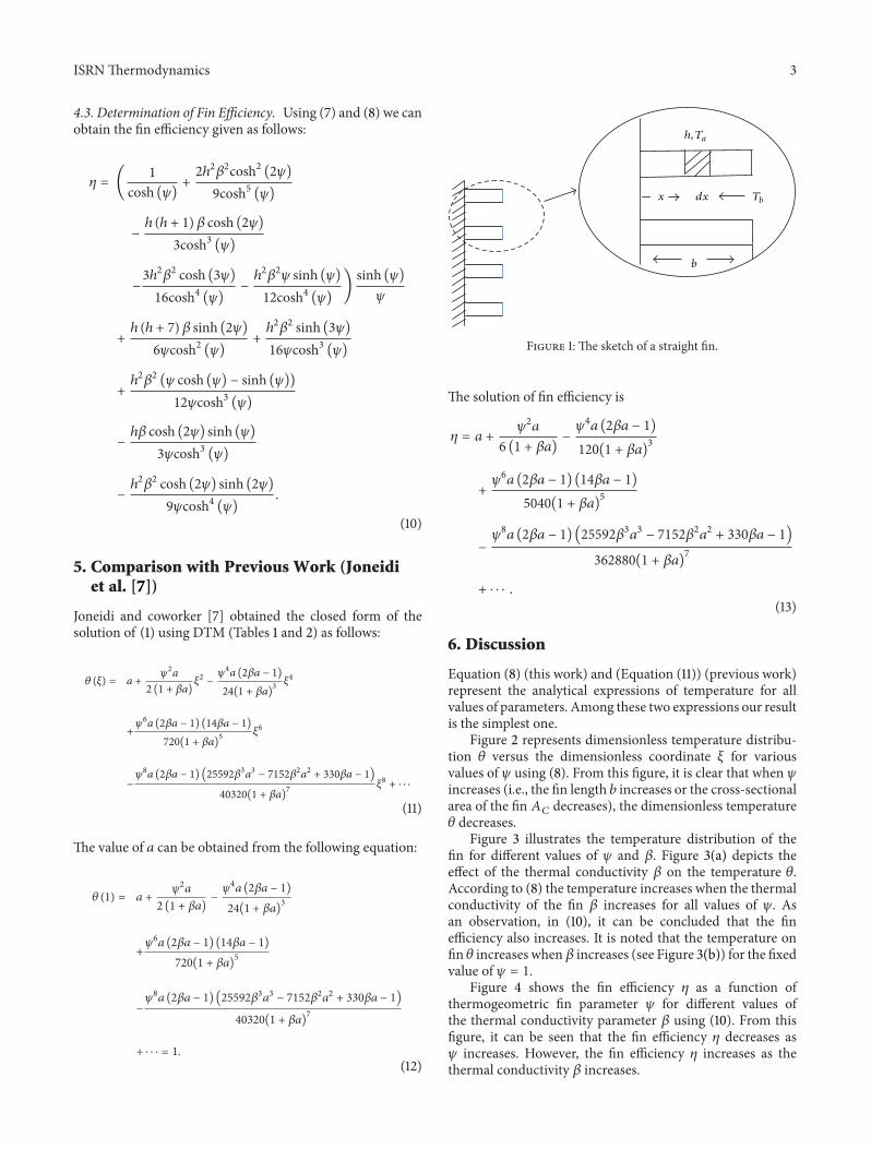
Consider a straight fin with a temperature-dependent ther-mal conductivity arbitrary constant cross-sectional area 119860119862perimeter 119875 and length 119887 (see Figure 1) The fin is attached toa base surface of temperature 119879119887 and extends into a fluid oftemperature 119879119886 and its tip is insulated The one-dimensionalenergy balance equation is given as follows
119860119862
119889
119889119909[119896 (119879)
119889119879
119889119909] minus 119875ℏ (119879
119887minus 119879119886) = 0 (1)
2 ISRNThermodynamics
where 119879 is the temperature 119896(119879) is the temperature-dependent thermal conductivity of the fin material 119875 isthe fin perimeter and ℏ is the heat transfer coefficient Thethermal conductivity of the finmaterial is assumed as follows
119896 (119879) = 119896119886 [1 + 120582 (119879 minus 119879
119886)] (2)
where 119896119886is the thermal conductivity at the ambient fluid
temperature of the fin and 120582 is the parameter describingthe variation of the thermal conductivity The followingdimensionless parameters are introduced [4]
120579 =119879 minus 119879119886
119879119887minus 119879119886
120585 =119909
119887 120573 = 120582 (119879
119887minus 119879119886)
120595 = (ℏ1198751198872
119896119886119860119862
)
12
(3)
Using the previous dimensionless variables the dimension-less form of (1) becomes as follows
1198892120579
1198891205852+ 120573120579
1198892120579
1198891205852+ 120573(
119889120579
119889120585)
2
minus 1205952120579 = 0 (4)
where 120579 is the dimensionless temperature 120585 is the dimension-less coordinate 120573 is the dimensionless parameter describingthermal conductivity and 120595 is the thermogeometric finparameter The boundary conditions are given as follows
119889120579
119889120585= 0 when 120585 = 0
120579 = 1 when 120585 = 1
(5)
3 Fin Efficiency
The heat transfer rate from the fin is found by using Newtonrsquoslaw of cooling
Consider
119876 = int
119887
0
119875 (119879 minus 119879119886) 119889119909(6)
The ratio of the fin heat transfer rate to the heat transferrate of the fin if the entire fin was at the base temperature iscommonly called as the fin efficiency
120578 =119876
119876ideal=
int
119887
0
119875 (119879 minus 119879119886) 119889119909
119875119887 (119879119887minus 119879119886)
= int
1
120585=0
120579 (120585) 119889120585(7)
4 Approximation of Analytical Solution
41 Homotopy Analysis Method (HAM) Thehomotopy anal-ysis method employs the concept of the homotopy fromtopology to flexibly generate a convergent series solutionfor nonlinear systems The HAM [8ndash13] was devised byShijun Liao which is a powerful analytical method for solving
nonlinear problems The greater generality of this methodoften allows for strong convergence of the solution overlarger spacial and parameter domains This method providesan analytical solution in terms of an infinite power seriesHowever there is a practical need to evaluate this solutionand to obtain numerical values from the infinite power seriesIn order to investigate the accuracy of the homotopy analysismethod (HAM) solution with a finite number of terms thesystem of differential equations was solved
The homotopy analysis method [14] is a good techniquecomparing to another perturbation method The HAM givesexcellent flexibility in the expression of the solution and howthe solution is explicitly obtained Different from all reportedperturbation and nonperturbative techniques the homotopyanalysis method itself provides us with a convenient wayto control and adjust the convergence region and rate ofapproximation series when necessary Briefly speaking thehomotopy analysis method has the following advantages itis valid even if a given nonlinear problem does not containany smalllarge parameters at all it can be employed toefficiently approximate a nonlinear problem by choosingdifferent sets of base functions In this paper we employHAM(see Appendix A) to solve the nonlinear equation
42 Solution of Dimensionless Temperature Using HAM wecan obtain the dimensionless temperature (see Appendix B)as follows
120579 (120585) = (1
cosh (120595)minus
ℎ (ℎ + 2) 120573 cosh (2120595)
3cosh3 (120595)
+2ℎ21205732cosh2 (2120595)
9cosh5 (120595)
minus3ℎ21205732 cosh (3120595)
16cosh4 (120595)minus
ℎ21205732120595 sinh (120595)
12cosh4 (120595)) cosh (120595120585)
+ (ℎ (ℎ + 2) 120573
3cosh2 (120595)minus
2ℎ21205732 cosh (2120595)
9cosh4 (120595)) cosh (2120595120585)
+3ℎ21205732 cosh (3120595120585)
16cosh3 (120595)+
ℎ21205732120595120585 sinh (120595120585)
12cosh3 (120595)
(8)
When 120573 rarr 0 from (4) the temperature is as follows
120579 (120585) =cosh (120595120585)
cosh (120595) (9)
This is the exact solution of (4) when 120573 = 0
ISRNThermodynamics 3
43 Determination of Fin Efficiency Using (7) and (8) we canobtain the fin efficiency given as follows
120578 = (1
cosh (120595)+
2ℎ21205732cosh2 (2120595)
9cosh5 (120595)
minusℎ (ℎ + 1) 120573 cosh (2120595)
3cosh3 (120595)
minus3ℎ21205732 cosh (3120595)
16cosh4 (120595)minus
ℎ21205732120595 sinh (120595)
12cosh4 (120595))sinh (120595)
120595
+ℎ (ℎ + 7) 120573 sinh (2120595)
6120595cosh2 (120595)+
ℎ21205732 sinh (3120595)
16120595cosh3 (120595)
+ℎ21205732(120595 cosh (120595) minus sinh (120595))
12120595cosh3 (120595)
minusℎ120573 cosh (2120595) sinh (120595)
3120595cosh3 (120595)
minusℎ21205732 cosh (2120595) sinh (2120595)
9120595cosh4 (120595)
(10)
5 Comparison with Previous Work (Joneidiet al [7])
Joneidi and coworker [7] obtained the closed form of thesolution of (1) using DTM (Tables 1 and 2) as follows
120579 (120585) = 119886 +1205952119886
2 (1 + 120573119886)1205852minus1205954119886 (2120573119886 minus 1)
24(1 + 120573119886)31205854
+1205956119886 (2120573119886 minus 1) (14120573119886 minus 1)
720(1 + 120573119886)51205856
minus
1205958119886 (2120573119886 minus 1) (25592120573
31198863minus 7152120573
21198862+ 330120573119886 minus 1)
40320(1 + 120573119886)7
1205858+ sdot sdot sdot
(11)
The value of 119886 can be obtained from the following equation
120579 (1) = 119886 +1205952119886
2 (1 + 120573119886)minus
1205954119886 (2120573119886 minus 1)
24(1 + 120573119886)3
+1205956119886 (2120573119886 minus 1) (14120573119886 minus 1)
720(1 + 120573119886)5
minus
1205958119886 (2120573119886 minus 1) (25592120573
31198863minus 7152120573
21198862+ 330120573119886 minus 1)
40320(1 + 120573119886)7
+ sdot sdot sdot = 1
(12)
b
x dx Tb
h Ta
Figure 1 The sketch of a straight fin
The solution of fin efficiency is
120578 = 119886 +1205952119886
6 (1 + 120573119886)minus
1205954119886 (2120573119886 minus 1)
120(1 + 120573119886)3
+1205956119886 (2120573119886 minus 1) (14120573119886 minus 1)
5040(1 + 120573119886)5
minus
1205958119886 (2120573119886 minus 1) (25592120573
31198863minus 7152120573
21198862+ 330120573119886 minus 1)
362880(1 + 120573119886)7
+ sdot sdot sdot
(13)
6 Discussion
Equation (8) (this work) and (Equation (11)) (previous work)represent the analytical expressions of temperature for allvalues of parameters Among these two expressions our resultis the simplest one
Figure 2 represents dimensionless temperature distribu-tion 120579 versus the dimensionless coordinate 120585 for variousvalues of 120595 using (8) From this figure it is clear that when 120595
increases (ie the fin length 119887 increases or the cross-sectionalarea of the fin 119860
119862decreases) the dimensionless temperature
120579 decreasesFigure 3 illustrates the temperature distribution of the
fin for different values of 120595 and 120573 Figure 3(a) depicts theeffect of the thermal conductivity 120573 on the temperature 120579According to (8) the temperature increases when the thermalconductivity of the fin 120573 increases for all values of 120595 Asan observation in (10) it can be concluded that the finefficiency also increases It is noted that the temperature onfin 120579 increases when 120573 increases (see Figure 3(b)) for the fixedvalue of 120595 = 1
Figure 4 shows the fin efficiency 120578 as a function ofthermogeometric fin parameter 120595 for different values ofthe thermal conductivity parameter 120573 using (10) From thisfigure it can be seen that the fin efficiency 120578 decreases as120595 increases However the fin efficiency 120578 increases as thethermal conductivity 120573 increases
4 ISRNThermodynamics
Table 1 Our work is compared with Joneidi et alrsquos [7] work and exact solution of dimensionless temperature 120579(120585) (linear case)
120585(a) 120573 = 0 120595 = 05 (b) 120573 = 0 120595 = 1
HAM (8)(this work)
DTM [7](11) Exact HAM (8)
(this work)DTM [7]
(11) Exact
0 088681 088681 088681 064805 064805 064805005 088709 088709 088709 064886 064886 064886010 088792 088792 088792 065129 065129 065129015 088931 088931 088931 065535 065535 065535020 089125 089125 089125 066105 066105 066105025 089375 089375 089375 066841 066841 066841030 089681 089681 089681 067743 067743 067743035 090043 090043 090043 068815 068815 068815040 090461 090461 090461 070059 070059 070059045 090936 090936 090936 071478 071478 071478050 091467 091467 091467 073076 073076 073076055 092056 092056 092056 074856 074856 074856060 092702 092702 092702 076824 076824 076824065 093406 093406 093406 078984 078984 078984070 094169 094169 094169 081341 081341 081341075 094990 094990 094990 083902 083902 083902080 095871 095871 095871 086673 086673 086673085 096812 096812 096812 089660 089660 089660090 097813 097813 097813 092871 092871 092871095 098875 098875 098875 096315 096315 096315100 100000 100000 099999 100000 100000 100000
0 01 02 03 04 05 06 07 08 09 1082
084
086
088
09
092
094
096
098
1
102
Dimensionless coordinate 120585
Dim
ensio
nles
s tem
pera
ture
120579
120595 = 05
120595 = 055
120595 = 06
120595 = 065
120573 = 0
Figure 2 Dimensionless temperature 120579 versus dimensionless coor-dinate 120585 for various values of 120595 when 120573 = 0 and ℎ = minus084 Thekey to the graph (solid line) represents our approximate solutionpresented in this work (8) and (+) represents Joneidi et alrsquos [7] work(Equation (11))
7 Conclusions
There are two main goals that we aimed for this work Thefirst is to employ the powerful homotopy analysis method
to investigate nonlinear differential equation arising in con-vective straight fins with temperature-dependent thermalconductivity problem The second is to achieve good resultsin predicting the solution of the heat transfer equationsin engineering The two goals are achieved successfully InHAM we can choose ℎ in an appropriate way which controlsthe convergence of the series
Appendices
A Basic Idea of Liaorsquos [15] HomotopyAnalysis Method
Consider the following differential equation [15]
119873[119906 (119905)] = 0 (A1)
where 119873 is a nonlinear operator 119905 denotes an independentvariable and 119906(119905) is an unknown function For simplicity weignore all boundary or initial conditions which can be treatedin the similar way By means of generalizing the conventionalhomotopymethod Liao constructed the so-called zero-orderdeformation equation as follows
(1 minus 119901) 119871 [120593 (119905 119901) minus 1199060 (119905)] = 119901ℎ119867 (119905)119873 [120593 (119905 119901)] (A2)
where 119901 isin [0 1] is the embedding parameter ℎ = 0 is anonzero auxiliary parameter 119867(119905) = 0 is an auxiliary func-tion 119871 is an auxiliary linear operator 119906
0(119905) is an initial guess
ISRNThermodynamics 5
Table 2 Our work is compared with Joneidi et alrsquos [7] work and numerical solution of dimensionless temperature 120579(120585) (nonlinear case)
120585120573 = 04 120595 = 1 120573 = 02 120595 = 05
NS DTM [7](11)
HAM (8)(this work) NS DTM [7]
(11)HAM (8)(this work)
0 071604 071604 071604 090344 090344 090344005 071674 071674 071674 090368 090368 090368010 071883 071883 071883 090440 090440 090440015 072231 072231 072231 090559 090559 090559020 072718 072718 072718 090727 090727 090727025 073346 073346 073346 090942 090942 090942030 074114 074114 074114 091206 091206 091206035 075022 075022 075022 091517 091517 091517040 076072 076072 076072 091877 091877 091877045 077264 077264 077264 092285 092285 092285050 078599 078599 078599 092741 092741 092741055 080077 080077 080077 093246 093246 093246060 081699 081699 081699 093799 093799 093799065 083467 083467 083467 094402 094402 094402070 085381 085381 085381 095053 095053 095053075 087442 087442 087442 095753 095753 095753080 089652 089652 089652 096503 096503 096503085 092011 092011 092009 097302 097302 097302090 094522 094522 094518 098151 098151 098151095 097184 097184 097181 099050 099050 099050100 100000 099999 100000 099999 099999 099999
0 01 02 03 04 05 06 07 08 09 1084
086
088
09
092
094
096
098
1
102
120573 = 03
120573 = 01
120573 = minus01
120573 = minus03
120573 = minus02
120595 = 05
Dimensionless coordinate 120585
Dim
ensio
nles
s tem
pera
ture
120579
(a)
0 01 02 03 04 05 06 07 08 09 1055
06
065
07
075
08
085
09
095
1
120573 = 03120573 = 01
120573 = minus01
120573 = minus03
120573 = minus02
120595 = 1
Dimensionless coordinate 120585
Dim
ensio
nles
s tem
pera
ture
120579
(b)
Figure 3 Dimensionless temperature 120579 versus dimensionless coordinate 120585 for various values of 120573 when (a) 120595 = 05 ℎ = minus084 and (b)120595 = 1 ℎ = minus084 The key to the graph (solid line) represents our approximate solution presented in this work (8) and (+) representsEquation (11) [7]
of 119906(119905) and 120593(119905 119901) is an unknown function It is importantthat one has great freedom to choose auxiliary unknowns inHAM Obviously when 119901 = 0 and 119901 = 1 it holds
120593 (119905 0) = 1199060 (119905) 120593 (119905 1) = 119906 (119905) (A3)
respectively Thus as 119901 increases from 0 to 1 the solution120593(119905 119901) varies from the initial guess 119906
0(119905) to the solution 119906(119905)
Expanding 120593(119905 119901) in Taylor series with respect to 119901 we have
120593 (119905 119901) = 1199060 (119905) +
+infin
sum
119898=1
119906119898 (119905) 119901
119898 (A4)
6 ISRNThermodynamics
0 05 1 15 2 25 3 35 402
03
04
05
06
07
08
09
1
120573 = 04120573 = 06
120573 = minus02120573 = 0
120573 = minus04 120573 = 02
120595
120578
Figure 4 Influence of thermal conductivity parameter 120573 on the finefficiency 120578 with the thermogeometric fin parameter 120595
where
119906119898 (119905) =1
119898
120597119898120593 (119905 119901)
120597119901119898
100381610038161003816100381610038161003816100381610038161003816119901=0
(A5)
If the auxiliary linear operator the initial guess the auxiliaryparameter ℎ and the auxiliary function are so properlychosen the series equation (A4) converges at 119901 = 1 thenwe have
119906 (119905) = 1199060 (119905) +
+infin
sum
119898=1
119906119898 (119905) (A6)
Define the vector
119906119899= 1199060 1199061 119906
119899 (A7)
Differentiating (A2) for 119898 times with respect to the embed-ding parameter 119901 then setting 119901 = 0 and finally dividingthembym wewill have the so-called119898th-order deformationequation as follows
119871 [119906119898minus 120594119898119906119898minus1
] = ℎ119867 (119905)R119898 (119898minus1) (A8)
where
R119898(119898minus1
) =1
(119898 minus 1)
120597119898minus1
119873[120593 (119905 119901)]
120597119901119898minus1
100381610038161003816100381610038161003816100381610038161003816119901=0
120594119898
= 0 119898 le 1
1 119898 gt 1
(A9)
Applying 119871minus1 on both sides of (A8) we get
119906119898 (119905) = 120594
119898119906119898minus1 (119905) + ℎ119871
minus1[119867 (119905)R119898 (119898minus1)] (A10)
In this way it is easily to obtain 119906119898for 119898 ge 1 at 119872th order
we have
119906 (119905) =
119872
sum
119898=0
119906119898 (119905) (A11)
When 119872 rarr +infin we get an accurate approximation ofthe original (A1) For the convergence of the above methodwe refer the reader to Liao [15] If (A1) admits uniquesolution then this method will produce the unique solutionIf (A1) does not possess unique solution the HAM will givea solution among many other (possible) solutions
B Solution of (4) Using HomotopyAnalysis Method
In this appendix we indicate how (8) in this paper is derivedThehomotopy analysismethodwas constructed to determinethe solution of (4)-(5) as follows
1198892120579
1198891205852+ 120573120579
1198892120579
1198891205852+ 120573(
119889120579
119889120585)
2
minus 1205952120579 = 0 (B1)
In order to solve (B1) bymeans of theHAMwefirst constructthe zeroth-order deformation equation by taking119867(119905) = 1
Consider
(1 minus 119901) [1198892120579
1198891205852minus 1205952120579]
= 119901ℎ[1198892120579
1198891205852+ 120573120579
1198892120579
1198891205852+ 120573(
119889120579
119889120585)
2
minus 1205952120579]
(B2)
The approximate solution of (B2) is as follows
120579 = 1205790+ 1199011205791+ 1199011205792+ sdot sdot sdot (B3)
Substituting (B3) into (B1) and comparing the coefficients oflike powers of p we get
119901011988921205790
1198891205852minus 12059521205790= 0 (B4)
119901111988921205791
1198891205852minus 12059521205791
= (ℎ + 1) [11988921205790
1198891205852minus 12059521205790]
+ ℎ120573[1205790
11988921205790
1198891205852+ (
11988921205790
1198891205852)
2
]
(B5)
119901211988921205792
1198891205852minus 12059521205792
= (ℎ + 1) [11988921205791
1198891205852minus 12059521205791]
+ ℎ120573[1205790
11988921205791
1198891205852+ 1205791
11988921205790
1198891205852+ 2
1198891205790
1198891205852
1198891205791
1198891205852]
(B6)
ISRNThermodynamics 7
09982
09982
09982
09982
09982
09982
09982
09982
09982
09982
minus1 minus095 minus09 minus085 minus08 minus075 minus07
h
120573 = 02 120595 = 01
120579(0
75)
(a)
623
6235
624
6245
625
6255
626
6265
627
6275
628
minus1 minus095 minus09 minus085 minus08 minus075 minus07
h
120573 = 02 120595 = 01
120579998400 (0
75)
times10minus3
(b)
Figure 5 The ℎ curves to indicate the convergence region for 120573 = 02 and 120595 = 01
The boundary conditions are
1198891205790
119889120585= 0 when 120585 = 0 120579
0= 1 when 120585 = 1 (B7)
119889120579119894
119889120585= 0 when 120585 = 0 120579119894 = 0 when 120585 = 1
forall119894 = 1 2 3
(B8)
Now applying the boundary conditions (B7) in (B4) we get
1205790 (120585) =
cosh (120595120585)
cosh (120595) (B9)
Substituting the value of 1205790in (B5) and solving the equation
using the boundary conditions (B8) we obtain the followingresults
1205791 (120585) = minus
ℎ120573 cosh (2120595)
3cosh3 (120595)cosh (120595120585) +
ℎ120573 cosh (2120595120585)
3cosh2 (120595) (B10)
Upon solving (B6) by substituting the values of 1205790and 1205791and
using the boundary conditions equation (B8) we can find thefollowing results
1205792 (120585) = (
2ℎ21205732cosh2 (2120595)
9cosh5 (120595)minus
ℎ (ℎ + 1) 120573 cosh (2120595)
3cosh3 (120595)
minus3ℎ21205732 cosh (3120595)
16cosh4 (120595)minus
ℎ21205732120595 sinh (120595)
12cosh4 (120595)) cosh (120595120585)
+ (ℎ (ℎ + 1) 120573
3cosh2 (120595)minus
2ℎ21205732 cosh (2120595)
9cosh4 (120595)) cosh (2120595120585)
+3ℎ21205732 cosh (3120595120585)
16cosh3 (120595)+
ℎ21205732120595120585 sinh (120595120585)
12cosh3 (120595)
(B11)
After three successive iterations the solutions of 120579 reach thebetter approximation Adding (B9) to (B11) we get (8) in thetext
C Determining the Region of ℎ for Validity
The analytical solution should converge It should be notedthat the auxiliary parameter ℎ controls the convergenceand accuracy of the solution series The analytical solutionrepresented by (8) contains the auxiliary parameter ℎ whichgives the convergence region and rate of approximation forthe homotopy analysis method In order to define the regionsuch that the solution series is independent of ℎ a multipleof ℎ curves are plotted The region where the dimensionlesstemperature 120579(120585) and 120579
1015840(120585) versus ℎ is a horizontal line
known as the convergence region for the correspondingfunctionThe common region among 120579(120585) and its derivativesare known as the overall convergence region To study theinfluence of ℎ on the convergence of solution ℎ-curves of120579(075) and 120579
1015840(075) are plotted in Figures 5(a) and 5(b)
respectively for 120573 = 02 120595 = 01 These figures clearly in-dicate that the valid region of ℎ is about minus086 to minus082Similarly we can find the value of the convergence controlparameter ℎ for different values of the constant parameters
Nomenclature
119860119862 Cross-sectional area of the fin (m2)
119887 Fin length (m)ℏ Heat transfer coefficient (W mminus1 Kminus1)119896 Thermal conductivity of the fin material (W
mminus1 Kminus1)119896119886 Thermal conductivity at the ambient fluid
temperature (W mminus1 Kminus1)119896119887 Thermal conductivity at the base
temperature (W mminus1 Kminus1)
8 ISRNThermodynamics
119875 Fin perimeter (m)119876 Heat-transfer rate (W)119879119886 Temperature of surface 119886 (K)
119879119887 Temperature of surface 119887 (K)
119909 Distance measured from the fin tip (m)
Greek Letters
120582 The slope of the thermalconductivity-temperature curve
120573 Dimensionless parameter describingvariation of the thermal conductivity
120578 Fin efficiency120585 Dimensionless coordinate120595 Thermogeometric fin parameter120579 Dimensionless temperature
Acknowledgments
This work is supported by the University Grant Commis-sion (UGC) Minor project no F MRP-412212 (MRPUGC-SERO) Hyderabad Government of India The authors arethankful to Shri S Natanagopal Secretary at the MaduraCollege Board and Dr R Murali Principal at the MaduraCollege (Autonomous)Madurai Tamil Nadu India for theirconstant encouragement
References
[1] A Kraus A Aziz and J Welty Extended Surface Heat TransferJohn Wiley amp Sons New York NY USA 2001
[2] C Arslanturk ldquoA decomposition method for fin efficiency ofconvective straight fins with temperature-dependent thermalconductivityrdquo International Communications in Heat and MassTransfer vol 32 no 6 pp 831ndash841 2005
[3] F P Incropera and D P Dewitt Introduction to Heat TransferJohn Wiley amp Sons New York NY USA 3rd edition 1996
[4] E M A Mokheimer ldquoPerformance of annular fins withdifferent profiles subject to variable heat transfer coefficientrdquoInternational Journal of Heat and Mass Transfer vol 45 no 17pp 3631ndash3642 2002
[5] S M Zubair A Z Al-Garni and J S Nizami ldquoThe opti-mal dimensions of circular fins with variable profile andtemperature-dependent thermal conductivityrdquo InternationalJournal of Heat andMass Transfer vol 39 no 16 pp 3431ndash34391996
[6] H-S Kou J-J Lee and C-Y Lai ldquoThermal analysis of alongitudinal fin with variable thermal properties by recursiveformulationrdquo International Journal of Heat and Mass Transfervol 48 no 11 pp 2266ndash2277 2005
[7] AA Joneidi DDGanji andMBabaelahi ldquoDifferential Trans-formation Method to determine fin efficiency of convectivestraight fins with temperature dependent thermal conductivityrdquoInternational Communications in Heat and Mass Transfer vol36 no 7 pp 757ndash762 2009
[8] S J Liao The proposed homotopy analysis technique for thesolution of non linear problems [PhD thesis] Shanghai JiaoTongUniversity 1992
[9] S-J Liao ldquoAn approximate solution technique not dependingon small parameters a special examplerdquo International Journalof Non-Linear Mechanics vol 30 no 3 pp 371ndash380 1995
[10] S J Liao ldquoOn the homotopy analysis method for nonlinearproblemsrdquo Applied Mathematics and Computation vol 147 no2 pp 499ndash513 2004
[11] S J Liao ldquoAn optimal homotopy-analysis approach for stronglynonlinear differential equationsrdquo Communications in NonlinearScience and Numerical Simulation vol 15 no 8 pp 2003ndash20162010
[12] S J Liao The Homotopy Analysis Method in Non LinearDifferential Equations Springer New York NY USA 2012
[13] G Domairry and H Bararnia ldquoAn approximation of theanalytic solution of some nonlinear heat transfer equations asurvey by using homotopy analysis methodrdquo Advanced Studiesin Theoretical Physics vol 2 no 11 pp 507ndash518 2008
[14] H Jafari C Chun and S M Saeidy ldquoAnalytical solution fornonlinear gas dynamic Homotopy analysis methodrdquo AppliedMathematics vol 4 pp 149ndash154 2009
[15] S J Liao Beyond Perturbation Introduction to the HomotopyAnalysis Method ChapmanampHallCRC Boca Raton Fla USA1st edition 2003
Submit your manuscripts athttpwwwhindawicom
Hindawi Publishing Corporationhttpwwwhindawicom Volume 2013
FluidsJournal of
Hindawi Publishing Corporation httpwwwhindawicom Volume 2013Hindawi Publishing Corporation httpwwwhindawicom Volume 2013
The Scientific World Journal
Computational Methods in Physics
Journal of
Hindawi Publishing Corporationhttpwwwhindawicom Volume 2013
Hindawi Publishing Corporationhttpwwwhindawicom
ISRN Astronomy and Astrophysics
Volume 2013
Hindawi Publishing Corporationhttpwwwhindawicom Volume 2013
Condensed Matter PhysicsAdvances in
OpticsInternational Journal of
Hindawi Publishing Corporationhttpwwwhindawicom Volume 2013
Hindawi Publishing Corporationhttpwwwhindawicom
Physics Research International
Volume 2013
ISRN High Energy Physics
Hindawi Publishing Corporationhttpwwwhindawicom Volume 2013
Hindawi Publishing Corporationhttpwwwhindawicom Volume 2013
Advances in
Astronomy
Hindawi Publishing Corporationhttpwwwhindawicom Volume 2013
GravityJournal of
ISRN Condensed Matter Physics
Hindawi Publishing Corporationhttpwwwhindawicom Volume 2013
Hindawi Publishing Corporationhttpwwwhindawicom
AerodynamicsJournal of
Volume 2013
ISRN Thermodynamics
Volume 2013Hindawi Publishing Corporationhttpwwwhindawicom
Hindawi Publishing Corporationhttpwwwhindawicom Volume 2013
High Energy PhysicsAdvances in
Hindawi Publishing Corporationhttpwwwhindawicom Volume 2013
Soft MatterJournal of
Hindawi Publishing Corporationhttpwwwhindawicom Volume 2013
Statistical MechanicsInternational Journal of
Hindawi Publishing Corporationhttpwwwhindawicom Volume 2013
PhotonicsJournal of
ISRN Optics
Hindawi Publishing Corporationhttpwwwhindawicom Volume 2013
Hindawi Publishing Corporationhttpwwwhindawicom Volume 2013
ThermodynamicsJournal of
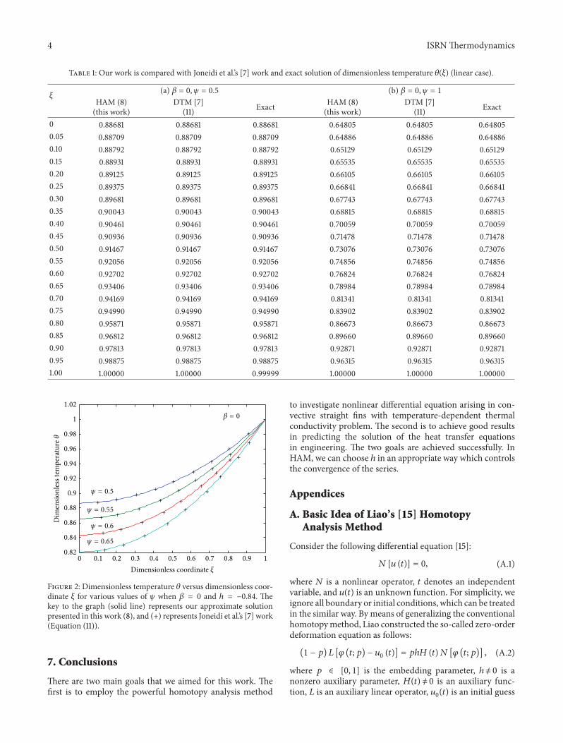
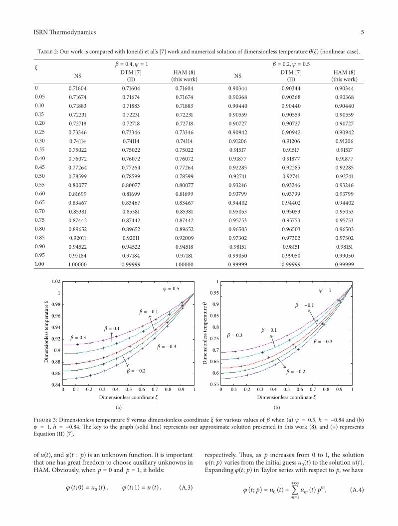
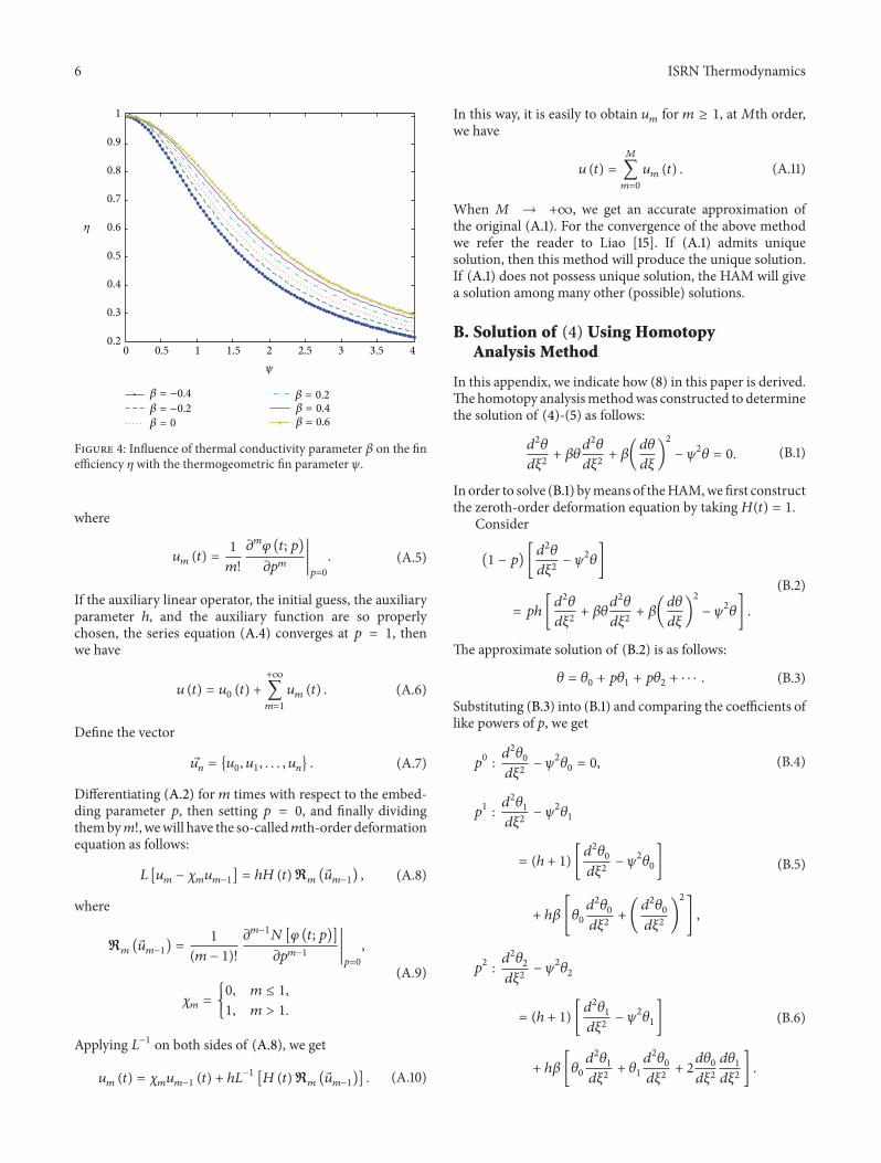
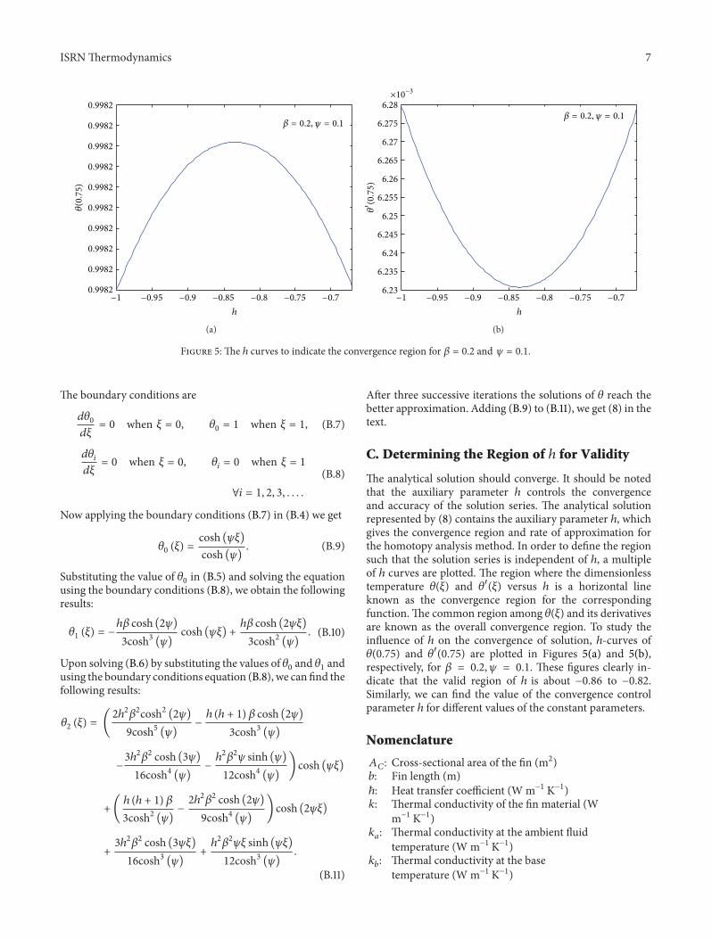