arX

iv:1

110.

5418

v2 [

astr

o-ph

.GA

] 3

0 Ju

l 201

2Draft version July 31, 2012Preprint typeset using LATEX style emulateapj v. 08/22/09

ANALYSIS OF WMAP 7-YEAR TEMPERATURE DATA: ASTROPHYSICS OF THE GALACTIC HAZE

Davide Pietrobon1, Krzysztof M. Gorski1,2, James Bartlett1,3, A. J. Banday4,5, Gregory Dobler6, LorisP. L. Colombo7,1, Sergi R. Hildebrandt8, Jeffrey B. Jewell1, Luca Pagano1, Graca Rocha1,

Hans Kristian Eriksen9,10, Rajib Saha11, and Charles R. Lawrence1

Draft version July 31, 2012

Abstract

We perform a joint analysis of the cosmic microwave background (CMB) and Galactic emissionfrom the WMAP 7-year temperature data. Using the Commander code, based on Gibbs sampling,we simultaneously derive the CMB and Galactic components on scales larger than 1◦ with improvedsensitivity over previous work. We conduct a detailed study of the low-frequency Galactic foreground,focussing on the “microwave haze” emission around the Galactic center. We demonstrate improvedperformance in quantifying the diffuse Galactic emission when including Haslam 408MHz data andwhen jointly modeling the spinning and thermal dust emission. We examine whether the hypotheticalGalactic haze can be explained by a spatial variation of the synchrotron spectral index, and find thatthe excess of emission around the Galactic center is stable with respect to variations of the foregroundmodel. Our results demonstrate that the new Galactic foreground component - the microwave haze -is indeed present.Subject headings: cosmology: observations, cosmic background radiation, diffuse radiation, methods:

data analysis, numerical, statistical, Galaxy: center

1. INTRODUCTION

While data from the Wilkinson Microwave AnisotropyProbe (WMAP) (see Jarosik et al. 2010; Komatsu et al.2010, and references therein) has enabled unprecedentedadvances in the understanding of cosmology over the pastdecade, it has also opened a unique window into the fun-damental physical processes of the interstellar medium(ISM). The choice of observing bands for WMAP insuredthat multiple emission mechanisms would be observedacross the frequency coverage. In particular, there are atleast three distinct physical processes at low frequencies(23-33-41 GHz),: free-free, synchrotron, and anomalousmicrowave emission (AME), which falls with frequencyand is highly correlated with 100 µm thermal dust emis-sion. At high frequencies (61-94 GHz), Galactic emis-sion is completely dominated by thermal dust emission

Electronic address: davide.pietrobon@jpl.nasa.gov1 Jet Propulsion Laboratory, California Institute of Technology,

4800 Oak Grove Drive, Pasadena, CA 91109-8099, U.S.A.2 Warsaw University Observatory, Aleje Ujazdowskie 4, 00478

Warszawa, Poland3 Laboratoire AstroParticule & Cosmologie (APC), Universite

Paris Diderot, CNRS/IN2P3, CEA/lrfu, Observatoire de Paris,Sorbonne Paris Cite, 10, rue Alice Domon et Leonie Duquet, 75205Paris Cedex 13, France

4 Universite de Toulouse; UPS-OMP; IRAP; Toulouse, France5 CNRS; IRAP; 9 Av. Colonel Roche, BP 44346, F-31028

Toulouse Cedex 4, France6 Kavli Institute for Theoretical Physics, University of Califor-

nia, Santa Barbara Kohn Hall, Santa Barbara, CA 93106 USA7 USC Dana and David Dornsife College of Letters, Arts and

Sciences, University of Southern California, University Park Cam-pus, Los Angeles, CA 90089

8 Division of Physics, Mathematics and Astronomy, Califor-nia Institute of Technology, 1200 East California Blvd. , 91125Pasadena, CA

9 Institute of Theoretical Astrophysics, University of Oslo, P.O.Box 1029 Blindern, N-0315 Oslo, Norway

10 4 Centre of Mathematics for Applications, University of Oslo,P.O. Box 1053 Blindern, N-0316 Oslo, Norway

11 Physics Department, Indian Institute of Science Educationand Research Bhopal, Bhopal, M.P, 462023, India

(Gold et al. 2011).Free-free emission (or thermal bremsstrahlung) is gen-

erated by scattering of ionized electrons off the pro-ton nuclei in hot (∼ 5000 K) gas, and has a bright-ness temperature which scales as T ∝ ν−2.15 throughthe WMAP bands, where ν represents frequency. Thebulk of the synchrotron emission observed by WMAP isseen to closely follow a power-law T ∝ ν−3 (Kogut et al.2007; Dobler 2011). Lastly, spinning dust (whosepresence has been observed in small, dusty clouds(Casassus et al. 2008; Planck Collaboration et al. 2011),as well as hotter diffuse regions (Dobler & Finkbeiner2008b; Dobler et al. 2009)), is the likely cause of theanomalous microwave emission. Small dust grains withnon-zero dipole moments are spun up by a variety ofmechanisms such as ion collisions, plasma density fluctu-ations, photon fields, etc., and produce spinning dipoleradiation (see Erickson 1957; Draine & Lazarian 1998,for the original theoretical realization of this idea).Using simple template regression techniques (see Sec-

tion 3), Bennett et al. (2003) and Finkbeiner (2004)showed that the Galactic emissions are highly spatiallycorrelated with maps at other frequencies. Free-freeemission is morphologically correlated with Hα recom-bination line emission, synchrotron with low frequencyradio emission (e.g., at 408 MHz), and spinning (andthermal) dust with total dust column density (e.g.,Schlegel et al. (1998) evaluated using models for the ther-mal emission to 94 GHz by Finkbeiner et al. 1999). Af-ter removing emission correlated with these templates,Finkbeiner (2004) found that there was an excess sig-nal centered on the Galactic center (GC) and extend-ing out roughly ∼ 30 degrees. A more detailed studyof this Galactic “haze” by (Dobler & Finkbeiner 2008a)(and more recently with the 7-year data by Dobler 2011)showed that its spectrum (T ∝ νβ with β ∼ −2.5) wastoo soft to be free-free emission and too hard to be syn-

2

chrotron emission associated with acceleration by supernovae (SN) shocks (after taking into account cosmic-raydiffusion). The origin of this residual component remainsa mystery and has been the object of intense theoreti-cal scrutiny (e.g., Hooper et al. 2007; Cholis et al. 2009;Biermann et al. 2010; Dobler et al. 2011; Crocker et al.2011; Guo et al. 2011).However, the subject of the haze has not been with-

out controversy, most notably due to the claim by theWMAP team (as well as others, e.g., Dickinson et al.2009) that the haze is not detected in their analyses.In particular, Gold et al. (2011) claimed lack of evi-dence for the haze based on WMAP polarization data,though it is unclear that a polarization signal would bedetectable (see Dobler 2011). A comprehensive studyof component separation (and CMB cleaning) was per-formed by Eriksen et al. (2006, 2007b); Dickinson et al.(2009) utilizing Bayesian inference of foreground ampli-tudes and spectra via Gibbs sampling. These studieshave never claimed a significant excess of emission to-wards the GC. Nevertheless, with the release of gamma-ray data from the Fermi Gamma-Ray Space Telescopein 2009, a corresponding feature at high energies wasdiscovered (Dobler et al. 2010), likely generated by thehaze electron inverse Compton (IC) scattering starlight,infrared, and CMB photons up to Fermi energies.With few exceptions (see for example Bottino et al.

2010), foreground studies using template fitting pre-subtract a CMB estimate which imprints a bias inthe foreground spectra (see Dobler & Finkbeiner 2008a)since no CMB estimate is completely clean of fore-grounds. In this work, we attempt to minimize this effectby solving jointly for the CMB map and angular powerspectrum and Galactic emission parameters, within aBayesian framework. We fit foreground parameters inevery pixel, thus taking into account spatial variation offoreground spectra, and we test the stability of the so-lution against several Galactic emission models. Seekinggreater independence from correlation with external tem-plates, we instead treat other data sets as input channelmaps and process them through the Gibbs sampler: tothis end we add Haslam at 408 MHz (Haslam et al. 1982)to the WMAP data set.In §2 we describe the data and our foreground model,

while in §3 we describe our its application in ourCommander analysis. Our approach enables us to improveupon previous studies. In §4 we discuss our results andrefine the methodology by performing a joint analysis ofthe WMAP 7-year data set and Haslam at 408 MHz.Lastly in §5 we summarize and draw our conclusions.

2. DATASETS AND FOREGROUND MODEL

Our approach uses the Gibbs sampling algorithmintroduced by Jewell et al. (2004) and Wandelt et al.(2004), and further developed by Eriksen et al. (2004);O’Dwyer et al. (2004); Eriksen et al. (2007b); Chu et al.(2005); Jewell et al. (2009); Rudjord et al. (2009);Larson et al. (2007). The method has been nu-merically implemented in a computer program calledCommander, and successfully applied to previous re-leases of the WMAP data as reported in Eriksen et al.(2008a), Eriksen et al. (2007a), and Dickinson et al.(2009). Commander is a maximum likelihood method,which generates samples from the joint posterior density

for the CMB map and angular power spectrum, as well asforeground components for the chosen sky model. A de-tailed description of the algorithm and its validation onsimulated data is provided by Eriksen et al. (2007b, andreferences therein). For the interested reader, we sum-marize the technical aspects of the sampling procedurein Appendix A.The main advantage of the approach is full charac-

terization of the (posterior) probability distribution ofthe parameter space spanned by the adopted sky model.Moreover, we can evaluate the goodness-of-fit of eachsample, i.e., of a given set of model parameters. Anyparametric model can be encoded, leaving the freedomto vary parameters pixel-by-pixel as well as to fit tem-plates.In the following we describe the data used in our anal-

ysis and their processing.

2.1. WMAP 7-year dataset

Our aim is to perform a comprehensive study of theWMAP 7-year temperature data (Jarosik et al. 2010),focusing not only on estimating the CMB signal and cor-responding power spectrum, but also on characterizingthe properties of the foreground emission, with particu-lar attention to evidence for the haze signal.The WMAP data set comprises data from ten Differ-

ential Assemblies (DAs) covering five frequencies from 23to 94 GHz. The WMAP team provided maps centered atfrequencies of 23, 30, 40, 60 and 90 GHz [K,Ka,Q,V,Wbands] resulting from the coadition of the DAs. Wesmooth the frequency maps to an effective 60 arcminuteresolution by deconvolving the maps with the appropri-ately coadded transfer functions provided by the WMAPteam and convolving with a Gaussian beam of 1 degreeFWHM. We then downgraded the sky maps to a work-ing resolution of Nside = 128 in the HEALPix12 scheme(Gorski et al. 2005). The choice of angular resolution,and subsequently of the pixelization, was dictated byboth the angular resolution of the available foregroundtemplates and by the need to resolve the first acousticpeak of the CMB power spectrum. This represents anovel element of our analysis compared to previous work(Eriksen et al. 2008a; Dickinson et al. 2009).In a further break with earlier analyses, we do

not add uniform white noise to regularize the maps(Eriksen et al. 2007a), but instead add a noise compo-nent proportional to the actual noise variance in thesmoothed, processed maps. To do so, we compute theRMS noise per pixel of the maps at the lower resolu-tion via a Monte Carlo approach. We generate 1,000non-uniform white noise realizations for each channel fol-lowing the prescription given by the WMAP team. Inpractice, we draw random Gaussian noise maps for eachfrequency band with zero mean and a variance given byσ2ν/Nobs at the native WMAP resolution Nside = 512,

where Nobs represents the number of observations in agiven pixel. We then smooth and downgrade the noisemaps as above and finally recompute the variance perpixel averaged over 1,000 simulations. Noise is thenadded to each frequency based on the computed noisevariance, and chosen so that the signal-to-noise ratio ofthe masked smoothed map at ℓ ≃ 2Nside is of order

12 http://healpix.jpl.nasa.gov/

3

unity. The scaling factors applied are [16,12,12,6,6] forthe [K,Ka,Q,V,W] channels respectively. One of the ad-vantages of this approach is that it preserves the noisestructure imposed by the scanning strategy and describesat least the diagonal part of the instrumental noise, whichhas been correlated by the smoothing procedure.

2.2. Foregrounds

The diffuse Galactic emission consists of three contri-butions from well understood foregrounds – synchrotronradiation from cosmic ray electrons losing energy in theGalactic magnetic field, free-free emission in the diffuseionised medium, and radiation from dust grains heatedby the interstellar radiation field. In addition, there isa strong contribution at frequencies in the range 20 –70 GHz referred to as anomalous microwave emission(AME) that is strongly correlated with the thermal dustemission and which has been explained by rotational ex-citation of small grains - the so-called spinning dust emis-sion (see for example Hoang et al. 2010, 2011, for recentstudies on the subject and references therein). In the fre-quency range spanned by WMAP, the synchrotron emis-sion is reasonably well described by a power law bright-ness temperature emissivity with spectral index β ∼ −3.The free-free emission also follows an approximate powerlaw, well described by a spectral index α ∼ −2.15. Thethermal dust component is usually modeled as a graybody with emissivity of the form T (ν) ∝ νǫB(ν, Td) withtypical values for the parameters given by ǫ ≃ 1.6 − 2.0and Td ≈ 18K. Since the highest frequency WMAP bandW has a nominal central frequency of 94 GHz, the over-all thermal dust contribution is small and can be ap-proximated by a simpler power law model with a spec-tral index ǫ ≃ 1.7. The AME is not completely well-characterised as yet, but falls rapidly below 20 GHz. Fitsto the high latitude sky suggest that it may be reasonablywell approximated by a power-law emissivity over theWMAP range of wavelengths, although this may reflectthe combination of multiple spinning dust populations indifferent physical conditions along a given line-of-sight.The total foreground intensity observed by the ν chan-

nel in a given direction p can then be summarized asfollows:

Tν(p) = M +∑

d=x,y,z

Dν,d(p) +( ν

ν0

)β(p)

Asynch(p)

+( ν

µ0

)α(p)

Af−f(p) +( ν

λ0

)ǫ

Adust(p)

+ AME(ν) ,

(1)

where M and D represent monopole and dipole residuals,respectively, Ai is the amplitude in antenna temperatureunits of the ith foreground component at the referencefrequency (ν0, µ0, λ0), and β, α and ǫ describe the spec-tral response of synchrotron, free-free and thermal dustemission, and an AME contribution has also been in-cluded.In principle, there is no reason why these parameters

should be constant over the sky, so we should allow themto vary pixel by pixel and let Commander solve for themost likely value. In practice, we are limited by thenumber of frequency bands, five in the case of WMAP,from which we also wish to determine the CMB contri-

bution. Therefore, there remain only 4 maps that canbe used to infer the foreground emission. Addressing thefull problem as posed in Eq. 1 in an independent andself-consistent way is therefore not possible. Since ourpresent analysis is motivated by a desire to assess thepresence of a hard synchrotron component in the Galac-tic center, the microwave haze, we prefer to disentanglethe foreground contributions in the low frequency range.A plausible and widely used alternative, which allows

for more realistic foreground modeling, is the use of ex-ternal templates. At very low frequency (< 1 GHz),the observed sky signal is dominated by the synchrotronemission from our Galaxy, and is little contaminated byfree-free emission, at least away from the Galactic plane.A full-sky map of the synchrotron emission is provided bythe 408 MHz map of Haslam et al. (1982). The opticalHα line is known to be a tracer of the free-free continuumemission at microwave wavelengths. Finkbeiner (2003)produced a full-sky Hα map as a composite of varioussurveys in both the northern and southern hemispheres.Finally, Finkbeiner et al. (1999) predicted the thermaldust contribution at microwave frequencies from a se-ries of models based on the COBE -DIRBE 100 and 240µm maps tied to COBE -FIRAS spectral data. We usepredicted emission at 94 GHz from the preferred Model8 (FDS8) as our reference template for dust emission.These templates, smoothed to 60 arcminutes and down-graded to Nside = 128, are shown in Figure 1.Since the thermal dust contribution to the WMAP

bands is small compared to synchrotron and free-freeemission, we can describe it by means of the FDS tem-plate with a fixed spectral index β = 1.7, allowing foran overall amplitude, b. The same can be done for thebremsstrahlung emission, assuming the Hα template asa sufficiently accurate description at 23 GHz and rescal-ing the amplitude according to a power law with indexα = −2.15. The synchrotron emission is expected to varyacross the sky, and the template we have is at 408 MHz,quite a large stretch from the first band of WMAP. Awise choice is to let Commander solve for an amplitudeand spectral index at every pixel, choosing 23 GHz aspivot. It should be noted that variations in the gas tem-perature will be imprinted onto the synchrotron compo-nent, as will deviations in the spectrum of thermal dust(which is a much smaller contribution).A detailed study of the foreground emission in the fre-

quency range 23-94 GHz employing external templatescan be found in Dickinson et al. (2009). Notice that thevalue of the spectral index of the dust, 1.7, is somewhatdependent on the specific method used to derive it. Adirect fit to the predicted dust templates at WMAP fre-quencies using the FDS8 model yields a lower value ofβ = 1.55, which is in agreement with what we find whenapplying template fitting procedure to WMAP maps (seeFigure 8).

3. WMAP ANALYSIS

Previous work on the Galactic Haze relied heavily ontemplate regression techniques, raising a debate as towhether the assumption of constant spectral behavioracross the sky is the cause of the excess emission nearthe Galactic Center. To address this issue, we follow analternate approach and solve instead for a simple modeldescribing Galactic emission with two power laws. One

4

Fig. 1.— Top to bottom, the three templates used to tracesynchrotron (Haslam 408 MHz, top panel), free-free (Hα, middlepanel) and dust, both thermal and spinning components (FDS,lower panel).

is a low-frequency component with a falling spectrum toaccount for synchrotron and free-free emission, as wellas AME. The second is a higher frequency componentwith a rising spectrum to represent thermal dust emis-sion. This appears to be well-motivated in studies of theWMAP Maximum Entropy Method (MEM) foregroundsolutions, as in Park et al. (2007). While we can solvefor the amplitude and spectral index at every pixel atof the low-frequency component, where the variability ofthe signal is large, we fix the dust emissivity at high fre-quency to ǫ = 1.7, consistent with previous applicationsof the Gibbs sampling technique to the WMAP data.We choose 22.8 GHz and 94 GHz as pivot frequency forthe low-frequency and thermal dust component respec-tively. The drawback of this approach is that the threelow-frequency emission mechanisms are combined into asingle power law component that may not provide anfully adequate description of their physical complexity.However, we will attempt to separate these componentspost-sampling in Section 3.1.We stress that our approach differs from that fol-

lowed by Cumberbatch et al. (2009), where Commander

was only used to extract a CMB map while modeling the

foreground components with templates. The main focusof that work was comparison between the WMAP In-ternal Linear Combination (ILC) CMB map, previouslyadopted in studies of the Haze, and the posterior meanCMB map derived from Gibbs sampling. The presence ofthe Haze was found to be stable with respect to the CMBmap choice. In the present paper, we take full advantageof Commander to jointly sample from foregrounds andCMB. In addition, we choose a less aggressive smooth-ing of the WMAP maps and mask, both factors that arelikely to enhance the signal-to-noise ratio of the Hazecomponent.The Commander result for the CMB map is shown in

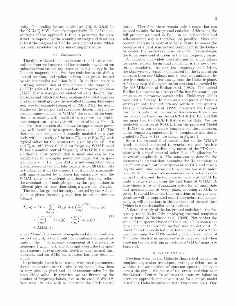
Figure 2. As a diagnostic, we show the mean χ2 mapin the lower panel of Figure 2. The number of pixelswith χ2 > 20, corresponding to the 99.9% confidencelevel for 5 degrees of freedom, is 0.7%. Most of thesepixels lie near point sources and we conclude that theycorrespond to point source bleeding outside the maskafter convolution with a large beam. The overall lack offeatures in the χ2 map is an indication of the goodness-of-fit of the model and that the residuals at each frequencyare compatible with our noise description.We checked that the Commander power spectrum is con-

sistent with the best estimate provided by the WMAPteam (Larson et al. 2011) at the 1σ level up to ℓ = 200.Beyond that, the Commander solution has significantlymore scatter due to the regularizing noise added to thesmoothed, binned maps (see Sec. 2.1). In addition, whilethe WMAP team also used Gibbs sampling techniquesfor low multiples, their high ℓ power spectrum was ob-tained by applying a quadratic estimator to the cross-spectra of V and W bands. We emphasize that theagreement between the two power spectra below ℓ = 200is what is important for our purposes since we are con-centrating on features in the map that are much largerthan 1◦. The possible presence of a residual monopoleand dipole in the ∆T data has been taken into accountand the mean values obtained are displayed in Table1. They are small and compatible with those foundby Dickinson et al. (2009) in the WMAP 5-year data,though it is important to keep in mind that monopoleand dipole features become strongly coupled to fore-grounds in CMB analyses, as discussed by Eriksen et al.(2008b).

TABLE 1Mean values (µK) for the monopole and dipole residuals

at every frequency.

K-band Ka-band Q-band V-band W-band23 GHz 33 GHz 41 GHz 61 GHz 94 GHz

M 2.4± 0.9 5.6± 1.0 3.5± 1.1 2.7± 1.0 3.9± 1.0Dx −2.6± 1.2 −3.4± 1.2 −2.7± 1.2 −2.7± 1.2 −3.0± 1.2Dy −3.6± 0.9 −4.3± 0.9 −4.4± 0.9 −3.5± 0.9 −4.0± 0.9Dz 1.9± 0.2 1.9± 0.2 2.4± 0.2 1.8± 0.2 2.0± 0.2

Foreground maps (left column) and associated errors(right column) for low frequency amplitude and spectralindex measured at 23 GHz and the thermal dust contri-bution at 94 GHz are shown in Figure 3.It is clear that our derived low frequency component

represents a combination of multiple emission mecha-

5

Fig. 2.— CMB Commander posterior average, rms and mean χ2

map. No particular features are present, meaning that the modelis a very good fit to the WMAP 7-year data. The lower limitresults 1.9, whereas the upper limit, 20, corresponds to 0.001probability for a χ

2 distribution with 5 degrees of freedom. Withinthe Gibbs sampling framework, we do not search for the maximum-likelihood (ML) point, but rather sample from the posterior: inpractice, we add a scatter term around the the ML point, drawnfrom the noise model of the data. This results into a number thatis distributed with 5 degrees of freedom.

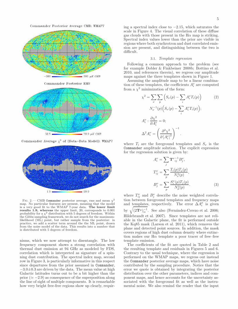
nisms, which we now attempt to disentangle. The lowfrequency component shows a strong correlation withthermal dust emission at 94 GHz as modeled by FDS,correlation which is interpreted as signature of a spin-ning dust contribution. The spectral index map, secondrow in Figure 3, is particularly informative in this respectsince departures from the prior assumed in Commander,−3.0±0.3 are driven by the data. The mean value at highGalactic latitudes turns out to be a bit higher than theprior (≃ −2.9) as consequence of the superposition alongthe line of sight of multiple components. It is remarkablehow very bright free-free regions show up clearly, requir-

ing a spectral index close to −2.15, which saturates thescale in Figure 4. The visual correlation of these diffusegas clouds with those present in the Hα map is striking.Spectral index values lower than the prior are visible inregions where both synchrotron and dust correlated emis-sion are present, and distinguishing between the two isdifficult.

3.1. Template regression

Following a common approach to the problem (seefor example Dobler & Finkbeiner 2008b; Bottino et al.2010, and references therein), we regress our amplitudemaps against the three templates shown in Figure 1.Assuming the amplitude map to be a linear combina-

tion of these templates, the coefficients Aνi are computed

from a χ2 minimization of the form:

χ2 =∑

ν

∑

p

(

Sν(p)−∑

i

Aνi Ti(p)

)

(2)

N−1ν (p)

(

Sν(p)−∑

i

Aνi Ti(p)

)

;

Aνi :

∂χ2

∂Aνi

= 0;

∆2Aνi =

(

∂2χ2

∂ [Aνi ]

2

)

−1

.

where Ti are the foreground templates and Sν is theCommander amplitude solution. The explicit expressionfor the regression solution is given by:

Aνi =

∑

j

Tν−1ij Bν

j ,

T νij =

∑

p

Ti(p)Tj(p)

N2ν (p)

,

Bνj =

∑

p

Sνi (p)Tj(p)

N2µ(p)

. (3)

where T νij and Bν

j describe the noise weighted correla-tion between foreground templates and frequency mapsand templates, respectively. The error ∆Aµ

i is given

by√

(2Tµ)−1ii . See also (Fernandez-Cerezo et al. 2006;

Hildebrandt et al. 2007). Since templates are not reli-able in the Galactic plane, the fit is performed outsidethe Kq85 mask (Larson et al. 2011), which removes theplane and detected point sources. In addition, the maskcovers regions of high dust column density where extinc-tion makes our Hα template a poor tracer of free–freetemplate emission.The coefficients of the fit are quoted in Table 2 and

the resulting template and residuals in Figures 5 and 6.Contrary to the usual technique, where the regression isperformed on the WMAP maps, we regress out insteadthe Commander posterior average maps, which have noisecontributed by the sampling procedure. Notice that theerror we quote is obtained by integrating the posteriordistribution over the other parameters, indices and com-ponent maps, and hence accounts for the uncertainty as-sociated with the foreground fit as well as the instru-mental noise. We also remind the reader that the input

6

Fig. 3.— Mean field map (left column) and rms (right column) for low-frequency component amplitude (upper panel) and spectral index(middle panel) and dust amplitude (lower panel) for the foreground model with two power laws.

7

Fig. 4.— Full sky spectral index mean field map. The Galacticplane shows strong variation corresponding to regions where onecomponent among synchrotron, free-free and spinning dust emis-sion dominates.

maps analyzed by Commander are noisier than the ex-pected from simply smoothing them because we add reg-ularizing noise required by the sampling algorithm (seeSection 2.1). These two factors increase the uncertaintyon the template amplitudes. A detailed investigation ispresented in Appendix B.As expected, the high frequency foreground component

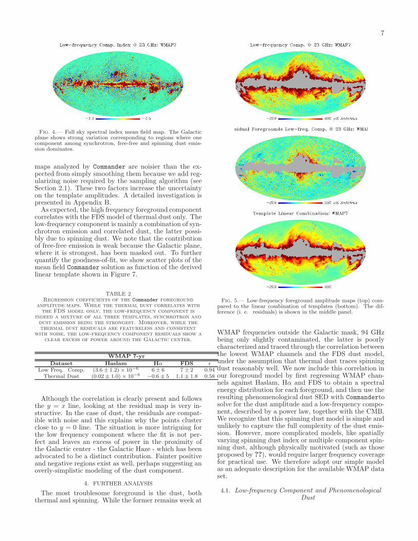
correlates with the FDS model of thermal dust only. Thelow-frequency component is mainly a combination of syn-chrotron emission and correlated dust, the latter possi-bly due to spinning dust. We note that the contributionof free-free emission is weak because the Galactic plane,where it is strongest, has been masked out. To furtherquantify the goodness-of-fit, we show scatter plots of themean field Commander solution as function of the derivedlinear template shown in Figure 7.

TABLE 2Regression coefficients of the Commander foreground

amplitude maps. While the thermal dust correlates withthe FDS model only, the low-frequency component is

indeed a mixture of all three templates, synchrotron anddust emission being the strongest. Moreover, while thethermal dust residuals are featureless and consistent

with noise, the low-frequency component residuals show aclear excess of power around the Galactic center.

WMAP 7-yr

Dataset Haslam Hα FDS rLow Freq. Comp. (3.6± 1.2) × 10−6 6± 6 7± 2 0.94Thermal Dust (0.02± 1.0)× 10−6

−0.6± 5 1.1± 1.8 0.58

Although the correlation is clearly present and followsthe y = x line, looking at the residual map is very in-structive. In the case of dust, the residuals are compat-ible with noise and this explains why the points clusterclose to y = 0 line. The situation is more intriguing forthe low frequency component where the fit is not per-fect and leaves an excess of power in the proximity ofthe Galactic center - the Galactic Haze - which has beenadvocated to be a distinct contribution. Fainter positiveand negative regions exist as well, perhaps suggesting anoverly-simplistic modeling of the dust component.

4. FURTHER ANALYSIS

The most troublesome foreground is the dust, boththermal and spinning. While the former remains week at

Fig. 5.— Low-frequency foreground amplitude maps (top) com-pared to the linear combination of templates (bottom). The dif-ference (i. e. residuals) is shown in the middle panel.

WMAP frequencies outside the Galactic mask, 94 GHzbeing only slightly contaminated, the latter is poorlycharacterized and traced through the correlation betweenthe lowest WMAP channels and the FDS dust model,under the assumption that thermal dust traces spinningdust reasonably well. We now include this correlation inour foreground model by first regressing WMAP chan-nels against Haslam, Hα and FDS to obtain a spectralenergy distribution for each foreground, and then use theresulting phenomenological dust SED with Commandertosolve for the dust amplitude and a low-frequency compo-nent, described by a power law, together with the CMB.We recognize that this spinning dust model is simple andunlikely to capture the full complexity of the dust emis-sion. However, more complicated models, like spatiallyvarying spinning dust index or multiple component spin-ning dust, although physically motivated (such as thoseproposed by ??), would require larger frequency coveragefor practical use. We therefore adopt our simple modelas an adequate description for the available WMAP dataset.

4.1. Low-frequency Component and PhenomenologicalDust

8

Fig. 6.— Thermal dust amplitude maps (top) compared to thelinear combination of templates (bottom) the difference (i. e. resid-uals) is shown in the middle panel.

The first Commander run with this model returned avery steep spectral index for the low-frequency compo-nent, close to the limit of our prior for some regions in theGalactic plane known to have strong spinning dust emis-sion. The χ2 of our solution in those regions was high,a sign that the foreground model fails. We then tunedthe amplitude of our dust model, increasing it at low fre-quencies until we obtained a shallower spectral index forthe low frequency component and smaller χ2 values forthe same regions. In practice, this means that we mod-ify the SED template to increase the relative amount ofspinning dust to thermal dust. The resulting spectralresponse is shown in Figure 8, together with those of thesoft synchrotron (β = −3), free-free (β = −2.15) andthermal dust components (β = 1.7).Figure 9 shows the mean field amplitude maps of the

thermal/spinning dust, and of the low-frequency com-ponent along with its spectral index. At high Galac-tic latitudes, where the signal-to-noise is very low, thespectral index is consistent with the Gaussian prior,β = −3.0±0.3,−2.9 being the mean value, whereas closerto the plane the solution is driven by the data. In highlatitude regions of strong synchrotron features, such asLoop I, the spectral index is noticeably softer than close

Fig. 7.— For the low-frequency foreground (top) and dust ampli-tude (bottom) we show the pixel-to-pixel comparison between thebest-fitting template combination (y-axis) and the Commander val-ues (x-axis). The red line marks the y=x scaling. Blue and greendots denote residuals with a significance larger than 3σ, positiveand negative, respectively. Orange points are pixels correspondingto the Haze: 3σ positive excess within a disc of 36 degrees aroundthe Galactic center.

Fig. 8.— SED for the phenomenological dust, compared to thoseof other components of interest: synchrotron, free-free and thermaldust emission.

to the plane, where spinning dust and free-free emissionbecome more important. Finally, it is interesting to notethat the dust map recovered at 94 GHz is remarkablysimilar to the FDS prediction.As noted above, the low-frequency Commander solu-

tion represents the combination of several different emis-

9

Fig. 9.— Low-frequency component mean field amplitude (upperpanel) and spectral index (middle panel) map at 23 GHz and dust-correlated emission (lower panel).

sion mechanisms known to coexist at 23-41 GHz: syn-chrotron, free-free, and possible spinning dust residu-als. This is confirmed by the low-frequency spectral in-dex map that presents shallower values at high Galacticlatitude, but clearly emphasizes regions in the Galac-tic plane with a very steep spectral index, likely to bespinning dust clouds. A comparison between the low-frequency component spectral index and amplitude forthe two models is shown in Figure 10. The evidence fordust-correlated emission is compelling, implying that ourphenomenological dust SED is a good approximation ofthe sky.For the most part, all of these emission mecha-

nisms decrease in intensity above 23 GHz (but seeDobler & Finkbeiner 2008b; Dobler et al. 2009), and itis because of the noise in the data that a single powerlaw results in a good χ2. In an effort to disentangle theseprimary sources of emission, we again apply template re-gression to the Commander outputs using the Haslam 408MHz map, the Hα map, and the FDS map as tracers ofsynchrotron, free-free, and dust (thermal and spinning)emission, respectively.The regression coefficients are quoted in Table 3 and

indeed they confirm our success: outside the applied

Fig. 10.— Difference between two Commander posterior mean low-frequency component amplitudes (upper panel) and spectral in-dices (lower panel) assuming two different foreground models: twopower-laws, and a power law with the phenomenological dust SED.

mask, dust is positively correlated with the FDS maponly, whereas the low-frequency component map can bedescribed as a linear combination of Haslam and Hα.The goodness of the regression is expressed by the coef-ficient.

TABLE 3Regression coefficients for Commander foreground

amplitudes: Top: WMAP 7-yr run; Bottom WMAP 7-yr andHaslam. The Galactic emission is decomposed into physical

components, each of which shows a clear correlationwith one template only.

Dataset Haslam Hα FDSWMAP 7-yr

Low-freq. Comp. (3.4± 3.3)× 10−6 9± 15 0.6± 6Dust (0.1± 1.3)× 10−6 −1± 6 2.3± 2.3

Haslam+WMAP 7-yr

Soft Sync. (5.9± 0.4)× 10−6−0.4± 1.3 (−0.6± 7)× 10−1

Low-freq. Comp. (−1.7± 3.5) × 10−6 8± 15 0.4± 6Dust (−0.3± 1.2) × 10−6 −0.25± 6 2.4± 2.2

As in the former run with thermal dust described bya power law, the FDS template shows itself a remark-able tracer of the dust map recovered by Commander,with the residual showing no evidence for large scale de-viations from the template. The same is true for thelow frequency component with the significant exceptionof the “haze region” around the Galactic center. Fig-ure 11 shows the residuals after removing the template-correlated emission from the Commander mean field low-frequency foreground map. In other words, synchrotronemission elsewhere (in Loop I and in the Galactic plane)as well as free-free emission are traced well by our tem-plates while the haze is definitely not, indicating that this

10

Fig. 11.— WMAP 7-yr: Comparison between low-frequency fore-ground component amplitude solution and linear fit of the tem-plates: an excess of power around the Galactic center is present.

large structure is not morphologically correlated withany of the templates. We find that the haze emissionis present in the data and contributes significantly to thetotal emission towards the Galactic center (and particu-larly in the south).Our findings are in agreement with what has been

described by several authors and in particular byDobler & Finkbeiner (2008a), who claim the presenceof an additional foreground component characterized bya spectral behaviour harder than a synchrotron compo-nent, but compatible with neither free-free (because thespectrum is too soft) nor spinning dust emission (becauseof lack of a thermal feature). Previous analyses werebased on presubtraction of CMB cleaned maps from thedata, which is problematic due to the fact that no CMBestimator is completely clean of foregrounds. This leadsto a bias in the inferred spectrum of the Galactic emis-sions. To the extent that it is possible with five bands,we have attempted to reduce this systematic by simulta-neously solving for the cleaned CMB map and the fore-ground maps while also determining a spectral index onthe sky, within a Bayesian framework, where the good-ness of the fit is controlled pixel-by-pixel through a χ2

evaluation.

4.2. WMAP 7-year Data combined with Ancillary Data

Our results in the previous section indicate that thehaze represents either a new component not present inthe Haslam map or a variation of the spectral index as-sociated with Haslam 408 MHz data. In order to as-sess this, we include the 408 MHz Haslam map togetherwith WMAP data and run Commander on six bands cov-ering a factor of ∼250 in frequency. This allows us tofit for an additional component and separate soft syn-chrotron from other emission mechanisms, the formerbeing described by a power law with fixed spectral indexβ = −3, the latter by a spatially varying spectral index.We expect the soft contribution to be mainly driven bythe Haslam map. Our foreground model in this secondCommander run becomes: CMB, dust described by a spa-tially constant spectrum which accounts for both spin-ning and thermal emission, soft synchrotron with fixedspectral response and an additional low frequency com-ponent with spatially varying spectral index:

Tν(p) = Mν +∑

d=x,y,z

Dν,d(p) +( ν

ν0

)β

(p)Alowfreq(p)

+( ν

λ0

)

−3

Asoft synch(p) + s(ν)Adust(p),

(4)

where ν0 = 22.8 GHz and λ0 = 408 MHz, and s(ν) isthe fixed effective dust spectrum, normalized to µ0 =33 GHz.The mean posterior CMB we obtain with this

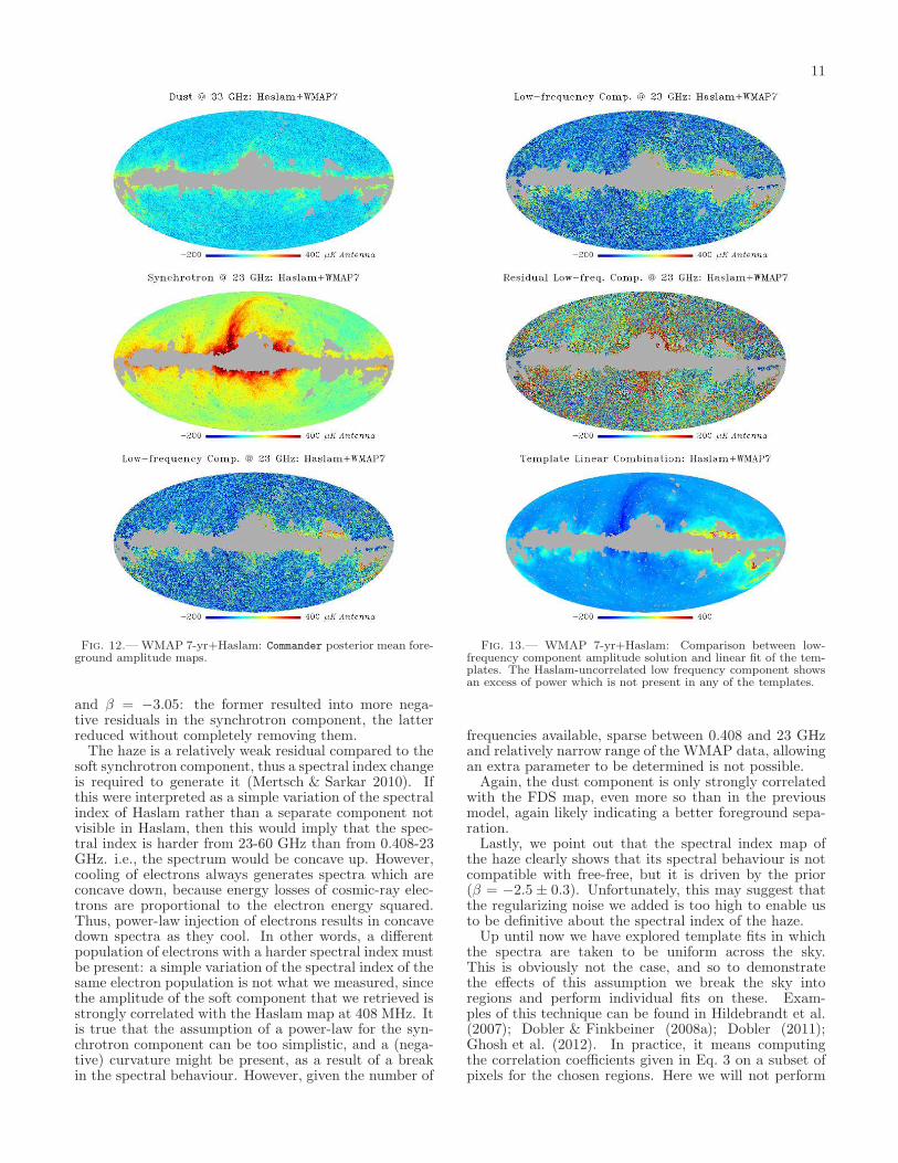
Commandermodel is slightly different compared to the 5-band case showing less power close to the Galactic plane.This suggests that the improved flexibility of our modelhas resulted in better component separation. The over-all χ2 of these 6-band run does not change, since we addone map and we fit for one more foreground component.It is interesting to notice that we retrieve a value of themonopole in the Haslam map of ≃ 3.2K.In Figure 12 we report the mean field map of the

foreground amplitudes: by visual inspection, the threeamplitude maps look strongly correlated with the fore-ground templates. The coefficients of the regression aresummarized in Table 3.The residuals obtained after regressing out the tem-

plates from the Commander solution obtained for thismore flexible foreground model are shown in Figure 13.The residuals are quite striking and demonstrate that thesoft synchrotron component (i.e., emission with a spec-tral index of ν−3.0) is almost perfectly correlated withHaslam and is not present, while the low frequency com-ponent clearly has a ν−2.15 free-free component that isstrongly correlated with Hα and the haze component,which is softer. This may suggest that the haze is notmerely a spectral index variation of emission present inthe Haslam map. In fact, the low frequency componentis anti-correlated with Haslam (driven primarily by thesmall negative residuals of Loop I). It is plausible thatthe prior we set for the spectral index of the soft com-ponent, β = −3, is not steep enough to characterize theSpur (β = −3.05), although at high Galactic latitudesa flatter behavior is measured (β = −2.9). Driven bythis consideration, we ran Commander setting the spec-tral index of the synchrotron component to β = −2.9

11

Fig. 12.— WMAP 7-yr+Haslam: Commander posterior mean fore-ground amplitude maps.

and β = −3.05: the former resulted into more nega-tive residuals in the synchrotron component, the latterreduced without completely removing them.The haze is a relatively weak residual compared to the

soft synchrotron component, thus a spectral index changeis required to generate it (Mertsch & Sarkar 2010). Ifthis were interpreted as a simple variation of the spectralindex of Haslam rather than a separate component notvisible in Haslam, then this would imply that the spec-tral index is harder from 23-60 GHz than from 0.408-23GHz. i.e., the spectrum would be concave up. However,cooling of electrons always generates spectra which areconcave down, because energy losses of cosmic-ray elec-trons are proportional to the electron energy squared.Thus, power-law injection of electrons results in concavedown spectra as they cool. In other words, a differentpopulation of electrons with a harder spectral index mustbe present: a simple variation of the spectral index of thesame electron population is not what we measured, sincethe amplitude of the soft component that we retrieved isstrongly correlated with the Haslam map at 408 MHz. Itis true that the assumption of a power-law for the syn-chrotron component can be too simplistic, and a (nega-tive) curvature might be present, as a result of a breakin the spectral behaviour. However, given the number of

Fig. 13.— WMAP 7-yr+Haslam: Comparison between low-frequency component amplitude solution and linear fit of the tem-plates. The Haslam-uncorrelated low frequency component showsan excess of power which is not present in any of the templates.

frequencies available, sparse between 0.408 and 23 GHzand relatively narrow range of the WMAP data, allowingan extra parameter to be determined is not possible.Again, the dust component is only strongly correlated

with the FDS map, even more so than in the previousmodel, again likely indicating a better foreground sepa-ration.Lastly, we point out that the spectral index map of

the haze clearly shows that its spectral behaviour is notcompatible with free-free, but it is driven by the prior(β = −2.5 ± 0.3). Unfortunately, this may suggest thatthe regularizing noise we added is too high to enable usto be definitive about the spectral index of the haze.Up until now we have explored template fits in which

the spectra are taken to be uniform across the sky.This is obviously not the case, and so to demonstratethe effects of this assumption we break the sky intoregions and perform individual fits on these. Exam-ples of this technique can be found in Hildebrandt et al.(2007); Dobler & Finkbeiner (2008a); Dobler (2011);Ghosh et al. (2012). In practice, it means computingthe correlation coefficients given in Eq. 3 on a subset ofpixels for the chosen regions. Here we will not perform

12

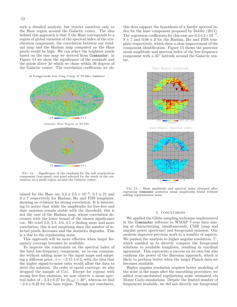
such a detailed analysis, but restrict ourselves only tothe Haze region around the Galactic center. The ideabehind this approach is that if the Haze corresponds to aregion of global variation of the spectral index of the syn-chrotron component, the correlation between our resid-ual map and the Haslam map computed on the Hazepixels would be high. We can select the brightest pixelsbased on the rms map we derived from Commander: inFigure 14 we show the significance of the residuals andthe pixels above 3σ which we chose within 36 degrees ofthe Galactic center. The correlation coefficients we ob-

Fig. 14.— Significance of the residuals for the soft synchrotroncomponent (top panel) and pixel selected for the study of the cor-relation on a small region around the Galactic center.

tained for the Haze are 3.3 ± 3.5 × 10−6, 0.1 ± 21 and3 ± 7 respectively for Haslam, Hα and FDS templates,showing no evidence for strong correlation. It is interest-ing to notice that while the amplitudes for free-free anddust emission remain stable with the threshold, this isnot the case of the Haslam map, whose correlation de-creases with the lower bound of the chosen significancecut. We tried 2.0, 2.5, 3.0, 3.5 σ finding more and morecorrelation: this is not surprising since the number of se-lected pixels decreases and the statistics degrades. Thisis a due to the regularizing noise.This approach will be more effective when larger fre-

quency coverage becomes be available.To improve the constraints on the spectral index of

the hard low-frequency component, we re-ran comman-der without adding noise to the input maps and adopt-ing a different prior, β = −2.15± 0.3, with the idea thatthe higher signal-to-noise ratio would allow the data todrive the solution. (In order to speed converge, we alsodropped the sample of Cls). Except for regions withstrong free-free emission, we now observe a mean spec-tral index of −2.3±0.27 for |bGal| > 30◦, whereas we find−2.4± 0.22 for the haze region. Though not conclusive,

this does support the hypothesis of a harder spectral in-dex for the haze component proposed by Dobler (2011).The regression coefficients for this case are 0.4±2×10−7,9 ± 7 and 0.08 ± 2 for the Haslam, Hα and FDS tem-plate respectively, which show a clear improvement of thecomponent identification. Figure 15 shows the posteriormean amplitude and spectral index of the low-frequencycomponent with a 35◦ latitude around the Galactic cen-ter.

Fig. 15.— Haze amplitude and spectral index obtained afterregressing Commander posterior mean amplitudes found withoutadding regularization noise.

5. CONCLUSIONS

We applied the Gibbs sampling technique implementedin the Commander software to WMAP 7-year data aim-ing at characterizing, simultaneously, CMB (map andangular power spectrum) and foreground emission. Ouranalysis improves previous work in a number of aspects.We pushed the analysis to higher angular resolution, 1◦,which enabled us to directly compare the foregroundsolutions to available templates, resulting in excellentagreement. This represents a success on its own but alsoconfirms the power of the Bayesian approach, which islikely to perform better when the larger Planck data setbecomes available.Higher angular resolution requires better modeling of

the noise in the maps after the smoothing procedure: weadded scan-modulated regularizing noise estimated viaMonte Carlo simulations. Despite the limited number offrequencies available, we did not directly use foreground

13

templates in the Gibbs sampling run, but rather let theparameters of the model vary across the sky. This al-lowed us to distinguish regions in the sky where a specificforeground mechanism dominates on the basis of the itsspectral behaviour. The presence of a strongly dust cor-related emission at low frequencies, explained by invok-ing spinning dust grains, emerges not only through theamplitude map but also in the spatial variation of thespectral index of the low frequency component, whichmainly results from a mixture of synchrotron emissionand dust-correlated emission. The number of availablefrequencies still limits us, since it forces us to use a con-stant spectral index for the dust.Regressing Commander solutions against foreground

templates is a complementary way to disentanglethe various emission mechanisms. It is by apply-ing this procedure that we confirm the presence ofexcess of signal localized around the Galactic cen-ter, the microwave haze. A hint of such a emis-sion has been found in the Fermi data (Dobler et al.2010, 2011). The study of this component has stim-ulated a rich production, both pointing out possiblesystematics in the applied regression procedures (,seefor instance Linden & Profumo 2010; Mertsch & Sarkar2010, and) and proposing possible physical mecha-nisms (Bottino et al. 2010; Dobler et al. 2011; Guo et al.2011; Guo & Mathews 2011; Biermann et al. 2010;Crocker & Aharonian 2011; Mertsch & Sarkar 2011).The WMAP team remains skeptical about the presenceof the haze (Gold et al. 2011), their main counter ar-gument being the lack of evidence for such a signalin the polarization maps (though Dobler 2011, showedthat such a signal would likely not be detectable inthe WMAP data given the noise). Regarding the spa-tial correspondence between the WMAP haze and theFermi haze/bubbles, we note that the increased noisein our output maps makes a direct comparison difficult.Comparison with earlier WMAP data was presented byDobler et al. (2010); Su et al. (2010), and more recentlywith WMAP 7-year data by Dobler (2011). We find, asin those studies, that the morphological correlation be-tween the two is reasonable at |bGal| < 30◦, where thesignal in microwaves is most unambiguous.We emphasize that our analysis overcomes the problem

of CMB subtraction and the circularity argument aris-ing from the removal of an internal linear combinationof the channels used in previous analyses. Moreover, weaddressed the issue of possible contamination of spinningdust as an explanation of the excess signal by including acorrelation between the low frequency emission and ther-mal dust. We computed the spectral energy distributionof the dust as described by the FDS model, performing atemplate fitting of the WMAP channels as a preprocess-ing step. We input the resulting SED to Commander, solv-ing for an amplitude map, together with a low-frequency

component. The resulting dust map is highly correlatedwith the FDS model, and the low-frequency componentresults from a sum of synchrotron and free-free emissiononly. When regressing this map against foreground tem-plates, the Galactic Haze is still present. One criticismto our approach could be the simplicity of the spinningdust model, but since one of our goals was to be indepen-dent of external data sets within a completely Bayesianframework, adding more complexity to the dust model isnot possible given the available degrees of freedom.We also argued that the haze is not an artifact of the

spectral variation of the synchrotron component acrossthe sky. To this end, we included the Haslam map at 408MHz in the Commander run and expanding the foregroundmodel: dust, combing both thermal and spinning contri-bution, synchrotron emission with fixed spectral responseβ = −3 and an additional component with a free spec-tral index, which would describe free-free, and any othercontribution. We found that we could completely sepa-rate synchrotron and dust emission, and that we were leftwith an amplitude map that can be easily characterizedby its spectral index. Free-free emission clearly showsup in the Galactic plane, together with the Haze whichseems to have a harder spectrum than the synchrotroncomponent. Unfortunately, outside the Galactic plane,the index map is quite noisy and the haze does not havea distinctive signature compared to the rest of the sky, al-though it is definitely not compatible with free-free emis-sion.Our analysis has improved previous knowledge of the

foreground and shed new light on the nature of the Galac-tic Haze. We addressed at least three criticisms oftenattached to haze studies: coherent CMB removal, con-tamination from spinning dust, and the spatial variationof the synchrotron component spectral index. The ex-cess of signal seems to be stable with respect to them.However, we have made assumptions on the dust spectralbehaviour, forced by the number of frequencies available,and we did not rule out the possibility of the presence ofcurvature in the synchrotron component spectral indexor a model with a broken power law. Planck data will ad-dress these remaining issues and enable a more completeforeground model.

ACKNOWLEDGEMENTS

Many of the results in this paper have been derived us-ing the HEALPix (Gorski et al. 2005) software and anal-ysis package. We acknowledge use of the Legacy Archivefor Microwave Background Data Analysis (LAMBDA).Support for LAMBDA is provided by the NASA Officeof Space Science. JGB gratefully acknowledges supportby the Institut Universitaire de France. GD has beensupported by the Harvey L. Karp discovery award.

REFERENCES

Bennett, C. et al. 2003, ApJ, 148, 97Biermann, P. L., Becker, J. K., Caceres, G. et al. 2010, ApJ, 710,

L53Bottino, M., Banday, A. J., & Maino, D. 2010, MNRAS, 402, 207Casassus, S., Dickinson, C., Cleary, K. et al. 2008, MNRAS, 391,

1075Cholis, I., Dobler, G., Finkbeiner, D. P., Goodenough, L., &

Weiner, N. 2009, Phys. Rev. D, 80, 123518

Chu, M., Eriksen, H. K., Knox, L. et al. 2005, Phys. Rev. D, 71,103002

Crocker, R. M. & Aharonian, F. 2011, Physical Review Letters,106, 101102

Crocker, R. M., Jones, D. I., Aharonian, F. et al. 2011, MNRAS,413, 763

Cumberbatch, D. T., Zuntz, J., Kamfjord Eriksen, H. K., & Silk,J. 2009, arXiv:0902.0039

14

Dickinson, C., Eriksen, H. K., Banday, A. J. et al. 2009, ApJ,705, 1607

Dobler, G. 2012, ApJ, 750, 17Dobler, G., Cholis, I., & Weiner, N. 2011, ApJ, 741, 25Dobler, G., Draine, B., & Finkbeiner, D. P. 2009, ApJ, 699, 1374Dobler, G. & Finkbeiner, D. P. 2008a, ApJ, 680, 1222—. 2008b, ApJ, 680, 1235Dobler, G., Finkbeiner, D. P., Cholis, I., Slatyer, T., & Weiner, N.

2010, ApJ, 717, 825Draine, B. T. & Lazarian, A. 1998, ApJ, 508, 157Erickson, W. C. 1957, ApJ, 126, 480Eriksen, H. K., Dickinson, C., Jewell, J. B. et al. 2008a, ApJ, 672,

L87Eriksen, H. K., Dickinson, C., Lawrence, C. R. et al. 2006, ApJ,

641, 665Eriksen, H. K., Huey, G., Banday, A. J. et al. 2007a, ApJ, 665, L1Eriksen, H. K., Huey, G., Saha, R. et al. 2007b, ApJ, 656, 641Eriksen, H. K., Jewell, J. B., Dickinson, C. et al. 2008b, ApJ, 676,

10Eriksen, H. K., O’Dwyer, I. J., Jewell, J. B. et al. 2004, ApJ, 155,

227Fernandez-Cerezo, S., Gutierrez, C. M., Rebolo, R. et al. P. 2006,

MNRAS, 370, 15Finkbeiner, D. P. 2003, ApJ, 146, 407—. 2004, ApJ, 614, 186Finkbeiner, D. P., Davis, M., & Schlegel, D. J. 1999, ApJ, 524,

867Ghosh, T., Banday, A. J., Jaffe, T. et al. 2012, MNRAS, 422, 3617Gold, B., Odegard, N., Weiland, J. L. et al. 2011, ApJ, 192, 15Gorski, K. M., Hivon, E., Banday, A. J. et al. 2005, ApJ, 622, 759Guo, F. & Mathews, W. G. 2011, arXiv:1103.0055Guo, F., Mathews, W. G., Dobler, G., & Oh, S. P. 2011,

arXiv:1110.0834

Haslam, C. G. T., Salter, C. J., Stoffel, H., & Wilson, W. E. 1982,A&AS, 47, 1

Hildebrandt, S. R., Rebolo, R., Rubino-Martın, J. A. et al. 2007,MNRAS, 382, 594

Hoang, T., Draine, B. T., & Lazarian, A. 2010, ApJ, 715, 1462Hoang, T., Lazarian, A., & Draine, B. T. 2011, ApJ, 741, 87Hooper, D., Finkbeiner, D. P., & Dobler, G. 2007, Phys. Rev. D,

76, 083012Jarosik, N., Bennett, C. L., Dunkley, J. et al. 2011, ApJ, 192, 14Jewell, J., Levin, S., & Anderson, C. H. 2004, ApJ, 609, 1Jewell, J. B., Eriksen, H. K., Wandelt, B. D. et al. 2009, ApJ,

697, 258Kogut, A., Dunkley, J., Bennett, C. L. et al. 2007, ApJ, 665, 355Komatsu, E., Smith, K. M., Dunkley, J. et al. 2011, ApJ, 192, 18Larson, D., Dunkley, J., Hinshaw, G. et al. 2011, ApJ, 192, 16Larson, D. L., Eriksen, H. K., Wandelt, B. D. et al. 2007, ApJ,

656, 653Linden, T. & Profumo, S. 2010, ApJ, 714, L228Mertsch, P. & Sarkar, S. 2010, JCAP, 10, 19—. 2011, Physical Review Letters, 107, 091101O’Dwyer, I. J., Eriksen, H. K., Wandelt, B. D. et al. 2004, ApJ,

617, L99Park, C.-G., Park, C., & Gott, III, J. R. 2007, ApJ, 660, 959Planck Collaboration 2011, A&A, 536, A20Rudjord, Ø., Groeneboom, N. E., Eriksen, H. K. et al. 2009, ApJ,

692, 1669Schlegel, D. J., Finkbeiner, D. P., & Davis, M. 1998, ApJ, 500,

525Su, M., Slatyer, T. R., & Finkbeiner, D. P. 2010, ApJ, 724, 1044Wandelt, B. D., Larson, D. L., & Lakshminarayanan, A. 2004,

Phys. Rev. D, 70, 083511

APPENDIX

THE CMB MAP AND POWER SPECTRUM POSTERIOR

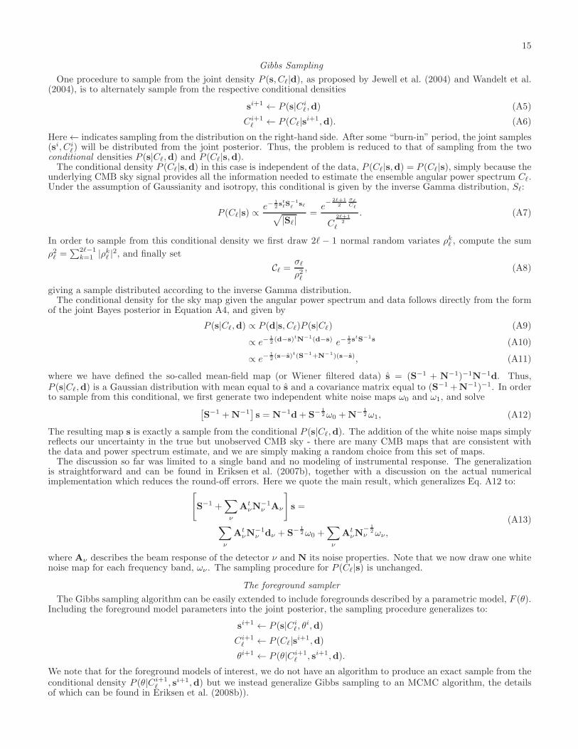
Here we review the basic concept behind Gibbs sampling. Let us first focus on the case of one frequency map andno foregrounds. The data model for this case is

d = s+ n, (A1)

where d is the data, s the CMB sky signal, and n instrumental noise. We assume both the CMB signal and noise tobe Gaussian random fields with vanishing mean and covariance matrices S and N, respectively. The CMB sky can bewritten in spherical harmonics as s =

∑

ℓ,m aℓmYℓm, with the CMB covariance matrix then fully characterized by the

angular power spectrum Cℓ according to Cℓm,ℓ′m′ = 〈a∗ℓmaℓ′m′〉 = Cℓδℓℓ′δmm′ . The noise matrix N is left unspecifiedfor now, but we note that for white noise it is diagonal in pixel space, Nij = σ2

i δij , for pixels i and j and noise varianceσ2i .Our goal is to sample from the posterior density for both the sky signal s and the power spectrum Cℓ, given by

P (s, Cℓ|d) ∝ P (d|s, Cℓ)P (s, Cℓ) (A2)

∝ P (d|s, Cℓ)P (s|Cℓ)P (Cℓ), (A3)

In what follows we assume the prior P (Cℓ) is uniform. Since we have assumed Gaussianity, the joint posteriordistribution may be written as

P (s, Cℓ|d) ∝ e−12(d−s)tN−1(d−s)

∏

ℓ

e−

2ℓ+1

2

σℓ

Cℓ

C2ℓ+1

2

ℓ

P (Cℓ), (A4)

where we have defined the quantity σℓ ≡1

2ℓ+1

∑ℓ

m=−ℓ |aℓm|2 as the angular power spectrum of the full-sky CMB

signal.For the case here with the CMB signal assumed to be a Gaussian field, one can integrate over the CMB sky signal

and analytically solve for the marginalized posterior P (Cℓ|d). However, evaluating the posterior numerically for anyspecific angular power spectrum is computationally prohibitive as it involves the computation of the inverse anddeterminant of very large matrices. We therefore sample from the posterior using a Gibbs sampling algorithm.

15

Gibbs Sampling

One procedure to sample from the joint density P (s, Cℓ|d), as proposed by Jewell et al. (2004) and Wandelt et al.(2004), is to alternately sample from the respective conditional densities

si+1 ← P (s|Ciℓ,d) (A5)

Ci+1ℓ ← P (Cℓ|s

i+1,d). (A6)

Here← indicates sampling from the distribution on the right-hand side. After some “burn-in” period, the joint samples(si, Ci

ℓ) will be distributed from the joint posterior. Thus, the problem is reduced to that of sampling from the twoconditional densities P (s|Cℓ,d) and P (Cℓ|s,d).The conditional density P (Cℓ|s,d) in this case is independent of the data, P (Cℓ|s,d) = P (Cℓ|s), simply because the

underlying CMB sky signal provides all the information needed to estimate the ensemble angular power spectrum Cℓ.Under the assumption of Gaussianity and isotropy, this conditional is given by the inverse Gamma distribution, Sℓ:

P (Cℓ|s) ∝e−

12st

ℓS

−1

ℓsℓ

√

|Sℓ|=

e−

2ℓ+1

2

σℓ

Cℓ

C2ℓ+1

2

ℓ

. (A7)

In order to sample from this conditional density we first draw 2ℓ − 1 normal random variates ρkℓ , compute the sum

ρ2ℓ =∑2ℓ−1

k=1 |ρkℓ |

2, and finally set

Cℓ =σℓ

ρ2ℓ, (A8)

giving a sample distributed according to the inverse Gamma distribution.The conditional density for the sky map given the angular power spectrum and data follows directly from the form

of the joint Bayes posterior in Equation A4, and given by

P (s|Cℓ,d) ∝ P (d|s, Cℓ)P (s|Cℓ) (A9)

∝ e−12(d−s)tN−1(d−s) e−

12stS

−1s (A10)

∝ e−12(s−s)t(S−1+N

−1)(s−s), (A11)

where we have defined the so-called mean-field map (or Wiener filtered data) s = (S−1 + N−1)−1N−1d. Thus,P (s|Cℓ,d) is a Gaussian distribution with mean equal to s and a covariance matrix equal to (S−1 +N−1)−1. In orderto sample from this conditional, we first generate two independent white noise maps ω0 and ω1, and solve

[

S−1 +N−1]

s = N−1d+ S−12ω0 +N−

12ω1, (A12)

The resulting map s is exactly a sample from the conditional P (s|Cℓ,d). The addition of the white noise maps simplyreflects our uncertainty in the true but unobserved CMB sky - there are many CMB maps that are consistent withthe data and power spectrum estimate, and we are simply making a random choice from this set of maps.The discussion so far was limited to a single band and no modeling of instrumental response. The generalization

is straightforward and can be found in Eriksen et al. (2007b), together with a discussion on the actual numericalimplementation which reduces the round-off errors. Here we quote the main result, which generalizes Eq. A12 to:

[

S−1 +∑

ν

AtνN

−1ν Aν

]

s =

∑

ν

AtνN

−1ν dν + S−

12ω0 +

∑

ν

AtνN

−12

ν ων ,

(A13)

where Aν describes the beam response of the detector ν and N its noise properties. Note that we now draw one whitenoise map for each frequency band, ων . The sampling procedure for P (Cℓ|s) is unchanged.

The foreground sampler

The Gibbs sampling algorithm can be easily extended to include foregrounds described by a parametric model, F (θ).Including the foreground model parameters into the joint posterior, the sampling procedure generalizes to:

si+1 ← P (s|Ciℓ, θ

i,d)

Ci+1ℓ ← P (Cℓ|s

i+1,d)

θi+1 ← P (θ|Ci+1ℓ , si+1,d).

We note that for the foreground models of interest, we do not have an algorithm to produce an exact sample from theconditional density P (θ|Ci+1

ℓ , si+1,d) but we instead generalize Gibbs sampling to an MCMC algorithm, the detailsof which can be found in Eriksen et al. (2008b)).

16

The parametric family of data models including foregrounds implemented in Commander are of the form

dν = Aνs+

M∑

m=1

aν,mtm+

+

N∑

n=1

bnfn(ν)fn +

K∑

k=1

ck gk(ν; θk) + nν .

(A14)

We may identify three main classes of foregrounds:

i) tm are M templates multiplied by an amplitude at every frequency, aν,m;

ii) fn are N templates whose spectral behaviour is known and described by the function fn(ν); we allow for anoverall rescaling, bn, for each of them;

iii) K foregrounds are described by a map of coefficients, ck, multiplied by the spectral response which is functionof the frequency and the parameters of the foreground model, θk.

We remind the reader that the bold face notation means an array of size Npix. An example of the first class offoregrounds is given by monopole and dipole residuals; a special case of the second class is a free-free template(Figure 1, top panel) whose spectral behaviour is known and follows the relation (ν/ν0)

−2.15; for the third type wemay quote synchrotron emission described by an amplitude we solve for at the reference frequency, e. g. µ0 = 23 GHz,and a spectral response given by (ν/µ0)

β .It is instructive to compute the degrees of freedom for such a foreground model applied to WMAP data. We solve

three maps, s, β and Asynch, 5 monopoles and dipoles, and two overall amplitudes if we describe free-free emission andthermal dust by means of the second class of foreground models. In total we look for 3Npix + 22 parameters. This isalready pretty close to the maximum number of parameters allowed by the WMAP, ≤ 5Npix. We could ask for onemore map, either dust or free-free, assuming a single power law and fixing the spectral index, or allowing a curvatureterm in the synchrotron model. Since a simple power law for thermal dust and free-free emission has been shown tobe consistent with the data in the frequency range spanned by WMAP (Dickinson et al. 2009), this may be used todisentangle the spinning dust contribution from thermal dust.We notice that to solve for the spectral index of a given component, the instrumental beam response of each channel

must be taken into account. Up to now, Commander is able to work with maps at the same angular resolution only.Smoothing all frequency maps and ancillary data to a common angular scale is then a necessary pre-processing step.As discussed in Eriksen et al. (2008b), it turns out to be more efficient to sample all the map amplitudes at once,

followed by the spectral response parameter, and finally the angular power spectrum, following the iterative scheme:

{si+1, am, bn, ck}i+1 ← P (s, am, bn, ck|C

iℓ, θ

i,d)

θi+1 ← P (θ|Ciℓ , s

i+1, ai+1m , bi+1

n , ci+1k ,d)

Ci+1ℓ ← P (Cℓ|s

i+1,d). (A15)

Sampling from the conditional density P (s, am, bn, ck|Ciℓ, θ

i,d) is a generalization of Eq. A13, whereas the samplingof the angular power spectrum remains unchanged, since Cℓ are functions of the sky signal only. Sampling of the non-linear degrees of freedom is through a standard inversion sampler: first compute the conditional probability densityP (x|θ), where x is the currently sampled parameter and θ denotes the set of all other parameters in the model, assumingthe likelihood to be independent pixel by pixel: −2lnL(x) = χ2 =

∑

ν(dν − sν(X, θ))2/σ2ν . Then, the corresponding

cumulative distribution is computed, F (x|θ) =∫ x

−∞P (y|θ)dy, and the value of the x variable is chosen by drawing a

uniformly distributed random number, u, and reading F (x|θ) = u.This concludes the review on the implementation of Gibbs sampling as implemented in the computer code Commander.

NOISE IMPACT ON THE REGRESSION PROCEDURE

We have observed that the regression coefficients we found when fitting foreground templates to Commander posteriormean amplitudes are consistent with those discussed in other works, but they have much larger errors. We argued inthe text that this is the result of the sampling procedure and has two causes: i) our input maps are noisier becauseof the additional noise term and ii) our uncertainties on the foreground amplitudes take into account the error on theother parameters of the model: CMB, other foreground amplitudes and spectral indices. In this respect, our errorsare more conservative.To clearly show this, we perform the same regression described in Equations 3 and 3 on two different maps: 1)

smoothedWMAP K-band and 2) Commander input K-band, which have to be compared to Commander output amplitudeperformance. The three maps are shown in Figure 16, together with the fit residuals and the corresponding χ2.Table 4 compares the regression coefficients for the signal at 23 GHz. Consistently, the amplitudes are the same but

the error bars increase dramatically due to the noise added to the maps. In particular we move from 10-30σ detectionto 1-3σ, which is driven by the scaling factor applied to the K-band (16, see Section 2.1).

17

This comparison suggests that a lower level of noise added to the input maps is useful to better characterize diffuseforeground emission. We will further investigate this issue in a forthcoming work.

TABLE 4Regression coefficients of the Commander foreground amplitude maps compared to those obtained when regressing

smoothed WMAP channel and Commander input WMAP maps

WMAP 7-yr

Dataset Haslam Hα FDS rSmoothed K-band (3.7± 0.17) × 10−6 6.4± .6 7.0± .25 0.91

Commander Input K-band (3.7± 1.1)× 10−6 6± 5 7± 2 0.85Commander output @ 23GHz (3.6± 1.2)× 10−6 6± 6 7± 2 0.94

Fig. 16.— Example of three regressions performed on the WMAP K-band smoothed to 60 arcminute (top), Commander input K-band(middle row) and output foreground amplitude (bottom).