Plasma in Astrophysics and in Fusion: • The X-Ray ... - IRIS UniPA

DOTTORATO DI RICERCA IN FISICA DIPARTIMENTO DI FISICA E CHIMICA

FISICA DEL PLASMA

Plasma in Astrophysics and in Fusion:

The X-Ray Dark Side of Venus

AND

The Study of Hot Electrons in Shock Ignition relevant Regime

IL DOTTORE IL COORDINATORE

Masoud Afshari Antonio Cupane

IL TUTOR

Giovanni Peres

CICLO XXVI

2016

Dedication

Dedicated to my family especially my father and mother

for their unconditional love and support

Acknowledgements I have to thanks all those who helped make this work possible. First I would like to appreciate my academic advisor, Professor Giovanni Peres, for his nice guidance and full support of me during Ph.D. He allowed me to have an opportunity of working in Astrophysics field. I would like to express my sincere gratitude to Professor Dimitri Batani who paved my way to nuclear fusion field in spite of lots of difficulties. Many colleagues deserve my appreciation. First, I would like to thank to Professor Fabio Reale for helpful suggestion, Antonino Petralia and Angelo F. Gambino for discussion about IDL programming. I am very much obliged to Professor Leon Golub, P. R. Jibben & the XRT Team, Harvard-Smithsonian Center for Astrophysics, for providing firsthand information about Hinode/XRT PSF and their suggestions about Venus analysis. I also acknowledge Luca Volpe, Francesco Barbato, Luca Antonelli and Giulia Folpini for their beneficial guidance for hot electron measurement and our collaborators at PALS Lab especially Prof. Jiri Ullschmied the head of PALS Lab and O.Renner, M.Smid, E.Krousky. Finally, I deeply appreciate the devotion from my parents and concerns from my family. I could not finish this work without them.

This thesis addresses the study of plasma and plasma related phenomena in two neighboring fields: solar astrophysics and fusion plasma physics. Traditionally each of them has benefitted from the influence of the other. Below they are sketched:

Plasma in Astrophysics Venus transit has been observed with Hinode/XRT and SDO/AIA in 2012. We have measured

significant X-Ray residual flux from Venus’ dark side but analogous residual flux has not been

detected in the UV band. Mercury transit across solar disk was observed with Hinode/XRT in 2006

and the relevant observations have been used in other works, among other things to test the effect

of the instrument’s Point Spread Function Hinode/XRT Point Spread Function (PSF).

In this research first we have used a new version of the Hinode/XRT PSF to explore to which

extent such a significant flux from Venus shadow can be due to instrumental scattering: we have

selected well illuminated images in X-Ray band and deconvolved them, for Venus and Mercury.

Even after deconvolution, flux from Venus shadow remains significant while in Mercury case it

becomes negligible. Furthermore the emission from Venus shadow on one hand gradually

increases as Venus crosses the solar disk, approximately doubling at the center of its path across

the Sun, to return low at the solar limb, on the other the emission does not change with the emission

from the surrounding regions of the solar disk, thus excluding simple scattering mechanisms. We

comment that the observed residual flux of Venus is not due to the PSF scattering but may come

from the atmosphere of Venus. According to the fact related to Venus transit observation and

Hinode/XRT telescope and also previous observation with Chandra X-Ray telescope we suggest

solar scattering, especially fluorescent emissions, are the main mechanism for observed X-rays

emissions.

Plasma in Fusion

Shock ignition (SI) scheme is a promising approach to Inertial Confinement Fusion (ICF) for the

simplicity of the target and of laser parameters required and for its potential high gain.

In SI scheme the role of hot electrons (HEs) is ambiguous. They traditionally have been considered

to be dangerous in ICF since they could preheat the assembled fuel leading to a premature

expansion. They can also enhance the ablation pressure if their energies is below 100 keV.

We performed a shock ignition experiment at PALS in April 2014 to study the generation of HEs.

This experiment was in a series of preparatory studies on ICF in the framework of the HiPER, a

European collaboration.

In my thesis I present the experimental results related to the experiment. We measured the HE

energy in the range ≈ 18- 30 keV. These results (at 3ω frequency) are in good agreement with

existing literature: OMEGA Lab: Thot≈30 keV; PALS Lab: Thot≈50 keV and PIC calculations:

Thot=20-40 keV. Since HE have energy less than 100 keV it seems HEs play a positive effect on

the enhancement of the ablation pressure.

The laser to HE energy conversion efficiency is estimated to be ≈ 0.7 %. The spreading angle of

HEs, is a crucial parameter which shows how much HEs scattered during crossing the target. In

our experiment we measured a value ≈ 48°.

Contents Chapter 1 Introduction ............................................................................................................................... 1

1.1 Transits of Mercury and Venus ........................................................................................................... 2

1.2 Instruments and Data Sets ................................................................................................................... 3

1.2.1 Hinode Spacecraft ........................................................................................................................ 3

1.2.2 SDO/AIA ..................................................................................................................................... 4

1.2.3 Data Set ........................................................................................................................................ 4

1.3 Data Analysis ...................................................................................................................................... 4

1.3.1 Venus Analysis ............................................................................................................................ 5

1.3.2 Mercury Analysis ....................................................................................................................... 11

1.3.3 Solar Eclipse Analysis ............................................................................................................... 11

Chapter 2 Deconvolution .......................................................................................................................... 16

2.1 Image Processing .............................................................................................................................. 16

2.1.1 Convolution ................................................................................................................................ 16

2.1.2 Deconvolution ............................................................................................................................ 16

2.1.3 Point Spread Function (PSF) ...................................................................................................... 17

2.2 Hinode/XRT PSF .............................................................................................................................. 18

2.3 Deconvolution of Mercury shadows ................................................................................................. 19

2.4 Deconvolution of Venus shadows ..................................................................................................... 20

Chapter 3 Light Leak Contamination ..................................................................................................... 23

3.1 Light Leak Effect on XRT Filters ..................................................................................................... 23

3.2 Al-mesh Filter Analysis .................................................................................................................... 25

Chapter 4 X-Ray Emission From Venus ................................................................................................. 30

4.1 X-RAY PRODUCTION MECHANISMS ........................................................................................ 30

4.1.1 Solar Scattering: Fluorescence Emission and Elastic Scattering of Solar X-rays ...................... 30

4.1.2 Solar Wind Charge-Exchange (SWCX)..................................................................................... 31

4.1.3 Bremsstrahlung and Line Emissions .......................................................................................... 31

4.1.4 Grain Scattering ......................................................................................................................... 31

4.1.5 Discussion .................................................................................................................................. 31

4.2 Possible X-ray Mechanism for 2012 Venus transit ........................................................................... 32

4.3 Grain Scattering ................................................................................................................................ 33

4.3.1 Fundamentals of Grain Scattering .............................................................................................. 33

4.3.2 Vertical Distribution of Particles at the Lower Altitudes of Venus Atmosphere ....................... 35

4.3.3 Particle Scattering Possibility .................................................................................................... 40

4.4 Conclusion ........................................................................................................................................ 41

Chapter 5 Nuclear Fusion ........................................................................................................................ 43

5.1 Introduction ....................................................................................................................................... 43

5.2 Direct-Drive ICF ............................................................................................................................... 46

5.3 Indirect-Drive ICF ............................................................................................................................ 47

5.4 Fast Ignition ...................................................................................................................................... 47

5.5 Shock Ignition ................................................................................................................................... 48

Chapter 6 Shock Wave Propagation Theory .......................................................................................... 49

6.1 Acoustic Waves ................................................................................................................................ 49

6.2 Shock Waves: Rankine - Hugoniot Relations ................................................................................... 50

6.3 Shock Polar ....................................................................................................................................... 56

6.4 Energy Transport .............................................................................................................................. 57

6.5 Ablation Pressure .............................................................................................................................. 58

Chapter 7 Shock Ignition ......................................................................................................................... 62

7.1 Direct Drive Theory .......................................................................................................................... 62

7.2 Shock Ignition ................................................................................................................................... 63

7.2.1 Timing ........................................................................................................................................ 65

7.2.2 Laser–Plasma Interaction ........................................................................................................... 65

7.3 Linear Absorption Mechanisms ........................................................................................................ 66

7.3.1 Inverse Bremsstrahlung.............................................................................................................. 66

7.3.2 Resonant Absorption .................................................................................................................. 67

7.4 Nonlinear Absorption Mechanisms .................................................................................................. 69

7.4.1 Self-Focusing and Filamentation ............................................................................................... 69

7.4.2 Stimulated Raman Scattering ..................................................................................................... 70

7.4.3 Brillouin Scattering .................................................................................................................... 72

7.4.4 Two Plasmon Decay .................................................................................................................. 73

7.5 Hot Electron Generation and Propagation ........................................................................................ 74

7.5.1 Stopping Power .......................................................................................................................... 75

7.5.2 Angular Deviation ...................................................................................................................... 77

7.5.3 Refluxing .................................................................................................................................... 79

Chapter 8 The SI experimental Setup in Prague Asterix Laser System (PALS) ................................ 80

8.1 Motivation ......................................................................................................................................... 80

8.2 Prague Asterix Laser System ............................................................................................................ 81

8.3 Random Phase Plate .......................................................................................................................... 82

8.4 Targets............................................................................................................................................... 82

8.5 Kα Emission ...................................................................................................................................... 84

8.6 Kα Setup ........................................................................................................................................... 85

Chapter 9 Experimental Results .............................................................................................................. 87

9.1 Introduction ....................................................................................................................................... 87

9.2 Analysis of Kα Images ...................................................................................................................... 87

9.3 The study of the effect of laser and target parameters on Kα signal ................................................. 93

9.3.1 Kα Source Size vs. Laser Energy ............................................................................................... 93

9.4 Number of Kα Photons on 4π vs. Laser Energy ............................................................................... 95

9.5 Discussion ......................................................................................................................................... 97

9.6 The Effect of Preplasma on Kα Source Size ..................................................................................... 97

9.7 The Effect of Preplasma on the Number of Kα Photon .................................................................... 99

9.8 The Effect of CHCl Thickness on Kα Signal .................................................................................. 100

9.9 Spreading Angle of HEs ................................................................................................................. 101

9.10 Penetration Depth of Hot Electrons .............................................................................................. 102

9.11 Conversion Efficiency .................................................................................................................. 106

Appendix A Appendix B

1

“Ibn Sina observed the planet of Venus as a discrete spot against the Sun’s surface in 1032, correctly conducting that Venus lies between the Earth and the Sun and also that the planet is located closer to the Earth than to the Sun. In astronomy, he wrote of his observations and research done at Isfahan and Hamedan over a twenty-year period”. Isfahan, where he lived after 1023, and Hamadan, where he died, and where a university is named after him. Healers and achievers physicians who excelled in other fields and the times in which they lived, Raphael S. Bloch, M.D., Xlibris Corporation, May 31, 2012.

Introduction

X-ray astronomy is one of the youngest fields of astronomy which had huge progress during the

last decades. The first detection of X-ray emission was from the solar corona in 1949 and then the

discovery of the first X-ray source outside the solar system in 1962. Unexpected detection of bright

X-ray emission from Hyakutake comet (Lisse et al., 1996) caused higher attraction. The most

detected distant X-ray sources until 2000 is 13 billion light years away from the earth.

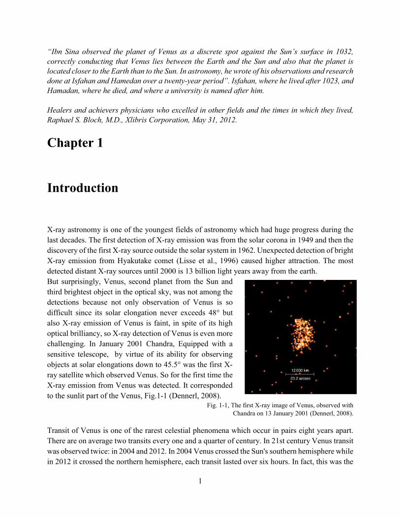
But surprisingly, Venus, second planet from the Sun and

third brightest object in the optical sky, was not among the

detections because not only observation of Venus is so

difficult since its solar elongation never exceeds 48° but

also X-ray emission of Venus is faint, in spite of its high

optical brilliancy, so X-ray detection of Venus is even more

challenging. In January 2001 Chandra, Equipped with a

sensitive telescope, by virtue of its ability for observing

objects at solar elongations down to 45.5° was the first X-

ray satellite which observed Venus. So for the first time the

X-ray emission from Venus was detected. It corresponded

to the sunlit part of the Venus, Fig.1-1 (Dennerl, 2008). Fig. 1-1, The first X-ray image of Venus, observed with

Chandra on 13 January 2001 (Dennerl, 2008).

Transit of Venus is one of the rarest celestial phenomena which occur in pairs eight years apart.

There are on average two transits every one and a quarter of century. In 21st century Venus transit

was observed twice: in 2004 and 2012. In 2004 Venus crossed the Sun's southern hemisphere while

in 2012 it crossed the northern hemisphere, each transit lasted over six hours. In fact, this was the

2

last chance to observe such a ‘transit’ until the 22nd century. In contrast, Transits of Mercury with

respect to the Earth are much more frequent than transits of Venus, with about 13 or 14 per century,

in part because Mercury is closer to the Sun and orbits it more rapidly.

Studies of transits of Mercury and Venus across the solar disk are among the oldest subjects of

astronomical observations and studies. The reason to observe them has changed over the centuries.

In the 1700s, such observations helped scientist to determine the Sun Earth distance and gave the

first clue that Venus might have an atmosphere. More recently, as for Hinode/XRT (Golub et al.

2007) observations, the transit of Mercury has been used by Weber et al. (2007) to test the

sharpness of the instrument Point Spread Function (PSF).

Reale et al. (2015) used Venus transit to measure the size of Venus in the X-ray band and therefore

the extension and optical thickness of Venus atmosphere. The implications of the latter work reach

into planetary physics and hint at similar methods to be used, in the future, for exoplanets.

In this research I analyzed the same set of transit observations to explore the residual X-ray

emission observed in Venus’ shadow and find, with the help of an updated version of Hinode/XRT

PSF, that this emission is not due to instrumental scattering and may origin from the Venus

atmosphere possibly due to the interaction of X-ray solar emission with Venus atmosphere.

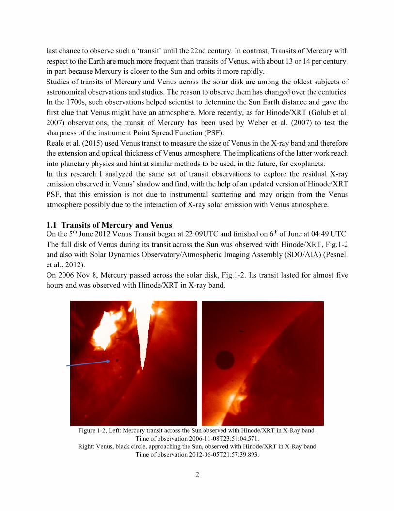
1.1 Transits of Mercury and Venus On the 5th June 2012 Venus Transit began at 22:09UTC and finished on 6th of June at 04:49 UTC.

The full disk of Venus during its transit across the Sun was observed with Hinode/XRT, Fig.1-2

and also with Solar Dynamics Observatory/Atmospheric Imaging Assembly (SDO/AIA) (Pesnell

et al., 2012).

On 2006 Nov 8, Mercury passed across the solar disk, Fig.1-2. Its transit lasted for almost five

hours and was observed with Hinode/XRT in X-ray band.

Figure 1-2, Left: Mercury transit across the Sun observed with Hinode/XRT in X-Ray band.

Time of observation 2006-11-08T23:51:04.571. Right: Venus, black circle, approaching the Sun, observed with Hinode/XRT in X-Ray band

Time of observation 2012-06-05T21:57:39.893.

3

The 2012 Venus transit which observed with Hinode/XRT can be divided in three stages: first

passing through the solar limb and entering to the solar disk, second passing close to a big active

region and, third, approaching the other limb.

1.2 Instruments and Data Sets In this section I briefly discuss the satellites and the instruments I used. 1.2.1 Hinode Spacecraft Hinode (in Japanese: Sunrise), formerly Solar-B, is a Japan Aerospace Exploration Agency Solar

mission which was launched on 22 September 2006 at 21:36 UTC. Hinode was planned as a three-

year mission. On 28 Oct 2006, the probe's instruments captured their first images. Hinode carries

three main instruments (Kosugi et al., 2007):

SOT (Solar Optical Telescope)

EIS (Extreme-Ultraviolet Imaging Spectrometer)

XRT (X-ray Telescope)

The images of interest for this research are those in X-Ray band, so I only present XRT in detail:

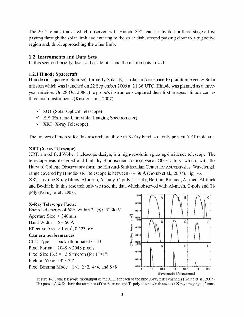
XRT (X-ray Telescope) XRT, a modified Wolter I telescope design, is a high-resolution grazing-incidence telescope. The

telescope was designed and built by Smithsonian Astrophysical Observatory, which, with the

Harvard College Observatory form the Harvard-Smithsonian Center for Astrophysics. Wavelength

range covered by Hinode/XRT telescope is between 6 – 60 Å (Golub et al., 2007), Fig.1-3.

XRT has nine X-ray filters: Al-mesh, Al-poly, C-poly, Ti-poly, Be-thin, Be-med, Al-med, Al-thick

and Be-thick. In this research only we used the data which observed with Al-mesh, C-poly and Ti-

poly (Kosugi et al., 2007). X-Ray Telescope Facts: Encircled energy of 68% within 2" @ 0.523keV

Aperture Size > 340mm

Band Width 6 – 60 Å

Effective Area > 1 cm2, 0.523keV

Camera performances

CCD Type back-illuminated CCD

Pixel Format 2048 × 2048 pixels

Pixel Size 13.5 × 13.5 micron (for 1"×1")

Field of View 34' × 34'

Pixel Binning Mode 1×1, 2×2, 4×4, and 8×8

Figure 1-3 Total telescope throughput of the XRT for each of the nine X-ray filter channels (Golub et al., 2007).

The panels A & D, show the response of the Al-mesh and Ti-poly filters which used for X-ray imaging of Venus.

4

1.2.2 SDO/AIA SDO, The Solar Dynamics Observatory was launched on 11 February 2010. The spacecraft includes three instruments: Extreme UV Variability Experiment (EVE) Helioseismic and Magnetic Imager (HMI) Atmospheric Imaging Assembly (AIA) Since the images of interest are taken in the UV band I only present the AIA characteristics: Atmospheric Imaging Assembly (AIA) AIA (Pesnell et al., 2012) with an angular resolution 0.6 arcsec per pixel provides narrow-band imaging in seven extreme ultraviolet (EUV) band passes centered on specific lines: (94 Å, 131 Å, 171 Å, 193 Å, 211 Å, 304 Å and 335 Å) and in two UV band passes near 1600 Å and 1700 Å (Lemen et al., 2012). 1.2.3 Data Set For Venus shadow analysis I used five different data sets in X-ray band, each of which with more than 300 images, and one data set in EUV band, 335 Å, with 169 images. For Mercury shadow analysis I used one data set in X-ray band. A summary of the data sets is presented in Table.1.1.

Table 1-1 Data sets of Venus and Mercury.

1.3 Data Analysis To analyze the features of Venus’ and Mercury’s shadows in X-Ray I’ve measured, in each image, the flux across the planet disk and in the nearby solar disk regions. The strips over which I measured the flux are 3 pixels wide (in order to have a significant S/N ratio). I have considered strips across planets diameters both along the N-S (vertical) and the E-W (horizontal) directions. I analyzed the images of SDO/AIA in UV (1,600 and 1,700Å) and extreme UV (171, 193, 211, 304 and 335Å) channels, and of Hinode/ XRT that has the maximum sensitivity at ~10Å. The AIA and XRT plate scales are 0.6 arcsec per pixel and 1.0286 arcsec per pixel, respectively. I selected about 280 among all the available images in the X-ray band and about 169 images in the UV band. The filters which used for Venus and Mercury images in X-ray band were Ti-Poly and C-poly respectively and the Field of view for both Venus and Mercury images in X-ray band was

Planet Filter Instrument Start Time of observation

(UTC Time)

Final Time of observation

(UTC Time)

Venus Ti-poly Hinode/XRT 2012-06-05T20:03:00.615 2012-06-05T21:58:33.335





Venus Al-Mesh Hinode/XRT 2012-06-05T21:06:28.326 2012-06-06T06:44:46.712

Mercury Al- poly Hinode/XRT 2006-11-08T23:50:12.052 2006-11-08T23:51:50.145

Venus 335 Å SDO/AIA 2012-06-05T22:25:03.62 2012-06-06T04:01:03.62

5

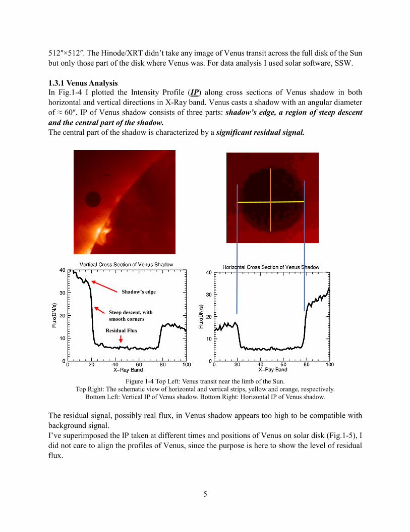
512ʺ×512ʺ. The Hinode/XRT didn’t take any image of Venus transit across the full disk of the Sun but only those part of the disk where Venus was. For data analysis I used solar software, SSW. 1.3.1 Venus Analysis In Fig.1-4 I plotted the Intensity Profile (IP) along cross sections of Venus shadow in both horizontal and vertical directions in X-Ray band. Venus casts a shadow with an angular diameter of ≈ 60ʺ. IP of Venus shadow consists of three parts: shadow’s edge, a region of steep descent

and the central part of the shadow. The central part of the shadow is characterized by a significant residual signal.

Figure 1-4 Top Left: Venus transit near the limb of the Sun.

Top Right: The schematic view of horizontal and vertical strips, yellow and orange, respectively. Bottom Left: Vertical IP of Venus shadow. Bottom Right: Horizontal IP of Venus shadow.

The residual signal, possibly real flux, in Venus shadow appears too high to be compatible with background signal. I’ve superimposed the IP taken at different times and positions of Venus on solar disk (Fig.1-5), I did not care to align the profiles of Venus, since the purpose is here to show the level of residual flux.

Steep descent, with smooth corners

Residual Flux

Shadow’s edge

6

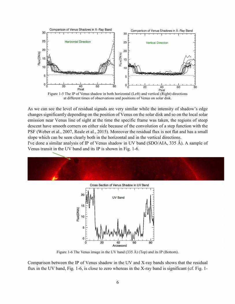
Figure 1-5 The IP of Venus shadow in both horizontal (Left) and vertical (Right) directions

at different times of observations and positions of Venus on solar disk.

As we can see the level of residual signals are very similar while the intensity of shadow’s edge changes significantly depending on the position of Venus on the solar disk and so on the local solar emission near Venus line of sight at the time the specific frame was taken, the regions of steep descent have smooth corners on either side because of the convolution of a step function with the PSF (Weber et al., 2007, Reale et al., 2015). Moreover the residual flux is not flat and has a small slope which can be seen clearly both in the horizontal and in the vertical directions. I've done a similar analysis of IP of Venus shadow in UV band (SDO/AIA, 335 Ǻ). A sample of Venus transit in the UV band and its IP is shown in Fig. 1-6.

Figure 1-6 The Venus image in the UV band (335 Ǻ) (Top) and its IP (Bottom).

Comparison between the IP of Venus shadow in the UV and X-ray bands shows that the residual flux in the UV band, Fig. 1-6, is close to zero whereas in the X-ray band is significant (cf. Fig. 1-

7

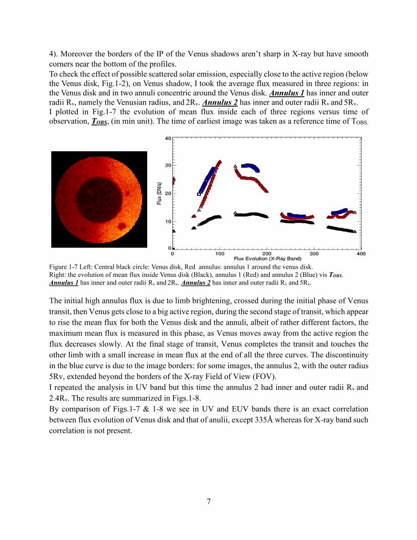
4). Moreover the borders of the IP of the Venus shadows aren’t sharp in X-ray but have smooth corners near the bottom of the profiles. To check the effect of possible scattered solar emission, especially close to the active region (below the Venus disk, Fig.1-2), on Venus shadow, I took the average flux measured in three regions: in the Venus disk and in two annuli concentric around the Venus disk. Annulus 1 has inner and outer radii Rv, namely the Venusian radius, and 2Rv. Annulus 2 has inner and outer radii Rv and 5Rv. I plotted in Fig.1-7 the evolution of mean flux inside each of three regions versus time of observation, TOBS, (in min unit). The time of earliest image was taken as a reference time of TOBS.

Figure 1-7 Left: Central black circle: Venus disk, Red annulus: annulus 1 around the venus disk.

Right: the evolution of mean flux inside Venus disk (Black), annulus 1 (Red) and annulus 2 (Blue) vis TOBS. Annulus 1 has inner and outer radii Rv and 2Rv. Annulus 2 has inner and outer radii Rv and 5Rv.

The initial high annulus flux is due to limb brightening, crossed during the initial phase of Venus

transit, then Venus gets close to a big active region, during the second stage of transit, which appear

to rise the mean flux for both the Venus disk and the annuli, albeit of rather different factors, the

maximum mean flux is measured in this phase, as Venus moves away from the active region the

flux decreases slowly. At the final stage of transit, Venus completes the transit and touches the

other limb with a small increase in mean flux at the end of all the three curves. The discontinuity

in the blue curve is due to the image borders: for some images, the annulus 2, with the outer radius

5Rv, extended beyond the borders of the X-ray Field of View (FOV).

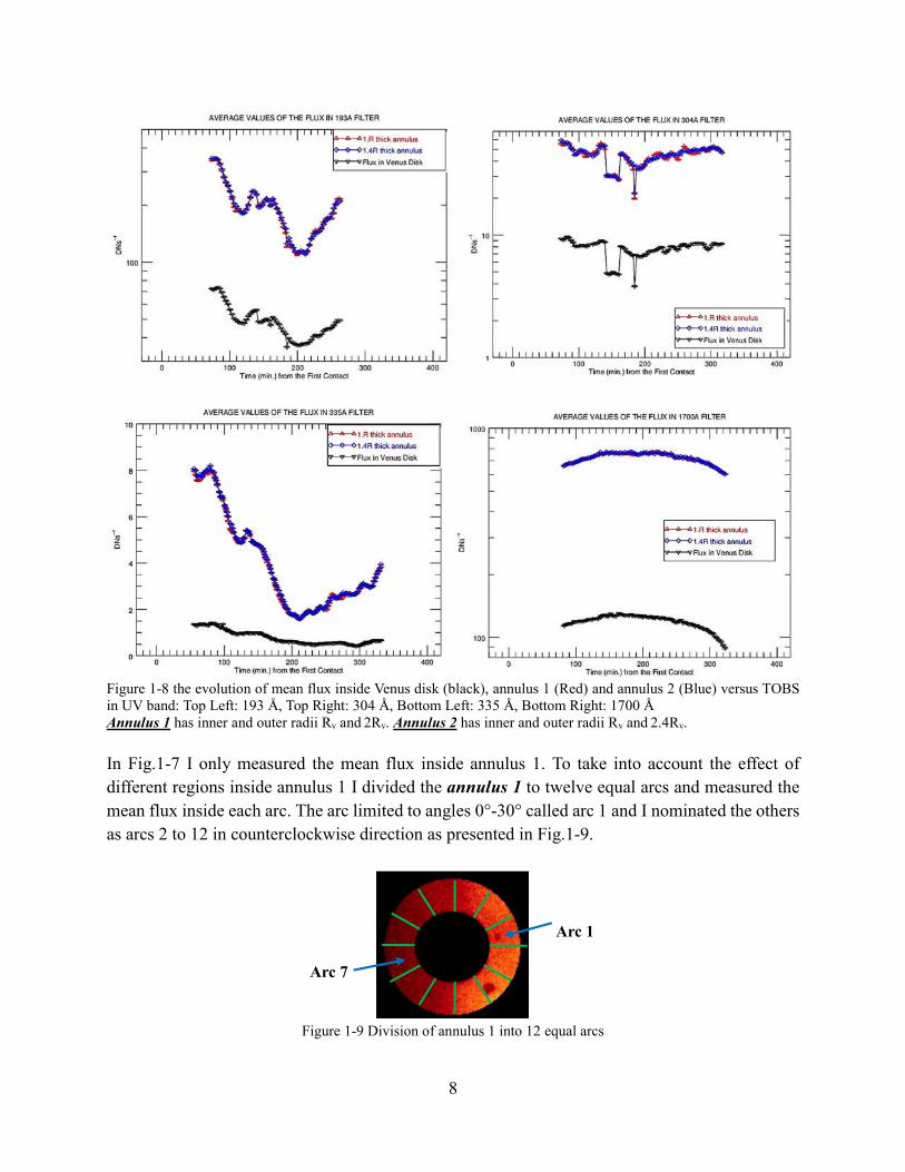
I repeated the analysis in UV band but this time the annulus 2 had inner and outer radii Rv and

2.4Rv. The results are summarized in Figs.1-8.

By comparison of Figs.1-7 & 1-8 we see in UV and EUV bands there is an exact correlation

between flux evolution of Venus disk and that of anulii, except 335Å whereas for X-ray band such

correlation is not present.

8

Figure 1-8 the evolution of mean flux inside Venus disk (black), annulus 1 (Red) and annulus 2 (Blue) versus TOBS in UV band: Top Left: 193 Å, Top Right: 304 Å, Bottom Left: 335 Å, Bottom Right: 1700 Å Annulus 1 has inner and outer radii Rv and 2Rv. Annulus 2 has inner and outer radii Rv and 2.4Rv.

In Fig.1-7 I only measured the mean flux inside annulus 1. To take into account the effect of

different regions inside annulus 1 I divided the annulus 1 to twelve equal arcs and measured the

mean flux inside each arc. The arc limited to angles 0°-30° called arc 1 and I nominated the others

as arcs 2 to 12 in counterclockwise direction as presented in Fig.1-9.

Figure 1-9 Division of annulus 1 into 12 equal arcs

Arc 1

Arc 7

9

Since the arcs in front of each other represent a unique direction I chose arcs 1-7 together, arcs 2-8 together till arcs 6-12. In Fig.1-10 I plotted the flux evolution inside each of these pairs versus TOBS and compared them with the mean flux of annulus 1 (whole ring around Venus) as reference.

Figure 1-10 Top Left: flux evolution inside arc1 (black) and arc7 (red) and annulus 1 (blue) in X-Ray band. Top Right: flux evolution inside arc2 (black) and arc8 (red) and annulus 1 (blue) in X-Ray band. Middle Left: flux evolution inside arc3 (black) and arc8 (red) and annulus 1 (blue) in X-Ray band. Middle Left: flux evolution inside arc4 (black) and arc10 (red) and annulus 1 (blue) in X-Ray band. Bottom Left: flux evolution inside arc5 (black) and arc11 (red) and annulus 1 (blue) in X-Ray band. Bottom Left: flux evolution inside arc6 (black) and arc12 (red) and anuulus 1 (blue) in X-Ray band.

10

The advantage of this method is that the effect of active region is seen clearly inside a narrow

region (arc) and can be compared with other regions of annulus 1. As we can see the flux evolution

of southeastern arcs, i.e. arcs 9-10-11-12 are significantly higher than others. Reversely the flux

evolution of northwestern arcs, i.e. arcs 4-5-6 are significantly lower than others. I subtracted the

flux inside each pairs, i.e. (flux 7-flux 1) and so on, and plotted the net flux versus TOBS as

presented in Fig.1-11.

Figure 1-11 subtraction of flux inside arc 7 and arc 1in X-Ray band. Top Left: subtraction of flux inside arc 8 and arc 2 in X-Ray band.

Top Right: subtraction of flux inside arc 9 and arc 3 in X-Ray band. Middle Left: subtraction of flux inside arc 10 and arc 4 in X-Ray band. Middle Left: subtraction of flux inside arc 11 and arc 5 in X-Ray band. Bottom Left: subtraction of flux inside arc 12 and arc 6 in X-Ray band.

11

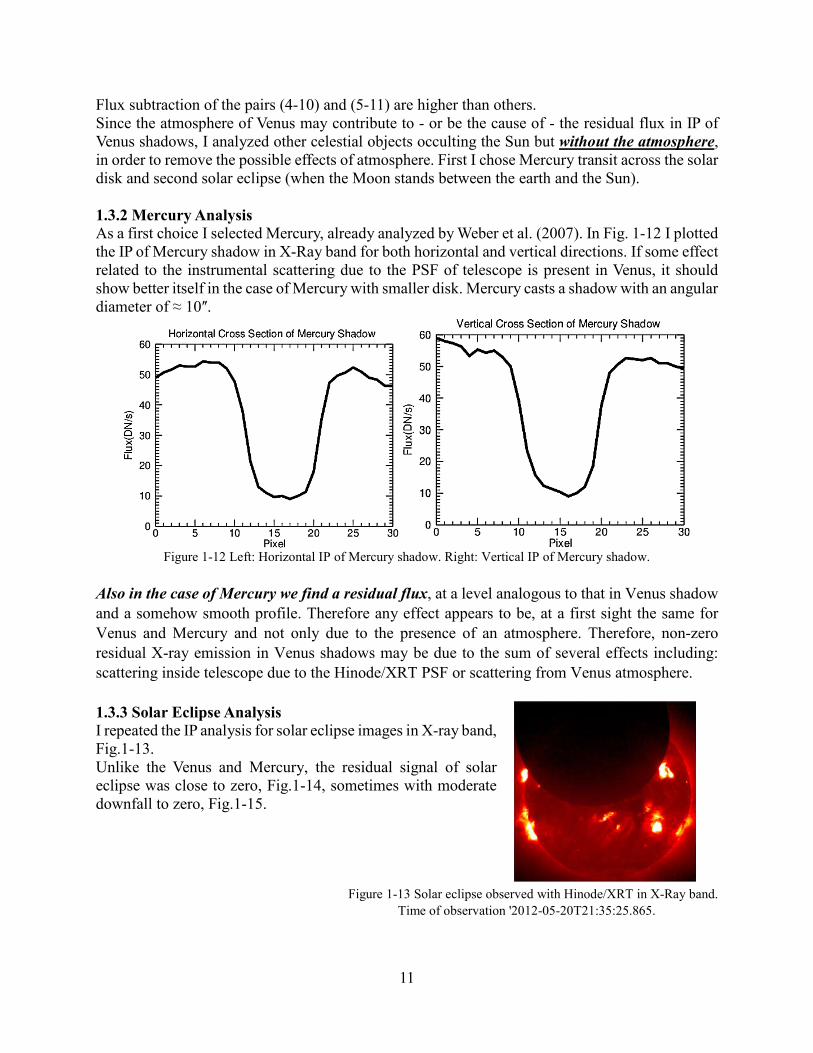
Flux subtraction of the pairs (4-10) and (5-11) are higher than others. Since the atmosphere of Venus may contribute to - or be the cause of - the residual flux in IP of Venus shadows, I analyzed other celestial objects occulting the Sun but without the atmosphere, in order to remove the possible effects of atmosphere. First I chose Mercury transit across the solar disk and second solar eclipse (when the Moon stands between the earth and the Sun). 1.3.2 Mercury Analysis As a first choice I selected Mercury, already analyzed by Weber et al. (2007). In Fig. 1-12 I plotted the IP of Mercury shadow in X-Ray band for both horizontal and vertical directions. If some effect related to the instrumental scattering due to the PSF of telescope is present in Venus, it should show better itself in the case of Mercury with smaller disk. Mercury casts a shadow with an angular diameter of ≈ 10ʺ.

Figure 1-12 Left: Horizontal IP of Mercury shadow. Right: Vertical IP of Mercury shadow.

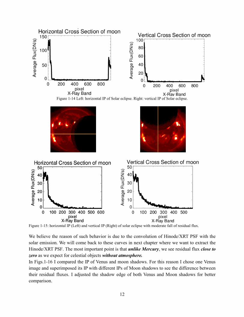
Also in the case of Mercury we find a residual flux, at a level analogous to that in Venus shadow and a somehow smooth profile. Therefore any effect appears to be, at a first sight the same for Venus and Mercury and not only due to the presence of an atmosphere. Therefore, non-zero residual X-ray emission in Venus shadows may be due to the sum of several effects including: scattering inside telescope due to the Hinode/XRT PSF or scattering from Venus atmosphere. 1.3.3 Solar Eclipse Analysis I repeated the IP analysis for solar eclipse images in X-ray band, Fig.1-13. Unlike the Venus and Mercury, the residual signal of solar eclipse was close to zero, Fig.1-14, sometimes with moderate downfall to zero, Fig.1-15.

Figure 1-13 Solar eclipse observed with Hinode/XRT in X-Ray band.

Time of observation '2012-05-20T21:35:25.865.

12

Figure 1-14 Left: horizontal IP of Solar eclipse. Right: vertical IP of Solar eclipse.

Figure 1-15: horizontal IP (Left) and vertical IP (Right) of solar eclipse with moderate fall of residual flux.

We believe the reason of such behavior is due to the convolution of Hinode/XRT PSF with the

solar emission. We will come back to these curves in next chapter where we want to extract the

Hinode/XRT PSF. The most important point is that unlike Mercury, we see residual flux close to

zero as we expect for celestial objects without atmosphere.

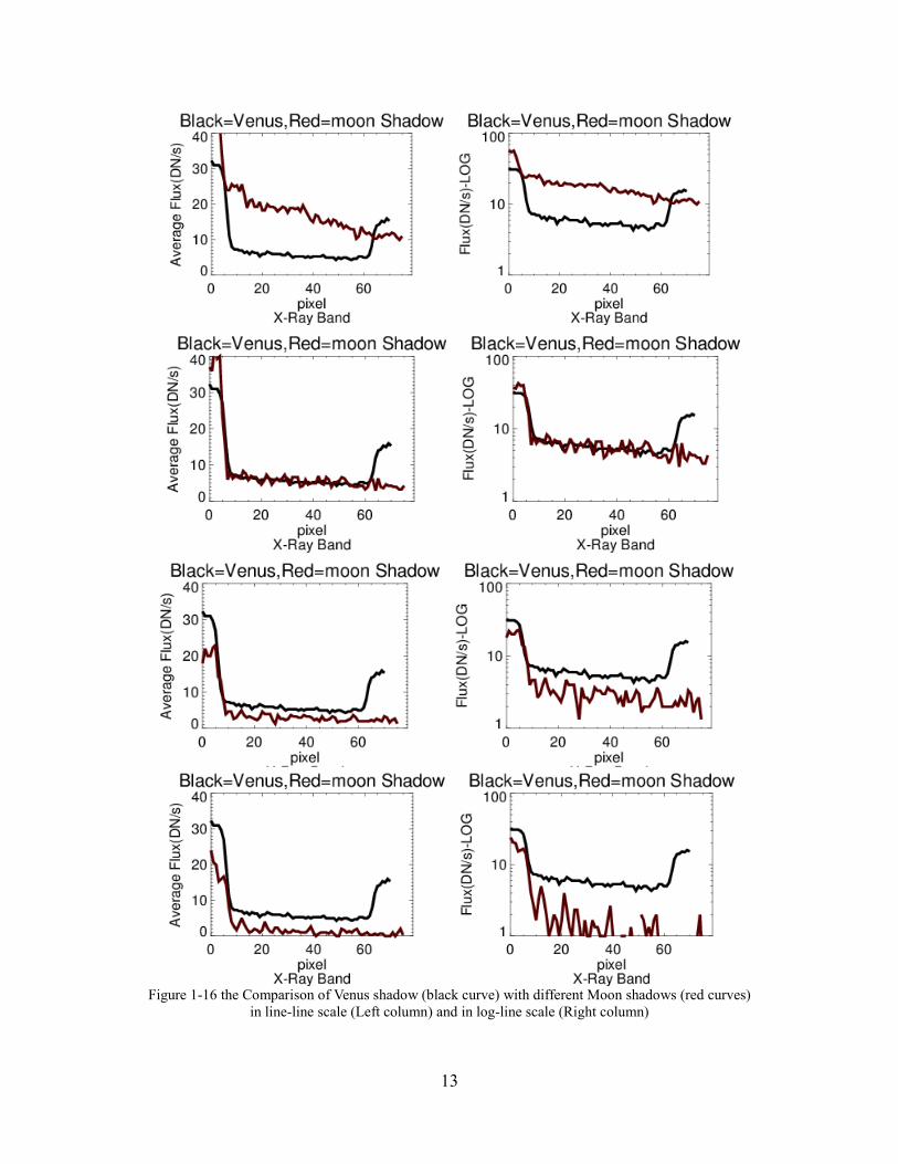
In Figs.1-16 I compared the IP of Venus and moon shadows. For this reason I chose one Venus

image and superimposed its IP with different IPs of Moon shadows to see the difference between

their residual fluxes. I adjusted the shadow edge of both Venus and Moon shadows for better

comparison.

13

Figure 1-16 the Comparison of Venus shadow (black curve) with different Moon shadows (red curves)

in line-line scale (Left column) and in log-line scale (Right column)

14

Depend to moon shadows images, the central part of IPs sometimes are higher than Venus one and

sometimes lower than Venus one. Moreover the downfall rate of IPs in moon shadows sometimes

is very high and sometimes is moderate.

To check the zero flux, seen in moon IP, I selected two squares in dark regions of moon images

and measured the mean flux inside each to consider them as a reference flux since in dark regions

there is no emission except some noise. In Fig.1-17 the position of each square and the mean flux

inside each of which is presented for different images.

Figure 1-17 left: solar eclipse image in X-Ray band with two squares at the top left and bottom left corners. Middle: average flux inside the square at the top left corner of images.

Right: average flux inside the square at the bottom left corner of images.

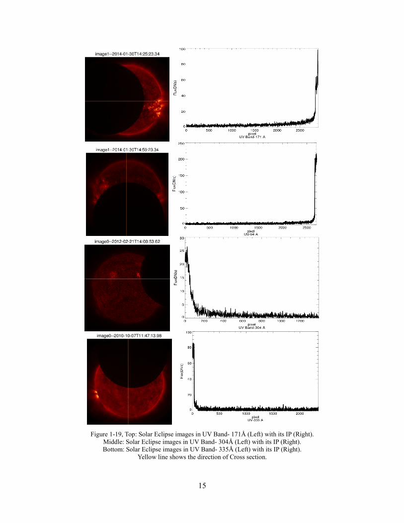
As we can see the maximum value of mean flux in dark regions is close to 4 so we can consider residual flux close to 4 as flux level. In the series of analysis I studied solar eclipse images in UV bands taken with SDO/AIA. In this case, datasets have different UV bands and had been taken in different periods: The first dataset was in 335Å band and observed in 2010, the second one was in 304Å and observed in 2012 and the third one was in 171Å and observed in 2014.

Figure 1-18 Left: Solar Eclipse in UV Band- 171Å- SDO/AIA, TOBS '2014-01-30T14:25:23.34.

Middle: Solar Eclipse in UV Band- 304Å- SDO/AIA, TOBS '2012-02-21T14:00:53.62. Right: Solar Eclipse in UV Band- 335Å- SDO/AIA, TOBS '2010-10-07T11:47:37.41.

I repeated the IP analysis, Fig.1-19, and observed a residual flux close to zero, except some noise, with sharp vertical line for different UV bands and with different TOBS.

15

Figure 1-19, Top: Solar Eclipse images in UV Band- 171Å (Left) with its IP (Right). Middle: Solar Eclipse images in UV Band- 304Å (Left) with its IP (Right). Bottom: Solar Eclipse images in UV Band- 335Å (Left) with its IP (Right).

Yellow line shows the direction of Cross section.

16

Deconvolution

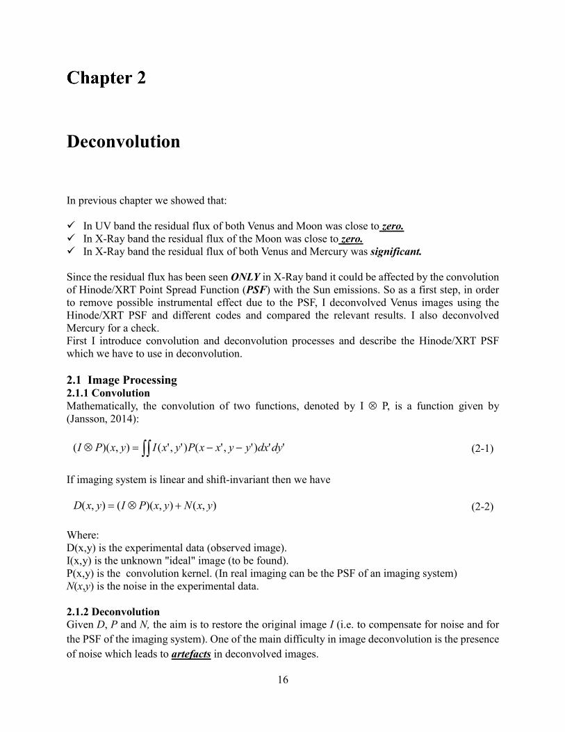
In previous chapter we showed that: In UV band the residual flux of both Venus and Moon was close to zero. In X-Ray band the residual flux of the Moon was close to zero. In X-Ray band the residual flux of both Venus and Mercury was significant. Since the residual flux has been seen ONLY in X-Ray band it could be affected by the convolution of Hinode/XRT Point Spread Function (PSF) with the Sun emissions. So as a first step, in order to remove possible instrumental effect due to the PSF, I deconvolved Venus images using the Hinode/XRT PSF and different codes and compared the relevant results. I also deconvolved Mercury for a check. First I introduce convolution and deconvolution processes and describe the Hinode/XRT PSF which we have to use in deconvolution.

2.1 Image Processing 2.1.1 Convolution Mathematically, the convolution of two functions, denoted by I P, is a function given by (Jansson, 2014):

'')','()','(),)(( dydxyyxxPyxIyxPI (2-1)

If imaging system is linear and shift-invariant then we have

),(),)((),( yxNyxPIyxD (2-2)

Where: D(x,y) is the experimental data (observed image). I(x,y) is the unknown "ideal" image (to be found). P(x,y) is the convolution kernel. (In real imaging can be the PSF of an imaging system) N(x,y) is the noise in the experimental data. 2.1.2 Deconvolution Given D, P and N, the aim is to restore the original image I (i.e. to compensate for noise and for

the PSF of the imaging system). One of the main difficulty in image deconvolution is the presence

of noise which leads to artefacts in deconvolved images.

17

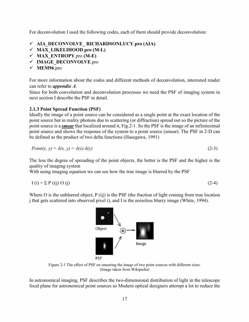
For deconvolution I used the following codes, each of them should provide deconvolution: AIA_DECONVOLVE_ RICHARDSONLUCY.pro (AIA) MAX_LIKELIHOOD.pro (M-L) MAX_ENTROPY.pro (M-E) IMAGE_DECONVOLVE.pro MEM96.pro For more information about the codes and different methods of deconvolution, interested reader can refer to appendix A. Since for both convolution and deconvolution processes we need the PSF of imaging system in next section I describe the PSF in detail. 2.1.3 Point Spread Function (PSF) Ideally the image of a point source can be considered as a single point at the exact location of the point source but in reality photons due to scattering (or diffraction) spread out so the picture of the point source is a smear that localized around it, Fig.2-1. So the PSF is the image of an infinitesimal point source and shows the response of the system to a point source (smear). The PSF in 2-D can be defined as the product of two delta functions (Hasegawa, 1991) Point(x, y) = δ(x, y) = δ(x) δ(y) (2-3)

The less the degree of spreading of the point objects, the better is the PSF and the higher is the quality of imaging system With using imaging equation we can see how the true image is blurred by the PSF I (i) = Σ P (i|j) O (j) (2-4)

Where O is the unblurred object, P (i|j) is the PSF (the fraction of light coming from true location j that gets scattered into observed pixel i), and I is the noiseless blurry image (White, 1994).

Figure 2-1 The effect of PSF on smearing the image of two point sources with different sizes.

(Image taken from Wikipedia)

In astronomical imaging, PSF describes the two-dimensional distribution of light in the telescope focal plane for astronomical point sources so Modern optical designers attempt a lot to reduce the

18

size of the PSF for large telescopes.

2.2 Hinode/XRT PSF As discussed in appendix B, solar eclipse analysis near active region can be used to determine the PSF format. The second version of Hinode /XRT PSF has been recently derived by P. R. Jibben and L.Golub. They used solar eclipse and limb flare analysis to reconstruct the new version of Hinode /XRT PSF so that: 80% of the encircled energy is enclosed in 5ʺ diameter. The solar eclipse analysis shows that close to a bright active region (60ʺ to 200ʺ) the scattered

light falls off as r−4. (r is the radial distance from solar eclipse in arcseconds) The limb flare analysis show that far from the flare, the scattered light also falls off as r−4.

(r is the radial distance from flare in arcseconds) The r−4 wings provide 8% of encircled energy with less than 1% of that energy beyond 100 ʺ. The final form of the PSF is:

a

exp (- r2

σ2 )

γ2 + r2 if r ≤ 3.4176

0.03

r if 3.4176 ≤ r ≤ 5

0.15

r2 if 5 ≤ r ≤ 11.1

(11.1)2 0.15

r4 if 11.1 ≤ r

Where r = radius in arc seconds, a = 1.31946, σ = 2.19256 and γ = 1.24891. In Fig.2-2 I’ve Compared the radial IP of the Moon with second version of Hinode/XRT PSF. The moon shadow profile is a 2D convolution of the solar corona at the moon border with the PSF while the PSF plot is just a cut across PSF in 1D given by the above analytical formula.

Figure 2-2 Comparison between Moon radial IP (Black) and new version of XRT PSF (Red).

19

With above codes and Hinode/XRT PSF I performed deconvolution of the images and compared the similarities and differences between the results. Then I repeated the cross section analysis for deconvolved images.

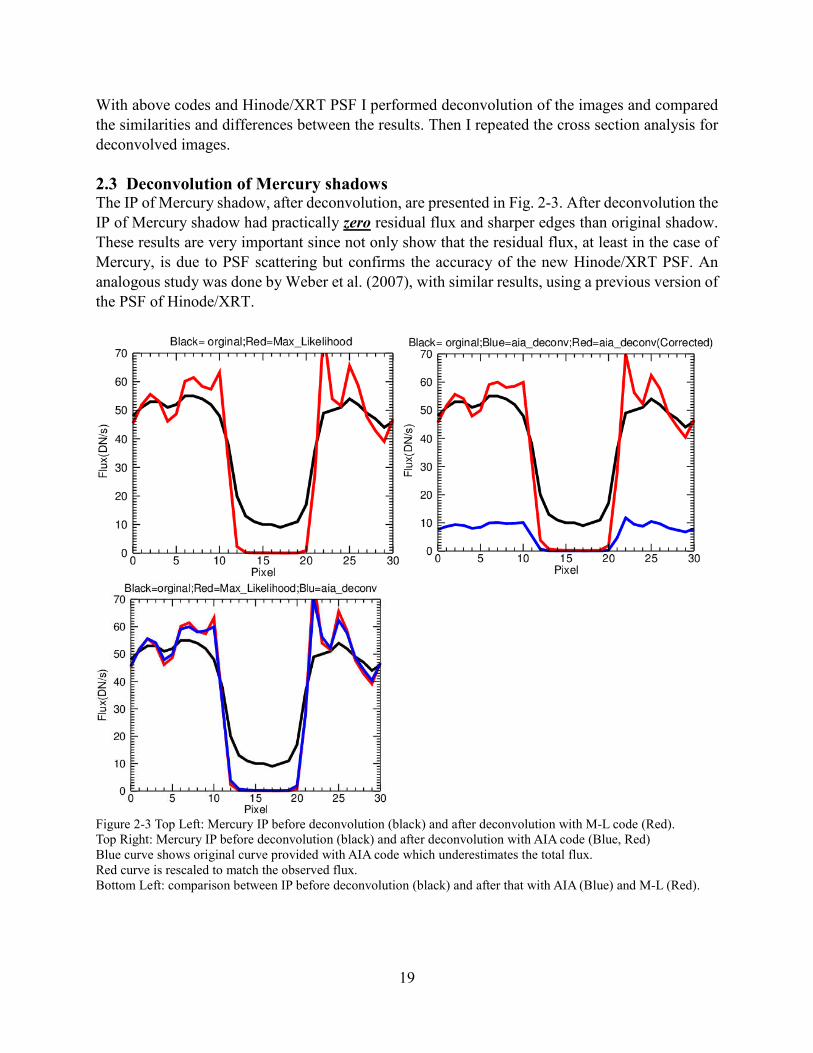
2.3 Deconvolution of Mercury shadows The IP of Mercury shadow, after deconvolution, are presented in Fig. 2-3. After deconvolution the IP of Mercury shadow had practically zero residual flux and sharper edges than original shadow. These results are very important since not only show that the residual flux, at least in the case of Mercury, is due to PSF scattering but confirms the accuracy of the new Hinode/XRT PSF. An analogous study was done by Weber et al. (2007), with similar results, using a previous version of the PSF of Hinode/XRT.

Figure 2-3 Top Left: Mercury IP before deconvolution (black) and after deconvolution with M-L code (Red). Top Right: Mercury IP before deconvolution (black) and after deconvolution with AIA code (Blue, Red) Blue curve shows original curve provided with AIA code which underestimates the total flux. Red curve is rescaled to match the observed flux. Bottom Left: comparison between IP before deconvolution (black) and after that with AIA (Blue) and M-L (Red).

20

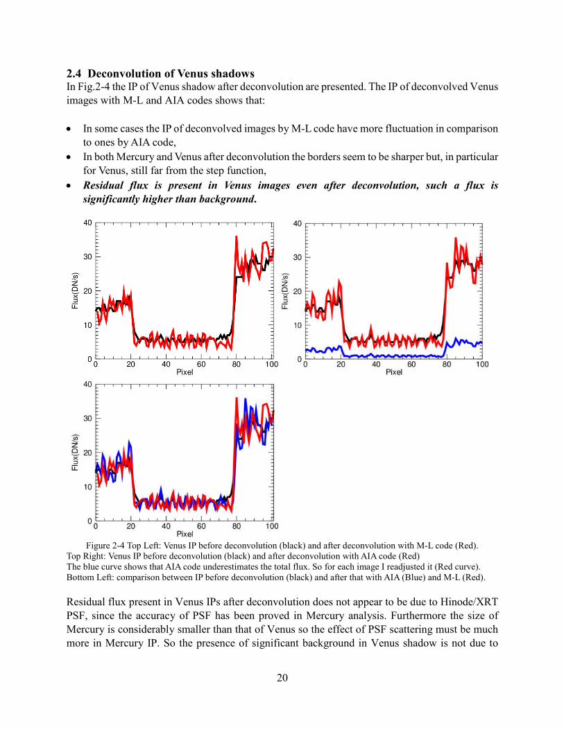
2.4 Deconvolution of Venus shadows In Fig.2-4 the IP of Venus shadow after deconvolution are presented. The IP of deconvolved Venus images with M-L and AIA codes shows that:

In some cases the IP of deconvolved images by M-L code have more fluctuation in comparison to ones by AIA code,

In both Mercury and Venus after deconvolution the borders seem to be sharper but, in particular for Venus, still far from the step function,

Residual flux is present in Venus images even after deconvolution, such a flux is significantly higher than background.

Figure 2-4 Top Left: Venus IP before deconvolution (black) and after deconvolution with M-L code (Red).

Top Right: Venus IP before deconvolution (black) and after deconvolution with AIA code (Red) The blue curve shows that AIA code underestimates the total flux. So for each image I readjusted it (Red curve). Bottom Left: comparison between IP before deconvolution (black) and after that with AIA (Blue) and M-L (Red).

Residual flux present in Venus IPs after deconvolution does not appear to be due to Hinode/XRT PSF, since the accuracy of PSF has been proved in Mercury analysis. Furthermore the size of Mercury is considerably smaller than that of Venus so the effect of PSF scattering must be much more in Mercury IP. So the presence of significant background in Venus shadow is not due to

21

instrumental scattering but should be related to Venus, for instance it could originate from some effect occurring in Venus’ atmosphere. Comprehensive analysis of deconvolution shows that: Only M-L and AIA codes could rectify and deliver images while other codes failed to converge

and deliver images. AIA code doesn’t conserve the total flux yielding curves with ≈15 % of total flux. So for each

image I readjusted the amplitude, Figs.2-3, 2-4. Deconvolution causes artefacts and spurious "sources" at the edge (borders), common problem

in deconvolution (due to the noise), which in the case of Venus are completely clear but don’t affect the evaluation of the average fluxes in the shadow, Fig.2-4.

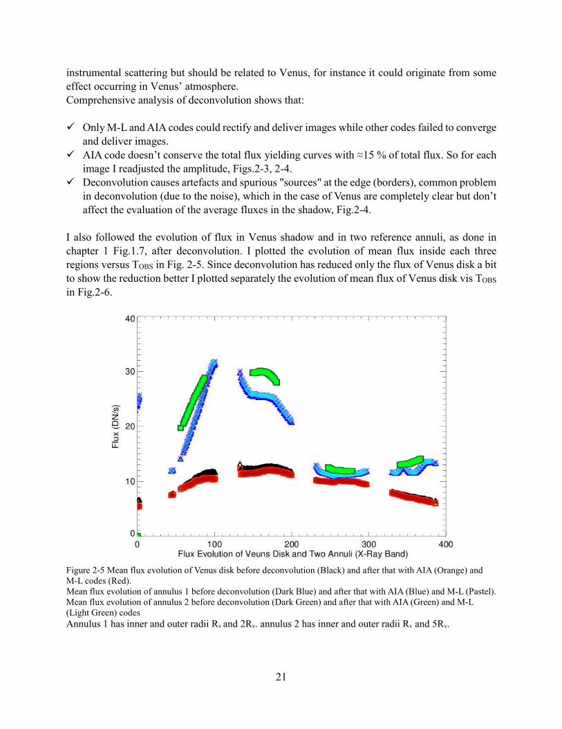
I also followed the evolution of flux in Venus shadow and in two reference annuli, as done in chapter 1 Fig.1.7, after deconvolution. I plotted the evolution of mean flux inside each three regions versus TOBS in Fig. 2-5. Since deconvolution has reduced only the flux of Venus disk a bit to show the reduction better I plotted separately the evolution of mean flux of Venus disk vis TOBS

in Fig.2-6.

Figure 2-5 Mean flux evolution of Venus disk before deconvolution (Black) and after that with AIA (Orange) and M-L codes (Red). Mean flux evolution of annulus 1 before deconvolution (Dark Blue) and after that with AIA (Blue) and M-L (Pastel). Mean flux evolution of annulus 2 before deconvolution (Dark Green) and after that with AIA (Green) and M-L (Light Green) codes

Annulus 1 has inner and outer radii Rv and 2Rv. annulus 2 has inner and outer radii Rv and 5Rv.

22

Figure 2-6 Black: Evolution of mean flux inside Venus disk before deconvolution. Blue: Evolution of mean flux inside Venus disk after deconvolution with AIA code. Red: Evolution of mean flux inside Venus disk after deconvolution with M-L code

The most important points in Figs. 2-5, 2-6 are:

The amount of mean flux inside Venus disk after deconvolution has decreased especially close to active region, therefore deconvolution appears to have removed the high scattering from the active region (Fig. 2-6),

Mean flux inside the two annuli haven’t changed even after deconvolution (Figs. 2-5, 2-6),

we see the flux inside Venus disk and that inside the two annuli gradually rise as Venus gets more and more inside the solar disk and decrease thereafter (Fig. 2-5), however the flux inside Venus disk is not correlated to the others,

Although deconvolution has decreased the intensity, especially when Venus is near the active region, the maximum flux is still measured there, so there may be some relationship between the observed residual flux and the high surrounding flux due to the active region (Fig. 2-5),

Mean flux value for both AIA and M-L deconvolution codes are virtually the same in spite of profiles of deconvolved images which do not seem to be the same.

23

Light Leak Contamination

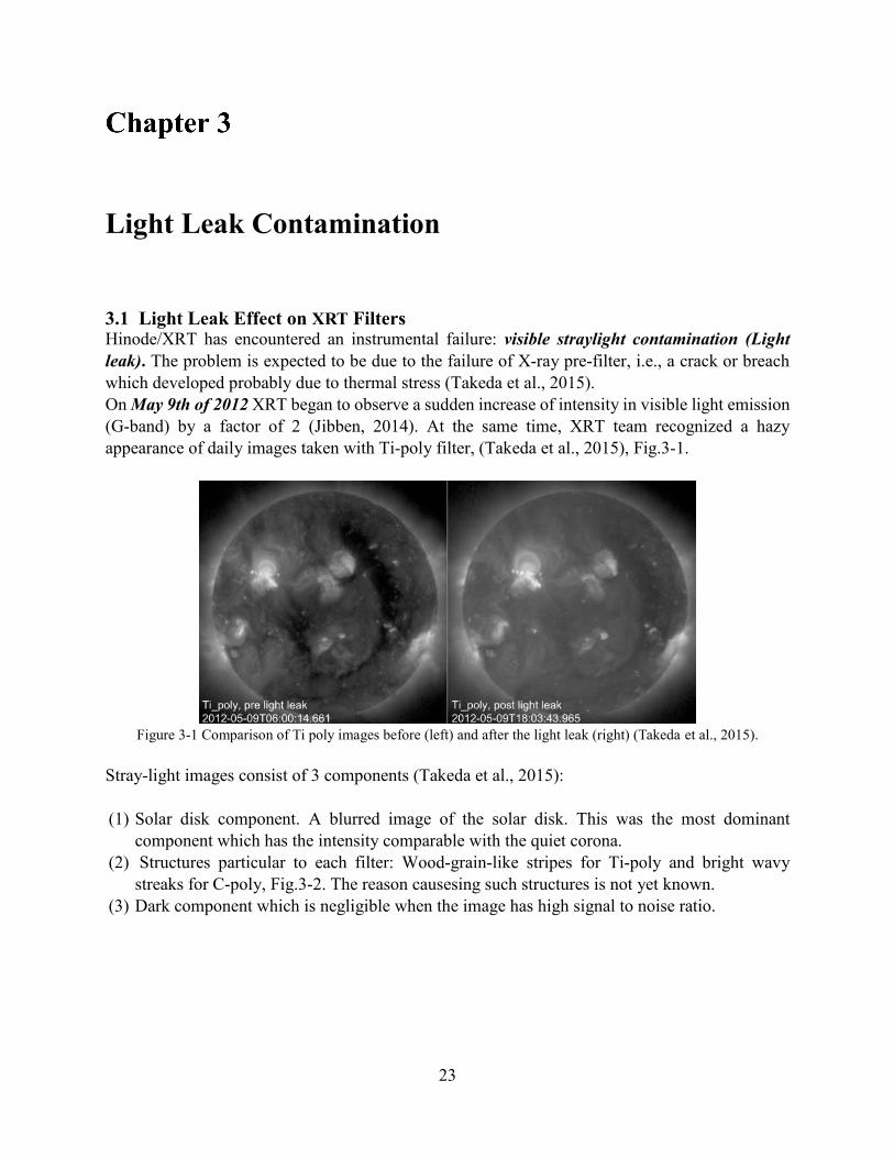
3.1 Light Leak Effect on XRT Filters Hinode/XRT has encountered an instrumental failure: visible straylight contamination (Light leak). The problem is expected to be due to the failure of X-ray pre-filter, i.e., a crack or breach which developed probably due to thermal stress (Takeda et al., 2015). On May 9th of 2012 XRT began to observe a sudden increase of intensity in visible light emission (G-band) by a factor of 2 (Jibben, 2014). At the same time, XRT team recognized a hazy appearance of daily images taken with Ti-poly filter, (Takeda et al., 2015), Fig.3-1.

Figure 3-1 Comparison of Ti poly images before (left) and after the light leak (right) (Takeda et al., 2015).

Stray-light images consist of 3 components (Takeda et al., 2015): (1) Solar disk component. A blurred image of the solar disk. This was the most dominant

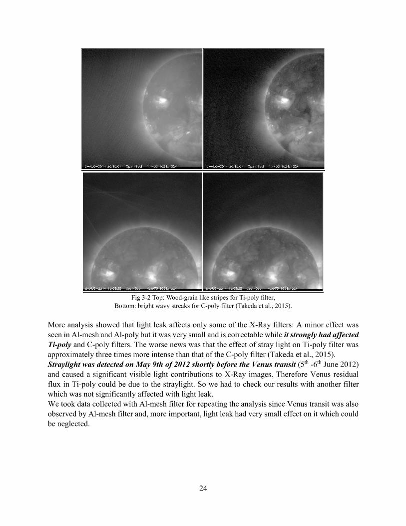
component which has the intensity comparable with the quiet corona. (2) Structures particular to each filter: Wood-grain-like stripes for Ti-poly and bright wavy

streaks for C-poly, Fig.3-2. The reason causesing such structures is not yet known. (3) Dark component which is negligible when the image has high signal to noise ratio.

24

Fig 3-2 Top: Wood-grain like stripes for Ti-poly filter,

Bottom: bright wavy streaks for C-poly filter (Takeda et al., 2015).

More analysis showed that light leak affects only some of the X-Ray filters: A minor effect was seen in Al-mesh and Al-poly but it was very small and is correctable while it strongly had affected Ti-poly and C-poly filters. The worse news was that the effect of stray light on Ti-poly filter was approximately three times more intense than that of the C-poly filter (Takeda et al., 2015). Straylight was detected on May 9th of 2012 shortly before the Venus transit (5th -6th June 2012) and caused a significant visible light contributions to X-Ray images. Therefore Venus residual flux in Ti-poly could be due to the straylight. So we had to check our results with another filter which was not significantly affected with light leak. We took data collected with Al-mesh filter for repeating the analysis since Venus transit was also observed by Al-mesh filter and, more important, light leak had very small effect on it which could be neglected.

25

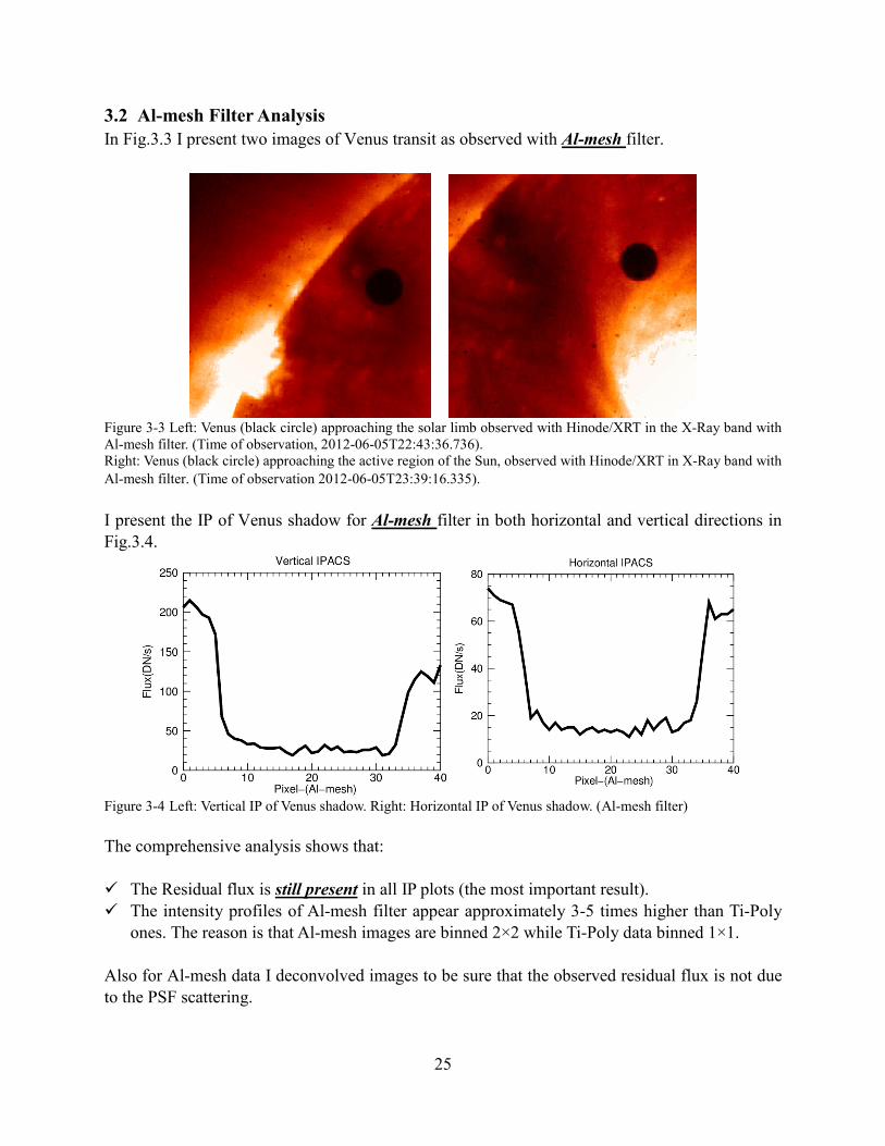
3.2 Al-mesh Filter Analysis In Fig.3.3 I present two images of Venus transit as observed with Al-mesh filter.

Figure 3-3 Left: Venus (black circle) approaching the solar limb observed with Hinode/XRT in the X-Ray band with Al-mesh filter. (Time of observation, 2012-06-05T22:43:36.736). Right: Venus (black circle) approaching the active region of the Sun, observed with Hinode/XRT in X-Ray band with

Al-mesh filter. (Time of observation 2012-06-05T23:39:16.335).

I present the IP of Venus shadow for Al-mesh filter in both horizontal and vertical directions in Fig.3.4.

Figure 3-4 Left: Vertical IP of Venus shadow. Right: Horizontal IP of Venus shadow. (Al-mesh filter) The comprehensive analysis shows that: The Residual flux is still present in all IP plots (the most important result). The intensity profiles of Al-mesh filter appear approximately 3-5 times higher than Ti-Poly

ones. The reason is that Al-mesh images are binned 2×2 while Ti-Poly data binned 1×1.

Also for Al-mesh data I deconvolved images to be sure that the observed residual flux is not due to the PSF scattering.

26

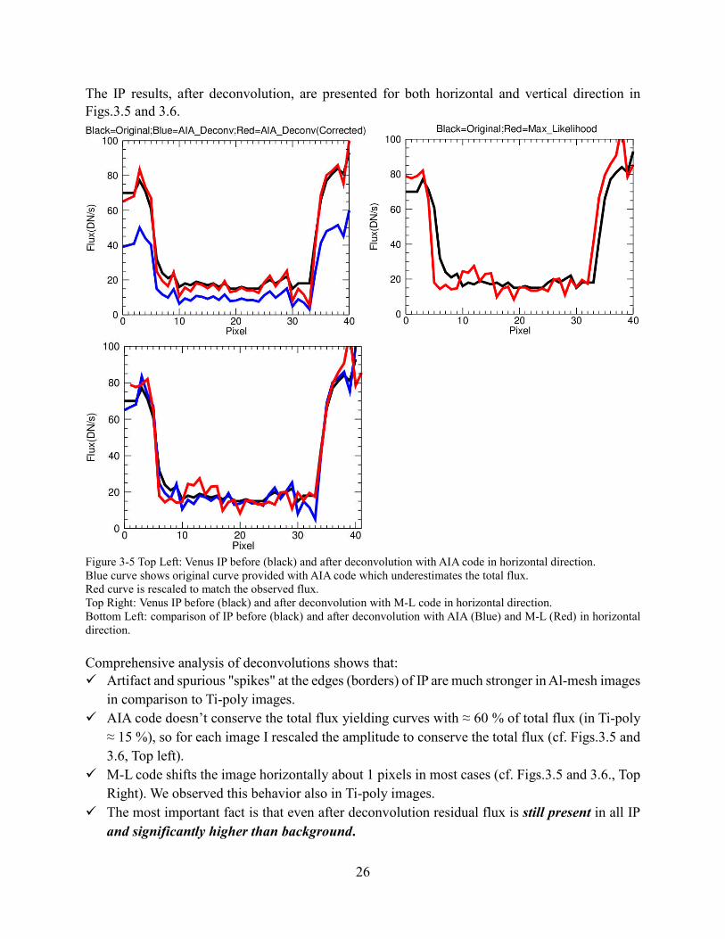
The IP results, after deconvolution, are presented for both horizontal and vertical direction in Figs.3.5 and 3.6.

Figure 3-5 Top Left: Venus IP before (black) and after deconvolution with AIA code in horizontal direction. Blue curve shows original curve provided with AIA code which underestimates the total flux. Red curve is rescaled to match the observed flux. Top Right: Venus IP before (black) and after deconvolution with M-L code in horizontal direction. Bottom Left: comparison of IP before (black) and after deconvolution with AIA (Blue) and M-L (Red) in horizontal direction.

Comprehensive analysis of deconvolutions shows that: Artifact and spurious "spikes" at the edges (borders) of IP are much stronger in Al-mesh images

in comparison to Ti-poly images.

AIA code doesn’t conserve the total flux yielding curves with ≈ 60 % of total flux (in Ti-poly

≈ 15 %), so for each image I rescaled the amplitude to conserve the total flux (cf. Figs.3.5 and

3.6, Top left).

M-L code shifts the image horizontally about 1 pixels in most cases (cf. Figs.3.5 and 3.6., Top

Right). We observed this behavior also in Ti-poly images.

The most important fact is that even after deconvolution residual flux is still present in all IP

and significantly higher than background.

27

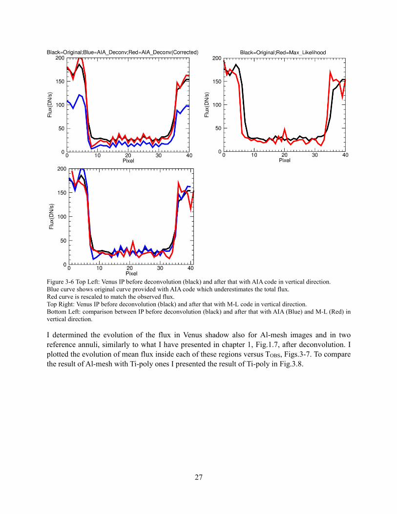
Figure 3-6 Top Left: Venus IP before deconvolution (black) and after that with AIA code in vertical direction. Blue curve shows original curve provided with AIA code which underestimates the total flux. Red curve is rescaled to match the observed flux. Top Right: Venus IP before deconvolution (black) and after that with M-L code in vertical direction. Bottom Left: comparison between IP before deconvolution (black) and after that with AIA (Blue) and M-L (Red) in vertical direction.

I determined the evolution of the flux in Venus shadow also for Al-mesh images and in two reference annuli, similarly to what I have presented in chapter 1, Fig.1.7, after deconvolution. I plotted the evolution of mean flux inside each of these regions versus TOBS, Figs.3-7. To compare the result of Al-mesh with Ti-poly ones I presented the result of Ti-poly in Fig.3.8.

28

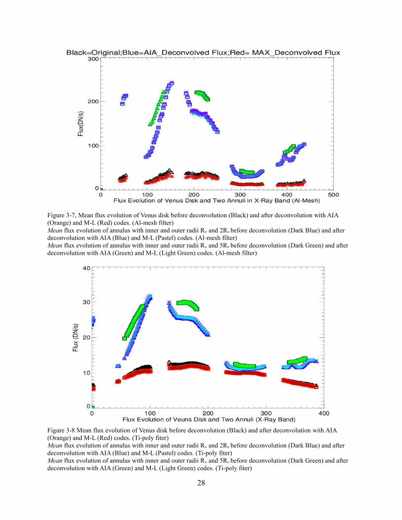
Figure 3-7, Mean flux evolution of Venus disk before deconvolution (Black) and after deconvolution with AIA (Orange) and M-L (Red) codes. (Al-mesh filter) Mean flux evolution of annulus with inner and outer radii Rv and 2Rv before deconvolution (Dark Blue) and after deconvolution with AIA (Blue) and M-L (Pastel) codes. (Al-mesh filter) Mean flux evolution of annulus with inner and outer radii Rv and 5Rv before deconvolution (Dark Green) and after deconvolution with AIA (Green) and M-L (Light Green) codes. (Al-mesh filter)

Figure 3-8 Mean flux evolution of Venus disk before deconvolution (Black) and after deconvolution with AIA (Orange) and M-L (Red) codes. (Ti-poly fiter) Mean flux evolution of annulus with inner and outer radii Rv and 2Rv before deconvolution (Dark Blue) and after deconvolution with AIA (Blue) and M-L (Pastel) codes. (Ti-poly fiter) Mean flux evolution of annulus with inner and outer radii Rv and 5Rv before deconvolution (Dark Green) and after deconvolution with AIA (Green) and M-L (Light Green) codes. (Ti-poly fiter)

29

In order to show the lower flux in the Venus shadow after deconvolution I plotted only the evolution of mean flux of Venus disk versus TOBS in Fig.3.9.

Figure 3-9, Black: Evolution of mean flux inside Venus disk before deconvolution. Blue: Evolution of mean flux inside Venus disk after deconvolution with AIA code. Red: Evolution of mean flux inside Venus disk after deconvolution with M-L code.

The ratio of the maximum value of flux inside annulus 1 to the lowest one for Ti-poly data is about 7.8 while for Al-mesh data this ratio is about 3.5 approximately. The ratio is different because: Light leak effect is very small in the case of Al-mesh. The intensity profiles of Al-mesh IP are approximately 3-5 times higher than Ti-Poly ones,

since Al-mesh images are binned 2×2 while Ti-Poly data binned 1×1. According to these results we can say with more certainty that: To check the level of noise in our data I used solar eclipse observed with Hinode/XR, Ti-poly filter, in 21 Feb 2012. The noise level in all cases was less than 4 DN/s, Fig.1.17. This result is very important since it implies that the observed results are not noise and, more important, that the

residual flux is still present and should not be due to the PSF scattering or light leak. So it may originates from Venus or the Venus atmosphere.

30

X-Ray Emission From Venus

Since we are sure that the residual flux is not due to the PSF scattering and it may come from the atmosphere of Venus I present some possible X-Ray production mechanisms.

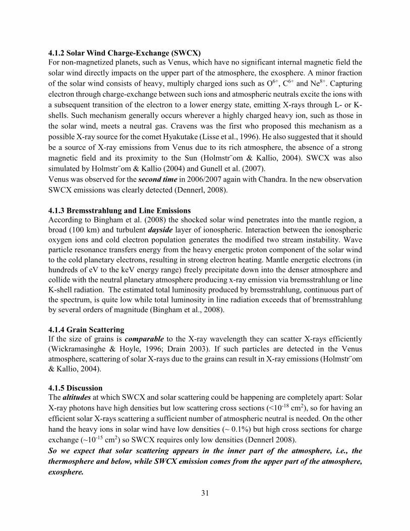
4.1 X-RAY PRODUCTION MECHANISMS Since Venus is not a source of X-ray emission all proposed mechanisms should find a connection between the Sun as X-ray star and the X-ray emission from Venus, most likely as the effect of the interaction of solar wind and solar X-rays with the atmospheric neutrals of Venus. The atmosphere of Venus consists of Carbon dioxide (CO2, 96.5 %) and nitrogen (N2, 3.5%) which already represent more than 99.9% of the composition. Recent analysis show new minor molecular constituents such as H2, O2, Kr, H2O, H2S and COS (Be´zard et al., 2007). In the following the general mechanisms of X-ray emission are introduced and relative importance of each is discussed: 4.1.1 Solar Scattering: Fluorescence Emission and Elastic Scattering of Solar X-rays Solar X-ray photons can be elastically scattered by atmospheric neutrals or they can be absorbed by atmospheric neutrals and then re-emitted isotropically by fluorescence emission (Kα emission). According to the composition of Venus atmosphere the main species, below thermosphere, responsible of fluorescence emission are C, O and N which are in the form of CO2 and N2. In Table 4.1, the wavelengths of K-shell of related species is presented (Cravens & Maurellis 2001).

Table 4-1 Fluorescence emission and related wavelengths. (Cravens & Maurellis, 2001)

In January 2001 Venus was observed for the first time with Chandra X–ray telescope. Dennerl et.al. (2002) proposed that the fluorescent scattering of solar X–rays from the Venus atmosphere was the primary source of X–ray emission. Such a mechanism has also been predicted for X-ray emission from the atmosphere of Mars and Jupiter (Holmstr¨om & Kallio, 2004).

Species Wavelength (nm)

Elastically scattered 0.2-12

K-shell C 4.4

K-shell N 3.1

K-shell O 2.3

31

4.1.2 Solar Wind Charge-Exchange (SWCX) For non-magnetized planets, such as Venus, which have no significant internal magnetic field the

solar wind directly impacts on the upper part of the atmosphere, the exosphere. A minor fraction

of the solar wind consists of heavy, multiply charged ions such as O6+, C6+ and Ne8+. Capturing

electron through charge-exchange between such ions and atmospheric neutrals excite the ions with

a subsequent transition of the electron to a lower energy state, emitting X-rays through L- or K-

shells. Such mechanism generally occurs wherever a highly charged heavy ion, such as those in

the solar wind, meets a neutral gas. Cravens was the first who proposed this mechanism as a

possible X-ray source for the comet Hyakutake (Lisse et al., 1996). He also suggested that it should

be a source of X-ray emissions from Venus due to its rich atmosphere, the absence of a strong

magnetic field and its proximity to the Sun (Holmström & Kallio, 2004). SWCX was also

simulated by Holmström & Kallio (2004) and Gunell et al. (2007).

Venus was observed for the second time in 2006/2007 again with Chandra. In the new observation

SWCX emissions was clearly detected (Dennerl, 2008).

4.1.3 Bremsstrahlung and Line Emissions According to Bingham et al. (2008) the shocked solar wind penetrates into the mantle region, a broad (100 km) and turbulent dayside layer of ionospheric. Interaction between the ionospheric oxygen ions and cold electron population generates the modified two stream instability. Wave particle resonance transfers energy from the heavy energetic proton component of the solar wind to the cold planetary electrons, resulting in strong electron heating. Mantle energetic electrons (in hundreds of eV to the keV energy range) freely precipitate down into the denser atmosphere and collide with the neutral planetary atmosphere producing x-ray emission via bremsstrahlung or line K-shell radiation. The estimated total luminosity produced by bremsstrahlung, continuous part of the spectrum, is quite low while total luminosity in line radiation exceeds that of bremsstrahlung by several orders of magnitude (Bingham et al., 2008). 4.1.4 Grain Scattering If the size of grains is comparable to the X-ray wavelength they can scatter X-rays efficiently (Wickramasinghe & Hoyle, 1996; Drain 2003). If such particles are detected in the Venus atmosphere, scattering of solar X-rays due to the grains can result in X-ray emissions (Holmström & Kallio, 2004).

4.1.5 Discussion The altitudes at which SWCX and solar scattering could be happening are completely apart: Solar

X-ray photons have high densities but low scattering cross sections (˂10-18 cm2), so for having an

efficient solar X-rays scattering a sufficient number of atmospheric neutral is needed. On the other

hand the heavy ions in solar wind have low densities (~ 0.1%) but high cross sections for charge

exchange (~10-15 cm2) so SWCX requires only low densities (Dennerl 2008).

So we expect that solar scattering appears in the inner part of the atmosphere, i.e., the

thermosphere and below, while SWCX emission comes from the upper part of the atmosphere,

exosphere.

32

The high mass of Venus causes high gravitational field which condense the exosphere of Venus so exospheric radiation must occur very close to the limb, where the solar X-ray scattering also peaks there making it difficult to find the fainter SWCX mechanism (Dennerl, 2008).

4.2 Possible X-ray Mechanism for 2012 Venus transit First I have to mention some important differences between Venus observation in 2012 and those

in 2001, 2006/2007:

In previous observations Venus was observed from side-view i.e. at the same time the nightside

and the dayside were visible while in our case only the dark side (nightside) was visible.

Limb brightening due to the solar X-ray scattering and especially SWCX emission is not

visible due to the high background emission of the Sun.

Hinode/XRT had no X-ray spectroscopic instrument so we have no spectral information

important to identify the mechanism(s).

There are some facts about this observation, features of Hinode/XRT and X-ray mechanisms which

can help us to deduce the prominent mechanism for observed residual flux. The facts are:

1- The transit of Venus in 2012 occurred during highest solar cycle activity. 2- Scattering of solar emission should follow Sun emission. According to Figs.3.7 and 3.8 we see

a weak correlation between mean flux of Venus disk and that of annuli around Venus. 3- However during Venus transit, according to Dennerl et al. (2002, fig.9) X–rays emission is

back scattered to the Sun. 4- According to Table.4.1 and the wavelength range covered by Hinode/XRT, between 0.2 –20

nm, Fig.1.2, we expect fluorescence emission to be detected by Hinode/XRT (Golub et al., 2007).

5- The fluorescence luminosity is one order of magnitude higher than elastic scattering luminosity. (Cravens & Maurellis, 2001).

6- According to Maurellis et al. (2000), in Jovian X-ray emission, the contribution of the carbon K-shell to total emission depends on solar activity which was high during our observation.

7- Bremsstrahlung X-ray emissions happen in the dayside mantle of Venus while in our case X-ray emissions come from the night side (Bingham et al., 2008).

8- SWCX occur mostly on the dayside with lower effect on the nightside. (Gunell et al., 2007). So according to above facts and Venus observations in 2001, 2006/2007 we believe that solar

elastic scattering with more emphasis on fluorescent emission are the most prominent mechanisms for X-ray emission from Venus transit 2012. Finally Dennerl et al. (2002, fig.9) predicted a faint thin ring around the Venus disk, with intensity only 0.3% of the fully illuminated disk, immediately before and after Venus transits upcoming in 2012. But as he mentioned such observation is very challenging since it needs a very sensitive solar X–ray instrument to distinguish such a faint ring.

33

Unfortunately Hinode/XRT couldn’t distinguish this thin faint ring among high background limb brightening in Venus transit images.

4.3 Grain Scattering

In this section we discuss the possibility of grain scattering as proposed initially by Holmstr¨om &

Kallio (2001) as a possible X-Ray production mechanism.

But first we have to pay attention to the following facts: X-Rays are absorbed in the upper apart of the mesosphere and the lower part of the

thermosphere.

It is important to determine whether grains with the size comparable to the X-rays wavelength are present in the atmospheres of Venus. This will be the subject of the coming discussion.

In the following parts first I discuss the fundamentals of particles scattering and related cross sections. Then I present recent discoveries about vertical distributions of key elements of Venus atmosphere important for scattering at desirable altitudes as detected by SOIR instrument.

4.3.1 Fundamentals of Grain Scattering

First I describe the characteristic of particles scattering.

Forward scattering: The grains are strongly forward-scattering if they have small radius in

comparison to the X-ray wavelength. If this is the case scattering via small angles would

produce a halo of X-rays scattered from the X-ray source within ~1°. (Draine, 2003).

Mostly single scattering: The main contributions to the scattered halo come from the single

and double scattered photons while multiple scattered photons, three or more, have minor

contributions on total halo counts (Draine –Tan, 2003).

The profile of halo is sensitive to the dust distribution along the line of sight (Draine–Tan,

2003). Grains with radii r ≥100 Å, containing ≥106 atoms, make scattering dominant. Smaller grains,

containing less than 105 atoms, are more numerous but their contribution to the scattering is

negligible at E ≥ 0.5 keV. (Draine, 2003)

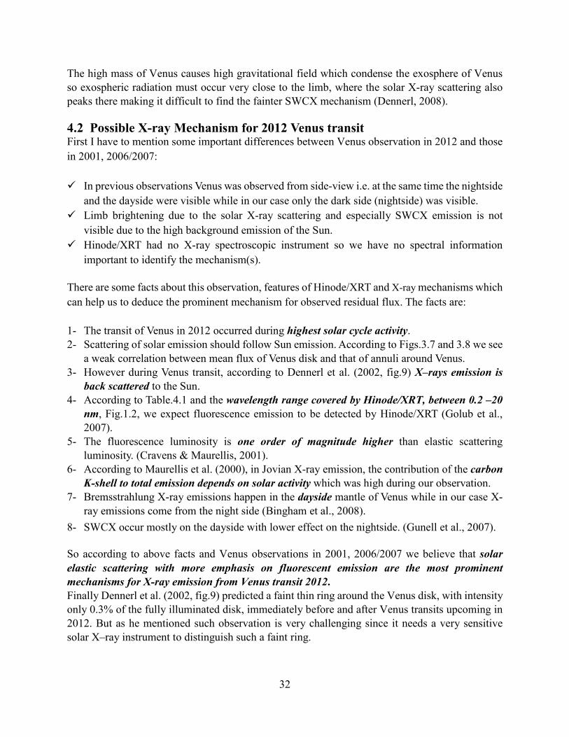
The X-ray radiation is attenuated by the absorption in gas and extinction (absorption and

scattering) by dust. In Fig.4.1 the optical depths of absorption by gas and extinction by dust as a

function of photon energy is presented (Draine–Tan, 2003). At energies above 1 keV the extinction

by dust grains dominate while below 0.5 keV absorption by gas is dominant making it difficult to

observe the dust extinction. However observations of extinction by dust become feasible for bright

sources (Draine –Tan, 2003).

34

Figure 4-1 Optical depths due to the absorption by gas and extinction by dust.

The contribution of scattering to dust extinction is presented. Absorption lines for CII, NI, OI, and NeI are indicated (Draine –Tan, 2003).

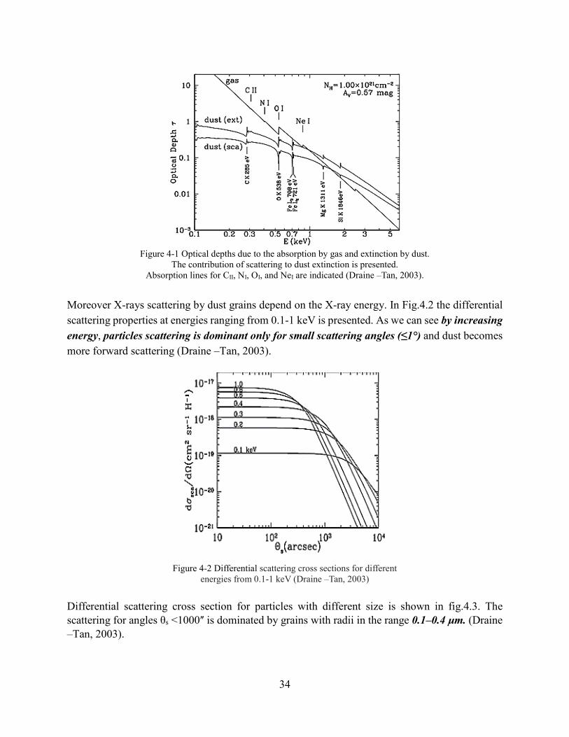
Moreover X-rays scattering by dust grains depend on the X-ray energy. In Fig.4.2 the differential

scattering properties at energies ranging from 0.1-1 keV is presented. As we can see by increasing

energy, particles scattering is dominant only for small scattering angles (≤1°) and dust becomes

more forward scattering (Draine –Tan, 2003).

Figure 4-2 Differential scattering cross sections for different

energies from 0.1-1 keV (Draine –Tan, 2003)

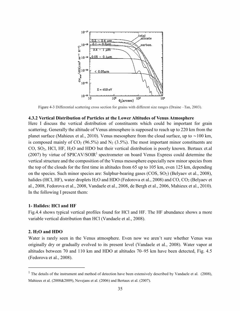
Differential scattering cross section for particles with different size is shown in fig.4.3. The scattering for angles θs <1000ʺ is dominated by grains with radii in the range 0.1–0.4 μm. (Draine –Tan, 2003).

35

Figure 4-3 Differential scattering cross section for grains with different size ranges (Draine –Tan, 2003).

4.3.2 Vertical Distribution of Particles at the Lower Altitudes of Venus Atmosphere Here I discuss the vertical distribution of constituents which could be important for grain

scattering. Generally the altitude of Venus atmosphere is supposed to reach up to 220 km from the

planet surface (Mahieux et al., 2010). Venus mesosphere from the cloud surface, up to ∼100 km,

is composed mainly of CO2 (96.5%) and N2 (3.5%). The most important minor constituents are

CO, SO2, HCl, HF, H2O and HDO but their vertical distribution is poorly known. Bertaux et.al

(2007) by virtue of SPICAV/SOIR1 spectrometer on board Venus Express could determine the

vertical structure and the composition of the Venus mesosphere especially new minor species from

the top of the clouds for the first time in altitudes from 65 up to 105 km, even 125 km, depending

on the species. Such minor species are: Sulphur‐bearing gases (COS, SO2) (Belyaev et al., 2008),

halides (HCl, HF), water droplets H2O and HDO (Fedorova et al., 2008) and CO, CO2 (Belyaev et

al., 2008, Fedorova et al., 2008, Vandaele et al., 2008, de Bergh et al., 2006, Mahieux et al., 2010).

In the following I present them:

1- Halides: HCl and HF

Fig.4.4 shows typical vertical profiles found for HCl and HF. The HF abundance shows a more

variable vertical distribution than HCl (Vandaele et al., 2008).

2. H2O and HDO

Water is rarely seen in the Venus atmosphere. Even now we aren’t sure whether Venus was

originally dry or gradually evolved to its present level (Vandaele et al., 2008). Water vapor at

altitudes between 70 and 110 km and HDO at altitudes 70–95 km have been detected, Fig. 4.5

(Fedorova et al., 2008).

1 The details of the instrument and method of detection have been extensively described by Vandaele et al. (2008),

Mahieux et al. (2008&2009), Nevejans et al. (2006) and Bertaux et al. (2007).

36

Figure 4-4 Left: Vertical profiles of the HCl density for three different occultations

Right: Vertical profiles of HF density for three different occultations (Vandaele et al., 2008)

Figure 4-5 Vertical distributions of the H2O (Left) and HDO (Right) for different eight orbits (Fedorova et al., 2008).

37

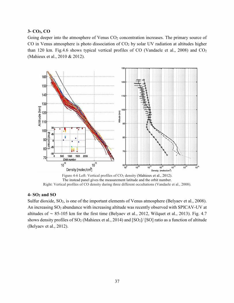
3- CO2, CO

Going deeper into the atmosphere of Venus CO2 concentration increases. The primary source of

CO in Venus atmosphere is photo dissociation of CO2 by solar UV radiation at altitudes higher

than 120 km. Fig.4.6 shows typical vertical profiles of CO (Vandaele et al., 2008) and CO2

(Mahieux et al., 2010 & 2012).

Figure 4-6 Left: Vertical profiles of CO2 density (Mahieux et al., 2012). The instead panel gives the measurement latitude and the orbit number.

Right: Vertical profiles of CO density during three different occultations (Vandaele et al., 2008).

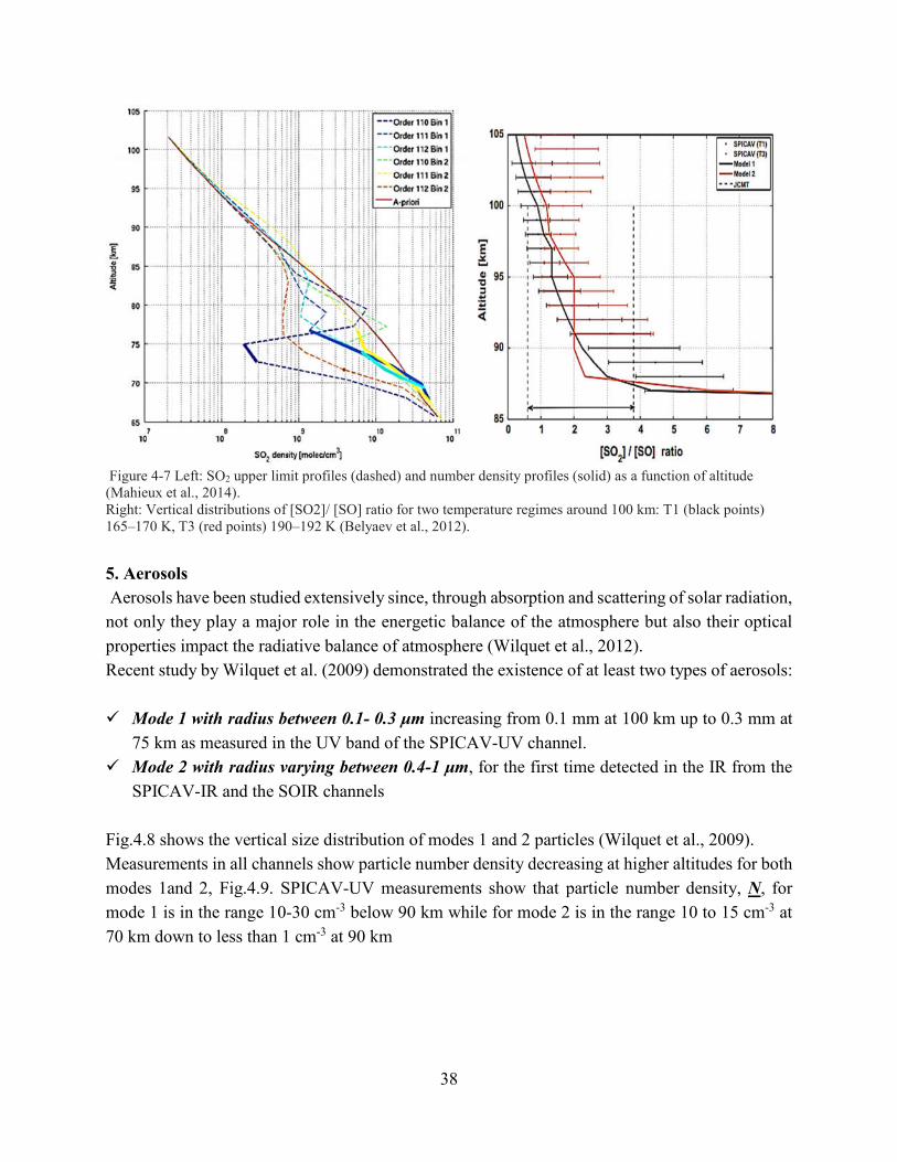
4- SO2 and SO

Sulfur dioxide, SO2, is one of the important elements of Venus atmosphere (Belyaev et al., 2008).

An increasing SO2 abundance with increasing altitude was recently observed with SPICAV-UV at

altitudes of ∼ 85-105 km for the first time (Belyaev et al., 2012, Wilquet et al., 2013). Fig. 4.7

shows density profiles of SO2 (Mahieux et al., 2014) and [SO2]/ [SO] ratio as a function of altitude

(Belyaev et al., 2012).

38

Figure 4-7 Left: SO2 upper limit profiles (dashed) and number density profiles (solid) as a function of altitude (Mahieux et al., 2014). Right: Vertical distributions of [SO2]/ [SO] ratio for two temperature regimes around 100 km: T1 (black points) 165–170 K, T3 (red points) 190–192 K (Belyaev et al., 2012).

5. Aerosols

Aerosols have been studied extensively since, through absorption and scattering of solar radiation,

not only they play a major role in the energetic balance of the atmosphere but also their optical

properties impact the radiative balance of atmosphere (Wilquet et al., 2012).

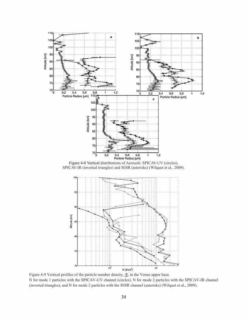
Recent study by Wilquet et al. (2009) demonstrated the existence of at least two types of aerosols:

Mode 1 with radius between 0.1- 0.3 μm increasing from 0.1 mm at 100 km up to 0.3 mm at

75 km as measured in the UV band of the SPICAV-UV channel.

Mode 2 with radius varying between 0.4-1 μm, for the first time detected in the IR from the

SPICAV-IR and the SOIR channels

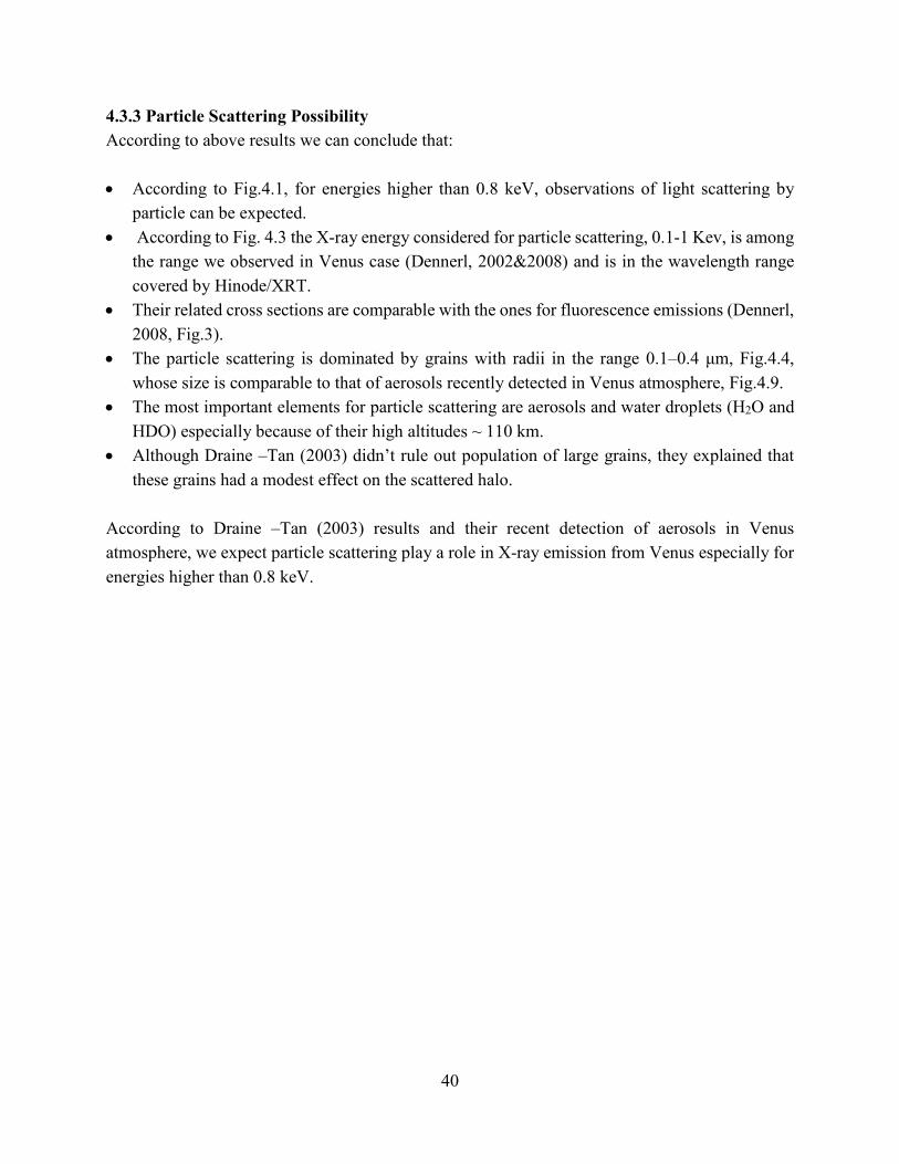
Fig.4.8 shows the vertical size distribution of modes 1 and 2 particles (Wilquet et al., 2009).

Measurements in all channels show particle number density decreasing at higher altitudes for both

modes 1and 2, Fig.4.9. SPICAV-UV measurements show that particle number density, N, for

mode 1 is in the range 10-30 cm-3 below 90 km while for mode 2 is in the range 10 to 15 cm-3 at

70 km down to less than 1 cm-3 at 90 km

39

Figure 4-8 Vertical distributions of Aerosols: SPICAV-UV (circles),

SPICAV-IR (inverted triangles) and SOIR (asterisks) (Wilquet et al., 2009).

Figure 4-9 Vertical profiles of the particle number density, N, in the Venus upper haze.

N for mode 1 particles with the SPICAV-UV channel (circles), N for mode 2 particles with the SPICAV-IR channel

(inverted triangles), and N for mode 2 particles with the SOIR channel (asterisks) (Wilquet et al., 2009).

40

4.3.3 Particle Scattering Possibility

According to above results we can conclude that:

According to Fig.4.1, for energies higher than 0.8 keV, observations of light scattering by

particle can be expected.

According to Fig. 4.3 the X-ray energy considered for particle scattering, 0.1-1 Kev, is among

the range we observed in Venus case (Dennerl, 2002&2008) and is in the wavelength range

covered by Hinode/XRT.

Their related cross sections are comparable with the ones for fluorescence emissions (Dennerl,

2008, Fig.3).

The particle scattering is dominated by grains with radii in the range 0.1–0.4 μm, Fig.4.4,

whose size is comparable to that of aerosols recently detected in Venus atmosphere, Fig.4.9.

The most important elements for particle scattering are aerosols and water droplets (H2O and

HDO) especially because of their high altitudes ~ 110 km.

Although Draine –Tan (2003) didn’t rule out population of large grains, they explained that

these grains had a modest effect on the scattered halo.

According to Draine –Tan (2003) results and their recent detection of aerosols in Venus

atmosphere, we expect particle scattering play a role in X-ray emission from Venus especially for

energies higher than 0.8 keV.

41

4.4 Conclusion I studied the Venus transit across the solar disk in 2012 which has been observed with Hinode/XRT

in the X-Ray band and SDO/AIA in the UV band. I’ve measured a significant X-Ray residual flux

from the Venus’ dark side which was completely above the noise level. Analogous residual flux

has NOT been detected in the UV band.

To remove the possible effect of the atmosphere on the residual flux I also studied a Mercury

transit and some solar eclipses.

Mercury transit across the solar disk was observed with Hinode/XRT in 2006. Also I measured an

apparent X-Ray residual flux in the case of Mercury.

Solar eclipse has been observed with Hinode/XRT in the X-Ray band and SDO/AIA in the UV

band. In solar eclipse analysis NO residual flux was detected.

I used a new version of the Hinode/XRT PSF to explore to which extent such a significant flux

from the Venus shadow can be due to instrumental scattering. I selected well illuminated images

in X-Ray band and deconvolved them, for Venus and Mercury. Even after deconvolution, flux

from Venus shadow remains significant while in the Mercury case it becomes negligible. So we

may be sure the observed residual flux is real and possibly come from the atmosphere of Venus.

Since our initial analysis with Ti-poly filter was affected by stray light contamination I also

analyzed Venus transit images observed with Al-mesh filter since light leak had very negligible

effect on it.

My analysis in Al-mesh filter confirms the results of Ti-poly filter since in all intensity profiles

residual flux still seen and above the noise level confirming that the residual flux comes from

Venus possibly from its atmosphere. Since Venus is not a source of X-Ray emission we must find

a mechanism to relate observed such X-Ray emission of Venus to the X-Ray emission of the Sun.

According to the fact related to Venus transit observation and Hinode/XRT telescope and also

previous observations with Chandra X-Ray telescope in 2001 and 2006/2007 we suggest solar

scattering especially fluorescent emissions are the main mechanism for observed x-rays

emissions; unfortunately no spectrometer was onboard Hinode/XRT to validate this hypothesis.

We also propose grain scattering as possible X-Ray emission especially by water droplets and

aerosols according to the new observations by SOIR instrument and detection of vertical profiles

of key elements at altitudes ≈80-120 km above Venus surface.

The most important particles for grain scattering must have the size in the range 0.1–0.4 μm and

according to SOIR observations such grains were detected in the Venus atmosphere. Also the

energy range for grain scattering, 0.1-1 Kev, is detected according to the previous observations

with Chandra X-Ray telescope.

Finally the accuracy of Hinode/XRT PSF must be validated by future works. Also the spatial and

temporal variability of key elements in Venus atmosphere must be investigated and careful

analysis of trace gases must be done to understand better the processes which occur in the upper

atmosphere of Venus. Moreover the resolution of Hinode/XRT during observation of 2012 Venus

transit was not high which summarized altitudes, from the rocky surface up to 200 km in ≈1 pixel

and also there was no images of Venus transit across the full disk of the Sun to see the effect of

whole disk of the Sun on Venus shadow images.

42

The Study of Hot Electrons in

Shock Ignition Relevant Regime

Proposer and Team Leader:

Prof. Dimitri Batani

43

Frequently, in a variety of experiments though I miss what I expected to find, yet something valuable turns out, something surprising, and instructing, though unthought of.

Benjamin Franklin

Nuclear Fusion

5.1 Introduction Nuclear fusion is a nuclear reaction in which two atomic nuclei collide at a very high speed and join

to form a new type of atomic nucleus. For atomic nuclei smaller than iron and nickel

fusion reactors releases extra energy.

Normally, fusion is not possible because the strongly repulsive Coulomb forces between the

positively charged nuclei prevent them from getting close enough together to fuse. However, if the

conditions are such that the nuclei can overcome the Coulomb forces to the extent that they can

come within a very close range of each other, then the attractive nuclear force between the nuclei

will outweigh the repulsive (electrostatic) force, allowing the nuclei to fuse together. Such

conditions can occur when the temperature increases, causing the ions to move faster and

eventually reach speeds high enough to bring the ions close enough together. The nuclei can then

fuse, causing a release of energy (Krane, 1987).

In astrophysical contexts (Gravitational confinement), massive gravitational forces create the right

conditions for fusion. The fusion chain is complex but the net result is the fusion of

four protons into one alpha particle, (i.e. helium nucleon) with the release of two positrons,

two neutrinos.

On earth the reproduction of stellar core conditions for terrestrial nuclear fusion power plants is

completely impractical. Because nuclear reaction rates strongly depend on temperature achieving

reasonable power levels in terrestrial fusion reactors requires, T ≈ 0.1GK or 10 keV (1 eV ≈ 104k).

in addition in order to produce both high energy output and high average power a combination of

a high repetition rate with a high energy gain and a large enough fuel mass in each target is required

(Ribeyre et al., 2009).

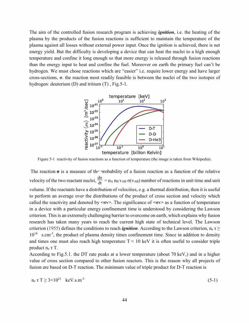
44

The aim of the controlled fusion research program is achieving ignition, i.e. the heating of the

plasma by the products of the fusion reactions is sufficient to maintain the temperature of the

plasma against all losses without external power input. Once the ignition is achieved, there is net

energy yield. But the difficulty is developing a device that can heat the nuclei to a high enough

temperature and confine it long enough so that more energy is released through fusion reactions

than the energy input to heat and confine the fuel. Moreover on earth the primary fuel can’t be

hydrogen. We must chose reactions which are “easier” i.e. require lower energy and have larger

cross-sections, σ. the reaction most readily feasible is between the nuclei of the two isotopes of

hydrogen: deuterium (D) and tritium (T) , Fig.5-1.

Figure 5-1 reactivity of fusion reactions as a function of temperature (the image is taken from Wikipedia).

The reaction σ is a measure of the probability of a fusion reaction as a function of the relative

velocity of the two reactant nuclei, dndt = nA nB vAB σ(vAB) number of reactions in unit time and unit

volume. If the reactants have a distribution of velocities, e.g. a thermal distribution, then it is useful

to perform an average over the distributions of the product of cross section and velocity which

called the reactivity and denoted by <σv>. The significance of <σv> as a function of temperature

in a device with a particular energy confinement time is understood by considering the Lawson

criterion. This is an extremely challenging barrier to overcome on earth, which explains why fusion

research has taken many years to reach the current high state of technical level. The Lawson

criterion (1955) defines the conditions to reach ignition. According to the Lawson criterion, ne τ ≥

1014 s.cm-3, the product of plasma density times confinement time. Since in addition to density

and times one must also reach high temperature T ≈ 10 keV it is often useful to consider triple

product ne τ T.

According to Fig.5.1. the DT rate peaks at a lower temperature (about 70 keV,) and in a higher

value of cross section compared to other fusion reactors. This is the reason why all projects of

fusion are based on D-T reaction. The minimum value of triple product for D-T reaction is

ne τ T ≥ 3×1021 keV.s.m-3 (5-1)

45

Where n is the density (in m3), τ the confinement time (in seconds) and T the temperature (in keV).

The (intermediate) result of D-T reaction, Fig.5-2, is an unstable 5He nucleus, which immediately

ejects a neutron with 14.1 MeV. The recoil energy of the remaining 4He nucleus is 3.5 MeV, so

the total energy liberated is 17.6 MeV. While the D-T reaction is the main focus of attention, long-

term hopes are for a D-D reaction, but this requires much higher temperatures.

Figure 5-2 D-T nuclear reaction and final production (the image is taken from ITER website).

At present, two main experimental approaches are being studied: magnetic confinement fusion

(MCF) and inertial confinement fusion (ICF). The MCF uses strong magnetic fields to contain

the hot plasma while the ICF involves compressing a small pellet containing fusion fuel to

extremely high densities using strong lasers or particles beam. For each approach different

schemes are proposed. The MCF schemes are based on:

Tokomak

Z-Pinch machine

Dense plasma focus

Stellarator

For ICF two main paths with using lasers are under investigation (Radha et al., 2011):

Direct-Drive

Indirect-Drive

Unfortunately, until now the ignition hasn’t been achieved yet. Recently two advanced ignition

schemes have been proposed. They are based on the direct drive approach (DD) but with the

concept of separating the heating and compression phases of the implosion. These schemes not

only increase the gain of reactions but also mitigate the constraints on the target and irradiation

uniformity making it possible to achieve inertial fusion with current facilities (Batani et al., 2012).

These schemes are:

Fast ignition

Shock ignition

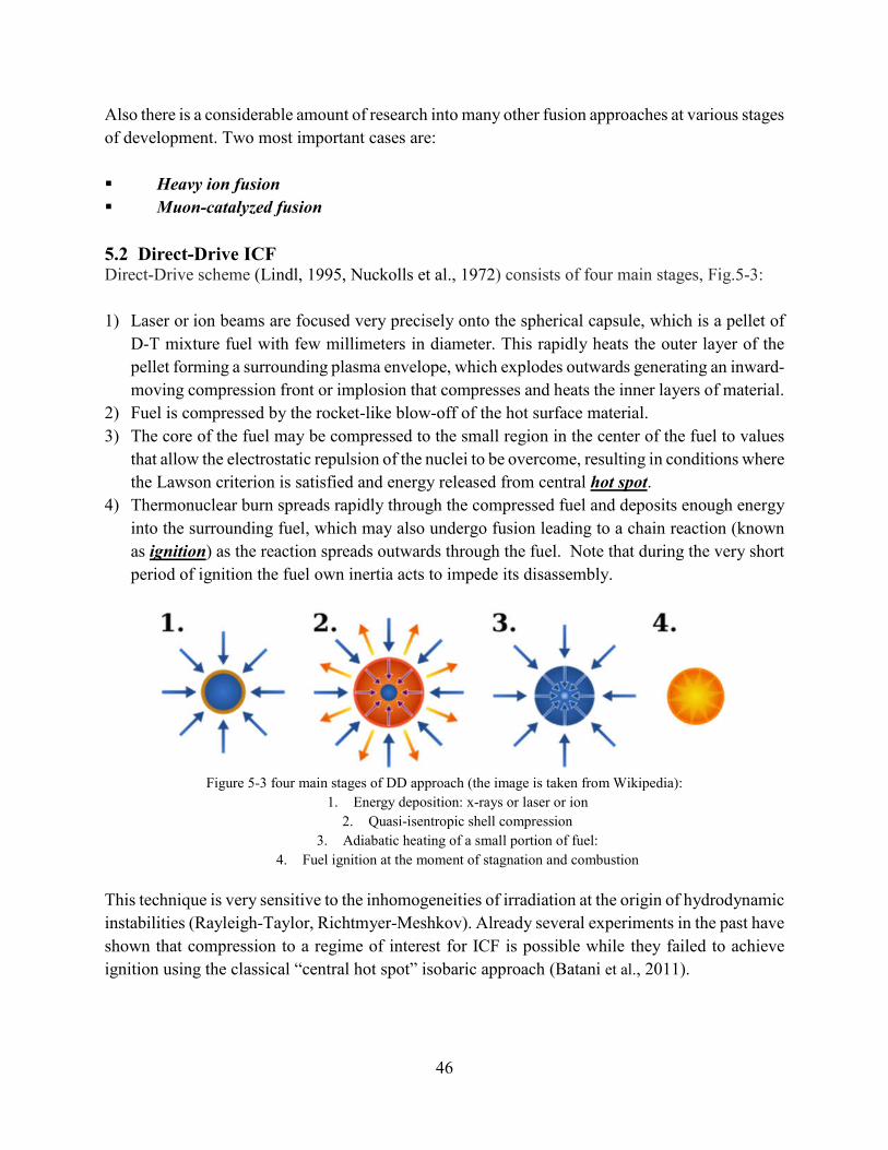
46

Also there is a considerable amount of research into many other fusion approaches at various stages

of development. Two most important cases are:

Heavy ion fusion

Muon-catalyzed fusion

5.2 Direct-Drive ICF Direct-Drive scheme (Lindl, 1995, Nuckolls et al., 1972) consists of four main stages, Fig.5-3:

1) Laser or ion beams are focused very precisely onto the spherical capsule, which is a pellet of

D-T mixture fuel with few millimeters in diameter. This rapidly heats the outer layer of the

pellet forming a surrounding plasma envelope, which explodes outwards generating an inward-

moving compression front or implosion that compresses and heats the inner layers of material.

2) Fuel is compressed by the rocket-like blow-off of the hot surface material.

3) The core of the fuel may be compressed to the small region in the center of the fuel to values

that allow the electrostatic repulsion of the nuclei to be overcome, resulting in conditions where

the Lawson criterion is satisfied and energy released from central hot spot.

4) Thermonuclear burn spreads rapidly through the compressed fuel and deposits enough energy

into the surrounding fuel, which may also undergo fusion leading to a chain reaction (known

as ignition) as the reaction spreads outwards through the fuel. Note that during the very short

period of ignition the fuel own inertia acts to impede its disassembly.

Figure 5-3 four main stages of DD approach (the image is taken from Wikipedia):

1. Energy deposition: x-rays or laser or ion

2. Quasi-isentropic shell compression

3. Adiabatic heating of a small portion of fuel:

4. Fuel ignition at the moment of stagnation and combustion

This technique is very sensitive to the inhomogeneities of irradiation at the origin of hydrodynamic

instabilities (Rayleigh-Taylor, Richtmyer-Meshkov). Already several experiments in the past have

shown that compression to a regime of interest for ICF is possible while they failed to achieve

ignition using the classical “central hot spot” isobaric approach (Batani et al., 2011).

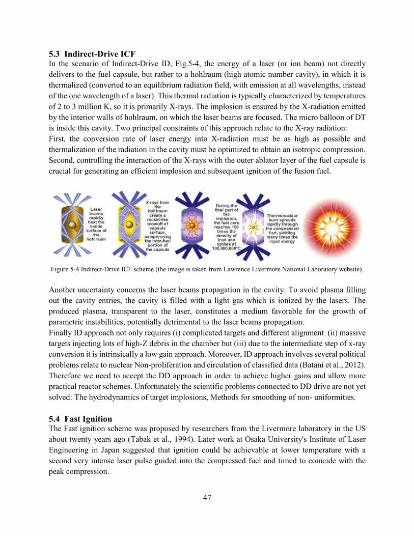
47

5.3 Indirect-Drive ICF In the scenario of Indirect-Drive ID, Fig.5-4, the energy of a laser (or ion beam) not directly

delivers to the fuel capsule, but rather to a hohlraum (high atomic number cavity), in which it is

thermalized (converted to an equilibrium radiation field, with emission at all wavelengths, instead

of the one wavelength of a laser). This thermal radiation is typically characterized by temperatures

of 2 to 3 million K, so it is primarily X-rays. The implosion is ensured by the X-radiation emitted

by the interior walls of hohlraum, on which the laser beams are focused. The micro balloon of DT

is inside this cavity. Two principal constraints of this approach relate to the X-ray radiation:

First, the conversion rate of laser energy into X-radiation must be as high as possible and

thermalization of the radiation in the cavity must be optimized to obtain an isotropic compression.

Second, controlling the interaction of the X-rays with the outer ablator layer of the fuel capsule is

crucial for generating an efficient implosion and subsequent ignition of the fusion fuel.

Figure 5-4 Indirect-Drive ICF scheme (the image is taken from Lawrence Livermore National Laboratory website).

Another uncertainty concerns the laser beams propagation in the cavity. To avoid plasma filling

out the cavity entries, the cavity is filled with a light gas which is ionized by the lasers. The

produced plasma, transparent to the laser, constitutes a medium favorable for the growth of

parametric instabilities, potentially detrimental to the laser beams propagation.

Finally ID approach not only requires (i) complicated targets and different alignment (ii) massive

targets injecting lots of high-Z debris in the chamber but (iii) due to the intermediate step of x-ray

conversion it is intrinsically a low gain approach. Moreover, ID approach involves several political

problems relate to nuclear Non-proliferation and circulation of classified data (Batani et al., 2012).

Therefore we need to accept the DD approach in order to achieve higher gains and allow more

practical reactor schemes. Unfortunately the scientific problems connected to DD drive are not yet

solved: The hydrodynamics of target implosions, Methods for smoothing of non- uniformities.

5.4 Fast Ignition The Fast ignition scheme was proposed by researchers from the Livermore laboratory in the US

about twenty years ago (Tabak et al., 1994). Later work at Osaka University's Institute of Laser

Engineering in Japan suggested that ignition could be achievable at lower temperature with a

second very intense laser pulse guided into the compressed fuel and timed to coincide with the

peak compression.

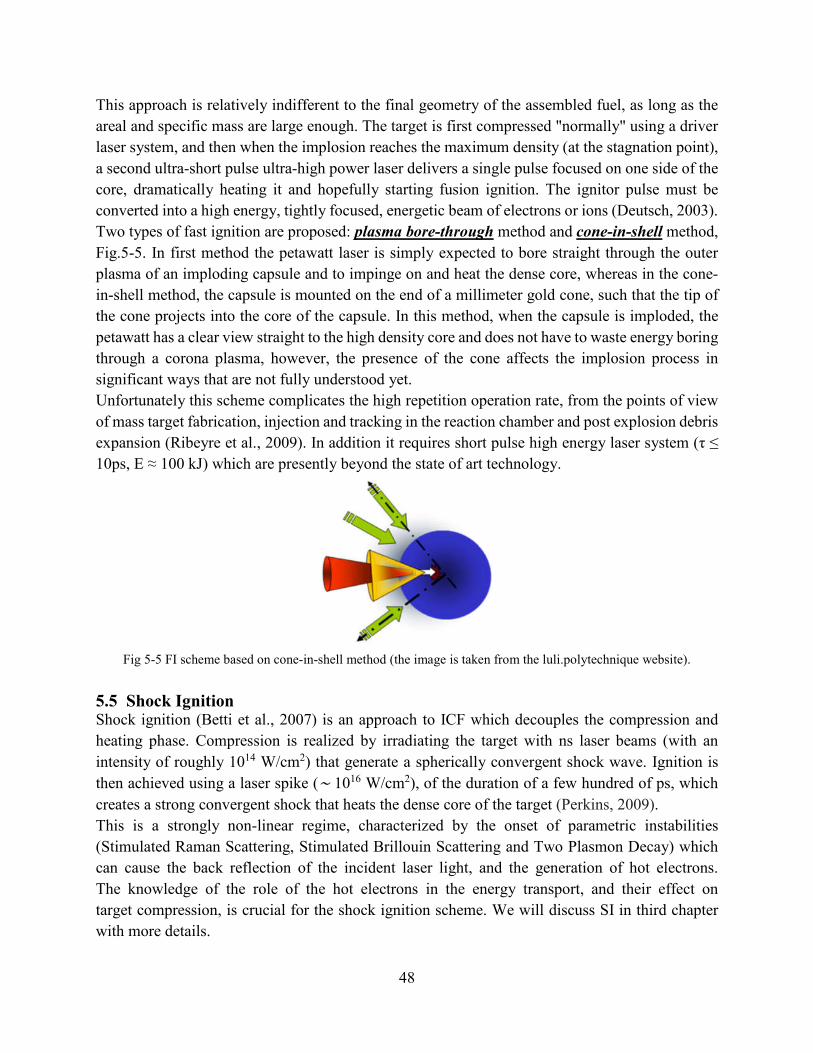
48

This approach is relatively indifferent to the final geometry of the assembled fuel, as long as the

areal and specific mass are large enough. The target is first compressed "normally" using a driver

laser system, and then when the implosion reaches the maximum density (at the stagnation point),

a second ultra-short pulse ultra-high power laser delivers a single pulse focused on one side of the

core, dramatically heating it and hopefully starting fusion ignition. The ignitor pulse must be

converted into a high energy, tightly focused, energetic beam of electrons or ions (Deutsch, 2003).

Two types of fast ignition are proposed: plasma bore-through method and cone-in-shell method,

Fig.5-5. In first method the petawatt laser is simply expected to bore straight through the outer

plasma of an imploding capsule and to impinge on and heat the dense core, whereas in the cone-

in-shell method, the capsule is mounted on the end of a millimeter gold cone, such that the tip of

the cone projects into the core of the capsule. In this method, when the capsule is imploded, the

petawatt has a clear view straight to the high density core and does not have to waste energy boring

through a corona plasma, however, the presence of the cone affects the implosion process in

significant ways that are not fully understood yet.

Unfortunately this scheme complicates the high repetition operation rate, from the points of view

of mass target fabrication, injection and tracking in the reaction chamber and post explosion debris

expansion (Ribeyre et al., 2009). In addition it requires short pulse high energy laser system (τ ≤

10ps, E ≈ 100 kJ) which are presently beyond the state of art technology.

Fig 5-5 FI scheme based on cone-in-shell method (the image is taken from the luli.polytechnique website).

5.5 Shock Ignition Shock ignition (Betti et al., 2007) is an approach to ICF which decouples the compression and

heating phase. Compression is realized by irradiating the target with ns laser beams (with an

intensity of roughly 1014 W/cm2) that generate a spherically convergent shock wave. Ignition is

then achieved using a laser spike (∼ 1016 W/cm2), of the duration of a few hundred of ps, which

creates a strong convergent shock that heats the dense core of the target (Perkins, 2009).

This is a strongly non-linear regime, characterized by the onset of parametric instabilities

(Stimulated Raman Scattering, Stimulated Brillouin Scattering and Two Plasmon Decay) which

can cause the back reflection of the incident laser light, and the generation of hot electrons.

The knowledge of the role of the hot electrons in the energy transport, and their effect on

target compression, is crucial for the shock ignition scheme. We will discuss SI in third chapter

with more details.

49

Shock Wave Propagation Theory

The central idea behind the shock ignition approach is to compress a target to high density

using direct drive, and then use a strong shock wave to compress the DT pellet and achieve

ignition so the propagation of supersonic waves is an essential issue in shock ignition scheme. In

this chapter I present the shock wave theory and the principal equations governs on the dynamic

of physical system (Zel'dovichand & Razier, 1966).

6.1 Acoustic Waves Acoustic waves are compression waves which travel inside a material with a velocity lower than

its sound velocity, cs. They can be considered as a small perturbation of pressure and density of a

system from its equilibrium state, P0 and ρ0,

ρ = ρ0 + ∆ρ (6-1)

P = P0 + ∆P (6-2)

Where ∆ρ is the perturbation. The evolution of the system is described by the equation of

continuity, expressing the conservation of mass:

dρ/ dt + ∇. (ρu) = 0 (6-3)

And by Euler's equation, expressing the conservation of momentum

∂u/∂t + u∇. (u) = −1/ρ∇P (6-4)

By substitution of P and ρ from equations (2-1) and (2-2) and differentiating the continuity

equation with respect to time, and Euler's equation with respect to space, simultaneously, we obtain

the equation of propagation of small perturbations:

∂2∆ρ/∂t2 = cs ∂2∆ρ/∂x2 with cs =(∂P/ ∂ρ)S 1/2 (6-5)

So the small densities perturbations propagate with the sound velocity and suffix S indicates the

derivation carried out on an isentropic transition.

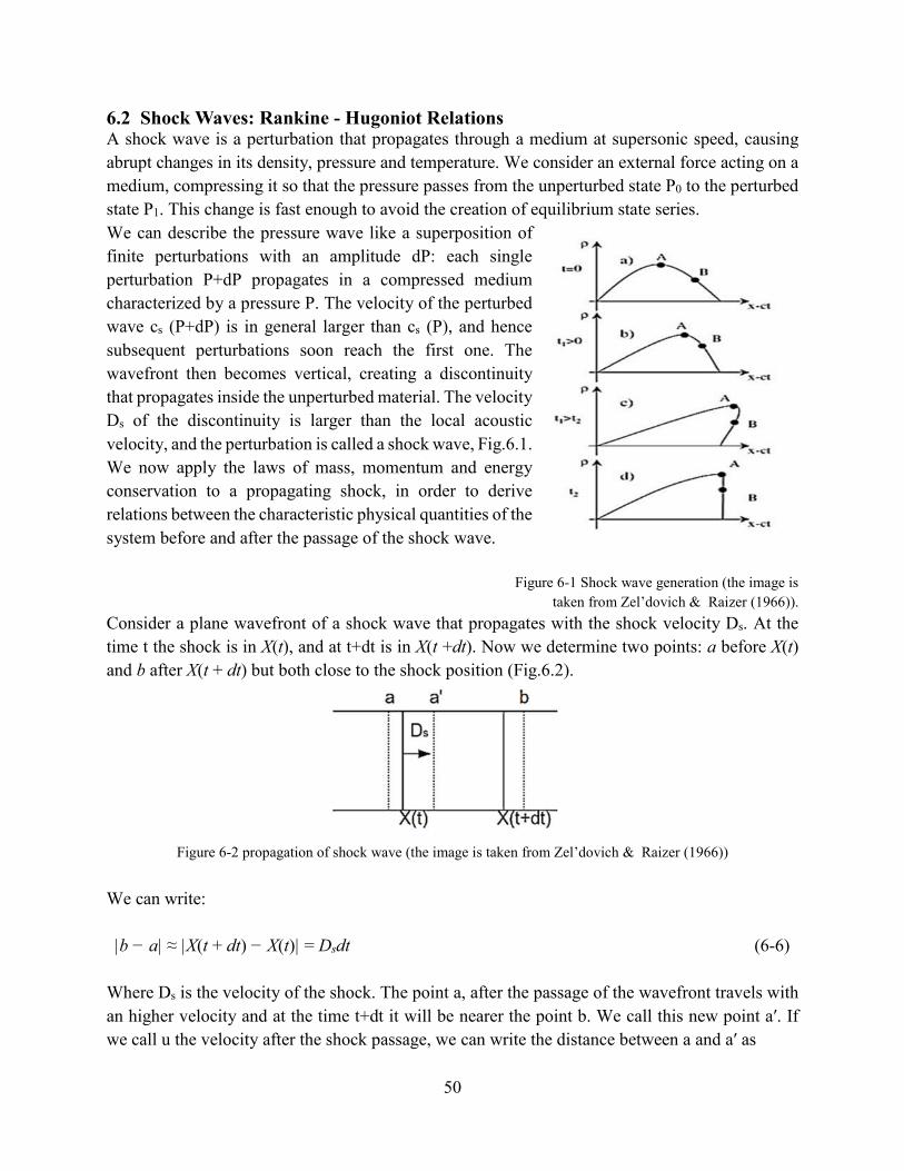
50

6.2 Shock Waves: Rankine - Hugoniot Relations A shock wave is a perturbation that propagates through a medium at supersonic speed, causing

abrupt changes in its density, pressure and temperature. We consider an external force acting on a

medium, compressing it so that the pressure passes from the unperturbed state P0 to the perturbed

state P1. This change is fast enough to avoid the creation of equilibrium state series.

We can describe the pressure wave like a superposition of

finite perturbations with an amplitude dP: each single

perturbation P+dP propagates in a compressed medium

characterized by a pressure P. The velocity of the perturbed

wave cs (P+dP) is in general larger than cs (P), and hence

subsequent perturbations soon reach the first one. The

wavefront then becomes vertical, creating a discontinuity

that propagates inside the unperturbed material. The velocity

Ds of the discontinuity is larger than the local acoustic

velocity, and the perturbation is called a shock wave, Fig.6.1.

We now apply the laws of mass, momentum and energy

conservation to a propagating shock, in order to derive

relations between the characteristic physical quantities of the

system before and after the passage of the shock wave.

Figure 6-1 Shock wave generation (the image is

taken from Zel’dovich & Raizer (1966)).

Consider a plane wavefront of a shock wave that propagates with the shock velocity Ds. At the

time t the shock is in X(t), and at t+dt is in X(t +dt). Now we determine two points: a before X(t)

and b after X(t + dt) but both close to the shock position (Fig.6.2).

Figure 6-2 propagation of shock wave (the image is taken from Zel’dovich & Raizer (1966))

We can write:

|b − a| ≈ |X(t + dt) − X(t)| = Dsdt (6-6)

Where Ds is the velocity of the shock. The point a, after the passage of the wavefront travels with

an higher velocity and at the time t+dt it will be nearer the point b. We call this new point aʹ. If

we call u the velocity after the shock passage, we can write the distance between a and aʹ as

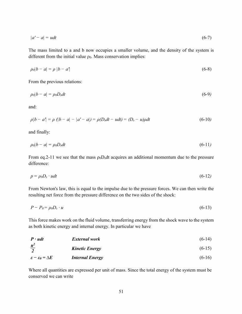
51

|aʹ − a| = udt (6-7)

The mass limited to a and b now occupies a smaller volume, and the density of the system is

different from the initial value ρ0. Mass conservation implies:

ρ0|b − a| = ρ |b − aʹ| (6-8)

From the previous relations:

ρ0|b − a| = ρ0Dsdt (6-9)

and:

ρ|b − aʹ| = ρ (|b − a| − |aʹ − a|) = ρ(Dsdt − udt) = (Ds − u)ρdt (6-10)

and finally:

ρ0|b − a| = ρ0Dsdt (6-11)

From eq.2-11 we see that the mass ρ0Dsdt acquires an additional momentum due to the pressure

difference:

p = ρ0Ds · udt (6-12)

From Newton's law, this is equal to the impulse due to the pressure forces. We can then write the

resulting net force from the pressure difference on the two sides of the shock:

P − P0 = ρ0Ds · u (6-13)

This force makes work on the fluid volume, transferring energy from the shock wave to the system

as both kinetic energy and internal energy. In particular we have

P · udt External work (6-14)

u2

2 Kinetic Energy

(6-15)

ε − ε0 = ∆E Internal Energy (6-16)

Where all quantities are expressed per unit of mass. Since the total energy of the system must be

conserved we can write

52

(∆E + u2

2 ) ρ0Ds dt = Pudt

(6-17)

and so:

∆E = Pu

ρ0Ds −

12 u2

(6-18)

If the shock is strong (P >> P0) the term Pu/ ρ0Ds becomes negligible and the energy is distributed

in internal and kinetic energy in the same way. We can rewrite conservation laws of mass,

momentum and energy in differential form:

∂∂t ρ = −

∂∂x (ρu)

(6-19)

∂∂t (ρu) = −

∂∂x (p + ρu2)

(6-20)

∂∂t (ρε +

12 ρu2)= −

∂∂x [ρu (ε +

12u2+

p ρ ]

(6-21)

It is possible to consider a thin layer (x0, x1) which contains large gradients of every physical

quantities. The discontinuity will be the limit of such layer for | x0, x1| → 0. In this way it is

possible to integrate from x0 to x1:

∫∂∂t (ρu)dx

�

�� = ∫

∂∂x

�

�� (p + ρu2) dx

(6-22)

If we take the limit, the integral on the left-hand side vanishes while the integral in the right-hand

side cover all fluxes on each side of the discontinuity. Acting similarly for two other equations,

one gets the formulae of conservation of mass, momentum and energy in the shock rest frame 2:

ρ1u1 = ρ0u0 (6-23)

p1 + ρ1u12 = p0 + ρ0u1

2 (6-24)

ε1 +p1

ρ1 +

12 u1

2 = ε0 + p0

ρ0 +

12u0

2

(6-25)

These equations are called Rankine - Hugoniot relations, and express respectively the

conservation of mass, momentum and energy across the shock surface.

2 Placing u1 = u − Ds and u0 = u + Ds with u = 0 in the second relation.

53

Fixing the initial conditions p0 =0 and u0 =0, and choosing the values for the initial specific

volume V = 1/ρ0 and for the shock strength P1 we can calculate the remaining variables from

the Hugoniot relations. From the mass conservation we write

V0

V1 =

u0

u1

(6-26)

and by eliminating either u0 or u1 from the momentum conservation

u02 = V0

2 P1 − P0

V0 − V1

(6-27)

u12 = V1

2 P1 − P0

V0 − V1

(6-28)

By introducing the net velocity of the gas flow |u| we can write

|u| = u0 − u1 = (P1 − P0)(V0 − V1)1/2 (6-29)

Which is the velocity of the compressed flow. We can then write the differences in kinetic energy

in the shock rest frame as

12 (u0

2 –u12) =

12 (P1 − P0)(V0 + V1)

(6-30)

And by substituting in the energy conservation law we have:

∆E = 12 (P1 + P0)(V0 − V1)

(6-31)

Since the internal energy is a function of pressure and specific volume (adiabatic shock), we can

imagine to substitute ε = ε (P, V), and thus determine the Hugoniot curve which is a representation

of P1 in the (V1, P0, V0) space

P1 = H (V1, P0, V0) (6-32)

Which depends on two parameters P0 and V0, Fig.6-3.

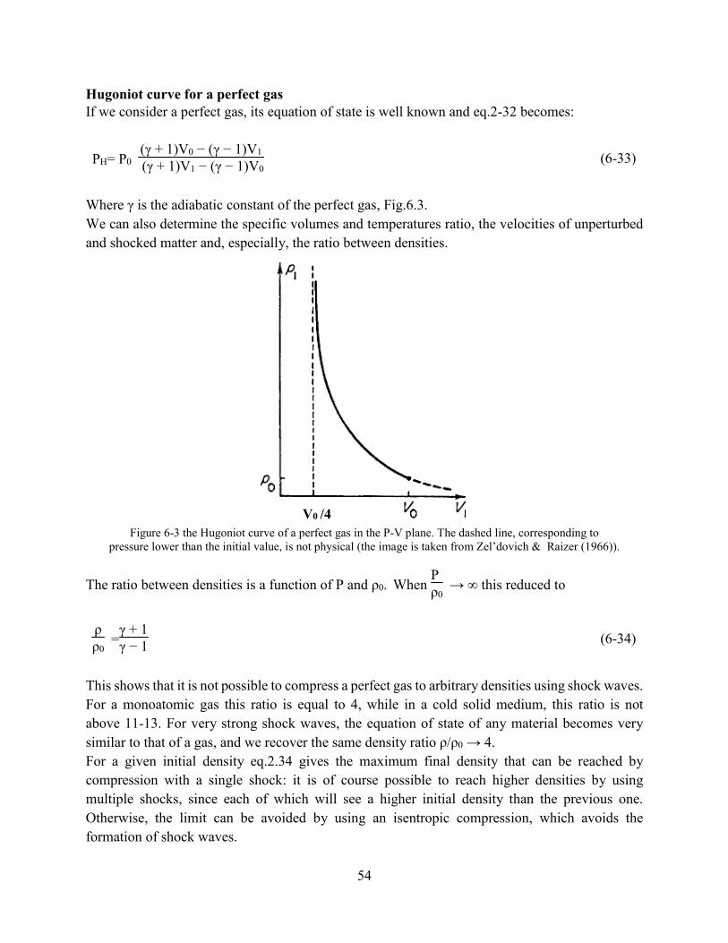
54

Hugoniot curve for a perfect gas If we consider a perfect gas, its equation of state is well known and eq.2-32 becomes:

PH= P0 (γ + 1)V0 − (γ − 1)V1

(γ + 1)V1 − (γ − 1)V0

(6-33)

Where γ is the adiabatic constant of the perfect gas, Fig.6.3.

We can also determine the specific volumes and temperatures ratio, the velocities of unperturbed

and shocked matter and, especially, the ratio between densities.

Figure 6-3 the Hugoniot curve of a perfect gas in the P-V plane. The dashed line, corresponding to

pressure lower than the initial value, is not physical (the image is taken from Zel’dovich & Raizer (1966)).

The ratio between densities is a function of P and ρ0. When P ρ0

→ ∞ this reduced to

ρρ0

=γ + 1γ − 1

(6-34)

This shows that it is not possible to compress a perfect gas to arbitrary densities using shock waves.

For a monoatomic gas this ratio is equal to 4, while in a cold solid medium, this ratio is not

above 11-13. For very strong shock waves, the equation of state of any material becomes very

similar to that of a gas, and we recover the same density ratio ρ/ρ0 → 4.

For a given initial density eq.2.34 gives the maximum final density that can be reached by

compression with a single shock: it is of course possible to reach higher densities by using

multiple shocks, since each of which will see a higher initial density than the previous one.

Otherwise, the limit can be avoided by using an isentropic compression, which avoids the

formation of shock waves.

V0 /4

55

Comparison with isentropic compression The propagation of a shock wave causes an increase in the entropy of the shocked material. If we

draw the Hugoniot curve and the isentropic curve in a P-V plane, the Hugoniot curve is tangent to

the isentropic curve for low P (standard conditions) while it remains always above the isentropic

curve as pressure increases, Fig.6-4.

For an ideal gas the increase in entropy can be written as:

S1 − S0 = cv log((PV)γ

(P0V0)γ)

(6-35)

Figure 6-4 Comparison between the Hugoniot curve HH and an isentrope PP.

KK is theircommon tangent in the initial state (the image is taken from Zel’dovich & Raizer (1966)).

It is also possible to show that the shock wave is indeed supersonic. In fact we can write the shock

propagation velocity Ds as:

Ds = u02 = V0

2 P1 − P0

V0 − V1

(6-36)

For a weak shock we can approximate the second part of eq.2-36 with V02 (

∆P∆V)S = cS, so

the shock velocity is close to the speed of sound. For higher pressures on the other hand the

Hugoniot curve is always higher than the isentrope, and the shock wave moves faster than sound.

Hugoniot relations in a solid medium The pressure required to compress a solid medium is higher (in the order of magnitudes) than that

required to compress a gas: this is due to the fact that in a solid, pressure not only must overcome

the thermal motion of atoms, but also the elastic bonds between the atoms forming a crystalline

lattice. We can write the pressure inside a solid material as the sum of two components:

56

Pc: Elastic component related to the lattice potential energy, hence directly dependent

by the density (V = 1/ρ)

PT: Thermal component due to the vibrations around the equilibrium position, function

of V and T.

If the temperature is not too high the lattice structure of the solid is preserved and we

can express the pressure as:

P = Pc(V ) + PT(V, T) (6-37)

In the rest frame of the unperturbed medium, the velocity of the shock Ds for solids is linearly

related to the velocity of the material:

Ds = A + Bu (6-38)

For weak shocks, the fluid velocity is u ∼ 0, and the shock velocity is approximately equal

to the sound velocity Cs therefore A=Cs. Using the Hugoniot-Rankine relation, eq.2.25, we can

obtain the Hugoniot curve for solids:

PH = A2(V0 − V1)

V12(B − 1)2 [

BB −1 -

V0

V1 ]2

(6-39)

This relations are true far from phase transitions: if we approach a solid-solid transition, linear

relations eq.2.38 will hold in both phases but the coefficients A and B will have different values.

6.3 Shock Polar The Hugoniot curve relates the final pressure of the shocked material to its initial conditions

in the P-V plane. However it can be useful to connect the final pressure to the fluid velocity, which

we can measure in experiments. To do so we rewrite eq.2.34, remembering that from mass

conservation we have ρ/ρ0 = V0/V1 = u0/u1. Using the second Hugoniot relation (eq.2.24) we get:

P = γ + 1

2 ρ0u2

(6-40)

This equation is called Shock Polar which gives the pressure as a function of the velocity u.

Although this expression has been derived for a perfect gas, for high pressures it can be applied to

all materials: under extreme pressures in fact the elastic component of compressibility becomes

negligible compared to the thermic one, and solids can be treated as perfect gase. When (2-38)

holds we have instead:

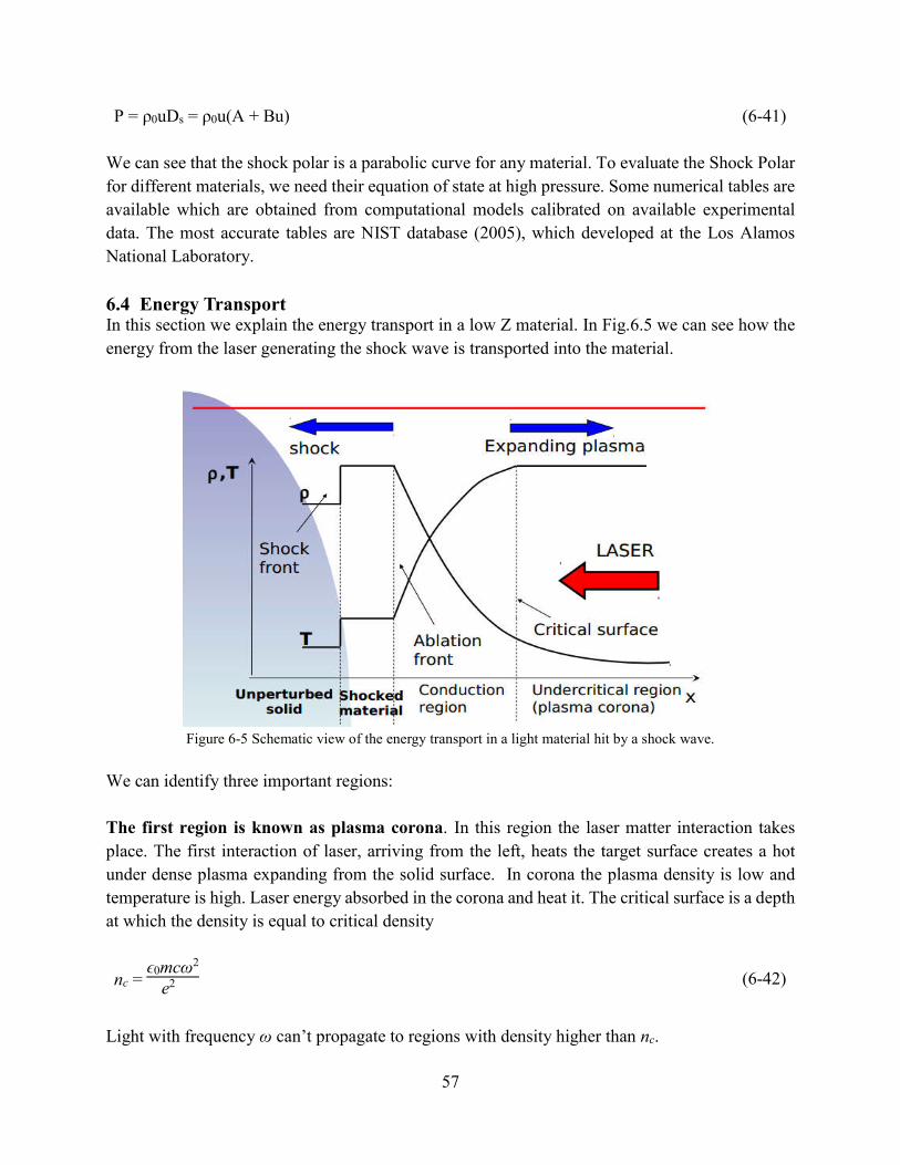
57

P = ρ0uDs = ρ0u(A + Bu) (6-41)

We can see that the shock polar is a parabolic curve for any material. To evaluate the Shock Polar

for different materials, we need their equation of state at high pressure. Some numerical tables are

available which are obtained from computational models calibrated on available experimental

data. The most accurate tables are NIST database (2005), which developed at the Los Alamos

National Laboratory.

6.4 Energy Transport In this section we explain the energy transport in a low Z material. In Fig.6.5 we can see how the

energy from the laser generating the shock wave is transported into the material.

Figure 6-5 Schematic view of the energy transport in a light material hit by a shock wave.

We can identify three important regions:

The first region is known as plasma corona. In this region the laser matter interaction takes

place. The first interaction of laser, arriving from the left, heats the target surface creates a hot

under dense plasma expanding from the solid surface. In corona the plasma density is low and

temperature is high. Laser energy absorbed in the corona and heat it. The critical surface is a depth

at which the density is equal to critical density

nc = ϵ0mcω2

e2

(6-42)

Light with frequency ω can’t propagate to regions with density higher than nc.

58

The second region is conduction region, where the energy transport is realized by the thermal

electronic conduction and as the density increases the matter becomes colder.

The heat flux is given by the Spitzer-Harm law

QSH = −k0T05/2

dTe

dx

(6-43)

Where k0 is the thermal electronic conductivity. This formula is valid if the characteristic size of

temperature gradient is greater than the electron mean free path so we can employ it in the plasma

corona. In the conduction region the gradients can be very steep for eq.43 to be applicable.

Experimental results show that the thermal flux is strongly reduced. To take this reduction into

account an empirical law is used:

Q = min (|QSH|, f ne veTe) (6-44)

Where ve is the electron thermal velocity and f is the flux limiting factor which is generally f ∼

0.06.

The third region is shocked region, which has a very high density (higher than solid density at

standard conditions). In fact the immediate effect of the shock wave passage is to rise both density

and temperature of the unperturbed material. We consider a strong shock: in this way we can see

the shocked material as a perfect gas, since the high pressure of the propagating shock will create

a plasma expanding in the opposite direction.

6.5 Ablation Pressure When the laser wave hits the unperturbed material, matter is strongly heated and passes from solid

to plasma state: this process is called ablation. For this reason the surface between the conduction

and shocked zones is called ablation front. In this model the corona is isothermal. Far from the

ablation surface a steady flow of particles is established. We assume a 1-D plasma with the

equation of state in the form Pρ−γ = cost and a temperature T. The sound velocity is given by:

cs =kB

mi (γiT + γe

ZT 1 + γe

)1/2

(6-45)

Where KB is the Boltzmann constant, mi is the ion mass, Ti is the ion temperature, Te the electron

temperature, the indexes i and e identify ion and electron respectively. In our case γe = γi = γ = 1

so we can define the Mach number M as

M = vcs

(6-46)

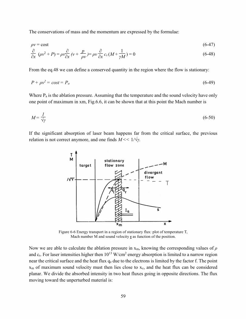
59

The conservations of mass and the momentum are expressed by the formulae:

ρv = cost (6-47)

∂∂x (ρv2 + P) = ρv

∂∂x (v +

p ρv )= ρv

∂∂x cs (M +

1γM ) = 0

(6-48)

From the eq.48 we can define a conserved quantity in the region where the flow is stationary:

P + ρv2 = cost = Pa (6-49)

Where Pa is the ablation pressure. Assuming that the temperature and the sound velocity have only

one point of maximum in xm, Fig.6.6, it can be shown that at this point the Mach number is

M = 1√γ

(6-50)

If the significant absorption of laser beam happens far from the critical surface, the previous

relation is not correct anymore, and one finds M << 1/√γ.

Figure 6-6 Energy transport in a region of stationary flux: plot of temperature T,

Mach number M and sound velocity s as function of the position.

Now we are able to calculate the ablation pressure in xm, knowing the corresponding values of ρ

and cs. For laser intensities higher then 1013 W/cm2 energy absorption is limited to a narrow region

near the critical surface and the heat flux qe due to the electrons is limited by the factor f. The point

xm of maximum sound velocity must then lies close to xc, and the heat flux can be considered

planar. We divide the absorbed intensity in two heat fluxes going in opposite directions. The flux

moving toward the unperturbed material is:

60

ql = k (∂T

∂x )xm

(6-51)

From the Spitzer-Harm law

k=k0T05/2 (6-52)

Where κ is the thermal conductivity and k0 and T0 are defined in previous section. ql accounts for

the convection of enthalpy and for the kinetic energy of the ablated material. The flux qr (qr =−ql)

moves backwards, driving the plasma expansion, and does not contribute to the pressure. We are

now able to write the energy balance at xm:

ql = Ia − qr = ρv(w +v2

2 ) + qe + Pav1 with w = σ +ε + P ρ

(6-53)

Where ε is the internal energy, σ is the heat of ionization and v1 is the velocity of shocked

matter. The term P/ρ accounts for the work done by the out flowing matter against the rarefying

plasma, while Pav1 accounts for the work done by the laser to generate the shock wave traveling

into the over dense material. qe represents the heat needed to preserve a steady state in the plasma

corona which can be transversal and longitudinal.

To evaluate qr we use an upper limit derived for a rarefaction wave:

qr = P cs|xm (6-54)

Which is a good approximation for high electron temperatures. In this simple case we can also

assume ε = 3P/2ρ, and neglect the ionization energy, the electron heat transport and the

work done by the laser. We can then calculate

ql = 3ρmcs3 (6-55)

The minimum ratio between the two heat fluxes is 1/3.

To build the model we describe the divergent flow in the outer plasma corona as a spherical

isothermal rarefaction wave, which is the solution of:

rv2∂r ρ = 0 (6-56)

∂r v2

2 = −cs2 ∂ρ

ρ

(6-57)

We write the wave in xm as:

ρ = ρm exp[−(v2−cs2)/ 2cs

2] (6-58)

61

r2 = r02 exp[(v2−cs

2)/2cs 2] (6-59)

Where r is the radius. We obtain for qr:

qr = ∫ pr2

�

� ∂∂r (r2v)dr = 1.65ρmcs

3

(6-60)

Which is higher than in the case of a planar rarefaction wave. We can also write a more general

expression for ql for non-isothermal compression:

ql= 3γ − 1

2γ3/2(γ − 1) ρmcs3 if γ ≠1

(6-61)

For γ =1 ql is equal (eq.57). We can eliminate Cs in these equation obtaining:

Pa= 2[ 2(γ− 1)(3γ-1) ]2/3ρm

1/3(Ia − qr)2/3 if γ≠1

(6-62)

Pa= 2

32/3 ρm1/3(Ia − qr)2/3 if γ = 1

(6-63)

In planar isothermal heat flow:

Pa=2

42/3 ρm1/3 Ia 2/3 = 0.79 ρm

1/3 Ia 2/3

(6-64)

And for spherical case:

Pa=2

4.652/3 ρm1/3 Ia 2/3 = 0.72 ρm

1/3 Ia 2/3

(6-65)

Finally we can give a scaling law valid for a quasi-stationary laser-plasma interaction regime

(Batani, et al., 2014):

Pa ∼ 57(ηabs I[1015 W/cm2]λ2[µm])2/3 Mbar (6-66)

where ηabs ∼ 0.6 − 0.7 is the laser absorption coefficient. In an intensity regime in the order of 1016

W/cm2, this scaling law would predict a pressure of roughly 200 Mbar.

62

Shock Ignition

In this chapter I describe in detail some of the theoretical aspects of shock ignition (SI). Since SI

is based on direct drive (DD) approach we shortly review the fundamentals of DD.

7.1 Direct Drive Theory We consider a cryogenic DT pellet. Laser ablation causes an acceleration of the external shell

inward the target. The ignition condition is achieved in central hot spot surrounded by a high

density shell. Part of the heat lost from the hot spot because of radiative losses and heat conduction

is deposited on the high density shell, causing further implosion. The efficiency of reaction

depends on the capacity of confinement time of the hot core. This time depends on the high density

shell, area and areal density ρR. If ignition is achieved, the fraction of the fuel mass involved in

thermonuclear burning is related to the areal density ρR of the target as:

fburn (ρR) ≈ ρR

ρR +6

(7-1)

With ρR in g/cm2. The maximal areal density (ρR)Max increases with the energy of the incident

laser and decreases with the inflight adiabat coefficient, α:

(ρR)Max ≈ ( EL

0.33

α0.55 )

(7-2)

Where EL is the laser energy on target and α, inflight adiabat, is the ratio between the fuel pressure

during compression and the Fermi pressure (which in an electron degenerate gas is the minimum

pressure corresponds to the obtained density). The energy produced during the burning of the fuel

should be high enough to compensate the work (pdV) necessary to compress the fuel, the energy

used to heat it and the thermal losses throughout the process. The energy gain of the fusion yield

is then related to the burn fraction and to the implosion velocity as:

G ∝ fburn(ρR)

vimp5/4 IL

1/4

(7-3)

63

Which IL is the incident laser intensity and vimp is the implosion velocity in cm/s. The gain increases

for lower implosion velocity, because for the same laser energy a greater fraction of fuel mass can

be assembled in the center and burned. Thicker shells allow to obtain a higher gain, and are also

more stable during the accelerating process. In fact one of the limiting factor to achieving ignition

is the onset of Rayleigh - Taylor instability which reduced for thicker shells since kRT ∼ 1/∆R. The

numbers of folds (e-folding) for these modes is given by:

γt ≈ 0.9√IFARmax (7-4)

Which IFAR is the inflight aspect ratio defined as the ratio between shell radius and the thickness

of the same shell during implosion:

IFARmax ≈ v2

imp (cm/s) <α>0.6 I15

4/15

(7-5)

Where <α> is the average value of the inflight adiabat. Implosions which have small IFAR value

are not affected by RT instability, but they required a big laser energy (the energy required goes

as the inverse cube of IFAR for a fixed laser intensity). Large Gains imply small values of α and

vimp but in these conditions the energy of hot spot is not high enough to achieve the ignition.

7.2 Shock Ignition Shcherbakov (1983) was the first who proposed to ignite a spherical target which compress to a

high density with a converging shock. In that scenario the initial temperature of the compressed

fuel was less than 1 keV, and all energy of ignition essentially provided by the shock. But even

now no current laser can generate such required shock pressures (Batani, et al., 2014).

Betti et al. (2007) proposed a more realistic scenario in the prospect of reducing the laser driver

energy based on central ignition triggered by a strong shock generated at the end of the

compression pulse.

In SI, the compression of the fuel and the ignition are decoupled, Fig.7.1. A compression pulse

with intensities ≈1013-1014 W/cm2 and the duration in the order of nanoseconds compresses

cryogenic shell at low velocity. Now the corona surrounding the compressed fuel extends on a

millimeter distance and contains a hot (∼2–5 keV) under dense plasma (Batani, 2011). Then the

spike pulse at intensities ≈1015-1016 W/cm2 and the duration in the order of hundreds of

picoseconds lunching a strong spherical convergent shock (P ≈ several 100 Mbar) on the hot spot

at the last stage of the implosion (Depierreux, 2011). When this shock collides with the return

shock near the inner shell surface, it creates a third converging shock results in a high pressure

which finally compresses a small part of the fuel leading to ignition (Goyon et al., 2013). Most of

the laser energy is contained in the compression pulse, while only 20-30% is contained in the peak

used for shock ignition. The initial thermonuclear fusion reactions then propagate to the

surrounding cold high-density fuel. So the particularity of shock ignition lies in the fact that a

64

stagnating core with a nonuniform pressure peaked inside the hot spot which has a lower ignition

threshold.

Figure 7-1 Comparison between FI and SI schemes (image is taken from luli.polytechnique.fr website)

It is instructive to compare DD approach with SI scheme:

The DD approach is isobaric compression phase, creation of a high density shell and hot spot, with

a plasma pressure approximately constant. We have seen that in the fuel compression stage of ICF

is more efficient when carried out at low velocities. However, in conventional isobaric scheme a

low adiabat compression is not able to heat the hot spot enough to achieve ignition. On the other

hand if we increase adiabat compression there is a high risk of hydrodynamic instabilities.

In SI Since the compression of the pellet takes place slowly, driven by a low power pulse, not only

increases the gain of reaction but also the implosion velocity is small made it robust to

hydrodynamic instabilities during the shell acceleration. More surprisingly, it mitigates the

Rayleigh–Taylor instability at the stagnation time which is one of the most important advantage

of SI on DD scheme (Ribeyre, 2009). So the SI stands between two limits: first the hydrodynamic

instabilities at high implosion velocity, vimp, second the parametric instabilities at high intensity

(but low vimp) (Jacquemot, 2011).

Shock ignition in comparison to fast ignition, the other advanced scheme, has the following

advantages:

The laser system providing the final spike has a power 120–200 TW which is one order of

magnitude lower than the power required by fast ignition and is achievable with NIF–LMJ

technology. The actual value depends on the ablator material and focal spot diameter,

independently of the irradiation pattern (Ribeyre, 2009, Batani, et al., 2014).

Unlike fast ignition it does not require any complex targets like cone-in-a-shell (Ribeyre, 2009,).

The synchronization of the ignition spike with the compression pulse is in the order of hundreds

of picoseconds instead of tens of picoseconds in fast ignition (Ribeyre, 2009).

65

In shock ignition since the compression of the pellet takes place slowly, driven by a low power

pulse, the implosion velocity is small which promises to achieve a higher efficiency and gain in

the order of 100 which is comparable to fast ignition scheme with laser energies of about a quarter

of mega joule (Batani, et al., 2014).

The complexity of physics is not the same as fast ignition (relativistic limit) (Batani, Malka et.al,

2012) and is laser driven hydrodynamics, a well-known and largely experimented discipline

(Ribeyre, 2009).

This new scheme is an intermediate solution which combines self-ignition capsules simplicity to

the hydrodynamic robustness of the fast ignition fuel assemble. (Ribeyre, 2009).

It has to be mention that despite high performance of shock ignition there are still unresolved

issues. Recent research are focused to following crucial parameters:

Timing between compression pulse and ignition spike

Several plasma physics effects can impede the target performances in the shock ignition scenario.

They are related to the laser–plasma interaction in the corona, excitation of large amplitude plasma

waves, parametric instabilities and generation of hot electrons and, finally, non-classical heat

transport (Ribeyre, 2009).

7.2.1 Timing The timing of the final peak is one of the most important and critical parameter in the shock

ignition scheme. Laser spike has to hit the target during the stagnation phase, as the compressed

fuel is starting to expand back (Batani, et al., 2014). So to maximize the peak pressure the ignitor

shock must collide with the return shock near the inner surface of the dense shell (Goyon et al.,

2013). In this condition we are able to generate a non-isobaric assembly. Numerical simulations

estimate an internal hot spot pressure 70% higher than the one from the isobaric DD approach.

Two dimensional hydrodynamic simulations indicate that the time window for launching the final

shock is in the order of hundreds of picoseconds. It is proved that lunching final shock at proper

time can enhance the neutron yield by a factor of 4 (Ribeyre, 2009). To evaluate the correct time

for the ignitor shock it is necessary to study the mechanisms of the laser absorption.

7.2.2 Laser–Plasma Interaction The main objective of SI is to ensure a high efficiency coupling with the plasma while avoiding

all possible losses through different loss mechanisms.

A large plasma corona around the target due to low Z material of the external shell, could inhibit

the absorption of the laser light. It is possible to assume that the absorption happens on the critical

density surface of the target while it can happen also far away the critical surface. In this case the

absorption is delocalized so the shock wave has a lower pressure. When an intense laser beam, in

the intensity range suitable for shock ignition, interacts with matter the absorbed energy is

transferred mostly to electrons (not ions). Energy transfer strongly depends to laser intensity:

66

For classical intensity regime, less than ~ 1013 w/cm2, the linear absorption mechanisms, either

collisional or resonant absorption govern.

For laser intensity, higher than ~ 1014 w/cm2, nonlinear absorption mechanisms, related to the

growth of parametric instabilities, become prominent.

7.3 Linear Absorption Mechanisms Linear absorption mechanisms are: Inverse bremsstrahlung and resonance absorption which

depend on: laser wavelength λLaser, laser intensity ILaser, identified with Iλ2, and laser radius RLaser.

ILλL2 represents the quiver energy of electrons.

Inverse bremsstrahlung absorption also called “collisional absorption” is dominant in lower value

of parameter Iλ2 (low laser intensity and shorter wavelength), whereas resonance absorption is

dominant in higher one (high laser intensity and longer wavelength). Hence inverse

bremsstrahlung is dominant in third harmonic. Since it is an ordinary absorption by Coulomb

collisions, so the efficiency of laser absorption depends on the rate of electron-ion collisions, which

is higher for lower plasma temperature. On the other hand the resonance absorption is prominent

in first harmonic due to higher temperature of plasma produced by the first harmonic (Kalinowska

et.al, 2012).

Moreover while inverse bremsstrahlung is seen in the whole range of the focal spot radius,

especially for higher RLaser, the resonance absorption is more effective for small focal spot radius

and drops drastically with increasing RLaser. (Kalinowska et.al, 2012)

For these reasons generally inverse bremsstrahlung is the standard linear mechanism of laser

absorption in the plasma corona and compression stage (Goyon et al., 2013).

7.3.1 Inverse Bremsstrahlung Inverse bremsstrahlung (Collisional Absorption) is a three body process involving a laser photon,

a free electron and an ion: the collision between the electron and the ion allows the photon to be

absorbed taking into account the conservation of energy and momentum. This absorption

mechanism thermalizes electrons locally creating thermal electrons. As the laser propagates inside

the material we have:

dIlaser

dx = −α Ilaser

(7-6)

Where α is absorption coefficient in m−1

α = νeiωp

ω2cR (n) [1 + (νei/ω) 2]

(7-7)

Where νei is the electron-ion collision frequency, Z the ionization degree, ωp the plasma frequency,

ω the laser frequency and R (n) the real part of the refraction index defined as:

67

R (n) = (1− ne

nc )1/2

(7-8)

Light with wavelength λ0 can propagate in a plasma only up to the critical density

nc = πmec2

e2λ02 =

1.1×1021

λ02 cm−3

(7-9)

If the plasma is large enough there will be enough collisions before the critical density allowing

absorption most of the laser light, and inverse bremsstrahlung will be the dominant mechanism.

We can write the electron-ion collision frequency, which is calculated from the Fokker-Planck

equation as:

νei = 3.6Z2ni logΛTe

3/2

(7-10)

Where Te is electron temperature, ni the ion density and logΛ is the Coulomb logarithm given by:

logΛ = λD

b0

(7-11)

Where λD is Debye length and b0 the impact parameter corresponding to a 90° deflection. The

range of the Coulomb logarithm is between 5 and 10 for laser produced plasma. The optical plasma

thickness, τc =νei Ln/c, can define the efficiency of inverse bremsstrahlung where Ln is the

characteristic scale length. In SI domain it is in the order of unity which corresponds to the

absorption ηabs ∼70% for normal incidence case (Batani, et al., 2014).

Finally we can write the absorption coefficient as

α =3.6Z2niωp

2logΛTe

3/2ω2c(ne/nc)1/2

(7-12)

So the absorption coefficient depends on the laser frequency, and thus on its wavelength. The

longer the plasma, the more efficient the absorption. For long delays the laser light is absorbed

almost completely very far from the critical density.

7.3.2 Resonant Absorption Resonant Absorption does not involve electron collisions. Energy is instead subtracted from the

laser oscillation by a resonant electronic wave. This mechanism is only possible for oblique

incidence of p-polarized light wave, which has polarization vector in the plane of incidence, on a

non-homogeneous plasma. Light propagating at an angle α with respect to the plasma axis can

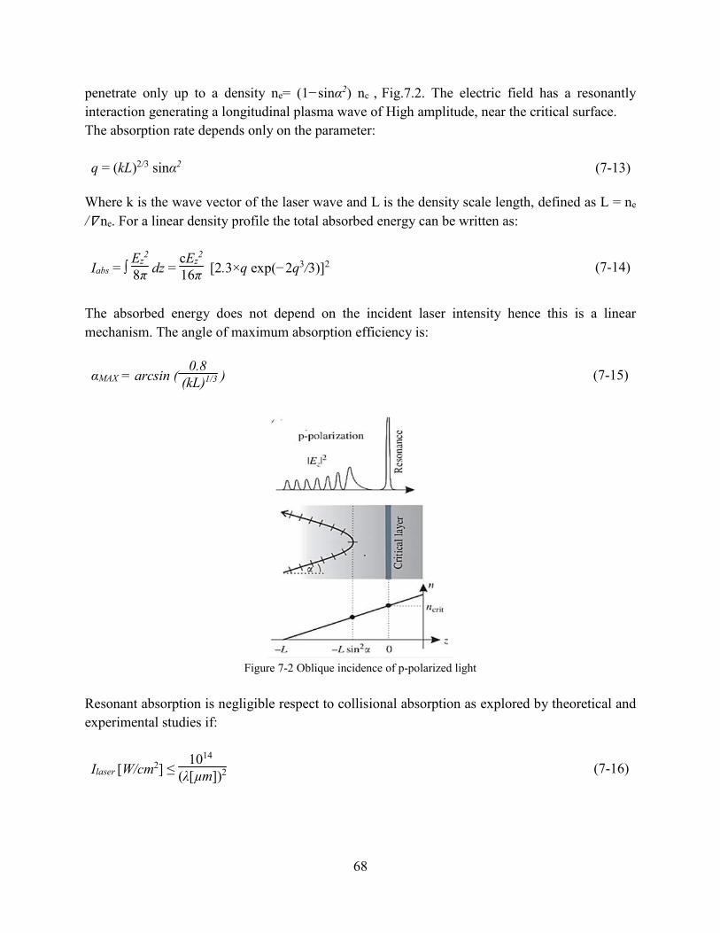
68

penetrate only up to a density ne= (1−sinα2) nc , Fig.7.2. The electric field has a resonantly

interaction generating a longitudinal plasma wave of High amplitude, near the critical surface.

The absorption rate depends only on the parameter:

q = (kL)2/3 sinα2 (7-13)

Where k is the wave vector of the laser wave and L is the density scale length, defined as L = ne

/∇ ne. For a linear density profile the total absorbed energy can be written as:

Iabs = ∫ Ez

2

8π dz = cEz

2

16π [2.3×q exp(−2q3/3)]2

(7-14)

The absorbed energy does not depend on the incident laser intensity hence this is a linear

mechanism. The angle of maximum absorption efficiency is:

αMAX = arcsin (0.8

(kL)1/3 )

(7-15)

Figure 7-2 Oblique incidence of p-polarized light

Resonant absorption is negligible respect to collisional absorption as explored by theoretical and

experimental studies if:

Ilaser [W/cm2] ≤ 1014

(λ[µm])2

(7-16)

69

Unlike inverse bremsstrahlung which thermalizes electrons the most important effect of resonant

absorption is creating large plasma electric field. Since the electric field in plasma wave is

longitudinal, they can accelerate electrons to high energies and creates hot electrons.

7.4 Nonlinear Absorption Mechanisms The initial analysis of the SI only considered collisional absorption of SI pulse in the plasma.The

excitation of nonlinear effects were ignored in standard versions of hydrodynamic codes since

there was no reliable model to completely describe their non-linear behavior (Depierreux, 2011).

Since in the SI, the laser spike intensity is above the threshold of parametric instabilities so linear

absorption mechanisms of laser light become inefficient and nonlinear processes play an important

role (Ribeyre, 2009, Batani et.al, 2014). The most important consequence of nonlinear absorption

mechanisms which attracted lots of attention is generation of hot electrons which have ambiguous

effect on shock efficiency which justifies new experiments which are performing to understand

the correlations between the hot electron production and parametric instabilities. Experiments

performed around 1980 demonstrated an increasing level of Stimulated Raman Scattering that was

correlated with production of hot electrons. After that no other results in this parameter domain

have been reported. The efficiency of nonlinear processes is proportional to the quivering electron

energy in the laser field,

εosc =e2EL2/meω0

2 (7-17)

Where EL is the laser pulse amplitude. The qualitative estimates and experiments indicate that the

parametric instabilities manifest themselves in enhanced light scattering and hot-electron

generation starting above 10 TWµm2cm−2. However, they become the dominant effect in the laser

intensities above 1PWcm−2 for the 3ω laser radiation. The inverse proportionality of the parametric

instability thresholds with the λLaser explains an interest of using the short wavelength lasers for

suppressing the nonlinear processes and enhancing the collisional absorption (Batani, et al., 2014).

In SI scheme the effects which mostly studied due to the high intensity of laser are (Klimo, 2012):

Self-focusing and filamentation (SF)

parametric instabilities: they identified by the type of waves involved which are:

Stimulated Raman Scattering (SRS)

Stimulated Scattering Brillouin (SBS)

Two Plasmon Decay (TPD)

7.4.1 Self-Focusing and Filamentation SF can modify the propagation of high intensity laser spike in the lower density part of the plasma

located in front of the absorption region and produce strong inhomogeneities, which alter the

uniformity of target compression and increase the parametric instabilities (Batani , Malka et.al,

70

2012). SF is characterized by the quantity <P>/Pc, which is the ratio of the average speckle power

to the critical power of the ponderomotive self-focusing with

Pc =34Te (keV) (nc/ne) (1−ne/nc)1/2 MW (7-18)

Which for laser intensities considered for SI is in the order of a hundred MW in front of the

absorption region (Depierreux, 2011).

7.4.2 Stimulated Raman Scattering The SRS scattering corresponds to the decay of an incident electromagnetic (e.m.) wave into

another e.m. wave and an electron plasma wave. The emitted e.m. wave is reflected with a

modified frequency spectrum and electron plasma wave is excited along the laser direction which

accelerates free electrons to high energies (hot electron generation) (Šmíd et al., 2013).

The frequency of the SRS light, ωSRS, is red shifted with respect to the laser light by the local

plasma frequency, ωpe, that is,

ωSRS= ωL −ωpe (7-19)

The e.m. waves can propagate inside a plasma only if their frequency is higher than the local

plasma frequency so both the incident and the scattered photons in the Raman process need to have

a frequency higher than ωPl. Therefore, energy conservation implies that for the incident photon

ωL ≥ 2ωPl. The local plasma frequency is related to the local electron density as

ne = meω2

Pl (x)4πe2

(7-20)

While ωL determines the critical density as:

nc = me ωL

2

4πe2

(7-21)

Thus Raman scattering can only occur in the underdense plasma, up to the layer where ne ≤ nc/4.

In particular at nc/4, the back scattered photon will have ωSRS = ωL/2. The relation between the

SRS wavelength and the plasma density is

λSRS ≈ λL[1−(ne/nc)1/2]−1 (7-22)

Thus the spectral shift of the SRS light provides information about the plasma density (Batani, et

al., 2014).

71

The physical mechanism of SRS involves the amplification of light scattered by quivering

electrons. This radiation is proportional to the local electron density. The local variation of the

light pressure is:

∇ (E2 8π ) =

EiδE4 π

(7-23)

The fields related to the scattered light will create local changes in pressure, and thus in the

ponderomotive force (i.e. the radiation pressure):

<Fpond>=−1

16 π ω2

P

ω2L ∇|E1|2

(7-24)

In this way the light is coupled with the density fluctuations δne. Electrons start to oscillate in the

electric field Ei and a current density δJ = −evδn is associated to this:

v = −(eEi)

(mωi)

(7-25)

So the initial oscillation is amplified which increase the scattering of energy, and the amplitude of

the instability also increases. We can calculate the growth rate γ in the hypothesis of a plasma wave

with ωe = ωPl :

γ = kevosc

4 (ωpl

ωL − ωpl )1/2 ~

kevosc

2

(7-26)

near nc/4. Both the plasma wave and the light wave will be damped while propagating in the

plasma. For the instability to grow, γ must exceed the losses. Considering collisional damping:

γ > ωpl

2ωs νe

(7-27)

Where νe is the collision frequency. The growth rate for Raman scattering depends only weakly

on the electron density, while the damping is very strong in underdense regions. Since the losses

are dependent from the electron density, we can correlate the instability threshold with the scale

length of the plasma. Ln:

(vosc

c ) 2 (k0Ln) 4/3 > 1

(7-28)

Which gives us a threshold intensity of ≈ 1014 W/cm2.

72

The SRS growth rates are relatively high in the plasma in front of nc/4. In the lower density plasma,

the growth of backward SRS is strongly reduced everywhere in the plasma corona by the Landau

damping of the electron plasma wave except in two small regions, near 1/4 nc and 1/16 nc

(Jacquemot, 2011). This is the characteristic of a high temperature plasma where the kinetic

parameter, kpλD, is relatively high. Here, kp is the plasma wave number and λD is the Debye

wavelength (Batani, et al., 2014).

7.4.3 Brillouin Scattering The SBS scattering is similar to Raman scattering and is corresponding to the decay of the incident

e.m. wave into another e.m. wave and ion acoustic wave. We assume the ions not fixed in space,

and can oscillate following the field of the incident e.m. wave. The absorption increases the inner

energy and causes a variation of the ion density which induces Brillouin instability.

The oscillation frequency of an acoustic wave is lower than the oscillation frequency of incident

wave and this implies that most of the energy will be absorbed by the scattered photon. The

scattered SBS photons have an equal probability of propagating in forward or backward directions.

The SBS in the backward direction is one of the principal laser energy losses in the plasma corona.

Its impact depends strongly on the velocity and temperature profiles in expanding plasmas and on

the spatial and temporal structure of the laser beam. The forward scattering, on the other hand,

may develop even below the FI threshold leads to strong beam spraying and reduces local laser

intensity, again reducing laser collisional absorption. The consequence is a large reflection of laser

radiation and the laser intensity on target decreases (Batani, et al., 2014).

Because the ion acoustic frequency is small compared with the laser frequency ωs/ω0 ∼cs/c «1 the

SBS develops in whole plasma corona up to the critical density (Batani et al., 2014) and it is

particularly effective for plasmas with a large scale length. We can write the growth rate of the

instability as:

γ0 = √32 (kL

2 vosc2 ωPi

2 /ωL)1/3

(7-29)

The gain of the SBS in an inhomogeneous plasma depends on the growth rate, on the damping of

the ionic waves and on the scale length Ln of the plasma. The spatial amplification of the scattered

waves in an inhomogeneous plasma is described by the gain factor:

G = πγ0

2 |∆kʹvsvion|

(7-30)

where vs the group velocities of the scattered, vion the ion acoustic wave and ∆kʹ is the spatial

derivative of the wave numbers of the interacting wave (near the resonant condition where ∆k =0).

The condition for the growth of the instability can be written as:

73

(vosc

ve ) 2 ≥

8kLL

(7-31)

and the threshold intensity for Brillouin scattering is then

Imin = 16cε0

2 nsc nf

γ2Ksc Kf Lsc Lf

(7-32)

where:

γ and t is constant of the material which forms the plasma

Lsc and Lf are damping length of the ion wave and e.m. wave.

nsc and nf are refraction indexes of scattered e.m. wave frequency and acoustic wave

For shock ignition regimes, it would correspond to a threshold intensity of I∼ 1014 W/cm2, which

is similar to SRS threshold intensity.

In a homogeneous plasma both the SBS and SRS instabilities are characterized by their growth

rates. They depend on the direction of the propagation of the scattered wave, and they attain the

maximum values for the backward scattering. This justifies a one-dimensional (1D) approach,

which is often used to study these instabilities (Batani et al., 2014).

7.4.4 Two Plasmon Decay In the case of TPD the incoming laser photon decays in two plasma waves traveling in

approximately opposite directions. The initial momentum is not zero but equals to photon

momentum. The two direction opposite in this reference. One of the plasma waves will travel

forwards keeping on the laser light direction, while the second one will be backscattered on the

main beam path. Energy conservation imposes that the two Plasmons must also have roughly the

same energy, with ωe1 ∼ ωe2 ∼ ωP ∼ ωL/2. TPD can only occur in the region of the plasma where

ne ∼ nc/4. The scattered light has a typical frequency of about 3/2ωL. This value depends on the

coupling of the laser wave and plasma wave. TPD usually forms in the first stages of plasma

growth before the SRS has time to develop and is finally inhibited by SRS. The threshold for the

TPD instability is related to the dumping of electronic waves and can be written as:

(vosc

ve ) 2 ≥

12kLL1/4

(7-33)

Where L1/4 is the scale length at a quarter of the critical density. The threshold intensity is

Imin ∼ 4 × 1015[W/cm2]Te[keV]

L1/4[µm]λL[µm]

(7-34)

which is ∼ 1015W/cm2 in typical SI conditions.

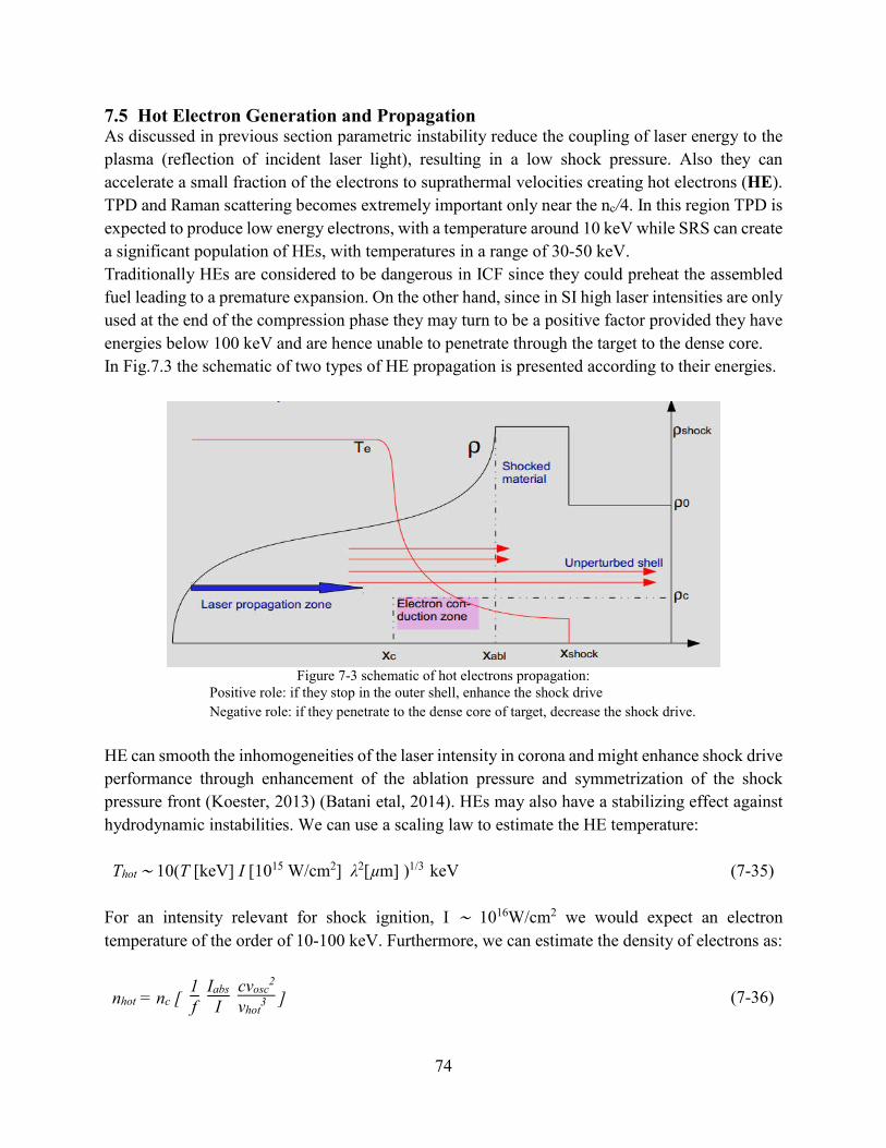
74

7.5 Hot Electron Generation and Propagation As discussed in previous section parametric instability reduce the coupling of laser energy to the

plasma (reflection of incident laser light), resulting in a low shock pressure. Also they can

accelerate a small fraction of the electrons to suprathermal velocities creating hot electrons (HE).

TPD and Raman scattering becomes extremely important only near the nc/4. In this region TPD is

expected to produce low energy electrons, with a temperature around 10 keV while SRS can create

a significant population of HEs, with temperatures in a range of 30-50 keV.

Traditionally HEs are considered to be dangerous in ICF since they could preheat the assembled

fuel leading to a premature expansion. On the other hand, since in SI high laser intensities are only

used at the end of the compression phase they may turn to be a positive factor provided they have

energies below 100 keV and are hence unable to penetrate through the target to the dense core.

In Fig.7.3 the schematic of two types of HE propagation is presented according to their energies.

Figure 7-3 schematic of hot electrons propagation:

Positive role: if they stop in the outer shell, enhance the shock drive

Negative role: if they penetrate to the dense core of target, decrease the shock drive.

HE can smooth the inhomogeneities of the laser intensity in corona and might enhance shock drive

performance through enhancement of the ablation pressure and symmetrization of the shock

pressure front (Koester, 2013) (Batani etal, 2014). HEs may also have a stabilizing effect against

hydrodynamic instabilities. We can use a scaling law to estimate the HE temperature:

Thot ∼ 10(T [keV] I [1015 W/cm2] λ2[µm] )1/3 keV (7-35)

For an intensity relevant for shock ignition, I ∼ 1016W/cm2 we would expect an electron

temperature of the order of 10-100 keV. Furthermore, we can estimate the density of electrons as:

nhot = nc [ 1f

Iabs

I cvosc

2

vhot3 ]

(7-36)

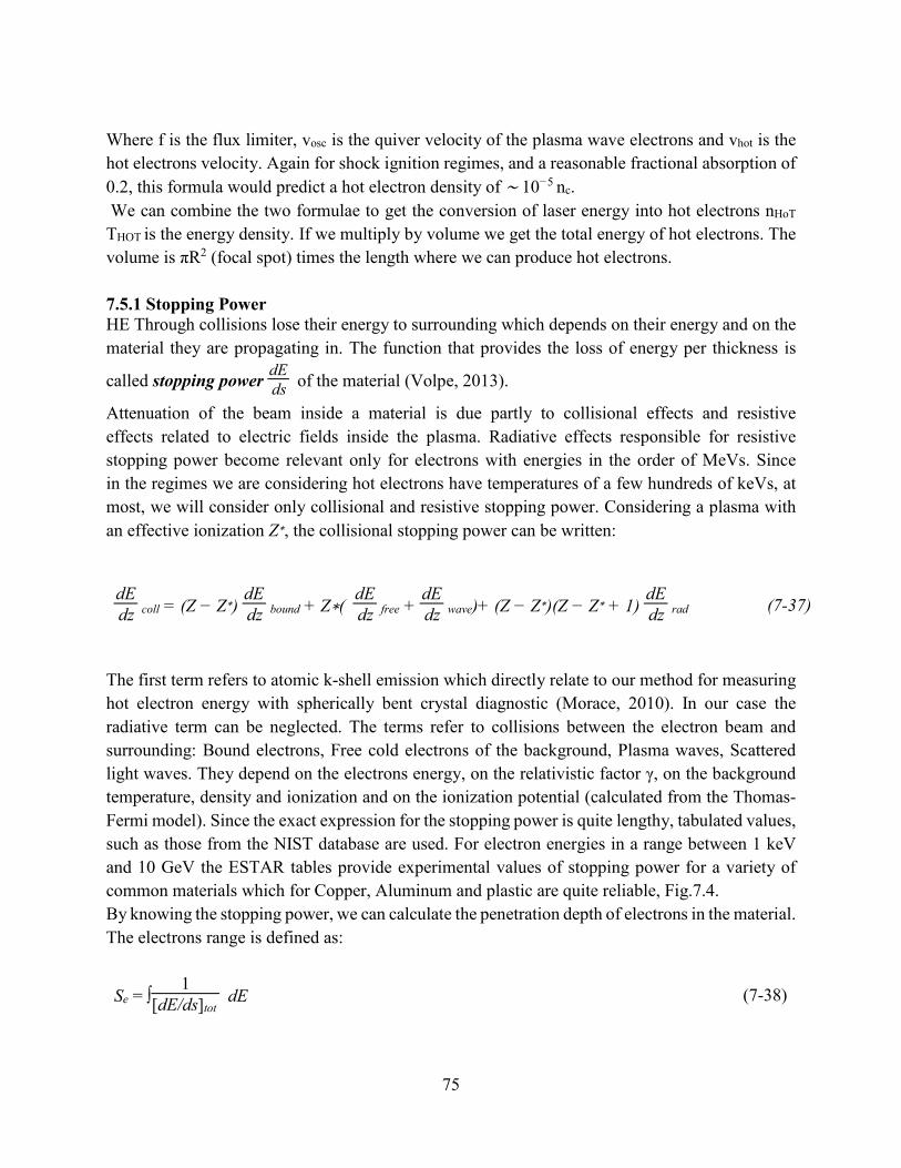
75

Where f is the flux limiter, vosc is the quiver velocity of the plasma wave electrons and vhot is the

hot electrons velocity. Again for shock ignition regimes, and a reasonable fractional absorption of

0.2, this formula would predict a hot electron density of ∼ 10−5 nc.

We can combine the two formulae to get the conversion of laser energy into hot electrons nHoT

THOT is the energy density. If we multiply by volume we get the total energy of hot electrons. The

volume is πR2 (focal spot) times the length where we can produce hot electrons.

7.5.1 Stopping Power HE Through collisions lose their energy to surrounding which depends on their energy and on the

material they are propagating in. The function that provides the loss of energy per thickness is

called stopping power dE ds

of the material (Volpe, 2013).

Attenuation of the beam inside a material is due partly to collisional effects and resistive

effects related to electric fields inside the plasma. Radiative effects responsible for resistive

stopping power become relevant only for electrons with energies in the order of MeVs. Since

in the regimes we are considering hot electrons have temperatures of a few hundreds of keVs, at

most, we will consider only collisional and resistive stopping power. Considering a plasma with

an effective ionization Z∗, the collisional stopping power can be written:

dE dz

coll = (Z − Z∗) dE dz

bound + Z∗( dE dz

free + dE dz

wave)+ (Z − Z∗)(Z − Z∗ + 1) dE dz

rad

(7-37)

The first term refers to atomic k-shell emission which directly relate to our method for measuring

hot electron energy with spherically bent crystal diagnostic (Morace, 2010). In our case the

radiative term can be neglected. The terms refer to collisions between the electron beam and

surrounding: Bound electrons, Free cold electrons of the background, Plasma waves, Scattered

light waves. They depend on the electrons energy, on the relativistic factor γ, on the background

temperature, density and ionization and on the ionization potential (calculated from the Thomas-

Fermi model). Since the exact expression for the stopping power is quite lengthy, tabulated values,

such as those from the NIST database are used. For electron energies in a range between 1 keV

and 10 GeV the ESTAR tables provide experimental values of stopping power for a variety of

common materials which for Copper, Aluminum and plastic are quite reliable, Fig.7.4.

By knowing the stopping power, we can calculate the penetration depth of electrons in the material.

The electrons range is defined as:

Se = ∫1

[dE/ds]tot dE

(7-38)

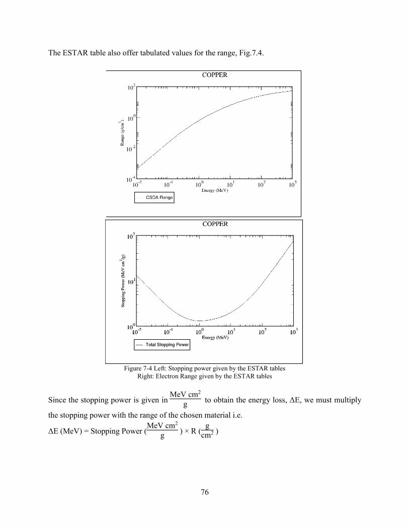
76

The ESTAR table also offer tabulated values for the range, Fig.7.4.

Figure 7-4 Left: Stopping power given by the ESTAR tables

Right: Electron Range given by the ESTAR tables

Since the stopping power is given in MeV cm2

g to obtain the energy loss, ΔE, we must multiply

the stopping power with the range of the chosen material i.e.

ΔE (MeV) = Stopping Power (MeV cm2

g ) × R (g

cm2 )

77

Also the range is given in g/cm2. To obtain the electrons penetration depth we must divide the

range to the density of the chosen material, i.e., L(cm) =

R (g

cm2 )

ρ(g

cm3 ) .

Comparing an experimental penetration depth with these values allows to retrieve the hot electrons

temperature.

7.5.2 Angular Deviation HEs can propagate inside the cold target beyond the ablation front, colliding with atoms and cold

electrons. Collisions not only cause the hot electrons lose their energy to the background, but also

change their direction of propagation (Volpe, Batani, 2013). The importance of spreading angle of

HE can be seen especially in fast igniting scheme which strongly depends on the generation,

collimation, transport, and energy deposition of HE in the over-dense region to concentrate energy

to a hot spot to start ignition (Morace, 2010). Angular diffusion is due to collisions with ions,

which can be described through the Rutherford cross section:

σRutherford=re2 Z

2

β4 1

sin4(θ/2)

(7-39)

Where θ is the incidence angle, β = v/c is the Lorentz factor and re = 1

4πε0

e2

mec2 =2.82 × 10−15 m

is the classical electron radius. We can correct this expression to include relativistic effects and

Debye screening due to the other electrons so the cross section becomes:

σ = 4 re2 Z2

γ2β4 (1

4 sin2(θ/2) + θ02 )2 with θ0 =

αZ1/3

0.885γβ

(7-40)

Where α is the fine structure constant. When the screening angle θ0 approaches zero, the formula

is reduced to the usual Rutherford cross section.

To describe propagation in a plasma however we need also to take into account the high density

of electrons and ions: hot electrons will undergo multiple collisions while propagating in a

material. It is possible to use the theory of multiple scattering by Molière (1948) to derive a mean

deviation angle for an electron of given energy crossing a material of thickness s. The angular

distribution function at the zeroth order is a Gaussian: we can take its FWHM as the quadratic

mean diffusion angle.

<θ2> = θc2 ln2 ln (

θc2

1.167 θ2M

)

(7-41)

θ2M = θ0

2 [1.13 + 3.76 (αZ β ) 2]

(7-42)

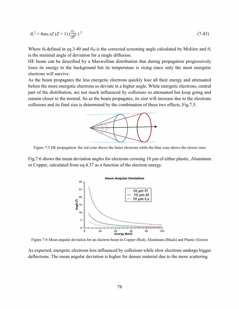
78

θc2 = 4πni sZ (Z + 1) (

re γβ2 ) 2

(7-43)

Where θ0 defined in eq.3-40 and θM is the corrected screening angle calculated by Molière and θc

is the minimal angle of deviation for a single diffusion.

HE beam can be described by a Maxwellian distribution that during propagation progressively

loses its energy to the background but its temperature is rising since only the most energetic

electrons will survive.

As the beam propagates the less energetic electrons quickly lose all their energy and attenuated

before the more energetic electrons so deviate in a higher angle. While energetic electrons, central

part of the distribution, are not much influenced by collisions so attenuated but keep going and

remain closer to the normal. So as the beam propagates, its size will increase due to the electrons

collisions and its final size is determined by the combination of these two effects, Fig.7.5.

Figure 7-5 HE propagation: the red cone shows the faster electrons while the blue cone shows the slower ones

Fig.7.6 shows the mean deviation angles for electrons crossing 10 µm of either plastic, Aluminum

or Copper, calculated from eq.4.37 as a function of the electron energy.

Figure 7-6 Mean angular deviation for an electron beam in Copper (Red), Aluminum (Black) and Plastic (Green)

As expected, energetic electrons less influenced by collisions while slow electrons undergo bigger

deflections. The mean angular deviation is higher for denser material due to the more scattering.

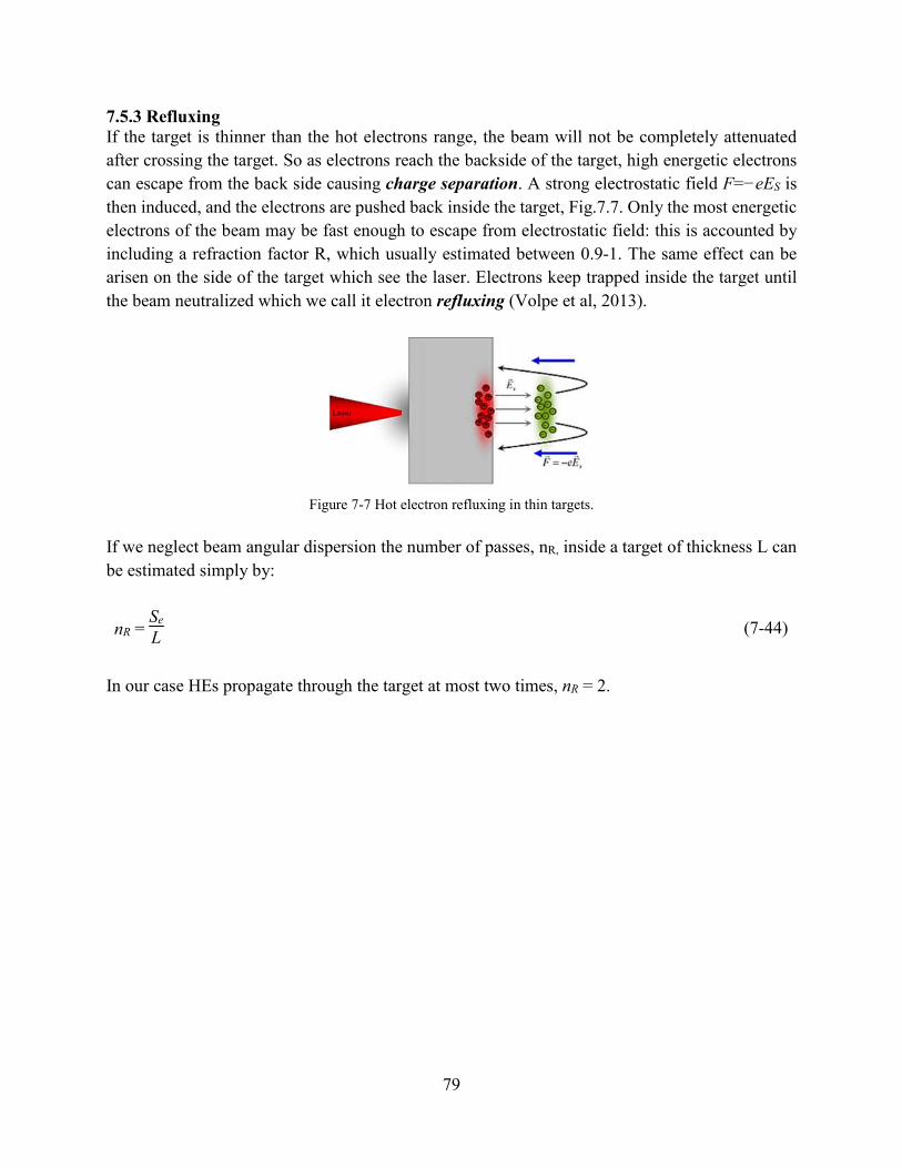
79

7.5.3 Refluxing If the target is thinner than the hot electrons range, the beam will not be completely attenuated

after crossing the target. So as electrons reach the backside of the target, high energetic electrons

can escape from the back side causing charge separation. A strong electrostatic field F=−eES is

then induced, and the electrons are pushed back inside the target, Fig.7.7. Only the most energetic

electrons of the beam may be fast enough to escape from electrostatic field: this is accounted by

including a refraction factor R, which usually estimated between 0.9-1. The same effect can be

arisen on the side of the target which see the laser. Electrons keep trapped inside the target until

the beam neutralized which we call it electron refluxing (Volpe et al, 2013).

Figure 7-7 Hot electron refluxing in thin targets.

If we neglect beam angular dispersion the number of passes, nR, inside a target of thickness L can

be estimated simply by:

nR = Se

L

(7-44)

In our case HEs propagate through the target at most two times, nR = 2.

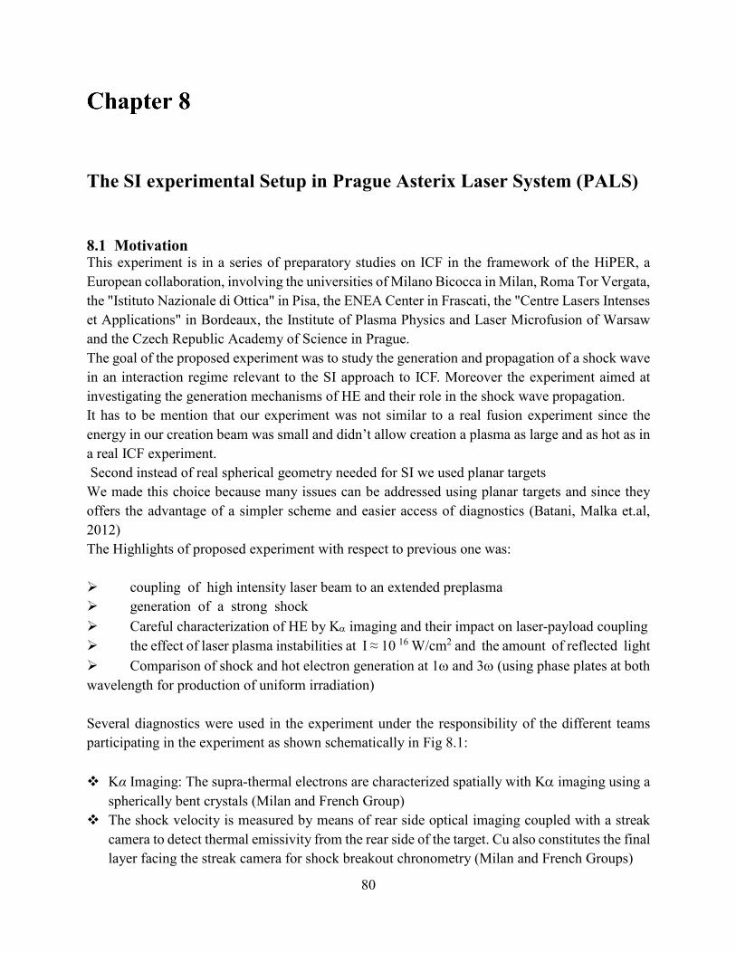
80

The SI experimental Setup in Prague Asterix Laser System (PALS)

8.1 Motivation This experiment is in a series of preparatory studies on ICF in the framework of the HiPER, a

European collaboration, involving the universities of Milano Bicocca in Milan, Roma Tor Vergata,

the "Istituto Nazionale di Ottica" in Pisa, the ENEA Center in Frascati, the "Centre Lasers Intenses

et Applications" in Bordeaux, the Institute of Plasma Physics and Laser Microfusion of Warsaw

and the Czech Republic Academy of Science in Prague.

The goal of the proposed experiment was to study the generation and propagation of a shock wave

in an interaction regime relevant to the SI approach to ICF. Moreover the experiment aimed at

investigating the generation mechanisms of HE and their role in the shock wave propagation.

It has to be mention that our experiment was not similar to a real fusion experiment since the

energy in our creation beam was small and didn’t allow creation a plasma as large and as hot as in

a real ICF experiment.

Second instead of real spherical geometry needed for SI we used planar targets

We made this choice because many issues can be addressed using planar targets and since they

offers the advantage of a simpler scheme and easier access of diagnostics (Batani, Malka et.al,

2012)

The Highlights of proposed experiment with respect to previous one was:

coupling of high intensity laser beam to an extended preplasma

generation of a strong shock

Careful characterization of HE by K imaging and their impact on laser-payload coupling

the effect of laser plasma instabilities at I ≈ 10 16 W/cm2 and the amount of reflected light

Comparison of shock and hot electron generation at 1 and 3 (using phase plates at both

wavelength for production of uniform irradiation)

Several diagnostics were used in the experiment under the responsibility of the different teams

participating in the experiment as shown schematically in Fig 8.1:

Kα Imaging: The supra-thermal electrons are characterized spatially with K imaging using a

spherically bent crystals (Milan and French Group)

The shock velocity is measured by means of rear side optical imaging coupled with a streak

camera to detect thermal emissivity from the rear side of the target. Cu also constitutes the final

layer facing the streak camera for shock breakout chronometry (Milan and French Groups)

81

Back-scattering light Diagnostics: The back-scattered radiation due to SRS and SBS,

calorimetry and spectroscopy of the scattered radiation. In this experiment, SRS was measured

because it could be one of the main source of hot electron generation (Pisa Group).

Optical Interferometry: Interferometry is employed for the characterization of plasma and

preplasma density at different stages of the plasma expansion (Polish Group).

High-resolution X-Ray Spectroscopy: X-ray spectroscopy with bent crystals was also

performed to get information on the plasma temperature and density by thermal shift of the

spectra from Chlorine-doped targets (Czech Group).

X-ray pin-hole camera to contribute to provide an estimation of plasma (and focal spot) size

(Pisa Group).

Ion Collectors: time-of flight detectors used to measure heavy ions emission (Polish Group).

Figure 8-1 the setup of PALS experiment with diagnostics used in the campaign (koester et el., 2013)

8.2 Prague Asterix Laser System The oscillator of PALS Iodine Laser produces a 220 mJ pulse, which travels through a chain of

five power amplifiers that can deliver up to 1 kJ of energy. A KDP crystal can convert the radiation

to 438 nm (3ω). In our case we used two laser beams:

Auxiliary beam The auxiliary beam (wavelength 1315 nm at 1ω, energy up to 100 J, pulse

duration 250 ps) is extracted from the third amplifier to create a long-scale plasma before the

arrival of the main laser pulse. It focused to the target with Gaussian focal spot (≈900 µm) and

intensity I ≈1013 W/cm2 in an angle of 30° from target normal in the vertical direction.

82

Main beam The full power beam after 5 stages of amplification is used to launch a shock wave by PALS main laser beam (λ= 1315 nm/438 nm, energy 440/170J, 9×1015/2×1016 W/cm2 ,pulse duration 300/250 ps, 1ω /3ω) which focused to the target with Gaussian focal spot 100µm. The intensity of the main laser pulse was varied by changing laser pulse energy, whereas pulse duration and focal spot size were kept fixed throughout the experiment. The main pulse shined to the preplasma with delays Δt = 0, 350, 600 and 1200 ps. The PALS oscillator produces a train pulses separated by 8 ns. A single pulse is extracted by a

Pockels cell to be sent to the amplification chain. Due to a synchronization mismatch of the Pockels

cell, also a small part of the previous impulse is amplified, creating a small prepulse 8 ns before

the main beam. (Batani, Malka et.al, 2012)

8.3 Random Phase Plate The focal spot of high energy laser beams has a highly irregular shape, with more than one hot

spot, Fig 8.2.

Figure 8-2 Images of the focal spot (left) without a phase plate (right) with a phase plate

So the intensity distribution on target would be far from uniform causing Self-focusing, SF, as

already discussed in third chapter. SF causes a non-uniform compression, creating areas with

different densities inside the plasma. Hence the incoming photons can scatter against the density

fluctuations, giving rise to SBS.

The technique of laser beam smoothing employed by putting the phase plate in the main beam path

to suppress the global beam self-focusing and ensure a better focal spot uniformity. It has been

shown experimentally that an increased smoothness of the laser profile can greatly reduce the

amount of backscattered radiation, bringing it from 10% to ≤ 1% for an initial intensity of 1015

W/cm2 (Batani et al., 2014). On a few shots, the phase plate on the main beam was removed to

reach higher intensities (up to 3×1016 Wcm−2) in a focal spot with diameter∼60µm.

8.4 Targets We used two types of targets consisted of Copper, plastic and Aluminum with different thickness.

The metal layers were deposited and plastic glued onto the metal. In some targets we used CHCl

layers as first layer which made of Chlorine doped plastic (Parylene-C, C8H7Cl) with different

thickness of 25 µm or 40 µm which doped with Cl for the X-ray spectroscopic measurements to

estimate plasma temperature. The CH layer was used to mimic the low-Z ablator material of ICF

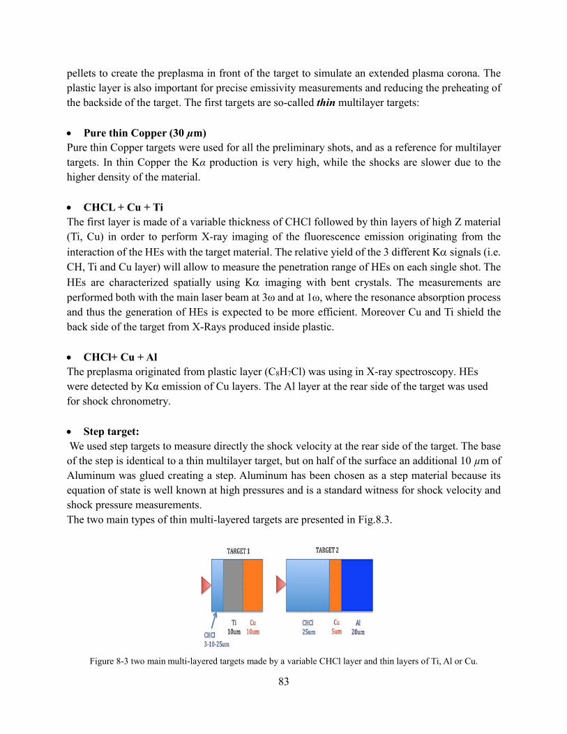
83

pellets to create the preplasma in front of the target to simulate an extended plasma corona. The

plastic layer is also important for precise emissivity measurements and reducing the preheating of

the backside of the target. The first targets are so-called thin multilayer targets:

Pure thin Copper (30 µm)

Pure thin Copper targets were used for all the preliminary shots, and as a reference for multilayer

targets. In thin Copper the Kα production is very high, while the shocks are slower due to the

higher density of the material.

CHCL + Cu + Ti

The first layer is made of a variable thickness of CHCl followed by thin layers of high Z material

(Ti, Cu) in order to perform X-ray imaging of the fluorescence emission originating from the

interaction of the HEs with the target material. The relative yield of the 3 different K signals (i.e.

CH, Ti and Cu layer) will allow to measure the penetration range of HEs on each single shot. The

HEs are characterized spatially using K imaging with bent crystals. The measurements are

performed both with the main laser beam at 3ω and at 1ω, where the resonance absorption process

and thus the generation of HEs is expected to be more efficient. Moreover Cu and Ti shield the

back side of the target from X-Rays produced inside plastic.

CHCl+ Cu + Al

The preplasma originated from plastic layer (C8H7Cl) was using in X-ray spectroscopy. HEs

were detected by Kα emission of Cu layers. The Al layer at the rear side of the target was used

for shock chronometry.

Step target:

We used step targets to measure directly the shock velocity at the rear side of the target. The base

of the step is identical to a thin multilayer target, but on half of the surface an additional 10 µm of

Aluminum was glued creating a step. Aluminum has been chosen as a step material because its

equation of state is well known at high pressures and is a standard witness for shock velocity and

shock pressure measurements.

The two main types of thin multi-layered targets are presented in Fig.8.3.

Figure 8-3 two main multi-layered targets made by a variable CHCl layer and thin layers of Ti, Al or Cu.

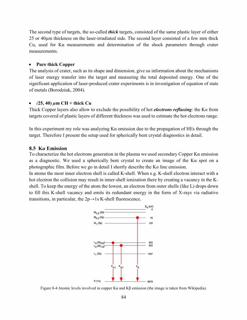
84

The second type of targets, the so-called thick targets, consisted of the same plastic layer of either

25 or 40µm thickness on the laser-irradiated side. The second layer consisted of a few mm thick

Cu, used for Kα measurements and determination of the shock parameters through crater

measurements.

Pure thick Copper

The analysis of crater, such as its shape and dimension, give us information about the mechanisms

of laser energy transfer into the target and measuring the total deposited energy. One of the

significant application of laser-produced crater experiments is in investigation of equation of state

of metals (Borodziuk, 2004).

(25, 40) µm CH + thick Cu

Thick Copper layers also allow to exclude the possibility of hot electrons refluxing: the Kα from

targets covered of plastic layers of different thickness was used to estimate the hot electrons range.

In this experiment my role was analyzing Kα emission due to the propagation of HEs through the

target. Therefore I present the setup used for spherically bent crystal diagnostics in detail.

8.5 Kα Emission To characterize the hot electrons generation in the plasma we used secondary Copper Kα emission

as a diagnostic. We used a spherically bent crystal to create an image of the Kα spot on a

photographic film. Before we go in detail I shortly describe the Kα line emission.

In atoms the most inner electron shell is called K-shell. When e.g. K-shell electron interact with a

hot electron the collision may result in inner-shell ionization there by creating a vacancy in the K-

shell. To keep the energy of the atom the lowest, an electron from outer shells (like L) drops down

to fill this K-shell vacancy and emits its redundant energy in the form of X-rays via radiative

transitions, in particular, the 2p→1s K-shell fluorescence.

Figure 8-4 Atomic levels involved in copper Kα and Kβ emission (the image is taken from Wikipedia).

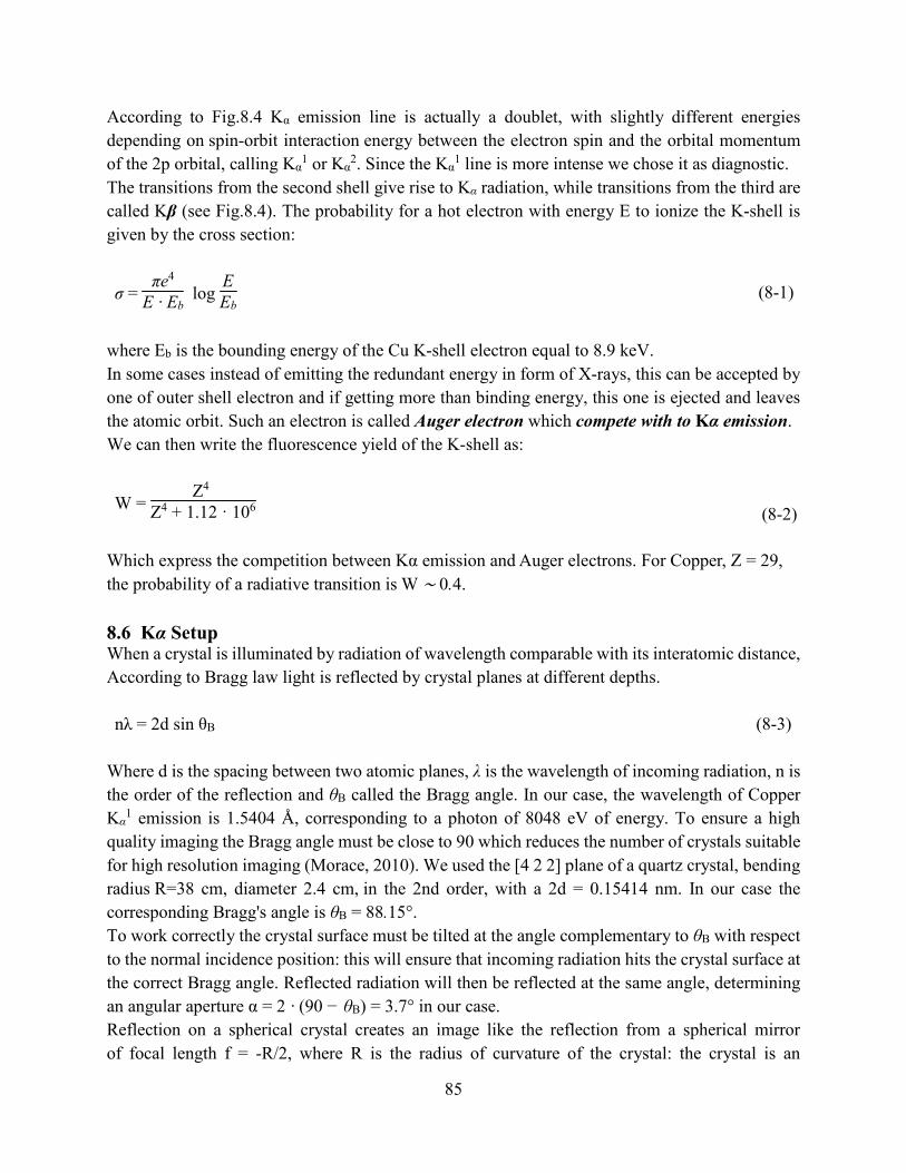
85

According to Fig.8.4 Kα emission line is actually a doublet, with slightly different energies

depending on spin-orbit interaction energy between the electron spin and the orbital momentum

of the 2p orbital, calling Kα1 or Kα

2. Since the Kα1 line is more intense we chose it as diagnostic.

The transitions from the second shell give rise to Kα radiation, while transitions from the third are

called Kβ (see Fig.8.4). The probability for a hot electron with energy E to ionize the K-shell is

given by the cross section:

σ = πe4

E · Eb log

EEb

(8-1)

where Eb is the bounding energy of the Cu K-shell electron equal to 8.9 keV.

In some cases instead of emitting the redundant energy in form of X-rays, this can be accepted by

one of outer shell electron and if getting more than binding energy, this one is ejected and leaves

the atomic orbit. Such an electron is called Auger electron which compete with to Kα emission.

We can then write the fluorescence yield of the K-shell as:

W = Z4

Z4 + 1.12 · 106

(8-2)

Which express the competition between Kα emission and Auger electrons. For Copper, Z = 29,

the probability of a radiative transition is W ∼ 0.4.

8.6 Kα Setup When a crystal is illuminated by radiation of wavelength comparable with its interatomic distance,

According to Bragg law light is reflected by crystal planes at different depths.

nλ = 2d sin θB (8-3)

Where d is the spacing between two atomic planes, λ is the wavelength of incoming radiation, n is

the order of the reflection and θB called the Bragg angle. In our case, the wavelength of Copper

Kα1 emission is 1.5404 Å, corresponding to a photon of 8048 eV of energy. To ensure a high

quality imaging the Bragg angle must be close to 90 which reduces the number of crystals suitable

for high resolution imaging (Morace, 2010). We used the [4 2 2] plane of a quartz crystal, bending

radius R=38 cm, diameter 2.4 cm, in the 2nd order, with a 2d = 0.15414 nm. In our case the

corresponding Bragg's angle is θB = 88.15°.

To work correctly the crystal surface must be tilted at the angle complementary to θB with respect

to the normal incidence position: this will ensure that incoming radiation hits the crystal surface at

the correct Bragg angle. Reflected radiation will then be reflected at the same angle, determining

an angular aperture α = 2 · (90 − θB) = 3.7° in our case.

Reflection on a spherical crystal creates an image like the reflection from a spherical mirror

of focal length f = -R/2, where R is the radius of curvature of the crystal: the crystal is an

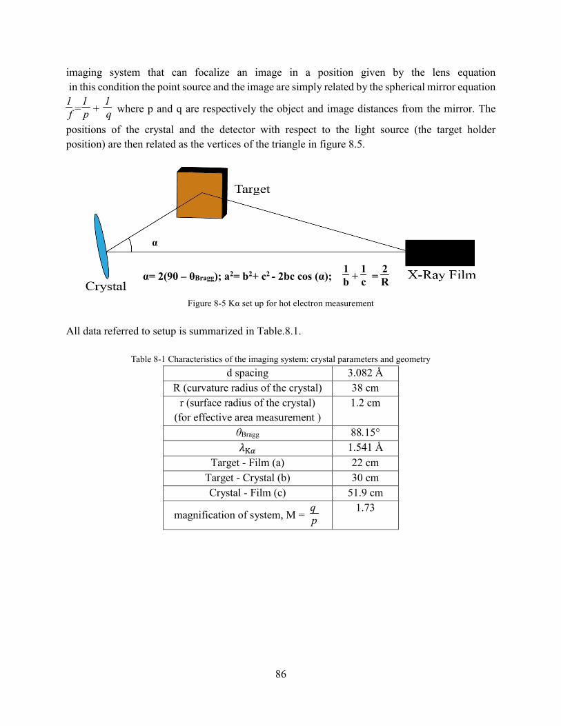
86

imaging system that can focalize an image in a position given by the lens equation

in this condition the point source and the image are simply related by the spherical mirror equation

1 f =

1 p +

1 q where p and q are respectively the object and image distances from the mirror. The

positions of the crystal and the detector with respect to the light source (the target holder

position) are then related as the vertices of the triangle in figure 8.5.

Figure 8-5 Kα set up for hot electron measurement

All data referred to setup is summarized in Table.8.1.

Table 8-1 Characteristics of the imaging system: crystal parameters and geometry

d spacing 3.082 Å

R (curvature radius of the crystal) 38 cm

r (surface radius of the crystal)

(for effective area measurement )

1.2 cm

θBragg 88.15°

�� 1.541 Å

Target - Film (a) 22 cm

Target - Crystal (b) 30 cm

Crystal - Film (c) 51.9 cm

magnification of system, M = q p

1.73

α

α= 2(90 – θBragg); a2= b2+ c2 - 2bc cos (α); 1b

+ 1c =

2R

87

Experimental Results

9.1 Introduction In this chapter I present the experimental results related to the generation of hot electrons (HEs)

obtained in the shock ignition experiment at PALS.

In this experiment we used two laser beams: the first one to create an extended plasma corona and

the second one to create the strong shock. Moreover we used different targets with different

thickness. Fig.9.1 shows a schematic view of one of the experimental thin multi-layer targets.

Figure 9-1 The Schematic view of one of the experimental thin multi-layer targets.

9.2 Analysis of Kα Images In our experiment the Kα emission due to the HE propagation inside the target was detected by

using diagnostics based on the spherically bent crystals. Observing kα emission from Ti layer

provides the evidence of HEs crossing this layer. Similarly, observing Kα emission from the Cu

layer implied electrons with energy large enough to cross the Cu layer.

Kα emission from the Ti and Cu layers were imaged by the spherically bent crystals on an X-ray

film placed in the image plate. A typical image is shown in Fig.9.2.

Figure 9-2 Typical Cu Kα spot (black spot) as imprinted on the X-Ray film (Left) with more detail in (Right).

Main Beam 1ω or 3ω

With Phase Plate 1016 W/cm2

Creation Beam With Phase Plate

1ω 1013 W/cm2

To Kα imaging

CHCl Ti Cu 3-10-25 μm 10μm 10μm

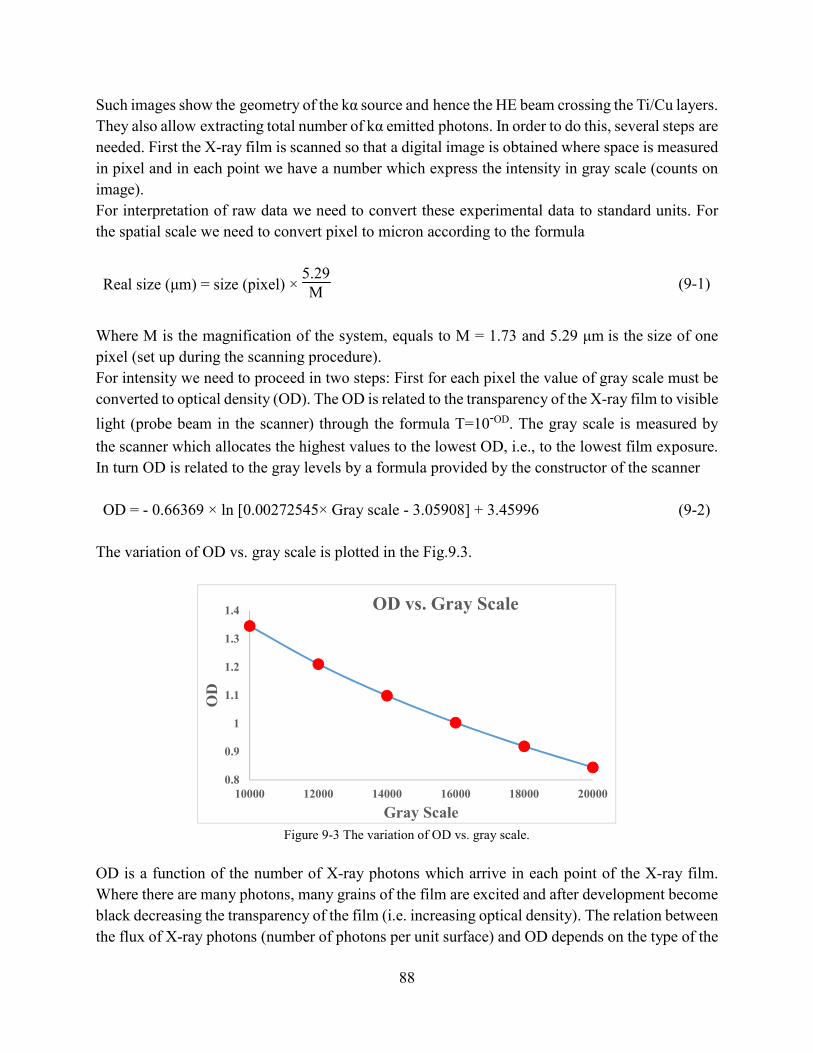
88

Such images show the geometry of the kα source and hence the HE beam crossing the Ti/Cu layers.

They also allow extracting total number of kα emitted photons. In order to do this, several steps are

needed. First the X-ray film is scanned so that a digital image is obtained where space is measured

in pixel and in each point we have a number which express the intensity in gray scale (counts on

image).

For interpretation of raw data we need to convert these experimental data to standard units. For

the spatial scale we need to convert pixel to micron according to the formula

Real size (μm) = size (pixel) × 5.29M

(9-1)

Where M is the magnification of the system, equals to M = 1.73 and 5.29 μm is the size of one

pixel (set up during the scanning procedure).

For intensity we need to proceed in two steps: First for each pixel the value of gray scale must be

converted to optical density (OD). The OD is related to the transparency of the X-ray film to visible

light (probe beam in the scanner) through the formula T=10-OD. The gray scale is measured by

the scanner which allocates the highest values to the lowest OD, i.e., to the lowest film exposure.

In turn OD is related to the gray levels by a formula provided by the constructor of the scanner

OD = - 0.66369 × ln [0.00272545× Gray scale - 3.05908] + 3.45996 (9-2)

The variation of OD vs. gray scale is plotted in the Fig.9.3.

Figure 9-3 The variation of OD vs. gray scale.

OD is a function of the number of X-ray photons which arrive in each point of the X-ray film.

Where there are many photons, many grains of the film are excited and after development become

black decreasing the transparency of the film (i.e. increasing optical density). The relation between

the flux of X-ray photons (number of photons per unit surface) and OD depends on the type of the

0.8

0.9

1

1.1

1.2

1.3

1.4

10000 12000 14000 16000 18000 20000

OD

Gray Scale

OD vs. Gray Scale

89

x-ray film according to specification given by the manufacturer. The X-ray film used in our

experiment (Kodak Industrex AA400 film) are digitized with the scanner providing the spatial

resolution of 5.29×5.29 μm2 per pixel. The relation between OD and the number of incident

photons per unit surface is:

y (NPhs/μm2) = 0.03227 + (1.09072×OD) + (0.34771×OD2)-(0.03272×OD3)

(9-3)

The variation of the NPhs/μm2 vs. OD is plotted in Fig.9.4.

Figure 9-4 The variation of the y (NPhs/μm2) vs. OD.

It has to be mention that these formulae can be used when the film is not saturated. At the end of

this procedure we have a digital image where the spectral scale in μm and the y scale is the number

of X-ray photons incident on the pixel size.

We can now plot the profile of the kα spot along one axis going through its center. Such profile

has a typical Gaussian shape as shown in Fig.9.5.

y = a + (b-a) × exp (- (x-c) 2

2d2 )

(9-4)

a = Min value of NPhs/μm2

b = Max value of NPhs/μm2

c = Center of Gaussian curve

d = Standard Deviation

Here the parameter b represents the noise, i.e. the gray level which is obtained even when no X-

Ray photon hits the film.

0

0.5

1

1.5

2

2.5

3

3.5

4

0 0.5 1 1.5 2 2.5

y (N

Ph

s/μ

m^

2)

OD

NPhs vs. OD

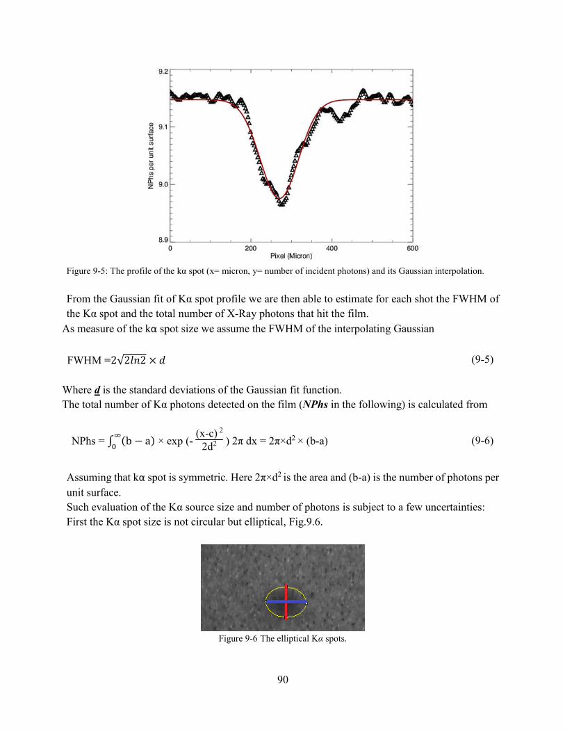
90

Figure 9-5: The profile of the kα spot (x= micron, y= number of incident photons) and its Gaussian interpolation.

From the Gaussian fit of Kα spot profile we are then able to estimate for each shot the FWHM of

the Kα spot and the total number of X-Ray photons that hit the film.

As measure of the kα spot size we assume the FWHM of the interpolating Gaussian

FWHM =2√2��2 × � (9-5)

Where d is the standard deviations of the Gaussian fit function.

The total number of Kα photons detected on the film (NPhs in the following) is calculated from

NPhs = ∫ (b − a)�

� × exp (-

(x-c) 2

2d2 ) 2π dx = 2π×d2 × (b-a)

(9-6)

Assuming that kα spot is symmetric. Here 2π×d2 is the area and (b-a) is the number of photons per

unit surface.

Such evaluation of the Kα source size and number of photons is subject to a few uncertainties:

First the Kα spot size is not circular but elliptical, Fig.9.6.

Figure 9-6 The elliptical Kα spots.

91

The elliptical shape corresponds to an oblique line of sight of the imager observing the target

surface at the angle of ~ 45°. Therefore a circle become an ellipse. So Kα source sizes in horizontal

direction are approximately 1.5 times bigger than those in vertical direction. We therefore take as

true measure of the Kα spot size the minor axis of the ellipse which is of course not affected by

the viewing angle. We chose vertical direction for our measurement.

Second the measured Kα source size can be bigger than is really due to optical aberrations of the

imaging system (Morace & Batani, 2010).The number of photons impinging on the film is instead

not affected by the optical aberration which just spread the same photons over a larger area.

Another problem is related to the analysis of images. In principle we should take a very fine strip

along the Kα spot to have a precise representation of the profile (as shown in Fig.9.6).

If the stripe is thin we pass precisely through the center but the profile will be noisy. If the stripe

is large we do an average. The profile will be less noisy but less close to real. So one must find a

good compromise.

To show the effect of the strip width on the Gaussian function parameters I increased smoothly the

width of the strip to cover the spot. The result for two different shots are summarized in Table.9.1.

Table 9-1 The effect of the strip width on the Kα source size and NPhs via parameters (a-b) and d of the Gaussian

function for two different shots.

Shot-104 Shot-118

Strip Width Kα source NPhs (a-b) d

Size (μm)

Kα source NPhs (a-b) d

Size (μm)

1 93.4 4056 0.40 39.7 113.3 6046 0.42 48.0

10 108.1 4982 0.38 45.9 120.8 6523 0.39 51.3

20 112.0 5247 0.37 47.6 122.0 6446 0.38 51.8

30 110.8 4973 0.36 47.0 122.3 6221 0.37 51.9

40 112.5 4752 0.33 47.8 121.5 5882 0.35 51.6

50 114.0 4550 0.31 48.4 123.0 5626 0.33 52.2

60 115.5 4217 0.28 49.0 123.9 5300 0.30 52.6

70 117.8 3961 0.25 50.0 125.4 4918 0.28 53.3

80 119 36867 0.23 50.5 126.7 4595 0.25 53.8

90 119.7 3432 0.21 50.8 128.8 4324 0.23 54.7

100 119.7 3197 0.20 50.8 133.5 4144 0.21 56.7

For each width the parameters of Gaussian function change and we have a set of a, b and d. As we

can see by increasing the width of the strip the Kα source sizes increase due to the increasing of

standard deviation (d) but NPhs decrease due to the decreasing of (a-b)×d2. Hence one should

select the size which covers the Kα spot precisely, i.e., the one small enough not to change the

profile but large enough not to cause too large noise.

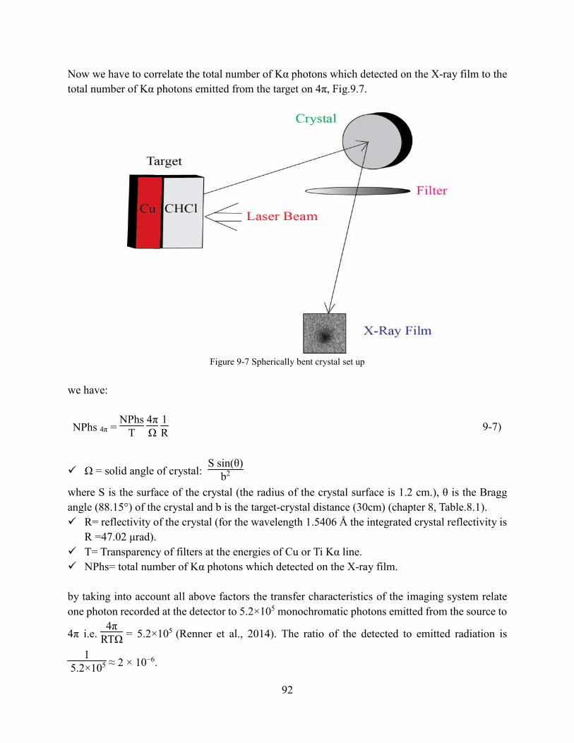
92

Now we have to correlate the total number of Kα photons which detected on the X-ray film to the

total number of Kα photons emitted from the target on 4π, Fig.9.7.

Figure 9-7 Spherically bent crystal set up

we have:

NPhs 4π = NPhs

T 4πΩ

1R

9-7)

Ω = solid angle of crystal: S sin(θ)

b2

where S is the surface of the crystal (the radius of the crystal surface is 1.2 cm.), θ is the Bragg

angle (88.15°) of the crystal and b is the target-crystal distance (30cm) (chapter 8, Table.8.1).

R= reflectivity of the crystal (for the wavelength 1.5406 Å the integrated crystal reflectivity is

R =47.02 μrad).

T= Transparency of filters at the energies of Cu or Ti Kα line.

NPhs= total number of Kα photons which detected on the X-ray film.

by taking into account all above factors the transfer characteristics of the imaging system relate

one photon recorded at the detector to 5.2×105 monochromatic photons emitted from the source to

4π i.e. 4π

RTΩ = 5.2×105 (Renner et al., 2014). The ratio of the detected to emitted radiation is

1 5.2×105 ≈ 2 × 10−6.

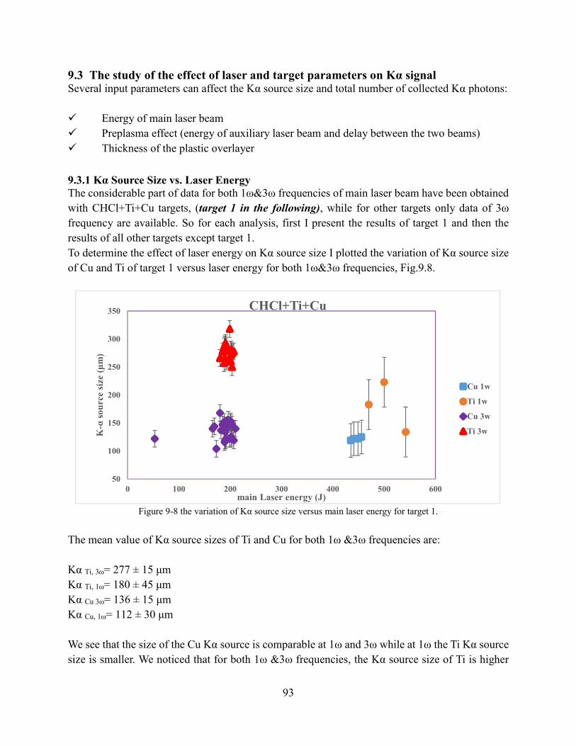
93

9.3 The study of the effect of laser and target parameters on Kα signal Several input parameters can affect the Kα source size and total number of collected Kα photons:

Energy of main laser beam

Preplasma effect (energy of auxiliary laser beam and delay between the two beams)

Thickness of the plastic overlayer

9.3.1 Kα Source Size vs. Laser Energy The considerable part of data for both 1ω&3ω frequencies of main laser beam have been obtained

with CHCl+Ti+Cu targets, (target 1 in the following), while for other targets only data of 3ω

frequency are available. So for each analysis, first I present the results of target 1 and then the

results of all other targets except target 1.

To determine the effect of laser energy on Kα source size I plotted the variation of Kα source size

of Cu and Ti of target 1 versus laser energy for both 1ω&3ω frequencies, Fig.9.8.

Figure 9-8 the variation of Kα source size versus main laser energy for target 1.

The mean value of Kα source sizes of Ti and Cu for both 1ω &3ω frequencies are:

Kα Ti, 3ω= 277 ± 15 μm

Kα Ti, 1ω= 180 ± 45 μm

Kα Cu 3ω= 136 ± 15 μm

Kα Cu, 1ω= 112 ± 30 μm

We see that the size of the Cu Kα source is comparable at 1ω and 3ω while at 1ω the Ti Kα source

size is smaller. We noticed that for both 1ω &3ω frequencies, the Kα source size of Ti is higher

50

100

150

200

250

300

350

0 100 200 300 400 500 600

K-α

sou

rce

size

(μ

m)

main Laser energy (J)

CHCl+Ti+Cu

Cu 1w

Ti 1w

Cu 3w

Ti 3w

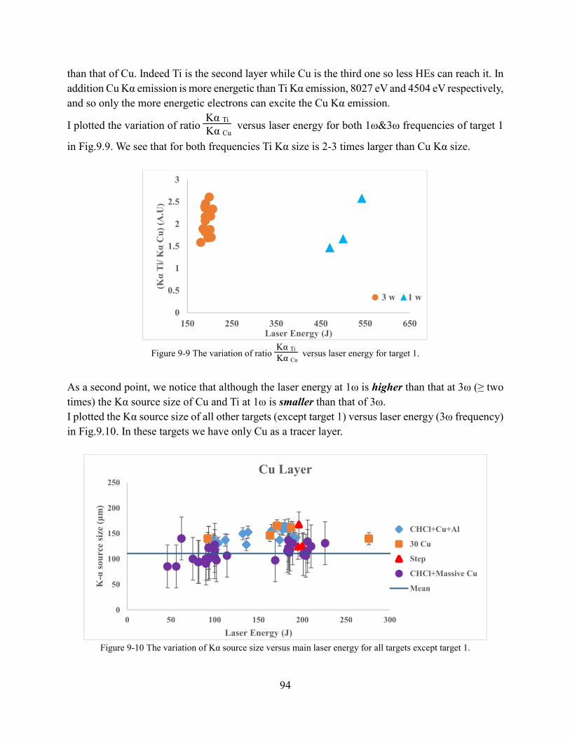
94

than that of Cu. Indeed Ti is the second layer while Cu is the third one so less HEs can reach it. In

addition Cu Kα emission is more energetic than Ti Kα emission, 8027 eV and 4504 eV respectively,

and so only the more energetic electrons can excite the Cu Kα emission.

I plotted the variation of ratio Kα Ti

Kα Cu versus laser energy for both 1ω&3ω frequencies of target 1

in Fig.9.9. We see that for both frequencies Ti Kα size is 2-3 times larger than Cu Kα size.

Figure 9-9 The variation of ratio Kα Ti

Kα Cu versus laser energy for target 1.

As a second point, we notice that although the laser energy at 1ω is higher than that at 3ω (≥ two

times) the Kα source size of Cu and Ti at 1ω is smaller than that of 3ω.

I plotted the Kα source size of all other targets (except target 1) versus laser energy (3ω frequency)

in Fig.9.10. In these targets we have only Cu as a tracer layer.

Figure 9-10 The variation of Kα source size versus main laser energy for all targets except target 1.

0

0.5

1

1.5

2

2.5

3

150 250 350 450 550 650

(Kα

Ti/

Kα

Cu

) (A

.U)

Laser Energy (J)

3 w 1 w

0

50

100

150

200

250

0 50 100 150 200 250 300

K-α

so

urc

e si

ze (

μm

)

Laser Energy (J)

Cu Layer

CHCl+Cu+Al

30 Cu

Step

CHCl+Massive Cu

Mean

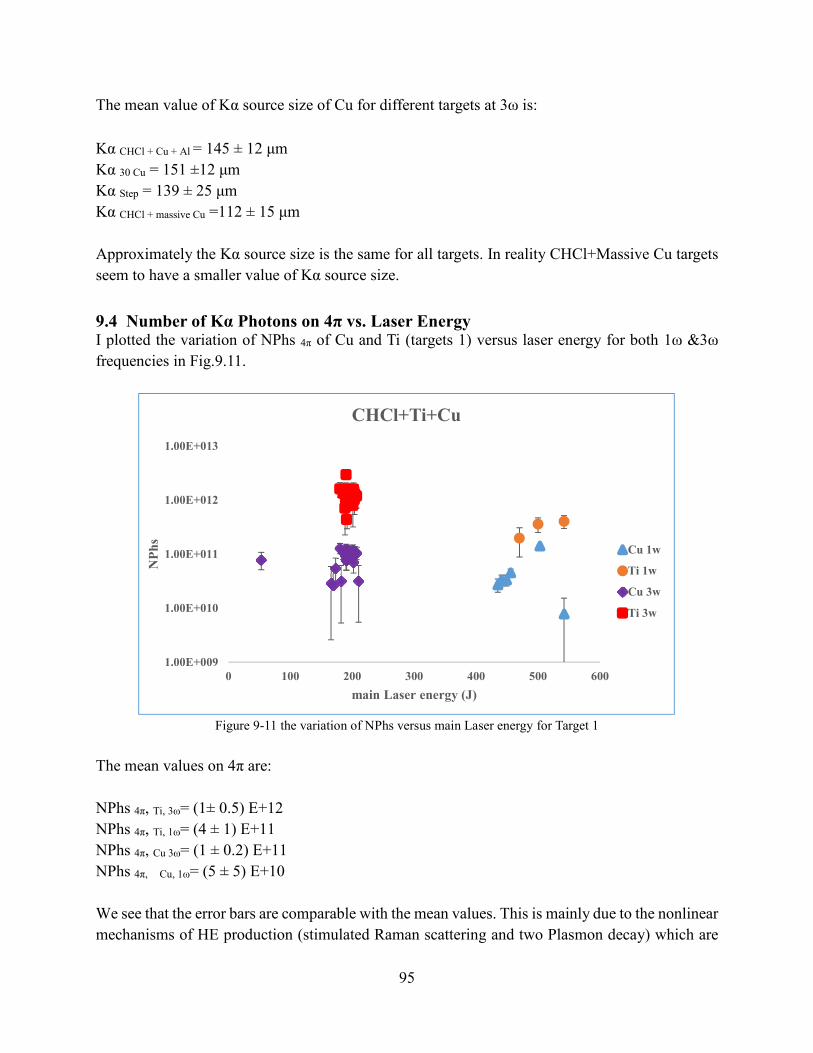
95

The mean value of Kα source size of Cu for different targets at 3ω is:

Kα CHCl + Cu + Al = 145 ± 12 μm

Kα 30 Cu = 151 ±12 μm

Kα Step = 139 ± 25 μm

Kα CHCl + massive Cu =112 ± 15 μm

Approximately the Kα source size is the same for all targets. In reality CHCl+Massive Cu targets

seem to have a smaller value of Kα source size.

9.4 Number of Kα Photons on 4π vs. Laser Energy I plotted the variation of NPhs 4π of Cu and Ti (targets 1) versus laser energy for both 1ω &3ω

frequencies in Fig.9.11.

Figure 9-11 the variation of NPhs versus main Laser energy for Target 1

The mean values on 4π are:

NPhs 4π, Ti, 3ω= (1± 0.5) E+12

NPhs 4π, Ti, 1ω= (4 ± 1) E+11

NPhs 4π, Cu 3ω= (1 ± 0.2) E+11

NPhs 4π, Cu, 1ω= (5 ± 5) E+10

We see that the error bars are comparable with the mean values. This is mainly due to the nonlinear

mechanisms of HE production (stimulated Raman scattering and two Plasmon decay) which are

1.00E+009

1.00E+010

1.00E+011

1.00E+012

1.00E+013

0 100 200 300 400 500 600

NP

hs

main Laser energy (J)

CHCl+Ti+Cu

Cu 1w

Ti 1w

Cu 3w

Ti 3w

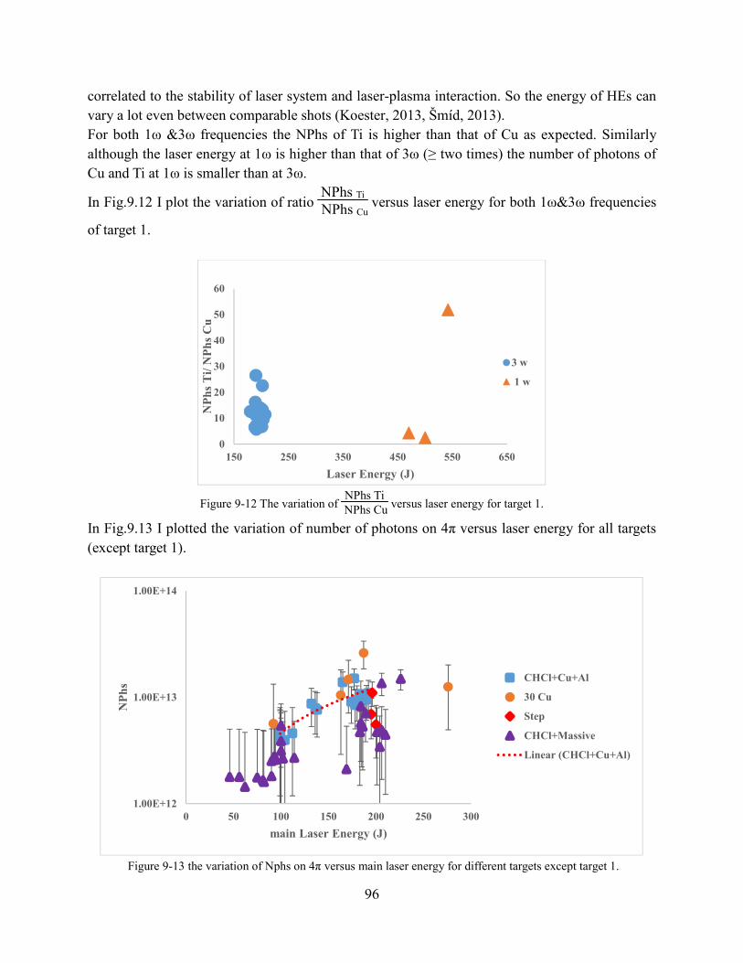
96

correlated to the stability of laser system and laser-plasma interaction. So the energy of HEs can

vary a lot even between comparable shots (Koester, 2013, Šmíd, 2013).

For both 1ω &3ω frequencies the NPhs of Ti is higher than that of Cu as expected. Similarly

although the laser energy at 1ω is higher than that of 3ω (≥ two times) the number of photons of

Cu and Ti at 1ω is smaller than at 3ω.

In Fig.9.12 I plot the variation of ratio NPhs Ti

NPhs Cu versus laser energy for both 1ω&3ω frequencies

of target 1.

Figure 9-12 The variation of NPhs Ti

NPhs Cu versus laser energy for target 1.

In Fig.9.13 I plotted the variation of number of photons on 4π versus laser energy for all targets

(except target 1).

Figure 9-13 the variation of Nphs on 4π versus main laser energy for different targets except target 1.

0

10

20

30

40

50

60

150 250 350 450 550 650

NP

hs

Ti/

NP

hs

Cu

Laser Energy (J)

3 w

1 w

1.00E+12

1.00E+13

1.00E+14

0 50 100 150 200 250 300

NP

hs

main Laser Energy (J)

CHCl+Cu+Al

30 Cu

Step

CHCl+Massive

Linear (CHCl+Cu+Al)

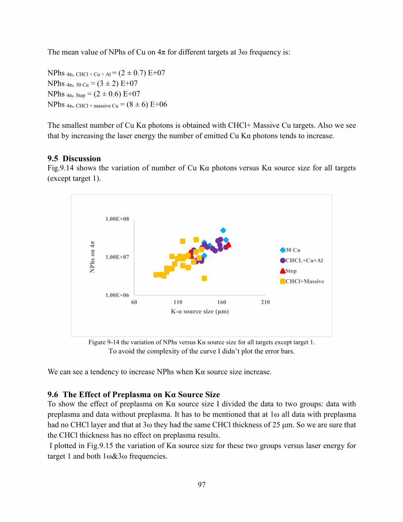
97

The mean value of NPhs of Cu on 4π for different targets at 3ω frequency is:

NPhs 4π, CHCl + Cu + Al = (2 ± 0.7) E+07

NPhs 4π, 30 Cu = (3 ± 2) E+07

NPhs 4π, Step = (2 ± 0.6) E+07

NPhs 4π, CHCl + massive Cu = (8 ± 6) E+06

The smallest number of Cu Kα photons is obtained with CHCl+ Massive Cu targets. Also we see

that by increasing the laser energy the number of emitted Cu Kα photons tends to increase.

9.5 Discussion Fig.9.14 shows the variation of number of Cu Kα photons versus Kα source size for all targets

(except target 1).

Figure 9-14 the variation of NPhs versus Kα source size for all targets except target 1.

To avoid the complexity of the curve I didn’t plot the error bars.

We can see a tendency to increase NPhs when Kα source size increase.

9.6 The Effect of Preplasma on Kα Source Size To show the effect of preplasma on Kα source size I divided the data to two groups: data with

preplasma and data without preplasma. It has to be mentioned that at 1ω all data with preplasma

had no CHCl layer and that at 3ω they had the same CHCl thickness of 25 μm. So we are sure that

the CHCl thickness has no effect on preplasma results.

I plotted in Fig.9.15 the variation of Kα source size for these two groups versus laser energy for

target 1 and both 1ω&3ω frequencies.

1.00E+06

1.00E+07

1.00E+08

60 110 160 210

NP

hs

on

4π

K-α source size (μm)

30 Cu

CHCL+Cu+Al

Step

CHCl+Massive

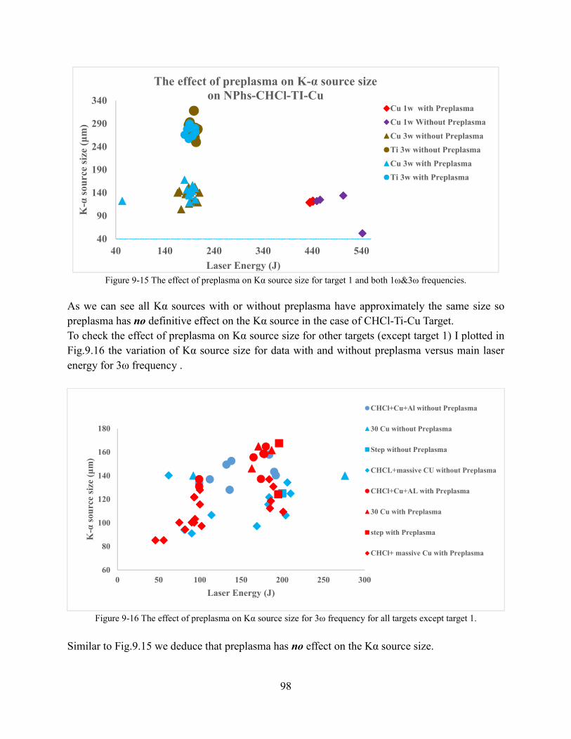
98

Figure 9-15 The effect of preplasma on Kα source size for target 1 and both 1ω&3ω frequencies.

As we can see all Kα sources with or without preplasma have approximately the same size so

preplasma has no definitive effect on the Kα source in the case of CHCl-Ti-Cu Target.

To check the effect of preplasma on Kα source size for other targets (except target 1) I plotted in

Fig.9.16 the variation of Kα source size for data with and without preplasma versus main laser

energy for 3ω frequency .

Figure 9-16 The effect of preplasma on Kα source size for 3ω frequency for all targets except target 1.

Similar to Fig.9.15 we deduce that preplasma has no effect on the Kα source size.

40

90

140

190

240

290

340

40 140 240 340 440 540

K-α

so

urc

e si

ze (

μm

)

Laser Energy (J)

The effect of preplasma on K-α source sizeon NPhs-CHCl-TI-Cu

Cu 1w with Preplasma

Cu 1w Without Preplasma

Cu 3w without Preplasma

Ti 3w without Preplasma

Cu 3w with Preplasma

Ti 3w with Preplasma

60

80

100

120

140

160

180

0 50 100 150 200 250 300

K-α

sou

rce

size

(μ

m)

Laser Energy (J)

CHCl+Cu+Al without Preplasma

30 Cu without Preplasma

Step without Preplasma

CHCL+massive CU without Preplasma

CHCl+Cu+AL with Preplasma

30 Cu with Preplasma

step with Preplasma

CHCl+ massive Cu with Preplasma

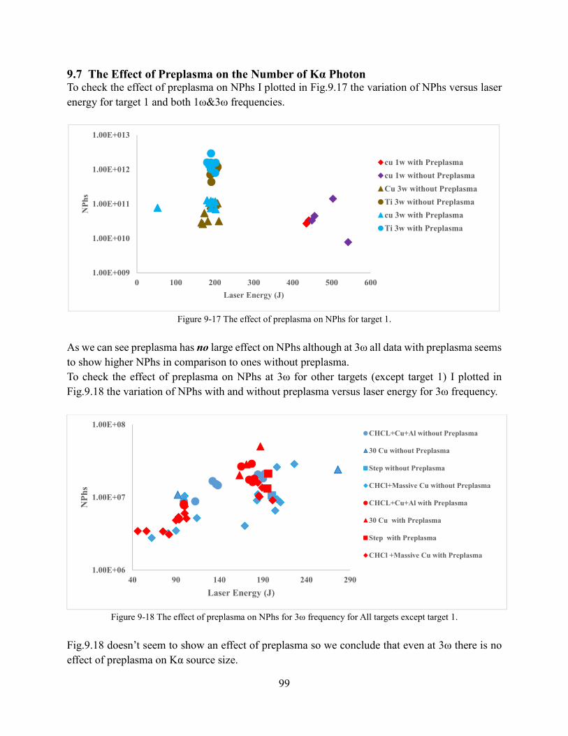
99

9.7 The Effect of Preplasma on the Number of Kα Photon To check the effect of preplasma on NPhs I plotted in Fig.9.17 the variation of NPhs versus laser

energy for target 1 and both 1ω&3ω frequencies.

Figure 9-17 The effect of preplasma on NPhs for target 1.

As we can see preplasma has no large effect on NPhs although at 3ω all data with preplasma seems

to show higher NPhs in comparison to ones without preplasma.

To check the effect of preplasma on NPhs at 3ω for other targets (except target 1) I plotted in

Fig.9.18 the variation of NPhs with and without preplasma versus laser energy for 3ω frequency.

Figure 9-18 The effect of preplasma on NPhs for 3ω frequency for All targets except target 1.

Fig.9.18 doesn’t seem to show an effect of preplasma so we conclude that even at 3ω there is no

effect of preplasma on Kα source size.

1.00E+009

1.00E+010

1.00E+011

1.00E+012

1.00E+013

0 100 200 300 400 500 600

NP

hs

Laser Energy (J)

cu 1w with Preplasma

cu 1w without Preplasma

Cu 3w without Preplasma

Ti 3w without Preplasma

cu 3w with Preplasma

Ti 3w with Preplasma

1.00E+06

1.00E+07

1.00E+08

40 90 140 190 240 290

NP

hs

Laser Energy (J)

CHCL+Cu+Al without Preplasma

30 Cu without Preplasma

Step without Preplasma

CHCl+Massive Cu without Preplasma

CHCL+Cu+Al with Preplasma

30 Cu with Preplasma

Step with Preplasma

CHCl +Massive Cu with Preplasma

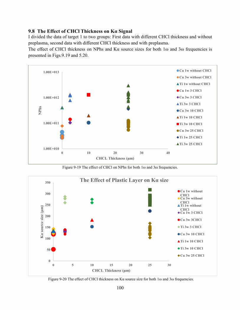
100

9.8 The Effect of CHCl Thickness on Kα Signal I divided the data of target 1 to two groups: First data with different CHCl thickness and without

preplasma, second data with different CHCl thickness and with preplasma.

The effect of CHCl thickness on NPhs and Kα source sizes for both 1ω and 3ω frequencies is

presented in Figs.9.19 and 5.20.

Figure 9-19 The effect of CHCl on NPhs for both 1ω and 3ω frequencies.

Figure 9-20 The effect of CHCl thickness on Kα source size for both 1ω and 3ω frequencies.

1.00E+010

1.00E+011

1.00E+012

1.00E+013

0 10 20 30 40

NP

hs

CHCL Thickness (μm)

Cu 1w without CHCl

Cu 3w without CHCl

Ti 1w without CHCl

Cu 1w 3 CHCl

Cu 3w 3 CHCl

Ti 3w 3 CHCl

Cu 3w 10 CHCl

Ti 1w 10 CHCl

Ti 3w 10 CHCl

Cu 3w 25 CHCl

Ti 1w 25 CHCl

Ti 3w 25 CHCl

0

50

100

150

200

250

300

350

0 5 10 15 20 25 30

Kα

sou

rce

size

(μ

m)

CHCL Thickness (μm)

The Effect of Plastic Layer on Kα size

Cu 1w withoutCHClCu 3w withoutCHClTi 1w withoutCHClCu 1w 3 CHCl

Cu 3w 3CHCl

Ti 3w 3 CHCl

Cu 3w 10 CHCl

Ti 1w 10 CHCl

Ti 3w 10 CHCl

Cu 3w 25 CHCl

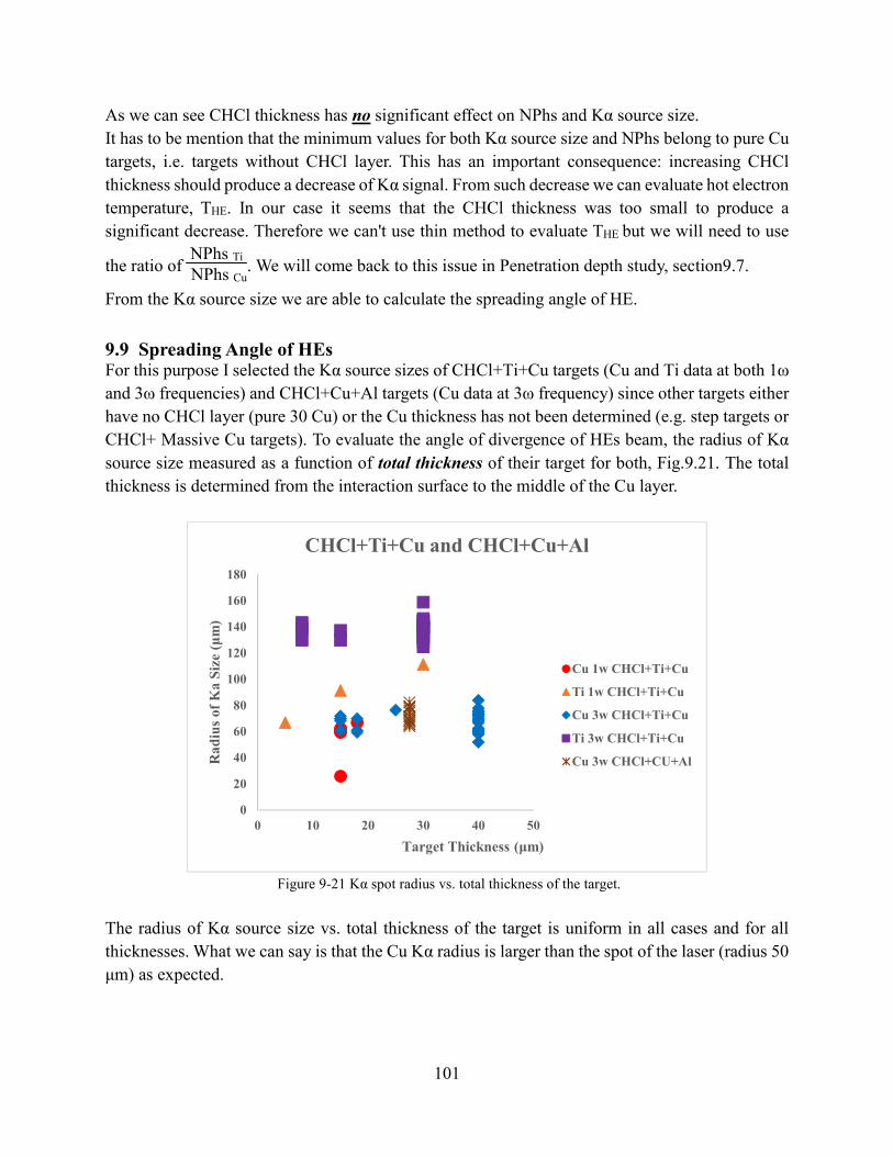
101

As we can see CHCl thickness has no significant effect on NPhs and Kα source size.

It has to be mention that the minimum values for both Kα source size and NPhs belong to pure Cu

targets, i.e. targets without CHCl layer. This has an important consequence: increasing CHCl

thickness should produce a decrease of Kα signal. From such decrease we can evaluate hot electron

temperature, THE. In our case it seems that the CHCl thickness was too small to produce a

significant decrease. Therefore we can't use thin method to evaluate THE but we will need to use

the ratio of NPhs Ti

NPhs Cu. We will come back to this issue in Penetration depth study, section9.7.

From the Kα source size we are able to calculate the spreading angle of HE.

9.9 Spreading Angle of HEs For this purpose I selected the Kα source sizes of CHCl+Ti+Cu targets (Cu and Ti data at both 1ω

and 3ω frequencies) and CHCl+Cu+Al targets (Cu data at 3ω frequency) since other targets either

have no CHCl layer (pure 30 Cu) or the Cu thickness has not been determined (e.g. step targets or

CHCl+ Massive Cu targets). To evaluate the angle of divergence of HEs beam, the radius of Kα

source size measured as a function of total thickness of their target for both, Fig.9.21. The total

thickness is determined from the interaction surface to the middle of the Cu layer.

Figure 9-21 Kα spot radius vs. total thickness of the target.

The radius of Kα source size vs. total thickness of the target is uniform in all cases and for all

thicknesses. What we can say is that the Cu Kα radius is larger than the spot of the laser (radius 50

μm) as expected.

0

20

40

60

80

100

120

140

160

180

0 10 20 30 40 50

Ra

diu

s of

Ka

Siz

e (μ

m)

Target Thickness (μm)

CHCl+Ti+Cu and CHCl+Cu+Al

Cu 1w CHCl+Ti+Cu

Ti 1w CHCl+Ti+Cu

Cu 3w CHCl+Ti+Cu

Ti 3w CHCl+Ti+Cu

Cu 3w CHCl+CU+Al

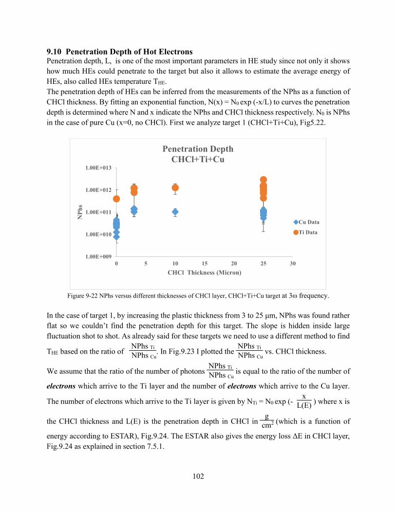
102

9.10 Penetration Depth of Hot Electrons Penetration depth, L, is one of the most important parameters in HE study since not only it shows

how much HEs could penetrate to the target but also it allows to estimate the average energy of

HEs, also called HEs temperature THE.

The penetration depth of HEs can be inferred from the measurements of the NPhs as a function of

CHCl thickness. By fitting an exponential function, N(x) = N0 exp (-x/L) to curves the penetration

depth is determined where N and x indicate the NPhs and CHCl thickness respectively. N0 is NPhs

in the case of pure Cu (x=0, no CHCl). First we analyze target 1 (CHCl+Ti+Cu), Fig5.22.

Figure 9-22 NPhs versus different thicknesses of CHCl layer, CHCl+Ti+Cu target at 3ω frequency.

In the case of target 1, by increasing the plastic thickness from 3 to 25 μm, NPhs was found rather

flat so we couldn’t find the penetration depth for this target. The slope is hidden inside large

fluctuation shot to shot. As already said for these targets we need to use a different method to find

THE based on the ratio of NPhs Ti

NPhs Cu. In Fig.9.23 I plotted the

NPhs Ti

NPhs Cu vs. CHCl thickness.

We assume that the ratio of the number of photons NPhs Ti

NPhs Cu is equal to the ratio of the number of

electrons which arrive to the Ti layer and the number of electrons which arrive to the Cu layer.

The number of electrons which arrive to the Ti layer is given by NTi = N0 exp (- x

L(E) ) where x is

the CHCl thickness and L(E) is the penetration depth in CHCl in g

cm2 (which is a function of

energy according to ESTAR), Fig.9.24. The ESTAR also gives the energy loss ΔE in CHCl layer,

Fig.9.24 as explained in section 7.5.1.

1.00E+009

1.00E+010

1.00E+011

1.00E+012

1.00E+013

0 5 10 15 20 25 30

NP

hs

CHCl Thickness (Micron)

Penetration DepthCHCl+Ti+Cu

Cu Data

Ti Data

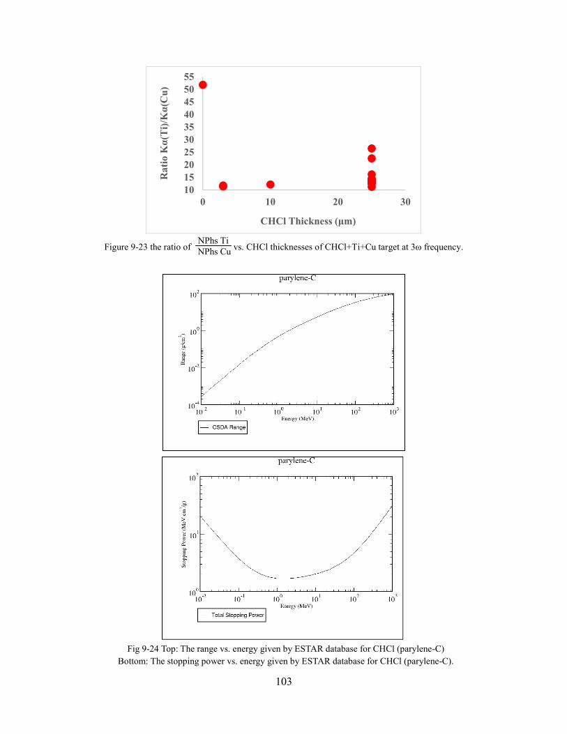
103

Figure 9-23 the ratio of NPhs Ti

NPhs Cu vs. CHCl thicknesses of CHCl+Ti+Cu target at 3ω frequency.

Fig 9-24 Top: The range vs. energy given by ESTAR database for CHCl (parylene-C)

Bottom: The stopping power vs. energy given by ESTAR database for CHCl (parylene-C).

10152025303540455055

0 10 20 30

Ra

tio

Kα

(Ti)

/Kα

(Cu

)

CHCl Thickness (μm)

104

Then electrons arrive to Ti layer with energy E - ΔE. The number of electrons which arrive to the

Cu layer is then NCu = N0 exp (- xTi

LTi (E- ΔE) ) where xTi is the titanium thickness and LTi(E- ΔE) is

the penetration depth (g

cm2) in titanium for electrons with energy E- ΔE. The range of Ti element

according to the ESTAR database is presented in Fig.9.25.

Fig 9-25 The Range vs. Energy given by ESTAR database for Ti element.

Finally we have:

NPhs Ti

NPhs Cu ≈

N Ti

N Cu =

N0 exp (- x

L(E) )

N0 exp (- xTi

LTi (E- ΔE) ) =

exp (- x

L(E) )

exp (- xTi

LTi (E- ΔE) )

I summarized the data in Table.9.2.

Table 9-2 The thickness, energy and the penetration depth related to the CHCl layer and Ti layer.

E

(keV)

L(E) (μm)

ΔE

(keV)

NTi E- ΔE

(keV)

LTi (E- ΔE)

(μm)

NCu N Ti

N Cu

10 2.1 5.7 8 E-06 4.3 0.9 1.6E-05 0.5

20 7.2 11.3 0.031 8.7 0.9 1.6E-05 2007.3

30 14.8 17 0.184 13 1.3 0.0005 364.7

40 24.6 22.7 0.361 17.3 2.3 0.01 26.0

50 36.3 28.6 0.502 21.4 2.9 0.03 15.1

60 49.9 34.5 0.605 25.5 4.3 0.09 6.2

70 65.2 40.5 0.681 29.5 5.9 0.18 3.7

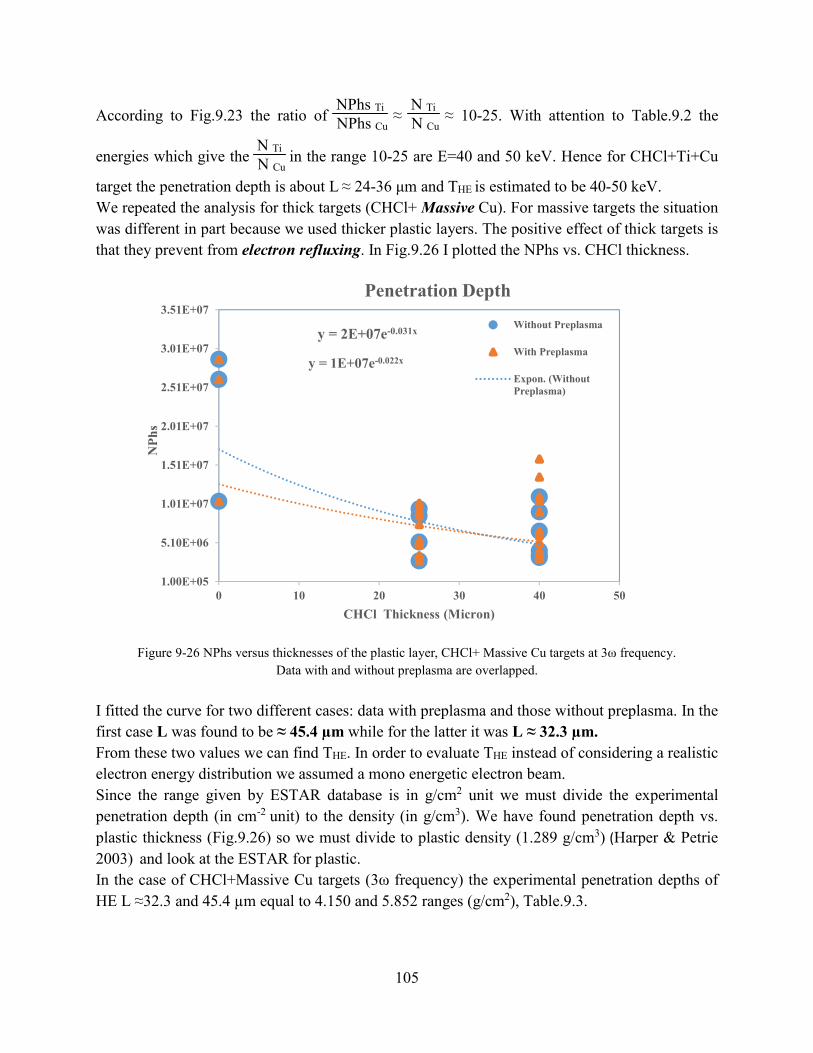
105

According to Fig.9.23 the ratio of NPhs Ti

NPhs Cu ≈

N Ti

N Cu ≈ 10-25. With attention to Table.9.2 the

energies which give the N Ti

N Cu in the range 10-25 are E=40 and 50 keV. Hence for CHCl+Ti+Cu

target the penetration depth is about L ≈ 24-36 μm and THE is estimated to be 40-50 keV.

We repeated the analysis for thick targets (CHCl+ Massive Cu). For massive targets the situation

was different in part because we used thicker plastic layers. The positive effect of thick targets is

that they prevent from electron refluxing. In Fig.9.26 I plotted the NPhs vs. CHCl thickness.

Figure 9-26 NPhs versus thicknesses of the plastic layer, CHCl+ Massive Cu targets at 3ω frequency.

Data with and without preplasma are overlapped.

I fitted the curve for two different cases: data with preplasma and those without preplasma. In the

first case L was found to be ≈ 45.4 µm while for the latter it was L ≈ 32.3 µm.

From these two values we can find THE. In order to evaluate THE instead of considering a realistic

electron energy distribution we assumed a mono energetic electron beam.

Since the range given by ESTAR database is in g/cm2 unit we must divide the experimental

penetration depth (in cm-2 unit) to the density (in g/cm3). We have found penetration depth vs.

plastic thickness (Fig.9.26) so we must divide to plastic density (1.289 g/cm3) (Harper & Petrie

2003) and look at the ESTAR for plastic.

In the case of CHCl+Massive Cu targets (3ω frequency) the experimental penetration depths of

HE L ≈32.3 and 45.4 µm equal to 4.150 and 5.852 ranges (g/cm2), Table.9.3.

y = 2E+07e-0.031x

y = 1E+07e-0.022x

1.00E+05

5.10E+06

1.01E+07

1.51E+07

2.01E+07

2.51E+07

3.01E+07

3.51E+07

0 10 20 30 40 50

NP

hs

CHCl Thickness (Micron)

Penetration Depth

Without Preplasma

With Preplasma

Expon. (WithoutPreplasma)

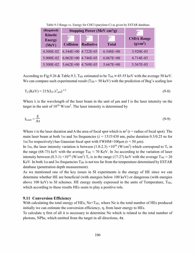
106

Table 9-3 Range vs. Energy for CHCl (parylene-C) as given by ESTAR database.

(Required)

Kinetic

Energy

(MeV)

Stopping Power (MeV cm2/g)

CSDA Range

(g/cm2)

Collision

Radiative

Total

4.500E-02 6.544E+00 4.722E-03 6.548E+00 3.920E-03

5.000E-02 6.062E+00 4.746E-03 6.067E+00 4.714E-03

5.500E-02 5.662E+00 4.769E-03 5.667E+00 5.567E-03

According to Fig.9.26 & Table.9.3, THE estimated to be THE ≈ 45-55 keV with the average 50 keV.

We can compare such experimental result (THE∼ 50 keV) with the prediction of Beg’s scaling law

Te (KeV) = 215(I18 λ2μm) 1/3 (9-8)

Where λ is the wavelength of the laser beam in the unit of μm and I is the laser intensity on the

target in the unit of 1018 W/cm2. The laser intensity is determined by

ILaser = EAτ

(9-9)

Where τ is the laser duration and A the area of focal spot which is πr2 (r = radius of focal spot). The

main laser beam at both 1ω and 3ω frequencies (λ = 1315/438 nm, pulse duration 0.3/0.25 ns for

1ω/3ω respectively) has Gaussian focal spot with FWHM=100µm (r = 50 µm).

In 1ω, the laser intensity variation is between (1.8-2.3) ×1016 (W/cm2) which correspond to Te in

the range (68-73) keV with the average THE ≈ 70 KeV. In 3ω according to the variation of laser

intensity between (0.3-1) ×1016 (W/cm2) Te is in the range (17-27) keV with the average THE ≈ 26

KeV. In both 1ω and 3ω frequencies THE is not too far from the temperature determined by ESTAR

database (penetration depth measurement).

As we mentioned one of the key issues in SI experiments is the energy of HE since we can

determine whether HE are beneficial (with energies below 100 keV) or dangerous (with energies

above 100 keV) to SI schemes. HE energy mostly expressed in the units of Temperature, THE,

which according to these results HEs seem to play a positive role.

9.11 Conversion Efficiency With calculating the total energy of HEs, Ne×THE, where Ne is the total number of HEs produced

initially we can estimate the conversion efficiency, η, from laser energy to HEs.

To calculate η first of all it is necessary to determine Ne which is related to the total number of

photons, NPhs, which emitted from the target in all directions, 4π.

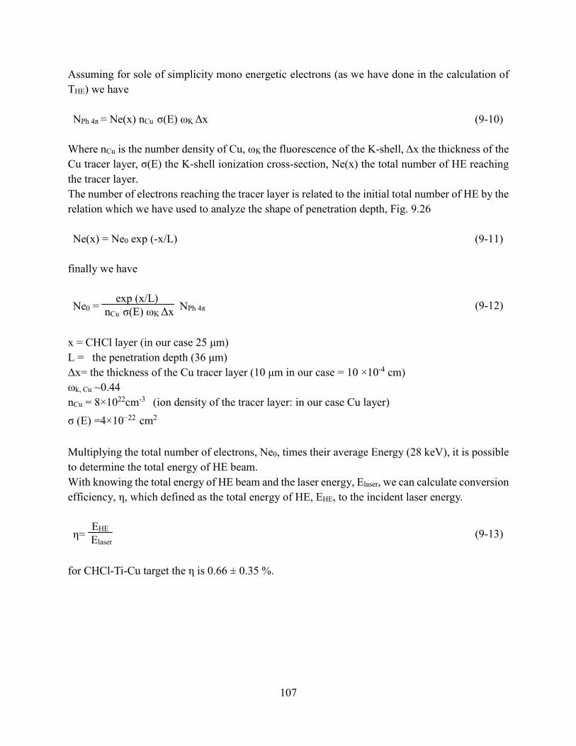
107

Assuming for sole of simplicity mono energetic electrons (as we have done in the calculation of

THE) we have

NPh 4π = Ne(x) nCu σ(E) ωK Δx (9-10)

Where nCu is the number density of Cu, ωK the fluorescence of the K-shell, Δx the thickness of the

Cu tracer layer, σ(E) the K-shell ionization cross-section, Ne(x) the total number of HE reaching

the tracer layer.

The number of electrons reaching the tracer layer is related to the initial total number of HE by the

relation which we have used to analyze the shape of penetration depth, Fig. 9.26

Ne(x) = Ne0 exp (-x/L) (9-11)

finally we have

Ne0 = exp (x/L)

nCu σ(E) ωK Δx NPh 4π

(9-12)

x = CHCl layer (in our case 25 μm)

L = the penetration depth (36 μm)

Δx= the thickness of the Cu tracer layer (10 μm in our case = 10 ×10-4 cm)

ωk, Cu ~0.44

nCu = 8×1022cm-3 (ion density of the tracer layer: in our case Cu layer)

σ (E) =4×10−22 cm2

Multiplying the total number of electrons, Ne0, times their average Energy (28 keV), it is possible

to determine the total energy of HE beam.

With knowing the total energy of HE beam and the laser energy, Elaser, we can calculate conversion

efficiency, η, which defined as the total energy of HE, EHE, to the incident laser energy.

η= EHE

Elaser

(9-13)

for CHCl-Ti-Cu target the η is 0.66 ± 0.35 %.

108

9.12 Conclusion In Shock ignition (SI) scheme the role of hot electrons (HEs) is ambiguous. They traditionally have been considered to be dangerous in ICF since they could preheat the assembled fuel leading to a premature expansion. They can also enhance the ablation pressure if their energies is below 100 keV. We performed a SI experiment at PALS in April 2014 to study the generation of HEs. This experiment was in a series of preparatory studies on ICF in the framework of the HiPER, a European collaboration. The goal of the proposed experiment was to study the generation and propagation of a shock wave in an interaction regime relevant to the SI approach to ICF. Moreover the experiment aimed at investigating the generation mechanisms of HE and their role in the shock wave propagation. In this experiment my role was analyzing the Kα emission due to the propagation of HEs through the target. In my thesis I present the experimental results related to the HEs measurements. We used two types of targets: The first targets are so-called thin multilayer targets which used to measure different characteristics of HEs. The second type of targets, the so-called thick (massive) targets are used to analyze the crater, such as its shape and dimension, which gives us some information about the mechanisms of laser energy transfer into the target and measuring the total deposited energy. The Kα emission due to the HE propagation inside the target was detected by using diagnostics based on the spherically bent crystals. We measured the Kα source size and the total number of photons on 4π, NPhs4π. My results show a tendency to increase NPhs4π when the Kα source size increase. Also the effect of preplasma on the Kα source size and NPhs4π is investigated. According to my results it doesn’t seem that the preplasma has a direct effect on the Kα Source Size and NPhs4π. The penetration depth of HEs inside the CHCl-Ti-Cu targets was found to be L ≈ 24-36 μm. According to ESTAR database HEs temperature, THE, is estimated to be 40-50 keV. For the massive targets for the case with preplasma L was found to be ≈ 45.4 µm while for the case without preplasma it was L ≈ 32.3 µm. THE estimated to be THE ≈ 45-55 keV with the average 50 keV. These results are in good agreement with the results of other experiments, e.g. (OMEGA Lab, THE ≈30 keV), (PALS, THE ≈50 keV) and (PIC simulations, THE =20-40 keV). Since the HEs have energy less than 100 keV it seems HEs play a positive role on the enhancement of the shock pressure which can be one of the most important results of this experiment. Finally the conversion efficiency, η, of total energy of HEs, to the incident laser energy estimated to be 0.66 ± 0.35 %.

109

Appendix A Among different indirect methods of deconvolution available at IDL library I used codes based on Maximum Entropy, Maximum likelihood, Richardson-Lucy method which are: AIA_DECONVOLVE_ RICHARDSONLUCY.pro (AIA) based on Richardson-Lucy

algorithm. https://darts.isas.jaxa.jp/pub/ssw/sdo/aia/idl/psf/PRO/aia_deconvolve_richardsonlucy.pro

The Richardson-Lucy algorithm performed in this code follows closely the algorithm explained

by (Jansson, 1997).

MAX_LIKELIHOOD.pro (M-L) based on Maximum likelihood algorithm. idlastro.gsfc.nasa.gov/ftp/pro/image/max_likelihood.pro Based on papers by (Richardson, 1972, Lucy, 1974). MAX_ENTROPY.pro (M-E) based on MAX_ENTROPY algorithm. http://idlastro.gsfc.nasa.gov/ftp/pro/image/max_entropy.pro Based on papers by (Hollis et al., 1979, Agmon et al., 1979). IMAGE_DECONVOLVE.pro based on MAX_ENTROPY algorithm. http://sohowww.nascom.nasa.gov/solarsoft/gen/idl/image/image_deconvolve.pro MEM96.pro based on MAX_ENTROPY algorithm. www.bbso.njit.edu/~chae/IDL/mem96.pro (Choi C. C., 2003).

110

Appendix B : Moon Shadow Analysis The work on the Moon shadow analysis was the part of my preliminary study to determine the PSF. As I discussed in chapter 1, Fig.1.15, the reason of a moderate fall in the IP of Moon shadow can be due to the convolution of Hinode/XRT PSF with the Sun emission. So the IP analysis of Moon shadow is a good method to check the effect of the PSF on intensity profiles. In Fig.1 I plotted the IP profile of Moon shadow when the border of the Moon was tangent to an active region. In this method not only the effect and the shape of the PSF is more visible due to the high flux of active region but also signal to noise ratio is very high so the noise doesn’t affect the measurement.

Fig.1 Top: cross section across solar eclipse in horizontal directions (Left) and vertical direction (Right). Bottom: horizontal IP (Left) and vertical IP (Right) of Solar eclipses.

The moon border is indicated with green arrows and active region of the Sun with red arrows. Since on the one hand the cross section must crosses the Moon disk vertically on the other hand the active regions scattered arbitrary around the moon disk I measured the IP in RADIAL DIRECTION. Moreover the shape of IP in horizontal and vertical directions are different which radial analysis such differences also remove. To do this I determined the center of the Moon and the position of active region and plotted a line crossing through these two points, Fig.2.

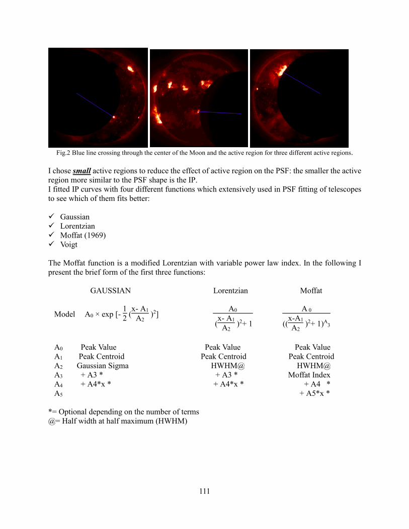
111

Fig.2 Blue line crossing through the center of the Moon and the active region for three different active regions.

I chose small active regions to reduce the effect of active region on the PSF: the smaller the active region more similar to the PSF shape is the IP. I fitted IP curves with four different functions which extensively used in PSF fitting of telescopes to see which of them fits better: Gaussian Lorentzian Moffat (1969) Voigt The Moffat function is a modified Lorentzian with variable power law index. In the following I present the brief form of the first three functions: GAUSSIAN Lorentzian Moffat

Model A0 × exp [- 12 (

x- A1

A2 )2]

A0

(x- A1

A2 )2+ 1

A 0

((x-A1

A2 )2+ 1)A

3

A0 Peak Value Peak Value Peak Value A1 Peak Centroid Peak Centroid Peak Centroid A2 Gaussian Sigma HWHM@ HWHM@ A3 + A3 * + A3 * Moffat Index A4 + A4*x * + A4*x * + A4 * A5 + A5*x * *= Optional depending on the number of terms @= Half width at half maximum (HWHM)

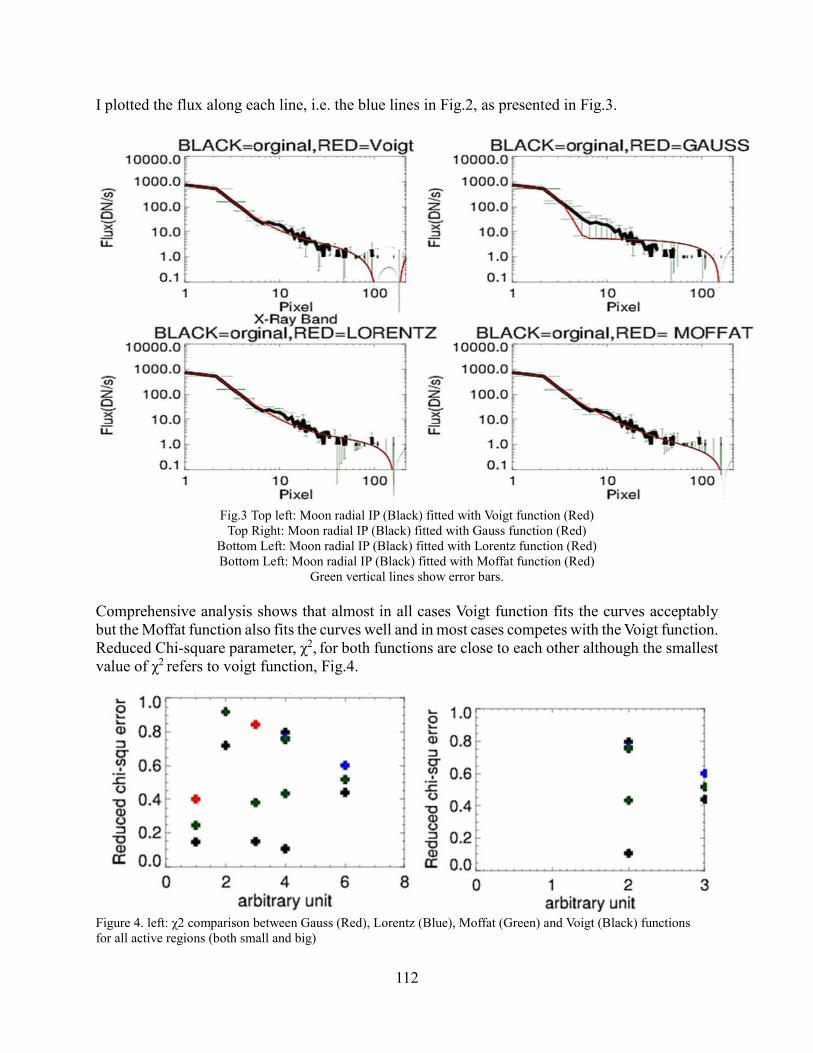
112

I plotted the flux along each line, i.e. the blue lines in Fig.2, as presented in Fig.3.

Fig.3 Top left: Moon radial IP (Black) fitted with Voigt function (Red)

Top Right: Moon radial IP (Black) fitted with Gauss function (Red) Bottom Left: Moon radial IP (Black) fitted with Lorentz function (Red) Bottom Left: Moon radial IP (Black) fitted with Moffat function (Red)

Green vertical lines show error bars.

Comprehensive analysis shows that almost in all cases Voigt function fits the curves acceptably but the Moffat function also fits the curves well and in most cases competes with the Voigt function. Reduced Chi-square parameter, χ2, for both functions are close to each other although the smallest value of χ2 refers to voigt function, Fig.4.

Figure 4. left: χ2 comparison between Gauss (Red), Lorentz (Blue), Moffat (Green) and Voigt (Black) functions for all active regions (both small and big)

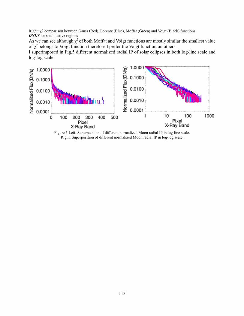
113

Right: χ2 comparison between Gauss (Red), Lorentz (Blue), Moffat (Green) and Voigt (Black) functions ONLY for small active regions

As we can see although χ2 of both Moffat and Voigt functions are mostly similar the smallest value of χ2 belongs to Voigt function therefore I prefer the Voigt function on others. I superimposed in Fig.5 different normalized radial IP of solar eclipses in both log-line scale and log-log scale.

Figure 5 Left: Superposition of different normalized Moon radial IP in log-line scale.

Right: Superposition of different normalized Moon radial IP in log-log scale.

114

Reference [Plasma in Astrophysics]

Belyaev D. et al. (2008), First observations of SO2 above Venus’ clouds by means of Solar

Occultation in the Infrared, J. Geophys. Res., 113, E00B25, doi: 10.1029/2008JE003143.

Belyaev D. A. et al. (2012), Vertical profiling of SO2 and SO above Venus’ clouds by

SPICAV/SOIR solar occultations, Icarus, 217, 740–751.

Bertaux J. L. et al. (2007), A warm layer in Venus’ cryosphere and high-altitude measurements of

HF, HCl, H2O and HDO, Nature, 450, 646-649.

Be´zard B., C. de Bergh (2007), Composition of the atmosphere of Venus below the clouds, J. Geophys. Res., 112, E04S07, doi: 10.1029/2006JE002794. Bhardwaj A. et al. (2007), X-rays from solar system objects, Planetary and Space Science, 55, 1135–1189. Bingham, R. et al. (1997), Generation of X-rays from Comet C/Hyakutake 1996 B2, Science, 275, 49-51. Bingham R. et al. (2008), Radiation by energetic electrons accelerated by wave-particle interaction: a plausible mechanism for x-ray emission from the Venus mantle, Ann. Geophys., 26, 1829–1836. Cravens T. E. (2001), Maurellis A. N., X-ray emission from scattering and fluorescence of solar x-rays at Venus and Mars, Geophysical Research Letters, 28, 3043-3046. De Bergh et.al (2006), The composition of the atmosphere of Venus below 100 km altitude: An overview, Planet. Space Sci., 54, 1389 – 1397, doi:10.1016/j.pss.2006.04.020. Dennerl K. et al. (2002), Discovery of X–rays from Venus with Chandra, A&A, 386, 319-330. Dennerl, K. (2008), X-rays from Venus observed with Chandra, Planetary and Space Science, 56 1414–1423. Draine B. T. (2003), Scattering by Interstellar Dust Grains. II. X-RAYS, ApJ, 598, 1026-1037. Draine B. T. (2003), Tan J. C., The scattered X-RAY halo around nova CYGNI 1992: Testing a model for interstellar dust, ApJ, 594,347–362. Fedorova, A., et al. (2008), HDO and H2O vertical distributions and isotopic ratio in the Venus mesosphere by Solar Occultation at Infrared spectrometer on board Venus Express, J. Geophys. Res., 113, E00B22, doi: 10.1029/2008JE003146. Golub L. et.al (2007), The X-Ray Telescope (XRT) for the Hinode Mission, Solar Phys, 243, 63–86.

115

Gunell H. et al. (2007), Simulations of solar wind charge exchange X-ray emissions at Venus, Geophys. Res. Lett., 34, L03107, doi: 10.1029/2006GL028602. Holmstr¨om M., Kallio E. (2004), The solar wind interaction with Venus and mars: energetic neutral atom and x-ray imaging, Advances in Space Research, 33, 187-193. Jansson P. A. (1997), Deconvolution of Images and Spectra, 2nd edition, Chapter 10.

Jibben P. R. (2014), Solar Soft XRT Analysis Guide, Hinode X-Ray Telescope.

Kosugi T. et al. (2007), The Hinode (Solar-B) Mission: An Overview, Solar Phys, 243, 3–17. Lemen, J. R. et al. (2012), The Atmospheric Imaging Assembly (AIA) on the Solar Dynamics Observatory (SDO), Solar Physics, 275, 17–40. Lisse et al. (1996), Discovery of X-ray and extreme ultraviolet emission from comet C/Hyakutake 1996 B2, Science, 274, 205-209.

Mahieux, A. et al. (2008), In-flight performance and calibration of SPICAV SOIR on board Venus

Express, Appl. Opt., 47(13), 2252 – 2265.

Mahieux, A. et al. (2009)., A new method for determining the transfer function of an Acousto

optical tunable filter, Opt. Express, 17, 2005–2014.

Mahieux, A., et al. (2010), Densities and temperatures in the Venus mesosphere and lower

thermosphere retrieved from SOIR on board Venus Express: Retrieval technique, J. Geophys.

Res., 115, E12014, doi: 10.1029/2010JE003589.

Mahieux, A. et al. (2014), Venus mesospheric sulfur dioxide measurement retrieved from SOIR

on board Venus Express, Planetary and Space Science, 113–114, 193–204.

Maurellis A. N. (2000), Jovian X-ray Emission from Solar X-ray Scattering, Geophysical

Research Letters, 27, 1339-1342.

Nevejans, D. (2006), et al, Compact high-resolution space-borne echelle grating spectrometer with AOTF based on order sorting for the infrared domain from 2.2 to 4.3 micrometer, Appl. Opt., 45(21), 5191–5206, doi:10.1364/AO.45.005191. Pesnell, W. D. (2012), Thompson, B. J. & Chamberlin, P. C. The solar dynamics observatory (SDO), Sol. Phys., 275: 3–15. Reale, F. et al. (2015), Using the transit of Venus to probe the upper planetary atmosphere, Nature Communications, 6, 7563.

116

Takeda A. (2015), The Hinode/XRT full-Sun image corrections and the improved synoptic composite image archive, Solar Physics, In Press. Vandaele A. C. et al. (2008), Composition of the Venus mesosphere measured by Solar Occultation at Infrared on board Venus Express, J. Geophys. Res, 113, E00B23, doi: 10.1029/2008JE003140. WEBER M. et al. (2007), An On-Orbit Determination of the On-Axis Point Spread Function of the Hinode X-Ray Telescope, Astron. Soc. Japan, 59,853–855. Wei Y. (2012), A teardrop-shaped ionosphere at Venus in tenuous solar wind, Planetary and Space Science, 73 254–261. Wickramasinghe, N. C. (1996), and Hoyle, F., Very small dust particles (VSDP’s) in comet C/1996 B2 (Hyakutake), Astrophys. Space Sci., 239, 121-123.

Wilquet, V. et al. (2009), Preliminary characterization of the upper haze by SPICAV/SOIR solar

occultation in UV to mid-IR onboard Venus Express, J. Geophys. Res., 114 (E00B42), doi:

10.1029/2008JE003186.

Wilquet, V. et al. (2012), Optical extinction due to aerosols in the upper haze of Venus: Four years

of SOIR/VEX observations from 2006 to 2010, Icarus, 217, 875-881.

Wilquet, V. et al. (2013), SOIR/VEX mesospheric aerosols observations and modelling,

SOIR/VEX mesospheric aerosols observations and modelling, J. Geophys. Res., 15, EGU2013-

3869-2.

117

Reference [Plasma in Fusion] Batani D. et al. (2011), The HiPER project for inertial confinement fusion and some experimental results on advanced ignition schemes, Plasma Phys. Control. Fusion, 53, 124041, (13pp). Batani D. et al., G Malka et.al (2012), Preliminary results from recent experiments and future roadmap to Shock Ignition of Fusion Targets, Journal of Physics: Conference Series, 399, 012005. Batani D. et al. (2012), Experimental results on advanced inertial fusion schemes obtained within the HiPER project, Nukleonika, 57(1), 3−10. Batani D., et al. (2014), Special Topic: Physics issues for shock ignition, Nucl Fusion, 54, 054009 (29pp). Betti R. et al. (2007), Shock Ignition of Thermonuclear Fuel with High Areal Density, PRL, 98, 155001. Borodziuk S. et al. (2004), Experimental and theoretical investigations of crater formation in an aluminum target in a PALS experiment, Nukleonika, 49(1), 7−14. Depierreux S. et al. (2011), Interaction physics for the shock ignition scheme of inertial confinement fusion targets, Plasma Phys. Control. Fusion, 53, 124034 (10pp). Deutsch C. (2003), Fast ignition schemes for inertial confinement fusion, Eur. Phys. J. Appl. Phys., 24, 95–113. Goyon C. et al. (2013), Laser-plasma interaction physics for shock ignition, EPJ Web of Conferences 59, 05006. Harper C. A., E. M. Petrie, Plastics Materials and Processes: A Concise Encyclopedia, John Wiley & Sons, 2003, pp.394. Jacquemot S. et al. (2011), Studying ignition schemes on European laser facilities, Nucl.Fusion, 51, 094025 (9pp). Kalinowska Z. et al. (2012), Investigations of mechanisms of laser radiation absorption at PALS, Nukleonika, 57(2), 227−230. Klimo et al. (2012), Simulations of laser plasma interaction for shock ignition in the high intensity regime, 39th EPS Conference & 16th Int. Congress on Plasma Physics. Koester P. et al. (2013), Recent results from experimental studies on laser–plasma coupling in a shock ignition relevant regime, Plasma Phys. Control. Fusion, 55, 124045 (8pp).

118

Krane K. (1987), Introductory Nuclear Physics, Wiley and Sons.

Lawson, J. D. (1955), Some Criteria for a Power producing thermonuclear reactor, Atomic Energy Research Establishment, A.E.R.E. GP/R 1807.

Lindl J (1995), Phys. Plasmas, 3933. Molière G., Z. Naturforsch (1948), Theory of the scattering of fast charged particles, 3, 78-97. Morace A., D. Batani (2010), Spherically bent crystal for X-ray imaging of laser produced plasmas, Nuclear Instruments and Methods in Physics Research A, 623, 797–800. NIST database: http://www.nist.gov/pml/data/star/index.cfm

Nuckolls J. et al. (1972), Nature, 239, 139. Perkins L. J. et al. (2009), Shock Ignition: A New Approach to High Gain Inertial Confinement Fusion on the National Ignition Facility, PRL, 103, 045004. Radha P. B. et al. (2011), Inertial Confinement Fusion Using the OMEGA Laser System, IEEE transactions on plasma science, 39. Ribeyre X. et al. (2009), Shock ignition: an alternative scheme for HiPER, Plasma Phys. Control. Fusion, 51, 015013 (19pp). Šmíd M., Luca A., Renner O. (2013), X-RAY spectroscopic characterization of shock-ignition-relevant plasmas, Acta Polytechnica, 53(2):233–236,. Tabak M. et al. (1994), Phys. Plasmas, 1626. Shcherbakov V. A. (1983), Sov. J. Plasma Phys, 9 240. Volpe L. et al. (2013), Collisional and collective effects in two dimensional model for fast-electron transport in refluxing regime, Phys. Plasmas, 20, 013104. Volpe L., D. Batani, et al. (2013), Propagation of a short-pulse laser-driven electron beam in matter, Phys. Plasmas, 20, 033105. Zel'dovichand Y. B. and Razier Y. P. (1966), Physics of Shock Waves and High-Temperature Hydrodinamic Phenomena, Academic Press.

Plasma in Astrophysics and in Fusion: • The X-Ray ... - IRIS UniPA

Documents

Transcript of Plasma in Astrophysics and in Fusion: • The X-Ray ... - IRIS UniPA