Course DescriptionPart III Astrophysics: Galaxies

Lent Term 2011:Mon, Wed, Fri. 11am. MR11Instructor: Dr. Scott Chapman

schapman@ast.cam.ac.ukOffice phone: 01223 330803

Galaxies 2

GalaxiesLecture 1: Overview

• Intro to course• Detail on Topics covered• Historical Overview• Overview of course

Galaxies 3

Intro to course

• Galaxies provide laboratories for a widerange of astrophysical phenomena:

• stellar dynamics, gas dynamics, dark matter,and stellar and chemical evolution.

• Moreover the problem of the formation andevolution of galaxies stands as one of themost important challenges to 21st centuryastrophysics.

Galaxies 4

Intro to course• Part of this subject has traditionally been

covered in the Part III course AstrophysicalDynamics,– covers basic stellar dynamics theory and selected

applications to galaxies and galactic systems.• This course, Galaxies, is designed as a

companion to the Dynamics course.• It includes a comprehensive introduction to

the observed structural, kinematical, andevolutionary properties of galaxies and therelevant theoretical models.

Galaxies 5

Textbooks• The main text for this course is Galactic

Astronomy by Binney and Merrifield(Princeton University Press, 1998).– companion volume to Galactic Dynamics by

Binney and Tremaine (Princeton University Press,2007), which serves as the text for the Part IIIAstrophysical Dynamics course.

• We will cover the topics in a different order– first ~half of the course covering the basic

structural and kinematical properties of galaxies– second ~half covering stellar populations and

galaxy evolution, beginning in the solarneighbourhood and ending with cosmologicallookback studies.

Galaxies 6

Textbooks• The two- volume set of books provides a

comprehensive coverage of galaxies from anobservational and theoretical perspective– Both are highly recommend for those who plan to continue

work in the field at the postgraduate level and beyond.• An excellent supplemental text is “Galaxies in the

Universe” by Sparke and Gallagher (CambridgeUniversity Press, 2007). It covers much of the samematerial as the pair of Princeton series texts, but at asomewhat lower level.

• "Galaxies and Galactic Structure" by Elmegreenprovides a good qualitative introduction to thesubject.

Galaxies 7

Example Sheets and Classes• There are four example classes associated

with this course, three to be held during Lentterm and one early in the Easter term, ondates and times TBD. The instructor forthese classes will be Dr. Dan Stark(dps@ast.cam.ac.uk).

• Example sheets will be distributed inadvance in the lectures. The material in theexample classes will provide more in-depthcoverage of some of the mathematicalmaterial in the course and provide examplesof the types of questions that may appear onthe course examination.

Galaxies 8

Examination• The examination for this course is tentatively

scheduled for June 3, 2011 at 13:30pm. Theexamination will mainly consist of problems with thechoice of an essay question.

• Although the emphasis in the problems will be onmathematical and physical concepts and derivations,you may also be asked to relate the results toobservations of galaxies as discussed in the lectures.

• The examination will be “open book”, meaning thatyou may bring handwritten class notes to theexamination (but not printed lecture notes,photocopied material, or calculators).

Galaxies 9

Topics• Background, historical introduction

– galaxy catalogs, atlases, and databases• Form and classification

– morphological classification systems– quantitative and physical classification systems

• Photometric and physical structure– luminosity function– spheroids & disks

• Interstellar media in galaxies• Kinematics, dynamics

– internal kinematics and dynamics– scaling laws and the fundamental plane– dark matter

Galaxies 10

Galaxies 11

Topics: stellar content and evolution

• The extragalactic distance scale• Chemical evolution models• The Solar neighborhood

– stellar statistics, luminosity function, IMF– disk population: ages, abundances, orbits

• The Galactic halo and bulge (near-fieldcosmology)– field stars– formation scenarios: instantaneous collapse vs

hierarchical formation

Galaxies 12

Topics: stellar content and evolution

• Stellar populations in nearby galaxies– resolved stellar populations in nearby galaxies– diagnostics of star formation rates and histories– spectral and evolutionary synthesis– star formation properties of the Hubble sequence– environmental influences and starbursts– chemical abundances and evolution

Galaxies 13

Fossil Record of Galaxy Formation: M31 (Andromeda)

Classical (Palomar)view of M31

Modern (wide-field CCD)view of M31 (Irwin+05)

6 degrees(12 full moons)

100 kpc

Theory: Building the Galaxy Spheroid (e.g,Bullock etal. 2006)

Galaxies 15

The Incessant Drumbeat of Minor Mergers

M31’s Outskirts (PAndAS, Ibata+07; McConnachie+ 2010)

150kpc

Galaxies 16Martinez-Delgado et al 2010

Galaxies 17

Topics: Galaxy Formation and Evolution

• Stars exist in galaxies but galaxies aredistributed throughout the Universe.– Therefore, to understand questions such as the

physical origins of galaxies, distances to galaxies andthe ages of stars in galaxies one must consider thefundamental properties of the Universe in which theyexist -- Cosmology

• In a hierarchical Universe massive galaxies arepredicted to be the result of the successivemergers of less massive galaxies (White and Rees 1978).

Galaxies 18

Galaxies 19

Galaxies 20

Topics: Galaxy Formation and Evolution

• Instantaneous collapse (ELS) picture– galaxies form from single protogalactic clouds– formation of all principal components (mass, gas, stars, metals)

begins simultaneously– galaxy type dictated mainly by angular momentum and mass of

protogalactic cloud– galaxy type imprinted at birth- no subsequent changes

• Cold Dark Matter (CDM) hierarchical picture– galaxies grow from merging of small protogalactic fragments,

plus accretion of intergalactic gas– formation is continuous, with assembly of mass, gas, stars,

metals only indirectly coupled– galaxy type determined by cloud mass, merger history, local

environment– major transformations in type possible

Galaxies 21

time

Galaxies 22

Historical Introduction• A good modern working definition of a galaxy is a

population of stars, gas and dust bound gravitationallywithin a dark matter halo (TBD).

• The early history of galaxy studies led up to andculminated in Hubbleʼs confirmation that they arestellar systems external to our own Galaxy and thatthey are receding from us (Hubbleʼs expansion law -1929)

• This marked a turning point towards the beginning ofgalaxy “evolution” studies as we know it now.

Galaxies 23

Historical Introduction• 1610 Galileo resolves Milky Way into stars• 1755 Kant introduces island universe

hypothesis for Milky Way• 1785 Herschel makes first mapping of MW

structure• 1800’s thousands of galaxies catalogued, but

nature misunderstood• 1918 Shapley uses Cepheid distances to

globular clusters to show that Galactic centeris 15 kpc from Sun, MW diameter ~100 kpc

• 1922 Kapteyn models MW: R ~ 10 kpc,roughly centered on Sun (the observableUniverse)

Galaxies 24

Astronomers were trying to determine the structure of our galaxy(which was thought to be the known Universe)and locate the relative position of the Sun in the vast array of stars.

Galaxies 25

“spiral nebulae” (galaxies)• Some astronomers postulated that

they were island universes justlike our own Galaxy (but theyhad no proof)

• most astronomers suspected theywere part of our own Galaxy,just like other nebulae andclusters.

• But recent studies had shownthem to have very high radialvelocities.

• If only astronomers coulddetermine the distance to thesespiral nebulae, their nature couldbe tied into the structure of theGalaxy.

Galaxies 26

Galaxies 27

Shapley’s Milky Way• Harlow Shapely (1914) began studying globular clusters (associations of stars)• Noted they were widely distributed above and below the galactic equator.• Yet largely concentrated around one hemisphere in galactic longitude.• this skewing in galactic longitude was unique to globular clusters and no other

type of object – nebulae, open clusters, double stars, etc.

• Determined the distances to the globular clusters using a the newly foundtechnique, the period-luminosity relation.

• 1916: found the distance to M13 as 30kpc, which placed it well outside the size ofKapteyn’s Universe.

• Since the globular clusters were of probably similar size,and if they are outside of our galaxy but associated with it,then their distribution might suggest that we - not they – are in a skewed position !!

• Perhaps the Sun is located toward the edge of an enormous system, 5 times largerthan previously thought, defined by the globular clusters.

Galaxies 28

Modern view of our Milky way

Galaxies 29

Historical Introduction• 1918 Curtis notes similarity of edge-on

“nebulae” (galaxies) to Milky Way• 1920 Shapley-Curtis debate on nature of

spiral nebulae• 1924 Hubble detects Cepheid variables in

M31, confirming extragalactic nature ofgalaxies

• 1928 Oort measures solar orbit (frommotions of stars), deduces mass of Milky Way

• 1929 Hubble & Humason discover linearexpansion of universe

• 1930 Trumpler discovers diffuse interstellarextinction (more accurate distance scales)

Galaxies 30

Galaxies 31

Rotation of the Spiral Nebulae?

Galaxies 32

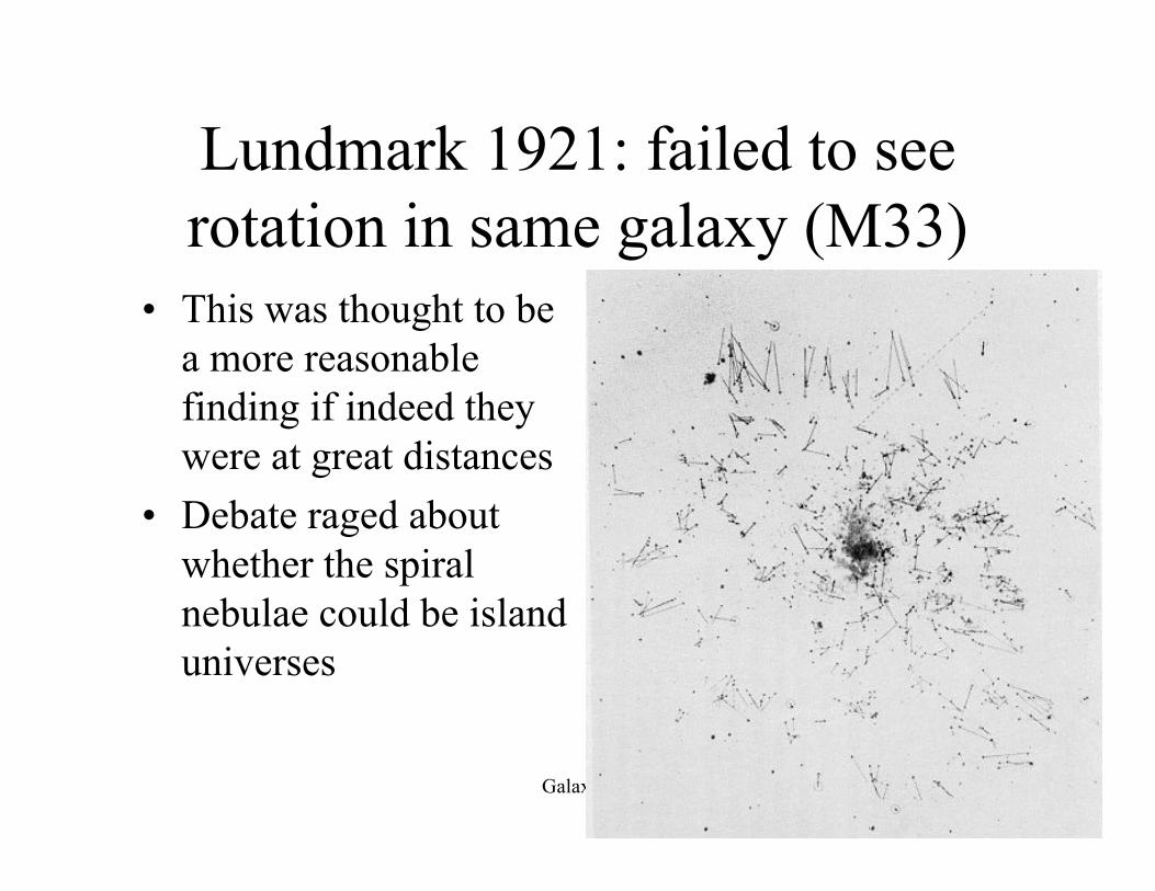
Lundmark 1921: failed to seerotation in same galaxy (M33)

• This was thought to bea more reasonablefinding if indeed theywere at great distances

• Debate raged aboutwhether the spiralnebulae could be islanduniverses

Galaxies 33

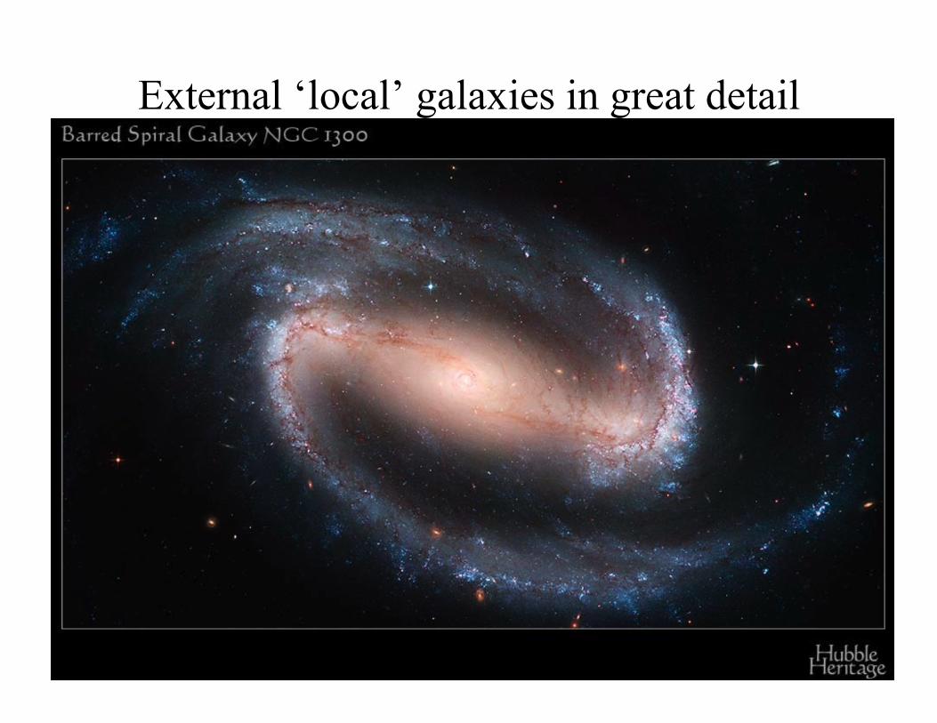
External ‘local’ galaxies in great detail

Galaxies 34Chandra

A modern view: past decade of discovery:laboratory for studying galaxy evolution

VLA

Palomar5-m

IRAM

HST

MERLIN

UKIRT CSO JCMT Subaru Keck-I/II IRTF Gemini CFHT

OVRO

Herschel

Spitzer

Galaxies 35

10-m mirrors

2-m astronomer

(Keck Telescopes)

The Keck, VLT, GeminiOptical Telescopes alongwith the Hubble, Spitzer,Chandra, Newton, andHerschel SpaceTelescopes have beenresponsible for many ofthe biggest advances

85cm mirror

(Spitzer Space Telescope)

2.4m mirror

(Hubble Space Telescope)

Galaxies 36

The Sun and Solar System live in a largeSpiral Galaxy with a 100 million “sun”

black hole at the centre• A large spiral galaxy like the Milky

Way Galaxy contains around 100billion stars, with a total mass of~1012 “solar masses”

– a galaxy is a big group of stars, gas anddark matter.

• We live in the suburbs

• Hard to comprehend the size, shape,and age of the Universe ;-(

• Speed of light as a time machineallows us to study it!

8kpc2600 lyrs

Galaxies 37

The Milky Way Galaxy is a member of a small group ofGalaxies (M31 & M33 are other two big galaxies)

Galaxies 38The Local Group is falling into the Local Super Cluster

Galaxies 39

There are muchlargerconcentrationsof galaxies

“Rich” GalaxyClusters(this one seen about1/4 the way back toBig Bang)

Cluster galaxiesevolvedifferently/fasterthan field galaxies

Galaxies 40

All the galaxies in thecluster represent only atiny fraction of the totalnumber of galaxies inthe Universe (severalbillions)

(The Hubble SpaceTelescope DEEP field)

Large-Scale Structure of local galaxiesAll-sky surveys

2dF redshift survey: LSS out to large distances

Galaxies 43

The big picture - the history of the Universe

• The big bang (Quantum Gravity at work) … What comes before ??????

– Our physics is not good enough yet to tell us!

Galaxies 44

The “seeds” of galaxies

• The Cosmic Microwave Background, 400,000yrs after Big Bang: light and matter have“decoupled” (well understood physics:COBE/WMAP satellites)– The first “easily observable” Universe

Galaxies 45

Galaxy Formation? (when/how do the stars form?)

– Starting ~1 billion years after the big bang, the first recognizable(now detectable!) “galaxies” started to form.

– Gas falling into overdensities of Dark Matter …cools, compresses, forms stars.

– Small galaxies merge to form bigger galaxies

Galaxies 46

Galaxy Evolution - Dark Matter and Gravity

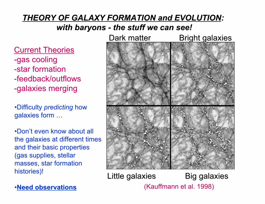
(Kauffmann et al. 1998)(Kauffmann et al. 1998)

Current TheoriesCurrent Theories-gas cooling-gas cooling-star formation-star formation-feedback/outflows-feedback/outflows-galaxies merging -galaxies merging

Dark matterDark matter Bright galaxiesBright galaxies

Little galaxiesLittle galaxies Big galaxiesBig galaxies

••Difficulty Difficulty predictingpredicting how howgalaxies form galaxies form ……

••DonDon’’t even know about allt even know about allthe galaxies at different timesthe galaxies at different timesand their basic propertiesand their basic properties(gas supplies, stellar(gas supplies, stellarmasses, star formationmasses, star formationhistories)!histories)!

••Need observationsNeed observations

THEORY OF GALAXY FORMATION and EVOLUTIONTHEORY OF GALAXY FORMATION and EVOLUTION: : with baryons - the stuff we can see!with baryons - the stuff we can see!

Add gas (hydrodynamics) to build big SpiralGalaxy (eg, Abadi+2003)

Galaxies 49

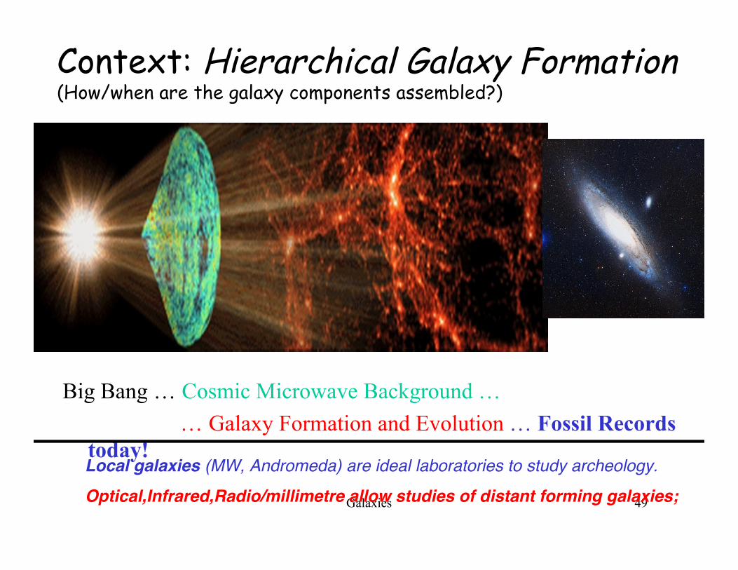
Context: Hierarchical Galaxy Formation(How/when are the galaxy components assembled?)

Big Bang … Cosmic Microwave Background … … Galaxy Formation and Evolution … Fossil Records

today!Local galaxies (MW, Andromeda) are ideal laboratories to study archeology.Optical,Infrared,Radio/millimetre allow studies of distant forming galaxies;

Galaxies 50

End lecture 1

Galaxies 1

GalaxiesLecture 2: Review ; Galaxy Classification

• Review of some basic astronomy concepts needed

Classification• Hubble tuning fork• Other schemes

http://www.ast.cam.ac.uk/~schapman/Part3Galaxies/

Galaxies 2

The Magnitude Scale• L = 4πd2f – where L is the intrinsic luminosity, d is the distance and f is

the flux measured by the observer. [assumes that the source radiatesisotropically – good approximation for most galaxies and stars]

• For historical reasons the apparent brightness (= measured flux) ofsources is specified using a magnitude scale

• Definition:mλ = -2.5 × log10 f + constant

where mλ is the “apparent magnitude”. The flux, f, is measured within awell-defined magnitude range, with standard “passbands” indicated by“λ” or similar, e.g. mB = m(B) = B = B all used for B-bandmagnitude

Galaxies 3

mλ = -2.5 × log10 f + constant• The minus sign, “-”, is important – fainter objects have large values of m• The constant that defines the zero-point of the scale was defined

historically such that the bright visible star Vega (αLyr) has zero-magnitude in all passbands. Thus, for Vega

mB = mV = mR = … = mK = 0.0where the subscripts indicate passbands that span the optical through near-

infrared region (400-2500nm)

Astronomers use of the “magnitude” system causes disbelief in many aphysicist(!) but even today the system is essentially unchanged from thatset up originally

• The AB magnitude system has a common «zeropoint» at all wavelengthsgiving a more useful magnitude scale to flux conversion:

MAB = -2.5 lg(f) -48.6 f [ergs/s/cm2/Hz]

Galaxies 4

Galaxies 5

limited by thermal emission2200K

near-infrared1600H

near-infrared1200J850Z750I

visible650R

visible550V

visible440B

Shortest possible from ground360UCommentλeff (nm)Passband

Standard Passbands in the Visible and Near-infrared

Galaxies 6

Galaxies 7

Apparent Magnitudes

30.0Faintest object detected

21.5□˝Dark night sky (surface brightness)

12.0Brightest quasar

6.0Faintest star (dark site, dark-adapted)

3.5M31 (brightest galaxy)

3.5Faintest star (from Cambridge street)

0.0Vega

-1.4Sirius (brightest star)

-4.5Venus (brightest)

-26.7Sun

mVObject

Galaxies 8

Absolute Magnitudes and Distance• Absolute magnitude is defined as the magnitude an object would have

if observed at a distance of 10pc• Absolute magnitudes are indicated using capital letters e.g. MV is the

V-band absolute magnitude• Absolute magnitude is astronomers’ scheme for quantifying the

luminosity of objects, L = 4πd2f, and provides a convenient measure ofthe distance of an object via the “distance modulus” (DM)

DM = m - M = -2.5 log fd + 2.5 log f10

= -2.5 log (fd /f10)Useful for local volume of galaxies, but less sensible for cosmological

distances. IE: M31 (Andromeda) has a DM=24, Virgo cluster hasDM=31

Galaxies 9

From inverse-square law, f α 1/d2, and

fd /f10 = (10/d)2

and m – M = -2.5 log (10/d)2

Distance modulus: DM = m – M = 5 log d -5

or d = 10(m-M+5)/5 pc

If absolute magnitude for an object known then can measureapparent magnitude, m, and calculate distance, d.

CAUTION: ‘d’ in a cosmological context is “Luminosty Distance” TBD

[Will drop explicit base for “log”s, “log” = “log10”]

Galaxies 10

1/

/2()(

2

!=)",=

5

kThce

hcBTB

#

###

Spectrum of blackbody as a function of temperature, T:

where h is Planck’s constant and c is the velocity of lightwith common units in astronomy, ergs cm-2 A-1 sr-1 s-1 orWatts m-2 nm-1 sr-1 Alternatively, in terms of frequency, υ:

1/

/2()(

23

!=)",=

kThve

chvvBTB

v

Blackbody Radiation

units, ergs cm-2 Hz-1 sr-1 s-1 or Watts m-2 Hz-1 sr-1

The blackbody spectrum is strongly peaked – most energyemitted within narrow wavelength (frequency) range

Galaxies 11

Blackbodycurves fordifferent T

Galaxies 12

Wien’s Displacement Law

From the blackbody distribution can show that the wavelength at whichthe function peaks and the Temperature of the blackbody are simply

related by:

λmax × T = 0.290 (cm K)

Wien’s Law is extraordinarily useful and worth remembering

(How would you derive it?)

Galaxies 13

Wien’s Displacement Law

O star0.0740000Sun0.505800

Red giant0.853400Brown dwarf2.91000

Room temperature9.9293Molecular cloud14520

Sourceλ (µm)T (K)

Galaxies 14

Ratio of fluxes in two passbandsuniquely determines the temperatureof a blackbody

In terms of the magnitude system,the difference between magnitudes intwo passbands gives the “colourindex” or “colour” of an object, e.g.measures in the B and V band

B = -2.5 log fB +constV= -2.5 log fV + const

B-V = -2.5 log (fB/fV)

and the B-V colour thus measures T

Galaxies 15

Colours of Galaxies and Stars

It follows from the definition of the zero-point for the magnitude systemthat for Vega all colours have zero values, i.e. U-B = B-V = V-R = V-I=…= J-K = 0.0

Conventionally, all colours are specified in sense blue-redThus, objects with redder spectral energy distributions than Vega have

positive colours, e.g. for the Sun, B-V=0.6Objects with bluer spectral energy distributions than Vega have negative

colours, e.g. for an O star, B-V≈-1.0B-V colours most common for historical reasons (photographic

emulsions) but longer baseline often better

Galaxies 16

Most stellar spectra are well approximated by blackbodies.Galaxy light (in optical) is an integration of the individual stars’ light.

Galaxies 17

Galaxies 18

Galaxies 19

Stefan Boltzmann Law: ApproximatingGalaxies and Stars as Blackbodies

• Integrate the blackbody spectrum over all wavelengths

∫ Bλ(T)dλ = σ T4

where σ is the Stefan-Boltzmann constant.• If surface element of a galactic component (the photosphere of stars;

cool dust emission) emits like a blackbody thenL = 4 π R2 σ Te

4

relates luminosity, L, radius, R, and effective temperature, Te of thecomponent. None are in fact perfect blackbodies and Te is thetemperature (minimum radius R) would have if it were a blackbody.

Galaxies 20

Hertzsprung-Russell diagramfrom HIPPARCOS satellite– bright, nearby stars.

Galaxies 21

HR diagram: stellar evolution = galaxy evolution

Galaxies 22

Evolved versus ‘young’ galaxies

Galaxies 23

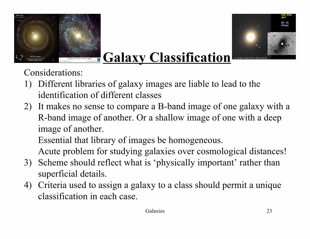
Galaxy ClassificationConsiderations:1) Different libraries of galaxy images are liable to lead to the

identification of different classes2) It makes no sense to compare a B-band image of one galaxy with a

R-band image of another. Or a shallow image of one with a deepimage of another.Essential that library of images be homogeneous.Acute problem for studying galaxies over cosmological distances!

3) Scheme should reflect what is ‘physically important’ rather thansuperficial details.

4) Criteria used to assign a galaxy to a class should permit a uniqueclassification in each case.

Galaxies 24

Morphology: the two-dimensionalphysical appearance of galaxies

• The first systematic attempts to studygalaxies focussed upon understanding therange of shapes they presented.

• Hubble - though not the first - presentedwhat is arguably the most complete yetsimple classification of galaxies based upontheir visible appearance: the Hubblesequence.

Galaxies 25

Hubble tuning fork

Hubble 1926, ApJ, 64, 321

“Early Type”

“Late Type”

Galaxies 26

Hubble tuning forkIrr

Galaxies 27

Why Begin with Classification?

• The Hubble system forms the basicvocabulary of the subject.

• The Hubble sequence of galaxy types reflectsan underlying physical and evolutionarysequence.– provides an overview of integrated properties– reproducing the variation in these properties along

the Hubble sequence is a major (unsolved)challenge for galaxy formation/evolution theory

Galaxies 28

Hubble Sequence

• An important aspect of the Hubble sequence isthat many intrinsic properties of galaxies, suchas luminosity, colour, and gas content,change systematically along this sequence.

• In addition, disks and ellipsoids most likelyhave very different formation mechanisms.

• Therefore, the morphology of a galaxy, or itslocation along the Hubble sequence, is directlyrelated to its formation history.

Galaxies 29

Hubble Sequence - Ellipticals

• The sequence is an interesting mix ofquantitative and qualitative criteria:

• Smooth, elliptical galaxies showing noevidence of a disk– Relatively little evidence of gas, dust– subtypes defined by projected flattening,

labelled with a number of E0 to E7 with thenumber computed as 10 x (1 - b/a),

• b and a are the minor and major axis lengths.b

a

Galaxies 30

Hubble Sequence - Ellipticals

• An S0 or lenticular galaxy is a bulgedominated galaxy with a smooth, purelystellar disk.

• introduced in 1936 revision of system• IE: disk and bulge but no spiral structure

Galaxies 31

Galaxies 32

Hubble Sequence - Spirals• Spiral galaxies are classified by more qualitative criteria such as the

prominence and tightness of spiral arms and the presence of acentral bar.

• flattened disk + central bulge (usually)• two major subclasses: normal and barredSubtypes Sa, Sb, Sc distinguished by 3 criteria• bulge/disk luminosity ratio

– B/D ranges from >1 (Sa) to <0.2 (Sc)• spiral arm pitch angle

– ranges from 1-7o (Sa) to 10-35o (Sc)• “resolution” of disk into knots, HII regions, stars

Galaxies 33

Hubble Sequence - Spirals• these three criteria are not necessarily

consistent!Each reflects an underlying physical variable:• B/D ratio ---> spheroid/disk mass fractions• pitch angle ---> rotation curve of disk, mass

concentration• resolution ---> star formation rate• Hubbleʼs system is simple yet subjective - in that it is dependent

upon human visual classification.• However, as numerous supporters of visual classification have

remarked, the eye is exceptionally adept at recognizing andclassifying two dimensional structures.

Galaxies 34

Galaxies 35

Galaxies 36

Hubble Sequence - Irr’s• Irregular galaxies

– little or no spatial symmetry– two major subtypes

• Irr I: highly resolved (e.g., Magellanic Clouds)• Irr II: smooth but chaotic, disturbed (e.g., M82)

Galaxies 37

Hubble Sequence - others?• Unclassifiable galaxies?

– ~2% of galaxies cannot be classified as E, S, Irr– predominantly disturbed or interacting systems

Galaxies 38

Extended Hubble Sequence

• Revised Hubble system– de Vaucouleurs 1958, Handbuch der Phys, 53, 275– de Vaucouleurs 1964, Reference Catalog of Bright Galaxies (RC1)

• goal: retain basic system, add more information• mixed types: E/S0, Sab, Sbc, etc• intermediate barred: SA, SAB, SB• extended types: Sd, Sm, Sdm• inner rings: S(r) , S(s)• outer rings: (R) S• Magellanic spirals, irregulars: Sm, Im

Galaxies 39

Galaxies 40

Extended Hubble Sequence• Attempts have been made to quote Hubbleʼs

scheme as a numerical sequence, T-types.• Physical quantities such as relative fractions of

bulge and disk light do correlate with T-type.• However, T-types remain a subjective, relative

classification scheme, i.e. there is no absolute“elliptical” or “spiral” reference. There is noabsolute “ground truth” for purely visualclassification schemes.

Galaxies 41

Galaxies 42

Other Classification Systems• Luminosity classification (DDO system)

van den Bergh 1960, ApJ, 131, 215

• goal: use morphology to subdivide galaxies byabsolute luminosity and mass– basic criterion is spiral arm “development” (arm length,

continuity, relative width)• secondary criterion surface brightness (dwarfs)• roman numeral designation after Hubble type

– Sc I, I-II, II, II-III, III, III-IV, IV– Sb I, I-II, II, II-III– Ir IV-V, V

• mean MB ranges from -21 (I) to -16 (V)

Galaxies 43

Galaxies 44

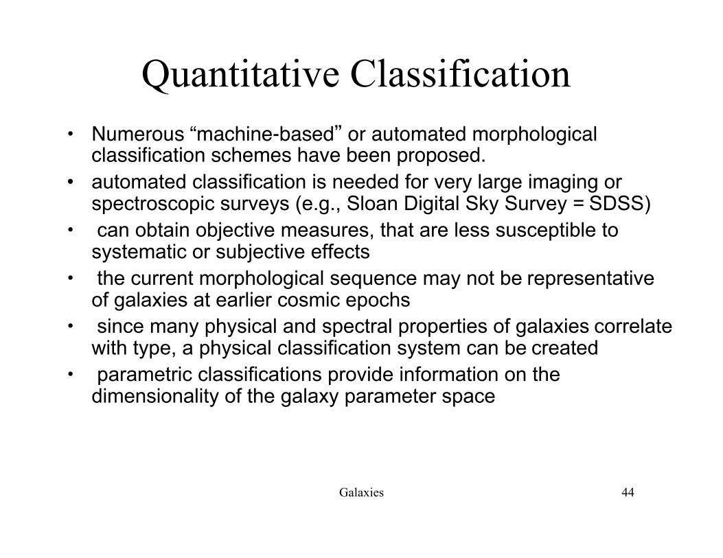
Quantitative Classification• Numerous “machine-based” or automated morphological

classification schemes have been proposed.• automated classification is needed for very large imaging or

spectroscopic surveys (e.g., Sloan Digital Sky Survey = SDSS)• can obtain objective measures, that are less susceptible to

systematic or subjective effects• the current morphological sequence may not be representative

of galaxies at earlier cosmic epochs• since many physical and spectral properties of galaxies correlate

with type, a physical classification system can be created• parametric classifications provide information on the

dimensionality of the galaxy parameter space

Galaxies 45

Quantitative Classification• Abraham et al. 1994, ApJ, 432, 75• Abraham et al. 1996, MNRAS,

279, L49• simple 2-parameter system• concentration index C --> ratio

of fluxes in two isophotalregions

• asymmetry index A --> flipimage, subtract from initialimage, measure fraction ofresidual flux

Galaxies 46

Galaxies 1

GalaxiesLecture 3: Parametric Classification;

Galaxy Profiles• Parametric Classification schemes

– PCA; quantitative spectral classes• Photometric structure• Surface brightness profiles

Galaxies 2

Parametric Classification

• Basic Idea: Hubble type correlates with several integratedproperties of galaxies (e.g., bulge fraction, gas fraction,color, star formation rate, angular momentum …

• Goal: define a physical classification in an n-space of galaxy properties

• Use correlations between these parameters to analyzethe number of independent variables that define galaxyproperties

Galaxies 3

Principal component analysis (PCA)• a mathematical procedure that uses an orthogonal

transformation to convert a set of observations ofpossibly correlated variables into a set of values ofuncorrelated variables called principal components.

• The number of principal components is less than orequal to the number of original variables.

• This transformation is defined in such a way that thefirst principal component has as high a variance aspossible (that is, accounts for as much of thevariability in the data as possible)

• each succeeding component in turn has the highestvariance possible under the constraint that it beorthogonal to (uncorrelated with) the precedingcomponents.

Galaxies 4

Principal component analysis (PCA)Djorgovski 1992, in Cosmology and Large Scale Structure of the Universe,

ASP Conf Ser, 24, 19; also see Box 4.2 (p207) of BM

• select a set of measured parameters for the galaxyset, and normalize the ranges to unity

• compute the correlation coefficient for each pair ofparameters (normalize each variable to full range ofunity

NΣ(xy)-ΣxΣyrij =

[NΣx2-(Σx)2]1/2 [NΣy2-(Σy)2]1/2

Galaxies 5

PCA ctd.• construct a correlation matrix of these coefficients,

dimension n x n, where n is the number ofparameters measured

• diagonalize the correlation matrix and solve for itseigenvalues and eigenfunctions– each eigenfunction is a linear combination of galaxy

properties, representing an independent degree of variability(or noise)

– the corresponding eigenvalues represent the fraction ofobserved variation of galaxy properties in each of theseeigenfunctions

– NB: This formalism should be familiar from Lagrangianmechanics, e.g., solving for normal modes of an oscillatingsystem

Galaxies 6

Galaxies 7

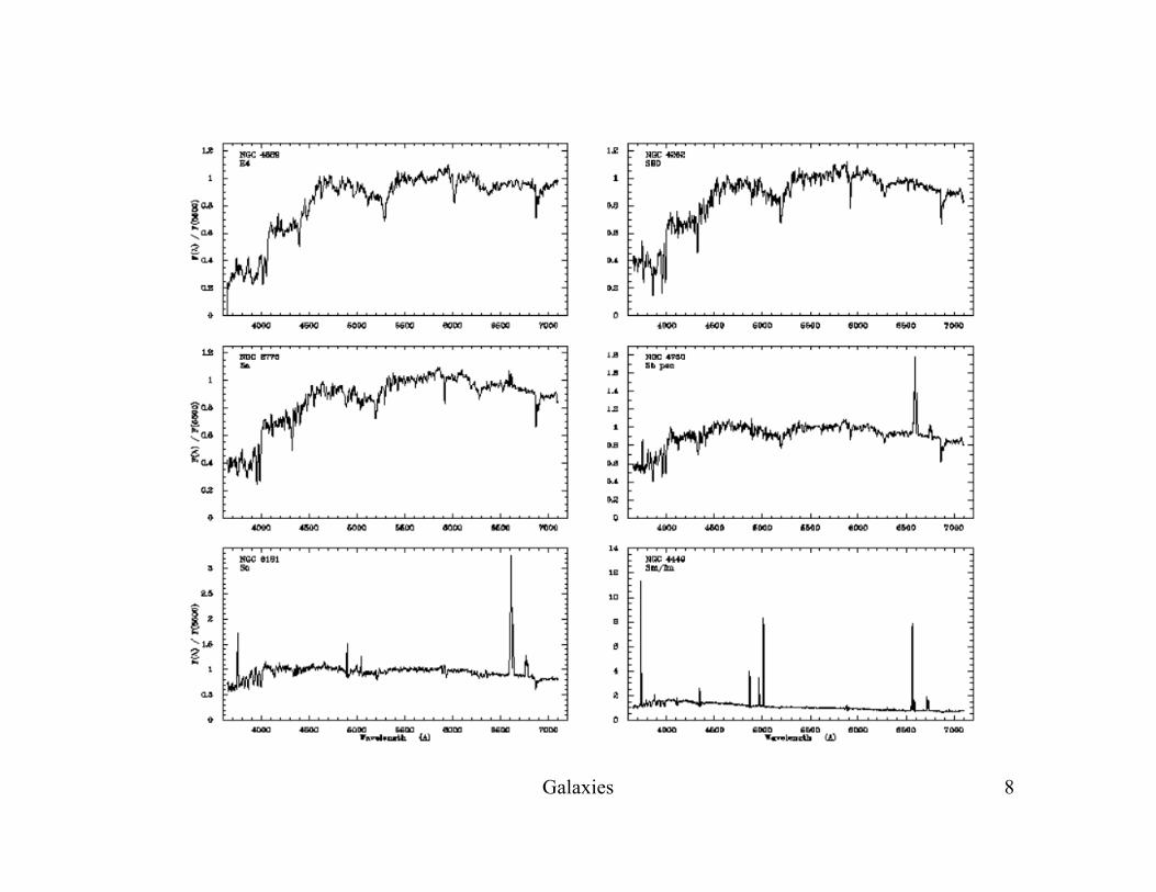
Quantitative spectral classificationKennicutt 1992, ApJS, 79, 255 Zaritsky, Zabludoff, Willick 1995, AJ, 110, 1602• galaxy spectra correlate strongly with Hubble type

– Morgan & Mayall (1957) developed a morphological classification system(Yerkes system) based on galaxy spectra (PASP, 69, 291)

• principle component analysis shows that most of the variation is dueto 2 parameters (eigenfunctions)– change in absorption spectrum: A stars vs K stars– change in emission line strength vs continuum + absorption

• fit each galaxy spectrum to these eigenspectra (maximum liklihood),measure spectral indices

• classifications are independent of morphology, but one can correlatespectral vs morphological types

Galaxies 8

Galaxies 9

morphology/spectral classificationKoopman & Kenney 1998, ApJ, 497, L5

Galaxies 10

Classification of Galaxies• Ultimately all classification schemes, whether human

or machine based, are fallible. However, machinebased schemes are certainly more repeatable, i.e.you and I can run the same classification script eventhough our by-eye results may not agree.

• A notable development in this field though is theadvent of Galaxy Zoo (Lintott et al. 2008): a largehuman based classification of the morphology ofSDSS galaxies.– The size of the data set and hard work of the classifiers has

allowed serious attempts to be made to understand thebiases involved in human classification.

Galaxies 11

Galaxy zoo

Galaxies 12

Galaxy colour-bimodality and classification

• one broad result should beemphasized: what may be termed themorphology-colour relation. Ellipticalgalaxies are typically redder in colourthan spirals. This phenomenon is alsoknown as colour-bimodality.

• Simply put, the forces that shape themorphology of a galaxy must alsoinfluence its star formation history.

• For, as we shall see later, theintegrated star formation history is theprime driver of its integrated colour.

Galaxies 13

Photometric Structure

Galaxies 14

Photometric Structure: Motivation• unlike more familiar dynamical systems (e.g., solar system,

stellar systems), the orbital properties of stars in galaxiesare not determined by few-body dynamics, but rather bythe mass distribution and dynamical history of the systemas a whole

• most relevant dynamical timescales in galaxies lie betweentwo limiting cases:– crossing time: time for a typical star to cross the systemτcross= R/v

– relaxation time: time for the system of stars torandomize orbits and attain an equilibrium configuration

• derive by computing frequency of 2-body gravitationalencounters and typical change in kinetic energy in eachencounter; relaxation time is that required for sum of δv2 to becomparable to typical orbital velocity v

• τrelax~ (N / 6 ln(N/2) ) (R/v) = N / (6 ln(N/2)) τcross where N isnumber of stars in system

Galaxies 15

Relaxation timescale• Idea: given enough time, molecules of air will

spread themselves out evenly in a room– Particles exchange energy and momentum during

“collisions” (close encounters)– Force between them is much stronger than the force

each feels from all other molecules together.• Similarly, can think of galaxy gravitation potentialΦ(x), as sum of– 1) smooth component averaged over region with many

stars,– 2) remainder: very deep potential well around each star.

Galaxies 16

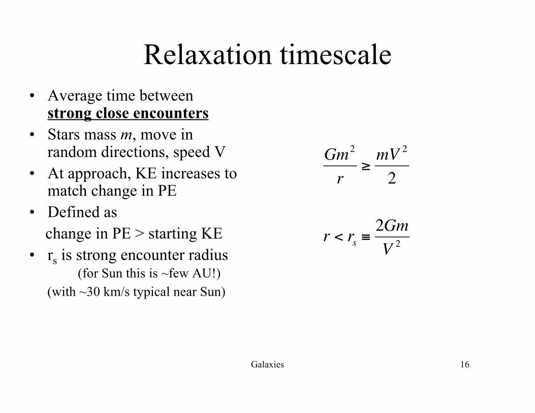
Relaxation timescale• Average time between

strong close encounters• Stars mass m, move in

random directions, speed V• At approach, KE increases to

match change in PE• Defined as change in PE > starting KE• rs is strong encounter radius

(for Sun this is ~few AU!)(with ~30 km/s typical near Sun)

!

Gm2

r"mV

2

2

r < rs#2Gm

V2

Galaxies 17

Relaxation timescale• Happens rarely: sun has not had

strong encounter in past ~5 Gyr• Imagine cylinder radius rs length Vt• n stars per unit volume, 1 encounter

in time ts withnπ rs

2 Vt = 1

• Around Sun n~0.1 pc-3

and ts ~ 1015 yrs!• Conclude that strong encounters are

only important in dense cores ofglobular clusters, and in galacticnuclei

!

ts /(4x1012yr) =

V3

4"G2m2n

#V

10km /s

$

% &

'

( )

3m

Msun

$

% &

'

( )

*2n

1pc*3

$

% &

'

( )

*1

Galaxies 18

Relaxation timescaleDistant weak encounters• Gravity always attractive, and star pulled toward other stars no matter

how far away• Cumulative pull of distant stars effective in changing stars direction

over time• Weak force implies stars hardly deviate from original path• Use impulse approximation, calculating force star would feel as they

continue on undisturbed path• Star mass M, moving at speed V along path that passes distance b from

a ‘stationary’ star of mass m

Vb M

m

Vt

Galaxies 19

Relaxation timescale• Measure time from point of

closest approach, perpendicularforce is

• Integrate over time, find that longafter encounter, M has speed …

• In this approximation, speed V ofM along original direction isunaffected - path of M is bentthrough angle α ...

• Momentum in direction Fperpmust be conserved, so star m isalso moving at 2Gm/bV

• Vperp must be small comparedwith V for valid approximation,thus weak encounter requires b tobe much larger than rs (strongencounter radius)

!

F" =GmMb

(b2

+V2t2)3 / 2

=MdV"

dt

#V" =1/M F"$%

%

& (t)dt =2Gm

bV

' =#V"

V=2Gm

bV2

b >>2G(m + M)

V2

Galaxies 20

Relaxation timescale• During t, number of stars m

passing M with separations fromb to b + Δb is

n . Vt 2πb Δb (their volume)• Multiply by vperp (previous slide)

and integrate over b gives theexpected squared speed: aftertime t …

!

"V#2

= nVtbmin

bmax$

2Gm

bV

%

& '

(

) *

2

2+b.db

=8+G2

m2nt

Vlnbmax

bmin

%

& '

(

) *

Galaxies 21

Relaxation timescale• After t ime t relax, such that <ΔVp

2> = V2, the star’s expected speed perpendicular toits original path becomes ~equal to original forward speed

– The memory of its initial path has been lost– Define Λ = bmax/bmin, we find this relaxation time is much shorter than the strong encounter

time ts (previous slides) …

!

trelax =V3

8"G2m2n ln#

=ts

2ln#

$2x10

9yr

ln#

V

10km /s

%

& '

(

) *

3

m

Msun

%

& '

(

) *

+2n

1000pc+3

%

& '

(

) *

+1

Not obvious what to use for Λ. Can’t have b < rs!Take bmin = rs and bmax equal to size of stellar system

For Sun bmax ~ 300pc to 30kpc, and ln Λ = 18−22 (exact values not important)

Galaxies 22

Relaxation timescale• In an isolated cluster of N stars, mass m, moving at speed V, average star

separation is ~1/2 R (size of the system).• Using the virial theorem: 2<KE> = -<PE>

• The crossing time tcross ~ R/V; since N=4nπR3/3, we have

!

1

2NmV

2"G(nm)

2

2R, so # = R /rs ~

GmN

V2.V2

2Gm~ N /2

"t _ relax

t _cross~

V4R2

NG2m2ln#

~N

6ln(N /2)

Galaxies 23

Dynamical Timescales of Stellar Systems

• Examples: (1 km/sec = 1 pc per 106 years)– open star cluster: N ~ 1000 R ~ 10 pc v ~ 1 km/sec

• τcross= 10/1 = 10 Myr• τrelax~ 18τcross~ 200 Myr

– globular star cluster: N ~ 105 R ~ 10 pc v ~ 10 km/sec• τcross= 10/10 ~ 1 Myr• τrelax~ 1100τcross~ 1 Gyr

– Milky Way: N ~ 1011 R ~ 10,000 pc v ~ 200 km/sec• τcross= 10000/200 = 50 Myr• τrelax~ 5 x 108τcross~ 2.5 x 1016yr

• implication: galaxies have dynamical memory!• present structure reflects dynamical history over >10 Gyr

Galaxies 24

Luminosity Functions• galaxies span enormous luminosity range: MB= -24 to -10• luminosity distribution well constrained for MB< -15

• parametrization: Schechter 1976, ApJ, 203, 297

Φ(L) dL = Φ(L*) (L/L*)α e-L/L* d(L/L*)where φ∗ is a characteristic density, L∗ is a characteristic luminosity and

α is a faint-end slope.

Galaxies 25

Luminosity Functions• The luminosity function (LF) describes the space density of galaxies

per unit luminosity as a function of luminosity.• Galaxy populations are almost universally described by the Schechter

(1976) function– can be thought of as a composite function consisting of a faint end power

law of slope alpha and a bright exponentially declining form.– Current redshift (distance) surveys provide the following best-fitting

parameters for the B-band luminosity function of:– φ∗ = 5.5 x 10−3 gals Mpc−3 L∗ = 2 x 1010 L⊙ or M∗ = −20.6.

1

Galaxies 1

GalaxiesLecture 4: Luminosity Function and

Galaxy Profiles• Luminosity function and galaxy formation• Photometric structure• Surface brightness profiles• Size of galaxies

Galaxies 2

GOALS:• Ultimately we want to understand how galaxies form,

evolve, and produce the Hubble diagram today• Relaxation timescale very long! … suggests that studying

galaxy morpology, structure and radial profile willunearth fossil records of the formation history

• The luminosity function of galaxies has also provided a lotof unexpected clues to how galaxies form

• All of these are strong motivations for carefully studyingthe properties of ‘local’ galaxies in as much detail aspossible.

Galaxies 3

Dynamical Timescales of Stellar Systems

• Examples: (1 km/sec = 1 pc per 106 years)– open star cluster: N ~ 1000 R ~ 10 pc v ~ 1 km/sec

• τcross= 10/1 = 10 Myr• τrelax~ 18τcross~ 200 Myr

– globular star cluster: N ~ 105 R ~ 10 pc v ~ 10 km/sec• τcross= 10/10 ~ 1 Myr• τrelax~ 1100τcross~ 1 Gyr

– Milky Way: N ~ 1011 R ~ 10,000 pc v ~ 200 km/sec• τcross= 10000/200 = 50 Myr• τrelax~ 5 x 108τcross~ 2.5 x 1016yr

• implication: galaxies have dynamical memory!• present structure reflects dynamical history over >10 Gyr

Galaxies 4

Luminosity Functions• galaxies span enormous luminosity range: MB= -24 to -10• luminosity distribution well constrained for MB< -15

• parametrization: Schechter 1976, ApJ, 203, 297

Φ(L) dL = Φ(L*) (L/L*)α e-L/L* d(L/L*)where φ∗ is a characteristic density, L∗ is a characteristic luminosity and

α is a faint-end slope.

Galaxies 5

Luminosity Functions• The luminosity function (LF) describes the space density of galaxies

per unit luminosity as a function of luminosity.• Galaxy populations are almost universally described by the Schechter

(1976) function– can be thought of as a composite function consisting of a faint end power

law of slope alpha and a bright exponentially declining form.– Current redshift (distance) surveys provide the following best-fitting

parameters for the B-band luminosity function of:– φ∗ = 5.5 x 10−3 gals Mpc−3 L∗ = 2 x 1010 L⊙ or M∗ = −20.6.

Galaxies 6

Luminosity Functions• The total density of galaxies is:

• where Γ(a) is the Gamma function. Note thatthis integral diverges for α<-1, in which casethe alternative form should be used:

• where Γ(a, b) is the incomplete Gammafunction.

2

Galaxies 7

Luminosity Functions

• The luminosity density of galaxies is

• Taking α = −1 gives Γ(α + 2) = Γ(1) = 1and L = φ∗ L∗ = 1.1x108 L⊙Mpc−3 .

Galaxies 8

Luminosity Functions• Mulitplying the LF by a single M/L ratio (see Dark

Matter later) generates a very simple galaxy massfunction.

• Why does the crude galaxy mass function deviatefrom the expectation of a dark matter mass functionat the high- and low-mass ends?

• This is similar to the question of what determines themaximum and minimum mass of a galaxy?

• Answers include supernova driven mass loss andAGN moderated feedback.

Galaxies 9

Galaxy Evolution - Dark Matter and Gravity

Galaxies 10

Galaxies 11

Luminosity Function• The LF can be applied

across all galaxy types orsplit by galaxy properties

• Form of LF at faintluminosities still uncertain,controversial

• LF is strong function ofgalaxy type

• LF probably is dependenton galaxy environment

Binggeli, Sandage, Tammann1988, ARAA, 26, 509

Galaxies 12

Theory: Structure of Galactic SpheroidsRadial structure:• if we approximate spheroids as relaxed, purely stellar systems, stellar

dynamical theory provides a semi-empirical description (King 1962, AJ, 67, 471)

– Look at this in detail in Lec_5• profile follows isothermal profile (ρ~ 1/r2) over several magnitudes in

surface brightness• central core, with projected brightness I(r ) = I0/ (1 + r/rc) rc -> core radius• King model also requires outer truncation, parametrized by a tidal radius c -> log (rt / rc)

King 1966, AJ, 71, 64

3

Galaxies 13

= M49. Galaxy in Virgo

Galaxies 14

King modelsare reasonabledescriptions of

a range ofspheroidclasses

Galaxies 15

Surface brightness profiles

• One could think of this as one-dimensionalmorphology where the intensity per unitsurface area is expressed via an analyticfunction.

• Surface brightness data is generated byaveraging along elliptical isophotes togenerate 1D elliptically averaged lightprofiles.

Galaxies 16

Surface brightness profiles

Chapman et al. (2000)

Galaxies 17

Surface Brightness• Surface brightness is quoted in L⊙pc-2 ,• i.e. 1L⊙pc-2 = (3.86 x 1024 W)/(3.09 x 1016 m)2 = 4.05 x 10-7 Wm-2 .• The B-band solar magnitude is MB,⊙ = 5.48 and 1 pc at

10 pc subtends 0.1 radians (20626.5 arcseconds).• Expressing L⊙pc-2 in magnitudes per square arcsecond gives

µB = −2.5 log(L/pc2 ) = MB,⊙ + 5 log(20626.5) = 27.05 B magnitudes per square arcsecond (at 10 pc).

Galaxies 18

Empirical luminosity laws

• Generally, features such as spiral arms anddust lanes average out in this process(though as will be seen some ripples andbumps can remain).

• Simplistically:– Spiral galaxy disks display surface brightness

profiles that are well fit by exponential intensityprofiles

– Elliptical galaxies are fit by a de Vaucouleurs(1948) or R1/4 intensity profile.

4

Galaxies 19

Empirical luminosity laws• Hubble (1926) profile

I(r ) = I0 / (1 + r/ro)2

• de Vaucouleurs r 1/4 lawlog I(r )/I0 = (r/re)1/4 -1where re -> effective radius(radius containing half of integrated luminosity)

• although the r 1/4 law is empirical in origin, n-body simulations of merging/formingspheroids can reproduce the profile

Galaxies 20

de Vaucouleurs profile:Good fit to outer regions of

spheroidal galaxies(ellipticals)

Galaxies 21

Surface brightness (spirals)

• Exponential (spiral) intensity profile:I (R) = I0 exp( −R/ rs),

• where I0 is the central intensity and rs isa scale length.

• Expressed in magnitudesµ(R) = µ0 + 1.086(R/ rs)

where 1.086 = 2.5 log e.

Galaxies 22

Sersic Luminosity Profiles• Sersic 1968, Atlas de Galaxias Australes

(Cordoba: Obs. Astr. Cordoba) BM Box 4.1 (p187)• the de Vaucouleurs law is a specific form of a

more generalized law:log I(r )/I(re) = -bn [(r/re)1/n-1]where re -> effective radius

(‘b’ chosen so radius contains half of integrated luminosity)• case n = 4: de Vaucouleurs r1/4 law• case n = 1: exponential (disc) law• intermediate cases do exist (e.g., pseudo-bulges)• a galaxy can be fitted with a sum of Sersic

profiles (one for each distinct component)

Galaxies 23

Surface Brightness Profiles

• In practice many galaxies display a surfacebrightness profile that is best described by asuperposition of two intensity profiles.

• This is achieved by fitting a galaxy with eachprofile applied over a selected range of radii,– e.g. R1/4 over inner radii and exponential over

outer radii.• Such an approach is referred to as bulge-disk

decomposition.

Galaxies 24

SurfaceBrightness

Profiles

5

Galaxies 25

Surface brightness• Surface brightness can be expressed as• LTotal / 2πRe

2 where Re is the half-light radius.• Using this simple definition, both spirals and

ellipticals display surface brightnesses oforder 100 L⊙pc-2 or µB = 22.

• Central values of surface brightness candiffer greatly,

• e.g. of order a few hundred L⊙ pc−2 for spiralsto ∼104 L⊙ pc−2 for ellipticals.

Galaxies 26

Size of galaxies

• A closely related topic is the idea of the totalsize of a galaxy.

• The detectable extent of a galaxy on adetector is determined by the radius at whichthe surface brightness approaches theeffective surface brightness of the combinedsky plus detector noise.

• This isophotal area can be thought of as alower limit on the size of a galaxy.

Galaxies 27

Size of galaxies• One could simply integrate the relevant surface

brightness profile to infinite radius. However, this• a) requires obtaining an accurate determination of the

SB profile• b) assumes that the profile can be reasonably

extrapolated beyond the isophotal radius.• An alternative, practical approach is to determine a

radius based upon a statistical analysis of the lightdistribution in the galaxy itself.

• This has the advantage that the radius is modelindependent and can be computed for galaxieswhere only a few tens (or less) of pixels are detectedabove the isophotal threshold.

• This is the idea behind the Kron (1980) and Petrosian(1976) radii.

Galaxies 28

Surface brightness

One inverts the equation to obtain RP . Typically, L(RP) ∼ 90% LT

twice the image moment radius

Galaxies 29

Core structure of spheroid galaxies

• Lauer et al. 1995, AJ, 110, 2622 (Nuker team)• Jaffe et al. 1995, AJ, 108, 1567• subject revolutionized by HST

- resolution at larger distances wheretypical ellipticals live

• luminous galaxies show strong turnover ininner ~100 pc cores; or “shallow cusps”

• lower luminosity galaxies show continued (1/r)increase in brightness into the galactic centers

• few ellipticals show asymptotic flat brightnessprofile in center

Galaxies 30Lauer et al. 1995, AJ, 110, 2622

6

Galaxies 31 Galaxies 32

Ellipticals with faint disks

Galaxies 33

dSph galaxies: mini-ellipticals?

Galaxies 34

Galaxies 35 Galaxies 36

1

Galaxies 1

Elliptical GalaxiesLectures 5-7: 3D structure of ellipticals, their

stars, a physical understanding, and theirformation mechanisms

• 3D structure of ellipticals & scaling relations• Stellar populations in Ellipticals,• cusps/cores and clues to the formation of E’s• Collisionless Boltzmann Equation• Isothermal sphere and King model• Violent relaxation (rapid change in potential)• Relation to observed Sersic profiles

– Sersic index varies with Elliptical luminosity

Galaxies 2

Parameterization of the SurfaceBrightness Profiles: Sersic profiles

• Sersic law (Sersic 1968):I(R) = Ieexp(-bn[R/Re)1/n -1])

• Has a number of attractive features forparameterizing both the small - and large-scaleprofiles of E/dE galaxies:– Accounts for the profiles’ curvature on kpc-scales– Parameters are robust against radial range of data

(Graham et al. 2003)– Integrals for r->infinity converge (c.f., Nuker law)

Galaxies 3

Cores/Cusps

Lauer et al. 1998

Galaxies 4

Elliptical GalaxiesInferring the density from the surface brightness• The surface brightness profile, which

essentially traces the distribution of stars, canbe used to infer the underlying 3D matterdensity distribution.

• The projected stellar surface densitydistribution is the integral over the 3D stellardensity distribution.

• This in turn can be viewed as the total matter3D density distribution scaled by a suitablemass-to-light ratio– (in practice the use of a single M/L may be

simplistic, though useful, assumption).

Galaxies 5

Elliptical Galaxies• So what can we learn about the underlying

3D matter density distribution from the radialdistribution of starlight alone?

• Consider a power law distribution of 3Ddensity, e.g. ρ ∝ r -γ . The projected surfacebrightness distribution will be a scaled versionof the projected density, i.e.

where the z -axis is defined by the line-of-sightto the observer.

Galaxies 6

3D structure

• Taking g = z /R, this integral becomes

where G(γ ) depends only on γ.Therefore a power-law 3D density of slope −γ

projects onto a surface density profile of slope−γ + 1.

(likewise King models have similar behaviourfrom 3D density to 2d surface density profile)

2

Galaxies 7

• One of the drawbacks of the de Vaucouleurs surface brightnessdistribution is that it does not have an analytic counterpart in 3Ddensity.

• Various density profiles have been suggested that provide agood match to observed surface brightness profiles whenprojected, e.g. the Hernquist (1992) profile

• The Hernquist model is particularly appealing as it arises fromthe numerical simulation of the merger of two equal mass diskgalaxies, each embedded within a dark matter halo.

Galaxies 8

Hernquist Profile

Galaxies 9

Relation to orbital properties• The 2D shapes of elliptical galaxies results from the

3D distribution of stars.• This in turn may be thought of as a reflection of the

3D orbital structure of the galaxy.• The debate as to the orbital structure of bright

ellipticals was eventually resolved via resolvedabsorption line spectroscopy during the 1970s andearly 1980s.

• Ellipticals are not isotropicsystems whose 2D morphologyarises from rotational flattening.• They are slow rotatorscompared to their randomvelocity dispersion.

Galaxies 10

Relation to orbital properties• The 2D morphology of bright ellipticals results from

an anisotropic mix of stellar orbits.• As the stellar orbits are incoherent (both positive and

negative along the line of sight) let us consider themean square velocity ⟨v 2 ⟩ along each axis.

• We refer to the mean square velocity along each axisas σ2 (i.e. ⟨vx

2 ⟩ = σx 2 where σ is the velocitydispersion).

• Consider a galaxy rotating in the x-y plane (i.e. aboutthe z -axis) with a rotational velocity V .

• The velocity dispersions are isotropic,i.e. σx

2 = σy2 = σz

2 .

Galaxies 11

Orbital properties• The radial extent of stars along each axis should be

proportional to their kinetic energies.• Assuming we view the system from the y-axis (side

on), then a non zero axis ratio should result fromrotational flattening according to

• The 1D velocity dispersion σr = σy which is equal tothe other components following our isotropycondition.

Galaxies 12

• We therefore have

• which can be re-arranged to yield

• where ϵ = 1 − b/a is the observed ellipticity.

3

Galaxies 13

Orbital properties• As can be seen (next slide), to obtain b/a = 0.5

(an E5 elliptical) requires V /σ ≈ 1.• As a typical bright elliptical may display σ = 250kms−1

this means it would have to rotate as fast as a massivespiral !!!

• In practice most bright ellipticals rotate much slowerthan this limit.

• One concludes that rotational flattening does notcontribute to the 2D shapes of ellipticals

• And that they are instead caused by anisotropic orbits.

Galaxies 14

Galaxies 15 Galaxies 16

3-Dimensional Form of Spheroids

• Approximated 3D formsas oblate or prolatespheroids

• Get distribution if trueflattenings can bedetermined (detailedkinematics?)

• Photometric andkinematic tests moreconsistent with oblategeometry

Sandage, Freeman, Stokes

1970, ApJ, 160, 831

Galaxies 17 Galaxies 18

4

Galaxies 19

Orbital properties• Clearly some ellipticals do rotate to the extent

that rotational flattening contributes to theirmorphology.

• These are generally lower luminosityellipticals and their morphologies as oftenreferred to as “disky” (as opposed to the“boxy” bright ellipticals) - thought to indicate arotating stellar disk.

Galaxies 20

Galaxies 21 Galaxies 22

Departures from ellipticity

In the limit, S0 galaxies couldbe considered the extreme

of ‘disky’ ellipticals

Boxy ellipticals suggest somedegree of triaxiality.

Galaxies 23 Galaxies 24

Yerkes classifications: "c" in "cD" refers to galaxies being very large, hence supergiant, "D" refers diffuse.A backformation of "cD" is frequently used to mean central Dominant galaxy.

5

Galaxies 25

cD elliptical

Galaxies 26

Galaxies 27

• Shells have been used to constrain stellar orbitsand potential of ellipticals

Galaxies 28

SCALING RELATIONS inElliptical Galaxies

Galaxies 29

• Luminous (Giant = Normal = Ordinary) galaxies obey a well-definedset of scaling relations between their photometric and kinematicstructural parameters:

• e.g., Fish (1964), Faber & Jackson (1976), Kormendy (1977), Binggeli,Sandage & Tammann (1984), Dressler et al. (1987), Djorgovski & Davis(1987), and many, many others.

• Late-types usually considered separately, and dwarfs, usually not atall.

Guzman et al 1993

Galaxies 30

Kormendy 1977Early suggestions for

parameter correlations inEllipticals

6

Galaxies 31

• Ellipticals, dSphs, and globular star clustersare not all obviously an extension of thesame spheroid sequence … (dSphs later lecture)

Galaxies 32

Faber-Jackson and the virial theorem

• Faber and Jackson (1976) determined(empirically) that the luminosity of brightellipticals is related to their velocitydispersion via

L ∝ σrn with 3 < n < 5.

• More luminous ellipticals are moremassive.

Galaxies 33

Faber-Jackson and the virial theorem

• One can take a simple approach to theFJ relation by noting that

• v2 ∝ GM/R (virial theorem) and L ∝ Ie Re 2

• This indicates that L ∝ v4 / (le (M/L)2),which nominally reproduces the FJ relation

(if both the M/L ratios and surface brightnessproperties are relatively constant for brightellipticals).

Galaxies 34

Faber-Jackson and the virial theorem

• As we have noted, the FJ relation is areflection of the virial theorem applied toelliptical galaxies, assuming that their surfacebrightnesses and mass-to-light ratios arerelatively constant.

• Beginning with the virial theorem we can write2K + U = 0

• For the kinetic energy of the system we have

Galaxies 35

Faber-Jackson and the virial theorem

• We further note that ⟨v 2 ⟩ = σ 2 = 3 σr2 ,

where σr is the 1D velocity dispersion.The potential energy takes the form

where rg is a weighted average separationof the stars in the galaxy.

Galaxies 36

Faber-Jackson and the virial theorem• Generally we may write

• where α is a constant of order unity whosevalue depends upon the form of the densityprofile.

• We can therefore write

7

Galaxies 37

• Which corresponds to the FJ relationassuming that Ie and M/L are relativelyconstant for bright ellipticals. Galaxies 38

The Fundamental Plane• Djorgovski and Davis (1987) were among a

number of researchers to note that twoparameter scaling relations– Faber-Jackson sigma-L– Kormendy (core/cusp surface brightness, vs L)

contained real scatter in which the residualsin one plot correlated with those on the other.

• This suggested the existence of a threeparameter relation encompassing the aboverelationships,– i.e. a tilted plane of points in 3D of which the FJ

and Kormendy relations are 2D projections.

Galaxies 39

Es/S0s and the Fundamental Plane• Edge-on projection of the Fundamental Plane for

10K early-type galaxies from the 6dFGS (Colless et al. 2009; www.aao.gov.au/6dFGS).

• Note: does not include “dwarfs” (i.e., the samplehas a mass cutoff of 1010.5 solar masses).

Galaxies 40

The Fundamental Plane

• The Fundamental Plane (FP) relationfor bright ellipticals takes the form

log Re = 1.4 log σe + 0.36Σe + constant,• where σe is the 1D velocity dispersion

measured within Re and Σe = −2.5 log Ie

Galaxies 41

The Fundamental Plane• The FP relation can be reconstructed using

the following arguments

with this second equation being a statement ofvirial equilibrium and c denoting acombination of physical constants.

Galaxies 42

The Fundamental Plane• Dividing these two equations one obtains

which is close to but not exactly equal to theobserved FP relation.

8

Galaxies 43

The Fundamental Plane• We conclude that1. Bright ellipticals are in virial equilibrium.2. To 1st order M/L ratios and structural

parameters are very similar.3. Therefore, their stellar populations, ages and DM

properties are very similar.4. To obtain an exact match to observed FP data

requires M/L ∝ M 0.2 , i.e. massive ellipticals areslightly older than less massive counterparts.