
analysis of fluid flow and losses in regenerative flow ...
164
ANALYSIS OF FLUID FLOW AND LOSSES IN REGENERATIVE FLOW COMPRESSORS USING CFD A THESIS BY Kassa Teferi Submitted to the School of Graduate Studies Addis Ababa University In Partial Fulfillment of the Requirement for the Degree of Masters of Science in Mechanical Engineering ( With Specialization in Thermal Engineering ) ADVISOR: Dr. - Ing. Edessa Dribsa April, 2008
-
Upload
khangminh22 -
Category
Documents
-
view
3 -
download
0
Transcript of analysis of fluid flow and losses in regenerative flow ...
ANALYSIS OF FLUID FLOW AND LOSSES IN REGENERATIVE
FLOW COMPRESSORS USING CFD
A THESIS
BY
Kas s a Te fe ri
Subm it t e d t o t he Sc hoo l o f Graduat e St udie s
Addis Ababa Unive rs it y
In Part ial Fulfillm e nt o f t he Re quire m e nt for t he De gre e o f
Mas t e rs o f Sc ie nc e in Me c han ic al Engine e ring
( With Spe c ializat ion in Th e rm al En gin e e rin g )
ADVISOR: Dr. - Ing. Ede s s a Dribs a
April, 2 0 0 8
ii

I
ACKNOWLEDGEMENT
First I thank God for giving me strength to finish my work and also the work described
would not have been possible with out the valuable assistance of many people. I would like
to express my deepest gratitude to my thesis advisor, Dr. - Ing. Edessa Dribsa, for his skillful
guidance, encouragement, enormous patience and willing attitude throughout the course of
this research.
I would also like to thank my friends, and specially Ato Yonas Theshome, for his support in
giving me important research papers, journals and in sharing of his ideas. I also want to
appreciate all of my instructors / colleague in the Department of Mechanical Engineering,
Addis Ababa University for their continuous encouragement.
Finally, I would like to thank my family for the unending confidence, constant support and
endless love.

II
ABSTRACT
Regenerative flow compressors are rotodynamic machines capable of producing high heads
at very low flow rates. With comparable tip speed, they can produce heads equivalent to that
of several centrifugal stages from a single rotor. They have found many applications for
duties requiring high heads at low flow rates but the compression process is usually with very
low efficiency which is their major drawback.
Even though there are several factors that can be considered to improve the efficiency of
these machines in this thesis various models will be developed with different blade and flow
channel geometries to investigate their effect on performance.
Details of CFD analysis on the models of the compressor, using a commercial software
“FLUENT”, will be presented. And based on simulation results of the different models a
blade and channel geometry that gives significant improvement on performance will be
suggested.
III
Title Page No.
Acknowledgement....................................................................................................................I
Abstract.… .....................................................................................................................……II
Table of Contents...............................................................................................................…III
List of Figures.......................................................................................................................VII
List of Tables................................................................................................................…...XIV
CHAPTER ONE INTRODUCTION
1.1 Classifications of compressors.…………………………….……………………..1
1.2 Turbocompressors………………………………………………………………...3
1.3 Regenerative Flow Compressors…………...……………………………………..4
1.4 Objective of the thesis.…………………………………………………………....5
1.5 Methodology………………………………………………………………………6
1.6 Outline of the thesis…...…………………………………………………………..7
CHAPTER TWO DESIGN AND OPERATIONAL FEATURES OF REGENERATIVE
TURBOMACHINES
2.1 Essential components of Regenerative Turbomachine…………………...………9
2.1.1 Impeller………..…………………………………………….……...…...10
2.1.1.1 Impeller blades...............................…………………………........11
2.1.2 Inlet and Exit Ports……..…………..………………….………..…...…..14
2.1.3 Stripper.…………………………………..…………….……………......14
2.1.4 Flow Channel......………..……….…..……………………………….….14
2.2 Working Principle ………................................................……........……...…......15
2.3 Performance characteristic s of RFC………….………….....……....…………...17
2.4 Comparison of Centrifugal and Regenerative Flow Compressors.....…….…......18
2.5 Applications of Regenerative Flow Compressors ………………………...…….20

IV
CHAPTER THREE LITERATURE REVIEW
3.1 Introduction… … … … ....… … … … ..… … … … … … … … … … .… … … … … … ...23
3.2 Theoretical Models … … ...… ..… … … ..… … … … … … ..… … … … … … … ...… .23
3.3 Experimental Work … ....… … … … … ..… … … … .… … … … … … … … .....… … 25
3.4 Losses in Regenerative Turbomachines..........… … … … … … … … … … ..… … ..26
3.5 Impeller Blades Profile...… ...… … … .....… … .… … … … … … … … … … .… … ..27
3.6 CFD Work … … … ...… … … ..… … … .… … … … … … … … … … … … … ..… … ..28
CHAPTER FOUR ANALYSIS OF RFC USING FLUENT
4.1 Introduction… … … … … … … … … … … … … … … … … … … … .… … … … … .… .30
4.2 Compressible flow theory… … … … … … … … .… … … … … … … … … … … … … 30
4.3 Flows in Rotating (Moving) Frame of Reference...… … … … … … … … .… … … .32
4.4 Governing Equations… … … … … … … … … … … … … … .… … … … … … .… ......33
4.4.1 The Mass Conservation Equation… .… .… ..… … .… … … … … … … … … .33
4.4.2 Momentum Conservation Equation......… … ....… .… … … … … … … … … 33
4.4.3 The Energy Equation… … … … … … … … … … .… … … … … … … … … ....35
4.5 Governing Equations in a Rotating Reference Frame… … … … … … … … … … ...36
4.6 Turbulent Flow Models… .....................................................................................39
4.6.1 Transport Equations for the Realizable - Model… … … … … … … … .40
4.7 Numerical Computation..............................................................................… ......42
4.7. 1 Pressure-Based Segregated Algorithm… … … … … … … … … … … … ...43
4.7. 2 Discretization Technique in FLUENT… … … … … … … … … … … … ....44
4.7.2.1 Solving the Linear System… … … … … … … .… … … … … … … … 46
4.7.2.2 Spatial Discretization… … … … … … … … … … … … … … … ..… ...47
4.7.2.3 Evaluation of Gradients and Derivatives… … … … … … … ....… ...48
4.7.2.4 Implicit Linearization… … … … … … … ..… … … ..… … … … … … 49
4.7.2.5 Pressure Interpolation and Pressure-Velocity Coupling… ..… .....50
4.7.2.6 Density Interpolation Schemes… … … ..… … … … … … ..… … … .53
4.7.2.7 Under-Relaxation… … … … … … … ..… … … … ..… … … … … … ..53

V
4.8 Multigrid Method...........................................................................................… ...54
4.8.1 The Need for Multigrid… … … … … … … … … … … … … … … … … … … 54
4.8.2 Algebraic Multigrid (AMG)… … … … … … … … … … … … … … … … … .55
4.9 Standard Wall Functions… … … … … … … … … … … … … … … … … … … … … ...56
CHAPTER FIVE RFC MODIFICATION AND SIMULATION PROCEDURES
5.1 Introduction… … … .… … … … … … … … … … … … … .… … … … … .… … … .… ...62
5.2 Non-dimensional Design Parameters… … … … … … … .… … … … … … … ..… … .63
5.3 Base Regenerative Flow Compressor...................................................................66
5.3.1 Dimensions of the Base Machine....… … … … … … … … … … … … … … .67
5.3.2 Operation points of the Base Machine… ....… … … … … … … … .… … … .69
5.3.3 Performance Characteristics of the Base Machine… ...............................70
5.4 Modification of the Base RFC.............................................................................72
5.4.1 Major Losses in RFC… ...................… … … … … … … … … … … … … … .72
5.4.2 Modification of the basic Geometries… .....… … … … … … … … .… … … .74
5.5 Basic Steps for CFD Analysis… .........................................................................79
5.5.1 Preprocessing of Simulation… … .............................................................81
5.5.1.1 Preprocessing in GAMBIT… … … … … … … … … … … … … .… ...81
5.5.1.2 Preprocessing in FLUENT… … … … … … … … … … … … … .… ...85
5.5.2 Processing in FLUENT… … … … … … … … … … … .… … … ..… … .… … .91
5.5.2.1 Setting of Solution controls… … ....................................................92
5.5.2.2 Selecting Solution monitors… … ...................................................93
5.5.2.3 Solution Computing… … ...............................................................96
5.5.3 Post processing in FLUENT… … … … … … … … … … … … .....................96
CHAPTER SIX RESULTS AND DISCUSION
6.1 Introduction… … … … … … … … … … … … … … … … … … … … … … … … … … … 98
6.2 Results of CFD Analysis........................................................................................99
6.2.1 Graphical Displays… ...… … … … … … … … … … … … … … … … … … … 99

VI
6.2.2 Numerical Results.........… … … … … … … … … … … .… … … … … ........110
6.3 Evaluation of Design Parameters… … .… … … … … … … … … … … … … … … … 111
6.4 Validation..............................................................................… … … … … … .......115
6.5 Results of Modifications done to Improve Performance .........… … … … … .......115
6.5.1 Effect of changing Flow Channel and Impeller Profile..........................115
6.5.2 Effect of changing Blade Angles...… .… ................................................116
6.5.3 Effect of adding a Core… … ...................................................................117
6.5.4 Effect of changing the Working Fluid....… … … … … … … … … … … … 118
CHAPTER SEVEN CONCLUSION AND RECOMMENDATIONS
7.1 Conclusion...................................… … … … … … … … … … … … … … … … … … 119
7.2 Recommendations...............................................................................................120
REFERENCES.....................................................................................................................122
APPENDIX...........................................................................................................................123
1. Output results for model RFCR-90.........................................................................123
2. Output results for model RFCS-135.......................................................................125
3. Output results for model RFCA-135.......................................................................127
4. Output results for model RFCA-145.......................................................................130
5. Output results for model RFCA-150.......................................................................132
6. Output results for model RFCA-160.......................................................................135
7. Output results for model RFCA-180.......................................................................137
8. Output results for model RFCSE-145.....................................................................140
9. Output results for model RFCNGA-145.................................................................142
10. Output results for model RFCCA-145....................................................................145
VII
List of figures
Title Page No.
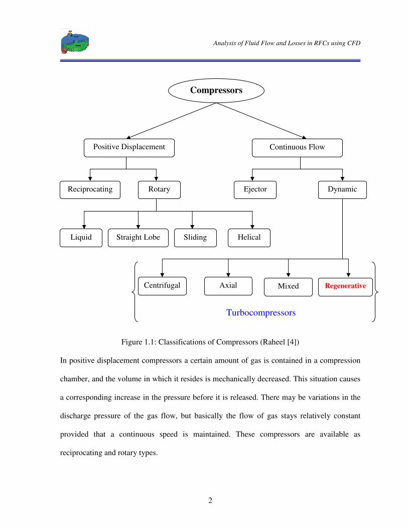
Figure 1.1: Classifications of Compressors...............................................................................2
Figure 2.1: A Regenerative Turbomachine....… … … … … … … … … … … … … … … … … .… ...8
Figure 2.2: A Regenerative Turbomachine with magnified fluid flow between blades… … ....9
Figure 2.3: Schematic diagram of a Regenerative Turbomachine… .........................................9
Figure 2.4: Section A-A enlarged.… … … … … … … … ...… … … … … … .… … … … … … … . .10
Figure 2.5: Section B-B enlarged… … ..........................… … … … … … .… … … … … … … .. ...10
Figure 2.6: Regenerative Turbomachines blades with radial and non-radial profiles… … … .12
Figure 2.7: Regenerative Turbomachine blades with semi-circular profiles… .… … … … ......13
Figure 2.8: Regenerative Turbomachine blades with aerofoil profile and having a core… … 13
Figure 2.9: Tangential pressure variation in a Regenerative Turbomachine… .......................16
Figure 2.10: Performance characteristics of Regenerative Turbomachine..............................18
Figure 4.1: Stationary and Rotating Reference Frames.......… … … … … … … … … … … .… ...36
Figure 4.2: Overview of the Pressure-Based Solution Methods… … … … … … … … … … ......44
Figure 4.3: Control volume used to illustrate discretization of a scalar transport
equation.................................................................................................................46
Figure 5.1: Schematic of blade and channel geometry for Single stage RFC… … … … … .… 68
Figure 5.2: Pressure ratio Vs Specific mass flow rate at various tip Mach number… … … ....71
Figure5.3: Isothermal efficiency Vs Specific mass flow rate at various tip Mach number… .71
Figure 5.4: Modified schematic of flow channel and impeller geometry.......................… .....75
Figure 5.5: Blade variations with blade angle - β and velocity triangles on the cross
section of the flow field...................................… … … … … … … … … … … … … ..76
Figure 5.6: Modified schematic geometry with Core..............................................................77
VIII
Figure 5.7 Basic Program Structure… .....................................................................................80
Figure 5.8: Numerical model of Regenerative Flow Compressor… .......................................84
Figure 5.9: Scaled residuals at the final iterations for Model RFCA-145...............................93
Figure 5.10: Convergence history of total pressure at exit port for Model RFCA-145...........94
Figure 5.11: Convergence history of mass flow rate at exit port for Model RFCA-145.........95
Figure 6.1: Plot of total pressure contours over the entire flow field for model
RFCR-90 (at design point running speed, 28910 rpm)........................................99
Figure 6.2: Plot of total pressure contours over the entire flow field for model
RFCA-145 (at design point running speed, 28910 rpm)....................................100
Figure 6.3: Plot of density contours over the entire flow field for model RFCA-145
(at design point running speed, 28910 rpm).......................................................101
Figure 6.4: Plot of a particle path line from inlet to exit port for Model RFCA-145
(at starting running speed, 2891 rpm)................................................................102
Figure 6.5: Detail view of plot of a particle path line from inlet to exit port for Model
RFCA-145 (at starting running speed, 2891 rpm).............................................103
Figure 6.6: Plot of Isothermal power gained by a particle along its path line from inlet to
exit port for Model RFCR-90 (at starting running speed, 2891 rpm)................104
Figure 6.7: Plot of Isothermal power gained by a particle along its path line from inlet to
exit port for Model RFCA-145 (at starting running speed, 2891 rpm)...............105
Figure 6.8: Plot of Isothermal power gained by a particle along its path line from inlet to
exit port for Model RFCA-145 (at the second running speed, 5782 rpm)..........105
Figure 6.9: Plot of Isothermal power gained by a particle along its path line from inlet to
exit port for Model RFCA-145 (at the third running speed, 8673 rpm).............106

IX
Figure 6.10: Plot of Isothermal power gained by a particle along its path line from inlet to
exit port for Model RFCA-145 (at the fourth running speed, 11564 rpm).......106
Figure 6.11: Plot of Isothermal power gained by a particle along its path line from inlet to
exit port for Model RFCA-145 (at running speed, 20237 rpm)… … … … … … 107
Figure 6.12: Plot of Isothermal power gained by a particle along its path line from inlet to
exit port for Model RFCA-145 (at the design point speed, 28910 rpm)...........108
Figure 6.13: Plot of relative velocity vectors on a cross-sectional surface in the flow field for
Model RFCR-90 (at the design point running speed, 28910 rpm)....................109
Figure 6.14: Plot of relative velocity vectors on a cross-sectional surface in the flow field for
Model RFCA-145 (at the design point running speed, 28910 rpm)..................109
Figure 6.15: Plot of a particle path line from inlet to exit port for Model RFCCA-145
(at starting running speed, 2891 rpm)...............................................................117
Figure 6.16: Plot of total pressure contours over the entire flow field for model
RFCCA-145 (at design point running speed, 28910 rpm)................................118
Figure 6.17: Plot of total pressure contours over the entire flow field for Model
RFCR-90............................................................................................................123
Figure 6.18: Plot of density contours over the entire flow field for Model
RFCR-90............................................................................................................123
Figure 6.19: Plot of relative velocity vectors on a cross-sectional surface in the flow field for
Model RFCR-90................................................................................................124
Figure 6.20: Plot of Isothermal power gained by a particle along its path line from inlet
to exit port for Model RFCR-90........................................................................124

X
Figure 6.21: Plot of total pressure contours over the entire flow field for Model
RFCS-135..........................................................................................................125
Figure 6.22 Plot of density contours over the entire flow field for Model
RFCS-135..........................................................................................................125
Figure 6.23: Plot of a particle path line from inlet to exit port for Model
RFCS-135(at starting running speed, 2891 rpm)..............................................126
Figure 6.24: Plot of Isothermal power gained by a particle along its path line from
inlet to exit port for Model RFCS-135..............................................................126
Figure 6.25: Plot of relative velocity vectors on a cross-sectional surface in the flow field for
Model RFCS-135...............................................................................................127
Figure 6.26: Plot of total pressure contours over the entire flow field for
Model RFCA-135..............................................................................................127
Figure 6.27: Plot of density contours over the entire flow field for Model RFCA-135........128
Figure 6.28: Plot of a particle path line from inlet to exit port for Model RFCA-135
(at starting running speed, 2891 rpm)...............................................................128
Figure 6.29: Plot of Isothermal power gained by a particle along its path line from inlet
to exit port for Model RFCA-135......................................................................129
Figure 6.30: Plot of relative velocity vectors on a cross-sectional surface in the flow field for
Model RFCA-135..............................................................................................129
Figure 6.31: Plot of total pressure contours over the entire flow field for
Model RFCA-145..............................................................................................130
Figure 6.32: Plot of density contours over the entire flow field for Model RFCA-145........130

XI
Figure 6.33: Plot of a particle path line from inlet to exit port for Model RFCA-145
(at starting running speed, 2891 rpm)..............................................................131
Figure 6.34: Plot of Isothermal power gained by a particle along its path line from inlet
to exit port for Model RFCA-145 ....................................................................131
Figure 6.35: Plot of relative velocity vectors on a cross-sectional surface in the flow field for
Model RFCA-145..............................................................................................132
Figure 6.36: Plot of total pressure contours over the entire flow field for
Model RFCA-150..............................................................................................132
Figure 6.37: Plot of density contours over the entire flow field for Model RFCA-150........133
Figure 6.38: Plot of a particle path line from inlet to exit port for Model RFCA-150
(at starting running speed, 2891 rpm)..............................................................133
Figure 6.39: Plot of Isothermal power gained by a particle along its path line from inlet
to exit port for Model RFCA-150 ....................................................................134
Figure 6.40: Plot of relative velocity vectors on a cross-sectional surface in the flow field for
Model RFCA-150..............................................................................................134
Figure 6.41: Plot of total pressure contours over the entire flow field for
Model RFCA-160..............................................................................................135
Figure 6.42: Plot of density contours over the entire flow field for Model RFCA-160........135
Figure 6.43: Plot of a particle path line from inlet to exit port for Model RFCA-160
(at starting running speed, 2891 rpm)...............................................................136
Figure 6.44: Plot of Isothermal power gained by a particle along its path line from inlet
to exit port for Model RFCA-160......................................................................136

XII
Figure 6.45: Plot of relative velocity vectors on a cross-sectional surface in the flow field for
Model RFCA-160..............................................................................................137
Figure 6.46: Plot of total pressure contours over the entire flow field for
Model RFCA-180..............................................................................................137
Figure 6.47: Plot of density contours over the entire flow field for Model RFCA-180........138
Figure 6.48: Plot of a particle path line from inlet to exit port for Model RFCA-180
(at starting running speed, 2891 rpm)...............................................................138
Figure 6.49: Plot of Isothermal power gained by a particle along its path line from inlet
to exit port for Model RFCA-180......................................................................139
Figure 6.50: Plot of relative velocity vectors on a cross-sectional surface in the flow field for
Model RFCA-180..............................................................................................139
Figure 6.51: Plot of total pressure contours over the entire flow field for
Model RFCSEA-145..........................................................................................140
Figure 6.52: Plot of density contours over the entire flow field for
Model RFCSEA-145..........................................................................................140
Figure 6.53: Plot of a particle path line from inlet to exit port for Model RFCSEA-145
(at starting running speed, 2891 rpm)...............................................................141
Figure 6.54: Plot of Isothermal power gained by a particle along its path line from inlet
to exit port for Model RFCSEA-145.................................................................141
Figure 6.55: Plot of relative velocity vectors on a cross-sectional surface in the flow field for
Model RFCSEA-145..........................................................................................142
Figure 6.56: Plot of total pressure contours over the entire flow field for
Model RFCNGA-145........................................................................................142

XIII
Figure 6.57: Plot of density contours over the entire flow field for
Model RFCNGA-145........................................................................................143
Figure 6.58: Plot of a particle path line from inlet to exit port for Model RFCNGA-145
(at starting running speed, 2891 rpm)...............................................................143
Figure 6.59: Plot of Isothermal power gained by a particle along its path line from inlet
to exit port for Model RFCNGA-145................................................................144
Figure 6.60: Plot of relative velocity vectors on a cross-sectional surface in the flow field for
Model RFCNGA-145........................................................................................144
Figure 6.61: Plot of total pressure contours over the entire flow field for
Model RFCCA-145............................................................................................145
Figure 6.62: Plot of density contours over the entire flow field for
Model RFCCA-145............................................................................................145
Figure 6.63: Plot of a particle path line from inlet to exit port for Model RFCCA-145
(at starting running speed, 2891 rpm)...............................................................146
Figure 6.64: Plot of Isothermal power gained by a particle along its path line from inlet
to exit port for Model RFCCA-145...................................................................146
Figure 6.65: Plot of relative velocity vectors on a cross-sectional surface in the flow field for
Model RFCCA-145............................................................................................147

XIV
List of Tables
Title Page No.
Table 5.1: Non-dimensionalized geometric data’s for configuration 4 (S4)… … … ...............68
Table 5.2: Geometric data’s calculated for S4… .....................................................................69
Table 5.3: Material Properties...… ...........................................................................................89
Table 6.1: Numerical inputs and results of CFD analysis for RFC Models..........................113
Analysis of Fluid Flow and Losses in RFCs using CFD
1
CHAPTER ONE
INTRODUCTION
A compressor is a mechanical device that increases the pressure (or enthalpy) of a gas. The
pressure (or enthalpy) of the gas is increased by reducing the gas specific volume during its
passage through the compressor. There are various types of compressors used in different
sectors because of indefinite range of service requirements. Before a compressor type is
selected for a particular application certain basic information related to its performance
requirements should be at hand. This includes: pressure ratio, flow rate, efficiencies desired
and some other special characteristics. One can then consider the type of machine desired
from a range of types of compressors available.
In following sections of this chapter, different types of compressors, the basic characteristics
of regenerative flow compressor, the objective of this thesis, methodology used and the
outline of the thesis will be presented.
1.1 Classification of Compressors
Compressors are classified in to two basic types depending on how the mechanical elements
act on the fluid to be compressed. These are positive displacement compressors and
continuous flow compressors, as shown in Figure 1.1 [4].
Analysis of Fluid Flow and Losses in RFCs using CFD
2
Compressors
Positive Displacement
Continuous Flow
Reciprocating Dynamic Rotary Ejector
Helical Sliding Straight Lobe Liquid
Centrifugal Axial Regenerative Mixed
Turbocompressors
Figure 1.1: Classifications of Compressors (Raheel [4])
In positive displacement compressors a certain amount of gas is contained in a compression
chamber, and the volume in which it resides is mechanically decreased. This situation causes
a corresponding increase in the pressure before it is released. There may be variations in the
discharge pressure of the gas flow, but basically the flow of gas stays relatively constant
provided that a continuous speed is maintained. These compressors are available as
reciprocating and rotary types.
Analysis of Fluid Flow and Losses in RFCs using CFD
3
Reciprocating compressors use a piston driven by a crankshaft. They can be driven by
electric motors or internal combustion engines. They reduce the volume in the cylinder
occupied by the gas, compressing it to a higher pressure.
Rotary screw compressors work on the principle of gas filling the void between two helical
mated screws and their housing. As the two helical screws are turned, the volume is reduced
resulting in an increase of gas pressure. Most rotary screw compressors inject oil into the
bearing and compression area. The reasons are for cooling, lubrication and creating a seal
between screws and the housing wall to reduce internal leakage. After the compression cycle,
the oil and gas must be separated before the gas can be used by the system. Rotary screw
compressors have low initial cost, compact size, low weight and are easy to maintain.
In continuous flow compressors the fluid is accelerated to a high velocity (kinetic energy)
and this velocity energy is changed into pressure energy by decelerating the gas in the
discharge volutes or diffusers. The continuous flow compressors are categorized into ejector
and dynamic type compressors. The dynamic compressors are subdivided into axial,
centrifugal, mixed type and regenerative compressors. These four categories are also called
Turbocompressors.
1.2 Turbocompressors
Turbocompressors are classified by the predominant direction of flow path through the
device relative to the rotating shaft. When the meridian flow path is axial, the compressors
are called an axial-flow compressor. The flow enters and leaves the impeller of the
compressor in the axial direction. Axial-flow compressor uses cascade of blades to
progressively compress the working fluid. And the deceleration takes place in the stator blade
Analysis of Fluid Flow and Losses in RFCs using CFD
4
passages. These compressors are used where there is a requirement for a high flows or a
compact design.
If the flow is predominantly radial they are called radial or centrifugal compressors. In
centrifugal compressors the flow leaves the compressor in a direction perpendicular to the
axis of the rotating shaft. Centrifugal compressors use a vaned rotating disk or impeller in a
shaped housing to force the gas to the rim of the impeller, increasing the velocity of the gas.
A diffuser (divergent duct) section converts the velocity energy to pressure energy. They are
primarily used for continuous, stationary service in industries such as oil refineries, chemical
and petrochemical plants and natural gas processing plants.
The third category is called the mixed flow compressors in which the flow path is a
combination of axial and radial flows. Mixed flow compressors have impellers which
combine the characteristics of both axial and centrifugal compressors.
1.3 Regenerative Flow Compressors (RFC)
The regenerative flow compressor (RFC) is a turbomachine that permits a head equivalent to
that of several stages of a traditional machine of comparable tip speed, but at low flow rate.
The flow through the rotor of this machine is helical superimposed on tangential flow
through its annular / flow channel and hence the fluid passes through the vanes a number of
times. This repetitive action of the impeller blades on the fluid, in effect, “multistaging”
accounts for a high head per stage.
A regenerative flow compressor has a similar performance characteristic to those of a
positive displacement turbomachines for duties requiring a high head at low flow rate, but the
isothermal efficiency of RFC is usually less than 50 %. The low efficiency arises from
Analysis of Fluid Flow and Losses in RFCs using CFD
5
various losses which are directly related to the geometry and operating principle of the
machine. These are turbulence and friction losses, shock loss, the carry-over of the liquid
through the stripper seal and the leakage through the clearance spaces and they will be
discussed in detail in chapter five.
Despite this, RFC machines have found a wide application in chemical, petroleum, food staff
and nuclear industries. This is because of their simplicity, absence of wear, oil free operation
and no surge or stall instability as compared to a comparable positive displacement
turbomachine. Earlier the benefits of RFC were not well studied and supported, but through
time many researches were conducted and several papers have been published with the aim
of improving the performance of this machine due to their advantage in different sectors.
The need for this thesis then arises from this fact i.e. RFCs have wide advantage in different
sectors, but the low efficiency is the usual problem. Actually alleviating or minimizing the
losses means increasing the performance of the compressor. Even though the determining
factors for enhancing the performance of RFC are many, this thesis focuses on changing
basic geometries to improve the performance of the machine.
1.4 Objective of the Thesis
The objective of this thesis is to improve the performance of a regenerative flow compressor
by studying the fluid flow for varies channel and vane geometries using CFD coded software,
FLUENT. The specific objectives are to study the effect of different geometries on the
performance of the machine and to discuss the different losses based on the modified
geometries. The other intention is to introduce and motivate CFD analysis to get a better
insight of a complicated flow patterns in regenerative turbomachines, so that it can serve as
Analysis of Fluid Flow and Losses in RFCs using CFD
6
reference for those interested to work on regenerative turbomachines using commercially
available CFD software’ s.
1.5 Methodology
A CFD coded software called FLUENT is chosen for this project because of the ease with
which the analyzed model can be created and because the software allows users to modify
the code for special analysis conditions through the use of user subroutines. FLUENT code
uses the finite-volume method to solve the momentum and energy equations of the flow.
CFD offers advantages over experimental systems for simulating fluid flows and this
technique is finding increased acceptance for the study of fluid flows. It is attractive to
industry since it is more cost-effective than physical testing. This obviously drives the
researcher to use CFD coded software to tackle the problem.
A single stage RFCs tested by Capstone Turbine Corporation [4] are used as a base to
develop different models with modified geometry and their simulation results will be
compared with the experimental data’ s. These RFCs are employed for the compression of a
low pressure natural gas for C30 microturbine system. But the required pressure is achieved
with an isothermal efficiency in the range of 8 - 20 % at the operation point. These efficiency
values are very low and there is significant room for improvement.
The working conditions (i.e. speed, inlet and discharge pressure) are kept the same for each
simulation. And at last the output results are analyzed and interpreted to give some design
recommendation.

Analysis of Fluid Flow and Losses in RFCs using CFD
7
1.6 Outline of Thesis
This thesis has seven chapters and it starts with a detail discussion of fundamentals,
hypothesis of operation and applications of regenerative turobmachines in chapter 2. Chapter
3 deals with previous research work done on regenerative turbomachines. The literature
survey presented in chapter 3 consists of published theoretical models, experimental
investigations, blade designs, loss analysis and CFD work performed on regenerative
turbomachines. Chapter 4 describes basic assumptions, governing equations and the
numerical computation scheme, that is CFD analysis using FLUENT. Chapter 5 deals with
the procedures of flow simulation through RFC which includes building geometry with
varying flow channel and blade profiles and mesh generation in GAMBIT and problem set
up for the numerical computation in FLUENT. The analysis and interpretation of the results
is discussed in Chapter 6 by using graphical displays and empirical reporting of results. In the
last chapter conclusions are drawn based on results obtained and some recommendations are
given in regard to the long-term objectives.
Analysis of Fluid Flow and Losses in RFCs using CFD
8
CHAPTER TWO
DESIGN AND OPERATIONAL FEATURES OF
REGENERATIVE TURBOMACHINES
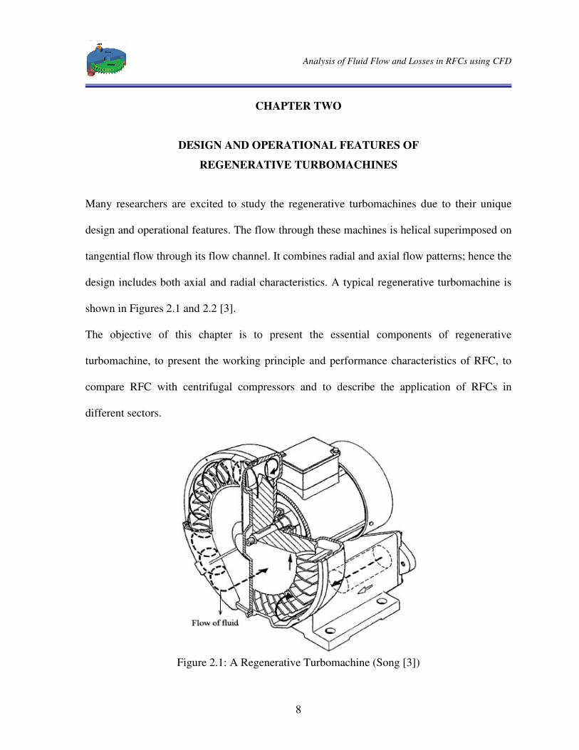
Many researchers are excited to study the regenerative turbomachines due to their unique
design and operational features. The flow through these machines is helical superimposed on
tangential flow through its flow channel. It combines radial and axial flow patterns; hence the
design includes both axial and radial characteristics. A typical regenerative turbomachine is
shown in Figures 2.1 and 2.2 [3].
The objective of this chapter is to present the essential components of regenerative
turbomachine, to present the working principle and performance characteristics of RFC, to
compare RFC with centrifugal compressors and to describe the application of RFCs in
different sectors.
Figure 2.1: A Regenerative Turbomachine (Song [3])

Analysis of Fluid Flow and Losses in RFCs using CFD
9
Figure 2.2: A Regenerative Turbomachine with magnified fluid flow
between blades (Raheel [4])
2.1 Essential Components of Regenerative Turbomachine
The essential components of a regenerative turbomachine include impeller (rotor) with
blades, inlet port, exit port, stripper, and flow channel (open channel) which are shown in
Figure 2.3 below.
Figure 2.3: Schematic diagram of a Regenerative Turbomachine (Engda [2])
Analysis of Fluid Flow and Losses in RFCs using CFD
10
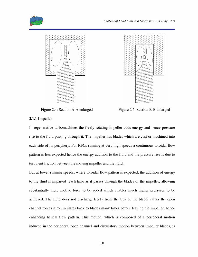
Figure 2.4: Section A-A enlarged Figure 2.5: Section B-B enlarged 2.1.1 Impeller
In regenerative turbomachines the freely rotating impeller adds energy and hence pressure
rise to the fluid passing through it. The impeller has blades which are cast or machined into
each side of its periphery. For RFCs running at very high speeds a continuous toroidal flow
pattern is less expected hence the energy addition to the fluid and the pressure rise is due to
turbulent friction between the moving impeller and the fluid.
But at lower running speeds, where toroidal flow pattern is expected, the addition of energy
to the fluid is imparted each time as it passes through the blades of the impeller, allowing
substantially more motive force to be added which enables much higher pressures to be
achieved. The fluid does not discharge freely from the tips of the blades rather the open
channel forces it to circulates back to blades many times before leaving the impeller, hence
enhancing helical flow pattern. This motion, which is composed of a peripheral motion
induced in the peripheral open channel and circulatory motion between impeller blades, is

Analysis of Fluid Flow and Losses in RFCs using CFD
11
caused by the centrifugal pressure gradient. There is a gradual increase of pressure in
peripheral direction.
The action of impeller blades, operating in series instead of in parallel to each other, makes
them different from centrifugal turbomachines. Each passage through the blades may be
regarded as a conventional stage of compression. It is due to the repeated flow through
impeller blades that has made a regenerative compressor capable of replacing several stages
of centrifugal compressors, producing the same head. Thus the equivalent of several stages of
compression may be obtained from a single impeller in a relatively smaller compressor
The enclosing chambers conduct the fluid into twin vortices around the impeller blade as
shown in Figure 2.4. A very small pressure rise occurs in the vicinity of each impeller blade.
Regenerative turbomachines can also be designed in multistage configurations to meet
certain design requirements.
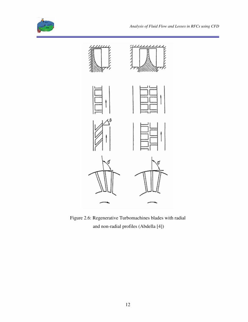
2.1.1.1 Impeller Blades
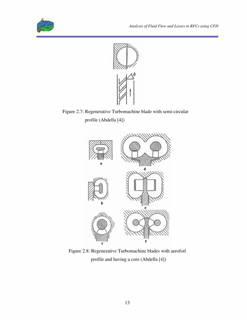
The impeller of regenerative turbomachines can have blades of different shapes. The
commonly used blade types are radial blades, non-radial blades, semi-circular blades and
aerofoil blades. Some examples of these blade shapes are given in Figures 2.6, 2.7 and 2.8
[4]. Regenerative turbomachines having aerofoil blades can be fitted with a core to guide the
circulation through the blading and to minimize the loss due to formation of vortices at the
tips of blades. The core can be fixed to the blades and rotate with them or be fixed to
machine casing. The blades can be constructed as a single row, or as two rows side by side to
provide parallel contra-rotating paths.
Analysis of Fluid Flow and Losses in RFCs using CFD
12
Figure 2.6: Regenerative Turbomachines blades with radial
and non-radial profiles (Abdella [4])
Analysis of Fluid Flow and Losses in RFCs using CFD
13
Figure 2.7: Regenerative Turbomachine blade with semi-circular
profile (Abdella [4])
Figure 2.8: Regenerative Turbomachine blades with aerofoil
profile and having a core (Abdella [4])
Analysis of Fluid Flow and Losses in RFCs using CFD
14
2.1.2 Inlet and Exit (Outlet) Ports
Inlet and exit ports are components which connects the external system piping to the flow
channel. The fluid enters the flow channel via the inlet port, which is shaped to set up spiral
flow around the annular channel. The fluid at high pressure is discharged to the external
system through the exit port.
2.1.3 Stripper
Stripper, which is also known as septum, is used to block the high pressure fluid to be mixed
with the fluid in the inlet region. As shown in Figure 2.5 the casing clearance is reduced so
that the fluid is forced to exit the domain through the exit port. In this region, the open
channel closes to within a very small tolerance of the sides and tip of the rotor and only the
fluid between the blades allowed to pass through the suction.
Clearances between the impeller disk and the casing are kept to a minimum to prevent
leakage from the high pressure side back to the low pressure side. The stripper also helps to
establish and maintain the regenerative flow pattern.
2.1.4 Flow Channel
Flow channel forces the fluid to circulate back to the blades. The fluid between the blades is
thrown out and across the flow channel which has cross sectional area greater that that of the
impeller blades. After the fluid leaves the blades a violent mixing occurs in the flow channel
and the angular momentum acquired by the fluid in its passage between the vanes is
transferred to the fluid in this open channel. This mixing process results in high turbulence,
and this implies inherent waste of power.

Analysis of Fluid Flow and Losses in RFCs using CFD
15
2.2 Working Principle
In regenerative turbomachine the predominant direction of flow is parallel to the velocity of
the blades. Every time the fluid passes through the impeller blades, work is done on it and its
stagnation pressure and tangential velocity are increased. The tangential velocity is removed,
not by a row of stator blades as in a conventional turbomachine, but by the action of
tangential pressure gradient around the periphery of the machine between the exit and inlet
ports. Thus by the time the fluid re-enters the blade row, the magnitude of its tangential
velocity will be reduced and its direction will be reversed. Hence during each loop of the
spiral, the fluid is accelerated in the tangential direction as it passes through the blades and is
decelerated by the tangential pressure gradient as it passes through the flow channel. Because
the flow passes through the same blade row several times between the entry and exit, the
work done on it and hence the pressure rise is considerably greater than that which can be
obtained from a conventional turbomachine with the same tip speed. The specific speed is
therefore low and the machines operate in the usual range of positive displacement machines
[4]. Pressure variation of the fluid as it circulates through regenerative turbomachine is
shown in Figure 2.9 [2]. These curves suggest five regions in the machines operation, which
are also marked in Figure 2.3 [2].
Analysis of Fluid Flow and Losses in RFCs using CFD
16
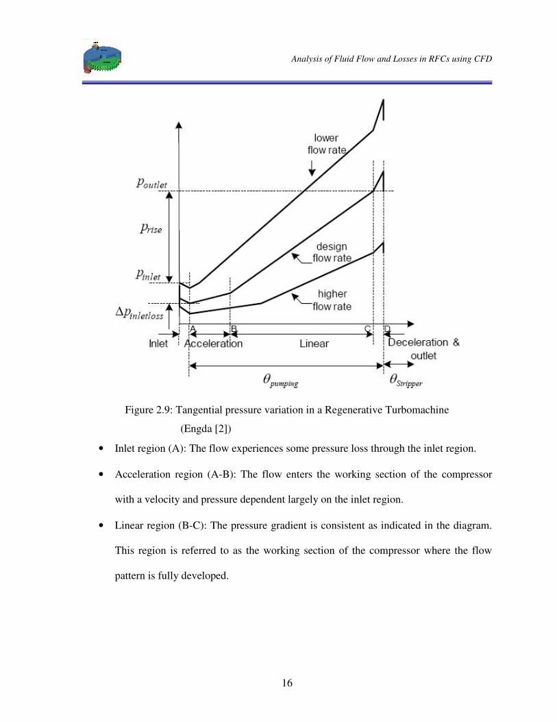
Figure 2.9: Tangential pressure variation in a Regenerative Turbomachine
(Engda [2])
• Inlet region (A): The flow experiences some pressure loss through the inlet region.
• Acceleration region (A-B): The flow enters the working section of the compressor
with a velocity and pressure dependent largely on the inlet region.
• Linear region (B-C): The pressure gradient is consistent as indicated in the diagram.
This region is referred to as the working section of the compressor where the flow
pattern is fully developed.

Analysis of Fluid Flow and Losses in RFCs using CFD
17
• Deceleration region (C-D): In this region, a deceleration occurs and the kinetic energy
of the circulatory velocity is changed as a pressure rise. Therefore, there is a little
pressure rise as shown in Figure 2.9 [2].
• Outlet region (D): A loss similar to that at the inlet region occurs at the outlet region.
2.3 Performance Characteristics of RFC
Most regenerative compressors have an isothermal efficiency less than 50 %, but still they
have found many applications because they allow the use of fluid dynamic compressors in
place of positive displacement compressors for duties requiring high head and low flow rates.
Although regenerative turbomachines are widely used in the industry there is still a need to
study and make design changes in their geometry to improve the performance.
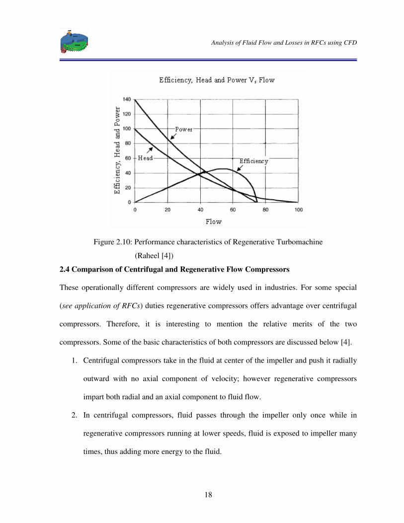
The head, power, and efficiency relationships as a function of flow rate for a typical
regenerative flow compressor are shown in Figure 2.10[4]. The maximum efficiency in this
machine occurs at comparatively large flow rates. At low flow rates, high heads can be
obtained at lower isothermal efficiency. This is due to the fact that circulatory velocity is
higher at lower flow rate resulting in higher pressure rise. However, since the fluid enters the
blades several times, the power requirement is also higher at low flow rates.
It should also be noted that in a very low specific speed ranges, regenerative flow
compressors are more efficient than the centrifugal compressors.
Analysis of Fluid Flow and Losses in RFCs using CFD
18
Figure 2.10: Performance characteristics of Regenerative Turbomachine
(Raheel [4])
2.4 Comparison of Centrifugal and Regenerative Flow Compressors
These operationally different compressors are widely used in industries. For some special
(see application of RFCs) duties regenerative compressors offers advantage over centrifugal
compressors. Therefore, it is interesting to mention the relative merits of the two
compressors. Some of the basic characteristics of both compressors are discussed below [4].
1. Centrifugal compressors take in the fluid at center of the impeller and push it radially
outward with no axial component of velocity; however regenerative compressors
impart both radial and an axial component to fluid flow.
2. In centrifugal compressors, fluid passes through the impeller only once while in
regenerative compressors running at lower speeds, fluid is exposed to impeller many
times, thus adding more energy to the fluid.

Analysis of Fluid Flow and Losses in RFCs using CFD
19
3. One of the most significant structural advantages of the regenerative type
compressors is that no complex flow passages or vaning is required. They are simple
and easy to machine and there is no need of diffusers. Regenerative compressors tend
to have more internal components than the centrifugal compressors, and we can cast
the centrifugal compressor impeller with the outside diameter machined, however
regenerative compressor impeller is completely machined.
4. Centrifugal compressors have large axial length per stage and large overall diameter
because of diffusers. On the other hand, in the regenerative compressors, the suction
and discharge nozzles are at periphery, thus the axial and radial dimensions are small
compared to centrifugal compressor. Regenerative compressors provide much more
pressure rise in a more compact compressor design.
5. The power requirement of a regenerative compressor decreases with increasing flow
rate, whereas the power requirement increases with increasing flow rate in case of a
centrifugal compressor. Moreover, the head and flow rate characteristics of the two
machines are also significantly different.
6. The centrifugal compressor surges at low flow rate, sometimes at flow rate as great as
50% of maximum flow rate. In a regenerative compressor, the flow can be shut off
without surging; however, there will be a temperature rise. The regenerative
compressors have advantages of stability, since they have a stable operation
throughout the flow range (a regenerative compressor will not surge under any
condition).
Analysis of Fluid Flow and Losses in RFCs using CFD
20
7. Higher rotational speeds and/or a large number of stages are usually required with
centrifugal compressors. Regenerative compressors produce heads several times
greater for a given impeller tip speed.
8. Another difference between a regenerative compressor and a centrifugal compressor
is that in the centrifugal compressor, gain in pressure is proportional to the square of
the peripheral velocity of the impeller, whereas in a regenerative compressor it is the
relative velocity to the blades that depends on the pressure gradient.
9. The clearances for regenerative compressors are held to closer tolerances than for the
centrifugal compressors.
10. The centrifugal compressors have no radial shaft loading except gravitational, but
with usual design there can be high axial loading. However, in a regenerative
compressor there are no axial shaft loadings with usual design, but there is a radial
loading due to pressure difference around periphery.
11. Problems due to wear are minimal in regenerative compressors than in centrifugal
compressors [5].
12. The compact size, high reliability and low noise of regenerative turbomachines make
them attractive in certain applications. Better efficiency at low specific speeds makes
them a tough competitor of centrifugal turbomachines in low specific speed
applications [5].
2.5 Applications of Regenerative Flow Compressors
Regenerative compressors are being used in a number of applications that requires high
pressure rise at low flow rates. The relative simplicity of construction and stable operating
Analysis of Fluid Flow and Losses in RFCs using CFD
21
characteristics of the regenerative flow compressors are making them more and more
attractive to users in several areas, including chemical, power, food processing, petroleum,
and nuclear industries.
RFCs have been proposed for use in hydrogen gas pipelines and as helium compressors for
cryogenic applications in space vehicles [4].
RFCs can also be used as natural gas pipeline compressors; in fact, they can be designed to
handle both natural gas or hydrogen or any mixture of the two. Further, it may be possible to
accomplish this in a single design, which can be adjusted to handle a varying mixture by
speed control or other means. Moreover, RFCs are advantageous for incorporation in small
closed cycle helium refrigerators [4].
Because of the reliability, compact size and low maintenance, recently there is an increasing
use of regenerative compressors in low pressure (1.38-103.5 kPa gauge) natural gas
compression required by microturbine systems [2]. Other applications of RFC include
boosting and recycling of hydrogen mixtures and hydrocarbon gases, gas phase reactor
recycling, molecular sieve regeneration in gas drying processes, vent/purge gas recovery, fuel
gas boosting for gas turbine feed and gas compression in many other industrial processes.
Regenerative blowers are used in scavenging of small S.I power plants [4]. The regenerative
blower was found to be the most suitable option since it was able to match the engine air
breath demand all over its utilization range. Regenerative blowers have found many
industrial applications in solids conveying systems. Historically, the pressure and flow rates
demanded by many solids conveying systems made roots or vaned-type blowers, almost
automatic choice despite their limitations.

Analysis of Fluid Flow and Losses in RFCs using CFD
22
Many packaging and paper handling jobs were historically beyond the regenerative blowers
capability, but now with increasing emphasis on working environment, the low noise
regenerative blowers are welcomed in these areas. Regenerative blowers also find use in
sewage treatment, which require considerable volume to be blown against a head of water.
Regenerative blowers are also used for powder coating recovery applications, plating,
cleaning and rinse tank agitation. Since regenerative blowers provide high airflow capacities
at low pressure differentials, they become excellent for air moving applications, such as
agitation of bath or aeration of a pond [4].

Analysis of Fluid Flow and Losses in RFCs using CFD
23
CHAPTER THREE
LITERATURE REVIEW
3.1 Introduction
Regenerative turbomachines have found many applications in different sectors. Despite this
there was no much research conducted in the past and as compared to centrifugal and axial
turbomachines the number of publications existing in literatures for regenerative
turbomachine is very small. Both regenerative flow compressors and pumps have close
operating principle; hence the literature review presented in this chapter is based on
researches done on both machines. It is categorized in the following five areas of research:
1) Theoretical Models
2) Experimental Work
3) Loss in Regenerative Turbomachines
4) Impeller Blades Profile
5) CFD Work
3.2 Theoretical Models
Some theoretical models have been used in attempts to describe the flow in regenerative
turbomachinery. Theories for the flow of compressible fluid in regenerative turbomachines
are rarely found in literature.
Wilson [9] developed the momentum exchange theory for a radial blade impeller which was
able to explain the helical flow pattern. He concluded that as the circulatory flow passes
radially through the rotor its angular momentum in the direction of the rotor motion is

Analysis of Fluid Flow and Losses in RFCs using CFD
24
increased by virtue of the work of the impeller. To maintain the pressure gradient in the flow
channel the angular momentum of the circulatory flow continually decreases after it leaves
the rotor.
Andrew [1] used a simplified theoretical model to describe flow details in regenerative
turbomachines. With the help of streamline passing through the impeller a cork screw flow
pattern through regenerative turbomachine was shown.
Burton [3] made an effort and reported a simplified theory, which took account of area
change and compressibility effects in regenerative flow compressors. He assumed that energy
exchange is obtained through shear stress between the impeller and the fluid in casing. Any
radial components of flow were ignored. The continuity, momentum and energy equations
were applied to a linear control volume and differential equations were obtained. Burton’ s
model was also based on shear stress theory which was experimentally proven as unable to
explain the fluid motion inside regenerative turbomachines.
Sixsmith and Altmann [5] introduce the idea of aerofoil blades with addition of a core in the
flow channel to direct the circulating flow and it resulted in significant improvements in
performance. The flow channel had the core to assist in guiding the fluid such that it
circulates through the blading with a minimum of loss. The core also acted as a shroud to
reduce losses due to formation of vortices at the tips of the blades. The efficiency was
considerably improved compared to the efficiency of regenerative compressor tested with
radial blades.
Analysis of Fluid Flow and Losses in RFCs using CFD
25
3.3 Experimental Work
Most experimental work involved varying the geometry of regenerative turbomachines. This
includes the proportions of blading to coverage of the flow channel, shape of the flow
channel and impeller / blade profiles. There is limited data available on gases as the working
fluids in regenerative turbomachines.
Raheel [4] presented the tested data’ s of several single and multi stage RFCs done by
Capstone Turbine Corporation, CA. They are designed to compress natural gas for
microturbine application. The single stage RFCs have rectangular flow channel with straight
impeller blade profile and for the multi stage RFCs the flow channel is modified to semi-
circular. The performance characteristics of these machine shows that the efficiency was
improved by varying the basic geometries.
As described in Raheel [4], Cates also reported the test data of the regenerative compressor
with a variety of gases having molecular weights of 4 to 400. He presented general
characteristics in Mach numbers extending well into the compressible dominion of operation.
The regenerative compressor operated satisfactorily without surging or unstable operation
with the variety of gases. Compressibility effects had an important influence on performance
because lower pressure ratios were measured at impeller tip mach numbers approaching 1.
The other conclusion that was reached by the tests performed indicated that increasing
impeller-to-casing clearances had little effect on performance.
Sixsmith and Altmann [6] tested two regenerative compressors MK1 and MK2 with aerofoil
blading, a core and decompression ducts by blowing air through them. These regenerative
compressors were designed to run up to 10,000 rpm and deliver 0.25m3/sec at a pressure of

Analysis of Fluid Flow and Losses in RFCs using CFD
26
202.65 kPa. They differ in the number of blade, chord length of the blades and number of
rows for the blades. MK2 has increased number of blades with reduced chord length and the
row of blades is doubled (two rows) to increase the flow rate. The characteristics resembled
to those of a positive displacement compressor and the efficiency was maintained over a
wide range of operating conditions.
3.4 Loss in Regenerative Turbomachines
It is thought that more than 40 - 50% of the input power in a regenerative turbomachine is
consumed in overcoming losses. The regenerative turbomachines operation is affected by
different types of losses and they will be discussed in detail in chapter five. These include:
• Turbulent losses: caused by turbulence, fluid friction and the blade drag occurring in
the flow field.
• Shock loss: is caused by difference between blade angle and flow angle when fluid
enters the blades.
• Inlet and outlet loss: are losses occurred at the inlet and exit ports respectively.
• Leakage loss: is caused by leakage between clearances of the impeller face and the
compressor casing.
• Carry over loss: as the blades enter the stripper seal between the outlet and inlet ports,
a high pressure compressed gas in the blade passages is carried through the stripper to
the low pressure inlet region. The stream is mixed with the incoming gas and
recompressed, and the work of recompression represents wasted energy.
Sixsmith and Altmann [5] concluded that the major source of loss of efficiency is due to
turbulence, fluid friction and the blade drag. It is by far the greatest and efforts to raise the

Analysis of Fluid Flow and Losses in RFCs using CFD
27
efficiency should be directed towards its reduction. They replaced the usual straight radial
blades by the aerodynamic blading and also redesigned the flow channel in order to reduce
these losses. They proposed a circular cross section flow channel to promote vortex
circulation and a minimum of turbulence. In addition to this loss, these authors pointed out
leakage loss and carryover loss of compressed gas between the blades as they pass through
the stripper. The flow rate delivered by the compressor was reduced by leakage through the
clearances. A small fraction of the compressed gas was found to be carried through the
stripper from the high pressure region and expanded down to the inlet pressure.
Sixsmith and Altmann [5] suggested that the blade angles should be designed to match fluid
angles to ensure smooth entry to the blades to prevent shock losses.
Sixsmith and Altmann [6] adopted Burton idea that the carryover loss might be reduced by
extracting some of the compressed gas passing through the stripper and feeding it back at an
intermediate pressure to a less harmful flow channel region. The work of recompressing the
gas expelled from the cells as they pass through the stripper seal is reduced so that the overall
efficiency of the compressor is increased. Engda, Song and Raheel [3] further studied the
effect of carry over losses on Sixsmith and Altmann RFC models. They concluded that this
effect is more pronounced at lower flow rate.
3.5 Impeller Blade Profile
Many authors have studied regenerative turbomachines with radial blades. Blade shape is
also responsible to turbulence and shock losses.
Sixsmith and Altmann [5] studied the regenerative compressor with aerofoil blades. They
replaced the radial blades by blades with an aerofoil section. The blades were designed to

Analysis of Fluid Flow and Losses in RFCs using CFD
28
transfer momentum to the fluid with a minimum of turbulence and friction. There found an
improved in efficiency as compared to radial blades. These authors reported a performance
comparison to illustrate the advantages of aerofoil blade RFC over purely radial blade RFC
design.
Engda and Raheel [2] conducted a design sensitivity analysis on regenerative flow
compressors to propose guidelines and design criteria’ s. They concluded that, for best
performance, the blade angle must be selected in the range between 135O to 150O.
3.6 CFD Work
There is little effort done in the past to apply CFD techniques to solve flow details inside
regenerative turbomachines. The computational methods seem very attractive to be applied to
regenerative turbomachines because they provide a possibility of analyzing the flow. It
enables us to predict the effects of design modifications on performance and gaining a clearer
insight into some of the losses.
An attempt to calculate the flow details in regenerative turbomachines was undertaken by
Raheel [4] using commercial available CFD software - STAR CD. He used the results of
CFD analysis as a comparison tool with the experimental output. He indicated that CFD
analysis helps to validate the effect of proposed design changes on performance.
Generally these literatures give me a good insight to my objective. I have found that different
geometries of the machine have to be considered to study their effect on the performance of
the machine. As describe above the different losses are related to the basic geometries of the
machine. The suggested geometry modifications will be considered when RFC models are
developed. The flow channel and impeller / blade profile will be varied to alleviate or

Analysis of Fluid Flow and Losses in RFCs using CFD
29
minimize the losses in order to gain better performance. In this thesis different blade angles
will be considered from the reference radial straight blades to aerofoil blade profiles and
optimum performance will be expected in the suggested blade angle ranges.
CFD analysis on RFC will be performed using commercially available CFD software -
FLUENT. An effort to calculate the flow in RFCs will be undertaken. The flow patterns
inside RFC, as shown in the Figure 2.1 [3], will be examined and based on the results
obtained design modifications will be suggested.

Analysis of Fluid Flow and Losses in RFCs using CFD
30
CHAPTER FOUR
ANALYSIS OF RFC USING FLUENT
4.1 Introduction
FLUENT is a CFD package for modeling fluid flow and heat transfer. FLUENT provides
CAD/GUI based facility packages for generating unstructured meshes to solve flow problems
in complex geometries.
The flow characteristics in the analysis of RFC, as described in chapter two are 3D,
compressible, viscous, turbulent and rotating flow. It is also assumed to be steady where the
flow variables become independent of time. The appropriate physical flow model, which is
available in FLUENT, will then be specified based on these flow characteristics of the
machine.
In this chapter the necessary governing equations that FLUENT uses to solve the flow in
RFC along with the method of numerical computation of the flow variables will be
discussed. It is based on the FLUENT documentation [8] which describes the numerical
approach to solve the flow variables during CFD simulation.
4.2 Compressible Flow Theory
Compressibility effects are encountered in gas flows at high velocity and/or in which there
are large pressure variations.
Compressible flows can be characterized by the value of the Mach number, M given as
av
M = (4.1)

Analysis of Fluid Flow and Losses in RFCs using CFD
31
Where v is the flow velocity and a is the speed of sound in the gas given as
RTa γ= (4.2)
If the Mach number is less than 1.0, the flow is termed subsonic. Generally at Mach numbers
much less than 1.0 (M < 0.32), compressibility effects are negligible and the variation of the
gas density with pressure can safely be ignored in flow modeling. As the Mach number
approaches 1.0 (which is referred to as the transonic flow regime), compressibility effects
become important. When the Mach number exceeds 1.0, the flow is termed supersonic, and
may contain shocks which can impact the flow pattern significantly.
Cates, based on his test data’ s [4], suggested that the compressibility effects for RFC starts to
appear when the value of Mach number is larger than 0.4. The operating machine Mach
number for the models developed in this thesis ranges from 0.12 - 0.28, which is much
smaller than 0.4. Hence the assumption of compressibility may results in mismatch with the
experimental data’ s.
Physics of Compressible Flows: Compressible flows are typically characterized by the total
pressure, op and total temperature, oT of the flow. For an ideal gas, these quantities can be
related to the static pressure and temperature by the following relations;
=∫
R
dTT
C
pp
oT
T
p
o exp (4.3)

Analysis of Fluid Flow and Losses in RFCs using CFD
32
For constant Cp, equation 4.3 reduces to
2
12
21
1
21
1
MTT
Mpp
o
o
−+=
−+=
−
γ
γ γγ
(4.4)
These relationships describe the variation of the static pressure and temperature in the flow as
the velocity (Mach number) changes under isentropic conditions. For example, given a
pressure ratio from inlet to exit (total to static), equation 4.4 can be used to estimate the exit
Mach number which would exist in isentropic flow. But the efficiency of RFCs is very low
so that we cannot directly apply those isentropic equations.
4.3 Flows in Rotating (Moving) Reference Frame
FLUENT solves the equations of fluid flow and heat transfer, by default, in a stationary (or
inertial) reference frame. However, for problem which involves moving parts (such as
rotating impellers blades in RFC) it is advantageous to solve the equations in a moving (or
non-inertial) reference frame. In RFC since the impeller blades sweep the domain
periodically the flow is unsteady in an inertial frame that is a domain fixed in the laboratory
frame and the assumption of steady flow may result a mismatch. With a moving reference
frame the flow around such moving part can be modeled as a steady-state problem with
respect to the moving frame.
The moving cell zone capability in FLUENT provides a powerful set of features for solving
problems in which the domain or parts of the domain are in motion like the fluid zones in
RFC; one option is to model the flow in an accelerating reference frame. In this situation, the
acceleration of the coordinate system is included in the equations of motion describing the

Analysis of Fluid Flow and Losses in RFCs using CFD
33
flow. Many such flows can be modeled in a coordinate system that is moving with the
rotating equipment and thus experiences a constant acceleration in the radial direction. These
classes of rotating flows are treated using the rotating reference frame capability in FLUENT.
4.4 Governing Equations
All the governing equations are based on the physical flow models defined above. These
equations are written using inertial reference frame later they will be written in rotating
reference frame and in integral form. For flows, FLUENT solves numerically the
conservation equations for Mass and Momentum. In RFC since the flow involves
compressibility an additional equation for energy conservation is solved. Moreover for
turbulent flow an additional transport equations for a fluid in a given flow geometry is solved
and the transport equations have different forms depending on the turbulence modeling used.
4.4.1 The Mass Conservation Equation
The equation for conservation of mass, or continuity equation, can be written as follows:
( ) msvt
=⋅∇+∂∂ ρρ
(4.5)
Equation 4.5 is the general form of the mass conservation equation and is valid for all flows.
The source, Sm is the mass added to the continuous phase from the dispersed second phase
(e.g., due to vaporization of liquid droplets) and any user-defined sources. This equation can
be written to a reduced form for the flow in RFC as;
( ) 0=⋅∇ v (4.6)
4.4.2 Momentum Conservation Equations
Conservation of momentum in an inertial (non-accelerating) reference frame is described by:
Analysis of Fluid Flow and Losses in RFCs using CFD
34
( ) ( ) ( ) Fgpvvvt
++⋅∇+−∇=⋅∇+∂∂ ρτρρ (4.7)
Where p is the static pressure, τ is the stress tensor given as;
∇−
∇+∇= Ivvv�
T .
32
(4.8)
Where µ is the molecular viscosity, I is the unit tensor, and the second term on the right
hand side is the effect of volume dilation.
And gρ and F are the gravitational body force and external body forces (e.g., that arise
from interaction with the dispersed phase), respectively. Also F contains other model-
dependent source terms such as porous-media and user-defined sources. These terms can be
ignored in the analysis of RFC hence the equation is reduced to;
( ) ( )τρ ⋅∇+−∇=⋅∇ pvv (4.9)
FLUENT also solves angular momentum equations for rotating flows. Power transferred to
the impeller of RFC is determined from the product of torque and its angular velocity where
the torque is the output result of FLUENT after solving the angular momentum equations. A
simplified analysis applicable to RFC - Euler turbomachine equation is written as.
( ) ( ) Frgrvvrvrt
shaft ×+×+=×⋅∇+×∂∂ ρρρ T (4.10)
In RFC analysis usually a large shaft torque is expected. Torques due to surface and body
forces may be ignored. For steady flow, equation 4.10 reduces to
( )vvrshaft ρ T ×⋅∇= (4.11)

Analysis of Fluid Flow and Losses in RFCs using CFD
35
4.4.3 The Energy Equation
The energy equation solved by FLUENT correctly incorporates the coupling between the
flow velocity and the static temperature, and should be activated whenever we are solving a
compressible flow.
FLUENT solves the energy equation in the following form:
( ) ( )( ) ( )( ) hjj svJhTkpEvEt
+⋅+−∇⋅∇=+⋅∇+∂∂ ∑ τρρ (4.12)
Where k is the effective conductivity (which includes the turbulent thermal conductivity,
defined according to the turbulence model being used), and Ji is the species diffusion flux.
The first three terms on the right-hand side of equation 4.12 represent energy transfer due to
conduction, species diffusion, and viscous dissipation, respectively. Sh includes heat of
chemical reaction, and any other volumetric heat sources defined.
For the analysis of RFC the equation is reduced to;
( )( ) ( )vTkpEv ⋅+∇⋅∇=+⋅∇ τρ (4.13)
In equation 4.13, E is the total energy given as
2
2
vphE +−=
ρ (4.14)
Where sensible enthalpy, h is defined for ideal gases as;
∫=T
refTdTpCh (4.15)
Where Tref is 298.15 K
Analysis of Fluid Flow and Losses in RFCs using CFD
36
• Inclusion of Pressure Work and Kinetic Energy Terms
Equation 4.13 includes pressure work and kinetic energy terms which are often negligible in
incompressible flows. Pressure work and kinetic energy are always accounted for when
compressible flow are modeled.
• Inclusion of the Viscous Dissipation Terms
Equation 4.13 includes viscous dissipation terms, which describe the thermal energy created
by viscous shear in the flow. When the pressure based solver (defined later) is used,
FLUENT’s default form of the energy equation does not include them (because viscous
heating is often negligible). When a problem requires inclusion of the viscous dissipation
terms and using the segregated solver, the Viscous Heating option is activated using the
Viscous Model panel. When one of the density based solvers (defined later) is used, the
viscous dissipation terms are always included when the energy equation is solved.
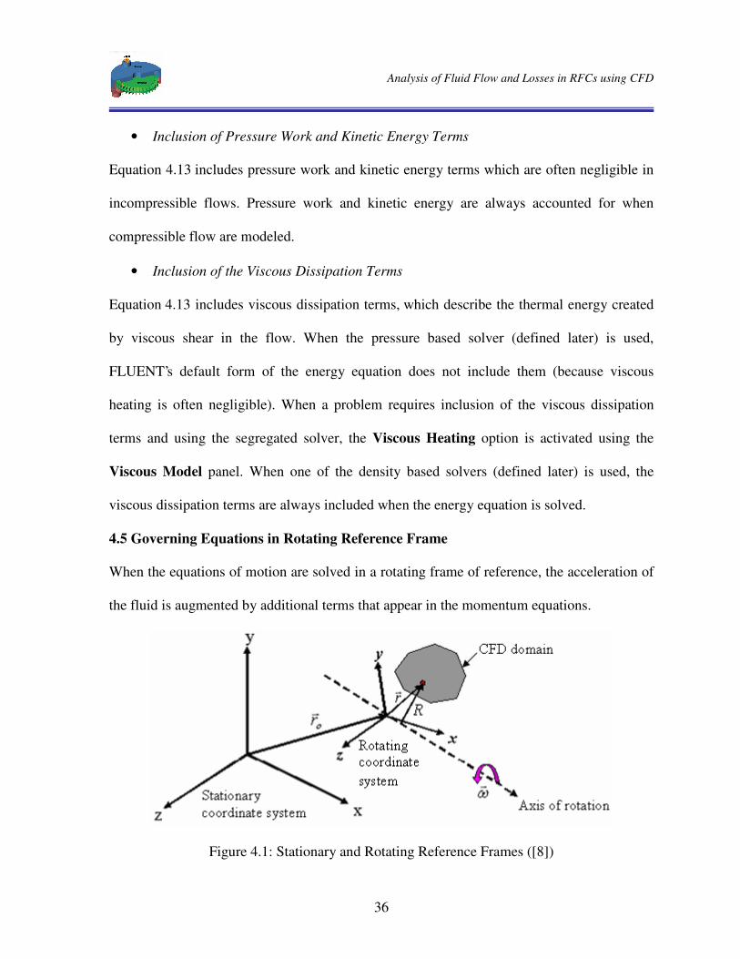
4.5 Governing Equations in Rotating Reference Frame
When the equations of motion are solved in a rotating frame of reference, the acceleration of
the fluid is augmented by additional terms that appear in the momentum equations.
Figure 4.1: Stationary and Rotating Reference Frames ([8])
Analysis of Fluid Flow and Losses in RFCs using CFD
37
The computational domain for the CFD problem is defined with respect to the rotating frame
such that an arbitrary point in the CFD domain is located by a position vector r from the
origin of the rotating frame.
Rotating frame problems are solved using either the absolute velocity, v (the velocity viewed
from the stationary frame), or the relative velocity, rv (the velocity viewed from the rotating
frame), as the dependent variable. The two velocities are related by the following equation:
( )rvv r ×−= ω (4.16)
Where, )( ru r ×= ω is the “whirl” velocity (the velocity due to the moving frame) and ω
is the angular velocity of the rotating frame.
Moreover, the governing equations can be formulated in two different ways:
• Expressing the momentum equations using the relative velocities as dependent
variables (known as the relative velocity formulation).
• Expressing the momentum equations using the absolute velocities as dependent
variables in the momentum equations (known as the absolute velocity formulation).
The selection of those velocity formulations depends on the model geometry. For the
simulation of RFC considered in this thesis, since the non-rotating fluid domain in the flow
channel is larger than in the impeller blades absolute velocity formulation is recommended
for flow analysis.
Absolute Velocity Formulation and Integral form of Governing Equations
For the absolute velocity formulation, the governing equations of fluid flow and in integral
form for a steadily rotating frame can be written as follows:
Analysis of Fluid Flow and Losses in RFCs using CFD
38
Conservation of mass:
( ) 0 . =∇ rvρ (4.17)
The integral form of equation 4.17 can be written as:
∫ =⋅ 0Adv rρ (4.18)
Conservation of momentum:
( ) ( ) τωρρ ∇+−∇=×+∇ pvvv r . (4.19)
The integral form of equation for the conservation of momentum can be written as:
AdAdpAdvv .. ∫∫ ∫ +−=⋅ τρ (4.20)
The integral form of angular momentum equations can be written as:
( )∫ ×= Advvrshaft . T ρ (4.21)
Conservation of energy:
( ) ( )rrr vTkupHv . . τρ +∇−∇=+∇ (4.22)
In this formulation, the coriolis, ( rv 2 ×ω ) and centrifugal, ( r××ωω ) accelerations can be
collapsed into a single term ( v×ω ). In addition, the viscous stress (τ ) is identical to
equation 4.8. The energy equation is written in terms of the total enthalpy, H also known as
the rothalpy and is defined as:
ρp
EH += (4.23)

Analysis of Fluid Flow and Losses in RFCs using CFD
39
Where total energy, E is given as:
2
21
vp
hE +−=ρ
(4.24)
The integral form of equation 4.22 can be written as:
( ) AdvAdTk Ad upHv rrr . . . ∫∫∫ +−=+ τρ (4.25)
4.6 Turbulent Flow Models
Turbulent flows are characterized by fluctuating velocity fields. Since these fluctuations can
be of small scale and high frequency, they are too computationally expensive to simulate
directly in practical engineering calculations. Instead, the exact governing equations can be
time-averaged, ensemble-averaged, or otherwise manipulated to remove the small scales,
resulting in a modified set of equations that are computationally less expensive to solve.
However, the modified equations contain additional unknown variables, and turbulence
models are needed to determine these variables in terms of known quantities. The approach
in solving the flow equations for a turbulent flow field is to solve the Reynolds Averaged
Navier Stokes (RANS) equations. Reynolds Averaged approach transforms the momentum
equations in such a way that the small-scale turbulent fluctuations do not have to be directly
simulated. RANS equations represent transport equations for the mean flow quantities only.
This greatly reduces the computational effort and all the scales of the turbulence are
modeled.
There are various turbulence models available in FLUENT and the choice of those
turbulence model depends on the flow model, the level of accuracy required, the available
computational resources, and the amount of time available for the simulation. Amongst the
realizable ε−k is the widely accepted turbulence model for practical engineering flow
Analysis of Fluid Flow and Losses in RFCs using CFD
40
calculations and is found most appropriate for the CFD analysis of flow inside a RFC. This
turbulence model provides better performance for flows involving rotation under adverse
pressure gradients, separation, and recirculation.
The realizable ε−k model is a semi-empirical model based on model transport equations for
the turbulence kinetic energy (k) and its dissipation rate (ε ). These quantities can be
evaluated based on the turbulence specification method used. When the intensity and
hydraulic diameter (defined later in next chapter) method is used values for k and ε are
evaluated as;
( )2 23
Ivk avg= (4.26)
lk
C2/3
4/3µε = (4.27)
Where vavg is the mean flow velocity, I is the turbulent intensity given as a ratio of the
velocity fluctuations, ’v to the mean flow velocity, vavg. µC = 0.09 is an empirical constant
specified for a turbulence model. l is the turbulence length scale and is a physical quantity
related to the size of the large eddies that contain the energy in turbulent flows. An
approximate relationship for turbulence length is l = 0.07DH where DH is the hydraulic
diameter of the flow.
4.6.1 Transport Equations for the Realizable - Model
The transport equations are the modelling basis for all engineering processes involving
momentum, mass or heat transfer. They express the conservation relationship for intensive
properties in terms of accumulation, advection, diffusion, generation and destruction.
Analysis of Fluid Flow and Losses in RFCs using CFD
41
The modeled transport equations for k and ε in the realizable ε−k model are,
Mbkk
t YGGyk
xkv
xk
t−−++
∂∂
+
∂∂=
∂∂+
∂∂ ρε
σµµρρ )()( (4.28)
and
bt GC
kC
kC
yxv
yt εε
ενεερε
σµµρερε
ε31
2
2)()( ++
−
∂∂
+
∂∂=
∂∂+
∂∂
(4.29)
In these equations; kG represents the generation of turbulence kinetic energy due to the mean
velocity gradients. From the exact equation for the transport of k, the term, kG may be
defined as,
xv
vuGk ∂∂−= ’’ρ (4.30)
To evaluate kG in a manner consistent with the Boussinesq hypothesis,
2SG tk µ= (4.31)
Where S is the modulus of the mean rate-of-strain tensor and defined as,
ijij SSS 2≡ (4.32)
bG is the generation of turbulence kinetic energy due to buoyancy.
MY represents the contribution of the fluctuating dilatation in compressible turbulence to the
overall dissipation rate.
YM22t
0= (4.33)
Where Mt is the turbulent Mach number, defined as
Mt 2a
k= (4.34)
Where RTa γ= is the speed of sound. This compressibility modification always takes
effect when the compressible form of the ideal gas law is used.

Analysis of Fluid Flow and Losses in RFCs using CFD
42
9.12 =C and 44.11 =εC are constants. 0.1=kσ and 2.1=εσ are the turbulent Prandtl
numbers for k andε , respectively.
For flow in RFC equations (4.28) and (4.29) can be reduced to,
ρεσµµρ −+
∂∂
+
∂∂=
∂∂
kk
t Gyk
xkv
x)(
MY− (4.35)
and
νεερε
σµµρε
ε +−
∂∂
+
∂∂=
∂∂
kC
yyv
yt
2
2)( (4.36)
4.7 Numerical Computation
There are two numerical methods used in FLUENT. Either pressure based or density based
solver can be used to solve the governing integral equations for the conservation of mass,
momentum, energy and other scalars such as turbulence. In both cases a control volume
based technique is used which consists of:
• Division of the domain into discrete control volumes using a computational
grid.
• Integration of the governing equations on the individual control volumes to
construct algebraic equations for the discrete dependent variables (“unknowns”)
such as velocities, pressure, temperature, and conserved scalars.
• Linearization of the discretized equations and
• Solution of the resultant linear equation system to yield updated values of the
dependent variables.
The two numerical methods employ a similar discretization process (finite-volume), but the
approach used to linearize and solve the discretized equations is different. For the CFD

Analysis of Fluid Flow and Losses in RFCs using CFD
43
analysis of flow through the RFC pressure-based solver, which is a memory-efficient, is
used.
4.7. 1 Pressure-Based Segregated Algorithm
The pressure-based solver uses a solution algorithm where the governing equations are
solved sequentially (i.e., segregated from one another). Because the governing equations are
non-linear and coupled, the solution loop must be carried out iteratively in order to obtain a
converged numerical solution.
In the segregated algorithm, the individual governing equations for the solution variables
(e.g., u, v, w, p, T, k,ε etc) are solved one after another. Each governing equation, while
being solved, is decoupled / segregated from other equations.
The segregated algorithm is memory-efficient, since the discretized equations need only be
stored in the memory one at a time. However, the solution convergence is relatively slow, in
as much as the equations are solved in a decoupled manner. With the segregated algorithm,
each iteration consists of the steps illustrated in the figure and outlined below:
1. Update fluid properties (e.g., density, viscosity, specific heat) on the current solution.
2. Solve the momentum equations (u, v, and w) one after another, using the recently
updated values of pressure and face mass fluxes.
3. Solve the pressure correction equation using the recently obtained velocity field and
the mass-flux.
4. Correct face mass fluxes, pressure, and the velocity field using the pressure correction
obtained from Step 3.

Analysis of Fluid Flow and Losses in RFCs using CFD
44
Update properties
Solve Pressure- Correction (Continuity) equation
Solve momentum equation.
Update Mass flux, Pressure and Velocity
Solve energy, turbulence, and other scalar equations
Converged? No Yes Stop
5. Solve the equations for additional scalars, if any, such as turbulent quantities and
energy using the current values of the solution variables.
6. Check for the convergence of the equations.
These steps are continued until the convergence criteria are met.
Figure 4.2: Overview of the Pressure-Based Solution Methods [8]
4.7. 2 Discretization Technique in FLUENT
FLUENT uses a control volume based technique to convert a general scalar transport
equation to an algebraic equation that can be solved numerically. This control volume
Analysis of Fluid Flow and Losses in RFCs using CFD
45
technique consists of integrating the transport equation about each control volume, yielding a
discrete equation that expresses the conservation law on a control volume basis.
Considering the integral form of conservation equation of the flow in RFC, for transport of a
scalar quantity φ for an arbitrary control volume V, the discretization of the governing
equations is given by:
∫ ∫ ⋅∇Γ=⋅ AdAdv r φρφ φ (4.37)
Where;
ρ = density
v = relative velocity vector
A = surface area vector
φ = diffusion coefficient for φ
φ∇ = gradient of φ (= kz
jy
ix ∂
∂+∂∂+
∂∂ φφφ )
The scalar quantity, φ can be 1, v or H when solving the mass, momentum and energy
conservation equation respectively. Equation 4.37 is applied to each control volume, or cell,
in the computational domain. The two dimensional, triangular cell shown in Figure 4.3 is an
example of such a control volume. Discretization of equation 4.37 on a given cell yields,
fn
N
f
ff
N
f
rff AAvfacesfaces
⋅∇Γ=⋅ ∑∑ )( φφρ φ (4.38)
Where;
facesN = number of faces enclosing the cell
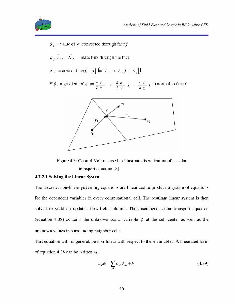
Analysis of Fluid Flow and Losses in RFCs using CFD
46
fφ = value of φ convected through face f
ffrf v A ⋅ρ = mass flux through the face
fA = area of face f, ( )zyx AjAiA A ++=
fφ∇ = gradient of φ (= kz
jy
ix ∂
∂+∂∂+
∂∂ φφφ ) normal to face f
Figure 4.3: Control Volume used to illustrate discretization of a scalar
transport equation [8]
4.7.2.1 Solving the Linear System
The discrete, non-linear governing equations are linearized to produce a system of equations
for the dependent variables in every computational cell. The resultant linear system is then
solved to yield an updated flow-field solution. The discretized scalar transport equation
(equation 4.38) contains the unknown scalar variable φ at the cell center as well as the
unknown values in surrounding neighbor cells.
This equation will, in general, be non-linear with respect to these variables. A linearized form
of equation 4.38 can be written as;
baanb
nbnbP += ∑ φφ (4.39)

Analysis of Fluid Flow and Losses in RFCs using CFD
47
Where the subscript nb refers to neighbor cells, and Pa & nba are the linearized coefficients
for φ and nbφ .
The number of neighbors for each cell depends on the grid topology, but will typically equal
to the number of faces enclosing the cell except the boundary cells.
Similar equations can be written for each cell in the grid. This results in a set of algebraic
equations with a sparse coefficient matrix. For scalar equations, FLUENT solves this linear
system using a point implicit linear equation solver (Gauss-Seidel scheme) in conjunction
with an algebraic multigrid (AMG) method, which will be described later.
4.7.2.2 Spatial Discretization
By default, FLUENT stores discrete values of the scalarφ at the cell centers (c0 and c1 in
Figure 4.3). However, face values fφ are required for the convection terms in equation 4.38
and must be interpolated from the cell center values. This is accomplished using an upwind
scheme.
Upwinding means that the face value fφ is derived from quantities in the cell upstream, or
“upwind”, relative to the direction of the normal velocity nv in equation 4.38. First-order
upwind and second-order upwind schemes have been utilized in the CFD analysis of RFC.
They are described as follows;
• First-Order Upwind Scheme (FOU)
When first-order accuracy is desired, quantities at cell faces are determined by assuming that
the cell-center values of any field variable represent a cell-average value and hold throughout
the entire cell; the face quantities are identical to the cell quantities. Thus when first-order

Analysis of Fluid Flow and Losses in RFCs using CFD
48
upwind scheme is selected, the face value fφ is set equal to the cell-center value of φ in the
upstream cell.
• Second-Order Upwind Scheme (SOU)
When second-order accuracy is desired, quantities at cell faces are computed using a
multidimensional linear reconstruction approach. In this approach, higher-order accuracy is
achieved at cell faces through a Taylor series expansion of the cell-centered solution about
the cell centroid. Thus when second-order upwinding is selected, the face value fφ is
computed using the following expression:
rf ⋅∇+= φφφ (4.40)
Where φ and φ∇ are the cell-centered value and its gradient in the upstream cell, and r is
the displacement vector from the upstream cell centroid to the face centroid.
4.7.2.3 Evaluation of Gradients and Derivatives
Gradients are needed not only for constructing values of a scalar at the cell faces, but also for
computing secondary diffusion terms and velocity derivatives. The gradient φ of a given
variable φ is used to discretize the convection and diffusion terms in the flow conservation
equations. There are three methods by which gradients are computed in FLUENT these are
green-Gauss cell-based, green-Gauss node-based and Least Squares cell-based. All the
methods are based on Green-Gauss Theorem which is written as;
( ) ∑=∇f
ffc AV
φφ 10
(4.41)
Analysis of Fluid Flow and Losses in RFCs using CFD
49
Where fφ is, the value of φ at the cell face centroid, computed by the three methods
available in FLUENT and V is the cell volume. The summation is over all the faces
enclosing the cell.
• Green-Gauss Node-Based Gradient Evaluation
The node-based averaging scheme is known to be more accurate for unstructured meshes
(defined later), most notably for triangular and tetrahedral meshes. For green-gauss node-
based gradient evaluation fφ can be computed by the arithmetic average of the nodal values
on the face.
∑=fN
nn
ff N
φφ 1 (4.42)
Where Nf is the number of nodes on the face.
The nodal values, nφ in equation 4.42, are constructed from the weighted average of the cell
values surrounding the nodes. This scheme reconstructs exact values of a linear function at a
node from surrounding cell-centered values on arbitrary unstructured meshes by solving a
constrained minimization problem, preserving a second-order spatial accuracy.
4.7.2.4 Implicit Linearization
The manner in which the governing equations are linearized may take an “implicit” or
“explicit” form with respect to a set of variables of interest. In the pressure based solution
method each discrete governing equation is linearized implicitly with respect to that
equation's dependent variable. This will result in a system of linear equations with one
equation for each cell in the domain. Because there is only one equation per cell, this is
sometimes called a “scalar” system of equations. A point implicit linear equation solver is
Analysis of Fluid Flow and Losses in RFCs using CFD
50
used in conjunction with an algebraic multigrid (AMG) method to solve the resultant scalar
system of equations for the dependent variable in each cell. For example, the x -momentum
equation is linearized to produce a system of equations in which u velocity is the unknown.
Simultaneous solution of this equation system (using the scalar AMG solver) yields an
updated u velocity field. The pressure based approach solves for a single variable field by
considering all cells at the same time. It then solves for the next variable field by again
considering all cells at the same time, and so on. There is no explicit option for the pressure
based solver.
4.7.2.5 Pressure Interpolation and Pressure - Velocity Coupling
The momentum and continuity equations are solved sequentially. In this sequential
procedure, the continuity equation is used as an equation for pressure.
The discrete form of the x-momentum equation can be derived from equation 4.39 as;
SiApuaua fnb
nbnb +⋅+= ∑∑Ρˆ (4.43)
If the pressure field and face mass fluxes were known, equation 4.43 could be solved and a
velocity field obtained. However, the pressure field and face mass fluxes are not known a
priori and must be obtained as a part of the solution. The important issues with respect to the
storage of pressure and the discretization of the pressure gradient term are discussed next.
FLUENT uses a co-located scheme, whereby pressure and velocity are both stored at cell
centers. However, equation 4.43 requires the value of the pressure at the face between cells
c0 and c1. The second-order scheme for pressure interpolation reconstructs the face pressure
in the manner used for second-order accurate convection terms. This scheme may provide
Analysis of Fluid Flow and Losses in RFCs using CFD
51
some improvement over the standard and linear schemes for compressible flow. But it may
have some trouble if it is used at the start of a calculation and/or with a bad mesh, hence it is
recommended to start with standard scheme for few iterations.
The discrete form of the continuity equation can also be given as;
0=∑facesN
fff AJ
(4.44)
Where fJ is the mass flux through face, f given as, nvρ .
In order to proceed further, it is necessary to relate the face values of velocity, nv to the
stored values of velocity at the cell centers. Linear interpolation of cell-centered velocities to
the face results in unphysical value of pressure. To prevent this the face value of velocity is
not averaged linearly instead momentum weighted averaging, using weighting factors based
on the Pa coefficient from equation 4.39, is performed. Using this procedure, the face flux
fJ may be written as;
)(ˆ10 εε ppdJJ fff −+= (4.45)
Where 0εp and 1εp are the pressures within the two cells on either side of the face, and
fJ contains the influence of velocities in these cells. The term fd is a function of Pa .
The SIMPLE (Semi-Implicit Method for Pressure-Linked Equations) algorithms is used for
introducing pressure into the continuity equation. Pressure-velocity coupling is achieved by
using equation 4.45 to derive an equation for pressure from the discrete continuity equation.
The SIMPLE algorithm uses a relationship between velocity and pressure corrections to
enforce mass conservation and to obtain the pressure field.

Analysis of Fluid Flow and Losses in RFCs using CFD
52
If the momentum equation is solved with a guessed pressure field *p , the resulting face
flux, *fJ computed from equation 4.45 does not satisfy the continuity equation.
)(ˆ10
∗∗∗∗ −+= εε ppdJJ fff (4.46)
Consequently, a correction ’fJ is added to the face flux *
fJ so that the corrected face flux fJ
satisfies the continuity equation.
’fff JJJ += ∗ (4.47)
The SIMPLE algorithm postulates that ’fJ be written as;
( )’
1’0
’ccff ppdJ −= (4.48)
Where ’p is the cell pressure correction
The SIMPLE algorithm substitutes the flux correction equations (equations 4.47 and 4.48)
into the discrete continuity equation (equation 4.44) to obtain a discrete equation for the
pressure correction ’p in the cell;
bpapa nbnb
nbP += ∑ ’’ (4.49)
Where the source term b is the net flow rate into the cell;
∑=facesN
fff AJb * (4.50)
The pressure-correction equation (equation 4.49) may be solved using the algebraic multigrid
(AMG) method (described later). Once a solution is obtained, the cell pressure and the face
flux are corrected using;
’ppp ρα+= ∗ (4.51)
Analysis of Fluid Flow and Losses in RFCs using CFD
53
)( ’1
’0 εε ppdJJ fff −+= ∗ (4.52)
Here Pα is the under-relaxation factor for pressure. The corrected face flux, fJ satisfies the
discrete continuity equation identically during each iteration.
4.7.2.6 Density Interpolation Schemes
For compressible flow calculations (i.e., calculations that use the ideal gas law for density),
FLUENT applies upwind interpolation of density at cell faces. Several interpolation schemes
are available for the density up-winding at cell faces. The first-order upwind scheme (the
default) provides stability for the discretization of the pressure-correction equation, and gives
good results for most classes of flows.
4.7.2.7 Under-Relaxation Because of the nonlinearity of the equation set being solved by FLUENT, it is necessary to
control the change of φ during iteration. This is typically achieved by under-relaxation,
which reduces the change of φ produced during each iteration. It is the main technique by
which the solver is stabilised. In a simple form, the new value of the variable φ within a cell
depends upon the old value ( oldφ ) the computed change inφ ( φ∆ ) and the under-relaxation
factor (α ) as follows;
φαφφ ∆+= old (4.53)
Reducing the under-relaxation factor α will stabilise the solver at the expense of slowing the
rate of convergence.

Analysis of Fluid Flow and Losses in RFCs using CFD
54
4.8 Multigrid Method
FLUENT uses a multigrid scheme to accelerate the convergence of the solver by computing
corrections on a series of coarse grid levels. The use of this multigrid scheme can greatly
reduce the number of iterations and the computer processing time required to obtain a
converged solution, particularly when the model contains a large number of control volumes.
4.8.1 The Need for Multigrid
Implicit solution of the linearized equations on unstructured meshes is complicated by the
fact that there is no equivalent of the line-iterative methods that are commonly used on
structured grids. Point implicit solvers like Gauss-Seidel method are the best choices for
solving realistic problems on unstructured meshes. Although the Gauss-Seidel scheme
rapidly removes high-frequency errors in the solution, low-frequency errors are reduced at a
rate inversely related to the grid size. Thus, for a large number of nodes, the solver stalls and
the residual reduction rate becomes prohibitively low.
Multigrid techniques allow global error to be addressed by using a sequence of successively
coarser meshes. This method is based upon the principle that low-frequency error existing on
a fine mesh can be represented on a coarse mesh where it again becomes accessible as high-
frequency error, because there are fewer coarse cells overall, the global corrections can be
communicated more quickly between adjacent cells. Since computations can be performed at
exponentially decaying expense in both CPU time and memory storage on coarser meshes,
there is the potential for very efficient elimination of global error. The fine-grid relaxation
scheme or smoother, in this case the point-implicit Gauss-Seidel, is not required to be

Analysis of Fluid Flow and Losses in RFCs using CFD
55
particularly effective at reducing global error and can be tuned for efficient reduction of local
error.
4.8.2 Algebraic Multigrid (AMG)
This algorithm is referred to as an algebraic multigrid scheme because the coarse level
equations are generated without the use of any geometry or re-discretization on the coarse
levels a feature that makes AMG particularly attractive for use on unstructured meshes. The
advantage being that no coarse grids have to be constructed or stored, and no fluxes or source
terms need be evaluated on the coarse levels. However, once the system is linearized, non-
linearities are not felt by the solver until the fine level operator is next updated, which is a
demerit for non-linear problems, since non-linearities in the system are carried down to the
coarse levels through the re-discretization.
Consider the set of discretized linear (or linearized) equations given by,
0=+ bA eφ (4.54)
Where eφ is the exact solution.
Before the solution has converged there will be a defect, d associated with the approximate
solutionφ ;
dbA =+φ (4.55)
We seek a correction ψ to φ such that the exact solution is given by,
ψφφ +=e (4.56)
Substituting equation 4.56 into equation 4.54 gives,
0)( =++ bA ψφ (4.57)
0)( =++ bAA φψ (4.58)
Now using equations 4.55 and 4.58 we obtain,
0=+ dAψ (4.59)

Analysis of Fluid Flow and Losses in RFCs using CFD
56
Which is an equation for the correction in terms of the original fine level operator A and the
defect, d. Assuming the high-frequency errors have been sufficiently damped by the
relaxation scheme on the fine level, the correction ψ will be smooth and therefore more
effectively solved on the next coarser level.
4.9 Standard Wall Functions
Wall functions are a collection of semi-empirical formulas and functions that in effect link
the solution variables at the near-wall cells and the corresponding quantities on the wall.
They are used to bridge the viscosity affected region between the wall and the fully turbulent
region. The basis of standard wall functions in FLUENT is most widely used for industrial
flows.
Figure 4.4: Near-Wall Treatments in FLUENT [8]
Momentum
The law-of-the-wall for mean velocity, *U yields:
) ln(1 ∗=∗
yEUN
(4.60)
Analysis of Fluid Flow and Losses in RFCs using CFD
57
Where,
ρτ ω
µ
/
21
41
PP kCUU ≡∗
µρ µ ΡΡ∗ =
ykCy
21
41
and κ = von Kármán constant (= 0.42)
E = empirical constant (= 9.793)
µC = empirical constant (= 0.09)
PU = mean velocity of the fluid at point P
Pk = turbulence kinetic energy at point P
Py = distance from point P to the wall
µ = dynamic viscosity of the fluid
The logarithmic law for mean velocity is known to be valid for >*y about 30 to 60. In
FLUENT, the log-law is employed when 225.11>∗y .
When the mesh is such that 225.11<∗y at the wall-adjacent cells, FLUENT applies the
laminar stress-strain relationship that can be written as,
∗∗ = yU (4.61)
It should be noted that, in FLUENT, the laws-of-the-wall for mean velocity and temperature
are based on the wall unit, *y rather than )/ ( µρ τ yuy ≡+ . These quantities are approximately
equal in equilibrium turbulent boundary layers.
Analysis of Fluid Flow and Losses in RFCs using CFD
58
Energy
The law-of-the-wall implemented in FLUENT has the following composite form,
(4.62)
Where P is computed by using the formula,
(4.63)
and
kf = thermal conductivity of fluid
U = density of fluid
cp = specific heat of fluid
"�
q = wall heat flux
TP = temperature at the cell adjacent to wall
Tw = temperature at the wall
Pr = molecular Prandtl number
Prt = turbulent Prandtl number (0.85 at the wall)
A = Van Driest constant (= 26)
( )
4/1
1
2/1
4/sin
4/
−=pr
tpr
tpr
pr
k
AP
S
S
( ) { }
>−++
+
<+=
−=
*)y(y* )("
21
*ln1
*)y(y* "
21
*
"
2/1 4/1 *
T22
2/14/1
T2
2/14/1
ctptp
yt
pp
UprprUprq
kCpE
kpr
Uq
kCprypr
qpkCpCpTwT
T
µ
µ
ρ
ρ
µρ

Analysis of Fluid Flow and Losses in RFCs using CFD
59
k = 0.42 (von Karman’s constant)
E = 9.793 (wall function constant)
Uc = mean velocity magnitude at y*=yT*
Note that, for the segregated solver, the terms
and
( ){ }2 2 "
2/14/1
21
cUtprprpUtprq
pkC−+⋅
µρ
will be included in equation 4.62 only for compressible flow calculations.
The non-dimensional thermal sub-layer thickness, y*T, in equation 4.62 is computed as the y*
value at which the linear law and the logarithmic law intersect, given the molecular Prandtl
number of the fluid being modeled. The procedure of applying the law-of-the-wall for
temperature is as follows. Once the physical properties of the fluid being modeled are
specified, its molecular Prandtl number is computed. Then, given the molecular Prandtl
number, the thermal sub-layer thickness, y*T, is computed from the intersection of the linear
and logarithmic profiles, and stored.
During the iteration, depending on the y* value at the near-wall cell, either the linear or the
logarithmic profile in equation 4.62 is applied to compute the wall temperature Tw or heat
flux "�
q (depending on the type of the thermal boundary conditions).
2
"
2/14/1
2
1 pU
q
pkCpr ⋅
PU
Analysis of Fluid Flow and Losses in RFCs using CFD
60
Turbulence
In the ε−k models, the k equation is solved in the whole domain including the wall-
adjacent cells. The boundary condition for k imposed at the wall is,
0=∂∂nk
(4.64)
Where n is the local coordinate normal to the wall.
The production of kinetic energy, kG and its dissipation rate,ε at the wall-adjacent cells are
computed on the basis of the local equilibrium hypothesis. Under this assumption, the
production of k and its dissipation rate are assumed to be equal in the wall-adjacent control
volume.
Thus, the production of k is computed from,
Ρ
=∂∂≈
ykCyU
GP
k 2
14
1
µ
ωωω
ρκτττ (4.65)
and ε is computed from:
P
PP y
kC 2
34
3
κε µ= (4.66)
The ε equation is not solved at the wall-adjacent cells, but instead is computed using
equation 4.66.
As shown here, the wall boundary conditions for the solution variables, including mean
velocity, k and ε are all taken care of by the wall functions; therefore, no need to be
concerned about the boundary conditions at the walls.
The standard wall functions work reasonably well for a broad range of wall-bounded flows.
However, they tend to become less reliable when the flow situations depart too much from
the ideal conditions that are assumed in their derivation. Among others, the constant-shear

Analysis of Fluid Flow and Losses in RFCs using CFD
61
and local equilibrium hypotheses are the ones that most restrict the universality of the
standard wall functions. Accordingly, when the near-wall flows are subjected to severe
pressure gradients, and when the flows are in strong non-equilibrium, the quality of the
predictions is likely to be compromised.

Analysis of Fluid Flow and Losses in RFCs using CFD
62
CHAPTER FIVE
RFC MODIFICATION AND SIMULATION
PROCEDURES
5.1 Introduction
Capstone Turbine Corporation, CA [4] has tested single stage RFCs with air as working
fluids. The base machine for the CFD study in this thesis is taken from the non-
dimensionalized geometric and performance data’ s for single stage RFCs that are available
from CA. This base machine is a commercially available RFC for the compression of natural
gas in a microgasturbine application. It will be analyzed using FLUENT and the output
results are compared with the existing tested data’ s of the machine. Various modifications
will be done on the basic geometries with the intent of reducing the different losses and each
will be compared with the base machine.
The objective of this chapter is to:
• introduce non-dimensional design parameters which are used in the design
and performance investigation of a regenerative flow compressor,
• introduce the geometry and performance characteristic of the base machine,
• describe the major losses that are responsible for a low efficiency in RFC,
• present the various modification proposed on the base machine together with
the reason of the proposal and
• present the major steps involved in the simulation analysis of the machines
using FLUENT. This includes building of the geometry, meshing, processing

Analysis of Fluid Flow and Losses in RFCs using CFD
63
in FLUENT, displaying and reporting of simulation results. Where these
results of the analysis will then be discussed in detail in chapter six.
This chapter starts by introducing the non-dimensional parameters used in the design and
performance investigation of a RFC.
5.2 Non-dimensional Design Parameters
The parameters such as the flow rate, speed and power can be made dimensionless and be
used for the performance comparison. Dimensional analysis of turbomachines is employed to
normalize these performance parameters by using geometric variable, controlled variable and
fluid properties. These three variables includes impeller tip diameter which determines the
shape and size of the machine; inlet density, ratio of specific heat and the inlet sonic velocity
of the gas which characterizes the flow; and shaft speed which is an externally observed
variable controlled by the motor.
The following six non-dimensional parameters are used in the design and performance
analysis of a regenerative flow compressor. These are; pressure ratio, impeller tip (machine)
Mach number, isothermal efficiency, power coefficient, flow coefficient and specific mass
flow rate; and are discussed below.
a. Pressure Ratio, π : the job of RFC is to increase the pressure of the fluid. This
increase in pressure is measured by the compressor pressure ratio (CPR) given as a
ratio of outlet to inlet total pressure.
CPR, in
out
pp
=π (5.1)
b. Impeller Tip (Machine) Mach Number, OTM : it is a non-dimensional parameter
defined as the ratio of the impeller tip speed to the inlet sonic velocity of the gas.
Analysis of Fluid Flow and Losses in RFCs using CFD
64
in
OT au
M 2=
ingas
OTTR
rM
2
γω
=⇒ (5.2)
c. Isothermal Efficiency, isoη : RFC usually operates under isothermal condition.
During compression the compressor work / power can be reduced by maintaining the
temperature of the gas as low as possible, i.e. Tin = T = Constant. Isothermal
efficiency is then used to qualify the mass flow and power performance
characteristics of RFC.
At constant temperature the equation of state becomes,
constant== ingasTmRpV
V
TmR
VVp
p
pVVpVp
ingas==⇒
===⇒
11
2211 constant (5.3)
The work, WS which is theoretically required to compress a gas under constant
temperature from a given inlet pressure to discharge pressure can be determined from;
∫= pdVWS
=⇒
in
outingasS p
pTmRW ln (5.4)
And the theoretical power is given as;
( )πln ln ingasin
outingasS TRm
pp
TRmW•••
=
= (5.5)
Analysis of Fluid Flow and Losses in RFCs using CFD
65
The actual power delivered, •
aW can be determined from the product of torque and
DQJXODU�VSHHG�� �RI�WKH�VKDIW�
Power Drawn = ω T ×=•
shaftaW (5.6)
Hence isothermal efficiency is defined as the ratio of isothermal power to actual
power.
•
•
=a
Siso
W
Wη
( )ω
πη
T
ln
×=⇒
•
shaft
ingasiso
TRm (5.7)
d. Flow Coefficient, : the flow coefficient is a dimensionless parameter used in RFC
design and performance analysis where the suction (inlet) volume flow rate, SQ is
normalized by the impeller tip diameter, D and angular speed of the machine.
3DQS
ωλ =
8 3
2r
m
inωρ
•
=⇒ (5.8)
e. Power Coefficient, <: the power coefficient is also a non-dimensional parameter
where the power drawn is normalized by the impeller tip diameter, inlet density and
angular speed of the machine.
��������������������< 53
DDrawPower
inωρ=
Analysis of Fluid Flow and Losses in RFCs using CFD
66
⇒< 52
332
r
DrawPower
inωρ= (5.9)
f. Specific Mass Flow Rate, φ : Specific Mass Flow Rate is another non-dimensional
parameter defined by normalizing mass flow rate through the machine using the
impeller tip diameter, inlet density and inlet sonic velocity of the gas. It is given as;
2 Dam
ininρφ
•
=
Substituting ideal gas relation for density;
2 ) ( )/( DTRRTp
m
ingasinin γφ
•
=
γ
φ ingas
in
TR
prm2
24
•
=⇒ (5.10)
Where r2 (2
D= ) is impeller tip radius in m, is the angular speed in rad/s, 2u is
impeller tip speed in m/s, Tin is inlet temperature of gas in K, � is ratio of specific
heat, p is the total pressure in Pa, SQ is volume flow rate at inlet in m3/s, Rgas is gas
constant in J/ kg K, inρ is the density of the gas at inlet in kg/m3, Tshaft is the shaft
power (power transferred to the impeller) in N-m, ain is the inlet sonic velocity in m/s
and •m is the mass flow rate in kg/s.
5.3 Base Regenerative Flow Compressor
Microgasturbines are employed for small scale power generation. They offer a number of
advantage compared to other technologies of the same. This advantage includes a small

Analysis of Fluid Flow and Losses in RFCs using CFD
67
number of moving parts, compact size, light weight, greater efficiency, lower emission and
opportunity to use waste fuels [4]. They can burn various types of fuels but usually natural
gas because it provides the advantage of less cost, no storage problems, cleaner burning, less
NO emissions and more power output at higher efficiency. As compared to a high cost
centrifugal compressors, RFC is highly accepted for raising a low pressure natural gas supply
to that required for injection into the combustion system at low flow rate. And RFC operates
with better performance.
For this purpose four different geometric configuration of a single stage RFCs were tested by
Capstone Turbine Corporation, CA. All has the same impeller tip diameter and they consist
of a straight and radial blade with rectangular flow channel. The differences between these
configurations are the impeller hub diameter and the width of the flow channel. Among the
different configuration, configuration 3 (S3) has higher pressure ratio and better efficiency.
But the flow channel geometry, where its cross sectional area varies linearly from inlet to exit
port, lacks data to develop the model hence configuration 4 (S4) is considered as a base
machine. Configuration 4 (S4) has a constant flow channel cross sectional area. It has nearly
the same pressure ratio and close efficiency with configuration 3 (S3).
5.3.1 Dimensions of the Base Machine
Non-dimensionalized geometric data of configuration 4(S4) is presented in Table 5.1.
Stations A and B refer to peripheral locations near inlet and outlet respectively. Below a
schematic diagram of impeller and flow channel shape is shown for the base machine.
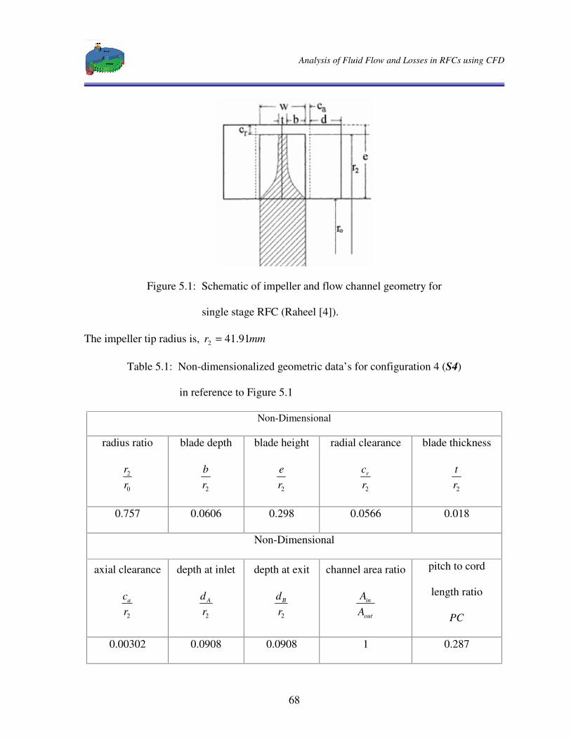
Analysis of Fluid Flow and Losses in RFCs using CFD
68
Figure 5.1: Schematic of impeller and flow channel geometry for
single stage RFC (Raheel [4]).
The impeller tip radius is, mmr 91.412 =
Table 5.1: Non-dimensionalized geometric data’ s for configuration 4 (S4)
in reference to Figure 5.1
Non-Dimensional
radius ratio
0
2
rr
blade depth
2rb
blade height
2re
radial clearance
2rcr
blade thickness
2rt
0.757 0.0606 0.298 0.0566 0.018
Non-Dimensional
axial clearance
2rca
depth at inlet
2rdA
depth at exit
2rdB
channel area ratio
out
in
AA
pitch to cord
length ratio
PC
0.00302 0.0908 0.0908 1 0.287
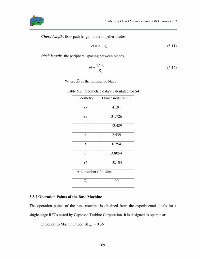
Analysis of Fluid Flow and Losses in RFCs using CFD
69
Chord length: flow path length in the impeller blades,
02 rrcl −= (5.11)
Pitch length: the peripheral spacing between blades,
bZr
pl 2 2π= (5.12)
Where Zb is the number of blade
Table 5.2: Geometric data’ s calculated for S4
Geometry Dimensions in mm
r2 41.91
r0 31.726
e 12.489
b 2.539
t 0.754
d 3.8054
cl 10.184
And number of blades,
Zb 90
5.3.2 Operation Points of the Base Machine
The operation points of the base machine is obtained from the experimental data’ s for a
single stage RFCs tested by Capstone Turbine Corporation. It is designed to operate at:
Impeller tip Mach number, 36.0=OTM

Analysis of Fluid Flow and Losses in RFCs using CFD
70
Rotational speed, ^= 28,910 rpm
3UHVVXUH�UDWLR�� � ����
Inlet temperature, Tin = 700F (294.26K)
Inlet pressure, pin = 100000 Pa
During the test, air is used as a working fluid but here it is also simulated using natural gas.
The properties of both gases are:
For air;
Molecular weight, M = 28.97 kg/K mol
Cpa = 1005.244 J/ kg K Cva = 718 J/kg K
Ra = 287 J/kg K
Ratio of specific heat, �$1.4��
For natural gas; �Molecular weight, M = 16 kg/K mol
CpNG = 2253.7 J/ kg K CvNG = 1735.4 J/kg K
RNG = 518.3 J/kg K
Ratio of specific heat, �$1.31��
5.3.3 Performance characteristic of the Base Machine
Below the performance characteristics for the base machine is shown for comparison and
discussion purpose. From the performance characteristics a peak isothermal efficiency of
8.1% can be obtained at Mach number 0.325 and specific flow rate of 9.73x10⁻⁴. The
corresponding pressure ratio at these operating points is 1.19. Performance at operation
points is calculated by correlating the test data’ s and it is found that an efficiency of 8.13%
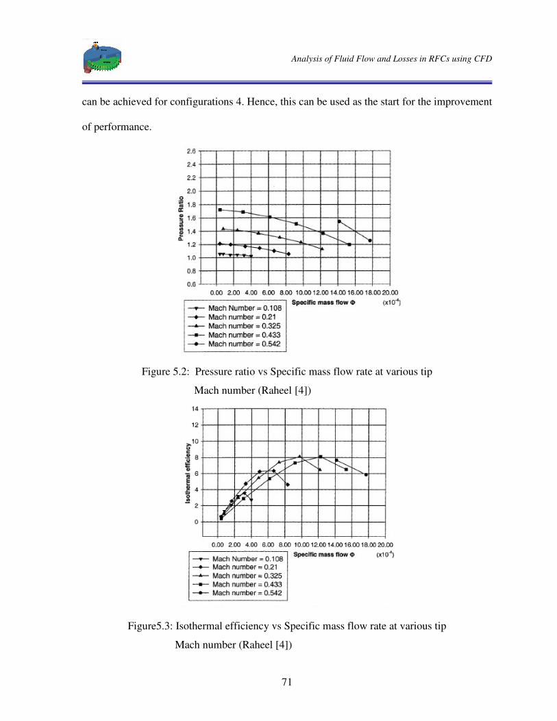
Analysis of Fluid Flow and Losses in RFCs using CFD
71
can be achieved for configurations 4. Hence, this can be used as the start for the improvement
of performance.
Figure 5.2: Pressure ratio vs Specific mass flow rate at various tip
Mach number (Raheel [4])
Figure5.3: Isothermal efficiency vs Specific mass flow rate at various tip
Mach number (Raheel [4])
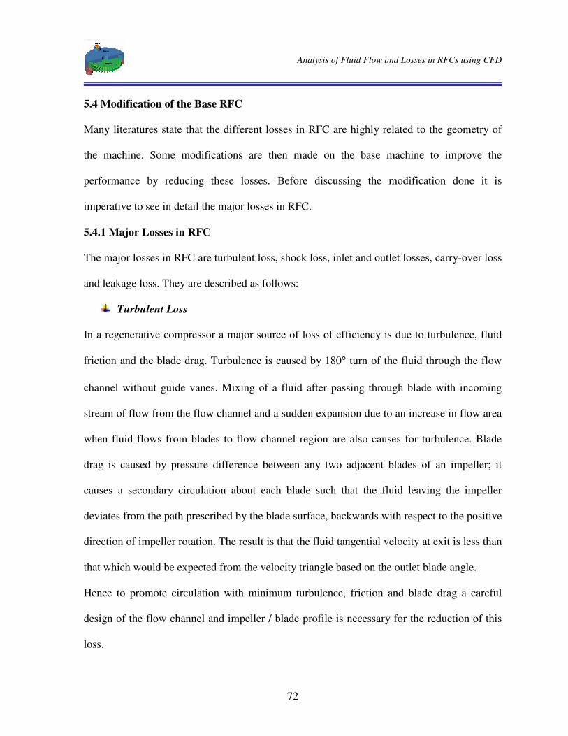
Analysis of Fluid Flow and Losses in RFCs using CFD
72
5.4 Modification of the Base RFC
Many literatures state that the different losses in RFC are highly related to the geometry of
the machine. Some modifications are then made on the base machine to improve the
performance by reducing these losses. Before discussing the modification done it is
imperative to see in detail the major losses in RFC.
5.4.1 Major Losses in RFC
The major losses in RFC are turbulent loss, shock loss, inlet and outlet losses, carry-over loss
and leakage loss. They are described as follows:
Turbulent Loss
In a regenerative compressor a major source of loss of efficiency is due to turbulence, fluid
friction and the blade drag. Turbulence is caused by 180° turn of the fluid through the flow
channel without guide vanes. Mixing of a fluid after passing through blade with incoming
stream of flow from the flow channel and a sudden expansion due to an increase in flow area
when fluid flows from blades to flow channel region are also causes for turbulence. Blade
drag is caused by pressure difference between any two adjacent blades of an impeller; it
causes a secondary circulation about each blade such that the fluid leaving the impeller
deviates from the path prescribed by the blade surface, backwards with respect to the positive
direction of impeller rotation. The result is that the fluid tangential velocity at exit is less than
that which would be expected from the velocity triangle based on the outlet blade angle.
Hence to promote circulation with minimum turbulence, friction and blade drag a careful
design of the flow channel and impeller / blade profile is necessary for the reduction of this
loss.

Analysis of Fluid Flow and Losses in RFCs using CFD
73
Shock loss
Shock or incidence losses are caused by difference between blade angle and flow angle when
fluid enters the blades. Flow channels should be designed properly to avoid a huge mismatch
between the blade angle and fluid angle. The blade angles also are designed to match fluid
angles to ensure smooth entry to the blades.
Inlet and outlet losses
Some losses are also introduced at the inlet and outlet ports. To reduce these losses the inlet
port should be designed to project the fluid towards the inlet edge of the blade with the
velocity and direction needed to ensure smooth entry. The outlet port should be followed by a
conical diffuser to reduce the fluid velocity there by converting some of the kinetic energy to
a further gain in pressure.
The Carry - Over loss
When the blades enter the stripper seal between the outlet and inlet ports, compressed gas in
the blade passages is carried through the stripper seal from the high pressure delivery region
to the low pressure inlet region. Gas is carried through at the delivery pressure and expanded
down to the inlet pressure as the pockets between the blades open into the flow channel at the
inlet end. The stream which escapes from the blade pockets is mixed with the incoming gas
and recompressed, and the work of recompression represents wasted energy. The flow rate
and the high pressure of the expelled stream cause the inlet flow rate to reduce, this represent
unavoidable loss of efficiency.

Analysis of Fluid Flow and Losses in RFCs using CFD
74
Leakage losses
This is also other source of loss where the flow rate is reduced due to leakage through the
clearance spaces.
During the simulation of RFC the last two losses are not optimized. In the actual machine to
reduce carry-over loss decompression ducts (pipes) may be employed to extract the
compressed gases from the blade pockets and return it to the flow field with relatively higher
pressure magnitude than the inlet and leakages are also considered. Therefore this will results
in mismatch with the experimental data’ s.
5.4.2 Modification on the Basic Geometries
Referring the previous discussion, the lower efficiency of the base machine is due to these
losses caused by its geometry. To improve the performance of the machine the following
modifications are made on the basic geometries.
a. Rectangular flow channel area and straight impeller do not guide the flow
properly and there can be huge mismatch between the blade and flow angle (see
figure 5.5). Therefore first the flow channel is modified to be semi-circular in
cross section and the impeller is made semi-elliptic. By doing this the flow is
guided properly and circulation is promoted with minimum losses.
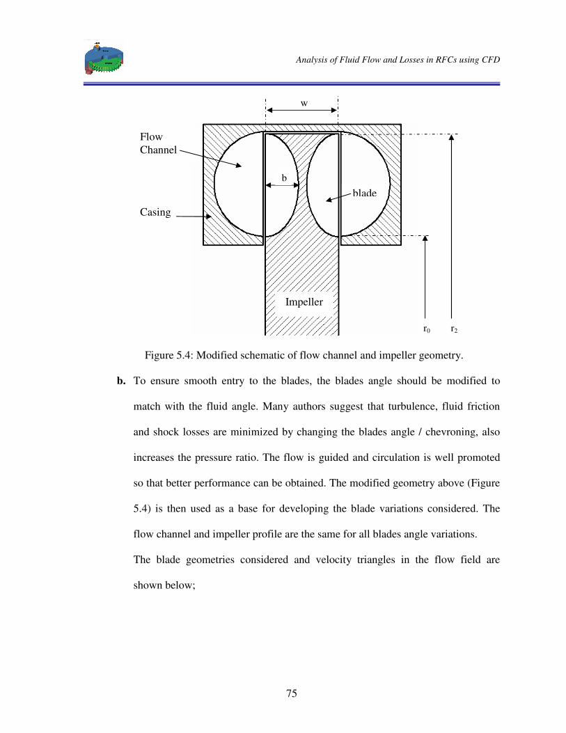
Analysis of Fluid Flow and Losses in RFCs using CFD
75
w
Figure 5.4: Modified schematic of flow channel and impeller geometry.
b. To ensure smooth entry to the blades, the blades angle should be modified to
match with the fluid angle. Many authors suggest that turbulence, fluid friction
and shock losses are minimized by changing the blades angle / chevroning, also
increases the pressure ratio. The flow is guided and circulation is well promoted
so that better performance can be obtained. The modified geometry above (Figure
5.4) is then used as a base for developing the blade variations considered. The
flow channel and impeller profile are the same for all blades angle variations.
The blade geometries considered and velocity triangles in the flow field are
shown below;
Flow Channel
Impeller
blade
Casing
b
r2 r0
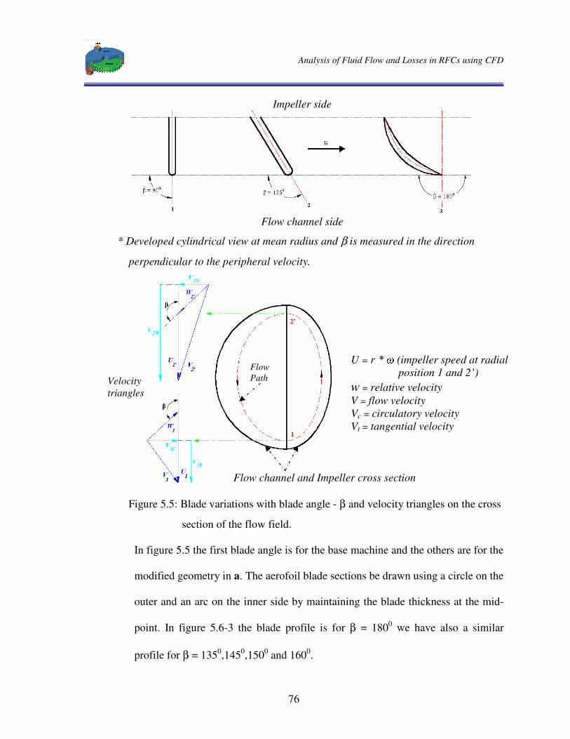
Analysis of Fluid Flow and Losses in RFCs using CFD
76
Impeller side
Flow channel side
* Developed cylindrical view at mean radius and β is measured in the direction
perpendicular to the peripheral velocity.
Figure 5.5: Blade variations with blade angle - β and velocity triangles on the cross
section of the flow field.
In figure 5.5 the first blade angle is for the base machine and the others are for the
modified geometry in a. The aerofoil blade sections be drawn using a circle on the
outer and an arc on the inner side by maintaining the blade thickness at the mid-
point. In figure 5.6-3 the blade profile is for β = 1800 we have also a similar
profile for β = 1350,1450,1500 and 1600.
U =�U� � (impeller speed at radial position 1 and 2’) w = relative velocity V = flow velocity Vc = circulatory velocity Vt = tangential velocity
Velocity triangles
Flow Path
Flow channel and Impeller cross section
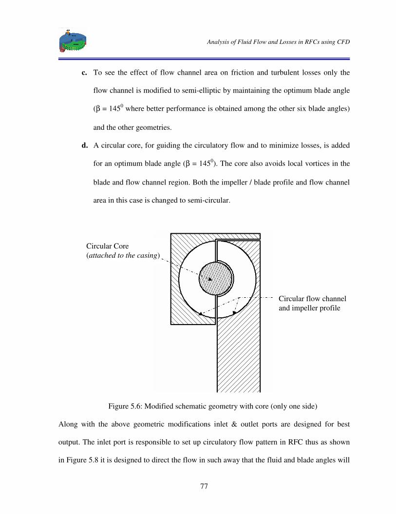
Analysis of Fluid Flow and Losses in RFCs using CFD
77
c. To see the effect of flow channel area on friction and turbulent losses only the
flow channel is modified to semi-elliptic by maintaining the optimum blade angle
(β = 1450 where better performance is obtained among the other six blade angles)
and the other geometries.
d. A circular core, for guiding the circulatory flow and to minimize losses, is added
for an optimum blade angle (β = 1450). The core also avoids local vortices in the
blade and flow channel region. Both the impeller / blade profile and flow channel
area in this case is changed to semi-circular.
Figure 5.6: Modified schematic geometry with core (only one side)
Along with the above geometric modifications inlet & outlet ports are designed for best
output. The inlet port is responsible to set up circulatory flow pattern in RFC thus as shown
in Figure 5.8 it is designed to direct the flow in such away that the fluid and blade angles will
Circular Core (attached to the casing)
Circular flow channel and impeller profile
Analysis of Fluid Flow and Losses in RFCs using CFD
78
much. The outlet port is aligned in the tangential direction to have smooth flow and shaped
as a diffuser to further exploit the kinetic energy of the flow for pressure rise. The inlet and
exit ports are separated by stripper angle which is about 30O of the periphery. To save
computation time only one-side of the blade and flow channel section is considered for CFD
analysis. Clearances are neglected for the simulation analysis due to the difficulty in mesh
generation. To investigate the effect of the working fluid the model, for optimum blade angle
in b�� � ����O), will also be simulated for natural gas where natural gas is the actual working
fluid. The working conditions (i.e. speed, inlet and discharge pressure) are also kept the same
for each simulation.
The following are the different RFC models developed.
1. The base machine (S4) with straight and radial blade profile for β = 900 : RFCR-90
2. Semi-elliptic impeller and semi-circular flow channel with radial blade profile and
β = 1350: RFCS-135
3. Airfoil blade profile with semi-elliptic impeller, semi-circular flow channel and
β = 1350: RFCA-135
4. Airfoil blade profile with semi-elliptic impeller, semi-circular flow channel and
β = 1450: RFCA-145
5. Airfoil blade profile with semi-elliptic impeller, semi-circular flow channel and
β = 1500: RFCA-150
6. Airfoil blade profile with semi-elliptic impeller, semi-circular flow channel and
β = 1600: RFCA-160

Analysis of Fluid Flow and Losses in RFCs using CFD
79
7. Airfoil blade profile with semi-elliptic impeller, semi-circular flow channel and
β = 1800: RFCA-180
For the remaining models the blade angle, β = 1450, where better performance is obtained
among the other six blade angles, is used.
8. Airfoil blade profile with semi-elliptic flow channel and semi-elliptic impeller for β =1450:
RFCSEA-145
9. Airfoil blade profile with semi-elliptic impeller and semi-circular flow channel with
natural gas as a working fluid and for β =1450 :RFCNGA-145
10. Airfoil blade profile with semi-circular flow channel and impeller having a core for
β = 1450: RFCCA-145
5.5 Basic Steps for CFD Analysis
Before CFD analysis begins using FLUENT, careful consideration of the issues here will
contribute significantly to the success of modeling effort. This section provides details about
the simulation procedure in FLUENT. It is extracted from FLUENT 6.3.26 documentations
[8]. Topics presented in these subsequent sections are:
• the three major steps involved for the CFD analysis using FLUENT, namely
Preprocessing, Processing and Post processing,
• steps for building RFC geometries using GAMBIT,
• meshing and specifying boundary condition of the flow domain in GAMBIT,
• importing of mesh and further steps of CFD analysis in FLUENT and
• the necessary output results of FLUENT that are used to analyze and compare the
performance of the base machine and other models with the tested data’ s.
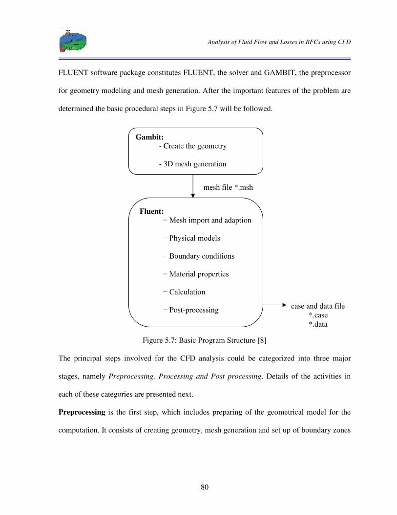
Analysis of Fluid Flow and Losses in RFCs using CFD
80
FLUENT software package constitutes FLUENT, the solver and GAMBIT, the preprocessor
for geometry modeling and mesh generation. After the important features of the problem are
determined the basic procedural steps in Figure 5.7 will be followed.
Figure 5.7: Basic Program Structure [8]
The principal steps involved for the CFD analysis could be categorized into three major
stages, namely Preprocessing, Processing and Post processing. Details of the activities in
each of these categories are presented next.
Preprocessing is the first step, which includes preparing of the geometrical model for the
computation. It consists of creating geometry, mesh generation and set up of boundary zones
Gambit: - Create the geometry
- 3D mesh generation
Fluent: í�Mesh import and adaption
í�3K\VLFDO�PRGHOV í�%RXQGDU\�FRQGLWLRQV í�0DWHULDO�SURSHUWLHV í�&DOFXODWLRQ
í�Post-processing
mesh file *.msh
case and data file *.case *.data

Analysis of Fluid Flow and Losses in RFCs using CFD
81
in GAMBIT and reading mesh file, checking grid, scaling grid, smooth/swap the grid,
specifying physical flow models, fluid properties, boundary conditions, etc in FLUENT.
Processing is the second step where the solution control and monitoring are carried on along
with the actual computation process in FLUENT.
Postprocessing is the activity of displaying of graphical results, reporting control variables
and plotting of solution files for areas of interest in the flow field.
5.5.1 Preprocessing of Simulation
The preprocessing procedures of the CFD simulation are classified in to two categories.
These are preprocessing in GAMBIT and preprocessing in FLUENT.
5.5.1.1 Preprocessing in GAMBIT
The GAMBIT package is used to build the geometry, to generate meshes and set up
boundary zones of the RFC model for the CFD simulation analysis. The mesh file contains
the coordinates of all the nodes, connectivity information that tells how the nodes are
connected to one another to form faces and cells, and the zone types and numbers of all the
faces. The grid file does not contain any boundary conditions, flow parameters, or solution
parameters. It is an intermediate steps in the overall process of creating a usable model which
is exported, as a mesh file, to be read in FLUENT.
Building the Geometry of RFC
GAMBIT uses vertices, edges, faces and volumes to draw geometry of the flow domain of
the RFC and by generating complex 3D volumes through unite & split operations.

Analysis of Fluid Flow and Losses in RFCs using CFD
82
Steps to create the flow geometry of RFC in GAMBIT
1. The side view of the flow channel and the impeller are drawn by locating the respective
vertices for the edges.
2. Faces are created from the bounding edges of those components independently. These
faces are then used for developing volume entities through 3D CAD operations i.e. by
revolving and sweeping of faces.
3. The blade geometry is drawn independently through the steps above and they are copied
89 number of times, i.e. 1−bZ with 40 between them, i.e. bZ
360 which are then united to
the impeller. The fluid zone between the blades is created by subtracting this resulting
geometry from a solid cylinder having similar overall dimension of the impeller.
4. The face representing cross section of the flow channel is used to create stripper volume
by revolving through 300, i.e. s. Then subtract it from the channel geometry.
5. To draw the outlet and the inlet ports, Coordinate axes are declared at their respective
locations in such a way that the 3D operations can be used easily. Vertices, Edges, Faces
and Volumes of those components are created in the same way above.
6. The fluid zone in casing is defined by uniting the flow channel (step-4) volume, the outlet
port volume and the inlet port volume.
7. The volume enclosed by the two fluid zones constitutes the flow field in RFC which is
now to be meshed and exported for the CFD analysis.

Analysis of Fluid Flow and Losses in RFCs using CFD
83
Meshing the Flow domain
Solutions by numerical methods require physical discretization/meshing of the domain. A
good solution is obtained if good meshes for the models are generated. The accuracy of the
solutions depends on the sizes of the meshes. Finer cells are more accurate but are usually
less stable and they require large computing capacity and time. Mesh types are selected based
on the problem at our hand. The following general points are considered when models are
meshed in GAMBIT.
Setup Time: many flow problems solved in engineering practice involve complex geometries
like RFC. The creation of structured or block structured grids for such flow problems can be
extremely time consuming. Therefore unstructured grids are generated for each RFC models
to minimize setup time.
Computational Expense: when the range of length scales of the flow is large, a tetrahedral
mesh can often be created with far fewer cells than the equivalent mesh consisting of
quadrilateral/hexahedral elements. This is because a tetrahedral mesh allows cells to be
clustered in selected regions of the flow domain. However, a large aspect ratio in a
tetrahedral cell will invariably affect its skewness which is undesirable as it may impede
accuracy and convergence.
Numerical Diffusion: a dominant source of error in multidimensional situations is numerical
diffusion. All practical numerical schemes for solving fluid flow contain a finite amount of
numerical diffusion. This is because numerical diffusion arises from truncation errors that are
a consequence of representing the fluid flow equations in discrete form. The second-order
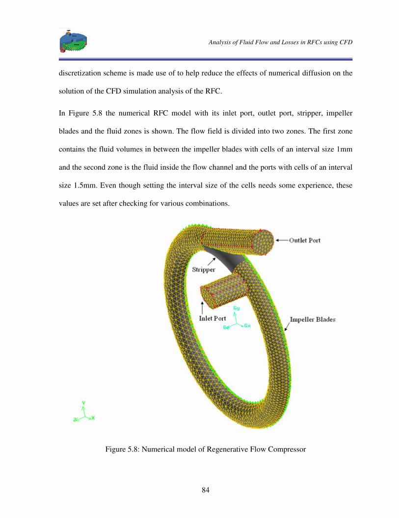
Analysis of Fluid Flow and Losses in RFCs using CFD
84
discretization scheme is made use of to help reduce the effects of numerical diffusion on the
solution of the CFD simulation analysis of the RFC.
In Figure 5.8 the numerical RFC model with its inlet port, outlet port, stripper, impeller
blades and the fluid zones is shown. The flow field is divided into two zones. The first zone
contains the fluid volumes in between the impeller blades with cells of an interval size 1mm
and the second zone is the fluid inside the flow channel and the ports with cells of an interval
size 1.5mm. Even though setting the interval size of the cells needs some experience, these
values are set after checking for various combinations.
Figure 5.8: Numerical model of Regenerative Flow Compressor
Analysis of Fluid Flow and Losses in RFCs using CFD
85
Specifying Zone Types
Zone-type specifications define the physical and operational characteristics of the model at
its boundaries and within specific regions of its domain. There are two classes of zone-type
specification: Boundary types and Continuum types
Boundary type specifications: when the model is developed in GAMBIT the solver type
FLUENT has been set initially so that boundary conditions relevant to the RFC simulation
are made available. Boundary-type specifications, such as pressure inlet, pressure outlet,
walls and the fluid zones, described in the previous section for defining rotating reference
frame, are set in GAMBIT.
Continuum type specifications: defines the characteristics of the model, such as fluid or
solid, within specified regions of its domain. In most turbomachinery problems, only the
fluid region is prepared for numerical computation and the solid regions are walls which
bounds the flow. Hence, only fluid type of continuum is specified for both zones of the
numerical RFC model and walls that corresponds to the fluid zones are set by default.
After specifying the boundary zones and the continuum types, the mesh and geometry
developed in GAMBIT is saved in a database file *.dbs. This model is exported to a mesh
file *.msh so that FLUENT can read the grid information and use it for further preprocessing
and computation analysis.
5.5.1.2 Preprocessing in FLUENT
Preprocessing in FLUENT starts with reading the mesh file which was exported from
GAMBIT. The mesh file does not contain any information on boundary conditions, fluid
properties, flow models and solution parameters. Case files contain the grid, boundary types,

Analysis of Fluid Flow and Losses in RFCs using CFD
86
and solution parameters for a problem, as well as information about the user interface and
graphics environment. Therefore, the main purpose of this section is to upgrade the mesh file
into a case file equipped with the proper information for the CFD analysis of the flow
through a RFC. The mesh first read by FLUENT and on the console window the following
information’ s are printed.
> Reading "D:\Thesis\Gambit Geometry (RFC)\Semi-Elliptic\airfoil-55\mesh.msh"...
12887 nodes.
19266 mixed wall faces, zone 4.
72 mixed mass-flow-inlet faces, zone 5.
88 mixed pressure-outlet faces, zone 6.
80857 mixed interior faces, zone 8.
20631 tetrahedral cells, zone 2.
24654 tetrahedral cells, zone 3.
Building...
grid,
Note: Separating wall zone 4 into zones 4 and 1.
wall -> wall (4) and wall:001 (1)
Note: Separating interior zone 8 into zones 8 and 7.
default-interior -> default-interior (8) and default-interior:007 (7)
Note: Separating interior zone 8 into zones 8 and 9.
default-interior -> default-interior (8) and default-interior:009 (9)
materials,
interface,
domains,

Analysis of Fluid Flow and Losses in RFCs using CFD
87
zones,
default-interior:009
default-interior:007
wall:001
default-interior
outlet
inlet
wall
rotor_fluid
flow channel_fluid
shell conduction zones,
Done.
Grid Manipulation
This is the opening stage on the imported mesh file before the start of the computation
process. These include scaling, smoothing/swapping, checking and displaying the grid.
Scaling the Grid: when the computational grid is read by FLUENT, all the dimensions are
considered in meters, m and internally FLUENT stores the data’ s in meters. But grid of the
RFC geometry was created in units of mm in the GAMBIT application and scaling of the
grid to units of meters must be performed so that each node coordinate will be multiplied by
the corresponding scale factor.
Smoothing/Swapping the Grid: the mesh quality can be further improved for better accuracy
and stability of the numerical computation. FLUENT provides the capability to improve the
smoothness by refining the mesh based on the change in cell volume. Smoothing and face
Analysis of Fluid Flow and Losses in RFCs using CFD
88
swapping are used as grid adaption, they increase the quality of the final numerical mesh by
modifying the cell connectivity through repositioning of interior nodes to decrease the
skewness of cells to a specified minimum value (default value = 0.8) and until the number of
swapped faces comes to 0. Skewness can be defined as the difference between the cell’s
shape and the shape of an equilateral cell of equivalent volume. Rapid changes in cell volume
between adjacent cells translate into larger truncation errors. Highly skewed cells can also
decrease accuracy and destabilize the solution.
Checking Mesh: here the domain extents, volume statistics, grid topology and verification of
simplex counters are checked. It is generally a good idea to check the grid in order to detect
any grid trouble before getting started with the problem setup. The domain extents list the
minimum and maximum x, y, and z coordinates in meters. The volume statistics include
minimum, maximum, and total cell volume in m3. A negative value for the minimum volume
indicates that one or more cells have improper connectivity. This must be eliminated before
continuing the flow solution process for flow.
Displaying Grids: grids can be visually inspected to check grid problems and to take action if
necessary. Later grids can also be used when examining solution results to include surfaces,
the outline of all or part the domain, the grid lines, the nodes on the domain surfaces and the
solid surfaces.
Defining Analysis Bases
Analysis bases such as the solver type, physical models for the flow nature, fluid properties,
boundary conditions and solution parameters are set after the grid manipulations were
performed in the preprocessing step of FLUENT.
Analysis of Fluid Flow and Losses in RFCs using CFD
89
Setting Models: the flow in RFC is 3D, steady-state, compressible, turbulent, viscous and
rotating flow (rotating reference frame). These flow models are set for the simulation process
to determine the governing equations of the CFD analysis discussed in chapter four.
Setting Materials: the material types with their physical properties will be set in the material
panel. The RFC is intended to operate in a microturbine for the compression of natural gas
but since it is tested with air we take properties of air first. The solid material used for the
casing and impeller blades is the default, aluminum. For isothermal condition we can set a
constant magnitude for properties of air except for density which is defined by an equation.
FLUENT provides several options for definition of the fluid density for compressible flow,
and are either temperature and/or composition-dependent. For compressible flows, the ideal
gas law is the appropriate density relationship. The gas law has the following form;
RT
ppop += (5.13)
Where p is the local relative pressure predicted by FLUENT and opp is the operating pressure
defined in the operating conditions panel and the recommended value is zero.
Table 5.3: Material Properties
Material
U [kg/m3]
Cp [J/kg-K]
k [w/m-K]
P [kg/m-s]
Air - 1005.244 0.02575561 1.7924e-05 Natural Gas - 2222 0.0332 1.087e-05 Aluminum 2719 871 202.4 -
Defining Boundary Conditions: boundary conditions specify the flow and thermal variables
on the boundaries of the physical model. They are a critical component of FLUENT
simulation and it should be specified appropriately. The boundary conditions are applied first
Analysis of Fluid Flow and Losses in RFCs using CFD
90
in GAMBIT as discussed above and here also they are re-applied for the flow condition of
RFC.
a. Pressure Inlet boundary condition: It can be used in compressible flow inlets to
set the inlet total pressure. This is in contrast to the mass flow inlet boundary
condition where the total pressure is fixed while the mass flux varies to design point.
Hence; pa100000=inp .The other properties of the flow at inlet, the hydraulic
diameter (8.6902mm), turbulence intensity (4.579%), total temperature (294.26K)
and flow direction (normal to boundary) are also specified.
b. Pressure Outlet boundary condition: This is used to define the static pressure of
the flow at outlets for initial back flow calculations and a constant pressure of
130000Pa is set. The other properties of the flow at outlet, the hydraulic diameter
(10.18mm), turbulence intensity (4.79%), total temperature (294.26K) and flow
direction (normal to boundary) are also specified.
c. Rotating Reference Frame: the rotating boundaries become stationary relative to
the rotating frame. That is, on imposing the boundary conditions for RRF, the
impeller blades are made stationary while the surrounding fluid appears to move with
a specified rotational speed in opposite direction relative to the actual impeller
motion. An angular speed of 28,910 rpm is set for the RFC in the direction of positive
Z-axis.
d. Wall boundary conditions: are used to bound fluid regions of the flow domain.
The casing boundaries as well as the impeller blades are represented as walls in the
flow simulation of the RFC. In viscous flows, the no-slip boundary condition is
Analysis of Fluid Flow and Losses in RFCs using CFD
91
enforced at walls by default and a tangential velocity component is incorporated in
terms of the rotational motion of the wall boundary. Fixed temperature condition is
selected at the walls
5.5.2 Processing in FLUENT
When the discretized equations are solved iteratively there should be some convergence
criteria specified. A number of iterations are usually required to reach a converged solution.
In FLUENT convergence is reached when:
• Changes in solution variables from one iteration to the next reach to prescribed
values known as residuals that provide a mechanism to help monitor this trend or,
• Overall property conservation is achieved.
Convergence is not mean accuracy. The solution is accurate if it matches with experimental
data. The accuracy of a converged solution depends upon appropriateness and accuracy of
physical models, grid resolution and problem setup.
The other problem is the high degree of coupling between the momentum equations when the
rotational term is large. A high degree of rotation introduces a large radial pressure gradient
which drives the flow in the axial and radial directions, thereby setting up a distribution of
the rotation in the field. This coupling may lead to instabilities in the solution process, and
hence require special solution techniques to obtain a converged solution. One of the most
effective controls exerted on the solution is to start with a low rotational speed and then
slowly increase the rotation up to the desired level. The procedure used to accomplish this is
as follows:

Analysis of Fluid Flow and Losses in RFCs using CFD
92
1. Set up the problem using a low rotational speed in the inputs for boundary conditions
and for the angular velocity of the reference frame. The rotational speed in this first
attempt might be selected as 10% (2891 rpm) of the actual operating condition.
2. Solve the problem at these conditions.
3. Save this initial solution data.
4. Modify your inputs (i.e., boundary conditions and angular velocity of the reference
frame). Increase the speed of rotation, perhaps doubling it.
5. Continue the calculation using the solution data saved in Step 3 as the initial guess for
the new calculation. Save the new data.
6. Continue to increment the rotational speed, following Steps 4 and 5, until you reach
the desired operating condition.
5.5.2.1 Setting of Solution Controls
Solution controls in FLUENT are under-relaxation factors and discretization schemes. The
pressure based solver uses under-relaxation factors to control the update of computed
variables at each iteration. The default settings 0.3 for pressure, 1 for density, 1 body force,
0.7 for momentum, 0.8 for turbulence kinetic energy and dissipation rate, 1 for turbulence
viscosity and 1 for energy can be used safely in the simulation of flow in the RFC. The
SIMPLE pressure-velocity is used for the pressure correction. Second Order for pressure
interpolation is selected. The default discretization scheme is chosen initially for solving each
scalar equation, i.e. momentum, turbulence kinetic energy, turbulence dissipation rate and
energy. Then using the converged solution as an initial data, the other can be applied to
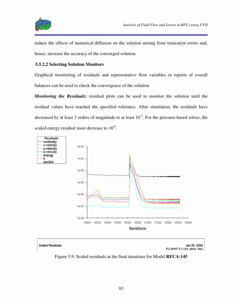
Analysis of Fluid Flow and Losses in RFCs using CFD
93
reduce the effects of numerical diffusion on the solution arising from truncation errors and,
hence, increase the accuracy of the converged solution.
5.5.2.2 Selecting Solution Monitors
Graphical monitoring of residuals and representative flow variables or reports of overall
balances can be used to check the convergence of the solution.
Monitoring the Residuals: residual plots can be used to monitor the solution until the
residual values have reached the specified tolerance. After simulation, the residuals have
decreased by at least 3 orders of magnitude to at least 10-3. For the pressure-based solver, the
scaled energy residual must decrease to 10-6.
Figure 5.9: Scaled residuals at the final iterations for Model RFCA-145
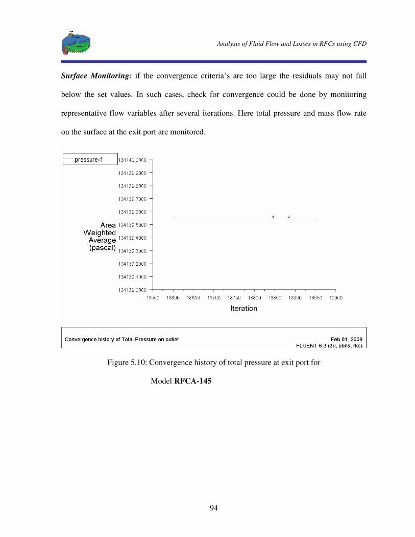
Analysis of Fluid Flow and Losses in RFCs using CFD
94
Surface Monitoring: if the convergence criteria’ s are too large the residuals may not fall
below the set values. In such cases, check for convergence could be done by monitoring
representative flow variables after several iterations. Here total pressure and mass flow rate
on the surface at the exit port are monitored.
Figure 5.10: Convergence history of total pressure at exit port for
Model RFCA-145

Analysis of Fluid Flow and Losses in RFCs using CFD
95
Figure 5.11: Convergence history of mass flow rate at exit port for
Model RFCA-145
Report of Overall balances: overall balance of mass flow rate can also be used as another
means to monitor convergence of solution after simulation.
Mass Flow Rate (kg/s) -------------------------------- ----------------------
Inlet 0.006825326 Outlet 0.0068253237 ------------------------------------- Net 2.3283064e-09 The overall imbalance can be calculated as percentage of the net mass flow out of the mass
flow at outlet and is compared to the minimum tolerable value of 0.2%.

Analysis of Fluid Flow and Losses in RFCs using CFD
96
5.5.2.3 Solution Computing
This is the last step in the CFD analysis of the flow in RFC. Calculation of solutions needs
initialization of the flow field with specified initial values of the flow variables for the entire
domain or a zone in the domain to start the iterating process.
Initializing the Solution: FLUENT needs an initial guess for starting the solution flow field.
Initialization of the flow field in the RFC simulation begins by setting the inlet values in the
starting 2891rpm. The converged solution at previous iteration of rpm is provided as an
initialization for the next increment of rpm until the final design point speed (28910rpm) is
reached.
Performing Calculations: for the first 100 iterations the flow is considered to be
compressible to stabilize the solution then the incompressible flow condition is activated to
proceed by adding more iteration until the solution is satisfactorily converged to any of the
specified solution monitoring methods. Plots of residuals and other solution monitors are
displayed in separate graphics windows while the iterations going on.
As shown in Figure 5.7 FLUENT stores the inputs that define the problem and the results
computed in two separate files; the case file and the data file. When starting the calculations
from current solution data, FLUENT begins at the last iteration performed, using the current
solution data as its starting point.
5.5.3 Post processing in FLUENT
In post processing, the results are examined to review the solution and to extract useful
data’ s. It can be through graphical display or numerical report. In graphical display the
overall flow pattern and determination of key flow features can be examined while in

Analysis of Fluid Flow and Losses in RFCs using CFD
97
numerical reporting necessary integral quantities can be computed at boundaries of the flow
domain. Amongst; the mass flow rate on boundaries, the moments about a specified center
for selected wall zones and area-weighted average field variables on a surface in the domain
are reported.
In the next chapter details of these output results will be presented.

Analysis of Fluid Flow and Losses in RFCs using CFD
98
CHAPTER SIX
RESULTS AND DISCUSION
6.1 Introduction
Different modifications on the basic geometries were investigated to optimize the
performance of the machine. First a model for the base machine was developed by taking its
geometric data’ s from literature [4] and the performance data’ s serve as a reference for
comparing the performance of the modified. As shown in Figure 5.1 and 5.3-1 the base
machine (RFCR-90) has rectangular flow channel and a straight impeller / blade profile.
Then different models were developed by varying both, the flow channel and impeller / blade
profile with the intent of minimizing losses and improving the performance of the machine.
An attempt was made to solve the flow details using FLUENT. Each model undergoes
through all simulation procedures; and evaluation is performed by using the output results
and computed values from these output results.
The objective of this chapter is:
• to present and discuss the output results i.e. plots and numerical outputs which
shows the flow characteristics in the base machine and the modified ones,
• to compute the design parameters for the comparison purpose with the
performance data’ s of the base machine,
• to analyze the performance of the base RFC simulated and to compare the output
results with the available performance data’ s.
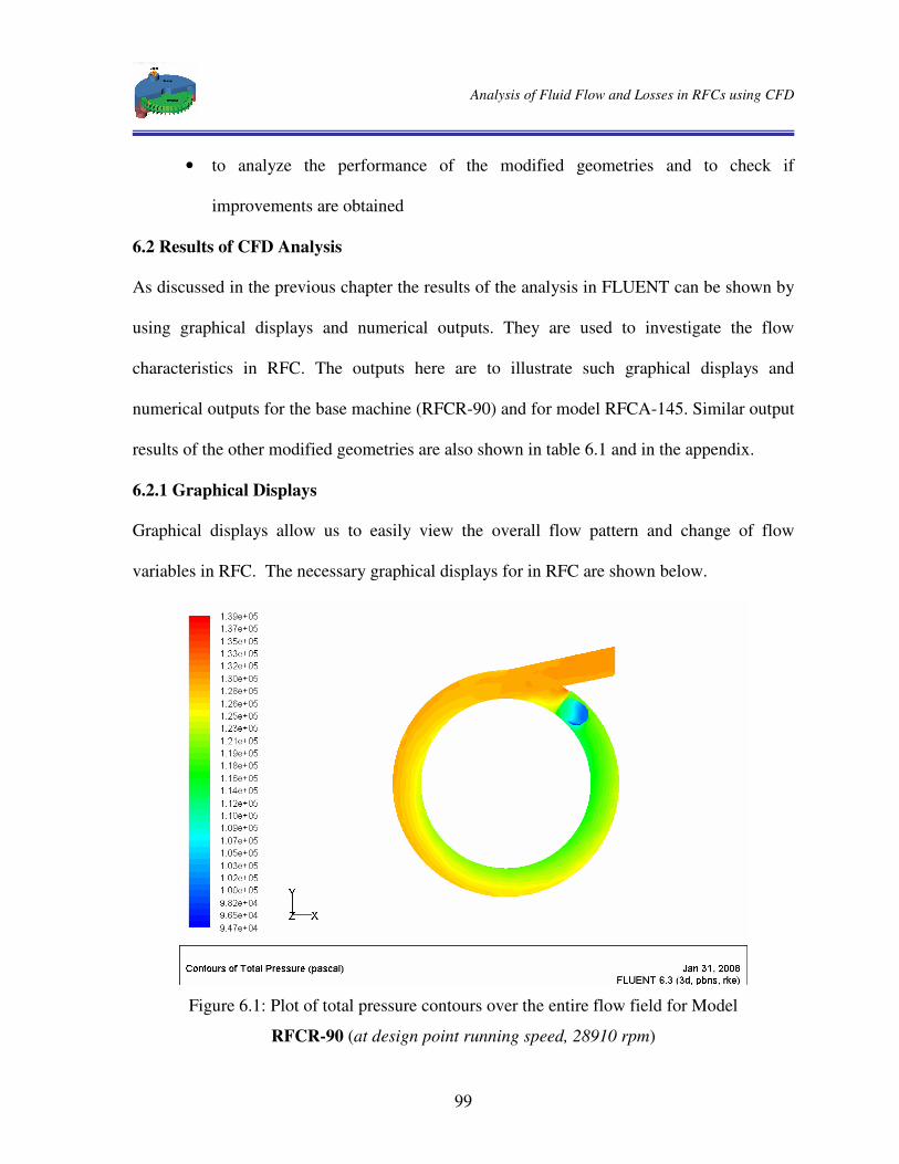
Analysis of Fluid Flow and Losses in RFCs using CFD
99
• to analyze the performance of the modified geometries and to check if
improvements are obtained
6.2 Results of CFD Analysis
As discussed in the previous chapter the results of the analysis in FLUENT can be shown by
using graphical displays and numerical outputs. They are used to investigate the flow
characteristics in RFC. The outputs here are to illustrate such graphical displays and
numerical outputs for the base machine (RFCR-90) and for model RFCA-145. Similar output
results of the other modified geometries are also shown in table 6.1 and in the appendix.
6.2.1 Graphical Displays
Graphical displays allow us to easily view the overall flow pattern and change of flow
variables in RFC. The necessary graphical displays for in RFC are shown below.
Figure 6.1: Plot of total pressure contours over the entire flow field for Model
RFCR-90 (at design point running speed, 28910 rpm)

Analysis of Fluid Flow and Losses in RFCs using CFD
100
Figure 6.1 shows the contour of total pressure for model RFCR-90 over the entire flow field.
As can be shown in the figure the pressure of the fluid increases gradually from inlet to the
exit port and an averaged total pressure of 129996.31 pa is obtained at the outlet. The flow
channel was then modified to be semi-circular in cross section and the impeller made semi-
elliptic with the intent of maximizing the pressure ratio (performance) of the machine. This
modified geometry then used as a base for developing subsequent blade variations. By doing
this an increase in total pressure is observed for the modified models and for model RFCA-
145 an averaged total pressure of 134139.55 pa is obtained at design point running speed.
Figure 6.2: Plot of total pressure contours over the entire flow field for Model
RFCA-145 (at design point running speed, 28910 rpm)

Analysis of Fluid Flow and Losses in RFCs using CFD
101
Figure 6.3 shows the contour of density for model RFCA-145 over the entire flow field. As
can be shown in the figure the density of the fluid also increases gradually from inlet to the
exit port which confirms the compressible flow characteristic in regenerative flow
compressors where we have gradual increase in density. This characteristic is observed for all
of the models considered (see the appendix).
Figure 6.3: Plot of density contours over the entire flow field for Model RFCA-145
(at design point running speed, 28910 rpm)
Figure 6.4 and 6.5 below show the path followed by a fluid particle from inlet to the exit port
for model RFCA-145 running at the starting speed, 2891 rpm. As shown on the figure, the
flow circulates through the blades and flow channel a number of times. This repetitive action
of the impeller blades on the fluid accounts for a pressure rise at lower running speed. The
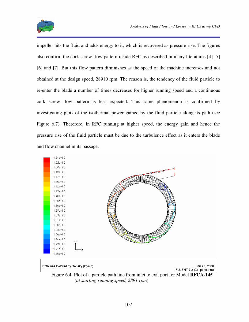
Analysis of Fluid Flow and Losses in RFCs using CFD
102
impeller hits the fluid and adds energy to it, which is recovered as pressure rise. The figures
also confirm the cork screw flow pattern inside RFC as described in many literatures [4] [5]
[6] and [7]. But this flow pattern diminishes as the speed of the machine increases and not
obtained at the design speed, 28910 rpm. The reason is, the tendency of the fluid particle to
re-enter the blade a number of times decreases for higher running speed and a continuous
cork screw flow pattern is less expected. This same phenomenon is confirmed by
investigating plots of the isothermal power gained by the fluid particle along its path (see
Figure 6.7). Therefore, in RFC running at higher speed, the energy gain and hence the
pressure rise of the fluid particle must be due to the turbulence effect as it enters the blade
and flow channel in its passage.
Figure 6.4: Plot of a particle path line from inlet to exit port for Model RFCA-145 (at starting running speed, 2891 rpm)
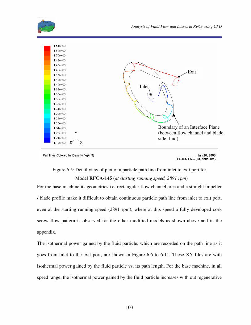
Analysis of Fluid Flow and Losses in RFCs using CFD
103
Figure 6.5: Detail view of plot of a particle path line from inlet to exit port for
Model RFCA-145 (at starting running speed, 2891 rpm)
For the base machine its geometries i.e. rectangular flow channel area and a straight impeller
/ blade profile make it difficult to obtain continuous particle path line from inlet to exit port,
even at the starting running speed (2891 rpm), where at this speed a fully developed cork
screw flow pattern is observed for the other modified models as shown above and in the
appendix.
The isothermal power gained by the fluid particle, which are recorded on the path line as it
goes from inlet to the exit port, are shown in Figure 6.6 to 6.11. These XY files are with
isothermal power gained by the fluid particle vs. its path length. For the base machine, in all
speed range, the isothermal power gained by the fluid particle increases with out regenerative
Exit
Inlet
Boundary of an Interface Plane (between flow channel and blade side fluid)
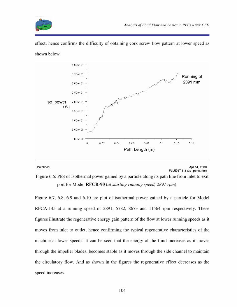
Analysis of Fluid Flow and Losses in RFCs using CFD
104
effect; hence confirms the difficulty of obtaining cork screw flow pattern at lower speed as
shown below.
Figure 6.6: Plot of Isothermal power gained by a particle along its path line from inlet to exit
port for Model RFCR-90 (at starting running speed, 2891 rpm)
Figure 6.7, 6.8, 6.9 and 6.10 are plot of isothermal power gained by a particle for Model
RFCA-145 at a running speed of 2891, 5782, 8673 and 11564 rpm respectively. These
figures illustrate the regenerative energy gain pattern of the flow at lower running speeds as it
moves from inlet to outlet; hence confirming the typical regenerative characteristics of the
machine at lower speeds. It can be seen that the energy of the fluid increases as it moves
through the impeller blades, becomes stable as it moves through the side channel to maintain
the circulatory flow. And as shown in the figures the regenerative effect decreases as the
speed increases.

Analysis of Fluid Flow and Losses in RFCs using CFD
105
Figure 6.7: Plot of Isothermal power gained by a particle along its path line from inlet to exit
port for Model RFCA-145 (at starting running speed, 2891 rpm)
Figure 6.8: Plot of Isothermal power gained by a particle along its path line from inlet to exit
port for Model RFCA-145 (at the second running speed, 5782 rpm)
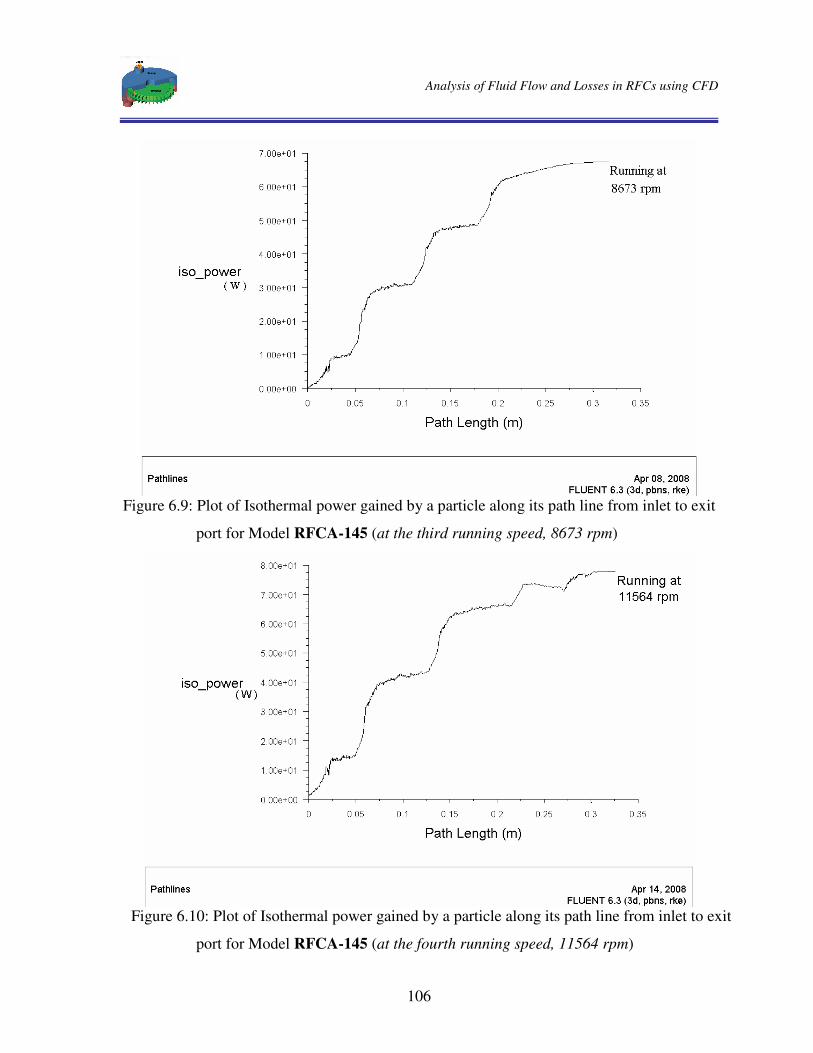
Analysis of Fluid Flow and Losses in RFCs using CFD
106
Figure 6.9: Plot of Isothermal power gained by a particle along its path line from inlet to exit
port for Model RFCA-145 (at the third running speed, 8673 rpm)
Figure 6.10: Plot of Isothermal power gained by a particle along its path line from inlet to exit
port for Model RFCA-145 (at the fourth running speed, 11564 rpm)
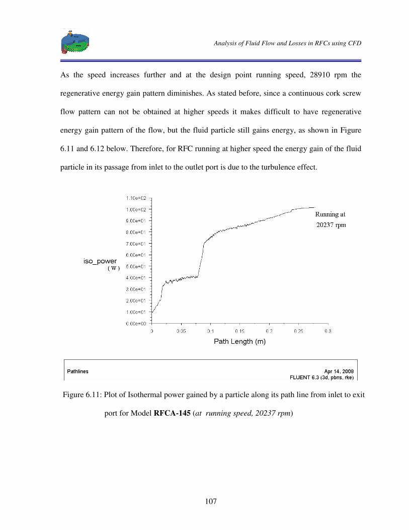
Analysis of Fluid Flow and Losses in RFCs using CFD
107
As the speed increases further and at the design point running speed, 28910 rpm the
regenerative energy gain pattern diminishes. As stated before, since a continuous cork screw
flow pattern can not be obtained at higher speeds it makes difficult to have regenerative
energy gain pattern of the flow, but the fluid particle still gains energy, as shown in Figure
6.11 and 6.12 below. Therefore, for RFC running at higher speed the energy gain of the fluid
particle in its passage from inlet to the outlet port is due to the turbulence effect.
Figure 6.11: Plot of Isothermal power gained by a particle along its path line from inlet to exit
port for Model RFCA-145 (at running speed, 20237 rpm)
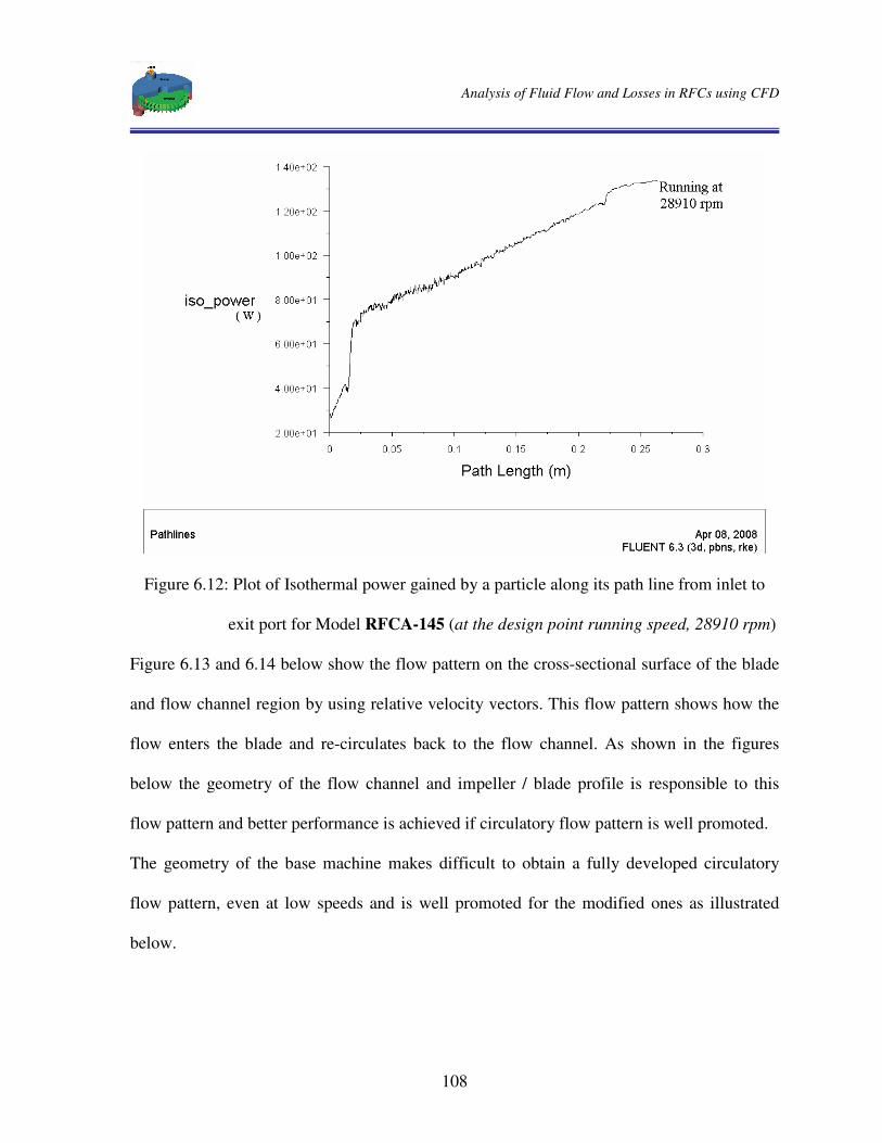
Analysis of Fluid Flow and Losses in RFCs using CFD
108
Figure 6.12: Plot of Isothermal power gained by a particle along its path line from inlet to
exit port for Model RFCA-145 (at the design point running speed, 28910 rpm)
Figure 6.13 and 6.14 below show the flow pattern on the cross-sectional surface of the blade
and flow channel region by using relative velocity vectors. This flow pattern shows how the
flow enters the blade and re-circulates back to the flow channel. As shown in the figures
below the geometry of the flow channel and impeller / blade profile is responsible to this
flow pattern and better performance is achieved if circulatory flow pattern is well promoted.
The geometry of the base machine makes difficult to obtain a fully developed circulatory
flow pattern, even at low speeds and is well promoted for the modified ones as illustrated
below.
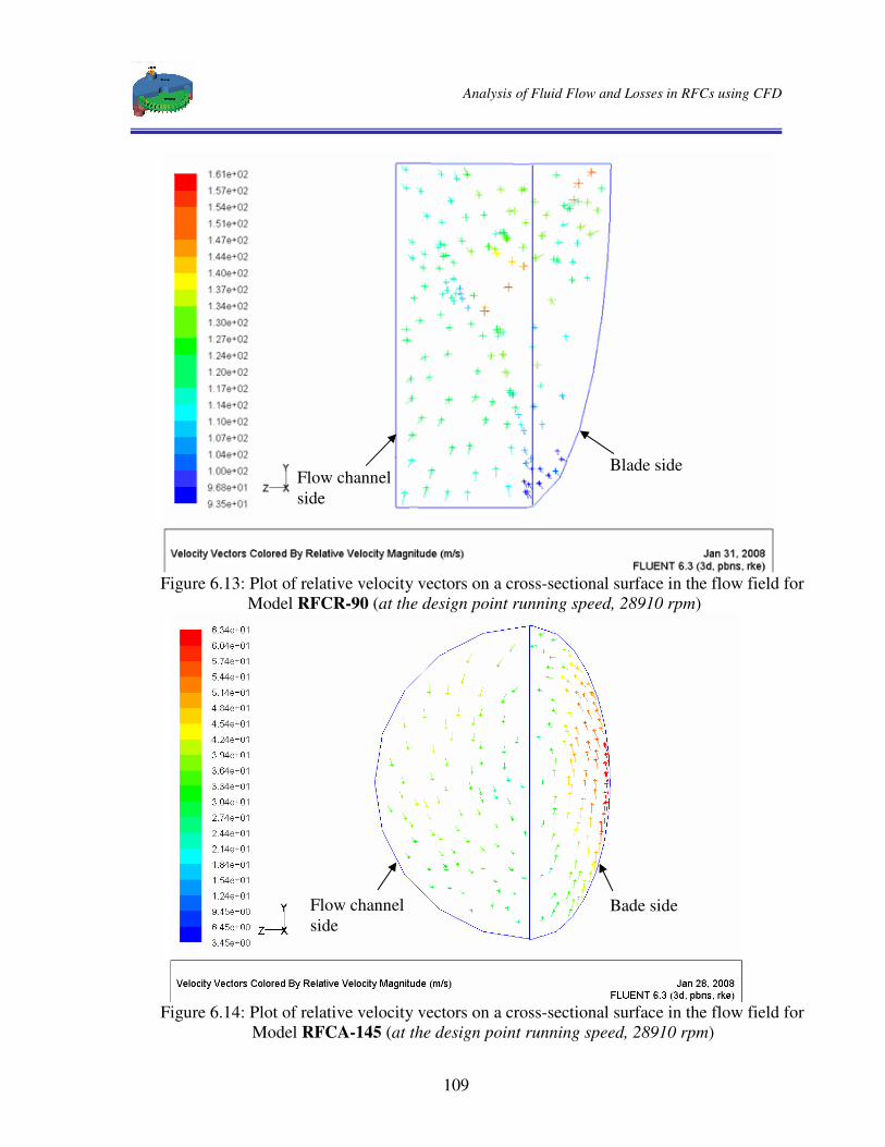
Analysis of Fluid Flow and Losses in RFCs using CFD
109
Figure 6.13: Plot of relative velocity vectors on a cross-sectional surface in the flow field for
Model RFCR-90 (at the design point running speed, 28910 rpm)
Figure 6.14: Plot of relative velocity vectors on a cross-sectional surface in the flow field for
Model RFCA-145 (at the design point running speed, 28910 rpm)
Bade side
Flow channel side
Blade side
Flow channel side

Analysis of Fluid Flow and Losses in RFCs using CFD
110
6.2.2 Numerical Results
After convergence is reached printed quantitative results like flux balances, moments and
surface integrated quantities are taken for the evaluation of design parameters. Reports of
area-weighted average field variables on inlet and outlet surfaces, mass flow rate on inlet and
outlet surfaces and moment about center (0, 0, 0) are illustrated below for model RFCA-145.
Area-weighted average field variables are the average value of field variables on inlet and
outlet surfaces. They are computed by dividing the summation of the product of the selected
field variable and facet area by the total area of the surface.
Area-Weighted Average
Total Pressure (Pascal) -------------------------------------------------------- Inlet 106464.97 Outlet 134139.55
Area-Weighted Average Density (kg/m3) --------------------------------------------------------
Inlet 1.2178888 Outlet 1.5376899
As shown in the results the inlet values slightly deviates from the prescribed inlet values. It is
caused by the carry over loss and becomes more noticeable at higher speed. This can be
considered as the draw back of CFD analysis of RFCs where the required pressure ratio may
not be obtained [4].
The total moment vector about center (0, 0, 0) is computed by summing the pressure and
viscous moment vectors on the rotor wall. The z-component of total moment is then taken for
the evaluation of shaft power.
Analysis of Fluid Flow and Losses in RFCs using CFD
111
Moment Center: (0, 0, 0) Zone name total moment, M (x, y, z: in N-m)
---------------------------------------------------------------------------------------------------- Rotor-wall (-0.12781679 -3.2379046 0.12876165)
The mass flow rate through the inlet and outlet boundaries is also computed by FLUENT. As
described in chapter five there should be a mass flow rate balance at the inlet and out let
boundaries.
Mass Flow Rate (kg/s) --------------------------------------------------------
Inlet 0.006825326 Outlet 0.0068253237 Table 6.1 below shows a summary of numerical inputs, output results obtained and computed
design parameters for different RFC models. The design parameters evaluated from the
numerical output results are then used for comparison purpose and for suggesting new design
geometries of a regenerative flow compressor.
6.3 Evaluation of Design Parameters
The design parameters i.e. pressure ratio, isothermal efficiency, power coefficient, flow
coefficient and specific mass flow rate are evaluated from the numerical output results of
FLUENT. These parameters are used to compare the performance characteristics of RFC
models. They were defined in Chapter five, section 5.2 and here they will be evaluated for
each model.
Isothermal efficiency, a
S
in
outiso
W
WPP
•
•
==η (6.1)
Pressure ratio, in
out
pp
=π (6.2)
Analysis of Fluid Flow and Losses in RFCs using CFD
112
Flow coefficient, 32 8 r
m
inωρ
•
= (6.3)
Power Coefficient, < 52
3 32
rDrawPower
inωρ= (6.4)
Specific mass flow rate,γ
φ ingas
in
TR
prm2
24
•
= (6.5)
Where;
Pin is the actual power transferred to impeller and evaluated as,
Pin = Power Drawn = ω T ×=•
shaftaW (6.6)
Pout is a power used to compress the fluid under isothermal condition (isothermal power
gained by the fluid) and evaluated as,
==
••
in
outingasSout p
pTRmWP ln (6.7)
Output result of FLUENT are, •m = mass flow rate [kg/s]
inp = total pressure at inlet [Pa]
outp = total pressure at exit port [Pa]
shaftT = shaft torque (the moment on rotor-wall about the z-axis, Mz [N-m])
inρ = density at inlet [kg / m3]
Input variable are,
n = rotational speed [rpm]
ω = angular speed of impeller [rad/s] =60
2 nπ (6.8)
inT = total temperature at inlet [K]
Rgas is the gas constant

Analysis of Fluid Flow and Losses in RFCs using CFD
113
Table 6.1: Numerical inputs and results of CFD analysis for RFC Models developed
RFCR-90 RFCS-135 RFCA-135 RFCA-145 RFCA-150 RFCA-160
Impeller tip dia, mm 82.82 (It is the same for all)
Impeller hub dia, mm 63.46 (It is the same for all)
Blade depth, mm 2.54 2.54 2.54 2.54 2.54 2.54
Flow channel depth, mm 3.805 5.09 5.09 5.09 5.09 5.09
Geometric data’s
Mesh size, mm 1.5, 1 1.5, 1 1.5, 1 1.5, 1 1.5, 1 1.5, 1
Inlet pressure, pin [pa] 100000 100000 100000 100000 100000 100000
Outlet pressure, pout [pa] 130000 130000 130000 130000 130000 130000
Inlet temperature, Tin [K] 294.26 294.26 294.26 294.26 294.26 294.26 Input Variables
Angular velocity, rpm 28910 28910 28910 28910 28910 28910 Fluid Property Gas constant, R [J/kg K] 287 287 287 287 287 287
Density at inlet, kg/s 1.1825112 1.2144295 1.2103574 1.2178888 1.2094109 1.2042608
Density at outlet, kg/s 1.5210673 1.5189388 1.5193921 1.5676898 1.5202744 1.5204897
Mass flow rate, kg/s 0.0061007 0.00665797 0.006584102 0.006825324 0.006557565 0.006502501
Torque, Mz [N-m] 0.32542422 0.14210897 0.1186897 0.12876165 0.11520059 0.11967433
Inlet pressure, pin [pa] 105869.22 106373.05 106139.9 106464.97 106030.04 105984.47
FLUENT Output Values
Outlet pressure, pout [pa] 129996.31 129984.43 129982.46 134139.55 130042.62 130032.91
Pressure ratio, in
out
pp
=π 1.227895228 1.221967688 1.224633338 1.259940711 1.226469593 1.226905319
Output power Pout [ w] 105.7754625 112.7166072 112.6777154 133.1894783 113.0533357 112.2990869
Input power, Pin [ w] 985.2049432 430.2275341 359.3269092 389.8192153 348.7638097 362.3078254 Isothermal efficiency, iso [%] 10.73639178 26.19930112 31.35799533 34.16698641 32.41544351 30.99549031 Flow Coefficient, 0.002999798 0.003187771 0.00316301 0.003258616 0.003152727 0.003139623 Power Coefficient, < 0.007705753 0.003276571 0.002745806 0.002960393 0.002667174 0.002782601
Computed Values
Specific Mass Flow Rate, φ 0.002063393 0.002241209 0.002221212 0.00229556 0.002214551 0.0021969
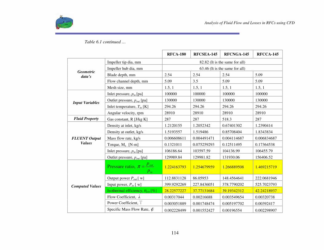
Analysis of Fluid Flow and Losses in RFCs using CFD
114
Table 6.1 continued …
RFCA-180 RFCSEA-145 RFCNGA-145 RFCCA-145
Impeller tip dia, mm 82.82 (It is the same for all)
Impeller hub dia, mm 63.46 (It is the same for all)
Blade depth, mm 2.54 2.54 2.54 5.09
Flow channel depth, mm 5.09 3.5 5.09 5.09
Geometric data’s
Mesh size, mm 1.5, 1 1.5, 1 1.5, 1 1.5, 1
Inlet pressure, pin [pa] 100000 100000 100000 100000
Outlet pressure, pout [pa] 130000 130000 130000 130000
Inlet temperature, Tin [K] 294.26 294.26 294.26 294.26 Input Variables
Angular velocity, rpm 28910 28910 28910 28910 Fluid Property Gas constant, R [J/kg K] 287 287 518.3 287
Density at inlet, kg/s 1.2120155 1.2052342 0.67401302 1.2390414
Density at outlet, kg/s 1.5193557 1.519486 0.85708404 1.8343834
Mass flow rate, kg/s 0.006608611 0.004491471 0.004114687 0.006834687
Torque, Mz [N-m] 0.1321011 0.075259293 0.12511495 0.17364538
Inlet pressure, pin [pa] 106186.64 103597.59 104136.99 106455.79
FLUENT Output Values
Outlet pressure, pout [pa] 129989.84 129981.82 131930.06 156406.52
Pressure ratio, in
out
pp
=π 1.224163793 1.254679959 1.266889508 1.469215719
Output power Pout [ w] 112.8831128 86.05953 148.4564641 222.0681946
Input power, Pin [ w] 399.9292269 227.8436051 378.7790202 525.7023793 Isothermal efficiency, iso [%] 28.22577227 37.77131684 39.19342312 42.24218937 Flow Coefficient, 0.00317044 0.00216688 0.003549654 0.00320738 Power Coefficient, < 0.003051889 0.001748474 0.005197702 0.00392417
Computed Values
Specific Mass Flow Rate, φ 0.002228499 0.001552427 0.00196554 0.002298907

Analysis of Fluid Flow and Losses in RFCs using CFD
115
6.4 Validation
Performance of the model of the base machine is compared with its tested data’ s for
validation purpose. The base machine was tested at operation points and an isothermal
efficiency of 8.13% was achieved. The simulation result gives an isothermal efficiency of
10.74%, which is close to the tested value, and a pressure ratio of 1.228 is obtained for the
base machine. As discussed in chapter five the mismatch may arise from the unidentified
losses which are not considered during the simulation process.
The geometry of the base machine i.e. rectangular flow channel area and a straight impeller /
blade profile is a major cause for this very low efficiency value. As discussed before cork
screw and circulatory flow patterns can not be obtained for this machine. It results in high
turbulence and mismatches between flow and blade angles, so that the losses become
dominant.
The blade shape, impeller profile and flow channel was then changed for the other models to
develop better circulation and regeneration and to minimize losses.
6.5 Results of Modifications done to Improve Performance
6.5.1 Effect of changing Flow Channel and Impeller Profile
For the six successive models the flow channel is changed to semi-circular and the impeller /
blade profile is changed to semi-elliptic. To this modified geometry the blades are changed
from a straight radial profile for the base machine to airfoil shape with blade angles of 135O,
145O, 150O, 160O and 180O. As shown in the figures above by doing those modifications
regeneration is well promoted and the path line of fluid particle is obtained at low speeds.
Turbulence and mismatch between the blade and flow angle are minimized, hence better
Analysis of Fluid Flow and Losses in RFCs using CFD
116
performance is obtained. As can be shown in Table 6.1 and Figure 6.2 a maximum efficiency
of 34.17% and a pressure ratio of 1.26�LV�REWDLQHG�IRU�EODGHV�DQJOH� � ����O.
0DLQWDLQLQJ�WKH�EODGH�DQJOH�WR�WKLV�RSWLPXP�YDOXH�� � ����O) and the impeller / blade profile
to semi-elliptic shape the flow channel depth is decreased (made semi-elliptic) to investigate
its effect on turbulence and fluid friction. As can be seen in the table the efficiency is
improved to 37.77% with very close pressure ratio (1.255). Therefore changing the flow
channel area to semi-elliptic reduces the flow turbulence and optimum cross sectional area
can be obtained by investigating other dimensions.
6.5.2 Effect of changing Blades Angle
Blades angle were varied from purely radial 90O to chevroned blade with an angle of 135O,
145O, 150O, 160O and 180O. This angle variations / chevroning are also responsible to
establish circulatory flow pattern and regeneration. Many authors suggest that changing the
blades angle / chevroning reduce losses and increases the pressure ratio in RFCs [3] [4] [5].
The advantage of changing blade angles on performance is shown in Table 6.1. The blade
angle variation from straight radial to aerodynamic shape results in an improved performance
and pressure ratio. By varying the blade angle for the first modified geometry i.e. semi-
circular flow channel and semi-elliptic impeller / blade profile a maximum efficiency of
34.17% and pressure ratio of 1.26�DUH�REWDLQHG�IRU�EODGH�DQJOH� � ����O.
It must however be noted that the chevron angle should not deviate more from 145O, because
doing that might bring in excessive slow down to the flow. And this results in a lower
efficiency and pressure ratio. As shown in Table 6.1 an efficiency of 28.23% and pressure
ratio of 1.224�DUH�REWDLQHG�IRU� � ����O.

Analysis of Fluid Flow and Losses in RFCs using CFD
117
6.5.3 Effect of adding a Core
)RU�WKH�DERYH�RSWLPXP�EODGH�DQJOH�� � ����O) adding a core in between a semi-circular flow
channel and impeller / blade profile maximizes both the efficiency and pressure ratio. The
core guides the flow properly and avoids local vortices in the blade and flow channel region.
At lower running speed addition of core promotes a well developed continuous cork screw
flow pattern which is shown in Figure 6.18 for the starting speed of 2891 rpm. As shown in
Figure 6.19 also the pressure ratio is increased and a maximum pressure ratio of 1.47 is
obtained at the design point with an efficiency of 42.24%.
Figure 6.15: Plot of a particle path line from inlet to exit port for Model RFCCA-145
(at starting running speed, 2891 rpm)
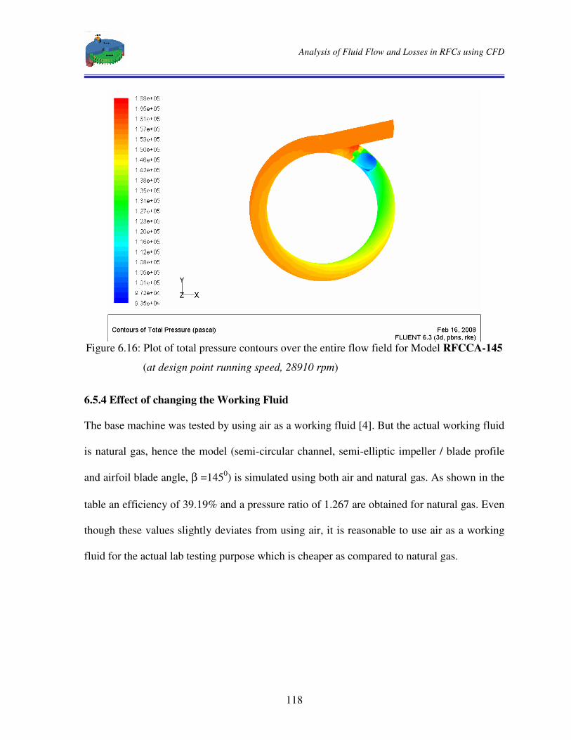
Analysis of Fluid Flow and Losses in RFCs using CFD
118
Figure 6.16: Plot of total pressure contours over the entire flow field for Model RFCCA-145
(at design point running speed, 28910 rpm)
6.5.4 Effect of changing the Working Fluid
The base machine was tested by using air as a working fluid [4]. But the actual working fluid
is natural gas, hence the model (semi-circular channel, semi-elliptic impeller / blade profile
and airfoil blade angle, β =1450) is simulated using both air and natural gas. As shown in the
table an efficiency of 39.19% and a pressure ratio of 1.267 are obtained for natural gas. Even
though these values slightly deviates from using air, it is reasonable to use air as a working
fluid for the actual lab testing purpose which is cheaper as compared to natural gas.

Analysis of Fluid Flow and Losses in RFCs using CFD
119
CHAPTER SEVEN
CONCLUSIONS AND RECOMMENDATIONS
RFC has a wide application especially for duties requiring high head at low flow rate, but
unfortunately it has low efficiency. This research was started with an objective of improving
the performance of the machine by modifying its geometry to aerodynamic shape. Attempt
was made to investigate the flow characteristic using FLUENT and the results obtained from
the analysis motivate to use CFD software’ s for further study of these machines.
In this section, based on the results, conclusions will be given and recommendation will be
presented in regard to the long-term objectives.
7.1 Conclusions
The following conclusions are drawn from the CFD results:
a. Aerodynamically designed geometries give better performance. The flow channel
and impeller / blade geometries of the base machine are changed to aerodynamic
shape so that regeneration effect is highly facilitated at lower speeds and better
efficiency is obtained in all speed range.
b. The addition of a core in the flow field further increases the performance of
RFCs. This merit is investigated by adding a core for a selecWHG�EODGH�DQJOH�� � �145O) and an improved pressure ratio and efficiency is obtained.
c. Flow characteristics in RFC are examined. On the graphical display of FLUENT
the three-dimensional continuous cork screw flow patterns are illustrated for
lower running speeds; however this regeneration effect diminishes as the running
speed of the machine increases. This same phenomenon is also confirmed by

Analysis of Fluid Flow and Losses in RFCs using CFD
120
investigating the isothermal power gained by the fluid particle in its passage from
inlet to the exit port where at higher speeds no regenerative energy gain is
observed.
d. Performance characteristic of RFC that is capability of producing a pressure ratio
at low specific mass flow rate is also investigated. As can be shown in Table 6.1
the pressure ratio obtained are at lower specific mass flow rate.
e. High efficiency and pressure ratio is obtained as the blade angle increases from
radial straight to aerodynamic shape; however after a certain point where peak
efficiency is achieved its value starts to go down with blade angle.
f. Agreement between test data’ s and those experimental values is observed. This
motivates to carry out extensive design analysis on RFC using commercially
available CFD software’ s.
7.2 Recommendations
In this research the design changes focus on the flow channel geometry and impeller / blade
profile. The blade angles are also selected randomly from the recommended range. Therefore
further design changes can also be considered on the other geometries for improving the
performance of the machine.
a. The inlet port is responsible to set up circulatory flow pattern in regenerative flow
machine by projecting the fluid towards the inlet edge of the blade with the
velocity and direction needed to ensure smooth entry. Hence inlet ports can be
further optimized for generating such flow pattern and to ensure smooth entry to
the blades. The same is true for outlet ports where they can be designed further to
exploit the kinetic energy of the flow for pressure rise.

Analysis of Fluid Flow and Losses in RFCs using CFD
121
b. The blade angle can also be varied to obtain other optimum value in the range
135O��� ������O.
c. For RFC the maximum blade number suggested by many authors is Zb = 90,
hence the number of blades can be reduced for the optimum blade angle to check
for better performance.
d. Geometry of the stripper, just like the inlet port, is also responsible for generating
circulatory flow pattern. Hence various stripper geometries can be considered
together with inlet and outlet ports for upgrading the performance of the machine.
Generally a complete analysis of various geometric parameters is very much needed to
establish design criteria’ s for regenerative flow compressors.
Analysis of Fluid Flow and Losses in RFCs using CFD
122
REFERENCES
1. Andrew D.N.: The Calculation of flow in regenerative turbomachines by a
streamline curvature method, Whittle Laboratory, University of Cambridge, 1990.
2. Engda A. and Raheel M.: Theory and design of the regenerative flow compressor,
Proc. International Gas Turbine Congress – TS050, 2003.
3. Engda A., Song J.W. and Raheel M.: A Compressible Flow Theory for Regenerative
Compressor with Aerofoil Blades, Proc. Instn Mech. Engrs- 2003.
4. Raheel M.: A Theoretical, Experimental and CFD Analysis of regenerative flow
compressors and regenerative flow pumps for microturbine and automotive fuel
applications, Ph.D. thesis, Michigan State University, USA, 2003.
5. Sixsmith H.: The theory and design of a regenerative compressor, Research paper for
Institute of Refrigeration, Institute of Marine Engineers, 1981, 69-77.
6. Sixsmith H. and Altmann H.: A regenerative Compressor, Trans. ASME Journal of
Eng’ g for Industry, 1977, 637-647.
7. Song J.W., Engda A. and Chung M. K.: A modified theory for the flow mechanism in
regenerative flow pump, Proc. Instn Mech. Engrs – A05202, 2003.
8. Dixon S.L.: Fluid Mechanics and Thermodynamics of Turbomachines, Fourth
Edition, University of Liverpool, 2005.
9. Wilson W.A., Santalo M.A. and Oelrich, J.A.: A Theory of the Fluid Dynamic
Mechanism of Regenerative Pumps, ASME Journal of Eng’ g for Industry, 54-A59/60,
August 1954.
10. Meakhail T. and Park S. O.: An improved theory for regenerative pump
performance, Proc. Instn Mech. Engrs - A05604, Korea Advanced Institute of Science
and Technology, 18 October 2004.
11. Fluent Inc.: FLUENT 6.3.26 Documentation – User’ s Guide, 2006.
12. http://en.wikipedia.org/wiki/gas compressors

Analysis of Fluid Flow and Losses in RFCs using CFD
123
APPENDIX
OUTPUT RESULTS FOR RFC MODELS * All the figures are at the design point except for the particle path line, which is taken at 2891 rpm.
1. Output results for model RFCR-90
Figure 6.17: Plot of total pressure contours over the entire flow field for Model RFCR-90
Figure 6.18: Plot of density contours over the entire flow field for Model RFCR-90
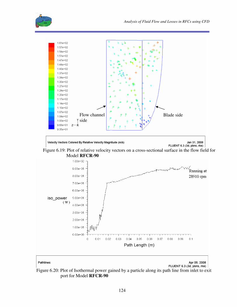
Analysis of Fluid Flow and Losses in RFCs using CFD
124
Figure 6.19: Plot of relative velocity vectors on a cross-sectional surface in the flow field for
Model RFCR-90
Figure 6.20: Plot of Isothermal power gained by a particle along its path line from inlet to exit
port for Model RFCR-90
Flow channel side
Blade side
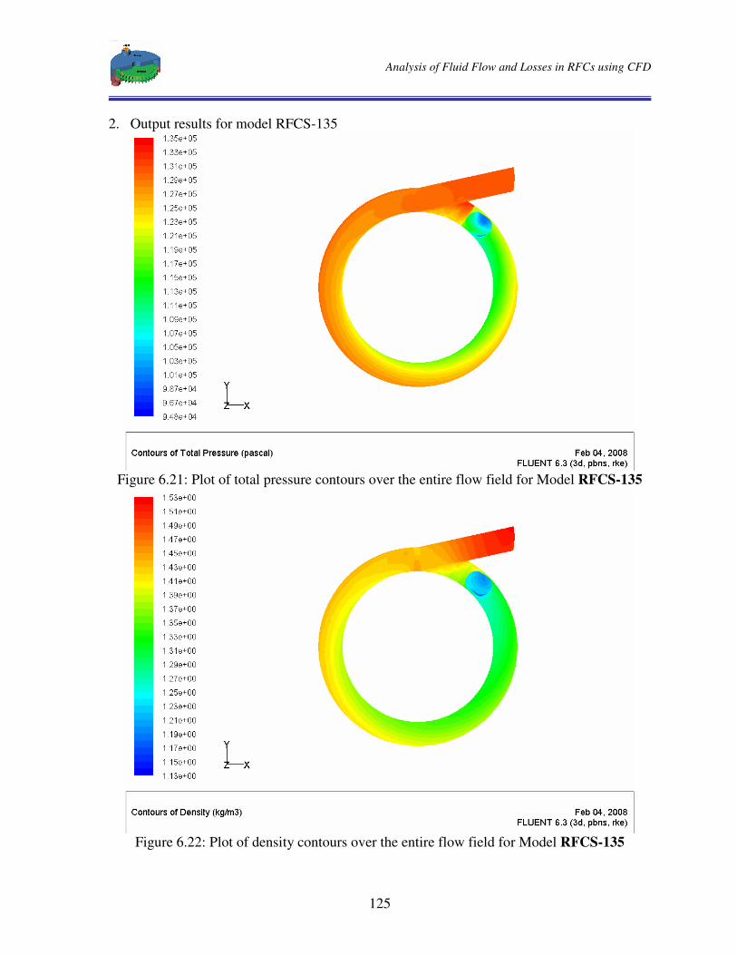
Analysis of Fluid Flow and Losses in RFCs using CFD
125
2. Output results for model RFCS-135
Figure 6.21: Plot of total pressure contours over the entire flow field for Model RFCS-135
Figure 6.22: Plot of density contours over the entire flow field for Model RFCS-135
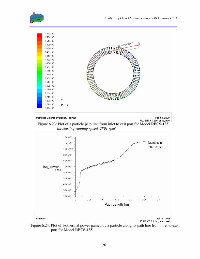
Analysis of Fluid Flow and Losses in RFCs using CFD
126
Figure 6.23: Plot of a particle path line from inlet to exit port for Model RFCS-135
(at starting running speed, 2891 rpm)
Figure 6.24: Plot of Isothermal power gained by a particle along its path line from inlet to exit
port for Model RFCS-135

Analysis of Fluid Flow and Losses in RFCs using CFD
127
Figure 6.25: Plot of relative velocity vectors on a cross-sectional surface in the flow field for
Model RFCS-135 3. Output results for model RFCA-135
Figure 6.26: Plot of total pressure contours over the entire flow field for Model RFCA-135
Blade side Flow channel
side

Analysis of Fluid Flow and Losses in RFCs using CFD
128
Figure 6.27: Plot of density contours over the entire flow field for Model RFCA-135
Figure 6.28: Plot of a particle path line from inlet to exit port for Model RFCA-135
(at starting running speed, 2891 rpm)
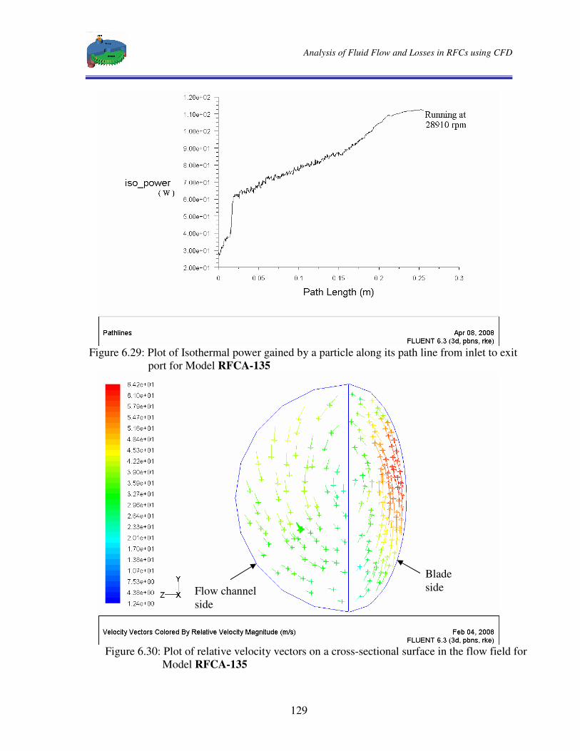
Analysis of Fluid Flow and Losses in RFCs using CFD
129
Figure 6.29: Plot of Isothermal power gained by a particle along its path line from inlet to exit
port for Model RFCA-135
Figure 6.30: Plot of relative velocity vectors on a cross-sectional surface in the flow field for
Model RFCA-135
Blade side Flow channel
side

Analysis of Fluid Flow and Losses in RFCs using CFD
130
4. Output results for model RFCA-145
Figure 6.31: Plot of total pressure contours over the entire flow field for Model RFCA-145
Figure 6.32: Plot of density contours over the entire flow field for Model RFCA-145
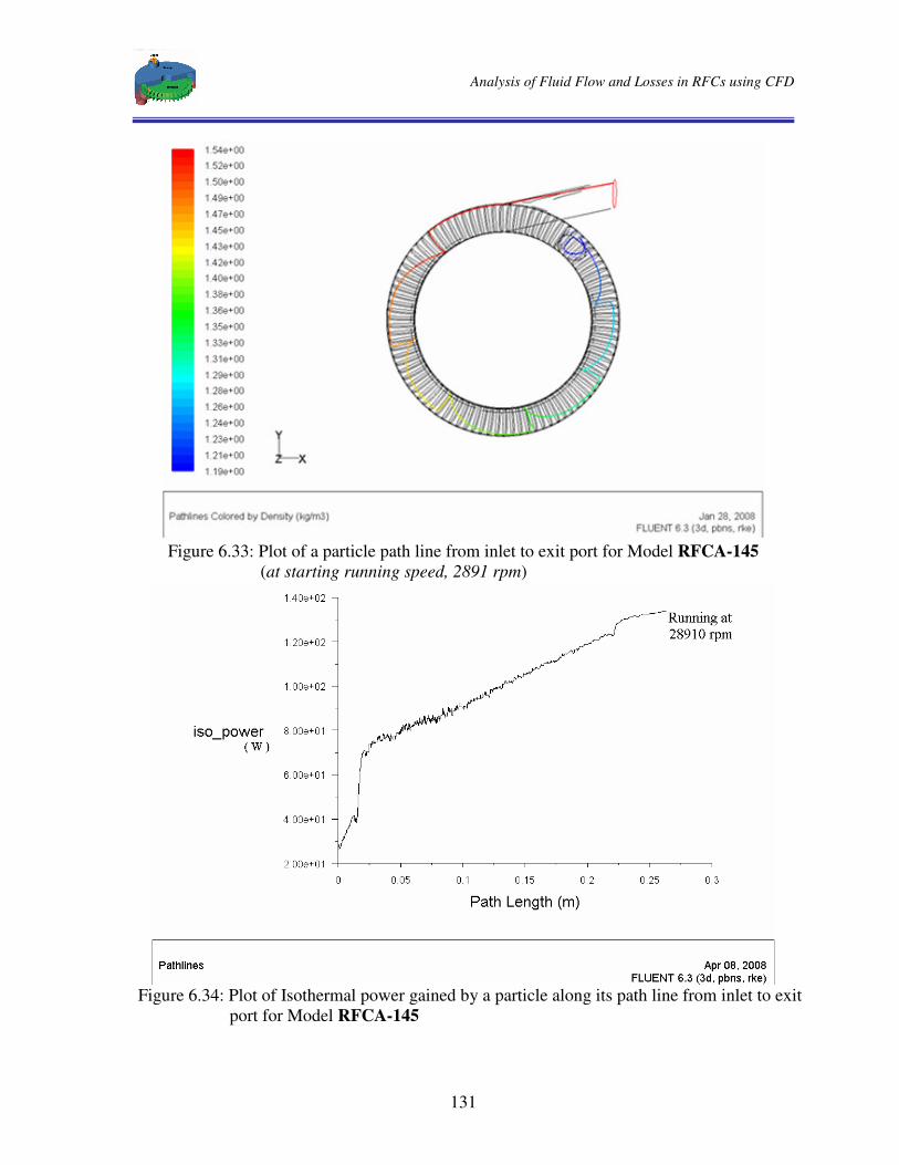
Analysis of Fluid Flow and Losses in RFCs using CFD
131
Figure 6.33: Plot of a particle path line from inlet to exit port for Model RFCA-145
(at starting running speed, 2891 rpm)
Figure 6.34: Plot of Isothermal power gained by a particle along its path line from inlet to exit
port for Model RFCA-145
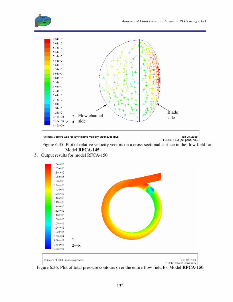
Analysis of Fluid Flow and Losses in RFCs using CFD
132
Figure 6.35: Plot of relative velocity vectors on a cross-sectional surface in the flow field for
Model RFCA-145 5. Output results for model RFCA-150
Figure 6.36: Plot of total pressure contours over the entire flow field for Model RFCA-150
Blade side Flow channel
side

Analysis of Fluid Flow and Losses in RFCs using CFD
133
Figure 6.37: Plot of density contours over the entire flow field for Model RFCA-150
Figure 6.38: Plot of a particle path line from inlet to exit port for Model RFCA-150
(at starting running speed, 2891 rpm)

Analysis of Fluid Flow and Losses in RFCs using CFD
134
Figure 6.39: Plot of Isothermal power gained by a particle along its path line from inlet to exit
port for Model RFCA-150
Figure 6.40: Plot of relative velocity vectors on a cross-sectional surface in the flow field for
Model RFCA-150
Flow channel side
Blade side
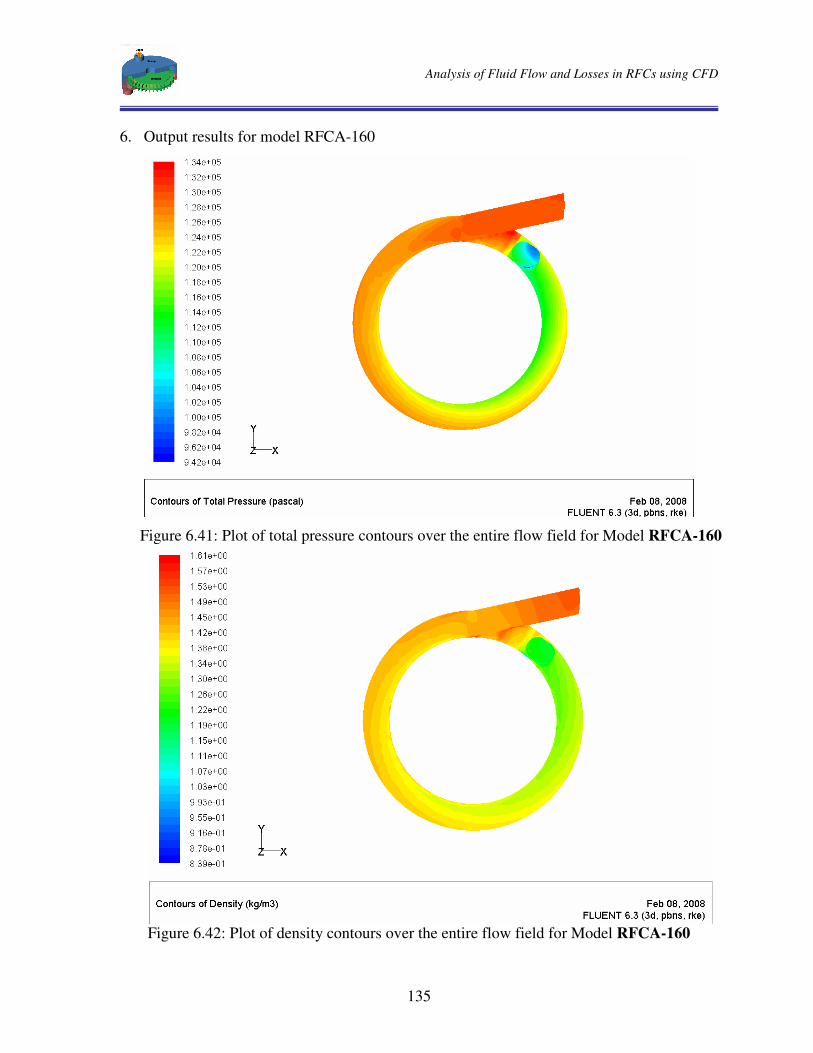
Analysis of Fluid Flow and Losses in RFCs using CFD
135
6. Output results for model RFCA-160
Figure 6.41: Plot of total pressure contours over the entire flow field for Model RFCA-160
Figure 6.42: Plot of density contours over the entire flow field for Model RFCA-160
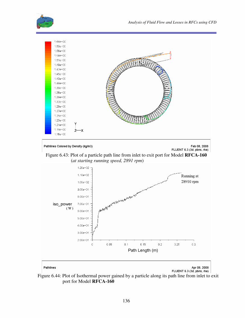
Analysis of Fluid Flow and Losses in RFCs using CFD
136
Figure 6.43: Plot of a particle path line from inlet to exit port for Model RFCA-160
(at starting running speed, 2891 rpm)
Figure 6.44: Plot of Isothermal power gained by a particle along its path line from inlet to exit
port for Model RFCA-160
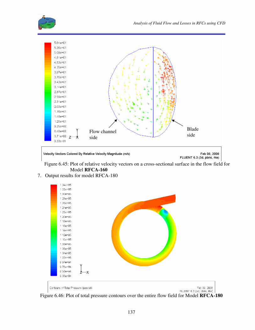
Analysis of Fluid Flow and Losses in RFCs using CFD
137
Figure 6.45: Plot of relative velocity vectors on a cross-sectional surface in the flow field for
Model RFCA-160 7. Output results for model RFCA-180
Figure 6.46: Plot of total pressure contours over the entire flow field for Model RFCA-180
Blade side
Flow channel side
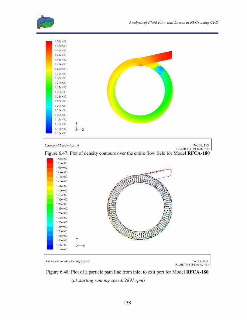
Analysis of Fluid Flow and Losses in RFCs using CFD
138
Figure 6.47: Plot of density contours over the entire flow field for Model RFCA-180
Figure 6.48: Plot of a particle path line from inlet to exit port for Model RFCA-180
(at starting running speed, 2891 rpm)
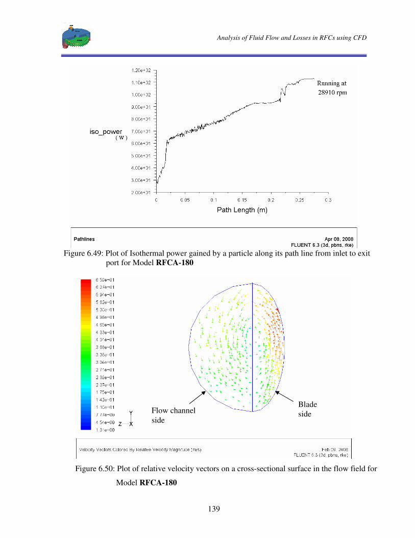
Analysis of Fluid Flow and Losses in RFCs using CFD
139
Figure 6.49: Plot of Isothermal power gained by a particle along its path line from inlet to exit
port for Model RFCA-180
Figure 6.50: Plot of relative velocity vectors on a cross-sectional surface in the flow field for
Model RFCA-180
Blade side Flow channel
side

Analysis of Fluid Flow and Losses in RFCs using CFD
140
8. Output results for model RFCSEA-145
Figure 6.51: Plot of total pressure contours over the entire flow field for Model RFCSEA-145
Figure 6.52: Plot of density contours over the entire flow field for Model RFCSEA-145

Analysis of Fluid Flow and Losses in RFCs using CFD
141
Figure 6.53: Plot of a particle path line from inlet to exit port for Model RFCSEA-145
(at starting running speed, 2891 rpm)
Figure 6.54: Plot of Isothermal power gained by a particle along its path line from inlet to exit
port for Model RFCSEA-145
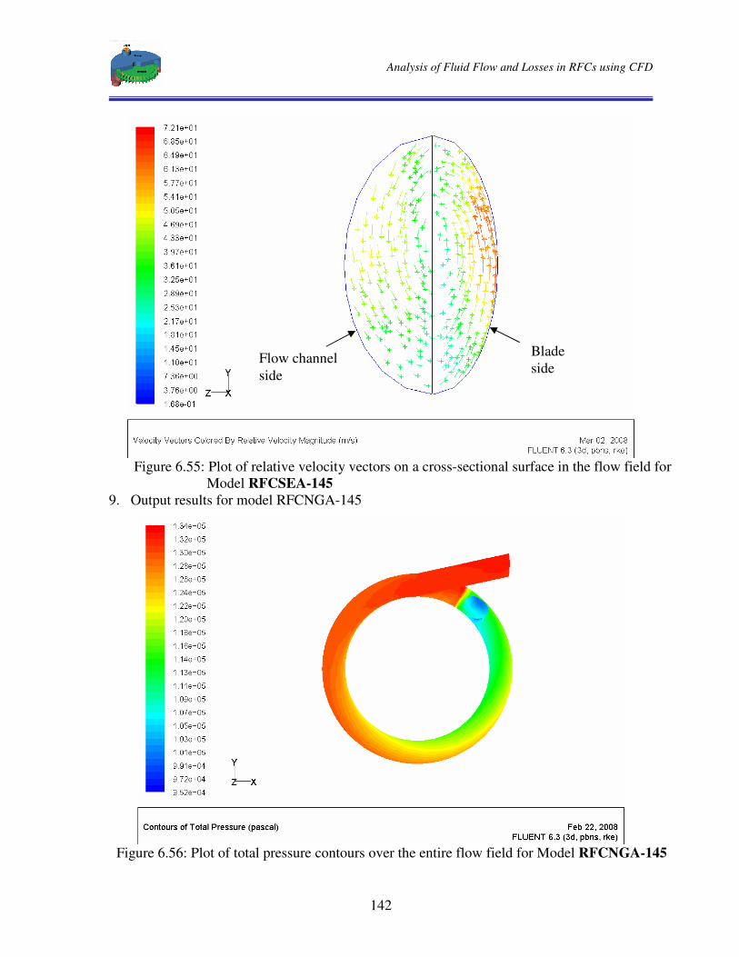
Analysis of Fluid Flow and Losses in RFCs using CFD
142
Figure 6.55: Plot of relative velocity vectors on a cross-sectional surface in the flow field for
Model RFCSEA-145 9. Output results for model RFCNGA-145
Figure 6.56: Plot of total pressure contours over the entire flow field for Model RFCNGA-145
Blade side
Flow channel side

Analysis of Fluid Flow and Losses in RFCs using CFD
143
Figure 6.57: Plot of density contours over the entire flow field for Model RFCNGA-145
Figure 6.58: Plot of a particle path line from inlet to exit port for Model RFCNGA-145
(at starting running speed, 2891 rpm)
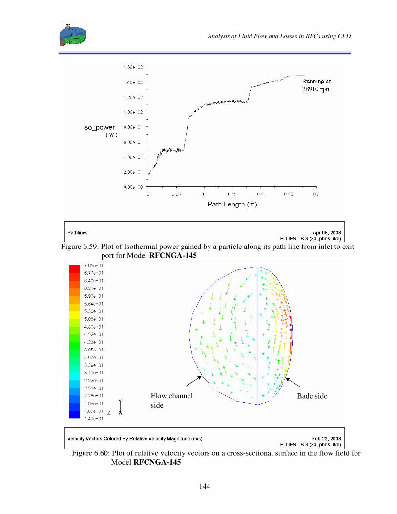
Analysis of Fluid Flow and Losses in RFCs using CFD
144
Figure 6.59: Plot of Isothermal power gained by a particle along its path line from inlet to exit
port for Model RFCNGA-145
Figure 6.60: Plot of relative velocity vectors on a cross-sectional surface in the flow field for
Model RFCNGA-145
Flow channel side
Bade side

Analysis of Fluid Flow and Losses in RFCs using CFD
145
10. Output results for model RFCCA-145
Figure 6.61: Plot of total pressure contours over the entire flow field for Model RFCCA-145
Figure 6.62: Plot of density contours over the entire flow field for Model RFCCA-145
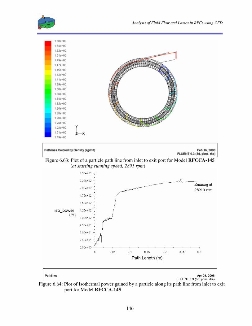
Analysis of Fluid Flow and Losses in RFCs using CFD
146
Figure 6.63: Plot of a particle path line from inlet to exit port for Model RFCCA-145
(at starting running speed, 2891 rpm)
Figure 6.64: Plot of Isothermal power gained by a particle along its path line from inlet to exit
port for Model RFCCA-145

Analysis of Fluid Flow and Losses in RFCs using CFD
147
Figure 6.65: Plot of relative velocity vectors on a cross-sectional surface in the flow field
for Model RFCCA-145
Blade side Flow channel
side
Analysis of Fluid Flow and Losses in RFCs using CFD
148