1

Analysis Data For Multiple Correlation Inferential Statistic: Regression and Partial Correlation 11/25/2014

Irwan Sulistyanto, S.Pd

Analysis Data

Data analysis is the important thing in research report either quantitative or qualitative

research. To know the research report succeeds or no it needs data analysis. There are

many kinds of data analysis. Here, the focus of this paper is describing the data analysis

on quantitative research. The data analysis of quantitative here are regression and partial

correlation.

A. Regression

Regression analysis is a statistical process for estimating the relationships among

variables. It uses in the modeling and analyzing several variables when the focus is on the

relationship between a dependent and one or more independent variables. It means that

this analysis helps one understand how the typically value of the dependent variable (its

called ‘Criterion Variable’) changes when any one of the independent variables is varied,

while the other independent variables are held fixed.

Regression analysis is widely used for prediction and forecasting, where its use

has substantial overlap with the field of machine learning. It is also used to understand

which among the independent variables are related to the dependent variable. The last

function of regression analysis is to explore the forms of these relationships. Generally,

regression are used to describe, control, and prediction.

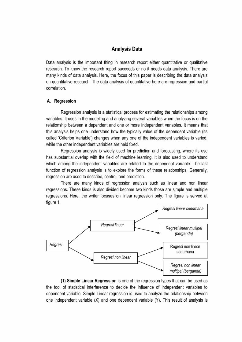
There are many kinds of regression analysis such as linear and non linear

regressions. These kinds is also divided become two kinds those are simple and multiple

regressions. Here, the writer focuses on linear regression only. The figure is served at

figure 1.

(1) Simple Linear Regression is one of the regression types that can be used as

the tool of statistical interference to decide the influence of independent variables to

dependent variable. Simple Linear regression is used to analyze the relationship between

one independent variable (X) and one dependent variable (Y). This result of analysis is

Regresi

Regresi linear

Regresi non linear

Regresi linear multipel

(berganda)

Regresi non linear

sederhana

Regresi non linear

multipel (berganda)

Regresi linear sederhana

showing the direction between the relationships among independent (predictor variable)

and dependent variable (response variable). The direction can be positive or negative. It is

also used to predict the value of dependent variable when the value of independent

variables is changed. Simple linear regression is used the interval or ratio data. It is also

has the normal distribution. Below is the linear regression formula:

1. Y = α + βX + ε (model populasi)

2. Y = a + bX + e (model sampel)

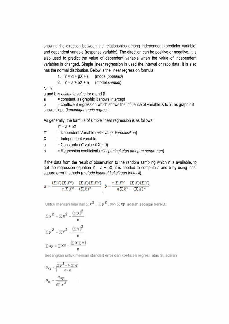
Note: a and b is estimate value for α and β a = constant, as graphic it shows intercept b = coefficient regression which shows the influence of variable X to Y, as graphic it shows slope (kemiringan garis regresi). As generally, the formula of simple linear regression is as follows:

Y’ = a + bX

Y’ = Dependent Variable (nilai yang diprediksikan)

X = Independent variable

a = Constanta (Y’ value if X = 0)

b = Regression coefficient (nilai peningkatan ataupun penurunan)

If the data from the result of observation to the random sampling which n is available, to get the regression equation Y = a + bX, it is needed to compute a and b by using least square error methods (metode kuadrat kekeliruan terkecil).

;

To compute T-test, use formula as follows:

T = b : Sb then the result is consulted with T-table to know the hypothesis is accepted or

no.

If using Microsoft excel, we can use the formula as follows:

1. To compute intercept = intercept (array y; array x)

2. To compute slope = slope (array y; array x)

After we know the formula above, the next step is that we have to use this formula to

compute the value of between two variables manually. But, beside we can use that formula

we can also use the SPSS to compute the regression. Before we do the calculation by

using the SPSS, we must make some basic assumptions and requirements to examine it

are right or no. Those are:

1. Independent variable not correlates with disturbance term (Error). The value of

disturbance term is 0 or it can write as follows: (E (U / X) = 0.

2. If there is more than one independent variable, so there is not real linear relation

each independent variable (explanatory).

3. The good model of regression is that the value of ANOVA is <0.05.

4. The predictor as the independent variable should be properly. It can see if the

value of Standard Error of Estimate < Standard Deviation.

5. Coefficient of regression should be significant. It can use T-Test. Coefficient of

regression is significant if T0 > T-table.

6. Model of regression can be described by using the value of determination

coefficient (KD = r2 x 100%). Higher the results of the formula before, better the

model of regression. If the result is closed on 1 so the model of regression is

better.

7. Data should have the normal distribution

8. Data is interval and ratio.

9. Both variables are dependent variable, it means that one variable is independent

variable (predictor variable) while the other is dependent variable (response

variable).

Example:

Simple Linear Regression is used to analyze two variables. We will take the name of

variable from data T0 which is given by your lecturer. The variables are family background

(X1), Motivation (Y). We will calculate the value of linear regression between X1 and Y. The

steps to do this calculation are below:

1. Open SPSS

2. Insert data from excel. Copy then paste.

3. Click variable view on SPSS data editor

4. See column Name, type X1 at first row, column Name, second row type Y.

5. Column Label, at first row type Family Background and second row type

Motivation.

6. Type 0 at column decimals.

7. The others column can be ignored (default)

8. Open data view at SPSS data editor, see the top column, we will see column for

variable X1 and Y.

9. Click Analyze - Regression – Linear

10. Click variable Y then click arrow to the Dependent box. Next, click variable X1 then

click arrow to the Independent box.

11. Click Statistics, click/thick estimates on regression coefficient, and thick model fit.

Click Continue.

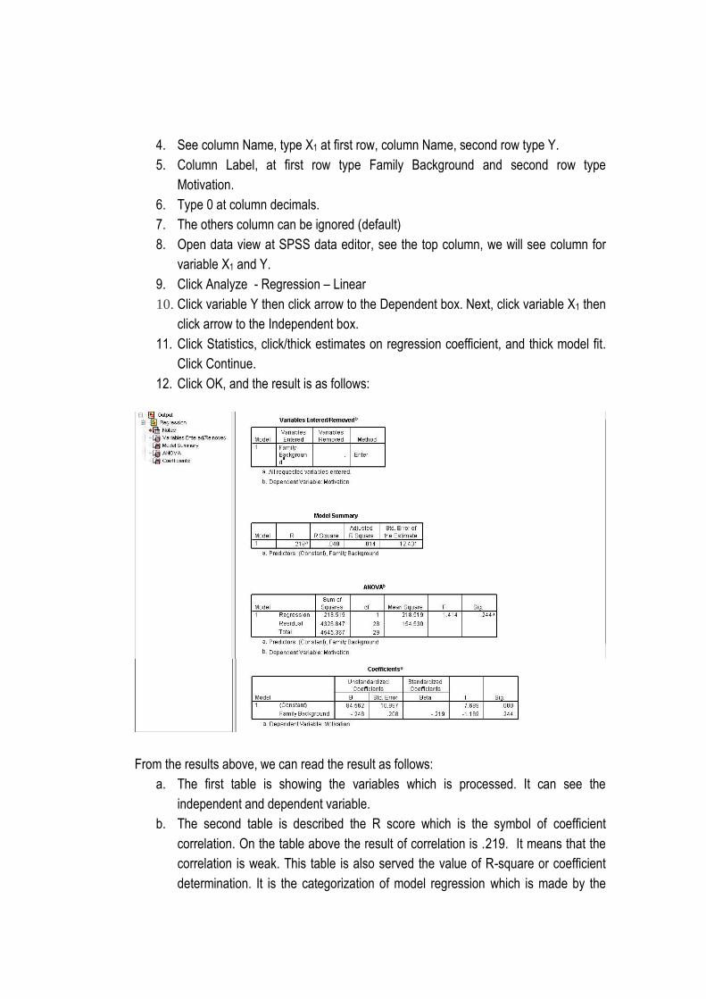
12. Click OK, and the result is as follows:

From the results above, we can read the result as follows:

a. The first table is showing the variables which is processed. It can see the

independent and dependent variable.

b. The second table is described the R score which is the symbol of coefficient

correlation. On the table above the result of correlation is .219. It means that the

correlation is weak. This table is also served the value of R-square or coefficient

determination. It is the categorization of model regression which is made by the

dependent and independent variable. From the table, R-square is .048 or 4.8%. It

means that the variable Y is influenced by the variable X1 as big as 4.8% and

95.2% is influenced by the others factor outside the variable X1.

c. The third table is used to decide the linearity of regression or significance level.

The criteria can be seeing from F-test or significance test (Sig.). The easiest way is

by using significance test (Sig.). If the Sig. value is < 0.05 the model is linear or

vise versa. From the table, the score of Sig. is .244. It means that Sig. score > than

0.05. If it can conclude that the result of data analysis is not significant and it is not

inline with the model of linearity.

d. The last table is described the model of regression which is made by Constant and

coefficient variable in the column Unstandardized coefficient B. Based on the

table, we have the regression equation as follows: Y = 84.562 + (-248X1). It means

that Constant as big as 84.562 if the score of variable X1 = 0, so the score of

variable Y is 84.562. Then, the score of coefficient variable X1 is (-248). It means

that if the score of Variable X1 increase 1 point it will decrease -248 point of

variable Y.

e. After we get the result of regression, we should consult the result of regression

with T-table. It is used to know how far the relation between two variables. It is

significant or not. Significant means that the influence which is made by variable X1

to variable Y can be generalized. T0 = -1.189, T-table at 5% = 2.05 and 1% = 2.76

at degree of freedom = 28. So, the result is that T-table > T0 either 5% or 1% the

result is not significant (2.05>1.189<2.76). If you do not know about the value of

significance level at 5% or 1% you can see at Nukilan table from Henry E (1984) or

if it uses Microsoft excel type = tinv (0.05 or 0.01), degree of freedom) then click

enter.

(2) Multiple Linear Regressions or Regresi Linear Berganda is the types of

regression which is used to analyze the relationships among more than one independent

variable as variable X ( it can be X1, X2, or X3 and etc) and has one dependent variable as

variable Y. As like simple linear regression, multiple linear regressions are used (1) to

know the estimation of average and value of dependent variable based on the score of

independent variable. (2) Testing the hypothesis dependency and (3) predict the average

score of independent variable based on the independent variable outside the sample

range.

To get simple or multiple linear regressions, it can use some estimation toward

their parameters. The method that can be used to estimate the parameters are ordinary

least score (OLS) and maximum likelihood estimation (MLE) (Kutner, Nachtsheim and

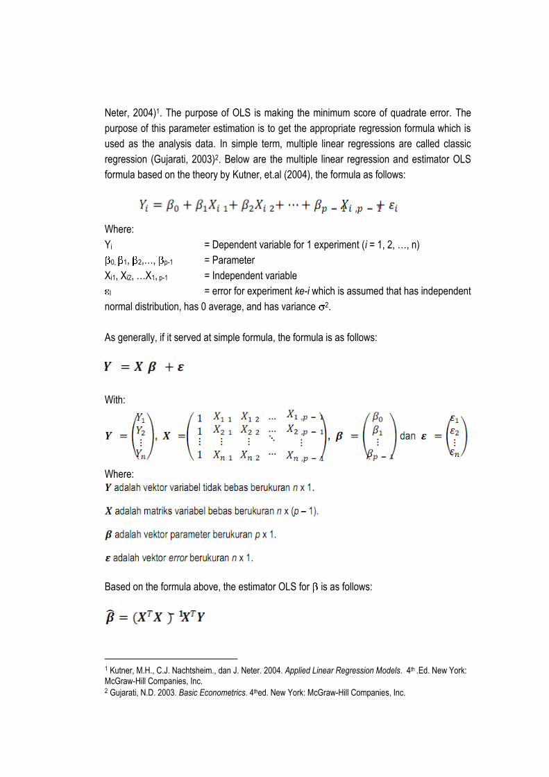
Neter, 2004)1. The purpose of OLS is making the minimum score of quadrate error. The

purpose of this parameter estimation is to get the appropriate regression formula which is

used as the analysis data. In simple term, multiple linear regressions are called classic

regression (Gujarati, 2003)2. Below are the multiple linear regression and estimator OLS

formula based on the theory by Kutner, et.al (2004), the formula as follows:

Where:

Yi = Dependent variable for 1 experiment (i = 1, 2, …, n)

0, 1, 2,…, p-1 = Parameter

Xi1, Xi2, …X1, p-1 = Independent variable

I = error for experiment ke-i which is assumed that has independent

normal distribution, has 0 average, and has variance 2.

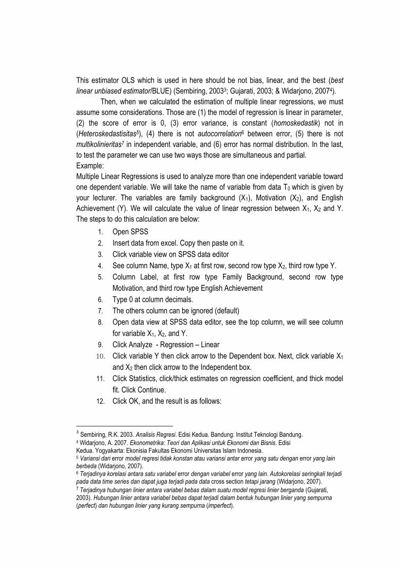
As generally, if it served at simple formula, the formula is as follows:

With:

Where:

Based on the formula above, the estimator OLS for is as follows:

1 Kutner, M.H., C.J. Nachtsheim., dan J. Neter. 2004. Applied Linear Regression Models. 4th .Ed. New York: McGraw-Hill Companies, Inc. 2 Gujarati, N.D. 2003. Basic Econometrics. 4thed. New York: McGraw-Hill Companies, Inc.

This estimator OLS which is used in here should be not bias, linear, and the best (best

linear unbiased estimator/BLUE) (Sembiring, 20033; Gujarati, 2003; & Widarjono, 20074).

Then, when we calculated the estimation of multiple linear regressions, we must

assume some considerations. Those are (1) the model of regression is linear in parameter,

(2) the score of error is 0, (3) error variance, is constant (homoskedastik) not in

(Heteroskedastisitas5), (4) there is not autocorrelation6 between error, (5) there is not

multikolinieritas7 in independent variable, and (6) error has normal distribution. In the last,

to test the parameter we can use two ways those are simultaneous and partial.

Example:

Multiple Linear Regressions is used to analyze more than one independent variable toward

one dependent variable. We will take the name of variable from data T0 which is given by

your lecturer. The variables are family background (X1), Motivation (X2), and English

Achievement (Y). We will calculate the value of linear regression between X1, X2 and Y.

The steps to do this calculation are below:

1. Open SPSS

2. Insert data from excel. Copy then paste on it.

3. Click variable view on SPSS data editor

4. See column Name, type X1 at first row, second row type X2, third row type Y.

5. Column Label, at first row type Family Background, second row type

Motivation, and third row type English Achievement

6. Type 0 at column decimals.

7. The others column can be ignored (default)

8. Open data view at SPSS data editor, see the top column, we will see column

for variable X1, X2, and Y.

9. Click Analyze - Regression – Linear

10. Click variable Y then click arrow to the Dependent box. Next, click variable X1

and X2 then click arrow to the Independent box.

11. Click Statistics, click/thick estimates on regression coefficient, and thick model

fit. Click Continue.

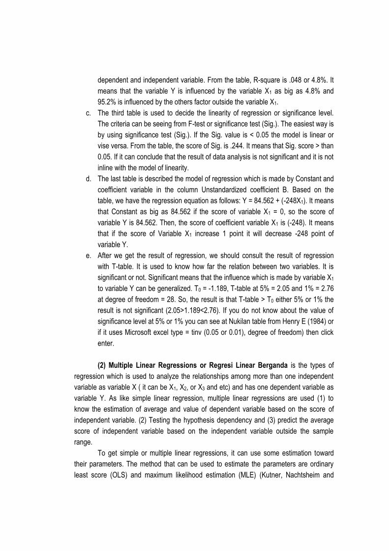
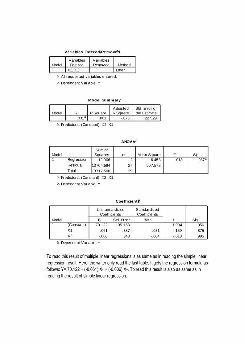
12. Click OK, and the result is as follows:

3 Sembiring, R.K. 2003. Analisis Regresi. Edisi Kedua. Bandung: Institut Teknologi Bandung. 4 Widarjono, A. 2007. Ekonometrika: Teori dan Aplikasi untuk Ekonomi dan Bisnis. Edisi Kedua. Yogyakarta: Ekonisia Fakultas Ekonomi Universitas Islam Indonesia. 5 Variansi dari error model regresi tidak konstan atau variansi antar error yang satu dengan error yang lain berbeda (Widarjono, 2007). 6 Terjadinya korelasi antara satu variabel error dengan variabel error yang lain. Autokorelasi seringkali terjadi pada data time series dan dapat juga terjadi pada data cross section tetapi jarang (Widarjono, 2007). 7 Terjadinya hubungan linier antara variabel bebas dalam suatu model regresi linier berganda (Gujarati, 2003). Hubungan linier antara variabel bebas dapat terjadi dalam bentuk hubungan linier yang sempurna (perfect) dan hubungan linier yang kurang sempurna (imperfect).

Variables Enter ed/Removedb

X2, X1a . Enter

Model

1

Variables

Entered

Variables

Removed Method

All requested variables entered.a.

Dependent Variable: Yb.

Model Summ ary

.031a .001 -.073 22.529

Model

1

R R Square

Adjusted

R Square

Std. Error of

the Estimate

Predictors: (Constant), X2, X1a.

ANOVAb

12.906 2 6.453 .013 .987a

13704.594 27 507.578

13717.500 29

Regression

Residual

Total

Model

1

Sum of

Squares df Mean Square F Sig.

Predictors: (Constant), X2, X1a.

Dependent Variable: Yb.

Coefficientsa

70.122 35.158 1.994 .056

-.061 .387 -.031 -.159 .875

-.006 .343 -.004 -.018 .985

(Constant)

X1

X2

Model

1

B Std. Error

Unstandardized

Coeff icients

Beta

Standardized

Coeff icients

t Sig.

Dependent Variable: Ya.

To read this result of multiple linear regressions is as same as in reading the simple linear

regression result. Here, the writer only read the last table. It gets the regression formula as

follows: Y= 70.122 + (-0.061) X1 + (-0.006) X2. To read this result is also as same as in

reading the result of simple linear regression.

B. Partial Correlation

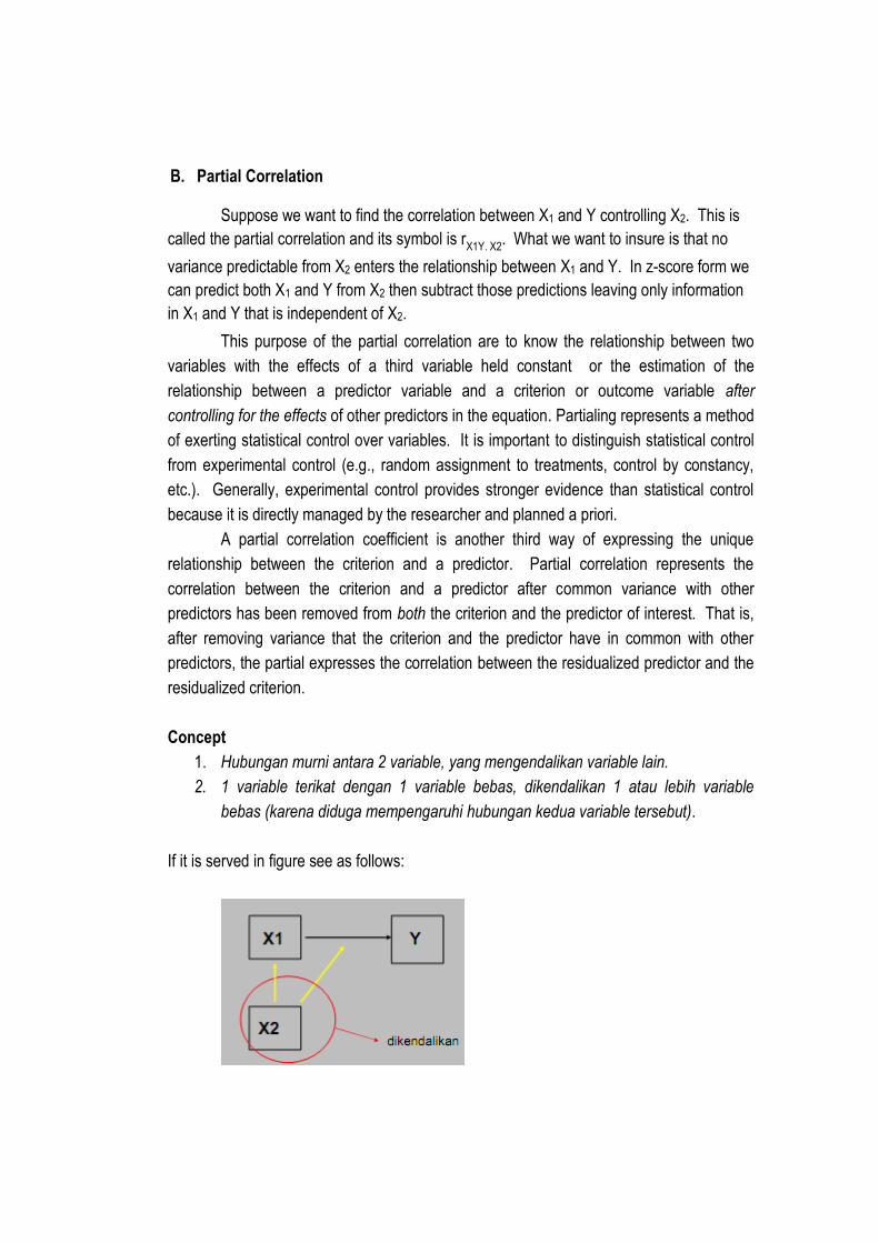
Suppose we want to find the correlation between X1 and Y controlling X2. This is

called the partial correlation and its symbol is rX1Y. X2

. What we want to insure is that no

variance predictable from X2 enters the relationship between X1 and Y. In z-score form we

can predict both X1 and Y from X2 then subtract those predictions leaving only information

in X1 and Y that is independent of X2.

This purpose of the partial correlation are to know the relationship between two

variables with the effects of a third variable held constant or the estimation of the

relationship between a predictor variable and a criterion or outcome variable after

controlling for the effects of other predictors in the equation. Partialing represents a method

of exerting statistical control over variables. It is important to distinguish statistical control

from experimental control (e.g., random assignment to treatments, control by constancy,

etc.). Generally, experimental control provides stronger evidence than statistical control

because it is directly managed by the researcher and planned a priori.

A partial correlation coefficient is another third way of expressing the unique

relationship between the criterion and a predictor. Partial correlation represents the

correlation between the criterion and a predictor after common variance with other

predictors has been removed from both the criterion and the predictor of interest. That is,

after removing variance that the criterion and the predictor have in common with other

predictors, the partial expresses the correlation between the residualized predictor and the

residualized criterion.

Concept

1. Hubungan murni antara 2 variable, yang mengendalikan variable lain.

2. 1 variable terikat dengan 1 variable bebas, dikendalikan 1 atau lebih variable

bebas (karena diduga mempengaruhi hubungan kedua variable tersebut).

If it is served in figure see as follows:

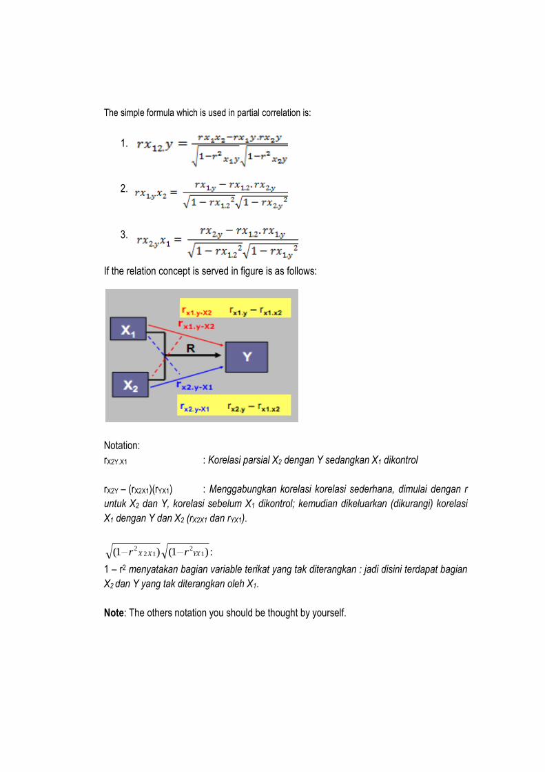
The simple formula which is used in partial correlation is:

1.

2.

3.

If the relation concept is served in figure is as follows:

Notation:

rX2Y.X1 : Korelasi parsial X2 dengan Y sedangkan X1 dikontrol

rX2Y – (rX2X1)(rYX1) : Menggabungkan korelasi korelasi sederhana, dimulai dengan r

untuk X2 dan Y, korelasi sebelum X1 dikontrol; kemudian dikeluarkan (dikurangi) korelasi

X1 dengan Y dan X2 (rX2X1 dan rYX1).

:)1()1( 12

122

YXXX rr

1 – r2 menyatakan bagian variable terikat yang tak diterangkan : jadi disini terdapat bagian

X2 dan Y yang tak diterangkan oleh X1.

Note: The others notation you should be thought by yourself.

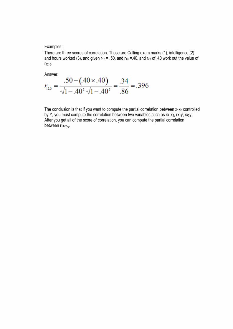
Examples:

There are three scores of correlation. Those are Calling exam marks (1), intelligence (2) and hours worked (3), and given r12 = .50, and r13 =.40, and r23 of .40 work out the value of r12.3. Answer:

The conclusion is that if you want to compute the partial correlation between x1x2 controlled by Y, you must compute the correlation between two variables such as rx1x2, rx1y, rx2y. After you get all of the score of correlation, you can compute the partial correlation between rx1x2.y.