Data Collection with Multiple Sinksin Wireless Sensor Networks

Sixia Chen, Matthew Coolbeth, Hieu Dinh, Yoo-Ah Kim, and Bing Wang?

Computer Science & Engineering Department, University of Connecticut

Abstract. In this paper, we consider Multiple-Sink Data CollectionProblem in wireless sensor networks, where a large amount of data fromsensor nodes need to be transmitted to one of multiple sinks. We designan approximation algorithm to minimize the latency of data collectionschedule and show that it gives a constant-factor performance guarantee.We also present a heuristic algorithm based on breadth first search forthis problem. Using simulation, we evaluate the performance of these twoalgorithms, and show that the approximation algorithm outperforms theheuristic up to 60%.

1 IntroductionA wireless sensor network, which consists of an ad hoc group of small sensornodes communicating with one another, have a variety of applications such astraffic monitoring, emergency medical care, battlefield surveillance, and under-water surveillance. In such applications, it is often necessary to collect the dataaccumulated by each sensor node for processing. We call the operation of trans-mitting accumulated data from sensor nodes to the sinks data collection. In thispaper, we consider the problem to find a schedule to quickly collect a largeamount of data from sensor nodes to sinks. Data need to be collected withoutmerging. If the data can be merged, the operation is called data aggregation.

One of the challenges in data collection in wireless networks is radio inter-ferences that may prevent nearby sensor nodes from transmitting packets si-multaneously. Scheduling data transmissions without carefully considering suchinferences can result in significant delay in data collection.

When there is only one gateway (or sink) to collect data and the amountof data at all sensor nodes is similar, a greedy algorithm may work well. Forexample, there is a 3-approximation algorithm for general graphs and optimalalgorithms for simpler graphs in this case [5]. When there are multiple gatewaysand the distribution of the data is not uniform, the problem becomes morechallenging as the amount of data to be sent to each gateway need to be balancedto avoid congestion.

In this paper, we consider the problem of minimizing the latency of datacollection in settings where (i) data cannot be merged, (ii) there are multiplesinks, and (iii) the amount of data accumulated at sensor nodes as well as thecapacity of links may not be uniform. We present an approximation algorithm tofind a schedule with a constant-factor guarantee. We evaluate the performance? Y. Kim and B. Wang were partially supported by UConn Faculty Large Grant and

NSF CAREER award 0746841, respectively.

of this algorithm as well as a greedy heuristic algorithm using simulation invarious settings. Our simulation results show that the approximation algorithmoutperforms the naive heuristic up to 60%.

The rest of the paper is organized as follows: We present related work andproblem formulation in Sections 2 and 3, respectively. In Section 4, we introducean LP-based approximation algorithm and show that it gives a constant-factorperformance guarantee. We then present a greedy breadth-first-search (BFS)based heuristic algorithm in Section 5, and the experimental results in Section6. Conclusion is presented in Section 7.

2 Related WorkData broadcast and collection are among the most fundamental operations inmany communication networks. Algorithms for broadcasting in wireless net-works, in which the objective is to transmit data from one source to all the othernodes, have been extensively studied in the literature [1, 3, 7, 13, 12, 8]. Data col-lection and aggregation problem in wireless networks, on the other hand, arerelatively new but have recently received much attention [14, 15, 11, 18, 5].

Florens and McEliece [5] studied data distribution and collection problemswith a single source/sink. They present data distribution/collection schedule forseveral types of graphs, and show that it provides 3-approximation for generalgraphs and optimal solution for simpler graphs such as trees. Their algorithm(and the analysis) cannot be easily extended to the case of multiple sinks. Inaddition, they assume that all the links have uniform capacity, i.e., one packetcan be transmitted over a link at each time unit.

Another problem closely related data collection is the data aggregation prob-lem (also called convergecast), in which gathered data can be merged by takingthe maximum or minimum for example. Huang et al. [14] designed a nearly con-stant approximation algorithm for minimum latency data aggregation problem.

Cheng et al. [4] considered large-scale data collection problem in wired net-works, in which a large amount of data need to be collected from multiple hoststo a single destination. They present coordinated data collection algorithm us-ing a time-expanded graph to minimizes the latency. Unlike our problem, radiointerference is not an issue in their problem as they consider data collection inwired networks.

3 Problem Formulation3.1 Network ModelA wireless sensor network can be modeled as a graph G = (V, E) in which eachnode in V represents a sensor node and each link, e ∈ E, represents a wirelesscommunication link between two nodes. The capacity of a link, e, specifies theamount of data that can be transmitted over e during a unit time. For any twonetwork nodes, u, v ∈ V , (u, v) and C(u, v) respectively denote the link fromu to v and its capacity. Finally, every link (u, v) ∈ E has an interference set,denoted as I(u, v), which represents the set of links in E that may not be usedconcurrently with (u, v) due to interference. Interference has been modeled in avariety of ways in the literature, including protocol model [9], transmitter model(Tx-model) [19], transmitter-receiver model (Tx-Rx model) [2, 16], and so on.

Our algorithm is applicable to any of those models by appropriately defininginterference sets I(u, v) according to the model.

3.2 Data Collection ProblemWe consider the Multiple-Sink Data Collection Problem (MSDC), in which thereare multiple sinks and a large amount of data from sensor nodes need to betransmitted to one of the sinks. Formally, we are given a wireless directed networkgraph, G = (V, E). Each link (vi, vj) in the graph from node vi ∈ V to vj ∈V is associated with a capacity, C(vi, vj), and an interference set, I(vi, vj) ={(vi′ , vj′) ∈ E | link (vi′ , vj′) interferes with link (vi, vj)}. A link cannot be usedwhen another link in its interference set is activated. We have a set of sinksD ⊂ V . For node vi ∈ V \D, let si denote the amount of accumulated data atthis node, and the data need to be sent to one of the nodes in D. Note that thedata can be sent to any of the sinks. We want to find a data-collection scheduleto transmit all the data to the sinks. The schedule must specify in each timeslot which links are used for data transfer. In order for the schedule to be valid,it must not allow two interfering links to be used for data transfer at the sametime. Our objective is to find a data-collection schedule of the minimum latency.

4 A constant approximation algorithmIn this section, we present an approximation algorithm with a constant-factorguarantee. The algorithm consists of three components. The first componentconstructs a time-expanded graph [10, 6], which represents the progression of thestate of the network throughout a given time period T , during which data collec-tion occurs. The second component uses a linear programming (LP) formulationto generate feasible flows to send data over edges in the time-expanded graph.The first and second components need to be repeatedly run until we can find afeasible flow with latency close enough to the optimal solution. The details ofthe iterations are given in the end of Section 4.2 and Algorithm 1. Once a feasi-ble flow solution is obtained, the third component finds an exact data collectionschedule for each time slot. We refer to this algorithm as LP-based algorithm. InSection 4.4 we show that it gives constant factor guarantees, with the constantdepending on the interference model (e.g., it gives 5-approximation under unitdisk model). We next describe the three components in the algorithm in detail.

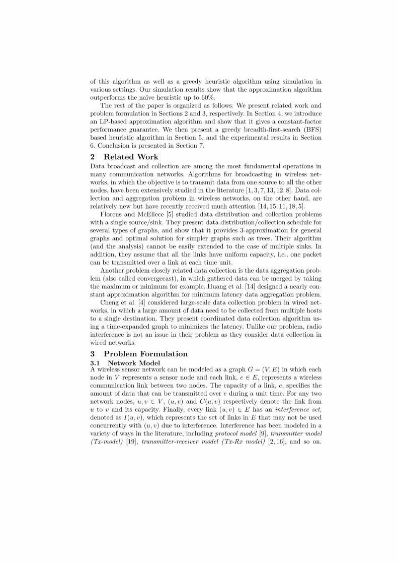
4.1 Generating a time-expanded graphOne core component of our algorithm is expanding the network graph, G, toa time-expanded graph, GT = (VT , ET ), which represents the network over aperiod of T time units, and in which we can compute a network flow that corre-sponds to a valid data collection schedule. Figure 1 depicts an example networkgraph and its corresponding time-expanded flow graph.

Given a graph G and time T , the expanded time graph, GT = (VT , ET ),can be constructed as follows. For each network node vi ∈ V , and for everyt ∈ {0...T}, we add a vertex vi,t to VT . These vertices represent vi at T + 1points of time, where vi,t+1 is one time unit later than vi,t. To represent thestorage of data over time at a node in V , we assign an unlimited flow capacity,CT (vi,t, vi,t+1) = ∞, to any vi ∈ V and t ∈ {0...T − 1}. Furthermore, we assign

26 20

5

9 2

6 v2

v1

v3

v4

v5 4

11

∞

∞

∞

2 ∞

6

4 ∞

∞

∞

∞

∞

5

4

6

9 2

11

26

20

v2,0

v1,0

v3,0

v4,0

v5,0

v2,1

v1,1

v4,1

v5,1 ∞

∞

5

9

v5,2

v3,1 ∞

∞

∞

∞

∞

5

4

6

9 2

v2,3

v1,3

v3,3

v4,3

v5,3

v1,2

v3,2

v4,2

v2,2

d

∞

s

Fig. 1. A network graph, G, and its corresponding time-expanded graph, GT , whereT = 3, and the shaded nodes represent the sinks.

a flow capacity CT (vi,t, vj,t+1) = C(vi, vj) to each edge (vi,t, vj,t+1) ∈ ET , whichrepresents the maximum amount of flow allowed on this edge in a time unit. Inaddition, we associate a flow interference set, IT (vi,t, vj,t+1), to (vi,t, vj,t+1) ∈ET , which can be inferred from the interference set of the corresponding linkin E. Specifically, for all vi, vj , vi′ , vj′ ∈ V with (vi′ , vj′) ∈ I(vi, vj), and for allt ∈ {1...T −1}, (vi′,t, vj′,t+1) ∈ IT (vi,t, vj,t+1). Last, we add a super source s anda super sink d into the time expanded graph. We also create a link from s tovi,0 with capacity si for any node vi ∈ V \D. Meanwhile, for any node vj ∈ Din the original graph, we have a link from vj,T to d with unlimited capacity.

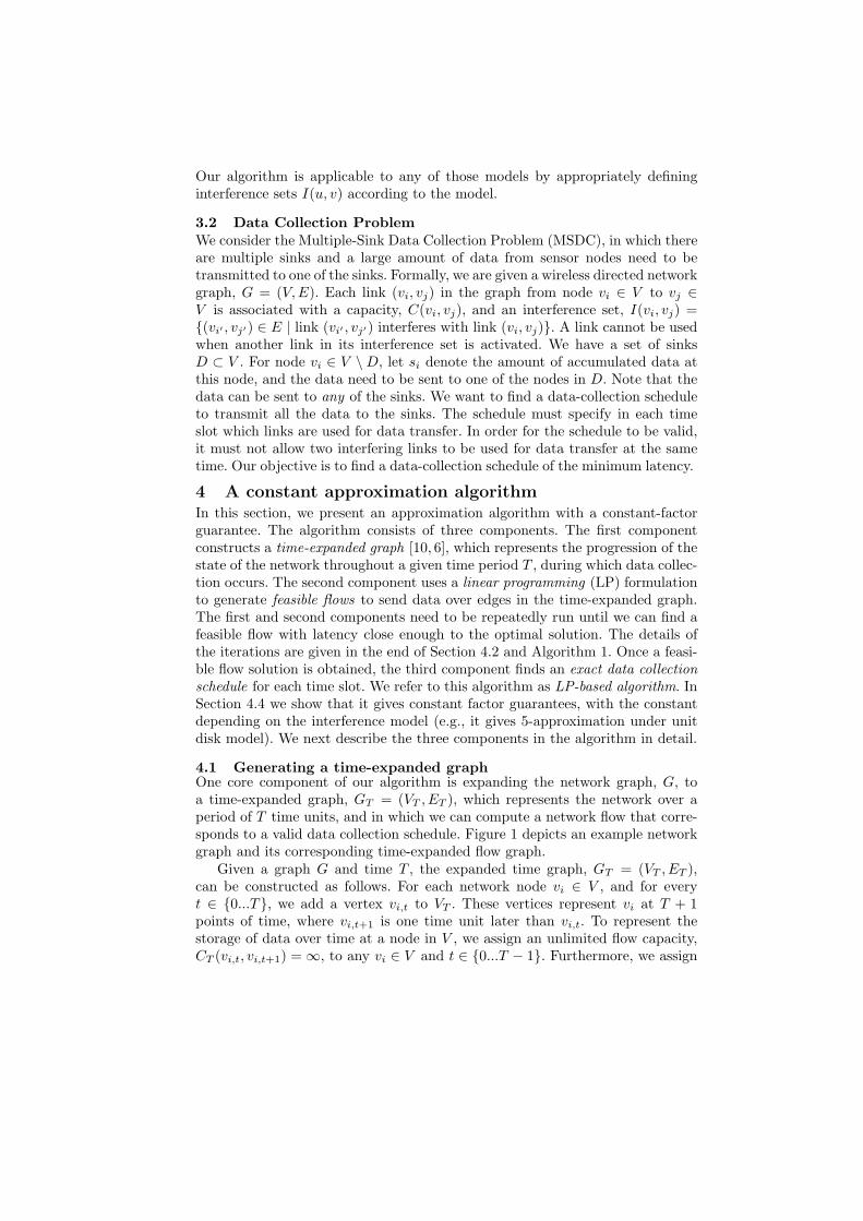
4.2 Computing a data flowThe constructed time-expanded graph GT , along with the associated supplies,edge capacities, and interference constraints, form an interference-bound networkflow problem. In this problem, if the maximum flow from s to d is

∑vi∈V \D si,

then in the original graph we can collect all the data to the sink in time T . Wesolve the network flow problem using a linear programming (LP) formulationas follows. Denote fu,v as the flow along the edge from vertex u to v for anyu, v ∈ VT and (u, v) ∈ ET . In particular, fs,u represents the flow along the linkfrom the super source s to node u ∈ VT , and fv,d represents the flow along thelink from node v ∈ VT to the super sink d. Let Out(u) denote the set of theendpoints of the outgoing links of u, u ∈ VT , and let In(v) denote the set of theendpoints of the incoming links of v, v ∈ VT . Then the LP formulation is:

Maximize:∑

u∈Out(s)

fs,u

Subject to:∑

u∈Out(s)

fs,u −∑

v∈In(d)

fv,d = 0 (1)

∑

v∈In(u)

fv,u −∑

v∈Out(u)

fu,v = 0, ∀ u 6= s, d (2)

fu,v

CT (u, v)+

∑

(u′,v′)∈I(u,v)

fu′,v′

CT (u′, v′)≤ 1, ∀ u, v ∈ VT (3)

fu,v ≤ CT (u, v), ∀ u, v ∈ VT (4)

fu,v ≥ 0, ∀ u, v ∈ VT (5)

The above LP formulation represents a network flow problem with additionalconstraints to ensure interference-free property. More specifically, Constraints(1) and (2) are for flow conservation, and Constraint (4) is for link capacity.Constraint (3) provides a sufficient condition for interference-free schedule. Inother words, the constraints ensure that, throughout any time slot, only onenetwork link in each interference set can be active.

For a given time T , if the resulting maximum flow from s to d after solvingthe LP problem is

∑vi∈V \D si, then we can infer a complete schedule for all

data in the network to be collected in time at most T . By performing a standarddoubling/binary search, we can find the minimum latency Tmin necessary tohave a valid network flow solution in logarithmic time. Once Tmin is found, thesolution of network flow in the time-expanded graph GTmin can be obtained,and will be used in the third step (see Section 4.3) to generate an exact datacollection schedule. Algorithm 1 presents a high-level description of the aboveprocedure.

Algorithm 1 Compute feasible data flow1. Guess Tmin in logarithmic time, using doubling and binary search:

(a) Generate a time-expanded graph GT of length T from the given network G.(b) Check whether there exists a valid flow in GT using the LP formulation.

2. Compute the solution of network flow in time-expanded graph GTmin .

4.3 Data collection scheduleWe now present a scheduling algorithm for each time interval. We assume thatthe amount of data to be collected is sufficiently large, and so we can split thedata into pieces as small as necessary. Without loss of generality, we assume thetime interval to be one second.

Consider time interval [t, t+1]. Let Gt = (Vt, Et) denote a subgraph of GT =(VT , ET ), where Vt = {vi,t, vi,t+1 | vi ∈ V } and Et = {(vi,t, vj,t+1) | (vi, vj) ∈E}. We derive an link interference graph GIt = (VIt , EIt) from Gt = (Vt, Et),where node vI

i,t ∈ VIt corresponds to an edge in Et, and an edge in EIt connectstwo vertices, vI

i,t and vIj,t, if and only if vI

i,t and vIj,t interfere with each other

in Gt. Let f ti denote the amount of flow that is transmitted through vI

i,t. LetN(vI

i,t) be the set of nodes in VIt that are connected to vIi,t. That is, N(vI

i,t)contains all the edges that interfere with vI

i,t in Et. Let xti = f t

i /CT (vIi,t), where

CT (vIi,t) represents the capacity along the edge vI

i,t ∈ Et. Then xti represents the

amount of time that vIi,t needs to occupy in interval [t, t + 1].

Algorithm 2 describes how to construct a data collection schedule for interval[t, t + 1]. Basically, for each node vI

i,t ∈ VIt, it schedules a duration of xt

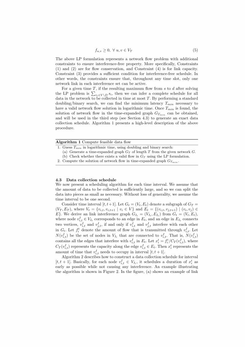
i asearly as possible while not causing any interference. An example illustratingthe algorithm is shown in Figure 2. In the figure, (a) shows an example of link

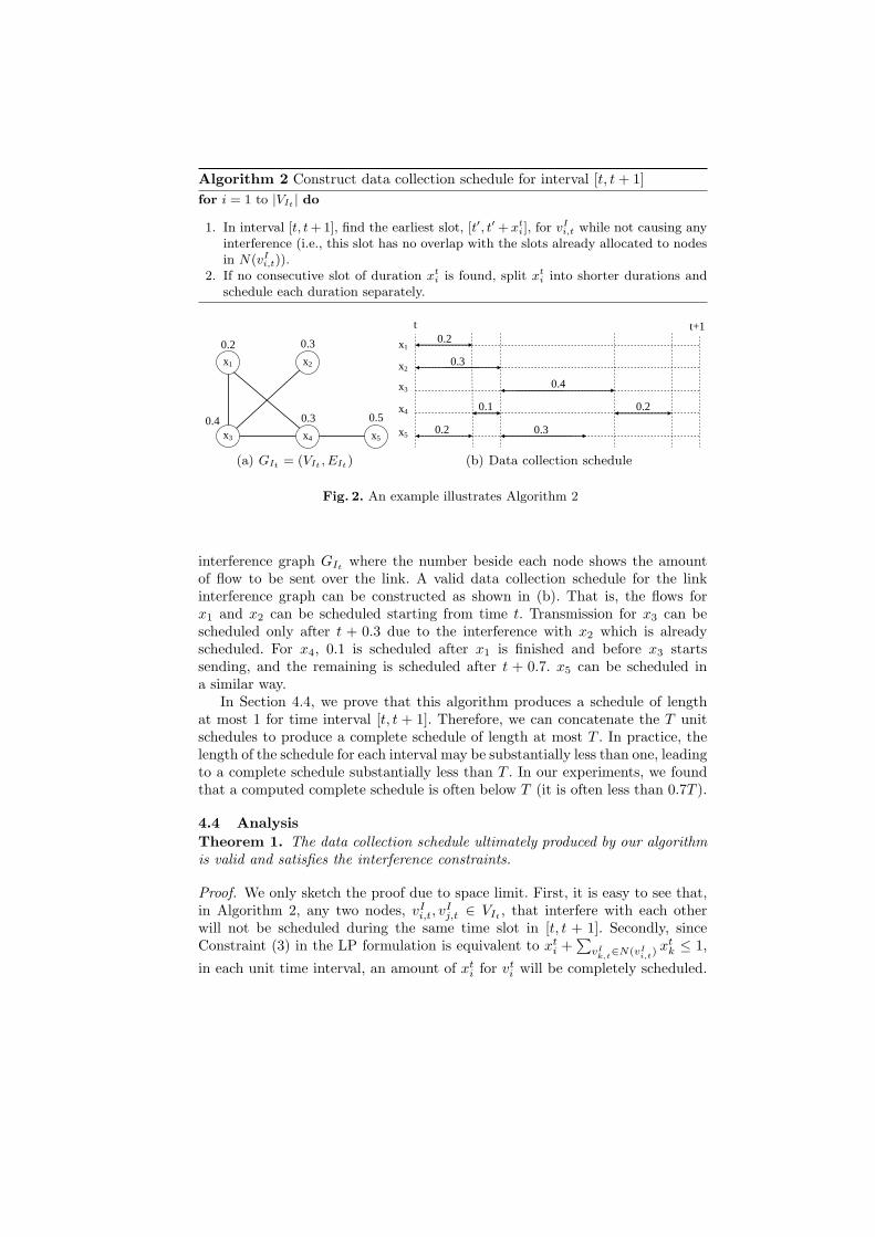
Algorithm 2 Construct data collection schedule for interval [t, t + 1]for i = 1 to |VIt | do

1. In interval [t, t + 1], find the earliest slot, [t′, t′ + xti], for vI

i,t while not causing anyinterference (i.e., this slot has no overlap with the slots already allocated to nodesin N(vI

i,t)).2. If no consecutive slot of duration xt

i is found, split xti into shorter durations and

schedule each duration separately.

0.5 0.3 0.4

0.3 0.2

x1

x3

x2

x4 x5

(a) GIt = (VIt , EIt)

0.3 0.2

0.2 0.1

0.4

0.3

0.2 x1

x2

x3

x4

x5

t t+1

(b) Data collection schedule

Fig. 2. An example illustrates Algorithm 2

interference graph GIt where the number beside each node shows the amountof flow to be sent over the link. A valid data collection schedule for the linkinterference graph can be constructed as shown in (b). That is, the flows forx1 and x2 can be scheduled starting from time t. Transmission for x3 can bescheduled only after t + 0.3 due to the interference with x2 which is alreadyscheduled. For x4, 0.1 is scheduled after x1 is finished and before x3 startssending, and the remaining is scheduled after t + 0.7. x5 can be scheduled ina similar way.

In Section 4.4, we prove that this algorithm produces a schedule of lengthat most 1 for time interval [t, t + 1]. Therefore, we can concatenate the T unitschedules to produce a complete schedule of length at most T . In practice, thelength of the schedule for each interval may be substantially less than one, leadingto a complete schedule substantially less than T . In our experiments, we foundthat a computed complete schedule is often below T (it is often less than 0.7T ).

4.4 AnalysisTheorem 1. The data collection schedule ultimately produced by our algorithmis valid and satisfies the interference constraints.

Proof. We only sketch the proof due to space limit. First, it is easy to see that,in Algorithm 2, any two nodes, vI

i,t, vIj,t ∈ VIt

, that interfere with each otherwill not be scheduled during the same time slot in [t, t + 1]. Secondly, sinceConstraint (3) in the LP formulation is equivalent to xt

i +∑

vIk,t∈N(vI

i,t) xt

k ≤ 1,

in each unit time interval, an amount of xti for vt

i will be completely scheduled.

Last, Constraints (1) in the LP formulation guarantee that all the data from thesources will be delivered to the sinks at the end of the schedule. Therefore, theabove claim holds. ut

We next establish that, under several network models, our algorithm approx-imates an optimal schedule within a constant factor. In particular, under a unitdisk model, it approximates the optimal schedule within a factor of five. To provethe approximation guarantee, we use the following lemma from [17].

Lemma 2. [17] For every edge (u, v) ∈ E, there are at most c edges in I(u, v)that can transfer data at the same time, where c is a constant depending on themodel used to determine the network’s interference constraints. Under a unitdisk model, c = 5.

Theorem 3. The LP-based algorithm gives c-approximation for Multi-sink DataCollection problem.

Proof. Let LPk refer to a linear programming formulation, which differs fromthat in Section 4.2 in that the interference constraint (3) is replaced by

fu,v

CT (u, v)+

∑

(u′,v′)∈I(u,v)

fu′,v′

CT (u′, v′)≤ k, ∀ u, v ∈ VT . (6)

That is, LPk allows using k edges simultaneously in each interference set (ouroriginal LP formulation is LP1).

By Lemma 2, an optimal data collection schedule may use no more thanc edges in a given interference group simultaneously. It has been shown thatConstraints (6) provide a necessary condition to obtain a valid flow withoutinterferences when k is set to c (c depends on the interference model) [17].Therefore, the optimal solution is lower bounded by the solution to LPc. Wecan also see that, at any point in time, the schedule produced by LPc allows cedges in each interference group to be active. If the amount of time available ismultiplied by c, then each of these potentially interfering transmissions can beplaced in its own time period. The resulting schedule satisfies the constraintsimposed in LP1. Let OPT refer to an optimal algorithm, and let T (X) denotethe latency of the schedule produced by an algorithm, X. Therefore, T (LP1) ≤c · dT (LPc)e ≤ c · dT (OPT )e. ut

5 A Greedy BFS-based AlgorithmIn this section, we design a heuristic algorithm for the special case where all thelinks have the same capacity. This heuristic algorithm is greedy in nature anduses breadth first search. Therefore, we call it Greedy BFS-based Algorithm.

The main idea of the algorithm is to divide nodes into layers according totheir distance to the set of sinks, and let nodes far away from the sinks transmitdata to nodes close to the sinks, which in turn forward the data to the sinks.More specifically, let Dist(u, v) denote the distance between u and v in graph G,which is the length (in hop counts) of the shortest path connecting u and v in G.

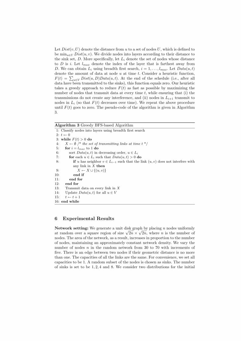
Let Dist(v, U) denote the distance from u to a set of nodes U , which is defined tobe minu∈U Dist(u, v). We divide nodes into layers according to their distance tothe sink set, D. More specifically, let Li denote the set of nodes whose distanceto D is i. Let lmax denote the index of the layer that is farthest away fromD. We can obtain Li using breadth first search, i = 1, . . . , lmax. Let Data(u, t)denote the amount of data at node u at time t. Consider a heuristic function,F (t) =

∑u∈V Dist(u,D)Data(u, t). At the end of the schedule (i.e., after all

data have been transmitted to the sinks), this function equals zero. Our heuristictakes a greedy approach to reduce F (t) as fast as possible by maximizing thenumber of nodes that transmit data at every time t, while ensuring that (i) thetransmissions do not create any interference, and (ii) nodes in Li+1 transmit tonodes in Li (so that F (t) decreases over time). We repeat the above procedureuntil F (t) goes to zero. The pseudo-code of the algorithm is given in Algorithm3.

Algorithm 3 Greedy BFS-based Algorithm1: Classify nodes into layers using breadth first search2: t ← 03: while F (t) > 0 do4: X ← ∅ /* the set of transmitting links at time t */5: for i = lmax to 1 do6: sort Data(u, t) in decreasing order, u ∈ Li

7: for each u ∈ Li such that Data(u, t) > 0 do8: if u has neighbor v ∈ Li−1 such that the link (u, v) does not interfere with

any link in X then9: X ← X ∪ {(u, v)}

10: end if11: end for12: end for13: Transmit data on every link in X14: Update Data(u, t) for all u ∈ V15: t ← t + 116: end while

6 Experimental Results

Network setting: We generate a unit disk graph by placing n nodes uniformlyat random over a square region of size

√2n × √2n, where n is the number of

nodes. The area of the network, as a result, increases in proportion to the numberof nodes, maintaining an approximately constant network density. We vary thenumber of nodes n in the random network from 30 to 70 with increments offive. There is an edge between two nodes if their geometric distance is no morethan one. The capacities of all the links are the same. For convenience, we set allcapacities to be 1. A random subset of the nodes is chosen as sinks. The numberof sinks is set to be 1, 2, 4 and 8. We consider two distributions for the initial

amount of data at non-sink nodes: uniform distribution, where the initial dataat each non-sink node is set to be 1, and skewed distribution, where the initialdata si at node i is 1/i.Interference model: Our algorithm is applicable to any interference model.In our experiments, we use two-hop interference model, in which two edges caninterfere with each other if they are within two-hop distance [16].Performance comparison. For each setting, we generate ten independent in-puts and compare the average latencies of the two algorithms over the ten in-puts. Figure 3(a) and (b) depict the ratio between average latencies of GreedyBFS-based Algorithm and LP-based Algorithm for uniform and skewed distribu-tion, respectively (the results using 8 sinks are similar and omitted for clarity).The confidence intervals are tight and hence omitted. We observe that the la-tency of LP-based Algorithm is around 20% to 70% shorter than that of GreedyBFS-based Algorithm. For uniform distribution, the gain of LP-based Algorithmincreases from 1.1 to 1.5 as the number of nodes increases. For skewed distribu-tion, LP-based algorithm outperforms Greedy Algorithm by 40%-60%, even forsmall networks. Last, we observe similar results for different number of sinks.

00.20.40.60.811.21.41.6

30 35 40 45 50 55 60 65 70Greedy/LPBANumber of nodes

m=1m=2m=4(a) Uniform distribution

00.20.40.60.811.21.41.61.8

30 35 40 45 50 55 60 65 70Greedy/LPBANumber of nodes

m=1m=2m=4(b) Skewed distribution

Fig. 3. Ratio between average latencies of Greedy BFS-based Algorithm and LP-basedAlgorithm. m is the number of sinks

7 ConclusionWe proposed a constant approximation algorithm and a heuristic for Multiple-Sink Data Collection Problem in wireless sensor networks. The constant approxi-mation algorithm first constructs a time-expanded graph, then generates feasibleflows in the expanded graph, and finally finds an exact data collection schedule.The heuristic algorithm is based on greedy breadth first search. Our experimen-tal results show that the approximation algorithm can significantly outperformthe simple heuristic (up to 60%).

References

1. N. Alon, A. Bar-Noy, N. Linial, and D. Peleg. A lower bound for radio broadcast.Journal of Computer and System Sciences, 43(2):290C298, 1991.

2. H. Balakrishnan, C. Barrett, V. S. Anil Kumar, M. Marathe, and S. Thite. Thedistance 2-matching problem and its relationship to the mac layer capacity of adhocwireless networks. IEEE J. Selected Areas in Connunications, 22(6), August 2004.

3. R. Bar-Yehuda, O. Goldreich, and A. Itai. On the time-complexity of broadcast inmulti-hop radio networks: An exponential gap between determinism and random-ization. Journal of Computer and System Sciences, 45(1):104C126, 1992.

4. William C. Cheng, Cheng-Fu Chou, Leana Golubchik, Samir Khuller, and Yung-Chun (Justin) Wan. Large-scale data collection: a coordinated approach. In IEEEInfocom, 2003.

5. Cedric Florens and Robert McEliece. Packets distribution algorithms for sensornetworks. In IEEE Infocom, 2003.

6. L.R. Ford and D.R. Fulkerson. Flows in networks. In Princeton University Press,New Jersey, 1962.

7. R. Gandhi, S. Parthasarathy, and A. Mishra. Minimizing broadcast latency andredundancy in ad hoc networks. In ACM MobiHoc03, pages 222–232, 2003.

8. Rajiv Gandhi, Yoo-Ah Kim, Seungjoon Lee, Jiho Ryu, and Peng-Jun Wan. Ap-proximation algorithm for data broadcast and collection in wireless networks. InIEEE Infocom (Mini conference), 2009.

9. P. Gupta and P. R. Kumar. The capacity of wireless networks. IEEE Transactionson Information Theory, 46(2):388–404, March 2000.

10. B. Hopper and E. Tardors. Polynomial time algorithms for some evacuation prob-lems. In SODA: ACM-SIAM Symposium on Discrete Algorithms, pages 512 – 521,1994.

11. Qingfeng Huang and Ying Zhang. Radial coordination for convergecast in wirelesssensor networks. In LCN ’04: Proceedings of the 29th Annual IEEE InternationalConference on Local Computer Networks, pages 542–549, Washington, DC, USA,2004. IEEE Computer Society.

12. Scott C.-H. Huang, Peng-Jun Wan, Jing Deng, and Yunghsiang S Han. Broad-cast scheduling in interference environment. IEEE Trans. on Mobile Computing,7(11):1338 – 1348, November 2008.

13. Scott C.-H. Huang, Peng-Jun Wan, Xiaohua Jia, Homngwei Du, and WeipingShang. Minimum-latency broadcast scheduling in wireless ad hoc networks. InProceedings of 26th IEEE Infocom, pages 733 – 739, 2007.

14. Scott C.-H. Huang, Peng-Jun Wan, Chinh T. Vu, Yingshu Li, and Frances. Yao.Nearly constant approximation for data aggregation scheduling in wireless sensornetworks. In Proceedings of 26th IEEE Infocom, pages 366 – 372, 2007.

15. Alex Kesselman and Dariusz R. Kowalski. Fast distributed algorithm for converge-cast in ad hoc geometric radio networks. J. Parallel Distrib. Comput., 66(4):578–585, 2006.

16. V.S. Anil Kumar, M. Marathe, S. Parthasarathy, and A. Srinivasan. End-to-endpacket scheduling in ad hoc networks. In ACM-SIAM symposium on DiscreteAlgorithms, SODA, pages 1014–1023, 2004.

17. V.S. Anil Kumar, Madhav V. Marathe, Srinivasan Parthasarathy, and AravindSrinivasan. Algorithmic aspects of capacity in wireless networks. In SIGMETRICS,Banff, Alberta, Canada, June 2005.

18. S. Upadhyayula, V. Annamalai, and S. K. S. Gupta. A low-latency and energy-efficient algorithm for convergecast in wireless sensor networks. In IEEE GlobalTelecommunications Conference, pages 3525–3530, 2003.

19. S. Yi, Y. Pei, and S. Kalyanaraman. On the capacity improvement of ad hoc wire-less networks using deirectional antennas. In Proceedings of 4th ACM internationalsymposium on Mobile ad hoc networking and computing, pages 108–116, 2003.