Contract Nos. 94-33825-0383 and 98-38825-6063 10 August 2001

INTERIM REPORT Sources and Sinks of PM10 in the San Joaquin Valley

A study for United States Department of Agriculture Special Research Grants Program

Robert G. Flocchini, Principal Investigator Crocker Nuclear Laboratory

Teresa A. James, Investigator Crocker Nuclear Laboratory

Lowell L. Ashbaugh, Michael S. Brown, Omar F. Carvacho, Britt A. Holmén, Robert T. Matsumura, Krystyna Trzepla-Nabaglo, Chris

Tsubamoto, Investigators Crocker Nuclear Laboratory

Air Quality Group

Crocker Nuclear

Laboratory University of

California Davis, CA 95616-8569

i

Table of Contents

1 Background ..................................................................................................................1

1.1 Air Quality in the San Joaquin Valley..................................................................1

1.2 Agricultural Impacts on Air Quality.....................................................................3

2 Overview......................................................................................................................5

2.1 Objectives .........................................................................................................5

2.2 Approach ..........................................................................................................8

2.3 Reporting.........................................................................................................10

3 Methods .....................................................................................................................12

3.1 PM10 Field Test Strategy and Array Design ......................................................12 3.1.1 Field Crops.....................................................................................................12 3.1.2 Orchard Crops ...............................................................................................12 3.1.3 Livestock........................................................................................................13

3.2 PM Point Samplers ..........................................................................................13

3.3 Gravimetric and Reconstructed Mass (RCMA) Concentrations.........................15

3.4 Ammonia .........................................................................................................16 3.4.1 Active Methods ..............................................................................................16 3.4.2 Passive Methods.............................................................................................17 3.4.3 Facility Description..........................................................................................18

3.5 Quality Assurance............................................................................................19 3.5.1 Filter Samples (PM2.5 and PM10).....................................................................19 3.5.2 Ammonia Samples (active and passive)............................................................20

3.6 Soils ................................................................................................................20 3.6.1 Soil Moisture ..................................................................................................22 3.6.2 Dry Sieving.....................................................................................................22 3.6.3 Wet Sieving ....................................................................................................23

3.7 Light detection and ranging (lidar).....................................................................24

4 Emission Rate Calculations ..........................................................................................25

4.1 PM from 1994 data .........................................................................................26

4.2 PM from 1995 data .........................................................................................27

4.3 PM from 1995 – 1998 data .............................................................................27 4.3.1 Integration of lidar data....................................................................................29 4.3.2 Plume Height and Uncertainty Calculations.......................................................31

ii

4.3.3 Emission Factor Calculations ...........................................................................32 4.3.4 Emission Factor Confidence Rating..................................................................34

4.4 Ammonia from Measurements..........................................................................35

5 Results from Field Measurements ................................................................................39

5.1 Orchard Crops ................................................................................................41 5.1.1 1994 Field Tests .............................................................................................41 5.1.2 1995 Field Tests .............................................................................................45 5.1.3 1998 Field Tests .............................................................................................47

5.2 Cotton Harvest ................................................................................................51 5.2.1 1994 Field Tests .............................................................................................51 5.2.2 Assessment of simple box model emission factor calculations using 1995 Field Tests........................................................................................................................52 5.2.3 1996-1998 Field Tests....................................................................................56

5.3 Wheat Harvest.................................................................................................61

5.4 Land Preparation.............................................................................................62

5.5 PM from confined cattle facilities ......................................................................67

5.6 Ammonia from confined cattle facilities..............................................................72 5.6.1 1996 Field Tests .............................................................................................72 5.6.2 1997 Field Tests .............................................................................................75 5.6.3 1999 Field Tests .............................................................................................76

6 Conclusions from field measurements...........................................................................82

6.1 Orchard Crops ................................................................................................84

6.2 Cotton Harvest ................................................................................................86 6.2.1 Cotton Picking................................................................................................86 6.2.2 Cotton Stalk Cutting........................................................................................87 6.2.3 Cotton Root Cutting........................................................................................89

6.3 Wheat Harvest.................................................................................................91

6.4 Land Preparation .............................................................................................93 6.4.1 Discing............................................................................................................93 6.4.2 Chiseling.........................................................................................................94 6.4.3 Weeding.........................................................................................................95

6.5 Confined Animal Facilities ................................................................................97 6.5.1 Dairy ..............................................................................................................98 6.5.2 Beef Feedlot ...................................................................................................99

6.6 Ammonia emission factors..............................................................................100 6.6.1 Beef Feedlot .................................................................................................100 6.6.2 Dairies ..........................................................................................................101

iii

6.7 Ongoing Research Directions..........................................................................102

7 Associated Research: PM10 Potential.........................................................................104

7.1 Dust Collection Chamber:...............................................................................106

7.2 PM10 Inlet and the IMPROVE Sampler..........................................................106

8 Appendix A – Inventory of 1994 Field Tests .............................................................122

9 Appendix B – Inventory of 1995 Field Tests..............................................................127

10 Appendix C – Inventory of 1996 Field Tests .............................................................128

10 Appendix C – Inventory of 1996 Field Tests .............................................................129

11 Appendix D – Inventory of 1997 Field Tests .............................................................130

11 Appendix D – Inventory of 1997 Field Tests .............................................................131

12 Appendix E – Inventory of 1998 Field Tests..............................................................132

13 Appendix F – Text of Almond Harvester Report........................................................133

14 Appendix G – Description of Database Structure.........................................................29

15 Appendix H – Text of Atmospheric Environment Papers..............................................33

iv

List of Tables

Table 1.1 Value and Production of some major San Joaquin Valley crops, 1997 .....................1 Table 2.1 Summary of tests ....................................................................................................7 Table 2.2 Summary of field equipment placement and year of introduction.............................11 Table 3.1 Description of the ammonia sampling arrays...........................................................16 Table 3.2 Nest of sieves used for particle size distribution analysis by dry sieving. ..................22 Table 3.3 Sieve sizes which define texture gradients of sand in wet sieving. ............................23 Table 4.1 Summary of exceptions to emission factor calculations for PM emissions from

row crops and livestock........................................................................................28 Table 4.2 Emission factor confidence ratings summary...........................................................35 Table 5.1 Comparison of fig harvest to almond harvest emission factors (kg/km4) ..................44 Table 5.2 PM10 emission factors (kg/km4) by three calculation methods.................................46 Table 5.3 PM10 emission factors for almond pick-up tests during which both PM10 and

wind speed were measured outside of the canopy..................................................46 Table 5.4 Environmental conditions during almond pick-up tests............................................47 Table 5.5 PM10 concentrations normalized to amount of windrow trash <2mm prior to

harvest (µg/m4/g)...................................................................................................50 Table 5.6 PM10 emission rates from cotton operations, 1994.................................................51 Table 5.7 Correlation statistics for models.............................................................................55 Table 5.8 PM10 Emission flux (kg/km4) by three calculation methods .....................................55 Table 5.9 Emission factors for cotton picking compiled from field data collected in

1995-1998...........................................................................................................57 Table 5.10 Environmental conditions during cotton picking tests. ...........................................57 Table 5.11 Emission factors and uncertainties for cotton stalk cutting.....................................59 Table 5.12 Environmental conditions during cotton stalk cutting tests. ....................................60 Table 5.13 Emission factors and uncertainties for wheat harvest.............................................61 Table 5.14 Environmental conditions during wheat harvest tests.............................................62 Table 5.15 Emission factors and uncertainties for land preparation. ........................................64 Table 5.16 Environmental conditions during land preparation tests. ........................................65 Table 5.17 Emission factors and uncertainties for cultivation..................................................66 Table 5.18 Environmental conditions during cultivation tests...................................................66 Table 5.19 Best fit PM10 emission factors from open lot dairies .............................................68 Table 5.20 Environmental conditions during dairy tests. .........................................................69 Table 5.21 Best fit PM10 emission factors from feedlots.........................................................70 Table 5.22 Environmental conditions during feedlot tests. ......................................................71 Table 5.23 Results of ammonia emission factor calculation.....................................................76 Table 5.24 Ammonia concentration profiles and mass fluxes at downwind locations

instrumented with active (bubbler) samplers...........................................................79 Table 6.1 Summary of average PM10 emission factors...........................................................83 Table 6.2 Ammonia emission factors for open lot feedlots and dairies. .................................100 Table 6.3 Completed measurements of PM10 requiring further analysis and data

reduction for the calculation of emission factors....................................................102

v

Table 7.1 Averages of cumulative mass (mg/g) as a function of time for tested soils. .............109 Table 7.2 Partial list of the USDA soil tested from San Joaquin Valley.................................110 Table 7.3 USDA soils tested for PM10 index ......................................................................112 Table 7.4 Results from soil samples collected in 1995 .........................................................115 Table 7.5 Results from soil samples collected in 1996 .........................................................115 Table 7.6 Results from soil samples collected in 1997 .........................................................115 Table 7.7 Results from soil samples collected in 1998 .........................................................116

vi

List of Figures

Figure 1.1 Primary PM10 emissions inventory compiled by the California Air Resources Board (1993 Annual Average)................................................................................3

Figure 4.1 Lidar vertical profiles for PM tests 06 Nov 1998..................................................30

Figure 5.1 Example of the PM10 horizontal distribution downwind of an almond harvest

Figure 3.1 Standard sampling array for measuring agricultural emissions of fugitive dust..........14 Figure 3.2 Facility layout and sampler configuration for 1997 ammonia study.........................19

Figure 4.2 Average plume heights: Lidar vs. point sampler estimates. .....................................31

tree shaking operation for silt and clay soil textures. ...............................................42 Figure 5.2 Example of the PM10 horizontal distribution downwind of an almond harvest

sweeping (windrowing) operation for silt and clay soil textures. ..............................43 Figure 5.3 Example of the PM10 horizontal distribution downwind of an almond harvest,

nut pickup operation for silt and clay soil textures...................................................43 Figure 5.4 Vertical distribution of aerosols from vertical profile tower. ...................................44 Figure 5.5 PM10 emission factors for eight agricultural operations...........................................45 Figure 5.6 PM2.5 emission factors for eight agricultural operations..........................................45 Figure 5.7 PM10 concentrations downwind of harvester #1 and #2, (a) all tests, (b)

solid–set irrigation, (c) micro–spray irrigation.........................................................49 Figure 5.8 PM10 emission rates from cotton operations, 1994................................................52 Figure 5.9 PM10 emission factor for 1995 cotton picking tests ...............................................53 Figure 5.10 PM10 emission factor for 1995 cotton stalk shredding tests .................................53 Figure 5.11 PM10 emission factor for 1995 cotton stalk incorporation tests............................54 Figure 5.12 Ammonia emission factors for dairy and beef cattle derived from mass flux

model...................................................................................................................74 Figure 5.13 Comparison of ammonia emission rates derived from mass flux model of

measurements made at two locations on the downwind fence line...........................75 Figure 5.14 Ammonia emission factors for day-time and night-time for dairy and beef

cattle derived from mass flux model.......................................................................75 Figure 5.15 Diurnal trend in ammonia emission factors from 1997 data. .................................76 Figure 5.16 Average NH3 fluxes calculated from measurements.............................................78 Figure 5.17 Emission factors calculated from measurements. .................................................80 Figure 6.1 PM10 emission factors (mg/m2) and soil moisture (%) from 1995 tests of

highest confidence for Almond pickup operations. .................................................85 Figure 6.2 PM10 emission factors (mg/m2) and relative humidity (%) for cotton picking

Figure 6.3 PM10 emission factors (mg/m2) and relative humidity (%) for cotton stalk

Figure 6.4 PM10 emission factors (mg/m2) and relative humidity (%) for cotton root

Figure 6.5 PM10 emission factors (mg/m2) and relative humidity (%) for wheat

tests with highest confidence ratings.......................................................................87

cutting tests with highest confidence ratings............................................................89

cutting tests with highest confidence ratings............................................................90

harvesting tests with highest confidence ratings.......................................................92

vii

Figure 6.6 PM10 emission factors (mg/m2) and soil moisture (%) for discing tests with highest confidence ratings......................................................................................94

Figure 6.7 PM10 emission factors (mg/m2) and relative humidity (%) for chiseling tests

Figure 6.8 PM10 emission factors (mg/m2) and soil moisture (%) for weeding tests with

Figure 6.9 Correlation of PM10 emission factors (mg/m2) and relative humidity (%) for

Figure 6.10 PM10 emission factors (lbs/d*1000hd) and relative humidity (%) for dairy

Figure 6.11 PM10 emission factors (lbs/d*1000hd) and solar radiation (W/m2) for

with highest confidence ratings...............................................................................95

highest confidence ratings......................................................................................96

confined cattle tests with highest confidence ratings. ...............................................97

tests with highest confidence ratings.......................................................................98

feedlot tests with highest confidence ratings............................................................99 Figure 7.1 Diagram of dust resuspension chamber...............................................................105 Figure 7.2 Diagram of CNL resuspension and collection chamber .......................................106 Figure 7.3 PM10 Index curve for the clay soils data in table 7.2............................................110 Figure 7.4 Cumulative mass for resuspension of select soils collected simultaneously

with PM10 emission factor measurements.............................................................111 Figure 7.5 Relationship between PM10 Index calculated by the straight line and

experimental PM10 Index. ...................................................................................112 Figure 7.6 Distribution of soil texture for soils analyzed, based on wet sieving.......................113

viii

1 BACKGROUND

California’s San Joaquin Valley is one of the most productive agricultural regions in the United States. Over 350 crops are produced, including seeds, flowers and ornamentals. Over eight million acres were harvested in 1997, and a number of crops are produced exclusively, or nearly so, in California. In 1997 agriculture contributed $26.8 billion to the state’s economy. Table 1.1 lists a few of the major crops in the San Joaquin Valley by dollar value, along with the percent of U.S. production and the number of acres harvested in 1997 (Johnston and Carter

2000).

Table 1.1 Value and Production of some major San Joaquin Valley crops, 1997

Crop Value (Millions)

U.S. Ranking

Harvested acreage in 1993

Percent of U.S. Production

Grapes $2,819 1 497,100 91%

Cotton $984 2 1,036,316 14%

Almonds $1,127 1 410,000 100%

Walnuts $352 1 177,200 100%

The San Joaquin Valley is experiencing rapid population growth, especially in the northern and central regions. As home prices in the San Francisco Bay Area continue to rise, prospective homeowners increasingly turn to the northern San Joaquin Valley to find affordable housing. The central region of the valley also continues to grow as the economy of Fresno and surrounding areas continue to expand. The expansion of major employers in the area, such as the new University of California campus near Merced, will drive additional population growth.

The expansion of residential housing into agricultural areas can lead to conflicts between traditional practices and new expectations. These conflicts were minimal when the encroaching residential areas were associated with agricultural livelihoods and lifestyles. They are magnified, though, when a large percentage of the incoming residents lead lives separate from the agricultural community.

Air quality conflicts that develop between traditional agricultural uses of the land and encroaching urban development include odor and dust issues. Resolving these conflicts requires a concerted effort by affected parties to understand the characteristics of living in a rural setting and to take steps to reduce emissions where appropriate.

1.1 Air Quality in the San Joaquin Valley

The United States Environmental Protection Agency has designated the San Joaquin Valley a serious non-attainment area for PM10, particulate matter with an aerodynamic diameter less than 10 micrometers. This means the valley exceeds the National Ambient Air Quality Standards

1

(NAAQS) for PM10 to such a degree that extreme actions may be required to meet them. PM10 particles bypass the body’s defense mechanisms and penetrate into the respiratory system. These particles have been linked to death by cardiac and respiratory disease. The valley also exceeds the NAAQS for ozone, a key component of photochemical smog. Ozone causes respiratory distress in some individuals, and also reduces crop yields.

The United States EPA recently enacted new standards for PM2.5, particles with an aerodynamic diameter less than 2.5 micrometers. These particles penetrate more deeply into the lung than PM10, and have been linked even more strongly to human deaths. The San Joaquin Valley is expected to exceed the new standards, although this will not be known for certain until a monitoring network has been established and operated for several years.

Particulate matter in the San Joaquin Valley typically peaks in the fall and winter, and exceeds the PM10 standards during the early winter. During the spring and summer the concentrations are relatively low. Moreover, the nature of the particulate matter changes between early and late fall. From early September to mid-November, the PM10 is composed primarily of soil dust in a size range greater than 1-2 micrometers. After the first winter rains fall, which normally happens in mid-November, the soil dust source is suppressed. At this same time, the soil surface cools and the atmospheric temperature inversion lowers from a few thousand meters to several hundred meters. Air temperature drops and humidity increases. Pollutants emitted into this atmosphere are trapped in a relatively small volume of cool, damp air. Thus, the particulate matter includes fewer soil dust particles and more particles from automotive tailpipes, burning of wood for heat, and particles formed in the atmosphere from gases such as ammonia, nitric acid, and sulfur dioxide. These particles differ from the earlier ones not only in their chemistry, but also in their size; they are primarily smaller than 2.5 micrometers in size.

The 1993 PM10 annual average emissions inventory, compiled by the state Air Resources Board, is shown in Figure 1.1 (Chow, Watson et al. 1992). According to this inventory, the major sources of primary particulate matter in the San Joaquin Valley include farming operations, entrained road dust from paved and unpaved roads, and windblown dust. Smaller sources include fuel combustion, waste burning, industrial processes, and mobile sources. The inventory does not include residential wood combustion or secondary particles, though, and these are thought to make up much of the particulate matter in the winter. Although inventories are helpful tools for understanding the annual impact of various sources on air quality, seasonal variations in the relative importance of sources (as mentioned above) are not reflected in an annual inventory.

Secondary particles are formed in the atmosphere from ammonia, nitric acid, and sulfur dioxide, and from some organic gases as they condense from the vapor phase. Ammonia gas is produced largely from livestock operations, and to a lesser degree from sewage treatment facilities and fertilizer application. Nitric acid is a by-product of NOx emissions produced by motor vehicles and other combustion sources. Sulfur dioxide is produced from combustion and by numerous sources in the oil fields of the southern San Joaquin Valley. The formation of

2

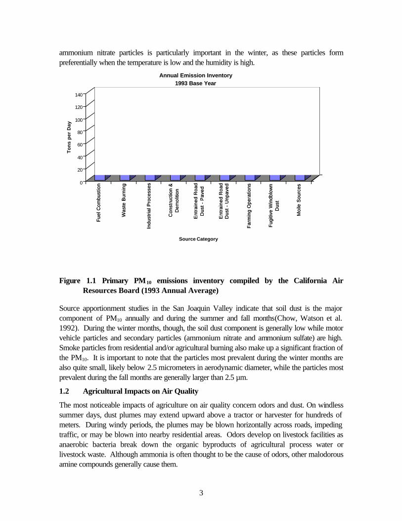
ammonium nitrate particles is particularly important in the winter, as these particles form preferentially when the temperature is low and the humidity is high.

Annual Emission Inventory 1993 Base Year

Fue

l Com

bust

ion

Was

te B

urni

ng

Indu

stria

l Pro

cess

es

Con

stru

ctio

n &

Dem

oliti

on

Ent

rain

ed R

oad

Dus

t - P

aved

Ent

rain

ed R

oad

Dus

t - U

npav

ed

Far

min

g O

pera

tions

Fug

itive

Win

dblo

wn

Dus

t

Moi

le S

ourc

es

0

20

40

60

80

100

120

140

To

ns

per

Day

Fue

l Com

bust

ion

Was

te B

urni

ng

Indu

stria

l Pro

cess

es

Con

stru

ctio

n &

Dem

oliti

on

Ent

rain

ed R

oad

Dus

t - P

aved

Ent

rain

ed R

oad

Dus

t - U

npav

ed

Far

min

g O

pera

tions

Fug

itive

Win

dblo

wn

Dus

t

Moi

le S

ourc

es

Source Category

Figure 1.1 Primary PM10 emissions inventory compiled by the California Air Resources Board (1993 Annual Average)

Source apportionment studies in the San Joaquin Valley indicate that soil dust is the major component of PM10 annually and during the summer and fall months(Chow, Watson et al. 1992). During the winter months, though, the soil dust component is generally low while motor vehicle particles and secondary particles (ammonium nitrate and ammonium sulfate) are high. Smoke particles from residential and/or agricultural burning also make up a significant fraction of the PM10. It is important to note that the particles most prevalent during the winter months are also quite small, likely below 2.5 micrometers in aerodynamic diameter, while the particles most prevalent during the fall months are generally larger than 2.5 µm.

1.2 Agricultural Impacts on Air Quality

The most noticeable impacts of agriculture on air quality concern odors and dust. On windless summer days, dust plumes may extend upward above a tractor or harvester for hundreds of meters. During windy periods, the plumes may be blown horizontally across roads, impeding traffic, or may be blown into nearby residential areas. Odors develop on livestock facilities as anaerobic bacteria break down the organic byproducts of agricultural process water or livestock waste. Although ammonia is often thought to be the cause of odors, other malodorous amine compounds generally cause them.

3

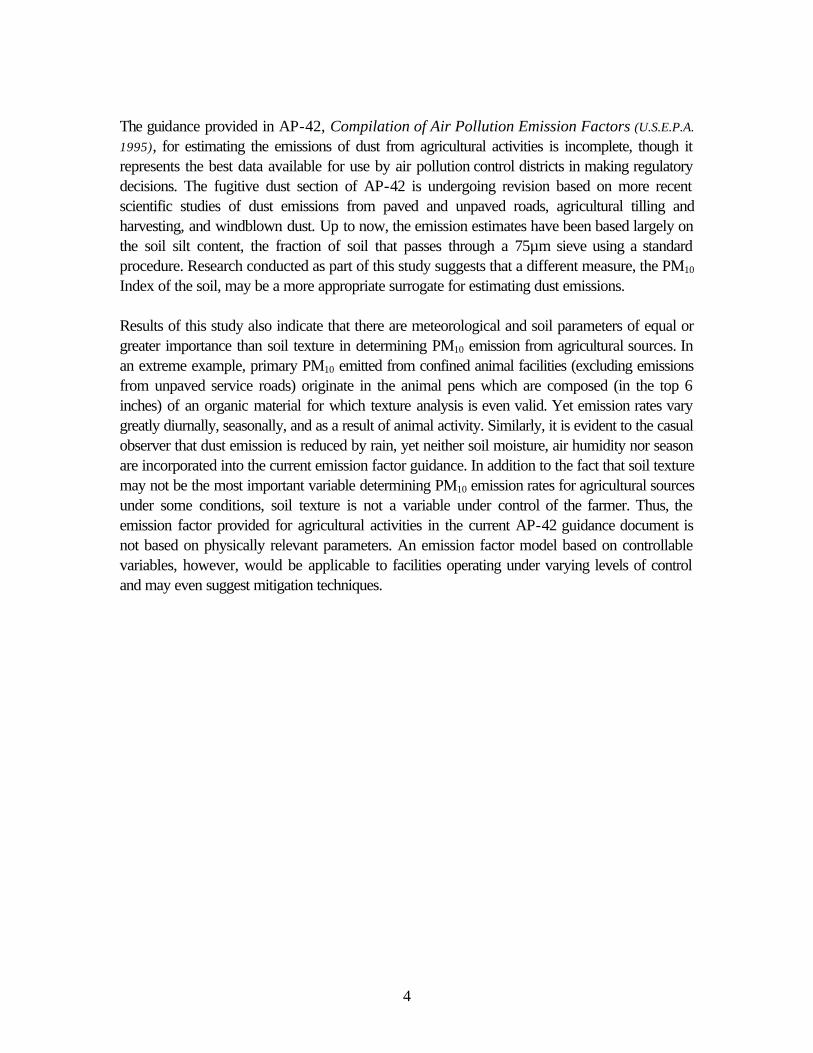
The guidance provided in AP-42, Compilation of Air Pollution Emission Factors (U.S.E.P.A.

1995), for estimating the emissions of dust from agricultural activities is incomplete, though it represents the best data available for use by air pollution control districts in making regulatory decisions. The fugitive dust section of AP-42 is undergoing revision based on more recent scientific studies of dust emissions from paved and unpaved roads, agricultural tilling and harvesting, and windblown dust. Up to now, the emission estimates have been based largely on the soil silt content, the fraction of soil that passes through a 75mm sieve using a standard procedure. Research conducted as part of this study suggests that a different measure, the PM10

Index of the soil, may be a more appropriate surrogate for estimating dust emissions.

Results of this study also indicate that there are meteorological and soil parameters of equal or greater importance than soil texture in determining PM10 emission from agricultural sources. In an extreme example, primary PM10 emitted from confined animal facilities (excluding emissions from unpaved service roads) originate in the animal pens which are composed (in the top 6 inches) of an organic material for which texture analysis is even valid. Yet emission rates vary greatly diurnally, seasonally, and as a result of animal activity. Similarly, it is evident to the casual observer that dust emission is reduced by rain, yet neither soil moisture, air humidity nor season are incorporated into the current emission factor guidance. In addition to the fact that soil texture may not be the most important variable determining PM10 emission rates for agricultural sources under some conditions, soil texture is not a variable under control of the farmer. Thus, the emission factor provided for agricultural activities in the current AP-42 guidance document is not based on physically relevant parameters. An emission factor model based on controllable variables, however, would be applicable to facilities operating under varying levels of control and may even suggest mitigation techniques.

4

2 OVERVIEW

2.1 Objectives

The primary objectives of this study are: · to measure the PM10 emission factors from agricultural operations, including harvesting

of both row and orchard crops, land preparation (discing, ripping, floating, planning), and livestock (diary, feedlot).

· to measure ammonia emission factors from livestock operations (dairy, feedlot).

The study began in 1994 with measurements of PM10 and PM2.5 production from almond, fig, walnut, and cotton harvesting operations. The 1995 and 1996 work extended our 1994 studies by including additional soil types, harvesters, and harvesting practices. We extended the measurements to include some cotton stalk incorporation and wheat harvesting tests. Livestock as sources of PM10 were also added in 1995 and 1996. The 1997 and 1998 work branched out to include various land preparation activities and a comparison of almond harvesting equipment. Both PM10 and PM2.5 have been collected using side by side samplers at 3 m during all phases of the project, though PM10 has been used to calculated emission factors throughout due to higher frequency of analytical detection and the more complete profile measurements that were made. Particle size distributions have been evaluated for several operations (see section 5.1.1) and are an important component of filter sample quality assurance protocols (see section 3.5.1). We also measured ammonia emission from dairies and a feedlot, starting in 1996, with a comparison study in 1997, and culminating in a thorough study of wet season ammonia emission from dairies in 1999. Our most recent studies are focused on the comparison of land preparation operations following crops of characteristically different soil moisture and the integration of lidar data with PM10 emission calculations. Table 2.1 summarizes the field tests analyzed in this study to date.

Beginning in June, 1997 use of (lidar) light detection and ranging has been incorporated with collection of PM10 and PM2.5 samples because the filter measurements cannot reasonably capture the entire PM plume generated across an agricultural source. Lidar applications have been developed in this project to address the limited ability of conventional point PM samplers to quantify PM emissions from these operations due to the following factors:

· The large spatial dimensions of agricultural sources, the spatial irregularity of dust plumes and the small number of point sampling locations results in under-sampling of the dust plume.

· The spatial variability in the PM source location (i.e., tractor) within the entire field as the operation traverses the field means the direction and distance from a point sampler to the PM source changes with time.

· The vertical extent of point sampling is limited to the height of portable towers. The lidar technique offers high temporal (seconds) and spatial resolution (2.5 meters) and extensive analysis range (over 5 km) capabilities. It can currently provide important qualitative

5

data on agricultural PM10 emissions and has been used to improve the point sampling methods used to estimate PM10 emission factors from non-point agricultural sources[Holmén, 2000 #38; Holmén, 2000 #39].

The UCD studies are secondarily directed at improving information needed for estimating the emissions of dust from agricultural sources. Based on the current guidance provided in AP-42 (see section 1.2), soil properties have been examined by several methods since the initiation of this project. Both bulk and moisture samples of soils have been collected from each of the fields where PM10 emissions were measured since 1994 (see section 3.6). Soil moisture has been measured throughout the study as a variable of potential importance in predicting PM10

emissions. Dry sieving of soil samples to determine soil silt content as defined in the current guidance method for estimating PM10 emissions has been performed in the lab of co-principal investigator Randy Southard. Wet sieving of soil samples has also been performed in Dr. Southard’s lab to characterize the texture of the soils. This analysis has been performed on all samples collected in the project to obtain size fractions which complement the data obtained in the dry sieving analysis and which permit evaluation of the importance of aggregation in the soils studied. These procedures support the original research into PM10 potential based on resuspension, which has been developed as part of this project since 1994.

The overall goal of soil resuspension is to provide a laboratory-based method of estimating the fugitive dust emission "potential" of soils. This will allow us to control, isolate, and vary environmental and agricultural factors that affect dust generation. The basic steps of the resuspension experiments include:

· Generating dust in an enclosed chamber. Bulk and size-fractionated soil samples are mechanically disturbed and/or entrained in turbulent airflow.

· Measuring the airborne dust by size and composition using the same techniques as in actual field tests.

· Varying specific environmental factors (e.g. soil moisture, energy input, soil texture, etc.) to isolate and quantify their impacts upon dust generation.

Measurements of the mass of dust generated in resuspension experiments have been used to define correlations between the dust potential as a function of soil texture (clay, silt, sand). These experiments provide an opportunity to measure the effect of mechanical energy input (for dust generation), soil moisture, and relative humidity on soil dust potential. Additionally, elemental analysis of resuspended dust samples provides a method for comparing soil elements and gravimetric mass from resuspended samples to obtain "soil factors" for the reconstruction of soils in PM2.5 and PM10 field samples. This analysis has been performed on samples collected since 1995.

6

Table 2.1 Summary of tests

PM Tests Summary (1994-1998) Seasons: (Nov-Apr) Winter; (May-Oct) Summer 1994

County Crop Practice Operation # of Tests Season/Yr. Kern Almond Harvest Sweeping 6 Summer 94 Kern Almond Harvest Shaking 3 Summer 94 Kern Almond Harvest Pickup 20 Summer 94 Merced Figs Harvest Sweeping 6 Summer 94 Merced Figs Harvest Pickup 3 Summer 94 Kings Walnut Harvest Shaking 1 Summer 94 Kings Walnut Harvest Sweeping 3 Summer 94 Hanford Walnut Harvest Pickup 2 Summer 94 Hanford Walnut Harvest Sweeping 1 Summer 94 Kern Cotton Harvest Picking 5 Summer 94 Kern Cotton Harvest Stalk cutting 3 Summer 94 Kern Cotton Harvest Picking 3 Summer 94 Fresno Cotton Harvest Picking 5 Summer 94 Kern Cotton Harvest Picking 3 Summer 94 Kern Cotton Harvest Stalk cutting 2 Summer 94 Kings Cotton Harvest Picking 3 Winter 94 (10/30) Kings Cotton Harvest Stalk cutting 3 Winter 94 (11/1) Fresno Cotton Harvest Picking 2 Winter 94 Fresno Cotton Harvest Stalk cutting 4 Winter 94 Kings Cotton Harvest Picking 2 Winter 94

1995 Fresno Raisins Harvest Tray burning 1 Summer 95 Kern Almonds Harvest Pickup 14 Summer 95 Kern Almonds Harvest Shaking 17 Summer 95 Kern Almonds Harvest Sweeping 5 Summer 95 Kings Cotton Harvest Picking 9 Summer 95 Kings Cotton Harvest Stalk cutting 16 Summer 95 Kings Cotton Harvest Stalk incorporation 4 Summer 95 Kings Cotton Harvest Picking 4 Summer 95 Kings Cotton Harvest Stalk incorporation 7 Winter 95 Kings Cotton Harvest Picking 4 Winter 95 Kings Cotton Harvest Stalk cutting 4 Winter 95 Kings Cotton Harvest Picking 5 Winter 95 Kings Cotton Harvest Stalk incorporation 2 Winter 95 Kings Cotton Harvest Stalk cutting 2 Winter 95 Merced Wheat Harvest Harvest 17 Summer 95 Yolo Land Land preparation Land planning 5 Summer 95 Tulare Milk Dairy Feeding 6 Summer 95 Tulare Milk Dairy Activity 5 Summer 95 Tulare Milk Dairy Sleeping 3 Summer 95 Tulare Milk Dairy Loafing 3 Summer 95

1996 Kern Beef Feedlot Loafing 2 Winter 96 Kern Beef Feedlot Activity 3 Winter 96 Kern Beef Feedlot Sleeping 3 Winter 96 Kern Beef Feedlot Loafing 5 Summer 96 Kern Beef Feedlot Activity 7 Summer 96 Kern Beef Feedlot Sleeping 10 Summer 96 Kern Beef Feedlot Feeding 1 Summer 96 Tulare Milk Dairy Loafing 12 Winter 96 Tulare Milk Dairy Activity 6 Winter 96 Tulare Milk Dairy Sleeping 7 Winter 96 Kings Wheat Harvest Harvest 15 Summer 96 Merced Wheat Harvest Harvest 8 Summer 96 Kings Cotton Harvest Picking 5 Winter 96 Kings Cotton Harvest Stalk cutting 4 Winter 96 Kings Cotton Land preparation Listing 4 Winter 96 Kings Cotton Land preparation Root cutting 4 Winter 96 Kings Cotton Land preparation Disking 8 Winter 96 Kings Cotton Land preparation Chiseling 2 Winter 96

7

1997 Kings Wheat Harvest Harvest 7 Summer 97 Kings Wheat Land preparation Disking 7 Summer 97 Kings Wheat Land preparation Ripping 6 Summer 97

1998 Kern Almonds Harvest Pickup 31 Summer 98 Fresno Cotton Cultivation Weeding 11 Summer 98 Fresno Cotton Harvest Stalk cutting 2 Winter 98 Fresno Cotton Land preparation Disking 6 Winter 98

N H 3 T e s t s S u m m a r y ( 1 9 9 4 - 1 9 9 8 ) 1 9 9 6

K e r n B e e f F e e d l o t L o a f i n g 1 0 W i n t e r 9 6 K e r n B e e f F e e d l o t A c t i v i t y 3 W i n t e r 9 6 K e r n B e e f F e e d l o t S l e e p i n g 1 0 W i n t e r 9 6 K e r n B e e f F e e d l o t L o a f i n g 4 S u m m e r 9 6 K e r n B e e f F e e d l o t A c t i v i t y 5 S u m m e r 9 6 K e r n B e e f F e e d l o t S l e e p i n g 9 S u m m e r 9 6 K e r n B e e f F e e d l o t F e e d i n g 1 S u m m e r 9 6 T u l a r e M i l k D a i r y L o a f i n g 1 2 W i n t e r 9 6 T u l a r e M i l k D a i r y A c t i v i t y 6 W i n t e r 9 6 T u l a r e M i l k D a i r y S l e e p i n g 7 W i n t e r 9 6

1 9 9 7 T u l a r e M i l k D a i r y L o a f i n g 9 W i n t e r 9 7 T u l a r e M i l k D a i r y S l e e p i n g 1 W i n t e r 9 7

1 9 9 9 T u l a r e M i l k D a i r y F e e d i n g 2 W i n t e r 9 9 T u l a r e M i l k D a i r y A c t i v i t y 1 W i n t e r 9 9 T u l a r e M i l k D a i r y L o a f i n g 1 9 W i n t e r 9 9 T u l a r e M i l k D a i r y S l e e p i n g 5 W i n t e r 9 9

2.2 Approach

When work began on the project in 1994, few methods had been explored by others to quantify PM emission rates from agricultural operations. The first techniques used were pioneered by Cowherd et al. (Cowherd, Axetall et al. 1974; Cowherd and Kinsey 1986) using vertical profiles of TSP to characterize dust plumes and PM10 measurements at a single height to quantify PM concentrations. In our application of this method we used a telescoping pole to support stacked filter units to monitor TSP concentrations at four heights up to 7 m above ground. Low flow rates (10 l min-1) and insufficient sensitivity of the method over the short (0.25 to 2 h) sampling duration used in plume characterization, however, made this sampler inappropriate for this purpose and very few (less than 10%) of the TSP mass profiles were

and PM2.5 samplers at 7.5 m above ground. This provided the means for measurement of a three point vertical profile of size-selected aerosol concentrations and direct characterization of the PM10 plume. These towers were also fitted with brackets to support anemometers and thermometers at 5 heights for more precise monitoring of wind speed and temperature gradients than had been possible with the tripod we used in 1994. However, each stationary tower required 3-4 man hours to construct and use was limited to areas accessible by road, since the components were heavy and the footprint (75 m2) was large.

interpretable. In 1995 we modified two 30-foot antenna towers to deploy IMPROVE PM10

8

Later in 1995 we obtained a pneumatic tower with a generator and air compressor and installed it in the bed of a pick-up truck with PM10 and PM2.5 samplers at 10 and 3 m and a PM10

sampler to be set on the ground (1 m). This mobile array is effective in accessing most points within a field or orchard during harvesting activities and can be deployed by one person in as little as 10 minutes.

The addition of ammonia sampling equipment to the towers in 1996 required little technological development, since the acid-coated filtration method routinely used in our lab was modified for deployment on the towers by simply hanging the filter cassettes at the appropriate levels. This technique was adequate for sampling conducted in the winter of 1996, but the filters provided insufficient capacity for measuring ammonia concentrations downwind of a feedlot in summer. Thus, a sample collection method was developed based on a liquid bubbler and field tested in winter of 1997. While the bubbler sampler was shown to be accurate (compared to independent methods) and to have a high capacity (in laboratory testing), significant modifications were required to enable reliable, repetitive sampling at multiple heights. More importantly, the highly variable ammonia concentrations we had measured along the downwind edge of both dairies and feedlots indicated a need for at least three downwind profiles to adequately characterize the source.

We borrowed a pair of trailer mounted, semi-hydraulic towers from the UCD Engineering Department in 1998 for use in the almond harvester comparison study we conducted that summer. Used with the mobile array, these trailer towers gave us the ability to measure the PM10 concentration profile at three locations downwind of the source simultaneously, and to relocate the samplers with the movement of the source. One person can deploy the trailer towers in less than half an hour. They also provided excellent platforms for the multi-height bubblers that had been developed for measuring ammonia profiles. The trailer towers were used at two dairies in the winter of 1999. Unfortunately, these towers are too heavy to be deployed within cropped fields when soil conditions are not firm and flat, as we found during disking and the harvest of wet crops such as melons and tomatoes in the summer of 1999. Nevertheless, this ability to measure the PM10 and PM2.5 concentration profiles at three locations downwind of a source simultaneously with an upwind concentration profile and a wind speed profile will be exploited to the fullest extent possible in our future research.

Protocols for the identification and tracking of individual samples in the data stream dictate how the data will be accessed, and to a large extent determine the interpretability of field-collected data. Aerosol samples collected from 1994 through 1999 underwent identical analyses using essentially the same instruments and data acquisition software. A database system for PM, meteorological, ammonia, and soil data has been created to include custom screens for data entry, error trapping, generation of sample labels, interface with data acquisition software, QA plotting, and flux and emission factor calculation. To the extent possible, all data generated during the project have been archived in a standardized format to enable all of the above listed functions. Exceptions are the 1994 data, which contain no usable PM profiles, and the 1995 data, which are archived in separate, but comparable, databases and cannot be accessed

9

directly by our most current QA plotting platform. The 1995 data were processed through Level II quality assurance using the same protocols as were used for all subsequent field samples, as described below.

2.3 Reporting

This report is organized to provide easy reference to raw PM10 concentrations and meteorological data as well as the estimated plume heights, emission factors, and associated errors and quality ratings, by source classification. Because sampling equipment was modified and introduced numerous times over the course of the reporting period (Table 2.2), the data available for the calculation of emission factors depends on the phase of the experiment in which those data were collected. Data collected in 1994 were analyzed using the simple box model (see section 4.1) only. These tests include all of our fig and walnut harvest data and our first year of almond harvest data. Emission factors were calculated from vertical profiles of wind speed and PM concentrations measured downwind of almond and cotton harvesting operations in 1995 using the block and logarithmic integration methods (see section 4.2) as well as the simple box model. These data provide a comparison by which to judge the 1994 results (see section 5.2.2). Emission factors were also calculated from the cotton harvesting data collected in 1995 using our most recently derived block, logarithmic, linear, and box modeling methods (see section 4.3). These results can be compared to the two previously reported methods results (see section 5.2). Emissions factors reported for wheat harvesting, land preparation operations and PM emissions from dairies and feedlots were calculated from data collected in 1995 - 1998 (Table 2.1) using slight modifications of this latest computational method (section 4.3). It is especially important to note that PM emission factors for dairies and feedlots are presented in the same units as those for row crop agriculture, mass per unit area, NOT on a per head basis (section 5.5). Ammonia emission factors were calculated from vertical profiles of wind speed and ammonia concentrations measured in 1996, 1997, and 1999 and from estimates of dietary nitrogen and animal population parameters (section 4.4). The ammonia emission factors are reported in mass of nitrogen per head per year.

10

Table 2.2 Summary of field equipment placement and year of introduction

Variable Sampler Height (m) Year Analyses (METHOD) PM10 (mg/m3)

IMPROVE Module D

PM10 inlet

1

3

(8.25, 9 or 10)

1995

1994

1995

Gravimetric mass (PM10

concentration) Optical absorption (LIPM, HIPS) Elemental analysis (PIXE, PESA, XRF) [Highest height nominally 9 m]

PM2.5 (mg/m3)

IMPROVE Module A

AIHL Cyclone

3

(8.25, 9 or 10)

1994

1995

Gravimetric mass (PM2.5

concentration) Optical absorption (LIPM, HIPS) Elemental analysis (PIXE, PESA, XRF)

Temperature (°C)

Fenwal UUT51J1 ± 0.4°C radiation-shielded thermistor

2

7.5

.5, 1, 4

1994

Early 1995 1995

Vertical temperature profile Bulk Richardson number

Wind Speed (m/s)

Met One 014A cup anemometer 0.45m/s threshold ± 0.11m/s

2

7.5, .5, 1, 4

1994

1995

vertical wind speed profile, zo, u* used in PM flux calculation

Wind Direction (deg)

Met One 024A vane 2

4

1994-1996 1997

used in PM flux calculation

Relative Humidity (%)

HMP35C Vaisaia capacitive

2 1994 atmospheric conditions

Solar Radiation (W/m2)

pyranometer 4 1996 stability class

Qualitative measurement of dust plumes

CNL elastic lidar light source: Nd:YAG (1.064 mm) receiver: Cassegrain telescope (26 cm, f/10)

1997 Elastic backscattering is used to obtain information on the distribution and properties of atmospheric aerosols

11

3 METHODS

3.1 PM10 Field Test Strategy and Array Design

All field measurements were made under actual field conditions. While sampling was coordinated with cooperative growers, special treatment of the fields to accommodate PM10

sampling was not requested. No attempt was made to modify normal activities and great effort was taken to interview the staff and spend days in observation to ascertain what was “normal”. This policy lowered sampling efficiency and limited the range of conditions or implements that could be assessed but it assured that the conditions would be representative. All valid measurements (the only ones reported) were made under equally representative conditions. A combination of upwind/downwind source isolation and vertical profiling methods was used to quantify PM10 emission factors(Cowherd, Axetall et al. 1974; Cuscino, Kinsey et al. 1984; Cowherd and

Kinsey 1986; Flocchini, Cahill et al. 1994; James, Matsumura et al. 1996). As described above, field equipment was augmented from year to year to increase the number of vertical profiles collected and to improve the proximity of the samplers to the operations. In all cases for which data are presented in this report, with the exception of data collected in 1994, aerosol samples were collected using one upwind and at least one downwind vertical profile. Bulk soil and soil moisture samples were collected at locations representative of the source and conditions to correspond with each PM sampling period. Aerosol, ammonia, and soil samples were collected in the field using the methods described. Specific time periods are referred to as tests (Test ID), locations are referred to as (Loc) on a field or facility (Array). Along with a designation of the type of sample collected, referred to as the channel (Chan), these fields define each sample uniquely. Details regarding the use of these fields can be found in Appendix G.

3.1.1 Field Crops Aerosol samples and meteorological data were collected at the heights indicated in Table 2.2. Particulate matter measurements at the top of the tower are referred to by the nominal height of 9 m throughout this report. Both PM10 and PM2.5 were collected downwind of the agricultural operation in a sampling array (Figure 3.1) that was flexible enough to ensure downwind sampling relatively close to the moving source. When possible, two or three towers were used in different locations downwind of the source to better characterize the plume and provide analysis of sampling uncertainty. Soil samples were collected from the region of the field over which the tractor traveled whenever the operation or the soil conditions changed.

3.1.2 Orchard Crops Concentrations of PM10 and PM2.5 were measured in 1994 at one height, 3 m. Also, single height wind speed data was collected in 1994 (Table 2.2). Additionally, most of the 1994 PM and meteorological data were measured outside of the orchards. Appendix A includes a summary of all 1994 field tests. Almond harvesting was, chronologically, the first operation tested in 1995 and our profiling methods were developed during that field sampling campaign. Consequentially, many of those tests were conducted with vertical profiles of either wind speed or PM concentrations, but not both. Or, wind speed and PM concentrations were not both measured under the same conditions with regard to being either within or outside of the tree

12

canopy. Soil samples were collected as composites near the trees and in the lanes between the trees for both textural and moisture analyses.

A test was conducted in July 1998 to measure PM10 dust emissions under controlled conditions from older and newer models of the two major manufacturers of almond or “orchard crop” harvesting equipment. The overall test strategy was to sample PM10 dust concentrations upwind and downwind for each harvester under conditions that were as identical as possible. Three sampling towers were used to collect replicate test data simultaneously. The tests were conducted on two different orchards; one with solid-set and one with micro–spray irrigation. Three replicate measurements were made concurrently for each harvester/orchard combination, and the three replicate tests were repeated three times. The orchards were planted with two rows of Nonpareil trees, then a row of pollinator trees, followed by two more rows of Nonpareil trees. Each harvester was tested sequentially on three rows, once on the outside of the two Nonpareil rows near the towers, once on the middle row between the Nonpareil trees, and once on the outside of the two Nonpareil trees far from the towers. After these three tests, the sampling platforms were moved three rows and the tests were repeated using another harvester. Each harvester was tested in a configuration that had the fan blower pointing toward the particle samplers during operation so that the dust plume was carried over the samplers as the harvester passed them. Two meteorological towers were used to collect wind speed and direction data. One was located outside the orchard; the other was located inside. The meteorological data were examined to confirm valid test conditions. Soil samples were collected for this study as for previous orchard tests. Additionally, samples of the windrows on each row were collected and evaluated to determine the similarity of conditions tested by each harvester.

3.1.3 Livestock Measurements of PM emission from dairies and feedlots were made at the same locations, using the same sampling strategies, as for active ammonia measurements (see section 3.4). In winter of 1996 vertical profiles of PM10 were measured at one location downwind of both the feedlot and the dairy (Table 3.1). In summer, 1996 vertical profiles of PM10 were measured at two locations downwind of the feedlot. No aerosol measurements were made at the dairy in 1997 and PM2.5 was collected at 3 m only in 1999. At the dairies in 1996 and 1999 PM samples were also collected using a calcium carbonate coated aluminum denuder upstream of a nylon filter and both Teflon and nylon filters were analyzed for the ions ammonium and nitrate to provide a measure of particulate ammonium concentrations and dissociation on the Teflon pre-filters. Soil samples collected within the animal confinement areas were not successfully analyzed for particle size characteristics due to the organic matter clogging the 50 mm sieve during wet sieving. Soil moisture samples were collected from a representative area of mineral soil (outside the animal enclosures) for evaluation of relative soil moisture conditions.

3.2 PM Point Samplers

The Interagency Monitoring of Protected Visual Environments (IMPROVE) aerosol samplers(Eldred, Cahill et al. 1988; Eldred, Cahill et al. 1990) were used to collect PM10 and PM2.5 on 25mm stretched Teflon filters (3 mm pore-size Teflo®, Gelman R2P1025). These samplers have been used extensively in a nationwide monitoring program at remote sites (Malm, Sisler et al.

13

J J

I I

I

l I I

I I

I 7 l 7 I I

I

) / 7

I I

I I

I ., 7

1994). Portable gasoline-powered generators placed downwind of the samplers provided power. EPA approved Sierra Anderson inlets (Model 246b) produced the 10 mm size-cut, a cyclone was used for the PM2.5 size-cut (John and Reischl 1980). The IMPROVE samplers were modified to reduce their size and weight for placement atop the towers. The essential elements of the modified samplers from inlet to filter were identical to that of IMPROVE samplers, the differences were a shortened inlet stack (less than a meter long) and replacement of electronic solenoids with manual ones in some cases. Additionally, a calibration device used to audit flow rates directly was substituted for in situ flow measurement gauges for samples collected in 1998, and flow measurements for the samplers at the top of the towers were made using only vacuum gauges, rather than both magnehelic and vacuum gauges, for samples collected in 1996 and 1997. These modifications were shown in laboratory testing to have no effect on the integrity of the PM10 and PM2.5 samples collected or on the quality of the flow measurement (unpublished data).

Wind

10 m Tower 3 m sampler

uu-50m 0 50m10m 100m 150m

D D

D = DRUM Sampler

PM10 Source

Mobile Tower

lidar

laser beam

Figure 3.1 Standard sampling array for measuring agricultural emissions of fugitive dust

All PM samples were analyzed for gravimetric mass, light absorbing carbon, and elemental composition in accordance with IMPROVE protocols (Eldred, Cahill et al. 1989; Eldred, Cahill et al.

1990; Eldred, Cahill et al. 1997). The mass gain of dynamic field blanks (i.e., filters loaded into the samplers, subjected to flow measurement, but no air sampling) was used to calculate blank concentrations and minimum quantifiable limits (MQLs) for both PM10 and PM2.5 (Eldred, Cahill

et al. 1990). The MQLs were calculated from the standard deviation of the average of the blanks and the sampled air volumes. Uncertainties in mass concentration were calculated by propagation of the analytical errors introduced in the measurements of mass and air volume.

The hybrid integrating plate and sphere laser analysis technique (Campbell, Copeland et al. 1995;

Bond, Anderson et al. 1999) was used to provide an estimate of light absorbing carbon soot.

14

Particle induced x-ray emission (PIXE) and x-ray florescence (XRF) spectroscopy were used to determine the mass concentration of the elements of atomic mass between sodium and lead (Cahill 1995). There is considerable overlap in the range of elements analyzed by these two methods such that independent analyses of the transition metals facilitate quality control between them (Cahill 1995). Proton elastic scattering analysis (PESA), performed simultaneously with PIXE, provided a measure of the mass concentration of the bound hydrogen (as these analyses are performed under vacuum). Minimum detectable limits (MDLs) were defined as 3.3 times the square root of the background counts and analytical uncertainties were based on the propagation of counting errors and uncertainties in the measurement of the elemental mass (from reanalysis) and air volume.

3.3 Gravimetric and Reconstructed Mass (RCMA) Concentrations

The accumulation of a large database of measurements of PM10 and PM2.5 mass and elemental profiles through the operation of the IMPROVE particulate matter sampling and analysis network provides a series of composite variables that are defined by assumptions regarding the likely atomic mass ratio of the dominant elements of an aerosol constituent (Cahill, Eldred et al.

1977; Eldred, Cahill et al. 1997). These assumptions have been tested against independent analyses of related measurements for the database of IMPROVE samples (Cahill, Ashbaugh et al. 1981) and for agricultural source samples (James, Fan et al. 2000). For example, the gravimetric mass has been shown to be consistently well correlated with the composite variable “RCMA” which is the reconstructed mass obtained by summing factors of the common crustal elements (Al, Si, Ca, Ti, Fe), sulfur, light absorbing elemental carbon, hydrogen and non-soil potassium to emulate an average aerosol (Cahill, Eldred et al. 1989):

RCMA = 0 .5 BABS + 2 .5 Na + SOIL + 13 .75 ( H - 0 .25 S ) (3.1)

+ 4 .125 S + 1 .4 ( K - 0 .6 Fe )

where SOIL = 2.2Al + 2.49Si + 1.63Ca +1.94Ti + 2.42Fe

BABS is an estimate of the mass concentration of light absorbing carbon (Campbell, Copeland et al.

1995; Bond, Anderson et al. 1999), and the elemental mass concentrations are represented by their atomic symbols. The uncertainty in this composite variable was calculated as a propagation of the uncertainties calculated for the mass concentrations of each constituent weighted by its coefficient.

Gravimetric PM10 and RCMA were highly correlated for all of the sample sets collected during this project. An example is the set of concentration measurements made during land preparation activities between 1996-98. The 525 non-zero gravimetric and RCMA masses measured during these three analysis year sets were well correlated as indicated by the slope of the linear regression between these variables (0.77 with standard error = .0065). Therefore, either measure of PM10 can be used to model the plume characteristics and estimate emission factors. The reconstructed mass was generally lower than gravimetric mass by an average of 13%, (stdev = 23%), due in part to the loss of volatile constituents in the vacuum of PIXE analysis.

15

Other mass losses sometimes occurred due to sample handling between the two analytical procedures and where the sequential mass loss from gravimetric to elemental analyses was atypically high, the samples were considered invalid. Because the elemental analyses were sufficiently more sensitive than the gravimetric mass measurements, the calculated RCMA was above detectable limits for 13 samples (of 90 in the example dataset) for which measured mass was not. Thus, RCMA was the parameter chosen for analysis of the PM10 mass concentration profiles.

Data presented in this report for samples collected in 1994 and for the comparison of vertical profile-based and simple box model calculations of 1995 data are gravimetric masses (sections 5.1 and 5.2). Except where noted, RCMA is used for all other calculations of PM10 emission factors. Where noted, gravimetric mass was substituted for RCMA where significant mass loss following weighing invalidated elemental analyses. Reconstructed mass was also calculated for all PM2.5 samples collected for this project.

3.4 Ammonia

A combination of active and passive methods was used to measure NH3 concentrations upwind and downwind of three commercial dairies and one feedlot. In 1996 we used a filter-based active method and in 1997 and 1999 changed to a bubbler active method. The passive method (see section 3.4.2) was unchanged throughout. The strategy for equipment placement was similar to that used for PM measurements, but was optimized for the stationary area source in the following manner. The meteorological tower was placed in a flat area as far as possible from any buildings or other obstructions. The active samplers were used at one, two, or three locations within 30 meters downwind of the animal enclosures. The passive filter packs were used at several cross-wind locations within 30 meters of the downwind fence line. A representative location was chosen upwind of the livestock, on the premises, for collection of a background sample using both sampling methods. The details of the sampler locations and the use of the data in the models are given in Table 2.1.

Table 3.1 Description of the ammonia sampling arrays

type of # animals Dates # and type # profile aerosols type of facility profile(s) heights measured active feedlot 15147 3/96 None 0 PM10 filter dairy 2000 4/96 1 active 2 PM10 filter feedlot 30455 8/96 2 active 2 PM10 filter dairy 4400 2/97 1 passive 5 None bubbler dairy 5720 2/99 3 active 3 PM2.5 bubbler dairy 3060 3/99 3 active 3 PM2.5 bubbler

3.4.1 Active Methods Active filter packs used in 1996 were prepared using 2.5 cm glass fiber filters impregnated in a laminar flow hood with a solution of 1.5 g of citric acid and 1 ml of glycerol in 100 ml of methanol. The filters were dried in individual petri dishes in a vacuum desiccator and loaded into

16

25 mm Nuclepore plastic filter holders. Multiple holder adapters were used to position a 2 mm pore Tefloâ pre-filter upstream of the first impregnated filter and a secondary impregnated filter downstream. This filter pack was suspended upside-down at heights of either 2 or 7 meters from the ground with a vacuum line that attached it through a needle valve to a single diaphragm pump. Air flow rates of 10 L min-1 were set using an orifice cap inserted at the face of the filter holder and a magnehelic gauge. The impregnated filters were removed from the filter holders and stored in individual petri dishes until analysis. They were eluted with acidified water and the resulting eluent was analyzed conductimetrically for ammonium ion concentration.

An impinger-like bubbler was developed for the 1997 measurements because of problems experienced with the capacity of the active filter pack being exceeded in the previous year. The bubbler also used a teflon pre-filter to remove particulate matter from the air stream, but had two 250-ml bottles of boric acid in tandem to strip the ammonia from the drawn air. It was operated at 2 L min-1 using a battery powered pump, and flows were measured in the same way as for the filters. It was tested using a 495 ppmv compressed ammonia gas standard, which corresponded to about 350 times the highest concentration measured in the field. Comparison of the primary and secondary units in the bubbler showed the efficiency of each unit to be greater than 90%, over sampling durations of 30 to 240 minutes.

The lower flow rate and very large capacity of the bubblers built for the 1997 work resulted in a decreased sensitivity to lower concentrations and made them cumbersome for use in vertical profiles. So the bubblers were redesigned for the 1999 work with a total of 40 ml 3% H3BO3 in two 60 ml glass vials with Teflon lined rubber septa connected in tandem by 1/8 inch Teflon tubing with plastic diffusion stones on the submersed end and a Teflon filter in a polypropylene holder at the inlet end. These were used at 2, 4, and 10 m above ground. Air flow rates between 1.5 and 3 L min-1 were recorded at the start and end of sampling using the same methods as before. In all cases, air concentrations were calculated by dividing the sample mass by the air volume.

3.4.2 Passive Methods The passive filter packs were adapted from Willems badges (Willems and Harssema 1995). Citric-acid coated Whatman filters were used in 37 mm Gelman filter holders with 2 mm pore Tefloâ pre-filters as described by Rabaud et al. (Rabaud, James et al. 2001). Field sampling with the passive samplers was initiated when the cap portion of the filter pack was removed, exposing the first spacer ring and most of the area of the pre-filter. The passive samplers were supported at 2 meters above the ground in all field trials, and 3, 6, 9, and 12 meter heights for the 1997 trial, at from 3 to 10 locations around the perimeter of the facility. Sampling was terminated by capping the cassette. When the filter packs were returned to the laboratory the spacer rings and the pre-filter were removed and the cap was replaced. The impregnated filters were eluted in the filter holders as described by Rabaud et al. (Rabaud, James et al. 2001). The eluent was analyzed conductimetrically for ammonium ion concentration.

17

3.4.3 Facility Description The commercial feedlot where measurements were made in 1996 is located in the South San Joaquin Valley. In order to collect samples downwind of the facility during as many time periods as possible, two arrays of samplers were used. During the winter period (Table 3.1), when the wind was from the north-west an active filter pack was used near the south-east corner of the facility, co-located with a passive filter pack. Three additional passive filters were placed along the fence line to the west, at intervals of 50 to 100 m. For easterly winds, an active filter pack was centered on the western fence line along with a passive filter pack. Two additional filter packs were placed along the fence line to the north, at intervals of 150 m. All measurements were made 2 m above ground level. The feedlot covers an area of 705x880 m and there were 15,147 cattle on feed during this field trial. The same facility was revisited in the summer for the final field trial of 1996. Active filter packs were used at 2 and 7 m at two locations spaced 150 meters apart on the downwind fence line of the facility with 2 passive filters. The feedlot was operating at near capacity during this time, with 30,455 head of cattle on feed. The commercial dairy monitored in 1996 is located in the central San Joaquin Valley. Active filter packs were used at 2 and 7 m above ground centered on the southern fence line along with a passive filter pack. Five passive filter packs were located at 50 to 100 m intervals both east and west of the active samplers. The dairy covers an area 522x220 m and there were approximately 2000 cows and calves in residence at the time of sampling (1000 milking).

A dairy in central San Joaquin Valley was the site of a collaborative study at which ammonia concentrations were simultaneously monitored for 3 time periods of 2 hours each by an OP -FTIR instrument (Coe, Chinkin et al. 1998), with a path length of 400 m, 4 denuder samplers, (Fitz

1997), and two of our reference samplers with 7 passive filter packs on 14 February, 1997 (Figure 3.2). An additional 5 tests were conducted on 12 February. At that time the facility, which is 840 m on the east-west axis by 375 m on the north-south axis, housed approximately 2050 milking cows and approximately 2350 non-producing heifers. The milking cows were located on the eastern side of the dairy, the non-producing heifers were on the eastern side, and the waste management systems, including the wastewater lagoon, were located in the center. Samplers were strategically placed downwind of each source area, defined by the different animal populations in each area, or by the fact that there were no animals in an area (i.e. source area 2, Figure 3.2). A single profile of ammonia concentration measurements was collected using passive samplers at the tower labeled D1 (Figure 3.2). This dairy was revisited in 1999 when similar sampling locations were used but ammonia concentration profiles were measured at locations labeled L4, D1, and D2 (Figure 3.2) using active samplers. At this time there were 5720 head of cattle on the facility. Ammonia concentrations were measured on a second dairy in 1999. This facility, located in central San Joaquin Valley, is not rectangular but was modeled as a combination of 2 rectangles, one 375X395 m and one 371X176 m. Here 3 vertical profiles of ammonia concentration were also collected downwind of the milking cows, calves and heifers, and waste storage areas separately. Six passive samplers were interspersed between the vertical profilers with spacing of about 100 m.

18

I

• Ill

D

A

R4 R3D2R1D1L1L2L3L4L5

R7R6R5UP 1

L6L7L8

UCD Met

FTIR Met

Source Area 1 Source

Area 2

Source Area 3

1997 Collaborative Study N

Scale 1:5000

R2

UCD Passive CE CERT Denuder Retro-reflector FTIRUCD Impinger Tower

Figure 3.2 Facility layout and sampler configuration for 1997 ammonia study

The managers of the dairies and feedlot provided dietary, animal weight, and milk production data for each of the feeding groups on their facilities. Dry matter intake was provided by the producer or estimated from body weights provided by the producer and recommended standard tables (National Research Council 1988). Nitrogen intake was estimated as the product of dietary N concentration and average dry matter intake. Quantity and form of the excreted N was estimated using the regression models developed from the results of feeding trials and published results(Tomlinson, Powers et al. 1996) for each class of animals.

3.5 Quality Assurance

3.5.1 Filter Samples (PM2.5 and PM10) Collection of PM10 and PM2.5 in side by side sampling facilitates determination of the quality of analytical results through assessment of PM10:PM2.5 ratios, which have been found to be consistent within a specific source. As the sampling arrays and protocols have been developed various crosschecks and error trapping procedures have been built into logsheets and data entry software to verify the essential elements of mass concentration calculations (elapsed time, flowrate, sample chain of custody). Elemental and optical absorption analyses also provide a great advantage in quality assurance of gravimetric data. The compilation of composite variables such as RCMA (see section 3.3) permit direct comparison of gravimetric mass with elemental data to identify samples that have either abnormally large artifacts in either analysis or have lost mass between analyses. Additionally, the concurrent administration of a large sample collection

19

network by this laboratory gives samples collected under this project the benefit of substrate acceptance testing, equipment development and testing, and general facilities maintenance performed by that group. Listed below are some of the major analytical validation checks made for filter samples that have undergone gravimetric mass, optical absorption, and elemental analysis:

· Elemental analysis of "clean" filters to check for elemental contamination of manufactured filters.

· Dynamic field blanks to determine gravimetric MQLs (section 3.1) for artifact subtraction.

· Reanalysis of previously analyzed samples to check the "precision" of elemental analysis measurements from different analytical sessions.

· Comparison of redundant measurements to check for consistency between separate and independent measurements.

· Comparison of "known" ratios of certain measured species (e.g. ratio of silicon to iron in soil-dominated aerosols, ratio of mass to hydrogen) to check for consistency between separate and independent measurements.

3.5.2 Ammonia Samples (active and passive) Ammonia analyses were developed through application of the same philosophies and many of the crosschecks and data validation protocols are the same as for the aerosol samples. All ammonia sample solutions were analyzed by the DANR laboratory at Davis except for those collected in 1997, which were analyzed by CNL personnel using an identical instrument as the one used at DANR. Each instrument was tested with blind submission of standard solutions. Each analytical session included appropriate blanks and re-analyses, as mentioned below.

· Laboratory blanks to determine ammonia "background" from sample handling and storage only.

· Dynamic field blanks to determine ammonia "background" for actual samples. These samples also serve to check the precision of the ammonia measurements.

Additionally, the following sample collections protocols were developed over the course of the study to assure the quality of the ammonia concentrations data:

· Comparison of ammonia concentrations with concentrations of particulate ammonium to understand the dynamics of the gas-particle interactions near the source.

· Quantification of ammonium nitrate dissociation on Teflon pre-filters analogous to those used in the ammonia sampling protocol to determine the possible “artifact” caused by particulate ammonium.

· Collection and analysis of secondary filters and bubblers in the active method to quantify ammonia collection efficiency and capacity.

· Comparison of ammonia concentrations measured using co-located passive samplers to check for consistency between separate and independent measurements.

3.6 Soils

Dust emissions that contribute to air pollution are caused by numerous processes, including wind erosion, construction activities, materials handling, and agricultural operations. Although these

20

activities are known to create fugitive dust emissions, the mechanisms that contribute to the suspension of soil dust into the atmosphere are not well understood. Nonetheless, the potential for exposed soil to release dust particles varies from place to place, and may depend on the soil type, soil moisture, and other factors. A method to quantify the PM10 potential of a soil sample would provide useful information about how to predict PM10 dust emissions, and may lead to cost-effective control measures.

The potential for natural soil to release dust into the atmosphere depends largely on the soil particle and aggregate size distributions. Suspendable particles exist in most natural soils, although particles in the PM10 size range may be bonded to other particles because of their chemistry and/or other surface bonding forces. Energy is needed to break the bonds between small particles and generate fugitive dust. Particles smaller than 10 micrometers can be suspended and are potential PM10 dust; particles greater than 80 micrometers rarely go into suspension because of their high settling velocity (Singh, Gregory et al. 1994).

The methods currently used to estimate dust emissions from soil sources rely on the silt content (defined as the fraction less than 75 mm physical size obtained by dry sieving) of the soil (U.S.E.P.A. 1995). These methods are coming under increasing scrutiny by both regulators and the regulated community, as plans are prepared to meet the National Ambient Air Quality Standard for PM10. The predictive equations to estimate dust emissions have been developed through empirical statistical relationships between measured emission rates and soil parameters. However, the equations developed in this way are not satisfying from a theoretical standpoint. The goal of our research is to extend our knowledge of PM10 resuspension processes to improve predictions of PM10 emissions from soils. Measurements of the moisture, silt content, and texture of soil samples collected simultaneously to the measurement of PM10 emission factors for various agricultural activities furthers this end.

All soil samples were collected using standard methods as described in AP-42 (U.S.E.P.A. 1995). At the agricultural sites, 1-1.5 kg of soil was collected from the top 0.5 – 1.5 inches of soil using a spade or shovel. All samples were sealed in plastic bags for transport to the laboratory. Soil samples have been analyzed for:

a. Moisture Content (percentage) b. Particle Size distribution by: Wet Sieving (Soil Texture) and Dry Sieving (Silt

Content) Methods based on those described by the American Society for Testing and Materials (ASTM), and the methods described in AP-42 form the basis for our analysis tests. In addition the PM10 Index was measured by resuspension from the 75 µm sieved (Silt Content) fraction (see section 7). This will help to elucidate the relationship between PM10 emissions and soil texture.

21

3.6.1 Soil Moisture Soil moisture was measured by determining the mass difference of tarred aluminum moisture cans, filled with the sample soil and sealed at the time of collection, before and after heating at 105°C for 12 hours or overnight to remove moisture. Soil moisture was calculated using the equation 3.2:

Mass of WaterMoisture(%) = ´ 100 (3.2)

Mass of Dry Soil

3.6.2 Dry Sieving The easiest and most rapid method for obtaining soil aggregate particle size distribution is by sieving. A sieve consists of a pan with a bottom of wire cloth having defined space and uniform square openings. A weighed sample of dried aggregate is separated by size by passing the material through a series of nested (stacked) sieves with progressively smaller openings. Particles smaller than the openings in the wire mesh pass through each sieve. Dry sieving was performed to obtain Silt Content and erodability. Silt content is defined as the mass fraction of material that passed through the No. 200 sieve or 75 µm sieve openings. Erodability is defined as the mass fraction of material passed through the No. 20 sieve or 850 µm sieve openings.

Sieve sizes, both in diameter and openings, were modified between sampling years 1995 and 1998, as described in Table 3.2, to permit direct comparisons between aggregate sizing (dry sieving) and sizing of disaggregated samples (wet sieving). All sieves were cleaned with a brush and/or dry compressed air prior to and after use. Soil samples were first dried to a constant weight at a temperature of 105 + 5 oC then 250 to 300 g (for the 8 inch diameter sieves) or 14 +/ - 0.5 g (for the 3 inch diameter sieves) were introduced to the top sieve of a nest of sieves with a collection pan at the bottom. All of the sieves, including the pan were first preweighed. Sieves were agitated by hand or mechanical apparatus for 10 min (for 8 inch diameter sieves) or 4 min. (for 3 inch diameter sieves). Each sieve was then weighed and individual size fractions were removed and stored. The percent of the mass of the less than 75 mm fraction (No.200 mesh screen) was calculated as the Silt Content and the percentage of the total sample that passes through the 850 mm, (No. 20 mesh) was calculated as the erodibility using equations 3.3 and 3.4, below:

Silt Content % å =

Dry Mass

Total Dry

< 75 um

Mass x 100% (3.3)

Dry Mass < 850 umå Erodability = x 100% (3.4)Total Dry Mass

Table 3.2 Nest of sieves used for particle size distribution analysis by dry sieving.

US Standard (ASTM) or

Nest of Sieves (µm) 1995

Nest of Sieves (µm) 1996

Nest of Sieves (µm) 1997

Nest of Sieves (µm) 1998

22

Alternate No, 10 2000 18 1000 20 850 850 850 850 35 500 40 425 50 300 60 250 250 250 80 180 100 150 150 140 106 106 106 106 200 75 75 75 75 230 63 270 53 53 53 53 400 38 38 38 Pan P P P P

3.6.3 Wet Sieving Particle size analysis (PSA) is used to define soil texture and the particle size distribution, these can be related to many other soil properties. In this procedure, two 15-g samples of soil aggregates < 2 mm are analyzed, one sample is dried in the oven to obtain the oven-dry weight. The other sample is dispersed with a sodium hexametaphosphate solution, and mechanically shaken overnight. For the first separation, the sand fraction is removed from the suspension by wet sieving using a 50 µm sieve and then the > 50 µm sand fraction is dried in an oven to be further fractionated by dry sieving according to Table 3.3. The clay fraction is determined using the suspension remaining from the wet sieving process. This suspension is diluted to 1 L in a sedimentation cylinder, stirred, and 25-mL aliquots removed with a pipette at calculated, predetermined intervals based on Stokes’ law (Jackson 1956). The aliquots are dried at 105°C and weighed. The silt fraction is calculated as the difference between 100% and the sum of the percentages of sand and clay.

Table 3.3 Sieve sizes which define texture gradients of sand in wet sieving.

Sand Opening U. S. Tyler Size (mm) No. Mesh Size

Very Coarse Sand (VCS) 1.0 18 16 Coarse Sand (CS) 0.5 35 32 Medium Sand (MS) 0.25 60 60 Fine Sand (FS) 0.105 140 150 Very Fine Sand (VFS) 0.047 300 300

23

3.7 Light detection and ranging (lidar)

Tests conducted since June 1997 often had corresponding light detection and ranging (lidar) data. The lidar instrument, described previously (Holmén, Eichinger et al. 1998), records range-resolved elastic backscattering signals from PM produced by the agricultural operations with high temporal (sec) and spatial (5 m) resolution. The lidar 2D vertical scans were collected downwind of the tractor operation, just upwind of the downwind point sampler tower, as depicted in Figure 3.1. The lidar scan plane therefore approximated a cross-section of the downwind edge of the area source being sampled by the upwind/downwind point sampler profile array. The lidar scans are qualitative measures of relative PM backscatter, but provide useful information on PM plume variability over time in terms of spatial homogeneity, size, and shape.

Vertical profiles of lidar data were obtained by averaging the lidar signal collected at 2 m height intervals over a specified range (distance from the lidar) interval. The range interval was selected to correspond to the location of the point sampler tower. Background vertical profiles were similarly obtained from the lidar scans collected when the tractor was either stopped or downwind of the lidar vertical scan plane.

Maximum plume heights were recorded for each 2D vertical scan collected over a point sampler test period and averaged for comparison with the point sampler estimates. These average values of test period plume heights were based on plumes located at all locations across the field and, unlike the lidar vertical profiles, were not restricted to the ranges where the point sampler towers were located.

Although the lidar cannot distinguish between PM generated by different sources, the plume generated by the tractor and implement was usually easily distinguished from background PM because of the distinctive movement of the plume across the field from one lidar scan to the next. Possible sources of error in measuring the maximum extent of the plume from the lidar vertical scans include the fact that some plumes extended higher than the programmed vertical limits of the lidar scan; when plumes were very close to the lidar this problem was most severe. Another source of measurement error resulted from near field-of-view geometric optics considerations: because of the lidar’s periscope arrangement, plumes within 200 meters of the lidar were not fully quantified by the lidar receiver. Both of these factors could result in underestimation of the maximum plume height when the plume was close to the lidar instrument.

24

4 EMISSION RATE CALCULATIONS

Emission rates were calculated for each test using a mass balance box model. This model requires that we define the plume characteristics sufficiently to calculate the mass transported across the downwind boundary of the field being tested. Because sampling equipment was modified and introduced several times over the course of the reporting period (Table 2.2), the data available for the calculation of emission factors depends on the phase of the experiment in which those data were collected. Data collected in 1994 were analyzed using the simple box model (see model types below) only. These tests include all of our fig and walnut harvest data and our first year of almond harvest data. Emission factors were calculated from vertical profiles of wind speed and PM concentrations measured in 1995 downwind of almond and cotton harvesting operations using the block and logarithmic integration methods (see section 4.2) as well as the simple box model. These data provide a comparison by which to judge the 1994 results (see sections 5.1 and 5.2). Emission factors were also calculated from the cotton harvesting data collected in 1995 using our most recently derived block, logarithmic, linear, and box modeling methods described below. These results can be compared to those of the two previously reported methods (see section 5.2). Emission factors reported for wheat harvesting, land preparation operations, and PM emissions from dairies and feedlots were calculated from data collected in 1995 - 1998 (Table 2.2) using slight modifications of this latest computational method (section 4.3). Ammonia emission factors were calculated from vertical profiles of wind speed and ammonia concentrations measured in 1996, 1997, and 1999 (section 4.4) and from estimates of dietary nitrogen and animal population parameters. The ammonia emission factors are reported in mass per head per year.

Our approach to measuring PM10 fugitive dust emissions is to collect samples upwind and downwind of cotton production activities. The upwind samples are used to subtract a "background" concentration from the downwind samples, thereby isolating the fugitive dust source. The emission rates are calculated using a model that combines the wind speed and direction, area harvested, and the upwind and downwind concentrations as input parameters. Equation 4.1 shows how the flux is calculated.

u × C × t × H × cos(θ )E = (4.1)

w where u = horizontal wind speed, C = net concentration (downwind - upwind), t = time period of the test, H = height of the plume, θ = difference of the wind direction from ideal, and w = width of field “treated”. The horizontal flux across the vertical plane at the downwind edge of the field is related to the emission flux within the field. To quantify the horizontal flux, we need to know its lower and upper limits. The lower limit is obtained from the wind profile, while the upper limit is obtained

25

from the concentration profile, when they are available. The initial calculations presented in this report assume a fixed plume height with uniform dust concentration and wind velocity from the ground surface to the top of the plume.

Three different methods – the line, block and logarithmic profile models – were used to fit the PM10 vertical concentration profiles. The height at which the best-fit function of the downwind concentration profile intersected the average upwind concentration was the calculated plume height, H. A fourth model, the box model was used to describe the PM10 flux in cases of uniform downwind vertical concentration profiles. Line Profile Model. In the line profile model, the three downwind PM10 concentrations were fit to a line as a function of height. Linear vertical profiles have been used previously for PM profiles downwind of unpaved roads (Venkatram, Fitz et al. 1999). Block Profile Model. The block model essentially ‘connects the dots’ of the three PM measurements in each vertical profile. The block fit assumed the 1 m concentration was constant down to zo, the PM10 concentration was linear from 1 to 3 m, and linear from 3 to 9 m. Above the highest PM10 measurement at 9 m, the vertical concentration profile was extrapolated linearly using the 3 to 9 m line until the block profile intersected the average upwind PM10

concentration at H. Logarithmic Profile Model. Downwind PM10 vertical profiles were also fit with natural logarithmic decay curves as a function of height. The block and logarithmic profile methods were previously shown to give similar results for almond and cotton harvesting operations (see sections 5.1 and 5.2 ). Box Model. The box model transforms the measured PM and wind speed profiles to a profile of uniform PM10 concentration and wind speed by defining the height, Hbox, required to give the same total integrated PM10 mass flux. The box model height was determined by different methods for use with data generated in different years, due to the increasing availability of PM10

vertical profiles. In 1994 and 1995, the box model height was estimated to be 4 m. In subsequent data reduction, the height was determined by regressing the line-fit integrated mass fluxes for all of the profiles for which the most appropriate model was not the box versus the product: [net 1 m PM10 concentration * 1 m wind speed * Hbox]. Height in this product was empirically adjusted until a unit slope was achieved; indicating the equivalent box height that would produce a PM10 integrated mass flux equal to that measured using the functional models.

4.1 PM from 1994 data

In 1994, most measurements were made at three meters above ground. Visual observations of the plume were used to establish a plume height of four meters. We used this value for the box height for each test. Ideally, the wind direction would be perpendicular to the downwind boundary of the test field. True wind direction was compensated by using the angle of the wind with respect to the angle of the field boundary. The wind speed was used, along with the plume height and the concentration of PM10 in the plume to calculate the mass flux across the downwind boundary of the field. Emission rates for the operation were calculated from net mass

26

flux by including the area of field operated on during the test. These data are presented in sections 5.1 and 5.2 for all valid tests. We continue to calculate an emission factor using the simple box model in addition to our application of vertical profiling models (see section 4.3).

4.2 PM from 1995 data

The vertical profiles of PM10 collected in 1995 provided the first opportunity to calculate a plume height for some tests and test the assumptions used to analyze the 1994 data. Results of these calculations showed that 4 m, when used with PM10 concentrations and wind speed measured at 3 m, was an underestimate of the true box height for the average plume sampled in 1995.

For the simple box model, the height H was set to 4 meters, and the concentration and wind speed at 2 meters were assumed to be uniform from the surface to H. For the block and logarithmic vertical profiling models, the upper and lower limits of the calculation were determined from the data, a flux was calculated at nine points equally spaced between the limits (eleven points including the limits), and the net flux was obtained by integration using Simpson’s Rule. The angle q is the difference between the line drawn perpendicular to the direction of the agricultural operation being measured and the wind direction. We set a limit of ±45° on this angle. The width w is found by measuring the width of implement used and counting the number of passes in front of the sampler for the test.

4.3 PM from 1995 – 1998 data

Emission factors of PM10 for harvest and land preparation of row crops and for dairies and feedlots were calculated by the simple box, log, and block methods described above and by a linear method. A summary of all four calculations, a method for estimating error for vertical profile heights and emission factors and an explanation of confidence rating assignments are presented below. These methods were also applied to PM10 concentrations measured upwind and downwind of harvest operations for cotton and wheat during 1995. However, emission factors for orchard crops could not be calculated using these methods because of the difficulties in measuring a representative wind speed profile. Exceptions to the method were made to accommodate differences in the sample collection capabilities of the project from year to year and these are summarized in Table 4.1.

27

Table 4.1 Summary of exceptions to emission factor calculations for PM emissions from row crops and livestock

Year Emission type Analysis affected Description 1995- PM from row crop Emission factors upwind PM profiles not always 96 harvest available, so averages of 2 points or a

single height measurement was used 1996 PM from cattle Emission factors upwind PM profiles not always

available, so averages of 2 points or a single height measurement was used

1995- PM from row crop Emission factor Edge effects not considered to be 98 harvest and cattle confidence rating important in harvesting operations, not

evaluated.

Criteria were established to determine: (1) that the profile data were adequate for calculating a reliable emission factor, and (2) that the measurements were made under conditions free of interference from other sources. First, only data sets ("tests") comprised of both upwind and downwind profiles with valid PM10 concentration measurements at three heights and concurrent meteorological data were accepted, with exceptions as noted above. If either the upwind or downwind profile had any PM10 RCMA concentrations (see section 3.3) below the MDL, or PM or meteorological data at one or more heights was missing, that test was considered invalid. Second, the upwind profiles were scrutinized to ascertain whether or not the upwind tower was influenced by another source. Since the upwind locations were generally ½ to 1 mile away from the downwind samplers, contamination of the upwind may not have influenced how well the measured downwind profile represented the source. However, isolation of the dust source was critical for characterizing the plume using the profiling method, so the upwind criterion was part of the test acceptance protocol. Most of the complete upwind profiles were as expected for an upwind free of interference: the PM10 concentrations did not vary with height when taking measurement uncertainties into account. However, when upwind mass concentrations at 1 m exceeded two times the 9 m upwind mass concentration, indicating the presence of an additional source upwind of the source being characterized the tests associated with these upwind profiles were considered invalid. Because the majority of upwind profiles had essentially uniform PM10

concentrations with height, the average upwind PM10 RCMA mass concentration was used to calculate all emission factors reported here. Use of the average upwind value resulted in calculated emission factors that did not differ significantly from the emission factors calculated using a linear profile fit to the upwind data. The final criterion used to evaluate profile validity was meteorological conditions. Wind speed and direction both affect the ability of the stationary tower array to adequately capture the PM10 plume from the moving point source (e.g., the tractor and implement). The wind speed was considered valid if the average speed at 2 m height over the test period was between 1.0 and 6.5 m/s. The upper limit on wind speed was intended to minimize the sampling and quantification of wind blown dust emissions and the

28

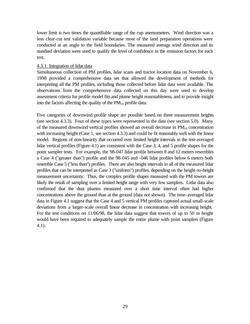
lower limit is two times the quantifiable range of the cup anemometers. Wind direction was a less clear-cut test validation variable because most of the land preparation operations were conducted at an angle to the field boundaries. The measured average wind direction and its standard deviation were used to qualify the level of confidence in the emission factors for each test.

4.3.1 Integration of lidar data Simultaneous collection of PM profiles, lidar scans and tractor location data on November 6, 1998 provided a comprehensive data set that allowed the development of methods for interpreting all the PM profiles, including those collected before lidar data were available. The observations from the comprehensive data collected on this day were used to develop assessment criteria for profile model fits and plume height reasonableness, and to provide insight into the factors affecting the quality of the PM10 profile data.

Five categories of downwind profile shape are possible based on three measurement heights (see section 4.3.3). Four of these types were represented in the data (see section 5.0). Many of the measured downwind vertical profiles showed an overall decrease in PM10 concentration with increasing height (Case 1, see section 4.3.3) and could be fit reasonably well with the linear model. Regions of non-linearity that occurred over limited height intervals in the test-averaged lidar vertical profiles (Figure 4.1) are consistent with the Case 3, 4, and 5 profile shapes for the point sampler tests. For example, the 98-047 lidar profile between 8 and 12 meters resembles a Case 4 ("greater than") profile and the 98-045 and -046 lidar profiles below 6 meters both resemble Case 5 ("less than") profiles. There are also height intervals in all of the measured lidar profiles that can be interpreted as Case 3 ("uniform") profiles, depending on the height-to-height measurement uncertainty. Thus, the complex profile shapes measured with the PM towers are likely the result of sampling over a limited height range with very few samplers. Lidar data also confirmed that the dust plumes measured over a short time interval often had higher concentrations above the ground than at the ground (data not shown). The time-averaged lidar data in Figure 4.1 suggest that the Case 4 and 5 vertical PM profiles captured actual small-scale deviations from a larger-scale overall linear decrease in concentration with increasing height. For the test conditions on 11/06/98, the lidar data suggest that towers of up to 50 m height would have been required to adequately sample the entire plume with point samplers (Figure 4.1).

29

6• 0 '

Q ~ D

I ---0------­~ _._ ----0-----+---0-~

Lidar vertical profiles for PM tests 06 Nov 98 08:20 - 12:47

Hei

ght (

m)

50

40

30

20

10

0.0 1.0x108

2.0x108

3.0x108

4.0x108

5.0x108

6.0x108

98-049 1137-1247 3.54-4.62 m/s

98-047 1015-1040 1.69-2.17 m/s 98-046

0929-1015 1.91-2.34 m/s

98-045 0820-0921 1.71-2.07 m/s

open symbols = background atmosphere closed symbols = PM plume 98-045

98-046 98-047 98-049

Average Lidar Signal (arbitrary units)

Figure 4.1 Lidar vertical profiles for PM tests 06 Nov 1998.

Maximum plume heights determined for individual lidar vertical scans (collected over a < 30 sec period) showed significant variability over the duration of a single PM test, but test-to-test variability in the averaged plume heights was smaller and comparable to the heights determined by fitting the point sampler vertical profiles to the line, block and log models (Figure 4.2). The test-averaged plume heights over only those range locations where the point sampler towers were located (Figure 4.1), agreed fairly well with the average heights from all ranges during a test period (Figure 4.2, compare open and closed bars). This indicates that, on average, the plume monitored at a specific location on the downwind edge of the field had the same height, within measurement uncertainty, as the plume over the entire crosswind length of the tractor pass.

For the lidar vertical profiles based on data only from the tower ranges (Figure 4.1), lidar field-of-view effects (see Section 3.7) could partly explain the significantly lower plume heights quantified for test 98-049 (Figure 4.1) because the tower was located only 180m from the lidar during this test whereas it was over 500 m from the lidar for the other three tests. However, the

30

agreement between the lidar height and the best-fit heights for all three point sampler models (Figure 4.2) suggest that field-of-view effects were not significant for this test and the smaller plume height measured by the lidar was real. A more likely explanation for the decrease in plume height during test 98-049 was the higher wind speed during this test (3.5 – 4.6 m/s) compared to the tests earlier in the day (1.7 – 2.3 m/s). The decrease in the lidar signal background in Figure 4.1 with time of day was likely due to relative humidity effects on the lidar response. The measured test period average (s.d.) relative humidity (%) values were 63.7 (3.2), 52.3 (1.7), 49.1 (0.8), 43.8 (0.8) for tests 98-045, 98-046, 98-047, 98-049, respectively. Thus, as relative humidity decreased, the lidar background signal decreased, as expected.

Average Plume Heights: Lidar vs. Point Sampler Estimates

100

80

60

40

20

0

-20

-40

-60

98-045R 98-045L 98-046R 98-046L 98-046M 98-047R 98-049

PM Test ID

Lidar test average (all ranges) PM line PM block PM log LidarProfileAtTower

>1000

Case 1 Case 4 Case 1Case 4Case 5Case 3Case 5

□

□

□

□ Iii

Hei

gh

t (m

)

Figure 4.2 Average plume heights: Lidar vs. point sampler estimates.

4.3.2 Plume Height and Uncertainty Calculations Functional fits to the vertical profiles of PM10 concentration were used to calculate the average heights of the plumes sampled from the harvest and land preparation operations for row crops and the dairies and feedlots and the most appropriate functional fits to each downwind profile type was determined. Three different methods – the line, block and logarithmic profile models – were used to fit the PM10 vertical concentration profiles. The height at which the best-fit function of the downwind concentration profile intersected the average upwind concentration was the calculated plume height, H. A fourth model, the box model was used to describe the PM10 flux in cases of uniform downwind vertical concentration profiles (see above).

31

Uncertainties in the modeled plume heights were estimated using error propagation techniques (Coleman and Steele 1989). Standard errors on the slope and intercept of the model fits to the downwind concentration profiles and the standard deviation in the upwind concentration measurements were used to propagate errors for the plume height estimate. The uncertainty calculations are described in Appendix H. The reported uncertainties do not take into account the uncertainty in individual upwind RCMA concentration measurements.

4.3.3 Emission Factor Calculations PM10 emission factors for agricultural operations such as tilling and harvesting are logically quantified on the basis of the area of land worked because the source being quantified is the field where the operation takes place, not the moving tractor/implement. Emission factors for confined animal production facilities were also calculated on this basis. Vertical profiles of wind speed and PM10 RCMA concentration were used to calculate emission factors for all of the agricultural operations. Because gravimetric mass was consistently well correlated with the “reconstructed mass” composite variable (RCMA) and the elemental analyses were sufficiently more sensitive than the gravimetric measurements (see section 3.3), all emission factors were calculated from PM10 RCMA concentrations. When the RCMA mass concentration was below the MDL at any of the three sampling heights, emission factors were not calculated for that test.

Each downwind PM10 profile was classified according to its shape into one of 5 types: Case 1 – decreasing PM10 with height (“decline”); Case 2 – increasing PM10 with height (“incline”); Case 3 – uniform PM10 with height (“uniform”); Case 4 – 3 m concentration highest (“greater than”); Case 5 – 3 m concentration lowest (“less than”).

Three different methods – the line, block and logarithmic profile models – were used to fit the PM10 RCMA vertical concentration profiles as described previously (see section 4.2). A fourth model, the box model, was used to describe the PM10 flux in cases of uniform downwind vertical concentration profiles. The choice of the appropriate model for each downwind concentration profile type was based on analysis of simultaneous lidar data collected during some of the field tests ([Holmén, 2000 #39]– Appendix H).

For each model, a horizontal PM10 flux was calculated as the product of the net (i.e., downwind – upwind) PM10 concentration [mg m-3], C(h), and the average horizontal wind speed [m s-1], U(h), at ten equally spaced height intervals [m], dh, between zo and the top of the plume, H. The plume height was defined by the intersection of the downwind profiles with the average upwind concentration (as in section 4.2). The flux was integrated over the height of the plume using Simpson’s Rule, and normalized by the time of the test, t, the upwind width of soil worked during the test period, w, and the angle between the measured wind direction and the direction perpendicular to the field edge, θ , to compute the PM10 emission factor [mg m-2]:

H U h C h t( ) ( ) cosθE = ∫ dh (4.2)

w z0

32

Considering the field illustrated in figure 4.3, the integration in equation 3 can be simplified by moving all variables not dependent on h out of the integral and computing the flux first. Thus, the product of mass concentration, in mass per unit volume, and wind speed, in units of length in the y direction per time, is integrated over z (out of the plane of the page) to yield flux in mass per unit length in the x direction per time. This product can then be multiplied by the total time of the test period and the inverse of the length in the y direction covered during the test, normalized for wind direction deviation from perpendicular, to give the emission factor in mass per unit area where the lengths in the area are in the x and y directions. One should note that the cos θ is dimensionless.

Uncertainties in the calculated emission factors were estimated using error propagation techniques (Coleman and Steele 1989) for the line, block and logarithmic fit models. The PM10

RCMA measurement uncertainties and the test period wind speed standard deviation at each measurement height were used to estimate the uncertainty in the horizontal flux at each of the ten model heights. Details about the uncertainty calculations are in Appendix H.

Wind

q

+Y

+X

Figure 4.3: Illustration of emission factor calculation parameters. The X-axis is the direction of tractor travel and the Y-axis represents the width of the field (W, in equation 3) treated during the test period. The wind direction vector is at approximately the limit of acceptance of 45 degrees from perpendicular to the X-axis.

Emission factors for the PM10 from dairies and feedlots were reduced further to the units of lbs (PM10) * d-1 * 1000head-1. This was accomplished by dividing each emission factor (mg (PM10) * m-2) by the duration of each test individually, multiplying by the area of the facility (m2) and dividing by the number of animals. Measurements of the feedlot for the purposes of applying the box model did not provide an accurate estimate of the area occupied by the animals, since it included feed-handling facilities, roads, and other areas. Since the number of animals on the feedlot during each sampling period is well known, a normative stocking density of 150 ft2 * head-1 was assumed in estimating the populated area of the feedlot for this calculation.

33

Conversely, the area of the dairy was much better defined by our measurements, while the number of animals was less well known. For these reasons, a compilation of the areas of all of the corrals was used in the calculation as the area of the facility and the approximate number of 2000 head was derived from the owner’s statement that he was milking 1000 cows.

4.3.4 Emission Factor Confidence Rating Each calculated emission factor was assigned an overall test rating based on five qualifiers that attempt to assess the ability of the emission factor estimate to quantify the actual nonpoint source emissions. The overall test ratings ranged from A to E- and were designed to account for a decreased reliability in the computed emission factor when: the upwind concentrations were equal to or exceeded the downwind concentrations at any height (Qup); the wind direction deviated from ideal (Qwd); the test suffered from multiple passes due to edge effects (Qedge); the fit to Case 5 profiles was poor (Qfit); or emission factor relative uncertainty (EFU) was high. Each of these qualifiers is described in Table 4.2 and was based on observations made for all tests.

34

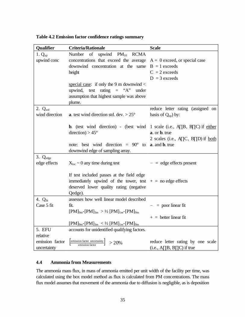
Table 4.2 Emission factor confidence ratings summary

Qualifier Criteria/Rationale Scale 1. Qup

upwind conc Number of upwind PM10 RCMA concentrations that exceed the average downwind concentration at the same height

special case: if only the 9 m downwind < upwind, test rating = “A” under assumption that highest sample was above plume.

A = 0 exceed, or special case B = 1 exceeds C = 2 exceeds D = 3 exceeds

2. Qwd

wind direction a. test wind direction std. dev. > 25°

b. (test wind direction) - (best wind direction) > 45°

note: best wind direction = 90° to downwind edge of sampling array.

reduce letter rating (assigned on basis of Qup) by:

1 scale (i.e., AÕB, BÕC) if either a. or b. true 2 scales (i.e., AÕC, BÕD) if both a. and b. true

3. Qedge

edge effects Xloc ~ 0 any time during test

If test included passes at the field edge immediately upwind of the tower, test deserved lower quality rating (negative Qedge).

- = edge effects present

+ = no edge effects

4. Qfit

Case 5 fit assesses how well linear model described fit. [PM]9m-[PM]3m > ½ [PM]1m-[PM]9m

[PM]9m-[PM]3m < ½ [PM]1m-[PM]9m

- = poor linear fit

+ = better linear fit

5. EFU relative emission factor uncertainty

accounts for unidentified qualifying factors.

emission factor uncertainty[ ] > 20%emission factor reduce letter rating by one scale (i.e., AÕB, BÕC) if true

4.4 Ammonia from Measurements

The ammonia mass flux, in mass of ammonia emitted per unit width of the facility per time, was calculated using the box model method as flux is calculated from PM concentrations. The mass flux model assumes that movement of the ammonia due to diffusion is negligible, as is deposition

35

----

or chemical transformation within the vicinity of the source. The general box model calculation solves the following equation (4.3), where the left-hand side is integrated over the measurement heights and the right-hand side incorporates the width of the facility for calculation of emission factors.

l

iåCi ´Vi ´ cos( )θ ´ DZ = E ´w (4.3) i=1

where Ci = Concentration (mass/volume) at height i, Vi = wind speed (length/time) at height i, q = wind direction angle from perpendicular to the facility *Zi = height (length) of layer i, E = Emission flux (mass/area), and w = width of facility (length)

The emission factor is then computed as the mass of ammonia per animal per unit time, using equation (4.5):

1F = E ´ W´ . (4.5)N

where F = Emission factor (mass/head * time), and N = number of animals

In our application of equation (4.4) we defined 10 height intervals between the surface roughness height and the top of the plume. We then computed ammonia concentrations and wind speeds for each height. The surface roughness height (i = 1 in eq. (4.4)) was obtained by calculating the point above ground where the logarithmic wind speed profile projected to zero. A logarithmic fit was made to the wind speed to facilitate calculation of wind speed for each layer i in the data sets from all of the field trials. The methods used to compute the concentrations and heights at each layer in the summation from the measurements of ammonia air concentration and wind speed evolved as a response to the differences in the physical deployment of the samplers for each field trial.

The calculations of ammonia concentration for each layer i were made using the two methods described above (see section 4.2). For the data collected in 1996 a linear relationship between the two measured concentrations and the natural log of the height provided a slope and intercept used to compute the height at which the downwind concentration equaled the upwind concentration (i = l, eq. (4)). For the data collected in 1997, a similar method was applied to more than two measured concentrations, fitting a series of linear curves to the concentration profile in a block form. This form assumes that from the roughness height to the first measured point, the concentration is constant at the first measured value. Between all the measured points, the concentration is interpolated from the measurements. The top of the plume is defined by extrapolating the valid measured concentration at the greatest height to the upwind concentration. Our 1999 field trial produced concentration measurements at 3 heights, allowing for the use of both methods. We used either a logarithmic or linear function to fit the measured concentrations with height depending on which provided the better fit. We found that logarithmic

36

fits were more appropriate for measurements of higher concentrations, and linear fits were better for lower concentrations.

We have used several methods to incorporate the variability in the rates of emission from different regions of the facilities into our estimate of the overall emission rate. Measurements made using the passive filter packs placed at 50 - 100 meter intervals along the downwind edge of the dairy in 1996 were averaged and divided by the concentration measured by active samplers at the same height on the vertical profile. The resulting ratio was used to normalize the ammonia air concentrations measured at both heights on the profile for incorporation into the mass flux model. Two vertical profiles were used at the feedlot in summer of 1996, such that independently computed emission rates were averaged for an estimate of the facility-wide emission rate. In analyzing the 1997 data we computed the ammonia mass flux at the point of the vertical measurements then scaled that value to the measurements made using the passive filter packs at approximately 90 meter intervals along the downwind edge of the dairy. The resulting scaled fluxes were integrated again over the downwind width of the dairy. The data from the 1999 field trials was reduced in much the same way as that used in 1997, except that up to three emission flux estimates based on vertical profiles were calculated. The larger number of directly calculated emission flux measurements were well correlated with the wind speed corrected concentrations measured at single heights. This relationship defined the effective height of the ammonia plume, assuming concentration constant with height, for application of the box model to calculate emission flux at each measurement location. These fluxes were then integrated over the width of the facility to compute an overall ammonia flux.

Because the box model method of computing mass flux relies on the wind to carry the ammonia to the locations for measurement, measurements made under conditions of unstable or inappropriate wind direction were not used to compute emission rates. A reliable measurement period was defined as one in which the average wind direction was within the arc described by radians drawn from the measurement location to the upwind corners of the facility. This criteria was applied to data collected in all of the field trials. Also, the capacity of the impregnated active filters (@ 400 mg/filter) was exceeded in many of the measurements at the feedlot during the first field trial. Emission factors were not calculated when the primary filter of the 7 meter measurement exceeded capacity.

4.5 Ammonia from dietary nitrogen balance

The methods we used to estimate emission rates from animal management parameters were based on estimates of nitrogen excretion and ammonia volatilization as a percent of nitrogen excreted. Experimental nitrogen excretion data for dairy calves and cows were used to estimate the ammonia emissions at the dairy in the 1996 field trial (Morse and DePeters 1996). In this application, we used a nitrogen excretion factor for yearling heifers equal to the average of the values for calves and cows. For the feedlot in the 1996 field trial, the nitrogen excretion rates were estimated from dietary and animal performance data, as described by Meyer et al. (Meyer, Ashbaugh et al. 1997) Two groups of cattle were fed different diets, according to body

37

weight. The weight of cattle entering each group and the rate of gain realized by the animals were used with the protein content of the diets to estimate nitrogen intake, accretion, and excretion from standard table values (National Research Council 1988).

The dairies on which our 1999 field trial was conducted were very cooperative in providing dietary, animal weight, and milk production data for each of the feeding groups on their facilities. We used a combination of standard table values (National Research Council 1988) and values provided by the producers to estimate dry matter intake based on the weight of the cattle. Diet formulations were used to calculate nitrogen intake from dry matter intake and animal weight data were used to estimate nitrogen retention for each feeding group. Milk production data, both for quantity and protein content, were used to estimate milk nitrogen removed from the farm. Nitrogen excretion was calculated as the difference between nitrogen intake and the sum of nitrogen retention and excretion in milk.

Emission factors were estimated based on both 50% and 70% manure nitrogen volatilized as ammonia for data collected in the first field trial. Subsequently, we determined the percent of manure nitrogen volatilized as ammonia through a series of feeding and laboratory experiments (James, Meyer et al. 1999). So for the data collected during the third field trial, we estimated ammonia emission rates separately for calves, heifers, and milking cows using these experimentally derived volatilization rates, then summed them for a facility-wide emission factor.

38

5 RESULTS FROM FIELD MEASUREMENTS

Results in this section are divided by source and presented chronologically. Tables 5.2 and 5.8 and the text at the end of section 5.2.2 are the result of our initial development of the vertical profiling method of calculating emission factors from data collected at multiple heights. Work done at that time only assessed 3 models, the box, the block, and the logarithmic. Starting with section 5.1.2, the methods developed for the Atmospheric Environment manuscripts (see Appendix H) and explained therein were used to re-calculate emission factors from all of the data collected from 1995 through 1998 under sampling conditions comparable to the recently established protocols. All data collected under other sampling conditions were not reported in these subsequent sections. Those calculation methods include 4 models, adding a linear method to the original 3 models. The much larger data set and new knowledge contributed by the lidar allowed a much more definitive assessment of which conditions favored which models and how to use the models together as complementary tools, rather than defining one model as best for all circumstances.

The results of a series of six comprehensive tests conducted during disking when a full complement of ancillary data (lidar, laser rangefinder) were collected were used to develop a framework for analyzing all of the upwind-downwind point PM10 concentration profiles measured during this project and identify conditions under which the field sampling strategies affect the reproducibility of PM10 concentration measurements. Results of recently developed lidar data reduction techniques were used to verify that the shapes of the plumes measured as three-point PM10 vertical profiles were representative of the average plumes recorded during the sampling period. From this assessment, a best-fit function for quantifying plume height and emissions was identified for each category of vertical profiles observed in the PM10 data. These observations based on comparisons of lidar and point sampler data were used to develop an emission factor quality rating system.

The computation and rating of PM10 emission factors using this framework is restricted to those profiles for which three valid measurements of concentration were collected. Additionally, application of this method requires simultaneously collected wind speed measurements representative of the meteorological conditions at the tower where the PM10 concentrations were measured. Because of these requirements, all of the samples collected in 1994 and all of the measurements of PM2.5 are insufficient for emission factor calculation by these protocols, as they lack three measurement heights. Similarly, many tests conducted in early 1995 lacked multiple height wind speed data or, in the case of many almond tests, wind speed measurements were not made under the same conditions as PM10 concentrations. However, estimates of PM10

emission factors calculated from these data are still of interest. Emission factors computed using earlier methods (see sections 4.1 and 4.2) are compiled here along with other assessments of data that do not fit the model for emission factor analysis derived from the lidar and PM10

concentration profile comparisons. The recently calculated best fit emission factors follow the earlier work in each of the source category sections.

39

Comparison of the average plume heights and vertical profile shapes determined by lidar to the profiles measured with the point samplers on 11/06/98 led to assignment of particular best-fit models to the PM10 profiles for each of the four observed profile shape categories (see section 4.3.3). Although there were some tests that were difficult to categorize, overall the model selected for each category tended to have the lowest calculated uncertainties for both plume height and emission factor. However, the large number of Case 4 and 5 profiles suggests that many plumes were not fully characterized by the three sampling heights. The spatial resolution and wide vertical scanning range of the lidar data on 11/06/98 confirmed that both local maxima and minima occurred in the overall plume profile, but the limited point sampler heights can bias the overall plume shape interpretation for plumes that are highly irregular or very tall (i.e., greater than highest point sampler height).

The calculated emission factors (and uncertainties) for all models are shown in Tables 5.3, 5.9, 5.11, 5.13, 5.15, 5.17, 5.19, and 5.21 for comparison; the bold type values represent the best-fit model plume height and emission factor values for each profile type. As the test results indicate, there was general agreement in the emission factors computed by the different functional fits to the profiles for an individual test when all four models could be calculated (Cases 1, 4 and 5). Thus, the magnitude of the computed emission factors was not biased by the selection of the best-fit model.

40

5.1 Orchard Crops

Sampling of PM was conducted upwind and downwind of operations in orchard crops in 1994, 1995, and 1998. Crops characterized in 1994 included almonds and a survey of figs and walnuts (Table 2.1). Almond harvesting operations were again monitored in 1995 and 1998. Emission rates were calculated from PM10 and PM2.5 measurements made in 1994 using the simple box model. This model does not require the characterization of the vertical wind speed profile, but uses the wind speed measured at 3 m to compute the PM flux (see section 4.1). Single height wind speed data was collected in 1994 (Table 2.2). Additionally, most of the PM and meteorological data collected in 1994 were measurements outside of the orchards (PM concentrations entering and leaving the orchards at the perimeters). Appendix A includes a summary of all 1994 field tests.

The emission factors for fig harvest operations are low compared to other operations tested. Combined with the small amount of acreage in the San Joaquin Valley, the net emissions from fig harvesting are minor. It should be noted that we have only tested fig harvest operations on one ranch and one soil type; other harvesting practices and soil types may lead to different emission factors than those measured. We have no valid walnut data. The 3 good tests collected in 1994 (see Appendix A) were of 2 simultaneous operations which could not be quantified separately using these data.

5.1.1 1994 Field Tests An effective method for assessing the PM10 emission potential of operations within an orchard canopy without calculating emission factors compares the horizontal distribution of PM10

concentrations. Figure 5.1, Figure 5.2, and Figure 5.3 show typical horizontal distributions of PM10 aerosols at 3 meters height downwind of orchards with clay and silt soil textures. Figures 5.1 through 5.4 illustrate the possibility of a relationship between PM10 transport distance and soil texture. Other variables such as wind speed, temperature, and relative humidity may have also played a role in producing the observed differences in the ground level extent of the dust plume. Although meteorological data were collected for these tests, the database to incorporate them with the PM data was not developed yet in 1994. A more complete hypothesis of the impact of soil texture on dust emissions is a fundamental aspect of the research quantifying PM10 potential (section 7).

41

PM

10 C

on

c. (

ug

/m**

3)

0

20

40

60

80

100

Silt

Clay

---0--

Almond Shaking

0 100 200 300-20

Downwind Distance (m)

Figure 5.1 Example of the PM 10 horizontal distribution downwind of an almond harvest tree shaking operation for silt and clay soil textures.

42

Almond Sweeping P

M10

Co

nc.

(u

g/m

**3)

600

500

400

300

200

100

0 0 100 200 300

Downwind Distance (m)

-■-

---0--

Silt

Clay

Figure 5.2 Example of the PM 10 horizontal distribution downwind of an almond harvest sweeping (windrowing) operation for silt and clay soil textures.

Almond Pickup

PM

10 C

onc.

(ug

/m**

3) 1400 1200 1000

800 600 400 200

0

Silt

Clay

0 50 100 150 200 250

Downwind Distance (m)

Figure 5.3 Example of the PM10 horizontal distribution downwind of an almond harvest, nut pickup operation for silt and clay soil textures.

Some of the vertical profiles of aerosols collected during 1994 field tests were above detectable limits for total suspended particulate matter. An example of the vertical distribution of aerosols is illustrated in Figure 5.4. In this example, the fine aerosols are relatively uniform by height while the coarse aerosols show a pronounced vertical gradient. An absence of profiles of PM10 led us to calculate emission factors from 1994 data using the simple box model.

43

--■--

---0--

■----■----■----■

Test 95, Fig Harvest-Pickup

80 io

n

70

trat 60

en 50 PM2.5

Con

c(u

g/m

**3)

40 30 Coarse

Mas

s 20 10

0 0 5 10

Height (m)

Figure 5.4 Vertical distribution of aerosols from vertical profile tower.

Calculation of emission factors using the simple box model yielded the following results. The average PM10 emission factors for the fig harvest operations were 13±8 kg/km2 for the sweeping operation and 39±4 kg/km2 for the pickup. This is significantly lower than the emission factors obtained for almond harvesting. Table 5.1 compares the emission factors measured from fig harvesting to those measured from almond harvesting. Part of the reason for the lower emission factors from fig harvesting is the lack of blower use in sweeping figs. It is not clear why the pickup operation for figs is low compared to that for almonds, although there was some rain before the fig pickup operation and the soil moisture was slightly higher than for almonds. Figure 5.5 and Figure 5.6 show the PM10 and PM2.5 emission factors for fig harvest in comparison to other agricultural operations tested. Note that the vertical scale is logarithmic, which exaggerates the smaller emission factors relative to the larger ones.

Table 5.1 Comparison of fig harvest to almond harvest emission factors (kg/km4)

Operation Fig Harvest Almond Harvest PM10 PM2.5 PM10 PM2.5

Shaking N/A N/A 15 --Sweeping 13 ± 8 2 ± 2 197 ± 155 24 ± 14 1st Pickup 39 ± 4 5 ± 2 1438 ± 395 170 ± 78 2nd Pickup N/A N/A 1840 ± 1810 179 ± 175

44

I

I -

I

I ~ -

I I I I I I

I I I I I I I

Figure 5.6 PM2.5 emission factors for eight agricultural operations

5.1.2 1995 Field Tests Almond harvesting was, chronologically, the first operation tested in 1995 and our profiling methods were developed during that field sampling campaign. Consequently, many of those tests were conducted with vertical profiles of either wind speed or PM concentrations, but not both. Or, wind speed and PM concentrations were not both measured under the same

45

PM

10 E

mis

sion

Fac

tor

(kg/

sq k

m)

PM

2.5

Em

issi

on F

acto

r (k

g/sq

km

)

10000

1000

100

10

1

1000

100

10

1

Figure 5.5 PM10 emission factors for eight agricultural operations

10000

Fig

Swee

ping

Fi

g Pi

ckup

Fig

Pick

up

Cot

ton

Pick

ing

Cot

ton

Pick

ing

Cot

ton

Stal

k C

uttin

gC

otto

n St

alk

Cut

ting

Alm

ond

Shak

ing

Alm

ond

Shak

ing

Alm

ond

Swee

ping

Alm

ond

Swee

ping

1s

t Alm

ond

Pick

up

1st A

lmon

dPi

ckup

2n

d A

lmon

d Pi

ckup

2nd

Alm

ond

Pick

up

Fig

Swee

ping

conditions with regard to being either within or outside of the tree canopy. It is vitally important that the wind speed measurements describe the exact wind field that carries the PM being sampled. Otherwise, it is meaningless to describe the PM flux as the product of a wind profile that is spatially unrelated to the PM profile. This fact did not become apparent until the detailed investigation conducted in 1998 to compare almond pick-up implements (see section 5.1.3).

Emission factors were initially calculated from the 1995 almond harvesting tests using all of the valid data, regardless of the position of the instruments with respect to the canopy. These preliminary data (Table 5.2) illustrate the relative importance of the almond harvest operations as PM10 sources both among the three almond operations and by comparison with cotton harvesting.

Table 5.2 PM10 emission factors (kg/km4) by three calculation methods

Log Integration Block Integration Simple Box Model

Almond Shaking 1670±1303 (4) 1647±1074 (4) 823±558 (4)

Almond Sweeping 1466±1042 (2) 1935±1403 (2) 1087±631 (2)

Almond Nut Pickup 4467±5830 (7) 3233±1956 (7) 1201±647 (8)

Measurements of PM10 concentration and wind speed profiles made in 1995 were reviewed to select only those tests in which both the PM10 and the wind speed were measured in the same wind field. These results provide emission factors that are most directly interpretable to quantification of the PM10 leaving the perimeter of an almond orchard (Table 5.3). Emission factor uncertainties have not been calculated for measurements made in 1995.

Table 5.3 PM10 emission factors for almond pick-up tests during which both PM10 and wind speed were measured outside of the canopy.

TestID date time of test Xloc (m) Upwind RCMA (ug m-3)

9m 3m 1m Plume height (m)

Linear Block Log Emission Factor (mg m-2)

Linear Block Log Box case Qup Qwd Almonds

1155 to 87.33 169.7 1197.2 877.1 95-044 I1 9/9/95 1236 22 (38.78) (10.8) (65.5) (46.3) 10.57 9.54 5.32E+03 2841.39 1663.30 -6.18E+07 1995.09 4 A B

1155 to 87.33 203.5 525.3 1009.2 95-044 D1 9/9/95 1236 32 (38.78) (12.80) (31.1) (55.6) 9.92 11.34 1.54E+06 1995.09 924.96 -3.21E+10 2841.39 1 A B

1347 to 87.33 746.9 1165.4 367.9 95-046 D1 9/9/95 1447 44 (38.78) (42.7) (66.9) (22.2) -29.20 18.59 3.05E+00 1647.52 2365.12 3.96E+01 539.37 4 A B

0745 to 175.80 711.5 1317.2 1118.8 95-054 D1 9/13/95 0825 102 (80.33) (39.6) (76.0) (65.1) 19.49 15.03 1.85E+15 18806.94 5259.02 -4.35E+20 1812.52 4 A A

0825 to0 102.45 6.70 613.0 549.8 95-055 D1 9/13/95 855 144 (23.41) (1.10) (36.4) (33.8) 8.14 8.05 5.09E+03 978.55 431.37 -2.51E+07 457.45 4 A B

0700 to 218.87 130.4 1565.3 1761.7 95-060 D1 9/16/95 0740 38 (168.74) (8.6) (85.7) (98.0) 8.74 8.63 6.13E+04 9248.42 2870.09 -1.18E+09 1763.53 1 A A

Values in parentheses are uncertainties; NC = not calculated (unreasonable value). QUP = upwind qualifier; QWD = wind direction qualifier; Plume heights and emission factors in bold type are the best-fit figures based on profile shape (see section 4.3.3).

46

I I I I I I I I I I I I

Table 5.4 Environmental conditions during almond pick-up tests.

TestID

Wind RH

Date Op DIR* %

SolarRac Bulk

Watt/m2 Ri

Wind Speed (m/s) Temperature (deg C) %Soil

moist

%Silt

Content1m 2m 4m 7.5m 1m 2m 4m 7.5m

95-044

95-046

95-054

95-055

95-060

09/09/95 Pick-up 265.9 26.27

09/09/95 Pick-up 243.6 22.57

09/13/95 Pick-up 261.4 80.63

09/13/95 Pick-up 225.7 69.47

09/16/95 2nd Pick-up 245.4 68.37

858.333 -0.068

812.625 -0.036

227.929 -0.019

357.483 -0.043

44.538 -0.045

0.000 1.390 0.000 2.103 30.199 29.68 28.394 27.636

0.000 1.907 0.000 3.082 31.750 31.60 30.298 29.604

0.000 1.110 0.000 1.598 18.176 18.45 18.076 18.114

0.000 1.258 0.000 1.670 21.762 21.41 20.605 20.560

0.447 0.916 1.188 1.997 17.904 18.40 17.735 17.829

4.80 8.75

4.80 8.75

2.50 11.34

2.50 11.34

3.00 14.90

*best wind = 270°

5.1.3 1998 Field Tests A test was conducted in July 1998 to measure PM10 dust emissions under controlled conditions from older and newer models of the two major manufacturers of almond harvesting equipment. The tests identify the extent of reduced emissions that can be expected from replacing older harvesters with newer ones. The tests also identify differences in emissions that could result from management practices of the grower. The full text of the report is included in appendix B. Multiple simultaneous tests were conducted on older and newer model harvesters from Flory Industries and Weiss-McNair, Inc. and an older model Ramacher harvester to determine whether there is a difference between the older and newer designs. The harvesters will be referred to here only by code, not by manufacturer. Three sampling towers were used to collect replicate test data simultaneously (see section 3.1.2). The tests were conducted on two different orchards; one with solid-set and one with micro–spray irrigation. Each harvester was tested in a configuration that had the fan blower pointing toward the particle samplers during operation so that the dust plume was carried over the samplers as the harvester passed them. Two meteorological towers were used to collect wind speed and direction data. One was located outside the orchard; the other was located inside. The meteorological data were examined to confirm valid test conditions.

The tree canopy creates a much different environment inside the orchard than exists outside, so the outside meteorology is not representative of the conditions experienced at the samplers. It is useful to examine the outside meteorology for overall sampling conditions, but it can not be used to calculate emission fluxes. The almond harvesters create their own winds, too, so the meteorology within the canopy is strongly affected by the harvest activities. Each time a harvester passes the sampler, it creates strong winds that are not necessarily aligned with the natural air movement in the canopy. Furthermore, the natural wind profile in the canopy is not logarithmic with height as is normally the case in the outside environment. Instead, the tree structure modifies the winds; the highest wind speeds are found close to the ground where there are few leaves and branches to slow it. The slowest winds are found at canopy height, about 3-5 meters above ground. Above the tree canopy, the wind speeds typically increase logarithmically with height. These factors combine to make it impossible to calculate emission fluxes for the harvester tests. Instead, this report will focus on the PM10 mass concentrations for each harvester and field tested.

47

The PM10 mass was measured at three heights on three towers for each test. A complete set of tests included one with the harvester two tree rows from the towers picking up nuts on the outside of the harvested trees, one with the harvester three rows from the towers picking up from between the two rows of harvested trees, and one with the harvester four rows from the towers picking up nuts on the outside again. In Figure 5.7 the uncertainty bar represents the standard deviation of all measurements that were averaged for that figure.

Figure 5.7 shows a set of plots for harvesters 1 and 2 on both fields, and on each field separately. In Figure 5.7a it appears harvester 1 created higher PM10 concentrations than the older harvester 2. Upon closer inspection, though, this seems to be the case only on the micro– spray irrigated field, and only at 1m above the soil surface. This may be due to the way in which dust and trash is ejected from the machine and to the field management practiced on the micro– spray irrigated field. In any case, dust ejected closer to the ground should deposit sooner than dust ejected higher up. On the solid–set irrigated field the PM10 concentrations created by the newer harvester 1 were lower than those from the older harvester 2.

On both fields, the newer harvester 3 also shows lower PM10 concentrations than the older model. For this harvester, too, the PM10 concentrations from the micro–spray irrigated field were higher than for the solid–set irrigated field. The PM10 concentration profile for the newer harvester 3 is similar to that for harvesters 1 and 2. Harvester 5 produced much higher PM10

concentrations than the other two harvesters.

48

D D

D D

D

10

9 H

eig

ht

(m)

8

7

6

5

4

3

2

1

0

0 2000

Harvester Comparison Harvester: #1

4000 6000 8000 10000 PM10 (µ g/m3)

Left tower

Middle tower

Right tower

Upwind

12000 14000

10

9

8

7

6

5

4

3

2

1

0

0

Hei

gh

t (m

)

2000

Harvester Comparison Harvester: #2

4000 6000 8000 10000 PM10 (µ g/m3)

Left tower

Middle tower

Right tower

Upwind

12000 14000

(a)

Hei

gh

t (m

)

10

9

8

7

6

5

4

3

2

1

0

0 2000

Harvester Comparison Harvester: #1

Field: Solid Set Irrigation

4000 6000 8000 10000 PM10 (µ g/m3)

Left tower

Middle tower

Right tower

Upwind

12000 14000

10

9

8

7

6H

eig

ht

(m)

5

4

3

2

1

0

0 2000

Harvester Comparison Harvester: #2

Field: Solid Set Irrigation

4000 6000 8000 10000 PM10 (µ g/m3)

Left tower

Middle tower

Right tower

Upwind

12000 14000

(b)

Hei

gh

t (m

)

10

9

8

7

6

5

4

3

2

1

0

0 2000

Harvester Comparison Harvester: #1

Field: Micro Spray irrigation

4000 6000 8000 10000 PM10 (µ g/m3)

Left tower

Middle tower

Right tower

Upwind

12000 14000

Hei

gh

t (m

)

10

9

8

7

6

5

4

3

2

1

0

0 2000

Harvester Comparison Harvester: #2

Field: Micro Spray irrigation

4000 6000 8000 10000 PM10 (µ g/m3)

Left tower

Middle tower

Right tower

Upwind

12000 14000

(c)

Figure 5.7 PM10 concentrations downwind of harvester #1 and #2, (a) all tests, (b) solid–set irrigation, (c) micro–spray irrigation.

49

The PM10 mass measurements from each tower were averaged to obtain mean PM10

concentrations by height for each harvester test. Each average vertical PM10 profile was then integrated from 1m to 9m using Simpson’s Rule to obtain an average PM10 concentration for the dust plume. The most appropriate way to compare the performance of the harvesters is to examine the PM10 concentrations normalized to the amount of windrow trash that passed through a 2mm screen. The results of this calculation are shown in Table 5.5. For the solid–set irrigated field, the newer harvester #2 showed overall lower concentrations than the older harvester #1 relative to the amount of windrow trash, but it showed higher concentrations for the micro–spray irrigated field. The newer harvester #4 showed decreases over the older harvester #3 in both fields, though the decrease was larger for the solid–set irrigated field than for the micro–spray irrigated field. The overall change in PM10 concentrations for both fields combined, normalized to the amount of windrow trash, ranged from +32% to -35%.

Table 5.5 PM10 concentrations normalized to amount of windrow trash <2mm prior to harvest (µg/m4/g)

Harvester 1 2 % 3 4 % 5

Difference Difference Solid–Set 4.1 2.4 -42% 12.1 4.7 -61% 9.8 Near 2.5 2.3 -9% 30.8 2.8 -91% 7.6 Middle 0.5 2.5 368% 8.6 3.9 -55% 24.1 Far 25.6 1.5 -94% 10.0 5.9 -40% 8.1 Micro–Spray 3.8 6.7 76% 5.5 3.5 -37% 12.1 Near 4.6 5.2 13% 6.3 1.7 -73% 16.2 Middle 2.6 6.1 130% 4.6 3.7 -20% 13.4 Far 4.2 8.4 101% 5.7 4.9 -14% 7.2 Both fields 4.1 5.4 32% 7.4 4.8 -35% 11.4 Near 3.4 3.8 13% 8.8 1.8 -79% 12.4 Middle 2.0 4.1 103% 6.1 5.1 -17% 16.1 Far 7.6 8.8 16% 7.9 6.6 -16% 7.6

Overall, for both fields combined, both new harvesters (#2 and #4) showed very similar PM10

concentrations relative to the amount of windrow trash. The newer harvester #2 showed better results on the solid–set irrigated field, while the newer harvester #4 showed better results on the micro–spray irrigated field. It is not possible to recommend one brand of harvester over the other. Harvester #5, on the other hand, showed 2-4 times the PM10 concentrations, relative to the amount of windrow trash, as the other two brands.

50

5.2 Cotton Harvest

5.2.1 1994 Field Tests Table 5.6 lists emission rate results for the valid cotton harvest tests conducted in 1994. These data are also shown in Figure 5.8. Emission rates calculated from data collected in 1994 were calculated using the simple box model (see section 4.1).

Table 5.6 PM10 emission rates from cotton operations, 1994

Test No. Implement used Soil Type Operation PM10 Emission Rate

(kg/km2) 94-049 Deere 9950 4-row pickers Clay, silt 1st Picking 79 ± 31 94-050 Deere 9950 4-row pickers Clay, silt 1st Picking 29 ± 9 94-068 2-row and 4-row pickers Clay 1st Picking 65 ± 20 94-069 2-row and 4-row pickers Clay 1st Picking 49 ± 15 94-070 2-row and 4-row pickers Clay 1st Picking 34 ± 10 94-079 Deere 9950 4-row pickers Clay 1st Picking 32 ± 12 94-087 Deere 5-row pickers Clay 1st Picking 42 ± 12 94-088 Deere 5-row pickers Clay 1st Picking 22 ± 7 94-089 Deere 5-row pickers Clay 1st Picking 42 ± 18 94-083 Alloway Ram 9-row flail shredder Clay Stalk Cutting 34 ± 12 94-084 Alloway Ram 9-row flail shredder Clay Stalk Cutting 16 ± 7 94-091 Rhino RC20 shredder Clay Stalk Cutting 106 ± 44 94-092 Rhino RC20 shredder Clay Stalk Cutting 118 ± 49 94-093 Rhino RC20 shredder Clay Stalk Cutting 165 ± 49

51

PM

10 E

mis

sion

Rat

e (k

g/sq

km

)

0

50

100

150

200

Dee

re 9

950

4-ro

w p

icke

rs

Dee

re 9

950

4-ro

w p

icke

rs

2-ro

w a

nd 4

-ro

w p

icke

rs

2-ro

w a

nd 4

-ro

w p

icke

rs

2-ro

w a

nd 4

-ro

w p

icke

rs

Dee

re 9

950

4-ro

w p

icke

rs

Dee

re 5

-row

pick

ers

Dee

re 5

-row

pick

ers

Dee

re 5

-row

pick

ers

Allo

way

Ram

9-

row

flai

lsh

redd

erA

llow

ay R

am 9

-ro

w fl

ail

shre

dder

Rhi

no R

C20

shre

dder

Rhi

no R

C20

shre

dder

Rhi

no R

C20

shre

dder

Figure 5.8 PM10 emission rates from cotton operations, 1994

The data in Figure 5.8 and Table 5.6 indicate that the PM10 emissions from cotton picking operations were fairly consistent from test to test. The emissions from stalk cutting operations were much more variable, and averaged about twice the emissions from picking. The Rhino RC20 shredder operating on clayey soils showed higher emission rates than the Alloway Ram shredder on clayey soils. These differences between equipment manufacturers may be real, or they may result from test conditions. Note that the two Alloway Ram Flail Shredder tests were conducted at over 100 meters downwind of the operation. The Rhino shredder tests were conducted less than 20 meters downwind of the operation. This may be the cause of the difference between the shredder tests. There were, however, too few valid tests of stalk shredding in this data set to draw any conclusions about equipment.

5.2.2 Assessment of simple box model emission factor calculations using 1995 Field Tests Emission rates, presented in Figure 5.9, Figure 5.10, and Figure 5.11 for cotton picking, stalk cutting, and stalk incorporation, respectively, were calculated using the simple box model from concentrations and wind speeds measured at a single height as described above (see section 4.1). Figure 5.9 shows the emission rates from picking tests conducted in 1995. The symbol shows the mean distance between the picking operation and the first downwind sampler. There seems to be a relationship between the distance and the emission rate; this relationship could be caused by application of the simple box model calculation method to PM10 concentrations measured at a single height. Single height measurements result in sampling different portions fo the plumes that vary in xize and concentration with distance from the implement. Further, the

52

-

-- ->-- - - -. .

n-nt- >-- - - i, - - -11!!1

11::1 g ,,. t:I r-,

emission rates are higher than those found in 1994; when measurements were made further from the operation. They averaged 114±100 kg/km2 in 1995, but only 44±18 kg/km2 in 1994.

Figure 5.9 PM10 emission factor for 1995 cotton picking tests

Figure 5.10 shows the emission rates from stalk shredding tests conducted in 1995. The relationship between emission rate and downwind distance of the measurement is not as apparent as for the picking tests, but there is a wide variation between individual tests. The rates for this operation were also higher than for 1994 tests; they averaged 141±152 kg/km2 in 1995, but 90±64 kg/km2 in 1994.

Figure 5.10 PM10 emission factor for 1995 cotton stalk shredding tests

Rhi

no M

-131

0 4-

row

Rot

ary

Rhi

no M

-131

0 4-

row

Rot

ary

Ci7

220

6-ro

w F

lail

Ci7

220

6-ro

w F

lail

Ci7

220

6-ro

w F

lail

Ci7

220

6-ro

w F

lail

Ci7

220

6-ro

w F

lail

Ci7

220

6-ro

w F

lail

Ci7

220

6-ro

w F

lail

Ci7

220

6-ro

w F

lail

Ci7

220

6-ro

w F

lail

Ci7

220

6-ro

w F

lail

Ci7

220

6-ro

w F

lail

Ci7

220

6-ro

w F

lail

Ci7

220

6-ro

w F

lail

6-ro

w F

lail

0

100

200

300

400

500

600

700

Em

issi

on

Fac

tor

kg/k

m2

0

100

200

300

400

500

600

Dis

tanc

e fr

om O

pera

tion

Cas

e/In

t'l 78

2 2-

row

Cas

e/In

t'l 78

2 2-

row

Cas

e/In

t'l 78

2 2-

row

Cas

e/In

t'l 78

2 2-

row

Cas

e/In

t'l 78

2 2-

row

Cas

e/In

t'l 78

2 2-

row

Cas

e/In

t'l 78

2 2-

row

Cas

e/In

t'l 78

2 2-

row

Cas

e/In

t'l 78

2 2-

row

Cas

e/In

t'l 4-

row

0

50

100

150

200

250

300

350

400

Em

issi

on

Fac

tor

kg/k

m 2

0

100

200

300

400

500

600

Dis

tanc

e fr

om O

pera

tion

53

Figure 5.11 shows the emission rates from stalk incorporation tests conducted in 1995. Once again, the relationship between emission rate and downwind distance of the measurement is not obvious, but there is a wide variation between individual tests. We did not measure emission rates for this operation in 1994, but for 1995 they averaged 140±104 kg/km2.

0

50

100

150

200

250

300

350

Em

issi

on

Fac

tor

kg/k

m 2

0

100

200

300

400

500

600

Dis

tanc

e fr

om O

pera

tion

15 b

lade

, 2 g

angs

15 b

lade

, 2 g

angs

15 b

lade

, 2 g

angs

15 b

lade

, 2 g

angs

15 b

lade

, 2 g

angs

15 b

lade

, 2 g

angs

15 b

lade

, 2 g

angs

Figure 5.11 PM10 emission factor for 1995 cotton stalk incorporation tests

These data indicate the presence of a bias in emission factors calculated using the simple box model which weights the tests conducted closer to the source over those conducted at a distance. An investigation of these effects was conducted using the vertical profiles of PM10

mass concentrations and wind speeds to recalculate emission factors for cotton harvesting operations (see section 4.2).

Table 5.7 shows the correlation statistics for emission factors calculated for 1995 cotton harvesting operations using the two vertical profile models and the box model with height set at 4 m. For these data, we tested a procedure to calculate PM2.5 emission factors using vertical profile fits to concentration measurements at two heights. We discontinued this procedure for post-1995 data pending the addition of PM2.5 measurements at more heights. The PM2.5

emission factors calculated for 1995 using vertical profile methods should be considered preliminary.

The block integration and log integration of the vertical profiles result in similar PM10 emission fluxes, but the simple box model results in a lower estimate by a factor of 1.9-2.3 (Table 5.8). For PM2.5, the box model is lower than the block or log integration by a factor of 1.7-1.8. This is probably due to the fact that the plume height is not correctly accounted for in the simple box model. The agreement between the log and block integration suggests that either one adequately accounts for the plume height and vertical variation of the plume, and that the number and spacing of the vertical measurements collected are adequate to define the plume. Inspection of individual test results, though, suggests that the block integration provides a better

54

fit to the plume height. The logarithmic integration sometimes give unrealistic plume heights due to a poor fit to the measured values. This is not surprising, as there is no a priori reason to believe that the particle concentrations should have a logarithmic vertical profile. Note that we developed procedures [Holmén, 2000 #38; Holmén, 2000 #39] to identify which model should be used for the vertical integration based on lidar profiles.

Table 5.8 shows the emission flux results for each calculation method for the cotton harvest tests conducted in 1995. The average and standard deviation of the individual test results are shown. The number of tests is given in parentheses. The variation in the test results may be due to differences in underlying soil type, but they may also be due to differences in soil moisture or some other variable. There is not a significant difference between the log and block integrations, but the box model is significantly lower than either the log or block integration in most cases.

Table 5.7 Correlation statistics for models

PM10 PM2.5

Slope Intercept 2r Slope Intercept 2r

Block (y) vs. Log (x) 0.99 +57.3 .928 0.90 -1.3 .982

Block (y) vs. Box (x) 2.33 -18.8 .896 1.80 +10.6 .868

Log (y) vs. Box (x) 1.90 +35.3 .883 1.74 +23.0 .899

Table 5.8 PM10 Emission flux (kg/km4) by three calculation methods

Log Integration Block Integration Simple Box Model

Cotton Picking 340±223 (11) 265±172 (13) 115±79 (16)

Cotton Stalk Cutting 258±157 (15) 278±209 (21) 119±99 (22)

Cotton Stalk Incorporation 319±165 (9) 237±207 (10) 103±90 (11)

The calculation of emission flux from area sources using measured concentrations requires a careful characterization of the horizontal flux at the downwind edge of the source. The results presented here indicate that the vertical profile of wind speed and concentration must be properly accounted for to obtain an accurate result. Either the log integration or the block integration seems to be adequate to characterize the vertical profile of particle concentrations, but the block integration gives more realistic results for plume height. The log integration gives unrealistically high plume heights when the fit is poor, and also gives unrealistically high concentrations near the surface.

55

Measurement of area source emission fluxes must account for the vertical profile of both wind and particle concentrations. The block integration method using measurement heights of 1m, 3m, and 9m gives satisfactory results. The logarithmic integration gives similar results, on average, but fails in some cases. The simple box model underestimates the emission flux when used with a plume height of 4 meters. The box model results could be improved by selecting a plume height of 7-9 meters.

5.2.3 1996-1998 Field Tests Cotton harvest operations were also monitored in 1996 and 1998 (Table 2.1). Data collected from these tests has been combined with the data collected in 1995 (presented above) and emission factors were calculated using the log, linear, block, and box methods (see section 4.3). The number of tests reported using these calculations varies slightly from the number reported previously due to the stringent application of data validity screening (see section 4.3). We believe that consistent application of these protocols for data validation greatly improves the consistency of resulting emission factors between practices and over time. The support of the lidar data in assessing plume height and other assumptions made in the calculations give these emission factors higher confidence than was possible using the previous computations. The inclusion of error calculations to estimate uncertainty and quality ratings also greatly improves the usefulness of these emission factors. Table 5.9 and Table 5.11 present these latest calculations of emission factors for cotton harvest operations; picking, stalk incorporation, and stalk cutting. The plume heights and emission factors in bold type are the result of the best fit to the concentration data, as defined in section 4.3. Average and standard deviations of the PM10

emission factors calculated by this method from data collected in 1995 were: 190 ± 167 mg/m2

(17), and 188 ± 219 mg/m2 (29) for cotton harvest, and stalk cutting, respectively with the number of tests averaged in parenthesis. These averages compare well with the initial calculations using the vertical profiles of PM10 mass concentration (see above).

56

-I I I I I I

Table 5.9 Emission factors for cotton picking compiled from field data collected in 1995-1998.

TestID cotton 95-093 D1

95-094 D1

95-095 D1

95-096 D1

95-123 D1

95-124 D1

95-136 D1

95-136 IA

95-137 D1

95-137 IA

95-138 D1

95-138 IA

95-146 I1

95-147 I2

96-095 I1

96-101 I1

96-108 D1

date time

10/18/95 1330 to 1530

10/18/95 1530 to 1700

10/18/95 1700 to 1750

10/18/95 1750 to 1838

10/29/95 1700 to 1904

10/29/95 2105 to 2205

11/6/95 1417 to 1509

11/6/95 1417 to 1509

11/6/95 1509 to 1602

11/6/95 1509 to 1602

11/6/95 1743 to 1917

11/6/95 1743 to 1917

11/14/95 919 to 959

11/14/95 1202 to 1302

11/10/96 1548 to 1727

11/15/96 1302 to 1427

11/20/96 1022 to 1206

Xloc (m)

253.50

139.50

69.00

20.50

217.00

23.00

5.00

5.00

10.00

10.00

94.00

94.00

25.00

28.00

74.00

46.00

119.00

RCMA (ug m-3) Upwind 9m 3m

69.57 104.40 184.88 (6.05) (6.32) (10.50) 69.57 142.10 157.65 (6.05) (9.19) (9.15) 90.12 218.20 456.29

(13.02) (13.05) (26.16) 90.12 174.98 669.83

(13.02) (10.85) (38.46) 156.99 159.63 315.45 (69.17) (9.23) (17.55) 156.99 135.21 257.71 (69.17) (8.32) (15.91) 57.25 54.22 105.20

(17.02) (3.70) (6.98) 57.25 61.72 185.61

(17.02) (4.15) (10.76) 57.25 85.57 160.78

(17.02) (5.59) (9.84) 57.25 84.24 114.05

(17.02) (6.48) (7.12) 81.36 140.25 201.87

(0) (8.23) (11.42) 81.36 121.65 245.83

(0) (6.94) (14.00) 112.25 145.11 77.49 (32.76) (8.6) (5.2) 81.52 119.50 97.87

(16.13) (7.0) (5.2) 101.16 151.73 229.94 (26.24) (8.43) (10.03) 26.72 99.02 136.7 (4.17) (4.56) (6.03) 14.09 25.55 71.21 (1.35) (1.46) (4.06)

1m

209.18 (11.60) 197.09 (11.80) 433.40 (25.16) 742.52 (43.49) 290.28 (16.64) 323.14 (20.69) 184.96 (12.60) 291.61 (16.89) 134.95 (8.71) 180.77 (12.22) 251.79 (14.42) 277.55 (16.58) 125.22 (8.5)

162.67 (8.5)

407.85 (17.14) 155.95 (6.77) 27.32 (1.68)

Plume height (m) Linear Block Log

11.66 11.60 19.05

16.53 36.98 110.99

12.71 12.23 20.32

10.21 10.03 12.60

8.84 9.10 8.21

7.88 7.93 7.58

8.37 10.06 9.48

9.06 9.80 10.81

11.76 12.22 13.73

10.34 16.85 17.46

12.81 14.73 29.58

11.08 10.95 16.19

-0.66 -0.66 2.98

20.68 20.68 3.4E+20

9.70 14.53 12.33

21.48 23.43 183.40

5.69 10.51 3.12

Emission Factor (mg m-2) Linear Block Log Box

88.63 88.72 97.35 65.65

233.90 496.92 927.34 105.55

265.95 278.56 287.80 134.01

503.58 520.06 442.48 274.95

99.73 117.47 72.55 59.93

22.11 20.92 16.41 21.18

183.54 163.84 148.58 260.12

367.43 345.38 312.10 458.63

204.87 240.23 173.07 127.66

184.55 231.75 206.24 192.83

101.41 108.26 151.52 50.48

102.91 103.57 103.57 58.12

0.08 NC -4.26 -1.40

619.65 203.07 -1.8E+24 2.76

83.50 88.83 71.67 54.57

203.20 214.33 750.80 92.62

34.77 41.56 162.48 8.82

case

1

1

4

1

4

1

1

1

4

1

1

1

1

1

1

4

4

Qup Qwd

A A

A A

A A

A A

A A

A B

A A

A A

A A

A A

A B

A B

C A

A B

A A

A B

A A

EFU

7%

5%

6%

6%

11%

13%

9%

8%

7%

8%

8%

9%

NC

NC

15%

13%

262%

Values in parentheses are uncertainties; NC = not calculated (unreasonable value). QUP = upwind qualifier; QWD = wind direction qualifier; EFU = relative emission factor uncertainty = (calculated uncertainty/emission factor)100. Plume heights and emission factors in bold type are the best-fit figures based on profile shape case.

Table 5.10 Environmental conditions during cotton picking tests.

TestID Date OP

Wind RH Solar Rad

DIR % Watt/m2

Bulk

Ri

Temperature (deg C) Wind Speed (m/s) % Soil % Silt

Moist Content1 m 2 m 4 m 7.5 m 1 m 2 m 4 m 7.5 m

95-093 10/18/95 1st Picking 342.1 36.89 584.87 -0.03 28.762 28.47 27.324 26.962 1.77 2.13 2.58 2.87 4.20 16.10

95-094 10/18/95 1st Picking 346.5 35.59 329.74 -0.01 28.881 28.87 27.918 27.648 1.92 2.47 3.09 3.54 4.20 16.10

95-095 10/18/95 1st Picking 350.8 37.18 129.24 -0.01 27.567 27.88 27.188 27.152 1.50 1.96 2.58 3.06 4.20 16.10

95-096 10/18/95 1st Picking 346.3 42.57 16.19 0.07 24.276 25.47 25.385 25.787 0.73 1.18 1.66 2.10 4.20 16.10

95-123 10/29/95 Cotton Picking 333.3 49.14 1.17 0.13 18.932 20.37 20.711 21.938 0.92 1.22 1.64 2.52 4.40 10.08

95-124 10/29/95 Cotton Picking 285.8 61.77 0.00 0.10 14.55 15.66 16.028 17.753 1.13 1.49 2.04 2.84 4.00 10.08

95-136 11/06/95 Cotton Picking 342 41.41 352.89 -0.01 21.971 22.19 21.322 21.08 2.08 2.26 2.62 2.84 5.50 16.59

95-136 11/06/95 Cotton Picking 342 41.41 352.89 -0.01 21.971 22.19 21.322 21.08 2.08 2.26 2.62 2.84 5.50 16.59

95-137 11/06/95 Cotton Picking 349.8 41.15 210.16 -0.01 21.624 21.99 21.235 21.054 1.83 1.98 2.33 2.50

95-138 11/06/95 Cotton Picking 313 53.17 0.06 0.11 13.942 15.48 16.136 17.361 1.00 1.47 2.07 2.55

95-146 11/14/95 Cotton Picking 148.9 58.90 420.60 -0.03 18.6 18.5 17.9 17.8 0.45 1.33 1.42 1.51 9.50 4.07

95-147 11/14/95 Cotton Picking 140.9 39.70 524.60 -0.03 24.9 25.3 24.1 24 0.45 1.34 1.41 1.45 9.50 4.07

96-095 11/10/96 Picking 152.9 ** 54.36 54.56 -1.31 18.19 18.53 19.66 20.07 0.52 0.59 1.42 1.67 12.40 15.00

96-101 11/15/96 Picking 343.65 43.67 481.67 0.66 17.28 16.47 16.53 16.29 1.80 1.91 2.21 2.36 17.40 20.70

96-108 11/20/96 2nd Picking 2.89 87.72 294.31 0.19 16.99 17.47 16.62 16.34 2.22 2.22 2.95 3.09 17.70

*best wind = 315 °; ** = best wind = 90 °; otherwise, best wind = 360 °

57

58

Table 5.11 Emission factors and uncertainties for cotton stalk cutting

TestID date time Stalk Cutting 95-097 D1 10/19/95 1400 to 1450

95-098 D1 10/19/95 1523 to 1533

95-098 I1 10/19/95 1523 to 1533

95-099 D1 10/20/95 1421 to 1523

95-099 I1 10/20/95 1421 to 1523

95-100 D1 10/20/95 1536 to 1605

95-100 I2 10/20/95 1536 to 1605

95-101 D1 10/20/95 1605 to 1703

95-101 I2 10/20/95 1605 to 1703

95-106 I3 10/22/95 1113 to 1152

95-110 I3 10/24/95 958 to 1016

95-125 D1 10/31/95 1455 to 1631

95-126 D1 10/31/95 1631 to 1723

95-127 D1 10/31/95 1723 to 1824

95-127 I1 10/31/95 1723 to 1824

95-139 D1 11/7/95 1433 to 1507

95-140 D1 11/7/95 1507 to 1554

95-140 I1 11/7/95 1507 to 1554

95-141 D1 11/7/95 1554 to 1620

95-142 D1 11/7/95 1620 to 1635

95-142 I3 11/7/95 1620 to 1635

95-148 D1 11/15/95 1424 to 1500

95-149 D1 11/15/95 1501 to 1605

96-096 D1 11/11/96 1435 to 1735

96-097 D1 11/12/96 1405 to 1535

96-097 I2 11/12/96 1405 to 1535

96-098 D1 11/12/96 1620 to 1650

96-102 I2 11/15/96 1713 to 1828

98-043 I1 11/5/98 0945 to 1032

98-044 I2 11/5/98 1050 to 1150

RCMA (ug m-3) Xloc (m) Upwind 9m 3m 1m

20.00 115.26 111.14 180.66 240.74 (56.66) (6.70) (11.90) (14.77)

48.00 115.26 254.83 374.88 379.25 (56.66) (20.23) (27.16) (25.06)

6.00 115.26 103.32 498.97 696.37 (56.66) (10.79) (32.15) (48.61)

71.50 93.07 109.80 112.41 88.76 (0) (5.78) (6.53) (6.68)

29.50 49.66 146.34 213.97 88.76 (0) (3.17) (8.84) (12.57)

104.00 70.47 73.03 127.98 88.76 (0) (4.42) (4.41) (8.00)

20.00 64.38 118.12 168.07 88.76 (0) (4.93) (7.83) (12.39)

140.00 70.47 73.03 127.98 88.76 (0) (4.42) (4.41) (8.00)

56.00 99.43 182.00 181.76 88.76 (0) (5.99) (11.33) (11.52)

49.00 119.94 116.01 184.00 137.03 (15.09) (7.3) (10.9) (9.6)

15.00 113.04 228.62 317.97 612.14 (16.12) (14.9) (19.5) (38.6)

33.00 35.55 87.28 137.19 110.92 (6.73) (5.49) (8.06) (6.83)

101.50 35.55 182.62 211.14 275.46 (6.73) (11.08) (12.25) (15.63)

111.00 35.55 182.62 211.14 275.46 (6.73) (11.08) (12.25) (15.63)

18.00 35.55 132.11 306.34 899.24 (6.73) (9.12) (21.68) (52.82)

17.00 95.01 110.25 501.31 1008.39 (48.64) (7.63) (29.04) (58.05)

47.00 95.01 116.50 251.30 444.39 (48.64) (7.17) (15.74) (26.18)

16.00 95.01 78.38 461.64 725.84 (48.64) (5.32) (26.70) (43.36)

77.00 95.01 185.11 246.25 381.05 (48.64) (12.19) (16.25) (23.23)

98.00 95.01 135.20 428.44 855.86 (48.64) (10.21) (26.28) (51.22)

25.00 95.01 141.90 653.89 1177.56 (48.64) (12.17) (39.48) (74.31)

18.00 91.30 92.35 246.74 330.83 (3.54) (5.82) (14.88) (20.31)

59.15 91.30 143.15 192.04 247.17 (3.54) (8.97) (11.64) (14.98)

67.00 214.89 160.87 189.71 297.56 (31.90) (6.75) (7.88) (11.1)

467.00 214.89 72.97 150.15 164.61 (31.90) (3.27) (6.19) (6.7)

35.00 214.89 166.18 183.84 258.6 (31.90) (7.65) (8.24) (10.46)

12.00 220.15 193.28 312.39 551.69 (41.46) (9.67) (15.32) (22.86)

71.50 25.94 56.49 261.24 392.52 (10.65) (2.65) (12.17) (15.69)

21.00 60.30 45.89 55.01 125.16 (20.66) (2.86) (3.93) (5.27)

22.00 60.30 40.19 46.96 71.88 (20.66) (2.25) (2.61) (3.07)

Plume height (m) Linear Block

8.22 8.65

17.08 15.98

8.69 8.82

10.77 10.55

6.71 6.57

4.49 -33.85

6.51 6.28

4.49 -33.85

9.90 9.78

9.89 9.89

11.11 11.11

13.22 15.22

18.74 39.93

18.74 39.93

7.87 12.33

8.19 9.23

8.45 9.96

8.45 8.74

10.76 17.84

8.35 9.82

8.67 9.55

8.85 9.04

12.15 15.36

4.39 -2.24

-2.87 -2.03

3.75 -9.31

7.02 7.65

10.45 11.04

5.89 -1.06

3.00 -10.80

Log

8.60

62.14

9.33

14.50

5.65

3.16

5.44

3.16

11.12

1.6E+05

6.6E+09

14.69

205.84

205.84

8.74

8.86

9.62

8.99

19.71

9.38

9.90

9.78

26.25

3.05

Emission Factor (mg m-2) Linear Block Log Box

89.15 80.63 69.10 128.65

915.08 890.71 2027.02 447.03

762.76 736.24 600.86 984.02

27.97 28.62 26.33 25.25

69.55 59.96 46.82 133.67

9.21 NC 5.42 27.96

27.95 22.18 18.89 56.54

11.94 NC 6.78 36.25

94.80 102.49 77.74 85.96

13.44 63.83 NC NC

216.55 108.08 NC NC

74.44 90.80

260.88 502.50

262.52 522.92

317.45 292.28

361.66 316.64

205.19 184.22

381.78 356.40

112.63 145.76

247.04 219.80

371.80 341.59

75.42 72.24

18.55 20.92

12.15 NC

0.51 NC NC

2.39 8.31 NC

6.56 80.34 58.20

12.94 276.79 265.45

4.46 68.35 NC

1.94 8.91 NC

62.27 40.71

1372.69 114.33

1488.41 99.74

254.58 359.06

285.91 546.64

167.73 302.65

300.50 546.45

133.78 120.19

202.18 324.26

309.11 461.36

60.14 35.69

26.33 6.22

8.00 31.14

0.66 -30.49

6.99 26.51

56.90 99.80

238.14 240.72

50.88 127.83

11.05 34.72

case Qup Qwd EFU

1 A A 15%

1 A A 3%

1 A A 5%

1 A A 18%

1 A A 12%

1 B B 24%

1 A A 16%

1 B B 28%

4 A A 11%

4 A A NC

1 A A NC

4 A C 13%

1 A A 6%

1 A B 40%

1 A B 40%

1 A A 9%

1 A A 359%

1 A A 359%

1 A A 4%

1 A A 8%

1 A A 8%

1 A A 31%

1 A B 22%

1 C C 38%

1 D D NC

1 C C 176%

1 A A 174%

1 A B 7%

1 A A 12%

1 D A 51%

Values in parentheses are uncertainties; NC = not calculated (unreasonable value). QUP = upwind qualifier; QWD = wind direction qualifier; EFU = relative emission factor uncertainty = (calculated uncertainty/emission factor)100. Plume heights and emission factors in bold type are the best-fit figures based on case.

59

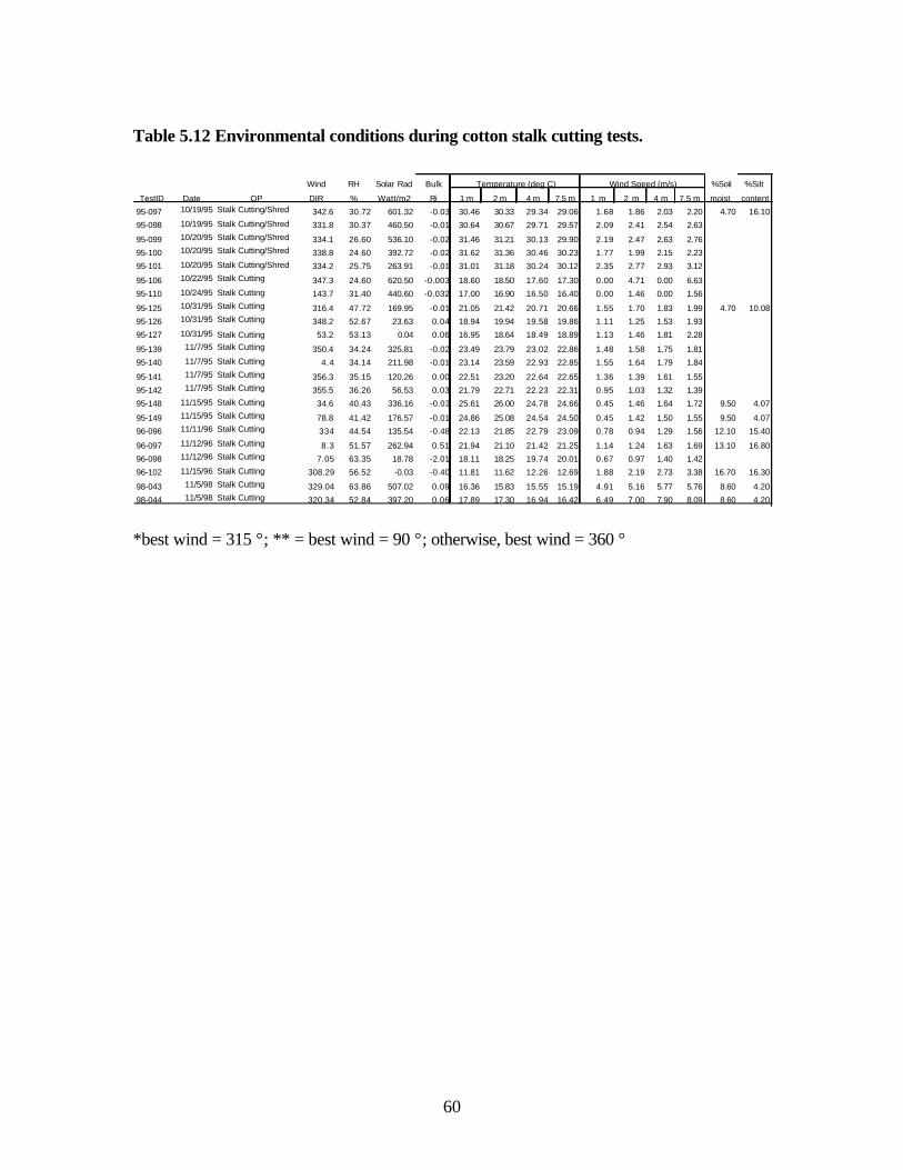
-I I I I I I

Table 5.12 Environmental conditions during cotton stalk cutting tests.

TestID Date OP

Wind

DIR

RH

%

Solar Rad

Watt/m2

Bulk

Ri

Temperature (deg C) Wind Speed (m/s) %Soil

moist

%Silt

content1 m 2 m 4 m 7.5 m 1 m 2 m 4 m 7.5 m

95-097 10/19/95 Stalk Cutting/Shred 342.6 30.72 601.32 -0.03 30.46 30.33 29.34 29.06 1.68 1.86 2.03 2.20 4.70 16.10

95-098 10/19/95 Stalk Cutting/Shred 331.8 30.37 460.50 -0.01 30.64 30.67 29.71 29.57 2.09 2.41 2.54 2.63

95-099 10/20/95 Stalk Cutting/Shred 334.1 26.60 536.10 -0.02 31.46 31.21 30.13 29.90 2.19 2.47 2.63 2.76

95-100 10/20/95 Stalk Cutting/Shred 338.8 24.60 392.72 -0.02 31.62 31.36 30.46 30.23 1.77 1.99 2.15 2.23

95-101 10/20/95 Stalk Cutting/Shred 334.2 25.75 263.91 -0.01 31.01 31.18 30.24 30.12 2.35 2.77 2.93 3.12

95-106 10/22/95 Stalk Cutting 347.3 24.60 620.50 -0.003 18.60 18.50 17.60 17.30 0.00 4.71 0.00 6.63

95-110 10/24/95 Stalk Cutting 143.7 31.40 440.60 -0.032 17.00 16.90 16.50 16.40 0.00 1.46 0.00 1.56

95-125 10/31/95 Stalk Cutting 316.4 47.72 169.95 -0.01 21.05 21.42 20.71 20.66 1.55 1.70 1.83 1.99 4.70 10.08

95-126 10/31/95 Stalk Cutting 348.2 52.67 23.63 0.04 18.94 19.94 19.58 19.86 1.11 1.25 1.53 1.93

95-127 10/31/95 Stalk Cutting 53.2 53.13 0.04 0.06 16.95 18.64 18.49 18.89 1.13 1.46 1.81 2.28

95-139 11/7/95 Stalk Cutting 350.4 34.24 325.81 -0.02 23.49 23.79 23.02 22.86 1.48 1.58 1.75 1.81

95-140 11/7/95 Stalk Cutting 4.4 34.14 211.98 -0.01 23.14 23.59 22.93 22.85 1.55 1.64 1.79 1.84

95-141 11/7/95 Stalk Cutting 356.3 35.15 120.26 0.00 22.51 23.20 22.64 22.65 1.36 1.39 1.61 1.55

95-142 11/7/95 Stalk Cutting 355.5 36.26 56.53 0.03 21.79 22.71 22.23 22.31 0.95 1.03 1.32 1.39

95-148 11/15/95 Stalk Cutting 34.6 40.43 336.16 -0.03 25.61 26.00 24.78 24.66 0.45 1.46 1.64 1.72 9.50 4.07

95-149 11/15/95 Stalk Cutting 78.8 41.42 176.57 -0.01 24.86 25.08 24.54 24.50 0.45 1.42 1.50 1.55 9.50 4.07

96-096 11/11/96 Stalk Cutting 334 44.54 135.54 -0.48 22.13 21.85 22.79 23.09 0.78 0.94 1.29 1.56 12.10 15.40

96-097 11/12/96 Stalk Cutting 8.3 51.57 262.94 0.51 21.94 21.10 21.42 21.25 1.14 1.24 1.63 1.69 13.10 16.80

96-098 11/12/96 Stalk Cutting 7.05 63.35 18.78 -2.01 18.11 18.25 19.74 20.01 0.67 0.97 1.40 1.42

96-102 11/15/96 Stalk Cutting 308.29 56.52 -0.03 -0.40 11.81 11.62 12.26 12.69 1.88 2.19 2.73 3.38 16.70 16.30

98-043 11/5/98 Stalk Cutting 329.04 63.86 507.02 0.09 16.36 15.83 15.55 15.19 4.91 5.16 5.77 5.76 8.60 4.20

98-044 11/5/98 Stalk Cutting 320.34 52.84 397.20 0.06 17.89 17.30 16.94 16.42 6.49 7.00 7.90 8.09 8.60 4.20

*best wind = 315 °; ** = best wind = 90 °; otherwise, best wind = 360 °

60

5.3 Wheat Harvest

Testing of PM emissions from wheat harvests began in 1995 and were continued through 1999 (Table 2.1). Unfortunately, tests conducted in 1995 did not include vertical profiles of wind speed, so calculation of emission factors by the vertical integration methods was not feasible. Data collected in 1996-1998 were analyzed using our most current methods (see section 4.3) and results are presented in Table 5.13.

Table 5.13 Emission factors and uncertainties for wheat harvest

TestID Wheat 96-051 I3

96-052 I4

96-053 I5

96-054 I6

96-058 I1

96-061 I3

96-063 I5

96-068 I1

96-068 D4

96-069 D4

96-069 I3

96-070 D4

96-070 I4

97-032 I1

97-033 I2

97-034 D1

97-034 I3

97-035 D1

97-036 D1

97-041 I1

date time

6/22/96 1230 to 1324

6/22/96 1343 to 1452

6/22/96 1516 to 1637

6/24/96 0945 to 1105

6/27/96 1738 to 1950

6/28/96 1250 to 1451

6/28/96 1724 to 1836

7/3/96 1355 to 1522

7/3/96 1355 to 1522

7/5/96 0845 to 0940

7/5/96 0845 to 0940

7/5/96 1048 to 1210

7/5/96 1048 to 1210

6/17/97 1638 to 1813

6/18/97 0940 to 1116

6/18/97 1600 to 1706

6/18/97 1600 to 1706

6/18/97 1706 to 1756

6/18/97 1756 to 1923

6/21/97 1306 to 1413

Xloc (m)

27.00

36.00

40.00

47.00

46.00

46.00

23.00

63.00

258.50

463.35

113.00

545.15

91.00

336.00

586.00

126.50

126.50

21.00

42.00

141.80

RCMA (ug m-3) Upwind 9m 3m

42.25 298.14 1302.64 (9.53) (13.29) (56.39) 42.25 126.83 795.09 (9.53) (6.06) (34.54) 42.25 66.74 704.23 (9.53) (3.28) (30.04) 64.04 59.78 539.47

(21.92) (2.89) (23.17) 18.54 36.18 216.8 (9.80) (1.69) (8.7) 32.42 50.07 439.44 (1.47) (2.28) (17.82) 32.42 15.41 176.59 (1.47) (1.35) (7.23) 78.86 135.63 231.69

(0) (5.63) (9.47) 78.86 46.22 80.26

(0) (2.12) (3.2) 84.77 79.08 92.93

(0) (3.78) (4.25) 84.77 152.85 281.88

(0) (6.52) (11.89) 84.77 50.79 48.5

(0) (2.72) (2.31) 84.77 180.67 327.63

(0) (7.66) (13.39) 43.56 134.36 447.55 (2.80) (5.38) (17.82) 32.41 163.45 254.41 (7.50) (6.58) (10.33) 46.57 184.47 163.2 (9.57) (7.2) (6.85) 46.57 339.28 564.37 (9.57) (13.6) (22.43) 46.57 130.46 607.39 (9.57) (5.77) (24.86) 46.57 97.26 703.69 (9.57) (3.81) (28.52) 67.01 78.36 68.42

(59.36) (3.22) (3.35)

1m

590.58 (24.66) 741.98 (31.32) 714.33 (30.77) 382.26 (15.74) 418.2 (16.4)

1243.32 (37.82)

854 (34.54) 255.89 (10.67) 89.02 (3.69) 57.04 (3.92)

233.11 (9.73) 43.02 (2.79)

323.76 (13.37) 586.65 (23.33) 344.56 (14.24) 517.62 (21.05)

1104.37 (44.91) 804.18 (32.6)

496.55 (19.62) 182.25 (7.88)

Plume height (m) Linear Block Log

8.21 11.78 4.99

10.92 10.89 11.85

10.32 10.27 10.79

9.03 9.94 7.21

9.45 10.68 10.68

8.37 10.32 8.50

7.34 9.26 6.67

14.24 14.14 28.76

3.04 3.25 2.17

5.04 6.54 4.10

12.94 13.69 14.65

38.24 98.03 65791.49

15.23 14.57 30.92

11.69 12.03 16.81

15.69 20.08 52.09

7.16 -25.79 8.69

11.07 19.10 18.11

9.13 9.17 11.54

7.92 8.69 6.69

6.62 2.00 5.84

Emission Factor (mg m-2) Linear Block Log Box

1341.08 1719.21 1288.88 693.53

1090.68 1169.38 903.56 940.29

1222.46 1291.87 1001.58 1160.02

412.20 485.64 331.63 324.49

584.49 530.19 480.30 664.23

779.98 633.03 617.01 1116.57

1036.90 671.01 757.19 1557.58

225.88 225.94 264.85 151.00

3.27 2.98 4.98 8.67

-15.50 -2.36 -9.55 -17.14

163.59 189.12 135.79 91.67

-244.54 -621.58 -126826.1 -57.23

569.60 579.05 671.26 327.60

1287.46 1273.03 1298.73 919.85

365.05 409.02 601.52 246.50

287.51 NC 246.17 396.14

907.38 1063.44 911.79 889.58

954.33 949.72 874.72 1031.81

979.29 1164.15 787.54 786.55

42.90 18.00 31.38 64.97

case

4

4

1

4

1

1

1

1

1

4

4

3

4

1

1

5

1

1

4

5

Qup Qwd EFU

A A 362%

A A 7%

A A 131%

A A 112%

A A 6%

A B 135%

A A 8%

A A 3%

A A 47%

A A 67%

A A 5%

C C 148%

A A 3%

A A 3%

A B 10%

A A 26%

A A 25%

A A 34%

A A 2388%

C E 114%

Values in parentheses are uncertainties; NC = not calculated (unreasonable value). QUP = upwind qualifier; QWD = wind direction qualifier; EFU = relative emission factor uncertainty = (calculated uncertainty/emission factor)100. Plume heights and emission factors in bold type are the best-fit figures based on case.

61

Table 5.14 Environmental conditions during wheat harvest tests.

Wind RH Solar Rad Bulk TestID Date DIR % Watt/m2 Ri

Temperature (deg C) 1 m 2 m 4 m 7.5 m

Wind Speed (m/s) 1 m 2 m 4 m 7.5 m

Soil Silt Moist (%) Content

96-051 6/22/96 6.2 41.32 1029.5 0.27 25.85 25.05 24.94 24.8 2.356 2.425 2.522 2.599 4.10 20.60 96-052 6/22/96 356.42 36.8 989.38 0.19 27.93 27.04 26.88 26.66 2.927 3.032 3.189 3.28 4.10 20.60 96-053 6/22/96 6.98 27.45 799.67 0.13 29.81 28.86 28.68 28.42 3.578 3.738 3.905 4.014 4.10 20.60 96-054 6/24/96 14.47 40.34 800.31 0.23 23.65 22.73 22.83 22.64 2.566 2.681 2.798 2.855 5.10 22.60 96-058 6/27/96 348.92 38.29 271.88 0.09 23.89 23.11 23.41 23.31 2.566 2.889 3.233 3.514 3.90 19.70 96-061 6/28/96 39.92 42.59 842.5 0.62 22.6 22.63 21.63 21.29 1.984 2.047 2.147 2.292 3.90 19.70 96-063 6/28/96 349.38 37.86 393.91 0.13 24.27 24.73 23.82 23.51 2.679 2.81 3.279 3.772 3.90 19.70 96-068 7/3/96 314.59 * 27.35 929.82 0.15 35.94 35.29 34.2 33.59 3.327 3.762 4.23 4.437 2.40 15.70 96-069 7/5/96 306.75 * 31.47 659.87 0.22 24.58 23.34 23.4 23.13 2.674 3.018 3.356 3.528 2.40 15.70 96-070 7/5/96 291.91 * 30.12 984.56 0.23 30.13 29 28.5 28.04 2.821 3.208 3.572 3.797 2.40 15.70 97-032 6/17/97 341.2 25.06 429.97 0.08 37.96 37.23 36.67 36.32 2.831 0.447 4.842 5.41 97-033 6/18/97 319.61 34.34 806.58 0.78 30.03 28.14 28.43 28.02 1.62 1.782 1.961 2.02 2.30 9.70 97-034 6/18/97 35.94 24.61 665.62 0.22 36.53 38.53 35.19 34.7 2.623 2.788 3.126 3.473 2.30 9.70 97-035 6/18/97 29.17 23.76 478.74 0.16 36.29 37.65 35.25 34.78 2.61 2.81 3.273 3.674 2.30 9.70 97-036 6/18/97 0.59 23.37 236.33 0.07 35.19 37.14 34.81 34.48 2.679 2.79 3.497 3.942 2.30 9.70 97-041 6/21/97 55.71 16.59 688.73 0.58 30.18 31.56 29.24 29.01 1.638 1.67 1.726 1.78 2.20 7.00

*best wind = 315 °; ** = best wind = 90 °; otherwise, best wind = 360 °

5.4 Land Preparation

Land preparation operations have been monitored following cotton and wheat harvests. These operations include root cutting, stubble discing, chiseling or ripping, finish discing, and listing. Root cutting is unique to cotton, but is included here for comparison with stubble discing.

The five highest best-fit emission factors (538 – 776 mg m-2) were seen for profiles collected on hot dry summer days for ripping and after dark in winter for stubble disking (Tables 5.15, 5.16). Similar field conditions, however, also resulted in a much lower ripping emission factor of 112 mg m-2 (test 97-050), thus complicating interpretation between different tests. There were no stubble discing tests conducted under conditions similar to 95-150 and 95-151 that had lower emission factors, but the single test of stubble discing following wheat, in midday in summer (97-045), had a comparable emission factor (430 mg m-2). When the downwind concentrations were uniform with height (Case 3) emissions were generally low but downwind PM10 values were significantly higher than upwind concentrations. The low emission factors were not due to the use of the box model, however, because the box model emission factors showed fairly good agreement (within a factor of 2) with the emission factors calculated by the other models for the other profile types (Table 5.15). Interestingly, the lowest 5 emission factors were measured in winter when temperatures were cooler and soil moisture was relatively high (Table 5.15 and 5.16), suggesting that environmental conditions greatly influence emission rates. The calculated emission factors for land preparation activities (Table 5.15) showed no correlation with wind speed, increased with decreasing relative humidity, were generally lower when soil moisture was higher and generally increased with increasing vertical temperature differential.

Differences in PM10 emission factors from two operations, for which a representative number of repeated measurements were made, disking and ripping, were used to examine the importance of implement type. The average emission factor for ripping operations, 512 ± 288 mg m-2, was significantly larger than that for disking, 134 ± 154 mg m-2 . However, direct comparison of

62

implement-average emissions is not reliable because differences in environmental conditions (e.g., relative humidity and wind direction variability) between individual tests appear to have a larger impact on measured emissions than does implement type. Variability in measured emissions due to environmental factors is highlighted by three Case 1 ripping tests collected on 6/26/97 (see Table 5.16). The emission factors for two tests (97-046, 765 ± 36 mg m-2 and 97-051, 776 ± 27 mg m-2) were similar and significantly higher than disking tests conducted under similar relative humidity conditions (98-050, 74.2 ± 6.3 mg m-2) but the emissions from the third ripping test, 97-050, 112 ± 5.3 mg m-2, was much lower and similar to emissions measured for disking. The much higher deviation of wind direction from the ideal direction during this third ripping test likely explains these results and highlights the complexity of comparing emission tests with different implements unless all other environmental factors are held constant.

Cultivation operations such as weeding have been generally regarded as a form of tillage. Several measurements of PM10 emission factors for mechanical cotton cultivation conducted in spring of 1998 show that emissions from this practice can be of similar magnitude as discing (Table 5.17). These tests also indicate a correlation between PM10 emissions from cultivation and soil moisture (Table 5.18).

63

ua m-31 Plume heiaht ml Emission Factor fma m-2 TestlD date time Xlac (ml Upwind 9m 3m 1m Linear Block Loa Linear Block Loa Bax case Qup Qwd EFU Stubble disc 95-118 17 10127/95 1255 to 142.71 138.43 185.36 255.66

1400 128.00 132.24) 18.3) (10.8) (15.1l 9.61 4.74 2.3E+46 257.68 39.96 -1.4E+50 6.77 1A B NC 95-128D1 1113/95 1001 to 155.00 66.74 81.34 131 .87 141.40

1139 166.74) /5 .14) 17.64) 18.27) 10.94 10.73 15.30 49.31 50.20 49.84 17.08 1 B B 9% 95-129D1 1113/95 1139 to 124 00 66.74 81.34 131.87 141.40

1200 166.741 (5.14) 17.641 18.271 10.94 10.73 15.30 27.47 27.97 27.77 9.56 1 B B 470% 95-130D1 1113/95 1238 to 74.00 66.74 178.31 334.42 411.68

1300 166.741 (12.671 f21 .30l f26.01l 12.75 13.29 26.79 231.04 235.80 371 .34 35.58 1 A A 4% 95-130 12 1113/95 1238 to 15.00 66.74 109.27 247.61 563.74

1300 (66.74) (8.79) (1532) (3559) 8.09 10.84 9.05 136.73 125.27 102.45 26.35 1 A A 7% 95-131 D1 1113/95 1300 to 27.50 66.74 156 97 206.65 464 86

1333 (66.74) (11.06) (1299) (2696) 8.52 19.90 10.97 140.80 249.66 126.36 24.82 1A A 6% 95-132 D1 1113/95 1333 to 10.50 66.74 158.22 464.61 841.23

1342 (66.74) (14.31) (2988) (54.70) 9.17 10.79 11.58 286.12 278.54 254.11 52.62 1A A 5% 95-150D1 11115/95 1838 to 11 .00 143.67 192.89 732.80 1272.34

1910 (1913) /1208) /4253) 174.77) 8.70 9.55 9.95 537.91 491.69 438.93 319.33 1A B 9% 95-151 D1 11115/95 1910 to 32.50 143.67 195.25 966.70 2090.62

1947 (19 13) (1296) /5603) (11739) 8.14 9.40 8.82 542.20 471 .01 430.39 472.14 1A A 125% 97-045 D1 6124197 0956 to 87.00 55.91 92.5 485. 1 325.9

1137 /20.94) 13.7) (18.5) (12.41 9.40 10.70 7.50 352.00 430.00 271.00 270.00 4A B 17% 98-045 R1 1116/98 0820 to 23.00 23.56 57.5 64.5 113.3

0921 (4881 /28) 13.0l (4.71 11 .10 43.90 20.50 50.00 117.00 55.00 5800 1A A 146% 98-045 L1 1116/98 0820 to 26.00 23.56 46.0 43.7 79.2

0921 f4.88l f4.1l f2.9l 13.31 9.60 -59.50 14.80 28.40 NC 27.00 36.00 5A A 145% 98-046 R1 1116/98 0929 to 30.00 23.56 627 69.3 65.9

1015 f20 .94l (4.51 13.71 13.91 49.20 51.90 5931 .00 164.00 180.00 5924.00 35.00 3A A NC 98-046 M1 1116/98 0929 to 63.00 23.56 29.1 58.2 40.0

1015 (2094) (20) (27) (1.8) 8.50 11.30 5.60 21 .50 28.00 18.00 14.00 4A A 10% 98-046 L1 1116/98 0929 to 30.00 23.56 94.2 47.4 131 .8

1015 (2094) (58) (33) (63) 5.80 -0.60 6.70 117.00 NC 61.00 89.00 SA A 18% 98-047 D1 1116/98 1015 to 98.00 23.56 56.5 78.5 47.6

1040 (2094) (5 1) (38) (31) 500 20.50 1.60 7000 32.40 ·280 760 4A A 9% 98-048 D1 1116/98 1050 to 123.00 23.56 56.8 164.5 243.3

1115 (2094) (3.4) 17 7) (10.3) 11.10 12.20 15.60 58.90 57.00 54.00 64.00 1A B 8% 98-049 D1 1116/98 1137 to 56.00 23.56 12.5 95.0 96.9

1347 (2094) (09) (4 1) (4 0) 9.00 9.10 8.00 93.50 100.40 7300 107.00 1A B 9% 98-050 D1 1116198 1404 to 34.00 17.37 44.9 74.5 114.8

1450 (404) (29) 137) (55) 12.20 16.50 22.40 74.20 8000 81.00 74.00 1A B 8% finish disc 96-111 15 11126/96 1240 to 10000 14.14 42.12 82.27 111.37

1320 /20.0l /2.68) f4.17l 16.091 13.22 14.88 26.15 124.29 127.82 152.70 80.17 1 A A 3% 96-112 16 11126/96 1330 to 114.00 14.14 49.18 115.89 276.84

1404 f20.0l 13.731 (5.711 (13.041 9.26 13.68 11.02 142.35 136.07 117.41 150.42 1A A 4% 96-113 17 11126/96 1518 to 188.00 14.14 48.15 142.46 208.66

1615 (200) (365) (636) (939) 11.48 12.52 16.90 97.53 96.13 94.93 74.65 1 A A 5% 96-117 D1 1212/96 1655 to 25.00 11.46 26.2 52.1 83.0

1815 (2.13) (20) (27) (36) 11.20 14.00 17.10 91.00 94 .00 92.00 65.00 1 A A 9% 96-118 D1 1214/96 1041 to 6000 33.72 59.1 53.6 51.5

1151 (218) (30) (29) (2 6) -17.80 -8.40 0.01 NC NC 0.00 9.20 3A B NC 96-119 D1 1214/96 1237 to 185.00 33.72 39.9 37.3 35.4

1411 (218) (22) (2 1) (1.9) -2.50 -5.10 0.50 NC NC -0.03 0.60 3D B NC 96-119 M1 1214/96 1237 to 7700 33.72 40.4 46.6 43.9

1411 (218) (20) (2.2) (2 2) 16.50 17.50 26.20 6.60 7.50 6.50 3.50 3A B NC 96-120 D1 1215/96 1046 to 7000 30.64 29.2 32.4 25.5

1200 (4.321 (1.7) (21) (1.6) 4.90 6.30 3.90 -5.40 .0.50 -2.90 -5.60 4 D A NC riooina 97-046 6124197 1342 to 75.00 55.91 56.4 250.6 299.9

1635 f20 .94l f2.3l (10.31 (12.0l 10.00 10.00 11 .00 765.00 770.00 623.00 853.00 1 A A 5% 97-050 6126197 0820 to 233.00 48.07 60.8 161.1 205.9

0950 (985) (25) (68) (82) 10.70 10.90 13.10 112.00 110.00 97.00 130.00 1 A A 5% 97-051 6126/97 1000 to 234.00 48.07 255.1 434.8 598.5

1040 (9.85) (110) (180) (24 1) 14.70 18.10 40.10 776.00 840.00 1109.00 651.00 1 A A 3% 97-048 6125197 1231 to 128.00 67.0 101.1 241 .8 221.6

1410 (1501) (4 2) (10.2) (88) 9.60 9.50 10.80 306.00 331.00 268.00 299.00 4A A 5% 97-049 6125197 1411 to 68.00 67.0 239 167.7 396.3

1551 (15.01) (10.3) (69) (14 9) 7.50 -5.50 10.60 577.00 NC 502.00 696.00 5A A 6% root cuttin 96-103D1 11116/96 1008 to 1[ 176.00 25.3 28.8 55.2 165.1 8.70 10.90 9.30 30.00 25.00 23.00 40.00 1A A 12%

(467) (25) (32) (51) 96-104D1 11116/96 1249 to 1 72.00 25.3 30.8 63.6 81.3 10.70 11.20 13.60 36.00 34.00 31.00 33.00 1A A 8%

(4.671 /2.0l /2.9) 13.71

Table 5.15 Emission factors and uncertainties for land preparation.

Values in parentheses are uncertainties; NC = not calculated (unreasonable value). QUP = upwind qualifier; QWD = wind direction qualifier; EFU = relative emission factor uncertainty = (calculated uncertainty/emission factor)100. Plume heights and emission factors in bold type are the best-fit figures based on case.

64

I I I I I I I

I

I

I

Table 5.16 Environmental conditions during land preparation tests.

TestID Date Crop Op Wind DIR*

RH %

SolarRac Bulk Watt/m2 Ri

Temperature (deg C) Wind Speed (m/s) %Soil moist

%Silt Content1m 2m 4m 7.5m 1m 2m 4m 7.5m

95-118 10/27/95 Cotton Disk 11.80 29.60 498.7 -0.028 25.2 25.5 24.5 24.3 1.81 1.85 2.03 2.14 95-128 11/03/95 Cotton Disk 346.50 61.62 358.9 -0.01 17.94 22.43 17.29 17.1 NA 2.68 NA 3.07 6.10 12.89 95-129 11/03/95 Cotton Disk 2.70 53.61 348.93 -0.01 19.1 23.72 18.47 18.2 NA 3.22 NA 3.64 95-130 11/03/95 Cotton Disk 351.70 51.71 506.63 -0.01 20.13 25.35 19.2 19 NA 3.55 NA 4.12 5.70 12.89 95-131 11/03/95 Cotton Disk 346.50 50.18 568.99 -0.01 20.51 26.76 19.66 19.4 NA 3.06 NA 3.51 95-132 11/03/95 Cotton Disk 346.30 47.7 510.65 -0.01 20.48 28.01 19.94 19.8 NA 3.24 NA 3.64 5.90 12.89 95-150 11/15/95 Cotton Disk 353.2 57.83 0 0.34 16.19 18 19.41 20.6 0.45 0.93 1.40 1.65 95-151 11/15/95 Cotton Disk 2.1 58.25 0.04 0.55 15.69 18.38 19.41 20.3 0.45 0.75 1.00 1.16 97-045 06/24/97 Wheat Disk 324.31 30.72 874.89 0.52 27.86 26.19 26.29 26 2.684 2.947 3.335 3.5 2.32 17.90 98-045R 11/06/98 Cotton Disk 11.43 63.68 352.44 1.16 11.62 11.29 11.19 11.1 1.707 1.91 1.676 2.07 12.95 7.00 98-045L 11/06/98 Cotton Disk 11.43 63.68 352.44 1.16 11.62 11.29 11.19 11.1 1.707 1.91 1.676 2.07 12.95 7.00 98-046R 11/06/98 Cotton Disk 338.75 52.26 480.94 1.22 14.33 13.13 13.02 12.8 1.906 2.107 2.19 2.34 12.95 7.00 98-046M 11/06/98 Cotton Disk 338.75 52.26 480.94 1.22 14.33 13.13 13.02 12.8 1.906 2.107 2.19 2.34 12.95 7.00 98-046L 11/06/98 Cotton Disk 338.75 52.26 480.94 1.22 14.33 13.02 13.02 12.8 1.906 2.107 2.19 2.34 12.95 7.00 98-047 11/06/98 Cotton Disk 317.6 49.13 483.6 2.5 15.68 14.18 13.96 13.7 1.691 1.925 2.038 2.17 12.95 7.00 98-048 11/06/98 Cotton Disk 312.12 46.45 381.61 0.45 16.04 14.85 14.63 14.4 2.709 3.083 3.451 3.59 12.95 7.00 98-049 11/06/98 Cotton Disk 312.12 43.67 382.21 0.2 17.21 16.38 16.11 15.8 3.538 3.958 4.442 4.62 11.50 2.30 98-050 11/06/98 Cotton Disk 309.50 41.17 246.51 0.16 18.3 17.65 17.43 17.1 3.688 4.198 4.706 4.93 11.50 2.30 Finish Disc 96-111 11/26/96 Cotton Disk 1.70 59.8 593.2 0.1 15.5 14.7 14.7 14.3 3.42 3.82 5.7 5.6 20.80 96-112 11/26/96 Cotton Disk 352 58.8 516.9 0.1 15.8 15 15 14.7 3.1 3.4 4.75 5.14 20.80 96-113 11/26/96 Cotton Disk 359.4 66.7 142.8 0.1 15 14.5 14.8 14.7 2.02 2.28 3.34 3.41 20.80 96-117 12/02/96 Cotton Disk 347.01 79.82 0.18 -2.39 7.26 7.35 8.31 8.9 0.896 1.266 1.998 2.16 18.15 96-118 12/04/96 Cotton Disk 134.18* 72.44 566.62 0.51 11.16 10.14 10.04 9.9 2.522 2.792 3.141 3.24 18.00 96-119 12/04/96 Cotton Disk 119.6* 59.78 454.29 0.39 13.35 12.43 12.43 12.3 2.484 2.702 3.002 3.13 16.25 20.00 96-119M 12/04/96 Cotton Disk 119.6* 59.78 454.29 0.39 13.35 12.43 12.43 12.3 2.484 2.702 3.002 3.13 16.25 20.00 96-120 12/05/96 Cotton Disk 140.27* 80.04 72.52 -0.02 11.3 10.97 11.44 11.5 4.098 4.649 5.498 5.92 16.65 14.50

97-046 06/24/97 Wheat Rip 358.26 22.49 893.47 0.19 33.11 31.08 31.28 30.9 3.036 3.444 3.884 4.11 2.32 97-050 06/26/97 Wheat Rip 317.45 40.45 586.59 0.36 25.21 23.71 24.17 23.9 1.994 2.113 2.404 2.45 2.21 97-051 06/26/97 Wheat Rip 331.62 36.92 806.5 0.41 27.72 25.62 26.32 26.1 2.008 2.174 2.475 2.49 2.21 97-048 06/25/97 Wheat Rip 347.78 23.34 799.46 0.26 34.39 32.37 32.44 32.1 2.601 2.928 3.303 3.43 2.21 97-049 06/25/97 Wheat Rip 358.83 21.62 915.05 0.17 35.49 33.7 33.66 33.4 3.016 3.435 3.91 4.13 2.21

96-103 11/16/96 Cotton Root cut 139.21* 53.93 585.39 0.6 14.96 14.11 13.84 13.5 1.79 2.118 2.629 2.83 12.20 27.00 96-104 11/16/96 Cotton Root cut 141.97* 46.58 371.9 0.26 16.95 16.12 16.08 15.8 2.076 2.54 3.359 3.67 12.20 27.00 96-114 11/27/96 Cotton Root cut 58.24 91.77 479.03 1.37 10.6 9.93 10.08 10 1.229 1.259 1.366 1.43 19.80

*best wind = 315 °; ** = best wind = 90 °; otherwise, best wind = 360 °

65

I I I I I I I

Table 5.17 Emission factors and uncertainties for cultivation

RCMA (ug m-3) Plume height (m) Emission Factor (mg m-2) TestID date time Xloc (m) Upwind 9m 3m 1m Linear Block Log Linear Block Log Box case Qup Qwd EFU weeding 98-001 D1 6/4/98 0905 to 26.00 20.90 34.99 25.36

1026 (6.04) (2.09) (1.21) 32.31 (1.4 -0.86 -1.10 1.47 NC NC -5.71 18.33 3 A A NC 98-001 I1 6/4/98 0905 to 26.00 20.90 38.8 27.12 32.45

1026 (6.04) (2.07) (1.36) (1.55) -2.77 -0.73 0.83 NC NC -1.43 18.55 3 A A NC 98-002 D1 6/4/98 1026 to 71.00 20.90 21.96 35.12 35.14

1205 (6.04) (1.05) (1.66) (1.55) 10.21 9.90 13.47 27.85 28.92 26.01 21.73 1 A B 17% 98-002 I2 6/4/98 1026 to 26.00 20.90 30.59 33.03 32.89

1205 (6.04) (1.86) (1.43) (1.4) 42.20 37.81 10105.50 74.25 68.71 4642.90 18.30 3 A B NC 98-003 D1 6/4/98 1231 to 122.00 20.16 34.46 26.51 27.37

1429 (5.16) (1.5) (1.21) (1.27) -4.25 -1.93 0.39 NC NC -0.31 9.40 3 A B NC 98-003 I3 6/4/98 1231 to 29.00 20.16 31.17 24.27 25.75

1429 (5.16) (1.52) (1.09) (1.09) -3.54 -1.17 0.59 NC NC -0.38 7.29 3 A B NC 98-004 D1 6/4/98 1231 to 161.00 20.16 38.42 74.52 131.01

1429 (5.16) (1.73) (3.38) (5,82) 8.72 11.07 11.83 248.03 243.54 230.98 325.31 1 A B 23% 98-004 I4 6/4/98 1231 to 14.00 20.16 43.66 38.59 75.58

1429 (5.16) (3.2) (1.74) (3.18) 9.05 -22.44 13.28 147.57 NC 131.25 162.63 5 A B 22% 98-005 D1 6/5/98 0834 to 294.00 15.28 38.08 61.31 64.8

0929 (2.86) (1.87) (3.15) (2.85) 16.13 15.41 53.76 329.03 324.74 555.04 191.00 5 A A 5% 98-005 I5 6/5/98 0834 to 20.00 15.28 40.86 44.29 70.4

0929 (2.86) (3.87) (2.28) (3.03) 12.66 62.21 32.74 256.54 784.56 347.09 212.59 1 A A 5% 98-007 I7 6/5/98 1133 to 79.00 15.28 29.58 46.82 64.03

1301 (2.86) (1.31) (1.99) (2.78) 12.91 15.81 25.57 107.77 112.03 121.05 93.84 1 A A 8% 98-008 I8 6/5/98 1308 to 80.00 24.55 33.57 56.74 68.17

1442 (4.75) (1.53) (2.33) (2.94) 12.19 12.72 19.20 68.38 67.78 66.92 61.68 1 A B 16% 98-009 I9 6/5/98 1450 to 95.00 24.55 49.5 44.81 77.37

1625 (4.75) (1.95) (1.99) (3.33) 9.64 -27.23 16.30 76.10 NC 73.91 77.06 5 A B 15% 98-010 IA 6/6/98 0755 to 36.00 21.96 26.98 27.33 41.29

0922 (6.71) (1.28) (1.48) (1.68) 8.61 110.47 10.39 31.54 129.46 25.92 38.22 1 B A 9% 98-011 IB 6/6/98 0932 to 91.00 21.96 24.29 30.01 44.87

1136 (6.71) (1.21) (1.33) (1.89) 8.85 12.86 9.89 37.36 33.11 30.36 48.29 1 A A 12%

Values in parentheses are uncertainties; NC = not calculated (unreasonable value). QUP = upwind qualifier; QWD = wind direction qualifier; EFU = relative emission factor uncertainty = (calculated uncertainty/emission factor)100. Plume heights and emission factors in bold type are the best-fit figures based on case.

Table 5.18 Environmental conditions during cultivation tests

Wind RH SolarRac Bulk Temperature (deg C) Wind Speed (m/s) %Soil

moist

%Silt

ContentTestID Date Crop Op DIR* % Watt/m2 Ri 1m 2m 4m 7.5m 1m 2m 4m 7.5m Weeding

98-001 06/04/98 Cotton Weeding 343.1 59.5 676.1 0.4 18.4 18.2 17.6 17.3 2.42 2.56 2.75 2.82 8.85 3.01

98-002 06/04/98 Cotton Weeding 352.4 51.2 834.1 0.8 20.5 20.2 19.6 19.3 2.07 2.14 2.31 2.33 9.80 3.01

98-003 06/04/98 Cotton Weeding 320.4 40 762.3 0.6 23.5 23.6 22.5 22.2 2.15 2.26 2.37 2.43 17.90 4.10

98-004 06/04/98 Cotton Weeding 320.4 40 762.3 0.6 23.5 23.6 22.5 22.2 2.15 2.26 2.37 2.43 2.60 3.01

98-005 06/05/98 Cotton Weeding 335.3 65.3 507.2 0.1 18.3 17.9 17.4 17.1 3.85 4.15 4.58 4.85 7.30 3.52

98-007 06/05/98 Cotton Weeding 334 45.2 762.8 0.2 24.3 23.8 23.2 22.8 3.24 3.47 3.73 3.85 4.80 3.50

98-008 06/05/98 Cotton Weeding 328.8 38.4 673.1 0.5 26 26.6 25.1 24.7 2.34 2.5 2.69 2.71 6.45 3.50

98-009 06/05/98 Cotton Weeding 343.3 37.3 537.8 0.3 26.8 26.9 25.9 25.7 2.68 2.89 3.06 3.16 3.60 3.50

98-010 IA 06/06/98 Cotton Weeding 330 69.2 496.9 0.2 18.2 17.6 17.4 17.2 3.5 3.79 4.06 4.26 5.05 4.00

98-011 IB 06/06/98 Cotton Weeding 337.2 53.1 662.9 0.2 22.2 22.3 21.2 20.8 3.07 3.26 3.58 3.7

*best wind = 315 °; ** = best wind = 90 °; otherwise, best wind = 360 °

66

5.5 PM from confined cattle facilities

Emission factors of PM10 from open lot dairies were calculated from measurements made downwind of a single facility in October and April (Table 5.19). The PM10 emission factor was highly influenced by relative humidity, with the highest measured emission factor coincident with the lowest relative humidity. The facility where these measurements were made did not have free stalls for any of the cows. With the exception of young heifers (<500 lbs), all animals were housed in open lots with paved, flushed feed lanes and free-standing shade structures. Highest production cows were misted with water at the feed lanes during high temperature episodes. No dust control measures were in use at the dairy during either sampling period and an unpaved road used by dairy personnel ran between the cow enclosures and the downwind sampling array.

Emission factors of PM10 from large feedlots were calculated from measurements made downwind of a feedlot in both winter and summer seasons (Table 5.21). PM from the feedlot was also was also highly influenced by relative humidity, but the lowest measured relative humidity was not coincident with the highest emission factor, probably because that measurement was made in March, when the ground surface was relatively wet. During the July sampling period water trucks were used for dust control in all of the animal enclosures and on the unpaved portions of roads surrounding the feedlot.

67

Table 5.19 Best fit PM 10 emission factors from open lot dairies

TestID Dairy 95-075

95-076

95-077

95-077

95-078

95-086

95-089

95-090

96-024

96-025

96-026

96-027

96-028

96-029

96-030

96-031

96-033

96-034

96-037

96-038

96-039

96-040

96-043

96-042

96-046

96-047

96-048

date time

10/03/95 1500 to 1701

10/03/95 1746 to 2003

10/03/95 2021 to 2301

10/03/95 2021 to 2301

10/04/95 1358 to 1700

10/06/95 1600 to 1700

10/07/95 1245 to 1452

10/07/95 1600 to 1800

4/19/96 1330 to 1635

4/19/96 1647 to 2000

4/20/96 0322 to 0538

4/20/96 0830 to 1213

4/20/96 1213 to 1455

4/20/96 1600 to 1900

4/20/96 1935 to 0000

4/21/96 0000 to 0200

4/21/96 1455 to 1915

4/21/96 1915 to 2133

4/22/96 1630 to 2000

4/22/96 2000 to 2247

4/23/96 0007 to 0202

4/23/96 0202 to 0405

4/23/96 1915 to 2330

4/23/96 1605 to 1915

4/24/96 1250 to 1630

4/24/96 1715 to 2000

4/24/96 2000 to 2350

Xloc (m)

220.00

130.00

130.00

220.00

220.00

220.00

140.00

220.00

128.00

128.00

128.00

128.00

128.00

128.00

128.00

128.00

128.00

128.00

128.00

128.00

128.00

128.00

128.00

128.00

128.00

128.00

128.00

RCMA (ug m-3) Upwind 9m 3m 1m

101.6 113.4 191.0 81.3 (20.8) (6.8) (11.2) (5.1) 80.1 224.0 791.8 1169.5

(11.3) (12.9) (44.8) (69.6) 138.3 97.8 109.4 419.0 (45.9) (5.7) (6.5) (25.5) 138.3 133.9 391.1 195.1 (45.9) (7.6) (22.3) (10.8) 290.2 330.9 430.1 503.1 (59.9) (18.6) (24.3) (30.0) 105.9 233.0 346.2 142.0 (18.8) (14.6) (21.4) (9.3) 108.9 154.1 225.0 209.6 (24.7) (9.4) (13.2) (12.3) 163.6 284.2 406.1 512.0 (20.0) (16.6) (23.2) (29.3) 13.24 30.48 64.53 78.4 (0.00) (1.5) (3.66) (3.81) 43.51 43.2 66.29 99.34 (0.00) (1.89) (3.37) (4.2) 17.5 13.8 27.18 64.88

(0.00) (0.92) (2.01) (3.04) 12.37 17.21 53.73 106.37 (0.00) (0.93) (2.66) (4.5) 12.37 22.49 33.02 81.64 (0.00) (1.2) (1.48) (3.89) 37.34 29.56 63.07 113.04 (0.00) (1.38) (2.63) (4.95) 15.67 15.84 28.3 45.25 (0.00) (0.93) (1.33) (2.06) 15.67 13.86 22.91 44.2 (0.00) (1.13) (1.53) (2.08) 57.35 46.08 77.57 250.15 (0.00) (2.03) (3.42) (11.51) 43.47 56.6 147.23 314.08 (0.00) (2.53) (5.95) (12.75) 35.73 70.4 124.27 174.85 (0.00) (2.89) (5.01) (6.94) 110.89 38.23 186.88 316.55 (0.00) (1.69) (7.54) (12.53) 47.62 47.6 70.06 99.98 (0.00) (2.19) (3.2) (4.37) 47.62 43.47 48.11 88.06 (0.00) (2.04) (2.22) (3.9) 54.81 46.49 115.61 225.79 (0.00) (1.97) (5.02) (8.97) 57.41 60.8 144.73 255.47

(0) (2.6) (5.89) (10.66) 89.27 56.49 62.99 5.36 (0.00) (2.42) (2.63) (0.49) 44.33 62.7 121.92 24.72 (0.00) (2.89) (5.05) (1.48) 26.6 26.27 58.47 6.84

(0.00) (1.33) (2.51) (0.54)

Plume height (m) Linear Block Log

4.30 9.90 2.60

9.90 10.52 13.30

5.50 -11.90 4.40

5.90 8.90 3.60

8.90 9.40 10.20

3.40 15.70 1.60

13.10 12.80 20.40

12.70 14.90 29.40

13.19 13.54 23.77

8.67 9.91 8.94

7.32 8.06 6.51

9.18 10.93 10.22

8.59 16.73 9.61

7.87 8.37 7.25

8.84 10.10 9.29

7.61 8.60 6.98

6.90 7.49 5.94

8.81 11.01 9.50

12.24 14.51 21.36

6.94 6.58 5.53

8.81 9.99 9.21

6.41 3.74 5.21

8.19 9.16 7.93

8.98 10.28 9.61

8.89 -25.30 12.36

4.45 12.17 2.50

4.62 9.93 2.93

Emission Factor (mg m-2) Linear Block Log Box

-684.50 31.37 -10.57 7.88

223.14 217.81 207.54 30.82

20.01 NC 12.29 -2.07

25.66 36.85 25.82 7.43

35.60 33.58 29.69 5.16

-15.00 87.65 -2.33 10.16

-10.93 64.88 63.22 10.29

150.05 161.59 221.24 17.72

62.61 62.48 66.54 51.86

36.80 31.15 29.12 48.28

6.12 3.89 4.20 8.14

55.75 49.51 45.57 73.99

29.45 27.45 23.77 39.31

489.35 387.45 377.49 730.22

22.53 19.29 17.71 27.44

3.63 2.48 2.49 4.79

133.26 77.26 99.38 217.46

38.92 33.08 29.34 45.33

98.98 100.50 103.79 89.24

14.10 10.05 7.73 24.61

-7.00 -5.94 -5.38 -7.97

-2.37 -1.01 -1.50 -3.62

56.98 44.02 40.57 71.21

139.11 121.52 112.20 180.40

-75.27 NC -65.47 -85.29

-200.10 86.24 -40.15 -21.11

-1042.23 188.11 -192.32 -156.04

case

4

1

1

5

1

4

4

1

1

1

1

1

1

1

1

1

1

1

1

1

1

1

1

1

4

4

4

Qup Qwd EFU

B A 15%

A A 19%

C C 109%

A C 108%

A C 33%

A A 5%

A A 14%

A A 8%

A A 8%

A A 13%

A A 100%

A B 18%

A B 13%

A A 9%

A A 22%

A A 17%

A A 13%

A A 26%

A A 11%

A A 14%

A C 42%

A C 32%

A A 28%

A A 7%

C C NC

A A 7%

B B 9%

E. Factor lbs per

1000hd*d

48.29

255.01

26.62

34.14

27.86

272.12

95.16

232.93

63.04

30.20

8.38

52.72

33.86

506.41

15.26

5.63

88.65

52.53

87.80

15.73

-20.06

-3.59

41.63

136.39

119.00

152.35

Values in parentheses are uncertainties; NC = not calculated (unreasonable value). QUP = upwind qualifier; QWD = wind direction qualifier; EFU = relative emission factor uncertainty = (calculated uncertainty/emission factor)100. Plume heights and emission factors in bold type are the best-fit figures based on case.

68

I I I I I I

Table 5.20 Environmental conditions during dairy tests.

TestID Date

Wind

DIR

RH Solar Rad

% Watt/m2

Bulk

Ri

Temperature (deg C) Wind Speed (m/s)

1 m 2 m 4 m 7.5 m 1 m 2 m 4 m 7.5 m

95-075 10/3/95 319.1 21.60 468.776 -0.023 32.422 32.70 31.594 31.372 1.909 2.090 2.337 2.540 95-076 10/3/95 347.5 43.21 23.544 0.353 23.326 25.95 25.798 27.218 0.844 0.985 1.202 1.707 95-077 10/3/95 58.2 65.27 0.006 0.354 16.603 18.79 19.524 21.965 0.610 0.891 1.193 1.578 95-078 10/4/95 221.1 29.74 523.650 -0.047 26.228 26.11 25.155 24.914 1.180 1.372 1.550 1.634 95-086 10/6/95 345.4 16.34 362.667 -0.013 30.66 29.642 29.463 2.142 2.348 2.542 2.780 95-089 10/7/95 262.4 30.91 685.608 -0.035 26.70 25.471 25.150 1.581 1.892 2.257 2.516 95-090 10/7/95 329.6 27.72 240.292 -0.017 28.30 27.368 27.258 1.926 2.118 2.390 2.741 96-024 4/19/96 340.22 34.99 NA 0.20 18.65 18.94 17.89 17.67 2.98 3.09 3.32 3.52 96-025 4/19/96 340.63 37.07 NA 0.00 17.72 18.25 17.56 17.52 3.08 3.31 3.65 3.96 96-026 4/20/96 5.77 92.61 NA -7.89 4.97 6.23 6.65 7.64 0.82 1.12 1.46 1.29 96-027 4/20/96 350.65 63.09 NA 1.63 13.63 13.95 12.9 12.7 2.32 2.41 2.34 2.71 96-028 4/20/96 322.24 39.53 NA 0.33 17.45 17.67 16.49 16.2 2.88 2.97 3.19 3.37 96-029 4/20/96 340.46 32.31 NA 0.12 18.15 18.48 17.48 17.28 3.79 4.00 4.35 4.63 96-030 4/20/96 334.46 62.69 NA -2.86 11.78 12.62 12.34 12.55 2.52 2.87 3.06 3.76 96-031 4/21/96 323.25 83.09 NA -5.65 7.98 8.96 8.98 9.39 1.14 1.40 1.57 2.24 96-033 4/21/96 350.64 34.85 NA 0.17 19.99 20.35 19.33 19.12 2.86 3.00 3.25 3.44 96-034 4/21/96 351.38 52.55 NA -21.15 14.73 16.22 15.98 16.58 0.80 0.93 0.94 1.55 96-037 4/22/96 346.25 34.69 NA -1.90 23.62 24.37 23.49 23.43 2.04 2.20 2.29 2.60 96-038 4/22/96 342.47 66.53 NA -36.30 15.7 17.22 17.39 18.89 0.49 0.66 0.45 0.98 96-039 4/23/96 183.99 83.96 NA -11.33 11.92 13.05 13.05 13.95 0.86 1.13 1.08 1.47 96-040 4/23/96 158.46 89.57 NA -21.18 9.74 10.98 11.3 12.24 0.51 0.65 0.71 0.98 96-042 4/23/96 355.83 28.6 NA 0.08 28.59 29.15 28.03 27.82 3.121 3.298 3.5 3.836 96-043 4/23/96 347.35 52.91 NA -15.57 20.13 21.68 22.04 22.81 1.09 1.36 1.36 2.08 96-046 4/24/96 352.65 37.72 NA 0.23 26.7 26.9 25.72 25.4 3.09 3.21 3.34 3.68 96-047 4/24/96 348.35 40.11 NA 0.02 26.59 27.21 26.28 26.16 4.42 4.74 5.17 5.64 96-048 4/24/96 345.4 61.1 NA -0.03 20.66 21.39 20.88 20.98 3.85 4.19 4.65 5.15

*best wind = 315 °; ** = best wind = 90 °; otherwise, best wind = 360 °

69

Table 5.21 Best fit PM 10 emission factors from feedlots

RCMA (ug m-3) Plume height (m) Emission Factor (mg m-2) E. Factor TestID date time Xloc (m) Upwind 9m 3m 1m Linear Block Log Linear Block Log Box case Qup Qwd EFU lbs per Feedlot 1000hd*d 96-003 D1 3/27/96 1800 to 1920 440.00 65.76 244.28 896.76 558.58 9.93 11.92 7.58 -2.89 -3.77 -2.09 -1.57 4 A B 39% -2.08

(0.00) (11.01) (39.67) (25.18) 96-006 D1 3/29/96 1307 to 1700 440.00 20.82 42.22 99.22 94.89 12.96 12.63 18.35 20.96 21.98 19.63 13.79 4 A B 13% 5.19

(0.00) (1.88) (4.43) (4.13) 96-007 D1 3/29/96 1700 to 1919 440.00 20.82 48.23 128.6 91.93 10.91 12.39 9.45 2.02 2.52 1.48 1.09 4 A B 60% 0.80

(0.00) (2.29) (5.71) (4.02) 96-013 D1 3/30/96 1144 to 1554 440.00 21.38 56.36 102.82 93.77 15.80 15.27 30.52 29.66 31.10 33.83 15.38 4 A A 8% 5.49

(0.00) (2.33) (4.4) (3.91) 96-020 D1 3/31/96 1350 to 1633 440.00 7.9 60.65 159.62 178.19 13.99 13.73 26.39 22.76 22.83 25.25 16.00 1 A B 17% 7.33

(0.00) (2.56) (6.79) (7.63) 96-021 D2 3/31/96 1948 to 2347 376.50 6.02 47.75 194.34 165.03 11.93 11.99 13.76 24.04 26.60 20.08 14.99 4 A C 125% 6.49

(0.00) (2.03) (7.7) (6.66) 96-022 D2 3/31/96 2347 to 0205 376.50 6.02 45.52 316.83 367.29 11.13 11.02 13.68 41.81 42.54 35.93 32.04 1 A A 25% 13.19

(0.00) (2.09) (12.07) (14.84) 96-023 D2 4/1/96 0205 to 0357 376.50 6.02 71.88 220.82 165.44 12.32 13.10 13.12 28.30 33.60 22.39 14.45 4 A A 15% 13.25

(0.00) (3.07) (8.77) (7.06) 96-073 D1 7/27/96 2203 to 0017 400.00 171.98 257.13 436.28 432.83 11.21 10.75 17.12 28.32 29.36 29.99 16.54 4 A A 10% 9.60

(0.00) (10.15) (17.93) (16.83) 96-073 I1 7/27/96 2203 to 0017 400.00 171.98 155.62 302.61 496.12 8.41 9.22 8.28 19.36 15.53 13.83 20.55 1 A A 12% 6.33

(0.00) (6.56) (12.84) (20.00) 96-074 D1 7/28/96 0154 to 0340 400.00 47.8 244.85 424.76 454.98 14.76 14.00 47.06 32.43 31.65 65.59 13.85 1 A A 19% 19.35

(0.00) (10.81) (17.91) (17.64) 96-074 I1 7/28/96 0154 to 0340 400.00 47.8 130.8 250.43 435.94 10.93 14.86 16.40 18.45 19.69 18.37 13.20 1 A A 22% 11.00

(0.00) (5.87) (10.37) (17.72) 96-078 D1 7/29/96 0109 to 0505 400.00 32.32 333.25 341.55 597.44 11.23 198.60 33.83 39.64 770.22 75.34 26.80 1 A A 28% 9.51

(0.00) (12.99) (13.23) (21.68) 96-076 I1 7/28/96 1245 to 1810 455.50 40.19 193.41 273.14 182.78 8.06 23.45 2.22 114.86 239.64 -55.25 55.51 4 A A 6% 31.58

(0.00) (8.3) (11.12) (7.13) 96-075 D1 7/28/96 0505 to 0703 400.00 47.8 320.83 365.06 414.96 28.41 40.66 3720.49 102.02 146.73 6359.11 25.96 1 A A 23% 72.64

(0.00) (13.03) (15.99) (16.77) 96-075 I1 7/28/96 0505 to 0703 400.00 47.8 235.1 339.31 418.54 18.82 22.58 107.11 60.91 69.36 191.55 26.22 1 A A 23% 43.37

(0.00) (9.63) (13.33) (16.8) 96-079 D1 7/29/96 0310 to 0505 400.00 32.32 333.25 341.55 597.44 12.08 226.54 37.30 31.35 654.29 60.22 21.97 1 A A 15% 21.29

(0) (12.99) (13.23) (21.68) 96-080 D1 7/29/96 1709 to 1946 455.50 24.51 10.81 891.39 549.14 7.13 8.17 5.53 92.70 109.73 79.52 73.89 4 A A 10% 30.85

(0.00) (0.73) (32.16) (20.53) 96-082 D1 7/29/96 2322 to 0123 400.00 32.54 289.09 646.1 662.37 12.72 12.02 25.89 37.50 37.51 51.16 18.12 1 A C 77% 13.79

(0.00) (11.49) (25.96) (24.69) 96-084 I1 7/30/96 1510 to 1746 455.50 34.12 217.15 476.89 312.8 11.51 14.93 8.68 64.66 85.86 48.51 35.55 4 A B 4% 24.30

(0.00) (9.24) (18.03) (13.32) 96-087 I1 7/30/96 2235 to 0009 455.50 64.54 353.66 809.14 501.88 10.58 14.44 7.17 44.94 70.28 26.75 16.23 4 A A 41% 36.08

(0) (14.38) (30.68) (20.0) 96-088 D1 7/31/96 1134 to 1352 455.50 54.77 559.37 613.49 335.87 -2.44 57.20 0.24 NC 518.24 -0.53 40.83 4 A A 5% 165.79

(0.00) (21.68) (24.11) (13.1) 96-088 I1 7/31/96 1134 to 1352 455.50 54.77 275.71 384.3 338.21 23.86 24.24 102.27 115.85 126.41 233.00 41.16 4 A A 5% 40.44

(0.00) (11.5) (15.44) (14.02) 96-089 D1 7/31/96 1450 to 1640 455.50 54.77 300.73 197.03 679.86 6.85 -4.20 8.48 59.22 NC 49.86 77.01 5 A B 7% 37.35

(0.00) (12.44) (9.53) (25.85) 96-089 I1 7/31/96 1450 to 1640 455.50 54.77 280.09 202.08 239 -12.44 -10.22 0.15 NC NC -0.09 22.70 5 A B NC NC

(0.00) (11.2) (8.27) (9.76) 96-090 D1 7/31/96 1643 to 1845 455.50 52.96 318.75 600.77 495.84 12.86 13.20 18.87 96.93 107.39 95.70 58.30 4 A A 5% 38.86

(0.00) (12.7) (24.12) (19.72) 96-090 I1 7/31/96 1643 to 1845 455.50 52.96 404.07 498.48 487.06 40.33 36.03 5759.29 266.14 245.74 12587.09 57.15 4 A A 4% 88.92

(0.00) (16.00) (20.11) (19.16)

Values in parentheses are uncertainties; NC = not calculated (unreasonable value). QUP = upwind qualifier; QWD = wind direction qualifier; EFU = relative emission factor uncertainty = (calculated uncertainty/emission factor)100. Plume heights and emission factors in bold type are the best-fit figures based on case.

70

I I I I I I

Table 5.22 Environmental conditions during feedlot tests.

TestID

Wind

Date DIR

RH Solar Rad

% Watt/m2

Bulk

Ri

Temperature (deg C) Wind Speed (m/s)

1 m 2 m 4 m 7.5 m 1 m 2 m 4 m 7.5 m

96-003 3/27/96 48.42 * 43.99 NA -0.44 16.67 17.48 17.00 17.65 1.64 1.80 2.20 2.52 96-006 3/29/96 340.48 * 33.6 NA 0.43 17.45 17.90 16.75 16.54 2.17 2.44 2.68 2.97 96-007 3/29/96 37.12 * 47.45 NA -0.18 14.15 14.78 14.08 14.26 1.97 2.26 2.63 3.09 96-013 3/30/96 336.48 * 29.55 NA 0.33 20.89 21.25 19.91 19.66 2.23 2.50 2.82 3.04 96-020 3/31/96 348.69 * 16.87 NA 0.51 25.54 26.24 24.85 24.65 1.69 1.83 2.02 2.16 96-021 3/31/96 21.68 ** 46.47 NA -0.67 15.78 16.44 15.99 16.25 2.29 2.58 2.97 3.53 96-022 3/31/96 61.06 ** 56.89 NA -3.14 10.83 11.55 11.41 12.49 1.57 1.85 1.93 2.80 96-023 4/1/96 54.87 ** 58.74 NA -0.89 10.54 11.20 11.17 12.54 2.12 2.44 2.91 3.61 96-073 7/27/96 72.47 ** 45.83 -0.05 -0.81 26.67 26.56 27.54 28.17 1.03 1.27 1.80 2.25 96-074 7/28/96 63.43 ** 52.91 -0.05 -3.63 23.69 23.98 25.20 25.96 0.74 0.91 1.33 1.71 96-075 7/28/96 104.49 ** 50.43 16.11 -0.69 24.50 24.34 25.13 25.45 1.28 1.29 1.71 2.27 96-076 7/28/96 320.96 22.48 723.06 0.09 37.68 39.21 36.57 36.16 3.64 3.95 4.40 4.87 96-078 7/29/96 68.53 ** 42.58 -0.05 -2.35 25.50 25.60 26.71 27.33 0.87 1.02 1.43 1.89 96-079 7/29/96 114.44 ** 45.87 -0.03 -3.28 24.94 25.12 26.17 26.72 0.77 0.77 1.01 1.48 96-080 7/29/96 323.25 24.32 252.11 0.06 37.79 39.92 37.31 37.08 2.64 2.87 3.18 3.60 96-082 7/29/96 36.74 ** 42.91 -0.05 -1.59 27.70 27.61 29.04 29.84 0.82 1.03 1.52 1.98 96-084 7/30/96 300.47 24.85 598.9 0.08 39.07 40.88 37.94 37.55 3.80 4.04 4.35 4.55 96-088 7/31/96 317.92 21.52 893.56 0.13 37.58 39.48 36.35 35.86 3.34 3.59 3.91 4.23 96-089 7/31/96 310.03 21.78 736.12 0.08 39.49 40.89 38.29 37.81 4.114 4.433 4.807 5.142 96-090 7/31/96 321.61 24.82 387.41 0.07 39.43 41.20 38.69 38.38 3.25 3.53 3.93 4.32

*best wind = 315 °; ** = best wind = 90 °; otherwise, best wind = 360 °

71

5.6 Ammonia from confined cattle facilities

Ambient PM10 measurements in California’s San Joaquin Valley frequently exceed state and federal PM10 air quality standards. During the winter months, a large fraction of the PM10 is attributed to secondary particles, including ammonium nitrate and ammonium sulfate. These particles are formed in the atmosphere by chemical reactions between ammonia gas and SO2

and NOx gases. They are also primarily in the PM2.5 size range, and may lead to violations of the recently promulgated fine particle standard.

Although it is believed that up to 60% of the total ammonia emissions result from livestock facilities, including large dairies and feedlots, there is little experimental data to verify it. We have conducted several field studies on dairies and feedlots in the San Joaquin Valley to measure the concentrations of ammonia upwind and downwind. The results of these field studies have been used to estimate the emissions of ammonia from a large dairy during the winter. We have found that the emissions are highly variable from different parts of the dairy, and that it is necessary to spatially characterize the emissions.

Ammonia emission factors were calculated from air sample measurements and animal dietary information (see section 4.4) collected at 1 feedlot and 3 dairies. The results are most logically divided by the year in which the data were collected, since methods for sample collection and/or emission factor calculation changed over time.

5.6.1 1996 Field Tests Average ammonia emission factors measured were 74 lb./head yr. with an uncertainty of 130 lb./head yr. for dairy cattle and 130 +/- 144 lb./head yr. for beef cattle. These figures are in the same range as ammonia emission factors currently used to assess emissions from livestock wastes in California (Figure 5.12). The significant variation in the emission factors can be partially explained as a diurnal fluctuation. Ammonia emissions at the feedlot estimated from dietary formulations and daily body weight gains data to estimate nitrogen intake and excretion and at the dairy using empirical nitrogen excretion data from calf and cow feeding trials were in the same range as the ammonia emission factors based on field measurements.

The precision of the mass flux model for area sources was evaluated using simultaneous measurements of the ammonia concentration at two heights, in two locations. Figure 5.13 shows the correlation between emissions measured at two points on the downwind edge of the feedlot. Restrictions in the acceptable wind direction for application of the model, and cases where the capacity of the filters was exceeded, limited the data set to four points. The linear fit of these data indicates that there is a systematic difference between the emission rates calculated from concentrations measured at two points on the fence line. This difference illustrates the need to adequately characterize concentrations along the fence line, as we did for the data collected at the dairy, using the passive filter packs. Additionally, the spatial variation seen here indicates a significant difference in emission rates for different parts of the facility. The correlation in Figure 5.13 also serves to validate the apparent variation seen in the ammonia emission factors determined in this work. Figure 5.13 illustrates that a wide range of emissions

72

was measured repeatably by this method. This variation in the data collected at the feedlot can be largely attributed to a diurnal fluctuation. However, there were not enough data available to verify this trend. Figure 5.14 compares ammonia emission factors averaged for day-time with those for night-time at the feedlot and the dairy. Of the data collected at the dairy, there was a single time period when we measured very high emissions. Although this time period was the same time of day, approximately 13:00, as the highest emissions recorded at the feedlot, the data collected at the dairy do not show a diurnal trend. Samples collected within one hour of the same time on different days do not provide similar results. In fact, exclusion of this point from the average day-time emission factor brings that average to about the value of the night-time average emissions for the dairy. This difference in the diurnal trend seen at the two facilities may be explained if the single spike in emissions seen at the dairy was due to temperature, or another meteorological condition that is not wind speed or direction. Diurnal fluctuations in temperature, humidity and atmospheric stability were more constant from day to day in the summer conditions at the feedlot than in the winter conditions at the dairy. The pertinent conditions may have been very similar for all collection periods at the dairy, whether they were day-time or night-time samples, except the one. The meteorological data collected during this study is yet to be examined for this variable. Alternately, the apparently smoother diurnal variation seen at the feedlot may be due to a bias in data collection. A large number of samples from the feedlot were not included in the calculation of averages due to exceedences of filter capacity. These samples were all collected at night, so that estimations of night-time emission rates at the feedlot may be biased low. This sample methodology bias does not necessarily exist, however, as ammonia concentrations are expected to be higher at night, due to a lower mixing height. Ammonia fluxes will not directly follow concentrations because of the dependence of flux on wind speed.

73

□

Am

monia em

ission factor(lbs of N

H3/head.year)

300

250

200

150

100

50

0

-50

-100

Battye et al.(9) Gharib and Cass (6)

Current study-measurements

N Mass balance, 50%

volatilized

N Mass balance, 70%

volatilized

Dairy Beef N=15

N=9

Figure 5.12 Ammonia emission factors for dairy and beef cattle derived from mass flux model.

74

•

y = 0.4432x + 1.0979

R 2 = 0.9944

0.0

2.0

4.0

6.0

8.0

10.0

12.0

14.0

Am

mon

ia e

mis

sion

fact

ors

(g/h

ead.

hour

)at

loca

tion

150

m c

ross

win

d of

cen

ter

0.0 5.0 10.0 15.0 20.0 25.0

Ammonia emission factors (g/head.hour) at location centred on the downwind fence line

Figure 5.13 Comparison of ammonia emission rates derived from mass flux model of measurements made at two locations on the downwind fence line.

-100.0

-50.0

0.0

50.0

100.0

150.0

200.0

250.0

300.0

350.0

400.0

450.0

dairy beef

Am

mon

ia e

mis

sion

fac

tors

lbs

NH

3/he

ad y

r.

Day

Night

N=4

N=5

N=8

N=7

Figure 5.14 Ammonia emission factors for day-time and night-time for dairy and beef cattle derived from mass flux model.

5.6.2 1997 Field Tests The emission factors calculated for this study are shown in Table 5.23. They range from a high of 227 lb/head·yr in the late morning to a low of 24 lb/head·yr during the night. Table 5.23 also

75

I I

shows the surface roughness height as determined from the wind profile and the maximum plume height as determined from the measured ammonia concentrations. Figure 5.15 shows the emission factors according to the time of day they were measured.

The measurements reported here are within the range estimated by Meyer, et al. (Meyer, Ashbaugh et al. 1997) and Battye, et al. (Battye, Battye et al. 1994), but are significantly larger than those of Schmidt and Winegar(Schmidt and Winegar 1996) and Gharib and Cass(Gharib and Cass 1984). The diurnal variation of the emission factor will be of interest to modelers, although additional measurements are needed to define the diurnal variation more completely.

Table 5.23 Results of ammonia emission factor calculation.

Test 2 Test 3 Test 4 Test 5 Test 6 z0 (m) Max Height (m) Emission factor

(lb/head·yr)

0.0047 9.0 227

0.0045 14.1 95

0.0070 17.2 102

0.0684 11.3 54

0.1101 13.6 24

Am

mo

nia

em

issi

on

fac

tor

(lb/h

ead

/yea

r)

250

200

150

100

50

0

12:00 AM 6:00 AM 12:00 PM 6:00 PM 12:00 AM 6:00 AM 12:00 PM 6:00 PM 12:00 AM

Time of day

Figure 5.15 Diurnal trend in ammonia emission factors from 1997 data.

5.6.3 1999 Field Tests The average horizontal ammonia fluxes measured during north wind episodes at each sampling location on dairies 1 and 2, with standard deviations, are presented in figures 5.16A and 5.16B, respectively. Fluxes measured on dairy 1 were averaged from 8 periods at all 9 locations and 1 period at 8 locations. Although only 3 locations were monitored for the 7 periods during which

76

wind was from the south, data describe the same trend as shown (data not shown). The fluxes presented for dairy 2 were calculated from results of 4 periods of valid data collected at 7 locations and 3 sampling periods at 6 locations. Negative and zero fluxes were included in the averages and standard deviations of NH3 flux. In 3 cases, the vertical integration resulted in negative computed fluxes when the ammonia concentration was greater at either 4 m or 10 m than at 2 m and the net concentration at 2 m was less than 25 mg/m3. In many cases the NH3

concentrations measured using the passive samplers was less than the limit of detection, resulting in a zero flux. Negative fluxes were calculated when upwind concentrations were detectable (by the reference method) and downwind concentrations were not, and flux was also zero when both upwind and downwind concentrations were below the limits of detection. To disregard these data because of the sensitivity limitations of the methods would bias the averages to the periods of highest NH3 emission. Including them may be underestimating the average flux, but the standard deviations of the averages provide an estimate of the overall uncertainty in the calculations.

77

-----~

- -- - .

----«

A

-2

0

2

4

6

8

10

12

14

16

NH

3 f

lux

(mg

NH

3 m

-1 s

ec -1

)

Source area 1 Source area 2 Source area 3

B

-2

0

2

4

6

8

10

12

14

NH

3 flu

x (m

g N

H3

m -1 s

ec-1

)

Source Area 1 Source Area 2 Source Area 3

Figure 5.16 Average NH3 fluxes calculated from measurements.

78

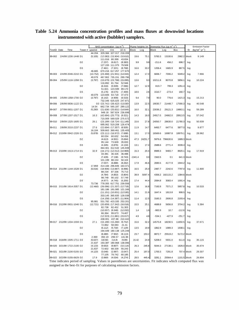
I

Table 5.24 Ammonia concentration profiles and mass fluxes at downwind locations instrumented with active (bubbler) samplers.

NH3 concentration (ug m-3) Plume heights (m) Ammonia Flux (ug m-1 s-1) Emission Factor TestID Date Time Tower # upwind 2 m 4 m 10 m Block Log Block Log Box fit (kg hd -1 yr-1)

44.204 329.366 327.317 218.209 99-002 2/4/99 1230-1448 D1 (5.105) (12.083) (15.904) (10.610) 19.6 75.1 5783.3 13100.6 2982.2 block 9.149

111.016 80.399 43.834 D2 (7.237) (6.817) (8.383) 9.9 9.8 -211.6 456.2 698.7 log

127.155 111.375 79.508 D3 (7.461) (7.321) (8.768) 16.6 33.2 1206.4 1665.9 867.5 log

46.665 670.216 617.257 177.670 99-003 2/4/99 2046-2210 D1 (13.752) (23.468) (21.941) (14.044) 12.4 17.0 6836.7 7006.2 5049.2 log 7.966

40.079 467.902 735.151 299.796 99-004 2/5/99 1116-1358 D1 (3.797) (15.679) (23.798) (15.095) 13.6 9.3 10211.8 8070.8 5856.1 log 10.224

116.892 81.764 52.946 D2 (6.316) (5.509) (7.066) 12.7 12.9 819.7 799.3 1051.4 log

51.821 123.599 89.170 D3 (5.176) (6.575) (7.469) 18.6 2.6 1510.7 -273.4 160.7 log

40.079 123.606 63.718 37.473 99-005 2/5/99 1358-1700 D2 (3.797) (6.142) (4.909) (6.533) 9.4 7.9 90.0 776.6 1421.3 log 15.213

732.346 625.025 247.871 99-006 2/6/99 0836-1122 D1 0.0 (23.741) (28.422) (13.030) 13.9 22.5 19030.7 21448.7 17590.3 log 40.548

14.54 662.734 565.187 289.122 99-007 2/7/99 0931-1207 D1 (5.290) (21.636) (25.831) (14.644) 16.0 32.1 23036.2 29121.3 19863.1 log 59.289

949.18 567.824 236.698 99-008 2/7/99 1207-1517 D1 16.3 (42.694) (25.773) (9.321) 14.3 16.0 24917.0 24662.0 28913.5 log 57.042

715.009 569.029 275.572 99-010 2/8/09 1325-1605 D1 26.1 (23.199) (18.724) (11.148) 15.6 27.8 24050.7 28630.0 21780.3 log 50.939

695.062 519.208 126.474 99-011 2/8/99 2010-2237 D1 27.6 (22.694) (17.357) (8.505) 11.9 14.7 6493.7 6477.6 5877.0 log 9.877

16.104 509.663 369.461 135.405 99-012 2/10/99 0942-1326 D1 (5.878) (23.111) (16.972) (7.698) 13.1 17.0 16569.6 16987.8 18979.1 log 28.962

60.034 60.632 54.456 D2 (4.613) (4.501) (5.694) 47.3 24251.7 5976.6 796630.6 1689.3 block

95.144 73.609 35.833 D3 (4.345) (3.876) (4.134) 13.1 17.4 2688.6 2771.4 3039.4 log

464.301 312.532 145.939 99-013 2/10/99 1513-1714 D1 32.9 (16.171) (12.012) (10.969) 15.3 20.4 8989.3 9483.7 8920.1 log 17.919

33.381 36.326 36.488 D2 (7.428) (7.138) (9.743) -1341.4 0.0 1563.5 0.1 641.3 block

101.199 88.154 50.104 D3 (7.037) (6.888) (8.262) 17.9 46.6 2690.5 4177.9 1944.2 log

17.859 414.166 296.846 163.371 99-014 2/11/99 1144-1528 D1 (6.016) (18.906) (13.887) (6.996) 16.5 25.0 2487.7 2242.6 7797.0 log 11.800

88.234 87.336 75.713 D2 (4.784) (4.853) (5.804) 39.9 5097.4 4356.2 182115.2 1384.6 block

98.748 90.102 57.749 D3 (4.977) (4.745) (5.200) 17.4 44.4 2084.8 3083.4 1591.4 log

73.736 778.355 617.751 239.556 99-015 2/11/99 1914-2057 D1 (12.460) (26.096) (21.207) (12.719) 12.6 16.8 7193.9 7571.2 5957.8 log 10.533

181.186 191.085 121.166 D2 (11.151) (10.831) (12.530) 14.1 21.9 1647.4 1813.8 908.5 log

333.145 365.835 128.038 D3 (14.158) (14.387) (11.904) 11.4 12.5 3160.3 2606.8 2193.4 log

95.981 531.782 423.335 253.201 99-016 2/12/99 0931-1046 D1 (12.721) (20.659) (17.342) (16.016) 15.5 25.1 4688.8 5656.8 3704.2 log 5.384

82.738 82.452 51.303 D2 (10.007) (9.348) (12.032) 1.4 1.6 -983.9 10.7 -112.6 log

66.364 99.673 74.407 D3 (12.523) (11.881) (15.017) 4.9 4.8 -534.1 -427.9 -251.7 log

438.001 437.88 210.442 99-017 2/12/99 1334-1559 D1 27.1 (15.196) (15.266) (9.752) 15.6 32.2 14575.8 18230.5 11650.5 log 37.671

72.862 58.083 21.41 D2 (6.112) (5.730) (7.129) 13.5 19.9 1862.9 1989.3 1938.1 log

194.449 180.138 125.249 D3 (8.480) (7.902) (8.113) 23.7 153.2 8872.7 25519.2 5172.2 block

2.369 392.19 296.57 141.96 99-018 3/16/99 1505-1711 D3 (6.637) (18.56) (14.8) (9.89) 15.42 24.9 5208.0 5931.0 611.0 log 35.115

21.637 193.387 180.968 138.096 99-020 3/21/99 1722-2100 D2 (4.123) (9.653) (9.807) (10.114) 26.3 245.8 5044.3 27138.1 1826.0 block 35.674

21.637 72.602 68.339 55.243 99-021 3/21/99 2100-0155 D2 (4.123) (3.046) (2.997) (3.047) 25.4 197.0 1700.3 7291.8 707.4 block 29.307

77.105 79.742 60.185 99-022 3/22/99 0155-0629 D2 17.9 (3.969) (4.034) (4.274) 28.5 445.4 3281.1 25564.4 1101.5 block 26.804

Time indicates period of sampling. Values in parentheses are uncertainties. Fit indicates which computed flux was assigned as the best-fit for purposes of calculating emission factors.

79

-

I I I

I I I I I

-. -...

fl --... '

... I . ' . . ~ . ,, . I ~ _,_ fl .

' I . • I . ur I I .. r---

... . • I t---

I

t--' fl ' -' ' •' . . '. '

' . I

' ~ . ' ' I ' ' I ' fl .

.I!. ' I ' .

, . I ' I

~ .. I • I

' 1 ..

Emission factors are reported for the 23 periods for which the wind direction was appropriate for all sampling locations, including those during south wind events on dairy 1 (Table 5.24 and Figure 5.17). The dates of measurements made on dairy 2 are shifted by -37 days in order to show both data sets on the same plot. Although emission factors were generally lower during night periods than at midday, the larger temporal trend overwhelmed any diurnal trend in the data. A storm on the fifth day of sampling at dairy 1 saturated the corral surfaces, lowering emission as expected (Asman 1992). The very low emission factor for the period directly preceding the storm is likely due to a combination of high relative humidity and highly unstable atmospheric conditions (RH = 85%, bulk Richardson’s number < -6). The only other period of unstable conditions was between 18:00 and 0:00 on the last day at dairy 1, for which the emission factor is consistent with the immediately previous measurement in time. The final period at dairy 1 was characterized by high wind speed (> 3.5 m/s at 4m) and the lowest RH of all sampling periods (42%), which accelerated drying and increased emissions. The higher emission factors measured on dairy 2 at midmorning and late afternoon may be evidence of a diurnal trend with animal activity, as they are the feeding times, but with data from only two days it is impossible to determine conclusively. Taken as three data sets, dairy 1 before the rain event, after the rain, and dairy 2, the emission factors show the expected decreasing trend with increasing relative humidity (r2 = .2, data not shown) and increased with increasing temperature (r2 = .3, data not shown). We also saw a trend of increasing emission with higher wind speed, which was expected, but this finding may be biased by the fact that wind speed is incorporated in the calculation of emission factor.

0

10

20

30

40

50

60

70

Em

issi

on F

acto

r(k

g N

H3 h

d -1

yr -1

)

Dairy1

Dairy2Rain

2/26/99 0:00

2/25/99 0:00

2/24/99 0:00

2/23/99 0:00

2/22/99 0:00

2/21/99 0:00

2/20/99 0:00

2/19/99 0:00

2/18/99 0:00

2/17/99 0:00

2/16/99 0:00

2/15/99 0:00

2/14/99 0:00

2/13/99 0:00

2/12/99 0:00

2/11/99 0:00

2/10/99 0:00

2/9/99 0:00

2/8/99 0:00

2/7/99 0:00

2/6/99 0:00

2/5/99 0:00

2/4/99 0:00

Sample Day

Figure 5.17 Emission factors calculated from measurements.

80

The average NH3 emission factor for the two dairies was 29.5 kg hd-1 yr-1 when calculated from the measurements and 30.3 kg hd-1 yr-1 when calculated by N balance. The agreement between the two methods indicates the robustness of the measurement method. Climatic conditions during the sampling periods were cooler and wetter than the conditions of the laboratory experiments from which the NH3 volatilization estimates were derived (27 °C, dried air). This should result in an overestimation, since hot, dry conditions increase NH3 volatilization (Asman 1992). Urea was demonstrated to be the only significant source of NH3-N in the laboratory experiments. These were run until the manure was well dried with no additional input of moisture. Conversely, the areas occupied by the cattle in the field trial were saturated throughout the measurement periods, which could cause field measured NH3 to include some contribution from organic forms of N. In this study, the climactic factors inhibiting NH3

volatilization during the field trials appear to balance the N sources that are not included in the laboratory derivation, resulting in a good agreement between the methods. This may not be the case in other circumstances.

A comparison of average NH3 fluxes calculated from measurements made downwind of the various sources within the two dairies with fluxes calculated by N balance for two general populations on each dairy show some consistent trends (Figure 5.16). Nitrogen balance estimates predict similar NH3 fluxes from source areas 1 and 3, while measurements indicate higher emission from source area 1 on both dairies. The primary reason for this difference was the manure management practices: source areas 3 included free stalls which were flushed, while source areas 1 were dry lot corrals from which manure was only flushed from about 20% of the area in dairy 1 and not removed in dairy 2. The lower measured fluxes, relative to N balance calculations, from source area 3 on dairy 1 compared to dairy 2 are most likely due to the fact that dairy 1 was removing manure from all of the milking cows while dairy 2 was flushing the manure from the 60% of the milking cows.

81

6 CONCLUSIONS FROM FIELD MEASUREMENTS

In order to better meet the regulatory needs of both California and national agencies for empirically derived PM10 emission factors for specific agricultural operations, the data presented in section 5.0 has been summarized in these conclusions. The five years (1994 - 1998) of field testing results from this study that have been used to compute PM10 emission rates were filtered to identify only those data for which the emission factor confidence rating was very high. The emission factor confidence rating applied in selecting data for the summaries was comprised of the elements identified in the systematic examination of the emission rates calculated for land preparation activities and the attendant lidar data as presented in section 4.3 and Appendix H. Due to the changes made in the equipment and the methods involved in collecting the data over the reporting period, some of the qualifiers in the rating system were more stringently applied to some sub-sets of the data than to others. This was necessary to attain the optimal compromise between data quality and recovery. The application of each qualifier in the rating system to each specific source category is explained as the data is presented below.

The PM10 emission factors calculated for land preparation activities showed some trends by operation (i.e. discing vs. ripping, see section 5.4), though there were individual tests that could be interpreted as exceptions to these trends. For the following summary, the selected PM10

emission factors have been grouped by commodity and operation with the exception of the confined animal facilities, which were grouped only by commodity (i.e. dairy or beef). The strongest trends in PM10 emission factors with environmental conditions were the relationships observed with relative humidity and soil moisture. As is illustrated in the categorical summaries below, there appears to be a critical relative humidity of 40% below which it is more likely that large emission factors will be measured. Data collected for discing operations and almond pickup indicate a more definite relationship of PM10 emission factors with soil moisture, with 10% soil moisture appearing to be a critical level observed to reduce emissions under the discing study conditions and 4% soil moisture defining the difference for almond pickup. Similar observations have been made by other researchers and a correlation of relative humidity with soil moisture indicates the relationship between these two important variables and PM10

emission factors (Holmén, James et al. 2001). Where data is available, average emission factors have been calculated for each source from those tests conducted in conditions below and above 40% relative humidity, with the exception of discing tests which are averaged for soil moisture conditions below and above 10%. Almond harvesting tests were averaged for soil moisture conditions below and above 4% and cotton weeding tests were averaged for soil moisture conditions below and above 8%.

82

Table 6.1 Summary of average PM 10 emission factors.

all valid - all conditstandard

SOURCE average deviation

ions

number

most confident - sestandard

average deviation

lected

number notes almond shaking

II 1670 1303

sweeping II

1466 1042 4 2

log model only log model only

pickup III

4106.19 3210.43 5 > 4 % 2007.83 351.08 < 4 % 7253.72 2820.93

3 2

high and low soil moisture

fig sweeping

I 13 8

pickup I

39 4 N/A N/A

box model, high soil moisture no blowers

cotton harvest IV

picking 189.80 166.61 17 cotton harvest VI

<40% 200.36 99.31 >40% 217.65 148.23

3 7

high and low relative humidity

stalk cutting 188.17 218.68 29 <40% 348.94 301.03 >40% 134.88 109.17

9 3

wheat harvest IV

combining 649.86 513.96 20 wheat harvest VI

<40% 889.64 346.02 >40% none

7 high and low relative humidity

land preparation IV

root cutting 33.00 4.24 2 land preparation

VI

>40% 33.00 4.24 2 high relative humidity only

discing 134.24 153.97 27 <10% 244.94 121.13 >10% 72.66 46.22

5 12

high and low soil moisture

chiseling 512.20 287.53 5 <40% 612.25 208.56 >40% 112.00 0.00

4 1

high and low relative humidity

weeding 89.21 107.98 15 > 8 % 5.98 10.73 < 8 % 144.70 108.05

6 9

high and low soil moisture

confined animal facilities V

dairy 80.42 102.64

lbs/d*1000hd 90.51 116.74

26

26

confined animal facilities V

<40% 113.26 126.22 >40% 54.70 64.08 <40% 112.95 142.25 >40% 53.39 80.89

12 10 12 10

high and low relative humidity

beef 79.21 107.32 27 <40% 158.11 159.26 9 high and low relative humidity >40% 42.31 24.21 12

lbs/d*1000hd 28.87 35.28 26 <40% 43.28 46.88 11 >40% 23.24 20.10 11

I Valid Upwind (UP) and Downwind (DN) PM10 and wind speed (WS) at one height. II 2 or more valid UP and DN and WS. III 2 or more valid UP and WS, 3 valid DN; PM and WS outside canopy; PM measured

100 m or less from operation. IV 2 or more uncontaminated UP and WS, 3 valid DN; sampler placement as in Holmén

et al., 2001. V 1 valid UP, 3 valid DN, WD within 45 ° of optimal, EFU < 100%. VI 2 or more uncontaminated UP and WS, 3 valid DN; sampler placement as in Holmén et

al., 2001; QUP = A, QWD = A, EFU <100%. Figures in italics indicate averaged results presented in English units.

Summarization of the PM10 emission factors measured in this study by 1) reducing the data set to those tests which are assigned the highest confidence ratings and 2) grouping the data by commodity, operation, and relative humidity produced average emission factors which represent the most directly applicable interpretation of the results of the first five years of this study currently possible.

83

6.1 Orchard Crops

Measurement of emission factors was attempted for walnuts, figs, and almonds. The three valid walnut tests (see Appendix A) were conducted during two simultaneous operations which could not be quantified separately using these data, so no PM10 emission factors are reported for walnuts. Fig harvesting operations of sweeping and pickup were monitored in 1994 only, so vertical profiles of the PM10 concentrations and wind speeds were not collected. Also, the climatic conditions during the fig sampling were unusually wet and it became necessary for the operator to sweep the figs without the blowers (which would be too rough on the high-moisture-content fruit) and to conduct the pickup on unusually wet ground. Therefore, the PM10

emission factors summarized in Table 6.1 are computed from single height measurements and are likely a lower-bound estimate of emissions, due to the unusual circumstances.

Two independent calculations of PM10 emission factors were performed on PM10 and wind speed profiles collected at almond harvesting operations (shaking, sweeping, and pickup) in 1995. The initial computations used the logarithmic model (see section 4.2) applied to all tests with valid PM10 concentration measurements at least two heights, a valid upwind measurement, and appropriate wind direction. Subsequent calculations used the methods described by Holmén et al. (2001) and confined the evaluation to those tests conducted under conditions shown to be appropriate to the application of those methods. In this evaluation, only six almond pickup tests were conducted under the appropriate conditions of having both PM10 and wind speed measurements in the same wind field. One of these tests was conducted significantly more than 100 m from the operation (95-055, Table 5.3) and the calculated emission factor for that test is much lower than all of the other tests conducted under similar conditions, so that data point is considered invalid for the purposes of this summary. There were no tests of almond shaking or sweeping that met all of the requirements of the published method.

A trend can be observed between PM10 emission factors and soil moisture in the five almond pickup tests of highest confidence. Interestingly, the trend with relative humidity and almond PM10 emission factors is opposite that expected, with the highest emission factors recorded under the highest relative humidity (see Table 5.4). This fact indicates clearly that the soil moisture is a more meaningful predictor of PM10 emissions from almond pickup than relative humidity. For this reason, the average emission factors summarized in Table 6.1 are provided for conditions of low (< 4%) and high (> 4%) soil moisture.

84

Best Fit emission factors (mg/m2) and soil moisture (%)

from tests with highest confidence ratings ALMOND PICKUP

0.00

1000.00

2000.00

3000.00

4000.00

5000.00

6000.00

7000.00

8000.00

9000.00

10000.00 B

est f

it e

mis

sio

n fa

cto

r (m

g/m

2 )

0.00

0.50

1.00

1.50

2.00

2.50

3.00

3.50

4.00

4.50

5.00

So

il M

ois

ture

(%)

95-044 95-044 95-046 95-054 95-060

Figure 6.1 PM10 emission factors (mg/m2) and soil moisture (%) from 1995 tests of highest confidence for Almond pickup operations.

85

6.2 Cotton Harvest

Tests of PM10 emission factors from cotton harvest were grouped by operation into picking, stalk cutting, and stalk incorporation. Only tests with upwind PM10 concentrations measured at 2 or more heights were included in this final summary to insure that instances of upwind contamination would be reliably identified (see section 4.3.4). Additionally, individual tests for which more than one concentration measured upwind was greater than the downwind concentration measured at the same height were excluded from this summary as were tests during which the average or standard deviation of the wind direction exceeded limits set by the confidence rating Qwd (see Table 4.2). Tests for which the emission factor relative uncertainty exceeded 100% were also excluded.

6.2.1 Cotton Picking Ten tests of cotton picking met all of the emission factor confidence criteria. All of these were conducted on a single ranch on 4 fields with very similar loam or clay loam soil types using the same Case-Harvester 2-row pickers. Seven tests were conducted in 1995 and the eighth in 1996. Soils analysis results are available for all of these tests except 95-137 and both moisture and dry sieve fraction less than 75 mm were essentially the same in 5 tests (soil moisture = 4 % and silt content = 16 %), but silt content was lower (10 %) in test 95-123 and moisture was higher (12.4 %) in test 96-095. These two tests resulted in relatively low PM10 emission factors, which may have been due to soil conditions or increased relative humidity. The two tests conducted in conditions with the highest relative humidity (tests 95-123 and 96-095) have two of the three lowest calculated PM10 emission factors. Also, tests conducted under identical (using side-by-side towers) or nearly identical conditions (95-136 and 95-137) have similar PM10 emission factors. However, tests 95-094 through 95-096, conducted sequentially as relative humidity increased have increasing PM10 emission factors. This phenomenon may be related to the change in atmospheric stability as the sun set, or it may be due to the fact that the distance between the pickers and the samplers decreased steadily in this series of tests. It is apparent that changes in relative humidity alone fail to describe the differences in PM10 emission factors. Because the cotton picking data for which confidence ratings are highest do not show a solid trend in PM10 emission factors with relative humidity, the average values for this operation under conditions of high and low relative humidity are essentially the same. This fact may be due, in part, to the fact that cotton picking can only be performed when the cotton is dry such that cotton is generally picked at times of low relative humidity.

86

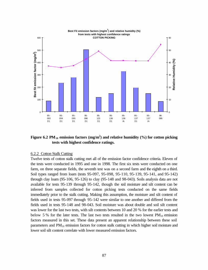
Best Fit emission factors (mg/m2) and relative humidity (%)

from tests with highest confidence ratings COTTON PICKING

0

100

200

300

400

500

600 B

est f

it e

mis

sio

n fa

cto

r (m

g/m

2 )

0

10

20

30

40

50

60

Rel

ativ

e H

um

idit

y (%

)

95- 95- 95- 95- 95- 95- 95- 95- 95- 96-093 094 095 096 123 136 136 137 137 095 D1 D1 D1 D1 D1 D1 IA D1 IA

Figure 6.2 PM10 emission factors (mg/m2) and relative humidity (%) for cotton picking tests with highest confidence ratings.

6.2.2 Cotton Stalk Cutting Twelve tests of cotton stalk cutting met all of the emission factor confidence criteria. Eleven of the tests were conducted in 1995 and one in 1998. The first six tests were conducted on one farm, on three separate fields, the seventh test was on a second farm and the eighth on a third. Soil types ranged from loam (tests 95-097, 95-098, 95-110, 95-139, 95-141, and 95-142) through clay loam (95-106, 95-126) to clay (95-148 and 98-043). Soils analysis data are not available for tests 95-139 through 95-142, though the soil moisture and silt content can be inferred from samples collected for cotton picking tests conducted on the same fields immediately prior to the stalk cutting. Making this assumption, the moisture and silt content of fields used in tests 95-097 through 95-142 were similar to one another and differed from the fields used in tests 95-148 and 98-043. Soil moisture was about double and soil silt content was lower for the last two tests, with silt contents between 10 and 20 % for the earlier tests and below 5 % for the later tests. The last two tests resulted in the two lowest PM10 emission factors measured in this set. These data present an apparent relationship between these soil parameters and PM10 emission factors for cotton stalk cutting in which higher soil moisture and lower soil silt content correlate with lower measured emission factors.

87

Two types of stalk cutting implements were represented in the valid tests; a 4-row rotary type was used for tests 95-097 and 95-098 and a 6-row flail type was used for the subsequent tests. While the side-by-side measurements made during test 95-098 agree very well and appear to indicate a larger PM10 emission factor for the rotary type stalk cutter, the equally valid test 95-097 does not support this hypothesis. Test 95-097 was taken earlier in the afternoon when the solar radiation was stronger, wind speeds were slightly lower, and the difference between temperature at the ground and aloft was greater than during test 95-098. The plume would be expected to loft higher under these conditions and dispersion upward could result in inaccurate measurements and underestimation of PM10 emission. Unfortunately, lidar data are not available for these tests and, considering the fact that the sampling towers were within 50 meters of the tractors for both tests, there is no data available to indicate that either test is a better measurement of the true PM10 emission factor for rotary type stalk cutters than the other.

The range in relative humidity was greater for cotton stalk cutting tests than for cotton picking tests, as picking is only practiced under conditions of favorable cotton moisture content and trends are apparent between PM10 emission factors for stalk cutting and relative humidity. The test performed under conditions of lowest relative humidity (95-098) measured the highest PM10 emission factor and the test with the highest relative humidity (98-043) had the lowest PM10 emission factor. For the cotton stalk cutting tests, this clearer delimitation of PM10

emission factor with relative humidity results in a lower average emission factor under conditions of higher relative humidity (> 40%) than when relative humidity is lower. Tests 95-139 to 95-142, collected sequentially under identical or nearly identical conditions, illustrate the variability in emission factor that cannot be accounted for in the measured variables.

88

Best Fit emission factors (mg/m2) and relative humidity (%)

from tests with highest confidence ratings COTTON STALK CUTTING

0

100

200

300

400

500

600

700

800

900

1000 B

est f

it e

mis

sio

n fa

cto

r (m

g/m

2 )

0

10

20

30

40

50

60

70

Rel

ativ

e H

um

idit

y (%

)

95- 95- 95- 95- 95- 95- 95- 95- 95- 98- 95- 95-097 098 098 126 139 141 142 142 148 043 110 106 D1 D1 I1 D1 D1 D1 D1 I3 D1 D1 D1

Figure 6.3 PM10 emission factors (mg/m2) and relative humidity (%) for cotton stalk cutting tests with highest confidence ratings.

6.2.3 Cotton Root Cutting Two tests of root cutting following cotton harvest met the emission factor confidence criteria. This practice has not been widely adopted, but its ability to break down the furrows and loosen the cotton plant residue from the soil makes it an attractive alternate practice to stubble discing for cotton. The tests were conducted sequentially on the same field under nearly identical conditions. This limited data set indicates that there may be a relationship between relative humidity and PM10 emission factors for cotton root cutting. It also indicates that, under these conditions, the average emission from root cutting is less than that for stubble discing. However, soil moisture data is not available for the tests of root cutting, and this information is essential for a meaningful comparison of the two practices (see section 6.4.1).

89

Best Fit emission factors (mg/m2) and relative humidity (%)

from tests with highest confidence ratings COTTON ROOT CUTTING

27

28

29

30

31

32

33

34

35

36 B

est f

it e

mis

sio

n fa

cto

r (m

g/m

2 )

42

44

46

48

50

52

54

Rel

ativ

e H

um

idit

y (%

)

96-103 D1 96-104 D1

Figure 6.4 PM10 emission factors (mg/m2) and relative humidity (%) for cotton root cutting tests with highest confidence ratings.

90

6.3 Wheat Harvest

As with tests of cotton harvest operations, only tests with upwind PM10 concentrations measured at 2 or more heights were included in this final summary and individual tests for which more thAn one concentration measured upwind was greater thAn the downwind concentration measured at the same height were excluded, as were tests during which the average or standard deviation of the wind direction exceeded limits set by the confidence rating Qwd (see Table 4.2). Tests for which the emission factor relative uncertainty exceeded 100% were also excluded.

The single operation identified with wheat harvest, combining, is represented in this summary by six tests for which measurement data met all reliability criteria. The first three were conducted in 1996 and the rest in 1997 on a single farm on three different fields with loam and clay loam soil types. Soil moisture and 75 mm dry sieved fraction data are available for all tests except 97-032 and soil moistures were very low, from 2.3 to 4.2%. Silt contents were about 20% for tests conducted in 1996 and 10% for the 1997 tests. All tests were conducted using the same combines.

There appears to be no readily discernible trend in PM10 emission factors from wheat harvesting with soil type or relative humidity, within the limited range of these variables during measurements. Tests 97-032 and 97-034 were conducted sequentially, with two towers side-by-side the same distance from the combine used in test 97-034, and the variance in PM10

emission factors from these tests indicate the variability that cannot be accounted for within the measured parameters. One possible source of error is the relatively large distance between the sampling tower and the combine during test 97-032, but the lack of lidar data for this test makes it impossible to identify any uncertainty in the estimate of plume height directly and the resulting data have been included in the summary average.

91

-- \ -~

-\. -

-- - -

-

-

Best Fit emission factors (mg/m2) and relative humidity (%)

from tests with highest confidence ratings WHEAT HARVEST

0

200

400

600

800

1000

1200

1400 B

est f

it e

mis

sio

n fa

cto

r (m

g/m

2 )

0

5

10

15

20

25

30

35

40

Rel

ativ

e H

um

idit

y (%

)

96-052 96-063 96-058 97-032 97-034 97-034 97-035

Figure 6.5 PM10 emission factors (mg/m2) and relative humidity (%) for wheat harvesting tests with highest confidence ratings.

92

6.4 Land Preparation

The most recent focus of this project has been on land preparation activities. Stubble discing following cotton was the first land preparation operation monitored in 1995 followed by chiseling, finish discing, and listing following cotton in 1996 and stubble discing, chiseling, and finish discing following wheat in 1997. Finally, the stubble discing tests following cotton in 1998 provided the basis for the lidar-assisted evaluation of emission factor confidence ratings. Unfortunately, none of the listing tests fulfill the emission factor confidence criteria, which is similar to that for the harvest of wheat and cotton (see sections 6.2 and 6.3), and only results for discing and chiseling are summarized below. Criteria for land preparation tests require valid PM10 concentration measurements at three heights upwind, due to the increased likelihood of upwind interferences with these later-season operations when simultaneous activities on neighboring fields is more common. Also, wind direction requirements were relaxed for tests of land preparation activities relative to those for harvest because these operations are conducted at an angle to the edge of the field making the distinction of wind direction within 45 degrees of perpendicular to the edge of the field less relevant to data interpretation. Thus, tests of land preparation are included in the following summary regardless of wind direction.

6.4.1 Discing Sixteen of the seventeen discing tests that met all of the emission factor confidence criteria were following cotton and only test 97-045 was following wheat. Twelve of the tests were conducted during stubble discing, immediately following stalk cutting or harvesting (in the case of 97-045) and five were conducted during second discing following chiseling (tests 96-111 through 96-119). Two farms and three different fields are represented in these data. The implements used in all of the tests were similar with respect to the variables measured in this study; the discs all had 2 gangs or rows of blades and were pulled by a track-drive diesel tractor. The finish disc (used in tests 96-111 through 96-119) was wider and the individual blades were smaller in circumference than those of the stubble discs and no rollers were used following the finishing disc.

Emission factors for PM10 from discing show a distinct relationship with soil moisture and soil silt content, with lower emission factors measured in conditions of higher soil moisture and lower soil silt contents. Soil moisture was lower during stubble discing than for finish discing because soil brought up to the surface (where it is collected for the analysis) by the chisel was wetter than soil sampled following the harvest. The farm where tests in 1998 were conducted had soil of much lower silt content (dry sieve fraction less than 75 mm) than the farm where all of the other tests in this summary were conducted. It is difficult to distinguish between the effects of soil moisture and silt content using only these data, but the stubble discing tests conducted on fields of similar soil silt content but much different soil moisture can be compared by comparison of stubble discing (tests 95-128 to 95-132) to finish discing (tests 96-111 to 96-119), making the assumption that the difference in soil moisture is the most significant difference between these operations. Since this comparison indicates that increased soil moisture decreased PM10

emission factors, average emission factors are presented for soil moisture above and below 10%.

93

Best Fit emission factors (mg/m2) and soil moisture (%)

from tests with highest confidence ratings DISCING

0

50

100

150

200

250

300

350

400

450

Bes

t fit

em

issi

on

fact

or

(mg

/m2 )

0

5

10

15

20

25

So

il M

ois

ture

(%)

95-1

30 D

1

95-1

30 I2

95-1

31 D

1

95-1

32 D

1

97-0

45 D

1

98-0

46 M

1

98-0

46 L

1

98-0

47 D

1

98-0

48 D

1

98-0

49 D

1

98-0

50 D

1

96-1

17 D

1

96-1

18 D

1

96-1

19 M

1

96-1

11 I5

96-1

12 I6

96-1

13 I7

Figure 6.6 PM10 emission factors (mg/m2) and soil moisture (%) for discing tests with highest confidence ratings.

Data are presented for tests 95-130 and 98-046 conducted under identical conditions using two towers for each test, and the variance in PM10 emission factors calculated for these tests indicate the variation that cannot be accounted for by the variables measured in this study.

6.4.2 Chiseling Five chiseling tests met all of the emission factor validity criteria. All of these tests were following wheat harvest and stubble discing on the same farm and field using the same implement. Soil moisture was about 2% for all of the tests. There appears to be a relationship between PM10

emission factors from chiseling and relative humidity. Test 97-050 was the only test conducted under conditions of relative humidity above 40% and has the lowest PM10 emission factor. While differences in relative humidity cannot account for all of the variation seen in the PM10

emission factors calculated for chiseling, the trend was also seen in other agricultural operations and these chiseling data are summarized for conditions above and below 40% relative humidity.

94

--.

- I = ---

Best Fit emission factors (mg/m2) and relative humidity (%)

from tests with highest confidence ratings DISCING

0

100

200

300

400

500

600

700

800 B

est f

it e

mis

sio

n fa

cto

r (m

g/m

2 )

0

5

10

15

20

25

30

35

40

45

Rel

ativ

e H

um

idit

y (%

)

97-046 D1 97-048 D1 97-049 D1 97-050 D1 97-051 D1

Figure 6.7 PM10 emission factors (mg/m2) and relative humidity (%) for chiseling tests with highest confidence ratings.

6.4.3 Weeding Fifteen cotton cultivation tests met all of the emission factor confidence criteria. Weeding, for these tests, was conducted using a Lilliston 6 blade cultivator 6.6 m wide pulled by a wheeled tractor at approximately 2.2 m/s. Several tests (98-001 through 98-005) were conducted with two simultaneous profiles, thus each pair of emission factors provides a good estimate of the repeatability of the measurements. Emissions of PM10 from these weeding operations, conducted on a clay loam soil, appear to be strongly affected by soil moisture. The data presented in Figure 6.8 illustrates a marked increase in PM10 emissions when soil moisture drops below 8 %.

95

Best Fit emission factors (mg/m2) and soil moisture (%)

from tests with highest confidence ratings WEEDING

0

50

100

150

200

250

300

350 B

est f

it e

mis

sio

n fa

cto

r (m

g/m

2 )

0

2

4

6

8

10

12

14

16

18

So

il M

ois

ture

(%)

98- 98- 98- 98- 98- 98- 98- 98- 98- 98- 98- 98- 98- 98- 98-001 001 002 002 003 003 004 004 005 005 007 008 009 010 011 D1 I1 D1 I2 D1 I3 D1 I4 D1 I5 I7 I8 I9 IA IB

Figure 6.8 PM10 emission factors (mg/m2) and soil moisture (%) for weeding tests with highest confidence ratings.

96

•

•• • )(

♦ • ♦ • ..

It • )( I( ♦ J(

•• !ft J( It

)( • • • •

6.5 Confined Animal Facilities

Vertical profiles of PM10 were collected downwind of confined animal facilities in 1995 and 1996. Emission factor confidence criteria used to select data for inclusion in this summary is similar to that used for the row crops but does not require upwind PM10 concentrations be measured at multiple heights due to the relative unlikelihood of upwind contamination from the hay fields and vineyards upwind of the facilities. However, tests for which the upwind PM10

concentration exceeded the downwind concentration at the height of measurement (3 m) were excluded from this summary. Average wind direction was restricted to within 45 degrees of perpendicular to the edge of the facility to ensure that the source was being measured quantitatively and tests with emission factor uncertainties of more than 100% were excluded from this summary.

The relationship between PM10 emission factors for confined animal facilities and relative humidity is most apparent in the correlation where it can be seen that high PM10 emissions are most likely in conditions of relative humidity under 40%. Thus, emission factors for dairy and beef are presented for conditions of less than and greater than 40% relative humidity.

Beef and dairy 1996, EFU<1, Qup = A, all have only 1 upwind

wind direction difference < 45 degrees

0

100

200

300

400

500

600

Bes

t fi

t em

issi

on

fac

tor

(mg

/m^

2)

0 10 20 30 40 50 60 70 80 90

Relative humidity (avg.) %

Figure 6.9 Correlation of PM10 emission factors (mg/m2) and relative humidity (%) for confined cattle tests with highest confidence ratings.

97

Best Fit emission factors (lbs/d*1000hd) and relative humidity (%) from tests with highest confidence ratings

DAIRY

0

100

200

300

400

500

600 B

est

fit

emis

sio

n f

acto

r(l

bs/

d*1

000h

ead

)

0

10

20

30

40

50

60

70

80

90

Rel

ativ

e H

um

idit

y (%

)

96-0

24

96-0

25

96-0

27

96-0

28

96-0

29

96-0

30

96-0

31

96-0

33

96-0

34

96-0

37

96-0

38

96-0

43

96-0

47

95-0

76

95-0

86

95-0

89

95-0

90

96-0

42 D

1

Figure 6.10 PM10 emission factors (lbs/d*1000hd) and relative humidity (%) for dairy tests with highest confidence ratings.

6.5.1 Dairy Eighteen measurements of PM10 emission factors from the dairy met the confidence rating criteria (Figure 6.10). Data collected in 1996 represent winter conditions (April) and those from 1995 represent summer conditions (October). The 1996 data show a strong relationship to relative humidity with the largest emission factor measured in the lowest relative humidity (test 96-029) and the lowest emission factor measured in the highest relative humidity (test 96-031). There is also a trend in the 1995 data collected during daytime (tests 95-086, 089, and 090; see table 5.19) linking relative humidity to PM10 emission factors. The single nighttime test conducted in the summer indicates that PM10 emissions in the early night hours (see Table 5.19 for exact times) can be elevated in the summertime, regardless of humidity. This phenomena can reasonably be attributed to the observed increased animal activity at dusk in the summer. Soil moisture and solar radiation data are not available for these tests but emission factors were lowest during night and morning hours and highest in the late afternoon and early evening. There was no precipitation during the time period over which samples were collected at this dairy and no dust control measures were applied.

98

6.5.2 Beef Feedlot

Best Fit emission factors (lbs/d*1000hd) and solar radiation (W m- 2

) from tests with highest confidence ratings

Bes

t fi

t em

issi

on

fac

tor

(lb

s/d

*100

0hea

d)

180

160

140

120

100

80

60

40

20

0

FEEDLOT 900

800

700

600

500

400

300

200

100

0

-100

So

lar

Rad

iati

on

(W m

-2)

96-0

06

96-0

13

96-0

20

96-0

22

96-0

23

96-0

73

96-0

73

96-0

74

96-0

74

96-0

79

96-0

78

96-0

76

96-0

75

96-0

75

96-0

80

96-0

88

96-0

88

96-0

90

96-0

90

96-0

87 I1

Figure 6.11 PM10 emission factors (lbs/d*1000hd) and solar radiation (W/m2) for feedlot tests with highest confidence ratings.

Measurements of PM10 were made at the feedlot in both March and July of 1996 (Figure 5.11). Solar radiation data is available for measurements made in July and a trend can be observed between PM10 emission and solar radiation. There is also a definite increase in PM10 emission in the summer season over that measured in the winter. Of the winter tests in this summary, the first three (96-006, 96-013, and 96-020) were conducted during daylight hours. Since emissions measured in those tests are not higher than emissions measured in the nighttime tests in the winter (tests 96-022 and 96-023), it is unlikely that variation in PM10 emission factor can be directly attributed to changes in solar radiation. However, it may be indicative of some underlying phenomena. The observed seasonal differences may be due to soil moisture but unfortunately, soil moisture data are not available for these tests. It is also likely that the peaks in PM10 emission factors observed at nighttime may be due to increased nighttime animal activity in the hot summer months.

99

6.6 Ammonia emission factors

Ammonia emission factors were quantified for a feedlot and three dairies using both direct measurements of ammonia concentrations and dietary nitrogen balance. In all cases, the average ammonia emission factors calculated by the two methods were comparable. Generally, ammonia emission factors calculated from dietary nitrogen will provide the most broadly applicable means for estimating average ammonia emission rates for any particular dry lot facility. However, in order to provide an estimate of the diurnal and seasonal variations of ammonia emissions from confined animal facilities, a summary of the measured ammonia emissions is also valuable. Calculated uncertainties for ammonia emission factors have not been developed as yet. Therefore, all of the data compiled from valid measurements over the term of the project (1996 to 1999) are summarized in this section with discussion to clarify the relative value of each data set.

Table 6.2 Ammonia emission factors for open lot feedlots and dairies.

SOURCE SEASON PERIOD

-1)Ammonia emission factors (kg hd-1 yr AVERAGE STDEV NUMBER

1996 field sampling campaign *Feedlot Winter Day 13.36 10.64 8

Night 28.48 11.30 8 Feedlot Summer Day 105.92 78.09 4

Night 21.65 7.86 5

Dairy Winter Day 48.11 79.39 8 Night 17.05 15.20 7

1999 field sampling campaign Dairy Winter Day 32.35 17.40 15

Night 26.95 17.94 8

*Winter feedlot factors are computed from single height measurements only, and are of lower certainty than other factors in the table. Day = test start times from 5:00 am to 5:00 pm. Night = from 5:00 pm to 5:00 am.

6.6.1 Beef Feedlot Field measurements of ammonia emissions underwent a similar evolution of methods to that of the PM10 emission factors. Measurements made at the feedlot in the winter did not include vertical profiles of ammonia concentration and measurements at the feedlot in the summer were seldom successful due to exceeding the capacity of the sampling apparatus. The feedlot ammonia emission factors presented in Table 6.2 are compiled from data collected during time periods when the wind direction was within 45 degrees of ideal and the use of secondary filters demonstrated that ammonia concentrations were measured accurately. Each emission factor is computed as an average of ammonia fluxes measured at two or more locations downwind of the facility to account for spatial variability in the source. The culling of lower confidence data results in relatively few data points, which may not be adequately representative of the source. Additionally, fewer measurement locations were used to characterize the heterogeneity of the

100

feedlot compared to the subsequent measurements made at the dairy in 1999, so confidence in the ammonia emission factors for feedlots is lower than that for dairies. Most importantly, emission factors for the feedlot in winter were calculated from ammonia concentrations measured at one height using the box model without the benefit of simultaneously collected profiles from which to judge the appropriate height of the plume. Therefore, the winter feedlot data should be used only for range finding and be considered highly uncertain.

Because the contribution of secondary particulate matter to PM10 is most significant in the winter, only one set of measurements was made in the summer, at the feedlot in 1996. A comparison of both the magnitude and the diurnal variation of ammonia emissions between winter and summer indicate the expected trends. While night time ammonia emission factors are similar in the two seasons, day time emissions in the summer were over 5 times those measured in the winter. Additional research is needed to verify this trend, however, using the concentration measured at a single height in the box model (as was done for the winter data) produces similar night time emission factors for the summer feedlot as were computed using the profiles, but underestimates the summer day time emission factors by an order of magnitude (10 times) (data not shown). Therefore, the ammonia emission factors for the feedlot in the summer most likely describe a real diurnal trend, because they are based on vertical profiles of ammonia concentration. The absence of a diurnal trend in the ammonia emission factors for the feedlot in the winter may be an artifact of the single height measurement technique, or it may be real (see discussion of diurnal trends in ammonia emission factors for dairies in the winter, section 6.6.2), but would need to be verified by measurements of the vertical profile of ammonia concentrations in the winter.

6.6.2 Dairies The ammonia emission factors for dairies averaged for Table 6.2 include only those tests for which the wind direction was within the arc described by lines drawn from the downwind measurement site to the two upwind corners of the facility. All of the included ammonia emission factors for dairies are computed from measurements of the vertical profile of ammonia concentration. Measurements were made at two heights in 1996 and at three heights in 1999, which indicates that emission factors computed from measurements made in 1999 are of lower uncertainty than the 1996 data. However, the climatic conditions were different in the two years and it is useful to consider both data sets in an interpretation of the diurnal trends in ammonia emissions from dairies.

Ammonia emission factors were computed from measurements made at three different dairies, one in 1996, and two in 1999. While all of the measurements were made in the winter season, the period of the 1996 measurements was characterized by spring-like conditions without rain or the temporal variability of frontal systems but both field trips in 1999 were interrupted by significant rain events. This fact may account for the observed variation in the evidence of diurnal patterns in ammonia emission factors of dairies between the two years. The more stable conditions of the 1996 field sampling period produced a larger difference between the day and night time averaged emission factors than the highly variable climate conditions experienced

101

during the 1999 field campaign. It is important to note that the larger number of tests used to compute the 1999 averages, and the relatively low standard deviations of those averages, indicate that the 1999 data merit higher confidence than the 1996 dairy ammonia emission factors.

6.7 Ongoing Research Directions

Table 6.3 Completed measurements of PM 10 requiring further analysis and data reduction for the calculation of emission factors.

PM Tests Summary (1999-2000) Seasons: (Nov-Apr) Winter; (May-Oct) Summer County Crop Practice Operation # of Tests Season/Yr.

1999 Kings Wheat Land Preparation Discing 3 Summer 99 Kings Wheat Land Preparation Floating 4 Summer 99 Kings Wheat Land Preparation Ripping 4 Summer 99 Kings Tomatoes Land Preparation Discing 11 Summer 99 Kings Tomatoes Land Preparation Floating 3 Summer 99 Kings Tomatoes Land Preparation Land Planing 4 Summer 99 Kings Garbonzo Land Preparation Discing 3 Summer 99 Kings Garbonzo Land Preparation Land Planing 8 Summer 99 Kings Melon Land Preparation Discing 6 Summer 99 Kings Melon Land Preparation Floating 1 Summer 99 Kings Tomatoes Harvest Picking 4 Summer 99 Tulare Milk Dairy Sleeping 3 Winter 99 Tulare Milk Dairy Feeding 1 Winter 99 Tulare Milk Dairy Activity 1 Winter 99 Tulare Milk Dairy Loafing 14 Winter 99 Kings Cotton Harvest Gin 7 Winter 99

2000 Fresno Wheat Land Prep Floating 23 Summer 00 Fresno Tomatoes Land Prep Discing 6 Summer 00 Fresno Cotton Land Prep Ripping 11 Winter 00 Fresno Cotton Land Prep Discing 4 Winter 00

Recent field sampling activities associated with this study (Table 5.3) have addressed the need for better understanding of PM10 emission factors for land preparation operations. There has been an emphasis on testing similar operations on similar fields following different crops and on fields of different soil texture properties following the same crop. These tests have been conducted with the intent to distinguish between the effects of soil moisture, soil silt content, and crop on PM10 emission factors for tillage operations. The PM samples collected at the dairy in 1999 were specifically used to understand the contribution of nitrate particulates to the measurements of ammonia and are not useful for the calculation of PM emission factors.

The importance of soil properties such as moisture and silt content demonstrate how crucial it is to integrate the soils data that has been generated for this study with the PM10 emission factors data. This database development will be an important task for this project in 2001 as will the

102

implementation of an improved sampling protocol and an assessment of analytical uncertainty in the measurement of soil parameters. These steps should result in better data recovery and greatly enhance the interpretability of the PM10 emission factors calculated from the concentrations measurements.

The PM10 concentrations and wind speeds used to calculate the emission factors presented in this report are currently archived in a collection of databases at Crocker Nuclear Laboratory (see Appendix G for structure information). Efforts are currently underway to automate data retrieval and emission factor calculation. These activities will be pursued concurrently with the development of the soil properties databases and the reduction of data from measurements made in 1999 and 2000. As these higher level data integration and quality assurance protocols and mechanisms are developed, a vehicle will be derived for the distribution of both raw data and computed emission factors to the research community. The air quality group will draw on experience gained in making data from the IMPROVE program available through a dial-in service to accomplish this task.

103

7 ASSOCIATED RESEARCH: PM10 POTENTIAL

Introduction Airborne particles are a regulated (criteria) air pollutant. Current regulations control the concentration of PM10, i.e. particulate matter less than 10 µm aerodynamic diameter. Particles of this size are hazardous to human health, as they can penetrate pulmonary defenses and lodge deep in the lung. In general, particles larger than 1-2 µm are created mostly from natural processes and are dominated by soil dust. Smaller particles are generally created from combustion sources and from chemical reactions between airborne gases. Considerable evidence exists that the smaller particles are more hazardous to health than are the larger particles (Pope, Thun et al. 1995); (Schwartz, Dockery et al. 1996); (Klemm, Mason et al. 2000), but the larger particles have not been exonerated and are still subject to regulation.

The concept of dustiness index has been explored by other researchers, including the British Occupational Hygiene Society Technology Committee Working Party on Dustiness Estimation (BOHS 1988), (Chung and Burdett 1994), (Heitbrink 1990), and (Hjemsted and Schneider 1996). Three different principles of dust generation were used by these researchers; a single drop of material into an enclosed chamber, a rotating drum to allow multiple drops of material, and fluidization by forcing air upward through the material. All methods produce a dustiness index that relates the mass of dust produced to the mass of soil that produced it. The BOHS working party evaluated the operating principles of the single drop method in detail (BOHS 1988) by varying the mass of material dropped, the drop height, and the method of dropping it (single drop or stream). They concluded that the dust yield is strongly influenced by the size of sample and the height of drop, and that reproducibility is greater when the sample is released as a stream. They also found differences in dustiness depending on the sample grain size distribution.

We have designed a dust resuspension chamber to examine the PM10 characteristics of soil samples collected in California’s San Joaquin Valley (SJV). The chamber allows us to determine the potential for PM10 production from soils collected in the San Joaquin Valley and the relative energy required to generate PM10 from the soil. In this section we describe the operating parameters of the resuspension chamber system and apply some observed relationships between soil texture and PM10 production to predict the PM10 potential of SJV soils. Experiments performed in the UC Davis CNL dust resuspension – collection chamber have shown that the ability of soil to release PM10 under controlled laboratory conditions depends on the soil texture, as defined by the percent sand, silt, and clay measured by wet sieving. Soils with the same dry silt content obtained by dry sieving, do not necessarily have equivalent potential to emit PM10. An index of PM10 emissions may improve our ability to estimate PM10 emissions from more easily measured parameters.

104

r~

Des

crip

tion:

The

Cro

cker

Nuc

lear

Lab

orat

ory

resu

spen

sion

sys

tem

con

sist

s of

thre

e m

ajor

com

pone

nts:

· D

ust R

esus

pens

ion

Cha

mbe

r·

Dus

t Col

lect

ion

Cha

mbe

r•

PM10

inle

t and

IMPR

OV

E Sa

mpl

er

Dus

t Res

uspe

nsio

n C

ham

ber:

The

dust

resu

spen

sion

cham

ber

is de

signe

d as

a f

luid

ized

bed

to

agita

te a

nd s

uspe

nd t

he ~

PM

50 f

rom

the

soil

sam

ple

faci

litat

ing

colle

ctio

n of

PM

10 fr

om th

e pr

oduc

ed a

ir str

eam

(Fig

ure

7.1)

. The

cha

mbe

r con

sist

s of

a s

tain

less

ste

el tu

be w

ith a

con

ical

tape

r at b

oth

ends

, and

has

avo

lum

e of

247

.2 c

m3 . A

n al

umin

um tu

be o

f 1.

0 cm

dia

met

er e

xten

ds f

rom

the

top

of th

e du

stre

susp

ensio

n ch

ambe

r to

the

insid

e of

the

dust

colle

ctio

n ch

ambe

r.

The

soil

sam

ple

is pl

aced

in th

e bo

ttom

, on

a 2.

5 cm

dia

met

er fr

itted

gla

ss fi

lter.

The

soil

sam

ple

is ag

itate

d at

3.5

lpm

for

15

seco

nds

to p

ut th

e PM

50 p

artic

les i

n su

spen

sion.

Hig

her f

low

rate

sth

roug

h th

e so

il sa

mpl

e do

not

cha

nge

the

parti

cle

size

colle

ctio

n ch

arac

teris

tics,

as t

hey

are

dete

rmin

ed b

y th

e sa

mpl

er i

nlet

, but

wou

ld r

emov

e la

rger

par

ticle

s fro

m t

he s

oil s

ampl

e. T

he

dust

resu

spen

sion

cham

ber

has

a se

para

te f

low

met

er a

nd p

ump

to c

ontro

l the

flo

w o

f ai

r in

toth

e so

il sa

mpl

e.

Du

st

Re

su

sp

en

sio

n

Air

, D

us

t,O

ut

cm

1.0

Dia

me

ter 2.2

O

-rin

g

3.5

cm

Dia

me

ter

cm

Dia

me

ter

Gla

ss F

ilte

r

O-r

ing

O-r

ing

O-r

ing

cm

3.4

cm

4.1

cm

14

.5

cm

4.1

cm

4.4

Ove

rall

Dim

en

sio

nc

m H

igh

30

.52

47

.2 c

m3

Vo

lum

e

Air

In

Figu

re 7

.1 D

iagr

am o

f dus

t res

uspe

nsio

n ch

ambe

r

105

I

7.1

Dus

t Col

lect

ion

Cha

mbe

r:

The

dust

colle

ctio

n ch

ambe

r (Fi

gure

7.2

) is

a pa

inte

d w

ood

box

with

inte

rior d

imen

sions

50

cm

high

by

37 c

m w

ide

by 5

0 cm

dee

p. It

has

a 1

9.8

cm b

y 30

.5 c

m P

lexi

glas

win

dow

in th

e fro

ntan

d a

hole

in th

e bo

ttom

for

the

PM10

inle

t. Th

e in

let h

ole

is se

aled

to th

e in

let t

ube.

Filt

ered

air

ente

rs th

e co

llect

ion

cham

ber t

hrou

gh a

hol

e in

the

top

to a

llow

cle

an m

ake-

up fl

ow to

ent

er a

s du

st-l

aden

air

is re

mov

ed b

y th

e sa

mpl

er. T

he to

tal w

orki

ng v

olum

e of

the

test

cham

ber i

s 92

.5

liter

s.

C.N

.L

Res

uspe

nsio

n an

d

Dus

t Res

uspe

nsio

n

To

air

Pum

p(+

Pre

ssur

e)

Col

lect

ion

Cha

mbe

r

50

cm

50

cm

37

30

.5cm

19

.8cm

Air

Filt

er

PM

10

inle

t

Tef

lon

Filt

er

Flo

w M

eter

Nee

dle

Val

ve

Val

ve

cm

Dus

t C

olle

ctio

n

Figu

re 7

.2 D

iagr

am o

f CN

L r

esus

pens

ion

and

colle

ctio

n ch

ambe

r

7.2

PM10

Inl

et a

nd th

e IM

PRO

VE

Sam

pler

A S

ierr

a A

nder

sen

PM10

inle

t is

used

to c

olle

ct th

e re

susp

ende

d du

st a

t a fl

ow ra

te o

f 16.

7 lp

m.

This

inle

t is

wid

ely

used

in s

ampl

ing

netw

orks

to o

btai

n a

10 m

m si

ze c

ut. P

artic

les g

reat

er th

an10

mm

aer

odyn

amic

dia

met

er a

re re

mov

ed fr

om th

e ai

r stre

am b

y in

ertia

l sep

arat

ion.

The

PM10

inl

et i

s at

tach

ed t

o an

IM

PRO

VE

(Inte

rage

ncy

Mon

itorin

g of

PR

Ote

cted

Visu

alEn

viro

nmen

ts) s

ampl

er c

onsis

ting

of fo

ur in

depe

nden

t filt

er c

asse

ttes,

a co

mm

on fl

ow c

ontro

ller,

a va

cuum

pum

p, a

nd a

flow

rate

mea

sure

men

t sys

tem

. The

act

ive

sam

ple

filte

r can

be

chan

ged

insta

ntly

by

activ

atin

g an

d de

activ

atin

g th

e co

ntro

lling

sol

enoi

ds.

In t

his

man

ner,

up t

o fo

ur

sequ

entia

l filt

er s

ampl

es c

an b

e co

llect

ed w

ithou

t ope

ning

the

cham

ber

or ta

king

tim

e fo

r fil

ter

chan

ges.

106

Experimental: Most dust resuspension systems that measure the “dustiness” potential of material are concerned with size modes coarser than PM10. (Singh, Gregory et al. 1994). Since the main concerns of this project is with soil particles that remain suspended in the ambient air, the soil samples are dried and sieved to obtain the fraction less than or equal to 75mm in physical diameter prior to introduction to the resuspension chamber. Tests have also been run on other soil size fractions to determine how much PM10 can be obtained from different fractions of the soil. To measure the maximum PM10 potential of the soil, only oven-dried soil is used. The moisture content of resuspended soil, as well as the humidity of the atmosphere, may have an effect upon PM10 potential of soils. The ambient relative humidity and temperature are kept relatively constant between experiments to ensure intercomparability.

Approximately 1g of sieved soil material (particles less than 75 mm physical diameter) is placed in the dust resuspension chamber, which is then sealed with a clamp. A measured volume of air (3.5 lpm for 15 seconds) is forced through the soil sample at the base of the fluidizing bed. The 3.5 lpm flow rate corresponds to a velocity of 15.4 cm/s at the bottom of the resuspension chamber, and is sufficient to suspend dust particles of ~50 mm aerodynamic diameter. The suspended particles are then carried into the middle section of the resuspension chamber, where the velocity drops to 10.6 cm/s due to the expansion of the chamber cross-section. Particles with an aerodynamic diameter greater than ~40 mm cannot be carried past the middle section of the resuspension chamber. Smaller particles are carried out of the resuspension chamber and into the collection chamber.

After the dust is separated from the soil sample in the resuspension chamber, it is introduced to the collection chamber at the top via the 1 cm diameter aluminum tube. The dust is mixed throughout the chamber and is collected through a Sierra Anderson PM10 inlet connected to an IMPROVE sampler containing four filter cartridges. The dust is collected on 47 mm Teflon filters that are changed regularly to obtain a time record of dust concentration. The design flow rate for the inlet is 16.7 lpm. Because the flow rate from the dust generation chamber lasts only 15 seconds and is only a fraction of the sampler flow rate, the remaining sample volume is replaced by fresh air introduced through a filtered hole in the top of the chamber.

Several methods of PM10 sample collection have been tried in developing the PM10 index measurement protocol. Initially, the first sample was collected for one minute, followed by two minutes for the second, four minutes for the third, and eight minutes for the fourth filter. Thus, the total sampling time was 15 minutes. In this time, the amount of PM10 collected on the fourth filter dropped to a nearly negligible amount, indicating that fifteen minutes was sufficient to collect all the dust that was introduced into the chamber. This time period corresponds to nearly three volume changes of the dust collection chamber.

Collection time was then increased such that all the PM10 produced by a 15-second “puff” was collected on a single filter in 15 minutes, then the PM10 produced by two cycles of a 15-second “puff” was collected during two 15-minute collections, then three cycles on a third filter, and

107

finally four cycles on a fourth filter. The total time for PM10 production and collection in this method is 150 minutes, but results in more complete removal of PM10 from the soil sample. The total suspension time, though, is only 150 seconds, to minimize disaggregation of particles that may be bound tightly together. The masses of PM10 collected on the four sequential filters in this manner are used to compute the PM10 potential of the soil through application of the following theory.

Theory

The differential equation for the mass of dust in the collection chamber can be written as: dM (t)

= E - D - R , (7.1)dt

where M(t) is the mass of dust suspended in the collection chamber at time t, E is the emission rate into the chamber, D is the deposition rate to the walls and floor of the chamber, and R is the sampling removal rate. These last three terms can be written as E = k1 Ms(t), (7.2)

M(t) ´ Vd A ́ M (t) ´ VdD = = ,and (7.3)

H V M(t ) ´ F

R = (7.4)V

where k1Ms(t) is the mass emission from the soil sample, H is the height at which the sample is introduced into the collection chamber, A is the floor area of the collection chamber, Vd is the deposition velocity of the dust, V is the collection chamber volume, and F is the sample collection flow rate. The dust concentration in the chamber can now be written as

dM (t) A ´ Vd + F = k1 Ms( )t -[ ]´ M( )t . (7.5)

dt V

In a normal laboratory atmosphere, the initial dust concentration in the chamber can be neglected relative to the concentration generated from resuspending a soil sample. We do not yet know the form of the input mass emission rate as a function of time (R1 MS(t)), but if it is constant during the experiment the equation becomes a first order differential equation of the form

dM (t) = k 3 - k 2 ´ M( )t (7.6)

dt with a solution given by

k 3 k 2 tM (t) = [1 - e ]. (7.7)k 2

Note that if the input mass emission rate is initially very high, then drops quickly (e.g., a puff entering the collection chamber), the form of the equation simplifies to

108

-k2 tM( )t = M 0 ´ e (7.8) -btafter the initial puff is over. This functional form (cumulative mass = a × (1-e ) ) has the

desired properties of an asymptotic limit (a) and a time constant (b) that depends on the chamber operating parameters. The asymptotic limit represents the potential of the soil to emit PM10, as tested using our operating conditions. This parameter represents the cumulative mass that would be measured if we extended the suspension sampling time indefinitely (and if soil particles did not break down due to the extended agitation). The time constant is related to the volume of the test chamber and the removal rate (sample flow rate) of air within the chamber.

The PM10 Index is calculated by fitting the cumulative mass M collected on the four sequential filters as a function of time t to the equation M=a(1-e-bt). The parameter a is the asymptote of the exponential curve and represents the PM10 Index; i.e. it is the maximum amount of PM10 that would be released by repeated “puffs” if disaggregation did not occur. The parameter b represents how rapidly the PM10 is released. An example of the curve fit for any of the resuspension data is shown in Figure 7.3.

Results:

A series of 44 soil samples representing a wide range of agricultural and urban uses and the entire spectrum of soil textures were resuspended to obtain PM10 indices. These soils were chosen as representative of a variety of textures, crops, and other sources of fugitive dust and were not necessarily collected at the same sites as where aerosols (PM emission) were measured. Average PM10 masses collected on each of the four filters used in the resuspension are presented in Table 7.1, grouped by the texture of the soils. The data for the average clay soil is presented graphically in Figure 7.3, indicating the PM10 potential = 18.203 mg/g.

Table 7.1 Averages of cumulative mass (mg/g) as a function of time for tested soils.

Filter Time (min)

Clay Loam Clay Loam Silty Clay Loam Sandy Loam Silty Clay Average St.Dev Average St.Dev Average St.Dev Average St.Dev Average St.Dev Average St.Dev

1 15 4.599 0.37 3.819 0.07 3.240 0.14 3.510 0.04 2.933 0.81 5.002 0.02 2 45 13.384 0.31 9.364 0.03 8.854 0.32 9.395 0.08 7.012 1.12 11.096 0.02 3 90 16.993 0.04 11.890 0.12 12.228 0.61 13.125 0.03 9.107 0.88 14.354 0.08 4 150 19.503 0.50 12.724 0.21 13.946 0.89 14.700 0.02 10.097 0.87 15.888 0.08

109

♦

0

2

4

6

8

1 0

1 2

1 4

1 6

1 8

2 0

0 3 0 6 0 9 0 120 150 180 Time (minutes)

Cu

mu

lati

ve

ma

ss (

mg

/g)

M = 18.203*(1-e-0.033*t)

Figure 7.3 PM10 Index curve for the clay soils data in table 7.2.

The potential of soil to emit PM10 quantified for these 44 soils is reproducible and displays a strong relationship between the PM10 Index and the properties of the soil texture (Sand %, and Clay %). Two linear equations were derived from this data set describing the dependence of PM10 potential on sand and clay percentages of the soil. These relationships were then tested by analyzing 11 soils samples, spanning different textures and collected simultaneously with the measurements of PM10 emission factors described in this report, for PM10 Index soil samples. The textures, collection dates, and associated PM10 emission factor test numbers are presented in Table 7.2 and the cumulative mass curves are shown in Figure 7.4.

Table 7.2 Partial list of the USDA soil tested from San Joaquin Valley

County Test # Array Date Soil Texture Kings 95-114-115 N1 10/25/95 Clay Merced 95-001-003 F1 7/6/95 Loam Kings 95-040-042 P2 9/8/95 Clay Loam Kings 96-051-053 S2 6/22/96 Silty Clay Loam Kings 96-099 S6 11/14/96 Loam Kings 96-096 S5 11/14/96 Sandy Loam Kings 97-045 S1 6/24/97 Sandy Loam Kings 97-041 S3 6/21/97 Silty Clay Loam Fresno 98-001 J1 6/4/98 Clay Loam Kings 98-012 P1 6/11/98 Clay Loam Kings 98-012-014 P2 9/13/98 Sandy Loam

110

t t t f t t

So

il Re

su

sp

en

sio

n C

urv

e F

its

Ma

ss

= A

*(1 - e

-bt )

0 5

10

15

20

25

0 5

0

10

0

15

0

20

0

Tim

e

(min

)

Cumulative Mass (mg/g) C

lay

Lo

am

Clay Loam

Silty C

lay Loam

Sa

nd

y Lo

am

Silty Loam

Figure 7.4 Cum

ulative mass for resuspension of select soils collected sim

ultaneously w

ith PM10 em

ission factor measurem

ents.

The results of these resuspension tests tend to group according to soil textures (Figure 7.4). The clay and silty clay sam

ples have the highest cumulative m

ass (PM10 potential), the clay loam

andloam

samples are next, the sandy loam

follows next,

and sand samples have the low

est PM10

potential. The analysis of additional soil samples w

ith high sand content should help clarify thisgrouping. The other soils tend to have cum

ulative mass (PM

10 potentials) that are similar for

similar textures (fractions of sand, silt, and clay).

These findings are in agreement w

ith the relationships initially observed between soil textural

properties and PM10 potential. Thus, the linear equations form

ulated from the original data set (

y = mx +b

; y = PM

10 Index and x = % Sand or %

Clay) w

ere used to calculate the PM10

Index for all soils collected in association with this study. Table 7.3 and Figure 7.5 show

therelationship betw

een the measured PM

10 potential and the PM10 Index calculated as the average

of computations m

ade using % sand and %

clay for the selected soils for which m

easurements

were m

ade.

111

Table 7.3 USDA soils tested for PM 10 index .

County Test # Array Date Soil Texture Experimental PM10

Calculated PM10

Kings 95-114-115

N1 10/25/95 Clay 20.545 20.073

Merced 95-001-003

F1 7/6/95 Loam 13.445 13.369

Kings 95-040-042

P2 9/8/95 Clay Loam 16.385 15.754

Kings 96-051-053

S2 6/22/96 Silty Clay Loam 15.794 15.546

Kings 96-099 S6 11/14/96 Loam 13.266 11.679 Kings 96-096 S5 11/14/96 Sandy Loam 9.924 9.798 Kings 97-045 S1 6/24/97 Sandy Loam 11.089 11.219 Kings 97-041 S3 6/21/97 Silty Clay Loam 16.212 16.395 Fresno 98-001 J1 6/4/98 Clay Loam 14.667 14.717 Kings 98-012 P1 6/11/98 Clay Loam 14.006 13.973 Kings 98-012-

014 P2 9/13/98 Sandy Loam 9.924 10.551

Relationship between PM10 Index Calculated by the Equation

and Experimental PM10 Index

y = 0.9605x + 0.3272 R2 = 0.9711

0

5

10

15

20

25

0 5 10 15 20 25

Experimental PM10 Index

Cal

cula

ted

PM

10 I

ndex

Figure 7.5 Relationship between PM 10 Index calculated by the straight line and experimental PM 10 Index.

Figure 7.6 shows the distribution of soil texture for all the soils analyzed in the development of the PM10 Index. These soil textures span the same range of soils collected for the study of PM10

emissions from agricultural operations. The sand ranges from ~5% to over 90%, silt ranges from

112

,,:,1 ~

t1 / :'i · ..

1/

less than 5% to over 40%

, and the clay ranges from less than 5%

to about 55%. Since the

application of this empirically derived relationship of PM

10 Index with soil texture appears to be

robust across much of this range, w

e have used measured sand %

and clay % to com

pute PM10

indices for all of the soils collected simultaneously w

ith PM10 em

ission factor measurem

ents.

Te

xtu

ral T

rian

gle

Cla

y (%

) S

ilt (%)

Clay

Sa

nd

yC

lay

Cla

y Lo

am

Sandy C

lay Loam

Sa

nd

y Lo

am

Lo

am

y

Sa

S

an

d

Lo

am

Silty

Cla

y

Silty C

lay

Lo

am

SIlt L

oa

m

Silt

Sa

nd

(%)

Figure 7.6 Distribution of soil texture for soils analyzed, based on w

et sieving.

PM10 Indices in Tables 7.4 to 7.7 w

ere derived from the relationship betw

een the PM10 Index

and the standard soil texture parameters sand, silt, and clay. The PM

10 Index is presented for 0-75 mm

fraction of dry-sieved soil. The sand, silt, and clay were m

easured by wet sieving and

represent the soil particle size distribution for completely disaggregated soil. There is an

excellent correlation between the PM

10 Index and all three soil size fractions, but the bestrelationship is w

ith the percent clay and sand, and the relationship with the percent silt has the

lowest correlation.

There is a poor relationship between the PM

10 Index and the soil dry silt content (i.e., the <75mm

fraction obtained by dry sieving), this fraction includes aggregates of smaller particles. The

relationship shows m

uch more scatter than for any of the soil texture param

eters obtained by w

et sieving.

Summ

ary and Conclusions:

The utility of any parameter used to estim

ate dust emissions depends on it being m

ore easilym

easured than a measurem

ent of the actual emissions. A

t this time, the U

.S. EPA recom

mends

using the dry silt content of a soil to estimate the em

issions through the use of published

113

empirical equations. However, the dry silt content of a soil is not readily available for large tracts of land and must therefore be measured for each soil. For use in agricultural emissions the soil texture is much more readily available in soil surveys published by the USDA. Our results show that the PM10 Index is better correlated to the readily available soil texture than to the dry silt content. For this reason, we expect it to be a better parameter to use in emission calculations. We plan to pursue the relationship between the PM10 Index and our measurements of dust emissions from various agricultural operations, including different soil types and with varying moisture content. If there is a good relationship between the dust emissions and the operation and soil conditions, we will be better able to predict dust emissions from readily available parameters.

We have developed a laboratory procedure to describe the potential of soil to release PM10

dust into the atmosphere. When applied to soil samples collected in California’s San Joaquin Valley the PM10 Index is highly correlated with the soil texture determined by wet sieving. For example, clay and silty clay soil have a higher potential to emit PM10 dust, and sandy and loamy sand soil have lower potential to emit PM10 dust.

Although there is a good relationship between the soil texture parameters (sand, silt, and clay) and the PM10 Index, there is a poor relationship between the dry silt content (fraction of soil <75 mm by dry sieving) and the PM10 Index. The dry silt content is currently used to estimate dust emissions for a variety of activities, including agricultural operations, that produce fugitive dust. We expect the PM10 Index to be more consistently related to measured dust emissions after accounting for differences between agricultural operations and soil moisture.

Additional research is planned to further define the potential of soils to emit PM10. This research will include additional soil textures that extend the range of soil testing beyond the 11 soil types (soil texture) analyzed so far. Examination of the PM10 potential of soil fractions other than the “silt” fraction (<75mm) is also planned.

114

Field Array Test # Date Soil type Sand Silt Clay Silt Cont PM10 Index

(%) (%) (%) (%) 4 F1 95-001-003 7/6/95 Loam 29.6 49.3 21.1 15.7 13.369 19 F2 95-004-007 7/795 Silt Loam 21.5 55.3 23.3 19.4 14.221 20 F3 95-008-010 7/10/95 Silt Loam 23.8 53.8 22.4 20.7 13.949 2 F4 95-015-017 7/12/95 Loam 30.6 46.4 24.7 15.5 13.501

341 P1 95-051-059 9/12/95 SaClLoam 57 23.8 19.2 11.7 11.1 350 P2 95-040-042 9/8/95 Clay Loam 24.4 37.6 38 8.04 15.754 342 P3 95-043-046 9/10/95 Clay Loam 33.7 37.8 28.5 8.75 13.929 328 P4 95-047-05 9/11/95 Loam 48.2 32 20.4 11.49 11.819

328A P5 95-057-059 9/18/95 Loam 41.3 34.6 24 11.14 12.841 328B P6 95-060-062 9/18/95 Loam 45.1 32.4 22.6 14.9 12.384 350B P7 95-063-065 9/18/95 Clay Loam 39 33.3 27.8 14.11 13.452

Sec.1,6 N1 95-114-115 10/25/95 Clay 1.5 38.2 60.3 10.47 20.074 Sec.17 N2 95-143-149 11/14/95 Clay 1.5 34.8 63.7 4.07 20.485

Vineyard R1 95-092 10/10/95 Sandy Loam 64 27.2 8.8 21.83 9.361 Sec.10 S1 95-093-096 10/18/95 Loam 32.3 39.9 27.8 16.1 13.957 Sec. 2 S2 95-095-113 10/20/95 Loam 49.2 32.4 18.4 19.69 12.653

Sec.13E S3 95-125-127 10/30/95 Clay Loam 40.6 33.5 26 10.08 13.127 Sec. 13 S5 95-128-132 11/3/95 Clay Loam 39.5 37 23.5 12.89 13.796 Sec. 1S S6 95-136-138 11/6/95 Loam 24.8 42.8 32.4 16.59 15.047 Sec. 1 N S7 95-135 11/5/95 Loam 25.6 41.2 33.2 13.19 15.082

Table 7.4 Results from soil samples collected in 1995

Table 7.5 Results from soil samples collected in 1996

Field Array Test # Date Soil Texture Sand Silt Clay Silt Cont PM10 Index

Sec.10 NE S1 N/A 6/21/96 Clay Loam 23.2 43.7 33.1 20.7 15.249 Sec.10 NE S1 N/A 6/21/96 Clay Loam 29.9 39.4 30.7 16.7 14.450 Sec.10 NE S1 N/A 6/21/96 Clay Loam 27.2 40.9 31.9 18.4 14.798 Sec.10 SE S2 96-049-050 6/21/96 Loam 40.5 33.9 25.6 17.2 13.063 Sec.10 SE S2 96-049-050 6/21/96 Loam 41.8 32.2 26 19.9 13.008 Sec.10 SE S2 96051-053 6/22/96 Silty Clay Loam 19.2 49.6 31.2 22 15.313 Sec.10 SE S2 96-051-053 6/22/96 Silty Clay Loam 16.8 49.7 33.6 19.2 15.779 Sec.10 SE S2 96-054-056 6/24/96 Silty Clay Loam 14.4 50.8 34.8 22.6 16.000

Sec.18 SW S3 96-057-063 6/27/96 Clay Loam 39.9 31.7 28.4 20.7 13.433 Sec.18 SW S3 96-057-063 6/27/96 Clay Loam 35.7 36 28.3 18.6 13.734

Sec.5 E S5 96-095 11/10/96 Sandy Loam 67.5 19.8 12.7 15.3 9.520 Sec.5 E S5 96-095 11/10/96 Sandy Loam 67.8 19 13.1 14.3 9.547 Sec.5 E S5 96-095 11/10/96 Sandy Loam 65.5 21.2 13.3 15.4 9.744 Sec.5 E S5 96-096 11/11/96 Sandy Loam 65.1 21.3 13.6 15.4 9.798 Sec.5 E S5 96-097 11/12/96 Loam 40.6 41 18.4 18.8 12.207 Sec.5 E S5 96-103-104 11/16/96 Sandy Loam 58.4 26.9 14.7 27 10.436

Sec.10 W S6 96-099 11/14/96 Sandy Loam 54.8 28.5 16.7 14.5 10.940 Sec.10W S6 96-099 11/14/96 Loam 44.2 41 14.8 13.7 11.515 Sec.10 W S6 96-099 11/14/96 Loam 34.9 47.2 18 15.9 12.583 Sec.11 E S8 96-101 11/15/96 Loam 44.7 31.8 23.6 20.7 12.511 Sec.11 E S8 96-108 11/20/96 Clay Loam 41.8 28.9 29.4 15.9 13.411 Sec.11 E S8 96108 11/20/96 Clay Loam 45.3 28.2 26.5 18.2 12.805 Sec.11 E S8 96108 11/20/96 Clay Loam 42.6 29.1 28.3 19.1 13.228 Sec. 1 W S9 96105 11/18/96 Clay Loam 40.2 32.9 27 17.3 13.244 Sec. 1 W S9 96-105 11/18/96 Clay Loam 37.6 32 30.3 16.5 13.836 Sec. 1 W S9 96-105 11/18/96 Clay Loam 33.5 38 28.5 17.5 13.933 Sec.11 E SA 96-115 12/2/96 Clay Loam 27.9 42 30.1 18.1 14.531 Sec.11 E SA 96-116 12/2/96 Clay Loam 21.3 43.2 35.5 15.1 15.662 Sec. 11 E SA 96-117 12/2/96 Clay Loam 39 31.8 29.2 12.9 13.600 Sec. 11 E SC 96-118 12/4/96 Clay Loam 39.3 33 27.7 19 13.395 Sec. 11 E SC 96-119 12/4/96 Clay Loam 31 38.1 30.9 20 14.399 Sec. 11 E SC 96-120 12/5/96 Loam 41.1 33.6 25.4 14.5 12.993 Block 6 F1 96-064-066 7/2/96 Loam 39.5 43.1 17.4 14.4 12.164 Block 9 F2 96-067-071 7/3/96 Loam 37.4 46 16.6 15.3 12.234 Block 9 F2 96-067-071 7/3/96 Loam 32.1 47.5 20.4 16.1 13.084

Table 7.6 Results from soil samples collected in 1997

Field Array Test # Date Soil Texture Sand Silt Clay Silt Cont PM10 Index

Sec. 2 S1 97-033-036 6/18/97 Loam 50.4 29.6 20 9.7 11.686 Sec. 2 S1 97-039-040 6/20/97 Sandy Loam 59.5 24.6 8 11.8 10.53 Sec.2 S1 97-047 6/24/97 Sandy Loam 53.1 29.1 17.8 17.9 11.219 Sec. 14 S3 97-041 6/21/97 Silty Clay Loam 18.7 41.3 39.9 7 16.395

115

Table 7.7 Results from soil samples collected in 1998

Field Array Test # Date Soil Texture Sand Silt Clay Silt Cont PM10 Index

Sec. 10 W J1 98-001-004 6/4/98 Clay Loam 32.1 33.9 34.1 3 14.717 Sec. 10 W J1 98-005-009 6/5/98 Clay Loam 37.2 29.9 32.9 3.5 14.188 Sec. 10 W J1 98-010-011 6/6/98 Clay Loam 37.1 28.6 33.8 4.1 14.299

PF7 P1 98-012-014 6/11/98 Clay Loam 38.5 27.7 34.4 5.6 14.207 PF7 P1 98-012-014 6/11/98 Clay Loam 41.1 26.7 32.2 3.3 13.818 PF7 P1 98-015-017 6/11/98 Clay Loam 44.9 23.5 31.7 2.8 13.473 PF7 P1 98-015-017 9/11/98 Clay Loam 42.5 25.6 32.1 4.3 13.702 PF7 P1 98-018-020 6/11/98 Clay Loam 41.2 27.1 31.8 4 13.758 PF7 P1 98-018-020 6/11/98 Clay Loam 41.6 26.8 31.7 3.4 13.716 PF7 P1 98-021-023 6/12/98 Clay 26.2 31.4 42.3 4.3 16.121 PF7 P1 98-021-023 6/12/98 Clay Loam 29.9 33.9 36.3 7.3 15.124 PF7 P1 98-024-027 6/12/98 Clay 29.8 30 40.9 2.5 15.683 PF7 P1 98-024-027 6/12/98 Clay Loam 28 34.2 37.3 2.6 15.386 PF4 P2 98-028-030 9/13/98 Sandy Loam 62.9 18.9 18.2 5.6 10.546 PF4 P2 98-028-030 9/13/98 Sandy Loam 59.7 21.4 18.8 4.8 10.853 PF4 P2 98-031-033 9/13/98 Sandy Loam 58.7 24.2 17.1 7.9 10.726 PF4 P2 98-031-033 9/13/98 Sandy Loam 59.6 22.4 18 7.4 10.771 PF4 P2 98-034-036 9/13/98 Sandy Loam 65 17.5 17.6 6.7 10.316 PF4 P2 98-034-036 9/13/98 Sandy Loam 63 18.9 18.2 6.8 10.535 PF4 P2 98-037-039 9/14/98 Sandy Loam 56.6 23.7 19.6 4.4 11.179 PF4 P2 98-037-039 9/14/98 Sandy Loam 59.34 22.1 18.51 5.4 10.846 PF4 P2 98-040-042 9/14/98 Sandy Loam 60 20.6 19.4 4.7 11.041 PF4 P2 98-040-042 9/14/98 Sandy Loam 63.8 18.2 18.1 3.7 10.474

Sec. 10 W J2 98-043-044 11/5/98 Clay Loam 37.7 28.2 34.2 3.4 14.306 Sec. 10 W J2 98-043-044 11/5/98 Clay Loam 37.5 29.7 32.8 5 14.156 Sec. 10 W J2 98-045-048 11/5/98 Clay Loam 31.7 36.1 32.2 11.8 14.515 Sec. 10 W J2 98-045-048 11/5/98 Clay Loam 31.9 37.8 32.8 2.3 14.571 Sec. 10 W J2 98-049-050 11/5/98 Clay Loam 36.9 29 34.1 2.3 14.354 Sec. 10 W J2 98-049-050 11/5/98 Clay Loam 35.8 30.3 33.9 2.2 14.412

116

REFERENCES CITED Asman, W. (1992). Ammonia emission in Europe: Updated emission and emission variations.

Bilthoven, The Netherlands, National institute of public health and environmental protection.

Battye, R., W. Battye, et al. (1994). Development and selection of ammonia emission factors. Durham, N.C., EC/R incorporated.

BOHS (1988). “Progress in dustiness estimation.” American Industrial Hygiene Association Journal 32(4): 535-544.

Bond, T. C., T. L. Anderson, et al. (1999). “Calibration and Intercomparison of Filter-based Measurements of Visible Light Absorption by Aerosols.” Aerosol Sci. Technol. 30: 582-600.

Cahill, T. A. (1995). Compositional analysis of atmospheric aerosols. Particle-Induced X-Ray Emission Spectrometry. S. A. E. Johansson, J. L. Campbell and K. G. Malmqvist. New York, John Wiley & Sons, Inc.

Cahill, T. A., L. L. Ashbaugh, et al. (1981). Comparisons between size-segregated resuspended soil samples and ambient aerosols in the western United States. Atmospheric Aerosol: Source/Air Quality Relationships. Washington, D.C., American Chemical Society: 269-285.

Cahill, T. A., R. A. Eldred, et al. (1977). “Statistical techniques for handling PIXE data.” Nuclear Instruments and Methods 142: 259-261.

Cahill, T. A., R. A. Eldred, et al. (1989). “Indirect measurement of hydrocarbon aerosols across the US by nonsulfate hydrogen-remaining gravimetric mass correlations.” Aerosol Sci. Technol. 10: 421-429.

Campbell, D., S. Copeland, et al. (1995). “Measurement of Aerosol Absorption Coefficient from Teflon Filters Using Integrating Plate and Integrating Sphere Techniques.” Aerosol Sci. Technol. 22: 287-292.

Chow, J. C., J. G. Watson, et al. (1992). “PM10 source apportionment in California's San Joaquin Valley.” Atmos. Environ. 26A: 3335-3354.

Chung, K. Y. K. and G. J. Burdett (1994). “Dustiness testing and moving toward a biologically relevant dustiness index.” Annals of Occupational Hygiene 38(6): 945-949.

117

Coe, D., L. Chinkin, et al. (1998). Evaluation and improvement of methods for determining ammonia emissions in the San Joaquin Valley. Sacramento, California Air Resources Board.

Coleman, H. W. and W. G. Steele , Jr. (1989). Experimentation and Uncertainty Analysis for Engineers. New York, John Wiley & Sons.

Cowherd, C., Jr., K. Axetall, Jr., et al. (1974). Development of Emission Factors for Fugitive Dust Sources. Kansas City, MO, Midwest Research Institute: EPA 450/3-74-037.

Cowherd, C., Jr. and J. S. Kinsey (1986). Identification, assessment and control of fugitive particulate emissions. Research Triangle Park, NC, US EPA.

Cuscino, T. A., Jr., J. S. Kinsey, et al. (1984). The role of agricultural practices in fugitive dust emissions. Kansas City, MO, Midwest Research Institute: Report for California Air Resources Board.

Eldred, R. A., T. A. Cahill, et al. (1997). “Composition of PM2.5 and PM10 aerosols in the IMPROVE network.” J. Air & Waste Manage. Assoc. 47: 194-201.

Eldred, R. A., T. A. Cahill, et al. (1988). IMPROVE- A new remote area particulate monitoring system for visibility studies. Air Pollution Control Association 81st Annual Meeting, Dallas, TX.

Eldred, R. A., T. A. Cahill, et al. (1990). Measurement of fine particles and their chemical components in the IMPROVE/NPS network. Visibility and Fine Particles. C. V. Mathai, Air & Waste Management Association: 187-196.

Eldred, R. A., T. A. Cahill, et al. (1989). Particulate characterization at remote sites across the U.S.: First year results of the NPS/IMPROVE network. Air & Waste Management Association 82nd Annual Meeting, Anaheim, CA, Air & Waste Management Association.

Fitz, D. (1997).

Flocchini, R. G., T. A. Cahill, et al. (1994). Study of fugitive PM-10 emissions for selected agricultural practices on selected agricultural soils. Davis, CA, University of California: 60pp.

Gharib, S. and G. R. Cass (1984). Ammonia emission in the South Coast Air Basin 1982. Pasadena, CA, Environmental Quality Laboratory, California Institute of Technology.

118

Heitbrink, W. A. (1990). “Factor affecting the Heubach and MRI dustiness tests.” American Industrial Hygiene Association Journal 51(4): 210-216.

Hjemsted, K. and T. Schneider (1996). “Documentation of a dustiness drum test.” Annals of Occupational Hygiene 40(6): 627-643.

Holmén, B. A., W. E. Eichinger, et al. (1998). “Application of elastic lidar to PM10 emissions from agricultural nonpoint sources.” Environ. Sci. Technol. 32: 3068-3076.

Holmén, B. A., T. A. James, et al. (2001). “Lidar-assisted measurement of PM10 emissions from agricultural tilling in California's San Joaquin Valley II: Emisison Factors.” Atmospheric Environment 35(19): 3265-3277.

Jackson, M. L. (1956). Soil Chemical analysis-Advanced course. Madison, Wisconsin, University of Wisconsin.

James, T. A., T. W.-M. Fan, et al. (2000). Size and elemental characterization of dust from agricultural sources. Second international conference on air pollution from agricultural operations specialty conference, St. Joseph, MI.

James, T. A., R. T. Matsumura, et al. (1996). Strategies for Measuring Fugitive Dust Emissions. International Conference on Air Pollution from Agricultural Operations, February 7-8, Kansas City, MO, Midwest Plan Service.

James, T. A., D. Meyer, et al. (1999). “Effects of dietary nitrogen manipulation on ammonia volatilization from manure from Holstein heifers.” Journal of Dairy Science 82: 2430-2439.

John, W. and G. Reischl (1980). “A cyclone for size-selective sampling of ambient air.” APCA Journal 30: 872-876.

Johnston, W. E. and H. O. Carter (2000). “Structural adjustment, resources, global economy to challenge California agriculture.” California Agriculture 54(4): 16-22.

Klemm, R. J., R. M. J. Mason, et al. (2000). “Is daily mortality associated specifically with fine particles? Data reconstruction and replication of analyses.” Journal of the Air and Waste Management Association 50(7): 1251-1222.

Malm, W. C., J. F. Sisler, et al. (1994). “Spatial and seasonal trends in particle concentration and optical extinction in the US.” Journal of geophysical research 99(D1): 1347-1370.

119

Meyer, D., L. L. Ashbaugh, et al. (1997). Estimated ammonia emission from manure decomposition. International Symposium for Ammonia and Odour Control from Animal Production Facilities, Vinkeloord, The Netherlands.

Morse, D. and E. DePeters (1996). Digestibility of nutrients and their presence in manure. Continuing Education conference, Coalinga, CA.

National Research Council (1988). Nutrient Requirements of Dairy Cattle. Washington, D.C., National Academy of Science.

Pope, C. A., M. J. Thun, et al. (1995). “Particulate air pollution as a predictor of mortality in a prospective study of U.S. adults.” American Journal of Respiratory and Critical Care Medicine 151(3, part1): 669-674.

Rabaud, N. E., T. A. James, et al. (2001). “A passive sampler for the determination of airborne ammonia concentrations near large-scale animal facilities.” Environmental Science & Technology 35: 1190-1196.

Schmidt, C. E. and E. Winegar (1996). Results of the measurement of PM10 precursor compounds from dairy industry livestock waste. Diamond Bar, CA, South Coast Air Quality Management District.

Schwartz, J., D. W. Dockery, et al. (1996). “Is daily mortality associated specifically with fine particles?” Journal of the Air and Waste Management Association 46(10): 927-939.

Singh, U. B., J. M. Gregory, et al. (1994). Dust production from a controlled energy environment. 1994 International summer meeting of the american Society of Agricultural Engineers, Crown Center, Kansas City, ASAE.

Tomlinson, A. P., W. J. Powers, et al. (1996). “Dietary protein effects on nitrogen excretion and manure characteristic of lactating cows.” Transactions of the American Society of Agricultural Engineers 39: 1441-1448.

U.S.E.P.A. (1995). Compilation of Air Pollution Emission Factors. Research Triangle Park, NC, United States Environmental Protection Agency.

Venkatram, A., D. Fitz, et al. (1999). “Using a dispersion model to estimate emission rates of particulate matter from paved roads.” Atmos. Environ. 33: 1903-1102.

Willems, J. J. H. and H. Harssema (1995). Measuring ammonia emissions from stables with natural ventilation based on passive sampling. Atmospheric Ammonia: Emission, Deposition and Environmental Impacts, Culham, Oxford England, Institute of Terrestrial Ecology, Midlothian.

120

121

8 APPENDIX A – INVENTORY OF 1994 FIELD TESTS

Inventory of 1994 field tests using upwind-downwind sampling array Test No. Commodity Operation County Site Name Soil Texture Date Start End Valid Comments

Time Time Test? 94A-001 Almond Sweeping-1st Kern Paramount Farms Field #306 Silty &Clayey 08/23/94 0800 0900 Yes OK 94A-002 Almond Sweeping-1st Kern Paramount Farms Field #306 Silty &Clayey 08/23/94 0900 1018 No Wind angle > 45° 94A-003 Almond Ambient-Night Kern Paramount Farms Field #306 Silty &Clayey 08/24/94 0000 0400 Yes OK 94A-004 Almond Field Blank Kern Paramount Farms Field #306 Silty &Clayey 08/23/94 No Field Blank 94A-005 Almond Pickup-1st Kern Paramount Farms Field #306 Silty &Clayey 08/24/94 0650 0739 Yes OK 94A-006 Almond Pickup-1st Kern Paramount Farms Field #306 Silty &Clayey 08/24/94 0739 0833 Yes OK 94A-007 Almond Pickup-1st Kern Paramount Farms Field #306 Silty &Clayey 08/24/94 0833 0933 No Wind direction

too variable 94A-008 Almond Ambient-Night Kern Paramount Farms Field #306 Silty &Clayey 08/25/94 0000 0600 No Ambient test, no

harvesting 94A-009 Almond Pickup-1st Kern Paramount Farms Field #306 Silty &Clayey 08/25/94 0712 0752 Yes OK 94A-010 Almond Pickup-1st Kern Paramount Farms Field #306 Silty &Clayey 08/25/94 0752 0813 Yes OK 94A-011 Almond Pickup-1st Kern Paramount Farms Field #306 Silty &Clayey 08/25/94 0813 0910 No Wind angle > 45° 94A-012 Almond Field Blank Kern Paramount Farms Field #306 Silty &Clayey 08/25/94 No Field Blank 94A-013 Almond Ambient-Night Kern Paramount Farms Field #302 Sandy 09/06/94 0000 0600 No Ambient test, no

harvesting 94A-014 Almond Shaking-2nd Kern Paramount Farms Field #302 Sandy 09/06/94 1248 1336 Yes OK 94A-015 Almond Shaking-2nd Kern Paramount Farms Field #302 Sandy 09/06/94 1336 1501 Yes OK 94A-016 Almond Field Blank Kern Paramount Farms Field #302 Sandy 09/05/94 No Field Blank 94A-017 Almond Sweeping-2nd Kern Paramount Farms Field #302 Sandy 09/07/94 1136 1224 Yes OK 94A-018 Almond Pickup-2nd Kern Paramount Farms Field #302 Sandy 09/09/94 1109 1230 Yes OK 94A-019 Almond Pickup-2nd Kern Paramount Farms Field #302 Sandy 09/09/94 1230 1423 Yes OK 94A-020 Almond Field Blank Kern Paramount Farms Field #302 Sandy 09/07/94 No Field Blank 94A-021 Almond Sweeping-2nd Kern Paramount Farms Field #326N Sandy 09/10/94 1108 1323 No Wind angle > 45° 94A-022 Almond Pickup-2nd Kern Paramount Farms Field #326N Sandy 09/12/94 1300 1403 No Wind angle > 45° 94A-023 Almond Pickup-2nd Kern Paramount Farms Field #326N Sandy 09/12/94 1403 1600 Yes OK 94A-024 Almond Pickup-2nd Kern Paramount Farms Field #326N Sandy 09/12/94 1600 1726 No Wind angle > 45° 94A-025 Almond Shaking-2nd Kern Paramount Farms Field #306 Silty & Clayey 09/14/94 0805 0940 No Number of

passes missing 94A-026 Almond Sweeping-2nd Kern Paramount Farms Field #306 Silty & Clayey 09/20/94 0720 0820 Yes OK

122

030

035

040

045

050

Test No. Commodity Operation County Site Name Soil Texture Date Start End Valid Comments Time Time Test?

94A-027 Almond Sweeping-2nd Kern Paramount Farms Field #306 Silty & Clayey 09/20/94 0820 0955 Yes OK 94A-028 Almond Ambient-Day Kern Paramount Farms Field #306 Silty & Clayey 09/20/94 0955 1220 No Ambient test, no

harvesting 94A-029 Almond Pickup-2nd Kern Paramount Farms Field #306 Silty & Clayey 09/21/94 0719 0745 Yes OK 94A- Almond Pickup-2nd Kern Paramount Farms Field #306 Silty & Clayey 09/21/94 0745 0825 Yes OK 94A-031 Almond Pickup-2nd Kern Paramount Farms Field #306 Silty & Clayey 09/21/94 0830 0933 Yes OK 94A-032 Almond Field Blank Kern Paramount Farms Field #306 Silty & Clayey 09/21/94 No Field Blank 94A-033 Fig Sweeping-2nd Merced Debenedetto-Bliss Ranch Sandy 09/26/94 0850 0948 Yes OK 94A-034 Fig Sweeping-2nd Merced Debenedetto-Bliss Ranch Sandy 09/26/94 0948 1039 Yes OK 94A- Fig Field Blank Merced Debenedetto-Bliss Ranch Sandy 09/26/94 No Field Blank 94A-036 Fig Field Blank Merced Debenedetto-Bliss Ranch Sandy 09/26/94 No Field Blank 94A-037 Fig Sweeping-2nd Merced Debenedetto-Bliss Ranch Sandy 09/26/94 1342 1453 Yes OK 94A-038 Fig Sweeping-2nd Merced Debenedetto-Bliss Ranch Sandy 09/26/94 1535 1700 Yes OK 94A-039 Fig Sweeping-2nd Merced Debenedetto-Bliss Ranch Sandy 09/26/94 No Field Blank 94A- Fig Sweeping-2nd Merced Debenedetto-Bliss Ranch Sandy 09/26/94 No Field Blank 94B-041 Cotton Picking-1st Kern Kern Lake Ranch, Section 6-1 Sandy 10/03/94 No Wind direction

too variable 94A-042 Cotton Stalk Cutting Kern Kern Lake Ranch, Section 6-1 Sandy 10/07/94 1237 1308 Yes OK 94A-043 Cotton Stalk Cutting Kern Kern Lake Ranch, Section 6-1 Sandy 10/07/94 1308 1507 Yes OK 94A-044 Cotton Stalk Cutting Kern Kern Lake Ranch, Section 6-1 Sandy 10/07/94 1507 1646 No Wind angle > 45° 94A- Cotton Field Blank Kern Kern Lake Ranch, Section 6-1 Sandy 10/07/94 No Field Blank 94B-046 Cotton Picking-1st Kern Kern Lake Ranch, Section 18-3 Clayey 10/08/94 No Number of

passes missing 94B-047 Cotton Picking-1st Kern Kern Lake Ranch, Section 18-3 Clayey 10/08/94 No Number of

passes missing 94A-048 Cotton Picking-1st Kern Buena Vista Ranch, Section 34-1,2 Clayey, Silty 10/10/94 1137 1521 Yes OK 94A-049 Cotton Picking-1st Kern Buena Vista Ranch, Section 34-1,2 Clayey, Silty 10/10/94 1521 1700 Yes OK 94A- Cotton Picking-1st Kern Buena Vista Ranch, Section 34-1,2 Clayey, Silty 10/10/94 1701 1821 Yes OK 94A-051 Cotton Field Blank Kern Buena Vista Ranch, Section 34-1,2 Clayey, Silty 10/10/94 No Field Blank 94B-052 Fig Pickup-2nd Merced Debenedetto-Bliss Ranch Sandy 10/12/84 1101 1249 Yes OK 94B-053 Fig Pickup-2nd Merced Debenedetto-Bliss Ranch Sandy 10/12/84 1249 1551 No Wind angle > 45° 94A-054 Fig Pickup-2nd Merced Debenedetto-Bliss Ranch Sandy 10/12/84 1837 2039 No Wind angle > 45°

123

055

060

065

070

075

Test No. Commodity Operation County Site Name Soil Texture Date Start End Valid Comments Time Time Test?

94A- Fig Ambient-Night Merced Debenedetto-Bliss Ranch Sandy 10/12/84 2200 0400 No Ambient test, no harvesting

94A-056 Fig Field Blank Merced Debenedetto-Bliss Ranch Sandy 10/12/84 No Field Blank 94A-057 Fig Field Blank Merced Debenedetto-Bliss Ranch Sandy 10/12/84 No Field Blank 94A-058 Cotton Picking-1st Kern Kern Lake Ranch, Section 10, SE 2/3 Clayey, Loam 10/14/94 0903 1139 No Number of

passes missing 94A-059 Cotton Picking-1st Kern Kern Lake Ranch, Section 10, SE 2/3 Clayey, Loam 10/14/94 1139 1243 Yes OK 94A- Cotton Ambient-Day Kern Kern Lake Ranch, Section 10, SE 2/3 Clayey, Loam 10/14/94 1400 1700 No Ambient test, no

harvesting 94A-061 Cotton Field Blank Kern Kern Lake Ranch, Section 10, SE 2/3 Clayey, Loam 10/14/94 No Field Blank 94B-062 Almond Pickup- Kern Paramount Farms Field # 306 Silty & Clayey 09/20/94 1308 1337 No Wind angle > 45°

Comparison 94B-063 Almond Pickup- Kern Paramount Farms Field # 306 Silty & Clayey 09/27/94 1640 1750 No Wind angle > 45°

Comparison 94B-064 Almond Pickup- Kern Paramount Farms Field # 310 Clayey 10/17/94 1051 1154 No Wind angle > 45°

Comparison 94B- Almond Pickup- Kern Paramount Farms Field # 310 Clayey 10/17/94 1306 1432 No Wind angle > 45°

Comparison 94B-066 Almond Pickup- Kern Paramount Farms Field # 308 Clayey 10/18/94 0734 0820 No Wind angle > 45°

Comparison 94B-067 Almond Pickup- Kern Paramount Farms Field # 308 Clayey 10/18/94 1009 1101 No Wind angle > 45°

Comparison 94A-068 Cotton Picking-1st Fresno Boston Ranch, Section 8, West Half Clayey 10/21/94 0923 1105 Yes OK 94A-069 Cotton Picking-1st Fresno Boston Ranch, Section 8, West Half Clayey 10/21/94 1105 1301 Yes OK 94A- Cotton Picking-1st Fresno Boston Ranch, Section 8, West Half Clayey 10/21/94 1301 1612 Yes OK 94A-071 Cotton Field Blank Fresno Boston Ranch, Section 8, West Half Clayey 10/21/94 No Field Blank 94A-072 Walnut Shaking Kings Fukano/Deremer Sandy 10/22/94 1116 1350 No Wind angle > 45° 94A-073 Walnut Sweeping, Kings Fukano/Deremer Sandy 10/22/94 1350 1526 Yes OK

Shaking 94A-074 Walnut Sweeping, Pickup Kings Fukano/Deremer Sandy 10/22/94 1526 1718 Yes OK 94A- Walnut Sweeping, Pickup Kings Fukano/Deremer Sandy 10/22/94 1718 1759 Yes OK 94A-076 Walnut Pickup Kings Deremer Sandy 10/23/94 1217 1307 No Wind angle > 45° 94A-077 Walnut Pickup Kings Deremer Sandy 10/23/94 1307 1504 No Wind angle > 45°

124

Test No. Commodity Operation County Site Name Soil Texture Date Start End Valid Comments Time Time Test?

94B-078 Walnut Sweeping Kings Deremer Sandy 10/23/94 1409 1649 No Number of passes missing

94A-079 Cotton Picking-1st Kern Buena Vista, Section 31, West Half Clayey 10/27/94 1617 1828 Yes OK 94A-080 Cotton Picking-1st Kern Buena Vista, Section 31, West Half Clayey 10/27/94 1828 1943 No Number of

passes missing 94A-081 Cotton Ambient Kern Buena Vista, Section 31, West Half Clayey 10/27/94 1943 2042 No Ambient test, no

harvesting 94A-082 Cotton Picking-1st Kern Buena Vista, Section 31, West Half Clayey 10/28/94 0912 1036 Yes OK 94A-083 Cotton Stalk Cutting Kern Buena Vista, Section 31, West Half Clayey 10/28/94 0000 0001 Yes OK 94A-084 Cotton Stalk Cutting Kern Buena Vista, Section 31, West Half Clayey 10/28/94 0001 0001 Yes OK 94A-085 Cotton Field Blank Kern Buena Vista, Section 31, West Half Clayey 10/28/94 No Field Blank 94A-086 Cotton Field Blank Kern Buena Vista, Section 31, West Half Clayey 10/28/94 No Field Blank 94A-087 Cotton Picking-1st Kings Corcoran Ranch, Sect. 27, East Half Clayey 10/30/94 0000 0001 Yes OK 94A-088 Cotton Picking-1st Kings Corcoran Ranch, Sect. 27, East Half Clayey 10/30/94 0001 0001 Yes OK 94A-089 Cotton Picking-1st Kings Corcoran Ranch, Sect. 27, East Half Clayey 10/30/94 1518 1702 Yes OK 94A-090 Cotton Field Blank Kings Corcoran Ranch, Sect. 27, East Half Clayey 10/30/94 No Field Blank 94A-091 Cotton Stalk Cutting Kings Corcoran Ranch, Sect. 27, East Half Clayey 11/01/94 0723 1007 Yes OK 94A-092 Cotton Stalk Cutting Kings Corcoran Ranch, Sect. 27, East Half Clayey 11/01/94 1330 1518 Yes OK 94A-093 Cotton Stalk Cutting Kings Corcoran Ranch, Sect. 27, East Half Clayey 11/01/94 1518 1610 Yes OK 94A-094 Cotton Field Blank Kings Corcoran Ranch, Sect. 27, East Half Clayey 11/01/94 No Field Blank 94A-095 Cotton Picking-1st Fresno Terranova Ranch, Field # 63 Sandy 11/03/94 1645 1742 Yes OK 94A-096 Cotton Picking-1st Fresno Terranova Ranch, Field # 63 Sandy 11/03/94 1742 1839 Yes OK 94A-097 Cotton Field Blank Fresno Terranova Ranch, Field # 63 Sandy 11/03/94 No Field Blank 94A-098 Cotton Field Blank Fresno Terranova Ranch, Field # 63 Sandy 11/03/94 No Field Blank 94A-099 Cotton Stalk Cutting Fresno Terranova Ranch, Field # 63 Sandy 11/05/94 1457 1628 Yes OK 94A-100 Cotton Stalk Cutting Fresno Terranova Ranch, Field # 62 Sandy 11/06/94 1146 1219 No Wind direction

too variable 94B-101 Cotton Stalk Cutting Fresno Terranova Ranch, Field # 62 Sandy 11/06/94 1256 1503 No Number of

passes missing 94B-102 Cotton Stalk Cutting Fresno Terranova Ranch, Field # 62 Sandy 11/06/94 1500 1547 No Number of

passes missing 94B-103 Cotton Picking-1st Kings Newton Brothers, Section 17 Clayey 11/07/94 0922 1240 No Number of

passes missing

125

Test No. Commodity Operation County Site Name Soil Texture Date Start End Valid Comments Time Time Test?

94B-104 Cotton Picking-1st Kings Newton Brothers, Section 17 Clayey 11/07/94 1246 1418 No Number of passes missing

94B-105 Cotton Picking -1st Fresno Boston Ranch, section 18 Clayey 10/20/94 1002 1337 No Wind direction too variable

94B-106 Cotton Picking -1st Fresno Boston Ranch, section 18 Clayey 10/20/94 1532 1810 No Wind direction too variable

126

9 APPENDIX B – INVENTORY OF 1995 FIELD TESTS

Inventory of 1995 field tests using upwind-downwind sampling array

TESTID COMMODITY OPERATION COUNTY SOIL TEXTURE SITEDESC TESTDATE TESTSTART TESTEND Valid Test? 95-001 Wheat Harvest Merced Loam Fancher Ranch, Field 4 7/6/95 1100 1130 No 95-002 Wheat Harvest Merced Loam Fancher Ranch, Field 4 7/6/95 1130 1200 No 95-003 Wheat Harvest Merced Loam Fancher Ranch, Field 4 7/6/95 1210 1220 No 95-004 Wheat Harvest Merced Silt Loam Fancher Ranch, Field 19 7/7/95 0943 1000 No 95-005 Wheat Harvest Merced Silt Loam Fancher Ranch, Field 19 7/7/95 1000 1100 No 95-006 Wheat Harvest Merced Silt Loam Fancher Ranch, Field 19 7/7/95 1100 1200 No 95-007 Wheat Harvest Merced Silt Loam Fancher Ranch, Field 19 7/7/95 1200 1300 No 95-008 Wheat Harvest Merced Silt Loam Fancher Ranch, Field 20 7/10/95 1025 1100 No 95-009 Wheat Harvest Merced Silt Loam Fancher Ranch, Field 20 7/10/95 1100 1200 No 95-010 Wheat Harvest Merced Silt Loam Fancher Ranch, Field 20 7/10/95 1200 1330 No 95-011 Wheat Harvest Merced Loam Fancher Ranch, Field 2 7/11/95 1100 1300 No 95-012 Wheat Harvest Merced Loam Fancher Ranch, Field 2 7/11/95 1300 1500 No 95-013 Wheat Harvest Merced Loam Fancher Ranch, Field 2 7/11/95 1607 1802 No 95-014 Wheat Harvest Merced Loam Fancher Ranch, Field 2 7/11/95 1812 1920 No 95-015 Wheat Harvest Merced Loam Fancher Ranch, Field 2 7/12/95 1035 1138 No 95-016 Wheat Harvest Merced Loam Fancher Ranch, Field 2 7/12/95 1138 1215 No 95-017 Wheat Harvest Merced Loam Fancher Ranch, Field 2 7/12/95 1215 1240 No 95-018->023 Research Land Planing Yolo Silt Loam Campbell Tract, Davis 8/15/95 1220 1240 No 95-024->037 Transportation Paved Roads - Emissions Sacramento NA Florin/Stockton Intersection 8/23/95 1200 1600 No 95-038 Almonds Second Shaking Kern Sandy Clay Loam Paramount Farms, Field 341 9/7/95 0948 1006 No 95-039 Almonds Second Shaking Kern Sandy Clay Loam Paramount Farms, Field 341 9/7/95 1007 1030 No 95-040 Almonds First Shaking Kern Clay Loam Paramount Farms, Field 350 9/8/95 0952 1041 No 95-041 Almonds First Shaking Kern Clay Loam Paramount Farms, Field 350 9/8/95 1243 1259 No 95-042 Almonds First Shaking Kern Clay Loam Paramount Farms, Field 350 9/8/95 1331 1426 No 95-043 Almonds Second Pickup Kern Clay Loam Paramount Farms, Field 342 9/9/95 1101 1155 No 95-044 Almonds Second Pickup Kern Clay Loam Paramount Farms, Field 342 9/9/95 1155 1236 Yes 95-045 Almonds Second Pickup Kern Clay Loam Paramount Farms, Field 342 9/9/95 1305 1347 No 95-046 Almonds Second Pickup Kern Clay Loam Paramount Farms, Field 342 9/9/95 1347 1447 Yes 95-047 Almonds Ambient Kern Loam Paramount Farms, Field 328B,4-2 9/11/95 0857 1050 No 95-048 Almonds Second Shaking Kern Loam Paramount Farms, Field 328B,4-2 9/11/95 1050 1122 No 95-049 Almonds Second Shaking Kern Loam Paramount Farms, Field 328B,4-2 9/11/95 1130 1202 No 95-050 Almonds Second Shaking Kern Loam Paramount Farms, Field 328B,4-2 9/11/95 1237 1300 No 95-051 Almonds Second Sweeping Kern Sandy Clay Loam Paramount Farms, Field 341 9/12/95 0915 1045 No 95-052 Almonds Second Sweeping Kern Sandy Clay Loam Paramount Farms, Field 341 9/12/95 1045 1153 No 95-053 Almonds Second Pickup Kern Sandy Clay Loam Paramount Farms, Field 341 9/13/95 0720 0745 No 95-054 Almonds Second Pickup Kern Sandy Clay Loam Paramount Farms, Field 341 9/13/95 0745 0825 Yes 95-055 Almonds Second Pickup Kern Sandy Clay Loam Paramount Farms, Field 341 9/13/95 0825 0855 Yes 95-056 Almonds Second Pickup Kern Sandy Clay Loam Paramount Farms, Field 341 9/13/95 0857 0926 No 95-057 Almonds Second Sweeping Kern Loam Paramount Farms, Field 328A,5-1 9/15/95 0728 0824 No 95-058 Almonds Second Sweeping Kern Loam Paramount Farms, Field 328A,5-1 9/15/95 0842 0901 No 95-059 Almonds Second Sweeping Kern Loam Paramount Farms, Field 328A,5-1 9/15/95 0927 0952 No 95-060 Almonds Second Pickup Kern Loam Paramount Farms, Field 328B,4-2 9/16/95 0700 0740 Yes 95-061 Almonds Second Pickup Kern Loam Paramount Farms, Field 328B,4-2 9/16/95 0810 0812 No 95-062 Almonds Second Pickup Kern Loam Paramount Farms, Field 328B,4-2 9/16/95 0837 0842 No 95-063 Almonds First Pickup Kern Clay Loam Paramount Farms, Field 350 9/18/95 0805 0818 No 95-064 Almonds First Pickup Kern Clay Loam Paramount Farms, Field 350 9/18/95 0818 0834 No 95-065 Almonds First Pickup Kern Clay Loam Paramount Farms, Field 350 9/18/95 0834 0846 No 95-066 Almonds Second Shaking Kern Clay Loam Paramount Farms, Field 350 9/19/95 1310 1323 No 95-067 Almonds Second Shaking Kern Clay Loam Paramount Farms, Field 350 9/19/95 1439 1450 No 95-068 Almonds Second Shaking Kern Clay Loam Paramount Farms, Field 350 9/20/95 0803 0808 No 95-069 Almonds Second Shaking Kern Clay Loam Paramount Farms, Field 350 9/20/95 0810 0816 No 95-070 Almonds Second Shaking Kern Clay Loam Paramount Farms, Field 350 9/20/95 0821 0827 No 95-071 Almonds Second Shaking Kern Clay Loam Paramount Farms, Field 350 9/20/95 0843 0850 No 95-072 Almonds Second Shaking Kern Clay Loam Paramount Farms, Field 350 9/20/95 0952 1002 No 95-073 Almonds Second Shaking Kern Clay Loam Paramount Farms, Field 350 9/20/95 1043 1049 No 95-074 Almonds Second Shaking Kern Clay Loam Paramount Farms, Field 350 9/20/95 1104 1112 No 95-075 Milk Dairy PM Feeding Tulare Loam Griffioen Dairy 10/3/95 1500 1701 Yes 95-076 Milk Dairy Dusk Activity Tulare Loam Griffioen Dairy 10/3/95 1746 2003 Yes 95-077 Milk Dairy Night Sleeping Tulare Loam Griffioen Dairy 10/3/95 2021 2301 Yes 95-078 Milk Dairy PM Feeding Tulare Loam Griffioen Dairy 10/4/95 1358 1700 Yes 95-079 Milk Dairy Dusk Activity Tulare Loam Griffioen Dairy 10/4/95 1700 2000 No 95-080 Milk Dairy Night Sleeping Tulare Loam Griffioen Dairy 10/4/95 2000 2200 No 95-081 Milk Dairy AM Feeding Tulare Loam Griffioen Dairy 10/5/95 0600 1009 No 95-082 Milk Dairy Midday Loafing Tulare Loam Griffioen Dairy 10/5/95 0948 1355 No 95-083 Milk Dairy PM Feeding Tulare Loam Griffioen Dairy 10/5/95 1504 1700 No 95-084 Milk Dairy Dusk Activity Tulare Loam Griffioen Dairy 10/5/95 1700 2000 No 95-085 Milk Dairy Night Sleeping Tulare Loam Griffioen Dairy 10/5/95 2000 2222 No 95-086 Milk Dairy PM Feeding Tulare Loam Griffioen Dairy 10/6/95 1600 1700 Yes 95-087 Milk Dairy Dusk Activity Tulare Loam Griffioen Dairy 10/6/95 1700 2000 No

127

TESTID COMMODITY OPERATION COUNTY SOIL TEXTURE SITEDESC TESTDATE TESTSTART TESTEND Valid Test? 95-088 Milk Dairy Midday Loafing Tulare Loam Griffioen Dairy 10/7/95 1000 1200 No 95-089 Milk Dairy Midday Loafing Tulare Loam Griffioen Dairy 10/7/95 1245 1452 Yes 95-090 Milk Dairy PM Feeding Tulare Loam Griffioen Dairy 10/7/95 1600 1800 Yes 95-091 Milk Dairy Dusk Activity Tulare Loam Griffioen Dairy 10/7/95 1800 2000 No 95-092 Raisins Tray Burning Fresno Sandy Loam Melkonian Vineyard 10/11/95 1000 1104 Yes 95-093 Cotton Picking Kings Clay Loam Stone Land Co., Section 10SE 10/18/95 1330 1530 Yes 95-094 Cotton Picking Kings Clay Loam Stone Land Co., Section 10SE 10/18/95 1530 1700 Yes 95-095 Cotton Picking Kings Clay Loam Stone Land Co., Section 10SE 10/18/95 1700 1750 Yes 95-096 Cotton Picking Kings Clay Loam Stone Land Co., Section 10SE 10/18/95 1750 1838 Yes 95-097 Cotton Stalk Cutting Kings Clay Loam Stone Land Co., Section 10SE 10/19/95 1400 1450 Yes 95-098 Cotton Stalk Cutting Kings Clay Loam Stone Land Co., Section 10SE 10/19/95 1523 1533 Yes 95-099 Cotton Stalk Cutting Kings Clay Loam Stone Land Co., Section 10SE 10/20/95 1421 1523 Yes 95-100 Cotton Stalk Cutting Kings Clay Loam Stone Land Co., Section 10SE 10/20/95 1536 1605 Yes 95-101 Cotton Stalk Cutting Kings Clay Loam Stone Land Co., Section 10SE 10/20/95 1605 1703 Yes 95-102 Cotton Picking KINGS Loam STONE LAND CO., SEC 2W 10/20/95 1903 1930 No 95-103 Cotton Picking KINGS Loam STONE LAND CO., SEC 2W 10/20/95 1930 2000 No 95-104 Cotton Picking KINGS Loam STONE LAND CO., SEC 2W 10/20/95 2000 2100 No 95-105 Cotton Stalk Cutting Kings Clay Loam Stone Land Co., Section 10SE 10/22/95 1051 1113 No 95-106 Cotton Stalk Cutting Kings Clay Loam Stone Land Co., Section 10SE 10/22/95 1113 1152 Yes 95-107 Cotton Stalk Cutting KINGS Loam STONE LAND CO., SEC 2W 10/22/95 1553 1605 No 95-108 Cotton Ambient KINGS Loam STONE LAND CO., SEC 2W 10/23/95 0850 1050 No 95-109 Cotton Stalk Cutting KINGS Loam STONE LAND CO., SEC 2W 10/24/95 0850 0916 No 95-110 Cotton Stalk Cutting KINGS Loam STONE LAND CO., SEC 2W 10/24/95 0958 1016 Yes 95-111 Cotton Stalk Cutting KINGS Loam STONE LAND CO., SEC 2W 10/24/95 1034 1100 No 95-112 Cotton Stalk Cutting KINGS Loam STONE LAND CO., SEC 2W 10/24/95 1116 1140 No 95-113 Cotton Stalk Cutting KINGS Loam STONE LAND CO., SEC 2W 10/24/95 1326 1402 No 95-114 Cotton Picking Kings Clay Newton Bros, Section 1, 6 10/25/95 1236 1445 No 95-115 Cotton Picking Kings Clay Newton Bros, Section 1, 6 10/25/95 1977 2051 No 95-116 Cotton Picking Kings Clay Newton Bros, Section 1, 6 10/26/95 0900 1120 No 95-117 Cotton Picking Kings Clay Newton Bros, Section 1, 6 10/26/95 1230 1430 No 95-118 Cotton Stalk Incorporation KINGS Loam STONE LAND CO., SEC 2W 10/27/95 1255 1400 Yes 95-119 Cotton Stalk Incorporation KINGS Loam STONE LAND CO., SEC 2W 10/27/95 1400 1456 Yes 95-120 Cotton Ambient KINGS Loam STONE LAND CO., SEC 2W 10/27/95 1646 1746 No 95-121 Cotton Stalk Incorporation Kings Clay Loam Stone Land Co., Section 18 10/29/95 1423 1434 No 95-122 Cotton Stalk Incorporation Kings Clay Loam Stone Land Co., Section 18 10/29/95 1445 1530 No 95-123 Cotton Picking Kings Loam Stone Land Co., Section 13E 10/29/95 1700 1904 No 95-124 Cotton Picking Kings Loam Stone Land Co., Section 13E 10/29/95 2105 2205 No 95-125 Cotton Stalk Cutting Kings Loam Stone Land Co., Section 13E 10/31/95 1455 1631 Yes 95-126 Cotton Stalk Cutting Kings Loam Stone Land Co., Section 13E 10/31/95 1631 1723 Yes 95-127 Cotton Stalk Cutting Kings Loam Stone Land Co., Section 13E 10/31/95 1723 1824 Yes 95-128 Cotton Stalk Incorporation Kings Loam Stone Land Co., Section 13W 11/3/95 1001 1139 Yes 95-129 Cotton Stalk Incorporation Kings Loam Stone Land Co., Section 13W 11/3/95 1139 1200 Yes 95-130 Cotton Stalk Incorporation Kings Loam Stone Land Co., Section 13W 11/3/95 1238 1300 Yes 95-131 Cotton Stalk Incorporation Kings Loam Stone Land Co., Section 13W 11/3/95 1300 1333 Yes 95-132 Cotton Stalk Incorporation Kings Loam Stone Land Co., Section 13W 11/3/95 1333 1342 Yes 95-133 Cotton Stalk Incorporation Kings Loam Stone Land Co., Section 13E 11/3/95 1452 1708 No 95-134 Cotton Stalk Incorporation Kings Loam Stone Land Co., Section 13E 11/3/95 1710 1800 No 95-135 Cotton Picking Kings Clay Loam Stone Land Co., Section 1N 11/5/95 1550 1633 Yes 95-136 Cotton Picking Kings Clay Loam Stone Land Co., Section 1S 11/6/95 1417 1509 Yes 95-137 Cotton Picking Kings Clay Loam Stone Land Co., Section 1S 11/6/95 1509 1602 Yes 95-138 Cotton Picking Kings Clay Loam Stone Land Co., Section 1S 11/6/95 1743 1917 Yes 95-139 Cotton Stalk Cutting Kings Clay Loam Stone Land Co., Section 1S 11/7/95 1433 1507 Yes 95-140 Cotton Stalk Cutting Kings Clay Loam Stone Land Co., Section 1S 11/7/95 1507 1554 Yes 95-141 Cotton Stalk Cutting Kings Clay Loam Stone Land Co., Section 1S 11/7/95 1554 1620 Yes 95-142 Cotton Stalk Cutting Kings Clay Loam Stone Land Co., Section 1S 11/7/95 1620 1635 Yes 95-143 Cotton Picking Kings Clay Newton Bros, Section 17 11/13/95 1338 1423 No 95-144 Cotton Picking Kings Clay Newton Bros, Section 17 11/13/95 1426 1605 No 95-145 Cotton Picking Kings Clay Newton Bros, Section 17 11/13/95 1605 1718 No 95-146 Cotton Picking Kings Clay Newton Bros, Section 17 11/14/95 0919 0959 Yes 95-147 Cotton Picking Kings Clay Newton Bros, Section 17 11/14/95 1202 1302 Yes 95-148 Cotton Stalk Cutting Kings Clay Newton Bros, Section 17 11/15/95 1424 1500 Yes 95-149 Cotton Stalk Cutting Kings Clay Newton Bros, Section 17 11/15/95 1501 1605 Yes 95-150 Cotton Stalk Incorporation Kings Clay Newton Bros, Section 17 11/15/95 1838 1910 Yes 95-151 Cotton Stalk Incorporation Kings Clay Newton Bros, Section 17 11/15/95 1910 1947 Yes

10

128

APPENDIX C – INVENTORY OF 1996 FIELD TESTS

Inventory of 1996 field tests using upwind-downwind sampling array

TESTID COMMODITY OPERATION COUNTY SITEDESC TESTDATE TESTSTART TESTEND SOIL TEXTURE(WET SIEVE) VALID? 96-001->002 Beef LOAFING - DAY Kern Three Brands Feedlot 3/27/96 0834 1033 No 96-003 Beef DUSK ACTIVITY Kern Three Brands Feedlot 3/27/96 1800 1920 Yes 96-004->005 Beef LOAFING - DAY Kern Three Brands Feedlot 3/28/96 1004 1330 No 96-006 Beef LOAFING - DAY Kern Three Brands Feedlot 3/29/96 1307 1700 Yes 96-007 Beef ACTIVITY - DUSK Kern Three Brands Feedlot 3/29/96 1700 1919 Yes 96-008->011 Beef SLEEPING - NIGHT Kern Three Brands Feedlot 3/29/96 2135 0043 No 96-012 Beef LOAFING - DAY Kern Three Brands Feedlot 3/30/96 0720 0930 No 96-013 Beef LOAFING - DAY Kern Three Brands Feedlot 3/30/96 1144 1554 Yes 96-014->019 Beef SLEEPING - NIGHT Kern Three Brands Feedlot 3/30/96 2017 2332 No 96-020 Beef ACTIVITY - DUSK Kern Three Brands Feedlot 3/31/96 1350 1633 Yes 96-021 Beef SLEEPING - NIGHT Kern Three Brands Feedlot 3/31/96 1948 2347 Yes 96-022 Beef SLEEPING - NIGHT Kern Three Brands Feedlot 3/31/96 2347 0205 Yes 96-023 Beef SLEEPING - NIGHT Kern Three Brands Feedlot 4/1/96 0205 0357 Yes 96-024 Milk LOAFING - DAY Tulare Griffioen Dairy 4/19/96 1330 1635 Yes 96-025 Milk ACTIVITY - NIGHT Tulare Griffioen Dairy 4/19/96 1647 2000 Yes 96-026 Milk SLEEPING - NIGHT Tulare Griffioen Dairy 4/20/96 0322 0538 Yes 96-027 Milk LOAFING - DAY Tulare Griffioen Dairy 4/20/96 0830 1213 Yes 96-028 Milk LOAFING - DAY Tulare Griffioen Dairy 4/20/96 1213 1455 Yes 96-029 Milk ACTIVITY - DUSK Tulare Griffioen Dairy 4/20/96 1600 1900 Yes 96-030 Milk LOAFING - NIGHT Tulare Griffioen Dairy 4/20/96 1935 0000 Yes 96-031 Milk SLEEPING - NIGHT Tulare Griffioen Dairy 4/21/96 0000 0200 Yes 96-032 Milk LOAFING - DAY Tulare Griffioen Dairy 4/21/96 1021 1430 No 96-033 Milk ACTIVITY - DUSK Tulare Griffioen Dairy 4/21/96 1455 1915 Yes 96-034 Milk LOAFING - NIGHT Tulare Griffioen Dairy 4/21/96 1915 2133 Yes 96-035 Milk SLEEPING - NIGHT Tulare Griffioen Dairy 4/22/96 0408 0608 No 96-036 Milk LOAFING - DAY Tulare Griffioen Dairy 4/22/96 0608 0810 No 96-037 Milk ACTIVITY - DUSK Tulare Griffioen Dairy 4/22/96 1630 2000 Yes 96-038 Milk ACTIVITY - DUSK Tulare Griffioen Dairy 4/22/96 2000 2247 Yes 96-039 Milk SLEEPING - NIGHT Tulare Griffioen Dairy 4/23/96 0007 0202 Yes 96-040 Milk SLEEPING - NIGHT Tulare Griffioen Dairy 4/23/96 0202 0405 Yes 96-041 Milk LOAFING - DAY Tulare Griffioen Dairy 4/23/96 0735 0950 No 96-042 Milk LOAFING - DAY Tulare Griffioen Dairy 4/23/96 1605 1915 Yes 96-043 Milk LOAFING - NIGHT Tulare Griffioen Dairy 4/23/96 1915 2330 Yes 96-044 Milk SLEEPING - NIGHT Tulare Griffioen Dairy 4/23/96 2330 0200 No 96-045 Milk SLEEPING - NIGHT Tulare Griffioen Dairy 4/24/96 0200 0400 No 96-046 Milk LOAFING - DAY Tulare Griffioen Dairy 4/24/96 1250 1630 Yes 96-047 Milk ACTIVITY - DUSK Tulare Griffioen Dairy 4/24/96 1715 2000 Yes 96-048 Milk LOAFING - NIGHT Tulare Griffioen Dairy 4/24/96 2000 2350 Yes 96-049 Wheat Harvest Kings Stone Land Co., Section 10SE 6/21/96 1428 1543 Clay Loam No 96-050 Wheat Harvest Kings Stone Land Co., Section 10SE 6/21/96 1546 1718 Clay Loam No 96-051 Wheat Harvest Kings Stone Land Co., Section 10SE 6/22/96 1230 1324 Silty Clay Loam Yes 96-052 Wheat Harvest Kings Stone Land Co., Section 10SE 6/22/96 1343 1452 Silty Clay Loam Yes 96-053 Wheat Harvest Kings Stone Land Co., Section 10SE 6/22/96 1516 1637 Silty Clay Loam Yes 96-054 Wheat Harvest Kings Stone Land Co., Section 10SE 6/24/96 0945 1105 Silty Clay Loam Yes 96-055 Wheat Harvest Kings Stone Land Co., Section 10SE 6/24/96 1118 1210 Silty Clay Loam No 96-056 Wheat Harvest Kings Stone Land Co., Section 10SE 6/24/96 1224 1428 Silty Clay Loam No 96-057 Wheat Harvest Kings Stone Land Co., Section 18NE 6/27/96 0955 1138 Clay Loam No 96-058 Wheat Harvest Kings Stone Land Co., Section 18SE 6/27/96 1738 1950 Clay Loam Yes 96-059 Wheat Harvest Kings Stone Land Co., Section 18SE 6/27/96 0804 1054 Clay Loam No 96-060 Wheat Harvest Kings Stone Land Co., Section 18SE 6/28/96 1110 1222 Clay Loam No 96-061 Wheat Harvest Kings Stone Land Co., Section 18SE 6/28/96 1250 1451 Clay Loam Yes 96-062 Wheat Harvest Kings Stone Land Co., Section 18SE 6/28/96 1516 1643 Clay Loam No 96-063 Wheat Harvest Kings Stone Land Co., Section 18SE 6/28/96 1724 1836 Loam Yes 96-064 Wheat Harvest Merced Fancher Ranch, Field 6 7/2/96 1642 1745 Loam No 96-065 Wheat Harvest Merced Fancher Ranch, Field 6 7/2/96 1746 1813 Loam No 96-066 Wheat Harvest Merced Fancher Ranch, Field 6 7/3/96 0828 0946 Loam No 96-067 Wheat Harvest Merced Fancher Ranch, Field 9 7/3/96 0920 1018 Loam No 96-068 Wheat Harvest Merced Fancher Ranch, Field 9 7/3/96 1355 1522 Loam Yes 96-069 Wheat Harvest Merced Fancher Ranch, Field 9 7/5/96 0845 0940 Loam Yes 96-070 Wheat Harvest Merced Fancher Ranch, Field 9 7/5/96 1048 1210 Loam Yes 96-071 Wheat Harvest Merced Fancher Ranch, Field 9 7/5/96 1423 1550 Loam No

129

11

TESTID COMMODITY OPERATION COUNTY SITEDESC TESTDATE TESTSTART TESTEND SOIL TEXTURE(WET SIEVE) VALID? 96-072 Beef PM Loafing Kern Three Brands Feedlot 7/27/96 1202 1505 No 96-073 Beef Night Sleeping Kern Three Brands Feedlot 7/27/96 2203 0017 Yes 96-074 Beef Night Sleeping Kern Three Brands Feedlot 7/28/96 0154 0340 Yes 96-075 Beef AM Feeding Kern Three Brands Feedlot 7/28/96 0505 0703 Yes 96-076 Beef PM Loafing Kern Three Brands Feedlot 7/28/96 1245 1810 Yes 96-077 Beef Dusk Activity Kern Three Brands Feedlot 7/28/96 2019 2220 No 96-078 Beef Night Sleeping Kern Three Brands Feedlot 7/29/96 0109 0310 Yes 96-079 Beef Night Sleeping Kern Three Brands Feedlot 7/29/96 0310 0505 Yes 96-080 Beef Dusk Activity Kern Three Brands Feedlot 7/29/96 1709 1946 Yes 96-081 Beef End of Activity Kern Three Brands Feedlot 7/29/96 1947 2200 No 96-082 Beef Night Sleeping Kern Three Brands Feedlot 7/29/96 2322 0123 Yes 96-083 Beef Night Sleeping Kern Three Brands Feedlot 7/30/96 0123 0402 No 96-084 Beef PM Napping Kern Three Brands Feedlot 7/30/96 1510 1746 Yes 96-085->086 Beef Dusk Activity Kern Three Brands Feedlot 7/30/96 1850 2007 No 96-087 Beef PM Napping Kern Three Brands Feedlot 7/30/96 2235 0009 Yes 96-088 Beef Daily Loafing Kern Three Brands Feedlot 7/31/96 1134 1352 Yes 96-089 Beef Daily Loafing Kern Three Brands Feedlot 7/31/96 1450 1640 Yes 96-090 Beef PM Loafing Kern Three Brands Feedlot 7/31/96 1643 1845 Yes 96-091->092 Beef PM Loafing Kern Three Brands Feedlot 7/31/96 1845 1955 No 96-093->094 Beef PM Sleeping Kern Three Brands Feedlot 7/31/96 2149 2335 No 96-095 Cotton Picking Kings Stone Land Co., Section 2E 11/10/96 1548 1727 Sandy Loam Yes 96-096 Cotton Stalk Cutting Kings Stone Land Co., Section 2E 11/11/96 1435 1735 Sandy Loam Yes 96-097 Cotton Stalk Cutting Kings Stone Land Co., Section 2E 11/12/96 1405 1535 Loam Yes 96-098 Cotton Stalk Cutting Kings Stone Land Co., Section 2E 11/12/96 1620 1650 Loam Yes 96-099 Cotton Listing Kings Stone Land Co., Section 10W 11/14/96 0926 1056 Sandy Loam No 96-100 Cotton Picking Kings Stone Land Co., Section 12W 11/15/96 1016 1136 Loam No 96-101 Cotton Picking Kings Stone Land Co., Section 11E 11/15/96 1302 1427 Loam Yes 96-102 Cotton Stalk Cutting Kings Stone Land Co., Section 12W 11/15/96 1713 1828 Loam Yes 96-103 Cotton Root Cutting Kings Stone Land Co., Section 2E 11/16/96 1008 1050 Sandy Loam Yes 96-104 Cotton Root Cutting Kings Stone Land Co., Section 2E 11/16/96 1249 1358 Sandy Loam Yes 96-105 Cotton Listing Kings Stone Land Co., Section 1W 11/18/96 1010 1144 Clay Loam No 96-106 Cotton Listing Kings Stone Land Co., Section 1W 11/18/96 1226 1454 Clay Loam No 96-107 Cotton Picking Kings Stone Land Co., Section 11E 11/18/96 1548 1615 Clay Loam No 96-108 Cotton 2nd Picking Kings Stone Land Co., Section 11E 11/20/96 1022 1206 Clay Loam Yes 96-109 Cotton Root Cutting Kings Stone Land Co., Section 12W 11/20/96 1548 1717 Clay Loam No 96-110 Cotton 1st discing Kings Stone Land Co., Section 12W 11/26/96 0920 1056 Loam* No 96-111 Cotton 1st Discing Kings Stone Land Co., Section 12W 11/26/96 1240 1320 Loam* Yes 96-112 Cotton 1st Discing Kings Stone Land Co., Section 12W 11/26/96 1330 1404 Loam* Yes 96-113 Cotton 1st Discing Kings Stone Land Co., Section 12W 11/26/96 1518 1615 Loam* Yes 96-114 Cotton Root Cutting Kings Stone Land Co., Section 12W 11/27/96 0855 1100 Loam* Yes 96-115 Cotton Chiseling Kings Stone Land Co., Section 11E 12/2/96 1035 1235 Clay Loam No 96-116 Cotton Chiseling Kings Stone Land Co., Section 11E 12/2/96 1235 1555 Clay Loam No 96-117 Cotton 2nd Discing Kings Stone Land Co., Section 11E 12/2/96 1655 1815 Clay Loam Yes 96-118 Cotton 2nd Discing Kings Stone Land Co., Section 11E 12/4/96 1041 1151 Clay Loam Yes 96-119 Cotton 2nd Discing Kings Stone Land Co., Section 11E 12/4/96 1237 1411 Clay Loam Yes 96-120 Cotton 3rd Discing Kings Stone Land Co., Section 11E 12/5/96 1047 1200 Loam Yes 96-121 Cotton Listing Kings Stone Land Co., Section 11E 12/5/96 1540 1637 Loam Yes

*Three soil samples analyzed, multiple textures recorded, Loam, Clay Loam, & Silty Clay Loam.

130

APPENDIX D – INVENTORY OF 1997 FIELD TESTS

Inventory of 1997 field tests using upwind-downwind sampling array TESTID COMMODITY OPERATION COUNTY SITEDESC TESTDATE TESTSTART TESTEND SOILTEXTURE(WETSIEVE) VALID? COMMENTS 97-001 Milk Loafing Tulare Curti Dairy #2 2/6/97 1355 1655 No 97-002 Milk Loafing Tulare Curti Dairy #2 2/12/97 0952 1156 No 97-003 Milk Loafing Tulare Curti Dairy #2 2/12/97 1156 1445 No 97-004 Milk Loafing Tulare Curti Dairy #2 2/12/97 1445 1715 No 97-005 Milk Evening Loafing Tulare Curti Dairy #2 2/12/97 1715 2231 No 97-006 Milk Sleeping Tulare Curti Dairy #2 2/12/97 2231 0830 No 97-007 Milk Loafing Tulare Curti Dairy #2 2/13/97 0959 1200 No 97-008 Milk Loafing Tulare Curti Dairy #2 2/14/97 0757 1000 No 97-009 Milk Loafing Tulare Curti Dairy #2 2/14/97 1200 1355 No 97-010 Milk Loafing Tulare Curti Dairy #2 2/14/97 1355 1550 No 97-011 Alfalfa Ambient Kings River Ranch, Section 03 2/15/97 1155 1354 No 97-012 97-013-->031

Alfalfa Caltrans Research

Ambient Kings River Ranch, Section 03 2/15/97 1338 1554 No No Not SJV Ag

97-032 Wheat Harvest Kings Stone Land Co., Section 2E 6/17/97 1638 1813 Yes 97-033 Wheat Harvest Kings Stone Land Co., Section 2E 6/18/97 0940 1116 Loam Yes 97-034 Wheat Harvest Kings Stone Land Co., Section 2E 6/18/97 1600 1706 Loam Yes 97-035 Wheat Harvest Kings Stone Land Co., Section 2E 6/18/97 1706 1756 Loam Yes 97-036 Wheat Harvest Kings Stone Land Co., Section 2E 6/18/97 1756 1923 Loam Yes 97-037 Wheat Discing Kings Stone Land Co., Section 2E 6/19/97 1040 1155 No Contaminated Upwind 97-038 Wheat First Discing Kings Stone Land Co., Section 2E 6/19/97 1544 1737 No Lacks Upwind PM 97-039 Wheat First Discing Kings Stone Land Co., Section 2E 6/20/97 1130 1258 Sandy Loam No Contaminated Upwind 97-040 Wheat First Discing Kings Stone Land Co., Section 2E 6/20/97 1319 1452 Sandy Loam No Contaminated Upwind 97-041 Wheat Harvest Kings Stone Land Co., Section 14 6/21/97 1306 1413 Silty Clay Loam Yes 97-042 Wheat First Discing Kings Stone Land Co., Section 2E 6/23/97 1241 1345 No 97-043 Wheat First Discing Kings Stone Land Co., Section 2E 6/23/97 1421 1552 No 97-044 Wheat First Discing Kings Stone Land Co., Section 2E 6/23/97 1552 1651 No 97-045 Wheat First Discing Kings Stone Land Co., Section 2E 6/24/97 0956 1137 Sandy Loam Yes 97-046 Wheat Ripping Kings Stone Land Co., Section 2E 6/24/97 1342 1635 Sandy Loam Yes 97-047 Wheat First Ripping Kings Stone Land Co., Section 2E 6/25/97 0941 1207 Sandy Loam No Lacks PM Profile 97-048 Wheat First Ripping Kings Stone Land Co., Section 2E 6/25/97 1231 1410 Sandy Loam Yes 97-049 Wheat Ripping Kings Stone Land Co., Section 2E 6/25/97 1411 1551 Sandy Loam Yes 97-050 Wheat Ripping Kings Stone Land Co., Section 2E 6/26/97 0820 0950 Yes 97-051 Wheat Ripping Kings Stone Land Co., Section 2E 6/26/97 1000 1040 Yes

131

12 APPENDIX E – INVENTORY OF 1998 FIELD TESTS

Inventory of 1998 field tests using upwind-downwind sampling array TESTID COMMODITY OPER_BASIC COUNTY SITEDESC TESTDATE TESTSTART TESTEND SOILTEXT(WETSIEVE) VALID? COMMENTS 98-001 Cotton Weeding Fresno J and J farms, Field 10W 6/4/98 0905 1026 Clay Loam Yes OK 98-002 Cotton Weeding Fresno J and J farms, Field 10W 6/4/98 1026 1205 Clay Loam Yes OK 98-003 Cotton Weeding Fresno J and J farms, Field 10W 6/4/98 1231 1429 Clay Loam Yes OK 98-004 Cotton Weeding Fresno J and J farms, Field 10W 6/4/98 1231 1429 Clay Loam Yes OK 98-005 Cotton Weeding Fresno J and J farms, Field 10W 6/5/98 0834 0929 Clay Loam Yes OK 98-006 Cotton Weeding Fresno J and J farms, Field 10W 6/5/98 0939 1128 Clay Loam Yes OK 98-007 Cotton Weeding Fresno J and J farms, Field 10W 6/5/98 1133 1301 Clay Loam Yes OK 98-008 Cotton Weeding Fresno J and J farms, Field 10W 6/5/98 1308 1442 Clay Loam Yes OK 98-009 Cotton Weeding Fresno J and J farms, Field 10W 6/5/98 1450 1625 Clay Loam Yes OK 98-010 Cotton Weeding Fresno J and J farms, Field 10W 6/6/98 0755 0922 Clay Loam Yes OK 98-011 Cotton Weeding Fresno J and J farms, Field 10W 6/6/98 0932 1136 Clay Loam Yes OK 98-012 Almonds Pickup Outside Near Kern Paramount Farms Field 310 9/11/98 0925 0955 Clay Loam No MET, PM NOT CO-LOCATED 98-013 Almonds Pickup Middle Kern Paramount Farms Field 310 9/11/98 1028 1047 Clay Loam No MET, PM NOT CO-LOCATED 98-014 Almonds Pickup Outside Far Kern Paramount Farms Field 310 9/11/98 1113 1130 Clay Loam No MET, PM NOT CO-LOCATED 98-015 Almonds Pickup Outside Near Kern Paramount Farms Field 310 9/11/98 1342 1406 Clay Loam No MET, PM NOT CO-LOCATED 98-016 Almonds Pickup Middle Kern Paramount Farms Field 310 9/11/98 1436 1453 Clay Loam No MET, PM NOT CO-LOCATED 98-017 Almonds Pickup Outside Far Kern Paramount Farms Field 310 9/11/98 1522 1533 Clay Loam No MET, PM NOT CO-LOCATED 98-018 Almonds Pickup Outside Far Kern Paramount Farms Field 310 9/11/98 1750 1802 Clay Loam No MET, PM NOT CO-LOCATED 98-019 Almonds Pickup Middle Kern Paramount Farms Field 310 9/11/98 1831 1841 Clay Loam No MET, PM NOT CO-LOCATED 98-020 Almonds Pickup Outside Near Kern Paramount Farms Field 310 9/11/98 1857 1905 Clay Loam No MET, PM NOT CO-LOCATED 98-021 Almonds Pickup Outside Near Kern Paramount Farms Field 310 9/12/98 0829 0838 Clay No MET, PM NOT CO-LOCATED 98-022 Almonds Pickup Middle Kern Paramount Farms Field 310 9/12/98 0944 0951 Clay No MET, PM NOT CO-LOCATED 98-023 Almonds Pickup Outside Far Kern Paramount Farms Field 310 9/12/98 1008 1018 Clay No MET, PM NOT CO-LOCATED 98-024 Almonds Pickup Outside Far Kern Paramount Farms Field 310 9/12/98 1220 1239 Clay Loam No MET, PM NOT CO-LOCATED 98-025 Almonds Pickup Middle Kern Paramount Farms Field 310 9/12/98 1254 1307 Clay Loam No MET, PM NOT CO-LOCATED 98-026 Almonds Pickup Outside Near Kern Paramount Farms Field 310 9/12/98 1318 1335 Clay Loam No MET, PM NOT CO-LOCATED 98-027 Almonds Pickup Outside Far Kern Paramount Farms Field 310 9/12/98 1405 1414 Clay Loam No MET, PM NOT CO-LOCATED 98-028 Almonds Pickup Outside Near Kern Paramount Farms Field 306 9/13/98 0902 0913 Sandy Loam No MET, PM NOT CO-LOCATED 98-029 Almonds Pickup Middle Kern Paramount Farms Field 306 9/13/98 0929 0943 Sandy Loam No MET, PM NOT CO-LOCATED 98-030 Almonds Pickup Outside Far Kern Paramount Farms Field 306 9/13/98 0959 1010 Sandy Loam No MET, PM NOT CO-LOCATED 98-031 Almonds Pickup Outside Far Kern Paramount Farms Field 306 9/13/98 1206 1216 Sandy Loam No MET, PM NOT CO-LOCATED 98-032 Almonds Pickup Middle Kern Paramount Farms Field 306 9/13/98 1231 1241 Sandy Loam No MET, PM NOT CO-LOCATED 98-033 Almonds Pickup Outside Near Kern Paramount Farms Field 306 9/13/98 1251 1301 Sandy Loam No MET, PM NOT CO-LOCATED 98-034 Almonds Pickup Outside Far Kern Paramount Farms Field 306 9/13/98 1517 1527 Sandy Loam No MET, PM NOT CO-LOCATED 98-035 Almonds Pickup Middle Kern Paramount Farms Field 306 9/13/98 1539 1549 Sandy Loam No MET, PM NOT CO-LOCATED 98-036 Almonds Pickup Outside Near Kern Paramount Farms Field 306 9/13/98 1601 1611 Sandy Loam No MET, PM NOT CO-LOCATED 98-037 Almonds Pickup Outside Near Kern Paramount Farms Field 306 9/14/98 0915 0925 Sandy Loam No MET, PM NOT CO-LOCATED 98-038 Almonds Pickup Middle Kern Paramount Farms Field 306 9/14/98 0938 0948 Sandy Loam No MET, PM NOT CO-LOCATED 98-039 Almonds Pickup Outside Far Kern Paramount Farms Field 306 9/14/98 0957 1007 Sandy Loam No MET, PM NOT CO-LOCATED 98-040 Almonds Pickup Outside Far Kern Paramount Farms Field 306 9/14/98 1153 1205 Sandy Loam No MET, PM NOT CO-LOCATED 98-041 Almonds Pickup Middle Kern Paramount Farms Field 306 9/14/98 1215 1226 Sandy Loam No MET, PM NOT CO-LOCATED 98-042 Almonds Pickup Outside Near Kern Paramount Farms Field 306 9/14/98 1240 1250 Sandy Loam No MET, PM NOT CO-LOCATED 98-043 Cotton Stalk Cutting Fresno J and J farms, Field 10W 11/5/98 0945 1032 Clay Loam Yes OK 98-044 Cotton Stalk Cutting Fresno J and J farms, Field 10W 11/5/98 1050 1150 Clay Loam Yes OK 98-045 Cotton Discing Fresno J and J farms, Field 10W 11/6/98 0820 0921 Clay Loam Yes OK 98-046 Cotton Discing Fresno J and J farms, Field 10W 11/6/98 0929 1015 Clay Loam Yes OK 98-047 Cotton Discing Fresno J and J farms, Field 10W 11/6/98 1015 1040 Clay Loam Yes OK 98-048 Cotton Discing Fresno J and J farms, Field 10W 11/6/98 1050 1115 Clay Loam Yes OK 98-049 Cotton Discing Fresno J and J farms, Field 10W 11/6/98 1137 1247 Clay Loam Yes OK 98-050 Cotton Discing Fresno J and J farms, Field 10W 11/6/98 1404 1450 Clay Loam Yes OK

132

13 APPENDIX F – TEXT OF ALMOND HARVESTER REPORT

Contract No. 98-38825-6063 November 29, 1999

PROGRESS REPORT Comparison of Almond Harvester PM10 Dust Emissions

A study for United States Department of Agriculture

Lowell L. Ashbaugh, Principal Investigator Crocker Nuclear Laboratory

Robert G. Flocchini, Investigator Department of Land, Air & Water Resources and

Crocker Nuclear Laboratory

Britt Holmén, Chris Tsubamoto, Teresa A. James, Omar F. Carvacho, Mike Brown,

Jose Mojica, Minh Cao, and Thinh Tran, Investigators Crocker Nuclear Laboratory

133

Air Quality Group Crocker Nuclear Laboratory

University of California Davis, CA 95616-8569

134

135

14 TABLE OF CONTENTS

Table of Contents....................................................................................................................i

List of Figures........................................................................................................................ ii

List of Tables........................................................................................................................ iii

Introduction...........................................................................................................................1

Study design ..........................................................................................................................1

Location and test period................................................................................................1

Test strategy .................................................................................................................1

Results...................................................................................................................................2

Meteorology.................................................................................................................2

PM10 Mass ...................................................................................................................9

Lidar data observations .................................................................................................9

Discussion............................................................................................................................13

Lidar data animations ..................................................................................................15

Averaged 2D vertical scans .........................................................................................17

Conclusions .........................................................................................................................18 15

i

LIST OF FIGURES

Figure 1. Mean wind speed, wind direction, and Richardson Number outside the tree canopy for each harvester test.............................................................................................3

Figure 2. Meteorology outside the tree canopy for September 10, 1999..................................7 Figure 3. Meteorology outside the tree canopy and test periods for September 11, 1999.........7 Figure 4. Meteorology outside the tree canopy and test periods for September 12, 1999.........8 Figure 5. Meteorology outside the tree canopy and test periods for September 13, 1999.........8 Figure 6. Meteorology outside the tree canopy and test periods for September 14, 1999.........9 Figure 7. Lidar configuration on solid-set irrigation field September 11, 1998.........................10 Figure 8. Diagram of lidar vertical scan configuration.............................................................11 Figure 9. Lidar configuration for horizontal scans...................................................................12 Figure 10. Lidar view at solid-set irrigated field (field 310) ....................................................13 Figure 11. Average lidar backscatter signal during harvester operation...................................19 Figure 12. PM10 concentrations downwind of harvester #1 and #2, (a) all tests, (b) Solid–set

irrigation, (c) Micro–spray irrigation. .....................................................................21 Figure 13. PM10 concentrations downwind of harvester #3 and #4, (a) all tests, (b) Solid–set

irrigation, (c) Micro–spray irrigation. .....................................................................22 Figure 14. Dust concentrations for harvesters #1–#4 on both fields by harvest row. ...............23 Figure 15. Dust concentrations for all harvesters #1–#4 on solid–set irrigated field by harvest

row. .....................................................................................................................24 Figure 16. Dust concentrations for harvesters #1–#4 on micro–sprayed field by harvest row..25 Figure 17. PM10 concentrations downwind of harvester #5, (a) all tests, (b) Solid–set irrigation,

(c) Micro–spray irrigation, (d) near row, (e) middle row, (f) far row.......................26

ii

16 LIST OF TABLES

Table 1. Mean wind speed, wind direction, and Richardson Number for each harvester test.....4 Table 2. Integrated PM10 concentrations (µg/m3) for each harvester test.................................14 Table 3. Pre-harvest windrow trash <2mm in size (grams).....................................................14 Table 4. PM10 concentrations normalized to amount of windrow trash <2mm prior to harvest

(µg/m3/g) ..............................................................................................................15

iii

iv

1998 Almond Harvester PM10 Emission Tests

17 INTRODUCTION

In 1994 and 1995, UC Davis tested PM10 emissions of almond shakers, sweepers, and nut pickup machines. All tests were conducted without interfering with the grower’s operation to obtain data on real-world harvesting operations. These tests identified almond harvesting, specifically nut pickup, as an operation that would benefit from efforts to reduce the dust emissions. This report describes a test conducted in July 1998 to measure PM10 dust emissions under controlled conditions from older and newer models of the two major manufacturers of harvesting equipment. The tests identify the extent of reduced emissions that can be expected from replacing older harvesters with newer ones. The tests also identify differences in emissions that could result from management practices of the grower. 18 STUDY DESIGN

18.1 Location and test period

The tests were conducted at Paramount Farms in Kern County on September 11-14, 1998 during the nonpareil almond harvest. The tests described here were conducted on fields 310 on September 11-12, and field 306 on September 13-14. Field 310 was irrigated with solid–set sprinklers, while field 306 was irrigated with micro-sprayers. The tree rows on each orchard are oriented along the north/south axis. The prevailing winds were from the east during most tests, but sometimes switched to the west.

18.2 Test strategy

The overall test strategy was to sample PM10 dust concentrations upwind and downwind for each harvester under conditions that were as identical as possible. Multiple simultaneous tests were conducted on older and newer model harvesters from Flory Industries and Weiss-McNair, Inc. and an older model Ramacher harvester to determine whether there is a difference between the older and newer designs. The harvesters will be referred to here only by code, not by manufacturer. Three sampling towers were used to collect replicate test data simultaneously. The tests were conducted on two different orchards; one with solid-set and one with micro–spray irrigation. Three replicate tests were conducted concurrently for each harvester/orchard combination, and the three replicate tests were repeated twice. The orchards were planted with two rows on nonpareil trees, then a pollinator tree, followed by two more rows of nonpareil trees. Each harvester was tested sequentially on three rows, once on the outside of the two nonpareil rows near the towers, once on the middle row between the nonpareil trees, and once on the outside of the two nonpareil trees far from the towers. After these three tests, the sampling platforms were moved three rows and the tests were repeated using another harvester. Flory Industries and Weiss-McNair each provided one older model harvester and one new model harvester with PTO for the tests. Weiss-McNair also provided a Ramacher harvester. The Weiss-McNair harvesters were models 948H for the older model and 8900X for the newer one. The Flory harvesters were models 3100 for the older model and 480 for the newer one. The Ramacher harvester

1

was a model 9500. The harvesters are referred to in this report only by numbers 1–5. Harvesters 1 and 2 were the new and old models from one manufacturer, while harvesters 3 and 4 were the new and old models from another manufacturer. Harvester 5 had no new model to compare to. Paramount Farms shook the trees and swept the nuts using a single sweeper model to prepare all the rows as identically as possible. The harvesting was performed using a single tractor to power the harvesters. The older models were operated at 0.8 mph, and the two new models were operated at 1.1 mph. Each harvester was tested in a configuration that had the fan blower pointing toward the particle samplers during operation so that the dust plume was carried over the samplers as the harvester passed them. UC Davis erected an upwind fixed tower for upwind particle and meteorological measurements, and three downwind towers for particle measurements for each test. The downwind towers were located two rows (nine meters) downwind of the nearest row harvested for each harvester, and were placed 15 meters apart in the row. For the second row harvested, the towers remained in place, but were 15 meters downwind. For the third row, the towers were 21 meters downwind. After testing each harvester on three successive rows, the towers were moved up three rows for the next harvester. UC Davis also used lidar to measure the plume characteristics, to the extent possible, throughout the testing. During the almond harvest the lidar was positioned to scan both vertically along the downwind edge of the orchard as well as horizontally over the top of the trees to assess the maximum height of the dust plume. The lidar data demonstrate the capability of lidar to detect PM as it is transported out of the orchard and to identify the routes of PM transport that can subsequently be quantified by other means. For example, the lidar data can be used to plan the placement of filter point samplers and to evaluate the results of the point samplers in terms of the larger scale of plume spatial distribution and plume variability. Because of the format (many multi-megabyte files) of the lidar data, it is currently best examined qualitatively as animations of successively collected two-dimensional vertical or horizontal scans. These files can be viewed using Netscape or Internet Explorer (see instructions below). Prior to discussion of the almond harvest data, a brief introduction to the lidar data scans is given. Two meteorological towers were used to collect wind speed and direction data. One was located outside the orchard; the other was located inside. The meteorological data were examined to confirm valid test conditions. 19 RESULTS

19.1 Meteorology

The tree canopy creates a much different environment inside the orchard than exists outside, so the outside meteorology is not representative of the conditions experienced at the samplers. It is useful to examine the outside meteorology for overall sampling conditions, but it can not be used to calculate emission fluxes. The almond harvesters create their own winds, too, so the meteorology within the canopy is strongly affected by the harvest activities. Each time a harvester passes the sampler, it creates strong winds that are not necessarily aligned with the natural air movement in the canopy. Furthermore, the natural wind profile in the canopy is not logarithmic with height as is normally the case in the outside environment. Instead, the tree structure modifies the winds; the highest wind speeds are found close to the ground where there are few leaves and branches to slow it. The slowest winds are found at canopy height, about 3-5 meters above ground. Above the tree canopy, the wind speeds typically increase

2

.. ,* .. , , · '

!r ____ ...... -- \ ~ I ;{ .·-... --# I I .

,. ... _. \ .· . _ ..... \ .. /r f f • ~ \__ . ,i {

logarithmically with height. These factors combine to make it impossible to calculate emission fluxes for the harvester tests. Instead, this report will focus on the PM10 mass concentrations for each harvester and field tested. Table 8 shows the mean and standard deviation of the wind direction, wind speed, temperature, and Richardson Number during each harvester test. These data are plotted in Figure 7. It’s clear that the most stable conditions (large positive Richardson Number) occurred during periods of light winds. During a few tests, notably 22 and 25, large shifts in wind direction took place. Most of the tests occurred during winds from the northeast, though several had south and southwest winds. The second set of tests, on the micro–sprayed field, had somewhat higher wind speeds than the first set, on the solid–set irrigated field. Temperatures ranged from a low of 20 °C to a high of 35 °C and increased slightly from the start of testing to the end.

Mean Meteorology by Test

60

-10

50

40

30

20

10

0

4m Temperature

4m Wind Speed (x10) Richardson Number

Wind Direction

450

360

270

180

90

0

Win

d S

pee

d (

m/s

)T

emp

erat

ure

(d

egre

es C

) .

Ric

har

dso

n N

um

ber

Win

d D

irec

tio

n (

deg

rees

) .

98-0

12

98-0

13

98-0

14

98-0

15

98-0

16

98-0

17

98-0

18

98-0

19

98-0

21

98-0

22

98-0

23

98-0

24

98-0

25

98-0

26

98-0

27

98-0

28

98-0

29

98-0

30

98-0

31

98-0

32

98-0

33

98-0

34

98-0

35

98-0

36

98-0

37

98-0

38

98-0

39

98-0

40

98-0

41

98-0

42

Test Number

Figure 7. Mean wind speed, wind direction, and Richardson Number outside the tree canopy for each harvester test

The meteorological data are shown in Figure 8 through Figure 12. Each figure shows the wind speed, wind direction, and the Richardson number, a measure of atmospheric stability. In general, negative Richardson numbers indicate a turbulent atmosphere, while positive Richardson numbers indicate a stable atmosphere. These data were collected outside the tree canopy, so are shown here as an indication of overall environmental conditions.

3

540

-90

15

20

25

30

35

40

Table 8. Mean wind speed, wind direction, and Richardson Number for each harvester test

Test Date and start time

Elapsed Time

Mean wind direction at 4m

Mean wind speed at 4m

Mean Richardson Number at 4m

Mean air temperature at 4m

12 9/11/98 9:25 30 212±69 0.56±0.13 4.52±2.53 22.8±0.4

13 9/11/98 10:28 19 96±90 1.17±0.43 -0.26±0.25 25.1±0.3

14 9/11/98 11:13 17 103±91 1.18±0.35 -0.82±0.51 26.2±0.3

9/11/98 13:42 24 82±92 1.53±0.45 -0.61±0.69 28.9±0.4

16 9/11/98 14:36 17 104±76 1.25±0.33 -0.92±0.44 29.5±0.3

17 9/11/98 15:22 11 60±23 1.59±0.43 -0.47±0.43 29.7±0.3

18 9/11/98 17:50 12 72±11 1.01±0.25 -0.83±0.50 28.4±0.1

19 9/11/98 18:31 10 73±49 0.52±0.11 2.35±1.06 26.6±0.3

9/11/98 18:57 8 117±0 0.45±0.00 9.57±0.44 23.6±0.3

21 9/12/98 8:29 9 186±9 0.64±0.19 4.87±2.15 19.6±0.2

22 9/12/98 9:44 7 318±118 0.61±0.16 4.53±2.31 26.3±0.1

23 9/12/98 10:08 10 101±100 1.01±0.35 -0.18±0.25 26.7±0.2

24 9/12/98 12:20 19 108±117 1.29±0.36 -0.78±0.55 29.7±0.2

9/12/98 12:54 13 145±91 1.44±0.46 -0.62±0.40 30.6±0.4

26 9/12/98 13:18 17 87±39 1.23±0.39 -1.17±0.85 31.1±0.3

27 9/12/98 14:05 9 66±108 1.84±0.33 -0.28±0.11 31.6±0.1

28 9/13/98 9:02 11 220±5 1.04±0.22 1.45±0.69 22.0±0.3

29 9/13/98 9:29 14 230±7 0.84±0.21 0.56±0.49 24.1±0.3

9/13/98 9:59 11 224±16 0.69±0.18 -0.87±0.45 25.9±0.2

31 9/13/98 12:06 10 79±20 1.79±0.66 -0.39±0.38 30.4±0.1

32 9/13/98 12:31 10 75±18 2.22±0.38 -0.17±0.07 30.7±0.1

33 9/13/98 12:51 10 67±21 2.50±0.57 -0.13±0.05 30.8±0.2

34 9/13/98 15:17 10 64±10 3.01±0.40 -0.10±0.03 33.1±0.3

9/13/98 15:39 10 27±17 2.79±0.55 -0.11±0.04 33.8±0.2

36 9/13/98 16:01 10 70±15 3.28±0.41 -0.07±0.02 33.8±0.2

37 9/14/98 9:15 10 205±17 0.78±0.24 -0.77±0.52 27.9±0.3

38 9/14/98 9:38 10 189±57 0.67±0.23 -1.82±0.89 29.8±0.3

39 9/14/98 9:57 10 170±20 0.89±0.30 -0.90±0.54 30.1±0.2

9/14/98 11:53 12 63±90 2.07±0.53 -0.26±0.28 32.1±0.4

41 9/14/98 12:15 11 40±22 1.97±0.60 -0.29±0.21 32.8±0.2

42 9/14/98 12:40 10 193±156 2.16±0.89 -0.24±0.21 33.6±0.2

4

Figure 8 shows the meteorological data for September 10, 1998. This was a setup day, so no PM10

tests were conducted. The meteorological data were used to confirm the expected wind direction. Unfortunately, on this day the wind was very light, though the direction was steady. The atmosphere was unstable from shortly after 9”00 a.m. until noon, then remained stable for the rest of the day. The first test day was September 11, 1998. The meteorological data and test periods are shown in Figure 42. The first test of the day, indicated as Test 12, occurred during stable air flow with light winds (<1 m/s) from the southwest. Tests 13 through 18 occurred during neutral to unstable air flow with slightly stronger winds (1-2 m/s) from the northeast. The final two tests occurred during progressively more stable calm air. The meteorological data and test periods for September 13 are shown in Figure 44. On this day the wind shifted from the south and southwest to the northeast between 9:00 a.m. and noon, and the wind speed picked up from very light (~1m/s) to moderate (3-4 m/s) as the day progressed. Tests 28-30 were conducted during the south/southwest very light wind period. Tests 31 through 36 were conducted in the later period of stronger northeasterly winds. The atmospheric stability ranged from slightly stable to slightly unstable in the morning to neutral or slightly unstable in the afternoon. The meteorological data and test periods for September 14 are shown in Figure 12. Only six tests were conducted on this day, all before 1:00 p.m. Tests 37-39 took place under moderately unstable very light winds (<1 m/s) from the south. Tests 40-42 occurred under near neutral light winds (1-3 m/s) from the northeast. The meteorological data and test periods for September 12 are shown in Figure 43. Tests 21 and 22 were conducted under calm, stable atmospheric conditions, while tests 23 through 27 were conducted during neutral to slightly unstable conditions with light winds (1-2 m/s) from the northeast. These latter tests were conducted under very similar conditions.

5

Meteorology During Almond Harvester Tests

630 70

9/10/98 6:00 9/10/98 9:00 9/10/98 12:00 9/10/98 15:00 9/10/98 18:00 9/10/98 21:00

Date/Time

WD @ 4.0m

Wind speed

Rib_040

540

450

360

270

180

90

0

-90

-180

60

50

40

30

20

10

0

-10

-20

Win

d D

irec

tion

(°)

Win

d S

peed

(x10

m/s

)R

icha

rdso

n N

umbe

r

6

EJ

Figure 8. Meteorology outside the tree canopy for September 10, 1998

Meteorology During Almond Harvester Tests

630 70

WD @ 4.0m

540 Wind speed 60

Rib_040

450 50

Win

d D

irec

tio

n (°

) 360 40

270 30

180 20

90 10

0 0

-90

-180

Test Number 12 13 14 15 16 17 18 19 20

-10

-20

Win

d S

peed

(x10

m/s

)R

icha

rdso

n N

umbe

r

9/11/98 6:00 9/11/98 9:00 9/11/98 12:00 9/11/98 15:00 9/11/98 18:00 9/11/98 21:00

Date/Time

Figure 42. Meteorology outside the tree canopy and test periods for September 11, 1998

Meteorology During Almond Harvester Tests

630 70

WD @ 4.0m 540 60Wind speed

Rib_040

450 50

Win

d D

irec

tio

n (°

) 360 40

270 30

180 20

90 10

0 0

-90

-180

Test Number 21 22 23 24 25 26 27-10

-20

Win

d S

peed

(x10

m/s

)R

icha

rdso

n N

umbe

r

9/12/98 6:00 9/12/98 9:00 9/12/98 12:00 9/12/98 15:00 9/12/98 18:00 9/12/98 21:00

Date/Time

7

EJ

EJ

Figure 43. Meteorology outside the tree canopy and test periods for September 12, 1998

Meteorology During Almond Harvester Tests

630 70

WD @ 4.0m 540 Wind speed 60

Rib_040

450 50

Win

d D

irec

tio

n (°

) 360 40

270 30

180 20

90 10

0 0

-90

-180

Test Number 28 29 30 31 32 33 34 35 36

-10

-20

Win

d S

peed

(x10

m/s

)R

icha

rdso

n N

umbe

r

9/13/98 6:00 9/13/98 9:00 9/13/98 12:00 9/13/98 15:00 9/13/98 18:00 9/13/98 21:00

Date/Time

Figure 44. Meteorology outside the tree canopy and test periods for September 13, 1998

Meteorology During Almond Harvester Tests

630 70

WD @ 4.0m 540 60Wind speed

Rib_040

450 50

Win

d D

irec

tio

n (°

) 360 40

270 30

180 20

90 10

0 0

-90 -10

Test Number 37 38 39 40 41 42

-180 -20

Win

d S

peed

(x10

m/s

)R

icha

rdso

n N

umbe

r

9/14/98 6:00 9/14/98 9:00 9/14/98 12:00 9/14/98 15:00 9/14/98 18:00 9/14/98 21:00

Date/Time

8

Figure 12. Meteorology outside the tree canopy and test periods for September 14, 1998

19.2 PM10 Mass

The PM10 mass was measured at three heights on three towers for each test. A complete set of tests included one with the harvester two tree rows from the towers picking up nuts on the outside of the harvested trees, one with the harvester three rows from the towers picking up from between the two rows of harvested trees, and one with the harvester four rows from the towers picking up nuts on the outside again. In Figure 51 through Figure 56 the uncertainty bar represents the standard deviation of all measurements that were averaged for that figure. Figure 51 shows a set of plots for harvesters 1 and 2 on both fields, and on each field separately. In Figure 51a it appears harvester 1 created higher PM10 concentrations than the older harvester 2. Upon closer inspection, though, this seems to be the case only on the micro–spray irrigated field, and only at 1m above the soil surface. This may be due to the way in which dust and trash is ejected from the machine and to the field management practiced on the micro–spray irrigated field. In any case, dust ejected closer to the ground should deposit sooner than dust ejected higher up. On the solid–set irrigated field the PM10 concentrations created by the newer harvester 1 were lower than those from the older harvester 2. Figure 52 shows PM10 plots for harvesters 3 and 4. On both fields, the newer harvester 3 shows lower PM10 concentrations than the older model. For this harvester, too, the PM10 concentrations from the micro–spray irrigated field were higher than for the solid–set irrigated field. The PM10 concentration profile for the newer harvester 3 is similar to that for harvesters 1 and 2. Figure 53 shows PM10 concentrations for harvesters 1–4 on all fields for the near outside, middle, and far outside harvest rows. The outside rows are those between nonpareil trees and pollinators, while the middle row is between two rows of nonpareil trees. There is a slight decrease in PM10 concentration with distance of the harvest operation from the sampling towers. Figure 54 shows the same plots for the solid–set irrigated field. There is little difference between the different harvest positions. Figure 55 shows the same plots for the micro–spray irrigated field. In this case there is a striking difference between the harvest positions. There is a clear decrease in PM10 concentrations from the near outside row to the far outside row. Figure 56 shows plots of PM10 concentration from harvester 5 on both fields combined, each field separately, and for each harvest row tested. Note that the horizontal PM10 scale for these plots is significantly higher than for the other harvesters. Harvester 5 produced much higher PM10

concentrations than the other two harvesters.

19.3 Lidar data observations

The following three observations were made regarding using lidar to sample PM emissions from harvest operations in orchards: (1) We were able to document intermittent PM plumes extending to heights of greater than 50 meters

during midday convective conditions; lidar data were collected for all five of the harvester machines being compared. The importance of holes in the orchard (due to dead or removed trees) as dust escape routes was noted during this field study. The holes seem to act as ‘chimneys’ for PM10

9

t

esca

pe d

urin

g m

idda

y ve

rtica

l con

vect

ive

perio

ds, a

llow

ing

the

dust

plum

es to

ext

end

visib

ly a

bove

th

e or

char

d to

ove

r 50

met

ers

heig

ht (A

nim

atio

n 1)

.(2

) Si

nce

the

lidar

can

det

ect d

ust f

rom

any

PM

10 so

urce

but

can

not e

asily

dist

ingu

ish b

etw

een

plum

esfro

m d

iffer

ent s

ourc

es, i

t is v

ery

impo

rtant

to k

eep

all o

ther

dus

t-pr

oduc

ing

activ

ities

on

neig

hbor

ing

field

s to

a m

inim

um d

urin

g lid

ar sa

mpl

ing.

At P

aram

ount

Far

ms,

the

harv

est w

as ru

shed

due

to th

epo

or w

eath

er c

ondi

tions

dur

ing

1998

(El N

iño)

. The

refo

re, m

any

diffe

rent

act

iviti

es w

ere

taki

ngpl

ace

in c

lose

pro

xim

ity to

our

lida

r sam

plin

g ar

ea. T

ruck

and

thre

e-w

heel

er tr

affic

on

the

dirt

road

s, po

ling

on a

djac

ent u

pwin

d or

char

ds a

nd im

patie

nt tr

affic

driv

ing

off p

aved

road

s and

thro

ugh

the

dirt

field

s (cr

eatin

g hu

ge d

ust c

loud

s!) o

ften

caus

ed in

terfe

renc

e in

the

lidar

dat

a se

t.(3

) Th

e us

e of

lida

r for

PM

10 sa

mpl

ing

in o

rcha

rds i

s exp

ecte

d to

giv

e qu

ite d

iffer

ent q

uant

itativ

e re

sults

than

for s

ampl

es c

olle

cted

usin

g fil

ters

pos

ition

ed w

ithin

the

cano

py b

ecau

se o

f (a)

diff

eren

tm

eteo

rolo

gica

l con

ditio

ns in

side

and

outsi

de th

e ca

nopy

, and

(b) t

he tr

ees

act t

o ‘c

atch

’ som

e of

the

PM, r

esul

ting

in lo

wer

PM

10 c

once

ntra

tions

out

side

the

orch

ard

boun

darie

s.Th

is la

tter c

oncl

usio

n, h

owev

er, d

oes n

ot h

old

for n

ut p

icku

p fro

m w

indr

ows a

t the

ver

y ed

ge o

f the

orch

ard.

For

thes

e ed

ge w

indr

ows,

the

harv

este

r’s p

ower

ful f

ans p

ush

the

dust

out o

f the

tree

s allo

win

g th

e lid

ar to

mon

itor t

he d

ust p

lum

e. T

hus,

to c

ompa

re th

e fiv

e ha

rves

ters

via

lida

r, w

e co

nduc

ted

lidar

-on

ly te

sts o

n th

e w

indr

ows a

t the

edg

e of

fiel

ds 3

10 (s

olid

–set

irrig

atio

n) a

nd 3

06 (m

icro

–spr

ay

irrig

atio

n).

For t

hese

test

s, ea

ch h

arve

ster

col

lect

ed n

uts

from

abo

ut a

100

m s

ectio

n of

the

near

-edg

e w

indr

ow a

nd th

e lid

ar c

olle

cted

2D

ver

tical

sca

ns p

aral

lel t

o th

e ed

ge o

f the

orc

hard

. (O

n th

e so

lid–s

et

field

the

2nd

win

drow

was

use

d du

e to

the

pres

ence

of a

n el

evat

ed b

erm

at t

he fi

eld

edge

that

cau

sed

dust

inte

rfere

nce)

. On

the

mic

ro–s

pray

fiel

d, th

e fir

st w

indr

ow w

as u

sed

to c

ompa

re a

ll fiv

e ha

rves

ters

. U

nfor

tuna

tely

, the

mic

ro–s

pray

fiel

d is

next

to a

wel

l-tra

vele

d pa

ved

road

and

the

traff

ic c

reat

ed

inte

rfere

nce

prob

lem

s, so

our

dat

a in

terp

reta

tion

will

focu

s on

the

solid

–set

fiel

d re

sults

for S

epte

mbe

r 11

, 199

8.Th

e lid

ar d

ata

on th

e so

lid–s

et fi

eld

wer

e co

llect

ed fr

om th

e sa

mpl

ing

layo

ut sh

own

in F

igur

e 46

. Fig

ure

47 sh

ows t

he c

onfig

urat

ion

of th

e lid

ar fo

r ver

tical

scan

s, an

d Fi

gure

48

show

s the

con

figur

atio

n fo

r ho

rizon

tal s

cans

. Bec

ause

of t

ime

cons

train

ts on

the

harv

este

r driv

ers,

only

four

har

veste

rs w

ere

com

pare

d on

win

drow

#2

(har

vest

er #

2 ra

n on

win

drow

#1

only

). Th

e lid

ar w

as p

ositi

oned

~30

0mno

rth o

f the

fiel

d an

d da

ta w

ere

colle

cted

usin

g a

2D v

ertic

al a

nd h

oriz

onta

l sca

n se

quen

ce c

ontro

lled

by

the

lidar

com

pute

r. Th

e ve

rtica

l sca

n pl

ane

was

app

roxi

mat

ely

five

met

ers e

ast o

f the

edg

e of

the

orch

ard

over

a d

ry ir

rigat

ion

cana

l tha

t bor

ders

the

east

edge

of t

he fi

eld

(see

Fig

ure

49).

Lida

r ver

tical

sca

ns w

ere

mad

e in

qui

ck s

ucce

ssio

n at

thre

e di

ffer

ent a

zim

uths

(90.

1, 8

9.6,

88.

6; th

e

LID

AR

Win

drow

2

#3

#4

#5

#1

18.8

m(N

to S

)

Lid

ar 9

0° v

ertic

al sc

an p

lane

300

m

600

m

900

m

1100

m

Ran

ge fr

om li

dar

Nor

th

Figu

re 4

6. L

idar

con

figur

atio

n on

sol

id-s

et ir

riga

tion

field

Sep

tem

ber

11, 1

998

10

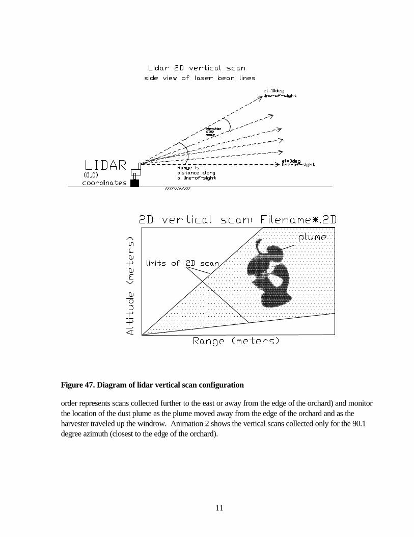
LIDAR (0,0) coordlno. tes

/"\ 1/1 l. OJ

..p OJ E

'-./

OJ 0 :)

-p -p

L iolo.r 2 D ver-tic o.l sc o.n siole view of lo.ser loeal'l lines

2D vertico.l sco.n: Fileno.Me*.2D

.:::::: ::::: :::::: :::::: P~VM?:::: . . . . . . . . . . ......... . . . . . ............ . . . . . . . ............. . . . . . . .............. .

Ro.nge (Me-ters)

Figure 47. Diagram of lidar vertical scan configuration

order represents scans collected further to the east or away from the edge of the orchard) and monitor the location of the dust plume as the plume moved away from the edge of the orchard and as the harvester traveled up the windrow. Animation 2 shows the vertical scans collected only for the 90.1 degree azimuth (closest to the edge of the orchard).

11

north

LIDAR ,. / .. ·.

/.:·:.:·.:-:.:·.:·. / .:: .. :: .. :: .. :: . ·.· . .-.:•:·.:·.:·>.:•:·.:·.:•:· (lJ

.. .-_..-._._._.._._._.._. _.· . .-._..-. ~

Field 310 o : ..• \:::::\:\ \::: ~ •0 - 1-. •.. • ........ ·. • ........ _.. ·:.·. 0. ~---.. ·.· .·· .. · .··

!.-.......................... _. ................... _. ........ +> ._-: . .-.. ·: .. ·.:o-:."·.o"·:._-.• ·: .. · .. a·._-:.o··:. ··: .. ·. L

1t••·••:••.:•••:i••·~•:i:!i••·•i·• •.:••· ~ .· .. · .. · ·.·· .· ... !DJ ........ ~ .. ·. ·-t•··· .·. -z:5

1:::::::::::::::::::::::::::::::::::::::::::::::::::::::i;e-.:::::: :::::::: ~

. t?•::: i} :: :: iii~: :~:i:i: )i ~ I .<> <\Vii\%@:!:%\\!lt@&

·:··~·--·.·--·.··.·.· .. · .. ·.· .. · .. ·.· .. ·._-.·._-._..-._. ............ · .. · .. ·.· .. ·._-.·._-._..-._.~J 99 deg ··¾@•:·.:·:J2>·."·· · 90 deg

south

.. \ 2D Horizonto.l Scan rnnge nbove orchard

Figure 48. Lidar configuration for horizontal scans

12

Dust plume from harvester exiting E side

Offield 310

LIDAR located 3 ~0Dl N __ ;a,.;;a_n_d 18m E Offield 310·

Figure 49. Lidar view at solid-set irrigated field (field 310) 20 DISCUSSION

The PM10 mass measurements from each tower were averaged to obtain mean PM10 concentrations by height for each harvester test. Each average vertical PM10 profile was then integrated from 1m to 9m using Simpson’s Rule to obtain an average PM10 concentration for the dust plume. The results are shown in Table 9. The older harvester #1 generated lower PM10 concentrations than the newer harvester #2 in all but one case. The older harvester #3 generated higher PM10 concentrations than the newer harvester #4 in all cases. Harvester #5 generated higher concentrations than any other harvester in all cases but one. The most appropriate way to compare the performance of the harvesters is to examine the PM10

concentrations normalized to the amount of windrow trash that passed through a 2mm (tabulated in Table 10). The results of this calculation are shown in Table 11. For the solid–set irrigated field, the newer harvester #2 showed overall lower concentrations than the older harvester #1 relative to the amount of windrow trash, but it showed higher concentrations for the micro–spray irrigated field. The newer harvester #4 showed decreases over the older harvester #3 in both fields, though the decrease was larger for the solid–set irrigated field than for the micro–spray irrigated field. The overall change in PM10 concentrations for both fields combined, normalized to the amount of windrow trash, ranged from +32% to -35%. Overall, for both fields combined, both new harvesters (#2 and #4) showed very similar PM10

concentrations relative to the amount of windrow trash. The newer harvester #2 showed better results on the solid–set irrigated field, while the newer harvester #4 showed better results on the micro–spray irrigated field. It is not possible to recommend one brand of harvester over the other. Harvester #5, on the other hand, showed 2-4 times the PM10 concentrations, relative to the amount of windrow trash, as the other two brands.

13

Table 9. Integrated PM 10 concentrations (µg/m3) for each harvester test

Harvester 1 2 % Difference 3 4 % Difference 5

Solid–Set 860 880 2% 2,336 671 -71% 2,953 Near 681 1,008 48% 2,465 282 -89% 3,096

Middle 158 1,186 652% 2,601 710 -73% 3,020 Far 1,782 302 -83% 1,942 827 -57% 2,957

Micro–Spray 1,537 3,314 116% 3,272 2,002 -39% 5,295 Near 1,594 2,663 67% 3,959 879 -78% 6,762

Middle 1,115 2,481 122% 3,077 2,852 -7% 5,787 Far 1,865 4,800 157% 2,761 2,174 -21% 3,338

Both fields 1,258 2,344 86% 2,916 1,730 -41% 4,195 Near 1,049 1,821 74% 3,099 573 -82% 5,125

Middle 730 1,824 150% 2,962 2,419 -18% 4,489 Far 1,971 3,424 74% 2,691 1,941 -28% 3,147

Table 10. Pre-harvest windrow trash <2mm in size (grams)

Harvester 1 2 % Difference 3 4 % Difference 5

Solid–Set 211 370 76% 193 142 -26% 300 Near 268 435 62% 80 103 28% 410

Middle 295 474 61% 303 184 -39% 126 Far 70 203 191% 195 139 -29% 366

Micro–Spray 405 498 23% 593 579 -2% 437 Near 348 512 47% 627 521 -17% 419

Middle 423 409 -3% 663 771 16% 432 Far 446 573 28% 489 446 -9% 461

Both fields 308 434 41% 393 361 -8% 369 Near 308 473 54% 354 312 -12% 414

Middle 359 441 23% 483 477 -1% 279 Far 258 388 50% 342 293 -14% 414

14

Table 11. PM10 concentrations normalized to amount of windrow trash <2mm prior to harvest (µg/m3/g)

Harvester 1 2 % Difference 3 4 % Difference 5

Solid–Set 4.1 2.4 -42% 12.1 4.7 -61% 9.8 Near 2.5 2.3 -9% 30.8 2.8 -91% 7.6

Middle 0.5 2.5 368% 8.6 3.9 -55% 24.1 Far 25.6 1.5 -94% 10.0 5.9 -40% 8.1

Micro–Spray 3.8 6.7 76% 5.5 3.5 -37% 12.1 Near 4.6 5.2 13% 6.3 1.7 -73% 16.2

Middle 2.6 6.1 130% 4.6 3.7 -20% 13.4 Far 4.2 8.4 101% 5.7 4.9 -14% 7.2

Both fields 4.1 5.4 32% 7.4 4.8 -35% 11.4 Near 3.4 3.8 13% 8.8 1.8 -79% 12.4

Middle 2.0 4.1 103% 6.1 5.1 -17% 16.1 Far 7.6 8.8 16% 7.9 6.6 -16% 7.6

20.1 Lidar data animations

Two animation files highlight the lidar results of monitoring the almond harvest operations. The lidar was positioned in the same location for both sets of data – north of the solid–set irrigated field along the levee of a wide irrigation channel that borders the east side of the field (see Figure 49). Animation 1 – 11SEP303ZOOM.GIF – Horizontal scans collected at three different elevation angles over the top of the field. The horizontal sweeps were made while the harvesters were picking up nuts from the 7th windrow, or about 42 meters inside the field’s east edge, during PM test 15. The scans were made at lidar azimuth angles between 90.1 (~True South) and 99.1 ( 9° West of South) degrees and lidar elevation angles of 1.8, 2 and 2.2 degrees. These elevation angles correspond to heights above ground of approximately 31, 35 and 38 meters at a range (i.e., distance along the lidar line-of-sight) of 1000 meters. Interesting features to notice in this animation include: (a) Note the movement of the plumes toward the top right of the images. This direction corresponds to

movement of the plumes that are rising out of the orchard towards the southwest due to the prevailing wind coming from the northeast at 1330 hr (see Figure 42, meteorology).

(b) The harvester was moving from the south end of the field (located at a distance of ~1100m from lidar) towards the north end where the PM towers were located. The harvester movement to the north is noticeable in the lidar data in that the high signal (red) moves toward the bottom of the images with time.

(c) The harvester was started on the second frame of the animation (file 11SEP304.2D) and the harvester was turned off during the last 6 frames of the animation. These latter frames therefore illustrate the manner in which the plume dies off. Note that the signal in these last frames is

15

significantly lower after the harvester was turned off. The first frame’s intensity is similar to that in the last frames, therefore is fairly representative of the ‘background’ atmospheric conditions for the test period.

Animation 2 – 11SEPALLup.GIF – Vertical scans collected at 90.1° azimuth angle for elevation angles between 0 and 2°. The scans were collected while the harvesters were picking up nuts from the 2nd (or 1st) windrow, or about 18 (or 12) meters inside the field’s east edge, during “lidar-only” PM tests. The animation is organized in the order the harvesters were run on windrow #2 from south to north (#1, #5, #4, #3) followed by the results for harvester #2 on windrow #1. The table at the bottom of Figure 16 indicates which lidar file numbers (appearing along the top of individual frames in the animation) correspond to the period during which the harvester was operating. File numbers outside the intervals indicated in the table represent periods either before or after harvester operation and show background atmospheric conditions and/or dissipation of the dust plumes generated by the harvesting. Interesting features to notice in this animation include: (a) The first harvester (#1) has a strong plume located at ranges (x-axis) > 1050 meters. This plume

did not dissipate very quickly after the harvester was turned off. The range location is consistent with the harvester operating at the far south end of the field and adjacent to the dirt road at the south end. The presence of the road may have allowed the plume to escape to the south and then it was moved further south by the northerly and northeasterly winds prevailing outside the canopy. Note the movement of the plume to the left of the images at the start of the animation – this is because the harvester was traveling south to north on the windrow. After the harvester stopped (file 11SEP545.2D), the plume moved to the right in the images (i.e., to the south) because of the prevailing winds.

(b) The animation sequence for the second harvester (#5) starts with a thin tall plume at ~900m range. The plume moves to the right (south) due to the wind and merges into a wide plume between 1000-1500m range in file 11SEP595.2D. Like harvester #1’s sequence, there is strong vertical movement at ranges >1200 meters after the harvesting stopped (file 11SEP604.2D).

(c) Harvester #4’s run shows the plume starting at a closer range, about 800m, and it also moves south, broadens and rises to over 30m height. Significant rapid dissipation of the plume from this harvester is observed after file 11SEP779.2D.

(d) Harvester #3 has its discharge on the left-hand side, therefore its lidar-only test was run with the harvester starting on the north end of its section of windrow #2, at about 450m range from the lidar. The plume is first visible in the lidar’s line-of-sight at a range of ~650m and it moves quickly to the south, both because of advection by the wind, and because the dust source is moving south. The plume rises immediately to over 30m height and maintains a sharp front on its south side. The plume dissipates much more slowly than harvester #4’s plume. Note, however that the mean wind speed was lower during the run with harvester #3 (see Figure 3).

(e) Like harvester #1, harvester #2 was run on the windrow section closest to the road at the south end of the field. However, the intensity of the plume from harvester #2 is not as great. Movement of the plume northward from the 1100m range is evident at the start of the sequence; plume dissipation begins after file 11SEP455.2D.

(f) Throughout the scan sequence of all harvesters, there is a low-elevation (i.e., between 5 and 20m height) signal at 1200-1500m range. This signal may represent dust that is “trapped” and recirculated within the open space along the drainage ditch between neighboring orchards. This

16

hypothesis supported by lidar data from the 2D vertical scans collected at azimuth angles farther east of the field.

Whereas the point sampler tests indicated that harvester #5 was the dirtiest, #4 was second and the other three harvesters gave similarly lower levels of PM10 when sampled immediately adjacent to the windrows. The lidar data seem to give different relative results between harvesters. The highest signals in the “lidar-only” tests were obtained for harvester #1. This may indicate differences in the portions of the plume sampled by the point samplers versus the lidar. For example, the lidar could not capture the plumes under the canopy that were sampled by the filters. Rather, the lidar measured the plume after it exited the orchard, where it was subject to convective and advective transport and dispersion. Any factors that affect dispersion will affect the intensity of the lidar signal, thus signal intensity alone is not a very useful comparison variable for different harvesters. We are continuing lidar data analysis to develop a quantitative measure that includes plume dimensions as well as signal intensity. Alternatively, the windrow sections sampled by each harvester during the lidar-only tests may have had different amounts of trash prior to harvesting. If so, the lidar data must be normalized to trash content as was done for the point sampler comparison. Another complication is the fact that harvester #4 was sampled in its lidar-only test while running south to north despite the fact that its discharge is to the left. Thus, the dust generated was blown away from the lidar line-of-sight. This may explain why the observed plume from #4 dissipated so quickly. Given the problems with interferences in the lidar data due to activity on neighboring fields and because (1) meteorological conditions were not the same for each “lidar-only” test, and (2) the wind was generally blowing the dust back towards the orchard (and back over the lidar beam line), rather than in one-direction away from the source (and the lidar line-of-sight), interpretation of the lidar data is extremely complex under these adverse testing conditions.

20.2 Averaged 2D vertical scans

The animation files provide a time series of images that show the movement of the dust plumes generated by the harvesters as the implement moved along the windrow. Another way of presenting the lidar data from the lidar-only test runs is to average the lidar images collected on the 90.1° azimuth during the time periods when each harvester was actively harvesting. In the averaged files (Figure 50), each pixel represents the average lidar backscatter signal at that specific location over the duration of an individual harvester’s run. Due to different harvester speeds, the test duration and the number of lidar files comprising a test varied between harvesters. To compare the harvesters, then, the average lidar signal is plotted in each image. The data in Figure 50 is a subset of the data in Animation 2. The harvester number and time of day of the beginning of the run is indicated in the header of each image in Figure 50. The range location of each harvester’s operation is shown in Figure 46. Harvesters #1 and #2 were run on the windrow section at the southernmost part of field 310 (see Figure 46). Therefore, it is likely that at least part of the high signal level at ranges of 1100-1200 meters is due to traffic on the road at 1100 meters range. This road-generated signal can be seen in the averaged images from Harvester #3 and #4 at a range of approximately 1175-1200m and a height between 5-15m. Observations we can make about differences in PM10 generation by the different harvesters from the averaged lidar data include:

17

(1) plume size and shape differ greatly between harvesters. This may be a real phenomenon, or it may be the result of differences in plume transport and dispersion because the harvesters were sampled by the lidar at different times of day when meteorological conditions were variable.

(2) because of changes in plume size and shape, direct comparisons of lidar signal intensity do not necessarily correlate directly with total PM10 emissions. In other words, a small area of high intensity on the averaged lidar image may correlate to a lower PM10 flux than a very large area of low intensity signal. This is due to the fact that PM10 flux is an integral function of concentration as well as areal distribution of the particulate matter. A two-dimensional integration of the plumes in the 2D vertical lidar scans is being investigated as a useful data analysis tool for comparing the harvesters, despite the complexities imposed by meteorological variability and less than ideal lidar-only test conditions.

21 CONCLUSIONS

The new harvesters #2 and #4 from either manufacturer perform comparably with regard to PM10 dust production. The older harvester #1 also performs comparably to the newer ones, but the older harvester #3 produces somewhat more dust. Harvester #5 produces significantly more dust than any of the other four models. The change in PM10 dust production, relative to the amount of windrow trash in the row, ranged from an increase of 76% to a decrease of 61%. On the solid–set irrigated field, which was sprinkler irrigated, both new harvesters produced 42-61% lower PM10 emissions than their older counterparts. On the micro–spray irrigated field, which was irrigated by micro-spray emitters, the newer harvester #2 produced 76% more PM10 dust relative to the amount of windrow trash, while the newer harvester #4 produced 37% less, than their older counterparts. Harvesters #1–#4 produced much less dust relative to the amount of windrow trash than harvester #5.

18

Animation 2 figure

Figure 50. Average lidar backscatter signal during harvester operation

19

Figure 50. Average lidar backscatter signal during harvester operation

20

D

D D

D

10 H

eig

ht

(m)

9

8

7

6

5

4

3

2

1

0 0 2000

Harvester Comparison Harvester: #1

4000 6000 8000 10000 PM10 (µ g/m3 )

Left tower

Middle tower

Right tower

Upwind

12000 14000

10

9

8

7

6

5

4

3

2

1

0 0

Hei

gh

t (m

)

2000

Harvester Comparison Harvester: #2

4000 6000 8000 10000 PM10 (µ g/m3 )

Left tower

Middle tower

Right tower

Upwind

12000 14000

(a)

Hei

gh

t (m

)

10

9

8

7

6

5

4

3

2

1

0 0 2000

Harvester Comparison Harvester: #1

Field: Solid Set Irrigation

4000 6000 8000 10000 PM10 (µ g/m 3)

Left tower

Middle tower

Right tower

Upwind

12000 14000

10

9

8

7

Hei

gh

t (m

) 6

5

4

3

2

1

0 0 2000

Harvester Comparison Harvester: #2

Field: Solid Set Irrigation

4000 6000 8000 10000 PM10 (µ g/m 3)

Left tower

Middle tower

Right tower

Upwind

12000 14000

(b)

0

1

2

3

4

5

6

7

8

9

10

0 2000 4000 6000 8000 10000 12000 14000 PM10 (µ g/m 3)

Hei

gh

t (m

)

Left tower

Middle tower

Right tower

Upwind

Harvester Comparison Harvester: #1

Field: Micro Spray irrigation

0

1

2

3

4

5

6

7

8

9

10

0 2000 4000 6000 8000 10000 12000 14000 PM10 (µ g/m 3)

Hei

gh

t (m

)

Left tower

Middle tower

Right tower

Upwind

Harvester Comparison Harvester: #2

Field: Micro Spray irrigation

(c)

Figure 51. PM10 concentrations downwind of harvester #1 and #2, (a) all tests, (b) Solid–set irrigation, (c) Micro–spray irrigation.

21

D D

D D

D

10 H

eig

ht

(m)

9

8

7

6

5

4

3

2

1

0 0 2000

Harvester Comparison Harvester: #3

4000 6000 8000 10000 PM10 (µ g/m3)

Left tower

Middle tower

Right tower

Upwind

12000 14000

10

9

8

7

6

5

4

3

2

1

0 0

Hei

gh

t (m

)

2000

Harvester Comparison Harvester: #4

4000 6000 8000 10000 PM10 (µ g/m3 )

Left tower

Middle tower

Right tower

Upwind

12000 14000

(a)

Hei

gh

t (m

)

10

9

8

7

6

5

4

3

2

1

0 0 2000

Harvester Comparison Harvester: #3

Field: Solid Set Irrigation

4000 6000 8000 10000 PM10 (µ g/m3)

Left tower

Middle tower

Right tower

Upwind

12000 14000

10

9

8

7

Hei

gh

t (m

) 6

5

4

3

2

1

0 0 2000

Harvester Comparison Harvester: #4

Field: Solid Set Irrigation

4000 6000 8000 10000 PM10 (µ g/m3 )

Left tower

Middle tower

Right tower

Upwind

12000 14000

(b)

Hei

ght

(m)

10

9

8

7

6

5

4

3

2

1

0

0 2000

Harvester Comparison Harvester: #3

Field: Micro Spray irrigation

4000 6000 8000 10000 PM10 (µ g/m3)

Left tower

Middle tower

Right tower

Upwind

12000 14000

Hei

ght

(m)

10

9

8

7

6

5

4

3

2

1

0

0 2000

Harvester Comparison Harvester: #4

Field: Micro Spray irrigation

4000 6000 8000 10000 PM10 (µ g/m3)

Left tower

Middle tower

Right tower

Upwind

12000 14000

(c)

Figure 52. PM10 concentrations downwind of harvester #3 and #4, (a) all tests, (b) Solid–set irrigation, (c) Micro–spray irrigation.

22

D

D

0

1

2

3

4

5

6

7

8

9

10

0 2000 4000 6000 8000 10000 12000 14000 PM10 (µ g/m3)

Hei

gh

t (m

)

Left tower

Middle tower

Right tower

Upwind

Harvester Comparison Harvester: #1–#4

0

1

2

3

4

5

6

7

8

9

10

0 2000 4000 6000 8000 10000 12000 14000 PM10 ( µ g/m3)

Hei

gh

t (m

)

Left tower

Middle tower

Right tower

Upwind

Harvester Comparison Harvester: #1–#4

Operation:Pickup Outside Near

0

1

2

3

4

5

6

7

8

9

10

0 2000 4000 6000 8000 10000 12000 14000 PM10 (µ g/m3)

Hei

gh

t (m

)

Left tower

Middle tower

Right tower

Upwind

Harvester Comparison Harvester: #1–#4

Operation:Pickup Middle

0

1

2

3

4

5

6

7

8

9

10

0 2000 4000 6000 8000 10000 12000 14000 PM10 ( µ g/m3)

Hei

gh

t (m

)

Left tower

Middle tower

Right tower

Upwind

Harvester Comparison Harvester: #1–#4

Operation:Pickup Outside Far

Figure 53. Dust concentrations for harvesters #1–#4 on both fields by harvest row.

23

D D

D D

10

9 H

eig

ht

(m)

8

7

6

5

4

3

2

1

0 0 2000

Harvester Comparison Harvester: #1–#4

Field: Solid Set Irrigation

4000 6000 8000 10000 PM10 (µ g/m 3)

Left tower

Middle tower

Right tower

Upwind

12000 14000

10

9

8

7

6

5

4

3

2

1

0 0

Hei

gh

t (m

)

2000

Harvester Comparison Harvester: #1–#4

Operation:Pickup Outside Near Field: Solid Set Irrigation

Left tower

Middle tower

Right tower

Upwind

4000 6000 8000 10000 12000 14000 PM10 (µ g/m 3)

0

1

2

3

4

5

6

7

8

9

10

0 2000 4000 6000 8000 10000 12000 14000 PM10 (µ g/m 3)

Hei

gh

t (m

)

Left tower

Middle tower

Right tower

Upwind

Harvester Comparison Harvester: #1–#4

Operation:Pickup Middle Field: Solid Set Irrigation

0

1

2

3

4

5

6

7

8

9

10

0 2000 4000 6000 8000 10000 12000 14000 PM10 (µ g/m 3)

Hei

gh

t (m

)Left tower

Middle tower

Right tower

Upwind

Harvester Comparison Harvester: #1–#4

Operation:Pickup Outside Far Field: Solid Set Irrigation

Figure 54. Dust concentrations for all harvesters #1–#4 on solid–set irrigated field by harvest row.

24

D

D D

10

9 H

eig

ht

(m)

8

7

6

5

4

3

2

1

0 0 2000

Harvester Comparison Harvester: #1–#4

Field: Micro Spray irrigation

4000 6000 8000 10000 PM10 (µ g/m3)

Left tower

Middle tower

Right tower

Upwind

12000 14000

10

9

8

7

6

5

4

3

2

1

0 0

Hei

gh

t (m

)

2000

Harvester Comparison Harvester: #1–#4

Operation:Pickup Outside Near Field: Micro Spray irrigation

Left tower

Middle tower

Right tower

Upwind

4000 6000 8000 10000 12000 14000 PM10 (µ g/m3)

Hei

gh

t (m

)

10

9

8

7

6

5

4

3

2

1

0 0 2000

Harvester Comparison Harvester: #1–#4

Operation:Pickup Middle Field: Micro Spray irrigation

4000 6000 8000 10000 PM10 (µ g/m3)

Left tower

Middle tower

Right tower

Upwind

12000 14000

10

9

8

7

6

5H

eig

ht

(m)

4

3

2

1

0 0 2000

Harvester Comparison Harvester: #1–#4

Operation:Pickup Outside Far Field: Micro Spray irrigation

4000 6000 8000 10000 PM10 (µ g/m3)

Left tower

Middle tower

Right tower

Upwind

12000 14000

Figure 55. Dust concentrations for harvesters #1–#4 on micro–sprayed field by harvest row.

25

D D

D D

D D

10

9 H

eig

ht

(m)

8

7

6

5

4

3

2

1

0 0 5000

Harvester Comparison Harvester: #5

10000 15000 20000 25000 PM10 (µ g/m3)

Left tower

Middle tower

Right tower

Upwind

30000 35000

10

9

8

7

6

5

4

3

2

1

0 0

Hei

gh

t (m

)

5000

Harvester Comparison Harvester: #5

Operation:Pickup Outside Near

10000 15000 20000 25000 PM10 (µ g/m3)

Left tower

Middle tower

Right tower

Upwind

30000 35000

(a) (d)

Hei

gh

t (m

)

10

9

8

7

6

5

4

3

2

1

0 0 5000

Harvester Comparison Harvester: #5

Field: Solid Set Irrigation

10000 15000 20000 25000 PM10 (µ g/m3)

Left tower

Middle tower

Right tower

Upwind

30000 35000

10

9

8

7

6

5H

eig

ht

(m)

4

3

2

1

0 0 5000

Harvester Comparison Harvester: #5

Operation:Pickup Middle

10000 15000 20000 25000 PM10 (µ g/m3)

Left tower

Middle tower

Right tower

Upwind

30000 35000

(b) (e)

Hei

gh

t (m

)

10

9

8

7

6

5

4

3

2

1

0 0 5000

Harvester Comparison Harvester: #5

Field: Micro Spray irrigation

10000 15000 20000 25000 PM10 (µ g/m3)

Left tower

Middle tower

Right tower

Upwind

30000 35000

Hei

gh

t (m

)

10

9

8

7

6

5

4

3

2

1

0 0 5000

Harvester Comparison Harvester: #5

Operation:Pickup Outside Far

10000 15000 20000 25000 PM10 (µ g/m3)

Left tower

Middle tower

Right tower

Upwind

30000 35000

(c) (f)

Figure 56. PM10 concentrations downwind of harvester #5, (a) all tests, (b) Solid–set irrigation, (c) Micro–spray irrigation, (d) near row, (e) middle row, (f) far row.

26

22 APPENDIX A

Simpson’s Rule and Application to these data

Simpson’s Rule is used to numerically integrate a function over an interval a to b. The form of the integration formula is b Dx∫ f ( x)dx » [ f (x0 ) + 4 f (x1 ) + 2 f (x2 ) + 4 f (x3 )+L+2 f ( x2n -2 ) + 4 f (x2n-1) + f ( x 2n )]3 a

. For this study, the limits of integration are a = 1, the lowest measurement height, and b = 9, the highest measurement height. The PM10 concentration was interpolated at each integral meter height between 1 and 9 meters, so there were eight intervals in the calculation. For some calculations, there was a measurement at 4m, due to a malfunction in the 9m sampler for one tower. The Dx, then, is 1m. For example, Harvester #2 on the micro-sprayed field produced the following PM10

measurements:

PM10 Mass (µg/m3)

Operation Height (m) Upwind Tower

Left Tower

Middle Tower

Right Tower

Pickup Outside Far 9

4

3

1

38

56

57

373

1864

5290

1476

3239

3355

1813

1998

3577

Pickup Middle 9

4

3

1

38*

56*

57*

2166

4780

454

2049

4882

357

1427

3973

Pickup Outside Near 9

4

3

1

38*

56*

57*

718

3496

8604

414

3674

7076

396

1453

4270

*The upwind were collected for an entire morning or afternoon to ensure that sufficient mass was collected for analysis.

27

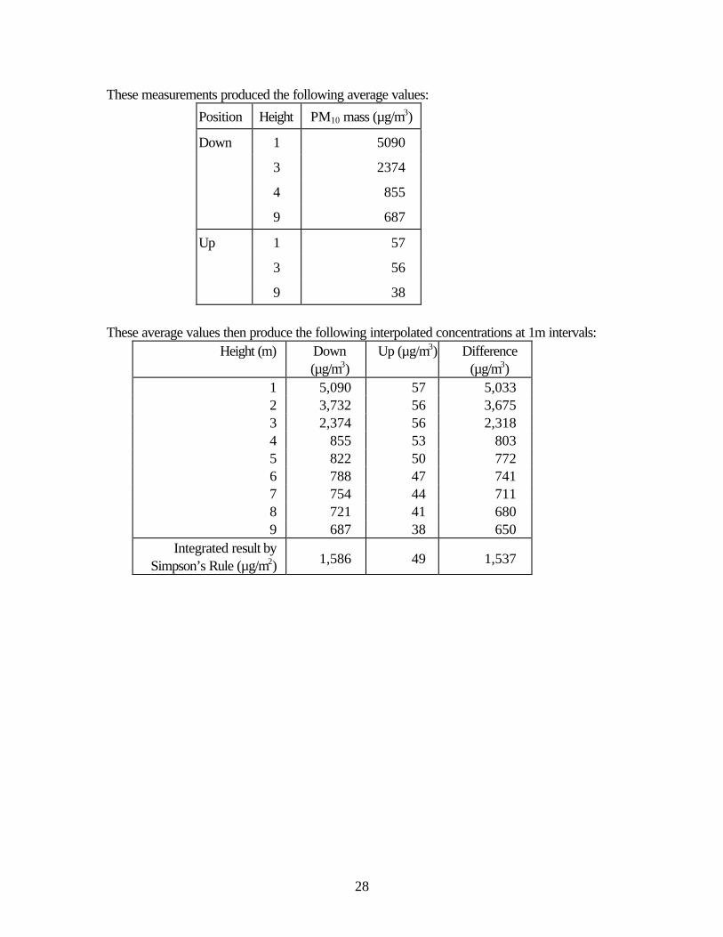
These measurements produced the following average values:

Position Height PM10 mass (µg/m3)

Down 1

3

4

9

5090

2374

855

687

Up 1

3

9

57

56

38

These average values then produce the following interpolated concentrations at 1m intervals: Height (m) Down

(µg/m3) Up (µg/m3) Difference

(µg/m3) 1 2 3 4 5 6 7 8 9

5,090 3,732 2,374

855 822 788 754 721 687

57 56 56 53 50 47 44 41 38

5,033 3,675 2,318

803 772 741 711 680 650

Integrated result by Simpson’s Rule (µg/m2) 1,586 49 1,537

28

23 APPENDIX G – DESCRIPTION OF DATABASE STRUCTURE

Description of database structure A test is considered to be a set of simultaneous measurements (aerosols, Ammonia gas, meteorology, source of emissions, etc.) of an emissions source. The duration of the test is normally dictated by the measurements of the closest downwind samplers, enough mass for species sensitivity without overloading. The start and end times the test is determined by the start and end times of the PM10 sample collected at 3 m height closest to the source. The meteorological data is averaged for the test based on these times, as are the lidar data.

Test ID = Year (2 characters) + “-“ + Test Number (3 characters) e.g. “99-001”, “99-002”, “99-003”, etc. or “00-001”, “00-002”, “00-003”, etc.

Oftentimes, an upwind or background measurement extends over several tests. In such cases, we use the variables StrTest and EndTest (each 3 characters) to identify which individual tests a background measurement is associated with (e.g. StrTest = “001” , EndTest = “003”)

A sampling array (2 characters) is defined as a collection of sampling locations which share a common origin as the basis for measuring distances. Typically, the array designation changes when the field or facility changes or with wind shifts. Some examples are:

Paramount Farms = P1, P2,......

A sampling location (3 characters) is the point, in three dimensional space relative to the origin, where the sample was collected. The first character indicates the general location of the sample in the array:

U = Upwind (UP) I = In field (IN) D = Downwind (DN) L = Left of array downwind axis (LT), left while facing upwind R = Right of array downwind axis (RT), right while facing upwind

The second character specifies the sequence of use for that location, for example D1, D2, and D3 for 3 downwind samplers. The final character designates the height at which the sample was collected, following some rules to stay within the single character: 1) Use the actual height as the character when £ 9 meters. 2) Use a letter designation for the character when > 9 meters in ascending order from the highest height (e.g. A = 100m , B = 50m, C = 10m)

Examples of elemental analysis site codes:

29

H

H

PERGAMON

ATMOSPHERIC ENVIRONMENT

www .elsevier.com/locate/atmosenv

Atmospheric E viro me t 35 (2001) 3251}3264

Lidar-assisted measureme t of PM emissio s from ��

agricultural tilli g i Califor ia's Sa Joaqui Valley } Part I: lidar

Britt A. Holme *, Teresa A. James, Lowell L. Ashbaugh, Robert G. Flocchi i

Air Quality Group, Crocker Nuclear Laboratory, University of California, Davis, CA 95616, USA

Received 25 April 2000; accepted 31 October 2000

Abstra t

Vertical pro"li g with poi t samplers is a accepted method for qua tifyi g the #uxes of PM from o -poi t��

fugitive dust sources, but is limited by u certai ty i estimates of the actual height of the dust plume, especially for plumes that exceed the highest sampli g height. Agricultural la d preparatio operatio s i the Sa Joaqui Valley were mo itored usi g upwi d}dow wi d vertical PM pro"les a d data collected duri g the "rst successful experime t to

��i clude light detectio a d ra gi g (lidar), i 1998, were a alyzed to provide modeli g criteria for the 1996 a d 1997 data. A series of six comprehe sive PM tests with co curre t lidar data was exami ed to: (a) develop a framework for

��a alyzi g upwi d}dow wi d poi t PM co ce tratio pro"les of la d preparatio operatio s (diski g, listi g, root

��cutti g, a d rippi g) a d (b) ide tify co ditio s u der which the "eld sampli g strategies a!ect the reproducibility of PM co ce tratio measureme ts. Lidar data were used to verify that the plume heights a d shapes extrapolated from

��the poi t sampler vertical pro"les adequately described the plumes. The shortcomi gs of the vertical pro"li g tech ique a d lidar methods are discussed i the light of developi g e cie t robust methods for accurate PM emissio s

��qua ti"catio from complex o -poi t sources. � 2001 Elsevier Scie ce Ltd. All rights reserved.

Keywor s: PM10, Lidar; Plume height; Agricultural dust; No poi t sources

1. Introdu tion

I late summer a d fall, a large fractio ('50%) of the PM i Califor ia's Sa Joaqui Valley (SJV) has bee

��attributed to primary geologic material, ge erally soil dust (Chow et al., 1990, 1992). This material becomes airbor e by suspe sio of surface soils duri g wi d ero-sio , agricultural activities, tra c o paved a d u paved roads, a d co structio activity. Late summer a d fall PM sta dard violatio s (Dolislager a d Motallebi,

��1999) coi cide with the harvest seaso of ma y Califor- ia crops (e.g., cotto , almo ds, tomatoes), suggesti g that agricultural activities (both harvesti g a d sub-

* Correspo di g author. Tel.: #1-530-752-1213; fax: #1-530-752-4107. E-mail a ress: baholme @ucdavis.edu (B.A. Holme ).

seque t la d preparatio ) may be sig i"ca t sources of PM duri g this time of year. Pote tial e!orts to co -

��trol this compo e t of PM require accurate qua ti"ca-

��tio of these sources, but little i formatio has bee available to date to estimate PM emissio s from SJV

��agricultural activities. Si ce 1991, the U iversity of Califor ia has collected

PM emissio s data from a wide ra ge of agricultural��

activities i the SJV. Curre t tech iques use (a) up-wi d/dow wi d vertical pro"les of wi d speed a d PM co ce tratio s (PM a d PM ) to qua tify PM emis-

��� ��sio factors a d (b) lidar vertical sca s to verify plume heights a d pro"le shapes. The PM poi t sampli g tech iques draw o observatio s made by previous fugitive dust researchers usi g upwi d/dow wi d arrays (Cowherd et al., 1974; Flocchi i et al., 1994), exposure pro"li g (Cowherd et al., 1974; Cusci o et al., 1984; Flocchi i et al., 1994), high-volume "ltratio samplers

1352-2310/01/$ - see fro t matter � 2001 Elsevier Scie ce Ltd. All rights reserved. PII: S 1 3 5 2 - 2 3 1 0 ( 0 0 ) 0 0 5 1 8 - 5

H

H

3252 B.A. Holme& n et al. / Atmospheric Environment 35 (2001) 3251}3264

(Cusci o et al., 1984; Cowherd a d Ki sey, 1986); cascade impactors (Cowherd et al., 1974; Cusci o et al., 1984; Flocchi i et al., 1994), a d respirable dust mo itors (S yder a d Blackwood, 1977; Claus itzer a d Si ger, 1996, 1997). Previous studies that qua ti"ed agricultural emissio s

represe t a very limited umber of sites, a low umber of replicate samples, a d few early studies qua ti"ed PM

���I stead, total suspe ded particulate (TSP) matter or i -dustrial workplace respirable dust (PM ) was measured.

�For example, early UCD "eld measureme ts i corpor-ated PM samplers at a si gle height (3.3 m) upwi d

��a d dow wi d, a d TSP mo itors at four heights (3, 5, 7, a d 9 m) dow wi d, of the source (Flocchi i et al., 1994; Ashbaugh et al., 1996), but the lack of PM vertical

�� pro"li g to de" e the vertical exte t of the plume was suspected to have caused u derestimatio of emissio factors usi g the box model (Ashbaugh et al., 1997). The applicatio of lidar to PM emissio factor

measureme ts is relatively ew (Holme et al., 1998). Lidar tech iques help overcome o e of the major limita-tio s of the vertical pro"li g methods, amely, the u cer-tai ty i determi i g the dust plume height over which to i tegrate the modeled PM co ce tratio s.

��I this paper, the results of a series of six comprehe s-

ive PM tests co ducted whe a full compleme t of��

a cillary data (lidar, laser ra ge" der) was collected are used to: (a) develop a framework for a alyzi g up-wi d}dow wi d poi t PM co ce tratio pro"les of

��SJV la d preparatio operatio s (diski g, listi g, root cutti g, a d rippi g) a d (b) ide tify co ditio s u der which the "eld sampli g strategies a!ect the reproduci-bility of PM co ce tratio measureme ts. Results of

��rece tly developed lidar data reductio tech iques are used to assess whether the shapes of the plumes measured as three-poi t PM vertical pro"les were represe tative

��of the average plumes recorded duri g the sampli g period. From this assessme t, a best-"t fu ctio for qua tifyi g plume height a d emissio s is ide ti"ed for each category of vertical pro"les observed i the PM

��data. The observatio s based o compariso s of lidar a d poi t sampler data are used to develop a emissio factor quality rati g system i a compa io paper (Holme et al., 2000).

2. Experimental methods

2.1. PM10 xel test strategy an array esign

All "eld measureme ts were made u der actual "eld co ditio s. While sampli g was coordi ated with cooperative growers, special treatme t of the "elds to accommodate PM sampli g was ot requested.

��A combi atio of upwi d/dow wi d source isolatio a d vertical pro"li g methods was used to qua tify

PM emissio s (Cowherd et al., 1974; Cusci o et al.,��

1984; Cowherd a d Ki sey, 1986; Flocchi i et al., 1994; James et al., 1996). The "elds studied were 0.4}0.8 km� (0.25}0.5 mile�) a d were pla ted a d worked i a direc-tio perpe dicular to the predomi a t wi d directio . Test duratio s were betwee 25 a d 175 mi . Valid tests were co ducted betwee fall 1996 a d wi ter 1998 o two farms ear Firebaugh a d Huro , CA. Average wi d speeds at 4 m were betwee 1.0 a d 6.5 m s �. I all cases aerosol samples were collected usi g o e upwi d a d at least o e dow wi d vertical pro"le. Aerosol samples a d meteorological data were col-

lected at the heights i dicated i Table 1 a d PM measureme ts made at the top of the tower are referred to by the omi al height of 9 m throughout this paper. Both PM a d PM were collected dow wi d of the

�� ���agricultural operatio i a sampli g array (Fig. 1) that was #exible e ough to e sure dow wi d sampli g rela-tively close to the movi g source. Note that PM was

��collected at three heights but PM was collected o ly at

���the upper two heights due to equipme t limitatio s. For the PM tests exami ed here, the average dista ce be-

�� twee the PM samplers a d the tractor/impleme t for the test period after correctio for the a gle of the opera-tio was betwee 1 a d 324 m (see Table 3). Whe the agricultural operatio was far from the statio ary PM tower located at the dow wi d edge of the "eld, the vertical pro"les of PM a d PM were sampled usi g

�� ��� a p eumatic tower mou ted i a mobile u it that was drive i to the "eld. While the PM emissio s data will

��� ot be discussed i this study, the ratio of PM to

���PM has bee reported i earlier reports (Matsumura

�� et al., 1996; James et al., 2000). Future sampli g will collect PM a d PM at four heights to e able PM

��� �� ���emissio factor estimatio .

2.2. PM point samplers

The I terage cy Mo itori g of Protected Visual E vir-o me ts (IMPROVE) aerosol samplers (Eldred et al., 1988, 1990) were used to collect PM a d PM o

�� ���25 mm stretched Te#o "lters (3 �m Te#o�, Gelma R2P1025). These samplers have bee used exte sively i a atio wide mo itori g program at Class 1 sites (Malm et al., 1994). Portable gasoli e-powered ge erators placed dow wi d of the samplers provided power. EPA-approved Sierra A derso i lets (Model 246b) produced the 10 �m size-cut, a cyclo e was used for the PM

���size-cut (Joh a d Reischl, 1980). The IMPROVE sam-plers were modi"ed to reduce their size a d weight for placeme t atop the towers. The esse tial eleme ts of the modi"ed samplers from i let to "lter were ide tical to that of IMPROVE samplers; the di!ere ces were a shorte ed i let stack (less tha a meter lo g) a d replace-me t of electro ic sole oids with ma ual o es i some cases. Additio ally, a calibratio device used to audit

H

B.A. Holme& n et al. / Atmospheric Environment 35 (2001) 3251}3264 3253

Table 1 Aerosol a d meteorological sampli g equipme t

Variable (u its) Sampler Speci"cs Heights (m) A alyses (Method)�

PM (�gm �) IMPROVE Module D PM i let 1, 3 (8.25, 9 or 10) Gravimetric mass (PM �� �� ��

(highest height omi ally 9 m) co ce tratio ); Optical absorptio (LIPM, HIPS); Eleme tal a alysis (PIXE, PESA, XRF)

PM (�gm �) IMPROVE Module A AIHL Cyclo e 3 (8.25, 9 or 10) Gravimetric mass (PM ��� ���

(highest height omi ally 9 m) co ce tratio ); Optical absorptio (LIPM, HIPS); Eleme tal a alysis (PIXE, PESA, XRF)

Note that PM was ot collected at 1 m height���

The following meteorological instruments were locate on upwin tower

Temperature (3C) Fe wal UUT51J1 radiatio - $0.43C 0.5, 1, 2, 4, 7.5 Vertical temperature pro"le shielded thermistor Bulk Richardso umber

Stability class Wi d speed (m s �) Met O e 014A cup 0.45 m s � threshold 1, 2, 4,7.5 Vertical wi d speed pro"le, z

�,

a emometer $0.11 m s � u* used i PM #ux calculatio Wi d directio (deg) Met O e 024A Va e 4 Used i PM #ux calculatio Relative humidity (%) HMP35C Vaisaia capacitive 2 Atmospheric co ditio s Solar radiatio (W m �) Pyra ometer 4 Stability class

�LIPM"laser i tegrati g plate method; HIPS"hybrid i tegrati g plate system (Campbell et al., 1995; Bo d et al., 1999); PIXE" proto -i duced X-ray emissio (for eleme ts Na}M ; Eldred et al., 1988); XRF"X-ray #uoresce ce (for eleme ts Fe}Pb); PESA" proto elastic scatteri g (for hydroge ; Cahill et al., 1989).

#ow rates directly was substituted for i situ #ow measureme t gauges for samples collected i 1998, a d #ow measureme ts for the 9 m samplers were made usi g o ly vacuum gauges, rather tha both mag ehelic a d vacuum gauges, for samples collected i 1996 a d 1997. These modi"catio s were show i laboratory testi g to have o e!ect o the i tegrity of the PM a d PM

�� ���samples collected or o the quality of the #ow measure-me t (u published data).

2.3. Tractor upwin istance

For some tests i 1998, a laser ra ge" der (Laser Atla ta) was used to i depe de tly observe the locatio of the tractor duri g the lidar sca s. The time, dista ce, a d beari g to the tractor were recorded every 30 s to 1 mi by a observer located alo g the edge of the "eld (see Fig. 1). For other tests, upwi d dista ces reported i Table 3 were calculated from the umber of impleme t passes, impleme t width, a gle of operatio , a d the measured start a d e d dista ces upwi d of the array origi .

2.4. Light etection an ranging (li ar)

Tests co ducted si ce Ju e 1997 ofte had corre-spo di g light detectio a d ra gi g (lidar) data. The lidar i strume t, described previously (Holme et al.,

1998), records ra ge-resolved elastic backscatter sig als from airbor e PM with high temporal (s) a d spatial (5 m) resolutio . The lidar 2D vertical sca s were col-lected dow wi d of the tractor operatio , just upwi d of the dow wi d poi t sampler tower, as depicted i Fig. 1. The lidar sca pla e therefore approximated a cross sectio of the dow wi d edge of the area source bei g sampled by the upwi d/dow wi d poi t sampler pro"le array. The lidar sca s are qualitative measures of relative PM backscatter, but provide useful i formatio o PM plume variability over time i terms of spatial homo-ge eity, size, a d shape.

2.4.1. Li ar vertical proxles an plume heights Vertical pro"les of lidar data were obtai ed by aver-

agi g the lidar sig al at 2 m height i tervals over a speci-"ed ra ge (dista ce from the lidar) i terval. The ra ge i terval was selected to correspo d to the locatio of the poi t sampler tower. Backgrou d vertical pro"les were similarly obtai ed from the lidar sca s collected whe the tractor was either stopped or dow wi d of the lidar vertical sca pla e. Maximum plume heights were recorded for each 2D

vertical sca collected over a poi t sampler test period a d averaged for compariso with the poi t sampler estimates. These average values of test period plume heights were based o plumes occurri g at all locatio s across the "eld a d, u like the lidar vertical pro"les, were

Tractor, lidar and PM tCJIIVer Sc111)1ing array locations -120

-100

-80

E' -§ -60

-m ci -40 "E I ::::> -20

0

• \ \ • • 98-046 (09:29 to 10:15) • • • • • 98-045 (08:20 to 09:21) ... k \ • Letters denote PM tovver locations - " ...

. -49~~-:45 • • • • WNDt · ~ .15:ai .A ......

'(~~~-~ ~1~ : ... ! ~ '•.:~ '-:: ~ ,~----1 .,> ~ ·~3)~ ' ~--......... ........... -~- ... ......___ ...

-......_ ' ~ ..;,.._ .. 12:45 '9!: •= :31::at- •=39:'Ki': '- .A .A ~ "-- "-......: ' ,'-- ✓-15 ...

.& •..:::-~.~.-~:"-. .12:t

t p~15 '~'\ ~------ ~ .A ..... ~·~~.~

... I. T'19,q, •~~ ~~ .11:05

•"*~~ 20

0 200 400 600 800 Crosswind Distance (m)

3254 B.A. Holme& n et al. / Atmospheric Environment 35 (2001) 3251}3264

Fig. 1. Map view of tractor poi t source locatio s (circles a d tria gles) o "eld duri g "rst diski g tests 98-045 a d 98-046. The tractor paths (determi ed by laser ra ge" der measureme ts) for the two di!ere t test periods are i dicated by circles (98-045) a d tria gles (98-046). The times for tractor locatio s duri g 98-045 are show . The arrow from the lidar locatio i dicates the projectio of the vertical sca pla e for lidar 2D sca s. Note that (0, 0) is at the SW cor er of the "eld a d (800, 0) is the SE cor er of "eld. Locatio s of the poi t sampler towers are i dicated by letters : right (R) a d left (L) statio ary towers, a d mobile tower (M). The upwi d tower was located at coordi ates (793,!805). The `Xa marks the locatio of observer collecti g laser ra ge" der data o tractor locatio .

ot restricted to the ra ges where the poi t sampler towers were located.

2.4.2. Li ar measurement error Although the lidar ca ot disti guish betwee PM

ge erated by di!ere t sources, the plume ge erated by the tractor a d impleme t was usually easily disti -guished from backgrou d PM because of the disti ctive moveme t of the plume across the "eld from o e lidar sca to the ext. Possible sources of error i measuri g the maximum exte t of the plume from the lidar vertical sca s i clude the fact that some plumes exte ded higher tha the programmed vertical limits of the lidar sca ; whe plumes were very close to the lidar this problem was most severe. A other source of measureme t error resulted from ear "eld-of-view geometric optics co sid-eratio s: because of the lidar's periscope arra geme t, plumes withi 200 m of the lidar were ot fully qua ti"ed by the lidar receiver. Both of these factors could result i u derestimatio of the maximum plume height whe the plume was close to the lidar i strume t.

2.5. Laboratory analyses an quality control

All PM samples were a alyzed for gravimetric mass, light absorbi g carbo , a d eleme tal compositio i accorda ce with IMPROVE protocols (Eldred et al., 1989, 1990, 1997). The eleme tal a d carbo a alyses are used chie#y for quality assura ce purposes but also provide chemical characterizatio of these ear-source aerosols for compariso with IMPROVE ambie t mo itori g data. The mass gai of dy amic "eld bla ks (i.e., "lters loaded i to the samplers, subjected to #ow measureme t, but o air sampli g) was used to calculate bla k co ce tratio s a d mi imum qua ti"able limits (MQLs) for both PM a d PM (Eldred et al., 1990).

�� ���The MQLs were calculated from the sta dard deviatio of the average of the bla ks a d the sampled air volumes. U certai ties i mass co ce tratio were calculated by propagatio of the a alytical errors i troduced i the measureme ts of mass a d air volume. The hybrid i tegrati g plate a d sphere (HIPS) laser

a alysis tech ique (Campbell et al., 1995; Bo d et al.,

B.A. Holme& n et al. / Atmospheric Environment 35 (2001) 3251}3264 3255

1999) was used to provide a estimate of light absorbi g carbo soot (BABS). Particle-i duced X-ray emissio (PIXE) a d X-ray #oresce ce (XRF) spectroscopy were used to determi e the mass co ce tratio of the eleme ts of atomic mass betwee sodium a d ma ga ese a d betwee iro a d lead, respectively (Cahill, 1995). There is co siderable overlap i the ra ge of eleme ts a alyzed by these two methods such that i depe de t a alyses of the tra sitio metals facilitate quality co trol betwee them (Cahill, 1995). Proto elastic scatteri g a alysis (PESA), performed simulta eously with PIXE, provided a measure of the mass co ce tratio of the bou d hydro-ge (as these a alyses are performed u der vacuum). Mass co ce tratio s i air of each eleme t were cal-culated from co ce tratio s ( g cm �) measured o a represe tative portio of the "lter (at least 28%), the area of the sample o the "lter, a d the volume of air sampled. Mi imum detectable limits (MDLs) were de-" ed as 3.3 times the square root of the backgrou d cou ts. A alytical u certai ties were based o the propa-gatio of cou ti g errors a d u certai ties i the measureme t of the eleme tal mass (from rea alysis) a d air volume.

2.6. Reconstructe mass (RCMA) concentrations

The accumulatio of a large database of measureme ts of PM a d PM mass a d eleme tal pro"les through

�� ���the operatio of the IMPROVE particulate matter sampli g a d a alysis etwork led to the developme t of a series of composite variables that are de" ed by as-sumptio s regardi g the likely atomic mass ratio of the domi a t eleme ts of a aerosol co stitue t (Cahill et al., 1977; Eldred et al., 1997). These assumptio s have bee tested agai st i depe de t a alyses of related measureme ts for the database of IMPROVE samples (Cahill et al., 1981) a d for agricultural source samples (James et al., 2000). For example, the gravimetric mass has bee show to be co siste tly well correlated with the composite variable ̀ RCMAa which is the reco struc-ted mass obtai ed by summi g factors of the commo crustal eleme ts (Al, Si, Ca, Ti, Fe), sulfur, light absorbi g eleme tal carbo , hydroge a d o -soil potassium to emulate a average aerosol (Cahill et al., 1989):

RCMA"0.5BABS#2.5Na#SOIL#13.75(H

!0.25S)#4.125S#1.4(K!0.6Fe), (1)

where SOIL"2.2Al#2.49Si#1.63Ca#1.94Ti#2.42Fe; BABS is a estimate of the mass co ce tratio of light absorbi g carbo (Campbell et al., 1995; Bo d et al., 1999), a d the eleme tal mass co ce tratio s are repre-se ted by their atomic symbols. The availability of eleme tal data for all aerosol sam-

ples collected i this study allowed assessme t of the applicability of RCMA for PM emissio factor estima-

��

tio . Gravimetric PM a d RCMA were highly corre-lated (r�"0.94) for

��the 525 samples with o -zero

RCMA measured duri g the three a alysis year sets (1996}98). Therefore, either measure of PM ca be

��used to model the plume characteristics a d estimate emissio factors. However, as i dicated by the slope of the li ear regressio betwee these variables (0.77 with sta dard error"0.0065), emissio s based o RCMA will represe t a lower limit. I the samples a alyzed here, the reco structed mass (RCMA) was ge erally lower tha gravimetric mass by a average of 13% (SD"23%) due i part to the loss of volatile co stitue ts i the vacuum of PIXE a alysis. Other mass losses sometimes occurred due to sample ha dli g betwee the two a alytical pro-cedures a d where the seque tial mass loss from gravimetric to eleme tal a alyses was atypically high, the samples were co sidered i valid. Because the eleme tal a alyses were su cie tly more se sitive tha the gravimetric mass measureme ts, the calculated RCMA was above detectable limits for 13 samples (of 90 i the la d preparatio dataset) for which measured mass was ot. Thus, RCMA was the parameter chose for a alysis of the PM mass co ce tratio pro"les. The u certai -

�� ty i the RCMA composite variable was calculated as a propagatio of the u certai ties calculated for the mass co ce tratio s of each co stitue t weighted by its coef-"cie t.

2.7. Plume height an uncertainty calculations

Fu ctio al "ts to the vertical pro"les of PM co ce -��

tratio were used to calculate the average heights of the plumes sampled from the la d preparatio operatio s a d the most appropriate fu ctio al "ts to each dow -wi d pro"le type were determi ed based o exami atio of lidar vertical pro"les. Three di!ere t methods } the li e, block, a d logarithmic pro"le models } were used to "t the PM vertical co ce tratio pro"les (Fig. 2). The

��height at which the best-"t fu ctio of the dow wi d co ce tratio pro"le i tersected the average upwi d co ce tratio was the calculated plume height, H. A fourth model, the box model, was used to describe the PM #ux i cases of u iform dow wi d vertical co ce -

��tratio pro"les.

2.7.1. Line proxle mo el I the li e pro"le model, the three dow wi d PM

��co ce tratio s were "t to a li e as a fu ctio of height. Li ear vertical pro"les have bee used previously for PM pro"les dow wi d of u paved roads (Ve katram et al., 1999).

2.7.2. Block proxle mo el The block model esse tially `co ects the dotsa of the

three PM measureme ts i each vertical pro"le. The

(a) Case 1, "Decline" Profile (b) Case 3, "Uniform" Profile

14 98-045 Right Tower 14 98-046 Right Tower

12 12

' 10 10 f-+-:-J

e 8 g 8 ';:' .r: .. Cl .r: 'ai 6 Cl 6 'ai :i:: :i::

4 4

2 2 ~ ' ' ~

0 0 ' 0 20 40 60 80 100 120 0 20 40 60 80

PM10 RCMA concentration (µg m4 ) PM10 RCMA concentration (µg m")

(c) Case 4, "Greater Than" Profile (d) Case 5, "Less Than" Profile

14 98-046 Mobile Tower 14 98-046 Left Tower

12 ' 12 ' ' ' '

10 '1♦.-1 10

7 g 8 g 8 .. .. .r: .r: Cl 6 .!al 6

---/--------------------. 'ii QI

:i:: :i::

4 4

2 ~ 2 I~

0 0 0 20 40 60 0 20 40 60 80 100 120 140

PM10 RCMA concentration (µg m4 ) PM 10 RCMA concentration (µg m")

3256 B.A. Holme& n et al. / Atmospheric Environment 35 (2001) 3251}3264

Fig. 2. PM RCMA mass co ce tratio pro"le types a d examples of the most appropriate fu ctio "ts (dashed li es). Pa els (b)}(d)��

were for samples collected simulta eously at three di!ere t tower locatio s (test 98-046). All three towers were located o the dow wi d edge of the "eld, but at di!ere t crosswi d coordi ates (see Fig. 1). The right (b) a d left (d) statio ary towers were 6 m apart from each other but were also located ear the tractor tur i g poi t at the "eld edge. The mobile tower (c) was located 145 m from the midpoi t betwee the other two towers. Due to di!ere ces i crosswi d locatio , the three towers were at di!ere t dow wi d locatio s from the tractor due to the a gle of the diski g operatio . This may explai the disti ct di!ere ces i pro"le shapes duri g simulta eous sampli g.

block "t assumed that the 1 m co ce tratio was co -sta t dow to z , the PM co ce tratio was li ear

� ��from 1 to 3 m, a d li ear from 3 to 9 m. Above the highest PM measureme t at 9 m, the vertical co ce tratio

�� pro"le was extrapolated li early usi g the 3}9 m li e u til the block pro"le i tersected the average upwi d PM co ce tratio at H.

��

2.7.3. Logarithmic proxle mo el Dow wi d PM vertical pro"les were also "t with

�� atural logarithmic decay curves as a fu ctio of height. The block a d logarithmic pro"le methods

were previously show to give similar results for almo d a d cotto harvesti g operatio s (Ashbaugh et al., 1997).

2.7.4. Box mo el The box model tra sforms the measured PM a d

��wi d speed pro"les to a pro"le of u iform PM co ce -

��tratio a d wi d speed by de" i g the height, H

���,

required to give the same total i tegrated PM mass��

-u . The box model height was determi ed by regressi g the li e-"t i tegrated mass #uxes for all of the pro"les for which the most appropriate model was ot the box

Profile class Profile features Profile shape' Model fit characteristics

1 "decline" Decreasing PM10 mass concentration

"'---Line, block, and log models give

with height reasonable and equivalent heights and emission factors

2 "incline" Increasing PM10 mass concentration / Negative heights for line, block, and with height log; box model required

3 "uniform" PM10 concentrations equal at all three

I Box model required otherwise heights

heights when measurement uncertainty unreasonable is considered

4 "greater than" PM10 concentration at lm < 3m and > Fit dependent on relative concentra-3m>9m tions. Block gives reasonable heights

5 "less than" PM10 concentration at lm > 3m and < Block fit gives unreasonable height 3m<9m

•Profile shapes assume height is on the y-axis and concentration on the x-axis.

hNumber of valid land preparation tests collected during 1996-98 analysis year sets.

Number of test casesb

10

0

4

5

5

B.A. Holme& n et al. / Atmospheric Environment 35 (2001) 3251}3264 3257

Table 2 Dow wi d vertical pro"le classi"catio

versus the product: ( et 1 m PM co ce tratio �1m��

wi d speed �H ). Height i this product was empiric-���

ally adjusted u til a u it slope was achieved, i dicati g the equivale t box height (7 m) that would produce a PM i tegrated mass #ux equal to that measured

��usi g the fu ctio al models. U certai ties i the modeled plume heights were esti-

mated usi g error propagatio tech iques (Colema a d Steele, 1989). Sta dard errors o the slope a d i tercept of the model "ts to the dow wi d co ce tratio pro"les a d the sta dard deviatio i the upwi d co ce tratio measureme ts were used to propagate errors for the plume height estimate. The u certai ty calculatio s are show i the appe dix. The reported u certai ties do ot take i to accou t the u certai ty i i dividual upwi d RCMA co ce tratio measureme ts.

3. Results and dis ussion

3.1. Vertical proxle ata recovery

For the three years of data exami ed, a total of 42 dow wi d a d 17 upwi d vertical pro"les of PM were

��collected for la d preparatio operatio s (diski g, rip-pi g, root cutti g, a d listi g). There were fewer upwi d pro"les because the measureme t times required to collect su cie t mass for gravimetric a alysis were sig i"ca tly lo ger for upwi d tha for dow wi d measureme ts. Average mass co ce tratio ratios of PM to PM measured at two heights dow wi d of

��� ��these operatio s ra ged from 0.12 to 0.65 (James et al., 2000). Criteria were established to determi e that: (1) the pro"le data were adequate for calculati g a reliable emis-

sio factor, a d (2) the measureme ts were made u der co ditio s free of i terfere ce from other sources. First, only ata sets (**tests++) comprise of both upwin

an ownwin proxles with vali PM10 concentration measurements at three heights an concurrent meteoro-logical ata were accepte . If either the upwi d or dow -wi d pro"le had a y PM RCMA co ce tratio s

��below the MDL, or PM or meteorological data at o e or more heights were missi g, that test was co sidered i va-lid. This was the case for 15 of the 42 dow wi d a d 2 of the 17 upwi d PM pro"les. Note that the three-

��height requireme t ruled out PM emissio factor calc-

���ulatio because PM was collected at two heights o ly

���(Table 1). Seco d, the upwin proxles were scrutinize to ascertain

whether or not the upwin tower was inyuence by another source. Si ce the upwi d locatio s were ge erally 0.5}1 mile away from the dow wi d samplers, co tami atio of the upwi d may ot have i #ue ced how well the measured dow wi d pro"le represe ted the source. However, isolatio of the dust source was critical for characterizi g the plume usi g the pro"li g method, so the upwi d criterio was part of the test accepta ce protocol. Most (11 of 15) of the complete upwi d pro"les were as expected for a upwi d free of i terfere ce: the PM co ce tratio s did ot vary with height whe

��taki g measureme t u certai ties i to accou t. How-ever, for 3 cases, upwi d mass co ce tratio s at 1 m exceeded two times the 9 m upwi d mass co ce tratio , i dicati g the prese ce of a additio al source upwi d of the source bei g characterized. Si ce these upwi d pro-"les were suspect, the tests associated with these upwi d pro"les were co sidered i valid. Because the majority of upwi d pro"les had esse tially u iform PM co ce -

��

H

55

Average lidar vertical profiles for PM tests 06Nov98

open symbols = background atmosphere closed symbols = PM plume --o- _______. 98-045

45 1015-104 0929-1015 '61 -A---A--98-046 ~--+- 98-04 7 ---e------.- 98-049

50 98-047 ' 98-046 7'.I

40 1.69-2.17 "'t1.91-2.34 m/s I 35 • ■ 98-045

:[ 30 ·~ ·~ : 0820-0921 t :: !~::1~:7 ~, \. i 1.71-2.07m/s :: !\♦ """'l \. 5 • • ·----♦, 'It.-£..■,.

• ♦'♦ er--.. ·------■ o+~-~~~~-~~-~-,--~-,--~-,-~ 0.0 1.0x1 o' 2.0x1 o' 3.0x1 o' 4.0x1 o' 5.0x1 o' 6.0x1 o'

Average Lidar Signal (arbitrary units)

3258 B.A. Holme& n et al. / Atmospheric Environment 35 (2001) 3251}3264

Fig. 3. Lidar vertical pro"les determi ed by averagi g lidar sig al at 2 m height i tervals for the ra ge i terval of the poi t sampler tower locatio (R tower for 98-045, -046, -047 a d M tower for 98-049). The lidar &sample' (closed symbols) a d &backgrou d' (ope symbols) pro"les are labeled by PM test ID, time period of test a d ra ge of measured wi d speeds. Back-grou d vertical pro"les were collected whe the tractor was dow wi d of the lidar beam (see Fig. 1) or whe the tractor was stopped a d ot ge erati g PM .

��

tratio s with height, the average upwi d PM RCMA��

mass co ce tratio was used to calculate all emissio factors reported here. Use of the average upwi d value resulted i calculated emissio factors that did ot di!er sig i"ca tly from the emissio factors calculated usi g a li ear pro"le "t to the upwi d data. The " al criterio used to evaluate pro"le validity was

meteorological co ditio s. Wi d speed a d directio both a!ect the ability of the statio ary tower array to adequately capture the PM plume from the movi g

��poi t source (e.g., the tractor a d impleme t). The win spee was consi ere vali if the average spee at 2 m height over the test perio was between 1.0 an 6.5 m s 1 . The upper limit o wi d speed was i te ded to mi imize the sampli g a d qua ti"catio of wi d-blow dust emissio s a d the lower limit is two times the qua ti"-able ra ge of the cup a emometers. Wi d directio was a less clear-cut test validatio variable because most of the la d preparatio operatio s were co ducted at a a gle to the "eld bou daries. Thus, u like the more regular harvest operatio s where a de" itive wi d direc-tio cuto! could be assig ed (Ashbaugh et al., 1997), wi d directio was ot used here as a criterio for i vali-dati g a y of the pro"les i the dataset. I stead, as discussed i the compa io paper (Holme et al., 2000), the measured average wi d directio a d its sta dard deviatio were used to qualify the level of co "de ce i the emissio factors for each test.

3.2. Using li ar ata to interpret PM10 vertical proxles

Simulta eous collectio of PM pro"les, lidar sca s, a d tractor locatio data o 6 November 1998 provided a comprehe sive data set that allowed the developme t of methods for i terpreti g all the PM pro"les, i cludi g those collected before lidar data were available. The observatio s from the comprehe sive data collected o this day were used to develop assessme t criteria for pro"le model "ts a d plume height reaso able ess, a d to provide i sight i to the factors a!ecti g the quality of the PM pro"le data.

��

3.2.1. Downwin proxle shape Five categories of dow wi d pro"le shape are possible

based o three measureme t heights (Table 2, Fig. 2). Four of these types were represe ted i the la d preparatio data (Fig. 5) a d three of the types were see i pro"les measured simulta eously (test 98-046, Fig. 2). Ma y of the measured dow wi d vertical pro"les showed a overall decrease i PM co ce tratio with

��i creasi g height (Case 1, see Table 2 a d Fig. 2) a d could be "t reaso ably well with the li ear model. Re-gio s of o -li earity that occurred over limited height i tervals i the test-averaged lidar vertical pro"les (Fig. 3) are co siste t with the Case 3}5 pro"le shapes for the poi t sampler tests. For example, the 98-047 lidar pro"le betwee 8 a d 12 m resembles a Case 4 (`greater tha a) pro"le a d the 98-045 a d -046 lidar pro"les below 6 m both resemble Case 5 (`less tha a) pro"les. There are also height i tervals i all of the measured lidar pro"les that ca be i terpreted as Case 3 (`u iforma) pro"les, depe d-i g o the height-to-height measureme t u certai ty. Thus, the complex pro"le shapes measured with the

PM towers are likely the result of sampli g over a limited height ra ge with very few samplers. I co trast, the relatively smooth test-averaged lidar vertical pro"les (Fig. 3) re#ect: (a) the high spatial resolutio of the lidar that allowed horizo tal a d vertical averagi g of the backscatter sig al compared to the poi t sampler data that ca ot be spatially averaged (Fig. 2), a d (b) the lidar's vertical sca i g capabilities that e abled measureme ts above the plume to backgrou d atmo-sphere levels. Note that the lidar beam diverges so that the beam cross sectio i creases with ra ge; this makes it di cult to sample at 1 m height with the lidar due to cha ges i the "eld elevatio with ra ge. Thus, while the lidar data co "rm the reaso able ess of the Cases 3}5 pro"le shapes over limited height i tervals, the lidar spatial averagi g a d beam diverge ce result i more `well-behaveda lidar pro"les o a test-by-test basis com-pared to those measured with the poi t samplers. Lidar data also co "rmed that the dust plumes mea-

sured over a short time i terval ofte had higher co ce -tratio s above the grou d tha at the grou d (data ot show ). The time-averaged lidar data i Fig. 3 suggest

H

Maximum Lidar Plume Height 90 -.----------------------------------,

-.c C)

'ai .c GI E

80

70

60 -

50

,.:! 40 C. >< ra 30 E

20

10

0-8:16

tractor pass direction Test 98-045

approximate range locations of maximum height

to NW to NW 730-40 680-200 to NW

710-90

to SE

"") :-fa('" '"\" n 8:24 8:31 8:38 8:45 8:52

local time

to NW

780-90

to SE 90-500

\ 9:00 9:07

to NW

800-240

to SE

\0-485

9:14 9:21 9:28

B.A. Holme& n et al. / Atmospheric Environment 35 (2001) 3251}3264 3259

Fig. 4. Maximum plume heights recorded from the lidar 2D vertical sca s duri g o e poi t sampler test period (98-045, see Fig. 1). Note the variability i plume height over the course of the test as the tractor traversed the "eld. For each peak the directio of tractor travel a d the ra ge i terval of plumes is oted. I teresti gly, the plumes were higher whe the tractor traveled to the NW (average wi d directio for this test was 9.6$15.73). This could be due to di!ere ces i the tractor's dista ce from the lidar vertical sca pla e because of the spiral path the tractor traveled (see Fig. 1 dotted li es).

that the Cases 4 a d 5 vertical PM pro"les captured actual small-scale deviatio s from a larger-scale overall li ear decrease i co ce tratio with i creasi g height. For the test co ditio s o 6 November 1998, the lidar data suggest that towers of up to 50 m height would have bee required to adequately sample the e tire plume with poi t samplers (Fig. 3).

3.2.2. Plume height Maximum plume heights determi ed for i dividual

lidar vertical sca s (collected over a (30 s period) showed sig i"ca t variability over the duratio of a si gle PM test (Fig. 4), but test-to-test variability i the averaged plume heights was smaller (Fig. 5, ope bars) a d comparable to the heights determi ed by "tti g the poi t sampler vertical pro"les to the li e, block, a d log models (Fig. 5). The test-averaged plume heights over o ly those ra ge locatio s where the poi t sampler towers were located (Fig. 3), agreed fairly well with the average heights from all ra ges duri g a test period (Fig. 5, compare ope a d closed bars). This i dicates that, o average, the plume mo itored at a speci"c locatio o the dow wi d edge of the "eld had the same height, withi measureme t u certai ty, as the plume over the e tire crosswi d le gth of the tractor pass. For the lidar vertical pro"les based o data o ly from

the tower ra ges (Fig. 3), lidar "eld-of-view e!ects (see Sectio 2.4.2) could partly explai the sig i"ca tly lower plume heights qua ti"ed for test 98-049 (Fig. 3) because

the tower was located o ly 180 m from the lidar duri g this test whereas it was over 500 m from the lidar for the other three tests. However, the agreeme t betwee the lidar height a d the best-"t heights for all three poi t sampler models (Fig. 5) suggests that "eld-of-view e!ects were ot sig i"ca t for this test a d the smaller plume height measured by the lidar was real. A more likely ex-pla atio for the decrease i plume height duri g test 98-049 was the higher wi d speed duri g this test (3.5}4.6 m s �) compared to the tests earlier i the day (1.7}2.3 m s �). The decrease i the backgrou d lidar sig al i Fig. 3 with time of day was likely due to relative humidity e!ects o the lidar respo se. The measured test period average (SD) relative humidity (%) values were 63.7 (3.2), 52.3 (1.7), 49.1 (0.8), 43.8 (0.8) for tests 98-045, 98-046, 98-047, 98-049, respectively. Thus, as relative humidity decreased, the lidar backgrou d sig al decreased, as expected.

3.3. Best-xt emission factor mo el selection for in ivi ual proxle types

Compariso of the lidar average plume heights a d vertical pro"le shapes to the pro"les measured with the poi t samplers o 6 November 1998 led to assig me t of particular best-"t models to each of the four observed pro"le shape categories (Table 2, Fig. 2). Si ce plume height is a critical parameter for emissio factor calcu-latio (Holme et al., 2000), models that gave reaso able "ts to plume height were assumed to provide best

Average Plume Heights: Lidar vs. Point Sarrper Estinetes

C:J Lidar test average (all ranges) 100 >1000 E3PMLine

90 lll!l!llll PM Block ~ PM Log

80 - Lidar profile at tov.er range

70 60

50

s 40

~ 30 20 i 10

~ 0 ::, a: -10

1 1 -20 case1 -30 case1 case1 C3se4 Gase4

-40 case3 -50

(box)

-60 cases

98-045R 98-045L 98-046R 98-046L 98-046M 98-047R 98-049

PM Test ID

3260 B.A. Holme& n et al. / Atmospheric Environment 35 (2001) 3251}3264

Fig. 5. Average plume heights determi ed by lidar (average a d sta dard deviatio of maximum plume heights recorded for each sca of PM test period, over all ra ge locatio s), by three model "ts to vertical exposure pro"les (see text for model de-scriptio s), a d by averagi g the lidar sig al at 2 m height i tervals at the tower pro"le ra ge (see Fig. 3). Data are for the tests where lidar a d poi t sampler data were collected simulta- eously. For tests 98-046 the lidar vertical pro"le was ot measured for the ra ge of the mobile tower ( o "lled bar for 98-046 M). Error bars for lidar test average (ope bar) are the sta dard deviatio of i dividual sca maximum plume heights over the test period. Error bars for PM models are based o error propagatio (see the appe dix). Arrows i dicate PM best-"t model height as determi ed by pro"le shape (Table 2).

estimates for emissio factor calculatio . The lidar aver-age heights co siste tly showed better agreeme t with the li e "ts to the vertical pro"les whereas the block a d log models could give u reaso ably high (i.e., 98-046R log) or low (i.e., 98-045L block) height estimates (Fig. 5). The best-"t model assig me ts for each pro"le type are described below. Case 1: Whe the dow wi d co ce tratio s were sig-

i"ca tly higher tha the upwi d co ce tratio s a d the overall pro"le shape showed a decrease with height (Case 1), there was very good agreeme t betwee the li e, block, a d log model "ts to the data. Therefore, the simple li e model was used for plume height a d emis-sio factor calculatio from Case 1 pro"les. Case 3: The plume heights determi ed by the li e a d

block models for the Case 3 pro"le (98-046R) agreed fairly well with the lidar vertical pro"le plume height, but the log model height was u realistically high (Fig. 5). The plume height u certai ty for the li e model was also very high a d both the li e a d block models could give egative heights for some Case 3 pro"les. Because of these di culties of "tti g the u iform co ce tratio pro-"les with the li e, block, a d log models i ge eral, the

box model was determi ed to be the most represe tative for all Case 3 pro"les. The 7 m box height determi ed by "tti g 24 valid la d preparatio tests (sta dard error of the u it slope"0.08) should be co sidered a very co servative estimate of the actual plume height. Case 4: For the `greater tha a pro"le shape tests

(98-046 M a d 98-047R), the block model provided height estimates closest to those measured with the lidar (Fig. 5). This observatio alo g with the fact that the u certai ties for the heights computed by the block model were less tha for the li e or log models suggests that Case 4 pro"le shapes (`greater tha a) are best "t usi g the block model. Case 5: The most di cult pro"le shape to "t with the

four models was Case 5 (`less tha a): the block "t could be ruled out as it gave u realistic egative heights for ma y Case 5 tests. Both the li e a d log models gave plume heights close to the average lidar values (Fig. 5), but because the log fu ctio could give u reaso ably high heights if the 3 a d 9 m co ce tratio s were similar, the li e "t model was selected as the best-"t model for all Case 5 pro"les. Use of the li ear model for all Case 5 tests was co "rmed by compari g the sta dard errors of the two models: the li e model always resulted i lower sta dard errors o the slope of the "t. However, the di culty of "tti g the Case 5 pro"le types i dicates the eed to further exami e these results relative to other pro"le types with a larger data set.

3.4. Downwin RCMA concentration `Replicatesa

Multiple PM samples were collected at the same��

height a d dow wi d array dista ce, but at di!ere t crosswi d locatio s duri g 1997, a d o 6 November 1998 similar replicates were collected at multiple heights. Because the lidar data o 6 November 1998 i dicated that the test-averaged plume height measured at a si gle locatio was represe tative of the average height over all crosswi d locatio s, suggesti g that the tractor was a u iform movi g poi t source, the poi t sampler co -ce tratio s at a give height were also expected to be similar regardless of crosswi d locatio . However, PM

��co ce tratio s at i dividual heights were ofte very di!ere t from locatio to locatio alo g the "eld edge (Table 3). The large di!ere ces betwee samplers that were i te ded to be replicates (based o their dow wi d array coordi ate) were attributed to di!ere t test-averaged dista ces betwee the samplers a d the tractor that resulted from the la d preparatio opera-tio s bei g co ducted o a a gle to the poi t sampler array. For example, duri g test 98-046 (Fig. 1) the mobile (M) a d statio ary (L a d R) towers were all located o a road at the dow wi d edge of the "eld, but the average dista ce to the operatio varied by about 30 m due to the a gle of the diski g operatio . The average upwi d trac-tor dista ces for each `replicatea sampler locatio varied

B.A. Holme& n et al. / Atmospheric Environment 35 (2001) 3251}3264 3261

Table 3 PM RCMA co ce tratio s (�gm �) for replicate PM samplers at di!ere t crosswi d locatio s but same dow wi d array

�� �� locatio s, a d all data collected o 6 November 1998

Test ID Array locatio � (m)

UP >��� Avg. UP

PM RCMA (�g m �)��

1 m 3 m 9 m

Operatio directio (compass)

97-037 L D R

20 43 97

!81 0 94

152$117 85.2$3.8

610.4$25.0 86.0$3.9

60/210

97-046 M R D L

75 149 243 324

168 94 0

!81

55.9$20.9 250.6$10.3 226.2$8.5 82.7$3.4 62.2$2.5

135/315

97-048 R D L

34 128 209

94 0

!81

67$15 118.4$4.8 241.8$10.2 101.2$4.2

135/315

97-049

98-045

R D L

R L

2� 68 111

23 26

94 0

!81

0

67$15

23.6$4.9 113.3$4.7 !679.2$3.3

74.2$3.0 167.7$6.9 195.1$8.3

64.5$3.0 43.7$2.9

57.5$2.8 46.0$4.1

135/315

100/280

98-046 R L M

30 30 63

23.6$4.9 065.9$3.9

!6131.8$6.3 !34840.0$1.8

69.3$3.7 47.4$3.3 58.2$2.7

62.7$4.5 94.2$5.8 29.1$2.0

100/280

98-047 R L

98 99

23.6$4.9 047.6$3.1

!687.7$5.5 78.5$3.8 ND

56.5$5.1 ND

100/280

98-048 98-049 98-050

M M M

123 56 34

!466 !385 !394

23.6$4.9 23.6$4.9 17.4$4.0

56.8$3.4 12.5$0.9 44.9$2.9

164.5$7.7 95$4.1

74.5$3.7

243$10.3 96.9$4.0 118$5.5

100/280 100/280 100/280

�UP"average upwi d dista ce betwee sampler a d tractor/impleme t. Y��� "crosswi d dista ce relative to array origi .

�Duri g most of test 97-049 the R sampler was upwi d of tractor.$values i dicate RCMA u certai ties based o error propagatio . Samplers listed i bold were impacted by edge e!ects. ND"below detectable limits.

by as much as 200 m for a si gle test (Table 3) a d may explai the data for tests, such as 97-046, where the measured PM co ce tratio s at a give height de-

��creased as the upwi d tractor dista ce i creased (Table 3). The average upwi d dista ces (Table 3) were estimated

from the upwi d tractor dista ce measured at the array origi at the begi i g of the test, the cou ted umber of tractor tower passes duri g the test, a d the impleme t width, taki g the approximated operatio a gle i to accou t. Whe ra ge" der data were available (98-045, 98-046) upwi d dista ce was estimated from the mea-

sured tractor path. It should be oted that duri g la d preparatio operatio s ma y impleme ts work i a spi-ral patter over small sectio s of grou d as show by the tractor path detailed i Fig. 1 (98-045, circles labeled with time). This complicated path makes assig me t of test-average upwi d dista ces di cult, especially for tests such as 98-046 where a outer ri g of grou d was disked duri g the test (Fig. 1, tria gles). Sampler-to-tractor dista ce did ot explai all of the

variability betwee replicates, however, because eve samplers located at the same average dista ce from the

H

H

3262 B.A. Holme& n et al. / Atmospheric Environment 35 (2001) 3251}3264

tractor a d withi 6 m of each other (98-045 to 98-047) had PM co ce tratio s that di!ered by up to a factor

��of 2. These results probably re#ect the fact that the tractor tur ed i the proximity of the L a d R towers duri g these tests because the edge of the "eld was reached at this crosswi d locatio (see Fig. 1). The tur -i g of the tractor ear the towers a!ected the PM

��co ce tratio s measured at each tower di!ere tly. For example, i test 98-045, the R tower was closer tha the L tower to the tractor tur locatio a d this could explai the higher PM co ce tratio i the R sampler

�� at 1 m. I test 98-046, however, the situatio was rever-sed: the L tower was closer to the tractor tur at the "eld edge a d correspo di gly, the L 1 m PM co ce tra-

��tio was higher. These i terpretatio s of tractor tur i g or `edge ef-

fectsa rely o the tractor locatio data that were collected throughout these tests usi g the laser ra ge" der. With-out these detailed data, ide tifyi g the reaso s for the discrepa cies betwee measureme ts made 6 m apart would be extremely di cult. The lack of ra ge" der data prior to 1998 tests makes it impossible to explai the discrepa cies i Table 3 for these tests, especially the disparate results of 97-037 where the measured D tower 3 m co ce tratio was over 6 times that of the L a d R samplers. The high variability i PM collectio by

��the poi t samplers due to the tractor's behavior ear the towers i dicates the eed for rati g the quality of i di-vidual test measureme ts o the basis of the prese ce or abse ce of edge e!ects (Holme et al., 2000).

3.5. Factors inyuencing plume height

I teresti gly, the lidar sca plume heights varied with the directio of tractor travel duri g o e test for which this i formatio was recorded i detail (98-045, Fig. 4). This was probably due to the relative upwi d dista ces betwee the tractor a d the lidar sca pla e duri g the operatio . As Fig. 1 shows, whe the tractor traveled to the NW duri g test 98-045 (see time poi ts, Fig. 1) it was also up to 40 m farther upwi d of the lidar measureme t pla e due to the spiral path of the tractor. These results bri g up the questio of whether or ot there is a max-imum sampli g dista ce for reliable determi atio of plume height a d emissio factors usi g 9}10 m towers. This issue is discussed i more detail i the compa io paper (Holme et al., 2000).

4. Con lusions

Micrometeorological mass bala ce methods have bee successfully applied to the qua ti"catio of emissio s of gases such as ammo ia a d metha e from homoge eous area sources with well-developed upwi d fetches (De -mead et al., 1998). The useful ess of these methods i

qua tifyi g PM emissio s from o poi t sources has bee restricted by di culties i measuri g the height of the plumes a d the complexities associated with adequately modeli g the vertical pro"le of PM mass co ce tratio s (Ve katram et al., 1999). The framework developed here for a alyzi g PM pro"les by shape class a d the ide ti"catio of problematic "eld co ditio s that a!ect the reproducibility of PM measureme ts relied o simulta eous collectio of lidar a d PM data. The lidar provided i formatio o plume height a d shape with much higher spatial a d temporal resolutio a d ra ge tha the PM samplers a d helped overcome ma y of the limitatio s experie ced i previous studies. The capabil-ity of the lidar sca s to exte d over the top of the plumes provided i depe de t measureme ts of plume height a d aided evaluatio of various models for estimati g plume height from PM vertical co ce tratio pro"les.

��The lidar a d laser ra ge" der data also helped ide tify the adverse impact "eld edge e!ects had o replicate PM co ce tratio measureme ts a d pro"le i ter-

��pretatio . The umber of valid vertical pro"le tests collected

without i terfere ce from other sources i creased from 50% i 1996 to 64% i 1997 a d 100% i 1998, i dicat-i g improveme t i the "eld reco aissa ce methods used for collecti g useful PM data. However, the lack

��of reproducibility i PM co ce tratio s a d pro"le shape duri g a si gle test suggests that cha ges i "eld sampli g methods are ecessary to further improve emis-sio s measureme ts from la d preparatio operatio s. For example, the large umber of Cases 4 a d 5 pro"les (where co ce tratio s did ot u iformly decrease with height) suggests that ma y plumes were ot fully charac-terized by the three sampli g heights. The lidar data o 6 November 1998 co "rmed that both local maxima a d mi ima occurred i the overall plume pro"le, but showed that limited poi t sampler heights ca bias overall plume shape i terpretatio for plumes that are highly irregular or very tall (i.e., greater tha the highest poi t sampler height). Additio of a other sampli g height to the pro"les at 5 m is expected to improve the ability to accurately characterize the more irregular Case 4 a d 5 pro"le types. The eed to represe t PM mass usi g

��RCMA rather tha gravimetric mass should also be reduced by the additio of a fourth height to the vertical pro"le because there will be a greater probability that at least three of the samples collected will have valid gravimetric masses. Additio of PM measureme ts at

��� a third a d a fourth height both upwi d a d dow wi d will e able calculatio of PM emissio factors i the

���future. Collectio of lidar data with future tests will co ti ue to provide i depe de t veri"catio of the plume parameters, such as plume height, determi ed from the poi t sampler data. Future la d preparatio tests should also i clude col-

lectio of as much i formatio as possible about the

B.A. Holme& n et al. / Atmospheric Environment 35 (2001) 3251}3264 3263

tractor locatio relative to the towers to e able ide ti-"catio of sampli g co ditio s that compromise the i -terpretatio of the poi t sampler data. The a gle of the impleme t relative to the poi t sampler array must be measured with greater accuracy i the future to e able calculatio of the limits of the test operatio . Fi ally, where feasible, towers should be erected to take the operatio a gles i to accou t, so true replicate pro"les ca be collected a d their measured masses compared.

A knowledgements

The authors tha k Robert Matsumura a d Chris-topher Tsubamoto for their hard work i desig i g a d impleme ti g the PM "eld equipme t, method protocols a d database structure, a d Krysty a Trzepla-Nabaglo for lidar data reductio assista ce. Support for this work was from USDA Special Research Gra ts Program gra ts 94-33825-0383 a d 98-38825-6063 a d NSF POWRE gra t 99-73434.

Appendix A. Plume height un ertainty al ulation

The PM pro"le as a fu ctio of height was "t to ��

a li e for all three models i order to determi e the plume height, H, where the dow wi d co ce tratio pro"le i tersected the average upwi d co ce tratio (AVE):

H"(AVE�slopeC)#I tC (for line "t a d 3}9m block co ce tratio "t),

l H"(AVE�slopeC)#I tC (for log model), (A.1)

where slopeC a d I tC are the slope a d i tercept of the dow wi d PM co ce tratio model "ts, respectively.

��The error o the (AVE slopeC) product term, S

, was

calculated as

����

S � #�S

��� , (A.2) "H�� S

slopeC��

AVE��

where S is the sta dard deviatio of the measured�

upwi d co ce tratio s, a d S is the sta dard error���

o the slope of the dow wi d pro"le best-"t li e. This error term combi ed with the error o the i tercept term gives the overall error o plume height:

S "[(S )�#(S )�]���, (A.3)� �

where S is the computed sta dard error o the i ter-�

cept of the dow wi d pro"le best-"t li e. Eqs. (A.2) a d (A.3) ca be combi ed to give the expa ded expressio for the u certai ty i the plume height:

S "�H�� S�� # S�

��� )�. (A.4)� AVE� slopeC��#(S

�

Referen es

Ashbaugh, L.L., Matsumura, R., James, T., Carvacho, O., Floc-chi i, R., 1996. Modeli g PM dust emissio s from "eld

��harvest operatio s. I ter atio al Co fere ce o Air Pollu-tio from Agricultural Operatio s, Ka sas City, KS.

Ashbaugh, L.L., Matsumura, R., Flocchi i, R., 1997. Calculatio of PM emissio rates usi g a simple box model a d

�� a vertical pro"li g method. I : Emissio I ve tory: Pla -i g for the Future. AWMA & EPA, Research Tria gle Park, NC.

Bo d, T.C., A derso , T.L., Campbell, D., 1999. Calibratio a d i tercompariso of "lter-based measureme ts of visible light absorptio by aerosols. Aerosol Scie ce a d Tech ology. 30, 582}600.

Cahill, T.A., 1995. Compositio al a alysis of atmospheric aero-sols. I : Joha sso , S.A.E., Campbell, J.L., Malmqvist, K.G. (Eds.), Particle-I duced X-Ray Emissio Spectrometry. Chemical A alysis Series, Vol. 133. Wiley, New York.

Cahill, T.A., Eldred, R.A., Flocchi i, R.G., Baro e, J., 1977. Statistical tech iques for ha dli g PIXE data. Nuclear I -strume ts a d Methods 142, 259}261.

Cahill, T.A., Ashbaugh, L.L., Eldred, R.A., Fee ey, P.J., Kusko, B.H., Flocchi i, R.G., 1981. Compariso s betwee size-seg-regated resuspe ded soil samples a d ambie t aerosols i the wester U ited States. Atmospheric Aerosol: Source/Air Quality Relatio ships, ACS Symposium Series � 167. America Chemical Society, Washi gto , DC, pp. 269}285.

Cahill, T.A., Eldred, R.A., Motallebi, N., Malm, W.C., 1989. I direct measureme t of hydrocarbo aerosols across the US by o sulfate hydroge -remai i g gravimetric mass correlatio s. Aerosol Scie ce a d Tech ology 10, 421}429.

Campbell, D., Copela d, S., Cahill, T., 1995. Measureme t of aerosol absorptio coe cie t from Te#o "lters usi g i teg-rati g plate a d i tegrati g sphere tech iques. Aerosol Scie ce a d Tech ology 22, 287}292.

Chow, J.C., Watso , J.G., Lowe thal, D.H., Pritchett, L.C., Richards, L.W., 1990. Sa Joaqui Valley Air Quality Study Phase. 2: PM10 Modeli g a d A alysis. DRI 8929.1F, Desert Research I stitute, Re o, NV.

Chow, J.C., Watso , J.G., Lowe thal, D.H., Solomo , P.A., Maglia o, K.L., Zima , S.D., Richards, L.W., 1992. PM

�� source apportio me t i Califor ia's Sa Joaqui Valley. Atmospheric E viro me t 26A, 3335}3354.

Claus itzer, H., Si ger, M.J., 1996. Respirable-dust productio from agricultural operatio s i the Sacrame to Valley, Califor ia. Jour al of E viro me tal Quality 25, 877}884.

Claus itzer, H., Si ger, M.J., 1997. I te sive la d preparatio emits respirable dust. Califor ia Agriculture 51, 27}30.

Colema , H.W., Steele Jr., W.G., 1989. Experime tatio a d U certai ty A alysis for E gi eers. Wiley, New York, 205pp.

Cowherd Jr., C., Ki sey, J.S., 1986. Ide ti"catio , assessme t a d co trol of fugitive particulate emissio s. EPA/600/8-86/023, US EPA, Research Tria gle Park, NC.

Cowherd Jr., C., Axetall Jr., K., Gue ther, C.M., Jutze, G.A., 1974. Developme t of Emissio Factors for Fugitive Dust Sources. NTIS PB-238 262, Midwest Research I stitute, Ka sas City, MO.

H

H

3264 B.A. Holme& n et al. / Atmospheric Environment 35 (2001) 3251}3264

Cusci o Jr., T.A., Ki sey, J.S., Hack ey, R., 1984. The Role of Agricultural Practices i Fugitive Dust Emissio s. Midwest Research I stitute, Ka sas City, MO.

De mead, O.T., Harper, L.A., Fre ey, J.R., Gri th, D.W.T., Leu i g, R., Sharpe, R.R., 1998. A mass bala ce method for o -i trusive measureme ts of surface-air trace gas ex-cha ge. Atmospheric E viro me t 32, 3679}3688.

Dolislager, L.J., Motallebi, N., 1999. Characterizatio of partic-ulate matter i Califor ia. Jour al of Air a d Waste Ma -ageme t Associatio , 49 (Special Issue o PM2.5: A Fi e Particulate Sta dard), PM 45}56.

Eldred, R.A., Cahill, T.A., Wilki so , L.K., Fee ey, P.J., Malm, W.C., 1989. Particulate characterizatio at remote sites across the U.S.: "rst year results of the NPS/IMPROVE etwork. Air a d Waste Ma ageme t Associatio 82 d A - ual Meeti g. Air a d Waste Ma ageme t Associatio , A aheim, CA, pp. 89}151.3.

Eldred, R.A., Cahill, T.A., Wilki so , L.K., Fee ey, P.J., Chow, J.C., Malm, W.C., 1990. Measureme t of " e particles a d their chemical compo e ts i the IMPROVE/NPS etwork. I : Mathai, C.V. (Ed.), Visibility a d Fi e Particles. Air a d Waste Ma ageme t Associatio , A aheim, CA, pp. 187}196.

Eldred, R.A., Cahill, T.A., Flocchi i, R.G., 1997. Compositio of PM a d PM aerosols i the IMPROVE etwork. Jour-

��� �� al of Air a d Waste Ma ageme t Associatio 47, 194}201.

Eldred, R.A., Cahill, T.A., Pitchford, M., Malm, W.C., 1988. IMPROVE } a ew remote area particulate mo itori g system for visibility studies. Air Pollutio Co trol Associ-atio 81st A ual Meeti g, Dallas, TX, pp. Paper 88}54.3.

Flocchi i, R.G., Cahill, T.A., Matsumura, R.T., Carvacho, O., Lu, Z., 1994. Study of fugitive PM-10 emissio s for selected agricultural practices o selected agricultural soils. SJV Gra t File � 20960, U iversity of Califor ia, Davis, CA.

Holme , B.A., Eichi ger, W.E., Flocchi i, R.G., 1998. Applica-tio of elastic lidar to PM emissio s from agricultural

��

o poi t sources. E viro me tal Scie ce a d Tech ology 32, 3068}3076.

Holme , B.A., James, T.A., Ashbaugh, L.L., Flocchi i, R.G., 2000. Lidar-assisted measureme t of PM emissio s from

��agricultural tilli g i Califor ia's Sa Joaqui Valley. II: emissio factors. Atmospheric E viro me t 35, 3265}3277.

James, T.A., Matsumura, R.T., Carvacho, O.F., Ashbaugh, L.L., Flocchi i, R.G., 1996. Strategies for measuri g fugitive dust emissio s. I ter atio al Co fere ce o Air Pollutio from Agricultural Operatio s, 7}8 February. Midwest Pla Ser-vice, Ka sas City, MO, pp. 161}168.

James, T.A., Fa , T.W.-M., Higashi, R.M, Flocchi i, R.G., 2000. Size a d eleme tal characterizatio of dust from agricultural sources. Seco d I ter atio al Co fere ce o Air Pollutio from Agricultural Operatio s Specialty Co fere ce. ASAE (America Society of Agriculture E gi eers), Des Moi es, IA.

Joh , W., Reischl, G., 1980. A cyclo e for size-selective sampli g of ambie t air. APCA Jour al 30, 872}876.

Malm, W.C., Sisler, J.F., Hu!ma , D., Eldred, R.A., Cahill, T.A., 1994. Spatial a d seaso al tre ds i particle co ce tratio a d optical exti ctio i the US. Jour al of Geophysical Research 99 (D1), 1347}1370.

Matsumura, R.T., Ashbaugh, L.L., James, T.A., Carvacho, O.F, Flocchi i, R.G., 1996. Size distributio of PM soil dust

��emissio s from harvesti g crops. I ter atio al Co fere ce o Air Pollutio from Agricultural Operatio s. Midwest Pla Service, Ka sas City, MO, pp. 147}153.

S yder, J.W., Blackwood, T.R., 1977. Source assessme t: mech-a ical harvesti g of cotto } State of the art. EPA/600/2-77-107d, US EPA, Research Tria gle Park, NC.

Ve katram, A., Fitz, D., Bumiller, D., Du, S., Boeck, M., Ga -guly, C., 1999. Usi g a dispersio model to estimate emissio rates of particulate matter from paved roads. Atmospheric E viro me t 33, 1903}1912.

1

Description Sampling Location Code

Upwind 1 - 1m U11 Downwind 1 - 3m D13 Downwind 1 - 9m D19

Each sampling location in an array is described by a downwind and crosswind location, in meters, measured from the origin. The convention of distance away from or towards the source (positive and negative, respectively) making up the X axis and distance in a plane parallel to the source boundary to the right and left (positive and negative when facing downwind, respectively) is followed for PM, ammonia, soil, and meteorological data collection. A diagram of the coordinate system follows:

-X

-Y +Y

LT2 RT2

Prevailing Wind

(0,0)

Dust/Ammonia Source

e.g. Agricultural Field, Dairy, etc.

DN1

DN2

DN4

+X

Channel codes are used to represent a set of specific measurements (sample collection and analysis) for specific specie(s). Soil samples have yet to be assigned channel codes, as the soils data is currently archived in a database independent of the aerosol, ammonia, and meteorological data.

30

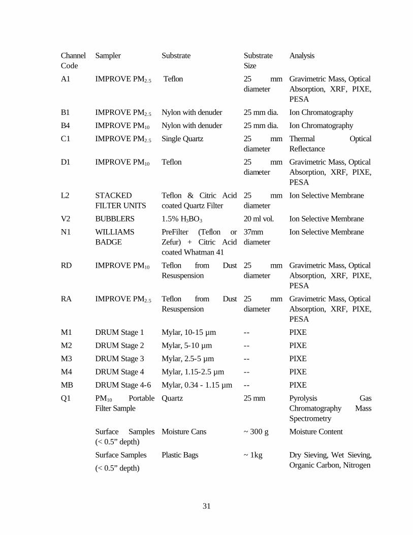
Channel Code

A1

B1

B4

C1

D1

L2

V2

N1

RD

RA

M1

M2

M3

M4

MB

Q1

Sampler Substrate Substrate Analysis Size

IMPROVE PM2.5 Teflon 25 mm Gravimetric Mass, Optical diameter Absorption, XRF, PIXE,

PESA

IMPROVE PM2.5 Nylon with denuder 25 mm dia. Ion Chromatography

IMPROVE PM10 Nylon with denuder 25 mm dia. Ion Chromatography

IMPROVE PM2.5 Single Quartz 25 mm Thermal Optical diameter Reflectance

IMPROVE PM10 Teflon 25 mm Gravimetric Mass, Optical diameter Absorption, XRF, PIXE,

PESA

STACKED Teflon & Citric Acid 25 mm Ion Selective Membrane FILTER UNITS coated Quartz Filter diameter

BUBBLERS 1.5% H3BO3 20 ml vol. Ion Selective Membrane

WILLIAMS PreFilter (Teflon or 37mm Ion Selective Membrane BADGE Zefur) + Citric Acid diameter

coated Whatman 41

IMPROVE PM10 Teflon from Dust 25 mm Gravimetric Mass, Optical Resuspension diameter Absorption, XRF, PIXE,

PESA

IMPROVE PM2.5 Teflon from Dust 25 mm Gravimetric Mass, Optical Resuspension diameter Absorption, XRF, PIXE,

PESA

DRUM Stage 1 Mylar, 10-15 mm -- PIXE

DRUM Stage 2 Mylar, 5-10 mm -- PIXE

DRUM Stage 3 Mylar, 2.5-5 mm -- PIXE

DRUM Stage 4 Mylar, 1.15-2.5 mm -- PIXE

DRUM Stage 4-6 Mylar, 0.34 - 1.15 mm -- PIXE

PM10 Portable Quartz 25 mm Pyrolysis Gas Filter Sample Chromatography Mass

Spectrometry

Surface Samples Moisture Cans ~ 300 g Moisture Content (< 0.5” depth)

Surface Samples Plastic Bags ~ 1kg Dry Sieving, Wet Sieving,

(< 0.5” depth) Organic Carbon, Nitrogen

31

Surface Samples Plastic Bags ~ 1 kg SFAME, PLFA, DNA

(< 0.5” depth)

W* Datalogger Anemometers Wind Vanes

-- Wind Speed Wind Direction

Temp. Probe RH Probe Pyranometer

Temperature Relative Humidity Solar Radiation

*Datalogger channels are numbered to designate the program used to collect and average the data.

Mass concentrations of PM and ammonia are calculated from constituent mass in the sample and the volume of air sampled. Air flow rates are measured before and after sampling as the differential pressure created using recorded using an inline orifice and recorded by a magnehelic gauge. The gauge and orifice as a unit is calibrated to a spirometer in Davis each year and the logarithmic relationship between flow and pressure difference is recorded as a slope and intercept. These parameters are entered into the database separately for each PM or ammonia sampler, allowing for the use of multiple magnehelic devices. Additionally, a second set of calibration parameters can be accommodated in the database for each sampler. This attribute was used in calculating flows for samples collected in 1994 through 1997 such that magnehelic gauges in each sampler were calibrated to the gauge and orifice unit and the in situ gauges were used to record readings.

Each PM and ammonia sample is labeled with a four digit number designated as the media ID. Teflon filter pre-weights are stored in one database and the empty weights of vials for the bubblers and lot numbers for all samples to undergo speciated analyses are stored in another. When substrates are transferred from sampling apparatus the media Id label is transferred to the holding vessel and a label is added to indicate the Test ID, the SamLoc, and the Chan. A third permanent label replaces both original labels once data entry is complete. Error trapping is performed in the relation of the databases to produce the permanent label which contains all of the data on the first two labels as well as the array code and a data to track the sample through the data acquisition software.

Gravimetric, elemental, and ammonia masses are reported from the analytical sources on a per-sample basis. These data are combined with the sample air volumes using relational databases which rebuild a temporary database from the raw data each time they are queried by the user. Meteorological data are also related to databases of test information to calculate average values for each test in a similar manner. This allows access to original data files by multiple users simultaneously and ensures that database corrections are universally available to all users. Quality assurance protocols are followed for each analysis year set using the temporary databases and erroneous data is listed in a perpetual file that is also related with the raw data to exclude those points from all subsequent queries. Current protocols for calculating emission

32

factors from PM or ammonia concentrations and meteorological data query the relevant temporary files and relate them to information about site locations, soil types, crop and livestock type, and specifics about implements on a test-by-test basis. General equations described in section 3.0 are used in spreadsheets by a dynamic process that we are still fine tuning to compute emission factors using several different models and methods for normalizing data collected from disparate operations to form a comparable, consistent table. Quality ratings and estimates of emission factor errors will help considerably in elucidating the essential sources of variance in the data set, determine the correct grouping of sources, and provide data will fit into a PM-10 emissions inventory of agricultural operations.

24 APPENDIX H – TEXT OF ATMOSPHERIC ENVIRONMENT PAPERS

Electronic versions of these documents are attached.

33

H

H

H

~ PERGAMON

ATMOSPHERIC ENVIRONMENT

www.elsevier.com/locate/atmosenv

Atmospheric E viro me t 35 (2001) 3265}3277

Lidar-assisted measureme t of PM emissio s��

from agricultural tilli g i Califor ia's Sa Joaqui Valley } Part II: emissio factors

Britt A. Holme *, Teresa A. James, Lowell L. Ashbaugh, Robert G. Flocchi i

Air Quality Group, Crocker Nuclear Laboratory, University of California, Davis, CA 95616, USA

Received 25 April 2000; accepted 31 October 2000

Abstra t

Emissio factors for agricultural operatio s are eeded i order to develop reliable PM emissio s i ve tories a d air ��

quality models for air basi s with sig i"ca t agricultural la d use. A framework was developed to a alyze the PM��

vertical pro"les collected dow wi d of tilli g operatio s i the Sa Joaqui Valley. The methods calculate emissio factors o the basis of pro"le shape a d assig quality rati gs to each la d preparatio test. U certai ties i the calculated emissio factors a d plume heights were used as o e criterio for evaluati g the relative quality of the reported emissio factor. Other quality rati gs were based o the mag itude of the di!ere ce i measured up- a d dow wi d co ce tratio s, wi d directio , whether the tests were co ducted ear the edges of the "eld, a d how well the proposed model "t the pro"le data. The emissio factors from di!ere t operatio s were compared taki g the quality of the emissio factor i to accou t. Plume heights a d emissio factors for 24 valid test pro"les ra ged from 2 to 20 m (mea "9.8; SD"3.6; media "9.8) a d zero to 800 mg m�� (mea "152; SD"240; media "43), respectively. Key e viro me tal properties gover i g PM emissio from these operatio s i clude relative humidity, soil moisture a d

��vertical temperature gradie t. Surprisi gly, o discer able relatio ships were fou d betwee impleme t type or wi d speed a d the measured emissio factors. � 2001 Elsevier Scie ce Ltd. All rights reserved.

Keywor s: PM ; Emissio factor; Quality rati g; Agricultural dust ��

1. Introdu tion

Methods to estimate agricultural tilli g co tributio s to PM i ve tories (U.S.E.P.A., 1995) are curre tly

��based o surface soil silt co te t, a parameter that ca ot accou t for the myriad of factors a!ecti g emis-sio s. Because the observed late summer a d fall PM

��sta dard violatio s i Califor ia's Sa Joaqui Valley (SJV) (Dolislager a d Motallebi, 1999) coi cide with the harvest seaso of ma y Califor ia crops (e.g., cotto , almo ds, tomatoes), agricultural activities (both harvest-i g a d subseque t la d preparatio ) have bee ide ti-

* Correspo di g author. Tel.: #1-530-752-1213; fax: #1-530-752-4107. E-mail a ress: baholme @ucdavis.edu (B.A. Holme ).

"ed as pote tially sig i"ca t sources of PM duri g this ��

time of year. Qua ti"catio of these sources a d u der-sta di g of the key e viro me tal variables co trolli g emissio s must be achieved before e!orts to co trol agricultural PM ca be pla ed.

��Lidar data were used to validate the choice of emissio

factor best-"t model for i dividual PM pro"les de-��

pe di g o dow wi d vertical pro"le shape (Holme et al., 2000). I this paper, the PM data for three years of

��testi g SJV la d preparatio operatio s (diski g, listi g, root cutti g a d rippi g) are discussed i terms of a ew a alysis framework for PM co ce tratio pro"le

��measureme ts that estimates a emissio factor, its asso-ciated u certai ty, a d assig s a test quality rati g. Rela-tio ships betwee PM emissio factors a d "eld

��sampli g co ditio s such as impleme t type, wi d speed, relative humidity, temperature gradie t a d dista ce betwee the dust-ge erati g impleme t/tractor a d the

1352-2310/01/$ - see fro t matter � 2001 Elsevier Scie ce Ltd. All rights reserved. PII: S 1 3 5 2 - 2 3 1 0 ( 0 0 ) 0 0 5 1 9 - 7

H

H

H H

H

3266 B.A. Holme& n et al. / Atmospheric Environment 35 (2001) 3265}3277

sampli g locatio are exami ed. The quality rati g system developed for i dividual sampli g tests is partly based o i terpretatio s of the simulta eously collected poi t sampler a d lidar data described previously (Holme et al., 2000). Modi"catio s to both the sampli g tech iques a d the modeli g methods that ca be employed i the future to achieve more realistic a d reliable PM emissio factors from o poi t agricultural operatio s are discussed.

2. Experimental methods

2.1. PM10 point sampling

A combi atio of upwi d/dow wi d source isolatio a d vertical pro"li g methods was used to qua tify PM emissio s from la d preparatio operatio s as

��described i detail i the accompa yi g paper (Holme et al., 2000). The tests were co ducted betwee Fall 1996 a d Wi ter 1998 i two cou ties, Ki gs a d Fres o, u der co ditio s (see Table 1) that varied from very hot a d dry (temperature"26}353C; soil moisture"1.5}2.3%; relative humidity"20}40%), prior to the seaso 's "rst precipitatio , to cool a d wet (temperature"7}203C; soil moisture"11}20%; relative humidity"40}90%), betwee wi ter storms. I all cases aerosol samples were collected usi g o e upwi d a d at least o e dow wi d vertical pro"le i a sampli g array diagramed previously (see Fig. 1, Holme et al. (2000) a d Fig. 2a, Holme et al. (1998)). For the tests exami ed here, the dow wi d sam-plers were located betwee 1 a d 235 m from the limits of the operatio (X

���, Table 2). Whe the agricultural op-

eratio was far from the statio ary PM tower that was located at the dow wi d edge of the "eld, the vertical pro"les of PM were sampled usi g a mobile tower u it

��that was drive i to the "eld. Vertical PM pro"les were based o three PM

�� �� measureme t heights } at 1, 3 a d 9 (or 10 for some towers) m } usi g modi"ed I terage cy Mo itori g of Protected Visual E viro me ts (IMPROVE) aerosol samplers (Eldred et al., 1988, 1990) that collected PM o 25 mm stretched Te o "lters (3 �m Te o� , Gelma

��

R2P1025). EPA-approved Sierra A derso i lets (Model 246b) produced the 10 �m size-cut, ow rates were regu-lated with critical ori"ces, a d the esse tial eleme ts of the modi"ed samplers from i let to "lter were ide tical to those of IMPROVE samplers (see Holme et al., 2000).

2.2. Soil moisture

Surface soil samples (upper 6 cm) were collected from at least two locatio s o each "eld for laboratory deter-mi atio of soil moisture, particle size distributio a d PM pote tial i dex (Carvacho et al., 1996a). Soil

��moisture was measured by determi i g the mass di!er-

e ce of tared alumi um moisture ca s before a d after heati g at 1053C for 12 h over ight to remove moisture (ASTM, 1992). Soil samples were collected a d a alyzed per "eld per operatio , u less meteorological co ditio s cha ged oticeably. Soil samples were ot available for tests 96-103 a d 96-104. All of the tests were co ducted o soils with sa dy

loam, clay loam or loam textures. For example, the Westhave loam, Pa oche clay loam a d Kimberli a " e sa dy loam of Ki gs Cou ty (Arroues a d A der-so , 1986) are represe ted i the samples collected. I vestigatio s of how soil texture i ue ces PM

��emissio s pote tial from these agricultural soils has bee reported previously (Carvacho et al., 1996a, b, 2000). While soil silt co te t has bee reported to be a key variable for emissio s estimatio (i.e., AP-42), soil texture is ot exami ed as a e viro me tal variable here be-cause of the arrow ra ge of textures i the soil samples with accompa yi g valid PM pro"les a d the fact that

��the Fres o Cou ty soils have ot bee mapped. A forth-comi g paper will summarize soil texture a d PM

��emissio s based o laboratory tests usi g a resuspe sio apparatus.

2.3. Meteorological parameters

Measureme ts of air temperature, wi d speed a d directio , relative humidity a d solar radiatio were re-corded at the upwi d towers usi g Campbell Scie ti"c CR10 data loggers to dow load data averages every 5 or 1 mi (the averagi g time was decreased to 1 mi ute i 1998 tests). Vertical pro"les of temperature a d wi d speed were mo itored for determi i g atmospheric stab-ility a d PM emissio uxes. I o e-third of the samp-li g periods prese ted here, simulta eous meteorological measureme ts of the same parameters were made at three heights (1, 2 a d 3 m) usi g a 3 m tripod dow wi d of the operatio for quality assura ce.

2.4. Implement an xel characteristics

Speci"c i formatio about the agricultural operatio was recorded to e able compariso s betwee crop a d impleme t types, soil co ditio s, irrigatio tech iques, a d to allow developme t of predictive relatio ships betwee PM emissio s a d "eld or impleme t co di-

��tio s. Typical parameters measured i cluded: impleme t type, make, model a d dime sio s (i.e., overall width; height/soil depth); umber of impleme t passes per test; tractor type; operatio speed; compass directio of op-eratio ; a d dista ce of the operatio from the PM samplers. Upwi d dista ces reported i Table 2 (X )

���represe t the average dista ce betwee the PM samplers a d the tractor/impleme t over the test period after cor-rectio for the a gle of the operatio . For some tests i 1998, a laser ra ge" der (Laser Atla ta) was used to

Table

1Average

meteorological a d

"eld parameters for PM

tests

��

TestID

Date

Crop

Op

Wi d

DIR

� RH

(%)

SR (W

m�

�) Bulk

Ri

Tem

perature

(3C)

Wi d

speed

(m

s��)

Soil

Moist

1m

2m

4m

7.5m

1m

2m

4m

7.5m

(%

)

Case 1:

` eclinea

}�}

all three concentrations

ecrease with increasing

height

96-103

11/16/96

Cotto

Root cut

139.21*

53.93

585.39

0.60

14.96

14.11

13.84

13.52

1.79

2.12

2.63

2.83

N/A

96-104

11/16/96

Cotto

Root cut

141.97*

46.58

371.90

0.26

16.95

16.12

16.08

15.79

2.08

2.54

3.36

3.67

N/A

96-117

12/02/96

Cotto

Disk

347.01

79.82

0.18

!

2.39

7.26

7.35

8.31

8.90

0.90

1.27

2.00

2.16

18.15

97-046

06/24/97

Wheat

Rip

358.26

22.49

893.47

0.19

33.11

31.08

31.28

30.92

3.04

3.44

3.88

4.11

2.32

97-050

06/26/97

Wheat

Rip

317.45

40.45

586.59

0.36

25.21

23.71

24.17

23.94

1.99

2.11

2.40

2.45

2.21

97-051

06/26/97

Wheat

Rip

331.62

36.92

806.50

0.41

27.72

25.62

26.32

26.07

2.01

2.17

2.48

2.49

2.21

98-045R

11/06/98

Cotto

Disk

11.43

63.68

352.44

1.16

11.62

11.29

11.19

11.06

1.71

1.91

1.68

2.07

12.95

98-048

11/06/98

Cotto

Disk

312.12

46.45

381.61

0.45

16.04

14.85

14.63

14.37

2.71

3.08

3.45

3.59

12.95

98-049

11/06/98

Cotto

Disk

312.12

43.67

382.21

0.20

17.21

16.38

16.11

15.80

3.54

3.96

4.44

4.62

11.50

98-050

11/06/98

Cotto

Disk

309.50

41.17

246.51

0.16

18.30

17.65

17.43

17.13

3.69

4.20

4.71

4.93

11.50

Case 3:

`uniforma }�} all three concentrations

&equal when uncertainties are consi ere

96-118

12/04/96

Cotto

Disk

134.18*

72.44

566.62

0.51

11.16

10.14

10.04

9.90

2.52

2.79

3.14

3.24

18.00

96-119

12/04/96

Cotto

Disk

119.96*

59.78

454.29

0.39

13.35

12.43

12.43

12.26

2.48

2.70

3.00

3.13

16.25

96-119M

12/04/96

Cotto

Disk

119.96*

59.78

454.29

0.39

13.35

12.43

12.43

12.26

2.48

2.70

3.00

3.13

16.25

98-046R

11/06/98

Cotto

Disk

338.75

52.26

480.94

1.22

14.33

13.13

13.02

12.79

1.91

2.11

2.19

2.34

12.95

Case 4:

`greater thana }'

} concentration at

3 m

is greater than

both 1 an 9 m

96-120

12/05/96

Cotto

Disk

140.27*

80.04

72.52

!0.02

11.30

10.97

11.44

11.49

4.10

4.65

5.50

5.92

16.65

97-045

06/24/97

Wheat

Disk

324.31

30.72

874.89

0.52

27.86

26.19

26.29

25.96

2.68

2.95

3.34

3.50

2.32

97-048

06/25/97

Wheat

Rip

347.78

23.34

799.46

0.26

34.39

32.37

32.44

32.11

2.60

2.93

3.30

3.43

2.21

98-046M

11/06/98

Cotto

Disk

338.75

52.26

480.94

1.22

14.33

13.13

13.02

12.79

1.91

2.11

2.19

2.34

12.95

98-047

11/06/98

Cotto

Disk

317.60

49.13

483.60

2.50

15.68

14.18

13.96

13.71

1.69

1.93

2.04

2.17

12.95

Case 5:

`less

thana

}(

} concentration at

3 m

is less

than both

1 an

9 m

96-114

11/27/96

Cotto

Root cut

58.24

91.77

479.03

1.37

10.60

9.93

10.08

10.03

1.23

1.26

1.37

1.43

19.80

96-121

12/05/96

Cotto

List

123.85*

91.49

16.51

!0.06

12.01

11.73

12.09

12.11

1.65

2.02

2.39

2.59

16.65

97-049

06/25/97

Wheat

Rip

358.83

21.62

915.05

0.17

35.49

33.70

33.66

33.35

3.02

3.44

3.91

4.13

2.21

98-045L

11/06/98

Cotto

Disk

11.43

63.68

352.44

1.16

11.62

11.29

11.19

11.06

1.71

1.91

1.68

2.07

12.95

98-046L

11/06/98

Cotto

Disk

338.75

52.26

480.94

1.22

14.33

13.13

13.02

12.79

1.91

2.11

2.19

2.34

12.95

�Best wi d

directio

was

360

for

all tests except those

marked

with

a

asterisk

where the best wi d

directio

was

180.

B.A. Holme& n et al. / Atmospheric Environment 35 (2001) 3265}3277 3267

'l'a'IJll Jln Tmc Up .il:i. ii'M ........ -, IIQoU,~1111-'} ,l'luo:• .,..i ,:.,. t.n:.uam 11,m,r ! 11,J;"'-') 'J'atnlm,p' l■I

Jn ,!,n L,:n 'l..im lbacl, !L:u Uu: !Hod: m... (k,, Cu:, 1.!',. Cl .. ,ci.._ u... r:ru 1a111

Ju fil fil fil Loil.I ... , IM u Y.I ts n -3 I j; ~ -1- I! I tl"'1 ~SI Q,;) 011 .~ ~ISi 1.1+ IHI 011 G1l ill .l!U 15.M au. 111.T 11.l l]Ji JI, l4 .u 1l I ii ~ -1- 8 " ljl,f'.lj a.Di ~ 4'P1 ilt.,) I l~fi I:!--~ r-11 G-11 ~ 11 l~ 11.4' .)il S:U 0 iU If ITJ ~L ~ ~ '5 I J. l'.lw - !ii ,.. _ (!Ill ~i (2.7J 411 ll iU:, ,:U.f I~ IHI f,1.11 fl-11 [Zl.11

I~ 1.0:S l:q; 'i'S m rn. :!14.:J> JS!II :s,s,:t ~ ~.,. jl) II) II ;1(5 ?~ ,ill m I :i, ,1.'i' ... ~ " ,p].'1-11 l';Z.!lf 1:11u:, il~ Ill) ,u, ls.JI< 11111 IHI IJll [T!IJ

il m ill :m, J.2'TB ~ 6H l~I.L ~ ID.? IM llJ m Ill] !117 Ill I J. Jit5 ... ~ f,l.lll <2-5! !.6.llli 41~1 11.6) 1'2.11 jl,.TJ, 11.JI 4-',II (-1.l l 1T.K)

H 05,'26,'9'1 I OOJ- I l)tJ l:rc):, ~ J~$ ~ la!U &3.G-1 .ill.~ ,._11_:9 m~ H.? IRL ~ n<li :,.tJ I.I!~ ~,. I It :it.• "' J ,rdft Cl I.Di (llillJ Pl,11 !iU) ,.t") IQ i:!.T! l:!ll IJII tit(,

SR ll,,)5, ~ (lD)-~I IXlt D ~ ™ mJo 1.Ui :S7.5 (,IJ LLU IJ I .liJl.9 ;!I.S ~ LL1 :55 51 I "' IJ.,I - laij; I -

+uil ¢ml !,lll.i fl.'fJ !U.JJ) ,~Ii IN.."+ rt.II llt!ll 11111 ili!i.5.1 IH: ,ID {I IT~ J,11-$ lUi :Sl5,! 1(-1.5 .MU IJ I IU IU :-.!J S1 !-I .. I t, fflJ - ~ I-

ittH! ~ ('l'.1) illll! IJ..\rJ (2.51 ILi+ ~'fl +u1 P.fl on.11, I) m, m!TJo ~!II l'U ~ ffl !1'0 !11,1 Hi -~n !00~ 73 ltl I

"'' If/a -t Q I

+mt i,11.~i (-1. IJ 44.Ct IJ..il.l i.l.~I !"'-"+ rL!t ¢.JI ¢11 4liu1, I) ~7 ~ 17.P .. ~ ,.., !l:11 l;i.:;' ,,.,_,

~ ;,.,IJ ill) 1!11 ;ic, I " ~ -t ~ I 0.1.1 4ll1 1T.)) 1).,1) !~ tot 45.1! ,15.5'!

ill .SIL! - 1·u - I~ till ~ ~ iLO) "J.! l J. 45.;3 - I I ~9j Gil 117,1 I 1;;:i IH't, 1-n,1<1i (11. !J

119 L;!,;J4,'516 IE7- l<III 0.... .lf:S 6J. ~ 4J.T nn fil Yi'.l IH _ :!.j - :H 11.:S »: ~ - ~] ti J :e ~ 4 C 1'!111 llZ,ij (21) 41Lt] 11:LX) llUJ II 1J, 4-0.J] 4m!..?I,

ll-111,1 L1,;J4,i51,5 IE1'-l.!II ~ Tl' S6.S :YT.I !U ll.'2 ..il.4 4'M ill jli.5 l'l'J llil: ,U u 15.S H 3 J. 11M ir-111 ~ ~· ~ ll JUI,) ,1.11 11LTJ, JUI f:1.11 i:11'1 411.21,

~llll:S lltll :JO £ 1 11,)1 lJ. ll:i<li 6.!.7 !59.3 U-'' ~t..: ~1.11 ~ .I Di-4 L:,J .mil JS J It H:.i ,i;!l.'1111 (,UJ t11J 4111 (IDli) 1 llllh 1mi!.-!1 IU~ f'.'.li J:!MI 11 !!.. I)

i!.dJDJ!i' .. iJi; :16.l .lu,i'I m n.11 ::.u .... ~ tLJ JJ,11 -h 1-11, -~, -ill. 'I I.J :w:I'

4'1.JJ1 Cl.'71 a.I.) 1m 1-:i.r..;i 1].1$1 Ill~ 1- Lll !~.JI 4 - 1.11 ($. I t:u5t,... 11.ll' Dulc if ~ !IM '.Im.fl ll'il fil ;!ill lilt• f.41 1u., ,.s .u~ ~ l !!'.Iii -i J. ~, -1- ., I

~I ~71 (lu,t R2'~1 .,,~ 1oi§1 lltllo !Va f,'.Ht Vfill flUI, t,...04) 0¢5,"r.' 1:Ul- 141U Itri, l::S 100.1 m J-11,.T o1 IJJ I.I 3.1.ill ~11., t.ti 9..5 lti .JJ,r, "· ::!t,,il 31 JI ,. ·~ -1- 5 " o,lllfl (,IJI tm..:i 4111 i61J) lo'lt i,~ 1~11 41'-'.11 U•_jJ ji'I.I)

~ llll.~ DWc 15.l> i) :lt;.5 ,,ji ll5' :!!!°I.I !S&2 41 l5 11..! i1i ~IL5 .:i8 Ill "' 4 J. :!;!.::? - Iii ,.._ 4Ull G.Oi ~7j 4Ll1 rl~ 11-4°1 1U4 r:rn Cll !fJ~l 11;1,,I)

1ll1.S-1!Ml Dul :Ii [I (I [I 215' 5,i.5 ~ 'IU· $ii !iL5 iii Ill J.U - ii '-6 4 ii ru -1- ~ " tllJl (i 11 (»!'I 011 CIIIIII) 1.Jllt fl ,q, ID~ ~~l 1-~,1 jZIJl) C...J.·°"ialiin" • ..: ■ --.:a1J■■ b,,_1rt, l•F•

IIJJ 1 lr.;',"M r:.t"°" I 100 -~ ~ 11-9 Tl. I ,,-T.T '!UJ ~ ;$2A 1$Jl 1411 -:;t: IM.'1' D} ~ ~, ., ' ·"' ~ -t ~ 74 I) , .... i12m ~· (.u) •U1 1Uu., (lll .. , 1i.u1 ,141..5'1 (40]

lf~L ~W,"MI l:Kl- lta? I.J.d. lll w Jll6 U!li .ilLi-4 :19..1 29.1 JI'!' u ].~ 1D -11:J. a.1 -11, 11 ! ,r:- & I, -1- - 167

+ur1 ~· (:;.L) 4L'!I I li~.6) (M) llli.J. I JJ.!I fHI 4- 051 (!. I) ,-n 1-111- l!!,lll ll>r ill!: Zil',. I lU ,t.lT.'I' ~ zw 11';7.; nu T.::O -~ lti, m is):· .lil:! ,Wj. ! ,. I.:! - ... 6 A-

41.5.0li l ClllJI (U) 4~1 1JTE,; (I~ 112.1• J:i&.J I 4-"i'.II IIJA;J , L Ll,Ull,"..:!i ~ I buk m D D tCilJi ~ "" ta:, ?'I.:!, 11<.fl -~ J4J; ::h hl:: :?'I ». ! ,. .I.I A - ... 1-11:'i II-

"4-11'1 (,ti) ~ ~ -Ji ll ~ (l:UJ IIIJ!, ~U11 ~JI ti~ L 11,'!.111,■1.11 1Ph,L.1llu IJulc :iii Ii [I m4ll ~ 'JC ff.JI UI.I .~~ I -iii, 11,.f . ., M.: Il l It ! ,. :ti :!! - - Ill ii

,j4_1Jj ~ (J.J) ti.J I (l).11 1l•D l~UI 411u1 fl~I

mh!.1~ Gm:1rc8ronf!bk ·,,..aluc:J, rw1lvc: i:ml!!lon f[!!;IIQ:r '1DQ:N!!11"1" ■-

3268 B.A. H

olme& n et al. / A

tmospheric E

nvironment 35

(2001) 3265}3277

Table 2 Poi t sampler test data, emissio s model results a d test quality rati gs�

H

H

H

H

H

H

H

H

��

B.A. Holme& n et al. / Atmospheric Environment 35 (2001) 3265}3277 3269

i depe de tly observe the locatio of the tractor duri g the lidar sca s. The time, dista ce a d beari g to the tractor were recorded every 30 s to 1 mi by a observer located alo g the edge of the "eld (see Holme et al., 2000, Fig. 1).

2.5. Li ar

Lidar data collected co curre tly with the poi t sam-pler tests were used to u dersta d plume behavior for plumes that exceeded the 10 m tower height, a d to co "rm that test-averaged plumes sampled at o e cross-wi d locatio o the "eld were represe tative of the operatio at all crosswi d locatio s (Holme et al., 2000).

2.6. Emission factor calculations

PM emissio factors for agricultural operatio s��

such as tilli g a d harvesti g are logically qua ti"ed o the basis of the area of la d worked because the source bei g qua ti"ed is the "eld where the operatio takes place, ot the movi g tractor/impleme t. Vertical pro-"les of wi d speed a d PM co ce tratio were used to

��calculate emissio factors for the la d preparatio opera-tio s. As discussed i the compa io paper, because gravimetric mass was co siste tly well correlated with the `reco structed massa composite variable (RCMA) a d the eleme tal a alyses were su$cie tly more se si-tive tha the gravimetric measureme ts (Holme et al., 2000), all emissio factors were calculated from PM

��RCMA co ce tratio s. The composite variable RCMA was calculated usi g a relatio ship based o the ratios of the commo crustal eleme ts (Al, Si, Ca, Ti, Fe), sulfur, light absorbi g eleme tal carbo , hydroge a d o soil potassium i a average aerosol (see Holme et al., 2000, Eq. (1) a d refere ces therei ). Whe the RCMA mass co ce tratio was below the MDL at a y of the three sampli g heights, emissio factors were ot calculated for that test. Each dow wi d PM pro"le was classi"ed accordi g

�� to its shape i to o e of "ve types (see Table 2, Holme et al., 2000):

Case 1 } decreasi g PM with height (`decli ea); Case 2 } i creasi g PM

�� with height (`i cli ea);

Case 3 } u iform PM ��with height (`u iforma);

��Case 4 } 3 m co ce tratio highest (`greater tha a); Case 5 } 3 m co ce tratio lowest (`less tha a).

Three di!ere t methods } the li e, block a d logarith-mic pro"le models } were used to "t the PM RCMA

��vertical co ce tratio pro"les as described previously (Holme et al., 2000). A fourth model, the box model, was used to describe the PM yux i cases of u iform dow -

��wi d vertical co ce tratio pro"les. The choice of the appropriate model for each dow wi d co ce tratio

pro"le type was based o a alysis of simulta eous lidar a d PM vertical pro"le data (Holme et al., 2000).

��For each model, a horizo tal PM ux was cal-

��culated as the product of the et (i.e., dow wi d } upwi d) PM co ce tratio (mg m��), C(h), a d the

�� average horizo tal wi d speed (m s��), ;(h), at 10 equally spaced height i tervals (m), dh, betwee the rough ess le gth, z , a d the top of the plume, . The

�rough ess le gth was determi ed by "tti g the wi d speed data to a logarithmic pro"le. The plume height was de" ed by the i tersectio of the dow wi d pro"les with the average upwi d co ce tratio (Holme et al., 2000). The ux was i tegrated over the height of the plume usi g Simpso 's Rule, a d ormalized by the time of the test, t, the upwi d width of soil worked duri g the test period, w, a d the a gle betwee the measured wi d directio a d the directio perpe dicular to the "eld edge, �, to compute the PM emissio factor (mg m��):

��

;(h)C(h)t cos � E"�

� dh. (1)

w��

U certai ties i the calculated emissio factors were estimated usi g error propagatio tech iques (Colema a d Steele, 1989) for the li e, block a d logarithmic "t models. The PM RCMA measureme t u certai ties

��a d the test period wi d speed sta dard deviatio at each measureme t height were used to estimate the u cer-tai ty i the horizo tal ux at each of the 10 model heights. Details regardi g the u certai ty calculatio s are i the appe dix.

2.7. Emission factor conx ence rating

Each calculated emissio factor was assig ed a over-all test rati g based o "ve quali"ers that attempt to assess the ability of the emissio factor estimate to qua -tify the actual o poi t source emissio s. The overall test rati gs ra ged from A to E a d were desig ed to accou t for a decreased reliability i the computed emissio fac-tor whe : (1) the upwi d co ce tratio s were equal to or exceeded the dow wi d co ce tratio s at a y height (Q ); (2) the wi d directio deviated from ideal (Q ); (3) �� �

the test su!ered from multiple passes due to edge e!ects (Q ); (4) the "t to Case 5 pro"les was poor (Q ); or (5)

�emissio factor relative u certai ty (EFU) was high. Each of these quali"ers is described i Table 3 a d was based o observatio s made for all tests (see Sectio 3.2).

3. Results and dis ussion

3.1. Best-xt emission factors for in ivi ual proxle types

Compariso of the average plume heights a d verti-cal pro"le shapes determi ed by lidar to the pro"les

H

l~h;;m Fat or ancl Ope b1on b . 1Pll'011 · s" p ,c 1 3 C;JL 4 ,eai.o

Ii: ~ 04,11 ... .ij.!IIJil.~llf,i--~ ..... ~

. ' .

3270 B.A. Holme& n et al. / Atmospheric Environment 35 (2001) 3265}3277

Fig. 1. Best-"t emissio factors did ot vary directly with type of operatio . The tests are i order by pro"le shape class as tabulated i Table 2. Error bars for Case 1, 4 a d 5 pro"le types represe t two times the best-"t emissio factor u certai ties reported i Table 2 (shaded values).

measured with the poi t samplers o 6 November 1998 led to assig me t of particular best-"t models to the PM pro"les for each of the four observed pro"le shape

��categories (Holme et al., 2000). Although there were some tests that were di$cult to categorize, overall the model selected for each category te ded to have the lowest calculated u certai ties for both plume height a d emissio factor. The calculated emissio factors (a d u certai ties) for

all models are show i Table 2 for compariso ; the shaded values represe t the best-"t model plume height a d emissio factor values for each pro"le type. As the test results i dicate, there was ge eral agreeme t i the emissio factors computed by the di!ere t fu ctio al "ts to the pro"les for a i dividual test whe all four models could be calculated (Cases 1, 4 a d 5). Thus, the mag i-tude of the computed emissio factors was ot biased by the selectio of the best-"t model. The "ve highest best-"t emissio factors (330}

776 mg m��) were see for Case 1, 4 a d 5 pro"les collected o hot dry summer days for rippi g a d diski g (Fig. 1, Tables 1 a d 2). Similar "eld co ditio s, however, also resulted i a much lower rippi g emissio factor of 112 mg m�� (test 97}050), thus complicati g i terpreta-tio betwee di!ere t tests. Whe the dow wi d co ce -tratio s were u iform with height (Case 3) emissio s were ge erally low but dow wi d PM values were

��sig i"ca tly higher tha upwi d co ce tratio s. The low emissio factors were ot due to the use of the box model, however, because the box model emissio factors showed fairly good agreeme t (withi a factor of 2) with the emissio factors calculated by the other models for the other pro"le types (Table 2). I teresti gly, the lowest 5 emissio factors were measured i wi ter whe temper-

atures were cooler a d soil moisture was relatively high (Tables 1 a d 2), suggesti g that e viro me tal co di-tio s greatly i ue ce emissio rates.

3.2. Test quality ratings

The emissio factors i Table 2 represe t a wide ra ge of values, but were collected u der disparate sampli g co ditio s. I order to compare the test results a d ide tify the key factors co trolli g emissio s, a i di-vidual measureme t co "de ce must be assig ed to each test. Five qualifyi g factors ide ti"ed for this purpose are de" ed i Table 3 a d justi"ed below.

3.2.1. Upwin qualixer, Q��

I dividual upwi d PM co ce tratio s were com-��

pared directly to the correspo di g dow wi d co -ce tratio s at the same height for each test pro"le i order to qualify the calculated emissio factor based o the relative upwi d}dow wi d co ce tratio values. The ratio ale for Q was that pro"les where upwi d a d

��dow wi d co ce tratio s were similar i dicate either that: (1) the dow wi d measureme ts were ot sig i"-ca tly di!ere t from backgrou d a d therefore the emis-sio s from the operatio were small a d more di$cult to accurately qua tify, or (2) the upwi d pro"le was i ue ced by a other source, but ot so obviously as to warra t omissio of the test. The latter sce ario would reduce the co "de ce that the computed emissio factor accurately describes the source of i terest. Tests were ot omitted o the basis of havi g i di-

vidual upwi d co ce tratio s higher tha those at dow wi d i order to preve t biasi g the emissio factor estimates to the high e d. For example, there were test co ditio s, especially i late wi ter, whe soil moisture was high, emissio s were sig i"ca tly lower tha at other times, a d upwi d co ce tratio s at a single height would be close to or greater tha the measured dow -wi d value. Such a test would be quali"ed with a `Ba rati g o the basis of the upwi d quali"er scale outli ed i Table 3. A special case occurred, however, if the si gle height where the upwi d a d dow wi d co ce tratio s were equal was the highest sampli g height. Because this occurre ce i dicates that the highest sampler was close to the top of the plume, the two special case tests (96}103; 98}049) received a `Aa value for Q

��, rather tha a `Ba.

The fact that the modeled plume heights for these tests were &9 m adds credibility to the de" itio of this special case. Note that all but three tests had Q rati gs of `Aa

��i dicati g that most of the dow wi d PM co ce tra-

��tio s were sig i"ca tly above backgrou d values. Of the three tests with poor Q rati gs, two tests (96-120, 96-

��121) were collected u der relatively u stable atmospheric co ditio s as i dicated by egative bulk Richardso umbers (Table 1). Test 96-120 (Case 4) was particularly

��

H

B.A. Holme& n et al. / Atmospheric Environment 35 (2001) 3265}3277 3271

Table 3 Emissio factor co "de ce rati gs summary

Quali"er Criteria/ratio ale Scale

1. Q��, upwi d co c

2. Q �, wi d directio

3. Q , edge e!ects�

4. Q , Case 5 "t

5. EFU, relative emissio factor u certai ty

Number of upwi d PM RCMA co ce tratio s ��

that exceed dow wi d co ce tratio at the same height

Special case: If o ly the 9 m dow wi d ( upwi d, test rati g"`Aa u der the assumptio that highest sample was above plume

(a) Test wi d directio SD'253

(b) (test wi d directio )-(best wi d directio )'453

Note: best wi d directio "903 to dow wi d edge of sampli g array

X���&0 a y time duri g test

If test i cluded passes at the "eld edge immediately upwi d of the tower, test deserved lower quality rati g ( egative Q )

�

Assesses how well li ear model described "t [PM] ![PM] '�[PM] ![PM]

� � � � � � � � �[PM] ![PM] (�[PM] ![PM]

� � � � � � � � �

�Accou ts for u ide ti"ed qualifyi g factors emissio factor u certai ty

�'20% emissio factor

A"0 exceed, or special case B"1 exceeds C"2 exceeds D"3 exceeds

Reduce letter rati g (assig ed o the basis of Q ) by

��1 scale (i.e., A B, B C) if either (a) or (b) is true 2 scales (i.e., A C, B D) if both (a) a d (b) are true

!"edge e!ects prese t #" o edge e!ects

!"poor li ear "t #"better li ear "t

Reduce letter rati g by o e scale (i.e., A B, B C) if true

di$cult to model because all the dow wi d co ce tra-tio s were similar to upwi d values. Co seque tly, to i dicate reduced co "de ce i the emissio factor computed for this test it received a `Da Q rati g.

��

3.2.2. Criteria for win irection, Q �

Co "de ce i the calculated emissio factor was also reduced whe : (1) the wi d directio was highly variable over the test period, or (2) the mea wi d directio was very di!ere t from the ideal wi d directio (de" ed as the directio perpe dicular to the dow wi d edge of the sampling array). Both of these co ditio s would reduce the ability of the poi t samplers to capture the e tire plume i a reproducible ma er. A emissio factor was assig ed a lower co "de ce rati g whe the sta dard deviatio i the mea wi d directio over the test period was greater tha $253 or if the wi d directio deviated from the ideal wi d directio by more tha $453 (Table 3). Whe either of these co ditio s occurred, the overall test rati g was reduced by o e level (i.e., a `Aa rati g would decrease to a `Ba level), a d, if both co ditio s occurred, the overall test rati g was reduced by

two levels (i.e., `Aa to `Ca). Ni e tests were collected whe wi d directio data met o e or both of the above criteria; these tests are i dicated by the bold Q values

�i Table 2.

3.2.3. Qualixer for e ge ewects, Q �

Because tractor tur i g ear towers located at the edge of the "elds was show to a!ect the PM measure-

�� me ts (Holme et al., 2000), i dividual tests were as-sig ed a egative Q rati g (Tables 2 a d 3) if the PM

� pro"le was collected ear the dow wi d edge of a operatio that was co ducted at a a gle such that tractor tur i g could have adversely a!ected the test. A (}) Q rati g i dicated a reduced co "de ce that the

�emissio factor was represe tative of the operatio . The Q rati g was used to modify the Q rati g o ly if� ��

Q was egative (e.g., a `Aa test based o Q was� ��

demoted to a `A!a if edge e!ects were suspected duri g sample collectio ). Te tests, e compassi g all of the observed pro"le shapes, were ide ti"ed as i ue ced by edge e!ects (Table 2).

��

��

��

H

Best-fit model EFU vs. average upwind tractor distance

~ 250 96-120

'E ■ (4) :fg CASE 3 not shown Q) 200 (Box fit, no errors propagated) () 96-121 C:

::::, ■ (5) 5 150 • ti 98-045R, L "" LL (1, 5) C: 100 0 96-114 "iii

■ 1/) (5) .E 50

UJ

i 0 .... .....

■ ■ • & 0 50 100 150 200 250

X,0 ,, upwind distance to middle of tractor path (m)

3272 B.A. Holme& n et al. / Atmospheric Environment 35 (2001) 3265}3277

Emissio factors calculated from towers a!ected by edge e!ects were expected to be sig i"ca tly di!ere t from each other; this was see for the two adjace t pro"les collected duri g a si gle test (98-046) that was impacted by edge e!ects: the L tower emissio factor (117$21 mg m��) was three times higher tha that for the R tower (35 mg m��) (Table 2). The large variatio i emissio factors calculated from measureme ts take withi 6 m of o e a other illustrates the di$culty i i terpreti g data impacted by these "eld edge e!ects.

3.2.4. Qualixer for case 5 xt, Q Each pro"le exhibiti g a Case 5 shape (`less tha a) was

assig ed a quali"er for the good ess-of-"t of the data to the li ear model (Q ). The quality of the li e "t to Case 5 pro"les depe ded o the exte t to which the PM

��co ce tratio measured at the 3 m height was less tha that which would be predicted by a li ear "t to the measured 1 a d 9 m co ce tratio s. The Q quali"er (Table 3) depe ded o the di!ere ce i measured RCMA co ce tratio s: if the 9 a d 3 m co ce tratio s were more similar tha the 1 a d 9 m co ce tratio s, the the li e "t was co sidered to give reaso able emissio esti-mates for Case 5 pro"les. Use of the li ear model was more problematic whe the 1 a d 9 m co ce tratio s were similar because the the li ear "t esse tially ig ored either the 1 or 9 m co ce tratio a d resulted i plume heights that were u realistically low (e.g., 98-046L (9 m ot "t) a d 96-121 (1 m ot "t)). The low plume heights resulted i correspo di gly low emissio factors i these cases a d therefore these tests received lower co "de ce rati gs because it was suspected that the di$culty of "tti g the three-poi t PM pro"le data was biasi g the

��emissio factor low. For test 98-046L, lidar vertical sca data i dicated a plume height of approximately 45 m (see Holme et al., 2000, Fig. 3) co "rmi g that the modeled plume height was u reaso ably low.

3.2.5. Relative emission factor uncertainty, EFU Relative emissio factor u certai ties (EFU) were

computed as the ratio of the propagated emissio factor u certai ty (see the appe dix) divided by the emissio factor, expressed as a perce tage. The emissio factor errors were expected to i crease whe the measured data did ot "t the appropriate model a d whe exter al factors such as edge e!ects a d highly variable meteoro-logical co ditio s occurred duri g a test period. This was ge erally the case for the tests summarized i Table 2, with the otable exceptio of tests 98-045R a d 98-045L, which both had very high EFU values (&145%), but had high quality rati gs (i.e., high co "de ce) for the other quality factors. The li ear "ts to both of these tests were ot sig i"ca tly poor compared to other tests, so the high relative u certai ties probably i dicate that some other as yet u ide ti"ed factor a!ected these pro"les to explai the low co "de ce i the computed emissio

factors. For test 98-045R, the high EFU was probably due to the fact that the 3 a d 9 m co ce tratio s were early equal; this te ded to reduce the ability of all the models to "t the measured pro"le (Table 2). The "ve tests where the u certai ty i the computed

emissio factor exceeded 20% of the emissio factor value had their test quality rati g reduced by o e level. EFU was used as a " al factor i quality rati g because there were tests that had high EFU values but o e of the other ide ti"ed co "de ce criteria i dicated a problem with the test. This suggests that there remai other u -ide ti"ed qualifyi g factors that a!ect co "de ce i the modeled emissio factors.

3.3. Maximum sampling istance

The questio of whether or ot there was a maximum dista ce betwee the tractor a d samplers beyo d which the pro"le tech ique was i capable of reliably qua tify-i g a emissio factor was exami ed. If the data collected by poi t samplers at farther dow wi d dista ces from the tractor had higher EFU values, the possibility of a limited reliable sampli g ra ge could be i ferred. This did ot appear to be the case because there was o systematic relatio ship betwee the dista ce from the tractor a d either the relative emissio factor error (Fig. 2) or the error o the plume height. The highest EFU values occurred at i termediate average upwi d dista ces betwee 30 a d 100 m from the towers a d predomi ately for Case 5 test pro"les.

Fig. 2. Relative error i calculated emissio factor (EFU) as a fu ctio of the average tractor-to-sampler dista ce over the test period. Note that for most test pro"les, the relative error was less tha 50%. The tests with high relative errors were usually Case 5 pro"les. Case 4 pro"le 96-120, had a egative emissio factor close to zero (!0.5 mg m��) with a high error (!1.2) a d was di$cult to "t because two of its three dow wi d co ce tratio s were below the average upwi d value.

H

H

B.A. Holme& n et al. / Atmospheric Environment 35 (2001) 3265}3277 3273

While it is likely that some physical limits exist regard-i g the proximity of the samplers to the poi t source i order to obtai i terpretable relatio ships betwee "eld co ditio s a d plume characteristics such as height, the la d preparatio data (Table 2, Fig. 2) suggest that dow wi d dista ces up to 250 m could be reliably sam-pled usi g the vertical pro"li g tech ique with a relative error of less tha 20% as lo g as the pro"le shape was ot Case 5. However, while relative errors were low, there is o way to k ow how accurate the reported emissio factor values are. The high EFU pro"les resulted from di!ere t factors, i cludi g: (a) dow wi d co ce tratio values close to backgrou d (96-120, 96-121), (b) highly variable or o -ideal wi d directio (96-114, 96-121), (c) edge e!ects (98-045R, L) a d (d) highly exaggerated Case 5 pro"le shapes (96-121). This latter e!ect is prob-ably due, as the lidar vertical pro"les showed (Holme et al., 2000), to the limited sampli g height of the towers that capture o ly part of the e tire vertical exte t of the plume u der some test co ditio s.

3.4. Replicate emission factors

The mobile tower could be positio ed well i side the "eld bou daries a d easily repositio ed to follow the operatio up the "eld a d achieve similar upwi d dista -ces to the tractor (X ) betwee tests. Such `duplicatea

��� pro"les resulted i similar emissio factor estimates whe the averaged activity of the tractor was the same relative to each sampli g locatio . This is evide ced by the agree-me t betwee the emissio factors calculated from mobile tower pro"les collected i tests 98-049 (93.5$ 8.5 mg m��) a d 98-050 (74.2$6.3 mg m��) at slightly di!ere t crosswi d locatio s (585 a d 594 m, respective-ly) but similar dista ces dow wi d of the tractor (56 a d 34 m, respectively) a d well away from the dow wi d "eld edge. The repeatability i these tests was e ha ced compared to those reported earlier (see Table 3, Holme et al., 2000) due to the more co siste t activity of the source whe worki g the ce tral areas of the "eld, where the abse ce of tractor tur i g elimi ated edge e!ects. The east}west impleme t a gle (i.e., perpe dicular to "eld crosswi d edges) also produced more co siste t results for these tests compared to 98-045 to 98-047, despite the fact that the tractor still worked the "eld i spiral sectio s. Whether the emissio factors measured at the edges of

the "eld should be weighted similarly to the values ob-tai ed by mo itori g the more repeatable a d represe -tative tractor activities i the midpoi ts of the "eld requires further i vestigatio . Of co cer is biasi g the average emissio factor high because of the prese ce of the statio ary sampli g array (at the "eld edge) that, despite e!orts to have mi imal impact o the agricultural operatio , i evitably did have some e!ect o the tractor's path a d therefore o emissio s estimates due to the multipass `edgea phe ome o .

3.5. Factors inyuencing plume height an emissions

Emissio factor compariso s amo g these o poi t sources must take i to accou t di!ere ces i soil co di-tio s, tractor/impleme t speed, sampler locatio relative to the tractor/impleme t a d meteorological co ditio s betwee sampli g tests. All of these factors ca i ue ce the measured PM co ce tratio s, the shape of the

��vertical pro"le, a d therefore, the calculated emissio factor. Some of the relatio ships expected based o at-mospheric dispersio theory i clude higher plume heights whe sampli g was co ducted farther from the tractor or whe the vertical temperature pro"le i dicated co vective co ditio s. Lower plumes were expected whe wi d speeds were high a d low emissio s were expected whe the soil was relatively moist. The la d preparatio data (lidar plus poi t measureme ts) sup-port most of these expectatio s, as outli ed below, but questio s arise as to how well the poi t samplers alo e are capable of ide tifyi g the expected relatio ships due to their limited height ra ge a d the lo g averagi g times required to collect measurable mass.

3.5.1. Plume height The relatio ship betwee maximum plume height a d

upwi d tractor dista ce determi ed from the lidar a d laser ra ge" der data (Fig. 3a) i dicates a tre d of higher plume heights for sca s collected whe the tractor was farther upwi d of the lidar sca pla e, as expected for a plume dispersi g from a grou d source. The correla-tio was ot very stro g, probably because o correctio was made for the time lag betwee emissio of the plume at the higher upwi d coordi ates a d the time of measureme t of the plume at the lidar sca locatio . A stro ger correlatio would take the i sta ta eous wi d speeds i to accou t, but this a alysis is beyo d the scope of the prese t work. The relatio ship betwee the plume heights estimated

from the poi t sampler pro"les a d upwi d dista ce was ot as stro g as that i dicated by the lidar sca data (Fig. 3b). This is probably the result of: (1) the di$culty of assig i g reliable upwi d dista ces to data collected be-fore the tractor locatio was mo itored closely a d (2) meteorological variability over the lo g poi t sampler test duratio s. Better de" itio of this relatio ship may require determi atio of the mi imum a d maximum upwi d dista ces of the tractor duri g the tests relative to the locatio of each pro"le tower. The a gle of the impleme t relative to the poi t sampler array must also be measured with greater accuracy i the future to e able calculatio of the limits of the test operatio . Improved estimates of plume height will also be possible if a other sampli g height is added to the vertical pro"les because this will improve the i terpretatio a d a alysis of plume shape a d best model "t.

80

I t 60 ·;; .c

~ ::, 40 ii E ::, E 20 -~ :ii

a. Lidar plume height

.. ■ ■ ■

I" .. ■"' •• ■

y = 0.299x + 0.364 R' = 0.361

■ ■

0-1"'"---....;:.....:c:;...-...::.,-~----'•c;--"_-,-___ ~---.---~--,

40

35

30 I l: 25 Cl 20 I

0 20 40 60 80 100 120

Upwind distance to lldar beam (m)

b. Best-fit plume height

Cases 1 and 5 = linear fit Case 3 = box model (no error bars) Case 4 = block fit

15

10 ----1 5

0

-5

140

-1o~r--....-'--,-----,--r---.--~--,---,-,--, 50 100 150 200 250

X,00, Average tractor upwind distance (m)

3274 B.A. Holme& n et al. / Atmospheric Environment 35 (2001) 3265}3277

Fig. 3. (a) Lidar maximum plume height measured from i di-vidual lidar 2D sca s versus upwi d tractor dista ce determi ed by laser ra ge" der for PM test 98-045; (b) calculated best-"t model plume height did ot correlate well with test-averaged dow wi d dista ce for samples collected usi g poi t samplers. The poor correlatio most likely re ects the di$culty of back-calculati g average tractor upwi d dista ces for tests co ducted i 1996 a d 1997 before careful measureme ts of relative tractor locatio were recorded.

3.5.2. Environmental con itions an emission factors The calculated emissio factors for la d preparatio

activities (Table 2): (a) showed o correlatio with wi d speed over the ra ge of wi d speeds tested (1}5.5 m s��); (b) i creased with decreasi g relative humidity; (c) were ge erally lower whe soil moisture was higher a d (d) ge erally i creased with i creasi g vertical temperature di!ere tial (Fig. 4). These depe de cies of emissio s from la d prepara-

tio activities o e viro me tal co ditio s such as tem-perature a d relative humidity have bee docume ted before (Claus itzer a d Si ger, 1996, 1997; Ka tama e i et al., 1996) a d illustrate the ecessity of i corporati g local meteorological co ditio s i to the developme t of predictive PM emissio factor models. This calls for

��the developme t of a empirically derived fu ctio al form of the emissio or the activity factors used to calcu-late PM i ve tories. The two disti ct populatio s of

��emissio factors below a d above 40% relative humidity (Fig. 4b) a d below a d above 10% soil moisture (Fig. 4c)

suggest that relative humidity a d soil moisture are im-porta t parameters requiri g further i vestigatio . As stated above, relatio ships betwee emissio factors a d soil properties other tha moisture were ot exami ed because soil texture data were ot available for a y of the 1998 tests exami ed here. The ra ge of soil types for the 24 tests that had valid

PM data is too arrow for us to draw a y co clusio s with respect to soil properties other tha moisture co -te t. A forthcomi g paper from our laboratory will exami e how laboratory resuspe sio a d soil texture experime ts ca be used for emissio s estimatio . The mai focus of the prese t paper is o developi g a method for a alyzi g "eld data for emissio factors that qua ti"es the measureme t u certai ty. Soil texture should ot be a source of measureme t u certai ty; rather it is more likely that soil texture will be a key e viro me tal variable, like relative humidity or temper-ature di!ere tial, that ca be correlated with the measured emissio factor.

3.5.3. Implement characteristics an emissions Di!ere ces i PM emissio factors from two opera-

��tio s, diski g a d rippi g, for which a represe tative umber of repeated measureme ts were made, were used to exami e the importa ce of impleme t type. The average emissio factor for rippi g operatio s, 507$292 mg m��, was sig i"ca tly larger tha that for diski g, 91.2$104 mg m��. However, direct compariso of impleme t-average emissio s is ot reliable because di!ere ces i e viro me tal co ditio s (e.g., relative hu-midity a d wi d directio variability) betwee i dividual tests appear to have a larger impact o measured emis-sio s tha does impleme t type. Variability i measured emissio s due to e viro me tal factors is highlighted by three Case 1 rippi g tests collected o 24}26 Ju e 1997 (see Table 2). The emissio factors for two tests (97-046, 765$36 mg m�� a d 97-051, 776$27 mg m��) were similar a d sig i"ca tly higher tha diski g tests co -ducted u der similar relative humidity co ditio s (98-050, 74.2$6.3 mg m��) but the emissio s from the third rippi g test, 97-050, 112$5.3 mg m��, were much lower a d similar to emissio s measured for diski g (see Fig. 1). The much higher deviatio of wi d directio from the ideal directio , the higher relative humidity a d lower solar radiatio duri g this third rippi g test likely explai these results a d highlights the complexity of compari g emissio tests with di!ere t impleme ts u -less all other e viro me tal factors are held co sta t. Emissio factors measured for di!ere t crops such as

cotto a d wheat that are harvested at di!ere t times of the year are also di$cult to compare because emissio s-related e viro me tal co ditio s vary sig i"ca tly with seaso . For example, wheat la d preparatio is co duc-ted i summer whe co ditio s are hot a d dry a d soil moisture is quite low, but co ditio s for cotto la d

800

~ 600

Cl .§. .. ~ LL 400 C 0 'iii "' ·e w ! 200

gJ ta

0

800

~ 600

Cl .§. .. i LL 400 C 0

"' 'iii ·e w ,l: 200

~ ta

0

a. Wind Speed at 4 m

+ + I

2 3 4 5 6

Average wind speed at 4 m height (m s'')

c. Soil Moisture

i

I I

• • - • :I

0 2 4 6 8 10 12 14 16 18 20 22

Soil Moisture (%)

800

~ 600

Cl .§. .. ~ LL 400 C 0 'iii "' ·e w ,l: 200

11 ta

~ Cl .§. .. ~ "' LL C 0 'iii .!a E w ,l:

i ta

0

900

800

700

600

500

400

300

200

100

0

-2

l

I

I I

b. Relative Humidity

•• I • • ·•--­• J • • l

20 30 40 50 60 70 80 90 100

Test-average RH (%)

d. Temperature Difference

■:96-117

- i -1 0

I I

I -.+

•: JI: ·- . •••

2

I

I

3

Temperature difference between 1 and 7 m heights (°C)

B.A. Holme& n et al. / Atmospheric Environment 35 (2001) 3265}3277 3275

Fig. 4. Best-"t emissio factors as a fu ctio of meteorological co ditio s for all tests i Table 2. (a) wi d speed (m s��) at 4 m height, (b) relative humidity (%), (c) soil moisture (%), (d) air temperature gradie t calculated as the temperature di!ere ce betwee 1 a d 7.5 m heights (3C). Error bars o wi d speed are based o two times the average sta dard deviatio of the wi d speeds recorded every 1 or 5 mi over the test duratio . Emissio factor error bars are 2 times the emissio factor u certai ties reported i Table 2.

�

3276 B.A. Holme& n et al. / Atmospheric Environment 35 (2001) 3265}3277

preparatio , i the late fall, are cold a d moist. Despite the fact that la d preparatio operatio s o these two crops use similar impleme ts, measured emissio s were very di!ere t due to seaso al e!ects. Thus, it seems prude t to develop empirical emissio factor models that take these seaso al e viro me tal variables i to ac-cou t. For example, correcti g AP-42 emissio factors for mo thly variatio s i soil moisture will result i more realistic emissio s estimates tha assumi g o relatio -ship betwee emissio s a d soil moisture (ARB, 1997).

3.5.4. Comparison to AP-42 Agricultural la d preparatio emissio factors are ge -

erally estimated usi g EPA's guida ce docume t, AP-42, based o the soil's silt co te t a d a default silt co te t of 18%. For Califor ia soils a d PM emissio s, the default

��emissio factor is therefore 4.02 lb acre�� (ARB, 1997). The emissio factors measured i this "eld study ra ge from zero (96-120 a d 96-121) to 6.9 lb acre�� (97-051) a ra ge that e compasses the default AP-42 value. Despite the appare t agreeme t, it is importa t to ote that a very high (44%) soil silt co te t ((75 �m, dry sieve) would be required to predict the highest emissio factor measured i this study usi g the AP-42 methodology a d that AP-42 would over predict emissio s for the majority of the tests exami ed here (mea "1.4 lb acre��, SD"2.1). Clearly, AP-42 is ot accou ti g for the myriad of e viro me tal factors that a!ect emissio s. A more robust estimatio procedure should accou t for the seaso al factors dis-cussed above.

4. Con lusions and future work

Quality rati gs for the i dividual emissio factors calculated from each PM pro"le demo strated the se -

��sitivity of the measureme ts to the followi g factors, listed i order of decreasi g importa ce: (1) whether dow wi d co ce tratio s exceeded upwi d co ce tratio s; (2) the variability i wi d directio over the test period; (3) whether or ot the pro"le was a!ected by tractor tur i g e!ects at the edge of the "eld; (4) for Case 5 pro"les, how well the li ear model "t the measured pro"le a d (5) other u ide ti"ed factors that resulted i high computed emis-sio factor relative u certai ty (EFU) values. The resolvi g power of the vertical pro"le method was

clearly reduced whe the emissio s were small a d mea-sured dow wi d PM co ce tratio s were close to

��backgrou d co ce tratio s. Co ti ui g e!orts to cali-brate the lidar i strume t to qua tify PM usi g this

��much more se sitive a d highly resolved tool will improve the quality of emissio s estimates for less dusty co ditio s. Because of the eed to use RCMA to improve the se sitivity of the method i the reported a alyses, emissio factors prese ted here are co servative esti-mates of the total PM emissio s by mass.

��

Because emissio factors computed from di!ere t models showed good agreeme t for i dividual tests where multiple models could be reaso ably applied, the methods developed here are i depe de t of model choice a d ca be used to ide tify the key variables co trolli g emissio s for a wide ra ge of co ditio s. For the 24 valid tests reported here, e viro me tal co ditio s such as soil moisture a d relative humidity had a greater i ue ce o PM emissio s tha crop, impleme t type or choice of

��vertical pro"le model. Emissio factors were i versely proportio al to relative humidity a d soil moisture a d positively correlated with the grou d-level temperature gradie t. These e viro me tal variables should be exam-i ed i more detail to develop predictive PM emissio

��factor expressio s based o a combi atio of e viro -me tal co ditio s a d agricultural operatio para-meters. Soil texture properties were ot exami ed here but should also be the focus of future i vestigatio s. The results of the "eld tests prese ted here represe t

a large collectio of PM emissio s measureme ts from ��

tillage operatio s. Variability i measured emissio s was large (0}800 mg m��; mea "152, SD"240, me-dia "43) a d most likely due to the wide ra ge of e viro me tal co ditio s u der which samples were col-lected. Data reliability will be e ha ced by the additio of a fourth sampli g height to the pro"le, avoidi g "eld edge e!ects, a d restricti g sampli g to periods of re-liable a d steady wi d directio . O e focus of future e!orts should be to collect more

replicate PM samples from a si gle operatio , so e vir-��

o me tal e!ects are held co sta t a d the i here t sampli g variability ca be determi ed. This was attem-pted i tests 98-045 a d 98-046, but was ot successful because di!ere t spatial relatio ships betwee the towers a d the operatio resulted i di!ere t pro"le types a d calculated emissio factors that varied by a factor of 2}4. Additio al "eld tests should also be co ducted o a wider ra ge of soil types for the same types of opera-tio s studied here i order to elucidate the key relatio -ship betwee soil properties a d emissio s.

A knowledgements

The authors tha k Robert Matsumura, Christopher Tsubamoto a d Omar Carvacho for data collectio a d a alysis assista ce. Support for this work was from USDA Special Research Gra ts Program gra ts 94-33825-0383 a d 98-38825-6063 a d NSF POWRE gra t 99-73434.

Appendix A. Emission fa tor un ertainty al ulation

The error o the computed horizo tal ux at height i, SFh depe ds o : (1) F } the calculated horizo tal ux

��

�

�

H

H

B.A. Holme& n et al. / Atmospheric Environment 35 (2001) 3265}3277 3277

at model height i; (2) S } the u certai ty i measured��

PM co ce tratio at the measureme t height closest��

to height i; (3) S } the measured sta dard deviatio o ��

wi d speed at the height closest to i; (4) the modeled co ce tratio at height i, C a d (5) the modeled wi d

�speed at height i, ; :

�

���

SFh " F �� ��#�

S�� �

� . (A.1)

� C����S

� ;�

I Eq. (A.1) for each modeled height value of i greater tha 1.5 m, the measured a alytical u certai ties for the measureme t height closest to, but less tha i were as-sig ed to the variables S a d S

�� ��.

The F values at each of the 10 model heights were��

summed to calculate the total horizo tal ux, FH. There-fore, the error o the total horizo tal ux was calculated as

S " [(SFh�)�#(SFh

�)�# (SFh

�)�

#2# (SFh�)�# (SFh

��)�]�� . (A.2)

Fi ally, because the emissio factor, E, is a product of the total horizo tal ux, the cosi e of wi d directio a d the duratio a d operatio dista ce of the test (see Eq. (1)), the overall u certai ty i the emissio factor, S

�, ca be

expressed as

���

S #�S� # �

S� # �

S� . (A.3)

� "E��S

FH ��

� ��

t ��

w ��

Note that height is ot explicitly represe ted i Eq. (A.3) because it is imbedded i the horizo tal ux term that was summed over the 10 model heights. Errors o the duratio of the test (t) a d the operatio dista ce (w) were assumed to be small a d were ig ored. This leaves the followi g expa ded form of the emissio factor u certai ty:

"E�[(SFh )�#2#(SFh )�]

S � �� #�S

� � �

� . (A.4)

� F �

The reported u certai ties (Table 2) do ot take i to accou t the a alytical u certai ties i i dividual upwi d RCMA co ce tratio measureme ts or whether the dow wi d co ce tratio s were close to the upwi d values. The latter co sideratio was evaluated for each test usi g a upwi d quali"er as described i the text.

Referen es

ARB, 1997. Emissio I ve tory Procedural Ma ual Volume III: Methods for Assessi g Area Source Emissio s. Califor ia E viro me tal Protectio Age cy Air Resources Board, Sacrame to, CA.

Arroues, K.D., A derso , C.H.J., 1986. Soil Survey of Ki gs Cou ty Califor ia. Soil Co servatio Service, USDA.

ASTM, 1992. Sta dard Test Method for Laboratory Deter-mi atio of Water (Moisture) Co te t of Soil a d Rock. America Society for Testi g a d Materials.

Carvacho, O.F., Ashbaugh, L.L., Flocchi i, R.G., 1996a. Char-acteristics of the UC Davis dust resuspe sio test chamber. Proceedi gs of the 15th A ual Co fere ce, The America Associatio for Aerosol Research, 14}18 October, Orla do, FL.

Carvacho, O.F., Ashbaugh, L.L., Matsumura, R.T., Southard, R.J., Flocchi i, R.G., 1996b. Measureme t of PM pote -

��tial from agricultural soils usi g a dust resuspe sio test chamber. I ter atio al Co fere ce o Air Pollutio from Agricultural Operatio s, 7}8 February. Midwest Pla Ser-vice, Ka sas City, MO, pp. 87}92.

Carvacho, O.F., Ashbaugh, L.L., Brow , M.S., Flocchi i, R.G., 2000. Compariso of PM emissio pote tial usi g the UC

��Davis dust resuspe sio test chamber a d the soil texture of Sa Joaqui Valley soils. Proceedi gs of the Seco d I ter a-tio al Co fere ce o Air Pollutio from Agricultural Opera-tio s. America Society of Agricultural E gi eers, Des Moi es, IA.

Claus itzer, H., Si ger, M.J., 1996. Respirable-dust productio from agricultural operatio s i the Sacrame to Valley, Cali-for ia. Jour al of E viro me tal Quality 25, 877}884.

Claus itzer, H., Si ger, M.J., 1997. I te sive la d preparatio emits respirable dust. Califor ia Agriculture 51, 27}30.

Colema , H.W., Steele Jr., W.G., 1989. Experime tatio a d U certai ty A alysis for E gi eers. Wiley, New York, 205pp.

Dolislager, L.J., Motallebi, N., 1999. Characterizatio of partic-ulate matter i Califor ia, (Special Issue o PM2.5: A Fi e Particulate Sta dard). Jour al of Air a d Waste Ma age-me t Associatio 49, PM 45}56.

Eldred, R.A., Cahill, T.A., Pitchford, M., Malm, W.C., 1988. IMPROVE } a ew remote area particulate mo itori g system for visibility studies. Air Pollutio Co trol Associ-atio 81st A ual Meeti g, Dallas, TX, pp. Paper 88}54.3.

Eldred, R.A., Cahill, T.A., Wilki so , L.K., Fee ey, P.J., Chow, J.C., Malm, W.C., 1990. Measureme t of " e particles a d their chemical compo e ts i the IMPROVE/NPS etwork. I : Mathai, C.V. (Ed.), Visibility a d Fi e Particles. Air & Waste Ma ageme t Associatio , Pittsburgh, PA, pp. 187}196.

Holme , B.A., Eichi ger, W.E., Flocchi i, R.G., 1998. Applica-tio of elastic lidar to PM emissio s from agricultural

�� o poi t sources. E viro me tal Scie ce a d Tech ology 32, 3068}3076.

Holme , B.A., James, T.A., Ashbaugh, L.L., Flocchi i, R.G., 2000. Lidar-assisted measureme t of PM emissio s from

��agricultural tilli g i Califor ia's Sa Joaqui Valley. I: Lidar. Atmospheric E viro me t 35, 3251}3264.

Ka tama e i, A.G., Bamesberger, L., Allwi e, E., Westberg, H., Lamb, B., Claibor , C., 1996. The measureme t of roadway PM emissio rates usi g atmospheric tracer ratio tech-

�� iques. Atmospheric E viro me t 30, 4209}4223.

U.S.E.P.A., 1995. Compilatio of Air Pollutio Emissio Fac-tors. AP-42, U ited States E viro me tal Protectio Age cy, Research Tria gle Park, NC.