Design and development of a methodology to monitor PM10 ...
385
Design and development of a methodology to monitor PM10 dust particles produced by industrial activities using UAV’s Miguel Alvarado Molina Bch Environmental Engineering, MSc Environmental Management A thesis submitted for the degree of Doctor of Philosophy at The University of Queensland in 2018 Sustainable Mineral Institute
-
Upload
khangminh22 -
Category
Documents
-
view
1 -
download
0
Transcript of Design and development of a methodology to monitor PM10 ...

Design and development of a methodology
to monitor PM10 dust particles produced
by industrial activities using UAV’s
Miguel Alvarado Molina
Bch Environmental Engineering, MSc Environmental Management
A thesis submitted for the degree of Doctor of Philosophy at
The University of Queensland in 2018
Sustainable Mineral Institute

Abstract
Improvements in sensor technology and the increasingly mainstream accessibility of Unmanned
Aerial Vehicles (UAVs) has opened numerous possibilities for the measurement of a wide range of
atmospheric pollutants. The potential to use UAVs to measure dust from industrial activities is an
emerging area of research, as practical and safety considerations and overall costs can increasingly
limit the logistics of conducting onsite field campaigns by traditional means. Gas and dust sensing
with UAVs using electrochemical and optical sensors is a fast-developing area of interest. However,
it still requires in-depth investigation.
This project aims to develop a methodology that characterises and provides inputs for atmospheric
mathematical models for particulate or gaseous pollutants associated with activities from the
extractive industry. It aims to predict the dispersion of the plume by combining telemetry data of a
UAV with data from particulate or gas sensors.
The first objective of this investigation was to assess different types of UAVs, sensors and modular
components to identify options for an integrated airborne dust monitoring system. Assessment of
instrumentation (UAVs, dust and gas sensors, global positioning systems - GPS, development
boards and computers, meteorological sensors, and radios) was conducted considering predefined
selection criteria to identify a feasible integrated gas/dust monitoring device, (i.e. dimensions, cost,
and measuring range). Selection criteria were defined based on the aim of the investigation. A
second objective was to use low-cost and lightweight technology and materials to develop the
airborne dust monitoring system. A thorough literature search was conducted to identify
components necessary for the integration of the gas/dust monitoring devices which were low cost
and lightweight.
The third objective of the investigation was to conduct laboratory tests and field trials to verify the
bounds of the airborne dust monitoring system and define its capabilities. Independent tests were
conducted in the laboratory and in the field with the instruments to determine their feasibility to
integrate the gas/dust monitoring systems. Tests were essential to determine if the experimental
measuring range, response time and resolution were sufficient for the characterisation of dust
plumes in environments such as the extractive industry.
Fixed wing and multi-rotor UAVs were used in the methodology developed, which were capable of
carrying a payload of up to 300 g. Different gas and dust sensors were integrated to the UAVs and
tested to choose those that could provide quality data in near real-time. Optical sensors with light
emitting diodes (LEDs) and lasers as a light source were tested to determine their feasibility to

operate attached to UAVs, and produce quality data. Sensors were selected based on their weight,
dimensions, quick response time, data, and price.
Aerodynamic flow tests conducted to an IRIS+ (3DR, Berkeley, CA., USA) demonstrated high flow
velocities requiring the design of a 47.5 cm sampling probe to sample undisturbed air. To determine
the best position of the sampling probe in the IRIS+, the airborne system was collocated to a
duplicate of the monitoring system and a TSI DRX 8533 (TSI, Shoreview, MN, USA) inside a
testing chamber. The use of the sampling probe in horizontal and vertical position produced similar
effects on the total concentration of PM10 sampled.
Objective number four was to characterise PM10 dust particles within and across the boundaries of a
pollution plume with data collected by an airborne dust monitoring system. Experimental field
flights were conducted successfully collecting airborne data. Micro-meteorological and PM10 data
were collected from purpose-made dust sources. A total of five airborne monitoring systems were
tested. Two of the monitoring systems were integrated to the circuitry of the UAV (Met V.1 and
Sharp V.1), and three models were standalone devices carried by the UAVs (Sharp V.2, OPC-N2
V.1 and OPC-N2 V.2).
The fifth dust monitoring system was integrated making use of the laser particle counter OPC‐N2
from Alphasense, an airspeed sensor, a temperature/humidity/barometer, a radio module, and a
GPS, all integrated through a micro-computer (Raspberry Pi 3B). The OPC-N2 V.2 was tested in
the field using a point source and fixed validation tower and demonstrated that the data collected
could be used to estimate emission rates. The flight tests also used a TSI DRX and a duplicate of the
airborne modular sensor as reference dust monitoring devices. A high correlation was observed
between the collocated optical devices in the monitoring tower (R2 0.5-0.8).
Meteorological and dust sensors recorded changes in temperature and relative humidity at different
heights, and different PM10 concentration areas around the dust source. Airborne modules were able
to evaluate the spatial distribution and calculate dust concentrations and emission rates using a
range of flight patterns (i.e. concentric circles, zig-zag and triangle). Multi-rotor UAVs
demonstrated better performance to characterise low drifting dust plumes and fixed wing UAVs for
high drifting plumes.
The last objective was to use airborne data collected inside and across the boundaries of a dust
plume to improve the inputs of atmospheric models for PM10 emissions. Data from airborne and
ground datasets calculated concentrations and emission rates when using the Gaussian dispersion
model. Artificial neural networks (ANN) modelling techniques were used to create networks that

used 19 input variables (airborne and ground-based) and produced one output variable (dust
concentration). Through simulation, it was possible to predict dust concentrations with error ranging
from 1.5%-15.0%.
Future work may require, the addition of gas sensors, increasing the particle size range, redesign of
the sampling probe, and improved modelling/predicting methodology.

Declaration by author
This thesis is composed of my original work, and contains no material previously published or
written by another person except where due reference has been made in the text. I have clearly
stated the contribution by others to jointly-authored works that I have included in my thesis.
I have clearly stated the contribution of others to my thesis as a whole, including statistical
assistance, survey design, data analysis, significant technical procedures, professional editorial
advice, financial support and any other original research work used or reported in my thesis. The
content of my thesis is the result of work I have carried out since the commencement of my higher
degree by research candidature and does not include a substantial part of work that has been
submitted to qualify for the award of any other degree or diploma in any university or other tertiary
institution. I have clearly stated which parts of my thesis, if any, have been submitted to qualify for
another award.
I acknowledge that an electronic copy of my thesis must be lodged with the University Library and,
subject to the policy and procedures of The University of Queensland, the thesis be made available
for research and study in accordance with the Copyright Act 1968 unless a period of embargo has
been approved by the Dean of the Graduate School.
I acknowledge that copyright of all material contained in my thesis resides with the copyright
holder(s) of that material. Where appropriate I have obtained copyright permission from the
copyright holder to reproduce material in this thesis and have sought permission from co-authors for
any jointly authored works included in the thesis.

Publications during candidature
Conference abstracts:
Alvarado, M.; Gonzalez, F.; Erskine, P.; Cliff, D.; Heuff, D. In Overview of the development
of a methodology to monitor PM10 with UAS, Unmanned Aircraft Systems for Remote
Sensing - Beyond pretty pictures: Real data, real information, Hobart, May 24-25, 2017;
UAS4RS: Hobart, 2017; p 1.
Alvarado, M. In Predicting emissions dispersion with machine learning using airborne and
ground-based sensor data, The Critical Atmosphere, Brisbane, October 15-18, 2017;
CASANZ: Brisbane, 2017; p 1.
Alvarado, M. In Comparison between the use of a vertical and a horizontal sampling probe
for an airborne dust monitoring system, The Critical Atmosphere, Brisbane, October 15-18,
2017; CASANZ: Brisbane, 2017; p 1.
Posters:
Alvarado, M.; Erskine, P.; Fletcher, A.; Doshi, A. In Air quality monitoring using remote
sensors for the mining and CSG industries, Poster presented at: Sustainable Minerals
Institute - RHD Conference, Brisbane, November 21, 2013; Sustainable Mineral Institute:
Brisbane.
Alvarado, M.; Gonzalez, F.; Cliff, D.; Erskine, P.; Heuff, D. In Comparison between the use
of a vertical and a horizontal sampling probe for an airborne dust monitoring system, Poster
presented at: CASANZ 2017 - The Critical Atmosphere, Brisbane, October 15-18, 2017;
Brisbane.
Alvarado, M.; Gonzalez, F.; Cliff, D.; Heuff, D.; Pascasu, R. In Predicting dust dispersion
with machine learning techniques, Poster presented at: CASANZ 2017 - The Critical
Atmosphere, Brisbane, October 15-18, 2017; Brisbane.

Conference proceedings:
Alvarado, M.; Fletcher, A.; Doshi, A.; Gonzalez, F. In Development a low cost airborne
sensing system to monitor dust particles after mine blasting, CASANZ 2015 Conference,
Albert Park, Melbourne, 20-23 September, 2015; CASANZ: Albert Park, Melbourne, 2015.
Peer-reviewed papers:
Alvarado, M.; Gonzalez, F.; Fletcher, A.; Doshi, A. Towards the development of a low cost
airborne sensing system to monitor dust particles after blasting at open-pit mine sites.
Sensors 2015, 15, 19667-19687.
Alvarado, M.; Gonzalez, F.; Fletcher, A.; Doshi, A. Correction: Alvarado, M., et al.
Towards the development of a low cost airborne sensing system to monitor dust particles
after blasting at open-pit mine sites. Sensors 2015, 15, 19667–19687. Sensors 2016, 16,
1028.
Alvarado, M.; Gonzalez, F.; Erskine, P.; Cliff, D.; Heuff, D. A methodology to monitor
airborne PM10 dust particles using a small unmanned aerial vehicle. Sensors 2017, 17, 343.
Publications included in this thesis
Alvarado, M.; Gonzalez, F.; Fletcher, A.; Doshi, A. Towards the development of a low cost
airborne sensing system to monitor dust particles after blasting at open-pit mine sites. Sensors 2015,
15, 19667-19687 – Incorporated as Appendix A.
Contributor Statement of contribution
Miguel Ángel Alvarado Molina (Candidate) Conception and design (70%)
Analysis and interpretation (70%)

Contributor Statement of contribution
Drafting and production (75%)
Felipe Gonzalez Conception and design (10%)
Analysis and interpretation (15%)
Drafting and production (15%)
Andrew Fletcher Conception and design (10%)
Analysis and interpretation (10%)
Drafting and production (10%)
Ashray Doshi Conception and design (10%)
Analysis and interpretation (5%)
Alvarado, M.; Erskine, P.; Fletcher, A.; Doshi, A. Air quality monitoring using remote sensors for
the mining and CSG industries. Poster presented at: Sustainable Minerals Institute: RHD
Conference, November 21, 2013, Brisbane - Appendix B.
Contributor Statement of contribution
Miguel Ángel Alvarado Molina (Candidate) Conception and design (55%)
Analysis and interpretation (60%)
Drafting and production (90%)
Peter Erskine Conception and design (10%)
Andrew Fletcher Conception and design (20%)
Analysis and interpretation (25%)

Contributor Statement of contribution
Drafting and production (10%)
Ashray Doshi Conception and design (15%)
Analysis and interpretation (15%)
Alvarado, M.; Gonzalez, F.; Fletcher, A.; Doshi, A. Correction: Alvarado, M., et al. Towards the
development of a low cost airborne sensing system to monitor dust particles after blasting at open-
pit mine sites. Sensors 2015, 15, 19667–19687. Sensors 2016, 16, 1028 – Appendix C.
Contributor Statement of contribution
Miguel Ángel Alvarado Molina (Candidate) Conception and design (80%)
Analysis and interpretation (95%)
Drafting and production (100%)
Felipe Gonzalez Conception and design (5%)
Andrew Fletcher Conception and design (5%)
Ashray Doshi Conception and design (10%)
Analysis and interpretation (5%)
Alvarado, M.; Gonzalez, F.; Erskine, P.; Cliff, D.; Heuff, D. A methodology to monitor airborne
PM10 dust particles using a small unmanned aerial vehicle. Sensors 2017, 17, 343 - Appendix C.

Contributor Statement of contribution
Miguel Ángel Alvarado Molina (Candidate) Conception and design (70%)
Analysis and interpretation (70%)
Drafting and production (70%)
Felipe Gonzalez Conception and design (10%)
Analysis and interpretation (10%)
Drafting and production (30%)
David Cliff Analysis and interpretation (5%)
Peter Erskine Analysis and interpretation (5%)
Darlene Heuff Conception and design (20%)
Analysis and interpretation (10%)
Alvarado, M.; Felipe, G.; David, C.; Erskine, P.; Ruslan, P. Comparison between the use of a
vertical and a horizontal sampling. Poster presented at: CASANZ 2017, 15-18 October, 2017,
Brisbane - Appendix C.
Contributor Statement of contribution
Miguel Ángel Alvarado Molina (Candidate) Conception and design (65%)
Analysis and interpretation (70%)
Drafting and production (95%)
Felipe Gonzalez Conception and design (10%)
Analysis and interpretation (15%)

Contributor Statement of contribution
David Cliff Conception and design (10%)
Peter Erskine Conception and design (5%)
Drafting and production (5%)
Darlene Heuff Conception and design (10%)
Analysis and interpretation (15%)

Contributions by others to the thesis
The author declares that the Mr. Ashray Doshi provided significant input to develop the first gas
and dust sensor systems. In addition, he also instructed and provided advice regarding programming
languages, using and programming fixed wing and multi-rotor UAVs, and in the author’s
development of skills required for handling and understanding electronic circuits.
I declare that the MSc Nathan Unwin provided significant and continuous input to develop three
models of the dust monitoring module: OPC-N2 V.1, OPC-N2 V.2. He also coded the majority of
the script necessary to run each of the models of the dust monitoring module.
Statement of parts of the thesis submitted to qualify for the award of another degree
None
Research Involving Human or Animal Subjects
No animal or human subjects were involved in this research.

Acknowledgements
I would like to acknowledge my team of supervisors, which through several years oriented me and
provided advice in life and science: Assoc. Prof. David Cliff, Assoc, Prof. Peter Erskine, Assoc.
Prof. Felipe Gonzalez, Dr. Darlene Heuff, and Dr. Andrew Fletcher.
Expert advice in many areas was essential, for which I would like to thank Emeritus Prof. Tim
Napier-Mun, Dr. Ruslan Pascasu, Dr. Brett Wells, Dr. Matthew D’Souza, Dr. Ralph Riese, MSc.
Nathan Unwin, Mr. Ashray Doshi and Dr. Mark Giles.
Financial support
I wish to thank the financial support provided by the Australian Federal Government for the
Australian Postgraduate Award (APA), which enabled me to undertake the project. Also, I would
like to thank the Japan Coal Development Co. Ltd. for the grant given in 2015, which provided for
equipment to conduct experiments. To the Centre of Mine Land Rehabilitation (CMLR) and the
Minerals Industry Safety and Health Centre (MISHC), both at the Sustainable Mineral Institute
(SMI), for their support to initiate, develop, and take to completion the project.

Keywords
PM10, monitoring, industrial activities, unmanned aerial vehicle (UAV), fixed wing UAV, optical
sensor, multi-rotor UAV, airborne data
Australian and New Zealand Standard Research Classifications (ANZSRC)
ANZSRC code: 090701, Environmental Engineering Design, 50%
ANZSRC code: 090702, Environmental Engineering Modelling, 15%
ANZSRC code: 090703, Environmental Technologies, 35%
Fields of Research (FoR) Classification
FoR code: 0401 Atmospheric Sciences, 75%
FoR code: 0907 Environmental Engineering, 25%

Page | 1
Table of contents
Table of contents .......................................................................... 1
List of Tables ................................................................................ 7
List of Figures ............................................................................... 9
Acronyms and terminology ....................................................... 14
1. Introduction ........................................................................... 17
1.1. Aims ..................................................................................................................................... 18
1.2. Objectives ............................................................................................................................ 18
1.2.1. Relevance of objectives and benefits .................................................................... 19
1.2.2. Benefits of the investigation ................................................................................. 19
1.3. Hypotheses ........................................................................................................................... 20
1.4. Research questions ............................................................................................................. 21
1.5. Scope .................................................................................................................................... 21
1.6. Contributions to knowledge ............................................................................................... 21
1.7. Structure of the Thesis ....................................................................................................... 22
1.8. Statement of Sustainability ................................................................................................ 25
2. Literature Review ................................................................. 26
2.1.1. Health impacts of dust and gas ............................................................................. 29
2.1.1.1. Particulate Matter ................................................................................................................... 33
2.1.1.2. Carbon monoxide (CO) .......................................................................................................... 35
2.1.1.3. Methane (CH4) ....................................................................................................................... 35
2.1.1.4. Nitrogen oxides (NOx) ........................................................................................................... 35
2.2. Monitoring of gas and dust in the environment .............................................................. 36
2.2.1. Gas sensors and remote sensing in the mining, oil and gas industry .................... 37
2.3. Unmanned aerial vehicles (UAVs) .................................................................................... 46

Page | 2
2.4. UAV Regulations ................................................................................................................ 50
2.5. Use of UAVs for research and the industry ..................................................................... 51
2.5.1. Use of UAVs for gas and dust monitoring ............................................................ 55
2.6. Summary ............................................................................................................................. 59
3. UAVs used for research development ................................. 62
3.1. UAV Requirements and Selection Criteria ...................................................................... 62
3.2. UAV Options ....................................................................................................................... 64
3.2.1. Fixed Wing ............................................................................................................ 64
3.2.1.1. Testing of Fixed-Wing UAVs ................................................................................................ 66
3.2.2. Multi-rotor UAVs ................................................................................................. 67
3.2.2.1. Testing of Multi-Rotor UAVs ................................................................................................ 68
3.3. Summary ............................................................................................................................. 69
4. Instrumentation used for research development ................ 70
4.1. Instrumentation requirements and selection criteria ..................................................... 70
4.2. Gas sensors .......................................................................................................................... 73
4.2.1. Semiconductor sensors .......................................................................................... 73
4.2.1.1. Testing of semiconductor sensors .......................................................................................... 74
4.2.2. Electrochemical sensors ........................................................................................ 75
4.2.2.1. Field testing of electrochemical sensors ................................................................................. 76
4.2.3. Optical sensors ...................................................................................................... 78
4.2.3.1. Laboratory testing of MDS-3 evaluation system .................................................................... 79
4.3. Particulate matter reference monitoring devices ............................................................ 79
4.4. Particulate matter airborne instrumentation .................................................................. 82
4.4.1. SHARP GP2Y10 dust sensor ................................................................................ 85
4.4.1.1. Laboratory testing of SHARP ................................................................................................ 86
4.4.1.2. Results for SHARP sensor tests ............................................................................................. 87
4.4.2. Samyoung DSM501 dust sensor ........................................................................... 90
4.4.2.1. Laboratory testing of Samyoung ............................................................................................ 90
4.4.3. Particle sensor Alphasense OPC-N2 ..................................................................... 92
4.4.3.1. Laboratory testing of Alphasense OPC-N2 ............................................................................ 92
4.4.3.2. Correction factors tests and calculations ................................................................................ 92
4.4.3.3. Calcined alumina gravimetric calibration .............................................................................. 96

Page | 3
4.5. Global positioning system (GPS) units ............................................................................. 99
4.5.1. GPS units used for space-time data collection ...................................................... 99
4.5.1.1. Testing of GPS devices ........................................................................................................ 100
4.6. Meteorological Sensors .................................................................................................... 101
4.6.1. Temperature, humidity and pressure sensors ...................................................... 101
4.6.1.1. Testing of meteorological sensors ........................................................................................ 103
4.6.2. Wind speed sensor .............................................................................................. 103
4.6.2.1. Testing of wind speed sensor ............................................................................................... 104
4.7. Radio communication modules ....................................................................................... 104
4.7.1. Selection of radio communication modules ........................................................ 104
4.7.1.1. Testing of radio communication modules ............................................................................ 105
4.8. Development boards and computers .............................................................................. 106
4.8.1. Selection of development boards and computers ................................................ 106
4.8.1.1. Testing of development boards and computers .................................................................... 107
4.9. Summary ........................................................................................................................... 108
5. Integration of monitoring modules .................................... 112
5.1. Requirements and testing criteria for monitoring modules ......................................... 113
5.2. Fully integrated models .................................................................................................... 115
5.2.1. Meteorological V.1 (Met V.1) ............................................................................ 115
5.2.1.1. Design of Met V.1 ................................................................................................................ 115
5.2.1.2. Laboratory testing of Met V.1 .............................................................................................. 115
5.2.1.3. Field testing of Met V.1 ....................................................................................................... 116
5.2.2. SHARP V.1 ......................................................................................................... 117
5.2.2.1. Design of SHARP V.1 ......................................................................................................... 117
5.2.2.2. Laboratory testing of SHARP V.1 - Integration of sensors .................................................. 119
5.2.2.3. Field testing of SHARP V.1 ................................................................................................. 119
5.2.2.4. Field Test 1 of SHARP V.1 - Monitoring of PM10 particles ................................................ 120
5.2.2.5. Field test SHARP V.1 in conjunction with SHARP V.2 ...................................................... 122
5.3. Modular dust monitoring systems .................................................................................. 123
5.3.1. Dust monitoring system SHARP V.2 ................................................................. 123
5.3.1.1. Design of SHARP V.2 ......................................................................................................... 123
5.3.1.2. Laboratory testing of SHARP V.2 - Integration of sensors .................................................. 124
5.3.1.3. Field testing of SHARP V.1 and SHARP V.2 ...................................................................... 124
5.3.2. Dust monitoring system OPC-N2 V.1 ................................................................ 130
5.3.2.1. Design of OPC-N2 V.1 ........................................................................................................ 130

Page | 4
5.3.2.2. Development of probe .......................................................................................................... 132
5.3.2.3. Laboratory testing of OPC-N2 V.1 - Integration of sensors ................................................. 135
5.3.2.4. Testing of OPC-N2 V.1 in the field ..................................................................................... 135
5.3.3. Dust monitoring system OPC-N2 V.2 ................................................................ 136
5.3.3.1. Design of dust monitoring system OPC-N2 V.2 .................................................................. 136
5.3.3.2. Variable wind speed modelling with the sampling probe .................................................... 138
5.3.3.3. Results and analysis for the vertical sampling probe model................................................. 140
5.3.3.4. Results and analysis for the horizontal sampling probe model ............................................ 144
5.3.3.5. Particle size distribution for variable wind speed experiments ............................................ 148
5.4. Summary ........................................................................................................................... 155
6. OPC-N2 V.2 flight tests ...................................................... 157
6.1. Field testing of the OPC-N2 V.2 dust monitoring system ............................................. 158
6.1.1. Monitoring a dust point source ........................................................................... 158
6.1.1.1. Procedure for flight Tests 1 and 2 ........................................................................................ 161
6.1.1.2. Procedure for flight tests 3 and 4.......................................................................................... 163
6.2. Data processing methodologies ....................................................................................... 164
6.2.1. Procedure to estimate emission rates .................................................................. 164
6.2.1.1. Box model ............................................................................................................................ 164
6.2.1.2. Standard deviation ................................................................................................................ 166
6.2.1.3. Parameters for a puff release dispersion ............................................................................... 168
6.3. Results and analysis .......................................................................................................... 174
6.3.1. Results and analysis of data collected by the collocated module ....................... 174
6.3.2. Test 2, comparison of average concentrations - airborne module ...................... 178
6.3.3. Tests 1 and 2, comparison of average emission rates - airborne module ............ 180
6.3.4. Tests 3 and 4, comparison of emission rates - airborne module ......................... 185
6.3.5. Use of artificial neural networks for data fitting and prediction ......................... 190
6.4. Summary ........................................................................................................................... 196
7. Discussion ............................................................................ 198
7.1. Utilisation of UAVs to characterise dust plumes in hazardous or difficult to access
areas 200
7.1.1. Use of UAVs in hazardous environments ........................................................... 200
7.1.2. Characteristics of airborne monitoring systems .................................................. 202
7.1.3. Collecting representative readings from the atmosphere .................................... 202

Page | 5
7.2. Application of low cost and lightweight technology to monitor dust particles ........... 204
7.2.1. Selection of instrumentation ............................................................................... 204
7.2.2. Testing of dust sensors ........................................................................................ 205
7.2.3. Further instrumentation considerations ............................................................... 207
7.3. Utilisation of airborne data to characterise and model particulate matter plumes ... 207
7.3.1. Use of airborne data as input to model dust concentrations and emissions ........ 207
7.3.2. UAV flight control to collect suspended particulate matter readings ................. 209
7.3.3. Other challenges to integrate an airborne system and collect data ..................... 210
8. Conclusions and further work ........................................... 211
8.1. Conclusions ....................................................................................................................... 211
8.2. Further work ..................................................................................................................... 213
9. References ............................................................................ 217
APPENDIX A. Article: ‘Towards the development of a low
cost airborne sensing system to monitor dust particles after
blasting at open-pit mine sites’ ........................................... 245
APPENDIX B. Article: ‘A Methodology to Monitor Airborne
PM10 Dust Particles Using a Small Unmanned Aerial
Vehicle’ ................................................................................ 246
APPENDIX C. .......................................................................... 247
1) Correction to ‘Towards the development of a low cost airborne sensing system to
monitor dust particles after blasting at open-pit mine sites’ ................................................. 248
2) Air quality monitoring using remote sensors for the mining and CSG industries ..... 249
3) Comparison between the use of a vertical and a horizontal sampling probe for an
airborne dust monitoring system .............................................................................................. 254
APPENDIX D. Compendium of results for calculations of
experimental work .............................................................. 259

Page | 6
Section 4.4.1.2. Figure 20a. ........................................................................................................ 260
Section 4.4.1.2. Figure 20b. ........................................................................................................ 261
Section 4.4.2.1. Figure 24. .......................................................................................................... 262
Section 4.4.3.2. Figure 27a. ........................................................................................................ 263
Section 4.4.3.2. Figure 28a, b, c. ................................................................................................ 264
Section 4.4.3.3. Table 24, Figure 32. ......................................................................................... 266
Section 5.3.1.3. Figure 45. .......................................................................................................... 269
Section 5.3.3.3. Table 35, Table 37, Figure 56. ........................................................................ 269
Section 5.3.3.4. Table 38, Table 40, Figure 59. ........................................................................ 282
Section 6.2.1.4. Table 47 and Table 48. .................................................................................... 293
Section 6.3.2. Table 49. .............................................................................................................. 310
Section 6.3.3. Table 50. .............................................................................................................. 315
Section 6.3.4. Table 51. .............................................................................................................. 319
Section 6.3.5. ............................................................................................................................... 321
APPENDIX E. MSDS and particle size distribution for
calcined alumina (Al2O3). ................................................... 326
APPENDIX F. ALS Laboratory test results .......................... 327
Section 4.4.3.2 ............................................................................................................................. 328
Section 4.4.3.3 ............................................................................................................................. 329

Page | 7
List of Tables Table 1. Categorisation of potential industry/processes considered sources of fugitive emissions
[33]. .................................................................................................................................................... 27
Table 2. NEPM population Australian exposure standards and WHO exposure guidelines [11]. .... 30
Table 3. Occupational exposure standards and exposure limits for Australia and USA. .................. 32
Table 4. Classification of different methods currently used to monitor atmospheric pollution. ....... 39
Table 5. Example of sensing technology used to monitor pollutants in industries such as mining, oil
and gas [7]. ......................................................................................................................................... 41
Table 6. Classification of UAVs according to their size [142]. ......................................................... 46
Table 7. Differences between fixed wing and multi-rotor UAVs [153]. ........................................... 49
Table 8. Summary of criteria established for flying UAVs in different countries [166,168-171]. .... 50
Table 9. Typical spatial resolution (MS) for different remote sensing platforms [184]. ................... 53
Table 10. Characteristics of evaluated fixed wing UAVs [7]. ........................................................... 65
Table 11. Characteristics of evaluated multi-rotor UAVs. ................................................................ 68
Table 12. Selection criteria established for UAVs. ............................................................................ 69
Table 13. Specifications of semiconductor sensors tested. ................................................................ 74
Table 14. CH4 and CO health exposure guidelines for semiconductor sensors tested. ..................... 74
Table 15. Specifications of electrochemical sensors tested. .............................................................. 76
Table 16. CH4 and CO health exposure guidelines for semiconductor sensors tested. ..................... 76
Table 17. Characteristics of the gas sensor used during this investigation. ....................................... 78
Table 18. Characteristics of devices investigated for use as reference monitoring sensors. ............. 80
Table 19. Characteristics of particle sensors selected for this investigation. ..................................... 84
Table 20. Summary of dust particle health exposure international, Australian and occupational
guidelines. .......................................................................................................................................... 85
Table 21. Correlations and performance statistics for OPC-N2 units. ............................................... 94
Table 22. Correction factors calculated with the analysis of the data from the dust chamber. ......... 98
Table 23. Characteristics of GPS units selected for this investigation. ........................................... 100
Table 24. Characteristics of temperature and humidity sensors selected for this investigation. ..... 102
Table 25. Characteristics of the winds speed sensor selected for this investigation. ....................... 103
Table 26. Characteristics of radio selected for this investigation. ................................................... 105
Table 27. Characteristics of microprocessors and development boards selected for this investigation.
.......................................................................................................................................................... 107
Table 28. Selection criteria for electrochemical, semiconductor, and optical gas sensors. ............. 108
Table 29. Selection criteria for optical dust sensors and integrated devices. ................................... 109

Page | 8
Table 30. Selection criteria for GPS units........................................................................................ 110
Table 31. Selection criteria for Meteorological sensors. ................................................................. 110
Table 32. Selection criteria for radio communication components. ................................................ 111
Table 33. Selection criteria for radio development boards and computers. ..................................... 111
Table 34. Programmed flight parameters and UAV capabilities [7]. .............................................. 125
Table 35. Resulting coefficients for variables of equations for dust monitoring sensors with their R2
and confidence level. ........................................................................................................................ 141
Table 36. R2, statistical significance, and performance statistics for Equations 3 and 4. ................ 142
Table 37. Resulting 95% confidence intervals for coefficients of variables in model equations for
dust monitoring, sensors during the vertical probe experiments. .................................................... 143
Table 38. Resulting coefficients for the horizontal probe model variables with their p-value. ....... 145
Table 39. R2, statistical significance, and performance statistics for models generated with the
horizontal probe. .............................................................................................................................. 145
Table 40. Resulting 95% confidence intervals for coefficients of variables in model equations for
dust monitoring sensors, during the horizontal probe experiments. ................................................ 147
Table 41. Comparison of p-values for airborne module models [3]. ............................................... 155
Table 42. Design and development criteria for the dust monitoring systems used during the
investigation. .................................................................................................................................... 155
Table 43. Components of the five monitoring systems developed during the investigation. .......... 156
Table 44. Bins considered to calculate PM10 concentrations and their boundaries according to
particle diametre [9]. ........................................................................................................................ 163
Table 45. Characteristics of the four flight tests conducted [9]. ...................................................... 164
Table 46. Puff release parameters for dispersion factors. ................................................................ 168
Table 47. Models generated from data collected with the TSI DRX and the collocated module using
corrected concentrations and field data for Tests 1 and 2 [9]. ......................................................... 177
Table 48. Models generated from data collected with the TSI DRX and the collocated module using
corrected concentrations and field data for Tests 3 and 4 [9]. ......................................................... 177
Table 49. Models generated with data collected by the TSI DRX and airborne module using
corrected concentrations and field data for Test 2 [9]. .................................................................... 178
Table 50. Summary of concentrations and emission rates calculated for Tests 1 and 2 with their
percentage error [9]. ......................................................................................................................... 184
Table 51. Summary of concentrations and emission rates calculated for the triangle test with their
percentage error [9]. ......................................................................................................................... 189
Table 52. Summary of emission rate error per flight test and the average for all tests. .................. 190
Table 53. Input and target variables used to generate the dust concentration network [2]. ............. 191

Page | 9
Table 54. Predefined attributes for simulated points of interest inside and outside maximum
sampling area of the tower-stack experiments. ................................................................................ 194
List of Figures Figure 1. The overall structure of the thesis linked to the objectives established. ............................. 24
Figure 2. Potential atmospheric emission sources in a coal open cut mine [48]. .............................. 29
Figure 3. Particle size distribution for common substances and materials [64]. ............................... 33
Figure 4. Potential atmospheric emission sources in a metallic open cut mine [48]. ........................ 42
Figure 5. Classification of UAVs according to their weight and wingspan by Hassanalian and
Abdelkefi (2017) [144]. ..................................................................................................................... 47
Figure 6. Examples of fixed wing UAV, a) blimps [147], and b) flapping-wing [148]. ................... 48
Figure 7. Examples of fixed wing UAVs, a) WaveSight UAV with launching device [150], b) Silent
Falcon UAV with solar panels [149], and c) Parrot Disco FPV [151]. ............................................. 48
Figure 8. Examples of rotary wing UAVs, a) Aibotix X6 for surveying [157], b) ZX5 Trimble for
photogrammetry [158], and c) Amazon drone for parcel delivery [159]........................................... 49
Figure 9. Forecast of drone shipments for civil use in different industries [182]. ............................. 52
Figure 10. Fixed-wing UAV platforms, (a) Bonsai; (b) Teklite; (c) GoSurv; and (d) Swamp Fox
[4,7]. ................................................................................................................................................... 65
Figure 11. Multi-rotor systems used for the investigation, a) Sotiris quadcopter and modular gas-
sensor system attached [7], and b) 3DR IRIS+ quadcopter [247]. .................................................... 68
Figure 12. Circuit integration for gas sensor testing. ......................................................................... 73
Figure 13. Heating and response cycles for a) MQ4 in clean air and, b) MQ7 in exhaust fumes. .... 75
Figure 14. Test using the NODE in the urban area of Brisbane, a) Visualisation of CO (ppm)
concentrations, and b) NODE device and monitoring screen [260]. ................................................. 77
Figure 15. Plot of CO concentration against time. ............................................................................. 77
Figure 16. Methane optical gas sensor system MDS-3 from LED Microsensor NT [263]. .............. 78
Figure 17. Particulate sensors used for research, a) Samyoung DSM501 [286], b) SHARP GP2Y10
[287], c) Alphasense OPC-N2 [288]. ................................................................................................. 85
Figure 18. Interior of SHARP dust sensor [292]. .............................................................................. 86
Figure 19. Gas chamber for sensor testing and calibration showing a) experimental set up [7], and b)
circuit diagram used to test the SHARP sensor. ................................................................................ 87
Figure 20. Correlation of raw values obtained with SHARP GP2Y10 sensor for (a) PM2.5 and (b)
PM10 vs. readings collected with DustTrak (mg/m3) [7]. .................................................................. 88

Page | 10
Figure 21. Linear and quadratic fit for SHARP GP2Y10 values of (a) PM2.5 and (b) PM10 particle
concentrations [7]. .............................................................................................................................. 89
Figure 22. Dual SHARP and DustTrak test showing (a) raw values data and (b) corrected particle
measurements against DustTrak readings [7]. ................................................................................... 89
Figure 23. Raw values from Samyoung correlated to dust concentration values reported by the
DustTrak and raw SHARP values. ..................................................................................................... 91
Figure 24. Correlation test between DustTrak and Samyoung concentration readings. .................... 91
Figure 25. Particle counter OPC-N2 used for the dust monitoring module [288]. ............................ 92
Figure 26. Set up for the gravimetric test done with active sampling pumps, the TSI DRX and OPC-
N2 sensors. ......................................................................................................................................... 93
Figure 27. Correction factor calculation through a gravimetric test for the TSI DRX for a) TSP size
fraction and b) PM10 size fraction. ..................................................................................................... 93
Figure 28. Trend lines with coeficient of determination R2 for talcum calibration against TSI DRX
sensor for OPC-N2 a) unit 1 (n = 4,182), b) unit 2 (n = 3,631), and c) unit 3 (n = 4,182). ............... 95
Figure 29. OPC-N2 performance during calibration testing, a) showing lack of stability after
sensing spikes, and b) showing stable performance after upgrading to version 18.0. ....................... 96
Figure 30. Set up of monitoring devices and dust chamber for calcined alumina calibration tests [9].
............................................................................................................................................................ 97
Figure 31. The layout of all monitoring equipment and sensors used to obtain the particle correction
factor [9]. ............................................................................................................................................ 97
Figure 32. Correlation obtained to calculate the correction factor for the TSI DRX against the
gravimetric sampler [9]. ..................................................................................................................... 99
Figure 33. System architecture for the fixed wing UAV the temperature and humidity sensor. ..... 115
Figure 34. 3D view of the flight path followed by the fixed wing UAV carrying the temperature and
relative humidity sensor [4]. ............................................................................................................ 116
Figure 35. Data collected with the UAV for temperature and humidity at different altitudes for a)
Temperature (˚C), and b) Relative Humidity (%) [4]. ..................................................................... 117
Figure 36. Modifications made to Teklite and the SHARP sensor for flight, (a) Teklite and SHARP
sensor; (b) Air outlet for the SHARP sensor; (c) Air intake for SHARP sensor [7]. ...................... 118
Figure 37. System architecture for the fixed-wing UAV with dust sensor [7]. ............................... 118
Figure 38. Data collected from Teklite with the SHARP sensor showing (a) dust concentration, (b)
altitude, and (c) throttle [7]. ............................................................................................................. 120
Figure 39. 3D visualisation of data collected with SHARP V.1 monitoring system during the first
flight test [7]. .................................................................................................................................... 120

Page | 11
Figure 40. 3D visualisation of Test 2 data collected with the Teklite-SHARP sensor for PM10 (a)
Overview and (b) Side view [7]. ...................................................................................................... 121
Figure 41. System architecture for the Sotiris with the independent gas-sensing system [7]. ......... 123
Figure 42. System architecture for the dust monitoring module [8]. ............................................... 124
Figure 43. Flight test location and surrounding environment and infrastructure close to Gatton,
QLD, Australia. ................................................................................................................................ 125
Figure 44. Talcum powder stack setup [7]. ...................................................................................... 126
Figure 45. Correlation between talcum powder particles and raw value readings from the SHARP
sensor and DustTrak [7]. .................................................................................................................. 127
Figure 46. Flight path and PM10 concentrations monitored with the UAV quadcopter (a) top view,
(b) side view; and (c) fixed-wing and quadcopter (overlapped flights) [7]. .................................... 128
Figure 47. Volume rendering and contour plots created with quadcopter dataset showing (a) top
view 18 m above ground level (from the East), and (b) side view 30 m away from the source (from
the west) [7]. .................................................................................................................................... 129
Figure 48. Architecture of dust monitoring system OPC-N2 V.1. .................................................. 131
Figure 49. Airborne dust monitoring system OPC-N2 V.1, a) all components, and b) interior of the
module. ............................................................................................................................................. 131
Figure 50. Set up of the multi-rotor UAV and airspeed measuring pole for aerodynamics test [9].
.......................................................................................................................................................... 133
Figure 51. 3D visualisation of the different airspeed regions produced by the propellers upwash at
the top and sides of the IRIS+. Axis units in meters [9]. ................................................................. 133
Figure 52. 3D visualisation of the different airspeed regions produced by the propellers downwash
at bottom and sides of the IRIS+. Axis units in meters.................................................................... 134
Figure 53. Particle counting for two test flights using the OPC-N2 V.1 showing a) test flight 1 with
full scale in the y-axis, and b) test flight 2 with y-axis zoomed from 0 to 100 particles. ................ 135
Figure 54. The architecture of dust monitoring module [9]. ............................................................ 137
Figure 55. The physical configuration of the multi-rotor UAV with the sampling probe and dust
monitoring module attached, a) photo [9] and b) diagram. ............................................................. 138
Figure 56. Wind tunnel and equipment used for the variable wind speed tests [9]. ........................ 139
Figure 57. The test area of the wind tunnel set with the anemometer, OPC-N2, and TSI DRX, and
probe in a) vertical position, and b) in horizontal position. ............................................................. 140
Figure 58. Normality Q-Q plots for vertical sampling probe models for a) model using all variables
for the airborne module, b) model not using W for the airborne module, c) model using all variables
for the collocated module, and d) model not using W for the collocated module. .......................... 143

Page | 12
Figure 59. Normality Q-Q plots for horizontal sampling probe models for a) model using all
variables for the airborne module, b) model not using W for the airborne module, c) model using all
variables for the collocated module, and d) model not using W for the collocated module. ........... 147
Figure 60. Influence of the sampling probe used with the OPC-N2 over particle counting readings
per particle size range for a) use of vertical probe [9], and b) horizontal probe [3]. ....................... 149
Figure 61. Influence of different wind speeds over particle counting readings per particle size range
for a) OPC-N2 with the vertical probe [9] and b) OPC-N2 with the horizontal probe. ................... 151
Figure 62. Influence of wind speed variation over particle counting readings per particle size range
for OPC-N2 without a sampling probe during a) test with the vertical probe [9], and b) test with the
horizontal probe. .............................................................................................................................. 152
Figure 63. Influence of wind speed variation over dust concentration (raw) for different particle size
fractions reported by the TSI DRX for a) during the vertical probe experiment [9], and b) during the
horizontal probe experiment. ........................................................................................................... 153
Figure 64. Relative humidity and temperature variations during the variable wind speed experiment
using the vertical sampling probe. ................................................................................................... 154
Figure 65. Relative humidity and temperature variations during the variable wind speed experiment
using the horizontal sampling probe. ............................................................................................... 154
Figure 66. Experimental set up for the flight tests with the source stack and the monitoring tower
[9]. .................................................................................................................................................... 159
Figure 67. Aerial view of the test site indicating the location of the stack, monitoring tower and
meteorological stations. ................................................................................................................... 160
Figure 68. Flight test location and surrounding environment and infrastructure. ............................ 161
Figure 69. Characterizing zig-zag grids designed for (a) Test 1, and (b) Test 2 [9]. ....................... 162
Figure 70. Calculated correlation coefficients (r) for different averaging periods of PM10
concentrations for three sets of tests [9]........................................................................................... 162
Figure 71. Averaged emission rate estimated using the box model equation. ................................. 165
Figure 72. The observed correlation between optical devices and field data using box model
method, a) for the TSI DRX, b) for the airborne sensor, and c) for the collocated sensor. ............. 166
Figure 73. Average emission rate estimated using standard deviation values. ................................ 167
Figure 74. The observed correlation between optical devices and field data using standard deviation
method, a) for the TSI DRX, b) for the airborne sensor, and c) for the collocated sensor. ............. 168
Figure 75. Estimating average emission rates with the Gaussian model approach. ........................ 169
Figure 76. The observed correlation between optical devices and field data using dust supply as a
variable, a) for the TSI DRX, b) for the Airborne sensor, and c) for the collocated sensor. ........... 169

Page | 13
Figure 77. Average concentrations for optical devices corrected with multivariate regression
equation. ........................................................................................................................................... 170
Figure 78. Average concentrations for optical devices corrected with multivariate regression
equation without the use of dust supply variable. ............................................................................ 171
Figure 79. The observed correlation between optical devices and field data with no dust supply as a
variable, a) for the TSI DRX, b) for the Airborne sensor, and c) for the collocated sensor. ........... 171
Figure 80. Use of ‘on-the-fly’ adjustment for corrected average concentrations. ........................... 172
Figure 81. The observed correlation between optical devices and field data for the ‘on-the-fly’
adjustment, a) for the TSI DRX, b) for the Airborne sensor, and c) for the collocated sensor. ...... 172
Figure 82. Use of 5 min moving average to correlate PM10 concentration values, a) all data from
optical devices throughout time, b) TSI DRX vs unit 1 connected to the vertical sampling probe, c)
TSI DRX vs unit 4 without probe, and d) unit 1 connected to probe vs unit 4 without a probe. .... 173
Figure 83. Comparison between PM10 concentration readings obtained with the TSI DRX and the
predicted values calculated using the models generated for Test 2 with (a) raw values, and (b)
corrected data [9]. ............................................................................................................................ 176
Figure 84. Comparison between PM10 concentration readings obtained with the TSI DRX and the
predicted values calculated for Test 2 using the models generated with (a) airborne raw values; and
(b) airborne corrected data [9]. ........................................................................................................ 179
Figure 85. Field data collected for Test 1 with the airborne module before and after processing, (a)
3D view; and (b) top view with averaged locations indicated (repeated per height programmed) [9].
.......................................................................................................................................................... 181
Figure 86. Field data collected for Test 2 with the airborne module before and after processing, (a)
3D view; and (b) top view with averaged locations indicated (repeated per height programmed) [9].
.......................................................................................................................................................... 182
Figure 87. 3D visualisation for Test 3, showing (a) the waypoints grouped per high-density areas;
and (b) the raw data and waypoints used once averaged per area [9]. ............................................. 186
Figure 88. 3D visualisation for Test 4, showing (a) the waypoints grouped per high-density areas;
and (b) the raw data and waypoints used once averaged per area [9]. ............................................. 187
Figure 89. Regression plots for training, validation and testing ANN process for the PM10
concentration network [2]. ............................................................................................................... 192
Figure 90. Visualisation of concentration predictions using ANN at simulated points of interest. . 196
Figure 91. Relation between work undertaken during the investigation with the objectives and
research questions. ........................................................................................................................... 201

Page | 14
Acronyms and terminology
ACARP: Australian Coal Industry’s Research
Program
ACGIH: American Conference of
Governmental Industrial Hygienists
ADC: Analog to digital converter
AFTOX: Air Force Toxics Model
Al2O3: Chemical formula for alumina
ANFO: Ammonium Nitrate Fuel Oil
ANN: Artificial Neuronal Network
APA: Australian Postgraduate Award
AQICN: Air Quality Index China
BOM: Bureau of Meteorology of Australia
BVLOS: Beyond visual line of sight
CASA: Civil Aviation Safety Authority
CEIL: Acceptable ceiling concentration
CGS: Coal seam gas industry
CH4: Chemical formula for methane
CMLR: Centre for Mine Land Rehabilitation
CO: Chemical formula for carbon monoxide
CO2: Chemical formula for carbon dioxide
CMSHR: Coal Mining Safety and Health
Regulation
CRDS: Cavity ring-down spectroscopy
CSIRO: Commonwealth Scientific and
Industrial Research Organisation
DOAS: Differential optical absorption
spectroscopy
DSM: Digital surface model
EBAM: Beta Attenuation Monitor;
Environmental Beta Attenuation Monitor
EPA: Environmental Protection Agency
EPP: Expanded Polypropylene
Extractive industry: industry dedicated to
mining, oil and gas exploitation
EVLOS: Extended visual line of sight
GHG: Greenhouse gases
GNDVI: Green normalised difference
vegetation index
GPS: Global positioning system
GSD: Ground sampling distance
HDMI: High-Definition Multimedia Interface
IDLH: Immediately Dangerous to Life or
Health
IR: Infrared
LED: Light-emitting diodes

Page | 15
LIDAR: Light Detection and Ranging
magl: Meters above ground level
MR: Maximum concentration ratio
MQSHR: Mining and Quarrying. Safety and
Health Regulations
MISHC: Minerals Industry Safety and Health
Centre
MEMS: Micro-electro-mechanical systems
Met V.1: The nomenclature used for the first
temperature and humidity monitoring system.
MOX: Metal oxide
NiMH: Nickel–metal hydride battery
NDIR: Non-dispersive Infrared Sensor
NEPC: National Environment Protection
Council
NEPM: National Environment Protection
Measures
NIOSH: National Institute for Occupational
Safety and Health
NMSE: Normalised mean squared error
NOAEC: No observed adverse effect
concentration
NO: Chemical formula for nitrogen monoxide
NOx: Chemical formula for nitrogen oxide
NO2: Chemical formula for nitrogen dioxide
NPI: National Pollutant Inventory
OECD: Organisation for Economic Co-
operation and Development
OHS: Occupational Health and Safety
OPC: Optical particle counter
OPC-N2 V.1: The nomenclature used for the
first dust monitoring module constructed with
the OPC-N2 optical dust sensor.
OPC-N2 V.2: The nomenclature used for the
second dust monitoring module constructed
with an OPC-N2.
OSHA: Occupational Safety and Health
Administration
PAV: Pico UAV
PEL: Permissible exposure limit
PM1,2.5,4,10: Particulate matter size fraction 1,
2.5, 4 and 10 µm of aerodynamic diametre
Q Airborne: emission rate calculated using
concentration values measured by the
airborne dust monitoring system
Q Field: emission rate calculated with data
collected from point source (i.e. powder
weight, time of emission). Measured at the
stack
QLD EPP: Queensland Environmental
Protection Policy
Q Static: emission rate calculated using
concentration values measured by the
duplicate modular dust monitoring system,

Page | 16
called static as it was collocated at the tower
next to the TSI DRX
Q TSI DRX: emission rate calculated using
concentration values measured by the TSI
DRX (reference device) located at the
monitoring tower
QUT: Queensland University of Technology
REL: Recommended exposure limits
RbPi3B: Raspberry Pi 3B developing board
RF: Radio frequency
R.H.: Relative Humidity
SHARP V.1: The nomenclature used for the
first dust monitoring module constructed with
the SHARP dust sensor GP2Y10.
SHARP V.2: The nomenclature used for the
second dust monitoring module constructed
with the SHARP dust sensor GP2Y10.
SMI: Sustainable Mineral Institute
SSH: Secure Shell
STEL: Short-term exposure limit
SOx: Chemical formula for sulfur oxides
SO2: Chemical formula for sulfur dioxide
TAPM: The Air Pollution Model
TEOM: Tapered Element Oscillating
Microbalance
TLV: Threshold limit value
Tower-stack experiment: short name given to
the series of test flights conducted with the
modular dust monitoring system OPC-N2
V.2. The experiment used a stack to simulate
a point source and tower to collocate an
industrial dust monitor and a duplicate of the
dust monitoring system.
TSI DRX: Industrial dust particle counter
from the manufacturer Kenelec Scientific
used as a reference device in calibration and
verification experiments.
TSP: Total suspended particles
TWA: Time-weighted average
UAV: Unmanned aerial vehicle
UNEP: United Nations Environmental
Program
UQ: The University of Queensland
USEPA: The United States Environmental
Protection Agency
UV: Ultraviolet spectrum
VCSEL: Vertical Cavity Surface Emitting
Laser
VOC: Volatile organic compounds
VTOL: Vertical take-off and landing
WHO: World Health Organization

Page | 17
1.Introduction “Urban air pollution is set to become the top environmental cause of mortality worldwide
by 2050, ahead of dirty water and lack of sanitation. The number of premature deaths from
exposure to particulate air pollutants leading to respiratory failure could double from
current levels to 3.6 million every year globally, with most occurring in China and India.”
(OECD, 2012, para. 5).
The message stated by the Organisation for Economic Co-operation and Development (OECD) in
2012 in its report “Environmental Outlook to 2050: The Consequences of Inaction”, is supported by
other institutions and investigations such as the World Health Organisation (WHO), USA
Environmental Protection Agency (US EPA), United Nations Environmental Program (UNEP),
Health Effects Institute, National Asthma Council Australia, and others [11-17]. The environmental
effects and human health impacts caused by greenhouse gases (GHGs), has pushed international
cooperation to act on reducing emissions. The Paris Agreement signed on April 22, 2016, became
effective in November 2016. The agreement states that nationally determined contributions (NDCs)
are necessary to keep global temperature rise below 2 ˚C [18]. In total, 167 parties of a total of 197,
have ratified the agreement. Countries having signed and ratified the agreement are required to
report on concrete actions taken to reduce emissions.
Due to the previous scenario, the importance of continuing research in all aspects of air pollution is
regarded essential to improve human health and environmental conditions, regardless of goals
established in legislation.
However, the implementation of health and environmental goals considered within institutional or
other convened instruments requires data through which decisions can be made, and corrective
actions taken. The quality of the data will determine to a great extent the quality of the actions to
take. The measurement of environmental parameters, and specifically air quality values, can be a
challenging task due to the multiple variables implicated natural processes and the complexity of
their interaction [19,20].
Acquisition of data implies not only a scientific endeavour, it also requires sorting human and
economic resources to operate and analyse the information gathered. The availability of sufficient
resources to cover expenses produced by purchasing specialised equipment, training and reporting,
can be an overwhelming obstacle for parties responsible for hazardous atmospheric emissions.

Page | 18
Hence, the inability to comply with convened environmental goals which ultimately seek improving
living conditions for our society.
The research undertaken for this project lines up with the previous arguments, to provide a
methodology which facilitates collecting field data from fugitive industrial sources. In the literature
revised it is stated the necessity to develop research in measuring fugitive emissions as current
estimations accepted by governing environmental authorities have shown to overestimate or
underestimate total concentrations of contaminants. The methodology was developed to obtain in-
situ readings from dust plumes, which in combination with micro-meteorological parameters can
provide information to describe the source and predict dust dispersion.
The methodology proposed makes use of micro-UAVs (fixed wing and multi-rotor) fitted with a
sensing package, to fly inside and across the boundaries of dust plumes collecting readings from
contaminants, air quality parameters, and telemetry measurements. An essential aspect of the
development of the dust monitoring system was to procure low cost materials to facilitate its
application by parties responsible for hazardous atmospheric emissions.
The following sections of this chapter will present in detail the research questions, aim, objectives,
scope, contributions and overall structure of the thesis.
1.1. Aims
This project aims to develop a methodology that characterises and provides inputs for atmospheric
mathematical models for particulate or gaseous pollutants associated with activities from the
extractive industry. It aims to predict the dispersion of the plume by combining telemetry data of a
UAV and data from particulate or gas sensors.
1.2. Objectives
1. Assess different types of UAVs, sensors and modular components to identify options for
an integrated airborne dust monitoring system.
2. Use of low-cost and lightweight technology and materials to develop the airborne dust
monitoring system.
3. Conduct laboratory tests and field trials to verify the bounds of the airborne dust
monitoring system and define its capabilities.
4. Characterise PM10 dust particles within and across the boundaries of a pollution plume
with data collected by an airborne dust monitoring system.

Page | 19
5. Use of airborne data collected inside and across the boundaries of a dust plume to
improve the inputs of atmospheric models for PM10 emissions.
1.2.1. Relevance of objectives and benefits
Atmospheric pollution is an increasing problem, and the lack of cost-efficient monitoring
procedures represents an obstacle for authorities to enforce air quality legislation and for polluters
to keep track of their emissions. Having adequate monitoring data can result in adequate and
efficient strategies to control atmospheric contamination.
This investigation seeks a novel methodology to monitor dust plumes using UAVs, accessible to
countries and institutions with limited economic resources by making use of inexpensive and
accessible components. The objectives established for this research have the final purpose to
develop an alternative method to monitor atmospheric fugitive emissions. As discussed in the
Introduction (Section 1), different approaches have been used to characterise fugitive emission
contamination plumes. Among these methods is the use of UAVs to track contamination plumes
and measure their concentrations.
Mathematical atmospheric models are utilised by industries to predict the dispersion of pollution
plumes to decide if any potential adverse impacts on human health and the environment may have
occurred. Due to the absence of a detailed characterisation of dust or gas plumes, modelling inputs
and equations still can be improved to be more accurate. A common practice in the industry is to
use generic data as input to calculate dust or gas emission rates. Generic data is usually created at
foreign countries (such as the USA), were climatic conditions and industrial procedures can differ
significantly from local environment and circumstances. Limited work has been undertaken to
produce local and site-specific information for air quality modelling due to the complexity and high
cost of experimental procedures and data analysis [21-24].
Improvements produced by implementing the methodology proposed in this investigation, could
help polluting industries (such as mining and coal seam gas) to comply with their environmental
and social commitments, as well as optimising human and material resources (such as man hours,
explosives, maintenance, and rehabilitation costs).
1.2.2. Benefits of the investigation
The benefits that have been identified throughout the development and completion of the
investigation are the following:

Page | 20
1) Development of a low cost, lightweight (382.0 g) modular airborne dust monitoring system with
dimensions 14.0 cm × 9.0 cm × 10.0 cm, which has the benefit of low cost maintenance and
operation, and high portability.
2) The capability of the dust monitoring system to collect dust concentration, micrometeorological
parameters (temperature, relative humidity, and atmospheric pressure), and telemetry data to
characterise a dust plume inside and across its boundaries.
3) Dust concentration readings comparable to gravimetric sampling methods.
4) Estimation of emission rates from point sources, area sources, or volume sources, with precision
comparable to other industry grade optical monitoring devices.
5) Dust concentration and emission rate predictions with use of readings directly measured from
the contaminant plume.
6) Use of a modular device which can be attached to a multi-rotor or fixed wing UAV.
a) The use of a multi-rotor UAV provides high control in areas difficult to access or with
industrial infrastructure and vegetation.
b) The use of a fixed wing UAV has the advantage of scanning large areas at higher
altitudes (> 35 m) for extended periods of time (~45 min).
7) Reduced the exposure of industry workers to hazardous situations or risky environments.
8) Programmable flight paths and recording of parameters to increase the efficiency of plume
surveying and characterisation tasks.
1.3. Hypotheses
1.3.1. The capacity of UAVs to be flown manually or with programmed flight paths enables
this technology to monitor dust plumes at areas outside of the range of ground-based air
quality stations or monitoring towers. With the use of UAVs, it will also be possible to
collect pollution information from hazardous areas, such as industrial areas or sites with
emissions of contaminants at unknown concentrations that could pose a risk to human
health.
1.3.2. Technology in the areas of environmental sensors and UAVs has progressed at an
accelerated rate in the last decade producing lightweight and low cost instruments that
have demonstrated efficient performance and production of quality data. Through the
integration of environmental sensors with UAVs it will be possible to obtain airborne
data. However, factors concerning a system in a moving platform will have to be
considered when calibrating, reading and interpreting the information collected (i.e.
vibrations, response time, and travelling speeds).

Page | 21
1.3.3. The use of an airborne monitoring system will allow capture of micro-meteorological,
pollution and telemetry data. The flying platform will be capable of obtaining
information from inside and across the boundaries of a dust plume regardless of the
location (considering health and safety guidelines and Civil Aviation Safety Authority –
CASA- regulations), and direction of the wind, which is a limitation of using stationary
air quality stations. Increasing the detail in the description of the plume will improve
inputs used for atmospheric models, such as average concentrations and emission rates,
atmospheric conditions, and geolocation of sources and contaminant plume.
1.4. Research questions
1.4.1. How can UAVs be used to characterise dust plumes in difficult to access and hazardous
locations?
1.4.2. How can particulate dust matter be monitored with low cost and lightweight
technology?
1.4.3. How can airborne data improve the characterisation and modelling of particulate matter
pollution plumes?
1.5. Scope
This research will undertake three components will provide a step change capability for
environmental and OHS (Occupational Health and Safety) assessment of air quality associated with
pollution issues generated by the extractive industry. First, it will identify and evaluate small or
micro UAV platforms that could be the carriers of gas or dust sensors, enabling the collection of air
quality information, and detailed metadata of atmospheric conditions. Second, it will identify and
examine gas and dust sensors, and other components (such as global positioning system - GPS
units, radios, meteorological sensors, and others) to work on mobile platforms and modify them to
reduce weight and collect data from airborne and ground-based sensors. Third, data provided by the
sensing platform will be used to improve the inputs of atmospheric models to calculate pollution
concentrations and emission rates from fugitive sources.
1.6. Contributions to knowledge
Identified contributions to knowledge through the development of this investigation are:
1.6.1. The design and development of a low cost novel relative methodology to collect micro-
meteorological and dust emission data with low cost technology coupled with a
small/micro UAV.

Page | 22
1.6.2. Detailed characterisation of a dust plume and environmental conditions for small
monitoring areas making use of airborne contamination and micro-meteorological data.
1.6.3. Design of a vertical sampling probe to collect atmospheric samples, which had an R2 of
55% when compared to industrial monitoring equipment. Dust dispersion models
produced with data collected with the sampling probe demonstrated low error estimates
when calculating emission rates (~ 20%) when compared to field emission rate values.
1.6.3.1. The design of the sampling probe did not follow the conventional practice
accepted to sample suspended particulate matter, which requires isokinetic
and iso-axial air flow, amongst other factors.
1.6.4. A unique dataset which included information describing the performance of dust
particles in an experimental wind tunnel where optical particle counting sensors were
exposed to different wind speeds and particles monitored with a sampling probe in
vertical and horizontal position.
1.6.5. A unique dataset which included detailed contamination, atmospheric and telemetry data
collected from ground-based and airborne instrumentation. Experimental data produced
by the custom-made ‘modular dust monitoring system’, (airborne and collocated at a
monitoring tower), was verified by comparing it to industrial quality instrumentation and
field data.
1.6.6. The use of machine learning techniques to analyse a complex dataset consisting of
airborne and ground-based information, to model and simulate PM10 concentrations at
the specific points of interest.
1.7. Structure of the Thesis
This thesis is integrated with research material developed during the candidature and published in
academic journals. It includes a detailed desktop investigation of background information and state
of the art on UAVs, gas and dust sensing technology, radio and electronic telemetry components,
and health and safety exposure guidelines. The chapters are organised in a way to lead the reader
through a description of the individual components that integrate each one of the monitoring
module prototypes. Afterwards, a detailed description of the five monitoring modules is presented
(meteorological and dust-meteorological modules). A separate chapter is occupied to present the
flight tests conducted with the final monitoring module, the OPC-N2 V.2. The dataset collected
with a series of meteorological stations, dust sensors and the airborne system is used to estimate
dust concentrations and emission rates. The final chapters include the discussion of the work
undertaken with the overall findings, and the conclusions and further work.

Page | 23
Figure 1 presents in a diagram the structure of the thesis. Also, the objectives of this investigation
are shown linking the chapters of the thesis.
Chapter 1 – Introduction. This chapter contains the principal arguments which sustain the origin
and development of this investigation. It also presents the overall structure of the thesis.
Chapter 2 – Literature Review. The review presents a detailed desktop investigation of state of
the art on atmospheric pollution issues produced by mining and other industries. It provides
information on published work that is related to gas and dust sensors, UAVs, atmospheric
dispersion modelling, and their application to the industry (focusing on the extractive industry).
Chapter 3 – Unmanned Aerial Vehicles. The chapter presents a detailed description of the fixed
wing and multi-rotor UAVs used to transport the environmental sensors, as well as the selection
criteria.
Chapter 4 – Instrumentation. This chapter presents a description of the main components that
were used to integrate the various dust monitoring systems integrated together with the selection
criteria considered. Components include gas and particle sensors, GPS, meteorological sensors,
radio communication, and development boards.
Chapter 5 – Integration of monitoring modules. A detailed description of the design,
development and testing of each dust monitoring device used to collect ground or airborne data is
presented. Testing of modules includes experiments conducted in the laboratory and in the field.
Chapter 6 – Testing, results and data analysis of the OPC-N2 V.2 dust monitoring system.
Tests conducted to the final version of the dust monitoring system, OPC-N2 V.2, with the results
and analysis of data collected during field flight tests.
Chapter 7 – Discussion. The main findings of the PhD are presented indicating the linking between
the research questions and the objectives established.
Chapter 8 – Conclusions. This chapter summarises the main conclusions of the investigation and
presents the direction that further work can take based on the outcomes of this research.

Page | 24
Figure 1. The overall structure of the thesis linked to the objectives established.

Page | 25
1.8. Statement of Sustainability
Based on the ‘10 Sustainable Development Principles’, the investigation proposed will contribute to
the mining industry or other industries in their process to become more sustainable mainly by:
a) Implementing risk management strategies based on valid data and sound science;
b) Seek continual improvement of our health and safety performance;
c) Seek continual improvement of our environmental performance;
d) Implement efficient and transparent engagement, communication and independently verified
reporting arrangements with our stakeholders.
Dust and gas produced by industrial activities are common issues reported to the authorities and
responsible companies by residents living around them. The development of a new methodology
can help industries (i.e. extractive industry) and authorities to develop better strategies for control of
hazardous emissions generated through their processes implementing science-based solutions to
control, minimise and address dust and gas fugitive emissions.
This methodology will help improve environmental, health and safety performance, making a
positive impact in the community and improving their relationship by monitoring and analysing
scientifically collected data.

Page | 26
2.Literature Review Air quality is a global concern estimated to cause 3.7 million premature deaths per annum with
more than three-quarters of these occurring in developing countries [12]. In Australia, coal fires
started by bushfires in early February 2014 at Hazelwood Mine, covered urban areas in Victoria
with toxic smoke for more than a month resulting in significant health impacts [25]. A later report
indicated that the prolonged fire ‘likely’ contributed to an increase in deaths at the Latrobe Valley
[26]. A 3.6% rise in the mortality rate was determined by Johnston (2015) due to the fire [27].
In the USA it was estimated that high concentrations of sulfate particles in the atmosphere could
increase the mortality rate by 26% [16]; in Europe, the WHO estimated that tens of thousands of
premature deaths were related to poor air quality [13]. The UNEP, NIOSH/USA, and other
institutions [14,15,28] have undertaken investigations to determine the effects of contaminants such
as dust (PM10 and PM2.5), NOx (nitrogen oxides), SOx (sulfur oxides), mercury, lead, and radiation
on population health.
Cheremisinoff (2002) indicates that in industrialised countries pumps, valves, storage tanks and
handling operations of gases and volatile substances are dominant sources of atmospheric
particulate emissions [29]. Technological advance and engineering methods have been able to
control emissions from point sources such as stack emissions and venting systems of fuel-powered
equipment. However, fugitive emissions produced by area or volume sources are considered
significantly more impacting in the environment and human health. The USEPA (The United
States Environmental Protection Agency) defines fugitive emissions as [30]:
“…those emissions which could not reasonably pass through a stack, chimney, vent, or other
functionally-equivalent opening.” (Code of Federal Regulations, sections 70.2 and 71.2).
Fugitive emissions could be produced by human activities or natural process(es) and are generally
intermittent in release. Examples of natural sources of fugitive emissions are wildfires and swamps
or flooding areas [31,32]. Anthropogenic activities that produce fugitive emissions include the use
of paved and unpaved roads, landfills, the oil and gas industry, and the extraction industry, amongst
many others. The USEPA classified the potential industries that could be sources of fugitive
emissions into five categories and 18 processes (Table 1) [33].

Page | 27
Table 1. Categorisation of potential industry/processes considered sources of fugitive emissions [33].
Category Industry/Process Category Industry/Process
Metallurgical Primary aluminium
Primary copper
Electric furnace steel
Iron and steel
foundries
Coke Making
Energy Coal mining
Coal gasification
COG (Char-oil-gas)
Shale oil
Petroleum refining
Oil production
Agricultural
operations
Cattle feedlots
Soil tilling
Grain harvesting
Rock products Phosphate fertilizer
Lime
Sand and gravel
Asphalt batching
Chemical products Plastics
Tire and rubber
Data from 10 different class sources in the USA of fugitive emissions such as agriculture, unpaved
roads, mining, quarrying, wild and prescribed fires, were analysed to determine the highest
emission rates in a study conducted by Evans and Cooper (1976). The study indicated that the
activities that produced higher emissions were travelling on unpaved roads and wind erosion of
croplands, representing 86% of all emissions. While construction and agricultural tiling were also
significant sources [34].
Quarrying and other surface mining are considered to be industries that produce high volumes of
dust and combustion emissions, which when uncontrolled impact the environment and human
health of communities surrounding the sites [35]. Main activities within quarries that produce
emissions are the removal of overburden, drilling and blasting, cutting and handling of ore, and use
of roads [34,36]. An assessment undertaken at the Pomona stone Quarries, Zimbabwe, showed that
the activity responsible for more dust emissions was stone crushing followed by screening [37].
Other sources of emissions that have been investigated are processes of attrition and re-entrainment.
These elements of the material extraction process represent a complex combination of topography
and dynamic emission rates which make estimating and modelling of airborne pollutant dispersion
difficult [38].
Another industrial activity responsible for hazardous atmospheric emissions is the coal seam gas
sector [39]. Coal seam and shale gas exploration, development and operation, generate fugitive
emissions of greenhouse gases (GHG) such as methane and carbon dioxide. In 2010-2011 in
Australia 10.5 million tonnes of CO2-e (1.9% of GHG) were reported as fugitive emissions in the
natural gas sector alone [40].

Page | 28
In the mining industry, activities that contribute to emission of atmospheric contaminants include
exploration, drilling, blasting, material handling, erosion in haul roads, stockpiling, exposed pit
faces, and erosion from tailing dams (Figure 2) [41]. Mine sites are also considered significant
contributors of methane emissions, with an estimate of 10% of global emissions due to leaks from
coal mines [39].
In open cut mining, dust is considered the primary contaminant emitted. Thompson and Visser
(2001) identified defects in the design and maintenance programs of haul roads on open pit mines in
South Africa, and created a model to determine cost-effective strategies to limit the excessive dust
emissions [42]. The authors indicate that in a typical South African strip mine, coal transport
(roads) are responsible for 93.3% of dust emissions, followed by topsoil handling (2.7%) and
overburden stripping (1.6%). In Colombia, PM10 emissions were generated mainly by handling
overburden (52%), followed by transportation (25%), and coal handling (16%) [43]. In Spain, PM10
natural (i.e. Saharan desert intrusions and sea salt) and anthropogenic sources (i.e. cement plants
and traffic) were analysed. Results indicated that resuspension of particles from traffic (29%) was
exceeded only by ‘crustal’ sources (37%), which consisted of a combination of natural and
industrial sources [44].
Inefficient blasting produces flyrock, toxic gas emissions and particulate matter dispersion [45,46].
Among the primary pollutants generated by inefficient ANFO (Ammonium nitrate fuel oil) are
particulate matter, aerosols, ammonia, carbon dioxide (CO2), nitrogen, nitrogen oxides (NOx) and
sulfur oxides (SOx) [7]. These pollutants are produced due to environmental factors and possible
technical troubleshooting, as a complete combustion during the explosion would generate CO2,
water vapour and molecular nitrogen (N2) [7,23].
Dust particles can also be carriers of hazardous substances [44] or act as a catalyst for atmospheric
chemical reactions to form toxic compounds (e.g. NOx and SOx) [41,47]. Larger particulates may
also transport elements such as As, Cd, Cu, Cr, Mn, Ni, Pb, Zn, other heavy metals, and volatile
organic compounds resulting from anthropogenic activities [44]. In mining areas dust also contains
combustion particles which are produced by vehicles and plant machinery, and detonation of
explosives [39].

Page | 29
Figure 2. Potential atmospheric emission sources in a coal open cut mine [48].
Best practise methods for blasting call for blasts on low wind speed days and when wind direction
blows away from sensitive areas [28]. Dust particles with diameter >10 µm are prone to sediment
close to mine sites following blasting. Gas plumes and smaller particles (diameter <10 µm) will stay
airborne for extended periods [33]. However, wind direction can change, and contamination plumes
with high concentrations of NO2, SO2, ammonia, and dust can drift to population centres in the
surroundings of the site, presenting a health hazard to its inhabitants.
2.1.1. Health impacts of dust and gas
Mortality rates were found to increase 26% in the most polluted cities when compared to least
polluted cities in six U.S. cities as a result of higher levels of fine particles and sulfate (SO42-). A
strong correlation was found between concentrations of fine particles, sulfate and sulfur dioxide
(SO2) and mortality rates [16,49].
Repeated short-term exposures to sulfur and nitrogen oxides resulted in increased visits to
emergency centres and hospitals, mainly affecting asthmatics, elderlys, and children [50,51]. In this
instance, exposure mainly occurred at locations nearby fossil fuel combustion sources (e.g. near
main roadways, close to power plants) [50,52].

Page | 30
In Australia, hospital admissions at Sydney, Melbourne, and Brisbane have confirmed the
association between suspended particles, ozone and nitrogen dioxide with increased asthma cases
particularly in children [17]. Other investigations in the Hunter and Illawara region, correlated PM10
exposure with night cough and chest cold in children [53]. However, direct causal relationships are
difficult to establish due to the complex multivariate nature of gross mortality rate data that co-
varies with a combination of factors such as economic-education level, and smoking habits [16,52].
To limit and control emission of atmospheric pollutants, international organisations like the WHO
and the national and state governments in Australia, have published exposure limits for population
exposure to hazardous gases and dust. The Australian Government through the National
Environment Protection Council (NEPC) created the National Environment Protection Measures
(NEPM) exposure limits in 1998 (see Table 2).
‘Safe Work Australia’ (a tripartite body of government, workers and employers) has also created
exposure limits for workplaces [54]. Australia issued the exposure limits for working environments
[55] through the ‘Adopted National Exposure Standards for Atmospheric Contaminants in the
Occupational Environment [NOHSC:1003(1995)]’. In Queensland and New South Wales,
Australia, standards have been published in an attempt to address dust exposure for workers by
establishing thresholds for exposure to dust and hazardous gases in the mining and quarrying
industries [56,57]. Table 2, presents the ‘Air quality objectives’ established within Queensland
Environmental Protection (Air) Policy 2008 (QLD EPP), which derives from Air NEPM, for the
criteria gases included [58]. Table 3 presents the exposure limits for dust and gases of interest in
Australia and Queensland for this investigation. Exposure limits considered by independent USA
health and safety organisations commonly referenced and consulted for environmental and health
investigations are also included.
Further details of the adverse health effects that nitrogen oxides, carbon monoxide, and methane
exposure produce, are discussed in the following sections.
Table 2. NEPM population Australian exposure standards and WHO exposure guidelines [11].
Gas Period NEPM
(µg/m3)
QLD EPP
Air 2008
Goals (maximum
exceedances per year)
WHO
(µg/m3)
Carbon monoxide
(CO)
8hr 11,000 10,000 1 day 10,000
Nitrogen dioxide
(NO2)
1hr 230 250 1 day 200
1 year 56.5 62 None 40
Particulate Matter
PM10 24hr 50 50 5 days 50

Page | 31
Gas Period NEPM
(µg/m3)
QLD EPP
Air 2008
Goals (maximum
exceedances per year)
WHO
(µg/m3)
(40-50)
1 year NS
(20)
NS NS
(none)
20
PM2.5 24hr 25* 25 NS
(5 days)
25
1 year 8* 8 In review
(none)
10
Total suspended
particles
(TSP)
1 year 90 NS NS
NS: not specified *Advisory level only Italics: Proposed values published in the draft for review of the ‘National Environment Protection (Ambient Air Quality) Measure. NEPC (2014). National Environment Protection (Ambient Air Quality) Measure as varied 2014. Draft for public consultation, Australian Government, Department of Environment.

Page | 32
Table 3. Occupational exposure standards and exposure limits for Australia and USA.
Gas
NOHSC:1003 (1995)(1) (mg/m3)
CMSHR (2001)(7) (mg/m3)
MQSHR (mg/m3) (2001)(6)
ACGIH TLV-STEL (mg/m3)
OSHA PEL-TWA (mg/m3)
NIOSH REL-STEL (mg/m3) IDLH
(mg/m3) TWA STEL 8 hour 15min TWA STEL TWA STEL CEIL STEL CEIL
Methane (CH4) Asphyxiant ND ND ND Simple asphyxiant NS NS NS NS NS NS Nitrogen dioxide (NO2)
5.6 9.4 5.6 9.4 ND 5.6(8) 9.4(8) 9(2) 1.8(2) ND 1.8(2) ND 37.63(8)
Carbon monoxide (CO)
34 * 34.47 ND ND 58(9) 460(9) 40.3(9) ND 230(9) ND 230(9) 1,725(9)
PM2.5 ND ND ND ND ND ND ND ND ND ND ND ND ND PM10 ND ND ND ND ND ND ND 5(3) ND ND ND ND ND Total/Inert Dust(4) ND ND ND ND ND ND ND 15(3,4) ND ND NS ND ND Respirable Dust NOSHC§ NOSHC § 3 mg/m3
(coal dust) 0.1 mg/m3 (free silica)
ND 5 (0.5 fibre /mL
air§§)
ND ND 5(4) ND ND NS ND ND
Inhalable Particles
NOSHC § NOSHC § ND ND 10 10 (5) ND ND ND ND ND ND ND
*Check indication in the referenced document. § Specific values are assigned to different substances, e.g. Mica 2.5mg/m3 (inhalable); Fumed silica (respirable dust) 2 mg/m3. §§ Respirable synthetic mineral fibre exposure limit. ND: not determined; NS: not specified; IDLH: Immediately Dangerous to Life or Health; ACGIH: American Conference of Governmental Industrial Hygienists; NOHSC: National Code of Practice for the Labelling of Workplace Substances; TLV: Threshold limit value; STEL: Short-term exposure limit; CMSHR: Coal Mining Safety and Health Regulation; MQSHR: Mining and Quarrying. Safety and Health Regulations; TWA: Time-weighted average; OSHA PEL: Occupational Safety and Health Administration - Permissible exposure limit; NIOSH REL: National Institute for Occupational Safety and Health - Recommended exposure limits; CEIL: Acceptable ceiling concentration (1) ASW. Adopted National Exposure Standards for Atmospheric Contaminants in the Occupational Environment [NOHSC:1003(1995)]. Australia Safe Work 1994; pp 65-105. (2) USDL. Nitrogen Dioxide. Retrieved from https://www.osha.gov/dts/chemicalsampling/data/CH_257400.html (Access: October 8, 2017), 2012. (3) IVHHN. 2014. Particulate Matter (PM) and Aerosol [Online]. IVHHN. Available: http://www.ivhhn.org/index.php?option=com_content&view=article&id=87 [Accessed July 18 2014]. (4) DHHS. NIOSH Pocket guide to chemical hazards; Department of Health and Human Services: Cincinnati, Ohio, September 2007, 2007; p 424. (5) USDL. Particulates not otherwise regulated (total dust). Retrieved from https://www.osha.gov/dts/chemicalsampling/data/CH_259640.html (Access: August 14, 2014), 2014. (6) QLDGov. Mining and Quarrying Safety and Health Regulation 2001. Government of Queensland: 2014; p 123. (7) QLDGov. Coal Mining Safety and Health Regulation 2001. Government of Queensland: 2001; p 288. (8) DEEDI. Management of oxides of nitrogen in open cut blasting, QGN 20 v 3. DEEDI: Queensland, 2011; p 95. (9) OSHA. Carbon Monoxide. Retrieved from https://www.cdc.gov/niosh/pel88/630-08.html (Access: October 8, 2017), 1989.

Page | 33
2.1.1.1. Particulate Matter
Control of small particulate matter is an ongoing concern for mining companies. Mining activities
produce the suspension of solid and liquid particles in the atmosphere. Suspended particulate
material or dust can be classified by its diameter (see Figure 3), physical state (solid or liquid), and
environmental/health effects. For health and legislative purposes, the aerodynamic diameter of
particulates categorises potential harm at equal or less than 10 µm (PM10) and 2.5µm (PM2.5) [64].
Figure 3. Particle size distribution for common substances and materials [64].
Human exposure assessment within health and safety in the industry considers the distance travelled
from the nose to the lungs in a person after being inhaled. The inhalable dust fraction represents
particles that can deposit anywhere in the respiratory tract; the thoracic fraction represents particles
that can reach beyond the larynx, and respirable dust is the fraction that can reach the gas exchange
lung area [64]. Particulates which are >10 µm and <250 µm diameter are ingested and pass through
the gastrointestinal system. Particulates which are >250 µm diameter are excluded.
Particle size characteristics of dust measured at open cut mining sites are a combination of:

Page | 34
Mineral dust: produced by crushing of rocks and carbonised material, such as ANFO
packaging and fuel; and
Aerosols: volatile organic compounds (VOCs), nitrogen and sulfur oxides, unburnt diesel,
and others.
Any contributions from other local sources such as power stations, bushfires and domestic
wood heaters.
Health effects produced by exposure to the components above will depend on their toxicity,
carcinogenicity, capacity to react inside the body, size and in some cases radioactivity. The WHO
and IARC [65,66] provide a detailed explanation of airborne dust related diseases including:
Increase of respiratory diseases: pneumoconiosis, silicosis, asbestosis, lung cancer,
bronchitis, emphysema, asthma;
Ischaemic heart diseases; and
Damage to the skin (poisoning, dermatitis, cancer), eyes, throat, and nose.
Dust emissions (PM10) are associated with an increase of 1% in general mortality [44]. The effects
on human health will vary depending on the exposure conditions, whether it has been for short or
long periods of time. However, health investigations related to total suspended particles (TSP) make
clear that there is no safe concentration of exposure below which health deterioration will not occur
[67]. Due to the uncertainty in determining a safe exposure threshold, the creation of legislation,
guidelines and exposure standards to control particle emissions is under constant review. Most
countries use the WHO population exposure guidelines. However, for working conditions,
institutions like NIOSH1, OSHA2, and ACGIH (American Conference of Governmental Industrial
Hygienists), have established different particle classifications or thresholds (see Table 3) [62,64].
PM10 and PM2.5 particles can remain suspended for long periods of time in the atmosphere, as their
behaviour is similar to a gas, and can travel considerable distances reaching residential/industrial
areas surrounding the mine sites [33]. In the Upper Hunter Valley of New South Wales, Australia,
mining activities produced 90.6% of PM10 emissions, followed by power stations 5.3% [21]. Dust
monitoring is required at mine sites to assess the effectiveness of preventive, control, and mitigating
measures, and to avoid potential adverse effects to human health. While many of the diffuse and
routine dust sources associated with mine site operations can be ameliorated or controlled by
1 NIOSH: National Institute for Occupational Safety and Health 2 OSHA: Occupational Safety and Health Administration

Page | 35
suppression activities, blast events release large amounts of material in a way which is difficult to
control effectively.
2.1.1.2. Carbon monoxide (CO)
Carbon monoxide is naturally occurring in the environment and also generated by human activities.
It is naturally produced by cellular respiration of oxygen, volcanoes, and forest fires. CO
background levels are estimated to be 0.06 - 0.14 mg/m3 [68,69]. The main anthropogenic cause of
CO production is the combustion of fossil fuels, and other carbon-based materials (e.g. polymers
and cellulose) [70].
Adverse health effects due to exposure to continuous or acute CO levels is asphyxia. CO molecules
enter the bloodstream and bind to haemoglobin (COHb), reducing the oxygen available for cellular
respiration. Formation of COHb could quickly affect the brain, and heart tissues, as well as
developing foetus, due to their high oxygen demand to function [68,69]. The prevailing 8 hr
maximum exposure of 11.1 mg/m3 adopted by different government and health institutes (such as
NEPM and QLD EPP) is set to avoid any harmful effects to vulnerable population [71].
2.1.1.3. Methane (CH4)
Methane is described as an odourless, colourless, flammable gas that displaces oxygen in the
atmosphere when found in high volumes [72]. It is naturally occurring in the environment, stored
underground and produced by geochemical processes. The most common process by which
methane is produced is decomposition of decaying organic matter in lakes, wetlands, rivers, dams,
landfills, rice paddies, and during digestion of animals (such as ruminants) [73-75]. Methane is a
component of natural gas (92%) which is widely used for domestic and industrial activities. It is
also a fugitive emission from mining, oil, and gas extraction [75].
Toxicity of methane has been described as an asphyxiant in high concentrations. For example,
experiments with rats with 70% methane produced death in 18 min [72]. Other documented effects
of inhaling methane are nausea, agitation, vomiting, and headache [72,74]. The ACGIH proposed a
threshold limit value (TLV) of 654.4 mg/m3 for methane over a period of 8 hours [76,77]. However,
Prasad et al. (2011) discuss the lack of scientific basis for the threshold and suggest a new limit of
3,468.3 mg/m3 for methane considering its explosive nature [78].
2.1.1.4. Nitrogen oxides (NOx)
Nitrous oxide (N20), Nitric oxide (NO), nitrogen trioxide (N2O3), nitrogen tetraoxide (N2O4),
nitrogen pentoxide (N205) and nitrogen dioxide (NO2) can be formed as a consequence of

Page | 36
incomplete combustion. NO oxidises quickly to NO2 which is considered of higher toxicity than
NO [79].
Effects described for short-term exposure to NO2 include [80,81]:
Adverse effects to animals exposed to concentrations which ranged from 1-5 ppm such as
pulmonary injury, increased susceptibility to respiratory infections and physiological
changes.
Reduced lung performance in men exposed to concentrations equal or greater than 1.5 ppm
for a period of 1 hr.
Effects of long-term exposure to NO2 are [82]:
Frequent hospitalisation of children related to lower respiratory illness.
Chronic cough and respiratory infections (bronchitis and pneumonia) in children.
Increase in daily death rate in adults.
Threefold increase rates of asthma.
Lowry and Schuman [83] observed that exposure to nitrogen oxides had caused early pulmonary
oedema and bronchiolitis obliterans. Once inhaled, NO2 travels to the lower pulmonary tract
damaging bronchioles and the alveolar system. Also, its low solubility makes it difficult to excrete
by the body residing for long periods of time [84].
Exposure to concentrations up to 560-940 mg/m3 can cause pulmonary oedema or asphyxia, and
concentrations of 47-140 mg/m3 may cause bronchitis or pneumonia, depending on the age and
health status of the individual [85].
Currently, in mines across the state of Queensland and some in the state of New South Wales have
adopted an observation based system to monitor air polluting events like blasting. The Queensland
Government employs a ‘Management of oxides of nitrogen in open cut blasting’ reporting program
[23,86], which undertakes a systematic approach to rate and determine exclusion zones produced by
blasting events based on the appearance of the fume-particle plume. Using an observer-based colour
rating scale, and estimates of related concentrations, it is possible to assess the possible exposure
levels of communities and workers located within a maximum radius of 20 km.
2.2. Monitoring of gas and dust in the environment
As indicated in the previous section, natural and anthropogenic activities generate atmospheric
emissions, either gaseous or from suspended particles. A high priority has been progressively given

Page | 37
to monitoring emissions produced by industries during their life cycles due to changing factors in
the international, regional and local legislative area pushed by concerns from damage to the
environment and negative impact on human health [87]. However, through several decades of
seeking the reduction of harmful emissions, other benefits have been associated and have become
drivers of fuller monitoring programs, such as [64,87-90]:
1. Improving health and safety procedures;
2. Reducing complaints from neighbouring inhabitants;
3. Increasing efficiency in their processes, seeking cost-benefit solutions;
4. Generate tailored strategies for dust prevention and control;
5. Improved corporate image, by branding as environmentally friendly;
6. Collection of data for internal audits and investigation; and
7. Compliance with environmental internal and external regulations (i.e. government).
Monitoring systems currently used to detect atmospheric contamination from gas and particles
associated with industrial activities, are primarily fixed-point air samplers and dust traps. Fixed
point samplers are often appropriate for baseline or integrated measures of air quality, but are less
suited to unplanned releases that require pollution investigation. Choosing the correct method to
monitor emissions require numerous sets of decisions pertaining to the nature of the contaminant,
the exposure limits for human health and the environment, legal compliance, data output desired
and required, calibration, accuracy, and maintenance [87].
According to institutions such as Australia Safe Work and ACARP, methodologies for air
monitoring still need to be improved or established to provide accurate results [21,91]. Existing
methodologies are limited by the lack of detailed site data (e.g. geological), operational procedures
and restrictions and the range of instruments used (height, area, and location) and may not be able
to collect sufficient data [92,93]. A report on emissions associated with the CSG industry (coal
seam gas), concluded that more research was required to develop methodologies to measure
emissions accurately [94]. At present, mine operations require up to a week to report potentially
harmful events to regulators [95]. This delay may prevent adequate protection of the exposed
population from contaminants exceeding guideline values.
2.2.1. Gas sensors and remote sensing in the mining, oil and gas industry
Previous sections discussed the importance of maintaining atmospheric gas and particle levels
within an acceptable concentration for human health and the environment. Concentration of gases

Page | 38
commonly found in the atmosphere can vary due to anthropogenic and biogenic activities to
hazardous levels. Hence the importance of developing efficient and accurate monitoring systems.
A wide variety of methods have been used to monitor air quality of outdoor and indoor
environments [67,87,96]. Monitoring methodologies vary in complexity and nature and have
developed side by side with technology. In the last decades, their precision has been dramatically
improved being capable of detecting very small fractions of gases (e.g. parts per million or billion)
[97-99]. In conjunction with increasing sensitivity and selectivity, gas/particle sensing technology
has also progressed with reductions in power consumption and cost [100-105].
Sampling and measuring techniques may be broadly classified into five categories [64]:
Isokinetic sampling: mostly used when sampling from ducts as the air flow complies with
conditions such as being laminar and iso axial;
Taking samples from still air;
Direct or indirect mass concentration measurements, such as gravitational analysis and
sensors using optical principles (light scattering or absorption);
Continuous and real-time monitoring such as Beta gauges, Tapered Element Oscillating
Microbalance (TEOM), and optical sensors; and
Personal air samplers which use a pump to draw in the air and a collection substrate (i.e. a
filter).
A summary of different methods used to sample and monitor atmospheric pollution is presented in
Table 4. This list is not exhaustive but represents the range of apparatus and methodology that have
been developed.

Page | 39
Table 4. Classification of different methods currently used to monitor atmospheric pollution.
Type Subtype Description Examples
Electrochemical Potentiometric
Target gases produce a variation in the current applied to a semiconductor (ion selective electrodes), the resulting current is proportional to the concentration in the atmosphere.(1)
Thick film sensors(2)
Semiconductors(1)
Ceramic sensors(1)
Amperometric
An electric current is transferred through electrodes through electroactive substances. Measuring the potential difference related to the resulting transfer of electrons it is possible to measure the concentration of the targeted species.(3)
Ceramic sensors(1)
Gel electrolyte based sensors(4)
Ion chromatography(12)
Biological Bacteria Use of microorganisms to determine factors as toxicity or microbial content in the atmosphere.(5)
Index of microbial air contamination
Air samples are bubbled into solutions with specific bacteria that metabolise hydrocarbon gases and make use of oxygen, the concentration of oxygen is measured with a probe.(13)
Methane monitoring.
Proteins(13) Use of enzymes and antibodies to break down gases or to interact with target gases (based on their sensitivity).
Detection of phenol, pesticides, ethanol.
Plants Use of plants which absorb of metals or other pollutants and observation of stress signs and population distribution. (6,7)
Use of mosses to determine metal concentrations(6)
Physical Optical
Based on the capacity of aerosols and suspended particles to absorb and reflect light, different frequencies and wavelengths (human detection range, laser, IR, UV) of light are used to identify pollutants and their concentration (satellite images, observation of event).
Infrared and ultraviolet images(8)
Satellite Images (MODIS, SCIAMACHY, others)(9)
Light Detection and Ranging (LIDAR)(10)
Differential Optical Absorption
Spectroscopy (DOAS)(10)
Tunable Diode Laser Infrared Spectroscopy (TDLAS)(10)
Observation of event (blasting) (11)
Atomic Emission Spectroscopy
Vertical Cavity Surface Emitting Laser (VCSEL)(14)
Weight(15)
The mass concentration of aerosols is determined by sampling a known volume of air, filtering it through a screen of selected particle size and collecting the aerosols in a pre-weighted medium.
Gravimetric method to determine inhalable, thoracic and respirable fractions.
Volume(12) A sample of air is passed through different solutions that absorb the target gases, changing the volume of the initial sample.
Orsat apparatus (CO, CO2 and 02)
An air sample of non-hydrocarbon gases is passed through a thermal conductivity detector, making use of absorption columns with different packing and liquid solutions to separate the target gas and measure its concentrations.
Gas chromatography (Katharometer and Flame Ionization Detector-FID)

Page | 40
Type Subtype Description Examples
Chemical Titration(12) Use of acid-base balance for ions that can form acidic or basic solutions
SO2 titration
Colorimetry(12)
Air samples are bubbled into a liquid solution which due to a chemical reaction of the targeted gas will develop different hues. Quantification is done by measuring the absorption of UV or visible range wavelength. Filter papers can provide a qualitative value.
Use of a colourimeter or litmus paper.
(1) Wachsman, E.D. Solid-state ionic devices II: Ceramic sensors: Proceedings of the International Symposium. The Electrochemical Society: 2001; Vol. 1, p 530.
(2) Carotta, M.C.; Martinelli, G.; Crema, L.; Gallana, M.; Merli, M.; Ghiotti, G.; Traversa, E. Array of thick film sensors for atmospheric pollutant monitoring. Sensors and Actuators B: Chemical 2000, 68, 1-8.
(3) Wang, X.; Chancellor, G.; Evenstad, J.; Farnsworth, J.E.; Hase, A.; Olson, G.M.; Sreenath, A.; Agarwal, J.K. A novel optical instrument for estimating size segregated aerosol mass concentration in real time. Aerosol Science and Technology 2009, 43, 939-950.
(4) Gerboles, M.; Buzica, D. Evaluation of micro-sensors to monitor ozone in ambient air; 2009; p 39. (5) Pasquarella, C.; Pitzurra, O.; Savino, A. The index of microbial air contamination. Journal of Hospital Infection 2000, 46, 241-256. (6) Onianwa, P.C. Monitoring Atmospheric Metal Pollution: A Review of the Use of Mosses as Indicators. Environ Monit Assess 2001,
71, 13-50. (7) Feder, W.A. Plants as bioassay systems for monitoring atmospheric pollutants. Environmental health perspectives 1978, 27, 139-147. (8) Gibbs, D. IR / UV Spectrometry for air pollution monitoring. IEEE 1990, 1-3. (9) Frankenberg, C.; Platt, U.; Wagner, T. Retrieval of CO from SCIAMACHY onboard ENVISAT: detection of strongly polluted areas
and seasonal patterns in global CO abundances. Atmospheric Chemistry and Physics 2005, 5, 1639-1644. (10) Xu, H.L.; Daigle, J.F.; Luo, Q.; Chin, S.L. Femtosecond laser-induced nonlinear spectroscopy for remote sensing of methane.
Applied Physics B 2006, 82, 655-658. (11) DECCW. Environmental compliance and performance report; DECCW: Sydney December, 2010; p 107. (12) Clarke, A.G. Industrial air pollution monitoring. Springer Science & Business Media: 2012. (13) J. Mattias, K.; P. F. Turner, A. Biosensors in air monitoring. Journal of Environmental Monitoring 1999, 1, 293-298. (14) Khan, A.; Schaefer, D.; Tao, L.; Miller, D.J.; Sun, K.; Zondlo, M.a.; Harrison, W.a.; Roscoe, B.; Lary, D.J. Low power greenhouse
gas sensors for unmanned aerial vehicles. Remote Sensing 2012, 4, 1355-1368. (15) HSE. General methods for sampling and gravimetric analysis of respirable, thoracic and inhalable aerosols; Health and Safety
Executive: June 2014; p 13.

Page | 41
Chemical or biological methodologies mentioned in Table 4 are mainly used for research or in
laboratories for studies related to ecology chemistry, environmental impact assessment or analytical
chemistry.
Instruments in Table 5 are dust or gas monitoring devices used in the industry or urban centres for
environmental monitoring. These generally use optical, infrared, gravimetric, electrochemical and
other types of sensors developed from methodologies described in Table 4. The TEOM measures
dust concentration by determining particle mass variation in a known air volume. It is a sampling
and monitoring device which complies with USEPA and Australia EPA standards [73]. The Picarro
Surveyor uses a near-infrared Cavity Ring-Down Spectroscopy (CRDS) sensing system to monitor
CO2, CO and CH4 in the atmosphere. It has been adapted to a mobile platform to conduct fence line
studies at potential emission sites such as landfills, gas leaks at exploration/extraction sites and
industrial areas (e.g. shale gas basins) [116-118].
Recently atmospheric sensors have been combined with UAVs. For example, the Dräger X-am was
used by Neumann et al. (2011,2013), as it is a lightweight, off the shelf multi-gas monitoring
device, which could be carried by a multi-rotor UAV [119,120]. The multi-gas sensor used IR
(infrared) and electrochemical gas sensors. Gas values monitored with the device were used to
create concentration maps and predict navigation paths for the UAV.
Table 5. Example of sensing technology used to monitor pollutants in industries such as mining, oil and gas [7].
Instrument Description Gases/Particles Characteristics
Handheld
Dräger X-am 5600
[17]
Compact instrument for the measurement of up to 6
gases; complies with standard IP67; IR sensor for CO2
and electrochemical for other gases.
O2, Cl2, CO, CO2, H2, H2S,
HCN, NH3, NO, NO2, PH3,
SO2, O3, Amine, Odorant,
COCl2 and organic vapors.
Dimensions:
4.7 × 13.0 × 4.4 cm
Weight: 250 g
Installed in ground vehicles
Picarro Surveyor
[18,19]
Cavity ring-down spectroscopy (CRDS) technology,
sensitivity down to parts-per-billion (ppb); survey gas at
traffic speeds and map results in real-time;
real-time analysis to distinguish natural gas and
other biogenic sources.
CO2, CO, CH4,
and water vapour
Dimensions: Analyzer
43.2 × 17.8 × 44.6 cm;
external pump
19 × 10.2 × 28.0 cm
Weight: 24 kg + vehicle
Power: 100–240 VAC
Stationary
TEOM [20,21]. Continuous particle monitoring. The tapered element
consists of a filter cartridge installed on the tip of a
hollow glass tube. Additional weight from particles that
collect on the filter changes the frequency at which the
tube oscillates.
Total suspended particles
(TSP), PM10, PM2.5
Dimensions:
43.2 × 48.3 × 127.0 cm)
Weight: 34 kg
Power: 100–240 VAC

Page | 42
Instrument Description Gases/Particles Characteristics
Networks
AQMesh [22] Wireless monitor; high sensitivity (levels to ppb);
designed to work through a network of arrayed
monitors.
NO, NO2, O3, CO, SO2,
humidity and atmospheric
pressure.
Dimensions:
17.0 × 18.0 × 14.0 cm
Weight: <2 kg
Power: LiPo batteries
Airborne
Yellow scan [23] LIDAR technology with a total weight of 2.2 kg;
80,000 shots/s; resolution of 4 cm;
class 1 laser at 905 nm.
Dust and aerosols. Dimensions:
17.2 × 20.6 × 4.7 cm
Weight: 2.2 kg
Power: 20 W
Other techniques to monitor particulate and gaseous emissions are the use of ground-based stations
and networks, which have been used for several decades [121]. Ground-based stations can use a
combination of optical, electrochemical or physical (filter-weight) sensors. However, weight, size
power consumption, maintenance and operational costs can be high, and their monitoring radius
limited. Also, each of the gas sensors can have a high cost which limits its widespread use for
growing cities and industrial areas [99,121].
Figure 4. Potential atmospheric emission sources in a metallic open cut mine [48].

Page | 43
Figure 2 and Figure 4 present a simplified diagram of the atmospheric emissions produced at coal
and mineral mines. The method used to measure dust or gas emissions will vary according to the
activity. Some of the methodologies employed in the mining oil and gas sector to monitor
atmospheric emissions use optical, ultrasound, and electrochemical sensors [122-124]. These
sensors can either be handheld, installed in moving platforms, or used to integrate ground network
systems [7]. Examples of network systems used to monitor specific receptors are those employed in
urban areas (such as Sydney and Melbourne), and rural mining sites (such as Hunter Valley and
Mount Isa) [125,126].
Satellite images can be used to monitor gases like ozone or particulate matter in large areas, with
the capacity to provide results in near real-time displays [127,128]. The use of satellite images
represents a cost-benefit method to conduct environmental monitoring over large areas. The use of
different sensors within the visual, UV, hyperspectral and infrared spectrum allow scientists to
study the environment in detail. However, disadvantages of using satellite images include spatial
and temporal resolution, variable processing time, ground-truthing, superficial obstruction (i.e.
plumes and canopies), image resolution, and algorithms available [129,130].
Semiconductors, electrochemical and optical-LED sensors, are technologies that combine the
advantages of low cost, low power, and higher precision. There has been a rapid development of
electrochemical and semiconductor sensors to detect and measure multiple gases for local
environmental monitoring [104,108,109]. A combination of compact size, low cost, low weight and
a wide range of detectable chemicals make these sensors ideal for many applications. However,
performance studies have demonstrated that sensors can be significantly affected by changing
humidity and temperature, producing errors if calibrated at different sites and variable weather
conditions. Some of these sensors may also be subject to interference from other gases, and the
reproducibility of their readings can vary between identical sensors [104,108].
Design and operation tolerances combined with increased electrical power draw, has limited the use
of laser, infrared and ultrasonic sensors to ground stations, mid-sized aircraft (manned or
unmanned) and handheld devices. These sensors provide high gas selectivity, high concentration
reading accuracy, and reproducibility of results. In the last couple of years, research institutions and
commercial companies have developed smaller, low power consumption monitoring devices to
improve portability and still provide high-quality data [131-133].
Initial assessment of sensors suited to a UAV carriage for dust and NO2 sensors, identified optical
LED (light emitting diode) were suitable for DOAS (differential optical absorption spectroscopy)

Page | 44
devices as they had the characteristic of having low power consumption, compact size, robust, and
long lived [134]. The emission spectrum of the LED sensors was fined tuned to correct the
interference due to their characteristic strong narrowband emission patterns. Similar findings were
discussed by Kern et al. (2006) while experimenting with LEDs for long path DOAS adding that
their use reduces internal stray light, but that higher temperature stability was necessary to avoid
spectral displacement and significant changes in the LED spectral shape [135].
Choi et al. (2009) designed a device to monitor four gases and particulate matter, using LED
sensors for particulate matter [102]. A main advantage of the LED sensor was that it did not require
pre-heating time and immediately provided readings when turned on, in contrast to semiconductor
and non-dispersive infrared detector (NDIR) sensors used for CO2, CO, NO2, and VOCs. In an
investigation conducted by Thalman and Volkamer (2009), a blue LED light source employed in a
‘Cavity Enhanced Absorption Spectroscopy’ (CEAS) allowed detection of NO2, glyoxal
(CHOCHO), iodine monoxide (IO), water (H20) and oxygen dimers (O4). Authors used LEDs
which allowed compact – portable instruments that could be set in ground or airborne platforms for
field studies. The 3W Luxeon Royal blue LED used, consumed half the power of a Xe-arc lamp and
produced twice the light, while being cheaper [97].
Requirements in NSW to protect human health and comply with legislation resulted in an
investigation of methods for affordable and accurate dust/gas monitoring to measure NO2 and PM10
emissions from mining activities in the Upper Hunter Region, NSW, Australia [7,21]. Ground-
based gravimetric and laser sensors, as well as a LIDAR (Light Detection and Ranging) scanner,
were used selectively to measure dust concentration at strategic locations around the mining areas.
Based on registered concentrations and weather conditions, TAPM (The Air Pollution Model
developed by CSIRO) a pollution dispersion software package, was used to model the diffusion of
contaminants in the atmosphere. This investigation had calibration and instrument reliability
problems, height restrictions (LIDAR measurements only after 100m above ground level), better
definition variable input (e.g. plume volume, emission rate, and others), and background pollutant
levels [21].
Characterisation of NOx emissions in the Hunter Valley due to open cut mining has employed
NDIR (Non-Dispersion Infrared - Greenliner 8000), to measure ground-level concentrations of
carbon monoxide (CO), nitrogen oxide (NO), nitrogen dioxide (NO2) and sulfur dioxide (SO2) [23].
A mini-DOAS located at approximately 1 km from the blasting plume measured concentrations of
NO2. AFTOX (Air Force Toxics Model) dispersion model software using this data were found to
overestimate concentrations at long distances. Results were also compared with estimates used with

Page | 45
the emission factor proposed by USEPA (Environmental Protection Agency), finding that field data
was lower than calculated values. Opportunities identified for improvement were the
characterisation of the blasting plume and the modelling methodology to use and that the
methodology could be used to develop a systematic way of calculating emission factors for each
site.
Scintillation probe dust sensors (Environmental Beta Attenuation Monitors, EBAMs) and a real-
time laser photometer sensors, (DustTrak) used in the Hunter Valley (NSW) and at Goonyella
Riverside, Queensland [7,136]. Findings indicated that the major fraction of the sample
corresponded to PM10 and a smaller fraction to PM2.5 [7]. This investigation was limited by weather
conditions, access and safety issues. Opportunities identified to improve these methodologies were
to select more reliable sampling and monitoring equipment and liaising periodical access to mine
sites.
Multisystem platform approaches using ground-based dust samplers attached to balloons have been
developed but were limited by the availability of power points and stable ground platforms [137].
Data collected allowed emission factors for specific studied mines to be developed and it was
concluded that emission factors should be site-specific. However, emission factors from mines with
similar characteristics could be applied [137].
Advanced modelling approaches using multivariate regressions and neural network models to
monitor and predict drifting of blasting plumes have been used, requiring site blasting plans and
weather conditions [7,138]. Results indicated neural networks models had better predicting
outcomes. Consistent with previous studies reviewed in this Section, the ground based dust
samplers required being located within the blasting plume pathway and within close range to collect
appropriate information [138].
Roddis et al. (2015) presented the results of applying a robust methodology to measure fugitive dust
emissions generated by hauling and loading/unloading of material, the operation of bulldozers, and
wind erosion [22]. For their investigation, they used instruments such as the DustTrak 8530, Kestrel
3500, QAlite, and TEOM, among others. Its objective was to generate specific emission factors for
each activity. Also, dust control strategies to quantifying their efficiencies were investigated. The
results indicated that current use of USEPA AP-42 emission factors overestimates calculations of
dust emissions. Factors that influenced lower estimates were: road construction, differences in
temperature and humidity, new types of road vehicles, and composition of dust.

Page | 46
The capacity to move sensors dynamically in time and space into and through plumes has the
potential to radically improve the data available for the site of interest, creating specific models of
particulate matter in the air. The use of technological advances such as the use of land/
water/airborne remotely controlled instruments was described by Dunbabin and Marques (2012) as
an advantage when monitoring different sources of pollution [139].
In the following sections, the use of UAVs will be described in detail, covering their characteristics
and different applications, centring the attention to their use for investigation of atmospheric
pollution.
2.3. Unmanned aerial vehicles (UAVs)
The term UAV not only encompasses aeroplane models, but also blimps and paragliders which
have been used for research purposes previously [140]. Currently, the most popular types of UAVs
fall into three categories: fixed wing, helicopters, and multi-rotor. Categories vary mainly based on
the type of designs and targeted use (i.e. aero-acrobatics, photography, leisure, research, and others)
[141].
Classification of UAV platforms can be made on capability or payload (see Table 6) [142].
Alternatively, operational capability can be employed based on the height at which they are
designed to fly and endurance (e.g. low/high altitude and short/long endurance) [143].
Table 6. Classification of UAVs according to their size [142].
Size Characteristics Payload Operational constraint
Large
(HALE)
Large operating range
(~500 km); long flight time
(up to 2 days); medium to high
altitude (3–20 km).
~200 kg internally
and ~900 kg in
under-wing pods.
High set-up and running costs; requires
ground station support, full aviation
clearance, long runway for take-off and
landing, a hangar for storage; altitude ceiling
above commercial air traffic.
Medium
(MALE)
Large operating range
(~500 km); average flight time
(~10 hours); average altitude (< 4
km).
~50 kg Similar requirements to large UAVs but with
reduced overall costs, requirements for take-
off, landing and storage; and easier control.
Small/ Mini Small operating range
(< 10 km); low endurance
(< 2 hrs); low altitude (<1 km).
Less than 30 kg
(small); up to 5 kg
(mini).
Line-of-sight flight only; mostly fixed wing;
flown by flight planning software or by direct
radio control. Only able to carry small
payloads.
Micro/ Nano Small operating range (<10 km);
very short flight time (<1 hour);
very low altitude
(< 250 m)
Less than 5 kg. Line-of-sight flight only; mostly fixed wing;
increased instability with increasing wind
speed. Only able to carry very small
payloads.

Page | 47
Hassanalian and Abdelkefi (2017), included an additional category, the PAVs, or Pico UAVs which
have an approximate weight of 0.5-1.5 g and a wingspan of 3-1.5 cm [144]. Authors mentioned the
potential of developing the ‘smart dust’, which consists of micro-electro-mechanical systems
(MEMS), to execute monitoring tasks once dispersed over targeted areas or suspended in the air.
MEMS could be used for detecting changes in environmental parameters (i.e. temperature, light,
vibration), and presence of pollutants. Figure 5 presents a schematic view of the classification of
UAVs according to their review by weight and wingspan. Functionally, the selection of a UAV is
determined by the required task, payload and price of the system.
Figure 5. Classification of UAVs according to their weight and wingspan by Hassanalian and Abdelkefi (2017) [144].
Military missions are one of the most extensive applications for UAVs with approximately 90% of
their global use [145,146]. Classification for military type UAVs is similar to the one proposed in
Table 6. In addition to the categories presented, UAVs are also classified into Tactical and
Strike/Combat. Their characteristics are the following [146]:
Tactical: weight between 150 to 600 kg, an operating altitude up to 3 km, operating range of
200 km. Used for gathering tactical information.
Strike/Combat: weight greater than 600 kg, an operating altitude up to 20 km, ‘unlimited’
operating range. Used for surveillance, data gathering, and signal relay.
In Australia, CASA separates different types of UAVs in 4 categories depending on their weight:
very small (100 g ≤ 2 kg), small (2 g ≤ 25 kg), medium (25 ≤ 150 kg), and large (> 150 kg).
Considering only their design, most UAVs can fall within one of four categories [146]:
Blimps (lighter than air): described earlier in this section, they are characterised by low
travelling speed, high manoeuvrability, low maintenance cost, low noise and vibration
levels, low disturbance of the environment, capacity to hover and long flight endurance
[141].

Page | 48
Flapping-wing: inspired by the movement of insect and bird wings; flight range and
endurance are low compared to the previous UAV types.
a) b)
Figure 6. Examples of fixed wing UAV, a) blimps [147], and b) flapping-wing [148].
Fixed wing: Fixed wing UAVs vary significantly in size and design of wing spans (Figure 7)
[149-151]. Fixed wings are more suitable for tasks involving long flights and variable
payloads. As these UAVs glide in the air, they require less power to function and can endure
longer periods and cover larger areas. However, because they cannot hover in a set point,
fixed wings are less recommended for high precision data recording (e.g. ultra-high
definition imagery) [80,140,152-155]. Flight and control of fixed wing UAVs are also
restricted by their size and minimum flight velocity before stalling. Up to ~100 m are
required of clear land for take-off and landing, as well as open areas to fly and a minimum
flight height of >30-35 m to fly safely [7]. Catapults, bungees, or hand thrust are used for
launching, and landing may also require additional mechanisms such as a parachute.
However, their build usually is integrated with fewer components than a multi-rotor UAV,
hence being less prone to crashes or other accidents [153].
a) b) c)
Figure 7. Examples of fixed wing UAVs, a) WaveSight UAV with launching device [150], b) Silent Falcon UAV with solar panels [149], and c) Parrot Disco FPV [151].

Page | 49
Rotary wing: also called vertical take-off and landing (VTOL), they have lower cruising
speeds. However, their high flight control and hovering capacity are characteristics which
make them useful for scanning small areas with detail. Rotary wings are capable of
withstanding high wind speeds and gust wind when compared to other types of UAVs. They
require a greater amount of battery life to power multiple motors. Hence their flight
endurance is lower than fixed wing UAVs [140,153-156]. They are used for industrial
inspections and calculations mainly due to their easier operation (launching and landing),
their stability, and capacity to operate in different atmospheric conditions [155]. They are
preferred for research and civilian use due to their smaller footprint [153].
a) b) c)
Figure 8. Examples of rotary wing UAVs, a) Aibotix X6 for surveying [157], b) ZX5 Trimble for photogrammetry [158], and c) Amazon drone for parcel delivery [159].
Hackney and Cleyton (2015) presented a summary of characteristics for small fixed wing UAVs
and multi-rotor UAVs which reflect some of the differences described previously [153] (Table 7).
Table 7. Differences between fixed wing and multi-rotor UAVs [153].
Characteristics Fixed wing UAV Multi-rotor UAV
Wingspan (m) 1 – 3 < 1
Flight time (min) 20 – 60 20
Max payload weight (kg) 30 15
Max speed (km/h) 50 – 80 30 – 50
Operating range (km) 1 – 5 1 – 2
Altitude range (m) > 2000 400
Hybrid fixed wing VTOL UAVs have also been developed. However, the complexity of their
aerodynamics and electronic design has limited their widespread use for research, industry or civil
use [160-162]. The hybrid VTOL UAVs has the benefits of vertical take-off and landing, and

Page | 50
hovering capacity of the multi-rotor UAV, and the endurance and area coverage of fixed wing
UAV. VTOL UAVs will be widely used as technology progresses due to the benefits they have
over other UAVs [145,160,163].
2.4. UAV Regulations
UAV regulations have become an essential focus in the rapid development of the UAV industry,
mainly due to the increasing civil use of this technology. The scarce legal instruments that existed
15 to 20 years ago required review to keep updated with the increase of different drones in the
airspace, and with the varied applications for which they can be used [164]. Other than technical
and aviation information, regulations have also added privacy, social and ethical sections in their
use, due to complaints and concerns from the population and corresponding authorities [164,165].
In developed countries with a history of UAV regulation like Canada, the USA and the United
Kingdom it is possible to identify standard criteria used to construct their UAV regulations [166].
The main aspects described the establishment of limits for vertical flight, keeping visual contact
with the UAV, and buffer distances with built-up areas and over people [166]. In Australia, these
three aspects are also clearly defined in the Civil Aviation Safety Regulations (1998) under the
Civil Aviation Act 1998 [167,168]. Table 8 presents the height and distances established for the
four countries in their legislation for recreational use of UAVs [168-171].
Table 8. Summary of criteria established for flying UAVs in different countries [166,168-171].
Country Dist. People
(m)
Max flight
height (m)
Dist. Airports /
strips (km)
Dist. to built
areas (m)
Visual contact
w/UAV
Pilot
certificate
Australia 30.0 120.0 5.5 30.0 YES / BVLOS Licence
UAV > 2 kg
Canada 150.0 90.0 9.0 75.0 YES Pilot
competency
United
Kingdom
50.0 122.0 ‡ 150.0 YES / EVLOS /
BVLOS
Pilot
competency
USA Stay away 122.0 8.0 Stay away YES / EVLOS /
BVLOS
Certificate
NA: Not applicable; EVLOS: Extended visual line of sight; BVLOS: Beyond visual line of sight; ‡ regulation states must make sure it does not collide with objects especially other aircrafts.
Regarding guidelines for visual contact, different categories have emerged depending on the flight
extent allowed by each country. For example, in the USA an extended visual line of sight (EVLOS)
is permitted, which consists of having a second observer to increase the flight range. A beyond
visual line of sight (BVLOS), is also permitted in UK, USA, and Australia under special licensing

Page | 51
[165]. Restrictions vary depending on the different categories established by each governing entity,
in most cases UAVs are classified depending on their type (i.e. fixed wing, multi-rotor), their size
and weight [164,172]. Other restrictions and limitations that UAV regulations include are related to
technical, administrative and human (piloting and observer) requirements, airspace classes, specific
uses (i.e. experimental/research) and ethical restrictions [164,173].
In addition to the restrictions established in regulations regarding airports, people or built areas,
some countries have made available mobile phone applications with information concerning the
airspace where civil users are allowed to fly. The applications indicate the ‘no fly’ or ‘no drone’
zones, such as historical places, prisons, and stadiums [174-176].
2.5. Use of UAVs for research and the industry
UAVs have seen increasing use in defence, leisure, and cadastral studies. Military drone use
increased after the 9/11 terrorist attacks at New York City, with more than 700 UAVs being used
during 2007 in Iraq for surveillance [177]. UAVs as platforms for environmental monitoring are
becoming common with demonstrated applicability as a cost-effective tool for tasks like high
resolution imagery and surveying [142,143,178]. Gupta et al. (2013), use the terms ‘dull, dirty and
dangerous’, to describe the tasks suited to drones [146].
In the previous sections, when describing different types of UAVs, and in the overview of the
regulations, several advantages and disadvantages of UAVs have been indicated (Section 2.3).
Advantages of using UAVs for environmental research include [140,142,145,177-179]:
Configuration flexibility to meet specific requirements;
Non-existing risk of onboard pilot during missions;
Flexibility for managing event frequency and duration of data gathering;
Capacity to record detailed information including imagery and environmental parameters
based on specific sensors (local humidity, temperature, radiation, gas concentration, and
others);
Produced at lower cost when compared to manned aircrafts previously used to undertake
similar tasks;
Lengthy and repetitive tasks unsuited to human capabilities; and
Planning flexibility.
The use of UAVs has grown at an accelerated rate in the last five years. It is estimated that by 2022,
the UAV market will be worth $28.27 billion USD, having an approximate of $13.22 billion USD

Page | 52
in 2016, according to the report “Unmanned Aerial Vehicle Market by Application (Military, Civil
& Commercial, Homeland Security), Class (Small, Tactical, Strategic, Special Purpose),
Subsystem, Energy Source, Material Type, Payload and Region – Global Forecast to 2022” [180].
Academic, government and commercial institutions are leading users of UAVs as technological
progress offers a greater variety of sensors and UAVs. Also, to this progress in technology,
microelectronics and programming languages to develop robotic mechanisms of any level of
complexity, have also advanced becoming accessible to users without a considerable budget to
invest, and limited electronics skills [140,154,181]. Civil use of UAVs is split into ten categories
including scientific research (Figure 9) [182]. The categories with the highest amount of shipments
in the forecast were film industry, agriculture, and media (approximately 500,000 units). Scientific
research with close to 100,000 units by 2025 represents a small segment. Other industries that have
included UAVs within their operations are oil and gas, insurance, mining, media, transportation,
telecommunication, and infrastructure inspection [183].
Figure 9. Forecast of drone shipments for civil use in different industries [182].
The primary value in UAVs in the projections remain the capability to record aerial video and
photographs at different scales, angles, resolution, and in different ranges within the optical
spectrum. Nebiker et al. (2008), presented a summary of imagery acquired by different airborne
platforms, which ranged from a resolution of 2-15 m from a satellite sensor with a field of view of
10-50 m, down to 1-20 cm resolution for a UAV with a 50-500 m field of view (Table 9) [184].

Page | 53
Table 9. Typical spatial resolution (MS) for different remote sensing platforms [184].
Remote sensing
platform
Typical spatial
resolution (MS)
Typical field-of-
view (FOV)
Satellite 2-15 m 10-50 km
Aircraft (piloted) 0.2-2 m 2-5 km
UAV 1-20 cm 50-500 m
Ground-based < 1 cm < 2 m
With the improvement of cameras making them lighter, smaller and accessible at lower cost, the
imagery acquired by UAVs, either fix winged or multi-rotor, has increased considerably in the
resolution achieved. For example, Zarco-Tejada et al. (2014) achieved 5 cm/pixel with a Panasonic
Lumix DMC-GF1 camera, with pixel detection of 4,000 by 3,000, flying at a ground speed of ~63
m/s at 200 m above ground level. Images were taken in the infrared range with the purpose of
quantifying the canopies of trees in orchard fields [185]. Vetrivel et al. (2015) conducted a damage
evaluation of buildings due to the earthquake at Mirabello (Italy) in 2012. Images with a ground
sampling distance (GSD) of 1-2 cm were obtained using a multi-rotor UAV to produce 3D point
clouds at an average density of 650 points per square metre. Their case study demonstrated the
feasibility of using airborne imagery to map damaged elements of buildings.
Hunt et al. (2010) used a Fuji Photofilm Co., Ltd (Tokyo, Japan) FinePix S3 Pro camera for
ultraviolet-infrared images (UVIR) mounted on a fixed wing UAV [186]. Experimental flights were
conducted to evaluate agricultural fields using the leaf area index and the green normalised
difference vegetation index (GNDVI). Authors provided a summary resolution achieved at different
flight height:
Focal length of 24 mm had a minimum pixel size was 1.7 cm at an altitude of 76 cm, and
Focal length of 55 mm, had a minimum pixel size was of 0.75 cm at an altitude of 76 cm.
A resolution of 0.75 cm/pixel is among the highest acquired in the literature reviewed
[146,155,156,165,184,185,187,188].
In 2012 Zarco-Tejada et al. used a fixed wing UAV with a thermal camera (Miricle 307,
Thermoteknix Systems Ltd., Cambridge, UK) and a micro-hyperspectral imager (Micro-Hyperspec
VNIR model, Headwall Photonics, MA, USA) with 260 bands. Hyperspectral and thermal airborne
imagery were acquired to assess the water stress parameters in a citrus orchard. Parameters
measured were crown temperature, chlorophyll fluorescence, and narrow-band visible to near infra-
red indices (VIS-NIR). Authors demonstrated a flexible and cost-effective method to collect data
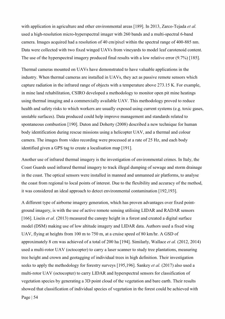
Page | 54
with application in agriculture and other environmental areas [189]. In 2013, Zarco-Tejada et al.
used a high-resolution micro-hyperspectral imager with 260 bands and a multi-spectral 6-band
camera. Images acquired had a resolution of 40 cm/pixel within the spectral range of 400-885 nm.
Data were collected with two fixed winged UAVs from vineyards to model leaf carotenoid content.
The use of the hyperspectral imagery produced final results with a low relative error (9.7%) [185].
Thermal cameras mounted on UAVs have demonstrated to have valuable applications in the
industry. When thermal cameras are installed in UAVs, they act as passive remote sensors which
capture radiation in the infrared range of objects with a temperature above 273.15 K. For example,
in mine land rehabilitation, CSIRO developed a methodology to monitor open pit mine heatings
using thermal imaging and a commercially available UAV. This methodology proved to reduce
health and safety risks to which workers are usually exposed using current systems (e.g. toxic gases,
unstable surfaces). Data produced could help improve management and standards related to
spontaneous combustion [190]. Duton and Doherty (2008) described a new technique for human
body identification during rescue missions using a helicopter UAV, and a thermal and colour
camera. The images from video recording were processed at a rate of 25 Hz, and each body
identified given a GPS tag to create a localisation map [191].
Another use of infrared thermal imagery is the investigation of environmental crimes. In Italy, the
Coast Guards used infrared thermal imagery to track illegal dumping of sewage and storm drainage
in the coast. The optical sensors were installed in manned and unmanned air platforms, to analyse
the coast from regional to local points of interest. Due to the flexibility and accuracy of the method,
it was considered an ideal approach to detect environmental contamination [192,193].
A different type of airborne imagery generation, which has proven advantages over fixed point-
ground imagery, is with the use of active remote sensing utilising LIDAR and RADAR sensors
[166]. Lisein et al. (2013) measured the canopy height in a forest and created a digital surface
model (DSM) making use of low altitude imagery and LIDAR data. Authors used a fixed wing
UAV, flying at heights from 100 m to 750 m, at a cruise speed of 80 km/hr. A GSD of
approximately 8 cm was achieved of a total of 200 ha [194]. Similarly, Wallace et al. (2012, 2014)
used a multi-rotor UAV (octocopter) to carry a laser scanner to study tree plantations, measuring
tree height and crown and geotagging of individual trees in high definition. Their investigation
seeks to apply the methodology for forestry surveys [195,196]. Sankey et al. (2017) also used a
multi-rotor UAV (octocopter) to carry LIDAR and hyperspectral sensors for classification of
vegetation species by generating a 3D point cloud of the vegetation and bare earth. Their results
showed that classification of individual species of vegetation in the forest could be achieved with

Page | 55
the hyperspectral imagery, and individual tree canopy and height, total tree canopy and density
[197].
Use of RADAR, also known as synthetic aperture RADAR (SAR), has not been as widely applied
in the industry and research when compared to thermal, multispectral, hyperspectral and LIDAR
technology. Zhang and Kovacs (2012), mention that costs, processing time, and interpretation of
data, size and weight of sensors, amongst other factors, have limited their use [198]. Advantages of
using SAR imagery is the capacity to penetrate foliage and structures. Borowiec (2015) published
the description of the SARape project - SAR for all weather penetrating UAV application [199].
The project consisted on acquiring and displaying SAR images in real-time. Similarly, Marino and
Davis (2005) developed laser and RADAR sensor technology (LADAR), and systems in high
definition. This technology could enable them to detect military weaponry below the tree canopy or
camouflaged [200]. In both cases, the devices were mounted on manned aircrafts due to their size
and weight. However, authors mentioned the intention to use UAVs in the future.
The use of UAVs for scientific research is widespread in a multitude of disciplines due to their
capacity to collect a large amount of data efficiently and at low cost. Industrial applications focus
on making more efficient, low cost and higher quality datasets applications as imagery and
transport, and new areas are targeted to habilitate and collect data. Some of these new areas include
radiation investigation [201-203], gas and dust monitoring [119,204-207], microclimate
characterisation [139,208,209], magnetic field detection [210,211], and field sampling [205,212].
Examples of the previous applications in research will be explained in the following section,
making emphasis on the use of UAVs for gas and dust particle monitoring.
2.5.1. Use of UAVs for gas and dust monitoring
Authors like, Malaver et al. (2015), Villa et al. (2016), Yu et al. (2017), Neumann et al. (2013), and
Rossi et al. (2014, 2016, 2017), used gas sensors (electrochemical and semiconductors) and dust
sensors (optical sensors) coupled to mini, micro, and nano UAVs, identifying opportunities and
challenges [120,213-218].
A kite plane type UAV was used by Watai et al. (2005) to monitor CO2 levels. The CO2 sensor was
an NDIR gas analyser with a response time of 20 s. The UAV was capable of reaching a height of
3.0 km, a flight length of 1 hr and carried a payload of 3.5 kg, and obtained high-quality results at
lower cost than using a manned aircraft [7,207].
Brown and Taras (2008) developed a 2D real-time gas video camera to monitor SO2 emissions from
volcanoes [219]. The camera used an SO2 cell which filtered the light absorbed by a camera

Page | 56
producing a false colour image from which concentrations could be calculated. The camera was
light enough to be carried by a small UAV (< 1 kg). It was reported by authors to be also capable of
monitoring NO2 [220-222].
Another gas sensor developed was a compact vertical cavity surface emitting laser (VCSEL) for
sensing CO2, CH4 and water with a total mass < 2 kg and dimensions of 20 cm × 5 cm × 5 cm
[223]. The VCSEL was installed in a small UAV and provided robust, cost-effective, lightweight
and high-resolution data. The total mass of the system was approximately 7 kg with a flight
duration of 10 min. Stearns and Brake (2008) used mid-infrared differential absorption LIDAR
(mid-IR DIAL) to measure methane from a manned aircraft [224]. Their system mapped methane
leaks with a resolution of ~30 cm and provided concentration readings.
Bennetts et al. (2011) and Neumann et al. (2011, 2013) used micro multi-rotor UAVs to detect CO2,
SO2 and CH4 with infrared and electrochemical sensors [119,120,225]. The response time of
electrochemical sensors varied between 10 to 20 seconds, providing accurate information to the
plume monitoring and tracking system. Their investigation mainly focused on the development of
algorithms for plume tracking and air quality mapping. Their approach towards plume tracking was
bio-inspired using a zig-zag dung beetle algorithm and the pseudo-gradient based algorithm. Field
experiments demonstrated quick pollutant dissipation, and high wind turbulence lessen the
effectiveness of the algorithms. Air quality mapping was only achieved in 2D, and data recorded
was represented as a snapshot of different time periods.
Lega and Napoli (2011) patented a tri-copter to monitor air pollutants in real-time and with 3D
visualisation [204]. The device was integrated by a flying platform (tri-rotor), a fluid dynamic
conveyor, and a case to enclose the gas sensor. Authors used variations of the patent (StillFly and
BiLIFT) to detect gases like CO, C6H6, NO2, O3, SO2, NOX and PM10. In addition, IR thermal
imagery was used to identify illegal sewage discharges to the sea [192,226]. Poppa and Zimmer
(2013) used a helicopter type UAV to monitor CO2 emissions in laboratory and field tests. The CO2
sensor selected was a probe type non-dispersive infrared sensor (NDIR), the Vaisala GMP343
[227]. Authors indicated that further work could require the use of multi-rotor platforms due to
greater payload requirements.
Malaver et al. (2012), designed a small gas sensing UAV for NO2 and ammonia (NH3). The UAV
also had the characteristic of being alternatively powered with solar cells located in its wings [228].
The sensor used to detect gases was a nanosensor system which was lightweight, required low
power and was compact. However, it had relatively high response time (6 min) and required pre-

Page | 57
heating to 250°C for optimum performance. All data were georeferenced. In 2015, Malaver et al.
used the solar fix winged UAV to detect CH4 and CO2 making use of resistor based sensors and
NDIR sensor. Through a wireless connection, the UAV and a solar-powered ground gas sensing
network streamed information and communicated with a data management platform for data
processing and visualisation [213,229].
Gonzalez et al. (2012) experimented with an off-shelf particle detecting optical sensor (EVM-7)
mounted in a fixed wing UAV. Laboratory and field experiments demonstrated the integration of
the UAV and the optical sensor, which was capable of sampling particles suspended in the
atmosphere. However, sensors were not calibrated for specific dust particles [230]. In conjunction
with other authors, Gonzalez (Kersnovski 2017; Letheren et al. 2016) has worked in bio-inspired
plume tracking algorithms and target identification in constrained or difficult to access
environments [231,232].
Rossi et al. (2014) used a metal oxide sensor (MOX) for VOCs attached to a multi-rotor UAV (DJi
hexacopter). The sensing package was capable of monitoring air temperature, air velocity, and GPS
with a total weight of 30 g and 4 cm × 4 cm dimensions and was placed under the multi-rotor UAV.
Two experimental flights demonstrated the capacity of their system to detect VOC plumes [216]. In
2014 Rossi and Brunelli, published their work on the development of a tracking algorithm for their
gas monitoring system. Results of simulations using a Gaussian dispersion based model were
presented. The algorithm compares gas readings during the flight giving feedback to produce a
decision flight path and locate the gas source [216]. In 2014 and 2017, Rossi and Brunelly used a
micro multi-rotor UAV (Sense-Fly) and attached the MOX sensor, which operated with a ‘duty-
cycle’ algorithm to reduce power consumption. Authors studied different configurations to place a
sampling probe in the UAV to collect air samples. Due to the small size (4 mm × 7 mm) and
lightweight (27 g), the use of a sampling probe compromised flight stability due to added weight
and centre of gravity modification. Their solution was to use a butterfly flight pattern, by flying and
landing at points of interest, to collect representative VOCs readings during their experiments [218].
Egorova et al. presented their work in 2016 modelling the use of fixed wing UAVs to estimate the
concentration of a gas plume using a moving airborne source and a point source [233]. Authors
used an unsteady state advection-diffusion equation in three dimensions, considering turbulence
coefficients and wind profiles. Results of the modelling were reported as successful when
comparing data from an estimated plume and a simulated plume data.

Page | 58
In 2015, Salaheldin published the results of a study undertaken in Saudi Arabia of the dust
concentration and its composition at altitudes of 0.6 m, 400 m, and 800 m using a fixed wing UAV
[234]. Samples at 0.6 m were acquired once the UAV had landed. The UAV collected air samples
making use of 0.8 µm (pore size) polycrystalline filters which were analysed for a total of 16
substances, mostly metal elements. The objective of the authors was to produce a three dimensions
map of potential hazards in the airspace of the region.
For aerosol profiling at coastal areas, Brady et al. (2016) used an optical sensor (OEM MetOne
particle counter) to conduct near-surface characterisation [235]. An IRIS+ (3DR, Berkley, CA,
USA) was used as a flying platform, indicating high precision when navigating horizontally and
vertically. The system used had a total weight of ~2.0 kg (1.5 kg for IRIS+ and 0.49 kg sensing
package) and dimensions 203 mm × 445 mm × 508 mm [235].
Yu et al. in 2017 reported the use of a lightweight quadrotor UAV with multiple gas and dust
sensors, to collect information from atmospheric vertical profiles [215]. The UAV was also
equipped with sensors to read atmospheric parameters (temperature and relative humidity). Their
experiments indicated that there was a high correlation between particle size concentrations (PM2.5
and PM10) and atmospheric parameters.
The design of another multi-gas and dust particle airborne system was also presented by Villa et al.
(2016) using a hexacopter UAV [214]. In their investigation, they used a built-in multi-gas sensor to
detect carbon monoxide (CO), carbon dioxide (CO2), nitrogen dioxide (NO2), and nitrogen
monoxide (NO). For particle detection, a DISCmini particle counter for aerosols (10-500 nm) was
used. The system was tested for diesel combustion gases and particles. As part of their findings,
they designed a sampling probe in a horizontal position, and a mathematical model was proposed to
estimate the effects of the sensors at different distances from the centre of the UAV. Data collected
was streamed to a ground station and displayed in real-time.
Within the mining and energy industry, UAVs have been used as a means to obtain aerial
photography and video for surveying and auditing large and difficult to reach areas. Some of the
most common applications are topographic mapping, safety audits, environmental surveying, and
volumetric measurements [236]. For atmospheric monitoring, Danilov et al. (2015), presented the
description of a methodology to monitor several gases, suspended particles and take imagery from
mine sites to assess the status of the atmosphere at mine sites [237]. The method proposed by the
authors would provide data in real-time to predict and make volumetric calculations of gas and

Page | 59
particle plumes using multi-rotor and fixed wing UAVs. These authors did not present results in
detail. However, they concluded their procedures were precise.
To monitor nitrogen oxides due to blasting, McCray (2016) used a multi-rotor UAV to fly close to
blasting sites after explosions in open mine sites at Powder River Basin [238]. He used an MX6
iBrid with sensors for oxygen, carbon dioxide, carbon monoxide, nitrogen dioxide, and nitric oxide.
All sensors are electrochemical, except the carbon dioxide sensor which uses infrared technology.
To take an air sample, it used 2.32 m of tubing which dropped from the bottom of the UAV. The
author conducted three flights, demonstrating the UAV-monitoring system could detect peaks of
NOx produced after blasting. Within the improvements to the system, it was mentioned the need to
extend the sampling tube to be out of the downwash zone.
Keywood and Selleck (2016) evaluated the different alternatives that could be used to monitor coal
dust emissions produced by trains along the railway. Among several alternatives were traditional
and Australian standard accepted methods such as gravimetric analysis (using TEOM, EBAM,
others), chemical analysis, use of laser-based sensors, and also emerging technology such as low
cost sensor networks and UAV monitoring [98].
An objective of many researchers is to add to the airborne monitoring system a real-time plotting
ground station or interface which allows the visualisation in three dimensions of the plume. A
methodology to achieve this was proposed by Tripolitsiotis et al. (2017) by using a new
communication algorithm between the UAV-sensors and Android application for mobile phones
[239]. The devices can communicate by Wi-Fi and Bluetooth. Also, they used collision avoidance
algorithms which can be very useful in field applications as areas of interest might have obstacles
like infrastructure or vegetation.
2.6. Summary
For the last 20 years UAVs have been used to gather data from hazardous locations, and remote or
difficult to access places. The military sector dominates UAV operation compared to agriculture,
recreational, and scientific research. Scientific research has primarily investigated imagery
collection using UAVs due to low operational costs and flexibility when compared to the use of
other remote sensing technologies. Other areas of research include gas/dust/radiation using small
and low cost yet sophisticated instrumentation. The common scientific paradigm is the development
of small, relatively low cost instruments that can be carried by UAVs of equally small and low cost
characteristics. The central research goal being to provide detailed and precise information about
our environment, social dynamics, and industrial activities.

Page | 60
The high impact of air pollution on human health and the environment motivates the development
of relative and absolute methodologies to monitor air quality. Measurement of fugitive emissions is
a challenging aspect of air quality monitoring due to their variable and unpredictable nature in space
and time. Flexibility and reliability in the field data collection will produce better estimates and risk
assessments. Small UAV air quality sampling systems may provide these characteristics.
Use of small UAVs for gas and dust monitoring is relatively immature compared to acquisition and
analysis of aerial imagery products. Therefore continued development of innovative research in this
area will increase capacity to validate models and add value to current fixed monitoring systems.
The literature review identified gas and dust sensors used to characterise atmospheric
meteorological and pollution status with airborne and ground systems. Characteristics of the devices
described in the literature, i.e. size, weight, and cost, vary greatly depending on factors such as
targeted atmospheric elements, industry and location where it could be used, and pollution source
type. An important factor observed was the availability of lightweight, small size and low cost
technology. The number of applications for gas/dust sensors is increasing with development of
suitable sensors with reduced size, weight, and cost. Historically air quality monitoring has been
restricted by the variety of platforms and locations where they could be utilised.
Lightweight, small size and low cost sensors may remain unsuitable due to requirements such as
pre-heating, stability, calibration, power demand, measuring range, and maintenance requirements
(vibration tolerance, size and weight, air flow dynamics). It is therefore essential to develop detailed
specifications when choosing gas/dust sensors for their research.
For example, sensors with high response provide a higher frequency of atmospheric readings that
could be used as inputs for atmospheric models. Power availability is also a limiting factor, which
makes necessary the use of energy efficient UAVs and sensors.
The literature review highlights the impact of design and operation on sensor performance of
UAVs. Multi-rotor and fixed wing platforms cause the sensor to interact differently with the air.
Factors such as disturbance of the samples, robustness (due to exposure to rough environments),
flight endurance, hovering capacity, and UAV operation and legislation were important
considerations.
Greater availability of low cost, lightweight, and small size sensors, increases the possibility to
collect airborne data to study gas/dust dispersion, in a similar way to research conducted using
aerial imagery.

Page | 61
The current literature review permitted the identification of a number of knowledge and capability
gaps. These include the health and environmental impacts of gas and dust emissions, how
atmospheric pollution monitoring is conducted in the extractive industry, effective use of
technology to monitor environmental issues, and technological and atmospheric pollution
regulatory development.
The main knowledge gaps identified can thus be summarised as:
1) Further investigation on the impacts of human and environmental exposure to dust particles
considering a greater range of substances and sources.
2) Consensus of guidelines and existing regulatory instruments on human and environmental
exposure thresholds.
3) In-depth investigation of the effects of atmospheric monitoring and sampling with small
UAVs.
4) Further investigation of mathematical models that accurately predict and represent gas and
dust dispersion when using airborne data (small UAVs) as inputs.
5) In-depth understanding of the atmospheric physicochemical dynamics implicated when
combining monitoring/sampling of atmospheric pollutants with small UAVs.
6) Creation and establishment of clear and sensible regulations for UAVs with environmental
investigation purposes.
7) Development of accurate tracking algorithms to identify atmospheric pollution sources that
can spatially describe a plume.
The main capability gaps identified can be summarised as:
1) Development of cost-benefit methodologies and instrumentation to monitor difficult to
access sites for atmospheric pollution investigation.
2) Development of accurate, robust, low-cost, lightweight and low powered instrumentation
and fully integrated systems for atmospheric pollution sampling and monitoring.
3) Development of systems to collect relevant and representative gas and dust readings and
samples.
4) Development of industry-approved sensing system for atmospheric pollution sampling and
monitoring (health and safety guidelines/regulation complying).
5) Development of a system that complies with monitoring/sampling standards dictated by
governing institutions.
6) Development of a UAV with simple launch-landing procedures, high flight control capability and minimum air mixing operation.

Page | 62
3.UAVs used for research development The advantage of UAVs to access remote and hazardous areas has involved scientists, public
servants, commercial entrepreneurs, and civilians to use them for research, work, and entertainment
[7]. A novel application of the UAVs, is their use to monitor suspended dust particles and gases
making use of electrochemical and optical sensors. However, due to the recent rapid development
of sensing technology and UAVs, their application is still not well established [7]. As described in
Section 2.3, different types of UAVs can be used specifically for varied tasks depending on their
characteristics. For example, fixed-wing systems are capable of long flights covering extense areas
and collecting a high volume of data. In the contrary, multi-rotor UAVs are less stable when flying
long distances and have less endurance. However, they have the advantage of being easily
controlled at sites with scattered vegetation and infrastructure. They also can be flown at low
heights, and hover at predetermined points of interest.
3.1. UAV Requirements and Selection Criteria
The selection of the UAVs used for the different monitoring modules was mainly based on the
research questions and objectives established. UAVs needed to match the sensor systems designed,
by being low cost and lightweight, always maximising flight endurance. It was essential to be able
to have all the sensors and other electronic components necessary to collect the desired data,
however keeping the design simple and compatible with the UAV chosen was always a concern to
be able to obtain relevant air samples and still be able to communicate and control the system
easily. Overall the airborne system would also need to comply with Australian UAV regulations to
conduct field experiments.
The initial UAVs selected for this investigation had been developed and used by UQ SMI-CMLR
team (The University of Queensland Sustainable Mineral Institute - Centre for Mine Land
Rehabilitation), mainly for ecological investigation fieldwork (see Table 10). However, the use of
other UAVs (multi-rotor, commercial or developed by UQ or Queensland University of Technology
- QUT) had to be considered due to the different physical characteristics and flying capabilities of
each type of UAV.
In summary, the criteria applied to the selection of the UAVs are the following:
1. Size and weight: preferred size and weight of the UAV would be small or micro
dimensions, with a total weight of 2 kg as a maximum.

Page | 63
2. Power consumption: power would have to be balanced to provide the voltage demanded by
instrumentation and maximum flight time.
3. Cost: as per one of the objectives of this investigation, the cost of the drone would
preferably be low.
4. Payload: the payload would have to be as light as possible, trying to keep the total weight of
the UAV and dust monitoring module below or equal to 2 kg. CASA guidelines permitted
flying UAV with a total weight up to 2 kg without a Flight Certificate in September 2016.
Payload would have to be adapted depending on the UAV selected.
5. Flight endurance: maximum flight time would have to be achieved by balancing the
previous criteria for the UAV and consider the criteria established to select the sensors.
6. Sampling capacity: Due to the complexity of collecting an undisturbed air sample, UAVs
need to be evaluated to determine if the design of a ‘system’ (e.g. a sampling probe) is
required to collect a sample. Given the case a ‘system’ is required, further analysis will be
conducted to determine its feasibility and practicality when airborne.
7. Communication: between dust monitoring module and UAV telemetry system to ground
stations;
8. UAV flight control: having control of the flight path of the UAV is an important feature
that allowed programming different flight patterns, modify flight speed, easy manual take
over, and ‘on-flight’ corrections.
9. Programming and calibration: having the capacity to program GPS features, flight modes
(i.e. auto, loiter, stabilise), landing/take off/flight speed, hovering periods, and many other
features of the UAV help run each experiment to environmental and data collection
specifications. Also, calibrating the UAV with the modular dust system was necessary, as
the extra weight or dimensions, would modify calibration of UAV parameters (i.e.
accelerometers).
10. Regulations: Compliance with CASA established guidelines to fly UAVs safely (or
relevant state/national requirements). Also, if UAVs are to be used at industrial sites, they
should comply with all health and safety requirements.
Modifications were done to the UAV as required, for example by tuning of the flight speed,
evaluating different flying patterns, defining UAV flight orientation, examining hovering periods of
time, and calibrating UAV instrumentation (such as accelerometers and compass).
Section 3.3 (Summary) presents in Table 12 whether each UAV assessed complied or did not
comply with the requirements and selection criteria established.

Page | 64
3.2. UAV Options
3.2.1. Fixed Wing
The suitability of four fixed-wing UAV platforms for integration with the optical (LED or laser),
electrochemical, and semiconductor sensors was investigated (Figure 10 and Table 10):
Bonsai (Turnigy, Kwun Tong, Hong Kong, China): a micro fixed wing UAV with EPP
(expanded polypropylene) build, a wingspan of 600 mm and a flying weight of
approximately 180 g [240]. During field tests, it demonstrated a flight endurance of up to 45
min and the capacity of carrying approximately 200 g of payload. It was re-designed and
adapted for ecological surveying (Ashray Doshi, pers. comm., November 2013) [241,242].
TekSumo (Turnigy, Kwun Tong, Hong Kong, China): micro fixed wing UAV with EPP
build, a wingspan of 900 mm and a flying weight of 350 g [243]. It was re-named ‘Teklite’
after being adapted for air quality monitoring, having a flying weight of 850 g, and a
payload capacity of 300 g approximately [241,242]. During field tests, it demonstrated a
flight endurance of up to 45 min.
GoSurv (custom made UAV for SMI-CMLR): micro fixed wing UAV with EPP build, a
wingspan of 850 mm, flying weight of 900-1,200 g, and a payload capacity of 300g. During
test flights, it demonstrated a flight endurance of 50 min [242].
Swamp Fox (Skycam UAV NZ Ltd., Palmerston North, NZ): small fixed wing UAV built of
fibreglass and composite material with a wingspan of 850 mm and an endurance of 40 min.
It had a flying weight of 4,500 g and a payload capacity of 900 g approximately [244].
a) b)

Page | 65
c) d)
Figure 10. Fixed-wing UAV platforms, (a) Bonsai; (b) Teklite; (c) GoSurv; and (d) Swamp Fox [4,7].
Table 10. Characteristics of evaluated fixed wing UAVs [7].
Description Model
Bonsai [240] Teklite [243] GoSurv [242] Swamp Fox [244]
Wingspan (mm) 600 900 850 1,800
Length (mm) 300 575 350 1,000
Flying weight (g) 160 - 180 850 900 – 1,200 4,500
Endurance (min) 45 45 50 40
Approximate Payload+ (g) 200 300 300 ≤ 2,000
Material EPP EPP EPP Fibre glass and composite
Cost (AUD) 145.00 199.00 ~8,000+ ~45,000+
+ Assoc. Prof. Peter Erskine, pers. comm., May 5, 2017. Note: prices of all components could have changed over time.
The three small UAVs listed in Table 10 (Bonsai, Teklite and GoSurv), had low kinetic energy (<60
joules) and low airspeed (<60 km/h). Swampfox was a larger platform and used a parachute for
emergency and normal recovery to reduce its kinetic energy during landing. During field flights all
UAVs in Table 10 were safe and robust to use in challenging environments such as open cut mine
sites (Assoc. Prof. Peter Erskine, pers. comm., May 31, 2017).
Advantages of low kinetic energy UAVs are increased safety during operation and data acquisition
performance in stable and low wind speed conditions. Low kinetic energy and speed improve safety
and simplifies data acquisition performance. However, the system will perform poorly under high
winds or gusts. All fixed wing models could provide clean air flow to the sensors due to their
pusher-propeller design [7].
The Swamp Fox had the highest cost (AUD 45,000) and dimensions from the UAV alternative
considered, hence it was deemed as not suitable for the investigation. The Bonsai was the best

Page | 66
option in terms of dimensions. However, for the same reason, its payload capacity was reduced to
200g. The Teklite and GoSurv had characteristics such as high portability and compatibility with
meteorological and dust sensors, and higher payload capacity than the Bonsai (300 g).
Flight path planning of the Bonsai, Teklite and GoSurv, was possible using the Paparazzi autopilot
software (The Paparazzi Project, ENAC University, Toulouse, France), having a real-time display
of telemetry parameters and dust particle readings. The Paparazzi autopilot registers geolocation
(altitude and platform coordinates), UAV speed, and direction. Wind speed and direction are
estimated by environmental response difference. All telemetry data was recorded and available for
download to analyse flight path and performance [7]. The Teklite was selected to integrate
meteorological and dust sensors due to its dimensions and flight performance, as the GoSurv
required further development during the experimental stages of the dust monitoring system [7,242].
3.2.1.1. Testing of Fixed-Wing UAVs
Preliminary field tests were conducted to the Bonsai and Teklite to check their payload carrying
capacity, the range of flight speed, easy control and deployment, and flight path programming
capabilities. Both UAVs demonstrated to easily operated and programmed using the free access
Paparazzi software [245]. Their build of EPP made them a good candidate for flying at industrial
sites as they did not represent a risk weighing under 350 g. However, due to the decision of
monitoring sources close to the ground, their flying height restrictions above 35 m made them
unsuitable for experimental flights with a dust source at 5 magl (meters above ground level).
Similarly, the GoSurv was tested several times in the field, demonstrating satisfactory performance.
However, it was determined unsuitable due to its flight restrictions to fly close to the ground, and
also because it was in its early stages of development [242]. These three fixed wing UAVs used a
novel control algorithm for micro-UAVs which used online motion planning considering wind
conditions to improve stability even with wind speeds of 25 km/h or higher [241,242]. Flight
performance evaluation is described in detail in Doshi et al. 2014 and Doshi et al. 2015. Additional
flight performance metrics consisted of data such as:
1. GPS connection,
2. Connectivity between receiving/sending radios,
3. Voltage monitoring,
4. Altitude, speed, climb and descent rate monitoring,
5. Vibrations, and
6. Compass, accelerometer, gyroscope monitoring.

Page | 67
The Swamp Fox was not evaluated in the laboratory or field for this investigation, as the SMI-
CMLR team used it routinely for ecological surveys, and its flight capabilities and payload range
had been extensively tested previously (Assoc. Prof. Peter Erskine, pers. comm., May 31, 2017).
3.2.2. Multi-rotor UAVs
Multi-rotor platforms were identified as an alternative to fixed wing UAVs, as they could be used to
record readings below 35 magl due to their capacity to hover and fly at a slow speed in small areas.
Two multi-rotor UAVs were used during the investigation (Figure 11 and Table 11):
The ‘Sotiris’ multi-rotor UAV; a micro UAV designed and constructed for agricultural and
air-monitoring surveys for the Faculty of Science at The University of Queensland (Mr.
Sotiris Ioannou, pers. comm., April 2015). The Sotiris was a multi-rotor UAV with four
propellers, a 750 mm motor to motor span, and an endurance of 25 min approximately. It
had a flying weight of 2,500 g (with batteries) and a payload capacity of 450 g. In the field,
the Sotiris demonstrated a flying endurance of 20-25 min. Figure 11 shows the quadcopter
integrated with the modular dust sensor. The Sotiris had a build of carbon fibre, composite
material and metallic components.
3DR IRIS+ (3DR, Berkeley, CA, USA): a multi-rotor micro UAV with four propellers, with
a flying weight of 1,282 g, and a payload capacity of 450 g. It has a motor to motor span of
550 mm and an endurance of 20 min without payload [246]. The IRIS+ has a frame and
make of composite material and metallic components.
The IRIS+ was selected as the multi-rotor investigation platform as it was a low cost off-the-shelf
product, easy to service and modify, robust, and had a user-friendly interface [7]. As part of the
development of the dust monitoring system, the IRIS+ was adapted with a vertical air sampling
probe and a detachable dust monitoring module (see Section 5.3.2 and 5.3.2).

Page | 68
a) b)
Figure 11. Multi-rotor systems used for the investigation, a) Sotiris quadcopter and modular gas-sensor system attached [7], and b) 3DR IRIS+ quadcopter [247].
Table 11. Characteristics of evaluated multi-rotor UAVs.
Description Model
Sotiris* Iris+ [246]
Number of rotors 4 4
Size (mm) Motor to motor 750 550
Flying weight (g) 2500 1282
Endurance (min) 20-25 16-22
Approximate Payload+ (g) 450 400
Cost (AUD) ~900.00+ 1,010 * Mr. Sotiris Ioannou, pers. comm., April 2015 + Mr. Armando Navas, pers. comm., April 12, 2015 Note: prices of UAVs could have changed over time.
3.2.2.1. Testing of Multi-Rotor UAVs
Different simple tests were undertaken to learn and evaluate the flying capacity of each multi-rotor
UAV to determine their suitability to be integrated with the dust monitoring modules. The Sotiris
multi-rotor UAV was tested for programming as it had been used previously for different tasks to
gather information for precision agriculture investigations [248]. A set of waypoints and flight
instructions were pre-programmed using ArduPilot in the Mission Planner software (DIY Drones
Team, Berkley, California), and uploaded to the UAV. Several flight missions were tested
successfully.
Performance of the UAVs was evaluated based on their capacity to couple with the meteorological
and dust sensors. Flight performance was evaluated during the tests and also once the tests had
finalised by analysing logged telemetry data. Performance metrics consisted of data such as:

Page | 69
1. GPS connection,
2. Connectivity between receiving/sending radios,
3. Voltage monitoring,
4. Altitude, speed, climb and descent rate monitoring,
5. Vibrations, and
6. Compass, accelerometer, gyroscope monitoring.
Telemetry data from UAVs were always recorded during tests and were used to determine causes of
errors during flights.
The Sotiris and IRIS+ were tested to fly pre-programmed patterns using Mission Planner. Its
manoeuvring capacity was evaluated making use of the radio control, and a mobile phone and tablet
using the ‘Tower’ Android application (3DR, Berkley, California). The UAV system demonstrated
to be easily controlled and carry up to 350 g as payload.
The IRIS+ was also examined to describe the airflow around the propellers to determine the
boundaries of the air disturbed around the UAV. This test is described in detail in Section 5.3.2.1.
3.3. Summary
Table 12 presents the UAVs evaluated for the development of the dust monitoring methodology
related to the selection criteria, indicating if each factor was satisfactorily met. The six UAV’s
(fixed wing and multi-rotor), comply with most of the criteria factors defined as explained in the
previous sections.
Table 12. Selection criteria established for UAVs.
Criteria Category Fixed Wing Multi-rotor
Bonsai Teklite GoSurv Swamp Fox Sotiris Iris+
1 Regulations ✔ ✔ ✔ ✔ ✔ ✔
2 Sampling capacity × ✔ ✔ ✔ ✔ ✔
3 Payload × ✔ ✔ ✔ ✔ ✔
4 Size and weight ✔ ✔ ✔ × ✔ ✔
5 Power consumption ✔ ✔ ✔ × ✔ ✔
6 Cost ✔ ✔ × × ✔ ✔
7 Flight endurance ✔ ✔ ✔ ✔ × ×
8 Communication × ✔ ✔ ✔ ✔ ✔
9 UAV flight control × × ✔ × ✔ ✔
10 Programming and
calibration
✔ ✔ × ✔ ✔ ✔
Total ✔ 6 9 8 6 9 9

Page | 70
4.Instrumentation used for research
development The type of sensors used in ground network applications, handheld devices, vehicle monitoring
systems, airborne platforms, and monitoring towers will vary depending on factors such as expected
monitoring radius, portability, capacity to operate under challenging environments, calibration
requirements, and targeted pollutants [7,99,249,250]. For this investigation a thorough desktop
search was conducted to identify dust and gas sensors which could be coupled with fixed wing or
multi-rotor UAVs, integrating them to their circuitry or as an independent sensing module.
The following sections in Chapter 4 describe the selection criteria applied during the search and
evaluation of gas and dust sensors, as well as the testing procedures conducted.
Sections 4.4.1.1. Laboratory testing of SHARP and 4.4.1.2. Results for SHARP sensor tests, were
taken from the publication ‘Alvarado, M.; Gonzalez, F.; Fletcher, A.; Doshi, A. Towards the
development of a low cost airborne sensing system to monitor dust particles after blasting at open-
pit mine sites. Sensors 2015, 15, 19667-19687.’ Paragraphs 1-3, Figure 26 and Figure 27 from
Section 4.4.3.2. Correction factors tests and calculations, and Section 4.4.3.3. Calcined alumina
gravimetric calibration were taken from the publication ‘Alvarado, M.; Gonzalez, F.; Erskine, P.;
Cliff, D.; Heuff, D. A methodology to monitor airborne PM10 dust particles using a small unmanned
aerial vehicle. Sensors 2017, 17, 343.’
The following text and Figures added to the previous sections a posteriori to the publication as part
of the Thesis manuscript:
Figure 19.b from Section 4.4.1.1. Laboratory testing of SHARP.
Statistical normality tests included in Sections 4.4.1.2. Results for SHARP sensor tests and
4.4.3.3. Calcined alumina gravimetric calibration.
4.1. Instrumentation requirements and selection criteria
Progress in electric and optical technology has produced dust and gas sensors of unprecedented
small size, reduced weight, and low cost that can be used as relative methods to monitor human and
environmental contamination exposure levels. Standardised and absolute monitoring methods
commonly require high-cost equipment which is not affordable to individuals, companies, and
government institutions requiring continuous data on the status of the atmosphere they live in. Also,
the equipment can be difficult to transport or can only be operated at a fixed location due to its large

Page | 71
size and heavyweight. These characteristics make it difficult to collect information from places with
high risk or hazardous access.
A thorough search was performed to select the best sensors from the wide variety of meteorological,
dust/gas, and electronic telemetry components available commercially. Fully operational off the
shelf monitoring devices were also considered, to reduce time consumption for design, integration
and testing. However, due to weight and size restrictions, and also hight cost of most of the devices
that could be used in a UAV, such as portable and handheld instruments, it was necessary to
integrate the monitoring modules from separate components. Four fully operational models of the
dust module were built and tested successfully. Details of the completed sensing systems are
described in Section 5.
The selection criteria established to select the components of the dust monitoring modules were
defined based on the research questions and objectives. Sensors and electronic components had to
comply with the majority of the following conditions:
1. Dimensions (weight and size): considering the UAVs selected as possible platforms to
transport the dust monitoring module, dimensions of all components are a limiting factor, as
micro UAV’s could carry a payload not higher than 450 g and small UAVs below 2 kg.
Weight and size influenced flight time, stability and aerodynamics.
2. Power: the amount of power to operate each sensor was essential to maintain balance in the
overall consumption of the system. Whether it was connected directly to the power supply
of the UAVs or it was connected to its power source. Both configurations impacted the
overall weight of the system and UAV endurance.
3. Operability: The sensors required achieving optimum performance in an elevated and
moving platform. Also, they would be exposed to constant vibrations during operation.
Tolerance of vibration and movement given mounting on a UAV platform with approximate
travel speed up to 15 m/s for a multi-rotor UAV (e.g. IRIS+) [251], and up to 30 m/s for a
fixed wing UAV (e.g. Teklite) (Dr. Andrew Fletcher, pers. comm., May 2014).
4. Sensitivity: The concentration range and resolution of the sensors had to be within the
guidelines for exposure levels of health and safety industries within Australia and those of
the WHO.
5. Measuring and device specifications: accuracy and limitations of the sensor such as
interference with other gases, the influence of humidity and temperature, calibration
requirements, exposure to different levels of environmental light (for optical sensors),
among others.

Page | 72
6. Connectivity: each sensor, whether a standalone or being part of a system, has specific data
output specifications (e.g. analogue, digital, SPI, and others). It was important that all
sensors chosen to integrate the dust monitoring system could connect to a micro-controller
and log all data streamed from the sensors.
7. Response time: a quick response time of less than or equal to 1 second, due to the flight
speed of fixed wing UAVs and also reduced flight endurance of multi-rotor UAVs.
8. Robustness: this refers to sensor exposure to hazardous environmental conditions such as
high dust concentrations as well as corrosive gases (such as NOx and H2S) that could
compromise the sensors. Rough operating conditions produced by vibrations, and possible
crashes and harsh landings could damage the sensors.
9. Stability: continuous readings for different periods of time and exposed to different
environmental conditions were necessary.
10. Influence of other factors in performance: exposure to factors such as high levels of
humidity and temperature; also, presence of other pollutants with physicochemical
characteristics that could affect or interfere with the sensors (e.g. corrosive gases and
hygroscopic dust)
11. Calibration requirements: exposure to different concentrations of the targeted contaminant
for variable periods of time and external factors.
12. Cost: as per one of the objectives of this investigation, the cost of instruments would
preferably be low.
Laboratory tests were designed to assess potential instruments that could be used to integrate an
airborne sensing system, identify low cost and lightweight components, and evaluate the bounds of
the instruments. Field tests were designed to also evaluate the previous criteria and determine if
instrumentation could be used to develop a sensing system which collected relevant meteorological,
telemetry and pollution data of plumes and local environment. Experimental design criteria were
defined based on the objectives established in Chapter 1.
Selection criteria of instrumentation were conducted by evaluating instrumentation specifications
and by directly testing their capabilities in the laboratory and field. Testing was undertaken by
supplying dust/gas particles of different substances such as smoke, talcum powder, calcined
alumina, and natural gas. Field tests were designed to evaluate the performance of the instruments
when exposed to the environment and pollutants such as CO, NO2, dust particles (smoke, talcum
powder, and calcined alumina).

Page | 73
In-depth testing of dust sensors required calibration by comparing raw data against concentration
readings from commercial/industrial reference devices. Due to health and safety issues, and
difficulty in accessing industrial or educational dust chambers and wind tunnels from UQ and QUT,
it was necessary to build the testing equipment required for the experiments. The following sections
describe in detail the characteristics of the sensors used, and the laboratory and field tests conducted
to evaluate each of the instruments which determined if requirements and selection criteria were
satisfactorily met. Section 4.9 (Summary) presents in Table 28 to Table 33 whether each instrument
assessed complied or did not comply with the requirements and selection criteria established.
4.2. Gas sensors
4.2.1. Semiconductor sensors
Initial testing for gases was done with semiconductor and electrochemical sensors as their low cost,
low power consumption and compact size made them a candidate for their integration to micro and
small UAVs. Semiconductor sensors for carbon monoxide (CO) and natural gas (CH4) from the
series MQ of Hanwei Electronics Co. Ltd. (Zhengzhou, Henan, China), were checked and tested to
comply with the 12 requirements and criteria presented in Section 4.1 (Figure 12 and Table 13).
The system was constructed around an Arduino UNO (Arduino, Italy), powered by a 7.4 V lithium
polymer battery, a TB6612FNG motor driver (Sparkfun Electronics, Boulder, CO, USA), and either
a MQ series carbon monoxide (MQ7 - CO) or natural gas (MQ4 - CH4) sensor.
Figure 12. Circuit integration for gas sensor testing.

Page | 74
Table 13. Specifications of semiconductor sensors tested.
Senor Gas detected Voltage Detecting range
(μg/m3) Pre-heating time
MQ-4
[252] CH4 5 V
1.3×10⁵ -
6.6×10⁶ 60 s
MQ-7
[253] CO 5 V
2.3×10⁴ -
2.3×10⁶ 60 s
The sensing range of the MQ-4 is between 1.3×10⁵ -6.6×10⁶ CH4 μg/m3 [252], which would be able
to detect the NOAEC (No observed adverse effect concentration) threshold of 2.6×10⁶ μg/m3 [76].
The MQ-7 has a measuring range of 2.3×10⁴ -2.3×10⁶ CO μg/m3 [253], which covers the ACGIH
TWA and NOHSC TWA health threshold for 8 hr exposure of 5.8×10⁴ μg/m3 and 3.4×10⁴ μg/m3
respectively (Table 14) [68]. However, it does not cover the WHO, NEPM, and IDLH exposure
limits (Table 3 and Table 14).
Table 14. CH4 and CO health exposure guidelines for semiconductor sensors tested.
Gas WHO
(μg/m3) [254]
NEPM+ (μg/m3) [255]
NOHSC:1003 TWA
(μg/m3) [55] Other [76,256]
Methane (CH4) NS NS Asphyxiant*
Acute toxicity = LC 50 (Rat, 4h): >8.6×10⁶ μg/m3 Repeated dose toxicity = NOAEC (Rat, Inhalation): 2.6×10⁶ μg/m3 LOAEC (Rat, Inhalation): 8.0×10⁶ μg/m3
Carbon monoxide (CO), 8 hr
1.0×10⁴ 1.1×10⁴ 3.4×10⁴ 5.8×10⁴ μg/m3 ACGIH TLV-TWA
+ Advisory level only. * Methane is a simple asphyxiant and oxygen balance should be kept at all times at 21%; NS = Not Specified; NA = Not Available
4.2.1.1. Testing of semiconductor sensors
Sensors were tested only inside the laboratory to observe their reaction to different concentrations
of gases (CH4 and CO). Voltage variations were observed making use of an oscilloscope and logged
to a computer following the recommendations of the MQ4 and MQ7 datasheets [252,253]. Figure
13 shows the readings obtained from each sensor for cycles of 150 s, which consisted of 60 s for the
heating phase and 90 s for the reading phase. Both sensors were left running for approximately 48
hours for pre-heating and tested in clean air. The MQ-7 was also exposed to exhaust fumes from a
vehicle Figure 13.b.

Page | 75
a) b)
Figure 13. Heating and response cycles for a) MQ4 in clean air and, b) MQ7 in exhaust fumes.
It was observed that they required 60 s of heating time and 150 s cycles to obtain a reading, which
were considered extended periods considering the travelling speed of some UAVs (e.g. Teklite ~ 30
m/s), and short flight endurance (e.g. IRIS+ 10-20 minutes) [252,253]. Pre-heating time, extended
response and recovery time, are considered obstacles when semiconductor sensors are used for
UAV applications. As stated by Gallego et al. (2015), power consumption of semiconductor sensors
is high and readings require extended exposure periods [257]. Due to these characteristics and that
their measuring range did not cover WHO and NEPM health exposure threshold values, the sensors
were not considered suitable for collecting data with the fixed wing or multi-rotor UAVs. For a
sensor to be adequate to collect data, it should have minimum variability produced by changing
temperatures and relative humidity, and have a quick response (of approximately ≤1 s).
4.2.2. Electrochemical sensors
Two electrochemical sensors were also evaluated to determine their feasibility to be integrated into
the dust monitoring module, the NO2-4 and the CO-D4 for nitrogen dioxide and carbon monoxide
respectively, from Alphasense (Great Notley, Essex, UK) (Table 15). The sensors were checked and
tested to cover the 12 requirements and criteria presented in Section 4.1. The NO2-4 has a sensing
range of 0.0-3.7×10⁴ μg/m3 [258], covering health exposure thresholds established by WHO,
NEPM, NOHSC, and the IDLH (Table 16). The CO-D4 had a detecting range of 0.0-1.14×10⁴
μg/m3 [259], also covering the exposure threshold guidelines established by WHO, NEPM, and
NOHSC. However, the IDLH is not reached with a value of 1.7×10⁶ μg/m3.

Page | 76
Table 15. Specifications of electrochemical sensors tested.
Senor Gas detected Voltage Detecting range
(μg/m3)
Response
time (s)
NO2-D4 [258] NO2 NA 0.0-3.7 ×10⁴ < 35
CO-D4 [259] CO NA 0.0-1.14×10⁶ < 25
Table 16. CH4 and CO health exposure guidelines for semiconductor sensors tested.
Gas WHO (μg/m3) [11,254]
NEPM (μg/m3) [255]
NOHSC:1003 TWA
(μg/m3) [55]
IDLH (μg/m3) [60,256]
Nitrogen dioxide (NO2)
200.0* 40**
230.0* 56.5**
5.6×10³ 3.7×10⁴
Carbon monoxide (CO), 8 hr
1.0×10⁴ 1.1×10⁴ 3.4×10⁴ 1.7×10⁶
+ Advisory level only. * Value for 1 hr exposure; ** Value for 1 year exposure; NS = Not Specified NA = Not Available.
These sensors functioned by connecting them to an off-the-shelf multi-sensing device, the ‘NODE’
from Variable Inc. (Chattanooga, TN, USA) [260] (Figure 14). The NODE was operated by using
an Android mobile phone application (Variable Inc., Chattanooga, TN, USA). The device was
designed to carry two gas sensors simultaneously. However, the mobile phone application only
reported the readings of one sensor when running. All gas concentration readings were logged by
the Android application in periods of 2 s and could be exported to spreadsheet software programs.
4.2.2.1. Field testing of electrochemical sensors
The sensors were tested at the ‘Story Bridge’ in the city of Brisbane, QLD, Australia. Tests of the
sensor in the fixed wing UAV and multi-rotor UAV were not conducted at that moment due to
limitations such as: exceeding total weight and size of the NODE and mobile phone, configuration
of the elements required (NODE, mobile phone, meteorological sensor, and battery), and UAV
flight regulations at residential/commercial areas.
Tests consisted in carrying the NODE while walking along a high traffic area at peak hour, in this
case, the Story Bridge with the objective to detect variations of CO and NO2. Figure 14.a and Figure
15 show the results of one of the transects conducted for CO with variable concentrations of the gas
detected over time and at different points along the main artery. However, due to instability and
long response time, their use was not further considered. An additional limitation observed in the
use of the NODE sensor was that the Android application which logged the information of the
sensors, humidity and temperature, only recorded the readings of one sensor when operational.

Page | 77
a) b)
Figure 14. Test using the NODE in the urban area of Brisbane, a) Visualisation of CO (ppm) concentrations, and b) NODE device and monitoring screen [260].
Figure 15. Plot of CO concentration against time.
Through several tests conducted, the following observations were made:
Unstable Android mobile application, disconnecting continuously and requiring calibration
when the application was restarted which could take over 20 min;
High variability between readings; and
Gas sensor response times between 25-35 s.

Page | 78
After the tests were conducted with the semiconductor and electrochemical sensors, and weighing
their limitations and benefits (size, easy to operate, documentation and coding available), they were
not considered a feasible option to integrate to the UAVs for the investigation. However, they were
considered useful to detect background levels of gases as exposure times would not be limited by
flight endurance.
4.2.3. Optical sensors
Contrary to semiconductors and electrochemical sensors, optical sensors have a quicker response
which could be modified to ≤ 1 s. Due to this fast response, they were considered a practical option
for their integration into a micro UAV and its navigation system. A thorough search was conducted
as many optical sensors for gases require high power consumption, are large, heavy, and expensive
[4,131,250,261]. The MDS-3 from LED Microsensor NT (Kurchatova Str., Saint-Petersburg,
Russia), was chosen to measure CH4 as it was lightweight (250 g), small in size, and provides
continuous readings with an averaging time of 100 µs (Table 17 and Figure 16). The MDS-3 was
checked and tested to comply with the 12 requirements and criteria presented in Section 4.1. This
sensor was designed for methane monitoring. However, due to the wavelength detection range of
0.0–3.3 µg/m3, it is possible to use for nitrogen dioxide monitoring [262].
Table 17. Characteristics of the gas sensor used during this investigation.
Model Pollutant / Range Characteristics
MDS-3 (LED Microsensor
NT) [263]
CH4* /
0.0-3.3×10⁵ µg/m3
Detects NO2 in same Mid-IR wavelength, LED optical sensor,
lightweight (250 g), continuous readings, and voltage supply
12 V.
* Can be used to monitor NO2 as it has an absorption band in the 3.4 µm region [264].
Figure 16. Methane optical gas sensor system MDS-3 from LED Microsensor NT [263].

Page | 79
4.2.3.1. Laboratory testing of MDS-3 evaluation system
This sensor was tested in the laboratory by exposing it to domestic natural gas and observing its
response with an oscilloscope. In-depth testing was not finalised due to weight limitations, high
power consumption, complex operation and interconnectivity with other instrumentation. Due to
these characteristics and higher cost, when compared to previously described electrochemical and
semiconductors, it was not considered a candidate to integrate in the airborne system.
4.3. Particulate matter reference monitoring devices
Several tests and calibrations were conducted to evaluate the low cost sensors. During these tests,
calibrated industrial optical sensors were used as a reference monitor to compare readings and
calibrate the experimental sensors.
Requirements and selection criteria for reference devices differed from instrumentation to be
integrated to the airborne sensing system established in Section 4.1, requiring to comply with:
1. Dimensions: a small and low weight device would be required for easy handling (i.e.
facilitate transportation to field experiments).
2. Power: low power consumption and battery operation capability, as instruments would be
used in sites without direct power supply.
3. Sensitivity: The concentration range and resolution of the sensors had to be within the
guidelines for exposure levels of health and safety industries within Australia and those of
the WHO.
4. Measuring and device specifications: accuracy and limitations of the sensor such as the
influence of humidity and temperature, and calibration requirements.
5. Response time: a quick response time of less than or equal to 1 second, to have comparable
readings with data obtained from the airborne sensing system.
6. Robustness: this refers to sensor exposure to hazardous environmental conditions such as
high dust concentrations could compromise the system.
7. Stability: continuous readings for different periods of time and exposed to different
environmental conditions were necessary.
8. Calibration: calibration against standards and in-situ adjustment capability.
9. Cost: low cost for hire or purchase of instruments.
The devices used as reference dust monitors were the TSI DustTrak 8520 and the TSI DRX 8533
(TSI, Shoreview, MN, USA - further referred to DustTrak and TSI DRX). Details of the TSI optical
dust monitors are presented in Table 18. Reference dust monitoring devices were chosen amongst

Page | 80
other monitoring equipment due to their low cost and calibration against Australian standards [ISO
12103-1]. Also, for calibration purposes of the optical sensors under evaluation and the reference
devices, the gravimetric dust sampler AirChek 2000 (Eighty Four, PA, USA) was used to compare
results obtained against results provided by a NATA accredited laboratory: ALS Global (ALS
Environmental, New Castle, Australia).
Table 18. Characteristics of devices investigated for use as reference monitoring sensors.
Model Pollutant Characteristics
Reference dust monitoring devices
AirChek 2000 [275] PM10 and TSP Operation: 25 mm or 37 mm filters for PM10 and TSP
Weight: 0.62 kg
Flow range: 1,000 to 3,250 ml/min
Power: 4.8 V × 3.5 Ah NiMH++ battery
Dimensions: 142.24 mm × 76.2 mm × 58 mm
Cost: AUD 50.0 per day (lease in 2016)
TSI DustTrak 8520 [265] PM1.0, PM2.5, PM10 Operation: Class 1 laser diode
Dimensions: 221 mm × 150 mm × 87 mm
Weight: 1.5 kg
Range: 0.002 mg/m3 to 100 mg/m3
Resolution: ±0.1 % of reading or ±0.001 mg/m3,
whichever is greater
Power: 220 V or LiPo batteries
Response time: Adjustable 1 to 60 s
Cost: AUD 75.0 per day (lease in 2013)
TSI DRX 8533 [266] PM2.5, PM4.0, PM10, TSP Operation: Class 1 laser diode
Dimensions: 135 mm × 216 mm × 224 mm
Weight: 2.5 kg
Range: 0.001 mg/m3 to 150 mg/m3
Resolution: ±0.1 % of reading or ±0.001 mg/m3,
whichever is greater
Power: 220 V or LiPo batteries
Response time: Adjustable 1 to 60 s
Cost: AUD 210.0 per day (lease in 2016)
GRIMM 11-A [267] 0.25 µm to 32 µm in 31 size
channels
Operation: laser spectrometer
Dimensions: 24 cm × 13 cm × 7 cm
Weight: 2.4 kg
Range: 0.1 µg/m3 to 100,000 µg/m3
Resolution: 0.1 µg/m3
Power: 110 - 230 VAC or 12 VDC batteries
Response time: Adjustable 1s and upwards
Cost: AUD 13,995.00 (2015), not for lease
GRIMM 11-E [267-269] 0.25 µm to 32 µm in 31 size
channels
Operation: laser spectrometer
Dimensions: 27 cm × 17 cm × 5 cm
Weight: 2.1 kg

Page | 81
Model Pollutant Characteristics
Range: 0.1 µg/m3 to 6.0 mg/m3
Resolution: 0.1 µg/m3,
Power: 95 - 250 VAC; 12 VDC batteries
Response time: Adjustable 1s and upwards
Cost: AUD 11,995.00
Kanomax 3521 [267,269,270] 0.1 µm to 10 µm Operation: piezobalance measuring technology
Dimensions: 6.60 cm × 18.0 cm × 15.0 mm
Weight: 1.75 kg
Range: 0.01 to 10 mg/m3
Response time: real-time
Cost: AUD 4,995.00
Aerocet 831 [271] PM2.5, PM4.0, PM10, TSP Operation: Laser diode
Dimensions: 15.9 cm × 9.22 cm × 5.08 cm
Weight: 0.79 kg
Range: 0 to 1000 ug/m3
Resolution: 0.1 ug/m3,
Power: 100-240 VAC to 8.4 VDC batteries
Response time: 60 s
TEOM 1400AB [272,273] PM1, PM2.5, PM10, TSP Operation: Tapered Element Oscillating Microbalance
Dimensions: 22 cm × 43 cm × 28 mm
Weight: 18 kg (unit base); 15 kg (control unit)
Range: 0 to 5 g/m3
Resolution: 0.1 µg/m3
Precision: ±5.0 µg/m3 10-min average; ±1.5 µg/m³ 1-hr
averages
Power: 120-240 V
Response time: 2 s
Cost: AUD 500.00 (minimum one month lease)
E-Sampler [273,274] PM1, PM2.5, PM10, TSP Operation: gravimetric sampling and light scattering
Dimensions: 26.7 cm × 23.5 cm × 14.5 mm
Weight: 6.4 kg
Range: 0-65 mg/ m3
Resolution: 1 µg/m3
Power: 240 V; 12 V battery
Response time: 1 s
Cost: AUD 1,200 (minimum one month lease)
*Note: prices of all components could have changed over time; ++ Nickel–metal hydride battery
The TSI DustTrak series has been used as a dust monitoring device within the Australian industry
and also for research [98,139,275]. The DustTrak was used by Riddell, K. (2009) for calibration and
attached to a helicopter UAV to obtain dust concentrations [276]. Following the previous
publications, the DustTrak was used for the initial calibrations of particulate matter sensors (Section

Page | 82
4.4.1.1, 4.4.1.2, and 4.4.2.1). However, further tests and calibrations of the dust systems used the
TSI DRX as a reference device, as one of its features is to measure PM1, PM2.5, PM4, PM10 and TSP
simultaneously (Sections 4.4.3.1, 4.4.3.2, 4.4.3.3, 6.1.1, 6.2). The TSI DRX combines a photometer
with an optical particle counter (OPC) to provide more accurate mass concentration readings and
particle size classification, which improves readings compared to the DustTrak which is only a
photometer [277]. Other characteristics that the DustTrak was lacking of were: a USB port to
download data, a software interface to produce reports and synchronise time with other sensors, a
display screen to program and follow the performance of the instrument, amongst others. Wang et
al. (2009) also compared the TSI DRX to a TEOM 1400a and demonstrated that dust concentration
readings for mass had only varied in ±10%. However, as other optical sensors that use the light
scattering principle to read dust concentrations, it is affected by the physical characteristics of the
dust particle substance used [277].
The TSI DRX was chosen amongst other dust monitoring devices due to its dimensions, easy usage,
and low price, it was the best option amongst the devices possibly used for experiments undertaken
for the investigation. Other dust monitoring devices investigated, had better resolution and were
more lightweight, making them an option to be attached to a UAV. For example, the Kanomax
3521 (Kanomax, Andover, NJ, USA), weighed less than 2 Kg and the Aerocet 831 (Aerocet, Priest
River, ID, USA) less than 1 kg. However their cost did not make them accessible or the best
candidates for experimental flights (Table 18) [271]. Other devices investigated were the GRIMM
11-A and the GRIMM 11-E (Grimm Aerosol Technik Ainring GmbH & Co., Ainring, Germany),
which were close to the 2 kg, had good resolution, covered a good range of particle sizes, and had a
quick response. The devices complied with international measuring standards, but they were only
available for purchase, and experimental flights could be of high risk [267-269]. From the different
options, only the TEOM and E-Sampler could be leased from Australian suppliers. Other options
were only for sale at high prices [273].
Table 29 in Section 4.9 summarises the characteristics that each device presented which lead to the
decision on using the TSI devices for experimentation. The DustTrak, TSI DRX, and AirChek 2000
reference devices were calibrated and tested by the rental/hire company: Thermo Fisher Scientific
Inc. and Air-Met Scientific.
4.4. Particulate matter airborne instrumentation
Three different optical dust sensors where evaluated during the investigation for the integration of
the dust monitoring module (Table 19). The sensors were checked and tested to cover the 12
requirements and criteria presented in Section 4.1. The first sensors to be tested were the GP2Y10

Page | 83
from SHARP (Sakai-ku, Sakai, Japan), and the DSM501A from Samyoung S&C (Sangdaewon-
dong, Korea) optical LED sensors (referred to as SHARP and Samyoung respectively in this
manuscript). These sensors are particle counting sensors, which detect the amount of light dispersed
by each particle to give a voltage variation which is converted to a total concentration value through
a calibration equation [278,279]. Dust optical sensors operate using the light scattering principle
which consists on interpreting the information provided by the way light at a defined angle sources
and sinks varying its radiation intensity depending on the spatial distribution of dust particles and its
physical-optical characteristics [280]. These optical sensors have the advantage over other sensors,
such as electrochemical or semiconductor sensors, that they have a quick response time providing
data at a faster rate. However, the accuracy of the readings is affected by the characteristics of the
particles of each substance monitored. The light will be scattered in different ways depending on the
shape of the particle, its size distribution, density, materials that compose it, and refractive index
[277]. As a consequence, sensors require being calibrated for each different substance investigated.
Through several tests and calibrations, it was determined that LED sensors SHARP and Samyoung,
did not have the accuracy and resolution desired to monitor suspended particles to compare readings
against health exposure concentration thresholds established in international, Australian and
occupational guidelines. The SHARP had a resolution of 100 µg/m3 and a range of ~0 µg/m3 -1,400
µg/m3, and the Samyoung had a resolution of 100 µg/m3 and a range of 100 µg/m3 -150,000 µg/m3
[275,278,281]. The measuring ranges of the SHARP and Samyoung sensors do not cover the WHO
exposure thresholds of 50 µg/m3 for PM10 24 hour exposure and of 25 µg/m3 for PM2.5 24 hour
exposure, which have the same value for Australia’s NEPM guidelines (Table 20). Health and
safety occupational guidelines have higher thresholds, such as the OSHA PEL-TWA with 15,000
µg/m3 for total/inert dust and 5,000 µg/m3 for PM10 and respirable dust.
The OPC-N2 from Alphasense (Great Notley, Essex, UK) was the next optical sensor chosen for
the integration of the dust monitoring module, which after several tests proved to be suitable to
accomplish the objectives of the research project (Table 19 and Figure 17). The OPC-N2 is a laser
sensor (Class 1), which operates in a similar way to the previous LED sensors. However, has a
measuring range of 0.01 µg/m3-1.5×106 µg/m3 and resolution of 0.01 µg/m3, covering the lower
health exposure levels published by WHO and in the Australian NEPM.
The OPC-N2 works by counting the number of particles that pass through the laser beam scattering
a fraction of light which is registered by a photodetector. Particles are classified in 16 fraction sizes
predetermined in the source code of the OPC-N2 [282].

Page | 84
Other off-shelf alternatives were also evaluated, like the Fidas Fly, however, due to their high cost
(AUD 37,300.00), it was not considered a viable option, even though it was a ready-to-fly option
(Table 19) [283]. This sensor can be used with multi-rotor UAV which was also supplied by the
provider.
Table 19. Characteristics of particle sensors selected for this investigation.
Model Pollutant System to which
it was integrated Characteristics
Experimental dust sensors
DSM501A (Samyoung)
[275,281]
Dust* > 1 µm
Not used in
modules
Operation: LED optical sensor
Dimensions: 59 mm × 45 mm × 20 mm
Weight: 25 g
Range+: ~0 µg/m3 -1,400 µg/m3
Resolution: 100 µg/m3
Power: 5 V
Response time: from 0.25 s
Other: counts with a resistor which acts as a heater
to produce air flow
Cost: AUD 11.00
GP2Y10 (SHARP)
[275,278]
PM2.5** and PM10
Integrated
SHARP module
and SHARP V.1
Operation: LED optical sensor
Dimensions: 58 mm × 38 mm × 20.7 mm
Weight: 16 g
Range+: ~ 100 µg/m3 -50,00 µg/m3
Resolution: 100 µg/m3
Power: 5 V
Other: Response time: from 0.25 s
Cost: AUD 15.00
OPC-N2, Alphasense [284] PM1, PM2.5, PM10 OPC-N2 V.1 and
OPC-N2 V.2
Operation: Class 1 laser diode
Dimensions: 75 mm × 63.5 mm × 60 mm
Weight: < 105 g
Range: 0.01 µg/m3 -1.5×10⁶ µg/m3
Resolution: 0.01 µg/m3
Power: 5 V
Response time: 1 to 10 s (recommended)
Cost: approx. AUD 975.00
Fidas Fly 100 [261,283] PM1, PM2.5, PM4,
PM10, TSP
Sensor only
quoted
Operation: LED light source
Dimensions: 24 cm × 15 cm × 9 mm
Weight: 1.4 kg
Range: ~0 µg/m3 -1.5×10⁶ µg/m3
Power: Batteries
Response time: Adjustable 1 s to 24 h
Cost: AUD 37,300 (no UAV)

Page | 85
* Has previously been used to determine PM2.5 concentrations [285]; ** Has been previously modified to determine PM2.5 and PM10 concentrations [35]; + Determined empirically through calibration tests; NA = Not Applicable; Note: prices of all components could have changed over time.
a) b) c)
Figure 17. Particulate sensors used for research, a) Samyoung DSM501 [286], b) SHARP GP2Y10 [287], c) Alphasense OPC-N2 [288].
Table 20. Summary of dust particle health exposure international, Australian and occupational guidelines.
Size fraction WHO (μg/m3) [11,254]
NEPM+ (μg/m3) [255]
ACGIH TLV-TWA (μg/m3) [63]
OSHA PEL-TWA(μg/m3)
[61,62] PM10 50-24 hr 50-24 hr NA 5,000
20-year NS (20-year)
PM2.5 25-24 hr 25-24 hr NA NA
10-year 8-year
Total/Inert dust NA NA NA 15,000
Respirable dust (4 µm)
NA NA NA 5,000
Inhalable particles (100 µm)
NA NA 10,000 NA
+ Advisory level only. NS = Not Specified. NA = Not Available.
4.4.1. SHARP GP2Y10 dust sensor
The SHARP dust sensor has been used by many authors for investigation purposes for ground-
based monitoring stations, and also for UAV or other portable devices. As such, it has been widely
tested demonstrating acceptable performance [275,289,290]. It uses LEDs to produce light which is
scattered when particles of different sizes pass through the ace of light [278]. The use of LED
sensors in different investigations has been due to their potential to build compact – portable
instruments that could be used in ground or airborne platforms for field studies. They are known to
have low power consumption, are easy to handle and have extended durability [97,102,291].
In the SHARP sensor, light intensity variations are sensed by a detector (photodiode) in the form of
voltage variation (Figure 18). Through calibration, by exposing the sensor to different dust

Page | 86
concentrations, it is possible to correlate dust concentrations and voltage variation. It is crucial to
run calibrations for different dust particles, as particles of each substance will have unique physical
characteristics (such as colour, shape, and texture) which will produce variations in the way they
scatter light.
Figure 18. Interior of SHARP dust sensor [292].
4.4.1.1. Laboratory testing of SHARP
A dust chamber (see Figure 19) based on the work of Budde et al. (2013) was constructed to expose
the sensor node to different concentrations of particles and compare the readings against a reference
device which would be calibrated to comply with environmental standards (ISO 12103-1 A1 Test
Dust) [293]. As mentioned in Section 4.3, the DustTrak was chosen as a reference device for
calibration and testing, as it had a response time of 1 s, a resolution of 0.001 mg/m3 and was capable
of monitoring PM10 and PM2.5 (not simultaneously). Smoke from standard incense sticks was used
as an airborne particulate source.
The testing procedure consisted in varying the smoke concentration approximately every three
minutes by increasing or reducing the number of incense sticks inside the smoke producing
chamber. Axial fans of 5 cm in length (Deep Cool, Beijing, China), located to the sides of the
smoke producing and dust chambers, created a continuous flow of air and smoke through the
system (Figure 19.a). All data from the optical sensors and reference device was logged directly to a
portable computer Figure 19.b.

Page | 87
a)
b)
Figure 19. Gas chamber for sensor testing and calibration showing a) experimental set up [7], and b) circuit diagram used to test the SHARP sensor.
4.4.1.2. Results for SHARP sensor tests
Tests for PM10 and PM2.5 were undertaken for the SHARP dust sensor. An initial data collection test
was used to correlate the raw values obtained from the sensor, which is the voltage modified by the
light absorption of the receiver, with the values registered by the DustTrak (Figure 20). A linear and
second-degree calibration equation, with correlation coefficients greater than 0.9, were obtained and
applied to the sensor data. A total of n = 923 and n = 1,165 observations were used for the linear
regression analysis of PM2.5 and PM10, with a p-value of ~0.0 for the linear regression (See
Appendix D). Coefficients within a 95% confidence level interval indicated a strong influence on
the model outcome [294]. Coefficients with a p-value < 0.05 (95% confidence) are regarded as
statistically significant. Coefficients within a 95% confidence level interval indicated a strong
influence on the model outcome (calculated as 1-p and expressed as a percentage) [294].
The standard residuals of regressions for PM2.5 and PM10 were tested with the Kolmogorov-
Smirnov with Lilliefors significance correction (K-S) to determine statistical significance and with
Quantile-Quantile plots (Q-Q plots). Results for K-S tests and Q-Q plots indicated a non-normal
distribution (see Appendix D for details). Due to the large dataset used to calculate the correction
factor between the OPC N2 and the TSI DRX (n = 923-165), the coefficient of determination (R2)
and p-value were also considered significative even though the Q-Q plot for the standardised
residuals indicated non-normal data, as the regression analysis is robust due to the central limit

Page | 88
theorem [295,296]. Williams et al. (2013), indicate that for regressions, normal distribution of
standardised errors is not required for R2 to be considered unbiased, consistent, and efficient [296],
therefore capable of use for predictions and inferences.
a)
b)
Figure 20. Correlation of raw values obtained with SHARP GP2Y10 sensor for (a) PM2.5 and (b) PM10 vs. readings collected with DustTrak (mg/m3) [7].
The original algorithm of M. Chardon and Trefois developed to use the SHARP sensor with an
Arduino board was modified to take readings every second [297]. The objective of this test was to
check that the data collected by the SHARP sensor was comparable to the DustTrak readings,
results are shown in Figure 21. The offset observed in the initial test was reduced having a
satisfactory match between sensors. Percentage errors were calculated obtaining 38.0% and 13.6%
for PM10 linear and quadratic fits respectively. Errors in the PM2.5 readings were 11.9% and 9.96%
for linear and quadratic fits respectively.

Page | 89
a) b)
Figure 21. Linear and quadratic fit for SHARP GP2Y10 values of (a) PM2.5 and (b) PM10 particle concentrations [7].
A third test was done using two SHARP sensors and the DustTrak (Figure 22). An offset between
the two SHARP sensors was also observed; however, this error was reduced after correlating data
with the linear equation fitted previously. For this test, the linear fit produced a lower percentage
error for SHARP ‘A’ and ‘B’, of 19.3% and 12.5% respectively. However, the second-degree fit
produced very similar results with errors of SHARP ‘A’of 21.5% and SHARP ‘B’ of 14.9%.
a) b)
Figure 22. Dual SHARP and DustTrak test showing (a) raw values data and (b) corrected particle measurements against DustTrak readings [7].
The specification of the SHARP sensors, and test results previously described proved to be low
power consuming, have quick response, robust, stable, and easy to operate. Even though it was
lightweight and small, its sensitivity and resolution were not adequate for the purpose of this
investigation. Sensor variability due to temperature and humidity changes [120,278], was not tested.

Page | 90
4.4.2. Samyoung DSM501 dust sensor
4.4.2.1. Laboratory testing of Samyoung
The Samyoung was chosen as a candidate to integrate a dust monitoring system as it covered the
criteria of being low weight, low power, inexpensive, and had a quick response time.
The sensor was integrated into an Arduino UNO board to develop the monitoring module. The same
in-house dust chamber built to test the SHARP sensor was used to calibrate the Samyoung sensor
with different concentrations of dust particles (Figure 19). Readings were compared against values
reported by a DustTrak. Standard incense sticks were used as a source of dust particles.
The testing procedure for the Samyoung sensor was the same used with the SHARP sensor.
However, the operating code developed was based on the work previously undertaken by Nafis
(2012) [298]. Results gathered were compared to results logged by the DustTrak by using linear
regression to correlate the data. Nevertheless, after several tests and modifications to the code (to
achieve better operation), an acceptable correlation between optical devices was considered not
useful for further calculations. The reasons attributed to the low performance of the Samyoung
sensor were the following:
Observed high levels of interference. Even though a capacitor was added and other
corrections were made to the configuration of the circuit to reduce ‘noise’, significant
improvement was not achieved;
The calibration equation suggested in product documentation [279] did not produce a
correlation with lower R2 than the SHARP sensor of R2 = 0.55 (n = 768 and p-value <
0.05, see Appendix D); and
The correlation was observed to present high disparity between readings of the sensor and
DustTrak (Figure 23 and Figure 24).

Page | 91
Figure 23. Raw values from Samyoung correlated to dust concentration values reported by the DustTrak and raw SHARP values.
Figure 24. Correlation test between DustTrak and Samyoung concentration readings.
Also, information published on a website by AQICN (Air Quality Index China), presents also
results from experiments with several dust sensors and concluded, after several tests conducted, that
the DSM501A sensor was not a reliable sensor [299]. Further experiments with the Samyoung
sensor were not considered and it was determined unsuitable for the integration of the dust
monitoring module.
0
100000
200000
300000
400000
500000
600000
0
100
200
300
400
500
600
700
800
200 300 400 500 600 700 800 900 1000
Raw
Sam
youn
g
Dus
t co
nce
ntra
tion
PM
2.5
(mg/
m3 )
Time (s)
DUSTTRACK
RAW SHARP A
LINEAR SHARP A
Dust concentration(mg/m3) - SamyungRAW SAMYUNG

Page | 92
4.4.3. Particle sensor Alphasense OPC-N2
The sensor chosen for the integration of the dust monitoring module was the OPC-N2 from
Alphasense, which after several tests (details in following sections), proved to be suitable to
accomplish the objectives of the research project (Figure 25). This sensor is a laser sensor (Class 1)
which operates in a similar way to the previous LED sensors. It also counts the number of particles
that pass through the laser beam scattering a percentage and is detected by a photodetector.
Figure 25. Particle counter OPC-N2 used for the dust monitoring module [288].
4.4.3.1. Laboratory testing of Alphasense OPC-N2
The OPC-N2 was tested making use of the computer interface provided by Alphasense to check the
correct operation and communication between sensors and ground station, logging protocol, and
reporting formats.
4.4.3.2. Correction factors tests and calculations
The OPC-N2 sensor in the module V.1 was calibrated using as reference a TSI DRX optical particle
sensor, and TSP/PM10 air samplers (AirChek 2000). As a source of dust, commercially available
talcum powder was preferred instead of smoke due to lower risk and implications related to health
and safety when conducting experiments. The TSI DRX was chosen as a reference monitoring
device. Documentation provided by Kenelec Scientific and a publication by Wang et al. (2009),
indicated that the TSI DRX produced comparable results to a TEOM [277,300]. The purpose of
using a TSI DRX in this calibration was to have a reference device that could easily be transported
to the field for quick deployment and re-calibration of the dust module system if required. The
purpose of the active air sampler was to compare the results against a gravimetric test to generate
correction factors for the TSI DRX and the OPC-N2. The gravimetric samples were sent to the
certified laboratory ALS Laboratories (New Castle, Australia) to determine TSP and PM10

Page | 93
concentrations. Detailed laboratory results are attached in Appendix F. The setup for the calibration
test is presented in Figure 26.
Figure 26. Set up for the gravimetric test done with active sampling pumps, the TSI DRX and OPC-N2 sensors.
Results of the calibration to obtain the correction factor for the TSI DRX for TSP and PM10 are
presented in Figure 27. The regression analysis indicated a p-value of 93% and 98% for the TSP
and PM10 size fractions respectively. Even though p-value for TSP is below 95%, to determine
statistical significance, the Shapiro-Wilk test for normality and Q-Q plots were used in the standard
residual using the software SPSS. Results for TSP and PM10 above 0.05 (0.45 TSP and 0.50 PM10),
indicate normality and statistically significative (see Appendix D for detailed data). A p-value
below 95% indicates a lower linear relation between the evaluated variables.
a) b)
Figure 27. Correction factor calculation through a gravimetric test for the TSI DRX for a) TSP size fraction and b) PM10 size fraction.
The correction factor calculated for the TSI DRX using talcum powder for TSP and PM10 are the
following:
y = 1.1406x + 0.29R² = 0.8708
0.0000
0.5000
1.0000
1.5000
2.0000
2.5000
3.0000
3.5000
0.0000 0.5000 1.0000 1.5000 2.0000 2.5000
SP T
SP a
vg (
mg/
m3 )
TSI TSP avg (mg/m3)
TSP Sampling pump vs TSI DRX
y = 0.9646x + 0.0865R² = 0.9678
0.0000
0.5000
1.0000
1.5000
2.0000
2.5000
0.0000 0.5000 1.0000 1.5000 2.0000 2.5000
SP P
M10
avg
(m
g/m
3 )
TSI PM10 avg (mg/m3)
PM10 Sampling pump vs TSI DRX

Page | 94
TSP(talcum) = 1.1406(TSI DRX, TSP) + 0.29 Equation 1
PM10(talcum) = 0.9646(TSI DRX, PM10) + 0.0865 Equation 2
The OPC-N2 calibrations required correction due to a time offset produced by starting the
measuring devices at different times, a-synchronic internal clocks, and intrinsic factors such as
response time of each sensor. In total, for this calibration tests, three OPC-N2 units were used.
Figure 28 shows the results of the correlation between the three units against the TSI DRX.
To determine the accuracy achieved by the three OPC-N2 units, the ‘Maximum concentration ratio’
(MR) and ‘Normalised mean squared error’ (NMSE) were calculated for the linear correlations
(models) obtained. MR and NMSE have been used in atmospheric modelling to evaluate the
accuracy of a model to predict observed conditions (i.e. pollution dispersion) [301-303]. The NMSE
is a robust and sensitive test for atmospheric model evaluation as its calculation (squared sum of
differences between estimates and experimental values), can show if significant differences in the
models exist. A lower value indicates better model performance in space and time, NMSE ~ 0.0.
The MR of a model provides important information on model errors generated in a systematic or
random manner. The MR is calculated by dividing the estimated values by the experimental values
in a period of time. When MR is ~ 1.0 better performance of the model is achieved.
The values of the resulting MR, NMSE and R2 (target value 1.0) indicate the models were not
highly accurate with NMSE values ˃ 2.5 even though R2 were ˃ 0.75 and MR were ~ 1.0 (Table
21).
Table 21. Correlations and performance statistics for OPC-N2 units.
OPC-N2 Unit Correlation R2 NMSE MR Unit 1 TSI DRX = 0.84(OPC-N2) 0.79 2.31 1.33 Unit 2 TSI DRX = 1.40(OPC-N2) 0.85 3.46 1.09
Unit 3 TSI DRX = 1.79(OPC-N2) 0.76 2.88 1.46
It was observed that a standardised calibration could not be used for all sensors in further
calculations once calibrations for the SHARP and OPC-N2 sensors where conducted. As with any
other monitoring device, individual calibrations had to be done for each sensor used to find accurate
results.
Throughout the calibration tests, units 2 and 3 failed due to talcum powder collecting inside the
casing and becoming attached to the sensor components. This outcome resulted in choosing a new

Page | 95
test powder which was less hygroscopic and was less reactive to electrostatic energy. The new test
powder chosen was calcined alumina (Al2O3) which has a higher proportion of PM10 particles and
being calcined is less hygroscopic (see Appendix E for details). For this powder, new calibration
tests were conducted as data collected by the faulty OPC-N2 units could not be used for further
calculations.
a)
b)
c)
Figure 28. Trend lines with coeficient of determination R2 for talcum calibration against TSI DRX sensor for OPC-N2 a) unit 1 (n = 4,182), b) unit 2 (n = 3,631), and c) unit 3 (n = 4,182).
Another finding in the performance of the units, the OPC-N2 sensors produced a ‘tail’ after
recording dust spikes (Figure 29). Data of this observation was sent to the manufacturer in August
2015. Once data was analysed it was observed that the ‘tail’ was not produced after detecting spikes
y = 0.8418xR² = 0.792
0
20000
40000
60000
80000
100000
0 20000 40000 60000 80000 100000 120000
TSI D
RX P
M10
(µg/
m3 )
OPC-N2 PM10 (µg/m3)
OPC-N2 Unit 1
y = 1.3986xR² = 0.8532
020000400006000080000
100000120000140000160000180000
0 20000 40000 60000 80000 100000 120000 140000
TSI D
RX P
M10
(µg/
m3 )
OPC-N2 PM10 (µg/m3)
OPC-N2 Unit 2
y = 1.7941xR² = 0.7646
0
20000
40000
60000
80000
100000
120000
0 10000 20000 30000 40000 50000 60000 70000
TSI D
RX P
M10
(µg/
m3 )
OPC-N2 PM10 (µg/m3)
OPC-N2 Unit 3

Page | 96
which corresponded to the moment dust was supplied to the dust chamber or wind tunnel. This
improvement was achieved by updating the OPC-N2 software to version 18.0 [282].
a) b)
Figure 29. OPC-N2 performance during calibration testing, a) showing lack of stability after sensing spikes, and b) showing stable performance after upgrading to version 18.0.
4.4.3.3. Calcined alumina gravimetric calibration
A correction factor was calculated for the dust source, so the data collected by the OPC-N2 could be
used to estimate particle concentrations and emission rates. The source of dust chosen for the test
was calcined alumina, which as mentioned previously, is less hygroscopic than talcum powder [7].
Being less hygroscopic helped keep the optical sensors free of dust adhering to the components and
accumulating inside the protective casing of the OPC-N2. Also, according to the particle size
distribution of the calcined alumina used for the experiment, the dust had a PM10 content of
approximately 30% (Appendix D). This value is ten times higher than the average PM10 content
found in talcum powder. A higher PM10 content allowed testing the sensor with fewer amounts of
powder. The highest concentration of PM10 measured during the experiment was 17.32 mg/m3
(19.42 mg/m3 TSP). An OPC-N2 optical particle counter and a TSI DRX [266] were collocated
with a gravimetric sampler, an AirChek 2000, to calculate their correction factor (Figure 30and
Figure 31). Concentrations from the OPC-N2 and the TSI DRX were obtained directly from the
logging files produced by the interface software provided by Alphasense. Tests were conducted in a
dust chamber of approximately 0.104 m3.
0
20,000
40,000
60,000
80,000
100,000
120,000
500 1,000 1,500 2,000 2,500
PM
10
Co
nc.
(µ
g/m
3)
Time (s)
PM10 Conc. vs Time
A3 PM10 (µg/m3) A1 PM10 (µg/m3)
0
1000
2000
3000
4000
5000
500 1000 1500 2000 2500
PM
10C
onc.
(µg/
m3 )
Time (s)
PM10 Conc. vs Time
A4 PM10(µg/m3) A1 PM10(µg/m3)
Tail Tail Tail

Page | 97
Figure 30. Set up of monitoring devices and dust chamber for calcined alumina calibration tests [9].
Figure 31. The layout of all monitoring equipment and sensors used to obtain the particle correction factor [9].
The tests consisted of adding dust into the chamber with the aid of an axial fan. Three tests were
conducted using a constant supply of dust at intervals of 3 min for the first test, 6 min for the second
test, and 9 min for the last test. In addition to the tests where dust was supplied, two blank tests
were conducted to determine background dust levels, resulting in an average concentration of 4.82
μg/m3 of PM10. Once all the data was collected, linear regression analysis was used to calculate the
correction factors between devices.

Page | 98
The samples collected with the AirChek 2000 were used as the primary reference. The filters used
by the sampler were sent to ALS Environmental for analysis and determination of calcined alumina
PM10 concentrations (Appendix F). The correction factors calculated are shown in Table 22. Figure
32 shows the resulting predicted values for the AirChek 2000 making use of the particle correction
factor calculated with the correlation between the TSI DRX and the air sampler. An R2 of 0.92 for
the correlation indicates a good fit between the optical sensor and the air sampler. Normality test
Shapiro-Wilk and Q-Q plots were used to test for normality of the regressions for the OPC N2/TSI
DRX with the AirChek 2000, obtaining a normal distribution of the standardised residuals
(Appendix D). Due to the large dataset used to calculate the correction factor between the OPC N2
and the TSI DRX (n = 10,871), R2 and p-values are also considered significative even though the Q-
Q plot for the standardised residuals indicates non-normal data.
Table 22. Correction factors calculated with the analysis of the data from the dust chamber.
Devices OPC N2 TSI DRX
TSI DRX
Correction Factor 0.342 NA
R2 0.62 NA
p-value ~0.00 NA
n 10,871
Shapiro-Wilk significance NA NA
AirChek 2000
Correction Factor 0.510* 1.312
R2 0.97 0.92
p-value 0.0023 0.00019
n 4 7
Shapiro-Wilk significance 0.58 0.6
*Corrected value from Alvarado et al. 2017, the correction factor was not used for further calculations; NA = Not Applicable.

Page | 99
Figure 32. Correlation obtained to calculate the correction factor for the TSI DRX against the gravimetric sampler [9].
4.5. Global positioning system (GPS) units
4.5.1. GPS units used for space-time data collection
For the development of the different atmospheric and dust monitoring devices, an essential element
to include was the geographical position of each string of data collected from all sensors. The
position provided is also known as the ‘Geo-tag’, which also includes the time stamp of the data.
This information is crucial to analyse the dataset for synchronisation with other sensors,
identification purposes in statistical analysis, and visualisation in 2D and 3D.
Three different GPS units where evaluated during the investigation for the integration of the dust
monitoring module (Table 23). The sensors were checked and tested to cover the following
requirements and criteria of Section 4.1: dimensions, power, operability, measuring and device
specifications, connectivity, response time, robustness, stability, and cost. The first GPS unit was a
GP-635T (ADH Technology Co. Ltd., Datong Dist., Taipei, Taiwan) which was connected directly
to the monitoring module device using the SHARP dust sensor for the SHARP V.2 module
(described in Section 5.3.1). The u-blox LEA-6 GPS (u-blox, Thalwil, Switzerland) was used in two
designs of dust monitoring modules which used the OPC-N2 as dust detector (described in Sections
5.3.2 and 5.3.3). The Sotiris used a u-blox NEO-7M GPS (u-blox, Thalwil, Switzerland) and the
IRIS+ used a u-blox LEA-6 connected directly to the autopilots (Table 23). These two GPS have
very similar characteristics. However, the u-blox LEA-6H had lower weight and was the GPS that
was integrated to the IRIS+, which made it easier to compare information when analysing datasets
from the IRIS+ and the dust monitoring modules. It was observed that the information provided by
0
100
200
300
400
500
600
1 2 3 4 5 6 7
PM
10C
once
ntra
tion
(µ
g/m
3 )
Tests
AirChek 2000 vs TSI DRX, PM10 (µg/m3)
TSI DRX AirChek 2000 Predicted AirChek 2000

Page | 100
the GP-635 had an offset greater than 10 m, and the u-blox NEO-7M recorded coordinates that
followed the programmed flight path (Table 34, Figure 46).
Table 23. Characteristics of GPS units selected for this investigation.
Model Parameters System to which it
was integrated
Characteristics (only GPS)
u-blox NEO-7M
GPS [304,305]
Time and spatial
location
SHARP V.1 – used by
Sotiris multi-rotor
UAV
Dimensions: 60 mm × 11.5 mm
Weight: 26.0 g
Voltage: 3.3 V
Frequency: L1 (receiver); 1,575.4 MHz
Accuracy: 2.5 m (horizontal)*
Tracking sensitivity: -161 dBm
Tracking reacquisition: -160 dBm
Cost: ~ AUD 20.00
GP-635T [306] Time and spatial
location
SHARP V.1 – used by
the dust monitoring
module
Dimensions: 8 mm × 35 mm × 6.55 mm
Weight: < 10 g
Voltage: 3.3 V - 5.5 V
Frequency: L1 (receiver); 1,575.4 MHz
Precision: 2.5 m (horizontal)*
Tracking sensitivity: -161 dBm
Acquisition sensitivity:-147 dBm
Cost: ~ AUD 55.00
u-blox LEA-6H
[307,308]
Time and spatial
location
OPC-N2 V.1 and V.2 –
used by the IRIS+ and
dust monitoring
modules
Dimensions: 38 mm × 38 mm × 8.5 mm
Weight: 16.8 g
Voltage: 3.3 V - 5.5 V
Frequency: L1 (receiver); 1,575.4 MHz
Accuracy: 2.5 m (horizontal)*
Tracking sensitivity: -162 dBm
Reacquisition sensitivity: -160 dBm
Cost: ~ AUD 40.00
Note: prices of all components could have changed over time; * Accuracy reported in specifications datasheet could differ up to
8 m for the GP-635T and 3.5 m for the LEA-6H and NEO-7M.
4.5.1.1. Testing of GPS devices
Testing of GPS units was conducted at a laboratory and on the field (once they were integrated into
the dust monitoring modules) to check they functioned correctly. The procedure followed to test the
GPS units previous to field trials was the following:

Page | 101
a) GPS units were connected to a logic analyser (1670G Series, Agilent Technologies, Santa
Clara, CA, USA) to check the digital signal protocol was executed and there was reliable
communication.
b) The GPS units were tested at an open area, while static and in movement, to obtain satellite
signal lock and check if they reported correct coordinates with a time stamp.
c) The GPS units were tested over long periods of time (i.e. overnight) to check their stability
regarding satellite signal reception, data logging, and overheating, amongst other factors.
The u-blox NEO-7M and LEA-6H demonstrated to comply with the requirements and selection
criteria. The GP-635T lacked stability when tested in the field (Section 5.2.2.3, 5.2.2.4, and 5.2.2.5).
Once each device was tested for the requirements and selection criteria in Section 4.1, it was tested
with the airborne system. The series of tests conducted to the airborne systems are described in
Chapter 5 Section 5.3.
4.6. Meteorological Sensors
4.6.1. Temperature, humidity and pressure sensors
Several atmospheric sensors were used in the development of different modules tested throughout
the investigation. Meteorological sensors investigated needed to comply with requirements and
criteria stated in Section 4.1: dimensions, power, sensitivity, measuring and device specifications,
connectivity, response time, robustness, and cost. Sensors needed to be functional within ambient
conditions in Australia: -23.0˚C to 50.7 ˚C [309], 0 to 100% humidity, and ~ 1012.5 Pa. The
temperature and humidity sensor SHT1X DF-DFR0066 (DFRobot, Pudong, Shanghai, China) was
connected to the fixed wing platform Teklite for initial testing of the concept and also once the
SHARP dust sensor was integrated to the UAV (see Sections 5.2.1 and 5.2.2).
The SEN51035P (Grove Electronics Ltd., Cambridgeshire, UK) was used in the design a modular
dust monitoring system which was attached to the IRIS+ (see Section 5.3.1). The advantage of the
SEN51035P over the SHT1X DF was its smaller size. For the first dust monitoring module
designed to use the OPC-N2, the HTU21D (Measurements Specialties, Inc. Toulouse, Cedex,
France) was utilised, this sensor was even smaller than the previous, and had a quicker response
time (10s) (see Section 5.3.2.1). The last sensor used was the BME280 (Bosch, Reutlingen,
Germany), which was a similar size to the HTU21D but had a response time of 1 s. However, it was
preferred because it also monitored atmospheric pressure. The sensor was used in the second design
which utilised the OPC-N2 (see Section 5.3.2). Characteristics of each of the sensors used are
presented in Table 24.

Page | 102
Table 24. Characteristics of temperature and humidity sensors selected for this investigation.
Model Parameters System to which it was
integrated Characteristics
SHT1X DF-DFR0066
[310,311]
Temperature and
humidity
Integrated module for
Teklite fixed wing
UAV (Met V.1)
Dimensions: 32 mm × 17 mm
Weight: 5 g
Voltage: 3.3 V – 5.0 V
Humidity range: 0 - 100 %R.H.
Humidity accuracy: ± 2.0 %R.H.
Temperature range: -40-128.8 °C
Temperature accuracy: ± 0.3 °C
Response time: < 4 s
Cost: ~ AUD 35.00
SEN51035P
[312,313]
Temperature and
humidity
SHARP V.2 for multi-
rotor UAV
Dimensions: 39 mm × 20 mm × 9 mm
Weight: 4 g
Voltage: 3.3 V – 5.0 V
Humidity range: 5-99 %R.H.
Humidity accuracy: ± 2.0 %R.H.
Temperature range: -40-80 °C
Temperature accuracy: ± 0.2 °C
Response time: 6 - 20 s
Cost: AUD 24.00
HTU21D [314,315] Temperature and
humidity
OPC-N2 V.1 Dimensions: 15 mm × 15 mm × 2 mm
Weight: 5 g
Voltage: 3.3 V
Humidity range: 0 - 100 %R.H.
Humidity accuracy: ± 2.0 %R.H. (typical)
Temperature range: -40-125 °C
Temperature accuracy: ± 0.3 °C (typical)
Response time: 5-10 s
Cost: AUD 23.02
BME280 [316,317] Humidity,
temperature,
pressure
OPC-N2 V.2 Dimensions: 20 mm × 13 mm × 3 mm
Weight: 5 g
Voltage: 3.3 V
Humidity range: 0-100 %R.H.
Humidity accuracy: ± 3 %R.H.
Temperature range: -40-85 °C
Temperature accuracy: ± 0.5 °C (typical)
Pressure range: 300-1100 hPa
Pressure accuracy: ± 1 hPa
Response time: 1 s
Cost: AUD 30.72
*Note: prices of all components could have changed over time; R.H.: Relative Humidity

Page | 103
4.6.1.1. Testing of meteorological sensors
Testing of meteorological sensors to determine their correct operation was conducted by applying
the following procedure:
a) The sensors were connected to a logic analyser to check the digital signal protocol was
executed and there was reliable communication.
b) The sensors were exposed to different atmospheric conditions to observe changes in
temperature, humidity and pressure (for the BME280) to check changes in the signal
produced.
c) The sensors were tested over long periods of time (i.e. overnight) to check their stability
regarding connectivity, data logging, and overheating, amongst other factors. Readings were
compared to the measurements provided by the Bureau of Meteorology of Australia (BOM)
to determine their accuracy.
All sensors tested complied with most of the requirements and selection criteria, with the exception
of atmospheric pressure, which was only measured simultaneously to temperature and relative
humidity by the BME-380. Once each device was tested for the requirements and selection criteria
in Section 4.1, it was tested with the airborne system. The series of tests conducted to the airborne
systems are described in Chapter 5 Section 5.3.
4.6.2. Wind speed sensor
The wind speed sensor evaluated was the HK Pilot32 for Pixhawk – MS 4525DO (3DR, Berkeley,
California). This sensor connects to a pitot tube of 86 mm making use of silicone tubing. The sensor
was only used in the modules integrated with the OPC-N2. To avoid disturbance of readings from
the propellers of the IRIS+, the airspeed sensor was placed at the top of the sampling probe. The
sensor features a measuring range between 0.0-6.9×10³ Pa (1 psi), equivalent to 100 m/s
approximately, with a resolution of 0.84 Pa. It also counts with a temperature sensor for comparison
with other atmospheric sensors [318]. Characteristics of the wind speed sensor are presented in
Table 25.
Table 25. Characteristics of the winds speed sensor selected for this investigation.
Model Parameters System to which it was
integrated Characteristics
HK Pilot32 for
Pixhawk – MS
4525DO (also known
as 3DR Airspeed
sensor) [318,319]
Pressure and
temperature
OPC-N2 V.1 and V.2 Dimensions: 30 mm × 18 mm (shield)
86 mm (pitot tube)
Weight: 18 g
Voltage: 3.3 V-5.0 V
Pressure range: 1 psi

Page | 104
Model Parameters System to which it was
integrated Characteristics
Pressure accuracy: ± 0.25 %Span
Temperature range: -25-105 °C
Temperature accuracy: ± 1.5 °C
Update time: 0.5 ms
Cost: AUD 55.00
*Note: prices of all components could have changed over time.
4.6.2.1. Testing of wind speed sensor
Testing of the HK Pilot32 for Pixhawk – MS 4525DO to determine their correct operation was
conducted by applying the following procedure:
a) The sensor was connected to a logic analyser to check the digital signal protocol was
executed and there was reliable communication.
b) The sensor was exposed to changes in air pressure to check variation in the signal produced.
Changes due to different airspeeds were produced by attaching the sensor to a moving
object, i.e. car, and observing the readings changed accordingly.
c) The sensor was used with the dust monitoring system OPC-N2 V.2 and tested in the field
(Section 5.3.2.3 and 6.1). To obtain correct readings from the pitot tube, the orientation of
the IRIS+ was procured downwind during all tests. However, variability of the wind
hindered obtaining optimum readings.
Once the wind speed sensor was tested to comply with its requirements and selection criteria, it was
tested with the airborne system. The series of tests conducted to the airborne systems are described
in Chapter 5 Section 5.3.
4.7. Radio communication modules
4.7.1. Selection of radio communication modules
Data collected with the dust monitoring systems for all models developed (Chapter 5), was
streamed to ground stations using long-range wireless mesh networking radio frequency (RF)
modules (Table 26). They were selected as part of the architecture of the dust monitoring systems
due to their low cost, low power consumption and interoperability with different microprocessors
and computers, as well as with other electronic components needed to construct the monitoring
systems (See Section 4.1 and Table 32). The XBee 3B (XBee, Minnetonka, MN, USA) (labelled by
error as XBee 39 in Alvarado et al. 2015), was used for transmitting data from the Teklite to the

Page | 105
ground station. The XBee Pro S1 (XBee, Minnetonka, MN, USA) was used for the module systems
developed with multi-rotor systems which used the SHARP and OPC-N2 dust sensors. The change
of radio module was considered due to the increased capacity of the radio to transmit data making it
more reliable, from approximately 928 MHz in the XBee Pro S3B to 2.4 GHz in the XBee Pro S1.
Table 26. Characteristics of radio selected for this investigation.
Model Range (m) System to which it
was integrated
Characteristics
XBee Pro S3B* [320] 14 km Teklite-SHARP Frequency: 902 – 928 MHz
Transmit power: 24 dBm
Receiver sensitivity: -109 dBm at 9600 baud; -
107 dBm at 19200 baud
RF data rate: 10 kbps or 20 kbps
Voltage: 2.4-3.6 V
Cost: AUD 55.00
XBee Pro S1 [321] 1.6 km Modules SHARP
V.1, OPC-N2 V.1,
OPC-N2 V.2
Frequency: 2.4 GHz
Transmit power: +18 dBm
Receiver sensitivity: -100 dBm
RF data rate: 250 kbps
Voltage: 2.8-3.4 V
Cost: AUD 57.95
* This radio was incorrectly labelled and mentioned in the text of Alvarado et al. (2015) as XBeeS39.
4.7.1.1. Testing of radio communication modules
The communication capabilities of the radio modules were tested using open access software such
as:
XCTU (Digi International Inc., Minnetonka, MN, USA);
Terminal (Br@y++), and
RealTerm serial terminal (RealTerm).
The radios were tested once they were connected to a dust monitoring module. They were
connected via USB port to the modules and a ground station (a laptop computer). Reception and
transmission of data packages were checked to be continuous and to contain all information of the
sensors that integrated each module. Even though both radios complied with their requirements and
selection criteria, the XBee Pro S1 series was preferred due to its increased capacity of the transmit
data. The series of tests conducted to the airborne systems are described in Chapter 5 Section 5.3.

Page | 106
4.8. Development boards and computers
4.8.1. Selection of development boards and computers
To construct the different sensor systems several development boards where used depending on the
amount and type of sensors (Table 27). Development boards and computers needed to cover the
following requirements and criteria stated in Section 4.1: dimensions, power, connectivity,
robustness, and cost.
The Arduino mini board was used to connect the SHARP sensor to the Paparazzi autopilot. Due to
the compact size (30 mm × 18 mm) and low weight (< 2 g) of the Arduino mini, it did not increase
the total circuitry of the Teklite considerably.
The Arduino UNO, was used to integrate and test the first gas and modular dust sensors due to its
small size, low power consumption and low weight. In the case of the gas sensors, the modular
system was not completed, as it was decided not to use semiconductor or electrochemical gas
sensors as previously explained in Sections 4.2.1 and 4.2.2. However, for the SHARP sensor, initial
integration of the modular system was possible with the Arduino UNO. The module was used to do
calibration tests with the SHARP sensor in the dust chamber, recording dust concentrations,
temperature and humidity, and time stamping each string of data collected. However, to construct
the first modular monitoring system with the SHARP sensor, the Arduino UNO was changed for the
Arduino MEGA 2560 (Arduino, Italy), as it was capable of connecting with four sensors for a more
comprehensive data set. Using the Arduino MEGA became easier than using the Arduino UNO to
connect the same set of electronic components due to a higher amount of digital and analogue
connections available.
When the selected dust sensor was changed from the SHARP sensor to the OPC-N2 sensor, it was
determined that an Arduino DUE (Arduino, Italy) would be used, as it operates in 3.3 V, which met
the power supply demand of the OPC-N2. The OPC-N2 V.1 was developed and tested successfully.
However, due to the need to increase the amount of data collected with the OPC-N2 and an
increasing number of sensors, it was decided to change to a Raspberry Pi 3B (RbPi3B) (Raspberry
Pi Foundation, Cambridge, UK). The decision was made due to the increased capacity to manage
data with 1 Gb of memory in the RbPi3B compared to 512 Kb in the Arduino DUE. A second
advantage when using the RbPi3B was the vast amount of ‘developer’s information’ accessible at
shareware websites to use the OPC-N2 sensor. Also, it provided features like data storage, 4 USB
ports, HDMI connection (High-Definition Multimedia Interface), Ethernet and WiFi enabled, and
12 V socket.

Page | 107
Table 27. Characteristics of microprocessors and development boards selected for this investigation.
Model System to which it was
integrated
Characteristics
Arduino mini [322,323] Teklite-SHARP Microcontroller: ATmega328
Voltage: 5 V
Flash memory: 32 KB (2KB bootloader)
Dimensions: 30 mm × 18 mm
Weight: < 2 g
Cost: ~ AUD 14.00
Arduino UNO [324] MQ7 and MQ4 gas
testing, SHARP sensor
testing
Microcontroller: ATMegga328P
Voltage: 5 V
Flash memory: 32 KB (0.5 KB bootloader)
Dimensions: 68.6 mm × 53.4 mm
Weight: 25 g
Cost: ~ AUD 50.00
Arduino MEGA 2560
[325]
SHARP V.1 Microcontroller: ATmegga2560
Voltage: 5 V
Flash memory: 256 KB (8 KB bootloader)
Dimensions: 101.52 mm × 53.3 mm
Weight: 37 g
Cost: ~ AUD 55.00
Arduino DUE [326] OPC-N2 V.1 Microcontroller: AT91SAM3X8E
Voltage: 3.3 V
Flash memory: 512 KB
Dimensions: 101.52 mm × 53.3 mm
Weight: 36 g
Cost: AUD 68.4
Raspberry Pi 3B [327] OPC-N2 V.2 Microcontroller: 1.2GHz Quad-Core ARM Cortex-A53
Voltage: Micro USB socket 5 V, 2.5 A
Memory: 1 GB
Dimensions: 85 mm × 56 mm × 17 mm
Weight*: 45 g
Cost: AUD 56.00
* Component weighed in the laboratory
4.8.1.1. Testing of development boards and computers
Individual testing of the Arduino boards was not conducted previous to testing the complete dust
monitoring systems (Chapter 5). The RbPi 3B was evaluated by making use of essential functions
once the operating system Raspbian was installed, such as:
Accessing files, folders and directories from prompt window and Raspbian interface;
Configuring settings;

Page | 108
Accessing internet through Ethernet a WiFi; and
Connecting HDMI and USB adapted components (e.g. screen, storage units, keyboard, and
mouse).
4.9. Summary
The following tables (Table 28 to Table 33) are the summary of the selection criteria for
components of the modular dust system, such as the gas/particle sensors, GPS, meteorological
sensors, and the development boards and computer.
Table 28. Selection criteria for electrochemical, semiconductor, and optical gas sensors.
Criteria Category Gas
MQ-4 MQ-7 NO2-D4 CO-D4 MDS-3
1 Dimensions ✔ ✔ ✔ ✔ ✔
2 Power ✔ ✔ ✔ ✔ ✔
3 Operability ✔ ✔ ✔ ✔ ×
4 Sensitivity ✔ ✔ ✔ ✔ ✔
5 Measuring and device
specifications
✔ ✔ ✔ ✔ ✔
6 Connectivity ✔ ✔ ✔ ✔ ×
7 Response time × × × × ✔
8 Robustness ✔ ✔ ✔ ✔ ×
9 Stability × × × × #
10 Influence of other factors
in performance
× × × × ×
11 Calibration × × × × ×
12 Cost ✔ ✔ ✔ ✔ ×
Total ✔ 8 8 8 8 5
# The sensor was not tested successfully in the laboratory

Page | 109
Table 29. Selection criteria for optical dust sensors and integrated devices.
Criteria
Dust particle sensors
Dim
ensi
ons
Pow
er
Op
erab
ilit
y
Sen
siti
vity
Mea
suri
ng
and
dev
ice
spec
ific
atio
ns
Con
nec
tivi
ty
Res
pon
se t
ime
Rob
ust
nes
s
Sta
bili
ty
Infl
uen
ce o
f
oth
er f
acto
rs
Cal
ibra
tion
*
Cos
t
Tot
al ✔
Sensors evaluated to be integrated into the modular systems
1 Samyoung ✔ ✔ ✔ × ✔ ✔ ✔ ✔ × ✔ × ✔ 9
2 SHARP ✔ ✔ ✔ × ✔ ✔ ✔ ✔ ✔ ✔ ✔ ✔ 11
3 OPC-N2 ✔ ✔ ✔ ✔ ✔ ✔ ✔ ✔ ✔ ✔ ✔ ✔ 12
4 Fidas Fly 100 ✔ ✔ ✔ ✔ ✔ ✔ ✔ ✔ ✔ ✔ ✔ × 11
Sensors evaluated to be reference monitoring devices
5 AirChek 2000 ✔ ✔ NA ✔ ✔ NA ✔ ✔ ✔ NA ✔ ✔ 9
6 DustTrak 8520 ✔ ✔ NA ✔ ✔ NA ✔ ✔ ✔ NA ✔ ✔ 9
7 TSI DRX ✔ ✔ NA ✔ ✔ NA ✔ ✔ ✔ NA ✔ ✔ 9
8 GRIMM 11-A ✔ ✔ NA ✔ ✔ NA ✔ ✔ ✔ NA ✔ × 8
9 GRIMM 11-E ✔ ✔ NA ✔ ✔ NA ✔ ✔ ✔ NA ✔ × 8
10 Kanomax ✔ ✔ NA ✔ ✔ NA ✔ ✔ ✔ NA ✔ × 8
11 Aerocet 831 ✔ ✔ NA ✔ ✔ NA ✔ ✔ ✔ NA ✔ × 8
12 TEOM 1400AB × × NA ✔ ✔ NA × ✔ ✔ NA × × 4
13 E-Sampler × × NA ✔ ✔ NA × ✔ ✔ NA × × 4
* Based on instrument’s datasheet; NA = Not Applicable

Page | 110
Table 30. Selection criteria for GPS units.
Criteria Units
GP-635T u-blox LEA-6H u-blox NEO-7M GPS
1 Dimensions ✔ ✔ ✔
2 Power ✔ ✔ ✔
3 Operability ✔* ✔ ✔
5 Measuring and device
specifications ✔ ✔ ✔
6 Connectivity ✔ ✔ ✔
7 Response time ✔ ✔ ✔
8 Robustness ✔ ✔ ✔
9 Stability ×** ✔ ✔
10 Cost ✔ ✔ ✔
Total ✔ 8 9 9
* Good operability observed in laboratory tests; ** Observed during field tests.
Table 31. Selection criteria for Meteorological sensors.
Criteria Components
SHT1X DF-DFR0066 SEN51035P HTU21D BME280
1 Dimensions ✔ ✔ ✔ ✔
2 Power ✔ ✔ ✔ ✔
3 Sensitivity ✔ ✔ ✔ ✔
4 Measuring and device
specifications × × × ✔
5 Connectivity ✔ ✔ ✔ ✔
6 Response time ✔ ✔ ✔ ✔
7 Robustness ✔ ✔ ✔ ✔
8 Cost ✔ ✔ ✔ ✔
Total ✔ 7 7 7 8

Page | 111
Table 32. Selection criteria for radio communication components.
Criteria Components
XBee Pro S3B XBee Pro S1
1 Dimensions ✔ ✔
2 Power ✔ ✔
3 Operability ✔ ✔
4 Range ✔ ✔
5 Connectivity ✔ ✔
6 Robustness ✔ ✔
7 Cost ✔ ✔
Total ✔ 7 7
Table 33. Selection criteria for radio development boards and computers.
Criteria
Components
Arduino mini
Arduino UNO
Arduino MEGA 2560
Arduino DUE
Raspberry Pi 3B
1 Dimensions ✔ ✔ ✔ ✔ ✔
2 Power ✔ ✔ ✔ ✔ ✔
3 Connectivity × × × × ✔
4 Robustness ✔ ✔ ✔ ✔ ✔
5 Cost ✔ ✔ ✔ ✔ ✔ Total ✔ 4 4 4 4 5

Page | 112
5.Integration of monitoring modules The evaluation of all the components described in the previous sections had the final objective of
integrating a sensor system that could collect atmospheric and contamination data as a time series
which could be analysed to characterise a dust plume and the atmosphere.
The initial stages of this investigation evolved from simple sensing arrays only using temperature
and humidity sensors, to complex arrays which used up to five different sensors to collect time,
coordinates, dust concentrations, and micrometeorological data from the volume of air sampled.
Experiments also required the use of different UAVs, to which atmospheric and dust sensors where
fully integrated or only attached in the form of a detachable module. Through several trials, it was
observed that making a modular system had the advantages of being interchangeable between
different flying platforms and also using them as reference devices in monitoring towers. The
modular designs had the advantage of being connected to the power system of the UAVs or having
an independent source of power. However, when the modules were connected to the UAV, the
flight endurance was compromised.
The following Sections of Chapter 5 were taken from the publication ‘Alvarado, M.; Gonzalez, F.;
Fletcher, A.; Doshi, A. Towards the development of a low cost airborne sensing system to monitor
dust particles after blasting at open-pit mine sites. Sensors 2015, 15, 19667-19687’:
5.2.2.3. Field testing of SHARP V.1 ;
5.2.2.4. Field Test 1 of SHARP V.1 - Monitoring of PM10 particles;
5.3.1.1. Design of SHARP V.2; and
5.3.1.3. Field testing of SHARP V.1 and SHARP V.2.
From the publication ‘Alvarado, M.; Gonzalez, F.; Erskine, P.; Cliff, D.; Heuff, D. A methodology
to monitor airborne PM10 dust particles using a small unmanned aerial vehicle. Sensors 2017, 17,
343’:
5.3.1.3. Field testing of SHARP V.1 and SHARP V.2;
5.3.3.1. Design of dust monitoring system OPC-N2 V.2; and
5.3.3.2. Variable wind speed modelling with the sampling probe.
5.3.3.3. Results and analysis for the vertical sampling probe model
The following text and Figures added to the previous sections a posteriori to the publication as part
of the Thesis manuscript:

Page | 113
Figure 52 (with its description), Figure 54, Figure 55.b, Figure 57.a, Figure 57.b,
Paragraph 6 of Section 5.3.1.3. Field testing of SHARP V.1 and SHARP V.2,
All information regarding the design and testing of the horizontal sampling probe in Section
5.3.3.2. Variable wind speed modelling with the sampling probe, and
Statistical significance and performance statistics in Section 5.3.3.3. Results and analysis for
the vertical sampling probe model.
5.1. Requirements and testing criteria for monitoring modules
All modules were designed considering the objective of the investigation, developing a low cost,
lightweight dust monitoring system which could provide data from inside and across the boundaries
of a contamination plume.
As with all the components which integrated each module, the airborne modules were evaluated to
determine their physical and performance bounds. Testing and characteristics of the integrated and
modular systems included the following:
1. Communication between dust monitoring modules and UAV telemetry system to
ground station: communication between the airborne system and the ground station was an
essential factor, as data was provided to the controller to determine the right performance of
the UAV and the dust monitoring module. It is a way of verifying that the objective of each
flight is running according to expectations. When errors were observed, corrective actions
could be implemented.
2. UAV-module manoeuvre: having control of the UAV-module system, as errors in
commands and flight path can produce damage or loss of the equipment. Ease to plan flight
patterns, modify flight speed, manual control, and ‘on-flight’ corrections were desired
features.
3. UAV-module programming and calibration: this refers to having the capacity to program
features of the whole UAV-module system such as data streaming, GPS features, flight
modes (i.e. auto, loiter, stabilise), landing/take off/flight speed, and hovering periods. Also,
a simple procedure to calibrate the UAV with the modular dust system was necessary, as the
extra weight or dimensions, would modify calibration of UAV parameters (i.e. compass).
4. UAV-module endurance: maximum flight time would have to be achieved by considering
the weight of the UAV, the module and the sampling probe.
5. Design of system within size, weight and power restrictions: total weight of the UAV-
module system would be preferable below 2 kg to comply with CASA regulations. Power

Page | 114
would have to be balanced to provide the voltage demanded by instrumentation and
maximum flight time.
6. Logging and data retrieval: the modules were designed to obtain data every 0.2-1.0 s,
producing large strings of information from several sensors. The logging time-stamped and
geotagged the desired data for further analysis was vital for a module to be considered
successfully integrated.
7. Robustness: this refers to UAV-module system being exposed to hazardous environmental
conditions such as high dust concentrations, wind gusts, high environmental temperatures
(up to 45 ˚C), amongst others. Rough conditions such as crashes and harsh landings could
damage the sensors and UAV.
8. Cost: as per one of the objectives of this investigation, the cost of the UAV-module system
would preferably be ≤ AUD 3,000.00.
Two main configurations were designed throughout the development of the investigation: integrated
and modular sensing systems. An integrated design had the advantages of reducing the number of
instruments added to the system, as it could make use of telemetry data from the UAV. Less
instrumentation was translated into less power consumption, greater flight endurance, and lower
cost. However, disadvantages of having an integrated system were increased complexity to connect
sensors with UAV circuitry, which also affected logging and data transmission. Also, integrated
systems could imply losing the whole system in case the UAV or dust/meteorological sensors were
compromised. Flexibility to interchange the sensors to different platforms, depending on the
pollution source, would be greatly reduced.
A modular system would have the advantages of platform exchange flexibility, simple service and
maintenance to UAVs or dust/meteorological sensors, telemetry back up data (cross-checking),
additional logging and transmission systems, making a robust system. However, additional
instrumentation would translate into increased size, weight, power consumption, cost, and added
complexity by operating separate systems.
Experiments conducted to test integrated and modular systems were designed to check the eight
basic requirements and criteria. Testing of initial sensing systems led to the improvement of later
designs, seeking balance of design criteria to obtain optimal performance and collection of the
targeted data: micro-meteorological, telemetry, and pollution information of the plume.
In the following sections are described each of the monitoring modules developed, indicating their
specifications, testing procedures, and results of experiments conducted.

Page | 115
5.2. Fully integrated models
5.2.1. Meteorological V.1 (Met V.1)
5.2.1.1. Design of Met V.1
This experiment was the initial test to observe the behaviour of temperature and humidity
parameters versus time and altitude. The Teklite, a Bonsai Tek-Sumo from Turnigy, was used as the
flying test platform. UAV telemetry systems recorded altitude, platform GPS coordinates, wind
speed, and direction. An Arduino mini was used to connect the fixed wing platform to a temperature
and humidity sensor - SHT1X DF-DFR0066 (Figure 33). A real-time clock (RTC) DS1307 was
added to label the readings with the time at a rate of 1 s. Total weight of the Met V.1 not connected
to the UAV circuitry was 8 g and dimensions of 4.5 × 4.0 cm, for a total of 858 g integrated to the
Teklite and 900 mm wingspan.
Figure 33. System architecture for the fixed wing UAV the temperature and humidity sensor.
5.2.1.2. Laboratory testing of Met V.1
The sensor integrated to the UAV was tested in the laboratory to operate and stream data to the
ground station as programmed. The meteorological sensor was individually tested as described in

Page | 116
Chapter 4, Section 4.6.1.1. Once the MET V.1 was integrated and observed to be fully operational it
was tested in the field.
5.2.1.3. Field testing of Met V.1
The Met V.1 was flown in an upward spiral pattern at an open area in Pinjarra Hills, QLD, Australia
(Figure 34). A spiral pattern was chosen as it facilitated the later analysis of the meteorological data
collected. Data collected during one experimental flight was plotted, and three layers of air were
identified at 25-64 m, 65-115 m, and 116-225 m (Figure 35). Humidity and temperature sensors in
the Met V.1 helped characterise layers of air at the site showing how at different altitudes relative
humidity increased and temperature decreased. A total of 873 readings were collected during the
experimental flight.
Figure 34. 3D view of the flight path followed by the fixed wing UAV carrying the temperature and relative humidity sensor [4].

Page | 117
a)
b)
Figure 35. Data collected with the UAV for temperature and humidity at different altitudes for a) Temperature (˚C), and b) Relative Humidity (%) [4].
5.2.2. SHARP V.1
5.2.2.1. Design of SHARP V.1
The Teklite used to put together Met V.1, was also used as the flying platform to integrate the
SHARP dust sensor. However, it required to be adapted to produce a constant airflow through the
sensor. The sensor and structure were modified to create an air intake and discharge (see Figure 36).
An air sampling structure was adapted at the top side of the Teklite. The structure consisted of a
carbon fibre scooped cowl which directed the air flow to the intake of the SHARP sensor. The
sampling exhaust was designed using a 4 mm tube attached to the sensor outlet and extended
through the lower surface of the platform. The architecture of the design for the integration of the
SHARP sensor into the electronic structure of the Teklite is presented in Figure 37. The dust sensor
was connected to the Paparazzi autopilot through an Arduino mini board to obtain dust
concentration readings at a rate of 0.25 s. All telemetry data was produced by the Teklite flight

Page | 118
components, e.g. sample coordinates and time stamp with the u-blox LEA-6H GPS, and data
streaming with the Xbee PRO S3B.
a)
b) c)
Figure 36. Modifications made to Teklite and the SHARP sensor for flight, (a) Teklite and SHARP sensor; (b) Air outlet for the SHARP sensor; (c) Air intake for SHARP sensor [7].
Figure 37. System architecture for the fixed-wing UAV with dust sensor [7].
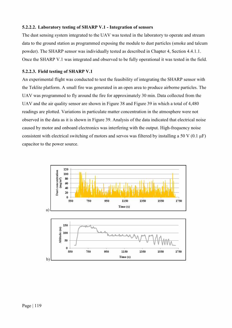
Page | 119
5.2.2.2. Laboratory testing of SHARP V.1 - Integration of sensors
The dust sensing system integrated to the UAV was tested in the laboratory to operate and stream
data to the ground station as programmed exposing the module to dust particles (smoke and talcum
powder). The SHARP sensor was individually tested as described in Chapter 4, Section 4.4.1.1.
Once the SHARP V.1 was integrated and observed to be fully operational it was tested in the field.
5.2.2.3. Field testing of SHARP V.1
An experimental flight was conducted to test the feasibility of integrating the SHARP sensor with
the Teklite platform. A small fire was generated in an open area to produce airborne particles. The
UAV was programmed to fly around the fire for approximately 30 min. Data collected from the
UAV and the air quality sensor are shown in Figure 38 and Figure 39 in which a total of 4,480
readings are plotted. Variations in particulate matter concentration in the atmosphere were not
observed in the data as it is shown in Figure 39. Analysis of the data indicated that electrical noise
caused by motor and onboard electronics was interfering with the output. High-frequency noise
consistent with electrical switching of motors and servos was filtered by installing a 50 V (0.1 μF)
capacitor to the power source.
a)
b)

Page | 120
c)
Figure 38. Data collected from Teklite with the SHARP sensor showing (a) dust concentration, (b) altitude, and (c) throttle [7].
Figure 39. 3D visualisation of data collected with SHARP V.1 monitoring system during the first flight test [7].
5.2.2.4. Field Test 1 of SHARP V.1 - Monitoring of PM10 particles
A second field test was conducted using commercial talcum powder suspended in the atmosphere
using a petrol-powered leaf blower (STIHL BG 56 Blower - max of 730 m3/h) (STIHL,
Waiblingen, Germany). Talcum powder was used due to its safe handling and availability. Talcum
powder is composed of 0.2-0.3 mass fraction with a particle diameter no greater than 10 μm
[328,329].
0.0
20.0
40.0
60.0
80.0
100.0
550 750 950 1150 1350 1550 1750T
hrot
tle
(%)
Time (s)
Dust concentration: 0 – 30 mg/m
3 61 – 90 mg/m
3 31 – 60 mg/m
3 91 – 110 mg/m
3

Page | 121
a)
b)
Figure 40. 3D visualisation of Test 2 data collected with the Teklite-SHARP sensor for PM10 (a) Overview and (b) Side view [7].
The data was processed using the particle correlation (Figure 20) obtained from laboratory testing
of the SHARP sensors to determine PM10 concentrations measured during the flight, (Section
4.4.1).
Figure 40 shows the distribution of PM10 concentrations in the atmosphere registered by the optical
sensor by using top and side 3D visualisation of the dust plume, with a total of 3,115 readings
plotted. Wind direction was towards the west-southwest, and concentrations ranged from 15-66
mg/m3. It was observed that the different concentrations registered described the shape of the plume
when dispersed by the wind.
Win
d d
irec
tion
(S
) Take off Landing
Source
Dust concentration PM10
:
0 – 10 mg/m3
10 – 12.5 mg/m
3 12.5 – 15 mg/m
3
15 – 20 mg/m
3 20 – 50 mg/m
3
50 – 75 mg/m
3
Take off
Landing
Source

Page | 122
The first and second flight tests demonstrated the functionality and possible integration of the
system. However, the need for a systematic characterisation of a particulate plume of known
composition and size remained. A systematic characterisation was required to demonstrate the
ability to calculate particulate emission rates, as most parameters could be independently measured
using a constant powder emission, constant emission rate, known atmospheric conditions, and
particle size distribution of the source.
It was necessary that the UAV reproduced a fixed experimental flight pattern to aid spatial
calculations and also exclude biased measurements that could easily be made when flying manually
into the visible plume produced by the powder ejected to achieve a systematic plume
characterisation. A flight path consisting of concentric circles at different heights and radius was
planned for a third test. The flight path ensured the UAV covered the designated area around the
source. It also ensured that the sensor intersected the plume, testing the ability of the system to
collect data which described the behaviour of the plume in the airspace surrounding it.
5.2.2.5. Field test SHARP V.1 in conjunction with SHARP V.2
A fourth field flight test was conducted for the integrated module SHARP V.1 in which it was
flown in conjunction with the modular version of the sensing system, SHARP V.2, to monitor PM10
particles. The detailed procedure of the test and results are presented in Section 5.3.1.3.

Page | 123
5.3. Modular dust monitoring systems
5.3.1. Dust monitoring system SHARP V.2
5.3.1.1. Design of SHARP V.2
The dust sensor and associated electronics were chosen to be low weight and constrained in size to
allow simple installation in micro and small multi-rotor or fixed wing platforms. The dust
monitoring module was placed on the top side of the Sotiris platform to minimise high-velocity air
flow that is fundamental to similar quadcopters [330,331]. Figure 41 illustrates the system
architecture of the multi-rotor UAV with the module, and Figure 42 presents the architecture of the
module in detail.
Figure 41. System architecture for the Sotiris with the independent gas-sensing system [7].
The system was constructed around an Arduino MEGA 2560, powered by a 7.4 V lithium polymer
battery, data telemetry is via XBee Pro S1 (2.4 GHz) radio transmitter while a GP-635T provided a
timestamp for serial port data. Sensors included a SEN51035P temperature and humidity sensor and
SHARP dust sensor (Figure 42). All data was transmitted and logged on a ground station which
displayed received raw values and PM10 concentrations in real-time.

Page | 124
5.3.1.2. Laboratory testing of SHARP V.2 - Integration of sensors
The modular dust sensing system was tested in the laboratory to operate and stream data to the
ground station as programmed, exposing the module to dust particles (smoke and talcum powder).
The SHARP sensor was individually tested as described in Chapter 4, Section 4.4.1.1. Once the
SHARP V.2 was integrated and observed to be fully operational it was tested in the field.
Figure 42. System architecture for the dust monitoring module [8].
5.3.1.3. Field testing of SHARP V.1 and SHARP V.2
The setup for the field experiment was based on the lessons learnt from the flight tests conducted
with the SHARP V.1. The experiment incorporated modifications to satisfy UAV flight and
rigorous plume modelling requirements. The fixed-wing and multi-rotor UAVs were able to fly
following the patterns programmed for the tests. The site for the field test needed to be a large open
area without vegetation, infrastructure or other obstacles that could be a safety hazard when flying
the Sotiris or the Teklite. Table 34 presents the radius and heights used for the test. These
parameters were defined according to the capabilities of each UAV and to collect complementary
datasets at two spatial scales. Based on the previous criteria, an experimental farm from the
University of Queensland – Campus Gatton at Gatton, QLD, Australia was chosen for the flight test
(Figure 43). The site is located approximately 12.0 km from the closest airport.

Page | 125
Table 34. Programmed flight parameters and UAV capabilities [7].
Parameters Quadcopter Fixed-Wing
Max. Height * 120 m 120 m
Max. Radius 100 m 200 m
Programmed Heights (MAGL) 7, 14, 21 m 35, 45, 55 m
Programmed Radius 5, 15, 35 m 45, 55, 65, 75, 85 m
* Determined by UAV height flight restrictions [167].
Figure 43. Flight test location and surrounding environment and infrastructure close to Gatton, QLD, Australia.
The talcum powder plume was generated using a petrol-powered fan connected to a 5.5 m long and
0.05 m diameter PVC stack. The powder was loaded into the airstream through an intersection
custom made for the powder containers at an approximate rate of 300 g/min (Figure 44).
For this flight test, the SHARP sensor was recalibrated to obtain a correction factor for the dust
source used, talcum powder. The calibration procedure used in Section 4.4.1 for smoke particles
was repeated for the talcum powder, as the different characteristics of smoke particles (e.g. colour
and particle diameter) and talcum powder would produce an error when reading concentration
values. A correlation equation was calculated using a polynomial fit by processing the data obtained

Page | 126
with the DustTrak and with the SHARP sensor (Figure 45). To test for normality, the K-S and Q-Q
plots were used in the residuals of the equation, which indicated no significance (see Appendix D).
However, the equation generated and R2 are considered significative due to the large dataset used
with 1,759 values, as the regression analysis is robust due to the central limit theorem [295,296].
Accuracy achieved by the OPC-N2 was determined by calculating the MR and NMSE, which had a
value of 0.64 and 1.00 respectively. Performance statistics and R2 (0.88) indicated a good fit and
high accuracy of the SHARP and DustTrak data.
Integrated datasets from each platform were post-processed to visualise the concentrations
measured by the Teklite and the Sotiris during experimental flights (Figure 46).
PM10 concentration values ranged from 0.5 - 19.0 mg/m3 and their distribution described the path
followed by the powder plume to the west, downwind from the source (Figure 46 a,b). Mid-range
concentrations to the east (downwind) and north of the source are likely to be the result of petrol
motor exhaust particles and potentially suspended talcum powder in the atmosphere. Further
experiments would use battery-powered fans and powder loading to the stack by suction (ventury
effect) to eliminate cross-contamination sources in the characterisation of the dust plume.
Figure 44. Talcum powder stack setup [7].

Page | 127
Figure 45. Correlation between talcum powder particles and raw value readings from the SHARP sensor and DustTrak [7].
For safety reasons and the complexity involved in flying two UAVs simultaneously, the quadcopter
and the fixed-wing UAVs were not flown simultaneously. The fixed-wing UAV was flown after the
quadcopter and recorded maximum concentrations of 2.0 mg/m3 without an observable (Figure 47).
Weather conditions with wind speed ranging from 7 to 9 m/s prevented the powder plume rising to
the minimum programmed height of 35 m; therefore, it is unlikely that detectable particulates
associated with the plume were present.
Figure 47 illustrates the contour plots of the powder distribution at the height of 18 m above ground
level and 30 m to the west of the source. The contour plots together with the volume rendering
produced with the software Voxler (Golden Software, Golden, CO, USA) aid in the interpretation
of the data. They produce a model of the plume which can be challenging to interpret when plotting
all readings independently, due to the high density of information. Higher concentrations of PM10
particles are shown in red colour which is located on the western side of the source located at the
centre of the plot.
y = 1E-07x3 - 0.0001x2 + 0.0758xR² = 0.8829
0
5
10
15
20
25
30
35
40
45
0 100 200 300 400 500 600 700 800
PM
10
(mg/
m3 )
Dus
tTra
k
ADC UnitsSHARP valuesPoly. (SHARP values )
Page | 128
a) b)
c)
Figure 46. Flight path and PM10 concentrations monitored with the UAV quadcopter (a) top view, (b) side
view; and (c) fixed-wing and quadcopter (overlapped flights) [7].
Dust concentration PM10 (mg/m3) :
0.1 – 4.0 4.0 – 8.0 8.0 – 12.0 12.0 – 16.0 mg/m3
16.0 – 19.0
Win
d di
rect
ion
(W)
Wind direction (W
)
Wind direction (W
)

Page | 129
a)
b)
Figure 47. Volume rendering and contour plots created with quadcopter dataset showing (a) top view 18 m above ground level (from the East), and (b) side view 30 m away from the source (from the west) [7].

Page | 130
5.3.2. Dust monitoring system OPC-N2 V.1
Tests done with the SHARP sensor demonstrated its robustness and sensitivity for concentrations
above 1 mg/m3 and a resolution of 0.1 mg/m3. However, for lower concentrations within the annual
and weekly WHO thresholds, a sensor with higher sensitivity and resolution was required. After a
thorough search for a sensor that met these requirements in addition to the initial selection criteria
(lightweight, compact, and low cost), the OPC-N2 from Alphasense was selected for testing [282].
5.3.2.1. Design of OPC-N2 V.1
The dust monitoring system OPC-N2 V.1 was developed using the particle counter OPC-N2. The
module had a similar configuration to the SHARP V.2, with meteorological and dust sensors, and
instrumentation required to log and transmit geotagged airborne readings. The OPC-N2 V.1 was
mainly integrated by the following instrumentation:
Temperature and humidity sensor, HTU21D;
Arduino DUE MCU Pre-processor;
3DR LEA-6H GPS;
XBee Pro S1 2.4 GHz radio;
3DR Airspeed Sensor (MS4525DO); and
3DR Lipo battery (11.1 V), connected to UAV battery.
The architecture of the dust monitoring module is presented in Figure 48. Information from each
sensor (e.g. particle counting, coordinates, temperature, and humidity) was sent to a ground station
via the XBee 2.4 GHz radio for monitoring at a pre-programmed rate of 2.0 s. All readings were
recorded in the memory of the ground station. Time synchronisation was achieved using the GPS
time stamp of each reading.

Page | 131
Figure 48. Architecture of dust monitoring system OPC-N2 V.1.
The total weight of the dust monitoring module was of 320.0 g approximately and had the following
dimensions: 12.0 cm × 15.0 cm × 7.0 cm. The IRIS+ had an endurance of approximately 10 min
when the module was attached. As described in Section 3.2.2, the IRIS+ was the selected UAV to
carry the OPC-N2 V.1 due to low cost off-the-shelf product, easy to service and modify, user-
friendly interface, and robust characteristics. The final configuration of the dust monitoring system
OPC-N2 V.1 is shown in Figure 49.
a) b)
Figure 49. Airborne dust monitoring system OPC-N2 V.1, a) all components, and b) interior of the module.

Page | 132
5.3.2.2. Development of probe
When using a multi-rotor UAV, two main issues were identified to obtain a representative air
sample from the atmosphere: difficulty to produce isokinetic flow and designing an air sampling
probe. Designing a sampling probe also implied determining the best position in the multi-rotor
UAV.
To understand the disturbance produced by the propellers in the volume of air that would be
sampled, an experiment to evaluate the aerodynamics was executed. Through this experiment, it
was possible to observe the behaviour of the volume of air surrounding the IRIS+ and determine if
isokinetic flow and sampling would be possible. Isokinetic flow is an important consideration when
monitoring or sampling particles below 10 μm in diameter, otherwise the resulting value could be
under or over-predicted [332]. However, being able to obtain isokinetic flow in non-static
conditions has been reported to be extremely difficult [333,334]. Airflow intake needs to be
controlled so the air streamlines are unaltered during the transportation of particles from the
atmosphere past the probe’s nozzle. Several factors have to be considered to achieve these
conditions: air velocity has to be equal inside and outside the sampling nozzle, air intake has to have
the same direction (iso-axial), and has to be placed out of the air mixing zone [334-336]. Other
variables to consider for isokinetic measurements with aircraft are the diffusion, sedimentation and
turbulent inertial deposition of particles. However, the variables considered vary depending on the
type of aircraft [335-337]. Related literature on the topic mainly focuses on fixed wing UAVs
which, due to their flight characteristics, could provide better conditions for isokinetic sampling
[336,337]. Factors such as angled flight, static flight or hovering, and constant change in wind
direction, make achieving isokinetic conditions very challenging for multi-rotor UAVs. Von der
Weiden et al. [332], used a different approach due to the difficulty of sampling in isokinetic
conditions. They created a correction calculator for air sampling that does not meet the criteria
necessary to be isokinetic and iso-axial. The calculator considers variation in sedimentation,
deposition due to inlets, bends, contractions, and diffusion factors. However, their approach was
only used and tested for the fixed wing UAV specified in their study.
For the aerodynamics experiment, the UAV was placed indoors and mounted on a 2.5 m pole.
Measurements were taken with a Kestrel 2500 anemometer (Minneapolis, MN, USA) which was
positioned around the UAV following a grid pattern at different x, y and z positions (Figure 50).
Vertical measurements were taken above and below the IRIS+, and horizontal measurements to the
sides of the body and propellers. With the readings collected, a 3D visualisation map was generated
to observe the airflow produced by the propeller downwash and upwash (Figure 51).

Page | 133
Figure 50. Set up of the multi-rotor UAV and airspeed measuring pole for aerodynamics test [9].
Figure 51. 3D visualisation of the different airspeed regions produced by the propellers upwash at the top and sides of the IRIS+. Axis units in meters [9].

Page | 134
It was determined that the downwash produced by the IRIS+, did not generate a uniform pattern by
analysing the readings and visualisations. The downwash varied by forming a cone which increased
its base as the distance from the centre of the IRIS+ also increased (Figure 52). The top side of the
IRIS+, on the other hand, had a constant airspeed flux which dropped after 40.0-45.0 cm
approximately. This constant air flux was also observed to the sides of the IRIS+ to a distance of
40.0-45.0 cm. A zone of low airspeed was found in front of the IRIS+ between the propellers
(Figure 51 and Figure 52).
Figure 52. 3D visualisation of the different airspeed regions produced by the propellers downwash at bottom and sides of the IRIS+. Axis units in meters.
The defined mixed air boundaries around the IRIS+ helped determine the position of the probe on
the side of the IRIS+ (horizontally) or the top of it (vertically). A horizontal probe would increase
the capacity of the IRIS+ to collect an isokinetic sample when the wind direction is in line with the
direction of the probe. However, when conducting field tests, wind direction varied up to 68˚ during
the testing period (10 min approximately) during experimental flights (Section 6.1). Such ample
variation in the intake angle is a considerable change of the ideal conditions required for isokinetic
sampling. It was decided to use the vertical probe on top of the UAV at a distance of 47.5 cm from
the centre of the UAV to overcome this issue (Figure 49). The use of a ‘canopy’ on the top could

Page | 135
increase its capacity to retain small volumes of the air targeted. The canopy could be useful when
flying through high wind speeds. A vertical probe has the same exposure when taking air samples
regardless of the orientation of the multi-rotor UAV or the wind flow.
For the fixed wing UAV, the probe would be placed on the front of the UAV, extending
approximately 10-20 cm from the tip of the structure. Testing and modelling would be required to
determine the optimum length of the probe. Contrary to multi-rotor UAVs, fixed wing aircrafts fly
at a constant speed relative to the ambient wind speed, allowing a constant air flow through the
sensor.
5.3.2.3. Laboratory testing of OPC-N2 V.1 - Integration of sensors
The modular dust sensing system was tested in the laboratory to operate and stream data to the
ground station as programmed, exposing the module to dust particles (talcum powder). The OPC-
N2 sensor was individually tested as described in Chapter 4, Sections 4.4.3.1 and 4.4.3.2. Once the
OPC-N2 V.1 was integrated and observed to be fully operational it was tested in the field.
5.3.2.4. Testing of OPC-N2 V.1 in the field
The system was tested once the OPC-N2 V.1 was integrated and the sampling probe placed on the
IRIS+. Smoke from a bonfire was used as a source of particles to test the airborne system which
was flown manually inside and across the smoke plume at an open area. Results were only reported
as the number of particles counted by the sensor within a particle diametre between 0.38 and 10.0
µm in a 0.2 s periods. Results are presented in Figure 53.
a) b)
Figure 53. Particle counting for two test flights using the OPC-N2 V.1 showing a) test flight 1 with full scale in the y-axis, and b) test flight 2 with y-axis zoomed from 0 to 100 particles.

Page | 136
5.3.3. Dust monitoring system OPC-N2 V.2
5.3.3.1. Design of dust monitoring system OPC-N2 V.2
Following Alvarado et al. (2015,2016) a sampling module and data logger transmission system
were developed using the OPC-N2 particle counter from Alphasense [282] with a response time of
0.2 s. In addition to the dust particle counter the module was mainly integrated by [7,8]:
Barometer, temperature and humidity sensor, BME-280;
Raspberry Pi 3 computer;
u-blox LEA-6H GPS;
XBee Pro S1 2.4 GHz Radio;
3DR Airspeed Sensor (MS4525DO); and
Lipo battery (11.1 V).
The architecture of the dust monitoring module is presented in Figure 54. Information from each
sensor (e.g., dust, pressure, temperature and humidity) was sent to a ground station via the XBee
Pro S1 radio for monitoring and recorded in a micro-SD card used by the RbPi 3B. Time
synchronisation was achieved using the GPS time stamp of each reading. The name of each log file
was also recorded with the time and date synchronised with the internet using a portable WiFi
hotspot.

Page | 137
Figure 54. The architecture of dust monitoring module [9].
The total weight of the dust monitoring module was of 382.0 g and had the following dimensions:
14.0 cm × 9.0 cm × 10.0 cm. The IRIS+ was also used for the tests as a flying platform and had an
endurance of approximately 10 min with the payload. The sampling probe consisted of a carbon
fibre tube (5 mm) located at the centre of the IRIS+, which gave support to a silicon hose (5 mm)
and reached a height of 47.5 cm directly connected to the OPC-N2 (Figure 55). The carbon fibre
tube also held the sampling probe canopy, which consisted of three concave polymer discs. The
final configuration of the OPC-N2 V.2 was very similar to the OPC-N2 V.1.

Page | 138
a) b)
Figure 55. The physical configuration of the multi-rotor UAV with the sampling probe and dust monitoring module attached, a) photo [9] and b) diagram.
5.3.3.2. Variable wind speed modelling with the sampling probe
In addition to the individual tests performed to the OPC-N2 in the laboratory (Section 4.4.3), a
variable air speed experiment was planned to study the response of the OPC-N2 with the probe
attached using different wind speeds. For this experiment, a wind tunnel was built to produce
laminar flow and have control of the airspeed changes (Figure 56), similar to the equipment
observed in Brady et al. (2016) [235]. The test area of the wind tunnel had 40.0 cm of cross-section,
in which the probe (attached to the OPC-N2), a secondary OPC-N2 without a probe, and the TSI
DRX (making use of an extension), were placed at the same height for uniformity of readings (15.0
cm from base of test area).

Page | 139
Figure 56. Wind tunnel and equipment used for the variable wind speed tests [9].
Four individual experiments were conducted to generate a variable wind speed model for each
position of the sampling probe, either vertical or horizontal (Figure 57 a, b). Each experiment used a
different wind speed: 1.11 m/s, 1.67 m/s, 3.06 m/s and 3.89 m/s. The air flow was produced with
fans and measured with a SkyWatch ATMOS anemometer (Sudbury, UK), and also temperature
and humidity with a Bosch BME-280 sensor. Dust particles were supplied using calcined alumina at
an approximate rate of 0.015 g every 10 min. The concentration read by the OPC-N2 was logged
and reported by the software interface provided by Alphasense Ltd. (Great Notley, Essex, UK).
Figure 57 a-d show the experimental setup inside the test area of the wind tunnel for the vertical and
horizontal position of the sampling probe. For the vertical position, the sampling probe was
perpendicular to the direction of the wind. For the horizontal position, the opening of the nozzle and
the sampling probe were aligned with the direction of the wind, following the iso-axial principle to
sample dust particles. Flow rate inside the OPC-N2 was not regulated to match the wind speed
selected to operate the wind tunnel. Isokinetic conditions were not accomplished as the OPC-N2
V.2 only used the axial fan inside the OPC-N2 to produce suction through the probe. For each
experiment, an OPC-N2 with a sampling probe, an OPC-N2 without a sampling probe, and a TSI
DRX were collocated.

Page | 140
a)
b)
Figure 57. The test area of the wind tunnel set with the anemometer, OPC-N2, and TSI DRX, and probe in a) vertical position, and b) in horizontal position.
5.3.3.3. Results and analysis for the vertical sampling probe model
The first set of experiments consisted of collecting values from the OPC-N2, the temperature and
moisture sensor, measuring dust supply, and the anemometer. Using multivariate lineal regression
for the variables considered (dust concentration - C, relative humidity - R.H., temperature - T, and
dust supply - W, and airspeed - U), one equation was generated for the airborne module (sampling
probe attached), and a second one for the collocated module (Equations 3 and 4):
CUAV = (2.062 × CR) − (1.180 × R.H.) − (1.921 × T) + (0.025 × W) + (3.048 × U) + 155.225 Equation 3
Ccoll = (0.201 CR) - (0.645 R.H.) - (0.672 T) + (0.034 W) + (1.389 U) + 57.607 Equation 4

Page | 141
Table 35 shows the coefficients calculated for each equation with their p-Value, and Table 36
shows their R2, statistical significance and performance statistics. An R2 of 0.66 was estimated for
Equations 3 and 4. MR and NMSE values showed better accuracy and performance for Equation 3
over Equation 4. Also, the p-values estimated for both equations had values < 0.05 (95%
confidence), indicating statistical significance of the coefficients [9]. For Equations (3) and (4), all
variables had a confidence level of approximately 100%.
The K-S test and Q-Q plots were used for both datasets to determine the statistical significance of
the multivariate regression (Table 35 and Figure 58). Results indicated the standardised residuals
had a non-normal distribution. However, it is considered regression analysis is robust to non-normal
data when analysing a large number of observations (>5,000 values), due to the central limit
theorem [295,296]. Williams et al. (2013), indicate that for regressions, normal distribution of
standardised errors is not required for R2 to be considered unbiased, consistent, and efficient [296],
therefore capable of use for predictions and inferences.
Table 35. Resulting coefficients for variables of equations for dust monitoring sensors with their R2 and confidence level.
Sensor Variable Coefficients p-Value Coefficients p-Value
(all variables) (W not considered)*
Airborne
module
(CUAV)
Intercept 155.225 6.3×10−281 102.082 2.5×10−223
Raw Conc. PM10 (CR, µg/m3) 2.062 ~0.00 2.118 ~0.0
Relative Humidity (R.H. %) -1.180 4.2×10−294 −1.175 4.2×10−235
Temperature (T, °C) -1.921 2.1×10−290 −1.261 2.1×10−231
Dust supply (W, µg/s) 0.025 1.1×10⁻¹⁴ NA NA
Air speed (U, m/s) 3.048 4.8×10−236 1.822 2.8×10−159
Collocated
module sensor
(CColl)
Intercept 57.608 1.0×10−86 57.292 2.7×10−84
Raw Conc. PM10 (CR, µg/m3) 0.201 ~0.00 0.197 ~0.0
Relative Humidity (R.H. %) -0.645 1.8×10−85 −0.623 5.6×10−79
Temperature (T, °C) -0.672 2.7×10−80 −0.641 1.7×10−72
Dust supply (W, µg/s) 0.034 6.32×10⁻³⁴ NA NA
Air speed (U, m/s) 1.387 7.8×10−101 1.125 2.0×10−74
*Alvarado, M.; Gonzalez, F.; Erskine, P.; Cliff, D.; Heuff, D. A methodology to monitor airborne PM10 dust particles using a small unmanned aerial vehicle. Sensors 2017, 17, 343; NA = Not applicable.

Page | 142
Table 36. R2, statistical significance, and performance statistics for Equations 3 and 4.
Sensor Variable Value Value
(all variables) (W not considered)*
Airborne module
(CUAV)
R2 0.66 0.55
K-S Significance ~0.00 ~0.00
MR 0.90 0.87
NMSE 0.05 0.08
n 5,396 7,768
Collocated module sensor (CColl)
R2 0.66 0.66
K-S Significance ~0.00 ~0.00
MR 0.83 0.83
NMSE 0.06 0.14
n 7,769 7,769
*Alvarado, M.; Gonzalez, F.; Erskine, P.; Cliff, D.; Heuff, D. A methodology to monitor airborne PM10 dust particles using a small unmanned aerial vehicle. Sensors 2017, 17, 343.
To confirm the coefficients of the models generated where statistically significative, bootstrapping
was used to obtain the 95% confidence intervals and compare them against the coefficients of
Equations 3 and 4. Bootstrapping is a non-parametric test that uses re-sampling with replacement in
the original dataset (population) to calculate percentiles. It can be used when the standard residuals
of a regression do not follow a normal distribution [338,339]. The test was performed with the
software R (Bell Laboratories, New Jersey, USA), using 10,000 bootstrap replicates and the BCa
interval type, which uses adjusted percentiles to account for skewness and bias.
Table 37 presents the results of the bootstrapping analysis, which indicates that all coefficients are
within the 95% confidence intervals. In Appendix D are included the details of the output from the
software R.
a) b)

Page | 143
c) d)
Figure 58. Normality Q-Q plots for vertical sampling probe models for a) model using all variables for the airborne module, b) model not using W for the airborne module, c) model using all variables for the
collocated module, and d) model not using W for the collocated module.
Table 37. Resulting 95% confidence intervals for coefficients of variables in model equations for dust monitoring, sensors during the vertical probe experiments.
Sensor Variable
95% Confidence
intervals
95% Confidence
interval
(all variables) (W not considered)*
Airborne
module (CUAV)
Intercept 96.9 107.2 52.37 62.75
Raw Conc. PM10 (CR, µg/m3) 2.058 2.183 0.197 0.206
Relative Humidity (R.H. %) -1.232 -1.119 -0.701 -0.587
Temperature (T, °C) -1.322 -1.199 -0.733 -0.610
Dust supply (W, µg/s) NA NA 0.0293 0.0385
Air speed (U, m/s) 1.716 1.926 1.291 1.475
Collocated
module sensor
(CColl)
Intercept 51.69 62.43 147.700 163.000
Raw Conc. PM10 (CR, µg/m3) 0.1934 0.2026 1.989 2.133
Relative Humidity (R.H. %) -0.6808 -0.5608 -1.884 -1.711
Temperature (T, °C) -0.7030 -0.5743 -2.015 -1.829
Dust supply (W, µg/s) NA NA 0.020 0.029
Air speed (U, m/s) 1.022 1.218 2.890 3.210
NA = Not applicable.
Even though R2 and confidence intervals were satisfactory, the second set of equations were
generated, as the dust supply was a parameter which varied as it was not produced with an
automated system. Equations 5 and 6 show the resulting coefficients when using multivariate linear
regression to the data without the dust supply parameter (W) [9]:
Page | 144
CUAV = (2.118 × CR) − (1.175 × R.H.) − (1.261 × T) + (1.822 × U) + 102.082 Equation 5
CColl = (0.197 × CR) − (0.623 × R.H.) − (0.641 × T) + (1.125 × U) + 57.292 Equation 6
Table 35 presents the R2, MR and NMSE for both equations. R2, MR and NMSE for Equations 5
and 6 indicate performance and accuracy is lower than Equations 3 and 4. Nevertheless, in Section
6.2.1.3, 6.3, and 6.3.2 will be demonstrated that the application of Equations 5 and 6 produced
calculations for dust concentration and dust emissions with low percentage errors.
When testing for normality of the standard residual, also the K-S test and Q-Q plots (Table 35 and
Figure 58) were used. The K-S test results presented no significance with a value of ~0.00 and the
scatter plots did not align to the reference line (at 45˚). Bootstrapping was used as a non-parametric
test, to calculate the coefficients of the multivariate regression with 95% confidence interval, with
10,000 re-sampling iterations. Results indicated all coefficients of the equations were within 95%
confidence intervals (Table 37 and Appendix D).
5.3.3.4. Results and analysis for the horizontal sampling probe model
The second set of tests were conducted with the sampling probe in horizontal position. Once data
was collected from all sensors, multivariate linear regression was used for the data analysis and
modelled by applying multivariate regression. A model was generated for the OPC-N2 connected to
the horizontal probe and a second model was generated for the sensor without the probe (Equations
7 and 8):
CUAV = (0.849 × CR) - (0.022 × W) + (0.045 × R.H.) - (0.070 × T) + (1.429 × U) - 2.569 Equation 7
CColl = (0.326 × CR) + (0.047 × W) + (0.166 × R.H.) - (0.111 × T) - (0.041 × U) - 7.548 Equation 8
Table 38 presents the coefficients calculated for each equation with their p-Value, and Table 39
shows their R2, statistical significance and performance statistics. The R2 resulting from the models
are high with values of 77% and 83% for the airborne module and collocated module sensors
respectively. Also, the performance statistics show Equations (7) and (8) have high accuracy with
MR ≥ 0.9 and NMSE ≤ 0.05. The multivariate linear regression demonstrated that in each model,

Page | 145
one variable did not reach 95% confidence level, contrary to the vertical sampling probe models in
which all models had values above 95%.
Table 38. Resulting coefficients for the horizontal probe model variables with their p-value.
Sensor Variable Coefficients p-value Coefficients p-value
(all variables) (W not considered)*
Airborne
module
(CUAV)
Intercept -2.569 0.160 -3.316 0.068
Raw Conc. PM10 (CR, µg/m3) 0.849 ~0.000 0.846 ~0.000
Dust supply (W, µg/s) -0.022 0.001 NA NA
Relative Humidity (R.H. %) 0.045 ~2.4610-7 0.047 5.8810-8
Temperature (T, ˚C) -0.070 0.058 -0.065 0.261
Air speed (U, m/s) 1.429 0.035 1.410 ~0.000
Collocated
module sensor
(CColl)
Intercept -7.548 1.410-6 -6.142 8.510-5
Raw Conc. PM10 (CR, µg/m3) 0.326 ~0.000 0.327 ~0.000
Dust supply (W, µg/s) 0.047 1.310-16 NA NA
Relative Humidity (R.H. %) 0.166 1.710-110 0.163 2.2E-106
Temperature (T, ˚C) -0.111 0.021 -0.118 0.018
Air speed (U, m/s) -0.041 0.145 -0.011 0.694
* Alvarado, M. In Comparison between the use of a vertical and a horizontal sampling probe for an airborne dust monitoring system, The Critical Atmosphere, Brisbane, October 15-18, 2017; CASANZ: Brisbane, 2017; p 1. NA = Not Applicable p-values in italics indicate they are outside of the 95% confidence level
Table 39. R2, statistical significance, and performance statistics for models generated with the horizontal probe.
Sensor Variable Value Value
(all variables) (W not considered)*
Airborne
module
(CUAV)
R2 0.77 0.77
K-S significance ~0.00 ~0.00
MR 0.98 1.22
NMSE 0.07 0.09
n 7,987 7,987
Collocated module sensor (CColl)
R2 0.83 0.83
K-S significance ~0.00 ~0.00
MR 0.90 0.90
NMSE 0.05 0.05
n 7,987 7,987
* Alvarado, M. In Comparison between the use of a vertical and a horizontal sampling probe for an airborne dust monitoring system, The Critical Atmosphere, Brisbane, October 15-18, 2017; CASANZ: Brisbane, 2017; p 1.

Page | 146
In a similar way to the analysis conducted with the results of the vertical probe, the second set of
equations were generated without the dust supply (W) as it could be the source of a more significant
error in the final results. Equations 9 [3] and 10 resulted from the second analysis. R2 and MR and
NMSE for the collocated module sensor did not increase. MR and NMSE for the airborne module
varied indicating lower performance, and variables that presented values below 95% confidence
level did not increase their p-value. Other trials were undertaken to determine if the variables with
high p-values were the cause of lower confidence levels. However, after each iteration, new
variables presented high p-values.
CUAV = (0.846 × CR) + (0.047 × R.H.) - (0.065 × T) + (1.410 × U) – 3.316 Equation 9
CColl = (0.327 × CR) + (0.163 × R.H.) - (0.118 × T) - (0.011 × U) – 6.142 Equation 10
Normality of the data was also evaluated, resulting in presenting a non-normal distribution when
calculating significance with the K-S test and using Q-Q plots for the standardised residuals of the
regressions (Table 38 and Figure 59). Results of the R2 and the p-value are considered trustworthy
due to the large sample size, for this experiment a total of 7,987 values.
a) b)

Page | 147
c) d)
Figure 59. Normality Q-Q plots for horizontal sampling probe models for a) model using all variables for the airborne module, b) model not using W for the airborne module, c) model using all variables for the
collocated module, and d) model not using W for the collocated module.
As with the tests performed for the vertical sampling probe, to confirm the coefficients of the
models generated where statistically significative, bootstrapping was also used to obtain the 95%
confidence intervals and compare them against the coefficients of Equations 5, 6, 7, and 8. The test
was performed using 10,000 bootstrap replicates and the BCa interval type. Table 40 presents the
results of the bootstrapping analysis, which shows that all coefficients are within the 95%
confidence intervals. In Appendix D are included the details of the output from the software R.
Table 40. Resulting 95% confidence intervals for coefficients of variables in model equations for dust monitoring sensors, during the horizontal probe experiments.
Sensor Variable 95% Confidence interval 95% Confidence interval
(all variables) (W not considered)
Airborne module
(CUAV)
Intercept -6.543 3.896 -7.302 2.932
Raw Conc. PM10 (CR, µg/m3) 0.8322 0.8668 0.8285 0.8636
Dust supply (W, µg/s) -0.0386 -0.0066 NA NA
Relative Humidity (R.H. %) 0.0140 0.0643 0.0161 0.0662
Temperature (T, ˚C) -0.2739 0.0552 -0.2563 0.0632
Air speed (U, m/s) 1.367 1.491 1.347 1.472
Collocated module
sensor (CColl)
Intercept -12.209 2.715 -10.685 4.006
Raw Conc. PM10 (CR, µg/m3) 0.3198 0.3336 0.3210 0.3344
Dust supply (W, µg/s) 0.0371 0.0570 NA NA
Relative Humidity (R.H. %) 0.1151 0.1883 0.1145 0.1852
Temperature (T, ˚C) -0.4392 0.0335 -0.4329 0.0256
Air speed (U, m/s) -0.1080 0.0203 -0.0781 0.0508
NA = Not applicable

Page | 148
5.3.3.5. Particle size distribution for variable wind speed experiments
In this section, results are compared regarding particle size distribution from experiments using the
sampling probe in horizontal and vertical position in different environmental conditions
(temperature, humidity, and wind speed). As indicated previously in Section 5.3.2.1 and discussed
in Alvarado et al. (2017), wind speed and direction, design characteristics of the air intake-nozzle,
among others, impact measurements of dust particles [332].
Particle count data resulting from exposing the airborne module with the vertical and horizontal
probe at variable wind speeds, were compared by normalising total particle count per dust bin and
calculating their percentage in the air sampled. Figure 60 presents data normalised for all wind
speeds classified by particle size diameter using the size ranges or ‘bins’ defined by the OPC-N2.
When using the vertical probe [9], it was observed that the particles ranging from 0.38–0.54 µm
were the predominant size fraction (63.7%) with a difference of 45.5% from the air sampled
without the probe.
A similar trend was observed when using the horizontal probe with particles in the first bin having a
percentage of 59.6%, and a difference of 41.0% when compared to the percentage of the sensor
without probe. Particles ranging from 0.54-4.00 µm integrated the second largest bracket of
particles counted, representing a total of 35.54% and 39.54% for the vertical and horizontal probe
respectively. Size fractions ranging from 5.00-10.00 µm conformed only 0.70% for the vertical test
and 0.81% for the horizontal test. This distribution indicates that particles up to 0.54 µm were less
affected by the use of the sampling probe, and the use of the probe in either position inside the wind
tunnel has a very similar effect. In total, smaller particles ranging from 0.38-4.00 µm represented
approximately 99.00% of particles within the volume of air sampled in both tests. A higher
percentage of smaller particles was attributed to their behaviour similar to a gas when suspended in
the atmosphere and could travel inside the sampling probe or dust sensor without being deviated by
non-isokinetic and non-isoaxial conditions (detailed explanation in Section 5.3.2.2).

Page | 149
a)
b)
Figure 60. Influence of the sampling probe used with the OPC-N2 over particle counting readings per particle size range for a) use of vertical probe [9], and b) horizontal probe [3].
For the particles counted with the OPC-N2 without a sampling probe, it was observed that particles
within 0.38-1.34 µm, represented a total of 78.6% and 76.5% for the vertical and horizontal position
respectively. These particles were the main fraction of the total sample. The second largest bracket
of particles was represented by size fractions ranging from 1.34-5.00 µm, with a value of 19.1% and
21.9% vertically and horizontally oriented respectively. Particles ranging from 5.00-10.00 µm had a
total between of 1.7% and 2.2%. As observed in the test where a sampling probe was used, particles
within smaller size fractions represented the highest percentage of the total. Even though particles
with greater size fractions were mostly affected by reducing the total number of particles counted,
values analysed and corrected using equations generated with multivariate linear regression

Page | 150
(Section 5.3.3.2, Equations 5 and 6), were comparable to values measured during field tests
(Sections 6.3, 6.3.3, 6.3.4).
Figure 61 shows the impact that variable wind speeds produced in the OPC-N2 with the vertical or
horizontal probe connected, per wind speed used. The distribution of particles counted by the
sensors in each bin described the same pattern observed in Figure 60. Patterns described by both
probe positions were very similar. Variations observed could be due to changes in temperature,
humidity or dust supply. Higher variation between particle numbers was observed when plotting
particle readings not using a sampling probe at different wind speeds (Figure 62). This result could
indicate that the use of the sampling probe buffered the effects of variable wind speeds in both
positions. However, as observed in Figure 60, particles within the greater size fractions represented
less than 0.1% of the total. Impacts of the use of the sampling probe were expected, nevertheless it
was possible to adjust and obtain results with low errors when applying multivariate linear
regression to analyse the data (Table 50, Table 51 and Table 52).
a)

Page | 151
b)
Figure 61. Influence of different wind speeds over particle counting readings per particle size range for a) OPC-N2 with the vertical probe [9] and b) OPC-N2 with the horizontal probe.
Results of both tests conducted using a sampling probe showed similar tendencies in particle size
distribution within the bins of the OPC-N2. However, tests were undertaken only considering the
wind in one direction. Further work will require testing the sampling probes in horizontal position
considering different wind directions to evaluate its impact on particles counted by the OPC-N2.
a)

Page | 152
b)
Figure 62. Influence of wind speed variation over particle counting readings per particle size range for OPC-N2 without a sampling probe during a) test with the vertical probe [9], and b) test with the horizontal probe.
Readings produced by the TSI DRX during both tests were analysed using dust concentration
readings. All particle size fractions reported by the TSI DRX, PM1.0, PM2.5, PM4.0 (respirable
according to ISO 12103-1, A1), and PM10, were used for the particle size distribution analysis.
Figure 63 shows the average raw concentration per wind speed used. Even though test conditions
were identical between the vertical and horizontal probe tests, the readings of the TSI DRX
presented higher differences between wind speeds in the test where the horizontal probe was used.
This pattern was also observed in the data produced by the OPC-N2 not connected to a probe during
the horizontal probe test. This difference in results could be due to changes in temperature, relative
humidity, and dust supply. Nevertheless, these variations being constant for the different particle
size fractions, improved the outcome when generating the models having high confidence levels
(>95%) and R2 above 50%.

Page | 153
a) b)
Figure 63. Influence of wind speed variation over dust concentration (raw) for different particle size fractions reported by the TSI DRX for a) during the vertical probe experiment [9], and b) during the horizontal probe
experiment.
To determine the influence of temperature and humidity, in the final concentration measured, the
values for each test were plotted to compare and observe any relevant changes (Figure 64 and
Figure 65). It was observed that for the vertical probe experiment relative humidity varied less than
15% throughout the experiment, which is half of the variation presented in the horizontal probe
experiment with approximately 30% variation.
For the temperature, the vertical probe experiment had an approximate variation of less than 4˚C,
and for the horizontal probe, it had a variation of 4.5 ˚C. Considering that temperature variation
range between the vertical and horizontal probe experiments was of approximately 0.5 ˚C, it can be
concluded that humidity impacted the behaviour of calcined alumina readings to determine final
concentrations in the atmosphere. Hence, producing high variations between readings recorded by
the OPC-N2 not attached to a probe and the TSI DRX.

Page | 154
a) b)
Figure 64. Relative humidity and temperature variations during the variable wind speed experiment using the vertical sampling probe.
a) b)
Figure 65. Relative humidity and temperature variations during the variable wind speed experiment using the horizontal sampling probe.
When comparing p-values from each experiment (Table 41), it was observed that for the vertical
probe the weight of all variables was very similar, except the raw concentration which was close to
zero (indicating higher significance). However, considerable bias was observed in the p-values for
the horizontal probe experiment. The raw concentration and airspeed variables had the highest
significance (approximately zero), followed by the relative humidity. Temperature values did not
reach 95% confidence level indicating the model was not as representative as the model calculated
with the vertical probe, where all variables surpassed 95%. The horizontal probe complies with the
condition of having iso-axial airflow, which increases the representative value of a dust sample.
Nevertheless, the vertical sampling probe, with almost equal significance for its variables and all of
them being above 95% confidence level, would represent better the real environment when
sampling outdoors, where isokinetic sampling with a multi-rotor UAV is very complicated.

Page | 155
Table 41. Comparison of p-values for airborne module models [3].
Sensor Variable p-Value
Vertical Horizontal
Airborne module
(CUAV)
Intercept 2.5×10−223 0.068
Raw Conc. PM10 (CR, µg/m3) ~0.0 ~0.0
Relative Humidity (R.H. %) 4.2×10−235 5.88E-08
Temperature (T, °C) 2.1×10−231 0.261
Air speed (U, m/s) 2.8×10−159 ~0.0
R2 0.55 0.73
p-values in italics indicate they are outside of the 95% confidence level
5.4. Summary
In Table 42 is presented a summary of all the criteria considered to examine the meteorological and
dust monitoring systems. Table 43 shows a summary of the components used to integrate each of
the dust monitoring systems designed and developed for the investigation.
Table 42. Design and development criteria for the dust monitoring systems used during the investigation.
Dust monitoring system
Criteria Category Met V.1 SHARP V.1 SHARP V.2 OPC-N2 V.1 OPC-N2 V.2
1 Communication ✔ ✔ ✔ × ✔
2 Manoeuvre × × ✔ ✔ ✔
3 Programming and calibration ✔ ✔ × ✔ ✔
4 Endurance ✔ ✔ ✔ ✔ ✔
5 Size, weight and power ✔ ✔ ✔ ✔ ✔
6 Data ✔ ✔ × × ✔
7 Robustness ✔ ✔ × ✔ ✔
8 Cost ✔ ✔ ✔ ✔* ✔*
Total ✔ 7 7 5 6 8
* The total cost of the OPC-N2 V.1 and V.2 were above AUD 3,000.00 due to investigation costs, such as re-engineering and sensors requiring
maintenance.

Page | 156
Table 43. Components of the five monitoring systems developed during the investigation.
Components
Name / Type
Met V.1 -
Integrated
SHARP V.1 -
Integrated
SHARP V.2 -
Modular
OPC-N2 V.1 -
Modular
OPC-N2 V.2 -
Modular
1 UAV Teklite (Fix
winged)
Teklite (Fix
winged)
Sotiris (multi-
rotor)
Iris+ (multi-
rotor) Iris+ (multi-rotor)
2 Meteorology SHT1X DF-
DFR0066 NA SEN51035P HTU21D BME-280
3 Dust sensor NA SHARP SHARP OPC-N2 OPC-N2
4 GPS uBlox LEA6 uBlox LEA6 GP-635T uBlox LEA6 uBlox LEA6
5 Radio XBee Pro S3B XBee Pro S3B XBee Pro S1 XBee Pro S1 XBee Pro S1
6
Development
Board /
Computer
NA Arduino Mini
Pro
Arduino Mega
2560 Arduino DUE Raspberry Pi 3B
7 Airspeed NA NA NA 3DR Airspeed
sensor
3DR Airspeed
sensor
8 Power 3700 mA LiPo 3700 mA LiPo 7.4 V LiPo 1.11 V LiPo 1.11 V LiPo
9 Size (cm) 3.2 × 17 ~ 5 × 5 × 3 3.5 × 14.5 × 6.5 12 × 15 × 7 14 × 10 × 9
10 Weight (g) < 5 < 15 11.4 320 382

Page | 157
6. OPC-N2 V.2 flight tests The instrumentation used and experiments conducted to test the OPC-N2 V.2 dust monitoring
system is a continuation of the work described in the previous chapters [7,8]. The OPC-N2 V.2 is
the evolution of four air quality monitoring modules. Improvements which characterise the OPC-N2
module include:
a) Use of the IRIS+ with a tailored sampling probe in vertical position;
b) A dust monitoring module which was integrated with a Class 1 laser optical particle
counting sensor (OPC-N2), a meteorological sensor for temperature, humidity and
atmospheric pressure (BME280), a wind speed sensor (3DR airspeed), GPS (3DR LEA6)
and radio communication (XBee Pro S1); and
c) The use of a micro-computer (RbPi 3B) to integrate the dust monitoring module to increase
the processing capacity of the system.
To test the OPC-N2 V.2 in the field, a purpose-made point source was created and monitored with a
5 m tower. PM10 field concentrations and emission rates from the point source were compared to
the readings collected with the airborne module and collocated module to determine the capability
of the methodology to be applied at industrial environments such as an open pit mine sites [9].
The following Sections of Chapter 6 were taken from the publication ‘Alvarado, M.; Gonzalez, F.;
Erskine, P.; Cliff, D.; Heuff, D. A methodology to monitor airborne PM10 dust particles using a
small unmanned aerial vehicle. Sensors 2017, 17, 343.’:
6.1.1. Monitoring a dust point source;
6.1.1.1. Procedure for flight Tests 1 and 2;
6.1.1.2. Procedure for flight tests 3 and 4;
6.3. Results and analysis
Results and analysis of data collected by the collocated module6.3.1. Results and analysis of
data collected by the collocated module;
6.3.2. Test 2, comparison of average concentrations - airborne module;
6.3.3. Tests 1 and 2, comparison of average emission rates - airborne module; and
6.3.4. Tests 3 and 4, comparison of emission rates - airborne module.
Page | 158
Figure 67 and Figure 68 with their description in Section 6.1.1. Monitoring a dust point source, as
well as Table 52 with its description in Section 6.3.4. Tests 3 and 4, comparison of emission rates -
airborne module, were integrated a posteriori to the publication as part of the Thesis manuscript.
Statistical normality tests included in Section 6.3. Results and analysis
Results and analysis of data collected by the collocated module, and 6.3.2. Test 2, comparison of
average concentrations - airborne module, were integrated a posteriori to the publication as part of
the Thesis manuscript.
6.1. Field testing of the OPC-N2 V.2 dust monitoring system
6.1.1. Monitoring a dust point source
An experiment was designed to collect experimental data similar to that obtained at industrial sites
such as open pit mine sites for hauling, stockpiling, blasting, and other activities. These activities
are area sources or fugitive emissions. However, to create an experimental site in which variables
could be easily monitored and controlled, a stack emission was the most feasible option. The
experiment consisted of using a 5.0 m stack (5.0 cm diameter), through which calcined alumina was
supplied and expelled with the use of an electric blower. An electric blower was chosen to eliminate
possible cross contamination with particles produced by fuel operated machines. Due to the
dimensions of the stack, it was not possible to sample PM10 concentration readings from inside the
stack in an isokinetic manner. However, this contributed to making the scenario similar to a real
fugitive emission, by measuring directly with the OPC-N2 V.2 from the plume generated. A 5.0 m
tall “monitoring tower” was installed at a distance of 10.0 m downwind from the stack. At the top of
the tower, a TSI DRX and a duplicate of the dust monitoring module were installed. This tower was
used to compare dust concentration readings from stationary devices against airborne data (Figure
66).
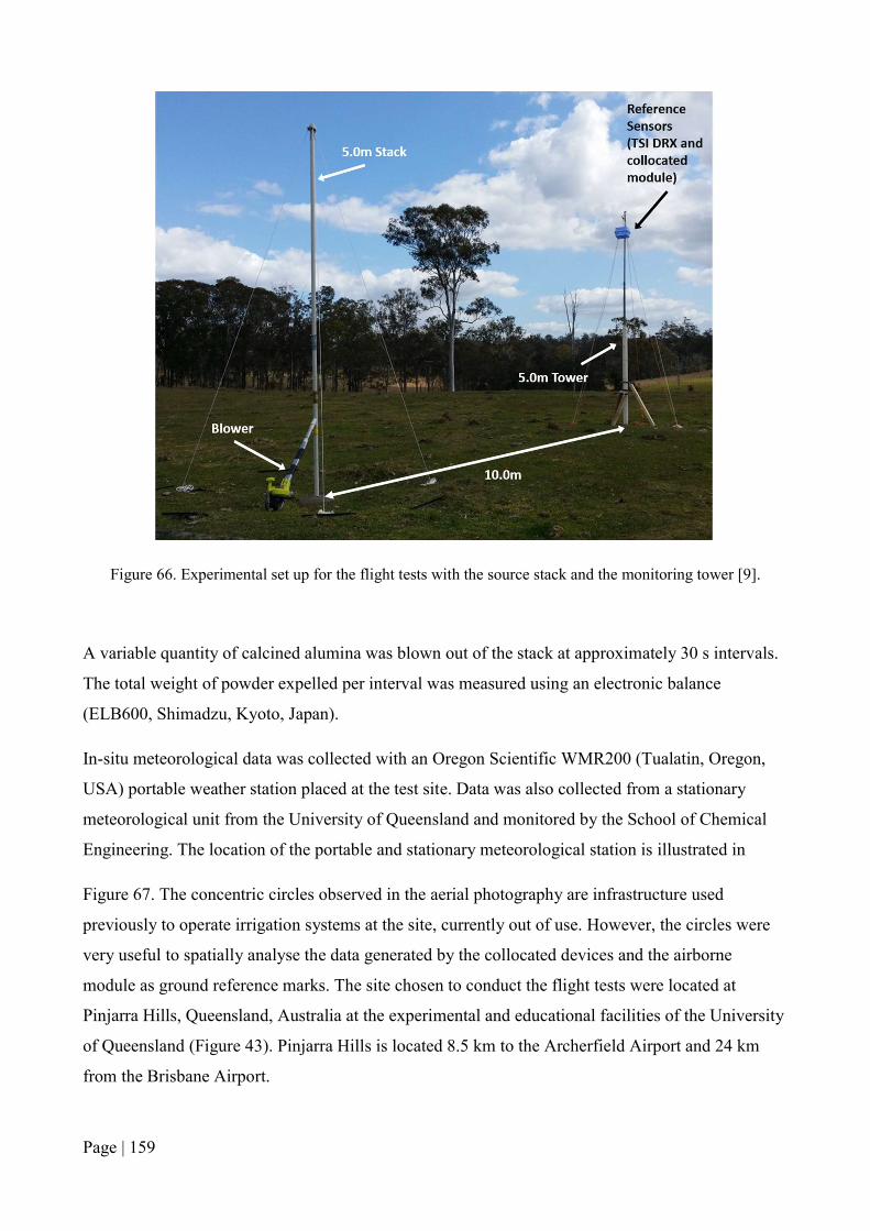
Page | 159
Figure 66. Experimental set up for the flight tests with the source stack and the monitoring tower [9].
A variable quantity of calcined alumina was blown out of the stack at approximately 30 s intervals.
The total weight of powder expelled per interval was measured using an electronic balance
(ELB600, Shimadzu, Kyoto, Japan).
In-situ meteorological data was collected with an Oregon Scientific WMR200 (Tualatin, Oregon,
USA) portable weather station placed at the test site. Data was also collected from a stationary
meteorological unit from the University of Queensland and monitored by the School of Chemical
Engineering. The location of the portable and stationary meteorological station is illustrated in
Figure 67. The concentric circles observed in the aerial photography are infrastructure used
previously to operate irrigation systems at the site, currently out of use. However, the circles were
very useful to spatially analyse the data generated by the collocated devices and the airborne
module as ground reference marks. The site chosen to conduct the flight tests were located at
Pinjarra Hills, Queensland, Australia at the experimental and educational facilities of the University
of Queensland (Figure 43). Pinjarra Hills is located 8.5 km to the Archerfield Airport and 24 km
from the Brisbane Airport.

Page | 160
Figure 67. Aerial view of the test site indicating the location of the stack, monitoring tower and meteorological stations.
Status and readings from the two modular sensors were followed via the radio link and controlled
using SSH (Secure Shell) connection with the ground station. To use the data produced by all the
monitoring devices (dust monitoring modules, TSI DRX, and meteorological station), it was
necessary to synchronise their datasets by programming the weather station and the TSI DRX.
However, the dust monitoring modules had to be adjusted by internet clock link using WiFi and a
portable hot-spot connection.
Stack Monitoring tower Portable Met Station Stationary Met Station
Former irrigation
infrastructure

Page | 161
Figure 68. Flight test location and surrounding environment and infrastructure.
6.1.1.1. Procedure for flight Tests 1 and 2
In Alvarado et al. (2015), a circular flight pattern was used to scan the area and create a grid to
characterise the dust plume [7]. However, for this flight test, a different grid was used due to the
small size of the plume and the short endurance of the OPC-N2 V.2, which was of approximately of
10 min. Two grids were designed for the first two flight tests. The grids were oriented northwest,
downwind from the stack (source), and followed a zig-zag path around the monitoring tower
(Figure 69).
For Test 1 the multi-rotor UAV was programmed to follow a predetermined path using the “Tower”
mobile application from 3DR (Berkeley, CA, USA), hovering at waypoints for 15 s. The pattern
was repeated at heights of 7.0 m and 9.0 m, at 5-15 m from the source (downwind), covering an
area of 225.0 m2 approximately. The hovering periods were estimated on 15 s lapses according to
the analysis of data produced in the laboratory during the calibration tests. Averaging

Page | 162
concentrations estimated this at different time periods and obtaining their correlation (linear
association) using the Pearson product-moment correlation coefficient (r). Making a plot of the
coefficients, it was possible to choose a period that could reduce noise in the readings produced by
the OPC-N2, and also allowed enough readings to be collected during the 10 min flights (Figure
70). The periods used were 3 min, 6 min, and 9 min, and the number of observations per test was
3,607, 3602, and 3, 663 respectively.
a) b)
Figure 69. Characterizing zig-zag grids designed for (a) Test 1, and (b) Test 2 [9].
Figure 70. Calculated correlation coefficients (r) for different averaging periods of PM10 concentrations for three sets of tests [9].

Page | 163
However, once in the field it was observed that the battery did not last long enough to cover the
flight programmed. A second grid was designed for flight test 2. For this test, the IRIS+ hovered at
the waypoints for 10 s, repeating the pattern at heights of 7.0 m, 9.0 m, and 11.0 m, at 5-15 m from
the source (downwind). The grid covered an approximate area of 130.0 m2. For this experiment, the
OPC-N2 software interface was not used to log the resulting concentration. A custom-made
program was coded to record the data from all sensors that integrated the dust monitoring module.
The OPC-N2 provided the particles counted for 16 predetermined bins, from which only 12 were
considered due to the particle size targeted (PM10) (Table 44).
The total bin volume of particles was estimated and multiplied by the particle density with a value
of 1.65×10¹² μg/m3 [282] to determine the total dust mass. The total mass was divided by the total
volume of air sampled to calculate the final concentration. The total volume of air sampled was
estimated with the sampling period and the sample flow rate (data provided by the sensor). The
sampling period was averaged for 1 s periods as all data had to be consistent to match the
periodicity of the TSI DRX.
Table 44. Bins considered to calculate PM10 concentrations and their boundaries according to particle diametre [9].
Bins Bin low boundary, particle
diametre (µm)
Bin high boundary, particle
diametre (µm)
0 0.38 0.54
1 0.54 0.78
2 0.78 1.05
3 1.05 1.34
4 1.34 1.59
5 1.59 2.07
6 2.07 3.00
7 3.00 4.00
8 4.00 5.00
9 5.00 6.50
10 6.50 8.00
11 8.00 10.00
6.1.1.2. Procedure for flight tests 3 and 4
Flight tests 3 and 4 followed a different flight strategy with the objective to only collect data flying
next to the monitoring tower to determine the best way to validate readings from the dust
monitoring module. These tests consisted of hovering close to the sides and behind the collocated
devices in a triangular pattern. The flight was made in hover (loiter) mode and controlled manually.

Page | 164
In total four experimental flights were undertaken, two with a zig-zag pattern and two with a
triangle pattern, each one of them with a total duration of 10 min approximately. Table 45
summarises the characteristics of the four tests conducted.
Table 45. Characteristics of the four flight tests conducted [9].
Test Pattern Flight Mode Hovering
Periods (s)
Approximate Area
Covered (m2)
Heights
Flown (m)
1 Zig-Zag Auto
(programmed)
10 225.0 7, 9
2 Zig-Zag Auto
(programmed)
15 130.0 7, 9, 11
3 Triangle Manual Variable 10.6 5 m approx.
4 Triangle Manual Variable 10.2 5 m approx.
6.2. Data processing methodologies
The primary objective of the tower-stack flight experiments was to estimate the emission rates of
dust and compare to field values obtained from the stack. The options considered for the analysis of
the data were the box model, the box model with standard deviations, and the Gaussian distribution
model.
6.2.1. Procedure to estimate emission rates
6.2.1.1. Box model
The box model was chosen due to its simplicity and capacity to quickly determine if data was
suitable for the quantitative analysis. The equation to calculate emission rates using a box model is:
Q = C Δy Δz U, Equation 11
Where ‘Q’ is the emission rate, ‘Δy’ and ‘Δz’ are the distance in y and z from the stack to the
waypoint, ‘C’ is the concentration measured by each device, and ‘U’ is the wind speed at the site.
After calculating the emission rates from data collected with the TSI DRX, the airborne module,
and the collocated module were averaged per dust supply period. It was decided that every 30s dust
would be supplied to the stack, giving time for the operator to read the digital scale and record the
total weight of the dust container. The averaged emission rates were plotted to observe the trends
for each monitoring device and determine if readings were comparable. Figure 71 shows the
resulting data. The lack of data in dust supply event 3 for the airborne system was produced by a
gap in the dataset collected. The following nomenclature was used in figures of this section:

Page | 165
Q TSI DRX: emission rate calculated using concentration values measured by the TSI DRX
(reference device) located at the monitoring tower.
Q Airborne: emission rate calculated using concentration values measured by the airborne
dust monitoring system.
Q Static: emission rate calculated using concentration values measured by the duplicate
modular dust monitoring system, called static as it was collocated at the tower next to the
TSI DRX.
Q Field: emission rate calculated with data collected from a point source (i.e. powder
weight, time of emission). Measured at the stack.
Figure 71. Averaged emission rate estimated using the box model equation.
The trends for the three sets of data and field data were not similar and the scale for field data
differed in at least two to three orders of magnitude. Also, when calculating the linear regression
between each optical device and field values, R2 values ranged between 0.30-0.54 (Figure 72). Due
to these differences, the model was not considered for further calculations of emission rates.

Page | 166
a) b)
c)
Figure 72. The observed correlation between optical devices and field data using box model method, a) for the TSI DRX, b) for the airborne sensor, and c) for the collocated sensor.
6.2.1.2. Standard deviation
The Gaussian model for atmospheric modelling requires two parameters known as dispersion
factors, σy and σz. These factors are derived from the standard deviation of a normal distribution
model. This approach was chosen as an indicative analysis and as an initial estimate to observe data
trends.
The standard deviation was calculated using the ‘y’, and ‘z’ coordinates registered by the IRIS+ and
using the descriptive statistical analysis of Excel to calculate each parameter. The standard
deviation of ‘y’ was 5.46 and of ‘z’ was 2.17. The resulting equation for calculating emission rates
using the standard deviation was the following:
Q = σy σz C U, Equation 12
Where ‘Q’ is the emission rate, ‘σy’ and ‘σz’ are the distance in y and z from the stack to the
waypoint, ‘C’ is the concentration measured by each device, and ‘U’ is the wind speed at the site.
The procedure previously explained for the box model was used for this approach. Figure 73 shows
the resulting emission rates and trends between monitoring devices.

Page | 167
Figure 73. Average emission rate estimated using standard deviation values.
Similar results to the box model estimate were obtained with this approach. When results were
compared they did not appear to have similar trends. The scale for field data differed in at least two
to three orders of magnitude and R2 between device readings and field values ranged from 0.46-
0.54 (Figure 74). Due to these differences, the model was also not considered for further
calculations.
a) b)

Page | 168
c)
Figure 74. The observed correlation between optical devices and field data using standard deviation method, a) for the TSI DRX, b) for the airborne sensor, and c) for the collocated sensor.
6.2.1.3. Parameters for a puff release dispersion
The last approach used was applying the Gaussian distribution model with puff release dispersion
parameters. The experiment expelled intermittent clouds of dust at the time calcined alumina was
manually supplied. Calcined alumina was supplied every 30 s and quantities were recorded
accordingly. The dispersion factors σy and σz were chosen depending on the Pasquill-Gifford
atmospheric stability classes. Table 46 presents the values and conditions considered [20].
Table 46. Puff release parameters for dispersion factors.
Stability X = 100 m
σy(m) σz(m)
Very stable 1.3 0.75
Neutral 4.0 3.8
Unstable 10.0 15.0
It was observed that according to these values, measurements were considered to be measured at a
distance of 100 m from the source. However, the flight experiments were designed with a maximum
distance from the source of approximately 20 m. Hence, the possibility of these values not being
appropriate for back-calculations and the need for other methods, such as the box and standard
deviation approaches as alternatives. However, two recommendations when using Gaussian models
are to avoid its use for complex terrain and non-stable atmospheric conditions [20]. Therefore, by
making short flights (10 min approximately) within a short distance (20 m), these two conditions
would be met, and a better fitting of the models generated by the data collected could be expected.

Page | 169
Results obtained once the Gaussian dispersion model and puff plume parameters are illustrated in
Figure 75 and Figure 76. As observed, the correlation between field data and data measured with
the optical sensors did not produce an acceptable correlation, with R2 ranging from 0.33-0.38.
Figure 75. Estimating average emission rates with the Gaussian model approach.
a) b)
c)
Figure 76. The observed correlation between optical devices and field data using dust supply as a variable, a) for the TSI DRX, b) for the Airborne sensor, and c) for the collocated sensor.

Page | 170
Next, to improve concentration calculations, PM10 concentrations were corrected using the models
generated by the wind speed variable experiments, Equations 3 and 4, with the field data.
Concentration estimates with these equations are presented in Figure 77. Values still differed in one
or two orders of magnitude and were not similar.
Figure 77. Average concentrations for optical devices corrected with multivariate regression equation.
Considering that the dust supply could produce the highest error amongst the variables to use in the
regression, Equation 5 and 6 (Section 5.3.3.3) which did not include dust supply (W), were used to
correct the concentration readings.
The resulting corrected data demonstrated a higher correlation between the concentrations
registered by the optical devices. However, the field values differed in one order of magnitude and
scatter plots had a horizontal distribution not aligning close to a 45-degree line indicating non-
existent correlation (Figure 78 and Figure 79).
With the previous results, which did not consider the dust supply, it was observed that the
concentrations registered by the three optical devices could be adjusted to minimise the offset
between them by subtracting the difference between the TSI DRX and the two dust monitoring
modules. These corrections were called by Budde et al.(2013), ‘on-the-fly’ corrections [293].
Figure 80 shows the results with a better match between concentration trends of optical devices.
However, these corrections did not produce a good correlation between field values and registered
with the TSI DRX and the dust monitoring modules with R2 between 0.47-0.57 and predominant
horizontal distribution (Figure 81).
PM10
Conc
. (µg
/m3 )

Page | 171
Figure 78. Average concentrations for optical devices corrected with multivariate regression equation without the use of dust supply variable.
a) b)
c)
Figure 79. The observed correlation between optical devices and field data with no dust supply as a variable, a) for the TSI DRX, b) for the Airborne sensor, and c) for the collocated sensor.
PM10
Conc
. (µg
/m3 )

Page | 172
Figure 80. Use of ‘on-the-fly’ adjustment for corrected average concentrations.
a) b)
c)
Figure 81. The observed correlation between optical devices and field data for the ‘on-the-fly’ adjustment, a) for the TSI DRX, b) for the Airborne sensor, and c) for the collocated sensor.
After using several combinations of variables and corrections for the puff plume approach and not
achieving a satisfactory result, the source data was re-analysed to check for inconsistencies or
errors. The focus was placed on the moving average (called rolling average by the Alphasense
PM10
Conc
. (µg
/m3 )

Page | 173
software) estimated by the OPC-N2 interface for the data generated in the variable wind speed
experiment. It was observed that a better correlation was produced when the moving average of the
datasets was plotted against time. Figure 82 shows how when applying a moving average of 5 min,
the R2 of the correlation between PM10 concentrations from the OPC-N2 (with and without the
vertical sampling probe) range from 0.75 – 0.97, showing an improvement of at least 24% from the
R2 of the best linear fit in Figure 81.
a) b)
c) d)
Figure 82. Use of 5 min moving average to correlate PM10 concentration values, a) all data from optical devices throughout time, b) TSI DRX vs unit 1 connected to the vertical sampling probe, c) TSI DRX vs unit
4 without probe, and d) unit 1 connected to probe vs unit 4 without a probe.
Using the moving average to process the data for analysis demonstrated to be a useful technique to
smoothen variations of the initial dataset and highlight the trend in the time series. The moving
average used by Alphasense utilised a period of 5 min, and considering each test had a duration of
PM10
Conc
. (µg
/m3 )
Conc
. (µg
/m3 )
Conc
. (µg
/m3 )
Conc
. (µg
/m3 )
PM10
PM10
PM10
40 50 60
Conc. (µg/m3)PM10
40 50 60
Conc. (µg/m3)PM10 40 50 60
Conc. (µg/m3)PM10

Page | 174
approximately 60 min (compared to 10 min flight times), it was possible to apply it. New
calculations were made to correct the concentrations of the data collocated by the devices, and the
model for the vertical and horizontal probe tests was generated using multivariate regression
analysis. The regressions for the vertical sampling probe had an R2 of 0.66 (see Section 5.3.3.3).
The regression analysis demonstrated that the vertical probe had 95% confidence levels for all
variables. However, for the horizontal probe, not all variables were within the 95% confidence
levels (see Section 5.3.3.4). These elements combined with the fact that a horizontal probe requires
air direction to be aligned with the sampling probe were decisive in considering the vertical probe
as the position to use in the field tests.
After observing the results produced by using a moving average in the variable wind tunnel
experiments, periods of 10 s, 15 s, 20 s, 30 s, 60 s, and 90 s were applied to evaluate the trends of
the data collected from the tower-flight experiments.
The following sections will describe the results and analysis conducted with the datasets collected
from the flight tests undertaken with the tower-stack experiments making use of the airborne
monitoring system and the vertical sampling probe.
6.3. Results and analysis
6.3.1. Results and analysis of data collected by the collocated module
Linear multivariate regression was used to observe the interaction between variables and obtain the
correlation between the TSI DRX and the two dust monitoring modules. The variables included in
the analysis were: airspeed (m/s), relative humidity (%), temperature (˚C), raw concentration
(μg/m3), and emission rate (μg/s). When the raw data was used as an input, no correlation was
observed. For all tests, moving averages of 15 s, 20 s, and 30 s were used to determine the best fit
for the linear multivariate regression (Section 2.3). Results indicated 20-30 s periods had the highest
correlations with R2 of up to 0.8 for the collocated module. Table 47 and Table 48 present a
summary of the different approaches used to correlate data collected with the TSI DRX and the
collocated module in the four tests analysed.
Methods used to evaluate statistical performance of the models were the calculation of R2 and
confidence level (p-values). In Table 47 and Table 48, coefficients in italics indicate values outside
95% confidence level. The results of all regressions with their p-values are presented in Appendix
D.

Page | 175
Equations (5) and (6) were used to correct the raw concentrations. It was observed that the R2
values for correlations made with corrected concentrations, were very close to R2 values from
regressions made with raw concentrations. Similar values indicated that a model could be generated
without correcting. However, the use of corrected values was necessary when calculating emission
rates. Figure 83 presents the values predicted using the model generated for Test 2, compared with
the readings from the TSI DRX. An R2 of 0.74 (moving average of 20 s) was obtained with linear
regression. By using a moving average of 30 s, the R2 was improved to 0.8, reducing substantially
the noise observed in the corrected values. Such R2 indicated that the sensor module design could
obtain reliable PM10 readings comparable to a TSI DRX in the field when placed at the monitoring
tower.
From Table 47 and Table 48 and comparing R2 from Tests 1 and 2 against Tests 3 and 4, it was
observed that Tests 1 and 2 had higher concentration values. Higher concentrations could indicate
that the airborne system was flown closer than necessary to the tower, affecting the natural flow of
the plume across the reference devices.
a)
0
10
20
30
40
50
60
1 16 31 46 61 76 91 106
121
136
151
166
181
196
211
226
241
256
271
286
301
316
331
346
361
376
391
406
421
436
PM10
Conc
entr
atio
n (μ
g/m
3 )
Time (s)
Predicted PM10 vs TSI DRX PM10(raw values - collocated module)
TSI DRX PM10 (moving ave. 20s) Predicted PM10

Page | 176
b)
Figure 83. Comparison between PM10 concentration readings obtained with the TSI DRX and the predicted values calculated using the models generated for Test 2 with (a) raw values, and (b) corrected data [9].
0
10
20
30
40
50
60
1 14 27 40 53 66 79 92 105
118
131
144
157
170
183
196
209
222
235
248
261
274
287
300
313
326
339
352
365
378
391
404
417
430
443
PM10
Conc
entr
atio
n (μ
g/m
3 )
Time (s)
Predicted PM10 vs TSI DRX PM10(corrected values - collocated module)
TSI DRX PM10 (moving ave. 20s) Predicted PM10

Page | 177
Table 47. Models generated from data collected with the TSI DRX and the collocated module using corrected concentrations and field data for Tests 1 and 2 [9].
Corrected Concentration Test 1 Raw Concentration Test 1 Corrected Concentration Test 2 Raw Concentration Test 2
Coefficients for different moving averages
Variables 15 20 30 15 20 30 15 20 30 15 20 30
Intercept 3527.905 3806.125 4339.276 2916.909 1225.689 −32.446 −734.98 −670.73 −413.48 −311.39 −279.21 −194.93
Air speed (m/s) −28.921 −15.235 8.638 −32.403 −20.484 −11.931 −5.052 −3.76 −1.56 0.53 0.74 0.84
Rel. Humidity (%) −53.060 −65.410 −84.957 −17.782 0.900 14.214 6.08 4.89 1.12 2.74 2.43 1.07
Temperature (˚C) −63.276 −55.941 −46.391 −78.939 −46.455 −21.134 15.65 15.79 13.55 7.37 6.60 5.58
Conc. PM10 (µg/m3) 25.568 25.720 23.828 5.347 6.200 6.584 4.85 3.69 1.40 1.77 1.88 1.88
Emission Rate (µg/s) 0.002 0.002 0.003 1.0×10⁻⁴ −9.5×10⁻⁵ −2.0×10⁻⁴ 3.0×10⁻⁴ 3.55×10⁻⁵ 4.0×10⁻⁴ 1.1×10⁻⁴ 9.96×10⁻⁵ 1.5×10⁻⁴
R2 0.61 0.64 0.61 0.67 0.81 0.89 0.46 0.54 0.59 0.63 0.74 0.80
K-S significance ~0.00 ~0.00 ~0.00 ~0.00 ~0.00 ~0.00 ~0.00 ~0.00 ~0.00 ~0.00 ~0.00 ~0.00
n 486 486 485 486 486 485 449 449 449 449 449 449
Note: Numbers in italics indicate a confidence level lower than 95%.
Table 48. Models generated from data collected with the TSI DRX and the collocated module using corrected concentrations and field data for Tests 3 and 4 [9].
Corrected Concentration Test 3 Raw Concentration Test 3 Corrected Concentration Test 4 Raw Concentration Test 4
Coefficients for different moving averages (s)
Variables 15 20 30 15 20 30 15 20 30 15 20 30
Intercept −3205.983 −2758.832 −2383.600 −2471.678 −2031.929 −1727.493 −2603.777 −2453.5 −1930.551 −2244.417 −2164.951 -1773.315
Air speed (m/s) −70.601 −60.273 −48.545 −58.775 −49.292 −39.101 −9.773 2.415 −8.908 3.379 3.002 2.615
Rel. Humidity (%) 26.778 24.405 24.722 17.740 15.217 16.573 14.641 13.608 10.115 9.471 8.975 6.509
Temperature (˚C) 83.074 67.556 52.224 80.139 64.912 48.573 69.263 65.052 50.422 71.857 69.719 58.798
Conc. PM10 (µg/m3) 16.947 16.412 13.282 80.139 3.383 2.839 14.059 14.349 14.679 2.813 2.916 3.058
Emission Rate (µg/s) −0.003 −0.002 −0.001 3.396 −0.002 −0.002 3.0×10⁻⁴ 3.0×10⁻⁴ 8.66×10⁻⁵ 4.0×10⁻⁴ 3.0×10⁻⁴ 2.0×10⁻⁴
R2 0.41 0.46 0.52 0.41 0.47 0.54 0.42 0.47 0.54 0.44 0.49 0.57
K-S significance ~0.00 ~0.00 ~0.00 ~0.00 ~0.00 ~0.00 ~0.00 ~0.00 ~0.00 ~0.00 ~0.00 ~0.00
n 319 319 319 319 319 319 509 509 509 509 509 509
Note: Numbers in italics indicate a confidence level lower than 95%.

Page | 178
Normality of the standardised residuals of models generated for the four data sets was conducted
using K-S tests and Q-Q plots to determine the statistical significance of the regression analysis.
Table 47 and Table 48 show the significance results when applying K-S and Q-Q plots, which are
presented detail in Appendix D. Results indicated the four data sets did not have a normal
distribution of the standardised residuals, with all values approximately of 0.00, and scatter plots
not aligned with the reference line at 45˚. However, due to the large size of the samples (n = 260-
640), R2 and p-values would be considered trustworthy and coefficients unbiased [295,296].
6.3.2. Test 2, comparison of average concentrations - airborne module
Table 49 presents the correlation between the data collected by the airborne module for Test 2 and
the TSI DRX. A linear multivariate regression was also performed for this dataset. The data is
presented as an example to show that models created for the airborne module while travelling to
different waypoints during the test, do not have a high correlation with data collected with the TSI
DRX. Statistical analysis was conducted to investigate if the model could be improved by including
other variables that affect the dispersion of dust, such as wind direction and coordinates of the
UAV. However, when the model was generated and used, the resulting predicted values were not
correlated and produced an R2 of 0.1-0.2.
Figure 84 presents the results of the concentrations calculated using the corrected concentration and
raw field values. The comparison between TSI DRX values and the predicted TSI DRX values
presented noise. For Figure 84 with corrected values, errors were identified due to their negative
value and removed. The regression was recalculated obtaining an R2 of 0.53. This value was closer
to the coefficient obtained with the regression generated with the raw concentration values.
Table 49. Models generated with data collected by the TSI DRX and airborne module using corrected concentrations and field data for Test 2 [9].
Corrected Concentration Raw Concentration
Coefficients for Different Moving Average (s)
Variable 15 20* 30 15 20* 30
Airborne module
Intercept 296.29 319.96 214.72 182.79 221.04 182.19
Air speed (m/s) –0.46 –0.77 –1.39 –1.91 –1.47 –0.67
Rel. Humidity (%) –3.30 –3.58 –2.62 –2.35 –2.81 –2.44
Temperature (°C) –3.66 –4.30 –3.01 –2.32 –3.06 –2.47
Conc. PM10 (µg/m3) –1.4 –1.11 –0.04 –4.39 –3.04 –1.72
Dist. to source (m) * * * 0.63 0.70 0.61
Emission Rate (µg/s) 0.00018 0.0002 0.0002 0.0002 0.0002 0.0002

Page | 179
Corrected Concentration Raw Concentration
Coefficients for Different Moving Average (s)
Variable 15 20* 30 15 20* 30
R2 0.43 0.49†/ 0.54 0.45 0.45 0.52†/ 0.56 0.51
K-S significance ~0.00 ~0.00 ~0.00 ~0.00 ~0.00 ~0.00
n 343 339 343 344 336 343
Note: Numbers in italics indicate a confidence level lower than 95%. * Distance value not used to obtain the best fit of the
equation. † R
2 value before errors was eliminated.
a)
b)
Figure 84. Comparison between PM10 concentration readings obtained with the TSI DRX and the predicted values calculated for Test 2 using the models generated with (a) airborne raw values; and (b) airborne
corrected data [9].
The confidence level for all the variables used in the correlation of the raw data, was above 95%,
indicating their high significance in the model to calculate dust emission concentrations. It was
observed that for the emission rate field values, even though they had a value higher than 95%, by
0
5
10
15
20
25
30
35
40
1 11 21 31 41 51 61 71 81 91 101
111
121
131
141
151
161
171
181
191
201
211
221
231
241
251
261
271
281
291
301
311
321
331
PM10
Conc
entr
atio
n (μ
g/m
3 )
Time (s)
Predicted PM10 vs TSI DRX PM10(raw values - drone module)
TSI DRX PM10 (moving ave. 20s) Predicted PM10
0
5
10
15
20
25
30
35
40
1 11 21 31 41 51 61 71 81 91 101
111
121
131
141
151
161
171
181
191
201
211
221
231
241
251
261
271
281
291
301
311
321
331
PM10
Conc
entr
atio
n (μ
g/m
3 )
Time (s)
Predicted PM10 vs TSI DRX PM10(corrected values - drone module)
TSI DRX PM10 (moving ave. 20s) Predicted PM10

Page | 180
excluding this value from the model equation the resulting corrected values (used to calculate
concentrations or emission rates) had a better fit. As mentioned before, this variation could be due
to manual recording of the feeding rate.
Normality of the standard residuals of models generated (Table 49) when analysing the data with
regression analysis was evaluated. Results of applying K-S test and Q-Q plots (Appendix D)
indicated the datasets did not have a normal distribution, however similar to the dataset in Section
6.3, due to the large size of the samples (339-343 values), R2 and p-values would be considered
trustworthy, and estimated coefficients unbiased.
6.3.3. Tests 1 and 2, comparison of average emission rates - airborne module
Analysis of the zig zag dataset collected with the airborne module required isolating groups of
waypoints corresponding to the 10 s and 15 s hovering periods programmed, and then averaging
them by 10 s and 15 s, respectively. Once again, the moving average of the TSI DRX values
together with the corrected values of the airborne module were calculated for periods of 10 s (only
Test 2), 15 s, 20 s, and 30 s. The percentage error between the reference device and the airborne
module was calculated to determine if the corrected concentration would be representative for the
analysis. A total of 23 averaged hovering positions were used for Test 1 (Figure 85). Two-thirds of
the 24 hovering positions collected were used from Test 2 (Figure 86). The hovering positions not
considered for analysis were left out due to errors in the logging of data with the airborne module.
a)

Page | 181
b)
Figure 85. Field data collected for Test 1 with the airborne module before and after processing, (a) 3D view; and (b) top view with averaged locations indicated (repeated per height programmed) [9].
As discussed in Section 4.2, concentrations of the airborne module were not considered comparable
to the TSI DRX in Tests 1 and 2. Therefore, to validate the field values obtained, the average
emission rate for the TSI DRX and the airborne module were calculated. Table 50 presents the
results of the emission rates obtained with the readings of the TSI DRX and the corrected values of
the airborne module. The emission rate was calculated using the general Gaussian equation for
sources at ground level [20]:
Q = C × 2π × σy × σz × U, Equation 13
With Q being the emission rate in μg/s, C is the concentration in μg/m3, σy and σz the dispersion
factors for a puff emission, and U the wind speed in m/s. A Gaussian model was used for this
investigation due to its simplicity and extensive use for different modelling scenarios [22,340,341].
Background levels were estimated by reviewing the data from all flight tests and checking the
minimum concentrations registered, which ranged from 0.0-5.6 μg/m3.
The values collected with the TSI DRX in Test 1 presented errors ranging from 8.9%-192.9% when
compared to an estimated average field emission rate of 20,449.15 μg/s.

Page | 182
a)
b)
Figure 86. Field data collected for Test 2 with the airborne module before and after processing, (a) 3D view; and (b) top view with averaged locations indicated (repeated per height programmed) [9].

Page | 183
The lower value corresponded to a moving average of 20 s. The percentage errors produced by
comparing the airborne module against the field emission rate have smaller differences ranging
from 8.9%-9.8%. The lowest percentage error corresponds to the emission rate calculated with a
moving average of 90 s. Errors were calculated by obtaining the differences between the estimated
emission rates (using the TSI DRX or OPC-N2) and the field emission rate, and divided by the field
emission rate. A high variability in the emission rates was observed between values calculated with
the TSI DRX and airborne module.
Calculations of the emission rate for Test 1 were performed considering an atmospheric stability
class D. The average wind speed of 3.0 m/s observed in this Test 1 should correspond to a stability
class B. However, wind speed values were measured at a height of 3.0 m (instead of using the
standard height of 10.0 m), and friction with the ground would slow the wind down resulting in a
different atmospheric stability. Considering this situation, a stability class D, better described the
atmospheric conditions in the field. Emission rates calculated with stability class B parameters
produced errors ranging from 150%-1,333%, hence being considered not applicable for the analysis
and interpretation of data.
Emission rates were calculated using stability class D parameters, having an average wind speed of
5.3 m/s for Test 2. Error values varied from 144.6%-181.7% between emission rates calculated with
the concentrations from the TSI DRX and the airborne module (Table 50 and Appendix D).
However, when comparing the emission rates against the average field emission rate of 15,383.67
μg/m3, the airborne module had percentage errors ranging from 18.5%-28.4%. Even though these
values overestimated the field value, they were closer than the emissions calculated using the values
obtained by the TSI DRX located at the tower, ranging from 47.8%-56.1%.
The raw values of the airborne module, for Tests 1 and 2, presented higher errors in their emission
rates. Higher errors indicated that the correction made to the readings with the model developed in
the laboratory (Section 5.3.3.3), produced a better fit, having a higher correlation between the real
value and the value obtained by the airborne module.

Page | 184
Table 50. Summary of concentrations and emission rates calculated for Tests 1 and 2 with their percentage error [9].
Measurement
Average
Concentration
(µg/m3)
Conc. Error (%),
TSI DRX vs.
Airborne Module
Emission
Rate (µg/s)
Emission Error (%),
Calculated Value vs.
Field Value
Average
Concentration
(µg/m3)
Conc. Error (%),
TSI DRX vs.
Airborne Module
Emission
Rate (µg/s)
Emission Error
(%), Calculated
Value vs. Field
Value
Test 1 Test 2
TSI DRX
Raw data 18.579 NA 10,646.214 47.9 14.339 NA 7213.353 53.1
10 s Mov. Ave. NA* NA NA* NA* 13.766 NA 6924.893 54.9
15 s Mov. Ave. 29.165 NA 16,712.084 18.27 13.874 NA 6979.260 54.6
20 s Mov. Ave. 32.500 NA 18,623.284 8.93 13.504 NA 6793.132 55.8
30 s Mov. Ave. 39.484 NA 22,625.078 10.64 13.414 NA 6747.759 56.1
60 s Mov. Ave. 93.055 NA 53,322.700 160.76 14.377 NA 7232.394 52.9
90 s Mov. Ave. 104.552 NA 59,911.108 192.98 15.952 NA 8024.461 47.8
Airborne module
Raw data 3.201 82.7 1,834.189 91.0 1.549 89.29 779.523 94.9
10 s Mov. Ave. Corr. NA* NA* NA* NA* 36.245 163.39 18,232.334 18.5
15 s Mov. Ave. Corr. 32.336 10.9 18,529.561 9.4 36.373 162.2 18,296.784 18.9
20 s Mov. Ave. Corr. 32.129 1.1 18,410.932 9.8 36.559 170.7 18,390.435 19.6
30 s Mov. Ave. Corr. 32.357 18.8 18,541.318 9.3 37.782 181.7 19,005.532 23.5
60 s Mov. Ave. Corr. 32.382 65.2 18,555.661 9.3 39.258 173.1 19,748.159 28.4
90 s Mov. Ave. Corr. 32.487 68.9 18,615.632 8.9 39.012 144.7 19,624.319 27.6
NA = Not Applicable. Mov. Ave. = Moving Average. Mov. Ave. Corr. = Moving Average of Corrected data from the airborne module. * A Moving Average of 10s was calculated only for Test 3 as the hovering period for each waypoint programmed was 10 s, for Test 1 the hovering period was 15 s.

Page | 185
6.3.4. Tests 3 and 4, comparison of emission rates - airborne module
The triangle flight pattern tests required a different approach for their analysis. The primary
objective was to collect as much data close to the TSI DRX and the collocated module by flying to
the sides and behind the monitoring devices. Once the data was collected, it was grouped into high-
density areas. Grouping resulted in six areas for Test 3 and five areas for Test 4 (Figure 87 and
Figure 88). The moving average of all values was calculated considering intervals of 15 s, 20 s, 30
s, 60 s, and 90 s. Then, each area was isolated and averaged per hovering period. This process was
done to determine the corrections with least error against the TSI DRX data. After observing the
data in Test 4, due to a high amount of blank readings it was considered necessary to eliminate an
area located west of the devices and another located south of them, (Figure 88). The other two areas
located west and south of the devices presented very few blank logging records. All other areas
selected for Tests 3 and 4 did not present drop-outs of sensor packets. The number of waypoints
averaged per area defined in both tests ranged from 25-175, each waypoint representing a reading
taken in one second.
a)

Page | 186
b)
Figure 87. 3D visualisation for Test 3, showing (a) the waypoints grouped per high-density areas; and (b) the raw data and waypoints used once averaged per area [9].
a)

Page | 187
b)
Figure 88. 3D visualisation for Test 4, showing (a) the waypoints grouped per high-density areas; and (b) the raw data and waypoints used once averaged per area [9].
Table 51 presents the resulting concentrations and emission rates obtained with the TSI DRX and
calculated with the airborne module, as well as the calculated emission rate and their corresponding
percentage error (see Appendix D for further details). The average estimated field value, to which
the airborne module values were compared, was of 22,589.09 μg/s for Test 3 and 50,864.86 μg/s for
Test 4. For both tests, atmospheric stability class D was used in the calculation of emission rates,
with average wind speeds of 5.2 m/s for Test 3 and 5.1 m/s for Test 4. From Table 51 it can be
determined, in a similar way to Tests 1 and 2, that the values that produced the highest errors in the
data were the raw concentration values, indicating that the use of the moving average and the
correction equation (Equation 5) improved the precision of the readings considerably.
Emission rates calculated with the airborne module obtained errors as low as 1.2% in Test 3, and
had the highest error in Test 4 at 43.3%. Percentage errors observed in Test 4 are considerably
higher than errors presented by Test 3. Errors were calculated by obtaining the differences between
the estimated emission rates (using the TSI DRX or OPC-N2) and the field emission rate, and
divided by the field emission rate. Higher errors could be due to the amount of data available to
calculate a final emission rate with Test 3 having a complete data set, and Test 4 having many

Page | 188
points not used due to errors in the log files. However, even with fewer data available, the airborne
module had a minimum error of 40.8% which was similar to errors obtained in the other tests with
the TSI DRX, indicating data could still be considered useful.
Average concentrations obtained with the TSI DRX and the airborne module for both tests have
similar errors for moving averages of 15 s to 30 s, with higher variability in the 60 s and 90 s
periods. Higher variability could be due to the lesser amount of information in Test 4. The same
behaviour was also observed in Tests 1 and 2. These observations lead to the conclusion that 15 s to
30 s periods would be preferred time periods to make calculations. Mean errors for all moving
averages used are presented in Table 52. Values show that moving averages from 15 s to 30 s have
the lowest emission rate errors, ranging from 32.0% to 36.1% for the TSI DRX and, from 18.0% to
20.2% for the airborne module.

Page | 189
Table 51. Summary of concentrations and emission rates calculated for the triangle test with their percentage error [9].
Measurement
Average
Concentration
(µg/m3)
Conc. error (%),
TSI DRX vs.
Airborne
Module
Emission
Rate (µg/s)
Emission error (%),
Calculated Value vs.
Field Value
Average
Concentration
(µg/m3)
Conc. Error (%),
TSI DRX vs.
Airborne Module
Emission Rate
(µg/s)
Emission Error
(%), Calculated
Value vs. Field
Value
Test 3 Test 4
TSI DRX
Raw data 67.263 NA 25,328.05 12.1 76.610 NA 37,452.015 26.4
15s Mov. Ave. 57.832 NA 21,777.01 3.6 55.746 NA 27,252.411 46.4
20s Mov. Ave. 50.777 NA 19,120.22 15.4 54.135 NA 26,464.745 47.9
30s Mov. Ave. 43.630 NA 16,428.88 27.3 51.831 NA 25,338.413 50.2
60s Mov. Ave. 36.639 NA 13,796.32 38.9 51.197 NA 25,028.419 50.8
90s Mov. Ave. 34.733 NA 13,078.78 42.1 48.600 NA 23,758.769 53.3
Airborne module
Raw data 9.2702 86.2 3490.715 84.5 8.464 88.95 4,137.911 91.9
15s Mov. Ave. Corr. 61.399 06.2 23,119.81 2.3 60.952 9.34 29,797.558 41.4
20s Mov. Ave. Corr. 59.276 16.7 22,320.61 1.2 61.017 12.71 29,829.075 41.4
30s Mov. Ave. Corr. 55.987 28.3 21,081.93 6.7 61.204 18.08 29,920.592 41.2
60s Mov. Ave. Corr. 55.455 51.4 20,881.7 7.6 61.548 20.22 30,088.789 40.8
90s Mov. Ave. Corr. 54.424 56.7 20,493.45 9.3 59.052 21.51 28,868.344 43.3
NA = Not Applicable. Mov. Ave. = Moving Average. Mov. Ave. Corr. = Moving Average of Corrected data from the airborne module.

Page | 190
Table 52. Summary of emission rate error per flight test and the average for all tests.
Measurement Error (%), Calculated Value vs. Field Value
TSI DRX Test 1 Test 2 Test 3 Test 4 Average Error (%)
Raw data 47.9 53.1 12.1 26.4 34.9
10 s Mov. Ave. NA 54.9 NA NA 54.9
15 s Mov. Ave. 18.27 54.6 3.6 46.4 30.7
20 s Mov. Ave. 8.93 55.8 15.4 47.9 32.0
30 s Mov. Ave. 10.64 56.1 27.3 50.2 36.1
60 s Mov. Ave. 160.76 52.9 38.9 50.8 75.8
90 s Mov. Ave. 192.98 47.8 42.1 53.3 84.0
Airborne module Test 1 Test 2 Test 3 Test 4 Average Error (%)
Raw data 91 94.9 84.5 91.9 90.6
10 s Mov. Ave. Corr. NA 18.5 NA NA 18.5
15 s Mov. Ave. Corr. 9.4 18.9 2.3 41.4 18.0
20 s Mov. Ave. Corr. 9.8 19.6 1.2 41.4 18.0
30 s Mov. Ave. Corr. 9.3 23.5 6.7 41.2 20.2
60 s Mov. Ave. Corr. 9.3 28.4 7.6 40.8 21.5
90 s Mov. Ave. Corr. 8.9 27.6 9.3 43.3 22.3
NA = Not Applicable. Mov. Ave. = Moving Average. Mov. Ave. Corr. = Moving Average of Corrected data
from the airborne module.
6.3.5. Use of artificial neural networks for data fitting and prediction
Having demonstrated that the concentrations of the collocated optical devices and the emission rates
calculated from the airborne module and field data, produced outcomes with low errors of
approximately ±20% (Table 52), the next step was to use the field data collected to predict the
behaviour of the dust plume. Artificial neural networks (ANN) were employed to model and
generate a network to predict dust concentrations. The software MATLAB R2015a (MathWorks,
Natick, MA, USA) was used to run the neural network fittings. Nineteen variables were used for the
analysis and prediction from the UAV, meteorological stations (portable and UQ stations), and the
stack. Variables were chosen based on modelling from previous experiments and observing the
influence of variables such as temperature and humidity in overall results. Table 53 shows the
variables used and the device that monitored them.

Page | 191
Table 53. Input and target variables used to generate the dust concentration network [2].
Variables Monitoring device Concentration
ANN
Temperature, (˚C) Meteorological station (portable) Input
Relative Humidity, (%) Meteorological station (portable) Input
Dewpoint, (˚C) Meteorological station (portable) Input
Wind speed, (m/s) Meteorological station (portable) Input
Wind gust speed, (m/s) Meteorological station (portable) Input
Wind direction, (degrees) Meteorological station (portable) Input
Heat index Meteorological station (portable) Input
X coordinate, GPS (m) UAV Input
Y coordinate, GPS (m) UAV Input
Z coordinate, GPS (m) UAV Input
UAV travel speed, GPS (m/s) UAV Input
Relative altitude, UAV (m) UAV Input
Pressure, UAV (Pa) UAV Input
Differential pressure (V) Airborne module Input
Pressure, (hPa) Airborne module Input
Relative Humidity, (%) Airborne module Input
Temperature, (˚C) Airborne module Input
Solar radiation, (W/m2) Meteorological station (UQ) Input
Field emission rate (µg/m3) Field stack data Input
PM10 dust concentration (µg/m3)* Airborne module Target
R2 NA 96
* Gravimetric value; NA = not applicable.
The data from the four stack-tower flight tests were used as inputs. Data were only averaged to
report one reading from each sensor per second. No other pre-processing and cleaning data
procedure was undertaken for the first trials. The backpropagation algorithm used to generate the
network was the Levenberg-Marquardt. A feed-forward network with two layers, 10 hidden neurons
(nodes), and a linear output neuron was used. Data was divided into 70% training, 15% testing, and
15% validation. Target data used for the training was the gravimetric concentration from data
collected with the UAV for the dust PM10 concentration network. Figure 89 shows the correlations
calculated from each stage to generate the concentration network. Correlations between target data
and outputs from the training, validation and testing stages were greater than or equal to 94%
indicating the network had a good performance. Estimated outputs from the PM10 concentration
networks present R2 of 96% when compared to all the data used to generate the ANN. A script and
code generated by MATLAB as output for further calculations are annexed in Appendix D.

Page | 192
Figure 89. Regression plots for training, validation and testing ANN process for the PM10 concentration network [2].
The networks created were tested to determine if they could be used for predicting concentrations
within the area covered by the UAV resulting in values that were congruent with previously
measured data. These networks could also be used to predict values outside the monitoring area.
However, to determine their validity more field data would need to be collected from a greater area.
Table 54 and Figure 90 present the calculations of concentrations from the extrapolation and
interpolation of the data using ANN for four simulated points of interest inside and outside of the
maximum area monitored with the airborne module. For each point of interest, the 19 input
variables were previously defined. It was observed that values of concentrations inside the
monitoring area were closer to values monitored in that location. Point 3 located further away from
the point source, had a higher emission rate (72.88 μg/m3) which would not be congruent with a
Gaussian dispersion of particles, however, concentrations in Point 3 and 4 (23.33 μg/m3) were not
comparble to field values as they were located outside the maximum flight area. It was also
observed that higher emission rates equal or greater than the maximum emission rate used to train
the dataset (86,000 μg/s approximately) produce under-predicting values (e.g. 7.2 μg/s) or over-

Page | 193
predicting values (e.g. above 150 μg/s). Values upwind from the source, are in all simulation runs,
very high compared to background values which were close to 0 μg/s. These values could be due to
the absence of a variable which indicated if a reading was taken upwind or downwind, and most
importantly, it shows the lack of information collected from that area. Most of the data were
collected downwind from the source, following the zig-zag or triangle grids, producing a low
volume of readings that could improve the upwind predictions. Estimations outside the maximum
flight area were expected to be inaccurate, requiring readings which covered a larger flight area to
improve any calculations in that section of the site.
Values estimated with the network were also compared with the Gaussian equation for ground-level
puff emissions.
𝐶 =
Equation 14
The variables used for these calculations were wind speed ‘U’ in m/s and the emission rates ‘Q’
(µg/s). Dispersion factors (σy and σz) were defined by the distance from the source and atmospheric
conditions. As presented in Figure 90, the concentrations estimated with the Gaussian model differ
from the concentrations calculated with the ANN, approximately 15% for Points 1 and 2. When
comparing average field concentration readings (40.84 µg/m3) with the ANN and Gaussian model
estimates, an error of 1.5% was obtained for ANN, and of 14.5% for the Gaussian model. A
difference observed when using a Gaussian model and ANN, was that when processing the input
variables, ANN used all information describing the surrounding scenario and flight conditions (19
input variables), and the Gaussian model used four input variables (Equation 14). Also, ANN uses a
site-specific and activity specific dataset similar to a ‘fingerprint’ of the scenario, to estimate the
desired answer. This characteristic makes ANN a useful tool for future analysis of combined
airborne and ground-based datasets used with the methodology developed in this investigation.
Further work could focus on the use of databases generated by meteorological and dust/gas
monitoring stations (from government and industry) in combination with datasets produced by the
airborne monitoring system. By combining these datasets, it could be possible to increase the area
and time periods for which predictions and simulations could be calculated with precision. Using
the tower-stack datasets demonstrated the potential of using ANN to model and predict PM10
concentrations, with an average data processing time between 5-15 s. Other advection-dispersion
models have a high computational demand and extended processing periods of time.

Page | 194
Table 54. Predefined attributes for simulated points of interest inside and outside maximum sampling area of the tower-stack experiments.
Variables Point 1 Point 2 Point 3 Point 4 Point 1 Point 2 Point 3 Point 4 Point 1 Point 2 Point 3 Point 4
Temperature, (˚C) 23.4 23.4 23.4 23.4 23.4 23.4 23.4 23.4 23.4 23.4 23.4 23.4
Relative Humidity, (%) 47 47 47 47 47 47 47 47 47 47 47 47
Dewpoint, (˚C) 11.4 11.4 11.4 11.4 11.4 11.4 11.4 11.4 11.4 11.4 11.4 11.4
Wind speed, (m/s) 3 3 3 3 3 3 3 3 3 3 3 3
Wind gust speed, (m/s) 2 2 2 2 2 2 2 2 2 2 2 2
Wind direction, (deg) 270 270 270 270 270 270 270 270 270 270 270 270
Heat index 25.2 25.2 25.2 25.2 25.2 25.2 25.2 25.2 25.2 25.2 25.2 25.2
X coordinate, GPS (m) 492212.95 492205.43 492171.12 492267.44 492212.950 492205.43 492171.12 492267.44 492212.95 492205.43 492171.12 492267.44
Y coordinate, GPS (m) 6954272.58 6954261.16 6954261.12 6954242.90 6954272.58 6954261.16 6954261.12 6954242.90 6954272.58 6954261.16 6954261.12 6954242.90
Z coordinate, GPS (m) 25.00 20.33 25.00 26.00 25.00 20.33 25.00 26.00 25.00 20.33 25.00 26.00
UAV travel speed, GPS
(m/s)
0.08 0.10 0.09 0.10 0.08 0.10 0.09 0.10 0.08 0.10 0.09 0.10
Relative altitude, UAV
(m)
7.00 7.10 7.00 7.00 7.00 7.10 7.00 7.00 7.00 7.10 7.00 7.00
Pressure, UAV (Pa) 102355.28 102355.36 102357.15 102354.20 102355.28 102355.36 102357.15 102354.20 102355.28 102355.36 102357.15 102354.20
Differential pressure (V) -0.0080648 -0.0084310 -0.0081868 -0.0084310 -0.0080648 -0.0084310 -0.0081868 -0.0084310 -0.0080648 -0.0084310 -0.0081868 -0.0084310
Pressure, (hPa) 102407.7432 102403.838 102406.298 102402.216 102407.7432 102403.8382 102406.2980 102402.2160 102407.7432 102403.8382 102406.2980 102402.2160
Relative Humidity, (%) 44.94 44.71 44.83 44.75 44.94 44.71 44.83 44.75 44.94 44.71 44.83 44.75
Temperature, (˚C) 25.77 25.73 25.76 25.74 25.77 25.73 25.76 25.74 25.77 25.73 25.76 25.74
Solar radiation, (W/m2) 464.4 464.4 464.4 464.4 464.4 464.4 464.4 464.4 464.4 464.4 464.4 464.4
Dust emission rate,
(μg/s)
10000 10000 10000 10000 30000 30000 30000 30000 50000 50000 50000 50000
ANN Outputs - PM10
Concentration Sample
(μg/m3) 39.305 41.084 72.882 23.332 41.858 40.225 69.201 22.246 43.041 35.859 64.579 24.882
Gaussian - PM10
Concentration Sample
(μg/m3)
34.902 34.902 34.902 34.902 104.707 104.707 104.707 104.707 174.512 174.512 174.512 174.512

Page | 195
Variables Point 1 Point 2 Point 3 Point 4 Point 1 Point 2 Point 3 Point 4
Temperature, (˚C) 23.4 23.4 23.4 23.4 23.4 23.4 23.4 23.4
Relative Humidity, (%) 47 47 47 47 47 47 47 47
Dewpoint, (˚C) 11.4 11.4 11.4 11.4 11.4 11.4 11.4 11.4
Wind speed, (m/s) 3 3 3 3 3 3 3 3
Wind gust speed, (m/s) 2 2 2 2 2 2 2 2
Wind direction, (deg) 270 270 270 270 270 270 270 270
Heat index 25.2 25.2 25.2 25.2 25.2 25.2 25.2 25.2
X coordinate, GPS (m) 492212.9500 492205.4300 492171.1200 492267.4400 492212.9500 492205.4300 492171.1200 492267.4400
Y coordinate, GPS (m) 6954272.5800 6954261.1600 6954261.1200 6954242.9000 6954272.5800 6954261.1600 6954261.1200 6954242.9000
Z coordinate, GPS (m) 25.00 20.33 25.00 26.00 25.00 20.33 25.00 26.00
UAV travel speed, GPS (m/s) 0.08 0.10 0.09 0.10 0.08 0.10 0.09 0.10
Relative altitude, UAV (m) 7.00 7.10 7.00 7.00 7.00 7.10 7.00 7.00
Pressure, UAV (Pa) 102355.28 102355.36 102357.15 102354.20 102355.28 102355.36 102357.15 102354.20
Differential pressure (V) -0.0080648 -0.0084310 -0.0081868 -0.0084310 -0.0080648 -0.0084310 -0.0081868 -0.0084310
Pressure, (hPa) 102407.7432 102403.8382 102406.2980 102402.2160 102407.7432 102403.8382 102406.2980 102402.2160
Relative Humidity, (%) 44.94 44.71 44.83 44.75 44.94 44.71 44.83 44.75
Temperature, (˚C) 25.77 25.73 25.76 25.74 25.77 25.73 25.76 25.74
Solar radiation, (W/m2) 464.4 464.4 464.4 464.4 464.4 464.4 464.4 464.4
Dust emission rate, (μg/s) 80000 80000 80000 80000 100000 100000 100000 100000
ANN Outputs - PM10
Concentration Sample (μg/m3) 43.671 24.858 55.679 163.108 174.169 7.207 48.353 167.086
Gaussian - PM10 Concentration
Sample (μg/m3) 279.219 279.219 279.219 279.219 349.024 349.024 349.024 349.024

Page | 196
ANN10 = ANN with 10 layers; AVEf = Average field value; G.D. = Gaussian distribution; NA = Not Available
Figure 90. Visualisation of concentration predictions using ANN at simulated points of interest.
6.4. Summary
The OPC-N2 V.2 dust monitoring system was tested in the field through four flights making
use of a monitoring tower and a dust point source. In the monitoring tower, a duplicate of the
OPC-N2 V.2 module was collocated to a TSI DRX. Two flights were conducted using a zig-
zag pattern and two more with a triangle pattern. A hovering period of 10 s and 15 s were
used having similar results. However, 10 s proved to be more energy efficient. Dust emission
rates calculated from the 5.0 m stack were compared to emission rates estimated with the
airborne dust monitoring system and the devices in the monitoring tower. Data were pre-
processed using the Gaussian equation for atmospheric dispersion applying puff plume
parameters at ground level to obtain comparable PM10 concentrations and emission rates.
Different moving average periods were evaluated. Findings indicated 15 to 30 s periods
produced lower errors (32.0-36.1%) to process PM10 emission rates.
PM10 concentrations were comparable between the collocated optical devices, showing R2 of
up to 0.8. However, a lower correlation was observed when compared with the airborne
system, with R2 of approximately 0.5. PM10 emission rates from the dust point source were
comparable to the airborne system, with an average error of approximately ±20%.

Page | 197
PM10 concentration values were estimated using the Gaussian dispersion model and ANN to
determine if airborne and ground data collected during the flight tests could be used to predict
PM10 concentrations. Results indicated the Gaussian model did not have enough sensibility
for the area and data used. The values estimated with ANN, considering 19 input variables
and one output variable, demonstrated to be comparable with field values inside the test flight
area. Estimates outside the test flight area had greater variability than estimates inside it.

Page | 198
7.Discussion This dissertation aimed to develop a methodology that characterises and provides inputs for
atmospheric mathematical models for particulate pollutants associated with activities from
the extractive industry. This data was used to predict the dispersion of the plume by
combining telemetry data of a UAV and data from particulate dust or gas sensors.
This section discusses the results and findings achieved throughout the literature review, as
well as the design and execution of experiments, and the analysis and interpretation of data.
Objective 1 was to assess different types of UAVs, sensors and modular components to
identify options for an integrated airborne dust monitoring system. Assessment of instruments
(UAVs, dust and gas sensors, GPS systems, development boards and computers,
meteorological sensors, and radios) was conducted against selection criteria (i.e. dimensions,
cost, and measuring range) to define suitability of each component. Selection criteria were
defined based on the aim of the investigation. Chapter 3 describes the fixed wing and multi-
rotor UAVs assessed and summarises their characteristics in Section 3.3. Chapter 4 presents
the components used to integrate the five different models of monitoring devices, with their
specifications and alignment with the selection criteria. Section 4.9 summarises their main
characteristics and overall evaluation.
Objective 2 was to use low-cost and lightweight technology and materials to develop the
airborne dust monitoring system. Low cost and lightweight components necessary for the
integration of the gas/dust monitoring devices were identified during the literature review and
catalogue searchers. Section 3.2.1 and 3.2.2 compare the cost and dimensions of the UAVs
considered for the development of the monitoring system. Throughout Chapter 4, are
presented the cost and dimensions of instrumentation used to integrate the airborne
monitoring systems in conjunction with other technical specifications. Also, the equipment
used as reference monitoring devices during calibration and flight experiments is presented
(Section 4.3). Comparison tables of all instrumentation used are presented in Chapter 4 and
summarised in Section 4.9.
Objective 3 was to conduct laboratory tests and field trials to verify the bounds of the
airborne dust monitoring system and define its capabilities. Tests were conducted in the
laboratory and in the field with independently calibrated instruments to determine the
feasibility to integrate the gas/dust monitoring systems and evaluate their performance.

Page | 199
Chapter 4 describes the tests conducted with each component of the module. Laboratory and
field tests were also conducted using the integrated modules to determine performance levels.
Laboratory tests were undertaken to observe the behaviour of the sensors under semi-
controlled environments and to calibrate the dust optical sensors to the experimental dust
sources (smoke, talcum powder and calcined alumina). Tests were also essential to determine
if the measurement range, response time and resolution were sufficient for the
characterisation of dust plumes in environments such as the extractive industry. Chapter 5
describes the integration and testing of the four initial dust monitoring systems. Chapter 6
describes the integration and testing of the final dust monitoring system, OPC-N2 V.2, which
used the laser optical sensor. Improvements were iteratively made with each set of tests
during development.
Objective 4 was to characterise PM10 dust particles within and across the boundaries of a
pollution plume with data collected by an airborne dust monitoring system. Field
experimental flights undertaken at Pinjarra Hills and Gatton were successful in collecting
airborne data. Micro-meteorological and PM10 data were collected from purpose-made dust
sources (smoke, talcum powder and calcined alumina). The five airborne monitoring systems
collected micro-meteorological data and counted suspended particulate matter. However, the
Met V.1 only monitored meteorological parameters as it was used as proof of concept when
initiating the investigation. The other four systems used either the SHARP or OPC-N2 dust
optical sensors to count particulate matter. Through the analysis of the information it was
possible to observe changes in temperature and relative humidity at different heights (Section
5.2.1.3), and different PM10 concentration areas around the dust source (Sections 5.2.2, 5.3,
and 6.1). Different flight patterns were used to evaluate the spatial distribution of the data
obtained and were used to calculate dust concentrations and emission rates (i.e. concentric
circles, zig-zag and triangle – Sections 5.3.1.3, 6.1.1, 6.3.3, and 6.3.4). Multi-rotor UAVs
demonstrated better performance to characterise low drifting dust plumes and fixed wing
UAVs for high drifting plumes.
Objective 5 was to use airborne data collected inside and across the boundaries of a dust
plume to improve the inputs of atmospheric models for PM10 emissions. This objective was
achieved by using variables from airborne and ground collected datasets as inputs to calculate
concentrations and emission rates using the Gaussian dispersion model (Section 6.3). ANN
modelling was used to create networks that used 19 input variables (airborne and ground-

Page | 200
based) and produced one output variable (dust concentration). Through simulation, it was
possible to predict dust concentrations (Section 6.3.5).
Figure 91 illustrates how the hypotheses relate to the objectives, and how the work conducted
in this investigation covered each one of the objectives. The following sections describe in
detail the findings identified per hypotheses stated.
7.1. Utilisation of UAVs to characterise dust plumes in
hazardous or difficult to access areas
7.1.1. Use of UAVs in hazardous environments
Contamination by dust particles produced by industrial and urban activities or by the natural
environment is a significant health and environmental problem recognised to be a cause of
increased mortality rate [12,16,26,27]. The source of the contamination plumes could be
generated in hazardous locations or difficult to access places. Such conditions hinder the
capacity of interested parties (scientists, health and safety staff, and other researchers) to
acquire and analyse data to minimise, control and prevent such emissions (i.e. such as
volcanoes, mining sites, and forest fires) [41,45,46,139,179,220,342,343]. The use of UAVs
has demonstrated throughout several decades high efficiency and cost-benefit operation when
used to execute tasks which could endanger industry workers, e.g. to collect airborne data
from aerial images at conflict zones, and large extensions challenging to access
(forests/bushland), and hazardous activities [122,145,154,157].This investigation was able to
demonstrate the potential to use micro UAVs to gather information of dust plumes in small
areas (< 25 m2) and low heights (< 30 m) using multi-rotor UAVs; and more extensive areas
at higher altitudes (≥ 30 m) using fixed winged UAVs (Sections 5.2.2.4 and 6.3).
Dust monitoring of fugitive emissions has been increasingly addressed by the private sector
and government institutions to comply with environmental regulations due to their high
impact on human health and the environment [21,98,344-347]. Hence, the importance of
monitoring suspended particles at locations where fixed monitoring stations cannot be placed,
or where mobile stations (either ground vehicles or manned aircrafts) will not access.

Page | 201
Figure 91. Relation between work undertaken during the investigation with the objectives and research questions.
R E S E A R C H Q U E S T I O N S
Develop a methodology that characterises and provide
inputs for atmospheric mathematical models for PM10. A I
M
1. Assess instrumentation necessary
to integrate the airborne dust
2. Use low cost and lightweight
components
3. Conduct laboratory tests and field
trials
4. Collect airborne data and
characterise dust plume
5. Use collected data as inputs for
atmospheric models
1. How can UAVs be used to characterise dust plumes
in difficult to access and hazardous locations? (Section 7.1)
2. How can particulate dust matter be monitored with low cost and lightweight technology? (Section 7.2)
3. How can airborne data improve modelling of dust plumes? (Section 7.3)
O B J E C T I V E S
Assessment of instruments (i.e. UAVs, dust and gas sensors, GPS systems, development boards and computers, meteorological sensors, and radios) was conducted considering predefined selection criteria to determine their feasibility to integrate a gas/dust monitoring device, (i.e. dimensions, cost, and measuring range) (Chapter 3 and 4).
Independent testing in the laboratory and at the field was conducted for instruments selected.
Once each monitoring systems was integrated, laboratory and field tests were also conducted to determine performance levels.
Improvements were achieved with each set of tests for development of following monitoring models (Chapters 4, 5 and 6).
Thorough literature and catalogue search was conducted to identify components necessary for the integration of the gas/dust monitoring device, which were low cost and lightweight (Chapter 2, 3 and 4).
Comparison tables of all instrumentation used are presented in Chapter 4 and summarised in Section 4.9.
Developed five airborne monitoring systems to collect micro-meteorological data and dust concentration.
The Met V.1 only monitored meteorological parameters. Other models used the SHARP or OPC- N2 dust sensors with meteorological sensors (Chapter 5).
Flight tests used smoke, talcum powder, and calcined alumina as experimental dust sources (Chapter 5 and 6).
Variables from airborne datasets were used as inputs to calculate concentrations and emission rates with the Gaussian dispersion model (Section 6.3.2, 6.3.3, 6.3.4).
ANN modeling was used to create networks that used 19 input variables (airborne and ground based) and produced 1 output variable (dust concentration). Through simulation it was possible to predict dust concentrations (Section 6.3.5).

Page | 202
The advantage that UAVs present to access industrial sites with high work and safety standards,
would facilitate sampling of dust-producing activities like hauling, stockpiling, and transportation
by conveyor belts. However, the footprint and portability of the UAVs are essential factors to
consider when choosing a flying platform and sensors to use for different tasks.
7.1.2. Characteristics of airborne monitoring systems
The airborne dust monitoring system developed was tested conducting flights at experimental farms
close to the city of Brisbane, Australia (Figure 43 and Figure 68). The multi-rotor UAV
demonstrated high manoeuvrability when following pre-programmed patterned paths, by using
manual control to guide its transect. This characteristic and its capacity to hover, were advantages
when flying at locations surrounded with infrastructure or other hazards (i.e. high vetegation)
(Section 6.1.1).
The airborne dust monitoring system has a total weight of 1.8 kg (1.36 kg for IRIS+ and 0.38 kg for
sensing package), and dimensions of 370 × 670 × 760 mm, taking into account the vertical
sampling probe, and length of propellers. Brady et al. (2016) also used the IRIS+ for aerosol air
column characterisation at coastal sites. The airborne system had a total weight of ~2.0 kg (1.5 kg
for IRIS+ and 0.49 kg sensing package) and dimensions 203 × 445 × 508 mm [235]. Smith et al.
(2016), also used an IRIS+. Authors did not present weight or dimensions of the airborne sensing
system [348]. Yu et al. (2017) used an Inspire 1 PRO from DJI, with a total weight of 2.87 kg and
438 × 451 × 301 mm. However, the weight of the sensing package is not reported either [215,349].
Other authors such as Villa et al. (2017) and Haas et al. (2014) use UAVs with weight >2 kg and
dimensions greater than an IRIS+ [214,331]. Rossi and Brunelli (2014, 2017) used a Crazyflie to
monitor VOCs, which weighs 27 g [218]. Hence the OPC-N2 has smaller dimensions and lower
weight than other airborne systems found in the literature.
Advantages of a lighter airborne dust/gas monitoring system are their increased control, ease of
transportation to areas of interest, and manoeuvrability at areas with obstacles or other features
which restrict movement of a UAV.
7.1.3. Collecting representative readings from the atmosphere
Even though a large number of scientists and commercial firms utilise UAVs for imagery
acquisition and analysis, their use for monitoring other environmental information is a small
proportion of the overall use within the private, military and commercial sectors [182,183]. The
collection of gases like CO, NOx, CO2, and CH4 has been achieved previously using multirotor and
fixed wing UAVs. The importance of monitoring CO and CO2 relates to their generation during

Page | 203
forest fires and determination of atmospheric emissions for emission inventory estimates
[48,350,351]. McCray (2016) used a multirotor UAV and an extended gas probe under the UAV to
sample NOx at an open pit mine [238]. However, by observing the flow of the air mixed by the
propellers during the aerodynamic experiment (Section 5.3.2.1), it was possible to notice that the
impact of the downwash would affect the integrity of the influx of air sampled by any gas sensors.
In a similar situation, the studies by Neumann et al. (2011), Brady et al. (2016), Jacob et al. (2016),
and Yu et al. (2016), did not present an analysis of the impact of the propellers above and below
the UAVs, which would be considered necessary to show that representative gas/dust or
atmospheric parameters were collected [119,215,235,352]. Contrary to the findings of this
investigation, Haas et al. (2014) indicated that placing the dust and gas sensors under the body of
the UAV would provide a representative sample [331]. Wind tunnel tests by Smith et al. (2016)
indicated an ‘uninhibited airflow region’ in the front of the IRIS+, which was also found by the
aerodynamic experiment (Section 5.3.2.1) [348]. Authors indicated 82% similarity between the
airborne dust sensor and a handheld sensor. Nonetheless, they attribute 18% errors to non-uniform
airflow and problems with the indoor air system. This error would be expected to increase in non-
ideal conditions at field tests. With the use of a sampling probe in vertical or horizontal position,
reaching out of the air mixing boundaries, the volume of air is not compromised.
Brunelli et al. (2014) placed an MOX sensor under a hexacopter indicating it detected VOC plumes.
However, further work with a nano-UAV with an MOX sensor, tested the use of a sampling probe
under the UAV in vertical and diagonal position [218]. Their findings agreed with findings in this
investigation, which indicated that a sampling probe under the UAV collects disturbed air samples.
Villa et al. (2017), presented an analysis of the upwash and down-wash produced by the multi-rotor
used and designed a sampling probe in horizontal position [214]. Riddell (2014) also uses a
horizontal probe to sample dust particles. However, both authors require manual adjustments to
keep the UAV in the direction of the wind as their systems do not include automatic wind direction
orientation algorithm or sensor [276]. High wind variation of wind speed and direction (up to 62
degrees), as well as non-laminar airflow at field tests, were important factors to consider a
horizontal or vertical sampling probe for the design of the OPC-N2 V.1 and V.2. The analysis of the
data collected during the testing of the sampling probe showed that the R2 and performance
statistics of the horizontal multivariate regression were higher (R2 = 0.77, MR = 1.2, NMSE = 0.9)
than the vertical position (R2 = 0.55, MR = 0.87, NMSE = 0.5). Nonetheless, data for the probe in
vertical position presented p-values for all coefficient within 95% confidence level (Table 41).
Calculations and comparison of the emission rates with the tower-stack experiments demonstrated
the design produced results with errors of approximately ±20%.

Page | 204
Contrary to the findings of this investigation, Yu et al. (2017) did not mention the use of an
extension of the inlet to the gas and dust sensors to avoid the impact of the upwash or down-wash
[215]. Authors also did not provide specifications for the sensing package, total weight and
dimensions of the UAV. The sensing package was calibrated comparing readings to the 3016-IAQ
handheld particle counter, demonstrating parity between them. Testing of the sensing package
conducted near a road demonstrated parity between a duplicate of the system elevated by a balloon
and the system attached to the UAV. However, the name and specifications of the laser aerosol
particle sensor used in their sensing system were not provided.
Other findings obtained through laboratory experiments regarding the effect of the sampling probe
in the dust sensor readings, indicated that the probe buffered the effect of changing environmental
parameters such as wind speed, temperature and humidity. Data of environmental parameters were
observed to produce variability in dust concentration readings from optical dust sensors (OPC-N2
and TSI DRX) which were not connected to a sampling probe (Section 5.3.3.4).
7.2. Application of low cost and lightweight technology to monitor
dust particles
7.2.1. Selection of instrumentation
Due to the increasing availability of environmental, flight and primary building electronic systems
of reduced dimensions in the market, it was possible to select gas, dust, meteorological, telemetry
and other devices to build different dust monitoring systems. A total of five monitoring systems
were developed throughout the investigation using low cost and lightweight components, from
which two were integrated into the UAV circuitry, and three of them were standalone designs that
were attached to different flying platforms or used as independent monitoring units.
The selection of electronic components and sensing devices required a thorough desktop search
among many different commercially available components. As stated in Section 4.1, electronic
components should comply with the selection criteria predetermined. Two important criteria were
being low cost and lightweight. These characteristics would enable the integration of a system that
could be easily carried by an equally low weight UAV such as the TekSumo and the IRIS+. The
weight of the five systems developed ranged from 0.86 kg (Met V.1) to 1.8 kg (OPC-N2 V.2). All
models of meteorological and dust sensing systems developed, had a final weight ˂2 kg, which was

Page | 205
the targeted weigh to comply with CASA regulations to conduct experiments and, in the future,
obtain field measurements at industrial sites.
An important aspect when choosing low cost and lightweight components was measuring their
range and resolution. It was observed that some low cost and lightweight sensors did not have the
resolution required or were outside the range of published exposure limits (i.e. the MQ-4, MQ-7,
NO2-D4, and SHARP) (Table 2, Table 3, Table 13, Table 14, Table 15, Table 16, Table 19, and
Table 20). However, they could be used as relative/reference devices. Sensors such as the MQ
series have a low price and are compact. However, they are limited regarding measuring range and
precision, which would be required for comparisons against exposure levels. Other published
monitoring systems, use devices with a broader concentration range and resolution but have the
disadvantage of being heavier and cost several thousands of dollars, such as the airborne system
developed by FidasFly 100 and DISCmini sensors that weigh 1.4 kg, and 0.78 kg respectively. Yu
et al. (2017) used a low cost and lightweight dust sensor. However, model name and specifications
were not reported [215]. As mentioned previously in Section 7.1, higher weight (>2 kg) and
dimensions, made difficult transport and handling, and have restrictions when flying in countries
like Australia.
As stated in the selection criteria (Section 4 and 5), the response time of the dust/gas sensors was
required ≤1 s to provide multiple readings during the flight of the UAV enabling delineation of the
boundaries of the plume and identifying different dust/gas concentration zones. However, when
testing and analysing calibration data for the OPC-N2, it was found that more extended periods of
exposure (averaged) produced readings with less error when compared to the gravimetric samples.
As a result, an estimated hovering time was set at 15 s, which during field tests were adjusted to 10
s due to reduced flight endurance (10 s) (Section 6.1.1.1). Further analysis of the tower-stack flight
experiments revealed that 10 s hovering time was comparable with 15 s hovering periods. A similar
analysis for optimum hovering time has not been found to the date in other studies.
7.2.2. Testing of dust sensors
Laboratory and field tests were conducted to compare results of the optical dust sensors selected
(Samyoung, SHARP, and OPC-N2), against gravimetric samplers (AirChek 2000), and
commercially available and industrial grade equipment (DustTrak and TSI DRX), to determine the
feasibility of using low cost and lightweight technology. The Samyoung was used for other studies
by Weekly et al. (2013) for indoor PM2.5 monitoring with a 66% correct rate reported for exposure
>7 hrs [285]. Rai et al. (2017) in their review of low-cost sensors for outdoor atmospheric
monitoring, presented the results of three separate investigations using the Samyoung which
Page | 206
generated R2 ranging from 0.5 - ~0.98 [353]. In the current investigation, calibration tests ran for
this sensor showed high levels of noise when compared to the SHARP sensor at 1 s intervals
(Section 4.4.2.1). Due to this reason and the inability to apply a correction to the data, the sensor
was deemed unsuitable for purpose.
The SHARP sensor has also been used by Budde et al. (2013) to use in a personal monitoring
device, and by Olivares and Edwards (2015) for potential use in monitoring networks
[276,289,290,293]. Their findings support the results obtained during laboratory testing in this
investigation, as authors reported good correlation with readings of reference monitoring devices,
namely the TSI DRX and TEOM-FDMS, respectively. Hening et al. (2013), also used the SHARP
sensor for an airborne device and reported satisfactory performance without specifying testing
procedures [290]. Contrary to results reported by Riddell (2014) who tested the sensor for use
coupled to a helicopter UAV, which indicated readings not divergent from the DustTrak, our
laboratory results indicated a high correlation between concentrations (R2 >0.8) [276]. Rai et al.
(2017) presented an R2 from ~0.65 - ~0.99 for the SHARP, aligning with the results of this
investigation [353].
Results obtained during calibration tests were comparable to the DustTrak. However, the resolution
obtained was insufficient to compare against WHO and other institutional health exposure
thresholds which required a resolution of 0.001 μg/m3. Observing this limitation, a different optical
sensor was chosen, the OPC-N2 (AUD 975.00). The OPC-N2 had a measuring range of particles
from 0.34-17.0 μm (aerodynamic diameter) and 0.01-1.5106 µg/m3. The sensor combined the
function of being a particle counter with particle size categorising in 16 pre-determined bins (Table
44). Off-the-shelf dust monitoring devices were also investigated. However, even though devices
such as the FidasFly complied with the majority of the predetermined criteria, its cost of AUD
37,300 made it too expensive.
The OPC-N2 was tested in the laboratory in a dust chamber and a wind tunnel, for calibration and
comparison against the AirChek 2000 and the TSI DRX (Section 4.4.3). The gravimetric
comparison produced a linear correlation with R2 of 0.73 and of 0.62 with the TSI DRX. The OPC-
N2 was also tested for performance with and without the use of the sampling probe, producing
correlations with R2 >0.5. Our findings have a lower correlation than the R2 range presented by Rai
et al. (2017) for laboratory testing of >0.95 approximately [353]. Through an analysis of particle
size distribution (Section 5.3.3.5), it was found that the use of the sampling probe attached to the
OPC-N2 reduced the influx of particles with diameter 0.38-0.54 µm when using the probe. With
the exception of a publication by Brady et al. (2016), who presented a classification of dust at

Page | 207
ranges from 0.5 µm < dp < 1 µm and < 1 µm, and Yu et al. (2017) who measured PM2.5 and PM10, a
similar analysis of dust particle distribution has not been found in other publications.
7.2.3. Further instrumentation considerations
As described in Sections 6.3.3 and 6.3.4, sensor data packages were lost throughout field
experiments. However, data was not lost during laboratory tests. Losses could be due to vibrations
produced by the movement of the drone and rotation of propellers. The use of gimbal or damping
system for future research could be used as a measure to counteract the effect of vibrations on the
airborne monitoring system. Gimbals are widely used for imagery acquisition systems with a
vibration reduction reported of 200 Hz to 20 Hz [354].
Implementing low cost and lightweight sensors for gas/dust monitoring in an airborne system
required rugged components. During operation, UAVs can be exposed to wind gusts and can have
rough landings or unfortunate crashes. By remaining low cost, they can be used as components with
a short life usage time. However, being of short usage, requires constant calibration and testing of
new components, which results in the reduction of the overall efficiency and cost-benefit of the
method. Therefore, subsequent searches for low cost and lightweight components, combining
ruggedness and quality data acquisition, should be considered a permanent task to improve the dust
monitoring systems.
7.3. Utilisation of airborne data to characterise and model particulate
matter plumes
The use of UAV, manned aircrafts, balloons, and blimps have been applied for the collection of
different types of data (i.e. images, meteorological parameters, atmospheric contaminants, and
surveying) by the scientific community, government and military institutions, and commercial firms
[142,177,178,182]. Airborne data provides information from locations and airspace which would
not be possible to collect with ground mobile/fixed, and relative/absolute methodologies
[139,193,355]. As technological progress permits monitoring of contaminants with smaller and low
cost reliable sensors, it will be possible to characterise dust/gas plumes routinely and include
airborne pollution data collected in atmospheric dispersion models.
7.3.1. Use of airborne data as input to model dust concentrations and emissions
During this investigation the development of different models, two integrated to the UAV circuitry
and three modular versions of airborne dust monitoring systems, permitted collecting atmospheric
Page | 208
and PM10 concentration readings from plumes of different nature (smoke, talcum powder, and
calcined alumina). Data from dust sensors and atmospheric parameters were processed, analysed
and visualised, observing the boundaries of the plumes and different concentration zones with three
dimensional models. Airborne data collected during the tower-stack experimental flights were also
used to calculate emission rates with the Gaussian dispersion model. Further analysis allowed
generating predictions within and outside the flight area of the UAV, by applying ANN processes
and Gaussian dispersion model. The main finding regarding PM10 concentration predictions was
that only downwind values calculated using ANN and the Gaussian dispersion model within the
flight area, were congruent with field values collected. It would be necessary to increase the
monitoring area covered by the UAV, and use stationary stations with duplicates of the dust
monitoring system to improve prediction performance.
The utilisation of airborne data for gas and dust modelling has been conducted as technology has
made it possible, i.e. using balloons with pollution sensors [137,356], and using manned aircrafts to
track dust particles [357-359]. However, the use of data collected with UAVs for gas and dust for
the characterisation of plumes or air columns has been reported by a reduced number of authors
[214,215,234,235,238,348]. Sensors and methodology used to collect air samples vary widely
among authors, making necessary field data obtained separately to compare emission rates and
concentrations and determine validity and representativeness of airborne dust/gas data. From the
previous studies mentioned, Yu et al. (2017) demonstrated that airborne data was validated by using
the 3016-IAQ which was attached to a balloon. Nevertheless, authors only exposed the airborne
system and the reference device to relatively stable concentrations. The methodology used in this
investigation exposed the airborne system to a contamination plume to demonstrate the readings
represented actual atmospheric conditions. Villa et al. (2017) compared values collected by the
UAV system against reference devices. However, the experimental procedure only acquired dust
and gas readings while the UAV operated static attached to a stand. McCray et al. (2016), Hening et
al. (2013), Riddel (2014), Rai et al. (2017), Brady et al. (2014), and Smith et al. (2016), among
other authors, did not use reference devices during field tests to compare results and determine
representativeness of results [238,276,290,348]. Hence, even though the tower-stack experiment
was conducted in small scale (Section 6.1), it was possible to demonstrate that concentrations of the
collocated optical dust monitors, and emission rates of the airborne dust monitoring system, where
comparable to field emission rates with low percentage errors (~ 20%).
Findings when using airborne data for use in mathematical models and predictive analysis included
the use of modelling equations to correct concentrations without using the dust supply rates, even

Page | 209
though R2, MR, NMSE, and p-values indicated satisfactory performance of the equation when used
to correct field values, errors up to 1,000% were obtained. Also, raw data from the OPC-N2
required the application of a smoothing technique to reduce the high variability of readings by
calculating the moving average at 15-30 s. Use of moving average is a common practice for
determining concentration values in time series, as observed in the output produced by the TSI
DRX [266], and reported by Chen et al. (2007) and Cohn et al. (2010) in their investigations to
process sensor data packages [360,361].
7.3.2. UAV flight control to collect suspended particulate matter readings
Other findings were the factors and means to overcome the difficulty of collecting representative
dust concentration values with a system attached to a multi-rotor and a fixed wing UAV.
Theoretically, dust samples should be collected in isokinetic and iso-axial conditions [332,334-336].
These conditions were not achieved in the variable environment the IRIS+ operated. However, the
hovering capability the multi-rotor UAV achieved air monitoring of a nearly fixed position for
periods of 10 and 15 s. However, hovering became a limitation when considering the approximate
endurance of the system of 10 min, making necessary to optimise travelling time, hovering, and
design of flight patterns.
Flight patterns required adjustments depending on the primary objective of the experiment. Focus
on plume boundary, and dust concentration zone definition required a concentric circle or extensive
zig-zag pattern. For validation of dust concentrations and emission rates, a narrow range zig-zag
pattern and triangle pattern were used. Our findings in pattern extend what Smith et al. (2016)
reported during laboratory and field studies. Villa et al. (2016) and Yu et al. (2017) sampled in
column pattern or by hovering. In the contrary, Brady et al. (2016) conducted their tests following a
jousting pattern and also by hovering. Authors reported the best performance of a smoke sensor by
flying downwind into the plume, with a minimum wind speed of 2 m/s, and not hovering or flying
over the plume, locating the sensor below the IRIS+ without a sampling probe. Findings of this
investigation were dissimilar in the sense that a sampling probe was used to obtain readings from air
undisturbed by the UAV. As a result hovering was possible without disturbing the air sampled, and
it was not necessary to fly into the plume, as long as the IRIS+ was located downwind from the
source.
Rossi and Brunelli (2017) during their experimental flights, concluded that a butterfly pattern was
best for their VOC monitoring UAV system to obtain representative air samples without
compromising UAV flight stability [218]. However, authors such as Letheren et al. (2016),
Gonzalez et al. (2009), Neumann et al. (2011, 2013), and Rossi and Brunelli (2014, 2017),

Page | 210
developed plume tracking algorithms to characterise the plume and also find the source, which is
linked to risk management issues [119,120,212,216,218,232]. Plume tracking could be of use for
further work for this investigation to optimise battery life usage during flights and location of
emission sources.
Due to the manoeuvrability of a multi-rotor UAV, variations of patterns are defined by the user and
the environment where it takes place. A fixed wing UAV is restricted by the height to fly safely and
low flight control (i.e. sharp turns). However, as per the use of dust sensors, technology improving
in hybrid-VTOL UAVs, have overcome disadvantages of fixed wing regarding flight control.
7.3.3. Other challenges to integrate an airborne system and collect data
A challenging task througout the development of the investigation was the balancing of elements
such as flight control, hovering time, dimensions of field area scanned, battery life, the total weight
of the airborne system, the total cost of the airborne system, and ruggedness of sensors (Sections 3.1
and 4.1). All criteria were necessary to balance to collect representative air samples and achieve
effective operation of the airborne dust monitoring system. Table 43 in Section 5.4, summarises the
balancing of all the elements considered in the investigation.
Due to the experimental character of this methodology, it was considered necessary the use of other
monitoring devices and meteorological sensors to cross-check results with airborne data collected.
Operating in a highly variable environment requires calibration against independent devices.
The development of a methodology to obtain airborne pollution data is the response to the present
necessity of measuring fugitive emissions directly measured at the source. Fugitive emissions
represent a challenging sector due to the variable readings and errors caused produced by an
intermittent emission source, changing emission conditions (e.g. flow rates, wind direction and
wind speed), and emission patterns (e.g. activity rates and external factors). As stated previously,
technological progress has pushed the feasibility to use UAVs. However, other factors like the lack
of consensus for regulatory frameworks could be considered a limiting factor to include them in the
everyday working tools for the industry (i.e. extractive industry).

Page | 211
8.Conclusions and further work
8.1. Conclusions
Monitoring of atmospheric contamination levels has been an essential task for industry and
governments. Increasing problems to human health and the environment due to poor air quality, are
a concern for health care and related institutions (governmental and private). Respiratory illness
impacts affect vulnerable populations creating acute and chronic disorders. Increase in mortality
rate has been reported as high as 26%. Environmental damage is observed in vegetation affected by
acid rain produced by emissions from combustion of fossil fuels.
This investigation provides a novel solution to monitor dust particles, seeking to improve air quality
and quality of life in our environment. Reporting air pollution data of contamination levels with
greater precision provides information on specific and overall pollution issues that can lead to clear
solutions. Current techniques used for air quality monitoring (i.e. emission factor estimates) provide
information which can mislead strategies to reduce contaminant emission if not applied for specific
environmental conditions and sources.
With the relative methodology developed to monitor PM10 dust particles through this investigation it
was possible to:
1. Collect and integrate readings of contaminant concentration, micro-meteorological
parameters (temperature, relative humidity, and atmospheric pressure) and telemetry data to
characterise a dust plume and its boundaries. Data acquisition was made by using a
‘modular dust monitoring system’ which consisted of a set of low cost, lightweight, and
small sized atmospheric sensors, and a Class 1 laser dust particle counter (OPC-N2 from
Alphasense).
2. Monitor atmospheric conditions using a multi-rotor UAV with minimum disruption of the
propellers by using a vertical sampling probe and different flight patterns (concentric circles,
zig-zag, and triangle).
3. Stream in near real-time dust concentration and atmospheric parameters, as well as
telemetry flight information to ground stations while the airborne system navigated inside
and across a contamination plume.
4. Integrate successfully four different models of dust and meteorology monitoring systems to
low cost, small size and lightweight multi-rotor and fixed wing UAVs. The weight of the
final model, OPC-N2 V.2 was of 1,800 g. The module without the IRIS+ had a total weight

Page | 212
of 382.0 g and dimensions of 14.0 cm × 9.0 cm × 10.0 cm. Estimated final cost of the
system was ˂ AUD 3,000.
5. Use dust, meteorological and telemetry airborne and ground data as inputs for the Gaussian
dispersion model to estimate PM10 concentrations and emission rates with a resulting
correlation between the reference device and predictions of R2 0.5-0.8.
6. Estimate emission rates with the airborne OPC-N2 V.2 from a point source with an error of
approximately ±20%. Field data of the collocated OPC-N2 V.2 with the TSI DRX on the
monitoring tower presented an R2 ranging from 0.5-0.8.
7. Predict concentrations and emission rates within the monitoring area using ANN. Field data
and ANN simulations had an average error of 1.6% and estimates with the Gaussian model
of 14.5% when compared with average field concentrations.
The methodology for measurement and variables calculation was successful. Nevertheless, the
predictive model requires further work. Using ANN, it was possible to calculate concentrations and
emission rates at specific points close to the area where the UAV monitored dust. However,
predictions have not been made considering time as an input. The ANN time series algorithm could
be used to combine time and space predictions. With the ANN data fitting algorithm, it was possible
to use the network as an interpolation and extrapolation function. Datasets collected by ground
stations from governments and industries could be combined with the airborne dataset to increase
the area covered to predict concentrations and emission rates accurately.
Having demonstrated that the relative methodology developed through this investigation is
comparable to emission rates of a point source, it could be used to calculate emission factors for
specific activities within the mining industry or any other industry with a high level of accuracy.
The airborne monitoring system could become a conventional device, enabling industries to report
their fugitive emissions with low error measurements. Studies reviewed in Chapter 2, demonstrated
that by using different methodologies (e.g. an EBAM installed in a utility vehicle, portable dust
chambers, and monitoring towers), it is possible to calculate accurate emission factors. However, by
using a mobile dust monitoring module attached to a UAV or by itself, it is possible to also obtain
accurate emission factors without having to acquire different sets of instruments for each activity
targeted. This feature makes the methodology described accessible emission generators increasing
their capacity to quantify and report their pollution levels and establish appropriate control
measures.
UAV technology and dust/gas sensors will continue improving in precision, robustness, and
performance, probably becoming smaller, lighter, more economical, and easier to operate, as

Page | 213
observed and reported in the literature review. However, it is considered that the most critical
element when using this relative methodology with innovative technology will be collecting
readings of representative air samples.
This relative methodology has the potential to improve decision making procedures and overall
performance of health and safety and environmental management. Increased accessibility to
technology enables researchers to find solutions adequate solutions. Consequently, increased data
availability creates an informed society which can improve their surrounding environment.
8.2. Further work
Significant progress was achieved in this investigation to estimate reliable concentrations and
emission rates by making use of an airborne dust monitoring system. Nevertheless, further work is
required to continue developing the methodology presented and to achieve completion of initial
objectives.
Overall, the dust monitoring module OPC-N2 V.2 requires fine-tuning to reduce noise and
interference produced by vibrations when flying in a multi-rotor UAV. A significant portion of the
data was lost due to this issue during the tests conducted with the experimental tower-stack set up.
As part of the interface of the program with the user, near real-time streaming of data was not fully
accomplished with the OPC-N2 V.2, as SSH Putty software was used to observe the data streamed
from the airborne and collocated module. Even though data was observed in near real-time, it was
challenging to keep track of independent readings and identify concentration trends, as two modules
were streaming data simultaneously. Furthermore, only when using the SHARP dust monitoring
sensor with Teklite, was it possible to visualise in 2D concentration data through a plot of
concentration versus time. Additional work would need to integrate equations and coding into the
main program to achieve near real-time visualisation during plume characterisation.
A further step in the use of the modular system is to modify it to include gas sensors, increasing its
capacity to monitor toxic levels of gases such as carbon monoxide, nitrogen oxides and sulfur
oxides. These gases are prevalent at industrial sites due to incomplete combustion of fossil fuels like
diesel. The system currently uses the axial fan of the OPC-N2 to produce an inward flow to the
sensor through the sampling probe. It can be modified to install electrochemical, semiconductor and
infrared sensors at the OPC-N2 air outlet.

Page | 214
Experiments using the horizontal sampling probe with the tower-stack setup would be necessary to
collect information to compare data against the vertical sampling probe experiments and make a
conclusion regarding the sampling efficiency of each position. With the data collected from the
variable wind experiment, it was observed that replicates of each test were necessary and, if
possible, improved experimental equipment should be used (e.g. industrial/educational wind tunnel
and automated dust supplier). An additional test using the probe at 45˚ could be conducted, to
generate an overall model which considers the air intake range from 0˚ to 90˚, hence being able to
use the sampling probe at either horizontal or vertical position.
It is highly recommended to conduct field tests at open cut mine sites or similar locations (e.g.
quarries, material stockpiles, and ports) to apply the method in a real scenario. It is crucial that the
technique is validated through rigorous field trials before such sampling platforms can be used
regularly at industrial sites.
Additional considerations when undertaking these trials would require measuring temperature and
moisture of source material (for example when monitoring dust from stockpiles or roads) and use
air samplers. The use of air samplers would add a layer of information to ground-truth data to the
experiment by providing dust samples from the plumes. Samples could be analysed by certificated
laboratories from which information, like dust concentration and the proportion of the targeted
pollutant, would produce data with greater accuracy for validation purposes.
Any other particle to be monitored with the dust monitoring system would require its correction
factor. An improvement when using dust/gas chambers for calibration of sensors would be the use
of an automated dust/gas supply system. The system would ensure a predefined amount of particles
are provided according to the requirements of the researchers. A known quantity of particles would
allow integrating the ‘W’ variable (dust supply rate) to models generated and possibly lower the
error obtained when estimating concentrations and emission rates. For concentration estimates using
the OPC-N2, the specific diameter of the dust particle of interest could be calculated. The specific
diametre would also customise the calibration process instead of using the generic value found in
the literature of 1.65 × 10¹² μg/m3 (see Section 6.1.1.1).
Future work with dust sensors should consider a full analysis of particle sizes like PM1.0, PM2.5,
PM4.0, and TSP. This investigation focused mainly on PM10 due to the particle size generated by
mechanical means, which would be substantial for the mining industry at open cut mines. However,
due to the ample range of activities to which this methodology can be applied, a detailed analysis of
other size fractions would produce a comprehensive dataset.

Page | 215
Research should be continued in the use of fixed wing UAV for atmospheric pollution. With the
advantage of an increased flight endurance (30-45 min approximately) and flights with larger area
coverage, fixed wing UAVs could be used as a tool to investigate cumulative impacts. Locations
such as the Hunter Valley in NSW, and industrial cities like Gladstone and Mt. Isa in Northern
Queensland, Australia, would benefit by applying detailed research to define pollution plume
extents and sources. However, as indicated previously, fixed wing UAVs have the disadvantage of
not being as controllable as a multi-rotors and could only be considered for flight heights above all
vegetation and site infrastructure.
Regarding the processing and use of airborne data, work should be continued to apply datasets to
commercially available models based on as Gaussian or Lagrangian algorithm (e.g. AERMOD,
CALPUFF, SCREEN, and TAPM). The next challenge would be to use all relevant data collected
by the airborne module, together with ground station data from governments and industries
(atmospheric pollution and meteorological) to create a predictive model using ANN. Lauret et al. in
2016 and 2017 [19,362] demonstrated that ANN could be used for large atmospheric and dust
pollution datasets. Further experiments could use a dataset from locations like Mt. Isa, Gladstone or
Hunter Valley, combined with airborne datasets to predict dust plume concentrations and emission
rates. Research also is needed to use ANN time series algorithms to make predictions over time
periods. The combination of 20 variables and an ANN structure of two layers, 10 hidden neurons,
and a linear output neuron produced a correlation of 95% or higher. However, other combinations
should be investigated together with alternate algorithms to find the optimum network for combined
ground and airborne datasets.
When analysing the stack-tower datasets with ANN and making predictions, it was observed that
simulations undertaken with samples located upwind would produce a high error, as not enough
data was collected from that direction. For further prediction exercises, it is suggested to collect
datasets with data from all directions around the ‘source’ of interest. Data collection should include
sensitive areas from where predictions would be necessary to investigate.
Another area of improvement for modelling and data correction is the calculation of dispersion
factors (σy and σz). As presented in Section 6.2.1.3, the dispersion factors used for the Gaussian
model were extracted from literature for puff emissions. Nonetheless, Zimmerman [363] published
equations to calculate dispersion factors based on the value of the location of the point of interest.
This consideration makes the dispersion factors a dynamic value, not a pre-calculated constant that
can lead to estimates with higher margin of error. The applicability of the Zimmerman dispersion
factors would need to be evaluated in the future to determine their use for modelling purposes.

Page | 216
Other less relevant yet still considerable factors like an industrial quality casing for the dust
monitoring module is deemed necessary to do field tests at an industrial site to comply with health
and safety measures. The possibility of making the system intrinsically safe and explosion proof
would provide a further application for monitoring areas that could be surrounded by dangerous
goods and or when monitoring highly flammable or explosive gases.
Opportunities for improvement of this prototype of a dust monitoring system are only limited by
creativity, components, and resources available. As demonstrated, the system was designed with
low cost components; hence more devices could be engineered to accommodate the needs of
governments, companies, and individuals. Air quality in our environment continues to be degraded
by anthropogenic activities at rapid pace. However, it is still within our reach to establish control
measures to minimise impacts on the air we breathe and other essential resources for the wellbeing
of future and present generations.

Page | 217
9.References 1. Alvarado, M.; Gonzalez, F.; Erskine, P.; Cliff, D.; Heuff, D. In Overview of the development
of a methodology to monitor PM10 with UAS, Unmanned Aircraft Systems for Remote
Sensing - Beyond pretty pictures: Real data, real information, Hobart, May 24-25, 2017;
UAS4RS: Hobart, 2017; p 1.
2. Alvarado, M. In Predicting emissions dispersion with machine learning using airborne and
ground-based sensor data, The Critical Atmosphere, Brisbane, October 15-18, 2017;
CASANZ: Brisbane, 2017; p 1.
3. Alvarado, M. In Comparison between the use of a vertical and a horizontal sampling probe
for an airborne dust monitoring system, The Critical Atmosphere, Brisbane, October 15-18,
2017; CASANZ: Brisbane, 2017; p 1.
4. Alvarado, M.; Erskine, P.; Fletcher, A.; Doshi, A. In Air quality monitoring using remote
sensors for the mining and CSG industries, Poster presented at: Sustainable Minerals
Institute - RHD Conference, Brisbane, November 21, 2013; Sustainable Mineral Institute:
Brisbane.
5. Alvarado, M.; Gonzalez, F.; Cliff, D.; Heuff, D.; Pascasu, R. In Predicting dust dispersion
with machine learning techniques, Poster presented at: CASANZ 2017 - The Critical
Atmosphere, Brisbane, October 15-18, 2017; Brisbane.
6. Alvarado, M.; Fletcher, A.; Doshi, A.; Gonzalez, F. In Development of a low cost airborne
sensing system to monitor dust particles after mine blasting, CASANZ 2015 Conference,
Albert Park, Melbourne, 20-23 September, 2015; CASANZ: Albert Park, Melbourne, 2015.
7. Alvarado, M.; Gonzalez, F.; Fletcher, A.; Doshi, A. Towards the development of a low cost
airborne sensing system to monitor dust particles after blasting at open-pit mine sites.
Sensors 2015, 15, 19667-19687.
8. Alvarado, M.; Gonzalez, F.; Fletcher, A.; Doshi, A. Correction: Alvarado, M., et al.
Towards the development of a low cost airborne sensing system to monitor dust particles
after blasting at open-pit mine sites. Sensors 2015, 15, 19667–19687. Sensors 2016, 16,
1028.
9. Alvarado, M.; Gonzalez, F.; Erskine, P.; Cliff, D.; Heuff, D. A methodology to monitor
airborne PM10 dust particles using a small unmanned aerial vehicle. Sensors 2017, 17, 343.
10. OECD. OECD environmental outlook to 2050. Retrieved from
https://www.oecd.org/newsroom/environmentactnoworfacecostlyconsequenceswarnsoecd.ht
m (Access: October 4, 2017), para. 5, 2012.

Page | 218
11. WHO. WHO Air quality guidelines for particulate matter, ozone, nitrogen dioxide and
sulfur dioxide. WHO Press: Geneva, Switzerland, 2006; p 21.
12. WHO. Ambient (outdoor) air quality and health. Retrieved from
http://www.who.int/mediacentre/factsheets/fs313/en/ (Access: August 9, 2014), 2014.
13. van Leeuwen, F.X.R. A European perspective on hazardous air pollutants. Toxicology 2002,
181-182, 355-359.
14. UNEP. Integrated assessment of black carbon and tropospheric ozone; 2011; p 285.
15. UNEP. Global mercury assessment 2013; sources, emissions, releases and environmental
transport; 2013; p 32.
16. Krewski, D., Burnett, R. T., Goldberg, M. S., Hoover, K., Siemiatycki, J. Special Report
Reanalysis of the Harvard Six Cities Study and the American Cancer Society Study of
Particulate Air Pollution and Mortality, Executive Summaries and Commentary; Health
Effects Institute: Cambridge, 2000; p 246
17. Abramson, M., Brown, S., Dharmage, S., Glasgow, N., Holder, P., Lewis, P., Markos, J.,
Simpson, R. Asthma and Air Pollution - A Guide for Health Professionals. National
Asthma Council Australia: 2004; Vol. 4, p 11.
18. UNFCCC. The Paris Agreement. Retrieved from
http://unfccc.int/paris_agreement/items/9485.php (Access: October 7, 2017), para. 2, 2014.
19. Lauret, P.; Heymes, F.; Forestier, S.; Aprin, L.; Pey, A.; Perrin, M. Forecasting powder
dispersion in a complex environment using artificial neural networks. Process Safety and
Environmental Protection 2017, 19.
20. Barrat, R. Atmospheric dispersion modelling, an introduction to practical applications.
Earthscan Publications Ltd: Virginia, 2001; p 151.
21. Bridgman, H.; Carras, J.N. Contribution of mining emissions to NO2 and PM10 in the Upper
Hunter Region; ACARP: NSW, 2005; p 30.
22. Roddis, D.; Laing, G.; Boulter, P.; Cox, J. ACARP Project C22027 - Development of
Australia-specific PM10 emission factors for coal mines; 06961P; ACARP: NSW,
September 21, 2015; p 98.
23. Attalla, M.; Day, S.; Lange, T.; Lilley, W.; Morgan, S. NOx Emissions from blasting in open
cut coal mining in the Hunter Valley; ACARP: 2007; p 25.
24. Day, S., Azzi, M., Fry, R., Garland, E., Jacyna, D., Javanmard, H., Patterson, M., Tibbett, A.
Emissions from blasting in open cut coal mining; ACARP: June 2013.

Page | 219
25. VICGov. Discussion and conclusions - Impact of the Hazelwood mine fire on health.
Retrieved from http://hazelwoodinquiry.vic.gov.au/ (Access: October 18, 2017), para. 2,
2014.
26. Aberle, N. 8 outrageous things we learnt at the inquiry into coal mine rehabilitation.
Retrieved from http://environmentvictoria.org.au/2016/02/09/8-outrageous-things-we-learnt-
at-the-inquiry-into-coal-mine-rehabilitation/ (Access: March 5, 2017), para. 5, 2016.
27. Johnston, F. Smoke from the Hazelwood mine fire and mortality. What magnitude of impact
might be expected from existing concentration response relationships? . 46; Menzies
Research Institute: Hobart, 2015; p 3.
28. DECCW. Environmental compliance and performance report; DECCW: Sydney December,
2010; p 107.
29. Cheremisinoff, N.P. Handbook of air pollution prevention and control. Butterworth-
Heinemann: 2002; p 296.
30. Curran, T. Interpretation of the definition of fugitive emissions in parts 70 and 71. MD-
12:541-5281:12/4/98; USEPA: USA, 1999; p 5.
31. Neulicht, R.; Shular, J. Emission factor documentation for AP-42. Section 13.0. Introduction
to Miscellaneous Sources 1995, 1.
32. Neulicht, R.; Shular, J. Emission factor documentation for AP-42. section 13.2. 2. Unpaved
roads 1998, 138.
33. Kalika, P.; Kenson, R.; Bartlett, P. Development of procedures for the measurement of
fugitive emissions. Final report, July 1974--June 1975; PB-263992; Research Corp. of New
England: Wethersfield, CT (USA), 1976-12-01, 1976; p 125.
34. Evans, J.S.; Cooper, D.W. An inventory of particulate emissions from open sources. Journal
of the Air Pollution Control Association 1980, 30, 1298-1303.
35. Silvester, S.A.; Lowndes, I.S.; Hargreaves, D.M. A computational study of particulate
emissions from an open pit quarry under neutral atmospheric conditions. Atmospheric
Environment 2009, 43, 6415-6424.
36. Vella, A.J.; Camilleri, R. Fine dust emissions from softstone quarrying in Malta. Xjenza
2005, 10, 47-54.
37. Madungwe, E.; Mukonzvi, T. Assessment of distribution and composition of quarry mine
dust: Case of Pomona Stone Quarries, Harare. Atmospheric and Climate Sciences 2012, 2,
52.
38. Silvester, S.; Lowndes, I.; Docx, J.; Kingman, S. In The application of computational fluid
dynamics to the improved prediction of dust emissions from surface quarrying operations,

Page | 220
Proceedings of the Fifth International Conference on CFD in the Process Industries, CSIRO,
Melbourne, Australia, 2006; pp 1-6.
39. Gratzfeld, J. Extractive industries in arid and semi-arid zones: environmental planning and
management. IUCN: 2003; p 113.
40. DIICCSRTE. Coal Seam Gas: Enhanced estimation and reporting of fugitive greenhouse
gas emissions under the National Greenhouse and Energy Reporting (Measurement)
Determination; Canberra, 2013; p 6.
41. Chaulya, S.K. Air quality status of an open pit mining area in India. Environ Monit Assess
2005, 105, 369-389.
42. Thompson, R.; Visser, A. Mine haul road fugitive dust emission and exposure
characterisation. University of Pretoria 2001, 20.
43. Huertas, J.I.; Camacho, D.A.; Huertas, M.E. Standardized emissions inventory methodology
for open-pit mining areas. Environmental Science and Pollution Research 2012, 19, 2784-
2794.
44. Yubero, E.; Carratalá, A.; Crespo, J.; Nicolás, J.; Santacatalina, M.; Nava, S.; Lucarelli, F.;
Chiari, M. PM10 source apportionment in the surroundings of the San Vicente del Raspeig
cement plant complex in southeastern Spain. Environmental Science and Pollution Research
2011, 18, 64-74.
45. Raj, R. Sustainable mining systems and technologies. In Sustainable Mining Practices,
Taylor & Francis: 2005; pp 91-178.
46. NSWEPA. EPA investigating reports of blasting fumes from Wambo Coal. Retrieved from
http://www.epa.nsw.gov.au/epamedia/EPAMedia14051501.htm (Access: July 29, 2014),
para. 1, 2014.
47. Ghose, M.K.; Majee, S.R. Sources of air pollution due to coal mining and their impacts in
Jharia coalfield. Environment International 2000, 26, 81-85.
48. DSEWPC. Emission estimation technique manual for mining; NPI: Canberra, January,
2012; pp 1-72.
49. Dockery, D.W.; Pope, C.A.; Xu, X.; Spengler, J.D.; Ware, J.H.; Fay, M.E.; Ferris, B.G.;
Speizer, F.E. An Association between air pollution and mortality in six U.S. cities. New
England Journal of Medicine 1993, 329, 1753-1759.
50. USEPAa. Nitrogen dioxide - Health. Retrieved from
http://www.epa.gov/airquality/nitrogenoxides/health.html (Access: December 12, 2013),
para. 2, 2013.

Page | 221
51. USEPAb. Sulfur dioxide - Health. Retrieved from
http://www.epa.gov/airquality/sulfurdioxide/health.html (Access: December 12, 2013), para.
2, 2013.
52. Caiazzo, F.; Ashok, A.; Waitz, I.A.; Yim, S.H.L.; Barrett, S.R.H. Air pollution and early
deaths in the United States. Part I: Quantifying the impact of major sectors in 2005.
Atmospheric Environment 2013, 79, 198-208.
53. Williams, G. Australian child health and air pollution study NEPC: Canberra, 2012; p 170.
54. SWA. Safe Work Australia - About us. Retrieved from
https://www.safeworkaustralia.gov.au/about-us (Access: September 9, 2017), para. 3, 2017.
55. ASW. Adopted National Exposure Standards for Atmospheric Contaminants in the
Occupational Environment [NOHSC:1003(1995)]. Australia Safe Work 1994; pp 65-105.
56. QLDGov. Coal Mining Safety and Health Regulation 2001. Government of Queensland:
2001; p 288.
57. QLDGov. Mining and Quarrying Safety and Health Regulation 2001. Government of
Queensland: 2014; p 123.
58. QLDGov. Environmental Protection (Air) Policy 2008. Queensland Government: 2012; p
15.
59. NEPC. National Environment Protection (Ambient Air Quality) Measure as varied 2014. In
Draft for public consultation, Australian Government, Department of Environment:
Canberra, 2014; pp 1-18.
60. USDL. Nitrogen Dioxide. Retrieved from
https://www.osha.gov/dts/chemicalsampling/data/CH_257400.html (Access: October 8,
2017), 2012.
61. IVHHN. Particulate Matter (PM) and Aerosol. Retrieved from
http://www.ivhhn.org/index.php?option=com_content&view=article&id=87 (Access: July
18, 2014), 2014.
62. DHHS. NIOSH Pocket guide to chemical hazards; Department of Health and Human
Services: Cincinnati, Ohio, Septamber 2007, 2007; p 424.
63. USDL. Particulates not otherwise regulated (total dust). Retrieved from
https://www.osha.gov/dts/chemicalsampling/data/CH_259640.html (Access: August 14,
2014), 2014.
64. Petavratzi, E.; Kingman, S.; Lowndes, I. Particulates from mining operations: A review of
sources, effects and regulations. Minerals Engineering 2005, 18, 1183-1199.

Page | 222
65. WHO. Hazard prevention and control in the work environment: Airborne dust;
WHO/SDE/OEH/99.14; World Health Organization: Geneva, August, 1999; p 219.
66. IARC. IARC: Outdoor air pollution a leading environmental cause of cancer deaths. In N.
221, WHO: Lyon/Geneva, 2013.
67. Taylor, M.P.; Isley, C.F. Measuring, monitoring and reporting but not intervening: Air
quality in Australian mining and smelting areas. 2014, 35-41.
68. Raub, J.A. The setting of health-based standards for ambient carbon monoxide and their
impact on atmospheric levels. Carbon Monoxide Toxicity 2000, 83-99.
69. Nadadur, S.S.; Hollingsworth, J.W. Air Pollution and Health Effects. London : Springer
London : Imprint: Springer: London, 2015; p 439.
70. Chen, R.; Pan, G.; Zhang, Y.; Xu, Q.; Zeng, G.; Xu, X.; Chen, B.; Kan, H. Ambient carbon
monoxide and daily mortality in three Chinese cities: the China Air Pollution and Health
Effects Study (CAPES). Science of the Total Environment 2011, 409, 4923-4928.
71. Raub, J. Health effects of exposure to ambient carbon monoxide. Chemosphere-Global
Change Science 1999, 1, 331-351.
72. Lazen, A. Emergency and Continuous Exposure Limits for Selected Airborne Contaminants.
; National Research Council Washington DC Committee on Toxicology: 1984; p 6.
73. Barret, D. What does science tell us about fugitive methane emissions from unconventional
gas?; CSIRO: Australia, 2017; p 4.
74. Bull, S. Methane - General information; Health Protection Agency: UK, 2010; p 4.
75. GMI. Coal mine methane: Reducing emissions, advancing recovery and use opportunities.
Initiative, G.M., Ed. GMI: 2011; p 4.
76. BOC. Safety data sheet, methane, compressed. 1 ed.; BOC: 2015; p 14.
77. Airgas. MSDS Library. Retrieved from http://www.airgas.com/msds/msds.aspx (Access:
December 9, 2013), 2012.
78. Prasad, S.; Zhao, L.; Gomes, J. Methane and natural gas exposure limits. Epidemiology
2011, 22, S251.
79. Rico-Mendez, F., Lopez-Castanares, R., Jaimes-Figueroa, E. Danos a la salud por
contaminacion atmosferica. IMSS: Toluca, 2001; p 481.
80. Hackney, J.D.; Thiede, F.C.; Linn, W.; Pedersen, E.E.; Spier, C.E.; Law, D.C.; Fischer,
D.A. Experimental studies on human health effects of air pollutants. IV. Short-Term
physiological and clinical effects on nitrogen dioxide exposure. Archives of Environmental
Health 1978, 33, 176-181.

Page | 223
81. Morrow, P.E. An evaluation of recent NOx toxicity data and an attempt to derive an ambient
air standard for NOx by established toxicological procedures. Environmental Research
1975, 10, 92-112.
82. Godish, T. Air quality. 4 ed.; Lewis Publishers: Florida, 2000; p 460.
83. Lowry, T.; Schuman, L.M. "Silo-filler's disease"—a syndrome caused by nitrogen dioxide.
Journal of the American Medical Association 1956, 162, 153-160.
84. OEHHA. Acute toxicity summary; Government of California: March 1999, 1999; pp 252-
263.
85. Oxides of Nitrogen and Health. The Lancet 1981, 317, 81-82.
86. DEEDI. Management of oxides of nitrogen in open cut blasting, QGN 20 v 3. DEEDI:
Queensland, 2011; p 95.
87. Clarke, A.G. Industrial Air Pollution Monitoring. Springer London, Limited: 2012.
88. Trefiak, T. Target Emission Services - Fugitive Emission Management. In Methane to
Markets, Global Methane Initiative: 2009.
89. Cottle, D.; Keys, A. Open-cut coal mining in Australia's Hunter Valley: Sustainability and
the industry's economic, ecological and social implications. 2014 2014, 7.
90. Voger, P. Report and recommendations of the environmental protection authority; 1427;
EAP: Western Australia, 2012; p 126.
91. Schultz, K. Greenhouse gas emissions measurement - Overseas practice; ACARP: April
2005, 2005; p 56.
92. Saghafi, A.; Day, S.; Fry, R.; Quintanar, A.; Roberts, D.; Williams, D.; Carras, J.N.
Development of an improved methodology for estimation of fugitive seam gas emissions
from open cut mining; ACARP: July 2005, 2005; p 61.
93. Trace, A.; Russell, S.; Rivory, J. Design of a remote methane detector (RMD) for the coal
industry; ACARP: NSW, 2004.
94. Day, S., Connell, L., Etheridge, D., Norgate, T., & Sherwood, N. Fugitive greenhouse gas
emissions from coal seam gas production in Australia; CSIRO: Australia, 2012; p 30.
95. Xstrata. Blast & vibration management plan; February 27, 2014, 2014; p 42.
96. Bowman, K.W. Toward the next generation of air quality monitoring: Ozone. Atmospheric
Environment 2013, 571-583.
97. Thalman, R.M.; Volkamer, R.M. In Light emitting diode cavity enhanced differential optical
absorption spectroscopy (LED-CE-DOAS): a novel technique for monitoring atmospheric
trace gases, Ultraviolet and Visible Ground- and Space-based Measurements, Trace Gases,

Page | 224
Aerosols and Effects VI, San Diego, CA, U.S.A., August 24, 2009; San Diego, CA, U.S.A.,
pp 74620H-74620H-74610.
98. Keywood, M.; Selleck, P. Advances in technologies for sampling, measuring and
monitoring coal dust and related emissions along the rail corridor. 2016, 32.
99. Mead, M.I.; Popoola, O.A.M.; Stewart, G.B.; Landshoff, P.; Calleja, M.; Hayes, M.;
Baldovi, J.J.; McLeod, M.W.; Hodgson, T.F.; Dicks, J., et al. The use of electrochemical
sensors for monitoring urban air quality in low-cost, high-density networks. Atmospheric
Environment 2013, 70, 186-203.
100. Amanzadeh, M.; Kizil, M.; Liu, T. Development and Utilisation of Fibre Optic-based
Monitoring Systems for Underground Coal Mines. In 14th Coal Operators' Conference
The Australasian Institute of Mining and Metallurgy & Mine Managers Association of
Australia: University of Wollongong, 2014; pp 369-380.
101. Engel-Cox, J.; Oanh, N.T.K.; van Donkelaar, A.; Martin, R.V.; Zell, E. Toward the next
generation of air quality monitoring: Particulate matter. Atmospheric Environment 2013,
584-590.
102. Choi, S.; Kim, N.; Cha, H.; Ha, R. Micro sensor node for air pollutant monitoring: Hardware
and software issues. Sensors 2009, 9, 7970-7987.
103. Katsoyiannis, A.; Birgul, A.; Ratola, N.; Cincinelli, A.; Sweetman, A.J.; Jones, K.C. Can car
air filters be useful as a sampling medium for air pollution monitoring purposes?
Environment International 2012, 48, 65-70.
104. Nihal, K.; Sudantha, B.H. An environmental air pollution monitoring system based on the
IEEE 1451 Standard for Low Cost Requirements. Sensors Journal, IEEE 2008, 8, 415-422.
105. Rai, A.C.; Kumar, P.; Pilla, F.; Skouloudis, A.N.; Di Sabatino, S.; Ratti, C.; Yasar, A.;
Rickerby, D. End-user perspective of low-cost sensors for outdoor air pollution monitoring.
Science of The Total Environment 2017, 607, 691-705.
106. Wachsman, E.D. Solid-state ionic devices II: Ceramic sensors: Proceedings of the
International Symposium. The Electrochemical Society: 2001; Vol. 1, p 530.
107. Carotta, M.C.; Martinelli, G.; Crema, L.; Gallana, M.; Merli, M.; Ghiotti, G.; Traversa, E.
Array of thick film sensors for atmospheric pollutant monitoring. Sensors and Actuators B:
Chemical 2000, 68, 1-8.
108. Wang, J. Electrochemical sensors for environmental monitoring: A review of recent
technology; New Mexico State University: Las Vegas, 1995; p 17.
109. Gerboles, M.; Buzica, D. Evaluation of micro-sensors to monitor ozone in ambient air;
2009; p 39.

Page | 225
110. Pasquarella, C.; Pitzurra, O.; Savino, A. The index of microbial air contamination. Journal
of Hospital Infection 2000, 46, 241-256.
111. Feder, W.A. Plants as bioassay systems for monitoring atmospheric pollutants.
Environmental health perspectives 1978, 27, 139-147.
112. Gibbs, D. IR / UV Spectrometry for air pollution monitoring. IEEE 1990, 1-3.
113. Frankenberg, C.; Platt, U.; Wagner, T. Retrieval of CO from SCIAMACHY onboard
ENVISAT: detection of strongly polluted areas and seasonal patterns in global CO
abundances. Atmospheric Chemistry and Physics 2005, 5, 1639-1644.
114. Xu, H.L.; Daigle, J.F.; Luo, Q.; Chin, S.L. Femtosecond laser-induced nonlinear
spectroscopy for remote sensing of methane. Applied Physics B 2006, 82, 655-658.
115. J. Mattias, K.; P. F. Turner, A. Biosensors in air monitoring. Journal of Environmental
Monitoring 1999, 1, 293-298.
116. Worrall, F.; Boothroyd, I.; Davies, R. In Assessing fugitive emissions of CH4 from high-
pressure gas pipelines, EGU General Assembly Conference Abstracts, 2017; p 6355.
117. Boothroyd, I.; Almond, S.; Worrall, F.; Davies, R. In Assessing the fugitive emission of CH4
via migration along fault zones-comparing shale basins to non-shale basins, EGU General
Assembly Conference Abstracts, 2016; p 6649.
118. Tsai, T.R.; Du, K.; Stavropoulos, B. New system for detecting, mapping, monitoring,
quantifying and reporting fugitive gas emissions. The APPEA Journal 2017, 57, 561-566.
119. Neumann, P.P.; Asadi, S.; Lilienthal, A.J.; Bartholomai, M.; Schiller, J.H. Micro-drone for
wind vector estimation and gas distribution mapping. Journal of IEEE Robotics and
Automation Magazine 2011, 6.
120. Neumann, P.P.; Hernandez Bennetts, V.; Lilienthal, A.J.; Bartholmai, M.; Schiller, J.H. Gas
source localization with a micro-drone using bio-inspired and particle filter-based
algorithms. Advanced Robotics 2013, 27, 725-738.
121. Rossano, A.T.; Thielke, J.F. The design and operation of air quality surveillance systems. In
Manual on Urban Air Pollution WHO: Copenhagen, Denmark, 1976; pp 153-177.
122. Koronowski, R. FAA approves use of drones by ConocoPhillips to monitor oil drilling
activities in Alaska. Retrieved from
http://thinkprogress.org/climate/2013/08/26/2524731/drones-conocophillips-alaska/
(Access: January 22, 2014), para. 1, 2013.
123. Fernandez, R. Methane emissions from the U.S. natural gas industry and leak detection and
measurement equipment. Retrieved from http://arpa-e.energy.gov/?q=arpa-e-site-

Page | 226
page/ubiquitous-methane-leak-detection-through-novel-sensors-sensing-platforms (Access:
May 4, 2014), 2012.
124. Nicolich, K. High Pprformance VCSEL-based sensors for use with UAVs. Retrieved from
http://www.princeton.edu/pccmeducation/undergrad/reu/2012/Nicolich.pdf (Access: May 4,
2014), 2012.
125. DECCW. Upper Hunter air quality monitoring network. Retrieved from
www.environment.nsw.gov.au/aqms/upperhunter.htm (Access: October 10, 2013), para. 1-3,
2013.
126. DEHP. Air Quality. Retrieved from http://www.ehp.qld.gov.au/air/ (Access: August 10,
2014), 2014.
127. AirNow. Current AQI. Retrieved from
http://www.airnow.gov/index.cfm?action=airnow.main#tabs-1 (Access: June 16, 2014),
2014.
128. ArcGIS. AirWatch - Near real time air quality data. Retrieved from
http://www.arcgis.com/home/item.html?id=22a5f0cb9d4f4d5089898b04ab1fd57c (Access:
June 16, 2014), 2013.
129. Manolakis, D.; Golowich, S.; DiPietro, R. Long-Wave Infrared Hyperspectral Remote
Sensing of Chemical Clouds: A focus on signal processing approaches. Signal Processing
Magazine, IEEE 2014, 31, 120-141.
130. Manyangadze, T. Forest fire detection for near real-time monitoring using geostationary
satellites. ITC, Enschede, Netherlands, 2009, p 80.
131. LAvionJaune. Ultra-light, standalone lidar system forUAVs (laser scanner, IMU, RTKGPS,
processing unit). Yellowscan, Ed. L'Avion Jaune S.A.R.L: Montferrier sur Lez, France,
2014; p 1.
132. Bluth, G.J.S.; Shannon, J.M.; Watson, I.M.; Prata, A.J.; Realmuto, V.J. Development of an
ultra-violet digital camera for volcanic SO2 imaging. Journal of Volcanology and
Geothermal Research 2007, 161, 47-56.
133. Drager. Dräger X-am® 5600. Drägerwerk AG & Co. KGaA: Lubeck, Germany, 2014; pp 1-
4.
134. Sihler, H.; Kern, C.; Pöhler, D.; Platt, U. Applying light-emitting diodes with narrowband
emission features in differential spectroscopy. Optics letters 2009, 34, 3716-3718.
135. Kern, C.; Trick, S.; Rippel, B.; Platt, U. Applicability of light-emitting diodes as light
sources for active differential optical absorption spectroscopy measurements. Applied Optics
2006, 45, 2077-2088.

Page | 227
136. Richardson, C. PM2.5 particulate emission rates from mining operations; ACARP: Castle
Hill, NSW, Australia, March 2013, 2013; p 62.
137. Roy, S.; Adhikari, G.R.; Singh, T.N. Development of emission factors for quantification of
blasting dust at surface coal mines. Journal of Environmental Protection 2010, 1, 346-361.
138. Roy, S.; Adhikari, G.; Renaldy, T.; Jha, A. Development of multiple regression and neural
network models for assessment of blasting dust at a large surface coal mine. Journal of
Environmental Science and Technology 2011, 4, 284-301.
139. Dunbabin, M.; Marques, L. Robotics for environmental monitoring. IEEE Robotics &
Automation Magazine February 24, 2012, 2012, pp 24-39.
140. Yan, L.; Gou, Z.; Duan, Y. A UAV remote sensing system: Design and tests. In Geospatial
Technology for Earth Observation, Li, D.; Shan, J.; Gong, J., Eds. Springer US: 2009; pp
27-44.
141. Elfes, A.; Bueno, S.S.; Bergerman, M.; Ramos, J.G. In A semi-autonomous robotic airship
for environmental monitoring missions, Robotics and Automation, 1998. Proceedings. 1998
IEEE International Conference on, 1998; IEEE: pp 3449-3455.
142. Anderson, K.; Gaston, K.J. Lightweight unmanned aerial vehicles will revolutionize spatial
ecology. Frontiers in Ecology and the Environment 2013, 11, 138-146.
143. Watts, A.C.; Ambrosia, V.G.; Hinkley, E.A. Unmanned aircraft systems in remote sensing
and scientific research: Classification and considerations of use. Remote Sensing 2012, 4,
1671-1692.
144. Hassanalian, M.; Abdelkefi, A. Classifications, applications, and design challenges of
drones: A review. Progress in Aerospace Sciences 2017, 1-33.
145. Ozdemir, U.; Aktas, Y.O.; Vuruskan, A.; Dereli, Y.; Tarhan, A.F.; Demirbag, K.; Erdem,
A.; Kalaycioglu, G.D.; Ozkol, I.; Inalhan, G. Design of a commercial hybrid VTOL UAV
system. J Intell Robot Syst 2014, 74, 371-393.
146. Gupta, S.G.; Ghonge, M.M.; Jawandhiya, P. Review of unmanned aircraft system (UAS).
International journal of advanced research in computer engineering & technology
(IJARCET) 2013, 2, pp: 1646-1658.
147. Dronethusiast. 16 Top drone programs at universities and colleges. Retrieved from
http://www.dronethusiast.com/top-universities-unmanned-aerial-system-programs/ (Access:
June 14, 2017), 2016.
148. AVFL. Projects. Retrieved from http://aeweb.tamu.edu/AVFL/research.html (Access: June
14, 2017), para. 1, 2017.

Page | 228
149. UST. First flight for production solar-powered Silent Falcon unmanned aircraft. Retrieved
from http://www.unmannedsystemstechnology.com/2014/05/first-flight-for-production-
solar-powered-silent-falcon-unmanned-aircraft/ (Access: June 12, 2017), para. 1-2, 2014.
150. VA. WaveSight. Retrieved from http://www.voltaerialrobotics.com/wavesight/ (Access:
June 7, 2017), 2016.
151. Bell, D. Parrot Unveils 50mph Fixed-Wing Disco Drone. Retrieved from
https://makezine.com/2016/01/05/parrot-unveils-fixed-wing-disco-drone/ (Access:
November 26, 2017), 2016.
152. 3DRobotics. APM:Plane. Retrieved from http://plane.ardupilot.com/ (Access: February 6,
2014), 2014.
153. Hackney, C.; Clayton, A. Section 1.7: Unmanned Aerial Vehicles (UAVs) and their
application in geomorphic mapping. In Geomorphological Techniques, online ed.; British
Society for Geomorphology: London, 2015; pp 1-12.
154. Deng, C.; Wang, S.; Huang, Z.; Tan, Z.; Liu, J. Unmanned aerial vehicles for power line
inspection: A cooperative way in platforms and communications. J. Commun 2014, 9, 687-
692.
155. Michele, C.D.; Avanzi, F.; Passoni, D.; Barzaghi, R.; Pinto, L.; Dosso, P.; Ghezzi, A.;
Gianatti, R.; Vedova, G.D. Using a fixed-wing UAS to map snow depth distribution: an
evaluation at peak accumulation. The Cryosphere 2016, 10, 511-522.
156. Tahar, K.N.; Ahmad, A. An evaluation on fixed wing and multi-rotor UAV images using
photogrammetric image processing. Int. J. Comput. Electr. Autom. Control Inf. Eng 2013, 7,
48-52.
157. Aibotix. Aibot X6 Surveys Argyle Diamond Mine in Australia. Retrieved from
http://trends.directindustry.com/aibotix-gmbh/project-81061-136582.html (Access: June 14,
2017), 2017.
158. Betsy, L. Trimble Introduces New ZX5 Multi-Rotor Unmanned Aircraft. Retrieved from
https://unmanned-aerial.com/trimble-introduces-new-zx5-multi-rotor-unmanned-aircraft
(Access: June 14, 2017), 2015.
159. PersonalDrones. A new announcement of a multirotor/drone based delivery service:
Amazon prime air. Retrieved from http://www.personal-drones.net/a-new-announcement-of-
a-multirotor-drone-based-delivery-service-amazon-prime-air/ (Access: June 14, 2017),
2013.

Page | 229
160. Saeed, A.S.; Younes, A.B.; Islam, S.; Dias, J.; Seneviratne, L.; Cai, G. In A review on the
platform design, dynamic modeling and control of hybrid UAVs, Unmanned Aircraft
Systems (ICUAS), 2015 International Conference on, 2015; IEEE: pp 806-815.
161. Çetinsoy, E.; Dikyar, S.; Hançer, C.; Oner, K.; Sirimoglu, E.; Unel, M.; Aksit, M. Design
and construction of a novel quad tilt-wing UAV. Mechatronics 2012, 22, 723-745.
162. Stone, R.H.; Anderson, P.; Hutchison, C.; Tsai, A.; Gibbens, P.; Wong, K. Flight testing of
the T-Wing tail-sitter unmanned air vehicle. Journal of Aircraft 2008, 45, 673-685.
163. Carlson, S. A hybrid tricopter/flying-wing VTOL UAV. American Institute of Aeronautics
and Astronautics 2014, 1-11.
164. Stöcker, C.; Bennett, R.; Nex, F.; Gerke, M.; Zevenbergen, J. Review of the current state of
UAV regulations. Remote Sensing 2017, 9, 459.
165. Colomina, I.; Molina, P. Unmanned aerial systems for photogrammetry and remote sensing:
A review. ISPRS Journal of Photogrammetry and Remote Sensing 2014, 92, 79-97.
166. Whitehead, K.; Hugenholtz, C.H. Remote sensing of the environment with small unmanned
aircraft systems (UASs), Part 1: A review of progress and challenges. Journal of Unmanned
Vehicle Systems 2014, 2, 69-85.
167. CASA. Civil Aviation Safety Regulations 1998 In Unmanned air and rockets, Civil
Aviation Safety Authority: Australia, 1998; Vol. Statutory Rules No. 237, pp 1-127.
168. CASA. Flying drones/remotely piloted aircraft in Australia. Retrieved from
https://www.casa.gov.au/aircraft/landing-page/flying-drones-australia (Access: July 19,
2017), 2017.
169. CAA. Model aircraft. Retrieved from https://www.caa.co.uk/Consumers/Unmanned-
aircraft/Model-aircraft/ (Access: July 19, 2017), 2015.
170. FAA. Where to fly. Retrieved from https://www.faa.gov/uas/where_to_fly/ (Access: July 19,
2017), 2017.
171. TC. New safety rules for recreational drone use take immediate effect. Retrieved from
https://www.canada.ca/en/transport-
canada/news/2017/03/new_safety_rulesforrecreationaldroneusetakeimmediateeffect.html
(Access: July 19, 2017), 2017.
172. Dalamagkidis, K. Aviation Regulation. In Handbook of Unmanned Aerial Vehicles,
Springer: 2015; pp 2117-2133.
173. Valavanis, K.P.; Vachtsevanos, G.J. UAV integration into the national airspace:
introduction. In Handbook of Unmanned Aerial Vehicles, Springer: 2015; pp 2113-2116.

Page | 230
174. CASA. Can I fly there? - Drone safety app. Retrieved from
https://www.casa.gov.au/droneapp (Access: July 19, 2017), para. 1-3, 2017.
175. FAA. B4UFLY Smartphone app. Retrieved from
https://www.faa.gov/uas/where_to_fly/b4ufly/ (Access: July 19, 2017), 2014.
176. CAA. Drone Assist. Retrieved from http://dronesafe.uk/ (Access: July 19, 2017), 2017.
177. Agbeyangi, A.O.; Odiete, J.O.; Olorunlomerue, A.B. Review on UAVs used for aerial
surveillance. Journal of Multidisciplinary Engineering Science and Technology 2016, 3,
5713-5719.
178. Everaerts, J. The use of unmanned aerial vehicles (UAVs) for remote sensing and mapping.
The International Archives of the Photogrammetry, Remote Sensing and Spatial Information
Sciences 2008, 37, 1187-1192.
179. Yuan, C.; Zhang, Y.; Liu, Z. A survey on technologies for automatic forest fire monitoring,
detection, and fighting using unmanned aerial vehicles and remote sensing techniques.
Canadian Journal of Forest Research 2015, 45, 783-792.
180. Anonymus. Unmanned aerial vehicle market worth 28.27 billion USD by 2022; New York,
Nov 23, 2016.
181. Marris, E. Fly, and bring me data. Nature 2013, 498, 156.
182. Dipert, B. Vision processing opportunities in drones. Retrieved from
https://www.embedded-vision.com/platinum-members/embedded-vision-
alliance/embedded-vision-training/documents/pages/drones (Access: July 22, 2017), 2017.
183. Michal, M.; Adam, W.; Jeffery, M. Clarity from above; PwC: Poland, 2016; p 38.
184. Nebiker, S.; Annen, A.; Scherrer, M.; Oesch, D. A light-weight multispectral sensor for
micro UAV—Opportunities for very high resolution airborne remote sensing. The
international archives of the photogrammetry, remote sensing and spatial information
sciences 2008, 37, 1193-1199.
185. Zarco-Tejada, P.J.; Guillén-Climent, M.; Hernández-Clemente, R.; Catalina, A.; González,
M.; Martín, P. Estimating leaf carotenoid content in vineyards using high resolution
hyperspectral imagery acquired from an unmanned aerial vehicle (UAV). Agricultural and
forest meteorology 2013, 171, 281-294.
186. Hunt, E.R.; Hively, W.D.; Fujikawa, S.J.; Linden, D.S.; Daughtry, C.S.; McCarty, G.W.
Acquisition of NIR-green-blue digital photographs from unmanned aircraft for crop
monitoring. Remote Sensing 2010, 2, 290-305.
187. Mancini, F.; Dubbini, M.; Gattelli, M.; Stecchi, F.; Fabbri, S.; Gabbianelli, G. Using
unmanned aerial vehicles (UAV) for high-resolution reconstruction of topography: The

Page | 231
structure from motion approach on coastal environments. Remote Sensing 2013, 5, 6880-
6898.
188. Zarco-Tejada, P.J.; Diaz-Varela, R.; Angileri, V.; Loudjani, P. Tree height quantification
using very high resolution imagery acquired from an unmanned aerial vehicle (UAV) and
automatic 3D photo-reconstruction methods. European Journal of Agronomy 2014, 55, 89-
99.
189. Zarco-Tejada, P.J.; González-Dugo, V.; Berni, J.A. Fluorescence, temperature and narrow-
band indices acquired from a UAV platform for water stress detection using a micro-
hyperspectral imager and a thermal camera. Remote Sensing of Environment 2012, 117, 322-
337.
190. Malos, J.; Beamish, B.; Munday, L.; Reid, P.; James, C. Remote monitoring of subsurface
heatings in opencut coal mines. In 13th Coal Operators' Conference, The Australasian
Institute of Mining and Metallurgy & Mine Managers Association of Australia: University
of Wollongong, 2013; pp 227-231.
191. Rudol, P.; Doherty, P. In Human body detection and geolocalization for UAV search and
rescue missions using color and thermal imagery, Aerospace Conference, 2008 IEEE, 2008;
IEEE: pp 1-8.
192. Lega, M.; Kosmatka, J.; Ferrara, C.; Russo, F.; Napoli, R.M.A.; Persechino, G. Using
advanced aerial platforms and infrared thermography to track environmental contamination.
Environmental Forensics 2012, 13, 332-338.
193. Ferrara, C.; Lega, M.; Fusco, G.; Bishop, P.; Endreny, T. Characterization of terrestrial
discharges into coastal waters with thermal imagery from a hierarchical monitoring
program. Water 2017, 9, 500.
194. Lisein, J.; Pierrot-Deseilligny, M.; Bonnet, S.; Lejeune, P. A photogrammetric workflow for
the creation of a forest canopy height model from small unmanned aerial system imagery.
Forests 2013, 4, 922-944.
195. Wallace, L.; Lucieer, A.; Watson, C.; Turner, D. Development of a UAV-LiDAR system
with application to forest inventory. Remote Sensing 2012, 4, 1519-1543.
196. Wallace, L.; Lucieer, A.; Watson, C.S. Evaluating tree detection and segmentation routines
on very high resolution UAV LiDAR data. IEEE Transactions on Geoscience and Remote
Sensing 2014, 52, 7619-7628.
197. Sankey, T.; Donager, J.; McVay, J.; Sankey, J.B. UAV LIDAR and hyperspectral fusion for
forest monitoring in the southwestern USA. Remote Sensing of Environment 2017, 195, 30-
43.

Page | 232
198. Zhang, C.; Kovacs, J.M. The application of small unmanned aerial systems for precision
agriculture: A review. Precision agriculture 2012, 13, 693-712.
199. Borowiec, K. Application for displaying synthetic aperture radar imagery in real-time
Implementation and results. International Journal of Electronics and Telecommunications
2015, 61, 345-350.
200. Marino, R.M.; Davis, W. Jigsaw: a foliage-penetrating 3D imaging laser radar system.
Lincoln Laboratory Journal 2005, 15, 23-36.
201. Han, J.; Xu, Y.; Di, L.; Chen, Y. Low-cost multi-UAV technologies for contour mapping of
nuclear radiation field. J Intell Robot Syst 2013, 1-10.
202. Towler, J.; Krawiec, B.; Kochersberger, K. Radiation mapping in post-disaster environments
using an autonomous helicopter. Remote Sensing 2012, 4, 1995-2015.
203. Pöllänen, R.; Toivonen, H.; Peräjärvi, K.; Karhunen, T.; Ilander, T.; Lehtinen, J.; Rintala,
K.; Katajainen, T.; Niemelä, J.; Juusela, M. Radiation surveillance using an unmanned aerial
vehicle. Applied radiation and isotopes 2009, 67, 340-344.
204. Lega, M.; Napoli, R. Air pollutants monitoring by a continuous process in real time and at
different altitudes. July 1, 2011, pp 1-10.
205. Gonzalez, F.; Castro, M.P.; Narayan, P.; Walker, R.; Zeller, L. Development of an
autonomous unmanned aerial system to collect time‐stamped samples from the atmosphere
and localize potential pathogen sources. Journal of Field Robotics 2011, 28, 961-976.
206. Camilli, R.; Bingham, B.; Jakuba, M.; Singh, H.; Whelan, J. In Integrating in-situ chemical
sampling with AUV control systems, OCEANS'04. MTTS/IEEE TECHNO-OCEAN'04,
2004; IEEE: pp 101-109.
207. Watai, T.; Machida, T.; Ishizaki, N.; Inoue, G. A lightweight observation system for
atmospheric carbon dioxide concentration using a small unmanned aerial vehicle. Journal of
Atmospheric and Oceanic Technology 2005, 23, 700-710.
208. Hobbs, S.; Dyer, D.; Courault, D.; Olioso, A.; Lagouarde, J.-P.; Kerr, Y.; Mcaneney, J.;
Bonnefond, J. Surface layer profiles of air temperature and humidity measured from
unmanned aircraft. Agronomie for Sustainable Development 2002, 22, 635-640.
209. Romboli, Y.; Di Gennaro, S.; Mangani, S.; Buscioni, G.; Matese, A.; Genesio, L.;
Vincenzini, M. Vine vigour modulates bunch microclimate and affects the composition of
grape and wine flavonoids: an unmanned aerial vehicle approach in a Sangiovese vineyard
in Tuscany. Australian Journal of Grape and Wine Research 2017, 23, 368-377.

Page | 233
210. Eck, C.; Imbach, B. Aerial magnetic sensing with an UAV helicopter. International
Archives of the Photogrammetry, Remote Sensing and Spatial Information Sciences 2011,
38.
211. Dascalu, S. Project OCTAGON: Special UAVs-Autonomous Airborne Platforms. In Geo-
information for Disaster Management, Springer: 2005; pp 559-567.
212. Gonzalez, L.F.; Lee, D.; Walker, R.A.; Periaux, J. In Optimal mission path planning (MPP)
for an air sampling unmanned aerial system, Proceedings of the Austral-Asian Conference
on Robotics and Automation, 2009; Australian Robotics and Automation: 2009; pp 1-9.
213. Malaver Rojas, A.J.; Gonzalez, L.F.; Motta, N.; Villa, T.F. Design and flight testing of an
integrated solar powered UAV and WSN for remote gas sensing. In IEEE Aerospace
Conference IEEE Big Sky, Montana, 2015; pp 1-10.
214. Villa, T.; Salimi, F.; Morton, K.; Morawska, L.; Gonzalez, F. Development and validation
of a UAV based system for air pollution measurements. Sensors 2016, 16, 2202.
215. Yu, F.; Liu, Y.; Fan, L.; Li, L.; Han, Y.; Chen, G. Design and implementation of
atmospheric multi-parameter sensor for UAV-based aerosol distribution detection. Sensor
Review 2017, 37, null.
216. Rossi, M.; Brunelli, D.; Adami, A.; Lorenzelli, L.; Menna, F.; Remondino, F. In Gas-drone:
Portable gas sensing system on UAVs for gas leakage localization, SENSORS, 2014 IEEE,
2014; IEEE: pp 1431-1434.
217. Rossi, M.; Brunelli, D. Autonomous gas detection and mapping with unmanned aerial
vehicles. IEEE Transactions on Instrumentation and Measurement 2016, 65, 765-775.
218. Rossi, M.; Brunelli, D. In Gas Sensing on Unmanned Vehicles: Challenges and
Opportunities, CAS (NGCAS), 2017 New Generation of, 2017; IEEE: pp 117-120.
219. Brown, J.; Taras, M. Remote gas sensing of SO2 on a 2D CCD (Gas Camera) Retrieved
from
http://www.resonance.on.ca/index_htm_files/Gas%20Camera,%20Remote%20Gas%20Sens
ing%20of%20SO2%20on%20a%202D%20CCD,%20Concept%20Paper.pdf (Access:
September 1 2014), 2008.
220. Brown, J.; Taras, M.; McGlashan, A. Development of remote gas sensing SO2 camera &
UAV. Niagara College Canada: Niagara, Canada, 2009.
221. Taras, M. SO2 gas camera information; Resonance Ltd: Canada, 2009.
222. ResonanceLtd. Gas camera - Remote sensors. Retrieved from
http://www.resonance.on.ca/gas_camera.htm (Access: September 1, 2014), 2011.

Page | 234
223. Khan, A.; Schaefer, D.; Roscoe, B.; Kang, S.; Lei, T.; Miller, D.; Lary, D.J.; Zondlo, M.A.
In Open-path greenhouse gas sensor for UAV applications, Lasers and Electro-Optics
(CLEO), 2012 Conference on, 6-11 May 2012, 2012; pp 1-2.
224. USEPA. In 2nd International worshop on remote sensing of emissions, Washington, DC,
April 1, 2008; USEPA: Washington, DC, p 55.
225. Bennetts, V.H.; Lilienthal, A.J.; Neumann, P.P.; Trincavelli, M. Mobile robots for localizing
gas emission sources on landfill sites: is bio-inspiration the way to go? Frontiers in
neuroengineering 2011, 4.
226. Lega, M.; Napoli, R.M.A.; Persechino, G.; Kosmatka, J. New techniques in real-time 3D air
quality monitoring: CO, NOx, O3, CO2, and PM. In NAQC 2011, San Diego, CA (USA),
2011.
227. Poppa, F.; Zimmer, U.; Feitz, A.; Berko, H. In Development of a carbon dioxide monitoring
rotorcraft unmanned aerial vehicle, Robotics: Science and Systems (RSS) Workshop on
Robotics for Environmental Monitoring (WREM), 2013; pp 24-28.
228. Malaver, A.; Gonzalez, F.; Motta, N.; Depari, A.; Corke, P. In Towards the development of
a gas sensor system for monitoring pollutant gases in the low troposphere using small
unmanned aerial vehicles, Workshop on Robotics for Environmental Monitoring, 2012;
2012; pp 1-6.
229. Malaver, A.; Motta, N.; Corke, P.; Gonzalez, F. Development and integration of a solar
powered unmanned aerial vehicle and a wireless sensor network to monitor greenhouse
gases. Sensors 2015, 15, 4072-4096.
230. Gonzalez, L.F.; Castro, M.P.; Tamagnone, F.F. In Multidisciplinary design and flight testing
of a remote gas/particle airborne sensor system, 28th International Congress of the
Aeronautical Sciences Brisbane, 23-28 September 2012; Optimage Ltd.: Brisbane, 2012; pp
1-13.
231. Kersnovski, T.; Gonzalez, F.; Morton, K. In A UAV system for autonomous target detection
and gas sensing, Aerospace Conference, 2017 IEEE, 2017; IEEE: pp 1-12.
232. Letheren, B.; Montes, G.; Villa, T.; Gonzalez, F. In Design and flight testing of a bio-
inspired plume tracking algorithm for unmanned aerial vehicles, Aerospace Conference,
2016 IEEE, 2016; IEEE: pp 1-9.
233. Egorova, T.; Gatsonis, N.A.; Demetriou, M.A. Estimation of gaseous plume concentration
with an unmanned aerial vehicle. Journal of Guidance, Control, and Dynamics 2016, 39,
1314-1324.

Page | 235
234. Salaheldin, H. 3D mapping of hazardous airborne dusts adversely affecting air/ground
transportation, health and environment using unmanned aerial vehicle northern Saudi
Arabia. International Journal of Application or Innovation in Engineering & Management
4, 51-68.
235. Brady, J.M.; Stokes, M.D.; Bonnardel, J.; Bertram, T.H. Characterization of a quadrotor
unmanned aircraft system for aerosol-particle-concentration measurements. Environmental
Science & Technology 2016, 50, 1376-1383.
236. Lee, S.; Choi, Y. Reviews of unmanned aerial vehicle (drone) technology trends and its
applications in the mining industry. Geosystem Engineering 2016, 19, 197-204.
237. Danilov, A.; Smirnov, U.D.; Pashkevich, M. The system of the ecological monitoring of
environment which is based on the usage of UAV. Russian Journal of Ecology 2015, 46, 14-
19.
238. McCray, R.B. Utilization of a small unmanned aircraft system for direct sampling of
nitrogen oxides produced by full-scale surface mine blasting. Univertisy of Kentucky,
Kentucky, 2016, p 87.
239. Tripolitsiotis, A.; Prokas, N.; Kyritsis, S.; Dollas, A.; Papaefstathiou, I.; Partsinevelos, P.
Dronesourcing: a modular, expandable multi-sensor UAV platform for combined, real-time
environmental monitoring. International Journal of Remote Sensing 2017, 1-14.
240. RCFoamFly. Bonsai V2 (Fully Loaded). Retrieved from
http://www.rcfoamfly.com/Products/SectionARFKits/Bonsai/index.shtml (Access: June 2,
2017), 2017.
241. Doshi, A.A.; Singh, S.P.; Postula, A.J. In Towards reduced-order models for online motion
planning and control of UAVs in the presence of wind, Proceedings of the Australasian
Conference on Robotics and Automation 2012, 2012; Citeseer: pp 1-7.
242. Doshi, A.A.; Postula, A.J.; Singh, S.P.; Fletcher, A. In Development of control platform for
micro-UAVs with integrated motion planning in wind, Embedded Computing (MECO),
2014 3rd Mediterranean Conference on, 2014; IEEE: pp 28-31.
243. RCFoamFly. Tek Sumo V2 (Fully Loaded). Retrieved from
http://www.rcfoamfly.com/Products/SectionARFKits/TecSumo/index.shtml (Access: June
2, 2017), 2017.
244. Skycam. Swamp Fox UAV. Retrieved from http://www.kahunet.co.nz/swampfox-uav.html
(Access: June 13, 2014), 2012.
245. Paparazzi. Welcome to Paparazzi UAV. Retrieved from
http://wiki.paparazziuav.org/wiki/Main_Page (Access: August 11, 2017), 2016.

Page | 236
246. 3DRobotics. IRIS+ Operation Manual. H ed.; 3DRobotics, Ed. 2015; p 24.
247. Nicegear. 3DR Iris - Autonomous quadcopter ready to fly unmanned aerial vehicle.
Retrieved from https://nicegear.nz/product/3dr-iris-autonomous-quadcopter (Access:
November 27, 2017), 2016.
248. Pearl, E. UQ answers call for skilled graduates in agriculture industry. In UQ News, The
University of Queensland Gatton, 2014.
249. Hahn, F.; Pablo, M.; Reyes, J. Solar Driven Wind Speed Monitoring System Using Wireless
or Wired Sensors. Energy and Power Engineering 2014, Vol.06No.09, 9.
250. Picarro. PICARRO Surveyor. Picarro: Santa Clara, CA, 2014; pp 1-4.
251. Brown, J. 3DR IRIS+ Review: nice RTC UAV for people with active lifestyle. Retrieved
from http://mydronelab.com/reviews/3dr-iris-plus.html (Access: June 9, 2017), 2017.
252. Hanwei. Technical data MQ-4 gas sensor. Electronics, H., Ed. Hanwei: 2013; pp 1-2.
253. Hanwei. Technical data MQ-7 gas sensor. Ltd., H.E.C., Ed. Hanwei: 2013; pp 1-3.
254. WHO. Chapter 5.5: Air quality guidelines for Europe; World Health Organisation:
Copenhagen, Denmark, 2000; pp 1-15.
255. NEPC. National Environment Protection (Ambient Air Quality) Measure. Office of
Legislative Drafting, Attorney-General’s Department: Canberra, 2003; p 1-20.
256. OSHA. Carbon Monoxide. Retrieved from https://www.cdc.gov/niosh/pel88/630-08.html
(Access: October 8, 2017), 1989.
257. Gallego, V.; Rossi, M.; Brunelli, D. In Unmanned aerial gas leakage localization and
mapping using microdrones, Sensors Applications Symposium (SAS), 2015 IEEE, 2015;
IEEE: pp 1-6.
258. Alphasense. NO2-D4 nitrogen dioxide sensor, miniature size. Alphasense Ltd.: Great
Notley, UK, 2012; pp 1-2.
259. Alphasense. CO-D4 carbon monoxide sensor, miniature size. Alphasense Ltd.: Great
Notley, UK, 2012; pp 1-2.
260. Variable. Variable. Retrieved from http://www.variableinc.com/ (Access: June 2, 2017),
2016.
261. Palas. Fidas® Fly 100. Retrieved from http://www.palas.de/en/product/fidasfly100 (Access:
May 7, 2017), 2015.
262. LEDMNT. MDS-3 Evaluation system for methane detection instruction manual. NT, L.M.,
Ed. Electro Optical Components, Inc.: Santa Rosa, CA, 2013; pp 1-14.
263. LEDMNT. MDS-3 Evaluation system for methane detection instruction manual. LED
Microsensor NT: St.Petersburg, Russia, 2014; Vol. rev. 240113, pp 1-10.

Page | 237
264. Grigoriev, M. RE: quote for evaluation kits - LED Microsensor. Alvarado, M., Ed. Brisbane,
Personal communication, 2014.
265. TSI. Model 8520 DUSTTRAK™ Aerosol Monitor. S ed.; TSI Incorporated: USA, 2010;
Vol. 1980198, pp 1-89.
266. TSI. Operation and service manual, DustTrakTM DRX. Retrieved from
http://www.tsi.com/uploadedFiles/_Site_Root/Products/Literature/Manuals/8533-8534-
DustTrak_DRX-6001898-web.pdf (Access: January 1, 2017), 2017.
267. LAFTech. Dust Mmnitoring solutions 2015. Ltd, L.T.P., Ed. LAFTech: Melbourne, VIC,
2015; pp 1-60.
268. GRIMM. The new portable environmental dust monitor 11-E, Mini Laser Aerosol
Spectrometer (Mini-LAS). 2 ed.; GmbH, G.A.T., Ed. GRIMM: Ainring, Germany, 2014; pp
1-4.
269. Mayfiled, C. Dust monitoring. Alvarado, M., Ed. LAFTech: Australia, Personal
communication, 2015; p 1.
270. Kanomax. Model 3521 / 3522, Piezobalace Dust Monitor. 1 ed.; LAFTech: Andorver, NJ,
2013; p 1.
271. MetOne. AEROCET 831 Aerosol Mass Monitor. Met One Instruments, I., Ed. EcoTech:
Washington, USA, 2014; pp 1-2.
272. ThermoScientific. Continuous Ambient Particulate TEOM™ Monitor, Series 1400ab.
Retrieved from https://www.thermofisher.com/order/catalog/product/1400AB (Access: May
10, 2017), 2017.
273. VanZyl, B. Instrumentation. Alvarado, M., Ed. Brisbane, Personal communication, 2015.
274. MetONe. E-Sampler particulate monitor operation manual. J ed.; Met One Instruments, I.,
Ed. ThermoScientific: Oregon, USA, 2011; pp 1-58.
275. Budde, M.; Busse, M.; Beigl, M. In Investigating the use of commodity dust sensors for the
embedded measurement of particulate matter, Networked Sensing Systems (INSS), 2012
Ninth International Conference on, 2012; IEEE: pp 1-4.
276. Riddell, K.D.A. Design, testing and demonstration of a small unmanned aircraft system
(SUAS) and payload for measuring wind speed and particulate matter in the atmospheric
boundary layer. Arts and Science, 2014, p 79.
277. Wang, X.; Chancellor, G.; Evenstad, J.; Farnsworth, J.E.; Hase, A.; Olson, G.M.; Sreenath,
A.; Agarwal, J.K. A novel optical instrument for estimating size segregated aerosol mass
concentration in real time. Aerosol Science and Technology 2009, 43, 939-950.

Page | 238
278. SHARP. Opto-Electronic Devices Division Electronic Components Group - Specification.
Corporation, S., Ed. SHARP Microelectronics of the Americas: Camas, WA, U.S.A., 2002;
pp 1-12.
279. Samyoung. Dust sensor module, specifications. In P/N: DSM501, Samyoung S&C Co. Ltd.:
Sungnam, Korea, 2013; pp 1-11.
280. Friedlander, S.K. Smoke, dust and haze: Fundamentals of aerosol behavior. New York,
Wiley-Interscience, 1977. 333 p. 1977.
281. SYhitech. DSM501A Dust sensor module. Retrieved from
http://i.publiclab.org/system/images/photos/000/003/726/original/tmp_DSM501A_Dust_Se
nsor630081629.pdf (Access: August 8, 2014), 2004.
282. Alphasense. Alphasense user manual. In OPC-N2 Optical Particle Counter Fifth ed.;
Alphasense Ltd.: Essex, UK, 2015; pp 1-34.
283. White, C. Quotation for Fidas Fly 100 Mobile real time particulate monitor. Alvarado, M.,
Ed. EcoTech: Brisbane, Australia, Personal communication, 2015; p 5.
284. Alphasense. Technical Specification - Gas Sensors DS_NO2A4, DS_SO2A4. Alphasense
Ltd.: Great Notley, UK, 2014; pp 1-4.
285. Weekly, K.; Rim, D.; Zhang, L.; Bayen, A.M.; Nazaroff, W.W.; Spanos, C.J. In Low-cost
coarse airborne particulate matter sensing for indoor occupancy detection, Automation
Science and Engineering (CASE), 2013 IEEE International Conference on, 2013; IEEE: pp
32-37.
286. RoboticX. Dust Sensor - DSM501A. Retrieved from http://roboticx.ps/product/dust-sensor-
dsm501a/ (Access: November 27, 2017), 2015.
287. DigiKey. SHARP/Socle Technology GP2Y1010AU0F. Retrieved from
https://www.digikey.com/product-detail/en/sharp-socle-technology/GP2Y1010AU0F/1855-
1012-ND/720164 (Access: November 27, 2017), 2017.
288. Alphasense. Particulates. Retrieved from
http://www.alphasense.com/index.php/products/optical-particle-counter/ (Access:
November 23, 2017), 2013.
289. Olivares, G.; Edwards, S. The Outdoor Dust Information Node (ODIN)–development and
performance assessment of a low cost ambient dust sensor. Atmospheric Measurement
Techniques Discussions 2015, 8, 7511-7533.
290. Hening, S.; Baumgartner, J.; Walden, C.; Kirmayer, R.; Teodorescu, M.; Nguyen, N.;
Ippolito, C. Distributed sampling using small unmanned aerial vehicles (UAVs) for
scientific missions. AIAA, Intelligent Systems 2013.

Page | 239
291. Sihler, H.; Kern, C.; Pöhler, D.; Platt, U. Applying light-emitting diodes with narrowband
emission features in differential spectroscopy. Opt. Lett. 2009, 34, 3716-3718.
292. Alibaba. GP2Y1014AU dust sensor detecting dust dust sensor PM2.5 for Arduino
Compatible (GP2Y1010AU0F). Retrieved from https://www.alibaba.com/product-
detail/GP2Y1014AU-dust-sensor-detecting-dust-dust_60487825331.html (Access:
November 27, 2017), 2017.
293. Budde, M.; ElMasri, R.; Riedel, T.; Beigl, M. Enabling low-cost particulate matter
measurement for participatory sensing scenarios. In MUM, 2013; p 19.
294. Napier-Munn, T. Statistical methods for mineral engineers-How to design experiments and
analyse data. Julius Kruttschnitt Mineral Research Centre: 2014; Vol. 5.
295. Ernst, A.F.; Albers, C.J. Regression assumptions in clinical psychology research practice—a
systematic review of common misconceptions. PeerJ 2017, 5, e3323.
296. Williams, M.N.; Grajales, C.A.G.; Kurkiewicz, D. Assumptions of multiple regression:
correcting two misconceptions. Practical Assessment, Research & Evaluation 2013, 18, 1-
14.
297. M.Chardon, C.; Trefois, C. Standalone Sketch to use with a Arduino Fio and a Sharp
Optical Dust Sensor GP2Y1010AU0F, Creative Commons: California, 2012.
298. Nafis, C. Interface to Shinyei Model PPD42NS particle sensor, SeeStudio.com: 2012.
299. AQICN. Air quality experiments on alternative sensors and prediction model. Retrieved
from http://aqicn.org/research/ (Access: August 28, 2014), 2014.
300. TSI. Mass concentration comparison netween the DustTrak(TM) DRX aerosol monitor and
TEOM. Incorporated, T., Ed. TSI: USA, 2012; Vol. EXPMN-004 Rev. B, pp 1-5.
301. Gibson, M.D.; Kundu, S.; Satish, M. Dispersion model evaluation of PM2.5, NOx and SO2
from point and major line sources in Nova Scotia, Canada using AERMOD Gaussian plume
air dispersion model. Atmospheric Pollution Research 2013, 4, 157-167.
302. Chang, J.C.; Hanna, S.R. Air quality model performance evaluation. Meteorology and
Atmospheric Physics 2004, 87, 167-196.
303. Hurley, P.J. An evaluation and inter-comparison of AUSPLUME, AERMOD and TAPM for
seven field datasets of point source dispersion. Clean Air and Environmental Quality 2006,
40, 45.
304. ublox. NEO-7 u-blox 7 GNSS modules data sheet. ublox: Thalwil, 2014; Vol. R07, pp 1-26.
305. HobbyKing. Ublox Neo-7M GPS with compass and pedestal mount. Retrieved from
https://hobbyking.com/en_us/ublox-neo-7m-gps-with-compass-and-pedestal-
mount.html?___store=en_us (Access: April 25, 2017), 2017.

Page | 240
306. ADH. Data Sheet / GP-635T. Ltd., A.T.C., Ed. ADH Technology Co. Ltd: Taipei 2012; pp
1-13.
307. ublox. LEA-6 series u-blox 6 GPS, QZSS, GLONASS and Galileo modules. ublox: Thalwil,
2012; pp 1-2.
308. UnmannedTech. UBLOX LEA-6H GPS with compass kit. Retrieved from
https://www.unmannedtechshop.co.uk/ublox-lea-6h-gps-with-compass-kit/ (Access: April
25, 2017), 2017.
309. BOM. Rainfall and temperature records. Retrieved from
http://www.bom.gov.au/climate/extreme/records.shtml (Access: May 21, 2018), 2017.
310. DFRobot. SHT1x Humidity and Temperature Sensor (SKU: DFR0066). Retrieved from
https://www.dfrobot.com/wiki/index.php/SHT1x_Humidity_and_Temperature_Sensor_(SK
U:_DFR0066) (Access: April 25, 2017), 2015.
311. RobotMesh. SHT1x humidity and temperature sensor. Retrieved from
http://www.robotmesh.com/df-robot/sht1x-humidity-and-temperature-sensor (Access: April
25, 2017), 2016.
312. SeeedStudio. Grove - Temperature and humidity sensor Pro. Retrieved from
http://wiki.seeed.cc/Grove-Temperature_and_Humidity_Sensor_Pro/ (Access: April 25,
2017), 2017.
313. DX. Seeedstudio SEN51035P Grove Temperature / Humidity Sensor Pro - Blue + White.
Retrieved from http://www.dx.com/p/seeedstudio-sen51035p-grove-temperature-humidity-
sensor-pro-blue-white-337209#.WP74h_mGO70 (Access: April 25, 2017), 2017.
314. DX. HTU21D Humidity and temperature sensor breakout. Retrieved from
http://www.dx.com/p/htu21d-humidity-and-temperature-sensor-breakout-
384251#.WQBF0fmGPRY (Access: April 26, 2017), 2017.
315. MEAS. HTU21D(F) Sensor, digital relative humidity sensor with temperature output.
Measurement Specialties: 2013; pp 1-21.
316. DX. CJMCU- BME280 inserted high precise atmospheric pressure sensor module.
Retrieved from http://www.dx.com/p/cjmcu-bme280-inserted-high-precise-atmospheric-
pressure-sensor-module-448815#.WQBLjPl97RY (Access: April 26, 2017), 2017.
317. BST. BME280 Combined humidity and pressure sensor. 1.1 ed.; Sensortec, B., Ed.
Reutlingen, Germany, 2015; Vol. BST-BME280-DS001-10, p 54.
318. HobbyKing. HKPilot 32 Digital air speed sensor and pitot tube set. Retrieved from
https://hobbyking.com/en_us/hkpilot-32-digital-air-speed-sensor-and-pitot-tube-
set.html?___store=en_us (Access: April 26, 2017), 2017.

Page | 241
319. TE. MS4525DO Specifications. TE Sensor Solutions: Fremont, CA, 2016; p 17.
320. Digi. XBee-PRO XSC. Retrieved from
https://dlnmh9ip6v2uc.cloudfront.net/datasheets/Wireless/Zigbee/ds_xbeeproxsc.pdf
(Access: May 5, 2017), 2012.
321. Digi. Product Datasheet - XBee™ ZigBee®/802.15.4 Modules. Inc., D.I., Ed. Digi
International Inc.: Minnetonka, USA, 2007; Vol. 91001412 A1/1007, p 2.
322. Arduino. Arduino Mini. Retrieved from https://www.arduino.cc/en/Main/arduinoBoardMini
(Access: April 30, 2017), 2017.
323. HT. Arduino Pro Mini 328 - 5V/16MHz. Retrieved from
http://www.hobbytronics.co.uk/arduino-pro-mini-16mhz-328-5v (Access: May 14, 2017),
2017.
324. Arduino. Arduino UNO & Genuino UNO. Retrieved from
https://www.arduino.cc/en/main/arduinoBoardUno (Access: April 30, 2017), 2017.
325. Arduino. Arduino MEGA 2560 & Genuino MEGA 2560. Retrieved from
https://www.arduino.cc/en/Main/arduinoBoardMega2560 (Access: April 30, 2017), 2017.
326. Arduino. Arduino Due. Retrieved from https://www.arduino.cc/en/Main/arduinoBoardDue
(Access: April 30, 2017), 2017.
327. RaspberryPi. Raspberry Pi 3 Model B. Retrieved from http://docs-
europe.electrocomponents.com/webdocs/14ba/0900766b814ba5fd.pdf (Access: April 30,
2017), 2017.
328. Fiume M, M. Safety assessment of talc as used in cosmetics Cosmetic Ingredient Review
Washington, 12 April 2013 2013; pp 1-83.
329. Klingler, G.A. Digital computer analysis of particle size distribution in dusts and powders;
DTIC Document: Wright-Patterson Air Force Base, Ohio, August, 1972; pp 1-92.
330. Roldán, J.J.; Joossen, G.; Sanz, D.; del Cerro, J.; Barrientos, A. Mini-UAV based sensory
system for measuring environmental variables in greenhouses. Sensors 2015, 15, 3334-3350.
331. Haas, P.; Balistreri, C.; Pontelandolfo, P.; Triscone, G.; Pekoz, H.; Pignatiello, A. In
Development of an unmanned aerial vehicle UAV for air quality measurements in urban
areas, 32nd AIAA Applied Aerodynamics Conference Atlanta, GA 16-20 June, 2014;
AIAA Aviation Atlanta, GA 2014; pp 1-10.
332. von der Weiden, S.L.; Drewnick, F.; Borrmann, S. Particle loss calculator – a new software
tool for the assessment of the performance of aerosol inlet systems. Atmos. Meas. Tech.
2009, 2, 479-494.
333. Lodge, J.P. Methods of air sampling and analysis. Taylor & Francis: 1988.

Page | 242
334. Pena, J.; Norman, J.; Thomson, D. Isokinetic sampler for continuous airborne aerosol
measurements. Journal of the Air Pollution Control Association 1977, 27, 337-341.
335. Wilcox, J.D. Isokinetic flow and sampling. Journal of the Air Pollution Control Association
1956, 5, 226-245.
336. Huebert, B.; Lee, G.; Warren, W. Airborne aerosol inlet passing efficiency measurement.
Journal of Geophysical Research: Atmospheres 1990, 95, 16369-16381.
337. Irshad, H.; McFarland, A.R.; Landis, M.S.; Stevens, R.K. Wind Tunnel Evaluation of an
Aircraft-Borne Sampling System. Aerosol Science and Technology 2004, 38, 311-321.
338. Larget, B. R bootstrap examples. In R Users Guide, 2 ed.; University of Wisconsin:
Wisconsin, 2014; pp 1-11.
339. Mooney, C.Z.; Duval, R.D. Bootstrapping: A nonparametric approach to statistical
inference. Sage: 1993; p 73.
340. Visscher, A.D. Gaussian dispersion modeling. In Air Dispersion Modeling, John Wiley &
Sons, Inc: 2013; pp 141-200.
341. Chakraborty, M.K.; Ahmad, M.; Singh, R.S.; Pal, D.; Bandopadhyay, C.; Chaulya, S.K.
Determination of the emission rate from various opencast mining operations. Environmental
Modelling & Software 2002, 17, 467-480.
342. Mori, T.; Hashimoto, T.; Terada, A.; Yoshimoto, M.; Kazahaya, R.; Shinohara, H.; Tanaka,
R. Volcanic plume measurements using a UAV for the 2014 Mt. Ontake eruption. Earth,
Planets and Space 2016, 68, 49.
343. Krüll, W.; Tobera, R.; Willms, I.; Essen, H.; von Wahl, N. Early forest fire detection and
verification using optical smoke, gas and microwave sensors. Procedia Engineering 2012,
45, 584-594.
344. Keywood, D., Gras, J. L. and Rotstayn, D. The Australian Aerosol and Climate Research
Program: A proposal The Centre for Australian Weather and Climate Research Canberra,
October, 2008; pp 1-22.
345. Moore, D.H., Mark; Frousheger, Dennis; Brosnan, Stephen. Real-time monitoring and
prediction of open cut blast fumes; C22025; CSIRO: Australia, December, 2014; p 88.
346. Newton, M. Mangoola Coal air quality management plan; Xstrata Mangoola Pty Ltd:
September, 2013; pp 1-45.
347. Xstrata. Ravensworth Mine Complex - Air quality and greenhouse gas management plan;
Ravensworth Complex - Environment and Community Coordinator: NSW, April, 2013; pp
1-62.

Page | 243
348. Smith, B.; John, G.; Stark, B.; Christensen, L.E.; Chen, Y. In Applicability of unmanned
aerial systems for leak detection, Unmanned Aircraft Systems (ICUAS), 2016 International
Conference on, 2016; IEEE: pp 1220-1227.
349. DroneWorld. Inspire 1 Pro Specs. Retrieved from http://www.drone-world.com/inspire-1-
pro-specs/ (Access: September 9, 2017), 2016.
350. DSEWPC. National Pollutant Inventory Guide; Commonwealth of Australia: Canberra,
May, 2012; pp 1-53.
351. USEPA. Basic information of air emissions factors and quantification. Retrieved from
https://www.epa.gov/air-emissions-factors-and-quantification/basic-information-air-
emissions-factors-and-quantification (Access: September 08, 2017), 2016.
352. Jacob, J.; Axisa, D.; Oncley, S. Unmanned aerial systems for atmospheric research:
Instrumentation issues for atmospheric measurements. In EOL Community Workshop on
Unmanned Aerial Systems for Atmospheric Research, National Center for Atmospheric
Research: Boulder, CO, 2017; pp 1-14.
353. Kumar, V. Swarms of micro aerial vehicles for active sensing and monitoring In Ubiquitous
Methane Leak Detection Through Novel Sensors & Sensing Platforms, University of
Pennsylvania: Washington, 2012.
354. Bloom, S.; Chan, V.; Arnold, R.; Kremer, R.; Liu, C. In Laser communications for UAV
applications, Proceedings of the Society of Photo-Optical Instrumentation Engineers, 1995;
pp 85-95.
355. Villa, T.F.; Gonzalez, F.; Miljievic, B.; Ristovski, Z.D.; Morawska, L. An overview of small
unmanned aerial vehicles for air quality measurements: Present applications and future
prospectives. Sensors 2016, 16, 1072.
356. Gao, R.-S.; Elkins, J.W.; Frost, G.J.; McComiskey, A.C.; Moore, F.L.; Murphy, D.M.;
Ogren, J.A.; Petropavlovskikh, I.; Rosenlof, K.H. A Novel Approach to Atmospheric
Measurements Using Gliding UASs. In Dynamic Data-Driven Environmental Systems
Science, Springer: 2015; pp 10-15.
357. Matsuki, A.; Schwarzenboeck, A.; Venzac, H.; Laj, P.; Crumeyrolle, S.; Gomes, L. Effect of
surface reaction on the cloud nucleating properties of mineral dust: AMMA aircraft
campaign in summer 2006. Atmospheric Chemistry & Physics Discussions 2009, 9.
358. Oh, S.-N.; Cha, J.-S.; Lee, D.-W.; Choi, J.-S. Aircraft measurements of long-range trans-
boundary air pollutants over Yellow sea. In Advanced Environmental Monitoring, Springer:
2008; pp 90-106.

Page | 244
359. Blechschmidt, A.-M.; Kristjansson, J.E.; Ólafsson, H.; Burkhart, J.; Hodnebrog, Ø.;
Rosenberg, P. Aircraft-based observations and high-resolution simulations of an Icelandic
dust storm. Atmospheric Chemistry and Physics 2012, 12, 10649-10666.
360. Chen, S.-J.; Hovde, D.C.; Peterson, K.A.; Marshall, A.W. Fire detection using smoke and
gas sensors. Fire Safety Journal 2007, 42, 507-515.
361. Cohn, G.; Gupta, S.; Froehlich, J.; Larson, E.; Patel, S.N. In GasSense: Appliance-level,
single-point sensing of gas activity in the home, International Conference on Pervasive
Computing, 2010; Springer: pp 265-282.
362. Lauret, P.; Heymes, F.; Aprin, L.; Johannet, A. Atmospheric dispersion modeling using
artificial neural network based cellular automata. Environmental Modelling & Software
2016, 85, 56-69.
363. Petersen, W.B. User's Guide for HIWAY-2. A highway air pollution model; North Carolina,
May, 1980; pp 1-71.

Page | 245
APPENDIX A. Article: ‘Towards the
development of a low cost airborne sensing
system to monitor dust particles after blasting
at open-pit mine sites’
Link to publication:
http://www.mdpi.com/1424-8220/15/8/19667

Page | 246
APPENDIX B. Article: ‘A Methodology to
Monitor Airborne PM10 Dust Particles Using a
Small Unmanned Aerial Vehicle’
Link to publication:
http://www.mdpi.com/1424-8220/17/2/343/htm

Page | 247
APPENDIX C.

Page | 248
1) Correction to ‘Towards the development of a low cost airborne
sensing system to monitor dust particles after blasting at open-pit
mine sites’
Link to publication:
https://espace.library.uq.edu.au/view/UQ:466911

Page | 249
2) Air quality monitoring using remote sensors for the mining and
CSG industries

Page | 250
Air Quality Monitoring Using Remote Sensors for the Mining and CSG Industries
Miguel Angel Alvarado Molina1, Peter Erskine1, Andrew Fletcher1, Ashray Doshi1
1The University of Queensland, Sustainable Minerals Institute, Centre for Mined Land Rehabilitation,
Australia
Context
Gas and particulate contaminants produced by the mining and coal seam gas (CSG) industries are a
source of concern to human health. The UNEP, NIOSH/USA, and other institutions (UNEP 2011,
2013, DECCW 2010) around the world have undertaken investigations to determine the effects of
contaminants such as dust (PM10, PM2.5), NOx, SOx, mercury, lead, and radiation on population
health. In USA was estimated that high concentrations of sulphate particles in the atmosphere can
increase the mortality rate by 26% (Krewski et al. 2000); in Europe the World Health Organization
(WHO) estimated that tens of thousands of premature deaths were related to poor air quality
(Leeuwen 2002).
Smelters, blasting and spontaneous combustion are known sources of methane, sulphur oxides, and
nitrogen oxides that are linked to respiratory problems (Attala et al. 2007, Carras et al. 2009). Coal
seam and shale gas exploration, development and operation also generate fugitive emissions of
greenhouse gases (GHG) such as methane and carbon dioxide (DIICCSRTE 2013). In Australia,
environmental legislation requires monitoring and reporting of GHGs in order to demonstrate
compliance with the National Air Quality Standards and any other state or local standards (NEPM
2003, CSIRO 2012).
Current and proposed approach
Monitoring systems currently used to detect atmospheric contamination associated with mining
activities mainly consist of fixed point air samplers and dust traps. Fixed point samplers are often
appropriate for baseline or integrated measures of air quality, but are less suited to unplanned
“event“ releases. Several top-down and bottom-up methodologies are used in the industry to
estimate fugitive emissions, however a report published by CSIRO in 2012 for CSG, indicates that
more research is required to develop methodologies to accurately measure emissions (2012).

Page | 251
My approach is to use UAVs (unmanned aerial vehicles) to implement a more cost-effective
methodology to monitor CO, CH4, SO2 and NO2. UAVs have a wide range of applications such as
military, surveying, and cadastral investigations. Small UAVs provide a local site scale platform for
very high spatio-temporal sampling of air quality at a range of altitudes making them an optimum
resource for the task. This project explores a number of potential applications of small UAVs to
collect of air quality data.
Platforms
I plan to use foam and composite flying wings (<5 kg), carrying air quality sensors to detect gas and
particulate pollutants. Their low kinetic energy and low air speed, improves data acquisition
performance. A pusher propeller design provides clean airflow to the sensors which can be mounted
anywhere along the leading edge of the platform. UAV systems record the altitude, attitude,
platform GPS coordinates and wind speed and direction. Telemetry will provide a real-time log of
sensor data and inform flight path planning to detect gas sources (Figure 2).
Initial experimentation
In order to observe the platforms’ performance during air quality monitoring, an initial test was
undertaken measuring air temperature and humidity.

Page | 252
Data obtained with the temperature and humidity sensor (SHT1XDF-DFR0066) connected to the
Teksumo platform, recorded data congruent with the Archerfield weather station on the date of the
first experimental flight.
Plotting the information gathered, three layers of air were identified at 25 m to 64 m, 65 m to 115
m, and 116 m to 225 m. These information is vital to understand for future modelling of
atmospheric contaminants and to calculate their concentrations.
Conclusion
Small UAV provide a novel platform for real-time gas and particulate sensing that can go beyond
the traditional point source data to describe plume and fallout distribution. This data is provided
with metadata on local atmospheric and meteorological information essential to UAV flight control.
Initial experimentation with humidity and temperature sensors helped characterise layers of air at
the site and demonstrated congruency with the closest weather station.
References
Attalla, M.; Day, S.; Lange, T.; Lilley, W.; Morgan, S. NOx Emissions from blasting in open cut
coal mining in the Hunter Valley; ACARP: 2007; p 25.
Carras, J. N., Day, S. J., Saghafi, A. & Williams, D. J. Greenhouse gas emissions from low-
temperature oxidation and spontaneous combustion at open-cut coal mines in Australia.
International Journal of Coal Geology, 2009, 78, 161-168.

Page | 253
Day, S., Connell, L., Etheridge, D., Norgate, T., & Sherwood, N. Fugitive greenhouse gas
emissions from coal seam gas production in Australia; CSIRO: Australia, 2012; p 30.
DECCW. Environmental compliance and performance report; DECCW: Sydney December, 2010;
p 107.
DIICCSRTE. Coal Seam Gas: Enhanced estimation and reporting of fugitive greenhouse gas
emissions under the National Greenhouse and Energy Reporting (Measurement) Determination;
Canberra, 2013; p 6.
Krewski, D., Burnett, R. T., Goldberg, M. S., Hoover, K., Siemiatycki, J. Special Report Reanalysis
of the Harvard Six Cities Study and the American Cancer Society Study of Particulate Air Pollution
and Mortality, Executive Summaries and Commentary; Health Effects Institute: Cambridge, 2000; p
246.
van Leeuwen, F.X.R. A European perspective on hazardous air pollutants. Toxicology 2002, 181-
182, 355-359.
NEPM. National Environment Protection (Ambient Air Quality) Measure, Office of Legislative
Drafting, Attorney-General’s Department, 2011, Canberra.
UNEP. Integrated assessment of black carbon and tropospheric ozone; 2011; p 285.
UNEP. Global mercury assessment 2013; sources, emissions, releases and environmental
transport; 2013; p 32.

Page | 254
3) Comparison between the use of a vertical and a horizontal
sampling probe for an airborne dust monitoring system

Page | 255
Comparison between the use of a vertical and a horizontal sampling probe for an
airborne dust monitoring system
Miguel Angel Alvarado Molina1, Gonzalez, Felipe2, Erskine, Peter1, Cliff, David3, Heuff,
Darlene4
1Environment Centre, Sustainable Mineral Institute, The University of Queensland; 2Science
and Engineering Faculty, Queensland University of Technology (QUT); 3People Centre,
Sustainable Mineral Institute, The University of Queensland; 4Advanced Environmental
Dynamics Pty Ltd
Context
The speed with which Unmanned Aerial Vehicles (UAVs) have been used to characterise
contaminants in the atmosphere during the past five years has impacted the way academic,
scientific and commercial institutions apply this technology [1,2]. A greater variety of low
cost UAVs and mountable sensors with user-friendly interfaces have become available in
recent times [3,4]. This poster presents a series of tests conducted using a custom-made
airborne dust sampling probe. Particulate sampling required consideration of several factors
including isokentic and iso-axial air flow in order to ensure the collection of quality in-situ
data. Additionally, the design of the sampling probe had to meet specific requirements (i.e.
pertaining to nozzle shape, material used, etc.) to avoid over, or under representing the size
distribution of the particulates being sampled [5,6]. Experiments conducted to the sampling
probe had the objective of generating particle concentration models using multivariate
regression.
Experimental procedure
The optical dust sensor (OPC N2, Alphasense Ltd.) was placed in a wind tunnel and exposed
to four different wind speeds (1.11 m/s, 1.67 m/s, 3.06 m/s, 3.89 m/s). Approximately 0.015 g
of calcined alumina was supplied at 10 min intervals. A TSI DRX was collocated to measure

Page | 256
PM10 concentration. Figure 1 and 2, illustrate the experimental setup inside the test area of
the wind tunnel. Isokinetic and iso-axial conditions were not achieved during tests.
Figure 1 Figure 2
Results and analysis – Dust model
Multivariate regression analysis using the variables:
Raw readings from dust sensor (OPC-N2, Alphasense Ltd.),
Temperature,
Relative humidity, and
Wind speed.
Higher R2 was obtained for the horizontal position (73%) compared to the vertical position
(55%) (Table 1). However, p-values indicated that all variables used for the vertical sampling
where within 95% confidence level, whereas data obtained using a horizontal probe had
variables with confidence levels below 95%.
Vertical sampling probe:
CUAV = (2.12 × CR) − (1.18 × R.H.) − (1.26 × T) + (1.82 × U) + 102.08
Horizontal sampling probe:
CUAV = (0.85 × CR) + (0.05 × R.H.) - (0.07 × T) + (1.41 × U) – 3.32

Page | 257
Results and analysis – Particle size distribution
To assess impact in particle size distribution on the probe exposed to different wind speeds,
experimental data was normalized for all wind speeds, and classified by particle size diameter
(using the size ranges or ‘bins’ defined by the OPC-N2).
Figure 3 Figure 4
The distribution indicates (Figures 3 and 4):
Particles up to ≤0.54 µm were less affected by the use of the sampling probes.
Use of the probe in either position (in wind tunnel) had similar effect. Particles 0.38-4.00 µm
represented 99% of total particles.
Higher percentage of smaller particles were attributed to their behaviour similar to a gas
when suspended in the atmosphere.
Sensor Variable p-Value
Vertical Horizontal
Airborne module
(CUAV)
Intercept 2.5 × 10−223 0.068
Raw Conc. PM10 (CR, µg/m3) ~0.0 ~0.0
Relative Humidity (R.H. %) 4.2 × 10−235 5.88E-08
Temperature (T, °C) 2.1 × 10−231 0.261
Air speed (U, m/s) 2.8 × 10−159 ~0.0 R2 0.55 0.73
p-values in italics indicate they are outside of the 95% confidence level
Non-parametric bootstrapping was used to corroborate coefficients of models where within 95% confidence intervals.

Page | 258
Conclusion and further work
Vertical and horizontal position for the sampling probe had similar effects in the OPC N2
dust readings. Data from the vertical test, had lower R2 than the horizontal. However, all
variables in the model were within 95% confidence level. In addition, field collection of dust
samples with a vertical probe would ensure no bias due to wind direction. The use of a
vertical sampling probe would be recommended for field tests.
References
[1] Nicolich, K. High performance VCSEL-based sensors for use with UAVs.
http://www.princeton.edu/pccmeducation/undergrad/reu/2012/Nicolich.pdf (May 4).
[2] Dunbabin, M.; Marques, L. Robotics for environmental monitoring. IEEE Robotics &
Automation Magazine February 24, 2012, pp 24-39.
[3] Colomina, I.; Molina, P. Unmanned aerial systems for photogrammetry and remote
sensing: A review. ISPRS Journal of Photogrammetry and Remote Sensing 2014, 92, 79-97.
[4] Nebiker, S.; Annen, A.; Scherrer, M.; Oesch, D. A light-weight multispectral sensor for
micro UAV—opportunities for very high resolution airborne remote sensing. The
international archives of the photogrammetry, remote sensing and spatial information
sciences 2008, 37, 1193-1199.
[5] Lodge, J.P. Methods of air sampling and analysis. Taylor & Francis: 1988.
[6] von der Weiden, S.L.; Drewnick, F.; Borrmann, S. Particle loss calculator – a new
software tool for the assessment of the performance of aerosol inlet systems. Atmos. Meas.
Tech. 2009, 2, 479-494.

Page | 259
APPENDIX D. Compendium of results for
calculations of experimental work

Page | 260
Section 4.4.1.2. Figure 20a.
Linear regression analysis (Output from Excel)
SHARP Raw SUMMARY OUTPUT
Regression Statistics
Multiple R 0.996798 R Square* 0.993607 Adjusted R Square 0.992522 Standard Error 6.096508
Observations 923 *Difference in R2 and coefficient values from Figure 18a and summary output are due to different Excel tools to calculate values: Trendline tool and Regression Data Analysis.
Coefficients Standard
Error t Stat P-value Lower 95%
Upper 95%
Lower 95.0%
Upper 95.0%
Intercept 0 #N/A #N/A #N/A #N/A #N/A #N/A #N/A SHARP Raw 0.199484 0.000527 378.5351 0 0.19845 0.200518 0.19845 0.200518
Normality tests of data (Output from SPSS)
Linear and polynomial test for normality
Kolmogorov-Smirnova
Statistic df Sig.
StdRes_Lin_PM2.5 .091 923 .000
StdRes_Quad_PM2.5 .335 1004 .000
a. Lilliefors Significance Correction

Page | 261
Section 4.4.1.2. Figure 20b.
Linear regression analysis (Output from Excel)
SHARP Raw
SUMMARY OUTPUT
Regression Statistics
Multiple R 0.989965 R Square 0.980031 Adjusted R Square 0.979172 Standard Error 9.007054
Observations 1165 *Difference in R2 and coefficient values from Figure 18b and summary output are due to different Excel tools to calculate values: Trendline tool and Regression Data Analysis.
Coefficients Standard
Error t Stat P-value Lower 95%
Upper 95%
Lower 95.0%
Upper 95.0%
Intercept 0 #N/A #N/A #N/A #N/A #N/A #N/A #N/A SHARP Raw 0.230853 0.000966 239.0092 0 0.228958 0.232748 0.228958 0.232748
Normality tests of data (Output from SPSS)
Linear and polynomial test for normality
Kolmogorov-Smirnova
Statistic df Sig.
StdRes_Lin_PM10 .114 1267 .000
StdRes_Quad_PM10 .263 1267 .000
a. Lilliefors Significance Correction

Page | 262
Section 4.4.2.1. Figure 24.
Linear regression analysis (Output from Excel)
Raw Samyoung
SUMMARY OUTPUT
Regression Statistics
Multiple R 0.741229 R Square 0.54942 Adjusted R Square 0.548832 Standard Error 29.95666
Observations 768
Coefficients Standard
Error t Stat P-value Lower 95%
Upper 95%
Lower 95.0%
Upper 95.0%
Intercept 22.74902 1.679889 13.54198 1.3E-37 19.45129 26.04675 19.45129 26.04675 Raw Samyoung 0.000272 8.91E-06 30.56191 9.6E-135 0.000255 0.00029 0.000255 0.00029
*Difference in R2 and coefficient values from Figure 22 and summary output are due to different Excel tools to calculate values: Trendline tool and Regression Data Analysis.

Page | 263
Section 4.4.3.2. Figure 27a.
Linear regression analysis (Output from Excel)
SP TSP avg
SUMMARY OUTPUT
Regression Statistics
Multiple R 0.933177 R Square 0.87082 Adjusted R Square 0.806229 Standard Error 0.609365
Observations 4
Coefficients Standard
Error t Stat p-value Lower 95%
Upper 95%
Lower 95.0%
Upper 95.0%
Intercept 0.289996 0.425972 0.680787 0.566252 -1.54281 2.122805 -1.54281 2.122805 TSI TSP avg 1.140584 0.310632 3.671815 0.066823 -0.19596 2.477127 -0.19596 2.477127
TSI PM10 avg
SUMMARY OUTPUT
Regression Statistics
Multiple R 0.98376 R Square 0.967785 Adjusted R Square 0.951677 Standard Error 0.212119
Observations 4
Coefficients Standard
Error t Stat p-value Lower 95%
Upper 95%
Lower 95.0%
Upper 95.0%
Intercept 0.086501 0.148996 0.580559 0.620237 -0.55458 0.727579 -0.55458 0.727579
TSI PM10 avg 0.964567 0.12444 7.751273 0.01624 0.429145 1.499988 0.429145 1.499988
Normality tests of data (Output from SPSS)
Shapiro-Wilk
Statistic df Sig.
SP_TSP 0.903 4 0.447
SP_PM10 0.914 4 0.502

Page | 264
Section 4.4.3.2. Figure 28a, b, c.
Linear regression analysis (Output from Excel)
Unit 1 OPC-N2
SUMMARY OUTPUT
Regression Statistics
Multiple R 0.899144 R Square 0.80846 Adjusted R Square 0.808221 Standard Error 3596.267
Observations 4182
Coefficients Standard
Error t Stat P-value Lower 95%
Upper 95%
Lower 95.0%
Upper 95.0%
Intercept 0 #N/A #N/A #N/A #N/A #N/A #N/A #N/A Unit 1 OPC-N2 0.84179
0.006337
132.8435 0
0.829367
0.854213
0.829367
0.854213

Page | 265
Unit 2 OPC-N2
SUMMARY OUTPUT
Regression Statistics
Multiple R 0.926348 R Square 0.858121 Adjusted R Square 0.857845 Standard Error 4055.195
Observations 3631
Coefficient
s Standard
Error t Stat P-value Lower 95%
Upper 95%
Lower 95.0%
Upper 95.0%
Intercept 0 #N/A #N/A #N/A #N/A #N/A #N/A #N/A Unit 2 OPC-N2 1.398589
0.009439
148.1725 0
1.380083
1.417096
1.380083
1.417096
Unit 3 OPC-N2
SUMMARY OUTPUT
Regression Statistics
Multiple R 0.884959 R Square 0.783152 Adjusted R Square 0.782913 Standard Error 3826.491
Observations 4182
Coefficients Standard
Error t Stat P-value Lower 95%
Upper 95%
Lower 95.0%
Upper 95.0%
Intercept 0 #N/A #N/A #N/A #N/A #N/A #N/A #N/A Unit 3 OPC-N2 1.794131 0.014601 122.8811 0 1.765506 1.822756 1.765506 1.822756

Page | 266
Section 4.4.3.3. Table 24, Figure 32.
Linear regression analysis (Output from Excel)
TSI DRX vs OPC N2
SUMMARY OUTPUT
Regression Statistics
Multiple R 0.790032 R Square 0.624151 Adjusted R Square 0.624059 Standard Error 352.3096
Observations 10871
Coefficients Standard
Error t Stat P-value Lower 95%
Upper 95%
Lower 95.0%
Upper 95.0%
Intercept 0 #N/A #N/A #N/A #N/A #N/A #N/A #N/A
OPC N2 0.341895 0.002545 134.3546 0 0.336907 0.346883 0.336907 0.346883
Normality tests of data (Output from SPSS)

Page | 267
Linear regression analysis (Output from Excel)
AirChek 2000 vs TSI DRX
SUMMARY OUTPUT
Regression Statistics
Multiple R 0.95717037 R Square 0.91617511 Adjusted R Square 0.74950845 Standard Error 79.8680548
Observations 7
Coefficients Standard Error t Stat P-value Lower 95%
Upper 95%
Lower 95.0%
Upper 95.0%
Intercept 0 #N/A #N/A #N/A #N/A #N/A #N/A #N/A
TSI DRX 1.31150984 0.16195456 8.09801 0.00019 0.915221 1.707798 0.915221 1.707798
Normality tests of data (Output from SPSS)
Shapiro-Wilk
Statistic df Sig.
StdRes_TSIDRX .936 7 .603

Page | 268
Linear regression analysis (Output from Excel)
AirChek 2000 vs OPC N2
SUMMARY OUTPUT
Regression Statistics
Multiple R 0.984427 R Square 0.969097 Adjusted R Square 0.635764 Standard Error 36.01649
Observations 4
Coefficients Standard
Error t Stat P-value Lower 95%
Upper 95%
Lower 95.0%
Upper 95.0%
Intercept 0 #N/A #N/A #N/A #N/A #N/A #N/A #N/A
OPC N2 0.509059 0.052483 9.699446 0.002327 0.342034 0.676084 0.342034 0.676084
Normality tests of data (Output from SPSS)
Shapiro-Wilk
Statistic df Sig.
StdRes_OPCN2 0.928 4 0.582

Page | 269
Section 5.3.1.3. Figure 45.
Normality tests of data (Output from SPSS)
Kolmogorov-Smirnova
Statistic df Sig.
StdRes_PolyPM10 .241 1758 .000
a. Lilliefors Significance Correction
Section 5.3.3.3. Table 35, Table 37, Figure 56.
Normality test for standard residual values of the multivariate regression analysis for the
sensor attached to the vertical probe (Output SPSS software computation).
Kolmogorov-Smirnova
Statistic df Sig.
Vert_Airbne .075 7768 .000
Std_res_air_vert_W .073 5396 .000
a. Lilliefors Significance Correction

Page | 270
Normality test for standard residual values of the multivariate regression analysis for the
sensor compared to the sensor with the vertical probe (Output SPSS software computation)
Kolmogorov-Smirnova
Statistic df Sig.
Vert_Coll .067 7768 .000
Std_res_col_ver_W .102 7768 .000
a. Lilliefors Significance Correction
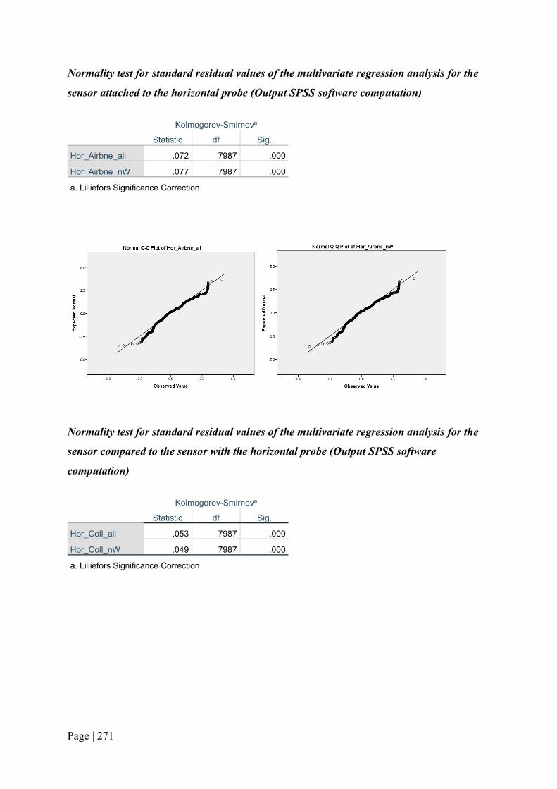
Page | 271
Normality test for standard residual values of the multivariate regression analysis for the
sensor attached to the horizontal probe (Output SPSS software computation)
Kolmogorov-Smirnova
Statistic df Sig.
Hor_Airbne_all .072 7987 .000
Hor_Airbne_nW .077 7987 .000
a. Lilliefors Significance Correction
Normality test for standard residual values of the multivariate regression analysis for the
sensor compared to the sensor with the horizontal probe (Output SPSS software
computation)
Kolmogorov-Smirnova
Statistic df Sig.
Hor_Coll_all .053 7987 .000
Hor_Coll_nW .049 7987 .000
a. Lilliefors Significance Correction

Page | 272
Data: Laboratory experiment for sensor with vertical sampling probe in wind tunnel using
4 variables (Output from R software computation).
Bootstrapping results for coefficient 95% confidence intervals
Bootstrapping analysis ‘interception’ Bootstrapping analysis ‘Raw Conc. PM10’
Bootstrapping analysis ‘Relative Humidity’ Bootstrapping analysis ‘Temperature’

Page | 273
Bootstrapping results for coefficient 95% confidence intervals
Bootstrapping analysis ‘Air speed’
ORDINARY NONPARAMETRIC BOOTSTRAP Call: boot(data = data, statistic = bs, R = 10000, formula = TSI_RM_PM10 ~ a1_RollMean_PM10 + avg_hum + avg_temp + Airspeed) Bootstrap Statistics : original bias std. error t1* 102.124644 0.0394381841 2.62073489 t2* 2.118898 0.0001339234 0.03169985 t3* -1.176318 -0.0004489518 0.02908638 t4* -1.261906 -0.0004929870 0.03151991 t5* 1.822717 0.0007841094 0.05382503 > boot.ci(results, type = "bca", index = 1) #intercept BOOTSTRAP CONFIDENCE INTERVAL CALCULATIONS Based on 10000 bootstrap replicates CALL : boot.ci(boot.out = results, type = "bca", index = 1) Intervals : Level BCa 95% ( 96.9, 107.2 ) Calculations and Intervals on Original Scale > boot.ci(results, type = "bca", index = 2) #coef 2 BOOTSTRAP CONFIDENCE INTERVAL CALCULATIONS Based on 10000 bootstrap replicates CALL : boot.ci(boot.out = results, type = "bca", index = 2) Intervals : Level BCa 95% ( 2.058, 2.183 ) Calculations and Intervals on Original Scale > boot.ci(results, type = "bca", index = 3) #coef 3 BOOTSTRAP CONFIDENCE INTERVAL CALCULATIONS Based on 10000 bootstrap replicates CALL : boot.ci(boot.out = results, type = "bca", index = 3)

Page | 274
Intervals : Level BCa 95% (-1.232, -1.119 ) Calculations and Intervals on Original Scale > boot.ci(results, type = "bca", index = 4) #coef 4 BOOTSTRAP CONFIDENCE INTERVAL CALCULATIONS Based on 10000 bootstrap replicates CALL : boot.ci(boot.out = results, type = "bca", index = 4) Intervals : Level BCa 95% (-1.322, -1.199 ) Calculations and Intervals on Original Scale > boot.ci(results, type = "bca", index = 5) #coef 5 BOOTSTRAP CONFIDENCE INTERVAL CALCULATIONS Based on 10000 bootstrap replicates CALL : boot.ci(boot.out = results, type = "bca", index = 5) Intervals : Level BCa 95% ( 1.716, 1.926 ) Calculations and Intervals on Original Scale
Data: Laboratory experiment for sensor compared against sensor with vertical sampling
probe in wind tunnel using 4 variables (Output from R software computation).
Bootstrapping results for coefficient 95% confidence intervals
Bootstrapping analysis ‘interception’ Bootstrapping analysis ‘Raw Conc. PM10’
Bootstrapping analysis ‘Relative Humidity’ Bootstrapping analysis ‘Temperature’

Page | 275
Bootstrapping results for coefficient 95% confidence intervals
Bootstrapping analysis ‘Air speed’
ORDINARY NONPARAMETRIC BOOTSTRAP Call: boot(data = data, statistic = bs, R = 10000, formula = TSI_RM_PM10 ~ a4_RollMean_PM10 + avg_hum + avg_temp + Airspeed) Bootstrap Statistics : original bias std. error t1* 57.0511038 2.921129e-03 2.743236221 t2* 0.1979099 2.918287e-05 0.002329849 t3* -0.6209442 -4.311184e-05 0.030703148 t4* -0.6387577 -4.507293e-05 0.033069371 t5* 1.1202046 1.389189e-04 0.049858652 > > #get 95% confidence intervals > boot.ci(results, type = "bca", index = 1) #intercept BOOTSTRAP CONFIDENCE INTERVAL CALCULATIONS Based on 10000 bootstrap replicates CALL : boot.ci(boot.out = results, type = "bca", index = 1)

Page | 276
Intervals : Level BCa 95% (51.69, 62.43 ) Calculations and Intervals on Original Scale > boot.ci(results, type = "bca", index = 2) #coef 2 BOOTSTRAP CONFIDENCE INTERVAL CALCULATIONS Based on 10000 bootstrap replicates CALL : boot.ci(boot.out = results, type = "bca", index = 2) Intervals : Level BCa 95% ( 0.1934, 0.2026 ) Calculations and Intervals on Original Scale > boot.ci(results, type = "bca", index = 3) #coef 3 BOOTSTRAP CONFIDENCE INTERVAL CALCULATIONS Based on 10000 bootstrap replicates CALL : boot.ci(boot.out = results, type = "bca", index = 3) Intervals : Level BCa 95% (-0.6808, -0.5608 ) Calculations and Intervals on Original Scale > boot.ci(results, type = "bca", index = 4) #coef 4 BOOTSTRAP CONFIDENCE INTERVAL CALCULATIONS Based on 10000 bootstrap replicates CALL : boot.ci(boot.out = results, type = "bca", index = 4) Intervals : Level BCa 95% (-0.7030, -0.5743 ) Calculations and Intervals on Original Scale > boot.ci(results, type = "bca", index = 5) #coef 5 BOOTSTRAP CONFIDENCE INTERVAL CALCULATIONS Based on 10000 bootstrap replicates CALL : boot.ci(boot.out = results, type = "bca", index = 5) Intervals : Level BCa 95% ( 1.022, 1.218 ) Calculations and Intervals on Original Scal

Page | 277
Data: Laboratory experiment for sensor with vertical sampling probe in wind tunnel using
5 variables (Output from R software computation).
Bootstrapping results for coefficient 95% confidence intervals
Bootstrapping analysis ‘interception’ Bootstrapping analysis ‘Raw Conc. PM10’
Bootstrapping analysis ‘Relative Humidity’ Bootstrapping analysis ‘Temperature’
Bootstrapping analysis ‘Air speed’ Bootstrapping analysis ‘Dust supply’

Page | 278
ORDINARY NONPARAMETRIC BOOTSTRAP Call: boot(data = data, statistic = bs, R = 10000, formula = TSI_rollmean_PM10 ~ a4_RollMean_PM10 + avg_hum + avg_temp + Ave_W + Airspeed) Bootstrap Statistics : original bias std. error t1* 57.39674705 -3.697117e-03 2.643501725 t2* 0.20118657 1.096343e-05 0.002250868 t3* -0.64251137 -4.015614e-06 0.029080252 t4* -0.66980533 7.212131e-06 0.031197059 t5* 0.03401256 5.414660e-05 0.002325753 t6* 1.38269919 6.488946e-04 0.046770980 > boot.ci(results, type = "bca", index = 1) #intercept BOOTSTRAP CONFIDENCE INTERVAL CALCULATIONS Based on 10000 bootstrap replicates CALL : boot.ci(boot.out = results, type = "bca", index = 1) Intervals : Level BCa 95% (52.37, 62.75 ) Calculations and Intervals on Original Scale > boot.ci(results, type = "bca", index = 2) #coef 2 BOOTSTRAP CONFIDENCE INTERVAL CALCULATIONS Based on 10000 bootstrap replicates CALL : boot.ci(boot.out = results, type = "bca", index = 2) Intervals : Level BCa 95% ( 0.1969, 0.2057 ) Calculations and Intervals on Original Scale > boot.ci(results, type = "bca", index = 3) #coef 3 BOOTSTRAP CONFIDENCE INTERVAL CALCULATIONS Based on 10000 bootstrap replicates CALL : boot.ci(boot.out = results, type = "bca", index = 3) Intervals : Level BCa 95% (-0.7014, -0.5873 ) Calculations and Intervals on Original Scale > boot.ci(results, type = "bca", index = 4) #coef 4 BOOTSTRAP CONFIDENCE INTERVAL CALCULATIONS Based on 10000 bootstrap replicates CALL : boot.ci(boot.out = results, type = "bca", index = 4) Intervals : Level BCa 95% (-0.7331, -0.6103 ) Calculations and Intervals on Original Scale > boot.ci(results, type = "bca", index = 5) #coef 5 BOOTSTRAP CONFIDENCE INTERVAL CALCULATIONS Based on 10000 bootstrap replicates CALL : boot.ci(boot.out = results, type = "bca", index = 5) Intervals : Level BCa

Page | 279
95% ( 0.0293, 0.0385 ) Calculations and Intervals on Original Scale > boot.ci(results, type = "bca", index = 6) #coef 6 BOOTSTRAP CONFIDENCE INTERVAL CALCULATIONS Based on 10000 bootstrap replicates CALL : boot.ci(boot.out = results, type = "bca", index = 6) Intervals : Level BCa 95% ( 1.291, 1.475 ) Calculations and Intervals on Original Scale
Data: Laboratory experiment for sensor compared against sensor with vertical sampling
probe in wind tunnel using 5 variables (Output from R software computation).
Bootstrapping results for coefficient 95% confidence intervals
Bootstrapping analysis ‘interception’ Bootstrapping analysis ‘Raw Conc. PM10’
Bootstrapping analysis ‘Relative Humidity’ Bootstrapping analysis ‘Temperature’

Page | 280
Bootstrapping results for coefficient 95% confidence intervals
Bootstrapping analysis ‘Air speed’ Bootstrapping analysis ‘Dust supply’
ORDINARY NONPARAMETRIC BOOTSTRAP Call: boot(data = data, statistic = bs, R = 10000, formula = TSI_rollmean_PM10 ~ a1_RollMean_PM10 + avg_hum + avg_temp + Ave_W + Airspeed) Bootstrap Statistics : original bias std. error t1* 155.22465297 2.405182e-02 3.939381915 t2* 2.06261694 1.649663e-04 0.036867929 t3* -1.79623717 -2.795953e-04 0.044407439 t4* -1.92171276 -2.933389e-04 0.047988977 t5* 0.02491539 1.341790e-06 0.002300596 t6* 3.04810155 4.196757e-04 0.081327813 > > #get 95% confidence intervals > boot.ci(results, type = "bca", index = 1) #intercept BOOTSTRAP CONFIDENCE INTERVAL CALCULATIONS Based on 10000 bootstrap replicates CALL : boot.ci(boot.out = results, type = "bca", index = 1) Intervals : Level BCa 95% (147.7, 163.0 ) Calculations and Intervals on Original Scale > boot.ci(results, type = "bca", index = 2) #coef 2 BOOTSTRAP CONFIDENCE INTERVAL CALCULATIONS Based on 10000 bootstrap replicates CALL : boot.ci(boot.out = results, type = "bca", index = 2) Intervals :

Page | 281
Level BCa 95% ( 1.989, 2.133 ) Calculations and Intervals on Original Scale > boot.ci(results, type = "bca", index = 3) #coef 3 BOOTSTRAP CONFIDENCE INTERVAL CALCULATIONS Based on 10000 bootstrap replicates CALL : boot.ci(boot.out = results, type = "bca", index = 3) Intervals : Level BCa 95% (-1.884, -1.711 ) Calculations and Intervals on Original Scale > boot.ci(results, type = "bca", index = 4) #coef 4 BOOTSTRAP CONFIDENCE INTERVAL CALCULATIONS Based on 10000 bootstrap replicates CALL : boot.ci(boot.out = results, type = "bca", index = 4) Intervals : Level BCa 95% (-2.015, -1.829 ) Calculations and Intervals on Original Scale > boot.ci(results, type = "bca", index = 5) #coef 5 BOOTSTRAP CONFIDENCE INTERVAL CALCULATIONS Based on 10000 bootstrap replicates CALL : boot.ci(boot.out = results, type = "bca", index = 5) Intervals : Level BCa 95% ( 0.0204, 0.0293 ) Calculations and Intervals on Original Scale > boot.ci(results, type = "bca", index = 6) #coef 6 BOOTSTRAP CONFIDENCE INTERVAL CALCULATIONS Based on 10000 bootstrap replicates CALL : boot.ci(boot.out = results, type = "bca", index = 6) Intervals : Level BCa 95% ( 2.89, 3.21 ) Calculations and Intervals on Original Scale

Page | 282
Section 5.3.3.4. Table 38, Table 40, Figure 59.
Data: Laboratory experiment for sensor with horizontal sampling probe in wind tunnel
using 5 variables (Output from R software computation).
Bootstrapping results for coefficient 95% confidence intervals
Bootstrapping analysis ‘interception’ Bootstrapping analysis ‘Raw Conc. PM10’
Bootstrapping analysis ‘Relative Humidity’ Bootstrapping analysis ‘Temperature’

Page | 283
Bootstrapping results for coefficient 95% confidence intervals
Bootstrapping analysis ‘Air speed’ Bootstrapping analysis ‘Dust supply’
ORDINARY NONPARAMETRIC BOOTSTRAP Call: boot(data = data, statistic = bs, R = 10000, formula = TSI_rollmean_PM10 ~ a1_RollMean_PM10 + avg_hum + avg_temp + airspeed + Ave_W) Bootstrap Statistics : original bias std. error t1* -2.58137263 -1.691979e-01 2.567505933 t2* 0.84913892 7.951166e-06 0.008871476 t3* 0.04516762 8.717255e-04 0.012436380 t4* -0.06982822 5.700890e-03 0.080023912 t5* 1.42916386 7.565323e-04 0.031756656 t6* -0.02221293 -5.841908e-04 0.008226684 > > #get 95% confidence intervals > boot.ci(results, type = "bca", index = 1) #intercept BOOTSTRAP CONFIDENCE INTERVAL CALCULATIONS Based on 10000 bootstrap replicates CALL : boot.ci(boot.out = results, type = "bca", index = 1) Intervals : Level BCa 95% (-6.543, 3.896 ) Calculations and Intervals on Original Scale > boot.ci(results, type = "bca", index = 2) #coef 2 BOOTSTRAP CONFIDENCE INTERVAL CALCULATIONS Based on 10000 bootstrap replicates CALL : boot.ci(boot.out = results, type = "bca", index = 2) Intervals : Level BCa 95% ( 0.8322, 0.8668 )

Page | 284
Calculations and Intervals on Original Scale > boot.ci(results, type = "bca", index = 3) #coef 3 BOOTSTRAP CONFIDENCE INTERVAL CALCULATIONS Based on 10000 bootstrap replicates CALL : boot.ci(boot.out = results, type = "bca", index = 3) Intervals : Level BCa 95% ( 0.0140, 0.0643 ) Calculations and Intervals on Original Scale > boot.ci(results, type = "bca", index = 4) #coef 4 BOOTSTRAP CONFIDENCE INTERVAL CALCULATIONS Based on 10000 bootstrap replicates CALL : boot.ci(boot.out = results, type = "bca", index = 4) Intervals : Level BCa 95% (-0.2739, 0.0552 ) Calculations and Intervals on Original Scale > boot.ci(results, type = "bca", index = 5) #coef 5 BOOTSTRAP CONFIDENCE INTERVAL CALCULATIONS Based on 10000 bootstrap replicates CALL : boot.ci(boot.out = results, type = "bca", index = 5) Intervals : Level BCa 95% ( 1.367, 1.491 ) Calculations and Intervals on Original Scale > boot.ci(results, type = "bca", index = 6) #coef 6 BOOTSTRAP CONFIDENCE INTERVAL CALCULATIONS Based on 10000 bootstrap replicates CALL : boot.ci(boot.out = results, type = "bca", index = 6) Intervals : Level BCa 95% (-0.0386, -0.0066 ) Calculations and Intervals on Original Scale

Page | 285
Data: Laboratory experiment for the sensor compared to the sensor with horizontal
sampling probe in wind tunnel using 5 variables (Output from R software computation).
Bootstrapping results for coefficient 95% confidence intervals
Bootstrapping analysis ‘interception’ Bootstrapping analysis ‘Raw Conc. PM10’
Bootstrapping analysis ‘Relative Humidity’ Bootstrapping analysis ‘Temperature’
Bootstrapping analysis ‘Air speed’ Bootstrapping analysis ‘Dust supply’

Page | 286
ORDINARY NONPARAMETRIC BOOTSTRAP Call: boot(data = data, statistic = bs, R = 10000, formula = TSI_rollmean_PM10 ~ a4_RollMean_PM10 + avg_hum + avg_temp + airspeed + Ave_W) Bootstrap Statistics : original bias std. error t1* -7.55639666 -2.569456e-01 3.374217286 t2* 0.32645257 1.563026e-05 0.003512197 t3* 0.16602152 1.183960e-03 0.016192865 t4* -0.11071278 7.796325e-03 0.104853242 t5* -0.04045237 9.092255e-04 0.033009502 t6* 0.04689453 2.538246e-04 0.005084780 > > #get 95% confidence intervals > boot.ci(results, type = "bca", index = 1) #intercept BOOTSTRAP CONFIDENCE INTERVAL CALCULATIONS Based on 10000 bootstrap replicates CALL : boot.ci(boot.out = results, type = "bca", index = 1) Intervals : Level BCa 95% (-12.209, 2.715 ) Calculations and Intervals on Original Scale > boot.ci(results, type = "bca", index = 2) #coef 2 BOOTSTRAP CONFIDENCE INTERVAL CALCULATIONS Based on 10000 bootstrap replicates CALL : boot.ci(boot.out = results, type = "bca", index = 2) Intervals : Level BCa 95% ( 0.3198, 0.3336 ) Calculations and Intervals on Original Scale > boot.ci(results, type = "bca", index = 3) #coef 3 BOOTSTRAP CONFIDENCE INTERVAL CALCULATIONS Based on 10000 bootstrap replicates CALL : boot.ci(boot.out = results, type = "bca", index = 3) Intervals : Level BCa 95% ( 0.1151, 0.1883 ) Calculations and Intervals on Original Scale > boot.ci(results, type = "bca", index = 4) #coef 4 BOOTSTRAP CONFIDENCE INTERVAL CALCULATIONS Based on 10000 bootstrap replicates CALL : boot.ci(boot.out = results, type = "bca", index = 4) Intervals : Level BCa 95% (-0.4392, 0.0335 )

Page | 287
Calculations and Intervals on Original Scale > boot.ci(results, type = "bca", index = 5) #coef 5 BOOTSTRAP CONFIDENCE INTERVAL CALCULATIONS Based on 10000 bootstrap replicates CALL : boot.ci(boot.out = results, type = "bca", index = 5) Intervals : Level BCa 95% (-0.1080, 0.0203 ) Calculations and Intervals on Original Scale > boot.ci(results, type = "bca", index = 6) #coef 6 BOOTSTRAP CONFIDENCE INTERVAL CALCULATIONS Based on 10000 bootstrap replicates CALL : boot.ci(boot.out = results, type = "bca", index = 6) Intervals : Level BCa 95% ( 0.0371, 0.0570 ) Calculations and Intervals on Original Scale
Data: Laboratory experiment for sensor with the horizontal sampling probe in the wind
tunnel using 4 variables (Output from R software computation).
Bootstrapping results for coefficient 95% confidence intervals
Bootstrapping analysis ‘interception’ Bootstrapping analysis ‘Raw Conc. PM10’

Page | 288
Bootstrapping results for coefficient 95% confidence intervals
Bootstrapping analysis ‘Relative Humidity’ Bootstrapping analysis ‘Temperature’
Bootstrapping analysis ‘Air speed’
ORDINARY NONPARAMETRIC BOOTSTRAP Call: boot(data = data, statistic = bs, R = 10000, formula = TSI_rollmean_PM10 ~ a4_RollMean_PM10 + avg_hum + avg_temp + airspeed + Ave_W) Bootstrap Statistics : original bias std. error t1* -7.55639666 -2.569456e-01 3.374217286 t2* 0.32645257 1.563026e-05 0.003512197 t3* 0.16602152 1.183960e-03 0.016192865 t4* -0.11071278 7.796325e-03 0.104853242 t5* -0.04045237 9.092255e-04 0.033009502 t6* 0.04689453 2.538246e-04 0.005084780 > > #get 95% confidence intervals > boot.ci(results, type = "bca", index = 1) #intercept > results <- boot(data = data, statistic = bs, R = 10000, formula = TSI_rollmean_PM10 ~ a1_RollMean_PM10 + avg_hum + avg_temp + airspeed)

Page | 289
> > #view results > results ORDINARY NONPARAMETRIC BOOTSTRAP Call: boot(data = data, statistic = bs, R = 10000, formula = TSI_rollmean_PM10 ~ a1_RollMean_PM10 + avg_hum + avg_temp + airspeed) Bootstrap Statistics : original bias std. error t1* -3.32435602 -1.713389e-01 2.54648997 t2* 0.84564852 -5.952109e-05 0.00901663 t3* 0.04734296 7.944425e-04 0.01234922 t4* -0.06451610 5.389901e-03 0.08015971 t5* 1.40946281 9.437095e-04 0.03190621 > > #get 95% confidence intervals > boot.ci(results, type = "bca", index = 1) #intercept BOOTSTRAP CONFIDENCE INTERVAL CALCULATIONS Based on 10000 bootstrap replicates CALL : boot.ci(boot.out = results, type = "bca", index = 1) Intervals : Level BCa 95% (-7.302, 2.932 ) Calculations and Intervals on Original Scale > boot.ci(results, type = "bca", index = 2) #coef 2 BOOTSTRAP CONFIDENCE INTERVAL CALCULATIONS Based on 10000 bootstrap replicates CALL : boot.ci(boot.out = results, type = "bca", index = 2) Intervals : Level BCa 95% ( 0.8285, 0.8636 ) Calculations and Intervals on Original Scale > boot.ci(results, type = "bca", index = 3) #coef 3 BOOTSTRAP CONFIDENCE INTERVAL CALCULATIONS Based on 10000 bootstrap replicates CALL : boot.ci(boot.out = results, type = "bca", index = 3) Intervals : Level BCa 95% ( 0.0161, 0.0662 ) Calculations and Intervals on Original Scale > boot.ci(results, type = "bca", index = 4) #coef 4 BOOTSTRAP CONFIDENCE INTERVAL CALCULATIONS Based on 10000 bootstrap replicates CALL : boot.ci(boot.out = results, type = "bca", index = 4) Intervals :

Page | 290
Level BCa 95% (-0.2563, 0.0632 ) Calculations and Intervals on Original Scale > boot.ci(results, type = "bca", index = 5) #coef 5 BOOTSTRAP CONFIDENCE INTERVAL CALCULATIONS Based on 10000 bootstrap replicates CALL : boot.ci(boot.out = results, type = "bca", index = 5) Intervals : Level BCa 95% ( 1.347, 1.472 ) Calculations and Intervals on Original Scale
Data: Laboratory experiment for the sensor compared to the sensor with the horizontal
sampling probe in the wind tunnel using 5 variables (Output from R software
computation).
Bootstrapping results for coefficient 95% confidence intervals
Bootstrapping analysis ‘interception’ Bootstrapping analysis ‘Raw Conc. PM10’

Page | 291
Bootstrapping results for coefficient 95% confidence intervals
Bootstrapping analysis ‘Relative
Humidity’
Bootstrapping analysis ‘Temperature’
Bootstrapping analysis ‘Air speed’
ORDINARY NONPARAMETRIC BOOTSTRAP Call: boot(data = data, statistic = bs, R = 10000, formula = TSI_rollmean_PM10 ~ a4_RollMean_PM10 + avg_hum + avg_temp + airspeed) Bootstrap Statistics : original bias std. error t1* -6.15081936 -0.2564259796 3.313407962 t2* 0.32745719 -0.0000501184 0.003455455 t3* 0.16327786 0.0012017954 0.015943226 t4* -0.11757606 0.0080142097 0.103577126 t5* -0.01086386 0.0012187987 0.032857865 > > #get 95% confidence intervals > boot.ci(results, type = "bca", index = 1) #intercept BOOTSTRAP CONFIDENCE INTERVAL CALCULATIONS Based on 10000 bootstrap replicates

Page | 292
CALL : boot.ci(boot.out = results, type = "bca", index = 1) Intervals : Level BCa 95% (-10.685, 4.006 ) Calculations and Intervals on Original Scale > boot.ci(results, type = "bca", index = 2) #coef 2 BOOTSTRAP CONFIDENCE INTERVAL CALCULATIONS Based on 10000 bootstrap replicates CALL : boot.ci(boot.out = results, type = "bca", index = 2) Intervals : Level BCa 95% ( 0.3210, 0.3344 ) Calculations and Intervals on Original Scale > boot.ci(results, type = "bca", index = 3) #coef 3 BOOTSTRAP CONFIDENCE INTERVAL CALCULATIONS Based on 10000 bootstrap replicates CALL : boot.ci(boot.out = results, type = "bca", index = 3) Intervals : Level BCa 95% ( 0.1145, 0.1852 ) Calculations and Intervals on Original Scale > boot.ci(results, type = "bca", index = 4) #coef 4 BOOTSTRAP CONFIDENCE INTERVAL CALCULATIONS Based on 10000 bootstrap replicates CALL : boot.ci(boot.out = results, type = "bca", index = 4) Intervals : Level BCa 95% (-0.4329, 0.0256 ) Calculations and Intervals on Original Scale > boot.ci(results, type = "bca", index = 5) #coef 5 BOOTSTRAP CONFIDENCE INTERVAL CALCULATIONS Based on 10000 bootstrap replicates CALL : boot.ci(boot.out = results, type = "bca", index = 5) Intervals : Level BCa 95% (-0.0781, 0.0508 ) Calculations and Intervals on Original Scale

Page | 293
Section 6.2.1.4. Table 47 and Table 48.
Data: Linear regression analysis results with p-values obtained for models generated with
data collected with the TSI DRX and the collocated modules using corrected
concentrations and field data for Test 1, Test 2, Test 3, and Test 2 (Output from Excel).
Flight 1 – 15s moving average Corrected Concentration
SUMMARY OUTPUT
Regression Statistics
Multiple R 0.783928 R Square 0.614543 Adjusted R Square 0.610528 Standard Error 210.8251
Observations 486
Coefficients Standard
Error t Stat P-value Lower 95%
Upper 95%
Lower 95.0%
Upper 95.0%
Intercept 3527.905 1013.563 3.480695 0.000546 1536.335 5519.474 1536.335 5519.474
windspeed -28.9207 11.59517 -2.4942 0.012959 -51.7043 -6.13716 -51.7043 -6.13716 15rollM_Corr_ ave_PM10 (ug/m3)_Tr 25.56809 0.929618 27.50387 1.1E-100 23.74146 27.39471 23.74146 27.39471
Humidity (%)_Tr -53.0595 14.84576 -3.57405 0.000387 -82.2303 -23.8888 -82.2303 -23.8888
Temp_Tr -63.276 21.99855 -2.87637 0.004202 -106.501 -20.0506 -106.501 -20.0506
corr weight 2 (ug/s) 0.001702 0.000569 2.991476 0.002919 0.000584 0.00282 0.000584 0.00282
Flight 1 – 15s moving average Raw Concentration
SUMMARY OUTPUT
Regression Statistics
Multiple R 0.818832 R Square 0.670485 Adjusted R Square 0.667053 Standard Error 194.9269
Observations 486

Page | 294
Coefficients Standard
Error t Stat P-value Lower 95%
Upper 95%
Lower 95.0%
Upper 95.0%
Intercept 2916.909 936.6151 3.114309 0.001954 1076.537 4757.281 1076.537 4757.281
windspeed -32.4032 10.72415 -3.02151 0.002649 -53.4752 -11.3311 -53.4752 -11.3311 15rollM_ave_PM10 (ug/m3)_Tr 5.346699 0.171993 31.08665 4.8E-117 5.008746 5.684652 5.008746 5.684652
Humidity (%)_Tr -17.7818 13.70376 -1.29759 0.195052 -44.7086 9.144934 -44.7086 9.144934
Temp_Tr -78.9391 20.35928 -3.8773 0.00012 -118.943 -38.9348 -118.943 -38.9348
corr weight 2 (ug/s) 0.000159 0.000523 0.303261 0.761822 -0.00087 0.001186 -0.00087 0.001186
Flight 1 – 20s moving average Corrected Concentration
SUMMARY OUTPUT
Regression Statistics
Multiple R 0.800798 R Square 0.641278 Adjusted R Square 0.637541 Standard Error 179.517
Observations 486
Coefficients Standard
Error t Stat P-value Lower 95%
Upper 95%
Lower 95.0%
Upper 95.0%
Intercept 3806.125 863.9418 4.405534 1.3E-05 2108.55 5503.701 2108.55 5503.701
windspeed -15.2355 9.869943 -1.54362 0.123339 -34.6291 4.158178 -34.6291 4.158178 20rollM_Corr_ ave_PM10 (ug/m3)_Tr 25.71997 0.883748 29.1033 4.6E-108 23.98348 27.45646 23.98348 27.45646
Humidity (%)_Tr -65.4088 12.69417 -5.15267 3.76E-07 -90.3518 -40.4658 -90.3518 -40.4658
Temp_Tr -55.9408 18.72846 -2.98694 0.002962 -92.7407 -19.1409 -92.7407 -19.1409
corr weight 2 (ug/s) 0.002227 0.000488 4.561442 6.46E-06 0.001267 0.003186 0.001267 0.003186
Flight 1 – 20s moving average Raw Concentration
SUMMARY OUTPUT
Regression Statistics
Multiple R 0.900914 R Square 0.811646 Adjusted R Square 0.809684 Standard Error 130.0811
Observations 486

Page | 295
Coefficients Standard
Error t Stat P-value Lower 95%
Upper 95%
Lower 95.0%
Upper 95.0%
Intercept 1225.689 625.4752 1.959612 0.050619 -3.31914 2454.696 -3.31914 2454.696
windspeed -20.4837 7.151199 -2.86438 0.004361 -34.5352 -6.4322 -34.5352 -6.4322 20rollM_ave_PM10 (ug/m3)_Tr 6.200095 0.137028 45.24694 2.9E-175 5.930846 6.469344 5.930846 6.469344
Humidity (%)_Tr 0.900274 9.159949 0.098284 0.921748 -17.0983 18.89883 -17.0983 18.89883
Temp_Tr -46.4553 13.56762 -3.42398 0.00067 -73.1146 -19.796 -73.1146 -19.796
corr weight 2 (ug/s) -9.5E-05 0.000349 -0.27317 0.78484 -0.00078 0.00059 -0.00078 0.00059
Flight 1 – 30s moving average Corrected Concentration
SUMMARY OUTPUT
Regression Statistics
Multiple R 0.778481 R Square 0.606033 Adjusted R Square 0.60192 Standard Error 157.3604
Observations 485
Coefficients Standard
Error t Stat P-value Lower 95%
Upper 95%
Lower 95.0%
Upper 95.0%
Intercept 4339.276 768.0659 5.649615 2.76E-08 2830.081 5848.471 2830.081 5848.471
windspeed 8.637793 8.747622 0.987445 0.323923 -8.55066 25.82625 -8.55066 25.82625 30rollM_Corr_ ave_PM10 (ug/m3)_Tr 23.82821 0.885359 26.91362 7.22E-98 22.08855 25.56788 22.08855 25.56788
Humidity (%)_Tr -84.9574 11.34485 -7.48863 3.37E-13 -107.249 -62.6655 -107.249 -62.6655
Temp_Tr -46.3905 16.57765 -2.79838 0.005343 -78.9645 -13.8166 -78.9645 -13.8166
corr weight 2 (ug/s) 0.002943 0.000438 6.721793 5.12E-11 0.002083 0.003804 0.002083 0.003804
Flight 1 – 30s moving average Raw Concentration
SUMMARY OUTPUT
Regression Statistics
Multiple R 0.94086 R Square 0.885217 Adjusted R Square 0.884018 Standard Error 84.93851
Observations 485

Page | 296
Coefficients Standard
Error t Stat P-value Lower 95%
Upper 95%
Lower 95.0%
Upper 95.0%
Intercept -32.4464 413.8607 -0.0784 0.937543 -845.653 780.7605 -845.653 780.7605
windspeed -11.9311 4.693903 -2.54184 0.011341 -21.1543 -2.70796 -21.1543 -2.70796 30rollM_ave_PM10 (ug/m3)_Tr 6.584244 0.108965 60.42514 3.2E-226 6.370135 6.798354 6.370135 6.798354
Humidity (%)_Tr 14.21384 6.030113 2.357143 0.018818 2.365096 26.06258 2.365096 26.06258
Temp_Tr -21.1338 8.95135 -2.36096 0.018627 -38.7225 -3.54499 -38.7225 -3.54499
corr weight 2 (ug/s) -0.00024 0.000228 -1.06177 0.288873 -0.00069 0.000206 -0.00069 0.000206
Flight 2 – 15s moving average Corrected Concentration
SUMMARY OUTPUT
Regression Statistics
Multiple R 0.684503 R Square 0.468544 Adjusted R Square 0.462546 Standard Error 8.030804
Observations 449
Coefficients Standard
Error t Stat P-value Lower 95%
Upper 95%
Lower 95.0%
Upper 95.0%
Intercept -734.977 62.00691 -11.8531 2.43E-28 -856.842 -613.113 -856.842 -613.113
U (m/s) -5.05248 0.589618 -8.56908 1.75E-16 -6.21128 -3.89368 -6.21128 -3.89368
Humidity (%)_Tr 6.07913 0.898769 6.76384 4.26E-11 4.312749 7.845511 4.312749 7.845511
Temp_Tr 15.64985 1.077411 14.52543 2.25E-39 13.53238 17.76733 13.53238 17.76733 15 rollM_Corr_ PM10(ug/m3)_Tr 4.844469 0.554297 8.73984 4.86E-17 3.75509 5.933848 3.75509 5.933848
W Al2O3 ug 0.000301 4.42E-05 6.808722 3.22E-11 0.000214 0.000388 0.000214 0.000388
Flight 2 – 15s moving average Raw Concentration
SUMMARY OUTPUT
Regression Statistics
Multiple R 0.796239 R Square 0.633996 Adjusted R Square 0.629865 Standard Error 6.66451
Observations 449

Page | 297
Coefficients Standard
Error t Stat P-value Lower 95%
Upper 95%
Lower 95.0%
Upper 95.0%
Intercept -311.392 54.61432 -5.70166 2.17E-08 -418.728 -204.057 -418.728 -204.057 15_ave_PM10 (ug/m3)_Tr 1.766915 0.100165 17.64009 3.87E-53 1.570058 1.963772 1.570058 1.963772
Humidity (%)_Tr 2.740218 0.75715 3.619122 0.00033 1.252166 4.22827 1.252166 4.22827
Temp_Tr 7.365016 1.038673 7.090798 5.3E-12 5.323679 9.406354 5.323679 9.406354
U (m/s) 0.532036 0.328996 1.617149 0.106558 -0.11455 1.178623 -0.11455 1.178623
W Al2O3 ug 0.000119 3.84E-05 3.090416 0.002125 4.32E-05 0.000194 4.32E-05 0.000194
Flight 2 – 20s moving average Corrected Concentration
SUMMARY OUTPUT
Regression Statistics
Multiple R 0.737347
R Square 0.543681
Adjusted R Square 0.538531
Standard Error 6.456013
Observations 449
Coefficients Standard
Error t Stat P-value Lower 95%
Upper 95%
Lower 95.0%
Upper 95.0%
Intercept -670.732 50.62962 -13.2478 5.57E-34 -770.236 -571.228 -770.236 -571.228
U (m/s) -3.76176 0.503463 -7.47177 4.26E-13 -4.75123 -2.77229 -4.75123 -2.77229
Humidity (%)_Tr 4.892376 0.728224 6.718232 5.67E-11 3.461174 6.323579 3.461174 6.323579
Temp_Tr 15.79096 0.86126 18.33472 2.77E-56 14.09829 17.48362 14.09829 17.48362 20 rollM_Corr_ PM10(ug/m3)_Tr 3.687562 0.510963 7.21688 2.33E-12 2.683348 4.691775 2.683348 4.691775
W Al2O3 ug 0.000352 3.55E-05 9.91355 4.68E-21 0.000282 0.000422 0.000282 0.000422
Flight 2 – 20s moving average Raw Concentration
SUMMARY OUTPUT
Regression Statistics
Multiple R 0.862043
R Square 0.743118
Adjusted R Square 0.740219
Standard Error 4.843921
Observations 449

Page | 298
Coefficients Standard
Error t Stat P-value Lower 95%
Upper 95%
Lower 95.0%
Upper 95.0%
Intercept -279.206 39.88823 -6.99971 9.55E-12 -357.6 -200.812 -357.6 -200.812 20_ave_PM10 (ug/m3)_Tr 1.883923 0.090177 20.89147 5.82E-68 1.706696 2.06115 1.706696 2.06115
Humidity (%)_Tr 2.42547 0.545488 4.446422 1.11E-05 1.353404 3.497535 1.353404 3.497535
Temp_Tr 6.600114 0.794529 8.306955 1.21E-15 5.0386 8.161627 5.0386 8.161627
U (m/s) 0.738824 0.24196 3.053495 0.002398 0.263292 1.214357 0.263292 1.214357
W Al2O3 ug 9.96E-05 2.95E-05 3.380058 0.000789 4.17E-05 0.000157 4.17E-05 0.000157
Flight 2 – 30s moving average Corrected Concentration
SUMMARY OUTPUT
Regression Statistics
Multiple R 0.770225
R Square 0.593246
Adjusted R Square 0.588655
Standard Error 5.203282
Observations 449
Coefficients Standard
Error t Stat P-value Lower 95%
Upper 95%
Lower 95.0%
Upper 95.0%
Intercept -413.483 41.98537 -9.84827 7.98E-21 -495.999 -330.968 -495.999 -330.968
U (m/s) -1.55506 0.398489 -3.9024 0.00011 -2.33823 -0.7719 -2.33823 -0.7719
Humidity (%)_Tr 1.117164 0.591786 1.887783 0.059708 -0.04589 2.280221 -0.04589 2.280221
Temp_Tr 13.54739 0.692341 19.56751 6.68E-62 12.18671 14.90807 12.18671 14.90807 30 rollM_Corr_ PM10(ug/m3)_Tr 1.397795 0.441344 3.167136 0.001646 0.530408 2.265182 0.530408 2.265182
W Al2O3 ug 0.000434 2.87E-05 15.15132 4.42E-42 0.000378 0.000491 0.000378 0.000491
Flight 2 – 30s moving average Raw Concentration
SUMMARY OUTPUT
Regression Statistics
Multiple R 0.89665831
R Square 0.80399612
Adjusted R Square 0.80178388
Standard Error 3.61196606
Observations 449

Page | 299
Coefficients Standard
Error t Stat P-value Lower 95%
Upper 95%
Lower 95.0%
Upper 95.0%
Intercept -194.93102 28.7159625 -6.78825 3.66E-11 -251.367 -138.495 -251.367 -138.495 30_ave_PM10 (ug/m3)_Tr 1.87574705 0.08412645 22.29676 2.15E-74 1.710411 2.041084 1.710411 2.041084
Humidity (%)_Tr 1.07255589 0.40274207 2.663133 0.008024 0.281033 1.864078 0.281033 1.864078
Temp_Tr 5.58126869 0.59560604 9.370739 3.7E-19 4.410704 6.751833 4.410704 6.751833
U (m/s) 0.83637685 0.1821422 4.591889 5.73E-06 0.478407 1.194347 0.478407 1.194347
W Al2O3 ug 0.00014995 2.3414E-05 6.404197 3.86E-10 0.000104 0.000196 0.000104 0.000196
Flight 3 – 15s moving average Corrected Concentration
SUMMARY OUTPUT
Regression Statistics
Multiple R 0.6414416
R Square 0.4114473
Adjusted R Square 0.4020455
Standard Error 72.85538
Observations 319
Coefficients Standard
Error t Stat P-value Lower 95%
Upper 95%
Lower 95.0%
Upper 95.0%
Intercept -3205.98 413.895 -7.745 1.33E-13 -4020.3 -2391.6 -4020.3 -2391.6 15 rollM_Corr Mod _ave_nW_PM10 (ug/m3)_Tr 16.9467 1.48477 11.413 1.84E-25 14.0253 19.8681 14.0253 19.8681
U (m/s) -70.6009 9.41972 -7.495 6.86E-13 -89.134 -52.066 -89.139 -52.066
Humidity (%)_Tr 26.7777 4.39672 6.0903 3.3E-09 18.126 35.4285 18.1268 35.4285
Temp_Tr 83.0736 12.5653 6.6113 1.64E-10 58.350 107.796 58.3503 107.796
W Al2O3 (ug) -0.00279 0.00041 -6.730 8.07E-11 -0.003 -0.001 -0.003 -0.001
Flight 3 – 15s moving average Raw Concentration
SUMMARY OUTPUT
Regression Statistics
Multiple R 0.64378614
R Square 0.41446059
Adjusted R Square 0.40510693
Standard Error 72.6686394
Observations 319

Page | 300
Coefficients Standard
Error t Stat P-value Lower 95%
Upper 95%
Lower 95.0%
Upper 95.0%
Intercept -2471.6775 421.9406 -5.85788 1.19E-08 -3301.88 -1641.48 -3301.88 -1641.48
U (m/s) -58.775294 9.4941 -6.19072 1.88E-09 -77.4556 -40.095 -77.4556 -40.095
Humidity (%)_Tr 17.7397959 4.565728 3.885425 0.000125 8.756397 26.7232 8.756397 26.7232
Temp_Tr 80.139465 12.56013 6.380464 6.35E-10 55.4265 104.8524 55.4265 104.8524 15 rollM_ave_ PM10 (ug/m3)_Tr 3.39613631 0.294978 11.5132 8.2E-26 2.815747 3.976526 2.815747 3.976526
Ave W Al2O3(ug) -0.0029014 0.000416 -6.97709 1.8E-11 -0.00372 -0.00208 -0.00372 -0.00208
Flight 3 – 20s moving average Corrected Concentration
SUMMARY OUTPUT
Regression Statistics
Multiple R 0.6783543
R Square 0.4601645
Adjusted R Square 0.4515409
Standard Error 56.290629
Observations 319
Coefficients Standard
Error t Stat P-value Lower 95%
Upper 95%
Lower 95.0%
Upper 95.0%
Intercept -2758.832 323.7074 -8.52261 6.71E-16 -3395.75 -2121.91 -3395.75 -2121.91 20 rollM_Corr Mod_ ave_nW_PM10 (ug/m3)_Tr 16.411997 1.397107 11.74713 1.21E-26 13.66309 19.1609 13.66309 19.1609
U (m/s) -60.27389 7.345268 -8.20581 6.03E-15 -74.7262 -45.8215 -74.7262 -45.8215
Humidity (%)_Tr 24.405129 3.461372 7.05071 1.14E-11 17.59463 31.21563 17.59463 31.21563
Temp_Tr 67.556241 9.86599 6.847386 3.98E-11 48.14419 86.96829 48.14419 86.96829
W Al2O3 (ug) -0.002167 0.000325 -6.67356 1.14E-10 -0.00281 -0.00153 -0.00281 -0.00153
Flight 3 – 20s moving average Raw Concentration
SUMMARY OUTPUT
Regression Statistics
Multiple R 0.6862564
R Square 0.47094785
Adjusted R Square 0.46249654
Standard Error 55.7255828
Observations 319

Page | 301
Coefficients Standard
Error t Stat P-value Lower 95%
Upper 95%
Lower 95.0%
Upper 95.0%
Intercept -
2031.92866 335.4102 -6.05804 3.95E-09 -2691.87 -1371.98 -2691.87 -1371.98 20 rollM_ave_ PM10 (ug/m3)_Tr 3.3832665 0.278869 12.13209 5.03E-28 2.834571 3.931962 2.834571 3.931962
U (m/s) -49.292646 7.447699 -6.61851 1.57E-10 -63.9465 -34.6388 -63.9465 -34.6388
Humidity (%)_Tr 15.2172797 3.674662 4.141137 4.45E-05 7.987118 22.44744 7.987118 22.44744
Temp_Tr 64.9124046 9.803869 6.621101 1.55E-10 45.62259 84.20222 45.62259 84.20222
Ave W Al2O3(ug) -0.0023258 0.000324 -7.17292 5.34E-12 -0.00296 -0.00169 -0.00296 -0.00169
Flight 3 – 30s moving average Corrected Concentration
SUMMARY OUTPUT
Regression Statistics
Multiple R 0.721672251
R Square 0.520810837
Adjusted R Square 0.513156059
Standard Error 39.82342358
Observations 319
Coefficients Standard
Error t Stat P-value Lower 95%
Upper 95%
Lower 95.0%
Upper 95.0%
Intercept -2383.60083 245.9684 -9.69068 1.36E-19 -2867.56 -1899.64 -2867.56 -1899.64
U (m/s) -48.5454838 5.565887 -8.72197 1.64E-16 -59.4968 -37.5942 -59.4968 -37.5942
Humidity (%)_Tr 24.72244947 2.62525 9.417177 1.05E-18 19.55708 29.88782 19.55708 29.88782
Temp_Tr 52.22369928 7.62529 6.848749 3.95E-11 37.22039 67.22701 37.22039 67.22701 30 rollM_Corr Mod_ ave_nW_PM10 (ug/m3)_Tr 13.2824427 1.394963 9.521716 4.83E-19 10.53775 16.02713 10.53775 16.02713
W Al2O3 (ug) -0.0013793 0.000235 -5.87495 1.08E-08 -0.00184 -0.00092 -0.00184 -0.00092
Flight 3 – 30s moving average Raw Concentration
SUMMARY OUTPUT
Regression Statistics
Multiple R 0.7328828
R Square 0.5371172
Adjusted R Square 0.5297229
Standard Error 39.139982
Observations 319

Page | 302
Coefficients Standard
Error t Stat P-value Lower 95%
Upper 95%
Lower 95.0%
Upper 95.0%
Intercept -1727.4932 270.5889 -6.3842 6.21E-10 -2259.9 -1195.09 -2259.9 -1195.09
U (m/s) -39.100824 5.827576 -6.70962 9.15E-11 -50.567 -27.6346 -50.567 -27.6346
Humidity (%)_Tr 16.57341 2.968553 5.582993 5.13E-08 10.73257 22.41425 10.73257 22.41425
Temp_Tr 48.573297 7.574531 6.412713 5.27E-10 33.66986 63.47673 33.66986 63.47673 30 rollM_ave_ PM10 (ug/m3)_Tr 2.8388203 0.277195 10.24125 2.03E-21 2.29342 3.384221 2.29342 3.384221
Ave W Al2O3(ug) -0.0015767 0.000236 -6.68266 1.07E-10 -0.00204 -0.00111 -0.00204 -0.00111
Flight 4 – 15s moving average Corrected Concentration
SUMMARY OUTPUT
Regression Statistics
Multiple R 0.655710092
R Square 0.429955725
Adjusted R Square 0.424289281
Standard Error 69.36201595
Observations 509
Coefficients Standard
Error t Stat P-value Lower 95%
Upper 95%
Lower 95.0%
Upper 95.0%
Intercept -2603.77672 645.5476 -4.03344 6.35E-05 -3872.08 -1335.47 -3872.08 -1335.47
weight Al2O3(ug) 0.000344469 0.000143 2.412546 0.016198 6.39E-05 0.000625 6.39E-05 0.000625
U (m/s) -9.77345376 2.880926 -3.39247 0.000747 -15.4336 -4.11332 -15.4336 -4.11332 15rollM_Corr_ nW_ave_PM10 (ug/m3)_Tr 14.05876535 0.874893 16.06913 3.38E-47 12.33987 15.77766 12.33987 15.77766
Humidity (%)_Tr 14.64093645 4.908625 2.982696 0.002996 4.997004 24.28487 4.997004 24.28487
Temp_Tr 69.26305097 17.94346 3.860072 0.000128 34.00968 104.5164 34.00968 104.5164
Flight 4 – 15s moving average Raw Concentration
SUMMARY OUTPUT
Regression Statistics
Multiple R 0.6625821
R Square 0.439015
Adjusted R Square 0.4334386
Standard Error 68.808649
Observations 509

Page | 303
Coefficients Standard
Error t Stat P-value Lower 95%
Upper 95%
Lower 95.0%
Upper 95.0%
Intercept -2244.417 645.052 -3.47944 0.000546 -3511.74 -977.089 -3511.74 -977.089
U (m/s) 3.3792752 2.751539 1.22814 0.219969 -2.02665 8.785201 -2.02665 8.785201
Humidity (%)_Tr 9.471732 4.923631 1.923729 0.054953 -0.20168 19.14515 -0.20168 19.14515
Temp_Tr 71.856537 17.73675 4.05128 5.9E-05 37.0093 106.7038 37.0093 106.7038 15 rollM_ave_ PM10 (ug/m3)_Tr 2.8125439 0.171005 16.44718 5.93E-49 2.476573 3.148515 2.476573 3.148515
weight Al2O3(ug) 0.0003783 0.000142 2.667169 0.007896 9.96E-05 0.000657 9.96E-05 0.000657
Flight 4 – 20s moving average Corrected Concentration
SUMMARY OUTPUT
Regression Statistics
Multiple R 0.687267
R Square 0.472336
Adjusted R Square 0.46709
Standard Error 57.31269
Observations 509
Coefficients Standard
Error t Stat P-value Lower 95%
Upper 95%
Lower 95.0%
Upper 95.0%
Intercept -2453.51 543.85 -4.511 8.03E-06 -3522.01 -1385 -3522.01 -1385 20rollM_Corr_ nW_ave_PM10 (ug/m3)_Tr 14.3493 0.8822 16.263 4.23E-48 12.61588 16.08271 12.61588 16.082
U (m/s) -9.67855 2.414 -4.008 7.05E-05 -14.4227 -4.93441 -14.4227 -4.934
Humidity (%)_Tr 13.60749 4.0956 3.3224 0.000957 5.560826 21.65415 5.560826 21.654
Temp_Tr 65.05232 15.247 4.2665 2.37E-05 35.09652 95.00813 35.09652 95.008
weight Al2O3(ug) 0.000257 0.0001 2.1815 0.029605 2.55E-05 0.000488 2.55E-05 0.0004
Flight 4 – 20s moving average Raw Concentration
SUMMARY OUTPUT
Regression Statistics
Multiple R 0.6986462
R Square 0.4881065
Adjusted R Square 0.4830181
Standard Error 56.449709
Observations 509

Page | 304
Coefficients Standard
Error t Stat P-value Lower 95%
Upper 95%
Lower 95.0%
Upper 95.0%
Intercept -2164.951 539.522 -4.01272 6.92E-05 -3224.95 -1104.96 -3224.95 -1104.96 20 rollM_ave_ PM10 (ug/m3)_Tr 2.9164545 0.171806 16.97524 1.99E-51 2.578908 3.254001 2.578908 3.254001
U (m/s) 3.0016235 2.257183 1.32981 0.184184 -1.43304 7.436291 -1.43304 7.436291
Humidity (%)_Tr 8.9754134 4.092023 2.193393 0.028736 0.935851 17.01498 0.935851 17.01498
Temp_Tr 69.718569 14.87191 4.687936 3.56E-06 40.49985 98.93729 40.49985 98.93729
weight Al2O3(ug) 0.0003122 0.000116 2.685493 0.007482 8.38E-05 0.000541 8.38E-05 0.000541
Flight 4 – 30s moving average Corrected Concentration
SUMMARY OUTPUT
Regression Statistics
Multiple R 0.7371793
R Square 0.5434333
Adjusted R Square 0.5388949
Standard Error 43.921553
Observations 509
Coefficients Standard
Error t Stat P-value Lower 95%
Upper 95%
Lower 95.0%
Upper 95.0%
Intercept -1930.551 441.2519 -4.37517 1.48E-05 -2797.48 -1063.63 -2797.48 -1063.63 30rollM_Corr_ nW_ave_PM10 (ug/m3)_Tr 14.679232 0.880316 16.67496 5.11E-50 12.94968 16.40878 12.94968 16.40878
U (m/s) -8.908366 1.884087 -4.72821 2.95E-06 -12.61 -5.20672 -12.61 -5.20672
Humidity (%)_Tr 10.1147 3.242396 3.119514 0.001915 3.744393 16.48501 3.744393 16.48501
Temp_Tr 50.42246 12.59578 4.003123 7.19E-05 25.67564 75.16928 25.67564 75.16928
weight Al2O3(ug) 8.661E-05 9.01E-05 0.961222 0.336902 -9E-05 0.000264 -9E-05 0.000264
Flight 4 – 30s moving average Raw Concentration
SUMMARY OUTPUT
Regression Statistics
Multiple R 0.753518125
R Square 0.567789565
Adjusted R Square 0.563493239
Standard Error 42.73396692
Observations 509

Page | 305
Coefficients Standard
Error t Stat P-value Lower 95%
Upper 95%
Lower 95.0%
Upper 95.0%
Intercept -1773.31464 429.5233 -4.12856 4.27E-05 -2617.2 -929.434 -2617.2 -929.434
U (m/s) 2.614669528 1.708714 1.530196 0.126597 -0.74243 5.971767 -0.74243 5.971767
Humidity (%)_Tr 6.509007584 3.207679 2.029195 0.042964 0.206907 12.81111 0.206907 12.81111
Temp_Tr 58.79791694 11.90167 4.940306 1.06E-06 35.4148 82.18103 35.4148 82.18103 30 rollM_ave _PM10 (ug/m3)_Tr 3.057246421 0.17035 17.94627 5.02E-56 2.72255 3.391942 2.72255 3.391942
weight Al2O3(ug) 0.000177607 8.767E-05 2.025685 0.043324 5.35E-06 0.00035 5.35E-06 0.00035
Normality tests for Flight 1 test with corrected concentrations and raw concentrations
(Output from SPSS)
Kolmogorov-Smirnova
Statistic df Sig.
Std_Res_15_Corr_F1_coll .272 485 .000
Std_Res_15_Raw_F1_coll .297 485 .000
Std_Res_20_Corr_F1_coll .248 485 .000
Std_Res_20_Raw_F1_coll .252 485 .000
Std_Res_30_Corr_F1_coll .223 485 .000
Std_Res_30_Raw_F1_coll .237 485 .000
a. Lilliefors Significance Correction
Flight 1 – Q-Q plots
Flight 1 – 15s moving average Corrected Concentration
Flight 1 – 15s moving average Raw Concentration

Page | 306
Flight 1 – 20s moving average Corrected Concentration
Flight 1 – 20s moving average Raw Concentration
Flight 1 – 30s moving average Corrected Concentration
Flight 1 – 30s moving average Raw Concentration
Normality tests for Flight 2 test with corrected concentrations and raw concentrations
(Output from SPSS)
Kolmogorov-Smirnova
Statistic df Sig.
Std_Res_15_Corr_F2_coll .134 449 .000
Std_Res_15_Raw_F2_coll .159 449 .000
Std_Res_20_Corr_F2_coll .080 449 .000
Std_Res_20_Raw_F2_coll .128 449 .000
Std_Res_30_Corr_F2_coll .098 449 .000
Std_Res_30_Raw_F2_coll .125 449 .000
a. Lilliefors Significance Correction

Page | 307
Flight 2 – Q-Q plots
Flight 2 – 15s moving average Corrected Concentration
Flight 2 – 15s moving average Raw Concentration
Flight 2 – 20s moving average Corrected Concentration
Flight 2 – 20s moving average Raw Concentration
Flight 2 – 30s moving average Corrected Concentration
Flight 2 – 30s moving average Raw Concentration

Page | 308
Normality tests for Flight 3 test with corrected concentrations and raw concentrations
(Output from SPSS)
Kolmogorov-Smirnova
Statistic df Sig.
Std_Res_15_Corr_F3_coll .196 319 .000
Std_Res_15_Raw_F3_coll .200 319 .000
Std_Res_20_Corr_F3_coll .178 319 .000
Std_Res_20_Raw_F3_coll .167 319 .000
Std_Res_30_Corr_F3_coll .107 319 .000
Std_Res_30_Raw_F3_coll .108 319 .000
a. Lilliefors Significance Correction
Flight 3 – Q-Q plots
Flight 3 – 15s moving average Corrected Concentration
Flight 3 – 15s moving average Raw Concentration
Flight 3 – 20s moving average Corrected Concentration
Flight 3 – 20s moving average Raw Concentration

Page | 309
Flight 3 – 30s moving average Corrected Concentration
Flight 3 – 30s moving average Raw Concentration
Normality tests for Flight 4 test with corrected concentrations and raw concentrations
(Output from SPSS)
Kolmogorov-Smirnova
Statistic df Sig.
Std_Res_15_Corr_F4_coll .210 509 .000
Std_Res_15_Raw_F4_coll .224 509 .000
Std_Res_20_Corr_F4_coll .180 509 .000
Std_Res_20_Raw_F4_coll .191 509 .000
Std_Res_30_Corr_F4_coll .124 509 .000
Std_Res_30_Raw_F4_coll .137 509 .000
a. Lilliefors Significance Correction
Flight 4 – Q-Q plots
Flight 4 – 15s moving average Corrected Concentration
Flight 4 – 15s moving average Raw Concentration

Page | 310
Flight 4 – 20s moving average Corrected Concentration
Flight 4 – 20s moving average Raw Concentration
Flight 4 – 30s moving average Corrected Concentration
Flight 4 – 30s moving average Raw Concentration
Section 6.3.2. Table 49.
Data: p-values obtained for models generated with data collected with the TSI DRX and
the airborne modules using corrected concentrations and field data for Test 2 (Output from
Excel).
Flight 2 – 15s moving average Corrected Concentration
SUMMARY OUTPUT
Regression Statistics
Multiple R 0.65518
R Square 0.429261
Adjusted R Square 0.420793
Standard Error 6.419853
Observations 343

Page | 311
Coefficients Standard
Error t Stat P-value Lower 95%
Upper 95%
Lower 95.0%
Upper 95.0%
Intercept 296.2891 22.73914 13.02992 1.04E-31 251.5606 341.0177 251.5606 341.017
U (m/s) -0.458 0.428772 -1.06816 0.286214 -1.3014 0.38541 -1.3014 0.38541
hum Dn -3.29917 0.258656 -12.755 1.13E-30 -3.80795 -2.79038 -3.80795 -2.79038
temp Dn -3.66173 0.3685 -9.93687 1.42E-20 -4.38658 -2.93688 -4.38658 -2.93688 15 rollM_Corr_ PM10(ug/m3)_Dn -1.4 0.19672 -7.11675 6.69E-12 -1.78696 -1.01305 -1.78696 -1.01305
W Al2O3 ug 0.000178 3.49E-05 5.115789 5.26E-07 0.00011 0.000247 0.00011 0.00024
Flight 2 – 15s moving average Raw Concentration
SUMMARY OUTPUT
Regression Statistics
Multiple R 0.667393
R Square 0.445413
Adjusted R Square 0.435539
Standard Error 6.330156
Observations 344
Coefficients Standard
Error t Stat P-value Lower 95%
Upper 95%
Lower 95.0%
Upper 95.0%
Intercept 182.7956 21.05607 8.681371 1.71E-16 141.3777 224.2135 141.3777 224.2135
U (m/s) -1.90796 0.37361 -5.10682 5.49E-07 -2.64286 -1.17306 -2.64286 -1.17306
W Al2O3 ug 0.000208 3.6E-05 5.787366 1.64E-08 0.000137 0.000279 0.000137 0.000279 rollM15_PM10 (ug/m3)_Dn -4.39232 0.603051 -7.2835 2.32E-12 -5.57854 -3.2061 -5.57854 -3.2061
hum Dn -2.34904 0.236186 -9.94573 1.32E-20 -2.81363 -1.88446 -2.81363 -1.88446
temp Dn -2.31713 0.373574 -6.20259 1.63E-09 -3.05196 -1.5823 -3.05196 -1.5823
DIST TOTAL 0.62785 0.139134 4.512557 8.86E-06 0.354169 0.90153 0.354169 0.90153
20s moving average Corrected Concentration
SUMMARY OUTPUT
Regression Statistics
Multiple R 0.734261
R Square 0.539139
Adjusted R Square 0.532219
Standard Error 4.977843
Observations 339

Page | 312
Coefficients Standard
Error t Stat P-value Lower 95%
Upper 95%
Lower 95.0%
Upper 95.0%
Intercept 319.9666 19.15955 16.70011 6.53E-46 282.2776 357.6556 282.2776 357.6556
U (m/s) -0.76967 0.337697 -2.27918 0.023289 -1.43396 -0.10538 -1.43396 -0.10538
hum Dn -3.58613 0.214973 -16.6818 7.72E-46 -4.00901 -3.16326 -4.00901 -3.16326
temp Dn -4.30208 0.310542 -13.8535 8.88E-35 -4.91295 -3.6912 -4.91295 -3.6912 20 rollM_Corr_ PM10(ug/m3)_Dn -1.10837 0.169073 -6.55558 2.11E-10 -1.44096 -0.77579 -1.44096 -0.77579
W Al2O3 ug 0.000189 2.78E-05 6.794745 5.01E-11 0.000134 0.000244 0.000134 0.000244
20s moving average Raw Concentration
SUMMARY OUTPUT
Regression Statistics
Multiple R 0.748112
R Square 0.559671
Adjusted R Square 0.551641
Standard Error 4.88816
Observations 336
Coefficients Standard
Error t Stat P-value Lower 95%
Upper 95%
Lower 95.0%
Upper 95.0%
Intercept 221.04 17.54576 12.59792 5.76E-30 186.524 255.5561 186.524 255.5561
U (m/s) -1.43918 0.290352 -4.95668 1.15E-06 -2.01036 -0.868 -2.01036 -0.868
W Al2O3 ug 0.000193 2.82E-05 6.856983 3.49E-11 0.000138 0.000249 0.000138 0.000249 rollM20_PM10 (ug/m3)_Dn -2.9915 0.545823 -5.48073 8.44E-08 -4.06525 -1.91776 -4.06525 -1.91776
hum Dn -2.84333 0.199037 -14.2854 2.35E-36 -3.23488 -2.45179 -3.23488 -2.45179
temp Dn -3.10221 0.31219 -9.93691 1.61E-20 -3.71635 -2.48807 -3.71635 -2.48807
DIST TOTAL 0.715972 0.109856 6.517351 2.69E-10 0.499862 0.932081 0.499862 0.932081
30s moving average Corrected Concentration
SUMMARY OUTPUT
Regression Statistics
Multiple R 0.668394
R Square 0.446751
Adjusted R Square 0.438542
Standard Error 5.049724
Observations 343

Page | 313
Coefficients Standad
Error t Stat P-value Lower 95%
Upper 95%
Lower 95.0%
Upper 95.0%
Intercept 214.7162 16.00045 13.41939 3.43E-33 183.2428 246.1895 183.2428 246.1895
U (m/s) -1.38962 0.282052 -4.9268 1.31E-06 -1.94442 -0.83481 -1.94442 -0.83481
hum Dn -2.61904 0.187813 -13.9449 3.29E-35 -2.98847 -2.2496 -2.98847 -2.2496
temp Dn -3.01403 0.283393 -10.6355 5.69E-23 -3.57147 -2.45658 -3.57147 -2.45658 30 rollM_Corr_PM10 (ug/m3)_Dn -0.03992 0.09445 -0.42263 0.672835 -0.2257 0.145868 -0.2257 0.145868
W Al2O3 ug 0.000238 2.79E-05 8.525162 5.21E-16 0.000183 0.000292 0.000183 0.000292
30s moving average Raw Concentration
SUMMARY OUTPUT
Regression Statistics
Multiple R 0.711442
R Square 0.50615
Adjusted R Square 0.497331
Standard Error 4.778042
Observations 343
Coefficients Standard
Error t Stat P-value Lower 95%
Upper 95%
Lower 95.0%
Upper 95.0%
Intercept 182.1937 15.90151 11.45763 7.04E-26 150.9146 213.4727 150.9146 213.4727
U (m/s) -0.67423 0.285075 -2.3651 0.018593 -1.23499 -0.11348 -1.23499 -0.11348
W Al2O3 ug 0.000197 2.71E-05 7.278895 2.4E-12 0.000144 0.000251 0.000144 0.000251 rollM30_PM10 (ug/m3)_Dn -1.71988 0.651065 -2.64164 0.008636 -3.00056 -0.4392 -3.00056 -0.4392
hum Dn -2.44937 0.179334 -13.6581 4.37E-34 -2.80213 -2.09661 -2.80213 -2.09661
temp Dn -2.47382 0.281335 -8.79313 7.69E-17 -3.02722 -1.92042 -3.02722 -1.92042
DIST TOTAL 0.611401 0.103355 5.91557 8.15E-09 0.408098 0.814705 0.408098 0.814705
Normality tests for Flight 2 test with corrected concentrations and raw concentrations
(Output from SPSS)
Kolmogorov-Smirnova
Statistic df Sig.
Std_Res_15_Corr_F2_DN .143 336 .000
Std_Res_15_Raw_F2_DN .123 336 .000
Std_Res_20_Corr_F2_DN .079 336 .000
Std_Res_20_Raw_F2_DN .055 336 .015
Std_Res_30_Corr_F2_DN .081 336 .000
Std_Res_30_Raw_F2_DN .099 336 .000
a. Lilliefors Significance Correction

Page | 314
Flight 2 – Q-Q plots
Flight 2 – 15s moving average Corrected Concentration
Flight 2 – 15s moving average Raw Concentration
Flight 2 – 20s moving average Corrected Concentration
Flight 2 – 20s moving average Raw Concentration
Flight 2 – 30s moving average Corrected Concentration
Flight 2 – 30s moving average Raw Concentration

Page | 315
Section 6.3.3. Table 50.
Data: Calculation of emission rates using different moving averages for a point source, TSI DRX, and airborne module. Test 1.
Hover point
PM10 concentration (µg/m3)
TSI DRX Airborne Module
Raw value
Corrected Value
1 s Ave. 15 s Ave. 20 s Ave. 30 s Ave. 60 s Ave. 90 s Ave. 1 s Ave. 15 s Ave. 20 s Ave. 30 s Ave. 60 s Ave. 90 s Ave.
1 8.429 11.367 18.736 25.371 33.268 33.268 1.118 24.440 24.925 26.180 26.462 26.462
2 8.071 8.567 8.521 8.733 17.130 26.906 2.728 26.842 26.100 25.487 26.519 26.414
3 10.600 8.996 8.737 8.704 14.600 20.839 2.221 28.820 28.777 28.250 26.706 26.927
4 12.615 80.800 115.312 101.462 55.269 41.719 3.276 NA NA 27.342 28.152 27.071
5 10.857 10.914 11.100 30.581 56.124 40.172 1.054 20.069 21.543 23.095 25.990 26.291
6 20.846 11.559 11.408 11.308 56.345 40.728 0.888 18.915 18.766 19.105 22.597 24.935
7 8.800 14.756 16.140 14.727 12.861 42.341 1.589 19.141 18.839 18.837 20.160 22.838
8 33.692 12.200 11.265 12.133 13.015 30.856 12.014 36.606 32.815 28.276 23.367 23.656
9 7.615 10.308 16.215 19.546 16.104 14.765 2.732 22.549 23.010 29.749 26.680 24.077
10 12.071 8.795 8.543 8.500 14.118 14.320 1.665 26.742 26.158 24.912 28.890 25.548
11 8.067 105.102 94.903 66.164 41.681 32.056 2.263 22.944 23.078 24.318 25.608 26.414
12 8.714 8.986 9.421 48.048 37.329 31.487 6.240 27.154 26.345 25.181 25.077 27.658
13 10.286 9.719 9.354 9.245 37.730 29.521 0.889 26.786 27.998 27.729 25.768 25.313
14 16.071 55.390 78.404 174.048 568.246 381.955 1.466 26.400 26.269 24.874 24.276 25.711
15 26.429 38.671 35.893 35.252 545.613 387.830 1.809 22.403 22.526 23.895 23.237 24.191
16 8.133 15.662 17.580 25.327 52.250 389.210 1.757 23.052 23.266 22.858 23.990 23.369
17 14.000 16.410 14.468 14.640 22.543 222.478 1.863 22.979 22.919 22.881 23.070 23.356
18 7.538 8.297 9.469 12.151 15.263 30.740 1.706 21.446 21.899 22.218 22.656 23.385

Page | 316
Hover point
PM10 concentration (µg/m3)
TSI DRX Airborne Module
Raw value Corrected Value
1 s Ave. 15 s Ave. 20 s Ave. 30 s Ave. 60 s Ave. 90 s Ave. 1 s Ave. 15 s Ave. 20 s Ave. 30 s Ave. 60 s Ave. 90 s Ave.
19 7.786 7.633 7.636 7.810 10.515 17.313 1.224 24.259 23.563 22.803 22.803 22.844
20 62.643 39.410 31.489 23.540 17.154 16.781 2.661 22.679 22.707 23.371 22.748 22.897
21 7.385 24.538 35.123 33.187 20.456 17.891 0.637 20.604 21.204 21.630 22.222 22.414
22 8.200 7.711 7.580 14.976 20.439 17.051 2.370 26.314 24.990 23.539 23.371 22.979
23 8.261 8.299 8.298 8.225 16.414 16.343 1.442 27.684 27.832 27.760 25.127 24.452
24 12.875 9.608 9.138 8.850 8.385 16.682 2.963 28.256 27.923 27.823 27.096 25.285
PM10 conc. (µg/m3) 14.166 22.237 24.780 30.105 70.952 79.719 2.441 24.656 24.498 24.671 24.691 24.770
PM10 conc. (µg/m3) - Grav. Corr.
18.579 29.165 32.500 39.483 93.055 104.552 3.201 32.336 32.129 32.357 32.382 32.487
Conc.error (%) NE NE NE NE NE NE 82.8 10.9 1.1 18.0 65.2 68.9 Emission Rate (µg/s)
10646.214 16712.084 18623.284 22625.078 53322.700 59911.108 1834.189 18529.561 18410.932 18541.318 18555.661 18615.632
Emis. error (%) 47.9 18.3 8.9 10.6 160.8 193.0 91.0 9.4 9.8 9.3 9.3 8.9 NA = Not available due to problems with data; NE = Not Estimated

Page | 317
Data: Calculation of emission rates using different moving averages for a point source, TSI DRX, and airborne module. Test 2.
Hover point
PM10 concentration (µg/m3)
TSI DRX Airborne Module
Raw value Corrected Value
1 s Ave. 10 s Ave. 15 s Ave. 20 s Ave. 30 s Ave. 60 s Ave. 90 s Ave. 1s 1 s Ave. 10 s Ave. 15 s Ave. 20 s Ave. 30 s Ave. 60 s Ave. 90 s Ave.
1 5.818 6.736 7.752 8.218 7.770 7.713 7.713 NA NA 27.658 28.925 29.787 29.488 29.062 29.062
2 6.500 7.110 6.787 6.780 7.460 7.484 7.484 NA NA NA NA NA 29.105 29.062 29.062
3 6.200 6.350 6.433 6.665 6.560 7.232 7.255 0.360 28.137 27.669 27.669 27.669 27.669 29.035 28.999
4 6.636 6.227 6.218 6.259 6.470 7.153 7.093 NA NA 28.482 28.243 28.137 28.137 29.599 28.930
5 78.455 62.673 44.939 35.277 25.567 16.138 13.545 NA NA NA NA 28.941 28.172 28.129 28.944
6 6.727 19.945 32.897 40.595 34.442 20.479 16.245 0.719 24.915 24.915 24.915 24.915 24.915 28.079 29.571
7 25.500 16.130 13.300 16.380 29.900 22.002 17.042 0.243 113.528 62.657 55.315 55.315 55.315 39.785 37.649
8 10.727 18.645 21.418 21.250 17.536 25.348 19.093 NA NA NA 92.022 65.803 55.315 49.725 39.785
9 5.818 6.818 8.182 10.282 15.500 24.676 19.160 1.186 29.169 31.351 31.351 31.351 42.743 45.388 37.333
10 7.818 6.327 5.976 5.927 6.558 12.047 19.085 1.148 29.365 28.962 28.586 28.682 28.851 32.374 32.135
11 20.727 17.227 13.685 12.373 11.100 8.782 11.408 1.323 29.828 29.777 30.060 30.231 29.519 29.225 30.653
12 8.600 9.230 12.313 14.340 12.390 9.845 11.239 0.991 29.488 29.181 29.395 29.476 29.757 29.202 29.384
13 6.700 7.410 7.707 7.990 10.877 10.250 9.054 0.759 28.180 28.949 29.308 29.233 29.373 29.386 29.258
14 7.545 7.755 7.382 7.464 7.791 10.114 8.984 3.435 27.705 28.397 28.545 28.723 29.007 29.495 29.146
15 6.909 6.191 6.485 6.886 6.924 9.742 9.124 1.300 23.884 24.490 24.826 25.491 26.722 28.141 28.557
16 43.273 24.673 18.727 15.614 12.658 10.330 10.989 1.018 24.127 23.186 23.336 23.705 24.295 26.755 27.783
17 9.200 26.790 33.487 28.720 21.383 14.268 13.656 0.874 25.153 25.073 24.642 24.165 24.072 25.889 27.172
18 9.900 8.040 7.820 8.280 12.017 13.178 19.228 0.601 29.589 30.409 30.525 30.907 30.826 31.334 29.143
19 8.000 8.230 8.927 8.885 8.300 10.155 14.820 0.674 28.616 28.983 29.150 29.404 29.923 30.921 29.935
20 9.700 8.710 8.473 8.380 8.813 10.305 13.328 1.370 28.693 28.599 28.553 28.637 28.933 29.967 30.370
21 6.833 7.758 8.244 8.304 8.181 8.890 9.430 0.636 26.065 27.210 27.656 27.884 28.141 29.303 30.419
22 6.545 6.518 6.406 6.491 7.024 7.892 9.198 1.118 25.745 26.027 26.310 26.286 26.711 27.842 28.894

Page | 318
Hover point
PM10 concentration (µg/m3)
TSI DRX Airborne Module
Raw value
Corrected Value
1 s Ave. 10 s Ave. 15 s Ave. 20 s Ave. 30 s Ave. 60 s Ave. 90 s Ave. 1s 1 s Ave. 10 s Ave. 15 s Ave. 20 s Ave. 30 s Ave. 60 s Ave. 90 s Ave.
23 7.100 6.360 6.433 6.470 6.423 7.318 8.024 1.666 26.506 26.668 26.240 26.232 26.370 27.254 28.347
24 10.273 9.909 9.018 8.345 7.712 7.611 7.888 0.806 24.416 24.918 25.261 25.607 25.691 26.467 27.412
PM10 conc. (µg/m3)
10.934 10.497 10.579 10.297 10.228 10.963 12.163 1.182 27.283 27.636 27.734 27.876 28.808 29.934 29.746
PM10 conc. (µg/m3) - Grav. corr.
14.340 13.766 13.875 13.505 13.414 14.378 15.952 1.550 35.782 36.245 36.373 36.560 37.782 39.259 39.013
Conc. error (%)
NE NE NE NE NE NE NE 0.9 149.5 163.3 162.2 170.7 181.7 173.1 144.6
Emission rate (µg/s)
7213.354 6924.893 6979.260 6793.133 6747.759 7232.395 8024.461 779.524 17999.299 18232.334 18296.784 18390.436 19005.533 19748.159 19624.320
Emis. error (%) 53.1 54.9 54.6 55.8 56.1 52.9 47.8 94.9 17.0 18.5 18.9 19.6 23.5 28.4 27.6
NA = Not available due to problems with data; NE = Not Estimated

Page | 319
Section 6.3.4. Table 51.
Data: Calculation of emission rates using different moving averages for a point source, TSI DRX, and airborne module. Test 3.
Hover point
PM10 concentration (µg/m3)
TSI DRX Airborne Module
Raw value Corrected Value
1 1 s Ave. 15 s Ave. 20 s Ave. 30 s Ave. 60 s Ave. 90 s Ave. 1 s Ave. 15 s Ave. 20 s Ave. 30 s Ave. 60 s Ave. 90 s Ave.
2 4.378 4.379 4.362 4.321 4.333 4.333 0.826 28.486 28.761 29.169 29.473 29.473
3 26.294 14.063 11.809 9.513 7.154 6.320 3.243 30.983 30.259 29.417 28.104 27.817
4 15.151 17.122 21.096 24.604 28.050 27.420 8.905 43.731 45.150 46.635 45.998 42.586
5 11.157 27.673 29.378 31.219 34.552 35.611 1.754 31.896 33.113 34.310 35.796 37.917
6 49.754 49.703 49.682 49.671 48.538 47.873 8.263 41.533 41.388 41.146 40.601 40.068
7 5.927 6.037 6.033 6.018 6.976 11.419 2.421 69.185 65.533 57.026 43.697 39.727
8 199.323 149.880 114.215 78.501 42.284 30.196 17.808 63.458 55.637 47.503 59.409 60.775
PM10 conc. (µg/m3) 51.268 44.080 38.702 33.254 27.926 26.473 7.066 46.798 45.180 42.673 42.268 41.482
PM10 conc. (µg/m3) - Grav. Corr.
67.263 57.833 50.777 43.630 36.639 34.733 9.270 61.399 59.276 55.987 55.455 54.424
Conc.error (%) NE NE NE NE NE NE 86.2 61.2 16.7 28.3 51.4 56.7
Emission Rate (µg/s) 25328.052 21777.009 19120.216 16428.876 13796.316 13078.776 3490.715 23119.805 22320.611 21081.930 20881.698 20493.454
Emis. error (%) 12.1 3.6 15.4 27.3 38.9 42.1 84.5 2.3 1.2 6.7 7.6 9.3
NE = Not estimated

Page | 320
Data: Calculation of emission rates using different moving averages for a point source, TSI DRX, and airborne module. Test 4.
Hover point
PM10 concentration (µg/m3)
TSI DRX Airborne Module
Raw value Corrected Value
1 s Ave. 15 s Ave. 20 s Ave. 30 s Ave. 60 s Ave. 90 s Ave. 1 s Ave. 15 s Ave. 20 s Ave. 30 s Ave. 60 s Ave. 90 s Ave.
1 76.392 76.874 76.917 73.979 70.184 62.468 15.084 53.399 53.454 53.553 53.700 53.389
2 12.655 12.708 12.687 14.039 21.057 28.449 1.637 20.788 20.881 21.210 21.849 22.725
3 86.127 37.886 34.180 30.498 25.825 20.210 2.633 65.185 65.185 65.185 65.185 58.912
PM10 conc. (µg/m3) 58.392 42.489 41.261 39.505 39.022 37.042 6.451 46.457 46.507 46.649 46.912 45.009 PM10 conc. (µg/m3) - Grav. Corr.
76.610 55.746 54.135 51.831 51.197 48.600 8.464 60.952 61.017 61.204 61.548 59.051
Conc.error (%) NE NE NE NE NE NE 89.0 9.3 12.7 18.1 20.2 21.5 Emission Rate (µg/s) 37452.015 27252.411 26464.745 25338.413 25028.419 23758.769 4137.911 29797.558 29829.075 29920.592 30088.789 28868.344
Emis. error (%) 26.4 46.4 48.0 50.2 50.8 53.3 91.9 41.4 41.4 41.2 40.8 43.2 NE = Not estimated

Page | 321
Section 6.3.5.
Script generated by Neural Fitting app
% Solve an Input-Output Fitting problem with a Neural Network % Script generated by Neural Fitting app % Created 06-Oct-2017 14:55:59 % % This script assumes these variables are defined: % % input_T1H1_V2 - input data. % output_conc_T1H1_V2 - target data. x = input_T1H1_V2; t = output_conc_T1H1_V2; % Choose a Training Function % For a list of all training functions type: help nntrain % 'trainlm' is usually fastest. % 'trainbr' takes longer but may be better for challenging problems. % 'trainscg' uses less memory. Suitable in low memory situations. trainFcn = 'trainlm'; % Levenberg-Marquardt backpropagation. % Create a Fitting Network hiddenLayerSize = 10; net = fitnet(hiddenLayerSize,trainFcn); % Choose Input and Output Pre/Post-Processing Functions % For a list of all processing functions type: help nnprocess net.input.processFcns = ('removeconstantrows','mapminmax'); net.output.processFcns = ('removeconstantrows','mapminmax'); % Setup Division of Data for Training, Validation, Testing % For a list of all data division functions type: help nndivide net.divideFcn = ('dividerand'); % Divide data randomly net.divideMode = ('sample'); % Divide up every sample net.divideParam.trainRatio = 70/100; net.divideParam.valRatio = 15/100; net.divideParam.testRatio = 15/100; % Choose a Performance Function % For a list of all performance functions type: help nnperformance net.performFcn = 'mse'; % Mean Squared Error % Choose Plot Functions % For a list of all plot functions type: help nnplot net.plotFcns = 'plotperform','plottrainstate','ploterrhist', ... 'plotregression', 'plotfit'; % Train the Network [net,tr] = train(net,x,t); % Test the Network y = net(x); e = gsubtract(t,y); performance = perform(net,t,y)

Page | 322
% Recalculate Training, Validation and Test Performance trainTargets = t .* tr.trainMask(1); valTargets = t .* tr.valMask(1); testTargets = t .* tr.testMask(1); trainPerformance = perform(net,trainTargets,y) valPerformance = perform(net,valTargets,y) testPerformance = perform(net,testTargets,y) % View the Network view(net) % Plots % Uncomment these lines to enable various plots. %figure, plotperform(tr) %figure, plottrainstate(tr) %figure, ploterrhist(e) %figure, plotregression(t,y) %figure, plotfit(net,x,t) % Deployment % Change the (false) values to (true) to enable the following code blocks. % See the help for each generation function for more information. if (false) % Generate MATLAB function for neural network for application % deployment in MATLAB scripts or with MATLAB Compiler and Builder % tools, or simply to examine the calculations your trained neural % network performs. genFunction(net,'myNeuralNetworkFunction'); y = myNeuralNetworkFunction(x); end if (false) % Generate a matrix-only MATLAB function for neural network code % generation with MATLAB Coder tools. genFunction(net,'myNeuralNetworkFunction','MatrixOnly','yes'); y = myNeuralNetworkFunction(x); end if (false) % Generate a Simulink diagram for simulation or deployment with. % Simulink Coder tools. gensim(net); end

Page | 323
Neural network simulation function
function [y1] = myNeuralNetworkFunction(x1) %MYNEURALNETWORKFUNCTION neural network simulation function. % % Generated by Neural Network Toolbox function genFunction, 06-Oct-2017 14:56:38. % % [y1] = myNeuralNetworkFunction(x1) takes these arguments: % x = 19xQ matrix, input #1 % and returns: % y = 1xQ matrix, output #1 % where Q is the number of samples. %#ok<*RPMT0> % ===== NEURAL NETWORK CONSTANTS ===== % Input 1 x1_step1.xoffset = [0;23.4;44;11;0;2;0;25.2;492201.5081;6954258.8436;14.06;0.02;1.95;102120.21;-0.014412806;102237.2299;26.50357503;24.50723915;159.5]; x1_step1.gain = [2.32323114988326e-05;0.869565217391304;0.5;1.05263157894737;0.333333333333333;0.181818181818182;0.00591715976331361;2;0.0768802014259846;0.0940901948620666;0.149142431021626;0.790513833992095;0.174520069808028;0.00796463701166818;280.052974820717;0.00729397262572092;0.0839404150021756;0.14914963980966;0.00218938149972633]; x1_step1.ymin = -1; % Layer 1 b1 = [-0.63647074064228093;1.2163224915874646;-1.7849433454577919;5.4493053884169411;0.71814448485820415;-5.0472612530691032;2.8146436320373303;-0.2666209941474722;0.17323634827718437;0.46773629014240636]; IW1_1 = [9.2255928083400907 -1.5860712759190556 0.21927943165397776 -2.7899358249767126 -2.669870669841484 5.1339761622117424 -8.9870436038213377 1.6905029858045941 1.2587086770813263 -1.0149096855170814 -7.4928555308976481 -0.26504204386309338 0.53131554560444239 1.8125985980093471 1.3966820367916886 4.5646968087207931 -5.6011776715429695 -3.8370675353606867 -4.4117724761175188;11.307954591938252 4.1350738020951363 -6.9393628852648757 -2.8810283255742557 3.1849144729292136 -13.364986710607612 0.35735959417638247 -1.0846489182426331 -0.44741049894458779 0.40198854637291459 2.9190127339244869 -0.30497589981166284 -0.16167729003864878 1.6050375391532836 0.072100793592590404 0.67515595855444399 -2.0674771620490162 7.5228386905774114 5.2681793655783764;-26.805795772143366 5.9131602155633356 5.1707595766125962 6.6601477090766812 -2.9972382978082237 12.112219072889493 -1.4859586032251006 -0.8801326775025563 -9.0893641069535303 -9.7995907229648029 8.827012719000507 0.83409485501134917 1.3520924322931032 7.1357396036031808 4.1559594606707462 -0.49005578457067117 3.3325668493568554 -14.064905062859332 -1.7012176102803174;-1.1093444542887179 3.2834437899943878 3.8785520374971245 6.2141383060263431 2.8791766789609281 3.3193708099010828 -6.1097983226317929 5.6556856324136771 -4.6659965614263994 -1.1249288551324998 0.9091995213159878 0.42245737741654676 0.25535830001011783 0.077603932931087166 -0.13253932598294185 -1.2041628376247795 -6.7753518717179189 9.3072825030814528 2.7541561482727683;-6.5950963043627002 -1.0175577628599708 -2.1420395400060857 -1.9747995931544393 8.5664408006571122 -0.12442027792256694 4.5325131709339868 -0.78497904156792075 -0.12987745651256627 -0.24719340699866596 -3.1862699734611222 0.028844133039057484 0.45789031071732023 -0.1136334346657219 1.0740646757235714 0.57626268271193726 -4.4950152565363934 3.458375086370074 -5.8580861099135717;-0.94903082675187433 -2.6497608467112492 2.6203119923668146 -0.94973672979973744 -0.44711325511608646 0.82754027041760836 -12.100795501221777 7.5929053619094455 3.0433390717307263

Page | 324
0.15021427517353947 -0.30085670059039171 0.53928162026808457 0.37375167924566494 3.1737596578278997 0.83578271127931547 1.1379838658609163 -5.3343466396698274 -14.687913362547352 1.2041554730676087;7.1505103181788421 6.0235728942339453 -2.5237090185824753 1.9652687355165592 -0.061176716372320715 0.10899329541242986 -7.0029869861260687 -3.248392798326782 2.9784196770928988 -2.934165648872431 -3.5982515106675006 0.76048508480581756 3.26248159930703 3.2380107879738316 -0.25936197282207873 2.8702269096508863 -1.9511525376993162 1.6115356724347962 1.3287363965143879;-2.9390088565897505 7.6200363712571946 -3.1234308452229667 5.9867760166994266 2.2987816879845693 -5.8874631417954006 -6.3857610674205247 -5.3065943501990676 -1.2877653985527224 0.11657201530935407 -0.86765703254633941 0.015619526356906319 -1.8240216956333775 -2.0028832383995487 0.23951474675202172 -2.1686748998368639 3.4992340533099431 14.017900795319377 3.9516263300010834;-0.82436344666848271 -1.1803814476589123 -0.12695410724218351 -3.6052816012098345 -0.19495886908708202 2.146890878242468 3.8190273551146823 1.4260055939011445 -0.62830076630804566 0.26780764302976789 -0.2357943307869706 -0.0082758257233333955 0.63326809248512894 0.96147862587498634 -0.034352804967728398 -0.056302196897972091 1.1187633038617062 0.99528220430618008 -3.9660917380080383;-1.8633103974833347 5.1575530314445599 1.5784806402753759 -0.19381529545319909 3.9450948049889396 -1.9945926431403422 0.11074686880649401 5.5500675466585951 -1.1475205631891012 0.27295421424618305 -1.8761474894118142 -0.055749924638461915 -3.7599098766463701 -1.043965013328459 0.93820171834130595 -0.14065366626474698 -0.49386218452705871 -0.65493488972990976 2.8931119446371714]; % Layer 2 b2 = 0.052826396214578998; LW2_1 = [0.44870100429538234 -1.0388769334118366 -1.0546163269082609 -0.22815824017024774 0.30786582399867429 -0.96177591679583285 -0.083255962304804573 0.73119261353391274 -0.41390671795569983 -0.34145326068956422]; % Output 1 y1_step1.ymin = -1; y1_step1.gain = 0.0133235585620064; y1_step1.xoffset = 9.85547217226276; % ===== SIMULATION ======== % Dimensions Q = size(x1,2); % samples % Input 1 xp1 = mapminmax_apply(x1,x1_step1); % Layer 1 a1 = tansig_apply(repmat(b1,1,Q) + IW1_1*xp1); % Layer 2 a2 = repmat(b2,1,Q) + LW2_1*a1; % Output 1 y1 = mapminmax_reverse(a2,y1_step1); end % ===== MODULE FUNCTIONS ======== % Map Minimum and Maximum Input Processing Function function y = mapminmax_apply(x,settings) y = bsxfun(@minus,x,settings.xoffset); y = bsxfun(@times,y,settings.gain); y = bsxfun(@plus,y,settings.ymin);

Page | 325
end % Sigmoid Symmetric Transfer Function function a = tansig_apply(n,~) a = 2 ./ (1 + exp(-2*n)) - 1; end % Map Minimum and Maximum Output Reverse-Processing Function function x = mapminmax_reverse(y,settings) x = bsxfun(@minus,y,settings.ymin); x = bsxfun(@rdivide,x,settings.gain); x = bsxfun(@plus,x,settings.xoffset); end

Page | 326
APPENDIX E. MSDS and particle size
distribution for calcined alumina (Al2O3).

BA20 Alumina Calcined 300 Mesh.doc
Material Safety Data Sheet BA20
Alumina Calcined 300
Company Details
Walker Ceramics 2/21 Research Drive, Croydon South, Victoria 3136, Australia Telephone (03) 8761 6322 Fax (03) 8761 6344 Email [email protected] Website www.walkerceramics.com.au Date Of Issue: April 2014
IDENTIFICATION Product Name Alumina Calcined 300 Mesh Other Names None Manufacturers Product Code BA20 UN Number None Dangerous Goods Class & Subsidiary Code None Hazchem Code None Poisons Schedule Number None Use(s) Used in ceramics and pottery. PHYSICAL DESCRIPTION / PROPERTIES Appearance Fine odourless white powder. Boiling Point / Melting Point >300 C Vapour Pressure Not applicable Specific Gravity 2.5 Flashpoint Not applicable Flammability Limits Not applicable Solubility in Water Insoluble in water but forms a gel on prolonged contact. Other Properties INGREDIENTS
Chemical Name CAS Number Proportion (%) Aluminium Oxide 1344-28-1 98
Aluminosilicate impurities none <1 Moisture none <1
HEALTH HAZARD INFORMATION Acute Swallowed This material is non-harmful if swallowed. Eye The dust may produce eye discomfort and abrasive eye inflammation. Skin This product is mildly discomforting and abrasive to the skin; may cause dryness Inhaled This product as dust may be discomforting and harmful from repeated exposure over long periods. Chronic The principle route of exposure is via inhalation. Prolonged exposure to the skin may lead to drying, cracking, irritation or possible
dermatitis.

BA20 Alumina Calcined 300 Mesh.doc FIRST AID Swallowed DO NOT INDUCE VOMITING. If conscious, give water or milk to rinse out mouth and then drink. Provide liquid slowly but as
much as the patient will drink. Transport to hospital without delay. Eye Immediately hold eyes open and wash continuously with running water for at least 15 minutes. Ensure irrigation includes
under eyelids. TRAINED STAFF ONLY ARE TO ATTEMPT THE REMOVAL OF CONTACT LENSES. Seek medical attention without delay.
Skin Wash affected areas thoroughly with soap and water if available. Seek medical attention in the event of irritation. Inhaled If fumes or combustion products are inhaled: Remove to fresh air. Encourage the patient to clear nasal passages by blowing
nose. Rinse mouth with water and consider drinking to clear throat. Seek medical attention. If breathing has stopped, ensure the airway is clear and apply resuscitation. Transport to hospital or doctor.
Advice To Doctor Manifestation of aluminium toxicity includes hypercalcaemia, anaemia, vitamin Arefractory osteodystrophy and a progressive encephalpathy ( mixed dysarthria-apraxia of speech, asterxis, tremulousness, myoclonus, dementia and focal seizures). Bone pain, pathological fractures and proximal myopathy can occur. Symptoms usually develop insidiously over months to years ( in chronic renal failure patients) unless dietary aluminium loads are excessive. Serum aluminium levels above 60 ug/ml indicate increased absorption. Potential toxicity occurs above 100 ug/ml and clinical symptoms are present when levels exceed 200 ug/ml. Deferoxamine has been used to treat dialsis encephalopathy and osteomalacia. CaNa2 EDTA is less effective in chelating aluminium.
PRECAUTIONS FOR USE Exposure Standards Aluminium Oxide
TLV TWA 10.0 mg/m3 as dust ACGIH = American Conference of Governmental Industrial Hygienists. TWA = Time Weighted Average NOHSC =National Health & Safety Commission
Engineering Controls Ensure workplace is well ventilated. Personal Protection Approved respirator to AS1715 to be worn, gloves, safety glasses and protective overalls. Wash hands and face
thoroughly after handling and before work breaks, eating, drinking, smoking and using toilet facilities. Flammability Not flammable under the conditions of use but the containers may burn. SAFE HANDLING INFORMATION Storage & Transport Store and transport in accordance with all regulations. Keep tightly closed in a dry, cool and well-ventilated
place. Not subject to hazardous substances labelling. Spills & Disposal Dispose of in accordance with all Local, State and Federal regulations by incineration or disposal to landfill. Fire / Explosion Hazard Fire-fighters should wear full protective clothing including self-contained breathing apparatus. Use water,
foam or dry extinguishing media. Use equipment/media appropriate to surrounding fire conditions. Dispose of fire debris and contaminated extinguishing water in accordance with local regulations.
OTHER INFORMATION
AUSTRALIAN POISONS INFORMATION CENTRE 24 HOUR SERVICE 13 11 26
POLICE / FIRE / AMBULANCE 000
CONTACT POINT Walker Ceramics 2/21 Research Drive, Croydon South, Victoria 3136, Australia
Telephone (03) 8761 6322 Fax (03) 8761 6344 Email [email protected] Website www.walkerceramics.com.au Date Of Issue: April 2014
This MSDS summarises, at the date of issue, our best knowledge of the health & safety hazard information for this product, and in particular how to safely handle and use this product in the workplace. Since Walker Ceramics and its agents cannot anticipate or control the conditions under which this product may be used, each user must prior to usage, review this MSDS in the context of how the user intends to handle and use this product in the workplace. If clarification or further information is needed to ensure that an appropriate assessment can be made, the user should contact us. Our responsibility for products sold, is subject to our standard terms and conditions, a copy of which is sent to our customers and is also available upon request.


Page | 327
APPENDIX F. ALS Laboratory test results

Page | 328
Section 4.4.3.2


Page | 329
Section 4.4.3.3


SKC Pump HistorySN 7265Date Printed: Wednesday, February 3, 2016 6:04 PMMin Temp 79.1FMax Temp 88.2FTWA Temp 84.3FMin Pressure 742.7 mm-HgMax Pressure 751.5 mm-HgTWA Pressure 746.4 mm-HgNo Flow Correction
Volume AccumMode Value Start Liters Volume Duration---- ----- ----- ------ ------ --------Hold Tue Feb 2 2016 6:18 PM 5:07Sleep Tue Feb 2 2016 6:23 PM 46:41Hold Tue Feb 2 2016 7:10 PM 0:04Flow 2000 Tue Feb 2 2016 7:10 PM 8.267 8.267 4:08Hold Tue Feb 2 2016 7:14 PM 1:42Flow 2000 Tue Feb 2 2016 7:16 PM 13.07 21.33 6:32Hold Tue Feb 2 2016 7:22 PM 6:39Sleep Tue Feb 2 2016 7:29 PM 1:00:22Hold Tue Feb 2 2016 8:29 PM 4:18Flow 2000 Tue Feb 2 2016 8:34 PM 120.2 141.6 1:00:07Hold Tue Feb 2 2016 9:34 PM 4:59Sleep Tue Feb 2 2016 9:39 PM 10:53:28Hold Wed Feb 3 2016 8:32 AM 4:57Sleep Wed Feb 3 2016 8:37 AM 5:26Hold Wed Feb 3 2016 8:43 AM 0:09Flow 2000 Wed Feb 3 2016 8:43 AM 120.0 261.6 1:00:00Hold Wed Feb 3 2016 9:43 AM 4:59Sleep Wed Feb 3 2016 9:48 AM 23:58Hold Wed Feb 3 2016 10:12 AM 1:23Flow 2000 Wed Feb 3 2016 10:13 AM 122.1 383.7 1:01:03Hold Wed Feb 3 2016 11:14 AM 4:59Sleep Wed Feb 3 2016 11:19 AM 27:20Hold Wed Feb 3 2016 11:47 AM 0:13Flow 2000 Wed Feb 3 2016 11:47 AM 120.1 503.7 1:00:02Hold Wed Feb 3 2016 12:47 PM 4:59Sleep Wed Feb 3 2016 12:52 PM 17:58Hold Wed Feb 3 2016 1:10 PM 0:42Flow 2000 Wed Feb 3 2016 1:10 PM 120.1 623.8 1:00:03Hold Wed Feb 3 2016 2:10 PM 5:00Sleep Wed Feb 3 2016 2:15 PM 14:03Hold Wed Feb 3 2016 2:30 PM 0:13Flow 2000 Wed Feb 3 2016 2:30 PM 120.5 744.4 1:00:16Hold Wed Feb 3 2016 3:30 PM 4:59Sleep Wed Feb 3 2016 3:35 PM 31:45Hold Wed Feb 3 2016 4:07 PM 0:17Flow 2000 Wed Feb 3 2016 4:07 PM 120.2 864.5 1:00:05Hold Wed Feb 3 2016 5:07 PM 4:59Sleep Wed Feb 3 2016 5:12 PM 48:31Hold Wed Feb 3 2016 6:01 PM 0:04Flow 2000 Wed Feb 3 2016 6:01 PM 4.767 869.3+ 2:50+

SKC Pump HistorySN 59999Date Printed: Wednesday, February 3, 2016 6:10 PMMin Temp 23.2CMax Temp 28.2CTWA Temp 25.8CMin Pressure 993.1 millibarMax Pressure 1009.1 millibarTWA Pressure 999.5 millibarNo Flow Correction
Volume AccumMode Value Start Liters Volume Duration---- ----- ----- ------ ------ --------Hold Tue Feb 2 2016 7:58 PM 2:07Flow 2000 Tue Feb 2 2016 8:00 PM 4.833 4.833 2:25Hold Tue Feb 2 2016 8:02 PM 5:19Sleep Tue Feb 2 2016 8:07 PM 22:39Hold Tue Feb 2 2016 8:30 PM 4:19Flow 2000 Tue Feb 2 2016 8:34 PM 120.2 125.1 1:00:07Hold Tue Feb 2 2016 9:35 PM 4:59Sleep Tue Feb 2 2016 9:40 PM 10:53:28Hold Wed Feb 3 2016 8:33 AM 4:58Sleep Wed Feb 3 2016 8:38 AM 5:27Hold Wed Feb 3 2016 8:43 AM 0:07Flow 2000 Wed Feb 3 2016 8:44 AM 120.0 245.1 1:00:01Hold Wed Feb 3 2016 9:44 AM 4:59Sleep Wed Feb 3 2016 9:49 AM 23:58Hold Wed Feb 3 2016 10:12 AM 1:22Flow 2000 Wed Feb 3 2016 10:14 AM 122.1 367.2 1:01:02Hold Wed Feb 3 2016 11:15 AM 4:59Sleep Wed Feb 3 2016 11:20 AM 27:21Hold Wed Feb 3 2016 11:47 AM 0:12Flow 2000 Wed Feb 3 2016 11:47 AM 120.1 487.3 1:00:03Hold Wed Feb 3 2016 12:47 PM 4:59Sleep Wed Feb 3 2016 12:52 PM 17:59Hold Wed Feb 3 2016 1:10 PM 0:40Flow 2000 Wed Feb 3 2016 1:11 PM 120.1 607.4 1:00:03Hold Wed Feb 3 2016 2:11 PM 4:59Sleep Wed Feb 3 2016 2:16 PM 14:04Hold Wed Feb 3 2016 2:30 PM 0:14Flow 2000 Wed Feb 3 2016 2:30 PM 120.6 727.9 1:00:17Hold Wed Feb 3 2016 3:31 PM 4:59Sleep Wed Feb 3 2016 3:36 PM 31:45Hold Wed Feb 3 2016 4:07 PM 0:15Flow 2000 Wed Feb 3 2016 4:08 PM 120.1 848.0 1:00:03Hold Wed Feb 3 2016 5:08 PM 4:59Sleep Wed Feb 3 2016 5:13 PM 43:30Hold Wed Feb 3 2016 5:56 PM 0:01Flow 2000 Wed Feb 3 2016 5:56 PM 4.167 852.2 2:05Hold Wed Feb 3 2016 5:58 PM 5:00Sleep Wed Feb 3 2016 6:03 PM 3:22Hold Wed Feb 3 2016 6:07 PM 0:02Flow 2000 Wed Feb 3 2016 6:07 PM 6.833 859.0+ 2:47+