New Jersey Institute of Technology New Jersey Institute of Technology

Digital Commons @ NJIT Digital Commons @ NJIT

Dissertations Electronic Theses and Dissertations

Spring 5-31-2008

Data allocation in disk arrays with multiple raid levels Data allocation in disk arrays with multiple raid levels

Jun Xu New Jersey Institute of Technology

Follow this and additional works at: https://digitalcommons.njit.edu/dissertations

Part of the Computer Sciences Commons

Recommended Citation Recommended Citation Xu, Jun, "Data allocation in disk arrays with multiple raid levels" (2008). Dissertations. 870. https://digitalcommons.njit.edu/dissertations/870

This Dissertation is brought to you for free and open access by the Electronic Theses and Dissertations at Digital Commons @ NJIT. It has been accepted for inclusion in Dissertations by an authorized administrator of Digital Commons @ NJIT. For more information, please contact digitalcommons@njit.edu.

Copyright Warning & Restrictions

The copyright law of the United States (Title 17, UnitedStates Code) governs the making of photocopies or other

reproductions of copyrighted material.

Under certain conditions specified in the law, libraries andarchives are authorized to furnish a photocopy or other

reproduction. One of these specified conditions is that thephotocopy or reproduction is not to be “used for any

purpose other than private study, scholarship, or research.”If a, user makes a request for, or later uses, a photocopy orreproduction for purposes in excess of “fair use” that user

may be liable for copyright infringement,

This institution reserves the right to refuse to accept acopying order if, in its judgment, fulfillment of the order

would involve violation of copyright law.

Please Note: The author retains the copyright while theNew Jersey Institute of Technology reserves the right to

distribute this thesis or dissertation

Printing note: If you do not wish to print this page, then select“Pages from: first page # to: last page #” on the print dialog screen

The Van Houten library has removed some ofthe personal information and all signatures fromthe approval page and biographical sketches oftheses and dissertations in order to protect theidentity of NJIT graduates and faculty.

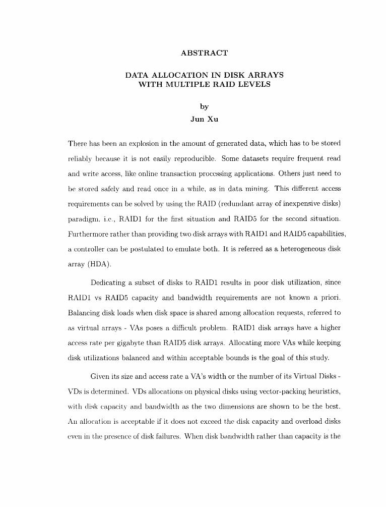
ABSTRACT

DATA ALLOCATION IN DISK ARRAYSWITH MULTIPLE RAID LEVELS

by

Jun Xu

There has been an explosion in the amount of generated data, which has to be stored

reliably because it is not easily reproducible. Some datasets require frequent read

and write access, like online transaction processing applications. Others just need to

be stored safely and read once in a while, as in data mining. This different access

requirements can be solved by using the RAID (redundant array of inexpensive disks)

paradigm. i.e., RAID1 for the first situation and RAID5 for the second situation.

Furthermore rather than providing two disk arrays with RAID1 and RAID5 capabilities,

a controller can be postulated to emulate both. It is referred as a heterogeneous disk

array (HDA).

Dedicating a subset of disks to RAID1 results in poor disk utilization, since

RAID1 vs RAID5 capacity and bandwidth requirements are not known a priori.

Balancing disk loads when disk space is shared among allocation requests, referred to

as virtual arrays - VAs poses a difficult problem. RAID1 disk arrays have a higher

access rate per gigabyte than RAID5 disk arrays. Allocating more VAs while keeping

disk utilizations balanced and within acceptable bounds is the goal of this study.

Given its size and access rate a VA's width or the number of its Virtual Disks -

VDs is determined. VDs allocations on physical disks using vector-packing heuristics,

with disk capacity and bandwidth as the two dimensions are shown to be the best.

An allocation is acceptable if it does not exceed the disk capacity and overload disks

even in the presence of disk failures. When disk bandwidth rather than capacity is the

bottleneck, the clustered RAID paradigm is applied, which offers a tradeoff between

disk space and bandwidth.

Another scenario is also considered where the RAID level is determined by a

classification algorithm utilizing the access characteristics of the VA, i.e., fractions of

small versus large access and the fraction of write versus read accesses.

The effect of RAID1 organization on its reliability and performance is studied

too. The effect of disk failures on the X-code two disk failure tolerant array is analyzed

and it is shown that the load across disks is highly unbalanced unless in an NxN array

groups of N stripes are randomly rotated.

2

DATA ALLOCATION IN DISK ARRAYSWITH MULTIPLE RAID LEVELS

byJun Xu

A DissertationSubmitted to the Faculty of

New Jersey Institute of Technologyin Partial Fulfillment of the Requirements for the Degree of

Doctor of Philosophy in Computer Science

Department of Computer Science

May 2008

Copyright © 2008 by Jun Xu

ALL RIGHTS RESERVED

APPROVAL PAGE

DATA ALLOCATION IN DISK ARRAYSWITH MULTIPLE RAID LEVELS

Jun Xu

Dr. Alexander Thomasian, Dissertation Advisor DateThomasian and Associates

Dr. David Nassimi, Committee Member DateAssociate Professor of Computer Science, NJIT

Dr. -Ali Mili, Committee Member 'DateProfessor of Computer Science, NJIT

Dr. Cristian Borcea, Committee Member DateAssistant Professor of Computer Science, NJIT

Dr. Jian Yang, Committee Member DateAssociate Professor of Industrial and Manufacturing Engineering, NJIT

BIOGRAPHICAL SKETCH

Author: Jun Xu

Degree: Doctor of Philosophy

Date: May 2008

Undergraduate and Graduate Education:

• Doctor of Philosophy in Computer Science,New Jersey Institute of Technology, Newark, NJ, 2008

• Master of Science in Computer Science,Towson University, Towson, MD, 2001

• MBA,University of Baltimore, Baltimore, MD, 1999

• Bachelor of Art in Economics,Shanghai Institute of Foreign Trade, Shanghai, China, 1993

Major: Computer Science

Presentations and Publications:

Alexander Thomasian, and Jun Xu, "Reliability and performance of mirrored diskorganizations", The Computer J., 2008, to appear.

Alexander Thomasian, and Jun Xu, "Cost Analysis of X-codes Double Parity Array",IEEE Symp. on Mass Storage Systems - MSST '07, page 269-274, San Diego,CA, September 2007.

Alexander Thomasian, and Jun Xu, "RAID Level Selection for Heterogeneous DiskArrays", The Computer J., December 2007, submitted.

Alexander Thomasian, and Jun Xu, "Data Allocation in Disk Arrays with MultipleRAID Levels", work in process.

iv

This work is dedicated to my beloved wife, son and family

ACKNOWLEDGMENT

I would like to gratefully and sincerely thank my esteemed advisor Dr. Alexander

Thomasian for his understanding, patience, and most importantly, his friendship

during my graduate studies at NJIT. Without his expert guidance this dissertation

would not have been possible. Not only was he readily available for me, as he so

generously is for all of his students, but he always read and responded to the drafts

of each chapter of my work more quickly than I could have hoped. His invaluable

guidance and encouragement have contributed significantly to the work presented in

this dissertation.

Many people on the faculty and staff of the NJIT Graduate School and the

NJIT computer science department assisted and encouraged me in various ways

during my course of studies. I am especially grateful to Dr. David Nassimi, Dr.

All Mili, Dr. Cristian Borcea and Dr. Jian Yang for their guidance and abundant

help throughout this research.

My graduate studies would not have been the same without the social and

academic challenges and diversions provided by all my student-colleagues in NJIT. I

am particularly thankful to my friends Pan Liu, Wugang Xu, Junilda Spirollari and

Yoo Jung An for all the good time we spent together.

I thank my parents for their faith in me and allowing me to be as ambitious

as I wanted. Without their moral and intellectual guidance through my life, all these

would be impossible. Also I would like to thank my parents-in-law and my brother,

his family for their continuous support and encouragement.

Finally, and most importantly, I would like to thank my wife Hannah for her

support, encouragement, help and unwavering love.

vi

TABLE OF CONTENTS

Chapter Page

1 INTRODUCTION 1

1.1 What is RAID? 1

1.2 Demand for Heterogeneous Disk Arrays 4

1.3 Related Studies 5

1.3.1 File Placement 5

1.3.2 HP AutoRAID 6

1.3.3 Previous Studies of HDA 7

1.3.4 Other Approaches 7

1.4 Organization of the Dissertation 8

2 DATA ALLOCATION IN HETEROGENEOUS DISK ARRAYS 9

2.1 Introduction 9

2.2 Allocation Requests 13

2.2.1 Load Increase in Normal Mode 16

2.2.2 Load Increase in Degraded Mode 16

2.3 Balancing Allocations 18

2.4 Experimental Results 21

2.4.1 Effects of ρmax and Vmax 35

2.5 Clustered RAID 36

2.6 Conclusions and Related Work 40

3 RAID LEVEL SELECTION FOR HETEROGENEOUS DISK ARRAYS . 42

vii

TABLE OF CONTENTS(Continued)

Chapter Page

3.1 Introduction 42

3.2 RAID Levels and Their Operation 44

3.3 Modeling Assumptions 48

3.4 Analytical Model 50

3.4.1 Operation in Normal Mode 51

3.4.2 Operation in Degraded Mode 51

3.5 Experimental Results 53

3.5.1 Disk Array Configuration 54

3.5.2 Classification Results 55

3.5.3 The Effect of RAID5 Width on Classification 58

3.5.4 The Effect of Number of Tracks per Stripe Unit 59

3.5.5 The Effect of Mean Seek Time on Classification 59

3.5.6 The Effect of Read/Write Ratio for Full Stripe Accesses . . . . 60

3.6 Effectiveness of Classification on HDA Performance 62

3.7 Conclusions 65

4 RELIABILITY AND PERFORMANCE OF MIRRORED DISK ORGANI-ZATIONS 67

4.1 Introduction 67

4.2 Related Work 69

4.3 RAID1 Organizations 73

4.4 RAID1 Reliability Analysis 76

viii

TABLE OF CONTENTS(Continued)

Chapter Page

4.5 Comparison of the Four RAID1 Organizations 79

4.5.1 Reliability Comparison 79

4.5.2 Performability Comparison 80

4.6 RAID1 Performance Analysis 82

4.6.1 Modeling Assumptions 82

4.6.2 Fault-Free or Normal Mode of Operation 83

4.6.3 Degraded Mode Analysis 85

4.7 Performance Results 88

4.8 Conclusions 93

5 ANALYSIS OF X-CODES 97

5.1 Coding for Multiple Disk Failure Tolerant Arrays 97

5.2 X-code Organization 99

5.3 Cost with One Failed Disk 102

5.3.1 Read Cost 102

5.3.2 Write Cost 102

5.4 Cost with Two Failed Disks 103

5.4.1 Read Cost 103

5.4.2 Write Cost 109

5.5 Summary 110

5.6 Discussion of Performance Results 111

5.6.1 One Failed Disk 111

ix

TABLE OF CONTENTS(Continued)

Chapter Page

5.6.2 Two Failed Disks 111

5.7 Load Imbalance with Disk Failures 112

5.7.1 Load Imbalance on Each Disk with One Disk Failure 113

5.7.2 Load Imbalance on Each Disk with Two Disk Failures 114

5.8 RM2 Coding Scheme and its Load Increase for Reads 119

5.8.1 Load Increase on Each Disk with One Disk Failure For RM2 121

5.8.2 Load Increase on Each Disk with Two Disk Failures For RM2 . 122

5.9 Comparison between Xcode and RM2 125

6 CONCLUSIONS 127

APPENDIX A M/G/1 QUEUING FORMULAS 129

APPENDIX B EXPECTED NUMBER OF PROCESSED REQUESTS . . . 130

APPENDIX C ANALYSIS OF READ COST FOR AN UNAVAILABLE DATABLOCK WITH TWO FAILED DISKS 135

APPENDIX D ALGORITHM TO COMPUTE THE LOAD INCREASE WITHTWO DISK FAILURES IN X-CODE 144

APPENDIX E ALGORITHM TO COMPUTE THE LOAD INCREASE WITHTWO DISK FAILURES IN RM2 148

REFERENCES 152

LIST OF TABLES

Table Page

2.1 Specifications of IBM 18ES Model DNES-309170W Disk Drives 21

2.2 Comparison of the Allocation Methods with R5:R1=3:1 and r = 1 inNormal Mode 23

2.3 Comparison of the Allocation Methods with R5:R1=3:1 and r = 0.75 inNormal Mode 24

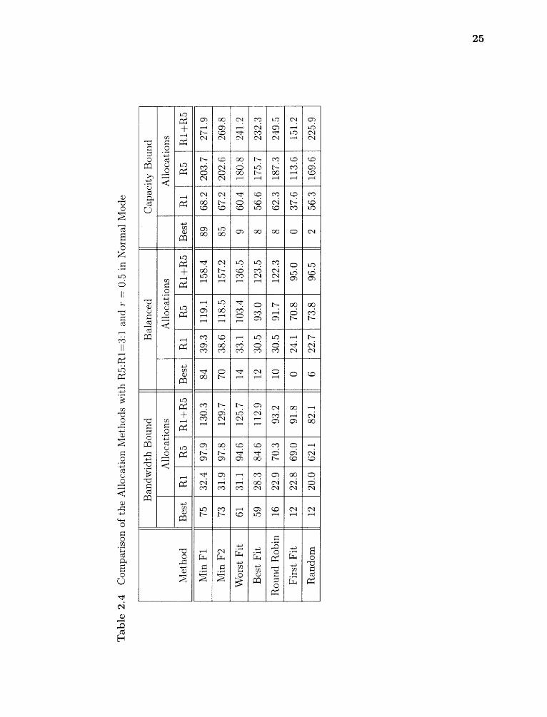
2.4 Comparison of the Allocation Methods with R5:R1=3:1 and r = 0.5 inNormal Mode 25

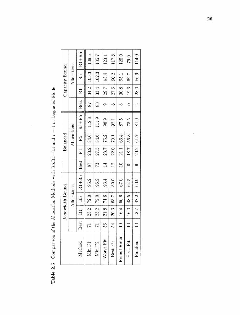
2.5 Comparison of the Allocation Methods with R5:R1=3:1 and r 1 inDegraded Mode 26

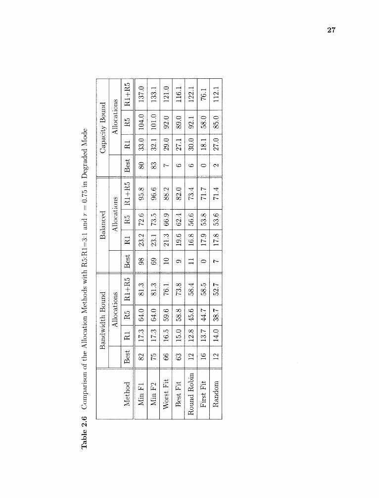
2.6 Comparison of the Allocation Methods with R5:R1=3:1 and r = 0.75 inDegraded Mode 27

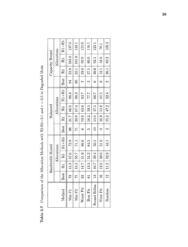
2.7 Comparison of the Allocation Methods with R5:R1=3:1 and r = 0.5 inDegraded Mode 28

2.8 Disk Utilizations After Allocations with R5 : R1 = 3 : 1, r = 1 andBandwidth Bound Workload in Degraded Mode 30

2.9 Disk Utilizations After Allocations with R5:R1=3:1, r = 1 and BalancedWorkload in Degraded Mode 30

2.10 Disk Utilizations After Allocations with R5:R1=3:1, r = 1 and CapacityBound Workload in Degraded Mode 30

2.11 Sensitivity of 0 in Min Fl with R5:R1=3:1 and r = 1 and in DegradedMode 34

2.12 Sensitivity of /3 in Min F2 with R5:R1=3:1 and r = 1 and in DegradedMode 34

2.13 Effects of ρmax and Vmax in VAs Allocations 35

2.14 Change of Capacity/Bandiwdth Ratio -y, 37

xi

LIST OF TABLES(Continued)

Table Page

2.15 Number of RAID5 Allocations with Bandwidth Bound Workload in DegradedMode N = 12 38

2.16 Number of RAID5 Allocations with Bandwidth Bound Workload in NormalMode N = 12 38

2.17 Number of RAIDS Allocations with Bandwidth Bound Workload in DegradedMode with Dynamic Parity Group Size W 38

2.18 Number of RAIDS Allocations with Bandwidth Bound Workload in NormalMode with Dynamic Parity Group Size W 38

2.19 Comparison of Relative Number of Allocations with and without ClusteredRAID and R5:R1=1:0 in Degraded Mode 39

3.1 Specifications of IBM 18ES Model DNES-309170W Disk Drives 53

3.2 Classification of RAID Levels for an Allocation Request with DifferentParameters in Normal Mode N = 12, M = 6, and K = 1 56

3.3 Classification of RAID Levels for an Allocation Request with DifferentParameters in Degraded Mode N = 12, M = 6, and K = 1 56

3.4 Classification of RAID Levels for an Allocation Request with DifferentParameters in Normal Mode N = 12, M = 4, and K = 1 57

3.5 Classification of RAID Levels for an Allocation Request with DifferentParameters in Degraded Mode N = 12, M = 4, and K = 1 57

3.6 Classification of RAID Levels for an Allocation Request with DifferentSeek Time in Normal Mode (N) and Degraded Mode (D) 60

3.7 Classification of RAID Levels for Allocation Requests with Different SeekTime in Normal (N) and Degraded (D) Mode 61

3.8 The Ratio of RAID1/RAID5 Allocations with Varying fR in Normal ModeN = 12, M = 6 and K = 1 61

3.9 The RAID1/RAID5 Ratio with Varying fR in Degraded Mode N = 12,M = 6 and K = 1 61

xii

LIST OF TABLES(Continued)

Table Page

3.10 Comparison of Relative Disk Bandwidth and Capacity with R1 Only andR5 Only, with respect to R1+R5 in Degraded Mode 64

3.11 Comparison of Relative Disk Bandwidth and Capacity Utilizations forR1+R5, R1 Only, and R5 Only with respect to R0 in Normal Mode . 64

3.12 Comparison of Relative Disk Bandwidth and Capacity Utilization withR1 Only and R5 Only, with respect to R1+R5 in Degraded Mode . . . 65

3.13 Comparison of Relative Disk Bandwidth and Capacity Utilizations forR1+R5, R1 Only, R5 Only with respect to R0 in Normal Mode . . . . 65

4.1 Notation Used in Chapter 4 69

4.2 Basic Mirroring with Striping with N=8 Disks 73

4.3 Group Rotate Declustering with N=8 Disks 74

4.4 Interleaved Declustering with N=8 Disks in One Cluster 75

4.5 Chained Declustering with N=8 Disks 75

4.6 Transition Probabilities and Number of Visits to Markov Chain States 78

4.7 Specifications for IBM 18ES Disk Drives 83

4.8 Comparison of Different Mirrored Disk Organizations with N=2M Disks 95

5.1 Notation Used in Chapter 5 101

5.2 Read Cost for the Failed Disks 1 and 2 with N=7 and d=1 106

5.3 Read Cost for the Failed Disks 1 and 4 with N=7 and d=3 107

5.4 Read Cost for Data Blocks (1:N — 2) on One Failed Disk with DifferentDistance and N Disks 108

5.5 Cost of Operation for Xcode with N Disks 111

C.1 Read Cost for the Failed Disks 1 and 2 with N=7 and d=1 140

xiii

LIST OF TABLES(Continued)

Table Page

C.2 Read Cost for the Failed Disks 1 and 3 with N=7 and d=2 142

C.3 Read Cost for the Failed Disks 1 and 4 with N=7 and d=3 143

xiv

LIST OF FIGURES

Figure Page

1.1 Data layout in RAID levels 0 through 5 3

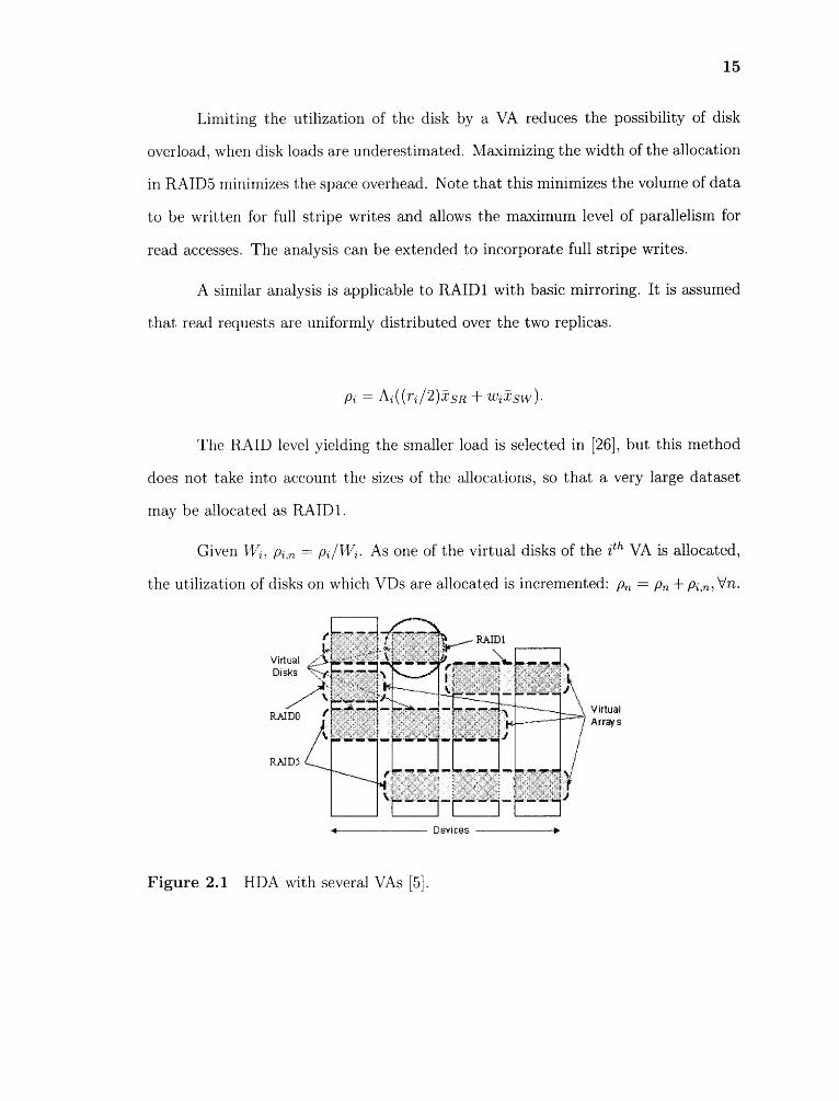
2.1 HDA with several VAs [5]. 15

2.2 Virtual array allocation vectors [5] 21

2.3 Disk bandwidth utilizations with R5:R1=3:1, r = 1 and bandwidth boundworkload in degraded mode. 31

2.4 Disk capacity utilizations with R5:R1=3:1, r = 1 and bandwidth boundworkload in degraded mode. 31

2.5 Disk bandwidth utilizations with R5:R1=3:1, r = 1 and balanced workloadin degraded mode 32

2.6 Disk capacity utilizations with R5:R1=3:1, r = 1 and balanced workloadin degraded mode 32

2.7 Disk bandwidth utilizations with R5:R1=3:1, r = 1 and capacity boundworkload in degraded mode. 33

2.8 Disk capacity utilizations with R5:R1=3:1, r = 1 and capacity boundworkload in degraded mode. 33

3.1 Disk loads per VA for RAID1 and RAIDS in degraded mode versus thefraction of small reads fr . . The fraction of full stripe writes (fFs) is setto 0.5, 0.6 and 0.7 and for each value there are two intersecting lines onefor RAID1 and the other for RAIDS. N = 12, M = 6, R : W = 3 : 1,and A = 8.7 accesses/second. 58

3.2 The R1/R5 ratio versus Al with N = 12, K = 1. The Read/Write ratiofor full stripe accesses R : W = 3 • 1 59

3.3 Variation of R1/R5 ratio versus K with N = 12 and M = 6. TheRead/Write ratio for full stripe accesses is R : W = 3 • 1. 60

4.1 Markov chain for a mirrored disk array with N=8 disks (the state specifiesthe number of failed disks, F is the failed state) 78

xv

LIST OF FIGURES(Continued)

Figure Page

4.2 Comparison of the expected number of requests processed by the fourRAID1 organizations. 81

4.3 Response time of read requests in normal mode R:W=1:0, N=8. Thegraphs for RAID0 and RAID5 overlap with RAID6, so that only RAID6is shown

4.4 Response time of read requests in normal mode, R:W=3:1, N=8. Notethat GRD, ID, and CD have the same response time. 90

4.5 Response time for read requests in normal mode, R:W=1:1, N=8. Notethat GRD, ID, and CD have the same response time. 91

4.6 Response time for read requests with one disk failure, R:W=1:0, N=8. 91

4.7 Response time for read requests with one disk failure, R:W=3:1, N=8. 92

4.8 Response time for read requests with one disk failure, R:W=1:1, N=8. 92

4.9 Response time for read requests with two disk failures, R:W=1:0, N=8 93

4.10 Response time for read requests with two disk failures, R:W=3:1, N=8 94

4.11 Response time for read requests with two disk failures, R:W=1:1, N=8 94

5.1 p parities with slope=1 and N = 7. 7th row is not considered. 100

5.2 q parities with slope=-1 and N =7. 6 th row is not considered. . . . . . 100

5.3 Possible recovery path for block (3,1) with p parity group and N = 7. . 105

5.4 Possible recovery path for block (3,1) with q parity group and N = 7. . 105

5.5 The case analysis for Xcode with two disk failures. 109

5.6 Mean cost of read operation with one disk failure versus number of disks. 112

5.7 Mean read cost of an unavailable data block with two failed disks versusnumber of disks 113

5.8 Mean read cost of a data block with two failed disks versus number of disks.114

90

xvi

LIST OF FIGURES(Continued)

Figure Page

5.9 Load increase on each disk for reads with two failed disks and N = 7,X axis is i th disk, Y axis is the distance. Z axis is the times of loadincrease comparing that in the normal mode. 115

5.10 Mean load increase on a disk for reads with two disk failures and N = 7 117

5.11 Mean load increase on a disk for reads with two disk failures and N = 19. 117

5.12 Mean load increase on a disk for reads with two disk failures and N = 37. 118

5.13 Mean load increase vs number of disks. 119

5.14 Sample RM2 Layout 121

5.15 Load increase (times of the original load) on disk 2 to 7 for reads withdisk 1 failed and N = 7, M = 3 for RM2. 122

5.16 Load increase on each disk for reads with two disk failures and N = 7,M = 3 for RM2. X axis is i th disk, Y axis is the distance. Z axis is thetimes of load increase comparing that in the normal mode. 123

5.17 Mean load increase on a disk for reads with two disk failures and N = 7,M = 3 for RM2 124

5.18 Mean load increase on a disk for reads with two disk failures and N = 19,M = 7 for RM2 125

5.19 Mean load increase on a disk for reads with two disk failures and N = 39,Al = 13 for RM2. 126

5.20 Maximum load increase on one disk as a function of N with two diskfailures for RM2. 126

B.1 Analysis of two disk failures when N=8 with CD, first row is the disknumber, 1 means the disk has failed and 0 means that the disk isfunctioning. The last column identifies different configurations 133

C.1 p parity groups with N = 7 136

C.2 q parity groups with N = 7 136

xvii

LIST OF FIGURES(Continued)

Figure Page

C.3 Block (2,1) can be reconstructed by p(3) when disk 1 and 3 are failed. . 138

C.4 Block (5,1) can be reconstructed by q(1) when disk 1 and 3 are failed . . 138

C.5 Block (3,1) can be reconstructed by p(4) when disk 1 and 4 are failed. . 139

C.6 Block (4,1) can be reconstructed by q(2) when disk 1 and 4 are failed. . 139

C.7 Recovery path for block (3,1) with N = 7 and slope =1 141

C.8 Recovery path for block (3,1) with N = 7 and slope =-1 141

xviii

CHAPTER 1

INTRODUCTION

There has been a recent explosion in the volume of data being generated by various

services, such as video on demand, internet data center, data warehousing, digital

imaging, nonlinear video editing. Five exabytes (5 x 2 60 bytes) of new information

were generated in 2002 and new data is growing annually at the rate of 30% [47].

The economic viability of these services depends on storing data at low cost, while

acceptance by their customers depends on their keeping data unaltered and accessible

with low latency. Fortunately, this has been accompanied with rapidly increasing

magnetic disk capacities and a drop per gigabyte in disk costs.

High data availability is important, because of the high cost of downtime for

many applications. Furthermore, the loss of certain data is unacceptable, since it is

irreproducible or very costly to reproduce. For example in 1975 the former USSR .

sent probes Venera 9 and 10 to the surface of Venus to collect data and imagery [73].

Had these data been lost, it would cost tens of millions of dollars to recollect them.

1.1 What is RAID?

The Redundant Array of Inexpensive Disks - RAID paradigm [48] is a solution to the

disk failure problem. A typical disk array consists of a bunch of identical hard disk

drives attached to an array controller, which is connected to a host computer using

high-bandwidth links. The responsibility of the array controller is maintaining address

mapping, maintaining redundant information, controlling individual disks, translating

host requests, and recovering from disk or link failures. The array controller provides

a linear address space to the host. The redundant information is maintained by the

1

2

disk array controller and is transparent to the user. The mapping of this host side

linear address space to individual disk address space is referred to as the data layout.

One of the fundamental concepts of RAID is striping [51, 28, 43], which

partitions the linear address space exported by the array controller into smaller fixed

size blocks called a stripe unit or striping unit - SUs. The benefits of striping include

automatic load balancing and high bandwidth for large sequential transfers through

parallel accesses.

RAID level 1 through 5 were first described in [51]. Even though not in the

original RAID classification, RAID level 0 is often used to indicate a non-redundant

disk array with striping, i.e., the failure of any disk in RAIDO results in data loss.

RAID1, known as mirroring, provides redundancy by duplicating all data from one

drive to another. In spite of the high degree of redundancy, RAID1 only guarantees

recovery from a single disk failure [63], [70]. However, the doubling of the disk access

bandwidth is beneficial from the viewpoint of the rapid increase in disk capacities,

especially for applications requiring reading and writing of small blocks.

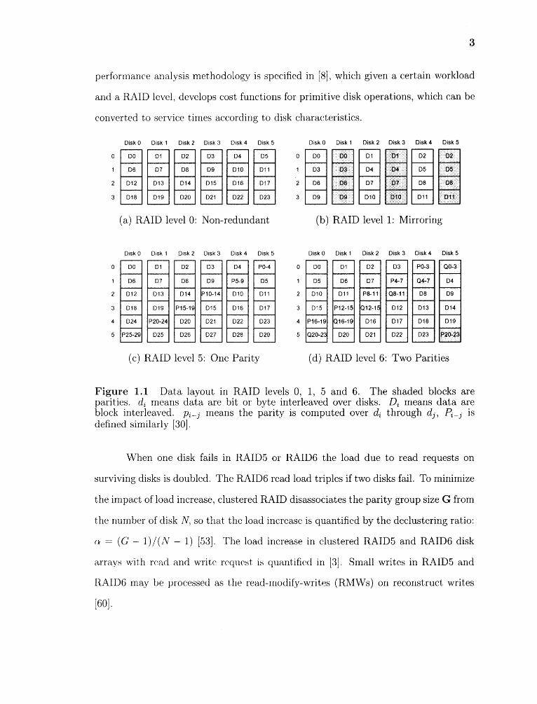
RAID5 stripes data at the block level and distributes parity SUs among the

drives. In other words, no single disk is dedicated to parity. RAID6 uses two parities

to tolerate two disk failures. In Figure 1.1, the data and redundancy information

organizations for RAID levels 0, 1, 5, and 6 are illustrated. The RAID5 design

shown uses left-symmetric organization [40], which repeats placing SUs in left to

right diagonals. The group of disks that a parity is computed over is called a parity

group. For the samples shown in Figure 1.1, there is only one parity group for each

RAID level for RAID5.

Two and more disk failures can be tolerated by using Reed-Solomon codes in

RAID6 [48] and sophisticated parity codings, such as EVENODD [41], RDP [46], and

X-codes [75]. Each data block is protected by two parity groups in these arrays. A

3

performance analysis methodology is specified in [8], which given a certain workload

and a RAID level, develops cost functions for primitive disk operations, which can be

converted to service times according to disk characteristics.

(a) RAID level 0: Non-redundant (b) RAID level 1: Mirroring

(c) RAID level 5: One Parity (d) RAID level 6: Two Parities

Figure 1.1 Data layout in RAID levels 0, 1, 5 and 6. The shaded blocks areparities. d i means data are bit or byte interleaved over disks. Di means data areblock interleaved. pi-j means the parity is computed over d i through di, isdefined similarly [30].

When one disk fails in RAID5 or RAID6 the load due to read requests on

surviving disks is doubled. The RAID6 read load triples if two disks fail. To minimize

the impact of load increase, clustered RAID disassociates the parity group size G from

the number of disk N, so that the load increase is quantified by the declustering ratio:

= (G — 1)/(N — 1) [53]. The load increase in clustered RAID5 and RAID6 disk

arrays with read and write request, is quantified in [3]. Small writes in RAID5 and

RAID6 may be processed as the read-modify-writes (RMWs) on reconstruct writes

[60].

4

Rebuild is a systematic reconstruction of the contents of a failed disk on a spare

disk in dedicated sparing [68] or empty space at surviving disks in distributed sparing

[67]. Distributed sparing is preferable to dedicated sparing, since disk bandwidth is

wasted otherwise [42], [67].

1.2 Demand for Heterogeneous Disk Arrays

Compared to the drop per gigabyte in disk costs, data management costs have

increased sharply. Recent studies have indicated that storage management costs

dominate the cost of large storage system over the course of their lifetime [11, 49].

Therefore it is important to automate this process, while optimizing storage utilization

and providing satisfactory disk throughput and response time for user requests.

Different RAID levels have different performance characteristics and perform

well only for a relatively narrow range of workloads. Hence, a typical RAID system

provides many configuration parameters: data- arid parity- layout choice, stripe

unit sizes, parity group sizes, cache sizes arid cache management policies, and so

or Setting these parameters correctly requires skilled, highly paid personnel and

a painful process of trial and error. It should be able to choose the right configu-

ration for different datasets based on their characteristics. It should be gracefully

expandable, so that there is no need to provide too much spare storage for future use.

Furthermore different applications have different requirements, including, but

not limited to capacity, bandwidth, and reliability. As far as reliability and performance

are concerned, there is no single RAID level that can meet all of the requirements.

Each RAID level has different characteristics arid performs well only for a relatively

narrow range of workloads. Hence ; a storage system which can combine different

RAID levels. i.e., RAIDO/1/5/6 etc., is required to meet the requirements of individual

5

stores. In other words, the storage system should be heterogeneous in terms of the

RAID level.

Rapid growth in disk capacity, high management cost and complex appli-

cation requirements create the demand for the heterogenous disk array, a system that

automates decision-making process, while optimizing storage utilization and providing

satisfactory disk bandwidth and response time for user requests has been an important

area of investigation see e.g., [26],[25].

1.3 Related Studies

HDA is built on many studies on RAID reliability, performance and design variations

for parity placement and recovery schemes.

1.3.1 File Placement

Each file (one allocation request) has different characteristics associated with it:

size, access frequency. Each system also has it own configuration: disk capacities,

maximum disk access rates, disk bandwidths (transfer rates), data path, etc. The

objective of the file placement problem is to match file characteristics with system

configurations so as to balance disk workloads (by eliminating disk access skew) or

to meet response time requirements for certain applications.

The file placement problem - FPP is modeled as 2-D vectors: size and access

rate in [52]. Forum [18], Minerva [12] and Ergastulum [13] are three generations of

design tools at HP for the "attribute mapping problem" [29] [55] to create a self-

configuring and self-managing storage system. Bin-packing is applicable to do the

data allocation problem at hand, e.g., the online best-fit bin packing with random

order described in [36] is used in HP's Ergastulum frame work.

6

1.3.2 HP AutoRAID

HP AutoRAID implements two RAID levels (RAID1 and RAID5) inside a single disk

array controller [34] to satisfy a wide variety of workloads. RAID1 is used at the

upper level to provide full redundancy and excellent performance, while RAID5 is

applied at the lower level to provide cost effective storage for less active data. The

data blocks can be promoted or demoted between these two levels as access patterns

change.

HP AutoRAID uses all disks for a stripe for RAID5. HDA computes the width

of a VA dynamically according to the size and estimated access rate of an allocation.

The average width of RAID5 VAs in HDA are usually less than the number of disks

in the system.

HP AutoRAID only deals with small datasets. The segment (VD in this

dissertation) size is fixed, i.e.. 128KB. HDA considers large file allocations.

Load balancing in HP AutoRAID may not be achieved because it focuses

on the balance of the amount of data on the disks instead of bandwidth usage.

HDA explicitly makes load balance as a target because nowadays bandwidth is the

bottleneck resource in disk storage systems.

The HP AutoRAID array uses static partition: part of the space is dedicated

to RAID1 while the rest is formatted as RAID5. The potential problem is that it may

run into a thrashing mode in which each update causes the target Relocation Block

(RB) , which is a unit of data migration with the size of 64KB, to be promoted up to

RAID1 and a second one demoted to RAID5 if the active write working set exceeds

the size of RAID1 storage for long periods of time.

7

1.3.3 Previous Studies of HDA

In [7] the effect of different allocation strategies for files that need to be allocated

inside R.AID1 or RAID5 "containers" [30],[5],[19],[7] was investigated. Since space

requirements for RAID1 and RAID5 allocations are not known a priori, these RAID

arrays are allocated on demand based on disk space availability.

The study of HDA in this dissertation differs from previous ones in that it

allocates the Virtual Disks - VDs of Virtual Arrays - VAs based not only on their

storage requirements, but also estimated access rates. The jth allocation request for a

VA is specified as: (i) the data volume (Di ), (ii) estimated arrival rate (Λj ), (iii) data

access characteristics (request sizes, random versus sequential access, the read/write

- R:W ratio, etc.), (iv) data availability requirements. Given VA attributes a rule-

based system can be used to determine the RAID level, but it is assumed in one study

(Chapter 2) that the RAID level is pre-specified. An analytic method to determine

the more desirable RAID level is give in another study (Chapter 3).

1.3.4 Other Approaches

OceanStore [54] aims for a high availability and high security world-wide peer-to-peer

system, buy does not provide high bandwidth. FARSITE [10] stores data in free

disk space on workstations in a corporate network. FARM [74] breaks files up into

fixed-size blocks: the default size of a block is 1 MB. The size of a block in this thesis

is determined on the fly according to bandwidth and capacity usage of disks.

8

1.4 Organization of the Dissertation

In Chapter 2 data allocation in HDA is discussed. Given its size and access rate the

VA's width or the number of its Virtual Disks - VDs is first determined. Then several

online single-pass data allocation methods are evaluated . An allocation is acceptable

if it does not exceed the disk capacity and overload disks especially in the presence

of disk failures. When disk bandwidth rather than capacity is the bottleneck, the

clustered RAID paradigm is applied, which offers a tradeoff between disk space and

bandwidth.

RΛID level classification in HDA is covered in Chapter 3. An analysis has been

developed to estimate the load per VA postulating that it is configured as RAID1 or

RAID5 and the RAID level which minimizes the load per VA is selected, since in this

way more VAs can be allocated in a disk bandwidth bound system.

Chapter 4 discusses four RAID1 organizations: basic mirroring - BM, group

rotate declustering - GRD, interleaved declustering - ID, and chained declustering -

CD. The last three organizations provide a more balanced disk load than BM when

a single disk fails, but are more susceptible to data loss than BM when additional

disks fail. The four organizations are compared from the viewpoint of: (a) reliability

(results are quoted from [63]), (b) performability, (c) performance. The ranking

from the viewpoint of reliability and perforrnability is: BM, CD, GRD, ID (with two

clusters). BM and CD provide the worst performance, ID has a better performance

than BM and CD, but is outperformed by GRD.

The load increase and imbalance of the X-code method is analyzed in Chapter

5. A general expression is derived for disk loads and graphs to quantify the load

imbalance are presented.

Conclusions are given in Chapter 6.

CHAPTER 2

DATA ALLOCATION IN HETEROGENEOUS DISK ARRAYS

2.1 Introduction

There has been a recent explosion in the volume of data being generated, but this

has been fortunately accompanied with rapidly increasing magnetic disk capacities

and a drop per gigabyte in disk costs. With decreasing storage costs the cost of

storage management is gaining more and more importance. Automating this process,

while optimizing storage utilization and providing satisfactory disk throughput and

response time for user requests has been an important area of investigation see e.g.,

[26],[25]. This is an attempt to take a fresh look at the problem with a simplified

setting.

High data availability is important, because of the high cost of downtime for

many applications. Furthermore, the loss of certain data is unacceptable, since it is

irreproducible or very costly to reproduce. The RAID paradigm [48] is a solution to

the disk failure problem. Single disk failures can be tolerated by mirroring data, as in

RAID1, or by erasure coding using parity, as in RAIDS. In fact, more than two disks

can be allocated to RAID1, in which case the data is striped across multiple arrays

in a RAID1/0 configuration. Two and more disk failures can be tolerated by using

Reed-Solomon codes in RAID6 [48] and more sophisticated parity codings, such as

EVENODD and RDP.

RAID1 or disk mirroring replicates the same data on two disks, so that it

can be read from either disk, i.e., the access bandwidth to data is doubled. A

further improvement in access bandwidth can be attained by judicious routing of

read requests, e.g., accessing the data from the disk which provides the lower service

9

10

time. Modified data should be updated at both disks. The read load on the surviving

disk is doubled when a single disk fails, but this load can be distributed over multiple

disks with a more sophisticated data allocation scheme than basic mirroring. One

such method is interleaved declustering, which has implications on the safeness of

data allocations, i.e., no overload in degraded mode.

Load balancing in RAID5 is achieved via striping, i.e., partitioning large files

into stripe units - SUs, which are allocated in a round-robin manner across the N

disks. One of the SUs in a row is the parity computed across the remaining SUs in that

row. If one of N disks fails, the contents of its blocks can be reconstructed on demand

by issuing a fork-join request to read and exclusive-OR - XOR the corresponding

blocks from the N — 1 surviving disks. This is obviously one of the constraints of the

allocation policy, that no two SUs in a stripe can be allocated on a single disk. Since

in addition to fork-join read requests, each disk processes its own read requests the

load at surviving disks is doubled in degraded mode. The load increase is smaller for

write requests [3].

Clustered RAID - CRA ID or parity declustering solves the load increase problem

by setting the parity group size G to be smaller than N, so that only a subset of N

disks will be involved in reconstructing a requested data block [53]. The load increase

of surviving disks for RAID5 as a result of read requests is given by declustering ratio:

a = (G-1)/(N-1) [53]. The size G affects the fraction of redundant data being held; i.e.

in RAID5, 1/G of the blocks hold redundant data. Clustering provides a continuum of

redundancy levels to minimize the impact of disk failures on performance in degraded

mode. In other words the same load increase for a parity group in degraded mode is

achieved by using less disks. The load in clustered RAID5 and RAID6 disk arrays

in normal and degraded operating modes is given in [3] and is used in this study in

estimating disk loads in degraded mode.

11

The rebuild process in RAID5 is a systematic reconstruction of the contents

of a failed disk on a spare disk, which involves the reading of successive rebuild units

(tracks), XORing them to recreate the lost track, and writing them to the spare disk.

RAID5 is susceptible to data loss if there is a second disk failure, before the rebuild

process is completed, or there is a latent sector failure - LSF, which is the more likely

event.

Datasets with different application access requirements is considered. OLTP

applications generate high access rates to read/write small, randomly placed blocks,

while some database applications read/write large chunks of data. The former induce

the small write penalty in RAID5, while the latter can be processed as full-stripe

writes efficiently. It follows that RAID1 is the appropriate configuration in the

former case, while RAID5 is more appropriate in the latter case, especially for high-

volume datasets. Rather than providing two disk arrays with RAID1 and RAID5

capabilities, a controller emulating both is postulated so that disk space can be shared

among RAID1 and RAID5 virtual arrays - VAs. This is a more flexible scheme than

dedicating n < N disks to RAID 1 and N — n disks to RAID5, since resource demands

in the two categories are not known a priori. Sharing of disk space among RAID1

and RAID5 arrays has a load balancing effect, since RAID1 arrays have higher access

rates per GB.

A synthetic workload is used to compare the effectiveness of several allocation

methods. Given its size and access rate, a VA's width or the number of its Virtual

Disks - VDs is first determined. Several "single-pass" data allocation methods are

proposed, which take into account both the capacity and bandwidth available at each

disk. An allocation is acceptable if it does not overload a disk or exceed its capacity

and can tolerate a single disk failure. When disk bandwidth, rather than capacity, is

the bottleneck, the clustered RAID paradigm is applied to RAID5 disk arrays, which

offers a tradeoff between disk space and bandwidth.

12

The assumption is that the RAID level is determined by its attributes. In

addition, there are many parameters associated with each RAID level that need to

be specified: stripe unit size. striping width or the width of a VA, parity group size

in clustered RAID, etc. Allocating a VA across all disks has the disadvantage that

if a disk fails then the load at all remaining disks is doubled. For N' < N the load

increase per utilized disk by the VA is higher, but fewer disks are affected, which is

in fact a form of CRAID. The HP AutoRAID selects the RAID level based on the

observed access pattern [34], i.e., a subset of data with a high access rate is stored in

RAID1 format. Objects to be stored on disk have different reliability and performance

requirements, so that the selection of the appropriate RAID level poses a dilemma

[26].

Since no single RAID level is satisfactory in all cases, rather than acquiring

multiple arrays with different RAID levels, a Heterogeneous Disk Array - HDA is

proposed, which supports heterogeneity at RAID level. Heterogeneity at disk level

was considered in an earlier study [7], but heterogeneity at the level of brick level or

storage nodes is more relevant nowadays. The earlier study is mainly concerned with

the allocation of smaller files inside containers with fixed RAID1 and RAID5 formats.

Directory structures developed in this study are applicable to the new HDA. In this

study RAIDs with the same level may have different widths, stripe unit sizes, and

parity group sizes.

The allocation problem at the VA level can be formulated by a two-dimensional

"bin-packing" or vector-packing problem [52], where one dimension is the number of

disks and the other dimension is the disk bandwidth utilization. Given rectangles

with varying heights and widths the goal is to allocate as many of them as possible

into a rectangle consisting of all disks. Branch-and-bound methods are applicable in

this case. The problem at hand is made more difficult by the fact that allocation

requests are malleable, i.e., the "wider" the allocation the lower the load at each disk.

13

Limits to capacity and bandwidth of allocations on each disk is used to determines

the width of the VA. The setting of these parameters remains an area of further

investigation.

In Section 2.2 how to calculate the load increase for a VA in both normal and

degraded mode is displayed. Allocation methods next given in Section 2.3. Next the

experimental approach used in comparing them is specified in Section 3.5. Sensitivity

tests are reported in Section 2.4.1. Following it the methods to compute the parity

group size G in clustered RAID is compared in Section 2.5. In Section 3.7 related

results are discussed.

2.2 Allocation Requests

There is a disk array with N disks, which may be allocated across multiple bricks.

Data allocation in a single brick is considered here for the sake of brevity, but

maintaining brick boundaries limits the propagation of overload due to disk failures.

Bricks may hold heterogeneous disk and be specialized, fast, small capacity versus

slow, large capacity disks. Allocation requests in the form of VAs (virtual arrays),

become available one at a time and are processed immediately. Each VA is specified

as follows:

• RAID level, which is specified by with = 1 for RAID1 and = 5 for RAID5.

• Size of dataset. The size of the dataset associated with i th VA is denoted by

V. V, is used to determine the access rate to the dataset, but its actual size Vi i

is larger due to replication (RAID1) or erasure coding (RAIDS), i.e., V' i = 214arid V' i = V(1 + 1/Wi ), respectively. Wi is determined below.

• The workload. The arrival rate from an infinite number of sources is Λ i = ViKl,

where ice, the I/O intensity per GB is determined by the RAID level l. The sizes

of disk requests and the distribution of accesses determines the transfer time

and positioning time respectively. Mean disk service time X- disk is computed

14

by assuming requests are uniformly distributed over all disk cylinders and that

requests are served in FCFS order, which are worst case scenarios. The fraction

of writes determines the processing overhead, which is high for RAID5 due to

the small write penalty [48], but even higher for RAID6 [3].

The width Wi of VA, is determined below. The fraction of read and write

requests to VAi is denoted by ri and wi = 1 — r,. The mean service time for single

read - SR, single write - SW, and read-modify-write - RMW requests is SR, sw, ,

RMW , respectivly. RMW requests can be processed as an SR followed by a disk

rotation to write the data and parity block, or independent SR and SW requests,

where the parity is computed at the disk array controller. The parity calculation is

carried out at the disks in the first case and the disk array controller in the second

case, providing a higher level of integrity.

The width of the array can be determined based on a maximum disk utilization

(ρmax) or capacity constraint (VMax ) per VA:

15

Limiting the utilization of the disk by a VA reduces the possibility of disk

overload, when disk loads are underestimated. Maximizing the width of the allocation

in RAID5 minimizes the space overhead. Note that this minimizes the volume of data

to be written for full stripe writes and allows the maximum level of parallelism for

read accesses. The analysis can be extended to incorporate full stripe writes.

A similar analysis is applicable to RAID1 with basic mirroring. It is assumed

that read requests are uniformly distributed over the two replicas.

pi = Λ i ((ri / 2Y xSR wixSW).

The RAID level yielding the smaller load is selected in [26], but this method

does not take into account the sizes of the allocations, so that a very large dataset

may be allocated as RAID 1.

Given Wi , pi,n= pi/Wi . As one of the virtual disks of the i th VA is allocated,

the utilization of disks on which VDs are allocated is incremented: pi, = pa + pi ,,, Vn•

Figure 2.1 HDA with several VAs [5].

16

2.2.1 Load Increase in Normal Mode

In [3] formulas are given to compute the disk utilization of reads and writes for RAID5

arid cluster RAID5. It is given for the worst case with all read requests (r = 1). It

is the load increase of ρi,n. The subscript is omitted in the following formulas. For

RAID1 only Basic Mirroring with width of two is considered.

2.2.1.1 RAID5. In normal mode the cost for the normal RAID and clustered

RAID are the same.

ρRAID5/F0 = irixSR + 2iwixRMW (2.1)

2.2.1.2 RAID1 for BM with W=2. In normal mode the cost for reads is only

half of the read requests because the requests can be redirected evenly to the mirrored

disks.

ρRAID1/F0 = 1 irixSR + iwixSW (2.2)

2.2.2 Load Increase in Degraded Mode

In order to make an allocation safe, it is important to make sure disks will not exceed

its maximum utilization in degraded mode, i.e. with disk failure(s). However, there is

no disk failures in degraded mode. The load increase for a VA is calculated as if one

disk fails. All the study discussed here are carried out in the degraded mode except

specified explicitly.

2.2.2.1 RAID5. In degraded mode the disk utilization for normal RAID5 is computed

as follows.

(2.3)

(2.4)

(2.5)

(2.6)

For Clustered RAID with group size G(G < W), the formulas are

2.2.2.2 RAID1 for BM with W=2. In degraded mode for a read request each

disk has to process its own load plus the load of the failed disk, i.e. W/2(W — 1). For

a write request it only needs to write data to W — 1 disks instead of W.

(2.7)

(2.8)

18

2.3 Balancing Allocations

Both disks and allocation requests are modeled as two-dimensional vectors [52], where

the first dimension is the access rate and the second dimension is size. The disk

bandwidth is determined by the maximum throughput (accesses per second).

Data allocation is modeled as vector addition, so that the sum of the allocations

should be less than the disk vector in both coordinates. The problem of balancing the

utilization in terms of both throughput and capacity is defined as follows. The focus

is on maximizing the number of allocations I =-+- R1 + _ R5, where IR1 and /R5 denote

the number of allocations in the two categories. The allocation requests appear as a

pseudo-random sequence.

The allocation requests considered here are at the level of VDs, so that the

allocation of VAi requires the allocation of Wi VDs, whose sequence is denoted by J,

whose elements are denoted by pj = (xi , c3 ), where xi is its expected access rate and

cj is the size of data. In fact, J is the concatenation of sequences J, due to VA,.

The n th disk is represented by a vector d, = (Xn , Ca), where X„, denotes the

maximum throughput and Ca the capacity of the nth drive. A valid solution allocates

from the sequence J of VDs into N sets J1, . . . , JN. VDs belonging to the same VA

should be allocated on a different disks. A VA is considered allocated if all of its VDs

are allocated. Let Uxn and Ur', denote the utilization of the bandwidth and capacity

of the n th disk. which are defined as follows:

The allocation of VAs is continued until an allocation is unsuccessful, at which

point no alternative drive is considered. Allocation policies are judged by the number

of allocations, which maximizes the number of allocated VDs.

19

1. Round Robin: Allocate on disk drives sequentially.

2. Random: Choose disk drives randomly.

3. Best Fit: Scan the disks and choose disks with minimum remaining bandwidth

or maximum disk utilization (after the allocation).

4. First Fit: Disks are considered in increasing order of their indices and a VD

is allocated on the first disk that can hold it.

5. Worst fit: Allocate requests on disk with minimum bandwidth utilization

provided that disk capacity constraint is satisfied.

Let Uxn and tin' denote the bandwidth and capacity utilization of the n th disk.

Two more sophisticated allocation methods minimizes the following objective

functions:

6. Minimize Fl:

0 < < 1 is an emphasis factor of capacity utilization.

7. Minimize F2:

Var(xn ) is the variance of xn over all possible N.

The focus is mainly on balanced disk utilizations, rather than disk capacities,

since unbalanced throughputs will result in highly variable response times, while disk

capacity is cheap.

Given the number of disks, say N = 12, the disk drive and disk access charac-

teristics, e.g., access to small randomly placed blocks of data, fraction of RAID1

versus R,AID5 requests (RAID level f), distribution of sizes of VAs, several runs are

made to determine the average number of allocations for each method. The allocation

experiment proceeds as in Algorithm 1:

Algorithm 1 VA allocation algorithm

Initialize VA allocation count: i = 0. Generate allocation requests until

a request is unsuccessful.

1. Increment i and generate VA i request with appropriate RAID

level P.

2. Determine VA i size: V based on size distribution for RAID level

3. Generate estimated access rate: Λ i =

4. Calculate load in degraded mode for this VA as discussed in

Section 2.2.2.

5. Determine allocation width Wi based on disk capacity and

utilization constraints.

6. Determine if a successful allocation of all VDs is possible. If not

stop allocation.

7. Increment the utilization of disks to which VA i is assigned.

8. i + + and return to Step 1.

20

Max 1-,(mnp

Figure 2.2 Virtual array allocation vectors [5].

2.4 Experimental Results

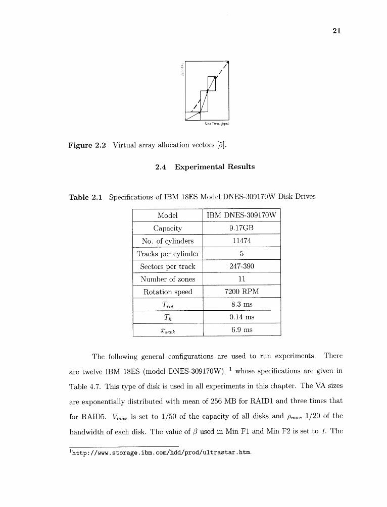
Table 2.1 Specifications of IBM 18ES Model DNES-309170W Disk Drives

21

The following general configurations are used to run experiments. There

are twelve IBM 18ES (model DNES-309170W), 1 whose specifications are given in

Table 4.7. This type of disk is used in all experiments in this chapter. The VA sizes

are exponentially distributed with mean of 256 MB for RAID1 and three times that

for RAIDS. V,-flax is set to 1/50 of the capacity of all disks and Amax 1/20 of the

bandwidth of each disk. The value of 0 used in Min Fl and Min F2 is set to 1. The

lhttp://www.storage.ibm.com/hdd/prod/ultrastar.htm.

22

access rates for RAID1 disk arrays are ten times the rates of RAID5. Three cases are

considered for disk requests.

Tabl

e 2.

2 C

ompa

riso

n o

f th

e Λ

lloca

tion

Met

hod

s w

ith

R5:

R1=

3:1

and

r =

1 in

Nor

mal

Mod

e

Tabl

e 2.

3 C

ompa

riso

n of

the

Allo

cati

on M

etho

ds w

ith

R5:

R,1

=3:1

and

r =

0.7

5 in

Nor

mal

Mod

e

Tabl

e 2.

4 C

ompa

riso

n of

the

Allo

cati

on M

etho

ds w

ith

R5:

R1=

3:1

and

r =

0.5

in N

orm

al M

ode

Tabl

e 2.

5 C

ompa

riso

n of

the

Λllo

cati

on M

etho

ds w

ith

R5:

R1=

3:1

and

r =

1 in

Deg

rade

d M

ode

Tabl

e 2.

6 C

ompa

riso

n o

f th

e Λ

lloca

tion

Met

hod

s w

ith

R5:

R1=

3:1

and

r =

0.75

in D

egra

ded

Mod

e

Tabl

e 2.

7 C

ompa

riso

n of

the

Allo

cati

on M

etho

ds w

ith

R5:

R1=

3:1

and

r =

0.5

in D

egra

ded

Mod

e

29

1. Bandwidth Bound: Allocation requests consume disk bandwidth faster than

disk capacity, i.e. the bandwidth and capacity utilization ratio of allocation

requests is higher than the disk ratio (8.5 accesses/sec. per GB for RAID5).

2. Balanced: The allocation requests consume disk capacity at almost the same

rate of disk bandwidth. (3.3 accesses/sec. per GB for RAID5).

3. Capacity Bound: Allocations consume disk capacity faster than disk bandwidth,

i.e. the capacity and bandwidth utilization ratio of allocation requests is greater

than that of disks. (2.1 accesses/sec. per GB for RAID5).

100 runs are made for each case and display the number of bests in 100 runs

for each method. The number of allocations for RAID1 and RAID5 is the average of

100 runs.

The following conclusions are drawn from experimental results in Tables 2.2,2.3,2.4,

2.5, 2.6 and 2.7.

1. The number of VAs allocated in normal mode is almost double that in degraded

mode when r = 1. That is because the load in normal mode is roughly half of

that in degrade mode.

2. It is necessary to consider both system utilization and capacity to get a robust

performance.

3. Minimize Fl and F2 are consistently the best in terms of the number of allocations

in all configurations.

4. First Fit, Random and Round Robin are the worst among all methods.

5. Worst Fit is comparable with Fl and F2 when bandwidth bound, but not when

capacity bound. The reason is that it balances the bandwidth utilization on

each disk, but not the capacity. So it works well in bandwidth bound workload

and poorly in capacity bound workload.

Tables 2.8, 2.9 and 2.10 display the comparison of average bandwidth and

capacity utilization of all disks and number of RAID 1 and RAIDS VAs allocated with

30

R5 : R1 = 3 : 1, r = 1 and bandwidth bound workload in degraded mode among

methods Min Fl, F2 and round robin.

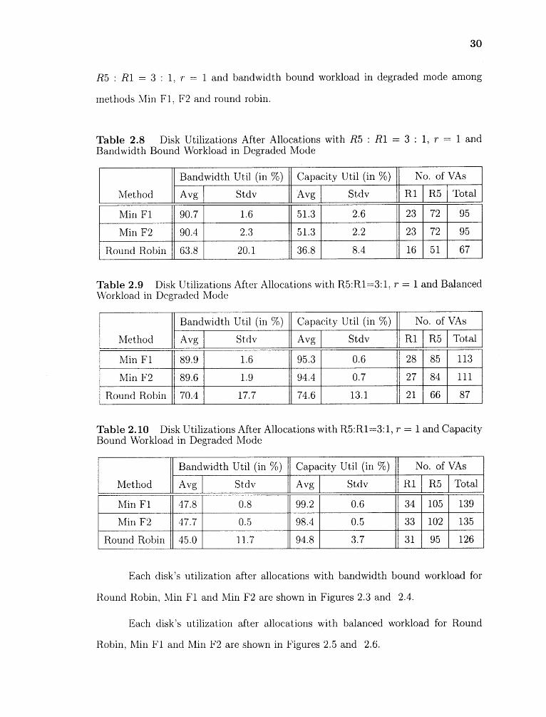
Table 2.8 Disk Utilizations After Allocations with R5 : R1 = 3 : 1, r = 1 andBandwidth Bound Workload in Degraded Mode

Table 2.9 Disk Utilizations After Allocations with R5:R1=3:1, r = 1 and BalancedWorkload in Degraded Mode

Table 2.10 Disk Utilizations After Allocations with R5:R1=3:1, r = 1 and CapacityBound Workload in Degraded Mode

Each disk's utilization after allocations with bandwidth bound workload for

Round Robin, Min Fl and Min F2 are shown in Figures 2.3 and 2.4.

Each disk's utilization after allocations with balanced workload for Round

Robin, Min F 1 and Min F2 are shown in Figures 2.5 and 2.6.

31

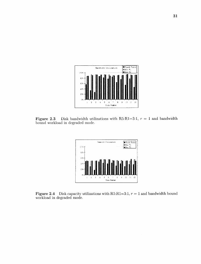
Figure 2.3 Disk bandwidth utilizations with R5:R1=3:1, r = 1 and bandwidthbound workload in degraded mode.

Figure 2.4 Disk capacity utilizations with R5:R1=3:1, r = 1 and bandwidth boundworkload in degraded mode.

32

Figure 2.5 Disk bandwidth utilizations with R5:R1=3:1, r = 1 and balancedworkload in degraded mode.

Figure 2.6 Disk capacity utilizations with R5:R1=3:1, r = 1 and balancedworkload in degraded mode.

33

Each disk's utilization after allocations with capacity bound workload for

Round Robin, Min Fl and Min F2 are shown in Figures 2.7 and 2.8.

Figure 2.7 Disk bandwidth utilizations with R5:R1=3:1, r = 1 and capacity boundworkload in degraded mode.

Figure 2.8 Disk capacity utilizations with R5:R1=3:1, r = 1 and capacity boundworkload in degraded mode.

Conclusions:

1. Minimizing the variation of each disk's utilization can increase the number ofVA allocations, like Min Fl and Min F2.

2. Bad allocation methods have large standard deviation of utilization on each

disk.

34

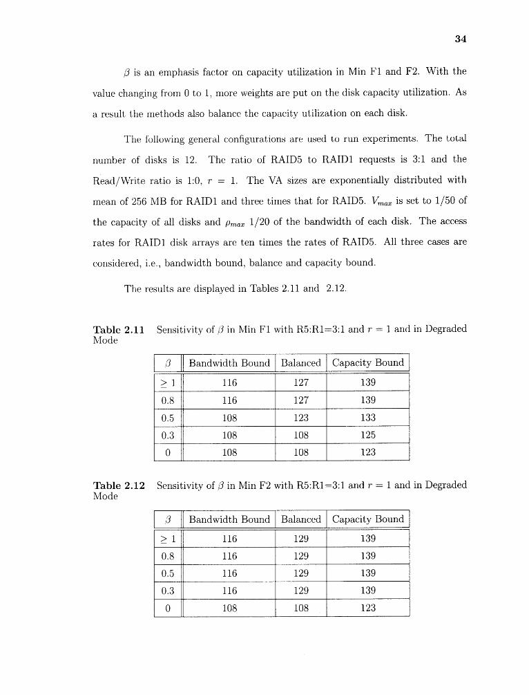
is an emphasis factor on capacity utilization in Min Fl and F2. With the

value changing from 0 to 1, more weights are put on the disk capacity utilization. As

a result the methods also balance the capacity utilization on each disk.

The following general configurations are used to run experiments. The total

number of disks is 12. The ratio of RAID5 to RAID1 requests is 3:1 and the

Read/Write ratio is 1:0, r = 1. The VA sizes are exponentially distributed with

mean of 256 MB for RAID1 and three times that for RAID5. Vmax is set to 1/50 of

the capacity of all disks and ρ„ -pax 1/20 of the bandwidth of each disk. The access

rates for RAID1 disk arrays are ten times the rates of RAID5. All three cases are

considered, i.e., bandwidth bound, balance and capacity bound.

The results are displayed in Tables 2.11 and 2.12.

Table 2.11 Sensitivity of 3 in Min Fl with R5:R1=3:1 and r 1 and in DegradedMode

Table 2.12 Sensitivity of in Min F2 with R5:R1=3:1 and r = 1 and in DegradedMode

35

Conclusions

1 . [3 has some effects on all three workloads.

2. In balance and capacity bound workloads the number of VAs allocated increasesmore than 10 percent when /3 varies from 0 to 1. The effects on bandwidthbound workload is less significant.

3. Rule of thumb is making 0 = 1.0.

2.4.1 Effects of ρm ax and Vmax

Amax and Vmax control the maximum size and estimated access rate of an allocation

request. If the values of these two parameters are set too small allocation requests

will be small in terms of both size and access rate too, which increases directory

space overhead. On the contrary if the values are too large, only a few requests can

be allocated. It is inefficiency due to fragmentation.

The following general configurations are used to run experiments. The total

number of disks is 12. The ratio of RAID5 to RAID1 requests is 1:0 and the

Read/Write ratio is 1:0, r = 1. The VA sizes are exponentially distributed with

mean of 768 MB for RAID5. Min Fl is used in this experiment because it is one of

the best reported in Section 2.3. /3 is set to 1. All three cases are considered, i.e.,

bandwidth bound, balance and capacity bound.

Table 2.13 Effects of Amax and Vmax in VAs Allocations

36

The following conclusions are drawn from the experiments in Table 2.13:

1. ()max can influence the number of allocations with both balanced and bandwidth

bound workload. The reason is Amax controls the maximum bandwidth of each

allocation, which will decide the size of the VA. As the size of VA varies theaffected disks in degraded mode also vary. Hence the number of allocations

fluctuates with Amax .

2. Amax has no effects on capacity hound workload. That is because with suchworkload, capacity is the bottleneck. It will reach its limit first before ()max

takes effect.

3. Vmax can influence the number of allocations with both balanced and capacity

bound workload. The reason is ρmax controls the maximum capacity of each

allocation, which will decide the size of the VA. As the size of VA varies theaffected disks in degraded mode also vary. Hence the number of allocations

fluctuates with Vmax•

4. Vmaxhas no effects on bandwidth bound workload. That is because with suchworkload, bandwidth is the bottleneck. It will reach its limit first before Vmaxtakes effect.

2.5 Clustered RAID

For a given disk model the capacity/bandwidth ratio (-yd) is fixed. If the capacity

bandwidth ratio for a VA without clustering (-y„) is same as that of disk then the

capacity/bandwidth utilization of the disk is balanced and more VAs can be allocated.

Unfortunately, most of the time -y, is riot equal 'Yd. By using clustering, i.e., changing

the parity group size G, the capacity and bandwidth of the VA can be changed. It is

possible to make the capacity/bandwidth ratio for the clustered VA -y, close to -yd.

a shows the load increase in CRAID5 and the parity group size G is related

with a (G = α(N — 1) + 1). If the 'm for a VA is lower than -yd (bandwidth utilization

is higher than capacity), then picking a small a can make the load increase small.

37

With a small a G is small too, which introduce more over head (1/G). As a result

the capacity utilization for this VA increases and bandwidth utilization decreases (-y,

increases). By varying a it is possible to find the best a to make -y, close to 7d.

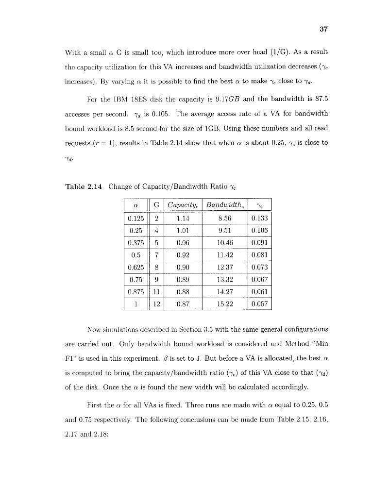
For the IBM 18ES disk the capacity is 9.17GB and the bandwidth is 87.5

accesses per second. -yd is 0.105. The average access rate of a VA for bandwidth

bound workload is 8.5 second for the size of 1GB. Using these numbers and all read

requests (r = 1), results in Table 2.14 show that when a is about 0.25, -y e is close to

Yd

Table 2.14 Change of Capacity/Bandiwdth Ratio -ye

Now simulations described in Section 3.5 with the same general configurations

are carried out. Only bandwidth bound workload is considered and Method "Min

Fl" is used in this experiment. fi is set to 1. But before a VA is allocated, the best a

is computed to bring the capacity/bandwidth ratio (-ye ) of this VA close to that (-yd)

of the disk. Once the a is found the new width will be calculated accordingly.

First the a for all VAs is fixed. Three runs are made with a equal to 0.25, 0.5

and 0.75 respectively. The following conclusions can be made from Table 2.15, 2.16,

2.17 and 2.18:

38

Table 2.15 Number of RAID5 Allocations with Bandwidth Bound Workload inDegraded Mode N = 12

Table 2.16 Number of RAID5 Allocations with Bandwidth Bound Workload inNormal Mode N = 12

Table 2.17 Number of RAID5 Allocations with Bandwidth Bound Workload inDegraded Mode with Dynamic Parity Group Size W

Table 2.18 Number of RAID5 Allocations with Bandwidth Bound Workload inNormal Mode with Dynamic Parity Group Size W

39

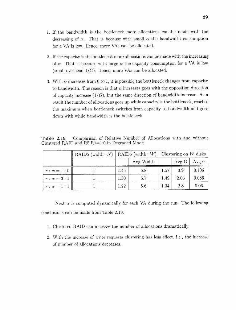
1. If the bandwidth is the bottleneck more allocations can be made with the

decreasing of a. That is because with small a the bandwidth consumption

for a VA is low. Hence, more VAs can be allocated.

2. If the capacity is the bottleneck more allocations can be made with the increasing

of a. That is because with large a the capacity consumption for a VA is low

(small overhead 1/G). Hence, more VAs can be allocated.

3. With a increases from 0 to 1, it is possible the bottleneck changes from capacity

to bandwidth. The reason is that a increases goes with the opposition direction

of capacity increase (1/G), but the same direction of bandwidth increase. As a

result the number of allocations goes up while capacity is the bottleneck, reaches

the maximum when bottleneck switches from capacity to bandwidth and goes

down with while bandwidth is the bottleneck.

Table 2.19 Comparison of Relative Number of Allocations with and withoutClustered RAID and R5:R1=1:0 in Degraded Mode

Next a is computed dynamically for each VA during the run. The following

conclusions can be made from Table 2.19:

1. Clustered RAID can increase the number of allocations dramatically.

2. With the increase of write requests clustering has less effect, i.e., the increase

of number of allocations decreases.

40

2.6 Conclusions and Related Work

HDA has been described in this study. Also several data allocation policies have been

specified and experimental results comparing the efficiency of several data allocation

methods have been reported. It is shown that two of these methods, which take into

account both disk access bandwidth and capacity outperform others across a wide

variety of allocation requests. The sensitivity of allocations to two of the parameter

settings, Amax and Vinci, has also been presented. Vmax has no effects on the number of

VA allocations while Amax has some impacts. Finally the effect of utilizing Clustered

RAID with bandwidth bound workload is analyzed. Results show that clustered

RAID can further improve the number of allocations.

HP AutoRAID implements two heterogeneous RAID levels (RAID1 and

RAID5) inside a single disk array controller [34] to satisfy a wide variety of workloads.

RAID1 is used , at the upper level to provide full redundancy and excellent performance

while RAID5 is applied at the lower level to improve storage cost for less active data, at

somewhat lower performance. The data blocks can be promoted or demoted between

these two levels as access patterns change.

HP AutoRAID uses all disks for a stripe (VA in this thesis) for RAID5. It is

well know that the performance of a full stripe in RAID5 is worse than a clustered

RAID5. HDA computes the width of a VA dynamically according to the size and

estimated access rate of an allocation. The average width of RAID5 VAs are usually

less than the number of disks in the system.

HP AutoRAID only deals with small datasets. The segment (VD in this study)

size is fixed, i.e. 128KB. HDA considers large file allocations.

Load balance in HP AutoRAID is just a hope because it focuses on the balance

of the amount of data on the disks instead of bandwidth usage. HDA explicitly makes

41

load balance as a target because nowadays bandwidth is the bottleneck in storage

systems.

The HP AutoRAID array uses static partition: part of the space are RAID1

while the rest are formatted to be RAID5. The potential problem is that it may run

into a thrashing mode in which each update causes the target Relocation Block (RB)

to be promoted up to RAID 1 and a second one demoted to RAID5 if the active write

working set exceeds the size of RAID 1 storage for long periods of time. HDA decides

RAID level of an allocation on the fly so that there is no static partition.

CHAPTER 3

RAID LEVEL SELECTION FOR HETEROGENEOUS DISK ARRAYS

3.1 Introduction

There has been an explosion in the volume of data being generated, but this has been

accompanied with an exponential increase in magnetic recording density resulting

in larger disk capacities in small form factor disks and dropping cost per gigabyte .

Storage represents a growing fraction of total system cost and more importantly

storage management ocosts are increasing rapidly. This is a step in simplifying this

process.

A method is proposed to maximize the number of allocated datasets, referred

to as Virtual Arrays - VAs in Heterogeneous Disk Arrays - HDAs. 1 HDAs support

two levels: RAID1 and RAID5, which both tolerate single disk failures, but have

different characteristics in processing database workloads [48]. The number of allocations

is constrained by the disk bandwidth, so a VA is allocated at a RAID level, which

minimizes the disk access bandwidth. A review of related work follows.

Disk space for RAID 1 and RAID5 containers are allocated on demand to make

space for file allocation requests, which are tagged as RAID1 or RAID5 in advance,

e.g., small files are allocated as R AID1 and large files as RAID5 [7]. RAID1 and

RAID5 containers share space on possibly heterogeneous disks.

The single level allocation of VAs with predetermined RAID 1 and RAID5

levels is investigated in [69], but only homogeneous disks are considered. Each VA

has an associated size and access rate proportional to size, which also depends to

its RAID level. VAs are partitioned into multiple Virtual Disks - VDs based on

VAs may be considered to be equivalent to Logical Units -L Us in RAID literature.

42

43

a maximum bandwidth and capacity per disk per VA. VDs are allocated to disks

taking into account current disk bandwidth and capacity utilizations in a single

pass algorithm, i.e. no optimization is attempted by batching requests. It is shown

in [7] [69] that allocation methods, which minimize the variation of bandwidth and

capacity utilization across disks perform better than others which do not.

In this study the realistic case is considered, where the disk bandwidth is

the only limiting resource, i.e., that disk capacity is not a constraining resource.

Unlike [69] the RAID level is not known a priori, but rather determined using a

simple queueing analysis based on VA's workload characteristics. VAs are subject to

two types of requests: (i) accesses to small blocks of data, as in the case of online

transaction processing applications, (ii) accesses to large blocks, as in the case of

batch applications. Such accesses are processed as full stripe reads and writes for

efficiency purposes. The frequencies of the two types of requests and the fraction of

reads and writes in each category are assumed to be known.

VAs are classified into two RAID levels based on the level, which provides

the lower load. The classification shows that RAID5 is the preferred level when the

frequency of full stripe requests spanning all disks is high. RAID1 is the preferred

level when the fraction of small writes is high. An allocation study with a synthetic

workload is reported, which shows that a combination of RAID levels results in more

allocations than a single level, either RAID1 or RAID5.

This chapter is organized as follows. In Section 3.2 the RAID1 and RAID5

levels are described, which are utilized in this study. In Section 3.3 the modeling

assumptions, the notation used in this chapter, and expressions for the parameters

used in the analysis are provided. The analytical formulas used in classification are

developed in Section 3.4. In Section 3.5 the results of a parametric study is presented

to gain insight into the results of classification. In Section 3.6 empirical study is

44

reported that HDA outperform a purely RAID1 or RAID5 allocation. Finally, in

Section 3.7 conclusions are presented.

3.2 RAID Levels and Their Operation

The RAID paradigm is necessitated by high data availability requirements due to

the high cost of downtime in many applications. Furthermore, the loss of certain

data is unacceptable, because the data is irreproducible or very costly to reproduce .

The original 1988 RAID proposal had five RAID levels tolerating single disk failures

via mirroring in RAID level 1 or RAID1, which introduces 100% redundancy, and

parity coding used in RAID levels 3-5 with one disk out of N dedicated to parity [48].

RAID2 based on the Hamming code is excluded from the discussion, because of its

high overhead when small blocks are updated. Striping is intended to eliminate disk

access skew. It partitions large datasets into stripe units - SUs, which are allocated

in a round-robin manner across the disks.

RAID3 and RAID4 both allocate parity blocks on one disk, but RAID3 is

riot suited for general-purpose applications, since it is geared for parallel access to

massive datasets via synchronized reading and writing of all disks. RAIDO is a RAID

with striping, but no redundancy, as a consequence disks are subjected to the least

possible load. The parity disk can become a bottleneck in RAID4 for a write-intensive

workload. RAIDS alleviates this problem by using the left-symmetric layout which

places parity SUs in left-to-right repeating diagonals [48].

The Basic Mirroring - BM configuration of RAID1 replicates the same data

on two disks, so that it can be read from either disk [63][70]. The fact that mirroring

doubles the access bandwidth to data is important from the viewpoint of rapidly

increasing disk capacities, i.e., a single disk may be unable to provide the bandwidth

45

required for accessing the data that it holds. Access time can be improved by judicious

routing of read requests, i.e., data is accessed from the disk providing the lower access

time. Updates should be carried out at both disks, but they can first be held in Non-

Volatile Storage - NVS. This allows read requests which affect application response

time to be processed at a higher priority than writes. Repeated updating of dirty

blocks in NVS reduces the number of disk accesses for destaging data. Furthermore,

destaging dirty blocks in batches reduces disk utilization for writing. Thees effects

can be quantified by analyzing I/O trace data, but this is beyond the scope of this

study. NVS caches are applicable to RAID5 disk arrays [67].

RAID1/0 stripes data across multiple RAID1 arrays, but when one of the disk

fails, the read load on the surviving disk is doubled as in BM. Striping is applicable

to RAID1 with multiple pairs of disks. Three RAID1 configurations with a smaller

overload than BM are described in [63][70]. For example, the interleaved declustering

layout distributes the load of a failed disk in a cluster of n disks over n — 1 disks, so

that the increase of read load per disk is n 1(n — 1) [63][70]. Only BM is considered

in this study for the sake of brevity, but the method developed here can be easily

applied to other RAID1 configurations.

The updating of small data blocks in RAID5 is costly and is hence referred

to as the small write penalty in RAID5. The reconstruct write reads the remaining

corresponding blocks in a stripe and exclusive-ORs (XORs) them with the modified

data block to compute the parity [60]. Reconstruct writes are preferable when the

parity group size is small or more than one parity block is to be computed. The

alternative read-modify-write method is costly in that it incurs two accesses to read

the data arid the parity block arid two accesses to write them [48]. Updates can be

carried out more efficiently by using Read- Modify - Writes - RMWs, i.e., the reading

of a data and parity block, followed by their overwriting after one disk rotation [8].

Disks have the capability to compute parities and the difference (XOR) of the new

46

and old data blocks computed at the data disk is sent to the parity disk, where the

new parity is computed. The parity is computed at disks given the old data and parity

blocks. Processing reads and writes of data and parity blocks as separate requests,

with the parity computed at the RAID controller, provides higher data integrity than

RMWs [8].

The updating of large data blocks in RAIDS, can be carried out efficiently

as full stripe writes, i.e., the writing of all SUs in a stripe over all disks. The

efficiency results from the fact that the new parity SU is calculated by

exclusive-ORing (XORing)the data SUs as they are being transmitted to consecutive disks.

If a disk block is requested on a failed disk it can be reconstructed on demand

by issuing a fork-join request, which reads the corresponding blocks from the N —1

surviving disks and XORs them to reconstruct the missing block. Since in addition

to fork-join read requests each disk processes its own read requests the read load of

the surviving disks is doubled in degraded mode. Clustered RAID which utilizes a

smaller parity group size (G) than the number of disks in the array is a solution to

the load increase problem [53]. Parity group layouts to balance the update load are

discussed in the Appendix of [3]. The load increase with read and write requests

in clustered RAID is given in [3]. Clustered RAID provides a tradeoff between disk

bandwidth and capacity utilization. It has been considered in [69], but will not be

considered in this study.

The rebuild process in RAIDS is a systematic reconstruction of the contents

of a failed disk on a spare disk. This involves the reading of successive rebuild units

(e.g., tracks), XORing corresponding tracks to recreate a lost track, and writing the

reconstructed track onto a spare disk. RAIDS is susceptible to data loss if there is

a second disk failure, before the rebuild process is completed, or the rebuild process

47

cannot complete because of a latent sector failure - LSF, which is the more likely

event.

Two disk failure tolerant - 2DFT can be used for storing datasets with very

high availability requirements at the cost of extra redundancy, two check disks versus

one in RAID5. Two disk failures are rather uncommon, but RAID6 allows the rebuild

process after one disk failure to be completed in spite of LSFs. Reed-Solomon codes

are utilized in RAID6 disk arrays, while EVENODD, RDP, X-code, and RM2 utilize

specialized parity codes. 2DFTs is not considered to shorten the discussion, but the

methods described in this chapter can be extended to include 2DFTs in HDA in a

straightforward manner. The performance of several 2DFT arrays from the viewpoint

of disk accesses is studied in [3] [8]. RAID6, EVENODD, and RDP exhibit the same

disk access pattern and for example with two disk failures the load on the surviving

disks is tripled for read requests.

HP's AutoRAID switches the RAID level between RAID1/0 and RAID5 dynam-

ically, i.e., data with a high access rate is stored as RAID1 [34]. Log-Structured Arrays

-LSAs accumulate modified files in a cache associated with the RAID controller, which

are then written out as full stripe writes. An example, is the Iceberg disk array, which

is also a RAID6 [48]. AutoRAID's RAID5 arrays also utilize the LSA paradigm.

The automatic selection of RAID levels into RAID1/0 and RAID5 is addressed

in a comprehensive study ,reported in [26], which is part of a study of data allocation

in disk arrays [25]. The two approaches considered in [26] are classified as the tagging

approach and a solver-based or integrated approach. The tagging approach is classified

as rule-based and model based. The rule-based tagging approach is based on a set of

rules of thumb. The model based approach selects the RAID level which minimizes

the umber of TOPS (I/Os per second). The solver-based approach has two variants.

partially adaptive and fully adaptive. In the former case the RAID level cannot be

48

reassigned, while this is possible in the latter case. A dozen initial goal functions are

proposed, such as minimize the average of capacities and utilizations of all the disks.

An analytic method is developed to select RAID levels for disk arrays and

provide empirical evidence that HDA outperforms a pure RAID1 or RAID5 configu-

ration.

3.3 Modeling Assumptions

Disk space constraints are not considered in this study, since this is not an issue with

increasing disk capacities, but still relative space requirements are interesting. The

SU size is K tracks with K = 1 initially, but the allocation size can be varied with

K. All VA allocations have the same size for data, i.e., M —1 SUs. In RAID5 arrays

with width M, a VA allocation will constitute a stripe. For RAID1 with the BM

configuration all M — 1 data tracks per allocation are written consecutively on one

disk and then replicated on another, i.e., there is no striping.

Variable size allocations will not have an effect on the total number of allocations,

since bandwidth bound disks are assumed to have an infinite capacity. To furthermore

simplify the discussion it is assumed that all allocation requests have the same arrival

rate. Although variable arrival rates of requests to disks can be accommodated, it

follows from the discussion that these variability will not effect the classification. The

number of tracks per SU (designated as K) is varied since this affects disk access

times.

Reads and writes are allowed to small and large blocks. The latter are processed

as full stripe writes or reads in RAID5. According to the LSA paradigm, full stripe

reads are used to reclaim the storage space for the old versions of datasets, but the

latest versions of datasets are copied first into a new stripe, so that stripes which are

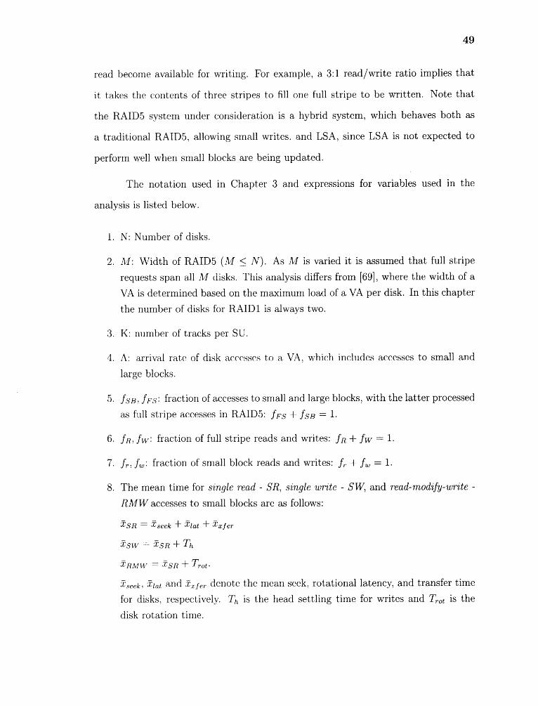
49

read become available for writing. For example, a 3:1 read/write ratio implies that

it takes the contents of three stripes to fill one full stripe to be written. Note that

the RAID5 system under consideration is a hybrid system, which behaves both as

a traditional RAID5, allowing small writes, and LSA, since LSA is not expected to

perform well when small blocks are being updated.

The notation used in Chapter 3 and expressions for variables used in the

analysis is listed below.

1. N: Number of disks.

2. M: Width of RAID5 (M < N). As M is varied it is assumed that full stripe

requests span all M disks. This analysis differs from [69], where the width of a

VA is determined based on the maximum load of a VA per disk. In this chapter

the number of disks for RAID1 is always two.

3. K: number of tracks per SU.

4. A: arrival rate of disk accesses to a VA, which includes accesses to small and

large blocks.

5. fsB, fFS : fraction of accesses to small and large blocks, with the latter processed

as full stripe accesses in RAID5: fFS + fSB = 1.

6. fR , fw : fraction of full stripe reads and writes: fR + fw = 1.

7. fr., fw : fraction of small block reads and writes: fr. + fa, = 1.

8. The mean time for single read - SR, single write - SW, and read-modify-write -RMW accesses to small blocks are as follows:

seek, xlatand xxfer denote the mean seek, rotational latency, and transfer time

for disks, respectively. Th is the head settling time for writes and Trot is the

disk rotation time.

50

9. For full stripe accesses, it is assumed that full tracks are read or written. In

both cases a zero-latency capability is assumed, i.e., once the head seeks to the

appropriate track, the access starts at the next sector boundary, so that the

rotational latency is almost eliminated. In this study the effect of track and

cylinder skews [14] are ignored, since they introduce a negligible delay. The SU

size is set to the average track size, so setting the transfer time to Trot is an

approximation.

For RAIDS:

For RAID1 (Basic Mirroring) with all M — 1 SUs on one disk.

10. U: relative disk bandwidth utilization.

11. C: relative disk capacity utilization.

3.4 Analytical Model

Two modes for RAID operation are considered.

Normal mode: VA loads are computed without considering the possibility of disk

failures, so that the allocations are carried out in normal mode.

Degraded mode: The load increase with one broken disk is calculated and used

when VAs are allocated. So that after the allocations the system will not be

overloaded because of a disk failure.

Accesses to small and large blocks are considered. The analysis for small

blocks appeared in [3], but necessary equations are repeated here for the sake of

completeness. Since VAs process accesses to small and large blocks, disk utilizations

are the sum of utilizations over the two types of requests.

In what follows ρ is used to denote disk utilization, but also as the total load

per VA or sum of utilizations of its VDs, in which case ρ can be greater than one.

51

(3.1)

(3.2)

(3.3)

(3.4)

(3.5)

(3.6)

3.4.1 Operation in Normal Mode

Disk utilizations for RAID5.

Utilization for small block requests.

Utilization for full stripe accesses.

Total utilization per VA:

Disk utilizations for RAID1.

Utilization for small block requests:

Utilization for full stripe accesses:

Total utilization per VA:

3.4.2 Operation in Degraded Mode

Disk utilizations in RAID5.

As far as read requests are concerned, fork-join requests to reconstruct missing

data blocks access M —1 disks in RAID5, while one disk access is required for RAID1.

The read load on surviving disks is doubled in both cases. Write requests in RAID5

spawn fork-join requests to compute the parity when the data block is missing, but

otherwise the data block is simply written.

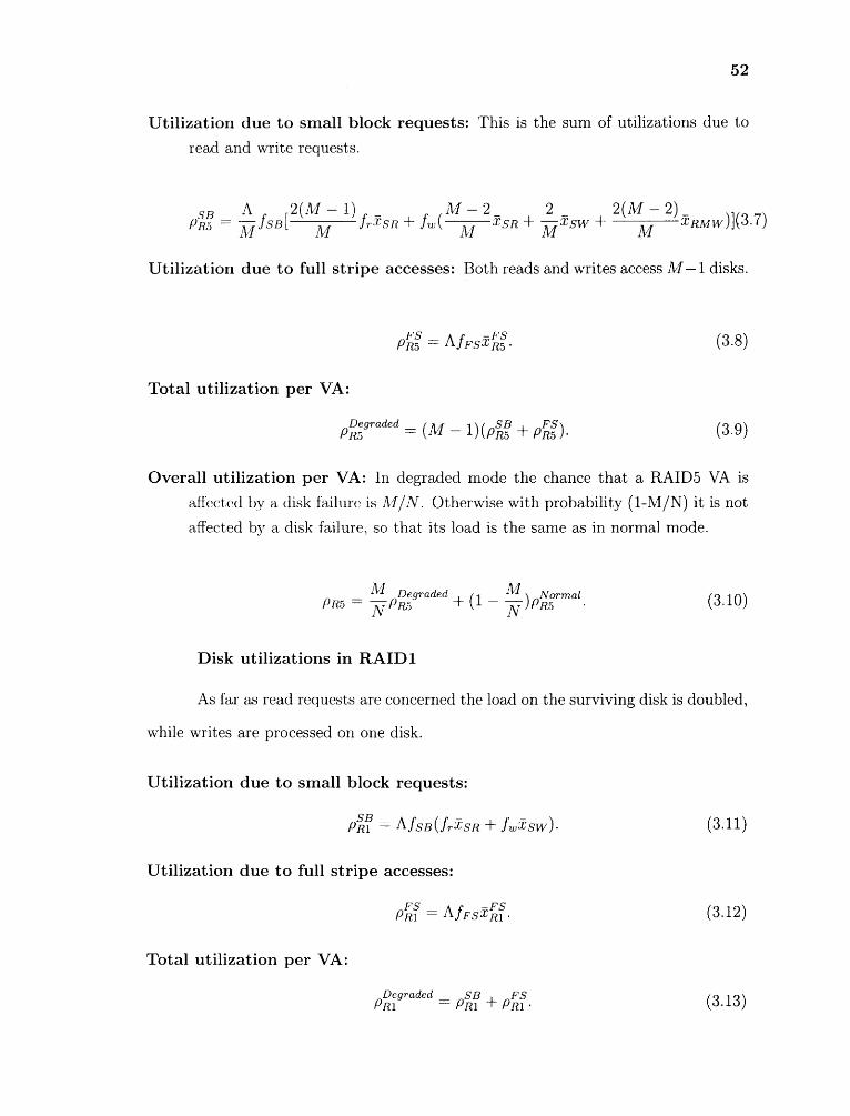
52

Utilization due to small block requests: This is the sum of utilizations due toread and write requests.

Utilization due to full stripe accesses: Both reads and writes access M-1 disks.

Total utilization per VA:

Overall utilization per VA: In degraded mode the chance that a RAID5 VA isaffected by a disk failure is M/N. Otherwise with probability (1-M/N) it is notaffected by a disk failure, so that its load is the same as in normal mode.

Disk utilizations in RAID1

As far as read requests are concerned the load on the surviving disk is doubled,

while writes are processed on one disk.

Utilization due to small block requests:

(3.8)

(3.9)

Utilization due to full stripe accesses:

Total utilization per VA:

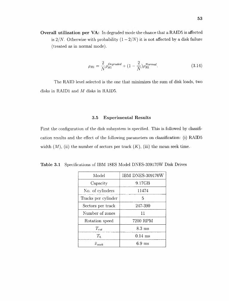
53

Overall utilization per VA: In degraded mode the chance that a RAID5 is affectedis 2/N. Otherwise with probability (1 — 2/N) it is not affected by a disk failure

(treated as in normal mode).

The RAID level selected is the one that minimizes the sum of disk loads, two

disks in RAID1 and M disks in RAID5.

3.5 Experimental Results

First the configuration of the disk subsystem is specified. This is followed by classifi-

cation results and the effect of the following parameters on classification: (i) RAID5

width (M), (ii) the number of sectors per track (K), (iii) the mean seek time.

Table 3.1 Specifications of IBM 18ES Model DNES-309170W Disk Drives

54

3.5.1 Disk Array Configuration

The disk array has N = 12 disk drives, where N determines the maximum width of

RAID5 arrays. IBM 18ES (model DNES-309170W) disk drives is used, 2 whose speci-

fications are given in Table 4.7. Particularly important is the seek time characteristic,

³ which is required in calculating its moments. The mean access time to small blocks

is the sum of mean seek time, rotational latency (approximately half a disk rotation),

and transfer time. The results of this study are expected to be applicable to other

disk drives as well.

The mean seek time given in Table 4.7 is based on the unrealistic assumption

that all disk blocks are accessed uniformly. A much lower seek time is observed in

operational systems for the following reasons: (i) disk cylinders are not fully populated

and in zoned disks it is the outer disk cylinders, which have a higher capacity that are

written first; (ii) spatial locality of reference; (iii) seek time can be reduced by reorga-

nizing disk data. For example, the organ pipe organization places files with higher

access frequencies on contiguous disk cylinders. The results given in this chapter

are based on -seek 1.2 milliseconds (ms), but the sensitivity study of classification

results to seek time is presented in Section 3.5.5.

The SU size (K) is initially set to one track, but K is varied to study its effect

on classification results (see Section 3.5.4). The Read/Write ratio for large accesses is

assumed to be R : W = 3 : 1, but in Section 3.5.6 the sensitivity of the classification

to this ratio is investigated.

2http://www.storage.ibm.com/hdd/prod/ultrastar.htm .³http://www.pdl.cmu.edu/DiskSim/diskspecs.html.

55

3.5.2 Classification Results

Table 3.2 provides the RAID level assignments in normal mode for N = 12, M = 6

and K = 1 as fFS (fraction of full stripe accesses - left column of the table) and

fr (fraction of reads accesses to small blocks - the first row in the table) are varied.

It can be observed that when the fraction of full stripe accesses is high, RAID5 is

preferable to RAID1 (the lower right hand corner of the tables). RAID1 is preferable

to RAID5 when the fraction of writes for small data blocks is high, which is due to

the small write penalty (upper left hand corner of the tables).

Table 3.3 is the counterpart of Table 3.2 in degraded mode.

In Table 3.4 and Table 3.5 the classification is repeated with M = 4. The

results are similar to the results for M = 6, but it is observed that a smaller M width

favors RAID5. The classification with M = 2 is RAID5 only when all accesses are

full stripe accesses or they are all reads. For M = 2 RAID5 in normal mode requires

two RMWs, while RAID 1 requires two writes.

Figure 3.1 displays the variation in overall disk utilization for RAID1 and

RAIDS in degraded mode, which determines the classification. Disk loads per VA

allocation or the total utilization is computed setting Λ = 8.7 accesses/second. From

the figure it is shown the load for RAID1 and R AID5 decreases as fr increases. The

reason is that the load increase in degraded mode is a weighted average of load for VAs

in normal mode and for VAs with a single disk failure. This follows from Equation

(3.10) and Equation (3.14). As fr increases the disk load in normal mode for RAID5

decreases, since the effect of the small write penalty is diminished. In RAID1 the load

is smaller for read requests than writes, since only one disk is involved in processing

a read request. Also with an increase in the fraction of full stripe accesses (fFS ) the

lines shift upward in parallel, which is simply because full stripe accesses result in a

higher load.

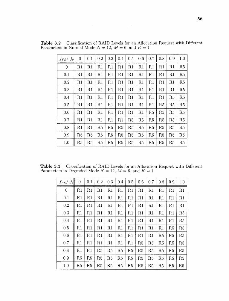
56

Table 3.2 Classification of RAID Levels for an Allocation Request with DifferentParameters in Normal Mode N = 12, M = 6, and K = 1

Table 3.3 Classification of RAID Levels for an Allocation Request with DifferentParameters in Degraded Mode N = 12, M = 6, and K = 1

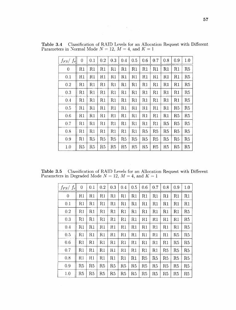
57

Table 3.4 Classification of RAID Levels for an Allocation Request with DifferentParameters in Normal Mode N = 12, M = 4, and K = 1

Table 3.5 Classification of RAID Levels for an Allocation Request with DifferentParameters in Degraded Mode N = 12, M = 4, and K = 1

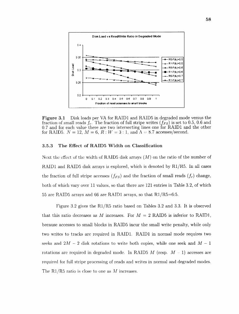
58

Figure 3.1 Disk loads per VA for RAID1 and RAIDS in degraded mode versus thefraction of small reads fr . . The fraction of full stripe writes (fFS ) is set to 0.5, 0.6 and0.7 and for each value there are two intersecting lines one for RAID1 and the otherfor RAID5. N = 12, M = 6, R : W = 3 : 1, and Λ = 8.7 accesses/second.

3.5.3 The Effect of RAID5 Width on Classification

Next the effect of the width of RΛID5 disk arrays (M) on the ratio of the number of

RAID1 and RAIDS disk arrays is explored, which is denoted by R1/R5. In all cases

the fraction of full stripe accesses (fFs ) and the fraction of small reads (L.) change,

both of which vary over 11 values, so that there are 121 entries in Table 3.2, of which

55 are RAID5 arrays and 66 are RAID1 arrays, so that R1/R5=6:5.

Figure 3.2 gives the R1/R5 ratio based on Tables 3.2 and 3.3. It is observed

that this ratio decreases as M increases. For M = 2 RAIDS is inferior to RAID1,

because accesses to small blocks in RAIDS incur the small write penalty, while only

two writes to tracks are required in RAID1. RAID1 in normal mode requires two

seeks and 2M — 2 disk rotations to write both copies, while one seek and M — 1

rotations are required in degraded mode. In RAIDS M (resp. M — 1) accesses are

required for full stripe processing of reads and writes in normal and degraded modes.

The Rl/R5 ratio is close to one as M increases.

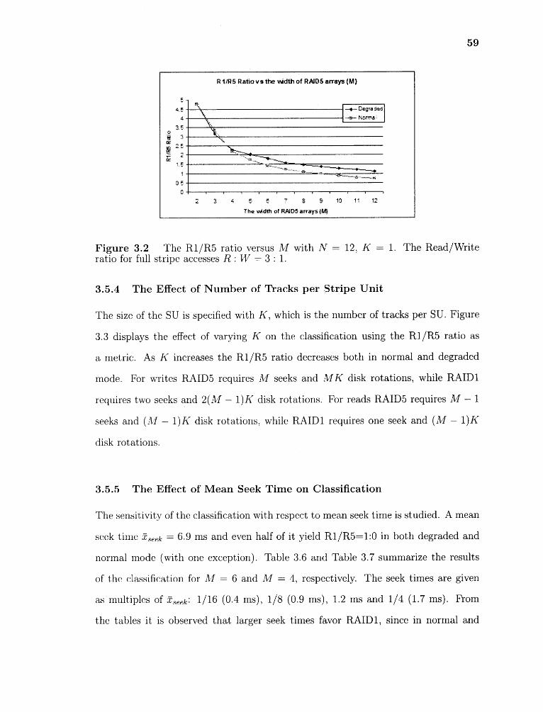
59

Figure 3.2 The R1/R5 ratio versus M with N = 12, K = 1. The Read/Writeratio for full stripe accesses R : W = 3 : 1.

3.5.4 The Effect of Number of Tracks per Stripe Unit

The size of the SU is specified with K, which is the number of tracks per SU. Figure

3.3 displays the effect of varying K on the classification using the R1/R5 ratio as

a metric. As K increases the R1/R5 ratio decreases both in normal and degraded

mode. For writes RAID5 requires M seeks and MK disk rotations, while RAID1

requires two seeks and 2(M — 1)K disk rotations. For reads RAID5 requires M — 1

seeks and (M — 1)K disk rotations, while RAID1 requires one seek and (M — 1)K

disk rotations.

3.5.5 The Effect of Mean Seek Time on Classification

The sensitivity of the classification with respect to mean seek time is studied. A mean

seek time xseek = 6.9 ms and even half of it yield R1/R5=1:0 in both degraded and

normal mode (with one exception). Table 3.6 and Table 3.7 summarize the results

of the classification for M = 6 and M = 4, respectively. The seek times are given

as multiples of seek: 1/16 (0.4 ms), 1/8 (0.9 ms), 1.2 ms and 1/4 (1.7 ms). From

the tables it is observed that larger seek times favor RAID1, since in normal and

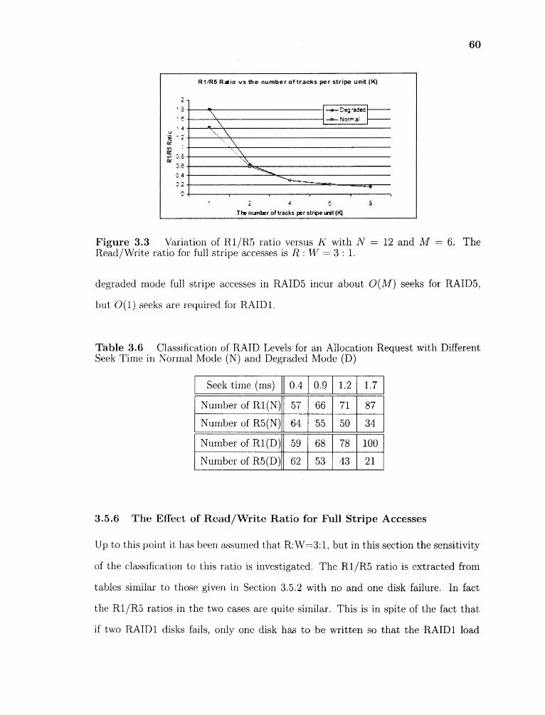
60

Figure 3.3 Variation of R1/R5 ratio versus K with N = 12 and M = 6. TheRead/Write ratio for full stripe accesses is R : W = 3 : 1.

degraded mode full stripe accesses in RAID5 incur about 0(M) seeks for RAID5,

but 0(1) seeks are required for RAID1.

Table 3.6 Classification of RAID Levels for an Allocation Request with DifferentSeek Time in Normal Mode (N) and Degraded Mode (D)

3.5.6 The Effect of Read/Write Ratio for Full Stripe Accesses

Up to this point it has been assumed that R:W=3:1, but in this section the sensitivity

of the classification to this ratio is investigated. The R1/R5 ratio is extracted from

tables similar to those given in Section 3.5.2 with no and one disk failure. In fact

the R1/R5 ratios in the two cases are quite similar. This is in spite of the fact that

if two RAID1 disks fails, only one disk has to be written so that the RAID1 load

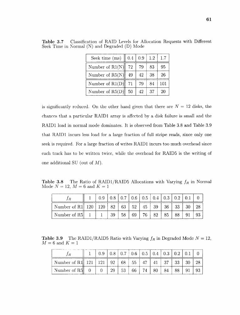
61

Table 3.7 Classification of RAID Levels for Allocation Requests with DifferentSeek Time in Normal (N) and Degraded (D) Mode

is significantly reduced. On the other hand given that there are N = 12 disks, the

chances that a particular RAID1 array is affected by a disk failure is small and the

RAID1 load in normal mode dominates. It is observed from Table 3.8 and Table 3.9

that RAID1 incurs less load for a large fraction of full stripe reads, since only one

seek is required. For a large fraction of writes RAID1 incurs too much overhead since

each track has to be written twice, while the overhead for RAID5 is the writing of

one additional SU (out of M).

Table 3.8 The Ratio of RAID1/RAID5 Allocations with Varying fR in NormalMode N = 12, M = 6 and K =1

Table 3.9 The RAID1/RAID5 Ratio with Varying fR in Degraded Mode N = 12,M = 6 and K = 1

62

3.6 Effectiveness of Classification on HDA Performance

Experiments are carried out to ascertain the effectiveness of the classification method

developed in this chapter and that an HDA populated with VAs (Virtual Arrays)

classified according to this method outperforms a disk array consisting solely of

RAID1 or RAID5 arrays.

A large number of allocation requests for VAs are generated by using a synthetic

workload based on randomly generated input parameters, classify them into RAID1

and RAID5, and allocate them on disks. The steps of the experiment are outlined

as Algorithm 2. The experiments which are run with the following input parameters,

measures the ratio of disk bandwidth and capacity utilization.

N = 12 disks.

One track per SU (K = 1).

The read/write ratio for full stripe accesses is R : W = 3 : 1 or fR = 0.75.

The fraction of reads for small blocks is r : w = 3 : 1 or fr = 0.75.

The fraction of full stripe accesses (fFS ) is uniform in the range (0, 1).

The width of RAID5 is M = 6 VDs.

The width of RAID1 arrays is two VDs.

The experiment was run for 'ma, = 1000 allocations to yields statistically accurate

results.

The arrival rate per VA (Λ) is sufficiently small so that the disk bandwidth limit is

not reached.

Disk capacities were assumed to be infinite.

In operation in degraded mode the overall laod in degraded mode is considered,

rather than assuming that all VAs are affected by a disk failure, which is overly

pessimistic.

63

Algorithm 2 HDA allocation experiment with VAs classified as RAID1 or RAID5.

Generate and allocate VAi for 1 < i < /max .

1. For VAi generate the fraction of full stripe reads and writes (IFS).

The remaining requests are accesses to small blocks. This is not

done in all experiments.

2. For VAi generate fraction of read requests to small blocks (fr ).The remaining requests are writes to small blocks. This is not

done in all experiments.

3. Compute the VA load assuming it is RAID 1 as the sum of two

VD utilizations in normal mode and with one failed disk. The

total load is ρR1 (see Equation (3.14)).

4. Compute the VA load assuming it is RAID5 as the sum of M VD

utilizations in normal mode and with one failed disk failure. The

total load is ρR5 (see Equation (3.10)).

5. The RAID level for a VA is selected to be the one with the

lower overall load, i.e., RAID1 or RAID5 depending on which

level yields the same organization, i.e., min(ρR1 , ρR5 ).

6. Allocate the VDs of VA i to disks with the minimum utilization

of their bandwidth, i.e., the worst fit method in [7][69].

7. Increment the bandwidth utilization of disks on which VDs of VAi

are assigned. Also increment allocated disk capacity: (M — 1)K

tracks per disk for RAID1 and K tracks per disk in RAIDS.

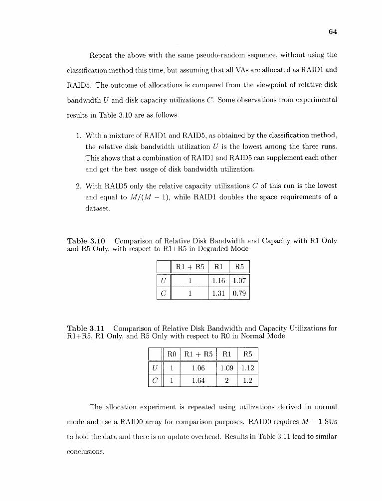
64

Repeat the above with the same pseudo-random sequence, without using the

classification method this time, but assuming that all VAs are allocated as RAID1 and

RAID5. The outcome of allocations is compared from the viewpoint of relative disk

bandwidth U and disk capacity utilizations C. Some observations from experimental

results in Table 3.10 are as follows.

1. With a mixture of RAID 1 and RAID5, as obtained by the classification method,

the relative disk bandwidth utilization U is the lowest among the three runs.

This shows that a combination of RAID1 and RAID5 can supplement each other

and get the best usage of disk bandwidth utilization.

2. With RAID5 only the relative capacity utilizations C of this run is the lowest

and equal to M/ (M — 1), while RAID1 doubles the space requirements of a

dataset.

Table 3.10 Comparison of Relative Disk Bandwidth and Capacity with R1 Onlyand R5 Only, with respect to Rl+R5 in Degraded Mode

R1 + R5 I R1 I R5

Table 3.11 Comparison of Relative Disk Bandwidth and Capacity Utilizations forR1+R5, R1 Only, and R5 Only with respect to R0 in Normal Mode

R0 I R1 + R5 I R1 I R5

The allocation experiment is repeated using utilizations derived in normal

mode and use a RAID0 array for comparison purposes. RAID0 requires M — 1 SUs

to hold the data and there is no update overhead. Results in Table 3.11 lead to similar

conclusions.

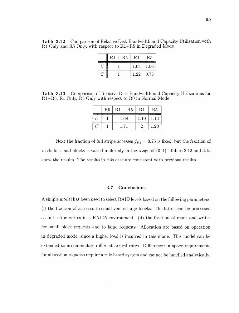
65

Table 3.12 Comparison of Relative Disk Bandwidth and Capacity Utilization withR1 Only and R5 Only, with respect to R1+R5 in Degraded Mode

Table 3.13 Comparison of Relative Disk Bandwidth and Capacity Utilizations forR1+R5, R1 Only, R5 Only with respect to R0 in Normal Mode

Next the fraction of full stripe accesses fFS = 0.75 is fixed, but the fraction of

reads for small blocks is varied uniformly in the range of (0, 1). Tables 3.12 and 3.13

show the results. The results in this case are consistent with previous results.

3.7 Conclusions

A simple model has been used to select RAID levels based on the following parameters:

(i) the fraction of accesses to small versus large blocks. The latter can be processed

as full stripe writes in a RAID5 environment. (ii) the fraction of reads and writes

for small block requests and to large requests. Allocation are based on operation

in degraded mode, since a higher load is incurred in this mode. This model can be

extended to accommodate different arrival rates. Differences in space requirements

for allocation requests require a rule based system and cannot be handled analytically.

66

The parametric study yields insight as to which RAID level is more appropriate

for different parameter settings. It has been shown that a combination of RAID1 and

RAID5 levels in one disk array results in a reduction in bandwidth utilization.

CHAPTER 4

RELIABILITY AND PERFORMANCE OF MIRRORED DISK

ORGANIZATIONS

4.1 Introduction

Disk mirroring or RAID level 1 (RAID1) predates the Redundant Arrays of Independent

Disks - RAID classification [51], but is still a very popular paradigm as exemplified

by EMC's Symmetrix disk array. It was used in two large-scale systems with a large

number of disks: Teradata's DBC/1012 [59] and Tandem's NonStop SQL system [58].

The initial five RAID level classification (RAID1-5) [51] was later extended to seven

levels by adding RAID0 and RAID6 [48]. RAID0 is based on striping, which partitions

large files into fixed size stripe units allocated in round-robin manner on the disks

in the array. Striping balances disk loads, since files with different access rates share

disk space. In this study it is assumed that disk loads in multi-disk R AID1 configu-

rations are balanced by via either striping or manual load balancing. RAID3-5 (resp.

RAID6) dedicate the capacity of one (resp. two) disks to allow recovery from one

(resp. two) disk failures. RAID5 disks can hold more user data, but this issue is

ignored since disk capacities are not fully utilized.

In basic mirroring - BM the data held on N/2 primary disks is replicated on

N/2 secondary disks. When data is modified the updating of one of two disks can

be deferred as long as one disk is updated. When modified data is written onto

nonvolatile storage - NVS, the updating of both disks can be deferred (see Section

4.2). The fact that data can be read from either disk is advantageous since: (i) disk

workloads tend to be dominated by read requests; (ii) advances in magnetic recording

density have resulted in several orders of magnitude increase in disk capacity in the

last decade, but it is difficult to exploit the increased capacity since the access rate to

67

68

each disk is proportional to the volume of data stored on that disk; (iii) disk access

time is improving very slowly due to its mechanical nature.

BM can tolerate up to N/2 disk failures, as long as one disk in each pair

survives. On the other hand the failure of a disk results in the doubling of the read load

on the surviving disk. In this chapter the performance, and performability of several

RAID1 organizations, which alleviate this shortcoming of BM, i.e., distribute the load

of a failed disk on multiple disks is investigated. These organizations are described

in Section 4.3. Expressions for the reliability of these organizations, which turn out

to be less reliable than basic mirroring are given in [63] and summarized in Section

4.4. An approximate method based on asymptotic expansions of disk unreliabilities

is given in [62]. This method allows a quick comparison of RAID reliabilities without

resorting to numerical methods. The performability measure combines reliability and

performance metrics [15].

The maximum throughput attainable by different RAID1 organizations is

obtained and an M/G/1 queueing model is utilized to compare their mean response

times in normal or fault-free mode and also degraded mode operation. RAID1

performance is also compared with RAID0, RAID5, and RAID6 organizations when

the total number of disks is fixed (equal to N). The case when the number of data disks

in RAID 1 is the same as the number of data disks in RAID5 has been considered in

[22], but this case is not considered here for sake of brevity and especially that RAID1

outperforms RAID5 significantly. The performance comparison is carried out with

read and write requests to small randomly placed data blocks.

The chapter is organized as follows. Work related to disk arrays is discussed

in Section 4.2. Section 4.3 provides the description of four RAID1 organizations,

whose reliabilities are derived in [63]. The reliability expressions are summarized

in Section 4.4. The reliability and performability in the four cases is compared in

Table 4.1 Notation Used in Chapter 4

69

Section 4.5. The details of the derivation of performability are lengthy and are given

in the Appendix. In Section 4.6 the analysis to obtain the mean response time for

read and write requests in RAID1 in both normal and degraded modes is provided.

Graphs for read response times, which incorporate the effect of write requests are

given in Section 4.7. This is followed by the conclusions given in Section 4.8. The

notation used in this chapter is summarized in Table 4.1.

4.2 Related Work

Disk arm scheduling is one method to improve disk performance. Shortest seek time

first - SSTF and SCAN are two policies to minimize seek time by reducing the seek

distance. The Shortest Positioning/Access Time First - SPTF or SATF significantly

outperforms these policies, since the contribution of seek time to positioning time

70

(the sum of seek time and rotational latency) has become less significant (see e.g.,

[6]).

With the advent of mirrored disks SSTF was extended by routing an incoming

request to the Nearest Server - NS, i.e., disk cylinder. When seek distances are

uniformly distributed, the expected value of the minimum of two seek distances is

5/24 = 0.2083, which is much smaller than the mean seek distance on a single disk

(1/3). The seek minimization issue is discussed in Section 3 in [16], which also presents

some simulation results. A notable but not well known analysis [1] obtains the average

motion over N randomly selected points. When the points are placed linearly, i.e.,

not in a circle, the average motion is approximately 0.1626, while the optimal policy

yields 0.1598.

Mirrored disk scheduling algorithms can be classified as static (or offline) and

dynamic (or online) [9]. Online or dynamic algorithms require knowledge of the

current state of the system, e.g., the position of the disk arms to apply the NS

algorithm. Other online algorithms are proposed in [9][4]. Static algorithms are

applied when the state of the system is difficult to determine. An example of a static

routing policy is the probabilistic or uniform policy, while the cyclical or round robin

policy can be shown to have superior performance for Poisson arrivals and exponential

service times [9]. Routing requests to the outer disk cylinders on one disk and the

inner disk cylinders at the other is a form of affinity based routing. The delineation

of inner and outer cylinders for this purpose in disks with zoning was considered

in [65]. Dynamic routing of requests in RAID 1 with the chained declustering - CD

organization [33] was evaluated in [39].

A greedy policy to minimize the mean seek distance in mirrored disks is to

choose the arm nearer to the target cylinder t (0 < t < 1) and place the other arm at

t/3, if t > 1/2, and 1— (1 t)/3, otherwise. With independent, uniformly distributed

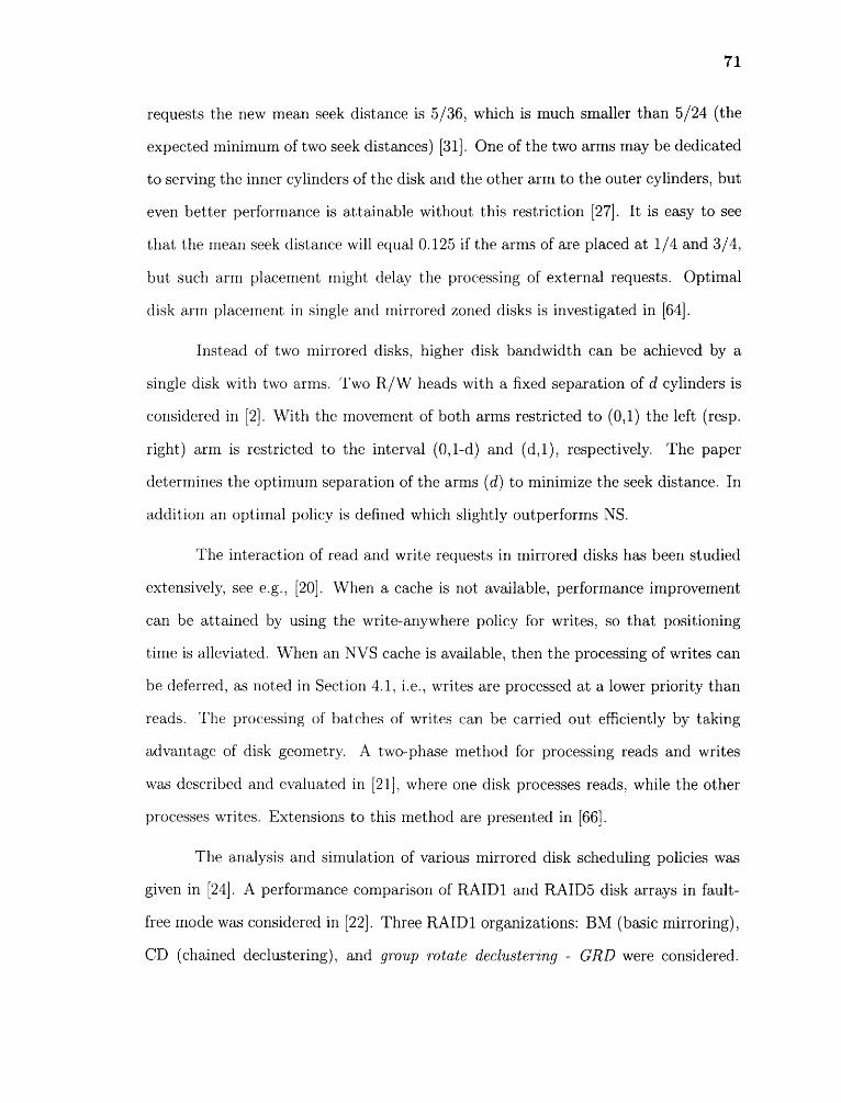
71

requests the new mean seek distance is 5/36, which is much smaller than 5/24 (the

expected minimum of two seek distances) [31]. One of the two arms may be dedicated

to serving the inner cylinders of the disk and the other arm to the outer cylinders, but

even better performance is attainable without this restriction [27]. It is easy to see

that the mean seek distance will equal 0.125 if the arms of are placed at 1/4 and 3/4,

but such arm placement might delay the processing of external requests. Optimal

disk arm placement in single and mirrored zoned disks is investigated in [64].

Instead of two mirrored disks, higher disk bandwidth can be achieved by a

single disk with two arms. Two R/W heads with a fixed separation of d cylinders is

considered in [2]. With the movement of both arms restricted to (0,1) the left (resp.

right) arm is restricted to the interval (0,1-d) and (d,1), respectively. The paper

determines the optimum separation of the arms (d) to minimize the seek distance. In

addition an optimal policy is defined which slightly outperforms NS.

The interaction of read and write requests in mirrored disks has been studied

extensively, see e.g., [20]. When a cache is not available, performance improvement

can be attained by using the write-anywhere policy for writes, so that positioning

time is alleviated. When an NVS cache is available, then the processing of writes can

be deferred, as noted in Section 4.1, i.e., writes are processed at a lower priority than

reads. The processing of batches of writes can be carried out efficiently by taking

advantage of disk geometry. A two-phase method for processing reads and writes

was described arid evaluated in [21], where one disk processes reads, while the other

processes writes. Extensions to this method are presented in [66].

The analysis and simulation of various mirrored disk scheduling policies was

given in [24]. A performance comparison of RAID1 and RAID5 disk arrays in fault-

free mode was considered in [22]. Three RAID1 organizations: BM (basic mirroring),

CD (chained declustering), and group rotate declustering - GRD were considered.

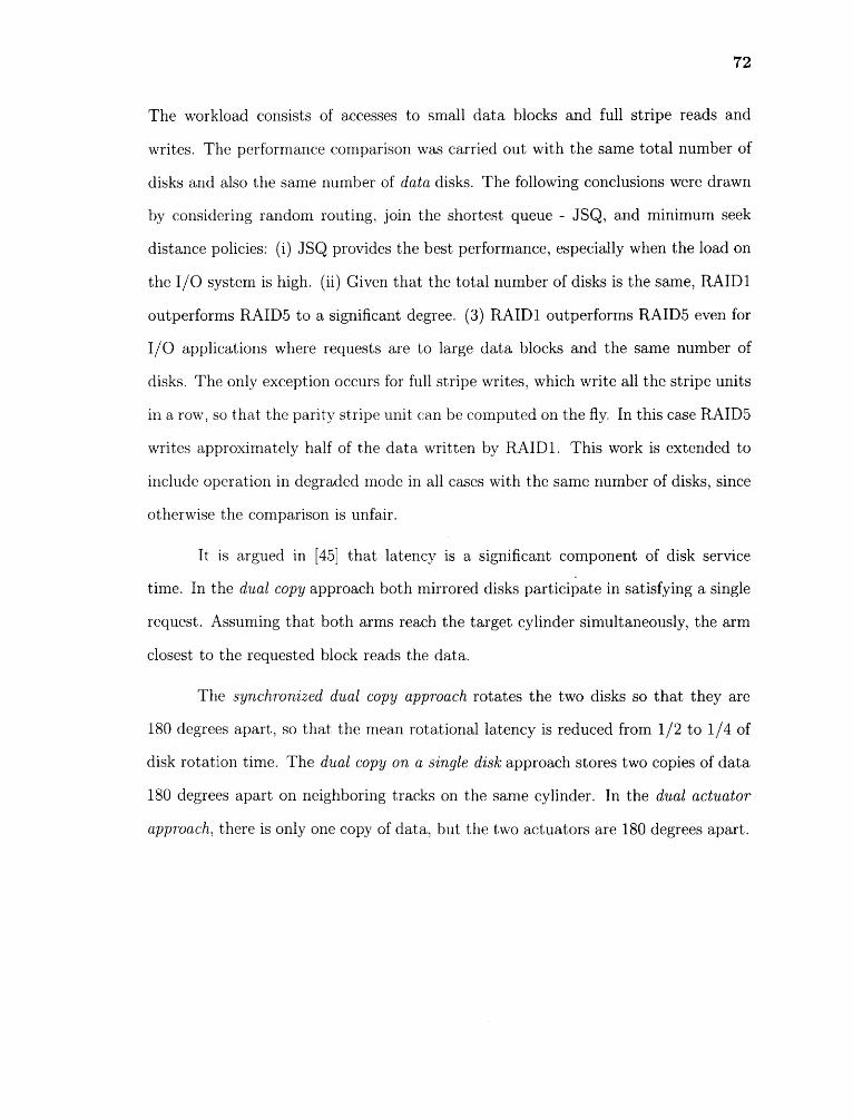
72

The workload consists of accesses to small data blocks and full stripe reads and

writes. The performance comparison was carried out with the same total number of

disks and also the same number of data disks. The following conclusions were drawn

by considering random routing, join the shortest queue - JSQ, and minimum seek

distance policies: (i) JSQ provides the best performance, especially when the load on

the I/O system is high. (ii) Given that the total number of disks is the same, RAID1

outperforms RAID5 to a significant degree. (3) RAID1 outperforms RAID5 even for

I/O applications where requests are to large data blocks and the same number of

disks. The only exception occurs for full stripe writes, which write all the stripe units

in a row, so that the parity stripe unit can be computed on the fly. In this case RAID5

writes approximately half of the data written by RAID1. This work is extended to

include operation in degraded mode in all cases with the same number of disks, since

otherwise the comparison is unfair.

It is argued in [45] that latency is a significant component of disk service

time. In the dual copy approach both mirrored disks participate in satisfying a single

request. Assuming that both arms reach the target cylinder simultaneously, the arm

closest to the requested block reads the data.

The synchronized dual copy approach rotates the two disks so that they are

180 degrees apart, so that the mean rotational latency is reduced from 1/2 to 1/4 of

disk rotation time. The dual copy on a single disk approach stores two copies of data

180 degrees apart on neighboring tracks on the same cylinder. In the dual actuator

approach, there is only one copy of data, but the two actuators are 180 degrees apart.

73

4.3 RAID1 Organizations

The four RAID 1 organizations considered in this study are described below. The

number of disks is set to N = 8 in all cases.

Basic Mirroring - BM This is the most common type of mirroring, which is

shown in Figure 4.2 with striping in effect. Each nonprimed letter denotes a primary

SU, while primed letters denote secondary SUs.

Load balancing of read requests across two disks is attained by appropriate

request routing, e.g. uniform versus round-robin routing. Other forms of routing in

BM are discussed in [24] [9]. When a disk fails, the read load at the mirroring disk is

doubled.

Table 4.2 Basic Mirroring with Striping with N=8 Disks

Group Rotate Declustering - GRD. This RAID1 data layout was proposed

in [22] to balance disk loads when a single disk failure occurs. Data is striped on

M = N/2 primary disks and the SUs on the primary disks are replicated in a rotated

manner on an equal number of secondary disks as shown in Figure 4.3. With no disk

failures reads are routed equally to primary and secondary disks. When a primary

disk fails its load will be distributed evenly on the secondary disks, but a smaller

fraction of the read load of surviving primary disks needs to be routed to secondary

disks to balance disk loads, e.g., with N = 8 each surviving primary disk will process a

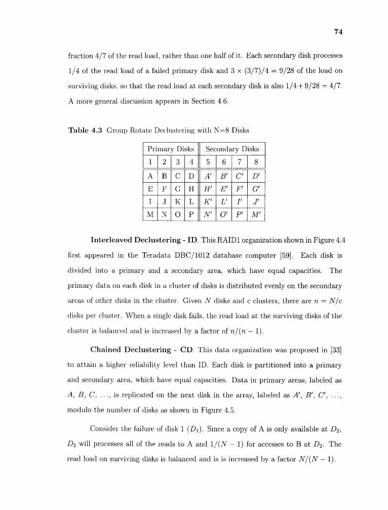
74

fraction 4/7 of the read load, rather than one half of it. Each secondary disk processes

1/4 of the read load of a failed primary disk and 3 x (3/7)/4 = 9/28 of the load on

surviving disks, so that the read load at each secondary disk is also 1/4+9/28 = 4/7.

A more general discussion appears in Section 4.6.

Table 4.3 Group Rotate Declustering with N=8 Disks

Interleaved Declustering - ID. This RAID1 organization shown in Figure 4.4

first appeared in the Teradata DBC/1012 database computer [59]. Each disk is

divided into a primary and a secondary area, which have equal capacities. The

primary data on each disk in a cluster of disks is distributed evenly on the secondary

areas of other disks in the cluster. Given N disks and c clusters, there are n N/c

disks per cluster. When a single disk fails, the read load at the surviving disks of the

cluster is balanced and is increased by a factor of n/ (n — 1).

Chained Declustering - CD. This data organization was proposed in [33]

to attain a higher reliability level than ID. Each disk is partitioned into a primary

and secondary area, which have equal capacities. Data in primary areas, labeled as

A, B, C, . . . , is replicated on the next disk in the array, labeled as A', B', C', . . . ,

modulo the number of disks as shown in Figure 4.5.

Consider the failure of disk 1 (D 1 ). Since a copy of A is only available at D2,

D2 will processes all of the reads to A and 1/(N — 1) for accesses to B at D2. The

read load on surviving disks is balanced and is is increased by a factor N/ (N — 1).

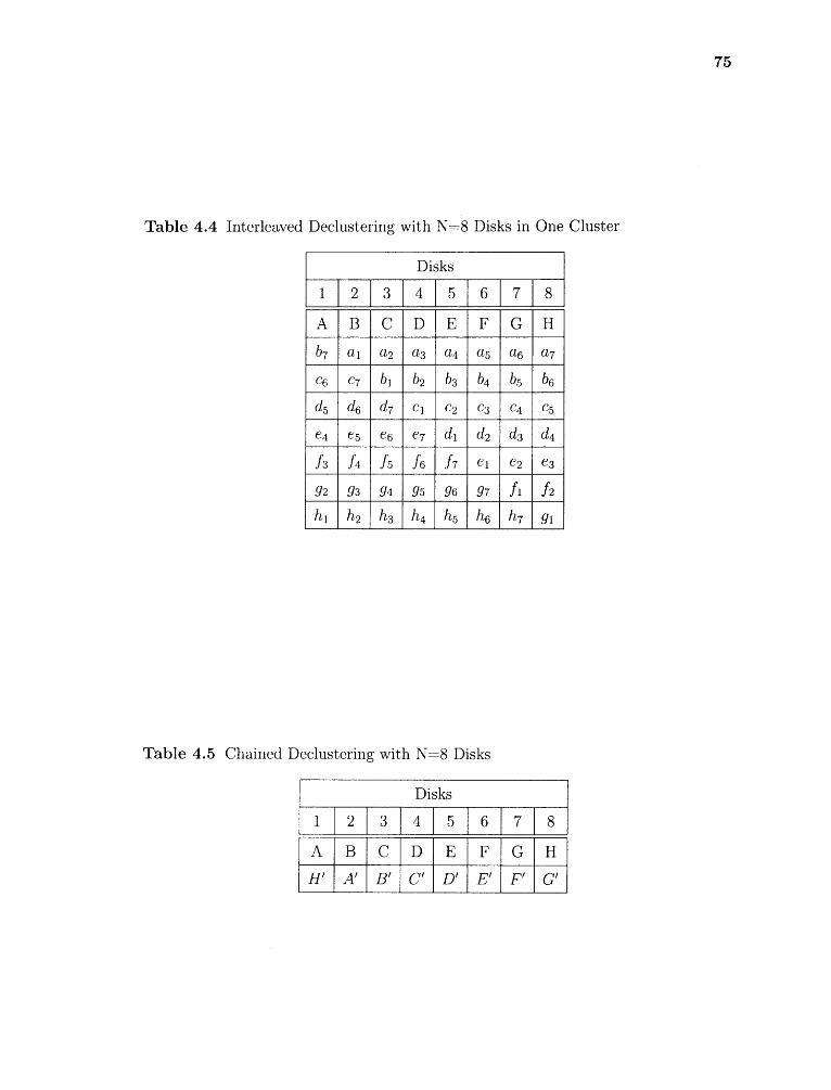
Table 4.4 Interleaved Declustering with N=8 Disks in One Cluster

75

Table 4.5 Chained Declustering with N=8 Disks

76

The failure of two disks is considered next: e.g., disk 1 (D 1 ) and disk k (Dk,k <

N). The two disk failures partition the array into two subarrays with k — 2 and N — k

disks with k — 1 and N — k + 1 unique data items per subarray, respectively. For

k = 4 there are items (A,B,C) in subarray 1 with two surviving disks and items

(D,E,F,G,H) in subarray 2 with four disks. The load increase is (k — 1)/(k — 2) and

(N — k + 1)/ (N — k) or 3/2 and 5/4, respectively. Thus the method of balancing read

requests only applies locally at the level of subarrays.

4.4 RAID1 Reliability Analysis

The basics for reliability analysis are reviewed. Then the reliability expressions for the

four RAID 1 organizations under consideration are summarized, which were derived

in [63]. An alternative approach to derive the reliabilities is given at the end.

Given the cumulative distribution function of time to component failure F(t),

its reliability function is R(t) = 1— F(t) [71]. It is concluded in [28] that the reliability

of a single disk can be approximated by an exponential distribution: Rdisk(t) = e -t ,

so that its mean time to failure - MTTF is MTTFdisk = fo e¯t = 1/A.

The reliability of a system without redundancy is the product of the relia-

bilities of its components [71], while the reliability of a system with redundancies is

determined by the subset of its components that are required for its operation [71].

For example, the reliability of an array of N disks is given as RN- disks = e¯Nt and

its MTTF as MTTFN-disks = 1/(NA).

The RAID paradigm utilizes redundancy to attain a sufficiently high reliability.

Let A(N, i) denote the number of cases that a RAID disk array with N disks can

tolerate i disk failures, so that A(N, 0) = 1 and A(N, i) = 0, i > imax , where max is

the maximum number of disk failures that can be tolerated. i max = 1 for RAID5,

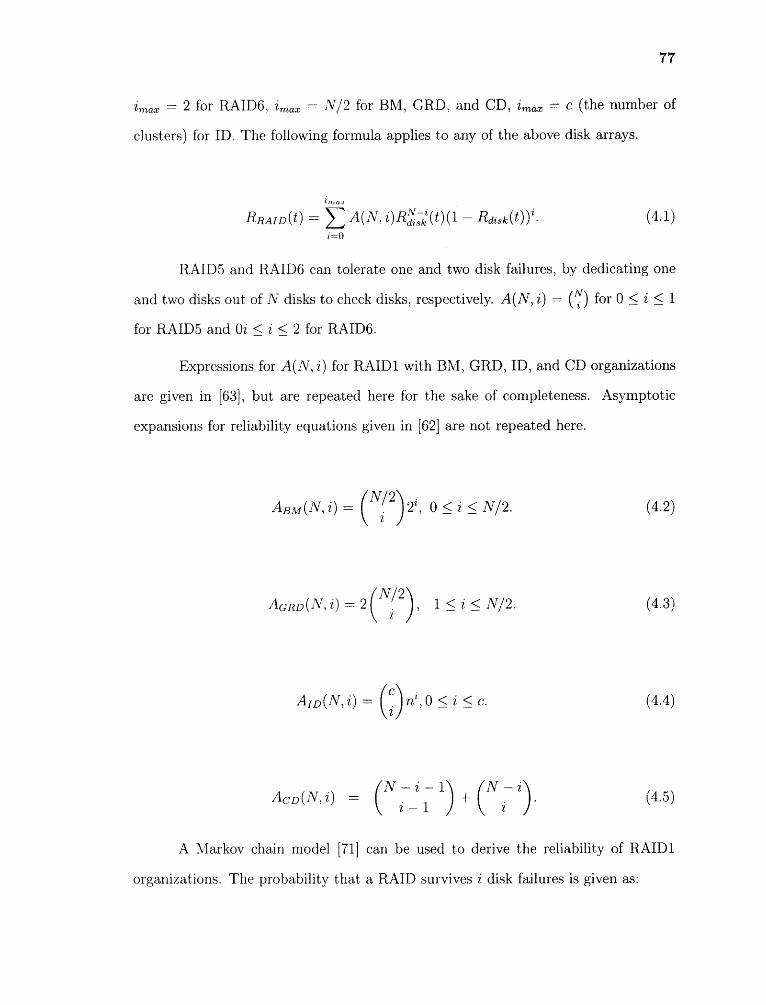
77

imax = 2 for RAID6, imax — N/2 for BM, GRD, and CD, max = c (the number of

clusters) for ID. The following formula applies to any of the above disk arrays.

RΛID5 and RAID6 can tolerate one and two disk failures, by dedicating one

and two disks out of N disks to check disks, respectively. A(N, i) = (N) for 0 < i < 1

for RAID5 and 0i < i < 2 for RAID6.

Expressions for A(N, i) for RAID1 with BM, GRD, ID, and CD organizations

are given in [63], but are repeated here for the sake of completeness. Asymptotic

expansions for reliability equations given in [62] are not repeated here.

A Markov chain model [71] can be used to derive the reliability of RAID 1

organizations. The probability that a RAID survives i disk failures is given as:

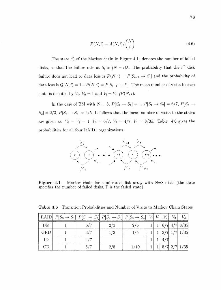
The state Si of the Markov chain in Figure 4.1. denotes the number of failed

disks, so that the failure rate at Si is (N — i)A. The probability that the its, disk

failure does riot lead to data loss is P(N, i) = P[Si-1 —4 Si ] and the probability of

data loss is Q(N, i) =1— P(N, i) = P[Si-1 —› F]. The mean number of visits to each

state is denoted by V. V0 = 1 and V = Vi-1P(N, i).

In the case of BM with N = 8, P[50 Si ] = 1, P[5 1 S2 ] = 6/7, P[S2

S³ ] = 2/3, P[5³ S4 ] = 2/5. It follows that the mean number of visits to the states

are given as: V0 = V = 1, 1/2 = 6/7, V³ = 4/7, V4 = 8/35. Table 4.6 gives the

probabilities for all four RAID 1 organizations.

Figure 4.1 Markov chain for a mirrored disk array with N=8 disks (the statespecifies the number of failed disks, F is the failed state).

Table 4.6 Transition Probabilities and Number of Visits to Markov Chain States

79

4.5 Comparison of the Four RAID1 Organizations

The four RAID1 organizations are compared from the viewpoint of their mean time

to data loss - MTTDL and their performability measure.

4.5.1 Reliability Comparison

Given that disk failure rates are exponential with rate A 1/MTTFdisk, the MTTDL

(without disk repair) can be expressed as MTTDL = E lmaxi=1 Vi /[(N — i)A]. For the

four organizations with N = 8 disks and c = 2 clusters for ID they are: MTTDLBM =

(163/280)/A = 0.582/A. MTTDLGRD = (3/8)/A = 0.375/A, MTTDL ID = (61/168)/A =

0.363/A, MTTDLCD = (379/840)/A = 0.451/A. The MTTDL for the RAID5 and

RAID6 disk arrays with N = 8 disks is MTTDLRAID5 = (15/56)/A = 0.268/A. and

11/ITT DL RAI D6 = (13/28)/A = 0.464/A.

It should be noted that MTTDL is not a good measure of reliability, in the

same way that the MTTF might be misleading. For example, the MTTF of Triple

Modular Redundancy - TMR system: MTTF = 5/(6A) is smaller than the MTTF

of a simplex system, which is 1/A. TMR systems are more reliable for missions with

duration t < (/712)/A) [71].

The MTTDL of disk arrays is usually computed when repair is allowed. For

example, the analysis of the Markov chain model in [28] leads to a disk failure if a

second disk failure occurs before the repair of the first disk is completed. This analysis

is simplified in that it does not take into account latent sector failures - LSFs [35],

which is the reason for the introduction of RAID6 disk arrays [41].

Figure 5 in [63] plots the reliability of the four RAID 1 organizations with

N = 8 (with c = 2 for the ID organization) plus RAIDS and RAID6 disks arrays

versus decreasing disk reliabilities. RAID6 is the most reliable and RAIDS the least

reliable, with RAID1 reliabilities lying between these two extremes. BM is the most

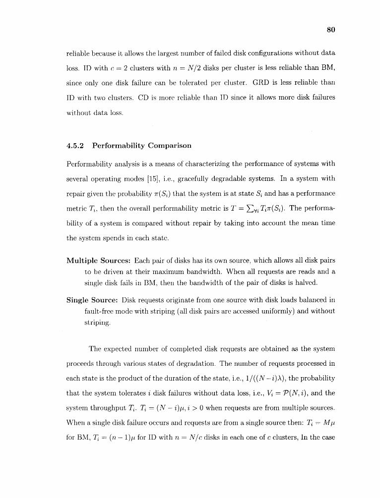
80

reliable because it allows the largest number of failed disk configurations without data

loss. ID with c = 2 clusters with n = N/2 disks per cluster is less reliable than BM,

since only one disk failure can be tolerated per cluster. GRD is less reliable than

ID with two clusters. CD is more reliable than ID since it allows more disk failures

without data loss.

4.5.2 Performability Comparison

Performability analysis is a means of characterizing the performance of systems with

several operating modes [15], i.e., gracefully degradable systems. In a system with

repair given the probability π(Si) that the system is at state Si and has a performance

metric Ti , then the overall performability metric is T = Evi Ti π(Si ) . The performa-

bility of a system is compared without repair by taking into account the mean time

the system spends in each state.

Multiple Sources: Each pair of disks has its own source, which allows all disk pairsto be driven at their maximum bandwidth. When all requests are reads and asingle disk fails in BM, then the bandwidth of the pair of disks is halved.

Single Source: Disk requests originate from one source with disk loads balanced infault-free mode with striping (all disk pairs are accessed uniformly) and withoutstriping.

The expected number of completed disk requests are obtained as the system

proceeds through various states of degradation. The number of requests processed in

each state is the product of the duration of the state, i.e., 1/((N —OA), the probability

that the system tolerates i disk failures without data loss, i.e., V = P(N, i), and the

system throughput Ti . T2 = (N — i) i > 0 when requests are from multiple sources.

When a single disk failure occurs and requests are from a single source then: Ti = M p,

for BM, Ti = (n — 1)/i, for ID with n = N/c disks in each one of c clusters, In the case

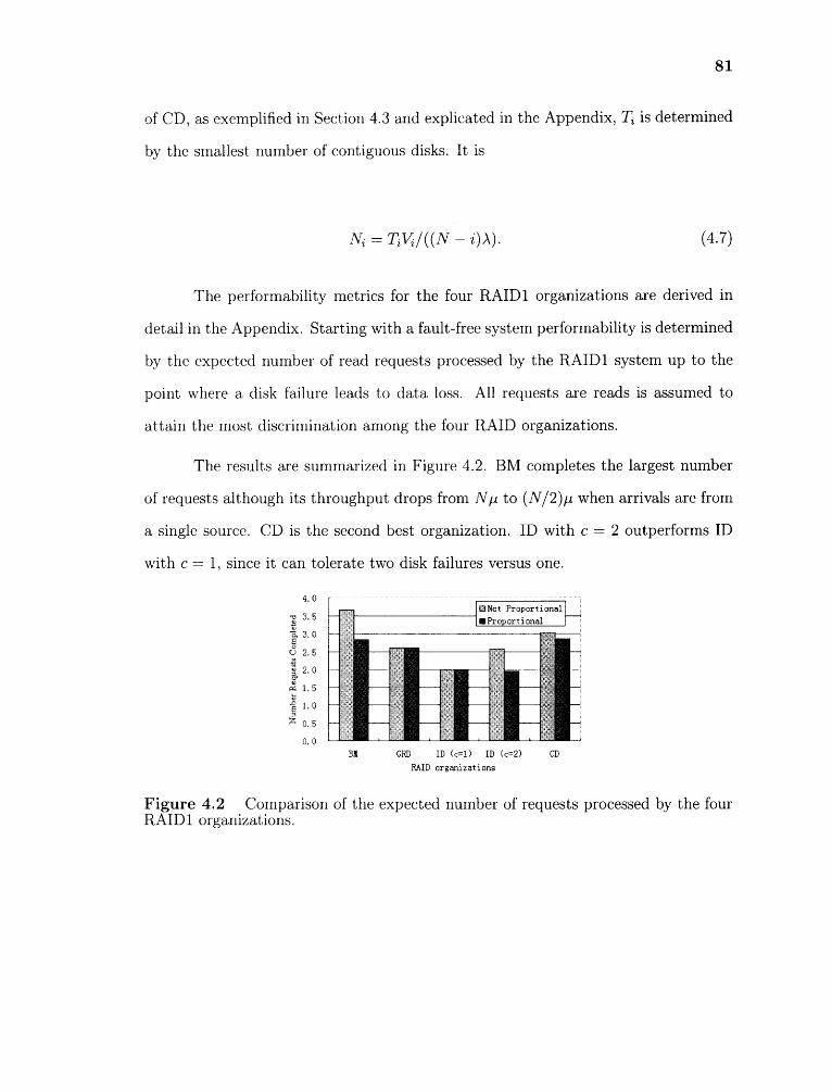
81

of CD, as exemplified in Section 4.3 and explicated in the Appendix, Ti is determined

by the smallest number of contiguous disks. It is

The performability metrics for the four RAID1 organizations are derived in

detail in the Appendix. Starting with a fault-free system performability is determined

by the expected number of read requests processed by the RAID1 system up to the

point where a disk failure leads to data loss. All requests are reads is assumed to

attain the most discrimination among the four RAID organizations.

The results are summarized in Figure 4.2. BM completes the largest number

of requests although its throughput drops from N,u to (N/2)// when arrivals are from

a single source. CD is the second best organization. ID with c = 2 outperforms ID

with c = 1, since it can tolerate two disk failures versus one.

Figure 4.2 Comparison of the expected number of requests processed by the fourRAID1 organizations.

82

4.6 RAID1 Performance Analysis

Formulas are developed to compare the relative performance of the four RAID1

organizations in fault-free mode and with disk failures. Modeling assumptions are

presented first.

4.6.1 Modeling Assumptions

• The arrivals of read and write accesses are according to a Poisson process.Probabilistic routing is used to balance the load due to reads, so that the arrivalprocess at the disks remains Poisson.

• Reads and writes are unformly distributed over all primary data, This assumptionis not required for the analysis, but simplifies the specification of the model.

• Discrete disk requests are to small randomly placed data blocks on disk, as inonline transaction processing - OLTP applications.

• Disk requests are processed in FCFS order since this allows a quick comparisonof the various RAID 1 organizations via a closed form expression for the meanwaiting time of the M/G/1 queueing model [37] [57].

• In the case of BM and GRD reads are evenly split between the two disks holdingthe same data to balance their read load. The read load for ID and CD organi-zations is already balanced. Routing of requests in the presence of disk faultsis discussed in Section 4.6.3.

The 9.17 GB, 7200 RPM, IBM 18ES (model DNES-309170W) disk drive is

considered in this studies. 1 The detailed characteristics of disk drive is used 2 whose

characteristics are summarized in Table 4.7,

The mean response times of discrete disk requests takes into account the effect

of zoning and detailed seek time characteristics [65] [64 R ead requests which affect

lhttp://www.storage.ibm.com/hdd/prod/ultrastar.htm²http://www.pdl.cmu.edu/DiskSim/diskspecs.

Table 4.7 Specifications for IBM 18ES Disk Drives

83

application response time may be given a higher priority than writes. This case can

be analyzed using the head-of-the-line priority queueing model [38][57].

The two assumptions that disk requests are uniformly distributed over disk

blocks is pessimistic, since one or few disk regions are active at any time, which

results in shorter seek distances than attained with a uniform distribution of requests.

The FCFS disk scheduling is outperformed by SATF, but is considered here since it

is amenable to a simple analysis. This is acceptable since interest is given in the

relative, rather than the absolute performance of the various RAID organizations.

4.6.2 Fault -Free or Normal Mode of Operation

The four RAID1 organizations have a similar performance when they are operating

in fault-free or normal mode. It is assumed that the load is balanced across disk

pairs, so the performance of one pair of disks with the BM organization is analyzed.

Otherwise, the mean response time overall disks would have to be weighted by the

arrival rate to each pair.

84

Given M = N/2 disk pairs, an arrival rate Λ to the disk array, and fr and fw

as the fractions of reads and writes, the arrival rate of reads and writes to each disk

pair is r = frΛ/M and Au, = fwΛ/M, respectively. With uniform routing of reads

the arrival rate to each disk is:

The utilization of each disk is:

With a fast-write capability with an NVS cache the time to complete a write

is negligibly small. The analysis is simple when the data has to be written onto one

disk, but becomes more complicated when a variation of write-anywhere policy is in

effect [20].

When a data block is to be written to both disks before a write is considered

completed, the write response time equals that of a 2-way fork-join request: R2F/J,

which is approximated by the easy to compute R2max· It is shown in [44] that in

the case of the exponential distribution the mean n-way fork-join response time is

upper-bounded by R maxn.

85

RTmax2 the write response time is the time to write both disk blocks. It can be

estimated by first approximating individual writes with the extreme-value distribution

- EVD: P[Y < y] = exp(—e- y-a/b ), which has a mean Y = a + -γb and a variance =

(7b) ² /6. The maximum of n random variables with EVD is: Ynmax = (a +-γb)+bln(n),

where 7 = 0.57721 is the Euler-Mascheroni constant. Let Hu, and a! denote the

mean and variance of write requests, then Y = f?„, and b=6σw/π. It follows that

R2max = + 6σwln(2)/π.

The current system is different in that each disk in addition to writes processes

reads (in FCFS order). This results in a higher variability of fork-join response times

and this makes R2max a better approximation. Write response times are not reported

in Section 4.7, since they do not affect the application response time.

4.6.3 Degraded Mode Analysis

The arrival rate of reads to surviving disks depends on the organization of the disk

array. In fact, the BM organization cannot balance disk loads in degraded mode,

while this is possible with the other RAID 1 organizations.

4.6.3.1 Basic Mirroring. The arrival rate of reads to the surviving disk is '\ r , so

that its utilization factor is given as:

(4.11)

With k failed disks the mean overall response time for reads is:

(4.12)

86

where the superscript d denotes the higher response time of reads in a pair with a

failed disk.

The response time for writes to failed disk pairs is computed differently, since

there are no fork-join requests, except that the individual write response time is

higher, since the read load is doubled.

4.6.3.2 Group Rotate Declustering. In GRD the utilizations of primary and

secondary disks with k primary (or secondary) disks fail can be balanced as follows.

Let αk denote the fraction of reads processed by the M — k surviving primary disks.

Then a fraction 1 — α k of reads from these disks are routed to secondary disks (the

value of α k is determined below). The read load of a failed disk is fully routed to

secondary disks. The routed reads in both cases are uniformly distributed.

Denoting the utilization of primary and secondary disks as ρ p and ρs , respec-

tively, formula is:

Disk utilizations are balanced for:

87

The mean read response times will be approximately the same, since the

utilizations of the primary and secondary disks are equal and reads and writes have

about the same response time. Write response times are computed similarly to BM.

4.6.3.3 Interleaved Declustering. With N disks and c clusters the increase in

read load on surviving disks in a cluster with n N/c disks and one failed disk is:

(4.17)

The arrival rate of reads to the surviving disks in the cluster is then:

(4.18)

The increase in the read load will affect the maximum throughout sustainable

by the cluster. When there are multiple clusters, the response times should be weighed

according to the number of clusters in the two categories, i.e., without or with failed

disks.

4.6.3.4 Chained Declustering. When a single disk fails in CD, its read load

can be distributed evenly over the surviving disks so that the arrival rate of reads

increases by a factor N/ (N — 1). When two non-consecutive disks fail, there will be

two groups of disks with sizes g1 and g² and g 1 + g² = N — 2. The read load in group

i = 1, 2 is increased by a factor α i = (gi + 1)/g 2 and the arrival rate of reads to the

i th group is then Air = frΛαi /N. This calculation generalizes to more than two disk

failures.

As shown in Figure B.1 in the Appendix, there are 20 configurations with

k = 2 disk failures for N = 8, but only I = 3 different group sizes as follows: (i) In

88

eight out of twenty cases (w 1 = 8/20) 9 1 = 1 and g² = 5. (ii) In eight out of twenty

cases (w² = 8/20) g 1 = 2 and 9² = 4. (iii) In four out of twenty cases (w ³ = 4/20)

g1 = g² = 3.

Let k 1 denote the mean Read response of group i in configuration j, The

mean Read response time for CD with N disks, k failed disks, and J configurations,

is as follows:

What is riot immediately clear from this equation is that Rkr is dominated

by response times from small group sizes, such that numerical results show that CD

response time with two disk failures is only slightly better than BM and in fact both

disk organizations attain the same maximum throughput.

The response times in each group are determined by its size, rather than its

membership in a certain configuration, so that the computation of response times

can be simplified by finding the fractions of different group sizes, say fk. The overall

mean response time is given as R, = I Vk fk Rk

4.7 Performance Results

The performance of RAID1 organizations is compared with RAID0, RAID5, and

RAID6 disks arrays. The ID organization has one cluster (c = 1). The case when the

total number of disks in the arrays is the same and equal to N is considered.

The workload consists of accesses to small (4 or 8 KB) blocks of data, so that

the transfer times is negligibly small compared to positioning time. This is because

disk requests are uniformly distributed over the blocks and are served in FCFS order,

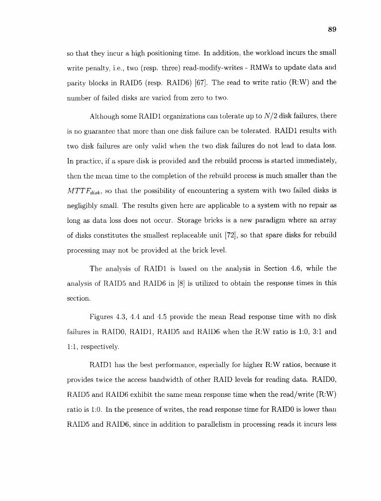
89

so that they incur a high positioning time. In addition, the workload incurs the small

write penalty, i.e., two (resp. three) read-modify-writes - RMWs to update data and

parity blocks in RAID5 (resp. RAID6) [67]. The read to write ratio (R:W) and the

number of failed disks are varied from zero to two.

Although some RAID1 organizations can tolerate up to N/2 disk failures, there

is no guarantee that more than one disk failure can be tolerated. RAID1 results with

two disk failures are only valid when the two disk failures do not lead to data loss.

In practice, if a spare disk is provided and the rebuild process is started immediately,

then the mean time to the completion of the rebuild process is much smaller than the

MTTFdisk , so that the possibility of encountering a system with two failed disks is

negligibly small. The results given here are applicable to a system with no repair as

long as data loss does not occur. Storage bricks is a new paradigm where an array

of disks constitutes the smallest replaceable unit [72], so that spare disks for rebuild

processing may not be provided at the brick level.

The analysis of RAID1 is based on the analysis in Section 4.6, while the

analysis of RAID5 and RAID6 in [8] is utilized to obtain the response times in this

section.

Figures 4.3, 4.4 and 4.5 provide the mean Read response time with no disk

failures in RAID0, RAID1, RAIDS and RAID6 when the R:W ratio is 1:0, 3:1 and

1:1, respectively.

RAID1 has the best performance, especially for higher R:W ratios, because it

provides twice the access bandwidth of other RAID levels for reading data. RAID0,

RAID5 and RAID6 exhibit the same mean response time when the read/write (R:W)

ratio is 1:0. In the presence of writes, the read response time for RAID0 is lower than

RAIDS and RAID6, since in addition to parallelism in processing reads it incurs less

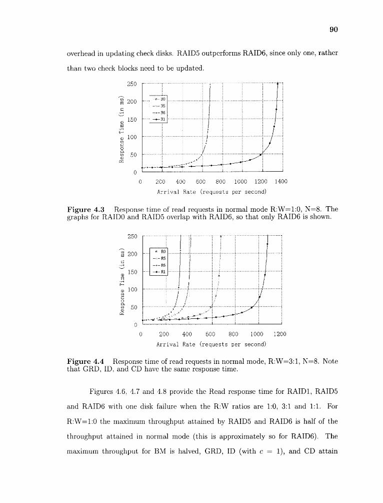
90

overhead in updating check disks. RAID5 outperforms RAID6, since only one, rather

than two check blocks need to be updated.

Figure 4.3 Response time of read requests in normal mode R:W=1:0, N=8. Thegraphs for RAID0 and RAID5 overlap with RAID6, so that only RAID6 is shown.

Figure 4.4 Response time of read requests in normal mode, R:W=3:1, N=8. Notethat GRD, ID, and CD have the same response time.

Figures 4.6, 4.7 and 4.8 provide the Read response time for RAID1, RAID5

and RAID6 with one disk failure when the R:W ratios are 1:0, 3:1 and 1:1. For

R:W=1:0 the maximum throughput attained by RAID5 and RAID6 is half of the

throughput attained in normal mode (this is approximately so for RAID6). The

maximum throughput for BM is halved, GRD, ID (with c = 1), and CD attain

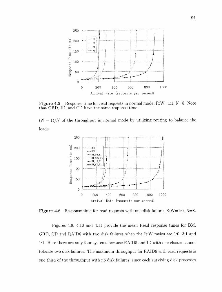
91

Figure 4.5 Response time for read requests in normal mode, R:W=1:1, N=8. Notethat GRD, ID, and CD have the same response time.

(N — 1)/N of the throughput in normal mode by utilizing routing to balance the

loads.

Figure 4.6 Response time for read requests with one disk failure, R:W=1:0, N=8.

Figures 4.9, 4.10 and 4.11 provide the mean Read response times for BM,

GRD, CD and RAID6 with two disk failures when the R:W ratios are 1:0, 3:1 and

1:1. Here there are only four systems because RAID5 and ID with one cluster cannot

tolerate two disk failures. The maximum throughput for RAID6 with read requests is

one third of the throughput with no disk failures, since each surviving disk processes

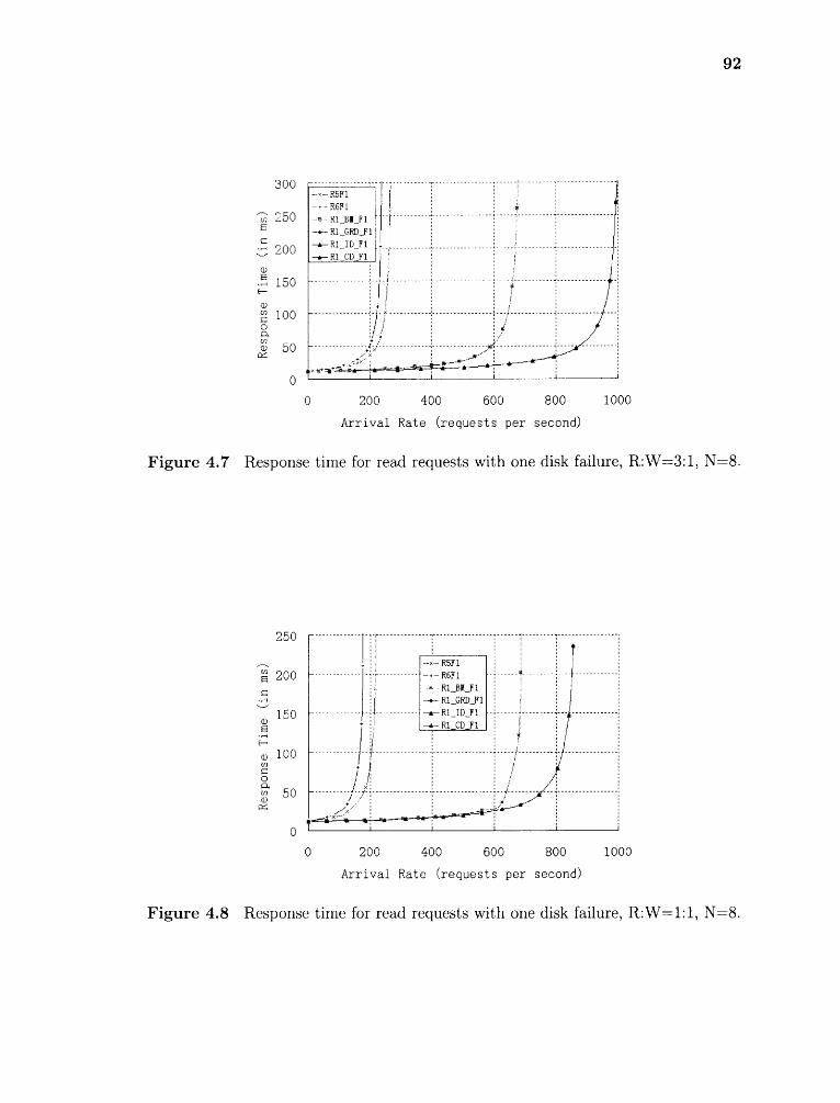
92

Figure 4.7 Response time for read requests with one disk failure, R:W=3:1, N=8.

Figure 4.8 Response time for read requests with one disk failure, R:W=1:1, N=8.

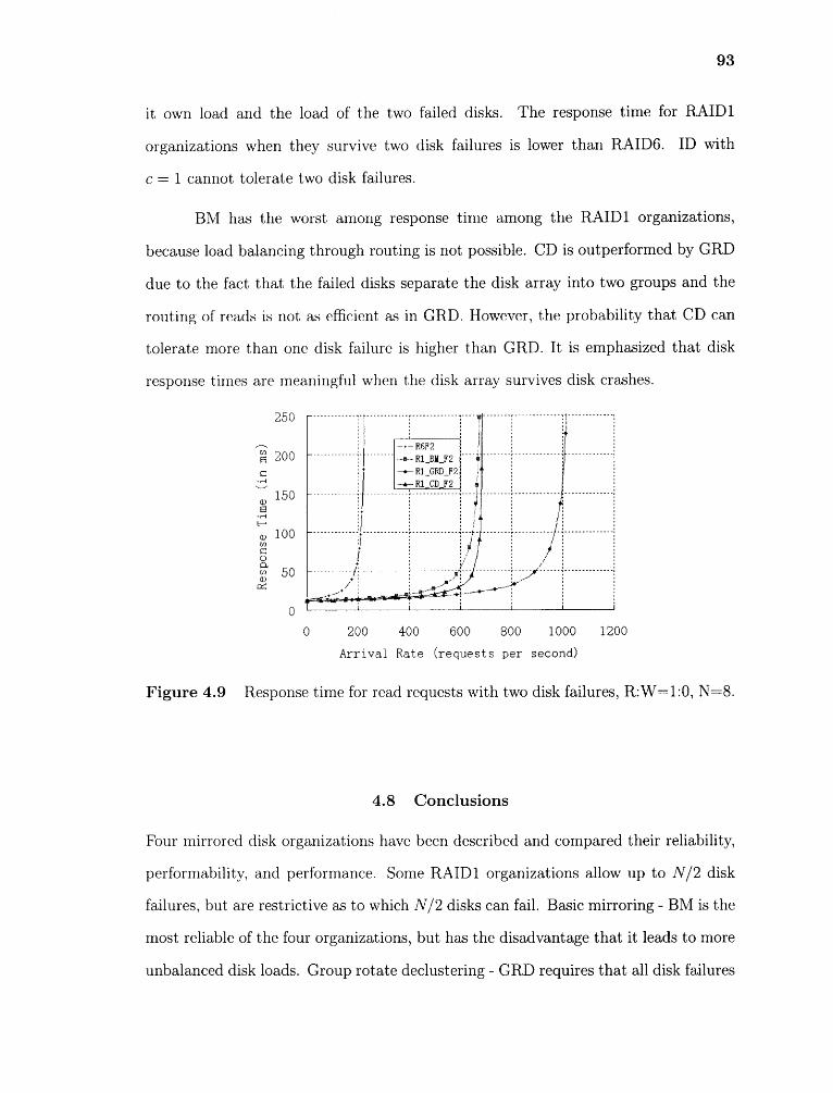
93

it own load and the load of the two failed disks. The response time for RAID1

organizations when they survive two disk failures is lower than RAID6. ID with

c = 1 cannot tolerate two disk failures.

BM has the worst among response time among the RAID1 organizations,

because load balancing through routing is not possible. CD is outperformed by GRD

due to the fact that the failed disks separate the disk array into two groups and the

routing of reads is not as efficient as in GRD. However, the probability that CD can

tolerate more than one disk failure is higher than GRD. It is emphasized that disk

response times are meaningful when the disk array survives disk crashes.

Figure 4.9 Response time for read requests with two disk failures, R:W=1:0, N=8.

4.8 Conclusions

Four mirrored disk organizations have been described and compared their reliability,

performability, and performance. Some RAID1 organizations allow up to N/2 disk

failures, but are restrictive as to which N/2 disks can fail. Basic mirroring - BM is the

most reliable of the four organizations, but has the disadvantage that it leads to more

unbalanced disk loads. Group rotate declustering - GRD requires that all disk failures

94

Figure 4.10 Response time for read requests with two disk failures, R:W=3:1,N=8.

Figure 4.11 Response time for read requests with two disk failures, R:W=1:1,N=8.

95

are either all primary or all secondary, but the loads can be balanced across surviving

disks. The reliability of Interleaved Declustering - ID can be improved by reducing the

number of disks in each cluster, but similarly to BM this introduces load imbalance

across clusters when disks fail. Chained declustering - CD is an improvement on ID,

since up to N/2 non-consecutive disks can fail and the load can be balanced among

surviving disks.

Table 4.8 Comparison of Different Mirrored Disk Organizations with N=2M Disks

When all requests are from a single source, BM attains half of the maximum

throughput of the other methods when a single disk fails, which is because load

balancing is not possible in this case. With two disk failures GRD outperforms CD

(when there is no data loss), because it can route reads among surviving disks more

efficiently than CD. On the other hand GRD is more susceptible than CD to data

loss. Some conclusions of this study are summarized in Table 4.8.

When the number of disks is the same for all RAID levels, RAID 1 outperforms

RAID0, RAIDS, and RAID6 in all cases. This is especially so with a high fraction

of reads, since RAID1 provides twice the access bandwidth of the other RAID levels.

96

The assumption that the number of data disks is the same, yields an even better

performance for RAID1 [22].

The performability of mirrored disks is compared by using the expected number

of completed read requests as the performance metric. The comparison is made under

the assumption that disk loads are initially balanced and the best attempt is made

to maximize the array bandwidth. BM outperforms the other organizations followed

by the ID organization when the number of clusters is larger, since in the limit with

n = 2 disks per cluster they are the same.

The analytical model of RAID 1 organizations in this study is quite naive from

the viewpoint of routing of requests and disk scheduling. Static probabilistic routing

is required to keep the analysis tractable, while simulation is required to study the

effect of dynamic routing. The comparison of request routing methods in mirrored

disks with BM (basic mirroring) showed that routing has little effect on performance

and that performance is dominated by the disk scheduling policy.

The RAID 1 organizations discussed in this study are applicable to storage

nodes - SNs or bricks. A technique such as CD (chained declustering) should be

helpful in balancing brick loads when brick failures occur. Distributed SPTF or D-

SPTF is a new algorithm which improves read performance by multicasting request

to pertinent SNs [23]. Once an SN claims a request, its processing at the other nodes

is cancelled. Additional work remains to be done to investigate disk scheduling,

including the schemes proposed in [24], for various RAID1 organizations.

CHAPTER 5

ANALYSIS OF X-CODES

5.1 Coding for Multiple Disk Failure Tolerant Arrays

Parity coding to recover from single disk failures was part of the original RAID

proposal [51], which introduced five RAID levels. The popular RAID level 5 (RAID5)

utilizes striping, which partitions large files into fixed size stripe units - SUs which are

allocated in a round-robin manner across the disks of the array. The capacity of one

disk out of N is dedicated to parity blocks, whose SUs according to the left symmetric

organization are placed in left to right repeating diagonals. Distributing the parity

blocks has the advantage of balancing the disk load due to updating activity.

The redundancy due to parities in RAID5 allows the on demand reconstruction

of the blocks of a single failed disk. A data access to the failed disk entails fork-join

requests to the corresponding blocks on the surviving disks. The load on these disks

doubles when all requests are reads, so that there is a degradation in response times.

More importantly, a RAID5 disk array with a single disk failure is susceptible to data

loss if another disk fails. The rebuild process in RAID5 systematically reconstructs

the contents of a failed disk on the spare disk, by reading and XORing the contents of

surviving disks. In spite of the very small bit error rates for the R,AID5 configuration

considered in [41] the rebuild process cannot be completed in 4% of cases due to latent

sector failures - LSFs.

Two-disk failure tolerant - 2DFTs arrays classified as RAID6 [48] are a solution

to this problem. There are several schemes to recover from multiple disk failures,

which from a coding viewpoint correspond to erasure correction. Maximum Distance

Separable - MDS codes meeting the Singleton bound require r parity disks in order

97

98

to correct r erasures. The most common class of MDS codes are Reed-Solomon (RS)

codes, which have been implemented in StorageTek's Iceberg [48] and HP's RAID

5DP (double parity) [32].

RS codes which are based on arithmetic on finite fields are quite expensive

to implement [17]. Several parity based methods have been proposed to reduce

the computational cost. The EVENODD code has two parity columns that are

independent from each other [41]. The Row-Diagonal Parity (RDP) family of codes,

optimizes the number of XORs at the encoding [46]. With an appropriate choice of

symbol sizes EVENODD and RDP incur the same disk access pattern as RAID6, i.e.,

three read-modify-writes to update data and parity blocks. The P and Q parity SUs

are organized according to the left symmetric organization to balance disk loads due

to updates.

RM2 [50] and the X-code [75] are distributed parity schemes, which have an

advantage over dedicated parity in that there are no bottlenecks. No disk gets more

accesses than others, so that there is no need to rotate the parity columns as in RAID5

arid RAID6. While RM2 allows an odd or an even number of disks, the distributed

parity codes cannot be shortened in general. For instance, the X-code consists of

N columns, where N is a prime. Although EVENODD requires a prime number of

disks, empty virtual disks with zero contents can be used to fill the gap.

As noted earlier the load of RAID arrays in processing read requests doubles

with a single disk failure and triples in RAID6 with two disk failures. The load

increase in RM2 is a function of the redundancy ratio and disk loads in RM2 tend

to quite unbalanced [8]. This study concentrates on the X-code organization. It is

shown that the load increase with two disk failures is a function of the distance of

the failed disks and derive a closed form expression in this case.

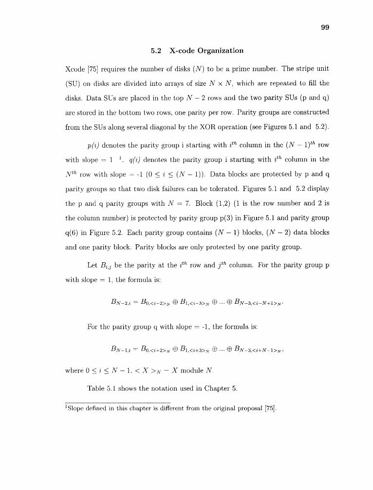
99

5.2 X-code Organization

Xcode [75] requires the number of disks (N) to be a prime number. The stripe unit

(SU) on disks are divided into arrays of size N x N, which are repeated to fill the

disks. Data SUs are placed in the top N — 2 rows and the two parity SUs (p and q)

are stored in the bottom two rows, one parity per row. Parity groups are constructed

from the SUs along several diagonal by the XOR operation (see Figures 5.1 and 5.2).

p(i) denotes the parity group i starting with i th column in the (N — 1) th row

with slope = 1 1 . q(i) denotes the parity group i starting with i th column in the

Nt h row with slope = -1 (0 < i < (N — 1)). Data blocks are protected by p and q

parity groups so that two disk failures can be tolerated. Figures 5.1 and 5.2 display

the p arid q parity groups with N = 7. Block (1,2) (1 is the row number and 2 is

the column number) is protected by parity group p(3) in Figure 5.1 and parity group

q(6) in Figure 5.2. Each parity group contains (N — 1) blocks, (N — 2) data blocks

and one parity block. Parity blocks are only protected by one parity group.

Let Bi j be the parity at the i th row and jth column. For the parity group p

with slope = 1, the formula is:

For the parity group q with slope = -1, the formula is:

¹Slope defined in this chapter is different from the original proposal [75].

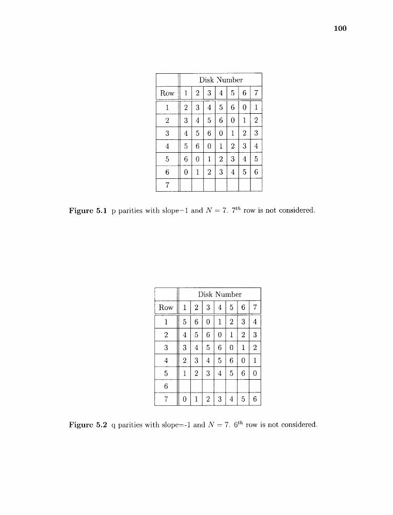
Figure 5.1 p parities with slope=1 and N =7. 7th row is not considered.

100

Figure 5.2 q parities with slope=-1 and N = 7. 6 th row is not considered.

Table 5.1 Notation Used in Chapter 5

101

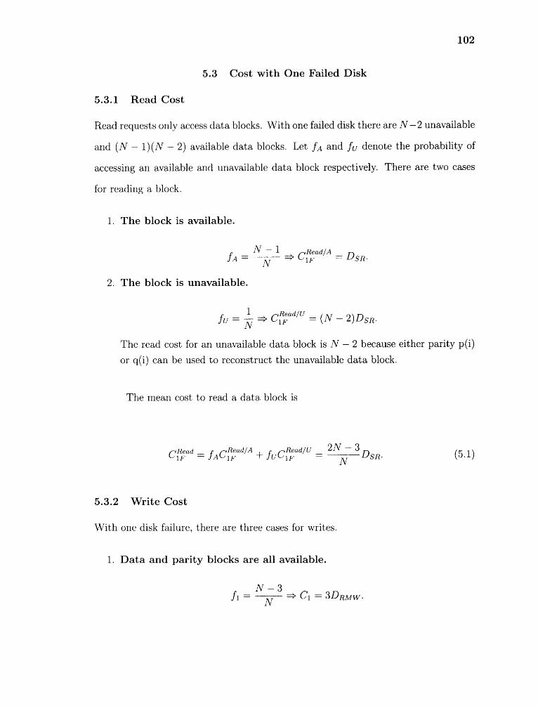
102

5.3 Cost with One Failed Disk

5.3.1 Read Cost

Read requests only access data blocks. With one failed disk there are N-2 unavailable

and (N —1)(N — 2) available data blocks. Let fA and fu denote the probability of

accessing an available and unavailable data block respectively. There are two cases

for reading a block.

1. The block is available.

2. The block is unavailable.

The read cost for an unavailable data block is N — 2 because either parity p(i)

or q(i) can be used to reconstruct the unavailable data block.

The mean cost to read a data block is

5.3.2 Write Cost

With one disk failure, there are three cases for writes.

1. Data and parity blocks are all available.

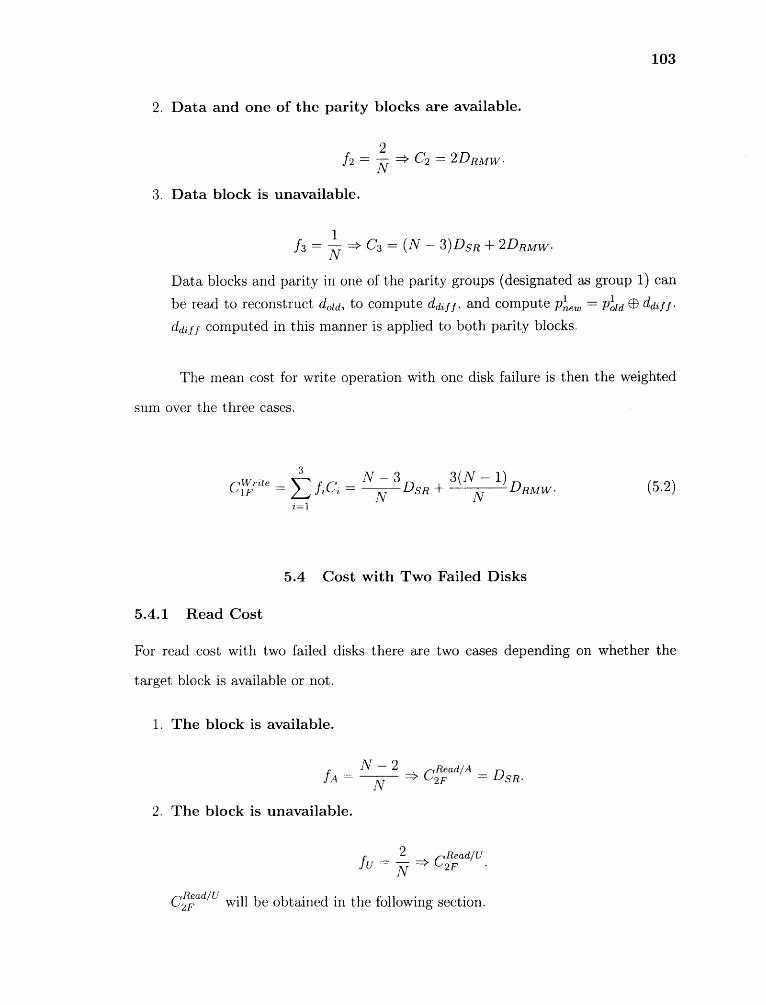
103

2. Data and one of the parity blocks are available.

3. Data block is unavailable.

Data blocks and parity in one of the parity groups (designated as group 1) can

be read to reconstruct dold, to compute ddif f, and compute phew P¹old 'ED ddif . f •

ddif f computed in this manner is applied to both parity blocks.

The mean cost for write operation with one disk failure is then the weighted

sum over the three cases.

5.4 Cost with Two Failed Disks

5.4.1 Read Cost

For read cost with two failed disks there are two cases depending on whether the

target block is available or not.

1. The block is available.

2. The block is unavailable.

CRead/U2Fwill be obtained in the following section.

With two disk failures the read cost for an unavailable data block depends on

the distance of two failed disks. The distance between disks i and j is defined as

For example, the distance of disk 1 and disk 6 for N = 7 is 2, not 5. It is

easy to see that the maximum distance is (N — 1)/2, N is a prime and hence, an odd

number.

Cost to read an unavailable data block Some unavailable data blocks can

be reconstructed by one parity group access and others need several parity groups

accesses, i.e., a recovery path.

For example in Figures 5.3 and 5.4 block (3,1) need to be reconstructed when

disk 1 and disk 2 are failed. Block (2,2) needs to be reconstructed for p(4) or block

(4,2) for q(3) first. So the read cost for block (3,1) is (N — 2) plus the minimum

read cost of block (2,2) or block (4,2). Then the same analysis for block (2,2) and

block (4,2) will be carried out until the block that can be reconstructed by one parity

group access is reached. However, it is impossible to reconstruct block (4,2) because

it needs block (5,1) which has two unavailable blocks (one is parity block) in parity

group q(1). So only block (2,2) can be used. Block (2,2) needs block (1,1) which can

be reconstructed by (N — 2) data block accesses. The total cost for block (3,1) is p(2),

q(5), and p(4), i.e., 3(N — 2). Table 5.2 displays the recovery path and read cost of all

unavailable data blocks with N = 7 and d = 1. Block (5,1) can not be recovered by

parity group q(1). It separates other data blocks on disk 1 into two groups. However,

since block (5,1) is the last data block, it only has one group.

Table 5.3 displays the recovery path and read cost of all unavailable data

blocks with N = 7 and d = 3. This time the recovery path is differently. It shows the

Figure 5.3 Possible recovery path forblock (3,1) with p parity group and N = 7.

105

Figure 5.4 Possible recovery path forblock (3,1) with q parity group and N = 7.

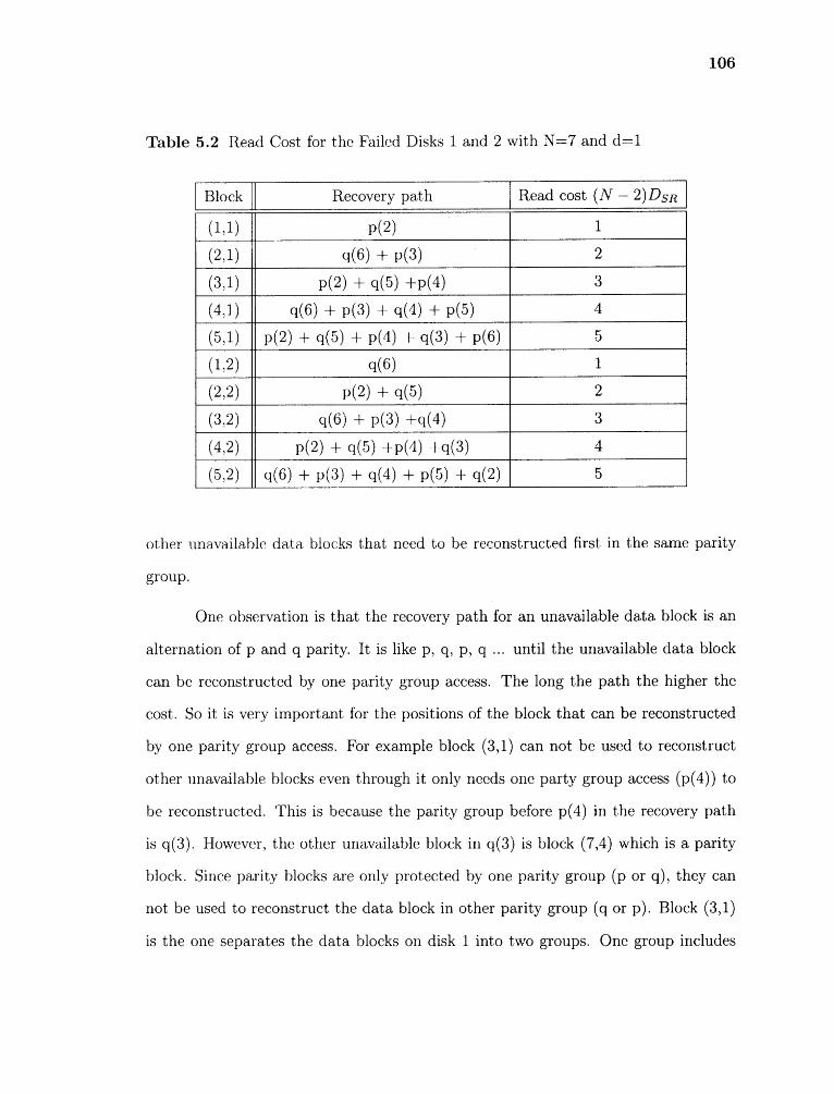
Table 5.2 Read Cost for the Failed Disks 1 and 2 with N=7 and d=1

106

other unavailable data blocks that need to be reconstructed first in the same parity

group.

One observation is that the recovery path for an unavailable data block is an

alternation of p and q parity. It is like p, q, p, q ... until the unavailable data block

can be reconstructed by one parity group access. The long the path the higher the

cost. So it is very important for the positions of the block that can be reconstructed

by one parity group access. For example block (3,1) can not be used to reconstruct

other unavailable blocks even through it only needs one party group access (p(4)) to

be reconstructed. This is because the parity group before p(4) in the recovery path

is q(3). However, the other unavailable block in q(3) is block (7,4) which is a parity

block. Since parity blocks are only protected by one parity group (p or q), they can

not be used to reconstruct the data block in other parity group (q or p). Block (3,1)

is the one separates the data blocks on disk 1 into two groups. One group includes

107

block (3,1) and the other group includes the rest of data blocks. Blocks in the same

group help each other with the reconstruction.

Table 5.3 Read Cost for the Failed Disks 1 and 4 with N=7 and d=3

Because of existence of an unrecoverable block the read cost of unavailable

data blocks on a failed disk shows the pattern in Table 5.4. The N — 2 columns

(N — 2 data blocks) show the parity group(s) needed to reconstruct an unavailable

data block. There are (N — 1)/2 rows, each row represents a distance. Detailed

analysis of read costs for unavailable data blocks for other distances are given in

Appendix C.

Mean cost to read an unavailable data block for a given distance For

a given distance d of two failed disks, 1 < d < (N — 1)/2, the sum of read cost for

one group (sum of one unshadowed row in Table 5.4) is

N-1-d

(N — 2)( i)DSR1=-1

108

Table 5.4 Read Cost for Data Blocks (1:N — 2) on One Failed Disk with DifferentDistance and N Disks

and for the other group

Because there are N — 2 data blocks on the failed disk, the mean read cost per

data block on a failed disk with distance d is:

Mean cost to read an unavailable data block for all distances The

mean read cost of an unavailable data block for all distances is (a = (N — 1)/2):

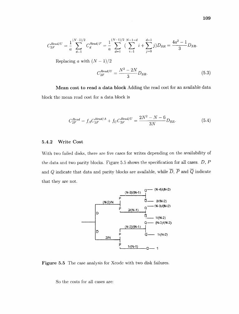
Replacing a with (N — 1)/2

Mean cost to read a data block Adding the read cost for an available data

block the mean read cost for a data block is

(5.4)

5.4.2 Write Cost

With two failed disks, there are five cases for writes depending on the availability of

the data and two parity blocks. Figure 5.5 shows the specification for all cases. D, P

and Q indicate that data and parity blocks are available, while D, P and Q indicate

that they are not.

109

Figure 5.5 The case analysis for Xcode with two disk failures.

So the costs for all cases are:

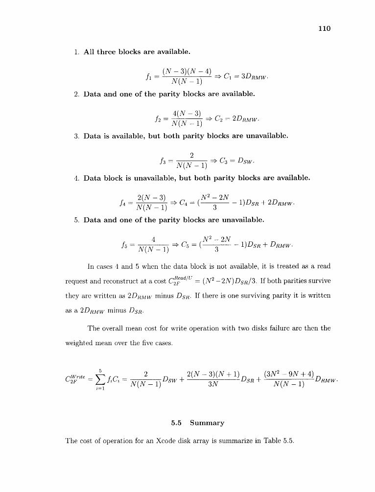
110

1. All three blocks are available.

2. Data and one of the parity blocks are available.

3. Data is available, but both parity blocks are unavailable.

4. Data block is unavailable, but both parity blocks are available.

5. Data and one of the parity blocks are unavailable.

In cases 4 and 5 when the data block is not available, it is treated as a readRead/U

request and reconstruct at a cost CRead2F = (N ² —2N)DSR/3. If both parities survive

they are written as 2DRMW minus DSR. If there is one surviving parity it is written

as a 2DRMW minus DSR.

The overall mean cost for write operation with two disks failure are then the

weighted mean over the five cases.

5.5 Summary

The cost of operation for an Xcode disk array is summarize in Table 5.5.

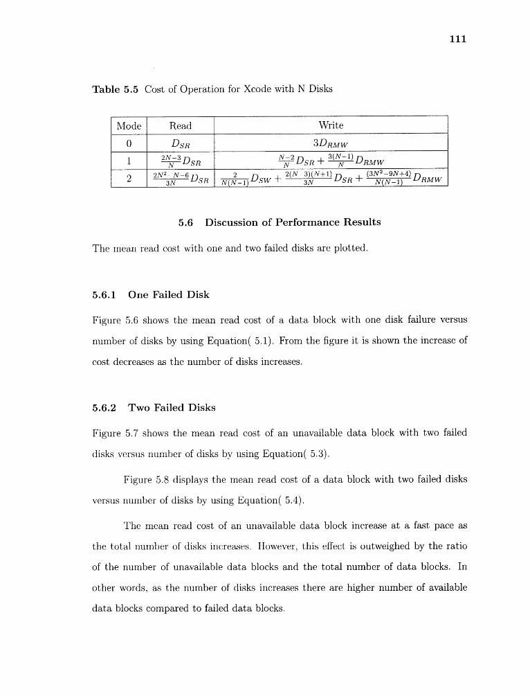
111

Table 5.5 Cost of Operation for Xcode with N Disks

5.6 Discussion of Performance Results

The mean read cost with one and two failed disks are plotted.

5.6.1 One Failed Disk

Figure 5.6 shows the mean read cost of a data block with one disk failure versus

number of disks by using Equation( 5.1). From the figure it is shown the increase of

cost decreases as the number of disks increases.

5.6.2 Two Failed Disks

Figure 5.7 shows the mean read cost of an unavailable data block with two failed

disks versus number of disks by using Equation( 5.3).

Figure 5.8 displays the mean read cost of a data block with two failed disks

versus number of disks by using Equation( 5.4).

The mean read cost of an unavailable data block increase at a fast pace as

the total number of disks increases. However, this effect is outweighed by the ratio

of the number of unavailable data blocks and the total number of data blocks. In

other words, as the number of disks increases there are higher number of available

data blocks compared to failed data blocks.

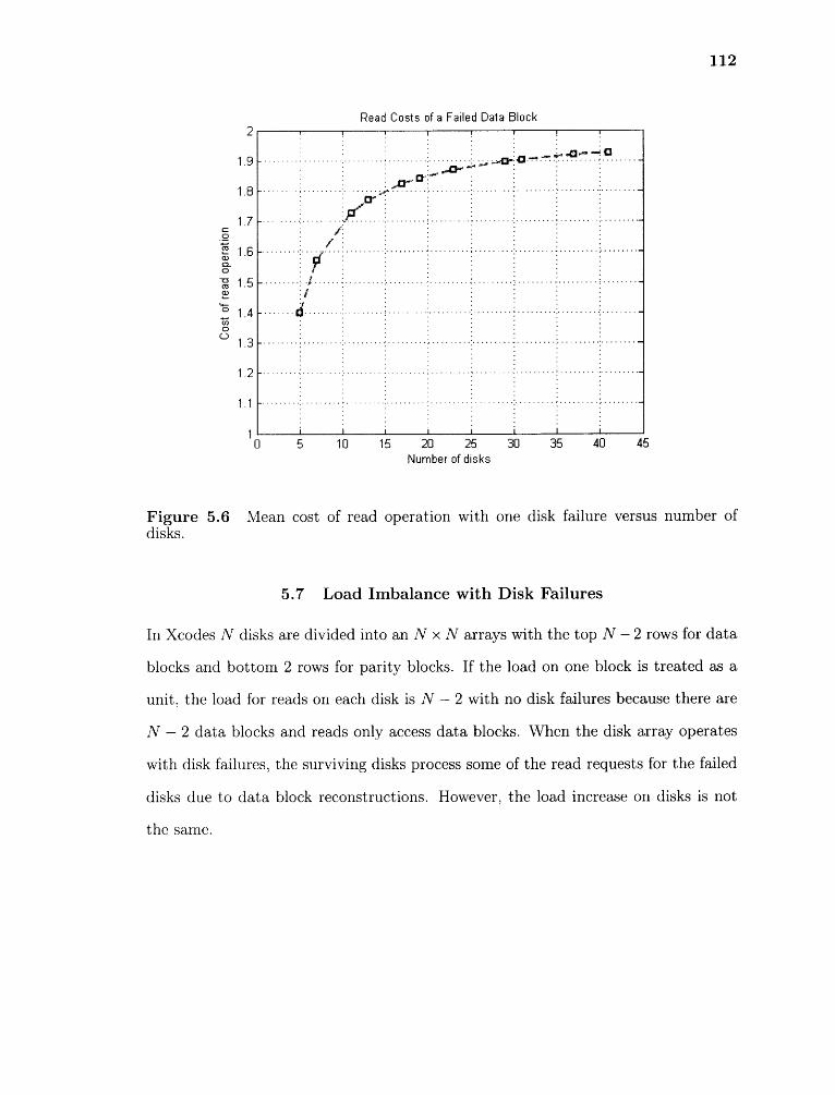
112

Figure 5.6 Mean cost of read operation with one disk failure versus number ofdisks.

5.7 Load Imbalance with Disk Failures

In Xcodes N disks are divided into an N x N arrays with the top N — 2 rows for data

blocks and bottom 2 rows for parity blocks. If the load on one block is treated as a

unit, the load for reads on each disk is N — 2 with no disk failures because there are

N — 2 data blocks and reads only access data blocks. When the disk array operates

with disk failures, the surviving disks process some of the read requests for the failed

disks due to data block reconstructions. However, the load increase on disks is not

the same.

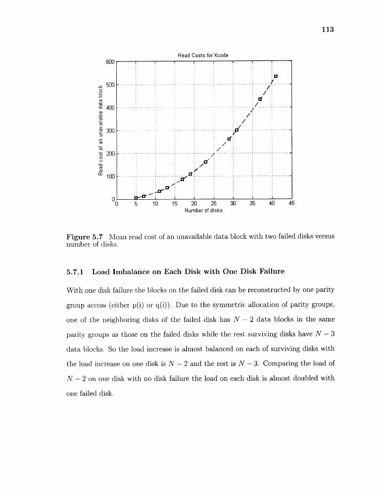
113

Figure 5.7 Mean read cost of an unavailable data block with two failed disks versusnumber of disks.

5.7.1 Load Imbalance on Each Disk with One Disk Failure

With one disk failure the blocks on the failed disk can be reconstructed by one parity

group access (either p(i) or q(i)). Due to the symmetric allocation of parity groups,

one of the neighboring disks of the failed disk has N — 2 data blocks in the same

parity groups as those on the failed disks while the rest surviving disks have N — 3

data blocks. So the load increase is almost balanced on each of surviving disks with

the load increase on one disk is N — 2 and the rest is N — 3. Comparing the load of

N — 2 on one disk with no disk failure the load on each disk is almost doubled with

one failed disk.

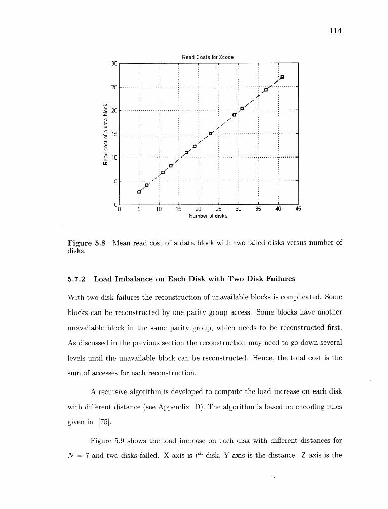
114

Figure 5.8 Mean read cost of a data block with two failed disks versus number ofdisks.

5.7.2 Load Imbalance on Each Disk with Two Disk Failures

With two disk failures the reconstruction of unavailable blocks is complicated. Some

blocks can be reconstructed by one parity group access. Some blocks have another

unavailable block in the same parity group, which needs to be reconstructed first.

As discussed in the previous section the reconstruction may need to go down several

levels until the unavailable block can be reconstructed. Hence, the total cost is the

sum of accesses for each reconstruction.

A recursive algorithm is developed to compute the load increase on each disk

with different distance (see Appendix D). The algorithm is based on encoding rules

given in [75].

Figure 5.9 shows the load increase on each disk with different distances for

N = 7 and two disks failed. X axis is i th disk, Y axis is the distance. Z axis is the

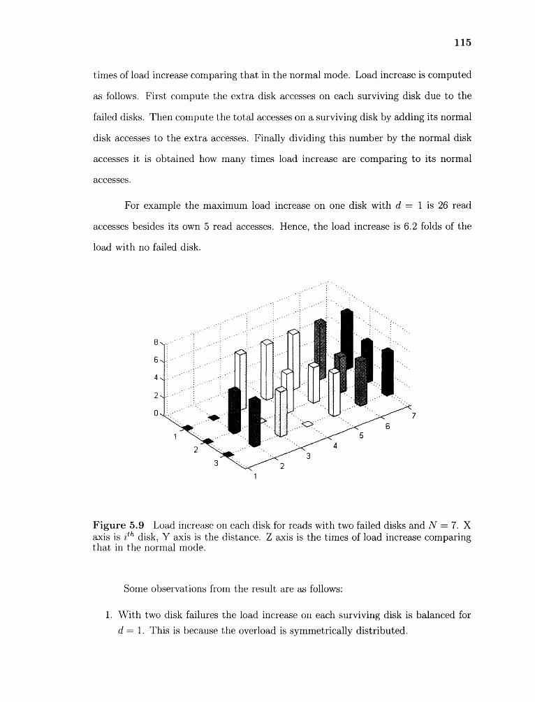
115

times of load increase comparing that in the normal mode. Load increase is computed

as follows. First compute the extra disk accesses on each surviving disk due to the

failed disks. Then compute the total accesses on a surviving disk by adding its normal

disk accesses to the extra accesses. Finally dividing this number by the normal disk

accesses it is obtained how many times load increase are comparing to its normal

accesses.

For example the maximum load increase on one disk with d = 1 is 26 read

accesses besides its own 5 read accesses. Hence, the load increase is 6.2 folds of the

load with no failed disk.

Figure 5.9 Load increase on each disk for reads with two failed disks and N = 7. Xaxis is i th disk, Y axis is the distance. Z axis is the times of load increase comparingthat in the normal mode.

Some observations from the result are as follows:

1. With two disk failures the load increase on each surviving disk is balanced ford = 1. This is because the overload is symmetrically distributed.

116

2. The load on the surviving disks is skewed when d > 1.

3. However, the load increase on each disk is the largest when d = 1.

Mean Load Increase on a Disk versus Distance: Mean load increase

on a disk varies with the distance. Figures 5.10, 5.11 and 5.12 show the mean

load increase on each disk with different distances when N is 7, 19, 37 and two disk

failures. Y axis shows the mean load increase of a disk for a given distance. It is

computed as follows. First obtain load increase on each surviving disk as discussed

above. Then get the mean of the load increase on each surviving disk to get the mean

load increase on a disk with a given distance.

Mean Load Increase vs Number of Disks: Figure 5.13 shows mean load

increase, best and worst cases among all distances, the maximum load increase on a

disk in both best and worst cases versus number of disks. To obtain the values of

these variables the load increase on each surviving disk for a given distance (LId,j, 1 <

j < N, 1 < d < (N — 1)/2) is computed first. Then the mean load increase for each

distance is calculated by the formula

The best and worst cases are

Mean load increase is

The maximum load increase on a disk in best case (d is the distance in MLIbest )

is

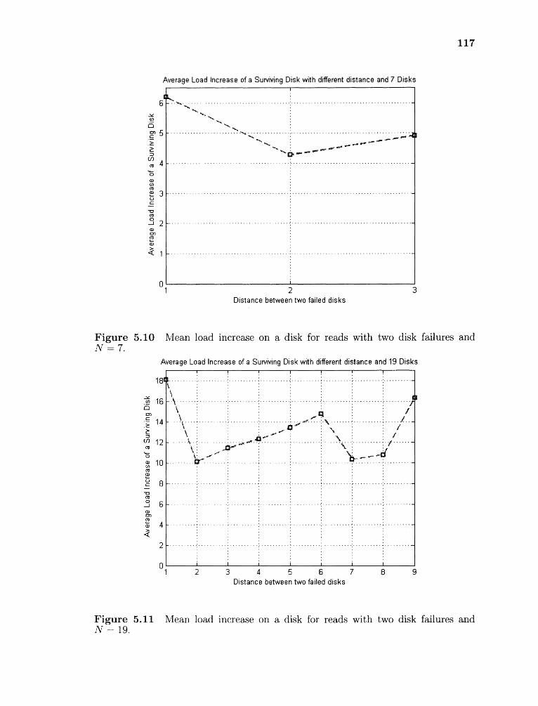
117

Figure 5.10 Mean load increase on a disk for reads with two disk failures andN = 7.

Figure 5.11 Mean load increase on a disk for reads with two disk failures andN = 19.

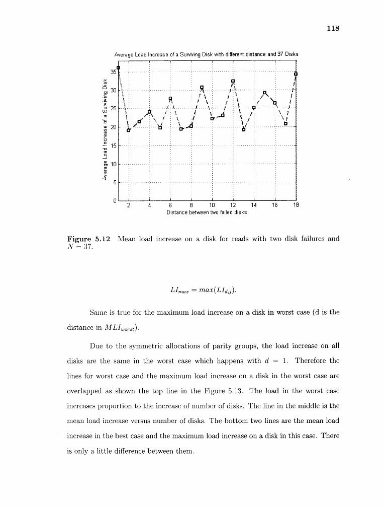
I.1.

118

Figure 5.12 Mean load increase on a disk for reads with two disk failures andN = 37.

Same is true for the maximum load increase on a disk in worst case (d is the

distance in MLIworstorst).

Due to the symmetric allocations of parity groups, the load increase on all

disks are the same in the worst case which happens with d = 1. Therefore the

lines for worst case and the maximum load increase on a disk in the worst case are

overlapped as shown the top line in the Figure 5.13. The load in the worst case

increases proportion to the increase of number of disks. The line in the middle is the

mean load increase versus number of disks. The bottom two lines are the mean load

increase in the best case and the maximum load increase on a disk in this case. There

is only a little difference between them.

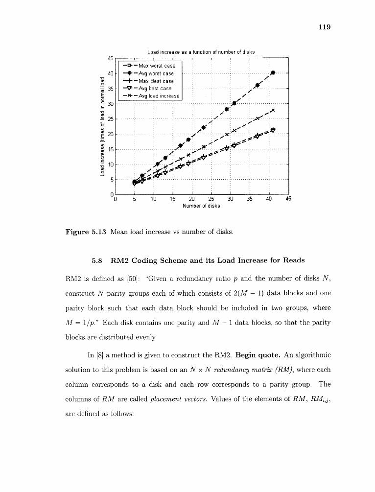
119

Figure 5.13 Mean load increase vs number of disks.

5.8 RM2 Coding Scheme and its Load Increase for Reads

RM2 is defined as [50]: "Given a redundancy ratio p and the number of disks N,

construct N parity groups each of which consists of 2(M — 1) data blocks and one

parity block such that each data block should be included in two groups, where

M = 1/p." Each disk contains one parity and M — 1 data blocks, so that the parity

blocks are distributed evenly.

In [8] a method is given to construct the RM2. Begin quote. An algorithmic

solution to this problem is based on an N x N redundancy matrix (RM), where each

column corresponds to a disk and each row corresponds to a parity group. The

columns of RM are called placement vectors. Values of the elements of RM, RMi ,j ,

are defined as follows:

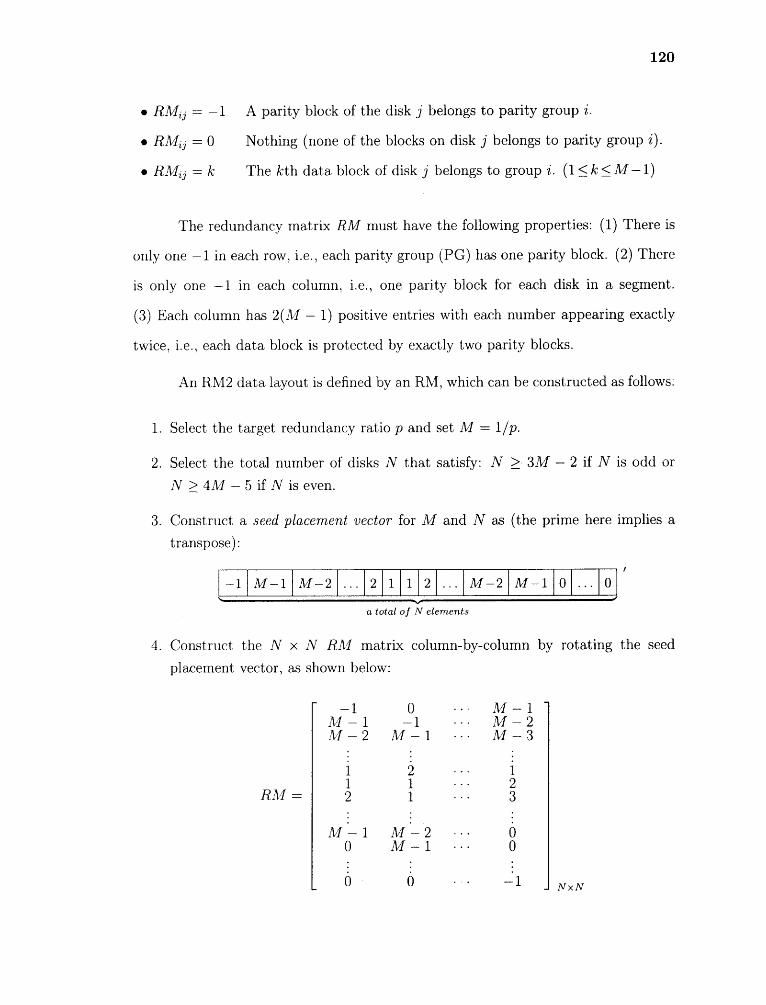
120

• RM ij = —1 A parity block of the disk j belongs to parity group i.

• RMij = 0 Nothing (none of the blocks on disk j belongs to parity group i).

• RMij = k The kth data block of disk j belongs to group i.. (1<k < M —1)

The redundancy matrix RM must have the following properties: (1) There is

only one —1 in each row, i.e., each parity group (PG) has one parity block. (2) There

is only one —1 in each column, i.e., one parity block for each disk in a segment.

(3) Each column has 2(M — 1) positive entries with each number appearing exactly

twice, i.e., each data block is protected by exactly two parity blocks.

An RM2 data layout is defined by an RM, which can be constructed as follows:

1. Select the target redundancy ratio p and set M = 1/p.

2. Select the total number of disks N that satisfy: N > 3M — 2 if N is odd or

N> 4M — 5 if N is even.

3. Construct a seed placement vector for M and N as (the prime here implies a

transpose):

a total of N elements

4. Construct the N x N RM matrix column-by-column by rotating the seed

placement vector, as shown below:

0

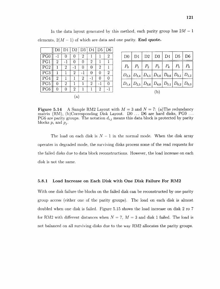
121

In the data layout generated by this method, each parity group has 2M — 1

elements, 2(M — 1) of which are data and one parity. End quote.

Figure 5.14 A Sample RM2 Layout with M = 3 and N = 7: (a)The redundancymatrix (RM), (b)Corresponding Disk Layout. D0 ... D6 are hard disks, PG0 ...PG6 are parity groups. The notation di,j means this data block is protected by parityblocks pi and p3 .

The load on each disk is N — 1 in the normal mode. When the disk array

operates in degraded mode, the surviving disks process some of the read requests for

the failed disks due to data block reconstructions. However, the load increase on each

disk is not the same.

5.8.1 Load Increase on Each Disk with One Disk Failure For RM2

With one disk failure the blocks on the failed disk can be reconstructed by one parity

group access (either one of the parity groups). The load on each disk is almost

doubled when one disk is failed. Figure 5.15 shows the load increase on disk 2 ro 7

for RM2 with different distances when N = 7, M = 3 and disk 1 failed. The load is

riot balanced on all surviving disks due to the way RM2 allocates the parity groups.

122

Load Increase with One Disk Failure and N=7

Figure 5.15 Load increase (times of the original load) on disk 2 to 7 for reads withdisk 1 failed and N = 7, M = 3 for RM2.

5.8.2 Load Increase on Each Disk with Two Disk Failures For RM2

Figure 5.16 shows the load increase on each disk with different distance when N is

7, M = 3 and two disk failures. X axis is i th disk, Y axis is the distance. Z axis

is the times of load increase comparing that in the normal mode. Load increase is

computed as follows. First compute the extra disk accesses on each surviving disk due

to the failed disks. Then compute the total accesses on a surviving disk by adding

itself normal disk accesses to the extra accesses. Finally Dividing this number by the

normal disk accesses it is obtained how many times load increase is comparing to it's

normal accesses.

Some observations from the result are as follows:

1. With two disk failures the load increase on each surviving disks is balancedwhen the distance of two failed disks is not one.

2. When the distance is one the load on the surviving disks is skewed.

3. The load increase on each disk is the largest when distance is one.

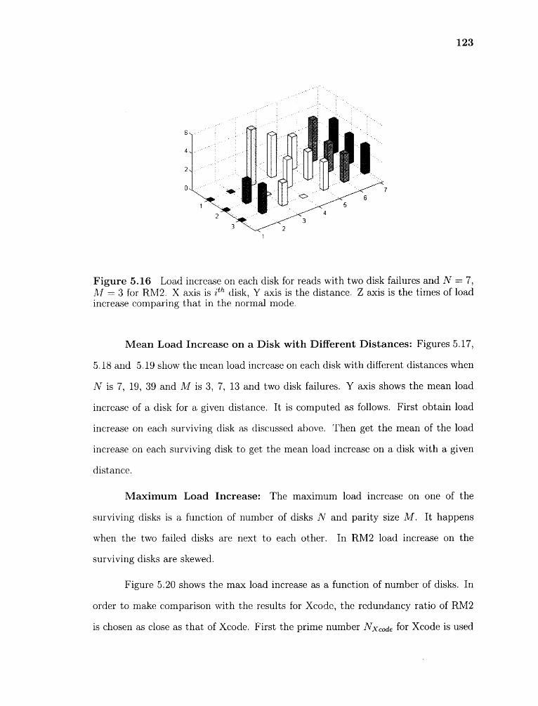
123

Figure 5.16 Load increase on each disk for reads with two disk failures and N = 7,M = 3 for RM2. X axis is i th disk, Y axis is the distance. Z axis is the times of loadincrease comparing that in the normal mode.

Mean Load Increase on a Disk with Different Distances: Figures 5.17,

5.18 and 5.19 show the mean load increase on each disk with different distances when

N is 7, 19, 39 and M is 3, 7, 13 and two disk failures. Y axis shows the mean load

increase of a disk for a given distance. It is computed as follows. First obtain load

increase on each surviving disk as discussed above. Then get the mean of the load

increase on each surviving disk to get the mean load increase on a disk with a given

distance.

Maximum Load Increase: The maximum load increase on one of the

surviving disks is a function of number of disks N and parity size M. It happens

when the two failed disks are next to each other. In RM2 load increase on the

surviving disks are skewed.

Figure 5.20 shows the max load increase as a function of number of disks. In

order to make comparison with the results for Xcode, the redundancy ratio of RM2

is chosen as close as that of Xcode. First the prime number NXcode for Xcode is used

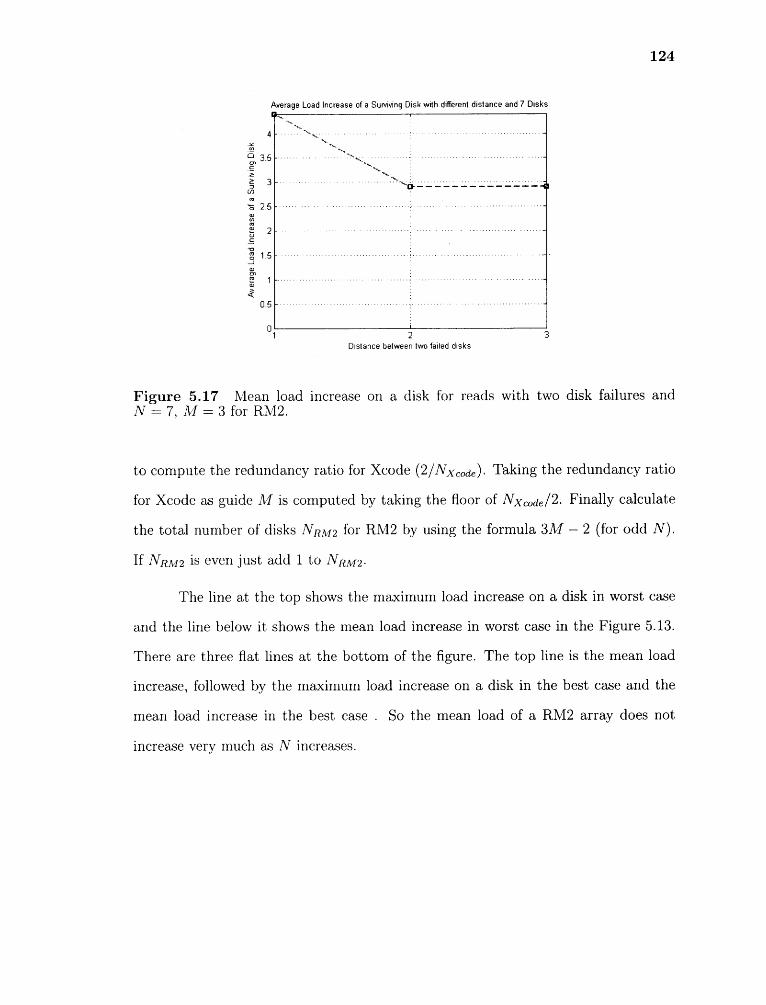
124

Figure 5.17 Mean load increase on a disk for reads with two disk failures andN =7, M = 3 for RM2.

to compute the redundancy ratio for Xcode (2/NX code). Taking the redundancy ratio

for Xcode as guide M is computed by taking the floor of NX code/2. Finally calculate

the total number of disks NRM2 for RM2 by using the formula 3M — 2 (for odd N).

If NRM2 is even just add 1 to NRM2.

The line at the top shows the maximum load increase on a disk in worst case

and the line below it shows the mean load increase in worst case in the Figure 5.13.

There are three flat lines at the bottom of the figure. The top line is the mean load

increase, followed by the maximum load increase on a disk in the best case and the

mean load increase in the best case . So the mean load of a RM2 array does not

increase very much as N increases.

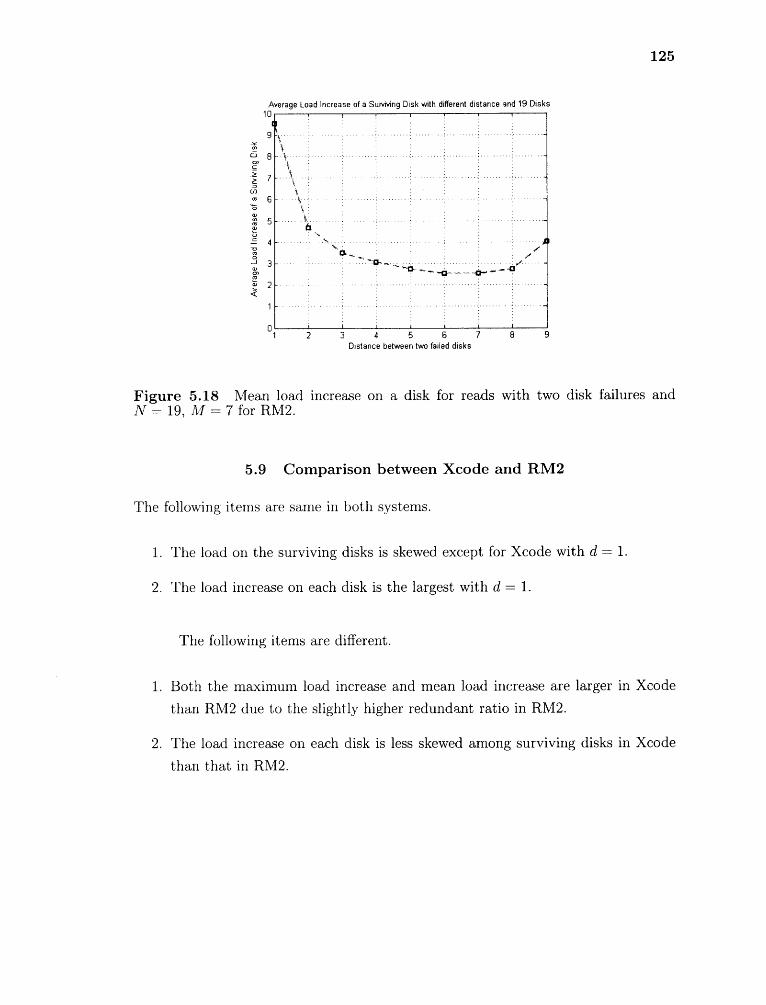
125

Figure 5.18 Mean load increase on a disk for reads with two disk failures andN = 19, M = 7 for RM2.

5.9 Comparison between Xcode and RM2

The following items are same in both systems.

1. The load on the surviving disks is skewed except for Xcode with d 1.

2. The load increase on each disk is the largest with d = 1.

The following items are different.

1. Both the maximum load increase and mean load increase are larger in Xcodethan RM2 due to the slightly higher redundant ratio in RM2.

2. The load increase on each disk is less skewed among surviving disks in Xcodethan that in RM2.

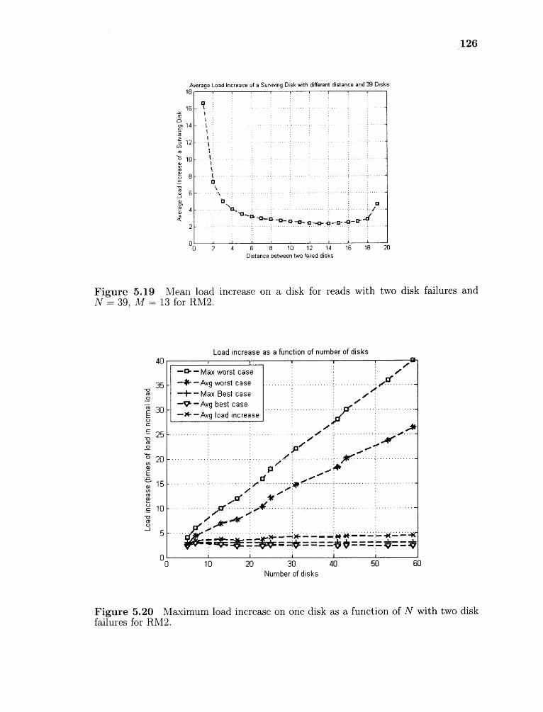
126

Figure 5.19 Mean load increase on a disk for reads with two disk failures andN = 39, M = 13 for RM2.

Figure 5.20 Maximum load increase on one disk as a function of N with two diskfailures for RM2.

CHAPTER 6

CONCLUSIONS

In this dissertation a brief discussion of the viability for HDA - Heterogenous Disk

Array is given: explosion of the amount of data generated, high data availability

requirement, rapid cost drop in storage cost, the high cost of storage management

and the need to automate it. A review of RAID levels builds the foundation for HDA.

There is the load balancing effect that R AID1 disk arrays have a higher access

rate than RAID5 disk arrays per GB. Given the Virtual Array (VA) size and access

rate its width or the number of its Virtual Disks (VDs) constituting the VA is

determined first. Several online single-pass data allocation methods are processed

and evaluated. An allocation is acceptable if it does not exceed the disk capacity

and overload disk bandwidth especially in the presence of disk failures. Results show

methods considering both bandwidth and capacity utilization of disks in the system

outperform the others.

When disk bandwidth rather than capacity is the bottleneck, the clustered

RAID paradigm is applied, which offers a tradeoff between disk space and bandwidth.

Experiments show clustered RAID can increase the number of allocations dramat-

ically when RAID5 requests dominate the allocations requests.

Four mirrored disk organizations are described in this study: basic mirroring

- BM, group rotate declustering - GRD, interleaved declustering - ID, and chained

declustering - CD. The last three organizations provide a more balanced disk load

than BM when a single disk fails, but are more susceptible to data loss than BM

when additional disks fail. The four organizations are compared from the viewpoint

of: (a) reliability (results are quoted from [63] ), (b) performability, (c) performance.

127

128

In (b) and (c) discrete requests to small randomly placed blocks are postulated. For

(b) the mean number of disk requests processed is computed to the point where

data loss occurs. For the sake of tractability in (c) the response time is obtained

assuming Poisson arrivals and a FCFS policy. The ranking from the viewpoint of

reliability and performability is: BM, CD, GRD, ID (with two clusters). BM and CD

provide the worst performance, ID has a better performance than BM and CD, but is

outperformed by GRD. These results are also shown using an asymptotic expansion

method.

The load increase and imbalance of the X-code method is analyzed in this

study. The X-codes method exhibits the same cost as RAID6 when operating in

normal mode. Similarly to RAID5 and RAID6 the read load in normal mode is

almost doubled with a single disk failure. With two disk failures the read cost for

unavailable blocks increases quadratically with the number of disks (N), while the

overall cost increases linearly with N. A general expression for disk loads is derived

and graphs to quantify the load imbalance are presented.

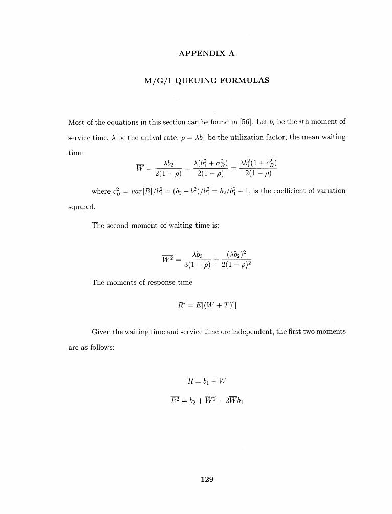
APPENDIX A

M/G/1 QUEUING FORMULAS

Most of the equations in this section can be found in [56]. Let b i be the ith moment of

service time, A be the arrival rate, ρ = b1 be the utilization factor, the mean waiting

time

where c²B = var[B] / = (b ² — b21) = b² / — 1, is the coefficient of variation

squared.

The second moment of waiting time is:

The moments of response time

Given the waiting time and service time are independent, the first two moments

are as follows:

129

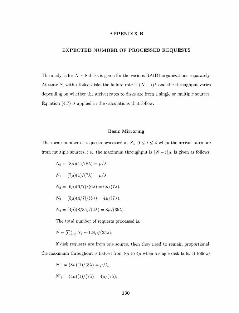
APPENDIX B

EXPECTED NUMBER OF PROCESSED REQUESTS

The analysis for N = 8 disks is given for the various RAID 1 organizations separately.

At state Si with i failed disks the failure rate is (N — i) and the throughput varies

depending on whether the arrival rates to disks are from a single or multiple sources.

Equation (4.7) is applied in the calculations that follow.

Basic Mirroring

The mean number of requests processed at S i , 0 < i < 4 when the arrival rates are

from multiple sources, i.e., the maximum throughput is (N — i)µ, is given as follows:

The total number of requests processed is:

If disk requests are from one source, then they need to remain proportional,

the maximum throughout is halved from 8p, to 4p, when a single disk fails. It follows

130

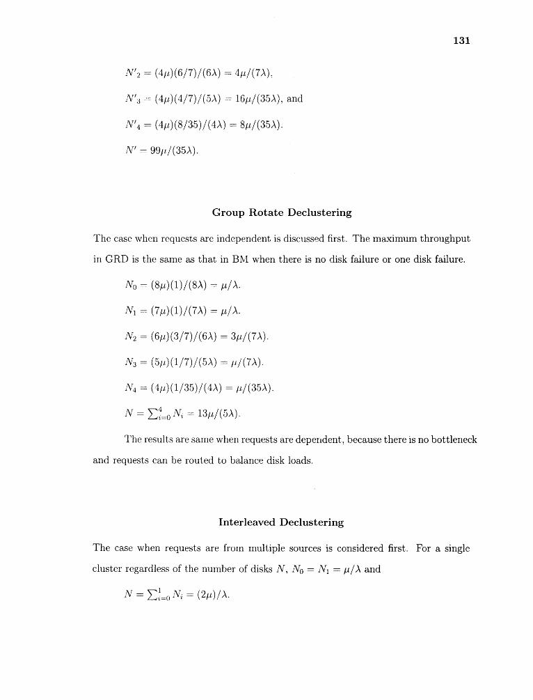
131

Group Rotate Declustering

The case when requests are independent is discussed first. The maximum throughput

in GRD is the same as that in BM when there is no disk failure or one disk failure.

The results are same when requests are dependent, because there is no bottleneck

and requests can be routed to balance disk loads.

Interleaved Declustering

The case when requests are from multiple sources is considered first. For a single

cluster regardless of the number of disks N, N0 = N1 = µ/ and

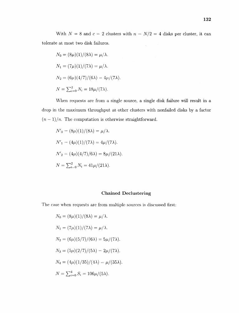
132

With N = 8 and c = 2 clusters with n = N/2 = 4 disks per cluster, it can

tolerate at most two disk failures.

When requests are from a single source, a single disk failure will result in a

drop in the maximum throughput at other clusters with nonfailed disks by a factor

(n — 1)/n. The computation is otherwise straightforward.

Chained Declustering

The case when requests are from multiple sources is discussed first:

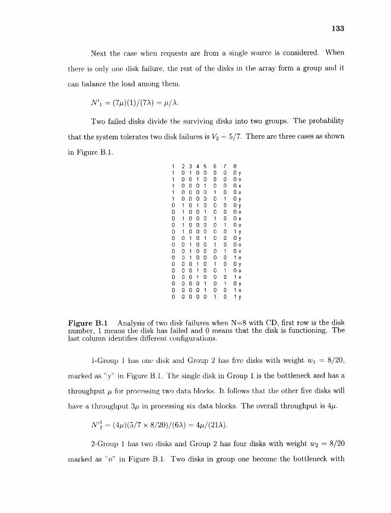
133

Next the case when requests are from a single source is considered. When

there is only one disk failure, the rest of the disks in the array form a group and it

can balance the load among them.

Two failed disks divide the surviving disks into two groups. The probability

that the system tolerates two disk failures is V² = 5/7. There are three cases as shown

in Figure B.1.

Figure B.1 Analysis of two disk failures when N=8 with CD, first row is the disknumber, 1 means the disk has failed and 0 means that the disk is functioning. Thelast column identifies different configurations.

1-Group 1 has one disk and Group 2 has five disks with weight w 1 = 8/20,

marked as "y" in Figure B.1. The single disk in Group 1 is the bottleneck and has a

throughput µ for processing two data blocks. It follows that the other five disks will

have a throughput 3,u, in processing six data blocks. The overall throughput is 4/.2.

2-Group 1 has two disks and Group 2 has four disks with weight w ² = 8/20

marked as "o" in Figure B.1. Two disks in group one become the bottleneck with

134

a throughput 2p for three data blocks. The throughput at four disks for five data

blocks will equal 10p/3, so that the total throughput is 16p/3

3-Each group of three disks processes the load associated with four data blocks,

so that the throughput is 6p . . This configuration has weight w ³ = 4/20 and is marked

with "x" in Figure B.1.

When three disks fail there is always a single disk between two failed disks,

which is a bottleneck. It is easy to show that the maximum throughput in this case

is 4p.

With four disk failures the throughputs at all surviving disks are the same and

APPENDIX C

ANALYSIS OF READ COST FOR AN UNAVAILABLE DATA BLOCK

WITH TWO FAILED DISKS

Observation 1 There are always two blocks on each failed disk which can be recon-

structed by using one parity group.

Proof: Because each parity group only contains N — 1 blocks, it only uses

N — 1 disks. In other words each disk only has blocks of N — 1 parities. So even

though one disk is failed the block in the parity that is not on the disk can be repaired

by using one parity group access. Since there are two parity groups (slope = 1 and

slope = -1), there are two such blocks on each failed disks.

However the position of these two blocks are changing when the distance of

two failed disks changes. The position has some impacts on the reconstructing cost

of an unavailable data block.

Example: Figures C.1 and C.2 show the two parity groups with N = 7.

When two failed disks are neighbors those two blocks that can be repaired by

one parity group access are the top and bottom blocks of the failed disks. Analysis

of two failed disks is identical. So the focus is on one disk. For example disk 1 and

disk 2 are failed. The two blocks are block (1,1) and block (7,1) from Figures C.1 and

C.2. Block (1,1) is a data block and block (7,1) is a parity block. The data block can

decide which way to go to reconstruct other data block. For example if block (2,2)

needs to be reconstructed, either block (1,1) for q(5) or block (3,1) for p(4) needs

to be reconstructed first. Obviously block (1,1) will be chosen for one parity group

access. The parity block won't give any help to reconstruct other data blocks because

all data blocks in that parity group is available. Had this block is not a parity block,

135

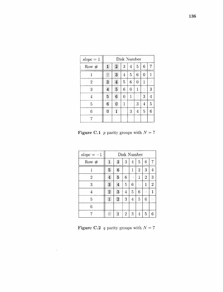
Figure C.1 p parity groups with N = 7

136

Figure C.2 q parity groups with N = 7

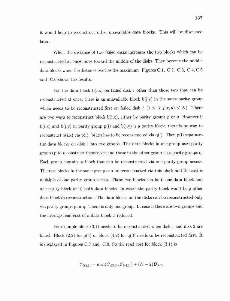
137

it would help to reconstruct other unavailable data blocks. This will be discussed

later.

When the distance of two failed disks increases the two blocks which can be

reconstructed at once move toward the middle of the disks. They become the middle

data blocks when the distance reaches the maximum. Figures C.1, C.2, C.3, C.4, C.5

and C.6 shows the results.

For the data block b(i,x) on failed disk i other than those two that can be

reconstructed at once, there is an unavailable block b(j,y) in the same parity group

which needs to be reconstructed first on failed disk j, (1 < (i, j, x, y) < N), There

are two ways to reconstruct block b(i,x), either by parity groups p or q. However if

b(i,x) and b(j,y) in parity group p(i) and b(j,y) is a parity block, there is no way to

reconstruct b(i,x) via p(i). b(i,x) has to be reconstructed via q(i). Then p(i) separates

the data blocks on disk i into two groups. The data blocks in one group uses parity

groups p to reconstruct themselves and those in the other group uses parity groups q.

Each group contains a block that can be reconstructed via one parity group access.

The rest blocks in the same group can be reconstructed via this block and the cost is

multiple of one parity group access. These two blocks can be i) one data block and

one parity block or ii) both data blocks. In case i the parity block won't help other

data blocks's reconstruction. The data blocks on the disks can be reconstructed only

via parity groups p or q. There is only one group. In case ii there are two groups and

the average read cost of a data block is reduced.

For example block (3,1) needs to be reconstructed when disk 1 and disk 2 are

failed. Block (2,2) for p(4) or block (4,2) for q(3) needs to be reconstructed first. It

is displayed in Figures C.7 and C.8. So the read cost for block (3,1) is

Cb(3,1) = min(Cb(2,2(²,²), Cb(4,2)) + (N — 2)D S R .

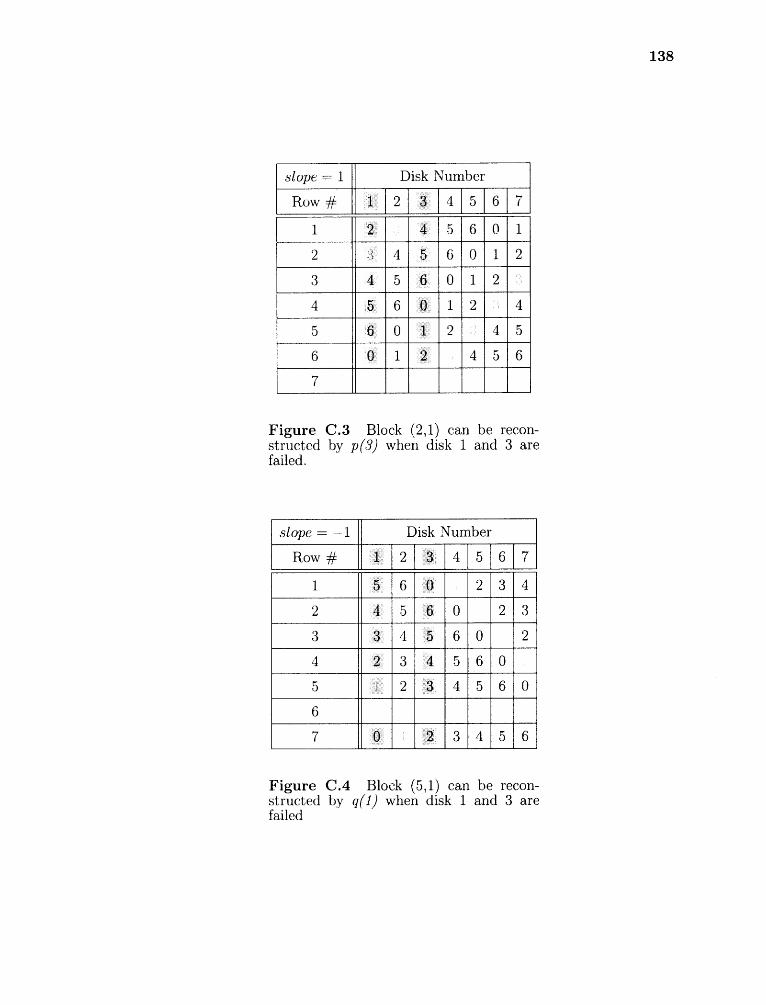
Figure C.3 Block (2,1) can be recon-structed by p(3) when disk 1 and 3 arefailed.

138

Figure C.4 Block (5,1) can be recon-structed by q(1) when disk 1 and 3 arefailed

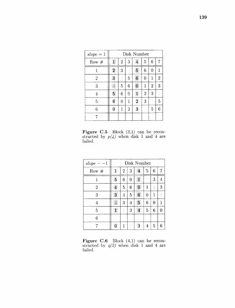
Figure C.5 Block (3,1) can be recon-structed by p(4) when disk 1 and 4 arefailed.

139

Figure C.6 Block (4,1) can be recon-structed by q(2) when disk 1 and 4 arefailed.

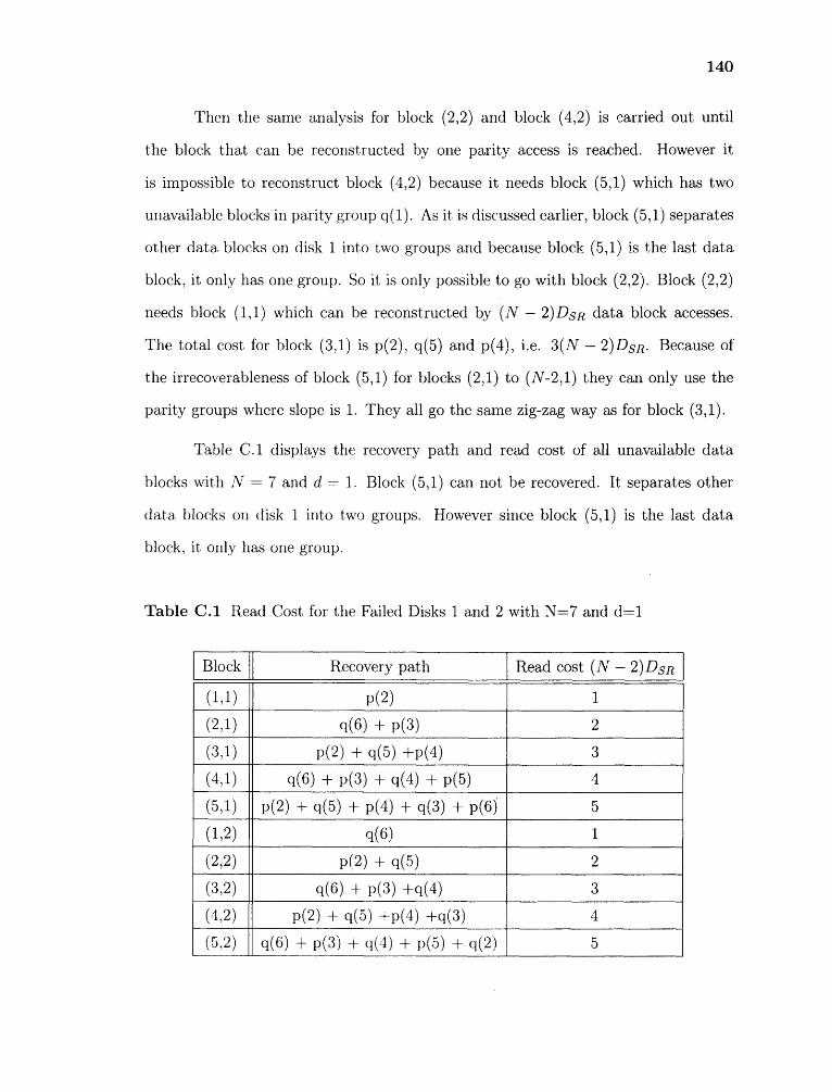
140

Then the same analysis for block (2,2) and block (4,2) is carried out until

the block that can be reconstructed by one parity access is reached. However it

is impossible to reconstruct block (4,2) because it needs block (5,1) which has two

unavailable blocks in parity group q(1). As it is discussed earlier, block (5,1) separates

other data blocks on disk 1 into two groups and because block (5,1) is the last data

block, it only has one group. So it is only possible to go with block (2,2). Block (2,2)

needs block (1,1) which can be reconstructed by (N — 2)DSR data block accesses.

The total cost for block (3,1) is p(2), q(5) and p(4), i.e. 3(N — 2)DSR . Because of

the irrecoverableness of block (5,1) for blocks (2,1) to (N-2,1) they can only use the

parity groups where slope is 1. They all go the same zig-zag way as for block (3,1).

Table C.1 displays the recovery path and read cost of all unavailable data

blocks with N = 7 and d = 1. Block (5,1) can not be recovered. It separates other

data blocks on disk 1 into two groups. However since block (5,1) is the last data

block, it only has one group.

Table C.1 Read Cost for the Failed Disks 1 and 2 with N=7 and d=1

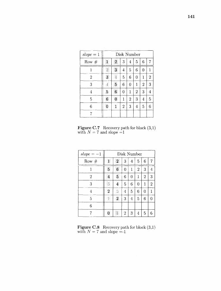
Figure C.7 Recovery path for block (3,1)with N = 7 and slope =1

141

Figure C.8 Recovery path for block (3,1)with N = 7 and slope =-1

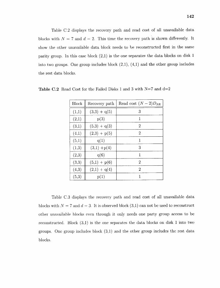
142

Table C.2 displays the recovery path and read cost of all unavailable data

blocks with N = 7 arid d = 2. This time the recovery path is shown differently. It

show the other unavailable data block needs to be reconstructed first in the same

parity group. In this case block (2,1) is the one separates the data blocks on disk 1

into two groups. One group includes block (2,1), (4,1) and the other group includes

the rest data blocks.

Table C.2 Read Cost for the Failed Disks 1 and 3 with N=7 and d=2

Table C.3 displays the recovery path and read cost of all unavailable data

blocks with N = 7 and d = 3. It is observed block (3,1) can not be used to reconstruct

other unavailable blocks even through it only needs one party group access to be

reconstructed. Block (3,1) is the one separates the data blocks on disk 1 into two

groups. One group includes block (3,1) and the other group includes the rest data

blocks.

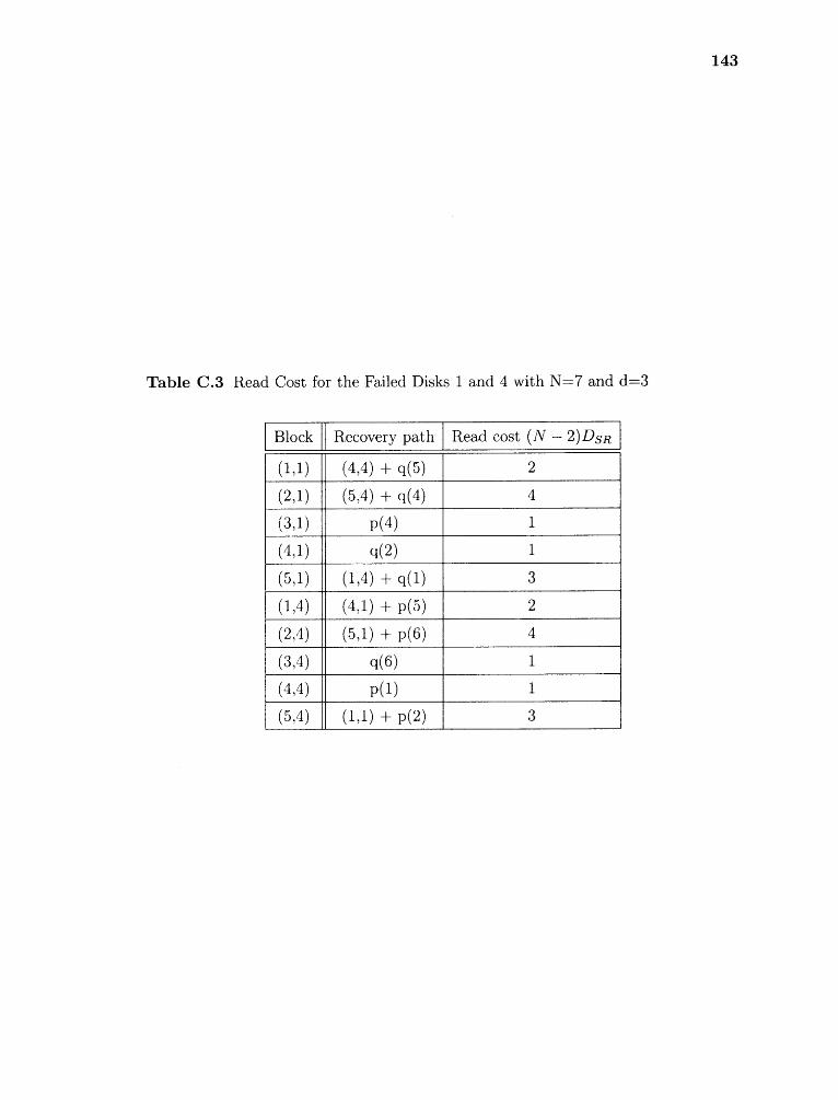
Table C.3 Read Cost for the Failed Disks 1 and 4 with N=7 and d=3

143

APPENDIX D

ALGORITHM TO COMPUTE THE LOAD INCREASE WITH TWO

DISK FAILURES IN X-CODE

Algorithm 3 computes the load increase for each unavailable block. Recursion is

carried out at Line 5 in the algorithm. If there is another data block unavailable

it needs to be reconstructed first by using the parity group with the opposite slope

Other part of the algorithm is trivial.

Now a test drive is developed to call the recursive algorithm. Algorithm 4

shows it. One point worth mention here is that for a given unavailable block there

are two possible ways to reconstruct it, by using either p or q parity group. The one

with minimum cost will be chosen. Also notice at the beginning it is necessary to

find the parity groups an unavailable block belongs to. This is due to the fact that

for a given data block it is not known which parity group it belongs to because of the

module operations in the above two formulas.

Now a main algorithm is deployed to loop through each failed data blocks. It

is displayed in Algorithm 5. The results are the times of load increase of each disk

comparing its load with no failed disk.

144

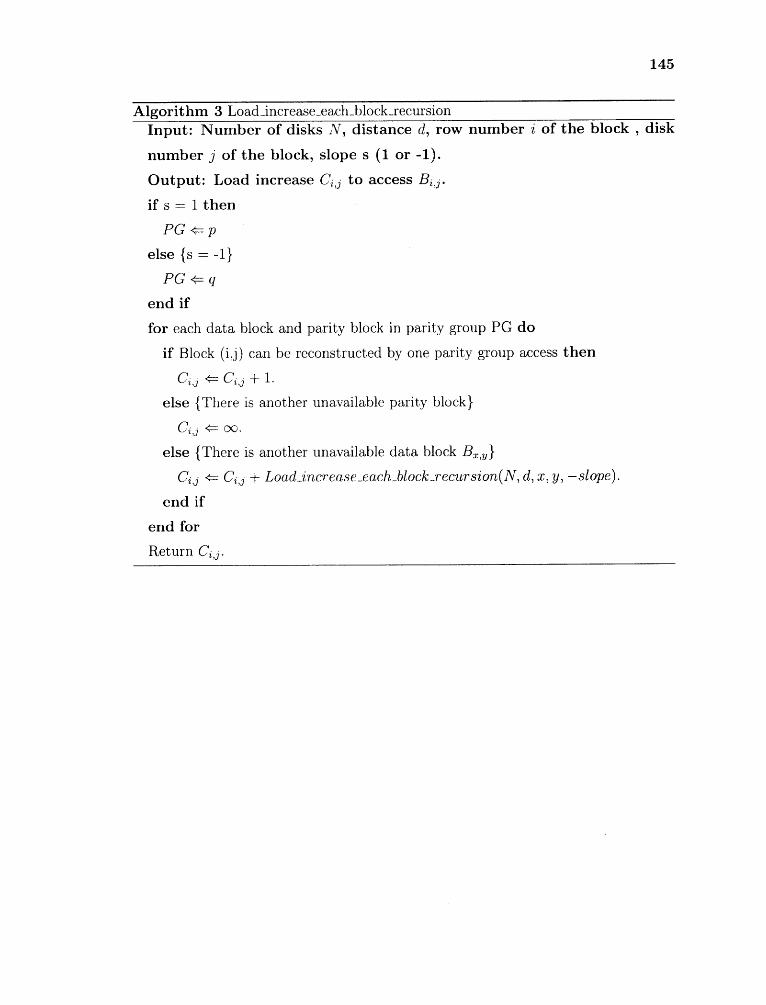
Algorithm 3 Load-increase_each_block_recursion

145

Algorithm 4 Load_increase_each_block

146

Algorithm 5 Loadincrease_with_two_disk_failuresInput: Number of disks N.

Output: Load increase of each disks with different distance CIncrease•

147

APPENDIX E

ALGORITHM TO COMPUTE THE LOAD INCREASE WITH TWO

DISK FAILURES IN RM2

Algorithm 6, 7 and 8 compute the load increase of each disks with two disks failures

in RM2.

Given parity blocks arc stored in the first row (row index from 1 to M and

column index from 0 to N- 1), the formula for a parity group is .13 1 , i = B2,<i+1+N-M>N ED

B3,<i+2+N-M>N e•-,EDBm.<i+N-1>NB2,<i+N-M>NB3,<i-1+N-M>N BM,<i+N_2m+2>N,

where 0 < i < N — 1, < X >N = X module N. On the contrary if block (i,j) is

given, column index of p and q parity groups the block belongs to is computed by

the following formulas

If x or y is less than zero

148

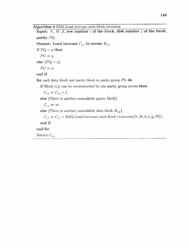
149

Algorithm 6 RM2_Load_increase_each_block_recursionInput: N, M ,d, row number i of the block, disk number j of the block,

parity PQ.

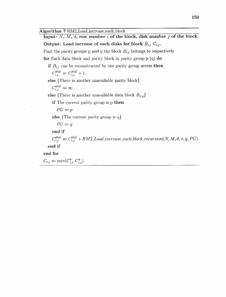
150

Algorithm 7 RM2_Load_increase_each_blockInput: N, M, d, row number i of the block, disk number j of the block.

Output: Load increase of each disks for block Bi,j Ci

Find the parity groups p and q the block belongs to respectively.

for Each data block and parity block in parity group p (q) do

if B. can be reconstructed by one parity group access then

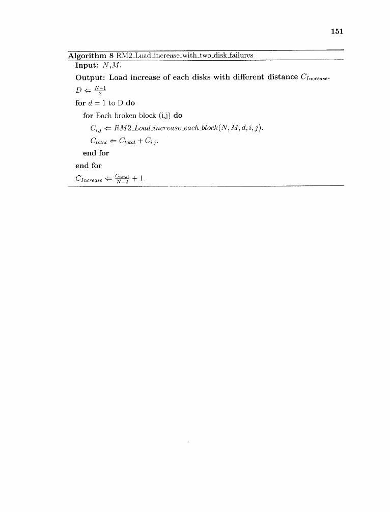
Algorithm 8 RM2_Load_increase_with_two_disk_failuresInput: N,M.

Output: Load increase of each disks with different distance CIncrease•

151

REFERENCES

[1] A. R. Calderbank, E. G. Coffman, Jr., and L. Flatto. Sequencing problems in twoserver systems. Mathematics of Operations Research, 10(4):585-598, 1985.

[2] A. R. Calderbank, E. G. Coffman, Jr.. and L. Flatto. Optimum head separation ina disk system with two heads. Journal of the ACM, 31(4):826-838, September1984.

[3] A. Thomasian. Access costs in clustered raid. The Computer Journal, 48(11):702-713,November 2005.

[4] A. Thomasian. Correction to "Clustered RAID Arrays and Their Access Costs". TheComputer Journal, November 2005.

[5] A. Thomasian and C. Han. Heterogeneous disk array architecture and its dataallocation policies. In Int'l Symp. on Performance Evaluation of Computer andTelecommunication Systems - SPECTS 2005, pages 617-624, Cherry Hill, NJ,July 2005.

[6] A. Thomasian and C. Liu. Some new disk scheduling policies and their performance.In Proc. ACM SIGMETRICS Conf. Measurement and Modeling of ComputerSystems, pages 266-267, Marina del Rey, CA, May 2002.

[7] A. Thomasian, B. A. Branzoi, and C. Han. Performance evaluation of a hetero-geneous disk array architecture. In 13th Int'l Symp. on Modeling, Analysis, andSimulation of Computer and Telecommunication Systems - MASCOTS '05, pages517-520, Atlanta, GA, September 2005.

[8] A. Thomasian, C. Han and G. Fu. Performance evaluation of two-disk failure tolerantarrays. IEEE Trans. Computers, 56(6):799-814, June 2007.

[9] A. Thomasian, J. Spirollari, C. Liu, C. Han and G. Fu. Mirrored disk scheduling. InProc. Int'l Symp. Performance Evaluation of Computer and TelecommunicationSystems -SPECTS'03, pages 580-584, Montreal, Quebec, Canada, July 2003.

j10] A. Adya, W. Bolosky, M. Castro, R. Chaiken, G. Cermak, J. Douceur, J. Howell,J. Lorch, M. Theimer, and R. Wattenhofer. Farsite: Federated, available, andreliable storage for an incompletely trusted environment. In In proc. of the 5thSymposium on Operating Systems Design and Implementation (OSDI)., Boston,MA,2002.

.11] N. Allen. Don't waste your storage dollars: what you need to know. Research NoteCOM-13-1217, Gartner Group, March 2001.

.12] G. A. Alvarez, E. Borowsky, S. Go, T. H. Romer, R. Becker-Szendy, R. Golding,A. Merchant, M. Spasojevic, A. Veitch, and J. Wilkes. Minerva: An automatedresource provisioning tool for large-scale storage systems. ACM Transactions onComputer Systems, 19(4):483-518, 2001.

-. 13] E. Anderson, M. Kallahalla, S. Spence, R. Swaminathan, and Q. Wang. Ergastulum:Quickly finding near-optimal storage system designs. HP Laboratories SSPTechnical Report HPL-SSP-2001-05, June 2002.

152

153

[14] B. Jacob, S. W. Ng, and D. T. Wang. Memory Systems: Cache, DRAM, Disk.Morgan-Kaufmann Publisher, 2008.

[15] B. R. Haverkort, R. Marie, R. Rubino, and K. S. Trivedi. Performability Modelling:Techniques and Tools. Wiley, New York, NY, 2001.

[16] E. Bachmat and T. K. Lain. On the effect of a configuration choice on the performanceof a mirrored storage system. J. Parallel and Distributed Computing, 65(3):382-395, March 2005.

[17] M. Blaum. An introduction to error-correcting codes, Coding and Signal Processingfor Magnetic Recording Systems, B Vasic and E M Kurtas, editors, Chapter 9,CRC Press, Orlando, FL.

[18] E. Borowsky, R. Golding, A. Merchant, L. Schrier, E. Shriver, M. Spasojevic, andJ. Wilkes. Using attribute-managed storage to achieve qos. In Proc. of the 5thInt'l Conf. Workshop on Quality of Service, Columbia University, New York,June 1997.

[19] B. A. Branzoi. Performance Evaluation of Various Allocation Methods in a Hetero-geneous Disk Array Architecture. Masters thesis, Computer Science Dept., NewJersey Institute of Technology, Newark, NJ, December 2004.

[20] C. Orji and J. A. Solworth. Doubly distorted mirrors. In Proc. ACM SIGMOD Int'lConf. on Management of Data, pages 307-316, Washington, D. C., May 1993.

[21] C. Polyzois, A. Bhide and D. M. Dias. Disk mirroring with alternating deferredupdates. In Proc. 19th Int'l Conf. Very Large Data Bases - VLDB, pages 604-617, Dublin, Ireland, August 1993.

[22] S. Z. Chen and D. F. Towsley. A performance evaluation of raid architectures. IEEETrans. Computers, 45(10):1116-1130, October 1996.

[23] C.R. Lumb, R. Golding and G. R. Ganger. D-SPTF: Decentralized request distri-bution in brick-based storage systems. In Proc 11th Int'l Conf. ArchitecturalSupport for Programming Languages and Operating Systems - ASPLOS, pages37-47, Cambridge, MA, October 2004.

[24] D. F. Towsley, S. Z. Chen and S. P. Yu. Mirrored disk scheduling. In Performanceanalysis of fault-tolerant mirrored disk systems, pages 239-253, P. J. B. King, I.Mitrani, and R. J. Pooley, editors, North-Holland, Amsterdam, The Netherlands,1990.

[25] E. Anderson, M. Hobbs K. Keeton, S. Spence, M. Uysal, and A. Veitch. Hippodrome:Running circles around storage administration. In Conf. File and StorageTechnologies - FAST'02, Monterey, CA, January 2002.

[26] E. Anderson, R. Swaminathan, A. Veitch, G. A. Alvarez, and J. Wilkes. SelectingRAID levels for disk arrays. In Conf. File and Storage Technologies - FAST'02,pages 189-201, Monterey, CA, January 2002.

[27] E. G. Coffman, Jr. and M. Hofri. Queueing models of secondary storage devices. InStochastic Analysis of Computer and Communication Systems, pages 549-588,H. Takagi, editor, Elsevier, Amsterdam, The Netherlands, 1990.

[28] G. A. Gibson. Redundant Disk Arrays: Reliable, Parallel Secondary Storage. MITPress, 1992.

154

[29] R. Golding, E. Shriver, T. Sullivan, and J. Wilkes. Attribute-managed storage. InWorkshop on Modeling and Specification of I/O, 1995.

[30] C. Han. Studies of disk arrays tolerating two disk failures and a proposal for a hetero-geneous disk array. PhD thesis, New Jersey Institute of Technology, Newark, NJ,May 2004.

[31] M. Hofri. Should the two-headed disk be greedy? - yes it should. InformationProcessing Letters - IPL, 16(2):83-85, 1983.

[32] HP, An analysis of RAID 5DP. HP White Paper, http://www.hp.com .

[33] H. I. Hsiao and D. J. DeWitt. A performance study of three high availability datareplication strategies. J. Distributed and Parallel Databases, 1(1):53-80, 1993.

[34] J. Wilkes, R. Golding, C. Staelin, and T. Sullivan. The HP autoraid hierarchicalstorage system. ACM Trans. Computer Systems, 14(1):108-136, 1996.

[35] H. H. Kari. Latent Sector Faults and Reliability of Disk Arrays. PhD thesis, HelsinkiUniversity of Technology, Espoo, Finland, 1997.

[36] C. Kenyon. Best-fit bin-packing with random order. In SODA: ACM-SIAM Symp.on Discrete Algorithms (A Conference on Theoretical and Experimental Analysisof Discrete Algorithms), pages 359-364, 1996.

[37] L. Kleinrock. Queueing Systems, Vol. I: Theory. John-Wiley, New York, NY, 1975.

[38] L. Kleinrock. Queueing Theory, Vol. II: Applications. John-Wiley, New York, NY,1975.

[39] L. Golubchik, J. S. Liu, and R. R. Muntz. Chained declustering: Load balancing androbustness to skew and failures. In Proc. 1st Int'l Workshop on Research Issuesin Data Engineering - RIDE, pages 88-95, Tempe, AZ, 1992.

[40] E. Lee and R. Katz. Performance consequences of parity placement in disk array. InInt'l Conf. on Architectural Support for Programming Languages and OperatingSystems - ASPLOS, pages 190-199, Santa Clara, CA, USA, 1991.

[41] M. Blaum, J. Brady, J. Bruck, and J. Menon. Evenodd: An optimal scheme fortolerating double disk failures in raid architectures. IEEE Trans. Computers,TC-44(2):192-202, February 1995.

[42] J. Menon and D. Mattson. Distributed sparing in disk arrays. In Proc. 37th AnnualIEEE Computer Society Conf. - COMPCON, pages 410-421, San Francisco, CA,February 1992.

[43] A. Merchant and P. Yu. Performance analysis of a dual striping strategy for replicateddisk arrays. In Proceedings of the Second International Conference on Paralleland Distributed Information Systems, pages 148-157, San Diego, January 1993.

[44] R. Nelson and A. Tantawi. Approximate analysis of fork-join synchronization inparallel queues. IEEE Transactions on Computers, 37(6):739-743, 1988.

[45] S. W. Ng. Improving disk performance via latency reduction. IEEE Trans.Computers, 40(1):22-30, January 1991.

155

[46] P. Corbett, B. English, A. Goel, T. Grcanac, S. Kleiman, J. Leong, and S. Sankar.Row-diagonal parity for double disk failure correction. In Proc. 3rd Conf. File andStorage Technologies - FAST'04, pages 1-14, San Francisco, CA, March/ April2004.

[47] P. Lyman, H. R. Varian, P. Charles, N. Good, L. L. Jordan and J. Pal. Howmuch informantion? http: / /www2. si ms. berkeley. edu/research/pro j ects/how-much-info-2003/, December 3, 2003.

[48] P. M. Chen, E. K. Lee, G. A. Gibson, R. H. Katz, and D. A. Patterson. RAID: High-performance, reliable secondary storage. ACM Computing Surveys, 26(2):145-185, June 1994.

[49] R. Paquet and M. Nicolett. The cost of storage management: A sanity check. Researchnote DF-14-6838, Gartner Group, November 2001.

[50] C.-I. Park. Efficient placement of parity and data to tolerate two disk failures in diskarray systems. IEEE Trans. Parallel and Distributed Systems, 6(11):1177-1184,November 1995.

[51] D. A. Patterson, G. A. Gibson, and R. H. Katz. A case for redundant arraysof inexpensive disks (RAID). In Proc. of ACM SIGMOD 1988 Int'l Conf.Management of Data, pages 109-116, Chicago, IL, June 1988.

[52] R. A. Hill. System for managing data storage based on vector-summed size-frequencyvectors for data sets, devices, and residual storage on devices. US Patent 5345584,1994.

[53] R. Muntz and J. Lui. Performance analysis of disk arrays under failure. In Proc. ofthe 16th Very Large Data Bases - VLDB Conference, pages 162-173, Brisbane,Australia, August 1990.

[54] S. Rhea, P. Eaton, D. Geels, H. Weatherspoon, B. Zhao, and J. Kubiatowicz. Pond:the oceanstore prototype. In Proc. of 2nd Conf. on File and Storage Technologies(FAST), pages 1-14, March 2003.

[55] E. Shriver. A formalization of the attribute mapping problem. HP Labs TechnicalReport HPL-SSP-95-10, HP Labs, July 1996.

[56] H. Takagi. Queueing Analysis - A Foundation of Performance Evaluation. North-Holland, 1991.

[57] H. Takagi. Queueing Analysis- Vol. 1: Vacation and Priority Systems. North-Holland,Amsterdam, The Netherlands, 1991.

[58] Tandem Database Group. Nonstop sql: A distributed, high-performance, high-reliability implementation of sql. In High Performance Transaction Systems,pages 60--103, D. Gawlick, M. N. Hayne, and A. Reuter, editors, Springer-Verlag,1987.

[59] Teradata Corporation. Dbc/1012 database computer system manual. Release 2,http://www.teradata.com , 1985.

[60] A. Thomasian. Reconstruct versus read-modify writes in raid. Information ProcessingLetters - IPL, 93(4):163- 168, February 2005.

156

[61] A. Thomasian. Comment on "raid performance with distributed sparing". IEEETrans. Parallel and Distributed Systems - TPDS, 17(4):399-400, April 2005.

[62] A. Thomasian. Shortcut method for reliability comparisons in raid. The Journal ofSystems and Software, 79(11):1599-1605, November 2006.

[63] A. Thomasian and M. Blaum. Mirrored disk organization reliability analysis. IEEETrans. Computers, 55(12):1640-1644, December 2006.

[64] A. Thomasian and G. Fu. Anticipatory disk arm placement to reduce seek time.Computer Systems: Science and Engineering - CSSE, 21(3):173-182, May 2006.

[65] A. Thomasian and C. Han. Affinity based routing in zoned mirrored disks. TheComputer Journal, 48(3):292-299, March 2005.

[66] A. Thomasian and C. Liu. Performance comparison of mirrored disk schedulingmethods with a shared non-volatile cache. J. Distributed and Parallel Databases,18(3):253-281, December 2005.

[67] A. Thomasian and J. Menon. RAID5 performance with distributed sparing. IEEETrans. Parallel and Distributed Systems, 8(6):640-657, 1997.

[68] A. Thomasian and J. Menon. Performance analysis of RAID5 disk arrays with avacationing server model for rebuild mode operation. In Proc. 10th Int'l Conf.Data Engineering, pages 111-119, Houston, TX, USA, February 1994.

[69] A. Thomasian and J. Xu. Data allocation in disk arrays with multiple raid levels. Inwork in process, Fall 2007.

[70] A. Thomasian and J. Xu. Reliability and performance of mirrored disk organizations.In The Computer Journal, 2008, to appear.

[71] K. S. Trivedi. Probability and Statistics with Reliability, Queueing, and ComputerScience Applications, Second Edition. Wiley, New York, NY, 2002.

[72] W. W. Wilcke, et al. IBM intelligent bricks project - petabytes and beyond. IBMJournal of Research and Development, 50(2/3):181-197, March/May 2006.

[73] D. Whitehouse. Reworked images reveal hot Venus, January 2004.

[74] Q. Xin, E. Miller, and T. Schwars. Evaluation of distributed recovery in large-scale storage systems. In Proc. of 13th IEEE Int'l Symp. on High PerformanceDistributed - HPDC Computing., Honolulu, HI, June 2004.

[75] L. Xu and J. Bruck. X-code: Mds array codes with optimal encoding. IEEE Trans.Information Theory, 45(4272-276, 1999.