Cost-Conscious Comparison of Supervised Learning

Algorithms over Multiple Data Sets

Aydın Ulasa,∗, Olcay Taner Yıldızb, Ethem Alpaydına

aDepartment of Computer Engineering, Bogazici University, TR-34342, Istanbul, TurkeybDepartment of Computer Engineering, Isık University, TR-34398, Istanbul, Turkey

Abstract

In the literature, there exist statistical tests to compare supervised learningalgorithms on multiple data sets in terms of accuracy but they do not al-ways generate an ordering. We propose Multi2Test, a generalization of ourprevious work, for ordering multiple learning algorithms on multiple datasets from “best” to “worst” where our goodness measure is composed of aprior cost term additional to generalization error. Our simulations show thatMulti2Test generates orderings using pairwise tests on error and differenttypes of cost using time and space complexity of the learning algorithms.

Keywords: Machine learning, statistical tests, classifier comparison, modelselection, model complexity.

1. Introduction

In choosing among multiple algorithms, one can either select accordingto past experience, choose the one that is currently the most popular, orresort to some kind of objective measure. In classification, there is no sin-gle algorithm which is always the most accurate and the user is faced withthe question of which one to favor. We also note that generalization error,though the most important, is rarely the sole criterion in choosing amongalgorithms and other criteria, such as training and/or testing time and/orspace complexity, interpretability of results, ease of programming, etc. mayalso play an important role.

∗Corresponding author. The author is currently with the Department of ComputerScience, University of Verona.

Email address: ulasmehm@boun.edu.tr (Aydın Ulas)

Preprint submitted to Pattern Recognition October 25, 2011

When a researcher proposes a new learning algorithm or a variant, he/shecompares its performance with a number of existing algorithms on a numberof data sets. These data sets may come from a variety of applications (suchas those in the UCI repository [1]) or may be from some particular domain(for example, a set of face recognition data sets). In either case, the aimis to see how this new algorithm/variant ranks with respect to the existingalgorithms either in general, or for the particular domain at hand, and this iswhere a method to compare algorithms on multiple data sets will be useful.Especially in data mining applications where users are not necessarily expertsin machine learning, a methodology is needed to compare multiple algorithmsover multiple data sets automatically without any user intervention.

To compare the generalization error of learning algorithms, statisticaltests have been proposed [2, 3]. In choosing between two, a pairwise testcan be used to compare their generalization error and select the one that haslower error. Typically, cross-validation is used to generate a set of training,validation folds, and we compare the expected error on the validation folds.Examples of such tests are parametric tests (such as k-fold paired t test, 5×2cv t test [2], 5×2 cv F test [4]) or nonparametric tests (such as the Sign testand Friedman’s test [5]), or range tests (such as Wilcoxon’s signed rank test[6, 7]) on error, or on other performance measures such as the Area Under theCurve (AUC) [8, 9]. Bouckeart [10] showed that the widely used t test showedsuperior performance compared to the Sign test in terms of replicability. Onthe other hand, he found the 5 × 2 cv t test dissatisfactory and suggestedthe corrected resampled t test. Resampling still has the problem of highType I error and this issue has been theoretically investigated by Nadeauand Bengio [11]. They propose variance correction to take into account notonly the variability due to test sets, but also the variability due to trainingexamples.

Although such tests are for comparing the means of two populations (thatis, the expected error rate of two algorithms), they cannot be used to comparemultiple populations (algorithms). In our previous work [12], we proposed theMultiTest method to order multiple algorithms in terms of “goodness” wheregoodness takes into account both the generalization error and a prior term ofcost. This cost term accounts for what we try to minimize additional to errorand allows us to choose between algorithms when they have equal expectederror; i.e. their expected errors are not pairwise significantly different fromeach other.

A further need is to be able to compare algorithms over not a single data

2

set but over multiple data sets. Demsar [3] examines various methods, such asthe Sign test and Friedman’s test together with its post hoc Nemenyi’s test,for comparing multiple algorithms over multiple data sets. These methodscan make pairwise comparisons, or find subsets of equal error, but lack amechanism of ordering and therefore, for example, cannot always tell whichalgorithm is the best.

In this paper, we generalize the MultiTest method so that it can workon multiple data sets and hence is able to choose the best, or in the generalcase, order an arbitrary number of learning algorithms from best to worston an arbitrary number of data sets. Our simulation results using eightclassification algorithms on 38 data sets indicate the utility of this novelMulti2Test method. We also show the effect of different cost terms on thefinal ordering.

This paper is organized as follows: In Section 2, we review the statisticaltests for comparing multiple algorithms. We propose the Multi2Test methodin Section 3. Our experimental results are given in Section 4 and Section 5concludes.

2. Comparing Multiple Algorithms over Multiple Data sets

When we compare two or more algorithms on multiple data sets, becausethese data sets may have different properties, we cannot make any parametricassumptions about the distribution of errors and we cannot use a parametrictest, for example, we cannot use the average accuracy over multiple datasets. We need to use nonparametric tests [3] which compare errors and usethe rank information.

2.1. The Sign Test

Given S data sets, we compare two algorithms by using a pairwise test(over the validation folds) and we let the number of wins of one algorithmover the other be w, and we let the number of losses be l where S = w+ l (ifthere are ties, they are split equally between w and l). The Sign test assumesthat the wins/losses are binomially distributed and tests the null hypothesisthat w = l. We calculate p = B(w, S) of the binomial distribution and ifp > α, we fail to reject the hypothesis that the two have equal error withsignificance α. Otherwise, we say that the first one is more accurate if w > l,and the second one is more accurate if w < l. For large values of S, we

can use an approximation for z = (w − S2)/√

S4; we fail to reject the test if

3

z ∈ (−zα/2, zα/2), where zα/2 is the value such that (α/2)100 per cent of thestandard normal distribution (Z) lies after zα/2 (or before −zα/2); in otherwords, it is c such that P (Z > c) = P (Z < −c) = α/2.

Note that the Sign test results cannot be used to find an ordering: Forthree algorithms A,B,C, if A is more accurate than C and B is also moreaccurate than C and if A and B have equal error, we do not know whichto pick as the first, A or B. This is where the concept of cost and themethodology of MultiTest comes into play.

2.2. Multiple Pairwise Comparisons on Multiple Data Sets

To compare multiple algorithms on multiple data sets, one can use Fried-man’s test, which is the nonparametric equivalent of ANOVA [3, 13]. First,all algorithms are ranked on each data set using the average error on thevalidation folds, giving rank 1 to the one with the smallest error. If thealgorithms have no difference between their expected errors, then their av-erage ranks should not be different either, which is what is checked for byFriedman’s test. Let rij be the rank of algorithm j = 1, . . . , L, on data seti = 1, . . . , S, and Rj = 1

S

∑i rij be the average rank of algorithm j. The

Friedman test statistic is:

X2 =12S

L(L+ 1)

[∑j

R2j −

L(L+ 1)2

4

]

which is chi-square distributed with L − 1 degrees of freedom. We reject ifX2 < χ2

α,L−1.If the test fails to reject, we say that we cannot find any difference between

the means of the L algorithms and we do no further processing. If the testrejects, that is, if we know that there is a significant difference between theranks, we use a post hoc test to check which pairs of algorithms have differentranks.

According to Nemenyi’s test, two algorithms have different error rates iftheir average ranks differ by at least a critical difference CD = qαSE where

SE =√

L(L+1)6S

, and the values for qα are based on the Studentized range

statistic divided by√2.

The subsets of algorithms which have equal error are denoted by under-lining them. An example result is:

A B C D

4

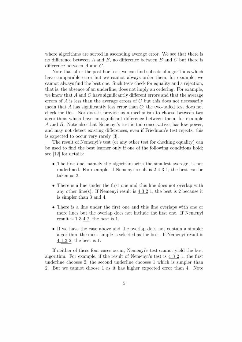
where algorithms are sorted in ascending average error. We see that there isno difference between A and B, no difference between B and C but there isdifference between A and C.

Note that after the post hoc test, we can find subsets of algorithms whichhave comparable error but we cannot always order them, for example, wecannot always find the best one. Such tests check for equality and a rejection,that is, the absence of an underline, does not imply an ordering. For example,we know that A and C have significantly different errors and that the averageerrors of A is less than the average errors of C but this does not necessarilymean that A has significantly less error than C; the two-tailed test does notcheck for this. Nor does it provide us a mechanism to choose between twoalgorithms which have no significant difference between them, for exampleA and B. Note also that Nemenyi’s test is too conservative, has low power,and may not detect existing differences, even if Friedman’s test rejects; thisis expected to occur very rarely [3].

The result of Nemenyi’s test (or any other test for checking equality) canbe used to find the best learner only if one of the following conditions hold;see [12] for details:

• The first one, namely the algorithm with the smallest average, is notunderlined. For example, if Nemenyi result is 2 4 3 1, the best can betaken as 2.

• There is a line under the first one and this line does not overlap withany other line(s). If Nemenyi result is 4 3 2 1, the best is 2 because itis simpler than 3 and 4.

• There is a line under the first one and this line overlaps with one ormore lines but the overlap does not include the first one. If Nemenyiresult is 1 3 4 2, the best is 1.

• If we have the case above and the overlap does not contain a simpleralgorithm, the most simple is selected as the best. If Nemenyi result is4 1 3 2, the best is 1.

If neither of these four cases occur, Nemenyi’s test cannot yield the bestalgorithm. For example, if the result of Nemenyi’s test is 4 3 2 1, the firstunderline chooses 2, the second underline chooses 1 which is simpler than2. But we cannot choose 1 as it has higher expected error than 4. Note

5

that these cases are only for finding the best algorithm; for creating the fullordering, the conditions must be satisfied by any group of algorithms, whichis very rarely possible.

2.3. Correction for Multiple Comparisons

When comparing multiple algorithms, to retain an overall significancelevel α, one has to adjust the value of α for each post hoc comparison. Thereare various methods for this. The simple method is to use Bonferroni cor-rection [14] which works as follows: Suppose that we want to compare Lalgorithms. There are L(L − 1)/2 comparisons, therefore Bonferroni cor-rection sets the significance level of each comparison to α/(L(L − 1)/2).Nemenyi’s test is based on this correction, and that is why it has low power.Garcia and Herrera [15] explain and compare the use of various correctionalgorithms, such as Holm’s correction [16], Shaffer’s static procedure [17]and Bergmann-Hommel’s dynamic procedure [18]. They show that althoughit requires intensive computation, Bergmann-Hommel, which we adopted inthis paper, has the highest power. All of these procedures use z =

(Ri−Rj)

SEas

the test statistic and compare it with the z value of the suitably correctedα. In a recent paper, Garcıa et al. [19] propose new nonparametric tests,two alternatives to Friedman’s test and four new correction procedures; theiranalysis focuses on comparing multiple algorithms against a control algo-rithm though, and not on ordering.

3. Multi2Test

Our proposed method is based on MultiTest on a single data set [12]. Wefirst review it and then discuss how we generalize it to work on multiple datasets.

3.1. MultiTest

MultiTest [12] is a cost-conscious methodology that orders algorithms ac-cording to their expected error and uses their costs for breaking ties. Weassume that we have a prior ordering of algorithms in terms of some costmeasure. We do not define nor look for statistically significant differencehere; the important requirement is that there should be no ties because thisordering is used for breaking ties due to error. Various types of cost canbe used [20], for example, the space and/or time complexity during train-ing and/or testing, interpretability, ease of programming, etc. The actual

6

cost measure is dependent on the application and different costs may inducedifferent orderings.

The effect of this cost measure is that, given any two algorithms withthe same expected error, we favor the simpler one in terms of the used costmeasure. The result of the pairwise test overrides this prior preference; thatis, we choose the more costly only if it has significantly less error.

Let us assume that we index the algorithms according to this prior orderas 1, 2 . . . L such that 1 is the simplest (most preferred) and L is the mostcostly (least preferred). A graph is formed with vertices Mj correspondingto algorithms and we place directed edges as follows: ∀i, j, i < j, we test ifalgorithm i has less or comparable expected error to j:

H0 : µi ≤ µj

Actually, we test if the prior preference holds. If this test rejects, we saythat Mj, the costlier algorithm, is statistically significantly more accuratethan Mi, and a directed edge is placed from i to j, indicating that we overridethe prior order. After L(L− 1)/2 pairwise tests (with correction for multiplecomparisons), the graph has edges where the test is rejected. The numberof incoming edges to a node j is the number of algorithms that are preferredover j but have significantly higher expected error. The number of outgoingedges from a node i is the number of algorithms that are less preferred thani but have significantly less expected error. The resulting graph need not beconnected. Once this graph is constructed, a topological sort gives us theorder of the algorithms.

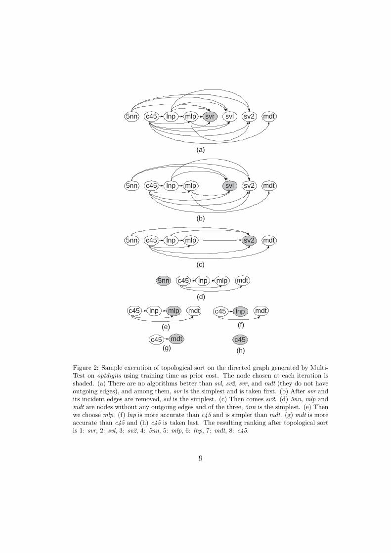
As an example, we show the application of MultiTest to one of our exam-ple data sets, optdigits. The result of the pairwise tests is shown in Table 1.Figure 1 shows the directed graph when the prior ordering is based on train-ing time (increasing from left to right). The sample execution of topologicalsort is shown in Figure 2. The resulting order after topological sort is 1: svr,2: svl, 3: sv2, 4: 5nn, 5: mlp, 6: lnp, 7: mdt, 8: c45.

3.2. Multi2Test

We now discuss how MultiTest can be generalized to run over multipledata sets. The pseudocode of the method is given in Table 2. First, we applyMultiTest separately on each data set using a pairwise test (with correctionfor multiple comparisons) and a prior ordering based on cost. We then con-vert the order found for each data set into ranks such that 1 is the best and

7

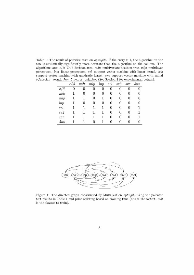
Table 1: The result of pairwise tests on optdigits. If the entry is 1, the algorithm on therow is statistically significantly more accurate than the algorithm on the column. Thealgorithms are: c45: C4.5 decision tree, mdt: multivariate decision tree, mlp: multilayerperceptron, lnp: linear perceptron, svl: support vector machine with linear kernel, sv2:support vector machine with quadratic kernel, svr: support vector machine with radial(Gaussian) kernel, 5nn: 5-nearest neighbor (See Section 4 for experimental details).

c45 mdt mlp lnp svl sv2 svr 5nnc45 0 0 0 0 0 0 0 0mdt 1 0 0 0 0 0 0 0mlp 1 1 0 1 0 0 0 0lnp 1 0 0 0 0 0 0 0svl 1 1 1 1 0 0 0 1sv2 1 1 1 1 0 0 0 1svr 1 1 1 1 0 0 0 15nn 1 1 0 1 0 0 0 0

5nn svl svr mlp c45 lnp mdt sv2

Figure 1: The directed graph constructed by MultiTest on optdigits using the pairwisetest results in Table 1 and prior ordering based on training time (5nn is the fastest, mdtis the slowest to train).

8

(a)

5nn svl svr mlp c45 lnp mdt sv2

(b)

5nn svl mlp c45 lnp mdt sv2

(c)

5nn mlp c45 lnp mdt sv2

(d)

5nn mlp c45 lnp mdt

(e)

mlp c45 lnp mdt

(f)

c45 lnp mdt

(g) c45 mdt

(h)

c45

Figure 2: Sample execution of topological sort on the directed graph generated by Multi-Test on optdigits using training time as prior cost. The node chosen at each iteration isshaded. (a) There are no algorithms better than svl, sv2, svr, and mdt (they do not haveoutgoing edges), and among them, svr is the simplest and is taken first. (b) After svr andits incident edges are removed, svl is the simplest. (c) Then comes sv2. (d) 5nn, mlp andmdt are nodes without any outgoing edges and of the three, 5nn is the simplest. (e) Thenwe choose mlp. (f) lnp is more accurate than c45 and is simpler than mdt. (g) mdt is moreaccurate than c45 and (h) c45 is taken last. The resulting ranking after topological sortis 1: svr, 2: svl, 3: sv2, 4: 5nn, 5: mlp, 6: lnp, 7: mdt, 8: c45.

9

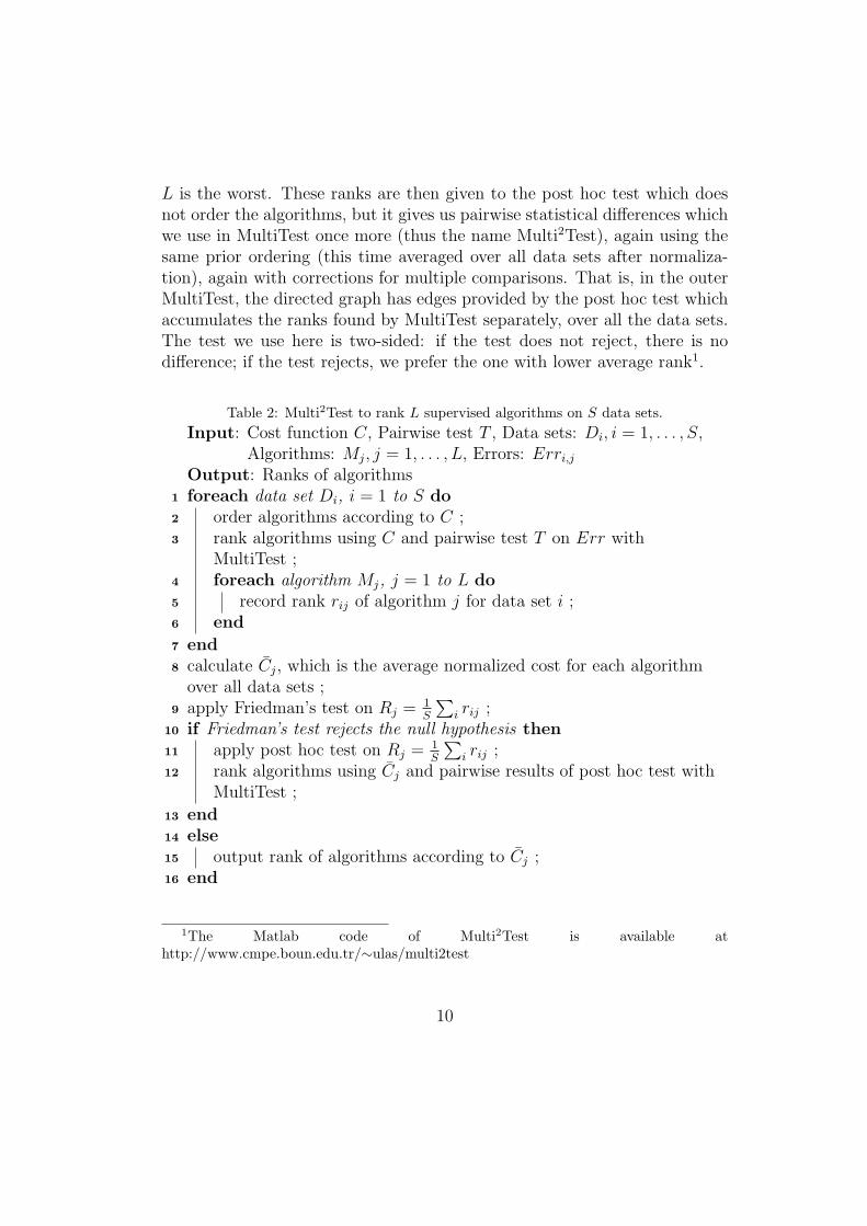
L is the worst. These ranks are then given to the post hoc test which doesnot order the algorithms, but it gives us pairwise statistical differences whichwe use in MultiTest once more (thus the name Multi2Test), again using thesame prior ordering (this time averaged over all data sets after normaliza-tion), again with corrections for multiple comparisons. That is, in the outerMultiTest, the directed graph has edges provided by the post hoc test whichaccumulates the ranks found by MultiTest separately, over all the data sets.The test we use here is two-sided: if the test does not reject, there is nodifference; if the test rejects, we prefer the one with lower average rank1.

Table 2: Multi2Test to rank L supervised algorithms on S data sets.

Input: Cost function C, Pairwise test T , Data sets: Di, i = 1, . . . , S,Algorithms: Mj, j = 1, . . . , L, Errors: Erri,j

Output: Ranks of algorithms1 foreach data set Di, i = 1 to S do2 order algorithms according to C ;3 rank algorithms using C and pairwise test T on Err with

MultiTest ;4 foreach algorithm Mj, j = 1 to L do5 record rank rij of algorithm j for data set i ;6 end

7 end8 calculate Cj, which is the average normalized cost for each algorithmover all data sets ;

9 apply Friedman’s test on Rj =1S

∑i rij ;

10 if Friedman’s test rejects the null hypothesis then11 apply post hoc test on Rj =

1S

∑i rij ;

12 rank algorithms using Cj and pairwise results of post hoc test withMultiTest ;

13 end14 else15 output rank of algorithms according to Cj ;16 end

1The Matlab code of Multi2Test is available athttp://www.cmpe.boun.edu.tr/∼ulas/multi2test

10

As an example for the second pass of Multi2Test, let us assume that wehave four algorithms A,B,C,D, according to the prior order of A < B <C < D, and the result of post hoc test after the first pass of MultiTest isB D A C. We then convert the results of post hoc test to pairwise statisticallysignificant differences (Table 3) and together with the prior ordering, theformed directed graph is shown in Figure 3. Doing a topological sort, wefind the final order as 1: B, 2: A, 3: D, 4: C.

Table 3: Tabular representation of post hoc test results for an example run.

A B C DA 0 0 0 0B 1 0 1 0C 0 0 0 0D 0 0 1 0

Figure 3: The directed graph constructed by MultiTest on the example problem using thepairwise test results in Table 3 and the prior ordering: A < B < C < D.

4. Results

4.1. Experimental Setup

We use a total of 38 data sets where 35 of them (zoo, iris, tae, hepatitis,wine, flags, glass, heart, haberman, flare, ecoli, bupa, ionosphere, dermatol-ogy, horse, monks, vote, cylinder, balance, australian, credit, breast, pima,tictactoe, cmc, yeast, car, segment, thyroid, optdigits, spambase, pageblock,pendigits, mushroom, and nursery) are from UCI [1] and 3 (titanic, ringnorm,and twonorm) are from Delve [21] repositories.

We use eight algorithms:

1) c45: C4.5 decision tree algorithm.2) mdt: Multivariate decision tree algorithm where the decision at each

node is not univariate as in C4.5 but uses a linear combination of allinputs [22].

11

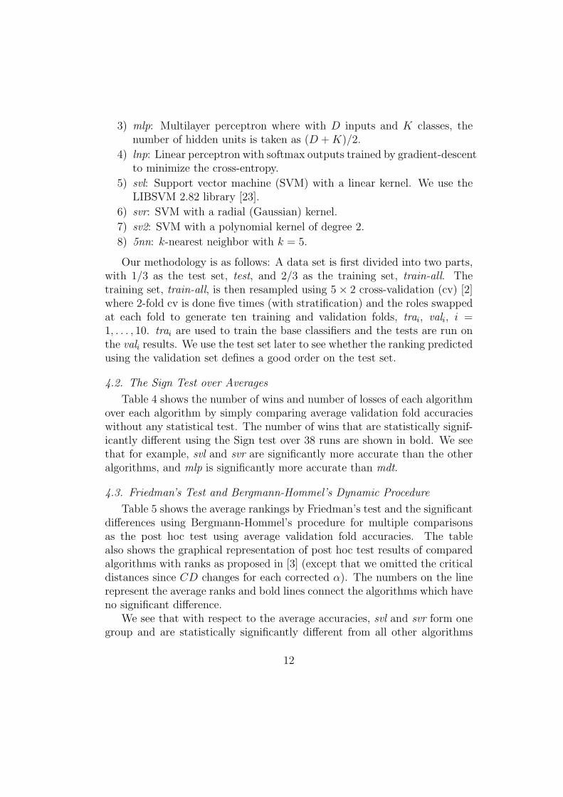
3) mlp: Multilayer perceptron where with D inputs and K classes, thenumber of hidden units is taken as (D +K)/2.

4) lnp: Linear perceptron with softmax outputs trained by gradient-descentto minimize the cross-entropy.

5) svl: Support vector machine (SVM) with a linear kernel. We use theLIBSVM 2.82 library [23].

6) svr: SVM with a radial (Gaussian) kernel.

7) sv2: SVM with a polynomial kernel of degree 2.

8) 5nn: k-nearest neighbor with k = 5.

Our methodology is as follows: A data set is first divided into two parts,with 1/3 as the test set, test, and 2/3 as the training set, train-all. Thetraining set, train-all, is then resampled using 5× 2 cross-validation (cv) [2]where 2-fold cv is done five times (with stratification) and the roles swappedat each fold to generate ten training and validation folds, trai, vali, i =1, . . . , 10. trai are used to train the base classifiers and the tests are run onthe vali results. We use the test set later to see whether the ranking predictedusing the validation set defines a good order on the test set.

4.2. The Sign Test over Averages

Table 4 shows the number of wins and number of losses of each algorithmover each algorithm by simply comparing average validation fold accuracieswithout any statistical test. The number of wins that are statistically signif-icantly different using the Sign test over 38 runs are shown in bold. We seethat for example, svl and svr are significantly more accurate than the otheralgorithms, and mlp is significantly more accurate than mdt.

4.3. Friedman’s Test and Bergmann-Hommel’s Dynamic Procedure

Table 5 shows the average rankings by Friedman’s test and the significantdifferences using Bergmann-Hommel’s procedure for multiple comparisonsas the post hoc test using average validation fold accuracies. The tablealso shows the graphical representation of post hoc test results of comparedalgorithms with ranks as proposed in [3] (except that we omitted the criticaldistances since CD changes for each corrected α). The numbers on the linerepresent the average ranks and bold lines connect the algorithms which haveno significant difference.

We see that with respect to the average accuracies, svl and svr form onegroup and are statistically significantly different from all other algorithms

12

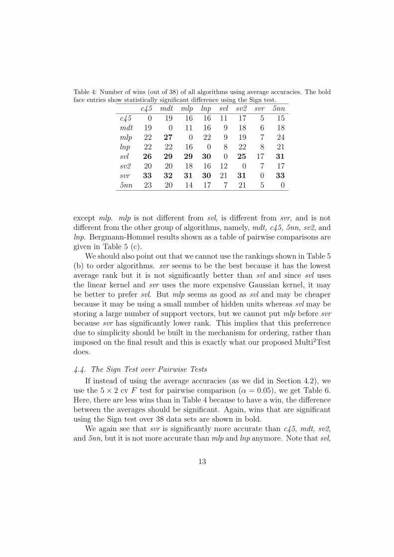
Table 4: Number of wins (out of 38) of all algorithms using average accuracies. The boldface entries show statistically significant difference using the Sign test.

c45 mdt mlp lnp svl sv2 svr 5nnc45 0 19 16 16 11 17 5 15mdt 19 0 11 16 9 18 6 18mlp 22 27 0 22 9 19 7 24lnp 22 22 16 0 8 22 8 21svl 26 29 29 30 0 25 17 31sv2 20 20 18 16 12 0 7 17svr 33 32 31 30 21 31 0 335nn 23 20 14 17 7 21 5 0

except mlp. mlp is not different from svl, is different from svr, and is notdifferent from the other group of algorithms, namely, mdt, c45, 5nn, sv2, andlnp. Bergmann-Hommel results shown as a table of pairwise comparisons aregiven in Table 5 (c).

We should also point out that we cannot use the rankings shown in Table 5(b) to order algorithms. svr seems to be the best because it has the lowestaverage rank but it is not significantly better than svl and since svl usesthe linear kernel and svr uses the more expensive Gaussian kernel, it maybe better to prefer svl. But mlp seems as good as svl and may be cheaperbecause it may be using a small number of hidden units whereas svl may bestoring a large number of support vectors, but we cannot put mlp before svrbecause svr has significantly lower rank. This implies that this preferrencedue to simplicity should be built in the mechanism for ordering, rather thanimposed on the final result and this is exactly what our proposed Multi2Testdoes.

4.4. The Sign Test over Pairwise Tests

If instead of using the average accuracies (as we did in Section 4.2), weuse the 5× 2 cv F test for pairwise comparison (α = 0.05), we get Table 6.Here, there are less wins than in Table 4 because to have a win, the differencebetween the averages should be significant. Again, wins that are significantusing the Sign test over 38 data sets are shown in bold.

We again see that svr is significantly more accurate than c45, mdt, sv2,and 5nn, but it is not more accurate thanmlp and lnp anymore. Note that svl,

13

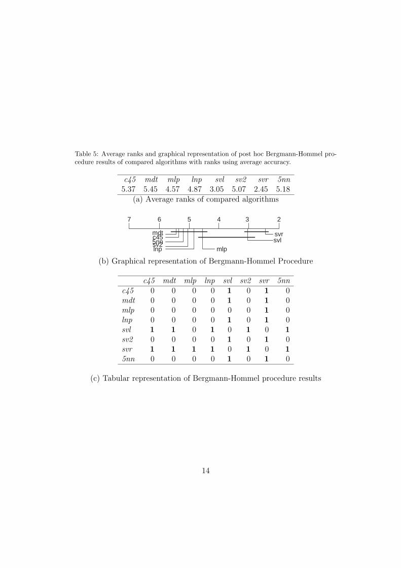
Table 5: Average ranks and graphical representation of post hoc Bergmann-Hommel pro-cedure results of compared algorithms with ranks using average accuracy.

c45 mdt mlp lnp svl sv2 svr 5nn5.37 5.45 4.57 4.87 3.05 5.07 2.45 5.18

(a) Average ranks of compared algorithms

2 4 3

lnp

5 7 6

mdt

sv2 svl svr c45

mlp 5nn

(b) Graphical representation of Bergmann-Hommel Procedure

c45 mdt mlp lnp svl sv2 svr 5nnc45 0 0 0 0 1 0 1 0mdt 0 0 0 0 1 0 1 0mlp 0 0 0 0 0 0 1 0lnp 0 0 0 0 1 0 1 0svl 1 1 0 1 0 1 0 1sv2 0 0 0 0 1 0 1 0svr 1 1 1 1 0 1 0 15nn 0 0 0 0 1 0 1 0

(c) Tabular representation of Bergmann-Hommel procedure results

14

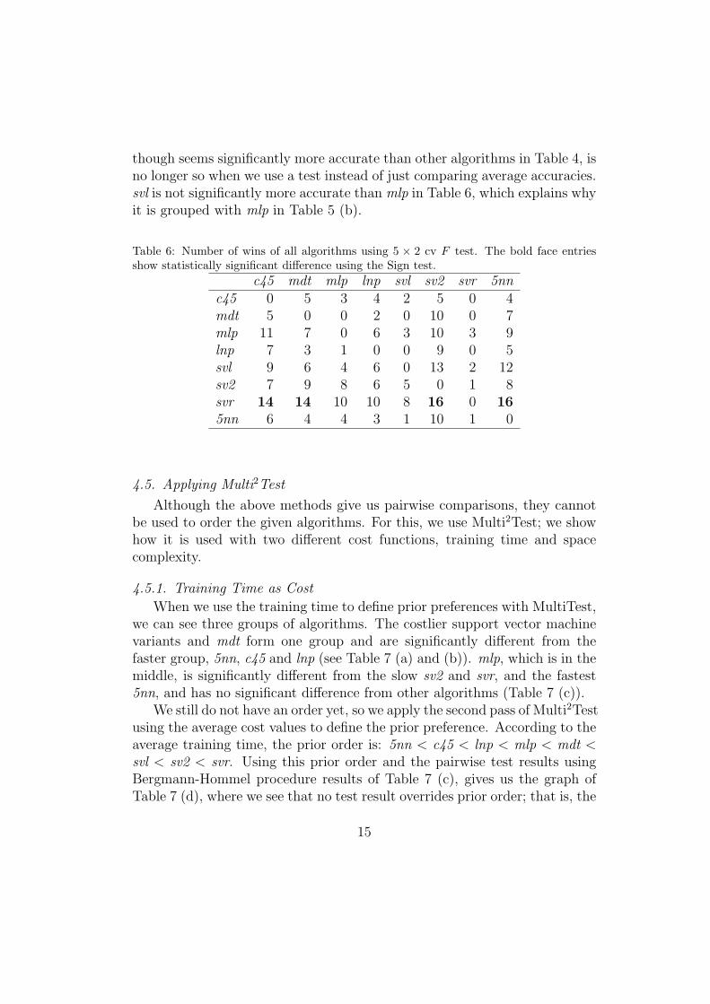
though seems significantly more accurate than other algorithms in Table 4, isno longer so when we use a test instead of just comparing average accuracies.svl is not significantly more accurate than mlp in Table 6, which explains whyit is grouped with mlp in Table 5 (b).

Table 6: Number of wins of all algorithms using 5 × 2 cv F test. The bold face entriesshow statistically significant difference using the Sign test.

c45 mdt mlp lnp svl sv2 svr 5nnc45 0 5 3 4 2 5 0 4mdt 5 0 0 2 0 10 0 7mlp 11 7 0 6 3 10 3 9lnp 7 3 1 0 0 9 0 5svl 9 6 4 6 0 13 2 12sv2 7 9 8 6 5 0 1 8svr 14 14 10 10 8 16 0 165nn 6 4 4 3 1 10 1 0

4.5. Applying Multi2Test

Although the above methods give us pairwise comparisons, they cannotbe used to order the given algorithms. For this, we use Multi2Test; we showhow it is used with two different cost functions, training time and spacecomplexity.

4.5.1. Training Time as Cost

When we use the training time to define prior preferences with MultiTest,we can see three groups of algorithms. The costlier support vector machinevariants and mdt form one group and are significantly different from thefaster group, 5nn, c45 and lnp (see Table 7 (a) and (b)). mlp, which is in themiddle, is significantly different from the slow sv2 and svr, and the fastest5nn, and has no significant difference from other algorithms (Table 7 (c)).

We still do not have an order yet, so we apply the second pass of Multi2Testusing the average cost values to define the prior preference. According to theaverage training time, the prior order is: 5nn < c45 < lnp < mlp < mdt <svl < sv2 < svr. Using this prior order and the pairwise test results usingBergmann-Hommel procedure results of Table 7 (c), gives us the graph ofTable 7 (d), where we see that no test result overrides prior order; that is, the

15

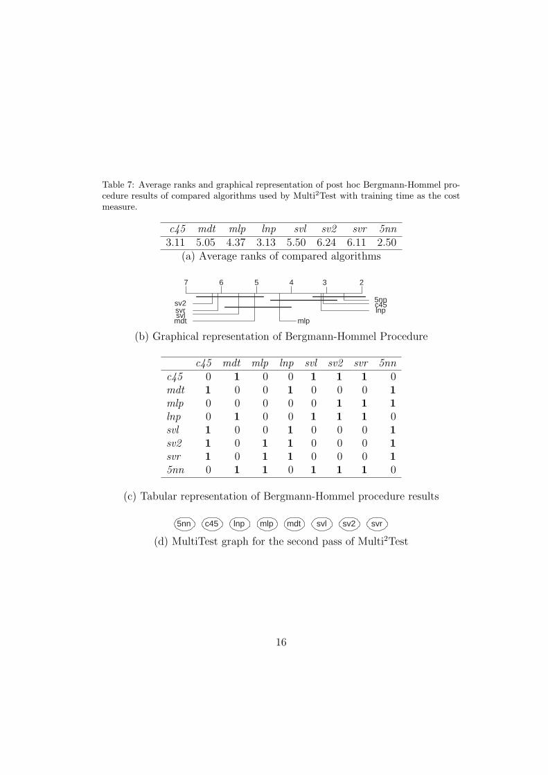
Table 7: Average ranks and graphical representation of post hoc Bergmann-Hommel pro-cedure results of compared algorithms used by Multi2Test with training time as the costmeasure.

c45 mdt mlp lnp svl sv2 svr 5nn3.11 5.05 4.37 3.13 5.50 6.24 6.11 2.50

(a) Average ranks of compared algorithms

2 4 3

mlp

5 7 6

mdt

sv2

svl svr

c45 lnp 5nn

(b) Graphical representation of Bergmann-Hommel Procedure

c45 mdt mlp lnp svl sv2 svr 5nnc45 0 1 0 0 1 1 1 0mdt 1 0 0 1 0 0 0 1mlp 0 0 0 0 0 1 1 1lnp 0 1 0 0 1 1 1 0svl 1 0 0 1 0 0 0 1sv2 1 0 1 1 0 0 0 1svr 1 0 1 1 0 0 0 15nn 0 1 1 0 1 1 1 0

(c) Tabular representation of Bergmann-Hommel procedure results

5nn svl mdt mlp c45 lnp svr sv2

(d) MultiTest graph for the second pass of Multi2Test

16

second MultiTest pass conforms with the accumulated first MultiTest passon data sets separately. And therefore, the ranking is: 1: 5nn, 2: c45, 3: lnp,4: mlp, 5: mdt, 6: svl, 7: sv2, 8: svr.

4.5.2. Space Complexity as Cost

When we use the space complexity with the same validation errors, wesee that, this time, 5nn has the highest rank, and forms a group with thecomplex support vector machine variants svl, svr and sv2 and is significantlydifferent from the simpler group of lnp, c45, mdt, and mlp (see Table 8 (a)and (b)). We also see that 5nn is significantly different from svr (Table 8(c)).

When we apply the second pass of Multi2Test according to the averagespace complexity, the prior order is: c45 < mdt < mlp < lnp < svl < svr <sv2 < 5nn. Using this and the pairwise test results using Bergmann-Hommelprocedure results of Table 8 (c), we get the graph of Table 8 (d). So theranking is: 1: c45, 2: mdt, 3: mlp, 4: lnp, 5: svl, 6: svr, 7: sv2, 8: 5nn. Wesee that 5nn, which is the best when training time is critical, becomes theworst when space complexity is used.

One may argue that it is useless to apply the second pass of MultiTest,but this is not always the case. We have relatively accurate classifiers andthe classifiers do not span a large range of accuracy and the diversity is small.We would expect different orderings going from one data set to another if theclassifiers were more diverse and the range spanned by the accuracies of theclassifiers were larger. We can construct an example where this is the case:Suppose that we have three algorithms A,B,C according to the prior order ofA < B < C and suppose that the result of the range test is CA B. The finalorder will be 1: C, 2: A, 3: B, which is different from the prior order whichis A,B,C. If we choose A as c45, B as mdt and C as svr, and use breast, car,nursery, optdigits, pendigits, ringnorm, spambase, tictactoe, and titanic datasets only, this is what we get using real data using space complexity as priorordering. We see that the average prior order is c45 < mdt < svr, but theresult of Multi2Test is 1: svr, 2: c45, 3: mdt which is different from the priororder. Note that the ordering depends also on the algorithms compared asthe critical difference depends on the number of populations compared.

4.6. Testing MultiTest and Multi2Test

We do experiments on synthetic data to observe the behavior of MultiTestand Multi2Test to see if they work as expected and hence comment on their

17

Table 8: Average ranks and graphical representation of post hoc Bergmann-Hommel pro-cedure results of compared algorithms used by Multi2Test with space complexity as thecost measure.

c45 mdt mlp lnp svl sv2 svr 5nn2.50 2.95 2.71 3.68 5.71 6.13 5.32 7.00

(a) Average ranks of compared algorithms

2 4 3

mlp

5 7 6

mdt sv2 svl svr

c45

lnp

5nn

(b) Graphical representation of Bergmann-Hommel Procedure

c45 mdt mlp lnp svl sv2 svr 5nnc45 0 0 0 0 1 1 1 1mdt 0 0 0 0 1 1 1 1mlp 0 0 0 0 1 1 1 1lnp 0 0 0 0 1 1 1 1svl 1 1 1 1 0 0 0 0sv2 1 1 1 1 0 0 0 0svr 1 1 1 1 0 0 0 15nn 1 1 1 1 0 0 1 0

(c) Tabular representation of Bergmann-Hommel procedure results

c45 svr svl lnp mdt mlp 5nn sv2

(d) MultiTest graph for the second pass of Multi2Test

18

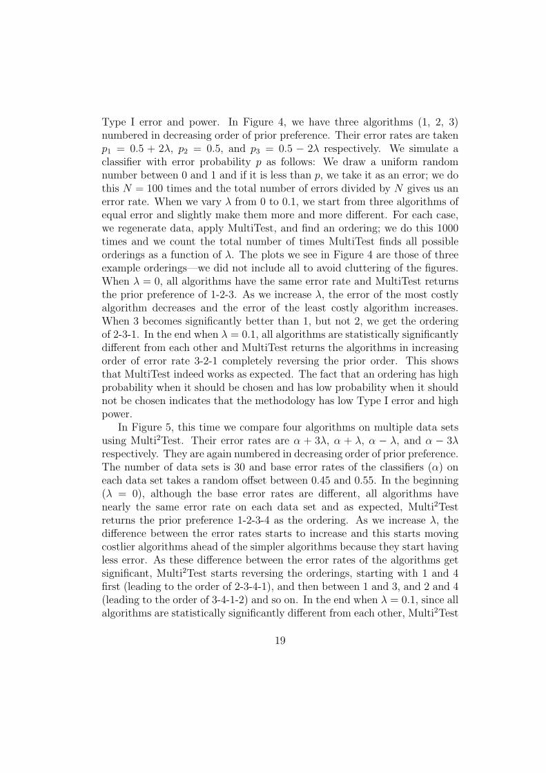
Type I error and power. In Figure 4, we have three algorithms (1, 2, 3)numbered in decreasing order of prior preference. Their error rates are takenp1 = 0.5 + 2λ, p2 = 0.5, and p3 = 0.5 − 2λ respectively. We simulate aclassifier with error probability p as follows: We draw a uniform randomnumber between 0 and 1 and if it is less than p, we take it as an error; we dothis N = 100 times and the total number of errors divided by N gives us anerror rate. When we vary λ from 0 to 0.1, we start from three algorithms ofequal error and slightly make them more and more different. For each case,we regenerate data, apply MultiTest, and find an ordering; we do this 1000times and we count the total number of times MultiTest finds all possibleorderings as a function of λ. The plots we see in Figure 4 are those of threeexample orderings—we did not include all to avoid cluttering of the figures.When λ = 0, all algorithms have the same error rate and MultiTest returnsthe prior preference of 1-2-3. As we increase λ, the error of the most costlyalgorithm decreases and the error of the least costly algorithm increases.When 3 becomes significantly better than 1, but not 2, we get the orderingof 2-3-1. In the end when λ = 0.1, all algorithms are statistically significantlydifferent from each other and MultiTest returns the algorithms in increasingorder of error rate 3-2-1 completely reversing the prior order. This showsthat MultiTest indeed works as expected. The fact that an ordering has highprobability when it should be chosen and has low probability when it shouldnot be chosen indicates that the methodology has low Type I error and highpower.

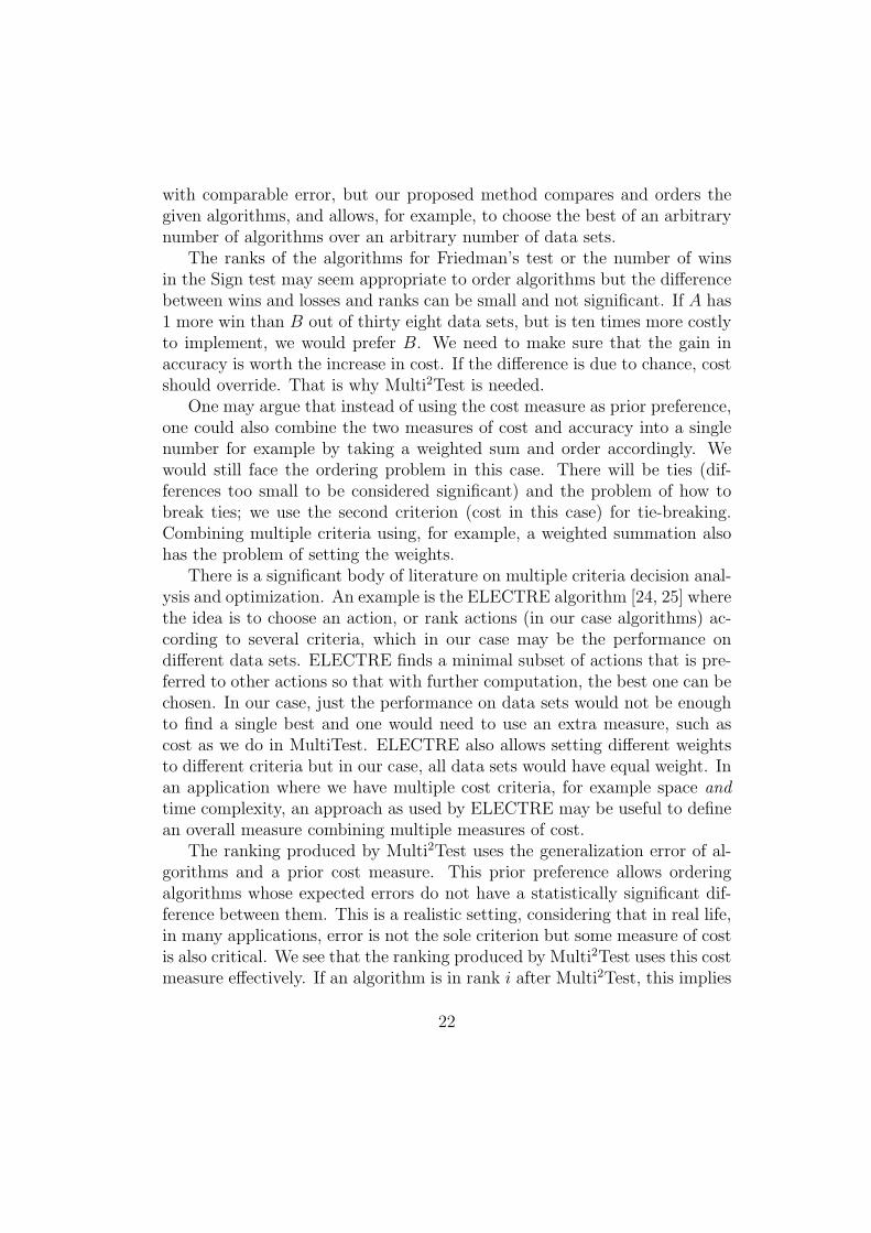
In Figure 5, this time we compare four algorithms on multiple data setsusing Multi2Test. Their error rates are α + 3λ, α + λ, α − λ, and α − 3λrespectively. They are again numbered in decreasing order of prior preference.The number of data sets is 30 and base error rates of the classifiers (α) oneach data set takes a random offset between 0.45 and 0.55. In the beginning(λ = 0), although the base error rates are different, all algorithms havenearly the same error rate on each data set and as expected, Multi2Testreturns the prior preference 1-2-3-4 as the ordering. As we increase λ, thedifference between the error rates starts to increase and this starts movingcostlier algorithms ahead of the simpler algorithms because they start havingless error. As these difference between the error rates of the algorithms getsignificant, Multi2Test starts reversing the orderings, starting with 1 and 4first (leading to the order of 2-3-4-1), and then between 1 and 3, and 2 and 4(leading to the order of 3-4-1-2) and so on. In the end when λ = 0.1, since allalgorithms are statistically significantly different from each other, Multi2Test

19

λ

Pro

bab

ilit

y o

f O

rder

ing

.00 .01 .02 .03 .04 .05 .06 .07 .08 .09 .100.0

0.1

0.2

0.3

0.4

0.5

0.6

0.7

0.8

0.9

1.0

1-2-3

2-3-13-2-1

Figure 4: Probabilities of different orderings found by MultiTest on synthetic data as afunction of a multiplier parameter λ that varies the difference between errors of algorithms.Only three example orderings are shown for clarity.

λ

Pro

bab

ilit

y o

f O

rder

ing

.00 .01 .02 .03 .04 .05 .06 .07 .08 .09 .100.0

0.1

0.2

0.3

0.4

0.5

0.6

0.7

0.8

0.9

1.01-2-3-4

3-4-1-2

2-3-4-1

4-3-2-1

Figure 5: Probabilities of different orderings found by Multi2Test on synthetic data as afunction of a multiplier parameter λ that varies the difference between errors of algorithms.

20

returns the algorithms in increasing order of error rate 4-3-2-1. Again, wesee that Multi2Test works as expected. How fast the probability of a certainordering rises and falls (and hence how much orderings overlap) depend onthe pairwise test used inside MultiTest, its significance α and the validationset size N .

4.7. Verification of Results on test

We also did experiments to verify the results of Multi2Test on the testset. What we do is we run the same Multi2Test on the test data and checkif the orderings we find using the validation set is a good predictor for whatwe find on the test set. We find that though there are small differences, forthe most part, the predicted orderings match what we find on the test set.

When we use the training time as the cost measure, out of the 38 data sets,on 19 data sets, we find the same ordering on validation and test sets. Thereare ten data sets where there are big rank changes. We observe this changefive times with 5nn, three times with c45 and twice with mdt. We believethat this is because decision tree and nearest neighbor algorithms have highvariance and hence their accuracies may differ slightly on different data whichmay lead to different orderings. A high variance in the algorithm’s accuracyover different folds would make the statistical test less likely to reject and insuch a case, the prior cost term would determine the final ordering. In thefinal ranking, this information as to whether the ordering is due to the resultof the test or the cost prior can be differentiated.

When we consider space complexity as the cost measure, we see that on24 out of the 38 data sets, the same ordering retained. This time there areonly five big changes and again mostly due to decision trees; two with c45,two with mdt and one with mlp.

From these experiments, we conclude that the rankings produced by Mul-tiTest are stable except for some high-variance algorithms, and the overallresults produced by Multi2Test on validation data is a good predictor of thereal ranking on the test data.

5. Discussions and Conclusions

We propose a statistical methodology, Multi2Test, a generalization of ourprevious work, which compares and orders multiple supervised learning al-gorithms over multiple data sets. Existing methods in the literature can findstatistical differences between two algorithms, or find subsets of algorithms

21

with comparable error, but our proposed method compares and orders thegiven algorithms, and allows, for example, to choose the best of an arbitrarynumber of algorithms over an arbitrary number of data sets.

The ranks of the algorithms for Friedman’s test or the number of winsin the Sign test may seem appropriate to order algorithms but the differencebetween wins and losses and ranks can be small and not significant. If A has1 more win than B out of thirty eight data sets, but is ten times more costlyto implement, we would prefer B. We need to make sure that the gain inaccuracy is worth the increase in cost. If the difference is due to chance, costshould override. That is why Multi2Test is needed.

One may argue that instead of using the cost measure as prior preference,one could also combine the two measures of cost and accuracy into a singlenumber for example by taking a weighted sum and order accordingly. Wewould still face the ordering problem in this case. There will be ties (dif-ferences too small to be considered significant) and the problem of how tobreak ties; we use the second criterion (cost in this case) for tie-breaking.Combining multiple criteria using, for example, a weighted summation alsohas the problem of setting the weights.

There is a significant body of literature on multiple criteria decision anal-ysis and optimization. An example is the ELECTRE algorithm [24, 25] wherethe idea is to choose an action, or rank actions (in our case algorithms) ac-cording to several criteria, which in our case may be the performance ondifferent data sets. ELECTRE finds a minimal subset of actions that is pre-ferred to other actions so that with further computation, the best one can bechosen. In our case, just the performance on data sets would not be enoughto find a single best and one would need to use an extra measure, such ascost as we do in MultiTest. ELECTRE also allows setting different weightsto different criteria but in our case, all data sets would have equal weight. Inan application where we have multiple cost criteria, for example space andtime complexity, an approach as used by ELECTRE may be useful to definean overall measure combining multiple measures of cost.

The ranking produced by Multi2Test uses the generalization error of al-gorithms and a prior cost measure. This prior preference allows orderingalgorithms whose expected errors do not have a statistically significant dif-ference between them. This is a realistic setting, considering that in real life,in many applications, error is not the sole criterion but some measure of costis also critical. We see that the ranking produced by Multi2Test uses this costmeasure effectively. If an algorithm is in rank i after Multi2Test, this implies

22

that all the algorithms that follow it with rank j > i are either significantlyworse or are equally accurate and costlier. The cost measure is used to breakties when there is no significant difference in terms of accuracy. If certainalgorithms incur a cost that is not affordable for a particular situation, theymay just be removed from the final ranked list and the current best can befound; or equivalently, Multi2Test can be run without them.

Note that MultiTest or Multi2Test do not significantly increase the overallcomputational and/or space complexity because the real cost is the trainingand validation of the algorithms. Once the algorithms are trained and val-idated over data sets and these validation errors are recorded, applying thecalculations necessary for MultiTest or Multi2Test is simple in comparison.

Our implementation uses the 5× 2 cv F test for pairwise comparison ofalgorithms on a single data set. One could use other pairwise tests or otherresampling schemes. For example, 10 × 10 folding [10] will have the advan-tage of decreasing Type I and II errors but will increase the computationalcomplexity. MultiTest and Multi2Test are statistical frameworks, and anyresampling method and a suitable pairwise statistical test on some loss mea-sure with appropriate α correction could be used. For example, the samemethodology can be used to compare regression algorithms over a single ormultiple data sets. These are interesting areas for further research.

If one has groups of data sets for similar applications, it would be betterto order algorithms separately on these. For example if one has six differentdata sets for different image recognition tasks, and four different data setsfor speech, it is preferable that Multi2Test be run twice separately instead ofonce on the combined ten. Multi2Test results are informative: Let us say wehave the ranking of L algorithms on S data sets. Instead of merging them tofind one overall ordering as Multi2Test does, these rankings may allow us todefine a measure of similarity which we can then use to find groups of similaralgorithms; such similar ranks of algorithms also imply a similarity betweendata sets. These would be other interesting uses of Multi2Test results2.

Acknowledgments

We would like to thank Mehmet Gonen for discussions. This work hasbeen supported by the Turkish Academy of Sciences in the framework of

2We are grateful to an anonymous reviewer for this suggestion.

23

the Young Scientist Award Program (EA-TUBA-GEBIP/2001-1-1), BogaziciUniversity Scientific Research Project 07HA101, Turkish Scientific TechnicalResearch Council (TUBITAK) EEEAG 107E127, 107E222 and 109E186.

References

[1] A. Asuncion, D. J. Newman, UCI machine learning repository, 2007.

[2] T. G. Dietterich, Approximate statistical tests for comparing supervisedclassification learning algorithms, Neural Computation 10 (1998) 1895–1923.

[3] J. Demsar, Statistical comparisons of classifiers over multiple data sets,Journal of Machine Learning Research 7 (2006) 1–30.

[4] E. Alpaydın, Combined 5× 2 cv F test for comparing supervised classi-fication learning algorithms, Neural Computation 11 (1999) 1885–1892.

[5] X. Zhu, Y. Yang, A lazy bagging approach to classification, PatternRecognition 41 (2008) 2980–2992.

[6] F. Wilcoxon, Individual comparisons by ranking methods, BiometricsBulletin 1 (1945) 80–83.

[7] M. Gonen, E. Alpaydın, Regularizing multiple kernel learning usingresponse surface methodology, Pattern Recognition 44 (2011) 159–171.

[8] A. P. Bradley, The use of the area under the roc curve in the evaluationof machine learning algorithms, Pattern Recognition 30 (1997) 1145–1159.

[9] S. G. Alsing, K. W. Bauer Jr., J. O. Miller, A multinomial selectionprocedure for evaluating pattern recognition algorithms, Pattern Recog-nition 35 (2002) 2397–2412.

[10] R. R. Bouckaert, Estimating replicability of classifier learning exper-iments, in: Proceedings of the International Conference on MachineLearning, ICML ’04, pp. 15–22.

[11] C. Nadeau, Y. Bengio, Inference for the generalization error, MachineLearning 52 (2003) 239–281.

24

[12] O. T. Yıldız, E. Alpaydın, Ordering and finding the best of K > 2supervised learning algorithms, IEEE Transactions on Pattern AnalysisMachine Intelligence 28 (2006) 392–402.

[13] M. Friedman, The use of ranks to avoid the assumption of normalityimplicit in the analysis of variance, Journal of the American StatisticalAssociation 32 (1937) 675–701.

[14] A. Dean, D. Voss, Design and Analysis of Experiments, Springer, NewYork, 1999.

[15] S. Garcıa, F. Herrera, An extension on “statistical comparisons of clas-sifiers over multiple data sets” for all pairwise comparisons, Journal ofMachine Learning Research 9 (2008) 2677–2694.

[16] S. Holm, A simple sequentially rejective multiple test procedure, Scan-dinavian Journal of Statistics 6 (1979) 65–70.

[17] J. P. Shaffer, Modified sequentially rejective multiple test procedures,Journal of the American Statistical Association 81 (1986) 826–831.

[18] G. Bergmann, G. Hommel, Improvements of general multiple test pro-cedures for redundant systems of hypotheses, in: P. Bauer, G. Hommel,E. Sonnemann (Eds.), Multiple Hypotheses Testing, pp. 100–115.

[19] S. Garcıa, A. Fernandez, J. Luengo, F. Herrera, Advanced nonpara-metric tests for multiple comparisons in the design of experiments incomputational intelligence and data mining: Experimental analysis ofpower, Information Sciences 180 (2010) 2044–2064.

[20] P. D. Turney, Types of cost in inductive concept learning, in: Pro-ceedings of the Workshop on Cost-Sensitive Learning, ICML ’00, pp.15–21.

[21] C. E. Rasmussen, R. M. Neal, G. Hinton, D. van Camp, M. Revow,Z. Ghahramani, R. Kustra, R. Tibshirani, Delve data for evaluatinglearning in valid experiments, 1995-1996.

[22] O. T. Yıldız, E. Alpaydın, Linear discriminant trees, in: Proceedingsof the International Conference on Machine Learning, ICML ’00, pp.1175–1182.

25

[23] C. C. Chang, C. J. Lin, LIBSVM: a library for support vector machines,2001.

[24] B. Roy, P. Vincke, Multicriteria analysis: survey and new directions,European Journal of Operational Research 8 (1981) 207–218.

[25] J. Figueira, V. Mousseau, B. Roy, ELECTRE methods, in: J. Figueira,S. Greco, M. Ehrgott (Eds.), Multiple Criteria Decision Analysis: Stateof the Art Surveys, Springer Verlag, Boston, Dordrecht, London, 2005,pp. 133–162.

26